ELSEVIER Journal of Economic Dynamics and Control

21 (1997) 1405-1425

Solving long-term financial planning via global optimization

&“Control

problems

C.D. Maranas, a I.P. Androulakis, a C.A. Floudas, a,* A.J. Berger, b

J.M. Mulvey b

a Department of Chemical Engineering, Princeton University, Princeton, NJ 08544-5263, USA b Department of Civil Engineering and Operations Research, Princeton University, Princeton, NJ

08544, USA

Abstract

A significant multi-stage financial planning problem is posed as a stochastic program with decision rules. The decision rule - called dynamically balanced - requires the pur- chase and sale of assets at each time stage so as to keep constant asset proportions in the portfolio composition. It leads to a nonconvex objective function. We show that the rule performs well as compared with other dynamic investment strategies. We special- ize a global optimization algorithm for this problem class - guaranteeing finite E-optimal convergence. Computational results demonstrate the procedure’s efficiency on a real-world financial planning problem. The tests confirm that local optimizers are prone to erroneously underestimate the efficient frontier. The concepts can be readily extended for other classes of long-term investment strategies.

Keywords: Global optimization algorithm; Financial planning problems; Fixed-Mix problem

1. Introduction

This paper addresses a significant problem in planning under uncertainty:

the allocation of financial assets to broad investment categories over a long-run horizon (10 to 20 years). The long-term asset allocation problem plays a critical

role in successful investing. It has been the subject of research over many years. For example, see Berger and Mulvey (1996), Dantzig and Infanger (1994), Davis and Norman ( 1990), Grauer and Hakansson (1985), and Merton (197 1). In many of these studies, the problem is posed as a multi-stage stochastic program and

* Corresponding author.

0165-1889/97/%17.00 0 1997 Elsevier Science B.V. All rights reserved PII SO165-1889(97)00032-8

1406 C. D. Muranas et al. I Journal of Economic Dynamics and Conrrol2I (1997) 1405-1425

solved using efficient solution algorithms. Unfortunately, traditional multi-stage

stochastic programs are difficult to solve. Not only does the problem size grow exponentially as a function of the number of stages and random variables, but the precision of the recommendations is difficult to measure since it is costly to perform out of sample experiments.

We investigate an alternative approach. The basic idea is to set up the invest- ment problem as a stochastic program with a popular decision rule. Time is dis-

cretized into n-stages across the planning horizon. Investment decisions are made at the beginning of each time period. The optimal parameters for the decision rule

are then determined by means of a global optimization algorithm. Although the model results in a nonconvex optimization problem, we have developed a special- ized global solver to handle this problem class. The approach extends the ideas of Maranas and Floudas ( 1993, 1994), and Floudas and Visweswaran (1990, 1993).

Due to nonconvexities, multiple local solutions exist which render the loca-

tion of the global one a very difficult task. Traditional local algorithms can only guarantee convergence to a local solution at best, thus failing sometimes to lo- cate the optimal recommendation. Since the proposed algorithm finds the global solution, the best tradeoff between risk and expected profit can be established for the multi-period investment problem. As a consequence, stochastic programming

with decision rules (SPDR) provides a viable alternative to multi-stage stochastic programming (MSP) (see, e.g. Garstka and Wets, 1974; Mulvey, 1996). Whereas the MSP may lead to outstanding decisions under uncertainty, there are several impediments to be overcome. First the size of the MSP must be considered. The

number of decision variables grows exponentially as a function of the number of time stages and random coefficients. The stochastic program represents condi- tional decisions for each branch of the scenario tree. Efficient algorithms exist for solving these problems, for instance, see Dantzig and Infanger (1994), Dempster and Thompson (1995), Mulvey and Ruszczynski (1992), Rockafellar and Wets ( 199 1 ), and Zenios and Yang ( 1996). Regardless, the resulting optimization prob- lem can be long running for most multi-stage examples.

An important consideration for MSP and SPDB models involves the generation of scenarios. This area has received attention by researchers who have applied importance sampling and other variance reduction methods (e.g. Dantzig and Infanger, 1994). Others have developed probabilistic algorithms, e.g. Higle and Sen (1991) for stochastic programs with fixed recourse. Also see Mulvey (1996), who designed a scenario generation system for the consulting company Towers Perrin. Because of the need to perform sampling when generating scenarios, it is critical that the precision of the recommendations be ascertained. The SPRB approach has a distinct advantage in this regard since it can be easily tested with out a sample data - thereby providing confidence that the recommendations are robust. A similar test is much harder in the case of MSP. For an example, see Worzel et al. (1994), who evaluated multi-stage stochastic programs in the context of a rolling-horizon simulation.

C L). Marunas et al. I Journal of Economic Dynamics and Conirol 21 i 1997) 1405 1425 1407

The decision rule-based model SPDR may appear more intuitive at least to

some investors, perhaps since the concepts are closer to the way that indivi-

duals handle their own affairs. Unfortunately, the use of SPDR model hinges on discovering policies that are intuitive and that will produce superior results. The modelers must thoroughly understand the application in order to find an appro-

priate set of decision rules. This step can be hard to carry out. Also, decision rules may lead to nonconvexities and highly nonlinear functions. The noncon-

vexity barrier may become less constraining, however, as algorithms such as the one proposed in this report becomes available.

2. The dynamically balanced strategy

In this section, we give a mathematical description of the decision rule we

consider, namely the dynamically balanced (DB) investment policy. We also show through empirical test on historical data that the DB decision rule compares

favorably to a stochastic optimal control approach and another decision rule. Also, the DB rule and its variants are based on considerable theoretical results (e.g. Davis and Norman, 1990; Merton 1971; Taksar et al., (1988).

2. I. Model dejinition

First, a set of discrete time steps

t = {1,2,...,z-}

in which the portfolio will be rebalanced is selected. We are interested in long planning horizons - 10 to 20+ years. Second, a number of assets

i = {1,2 ,..., Z},

where I is in most cases between 3 and 15, is selected where the initial wealth will be distributed at each stage during the planning horizon. A given set of scenarios

s = {1,2,...,S}

is generated based on the method presented in Mulvey (1996), depicting plausible outcomes for the uncertainties across the planning horizon. Five hundred to one thousand scenarios are typically required for adequately capturing the uncertain future trends in realistic portfolio problems.

The following parameters specify the DB model.

we: initial wealth (in dollars) rf,: return (in %) for asset i, in time period t, under scenario s

bs: probability of occurrence for scenario s, (note that Cf__, pS = 1).

1408 CD. Muranas et al. IJournal of‘ Economic Dynamics and Control 21 (1997) 14OS-1425

The decision variables are defined as follows:

w;: wealth (in dollars) at time period t, and according to scenario S. Ii: fraction of wealth invested in asset category i (constant across time).

Note that 0 _< li 5 1, Vi = 1,. ..,I and c;=, li = 1. At the beginning of each period, the investor rebalances his portfolio. The rule ensures that a fixed percentage of one’s wealth is invested in each asset category - at least at the beginning of each period.

Wealth wf at the end of the first period will be

wf=&(1+,sl)l;, s= I,2 ,...) S. (1) i=l

Accordingly, the relation in wealth for scenario s between any two consecutive periods t - 1 and t is given by

s WI = ws_l~(‘+$J;li, r=1,2 )...) T, s=1,2 )...) S. i=I

(2)

By utilizing (1) and (2), and assuming no transaction costs, we express the wealth wf for scenario s at the end of the last period T as a function of only Xii, i= l,... ,I after eliminating all ws.

T I

WT s = wo rI[cc

1 +r[t)li I

3 S= l,...,S (3) [=I i=l

By considering all scenarios, the expected wealth Mean at the end of the last period T is

The goal of the planning system is a multi-period extension of Markowitz’s mean-variance model. Two competing terms in the objective function are needed: (1) the average total wealth Mean and (2) the variance var(wr) across all scenarios s of the total expected wealth at the end of the planning horizon T. More specifically,

u(wr) = p Mean - (1 - B) var(wr),

where

Mean = 2 psdT, (5)

C. D. Murunas et ul. IJournal of Economic D_yrzamics and Control ?I 11997) 1405-1425 1409

Var(wr) = 2 ps [IV; - Mean(w s= I

(6)

and

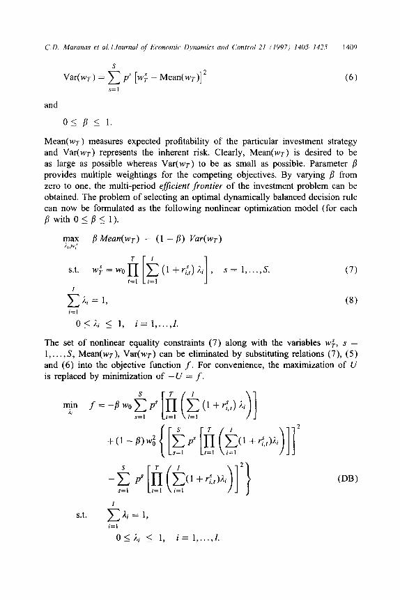
Mean( wr ) measures expected profitability of the particular investment strategy and Var(wr) represents the inherent risk. Clearly, Mean is desired to be as large as possible whereas Var(wr) to be as small as possible. Parameter /I provides multiple weightings for the competing objectives. By varying fi from

zero to one, the multi-period ejficient frontier of the investment problem can be obtained. The problem of selecting an optimal dynamically balanced decision rule can now be formulated as the following nonlinear optimization model (for each /I with 0 5 /I 5: 1).

T I

s.t. w; = wo rI[m l+r;,)Aj ) s= l)...) S, t=l i=l I

c Ai = 1, i=l

OS& 2 1, i=l,..., I.

(7)

(8)

The set of nonlinear equality constraints (7) along with the variables w;, s = 1,. . ,S, Mean( Var(wr) can be eliminated by substituting relations (7), (5) and (6) into the objective function f. For convenience, the maximization of U is replaced by minimization of -U = f.

n-II f=-/?wo$P” fi k( s=l [*=, (i=, l +rfJJA1)l

(DB)

S.t. C/Ii = 1, i=l

O<Ai 5 1, i=l,..., I.

1410 C. D. Mar-anas et al. I Journal of Economic Dynamics and Control 21 (1997) 1405-1425

This results in an optimization problem involving a single linear equality con-

straint (8) and a modest number of variables li, i = 1,. . . ,/. The compensating

cost is a more complicated objective function. The function f is a nonconvex multivariable polynomial function in li involving multiple local minima.

To see why function f is nonconvex, let us give a small example. Say, we have two assets - stock and bond. We consider two time periods. In each time

period, there is only one possible scenario for the return of each asset. Hence, in this example, I = T = 2, and S = 1. Let us assume that the possible returns of

the assets are as follows: r;,, = ri,2 = a, and rd,, = ri32 = b, for some a, b > 0.

Since there is only one scenario, it follows that p’ = 1. Suppose that /I = 1 and wo = 1. Then the objective function of (DB) is

= - [( 1 + a)il + (1 + b)&]' .

It is easy to verify that the above f is not a convex function of (Ai, AZ). In fact,

it is a concave function. This shows that the objective function f in (DB) is not convex even in a very special situation and hence it is not convex in general.

The (DB) model can be readily modified to address other measures of risk aversion across time. For example, we could maximize the expected utility of wealth at the end of the planning horizon; or we could conduct a multi-objective decision analysis. The proposed global optimization algorithm can be extended

for these alternative models. In Section 3, we introduce a global optimization algorithm which guarantees

s-converge to the global optimum solution in a finite number of iterations.

2.2. Empirical results

In this subsection, we test several popular versions of the dynamically balanced decision rule based on the lo-year historical data (January 1982 - December 1991) of monthly returns in three asset categories: cash, bond and stock. The investment problem involves a monthly decision on what portion to hold on each of the three asset categories. We examine seven variants of the DB rule, namely, mix 1, mix 2, . . . . mix 7, as shown in Table 1. These mixes are often proposed in the literature and by investment advisers as benchmarks for comparative studies. We conducted a backtest of the seven specified dynamically balanced decision rules as follows: At the beginning of each month, we examined the portfolio and re-balanced it to the target mixes. Thus, we sold (bought) stock and bought (sold) bonds if the equity market outperformed (underperformed) the bond market. Geo- metric means of monthly returns (p), standard deviations (c) and turnover (p) of the seven rules as well as the 100% stock rule computed based on the given data are illustrated in Table 2.

C. D. Mcuumzs el al. IJournnl of Economic Dynamics and Control 21 (1997) 1405-1425 141 I

Table 1

Composition of the seven mixes tested

mix1 mix2 mix3 mix4 mix5 mix6 mix7

Cash 0% 0% 0% 0% 0% 0% 0% Bond 20% 30% 40% 50% 60% 70% 80% Stock 80% 70% 60% 50% 40% 30% 20%

Table 2

Means (p), standard deviations (0) and turnovers (p) of the seven DB rules and the 100% stock rule

during 1982-199 I period

DB 100% stock mix1 mix2 mix3 mix4 mix5 mix6 mix7

P 1.5% I .48% 1.46% 1.45% 1.42% I .40% 1.35% 1.33%

0 4.7% 4.0% 3.6% 3.3% 3.2% 3.1% 3.0% 2.8%

P 0% 1.10% 1.10% 1.08% 1.05% 1 .OO% 0.93% 0.86%

Table 3 Means (p) and standard deviations (u) of scl, sc2 and sc3 during 1982-1991 period (from Brennan

et al., 1996)

SC1 SC2 SC3

P 1.3% 1.5% I .4%

0 2.8% 3.1% 3.1%

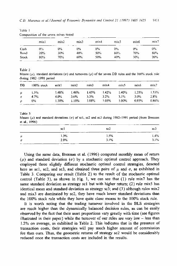
Using the same data, Brennan et al. (1996) computed monthly mean of return (p) and standard deviation (a) by a stochastic optimal control approach. They employed three slightly different stochastic optimal control strategies, denoted here as scl, sc2, and sc3, and obtained three pairs of p and 0, as exhibited in Table 3. Comparing our result (Table 2) to the result of the stochastic optimal control (Table 3), as shown in Fig. 1, we can see that (1) rule mix7 has the

same standard deviation as strategy scl but with higher return; (2) rule mix5 has identical mean and standard deviation as strategy sc3; and (3) although rules mix2 and mix3 are dominated by sc2, they have much lower standard deviations than the 100% stock rule while they have quite close means to the 100% stock rule.

It is worth noting that the trading turnover involved in the BLS strategies are much higher than the dynamically balanced decision rules, as can be easily observed by the fact that their asset proportions vary greatly with time (see figures illustrated in their paper) while the turnover of our rules are very low - less than 1.2% on average, as exhibited in Table 2. This indicates that in the presence of transaction costs, their strategies will pay much higher amount of commission fee than ours. Thus, the geometric returns of strategy sc2 would be considerably reduced once the transaction costs are included in the results.

1412 C. D. Muranas ef al. IJournal of Economic Dynamics and Control 21 (1997) 1405-142.5

0.0148 .-

E 0.0146 --

,; _ 0.014-I -- _ $ 0.0142 .-

: 0.014 --

; 0.0138 .-

: 0.0136 --

E 0.0134 --

0.0132 *-

0.02 0.022 0.024 0.026 0.028 0.03 0.032 o.a34 0.036 0.038 0.04

rlm.lud dwlrlian

l ovMnlalv- msmchsbopunw card

0.013 l’,

L

1

5 l 2

3’. l 4

5

l 6

l 7

Fig. 1. Dynamically balanced vs. stochastic optimal control

Table 4

Means (IO and standard deviations C(r) of the seven B&H rules

B&H b&h1 b&h2 b&h3 b&h4 b&h5 b&h6 b&h7

P 1.46% 1.44% 1.43% 1.39% 1.38% 1.33% 1.31%

u 4.0% 3.65% 3.35% 3.24% 3.14% 3.01% 2.8%

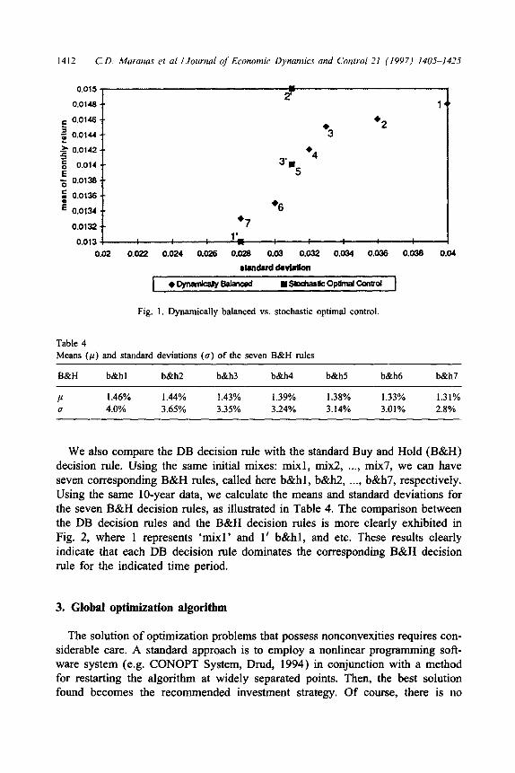
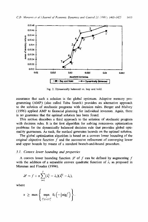
We also compare the DB decision rule with the standard Buy and Hold (B&H) decision rule. Using the same initial mixes: mixl, mix2, . . . . mix7, we can have seven corresponding B&H rules, called here b&hl, b&h2, . . . . b&h7, respectively. Using the same IO-year data, we calculate the means and standard deviations for the seven B&H decision rules, as illustrated in Table 4. The comparison between the DB decision rules and the B&H decision rules is more clearly exhibited in Fig. 2, where 1 represents ‘mix1 ’ and 1’ b&hl, and etc. These results clearly indicate that each DB decision rule dominates the corresponding B&H decision rule for the indicated time period.

3. Global optimization algorithm

The solution of optimization problems that possess nonconvexities requires con- siderable care. A standard approach is to employ a nonlinear programming soft- ware system (e.g. CONOPT System, Drud, 1994) in conjunction with a method for restarting the algorithm at widely separated points. Then, the best solution found becomes the recommended investment strategy. Of course, there is no

C. D. Mctranrrs PI rrl. I Journal of Economic D>wamics and Control 21 (1997) 1405.-1425 1413

e 0.0144

; 0.0142

2 0.014

I E 0.0138

‘d 3 0.0136

ii 0.0134

0.0132

0.013

0.025 0.03 0.035

stwtdwd deviation

-m--auyandHokJ

a04

Fig. 2. Dynamically balanced vs. buy and hold

assurance that such a solution is the global optimum. Adaptive memory pro- gramming (AMP) (also called Tabu Search) provides an alternative approach to the solution of stochastic programs with decision rules. Berger and Mulvey (1996) applied AMP to financial planning for individual investors. Again, there

is no guarantee that the optimal solution has been found. This section describes a third approach to the solution of stochastic program

with decision rules. It is the first algorithm for solving nonconvex optimization problems for the dynamically balanced decision rule that provides global opti- mality guarantees. As such, the method generates bounds on the optimal solution.

The global optimization algorithm is based on a convex lower bounding of the original objective function f and the successive refinement of converging lower

and upper bounds by means of a standard branch-and-bound procedure.

3. I. Convex lower bounding and properties

A convex lower bounding function 2 of f can be defined by augmenting f with the addition of a separable convex quadratic function of /li as proposed in

Maranas and Floudas (1994).

Y = f + c1 k(i.F - Li)(Lu - /li), i=l

where

tL 2 max

{ #

max 0,

( ,)

- f eigf . if 5 ;.; 5 / IJ

1414 C.D. Muranas el al. IJournal of Economic Dymmirs and Control 21 (1997) 1405-1425

Note that i$, Ry are the lower and upper bounds of li initially set to # = 0 and Lu = 1. Also, CY is a nonnegative parameter which ensures convexity and must

be greater or equal to the negative one-half of the minimum eigenvalue of f

over RF 5 Ai < JLU. The parameter cx can be estimated either through the solution of an optimization problem or by using the concept of the measure of a matrix

(Maranas and Floudas, 1994). The effect of adding the extra term,

’ c( c (1: - i,i)(/lv - Ai) i=l

to f is to make _!? convex by overpowering the nonconvexity characteristics of

f with the addition of the term 2a to all of its eigenvalues,

eig” = eigf + 2cr, i = I,...,1

Here eigiY,eigf are the ith eigenvalues of .P’, f respectively. This function Y defined over the box constraints [I$, I~?] , i = 1,. . . , I involves a number of

properties which enable us to construct a global optimization algorithm for finding the global minimum of f. These properties, whose proof is given in Maranas and Floudas ( 1994) are as follows.

Property 1. Y is a valid underestimator of f,

V ;ii E [2~,2~] 9 mY(Ai) < f (/Ii).

Property 2. _.Y matches f at all comer points.

Vii such that J.i = 1: or I.i = $, I = f (Ai).

Property 3. Y is convex in [#, Ai”].

Property 4. The maximum separation between LZ and f is bounded and propor- tional to a and to the square of the diagonal of the current box constraints.

Property 5. The underestimators constructed over supersets of the current set are always less tight than the underestimator constructed over the current box constraints for every point within the current box constraints.

Property 6. LZ’ corresponds to a relaxed dual bound of the original function f (see Floudas and Visweswaran, 1990, 1993).

C. D. Mat~mas et al. /Journal of Economic Dynamics and Conirol 21 (1997j 1405-1425 1415

3.2. Highlights of the algorithm

Based on the aforementioned properties, the global optimization algorithm lo-

cates the global minimum f * by constructing converging lower and upper bounds

on f*. A lower bound on j’*, denoted as fL, within some box constraints is derived by invoking Properties (1) and (3). Based on these properties 9 is a convex lower bounding function of f. Therefore, its single global minimum within some box constraints is a valid lower bound fL on the global minimum

solution f * and can be guaranteed to be found with available local optimization algorithms. An upper bound on f*, denoted as f”, is then simply the value of f at the global minimum point of 8.

The next step, after establishing an upper and a lower bound on the global minimum, is to refine them by using Property (5). This property implies that the value of 2 at every point, and therefore at the global minimum, is increased by restricting the box constraints within which it has been defined. Tighter box con- straints occur by partitioning the rectangle defined by the initial box constraints

into a number of smaller rectangles. One way of partitioning is to successively

divide the current rectangle in two subrectangles by halving on the middle point of the longest side of the initial rectangle (bisection). At each iteration the lower bound of f* is simply the minimum over all the minima of 2 in every sub-

rectangle composing the initial rectangle. Therefore, a straightforward (bound improving) way of tightening the lower bound f L is to halve at each iteration only the subrectangle responsible for the infimum of the minima of 2 over all subrectangles, according to the rules discussed earlier. This procedure generates a nondecreasing sequence for the lower bound f L of f *. Furthermore, we con- struct a nonincreasing sequence for the upper bound fU by selecting it to be the infimum over all the previously recorded upper bounds. Clearly, if the global

minimum of 2’ in any subrectangle is greater than the current upper bound f”

we can ignore this subrectangle because the global minimum of f cannot be

situated inside it (fanthoming step). Property (4) addresses the question of how small these subrectangles must

become before the upper and lower bounds of S inside these subrectangles are within s. If 6 is the diagonal of the subrectangle,

and E is the convergence tolerance, from Property (4) we have the following condition for convergence,

1416 C. D. Muranas et al. I Journal of Economic Dynamics and Control 21 (1997) 1405-1425

which means that if the diagonal 6 of a subrectangle is

then s-convergence to the global minimum of f has been achieved. In practice,

however, not only s-convergence to the global minimum is required, but con-

vergences in a finite number of iterations. By analyzing the structure (sparsity) of the branch-and-bound tree resulting from the subdivision process, finite upper and lower bounds on the total number of required steps for s-convergence can

be derived (see Maranas and Floudas, 1994):

Iter,i, = I log, xi=, (2: - 1:)’

J@ --l. I

The basic steps of the proposed global optimization algorithm are as follows:

3.3. Outline of algorithmic steps

Step I: Initialization. A convergence tolerance E is selected

counter Iter is set to one. Lower and upper bounds on the f LBD, fUBD are initialized.

and the iteration global minimum

Step 2: Update of upper bound f UBD If the value of f at the current point is . less than fUBD, then fUBD is set equal to the value of f at the current point.

Step 3: Partitioning of current rectangle. The current rectangle is partitioned

into two rectangles by halving along the longest side of the initial rectangle.

Step 4: Solution of convex problems in two subrectangles. The following convex nonlinear optimization problem is solved in both subrectangles using a standard convex nonlinear solver.

Iyin 9=f +@)!JA~-&) (/I~-j.i> i=l

I

s.t. c li= 1, i=I

1: 5 Ai<$, i= l,..., I.

C. D. Muranas et al. I Journul of Economic Dynamics and Control 21 11997) 1405-1425 1417

If a solution is less than the current upper bound, it is stored along with the

value of the variable 3&j at the solution point.

Step 5: Update iteration counter Iter and Lower Bound fLBD.

The iteration counter is increased by one, and the lower bound f LBD is updated to be the incumbent solution. Further, the selected solution is erased from the solutions set. Stop if iteration limit is reached.

Step 6: Update current point and variable bounds. The current point is selected

to be the solution point of the previously found minimum solution in Step 5, and the current rectangle is updated to be the one containing the previously found

solution,

Step 7: Check for convergence.

IF (fUBD - fLBD) > E, then return to Step 2

Otherwise, E-convergence has been reached. A detailed description of the algorithmic steps as well as a mathematical proof

of a-convergence to the global minimum for the employed global optimization

algorithm can be found in Maranas and Floudas (1994).

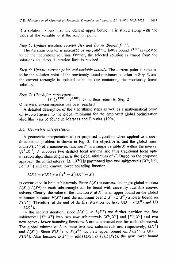
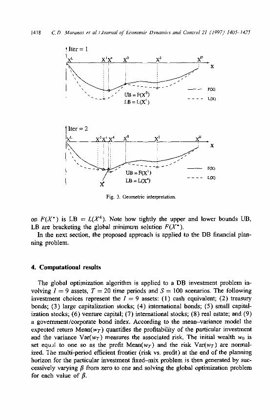
3.4. Geometric interpretation

A geometric interpretation of the proposed algorithm when applied to a one-

dimensional problem is shown in Fig. 3. The objective is find the global mini- mum F(X* ) of a nonconvex function F in a single variable X within the interval [XL,Xu]. F involves two distinct local minima and thus traditional local opti-

mization algorithms might miss the global minimum of F. Based on the proposed approach the initial interval [XL,Xu] is partitioned into two subintervals [XL,Xo], [X0,X”] and the convex lower bounding function

L(X) = F(X) + c1 (XL - X) (X” - X)

is constructed in both subintervals. Since L(X) is convex, its single global minima

L(X’ ),L(X2) in each subrectangle can be found with currently available convex solvers. Clearly, the value of the function F at X0 is an upper bound on the global minimum solution F(X*) and the minimum over L(X’),L(X2) a lower bound on F(X*). Therefore, at the end of the first iteration we have UB = F(X”) and LB = _qx’ ).

In the second iteration, since L(X’) < L(X2) we further partition the first subinterval [XL,Xo] into two new subintervals [XL,X’] and [X*,X0] and two new convex lower bounding functions L are constructed one for each subinterval. The global minima of L in these two new subintervals are, respectively, L(X3) and L(X4). Since F(X’) < F(X”) the new upper bound on F(X*) is UB = F(X’). Also because L(X4) = min (L(&),L(X3),L(&)), the new lower bound

1418 C. D. Moranus et al. /Journal oj’ Economic Dynamics and Conrrol 21 (1997) 1405-1425

f Iter = 1

1 her = 2

_--- ‘(x)

Fig. 3. Geometric interpretation.

on F(X*) is LB = &Y4). Note how tightly the upper and lower bounds UB,

LB are bracketing the global minimum solution F(X* ). In the next section, the proposed approach is applied to the DB financial plan-

ning problem.

4. Computational results

The global optimization algorithm is applied to a DB investment problem in-

volving I = 9 assets, T = 20 time periods and S = 100 scenarios. The following investment choices represent the I = 9 assets: (1) cash equivalent; (2) treasury bonds; (3) large capitalization stocks; (4) international bonds; (5) small capital- ization stocks; (6) venture capital; (7) international stocks; (8) real estate; and (9) a government/corporate bond index. According to the mean-variance model the expected return Mean quantifies the profitability of the particular investment and the variance Var(wr) measures the associated risk. The initial wealth wo is set equJ1 to one so as the profit Mean and the risk Var(wr) are normal- ized. I he multi-period efficient frontier (risk vs. profit) at the end of the planning horizon for the particular investment fixed-mix problem is then generated by suc- cessively varying /I from zero to one and solving the global optimization problem for each value of p.

As in Mulvey (1994) the probabilities of occurrence for scenarios s = 1.. , S are equal. Thus, we have

ps = ; = 0.01, ‘ds = 1,.,.,X

Next, by applying the scenario generation technique introduced in Mulvey ( 1996), the (I = 9) x (T = 20) x (S = 100) = 18000 returns Y:,, for asset i, in time step t, and scenario s are estimated. To provide some insight on their numerical

values, their respective minimum and maximum value as well as their mean and standard deviation are as follows:

Minimum = -0.70,

Maximum( r:, ) = 1 .oo,

Mean = 0.10,

Std Dev(ri,) = 0.18.

In the next step, we solve the nonconvex problem (DB) with different values of the parameter 8. Three different alternatives for the absolute convergence tol-

erance ei = 0.05, EZ = 0.03 and ~3 = 0.01 are considered. Regardless of the initial point, convergence to the c-global minimum solution is achieved. Exact

convergence to the global minimum f’ is then achieved by slightly perturbing the obtained solution f" with a gradient-based optimization algorithm until the

KKT conditions are satisfied. For different values of fl the value of the objective function at the global

minimum solution f * as well as the associated profit

Profit=Mean(wr*)=waep’ 5=l

and risk

Risk = Var(wr*) = wi { $PS [G (&1+01:)]’

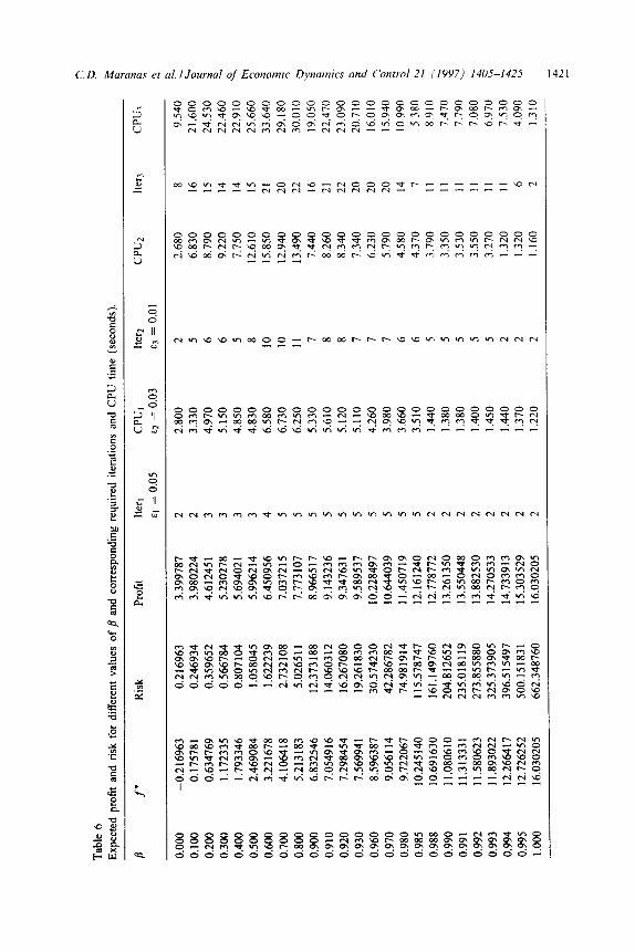
along with the required number of iterations Iter and CPU (seconds) time on a HP-730 workstation at Princeton University are shown in Table 6. Three cases

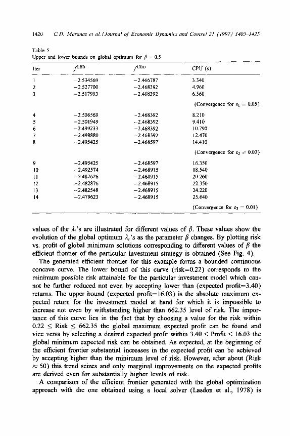
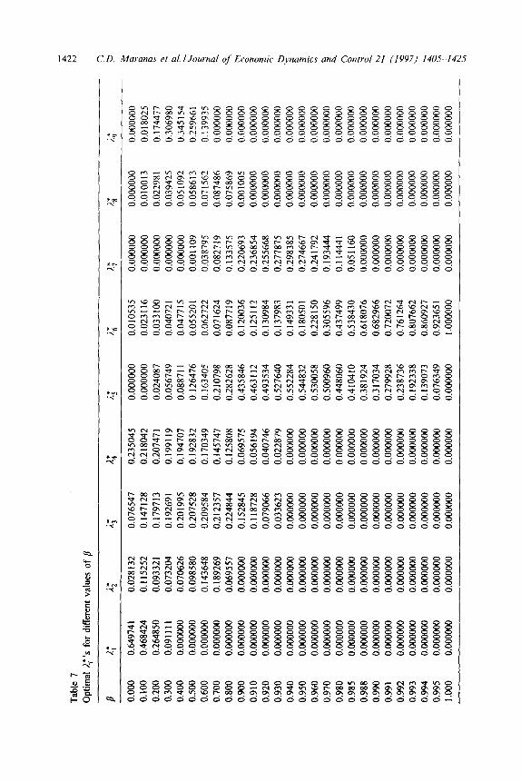
of absolute tolerances of ai = 0.05, ~2 = 0.03 and ~3 = 0.01 are considered. More specifically, the progress of the upper and lower bounds on the global optimum solution for the case p = 0.5 is shown in Table 5. In Table 7 the global optimum

1420 C. D. Maranas et al. IJournal of Economic Dynamics and Control 21 (1997) 1405-1425

Table 5

Upper and lower bounds on global optimum for /I = 0.5

Iter f LBD f UBD CPU (s)

1 -2.534569 -2.466187

2 -2.527700 -2.468392

3 -2.517993 -2.468392

3.340

4.960

6.560

(Convergence for q = 0.05)

4 -2.508569 -2.468392

5 -2.501949 -2.468392

6 -2.499233 -2.468392

7 -2.498880 -2.468392

8 -2.495425 -2.468591

8.210

9.410

10.790

12.470

14.410

(Convergence for ~2 = 0.03)

9 -2.495425 -2.468597

10 -2.492574 -2.468915

II -2.487626 -2.468915

12 -2.482876 -2.468915

13 -2.482548 -2.468915

14 -2.479623 -2.468915

16.350

18.540

20.260

22.350

24.220

25.640

(Convergence for 83 = 0.01)

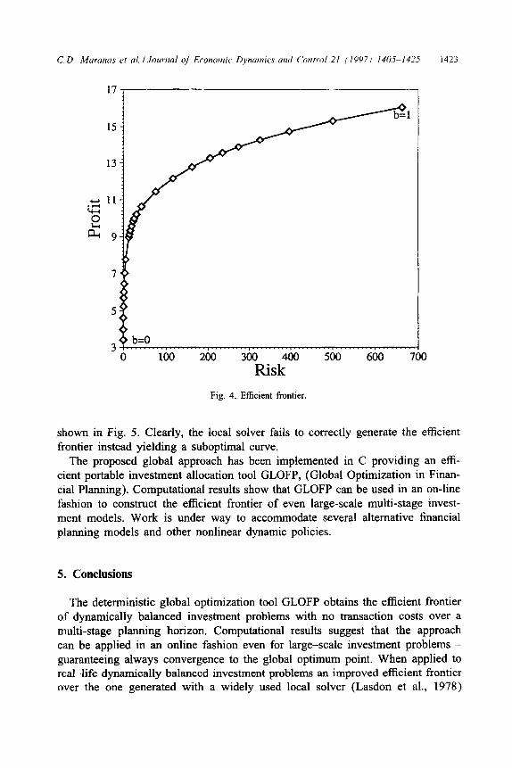
values of the ii’s are illustrated for different values of p. These values show the evolution of the global optimum ii’s as the parameter /I changes. By plotting risk vs. profit of global minimum solutions corresponding to different values of /3 the efficient frontier of the particular investment strategy is obtained (See Fig. 4).

The generated efficient frontier for this example forms a bounded continuous concave curve. The lower bound of this curve (risk=0.22) corresponds to the minimum possible risk attainable for the particular investment model which can- not be further reduced not even by accepting lower than (expected profit=3.40) returns. The upper bound (expected profit=16.03) is the absolute maximum ex-

pected return for the investment model at hand for which it is impossible to increase not even by withstanding higher than 662.35 level of risk. The impor- tance of this curve lies in the fact that by choosing a value for the risk within 0.22 5 Risk 5 662.35 the global maximum expected profit can be found and vice versa by selecting a desired expected profit within 3.40 5 Profit 5 16.03 the global minimum expected risk can be obtained. As expected, at the beginning of the efficient frontier substantial increases in the expected profit can be achieved by accepting higher than the minimum level of risk. However, after about (Risk N” 50) this trend seizes and only marginal improvements on the expected profits are derived even for substantially higher levels of risk.

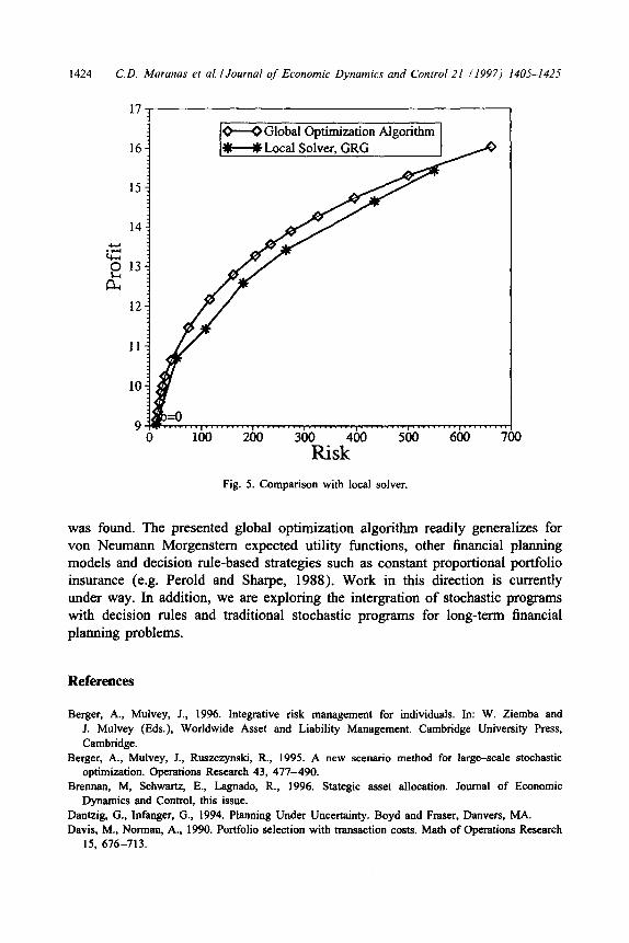
A comparison of the efficient frontier generated with the global optimization approach with the one obtained using a local solver (Lasdon et al., 1978) is

9 T

able

6

P

Exp

ecte

d pr

ofit

and

risk

fo

r di

ffer

ent

valu

es

of

/I a

nd

corr

espo

ndin

g re

quir

ed

itera

tions

an

d C

PU

time

(sec

onds

).

$

B

f’

Ris

k Pr

ofit

Iter

l C

PU,

her2

C

PU2

lter3

2

CP

U3

0

E,

= 0.

05

E2

= 0.

03

E)

= 0.

01

2

0.00

0 -0

.216

963

0.21

6963

3.

3997

87

2 2.

800

2 2.

680

8 9.

540

0.10

0 0.

1757

81

0.24

6934

3.

9802

24

2 3.

330

5 6.

830

16

2 I ,

600

0.20

0 0.

6347

69

0.35

9652

4.

6124

51

3 4.

970

6 8.

790

15

24.5

30

0.30

0 1.

1723

35

0.56

6784

5.

2302

78

3 5.

150

6 9.

220

14

22.4

60

0.40

0 1.

7933

46

0.80

7104

5.

6940

21

3 4.

850

5 7.

750

14

22.9

10

0.50

0 2.

4690

84

1.05

8045

5.

9962

14

3 4.

830

8 12

.610

15

25

.660

0.60

0 3.

2216

78

1.62

2239

6.

4509

56

4 6.

580

10

15.8

50

21

33.6

40

0.70

0 4.

1064

18

2.73

2108

7.

0372

15

5 6.

730

10

12.9

40

20

29.1

80

0.80

0 5.

2131

83

5.02

6511

7.

773

107

5 6.

250

11

13.4

90

22

30.0

10

0.90

0 6.

8325

46

12.3

7318

8 8.

9665

17

5 5.

330

7 7.

440

16

19.0

50

0.91

0 7.

0549

16

14.0

6031

2 9.

1432

36

5 5.

610

8 8.

260

21

22.4

70

0.92

0 7.

2984

54

16.2

6708

0 9.

3476

31

5 5.

120

8 8.

340

22

23.0

90

0.93

0 7.

5699

41

19.2

6183

0 9.

5895

37

5 5.

110

7 7.

340

20

20.7

10

0.96

0 8.

5963

87

30.5

7423

0 10

.228

497

5 4.

260

7 6.

230

20

16.0

10

0.97

0 9.

0561

14

42.2

8678

2 10

.644

039

5 3.

980

7 5.

790

20

15.9

40

0.98

0 9.

7220

67

74.9

8191

4 11

.450

719

5 3.

660

6 4.

580

14

10.9

90

0.98

5 10

.245

140

115.

5787

47

12.1

6124

0 5

3.51

0 6

4.37

0 7

5.38

0

0.98

8 10

.691

630

161.

1497

60

12.7

7877

2 2

1.44

0 5

3.79

0 11

8.

910

0.99

0 11

.080

610

204.

8 12

652

13.2

6135

0 2

1.38

0 5

3.35

0 11

7.

470

0.99

1 11

.313

331

235.

0181

19

13.5

5044

8 2

1.38

0 5

3.53

0 11

7.

790

0.99

2 11

.580

623

273.

8558

80

13.8

8253

0 2

1.40

0 5

3.55

0 11

7.

080

0.99

3 1 I

.893

022

325.

3739

05

14.2

7053

3 2

1.45

0 5

3.27

0 11

6.

970

0.99

4 12

.266

417

396.

5 15

497

14.7

3391

3 2

1.44

0 2

I .32

0 11

7.

530

0.99

5 12

.726

252

500.

1518

31

15.3

0352

9 2

1.37

0 2

1.32

0 6

4.09

0

1.00

0 16

.030

205

662.

3487

60

16.0

3020

5 2

1.22

0 2

1.16

0 2

1.31

0 -

e Table 7

k

Optimal Af's for different

values

of /I

n

B

1;

1;

G

1;

L;

I'

'6

I*

'7

2'

'R

i*

‘9

P

>

0.00

0

0.10

0

0.200

0.300

0.400

0.500

0.600

0.700

0.800

0.900

0.910

0.920

0.930

0.940

0.950

0.960

0.970

0.980

0.985

0.988

0.990

0.991

0.992

0.993

0.994

0.995

1 .oo

o

0.64

9741

0.468424

0.264850

0.091111

0.000000

0.000000

0.000000

0.000000

0.000000

0.000000

o.oOOOOo

0.000000

0.000000

0.000000

0.000000

0.000000

o.ooOOoO

0.000000

0.000000

0.000000

0.000000

0.000000

0.000000

0.000000

0.000000

0.000000

0.000000

0.028132

0.115252

0.093321

0.073204

0.070626

0.098580

0.143648

0.189269

0.069557

0.000000

0.000000

0.000000

0.000000

0.000000

0.000000

0.000000

0.000000

0.000000

0.000000

0.000000

0.000000

0.000000

0.000000

0.000000

0.000000

0.000000

0.000000

0.076547

0.147128

0.179713

0.192691

0.201995

0.207528

0.209584

0.212357

0.224844

0.152845

0.118728

0.079066

0.033623

0.000000

0.000000

0.000000

0.000000

0.000000

0.000000

0.000000

0.000000

0.000000

0.000000

0.000000

0.000000

0.000000

0.000000

0.235045

0.218042

0.207471

0.199119

0.194707

0.192832

0.170349

0.145747

0.125808

0.069575

0.056194

0.040746

0.022879

0.000000

0.000000

0.000000

0.000000

0.000000

0.000000

0.000000

0.000000

0.000000

0.000000

0.000000

0.000000

0.000000

0.000000

0.00

0000

0.00

0000

0.024087

0.056749

0.088711

0.126476

0.163405

0.210798

0.282628

0.435846

0.463112

0.493534

0.527640

0.552284

0.544832

0.530058

0.500960

0.448060

0.410410

0.381924

0.317034

0.279928

0.238736

0.192338

0.139073

0.076349

0.000000

0.010535

0.023116

0.033100

0.040721

0.047715

0.055201

0.062722

0.071624

0.087719

0.120036

0.125112

0.130984

0.137983

0.149331

0.180501

0.228150

0.305596

0.437499

0.538430

0.618076

0.682966

0.720072

0.761264

0.807662

0.860927

0.923651

I .oo

oooo

0.00

0000

0.00

0000

0.00

0000

0.

0000

00

0.00

0000

0.001109

0.038795

0.082719

0.133575

0.220693

0.236854

0.255668

0.277875

0.298385

0.274667

0.241792

0.193444

0.114441

0.051160

0.000000

0.000000

0.000000

0.000000

0.000000

0.000000

0.000000

0.000000

0.00

0000

0.010013

0.022981

0.039425

0.051092

0.058613

0.071562

0.087486

0.075869

0.001005

0.000000

0.000000

0.000000

0.000000

0.000000

0.000000

0.000000

0.000000

0.000000

0.000000

0.000000

0.000000

0.000000

0.000000

0.000000

0.000000

0.000000

0.00

0000

- 3

0.018025

2

0.174477

2

0.306980

z

0.345154

k

0.259661

2

0.139935

P

3

0.000000

a

0.000000

e

0.000000

$

0.000000

2

0

0.000000

g

0.000000

b

0.000000

3

0.000000

9

=.

0.000000

c

0.000000

2

0.000000

0.000000

:

8

0.000000

'=

0.000000

$.

0.000000

2

0.000000

.

0.000000

z

2

0.000000

2

0.000000

0.000000

?

2

C. D. Maranas et al. I Journal of Economic Dynamics and Control 21 (1997) 1405-1425 1423

5

3 0 100 200 300 400 500 600 7

Risk

Fig. 4. Efficient frontier

shown in Fig. 5. Clearly, the local solver fails to correctly generate the efficient frontier instead yielding a suboptimal curve.

The proposed global approach has been implemented in C providing an et%- cient portable investment allocation tool GLOFP, (Global Optimization in Finan- cial Planning). Computational results show that GLOFP can be used in an on-line fashion to construct the efficient frontier of even large-scale multi-stage invest- ment models. Work is under way to accommodate several alternative financial planning models and other nonlinear dynamic policies.

5. Conclusions

The deterministic global optimization tool GLOFP obtains the efficient frontier of dynamically balanced investment problems with no transaction costs over a multi-stage planning horizon. Computational results suggest that the approach can be applied in an online fashion even for large-scale investment problems -

guaranteeing always convergence to the global optimum point. When applied to real-life dynamically balanced investment problems an improved efficient frontier over the one generated with a widely used local solver (Lasdon et al., 1978)

1424 C. D. Maranas et al. IJournal of Economic Dynamics and Control 21 (1997) 1405-1425

16

10

9 0 100 200 300 400 500 600 7

Risk

Fig. 5. Comparison with local solver.

was found. The presented global optimization algorithm readily generalizes for von Neumann Morgenstem expected utility functions, other financial planning models and decision rule-based strategies such as constant proportional portfolio insurance (e.g. Perold and Sharpe, 1988). Work in this direction is currently under way. In addition, we are exploring the intergration of stochastic programs with decision rules and traditional stochastic programs for long-term financial planning problems.

References

Berger, A., Mulvey, J., 1996. Integrative risk management for individuals. In: W. Ziemba and

J. Mulvey (Eds.), Worldwide Asset and Liability Management. Cambridge University Press,

Cambridge.

Berger, A., Mulvey, J., Ruszczynski, R., 1995. A new scenario method for huge-scale stochastic optimization. Operations Research 43, 477-490.

Brennan, M, Schwartz, E., Lagnado, R., 1996. Stategic asset allocation. Journal of Economic Dynamics and Control, this issue.

Dantzig, G., Infanger, G., 1994. Planning Under Uncertainty. Boyd and Fraser, Danvers, MA.

Davis, M., Norman, A., 1990. Portfolio selection with transaction costs. Math of Operations Research

15, 676-713.

C. L3. Murortas er ul. ! Jourd OJ Economic Dwtumics ami Control 21 (1997) 140-1425 1425

Dempster, M., Thompson, R., 1995. Parallelization and aggregation of nested Benders decomposition.

presented at APMOD 95, Btunel University.

Drud, A., 1994. CONOPT - A large-scale GRG Code. ORSA Journal on Computing, 6, 207-216.

Floudas, C., Visweswaran, V., 1990. A global optimization algorithm for certain classes of nonconvex

NLPs, part I : theory. Computers and Chemical Engineering. 14, 1397-1417.

Floudas, C., Visweswaran, V., 1993. Primal-relaxed dual global optimization approach, Journal of

Optimization Theory and its Application. 78, 187-225.

Garstka, S., R J-B Wets, 1974. On decision rules in stochastic programming. Mathematical

Programming, 7, I 17-l 43.

Grauer, R., Hakansson, N., 1985. Returns on levered actively managed long-run portfolios of stocks,

bonds and bills. Financial Analysts Journal 24-43.

Higle, J., Sen, S., 1991. Stochastic decomposition: an algorithm for twostage linear programming

with recourse, Mathematics of Operations Research 16, 650-669.

Lasdon, L., Warren, A., Ratner, M., 1978. Design and testing of a CRC code for nonlinear

optimization. ACM Transaction on Mathematical Software 4, 34-50.

Maranas, C., Floudas, C., 1993. Global optimization for molecular conformation problems, Annals of

Operations Research 42, 85-l 17.

Maranas, C., Floudas, C., 1994. Global minimum potential energy conformations of small molecules.

Journal of Global Optimization 4, 155-170.

Merton, R., 1971. Optimum consumption and portfolio rules in continuous time model. Journal of

Economic Theory 3, 373-413.

Mulvey, J., 1994. An Asset-liability investment system. Interfaces 24, 22-33.

Mulvey, J., 1996. Generating scenarios for the Towers Perrin investment system. interfaces 26, I-15.

Mulvey, J., Vladimirou, H., 1992. Stochastic Network programming for financial planning problems.

Management Science 38, 1642-1664.

Perold, A., Sharpe, W., 1988. Dynamic strategies for asset allocation. Financial Analysts Journal 1,

16-27.

Rockafellar, R., R J-B. Wets, 1991. Scenario and policy aggregation in optimization under uncertainty.

Mathematics of Operations Research 16, 119-147.

Taksar, M., Klass M., Assaf, D., 1988. A diffusion model optimal portfolio selection in the presence

of brokerage fees. Math of Operations Research 13, 277-294.

Worzel, K., Vassiadou-Zeniou, C., Zenios, S., 1994. Integrated simulation and optimization models

for tracking indices of fixed income securities. Operations Research 42, 223-233.

Zenios, S., 1993. Financial Optimization, Cambridge University Press, Cambridge.

Zenios, S., Yang, D., 1996. A scaleable parallel interior algorithm for stochastic linear programming

and robust optimization. Computational Optimization and Applications. In print.