Solving Constrained Optimization Problemsby the ε Constrained Particle Swarm Optimizer

with Adaptive Velocity Limit ControlTetsuyuki Takahama

Department of Intelligent SystemsHiroshima City University

Asaminami-ku, Hiroshima, 731-3194 Japantakahama@its.hiroshima-cu.ac.jp

Setsuko SakaiFaculty of Commercial Sciences

Hiroshima Shudo UniversityAsaminami-ku, Hiroshima, 731-3195 Japan

setuko@shudo-u.ac.jp

Abstract— The ε constrained method is an algorithmtransformation method, which can convert algorithms forunconstrained problems to algorithms for constrained problemsusing the ε level comparison that compares the search pointsbased on the constraint violation of them. We proposed theε constrained particle swarm optimizer εPSO, which is thecombination of the ε constrained method and particle swarmoptimization. In the εPSO, the agents who satisfy the constraintsmove to optimize the objective function and the agents whodon’t satisfy the constraints move to satisfy the constraints. Butsometimes the velocity of agents becomes too big and they flyaway from feasible region. In this study, to solve this problem,we propose to divide agents into some groups and controlthe maximum velocity of agents adaptively by comparing themovement of agents in each group. The effectiveness of theimproved εPSO is shown by comparing it with various methodson well known nonlinear constrained problems.

Keywords—constrained optimization, nonlinear optimization,particle swarm optimization, ε constrained method, α constrainedmethod

I. INTRODUCTION

Constrained optimization problems, especially nonlinearoptimization problems, where objective functions are mini-mized under given constraints, are very important and fre-quently appear in the real world. In this study, the followingoptimization problem (P) with inequality constraints, equalityconstraints, upper bound constraints and lower bound con-straints will be discussed.

(P) minimize f(x)subject to gj(x) ≤ 0, j = 1, . . . , q

hj(x) = 0, j = q + 1, . . . ,mli ≤ xi ≤ ui, i = 1, . . . , n,

(1)

where x = (x1, x2, · · · , xn) is an n dimensional vector,f(x) is an objective function, gj(x) ≤ 0 and hj(x) = 0are q inequality constraints and m − q equality constraints,respectively. Functions f, gj and hj are linear or nonlinearreal-valued functions. Values ui and li are the upper boundand the lower bound of xi, respectively. Also, let the feasiblespace in which every point satisfies all constraints be denoted

by F and the search space in which every point satisfies theupper and lower bound constraints be denoted by S (⊃ F).

There exist many studies on solving constrained optimiza-tion problems using evolutionary computations[1], [2] andparticle swarm optimization[3]. These studies can be classifiedinto several categories according to the way the constraints aretreated as follows:

(1) Constraints are only used to see whether a search pointis feasible or not[4]. Approaches in this category are usuallycalled death penalty methods. In this category, the searchingprocess begins with one or more feasible points and continuesto search for new points within the feasible region. When a newsearch point is generated and the point is not feasible, the pointis repaired or discarded. In this category, generating initialfeasible points is difficult and computationally demandingwhen the feasible region is very small. If the feasible regionis extremely small, as in problems with equality constraints, itis almost impossible to find initial feasible points.

(2) The constraint violation, which is the sum of theviolation of all constraint functions, is combined with theobjective function. The penalty function method is in thiscategory[5], [6], [7], [8], [9], [10]. In the penalty functionmethod, an extended objective function is defined by addingthe constraint violation to the objective function as a penalty.The optimization of the objective function and the constraintviolation is realized by the optimization of the extendedobjective function. The main difficulty of the penalty functionmethod is the difficulty of selecting an appropriate value forthe penalty coefficient that adjusts the strength of the penalty.If the penalty coefficient is large, feasible solutions can beobtained, but the optimization of the objective function willbe insufficient. On the contrary, if the penalty coefficient issmall, high quality (but infeasible) solutions can be obtainedas it is difficult to decrease the constraint violation.

(3) The constraint violation and the objective function areused separately. In this category, both the constraint violationand the objective function are optimized by a lexicographicorder in which the constraint violation precedes the objectivefunction. Deb[11] proposed a method in which the extended

1–4244–0023–6/06/$20.00 c© 2006 IEEE CIS 2006683

objective function that realizes the lexicographic orderingis used. Takahama and Sakai proposed the α constrainedmethod[12] and ε constrained method[13], which adopt a lex-icographic ordering with relaxation of the constraints. Runars-son and Yao[14] proposed the stochastic ranking method inwhich the stochastic lexicographic order, which ignores theconstraint violation with some probability, is used. Thesemethods were successfully applied to various problems.

(4) The constraints and the objective function are optimizedby multiobjective optimization methods. In this category, theconstrained optimization problems are solved as the multiob-jective optimization problems in which the objective functionand the constraint functions are objectives to be optimized[15],[16], [17], [18]. But in many cases, solving multiobjectiveoptimization problems is a more difficult and expensive taskthan solving single objective optimization problems.

It has been shown that the methods in the third categoryhave better performance than methods in other categoriesin many benchmark problems. Especially, the α and the εconstrained methods are quite new and unique approachesto constrained optimization. We call these methods algo-rithm transformation methods, because these methods doesnot convert objective function, but convert an algorithm forunconstrained optimization into an algorithm for constrainedoptimization by replacing the ordinal comparisons with the αlevel and the ε level comparisons in direct search methods.These methods can be applied to various unconstrained directsearch methods and can obtain constrained optimization algo-rithms. We showed the advantage of the α constrained methodsby applied the methods to Powell’s method[12], the nonlinearsimplex method[19], [20], genetic algorithms (GAs)[21] andparticle swarm optimization (PSO)[22]. These methods canoptimize problems with severe constraints including equalityconstraints effectively through the relaxation of the constraints.

Recently, we proposed the ε constrained method and theε Constrained Particle Swarm Optimizer (εPSO)[13], whichis the combination of the ε constrained method and PSO. Inthe εPSO, the agent or point which satisfies the constraintswill move to optimize the objective function and the agentwhich does not satisfy the constraints will move to satisfy theconstraints, naturally. But sometimes the velocity of agentsbecomes too big and they fly away from feasible region. Inthis study, to solve this problem, we propose to divide agentsinto some groups and control the maximum velocity of agentsadaptively by comparing the movement of agents in eachgroup. The effectiveness of the εPSO with adaptive velocitylimit control is shown by comparing it with various methods onsome well known problems where the performance of manymethods in all categories were compared.

The ε constrained methods and the εPSO are describedin Section II and III, respectively. The εPSO with adaptivevelocity limit control is defined in Section IV. In Section V,experimental results on some constrained problems are shownand the results of the improved εPSO are compared with thoseof other methods. Finally, conclusions are described in SectionVI.

II. THE ε CONSTRAINED METHOD

A. Constraint violation and ε level comparison

In the ε constrained method, constraint violation φ(x) isdefined. The constraint violation can be given by the maximumof all constraints or the sum of all constraints.

φ(x) = max{maxj

{0, gj(x)}, maxj

|hj(x)|} (2)

φ(x) =∑

j

||max{0, gj(x)}||p +∑

j

||hj(x)||p (3)

where p is a positive number.The ε level comparison is defined as an order relation on

the set of (f(x), φ(x)). If the constraint violation of a point isgreater than 0, the point is not feasible and its worth is low. Theε level comparisons are defined basically as a lexicographicorder in which φ(x) precedes f(x), because the feasibilityof x is more important than the minimization of f(x). Thisprecedence can be adjusted by the parameter ε-level.

Let f1 (f2) and φ1 (φ2) be the function values and theconstraint violation at a point x1 (x2), respectively. Then, forany ε satisfying ε ≥ 0, ε level comparisons <ε and ≤ε between(f1, φ1) and (f2, φ2) are defined as follows:

(f1, φ1) <ε (f2, φ2) ⇔

f1 < f2, if φ1, φ2 ≤ εf1 < f2, if φ1 = φ2

φ1 < φ2, otherwise(4)

(f1, φ1) ≤ε (f2, φ2) ⇔

f1 ≤ f2, if φ1, φ2 ≤ εf1 ≤ f2, if φ1 = φ2

φ1 < φ2, otherwise(5)

In case of ε=∞, the ε level comparisons <∞ and ≤∞ areequivalent to the ordinary comparisons < and ≤ betweenfunction values. Also, in case of ε = 0, <0 and ≤0 areequivalent to the lexicographic orders in which the constraintviolation φ(x) precedes the function value f(x).

B. The properties of the ε constrained method

The ε constrained method converts a constrained optimiza-tion problem into an unconstrained one by replacing the orderrelation in direct search methods with the ε level comparison.An optimization problem solved by the ε constrained method,that is, a problem in which the ordinary comparison is replacedwith the ε level comparison, (P≤ε), is defined as follows:

(P≤ε ) minimize≤ε f(x), (6)

where minimize≤ε means the minimization based on the εlevel comparison ≤ε. Also, a problem (Pε) is defined that theconstraints of (P), that is, φ(x) = 0, is relaxed and replacedwith φ(x) ≤ ε:

(Pε) minimize f(x)subject to φ(x) ≤ ε

(7)

It is obvious that (P0) is equivalent to (P).For the three types of problems, (Pε), (P≤ε ) and (P), the

following theorems are given based on the ε constrainedmethod[13].

684

Theorem 1: If an optimal solution (P0) exists, any optimalsolution of (P≤ε

) is an optimal solution of (Pε).Theorem 2: If an optimal solution of (P) exists, any optimal

solution of (P≤0) is an optimal solution of (P).Theorem 3: Let {εn} be a strictly decreasing non-negative

sequence and converge to 0. Let f(x) and φ(x) be continuousfunctions of x. Assume that an optimal solution x∗ of (P0)exists and an optimal solution x̂n of (P≤εn

) exists for anyεn. Then, any accumulation point to the sequence {x̂n} is anoptimal solution of (P0).

Theorem 1 and 2 show that a constrained optimizationproblem can be transformed into an equivalent unconstrainedoptimization problem by using the ε level comparison. So,if the ε level comparison is incorporated into an existingunconstrained optimization method, constrained optimizationproblems can be solved. Theorem 3 shows that, in the εconstrained method, an optimal solution of (P0) can be givenby converging ε to 0 as well as by increasing the penaltycoefficient to infinity in the penalty method.

III. THE ε CONSTRAINED PARTICLE SWARM OPTIMIZER

In this section, the ε constrained particle swarm optimizerεPSO is defined by combining the ε constrained method withthe direct search method PSO.

A. Particle swarm optimization PSO

PSO[23] was inspired by the movement of a group ofanimals such as a bird flock or fish school, in which the animalsavoid predators and seek foods and mates as a group (notas an individual) while maintaining proper distance betweenthemselves and their neighbors. PSO imitates the movementto solve optimization problems and is considered as a proba-bilistic multi-point search method like genetic algorithms. ForPSO is based on such a very simple concept, it can be realizedby primitive mathematical operators. It computationally is veryefficient, runs very fast, and requires few memories. PSO hasbeen applied to various application fields.

Searching procedures by PSO can be described as follows:A group of agents optimizes a certain objective function f(·).At any time t, each agent i knows its current position xt

i. Italso remembers its private best value until now pbesti and theposition x∗

i .

pbesti = mint=1,··· ,k

f(xti), x∗

i = arg mint=1,··· ,k

f(xti) (8)

Moreover, every agent knows the best value in the group untilnow gbest and the position x∗

G.

gbest = mini

pbesti, x∗G = arg min

if(x∗

i ) (9)

The modified velocity vk+1i of each agent can be calculated

by using the current velocity vki and the difference among xk

i ,x∗

i and x∗G as shown below:

vk+1ij = wvk

ij +c1 rand (x∗ij−xk

ij)+c2 rand (x∗Gj−xk

ij) (10)

where rand is a random number in the interval [0, 1].The parameters c1 and c2 are called cognitive and social

parameters, respectively, and they are used to bias the agent’ssearch towards its own best previous position and towards thebest experience of the group. The parameter w is called inertiaweight and it is used to control the trade-off between the globaland the local searching ability of the group.

Using the above eq. (10), a certain velocity that graduallyget close to the agent best position x∗

i and the group bestposition x∗

G can be calculated. The position of agent i, xki , is

replaced with xk+1i as follows:

xk+1i = xk

i + vk+1i (11)

B. Algorithm of εPSO

The algorithm of the εPSO can be defined by replacing theordinary comparisons with the ε level comparisons in PSO asfollows:

1) Initializing agentsEach agent is initialized with a point x and a velocity v.The point is generated as a random point in search spaceS. The point is evaluated, and the values of the objectivefunction and the constraint violation are recorded. Thepoint becomes the best visited point of the agent.

2) Initializing the ε levelThe ε level is initialized to ε(0) where function ε controlsthe ε level.

3) Finding the best agentAll agents are compared by the ε level comparison <ε

and the best point x∗G is decided.

4) Updating the ε levelThe ε level is updated to ε(t) where t is the currentnumber of iterations.

5) Updating agentsFor each agent i, the velocity vi is updated based onthe current velocity, the best visited point of the agentx∗

i , and the best visited point in the group x∗G by eq.

(10). If the velocity for the j-th dimension is over themaximum velocity VMAXj , the velocity is limited withinVMAXj . Usually, VMAXj is assigned to the width of thej-th decision variable (uj − lj). The new point for theagent is updated by eq. (11).

If the current point is better than (i.e. <ε) the bestvisited point of the agent, the agent best point is replacedby the current point. If the current point is better than(i.e. <ε) the best visited point in the group, the groupbest point is replaced by the current point.

6) IterationIf the number of iterations is smaller than the predefinednumber T , go back to 4. Otherwise the execution isstopped.

IV. ADAPTIVE VELOCITY LIMIT CONTROL

The εPSO runs very fast and can find high quality solutionsefficiently. But in some cases, the velocity of agents becomestoo big and they fly away from feasible region. In this study,to avoid this situation, we propose to control the maximumvelocity of agents adaptively. As a matter of fact, the maximum

685

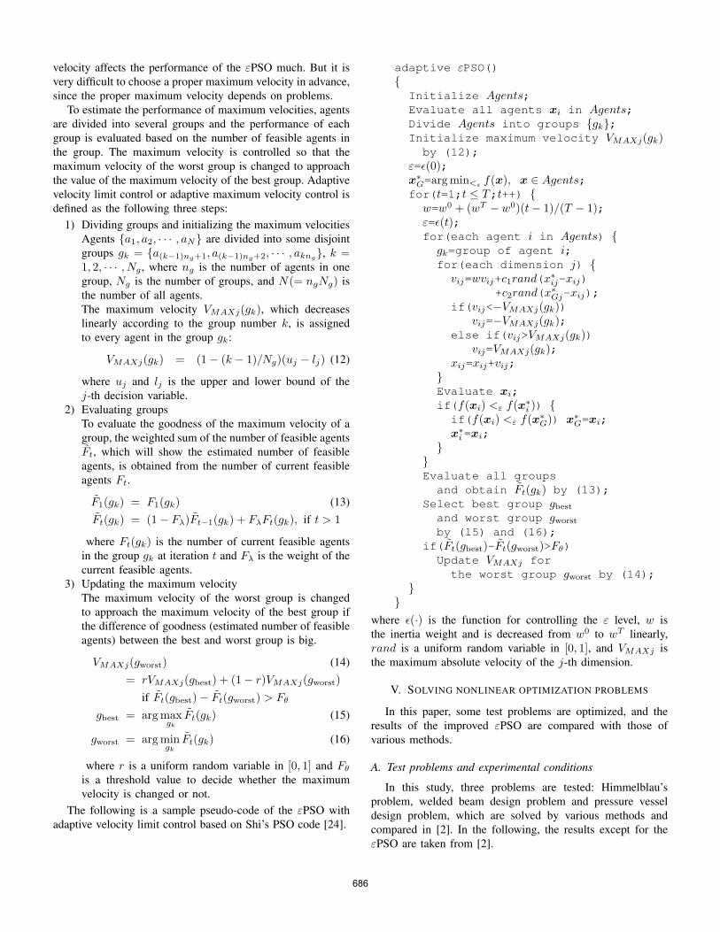
velocity affects the performance of the εPSO much. But it isvery difficult to choose a proper maximum velocity in advance,since the proper maximum velocity depends on problems.

To estimate the performance of maximum velocities, agentsare divided into several groups and the performance of eachgroup is evaluated based on the number of feasible agents inthe group. The maximum velocity is controlled so that themaximum velocity of the worst group is changed to approachthe value of the maximum velocity of the best group. Adaptivevelocity limit control or adaptive maximum velocity control isdefined as the following three steps:

1) Dividing groups and initializing the maximum velocitiesAgents {a1, a2, · · · , aN} are divided into some disjointgroups gk = {a(k−1)ng+1, a(k−1)ng+2, · · · , akng}, k =1, 2, · · · , Ng , where ng is the number of agents in onegroup, Ng is the number of groups, and N(= ngNg) isthe number of all agents.The maximum velocity VMAXj(gk), which decreaseslinearly according to the group number k, is assignedto every agent in the group gk:

VMAXj(gk) = (1 − (k − 1)/Ng)(uj − lj) (12)

where uj and lj is the upper and lower bound of thej-th decision variable.

2) Evaluating groupsTo evaluate the goodness of the maximum velocity of agroup, the weighted sum of the number of feasible agentsF̃t, which will show the estimated number of feasibleagents, is obtained from the number of current feasibleagents Ft.

F̃1(gk) = F1(gk) (13)F̃t(gk) = (1 − Fλ)F̃t−1(gk) + FλFt(gk), if t > 1

where Ft(gk) is the number of current feasible agentsin the group gk at iteration t and Fλ is the weight of thecurrent feasible agents.

3) Updating the maximum velocityThe maximum velocity of the worst group is changedto approach the maximum velocity of the best group ifthe difference of goodness (estimated number of feasibleagents) between the best and worst group is big.

VMAXj(gworst) (14)= rVMAXj(gbest) + (1 − r)VMAXj(gworst)

if F̃t(gbest) − F̃t(gworst) > Fθ

gbest = arg maxgk

F̃t(gk) (15)

gworst = arg mingk

F̃t(gk) (16)

where r is a uniform random variable in [0, 1] and Fθ

is a threshold value to decide whether the maximumvelocity is changed or not.

The following is a sample pseudo-code of the εPSO withadaptive velocity limit control based on Shi’s PSO code [24].

adaptive εPSO(){Initialize Agents;Evaluate all agents xi in Agents;Divide Agents into groups {gk};Initialize maximum velocity VMAXj(gk)

by (12);ε=ε(0);x∗

G=arg min<ε f(x), x ∈ Agents;for(t=1;t ≤ T;t++) {

w=w0 + (wT − w0)(t − 1)/(T − 1);ε=ε(t);for(each agent i in Agents) {

gk=group of agent i;for(each dimension j) {

vij=wvij+c1rand(x∗ij-xij)

+c2rand(x∗Gj-xij);

if(vij<−VMAXj(gk))vij=−VMAXj(gk);

else if(vij>VMAXj(gk))vij=VMAXj(gk);

xij=xij+vij;}Evaluate xi;if(f(xi) <ε f(x∗

i )) {if(f(xi) <ε f(x∗

G)) x∗G=xi;

x∗i=xi;

}}Evaluate all groupsand obtain F̃t(gk) by (13);

Select best group gbest

and worst group gworst

by (15) and (16);if(F̃t(gbest)-F̃t(gworst)>Fθ)Update VMAXj for

the worst group gworst by (14);}

}where ε(·) is the function for controlling the ε level, w isthe inertia weight and is decreased from w0 to wT linearly,rand is a uniform random variable in [0, 1], and VMAXj isthe maximum absolute velocity of the j-th dimension.

V. SOLVING NONLINEAR OPTIMIZATION PROBLEMS

In this paper, some test problems are optimized, and theresults of the improved εPSO are compared with those ofvarious methods.

A. Test problems and experimental conditions

In this study, three problems are tested: Himmelblau’sproblem, welded beam design problem and pressure vesseldesign problem, which are solved by various methods andcompared in [2]. In the following, the results except for theεPSO are taken from [2].

686

TABLE IRESULT OF HIMMELBLAU’S PROBLEM

Algorithm Best Average Worst S.D. FeasibleεPSO orig. (5,000) -31011.9988 -30947.3262 -30762.8890 55.8631 1027.00εPSO imp. (5,000) -31022.3463 -30990.3279 -30873.6902 29.0438 1273.60

(50,000) -31025.5599 -31025.5432 -31025.4674 0.0212GRG[25] -30373.949 N/A N/A N/AGen[26] -30183.576 N/A N/A N/ADeath[2] -30790.271 -30429.371 -29834.385 234.555Static[5] -30790.2716 -30446.4618 -29834.3847 226.3428Dynamic[6] -30903.877 -30539.9156 -30106.2498 200.035Annealing[7] -30829.201 -30442.126 -29773.085 244.619Adaptive[8] -30903.877 -30448.007 -29926.1544 249.485Co-evolutionary[9] -31020.859 -30984.2407 -30792.4077 73.6335MGA[17] -31005.7966 -30862.8735 -30721.0418 73.240

In the εPSO with adaptive velocity limit control, the samesettings are used for all problems. The parameters for theε constrained method are defined as follows: The constraintviolation φ is given by the square sum of all constraints (p=2)in eq. (3). The ε level is assigned to 0, i.e. ε(t) = 0 (0 ≤ t ≤T ). This means that problems are solved using a lexicographicorder in which the constraint violation precedes the objectivefunction. The number of groups Ng = 4, the number of agentsin a group ng = 5, the weight of the number of current feasibleagents Fλ = 0.2, the threshold of updating Fθ = 0.05. Theparameters for PSO are as follows: The number of agentsN = 20(= 5×4), w0 = 0.9, wT = 0.4. The initial velocity is0. The maximum velocity VMAXj is adaptively controlled. Themaximum number of iterations T = 249 (5,000 evaluations)and T = 2499 (50,000 evaluations). For each problem, 30independent runs are performed.

B. Himmelblau’s nonlinear optimization problem

Himmelblau’s problem was originally given byHimmelblau[25], and it has been used as a benchmarkfor several GA-based methods that use penalties. In thisproblem, there are 5 decision variables x1, x2, x3, x4, x5, 6nonlinear inequality constraints and 10 boundary conditions.

This problem was originally solved using the GeneralizedReduced Gradient method (GRG)[25]. Gen and Cheng[26]used a genetic algorithm based on both local and globalreference. The problem was solved using death penalty[2]in the first category and various penalty function approachesin the second category such as static penalty[5], dynamicpenalty[6], annealing penalty[7], adaptive penalty[8] and co-evolutionary penalty[9]. Also, the problem was solved usingMGA (multiobjective genetic algorithm)[17] in the fourthcategory.

Experimental results on the problem are shown in TableI. The columns labeled Best, Average, Worst, S.D. and Fea-sible are the best value, the average value, the worst value,the standard deviation of the best agent and the number ofsearched feasible points in each run, respectively. The good ap-proaches were the original and improved εPSO, MGA and Co-evolutionary penalty method. Note that both εPSO, MGA and

other penalty based approaches performed only 5,000 functionevaluations while Co-evolutionary penalty method performedvery higher number of function evaluations (900,000).

Especially, the improved εPSO showed better performancethan the original εPSO, MGA and Co-evolutionary penaltymethod on all values including the best, average, worst andstandard deviation. The improved εPSO succeeded in con-trolling the maximum velocity and searched 1273.6 feasiblepoints on average, which is about 24% greater than 1027.0feasible points searched by the original εPSO. So, the im-proved εPSO is the best method which can find very goodsolutions efficiently. The improved εPSO found the objectivevalue -31022.3463 in 5,000 evaluations and -31025.5599 in50,000 evaluations that could not be found by other methodsand found high quality solutions very stably for this problem.Also, the improved εPSO ran very fast and the executiontime for solving this problem was only 0.0079 seconds (5,000function evaluations) using notebook PC with Mobile PentiumIII 1.3GHz.

C. Welded beam design

A welded beam is designed for minimum cost subject toconstraints on shear stress (τ ), bending stress in the beam (σ),buckling load on the bar (Pc), end deflection of the beam (δ)and side constraints[27]. There are 4 design variables: weldthickness h(x1), length of weld l(x2), width of the beam t(x3),thickness of the beam b(x4). The problem has 7 inequalityconstraints.

Experimental results on the problem are shown in Table II.The good approaches were the original and improved εPSO,MGA and Co-evolutionary penalty method. Note that bothεPSO, MGA and other penalty based approaches performedonly 5,000 function evaluations while Co-evolutionary penaltymethod performed 900,000 function evaluations.

Especially, the improved εPSO showed better performancethan the original εPSO and MGA on all values and betterperformance than Co-evolutionary penalty method on the bestand average values. When the number of function evaluationsis 50,000, the improved εPSO showed better performance thanCo-evolutionary penalty method on all values. The improved

687

εPSO succeeded in controlling the maximum velocity andsearched 1257.23 feasible points, which is about 40% greaterthan 892.50 feasible points searched by the original εPSO.So, the improved εPSO is the best method which can findvery good solutions efficiently. The improved εPSO found theobjective value 1.7249 in 5,000 evaluations that could not befound by other methods, and found high quality solutions verystably for this problem. Also, the improved εPSO ran veryfast and the execution time for solving this problem was only0.0091 seconds (5,000 function evaluations).

TABLE IIRESULT OF WELDED BEAM DESIGN

Algorithm Best Average Worst S.D. FeasibleεPSO orig. (5,000) 1.7258 1.8073 2.1427 0.1200 892.50εPSO imp. (5,000) 1.7249 1.7545 1.8558 0.0370 1257.23

(50,000) 1.7249 1.7252 1.7348 0.0018Death[2] 2.0821 3.1158 4.5138 0.6625Static[5] 2.0469 2.9728 4.5741 0.6196Dynamic[6] 2.1062 3.1556 5.0359 0.7006Annealing[7] 2.0713 2.9533 4.1261 0.4902Adaptive[8] 1.9589 2.9898 4.8404 0.6515Co-evolutionary[9] 1.7483 1.7720 1.7858 0.0112MGA[17] 1.8245 1.9190 1.9950 0.0538

D. Pressure vessel design

A pressure vessel is a cylindrical vessel which is cappedat both ends by hemispherical heads. The vessel is designedto minimize total cost including the cost of material, formingand welding[28]. There are 4 design variables: thickness of theshell Ts(x1), thickness of the head Th(x2), inner radius R(x3),length of the cylindrical section of the vessel not including thehead L(x4). Ts and Th are integer multiples of 0.0625 inch,which are the available thickness of rolled steel plates, and Rand L are continuous. The problem has 4 inequality constraints.

This problem was solved by Sandgren[29] using Branchand Bound, by Kannan and Kramer[28] using an augmentedLagrangian Multiplier approach. Also, the problem was solvedby Deb[30] using Genetic Adaptive Search (GeneAS) in thethird category.

In the εPSO, to solve this mixed integer problem, newdecision variables x′

1 and x′2 are introduced and the value of

xi, i = 1, 2 is given by the multiple of 0.0625 and the integerpart of x′

i. Experimental results on the problem are shown inTable III. The good approaches were the original and improvedεPSO, MGA and Co-evolutionary penalty method. Note thatboth εPSO and MGA performed 50,000 function evaluations,Co-evolutionary penalty method performed 900,000 functionevaluations, and other penalty based approaches performed2,500,000 function evaluations.

The improved and original εPSO showed better perfor-mance than MGA and Co-evolutionary penalty method onthe best and average values. The improved εPSO showedbetter performance than the original εPSO on the averageand standard deviation value and searched about 15% greater

number of feasible points. So, the improved εPSO is verygood method which can find very good solutions efficiently.The improved (and original) εPSO found the objective value6059.7143 in 50,000 evaluations that could not be found byother methods, and found high quality solutions on average forthis problem. Also, the improved εPSO ran very fast and theexecution time for solving this problem was 0.0582 seconds(50,000 function evaluations).

TABLE IIIRESULTS OF PRESSURE VESSEL DESIGN

Algorithm Best Average Worst S.D.εPSO orig. (50,000) 6059.7143 6154.4386 6410.0868 132.6205εPSO imp. (50,000) 6059.7143 6136.7744 6410.0868 112.3306Sandgren[29] 8129.1036 N/A N/A N/AKannan[28] 7198.0428 N/A N/A N/ADeb[30] 6410.3811 N/A N/A N/ADeath[2] 6127.4143 6616.9333 7572.6591 358.8497Static[5] 6110.8117 6656.2616 7242.2035 320.8196Dynamic[6] 6213.6923 6691.5606 7445.6923 322.7647Annealing[7] 6127.4143 6660.8631 7380.4810 330.7516Adaptive[8] 6110.8117 6689.6049 7411.2532 330.4483Co-evolutionary[9] 6288.7445 6293.8432 6308.1497 7.4133MGA[17] 6069.3267 6263.7925 6403.4500 97.9445

E. Discussion

It is shown that the adaptive velocity limit control is veryeffective in all problems, especially in welded beam designproblem where the improved εPSO searched about 40% greaternumber of feasible solutions than the original εPSO. Table IVshows the ratio of feasible region in search space F/S, whichis obtained by generating 10 million random points withinsearch space. The ratio of welded beam design problem ismuch smaller than the other problems. So, it is thought thatthe adaptive velocity limit control is more effective to problemswhich have smaller feasible region, because agents easily flyaway from feasible region in such case.

TABLE IVRATIO OF FEASIBLE REGION

problem ratio(%)Himmelblau’s problem 52.0758Welded beam design 2.6667

Pressure vessel design 39.7384

To compare the execution time, the εGA, which is definedby applying the ε constrained method to a genetic algorithmwith linear ranking selection, is used. It is thought that theexecution time of the εGA is identical to or faster than otherGA-based methods, because the εGA only utilizes simple GAoperations. The improved εPSO ran 2.9 times faster than theεGA in Himmelblau’s problem, 2.4 times faster in weldedbeam design and 2.6 times faster in pressure vessel design.So, it is thought that the efficiency of the improved εPSO isvery high.

688

VI. CONCLUSIONS

Particle swarm optimization is a fast and an efficientoptimization algorithm for unconstrained problems. We haveproposed εPSO, which is the combination of the ε constrainedmethod and PSO, for constrained problems. In this study,we proposed the improved εPSO that controls the maximumvelocity of agents adaptively. By applying the improved εPSOto three constrained optimization problems, it was shown thatthe εPSO could find much better solutions that had beennever found by other methods for all problems and find bettersolutions on average for all problems. It was shown that theεPSO was an efficient and stable optimization algorithm.

In the penalty function method, feasible points can be foundby increasing the penalty coefficient towards infinity in a the-oretical sense, although it is difficult to do so computationally.In the εPSO, feasible points can be found by letting the εlevel to 0 or decreasing the ε level to 0, and this is easy todo computationally. If a point does not satisfy constraints, theconstraint violation is minimized, and the point will becomefeasible. In the penalty function method, the objective functionand the constraints must be evaluated for every new searchpoint. However in the εPSO, the objective function and theconstraints are treated separately, and the evaluation of theobjective function can often be omitted. Therefore, the εPSOcan find feasible points efficiently compared with the penaltyfunction method.

In future, we will introduce some operators such as themutation in order to improve the performance of the εPSO.Also, we will apply the εPSO to other benchmark problemsand various application fields.

ACKNOWLEDGMENTS

This research is supported in part by Grant-in-Aid forScientific Research (C) (No. 16500083, 17510139) of Japansociety for the promotion of science.

REFERENCES

[1] Z. Michalewicz and G. Nazhiyath, “GENOCOP III: A co-evolutionaryalgorithm for numerical optimization problems with nonlinear con-straints,” in Proc. of the 2nd IEEE International Conference on Evo-lutionary Computation, vol. 2, Perth, Australia, 1995, pp. 647–651.

[2] C. A. C. Coello, “Theoretical and numerical constraint-handling tech-niques used with evolutionary algorithms: A survey of the state of theart,” Computer Methods in Applied Mechanics and Engineering, vol.191, pp. 1245–1287, 2002.

[3] G. Coath and S. K. Halgamuge, “A comparison of constraint-handlingmethods for the application of particle swarm optimization to constrainednonlinear optimization problems,” in Proc. of IEEE Congress on Evolu-tionary Computation, Canberra, Australia, 2003, pp. 2419–2425.

[4] X. Hu and R. C. Eberhart, “Solving constrained nonlinear optimizationproblems with particle swarm optimization,” in Proc. of the Sixth WorldMulticonference on Systemics, Cybernetics and Informatics, Orlando,Florida, 2002.

[5] A. Homaifar, S. H. Y. Lai, and X. Qi, “Constrained optimization viagenetic algorithms,” Simulation, vol. 62, no. 4, pp. 242–254, 1994.

[6] J. Joines and C. Houck, “On the use of non-stationary penalty functionsto solve nonlinear constrained optimization problems with GAs,” in Proc.of the First IEEE Conference on Evolutionary Computation, Orlando,Florida, 1994, pp. 579–584.

[7] Z. Michalewicz and N. F. Attia, “Evolutionary optimization of con-strained problems,” in Proc. of the 3rd Annual Conference on Evolu-tionary Programming, Singapore, 1994, pp. 98–108.

[8] A. B. Hadj-Alouane and J. C. Bean, “A genetic algorithm for themultiple-choice integer program,” Operations Research, vol. 45, pp. 92–101, 1997.

[9] C. A. C. Coello, “Use of a self-adaptive penalty approach for engineeringoptimization problems,” Computers in Industry, vol. 41, no. 2, pp. 113–127, 2000.

[10] K. E. Parsopoulos and M. N. Vrahatis, “Particle swarm optimizationmethod for constrained optimization problems,” in Intelligent Technolo-gies — Theory and Application: New Trends in Intelligent Technologies,ser. Frontiers in Artificial Intelligence and Applications, P. Sincak,J. Vascak, and et al., Eds. IOS Press, 2002, vol. 76, pp. 214–220.

[11] K. Deb, “An efficient constraint handling method for genetic algorithms,”Computer Methods in Applied Mechanics and Engineering, vol. 186, no.2/4, pp. 311–338, 2000.

[12] T. Takahama and S. Sakai, “Tuning fuzzy control rules by the αconstrained method which solves constrained nonlinear optimizationproblems,” Electronics and Communications in Japan, vol. 83, no. 9,pp. 1–12, 2000.

[13] ——, “Constrained optimization by ε constrained particle swarm op-timizer with ε-level control,” in Proc. of the 4th IEEE InternationalWorkshop on Soft Computing as Transdisciplinary Science and Technol-ogy (WSTST’05), Muroran, Japan, May 2005, pp. 1019–1029.

[14] T. P. Runarsson and X. Yao, “Stochastic ranking for constrained evolu-tionary optimization,” IEEE Transactions on Evolutionary Computation,vol. 4, no. 3, pp. 284–294, Sept. 2000.

[15] E. Camponogara and S. N. Talukdar, “A genetic algorithm for con-strained and multiobjective optimization,” in 3rd Nordic Workshop onGenetic Algorithms and Their Applications, Vaasa, Finland, Aug. 1997,pp. 49–62.

[16] P. D. Surry and N. J. Radcliffe, “The COMOGA method: Constrainedoptimisation by multiobjective genetic algorithms,” Control and Cyber-netics, vol. 26, no. 3, pp. 391–412, 1997.

[17] C. A. C. Coello, “Constraint-handling using an evolutionary multiob-jective optimization technique,” Civil Engineering and EnvironmentalSystems, vol. 17, pp. 319–346, 2000.

[18] T. Ray, K. Liew, and P. Saini, “An intelligent information sharingstrategy within a swarm for unconstrained and constrained optimizationproblems,” Soft Computing – A Fusion of Foundations, Methodologiesand Applications, vol. 6, no. 1, pp. 38–44, Feb. 2002.

[19] T. Takahama and S. Sakai, “Learning fuzzy control rules by α-constrained simplex method,” System and Computers in Japan, vol. 34,no. 6, pp. 80–90, 2003.

[20] ——, “Constrained optimization by applying the α constrained methodto the nonlinear simplex method with mutations,” IEEE Trans. onEvolutionary Computation, to appear.

[21] ——, “Constrained optimization by α constrained genetic algorithm(αGA),” Systems and Computers in Japan, vol. 35, no. 5, pp. 11–22,May 2004.

[22] ——, “Constrained optimization by the α constrained particle swarmoptimizer,” Journal of Advanced Computational Intelligence and Intel-ligent Informatics, vol. 9, no. 3, pp. 282–289, May 2005.

[23] J. Kennedy and R. C. Eberhart, Swarm Intelligence. San Francisco:Morgan Kaufmann, 2001.

[24] Y. Shi and R. Eberhart, “A modified particle swarm optimizer,” inProc. of IEEE International Conference on Evolutionary Computation,Anchorage, May 1998, pp. 69–73.

[25] D. M. Himmelblau, Applied Nonlinear Programming. New York:McGrow-Hill, 1972.

[26] M. Gen and R. Cheng, Genetic Algorithms & Engineering Design. NewYork: Wiley, 1997.

[27] S. S. Rao, Engineering Optimization, 3rd ed. New York: Wiley, 1996.[28] B. K. Kannan and S. N. Kramer, “An augmented lagrange multiplier

based method for mixed integer discrete continuous optimization andits applications to mechanical design,” Journal of mechanical design,Transactions of the ASME, vol. 116, pp. 318–320, 1994.

[29] E. Sandgren, “Nonlinear integer and discrete programming in mechanicaldesign,” in Proc. of the ASME Design Technology Conference, Kissimine,Florida, 1988, pp. 95–105.

[30] K. Deb, “GeneAS: A robust optimal design technique for mechanicalcomponent design,” in Evolutionary Algorithms in Engineering Applica-tions, D. Dasgupta and Z. Michalewicz, Eds. Berlin: Springer, 1997,pp. 497–514.

689