Michigan Particle Swarm Optimization for Prototype Reduction in Classification Problems1

Michigan Particle Swarm Optimization for

Prototype Reduction in Classification Prob-

lems

Alejandro CERVANTES and Ines GALVAN and Pedro ISASI

Department of Computer Science

University Carlos III de Madrid

Avda. Universidad, 30

28911 Leganes, Madrid, Spain

{alejandro.cervantes,inesmaria.galvan,pedro.isasi}@uc3m.es

Received February 17 2009

Abstract This paper presents a new approach to Particle Swarm

Optimization, called Michigan Approach PSO (MPSO), and its applica-

tion to continuous classification problems as a Nearest Prototype (NP)

classifier. In Nearest Prototype classifiers, a collection of prototypes has

to be found that accurately represents the input patterns. The classifier

then assigns classes based on the nearest prototype in this collection. The

MPSO algorithm is used to process training data to find those prototypes.

In the MPSO algorithm each particle in a swarm represents a single pro-

totype in the solution and it uses modified movement rules with particle

competition and cooperation that ensure particle diversity. The proposed

method is tested both with artificial problems and with real benchmark

problems and compared with several algorithms of the same family. Re-

sults show that the particles are able to recognize clusters, find decision

boundaries and reach stable situations that also retain adaptation po-

tential. The MPSO algorithm is able to improve the accuracy of 1-NN

classifiers, obtains results comparable to the best among other classifiers,

and improves the accuracy reported in literature for one of the problems.

Keywords Nearest Neighbor Classification, Swarm Intelligence, Data

Mining, Metaheuristics.

2 Alejandro CERVANTES and Ines GALVAN and Pedro ISASI

§1 IntroductionThe Particle Swarm Optimization algorithm 1) is a biologically-inspired

algorithm motivated by a social analogy. The algorithm is based on a set of

potential solutions which evolves to find the global optimum of a real-valued

function (fitness function) defined in a given space (search space).

The PSO algorithm uses a population of particles which move in a mul-

tidimensional space that represents the space of solutions for the problem. Parti-

cles have memory, thus retain part of their previous state. There is no restriction

for particles to share the same point in the search space, but in any case their

individuality is preserved.

The basic PSO uses a real-valued multidimensional space as search space,

and evolves the position of each particle in that space using (1) and (2).

vt+1id = χ(w · vt

id + c1 ·ψ1 · (ptid −xt

id)+ c2 ·ψ2 · (ptgd −xt

id)) .(1)

xt+1id = xt

id + vt+1id . (2)

Where the meanings of symbols are:

vtid component in dimension d of the ith particle

velocity in iteration t

xtid same for the particle position

c1 ,c2 constant weight factors

pi best position achieved so far by particle i

pg best position found by the neighbors of particle i

ψ1 ,ψ2 Random factors in the [0,1] interval

w inertia weight

χ constriction factor

The neighborhood of the particle may either be composed of the whole

swarm (“gbest” topology) or only a subset of the swarm (“lbest” topologies).

Also, some versions of PSO use dynamic neighborhoods, where the relationship

between particles changes over time: Suganthan 2) proposed a swarm with a

local neighborhood whose size was gradually increased; Brits 3) justifies the

introduction of topological neighborhoods when searching for multiple solutions

to multimodal problems using niching techniques. A dynamic neighborhood has

been proposed by Hu and Eberhart 4) for multi-objective optimization.

There are also some good theoretical studies of PSO 5, 6, 7, 8) which ad-

dress the topics of convergence, parameter selection and trajectory analysis.

Michigan Particle Swarm Optimization for Prototype Reduction in Classification Problems3

The purpose of this paper is to use the continuous PSO for the selection

of prototypes in nearest neighbor learning. Some work has already been done

concerning PSO with classification problems. Sousa 9) uses PSO to extract in-

duction rules to classify data; the standard PSO algorithm is run several times,

extracting a single rule each time and using only unclassified patterns for the

subsequent iterations. In previous work by the authors10, 11), induction rules are

encoded using the binary version of PSO and both a single and an iterated ver-

sion of the algorithm. Wang 12, 13), has used a standard PSO for rule extraction

in discrete classification problems. There is also some work in fuzzy rule extrac-

tion using PSO 14). Recently 15) PSO has been used to locate cluster centers for

classification.

In this work we use Nearest Neighbor (NN) classification. NN is a lazy

learning method where the class assigned to a pattern is the class of the nearest

pattern known to the system, measured in terms of a distance defined on the

feature (attribute) space.

In 1-NN with Euclidean distance, the regions associated to a pattern

(called Voronoi regions) are delimited by linear borders. This can be modified if

the distance is changed, or if a K-NN strategy is used, where the class assigned

to a pattern is the most frequent class among its K nearest neighbors. K-NN

strategy can approximate non-linear borders of the Voronoi regions. In this

paper, however, we have consistently used the Euclidean distance to calculate

distances between particles and prototypes.

Both computational reasons and presence of noise in data led to the

development of techniques that reduce the number of patterns evaluated without

increasing the classification error. These methods calculate a reduced set of

prototypes, that are the only ones used for classification. In instance selection

methods 16) prototypes are a subset of the pattern set, but this is not true for

all the prototype methods 17, 18). Among these methods we shall use LVQ for

comparison.

In this paper, we use PSO to find a collection of prototypes that do

not belong to the problem data, but represent the training pattern set and

can classify the patterns according to the class of the nearest prototype in the

collection.

In a standard approach to this problem using PSO, we would have de-

cided the number of prototypes to use and we would have encoded the positions

of all the prototypes and their classes in each particle. This approach has several

4 Alejandro CERVANTES and Ines GALVAN and Pedro ISASI

disadvantages:

• Dimension of the search space grows with the number of prototypes; di-

mension is equal to the number of attributes times the number of proto-

types in the solution.

• The maximum number of prototypes in the solution must be fixed at the

start of the algorithm. It cannot grow if this number is not adequate to

the problem.

In order to apply PSO to the problem avoiding the increase in the search

space dimension, we want to test a different approach that we call the Michigan

Approach. This term is borrowed from the area of genetic Classifier Systems19, 20).

The Michigan approach was applied to PSO, using the binary version of

PSO discover a set of induction rules for discrete classification problems 11). In

that work the Michigan approach was able to reach better solutions in a much

lower number of rule evaluations.

In this approach, each particle represents a single prototype. The solu-

tion is a collection of particles instead of a single particle. For this approach to

work, the standard PSO has to be modified to ensure that the particles do not

converge; instead the swarm evolves toward a configuration where each particle

may be considered part of a collective solution. As the resulting algorithm is

different from the standard PSO algorithm, some testing is required to perform

selection of proper values for two of the algorithm parameters: χ, that is a scale

factor that influences the speed of the particle, and the number of particles used

for the experiments.

The advantages of the Michigan approach versus the conventional PSO

approach are:

• computational cost, as particles have much lower dimension

• flexibility and reduced assumptions, as the number of prototypes in the

solution is not fixed.

This paper is organized as follows: Section 2 shows how the solution

to the classification problem is encoded in the particles of the swarm; Section

3 details the modifications made to the original PSO algorithm to implement

the Michigan approach and adapt it to classification problems; Section 4 de-

scribes the experimental setting and results of experimentation; finally, Section

5 discusses our conclusions and future work related to the present study.

Michigan Particle Swarm Optimization for Prototype Reduction in Classification Problems5

§2 PSO Algorithm Encoding PrototypesIn the Michigan-approach PSO we propose, each particle represents a

potential prototype to be used to classify the patterns using the nearest neighbor

rule. The particle position will be interpreted as the position of a prototype.

Each particle has also a class; this class does not evolve following the PSO rules,

but remains fixed for each particle since its creation.

For a given problem, a particle swarm is created with an equal share of

particles of each of the classes present in the training set.

The following Table 1 represents the structure of a swarm with N par-

ticles each of which corresponds to a single prototype, in a problem with D

attributes and K classes. Among the whole population of the swarm, classes

are assigned from 0 to K-1 to the first K particles, and the sequence is repeated

until prototype N (so Ci = i mod K).

Table 1 Encoding of a set of prototypes in a whole swarm in the Michigan PSO. The swarm

may encode N prototypes in a problem of D attributes

Position Class

Particle 1 X11 X12 ... X1D C1

Particle 2 X21 X22 ... X2D C2

... ... ...Particle N XN1 XN2 ... XND CN

The swarm runs until a stopping criterion is met, and then the resulting

particles positions are interpreted as the positions of the prototypes of the nearest

neighbor classifier.

§3 MPSO Algorithm ModificationsIn the sections that follow, we introduce the pseudocode for the new algo-

rithm (MPSO). Some concepts that differ over the standard PSO are introduced

in the pseudocode and are explained in detail in the referenced subsections.

The basic variations in equations are the introduction of a repulsion force

and the use of a dynamic definition of the neighborhood of a particle. When

moving, each particle selects another one from what we call a “non-competing”

set as a leader for attraction, and a second one from a “competing” set as a leader

for repulsion. Both neighborhoods are defined dynamically on each iteration and

take into account the particles’ classes. In this definition, particles compete with

particles of the same class but cooperate with particles of different classes.

6 Alejandro CERVANTES and Ines GALVAN and Pedro ISASI

Also the concept of “local fitness” is used. A single particle is measured

as “good” if it classifies correctly patterns in its surroundings (more precisely,

in its Voronoi region). The formula for the particle fitness does not take into

account how the rest of the patterns are classified.

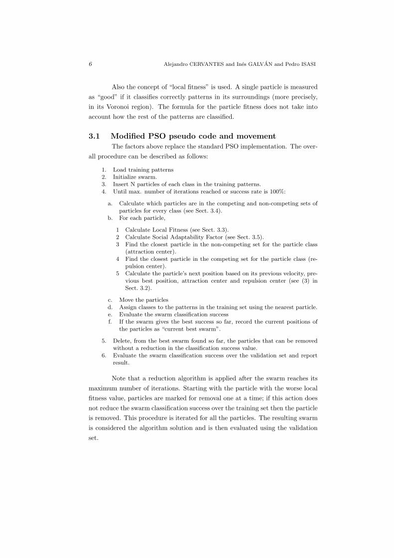
3.1 Modified PSO pseudo code and movement

The factors above replace the standard PSO implementation. The over-

all procedure can be described as follows:

1. Load training patterns2. Initialize swarm.3. Insert N particles of each class in the training patterns.4. Until max. number of iterations reached or success rate is 100%:

a. Calculate which particles are in the competing and non-competing sets ofparticles for every class (see Sect. 3.4).

b. For each particle,

1 Calculate Local Fitness (see Sect. 3.3).2 Calculate Social Adaptability Factor (see Sect. 3.5).3 Find the closest particle in the non-competing set for the particle class

(attraction center).4 Find the closest particle in the competing set for the particle class (re-

pulsion center).5 Calculate the particle’s next position based on its previous velocity, pre-

vious best position, attraction center and repulsion center (see (3) inSect. 3.2).

c. Move the particlesd. Assign classes to the patterns in the training set using the nearest particle.e. Evaluate the swarm classification successf. If the swarm gives the best success so far, record the current positions of

the particles as “current best swarm”.

5. Delete, from the best swarm found so far, the particles that can be removedwithout a reduction in the classification success value.

6. Evaluate the swarm classification success over the validation set and reportresult.

Note that a reduction algorithm is applied after the swarm reaches its

maximum number of iterations. Starting with the particle with the worse local

fitness value, particles are marked for removal one at a time; if this action does

not reduce the swarm classification success over the training set then the particle

is removed. This procedure is iterated for all the particles. The resulting swarm

is considered the algorithm solution and is then evaluated using the validation

set.

Michigan Particle Swarm Optimization for Prototype Reduction in Classification Problems7

In preliminary versions of the algorithm we performed particle deletion

during the evolution, but that decreased its performance. The reason was that,

during evolution, particles easily oscillate from good to very bad local fitness

values. This made the cleaning algorithm remove too many particles and reduce

the swarm size too much.

3.2 Modified PSO Equation

In order to take into account the modifications previously described,

the equation that determines the velocity at each iteration in the basic PSO

algorithm (1) has to be modified. In our work the velocity change is given by

(3).

vt+1id = χ(w · vt

id + c1 · ψ1 · (ptid − xt

id)+

c2 · ψ2 · sign(atid − xt

id) · Sfi+ (3)

c3 · ψ3 · sign(xtid − rt

id) · Sfi) .

Where symbols that were already in 1 still have the same meanings, and

the meanings of the new symbols are as follows:

c3 new constant repulsion weight factor

ai attraction center for particle i

ri repulsion center for particle i

Sfi Social Adaptability Factor, inversely dependent on the particle fitness; and

ψ3 random factor in the [0,1] interval

Note that the repulsion term is weighted by a random factor (ψ3) and a

fixed weight (c3). This weight becomes a new parameter for the algorithm.

If either ai or ri does not exist, the respective term is ignored.

3.3 Local Fitness Function

In the Michigan approach, a local fitness value has to be calculated

for each particle. This function is used to determine which is the best position

found by the particle. As each particle represents a single prototype, the function

takes into account the patterns to which the particle is the closest in the whole

swarm. The area in which those patterns are located is the Voronoi region of

the prototype represented by the particle. Those patterns are the ones that are

“classified” by the particle.

8 Alejandro CERVANTES and Ines GALVAN and Pedro ISASI

We also included an additional factor. We prefer particles that are close

to the patterns they classify. For this purpose, we first calculate the Gf and

Bf values using (4). The Gf factor evaluates how many patterns the particle

classifies correctly, and how close the particle is to those patterns. The Bf factor

is calculated using the patterns that the particle classifies incorrectly.

Gf =∑

{g}

1

dg,i + 1.0

Bf =∑

{b}

1

db,i + 1.0

(4)

Where {g} is the set of patterns of the same class classified by the

particle; {b} is the set of patterns of different class classified by the particle; and

dg,i, db,i are the Euclidean distances between the patterns and the particle.

Constant values 1.0 are just a way to ensure that no infinite values are

assigned to Gf and Bf . Particles may be initialized or placed “over” patterns if

desired at any moment of the algorithm evolution.

Local Fitness is then calculated using the Gf and Bf factors in (5).

Local Fitness =

0 if {g} = {b} = ∅

Gf

NP

+ 2.0 if {b} = ∅

Gf −Bf

Gf +Bf

+ 1.0 otherwise .

(5)

Where {g} and {b} have the same meanings as in ( 4) and NP is the

number of patterns in the training set.

In the fitness function, two constants (2.0 and 1.0) are used to define

two distinct intervals for particles that have different characteristics in terms of

patterns they classify:

• Particles that classify patterns both of their own class (true positives)

and of different classes (false positives) have fitness values in the range

[0.0, 2.0). In this range, the function only takes into account local infor-

mation.

• Particles that only classify patterns of their own class have fitness value

greater than 2.0, and so those positions are always preferred over the

previous. In this range, local fitness uses some global information: the

Michigan Particle Swarm Optimization for Prototype Reduction in Classification Problems9

total number of patterns to be classified. In this way, particles with

{b} = ∅ are still given different fitness values.

By using the distance between the pattern and the particle we give higher

fitness to particles close to the patterns they classify, so they can move closer to

the area where the patterns are located. This tendency may be compensated by

the social terms.

3.4 Neighborhood for the Michigan PSO

For the success of the Michigan approach, the algorithm has to avoid

convergence toward a single high-fitness particle, because this particle can only

represent a very limited solution (only one prototype).

In the standard PSO, the attractive sociality term in (1) tries to move

particles close to positions with good fitness. To change this behavior, in the

Michigan approach we introduce several modifications that are based on using

the particle class to define its neighborhood and divide the swarm into competing

and non-competing particles:

• For each particle of class Ci, non-competing particles are all the particles

of classes Cj 6= Ci that classify at least one pattern of class Ci.

• For each particle of class Ci, competing particles are all the particles of

class Ci that classify at least one pattern of that class (Ci).

When the movement for each particle is calculated, that particle is both:

1. Attracted by the closest (in terms of Euclidean distance) non-competing

particle in the swarm, which becomes the “attraction center” for the

movement. In this way, non-competing particles guide the search for

the patterns of different class.

2. Repelled by the closest competing particle in the swarm, which becomes

the “repulsion center” for the movement. In this way, competing par-

ticles retain diversity and push each other to find new patterns of their

class in different areas of the search space.

The rules above achieve the following results:

• A particle is only attracted by those particles that misclassify patterns.

In that case, it is only affected by the closest particle that meets that

criterion. Hence, particles may cluster around different points of the

search space instead of converging toward a single position.

• The way repulsion is defined means that, when several particles of a class

10 Alejandro CERVANTES and Ines GALVAN and Pedro ISASI

are close to a cluster of patterns of that class, instead of converging toward

the cluster center (or elsewhere the position that maximizes the fitness

function), they can stay near the border of the cluster. This allows more

accurate classification, as particles are able to locate the decision frontier

where classification is harder.

Other authors have already used the idea of repulsion in PSO in different

ways. For instance, Blackwell 21, 22), introduces repulsion to increase population

diversity in the standard PSO and allow the swarm to dynamically adapt to

change.

3.5 Social Adaptability Factor

The social part of the algorithm (influence from neighbors) determines

that particles are constantly moving toward their non-competing neighbor and

far from their competing neighbor. However, particles that are already located

in the proximity of a good position for a prototype should rather try to improve

their position and should possibly avoid the influence of neighbors.

To implement this effect we have generalized the influence of fitness in

the sociality terms by introducing a new term in the PSO equations, called

“Social Adaptability Factor” (Sf ), that depends inversely on the “best fitness”

of the particle. In particular, we have chosen plainly the expression in (6).

Sfi = 1/(Best Local Fitnessi + 1.0) . (6)

This coefficient should be positive. This requirement has to be taken

into account in the definition of the local fitness function. With the current

Local Fitness function the value for Sf is in the range [0.25, 1].

This factor contributes to the swarm stability because, as particles evolve

toward better positions, they are less likely to move away from those positions,

as the individual component of the particle velocity is not affected by this factor

as shown in ( 3).

§4 ExperimentationIn this section we describe the results of two sets of experiments. The

first one is aimed to understand the influence of the algorithm’s parameters in

the experiment results, and the second one is performed in order to compare

those results with other classification algorithms.

Michigan Particle Swarm Optimization for Prototype Reduction in Classification Problems11

4.1 Global Swarm Evaluation

The local fitness function, defined above, is used for the particles move-

ment. However, to evaluate the goodness of the swarm as a classifier system, we

use the classification success rate (7).

Swarm Evaluation =Good classifications

Total patterns· 100 (7)

Given the nearest neighbor criterion for classification, unclassified pat-

terns are not possible, as every pattern is assigned the class of the nearest pro-

totype.

The system stores the best swarm evaluation obtained when performing

classification on the training set. This function is also used to evaluate the final

best swarm success rate over the validation set.

4.2 Problems’ Description and Basic Experimentation Setup

We perform experimentation on the problems summarized in Table 2.

The first two (Clusters and Diagonal) are artificial problems and they are used to

understand the new algorithm’s properties; the rest are well-known real problems

taken from the UCI collection, used for comparison with other classification

algorithms.

Table 2 Problems used in the experiments

Name Instances Attrbs. Classes Class Distribution Validation

Clusters 80 2 2 40 / 40 Train set onlyDiagonal 2000 2 2 1000 / 1000 Train & TestDiabetes 768 8 2 500 / 268 10-fold CVBupa 345 6 2 200 / 145 10-fold CVGlass 214 9 6 70 / 76 / 17 / 13 / 9 / 29 10-fold CVThyroid (new) 215 5 3 150 / 35 / 30 10-fold CVWisconsin 699 6 2 458 / 241 10-fold CV

The Cluster problem is a very simple problem with five different clusters,

randomly generated and clearly separated.This problem was only used to provide

a clear graphic representation of the type of solutions found by the algorithm,

and not for comparison.

The Diagonal problem is a bi-dimensional problem that is very simple for

linear classifiers. We generate 500 random training patterns and 1500 validation

12 Alejandro CERVANTES and Ines GALVAN and Pedro ISASI

patterns with coordinates in the [0, 1] range. Patterns where x > y are assigned

class 1, and the rest are assigned class 0.

For UCI problems, attributes values were normalized to the [0, 1] inter-

val. As prototypes are placed in the same search space as patterns, the same

range was also used to constrain the particles’ positions.

Velocity was clamped to the interval [−1.0,+1.0] and w = 0.1 in all the

experiments.

Table 3 shows the parameters used for both the artificial and the UCI

problems.

It is clear that problem-specific tuning may provide better results than

selection of a single set of parameters for all the problems. However, we require

some starting values which may later be adjusted for the different problems.

For the UCI problems, we tried to find a fixed proportion between c1,

c2 and c3 which gives acceptable results on a variety of problems. Our starting

decision was to keep c1 = c2 = 1.0 so only the value for c3 had to be adjusted.

The choice of c1 = c2 is very common when constricted PSO is used 23). The

initial value for c3 was selected after some preliminary experimentation.

For the artificial problems, we used smaller values for the PSO parame-

ters (c1, c2, and c3) which lead to slower evolution but more accurate results.

Table 3 Parameters used for each of the problems

Problem Itera- w c1 c2 c3

tions

Artificial Problems 100 0.1 0.5 0.15 0.05UCI Problems 300 0.1 1.0 1.0 0.25

We performed 100 runs of the algorithm for the Cluster problem and

Diagonal problems, and 10 runs of the problems that use 10-fold cross validation,

which gives a total of 100 runs over each.

On each run, after the given number of iterations is reached, the best

solution found for the training set is cleaned (useless particles are removed) and

the resulting swarm is used to classify the validation set.

In the result tables, the success rate is averaged over the total number

of runs; we also provide the best result over the set of experiments. Wherever

cross-validation was used we provide the best of the 10 different runs.

Regarding the parameters, we experimentally found that a small value of

w lead to better results in all cases. The number of iterations (300) was selected

Michigan Particle Swarm Optimization for Prototype Reduction in Classification Problems13

after checking that number was roughly equal to double the average iteration in

which the best result was achieved.

Values for the rest of the parameters were selected after performing some

experimentation as shown in the following sections.

4.3 Number of Particles

In MPSO the number of particles in the swarm must be fixed at the

start of the algorithm. We were interested in the importance of the number of

particles on the algorithm result.

With this goal we ran a series of experiments with increasing values of

the number of particles per class (5,10,20 and 40). We used χ = 1.0 and the rest

of the parameters were kept as in Table 3.

Results in Table 4 show that the increase in the number of particles also

increases accuracy. The effect depends on the problem, and is more important

in the Diagonal, Bupa, Glass and Thyroid problems. The increment is gradual

and we must note that even the experiment with 5 particles per class has good

results in all the problems.

Table 4 Best swarm success rate (in %) with different values of the number of particles per

class

Particles Diagonal Diabetes Bupa Glass Thyroid Wisconsinper Class

5 94.60 73.45 62.89 81.61 93.33 95.8010 96.14 74.14 63.29 82.04 94.03 96.4620 96.88 74.68 64.28 83.46 93.63 96.3740 97.31 74.67 65.63 85.05 95.31 96.80

However this improvement must be balanced with the increase in the

number of prototypes in the solution shown in Table 5. Obviously a greater

number of particles in the swarm requires higher computing costs.

As the balance between accuracy and computational cost is important,

this experiment points toward the implementation of some automatic (adaptive)

method of increasing or decreasing population as needed during the run of the

algorithm.

4.4 Experimental Selection of the χ Coefficient

The proposed algorithm has two weight parameters originating from the

14 Alejandro CERVANTES and Ines GALVAN and Pedro ISASI

Table 5 Average number of prototypes in the solution, with different values of the number

of particles per class

Particles Diagonal Diabetes Bupa Glass Thyroid Wisconsinper Class

5 8.55 6.39 6.48 8.07 7.74 6.0310 17.39 10.47 10.89 10.30 11.37 11.1220 33.45 17.10 17.44 13.38 16.73 21.5440 57.67 29.50 29.08 17.99 22.08 40.63

standard PSO model (c1 and c2) and includes the c3 weight for the repulsion

term.

To simplify experimentation, we decided to start by keeping a fixed

proportion between them and only vary the constriction factor, χ. Lower values

for this parameter mean that the increments in velocity are smaller, so search is

performed in smaller steps.

For these experiments, we used 10 particles per class. Results are shown

in Table 6. For the Diagonal, Bupa, Glass and Thyroid problems results are

better when a small value of χ is used. Differences are very small in the rest of

the problems. Also, Table 7 shows that smaller values of χ allow more prototypes

in the solution.

Table 6 Best swarm success rate (in %) with different values of the χ coefficient

χ Diagonal Diabetes Bupa Glass Thyroid Wisconsin

0.25 96.20 73.76 64.42 87.64 95.68 96.240.50 96.14 74.25 64.76 86.27 95.90 96.500.75 95.85 73.88 64.51 84.60 94.61 96.431.00 96.14 74.14 63.29 82.04 94.03 96.46

Comparison with Table 4 and Table 5 suggest show that for the Glass

and Thyroid problems we can obtain similar solutions in terms of quality and

number of prototypes with half the number of particles if we reduce the value of

χ to 0.25 or 0.5, with a reduced computing cost.

From these results we recommend a value of χ = 0.5, which means that

actual values of the ci weights are half of the values initially set. It must be

noted that performance may be improved for specific problems by tuning the ci

coefficients independently in a neighborhood of the values used in this study.

Michigan Particle Swarm Optimization for Prototype Reduction in Classification Problems15

Table 7 Average number of prototypes in the solution, with different values of the χ coeffi-

cient

χ Diagonal Diabetes Bupa Glass Thyroid Wisconsin

0.25 15.41 11.53 12.78 18.81 16.30 12.280.50 15.04 11.28 11.75 15.58 16.33 11.990.75 14.69 11.15 11.47 12.46 13.53 11.531.00 17.39 10.47 10.89 10.30 11.37 11.12

4.5 Discussion of the Results

In this section we will discuss some of the results of our experimentation.

We have chosen the results of the series of experiments that use 10 particles per

class and χ = 0.50 for discussion as they provide good results for all the problems

with a small number of prototypes in the solution.

The two artificial experiments are used to show the behavior of the

swarm with the proposed modifications. This can be easily shown plotting some

of the solutions found by the swarm for these problems.

In Fig. 1 we represent one of the solutions for the “Cluster” problem. It

shows how the attraction and repulsion rules make the particles group around the

different clusters but also how the particles of the same class remain separated

(due to the repulsion force). Once the swarm reaches this kind of configuration,

attraction forces are null (no particle classifies patterns of the wrong class), and

repulsion forces are compensated if they move the particles toward positions of

lower local fitness, so the particles remain almost stable in positions near the

optimum. In this problem, the swarm easily finds and separates the clusters

every time.

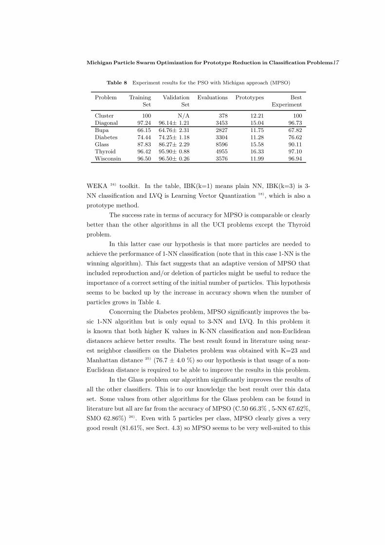
In Table 8 we summarize the results for all the problems. The table

shows the best swarm success rate (in %) on the validation and training set,

averaged over all the runs of the experiment and all the folds when 10-fold

validation is used; “Evaluations” is calculated as the average number of iterations

needed to find the best result for each individual run, times the number of

particles in the swarm; “Best Experiment” is the best success rate among all the

runs of each experiment; and “Prototypes” is the average number of prototypes

kept after cleaning the best swarm.

4.6 Comparison with other Classification Algorithms

In this section we compare the results of MPSO on the UCI data sets

16 Alejandro CERVANTES and Ines GALVAN and Pedro ISASI

0

0.2

0.4

0.6

0.8

1

0 0.2 0.4 0.6 0.8 1 1.2

Pattern 0Pattern 1

P0P1

Fig. 1 Sample solution for the problems “Cluster”.Patterns are outlined, particles are solid.

Particles locate clusters and cluster boundaries.

with the results of other algorithms. As our algorithm performs classification

using the NN rule, we first compare MPSO with related methods, such as the

basic 1-NN algorithm, 3-NN algorithm and LVQ (Learning Vector Quantization)

method, that is indeed a prototype selection algorithm. All those methods may

share common limitations, as all of them are based on the same distance measure

on the search space. Then, we perform the same comparison with algorithms

that are based on completely different strategies.

In all comparisons, two-tailed t-tests with significance level of 0.05 were

performed in order to determine which are the best algorithms for these prob-

lems. The plus and minus signs determine the result of the algorithm versus

MPSO; that is, a “‘+” sign means that the algorithm performed significantly

better than MPSO, and a “-” sign means that the algorithm performed signifi-

cantly worse than MPSO.

In Table 9 we compare our results on the UCI data sets with the re-

sults of our own tests with other Nearest Neighbor algorithms, performed using

Michigan Particle Swarm Optimization for Prototype Reduction in Classification Problems17

Table 8 Experiment results for the PSO with Michigan approach (MPSO)

Problem Training Validation Evaluations Prototypes BestSet Set Experiment

Cluster 100 N/A 378 12.21 100Diagonal 97.24 96.14± 1.21 3453 15.04 96.73

Bupa 66.15 64.76± 2.31 2827 11.75 67.82Diabetes 74.44 74.25± 1.18 3304 11.28 76.62Glass 87.83 86.27± 2.29 8596 15.58 90.11Thyroid 96.42 95.90± 0.88 4955 16.33 97.10Wisconsin 96.50 96.50± 0.26 3576 11.99 96.94

WEKA 24) toolkit. In the table, IBK(k=1) means plain NN, IBK(k=3) is 3-

NN classification and LVQ is Learning Vector Quantization 18), which is also a

prototype method.

The success rate in terms of accuracy for MPSO is comparable or clearly

better than the other algorithms in all the UCI problems except the Thyroid

problem.

In this latter case our hypothesis is that more particles are needed to

achieve the performance of 1-NN classification (note that in this case 1-NN is the

winning algorithm). This fact suggests that an adaptive version of MPSO that

included reproduction and/or deletion of particles might be useful to reduce the

importance of a correct setting of the initial number of particles. This hypothesis

seems to be backed up by the increase in accuracy shown when the number of

particles grows in Table 4.

Concerning the Diabetes problem, MPSO significantly improves the ba-

sic 1-NN algorithm but is only equal to 3-NN and LVQ. In this problem it

is known that both higher K values in K-NN classification and non-Euclidean

distances achieve better results. The best result found in literature using near-

est neighbor classifiers on the Diabetes problem was obtained with K=23 and

Manhattan distance 25) (76.7 ± 4.0 %) so our hypothesis is that usage of a non-

Euclidean distance is required to be able to improve the results in this problem.

In the Glass problem our algorithm significantly improves the results of

all the other classifiers. This is to our knowledge the best result over this data

set. Some values from other algorithms for the Glass problem can be found in

literature but all are far from the accuracy of MPSO (C.50 66.3% , 5-NN 67.62%,

SMO 62.86%) 26). Even with 5 particles per class, MPSO clearly gives a very

good result (81.61%, see Sect. 4.3) so MPSO seems to be very well-suited to this

18 Alejandro CERVANTES and Ines GALVAN and Pedro ISASI

Table 9 Success rate on validation data: average results and standard deviations

MPSO IBK 1 IBK LVQProblem (K=1) (K=3)

Bupa 64.76±2.31 62.22±1.15 (-) 62.48±1.48 (-) 62.18±2.13 (-)Diabetes 74.25±1.18 70.40±0.56 (-) 73.89±0.56 (=) 74.26±0.86 (=)Glass 86.27±2.29 69.07±1.47 (-) 69.05±1.13 (-) 62.56±1.74 (-)Thyroid 95.90±0.88 96.93±0.57 (+) 94.31±0.70 (-) 91.03±1.35 (-)Wisconsin 96.50±0.26 95.37±0.17 (-) 96.54±0.30 (=) 95.88±0.28 (-)

particular problem.

§5 ConclusionsThe purpose of this paper is to study the performance of PSO in classi-

fication problems with continuous attributes. We will use PSO to determine a

set of prototypes that represent the training patterns and that it can be used as

a classifier using the nearest neighbor (1-NN) rule.

This task might be performed using a straightforward PSO algorithm by

encoding a series of prototypes in each particle. However, this approach would

have the disadvantage of producing a search space of high dimension that would

lead to poor performance and high computational costs.

For this reason, we propose a Michigan Approach PSO (MPSO), in which

each particle represents a single prototype (not a set of prototypes). In MPSO,

each particle searches for a position that optimizes a Local Fitness function that

only takes into account patterns in the particle’s Voronoi region. The swarm

movement equations and neighborhood functions are modified to ensure this

behavior.

First, we performed experimentation on simple artificial problems to val-

idate the swarm behavior and to determine the correct rules to be used. We also

performed some experimentation in order to evaluate the influence in the per-

formance of the algorithm of the number of particles in the swarm and the value

of the χ parameter. The number of particles is important, as complex solutions

require more prototypes; however, for the datasets we used, we obtained that 10

prototypes per class was enough. The χ parameter determines the size of the

adjustment in velocity in each iteration, and may be decreased if needed. This

increases the exploitation ability of the algorithm, and thus sometimes obtains

a better performance, at the cost of a longer execution time.

Next, we tested the resulting swarm in five well-known benchmark prob-

Michigan Particle Swarm Optimization for Prototype Reduction in Classification Problems19

lems with parameter values obtained in the preliminary experimentation.

Results on the benchmark problems indicate that MPSO matches or

outperforms the 1-NN classifier on most problems. This proves that MPSO can

be used to produce a representative set of prototypes.

When the results are compared with algorithms of the same family (near-

est neighbor and LVQ), MPSO produces competitive results in all the domains.

Given that we have not yet introduced k-NN classification (with k > 1),

attribute processing, nor any hybridization, we think these results are quite

promising. However either attribute weighting or non Euclidean distances are

likely to be required to compete in other problems.

Closer observation of the MPSO behavior also shows that this approach

obtains a swarm with some characteristics which may be useful in other fields

of application:

• Particles in the swarm are able to locate different areas with high values of

the local fitness function and perform local search in those areas. This can

be seen as multimodal optimization of the local fitness function, and can

be of interest in that field. This behavior can also be useful in applications

in image processing.

• Particles are able to find equilibrium situations which can be altered by

the influence of intruders, forcing them to adapt to the new situation.

This behavior can be of interest for dynamically-adapting swarms.

It is also interesting to address the issue of the number of particles in

the swarm. MPSO can be improved by including a method for dynamic repro-

duction and deletion of particles. This would allow adaptive adjustment of this

parameter to the requirements of the problem. However, before adding one of

these methods to MPSO, some issues must be solved. First, any such mecha-

nism will certainly add new parameters that should be given values either in an

adaptive or in a problem-dependent way. In that case, further study would be re-

quired to give proper values or selection guidelines for those parameters. Second,

population explosion should be prevented when it does not lead to performance

improvement; this can be easy to do but may increase the computational cost of

the algorithm. Third, stagnation can happen if particles are deleted too early.

Acknowledgment This article has been financed by the Spanish

founded research project MSTAR::UC3M, Ref: TIN2008-06491-C04-03.

20 Alejandro CERVANTES and Ines GALVAN and Pedro ISASI

References

1) J. Kennedy, R.C. Eberhart, and Y. Shi. Swarm intelligence. Morgan KaufmannPublishers, San Francisco, 2001.

2) P. N. Suganthan. “Particle swarm optimiser with neighbourhood operator,” InProceedings of the IEEE Congress on Evolutionary Computation (CEC), pages1958–1962, 1999.

3) R. Brits. Niching strategies for particle swarm optimization. Master’s thesis,University of Pretoria, Pretoria, 2002.

4) X. Hu and R.C. Eberhart. “Multiobjective optimization using dynamic neigh-borhood particle swarm optimisation,” In Proceedings of the IEEE Congresson Evolutionary Computation (CEC), pages 1677–16, 2002.

5) M. Clerc and J. Kennedy. “The particle swarm - explosion, stability, and con-vergence in a multidimensional complex space,” IEEE Trans. EvolutionaryComputation, 6(1):58–73, 2002.

6) F. van den Bergh. An analysis of particle swarm optimizers. PhD thesis,University of Pretoria, South Africa, 2002.

7) I. C. Trelea. “The particle swarm optimization algorithm: convergence analysisand parameter selection,” Inf. Process. Lett., 85(6):317–325, 2003.

8) Riccardo Poli. “Dynamics and stability of the sampling distribution of particleswarm optimisers via moment analysis,” Journal of Artificial Evolution andApplications, 2008:1–10, 2008.

9) T. Sousa, A. Silva, and A. Neves. “Particle swarm based data mining algorithmsfor classification tasks,” Parallel Comput., 30(5-6):767–783, 2004.

10) A. Cervantes, P. Isasi, and I. Galvan. “Binary Particle Swarm Optimization inclassification,” Neural Network World, 15(3):229–241, 2005.

11) A. Cervantes, P. Isasi, and I. Galvan. “A comparison between the Pittsburghand Michigan approaches for the Binary PSO algorithm,” In Proceedings of theIEEE Congress on Evolutionary Computation 2005 (CEC 2005), pages 290–297,2005.

12) Z. Wang, X. Sun, and D. Zhang. “Classification Rule Mining Based on Parti-cle Swarm Optimization,” In Rough Sets and Knowledge Technology, volume4062/2006 of Lecture Notes in Computer Science, pages 436–441, SpringerBerlin / Heidelberg, 2006.

13) Z. Wang, X. Sun, and D. Zhan. “A PSO-Based Classification Rule MiningAlgorithm,” In Advanced Intelligent Computing Theories and Applications.With Aspects of Artificial Intelligence, volume 4682/2007 of Lecture Notes inComputer Science, pages 377–384, Springer Berlin / Heidelberg, 2007.

14) Ahmed Ali Abdalla Esmin. “Generating fuzzy rules from examples using theparticle swarm optimization algorithm,” In Proceedings of the 7th InternationalConference on Hybrid Intelligent Systems (HIS 2007), pages 340–343. IEEEComputer Society, 2007.

15) I. De Falco, A. Della Cioppa, and E. Tarantino. “Evaluation of Particle SwarmOptimization Effectiveness in Classification,” In Fuzzy Logic and Applica-

Michigan Particle Swarm Optimization for Prototype Reduction in Classification Problems21

tions, volume 3849/2006 of Lecture Notes in Computer Science, pages 164–171.Springer Berlin / Heidelberg, 2006.

16) H. Brighton and C. Mellish. “Advances in instance selection for instance-basedlearning algorithms,” Data mining and knowledge discovery, 6(2):153–172, 2002.

17) F. Fernandez and P. Isasi. “Evolutionary design of nearest prototype classifiers,”Journal of Heuristics, 10(4):431–454, 2004.

18) T. Kohonen. Self-Organizing Maps. Springer Verlag, Berlin, 1995.

19) J.H. Holland. “Adaptation,” In R. Rosen & F. M. Snell (Eds.), Progress intheoretical biology, 4. New York: Plenum,pages 263–293. 1976.

20) S. W. Wilson. “Classifier fitness based on accuracy,” Evolutionary Computa-tion, 3(2):149–175, 1995.

21) T. M. Blackwell and P. J. Bentley. “Don’t push me! collision-avoiding swarms,”In Proceedings of the IEEE Congress on Evolutionary Computation (CEC),pages 1691–1696, 2002.

22) T. M. Blackwell and P. J. Bentley. “Dynamic search with charged swarms,”In Proceedings of the Genetic and Evolutionary Computation Conference 2002(GECCO), pages 19–26, 2002.

23) D. Bratton and J. Kennedy. “Defining a standard for particle swarm optimiza-tion,” Swarm Intelligence Symposium, 2007. SIS 2007. IEEE, pages 120–127,1-5 April 2007.

24) I. H. Witten and E. Frank. Data Mining: Practical machine learning tools andtechniques. Morgan Kaufmann, San Francisco, 2005.

25) W. Duch. Datasets used for classification: comparison of results.http://www.phys.uni.torun.pl/kmk/projects/datasets.html.

26) G. Guo and D. Neagu. “Similarity-based classifier combination for decisionmaking,” Systems, Man and Cybernetics, 2005 IEEE International Conferenceon, 1:176–181 Vol. 1, Oct. 2005.