Abstract— This paper presents a Particle Swarm Optimization algorithm for the multi-criteria degree constrained minimum spanning tree problem. The operators for the particle’s velocity are based upon local search and path-relinking procedures. The proposed heuristic is compared with other evolutionary algorithm presented previously for the same problem. A computational experiment is reported. The results show that the method proposed in this paper finds high quality solutions for the problem.

I. INTRODUCTION spanning tree of a connected undirected graph G = (N, E) is an acyclic sub-graph of G with n - 1

edges, where n = |N|. If G is a weighted graph, a minimum spanning tree, MST, of G is a spanning tree for which the summation of the weights of its edges is minimal over all spanning trees of G. The MST is a well known combinatorial optimization problem with applications in distinct areas such as network design and clustering. The MST is solvable in polynomial time and the classical algorithms presented for it are due to Prim [19], Kruskal [16] and Borüvka [2]. The history of this problem is presented in the work of Graham and Hell [11]. A survey of the MST problem and algorithms is presented in the paper of Bazlamaçci and Hindi [1].

The MST problem is polynomial, but constraints often render it NP-hard, as described by Garey and Johnson [8]. One such example is the degree-constrained minimum spanning tree problem, where a bound is defined for the number of edges incident to a node.

Difficult variants of optimization problems with a single objective comprise multiple objectives. Those problems are, in general, NP-hard [5].

This paper presents a Particle Swarm Optimization algorithm for the bi-objective degree-constrained minimum

Elizabeth F. G. Goldbarg is with Universidade Federal do Rio Grande do

Norte, Brazil (phone: 55-84-3215-3814; fax: 55-84-3215-3815; e-mail: beth@dimap.ufrn.br).

G. R. de Souza is with Universidade Federal do Rio Grande do Norte, Brazil (e-mail: givanaldo@ yahoo.com.br). The author is partially supported by CAPES (Coordenação de Aperfeiçoamento de Pessoal de Nível Superior).

Marco C. Goldbarg is with Universidade Federal do Rio Grande do Norte, Brazil (e-mail: gold@dimap.ufrn.br).

This research was partially supported by ANP (Agência Nacional do Petróleo), program PRH-22 and CNPq (Conselho Nacional de Desenvolvimento Científico e Tecnológico).

spanning tree problem. Particle Swarm Optimization, PSO, algorithms belong to

the class of bio-inspired methods. PSO is a population-based technique introduced by a Psychologist, James Kennedy, and an Electrical Engineer, Russell Eberhart, who based their method upon the behavior of bird flocks [13].

In this paper local search and path-relinking procedures are proposed as velocity operators for a discrete optimization problem.

The paper is organized as follows. Particle swarm optimization is described in Section II. The multi-objective degree constrained minimum spanning tree problem is addressed in Section III. The proposed algorithm is described in Section IV. A computational experiment is reported in Section V. The experiment compares the results of the proposed approach with the results of AESSEA (Archived Elitist Steady State Evolutionary Algorithm) proposed by Knowles and Corne [15]. Finally, some concluding remarks are presented in Section VI.

II. PARTICLE SWARM OPTIMIZATION Particle swarm optimization, PSO, is an evolutionary

computation technique inspired in the behavior of bird flocks, fish schools and swarming theory. PSO algorithms were first introduced by Kennedy and Eberhart [13] for optimizing continuous nonlinear functions. The fundamentals of their method lie on researches on computer simulations of the movements of social creatures modeled in [12], [21] and [22].

Given a population of solutions (the swarm) for a given problem, each solution is seen as a social organism, also called particle. The method attempts to imitate the behavior of the real creatures making the particles “fly” over a solution space, thus balancing the efforts of search intensification and diversification. Each particle has a value associated with it. In general, particles are evaluated with the objective function being optimized. A velocity is also assigned to each particle in order to direct the “flight” through the problem space. The artificial creatures have a tendency to follow the best ones among them. In the classical PSO algorithm, each particle

Particle Swarm Optimization for the Bi-objective Degree-constrained Minimum Spanning Tree

Elizabeth F. G. Goldbarg, Givanaldo R. de Souza, and Marco C. Goldbarg

A

0-7803-9487-9/06/$20.00/©2006 IEEE

2006 IEEE Congress on Evolutionary ComputationSheraton Vancouver Wall Centre Hotel, Vancouver, BC, CanadaJuly 16-21, 2006

420

-- has a position and a velocity -- knows its own position and the value associated with it -- knows the best position it has ever achieved, and the

value associated with it -- knows its neighbors, their best positions and their

values. As pointed by Pomeroy [18], rather than exploration and

exploitation what has to be balanced is individuality and sociality. Initially, individualistic moves are preferable to social ones (moves influenced by other individuals), however it is important for an individual to know the best places visited by its neighbors in order to “learn” good moves.

The neighborhood may be physical or social [17]. Physical neighborhood takes distances into account, thus a distance metric has to be established. This approach tends to be time consuming, since each iteration distances must be computed. Social neighborhoods are based upon “relationships” defined at the very beginning of the algorithm.

The move of a particle is a composite of three possible choices:

-- To follow in its own way -- To go back to its best previous position -- To go towards its best neighbor’s previous position

or towards its best neighbor To apply PSO to discrete problems, one is required to

define a representation for the position of a particle and to define velocity operators regarding the movement options allowed for the particles (and ways for, possibly, combining movements).

A general framework of a PSO algorithm for a minimization problem is showed in figure 1.

III. THE MULTI-OBJECTIVE DEGREE CONSTRAINED MINIMUM SPANNING TREE

The general multi-objective minimization problem (with no restrictions) can be stated as:

“minimize” f(x) = (f1(x), ..., fk(x)), subjected to x ∈ X

where, x is a discrete value solution vector and X is a finite set of feasible solutions. Function f(x) maps the set of feasible solutions X in ℜk, k > 1 being the number of objectives.

Once there is not only a single solution for the problem, the word minimize has to be understood in another context. Let x, y ∈ X, then x dominates y, written x y, if and only if ∀i, i=1,...k, fi(x) ≤ fi(y) and ∃i, such that fi(x) < fi(y). The set of optimal solutions X* ⊆ X is called Pareto optimal. A solution x* ∈ X* if there is no x ∈ X such that x x*. The non-dominated solutions are said also to be efficient solutions. Thus, to solve a multi-criteria problem, one is required to find the set of efficient solutions. Solutions of this set can be divided in two classes: the supported and non-

supported efficient solutions. The supported efficient solutions can be obtained by solving the minimization problem with a weighted sum of those objectives. More formally [6],

Minimize ( )i

kii xfλ

,...,1∑

=

,

where 1λ,...,1

=∑= ki

i, λi > 0, I = 1,…,k

procedure PSO{

Initialize a population of particlesdo for each particle p

Evaluate particle pIf the value of p is better than the value of pbest

Then, update pbest with pend_forDefine gbest as the particle with the best valuefor each particle p do

Compute p’s velocityUpdate p’s position

end_forwhile (a stop criterion is not satisfied)

} Fig. 1. General framework of a PSO algorithm.

The non-supported efficient solutions are those which are

not optimal for any weighted sum of objectives. This set of solutions is a major challenge for researchers.

On the last three decades, a great effort has been dedicated to the research of multi-criteria problems. Some classes of exact algorithms are listed in the paper of Ehrgott and Gandibleux [6], where a number of applications are also reported.

Since exact approaches are able to solve only small instances within a reasonable computing time, approximation algorithms, mainly based upon metaheuristic techniques, have been proposed to solve multi-criteria problems [7]. Among those approaches, the Evolutionary Algorithms are one of the most popular. A survey of evolutionary algorithms for multi-objective problems is presented by Coello [4].

In the Multi-criteria Minimum Spanning Tree, given a graph G = (N,E), a vector of non negative weights wij = ( 1

ijw ,..., kijw ), k > 1, is assigned to each edge (i,j) ∈ E.

Let S be the set of all possible spanning trees, T = (NT,ET), of G and W = (W1,..., Wk), where

Wr = ∑

∈ TEji

rijw

),(

, r=1,..,k.

421

The problem seeks S* ⊆ S, such that T*∈ S* if and only if ∃/ T ∈ S, such that T T*. The multi-criteria degree constrained minimum spanning tree requires the additional constraint that each vertex has, at most, degree d.

An important application of the multi-criteria degree constrained MST is in communication networks [3].

IV. PSO FOR THE MULTI-OBJECTIVE DEGREE CONSTRAINED MINIMUM SPANNING TREE

In this work a tree is represented with the edge-set representation introduced by Raidl and Julstrom [20], where a solution is directly represented by the set of edges constituting the tree.

The main difference between the proposed algorithm and other approaches of PSO for discrete problems lies on the way velocity operators are defined. The first option of a particle, that is to follow its own way, is implemented by means of a local search procedure.

Another velocity operator is considered when a particle has to move from its current position to another one (pbest or gbest). In these cases the authors consider that a natural way to accomplish this task is to perform a path-relinking operation between the two solutions. Path-relinking is an intensification technique which ideas were originally proposed by Glover [9] in the context of scheduling methods to obtain improved local decision rules for job shop scheduling problems [10]. The strategy consists in generating a path between two solutions creating new solutions. Given an origin, xs, and a target solution, xt, a path from xs to xt leads to a sequence xs, xs(1), xs(2), …, xs(r) = xt, where xs(i+1) is obtained from xs(i) by a move that introduces in xs(i+1) an attribute that reduces the distance between attributes of the origin and target solutions. The roles of origin and target can be interchangeable. Some strategies for considering such roles are: • forward: the worst among xs and xt is the origin and the

other is the target solution; • backward: the best among xs and xt is the origin and the

other is the target solution; • back and forward: two different trajectories are explored,

the first using the best among xs and xt as the initial solution and the second using the other in this role;

• mixed: two paths are simultaneously explored, the first starting at the best and the second starting at the worst among xs and xt, until they meet at an intermediary solution equidistant from xs and xt. In this work, it is utilized the back and forward strategy. An archive, arc_global, keeps non-dominated solutions

generated during the search. This archive has at most 1000 solutions.

A local archive is created for each particle p, arc_local(p), which maintains at most 10 non-dominated solutions.

Those archives are utilized to choose pbest and gbest for the path-relinking procedures.

Initial probabilities are assigned to each one of the three possible movements. These probabilities change as the algorithm runs. A general framework of the algorithm implemented in this work is listed in figure 2.

procedure PSO_mcd-MST{

Define initial probabilitiespr1 = x /* to follow its own way, v1 */ pr2 = y /* to go back to its previous position, pbest, v2 */ pr3 = z /* to go towards gbest, v3 *//* x + y + z = 1 (100%) */

For i = 1 to #particles do /*Initialize population P*/λ1 = rand(0,1)λ2 = 1 - λ1root = rand(0,n-1)pi = init_search(root,λ1,λ2)

End_for

Generate arc_global with the non-dominated solutions of PFor each particle, generate arc_local(pi) with pi

Do µ1 = rand(0, 1)µ2 = 1 - µ1For each particle pi do

Choose a velocity for pi with basis on the pr1, pr2 and pr3Case

v1: pi = local_search(pi,µ1,µ2)v2:

Select pbest from arc_local(pi)q = path_rel(pi,pbest,µ1,µ2)pi = q

v3: Select gbest from arc_globalq = path_rel(pi,gbest,µ1,µ2)pi = q

Update (arc_local(pi),q)Update (arc_global,q)

End_forUpdate probabilitiespr1 = pr1×0.95; pr2 = pr2×1.01; pr3 = 100%-(pr1+pr2)

While stop_criterion is not satisfied}

Fig. 2. General framework of PSO_mcd-MST. At the beginning, the algorithm defines the probabilities

associated with each option for the velocity operator, where pr1, pr2 and pr3 correspond, respectively, to the likelihood that the particle follows its own way (v1), goes toward a good previous position (pbest) (v2) and goes toward a non-dominated solution of arc_global (gbest) (v3). One of the velocity operators is chosen at random. The algorithm, then, proceeds modifying the particle’s position according to the velocity operator. At the end, the probabilities are updated.

Initially, a high probability is set to pr1, and low values are assigned to pr2 and pr3. The goal is to allow that individualistic moves occur more frequently in the first iterations. During the execution this situation is being modified and, at the final iterations, pr3 has the highest value. The idea is to intensify the search in good regions of the search space in the final iterations.

422

Scalarizing vectors λ and µ are randomly chosen for the initialization and the remaining part of the algorithm, respectively.

Particles are initialized with an algorithm based on a depth first search. The algorithm is described in figure 3.

procedure init_search(j, λ1, λ2){

mark(j);push(j); // insert j in the stack

h = lowest_value_adjacent_not_marked(j, λ1, λ2);

if (h ≠ null) then {

g = lowest_value_adjacent_marked (h, λ1, λ2);if (g ≠ null) then

{if (value(h,g) < value(j,h)) andthe degree constraint is not violated

then insert(T,h,g);}else

if the degree constraint is not violatedthen insert(T,h,j);

init_search(h, λ1, λ2);}

j = pop(); // remove an element from the stack/* searching for not marked vertices */if (all_marked() == “false”) then{unmark(j);init_search(j);

}}

Fig. 3. General framework of the initialization procedure. Initially, the procedure marks the vertex j and puts it in a

stack. Then a vertex h, adjacent to j is selected, such that j is not marked and the edge (j,h) has the lowest value (scalarized with λ) among all the edges for which the vertices adjacent to j are not marked. If such a vertex exists, then the procedure search for a marked vertex, g, adjacent to h such that the edge (h,g) has the lowest value (scalarized with λ) among all the edges for which the vertices adjacent to h are marked. If g exists, then the algorithm which edge among (h,g) and (j,h) has the lowest scalarized value. If the degree constraint is not violated, then the edge is added to the solution tree, T. The algorithm verifies if all the vertices are already marked. If there is a vertex not marked, the algorithm removes the vertex on the top of the stack and reinitiates the process.

Given a solution tree, T, the local search procedure inserts and removes edges from T. There are a = m – n +1 edges of G that are not in T, where m and n are, respectively, the cardinalities of the edge set and of the vertex set of G. A list L is formed with those a edges sorted in non-decreasing order of their values (scalarized weights) with basis on µ. Each edge of L is analyzed as a candidate edge to be added to T. With the addition of an edge e, one of three cases can occur:

i) the insertion of e does not violates the degree

constraint of any of its terminal vertices ii) the degree constraint is violated When case ii) occurs the current edge is discarded and the

next edge of L is considered. When an edge is inserted in a tree, a cycle c is formed. Then, another edge of c must be removed. If case i) occurs, then the edge e’ with the highest scalarized value, e’ ≠ e, is removed from c. The procedure stops when the first edge of L is added to T.

Let T and T’ be two spanning trees of a graph G, ET , ET’ be, respectively, the set of edges of T and T’, and ET’-T = ET’\ET . Suppose that T and T’ are the origin and target solutions, respectively. The path-relinking procedure insert edges of ET’-T in T until T = T’. As in the local search procedure, the edges of ET’-T are sorted in non-decreasing order with basis on µ in a list L. All the edges in L are considered iteratively and the operator verifies whether the edge to be inserted violates the degree constraint. One of the steps regarding cases i)-ii) described in the local search procedure is then performed. The edges in the set ET’ ∩ ET cannot be removed during the procedure. Figure 4 illustrates the path-relinking operation when d = 3. The origin and target solutions, T and T’, are represented by xs (figure 4(a)) and xt (figure 4(h)). The edge (3,5) is in the origin and in the target solution. Thus, this edge is never removed. Let L = {(2,3), (4,5), (1,4)}. When the edge (2,3) is inserted the degree constraint is violated for vertex 3 (figure 4(b)), then this edge is not inserted at this moment. Edge (4,5) is inserted and edge (3,4) is removed, once the latter is the unique edge which can be removed of the recent formed cycle (figure 4 (c)). The first intermediary solution is shown in figure 4 (d). Since, the degree of vertex 3 changed, then the algorithm tries to insert edge (2,3) again. The edge in the cycle with the highest scalarized weight is removed, for instance edge (1,3) (figure 4(e)). Figure 4 (f) shows the second intermediary solution. Finally, edge (1,4) is inserted and edge (1,2) is removed.

Fig. 4. Path-relinking operation. The complexity of one iteration of the velocity operators

423

is given by the cycle verification which is O(n). The satisfaction of the degree constraint is done in constant time. At most, a edges are analyzed. Thus, one iteration of the procedures of the velocity operators has time complexity given by O(m+n).

Each tree, T”, built during the path-relinking operation is analyzed regarding arc_loc and arc_global. If T” is a non-dominated solution in one or both archives, then the archive is updated with the new solution. The same takes place with the solutions of the local search procedure.

To update an archive f with a solution q, a procedure verifies if q is a non-dominated solution in f. If q is a non-dominated solution in f, then the procedure chooses at random a solution q’ from f. In arc_local q has a probability of 50% of replace q’. In arc_global this probability is 60%.

Three values, 10, 20 and 30, were experimentally investigated for the number of particles, denoted by #particles in the algorithm of figure 2. The best results were obtained with 20 particles.

The initial probabilities were set to, pr1 = 90%, pr2 = 5% and pr3 = 5%.

The stop criterion is given by 100 iterations without any insertion of a solution in arc_global.

V. COMPUTATIONAL EXPERIMENTS The computational experiments were run on a Pentium IV

(3 GHz and 512 Mb of RAM) with Linux and the algorithms implemented in C. The proposed algorithm was compared with the algorithm called AESSEA presented by Knowles and Corne [15]. The algorithms were applied to twenty-nine instances generated in accordance with the method described in the work of Knowles [14], with n ranging from 10 to 500. Maximum degrees of 3 and 4 were utilized. Two groups with thirteen and sixteen instances belonging to the classes concave and correlated, respectively, were generated as complete graphs with two objectives. The correlated and anti-correlated instances require a correlation factor α and the concave instances require two parameters, ζ and η, to be generated. Table I summarizes the parameters utilized to generate the set of instances.

Tables II, III, IV and V show a comparison between runtimes and the number of non-dominated solutions found by each algorithm. Tables II and III show the results found for concave instances with d=3 and d=4, respectively. Similarly, Tables IV and V list the results of the computational experiment for correlated instances. The algorithm AESSEA did not found results for some instances. This is indicated in the tables with a “-” signal.

The results for concave instances show that AESSEA does not find results for twelve instances when d=3 and for eight instances when d=4. For instances with n = 10, d=3 and d=4, and n=25, d=4, AESSEA finds more non-dominated solutions than the proposed algorithm. However, as n increases, the proposed algorithm finds a greater number of non-dominated solutions than AESSEA with lower runtimes.

TABLE III COMPARISON OF THE ALGORITHMS : RUNTIME AND NUMBER OF SOLUTIONS

FOR CONCAVE INSTANCES WITH d=4

AESSEA PSO_mcd-MST Instance

Time (s)

Number of

Solutions

Time (s)

Number of

Solutions 10_1 3.64 1620 2.43 656 25_1 5.20 1240 4.49 1089 50_1 7.77 1700 7.11 3211 100_1 12.69 680 3.70 2114 100_2 8.35 640 3.10 1941 200_1 − − 16.14 2584 200_2 − − 13.51 2819 300_1 − − 87.05 3115 300_2 − − 58.73 3029 400_1 − − 160.68 3470 400_2 − − 118.76 3379 500_1 − − 256.33 3548 500_2 − − 195.02 3676

TABLE II COMPARISON OF THE ALGORITHMS : RUNTIME AND NUMBER OF SOLUTIONS

FOR CONCAVE INSTANCES WITH d=3

AESSEA PSO_mcd-MST Instance

Time (s)

Number of

Solutions

Time (s)

Number of

Solutions 10_1 4.40 1920 3.20 540 25_1 − − 5.60 1256 50_1 − − 8.70 2822 100_1 − − 16.00 1895 100_2 − − 16.10 1811 200_1 − − 51.82 2309 200_2 − − 43.92 2427 300_1 − − 120.25 2833 300_2 − − 89.13 2760 400_1 − − 191.08 3106 400_2 − − 149.96 3005 500_1 − − 288.53 3191 500_2 − − 227.40 3253

TABLE I INSTANCES’ PARAMETERS

concave correlated Instance

ζ η α

10_1 0.01 0.25 0.7 10_2 - - 0.7 25_1 0.05 0.2 0.7 25_2 - - 0.7 50_1 0.03 0.125 0.7 50_2 - - 0.7 100_1 0.01 0.02 0.3 100_2 0.02 0.1 0.7 200_1 0.05 0.2 0.3 200_2 0.08 0.1 0.7 300_1 0.03 0.1 0.3 300_2 0.05 0.125 0.7 400_1 0.025 0.125 0.3 400_2 0.04 0.2 0.7 500_1 0.02 0.1 0.3 500_2 0.03 0.15 0.7

424

The results for correlated instances are similar to the ones

reported for concave instances. When d=3, AESSEA finds solutions just for the instances with n = 10. When d=4, AESSEA presents results for nine of the sixteen instances.

A challenging issue in multi-criteria optimization is to define quantitative measures for the performance of different algorithms. Zitzler et al. [23] proposed a general binary indicator which is utilized in this work for the task of algorithms comparison. Their binary additive ε-indicator is considered to compare the quality of the sets of solutions generated by each algorithm. In accordance with this indicator, given two sets of solutions A and B, a value Iε+(A,B) < 0, indicates that every solution of B is strictly dominated by at least one solution of A. Values Iε+(A,B) ≤ 0 and Iε+(B,A) > 0, indicates that every solution of B is weakly

dominated by at least one solution of A. Values Iε+(A,B) > 0 and Iε+(B,A) > 0, indicates that neither A weakly dominates B nor B weakly dominates A.

The results of the comparisons for concave and correlated instances are shown in Tables VI and VII, respectively. The columns of those tables show the instance, the maximum degree and the indicators Iε+(A,B) and Iε+(B,A), where A denotes PSO_mcd-MST and B denotes AESSEA. The comparison is possible only for instances which both algorithms presented results.

Table VI shows that for small instances, n = 10, 25 and 50, the results are not conclusive. In fact, the results regarding dominance for those instances are very similar for both algorithms. However, for larger instances, n = 100, the results show that the solutions found by AESSEA are strictly dominated by at least one solution of the proposed algorithm. Similar results can be observed in Table VII for the correlated instances.

The Pareto frontiers of the tested algorithms for the

correlated instances 100_1 and 100_2 and for the concave instances 100_1, 200_1, 300_1 and 300_2, with d = 4, are illustrated in figures 5, 6, 7, 8, 9 and 10, respectively.

TABLE VII COMPARISON OF THE ALGORITHMS FOR CORRELATED INSTANCES

WITH THE INDICATOR Iε+

Instance d I ε+(A, B) I ε+(B, A)

10_1 3 0.174963 0.152756 10_2 3 0.058041 0.081451 10_1 4 0.112970 0.159899 10_2 4 0.009665 0.000000 25_1 4 0.071930 0.995310 25_2 4 0.059905 0.057574 50_1 4 0.036041 3.156154 50_2 4 0.198313 0.202730 100_1 4 -0.069800 1.218300 200_1 4 -0.175500 1.773000 300_1 4 -0.231500 2.162700

A – PSO_mcd-MST B - AESSEA

TABLE VI COMPARISON OF THE ALGORITHMS FOR CONCAVE INSTANCES WITH

THE INDICATOR Iε+

Instance d I ε+(A, B) I ε+(B, A)

10_1 3 0.224156 0.020807 10_1 4 0.222750 0.000570 25_1 4 0.213291 0.142495 50_1 4 0.169281 0.142616 100_1 4 -0.002650 0.027688 100_2 4 -0.018192 0.221779

A – PSO_mcd-MST B - AESSEA

TABLE V

COMPARISON OF THE ALGORITHMS : RUNTIME AND NUMBER OF SOLUTIONS FOR CORRELATED INSTANCES WITH d=4

AESSEA PSO_mcd-MST Instance

Time (s)

Number of

Solutions

Time (s)

Number of

Solutions 10_1 4.72 2020 3.71 1243 10_2 3.27 400 2.21 260 25_1 8.64 2020 7.89 3948 25_2 3.85 360 2.76 361 50_1 11.37 2020 10.02 5029 50_2 4.72 460 3.89 542 100_1 8.72 460 3.43 988 100_2 − − 4.78 681 200_1 44.42 230 19.85 1500 200_2 − − 13.91 971 300_1 585.19 330 84.85 1709 300_2 − − 58.93 1299 400_1 − − 161.29 2004 400_2 − − 119.36 1402 500_1 − − 257.33 2151 500_2 − − 196.20 1694

TABLE IV COMPARISON OF THE ALGORITHMS : RUNTIME AND NUMBER OF SOLUTIONS

FOR CORRELATED INSTANCES WITH d=3

AESSEA PSO_mcd-MST Instance

Time (s)

Number of

Solutions

Time (s)

Number of

Solutions 10_1 4.44 2020 4.28 1102 10_2 3.37 260 2.42 120 25_1 − − 6.10 3752 25_2 − − 6.60 301 50_1 − − 9.20 4804 50_2 − − 9.50 564 100_1 − − 17.40 872 100_2 − − 16.90 506 200_1 − − 52.02 1281 200_2 − − 44.12 920 300_1 − − 121.05 1526 300_2 − − 89.33 1101 400_1 − − 191.88 1815 400_2 − − 149.76 1191 500_1 − − 289.13 1934 500_2 − − 227.81 1448

425

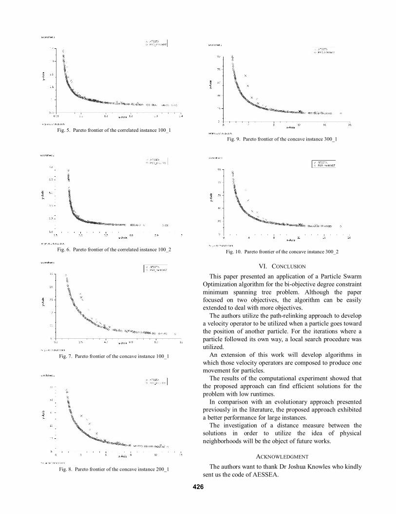
Fig. 5. Pareto frontier of the correlated instance 100_1

Fig. 6. Pareto frontier of the correlated instance 100_2

Fig. 7. Pareto frontier of the concave instance 100_1

Fig. 8. Pareto frontier of the concave instance 200_1

Fig. 9. Pareto frontier of the concave instance 300_1

Fig. 10. Pareto frontier of the concave instance 300_2

VI. CONCLUSION This paper presented an application of a Particle Swarm

Optimization algorithm for the bi-objective degree constraint minimum spanning tree problem. Although the paper focused on two objectives, the algorithm can be easily extended to deal with more objectives.

The authors utilize the path-relinking approach to develop a velocity operator to be utilized when a particle goes toward the position of another particle. For the iterations where a particle followed its own way, a local search procedure was utilized.

An extension of this work will develop algorithms in which those velocity operators are composed to produce one movement for particles.

The results of the computational experiment showed that the proposed approach can find efficient solutions for the problem with low runtimes.

In comparison with an evolutionary approach presented previously in the literature, the proposed approach exhibited a better performance for large instances.

The investigation of a distance measure between the solutions in order to utilize the idea of physical neighborhoods will be the object of future works.

ACKNOWLEDGMENT The authors want to thank Dr Joshua Knowles who kindly

sent us the code of AESSEA.

426

This research was partially funded by the program PRH 22 of the National Agency of Petroleum.

REFERENCES [1] C. F. Bazlamaçci and K. S. Hindi. “Minimum-weight spanning tree

algorithms a survey and empirical study,” Computers and Operations Research, vol. 28, pp. 767-785, 2001.

[2] G. Chartrand and O. R. Oellermann. Applied and Algorithmic Graph Theory. McGraw-Hill, 1993.

[3] H. Chou, G. Premkumar, and C.-H. Chu. “Genetic algorithms for communications network design – An empirical study if the factors that influence performance,” IEEE Transactions on Evolutionary Computation, vol. 4, no. 3, pp. 236–249, June 2001.

[4] C.A. Coello. “A comprehensive survey of evolutionary-based multiobjective optimization techniques,” Knowledge and Information Systems, vol.1, pp. 269-308, 1999.

[5] M. Ehrgott. “Approximation algorithms for combinatorial multicriteria optimization problems,” International Transactions in Operational Research, vol. 7, pp. 5-31, 2000.

[6] M. Ehrgott, and X. Gandibleux. “A survey and annotated bibliography of multiobjective combinatorial optimization,” OR Spektrum, vol. 22, pp. 425-460, 2000.

[7] M. Ehrgott, and X. Gandibleux. “Approximative solution methods for multiobjective combinatorial optimization,” Top, vol. 12, no. 1, pp. 1-89, 2004.

[8] M. R. Garey ad D. J. Johnson. Computers and Intractability: A Guide to the Theory of NP-completeness. Freeman, New York, 1979.

[9] F. Glover. “Parametric combinations of local job shop rules,” Chapter IV, ONR Research Memorandum N. 117, GSIA, Carnegie Mellon University, Pittsburgh, PA, 1963.

[10] F. Glover, M. Laguna, and R. Martí. “Fundamentals of scatter search and path relinking,” Control and Cybernetics, vol. 29, no. 3, pp. 653-684, 2000.

[11] R. L. Graham and P. Hell. “On the history of the minimum spanning tree problem,” Ann. History of Comp., vol. 7, pp. 43-57, 1985.

[12] F. Heppner, and U. Grenander. “A stochastic nonlinear model for coordinated bird flocks,” in The Ubiquity of Caos, S. Krasner, Ed., AAAS Publications, Washington, DC, 1990.

[13] J. Kennedy, and R. Eberhart. “Particle swarm optimization,” in Proceedings of the IEEE International Conference on Neural Networks, vol. 4, pp. 1942-1948, 1995.

[14] J.D. Knowles. “Local-search and hybrid evolutionary algorithms for Pareto optimization,” PhD dissertation, Department of Computer Science, University of Reading, Reading, UK, 2002.

[15] J. D. Knowles, and D. W. Corne. “A comparison of encodings and algorithms for multiobjective spanning tree problems,” in Proceedings of the 2001 Congress on Evolutionary Computation (CEC01), 2001, pp. 544-551.

[16] J. B. Kruskal. “On the shortest spanning subtree of a graph and the travelling salesman problem,” Pric. AMS, vol. 7, pp. 48-50, 1956.

[17] G.C. Onwubulu, M. Clerc. “Optimal path for automated drilling operations by a new heuristic approach using particle swarm optimization,” International Journal of Production Research, vol. 42, no. 3, pp. 473-491, 2004.

[18] P. Pomeroy. “An introduction to particle swarm optimization,” Electronic document available at www.adaptiveview.com/ipsop1.html

[19] R. C. Prim. “Shortest connection networks and some generalizations,”. Bell Systems Techn. J., vol. 36, pp. 1389-1401, 1957.

[20] G. Raidl, and B.A. Julstrom. “Edge sets: an efficient evolutionary coding of spanning trees,” IEEE Transactions on Evolutionary Computation, vol. 7, no. 3, pp. 225-239, 2003.

[21] W.T. Reeves. “Particle systems technique for modeling a class of fuzzy objects,” Computer Graphics, vol. 17, no. 3, pp. 359-376, 1983.

[22] C.W. Reynolds. “Flocks, herds and schools: a distributed behavioral model,” Computer Graphics, vol. 21, no. 4, pp. 24-34, 1987.

[23] E. Zitzler, L. Thiele, M. Laumanns, C. M. Fonseca, and V.G. Fonseca. “Performance assessment of multiobjective optimizers: An analysis and teview,” IEEE Transactions on Evolutionary Computation, vol. 7, no. 2, pp. 117-132, 2003.

427