J Math Model Algor (2007) 6:135–149DOI 10.1007/s10852-006-9053-2

Solving Large-scale Profit Maximization CapacitatedLot-size Problems by Heuristic Methods

Kjetil K. Haugen · Asmund Olstad · Bård I. Pettersen

Received: 18 October 2004 / Accepted: 30 November 2005 /Published online: 20 September 2006© Springer Science + Business Media B.V. 2006

Abstract This paper introduces a simple heuristic for a quadratic programming sub-problem within a Lagrangean relaxation heuristic for a dynamic pricing and lot-size problem. This simple heuristic is demonstrated to work well on both ‘standardproblem instances’ from the CLSP-literature, as well as on very large-scale cases.Additionally, we introduce price constraints within the framework of dynamicpricing, discuss their relevance in a real world market modelling, and demonstratetheir applicability within this algorithmic framework.

Mathematics Subject Classifications (2000) 90B05 · 90C20 · 90C10.

Key words Lagrangean relaxation heuristic · capacitated lot-size schedulingproblem · price constraints · profit maximization.

1 Introduction

This paper discuss a generalized version of the classical Capacitated Lot-SizeScheduling Problem (CLSP). The generalization, which we name PCLSP [8], in-volves adding dynamic pricing variables to the CLSP problem within a monopolisticmarket setting.

K. K. Haugen (B) · A. Olstad · B. I. PettersenMolde University College, Box 2110, 6402 Molde, Norwaye-mail: Kjetil.Haugen@himolde.no

A. Olstade-mail: Asmund.Olstad@himolde.no

B. I. Pettersene-mail: Bard.I.Pettersen@himolde.no

136 J Math Model Algor (2007) 6:135–149

The proposed solution procedure, applies a simple approximate heuristic as analternative to solving certain sub-problems to optimality. These sub-problems arisewithin the Lagrangean relaxation procedure used in [8].

Additionally, as most practical situations either will involve limitations on admis-sible prices or non-monopolistic market environments, we add price constraints tothe model with negligible effects on the algorithmic framework.

We demonstrate that both with and without price constraints, the PCLSP-algorithm with the proposed heuristic can solve large-scale problem instances fast.As an example, we show cases with 1,000 items in 50 periods which are solved in 13CPU minutes with a gap between upper and lower bounds less than 3%. As mostmodern manufacturing environments involve large product numbers, the model maybe practically interesting as an alternative to the CLSP-model.

In subsequent sections, we discuss characteristics of the CLSP-problem andrelevant literature. Furthermore, we introduce our formulation of the PCLSP-modelas well as the basic Lagrangean relaxation procedure. In final sections, we introducethe heuristic and discuss numerical consequences with and without price constraints.

2 Problem and Literature

2.1 The Capacitated Lot-size Scheduling Problem

The CLSP problem involves determination of production quantities of J items ona single machine over a planning horizon T, subject to a joint per period capacityconstraint such that set-up and holding costs are minimized and given (dynamic)product demand profiles are met.

Lot-sizing is one of the most important problems in production planning. Almostall manufacturing situations involving a product-line contain capacitated lot-sizingproblems. Unfortunately, the CLSP is one of the most difficult problems that arisesin production planning. Florian et al. [6] have shown that even the single-item CLSPis NP-hard. In the multi-item case, Chen and Thizy [1] showed that the problem isstrongly NP-hard. When set-up times are included in the problem, Maes et al. [13]have shown that finding even a feasible solution of the problem is NP-hard.

Due to the practical importance and the computational intractability of CLSP, theproblem is widely discussed and analyzed in the operations research and operationmanagement literature. Karimi et al. [11] have classified solution procedures forthe CLSP into three categories; (1) exact methods, (2) common sense or special-ized heuristics and (3) mathematical programming-based heuristics. Karimi et al.conclude that due to the results about NP-hardness, it is unlikely that any effectiveexact algorithm can be developed for the CLSP. Comparing common sense heuristicsand heuristics based on mathematical programming, they conclude that the lattermethods usually produce better quality solutions, have the advantage that solutionprocedures allow the use of many commercial solvers and finally, most of theheuristics produce a lower bound on the optimal solution.

Typical mathematical programming based heuristics for the multi-item CLSP, arebased on Lagrangean relaxation of the capacity constraints such that simple single-item uncapacitated lot-size problems emerge. These subproblems can be solved byefficient dynamic programming (DP)-algorithms for instance as described by Wagner

J Math Model Algor (2007) 6:135–149 137

and Whitin [18]. The solution of the relaxed (uncapacitated) single-item problemsgives a lower bound of the original problem. By fixing the set-up structure (notproduction quantities) given by the solution of the relaxed problem, the originalproblem becomes a linear program (LP) or transportation problem which, if feasible,creates an upper bound to the CLSP. Lagrangean multipliers are typically updatedby using subgradient methods like those proposed by Held et al. [9]. The process isrepeated until upper and lower bounds are equal, or until a pre-specified number ofiterations are completed. Work by Thizy and Wassenhove [14] (without set-up times)and Trigeiro et al. [16] (with set-up times) serve as valuable examples of Lagrangeanrelaxation solution procedures for the CLSP.

In spite of numerous articles with the label ‘CLSP and heuristics’, surprisinglyfew report solution procedures which are capable of handling large-scale problems.Today’s product variety may be very hard to fit into a lot-size framework which iscapable of handling only a few hundred items. Another important feature of theproposed solution methods in the literature is that they seem to produce ‘poorresults’ when the fixed capacity constraints are tight. This is unfortunate from apractical point of view. The famous Thizy and Wassenhove cases from [14] include8 products in 8 periods, while Trigeio et al. report solution of cases with 30 productsin 15 periods. When the capacity constraint is tight (93%), Thizy and Wassenhovereport a gap between upper and lower bounds for the 8 by 8 case of 10%.

In terms of problem sizes, a noteworthy result is that of Diaby et al. [2]. Theyreport computational experiments where they solve a problem with 5,000 items in30 periods (with set-up times) within 0.59% of the lower bound in 1,727.25 s ofIBM 3,081 computer time. Their solution method is an extension of the Lagrangeanrelaxation method of Thizy and Wassenhove, where they (1) propose another moreeffective procedure for solving the transportation problem (original problem withgiven set-up structure), (2) do not solve the transportation problem at each step ofthe subgradient optimization procedure and (3) add some ‘flexibility’ to the problemby allowing limited overtime instead of fixed capacity constraints.

2.2 Lot-sizing and Profit Maximization

Lately, several authors have stressed the importance of viewing operations manage-ment decisions and sales and marketing decisions within a common framework, seefor instance Eliashberg and Lilien [3]. According to Elmaghraby and Keskinocak [4],the historic reason for not doing so, is due to lack of price and/or marketinginformation, significant transaction costs related to price change as well as lack ofappropriate decision support tools. Another important conclusion in Elmaghrabyand Keskinocak’s paper is that so far, modelling with price or other demand affectinginstruments as decision variables in lot-size settings, presently is restricted to thesingle item case. Our approach, which may be described as an extension of the singleitem case of Thomas [15], to the multi-item capacity constrained case – seems to fitwell into what Lee [12] refers to as the next competitive battleground of the twenty-first century – demand based management (DBM).

138 J Math Model Algor (2007) 6:135–149

2.3 The PCLSP Problem

As briefly discussed above, a reasonable starting point for discussing our modellingapproach, is the work of Thomas [15]. In a pioneering article, he extended the simplelot-sizing model (typically solved by efficient dynamic programming as suggestedby Wagner and Whitin [18]) into a monopolistic market setting. His basic idea wasto establish whether the famous planning horizon theorems of Wagner and Whitincould be extended into the case with added price decision variables, and a per periodset of demand functions. Indeed, he showed existence of such planning horizontheorems, and proposed also an efficient DP-based algorithm. Our approach is toextend his model into a multi-item capacity constrained version. The model shownin Equations (1) to (8) below, is referred to as the Profit maximization CapacitatedLot-size Problem – PCLSP.

Max Z =T∑

t=1

J∑

j=1

[(α jt − β jt · pjt)pjt − s jtδ jt − h jt I jt − c jtx jt

](1)

s.t.

J∑

j=1

a jtx jt ≤ Rt ∀t (2)

x jt + I j,t−1 − I jt = α jt − β jt · pjt ∀ jt (3)

x jt ≤ Mjtδ jt ∀ jt (4)

x jt ≥ 0 ∀ jt (5)

I jt ≥ 0, ∀ jt (6)

δ jt ∈ {0, 1} ∀ jt (7)

α jt

β jt≥ pjt ≥ 0 ∀ jt (8)

with decision variables:

x jt = the amount of item j produced in period t

I jt = amount of item j held in inventory between periods t and t + 1

pjt = price of item j in period t

δ jt ={

1 if item i is produced in period t0 otherwise

J Math Model Algor (2007) 6:135–149 139

and parameters:

T = number of time periods

J = number of items

α jt = constant in linear demand function for item j in period t

β jt = slope of linear demand function for item j in period t

s jt = setup cost for item j in period t

h jt = unit storage cost for item j between periods t and t + 1

c jt = unit production cost for item j in period t

a jt = consumption of capacitated resource by item j in period t

Rt = amount of resource available in period t

Mjt = upper limit on the production of item j in period t, Mjt =T∑

s=t

α js

The objective (1) contains total revenue minus total costs (setup, storage andproduction costs). Note that the formulations (1) to (8) implicitly assumes lineardemand functions; α jt − β jt p jt. This assumption is not necessary in our algorithm,but it will prove very practical from a heuristic point of view. Constraints (2) arethe capacity constraints and (3) inventory balancing constraints, while (4), andthe integrality requirement (7), enforce set-up when production is positive. Non-negativity constraints (5), (6) and (8) are reasonable and the upper bound on pricein (8) is needed to secure positive demand.

The actual algorithms (more or less standard Lagrange Relaxation) applied in thesolution of the above model are extensively covered in Haugen et al. [8], and willhence not be discussed in detail here. Roughly however, the idea involves relaxingthe capacity constraints (2), which for given values of the Lagrange multipliers leadsto J decoupled ‘Thomas’-problems [15] which efficiently solve the relaxed model(1) to (8). For latter reference, we refer to this problem as the lagrange upperbound problem – LUBP. This procedure yields a set-up structure (or values for theδ jt-variables). The set-up structure defines production periods where production isallowed to take place for each product. Then, we ‘apply’ this set-up structure tothe original problem (Equations (1) to (8)) such that production only takes placewhen δ jt = 1. Consequently, all integer variables are removed from the problem.In addition, all production variable instances (x jt’s) where δ jt = 0 are also removed.The resulting problem is a standard quadratic programming problem referred to aslagrange lower bound problem – LLBP in Equations (9) to (14) below: (Observethat certain x jt’s removal – or fixation to zero – as a consequence of the given set-upstructure is not explicitly modelled in Equations (9) to (14).)

Max Z =T∑

t=1

J∑

j=1

[(α jt − β jt · pjt)pjt − h jt I jt − c jtx jt

](9)

140 J Math Model Algor (2007) 6:135–149

Figure 1 The Lagrangeanrelaxation algorithm forthe solution process.

Master problem

LLBP LUBP

Eqs.(1)-(8)

δ fixedjt

(2)active (2)relaxed

δ not fixedjt

δ

λ

s.t.

J∑

j=1

a jtx jt ≤ Rt ∀t (10)

x jt + I j,t−1 − I jt = α jt − β jt · pjt ∀ jt (11)

x jt ≥ 0 ∀ jt (12)

I jt ≥ 0, ∀ jt (13)

α jt

β jt≥ pjt ≥ 0 ∀ jt (14)

Solving the quadratic programming problem (9) to (14) to optimality providesmultipliers which are transferred back into the relaxed item by item sub-problems,and the algorithm progresses. Figure 1 sums up the structure of the Lagrangerelaxation algorithm.

The main topic here, as discussed above, is to investigate the effect of substitutinga simple heuristic as an alternative to solving the LLBP-problems to optimality.

3 LLBP Heuristics

As noted by several authors in the stochastic programming community (see forinstance Haugen et al. [7] or Helgasson and Wallace [10]) the point of solvingcertain sub-problems to optimality in decomposed optimization is not necessarilysensible. The point is very simple: The multiplier or shadow price on the capacityconstraint (10), which the LLBP problem (9) to (14) produces, is more of a signalfor direction in set-up structural changes in LUBP. As we also apply a multipliersmoothing procedure (see Haugen et al. [8]), this fact becomes even more evi-dent. Consequently, if we are able to construct a computationally efficient heuristicto replace the LLBP-problem, the overall algorithmic performance should not

J Math Model Algor (2007) 6:135–149 141

necessary be too adversely affected. Such a procedure is especially interesting ifthe replaced sub-problem involves significant computations, which is the case here.The clue to success would then be to control the trade-off between speed-up as aresult of applying a simple heuristic and informational loss due to approximatedmultipliers. Such a trade-off is hard to predict, so a reasonable strategy is trial anderror. Applying any approximation yields information loss. The key point is to tradeoff this information loss against the speed-up gained by the approximation.

Constructing approximative solutions to the problem (9) to (14) can be done inmany ways. One very simple alternative is to base the heuristic on ‘pricing out’products. Recall that the point of this procedure is that by solving the LUBP-problems, (item by item Thomas problems), the capacity constraint (2) is violated.If it is not, the initial LUBP-solution is optimal, and the problem is just J decoupleduncapacitated Thomas-problems. Consequently, after solving the LUBP problem,the capacity constraint is violated in one or several time periods.

As mentioned briefly in Subsection 2.3, the application of linear demand functionsbecomes especially handy here, as any product could be ‘priced out’ completely, bysetting pj,t+k,t = α j,t+k

β j,t+k, where pj,t+k,t is the price of product j produced in period t for

demand in period t + k. Then, the resulting demand d j,t+k,t equals 0.Hence, the following algorithm will yield an approximate (and feasible) solution

to the LLBP problem.

0. Jump to next period with∑J

j=1 a jtx jt > Rt. If this period is T + 1, Stop1. Choose new product for pricing.2. if

∑Jj=1 a jtx jt > Rt when pj,t+k,t = α j,t+k,t

β j,t+k,t, then Jump to 1.

else set pj,t+k,t such that∑J

j=1 a jtx jt = Rt and Jump to 3.3. Jump to 0.

Point 1 ‘Choose new product for pricing’ may need some further explanation.As we use the price to reduce demand, it seems sensible to start with the productthat implies smallest profit reduction. At the same time, we would like to choosethe product which uses most capacity units, that is the product with the largest a jt.Consequently, we sort all products in all periods (before the algorithm starts in orderto avoid repeated sorting ) by profit reduction per capacity usage.

This algorithm is obviously computationally efficient. Along with the initial sortof T vectors of size J, in the worst case, T · J computations in step 2 takes place.Consequently, this heuristic should be able to ‘solve’ almost any size of the LLBPproblems.

The pricing rule proposed above may not be practically sensible – given non-monopolistic market settings – since it may lead to solutions where certain productsgets an extremely high price while other product prices are kept unchanged. Theaddition of price constraints treated in Section 5 may serve as a practical solution.

4 Numerical Experiments

4.1 Computational Setup

The algorithm defined in Subsection 3 was implemented in JAVA along with animplementation for the LLUB problem. The numerical experiments (following in

142 J Math Model Algor (2007) 6:135–149

subsequent sections) were conducted on a 2.40 Ghz PC with 512 Mb RAM. Thesolver for the quadratic program used as a comparison to our LLBP heuristic,adapts Robert J. Vanderbei’s LOQO-system [17]. Surely, any other standard exactQP solver could have been used – for instance CPLEX; probably with betterperformance as we implemented the Vanderbei solver ourselves.

The space complexity of this algorithm ensures large scale cases as it is merely oforder J · T.

4.2 Some Initial Cases from Literature

In order to get some initial feeling for the algorithmic behavior, we ran some casesbased on the 8 product by 8 period Thizy and Wassenhove cases.1 Primarily, wewere interested in observing the effect of applying the heuristic as an alternative tothe exact QP-solver of Vanderbei [17]. Figure 2 shows the algorithmic developmentfor one instance of such a comparison. (The cases were run over 500 iterations, butFigure 2 contains only the 150 first.)

Firstly, Figure 2 shows the simple (and not very surprising) fact that the exactmethod performs better than the heuristic. The dashed curve reaches a gap closeto zero after around 20 iterations, while the heuristic reaches a similar gap at

0

0.5

1

1.5

2

2.5

3

0 20 40 60 80 100 120 140 160

Gap

(%

)

Iteration count

Comparing Exact and Heuristic LLBP, Thizy and Wassenhove 73% case

Heuristic LLBPExact LLBP

Figure 2 Gap (%) as a function of iteration count with the exact QP-solver and our heuristic.

1Obviously, we have not executed the actual Thizy and Wassenhove cases, simply due to the factthat our model is not a CLSP model. However, as can be observed from Haugen et al. [8], we haveconstructed our demand functions in a manner reflecting the content of these cases.

J Math Model Algor (2007) 6:135–149 143

Table I Gaps for various smoothing parameters for the 8 by 8 cases from Thizy and Wassenhove [14]

SP CAP61% CAP73% CAP91% CAP93% CAP110%(%) (%) (%) (%) (%)

0.1 0.29 2.80 4.82 5.71 8.740.5 0.23 2.11 4.82 5.01 8.740.7 0.11 0.40 3.03 1.59 8.740.9 0.03 0.23 0.88 1.23 4.540.99 0.00 0.00 0.24 0.79 2.110.999 0.00 0.02 0.59 0.39 2.39

around 60 iterations. Similar patterns are observed for other cases, but the heuristicperforms somewhat poorer when instances become tighter. However, as the heuristicintroduces a very significant speed-up, this fact is of minor importance. A very simpletime measurement experiment should clarify. Executing a somewhat larger case(100 products in 10 time periods) shows an execution time of 0.26 CPU secondsper iteration. The same case with the exact QP solver used 720 CPU seconds periteration. Hence, roughly speaking, a 500 iteration run should take 2.2 CPU minuteswith the LLBP heuristic, while usage of the exact QP-solver should take 100 CPUhours. Surely, this speed-up will only increase when problem size increases.

Table I shows final gaps (%) after 500 iterations for all ‘Thizy and Wassenhove[14] cases’ for various values of the smoothing parameter SP. Additionally, an extra,tighter case – CAP110% – was constructed.

As discussed in Haugen et al. [8], we apply a shadow price smoothing procedure.Simply, this implies constructing a convex combination of the new shadow pricefound at the present iteration, with the shadow price from the previous iteration.A large value of the smoothing parameter SP, hence indicates that the new shadowprice obtained in the present iteration is not too different from the previous shadowprice estimate. As Table I indicates, this procedure is indeed important for theperformance of the algorithm, but as these matters are thoroughly discussed inHaugen et al. [8], we will not repeat them here. However, the important informationin Table I is that all these cases show very small gaps for the given problem instances.For all practical purposes, the problems are solved to optimality.

4.3 Some Large-scale Cases

In order to be able to test large-scale cases, we constructed a case generator whichgenerated cases2 randomly by uniform distributions. In order to control problemtightness, the cases were constructed such that on average, the uncapacitated solution(the solution to the LUBP problem) yielded a certain capacity utilization percentage.Consequently, a case named 100�10100% yields – on average – full capacity utilizationfor a case with 100 products in 10 periods.

2All cases can be made available to readers by contacting the authors.

144 J Math Model Algor (2007) 6:135–149

Table II Gaps for various smoothing parameters for randomly generated cases: 100 products in 10periods

SP 100�1077% 100�1087% 100�1099% 100�10109% 100�10120%(%) (%) (%) (%) (%)

0.9 0.00 0.15 1.53 3.87 5.930.99 0.00 0.02 0.30 1.20 1.780.999 0.00 0.03 0.24 0.90 2.96

Firstly, we ran a set of instances with 100 products over 10 periods. The results(Gap (%) after 500 iterations) are shown in Table II. (The results are limited toSP ∈ {0.9, 0.99, 0.999}.)

As Table II indicates, results are good, with all gaps within a 2% limit and anaverage gap of 0.66% if SP = 0.99 is chosen. The reason why an SP of 0.999 producesa larger gap than an SP of 0.99 is due to the limited number of iterations (500) inTable II – refer to Figure 3. Table II also indicates (not surprisingly) that problemtightness has significant influence on algorithmic performance.

Finally, we ran a really large-scale case, 1,000 products over 50 periods. Addi-tionally, this case was made intentionally very tight at a 144% average capacityutilization. The case was executed over 1,000 iterations, with results as indicated inFigure 3.

As Figure 3 indicates, a very tight and very large case yields good results – less than3% Gap after 1,000 iterations with SP = 0.999. This case was executed in around

2

4

6

8

10

12

14

0 100 200 300 400 500 600 700 800 900 1000

Gap

(%

)

Iteration count

A large scale case: 1000 products in 50 periods, 1000 iterations

SP=0.999SP=0.99SP=0.9

Figure 3 A large-scale example – 1,000�50144%.

J Math Model Algor (2007) 6:135–149 145

13 CPU minutes. Consequently, more reasonable cases (read less tight) should bemanageable within significantly shorter execution times.

5 Price Constraints and More Advanced Market Situations

5.1 Initial Remarks

The transition from cost minimization to monopolistic profit maximization seems likea natural and logic step to take. However, the assumption of a monopolistic marketenvironment is strong, and few real world manufacturers may feel that such a marketdescription fits well. As such, the natural theoretical extension ought to be gametheory – that is, to explicitly include inventory, set-up and multiple products into agame model. Unfortunately, such a strategy may prove difficult, if not impossible,due to both computational and modelling intractability. Still, some very recentwork by Federgruen and Meissner [5] addresses – at least partially – this type ofproblem. They investigate a one-product competitive (Bertrand game) setting, anddemonstrate existence of a price equilibrium as well as design of efficient proceduresfor equilibrium price computations. However, since an extension of this line of workto the multi-product case by no means is elementary, we adopt a different and morepractical approach to the problem of obtaining a more versatile market description.

Most manufactures will face market conditions which neither are monopolistic norfree markets. However, within certain limits, prices may be changed without chang-ing the Nash equilibrium of the actual game they are playing. That is, there ought to

0

1

2

3

4

5

6

0 50 100 150 200 250 300 350 400 450 500

Gap

(%

)

Iteration count

An example with price constraints

20%30%60%90%98%

Figure 4 Thizy and Wassenhove [14] – CAP93% case with varying price constraints.

146 J Math Model Algor (2007) 6:135–149

be certain price intervals for the products, where a slight price change does not implychanges in the demand function. If this is the case, adding price constraints may proveinteresting from a practical point of view. For instance, if a certain manufacturer facesdifferent market conditions for different products that share a common productionline and hence common capacity constraints, a practical adaption could imply certainproducts with very tight price constraints (fierce competition) ranging up to otherproducts with loose price constraints (monopoly like market conditions).

In principle, such changes imply adding constraints like

pjt

≤ pjt ≤ pjt (15)

to the the model of Equations (1) to (8), where pjt

and pjt are given lower and upperbounds on price variables.

The algorithmic consequences for the LLBP problems are minor. The only neces-sary change is to replace pjt = α jt

β jtwith pjt = pjt in the algorithm of Section 3. This

means that the worst case behavior is unaffected, but on average, a tiny ‘speed-down’effect may be expected. However, as this algorithm runs fast, such a ‘speed-down’is practically uninteresting. Allowing for price constraints in the algorithm for theLUBP problems, is somewhat more complex. However, it boils down to changing thepricing results of Thomas[15], and does not imply significant performance reduction.

0

1

2

3

4

5

6

0 10 20 30 40 50 60 70 80 90

Gap

(%

)

Iteration count

Initial algorithmic steps for 60%, 90% and 98% price constraints cases

60%90%98%

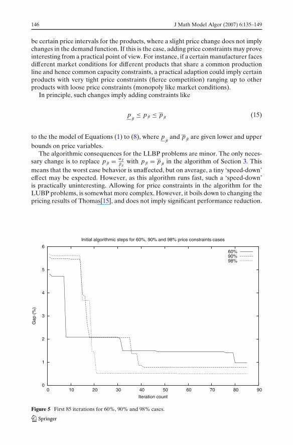
Figure 5 First 85 iterations for 60%, 90% and 98% cases.

J Math Model Algor (2007) 6:135–149 147

5.2 Numerical Experiments with Price Constraints

An experiment showing the algorithmic performance for various instances of priceconstraints (we use the CAP93%-case from Table I), is given in Figure 4.

The various price constraint alternatives are named 20% up to 98% in Figure 4.A given percentage indicates that prices in this case are allowed to vary thatpercentage around the initial LUBP-problem solution. Hence, the 20%-case is atightly constrained case, while the 98%-case is close to unconstrained. Note also thatfor the tightest cases (20% and 30%), observations for initial algorithmic steps aremissing. This is due to initial but recoverable infeasibilities in the algorithm.

All cases yield very good solutions (a maximal gap around 0.8%) within 150iterations. Consequently, introduction of price constraints is nicely taken care ofwithin our algorithmic framework.

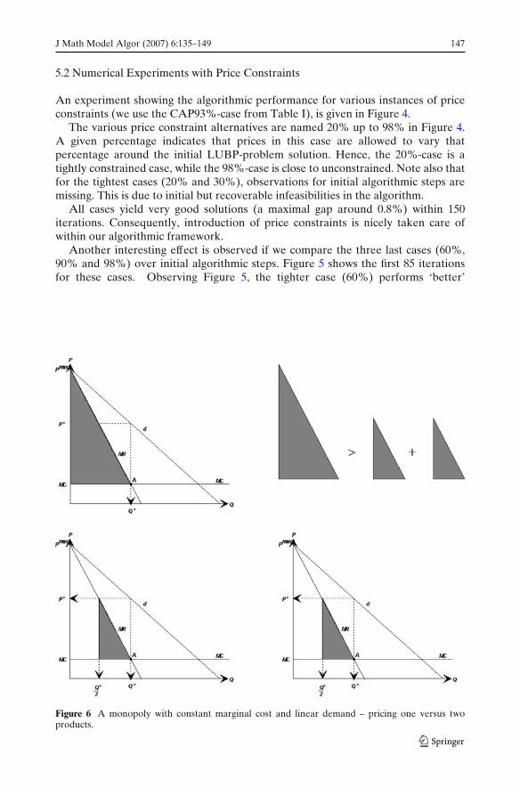
Another interesting effect is observed if we compare the three last cases (60%,90% and 98%) over initial algorithmic steps. Figure 5 shows the first 85 iterationsfor these cases. Observing Figure 5, the tighter case (60%) performs ‘better’

Figure 6 A monopoly with constant marginal cost and linear demand – pricing one versus twoproducts.

148 J Math Model Algor (2007) 6:135–149

initially than the two other cases. Similarly, the 90% case performs slightly betterinitially than the 98% case. At later iteration steps, this picture is reversed. Sucha development is actually reasonable. If we look back at our heuristic, it will pricefewer products in the unconstrained than in the constrained cases. It is obvious thatit is better to price more than one product at a time. A simple graphical argumentmay clarify.

Figure 6 shows a simple monopoly model with constant marginal costs, MC andlinear demand d. Then, marginal revenue, MR is also linear, and the monopolysolution is found for MC=MR, point A in Figure 6. Suppose we have two equalproducts, each correctly described by Figure 6 (lower part). Assume additionallya situation where the capacity constraint is violated by exactly the amount Q∗ andfull price flexibility. In such a case, the heuristic chooses to price out one of thetwo products (top left of Figure 6), that is, changing the price from P∗ to Pmax,reducing demand from Q∗ to 0 and a feasible situation is obtained. If alternatively,our heuristic meets price constraints, the same reduction in capacity overload, Q∗,must be obtained by pricing both products (lower part of Figure 6) such that theresulting demand reduction became Q∗

2 for each product. The profit loss would bethe area of the two grey-scaled triangles in Figure 6 – obviously smaller than theprofit loss of pricing out one product – as described in the top right part of Figure 6.As a consequence, when we add price constraints, the tighter they are, the moreproducts will be priced simultaneously, and the algorithm should perform betterinitially. However, when the algorithm progresses, the simple fact that the tighterproblems are tighter should lead to poorer performance.

6 Conclusions and Suggestions for Further Research

The main conclusion of this paper is that by substituting an exact QP-solver witha simple heuristic in a Lagrange-relaxation heuristic for the PCLSP-problem, weobtain good solutions and significant speed-ups. Additionally, we have demonstratedthat we are able to solve very large-scale instances in reasonable time. Actually, thepractical limits are merely computer memory. Combining this with the addition ofprice constraints, we have built a framework that we feel ought to be practicallyinteresting.

Surely, it is easy to point out performance enhancing possibilities in our heuristic.We could, as discussed in the previous paragraph, allow simultaneous pricing.Equally obvious: if the marginal profit loss from simultaneously pricing out productsis larger than the smallest storage cost, storage should be chosen as an alternative tofurther pricing. However, as Figure 2 indicates, it is not necessarily much to gain byfurther refinements of the heuristic.

Additionally, the proposed simple heuristic might also prove to be an effectivesubroutine for solving profit maximization CLSP problems with more difficult struc-tures. Such structures may involve multi level problems, problems with sequencedependent setup times, more complex demand structures, or stochastic cases. Insuch more complex model formulations, the ability to solve sub-problems very fast iscrucial.

J Math Model Algor (2007) 6:135–149 149

References

1. Chen, W.H., Thizy, J.M.: Analysis of relaxation for the multi-item capacitated lot-sizing prob-lem. Ann. Oper. Res. 26, 29–72 (1990)

2. Diaby, M., Bahl, H.C., Karwan, M.H., Zionts, S.: A lagrangean relaxation approach for very-large-scale capacitated lot-sizing. Manage. Sci. 38(9), 1329–1340 (1992)

3. Eliashberg, J., Lilien, G.L.: Handbooks in Operations Research and Management Science –Marketing. North-Holland, Amsterdam, The Netherlands (1993)

4. Elmaghraby, W., Keskinocak, P.: Dynamic pricing in the presence of inventory considerations:Research overview, current practice and future directions. Manage. Sci. 49(10), 1287–1309 (2003)

5. Federguren, A., Meissner, J.: Competition under time-varying demands and dynamic lot sizingcosts. Working Paper – in Journal Review, Graduate School of Business, Columbia University,New York (December 2005)

6. Florian, M., Lenstra, J. K., Rinnooy Kan, A.H.G: Deterministic production planning: Algorithmsand complexity. Manage. Sci. 26, 669–679 (1980)

7. Haugen, K., Løkketangen, A., Woodruff, D.: Progressive hedging as a meta-heuristic applied tostochastic lot-sizing. Eur. J. Oper. Res. 132, 116–122 (2001)

8. Haugen, K., Olstad, A., Pettersen, B.I.: The profit maximizing capacitated lot-size (pclsp) prob-lem. Eur. J. Oper. Res. (forthcoming) (2005)

9. Held, M., Wolfe, P., Crowder, H.P.: Validation of subgradient optimization. Math. Program. 6(1),62–88 (1974)

10. Helgasson, T., Wallace, S.W.: Approximate scenario solutions in the progressive hedging algo-rithm. Ann. Oper. Res. 31, 425–444 (1991)

11. Karimi, B., Fatemi Ghomi, S.M.T., Wilson, J.M.: The capacitated lot sizing problem: A review ofmodels and algorithms. Omega 31, 365–378 (2003)

12. Lee, H.L.: Ultimate enterprise value creation using demand-based management. Working paperSGSCMF-W1-2001, Stanford University, California (September 2001)

13. Maes, J., McClain, J.O., Van Wassenhove, L.N.: Multilevel capacitated lot sizing complexity andlp-based heuristics. Eur. J. Oper. Res. 53(2), 131–148 (1991)

14. Thizy, J.M., Van Wassenhove, L.N.: Lagrangean relaxation for the multi-item capacitated lot-sizing problem: A heuristic implementation. IEE Trans. 17(4), 308–313 (1985)

15. Thomas, J.: Price-production decisions with deterministic demand. Manage. Sci. 18(11), 747–750(1970)

16. Trigeiro, W.W., Thomas, L.J., McClain, J.O.: Capacitated lot sizing with setup times. Manage.Sci. 35(3), 353–366 (1989)

17. Vanderbei, R.J.: LOQO User’s Manual – Version 3.10. Princeton Univeristy Press, New Jersey(1998)

18. Wagner, H.M., Whitin, T.M.: Dynamic version of the economic lot size model. Manage. Sci. 5(3),89–96 (1958)