Solving infinite horizon nonlinear optimal control problems using an extended modal series method

Jajarmi et al. / J Zhejiang Univ-Sci C (Comput & Electron) 2011 12(8):667-677 667

Solving infinite horizon nonlinear optimal control problems using an extended modal series method

Amin JAJARMI†1, Naser PARIZ1, Sohrab EFFATI2, Ali VAHIDIAN KAMYAD2

(1Advanced Control and Nonlinear Laboratory, Department of Electrical Engineering, Ferdowsi University of Mashhad, Mashhad, Iran) (2Department of Applied Mathematics, Faculty of Mathematical Sciences, Ferdowsi University of Mashhad, Mashhad, Iran)

†E-mail: [email protected] Received Sept. 19, 2010; Revision accepted Apr. 6, 2011; Crosschecked July 4, 2011

Abstract: This paper presents a new approach for solving a class of infinite horizon nonlinear optimal control problems (OCPs). In this approach, a nonlinear two-point boundary value problem (TPBVP), derived from Pontryagin’s maximum principle, is transformed into a sequence of linear time-invariant TPBVPs. Solving the latter problems in a recursive manner provides the optimal control law and the optimal trajectory in the form of uniformly convergent series. Hence, to obtain the optimal solution, only the techniques for solving linear ordinary differential equations are employed. An efficient algorithm is also presented, which has low computational complexity and a fast convergence rate. Just a few iterations are required to find an accurate enough suboptimal trajectory-control pair for the nonlinear OCP. The results not only demonstrate the efficiency, simplicity, and high accuracy of the suggested approach, but also indicate its effectiveness in practical use. Key words: Infinite horizon nonlinear optimal control problem, Pontryagin’s maximum principle, Two-point boundary value

problem, Extended modal series method doi:10.1631/jzus.C1000325 Document code: A CLC number: TP13 1 Introduction

Optimal control is one of the most active re-search topics in control theory and has a wide range of applications in different fields such as physics, economy, aerospace, chemical engineering, and ro-botics (Garrard and Jordan, 1977; Manousiouthakis and Chmielewski, 2002; Notsu et al., 2008; Tang et al., 2009). For linear time-invariant systems, the the-ory and application of optimal control are highly developed (Bryson, 2002; Yousefi et al., 2010). However, optimal control of nonlinear systems is much more challenging and has been studied exten-sively for decades.

To solve nonlinear optimal control problems (OCPs), many computational techniques have been developed. One familiar scheme is the state- dependent Riccati equation (SDRE) method (Cimen,

2008). Although this technique has been widely used in various applications, its major limitation is that it requires solving a sequence of matrix Riccati alge-braic equations. This property may use up a lot of computing time and memory space. Another scheme is called the approximating sequence of Riccati equations (ASRE) (Banks and Dinesh, 2000). From a practical point of view, the ASRE is attractive; how-ever, it suffers from computational complexity since it requires solving a sequence of time-varying matrix Riccati differential equations.

For solving nonlinear OCPs, a numerical ap-proach has been suggested by Huang and Lin (1995) and Abu-Khalaf et al. (2006). This approach finds the Taylor series solution of the Hamilton-Jacobi-Isaacs (HJI) equation associated with the nonlinear H∞ con-trol problem. The coefficients of the Taylor series are generated by solving one Riccati algebraic equation and a sequence of linear algebraic equations. How-ever, deriving each linear equation in the sequence

Journal of Zhejiang University-SCIENCE C (Computers & Electronics) ISSN 1869-1951 (Print); ISSN 1869-196X (Online) www.zju.edu.cn/jzus; www.springerlink.com E-mail: [email protected]

© Zhejiang University and Springer-Verlag Berlin Heidelberg 2011


requires a number of matrix computations, which may introduce computational complexity.

To determine the optimal control law, there is another approach using dynamic programming (Bell- man, 1952). This approach leads to the Hamilton- Jacobi-Bellman (HJB) equation which in most cases is hard to solve. An excellent literature review on the methods for solving the HJB equation was provided by Beard et al. (1997) who also considered a succes-sive Galerkin approximation (SGA) approach. In the SGA, a sequence of generalized HJB equations is solved iteratively to obtain a sequence of approxima-tions leading eventually to the solution of the HJB equation. However, the proposed sequence may con-verge very slowly or even diverge.

The optimal control law can also be derived us-ing Pontryagin’s maximum principle (Pontryagin, 1959). For nonlinear OCPs, this approach leads to a nonlinear two-point boundary value problem (TPBVP) that unfortunately, in general, cannot be solved analytically. Therefore, many researchers have tried to find an approximate solution for nonlinear TPBVPs (Ascher et al., 1995). In recent years some better results have been obtained. For instance, a new successive approximation approach (SAA) was pro-posed by Tang (2005) where, instead of directly solving the nonlinear TPBVP derived from the maximum principle, a sequence of nonhomogeneous linear time-varying TPBVPs is solved iteratively. The sensitivity approach, proposed by Tang et al. (2002), is similar to the SAA. It requires solving iteratively only a sequence of nonhomogeneous linear time- varying TPBVPs to determine the infinite series pre-senting the optimal control law. Note that solving time-varying equations is much more difficult than solving time-invariant ones.

Recently, a novel numerical technique was proposed for solving nonlinear OCPs, which is based on differential transformation (DT) (Hwang et al., 2009). Using DT, a nonlinear TPBVP, derived from the maximum principle, is transformed into a system of nonlinear algebraic equations. Then, through in-verse DT, the optimal solution is obtained in the form of a finite-term Taylor series. A system of nonlinear algebraic equations can be solved numerically by various methods such as Newton’s method or the nonlinear least square method. Hwang et al. (2009) used a trust region Newton’s method for solving such

a system of nonlinear algebraic equations. Unfortu-nately, Newton’s method should start from a good initial guess, sufficiently close to the exact solution. Otherwise, the convergence of this method cannot be ensured.

In recent years, a new technique, called the modal series method, has been developed in the field of nonlinear system analysis (Pariz, 2001; Pariz et al., 2003; Shanechi et al., 2003; Wu et al., 2007; Khatibi and Shanechi, 2011). This method, which was ini-tially introduced by Pariz (2001), provides the solu-tion of autonomous nonlinear systems in terms of fundamental and interacting modes. This solution, which is called modal series, yields a good deal of physical insight into the system behavior. In contrast to the perturbation method (Murdock, 1999), the modal series method does not depend on the small/large physical parameters in the system model. In addition, unlike the traditional non-perturbation techniques, such as Lyapunov’s artificial small pa-rameter method (Lyapunov, 1892) and Adomian’s decomposition method (Adomian and Adomian, 1984), the modal series converges uniformly to the exact solution.

The aim of this paper is to extend the modal se-ries method to solve a class of infinite horizon nonlinear OCPs. By this extension, a nonlinear TPBVP, derived from the maximum principle, is transformed into a sequence of linear time-invariant TPBVPs. Solving the latter problems in a recursive manner leads to the optimal control law and the op-timal trajectory in the form of uniformly convergent series.

2 Statement of the problem

Consider an infinite horizon nonlinear OCP de-scribed by

0

T T

0

0 0

1min ( ( ) ( ) ( ) ( ))d2( ) ( ( )) ( ) , ,

s.t. ( ) ,

tJ t t t t t

t t t t tt

∞= +

= + >⎧⎨ =⎩

∫ x Qx u Ru

x F x Bux x

(1)

where x∈ún and u∈úm are the state and control vec-tors respectively, Q∈ún×n and R∈úm×m are positive semi-definite and positive definite matrices respec-


tively, F: ún→ún is a nonlinear analytic vector field where F(0)=0 (and hence x=0 is an equilibrium point of the system), B is a constant matrix of appropriate dimension, and x0∈ú

n is the initial state vector. Also, it is assumed that the pair (JF(0), B) is controllable and the pair (JF(0), sqrt(Q)) is observable, where JF is the Jacobian matrix of F, and sqrt(Q) is the square root of matrix Q. These assumptions guarantee the existence of a smooth optimal solution on a certain region of state space containing the equilibrium point (McCaffrey and Banks, 2005).

According to Pontryagin’s maximum principle, the optimality conditions are obtained as the follow-ing nonlinear TPBVP:

1 T

0 0

( ) ( ) ( ( )),

( ) ( ) ( ( ), ( )),( ) , ( ) ,

t t t

t t t tt

−⎧ = − +⎪

= − −⎨⎪ = ∞ =⎩

x BR B F x

Qx Ψ xx x 0

λ

λ λλ

(2)

where λ∈ún is the co-state vector, and Ψ(x(t), λ(t))=

T( ( )) ( )

( )t t

tF x λ

x⎛ ⎞∂ ⎟⎜ ⎟⎜ ⎟⎜ ⎟⎜ ∂⎝ ⎠

. The optimal control law is given

by * 1 T

0( ) ( ) , .t t t t−= − >u R B λ (3) Lemma 1 The solution of the nonlinear TPBVP (2) is analytic with respect to x0. Proof Let the pair (x(·), λ(·)) be a solution of TPBVP (2). Define (x0, λ0)=(x(t0), λ(t0)). Then, (x(·), λ(·)) is the solution of the following initial value problem (IVP):

1 T

0 0 0 0

( ) ( ) ( ( )),

( ) ( ) ( ( ), ( )),( ) , ( ) .

t t t

t t t tt t

−⎧ = − +⎪

= − −⎨⎪ = =⎩

x BR B F x

Qx Ψ xx x

λ

λ λλ λ

(4)

Since the nonlinear terms in Eq. (4) are analytic,

(x(·), λ(·)), as the solution of IVP (4), is analytic with respect to x0 (Arnold, 1992). Thus, (x(·), λ(·)) as the solution of TPBVP (2) is analytic with respect to x0, and the proof is complete.

Unfortunately, problem (2) is a nonlinear TPBVP that can be solved analytically only in a few simple cases. To overcome this difficulty, we will extend the modal series method in the next section.

3 Extending the modal series method and optimal control design strategy

The modal series method was originally pro-posed and further improved to solve a class of IVPs of the form 0 0( ) ( ( )) , ( )t t t= =x F x x x (Pariz, 2001; Pariz et al., 2003; Shanechi et al., 2003; Khatibi and Shanechi, 2011). In this section, we extend this method for solving a nonlinear TPBVP (2). To this end, first we need a Taylor series expansion of the nonlinear non-polynomial terms. Therefore, if the nonlinear terms in Eq. (2), i.e., F(x(t)) and Ψ(x(t), λ(t)), are not polynomial, they should be ex-panded in the Taylor series around the equilibrium point (x, λ)=(0, 0), which yields

T 1

201 T

10T

20

( ) ( )1( ) ( ) ( ) ,2!

( ) ( )n

t tt t t

t t

−

⎡ ⎤⎢ ⎥

= − + + +⎢ ⎥⎢ ⎥⎣ ⎦

x H xx BR B λ A x

x H x (5a)

T 111

01T

11

( ) ( )( ) ( ) ( ) ,

( ) ( )n

t tt t t

t t

⎡ ⎤⎢ ⎥= − − − −⎢ ⎥⎢ ⎥⎣ ⎦

x HQx A

x H

λλ λ

λ (5b)

where 10 ,=

∂=∂ x

FAx 0

2

20 2 ,i i

=

∂=∂

x

FH

x0

01 ,==

∂=∂ x

ΨA 00λλ

2

11i i

==

∂=∂ ∂ x

Hx 0

0λ

Ψλ

, in which Fi and Ψi are the ith com-

ponents of vector fields F and Ψ, respectively. Moreover, in the Taylor series of Ψ only the mixed partial derivatives which are of the first order with respect to λ are non-zero at the origin.

The solution of the nonlinear TPBVP (2) for ar-bitrary initial condition x0∈ú

n and for all t>t0 can be expressed as

0

0

( ) ( , ),( ) ( , ),t tt t=⎧

⎨ =⎩

x xx

Λλ Γ

(6)

where Λ: ún×ú→ún and Γ: ún×ú→ún are analytic vector fields with respect to the initial condition x0 (Lemma 1). In addition, it is easy to show that Λ(0, t) =Γ(0, t)=0, ∀t>t0. Therefore, we can expand Eq. (6) as a Maclaurin series about x0 as follows:


0

1

0

0

2

00 0

0

( )

2T 1 00 02

0

12

T 00 02

0

( )

( , )( ) ( , )

( , )

1 ( ),2!

( , )

t

ii

n

t

tt t

t

t

t

=

=∞

=

=

∂= =

∂

⎡ ⎤⎛ ⎞∂⎢ ⎥⎜ ⎟⎜ ⎟⎢ ⎥∂⎝ ⎠⎢ ⎥

⎢ ⎥+ + =⎢ ⎥

⎛ ⎞⎢ ⎥∂⎜ ⎟⎢ ⎥⎜ ⎟∂⎢ ⎥⎝ ⎠⎣ ⎦

∑

x

g

x

x

g

xx x x

x

xx x

x

g

xx x

x

0

0

0

ΛΛ

Λ

Λ

(7a)

0

1

0

0

2

00 0

0

( )

2T 1 00 02

0

12

T 00 02

0

( )

( , )( ) ( , )

( , )

1 ( ),2!

( , )

t

ii

n

t

tt t

t

t

t

=

=∞

=

=

∂= =

∂

⎡ ⎤⎛ ⎞∂⎢ ⎥⎜ ⎟⎜ ⎟⎢ ⎥∂⎝ ⎠⎢ ⎥

⎢ ⎥+ + =⎢ ⎥

⎛ ⎞⎢ ⎥∂⎜ ⎟⎢ ⎥⎜ ⎟∂⎢ ⎥⎝ ⎠⎣ ⎦

∑

x

h

x

x

h

xx x

x

xx x

x

h

xx x

x

0

0

0

Γλ Γ

Γ

Γ

(7b)

where Λi and Γi are the ith components of vector fields Λ and Γ respectively, and gi(t) and hi(t) are vector functions in which their components are linear combinations of all terms depending on the multi-plication of i elements of vector x0. For example, components of g2(t) and h2(t) contain linear combi-nations of all terms of the form x0,kx0,l for k, l∈{1, 2, …, n}, where x0,j is the jth element of vector x0. Moreover, since Λ and Γ are analytic with respect to x0, the existence and uniform convergence of the Maclaurin series in Eqs. (7a) and (7b) are guaranteed. Let Φ1 and Φ2 be the convergence domains of the Maclaurin series in Eqs. (7a) and (7b) for all t>t0 where Φ1⊆ú

n and Φ2⊆ún are subsets of the initial

state space. Assume that Φ3=Φ1∩Φ2 is non-empty and let the initial condition be εx0, i.e., x(t0)=εx0, where ε is an arbitrary scalar parameter such that εx0∈Φ3. Since Φ3 is assumed to be non-empty, such a parameter exists. This parameter simplifies only the calculations and its value does not have any signifi-cance. Similar to Eqs. (7a) and (7b), we can write

01

01

( ) ( , ) ( ),

( ) ( , ) ( ).

x x g

x h

Λ

λ Γ

∞

=

∞

=

⎧= =⎪⎪

⎨⎪ = =⎪⎩

∑

∑

ii

i

ii

i

t t t

t t t

ε ε

ε ε (8)

Since εx0∈Φ3, Eq. (8) must satisfy Eqs. (5a) and (5b). Satisfying Eq. (8) in Eqs. (5a) and (5b) and rearranging with respect to the order of ε yield

1 2 1 1 T1 2 10 1 1

T 11 20 1

2 1 T10 2 2

T1 20 1

1 2 11 2 1 01 1

T 11 11 1

22 01 2

( ) ( ) ( ( ) ( ))

( ) ( )1( ) ( ) ,2!

( ) ( )

( ) ( ) ( ( ) ( ))

( ) (( ) ( )

n

t t t t

t tt t

t t

t t t t

t tt t

ε ε ε

ε

ε ε ε

ε

−

−

+ + = −

⎛ ⎞⎡ ⎤⎜ ⎟⎢ ⎥+ − + +⎜ ⎟⎢ ⎥⎜ ⎟⎢ ⎥⎜ ⎣ ⎦⎠⎝+ + = − −

+ − − −

g g A g BR B h

g H gA g BR B h

g H g

h h Qg A h

g H hQg A h

T1 11 1

).

( ) ( )nt t

⎧⎪⎪⎪⎪⎪⎪⎨⎪⎪ ⎛ ⎞⎡ ⎤⎪ ⎜ ⎟⎢ ⎥⎪ +⎜ ⎟⎢ ⎥⎪ ⎜ ⎟⎢ ⎥⎜⎪ ⎣ ⎦⎠⎝⎩

g H h

(9)

Since Eq. (9) must hold for any ε as long as εx0∈Φ3, terms with the same order of ε on each side must be equal. This procedure yields

1 T

1 10 1 11

1 1 01 1

( ) ( ) ( ),:

( ) ( ) ( ),

g A g BR B h

h Qg A h

−⎧ = −⎪⎨

= − −⎪⎩

t t t

t t tε (10a)

T 11 20 1

1 T2 10 2 2

T1 20 12

T 11 11 1

2 2 01 2T1 11 1

( ) ( )1( ) ( ) ( ) ,2!

( ) ( ):

( ) ( )( ) ( ) ( ) ,

( ) ( )

n

n

t tt t t

t t

tt t t

t

ε

−

⎧ ⎡ ⎤⎪ ⎢ ⎥= − +⎪ ⎢ ⎥⎪ ⎢ ⎥⎪ ⎣ ⎦⎨

⎡ ⎤⎪⎢ ⎥⎪ = − − − ⎢ ⎥⎪⎢ ⎥⎪ ⎣ ⎦⎩

g H gg A g BR B h

g H g

g t H hh Qg A h

g t H h

(10b)

and so on. Note that Eq. (10a) is a system of homo-geneous linear time-invariant ordinary differential equations (ODEs). From Eq. (10a), g1(t) and h1(t) can be easily obtained. Assume that g1(t) and h1(t) have been obtained from Eq. (10a) in the first step. Then, g2(t) and h2(t) can be easily obtained from Eq. (10b) in the second step since Eq. (10b) is a system of non-homogeneous linear time-invariant ODEs. Note that the nonhomogeneous terms of Eq. (10b) are calcu-lated using the solution of Eq. (10a). Continuing as


above, gi(t) and hi(t) for i≥2 can be easily obtained in the ith step by solving only a system of nonhomoge-neous linear time-invariant ODEs. At each step, nonhomogeneous terms are calculated using the in-formation obtained from previous steps. Therefore, solving the presented sequence is a recursive process.

To obtain the boundary conditions for the se-quence, set t=t0 and t=∞ in Eq. (8) as follows:

0 0 0 0 01

01

( ) ( , ) ( ),

( ) ( , ) ( ).

ii

i

ii

i

t t tε ε ε

ε ε

∞

=

∞

=

⎧= = =⎪⎪

⎨⎪ = ∞ = ∞ = ∞⎪⎩

∑

∑0

x x x g

x h

Λ

λ Γ (11)

Equating the coefficients of the same powers of ε in Eq. (11), we obtain

01 0 0

1

( )( )and for 2.

( )( )gg xhh

== ⎧⎧≥⎨ ⎨ ∞ =∞ =⎩ ⎩

000

i

i

tti (12)

Finally, in accordance with the previous discus-sions, the following theorem can be stated, which is the major result of this section: Theorem 1 Let Φ3 be the intersection of conver-gence domains of series in Eqs. (7a) and (7b). For any x0∈Φ3, the solution of the nonlinear TPBVP (2) can be expressed as

1 1

( ) ( ), ( ) ( ),i ii i

t t t t∞ ∞

= =

= =∑ ∑x g hλ (13)

where gi(t) and hi(t) for i≥1 are obtained by solving recursively only the following sequence of linear time-invariant TPBVPs:

1 T1 10 1 1

11 1 01 1

1 0 0 1

( ) ( ) ( ),

: ( ) ( ) ( ),( ) , ( ) ,

t t t

t t tt

ε

−⎧ = −⎪⎪ = − −⎨⎪ = ∞ =⎪⎩

g A g BR B h

h Qg A hg x h 0

(14a)

1 T2 10 2 2

T 11 20 1

T1 20 12

T 11 11 1

2 2 01 2T1 11 1

2 0 2

( ) ( ) ( )

( ) ( )1 ,2!

( ) ( ):

( ) ( )( ) ( ) ( ) ,

( ) ( )

( ) , ( ) ,

n

n

t t t

t t

t t

t tt t t

t t

t

ε

−⎧ = −⎪

⎡ ⎤⎪⎢ ⎥⎪ + ⎢ ⎥⎪⎢ ⎥⎪⎪ ⎣ ⎦

⎨⎡ ⎤⎪⎢ ⎥⎪ = − − − ⎢ ⎥⎪⎢ ⎥⎪ ⎣ ⎦⎪

= ∞ =⎪⎩

g A g BR B h

g H g

g H g

g H hh Qg A h

g H h

g h0 0

(14b)

1 T

10

1 1

01

1 1 1 1

0

( ) ( ) ( )( ( ), , ( )),

: ( ) ( ) ( )( ( ), , ( ), ( ), , ( )),

( ) , ( ) ,

i i i

i i

ii i i

i i i

i i

t t tt t

t t tt t t t

t

ε

−

−

− −

⎧ = −⎪

+⎪⎪ = − −⎨⎪ −⎪⎪ = ∞ =⎩

g A g BR B hG g g

h Qg A hH g g h h

g h

…

… …0 0

(14c)

and so on, where the nonhomogeneous terms Gi and Hi in Eq. (14c) are determined by equating the coef-ficients of εi in Eq. (9). Corollary 1 Consider the infinite horizon nonlinear OCP (1) with x0∈Φ3. The optimal trajectory-control pair for all t>t0 is

* * 1 T

1 1

( ) ( ), ( ) ( ).i ii i

t t t t∞ ∞

−

= =

= = −∑ ∑x g u R B h (15)

The following theorem shows uniform conver-

gence of the obtained series solution in Eq. (15) to the optimal solution: Theorem 2 Define sequences ( )

1{ ( )} ,x ∞=

kkt

( )1{ ( )} ,λ ∞=

kkt and ( )

1{ ( )}u ∞=

kkt as follows:

( ) ( )

1 1

( ) 1 T ( )

( ) ( ) , ( ) ( ),

( ) ( ).

k kk k

i ii i

k k

t t t t

t t= =

−−

∑ ∑x g h

u R B

λ

λ (16)

Then, for the infinite horizon nonlinear OCP (1) with x0∈Φ3, the sequences ( )

1{ ( )}x ∞=

kkt and ( )

1{ ( )}u ∞=

kkt

converge uniformly to x*(t) and u*(t), respectively. Proof According to the previous discussions, the

Maclaurin series 1

( )g∞

=∑ iit and

1( )h∞

=∑ iit converge

uniformly to the exact solution of the nonlinear TPBVP (2). That is,

( ) Uniformly

1

( ) Uniformly

1

( ) lim ( ) ( ) ( ),

( ) lim ( ) ( ) ( ).

kk

ik i

kk

ik i

t t t t

t t t t

→∞=

→∞=

⎧= ⇔ ⎯⎯⎯⎯→⎪⎪

⎨⎪ = ⇔ ⎯⎯⎯⎯→⎪⎩

∑

∑

x g x x

hλ λ λ (17)

The control sequence ( )

1{ ( )}u ∞=

kkt depends only

on the co-state vector sequence ( )1{ ( )}λ ∞=

kkt through a

linear operator. Therefore, we have


* 1 T 1 T

1

1 T 1 T

1 1

1 T ( ) ( )

( ) ( ) ( )

lim ( ) lim ( )

lim( ( )) lim ( ).

ii

k k

i ik ki i

k k

k k

t t t

t t

t t

∞− −

=

− −

→∞ →∞= =

−

→∞ →∞

= − = −

⎛ ⎞ ⎛ ⎞= − = −⎜ ⎟ ⎜ ⎟

⎝ ⎠ ⎝ ⎠= − =

∑

∑ ∑

u R B R B h

R B h R B h

R B u

λ

λ (18)

That is, the control sequence ( )1{ ( )}u ∞=

kkt converges

uniformly to the optimal control law u*(t), and the proof is complete. 4 Approximate solution of a nonlinear TPBVP and its domain of validity

It is almost impossible to obtain the solution of

the nonlinear TPBVP (2) as in Eq. (13), since Eq. (13) contains infinite series. Therefore, in practical appli-cations, the Mth order approximate solution is ob-tained by replacing ∞ with a finite positive integer M in Eq. (13) as follows:

( ) ( )

1 1

( ) ( ), ( ) ( ).M M

M Mi i

i i

t t t t= =

= =∑ ∑x g hλ (19)

For this approximate solution, we define the

domain of validity through the following definition: Definition 1 Let δ>0 be fixed. For a given M, the domain of validity for the Mth order approximate solution (19), denoted by Φ(M), is defined as

0 0( ) { : ( ) },x x∈ <nM EΦ δ (20) where

0

2 20 1 0 2 2 0 2( ) (|| ( , ) || || ( , ) || )d ,

tE E t E t t

∞= +∫x x x (21)

in which ( ) 1 T ( ) ( )

1 0( , ) ( ) ( ) ( ( )),x x BR B F xλ−= + −M M ME t t t t (22a)

( ) ( ) ( ) ( )2 0( , ) ( ) ( ) ( ( ), ( )),M M M ME t t t t t= + +x Qx Ψ xλ λ

(22b)

and x(M)(t) and λ(M)(t) are as in Eq. (19) wherein gi(t) and hi(t) depend on x0 (see Eqs. (7a) and (7b)).

Φ(M) is the range of initial conditions for which the x(M)(t) and λ(M)(t) in Eq. (19) satisfy the nonlinear TPBVP (2) with the global error E(x0) less than a small enough constant δ>0.

Here, we suggest a practical technique to obtain the domain of validity for the Mth order approximate solution (19). We can obtain the domain of validity Φ(M) by solving the following optimization problem:

2

0 02max s.t. ( ) .E δ<x x (23)

Note that the integral in Eq. (21) is analytically

computable, and thus the constraint in Eq. (23) is a nonlinear inequality in variable x0. Therefore, the optimization problem (23) can be solved numerically by various methods such as sequential quadratic programming (SQP), penalty methods, and barrier methods (Bazaraa et al., 2006). In this work, we use the SQP, which is one of the most popular and robust algorithms for solving nonlinear continuous optimi-zation problems. A number of packages including MATLAB and MAPLE can be used to run the SQP. 5 Suboptimal control design strategy

In this section, we obtain an accurate enough suboptimal trajectory-control pair for the infinite horizon nonlinear OCP (1). For any x0∈Φ(M), the Mth order suboptimal trajectory-control pair can be obtained as follows:

( ) ( ) 1 T

1 1

( ) ( ), ( ) ( ).M M

M Mi i

i i

t t t t−

= =

= = −∑ ∑x g u R B h (24)

The integer M in Eq. (24) is generally deter-

mined according to a concrete control precision. For example, the Mth order suboptimal trajectory-control pair in Eq. (24) has the desirable accuracy if for a given positive constant e>0, the following condition holds:

( ) ( 1)

( ) ,−−

<M M

M

J J eJ

(25)

where

( )0

( ) ( ) T ( ) ( ) T ( )1 ( ( )) ( ) ( ( )) ( ) d .2

M M M M M

tJ t t t t t

∞= +∫ x Qx u Ru

(26)

To obtain an accurate enough suboptimal trajectory-control pair, we present an iterative algo-rithm which has low computational complexity and a


fast convergence rate. Therefore, only a few iterations are required to reach a desirable accuracy. This fact reduces the size of computations effectively.

Algorithm 1 Suboptimal control design

Step 1: Let i=1. Step 2: Calculate the ith order terms gi(t) and hi(t) from

the presented sequence of linear time-invariant TPBVPs in Eqs. (14a)–(14c).

Step 3: Let M=i and obtain x(M)(t) and u(M)(t) from Eq. (24). Then calculate J(M) according to Eq. (26).

Step 4: If Eq. (25) holds for the given small enough con-stant e>0, go to Step 5; else, replace i by i+1 and go to Step 2.

Step 5: Determine Φ(M). If x0∈Φ(M), then x(M)(t)-u(M)(t) is the desirable suboptimal trajectory-control pair. 6 Numerical example

In this section, the effectiveness of the proposed approach is verified by solving a numerical example. Here, we consider the optimal manoeuvres of a rigid asymmetric spacecraft (Junkins and Turner, 1986). Euler’s equations for the angular velocities of a spacecraft are given by

3 22 3

11

1 32 1 3

23

2 11 2

3

( ( ))

1 1

2 2

3 3

( )

( ) ( )( )

( ) ( ) ( ) ( )( )

( ) ( )

1 / 0 0 ( ) 0 1 / 0 ( ) ,

0 0 1 / ( )

t

t

I Ix t x t

Ix t

I It x t x t x t

Ix t

I I x t x tI

I u tI u t

I u t

⎡ ⎤−−⎢ ⎥⎢ ⎥⎡ ⎤ ⎢ ⎥−⎢ ⎥= = −⎢ ⎥⎢ ⎥ ⎢ ⎥⎢ ⎥⎣ ⎦ ⎢ ⎥−⎢ ⎥−⎢ ⎥⎣ ⎦

⎡ ⎤ ⎡ ⎤⎢ ⎥ ⎢ ⎥+ ⎢ ⎥ ⎢ ⎥⎢ ⎥ ⎢ ⎥⎣ ⎦ ⎣ ⎦

F x

B u

x

(27)

where x1, x2, and x3 are the angular velocities of the spacecraft, u1, u2, and u3 are control torques, and I1=86.24 kg·m2, I2=85.07 kg·m2, and I3=113.59 kg·m2 are the spacecraft’s principle inertia.

The infinite horizon quadratic cost functional to be minimized is given by

T T

0

1 ( ( ) ( ) ( ) ( ))d2

J t t t t t∞

= +∫ x Qx u Ru , (28)

where Q=R=I3×3. In addition, the initial conditions are

x1(0)=0.01 r/s, x2(0)=0.005 r/s, x3(0)=0.001 r/s. (29)

According to Pontryagin’s maximum principle, the following nonlinear TPBVP is obtained:

1 T

3 22 312

111

1 32 2 1 32

2 23

2 13 1 22

3 3

( ( ))( )

1 ( ) ( )( )( )

1( ) ( ) ( ) ( ) ( ) ,( )

1 ( ) ( ) ( )

tt

I Ix t x tt

IIx t

I It x t t x t x t

I Ix t

I It x t x tI I

λ

λ

λ

−−

⎡ ⎤⎡ ⎤ −−⎢ ⎥⎢ ⎥⎢ ⎥⎢ ⎥⎡ ⎤ ⎢ ⎥⎢ ⎥ −⎢ ⎥= = − + −⎢ ⎥⎢ ⎥⎢ ⎥ ⎢ ⎥⎢ ⎥⎢ ⎥⎣ ⎦ ⎢ ⎥⎢ ⎥ −⎢ ⎥−⎢ ⎥

⎢ ⎥ ⎢ ⎥⎣ ⎦ ⎣ ⎦F xBR B

x

λ

(30a)

1 1

2 2

3 3

( )

1 3 2 13 2 2 3

2 3

3 2 2 13 1 1 3

1 3

3 2 1 32 1 1 2

1 2

( ) ( )( ) ( ) ( )

( ) ( )

( ) ( ) ( ) ( )

( ) ( ) ( ) ( )

( ) ( ) ( ) ( )

t

t x tt t x t

t x t

I I I Ix t t x t tI I

I I I Ix t t x t tI I

I I I Ix t t x t t

I I

λλλ

λ λ

λ λ

λ λ

−

⎡ ⎤ ⎡ ⎤⎢ ⎥ ⎢ ⎥= = −⎢ ⎥ ⎢ ⎥⎢ ⎥ ⎢ ⎥⎣ ⎦⎣ ⎦

⎡ ⎤− −− −⎢ ⎥⎢ ⎥⎢ ⎥− −

− − −⎢ ⎥⎢ ⎥⎢ ⎥− −⎢ ⎥− −⎢⎣ ⎦

Qx

λ

T( ( )) ( )

( )

,

t tt

⎛ ⎞∂−⎜ ⎟

∂⎝ ⎠

⎥

F xx

λ

(30b)

1 1

2 2

3 3

(0) 0.01 ( ) 0(0) (0) 0.005 r/s, ( ) ( ) 0 ,

(0) 0.001 ( ) 0x λ

∞⎡ ⎤ ⎡ ⎤⎡ ⎤ ⎡ ⎤⎢ ⎥ ⎢ ⎥⎢ ⎥ ⎢ ⎥= = ∞ = ∞ =⎢ ⎥ ⎢ ⎥⎢ ⎥ ⎢ ⎥⎢ ⎥ ⎢ ⎥⎢ ⎥ ⎢ ⎥∞⎣ ⎦ ⎣ ⎦⎣ ⎦ ⎣ ⎦

xxx

λλλ (30c)

and the optimal control law is

1 T

*1 1 1

* *2 2 2*3 3 3

( )

( ) ( ) /( ) ( ) ( ) / , 0.

( ) ( ) /R B

u

λ−−

⎡ ⎤ ⎡ ⎤⎢ ⎥ ⎢ ⎥= = − >⎢ ⎥ ⎢ ⎥⎢ ⎥ ⎢ ⎥⎣ ⎦⎣ ⎦

t

u t t It u t t I t

u t t I

λλλ

(31)

Following the procedure proposed in Section 3,

we solve recursively the presented sequence of linear time-invariant TPBVPs in Eqs. (14a)–(14c). In ac-cordance with Eq. (14a), we obtain the following homogeneous linear time-invariant TPBVP:


1 T1

21,1 1,1 1

21 1,2 1,2 2

21,3 1,3 3

( )

( ) ( ) /( ) ( ) ( ) / ,

( ) ( ) /

BR B h

g

−−

⎡ ⎤⎡ ⎤⎢ ⎥⎢ ⎥= = − ⎢ ⎥⎢ ⎥⎢ ⎥⎢ ⎥⎣ ⎦ ⎣ ⎦

t

g t h t It g t h t I

g t h t I (32a)

1

1,1 1,1

1 1,2 1,2

1,31,3

( )

( ) ( )( ) ( ) ( ) ,

( )( )Qg

h

−

⎡ ⎤ ⎡ ⎤⎢ ⎥ ⎢ ⎥= = −⎢ ⎥ ⎢ ⎥⎢ ⎥ ⎢ ⎥⎣ ⎦⎢ ⎥⎣ ⎦

t

h t g tt h t g t

g th t

(32b)

1,1 1,1

1 1,2 1 1,2

1,3 1,3

(0) 0.01 ( ) 0(0) (0) 0.005 , ( ) ( ) 0 ,

(0) 0.001 ( ) 0g h

⎡ ⎤ ⎡ ⎤∞⎡ ⎤ ⎡ ⎤⎢ ⎥ ⎢ ⎥⎢ ⎥ ⎢ ⎥= = ∞ = ∞ =⎢ ⎥ ⎢ ⎥⎢ ⎥ ⎢ ⎥⎢ ⎥ ⎢ ⎥⎢ ⎥ ⎢ ⎥∞⎣ ⎦ ⎣ ⎦⎣ ⎦ ⎣ ⎦

g hg hg h

(32c)

where g1,j(t) and h1,j(t) are the jth elements of vectors g1(t) and h1(t), respectively. Solving Eqs. (32a)–(32c), g1(t) and h1(t) are obtained as

g1,1(t)=0.01e−0.01159554731t, (33a) g1,2(t)=0.005e−0.01175502527t, (33b) g1,3(t)=0.001e−0.008803591866t, (33c) h1,1(t)=0.8624e−0.01159554731t, (33d) h1,2(t)=0.4253500001e−0.01175502527t, (33e)

h1,3(t)=0.11359e−0.008803591866t. (33f) Substituting g1(t) and h1(t) from Eqs. (33a)–(33f)

into Eq. (14b), Eq. (14b) becomes the following non-homogeneous linear time-invariant TPBVP:

2

2,1 2,1 12

2 2,2 2,2 22

2,3 2,3 3

6 0.02055861714

6 0.02039913918

7 0.02335057258

( ) ( ) /( ) ( ) ( ) /

( ) ( ) /

1.653525046 10 e 3.214999412 10 e ,

5.150101240 10 e

t

t

t

g t h t It g t h t I

g t h t I− −

− −

− −

⎡ ⎤⎡ ⎤⎢ ⎥⎢ ⎥= = − ⎢ ⎥⎢ ⎥⎢ ⎥⎢ ⎥⎣ ⎦ ⎣ ⎦

⎡ ⎤− ×⎢ ⎥

+ ×⎢ ⎥⎢ ⎥×⎣ ⎦

g

(34a)

2,1 2,1

2 2,2 2,2

2,32,3

4 0.02055861714

4 0.02039913918

5 0.02335057258

( ) ( )( ) ( ) ( )

( )( )

1.426 10 e2.735 10 e ,5.85 10 e

t

t

t

h t g tt h t g t

g th t− −

− −

− −

⎡ ⎤ ⎡ ⎤⎢ ⎥ ⎢ ⎥= = −⎢ ⎥ ⎢ ⎥⎢ ⎥ ⎢ ⎥⎣ ⎦⎢ ⎥⎣ ⎦⎡ ⎤− ×⎢ ⎥

+ ×⎢ ⎥⎢ ⎥×⎣ ⎦

h

(34b)

2,1 2,1

2 2,2 2 2,2

2,3 2,3

(0) 0 ( ) 0(0) (0) 0 , ( ) ( ) 0 ,

(0) 0 ( ) 0g h

⎡ ⎤ ⎡ ⎤∞⎡ ⎤ ⎡ ⎤⎢ ⎥ ⎢ ⎥⎢ ⎥ ⎢ ⎥= = ∞ = ∞ =⎢ ⎥ ⎢ ⎥⎢ ⎥ ⎢ ⎥⎢ ⎥ ⎢ ⎥⎢ ⎥ ⎢ ⎥∞⎣ ⎦ ⎣ ⎦⎣ ⎦ ⎣ ⎦

g hg hg h

(34c)

where g2,j(t) and h2,j(t) are the jth elements of vectors g2(t) and h2(t), respectively. Solving Eqs. (34a)–(34c), g2(t) and h2(t) are obtained as

g2,1(t)=−0.0001844819998e−0.01159554731t +0.0001844819998e−0.02055861714t, (35a)

g2,2(t)=0.0003719293205e−0.01175502527t −0.0003719293205e−0.02039913918t, (35b)

g2,3(t)=0.00003540323138e−0.008803591866t −0.00003540323138e−0.02335057258t, (35c)

h2,1(t)=−0.01590972766e−0.01159554731t +0.01590972766e−0.02055861714t, (35d)

h2,2(t)=0.03164002730e−0.01175502527t −0.03164002729e−0.02039913918t, (35e)

h2,3(t)=0.004021453052e−0.008803591866t −0.004021453053e−0.02335057258t. (35f)

Continuing as above, gi(t) and hi(t) for i≥3 are

obtained by solving only a nonhomogeneous linear time-invariant TPBVP.

To obtain an accurate enough suboptimal trajectory-control pair, we applied the proposed al-gorithm in Section 5 with the tolerance error bound e= 2×10−4. In this case, convergence was achieved after three iterations, i.e., |(J(3)−J(2))/J(3)|=1.552263728×10−4

<2×10−4, and a minimum of J(3)=0.005432195475 was obtained. In addition, the third-order suboptimal trajectory-control pair was obtained as

3(3) 3 0.011595547311 ,1

1

4 0.02055861714

6 0.03510559785

6 0.02920273105

( ) ( ) 9.804739614 10 e

2.047361117 10 e2.490004422 10 e (36a)6.985721918 10 e ,

ti

i

t

t

t

x t g t − −

=

− −

− −

− −

= = ×

+ ×

− ×

− ×

∑

3(3) 3 0.011755025272 ,2

1

4 0.02039913918

6 0.03494611989

6 0.02936220901

( ) ( ) 5.378307474 10 e

3.808511240 10 e4.907977390 10 e (36b)2.364327034 10 e ,

ti

i

t

t

t

x t g t − −

=

− −

− −

− −

= = ×

− ×

+ ×

− ×

∑


3(3) 3 0.0088035918663 ,3

1

5 0.02335057258

6 0.03199468649

7 0.03231364241

( ) ( ) 1.036135826 10 e

3.738360544 10 e1.651904484 10 e (36c)4.041254502 10 e ,

ti

i

t

t

t

x t g t − −

=

− −

− −

− −

= = ×

− ×

+ ×

− ×

∑

3(3) 1 T1 ,1

1

3 0.01159554731

4 0.02055861714

6 0.03510559785

6 0.02920273105

( ) ( )

9.804739614 10 e2.047361117 10 e2.490004421 10 e6.985721917 10 e ,

ii

t

t

t

t

u t h t−

=

− −

− −

− −

− −

= −

= − ×

− ×

+ ×

+ ×

∑R B

(36d)

3(3) 1 T2 ,2

1

3 0.01175502527

4 0.02039913918

6 0.03494611989

7 0.02936220901

( ) ( )

5.378307474 10 e3.827746135 10 e4.907977391 10 e8.601353213 10 e ,

ii

t

t

t

t

u t h t−

=

− −

− −

− −

− −

= −

= − ×

+ ×

− ×

+ ×

∑R B

(36e)

3(3) 1 T3 ,3

1

3 0.008803591866

5 0.02335057258

6 0.03199468649

7 0.03231364241

( ) ( )

1.036135827 10 e3.738360543 10 e1.651904495 10 e4.041254505 10 e ,

ii

t

t

t

t

u t h t−

=

− −

− −

− −

− −

= −

= − ×

+ ×

− ×

+ ×

∑R B

(36f)

where xj

(3)(t) and uj(3)(t) are the jth elements of vectors

x(3)(t) and u(3)(t), respectively. Remark 1 Following the proposed procedure in Section 4 and using the SQP method for solving the optimization problem (23), the domain of validity for the third-order approximate solution with δ=10−6 is obtained as

Φ(3)={x0=(x1,0, x2,0, x3,0)∈ú3: |x1,0|<0.127, |x2,0|<0.0173, |x3,0|<0.00315}. (37)

Obviously, the initial conditions in Eq. (29) be-

long to Φ(3), which confirms the validity of the ob-tained approximate solutions.

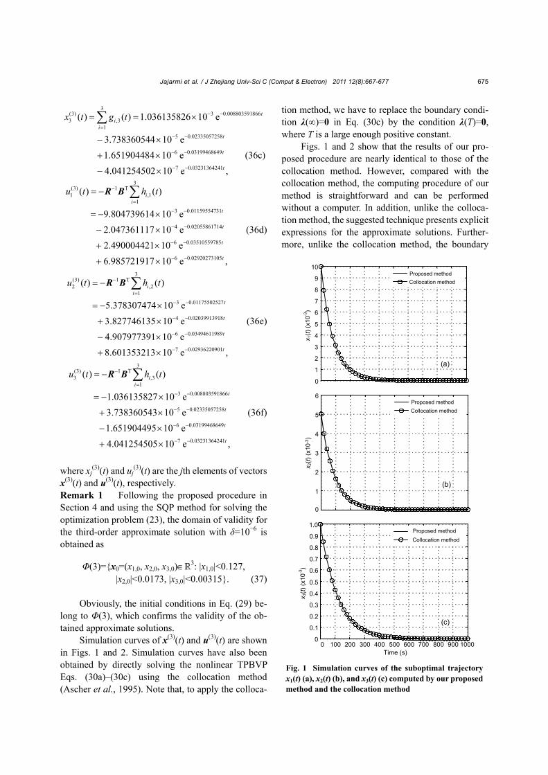
Simulation curves of x(3)(t) and u(3)(t) are shown in Figs. 1 and 2. Simulation curves have also been obtained by directly solving the nonlinear TPBVP Eqs. (30a)–(30c) using the collocation method (Ascher et al., 1995). Note that, to apply the colloca-

tion method, we have to replace the boundary condi-tion λ(∞)=0 in Eq. (30c) by the condition λ(T)=0, where T is a large enough positive constant.

Figs. 1 and 2 show that the results of our pro-posed procedure are nearly identical to those of the collocation method. However, compared with the collocation method, the computing procedure of our method is straightforward and can be performed without a computer. In addition, unlike the colloca-tion method, the suggested technique presents explicit expressions for the approximate solutions. Further-more, unlike the collocation method, the boundary

0

1

2

3

4

5

6

7

8

9

10

x 1(t)

(x10

-3)

(a)

Proposed methodCollocation method

0

1

2

3

4

5

6Proposed methodCollocation method

(b)

x 2(t)

(x10

-3)

0 100 200 300 400 500 600 700 800 900 10000

0.1

0.2

0.3

0.4

0.5

0.6

0.7

0.8

0.9

1.0

Time (s)


(c)

x 3(t)

(x10

-3)

Fig. 1 Simulation curves of the suboptimal trajectory x1(t) (a), x2(t) (b), and x3(t) (c) computed by our proposed method and the collocation method


condition at t=∞ for the co-state equation is handled easily in our proposed technique, since the general solution of each linear time-invariant ODE in Eqs. (14a)–(14c) is available explicitly. However, note that the proposed method may not work in as wide a range of initial conditions as the collocation method.

7 Conclusions and future work

This paper presents a new analytical technique, called the extended modal series method, for solving

a class of infinite horizon nonlinear OCPs. The pro-posed technique avoids directly solving the nonlinear TPBVP or the HJB equation. Furthermore, contrary to the other approximate approaches such as SAA (Tang, 2005), ASRE (Banks and Dinesh, 2000), SDRE (Cimen, 2008), and DT (Hwang et al., 2009), the suggested technique avoids solving a sequence of linear time-varying TPBVPs, a sequence of matrix Riccati differential (or algebraic) equations, or a system of nonlinear algebraic equations. Our pro-posed method requires solving only a sequence of linear time-invariant TPBVPs. Deriving each linear equation in the sequence is straightforward and can be performed without a computer. This property gives our method an advantage compared with the algo-rithms presented by Huang and Lin (1995) and Abu-Khalaf et al. (2006). Therefore, in terms of computational complexity, the proposed approach is more practical than the other approximate approaches. Future work can be focused on extending the modal series method for solving more general forms of nonlinear OCPs.

References Abu-Khalaf, M., Huang, J., Lewis, F.L., 2006. Nonlinear

H2/H∞ Constrained Feedback Control: a Practical Design Approach Using Neural Networks. Springer-Verlag, New York.

Adomian, G., Adomian, G.E., 1984. A global method for solu-tion of complex systems. Math. Model., 5(4):251-263. [doi:10.1016/0270-0255(84)90004-6]

Arnold, V.I., 1992. Ordinary Differential Equations. Springer- Verlag, New York.

Ascher, U.M., Mattheij, R.M.M., Russel, R.D., 1995. Nu-merical Solution of Boundary Value Problems for Ordi-nary Differential Equations. SIAM, Philadelphia.

Banks, S.P., Dinesh, K., 2000. Approximate optimal control and stability of nonlinear finite- and infinite-dimensional systems. Ann. Oper. Res., 98(1/4):19-44. [doi:10.1023/A: 1019279617898]

Bazaraa, M.S., Sherali, H.D., Shetty, C.M., 2006. Nonlinear Programming Theory and Algorithms (3rd Ed.). John Wiley & Sons, New York. [doi:10.1002/0471787779]

Beard, R.W., Saridis, G.N., Wen, J.T., 1997. Galerkin approximations of the generalized Hamilton-Jacobi- Bellman equation. Automatica, 33(12):2159-2177. [doi:10.1016/S0005-1098(97)00128-3]

Bellman, R., 1952. On the theory of dynamic programming. PNAS, 38(8):716-719. [doi:10.1073/pnas.38.8.716]

Bryson, A.E., 2002. Applied Linear Optimal Control: Exam-ples and Algorithms. Cambridge University Press, UK.

Cimen, T., 2008. State-Dependent Riccati Equation (SDRE) Control: a Survey. 17th IFAC World Congress. [doi:10.

-10

-9

-8

-7

-6

-5

-4

-3

-2

-1

0

Proposed method

Collocation method

(a)

u 1(t)

(x10

-3)

-5.0

-4.5

-4.0

-3.5

-3.0

-2.5

-2.0

-1.5

-1.0

-0.5

0


(b)

u 2(t)

(x10

-3)

0 100 200 300 400 500 600 700 800 900 1000-1.2

-1.0

-0.8

-0.6

-0.4

-0.2

0

Time (s)


(c)

u 3(t)

(x10

-3)

Fig. 2 Simulation curves of the suboptimal control law u1(t) (a), u2(t) (b), and u3(t) (c) computed by our pro-posed method and the collocation method


3182/20080706-5-KR-1001.00635] Garrard, W.L., Jordan, J.M., 1977. Design of nonlinear auto-

matic flight control systems. Automatica, 13(5):497-505. [doi:10.1016/0005-1098(77)90070-X]

Huang, J., Lin, C.F., 1995. Numerical approach to computing nonlinear H-infinity control laws. J. Guid. Control Dyn., 18(5):989-994. [doi:10.2514/3.21495]

Hwang, I., Li, J., Du, D., 2009. Differential transformation and its application to nonlinear optimal control. J. Dyn. Syst. Meas. Control, 131(5):051010-11. [doi:10.1115/1.3155 013]

Junkins, J.L., Turner, J.D., 1986. Optimal Spacecraft Rota-tional Maneuvers. Elsevier, Amsterdam.

Khatibi, M., Shanechi, H.M., 2011. Using modal series to analyze the transient response of oscillators. Int. J. Circ. Theor. Appl., 39(2):127-134. [doi:10.1002/cta.621]

Lyapunov, A.M., 1892. General Problem on Stability of Mo-tion. Fuller, A.T., translator, 1992. Taylor & Francis, London (in Russian).

Manousiouthakis, V., Chmielewski, D.J., 2002. On constrained infinite-time nonlinear optimal control. Chem. Eng. Sci., 57(1):105-114. [doi:10.1016/S0009-2509(01)00359-1]

McCaffrey, D., Banks, S.P., 2005. Geometric existence theory for the control-affine nonlinear optimal regulator. J. Math. Anal. Appl., 305(1):380-390. [doi:10.1016/j.jmaa.2004. 12.017]

Murdock, J.A., 1999. Perturbations: Theory and Methods. Classics in Applied Mathematics. SIAM, Philadelphia.

Notsu, T., Konishi, M., Imai, J., 2008. Optimal water cooling control for plate rolling. Int. J. Innov. Comput. Inform. Control, 4(12):3169-3181.

Pariz, N., 2001. Analysis of Nonlinear System Behavior: the Case of Stressed Power Systems. PhD Thesis, Depart-ment of Electrical Engineering, Ferdowsi University of Mashhad, Iran.

Pariz, N., Shanechi, H.M., Vaahedi, E., 2003. Explaining and validating stressed power systems behavior using modal series. IEEE Trans. Power Syst., 18(2):778-785. [doi:10. 1109/TPWRS.2003.811307]

Pontryagin, L.S., 1959. Optimal control processes. Usp. Mat. Nauk, 14:3-20 (in Russian).

Shanechi, H.M., Pariz, N., Vahedi, E., 2003. General nonlinear modal representation of large scale power systems. IEEE Trans. Power Syst., 18(3):1103-1109. [doi:10.1109/ TPWRS.2003.814883]

Tang, G.Y., 2005. Suboptimal control for nonlinear systems: a successive approximation approach. Syst. Control Lett., 54(5):429-434. [doi:10.1016/j.sysconle.2004.09.012]

Tang, G.Y., Qu, H.P., Gao, Y.M., 2002. Sensitivity approach of suboptimal control for a class of nonlinear systems. J. Ocean Univ. Qingdao, 32(4):615-620 (in Chinese).

Tang, L., Zhao, L.D., Guo, J., 2009. Research on pricing poli-cies for seasonal goods based on optimal control theory. ICIC Expr. Lett., 3(4B):1333-1338.

Wu, F.X., Wu, H., Han, Z.X., Gan, D.Q., 2007. Validation of power system non-linear modal analysis methods. Electr. Power Syst. Res., 77(10):1418-1424. [doi:10.1016/j.epsr. 2006.10.016]

Yousefi, S.A., Dehghan, M., Lotfi, A., 2010. Finding the op-timal control of linear systems via He’s variational itera-tion method. Int. J. Comput. Math., 87(5):1042-1050. [doi:10.1080/00207160903019480]

Solving infinite horizon nonlinear optimal control problems using an extended modal series method

Documents

Transcript of Solving infinite horizon nonlinear optimal control problems using an extended modal series method