Solutions to Part I Exercises - Springer Link

Appendix A

Solutions to Part I Exercises

306

A.1 Functions Appendix A Solutions to Part I Exercises

Exercise 2.1 Which of the following relations are functions and why?

(a) f = {(1,1),(3,4),(5,5),(5,6)} > plot([1,1,3,4,5,5,5,6]);

No. The last two points are connected by a vertical line. On a vertical line there are an infinite number of values in the range for each value in the domain.

(b) ~2+~2=1 > with(plots):

> implicitplot«x/4)-2+(y/2)-2=1,x=-4 .. 4,y=-2 .. 2,scaling=CONSTRAINED);

No. An ellipse, like a circle, has two values of y for each value of x.

(c) y = x3 - 2X2

> plot(x-3-2*x-2,x=-2 .. 4);

Yes. Each value in the domain maps onto a unique value in'the range.

(d) ~2 _ ~2 = 1

> implicitplot«x/4)-2-(y/2)-2=1,x=-10 .. 10,y=-10 .. 10);

No. A hyperbola also has two values of y for each value of x.

(e) y = l/x > plot(1/x,x=-2 .. 2,y=-10 .. 10);

Yes. Each value in the domain maps onto a unique value in the range. The function has an asymptote at x = o.

> plot([1,1,3,4,5,5,5,6]);

No. The last two points are connected by a vertical line. On a vertical line there are an infinite number of values in the range for each value in the domain.

Exercise 2.2 Given f(x) = 2x2 - 4x + 9, plot f(x) and 3f(x), -10 ~ x ~ 10, on the same graph.

> f:=x->2*x-2-4*x+9; f := x ---+ 2 x2 - 4 x + 9

> plot({f(x),3*f(x)},x=-10 .. 10);

Exercise 2.3 Perfect gases expand when heated according to the Ideal Gas Law PV = nRT where P is the pressure, V is the volume, n is proportional to the amount of gas present, R is a constant, and T is the Kelvin temperature. Engineers who design cars use this formula to determine the explosion point, that

A.l Functions 307

is, the condition when increase in temperature will cause the windshield of a car to pop out. (p5, Goldenberg and Greenwald [7])

(a) Assume the interior of a locked car is airtight, the contents are at one atmosphere, and the initial temperature is 293 Kelvin (about 20°C). Suppose the temperature inside the car increases 15 Kelvin for each hour the car remains in the sun. The car manufacturer has designed the windshield so that it will pop out when the interior pressure is 1.6 times the exterior pressure. How long would these conditions have to be maintained before the windshield pops out?

> eql:=Pl*V=n*R*Tl; eql := Pl V = n R Tl

eq2 := P2 V = n R T2

> Tl:=293; Tl := 293

> dT:=15; dT:= 15

> P2:=1.6*Pl; P2 := 1.6 Pl

> Ihs(eql)/lhs(eq2)=rhs(eql)/rhs(eq2);

> solve(O,{T2});

> assign(O); > hours:=(T2-Tl)/dT;

1 .6250000000 = 293 T2

{ T2 = 468.8000000 }

hours := 11.72000000

(b) A car with a sun roof will heat up faster than a car with a solid roof. Suppose the temperature of the interior of a closed car with a sun roof increases at a rate of 20 Kelvin per hour. Suppose the same pressure difference as described in the example will cause the windshield to pop out. How long will it take to reach this pressure?

> dT:=20; dT:= 20

308 Appendix A Solutions to Part I Exercises

> hours:=(T2-T1)/dT; hours := 8.790000000

(c) Older cars do not have windshields that pop out. If an older car has a sun roof and the interior temperature increases by 20 Kelvin per hour, what will the interior temperature be after 1.5 hours in the sun? (Assume the initial temperature is 293 Kelvin.)

> T2:=T1+1.5*dT; T2 := 323.0

> P1:=1; P1 := 1

> P2:='P2'; P2:= P2

> Ihs(eq1)/lhs(eq2)=rhs(eq1)/rhs(eq2); 1

P2 = .9071207430

> solve(" ,P2); 1.102389079

(d) A half-full bottle of sunscreen is left in the car. One window is partially open so the air pressure in the car does not build up, but the temperature does. The temperature in the bottle increases from 293 Kelvin to 353 Kelvin. Find the pressure within the bottle of sunscreen. Assume there is no change in volume and there is no increase in vapour pressure from the heated lotion.

> T1:=293; T1 := 293

> T2:=353; T2 := 353

> P1:=1; P1 := 1

> Ihs(eq1)/lhs(eq2)=rhs(eq1)/rhs(eq2); 1 293

- -P2 353

A.l Functions 309

> fsolve(",P2); 1.204778157

(e) The plastic bottle described above is empty and expands. The volume is 15% more when heated. What is the new pressure?

> eq1:=P1*V1=n*R*T1; eqi := Vi = 293nR

> eq2:=P2*V2=n*R*T2; . eq2:= P2 V2 = 353nR

> V2: =1. 15*V1 ; V2:= 1.15 Vi

> Ihs(eq1)/lhs(eq2)=rhs(eq1)/rhs(eq2);

.8695652174 ;2 = ~:~

> fsolve(",P2); 1.047633180

Exercise 2.4 Given f(x) = x3 - 8 and g(x) = x + 4, plot f(x), g(x), and f(x) + g(x), -2 ::; x::; 2, on the same graph.

> f:=x->x-3-8; f:= x -t x 3 - 8

> g:=x->x+4; g:= x -t x + 4

> plot({f(x),g(x),f(x)+g(x)},x=-2 .. 2);

Exercise 2.5 A function f is called even if f( -x) = f(x) for all x and it is called odd if f(-x) = -f(x) for all x. Give examples of even functions and of odd functions. Can you find a function that is odd and even?

> f:=x->x-2+2; f:= x -t x 2 + 2

> fe-x);


> f:=x->x; f:= x -+ x

> fe-x); -x

The zero function, f (x) = 0 for all x, is odd and even.

Exercise 2.6 Use the identity f(x) = tU(x) + f( -x)) + Hf(x) - f( -x)) to show that every function is expressible as a sum of an even function and an odd function.

> 1/2*(f(x)+f(-x))+1/2*(f(x)-f(-x)); x

> f:=x->2*x-2-3*x+l; f := x -+ 2 x2 - 3 x + 1

> 1/2*(f(x)+f(-x))+1/2*(f(x)-f(-x)); 2X2 - 3x + 1

> f:=x->l/x; 1

f:= x -+x

> 1/2*(f(x)+f(-x))+1/2*(f(x)-f(-x)); 1 x

> f:=x->sin(x); f := sin

> 1/2*(f(x)+f(-x))+1/2*(f(x)-f(-x)); sin( x )

Exercise 2.7 Let [[xlJ be the greatest integer less than or equal to x. Plot the

graphs of [[x]], x - [[xlJ, Jx - [[xlJ, x + Jx - [[xll, and [[x]] + Jx - [[xlJ using Maple's trunc function to calculate [[xll, ie trunc(x) = [[xlJ.

> f:=x->trunc(x); f := trunc

A.I Functions

> plot(f(x),x=-2 .. 2);

> f:=x->x-trunc(x); f := x ---t x - trunc( x )

> plot(f(x),x,-2 .. 2);

> f:=x->sqrt(x-trunc(x»; f := x ---t sqrt( x - trunc( x ) )

> plot(f(x),x,-2 .. 2);

> f:=x->x+sqrt(x-trunc(x»; f := x ---t x + sqrt( x - trunc( x ) )

> plot(f(x),x,O .. 5);

> f:=x->trunc(x)+sqrt(x-trunc(x»; f := x ---t trunc( x) + sqrt( x - trunc( x) )

> plot(f(x),x=O .. 5);

311

Exercise 2.8 Given f(x) = x2 - 1 and g(x) = x, plot f(x), g(x), and f(x) x g(x), -2::; x::; 2, on the same graph.

> f:=x->x-2-i; f := x ---t x 2 - 1

> g:=x->x; 9 := x ---t x

> plot({f(x),g(x),f(x)*g(x)},x=-2 .. 2);

> f(x)*g(x); (x2 - 1) x

> expand(II);

Exercise 2.9 Given f(x) = 8x - 7 and g(x) = x2 + x, find f(g(x)), g(J(x)), and f(J(g(x))).

> f:=x->8*x-7; f := x ---t 8 x - 7


> g:=x->x~2+x;

9 := x ---t X 2 + X

> (fIIIg) (x) ;

8x2 + 8x-7

> (gClf) (x);

(8x-7?+8x-7

> (fCl(fClg))(x); 64x2 + 64x - 63

Exercise 2.10 Let J(x) = X 1/ 3 and for -1 ::; x ::; 1. Consider the iterated functions h{x) = J{x), h(x) = J(fl{X)), h(x) = J(h{x)), ... Show that each of these new functions maps the interval [-1,1] to itself and plot their graphs for n = 1,2, ... Animate your sequence of plots for n up to 10. What do you expect the iterations of g{x) = X1/ 5 to look like?

> f:=x->x~(1/3);

> f1:=f(x);

> f2:=f(f1);

> f3:=f(f2);

> plot(f(x),x); > plot(f1,x); > plot(f2,x); > plot(f3,x);

J := x ---t X 1/ 3

J1 := X 1/ 3

J3 := X 1/ 27

> display([seq(plot«fClCln)(x),x=O .. 20),n=1 .. 10)],insequence=true);

Exercise 2.11 By considering the results of iterations of J(x) = X 1/ 3 in Exercise 2.10, deduce the form of iterations of h(x) = x3 •

> h:=x->x~3;

A.l Functions 313

> hl:=h(x);

> h2:=h(hl);

> h3:=h(h2);

Exercise 2.12 Given f(x) = 5x - 9, find the inverse of this function using simultaneous substitutions and plot these relations.

> y=5*x-9; y = 5x - 9

> subs({x=y,y=x},y=5*x-9); x = 5y - 9

> implicitplot({y=5*x-9,x=5*y-9},x=-10 .. 10,y=-10 .. 10);

The other way to plot these equations is to isolate y.

> with(student): > isolate(x=5*y-9,y);

1 9 y = -x +-

5 5

> plot({5*x-9,l/5*x+9/5},x=-10 .. 10);


A.2 Quadratics

Exercise 3.1 Given f(x) = x2, plot f(x), 2f(x), V(x), and -2f(x), -4 ::::; x ::::; 4, on the same graph.

> f:=x->x-2;

> plot({f(x),2*f(x),1/2*f(x),-2*f(x)},x=-4 .. 4);

Exercise 3.2 Given f(x) = 2x2+c, plot f(x) for c = 1,2, and -2, -4 ::::; x ::::; 4, on the same graph.

> f:=x->2*x-2;

> plot({f(x)+1,f(x)+2, f(x)-2},x=-4 .. 4);

Exercise 3.3 Given f(x) = 2X2 - 6x + 7, plot the function, -4 ::::; x ::::; 4, and find the vertex of the parabola, the axis of symmetry and the direction of opening.

> f:=x->2*x-2-6*x+7; f:= x --t 2x2 - 6x + 7

> plot(f(x),x=-4 .. 4);

> with(student):

> completesquare(f(x»;

Vertex at (~, ~). Axis of symmetry x = ~. Opens upward.

Exercise 3.4 Given f( x) = 5x2 , find the equation of the parabola which has its vertex two units to the right and three units above it. Plot the parabolas over the interval -4 ::::; x ::::; 4.

> f:=x->5*x-2;

> plot(f(x),x=-4 .. 4);

> eq:=f(x-2)+3;

eq := 5 ( x - 2? + 3

A.2 Quadratics 315

> plot({f(x),eq},x=-4 .. 4);

Alternatively, the equation of the parabola can be determined from the coordinates of the vertex like this,

> a:=5; a:= 5

> p:=2; p:= 2

> q:=3; q:= 3

y := 5 ( x - 2)2 + 3

Exercise 3.5 Given f(x) = -3x2 - 7x + 1, find the equation of the parabola which has its vertex one unit to the left and four units below it. Plot the parabolas over the interval -4 :::; x :::; 4.

Or,

> f:=x->-3*x-2-7*x+l; f := x -+ -3 x 2 - 7 x + 1

> plot(f(x),x=-4 .. 4); > eq:=f(x+l)-4;

eq := -3 ( x + 1 )2 - 7 x - 10

> plot({f(x),eq},x=-4 .. 4);

> completesquare(f(x));

( 7) 2 61 -3 x+ - +-

6 12

> pl:=-7/6;

> ql:=61/12;

> a:=-3;

-7 pi :=-

6

61 qi'= -. 12

a:= -3

316

> p2:=p1-1;

> q2:=q1-4;

> y:=a*(x-p2)-2+q2;

Appendix A Solutions to Part I Exercises

-13 p2:=-

6

13 q2:= -

12

( 13)2 13 Y := -3 x + (; + 12

> plot({y,f(x)},x=-4 .. 4);

> x:='x' :y:='y' :a:='a':

Exercise 3.6 A golf ball is hit and in the air follows a parabolic trajectory starting at x = 0, y = 0 with maximum altitude y = 20 m; it strikes the ground at x = 120 m. Find an equation for the parabola.

> f:=x->a*(x-p)-2+q; f := x --t a ( x - p? + q

> p:=60;

> q:=20;

> f(O)=O;

> solve(II,{a});

> assign(II);

> f(x);

p:= 60

q:= 20

3600a + 20 = 0

1 2 - - ( x - 60) + 20

180

> plot(f(x),x=O .. 120);

A.3 Solving Quadratics 317

A.3 Solving Quadratics

Exercise 4.1 Determine the roots of the function y = 2X2 - x -1 graphically.

> plot(y,x=-2 .. 2); > root1: =-0.5;

> root2:=1;

y := 2X2 - x-1

moil := -.5

root2 := 1

> y:=(x-root1)*(x-root2); y := ( x + .5) ( x - 1 )

> expand("); x 2 - .5x -.5

> 2*"; 2X2 -LOx -1.0

Exercise 4.2 Determine the roots of the following functions using any method.

( a) y = 2X2 + 3x + 9

> y:=2*x-2+3*x+9;

> plot(y,x=-5 .. 5);

y:= 2X2 + 3x + 9

As we can see on the graph, there are no real roots. > x:=[(-b+sqrt(b-2-4*a*c))/(2*a),(-b-sqrt(b-2-4*a*c))/(2*a)];

X '= [~-b+Vb2-4ac ~ -b- V b2 -4ac] . 2 a ' 2 a

> a:=2; a:= 2

> b:=3; b:= 3

318

> c:=9;

> x;

> simplify (") ;

> x:='x':

> solve(y,{x});


c:= 9

- - + - J-63 - - - - J-63 [ 3 1 3 1 ] 4 4 '4 4

[ 3 3 3 3 ] --+-1-17 ----1-17 4 4 '4 4

{X = - ~ + ~ I -I7} {X = - ~ - ~ I -I7} 4 4 ' 4 4

(b) y = x 2 - 9 > y:=x~2-9;

> plot(y,x=-5 .. 5);

y:= x 2 - 9

From the graph, the roots of this function are located at X = -3, 3. > rooti: =-3;

rootl := -3

> root2:=3; root2 := 3

> 'y'=(x-root1)*(x-root2); y=(x+3)(x-3)

> a:=i; a:= 1

> b:=O; b:= 0

> c:=-9; c:= -9

> x:=[(-b+sqrt(b~2-4*a*c))/(2*a),(-b-sqrt(b~2-4*a*c))/(2*a)]; x:= [3, -3]


> x:='x':

> solve(y,{x});

(c) y=x2-4x+l

> y:=x-2-4*x+1;

> plot(y,x=-5 .. 5);

319

{ x = 3}, { x = -3 }

y:= x 2 - 4x + 1

From the graph, the roots of this function are located at x = 0.25,3.75.

> root1: =0.25; mati := .25

> root2:=3.75; root2 := 3.75

> 'y'=(x-root1)*(x-root2); y = ( x - .25) ( x - 3.75 )

> a:=1; a:= 1

> b:=-4; b:= -4

> c:=1; c:= 1

> x:=[(-b+sqrt(b-2-4*a*c))/(2*a),(-b-sqrt(b-2-4*a*c))/(2*a)];

x := [2 + J3,2 - J3]

> evalf("); [3.732050808, .267949192]

> x:='x':

> solve(y,{x});

{ x = 2 + J3} , { x = 2 - J3}

The graphical estimate was a little off.


Exercise 4.3 The roots of x 2 + bx + care u, V; express (u 2 + v 2 ) in terms of b, c.

> a:='a' ;b:='b' :c:='c': a:= a

> u:=(-b+sqrt(b-2-4*c))/2;

u := - ~ b + ~ Vb2 - 4 c 2 2

> v:=(-b-sqrt(b-2-4*c))/2;

V := - ~ b - ~ Vb2 - 4c 2 2

> u-2+v-2;

( 1 1 )2 (1 1 )2 - "2 b + "2 Vb2 - 4 c + -"2 b - "2 Vb2 - 4 c

> simplify (") ;

Exercise 4.4 One root ofax2 + bx + c = 0 is twice the other root; prove that 2b2 = 9ac.

> r1:=(-b+sqrt(b-2-4*a*c))/(2*a); ~--

1 -b+ Vb2 - 4ac r1 := - -~~---

2 a

> r2:=(-b-sqrt(b-2-4*a*c))/(2*a);

> rl=2*r2;

1 - b - V'-'b2O;--_----c4-a-c '1'2 := - ---'----

2 a

1 -b+ Vb2 - 4ac -b - Vb2 - 4ac

2 a a

> with(student):

> isolate("I,b-2);

> isolate(",b-2); 9

b2 = - ac 2

A.3 Solving Quadratics 321

Exercise 4.5 Determine the nature of the roots of the following functions.

(a) y = 3x2 - 1

> a:='a' :b:='b' :c:='c':

> discriminant:=b-2-4*a*c; discriminant := b2 - 4 a c

y:= 3x2 - 1

> plot(y,x=-5 .. 5);

> a:=3; a:= 3

> b:=O; b:= 0

> c:=-l; c:= -1

> discriminant; 12

Two real roots.

(b) y = x 2 - 3x + 1 > y:=x-2-3*x+l;

y:= x 2 - 3x + 1

> plot(y,x=-5 .. 5);

> a:=l; a:= 1

> b:=-3; b:= -3

> c:=l; c:= 1

> discriminant; 5

322

Two real roots.

( c) y = 8x2 - X + 1

> y:=8*x-2-x+l;

> plot(y,x=-5 .. 5);

> a:=8;

> b:=-l;

> c:=l;

> discriminant;

No real roots.


y := 8x2 - x + 1

a:= 8

b:= -1

c:= 1

-31

Exercise 4.6 For which value of k do the following equations have one distinct real root?

> a:='a' :b:='b' :c:='c':

y := k x 2 - 3 x + 2

> discriminant:=b-2-4*a*c; discriminant := b2 - 4 a c

> a:=k; a:= k

> b:=-3; b:= -3

> c:=2; c:= 2


> k:=solve(discriminant);

> y;

> plot(y,x=-5 .. 5);

> k:='k':

(b) y=x2-2x+k

> y:=x-2-2*x+k;

9 k·- -.- 8

9 2 -x -3x+2 8

y:= x2 - 2x + k

> a:=1;

> b:=-2;

> c:=k;

> k:=solve(discriminant);

> y;

> plot(y,x=-5 .. 5);

> k:='k':

(c) y=x2+kx+5.

> y:=x-2+k*x+5;

a:= 1

b:= -2

c:= k

k:= 1

x2 - 2x + 1

y:= x2 + kx + 5

> a:=1; a:= 1

> b:=k; b:= k

323


> c:=5; c:= 5

> k:=[solve(discriminant)];

> k1 :=op(1 ,k);

> k2:=op(2,k);

> plot(y,x=-5 .. 5);

> y:=x-2+k2*x+5;

> plot(y,x=-5 .. 5);

k := [2 v5, -2 v5]

kl := 2v5

k2:= -2v5

y := x 2 + 2 v5 x + 5

y := x 2 - 2 v5 x + 5

Exercise 4.7 Find the equation of the tangent at the point (-1,0) on the parabola y = (x + 1)2.

> x:='x' :y:='y':

> f:=x->(x+1)-2;

> (f(x)-f(a))/(x-a);

> simplify(II);

> subs(x=a,");

> subs(a=-1,");

f := x -t (x + 1 )2

(x+l)2-4 x-I

x+3

4

4


> O=(y-O)/(x-(-l));

> isolate(",y);

o=_Yx+1

y=o

Exercise 4.8 Find the equation of the tangent at x

f(x)=x 2 +3x-1.

> (f(x)-f(a))/(x-a);

> simplify(II);

> subs(x=a,");

> subs(a=l,");

> f(1);

> 5=(y-3)/(x-l);

> isolate(II ,y);

f := x --+ x 2 + 3 x - I

x 2 + 3x - 4

x-I

x+4

5

5

3

y-3 5=-

x-I

y = 5x - 2

325

I on the parabola

Exercise 4.9 A line perpendicular to a tangent is called a normal line; its slope is equal to the negative inverse of the slope of the tangent. Find the equations of the tangent and normal lines to the parabola y = 4x2 at the points x = 0, ±0.2, ±0.4, ... , ±l. Construct two plots of the parabola, showing on one


the tangent lines and on the other the normal lines. Overlay these plots using the display command.

> f:=x->4*x-2;

> slope([x,f(x)],[a,f(a)]);

> simplify(II);

> subs(x=a,");

> tangent_slope: =" ;

> normal_slope:=-l/";

> a:=O;

4x2 - 4

x-I

4x+4

8

tangenLslope := 8

-1 normaLslope := 8

a:= 0

> tangent_slope=(y-f(a))/(x-a);

8 = ¥.. x

> isolate(1I ,y); y = 8x

> tangent_eq:=O; tangenLeq := 0

> normal_slope=(y-f(a))/(x-a); -1 y

8 x

As we should have spotted, if the tangent is horizontal then the normal will be vertical.

> plot({f(x),tangent_eq},x=-2 .. 2,y=-4 .. 4,scaling=CONSTRAINED);

> a:=O.2; a:= .2


> tangent_slope=(y-f(a))/(x-a);

> isolate(fI ,y);

y - .16 8=-

x -.2

y = 8 x - 1.44

> tangent_eq:=1.6*x-.16; tangenLeq := 1.6 x - .16

> normal_slope=(y-f(a))/(x-a); -1 y-.16

8 x -.2

> isolate(fI,y); 1

y = - 8" x + .1850000000

> normal_eq:=-O.625*x+.285; normaLeq := -.625 x + .285

> plot({f(x),tangent_eq,normal_eq},x=-2 .. 2,y=-4 .. 4, > scaling=CONSTRAINED);

327

Appendix A Solutions to Part I Exercises 328

A.4 Polynomials

Exercise 5.1 Divide the polynomial y = 2x3 + x 2 - 5x + 2 by x - l.

> y:=2*x-3+x-2-5*x+2;

> divisor :=x-l;

> divide(y,divisor);

> y/divisor;

> simplify (II) ;

y := 2x3 + x 2 - 5x + 2

divisor := x-I

true

2 x3 + x 2 - 5 x + 2 x-I

2X2 + 3x - 2

Exercise 5.2 Is the polynomial y = x 3 - 4x 2 + 2x - 1 divisible by x - 3? If not, find the quotient and remainder.

> y:=x-3-4*x-2+2*x-l; y:=x3 -4x2 +2x-l

> divisor:=x-3; divisor := x - 3

> divide(y,divisor); false

> remainder:=rem(y,divisor,x,quotient); remainder := -4

> quotient;

> expand(quotient*divisor+remainder);

x 3 - 4x2 + 2x-l

A.4 Polynomials 329

Exercise 5.3 Find the remainders on dividing x5 - 5x4 + x3 - 7 by (x - 1) and by (x - 1)2.

> rem(x-5-5*x-4+x-3-7,x-1,x); -10

> rem(x-5-5*x-4+x-3-7,(x-1)-2,x); 2 -12x

Exercise 5.4 Find quadratic equations with the following roots.

(a) (3,6)

y:= x 2 - S X + p

> S:=3+6; S:= 9

> P:=3*6; P:= 18

> y; x 2 - 9 x + 18

> solve(y); 6,3

(b) (2,-1)

> S:=2+(-1); S:= 1

> P:=2*(-1); P:= -2

> y;

> solve(y); 2, -1


(c) (9,0)

> 3:=9+0; S:= 9

P :=0

> y;

> solve(y); 0,9

Exercise 5.5 Show that if y = f(x) = a:~bl then x = f(y). Can you find other functions with this property?

> x:='x' :y:='y':

> y=(x+b)/(a*x-l);

> with(student):

> isolate(1I11 ,x);

x+b y=-

ax -1

b+y x=----

1- ya

y = f (x) = ~ has a similar property.

Exercise 5.6 Show that x 2 + 5x + 6 = (x + 2)(x + 3) and so

2X2 + 15x + 25 3 2 -~---=2+--+--

x 2 + 5x + 6 x + 2 x + 3

> divide(2*x~2+15*x+25,x~2+5*x+6); false

> rem(2*x~2+15*x+25,x~2+5*x+6,x,quot); 5x + 13

> quot; 2

A.4 Polynomials

> 2*x-2+15*x+25=2+(5*x+13)/(x-2+5*x+6);

2 2 15 25 2 5 x + 13 x + x+ = +----x2 + 5x + 6

> (5*x+13)/(x-2+5*x+6)=A/(x+2)+B/(x+3); 5x + 13 A B ----=--+-

x 2 + 5 x + 6 x + 2 x + 3

> (5*x+13)=A*(x+3)+B*(x+2); 5 x + 13 = A ( x + 3) + B ( x + 2)

> expand(II); 5 x + 13 = A x + 3 A + B x + 2 B

eql := 5 x = A x + B x

> eq2:=13=3*A+2*B; eq2 := 13 = 3 A + 2 B

> solve({eq1,eq2},{A,B}); {A = 3,B = 2}

Exercise 5.7 Use the Binomial Theorem in the form

(1 - x )-1 = 1 - x + x 2 + ...

331

to express l~x in terms of such a series of powers of x, for 1 x 1< 1. Hence deduce

that 2 = 1 + ~ + ~ + fo + ... > 1/(1-x)=2;

> solve(II,x);

1 --=2 I-x

1

2

> 1+(1/2)+(1/2)-2+(1/2)-3+(1/2)-4+(1/2)-5+(1/2)-6+(1/2)-7+(1/2)-8; 511 256

Etc. Try plotting the sum of the first n terms as a function of n.


Exercise 5.8 Find a when (x - 1) is a factor of 7x3 + ax2 - 2x + l. > f:=x-> 7*x-3+a*x-2-2*x+l;

f := x -+ 7 x3 + a x2 - 2 x + 1

> solve(f(l)=O,a); -6

Exercise 5.9 Find the sum and product of the roots of the following equations.

( a) y = x2 + 4x + 9

y:=x2+4x+9

Knowing that the general form of the second order polymonial is y =

x 2 - sumx + product, we can find the sum and product of the roots by inspection.

> 3:=-4; S:= -4

> P:=9; P :=9

We can also solve for the roots of the equations and then add and multiply them.

> x:=[solve(y)];

x:= [-2+IV5,-2-IJ5]

> 'sum'=op(1,x)+op(2,x); sum =-4

> 'product'=expand(op(1,x)*op(2,x)); product = 9

> x:='x':

(b) y=2x2 -5x+9

> y:=2*x-2-5*x+9; y := 2x2 - 5x + 9

A.4 Polynomials

> y/2;

> 5:=5/2;

> P:=9/2;

> x:=[solve(y)];

x .-

2 5 9 x --x+-

2 2

5 S·- -.- 2

9 p.- -.- 2

[5 1 5 1 ] -+-IV47 ---IV47 4 4 '4 4

> 'sum'=op(1,x)+op(2,x); 5

sum =-2

> 'product'=expand(op(1,x)*op(2,x)); 9

product = 2"

> x:='x':

Exercise 5.10 Find the second root for each of the following equations.

(a) y=x2 +4x-c, root = 1 > y:=x~2+4*x-c;

> root:=l; root:= 1

> eql:=root2+root=-4; eql := root2 + 1 = -4

> eq2:=root2*root=-c; eq2 := root2 = -c

> solve({eql,eq2}); { c = 5, root2 = -5 }

333


(b) y = x 2 - bx + 3, root = 2 > y:=x-2-d*x+3;

> root :=2; root := 2

> eq1:=root2+root=d; eql := mot2 + 2 = d

> eq2:=root2*root=3; eq2 := 2 mot2 = 3

> solve({eq1,eq2});

> S:='S' :P:='P':

Exercise 5.11 What is the equation of a polynomial whose roots are two less than those of y = x 2 - X - 3?

> y:=x-2-x-3; y := x 2 - x - 3

> eqn1:=S=r1+r2; eqnl := S = r1 + r2

> eqn2: =S=l; eqn2 := S = 1

> eqn3:=P=r1*r2; eqn3 := P = r1 r2

> eqn4:=P=-3; eqn4 := P =-3

> eqn5:=R1=rl-2; eqn5 := Rl = r1 ---.:. 2

> eqn6:=R2=r2-2; eqn6 := R2 = r2 - 2

AA Polynomials

> eqn7:=S2=Rl+R2; eqn 7 := 52 = Rl + R2

> eqn8:=P2=Rl*R2; eqn8 := P2 = Rl R2

> s:=solve({eqnl,eqn2,eqn3,eqn4,eqn5,eqn6,eqn7,eqn8});

s:= {5 = 1,P = -3,P2 = -1,7'2 = %1,52 = -3,Rl = -1- %1, r1 = 1 - %1, R2 = %1 - 2} %1 := RootOf( -3 - _Z + _Z2 )

> assign(s);

> 'y'=x-2-S2*x+P2;

y = x 2 + 3x - 1

335

Exercise 5.12 The roots of x3 + bx2 + ex + d = 0 are u, v, w. Express b, e, din terms of u, v, w.

> eql:=u-3+b*u-2+c*u+d=O;

eql := u3 + bu2 + eu + d = 0

> eq2:=v-3+b*v-2+c*v+d=O;

eq2 :=v3 +bv2 +ev+d=O

> eq3:=w-3+b*w-2+c*w+d=O; eq3 := w 3 + bw2 + cw + d = 0

> solve({eql,eq2,eq3},{b,c,d}); {b = -v - u - w, e = u v + u w + w v, d = -w u v}


A.5 Exponential Functions

Exercise 6.1 Solve the following equations for x.

(a) 2X = 32 > fsolve(2-x=32,{x});

{x = 5.000000000}

(b) 53x- 1 = 7x

> fsolve(5-(3*x-l)=7-x,{x}); {x = .5583666073}

(c) 7x = 494

> fsolve(7-x=49-4,{x}); {x = 8.000000000}

Exercise 6.2 A certain colony of bacteria has an initial population of 2500. If the population after 3 days is 8000, what is the doubling period? In how many days will the population be 20,000?

> y:=t->y_0*2-(t/k);

> y_0:=2500; y_O := 2500

> solve(y(3)=8000,{k});

{b\:(¥)} > assign(II);

> solve(y(t)=20000,{t});

{t=\:(¥)} > evalf(");

{ t = 5.363298183 }

A.5 Exponential Functions 337

Exercise 6.3 The half-life of one of the isotopes of polonium, P0216, is 0.15 s. How long would it take for a sample of Po216 to decay to 1 % of its original size?

> k:=-O.15; k:= -.15

> solve(y(t)=O.Ol*y_O,{t}); { t = .9965784284 }

338

A.6 Appendix A Solutions to Part I Exercises

Logarithmic Functions

Exercise 7.1 Solve the following logarithmic equations.

(a) log(x) = 9, base 3 > fsolve(log[3] (x)=9,{x});

{ x = 19683.00000 }

(b) 7log(4) = 2x, base 16

> fsolve(7*log[16] (4)=2*x,{x}); { x = 1. 750000000 }

(c) log(lO) = 5, base x > fsolve(log[x] (10)=5,{x});

{ x = 1.584893192 }

Exercise 7.2 Solve the following equalities.

(a) log(x) + log(2x) = 1, base 3 > fsolve(log[3](x)+log[3](2*x)=1,{x});

{ x = 1.224744871 }

(b) log(x2 ) -log(x) = log(3), base 10 > fsolve(log10(x-2)-log10(x)=log10(3),{x});

{ x = 3.000000000 }

(c) log(x + 7) + log(x2 ) = log(9), base 5 > fsolve(log[5] (x+7)+log[5] (x-2)=log[5] (9),{x});

{x = 1.056907697 }

Exercise 7.3 A scale for measuring the magnitude of earthquakes was developed in 1935 by Charles F. Richter of the California Institute of Technology. The so-called Richter Scale allows the 'size' of earthquakes to be compared. The Richter formula computes the magnitude of a quake from the logarithm of the amplitude of waves recorded by seismographs. Included in the formula is an adjustment to compensate for the variation in the distance of the seismograph and the earthquake's epicentre. The Richter Scale formula for magnitude M is given by M = log 10(~) where x is the amplitude of the largest seismic wave as

A.6 Logarithmic Functions 339

measured 100 kilometres from the epicentre and c is the amplitude of a reference earthquake of amplitude 1 micrometre on a standard graph at the same distance from the epicentre. (p63, Goldenberg and Greenwald [7])

(a) In 1989, San Francisco was struck by an earthquake of magnitude 7.l. As destructive as this earthquake was, it was not nearly as powerful as the 1906 San Francisco earthquake, which measured 8.3. The relative strengths of two earthquakes may be compared by looking at the ratio of the amplitudes. What is the ratio of amplitiude for these two San Francisco earthquakes?

> readlib(log10):

> solve({7.1=log10(xl/c),8.3=log10(x2/c)},{xl,x2}); { x2 = .1995262311109 c, xl = .1258925411108 c}

> assign(");

> x2/xl; 15.84893190

(b) The largest earthquake magnitude ever measured was 8.9 for an earthquake in Japan in 1933. The largest earthquake magnitude ever recorded in the United States was 8.5 for the Alaskan earthquake of 1964. Determine the ratio of amplitude for these earthquakes.

> xl:='xl':x2:='x2':

> solve({8.9=log10(xl/c),8.5=log10(x2/c)},{xl,x2}); {xl = .7943282366109 c, x2 = .3162277659109 c}

> assign(");

> xl/x2; 2.511886438

(c) When the amplitude of an earthquake is tripled, by how much does the magnitude increase?

> solve({Ml=log10(x/c),M2=log10(3*x/c)},{Ml.M2});

> M2=log10(3*x/c);

In (3 ~) M2 = In( 10)

> expand("); In( 3 ) In( x ) In( c )

M2 = In( 10) + In( 10) - In( 10)


(d) Assume that there are two earthquakes of unequal strength. If the ratio of amplitudes is 1.5 and the weaker earthquake has magnitude 5.6, determine the magnitude of the stronger earthquake.

> log10(x/c)=5.6;

In (~) In( 10) = 5.6

> eql :=subs(x/c=a, "); In( a )

eql := In( 10) = 5.6

> M=log10(1.5*x/c);

> eq2:=subs(x/c=a,"); ._ M _ In( 1.5 a )

eq2 .- - In( 10 )

> solve({eql,eq2}); {M = 5.776091259, a = 398107.1706}

> xl:='xl':c:='c':x2:='x2':

(e) If the difference in magnitudes of two earthquakes is 0.5, determine the ratio of amplitudes for the two earthquakes.

> M=log10(xl/c);

> with(student): > isolate(1I1I ,xl/c);

> isolate(1I ,xl) ;

> assign(II);

> M-O.5=log10(x2/c);

M= In(~) In( 10)

~ = e(Mln(lO)) c

xl =e(Mln(lO))c

In (~) M - .5 = In( 10 )

A.6 Logarithmic Functions

> isolate (10 , x2/ c) ;

> isolate(IO ,x2) ;

x2 = e( 2.302585093M -1.151292547)

C

x2 = e( 2.302585093M -1.151292547) C

> assign(IO); > xl/x2;

> simplify(IO);

e(Mln(10))

e( 2.302585093M -1.151292547)

3.162277662

341

Exercise 7.4 What is the concentration of H+ ions in a cola, the pH of which is 3.4?

> pH:=H->-log[10] (H); pH := H ---+ -loglo( H)

> solve(pH(H)=3.4,{H}); { H = .0003981071706 }

Exercise 7.5 Find the simple interest of each of the following.

(a) $500 for 2 years at 4% pa > eq:=A=P*(l+i*n);

eq := A = P ( 1 + in)

> P:=500; P:= 500

> i:=O.04; i:= .04

> n:=2; n:= 2

> solve(eq,{A}); {A = 540.}


(b) $800 for 4 years at 3% pa

> P:=800; P:= 800

> i:=O.03; i:= .03

> n:=4; n :=4

> solve(eq,{A}); {A = 896.}

Exercise 7.6 Calculate the amount for

(a) $500 for 2 years at 4% pa compounded annually

> A:='A' :P:='P' :i:='i' :n:='n':

eq := A = P ( 1 + it

> P:=500; P:= 500

> i:=O.04; i:= .04

> n:=2; n:= 2

> solve(eq,{A}); {A = 540.8000000}

(b) $500 for 2 years at 4% pa compounded daily

> i:=O.04/(365); i := .0001095890411

> n:=2*365; n:= 730

A.6 Logarithmic Functions 343

> A:='A': > solve(eq,{A});

{A = 541.6411435}

(c) $800 for 4 years at 3% pa compounded semi-annually. > P:=800;

P:= 800

> i:=O.03/2; i := .01500000000

n:= 8

> A:='A': > solve(eq,{A});

{ A = 901.1940696 }


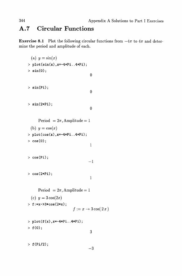
A.7 Circular Functions

Exercise 8.1 Plot the following circular functions from -47r to 47r and determine the period and amplitude of each.

(a) y = sin(x)

> plot(sin(x),x=-4*Pi .. 4*Pi);

> sin(O);

> sin(Pi);

> sin(2*Pi);

Period = 27r, Amplitude = 1

(b) y = cos(x)

> plot(cos(x),x=-4*Pi .. 4*Pi);

> cos(O);

> cos (Pi) ;

o

o

o

1

-1

> cos(2*Pi);


(c) y = 3cos(2x)

> f:=x->3*cos(2*x);

1

f:= x ~ 3cos(2x)

> plot(f(x),x=-4*Pi .. 4*Pi);

> f(O);

> f(Pi!2);

3

-3

A.7 Circular Functions 345

> f(Pi); 3


Exercise 8.2 Compare the plots of the functions f( x) = I sin( x) I and g( x) = sin(1 x I).

> f:=x->abs(sin(x)); f := x --t Isin( x)1

> g:=x->sin(abs(x)); 9 := x --t sin( Ixl )

> plot({f(x),g(x)},x=-4*Pi .. 4*Pi);

Exercise 8.3 In a certain city the average temperature f(t) on the tth day of the year (with t = 1 on January 1) is given by a formula of the form f(t) =

A + Bsin(k(t - 0:)). (The phase shift, 0:, can be thought of as the distance between the y-axis and the closest point at which the function intersects the x-axis.) (p438, Edwards and Penney [6])

(a) Plot the function using the values A = 15, B = -7, k = 1/50, and 0: = -7r /4 to get an idea of the shape of the curve. What must k be for the period of f(t) to be 365 days (where period = 2;)7

> 15-7*sin(1/50*(x+Pi/4));

15 - 7sin (~x + _1_7r) 50 200

> plot(15-7*sin(1/50*(x+Pi/4)),x=O .. 365);

(b) The minimum daily average temperature of lOoC occurs on January 20 and the maximum of 25°C occurs half a year later. What are the values of A, B, and o:?

> f:=x->A+B*sin(k*(x-t)); f := x --t A + B sin( k (x - t))

> period:=365; period := 365

> period=2*Pi/k;

365 = 2 ~

346

> solve(",{k});

> assign(II);

> t:=20-365/4;


-285 t·_-.- 4

> solve({f(20)=10,f(20+365/2)=25},{A,B});

> assign(II);

> f(x);

{ B = -15 A = 35} 2' 2

35 _ 15 sin (~7r (x + 285)) 2 2 365 4

(c) On what days of the year is the average temperature 15°C? Repeat for 20°C?

> plot(f(x),x=O .. 365);

Exercise 8.4 One French horn emits a 200 Hz note and a second horn emits a 400 Hz note. If the amplitudes of the wave forms that represent each note are equal, show that the resultant of the combined sounds differs from each original sound and has a frequency of 200 Hz.

> t:='t': > Vl:=t->sin(2*200*Pi*t);

V1 := t --+ sin( 400 7r t )

V2 := t --+ sin( 800 7r t )

> V1(t)+V2(t); sin( 400 7r t ) + sin( 800 7r t )

> plot({Vl(t),V2(t),Vl(t)+V2(t)},t=O .. O.Ol); > readlib(trigsubs):

> trigsubs(sin(2*x));

A.7 Circular Functions 347

[sin(2x),sin(2x),2sin(x)cos(x), / )' / ),2 tan(~)), csc 2 x csc 2 x 1 + tan x 2

_ ~ I ( e( 2 I x) _ e( -2 I x) )]

Notice that sin(2x) = 2sin(x)cos(x), therefore, the resultant sound has a frequency of 200 Hz.


A.8 Trigonometry

Exercise 9.1 Using this information and definitions of the circular functions, make a table of cos(x), sin(x), and tan(x) for x = 30°,45°,60°.

> cos(30*Pi/180);cos(45*Pi/180);cos(60*Pi/180);

~J3 2 1 -J2 2

1 -2

> sin(30*Pi/180);sin(45*Pi/180);sin(60*Pi/180); 1 -2

~J2 2

~J3 2

> tan(30*Pi/180);tan(45*Pi/180);tan(60*Pi/180);

~J3 3

1

V3

Exercise 9.2 Express the following in radians.

(a) 30° > convert(30*degrees,radians);

(b) 270°

1 -7r 6

> convert(270*degrees,radians); 3

(c) -210°

-7r 2

> convert(-210*degrees,radians); 7

- -7r 6

A.S Trigonometry

Exercise 9.3 Express the following in degrees.

(a) ~ rad

> convert(Pi/4,degrees); 45 degrees

(b) _9; rad

> convert(-9*Pi/4,degrees); -405 degrees

(c) 47r rad

> convert(4*Pi,degrees); 720 degrees

Exercise 9.4 Express the following in terms of sine and cosine.

(a) csc( x) > convert(csc(x),sincos);

(b) sec(x)2

> convert(sec(x)-2,sincos);

(c) tan(x) sin(x)

1

sin( x)

1 cos( x )2

> convert(tan(x)*sin(x),sincos); sin( x )2 cos( X )

Exercise 9.5 Find an equivalent form of the following.

(a) CSC(X)2

> simplify(csc(x)-2,trig); 1

cos( x)2 - 1

349


(b) -tan(x)2

> simplify(-tan(x)-2,trig);

(c) I + cot(X)2

cos( X)2 - I cos( X )2

> simplify(1+cot(x)-2,trig); I

cos( x)2 - I

Exercise 9.6 Solve the following trigonometric equations.

(a) sin(x) = t > solve(sin(x)=1/2,{x});

(b) sin(x)2 + 2sin(x) - 3 = 0

> solve(sin(x)-2+2*sin(x)-3=O,{x});

{ x = ~ 7r} , { x = -arcsin( 3 ) }

(c) 2sin(x) = cos(x) > solve(2*sin(x)=cos(x),{x});

{ x = arctan G) }

Exercise 9.7 Show that the general solution of cos(4x) = 0 is x = (2n + IH, and the general solution of sine x) = 0 is x = n7r, for n = 0, I, 2, ... Hence deduce the general solution of sin(5x) - sin(3x) = O.

> cos(4*x)=O; cos( 4x) = 0

> solve(",x); I -7r 8

I -7r 8

A.S Trigonometry 351

> (2*1+1)*Pi/8; 3 -7r S

o

> sin(x)=O; sin( x) = 0

> solve(" ,x); o

> sin(2*Pi); o

o

sin( 5 x ) - sin( 3 x )

> simplify(II); 16 sin( x ) cos( X )4 - 16 sin( x ) cos( X )2 + 2 sin( x )

Maple is unwilling to give us the trigonometric expression in the form we want, which is 2cos(4x)sin(x).

Exercise 9.8 Show that

3 cos x + sin x = b( cos x cos a + sin x sin a) = b cos( x - a)

where b cos a = 3 and b sin a = 1, and so tan a = ~ and b = v'lO. Hence solve the equation 3 cos x + sin x = 1 for values of x between 0 and 47r.

> b*(cos(x)*cos(a)+sin(x)*sin(a)); b ( cos( x ) cos( a ) + sin( x ) sin( a ) )

> expand(II); bcos( x) cos( a) + bsin( x) sin( a)

> subs({cos(a)=3/b,sin(a)=1/b},"); 3 cos( x ) + sin( x )


> sin(a)/cos(a)=(1/b)/(3/b); sin( a) 1

cos( a) 3

So we have a right-angled triangle with sides 1,3 and J1O; angle a being opposite the side of length 1. Also, tan(a) = 1/3 in J1Ocos(x - a) = 1 so x - a is the other angle in the triangle and x = ~.

Exercise 9.9 Use the approximations sin 0 ~ 0 and cos 0 ~ 1 - ~ to obtain an approximation to 4~i~o~~9. Over what range is this approximation accurate to three significant figures?

> f:=theta->sin(2*theta)/(4-cos(3*theta));

f := 0 -+ sin( 2 0 ) 4 - cos( 3 0)

> subs({sin(2*theta)=2*theta,cos(3*theta)=1-(3*theta)~2/2},f(theta)); o

2 9

> approx:=simplify(II);

> f(O);

3 + -02 2

4 0 approx:= 3" 2 + 302

o

> subs(theta=O,approx); o

> evalf(f(Pi/50)); .04153252613

> evalf(subs(theta=Pi/50,approx)); .04164131209

Exercise 9.10 Solve the right-angled triangle !::,.QRS given that LR = 90°, s = 5, and q = 7.

> with(geometry):

> triangle(QRS,[5,angle=Pi/2,7]); QRS

A.8 Trigonometry

> sides(QRS);

> evalf(");

> tan(S)=5/7;

> solve(",{S});

> assign(II);

> evalf(S);

> convert (" ,degrees);

> evalf(");

> tan(Q)=7/5;

> solve(II,{Q});

> assign(II);

> evalf(Q);

[ 5., 7.,8.602325267]

5 tan( S) = "7

.6202494860

degrees 111.6449075 7r

35.53767779 degrees

7 tan( Q) = 5"

{ Q = arctan G) }

.9505468408

> convert (" ,degrees); degrees

171.0984313 7r

> evalf (") ; 54.46232218 degrees

353


> Pi/2+Q+S;

~ 7r + arctan G) + arctan (~)

> convert(",degrees);

180 G 7r + arctan (D + arctan G)) degrees

7r

> evalf("); 180.0000000 degrees

Exercise 9.11 On a clear day in a flat desert how far away is the horizon seen by a person whose eyes are 1.5 m above the ground? You may take the radius of the Earth to be 6400 km, and you will need to know Pythagoras' theorem for a right-angled triangle.

> x-2=r-2+(r+h)-2;

> expand(");

> subs({r=6400,h=O.0015},")j x 2 = .8192001920108

> solve(" ,x) ; 9050.967856, -9050.967856

Exercise 9.12 Solve the following triangles using the Sine Law.

(a) 6.ABC, given a = 10, b = 15, LC = 3: > triangle(ABC,[10,angle=3/4*Pi,15]);

ABC

> sides (ABC) ;

[10,15,5 )13 + 6 v'2]

> 5*sqrt(13+6*sqrt(2»/sin(3/4*Pi)=10/sin(A);

5 )13 + 6 v'2 v'2 = 10 sin( A)

A.8 Trigonometry

> solve(",{A});

{A = arcsin G~ )13 + 6 v'2 v'2 - ~~ )13 + 6 v'2) }

> assign("); > convert(A,degrees);

arcsin (13 )'-13-+-6-)2-2)2 - 12 )13 + 6 )2) degrees 180 97 97

1l"

> evalf("); 17.76427608 degrees

> 5*sqrt(13+6*sqrt(2))/sin(3/4*Pi)=15/sin(B);

5 )13 + 6 v'2 v'2 = 15 sint B)

> solve(",{B});

{B = arcsin (13:4 )13 + 6 v'2 v'2 - ~~ )13 + 6 v'2) }

> assign("); > convert(B,degrees);

arcsin (~)'-13-+-6-)2-2)2 - 18 )13 + 6 )2) degrees 180 194 97

1l"

> convert(A+B+3/4*Pi,degrees);;

180 (arcsin G~ )13 + 6 v'2 -12 - ~~ )13 + 6 -12)

+ arcsin C3:4 )13 + 6 v'2 v'2 - ~~ )13 + 6 v'2) + ~ 1l") degrees /

1l"

> evalf("); 180.0000000 degrees

(b) l:.XYZ, given LX = 50°, z = 5, Y = 3.5 > triangle(XYZ,[5,angle=50*Pi/180,3.5]);

XYZ

> sides(XYZ);

355


> evalf(")i [5.,3.5,3.840889698]

> 3.840889698/sin(50*Pi/180)=5/sin(Z)i 1 1

3.840889698 . (5 ) = 5 sin( Z ) sm 187r

> solve(",{Z})i

> assign(lI) i

> convert(Z,degrees)i

> evalf(lI) i

{ Z = 1.496249254 }

269.3248657 degrees 7r

85.72876732 degrees

> 3.840889698/sin(50*Pi/180)=3.5/sin(Y)i 1 1

3.840889698 . (5 ) = 3.5 sin( Y ) sm 187r

> solve(",{Y});

> assign(lI) i

> convert(Y,degrees)i

> evalf(lI) i

> 50*Pi/180+Y+Zi


{ Y = .7726787718 }

139.0821789 degrees 7r

44.27123252 degrees

5 18 7r + 2.268928026

(~ 7r + 2.268928026) degrees 180 18

7r

A.8 Trigonometry

> evalf(lI) j 179.9999999 degrees

Exercise 9.13 Solve the following triangles.

(a) 6JKL, given LJ = 130°, LL = 30°, k = 10

> J:=130*Pi/180jL:=30*Pi/180jk:=10j

> K:=Pi-J-Lj

13 J:= -'If

18 1

L := 6 'If k:= 10

1 K:= g'lf

> eql:=j-2=k-2+1-2-2*k*1*cos(J)j

eql := p = 100 + 12 + 20 I cos (158 'If) > eq3:=1-2=j-2+k-2-2*j*k*cos(L)j

eq3 := 12 = j2 + 100 - 10 j J3

> solve({eql,eq3},{j,1})j

Maple cannot solve this system of equations, so use the Sine Law. > solve(j/sin(J)=k/sin(K),{j});

{ sin (~'If) }

j = 10 \8 sin (g 'If)

> evalf(lI) j {j = 22.39764114 }

> solve(l/sin(L)=k/sin(K),{l})j

{ I} 1=5 1 sin (g 'If)

> evalf (") j { I = 14.61902200 }

357


(b) !::'PQR, given p = 4, q = 6, LR = ~

> p:=4;q:=6;R:=Pi/4; p:= 4

q:= 6

1 R:= -7r

4

> r-2=p-2+q-2-2*p*q*cos(R);

r2 = 52 - 24v'2

> [solve(II ,r)];

> r: =op (1 , ") ;

r := 2 )13 - 6 v'2

> p-2=r-2+q-2-2*r*q*cos(P);

16 = 88 - 24 v'2 - 24)13 - 6 v'2 cos( P)

> solve(II,{P});

{p = arccos G~ )13 - 6 v'2 + 957 )13 - 6 v'2 v'2)}

> assign(II);

> convert(P,degrees);

arccos (27 )r-i3---6-v'2-2 + 57 )13 - 6 v'2 v'2) degrees 180 97 9

7r

> evalf(II); 41. 72676503 degrees

> q-2=r-2+p-2-2*r*p*cos(Q);

36 = 68 - 24 v'2 - 16 )13 - 6 v'2 cos( Q)

> solve(II,{Q});

{Q = arccos (987 )13 - 6 v'2 - 11954 )13 - 6 v'2 v'2) }

A.8 Trigonometry

> assign(II);

> convert(Q,degrees);

arccos (~ ';'--13---6-J2-2 - ~ V13 - 6 J2 J2) degrees 180 97 194

7r

> evalf("); 93.27323495 degrees

> P+Q+R;

arccos G; V13 - 6 J2 + ~ V13 - 6 v'2 v'2)

+ arccos (987 V13 - 6 v'2 - 119~ V13 - 6 v'2 v'2) + ~ 7r

> evalf(");


> evalf(");

3.141592654

565.4866777 degrees 7r

180.0000000 degrees

359

Exercise 9.14 If a 50 m tall structure casts an 80 m long shadow, what is the angle of the sun's elevation?

> tan(theta)=50/80;

> solve(",theta);

> evalf(");


5 tan( (}) = 8"

arctan G)

.5585993153

100.5478768 degrees 7r


> evalf("); 32.00538321 degrees

Exercise 9.15 Determine the angle enclosed by two vectors, a(6, 7) and b( 4,3).

> with(linalg): > a:=vector(2,[6,7]);

a:= [67]

> b:=vector(2,[4,3]); b:= [43]

> angle(a,b);

arccos (4~5 J85 55) > convert (" ,degrees);

arccos (4~5 y'85 /25) degrees 180----~~------~-----

7r

> evalf("); 12.52880767 degrees

Exercise 9.16 The angle between vectors c(2,3) and d(x,l) is 35°. Find x. > c:=vector(2,[2,3]);

c:= [23]

> d:=vector(2,[x,1]); d:= [xl]

> angle(c,d)=35*Pi/180;

arccos (~ (2 x + 3 ) V13) = ~ 7r

13 vfx2+I 36

> evalf(II);

( 2. x + 3.) arccos .2773500981.JX2+T." = .6108652381 x 2 + 1.

> solve(lI,x); 2.563554177

A.8 Trigonometry 361

Exercise 9.17 Use the dot product to determine the angle between the vectors a(5,3) and b(7, -4).

> a:=vector(2,[5,3]); a:= [53]

> b:=vector(2,[7,-4]); b:= [7 - 4]

> length_a:=sqrt(a[1]-2+a[2]-2);

length_a := J34

> length_b:=sqrt(b[1]-2+b[2]-2);

length_b := J65

> dotprod(a,b)=length_a*length_b*cos(theta);

23 = J34 J65 cos( ())

> solve(", theta);

arccos C~~O J65 J34)

> evalf(II);

> convert(lI,degrees);

> evalf(");

1.059565614

190.7218105 degrees 7r

60.70863778 degrees

Exercise 9.18 What is the x-coordinate of the vector a(x, -1) so that it forms a 40° angle with the vector 9(3,3).

> a:=vector(2,[x,-1]); a:= [x - 1]

> g:=vector(2,[3,3]); g:= [33]


> length_a:=sqrt(a[1]-2+a[2]-2);

length_a := #+1

> length_g:=sqrt(g[1]-2+g[2]-2);

length_g := 3 V2

> dotprod(a,g)=length_a*length_g*cos(40*Pi/180);

3x - 3 = 3#+1V2cos (~7r)

> Ihs(I)-2=rhs(")-2;

( 3 x - 3)2 = 18 ( x 2 + 1) cos a 7r r > expand(II);

9 x 2 - 18 x + 9 = 18 cos (~7r ) 2 x 2 + 18 cos (~7r ) 2

> evalf("); -11.43005230, - .08748866480

A.9 Similar Figures 363

A.9 Similar Figures

Exercise 10.1 If a 50 m tall structure casts an 80 m shadow at a given time of day, what would be the length of the shadow cast by a 1.8 m tall man?

> 50/80=1. 8/x;

> solve(",x);

5 1 - = 1.8-8 x

2.880000000

Exercise 10.2 What is the shortest distance between the point F(3,3) and the line y = 2x + 6 and what is the equation of the line joining them?

> with(geometry):

> point(F,(3,3»; F

> line(1,[2*x-y=-6]);

> distance(F,l);

> perpendicular(F,l,perp); perp

> perp[equation]; -x - 2y + 9 = 0

364

A.I0 Appendix A Solutions to Part I Exercises

Circles and Spheres

Exercise 11.1 Plot the relations y - x + 1 = 0 and (x - 1)2 + y2 = 1 to determine if they intersect. If so, calculate their point(s) of intersection.

> with(plots):

> pl:=implicitplot(y-x+l=O,x=-2 .. 2,y=-2 .. 2): > p2:=implicitplot((x-l)-2+y-2=1,x=-2 .. 2,y=-2 .. 2):

> display({pl,p2},scaling=CDNSTRAINED); > solve({y-x+l=O,(x-l)-2+y-2=1},{x,y}); {x = RootOf( 2 _Z2 - 4 _Z + 1 ), y = RootOf( 2 _Z2 - 4 _Z + 1) - 1 }

> allvalues(");

{y = ~ h, x = 1 + ~ h} , {y = - ~ h, x = 1 + ~ h} ,

{y = ~)2, x = 1 - ~ )2} , { y = - ~ )2, x = 1 - ~ )2}

> evalf(");

{ y = .7071067810, x = 1. 707106781 }, { y = -.7071067810, x = 1. 707106781 },

{ x = .2928932190, y = .7071067810 },

{x = .2928932190,y = -.7071067810}

From the plot, the first and fourth solutions are the points of intersection.

Exercise 11.2 The height of a circular cylinder is equal to its radius. Express its total surface area A (including both ends) as a function of its volume. (p38, Edwards and Penney [6])

> h:=r; h:= ,

volume := 7r,3

> area:=2*Pi*r*h+2*Pi*r-2; a,ea := 47r,2

> solve(area=volume*a,{a});

{a=4~}

A.lO Circles and Spheres

> assign(OI);

> surface_area='volume'*a; volume

surface_area = 4 --r

365

Exercise 11.3 A piece of wire 100 cm long is cut into two pieces of lengths x

and 100 - x. The first piece is bent into the shape of a square and the second is bent into the shape of a circle. Express as a function of x the sum A of the area of the square and the circle.

> Al:=(x/4)-2;

> perimeter:=2*Pi*r;

> perimeter=100-x;

> solve(OI,{r});

> assign(OI);

> A2: =r-2*Pi;

> A=A1+A2;

1 Ai := _x2

16

perimeter := 27r r

27r r = 100 - x

A2 := ~ ( -100 + x )2 4 7r

A = ~ x2 + ~ ( -100 + x? 16 4 7r

Exercise 11.4 A spherical cloud of toxic powder forms over a factory following a fire. The radius of the sphere is 100 m and contains a uniform dispersion of powder at a density of 0.001 kg·m-3 . This cloud subsequently is deposited on the ground over a circular region of radius 100 m. Find the total mass of powder in the cloud and find also the average areal density in kg· m-2 of powder deposited on the ground.

> r:=100; r := 100


4000000 v·- 7r

3

> evalf(v); .4188790204107

> density:=v/100; . 40000

denszty := -3-7r

> evalf(density); 41887.90204

> r:='r' :h:='h':

Exercise 11.5 A giant Sequoia tree, perhaps the largest tree in the world, stands 82.9 m tall and is about 10.4 m in diameter at its base. Its habitat is the central California mountain range, the Sierra Nevada, in the Sequoia National Park. The great age, size, and rapid growth of this tree have contributed to its fame. It has the heroic name General Sherman. (p4, Goldenberg and Greenwald [7))

(a) We can approximate the volume of a tree by disregarding the branch structure and considering the trunk as a cylinder. If the General Sherman has an average radius of 2.3 m, what is its volume?

> V:=Pi*r-2*h; V := 7r".2 h

> r:=2.3; ".:= 2.3

> h:=82.9; h:= 82.9

> evalf(V); 1377.717184

(b) Assuming the General Sherman produces an annual growth ring of 0.00009 m, how much new wood is added to the tree (trunk) each year?

> delta_r:=O.00009+r; delta_". := 2.30009

A.10 Circles and Spheres 367

> V:=Pi*(delta_r~2-r~2)*h; V := .034321263211"

> evalf(V); .1078234283

(c) Suppose the paper industry cultivated a fast-growing tree that could grow from a seedling to a height of 15.2 m in one year. If the increase in volume of this tree were to match that of the General Sherman, what would be the average radius of the tree?

> r:='r':delta_r:='delta_r': > h:=lS.2;

h:= 15.2

.034321263211" = 15.211" r2

> solve(",r); -.04751818433, .04751818433

(d) The baobab tree, native to Australia and Africa, has a trunk that measures as much as 18.3 m in diameter. However, this tree only grows to a height of 12.2 m. Approximate the amount of new wood this tree would produce each year. Use a cylindrical model with a radius of 12.2 m, a height of 18.3 m, and an annual growth ring of 0.0009 m.

> h:=18.3; h:= 18.3

> rl:=12.2; r1 := 12.2

> r2:=12.2+0.0009; r2 := 12.2009

> V:=Pi*r2~2*h-Pi*rl~2*h;; V := .40188311"


(e) Model the baobab tree as a cone. Approximate the amount of new wood it would produce in one year if the increase in thickness is 0.0009 m.

> V;=1/3*Pi*r2-2*h-1/3*Pi*r1-2*h; V := .13396107r

A.ll Loci 369

A.tt Loci

Exercise 12.1 Let a circle of diameter b have centre at x = ~. Take a straight line PQ of any length 2a and move it such that its midpoint M moves round the given circle and the line PQ passes through the origin O. Then the point P and Q have as loci the curve r = MP + OP = a + bcos(B). This curve is called a limafon; in particular it is called a cardioid if a = b. Plot a family of limac;:ons for a range of values of a and b.

> r:=theta->a+b*cos(theta); r := B -+ a + bcos( B)

> a:=l;b:=l; a:= 1

b:= 1

> with(plots):

> polarplot(r(theta),theta=-2*Pi .. 2*Pi);

> a:=2;b:=4; a:= 2

b:= 4

> polarplot(r(theta),theta=-2*Pi .. 2*Pi);

Exercise 12.2 Let AB be the diameter of a circle and P a point on the upper semicircle. The tangent to the circle at B is a vertical line and suppose that the line AP extends to meet this vertical line at T. Now choose Q on AT such that AQ = PT and the locus of Q is given by y2(2a - x) = x3 when A is the origin and AB lies along the x-axis. This is called a cissoid and has polar equation r = 2asin(J2 (J. Plot a family of cissoids for a range of values of a.

cos

> r:=theta->(2*a*sin(theta)-2)/(cos(theta));

r := B -+ 2 a sin( B )2 cos( B )

> a:=2; a:= 2

> plot(r(theta),theta=-O.3 .. 0.3,coords=polar);

> a:=l; a:= 1

> plot(r(theta),theta=-O.3 .. 0.3,coords=polar);


Exercise 12.3 Try plotting the cycloid curves with the following parameterizations:

(a) x(t) = t - sin(t),y(t) = 1- cos(t) (cycloid) > plot([t-sin(t),1-cos(t),t=-4*Pi .. 4*Pi],scaling=CONSTRAINED);

(b) x(t) = t - 3sin(t),y(t) = 1 - 3cos(t) (prolate cycloid) > plot([t-3*sin(t),1-3*cos(t),t=-4*Pi .. 4*Pi],scaling=CONSTRAINED);

(c) x(t) = 2t - sin(t), y(t) = 2 - cos(t) (curate cycloid) > plot([2*t-sin(t),2-cos(t),t=-4*Pi .. 4*Pi],scaling=CONSTRAINED);

A.12 Sequences and Series


Exercise 13.1 Calculate the first 4 terms of the following sequences.

(a) f(n) = n - 1 > seq(n-1,n=1 .. 4);

(b) f(n) = ~n + 7 > seq«1/2)*n+7,n=1 .. 4);

(c) f(n) = -3n

> seq(-3*n,n=1 .. 4);

> n:='n':

0,1,2,3

-3, -6, -9, -12

Exercise 13.2 Determine the nth term of the following sequences.

(a) 5,8,11,14, ... > 8-5;

> 11-8;

> d:=3;

> a:=5-d;

> a+n*d;

(b) ~,~,1,~,!, ... > 4/3-5/3;

3

3

d:= 3

a:= 2

2 + 3n

-1

3

371

372

> 1-4/3;

> d:=-1/3;

> a:=5/3-d;

> a+n*d;

(c) 5,9,13,17, ...

> 9-5;

> 13-9;

> d:=4;

> a:=5-d;

> a+n*d;

> a:='a' :d:='d':


-1

3

-1 d·-.- 3

a:= 2

1 2- -n

3

4

4

d:= 4

a:= 1

1 +4n

Exercise 13.3 The third term of an arithmetic sequence is 14 and the seventh is 26. Find the ninth term.

> solve({a+3*d=14,a+7*d=26},{a,d}); {d = 3,a = 5}

> 5+9*3; 32

A.12 Sequences and Series 373

Exercise 13.4 Calculate the first four terms of the following sequences.

(a) f(n) = 7n

> seq(7-n,n=1 .. 4); 7,49,343,2401

(b) f(n) = !(3)n > seq«1/2)*(3)-n,n=1 .. 4);

3 9 27 81

(c) f(n) = -5(2n) > seq(-5*(2-n),n=1 .. 4);

-10, -20, -40, -80

> n:='n':

Exercise 13.5 Calculate the nth term of the following sequences.

(a) 6,18,54,162, ...

> 18/6; 3

> 54/18; 3

> r:=3; r:= 3

> a:=6/r; a:= 2

> a*r-n; 23n

(b) 1,4,16,64, ... > 4/1;

4

> 16/4; 4

374

> r:=4;

> a:=l/r;

(c) -6,12,-24,96 ... " > 12/(-6);

> -24/12;

> r:=-2;

> a:=-6/r;


r :=4

1 a"- -.- 4

-2

-2

r:= -2

a:= 3

3( -2t

Exercise 13.6 For the geometric sequence -8,16, -32, ... , tn = 256, find n. > 16/(-8);

-2

> -32/16; -2

> r:=-2; r:= -2

> a:=-8/r; a:= 4

256


256

Exercise 13.7 Calculate the sum of the following arithmetic series.

(a) 5+11+17+ ... +59 > 11-5;

> 17-11;

> d:=6;

> a:=5-d;

> solve(a+n*d=59,{n});

> sum(a+n*d,n=1 .. 10);

6

6

d:= 6

a:= -1

{n = 10}

320

(b) -9 + (-11) + (-13) + ... + (-25) > -11-(-9);

-2

> -13- (-11) ; -2

> d:=-2; d:= -2

> a:=-9-d; a:= -7

> solve(a+n*d=-25,{n}); {n = 9}

375

376

> sum(a+n*d,n=1 .. 9);

( c) - 2 + 1 + 4 + ... + 295 > 1-(-2);

> 4-1;

> d:=3;

> a:=-2-d;

> solve(a+n*d=295,{n});

> sum(a+n*d,n=1 .. 100);


-153

3

3

d:= 3

a:= -5

{n = 100}

14650

Exercise 13.8 Calculate the sum of the first 20 terms of the following arithmetic series.

(a) 4+5+6+7+ ...

> 5-4; 1

> 6-5; 1

> d:=1; d:= 1

> a:=4-d; a:= 3

> sum(a+n*d,n=1 .. 20); 270


(b) 5 + 9 + 13 + 17 + ... > 9-5;

4

> 13-9; 4

> d:=4; d:= 4

> a:=5-d; a:= 1

> sum(a+n*d,n=1 .. 20); 860

(c) -¥ - 7 - ¥ - 6 - ...

> -7-(-15/2); 1 -2

> -13/2-(-7); 1 -2

> d:=1/2; 1

d·- -.- 2

> a:=-15/2-d; a:= -8

> sum(a+n*d,n=1 .. 20); -55

Exercise 13.9 Find the sum of the following geometric series.

(a) 6 + 12 + 24 + ... + 384 > 12/6;

2

377

378

> 24/12;

> r:=2;

> a:=6/r;

> evalf(");


2

r:= 2

a:= 3

In( 128) In( 2)

7.000000000

(b) ~ + 1~ + t.t + ... + 65!36

> (1/16) / (1/4) ;

> (1/64)/(1/16);

> r:=1/4;

> a:=1/4/r;

> solve(a*r~n=1/65536,n);

> evalf(");

762

1 -4

1

4

1 r:= 4

a:= 1

In( 65536) In( 4)

8.000000001

21845 65536

A.12 Sequences and Series 379

(c) -5+25-125+ ... +15625 > 25/(-5);

-5

> -125/25; -5

> r:=-5; r:= -5

> a:=-5/r; a:= 1

15625

13020

380

A.13 Appendix A Solutions to Part I Exercises

Statistics and Probability

Exercise 14.1 The mid-term and final exam marks for a given class are as follows.

Student Mid-term Mark Final Exam Mark 1 80 85 2 72 70 3 55 50 4 77 82 5 64 66 6 71 77 7 81 88 8 32 40 9 48 58 10 79 70 11 29 20 12 92 89 13 83 78 14 67 70 15 45 78

Create a scatterplot of the data and determine if the two data sets are associated. Using a pencil and paper, try to find the equation of the line which best fits this data.

> with(stats):

> midterm:=[80,72,55,77,64,71,81,32,48,79,29,92,83,67,45]:

> exam:=[85,70,50,82,66,77,88,40,58,70,20,89,78,70,78]:

> statplots[scatter2d] (midterm,exam);

Exercise 14.2 The circumferences of 40 trees living on a plot of land, given in centimetres, are listed below.

43.2 80.3 71.8 35.1 95.0 60.0 97.9 30.4 102.3 91.1 62.6 81.3 73.5 66.1 56.4 42.2 42.7 69.4 46.5 70.0 43.9 76.7 18.8 75.6 24.5 41.4 69.6 56.5 41.1 87.9 15.0 41.4 54.3 70.0 75.3 94.5 41.4 63.5 63.2 94.7

(a) Create a histogram of this data using a class width of 10. What is the modal frequency?

> tree:=[43.2,80.3,71.8,35.1,95.0,60.0,97.9,30.4,102.3,91.1,62.6,

A.13 Statistics and Probability 381

> 81.3,73.5,66.1,56.4,42.2,42.7,69.4,46.5,70.0,43.9,76.7,18.8,75.6, > 24.5,41.4,69.6,56.5,41.1,87.9,15.0,41.4,54.3,70.0,75.3,94.5,41.4, > 63.5,63.2;94.7]:

> tallied_tree:=transform[tallyinto](tree,[0 .. 10,10 .. 20,20 .. 30, > 30 .. 40,40 .. 50,50 .. 60,60 .. 70,70 .. 80,80 .. 90,90 .. 100,100 .. 110]);

tallied_tree := [Weight( 0 .. 10, 0), Weight ( 10 .. 20,2),20 .. 30, Weight( 40 .. 50, 9), Weight( 50 .. 60, 3), Weight ( 60 .. 70,7), Weight( 70 .. 80, 7), Weight( 80 .. 90, 3), Weight ( 90 .. 100, 5 ), 100 .. 110, Weight ( 30 . .40, 2))

> statplots[histogram](tallied_tree);

> describe Unode] (tree); 41.4

(b) What is the mean circumference of the trees? > describe Unean] (tree);

61.67750000

( c) What is the standard deviation? > describe [standarddeviation] (tree);

22.43890027

(d) What are the mean and standard deviation of the diameters of the trees?

> diameter:=[evalf(seq(tree[n]/Pi,n=1 .. 40))];

diameter := [13.75098708,25.56028385,22.85464982,11.17267700, 30.23943918, 19.09859317,31.16253785,9.676620537, 32.56310135,28.99803062,19.92619887,25.87859374, 23.39577663,21.04028347,17.95267758,13.43267719, 13.59183214,22.09070610,14.80140970,22.28169203, 13.97380400,24.41436826,5.984225859,24.06422739, 7.798592209,13.17802928,22.15436807,17.98450856, . 13.08253632,27.97943899,4.774648292,13.17802928, 17.28422682,22.28169203,23.96873442,30.08028424, 13.17802928,20.21267777,20.11718480,30.14394621)

> describe Unean] (diameter); 19.63255800

> describe [standarddeviation] (diameter); 7.142523779·


Exercise 14.3 Calculate the probability that a 13-card bridge hand contains

(a) 4 hearts, 3 clubs, 3 diamonds, 3 spades

> binomial(13,4)*binomial(13,3)*binomial(13,3)*binomial(13,3)/ > binomial(52,13);

> evalf(");

418161601

15875338990

.02634032579

(b) 5 hearts, 4 clubs, 2 diamonds, 2 spades

> binomial(13,5)*binomial(13,4) *binomial(13,2) *binomial ( 13,2)/ > binomial(52,13);

> evalf (") ;

279926361

31750677980

.008816390037

( c) 6 hearts, 3 clubs, 3 diamonds, 1 spade

> binomial(13,6)*binomial(13,3) *binomial(13,3) *binomial ( 13,1)/ > binomial(52,13);

> evalf(");

114044073 39688347475

.002873490086

Exercise 14.4 A computer operator has to invent a seven character password from the letters of the alphabet and the numbers 0,1,2, ... ,9. At least one letter must be a capital letter and exactly one character must be a number. In how many ways can the password by chosen? Another computer operator uses a random character selector to create a password meeting the same conditions; what is the probability that this password will contain at least two capital letters?

> case1:=binomial(26,1)*binomial(10,1)*binomial(26,5); easel := 17102800

> case2:=binomial(26,2)*binomial(10,1)*binomial(26,4); ease2 := 48587500

A.13 Statistics and Probability

> case3:=binomial(26,3)*binomial(10,1)*binomial(26,3); case3 := 67600000

> case4:=binomial(26,4)*binomial(10,1)*binomial(26,2); case4 := 48587500

> case5:=binomial(26,5)*binomial(10,1)*binomial(26,1); caseS := 17102800

> case6:=binomial(26,6)*binomial(10,1); case6 := 2302300

> casel+case2+case3+case4+case5+case6; 201282900

Total number of ways of creating the password is, > binomial(26,1)*binomial(10,1)*binomial(52,5);

675729600

> twocapitals:=binomial(26,1)*binomial(10,1)*binomial(26,2)* > binomial(26,3);

twocapitals := 219700000

> probability:=(I1)/(III1); . . 1625

probabzhty := 4998

> n:='n':

383

Exercise 14.5 In how many ways can 3 flags be flown on 2 flagpoles? What about, flags on n flagpoles?

> binomial(3,2); 3

> r!/(n!*(r-n)!); ,!

n! ( , - n )!

Exercise 14.6 In a manufacturing process N computer chips are made per day. Of these, on average d are defective and (N - d) are good. A sample of , chips is chosen at random from the production on a given day. What is the probability that this group will contain exactly k defectives where k varies from


o to the smaller of d and r? For the case N = 1000, r = 100, d = 10, plot this probability for k = 1,2, ... ,10.

The sample has r-k good chips and these can be chosen in (~~:) ways while the

k defective chips can be chosen in (~) ways. The ordering of chips is unimportant so we divide by the number of ways of choosing r from N to give the required

p<Dbabili!y p(k) = W(~) and p(k) = 0 if k > d m k > r.

> binomial(d,k)*binomial(N-d,r-k)/binomial(N,r); binomial( d, k ) binomial( N - d, r - k)

binomial( N, r )

> f:=(k)->binomial(10,k)*binomial(1000-10,100-k)/ > binomial(1000,100);

f .= k ----t binomial( 10, k ) binomial( 990, 100 - k) . binomial( 1000, 100 )

> t:=[[k,f(k)] $k=1 .. 10];

[[ 8271249852054420400] [ 1376996191737759450] t:= 1, 21242706488868565551 ' 2, 7080902162956188517 '

[ 402973129646287200] [ 76515311809236300] 3, 7080902162956188517 ' 4, 7080902162956188517 '

[ 9848674771423488] [ 870186107966175] 5, 7080902162956188517 ' 6, 7080902162956188517 '

[ 52108612294200] [ 4047411701025 ] 7, 7080902162956188517 ' 8, 14161804325912377034 '

[ 46021737300 ] [ 13959926981 ]] 9'7080902162956188517 ' 10, 212427064888685655510

> plot(t,x=1 .. 10, style=POINT);

Appendix B

Solutions to Part II Exercises

386 Appendix B Solutions to Part II Exercises

B.l Secants and Tangents

Exercise 15.1 Find the slope of a secant to y = 2x2 - 3x which passes through the following points:

(a) x = 1 and x = 4

> with(student):

> f:=x->2*x-2-3*x; j := x -t 2 x 2 - 3 x

> slope([1,f(1)],[4,f(4)]); 7

(b) x = 0 and x = -1 > slope([O,f(O)],[-l,f(-l)]);

-5

(c) x = -2 and x = 2

> slope([-2,f(-2)],[2,f(2)]); -3

Exercise 15.2 Find the general equation of the slope of a secant passing through the points (x,j(x)) and (a,j(a)) to the following curves:


x-a

> simplify(II); a+x

(b) 3x2 - 5x + 8

> f:=x->3*x-2-5*x+8; j := x -t 3 x 2 - 5 x + 8

B.I Secants and Tangents 387

> slope([x,f(x)],[a,f(a)]); 3x2 - 5x - 3a2 + 5a

x-a

> simplify("); 3a-5+3x

(c) -7x2 + 1 > f:=x-> -7*x-2+i;

f := x -t -7 x 2 + 1

> slope([x,f(x)], [a,f(a)]); -7 x 2 + 7 a2

x-a

> simplify("); -7a-7x

Exercise 15.3 Find the equation of the tangent at x = 2 to the following curves. Find also the equations of the normal lines to these curves.

(a) x 2

> f:=x->x-2;

> slope([x,f(x)],[a,f(a)])j

> simplify(");

> subs (x=a,") ;

> m:=subs(a=2,");

> m=(y-f(2))/(x-2);

x-a

a+x

2a

m:=4

y-4 4=-

x-2


> isolate(1I ,y) ; y = 4x - 4

> -1/m=(y-f(2))/(x-2); -1 y-4

= 4 x - 2

> isolate(1I ,y) ; 1 9

y=--x+-4 2

> m:='m':

(b) 3x2 - 5x + 8

> f:=x->3*x-2-5*x+8; f := x -+ 3 x2 - 5 x + 8

> slope([x,f(x)],[a,f(a)]); 3 x 2 - 5 x - 3 a2 + 5 a

> simplify(II);

> subsex=a,");

> m:=subs(a=2,");

> m=ey-f(2))/ex-2);

> isolate(1I ,y) ;

> -1/m=(y-f(2))/(x-2);

> isolate(",y);

x-a

3a-5+3x

6a - 5

m:=7

y -10 7=-

x-2

y=7x-4

-1 = y - 10 7 x-2

1 72 y=--x+-

7 7

B.1 Secants and Tangents

> m:='m':

(c) -7x2 + 1

f := x -+ -7 x 2 + 1

> slope( [x,f(x)], [a,f(a)]);

> simplify(II);

> subs(x=a,");

> m: =subs(a=2, ") ;

> m=(y-f(2))/(x-2);

> isolate(",y);

> -1/m=(y-f(2))/(x-2);

> isolate(1I ,y);

> m:='m':

-7 x 2 + 7 a2

x-a

-7a-7x

-14a

m:= -28

-28 = Y + 27 x-2

y = -28x + 29

1 Y + 27 28 x - 2

1 379 y= -x--

28 14

389

Exercise 15.4 Find the point on the graph y = 3x2 + 1 at which the slope is

(a) 2

f := x -+ 3 x 2 + 1



> simplify(II);

> subs(a=x, II);

> solve("=2,{x});

> assign(II);

> f(x);

> x:='x':

(b) k > 6*1/5;

> f(II);

(c) -4

> f(II);

3x2 - 3a2

x-a

3a + 3x

6x

4 3

6 -5

133

25

-24

1729

Exercise 15.5 Determine the equations of the lines through the following points:

(a) (0,1) and (4,1) > m:=slope([O,1],[4,1]);

m:=O

B.l Secants and Tangents

> m=(y-l)/(x-O);

> isolate (" ,y);

> m:='m'

(b) (7,0) and (8,9) > m:=slope( [7 ,0], [8,9]) ;

> m=(y-l)/(x-O);

> isolate(1I ,y) ;

> m:='m':

(c) (3,8) and (3, -1)

y-l 0=-

x

y = 1

m:=9

y-l 9=-

x

y = 9x + 1

391

Here the method fails, because the slope is infinite. However, the equation of the line is obvious: x = 3.

Exercise 15.6 Determine the equations of the lines with slope of 2 which pass through the following points:

(a) (2,1) > 2=(y-l)/(x-2);

> isolate(1I ,y) ;

(b) (-8, -1) > 2=(y-(-1))/(x-(-8));

> isolate(1I ,y) ;

y-l 2=-

x-2

y = 2x - 3

2=y+l x+8

y = 2x + 15

392

(c) (4,4) > 2=(y-4)/(x-4);

> isolate(1I ,y);

Appendix B Solutions to Part II Exercises

y-4 2=-

x-4

y = 2x - 4

Exercise 15.7 Determine the equations of the lines which pass through the point (2,4) and have the following slopes. Find also the equations of the lines perpendicular to these.

(a) 3 > 3=(y-4)/(x-2);

> isolate(1I ,y);

> -1/3=(y-4)/(x-2);

> isolate(1I ,y);

(b) ~ > 1/2=(y-4)/(x-2);

> isolate(1I ,y);

> -2=(y-4)/(x-2);

> isolate(1I ,y);

y-4 3=-

x-2

y = 3x - 2

-1 y-4 3 x - 2

1 14 y=--x+-

3 3

1 Y - 4 2 x - 2

y-4 -2=-

x-2

y=-2x+8


(c) -~ > -3/8=(y-4)/(x-2);

> isolate(1l ,y);

> 8/3=(y-4)/(x-2);

> isolate(1l ,y);

-3 y-4

8 x - 2

3 19 y=--x+-

8 4

8 y-4 -3 x - 2

8 4 y=-x--

3 3

393

Exercise 15.8 The owner of a grocery store finds that he can sell 980 litres of milk at $1.69/1 and 1220 litres of milk each week at $1.49/1. Assume a linear relationship between selling price and demand. How many litres could he sell weekly at $1.56/l? (p22, Edwards and Penney [6])

> m:=slope([1.69,980],[1.49,1220]); m := -1200.000000

> eq:m=(y-980)/(x-1.69);

> isolate(1l ,y);

-1200.000000 = Y - 980 x - 1.69

y = -1200.000000 x + 3008.000000

> assign(Il); > subs(x=1.56,y);

1136.000000

> y:='y':

Exercise 15.9 In hilly areas, reception for both television and radio is frequently poor. We consider a situation where an PM transmitter is located behind a hill, and a radio receiver is on the opposite side of the hill. How far from the base of the hill should the radio be located so that its reception is not obstructed? Obviously, the height of the transmitter, compared with the height of the hill is crucial, as is the specific positioning of the base of the transmitter. The radio


can receive a clear signal if located far from the hill, provided the signal is strong enough. What is the closest that the radio can be to the hill so that reception is not obstructed? (pIS, Goldenberg and Greenwald [7])

We consider an idealized situation: the contour of the hill is a semicircle of radius 1 unit. The transmitter is at the base of the hill and has a height of 2 units. The radio is on the side of the hill opposite the transmitter.

Figure B.l. Transmitter problem

Figure B.l illustrates the situation. The position of the tangent line T R is the key element, where T is the top of the transmitter and R is the radio receiver. P is the point where the tangent line intersects the circle.

(a) We wish to find R. In other words, how far from the base of the hill should the radio be placed in order for it to receive an unobstructed signal from the transmitter?

> circle:=y=sqrt(1-x-2);

circle := y = ~

> m:=diff(rhs(circle),x); x m:= - V'f=X2

> transmitter:=[-1,2]; transmitter := [ -1,2]

> tangent:=m=(transmitter[2]-y)/(transmitter[1]-x); x 2 - y

tangent := - = ------'--~ -1-x

> solve({circle,tangent},{x,y});

{x=~,y=~} > slope([-1,2],[3/5,4/5]);

-3 4


> -(3/5)/(sqrt(1-(3/5)-2));

> m:=";

-3 4

-3 m'-.- 4

> tangent:=m=(transmitter[2]-y)/(transmitter[1]-x); -3 2 - y

tangent := - = ----'--4 -1- x

> isolate(tangent,y); 5 3

y=---x 4 4

> assign(II);

> solve(y,{x});

> evalf("); { x = 1.666666667 }

395

(b) Solve the problem as given in the example if the transmitting tower (of height one unit) is placed on the top of the hill.

> y:='y':

> m:=diff(rhs(circle),x); x

m:=-~

> transmitter:=[O,2]; transmitter := [0,2 J

> tangent:=m=(transmitter[2]-y)/(transmitter[1]-x); x 2-y

tangent := - = - --~ x


{ X = - ~ V3 y =~} {x = ~ V3 y = ~} 2 ' 2' 2' 2

> subs(x=1/2*sqrt(3),m); 1 --J4V3 2

396

> m:=":


1 m·- --J4J3 .- 2

> tangent:=m=(transmitter[2]-y)/(transmitter[1]-x): 1 r; r.; 2-y

tangent := - - y 4 y 3 = - --2 x

> isolate(tangent,y):

> assign(II):

> solve(y,{x}):

> evalf("):

1 Y=-"2 J4J3x +2

{x = 1.154700539}

(c) Consider the problem as given in the example, but suppose the height of the transmitter is unknown. If it is known that the radio must be placed at least one unit from the base of the hill in order to receive an unobstructed signal, determine the height of the transmitter.

> m:='m' :y:='y':

> m:=diff(rhs(circle) ,x): x

m·- - --;=== .- ~

> receiver:=[2,O]; receiver := [2,0 1

> tangent:=m=(receiver[2]-y)/(receiver[1]-x); x y

tangent := - = - --~ 2-x


> subs(x=1/2,m);

{x=~,y=~J3}

1 - -J4J3 6


> m:=";

> tangent:=m=(receiver[2]-y)/(receiver[1]-x);

tangent := - ~ J4 J3 = - -y-6 2-x

> isolate(tangent,x);

> assign(Il);

> solve(x=-1,{y});

> evalf("); { y = 1.732050808 }

397

(d) Solve the problem as given in the example if the hill contour is described by the equation y = x - x 2 •

> m:='m' :x:='x':

> circle:=y=x-x-2; circle := y = x - x 2

> m:=diff(rhs(circle),x); m:= -2x + 1

> tangent:=m=(transmitter[2]-y)/(transmitter[1]-x); 2-y

tangent := -2x + 1 = ---x

> solve({circle,tangent},{x,y}); {y = RootOf( _Z2 - 2) - 2, x = RootOf( _Z2 - 2) }

> subs(x=sqrt(2),m);

-2V2+ 1

> m:=";

m:= -2V2 + 1


> tangent:=m=(transmitter[2]-y)/(transmitter[1]-x); ~ 2-y

tangent := -2 v2 + 1 = --x

> isolate(tangent,y);

y=-(2h-1) x+2

> assign(II);

> solve(y,{x});

{x = -2-_-2-~=2-+-1} > evalf(");

{ x = 1.093836322 }

(e) Solve the problem as given in the example, but suppose the transmitter is located at the point (-1,4).

> m:='m' :y:='y':

> circle:=y=sqrt(1-x-2);

circle := y = ~

> m:=diff(rhs(circle) ,x); x

m·- - --;:== .- v'L=X2

> transmitter:=[-1,4]; transmitter:= [-1,4]

> tangent:=m=(transmitter[2]-y)/(transmitter[1]-x); x 4 - y

tangent := - = ---v'f=X2 -1- x


> subs(x=15/17,m);

> m:=";

{ x = ~~, y = 187 }

15 --J64\h89 1088

15 m := - 1088 J64 v'289


> tangent:=m=(transmitter[2]-y)!(transmitter[1]-x); 15 ;;;-; ~ 4 - y

tangent := - 1088 v64v289 = -1- x

> isolate(tangent,y); 15

y = 1088 J64 v'289 ( -1 - x) + 4

> assign(II);

> solve(y,{x});

{ X = _1_ (-~ J64 v'289 + 4) J64 v'289} 255 1088

> evalf("); { x = 1.133333332 }

399

400

B.2 Appendix B Solutions to Part II Exercises

Sequences and Limits

Exercise 16.1 Find the first six terms of the sequence with the following nth terms:

(a) f(n) = 2n - 1, where n E N

> f:=n->2*n-1; f:=n~2n-1

> seq(f(n),n=1 .. 6); 1,3,5,7,9,11

(b) f(n) = 3n+! + n, where n E N

> f:=n->3-(n+1)+n; f:=n~3(n+!)+n

> seq(f(n),n=1 .. 6);

10,29,84,247,734,2193

(c) f(n) = 1 +~, where n E N

> f:=n->1+7/n;

> seq(f(n),n=1 .. 6);

1 f:= n ~ 1 + 7-

n

9 10 11 12 13 8'2'3'4'5'6

Exercise 16.2 Find the stated terms of sequences defined by the following functions:

(a) 7th term of f(n) = _5n, where n E N

> f:=n->-5-n; f:= n ~ _5n

> f(7); -78125

> seq(f(n),n=1 .. 7); -5, -25, -125, -625, -3125, -15625, -78125

B.2 Sequences and Limits

(b) 11th term of f(n) = 3n2 , where n E N

> f:=n->3*n~2;

> f(11); 363

(c) 100th term of f(n) = ;2' where n E N

> f:=n->3/n~2;

> f(100);

1 f:= n --+ 3-

n2

3 10000

401

Exercise 16.3 Try to prove analytically that lim J.f=X2 - 2 = O. Later in x->o X

this chapter we give a number of rules for limits but your intuition will probably guide you here since all of the rules are statements of what you would expect to be true! Here's a hint: on any exam about limits you can expect to need the formula for the difference of two squares. Try multiplying top and bottom of ...!4=f-2 by J 4 - x2 + 2 and simplify. Then find the limit of the result as x tends to zero. The multiplication is quite legitimate because as x --+ 0 so ( J 4 - x 2 + 2) --+ 4.

> f:=x->(sqrt(4-x~2)-2)/x;

f := x --+ sqrt( 4 - x 2 ) - 2 x

> f(x)*(sqrt(4-x~2)+2);

(~-2) (J.f=X2+2) x

> expand(II);

-x

> "*1/(sqrt(4-x~2)+2); x

J4 - x 2 + 2

> subs (x=O • II); o


Exercise 16.4 Find the limiting value, as x increases without bound, of the following functions, or explain why no real limit exists.

(a) f(x) = ~~~~ > f:=x->(x-2-1)/(x-2+1);

x 2 - 1 f:= x --+-

x 2 + 1

> limit(f(x),x=infinity);

(b) f(x) = ~

> f:=x->(3+x)/x;

1

3+x f:= x --+-

x

> limit(f(x),x=infinity); 1

(c) f(x) = eX > f:=x->exp(x);

f:= exp


Exercise 16.5 Tabulate the sequence (1 + ~)n for n = 1,2, ... and estimate its limiting value correct to five decimal places.

> f:=n->(1+1/n)-n;

> n:='n': > sum(f(n),n=1);

2

> evalf(sum(f(n),n=2); 2.250000000

> evalf(sum(f(n),n=10»); 2.593742460


> evalf(sum(f(n),n=100)); 2.704813829

> evalf(sum(f(n),n=1000)); 2.716923932

> limit(f(n),n=infinity); e

Exercise 16.6 Let x = 1 + z and use the Binomial Theorem

( ) n _ n(n - 1)z2 n(n - l)(n - 2)Z3 for 1 + z - 1 + nz + ,+ , + ... 1 x 1< 1

2. 3. xn -1

to prove that lim -- = n. x-+1 x-I

403

We create a function to third order in z, since we are interested in z tending to zero.

> (f(z)-1)/z; 1 1

n z + 2" n ( n - 1 ) Z2 + "6 n ( n - 1 ) ( n - 2 ) Z3

z

> simplify("); 1 "6 n (6 + 3 n z - 3 z + Z2 n2 - 3 z2 n + 2 z2 )

> subs(z=O,"); n

Exercise 16.7 Use the Binomial Theorem to expand (1 + ~)n and deduce that

1. ( 1 )n 1 1 1m 1 + - = 1 + 1 + -, + -, + ... n-+oo n 2. 3.

We create a function to third order in x, since we are interested in x = 1 tending n

to zero. > f:=x->1+n*x+(n*(n-1)*x-2)/(2!)+(n*(n-1)*(n-2)*x-3)/(3!);

1 1 f := x ---; 1 + n x + 2" n ( n - 1) x 2 + "6 n ( n - 1)( n - 2) x3


> f(1/n);

2 + ~ _n _-_1 + ~ -'--( n_-_1 '-C)(,--n_-_2---,-) 2 n 6 n 2

As n -+ 00, the n~l and (n-ll~n-2) approach one, so the limit of (1 + x)n is equal to the sum of the constants in the series. In fact, Maple can sum the whole series and gives the right answer, e.

> limit((1+1/n)-n,n=infinity); e

Exercise 16.8 Use Maple's series function to investigate the limits of si~x and tanx as x -+ o.

x

> series(sin(x)/x,x,9); 1 2 1 4 1 6 (8) l--x +-x ---x +0 x 6 120 5040

> series(tan(x)/x,x,9); 1 2 17

1 + 3" x 2 + 15 X4 + 315 x6 + O( x 8 )

Exercise 16.9 Determine whether the following functions are continuous over the whole real line.

(a) f(x) = x3±3~;:X-27 > f:=x->(x-3+3*x-2-9*x-27)/(x+3);

x 3 + 3 x2 - 9 x - 27 f := x -+ -~------3+x

> readlib(iscont):

> iscont(f(x),x=-4 .. -2); false

> limit(f(x),x=-3); o

(b) f( ()) = co~(B)

> f:=theta->cos(theta)/theta;

f := () -+ cos~ ())


> iscont(f(theta),theta=-l .. l); false

> limit(f(theta),theta=O);

(c) f(x) = ;2 > f:=x->2/x-2;

> iscont(f(x),x=-l .. l);

> limit(f(x),x=O);

undefined

1 f:=x ~22

x

false

00

405

Exercise 16.10 For which values of the real number x is the function log(log x) defined?

> f:=x->log(log(x)); f := x ~ log( log( x ) )

> plot(f(x) ,x);

Since log x is defined only for x > 0, log (log x) is defined only for log( x) > 0, which means x > 1.


B.3 Derivatives of Functions

Exercise 17.1 Differentiate the following functions from first principles using the concept of limits.

( a) y = 3x3 + 2X2 + 1 > f:=x->3*x-3+2*x-2+1;

f := x -t 3 x 3 + 2 x 2 + 1

> with(student): > slope([x+delta,f(x+delta)],[x,f(x)]);

3 ( x + 8 )3 + 2 ( x + 8 )2 - 3 x 3 - 2 x 2

8

> limit(" ,delta=O);

(b) y = si:hx) > f:=x->sin(x)/x-2;

f := x -t sin(2x ) x

> slope([x+delta,f(x+delta)],[x,f(x)]);

> limite" ,delta=O);

(c) y = ~ x 2 +7

> f:=x->(x+2)/(x-2+7);

sin( x + 8) sin( x ) (x+8)2 -~

8

cos( x ) x - 2 sin( x )

x 3

x+2 f:=x-t -

x 2 + 7

> slope([x+delta,f(x+delta)],[x,f(x)]); x+8+2 x+2

---( x + 8)2 + 7 x 2 + 7

8

> limit(" ,delta=O);


Exercise 17.2 Find the derivatives of the following functions.

(a) y = x 2 + 2 > f:=x->x A 2+2;

> diff(f(x) ,x);

> D(f)(x);

f := x --+ x 2 + 2

2x

2x

407

Can you see in what way the function f(x) = 2x is the best linear approximation to f(x) = x2 + 2 at point x? At x = a, the tangent to x2 + 2 has equation y = 2ax + 2 - a2 which has slope 2a and is the best linear approximation to y = x 2 + 2 near x = a. Obviously, it is the tangent line at x = a.

(b) y = 2:3X > f:=x->1/(2+3*x);

> diff(f(x) ,x);

(c) y = ;3 > f:=x->6/x A 3;

> diff(f(x) ,x);

1 f:= x --+--

2+3x

-3 1 (2+3x)2

1 f:= x --+ 6-

x 3

1 -18-

X4

Exercise 17.3 Differentiate the product of the functions f(x) and g(x) using the product rule.

(a) f(x) = (3x - 1) and g(x) = (x 2 + 2) > f:=x->(3*x-l);

f := x --+ 3 x-I


> g:=x->(x~2+2);

g:= x -t x 2 + 2

> g(x)*diff(f(x) ,x)+f(x)*diff(g(x) ,x);

3 x2 + 6 + 2 ( 3 x-I) x

> diff(f(x)*g(x) ,x);

3 x2 + 6 + 2 ( 3 x-I) x

(b) f(x) = In(x) and g(x) = 2X2 > f:=x->ln(x);

f:= In

g:=x-t2x2

> g(x)*diff(f(x),x)+f(x)*diff(g(x) ,x); 2x + 41n( x) x

> diff(f(x)*g(x),x); 2x + 41n( x) x

(c) f(x) = ; and g(x) = (5x - 6)

> f:=x->1/x;

> g:=x->(5*x-6);

1 f:= x -t -

X

g:= x -t 5x - 6

> g(x)*diff(f(x),x)+f(x)*diff(g(x) ,x); 5x - 6 1

---+5-x 2 x

> diff(f(x)*g(x),x); 5x - 6 1

---+5-x 2 x

B.3 Derivatives of Functions 409

Exercise 17.4 Differentiate the quotient of the functions f(x) and g(x) using the quotient rule.

(a) f(x) = x2 - 1 and g(x) = 6x - 8

f := x ---+ x 2 - 1

> g:=x->6*x-8; 9 := x ---+ 6 x - 8

> (g(x)*diff(f(x),x)-f(x)*diff(g(x),x))!g(x)-2; 2 ( 6 x - 8) x - 6 x2 + 6

(6x-8)2

> simplify(II);

> diff(f(x)!g(x),x);

> simplify(II);

1 3x2 - 8x + 3 2 (3 x - 4)2

x x 2 -1 2---6---6x-8 (6x-8)2

1 3x2 - 8x + 3 2 (3x-4)2

(b) f(x) = sin(x) and g(x) = x3 + X

> f:=x->sin(x); f := sin

> g:=x->x-3+x;

9 := x ---+ x 3 + X

> (g(x)*diff(f(x),x)-f(x)*diff(g(x),x))!g(x)-2; ( x3 + X ) cos( x ) - sin( x ) ( 3 x2 + 1 )

(x3 + x)2

> simplify(II); cos( x ) x3 + cos( X ) X - 3 sin( x ) x2 - sin( x )

x 2 ( X4 + 2 x 2 + 1 )

> diff(f(x)!g(x),x); cos( x) _ sin( x ) ( 3 x2 + 1 )

x3 + X (x3 + x F


> simplify("); cos( x ) x3 + cos( X ) X - 3 sin( x ) x 2 - sin( x )

x 2 ( X4 + 2 x 2 + 1 )

(c) f(x) = 11x + 9 and g(x) = eX

> f:=x->11*x+9; J := x -+ 11 x + 9

> g:=x->exp(x); g:= exp

> (g(x)*diff(f(x),x)-f(x)*diff(g(x),x»/g(x)-2; 11eX -(l1x+9)eX

(ex )2

> simplify(");

> diff(f(x)/g(x),x);

> simplify("); 2 e( -x) - 11 e( -x ) x

Exercise 17.5 Find the first and second derivatives of the following functions and plot them on the same graph.

(a) y = -2x > f:=x->-2*x;

J:=x-+-2x

> diff(f(x) ,x); -2

> diff(f(x),x$2); o

> plot({f(x) ,diff(f(x) ,x) ,diff(f(x) ,x$2)},x);

(b) y = x3 - 8

J:= x -+ x3 - 8


> diff(f(x) ,x);

> diff(f(x),x$2); 6x

> plot({f(x),diff(f(x),x),diff(f(x),x$2)},x);

(c) y = ~

> f:=x->9/x;

> diff(f(x) ,x);

> diff(f(x),x$2);

1 f:= x -t 9-

x

1 -9-

x 2

> plot({f(x),diff(f(x),x),diff(f(x),x$2)},x,y=-10 .. 10);

411

Exercise 17.6 Differentiate the following equations implicitly and solve for y(x).

(a) xy(x) = 6 > diff(x*y(x)=6,x);

y( x ) + x (:x y( x )) = 0

> isolate (II, diff (y (x) , x) ) ;

~ y( x ) = _ y( x ) ax x > lhs(I)=subs(y(x)=6/x,rhs("));

(b) xY(X)2 = 12

> diff(x*y(x)-2=12,x);

a 1 -y(x) = -6-ax x2

y( x )2 + 2 x y( x) (:x y( x )) = 0


> isolate (" , diff (y (x) , x) ) ;

~ y( x ) = _ ~ y( x ) ax 2 x

> lhs(I)=subs(y(x)=sqrt(12/x),rhs("));

v'3/fl a x - y( x ) = - --'--ax x

(c) x2y(x) = 18 > diff(x-2*y(x)=18,x);

2 x y( x ) + x2 (:x y( x )) = 0

> isolate (" , diff (y (x) , x) ) ;

~ y( x ) = -2 y( x ) ax x

> lhs(")=subs(y(x)=sqrt(18/x-2) ,rhs(II));

~ a Vi "2 -y(x) = -6 x ax x

Exercise 17.7 By now, pictures of astronauts and their equipment floating with their space vehicle are familiar. Here the concept of weight and weightlessness are quite visibly demonstrated. We know that an object at a distance from the earth has less weight than if measured on the earth's surface. But what of the rate of change of weight, as an object rises? Let's consider a rocket carrying a satellite of known weight on earth. To determine the rate of change of the weight of an object, we need to know the force, F, between the earth and the satellite as a function of the distance, r, between them. This is described by F (r) = If where K is a constant. Using the Chain Rule rift = ~~ . ft and calculating i~ and ft, we can determine rift, the quantity we wish to find. (p22, Goldenberg and Greenwald [7])

(a) A satellite weighs 10 kg on the surface of the earth. A rocket carrying the satellite is leaving the earth at a rate of 2000 km/hr. Assume that the radius of the earth is approximately 6373 km and that the force describing the rocket's weight varies inversely as the square of the distance from the centre of the earth. Determine the rate of change of the weight of the satellite with respect ot time, when the satellite is 60 km above the surface of the earth.

> F:=r->K/r-2;


K F:= r ---+ -

r2

> solve(F(6373)=10,{K});

> assign(II);

> F:='F':

{ K = 406151290 }

> diff(F(t) ,t)=diff(F(r) ,r)*diff(r(t),t);

:t F( t) = (:r F( r)) (:t r( t)) > subs(diff(r(t),t)=2000,F(r)=K/r~2,");

:t F( t ) = 2000 (! (406151290 :2) ) > subs(r=60+6373,");

~ F( t) = -1624605160000 at 266219984737

> evalf(");

:t F( t ) = -6.102491372

413

(b) Rework the example with the position of the satellite given by r = -16t 2 + 21120000 m. Find ft when t = l.

> r:=t->(-16*t~2+2ii20000)/1000;

r := t ---+ - ~ t 2 + 21120 125

> diff(F(t),t)=diff(K/r~2,r)*diff(r(t),t); ~ F( t ) = 649842064 !...at 25 r3

> r(i); 2639998

125

> Ihs("")=subs(r=",t=i,rhs(""»; a 6346113906250 at F( t ) = 2299962772803959999

> evalf(");

:t F( t ) = .275922461910-5


(c) The satellite in the example weighs about 1.66 kg on the surface of the moon. If the radius of the moon is approximately 1733 km, and if the speed of the rocket is 2000 km/hour, find the rate of change of the weight of the satellite when the satellite is 60. km above the surface of the moon.

> F:=r->K2/r~2; K2

F:= r ---+ -r2

> solve(F(1733)=1.66,{K2});

> assign(II);

> F:='F':

{ K2 = .4985459740107 }

> diff(F(t),t)=diff(F(r),r)*diff(r(t),t);

a 4 (a ) -F(t) = -- -F(r) t at 125 ar > subs(diff(r(t),t)=2000,F(r)=K2/r~2,1I);

:t F( t) = - 1~5 (! (.4985459740107 :2)) t

> subs(r=60+1733,");

! F( t) = .00005535340217 t

( d) The rocket in the example is rising at a constant velocity. If the change in the weight of the satellite is given by ~~ = -10 kg/hr determine the rate at which the rocket is rising when the rocket is 160 km above the surface of the earth.

> F:='F' :r:='r':

> diff(F(t),t)=diff(F(r),r)*diff(r(t),t);

! F( t ) = (:r F( r )) (:t r( t ))

> subs(diff(F(t),t)=-10,F(r)=K2/r~2,");

-10 = (:r (.4985459740107 :2)) (:tr(t))

> isolate(",diff(r(t),t));

:t r( t) = .100291653310-5 r3

B.3 Derivatives of Functions 415

> Ihs(I)=subs(r=160+6373,rhs("));

:t r( t) = 279642.2354

(e) Consider the satellite in the example except assume that the weight of the satellite is unknown and the change in the weight of the satellite is given by ft = -20 kg/hr when the satellite is 60 km above the surface of the earth, determine the weight of the satellite on the surface of the earth.

> F:='F':r:='r':K:='K': > diff(F(t) ,t)=diff(F(r) ,r)*diff(r(t) ,t);

:t F( t) = (:r F( r)) (:t r( t)) > subs(diff(F(t),t)=-20,diff(r(t),t)=2000,F(r)=K/r-2,");

-20 = 2000 (~K) or r2

> subs(r=60+6373,"); _ 0 - - 4000 K

2 - 266219984737

> solve(",{K});

> assign(II); > F:=K/r-2;

> subs(r=60+6373,F);

{ K = 266219984737} 200

F ._ 266219984 737 ~ .- 200 r2

6433 200


B.4 Functions and Graphs

Exercise 18.1 Determine the x- and y-intercepts for the following functions.

(a) y = 2X2 - 9

> f:=x->2*x-2-9;

> f(O);

> solve(f(x),x);

(b) y = _x3

> f:=x->-x-3;

> f(O);

> solve(f(x),x);

() _ x±ll C Y - 6x2±5x±1

f:= x ~ 2x2 - 9

-9

3 3 -J2 --J2 2 ' 2

° 0,0,0

> f:=x->(x+11)/(6*x-2+5*x+1);

f:= x ~ x + 11 6x2 + 5x + 1

> f(O); 11

> solve(f(x),x); -11

Exercise 18.2 Find the asymptotes of the following functions.

(a) f(x) = v'4;-1

> f:=x->x/(4*x-1)-(1/2); x f := x ~ --;===

yI4X-=-I


> solve(denom(f(x))=O);

> limit(f(x),x=1/4);

> limit(f(x),x=infinity);

1

4

undefined

00

The function f(x) = v'4:-1 has a vertical asymptote at x = ~.

(b) f( x) = 3X2::;-6 > f:=x->(3*x-2+5*x-6)/(x+2);

f:= x -+ 3x2 + 5x - 6 x+2

> solve(denom(f(x))=O); -2

> limit(f(x),x=-2); undefined


> solve(limit(diff(f(x),x)-m,x=infinity)=O,{m}); {m = 3}

> assign(II); > solve(limit(f(x)-(m*x+b),x=infinity)=O,{b});

{b = -I}

> m:='m':

417

The function f(x) = 3X2::;-6 has a vertical asymptote at x = -2 and an oblique asymptote at y = 3x - 1.

(c) f(x) = 7x:.x

> f:=x->x-2/(7-x);

> solve(denom(f(x))=O);

x 2

f:= x -+--7-x

7


> limit(f(x),x=7); undefined

> limit(f(x),x=infinity); -00

> solve(limit(diff(f(x),x)-m,x=infinity)=O,{m}); {m = -1}

> assign(II); > solve(limit(f(x)-(m*x+b),x=infinity)=O,{b});

{b=-7}

> m:='m':

The function f(x) = /-x has a vertical asymptote at x = 7 and an oblique asymptote at y = -x - 7.

Exercise 18.3 Determine whether the following functions are even, odd, or neither.

( a) y = 3x4 - x 2 + 2 > f:=x->3*x-4-x-2+2;

> f(-x);

Even.

> f(-x);

Neither. ( ) x3_x

C y=-3-

> f:=x->(x-3-x)/3;

x 2 - 4 f:=x-t -

x+2

-x +2

1 3 1 f .= X -t - X - - x . 3 3


> f(-x);

Odd.

( d) y = sin( x )

> f:=x->sin(x);

> f(-x);

Odd.

1 3 1 --x +-x

3 3

f := sin

-sin( x)

419

Exercise 18.4 Calculate the intervals over which the following functions are increasing, decreasing, concave, and convex.

(a) y = x 3 - 2x

> f:=x->x-3-2*x;

> diff(f(x),x);

> solve(">O,x);

> solve(""<O,x);

> diff(f(x),x$2);

> solve(">O);

> solve(""<O);

f:= x ----+ x 3 - 2x

6x

{O < x}

{x < O}

420

(b) y = X4 + 8x

> diff(f(x),x);

> solve(">O,x);

> solve("I<O,x);

> diff(f(x),x$2);

> solve(">O);

(c) y=;+x > f:=x->1/x+x;

> diff(f(x) ,x);

> solve(">O,x);

> solve("I<O,x);

> diff(f(x),x$2);

> solve(">O);


f:= x -t X4 + 8x

{ _21/ 3 < x}

{x=rfO}

1 f:= x -t - + X

X

1 --+1

x 2

{x<-l},{l<x}

{x=rfO,-l<x,x<l}

{O < x}

B.4 Functions and Graphs 421

> solve("I<O); {x < O}

Exercise 18.5 Find the local extrema of the following functions and determine if each is a maximum, minimum, or inflection point.

(a) y=-5x2 +8x-l > f:=x->-5*x-2+8*x-l;

> diff(f(x),x);

> solve(lI,x);

> f(");

> diff(f(x),x$2);

f := x --t -5 x 2 + 8 x-I

-10x+8

4

5

11

5

-10

The point (~, ¥-) is a local maximum.

(b) y = x3 - 7x > f:=x->x-3-7*x;

> diff(f(x) ,x);

> root :=solve(" ,x);

> f(root[l]);

> f (root [2] ) ;

f:= x ----+ x 3 -7 x

1 1 root := - V21 - - V21

3 '3

14 - -V21 9


> diff(f(x),x$2); 6x

> subs (x=root [1J , ") ;

> subs (x=root [2J , "") ;

The point (~J21, -~J21) is a local minimum. The point (-~J21, ~V2I) is a local maximum, show this on a plot.

> diff(f(x),x);

> root:=solve(",x);

3 1 3 1 root := 0 - + - .J393 - - - .J393

, 16 16 ' 16 16

> f (root [1J) ; 9

> evalf(f(root[2J)); 2.169452776

> evalf(f(root[3J)); 5.973613637

> subs(x=root[1J,diff(f(x),x$2)); -12

> evalf(subs(x=root[2J,diff(f(x),x$2))); 28.27954267


> evalf(subs(x=root[3],diff(f(x),x$2))); 20.84545731

> solve(diff(f(x),x$2)); 1 1 1 1 -+-J33 ---J33 8 8 '8 8

423


B.5 Rates

Exercise 19.1 A vehicle travelling at 100 km/h applies its breaks, giving a constant deceleration, and stops after a distance of 50 m is covered in a time of 4 s. What was the constant deceleration?

First convert km/h to m/s to keep units consistent.

> 100*(1000/3600);

> evalf(");

250

9

27.77777778

Then divide by the time taken to stop to get deceleration.

> "/4; 6.944444445

Exercise 19.2 A vehicle travelling at 150 km/h passes a stationary police car. It takes 10 s for the police car to start moving and then it continues at constant acceleration until it is adjacent to the vehicle, which happens 20 s after the initial passing. How far has the police car travelled and what is its speed when it catches up with the other vehicle? What was the constant acceleration of the police car?

> 150*(1000/3600);

> "*20;

> subs (t=20 • II) ;

125

3

2500

3

50a = 2500 3

Hence, a = 2J! and sp~ed of police car at passing is 5~O.

B.5 Rates 425

Exercise 19.3 In order to escape the earth's gravitational pull, a rocket must be launched with a certain initial velocity. This velocity is called the escape velocity. A rocket launched from the surface of the earth (approximate radius:

4000 miles) has velocity, v, given by v = )2~M + v5 - 2c;r >=::J )192rOOO + v5 - 48 mi/sec where Vo represents the initial velocity, r represents the distance from the rocket to the centre of the earth, G is the gravitational constant, M is the mass of the earth, and R is the radius of the earth. (p13, Goldenberg and Greenwald [7])

(a) Find the value of Vo for which we obtain an infinite limit for r as v --+ O. This value for Vo is the escape velocity for earth.

> eq1:=v=sqrt(192000/r+vO-2-48);

eql := v = Jr-19-2-0-00-~-+-v-02---4-8

> with(student): > isolate(eq1,r);

1 r = 192000 2 0 2

v - v + 48

> assign(II); > limit (r,v=O) ;

-192000 2 1 vO - 48

> solve(denom(")=O,{vO});

{ vO = 4 V3} , { vO = -4 V3}

If Vo > yI48, show that the velocity v is always positive. In this case, the rocket will travel indefinitely.

> r:='r': > eq1:=v=sqrt(192000/r+vO-2-48);

eql := v = V'-19-2-0-0-0-~-+-v-0-2 ---4-8

> eq2:=vO>sqrt(48);

eq2 := 4V3 < vO

(b) A rocket launched from the surface of the moon has velocity given by

v = )19r20 + v5 - 2.17 mi/sec. Find the escape velocity for the moon.

> eq3:=v=sqrt(1920/r+vO-2-2.17);

eq3 := v = V'-19-2-0-~-+-v-0-2---2.-1-7


> isolate(eq3,r);

r = 1/( .0005208333333 v2 - .0005208333333 v0 2 + .001130208333 )


1 -.33333333331013 .17361111111010 v0 2 - .37673611101010

> solve(denom(")=O,{vO}); { vO = 1.473091986}, { vO = -1.473091986}

(c) A rocket launched from the surface of Mars has velocity given by v = )20;44 + v~ - 9.55 mi/sec. Find the escape velocity for Mars.

> r:='r': > eq4:=v=sqrt(20544/r+vO-2-9.55);

eq4 := v = J,.....20-5-4-4-~-+-VO-2-_-9-.5-5

> isolate(eq4,r);

r = 1/( .00004867601246 v2 - .00004867601246 v0 2 + .0004648559190

)


1 -.50000000001014 .24338006231010 v0 2 _ .23242795951011


(d) A rocket launched from the surface of Planet X has velocity given by

v = )1O~00 + v~ - 6.99 mi/sec. Find the escape velocity for Planet X.

> r:='r': > eq5:=v=sqrt(10600/r+vO-2-6.99);

eq5 := v = Jr-10-6-0-0-~-+-vO-2---6-.9-9

> isolate(eq5,r);

r = 1/( .00009433962264v2 - .00009433962264 v0 2 + .0006594339623

)

B.5 Rates 427

> assign( ") ;

> limit(r,v=O);

-.5000000000 1014 --:-___ --:-:-::---,,-1 _____ ----,-,-.47169811321010 v0 2 - .32971698121011


( e) Is the planet larger or smaller than earth? (Assume that the mean density of Planet X is the same as that of the earth.)

Exercise 19.4 The surface area of a sphere of radius 'r is 471T2 and its volume is ~7IT3. What is the rate of change of volume per unit change in area? What is the percentage change in area caused by a 5% increase in radius?

> r:='r':

> diff(A(t),t)=4*Pi*diff(r(t)-2,t);

:t A( t ) = 87r r( t) (:t r( t )) > diff(V(t),t)=4/3*Pi*diff(r(t)-3,t);

:t V( t ) = 47r r( t)2 (:t r( t )) > diff(V(t),t)/diff(A(t),t)=(4/3*Pi*diff(r(t)-3,t))/ > (4*Pi*diff(r(t)-2,t));

ftV(t)_l () a - -r t &t A( t) 2

> diff(A(t),t)=4*Pi*diff(r(t)-2,t);

:t A( t ) = 87r r( t) (:t r( t )) > isolate(",diff(r(t),t));

~ r( t ) = ~ ft A( t ) at 8 7r r( t )

> lhs(I)=subs(r(t)=r(t)+.05*r(t),rhs("));

a ft A( t) ~ r( t ) = .1190476191 () ut 7r r t

Exercise 19.5 An inverted cone has radius 'r = ~ where z is the height above the x, y plane in metres. The top of the cone is at z = 1 m. Find the rate of


increase of fluid height in the cone if fluid is pumped in at the apex at a rate of 0.1 m3 /s. (Recall that the volume of a cone is ~7rT2h.)

> subs(diff(v(t),t)=O.1,lhs(I))=rhs(");

> isolate(",diff(h(t),t));

a 1 at h( t ) = .4 7r h( t )2

> evalf(");

a 1 at h( t ) = .1273239544 h( t )2

Exercise 19.6 Air is being pumped into a spherical balloon at the constant rate of 10 cm3/s. At what rate is the surface area of the balloon increasing when its radius is 5 cm? (p170, Edwards and Penney [6])

> diff(v(t),t)=10;

> solve(1I ,{diff(r(t) ,t)});

{ a 51} at r( t ) = 2" 7r r( t )2

a := t -t 4 7r r( t )2

> diff (a(t) , t) ;

8 7r r( t) (:t r( t ) )

B.5 Rates

> SUbS('"I',");

> subs(r(t)=5,");

1 20 r( t)

4

429

430

B.6 Integration Appendix B Solutions to Part II Exercises

Exercise 20.1 Approximate the area under the following curves by dividing the region into 10 rectangular subregions.

(a) y = _2x2 + 6, -1 ~ x ~ 1

> y:=x->-2*x~2+6;

y := x --t -2 x 2 + 6

> plot(y(x),x=-1 .. 1);

> with(student):

> leftbox(y(x),x=-1 .. 1,10);

> leftsum(y(x),x=-1 .. 1,10);

~ (~ (-2 ( -1 + ~ i r + 6) ) > value(");

> evalf(");

266

25

10.64000000

The above is an approximation to the integration:

> int(y(x),x=-1 .. 1); 32

3

(b) y = x 3 + X + 10, -2 ~ x ~ 2 > y:=x->x~3+x+10;

y := x --t x 3 + X + 10

> plot(y(x),x=-2 .. 2);

> rightbox(y(x),x=-2 .. 2,10);

> rightsum(y(x),x=-2 .. 2,10);

~ (~((_2+~i)3 +8+~i)) > value(II);

44

B.6 Integration

Here the correct answer is:

> int(y(x),x=-2 .. 2);

(c) y = Vf=X2, -1 ::; x ::; 1

> y:=x->(1-x-2)-(1/2);

40

y:=x-+~

> plot(sqrt(1-x-2),x=-1 .. 1);

> middlebox(y(x),x=-1 .. 1,10);

> middlesum(y(x),x=-1 .. 1,10); HE Jr-1 --(---190 -+ -~ i-----'-'Y)

> value(II);

> evalf("); 1.585993912

The correct answer is:

> int(y(x),x=-l .. l); 1 -7r 2

Exercise 20.2 Integrate the following functions.

(a) y = x 2 + 3x + 2,0 ::; x ::; 2

> y:=x->x-2+3*x+2;

y := x -+ x 2 + 3 x + 2

> plot(y(x),x=O .. 2);

> int(y(x),x=O .. 2); 38

3

431

432

(b) y = x 5 , - 2 ::; x ::; 2

> y:=x->x-s;

> plot(y(x),x=-2 .. 2);

> int(y(x),x=-2 .. 2);

(c) y = 2x , -7r ::; X ::; 7r

> y:=x->2-x;

> plot(y(x),x=-l .. l);

> int(y(x),x=-l .. l);


o

y:= x -+ 2x

3 1 ---2 In( 2)


(a) y=x+6

> y:=x->x+6;

> int(y(x) ,x);

(b) y = x2 + to > y:=x->x-2+x/l0;

> int(y(x) ,x);

(c) y = 4e2x

> y:=x->4*exp(2*x);

y:= x -+ x + 6

2 1 y := x -+ x + 10 x

y := x -+ 4e(2x)

B.6 Integration

> int(y(x),x);

> y:='y':

Exercise 20.4 Determine the area enclosed by the following curves.

(a) f(x) = 2X2 - 4,g(x) = -2x2

> f:=x->2*x-2-4; f := x -+ 2 x 2 - 4

g:=X-+_2X2

> plot({f(x),g(x)},x=-2 .. 2);

> solve(f(x)=g(x),x);

> int(g(x)-f(x),x=-1 .. 1);

(b) f(x) = x + 2,g(x) = x2

> f:=x->x+2;

1, -1

16

3

f:= x -+ x + 2

> plot({f(x),g(x)},x=-2 .. 3);

> solve(f(x)=g(x),x);

> int(f(x)-g(x),x=-1 .. 2);

(c) f(x) = y'X,g(x) = x2

> f:=x->x-(1/2);

-1,2

9 -2

f:= x -+ Vx

433

434

> plot({f(x),g(x)},x=-2 .. 2)j

> solve(f(x)=g(x),x)j


01 --+-IV3 ----IV3 ( 1 1 )2 ( 1 1 )2 " 2 2 ' 2 2

> int(f(x)-g(x),x=O .. 1)j 1 -3

Exercise 20.5 Solve the following differential equations, first investigating them with the fieldplot function.

(a) : = x,y(O) = 2

> with(plots):

> fieldplot( [x,x],x=-2 .. 2,y=2 .. 4)j

> diff(y(x),x)=Xj

> dsolve({",y(O)=2},y(x))j 1

y( x) = "2 x2 + 2

(b) : = x + y, y(O) = 0

> fieldplot( [x,x+y],x=-2 .. 2,y=-2 .. 2)j

> diff(y(x),x)=x+Y(X)j a ax y( x ) = x + y( x )

> dsolve({",y(O)=O},y(X))j y( x ) = -x - 1 + eX

(c) :=x2 +y,y(O)=1 > fieldplot( [x,x-2+y],x=-2 .. 2,y=O .. 2)j

> diff(y(x),x)=x-2+Y(X)j a ax y( x ) = x2 + y( X )

B.6 Integration 435

> dsolve({",y(O)=1},y(x)); y( x ) = _x2 - 2 x - 2 + 3 eX

Exercise 20.6 Using the method of integration by parts, integrate the following functions.

(a) y(x) = xeX

> y:=x->x*exp(x);

> intparts(Int(y(x),x),x);

xeX - Jex dx

> intparts(Int(y(x),x),exp(x));

(b) y(x) = ~ex

> y:=x->1/x*exp(x);

1 J1 2"eXx2 - 2"ex x2dx

eX y:= x -t

X

> intparts(Int(y(x),x),1/x);

-- - -dx eX J eX X x 2

> intparts(Int(y(x),x),exp(x));

eX In( x ) - J eX In( x ) dx

(c) y(x) = In(x) > y:=x->ln(x);

y:= In

> intparts(Int(y(x),x),1);

x In( x ) - x - J 0 dx

> intparts(Int(y(x),x),ln(x));

x In( x ) - J 1 dx


Exercise 20.7 Convert the following functions into partial fractions and then integrate them.

(a) y(x) = x2~~~2 > y:=x->(x-2-4)/(x-2+3*x+2);

x 2 - 4 y:=x-t---

x2 + 3x + 2

> convert(y(x),parfrac, x);

1_3_1_ x+l

> int(",x); x - 31n( x + 1)

(b) y(x) = 18x;~t~X-6 > y:=x->(2*x+8)/(18*x-2+52*x-6);

2x+8 y := x -t 18 x2 + 52 x - 6

> convert(y(x),parfrac, x); 1 1 37 1 ----+---

28 x + 3 28 9 x -:- 1

> int(",x); . 1 37

- -In( x + 3 ) + -In( 9 x-I ) 28 252

Exercise 20.8 Approximate the area under the curve y(x) = _~X2 + 4x + 9, -13 ~ x ~ 1

(a) using the Trapeziod rule with n = 20 > y:=x->-1/3*x-2-4*x+9;

1 2 y:=x-t-'3X -4x+9

> plot(y(x),x=-13 .. 1); > trapezoid(y(x),x=-13 .. 1,20);

49 +!..- (t (_~ (_13+!"-i)2 +61_ 14 i)) 15 10 i=1 3 10 5

> evalf("); 217.3966667

B.6 Integration

(b) using Simpson's rule with n = 10 > simpson(y(x),x=-13 .. 1,20);

98 + 14 (f (_ ~ (_ 137 + ~ i)2 + 319 _ 28 i)) 45 15 i=l 3 10 5 5 5

+ - :L - - -13 + - i + 61 - - i 7 (9 ( 1 ( 7 ) 2 28 )) 15 i=l 3 5 5

> evalf("); 217.7777778

c) > int(y(x),x=-13 .. 1);

> evalf(");

1960

9

217.7777778

437


B.7 Trigonometry

Exercise 21.1 Animate a family of ellipses x 2 + ~ using Maple's functions plot and implicitplot.

> with(plots):

1, for n 1,2,3, ...

> animate([cos(t),n*sin(t),t=O .. 2*Pi],n=1 .. 10,scaling=CONSTRAINED); > display({seq(implicitplot(x-2+y-2/(n)=1,x=-1 .. 1,y=-5 .. 5, > scaling=CONSTRAINED),n=1 .. 10)},insequence=true);

Exercise 21.2 Given that sin 300 = ~, use the approximation

. ( h) . h d sin x sm x + ~ sm x + d;-

with x = ~ radians and h = 0.0175 radians to estimate sin 310.

> sin(x)+h*diff(sin(x) ,x); sin( x ) + h cos( x )

> subs({x=Pi/6,h=O.0175},");

sin (~7r ) + .0175 cos G 7r )

> evalf("); .5151554446

Exercise 21.3 Differentiate the following trigonometric functions.

(a) y = sin(i)

> y:=x->sin(x/2);

y : = x ----+ sin G x) > diff(y(x) ,x);

(b) y = cOS(3X)2 > y:=x->cos(3*x)-2;

y := x ----+ cos( 3 X )2

> diff(y(x) ,x); -6 cos( 3 x ) sin( 3 x )

B.7 Trigonometry 439

(c) y = cot(x) > y:=x->cot(x);

y := cot

> diff(y(x) ,x); -1 - cot( X)2

(d) y = sin(x-1 )

> y:=x->sin(x-(-l));

y : = x -t sin (~)

> diff(y(x),x);

cos (~)

Exercise 21.4 Define, for constant a, b,

f(x) = cos(a + x) cos(b - x) - sin(a + x) sin(b - x)

and show that f'(x) = O. Hence f must be a constant function and in particular, f(O) = f(b). Hence deduce the formula for cos(a + b) and similarly derive that for sin(a + b).

> f:=x->cos(a+x)*cos(b-x)-sin(a+x)*sin(b-x); f := x -t cos( a + x) cos( b - x) - sin( a + x) sin( b - x)

> diff (f(x) ,x) ;

o

> f(O);

cos( a ) cos( b) - sin( a ) sin( b)

> feb); cos ( a + b)

Exercise 21.5 Integrate the following trigonometric functions.

(a) y = sin(3x) > y:=x->sin(3*x);

y := x -t sin( 3 x )

440

> int(y(x) ,x) ;

(b) y = cos(x)3/2sin(x)


1 - -cos( 3x)

3

> y:=x->cos(x)-(3/2)*sin(x);

y := x -+ cos( X )3/2 sin( x)

> int(y(x) ,x); 2

- - cos( X )5/2 5

(c) y=x2 cos(x3 +1) > y:=x->x-2*cos(x-3+1);

y := x -+ x 2 cos( x 3 + 1 )

> int(y(x) ,x);

(d) y = sin(x) + sin(2x) > y:=x->sin(x)+sin(2*x);

y := x -+ sin( x ) + sin( 2 x )

> int(y(x) ,x); 1

-cos( x ) - 2" cos( 2 x )

B.8 Exponents and Logarithms 441

B.8 Exponents and Logarithms

Exercise 22.1 Advertising of a certain product has been discontinued; the company plans to resume advertising when sales have declined to 75% of their initial rate. (This phenomenon actually occurred when the Sony Corporation first introduced home videotape recorders in the United States in 1976.) If after 1 week without advertising, sales have declined to 95% of their initial rate, when should the company expect to resume advertising? (p395, Edwards and Penney [6])

> diff(S(t),t)=-k*S(t);

:t S( t) = -k S( t )

> dsolve({",S(O)=l},S(t)); S( t ) = e( -k t)

> assign("); > solve({S(t)=O.95,t=7});

{ t = 7., k = .007327613486 }

> assign(op(2,")); > solve(S(t)=O.75,{t});

{ t = 39.25999551 }

Exercise 22.2 Differentiate the following logarithmic functions.

(a) y = log(3x) > y:=x->log(3*x);

> diff(y(x) ,x);

(b) y = loge v'2=X)

y := x --+ loge 3 x )

1 x

> y:=x->log«2-x)-(1/2));

y : = x --+ log ( )2 - x)

> diff(y(x),x); 1 1 22-x


(c) y = sin(log(x)) > y:=x->sin(log(x));

y := x --+ sin( log( x ) )

> diff(y(x) ,x); cos( In( x ) )

x

Exercise 22.3 Differentiate the following exponential functions.

(a) y = e2x- x2

> y:=x->exp(2*x-x-2); y := x --+ e(2x-x2 )

> diff(y(x) ,x);

(b) y = ;;

> y:=x->exp(x)/x-2;

> diff(y(x) ,x);

(c) y = esin(x)

> y:=x->exp(sin(x)); y := x --+ esin(x)

, > diff(y(x) ,x); cos( x ) esin( x)

Exercise 22.4 Use the Maple function series to obtain quadratic approximations to eX and l!X' Hence deduce that the slope of the tangent to l~X is approximately x when x is small.

> series(exp(x),x,9);

B.8 Exponents and Logarithms

> series(1/(1+x),x,9); 1 - x + x2 - x3 + X4 - x5 + x6 _ x7 + x8 + O( x9 )

> expand(II); 1213343556371819 -x --x +-x --x --x --x --x --x +1 2 3 8 8 8 8 8 24

> diff(",X); 2 3 3 15 4 15 5 21 6 7 3 8

x-x +-x --x --x --x -x --x 2 8 4 8 8

By inspection, the lowest order term here is x, as required.

443

Exercise 22.5 Use series to show that for small x the slope of the tangent to (~)1/3 is 1.

I-x 3

> series(((1+x)/(1-x))-(1/3),x,5); 2 2 22 38

1 + - x + - x2 + - x3 + - X4 + O( x5 ) 3 9 81 243

For small x, all of the terms except the constant ~ are negligible.


(a)Y=X!3 > y:=x->2/(x+3);

> int(y(x) ,x);

(b) y =_x x2 -I

> y:=x->x/(x-2-1);

1 y:= x -t 2-

x+3

21n( x + 3)

x y :=x-t-

x 2 -1


> int(y(x) ,x); 1 1 :2 In( x-I) + :2 In( 1 + x )

(c) y = e-x+2

> y:=x->exp(-x+2); y := x --t e(2-x)

> int(y(x) ,x); _e(2-x)

(d) y = x 3 ex4 +1

> y:=x->x-3*exp(x-4+1); y:= x --t x3 e(x4 +1)

> int(y(x) ,x);

B.9 Polar Coordinates 445

B.9 Polar Coordinates

Exercise 23.1 Convert the following Cartesian coordinates into polar coordinates.

(a) (2,-5) > eql:=r=sqrt(x-2+y-2);

eql :=r=vx2+y2

> eq2:=tan(theta)=y/x;

> p:=[2,-5];

> x:=p[l];

> y:=p[2];

> eql;

> eq2;

y eq2 := tan( 8) = -

x

p:= [2, -5]

x:= 2

y:= -5

r = J29

-5 tan( 8) ="2

> convert(solve(",theta),degrees);

arctan (~) degrees -180 2

1['

> evalf("); -68.19859053 degrees

(b) (-1,-3) > p:=[-1,-3];

p:=[-I,-3]

> x:=p[l]; x:= -1


> y:=p[2]; y:= -3

> eql;

r=v'1O

> eq2; tan( (}) = 3

> convert(solve(",theta),degrees);

> evalf(");

(c) (0,6) > p:=[O,6];

> x:=p[l];

> y:=p[2];

> eql;

> assign(II);

> sin(theta)=r/y;

180 arctan( 3 ) degrees 7r

71.56505115 degrees

p:= [0,6]

x:= 0

y:= 6

r = v'36

1 sin( (}) = "6 J36

> convert(solve(",theta),degrees); 90 degrees

B.9 Polar Coordinates 447

Exercise 23.2 Convert the following polar coordinates into Cartesian coordinates.

(a) (3,~)

> eql:=x=r*cos(theta); eql := x = r cos( () )

> eq2:=y=r*sin(theta); eq2 := Y = r sin( () )

> p:=[3,Pi/4];

> r:=p[l]; r:= 3

> theta:=p[2]; 1

() := - 7r 4

> solve({eql,eq2},{x,y});

{Y = ~V2,x = ~V2}

(b) (yI2, -~) > p:=[sqrt(2),-Pi/6];

>r:=p[l];

r:= V2

> theta: =p [2] ; 1 () .= - -7r . 6


{Y = - ~ V2, x = ~ V2 J3} (c) (1,50°)

> p:=[1,50*Pi/180];

448

> r:=p[lJ;

> theta: =p [2J ;


r:= 1

5 () := -7r

18


{ x = cos (158 7r ) ,y = sin (158 7r) }

> evalf("); { x = .6427876095, y = .7660444432}

Exercise 23.3 Convert the following functions into polar form.

(a) x+y+l=O

> theta:='theta':r:='r':

> eq:=x+y+l=O; eq := x + y + 1 = 0

> subs({x=r*cos(theta),y=r*sin(theta)},eq); r cos( () ) + r sin( () ) + 1 = 0

> with(student):

> isolate(1I11 ,r);

(b) x 2 + y2 - 4 = 0

> eq:=x-2+y-2-4=O;

1 r=-------

cos( () ) + sin( () )

eq := x 2 + y2 - 4 = 0

> subs({x=r*cos(theta),y=r*sin(theta)},eq); r2 cos( () )2 + r2 sin( ())2 - 4 = 0

r2 = 4 1 cos( () )2 + sin( () )2


(c) x 2 + xy + 8 = 0 > eq:=x-2+xy+8=O;

eq := x 2 + xy + 8 = 0

> subs({x=r*cos(theta),y=r*sin(theta)},eq); r2 eos( () )2 + xy + 8 = 0

> isolate(1I ,r-2) ;

r2 = _-_x.=:y-:--:-::-8 eos( () )2

449

Exercise 23.4 In each of the following cases, find the area enclosed by the loop of the graph.

(a) r = 3sin(2(}) Hint: 0 ~ () ~ ~

> with(plots): > polarplot(3*sin(2*theta),theta=O .. 2*Pi); > polarplot(3*sin(2*theta),theta=O .. Pi/2); > int(1/2*(3*sin(2*theta))-(2),theta=O .. Pi/2);

9 811"

(b) r = 5 eos(3(}) > polarplot(5*cos(3*theta),theta=O .. Pi); > solve(5*cos(3*theta)=5,{theta});

{(}=o}

> solve(5*cos(3*theta)=O,{theta});

{(}=~11"} > polarplot(5*cos(3*theta),theta=-Pi/6 .. Pi/6); > int(1/2*(5*cos(3*theta))-2,theta=-Pi/6 .. Pi/6);

25 -11" 12

(c) r = eos(3(}/2) > polarplot(cos(3*theta/2),theta=-2*Pi .. 2*Pi); > polarplot(cos(3*theta/2),theta=-Pi/3 .. Pi/3); > int(1/2*(cos(3*theta/2))-2,theta=-Pi/3 .. Pi/3);

1 -11" 6


Exercise 23.5 Find the area of the circle r = sin( x) + cos( x) by integration in polar coordinates. Check the answer by writing the equation of the circle in rectangular coordinates, finding its radius, and then using the familiar area formula. (p510, Edwards and Penney [6])

First plot the function r = sin( x) + cos( x) in polar coordinates and note that r is measured from the origin and not from the centre of the circle. When this happens, you will find that your range of integration will need to be 0 ~ 0 ~ 7f.

> r:=sin(theta)+cos(theta); r := cos ( 0) + sin( 0 )

> polarplot(r,theta=O .. Pi/2);

> Int(1/2*r-2,theta=O .. Pi);

111"1 - ( cos( 0) + sin( 0 ) )2 dO

o 2

> expand(II);

1111" 111" 1111" - cos( 0 )2 dO + cos( 0) sin( 0) dO + - sin( 0 )2 dO 2 0 0 2 0

> value("); 1 -7f 2

> r:='r':

> subs ({cos (theta)=x/r, sin(theta)=y/r},r=sin(theta)+cos ( theta)); x Y r=-+-r r

> isolate(",r); r = -y'x + Y

> assign(II);

> x-2+y-2=r-2;

> a1:=completesquare(x-2-x);

al;= (x- D2 > a2:=completesquare(y-2-y);

a2:= (Y - ~r

1 4

1 4


> a1+a2;

> r:='r':

1 a,ea = 2" 7r

Exercise 23.6

(a) Show that the area enclosed by the cardioid,

- ,2dB = --. 11211" 37ra2 2 0 2

> r:=theta->a*(1+cos(theta)); , := B --+ a ( 1 + cos( B ))

> 1/2*int(r(theta)-2,theta=O .. 2*Pi); 3 2 -7ra 2

451

a(l + cos B) IS

(b) Show that the area enclosed by one loop of the curve, = a cos 3B is 7ra2

2 > r:=theta->a*cos(3*theta);

, := B --+ a cos( 3 B)

(c) Show that the area enclosed by the loops of the curve ,2 = a2 sin 2B

. 1 i~ 2dB 1 i¥- 2dB 2 IS - , + - , = a . 2 0 2 0

> 1/2*int(a-2*sin(2*theta),theta=O .. Pi/2)+ > 1/2*int(a-2*sin(2*theta),theta=O .. 3*Pi/2);

a2

Appendix C

Maple Procedures

454 Appendix C Maple Procedures

C.l angles

> angles:=proc(T)

> local u1,u2,u3,A,B,C,unk;

> # Written by E.A. Gonzalez

> if type(T[given] [1],table) then

> u1 := T[given] [1];

> u2 := T[given] [2];

> u3 := T[given] [3];

> T[vertices] := T[given];

> T[u1] := sqrt(u2[x]-2+u3[x]-2+u2[y]-2+u3[y]-2-> 2*u2 [x] *u3 [x] -2*u2 [y] *u3 [y] ) ;

> T[u2] := sqrt(u1[x]-2+u3[x]-2+u1[y]-2+u3[y]-2-> 2*u1 [x] *u3 [x] -2*u1 [y] *u3 [y] ) ;

> T[u3] := sqrt(u2[x]-2+u1[x]-2+u2[y]-2+u1[y]-2-> 2*u2[x] *u1[x]-2*u2[y] *u1[y]) ;

> T[u4] := solve(T[u1]-2=T[u2]-2+T[u3]-2-> 2*T [u2] *T [u3] *cos (A) , A) ;

> T[uS] := solve(T[u2]-2=T[u1]-2+T[u3]-2-> 2*T [u1] *T[u3] *cos (B) ,B) ;

> T[u6] := solve(T[u3]-2=T[u1]-2+T[u2]-2-> 2*T[u1J*T[u2]*cos(C) ,e);

> T[angles] := [convert(T[u4],degrees), > convert (T [uS] ,degrees),convert(T[u6],degrees)]

> elif type(T[given] [2] • algebraic) and type(T[given] [1], > algebraic) > then

> T[u1] := T[given] [1] ;

> T[u2] := T[given] [2];

> T[u3] := T[given] [3];

> T[u4] :=solve(T[u1]-2=T[u2]-2+T[u3]-2-> 2*T[u2]*T[u3]*cos(A) ,A);

> T [uS] : =sol ve (T [u2] -2=T [u1] -2+T [u3] -2-> 2*T [u1] *T [u3] *cos (B) ,B) ;

> T [u6] : =sol ve (T [u3] -2=T [u1] -2+T [u2] -2-> 2*T [u1] *T[u2] *cos (e) ,e) ;

> T[angles] :=[convert(T[u4],degrees),convert(T[uS], > degrees),convert(T[u6],degrees)]

> else

> T[u1] := T[given] [1];

> T[u3] := T[given] [3];

> unk := sqrt(T[given] [1] -2+T[givenJ [3] -2-> 2*T[given] [1] *T[given] [3] *cos(op(2, T[given] [2]))) ;

> T[u4] :=solve(T[u1]-2=unk-2+T[u3]-2-2*unk* > T [u3] *cos (A) , A) ;

C.2 showAntiderivatives 455

> >

T[uS] :=solve(unk-2=T[u1]-2+T[u3]-2-2*T[u1]*T[u3]* cos(B),B);

> >

> >

>

> > end;

T[u6] :=solve(T[u3]-2= T[u1]-2+unk-2-2*T[u1]*unk* cos(C),C);

T[angles] := [convert(T[u4],degrees),convert(T[uS], degrees) ,convert (T[u6] ,degrees)]

fi;

RETURN(T[angles])

(j.2 showAntiderivatives

> # This function is based on a function of the same name in > D.C.M. Burbulla and C.T.] Dodson, "Self-Tutor for Computer > Calculus Using Maple", Prentice-Hall Canada Inc., Scarborough > 1993. It has been modified to include plot options such as > title.

> # Modified by E.A. Gonzalez

> showAntiderivatives:=proc(expression,plotrange);

> if nargs=2 then plot({expression}union{seq(int(expression,x)+i, > i=-S .. S)},plotrange)

> else plot({expression}union{seq(int(expression,x)+i,i=-S .. S), > plotrange,args[3 .. nargs])

> fi

> end:

Bibliography

[1] D.C.M. Burbulla and C.T.J. Dodson: Self-Tutor for Computer Calculus Using Maple. Prentice-Hall Canada Inc., Scarborough 1993.

[2] B.W. Char, K.O. Geddes, G.H. Gonnet, B.1. Leong, M.B. Monagan and S.M. Watt: Maple V Library Reference Manual. Springer, New York 1991.

[3] B.W. Char, K.O. Geddes, G.H. Gonnet, B.1. Leong, M.B. Monagan and S.M. Watt: Maple V Language Reference Manual. Springer, New York 1991.

[4] B.W. Char, K.O. Geddes, G.H. Gonnet, B.L. Leong, M.B. Monagan and S.M. Watt: Maple V First Leaves: A Tutorial Introduction to Maple V. Springer, New York 1991.

[5] J.S. Devitt: Calculus With Maple V. Brooks/Cole, Pacific Grove, California 1993.

[6] C.H. Edwards, Jr. and D.E. Penney: Calculus and Analytic Geometry. 2nd edn. Prentice-Hall, Inc., Englewood Cliffs, New Jersey 1986.

[7] S. Goldenberg and H. Greenwald: Calculus Applications in Engineering and Science. D.C. Heath and Company, Toronto 1990.

[8) J. Hahn: I~TEX For Everyone. Personal T.EX Inc., Mill Valley, California 1991.

[9] A. Heck: Introduction to Maple. Springer, New York 1993.

[10] M.H. Holmes, J.G. Ecker, W.E. Boyce, and W.1. Siegmann: Exploring Calculus with Maple. Addison-Wesley Publishing Company, Don Mills, Ontario 1993.

[11] 1. Lamport: UTEX A Document Preparation System. Addison-Wesley, California 1986.

[12] The Maple Technical Newsletter. Birkhiiuser, Boston

Index

A acceleration 245, 264, 247 addition formulas 275 altitude 156 angle 106 angle

between vectors 106 compound angles 275 sum of 275

animate 15 arc length 136 Archimedes 215 are_similar 119, 120 are_tangent 132 area 137 area

between two curves 265 enclosed by a cardioid 301 enclosed by a three-leaved rose

302 half circle 300 of a sector of a circle 300 of a rectangle 255 under a curve 255, 256

arithmetic sequence 167 arithmetic series 170 arrow notation 10 assign 43 assignment operator 9 asymptote 236

horizontal 237 oblique 238 vertical 236

axes 14

B binomial 182 binomial coefficient 182 Binomial Theorem 182 bisector

of a triangle 114, 115, 151 brackets 7

C cardioid 145 Cartesian coordinates 293, 294, 296 cell 175 center 148 centroid 155 chain rule 225 circle 132, 129

arc length 136 area of a sector 137 area 137 associated with a triangle 147 circumcircle 148 equation 129, 296 exscribed circle of a triangle 153 inscribed circle of a triangle 150 intersection with line 132 polar equation 296, 297, 298 radius 129 tangent 132, 133

circular function amplitude 87 compression 87 period 87 reflection 87 stretch 87 translation of 88

circumcentre 148 circumcircle 148 cissoid 146 class width 175 class 175 collect 11 commands

angle 106 animate 15 area 137

Index

are_similar 119, 120 are_tangent 132 assign 43 axes 14 binomial 182 center 148 circumcircle 148 collect 11 convert 230 diff 222, 224 display 14 distance 123 divide 57, 58 dot prod 111 dsolve 267 evalf 5 excircle 153 expand 11 factor 207 fieldplot 268 fit [least square] 180 fsolve 12 geometry 99 implici tplot 15 insequence 16 int 267 inter 115 intparts 270 iscont 215 isolate 6, 231 leftbox 257 leftsum 257 limit 205 linalg 106 logiO 71 maximize 40 middlesum 260 minimize 40 normal 11 op 13,43 perpendicular 123 plot 13, 14 plots 13 polar 295

polarplot 132 projection 14 quo 58 rand 163, 300 rem 58 restart 8 sides 102 simplify 12, 96 solve 12, 43, 119 sort 12 standarddeviation 179 stats 180 student 6 style 13, 14 sum 204 textplot 14 trigsubs 95, 96 trunc 26 vector 106 with 5

common ratio 169 complement rule 183 completing the square 39, 40 complex numbers 296 composite functions 27 composition notation 28 compound angles 275 compound interest 77 compression 21, 22, 87 Comte de Buffon 301 concave 241 concurrent 150 constant of integration 261, 267 constructive interference 90 continuity 33, 215, 216 convert 230 convex 241

459

coordinates - Cartesian 293, 294, 296 coordinates - polar 293, 294, 295 cosme

function 83 inverse function 87 reciprocal function 84

curvature 57, 281, 303

460

cycloid 163

D D operator notation 230 decreasing functions 241 definite integral 260 degree 57 derivative 193, 221

chain rule 225 differential equation 267 exponential function 289 formula 221 higher order 229 logarithmic function 288 of a constant 223, 261 of a product 226 of a quotient 227 of a sum of functions 224 power rule 224 sine function 277

Descartes 163, 164 destructive interference 90 diff 222, 224 differential equations 267 differentiating position 245 dilatation 125 discriminant 46 disjoint 181 disk 137 display 14 distance 123 distance 249 divide 57, 58 domain 17 dot product 110 dot prod 111 doubling period 68 dsolve 267 driving force 269

E E-centre 153 eccentricity 146 Einstein 91

ellipse 146 equivalent rate 80 evalf 5 even 25,239 event 180 excircle 153 expand 11 explosion point 23 exponential 65

decay 286

Index

derivative of exponential function 289

function 67 growth 286 integral of exponential function

290 inverse 71 natural exponential 285 properties of 65

exscribed circle 153 extrema 242

F factor 207 Factor Theorem 59 family of functions 223 Fibonacci Sequence 201 Fibonacci number 202 fieldplot 268 fit [least square] 180 Folium of Descartes 163, 164 fsolve 12 Fourier series 173 free fall 41 function 17, 235

addition 24, 25 composite 27 compression 21, 22 concave 241 continuity 216 continuous 215 convex 241 decreasing 241 division 24, 26

Index

even 239 exponential 67 extrema 242 family of 223 horizontal asymptote 237 identity 17, 31 increasing 241 inflection point 243 inverse 30 local maximum 242 local minimum 242 logarithmic 71 map 17 multiplication 24, 26, 27 oblique asymptote 238 odd 240 polynomial 57 quadratic 33 reflection 21, 22, 23 relative maximum 242 relative minimum 242 step function 216 stretch 21 subtraction 24, 25 vertical asymptote 236 x-intercept 236 y-intercept 235

Fundamental Theorem of Calculus 262, 263,283

G geometric sequence 169 geometric series 172 geometry 99 Golden Ratio 202 Golden Rectangle 203 gradient 52 grand mean point 177 greatest integer function 26

H half-life 68 help 3 histogram 175

cell 175, 176 class 175 class width 175

horizontal asymptote 237 hypotenuse 99

I identity function 17, 31 implicit differentiation 231, 232 implici tplot 15 incentre 150, 151 increasing functions 241 indefinite integral 261 indeterminate quotient 218 inequality rule 212 inflection point 243 inscribed circle 150 insequence 16 int 267 integral 256

bounds 261

461

constant of integration 261, 267 definite 260 exponential function 290 indefinite 261 logarithmic function 290 of a function times a constant 264 of a sum 264 power rule 264 primitives 261

integration by parts 270 inter 115 intercept

x-axis 236 y-axis 189, 235

interest compound 77 equivalent rate 80 simple 76

intersection 51, 132, 139 intparts 270 iscont 215 isolate 6, 231 inverse 20

462

inverse function 30 irrational number 67

L Law of Cosines 103, 104 Law of Sines 102, 103 leftbox 257 leftsum 257 Leibniz notation 230, 231 limar,;on 145 limit 205 limit 200, 201, 204, 206, 215, 224

Q 218 o inequality rule 212 of a constant 210 of a product 211 of a quotient 211 of a sum 210 of an exponential 211 of an infinite sequence 200 sandwich rule 212 squeeze rule 213

linalg 106 line of best fit 180 linear regression 180 locus 145

defining equation 145 equations and inequations 146

logarithm 71 derivative of logarithmic function

288 function 71 integral of logarithmic function

290 natural logarithm 285

log10 71

M map 17 maximize 40 maXImum

local 242 relative 242

mean 177, 178

grand mean point 177 median 155, 178 middlesum 260 minimize 40 mlllimum

local 242 relative 242

mode 178 model 67, 163 Monte Carlo Method 163

N natural logarithm 285 natural numbers 167 Needle Problem 301 Newton 280 Newton's Law of Cooling 269 normal 11 normal 55, 121, 193

slope of 121 notation

composition 28 D operator 230, 231 Leibniz 230, 231, 246 scientific 66 standard 66

numerical integration Simpson's Rule 273 Trapezoidal Rule 272

o oblique asymptote 238 octahedra 127 odd 25,240 op 13,43 order 57, 236 ordered pairs 17 orthocentre 156

P pH 75 parabola 34

axis of symmetry 36 direction of opening 34

Index

Index

equation of 34, 61 intersection with line 51 position in x-direction 35 position in y-direction 35 roots of 61 vertex 36

parameter 130 partial fractions 271 perpendicular 123 perpendicular 121 phase angle 276 plot 13, 14 plots 13 plotting

implicit plots 130 parametric plots 130

polar 295 polar

coordinates 293, 294, 295 equation 296, 297, 298

polarplot 132 polynomial 57

di vision of 57, 58 roots of 62

population growth 286 position 245, 246, 248, 249 power rule 224 power series expansions 98 primitives 261 probability 180

complement rule 181 distribution 180 multiplication rule 181, 183

procedures 105 product rule 226 projection 14 Pythagoras' Theorem 100, 106, 110,

130

Q quadratic 33, 34

completing the square 39 equation 38 maximum and minimum values

40 roots of 44, 60 zeros of 44

quadratic formulas 46 quartic function 63 quo 58 quotient rule 227

R radian 83, 94 radioactive decay 286 rand 163, 300

463

random number generator 163, 300 random walk 32 range 17 rate

average rate of change 250 of change 250 instantaneous rate of change 251 related rate of change 252

reflection 21, 22, 23, 87 related roots 62 relation 17 relativity theory 91 rem 58 restart 8 root mean square deviation 179 roots

S

complex 47,236 conjugate pair 47 graphical estimation of 63 nature of 46 of higher order polynomials 62 of parabola 61 of quadratic 44, 60 real 46, 47 related 62 solving for 45

sample space 180 sandwich rule 212 scatterplot 177

positive association 177

464

scientific notation 66 secant 52, 190

slope of 190, 191, 250 sequence 167, 199

arithmetic 167 common difference 168 common ratio 169 general form of arithmetic sequence

168 general form of geometric sequence

169 geometric 169 term 167

series 170 arithmetic 170 general form of arithmetic series

171 general form of geometric series

173 geometric 172 partial sums 170 sum of geometric series 203

service area 127 SI246 sides 102 similar triangles 117 similarity 117 simple harmonic motion 90 simple interest 76 simplify 12, 96 Simpson's Rule 273 simulations 163 sme

function 83 inverse function 87 reciprocal function 84

slope 52, 53, 189, 190, 195, 221 secant 190, 191 tangent 192

solve 12, 43, 119 sort 12 sound waves 89 speed 249 sphere 138

equation 138 intersection with plane 139 volume 142

squeeze rule 213 standard deviation 178, 179 standard exponent 66 standard factor 66 standard notation 66 st andarddevi at ion 179 statistic 178 stats 180 step function 216 Stirling's Formula 74 stretch 21, 22, 87 student 6 style 13, 14 sum 204 sum of angles 275 symmetry 239, 240

T tangent 54, 192, 221

equation 194 function 83 inverse function 87 reciprocal function 84 slope 192, 194 to circle 133

textplot 14 transformation 159

dilatation 125, 162 reflection 161 stretch 160 translation 159

trapezoid 272 Trapezoidal Rule 272 triangle 99

altitudes 156 area 124 bisector 114, 115 centroid 155

Index

circles associated with a triangle 147

circumcentre 148

Index

circumcircle 148 E-centre 153 equilateral 93, 147, 155 exscribed circle 153 generic 147 incentre 150 inscribed circle 150 median 155 orthocentre 156 right angled 99, 100, 106 similar 11 7, 124

trigonometric functions 278, 282 derivatives 279 integrals 282, 283

trigonometry addition formulas 275 asymptotes of trigonometric func-

tions 85 identities 94 inverse circular functions 85 maxima and minima 280 power series expansions 98 primary trigonometric functions

83 radian 94 reciprocal trigonometric functions

84 substitutions 95 trigonometric equations 96 trigonometric functions 275 zeros of trigonometric functions

85 trigsubs 95, 96 trunc 26 tutorial 3

U undefined quotient 218 units 246

V vector 106 vector 106

addition 109 angle between 106 components 106 defining 106 determination of 107 dot product 110 magnitude 110

velocity 245, 246, 248, 249 vertex 36

minimum 40 vertical asymptote 236 vertical line test 17 volume

sphere 142

W with 5

x x- intercept 236

y

y-intercept 189, 235

Z zeros 44

465

Solutions to Part I Exercises - Springer Link

Documents

Transcript of Solutions to Part I Exercises - Springer Link