PHYSICAL REVIEW E 84, 041143 (2011)

Solute trapping in rapid solidification of a binary dilute system: A phase-field study

P. K. Galenko*

Institut fur Materialphysik im Weltraum, Deutsches Zentrum fur Luft- und Raumfahrt (DLR), D-51170 Koln, Germany andInstitut fur Festkorperphysik, Ruhr-Universitat Bochum, D-44780 Bochum, Germany

E. V. AbramovaInstitut fur Materialphysik im Weltraum, Deutsches Zentrum fur Luft- und Raumfahrt (DLR), D-51170 Koln, Germany and

ICAMS, Ruhr-Universitat Bochum, D-44780 Bochum, Germany

D. JouDepartament de Fısica, Universitat Autonoma de Barcelona, E-08193 Bellaterra, Catalonia, Spain

D. A. Danilov and V. G. LebedevDepartment of Theoretical Physics, Udmurt State University, 426034 Izhevsk, Russia

D. M. HerlachInstitut fur Materialphysik im Weltraum, Deutsches Zentrum fur Luft- und Raumfahrt (DLR), D-51170 Koln, Germany

(Received 10 May 2011; revised manuscript received 21 September 2011; published 31 October 2011)

The phase-field model of Echebarria, Folch, Karma, and Plapp [Phys. Rev. E 70, 061604 (2004)] is extendedto the case of rapid solidification in which local nonequilibrium phenomena occur in the bulk phases and withinthe diffuse solid-liquid interface. Such an extension leads to the fully hyperbolic system of equations given by theatomic diffusion equation and the phase-field equation of motion. This model is applied to the problem of solutetrapping, which is accompanied by the entrapment of solute atoms beyond chemical equilibrium by a rapidlymoving interface. The model predicts the beginning of complete solute trapping and diffusionless solidificationat a finite solidification velocity equal to the diffusion speed in bulk liquid.

DOI: 10.1103/PhysRevE.84.041143 PACS number(s): 05.70.Ln, 05.70.Fh, 64.60.My

I. INTRODUCTION

The term “solute trapping” has been introduced to describethe process of nonequilibrium solute redistribution at the solid-liquid interface, which is accompanied by the entrapment ofsolute away from chemical equilibrium in solidification [1–3].This process results in the deviation of the partition coefficientfor solute distribution at the interface toward unity away fromits equilibrium value, independently of the sign of the chemicalpotential [4].

The effect of solute trapping has been investigated the-oretically using semisharp-interface models based on thecontinuous growth model [3,4] as well as using phase-fieldmodels [5–9] of rapid solidification. In particular, solutetrapping is characterized by the solute segregation coefficientk(V ), which is dependent on the interface velocity V , and isevaluated by the following ratio:

k(V ) = concentration in solid

concentration in liquid

∣∣∣∣interface

. (1)

This segregation coefficient k(V ) includes the kinetic pa-rameter in a form of the solute diffusion speed V I

D at theinterface [3,4]. Quantitative analysis of k(V ) shows reasonableagreement with experimental findings at small and moderategrowth velocities of crystals. However, the results of naturalexperiments exhibit a complete solute trapping regime which

*peter.galenko@dlr.de

occurs at k(V ) = 1 with a finite interface velocity V , whichis not predicted by the function k(V ) including the solutediffusion speed V I

D at the interface only. As it has beenanalytically derived [10] and numerically simulated [11], todescribe increasing k(V ) up to k(V ) = 1 at a finite interfacevelocity V the model has to include both the finite speed V I

D

at the interface and the finite speed V BD of atomic diffusion in

bulk phases.The main scope of the present paper is to develop a

phase-field model for solute trapping in rapid solidificationwhich takes into account both solute diffusion speeds withinthe diffuse interface and bulk phases. Rapid solidification isinitiated by the large difference of free energy between thestable solid and metastable liquid that in general occurs whena system is undercooled far below liquidus temperature [12].These conditions lead to rapid motion of the solid-liquidinterface with a velocity comparable to the speed of atomicdiffusion. The movement of a solidification front at such fastvelocities can lead to bulk phases that are not in a localchemical equilibrium and both speeds in the bulk and at theinterface should be taken into account. As shown [10], andrecently verified in atomistic simulations [13], the trapping ofsolutal atoms during rapid solidification cannot be describedby purely parabolic models of diffusion. Therefore we developthe hyperbolic model which takes these two diffusion speedsinto account. This development is given as an extensionof the Echebarria-Folch-Karma-Plapp phase-field model (theEFKP model) as is described in the original work [14] and issummarized in Appendixes A 1 and A 2. The EFKP-model was

041143-11539-3755/2011/84(4)/041143(17) ©2011 American Physical Society

P. K. GALENKO et al. PHYSICAL REVIEW E 84, 041143 (2011)

previously developed for the case of diluted binary systemssolidifying close to thermodynamic equilibrium. The presentextension of the EFKP model to the hyperbolic case leads to amodel represented by a couple of partial differential equationsof hyperbolic type. To predict the complete solute trappingobserved in experiments and predicted by the sharp-interfacemodel (see results and discussions in Refs. [10–12]), the fullyhyperbolic model is analyzed, and the results compared withthose of the parabolic phase-field model [14].

The paper is organized as follows. A phase-field modelis formulated in Sec. II. Equilibrium and dynamical featuresof the model are presented in Sec. III. Governing equationsand parameters of the model in one spatial dimension forthe diffuse interface moving with constant velocity are givenin Sec. IV. The method of numerical solution of equationsand the special definition of the solute segregation functionare then described in Sec. V. Numerical results obtainedfor concentration profiles, solute segregation, and kineticphase diagrams are discussed in Sec. VI. A summary of theconclusions is presented in Sec. VII. Finally, in Appendixes A,B, and C we summarize analytical results on phase-fieldmodels described by parabolic and hyperbolic equations.

II. MODEL

A condition of solute trapping by moving diffuse interfacein a rapidly solidifying system can be formulated as follows.During rapid solidification the solute trapping effect takesplace when a solute has not enough time to escape the advanc-ing diffuse interface and accumulates in it. This effect becomesimportant at interface velocities V higher than a characteristicvalue of the order of Vc ∼ D/δ (with D being characteristicdiffusion coefficient of a solute and δ the interface thickness).Indeed, when V > Vc, the characteristic time δ/V of advanceof one interface thickness δ becomes smaller than the timeδ2/D which the solute takes to diffuse through the interface.As a result of these definitions, the solute trapping by diffuseinterface exists by the following velocity condition:

V > D/δ,

or by the following time scale condition:

δ/V < δ2/D.

From these conditions follows that the critical velocity for thebeginning of solute trapping becomes smaller as the interfacialthickness increases. Therefore in solidifying systems withthicker phase interface the solute trapping is more pronounced.

To analyze the solute trapping during rapid solidification,consider a binary system consisting of A atoms (solvent)together with a tiny amount of B atoms (solute) under constanttemperature T and constant pressure. The requirement thatthe free energy monotonically decreases during the relaxationof the entire system to equilibrium leads to the followingequations [15]:

τD

∂2C

∂t2+ ∂C

∂t= �∇ ·

[MC

(∂2f

∂C2�∇C + ∂2f

∂C∂ϕ�∇ϕ

)], (2)

τϕ

∂2ϕ

∂t2+ ∂ϕ

∂t= Mϕ

(ε2ϕ∇2ϕ − ∂f

∂ϕ

), (3)

where f is the free energy density, C is the solute concentration(of B atoms), τD is the relaxation time for the diffusion flux,MC is the mobility of B atoms, τϕ is the time scale for therelaxation of the rate of change of the phase field ∂ϕ/∂t , andMϕ is the mobility of the phase field.

Equations (2) and (3) represent a fully hyperbolic systemof equations. It describes solidifying system in which the freeenergy does not increase in time [16] and the atomic balancelaw is satisfied with the assumption of positive values of themobility coefficients MC and Mϕ .

To complete the definition of the system (2) and (3), letus choose an explicit free energy density f under conditionof local equilibrium. Following the EFKP model, the localequilibrium free energy density f is chosen as the idealsolution of a dilute binary system [14]:

f (C,ϕ) = f A(TA) − (T − TA)s(ϕ)

+ ε(ϕ)C + RT

vm

(C ln C − C) + Wg(ϕ), (4)

where f A(T ) is the free energy density of a pure systemconsisting of a solvent (pure A atoms), TA is the solidificationtemperature of the solvent, R is the gas constant, vm is themolar volume (assumed equal for A and B atoms), W isthe height of the energetic barrier, which is modeled by thedouble-well function

g(ϕ) = ϕ2(1 − ϕ)2. (5)

The entropy density s(ϕ) and the internal energy density ε(ϕ)are derived using the dilute alloy approximation (see Ref. [14])

s(ϕ) = ss + sl

2− ps(ϕ)

L

2TA

, ps(ϕ) = 1 − 2p(ϕ), (6)

ε(ϕ) = εs + εl

2− pε(ϕ)

RT

2vm

ln ke,

(7)

pε(ϕ) = 2

ln ke

ln[ke + p(ϕ)(1 − ke)] − 1,

where L is the latent heat of solidification, ke is the equilibriumsolute partition coefficient, and indexes l and s are related tothe liquid and solid phase, respectively.

The interpolation function p(ϕ) is taken to be

p(ϕ) = ϕ2(3 − 2ϕ), (8)

with

1 − p(ϕ) = p(1 − ϕ),(9)

dp(ϕ)

dϕ

∣∣∣∣ϕ=0

= dp(ϕ)

dϕ

∣∣∣∣ϕ=1

= 0.

The functions g(ϕ) and p(ϕ) [given by Eqs. (5) and (8),respectively] are a feature of the specific choice of phase-fieldmodel used here, which is described in Refs. [7,17]. Thesefunctions define the liquid state for ϕ = 1 and the solid statefor ϕ = 0.

041143-2

SOLUTE TRAPPING IN RAPID SOLIDIFICATION OF A . . . PHYSICAL REVIEW E 84, 041143 (2011)

III. EQUILIBRIUM AND DYNAMICS

A. Features of the equilibrium state

1. Phase stability

The stability of the system given by the free energyminimum at equilibrium is defined by the sufficient condition∂2f/∂ϕ2 > 0. Taking Eqs. (4)–(8) into account, this conditionis obtained as

∂2f

∂ϕ2= RT

vm

[(1 − ke)2C

[ke + (1 − ke)p(ϕ)]26√

g(ϕ)

−(

TA − T

TA

Lvm

RT+ (1 − ke)C

ke + (1 − ke)p(ϕ)

)6d√

g(ϕ)

dϕ

+ Wvm

RT

d2g(ϕ)

dϕ2

]. (10)

Analysis shows that Eq. (10) is strictly positive at equilibriumT → TA in phases (ϕ = 0 and ϕ = 1). This gives sufficientthermodynamical stability, ∂2f/∂ϕ2 > 0, corresponding tocoexistence of both phases at equilibrium. Also, due to equalitybetween second-order crossed derivatives ∂2f/∂C∂ϕ and∂2f/∂ϕ∂C, and using Eqs. (5)–(8) one gets

∂2f

∂C∂ϕ= ∂2f

∂ϕ∂C= −RT

vm

· 6√

g(ϕ)(1 − ke)

ke + (1 − ke)p(ϕ). (11)

This equality is used below: it has zero value in phases (ϕ = 1or ϕ = 0) and it is negative within the diffuse interface (0 <

ϕ < 1).

2. Equilibrium phase-field profiles

Equilibrium profile of the phase field can be obtained fromsolution of the equation

ε2ϕ∇2ϕ − ∂f

∂ϕ= 0,

following naturally from Eq. (3). This solution can beillustrated in two models (taken for simplicity in one spatialdimension): the EFKP model in which the free energy density(4) gives the equation (see Appendix A 2)

ε2ϕ

d2ϕ

dx2− W

dg(ϕ)

dϕ

= − RT

2vm

Cl

[(1 − ke)

dps(ϕ)

dϕ+ ln ke

C0(x)

Cl

dpε(ϕ)

dϕ

]≡ 0,

(12)

and the Wheeler, Boettinger, and McFadden model (WBMmodel [5,7]) in which the free energy density (A24)–(A26)leads to the equation (see Appendix A 3)

d2ϕ

dx2− 9

2

dg(ϕ)

dϕ

= 1

2

δ

d0

T

TA

Cl[1 − ke + ln(ke)eln ke[1−p(ϕ)]]dp(ϕ)

dϕ, (13)

where C(x) and Cl are the equilibrium concentration profileand the liquid concentration, respectively, and the ratio δ/d0 isgiven by the parameters defined below by Eq. (36).

The EFKP model predicts the equilibrium state in such amanner that the right hand side of Eq. (12) has zero value.

FIG. 1. (Color online) Equilibrium profiles of the phase field ϕ

predicted by WBM model, Eq. (13), and EFKP model, Eq. (14).

This feature of EFKP model gives a simple kink solution (seeAppendix A 2)

ϕ = 1

2+ 1

2tanh

(√Wx√2εϕ

). (14)

Note, however, that the right hand side of Eq. (13) doesnot vanish in equilibrium predicted by the WBM model (seeAppendix A 3). This gives a more diffuse profile of ϕ obtainedfrom the WBM model in comparison with the steeper profileof ϕ obtained from the EFKP model. It is clearly shownin Fig. 1. Such difference in the equilibrium profiles of ϕ

affects, obviously, the concentration profiles and values ofsolute segregation coefficients not only in equilibrium but alsoin dynamics. Note finally that the critical analysis of the WBMmodel also was presented for equilibrium and near equilibriumconditions within the context of multiphase-field models [18].

B. Solute diffusion dynamics

To treat the dynamics of rapid solidification we use thesemihyperbolic phase-field model of solidification [19] inwhich the diffusion field is described by the hyperbolicequation and phase-field dynamics is given by the parabolicequation [20]. To do this, we generalize the set of thermo-dynamic variables for free energy (4) such that it includes acontribution from the diffuse interface energy ∝∇2ϕ and a purenonequilibrium contribution ∝J 2. Then, using the entropyrepresentation of nonequilibrium states in fast transitions [15],

S(C,ϕ, �∇ϕ, �J ) = − 1

Tf (C,ϕ) − 1

2ε2ϕ|∇ϕ|2 − 1

2α �J · �J ,

with the coefficient α = τD/(T D∗), the Gibbs equation isdescribed by

dS(C,ϕ, �∇ϕ, �J ) = −μ(C,ϕ)

TdC − η(C,ϕ)

Tdϕ

+ ε2ϕ∇2ϕdϕ − τD

T D∗�J · d �J , (15)

041143-3

P. K. GALENKO et al. PHYSICAL REVIEW E 84, 041143 (2011)

where τD is the relaxation time of flux �J to local equilibriumsteady state and

D∗(ϕ,C) = (∂μ/∂C)−1D(ϕ) (16)

is the diffusion coefficient. As compared to Eq. (4), thechemical potential μ and the function η from Eq. (15) aredefined by

μ(C,ϕ) = −T∂S

∂C= ε(ϕ) + RT

vm

ln C,

η(C,ϕ) = −T∂S

∂ϕ= (TA − T )

ds(ϕ)

dϕ

+Cdε(ϕ)

dϕ+ W

dg(ϕ)

dϕ. (17)

With Eq. (17), we arrive at the condition

∂η

∂C= ∂μ

∂ϕ, (18)

which is equivalent to Eq. (11). The third term on the righthand side of Eq. (15) is responsible for space nonlocalityin ϕ. Its existence is due to large spatial gradients of ϕ

within the diffuse interface. The form of the last term inEq. (15) is known from extended thermodynamics [21] andfrom the other nonequilibrium phenomenology, for instance,from the general equation for the nonequilibrium reversible-irreversible coupling (GENERIC) formalism [22]: it appearsdue to relaxation of the flux �J to its steady-state value with thecharacteristic time τD . The function D∗ defined by Eq. (16) isrelated to the diffusion coefficient D(ϕ) within the diffusiveinterface through the diffusion coefficient of B atoms dissolvedin A solvent within the diffuse interface taking into accountbulk diffusion coefficients DL and DS in the liquid and solid,respectively, as follows:

D(ϕ) = DS + p(ϕ)(DL − DS). (19)

To qualitatively evaluate the dynamics, we obtain theevolution equation for the flux coupled with the phase field.The mass balance has the following form:

∂C

∂t= −�∇ · �J , (20)

and the entropy balance reads as

∂S

∂t+ �∇ · �JS = σ, (21)

where �JS is the entropy flux, and σ is the entropy production.Obeying the restrictions of the second law of thermodynamics,the time derivative of Eq. (15) is described by

∂S

∂t= �∇ ·

[μ

T�J]

− 1

T

[(�∇μ + τD

D

∂ �J∂t

)· �J

+ (η − ε2

ϕ∇2ϕ)∂ϕ

∂t

], (22)

where ε2ϕ = T ε2

ϕ is the temperature dependent gradient energyfactor, and Eq. (20) has been used.

Now, using the structure of Eq. (22), we obtain the flux andproduction of entropy in such a way that the coupling between

ϕ and C will be explicitly revealed. First, we write the entropyflux as

�JS = −μ

T�J − β0η

T�J . (23)

Second, taking the structure of Eq. (22) into account, we findthe entropy production from the balance (21) as follows:

σ = −�JT

·[

�∇μ + τD

D∗∂ �J∂t

+ β0 �∇η

]

− 1

T

∂ϕ

∂t

[η − ε2

ϕ∇2ϕ + β0η �∇ · �J ]� 0. (24)

The terms ∝ β0η �J and ∝ β0η �∇ · �J in Eqs. (23) and (24) arenonlocal contributions vanishing at equilibrium and β0 is acoefficient providing nonlocal coupling between ϕ and C byanalogy with analysis of other coupled phenomena [21]. Wechoose the positive sign of β0 in such a way that this couplinghas led to the increase of entropy production and to accelerateapproaching toward equilibrium in solidification. Indeed, thefunction

η(ϕ) = RT

vm

{6√

g(ϕ)

[TA − T

TAT· L

(R/vm)

− (1 − ke)C

ke + (1 − ke)p(ϕ)

]+ Wvm

RT

dg(ϕ)

dϕ

}(25)

from Eq. (17) is always positive, η(ϕ) > 0, at the part ofdiffuse interface 0 < ϕ < 1/2 adjacent to the solid phasewhere ∇ · �J < 0. Also, we have η(ϕ) < 0 at the part ofdiffuse interface 1/2 < ϕ < 1 adjacent to the liquid phasewhere ∇ · �J > 0. Then, the terms ∝β0η �J and ∝β0η �∇ · �Jincrease the entropy production (24) with the positive value ofthe coupling coefficient, β0 > 0, which is used for the analysisbelow.

From the bilinear quadratic form (24) the relations betweenthermodynamic fluxes and their conjugated forces look like

�J = −L1

(τD

D∗∂ �J∂t

+ �∇μ + β0 �∇η

), (26)

∂ϕ

∂t= −L2

(η − ε2

ϕ∇2ϕ + β0 �∇ · �J ). (27)

Thus Eqs. (26) and (27) directly exhibit the coupling be-tween the diffusion flux �J and phase field ϕ with positivephenomenological coefficients L1 > 0 and L2 > 0 providinga non-negative value for the entropy production in Eq. (24).

In Eq. (26), the coefficient L1 may be identified as D∗,which leads to the following evolution equation for the solutediffusion flux:

τD

∂ �J∂t

+ �J = −D∗ �∇μ(C,ϕ) − D∗β0 �∇η(C,ϕ)

= −D∗[

∂μ

∂C+ β0

∂η

∂C

]�∇C

−D∗[∂μ

∂ϕ+ β0

∂η

∂ϕ

]�∇ϕ. (28)

The coefficient L2 in Eq. (27) is identified as the mobility ofthe phase field. However, just for the qualitative analysis ofsolute diffusion within the diffuse interface, we skip Eq. (27)

041143-4

SOLUTE TRAPPING IN RAPID SOLIDIFICATION OF A . . . PHYSICAL REVIEW E 84, 041143 (2011)

from the consideration and treat only Eq. (28) in this section.Namely, we analyze possible effects of solute trapping orsolute rejection existing due to motion of the diffuse interface.Taking the diffusion coefficient (16) into account, Eq. (28) canbe presented as

τD

∂ �J∂t

+ �J = �JC + �Jϕ, (29)

where the contribution from the concentration gradient is givenby

�JC = −D(ϕ)

[1 + β0

∂η/∂C

∂μ/∂C

]�∇C, (30)

the contribution from the phase-field gradient is presented as

�Jϕ = �J (1)ϕ + �J (2)

ϕ , (31)

�J (1)ϕ = −D(ϕ)

∂μ/∂ϕ

∂μ/∂C�∇ϕ, (32)

�J (2)ϕ = −D(ϕ)β0

∂η/∂ϕ

∂μ/∂C�∇ϕ, (33)

and the diffusion coefficient is given by Eq. (19). UsingEqs. (5)–(8), (17), and (18), derivatives from the flux con-tributions (30)–(33) are

∂η/∂C

∂μ/∂C≡ ∂μ/∂ϕ

∂μ/∂C= − 6(1 − ke)C

√g(ϕ)

ke + p(ϕ)(1 − ke), (34)

∂η/∂ϕ

∂μ/∂C= C

{(1 − ke)2C

[ke + (1 − ke)p(ϕ)]26√

g(ϕ)

−[TA − T

TA

Lvm

RT+ C(1 − ke)

ke + (1 − ke)p(ϕ)

]6d√

g(ϕ)

dϕ

+Wvm

RT

d2g(ϕ)

dϕ2

}≡ C

∂2f

∂ϕ2. (35)

As we noted, the coupling between fields of C and ϕ

proceeds with the positive coefficient β0 > 0 in Eqs. (26) and(27) that leads to an increase of the positive entropy productionby Eq. (24) within the diffuse interface. From this follow thespecific features of the solute diffusion dynamics within thediffuse interface.

(i) Solute diffusion in the presence of the diffuse interface.The function (34) reduces solute rejection by the flux �JC withinthe diffuse interface, Eq. (30), because g(ϕ) > 0 and β0 >

0. Also, due to equality (18), the function (34) contributesto solute accumulation by �J (1)

ϕ , Eq. (32), having the same

sign as �∇ϕ with g(ϕ) > 0. Therefore the flux �J (1)ϕ contributes

to decreased solute transport in the direction of the diffuseinterface motion, i.e., in the direction toward increasing valuesof ϕ.

(ii) Solute accumulation at the center of the diffuseinterface. The second contribution �J (2)

ϕ , Eq. (33), is definedby Eq. (35). This term is positive in both phases and at theboundaries of the diffuse interface. However, it has a minimumwith negative values around ϕ = 1/2. Therefore, with thisterm, the contribution of �J (2)

ϕ gives accumulation of the soluteat ϕ = 1/2, i.e., at the center of the diffuse interface. Thusthe contribution �J (2)

ϕ > 0 at β0 > 0 describes a solutal motiontoward the center of the diffuse interface. This contributes to

trapping, but not into the solid phase itself, but in the center ofthe diffuse interface, ϕ = 1/2.

IV. MODEL PARAMETERS ANDGOVERNING EQUATIONS

Here we summarize the main parameters and equations forthe hyperbolic extension of the EFKP model. Note that themodel parameters presented here can also be chosen for theWBM model [5,7] and for its hyperbolic extension [11].

A. Parameters of the phase field and solute diffusion

The present computations use the following model parame-ters: the gradient energy factor ε2

ϕ , the energetic barrier heightW , the capillary parameter d0, and the mobility Mϕ of thephase field expressed in terms of the surface energy σ , theinterfacial width δ, and the phase-field diffusion parameter ν:

ε2ϕ = 2σδ, W = 9σ

δ,

(36)d0 = σvm

RTA

, Mϕ = ν

2σδ,

the diffusion coefficient by Eq. (19), and the atomic mobility:

MC(T ,C,ϕ) =(

∂2f

∂C2

)−1

D(ϕ). (37)

Note that the phase-field mobility from Eq. (36) is assumed tobe positive at the positive phase-field diffusivity ν > 0 andthe atomic mobility (37) is positive at ∂2f/∂C2 >0. Thisguarantees monotonic behavior of the free energy with itsnonpositive dissipation in a solidifying system.

In addition to the parameters, used usually for the systemsevolving around equilibrium, the present problem of fast prop-agating interface includes four additional kinetic parametersas described in Appendix B and are given in Table I. Theparameters lead to characteristic speeds for solute diffusionand interface propagation. They are defined by the thicknessδ of the interface and relaxation times of the solute diffusionand phase fields to local equilibrium.

B. Equations in the moving reference frame

The solute trapping problem is analyzed in one spatialdimension with a planar interface using the model parameters(36) and (37) and the values of Table I. In this case, we usethe following dimensionless coordinate reference frame, x →(x − V t)/δ and t → tν/δ2, which is moving with the constant

TABLE I. Analytical expressions for the characteristic speeds ofatomic diffusion and phase-field propagation.

Parameter Expression

Speed of solute diffusion within the diffuseinterface

V ID = DL/δ

Scale of diffuse interface speed V Iϕ = ν/δ

Maximum speed of solute diffusion in bulkliquid

V BD = (DL/τD)1/2

Maximum speed for phase-field propagation V Bϕ = (ν/τϕ)1/2

041143-5

P. K. GALENKO et al. PHYSICAL REVIEW E 84, 041143 (2011)

interface velocity V with the origin x = 0 placed at ϕ = 1/2.Then, the governing equations (2) and (3) can be written in thefollowing dimensionless form for the concentration field (seeAppendix B 1):

V 2(V B

D

)2

d2C

dx2− V

V ID

dC

dx

= d

dx

(D(ϕ)

dC

dx

)+ d

dx

(D(ϕ)C (ϕ)

dp(ϕ)

dϕ

dϕ

dx

), (38)

and for the phase field (see Appendix B 2)

V 2(V B

ϕ

)2

d2ϕ

dx2− V

V Iϕ

dϕ

dx

= d2ϕ

dx2− 9

2

dg(ϕ)

dϕ+ 1

2

δ

d0

T

TA

�(T ,C,ϕ)dp(ϕ)

dϕ. (39)

Equations (38) and (39) describe quasistationary phase-fielddynamics in which, using contributions (5)–(9) to the freeenergy density (4), the following functions are introduced:

(ϕ) = − 1 − ke

ke + (1 − ke)p(ϕ), (40)

�(T ,C,ϕ) = (1 − ke)C

ke + (1 − ke)p(ϕ)− 1 − ke

me

(T − TA), (41)

and, using the definition (19), the dimensionless diffusioncoefficient is

D(ϕ) = D(ϕ)/DL = DS/DL + p(ϕ)(1 − DS/DL). (42)

Equations (38) and (39) include the interfacial and bulkcharacteristic speeds as presented in Table I. Using the analyticexpressions from this table, the bulk speeds may have infinitevalues V B

D → ∞ and V Bϕ → ∞ within the local equilibrium

limits τD → 0 and τϕ → 0. In this case, the system (38) and(39) transforms into the parabolic EFKP model.

V. NUMERICAL SOLUTION

A. Method of solution

Taking the first integral from Eq. (38), we arrive at thefollowing equation for solute diffusion:

D(ϕ)dC

dx+ (ϕ)D(ϕ)C

dp(ϕ)

dϕ

dϕ

dx+ V

V ID

(C − C0) = 0.

(43)

In this equation, the dimensionless diffusion parameter

D(ϕ) = (D(ϕ) − (

V/V B

D

)2)θ[D(ϕ) − (

V/V B

D

)2](44)

is introduced with the Heaviside function

θ [r] ={

1, r > 0,

0, r � 0.(45)

The definition of parameter (44) takes into account theextremely fast propagation of the interface when D(ϕ) −(V/V B

D )2 < 0. The latter inequality leads to the diffusionfield instability and abnormal increase of computed valuesfor concentrations (that can be obtained numerically). Thisinstability follows from the fact that diffusion has no timeto act in the rapidly crystallizing local bulk of the system in

which the interface velocity V is greater than the diffusionspeed V B

D in bulk liquid. Therefore instead of the differenceD(ϕ) − (V/V B

D )2 appearing after the first integration ofEq. (38), we introduce the diffusion parameter (44), whichexhibits suppression of the atomic diffusion when D(ϕ) −(V/V B

D )2 < 0.Equations (43)–(45) are solved numerically by the Runge-

Kutta method simultaneously with the phase-field equation(39) resolved by the relaxation method as follows:

∂ϕ

∂ξrel= [

1 − (V

/V B

ϕ

)2 ]∂2ϕ

∂x2+ V

V Iϕ

∂ϕ

∂x

− 9

2

dg(ϕ)

dϕ+ 1

2

δ

d0

T

TA

�(T ,C,ϕ)dp(ϕ)

dϕ. (46)

Here ξrel is the relaxation parameter allowing us to find thesolution for ϕ by Eq. (46) with appropriate accuracy.

The present phase-field model, Sec. II, is formulated in theisothermal approximation. Therefore, for a given temperature,the interface begins to move with zero velocity at the verybeginning of the triggered solidification and it will graduallyapproach a constant velocity of the steady-state stage. Focusingon the steady-state interface motion given by Eqs. (38) and(39) we exclude the initial transient stage of solidificationfrom consideration. Previous studies of the steady-state sharpinterfaces under local nonequilibrium conditions [23] showthat the “velocity-temperature relationships” functional depen-dence V (T ) of the interface velocity V on the temperature T

can be a multivalued function whereas the reverse functionT (V ) is always single valued. Therefore by looking forthe steady-state numerical solution we change from thetemperature to the interface velocity as the input parameter andthe corresponding temperature of the system is found duringthe numerical computations by an artificial relaxation in orderto match the position of the phase-field profile in the movingframe.

The origin x0 = 0 of the moving reference frame is placedin the point ϕ = 1/2 of the diffuse interface, therefore thetemperature T is relaxed by

1

TA

∂T

∂ξrel= 1

ξV

∂x0

∂ξrel+ 1

ξX

x0. (47)

Here ξV and ξX are numeric parameters of relaxation whichallow us to quickly and self-consistently obtain temperature T

and the center x0 = 0 of the diffuse interface. Indeed, the firstterm on the right hand side of Eq. (47) gives a feedback fromthe temperature to the relative interface velocity in the movingreference frame to reach ∂x0/∂ξrel → 0. The second term onthe right hand side of Eq. (47) “attracts” the moving interfaceto the point ϕ = 1/2 providing x0 → 0. In limiting cases∂ϕ/∂ξrel → 0 and ∂T /∂ξrel → 0, one obtains the stationaryprofiles of ϕ(x) and C(x) in the moving reference frame.These limits are provided by choosing appropriate values forthe parameters ηV and ηX used for optimizing the relaxationprocess. For a given interface velocity V , the relaxationtakes about 103 . . . 105 iterations with the step dξrel ≈ 0.01depending on the initial approximation and the value of V .

The initial condition for ϕ is taken as the diffuse stepfunction (14) at the temperatures below liquidus temperatures.

041143-6

SOLUTE TRAPPING IN RAPID SOLIDIFICATION OF A . . . PHYSICAL REVIEW E 84, 041143 (2011)

Boundary conditions for the phase field are ϕ(∞) = 1 andϕ(−∞) = 0.

Because Eq. (43) is a first-order differential equation, it doesnot require specific boundary conditions for the concentrationfield. Therefore we found the solution of Eqs. (43)–(45) forD(ϕ) > 0 within the Cauchy problem. The special three cases(i) (V/V B

D )2 < DS/DL, (ii) V/V BD > 1, and (iii) DS/DL �

(V/V BD )2 � 1 are specified in the numerical solution as

described in Ref. [11].

B. Definition of the chemical segregation coefficient

The solute trapping effect is evaluated by the chemicalsegregation coefficient k(V ) (which is also known as the solutepartitioning function), given by definition (1). To extract thesegregation coefficient k(V ) from results of the phase-fieldmodeling, several definitions of the k(V ) function were givenpreviously.

Ahmad et al. [7] defined the k(V ) function by the ratio

k(V ) = CS

CL

= C|ϕ=0.001

max(C). (48)

As a result, definition (48) introduces the solute concentrationin solid through the concentration at the end of the diffuseinterface and the liquid concentration by the concentrationmaximum.

Danilov and Nestler [9] made an attempt to describeexperimental data on solute trapping in the Si-9 at.% As alloyby specific definition of the solute segregation coefficient in theWBM-type parabolic model. They suggested to take the ratioof concentrations at some equidistance x = ±δeff from the“center” x = 0 of the diffuse interface. Ends of this distance,x = −δeff and x = +δeff, belong to the solid and liquid phases,respectively, from both sides of the diffuse interface. In thiscase, the solute segregation coefficient has been defined as

k(V ) = CS

CL

= C|x=−δeff

C|x=+δeff

, with δeff = 0.65δ. (49)

Lebedev et al. [11] have used a definition for the functionk(V ) through concentrations at the ends of the diffuse interfaceas is presented in Fig. 2. Their definition of the k(V ) functionis given by

k(V ) = CS

CL

= C|ϕ=0.001

C|ϕ=0.999. (50)

They analyzed the k(V ) function predicted by both parabolicand hyperbolic WBM models. It has been found that thecomplete solute trapping, CL = CS and k(V ) = 1, occurs at afinite crystal growth velocity. However, the complete trappinghas begun in that modeling not exactly at a finite velocitywhich equals the solute diffusion speed V = V B

D , but at smallervalues V < V B

D . This result is attributed to the definition (50),which only gives asymptotical values for the ends of the diffuseinterface in the nonequilibrium steady-state interfacial motion.With regard to phenomenon of the complete solute trapping,this result would be also expected from definitions (48)and (49).

In the present work we use another definition for thesegregation coefficient. First, the continuous concentrationC(x) is represented through the solute concentration in the

FIG. 2. Concentration profiles used in the definition of the solutesegregation coefficient k(V ). The upper figure shows phase-fieldprofile with values at the ends of the diffuse interface at whichconcentrations CS and CL in the bottom figure define segregationcoefficient (50). In the bottom figure, dashed line presents profile ofCS by Eq. (59) and dotted line presents profile of CL by Eq. (60).Indicated maxima of these profiles define segregation coefficientby Eq. (51).

liquid, CL, and the solute concentration in the solid, CS .Second, the representation is made by a specifically definedfunction h(ϕ), which provides smooth behavior of CL andCS through the interface with the continuous approachingphases. Third, the segregation coefficient of the solute isdefined by the maxima of liquid and solid concentrations,such that

k(V ) = max(CS(x))max(CL(x))

. (51)

These maxima of concentration from definition (51) are shownschematically in Fig. 2.

To define liquid and solid concentrations, we introducethe function h(p(x)), which provides monotonic behaviorfor equilibrium profiles Cs(x) and Cl(x). Therefore considera solution for concentration profile at equilibrium, i.e.,at V = 0:

C(x) = CL∞[ke + (1 − ke)p(ϕ)], (52)

041143-7

P. K. GALENKO et al. PHYSICAL REVIEW E 84, 041143 (2011)

where CL∞ is the solute concentration in bulk liquid. SplittingC(x) on concentration in the liquid, Cl(x), and the solid, Cs(x),gives

C(x) = Cs(x) + Cl(x), (53)

Cs(x) = [1 − h(p(ϕ))]C(x), (54)

Cl(x) = h(p(ϕ))C(x), (55)

where h(p) is a function which must be defined. For theappropriate explicit form of h(p), we add the followingcondition:

Cl(x) = CS∞p(ϕ) = keCL∞p(ϕ). (56)

Using Eqs. (54)–(56), the function h(p) is obtained as

h(p) = p(ϕ)

ke + (1 − ke)p(ϕ). (57)

As a result, Eq. (57) redefines concentrations Cl(x) and Cs(x)through the function h(p) in such a way that the conditionsh(0) = 0 and h(1) = 1 are satisfied.

Now, introduce the dependence of h(p) on velocity V

such that at V = 0 one gets h(p,V ) = h(p) as is given byEq. (57). Also, h(p,V ) must be a monotonic function of ϕ withthe conditions h[p(ϕ = 0),V ] = 0 and h[p(ϕ = 1),V ] = 1 atany V . Therefore the function h(p) in nonequilibrium can bechosen as [24]

h(p,V ) = p(ϕ)

k(V ) + [1 − k(V )]p(ϕ), (58)

where the solute segregation coefficient is given by Eq. (51).Then, concentrations CL(x) and CS(x) are defined by

CS(x) = [1 − h(p,V )]C(x), (59)

CL(x) = h(p,V )C(x). (60)

With the defined concentrations (59) and (60), the segregationcoefficient (51) is used in the present work to evaluate thesolute trapping effect. Numerically, this evaluation consists ofan iteration process in which a new value kj+1(V ) defined

FIG. 3. Concentration profiles for different interface velocities V . Continuous lines present C(x) profiles given by solution of Eqs. (43)–(47).Solid concentration CS(x) and liquid concentration CL(x) (given by dashed and dotted lines, respectively) are computed using the C(x) profilesby Eqs. (58)–(60). (a) Prediction of the hyperbolic EFKP model at V = 0.016 (m/s) � V B

D . (b) Prediction of the hyperbolic EFKP model atV = 1.51(m/s)� V B

D . (c) Prediction of the hyperbolic EFKP model at V = 2.81 (m/s) > V BD . (d) Prediction of the parabolic EFKP model [14]

at V = 2.81 (m/s).

041143-8

SOLUTE TRAPPING IN RAPID SOLIDIFICATION OF A . . . PHYSICAL REVIEW E 84, 041143 (2011)

TABLE II. Physical parameters of the Si-0.1 at.% As alloy usedfor phase-field modeling.

Parameter Value Reference

TA 1685 K [25]me −400 K/at. frac. [9]ke 0.3 [26]vm 1.2 × 10−5 m3/mole [9]DL 1.5 × 10−9 m2/s [26]DS 3 × 10−13 m2/s [26]σ 0.477 J/m2 [25]ν 1.57 × 10−8 m2/s present workδ 1.875 × 10−9 m [11]τϕ 1.0 × 10−11 s [11]τD 2.4 × 10−10 s from Table IV I

ϕ = ν/δ 8.37 m/s from Table I

V Bϕ = (ν/τϕ)1/2 39.6 m/s from Table I

V ID = DL/δ 0.8 m/s [10]

V BD = (DL/τD)1/2 2.5 m/s [10]

by Eq. (51) is obtained by the functions (58)–(60) having thevalue kj (V ) from the previous j th iteration.

VI. RESULTS OF MODELING

We consider the specific case of a Si-0.1 at.% As alloy withmaterial parameters given in Table II. Numerical solutionsfor the parabolic EFKP-model [14] are obtained by solvingEqs. (43), (46), and (47) [together with Eqs. (19), (41),and (42)] with the local equilibrium limits V B

D → ∞ andV B

ϕ → ∞. The full hyperbolic extension of the EFKP modelis given by the governing equations (43) and (46) [usingEqs. (41) and (42), the diffusion parameters (44) and (45),the temperature relaxation expression (47), and the boundaryand initial conditions as is given in Sec. V A]. The predictionsof the parabolic EFKP model and its hyperbolic extensionare compared for the obtained results of concentration fields(Fig. 3), the solute trapping by the solute segregation coef-ficient on a diffuse interface (Fig. 4), and the kinetic phasediagrams (Figs. 6 and 7).

A. Concentration profiles

The change in the concentration profile (for atoms of Asconsidered as solute in the Si-0.1 at.% As alloy) with theincrease of interface velocity is shown in Fig. 3. It is seenthat the width of concentration profile in the liquid in front ofthe interface of the present hyperbolic extension of the EFKPmodel shrinks as the velocity increases. Moreover, maximumof the C(x) profile localizes within the diffuse interface andshifts exactly to the center of the interface x = 0 as the velocityV increases [see Figs. 3(b) and 3(c)]. This numeric resultagrees well with the outcome from analytical treatment givenin Sec. III B where localization of the maximum in C(x) isexplained by the specific coupling between the concentrationand phase fields.

Predictions of the hyperbolic phase-field model give equalmaximum values for CS(x) and CL(x) at the interface velocityequal to or greater than the solute diffusion speed in bulk liquid,i.e., at V � V B

D . This result is presented in Fig. 3(c) for the

FIG. 4. Nonequilibrium solute segregation coefficient k(V ) forSi-0.1 at.% As alloy. Results of the modeling are given for thepresent hyperbolic EFKP model (solid line) in comparison with thehyperbolic WBM model [11] (dotted line), parabolic EFKP model(dashed-dotted line) [14], and hyperbolic CGM model [10] (dashedline). For EFKP and WBM models the coefficient k(V ) was definedby Eqs. (51) and (58)–(60).

interface velocity V = 2.81 (m/s) > V BD . Contrary to that, the

parabolic phase-field model does not converge to this result:max(CS(x)) = max(CL(x)) with the finite velocities V � V B

D

as is shown in Fig. 3(d).

B. Solute segregation

The solute segregation coefficient (1) has been obtained bythe definition Eq. (51) in which maximum concentration valuesare found from Eqs. (58)–(60). These maxima are shownschematically in Fig. 2 and have been obtained from resultsof modeling shown in Fig. 3. The k(V ) function has beenevaluated by the results of the present hyperbolic EFKP model,the previously developed hyperbolic WBM model [11], and thekinetic model [10], which can be considered as a hyperbolicextension of the continuous growth model (CGM model). Thelatter gives analytical expression for the segregation coefficientas

k(V,CL∞)

=[1−V 2

/(V B

D

)2][ke+(1−ke)CL∞]+V/V I

D

1−V 2/(V B

D

)2+V/V ID

, V < V BD ,

k(V,CL∞) = 1, V � V BD , (61)

where CL∞ is the initial (nominal) concentration havingdimension of the atomic fraction. Equation (61) predictsthat the transition from chemical partition growth at V <V B

D

to chemical partitionless (diffusionless) growth at V >V BD

occurs at V = V BD abruptly. Such behavior in trapping

of solute atoms is also obtained in molecular dynamicsimulations [13].

As is shown in Fig. 4, the hyperbolic EFKP modelpredicts the behavior closely following the analytical ex-pression (61). At V � V B

D the complete solute trapping,k(V ) = 1, is predicted by both these models. This result is

041143-9

P. K. GALENKO et al. PHYSICAL REVIEW E 84, 041143 (2011)

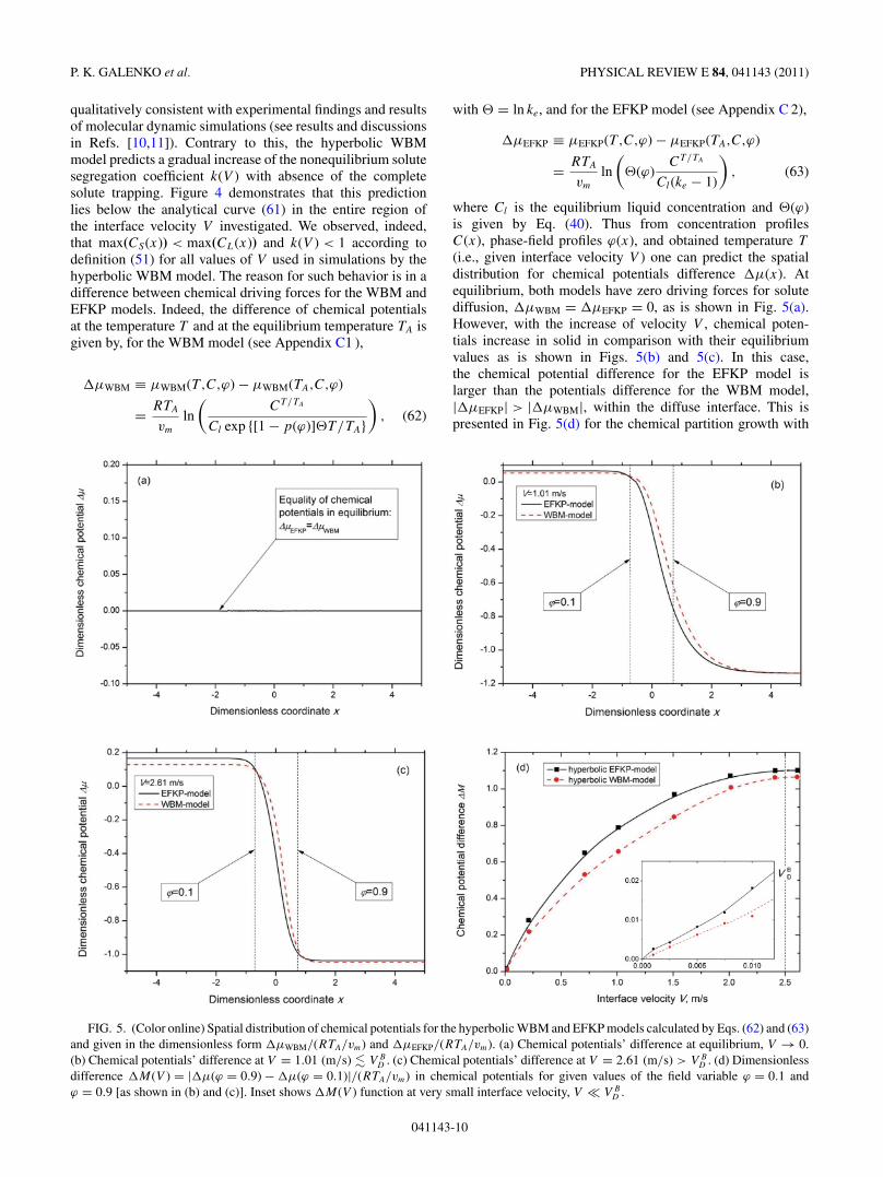
qualitatively consistent with experimental findings and resultsof molecular dynamic simulations (see results and discussionsin Refs. [10,11]). Contrary to this, the hyperbolic WBMmodel predicts a gradual increase of the nonequilibrium solutesegregation coefficient k(V ) with absence of the completesolute trapping. Figure 4 demonstrates that this predictionlies below the analytical curve (61) in the entire region ofthe interface velocity V investigated. We observed, indeed,that max(CS(x)) < max(CL(x)) and k(V ) < 1 according todefinition (51) for all values of V used in simulations by thehyperbolic WBM model. The reason for such behavior is in adifference between chemical driving forces for the WBM andEFKP models. Indeed, the difference of chemical potentialsat the temperature T and at the equilibrium temperature TA isgiven by, for the WBM model (see Appendix C1 ),

�μWBM ≡ μWBM(T ,C,ϕ) − μWBM(TA,C,ϕ)

= RTA

vm

ln

(CT/TA

Cl exp {[1 − p(ϕ)] T/TA})

, (62)

with = ln ke, and for the EFKP model (see Appendix C 2),

�μEFKP ≡ μEFKP(T ,C,ϕ) − μEFKP(TA,C,ϕ)

= RTA

vm

ln

( (ϕ)

CT/TA

Cl(ke − 1)

), (63)

where Cl is the equilibrium liquid concentration and (ϕ)is given by Eq. (40). Thus from concentration profilesC(x), phase-field profiles ϕ(x), and obtained temperature T

(i.e., given interface velocity V ) one can predict the spatialdistribution for chemical potentials difference �μ(x). Atequilibrium, both models have zero driving forces for solutediffusion, �μWBM = �μEFKP = 0, as is shown in Fig. 5(a).However, with the increase of velocity V , chemical poten-tials increase in solid in comparison with their equilibriumvalues as is shown in Figs. 5(b) and 5(c). In this case,the chemical potential difference for the EFKP model islarger than the potentials difference for the WBM model,|�μEFKP| > |�μWBM|, within the diffuse interface. This ispresented in Fig. 5(d) for the chemical partition growth with

FIG. 5. (Color online) Spatial distribution of chemical potentials for the hyperbolic WBM and EFKP models calculated by Eqs. (62) and (63)and given in the dimensionless form �μWBM/(RTA/vm) and �μEFKP/(RTA/vm). (a) Chemical potentials’ difference at equilibrium, V → 0.(b) Chemical potentials’ difference at V = 1.01 (m/s) � V B

D . (c) Chemical potentials’ difference at V = 2.61 (m/s) > V BD . (d) Dimensionless

difference �M(V ) = |�μ(ϕ = 0.9) − �μ(ϕ = 0.1)|/(RTA/vm) in chemical potentials for given values of the field variable ϕ = 0.1 andϕ = 0.9 [as shown in (b) and (c)]. Inset shows �M(V ) function at very small interface velocity, V � V B

D .

041143-10

SOLUTE TRAPPING IN RAPID SOLIDIFICATION OF A . . . PHYSICAL REVIEW E 84, 041143 (2011)

solute trapping at V < V BD and for the diffusionless growth

with the complete solute trapping at V � V BD . Because the

differences �μ are related to the functions introduced inthe transport equation (38) for both models (see also [11]), thelarger values of �μ provide stronger diffusion redistribution ofsolutal atoms. Therefore with �μEFKP > �μWBM, the drivingforce in the EFKP model provides solute diffusion in sucha way that max(CS(x)) = max(CL(x)) with the completesolute trapping, k(V ) = 1 at V � V B

D , and the driving forcein the WBM model provides max(CS(x)) < max(CL(x))with incomplete solute trapping for all investigated V

(Fig. 4).Finally, Fig. 4 clearly shows that the prediction of the

present hyperbolic EFKP model and the prediction of theparabolic EFKP model [14] are almost the same for solutepartitioning in the range of small and moderate velocity,0 < V/V B

D < 0.4. However, for V/V BD > 0.4 the hyperbolic

EFKP model predicts a steeper behavior for the k(V )function than the parabolic EFKP model. This results inthe complete solute trapping predicted by the hyperbolicEFKP model at V/V B

D = 1 and a gradual increasing of thek(V ) function with the increase of V by the prediction ofthe parabolic EFKP model. Such difference in behavior ofthe nonequilibrium solute partitioning is known from theanalysis of the kinetic models based on the continuous growthmodel [10].

C. Kinetic phase diagrams

By the definition [27], the kinetic phase diagram presentstemperature and chemical composition at the solidificationfront moving with nonzero velocity V in a steady-stateregime. With increasing V , kinetic liquidus and solidus linesdeviate more pronouncedly from their equilibrium lines andcharacterize chemical inhomogeneity in the nonequilibriumsolid state upon solidification.

FIG. 6. (Color online) Kinetic phase diagram with the linearapproximation of liquidus and solidus lines for Si-As alloys derivedfrom the present hyperbolic EFKP model. Solid lines representequilibrium lines of the liquidus and solidus. Dashed lines givekinetic liquidus and solidus. Shift of the kinetic liquidus and solidusfrom their equilibrium positions is shown at the interface velocityV = 0.01 (m/s) � V B

D .

It is straightforward to show that, using a common tangentconstruction, the accepted dilute alloy approximation leadsto straight lines of the solidus TS = TA + meCs and theliquidus TL = TA + meCl in the phase diagram with thetangent me = −(1 − ke)(RT/vm)(TA/L) of the liquidus lineand with the relation between equilibrium concentrationsas Cs = keCl (see Appendix A 1). Kinetic phase diagramscan be drawn relative to these equilibrium lines TS(Cs) andTL(Cl).

Figures 6 and 7 exhibit kinetic phase diagrams of alloyrapid solidification in the coordinates “interface temperatureand concentration” constructed using modeling results of thehyperbolic extension of the EFKP model. The interval ofsolidification, as a distance between lines of liquidus andsolidus, shrinks with the increase of interface velocity V .This is clearly seen by comparing the solid lines for theequilibrium state with V = 0 (m/s) and the dashed lines forkinetic liquidus and solidus lines for V = 0.01 (m/s), shown inFig. 6. With a higher interface velocity, V � V B

D , the kineticliquidus and solidus lines merge into one line, shown as adashed line in Fig. 7. This result indicates the equality of solidand liquid concentrations on both sides of the diffuse interface:in the modeling we obtained

max(CS(x)) = max(CL(x)) ≡ CL∞ with k(V ) ≡ 1.

FIG. 7. (Color online) Kinetic phase diagram with the linearapproximation of liquidus and solidus lines for Si-As alloys derivedfrom the present hyperbolic EFKP model. Solid lines representequilibrium lines of the liquidus and solidus. Confluence of the kineticliquidus and solidus in a single dashed line is shown as a result ofthe complete solute trapping and diffusionless solidification at theinterface velocity V = 2.56 (m/s) > V B

D .

041143-11

P. K. GALENKO et al. PHYSICAL REVIEW E 84, 041143 (2011)

This result can be recognized as one of the main characteristicsof complete solute trapping that accompanies diffusionlesssolidification.

Note that using the parabolic system of phase-field equa-tions one can find that kinetic liquidus and solidus lines onlygradually approach each other as the velocity V increases (see,e.g., the kinetic diagram in Fig. 4 of Ref. [8]). Chemicallypartitionless solidification is also predicted previously usinga sharp-interface model in which solute transport has beendescribed by the hyperbolic equation (see, e.g., the kineticdiagram in Fig. 4 of Ref. [28]).

Finally, two features of the kinetic phase diagrams, pre-sented in Figs. 6 and 7, should be outlined. First, in thepresent dilute alloy approximation, we have straight lines forthe kinetic liquidus and solidus. This follows from Taylorexpansions of the liquidus and solidus temperatures,

TL(V,C) = TA + m(V )C + O(C2),

TS(V,C) = TA + m(V )C/k(V ) + O(C2),

which show that by dropping high-order terms O(C2) inthe dilute limit we get straight lines for the liquidus andsolidus for the equilibrium and nonequilibrium states. Ofcourse, the liquidus slope m(V ) as well as the partitioncoefficient k(V ) remain velocity dependent functions andvary between equilibrium and nonequilibrium. Second, for thepure one-component system, the change of the temperatureT with respect to equilibrium solidification temperature TA isdescribed by [see Eqs. (B24)–(B27)]

T (V,C = 0) = TA − V

μ

√1 − V 2/

(V B

ϕ

)2, with

μ = νL

σTA

and V < V Bϕ . (64)

From this it follows that the temperature T (V,C = 0) deviatesfrom its equilibrium value TA by the nonlinear law only forthe highest velocity V ≈ V B

ϕ .

VII. CONCLUSIONS

The parabolic phase-field model of Echebarria, Folch,Karma, and Plapp (EFKP model) [14] has been extended tothe case of local nonequilibrium solidification. Four kineticparameters appear in the model as main characteristics of localnonequilibrium effects. These are the characteristic speedsof atomic diffusion and phase-field propagation within andaround the moving diffuse solid-liquid interface (see Table I).The resulting model is described by a system of hyperbolicpartial differential equations for the atomic diffusion transportand diffuse interface advancement.

The present hyperbolic EFKP model is applied to the solutetrapping problem. Modeling results have been analyzed byconsidering solute concentration profiles, the solute segrega-tion coefficient, and kinetic phase diagrams.

Predictions of the parabolic EFKP model [14] have beencompared with the results of the presently developed hyper-bolic EFKP model. As it is shown, the hyperbolic modelpredicts the complete solute trapping beginning at the fixedinterface velocity equal to the maximum diffusion speed

V = V BD . At this critical point, the alloy solidifies as a su-

persaturated solid solution with the initial (nominal) chemicalcomposition. With the velocity V > V B

D , solidification pro-ceeds by the diffusionless mechanism whose rate is boundedabove by the maximum speed for phase-field propagation, i.e.,V < V B

ϕ . Indeed, for the hyperbolic equation of the phasefield, we have found step solutions (B18), (B22), and (B24)in regimes V < V B

ϕ . Possible solutions for V � V Bϕ might be

obtained together with their stability analysis, existence, anduniqueness. Finally, to compare modeling predictions withexperimental data, the model can be generalized to nonidealsolutions and concentrated binary systems.

ACKNOWLEDGMENTS

We thank Mathis Plapp, Ingo Steinbach, Dmitry Medvedev,and Oleg Shchyglo for numerous fruitful discussions anduseful suggestions. P.K.G. and D.M.H. acknowledge supportfrom DFG (German Research Foundation) under Project No.HE 160/19 and DLR Space Management under ContractNo. 50WM1140. E.V.A. acknowledges support from DAAD(German Academic Exchanges Service) under StipendiumA/08/81583. D.J. acknowledges support by the DireccionGeneral de Investigacion of the Spanish Ministry of Educa-tion and Science under Grant No. Fis 2009-13370-C02-01and of the Generalitat of Catalonia under Grant No. 2009-SGR-00164. D.A.D. acknowledges support from RFBR (Rus-sian Foundation of Basic Research) under Project No. 09-02-12110-ofi-m. V.G.L. acknowledges support from RFBR(Russian Foundation of Basic Research) under Project No. 08-02-91957NNIO a and from ROSNAUKA (Russian ScientificFoundation) under Project No. 2009-1.5-507-007-002.

APPENDIX A: EQUILIBRIUM FEATURES AND PROFILESOF THE PHASE FIELD

Equilibrium conditions in the phase-field model are givenby

δF

δϕ= 0,

δF

δC= μeq(T ), (A1)

where μeq(T ) = μ(ϕ,C,T ). The measure of equilibrium, thechemical potential μeq, can be obtained from equilibrium freeenergy densities in both phases, fs(C,T ) and fl(C,T ), by

∂fs(C,T )

∂C

∣∣∣∣C=Cs

= ∂fl(C,T )

∂C

∣∣∣∣C=Cl

= μeq(T ), (A2)

fs(Cs,T ) − μeqCs = fl(Cl,T ) − μeqCl, (A3)

where Cs and Cl are equilibrium concentrations in solid andliquid, respectively. Equations (A2) and (A3) are used in thissection to obtain equilibrium concentration and phase-fieldprofiles as described by EFKP and WBM models [5,14].

1. Equilibrium features of the EFKP model

In the free energy density (4) the entropy density s(ϕ) andinner energy ε(ϕ) include interpolation functions ps(ϕ) and

041143-12

SOLUTE TRAPPING IN RAPID SOLIDIFICATION OF A . . . PHYSICAL REVIEW E 84, 041143 (2011)

pε(ϕ) and are given by [14]

s(ϕ) = ss + sl

2− ps(ϕ)

L

2TA

, (A4)

ε(ϕ) = εs + εl

2+ pε(ϕ)

�ε

2, (A5)

where �ε = εs − εl , L = TA(sl − ss). The functions ps andpε satisfy the following conditions:

ps(0) = pε(0) = 1, ps(1) = pε(1) = −1,

dps(ϕ)

dϕ

∣∣∣∣ϕ=0

= dpε(ϕ)

dϕ

∣∣∣∣ϕ=0

= 0, (A6)

dps(ϕ)

dϕ

∣∣∣∣ϕ=1

= dpε(ϕ)

dϕ

∣∣∣∣ϕ=1

= 0,

such that the free energy density (4) gives the free energies forthe liquid and solid phases as follows:

fs(Cs,T ) = f A(TA) − (T − TA)ss

+ εsCs + RTA

vm

(Cs ln Cs − Cs) , (A7)

fl(Cl,T ) = f A(TA) − (T − TA)sl

+ εlCl + RTA

vm

(Cl ln Cl − Cl) . (A8)

Choosing ps by Eq. (6), from Eqs. (A7) and (A8) follows

∂fs

∂Cs

= εs + RTA

vm

ln Cs, (A9)

∂fl

∂Cl

= εl + RTA

vm

ln Cl. (A10)

Substituting Eqs. (A9) and (A10) into definition (A3) gives theequilibrium chemical potential

εs + RTA

vm

ln Cs = εl + RTA

vm

ln Cl = μeq, (A11)

using of which one can define equilibrium solute partitioningby the solute segregation coefficient:

ke = Cs

Cl

= exp

(− vm

RTA

�ε

). (A12)

Further substituting Eqs. (A7) and (A8) into the same definition(A3) with use Eq. (A11) leads to the relation

vm

RT(T − TA)

L

TA

+ vm

RT�εCs + Cs ln ke − (Cs − Cl) = 0.

(A13)

With using Eq. (A12), finally, we obtain from Eq. (A13)equilibrium concentrations in phases

Cl = vm

RT

L

TA

1

1 − ke

(TA − T ), Cs = keCl, (A14)

and a slope of the liquidus line in equilibrium phase diagram

me = −(1 − ke)RT

vm

TA

L. (A15)

2. Concentration profile and phase-field profile in EFKP model

Equilibrium profile of concentration for a given value ofϕ(x) is obtained from Eq. (2) by(

∂2f

∂C2

)dC

dx+

(∂2f

∂C∂ϕ

)dϕ

dx= const. (A16)

Using expressions for the free energy (4) and internal energy(7), one gets

∂2f

∂C2= RT

vmC,

(A17)∂2f

∂C∂ϕ= dε(ϕ)

dϕ= −1

2

RT

vm

ln ke

dpε

dϕ.

Substituting Eq. (A17) into Eq. (A16) leads to

ln C − pε

2ln ke = const ≡ 0. (A18)

As a result, taking Eq. (A6) into account, the equilibriumconcentration profile in the EFKP model is described by

C(x) = Cl exp

(ln ke

2[1 + pε(ϕ)]

). (A19)

Phase-field equilibrium follows from Eq. (3) and is givenby

ε2ϕ

d2ϕ

dx2− W

dg(ϕ)

dϕ

= 1

2

dps(ϕ)

dϕ

T − TA

TA

L + 1

2

dpε(ϕ)

dϕ�εC0. (A20)

Using Eqs. (A12) and (A14) one gets from Eq. (A20) thefollowing equation:

ε2ϕ

d2ϕ

dx2− W

dg(ϕ)

dϕ

= − RT

2vm

Cl

[(1 − ke)

dps(ϕ)

dϕ+ ln ke

C(x)

Cl

dpε(ϕ)

dϕ

]. (A21)

With the equilibrium condition ∂f (ϕ,C,T )/∂ϕ = 0 andEq. (A19), one obtains

(1−ke)dps(ϕ)

dϕ+ ln(ke)

dpε(ϕ)

dϕexp

(ln ke

2[1+pε(ϕ)]

)= 0.

(A22)

This condition leads to the definition of functions (6) and(7) and gives zero for the right hand side of Eq. (A21).Then, the equation ε2

ϕd2ϕ/dx2 − Wdg(ϕ)/dϕ = 0 has thekink solution:

ϕ(x) = 1

2+ 1

2tanh

(3x

2δ

). (A23)

This distribution agrees with the equilibrium ϕ profile(14) in which δ = 3εϕ/

√2W according to the chosen

parameters (36).

041143-13

P. K. GALENKO et al. PHYSICAL REVIEW E 84, 041143 (2011)

3. Concentration profile and phase-field profilein WBM model

The free energy density in the Wheeler-Boettinger-McFadden model (WBM model) is given by [5]

fe(C,T ,ϕ) = fA(T ,ϕ) + CfB(T ,ϕ)

+ RTA

vm

(C ln C − C) + Wg(ϕ), (A24)

where the free energies fA(T ,ϕ) and fB(T ,ϕ) of A and B

particles are

fA(T ,ϕ) = −RTA

vm

1 − ke

me

(T − TA)[1 − p(ϕ)], (A25)

fB(T ,ϕ) = −RTA

vm

ln ke[1 − p(ϕ)]. (A26)

From solution of equilibrium conditions (A2) and (A3) weobtain the equilibrium concentration profile. The free energydensities in phases are

fs(Cs,T ) = RTA

vm

1 − ke

me

(TA − T )

−Cs

RTA

vm

ln ke + RTA

vm

(Cs ln Cs − Cs) , (A27)

fl(Cl,T ) = RTA

vm

(Cl ln Cl − Cl) . (A28)

Using Eq. (A2), one can obtain from Eqs. (A27) and (A28)the following expressions for equilibrium chemical potentialsin phases:

μeq = RTA

vm

ln Cl, μeq = −RTA

vm

ln ke + RTA

vm

ln Cs. (A29)

Then, from Eq. (A3) the equilibrium concentrations are givenby

Cl = −TA − T

me

, Cs = keCl, (A30)

and the equilibrium concentration profile is

C(x) = Cl exp {ln ke [1 − p(ϕ)]} . (A31)

Note that the above concentrations Cl and Cs as well as theslope me completely agree with those ones obtained for theEFKP model, Eqs. (A14) and (A15).

The equilibrium phase-field profile ϕ(x) in Eq. (A31) isdefined by

ε2ϕ

∂2ϕ

∂x2− ∂f

∂ϕ= 0. (A32)

Then, taking definitions (A24)–(A26) into account, we obtain

∂2ϕ

∂x2− 9

2

dg(ϕ)

dϕ

− 1

2

δ

d0

T

TA

(1 − ke

me

(T − TA) + C ln ke

)dp(ϕ)

dϕ= 0.

(A33)

Using Eqs. (A30) and (A31) in Eq. (A33), one gets

∂2ϕ

∂x2− 9

2

dg(ϕ)

dϕ

= 1

2

δ

d0

T

TA

Cl[1 − ke + ln(ke)eln ke(1−p(ϕ))]dp(ϕ)

dϕ. (A34)

This equation gives the phase-field profile with equilibriumcoexistence of liquid and crystal in the WBM model.

APPENDIX B: EQUATIONS OF THE HYPERBOLICEFKP MODEL

Consider a flat interface between solid and liquid phasesmoving in perpendicular direction to the x axis. Then one canconsider Eqs. (2) and (3) in one spatial dimension.

1. Concentration field

To obtain explicit form of one-dimensional equation (2) weuse the free energy density, Eqs. (4)–(8), and the derivativesfrom it, Eq. (A17), such that the mobility is

MC(T ,C,ϕ) =(

∂2f

∂C2

)−1

D(ϕ) = vmC

RTD(ϕ). (B1)

Then, using

dpε(ϕ)

dϕ= −1 − ke

ln ke

1

k(1+pε )/2e

dps(ϕ)

dϕ(B2)

with dps/dϕ = −2dp/dϕ and equality

1

k(1+pε )/2e

= 1

ke + (1 − ke)p(ϕ), (B3)

we obtain

∂2f

∂C∂ϕ= −RT

vm

1 − ke

ke + (1 − ke)p(ϕ)

dp

dϕ, (B4)

MC

∂2f

∂C∂ϕ= −D(ϕ)C

1 − ke

ke + (1 − ke)p(ϕ)

dp(ϕ)

dϕ. (B5)

Substituting Eqs. (B1) and (B5) into Eq. (2) gives

τD

∂2C

∂t2+ ∂C

∂t= ∂

∂x

(D(ϕ)

∂C

∂x

)− ∂

∂x

[D(ϕ)C

1 − ke

ke + (1 − ke)p(ϕ)

dp(ϕ)

dϕ

∂ϕ

∂x

]. (B6)

Introducing the function

(ϕ) = − 1 − ke

ke + (1 − ke)p(ϕ), (B7)

041143-14

SOLUTE TRAPPING IN RAPID SOLIDIFICATION OF A . . . PHYSICAL REVIEW E 84, 041143 (2011)

one-dimensional Eq. (2) reads in the moving reference frame as

τD

ν2

DLδ2

∂2C

∂t2− 2τD

νV

DL

∂2C

∂t∂x+ τDV 2

DL

∂2C

∂x2+ ν

DL

∂C

∂t− V δ

DL

∂C

∂x= ∂

∂x

(D(ϕ)

DL

∂C

∂x

)+ ∂

∂x

(D(ϕ)

DL

C (ϕ)dp(ϕ)

dϕ

∂ϕ

∂x

). (B8)

In a reference frame moving with constant velocity V , Eq. (B8) takes the following form:

V 2(V B

D

)2

d2C

dx2− V

V ID

dC

dx= d

dx

(D(ϕ)

DL

dC

dx

)+ d

dx

(D(ϕ)

DL

C (ϕ)dp(ϕ)

dϕ

dϕ

dx

). (B9)

Equation (B9) has two characteristic diffusion speeds as is given in Table I.

2. Phase field

To obtain the explicit form of one-dimensional Eq. (3), which describes evolution of the phase field ϕ, we obtain from Eqs. (4)–(8)that

∂f

∂ϕ= 9σ

δ

dg(ϕ)

dϕ− 1

2

RT

vm

(1 − ke

me

(T − TA)dps(ϕ)

dϕ+ C ln ke

dpε(ϕ)

dϕ

). (B10)

Then, using Eqs. (B2) and (B10), one-dimensional Eq. (3) is written as

τϕ

∂2ϕ

∂t2+ ∂ϕ

∂t= ν

∂2ϕ

∂x2− 9ν

2δ2

dg(ϕ)

dϕ− νRT

2σδvm

(1 − ke

me

(T − TA) − C1 − ke

ke + (1 − ke)p(ϕ)

)dp(ϕ)

dϕ. (B11)

In a moving reference frame Eq. (B11) reads

τϕν

δ2

∂2ϕ

∂t2− 2τϕV

d2ϕ

∂t∂x+ τϕV 2

ν

∂2ϕ

∂x2+ ∂ϕ

∂t− V δ

ν

∂ϕ

∂x

= ∂2ϕ

∂x2− 9

2

dg(ϕ)

dϕ− 1

2

δ

d0

T

TA

(1 − ke

me

(T − TA) − C1 − ke

ke + (1 − ke)p(ϕ)

)dp(ϕ)

dϕ, (B12)

where dimensionless time and spatial coordinate were used as described in Sec. IV B. In the case of moving reference frame withconstant velocity V , Eq. (B12) has the following form:

V 2(V B

ϕ

)2

d2ϕ

dx2− V

V Iϕ

dϕ

dx= d2ϕ

dx2− 9

2

dg(ϕ)

dϕ+ 1

2

δ

d0

T

TA

�(T ,C,ϕ)dp(ϕ)

dϕ, (B13)

where we used the function

�(T ,C,ϕ) = (1 − ke)C

ke + (1 − ke)p(ϕ)− 1 − ke

me

(T − TA). (B14)

Equation (B13) introduces two characteristic speeds for the phase field as is given in Table I.

We specially have to note that transport equation (B9) andequation of motion (B13) are the same as is described by thehyperbolic WBM model. The main difference in the modelsis that the functions (ϕ) and �(T ,C,ϕ), which are given byEqs. (B7) and (B14), respectively, differ substantially fromthose obtained for the hyperbolic WBM model [11].

In the specific case of a pure material one can obtainfrom Eq. (B13) an explicit relationship between the interfacevelocity V and the temperature T or the undercooling �T =TA − T . By setting C = 0 for pure substance of A atoms andby taking into account Eq. (A15), the function � reduces to

�(T ) = vmL

RT

T − TA

TA

= −vmL

RT

�T

TA

. (B15)

For the double-well function g(ϕ) in Eq. (5) and for theinterpolation function p(ϕ) in Eq. (8) we have

dg(ϕ)

dϕ= 2ϕ(1 − ϕ)(1 − 2ϕ) (B16)

and

dp(ϕ)

dϕ= 6ϕ(1 − ϕ). (B17)

For a steplike phase-field profile

ϕ(x) = 1

2

(1 + tanh

x

l

)(B18)

the derivatives in Eq. (B13) can be expressed as

dϕ

dx= 2

lϕ(1 − ϕ) (B19)

and

d2ϕ

dx2= 4

l2ϕ(1 − ϕ)(1 − 2ϕ). (B20)

041143-15

P. K. GALENKO et al. PHYSICAL REVIEW E 84, 041143 (2011)

The right hand sides in Eqs. (B16) and (B17) and in Eqs. (B19)and (B20) are similar. Therefore substituting these derivativesinto Eq. (B13) gives[(

1 − V 2(V B

ϕ

)2

)4

l2− 9

]ϕ(1 − ϕ)(1 − 2ϕ)

+[

V

V Iϕ

2

l+ 3

δ

d0

T

TA

�(T )

]ϕ(1 − ϕ) = 0. (B21)

The first summand gives the expression for the interfacethickness l in Eq. (B18),

l = 2

3

√√√√1 − V 2(V B

ϕ

)2 . (B22)

Note that in the parabolic case with V Bϕ → ∞, the interface

thickness l has a constant value and the phase-field profilein Eq. (B18) is equal to the equilibrium phase-field profilein Eq. (A23). Taking the relaxation effects into account, it isseen from Eq. (B22) that the interface thickness l graduallydecreases toward zero as the interface velocity V increases upto the maximum speed V B

ϕ for the phase-field propagation.The second summand in Eq. (B21) gives the relationship

between the interface velocity V and the temperature T .Indeed, using the expression V I

ϕ = ν/δ from Table I, one gets

V√1 − V 2/

(V B

ϕ

)2= − ν

d0

T

TA

�(T ). (B23)

Here, the function �(T ) represents the driving force for thephase-field propagation. Taking Eq. (B15) into account, therelationship in Eq. (B23) in terms of the undercooling �T

reads

V√1 − V 2/(V B

ϕ )2= ν

d0

vmL

RTA

�T

TA

. (B24)

With the interface velocity much smaller than the maximumspeed for the phase-field propagation, V � V B

ϕ , one obtainsthe linear relation

V = μ�T, (B25)

where the kinetic coefficient is given by

μ = ν

d0

vmL

RT 2A

. (B26)

Using Eq. (36), the kinetic coefficient related to the surfaceenergy is obtained as

μ = ν

σ

L

TA

. (B27)

In summary, we have found solutions for the interfacialthickness (B22) and velocity (B24), which are true for the stepform of the phase-field profile (B18) and for the regime V <

V Bϕ . Special consideration of possible solutions for regimes

V � V Bϕ might also be presented together with their stability

analysis, existence, and uniqueness.

APPENDIX C: DRIVING FORCESFOR SOLUTE DIFFUSION

1. Chemical potential difference for the WBM model

Using the definition μ = ∂f/∂C and the free energy(A24)–(A26) one can obtain the chemical potential

μWBM = −RT

vm

ln ke[1 − p(ϕ)] + RT

vm

ln C (C1)

for the phase-field WBM model [5]. Expression (C1) andthe equilibrium potential in liquid (A29) give the followingdifference:

�μWBM ≡ μWBM(T ,C,ϕ) − μWBM(TA,C,ϕ)

= RTA

vm

[T

TA

ln C − T

TA

[1 − p(ϕ)] ln ke − ln Cl

]

= RTA

vm

lnCT/TA

Clk[1−p(ϕ)]T/TAe

. (C2)

For the equilibrium potential μWBM(TA,C,ϕ) we assume thatthe equilibrium liquid concentration is C = Cl with ϕ = 1.

As we noted in the previous section, the solute dif-fusion equation (B9) is the same for WBM and EFKPmodels, however, the function is different for bothmodels. In particular, in the hyperbolic WBM model onefinds [11]

= ln

(1 + (TA − T )/me

1 + ke(TA − T )/me

)+ ln ke.

At a tiny amount of a solute, the dilute alloy approximationreads T → TA and me → ∞. Then, the above expression gives = ln ke and Eq. (C2) transforms as

�μWBM(T ,C,ϕ) = RTA

vm

lnCT/TA

Cle[1−p(ϕ)] T/TA. (C3)

This expression can be compared with the chemical potentialdifference predicted by the EFKP model as is given in thefollowing section.

2. Chemical potential difference for the EFKP model

From the definition of the chemical potential (17)and using the inner energy (A5) one can obtain thedifference between potentials at a given temperature and inequilibrium:

�μEFKP ≡ μEFKP(T ,C,ϕ) − μEFKP(TA,C,ϕ)

= ε(ϕ) − εl + RT

vm

ln C − RTA

vm

ln Cl

= εs − εl

2[1 + pε(ϕ)] + RT

vm

ln C − RTA

vm

ln Cl.

(C4)

As for the WBM model (see Appendix C 1), equilibrium liquidconcentration C = Cl with ϕ = 1 is taken for the equilibriumpotential μEFKP(TA,C,ϕ). Using the definition (7) for the pε(ϕ)function and taking the function from Eqs. (40) and (C4)

041143-16

SOLUTE TRAPPING IN RAPID SOLIDIFICATION OF A . . . PHYSICAL REVIEW E 84, 041143 (2011)

can be rewritten in the following form:

�μEFKP = RTA

vm

ln

(CT/TA (ϕ)

Cl(ke − 1)

), (C5)

convenient for the further analysis. Particularly, with knownprofiles C(x) and ϕ(x) one can compute and compare spatialprofiles of �μ by Eqs. (C3) and (C5) for the obtained value ofT , i.e., for a given interface velocity V .

[1] A. A. Chernov, in Rost Kristallov, edited by A. V. Shubnikovand N. N. Sheftal, Vol. 3 (Akademia Nauk SSSR, Moscow,1959), p. 35 [English translation: Growth of Crystals, Vol. 3(Consultants Bureau, New York, 1962), p. 65]; V. V. Voronkovand A. A. Chernov, Sov. Phys. Crystallogr. 12, 186 (1967);A. A. Chernov, Usp. Fiz. Nauk 100, 277 (1970) [Sov. Fiz. Usp.13, 101 (1970)].

[2] J. C. Baker and J. W. Cahn, Acta Metall. 17, 575 (1969).[3] M. J. Aziz, J. Appl. Phys. 53, 1158 (1982).[4] M. J. Aziz and T. Kaplan, Acta Metall. 36, 2335 (1988).[5] A. A. Wheeler, W. J. Boettinger, and G. B. McFadden, Phys.

Rev. E 47, 1893 (1993).[6] M. Conti, Phys. Rev. E 56, 3717 (1997).[7] N. A. Ahmad, A. A. Wheeler, W. J. Boettinger, and G. B.

McFadden, Phys. Rev. E 58, 3436 (1998).[8] K. Glasner, Physica D 151, 253 (2001).[9] D. Danilov and B. Nestler, Acta Mater. 54, 4659 (2006).

[10] P. Galenko, Phys. Rev. E 76, 031606 (2007).[11] V. G. Lebedev, E. V. Abramova, D. A. Danilov, and P. K.

Galenko, Int. J. Mater. Res. 101/04, 473 (2010).[12] D. Herlach, P. Galenko, and D. Holland-Moritz, Metastable

Solids from Undercooled Melts (Elsevier, Amsterdam, 2007).[13] Y. Yang, H. Humadi, D. Buta, B. B. Laird, D. Sun, J. J. Hoyt,

and M. Asta, Phys. Rev. Lett. 107, 025505 (2011).[14] B. Echebarria, R. Folch, A. Karma, and M. Plapp, Phys. Rev. E

70, 061604 (2004).[15] P. Galenko and D. Jou, Phys. Rev. E 71, 046125

(2005).[16] V. Lebedev, A. Sysoeva, and P. K. Galenko, Phys. Rev. E 83,

026705 (2011).[17] A. A. Wheeler, W. J. Boettinger, and G. B. McFadden, Phys.

Rev. A 45, 7424 (1992); G. B. McFadden and A. A. Wheeler,

Proc. R. Soc. London, Ser. A 458, 1129 (2002); D. Danilov andB. Nestler, Discrete Contin. Dyn. Syst. 15, 1035 (2006).

[18] J. Tiaden, B. Nestler, H. J. Diepers, and I. Steinbach, Physica D115, 73 (1998); D. A. Cogswell and W. C. Carter, Phys. Rev. E83, 061602 (2011).

[19] P. Galenko, Phys. Lett. A 287, 190 (2001).[20] The solute trapping phenomenon is studied in this work on the

time scales of τD . For most metallic and nonmetallic systemsthe inequality τϕ � τD holds [11]. Therefore investigations ofthe semihyperbolic phase-field model instead of fully hyperbolicmodel can be accepted as a reasonable approximation.

[21] D. Jou, J. Casas-Vazquez, and G. Lebon, Extended IrreversibleThermodynamics, 4th ed. (Springer, Berlin, 2010).

[22] M. Grmela and H. C. Ottinger, Phys. Rev. E 56, 6620 (1997);M. Grmela, G. Lebon, and Ch. Dubois, ibid. 83, 061134 (2011).

[23] P. K. Galenko and D. A. Danilov, J. Cryst. Growth 216, 512(2000).

[24] In principle, the h(p,V ) function can be arbitrarily chosen withthe conditions of its monotonic behavior at any values of V

and its transforming into the preliminary chosen h(p,V = 0)function at equilibrium. The detailed form of the h(p,V )function might also be optimized using the results of atomisticmodeling (like the molecular dynamics simulations) or theresults from modeling on the atomic lengths and diffusive timescales (like the phase-field crystal modeling).

[25] B. Vinet, L. Magnusson, H. Fredriksson, and P. J. Desre, J.Colloid Interface Sci. 255, 363 (2002).

[26] J. A. Kittl, M. J. Aziz, D. P. Brunco, and M. O. Thompson,J. Cryst. Growth 148, 172 (1995).

[27] V. T. Borisov, Dokl. Akad. Nauk SSSR 142, 69 (1962)[Sov. Phys. Dokl. 7, 50 (1962)].

[28] P. Galenko and S. Sobolev, Phys. Rev. E 55, 343 (1997).

041143-17