Iran. J. Chem. Chem. Eng. Research Article Vol. 40, No. 3, 2021

Research Article 945

Predicting Solute Transport Parameters

in Saturated Porous Media Using Hybrid Algorithm

Bouredji, Hamza*+; Bendjaballah Lalaoui, Nadia; Rennane, Samira

Laboratoire de Matériaux Catalytiques et Catalyseen Chimie Organique, Université des Sciences et de la

Technologie Houari Boumédiène, Alger, ALGÉRIE

Merzougui, Abdelkrim

Laboratoire de Recherche en Génie Civil, Hydraulique, Développement Durable et Environnement,

Université Mohamed Kheider, Biskra, ALGÉRIE

ABSTRACT: This study aims to estimate the solute transport parameters in saturated porous media

using a hybrid algorithm. In this study, the Physical Non-Equilibrium (PNE) model was used

to describe the transport of solutes in porous media. A numerical solution for the PNE model is obtained

using the Finite Volume Method (FVM) based on the Ttri-Diagonal Matrix Algorithm (TDMA). The

developed program, written in Matlab, is capable to solve the advection-dispersion (ADE) and the PNE

equations for the mobile -immobile (MIM)model with linear sorption isotherm. The Solute transport

parameters, (immobile water content, mass transfer coefficient, and dispersion coefficient), are estimated

using different algorithms such as the Levenberg-Marquardt algorithm (LM), genetic algorithm (GA),

simulated annealing algorithm (SA). To overcome the limitations of deterministic optimization models

which are rather unstable and divergent around a local minimum, a hybrid algorithm (GA+LM, SA+LM)

permits to estimate of the solute transport parameters. Numerical solutions are verified using the experiments

conducted by Semra (2003) which are about the transport of toluene through a column composed of

impregnated Chromosorb grains at ambient temperature (20 °C) for three flow rates (1, 2 and 5ml/min).

The results show that the hybrid algorithm (GA+LM, SA+LM) is more accurate than others (GA, SA, and

LM). Comparing to the ADE model, The PNE with linear isotherm model gives a better description to the

BeakThrough Curves (BTCs) with higher values of determination coefficient (R2) and lower values of Root

Mean Square Error (RMSE). Also, the solute transport parameters tended to vary with the flow rate.

KEYWORDS: Genetic algorithm; Finite volume method; Levenberg-Marquardt algorithm;

Numerical solution; Physical non-equilibrium.

INTRODUCTION

Prediction of the transport of solute in porous media is

important to evaluate contamination in soils and aquifers.

The advection-dispersion equation (ADE) is often used

to describe the solute transport in soils undersaturated

and unsaturated conditions. Dispersion coefficient, one

of the parameters of ADE, is a measure of dispersive properties

*To whom correspondence should be addressed.

+E-mail:bouredjih@gmail.com

1021-9986/2020/6/945-954 10/$/6.00

Iran. J. Chem. Chem. Eng. Bouredji H. et al. Vol. 40, No. 3, 2021

946 Research Article

of soil. In the literature, several models are proposed

for prediction of dispersion coefficient. In one dimension,

the dispersion coefficient is defined mathematically as

a linear function of the water velocity and a constant which

corresponds to the longitudinal dispersivity [30].

At column scale, dispersivity between 0.01 and 1.0 cm

Zheng and Bennett [30], Perkins and Johnston [19] found

an empirical relation to calculate the dispersivity according

to the particle diameter. Another empirical relation is also

given by Zheng and Bennett [30] to calculate

the dispersivity according to the length of the column.

The physical non equilibrium (PNE) model is often

used to calibrate the experimental results by optimization

of model parameters. The model divides the pore space

into “mobile” and “immobile” flow regions with first-

order mass transfer between these two regions.

Application of the PNE model requires the estimation

of three parameters. (θim), the immobile water content, (α),

the mass transfer coefficient between mobile and

immobile water region, and the dispersion coefficient

in mobile water or (Dm). For most applications, these three

parameters are difficult to estimate. It is suitable to obtain

such parameters based on experimental methodologies.

Consequently, these parameters must be optimized using

inverse methods to the solute concentrations in the column

outflow vs. time [21]. Inverse methods applied to solute

breakthrough curves are typically used to estimate the

parameter values [28].

A common way of estimating the mobile and immobile

water content is to use the curve fitting of tracer

breakthrough results [22], based on the following mass

balance equation:

m m im im C Θ C + Θ C (1)

When α is small enough to assume the concentration

in immobile water (Cim) negligible and C0 is the input

concentration at certain infiltration time t, an approximate

equation is obtained im 0Θ Θ 1 - C C . Applications

of this method can be found in Clothier et al. [3], and

Jaynes et al. [8]. Assuming that the concentration in the

mobile water (Cm) equals the input concentration C0,

Jaynes et al. [8] used the following formula:

Ln(1-C/C0)=at+b (2)

Where im

a / and im

b ln ( / ) .

m and

im

can be evaluated by plotting ln(1-C/C0)

versus elapsed time. However, the assumption of m 0

C C

associated with this method is debatable and

may not be correct as long as >0, Slightly different from

the approach of Jaynes et al. [8] and Clothier et al. [3],

Goltz and Roberts [7] estimated the fraction of mobile water

as the ratio of velocity calculated from hydraulic conductivity

to the velocity measured from tracer experiment. Several

examples are available on various parameters estimation

associated with the mobile immobile approach. For

unsaturated glass beads with diameters in the

neighborhood of 100 µm, De Smedt and Wierenga [5]

found m

= 0 .Θ 853 Θ . For dispersion coefficient in mobile

water, three models for dispersion coefficient were

presented by Sharma et al. [25], the Mobile-Immobile

model for constant dispersion (MIMC), linear distance

dependent dispersion (MIML), and exponential distance

dependent dispersion (MIME). The comparison of these

models shows that the MIM model with constant and

exponential distance-dependent dispersion can be used for

simulation of the breakthrough curves.

To date, different global optimization techniques have

been reported for the solute transport modeling, including

a variety of stochastic global optimization methods [17].

As example, the genetic algorithm (GA), simulated

annealing (SA), tabu search (TS), bees algorithm (BA) and

successive equimarginal approach (SEA) have been

reported as promising optimization methods [12, 17] and

can be used for solute transport calculations. In particular,

Giacobbo et al. [6] studied the transport of contaminants

through a three-layered monodimensional saturated

medium by a numerical solution of advection dispersion

equation and apply GA to evaluate the hydrodynamic

dispersion coefficient and the fluid velocity. Their results

indicate that the method is capable to estimate the

parameters values with accuracy.

It is convenient to remark that the stochastic global

optimization methods show disadvantages depending

on the optimization problem under analysis, which could

include a low convergence performance especially for

multivariable problems.

In the present paper, we propose a combination of a

stochastic global optimization method GA or SA with

Levenberg-Marquardt algorithm (LM), used to improve

the results of GA or SA methods. The motivation of using

Iran. J. Chem. Chem. Eng. Predicting Solute Transport Parameters ... Vol. 40, No. 3, 2021

Research Article 947

such a method is to avoid stopping on a local minimum

obtained by the GA or SA methods.

THEORETICAL

Problem formulation

The transport of a solute in a porous medium (soil)

with mobile and immobile regions of soil water is governed

by the following equations [10]:

m im m im

m im

S S C C

t t t t

(3)

2

m m

m m m m 2

C Cu D

x x

im im

im m im

C SC C

t t

(4)

Where um is the pore-water velocity in the mobile water

[L/T], Cm, Cim the solute concentration in the mobile and

immobile water respectively [M/L3], Sm, Sim the solid phase

concentration of solute from either the mobile and

immobile region per mass of dry soil respectively [M/M],

Dm the dispersion coefficient in the mobile water [L2/T],

the dry soil bulk density [M/L3], α the mass transfer

coefficient between mobile and immobile region[1/T],

m

andim

the mobile and immobile water contents

[L3/L3], x the direction, and t the time [T].

The linear sorption isotherm assumes that the sorbed

concentrations Sm, Sim for mobile and immobile regions

are directly proportional to the dissolved concentration Cm,

Cim:

m d mS K C (5a)

im d imS K C (5b)

With Kd a “distribution” constant expressed as volume

of aqueous phase per mass of dry soil [L3/M].

In such a case, the equation (3) can be written as:

d dm im im

m m m

K KC C1

t t

(6)

2

m m

m m2

C CD u

xx

This equation describes the physical non equilibrium

equation combined with linear isotherm model. Notice that

if θim=0, equation (6) is reduced to ADE with linear

isotherm model (equation 7).

2

d

m m2

K C C C1 D u

t xx

(7)

Numerical solution

Using dimensionless variables, the two transport

Equations (3), (4) become:

L L

t t t tm m

0

p

m

0

dR

L

C Cd x d x

x t

(8)

L L 2t t t tim im m

im

p

2

m e0 0

C C1R d x d x

Pt x

d

L

L L

t t t tim

im im m im

m0 0

C LR d x C C d x

ut

(9)

Where:m d m

R 1 K / ,im d im

R 1 K / ,

m*t ,

u

Lt *

0

CC ,

C

p

xx ,

d

p

e

m

md

Pu

D

C0 is the input concentration [M/L3], dp the diameter of

soil particle [L] and L the column length [L].

The dimensionless equation (9) has been solved using

the finite volume method according to second order Euler

backward (Fig .1) and the Adam Bashforth scheme [17].

After simplification, we can establish the following

relationship:

t t

m ( i

* t+ Δ t

im (i)

)

m

im im

m

LC

u

L

2

Ct

3u

t

2R

(10)

*t * tim im

im im

m

-Δ t

im (i) im (i)4 C C

2

R+

3 Ru

tL

Equation (10) gives the dimensionless immobile

concentration at time (t+∆t) according to dimensionless

mobile concentration at time (t+∆t).

We use the same method to solve the dimensionless

Equation (8), we substitute the Equation (10) into the

solved equation to obtain the following expression:

Iran. J. Chem. Chem. Eng. Bouredji H. et al. Vol. 40, No. 3, 2021

948 Research Article

Fig. 1: Numerical grid for the one dimensional column laboratory.

* *

(i) m (i) (i+ 1 ) m (i+ 1

t t

)

t t

A C A C

(11)

*

(i-1 ) m (i-

t

1 )

t

A C S r

Where:

p

( i )

e

m

1 13 d x (i )A R

2 L Δ t d X (i+ 1 ) d X (i-1 )

1+

P

(12a)

im im

mim im

m

m

p R

2 L3

3 d x (i)

uR

u

t

e

( i 1)A

d X (i

1

P + 1 )

(12b)

( i 1)

e

1A

P d X (i-1 )

(12c)

*

t t*

m ( i 1)m ( i 1)S r C C

(12d)

t t t t

* *

m ( i 1) m ( i 1) p t t t

m m ( i ) m ( i )

C C d x (i )R ( 4 C C )

2 2 L t

im im im

im

mim i

p * t * t-Δ t

im (i) m

m

i (i)

m

d x (i )1 4 C C

2 t2 .L .

3 RR +

L3 R

u

t

Equation (11) is a system of equations which form

tri-diagonal matrix that can be solved by the Thomas

algorithm [17].

The initial and boundary conditions (Dirichlet) are:

m m

m

x =

0

L

C x , 0 = 0 ,  C 0 , t = C

= 0,x

C

Solute transport parameters estimation

The different solute transport parameters are obtained

from experimental data by minimizing a suitable objective

function. The most common objective function is the sum

of the square of the error between the experimental and

calculated relative concentrations, the objective function can

be defined as [9]:

n

m e 2

i i

i 1

m in F (C C )

(13)

Where Cim is the measured relative concentration

and Cie the estimated relative concentration.

Both the determination coefficient (R2) and the root

mean square error (RMSE) were used as two criteria

to reflect the goodness of simulation [24]:

n2

m e

i i

2 i= 1

n 2

m m

i i

i= 1

C -C

R = 1 -

C -C

(14)

m

n 2e

i i

i = 1

1R M S E = C -C

n (15)

Where m

iC represent the mean values of m

iC , and n

the number of measurements.

To determine the solute transport parameters,

the levenberg-marquardt algorithm (LM), genetic

algorithm (GA) and simulated annealing algorithm (SA)

were used that are presented by the MATLAB functions

"lsqcurvefit", "ga" and "simulannealbnd", respectively.

The parameters used by MATLAB for GA and SA

algorithm are given in Table 1.

In order to improve the fitting of the breakthrough

curves, the non-classical algorithms (GA, SA) and

classical method of Levenberg–Marquardt were

hybridized. The basic step of the algorithm is to use the

obtained values of solute transport parameters by GA or

SA as start point to be used by Levenberg–Marquardt; then

we calculate new values of solute transport parameters by

the Levenberg–Marquardt method.

For all algorithms, before optimization of parameters,

we specified the lower and upper bounds also the start

point given in literature:

Dm(m2/s)є [10-14,0.1], θim є [10-14,0.1] and α (s-1) є [10-

14,0.1]

Start point: Dm= 0.1 m2/s, θim= 0.1, α= 0.1 s-1.

The solute transport parameters of PNE model

are unknown. They are determined by an inverse method

by comparing experimental results with those of the

simulation. It is the whole purpose of this work after

Iran. J. Chem. Chem. Eng. Predicting Solute Transport Parameters ... Vol. 40, No. 3, 2021

Research Article 949

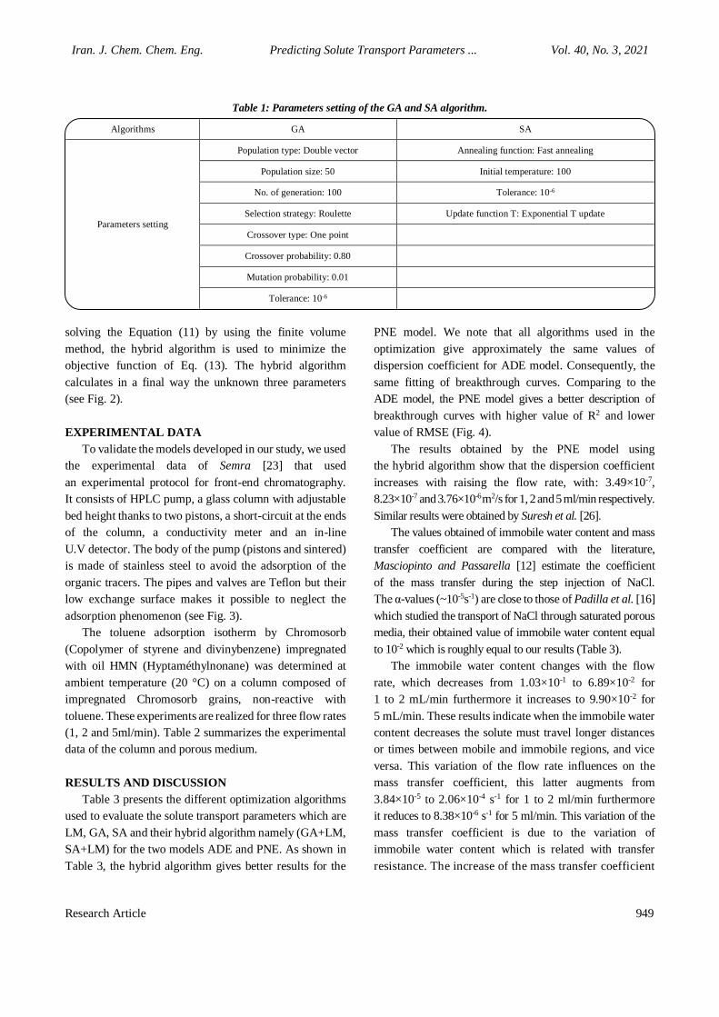
Table 1: Parameters setting of the GA and SA algorithm.

Algorithms GA SA

Parameters setting

Population type: Double vector Annealing function: Fast annealing

Population size: 50 Initial temperature: 100

No. of generation: 100 Tolerance: 10-6

Selection strategy: Roulette Update function T: Exponential T update

Crossover type: One point

Crossover probability: 0.80

Mutation probability: 0.01

Tolerance: 10-6

solving the Equation (11) by using the finite volume

method, the hybrid algorithm is used to minimize the

objective function of Eq. (13). The hybrid algorithm

calculates in a final way the unknown three parameters

(see Fig. 2).

EXPERIMENTAL DATA

To validate the models developed in our study, we used

the experimental data of Semra [23] that used

an experimental protocol for front-end chromatography.

It consists of HPLC pump, a glass column with adjustable

bed height thanks to two pistons, a short-circuit at the ends

of the column, a conductivity meter and an in-line

U.V detector. The body of the pump (pistons and sintered)

is made of stainless steel to avoid the adsorption of the

organic tracers. The pipes and valves are Teflon but their

low exchange surface makes it possible to neglect the

adsorption phenomenon (see Fig. 3).

The toluene adsorption isotherm by Chromosorb

(Copolymer of styrene and divinybenzene) impregnated

with oil HMN (Hyptaméthylnonane) was determined at

ambient temperature (20 °C) on a column composed of

impregnated Chromosorb grains, non-reactive with

toluene. These experiments are realized for three flow rates

(1, 2 and 5ml/min). Table 2 summarizes the experimental

data of the column and porous medium.

RESULTS AND DISCUSSION

Table 3 presents the different optimization algorithms

used to evaluate the solute transport parameters which are

LM, GA, SA and their hybrid algorithm namely (GA+LM,

SA+LM) for the two models ADE and PNE. As shown in

Table 3, the hybrid algorithm gives better results for the

PNE model. We note that all algorithms used in the

optimization give approximately the same values of

dispersion coefficient for ADE model. Consequently, the

same fitting of breakthrough curves. Comparing to the

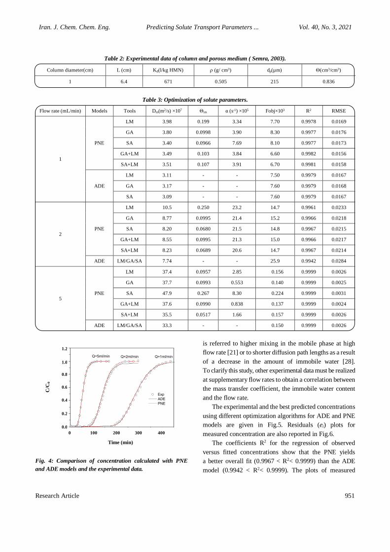
ADE model, the PNE model gives a better description of

breakthrough curves with higher value of R2 and lower

value of RMSE (Fig. 4).

The results obtained by the PNE model using

the hybrid algorithm show that the dispersion coefficient

increases with raising the flow rate, with: 3.49×10-7,

8.23×10-7 and 3.76×10-6 m2/s for 1, 2 and 5 ml/min respectively.

Similar results were obtained by Suresh et al. [26].

The values obtained of immobile water content and mass

transfer coefficient are compared with the literature,

Masciopinto and Passarella [12] estimate the coefficient

of the mass transfer during the step injection of NaCl.

The α-values (~10-5s-1) are close to those of Padilla et al. [16]

which studied the transport of NaCl through saturated porous

media, their obtained value of immobile water content equal

to 10-2 which is roughly equal to our results (Table 3).

The immobile water content changes with the flow

rate, which decreases from 1.03×10-1 to 6.89×10-2 for

1 to 2 mL/min furthermore it increases to 9.90×10-2 for

5 mL/min. These results indicate when the immobile water

content decreases the solute must travel longer distances

or times between mobile and immobile regions, and vice

versa. This variation of the flow rate influences on the

mass transfer coefficient, this latter augments from

3.84×10-5 to 2.06×10-4 s-1 for 1 to 2 ml/min furthermore

it reduces to 8.38×10-6 s-1 for 5 ml/min. This variation of the

mass transfer coefficient is due to the variation of

immobile water content which is related with transfer

resistance. The increase of the mass transfer coefficient

Iran. J. Chem. Chem. Eng. Bouredji H. et al. Vol. 40, No. 3, 2021

950 Research Article

Fig. 2: The flowchart for evaluating solute transport parameters.

Fig. 3: The experimental editing used by Semra [23].

Optimization Routine

N

Experimental data

Initialization of concentration

Calculation: A(i), A(i-1), A(i+1), Sr

Implement boundary condition

Calculation:

Input data

Optimal values of solute transport

parameters

Stopping criteria i.e. finding

minimum of objective

function

Y

Calculation:

C (L,t) /C0

U.V

HPLC Pump CO2

Tracer Solution

Acquisition

effluent

Conductivity

Iran. J. Chem. Chem. Eng. Predicting Solute Transport Parameters ... Vol. 40, No. 3, 2021

Research Article 951

Table 2: Experimental data of column and porous medium ( Semra, 2003).

Column diameter(cm) L (cm) Kd(l/kg HMN) (g/ cm3) dp(µm) (cm3/cm3)

1 6.4 671 0.505 215 0.836

Table 3: Optimization of solute parameters.

Flow rate (mL/min) Models Tools Dm(m2/s) ×107 Θim α (s-1) ×105 Fobj×103 R2 RMSE

1

PNE

LM 3.98 0.199 3.34 7.70 0.9978 0.0169

GA 3.80 0.0998 3.90 8.30 0.9977 0.0176

SA 3.40 0.0966 7.69 8.10 0.9977 0.0173

GA+LM 3.49 0.103 3.84 6.60 0.9982 0.0156

SA+LM 3.51 0.107 3.91 6.70 0.9981 0.0158

ADE

LM 3.11 - - 7.50 0.9979 0.0167

GA 3.17 - - 7.60 0.9979 0.0168

SA 3.09 - - 7.60 0.9979 0.0167

2 PNE

LM 10.5 0.250 23.2 14.7 0.9961 0.0233

GA 8.77 0.0995 21.4 15.2 0.9966 0.0218

SA 8.20 0.0680 21.5 14.8 0.9967 0.0215

GA+LM 8.55 0.0995 21.3 15.0 0.9966 0.0217

SA+LM 8.23 0.0689 20.6 14.7 0.9967 0.0214

ADE LM/GA/SA 7.74 - - 25.9 0.9942 0.0284

5 PNE

LM 37.4 0.0957 2.85 0.156 0.9999 0.0026

GA 37.7 0.0993 0.553 0.140 0.9999 0.0025

SA 47.9 0.267 8.30 0.224 0.9999 0.0031

GA+LM 37.6 0.0990 0.838 0.137 0.9999 0.0024

SA+LM 35.5 0.0517 1.66 0.157 0.9999 0.0026

ADE LM/GA/SA 33.3 - - 0.150 0.9999 0.0026

Fig. 4: Comparison of concentration calculated with PNE

and ADE models and the experimental data.

is referred to higher mixing in the mobile phase at high

flow rate [21] or to shorter diffusion path lengths as a result

of a decrease in the amount of immobile water [28].

To clarify this study, other experimental data must be realized

at supplementary flow rates to obtain a correlation between

the mass transfer coefficient, the immobile water content

and the flow rate.

The experimental and the best predicted concentrations

using different optimization algorithms for ADE and PNE

models are given in Fig.5. Residuals (ei) plots for

measured concentration are also reported in Fig.6.

The coefficients R2 for the regression of observed

versus fitted concentrations show that the PNE yields

a better overall fit (0.9967 < R2< 0.9999) than the ADE

model (0.9942 < R2< 0.9999). The plots of measured

0 100 200 300 400

0.0

0.2

0.4

0.6

0.8

1.0

1.2

Q=1ml/minQ=2ml/min

C/C

0

Time(min)

Exp

ADE

PNE

Q=5ml/min

Time (min)

0 100 200 300 400

C/C

0

1.2

1.0

0.8

0.6

0.4

0.2

0.0

Iran. J. Chem. Chem. Eng. Bouredji H. et al. Vol. 40, No. 3, 2021

952 Research Article

Fig. 5: Fitting measured and calculated concentration with PNE and ADE models.

Fig. 6: Residual plots of calculated concentration modeled with PNE and ADE.

versus simulated relative concentrations show that PNE-

simulated C/C0 fall on a 45° line, whereas those

of the ADE model are scattered about this line (Fig. 5).

This suggests that the relative concentrations (C/C0)

measured are better represented by the PNE simulated

C/C0 values than those from the ADE model.

In general, residual plots of PNE and ADE showed

a random distribution but with different error variances.

This residual analysis also confirms that the hybrid algorithm

was the best option for solute transport data fitting.

Objective functions values decreased from 7.5×10-3to

6.6×10-3 for flow rate 1 ml/min, from 2.59×10-2to 1.47× 10-

2 for flow rate 2 ml/min and from 1.5×10-4to 1.37×10-4 for

flow rate 5 ml/min (Table 3).

In addition, Fig. 6 shows the mean modeling errors

for the prediction of concentrations. These modeling errors

ranged from 3.1 to 5.6 % for LM and from 3.6 to 4.1 % for

GA+LM. The modeling performance of GA+LM was

better than those obtained with LM.

Finally, the application of hybrid algorithms on PNE

model can be used to handle the experimental data of

the solute transport in saturated porous media.

CONCLUSIONS

In this study, we have presented a one-dimensional

model that describes the transport of contaminants

in a column laboratory. A numerical algorithm has been

presented to solve PNE and ADE models. A semi-

stochastic method proposed to estimate the solute transport

parameters which is a combination of stochastic method

(GA, SA) with deterministic optimization models (LM).

The performance of GA, SA and LM algorithms have been

0.0 0.2 0.4 0.6 0.8 1.0

0.0

0.2

0.4

0.6

0.8

1.0

Ca

lcu

late

d C

/C0

Measured C/C0

R2=0.997

ADE

0.0 0.2 0.4 0.6 0.8 1.0

0.0

0.2

0.4

0.6

0.8

1.0

Ca

lcu

late

d C

/C0

Measured C/C0

R2=0.998

PNE

0.0 0.2 0.4 0.6 0.8 1.0

-0.06

-0.05

-0.04

-0.03

-0.02

-0.01

0.00

0.01

0.02

0.03

0.04

0.05

0.06

Re

sid

ua

l e

i

Measured C/C0

GA+LM PNE

0.0 0.2 0.4 0.6 0.8 1.0

-0.06

-0.05

-0.04

-0.03

-0.02

-0.01

0.00

0.01

0.02

0.03

0.04

0.05

0.06

Re

sid

ua

l e

i

Measured C/C0

LM ADE

Measured C/C0

0.0 0.2 0.4 0.6 0.8 1.0

Ca

lcu

late

d C

/C0

1.0

0.8

0.6

0.4

0.2

0.0

Measured C/C0

0.0 0.2 0.4 0.6 0.8 1.0

Ca

lcu

late

d C

/C0

1.0

0.8

0.6

0.4

0.2

0.0

Measured C/C0

0.0 0.2 0.4 0.6 0.8 1.0

Resi

du

al

ei

0.06

0.04

0.02

0.00

-0.02

-0.04

-0.06

Measured C/C0

0.0 0.2 0.4 0.6 0.8 1.0

Resi

du

al

ei

0.06

0.04

0.02

0.00

-0.02

-0.04

-0.06

Iran. J. Chem. Chem. Eng. Predicting Solute Transport Parameters ... Vol. 40, No. 3, 2021

Research Article 953

tested and compared with hybrid algorithms (GA+LM),

(SA+LM) for the solute transport modeling using

experimental data. In most cases, the average root mean

square error obtained by hybrid algorithms (GA+LM),

(SA+LM) is relatively better than the other ones

algorithms. A better description of breakthrough curves

was providing by the PNE combined with linear isotherm

model; it is found that the PNE parameter values

(immobile water content, mass transfer coefficient

and dispersion coefficient) tend to vary with the flow rate.

Received :Sept, 2019 ; Accepted : Jan. 13, 2020

REFERENCES

[1] Alwan G.M., Improving Operability of Lab-Scale

Spouted Bed Using GlobalStochastic Optimization,

Journal of Engineering Research and Applications,5:

136-146 (2015).

[2] Chen Y.M., Abriola L.M., Alvarez P.J.J., Anid P.J.,

Vogel T.M., Modeling Transport and Biodegradation

of Benzene and Toluene in Sand Aquifer Material:

Comparison with Experimental Measurements,

Water Resour. Res, 28(7): 1833-1847 (1992).

[3] Clothier B.E., Kirkham M.B., Mclean J.E., In Situ

Measurement of the Effective Transport Volume

for Solute Moving Through Soil, Soil Sci. Soc. Am.

J.,56: 733-736 (1992).

[4] Coats K.H., Smith B.D., Dead-End Pore Volume

and Dispersion in Porous Media. Soc. Pet. Eng. J., 4:

73-84 (1964).

[5] De Smedt F., Wierenga P.J., Solute Transfer Through

Columns of Glass Beads, WaterResour. Res., 20: 225-

232 (1984).

[6] Giacobbo F., Marseguerra M., Zio E., Solving

the Inverse Problem of Parameter Estimation by Genetic

Algorithms: The Case of a Groundwater Contaminant

Transport Model, Annals of Nuclear Energy,29:

967–981 (2002).

[7] Goltz M.N., Roberts P.V., Simulations of Physical

Nonequilibrium Solute Transport Models: Application

to a Large Scale Field Experiment, J. Contamin.

Hydrol., 3:37-63(1988).

[8] Jaynes D.B., Logsdon S.D., Horton R., Field Method

for Measuring Mobile/Immobile Water Content and

Solute Transfer Rate Coefficient, Soil Sci. Soc. Am. J.,

59: 352-356 (1995).

[9] Kabouche A., Meniai A., Hasseine A., Estimation of

Coalescence Parameters in an Agitated Extraction

Column Using a Hybrid Algorithm, Chem. Eng.

Technol.,34(5): 784–790 (2011).

[10] Leij F.J., Bradford S.A., Combined Physical and

Chemical Nonequilibrium Transport Model:

Analytical Solution, Moments, and Application

to Colloids, J. Contam. Hydrol.,110: 87–99 (2009).

[11] Manuel Alejandro Salaices Avila, "Experiment and

Modeling of the Competitive Sorption And Transport

of Chlorinated Ethenes in Porous Media", Göttingen–

Germany, (2005).

[12] Masciopinto C., Passarella G., Mass-Transfer Impact

on Solute Mobility in Porous Media: a New Mobile-

Immobile Model, J. Contam. Hydrol.,215: 21-28

(2018).

[13] Mehdinejadiani B., Estimating the Solute Transport

Parameters of the Spatial FractionalAdvection-

Dispersion Equation Using Bees Algorithm, J.

Contam. Hydrol.203: 51-61 (2017).

[14] Merzougui A., Hasseine A., Laiadi D., Liquid-Liquid

Equilibria of {N-Heptane + Toluene + Aniline}

Ternary System: Experimental Data and Correlation,

Fluid Phase Equilib. 308: 142–146 (2011).

[15] Nelson P.A., Galloway, T.R., Particle to Fluid Heat

and Mass Transfer in Dense System to Fine

Particles, Chemical Engineering Science. 30: 1-6

(1975).

[16]Padilla I.Y., Jim Yeh T.-C., Conklin M.H., The Effect

of Water Content on Solute Transport in Unsaturated

Porous Media, Water Resources Research, 35: 3303–

3313 (1999).

[17] Patankar S.V., "Numerical Heat Transfer And Fluid

Flow", USA: New York, Mcgraw-Hill Book

Company, (1980).

[18] Peralta R.C., "Groundwater Optimization Handbook:

Flow, Contaminant Transport, and Conjunctive

Management", Boca Raton, CRC Press, p.532,

(2012).

[19] Perkins T.K., Johnston O.C., A Review of Diffusion

and Dispersion in Porous Media, Society of

Petroleum Engineers Journal,3: 7&84, (1963).

[20] Sardin M., Schweich D., Leij F.J., Van Genuchten M.Th.,

Modeling the Nonequilibrium Transport of Linearly

Interacting Solutes in Porous Media: a Review, Water

Resources Research,27: 2287-2307 (1991).

Iran. J. Chem. Chem. Eng. Bouredji H. et al. Vol. 40, No. 3, 2021

954 Research Article

[21] Selim H.M., Ma L., "Physical Non-Equilibrium

in Soils: Modeling and Application", Ann Arbor Press,

Inc., Chelsea, Mich, (1998).

[22] Selim H.M., "Transport &Fate of Chemicals in Soils

Principles&Applications", CRC Press, (2015).

[23] Semra S., "Dispersion Réactive En Milieu Poreux

Naturel", Thèse, Génie Des Procédés. Nancy, INPL,

(2003).

[24] Shahram Shahmohammadi-Kalalagh, Modeling

Contaminant Transport In Saturated Soil Column

With The Continuous Time Random Walk, Journal

Of Porous Media, 18: 1181-1186 (2015).

[25] Sharma P.K., Shukla S.K., Rahul Choudhary, Deepak

Swami, Modeling for Solute Transport in Mobile–

Immobile Soil Column Experiment, ISH Journal of

Hydraulic Engineering, (2016).

[26] Suresh A.Kartha, Srivastava R., Effect of Immobile

Water Content Contaminant Transport in Unsaturated

Zone, Journal of Hydro-Environment Research, 1:

206-215 (2008).

[27] Van Genuchten M.Th., Cleary R.W., "Movement of

Solutes in Soil: Computer Simulated And Laboratory

Results", Chap. 10 In: Soil Chemistry: B.

Physicochemical Model, G.H. Bolt, (Ed.), Elsevier,

Amsterdam, (1979).

[28] Van Genuchten M. Th., Non-Equilibrium Transport

Parameters From Miscible Displacement

Experiments, Res. Rep. No. 119, U.S. Salinity Lab.

USDA, ARS, Riverside, CA, (1981).

[29] Van Viet Ngo, "Modélisation Du Transport De L’eau

Et Des Hydrocarbures Aromatiques Polycycliques

(HAP) Dans Les Sols De Friches Industrielles",

Thèse De Doctorat INPL, Nancy-France, 172 P,

(2009).

[30] Zheng C., Bennet G.D., "Applied Contaminant Transport

Modeling: Theory and Practice", van Nostrand

Reinhold, New York, 464 P, (1995).