Visualization of bacteria density distributions in saturated sand columns

using X-ray computed tomography

A thesis submitted to McGill University in partial fulfilment of the requirements of the degree of Master of Engineering

Presented by

Gregory McKenna

Department of Civil Engineering and Applied Mechanics McGill University, Montreal, Quebec, Canada

February 2008

© Gregory McKenna, 2008

1*1 Library and Archives Canada

Published Heritage Branch

395 Wellington Street Ottawa ON K1A0N4 Canada

Bibliotheque et Archives Canada

Direction du Patrimoine de I'edition

395, rue Wellington Ottawa ON K1A0N4 Canada

Your file Votre reference ISBN: 978-0-494-48334-3 Our file Notre reference ISBN: 978-0-494-48334-3

NOTICE: The author has granted a non­exclusive license allowing Library and Archives Canada to reproduce, publish, archive, preserve, conserve, communicate to the public by telecommunication or on the Internet, loan, distribute and sell theses worldwide, for commercial or non­commercial purposes, in microform, paper, electronic and/or any other formats.

AVIS: L'auteur a accorde une licence non exclusive permettant a la Bibliotheque et Archives Canada de reproduire, publier, archiver, sauvegarder, conserver, transmettre au public par telecommunication ou par Plntemet, prefer, distribuer et vendre des theses partout dans le monde, a des fins commerciales ou autres, sur support microforme, papier, electronique et/ou autres formats.

The author retains copyright ownership and moral rights in this thesis. Neither the thesis nor substantial extracts from it may be printed or otherwise reproduced without the author's permission.

L'auteur conserve la propriete du droit d'auteur et des droits moraux qui protege cette these. Ni la these ni des extraits substantiels de celle-ci ne doivent etre imprimes ou autrement reproduits sans son autorisation.

In compliance with the Canadian Privacy Act some supporting forms may have been removed from this thesis.

Conformement a la loi canadienne sur la protection de la vie privee, quelques formulaires secondaires ont ete enleves de cette these.

While these forms may be included in the document page count, their removal does not represent any loss of content from the thesis.

Canada

Bien que ces formulaires aient inclus dans la pagination, il n'y aura aucun contenu manquant.

Abstract

The transport of bacteria in granular porous media is important to many environmental

applications. Traditionally, the fate of bacteria in porous media has been studied using

bench-scale column experiments while monitoring the suspended effluent concentration.

Determining the spatial distribution of deposited bacteria in the column using a non­

invasive and non-destructive technique has the potential to improve the understanding of

some transport processes for bacteria. In this study, a preliminary X-ray computed

tomography (X-ray CT) technique is developed to analyze the density distribution of

bacteria within a saturated column. Bacteria cells are generally not detectable in water

saturated columns because their X-ray attenuation properties are similar to water.

Nanosized gold particles were synthesized in the presence of cetyltrirnethylammonium

bromide and were attached to the bacteria forming a monolayer of gold coverage at the

bacteria surface. These gold-labelled cells were detectable during CT scanning at

concentrations of 3 x 10 cells/mL when injected into water saturated sand columns and

thus allowed for the determination of areas of high deposition in packed sand columns.

i

Resume

Le transport des microbes est important pour une variete d'applications environmentales.

Traditionellement, le destin des microbes en media poreux est examine utilisant des

experiences en colonne en observant la concentration de 1'effluent. La determination de

la distribution spatiale des microbes deposes dans la colonne en relation a la structure des

pores en utilisant une methode non-destructive pourrait ameliorer nos connaissances des

mecanismes pour le transport des microbes. Dans cette etude, une technique preliminaire

est developee afin d'etudier la distribution des microbes dans des colonnes saturees en

utilisant la tomographic calculee aux rayons X. Des nanoparticules en or sont

synthetisees dans la presence de la bromure de cyltrimethylarnmonium et sont attachees

aux microbes afin de couvrir la surface des bacteries. Ces bacteries recouvertes en or

peuvent etre detectes avec la tomographic calculee aux rayons X a partir d'une

concentration de 3 x 107 microbes/mL lors de l'injection dans des colonnes saturees nous

permettes de determiner les regions de deposition elevees dans des colonnes de sable

saturees.

II

Acknowledgements

It is with great appreciation and much respect that I thank my supervisors, Prof. Subhasis

Ghoshal and Prof. Nathalie Tufenkji for their valuable assistance and guidance

throughout the course of this thesis project. Their ideas, insightful comments and

encouragement have kept this project and me on course and on time, and could not have

been completed without their help.

Along the way, I have had the privilege of working with numerous individuals who have

made contributions to this project and deserve to be thanked. Prof. Dominic Frigon, for

his help discussing many bacteria related questions. Line Mongeon, for her extensive

patience and assistance with the SEM, as well as the other technicians in the Facility for

Electron Microscopy Research who were always willing to help me out, especially Lee

Ann Monaghan and Jeannie Mui. Dr. Pierre Dutilleul and Liwen Han at the CT Scanning

for their help dealing with CT problems and issues, as well as their aid when using the

helical scanning mode of the CT scanner.

Funding for this research was made possible through grants from the Centre for

Biorecognition and Biosensors (CBB) and the Natural Sciences and Engineering

Research Council of Canada (NSERC).

Finally, this Master's thesis would not have been a success without the support, love and

encouragement from my family and friends who have been there for me through the good

and bad times and have kept me going this whole time. It is to them that I dedicate this

thesis.

in

Table of Contents

ABSTRACT i

RESUME n

ACKNOWLEDGEMENTS in

TABLE OF CONTENTS iv

LIST OF SYMBOLS vi

LIST OF TABLES vn

LIST OF FIGURES v m

LIST OF APPENDICES x

CHAPTER 1: INTRODUCTION 1

1.1 Problem Statement 3

1.2 Objectives 5

1.3 Scope and Approach 6

1.4 Thesis Organization 8

CHAPTER 2: LITERATURE REVIEW 9

2.1 Classical Colloid Filtration Theory 9

2.2 Deviations from Classical Colloid Filtration Theory 16

2.2.1 Dual Deposition Mode Model 16 2.2.2 Straining 17 2.2.3 Particle Shape 18 2.2.4 Biological Activity 19

2.3 Use of Nanoparticles in Biological Research.... 20

2.4 X-ray Computed Tomography 22

2.4.1 Basic Principles 22 2.4.2 Contrast agents '. 24

IV

CHAPTER 3: MATERIALS AND M E T H O D S 25

3.1 Bacteria 25

3.2 Porous Media Characterization 27

3.3 Gold Nanoparticle Synthesis and Preparation 28

3.4 Bacteria Labelling 31

3.5 SEM Imaging 31

3.6 Column Transport Experiments 33

3.7 CT Scanning 35

3.8 CT Data Analysis 38

CHAPTER 4: RESULTS AND DISCUSSION 43

4.1 Characterization of Bacillus subtilis Cells 43

4.2 Characterization of Synthesized Gold Nanoparticles 45

4.3 Characterization of Labelled Bacteria 49

4.4 Cell Viability in the Labelling Process... 54

4.5 Validation of SEM Imaging Technique 56

4.6 CT Number Measurements 58

4.7 Colloid Transport in Homogeneous Sand Columns 61

4.8 Colloid Transport in Layered Columns 68

4.9 Precision and Repeatability of Measurements Determined from X-ray CT 82

CHAPTER 5: SUMMARY AND CONCLUSIONS 85

C H A P T E R 6: FUTURE W O R K AND RECOMMENDATIONS 88

v

List of Symbols

A Hamaker constant As porosity-dependent parameter of Happel's model ap radius of particle C fluid phase concentration D hydrodynamic dispersion coefficient dc diameter of the collector grain dp di am eter of the parti cl e E energy of X-ray beam fa'J'k volume fraction for material a in voxel at position i,j,k I intensity of X-ray beam k particle deposition rate coefficient kB Boltzmann constant, 1.3805 x 10"23 J/K NA attraction number NG gravity number NLO London number Npe Peel et number NR aspect ratio Nvdw van der Waals number S solid phase concentration v velocity of fluid T absolute temperature / time U approach (superficial) velocity of fluid Vj'J'k volume of material a in voxel at position i,j,k v porewater velocity Xa'J' CT number for material a in voxel at position i,j,k x distance Z effective atomic number

Greek Symbols

a attachment efficiency s porosity r] single-collector removal efficiency ?7o single-collector contact efficiency rjD single-collector contact efficiency for transport by diffusion TJG single-collector contact efficiency for transport by gravity t]j single-collector contact efficiency for transport by interception fi absolute viscosity of fluid pb bulk density Pf density of fluid pp density of particle oj linear attenuation coefficient for material /

VI

List of Tables

Table 1: XVision scanner settings 37

Table 2: Measured mean CT numbers for materials used in study 58

Table 3: Calculated values ofrjgfor the different colloids and sand grain sizes 79

Table 4: Control volume calculations for error measurement 84

VII

List of Figures

Figure 1: An illustration of the different colloid transport mechanisms [4]. 11

Figure 2: The influence of particle size, dp, on the single collector efficiency, i] [4] 12

Figure 3: Microscope images of the coarse sand grains used in this study. 28

Figure 4: The set-up of the apparatus used for the column experiments. 34

Figure 5: SEM image showing Bacillus subtilis bacteria. The size of the bacteria is ca. 2.0 fim in length

and ca. 0.75 fjan in diameter. Note the chain-like structures formed by multiple bacteria. 44

Figure 6: Calibration curve for cell concentration versus absorbance. 45

Figure 7: Absorbance spectrum for gold seeds (A) and gold nanoparticles (B). The peak for the gold seeds

occurs at 520 nm whereas for the gold nanoparticles, the peak is at 535 nm. 46

Figure 8: SEM image showing gold nanoparticles. The size of the nanoparticle is approximately 100 nm.

47

Figure 9: Calibration curve for gold particle concentration versus absorbance. 48

Figure 10: SEM image's showing bacteria labelled with gold particles at low magnification (A) and high

magnification (B) to show nanoparticle detail. 51

Figure 11: SEM image showing cell bridging caused by high cell to nanoparticle ratio 52

Figure 12: SEM images taken 1 hour (A) and 24 hours (B) after labelling showing that the gold

nanoparticles remain bound to the cells and that the cells maintain their shape 55

Figure 13: Representative image of cells obtained using new preparation technique. 56

Figure 14: Representative image of cells obtained using the standard preparation technique (A) and from

Environmental SEM (B). 57

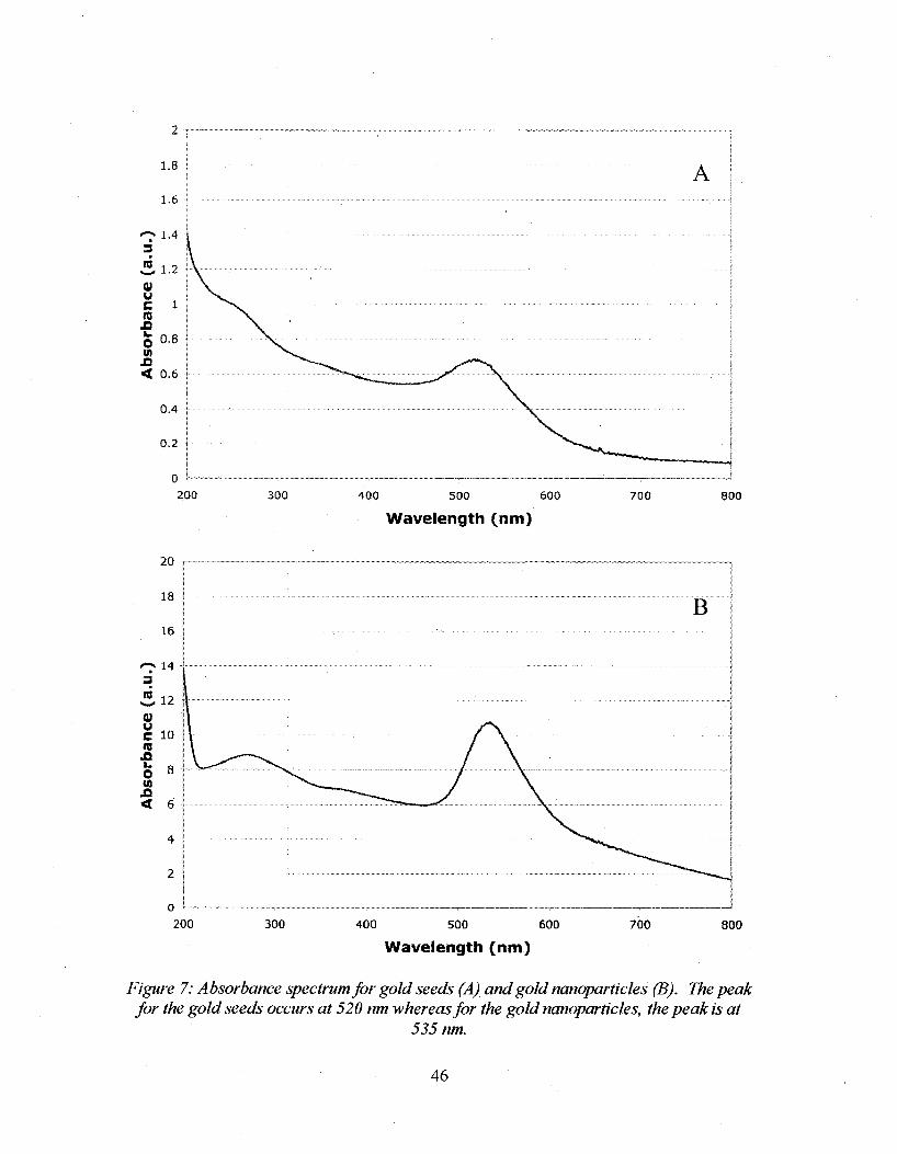
Figure 15: Calibration curve for gold nanoparticle concentration versus CT number. 60

Figure 16: Calibration curve for gold-labelled cells versus CT number. 60

Figure 17: Representative breakthrough curve for gold nanoparticles (+) and gold-labelled cells (O) in a

sand column with constant grain size. Key experimental conditions: pH =6.5, flow rate = lmL/min,

porosity = 0.42, mean sand grain diameter = 800 /urn, temperature = 25°C. 62

VIII

Figure 18: Retained profile for gold nanoparticles (+, left axis) and gold-labelled cells (O, right axis) in a

sand column with constant grain size. Key experimental conditions: pH =6.5, flow rate = lmL/min,

porosity = 0.42, mean sand grain diameter = 800 /urn, temperature = 25°C. 64

Figure 19: Representative slice images generated from CT data showing volume fractions of gold particles

in each voxel for the homogeneous columns 65

Figure 20: Representative slice images generated from CT data showing volume fractions of gold-labelled

cells in each voxel for homogeneous columns 66

Figure 21: Porosity per slice for the first experiment using a constant grain size. 67

Figure 22: Photograph of the column showing the interface between the coarse sand grains and the fine

sand grains. In this image, the flow direction is from top to bottom. 69

Figure 23: Representative breakthrough curve for gold nanoparticles (+) and gold-labelled cells (U\) in a

sand column with dual grain size. 70

Figure 24: Retained profile for gold nanoparticles (+, left axis) and gold-labelled cells (D, right axis) in a

sand column with coarse and fine sand. Key experimental conditions: ionic strength — constant, pH =6.5,

flow rate = lmL/min, porosity = 0.42, mean coarse grain diameter = 800 fxm, mean fine grain diameter =

200 pan, temperature = 25 °C, interface at 20 mm (slice 20). 73

Figure 25: Photograph showing the particle accumulation at the exterior of the column. 74

Figure 26: Representative slice images generated from CT data showing volume fractions of gold particles

in each voxel for layered columns 75

Figure 27: Representative slice images generated from CT data showing volume fractions of gold-labelled

cells in each voxel for layered columns ____ 76

Figure 28: Porosity per slice for the second experiment using coarse and fine sand 77

Figure 29: Photograph showing gold-labelled cell accumulation at the interface of the coarse and fine

sand grains (dark region in the middle of the column). 87

Figure 30: Photograph showing the retained gold-labelled cells (left) and the retained gold nanoparticles

(right) after a column experiment with coarse grains. 82

IX

List of Appendices

Appendix A: MA TLAB Programs 102

X

Chapter 1: Introduction

Recently in 1993, in Milwaukee, MI, and then again in 2000, in Walkerton, ON,

outbreaks of pathogens in local drinking water supplies have been linked to the

hospitalization and death of many people in those areas. It was later determined that the

source of the outbreaks was the infiltration of contaminated surface waters into the

groundwater that supplied the towns with their potable source [1]. Though this was

further impacted by negligence of town officials, these deaths may have been avoided

had better predictions been made concerning the fate of these types of pathogens in the

groundwater.

These incidents, among others, have directed a substantial research effort toward

understanding the transport behaviour of microorganisms and colloids in porous media.

Knowing the physical, chemical and biological mechanisms involved in the deposition

and removal of these colloids in the subsurface is also relevant to a broad range of

engineering, geophysical and environmental processes such as in situ bioremediation [2,

3], deep-bed filtration for water and wastewater treatment [4, 5], siltation of streambeds

[6], riverbank filtration [7] and pathogen transport in surface and subsurface waters [8, 9].

Colloids may also facilitate the transport of other contaminants by serving as carriers

thereby accelerating the arrival times of these contaminants relative to predictions based

on classic solute transport models [10-12].

1

Not only is it important to understand the transport behaviour of bacteria in the soil to

avoid negative consequences, bacteria can also be used in numerous positive degradation

schemes in which a knowledge of their behaviour in the soil is required. Bacteria, and

other microbes present in the soil, can degrade a wide variety of organic and inorganic

contaminants [2, 13], and enhance the mobility of radionuclides, metals and other toxic

contaminants in the subsurface [14]. These natural capabilities of the microorganisms in

the soil are harnessed and accelerated in biostimulation to restore contaminated aquifers,

and in other applications bacteria are injected into the soil or aquifer to increase and

diversify the microbial community in bioaugmentation strategies [3], or to degrade

mobile contaminants using biobarriers [3, 13]. An improved understanding of the factors

controlling the fate and transport of microbes is therefore essential in the design of these

various remediation applications.

The transport of microorganisms in the subsurface is also of interest, both from the

standpoint of mitigating pathogen contamination and for the protection of our drinking

water supplies. Viruses, protozoa and other bacteria are pathogens of concern that may be

introduced to the groundwater supply through infiltration from land disposal of waste or

from farms and feedlots [1, 14, 15]. Understanding the interaction and removal of these

microbes in the soil is essential for the safety of the population who drink water supplied

by groundwater sources.

2

1.1 Problem Statement

Traditionally, the transport of microorganisms and other colloids has been studied in

experiments with bench-scale packed columns filled with a homogeneous, "ideal" media

such as glass beads or clean sand, where the changes in effluent concentration are

monitored as a function of time and compared to the influent concentration [14, 15].

These experiments have allowed researchers to establish a basic understanding of the

nature of the interactions between colloids and porous media as well as the influence of

solution chemistry. However, solely analyzing these "breakthrough curves" has been

shown to be inadequate for identifying the fundamental mechanisms governing the

transport and deposition of the colloids. Instead, the spatial distribution of the colloids

within the packed column has been shown to provide a more accurate mechanistic

interpretation of colloid-media interactions [16-18]. As such, the packed columns must

be carefully extruded and sectioned following the flow experiments to allow the

researchers to examine the spatial distribution of the retained colloids. Though used

successfully in several studies, this destructive method of analysis does not allow for

observations over time in a particular column [15]. As such, it is apparent that non­

invasive visualization of columns during and after flow experiments could greatly

enhance the understanding of colloid transport and deposition behaviour in porous media.

A variety of studies have used non-invasive visualization techniques to evaluate the

transport and deposition of colloids in porous media. These occur generally at two

scales: porescale/microscale and Darcy/mesoscale. At the microscale, researchers use

3

direct observation to study the interaction of individual colloids with air, water,

contaminant and solid interfaces. This also enables the researchers to analyze the effect

of microscale heterogeneities such as pore configuration and surface roughness or

chemistry These studies regularly use a flow cell made of etched glass or silicon and a

fluorescent visualization technique [19-21]. For studies conducted at the mesoscale,

researchers do not track individual colloids. Rather, the concentration of the colloids in a

given volume of media is determined for tracking the overall movement of the colloid

and for the investigation of the influence of various media heterogeneities on the

deposition behaviour. Mesoscale studies are also able to work with larger volumes of

porous media than microscale studies.

Two main types of visualization systems are currently being used in mesoscale studies:

epifluorescent systems [22, 23], and magnetic resonance imaging (MRI) [24-26]. MRI

has been used to study both colloid [24] and bacteria [25, 26] transport in porous media.

Using iron-oxide nanoparticles attached to the surface of Pseudomonasputida and

Escherichia coli, the authors were able to visualize the distribution of the bacteria within

a saturated sand column. However, because MRI is not capable of imaging porous media

characteristics, those authors did not attempt any meaningful correlation of the bacterial

distributions with respect to the porous media structure.

X-ray computed tomography (X-ray CT) has the advantage that it can visualize and

quantify porous media characteristics and provide superior 3-D images of the interior

4

features of the column based on density differences. Particle colloid transport has been

visualized in X-ray CT, but only at the microscale [27], however, the use of X-ray CT for

the imaging of bacterial density distributions in porous media has not been previously

attempted. Using X-ray CT as a non-invasive visualization technique for the

investigation of the fate of colloids in column experiments will enhance the mechanistic

understanding of the transport and deposition behaviour of colloids and bacteria in porous

media.

1.2 Objectives

The overall objective of this study was to quantify the bacterial density distribution

within a saturated sand column using X-ray CT. Specifically, the objectives were to:

1) Use gold nanoparticles as a contrast agent for the detection of bacteria by the X-

ray CT scanner and develop a labelling technique to attach these nanoparticles to

the surface of the bacteria

2) Determine the detection limit for the gold nanoparticles and gold-labelled bacteria

in the X-ray CT scanner

3) Conduct conventional column transport experiments with both gold nanoparticles

and gold-labelled cells, and use the X-ray CT scanner to non-invasively quantify

their spatial distribution within the saturated sand column.

5

1.3 Scope and Approach

In this study, the density distribution of nanoparticles and bacteria within saturated soil

columns was quantified using X-ray CT technology. These columns were scanned using

a Toshiba XVision whole body medical CT scanner (Toshiba, 1994) installed at McGill

University's CT Scanning Laboratory for Agricultural and Environmental Research

located on the Macdonald Campus, Ste-Anne-de-Bellevue, Quebec, Canada. Though this

was not the first study to use the X-ray CT scanner at this lab, the helical scanning mode

was used for the first time when working with columns containing saturated porous

media. This required the determination of appropriate scanning parameters and optimum

scanner settings to be used for the remainder of the study.

In order to quantify the bacterial density distributions within the saturated sand columns,

a contrast agent was needed to enhance the attenuation of the bacteria in the X-ray CT

scanner. During X-ray CT scanning, the attenuation of the X-ray beam as it passes

through the sample is measured, and the 3-D distribution of attenuations is recorded over

the length of the sample. The attenuation of the X-ray by the sample is dependent on its

density and atomic number. In order to distinguish the X-ray attenuation of the bacteria

from the X-ray attenuation of the fluid phase, gold nanoparticles were selected as a

suitable contrast agent due to their high density and atomic number.

6

The gold nanoparticles used in this study were synthesized in the lab to allow for the

appropriate surface modifications that were required to attach the nanoparticles to the cell

surfaces. The Gram-positive bacterial strain, Bacillus subtilis, was used in this study. All

bacteria work was conducted in a Bio Safety Level 2 laboratory to conform to the safety

and health requirements.

The gold nanoparticles, and the labelled and unlabelled cells were characterized in the

laboratory. Images were obtained using a scanning electron microscope (SEM) in order

to visualize their surfaces. As well, their detection limits and behaviour in the X-ray CT

scanner were determined.

Traditional column experiments were conducted using both the gold nanoparticles and

the gold-labelled cells. Column experiments were first conducted using homogeneous,

coarse quartz sand. Subsequently, column experiments were conducted using a layered

combination of coarse and fine quartz sand to determine the effect of heterogeneity on the

deposition behaviour within the column. Before and after the injection of the colloids

into the column for each experiment, the sample was scanned using the X-ray CT

scanner. The data acquired from the X-ray CT scanner was used to quantify the spatial

distribution of the colloids within the sand columns by image subtraction.

7

1.4 Thesis Organization

This thesis is organized as follows:

Chapter 2: Literature Review. This section will be divided into four parts. The first

section will give an overview of classical colloid filtration theory. The second section

will look at possible explanations for the deviations observed from classical colloid

filtration theory models. Third, the use of nanoparticles in biological research will be

discussed. And finally, the fourth section will summarize the X-ray CT technology and

its uses in porous media applications.

Chapter 3: Materials and Methods. A detailed description of the methods used in this

study will be presented in this section. This will focus on the synthesis of gold

nanoparticles, the bacteria labelling, and the column experiments using X-ray computed

tomography.

Chapter 4: Results and Discussions. The characterization of the various components of

this study will first be discussed followed by the analysis of the column transport

experiments and the X-ray CT data.

Chapter 5: Summary and Conclusions. This section provides a summary of this study

and presents the final conclusions.

Chapter 6: Recommendations for Future Research. Based on the results and conclusions

in this thesis, recommendations are presented in this section for the further development

and use of this X-ray computed tomography technique.

8

Chapter 2: Literature Review

2.1 Classical Colloid Filtration Theory

Colloid deposition during transport in granular porous media is described using classical

colloid filtration theory. Colloids are generally described as particles with at least one

dimension less than 1 jxm. The most used model to describe these processes was

proposed by Yao et al. [4] and has been further expanded by others [5, 28]. The

underlying principle is that the filter bed (or porous media) is represented by Happel's

sphere-in-cell model [29]. The porous media is idealized as an assemblage of individual

spherical collectors (usually glass beads in experiments) that are each surrounded by a

spherical shell of fluid. This fluid envelope is scaled to maintain the porosity of the

actual porous media [29].

The colloids are transported in the fluid flowing around the spherical collectors and their

removal is represented by first order kinetics in which the concentration of suspended and

retained particles declines exponentially with distance. This can be expressed as:

dC d2C dC — = D—--v kC (1) dt dx dx

where D is the hydrodynamic dispersion coefficient, v is the porewater velocity and k is

the particle deposition rate coefficient. The removal of particles from the pore fluid to

the solid (collector) surface is described as follows:

9

* C - - ^ (2) 6 dt

where pi, and s represent the bulk density and the porosity of the porous medium,

respectively. In equations 1 and 2, C is the fluid phase concentration and S is the solid

phase concentration of the colloids. The particle deposition rate coefficient is also related

to the single-collector removal efficiency, //, which describes the probability of a colloid

collision with, and attachment to, the collector, k and r\ are related by the formula:

* = * ^ % (3) 2d,

where dc is the diameter of the collector.

The transport of the particles from the fluid phase to the collector is governed by three

main mechanisms: sedimentation, interception, and Brownian diffusion [4].

Sedimentation will occur when the particle density is greater than the fluid density.

Interception occurs when the streamline guides the particles onto the collector grains.

Brownian diffusion occurs when hydrodynamic forces cause particles to deviate from the

streamlines and contact the collectors. These three mechanisms are shown graphically in

Figure 1.

10

— — PARTICLE TRAJECTORY

— STREAMLINE

COLLECTOR-

A INTERCEPTION

8 SEDIMENTATION

C DIFFUSION

% .1

Figure J: An illustration of the different colloid transport mechanisms [4].

In the model proposed by Yao et al. [4], it was suggested that these three mechanisms are

additive and that their total effect described the single-collector contact efficiency, n0,

which is the ratio of the rate of particle contact with the collector to the rate of transport

of particles to the projected area of the collector. This can also be described as the total

number of possible contacts between particles and collectors. Considering the three

governing mechanisms of transport to the collectors, n0 is described as:

Vo = VD + Vi + *7G (4)

11

where no, tfi, and TJG are the contributions from diffusion, interception and sedimentation,

respectively. As seen in Figure 2, the size of the particles influences the effect of each of

these terms.

10** iO** I Id

Size OF THE $mmmm M*flCLE$ (mmmm)

Figure 2: The influence of particle size, dp, on the single collector efficiency, rj [4]

In this model, Yao et al. [4] proposed that each of these terms describing no could be

described as follows:

f]D=4.04N] Pe (5)

Vi" 3(dp\

\dc/

(6)

12

where NPe is the Peclet number, described as:

"r,=f (8)

where D w = - ^ - (9) 6jz[ia

and ap is the particle radius.

This model was further refined by Rajagopalan & Tien (1976) in order to further

parameterize the expression for rjo and validate this expression with experimental data.

Their final expression for the single-collector contact efficiency was:

ri0 - 4.04Al'3N-£3 + AXR'V + 0.00338A^-a40^'2 (10)

where NR=— (11) d„

A f t o = - A - (12) 9npiapU

2(1 -y5) A= o 3 ' (13)

1 Y + ~Y ~Y 2 2

r - ( i - « ) 1 / 3 (14)

13

Though this model is used in practice and in research, it is limited to certain applications.

The first limitation of this model is due to the fact that is describes a system where the

colloid particles are no less than 1 ^m [5]. Second, the model neglects van der Waals

forces and hydrodynamic interactions when looking at the Brownian motion of the

particles [28].

As such, a new model for rjo was proposed by Tufenkji and Elimelech [28] and describes

the three mechanisms of transport to a greater extent using additional dimensionless

parameters:

r70 = lAA^N-r'Nf^NZ1 + O.SSA^N0/25 + 0.22Nf™N^N^3 (15)

where Nvdw=-— (16) kBT

KA=NvdwX*Np: • 0? )

Nc = 2_al(pp-Pf)8 9 [ill

Many forces, such as electrostatic and hydrodynamic forces influence the attachment of

the particles to the collectors because, though the particles may contact the collectors,

they may not remain permanently attached. The attachment efficiency, or, is used to

describe the relationship between the number of successful collisions and the total

number of collisions where:

14

r\- ar}o (19)

Unfortunately, there are no current theories that are able to predict the attachment

efficiency, but the single-collector removal efficiency, //, can be determined

experimentally from:

V-^TATTHCICO) 3 (l-e)L

(20)

and related to a using the model for r\0 described above in Equation 15.

For most applications of classical colloidal filtration theory, the system is at steady state

and the influence of hydrodynamic dispersion is assumed to be negligible. Another

assumption is that a single particle deposition rate, k, can be assigned for the entire

system. With these assumptions, and for a continuous injection of colloids at a

concentration, C = Co, the concentrations of particles in the fluid and solid phases as a

function of distance for a specific time, t = to are determined as follows:

C(x) = C0exp -3 (1-e)

T 1 - -X

2 ' d = C (21)

and:

*f \C/C fn£/CC n S(X) = - ^ C ( x ) = ° °exp Pb Pb

(22)

15

This set of equations is commonly referred to as the classical colloid filtration model [16]

and has been used extensively for modelling the transport and fate of all types of colloids

in saturated porous media [12, 16, 17, 27, 28, 30-34].

2.2 Deviations from Classical Colloid Filtration Theory

2.2.1 Dual Deposition Mode Model

Classic filtration theory is based on the assumption that k is constant. However,

heterogeneity in the colloidal interactions between particles and collectors can give rise to

a variation in the deposition rate [16]. In some experiments, a dual deposition mode

seems to occur with a portion of the particles having a fast deposition rate and the others

being slow [16, 34]. The profile of the retained particles displays a bimodal distribution

in the particle deposition rate with a steep slope at the top of the column (near the

influent) and a more gradual slope at the bottom [18, 34].

One explanation of this phenomenon relies on DLVO theory. The interaction of the

repulsive electrostatic double layer and the attractive van der Waals forces change as a

function of ionic strength [35, 36]. At high ionic strengths, the electrostatic force is

weak, and thus the particles are able to deposit onto the collectors in the secondary

minimum, whereas, at low ionic strengths, the electrostatic force is strong, and the

particles require more energy to overcome this energy barrier. As such, a greater

attachment occurs at high ionic strengths than at low ionic strength [16]. This has been

verified by flushing the column after a high ionic strength solution with a low ionic

16

strength solution, causing the particles deposited in this secondary minimum to become

detached, leaving only those attached in the primary minimum [16, 34]. Furthermore, it

has been argued that heterogeneity in the particle population can give rise to distributed

particle-collector interaction energies, thereby leading to a non-constant particle

deposition rate [16, 37].

2.2.2 Straining

Another possible explanation for the observed deviation from classical colloid filtration

theory is straining. Straining is a physical removal process in which colloid particles are

trapped in the down-gradient pore throats that are too small to allow particle passage [38-

40]. This occurs when particles are not able to pass around collectors, as described by

Happel's sphere-in-cell fluid model, and become trapped between two or more collectors

[38, 41]. In this model, there is a sphere of fluid completely surrounding each of the

collectors [29], but in practice this is not true; a packed saturated porous media column

has the collector grains supported via grain-to-grain contacts and it is not possible to have

a single collector completely surrounded by a sphere of fluid [42]. The deposition of

particles at these grain-to-grain contacts have been shown to strongly influence the spatial

distribution of the retained colloids in porous media [27, 42]. From geometric modelling

of the relationship between particle diameter and the mean collector diameter, straining

was determined to be negligible if d/dc < 0.05 [43-45], but has been argued to be more in

the range of 0.002 based on experimental evidence [39, 40, 46-48].

17

The amount of straining observed in a packed column has also been related to other

physical and chemical mechanisms. Straining increases with increasing ionic strength

[49, 50], similarly to the dual deposition mode, and this has also been shown to be related

to fluid velocity [50]. As fluid velocity decreases, straining increases, but the amount is

dependent on the solution chemistry [50]. Straining has also been shown to vary with the

angularity of the porous medium. The model for classical filtration theory was developed

for spherical collector particles, but sand and soil in nature are not spherical in shape.

Irregularities in shape can contribute to smaller pore sizes due to the changing packing

structure of the porous media [40] and can also increase the contact time between the

particles and the collector [27, 42]. Because of this, it has been suggested that the dp/dc

ratio should not be used as the sole predictor for straining [40].

An additional mechanism similar to straining is ripening [51, 52]. This occurs when

colloids attach to the surface of other colloids that are already attached to the collector

particles. Through this effect, the size of the pores is decreased causing an accumulation

in those regions caused by a reduction in the local permeability of the porous media [53].

These straining and ripening mechanisms offer an alternative solution to the bimodal

deposition of the particles along the column.

2.2.3 Particle Shape

Particle shape also plays an important role in the deposition behaviour onto the collectors

[49, 54-56]. In the classical colloid filtration theory, the particles being transported are

assumed to be spherical. In reality, most colloids are not spherical and possess shapes

18

such as ellipsoids, rods, squares and stars. When modelling bacteria transport, the shape

of the bacteria is an important characteristic for deposition onto the collectors [56]. It has

been shown that particles with an aspect ratio of 2:1 and 3:1 will significantly change the

attachment efficiency, a, and lead to a higher variability between experiments [49].

Particles that are not spheres will either pass through the column in a very streamlined

fashion or not. When in a streamlined position, the attachment efficiency is much less

due to the fact that the particles will not deviate from the streamlines, and are able to fit

through smaller pore spaces than when the particles are oriented in a non-streamline

manner or when modelled using their equivalent spherical volume [49]. A high

variability in a occurs when the distribution of particles travelling in a streamline fashion

is not consistent from one experiment to another.

2.2.4 Biological Activity

In addition to the previously mentioned deviations from classical colloid filtration theory,

microorganisms behave differently than non-living colloids during filtration due to their

unique properties as living cells. Bacteria motility alters the flow path of the cells and is

another mechanism that must be considered in transport to the collectors [57-61].

Depending on the type of organism, the mobility may vary from a tumbling motion, or a

direct swim in a straight line, and depending on the type of mobility, the number of cells

contacting the collectors can change drastically [60]. Furthermore, the velocity of the

fluid can impact the effect of bacteria motility on the attachment efficiency [60]. The

production of biofilms is another important characteristic of microorganisms present in

the porous media. These biofilms increase the attachment of the bacteria to the collectors

19

and also alter their chemical and physical properties leading to an increase or decrease in

the electrostatic forces [62]. Additionally, adsorption of the bacteria to collectors through

other interactions, such as through pili on the cell surface, can increase the attachment

efficiency significantly. All in all, it is possible with bacteria to obtain an a > 1 due to

the different mechanisms used by cells to contact the collectors and remain adsorbed

[49].

2.3 Use of Nanoparticles in Biological Research

Nanoparticles are commonly used as signal reporters for the detection of biomolecules in

biological research applications such as DNA assays, immunoassays and cell bioimaging

[63-69]. To do so, the nanoparticles are commonly derivatized with different functional

groups onto which nucleic acid-targeted oligonucleotides, or other proteins such as

antibodies, are bound to form probes. Gold nanoparticles are the most common

nanoparticle-based probes due to their ease of surface modification and conjugation to

different biomolecules, such as biotin or steptavidin. Gold nanoparticles are also

prepared using the high affinity of thiol groups to gold surfaces to prepare probes bearing

functional groups that are strongly tethered to the particle [69].

Quantum dots (QDs) are also widely used in biological research. The term quantum dot

refers to the quantum confinement of electrons and hole carriers at dimensions smaller

than the Bohr radius [69]. QDs generally are made up of a core and shell system and

range in diameter from 3 - 1 2 nm. When excited by a single wavelength, QDs exhibit a

20

size-dependent emission characteristic. This allows QDs with different sizes to be

excited simultaneously resulting in a range of emission spectra. These QDs are also

easily functionalized for use as probes for the detection of cells and biomolecules [67, 68,

70].

The detection of cells is important in environmental research as well as biological

research. Nanoparticles are used commonly for the detection of bacteria in water [71, 72]

and in foods [73]. Furthermore, nanoparticles are commonly used for the separation and

isolation of specific cell strains from mixtures of cells [72, 74, 75]. For this application,

magnetic nanoparticles are used, commonly embedded inside a polystyrene microsphere

to allow for the immobilization of proteins and other marker probes placed on the

surface. Once the nanoparticles have been mixed with a cell suspension, they can be

easily separated from the solution by an external magnet.

Recently, labelled bacteria and biomolecules have also been used in the fabrication of

electronic devices. For example, using DNA as a scaffold, electrically conducting

nanowires have been fabricated [76, 77], as well as highly conductive hybrid systems

using bacteria chains coated with gold to conduct electricity [78, 79].

21

2.4 X-ray Computed Tomography

2.4.1 Basic Principles

X-ray CT produces non-invasive three-dimensional images of the interior of an object by

mapping the degree of X-ray attenuation within the sample. X-rays have since been used

extensively in medical and scientific investigation and are the basis for X-ray CT. These

X-rays are normally produced in a vacuum enclosure containing two electrodes between

which electrons are accelerated. The X-rays are produced by energy conversion when the

electron is quickly decelerated upon reaching the anode in the tube.

The intensity of the X-ray beam (I) is a function of the number of photons in the beam

and the energy of each photon. The applied voltage and the tube current for the

production of the X-ray control the intensity. As the X-ray passes through an object, the

intensity of the beam decreases due to the attenuation of the X-ray beam. This

attenuation is described by Beer's law for a homogeneous material:

/ = /0exp[-oa] (23)

where cris the linear attenuation coefficient for that material and x is the X-ray path

length.

For a non-homogenous material, the decrease in intensity is caused by the attenuation of

the X-ray beam in all the materials, and is described by a modification of Beer's law:

22

/ = /0exp[2-cr.x ;] (24)

where the subscript i denotes the different materials. The attenuation coefficient can be

calculated from the properties of the material knowing the X-ray beam characteristics:

/ A 7 3 8 \ a=Pb a + £3.2 (25)

where pb is the bulk density and Z is the effective atomic number of the material, a and b

are constants, and E is the X-ray beam energy.

In X-ray CT, the scanner measures the spatial distribution of the linear attenuation

coefficients over the object. Since cris dependent on the energy of the X-ray beam, the

measured linear attenuation coefficient is normalized using the linear attenuation of

water. This normalized value is called the CT number and is represented by:

X,. = a>~ 0v,Mer x 1000 (26)

and follows the Hounsfeld unit (HU) scale in which water has a CT number of 0 HU and

air has a CT number of-1000. The data acquired after each scan with the X-ray CT

scanner is an array of CT numbers for the object and the area within the scanning field.

Through data analysis using special software, volume calculations can be conducted

knowing the characteristics of the materials being scanned. This procedure is outlined in

the Materials and Methods section.

23

2.4.2 Contrast agents

In medical X-ray CT, it is often necessary that patients are injected with or ingest certain

fluids to improve the detection of organs and specific areas of interest. These fluids are

used as contrast agents, as they serve to increase the attenuation of the X-ray beam as it

passes through the region of interest. This allows doctors to clearly distinguish the

organs, blood vessels or intestines from the surrounding tissues. These contrast agents

usually contain barium or iodinated molecules to increase the X-ray attenuation due to

their high densities and atomic numbers.

Recently, nanoparticles have been used as contrast agents for X-ray CT because they

have longer residence time in the body, lower toxicity, and have been shown to have a

greater increase in X-ray attenuation than iodine [80-82]. Nanoparticles that have been

used in X-ray CT contrast studies include gold and bismuth sulphide. This use of

nanoparticles as a contrast agent for X-ray CT is promising since nanoparticles are able to

target specific cell types and may be used for the detection of tumors in cancer treatment.

With the knowledge of the theory and techniques described in this section, this study has

endeavours to develop an X-ray CT based technique to further understand the fate and

transport of bacteria in saturated sand columns.

24

Chapter 3: Materials and Methods

3.1 Bacteria

The Gram-positive bacterium, Bacillus subtilis (ATCC 6633) was used in this study.

Pure cultures were kept frozen at -80°C in Luria broth (LB) (20 g/L) (Fisher) with 15%

glycerol. Cultures were taken from the frozen stock, streaked onto LB plates (20 g/L,

15% agar) (Fisher) and incubated at 37°C for 24 hours. These plates were then stored at

4°C for a maximum of 1 week. From these plates, a single colony was used to inoculate

150 mL of liquid LB (20 g/L) in a 500 mL baffled flask for each experiment. After

inoculation, the liquid media was incubated on a rotating shaker at 37°C for 12 hours at

200 RPM to mid-exponential growth phase at which time the cells were harvested. To

wash the cells, the bacteria suspensions were centrifuged (Sorvall RC6) for 15 minutes at

7000 RPM (5860g) in an SS-34 rotor (Kendro) at 30°C. After each wash in the

centrifuge, the supernatant was decanted and the cells were resuspended in de-ionized

(DI) water. Three washes were completed to ensure that the growth medium was

completely replaced by the DI water. Bacteria were used within 15 minutes for cell

labelling to prevent the bacteria from excreting.too much extra-cellular polymeric

substance (EPS) because of the DI water. EPS is excreted by the bacteria as a defence

mechanism and has been shown to block nanoparticle attachment by creating regions of

the cell surface that are not negatively charged [78].

25

Bacteria cell concentration was determined using a combination of the most probable

number (MPN) tube test for the estimation of bacterial density [83] and the resazurin

reduction method [84]. To determine the concentration of bacteria, serial dilutions from

the original bacteria suspension were prepared. With each serial dilution, 5 tubes were

prepared as follows: 1 mL of the diluted cell suspension was added to 5 mL of LB (20

g/L) containing 1 mg/L of resazurin sodium (Sigma-Aldrich Chemical Co.). The tubes

were sealed with parafilm and incubated for 24 hours at 37°C. The number of positive

tube results was recorded at each dilution, and the original cell concentration was

determined by referring to Method 9221 C: Estimation of Bacterial Density in the

Standard Methods for the Examination of Water and Wastewater [83]. A positive result

was recorded when the tube colour ranged from pink to yellow; the colour of a negative

result was purple. This colour change resulted from the reduction of the resazurin by

microbial oxygen consumption [84].

Bacteria size was determined by the analysis of images taken by a scanning electron

microscope (SEM) (Hitachi S-4700 Field Emission-STEM). To calculate the dimensions

of the bacteria, an image-processing program (ImageJ, NIH) was used to determine the

average lengths of the major and minor axes of the cells.

The surface charge of the cell was determined by measuring the electrophoretic mobility

(EPM) (ZetaSizer Nano ZS, Malvern) in DI water. The EPM was measured, in triplicate,

at 25°C using a cell suspension of 1 x 108 cells/mL within 15 minutes after washing. Cell

26

^-potential was calculated from the EPM measurements using the Smoluchowski

equation.

3.2 Porous Media Characterization

Quartz sand (Unimin #2040, Saint Canut) was used as the granular porous media in this

study. The sand was fractionated into coarse and fine sands by sieving the sand between

the U.S. standard 20 and 25 meshes (850 urn and 750 urn) and the U.S. standard 60 and

100 meshes (250 \im and 150 \im), respectively. The resulting mean grain size for coarse

and fine sands was 800 um and 200 um, respectively. To generate the fine grain fraction,

an amount of coarse sand was placed in a ball mill containing several steel balls for ~1

hour before fractionating the resulting fine sand. The sand was acid washed in 12 N HC1

for 12 hours and rinsed with DI water, twice to remove any impurities and dried by

baking at 800°C for 6 hours. The cleaned sand was stored in a dry glass jar and wetted in

DI water for at least 12 hours at 25°C before each experiment. Microscopic examination

of the sand using an inverted fluorescent microscope (Axiovert 200m, Zeiss) showed the

grains to be slightly angular, as seen in Figure 3. The point of zero charge of quartz is

~pH 2, therefore the overall charge on the sand grains is negative at the pH of the

experiments [85]. The density of the sand was determined using standard gravimetric

methods to be 2.65 g/cm3.

27

solium ^ ^ ^ ^ B ^ bou>™

! T IF

Figure 3: Microscope images of the coarse sand grains used in this study.

3.3 Gold Nanoparticle Synthesis and Preparation

Gold nanoparticles were synthesized to serve as a contrast agent by labelling the B.

subtilis cells to facilitate the determination of bacterial density distributions within

saturated sand columns by X-ray CT. As described by Berry, et al. [79], for the

preparation of gold nanoparticles, gold nanoparticle seeds were first synthesized by the

reduction of HAuCU by NaBKU in the presence of sodium citrate. This was achieved by

combining 1 mL of 10 mM HAuCl4 (Sigma) with 1 mL of 10 mM sodium citrate (Sigma)

and 36 mL of DI water under constant stirring. 1 mL of 100 mM NaBH4 (Sigma) was

added to the solution and stirred for 1 minute. The solution turned orange-red indicating

the formation of the gold seeds. The stirring was then stopped and the seed solution was

28

PafeaJMaPWrnla^S

incubated for 3 hours at 25°C to allow the excess borohydride to be decomposed by the

water.

To form the gold nanoparticles used in this study, the size of the gold seeds was increased

by precipitating gold onto the seeds through a series of reduction reactions in the

presence of cetyltrimethylammonium bromide (CTAB), a cationic surfactant. In

preparation, three growth solutions were made, the first two containing 0.25 mL of 10

mM HAuCl4, 0.05 mL of 100 mM NaOH (Sigma), 0.05 mL of 100 mM L-Ascorbic acid

(Sigma), and 9 mL of 75 mM CTAB (Sigma). A third growth solution was prepared by

combining 2.5 mL of 10 mM HAuCl4, 0.5 mL of lOOmM NaOH, 0.5 mL of 100 mM L-

Ascorbic acid, and 9 mL of 75 mM CTAB.

The growth process was initiated by adding 1 mL of the seed solution, prepared as

described above, to the first growth solution and incubating for 5 minutes after briefly

mixing. Next, 1 mL of this resultant solution was added to the second growth solution

and was incubated for 5 minutes after briefly mixing. Finally, all of the second resultant

solution was added to the third growth solution and was incubated for 30 minutes. With

each subsequent addition, the colour of the solution changed from clear to pink to dark

magenta.

29

It was important to acid wash all vials used when synthesizing the gold nanoparticles

because any soap left after rinsing would react with the HAuCU in the growth solutions,

changing the solution colour from clear to orange, and reducing the final size of the gold

nanoparticles that were formed. Furthermore, it was important to keep the temperature of

all reactions above 28°C to ensure the complete solubility of CTAB.

After the final incubation, the synthesized gold nanoparticles were washed four times by

centrifugation. The total volume of prepared gold nanoparticles was 22.85 mL. For each

wash, the gold nanoparticle solution was transferred to a polypropylene centrifuge tube

and centrifuged (Sorvall RC6) for 20 minutes at 8000 RPM in an SS-34 rotor (Kendro) at

30°C. Twenty mL of the supernatant was removed using a glass pipette and 20 mL of DI

water was added before resuspending the gold nanoparticles using a vortex. After the

fourth and final centrifuge step, 20 mL of the supernatant was removed and the gold

nanoparticles were resuspended without the addition of DI water. This concentrated gold

nanoparticle solution (final volume = 2.85 mL) was used for the labelling of the bacteria

and in the sand column experiments.

A UV-Vis spectrophotometer (Hewlett-Packard Model 8453) was used to analyze the

absorbance spectrum of the gold seeds and gold nanoparticles. The ^-potential of the

particles was calculated from the EPM determined using the ZetaSizer Nano NS. To

analyze the size of the particles, dynamic light scattering (DLS) measurements were

made using the ZetaSizer Nano NS, and compared to images taken by SEM.

30

3.4 Bacteria Labelling

For the labelling of the bacteria cells with gold nanoparticles, a specific ratio of cells to

particles was used. The concentration of bacteria was adjusted to achieve an absorbance

of 7.0 a.u. at a wavelength of 600nm and the concentration of the gold nanoparticles was

adjusted to achieve an absorbance of 25.0 a.u. at a wavelength of 535nm. In order for

absorbances above one to be measured, absorbance measurements were conducted using

appropriate dilutions of the concentrated suspensions.

For labelling, 1 mL of cells was added to 10 mL of gold nanoparticles in a small glass

beaker. The mixture was vortexed for 5 seconds and then incubated at 25°C for a

minimum of 15 minutes before use.

The absorbance spectrum for the gold-labelled cells was analyzed using the UV-Vis

spectrophotometer and the ^-potential was measured using the ZetaSizer Nano NS. The

final size of the labelled cells, as well as the labelling efficiency, was determined from

SEM images of the labelled bacteria.

3.5 SEM Imaging

Scanning electron microscopy (SEM) was used to confirm that nanoparticle labelling of

cells was successful using a Hitachi S-4700 Field-Emission-STEM. SEM was used

because it provides images of surfaces at very high magnifications. When imaging

31

bacteria, it was necessary to develop a fixing technique that would not alter the surface

properties of the bacteria, nor change the structure (i.e., shape) of the bacteria during

analysis.

To start, a glass cover slip was cut using a razor blade to a square shape with 1 cm by 1

cm dimensions. Poly-L-lysine (Sigma), a fixing agent commonly used when imaging

bacteria, was dropped onto the glass cover slide and allowed to set for 1 minute. After

the setting time, the excess poly-L-lysine was removed using a KimWipe to absorb the

droplet. Fifty u,L of the labelled/unlabelled bacteria solution was dropped onto the coated

slide and allowed to set for 5 minutes. After this time, the slide was gently rinsed by

dipping the slide in a beaker of DI water for 5 seconds. The wet slide was then

transferred to the sample holder on the SEM and placed in the sample chamber. The low

vacuum was activated to equilibrate the sample chamber with the microscope chamber.

In the time that the low vacuum was activated, the excess water on the slide was slowly

evaporated from the slide by the vacuum. The low vacuum was left on for 5 minutes

before moving the sample from the sample chamber to the microscope chamber and

turning on the high vacuum for imaging. All imaging done in the SEM used the

following settings: 2.0 kV, 10 ^A, 12 mm, lens condition 6, and ultrahigh resolution. It

is common to use gold sputtering to coat the surface of bacteria when imaging in SEM to

increase the conductivity of the surface. In this study, this was avoided because of the

potential surface alteration caused by the gold sputtering. In order to compensate, lower

32

current and voltage potentials were used to mitigate damage to the cells by the electron

beam.

To verify that this SEM preparation technique did not damage the cells, these images

were compared with images taken after using the standard technique to prepare the

samples. This involved dewatering the sample with alcohol and drying the sample using

a critical point dryer under CO2. Furthermore, samples were also compared to images

taken in an Environmental SEM (ESEM) (Hitachi S-4300 SE/N VP-FE-SEM w/Peltier

cold stage) in which the sample is quickly frozen using liquid nitrogen.

3.6 Column Transport Experiments

Traditional column experiments were carried out to analyze the deposition of the gold

nanoparticles and gold-labelled bacteria using X-ray CT. These were conducted by

pumping either a gold-labelled bacteria or gold nanoparticle suspension through a

Plexiglas column packed with sand. A photograph of the column set-up is shown in

Figure 4. An adjustable height column, with an inner diameter of 2.5 cm, and adjustable

Teflon end fittings (Ace Glass), was used in this study. The sand was wet-packed to a

height of 40 mm using vibration.

33

Figure 4: The set-up of the apparatus used for the column experiments.

Two separate experiments were conducted to look at the effect of changing porous media

characteristics on the deposition behaviour of the gold nanoparticles and the gold-labelled

cells. In the first experiment, the entire height of the column was wet-packed with coarse

sand. In the second experiment, half the column (20 mm) was wet-packed with coarse

sand, and half the column (20 mm) was wet-packed with fine sand. This created an

interface where changes in the deposition behaviour could be observed. The flow was set

in the direction from the coarse sand to the fine sand.

34

Prior to the experiment, the wet-packed column (placed vertically) was equilibrated by

injecting 60 mL (~ 7 pore volumes (PV)) of DI water through the column at a flow rate of

1 mL/min in a downward direction. The column was then placed horizontally on the

scanning bed of the CT scanner and was scanned (in triplicate) to provide the baseline

scan for the CT data analysis. After scanning, the column was removed from the

scanning bed and replaced in the vertical position. Forty mL (~ 5 PV) of gold

nanoparticles or gold-labelled cells in DI water were then pumped through the column

followed by 40 mL of DI water. The effluent at the end of the outlet tube was collected

every 2 minutes for a duration of 1 minute (1 mL was collected for each sample). The

effluent samples were then analyzed using the UV-Vis spectrophotometer at a

wavelength of 535nm. At the end of the DI water injection, the column was returned to

its horizontal position on the CT scanning bed and was scanned. The first experiment

using a homogeneous sand grain size was carried out twice and very good reproducibility

was observed so the second experiment using a layered sand column was only conducted

once.

3.7 CT Scanning

CT scanning was used to non-invasively analyze the distribution of gold particles and

gold-labelled cells within the sand column. To do so, an XVision X-ray CT scanner

(Toshiba) was used in this study. This CT scanner is a medical whole-body CT scanner

with capabilities for both helical and conventional scanning modes. Previous researchers

at McGill University have used this CT scanner for the analysis of packed sand columns

[86-88] and the analysis of plant root and leaf systems [89-93].

35

The sand columns were positioned horizontally in the CT scanner so that the X-ray beam

was perpendicular to the longitudinal axis and fixed to the scanning bed using a Plexiglas

column holder. This column holder allows for the precise repositioning of the column

between scans in order to avoid positioning errors. Positioning errors are the most

common errors associated with fluid phase CT analysis using image subtraction [94]. In

image subtraction, two co-located scans are used to quantify the changes between the two

images. To quantify the changes in the distribution of gold nanoparticles or gold-labelled

cells along the length of the water saturated porous media column, the remaining phases

(the sand grains, the Plexiglas column, the air outside the column) must remain constant

in both scans. The CT number for each voxel depends on its position in relation to the X-

ray source and detector. Changing the relative position of the column with respect to the

X-ray may yield different CT numbers. The column holder, which fixed the horizontal

position of the column for all scans, averted this problem while the CT console was used

to control and maintain the vertical position.

The CT data used for the analysis of gold nanoparticle and gold-labelled cell deposition

in packed sand columns was acquired using the helical mode available on the XVision

scanner. The scanner settings are summarized in Table 1.

36

Table 1: XVision scanner settings

Parameter

Scan Mode X-ray Energy

Current Scan time per rotation X-ray beam thickness

Table movement per rotation Pitch

Reconstruction Interval Length of scan

Reconstruction Filter Scan Field

Setting

Helical 130 kV 200 mA

1.5 seconds 5 mm 2 mm

0.4 1 mm

45 mm FC30

SS

The helical scan mode offers several advantages over the conventional scan and view

method. First and foremost, helical scanning has lower noise resulting in greater low and

high contrast sensitivity than conventional scan and view CT scanning [95-101].

Furthermore, in the helical mode, the object is continuously moving in the horizontal

plane at a constant speed through the gantry while being scanned. This allows helical CT

to have shorter overall scan times. In the scan and view mode, the object remains

stationary while the X-ray completes one rotation at the scanning location. Upon

completion of the scan, the object is moved to the new scanning location, but no data is

acquired in this step. This poor scanning efficiency limits the volume coverage speed

[100] and also results in high X-ray tube temperatures that can be damaging to scanner.

For helical scanning the pitch is defined as the table movement per rotation divided by

the X-ray beam thickness and is one of two major factor influencing image quality [102].

37

Generally, the pitch should be kept below 2 [101, 103, 104] as lower pitch helical scans

provide better longitudinal resolutions [100, 102]. As well, overlapping significantly

improves overall scan contrast sensitivity of helical CT [102]. Using a pitch of 0.4, there

are 2.5 overlapping scans per data point which will improve the slice sensitivity profile,

and avoid aliasing [104]. In helical CT scanning, aliasing is an imaging artefact caused

by the under sampling of the object before reconstruction. The other factor that

influences image quality is X-ray beam thickness. By selecting the smallest beam

thickness (5 mm, 7 mm, and 10 mm are available), the highest image quality is achieved

[102],

The remaining parameters were chosen based on the recommendations by Goldstein [86]

and Haghighi [87], who also include a detailed discussion of CT image artefacts which

will not be repeated here.

3.8 CT Data Analysis

The raw data acquired from the CT scans was transferred to a personal computer using

the file transfer protocol (ftp). With the software MATLAB (Release 14, 2005, The

MathWorks, Inc.), the raw CT data is converted to an array of CT numbers using the

program ctconvert.m developed by Goldstein [86]. The size of each scan is then reduced

to eliminate the area around the sample made up entirely of air using the program

ctprecrop.m [86]. Next, the drift artefacts created by temperature changes of the X-ray

tube over the course of the scan [86] are removed by the program ctdrifteliminate.m [86].

38

Finally, a cropping and centering program, called newsupercrop.m (presented in

Appendix 1) is used to remove any misalignment due to the vibrations that are inherent to

the machine itself [86]. This program executes the following steps for each slice of the

CT data array: first, the boundaries of the object are defined using a threshold value

(usually 0 HU); second, a rectangular bounding box is placed around the circular edges of

the sample, and the co-ordinates and dimensions of the box are determined; third, the

sample is centered in each slice according to the center of the bounding box. From the

CT data that has been organized into an array in MATLAB, the image subtraction can be

carried out to analyze the deposition behaviour of the gold nanoparticles and the gold-

labelled cells.

As described by Haghighi [87], the CT number of a voxel element (i, j , k) is the weighted

linear combination of the different phases present in that voxel. With only two phases

present in a voxel, the CT number can be described as follows:

xiJ'k=f:j'%+m (27)

where/, and/j, are the volume fractions of the phases a and b present in the voxel (note

that/, +fb =1) and can represent, for example, sand and water. Knowing the CT number

for the two phases (Xa and JG), it is possible to calculate the volume fraction for each

phase using a single scan. Furthermore, the volume for each phase in each voxel element

can be determined knowing the volume of each voxel as shown here:

K' M = r M V _ , (28)

39

To calculate the porosity of the saturated column in each experiment, only a single scan is

needed. By excluding all data outside the sand column (air, Plexiglas, end pieces), the

volume ratio of sand to water is known for each voxel and can be summed to give the

total volume of sand and water. Knowing this, the porosity can be calculated as the ratio

of water volume to the total volume. The porosity is calculated for every slice of the

column using the program porosity, m presented in Appendix 1.

In a three-phase system, which describes when gold nanoparticles or gold-labelled cells

have been deposited within the sand column, the CT number for a voxel element can be

described as follows:

xij'k=f^kxa+frkxb+f:j'kxc (29)

where the volume fractions of all three phases (sand, water, gold nanoparticles or gold-

labelled cells) are represented by fa,fb mdfc. Again,/, +fi> +fc = 1. In order to calculate

the quantities for each of the volume fractions, an additional equation is needed since

there are three unknowns. In order to generate a new equation, a second, co-located scan

is needed. By scanning a saturated sample and then scanning the sample containing gold

nanoparticles or gold-labelled cells, a third equation can be generated knowing that the

sand grains do not change position between scans. In this case we have the following:

yi>j,k _ ri,j,k y f>>J<kY fl()\ Al J water\\Awater T J sand Asand \JyJJ

yij,k _ fi.j.k y f''J>kY _•_ f'^'kY CXW A2 J water,! water ̂ J gold A gold "*" J sand A sand V J 1 )

40

By subtracting the equations for each scan (i.e. image subtraction) we can obtain the

following equation, which eliminates the sand phase (which has not changed position)

and determines the volume fraction of gold nanoparticles or gold-labelled cells in each

voxel:

V'••/'•* _ Y''J'k

Jgold = ^ ~£ (32) gold water

ri,j,k _

By multiplying the volume fraction by the volume of each voxel and summing the total

volume of gold in each slice of the sample, gold transport.m (presented in Appendix 1)

determines the distribution of the gold nanoparticles or gold-labelled cells along the

length of the column.

For the porosity analysis, it is necessary to know the CT number for the sand grains. In

order to determine this number, two co-located scans were performed, the first being an

empty column (the only phase present is air) and the second scan containing a known

mass of sand. Using the following image subtraction equations modified for the

calculation of the sand volume:

Xi'M = &Xair (33)

yi,j,k _ fij.ky f''J-kY f^A\ AZ ~ Jair,.2 A air "*" Jsand A sand \J^J

yi.j.k _ yi,j,k fi,j,k _ ^ 2 A l / o r \

J sand v v \JJJ sand air

41

y = \ V f''J'k (26) sand / j voxel J sand \ ^ v /

the CT number is calculated iteratively from an initial guess, knowing the mass and

density of the sand, using the program CT calculator.m (presented in Appendix 1).

42

Chapter 4: Results and Discussion

4.1 Characterization of Bacillus subtilis Cells

For this study, Gram-positive Bacillus subtilis bacteria were grown in liquid LB for 12

hours to mid-exponential growth phase at which point they were harvested and washed 3

times with DI water by centrifugation. As seen in Figure 5, the B. subtilis cells are rod-

shaped bacteria, approximately 2 um long and 0.75 \xm in diameter. These bacteria

possess a negative surface charge under the experimental conditions used, as indicated by

a ^-potential of-9.6 ± 2.0 mV in DI water. The negative charge of bacterial cells is due

to the macromolecules on the outer cell wall (e.g. proteins, lipids). Specifically for

Gram-positive bacteria, it is the teichoic acid brushes present on the outer cell wall that

are the main reason for the negative surface charge [79, 105].

The B. subtilis cells tend to form chain-like links, with varying numbers of bacteria per

chain [105-107], as seen in Figure 5. As such, when plating these bacteria on LB agar

plates, individual colonies did not always originate from single cells. Instead, large

fluffy, interconnected colonies would form, but the colony counts were not consistent

with dilutions. Several attempts were made to use plate counting in order to obtain

accurate cell concentrations, but consistent results were not obtained. In order to

accurately determine the cell concentration, a combination of the MPN tube test for the

estimation of bacterial density [83] and the resazurin reduction method [84] was

employed. Using this combination of methods, consistent results for cell concentration

43

were obtained and correlated to the absorbance of bacteria suspensions in DI water at 600

nm. At an absorbance of 7.0 a.u. the cell concentration was determined to be 1.08 x 109

cells/mL. The calibration curve for cell concentration versus absorbance is shown in

Figure 6.

McGill 2.0kV 11.9mm x10.0k S.OOum

Figure 5: SEMimage showing Bacillus subtilis bacteria. The size of the bacteria is ca. 2.0 i*m in length and ca. 0.75 \xm in diameter. Note the chain-like structures formed by

multiple bacteria.

44

1.20E+09

O.OOE+00 3 4 5

Absorbance (a.u.)

Figure 6: Calibration curve for cell concentration versus absorbance.

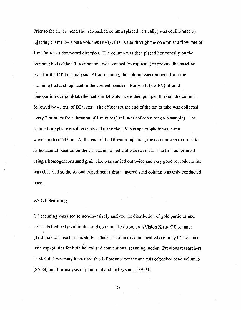
4.2 Characterization of Synthesized Gold Nanoparticles

In the first step of the gold synthesis process, small, monodispersed, gold nanoparticle

seeds were formed with an average size of 11.2 ± 2.8 nm. Citrate ions serve as the

capping agent [108, 109], which give the seeds a negative surface charge as indicated by

a ^-potential of-35.8 ±2.1 mV in the seed solution. This high negative surface charge

causes the solution to be stable for several weeks. These seeds have an absorbance peak

at 520 nm (see Figure 7a) that can be attributed to the surface plasmon resonance (SPR)

band for monodisperse gold nanoparticles [109].

45

2

200 300 400 500 600

Wavelength (nm) 700 800

200 300 400 500 600

Wavelength (nm) 700 800

Figure 7: Absorbance spectrum for gold seeds (A) and gold nanoparticles (B). The peak for the gold seeds occurs at 520 nm whereas for the gold nanoparticles, the peak is at

535 nm.

46

After the final growth step and washing, spherical gold nanoparticles were formed with

an average size of 94.3 ± 12.0 nm as determined by DLS. The size and shape of the gold

nanoparticles can be clearly seen in the SEM image shown in Figure 8. For these

nanoparticles, the CTAB molecules have replaced the citrate ions as the capping agent

giving the nanoparticles a positive surface charge as indicated by a ^-potential of 40.7 ±

13.4 mV in DI water and pH 6.5. These nanoparticles are stable in suspension for several

days. Compared to the gold seeds, the gold nanoparticles have an absorbance peak at 535

nm, as seen in Figure 7b. This red-shift of the absorbance peak is due to the increased

size of the nanoparticles [110].

McGill 2.0kV 11.9mm x50.0k SE(U) 1 .OOum

Figure 8: SEM image showing gold nanoparticles. The size of the nanoparticle is approximately 100 nm.

•47

The calibration curve for particle concentration versus absorbance is shown in Figure 9

and indicates a particle concentration of 1.406 x 1011 particles/mL at 25.0 a.u.

1.8E+11

1.6E+11

1.4E+11

0.0E+00 10 15 20

Absorbance (a.u.) 30

Figure 9: Calibration curve for gold particle concentration versus absorbance.

The number of particles in each sample was calculated theoretically with several

assumptions. The first assumption was that in each growth step, there was complete

reaction of the gold in the solution. The total mass of gold present could be then

calculated knowing the total number of moles involved in the reaction and converted to a

volume using the density of gold which is 19.3 g/cm3. With this information, the number

of particles could be determined using the average particle size from DLS measurements.

48

In order to account for experimental error when removing the supernatant after

centrifugation, a 10% loss of gold particles was accounted for in each wash.

4.3 Characterization of Labelled Bacteria

Labelled bacteria were obtained in a single step by mixing the cells with the synthesized

gold nanoparticles in DI water for 15 minutes. The positively charged CTAB-coated

gold nanoparticles are attracted to the negatively charged teichoic acid brushes present on

the surface the bacteria. This electrostatic interaction binds the CTAB-coated gold

nanoparticles to the teichoic acid brushes on the surface of the cells and it has been

reported that CTAB has a high affinity for teichoic acid [78].

An optimal ratio of cells to gold nanoparticles was identified such that the surface of the

bacteria is extensively covered with gold nanoparticles and there are very few unattached

gold nanoparticles remaining in the solution, as shown in Figure 10. A higher ratio of

cells to gold nanoparticles resulted in bridging of adjacent cells, as shown in Figure 11,

and a lower ratio resulted in many free nanoparticles in solution. The bridging or cross-

linking effect is created by the fact that each gold nanoparticle is completely covered with

CTAB molecules allowing for possible binding sites on all sides of the nanoparticle.

Through trial and error, the ratio of bacteria cells to gold nanoparticles was determined to

be approximately 1:1350, and could be accomplished by mixing 1 mL of cells with an

49

absorbance of 7.0 a.u. at 600 nm and 10 mL of gold nanoparticles with an absorbance of

25.0 a.u. at535nm.

By counting the number of particles on cells in SEM images, the number of particles per

cell was found to be 1077 ±110 particles/cell. When analyzing the SEM images, it

should be noted that all cells in the images were labelled with gold nanoparticles and that

there were very few non-attached nanoparticles observed.

It was difficult to accurately count the total number of gold particles on a cell because the

SEM images did not show the entire cell surface. However, as an approximation, the

number of particles present in several square regions (with a known area) were counted

and multiplied by the ratio of total cell surface area to the area of the square region.

Despite the limitations inherent in this technique, it yielded consistent results and

provided a method to visually confirm that the surface of the cells was being well

labelled. This high attachment rate is due to the strong electrostatic interactions between

the highly positively charged CTAB molecules and the negatively charged B. subtilis cell

surface.

50

A

McGill 2.0kV 11.9mm xlO.Ok

McGill 2.0kV11.8mm xSO.Ok

S.OOum

I *

i i i i i i i

SOOnm

Figure 10: SEM images showing bacteria labelled with gold particles at low magnification (A) and high magnification (B) to show nanoparticle detail.

51

McGil! 2.0kV 12.0mm x10.0k 5.00um

Figure 11: SEM image showing cell bridging caused by high cell to nanoparticle ratio

Once labelled, the bacterial surface is extensively covered with the gold nanoparticles.

These nanoparticles occupy the negatively charged areas of the cell surface, neutralizing

this charge and imposing their positive surface charge onto the bacteria surface. The t,-

potential for the labelled cells was determined to be 20.6 ± 12.3 mV in DI water, pH 6.5.

This strong surface charge on the labelled cells allows for a monolayer of coverage on the

cell surface. Once all the negative regions of the cell are occupied, positively charged

free gold nanoparticles are repulsed by the gold-labelled cell and seek another cell onto

which they can attach.

The positive surface charge on the gold-labelled cells also keeps the cells stable for

several hours, but the weight of the gold nanoparticles does increase the settling rate of

52

the bacteria. A single gold nanoparticle has a mass of approximately 8.5 x 10"3 pg,

whereas the mass of a single cell is approximately 0.95 pg [111]. By coating the surface

of the cell with up to 1500 gold nanoparticles, the mass of the cell is increased by

approximately 680%. It is because of this mass increase that the gold-labelled cells settle

out of suspension faster than the unlabelled cells. The density of the cells can also be

calculated knowing these parameters, and assuming that the total volume of the cell can

be calculated from a cylinder with a length of 2 um and a diameter of 0.95 um (the actual

diameter of the cell is 0.75 um, but must include the extra width due to the layer of gold

nanoparticles). It was found to be 8.9 kg/m3.

The overall motility of the cells before and after labelling was not determined in this

study, but it is known that B. subtilis is extensively flagellated, which gives it the ability

to move quite rapidly [59, 61]. Furthermore, at medium to high fluid velocities, the

transport and deposition behaviour of the bacteria in the porous media is not affected by

the motility of the bacteria [60]. In this study, the fluid velocity is ~3 m/day (3.4 x 10"3

cm/s) and can be considered a medium fluid velocity, so if there was a change in overall

motility due to the increase in mass, this should not affect the deposition and transport

behaviour of the cells.

53

4.4 Cell Viability in the Labelling Process

CTAB is toxic to cells at certain concentrations causing the release of different cellular

constituents, cell lysis, change of surface charge, and morphological changes visible by

electron microscope [112, 113]. Though free CTAB in solution is toxic, nanoparticles

coated with CTAB are not [79, 114]. The resazurin reduction method was used to verify

the viability of the gold-labelled cells one hour after labelling. From this test, all tubes

containing labelled cells were positive indicating that the cells were viable and .

consuming oxygen.

After labelling, the bacteria are not only viable but retain their cellular integrity and

structure over time. SEM images of the bacteria taken 24 hours after labelling were

compared to images taken one hour after labelling. Between imaging sessions, the

labelled bacteria were stored at 4°C and were not transferred to new media. These

images are shown in Figure 12. The cells retain their rod-like shape, are not damaged,

and the nanoparticles remain attached to their surface.

54

A

McGill 2.0kV 11.8mm x20.0k 2.00um

is

McGill 2.0kV 12.0mm x20.0k SE(M) 2.00um

Figure 12: SEM images taken 1 hour (A) and 24 hours (B) after labelling showing that the gold nanoparticles remain bound to the cells and that the cells maintain their shape

55

4.5 Validation of SEM Imaging Technique

A new technique to image the labelled and unlabelled bacteria was developed for the

SEM in this project. The technique reduced the sample preparation time significantly,

reduced the interaction of the sample with possibly harmful chemicals, and allowed for

clear images at high magnification of intact samples. The images taken using this

preparation technique were compared to images taken using the standard sample

preparation technique for SEM, and images taken in an ESEM. When using the standard

sample preparation technique, there were no qualitative differences in the images even at

high magnification, whereas the ESEM damaged the cells and comparisons could not be

made. A sample image obtained using the new technique is shown in Figure 13. The

other techniques are shown in Figure 14.

Figure 13: Representative image of cells obtained using new preparation technique.

56

McGill 2.0kV 5.0mm x10.0k SE(U) S.OOum

"̂*

%

FI B a a

Figure 14: Representative image of cells obtained using the standard preparation technique (A) and from Environmental SEM (B).

57

4.6 CT Number Measurements

In X-ray CT, different scanned materials are distinguished by differences in density and

atomic number at fixed X-ray energies. Changes in these two parameters will increase or

decrease the X-ray attenuation measured by the CT scanner and from these attenuations,

the CT number, in Hounsfeld units (HU) is determined. CT numbers are based on the

Hounsfeld CT number scale relative to the attenuation of water, which is given the CT

number of 0 HU. Air, in the Hounsfeld CT number scale, is set to -1000 HU. In order to

carry out the X-ray CT data analysis and image subtraction, it was necessary to know the

CT numbers of the materials being scanned. A summary of the measured mean CT

numbers for the different materials used in this study is presented in Table 2.

Table 2: Measured mean CT numbers for materials used in study

Material

Air DI Water

Sand

Mean CT number (HU)

-1100 34

2700

Note: Scans were conducted using the helical scanning mode of the scanner, X-ray beam energy of 130 kV, current of 200 mA, field of view diameter of 180mm, and standard FC30 reconstruction algorithm, scan time per rotation of 1.5 seconds.

The mean CT numbers measured with the XVision CT scanner are not strictly consistent

with the definition of the Hounsfeld CT number scale. These numbers also vary slightly

from previous studies using this scanner [86, 87]. This discrepancy is most likely due to

58

the scanner being calibrated at different settings than used in this study. This would also

explain the discrepancy in the values obtained in other works using the same instrument.

For example, Goldstein [86] used an X-ray beam power of 400 mAs compared to 300

mAs in the current study. As well, this study used the helical scanning mode, instead of

the conventional scan and view mode, with a shorter scan time per rotation than in both

previous studies [86, 87].

The CT numbers for the synthesized gold nanoparticles and the gold-labelled cells were

determined for different concentrations. Figures 15 and 16 show the calibration curves

for the gold nanoparticles and gold-labelled cells, respectively, with the error bars

showing the standard deviation for each measured CT number. From the two graphs, the

ratio of cells to particles can be calculated by taking the ratio of the slopes. This gives

approximately 1:1450, and is comparable to both theoretical labelling calculations from

absorbance measurements and particle counts on cells from SEM images as shown

above. When scanning the gold-labelled cells, the contribution of the bacteria to the

measured HU is negligible; it was found that even at concentrations of unlabelled

bacteria up to 109 cells/mL in DI water, the measured CT number remains equal to the

CT number of DI water.

59

120

. 10 ,

18

Particle concentration (10 particles/mL)

Figure 15: Calibration curve for gold nanoparticle concentration versus CT number.

100

3 80 X l a ® JO 60 E 3

z IT 40

20

n

y = 52,28x + 32.744

0.2 0.4 0.6 0.8

Labelled Cell Concentration (10 s cells/mL)

1.2

Figure 16: Calibration curve for gold-labelled cells versus CT number.

60

4.7 Colloid Transport in Homogeneous Sand Columns

Representative column breakthrough curves obtained for gold nanoparticles and gold-

labelled cells pumped through sand columns with constant grain size are shown in Figure

17 with the normalized effluent concentration, C/C0, plotted as a function of time.

During the first 40 minutes gold nanoparticles or gold-labelled cells were pumped into

the column at a flow rate of 1 mL/min. The effluent concentration remained zero for the

initial time period because there were almost no particles or cells that had reached the

outlet. Thereafter the concentrations of the particles or cells continued to increase until it

reached a plateau. During this plateau period, the gold nanoparticle breakthrough

concentration is rising with a stable slope. This is due to blocking of the porous media

surface by the deposited particles, preventing further nanoparticles from depositing [115].

After 40 minutes DI water was pumped through the columns at the same flow rate,

causing the non-deposited particles or cells to be flushed out of the column until no

further particles or cells were detected in the effluent. As indicated in Figure 17, the

value of C/Co is greater for gold nanoparticles than gold-labelled cells (C/C0 = 0.99 and

C/Co = 0.09 respectively) indicating that a higher relative concentration of gold-labelled

cells was retained in the column by deposition onto the sand grains than the gold

nanoparticles. The initial gold nanoparticle concentration was 1.46 x 1011 particles/mL

and the initial gold-labelled cell concentration was 1.0 x 108 cells/mL. In both cases, the

ionic strength was was consistent between experiment, and the pH = 6.5.

61

o U ^> u

1

0.9

0.8

0.7

0.6

0.5

0,4

0.3

0.2

0.1

•"•¥'•'*""

• • • • • , • • •

Start of DI water injection

.wsMBS^nBEiSD^EeHr^jwa D

10 20 30 40 50

Time (min)

60 70 80

Figure 17: Representative breakthrough curve for gold nanoparticles (+) and gold-labelled cells (D) in a sand column with constant grain size. Key experimental

conditions: pH =6.5, flow rate = lmL/min, porosity = 0.42, mean sand grain diameter 800 pan, temperature = 25 °C.

The profiles showing the density distribution of the retained nanoparticles and labelled

cells for this experiment were obtained from the X-ray CT data and are shown in Figure

18 with the retained particle or cell concentration plotted as a function of distance. To

calculate the retained concentration, the number of the gold nanoparticles or gold-labelled

cells per slice was calculated from the X-ray CT data using image subtraction and

Equation 32 as discussed in Section 3.8. In this calculation, the CT number for gold

(Xgoui) is assumed to be 100. For the gold nanoparticles and the gold-labelled cells, the

concentrations giving a CT number of 100 are 1.84 x 1011 particles/mL and 1.29 x 108

cells/mL, respectively. These values were extrapolated from Figures 15 and 16. In order

62

to obtain the number of particles in each voxel, a two step process is required. First,

volume fraction calculated by image subtraction for each voxel multiplies the cell

concentration corresponding to a CT number of 100. Next, the volume for each voxel

multiplies this product. It should be noted that a CT number of 100 was chosen for this

computation, but any CT number that corresponds to a particle or cell concentration

could have been chosen since they are linearly related. From the porosity calculation

using equations 27 and 28 described in Section 3.8, the total volume of sand per slice can

also be determined and converted to the mass of sand knowing its density (2.65 g/cm3).

In order to have a better qualitative interpretation of the data presented in Figure 18, the

y-axis for the gold nanoparticles (on the left) is set to a different scale than the gold-

labelled cells (on the right). Without altering the data, the scale for the particles was

divided by 1350 in order to obtain the scale for the cells. This enables the researcher to

compare data points that represented similar CT numbers. As predicted by the data in

Figure 17, the retained profiles show a low concentration of retained gold nanoparticles,

and relatively higher concentration of retained gold-labelled cells as indicated by the

sharp increase at the end of the column.

63

2.5E+07

2.0E+07

c m w S 1.5E+07 W

"v

10 1.0E+07

o.

5.0E+06

0.0E+00

a" c

D

n

a

•

nnoangg^SS^^^^fififfl^affiW^S^^^

20000

18000

16000

14000

T3 C

12000 n w at (A

10000

8000 o

6000

4000

2000

10 15 20 25

Slice Number 30 35 40

Figure 18: Retained profile for gold nanoparticles (+, left axis) and gold-labelled cells (O, right axis) in a sand column with constant grain size. Key experimental conditions: pH =6.5, flow rate = lmL/min, porosity = 0.42, mean sand grain diameter = 800 pan,

temperature = 25 °C.

From the CT data, slice images can be created showing the distribution of the gold

nanoparticles and gold-labelled cells at different locations along the length of the column.

These are shown in Figure 19 and Figure 20, respectively. The scale bar shown to the

right of the individual slices represents the variation in volume fraction for each voxel

shown. The data from the slice images is correlates very well to Figure 18.

64

Slice A SliceH

Slice 16 Slice 20 Slice 24

Slice 28 Slice 32 Slice 36

Figure 19: Representative slice images generated from CT data showing volume fractions of gold particles in each voxel for the homogeneous columns

65

Slice 4

Slice 16

Slice 1

Slice 20

Slice 32

Slice 24

Figure 20: Representative slice images generated from CT data showing volume fractions of gold-labelled cells in each voxel for homogeneous columns

The average porosity for this experiment was 0.42 as determined from the total mass of

sand compacted to a height of 40 mm. The porosity for each 1 mm section was also

calculated from the CT data for the saturated sand columns and is shown in Figure 21.

As indicated by this data, the porosity throughout the column is consistent with the

average porosity measured from the mass of packed sand, indicating that the column was

evenly packed. There is a slight increase in the porosity at the ends of the columns as

indicated in Figure 21. This phenomenon was also observed in the study by Haghighi

66

[87] and is most likely due to variations in the packing structure at the top and bottom of

the column that were not eliminated by vibration.

1

0,9

0.8

0.7

- 0 . 6

O 0.5 0

0.4

0.3

0.2

0.1

0 10 15 20 25

Slice Number 30 35 40

Figure 21: Porosity per slice for the first experiment using a constant grain size.

The ratio, dp/dc, of particle diameter to mean sand grain diameter (800 \am), is 0.0001 for

the gold nanoparticles (94.3 nm) and 0.002 for the gold-labelled cells (equivalent

spherical diameter = 1.65 ^m). At these low ratios, straining is usually not considered

significant [14] and deposition of the gold nanoparticles and gold-labelled cells should

follow the classical colloidal filtration theory model. But according to CFT, the

concentration of deposited colloids should decay exponentially with distance, not

increase suddenly at the end of the column.

67

Upon examination of the dismantled sand column and end fittings after the experiment, it

was discovered that a film of labelled bacteria was coating the exposed surface of the

glass filter disc placed at the outlet of the column used to retain the porous media. This

highly localized increase in bacteria concentration was the cause for the spike in gold-

labelled cell concentration detected by the CT scanner.

4.8 Colloid Transport in Layered Columns

In order to determine if a change of pore size in the porous media would cause an

accumulation of gold nanoparticles or gold-labelled cells, a second experiment using two

sizes of quartz sand was conducted. A 20 mm layer of fine quartz sand was first placed

at the bottom of the column and packed by vibration. On top of this, a 20 mm layer of

coarse quartz sand was placed and packed by vibration. The layered porous media is

shown in Figure 22. The gold nanoparticles and gold-labelled cells were pumped in the

direction from the coarse sand to the fine sand in order to observe the accumulation at the

interface of the two grain sizes. Representative column breakthrough curves obtained for

gold nanoparticles and gold-labelled cells pumped through layered sand columns are

shown in Figure 23 with the normalized effluent concentration, C/Co, plotted as a

function of time. A similar method for the injection of the gold nanoparticles or gold-

labelled cells was used as in the first experiment with homogeneous sand columns.

Furthermore, the same injection concentrations were used: 1.46 x 1011 particles/mL for

the gold nanoparticles, and 1.0 x 108 cells/mL for the gold-labelled cells.

68

Figure 22: Photograph of the column showing the interface between the coarse sand grains and the fine sand grains. In this image, the flow direction is from top to bottom.

It is difficult to compare the effluent breakthrough curves obtained for the gold

nanoparticles and gold-labelled cells. The maximum relative effluent concentration for

the gold nanoparticles was 0.32 and occurred after 48 minutes, whereas the maximum for

the gold-labelled cells was 0.19 and occurred after 14 minutes. The difference in the

shape of these two curves is most likely due to different governing removal mechanisms

for each type of colloid though both have an initial breakthrough at the same time after 1

PV (-10 minutes).

EsBSasSBaa

* *

• • I —

69

o U

u

o.s

0,5

0.4

0.3

0.2

0.1

Start of DI water injection

B LJ 1 I : : D

UUQU 1 ^

10 20

SB Kt $02 i n \M am BH HK OH an GKI i '"•M^-^an-m SB HB SB HBflRiBr-

60 70 80

Figure 23: Representative breakthrough curve for gold nanoparticles (+) and gold-labelled cells (U) in a sand column with dual grain size.

There was only a low concentration of gold nanoparticles in the column effluent until

after the flow had been switched back to DI water, at which point there was a sharp

increase. This did not occur in the column with gold-labelled cells. The low relative

effluent concentrations shown in the breakthrough curve indicate that a high

concentration of both gold nanoparticles and gold-labelled cells had been retained within

the column. The gold nanoparticles have a positive charge and are electrostatically

attracted to the negatively charged surface of the sand grains [85]. Furthermore, after the

interface, the diameter of the sand grains has decreased but the total surface area of the

sand particles has increased, providing a larger area for nanoparticle attachment which

70

could account for the increased rate of deposition. After these first forty minutes, the

injection is switched to DI water for a further 40 minutes. At this time, there is an

increase in the relative gold nanoparticle concentration in the effluent. This was not

expected and it may be proposed that this increase in gold nanoparticle concentration is

due to the elution of deposited nanoparticles when exposed to the DI water in the second

phase of the injection. In experiments used to study dual mode deposition [16], they

found that this phenomenon could be attributed to the release of particles from the

secondary energy minimum that were deposited in unfavourable conditions after the

injection of a lower ionic strength solution. This would indicate that the gold

nanoparticles were behaving as predicted by dual deposition mode theory [16]. However,

in this study, the ionic strength of the elution water is essentially the same as the ionic

strength of the suspension. In this case, such release of particles is not expected. Most

importantly, the charge of the particles makes the conditions for attachment favourable,

meaning that the particles would be irreversibly deposited and not released upon

moderate changes in solution chemistry. As such, it is possible that the sudden increase

in effluent concentration is caused by a disturbance in the flow when the solution is

switched from the gold nanoparticle suspension to DI water.

For the gold-labelled cells, there is a short increase in relative effluent concentration at

the beginning of the experiment followed by a gradual decline. This is most likely an

indication of straining or ripening occurring within the column. This same effect is

noticed with the gold nanoparticles, but not as significantly. Ripening occurs when

71

attached particles can act as additional collectors for attachment [51, 115, 116] and has

been linked to increased deposition in other bacteria transport studies [60]. On the other

hand, straining occurs when particles are caught at grain-to-grain contacts or in down-

gradient pore throats that are too small to allow particle passage [38-40]. Both of these

effects will increase the particle deposition rate, especially after the interface when the

pore size is decreased.

The profiles showing the spatial distribution of the retained gold nanoparticles and gold-

labelled cells for this experiment, obtained from the X-ray CT data, were calculated as

described in Section 4.6 for the transport of colloids in homogeneous sand columns, and

are shown in Figure 24 with the retained particle or cell concentration plotted as a

function of distance. Similar to Figure 18, the y-axes for the particles and cells have been

adjusted to allow for qualitative analysis between the two types of colloids. For the gold

nanoparticles, the retained concentration increases after the interface as predicted by the

increased surface area available for deposition. Furthermore, the curve for the gold

nanoparticles shows a sharp decrease at the end of the column indicating that the

nanoparticles had not completely penetrated through the entire column before switching

to DI water. The curve for the concentration of retained gold-labelled cells shows a sharp

increase in the retained concentration at the interface, followed by a region of very low

retention. Both curves confirm that there was a relatively high concentration of gold

nanoparticles and gold-labelled cells retained in the layered sand column. It should be

noted that photograph in Figure 25 displays the nanoparticle accumulation at the outer

72

surface of the column, and corresponds directly to the CT data concentration shown in

Figure 24.

2.5E+07

2.0E+07 XI c re w O) ^s 1.5E+07 (ft

u

1 10 1.0E+07 0.

5.0E+06

O.OE+00

D D

1

•

Coarse grains

- >

Fine grains

, • • • • •

Dx •

• • • • • •

2ffl^n3nftnft8fi^^ 9

•nn

D

• D, an 10 15 20 25

Slice Number 30 35

20000

18000

16000

14000

12000

10000

8000

t 6000

4000

2000

0

40

•a

c IS U> D) ">s

J5 "5 u ft

Figure 24: Retained profile for gold nanoparticles (+, left axis) and gold-labelled cells (U, right axis) in a sand column with coarse and fine sand. Key experimental conditions: ionic strength = constant, pH =6.5, flow rate = lmL/min, porosity = 0.42, mean coarse

grain diameter = 800 pan, mean fine grain diameter = 200 pan, temperature = 25 °C, interface at 20 mm (slice 20).

73

Figure 25: Photograph showing the particle accumulation at the exterior of the column.

Images showing the distribution of the gold nanoparticles and gold-labelled cells within

slices along the column are shown in Figure 26 and Figure 27, respectively. Note the

increased deposition beginning at the 20th slice for the gold nanoparticles, whereas the

gold-labelled cells show an increased deposition at the 20th slice and little deposition

thereafter. Again, the scale bars indicate the volume fraction for each voxel in the slice

image.

74

Slice 4 Slice 8 Slice 12

Slice 16 Slice 20 Slice 24

•0.5

Slice 28 Slice 32 Slice 36

Figure 26: Representative slice images generated from CT data showing volume fractions of gold particles in each voxel for layered columns

75

Slice 4 Slice? Slice 12

Slice Id

Slice 28

Slice 20

• - • " • ; ' • ' , " • >

• S . - J ^ - - -

Slice 32

Slice 24

Slice 3d

Figure 27: Representative slice images generated from CT data showing volume fractions of gold-labelled cells in each voxel for layered columns

The average porosity for this experiment was also 0.42. From the CT data, the porosity

for each slice is shown in Figure 28 and is consistent with the average porosity. At the

interface, there is a small fluctuation in the porosity caused by the interaction of the two

different grain sizes. When compacting sands, a well graded sand will have a lower

porosity than one that is uniformly graded [117]. At the interface of the two sizes of sand

grains, mixing occurs creating a small region that is not comprised of uniformly graded

sand resulting in the fluctuating porosity. Past this interface, the porosity is once again

consistent with the average porosity of the column. The porosity in the coarse sand

76

layers of the column is not expected to be different from the fine sand layer because both

layers are comprised of grains of relatively uniform size. As in the first experiment with

a homogeneous sand column, the ends show an increase in porosity, most likely due to

inconsistencies in the packing by vibration at the ends of the column.

0 5 10 15 20 25 30 35 40

Slice Number

Figure 28: Porosity per slice for the second experiment using coarse and fine sand

At the interface of the two sand layers, the pore size is reduced due to a decreased grain

size, which increased the effect of the straining on the gold-labelled cells. As the bacteria

are removed from the aqueous phase by the collector grains in this region, the pore spaces

become smaller and the labelled bacteria can no longer pass through [62]. This resulted

in a high concentration of gold-labelled cells being retained within the column in this

experiment. Furthermore, after the interface, the reduction of grain size results in a

77

further reduction of pore size, increasing effect of the straining due to an increase in the

dp/dc ratio. These combined effects resulted in a high concentration of gold-labelled cells

being deposited in the column in this experiment (C/Co = 0.03).

In the coarse sand region of the column, the dp/dc ratio is the same as in the homogeneous

sand columns used in the first experiment: 0.0001 for the gold nanoparticles and 0.002

for the gold-labelled cells. After the interface, in the fine sand region of the column, the

mean grain diameter is reduced to 200 um and the d/dc ratio increases to 0.0004 for the

gold nanoparticles and 0.008 for the gold-labelled cells. Again, at these low ratios,

straining is usually not considered significant [14], but above 0.002, experimental

evidence has shown that straining can be important [46] and was most likely the

governing mechanism in the removal of the gold-labelled cells.

The values for rjo were calculated for the gold nanoparticles and the gold-labelled cells in

both the fine and coarse sands. These values are shown in Table 3. From these values

for the single-collector contact efficiency, there should be an increase in deposition in the

fine sand compared to the coarse sand for both colloids, and there should be more

deposition in both sands of the gold-labelled cells than gold nanoparticles if the

attachment efficiency is constant. This is consistent with assumptions based on increased

surface area for the smaller grain size, and with the breakthrough curves and retained

concentration profiles in both experiments (Figures 17, 18, 23 and 24).

78

Table 3: Calculated values ofrjofor the different colloids and sand grain sizes

rjo

Gold nanoparticles

Gold-labelled cells

Fine Sand

7.68 x 10"4

2.40 x 10"3

Coarse Sand

3.16xl0"4

4.39 xlO"4

Note: These values were calculated from equations described in Section 2.1 using the model by Tufenkji and Elimelech [28] and the following values: e= 0.42, dPtgoidnanoparticies

= 94.3 nm, dPigM-iabeiiedceiu = 1-65 uin, dc, coarse= 800 ^m, dcjwe = 200 jim, U= 3.4 x 10"3

Cm/S, A = 2 . 5 X 10"19 J [ 1 1 8 ] , T= 2 9 8 K , Pb.goldnanoparticles^ 19 .3 k g / m 3 , Pp, gold labelled cells =

8.9 kg/m3, g = 9.81 m/s2, /#2<wr = 996.95 kg/m3, ^ s r = 0.903 kg/(m s).

Though straining was most likely the governing mechanism for the initial removal of the

gold-labelled cells at the interface, there was likely a combination of mechanisms that

resulted in the final retained particle profile. After the interface, there is little deposition

of the gold-labelled cells as seen in Figure 24 and 27. This is further demonstrated by the

photograph of the column taken at the end of the injection in Figure 29. In this photo, a

clear accumulation of the gold-labelled cells can be seen at the interface of the two sand

layers. This accumulation was most likely caused by clogging of the pores of the column

at the interface. As the collectors removed the gold-labelled cells, these accumulated on

the collector surfaces, reducing the pore spaces and causing other gold-labelled cells to be

deposited on their surfaces, rather than the surface of the collectors.

For further confirmation, following each column experiment, the column packing and

pore fluid was emptied into a vial. The vial was shaken and allowed to rest. A

representative image of these vials is presented in Figure 30. The vial on the left shows

79

the contents of the column following an experiment conducted with gold-labelled

bacteria, whereas the vial on the right shows the contents of a column following an

experiment conducted with gold nanoparticles alone. In the vial on the left, the

supernatant is dark red, indicating that the gold-labelled cells were readily released from

the porous media. This observation suggests that the cells were retained in the packed

bed by a physical trapping mechanism (i.e. straining or ripening) and were readily

released when the porous media was broken up. In the vial on the right, the supernatant

is very clear, even after mixing of the granular phase. The results show that the gold

nanoparticles are irreversibly attached onto the surface of the sand grains (most likely due

to attractive electrostatic forces) rather than retained by a reversible physical mechanism.

Figure 30 shows the results from a homogeneous column, though similar observations

were made for layered columns.

80

TfrfcL mam

^fcg^gi^ggjtvi^^^fe

Figure 29: Photograph showing gold-labelled cell accumulation at the interface of the coarse and fine sand grains (dark region in the middle of the column).

81

Figure 30: Photograph showing the retained gold-labelled cells (left) and the retained gold nanoparticles (right) after a column experiment with coarse grains.

4.9 Precision and Repeatability of Measurements Determined from X-ray CT

The calculations from the X-ray CT data are subject to errors and artefacts including

instrument noise, beam hardening and positioning errors. These errors have been

discussed in detail by Goldstein [86]. As a result of these errors the concentration of

particles retained in the column has a deviation from the actual retained concentration. In

this study, destructive sampling of the column was not conducted at the end of each

experiment so these could not be compared statistically. As such, the error analysis in

this study was conducted by the comparison of repeated scans of the same sample.

82

The X-ray CT scanner acquired triplicate scans of the same column consecutively. These

repeated scans of the same image served to quantify the measurement error of the CT

scanner using the standard deviation [119]. By applying the formula in Equation 32 to

the data, withX; and ̂ G being scans of the same object, the result forf'jk should be zero

for all voxels. The average/for each pair of scans is calculated and the standard

deviation determined. Normalizing the differences in CT numbers to the difference

between gold and water will enable any trends in the data to be determined and evaluate

the range of error. These repeated scans were performed for both homogeneous

(Experiment 1) and layered (Experiment 2) columns and the data can be found in Table 4.

Looking at the table, it is possible to see that the data does produce a mean difference in

CT numbers close to zero, but that the standard deviation is much higher. This is

indicative of a low signal to noise ratio. This phenomenon is due to the fact that the CT

number for the gold solutions is very close to the CT number of water. A small quantity

of gold in DI water does not produce a significant change in the CT number until a very

high concentration of gold is used. In this study, the detection limit for the gold (twice

the standard deviation above the CT number of water) is -50 HU. This corresponds to a

gold nanoparticle concentration of 4.5 x 1010 particles/mL and a gold-labelled cell

concentration of 3.3 x 107 cells/mL. This is equivalent to a gold concentration of 1.4

mg/mL. In other medical X-ray studies in which gold was used as a contrast agent, the

minimum concentration of gold used was 100 mg/mL in order to accurately quantify the

83

results [80]. From these error calculations, increasing the retained particle concentration

with a longer column, or further reducing the size of the sand grains to promote

deposition within the column, could reduce the error in the volume calculation from the

X-ray CT data. As such, this study demonstrates that using image subtraction allows us

to obtain significantly lower detection limits for gold nanoparticles with a medical X-ray

CT scanner.

Table 4: Control volume calculations for error measurement

Experiment

1

2

Average Normalized CT Number Difference

0.00028 0.00038 0.00010 0.00018 0.00027 0.00009 -0.00025 -0.00145 -0.00119 0.00022 0.00057 0.00036 -0.00021 -0.00013 0.00007 0.00059 0.00095 0.00036 0.00048 0.00056 0.00008 0.00014 0.00114 0.00100

Standard Deviation (mL)

0.119 0.117 0.096 0.074 0.091 0.058 0.143 0.172 0.147 0.105 0.125 0.094 0.083 0.120 0.101 0.076 0.094 0.062 0.074 0.086 0.054 0.078 0.101 0.068

84

Chapter 5: Summary and Conclusions

This study has provided the proof of concept for the detection and quantification of

bacterial density distribution in saturated porous media using X-ray CT. To do so,

Bacillus subtilis cells were labelled with CTAB-coated gold nanoparticles that were

synthesized using a surfactant-assisted seed-mediated growth process. The gold-labelled

bacteria cells were injected into the saturated porous media in traditional column

experiments containing both homogeneous and heterogeneous packed quartz sand. In

these experiments, the sand columns were equilibrated by first pumping a significant

volume of DI water through the column. The gold-labelled bacteria were then pumped

through the column, followed by an equal amount of DI water to remove any unbound

bacteria. The effluent concentration of suspended bacteria was monitored as a function

of time throughout injection of bacteria and DI water. A Toshiba XVision whole-body

medical X-ray CT scanner was used for the scanning of all columns. The experimental

protocol for imaging bacterial density distributions in saturated porous media involved

first scanning the saturated column after equilibration with X-ray CT to obtain the

baseline scan. Upon completion of the flow experiments, the columns containing the

deposited gold-labelled bacteria were scanned a second time with X-ray CT. The 3-D

data sets obtained from these scans were processed using MATLAB software to obtain

numerical arrays for porosity and cell concentration with respect to the porous media.

The results from these gold-labelled bacteria experiments were compared to identical

experiment using only the synthesized gold nanoparticles. Significant findings are

outlined below:

85

1) Gold nanoparticles were successfully synthesized and used to label B. subtilis

cells in suspension.

Using the surfactant-assisted seed-mediated growth process described by Berry, et

al. [79], gold nanoparticles capped with CTAB molecules were synthesized with a

diameter of 94.3 ± 12 nm and a positive surface charge (^-potential = 40.7 ± 13

mV) in experimental conditions. These gold nanoparticles were attached to

suspended B. subtilis cells (L = 2.0 um, D = 0.75 um, C,-potential = -9.6 ± 2.0 mV

in experimental conditions) in a single step. The attachment efficiency was

greater than 70% as shown in SEM images of the cell surface and through

calculations from X-ray CT data. These gold-labelled cells retained their

structural integrity over time and remained viable throughout the entire

experimental procedure.

2) The gold nanoparticles and labelled cells have predictable X-ray attenuation

properties that permit their quantification using X-ray CT

In the X-ray CT scanner, the measured mean CT number for the gold

nanoparticles and labelled cells increases linearly with particle and cell

concentration. A value of twice the standard deviation of the CT number for

water was used to determine their detection limit. By measuring the CT number

at various concentrations, the detection limits for the gold nanoparticles and

labelled cells were determined to be 4.5 x 1010 particles/mL (1.4 mg/mL) and 3.3

x 107 cells/mL, respectively. Compared to similar studies using MRI, the

86

detection limit for gold nanoparticles is at the same order of magnitude [24],

however, the detection limit in this study for cell concentration is one order of

magnitude less than the cell concentration possible with MRI [26].

3) The spatial density distribution of the gold nanoparticles and labelled cells within

a saturated sand column was quantified using X-ray CT

To the best of the author's knowledge, this study is the first to study the transport

and deposition behaviour of bacteria in porous media using X-ray CT at the

mesoscale. In this study, the density distribution of gold nanoparticles and

labelled cells was quantified at a spatial resolution of 1 mm. Furthermore, X-ray

CT permitted the non-invasive calculation of porosity in situ as well as observing

changes in deposition behaviour due to sand heterogeneities such as the

accumulation of gold-labelled bacteria at the interface between coarse and fine

sands. This knowledge on spatial distribution of bacterial density distributions

could not be otherwise determined from analyses of the effluent concentrations or

without sampling the porous media destructively.

87

Chapter 6: Future Work and Recommendations

This study has demonstrated the proof of concept for the use of X-ray CT in the

quantification and visualization of bacterial density distributions in saturated porous

media. The technique developed herein serves as the basis of a non-destructive in situ

method for studying the transport and deposition behaviour of nanoparticles and bacteria

in saturated porous media. The use of this technique would allow future researchers to

make meaningful correlations between the porous media characteristics and the fate of

colloids. These correlations can then be used to develop more accurate models for the

prediction of colloid transport in the subsurface. For the future development of this

technique, the following potential areas of study warrant further investigation:

1) Validation of the quantification methodology through destructive sampling of the

saturated sand columns.

The volume calculations used to determine the density distribution of gold

nanoparticles and labelled cells are subject to various X-ray CT errors as

described in detail by Goldstein [86]. Error analysis in this study was conducted

based on repeated measurements of the same samples. In order to further

determine the accuracy of the measurements made by the X-ray CT scanner, a

comparison of the actual retained volume to the volume computed using the X-ray

CT data is required. To determine the volume retained by the saturated porous

88

media, destructive sampling involving the extrusion and sectioning of the sand

column should be conducted as described by Tufenkji, et al. [18].

2) Determination of the effect of gold labelling on bacteria motility

In this study, the labelling of the bacteria increased its overall mass by over 600%

and caused the labelled bacteria to settle out of suspension in several hours. The

effect that this increase in mass had on the motility of the B. subtilis cells was not

investigated because the flow velocities used in the column experiments had been

shown to offset the effects of the bacteria motility on its transport and deposition

behaviour [60]. In order to perform transport experiments at a wider range of

flow velocities, it is essential that the bacteria retain their motility. Furthermore,

investigations into the chemotactic behaviour of the bacteria could be investigated

if the labelling process did not hinder the motility of the cells. As such, a study of

the bacteria motility before and after labelling is recommended.

3) Further development of the scanning procedure to more accurately determine the

porous media characteristics

Porosity calculations made in this study used only a single X-ray CT scan of the

saturated porous media. It is possible to calculate the porosity by the image

subtraction of two co-located scans, one containing only air and sand, and another

after the injection of water [86, 87]. An advantage of this method is that the

porosity of a sand column that is not completely saturated can be determined.

89

An additional characteristic that could be determined from the X-ray CT data is

permeability. Though porosity is an important characteristic of the porous media,

as shown in this study when using a homogeneous material the porosity is

invariant with grain size. By reducing the grain size, the pore size decreases as

well, but the ratio of pore volume to total volume does not. Permeability is a

measure of the ability of the porous medium to transmit fluid and is related to the

size of the pores. This parameter has been measured in other X-ray CT studies

[120, 121] and the methodology has been described in detail by Goldstein [86].

This characteristic of the porous media may be more relevant to the deposition

mechanisms involved in the removal of colloids in column experiments.

4) Use of time-lapse imaging

One of the major advantages of X-ray CT over destructive sampling methods is

that the information about colloid location relative to media grains and interfaces

is preserved. This allows for the observation of the colloid transport behaviour

over time. Time-lapse imaging could facilitate the assessment of the importance

of different transport and deposition mechanisms, allow for the investigation of

changes in transport as a function of time or changing conditions, and could lead

to the exposure of previously unrecognized mechanisms [15]. Furthermore, time-

lapse imaging is an important tool for studying bacterial chemotaxis [25].

90

5) Analysis of bacterial deposition behaviour in relation to contaminants in the

porous media

In previous work using this XVision X-ray CT scanner, methodologies were

developed to image the saturation of residual NAPLs [86] and to look at the

changing morphologies of the NAPLs caused by freeze-thaw effects [87]. By

incorporating these methods with the method for the analysis of bacterial density

distribution developed in this study, the bacterial deposition behaviour in relation

to NAPL contaminants could be quantified using X-ray CT. In order to do so, a

stationary NAPL phase would be required so that image subtraction of the X-ray

CT data can be conducted using co-located scans. This combination of X-ray CT

methods could greatly improve the understanding of the mechanisms involved in

bacterial adhesion to NAPLs and other contaminants.

91

References

1. Unc, A.; Goss, M. J., Transport of bacteria from manure and protection of water resources. Applied Soil Ecology 2004,25, (1), 1-8.

2. Madsen, E. L., Determining in situ biodegradation - Facts and challenges. Environmental Science and Technology 1991, 25, (10), 1663-1673.

3. Steffan, R. J.; Sperry, K. L.; Walsh, M. T.; Vainberg, S.; Condee, C. W., Field-scale evaluation of in situ bioaugmentation for remediation of chlorinated solvents in groundwater. Environmental Science and Technology 1999, 33, (16), 2771-2781.

4. Yao, K. M.; Habibian, M. T.; O'Melia, C. R., Water and waste water filtration: Concepts and applications. Environmental Science and Technology 1971,5, (11), 1105-1112.

5. Rajagopalan, R.; Tien, C, Trajectory analysis of deep-bed filtration with the sphere-in-cell porous media model. AIChE Journal 1976, 22, (3), 523-533.

6. Packman, A. I.; Brooks, N. H.; Morgan, J. J., Kaolinite exchange between a stream and streambed: Laboratory experiments and validation of a colloid transport model. Water Resources Research 2000, 36, (8), 2363-2372.

7. Tufenkji, N.; Ryan, J. N.; Elimelech, M., The promise of bank filtration. Environmental Science and Technology A-Pages 2002, 36, (21), 422A-428A.

8. Ferguson, C; De Roda Husman, A. M.; Altavilla, N.; Deere, D.; Ashbolt, N., Fate and transport of surface water pathogens in watersheds. Critical Reviews in Environmental Science and Technology 2003, 33, (3), 299-361.

9. Searcy, K. E.; Packman, A. I.; Atwill, E. R.; Harter, T., Deposition of Cryptosporidium oocysts in streambeds. Applied and Environmental Microbiology 2006, 72, (3), 1810-1816.

10. Puis, R. W.; Powell, R. M., Transport of inorganic colloids through natural aquifer material: Implications for contaminant transport. Environmental Science and Technology 1992, 26, (3), 614-621.

11. Corapcioglu, M. Y.; Shiyan, J., Colloid-facilitated groundwater contaminant transport. Water Resources Research 1993, 29, (7), 2215-2226.

12. Saiers, J. E., Laboratory observations and mathematical modeling of colloid-facilitated contaminant transport in chemically heterogeneous systems. Water Resources Research 2002, 38, (4), 31 -314.

92

13. Rittman, B. E.; McCarty, P. L., Environmental Biotechnology: Principles and Applications. McGraw Hill: New York, NY, 2001.

14. Tufenkji, N., Modeling microbial transport in porous media: Traditional approaches and recent developments. Advances in Water Resources 2007, 30, (6-7), 1455-1469.

15. Ochiai, N.; Kraft, E. L.; Selker, J. S., Methods for colloid transport visualization in pore networks. Water Resources Research 2006, 42, (12).

16. Tufenkji, N.; Elimelech, M., Deviation from the classical colloid filtration theory in the presence of repulsive DLVO interactions. Langmuir 2004, 20, (25), 10818-10828.

17. Li, X.; Johnson, W. P., Nonmonotonic variations in deposition rate coefficients of microspheres in porous media under unfavorable deposition conditions. Environmental Science and Technology 2005, 39, (6), 1658-1665.

18. Tufenkji, N.; Redman, J. A.; Elimelech, M., Interpreting deposition patterns of microbial particles in laboratory-scale column experiments. Environmental Science and Technology 2003, 37, (3), 616-623.

19. Baumann, T.; Werth, C. J., Visualization and modeling of polystyrol colloid transport in a silicon micromodel. Vadose Zone J. 2004, 3, 434-443.

20. Wan, J.; Wilson, J. L., Visualization of the role of the gas-water interface on the fate and transport of colloids in porous media. Water Resource Research 1994, 30, (1), 11-23.

21. Wan, J.; Tokunaga, T. K.; Tsang, C. F.; Bodvarsson, G. S., Improved glass micromodel methods for studies of flow and transport in fractured porous media. Water Resources Research 1996, 32, (7), 1955-1964.

22. Zhang, P.; Wang, Y., Epi-fluorescence imaging of colloid transport in porous media at decimeter scales. Environmental Science and Technology 2006, 40, (19), 6064-6069.

23. Bridge, J. W.; Banwart, S. A.; Heathwaite, A. L., Noninvasive quantitative measurement of colloid transport in mesoscale porous media using time lapse fluorescence imaging. Environmental Science and Technology 2006, 40, (19), 5930-5936.

24. Baumann, T.; Werth, C. J., Visualization of colloid transport through heterogeneous porous media using magnetic resonance imaging. Colloids and Surfaces A: Physicochemical and Engineering Aspects 2005, 265, (1-3), 2-10.

25. Olson, M. S.; Ford, R. M.; Smith, J. A.; Fernandez, E. J., Quantification of bacterial chemotaxis in porous media using magnetic resonance imaging. Environmental Science and Technology 2004, 38, (14), 3 864-3 870.

93

26. Sherwood, J. L.; Sung, J. C; Ford, R. M ; Fenandez, E. I ; Maneval, J. E.; Smith, J. A., Analysis of bacterial random motility in a porous medium using magnetic resonance imaging and immunomagnetic labeling. Environmental Science and Technology 2003, 37, (4), 781-785.

27. Li, X.; Lin, C. L.; Miller, I. D.; Johnson, W. P., Pore-scale observation of microsphere deposition at grain-to-grain contacts over assemblage-scale porous media domains using x-ray microtomography. Environmental Science and Technology 2006, 40, (12), 3762-3768.

28. Tufenkji, N.; Elimelech, M., Correlation Equation for Predicting Single-Collector Efficiency in Physicochemical Filtration in Saturated Porous Media. Environmental Science and Technology 2004, 38, (2), 529-536.

29. Happel, J., Viscous flow in multiparticle systems: Slow motion of fluids relative to beds of spherical particles. AIChEJ. 1958, 4, (2), 197-201.

30. Harvey, R. W.; Garabedian, S. P., Use of colloid filtration theory in modeling movement of bacteria through a contaminated sandy aquifer. Envirenmental Science and Technology 1991, 25, (1), 178-185.

31. Albinger, O.; Biesemeyer, B. K.; Arnold, R. G.; Logan, B. E., Effect of bacterial heterogeneity on adhesion to uniform collectors by monoclonal populations. FEMS Microbiology Letters 1994,124, (3), 321 -326.

32. Redman, J. A.; Estes, M. K.; Grant, S. B., Resolving macroscale and microscale heterogeneity in virus filtration. Colloids and Surfaces A: Physicochemical and Engineering Aspects 2001,191, (1-2), 57-70.

33. Kretzschmar, R.; Barmettler, K.; Grolimund, D.; Yan, Y. D.; Borkovec, M.; Sticher, H., Experimental determination of colloid deposition rates and collision efficiencies in natural porous media. Water Resources Research 1997, 33, (5), 1129-1137.

34. Foppen, J. W.; van Herwerden, M.; Schijven, J., Transport of Escherichia coli in saturated porous media: Dual mode deposition and intra-population heterogeneity. Water Research 2007, 41, (8), 1743-1753.

35. Derjaguin, B. V.; Landau, L., Theory of the stability of strongly charged lyophobic sols and of the adhesion of strongly charged particles in solutions of electrolytes. Acta Physicochim. URSS 1941,14, 633-662.

36. Verwey, E. J. W.; Overbeek, J. T. G., Theory of the Stability of Lyophobic Colloids. Elsevier: Amsterdam, The Netherlands, 1948.

37. Tufenkji, N.; Elimelech, M., Breakdown of colloid filtration theory: Role of the secondary energy minimum and surface charge heterogeneities. Langmuir 2005,21, (3), 841-852.

94

38. McDowell-Boyer, L. M.; Hunt, J. R.; Sitar, N., Particle transport through porous media. Water Resources Research 1986, 22, (13), 1901-1921.

39. Bradford, S. A.; Yates, S. R.; Bettahar, M.; Simunek, J., Physical factors affecting the transport and fate of colloids in saturated porous media. Water Resources Research 2002, 38, (12), 631-6312.

40. Tufenkji, N.; Miller, G. F.; Ryan, J. N.; Harvey, R. W.; Elimelech, M., Transport of Cryptosporidium oocysts in porous media: Role of straining and physicochemical filtration. Environmental Science and Technology 2004, 38, (22), 5932-5938.

41. Foppen, J. W. A.; Mporokoso, A.; Schijven, J. F., Determining straining of Escherichia coli from breakthrough curves. Journal of Contaminant Hydrology 2005, 76, (3-4), 191-210.

42. Li, X.; Lin, C. L.; Miller, J. D.; Johnson, W. P., Role of grain-to-grain contacts on profiles of retained colloids in porous media in the presence of an energy barrier to deposition. Environmental Science and Technology 2006, 40, (12), 3769-3774.

43. Sakthivadivel, R., Theory and Mechanisms of Filtration of Non-colloidal Fines Through a Porous Medium. Theory and Mechanism of Filtration of Non-colloidal Fines Through a Porous Medium 1966.

44. Sakthivadivel, R., "Clogging of a granular porous medium by sediment". Clogging of a Granular Porous Medium by Sediment 1969.

45. Herzig, J. P.; Leclerc, D. M.; Le Golf, P., Flow of suspensions through porous media - Application to deep filtration. Flow Through Porous Media 1970, 129-157.

46. Bradford, S. A.; Bettahar, M., Concentration dependent transport of colloids in saturated porous media. Journal of Contaminant Hydrology 2006,82, (1-2), 99-117.

47. Bradford, S. A.; Bettahar, M.; Simunek, J.; Van Genuchten, M. T., Straining and attachment of colloids in physically heterogeneous porous media. Vadose Zone J. 2004, 3, 384-394.

48. Xu, S.; Gao, B.; Saiers, J. E., Straining of colloidal particles in saturated porous media. Water Resources Research 2006, 42, (12).

49. Salerno, M. B.; Flamm, M.; Logan, B. E.; Velegol, D., Transport of rodlike colloids through packed beds. Environmental Science and Technology 2006, 40, (20), 6336-6340.

50. Bradford, S. A.; Torkzaban, S.; Walker, S. L., Coupling of physical and chemical mechanisms of colloid straining in saturated porous media. Water Research 2007, 41, (13), 3012-3024.

95

51. Liu, D.; Johnson, P. R.; Elimelech, M., Colloid deposition dynamics in flow through porous media: Role of electrolyte concentration. Environmental Science and Technology 1995, 29, (12), 2963-2973.

52. Tan, Y.; Gannon, J. T.; Baveye, P.; Alexander, M., Transport of bacteria in an aquifer sand: Experiments and model simulations. Water Resources Research 1994, 30, (12), 3243-3252.

53. Willis, M. S.; Tosun, I.; Collins, R. M., A rigorous filtration theory and a new characterization of filter cakes. 1979.

54. Becker, M. W.; Collins, S. A.; Metge, D. W.; Harvey, R. W.; Shapiro, A. M., Effect of cell physicochemical characteristics and motility on bacterial transport in groundwater. Journal of Contaminant Hydrology 2004, 69, (3-4), 195-213.

55. Fontes, D. E.; Mills, A. L.; Hornberger, G. M.; Herman, J. S., Physical and chemical factors influencing transport of microorganisms through porous media. Applied and Environmental Microbiology 1991, 57, (9), 2473-2481.

56. Weiss, T. H ; Mills, A. L.; Hornberger, G. M.; Herman, J. S., Effect of bacterial cell shape on transport of bacteria in porous media. Environmental Science and Technology 1995, 29, (7), 1737-1740.

57. Camper, A. K.; Hayes, J. T.; Sturman, P. J.; Jones, W. L.; Cunningham, A. B., Effects of motility and adsorption rate coefficient on transport of bacteria through saturated porous media. Applied and Environmental Microbiology 1993, 59, (10), 3455-3462.

58. McClaine, J. W.; Ford, R. M., Characterizing the adhesion of motile and nonmotile Escherichia coli to a glass surface using a parallel-plate flow chamber. Biotechnology and Bioengineering 2002, 78, (2), 179-189.

59. Arora, D. K.; Gupta, S., Effect of different environmental conditions on bacterial chemotaxis toward fungal spores. Canadian Journal of Microbiology 1993, 39, (10), 922-931.

60. Camesano, T. A.; Logan, B. E., Influence of fluid velocity and cell concentration on the transport of motile and nonmotile bacteria in porous media. Environmental Science and Technology 1998, 32, (11), 1699-1708.

61. Khan, S.; Macnab, R. M., Proton chemical potential, proton electrical potential and bacterial motility. Journal of Molecular Biology 1980,138, (3), 599-614.

62. Dunsmore, B. C; Bass, C. J.; Lappin-Scott, H. M., A novel approach to investigate biofilm accumulation and bacterial transport in porous matrices. EnvironmentalMicrobiology 2004, 6, (2), 183-187.

96

63. Nisman, R.; Dellaire, G.; Ren, Y.; Li, R.; Bazett-Jones, D. P., Application of Quantum Dots as Probes for Correlative Fluorescence, Conventional, and Energy-filtered Transmission Electron Microscopy. Journal of Histochemistry and Cytochemistry 2004, 52, (1), 13-18.

64. Chithrani, B. D.; Ghazani, A. A.; Chan, W. C. W., Determining the size and shape dependence of gold nanoparticle uptake into mammalian cells. Nano Letters 2006, 6, (4), 662-668.

65. El-Sayed, I. H.; Huang, X.; El-Sayed, M. A., Surface plasmon resonance scattering and absorption of anti-EGFR antibody conjugated gold nanoparticles in cancer diagnostics: Applications in oral cancer. Nano Letters 2005, 5, (5), 829-834.

66. Kent, S. P.; Allen, F. B., Antibody coated gold particles containing radioactive gold in demonstration of cell surface molecules. Histochemistry 1981, 72,(1), 83-90.

67. Yezhelyev, M. V.; Gao, X.; Xing, Y.; Al-Hajj, A.; Nie, S.; O'Regan, R. M., Emerging use of nanoparticles in diagnosis and treatment of breast cancer. Lancet Oncology 2006, 7, (8), 657-667.

68. Paunesku, T.; Vogt, S.; Maser, J.; Lai, B.; Woloschak, G., X-ray fluorescence microprobe imaging in biology and medicine. Journal of Cellular Biochemistry 2006, 99, (6), 1489-1502.

69. Liu, W. T., Nanoparticles and their biological and environmental applications. Journal of Bioscience and Bioengineering 2006,102, (1), 1-7.

70. Tan, W.; Wang, K.; He, X.; Zhao, X. J.; Drake, T.; Wang, L.; Bagwe, R. P., Bionanotechnology based on silica nanoparticles. Medicinal Research Reviews 2004, 24, (5), 621-638.

71. Zhang, P.; Johnson, W. P.; Rowland, R., Bacterial tracking using ferrographic separation. Environmental Science and Technology 1999, 33, (14), 2456-2460.

72. Gu, H.; Xu, K.; Xu, C; Xu, B., Biofunctional magnetic nanoparticles for protein separation and pathogen detection. Chemical Communications 2006, (9), 941-949.

73. Zhao, X.; Hilliard, L. R.; Mechery, S. J.; Wang, Y.; Bagwe, R. P.; Jin, S.; Tan, W., A rapid bioassay for single bacterial cell quantitation using bioconjugated nanoparticles. Proceedings of the National Academy of Sciences of the United States of America 2004, 101, (42), 15027-15032.

74. Ho, K. C; Tsai, P. J.; Lin, Y. S.; Chen, Y. C, Using biofunctionalized nanoparticles to probe pathogenic bacteria. Analytical Chemistry 2004, 76, (24), 7162-7168.

75. Nakamura, N.; Burgess, J. G.; Yagiuda, K.; Kudo, S.; Sakaguchi, T.; Matsunaga, T., Detection and removal of Escherichia coli using fluorescein isothiocyanate conjugated

97

monoclonal antibody immobilized on bacterial magnetic particles. Analytical Chemistry 1993, 65, (15), 2036-2039.

76. Li, H.; Park, S. H.; Reif, J. H.; LaBean, T. H.; Yan, H., DNA-Templated Self-Assembly of Protein and Nanoparticle Linear Arrays. Journal of the American Chemical Society 2004,126, (2), 418-419.

77. Yan, H.; Park, S. H.; Finkelstein, G.; Reif, J. H.; LaBean, T. H., DNA-templated self-assembly of protein arrays and highly conductive nanowires. Science 2003, 301, (5641), 1882-1884.

78. Berry, V. Metal nanoparticle deposition on biological and physical scaffolds to develop a new class of electronic devices. Virginia Polytechnic Institute and State University, Blacksburg, VA, 2006.

79. Berry, V.; Gole, A.; Kundu, S.; Murphy, C. J.; Saraf, R. F., Deposition of CTAB-terminated nanorods on bacteria to form highly conducting hybrid systems. Journal of the American Chemical Society 2005,127, (50), 17600-17601.

80. Kim, D.; Park, S.; Jae, H. L.; Yong, Y. J.; Jon, S., Antibiofouling polymer-coated gold nanoparticles as a contrast agent for in vivo X-ray computed tomography imaging. Journal of the American Chemical Society 2007,129, (24), 7661-7665.

81. Rabin, O.; Perez, J. M.; Grimm, J.; Wojtkiewicz, G; Weissleder, R., An X-ray computed tomography imaging agent based on long-circulating bismuth sulphide nanoparticles. Nature Materials 2006, 5, (2), 118-122.

82. Kattumuri, V.; Katti, K.; Bhaskaran, S.; Boote, E. J.; Casteel, S. W.; Fent, G. M.; Robertson, D. J.; Chandrasekhar, M.; Kannan, R.; Katti, K. V., Gum arabic as a phytochemical construct for the stabilization of gold nanoparticles: In vivo pharmacokinetics and X-ray-contrast-imaging studies. Small 2007, 3, (2), 333-341.

83. APHA, Standard Methods for the Examination of Water and Wastewater. 21st ed.; American Public Health Association: Washington, DC, 2005.

84. Song, H. G; Bartha, R., Effects of jet fuel spills on the microbial community of soil. Applied and Environmental Microbiology 1990, 56, (3), 646-651.

85. Castro, F. D.; Tufenkji, N., Relevance of nontoxigenic strains as surrogates for Escherichia coli 0157:H7 in groundwater contamination potential: Role of temperature and cell acclimation time. Environmental Science and Technology 2007, 41, (12), 4332-4338.

86. Goldstein, L. Three-dimensional visualization and quantification of residual non­aqueous phase liquids using X-ray computed tomography. McGill University, Montreal, QC, 2004.

98

87. Haghighi, S. K. Effect of freeze-thaw temperature cycles on the mobility and morphology of residual non-aqueous phase liquids. McGill University, Montreal, QC, 2006.

88. Goldstein, L.; Prasher, S. O.; Ghoshal, S., Three-dimensional visualization and quantification of non-aqueous phase liquid volumes in natural porous media using a medical X-ray Computed Tomography scanner. Journal of Contaminant Hydrology 2007,93, (1-4), 96-110.

89. Foroutan-pour, K.; Dutilleul, P.; Smith, D. L., Effects of plant population density and intercropping with soybean on the fractal dimension of corn plant skeletal images. Journal of Agronomy and Crop Science 2000,184, (2), 89-100.

90. Lontoc-Roy, M.; Dutilleul, P.; Prasher, S. O.; Han, L.; Smith, D. L., Computed tomography scanning for three-dimensional imaging and complexity analysis of developing root systems. Canadian Journal of Botany 2005, 83, (11), 1434-1442.

91. Dutilleul, P.; Lontoc-Roy, M.; Prasher, S. O., Branching out with a CT scanner. Trends in Plant Science 2005,10, (9), 411-412.

92. Lontoc-Roy, M.; Dutilleul, P.; Prasher, S. O.; Han, L.; Brouillet, T.; Smith, D. L., Advances in the acquisition and analysis of CT scan data to isolate a crop root system from the soil medium and quantify root system complexity in 3-D space. Geoderma 2006,137, (1-2), 231-241.

93. Dutilleul, P.; Han, L.; Smith, D. L., Plant light interception can be explained via computed tomography scanning: Demonstration with pyramidal cedar (Thuja occidentalis, Fastigiata). Annals of Botany 2008,101, (1), 19-23.

94. Akin, S., Studies of waterflooding in low-permeable chalk by use of X-ray CT scanning [J. Pet. Sci. Eng. 32 (2001) 1-10]. Journal of Petroleum Science and Engineering 2002, 36, (1 -2), 127-129.

95. Kalender, W. A.; Polacin, A., Physical performance characteristics of spiral CT scanning. Medical Physics 1991,18, (5), 910-915.

96. Polacin, A.; Kalender, W. A.; Marchal, G., Evaluation of section sensitivity profiles and image noise in spiral CT. Radiology 1992,185, (1), 29-35.

97. Wang, G.; Vannier, M. W., Helical CT image noise - Analytical results. Medical Physics 1993, 20, (6), 1635-1640.

98. Wang, G.; Vannier, M. W., Longitudinal resolution in volumetric x-ray computerized tomography - Analytical comparison between conventional and helical computerized tomography. Medical Physics 1994,21, (3), 429-433.

99

99. Wang, G.; Vannier, M. W., Low-contrast resolution in volumetric x-ray CT -Analytical comparison between conventional and spiral CT. Medical Physics 1997, 24, (3), 373-376.

100. Hu, H., Multi-slice helical CT: Scan and reconstruction. Medical Physics 1999, 26, (1), 5-18.

101. Kalender, W. A., Computed tomography: Fundamentals, system technology, image quality, applications. 2nd ed.; Publicis Corporate Publishing: Erlangen, 2005.

102. Hu, H.; Fox, S. H., The effect of helical pitch and beam collimation on the lesion contrast and slice profile in helical CT imaging. Medical Physics 1996, 23, (12), 1943-1954.

103. Paranjpe, D. V.; Bergin, C. J., Spiral CT of the lungs: Optimal technique and resolution compared with conventional CT. American Journal of Roentgenology 1994, 162, (3), 561-567.

104. Wang, G.; Vannier, M. W., Optimal pitch in spiral computed tomography. Medical Physics 1997, 24, (10), 1635-1639.

105. He, Y.; Yuan, J.; Su, F.; Xing, X.; Shi, G., Bacillus subtilis assisted assembly of gold nanoparticles into long conductive nodous ribbons. Journal of Physical Chemistry B 2006,110, (36), 17813-17818.

106. Davis, S. A.; Burkett, S. L.; Mendelson, N. H.; Mann, S., Bacterial templating of ordered macrostructures in silica and silica- surfactant mesophases. Nature 1997', 385, (6615), 420-423.

107. Morones, J. R.; Elechiguerra, J. L.; Camacho, A.; Holt, K.; Kouri, J. B.; Rami?rez, J. T.; Yacaman, M. J., The bactericidal effect of silver nanoparticles. Nanotechnology 2005,16, (10), 2346-2353.

108. Gole, A.; Murphy, C. J., Seed-mediated synthesis of gold nanorods: Role of the size and nature of the seed. Chemistry of Materials 2004,16, (19), 3633-3640.

109. Yang, Y.; Matsubara, S.; Nogami, M.; Shi, J., Controlling the aggregation behavior of gold nanoparticles. Materials Science and Engineering B: Solid-State Materials for Advanced Technology 2007,140, (3), 172-176.

110. Qian, L.; Yang, X., Preparation and characterization of Ag(Au) bimetallic core-shell nanoparticles with new seed growth method. Colloids and Surfaces A: Physicochemical and Engineering Aspects 2005,260, (1-3), 79-85.

111. Neidhart, F. C; Ingraham, J. L.; Schaechter, M., Physiology of the Bacterial Cell: A Molecular Approach. Sinauer Associates, Inc.: Sunderland, MA, 1990.

100

112. Ulitzur, S., The transport of beta-galactosides across the membrane of permeaseless Escherichia coli ML35 cells after treatment with cetyltrimethylammonium bromide. Biochimica et biophysica acta 1970, 211, (3), 533-541.

113. Vieira, D. B.; Carmona-Ribeiro, A. M., Cationic lipids and surfactants as antifungal agents: Mode of action. Journal of Antimicrobial Chemotherapy 2006, 58, (4), 760-767.

114. Connor, E. E.; Mwamuka, J.; Gole, A.; Murphy, C. J.; Wyatt, M. D., Gold nanoparticles are taken up by human cells but do not cause acute cytotoxicity. Small 2005, 7, (3), 325-327.

115. Camesano, T. A.; Unice, K. M.; Logan, B. E., Blocking and ripening of colloids in porous media and their implications for bacterial transport. Colloids and Surfaces A: Physicochemical and Engineering Aspects 1999,160, (3), 291 -307.

116. Rajagopalan, R.; Chu, R. Q., Dynamics of adsorption of colloidal particles in packed beds. Journal of Colloid and Interface Science 1982, 86, (2), 299-317.

117. Craig, R. F., Soil Mechanics. 6th ed.; Spon Press: New York, NY, 1997.

118. Biggs, S.; Mulvaney, P., Measurement of the forces between gold surfaces in water by atomic force microscopy. The Journal of Chemical Physics 1994,100, (11), 8501-8505.

119. Berthouex, P. M.; Brown, L. C, Statistics for Environmental Engineers. 2nd ed.; CRC Press: Boca Raton, 2002.

120. Withjack, E. M., Computerised tomography for rock property determination and fluid flow visualization. Society of Petroleum Engineers Formation Evaluation 1988, 696-704.

121. Auzerais, F. M., Transport in sandstone: a study based on three dimensional microtomography. Geophysical Research Letters 1996, 23, (7), 705-708.

101

Appendix A: MATLAB Programs

newsupercrop. m

% Oct 2003 Lucas Goldstein - Original Code % Dec 31 2007 Greg McKenna - Modifications

% Purpose: calculates center of object for each slice and crops % accordingly to render centered object and crop areas of no interest. % Note: MATLAB image analysis toobox required

clear all

% Load scan data after running programs ctconvert.m, ctprecrop.m and % ctdrifteliminate.m

load satcollnorm.mat binmatrix=normalized;

[numrows numcol numslice]=size(binmatrix); disp('centering and cropping array...')

% Set parameters for image cropping and centering

thresholdnum=000; % CT threshold number of conversion to binary objdia=60 % object diameter in mm pixsize=0.351; % pixie size in mm

% Set initial calculations

cropdim=round((objdia/pixsize)/2); for i= 1 :numslice

sr=binmatrix(:,:,i); for r=l:numrows

for c=l:numcol if sl(r,c)>thresholdnum;

sl(r,c)=l; else

sl(r,c)=0; end

end end

% Calculate bounding box and center object stats(i)=regionprops(sl,'BoundingBox'); ul_x(i)=stats(i).BoundingBox( 1); ul_y(i)=stats(i).BoundingBox(2); width x(i)=stats(i).BoundingBox(3); widuVy(i)=stats(i).BoundingBox(4); middle_x(i)=round(ul_x(i)+width_x(i)/2); middle_y(i)=round(ul_y(i)+widuVy(i)/2);

% Crop the array supercrop(:,:,i)=binmatrix((middle_y(i)-cropdirn): 1 :(middle_y(i)+crppdirn),(middle_x(i)-cropdim): 1 :(middle_x(i)+cropdim),i);

end

102

porosity.m

% Jan 22 2007 Greg McKenna - Original Code

% Porosity calculation per slice knowing CT number for water and sand

clear all

% Load scan data for saturated columns (in triplicate)

load satcoll supercrop.mat col 1 =supercrop;

load satcol2_supercrop.mat col2=supercrop;

load satcol3 supercrop.mat col3=supercrop;

[numcol numrow numslice]=size(co!l);

% Set CT Numbers for water and sand

X_water=34; X_sand=2700;

% Set voxel volume

V vox=0.0351*0.0351*0.1; %incmA3

% Initialize arrays

f_waterl=zeros([numcol numrow numslice]); f water2=zeros([numcol numrow numslice]); f^water3=zeros([numcol numrow numslice]); f_sandl=zeros([numcol numrow numslice]); f_sand2=zeros([numcol numrow numslice]); f_sand3=zeros([numcol numrow numslice]); V_waterl=zeros([numcol numrow numslice]); V_water2=zeros([numcol numrow numslice]); V water3=zeros([numcol numrow numslice]); V_sandl=zeros([numcol numrow numslice]); V_sand2=zeros([numcol numrow numslice]); V_sand3=zeros([numcol numrow numslice]); scan l=zeros([numcol numrow numslice]); scan2=zeros([numcol numrow numslice]); scan3=zeros([numcol numrow numslice]); V_water_slicel=zeros([numslice 1]); V_water_slice2=zeros([numslice 1]); V_water_slice3=zeros([numslice 1]); Vsand slice l=zeros([numslice 1]); V_sand_slice2=zeros([numslice 1]); Vsand slice3=zeros([numslice 1]); Vtotal slice 1 =zeros([numslice 1 ]); V_total_slice2=zeros([numslice 1 ]); V_total_slice3=zeros([numslice 1 ]); porosity l=zeros([numslice 1]); poroshy2=zeros([numslice 1]); porosity3=zeros([numslice 1]);

% Remove area outside the interior of the column

center=round(numrow/2);

fori=l:numslice forr=l:numrow

forc=l:numcoI

103

ifsqrt(((r-center)A2)+((c-center)A2))<=(36) scan 1 (r,c,i)=col 1 (r,c,i); scan2(r,c,i)=col2(r,c,i); scan3(r,c,i)=col3(r,c,i);

else scanl(r,c,i)=-10000; scan2(r,c,i)=-10000; scan3(r,c,i)=-10000;

end end

end end

% Determine the volume fraction for sand and water for each voxel

fori=l:numslice for r=l:numrow

forc=l:numcol ifsqrt(((r-center)A2)+((c-center)A2))<=(36)

f_sandl(r,c,i)=(scanl(r,c,i)-X_water)/(X sand-Xwater); f_sand2(r,c,i)=(scan2(r,c,i)-X_water)/(X sand-Xwater); f_sand3(r,c,i)=(scan3(r,c,i)-X_water)/(X sand-Xwater); fwater 1 (r,c, i)= 1 -fsand 1 (r, c,i); f_water2(r,c, i)= 1 -f_sand2(r, c,i); f water3(r,c,i)=l-f_sand3(r,c,i);

else f_sandl(r,c,i)=0; f sand2(r,c,i)=0; f_sand3(r,c,i)=0; f_waterl(r,c,i)^0; f water2(r,c,i)=0; f_water2(r,c,i)=0;

end end

end end

% Calculate the volume of sand and water for each voxel

Vsand 1 =f sand 1 * Vvox; V_sand2=f sand2*V_vox; V_sand3=f_sand3* Vvox; V_waterl=f waterl*V_vox; V_water2=f water2*V_vox; V water3=f_water3* Vvox;

% Initialize arrays

sand slicevolume 1=0; sand_slice_volume2=0; sand_slice_volume3=0; waterslicevolume 1 =0; water_slice_volume2=0; water_slice_volume3=0;

% Calculate the porosity for each slice in the column

for i=l mumslice forr=l:numrow

forc=l:numcol sandslicevolume 1 =sand_slice_volume 1+V_sandl (r,c,i); sand_slice_volume2=sand_slice_volume2+V sand2(r,c,i); sand_slice_volume3=sand_slice_volume3+V_sand3(r,c,i); water_slice_volumel=water_slice_volumel+V_waterl(r,c,i); water_slice_volume2=water_slice_volume2+V_water2(r,c,i); water_slice_volume3=water_slice_volume3+V_water3(r,c,i);

end end Vsandsl ice 1 (i, 1 )=sand_slice_volume 1; Vsand slice2(i,l)=sand_slice_volume2;

104

V_sand_slice3(i,l)=sand_slice_volume3; V water slice 1 (i, 1 )=water slicejvolume 1; V water slice2(i,l)=water slice volume2; V_water_slice3(i,l)=water_slice_volume3;

sand_slice_volumel=0; sand slice volume2=0; sand_slice_volume3=0; waterslicevolume 1 =0; water_slice_volume2—0; water_slice_volume3=0;

end

Vtotalslice 1 =Vsandslice 1 +Vwaterslice 1; V total slice2=V sand slice2+V_water_slice2; Vtotal_slice3=V_sand_slice3+V water slice3;

for i=l:numslice porosity 1 (i, 1 )=V_water_slice 1 (i, 1 )/V_total_slice 1 (i,l); porosity2(i, 1 )=V_water_slice2(i, 1)/V_total_slice2(i, 1); porosity 3(i, 1 )=V water slice3(i, 1 )/V_total_slice3(i, 1);

end

% Plot porosity data versus slice number

figure; plot(porosityl);

figure; plot(porosity2);

figure; plot(porosity3);

105

gold transport, m

% Dec 31 2007 Greg McKenna - Original Code

clear all;

% Load scans (in triplicate) of saturated column and after gold injection

load satcollsupercrop.mat coll=supercrop; load satcol2 supercrop.mat col2=supercrop; load satcoDsupercrop.mat col3=supercrop; load goldcollsupercrop.mat col4=supercrop; load goldcol2_supercrop.mat col5=supercrop; load goldcoBsupercrop.mat col6=supercrop;

[numcol numrow numslice]=size(coll);

% Set CT Number values for water and gold

X_water=34; X_gold=100;

% Set voxel volume

V_vox=0.0351*0.0351*0.1; % in cmA3

% Initialize arrays

f_goldl=zeros( [numcol numrow numslice]); f_gold2=zeros([numcol numrow numslice]); f gold3=zeros([numcol numrow numslice]); f_gold4=zeros([numcol numrow numslice]); f_gold5=zeros([numcol numrow numslice]); f gold6=zeros([numcol numrow numslice]); f_gold7=zeros([numcol numrow numslice]); f_gold8=zeros([numcol numrow numslice]); f_gold9=zeros( [numcol numrow numslice]); V_goldl=zeros([numcol numrow numslice]); V_gold2=zeros([numcol numrow numslice]); V_gold3=zeros([numcol numrow numslice]); V gold4=zeros([numcol numrow numslice]); V_gold5=zeros([numcol numrow numslice]); V_gold6=zeros([numcol numrow numslice]); V gold7=zeros([numcol numrow numslice]); V_gold8=zeros([numcol numrow numslice]); V_gold9=zeros([numcol numrow numslice]); scanl=zeros([numcol numrow numslice]); scan2=zeros([numcol numrow numslice]); scan3=zeros([numcol numrow numslice]); scan4=zeros([numcol numrow numslice]); scan5=zeros([numcol numrow numslice]); scan6=*zeros([numcol numrow numslice]); scan7=zeros([numcol numrow numslice]); scan8=zeros([numcol numrow numslice]); scan9=zeros([numcol numrow numslice]); V_gold_slicel=zeros([numslice 1]); V_gold_slice2=zeros([numslice 1 ]); V_gold_slice3=zeros([numslice 1]); V_gold_slice4=zeros([numslice I]); V_gold_slice5=zeros([numslice 1]); V_gold_slice6=zeros([numslice 1]);

106

V gold slice7=zeros([numslice 1]); V_gold_slice8=zeros([numslice 1 ]); V gold_slice9=zeros([numslice 1 ]);

% Remove area outside of the interior of the column

center=round(numrow/2);

for i= 1 :numslice forr=l:numrow

forc=l:numcol ifsqrt(((r-center)A2)+((c-center)A2))<=(36)

scan 1 (r,c,i)=col 1 (r,c,i); scan2(r,c,i)=col2(r,c,i); scan3(r,c,i)=col3(r,c,i); scan4(r,c,i)=col4(r,c,i); scan5(r,c,i)=col5(r,c,i); scan6(r,c,i)=col6(r,c,i);

else scan l(r,c,i)=-10000; scan2(r,c,i)=-10000; scan3(r,c,i)=-10000; scan4(r,c,i)=-10000; scan5(r,c,i)=-10000; scan6(r,c,i)=-10000;

end end

end end

% Conduct image subtraction to obtain volume fraction of gold in each voxel

for i=l:numslice for r=l:numrow

forc=l:numcol f_gold 1 (r,c,i)=(scan4(r,c,i)-scan l(r,c,i))/(X_gold-X_water); f_gold2(r,c,i)=(scan5(r,c,i)-scan 1 (r,c,i))/(X_gold-X_water); f_gold3(r,c,i)=(scan6(r,c,i)-scanl(r,c,i))/(X_gold-X_water); f_gold4(r,c,i)=(scan4(r,c,i)-scan2(r,c,i))/(X_gold-X_water); f gold5(r,c,i)=(scan5(r,c,i)-scan2(r,c,i))/(X gold-Xwater); f gold6(r,c,i)=(scan6(r,c,i)-scan2(r,c,i))/(X_gold-X_water); f_gold7(r,c,i)=(scan4(r,c,i)-scan3(r,c,i))/(X gold-Xwater); f gold8(r,c,i)=(scan5(r,c,i)-scan3(r,c,i))/(X_gold-X_water); f_gold9(r,c,i)=(scan6(r,c,i)-scan3(r,c,i))/(X gold-Xwater);

end end

end

% Convert volume fraction of gold in each voxel to volume of gold in each % voxel

V_goldl=f_goldl*V vox; V_gold2=f_gold2*Vvox; V_gold3=f_gold3 * Vvox; V gold4=f_gold4* Vvox; V gold5=f_gold5 * Vvox; V_gold6=f_gold6*V_vox; V gold7=f_gold7*Vvox; V_gold8=f_gold8* V vox; V gold9=f_gold9* Vvox;

slice_volumel=0; slice_volume2=0; slice_volume3=0; slice_volume4=0: slice_volume5=0; slice_volume6=0; slice_volume7=0: slice volume8=0:

107

slice_volume9=0;

% Calculate the volume of gold in each slice of the column

for i=l:numslice for r=l:numrow

forc=l:numeol slice volume 1 =slice volume 1 +V_gold 1 (r,c,i); slice_volume2=slice_volume2+V gold2(r,c,i): slice volume3=slice_volume3+V_gold3(r,c,i): slice_volume4=slice_volume4+V_gold4(r,c,i); slice_volume5=slice_volume5+V_gold5(r,c,i); slice_volume6=slice volume6+V gold6(r,c,i); slice volume7=slice_volume7+V_gold7(r,c,i); slice_volume8=slice_volume8+V gold8(r,c,i); slice volume9=slice volume9+V_gold9(r,c,i);

end end V gold slice 1 (i, 1 )=slice volume 1; V_gold_slice2(i, 1 )=slice_volume2; V gold slice3(i, 1 )=slice_volume3; V gold slice4(i, 1 )=slice_volume4; V_gold_slice5(i,l)=slice volume5; V_gold_slice6(i,l)=slice_volume6; V_gold_slice7(i, 1 )=slice_volume7; V_gold_slice8(i,l)=slice volume8; Vgold slice9(i,l)=slice volume9;

slice volume 1=0; slice volume2=0; slice volume3=0; slice_volume4=0; slice_volume5=0; slice volume6=0; slice volume7=0; slice volume8=0; slice_volume9=0;

end

CT calculator.m

% Sep 11 2007 Greg McKenna - Original Code % Jan 19 2008 Greg McKenna - Modifications

clear all;

% Load scan of an empty column

load blank2 supercrop.mat; coll=supercrop;

% Load scan of the column filled with sand

load sand2_supercrop.mat; col2=supercrop;

[numrows numcol numslice]=size(coll);

% Initialize arrays

sand=zeros(numrows, numcol, numslice); f sand=zeros(numrows, numcol, numslice); air=zeros(numrows, numcol, numslice); f_air=zeros(numrows, numcol, numslice); scanl=zeros(numrows, numcol, numslice); scan2=zeros(numrows, numcol, numslice); V_sand_slice=zeros(numslice, 1);

% Set CT Number for air

X_air=-1100;

% Guess the CT Number for sand

X_sand=l 50000;

% Initialize the CT parameters for sand

X_sand_toosmall=0; X sand_toobig=l 000000;

Xsand new=0;

% Input known density and mass for sand and calculate volume of sand

m_sand=15.53; %ing d_sand=2.65; % in g/cmA3 V_sand=m sand/dsand; % in cmA3 % Set initial conditions for iterations

V air calc=0; V_sand_calc=0; V_total_calc=0; iterations=0;

% Set voxel volume

V_vox=0.0351*0.0351*0.1; % in cmA3 center=round(numrows/2);

% Iterative loop to calculate the CT Number of sand from the known volume

while abs(V_sand-V_sand_calc)>0.001 for i=l:numslice

forr=l:numrows forc=l:numcoI

109

ifsqrt(((r-center)A2)+((c-center)A2))<=(36) scan 1 (r,c,i)=col 1 (r,c,i); scan2(r,c,i)=col2(r,c,i);

else scan l(r,c,i)=-10000; scan2(r,c,i)=-10000;

end end

end end

for i=l:numslice for r= 1 :numrows

forc=l:numcol f_sand(r,c,i)=(scan2(r,c,i)-scan 1 (r,c,i))/(X_sand-X_air); f_air(r,c,i)=l-f_sand(r,c,i);

end end

end

for i=l:numslice for r= 1 mumrows

forc=l:numcoI sand(r,c,i)=f_sand(r,c,i)*V_vox; air(r,c,i)=f_air(r,c,i)* Vvox;

end end

end

for i=l:numslice forr=l:numrows

forc=l:numcol V_air_calc—V_air_calc+air(r,c,i); V_sand_calc=V sand_calc+sand(r,c,i); V_sand_slice(i)=V sand_slice(i)+sand(r,c,i);

end end

end

% If CT Number for sand is acceptable, present final values

ifabs(V sand-V_sand_calc)<=0.001 display('Final values are:') X sand Vsand Vsandca lc iterations break

% If CT Number for sand is too high or too low, make new guess

else if V sand_calc<V sand

X_sand_new=(X_sand+X_sand_toosmall)/2; X_sand_toobig=X_sand; X sand=X_sand new;

else X_sand_new=(X_sand+X_sand_toobig)/2; X sand toosmall=X sand; X_sand=X sandnew;

end end

% Reset initial conditions

iterations=iterations+l; V_sand_calc=0; V_air_calc=0; V sand_slice=zeros(numslice,l);

end

110