AUTHOR QUERY FORM

Journal: GEOMOR Please e-mail or fax your responses and any corrections to:Narasimhan, KarunaE-mail: Corrections.ESCH@elsevier.spitech.comFax: +1 619 699 6721

Article Number: 4759

Dear Author,

Please check your proof carefully and mark all corrections at the appropriate place in the proof (e.g., by using on-screen annotationin the PDF file) or compile them in a separate list. Note: if you opt to annotate the file with software other than Adobe Reader thenplease also highlight the appropriate place in the PDF file. To ensure fast publication of your paper please return your correctionswithin 48 hours.

For correction or revision of any artwork, please consult http://www.elsevier.com/artworkinstructions.

We were unable to process your file(s) fully electronically and have proceeded by

Scanning (parts of) yourarticle

Rekeying (parts of) your article Scanning theartwork

Any queries or remarks that have arisen during the processing of your manuscript are listed below and highlighted by flags in theproof. Click on the ‘Q’ link to go to the location in the proof.

Location in article Query / Remark: click on the Q link to goPlease insert your reply or correction at the corresponding line in the proof

Q1 Please confirm that given names and surnames have been identified correctly.

Q2 Greece was inserted as country name for affiliation f. Please check, and correct if necessary.

Q3 Please identify the corresponding author and provide the correspondence address.

Q4 Citation “Boncio et al. 2009” has not been found in the reference list. Please supply full details for thisreference.

Q5 Please provide an update for reference “Crosby et al., in review”.

Please check this box if you have nocorrections to make to the PDF file. □

Thank you for your assistance.

Our reference: GEOMOR 4759 P-authorquery-v11

Page 1 of 1

Supplementary material.

1

2

3

4Q1

5

6

789101112Q2131415Q3

1 6

1718192021

2223242526

5051

52

53

54

55

56

57

58

59

Geomorphology xxx (2014) xxx–xxx

GEOMOR-04759; No of Pages 12

Contents lists available at ScienceDirect

Geomorphology

j ourna l homepage: www.e lsev ie r .com/ locate /geomorph

PRO

OF

Slip distributions on active normal faults measured from LiDAR and field mapping ofgeomorphic offsets: an example from L'Aquila, Italy, and implications for modellingseismic moment release

Maxwell Wilkinson a, Gerald P. Roberts b, Ken McCaffrey c, Patience A. Cowie d, Joanna P. Faure Walker e,Ioannis Papanikolaou f, Richard J. Phillips g, Alessandro Maria Michetti h, Eutizio Vittori i, Laura Gregory g,Luke Wedmore e, Zoe Watson e

a Geospatial Research Ltd., Suites 7 & 8, Harrison House, Hawthorn Terrace, Durham, DH1 4EL UKb Department of Earth and Planetary Sciences, Birkbeck, University of London, London, WC1E 7HX UKc Department of Earth Sciences, South Road, Durham University, Durham, UK DH1 3LEd University of Bergen, Department of Earth Science, P.O. Box 7803, N-5020 Bergen, Norwaye Institute for Risk and Disaster Reduction, Earth Sciences, UCL, University of London, WC1E 7HX UKf Laboratory Mineralogy – Geology, Agricultural University of Athens, Greeceg School of Earth and Environment, University of Leeds, Leeds, LS2 9JT UKh Dipartmento Di Scienza Alta Technologia, Via Valleggio 11, 22100, Como, Italyi Servizio Geologico d’Italia, ISPRA, Via Vitaliano Brancati, 48-00144, Roma, Italy

NCO

http://dx.doi.org/10.1016/j.geomorph.2014.04.0260169-555X/© 2014 Published by Elsevier B.V.

Please cite this article as: Wilkinson, M., et aoffsets: an example from L'Aquila, ..., Geomo

ED

a b s t r a c t

a r t i c l e i n f o

27

28

29

30

31

32

33

34

35

36

Article history:Received 15 June 2012Received in revised form 5 March 2014Accepted 12 April 2014Available online xxxx

Keywords:Earthquake slip distributionFault scarpsLast glacial maximumLiDAR

37

38

39

40

41

42

43

44

45

46

47

48

49

RRECTSurface slip distributions for an active normal fault in central Italy have been measured using terrestrial laser

scanning (TLS), in order to assess the impact of changes in fault orientation and kinematics when modellingsubsurface slip distributions that control seismic moment release. The southeastern segment of the surfacetrace of the Campo Felice active normal fault near the city of L'Aquilawasmapped and surveyed using techniquesfrom structural geology and using TLS to define the vertical and horizontal offsets of geomorphic slopes since thelast glacial maximum (15 ± 3 ka). The fault geometry and kinematics measured from 43 sites and throw/heavemeasurements from geomorphic offsets seen on 250 scarp profiles were analysed using a modification of theKostrov equations to calculate the magnitudes and directions of horizontal principal strain-rates. The maptrace of the studied fault is linear, except where a prominent bend has formed to link across a formerleft-stepping relay-zone. The dip of the fault and slip direction are constant across the bend. Throw-rates since15 ± 3 ka decrease linearly from the fault centre to the tip, except in the location of the prominent bendwhere higher throw rates are recorded. Vertical coseismic offsets for two palaeo earthquake ruptures seen asfresh strips of rock at the base of the bedrock scarp also increase within the prominent bend. The principalstrain-rate, calculated by combining strike, dip, slip-direction and post 15 ± 3 ka throw rate, decreases linearlyfrom the fault centre towards the tip; the strain-rate does not increase across the prominent fault bend. Theabove shows that changes in fault strike, whilst having no effect on the principal horizontal strain-rate, canproduce local maxima in throw-rates during single earthquakes that persist over the timescale of multipleearthquakes (15 ± 3 ka). Detailed geomorphological and structural characterisation of active faults is thereforea critical requirement in order to properly define fault activity for the purpose of accurate seismic hazardassessment. We discuss the implications of modelling subsurface slip distributions for earthquake rupturesthrough inversion of GPS, InSAR and strong motion data using planar fault approximations, referring to recentexamples on the nearby Paganica fault that ruptured in the Mw 6.3 2009 L'Aquila Earthquake.

© 2014 Published by Elsevier B.V.

U

60

61

62

63

64

65

66

1. Introduction

The spatial distribution of geomorphic offsets across active normalfaults reveal that surface fault traces are non-linear features,characterised by discontinuities such as relay zones and bends in thefault trace (Faure Walker et al., 2009). It is well-known that surfaceruptures to individual earthquakes can follow these discontinuities,

l., Slip distributions on activerphology (2014), http://dx.do

wrapping around small-scale bends in the fault trace and crossingrelay zones (Roberts, 1996a, 1996b; Wesnousky, 2006). This impliesthat at depth the fault may be continuous across such small-scalesurface discontinuities. Although the surface slip distribution can be ex-amined by geomorphologists, in contrast, the subsurface slip distribu-tion can only be inferred through inversion of seismological andgeodetic data, and then only for that particular earthquake (Fig. 1).

normal faults measured from LiDAR and field mapping of geomorphici.org/10.1016/j.geomorph.2014.04.026

UNCO

RRECT

67

68

69

70

71

72

73

74

75

76

77

78

79

80

81

82

83

84

85

86

87

88

89

90

91

92

93

94

95

96

97

98

99

100

101

102

103

104

105

106

107

108

109

110

111

112

113

114

115

116

117

118

119

120

121

122

200

400

600

0

5

10

15

0 5 10 15 20 25

Atzori et al. (2009) DInSAR

0

5

10

15

0 5 10 15 20 25

200

400

600

800

200

D’Agostino et al. (2012) Joint GPS and InSAR

0

5

10

15

0 5 10 15 20 25

300

700

Cirella et al. (2009) Strong motion data and GPS

400

600

800

0

5

10

15

0 5 10 15 20 25

Cheloni et al. (2010) GPS

0

5

10

15

0 5 10 15 20 25

200

400

600

800

Walters et al. (2009) InSAR

13o20 13o25 13o30

42o25

42o20

42o155 km

-140

-100

-60

-20

(a)

(b)

(c)

(d)

(e)

(f )

R

Surface faulting

(kilometres)

2 M. Wilkinson et al. / Geomorphology xxx (2014) xxx–xxx

Please cite this article as: Wilkinson, M., et al., Slip distributions on activeoffsets: an example from L'Aquila, ..., Geomorphology (2014), http://dx.do

ED P

RO

OF

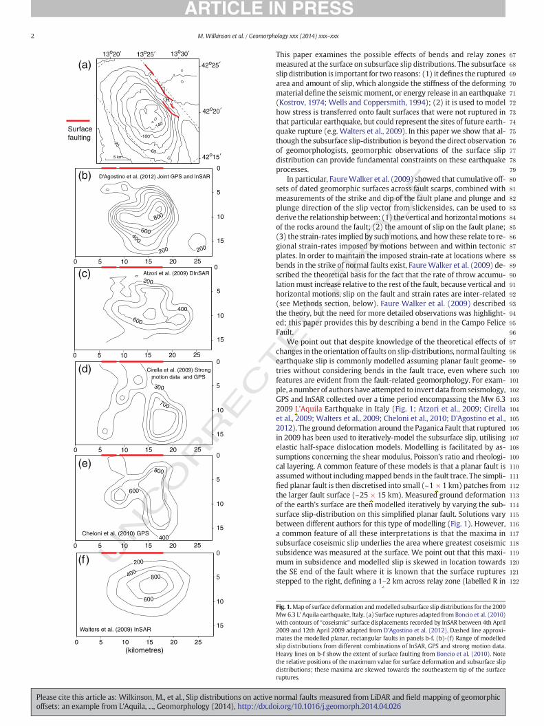
This paper examines the possible effects of bends and relay zonesmeasured at the surface on subsurface slip distributions. The subsurfaceslip distribution is important for two reasons: (1) it defines the rupturedarea and amount of slip, which alongside the stiffness of the deformingmaterial define the seismicmoment, or energy release in an earthquake(Kostrov, 1974; Wells and Coppersmith, 1994); (2) it is used to modelhow stress is transferred onto fault surfaces that were not ruptured inthat particular earthquake, but could represent the sites of future earth-quake rupture (e.g. Walters et al., 2009). In this paper we show that al-though the subsurface slip-distribution is beyond the direct observationof geomorphologists, geomorphic observations of the surface slipdistribution can provide fundamental constraints on these earthquakeprocesses.

In particular, FaureWalker et al. (2009) showed that cumulative off-sets of dated geomorphic surfaces across fault scarps, combined withmeasurements of the strike and dip of the fault plane and plunge andplunge direction of the slip vector from slickensides, can be used toderive the relationship between: (1) the vertical and horizontalmotionsof the rocks around the fault; (2) the amount of slip on the fault plane;(3) the strain-rates implied by suchmotions, and how these relate to re-gional strain-rates imposed by motions between and within tectonicplates. In order to maintain the imposed strain-rate at locations wherebends in the strike of normal faults exist, FaureWalker et al. (2009) de-scribed the theoretical basis for the fact that the rate of throw accumu-lationmust increase relative to the rest of the fault, because vertical andhorizontal motions, slip on the fault and strain rates are inter-related(see Methods section, below). Faure Walker et al. (2009) describedthe theory, but the need for more detailed observations was highlight-ed; this paper provides this by describing a bend in the Campo FeliceFault.

We point out that despite knowledge of the theoretical effects ofchanges in the orientation of faults on slip-distributions, normal faultingearthquake slip is commonly modelled assuming planar fault geome-tries without considering bends in the fault trace, even where suchfeatures are evident from the fault-related geomorphology. For exam-ple, a number of authors have attempted to invert data from seismology,GPS and InSAR collected over a time period encompassing the Mw 6.32009 L'Aquila Earthquake in Italy (Fig. 1; Atzori et al., 2009; Cirellaet al., 2009; Walters et al., 2009; Cheloni et al., 2010; D'Agostino et al.,2012). The ground deformation around the Paganica Fault that rupturedin 2009 has been used to iteratively-model the subsurface slip, utilisingelastic half-space dislocation models. Modelling is facilitated by as-sumptions concerning the shear modulus, Poisson’s ratio and rheologi-cal layering. A common feature of these models is that a planar fault isassumedwithout includingmapped bends in the fault trace. The simpli-fied planar fault is then discretised into small (~1 × 1 km) patches fromthe larger fault surface (~25 × 15 km). Measured ground deformationof the earth’s surface are then modelled iteratively by varying the sub-surface slip-distribution on this simplified planar fault. Solutions varybetween different authors for this type of modelling (Fig. 1). However,a common feature of all these interpretations is that the maxima insubsurface coseismic slip underlies the area where greatest coseismicsubsidence was measured at the surface. We point out that this maxi-mum in subsidence and modelled slip is skewed in location towardsthe SE end of the fault where it is known that the surface rupturesstepped to the right, defining a 1–2 km across relay zone (labelled R in

Fig. 1.Map of surface deformation andmodelled subsurface slip distributions for the 2009Mw 6.3 L’ Aquila earthquake, Italy. (a) Surface ruptures adapted from Boncio et al. (2010)with contours of “coseismic” surface displacements recorded by InSAR between 4th April2009 and 12th April 2009 adapted from D'Agostino et al. (2012). Dashed line approxi-mates the modelled planar, rectangular faults in panels b-f. (b)-(f) Range of modelledslip distributions from different combinations of InSAR, GPS and strong motion data.Heavy lines on b-f show the extent of surface faulting from Boncio et al. (2010). Notethe relative positions of the maximum value for surface deformation and subsurface slipdistributions; these maxima are skewed towards the southeastern tip of the surfaceruptures.

normal faults measured from LiDAR and field mapping of geomorphici.org/10.1016/j.geomorph.2014.04.026

123

124

125

126

127

128

129

130

131

132

133

134

135

136

137

138

139

140

141

142

143

144

145

146

147

148

149

150

151

152

153

154

155

156

157

158

159

160

161

162

163

164

165

166

167

168

169

170

171

172

173

174

175

176

177

178

179

180

181Q4

182

183

184

3M. Wilkinson et al. / Geomorphology xxx (2014) xxx–xxx

Fig. 1a) (compare Fig. 1a with b–e). In this paper we examine the rela-tionship between such relay-zones, slip on the fault plane at depthand vertical motions of the ground surface. We suggest, followingFaure Walker et al. (2009), that the relay zone may overlie a zone ofnon-planarity in the fault plane at depth that may have induced anom-alous surface deformation. This is important because Calderoni et al.(2012) have suggested from an analysis of fault-trapped seismicwaves for the 2009 earthquake that the discontinuous fault segmentsat the surface are part of a continuous fault system at depth. Unfortu-nately, the Paganica Fault is poorly-exposed relative to other nearbyfaults and thus the geomorphic signature of slip and fault kinematicsare difficult to retrieve, so we have been unable to directly apply thetheory from Faure Walker et al. (2009). Thus, to quantify how muchthe vertical deformation is affected by relay zones or bends in the faulttrace, we utilise observations of a well-exposed fault located ~15 kmto the south southwest of the faults that ruptured in 2009 – theCampo Felice active normal fault.

The Campo Felice fault exhibits a well-exposed bedrock fault scarpthat records slip since the last-glacial maximum (15 ± 3 ka). The faultdisplays clear evidence of coseismic slip due to past earthquakes inthe form of strips of freshly-exposed rock at the base of the fault plane(see Giaccio et al., 2002). The relationship between vertical motions,slip on the fault and strain-rate can be retrieved across a prominentfault bend because the fault plane is well-preserved and exhibitsnumerous examples of slickenside surfaces covered in frictional-wearstriae that record the slip vector orientation. We have measured theorientations of the fault plane and slip-vector in the field, and studiedthe geomorphology of the site using terrestrial laser-scanning (TLS) inorder to retrieve the slip distribution and throw recorded by offsetgeomorphology along strike. Similar approaches also exist for thestudy of offset geomorphic features within extensional basins and forstrike-slip and reverse faults from LiDAR data (see Chan et al., 2007;

UNCO

RRECT

Active normal faults

with Holocene offsets

L’Aquila

Avezza

Rieti

Active faultsdiscussed in thisstudy

PAG

CF

SD

Fig. 3

Fig. 1a

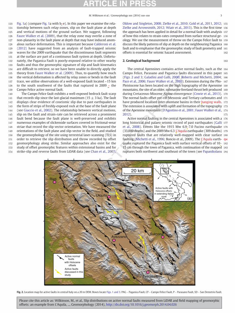
Fig. 2. Location map for active faults in central Italy on a 20m DEM. Boxes locate Figs. 1 and 3. P

Please cite this article as: Wilkinson, M., et al., Slip distributions on activeoffsets: an example from L'Aquila, ..., Geomorphology (2014), http://dx.do

ED P

RO

OF

Oldow and Singleton, 2008; Zielke et al., 2010; Gold et al., 2011, 2012;Zielke and Arrowsmith, 2012; Wiatr et al., 2013). This is the first timethe approach has been applied in detail for a normal fault with analysisof how this relates to strain-rates computed from surface structural ge-ology. We use the measurement of throw on the Campo Felice fault todiscuss the likely patterns of slip at depth on the neighbouring Paganicafault and to emphasise that the geomorphic study of fault geometry andoffsets is essential for seismic hazard assessment.

2. Geological background

The central Apennines contains active normal faults, such as theCampo Felice, Parasano and Paganica faults discussed in this paper(Figs. 2 and 3; Galadini and Galli, 2000; Roberts and Michetti, 2004;Pace et al., 2006; Faure Walker et al., 2010). Extension during the Plio-Pleistocene has been located on the high topography of the Apenninemountains, the site of an older, submarine foreland thrust belt producedduring Cretaceous-Miocene Alpine convergence (Cowie et al., 2013).The normal faults offset pre-rift Mesozoic and Tertiary carbonates andhave produced localised inter-montane basins in their hanging walls.The extension is associated with uplift and formation of the topographyof the Apenninemountains (D'Agostino et al., 2001; FaureWalker et al.,2012).

Active normal faulting in the central Apennines is associated with along historical and palaeo seismic record of past earthquakes (Galliet al., 2008). Events like the 1915 Mw 6.9–7.0 Fucino earthquake(33,000 deaths) and the 2009Mw6.3 L'Aquila earthquake (309 deaths)ruptured faults that are relatively well-mapped with clear surfacefaulting (Michetti et al., 1996; Boncio et al., 2009). The L'Aquila earth-quake ruptured the Paganica fault with surface vertical offsets of 10–15 cm through the town of Paganica, with continuation of the mappedruptures both northwest and southeast of the town (see Papanikolaou

(b)

(a)

Active faults with

in extending Italian crust

noSulmona

Pescasseroli

P

20 km

AG – Paganica Fault, CF – Campo Felice Fault, P – Parasano Fault, SD – San Demetrio Fault.

normal faults measured from LiDAR and field mapping of geomorphici.org/10.1016/j.geomorph.2014.04.026

RRECTED P

RO

OF

185

186

187

188

189

190

191

192

193

194

195

196

197

198

199

200

201

202

203

204

205

206

207

208

209

210

211

212

213

214

215

216

217

218

219

220

2072 m1558m

1523m

2128m

2043m

Quat-HoloceneOutwash

Fan

Morainelast glacial maximum

(LGM)

Moraine

Moraine

OlderMoraine?

OlderMoraine?

Holocenelake deposits

Miocene

LGM and Holocene

Screes

Upper Cretaceous

Upper Cretaceous

Upper Cretaceous

Lower Cretaceous - Upper Jurassic

Lower Cretaceous - Upper JurassicLower Cretaceous - Upper JurassicUpper

Cretaceous

Upper Cretaceous

Quat-HoloceneOutwash

Fan

Portion of fault covered with TLS data

and studied herein

500 m

500 m

N

Former drainage course

Campo Felice

(a)

(b)

Fig. 3. Location maps for the Campo Felice fault. (a) Geological map adapted from Giaccio et al. (2002) and Vezzani and Ghisetti (1998). (b) Satellite imagery from Google Earth™. Thefaults offset Cretaceous carbonates with normal sense displacements, controlling the position of a Quaternary Holocene intra-montane basin, and have offset a former (Quaternary?)drainage course.

4 M. Wilkinson et al. / Geomorphology xxx (2014) xxx–xxx

UNCO

et al., 2010; Vittori et al., 2011; D'Agostino et al., 2012 for reviews).Observations with InSAR and GPS demonstrate coseismic subsidence ofup to 25 cm between 5–6 km into the hanging wall of the fault(Fig. 1a). Elastic dislocation modelling suggests over 80 cm of slip atdepth on the fault (Fig. 1b–f). This area with high values of surface sub-sidence, and the implied area of high slip at depth, is located towardsthe southeastern end of the surface ruptures. Although some of thisslip may be due to the 7th April Mw 5.6 aftershock (Papanikolaouet al., 2010), and we note that this event that was not considered bythe papers reviewed in Fig. 1, below we argue that non-planarity of thefault plane may have a role to play in producing these maxima skewedto the SE. Unfortunately, the surface ruptures occur in unconsolidatedslope sediments in most places, so the orientation of the fault planeand the slip vectors of the earthquake are relatively poorly constrained,except in the central portion of the rupture within the town of Paganicawhere a study of offset tarmac and concrete surfaces along the rupturerevealed that the slip vector plunges at 21° towards 218° (±5° ), almostperpendicular to the strike of the fault (127° ), at least at the surface(Roberts et al., 2010). The relatively poor exposure of the ruptures to

Please cite this article as: Wilkinson, M., et al., Slip distributions on activeoffsets: an example from L'Aquila, ..., Geomorphology (2014), http://dx.do

the 2009 earthquake, especially in the region of the relay zone alongthe surface ruptures (R in Fig. 1a), led us to study the kinematics ofneighbouring active normal faults. Belowwe report a study of the nearbyCampo Felice fault (Figs. 2 and 3) accomplished using terrestrial laserscanning (TLS) and field structural mapping and analysis.

3. Methods

A TLS point cloud dataset of the Campo Felice fault was acquiredusing a Riegl LMS-z420i laser scanner. The dataset consisted of sixscan positions and 11 million measurement points, covering the 5 kmlong southeastern segment of the Campo Felice fault (Fig. 4a). Thepoint clouds from each scan position were co-registered using theRiSCAN Pro processing software. This process unites point clouds fromeach scan position within 3D space. Geo-referencing was carried outby surveying a network of cylindrical reflectors present within eachpoint cloud using real time kinematic (RTK) GPS. The vertical offsetsthat define the surface slip distribution can be recovered from thesedata following a number of data processing steps.

normal faults measured from LiDAR and field mapping of geomorphici.org/10.1016/j.geomorph.2014.04.026

RECTED P

RO

OF

221

222

223

224

225

226

227

228

229

230

231

232

233

234

235

236

237

238

239

240

241

242

243

244

245

246

247

248

249

250

251

252

253

254

255

256

257

258

259

260

261

262

263

264

265

266

NW SE

NW SE

NW SE

1200 m

1200 m

1200 m

(a)

(b)(c)

(d)

(e)

30 m

NW SE

1 2 34 5 6 7 8 9 10 111213

14

15 1617 18 19 20 21 22 23 24 25

Box edges locate (c)

Perspective view of similar area to (a)

Map view

Perspective view with contours

Slope map

Hillshade

Fig. 4. LiDARdata, processing and analysis. (a) Point cloud data. (b)Manual removal of vegetation from point cloud. (c) Contourmap located in (b). (d) TIN surfacewith the locations of 25study siteswhere 10 scarpprofileswere produced (250 scarpprofiles in total). Each red line is actually 10profile lines spaced 1mapart along strike. A representative set of 25 scarpprofilesfrom the 25 locations indicated are shown in Fig. 5. (e) A surface slopemap using the slope calculation algorithm in goCAD and displayed in Google Earth. Blue colours correspond to lowvalues of slope ~20 degrees. Yellow colours correspond to moderate values of slope ~40 degrees. Red colours correspond to high values of slope ~60 degrees.

5M. Wilkinson et al. / Geomorphology xxx (2014) xxx–xxx

UNCO

RThe point cloud dataset was filtered to remove vegetation using acombination of manual point removal and processing of the pointcloud using the GEON points2grid pseudo-vegetation filter (Crosbyet al., in review). A points2grid output point spacing of between 2–4 -meters, with corresponding search radius R between 1.41–2.8 meterswas found to be most suitable, as this preserves metre-scale changesin the ground surface whilst eradicating noise created by vegetation.Once the point cloud has been filtered to remove vegetation, a numberof derivatives can be created from the dataset in order to identifygeomorphic features.

Generation of a solid surface from a point cloud dataset facili-tates study of the tectono-geomorphic features within the originalpoint cloud dataset. A triangular irregular network (TIN) surfacerepresentation of the topography is created using Delaunay trian-gulation (Delaunay, 1934) with the vegetation-filtered pointset asinput. Visualisation of the TIN surface in 3D, with lighting appliedfrom a unidirectional source facilitates identification of geomor-phic features of the faults scarps that are also studied in the field.These include the base of the fault scarp, the fault plane itself,colluvial wedges, the upper and lower geomorphic slopes, andfootwall gullies and hanging wall erosional channels whose forma-tion postdates formation of the upper and lower slopes (Fig. 4dand e).

Please cite this article as: Wilkinson, M., et al., Slip distributions on activeoffsets: an example from L'Aquila, ..., Geomorphology (2014), http://dx.do

A further enhancement to a TIN surface is to calculate the angle(slope) from horizontal of each triangle and to interpolate these dataover the entire surface. These interpolated data can then be used to col-our the surface according to the local slope creating a surface slopemap(Fig. 4e), and to add topographic contours (Fig. 4c). Again, creation of asurface slope map with contours facilitates identification of the faultscarp and its constituent features. In particular, contours that are paral-lel, linear and equally spaced on the hangingwall and the footwall of thefault identify slopes from the last glacial maximum (LGM) that havebeen offset across the fault since 15 ± 3 ka (see Faure Walker et al.,2009 for an explanation).Weused this to identify 25 siteswhere surfaceoffsets have been produced solely by fault slip during earthquakes andnot affected by geomorphic processes such as post 15 ka erosional gul-lying, colluvial and alluvial fan sedimentation or landslides. Topographiccross sections were generated at each of these 25 sites from the surfaceTIN. At each of the 25 sites ten topographic cross sections were createdin the direction of slip, spaced at 1 m intervals (Fig. 4d; 250 in total).Each of the topographic cross sections was interpreted for throw usingthe GNU/octave program Crossint (Fig. 5; see Electronic Supplement).A complete description of the functionality of Crossint can be found inWilkinson (2012).

Throwwas interpreted bymanually picking representative portionsof the hanging wall slope, fault plane and footwall slope from the

normal faults measured from LiDAR and field mapping of geomorphici.org/10.1016/j.geomorph.2014.04.026

UNCO

RRECTED P

RO

OF

G5-00007

Throw:12.543

Heave:6.8157

Hangingwall dip:37.323

Scarp dip:61.48

Footwall dip:40.236

20 mV=H

G7-00001

Throw:12.928

Heave:7.2246

Hangingwall dip:37.816

Scarp dip:60.802

Footwall dip:43.866

20 mV=H

G4-00007

Throw:14.183

Heave:10.739

Hangingwall dip:34.959

Scarp dip:52.868

Footwall dip:38.856

20 mV=H20 mV=H

G8-00004

Throw:12.652

Heave:6.9396

Hangingwall dip:36.514

Scarp dip:61.255

Footwall dip:39.876

20 mV=H

G13-00006

Throw:9.8703

Heave:5.9659

Hangingwall dip:39.445

Scarp dip:58.85

Footwall dip:43.082

20 mV=H

G12-00007

Throw:11.016

Heave:6.2052

Hangingwall dip:34.974

Scarp dip:60.608

Footwall dip:50.129

20 mV=H

G11-00007

Throw:11.082

Heave:5.9235

Hangingwall dip:37.496

Scarp dip:61.874

Footwall dip:42.782

20 mV=H

G10-00006

Throw:12.143

Heave:7.3936

Hangingwall dip:34.526

Scarp dip:58.664

Footwall dip:38.502

20 mV=H

G14-00001

Throw:9.4019

Heave:5.2532

Hangingwall dip:36.003

Scarp dip:60.806

Footwall dip:38.386

20 mV=H

G18-00001

Throw:10.384

Heave:7.1154

Hangingwall dip:34.315

Scarp dip:55.581

Footwall dip:35.804

20 mV=H

G23-00003

Throw:10.793

Heave:5.8829

Hangingwall dip:29.306

Scarp dip:61.407

Footwall dip:36.887

20 mV=H

G37-00005

Throw:7.3804

Heave:3.028

Hangingwall dip:47.646

Scarp dip:67.693

Footwall dip:55.048

20 mV=H

Throw: 10.316

Heave: 6.784

Hangingwall dip: 37.278

Scarp dip: 56.672

Footwall dip: 41.508

20 mV=H

S75-00008

Throw:10.251

Heave:6.9648

Hangingwall dip:33.962

Scarp dip:55.806

Footwall dip:45.245

20 mV=H

S74-00005

Throw:9.3433

Heave:5.9587

Hangingwall dip:35.286

Scarp dip:57.472

Footwall dip:40.335

20 mV=H

N91-00008

Throw:14.184

Heave:8.2584

Hangingwall dip:35.273

Scarp dip:59.79

Footwall dip:38.773

20 mV=H

S2207

Throw: 8.2659

Heave: 5.2038

Hangingwall dip: 36.432

Scarp dip: 57.808

Footwall dip: 44.534

20 mV=H

S3210

Throw: 9.3395

Heave: 7.7969

Hangingwall dip: 38.188

Scarp dip: 50.144

Footwall dip: 39.073

20 mV=H

S4304

Throw: 10.747

Heave: 7.8084

Hangingwall dip: 32.756

Scarp dip: 54

Footwall dip: 35.245

20 mV=H

S4405

Throw:11.226

Heave:8.1838

Hangingwall dip:32.337

Scarp dip:53.907

Footwall dip:36.919

20 mV=H

S9313

Throw: 13.374

Heave: 10.772

Hangingwall dip: 34.794

Scarp dip: 51.149

Footwall dip: 36.851

20 mV=H

S9310

Throw:13.333

Heave:9.4083

Hangingwall dip:34

Scarp dip:54.791

Footwall dip:36.761

20 mV=H

S8503

Throw:12.299

Heave:9.0853

Hangingwall dip:34.052

Scarp dip:53.546

Footwall dip:35.715

20 mV=H

S5102

Throw: 9.5846

Heave: 5.5576

Hangingwall dip: 32.964

Scarp dip: 59.893

Footwall dip: 37.301

20 mV=H

S9409

Throw:14.519

Heave:11.523

Hangingwall dip:35.248

Scarp dip:51.562

Footwall dip:36.385

20 mV=H

65 7

9 10 11 12

13 14

18

21

25

1

15 16

2422

19 2017

8

2 3 4

23S2107

Carbonate bedrock fault plane (free-face) interpreted by linear regression through the TLS data.

Footwall surface (upper slope) interpreted by linear regression through the TLS data.

Hangingwall surface (lower slope) interpreted by linear regression through the TLS data.

Throw:

Heave:

6 M. Wilkinson et al. / Geomorphology xxx (2014) xxx–xxx

Please cite this article as: Wilkinson, M., et al., Slip distributions on active normal faults measured from LiDAR and field mapping of geomorphicoffsets: an example from L'Aquila, ..., Geomorphology (2014), http://dx.doi.org/10.1016/j.geomorph.2014.04.026

RECTED P

RO

OF

267

268

269

270

271

272

273

274

275

276

277

278

279

280

281

282

283

284

285

286

287

288

289

290

291

292

293

294

295

296

298298

N42.24

N42.23

N42.22

N42.21

E13.42 E13.44 E13.46

n=6

n=46

n=16

n=7n=32

n=16

n=45

n=27

Fig. 6. Lower hemisphere stereographic projection of the orientation of fault planes and the slip-vector orientation defined by striated faults, showing how the kinematics of faulting varyalong the Campo Felice fault. Data were collected from the 25 locations shown in Fig. 4.

7M. Wilkinson et al. / Geomorphology xxx (2014) xxx–xxx

UNCO

Rtopographic cross sections. Crossint performs linear regression of thedata points between the picks to calculate the footwall-scarp and hang-ing wall-scarp intersections, from which the throw is calculated. Thisprocess was repeated for all 250 topographic cross sections.

Structural field measurements comprising strike, dip, slip-directionand plunge of the slip direction were collected along the entire lengthof the Campo Felice fault (Fig. 6). These field measurements weretaken using a compass clinometer with locations provided by realtime kinematic GPS with centimetre precision. In order to visualise thechanging geometry and slip direction of the fault along its length, theGPS locations were converted to distance along the fault, fromthe northwestern end, to be plotted on the x-axis against the variousmeasurements from the TLS analysis.

A strain-rate profile was calculated from data for throw, fault geom-etry and slip, using themethod described by FaureWalker et al. (2009)(Fig. 7; Table 1). The advantage of converting to strain-rate compared tothrow-rate is that the former takes into account variations in faultgeometry and the direction of slip, as shown by Faure Walker et al.(2009). Strain-rate was calculated for boxed shaped areas usingthe equations below, as defined by FaureWalker et al. (2009). The com-ponents of strain e11, e12 and e22 were calculated for each sample box of

Fig. 5. Scarp profiles derived from terrestrial laser scan data (TLS) from the 25 sites indicated in F250 profiles generated to produce the values and error bars in Fig. 7. Offsets were interpreted u

Please cite this article as: Wilkinson, M., et al., Slip distributions on activeoffsets: an example from L'Aquila, ..., Geomorphology (2014), http://dx.do

width L and area a. T represents the average throw measured on thefault within the sample box and t is the time period over which thatthrow has formed (for instance 15 ± 3 kyrs in the case of post glacialfaulting in the central Apennines). The average values of plunge direc-tion (plunge), slip direction (slipdir) and strike (strike) for fieldmeasure-ments within the sample box were also used. The direction of principalstrain for each box is defined by θ. The principal strain-rate for each box(strainrate) was calculated in the direction of the regional principalstrain direction (θ) for each sample box along the fault.

e11 ¼ 1at

LT cot plungeð Þ sin slipdirð Þ cos strikeð Þ

e22 ¼ −1at

LT cot plungeð Þ cos slipdirð Þ sin strikeð Þ

e12 ¼ 12at

LT cot plungeð Þ cos slipdir þ strikeð Þ

θ ¼arctan 2

e12e11−e22

� �

2strainrate ¼ e11 þ e22

2− e11 þ e22

2cos 2θaveð Þ−e12 sin 2θaveð Þ

ig. 4d, showing offsets of a 15±3 ka periglacial slope. These 25 profiles are a sub-set of thesing Crossint.

normal faults measured from LiDAR and field mapping of geomorphici.org/10.1016/j.geomorph.2014.04.026

UNCO

RRECTED P

RO

OF

299

300

301

302

303

304

(d)

(c)

(b)

(a) Fault strike vs distance along fault

80

100

120

140

160

180

0 500 1000 1500 2000 2500 3000 3500 4000 4500 5000

0 500 1000 1500 2000 2500 3000 3500 4000 4500 5000

0 500 1000 1500 2000 2500 3000 3500 4000 4500 5000

0 500 1000 1500 2000 2500 3000 3500 4000 4500 5000

Distance along fault (m)

Fa

ult

strike

(d

eg

ree

s fr

om

No

rth

)

Fault dip vs distance along fault

0

10

20

30

40

50

60

70

80

90

Fau

lt di

p (d

egre

es fr

om h

oriz

onta

l)

190

200

210

220

230

240

250

260

Kin

emat

ic p

lung

e di

rect

ion

(deg

rees

from

nor

th)

Post 15 ±3 ka throw vs distance along fault

6

15

Distance along fault (m)

Pos

t 15

±3

ka th

row

(m)

9

12

NW SE

Kinematic plunge direction vs distance along fault

Fig. 7.Graphs showing the relationship between fault orientation andmeasures of the rate of faulting for theCampo Felice fault. (a) Fault strike. Error bars are±3o. The red line is amovingpoint average of fivemeasurements. The bend in the fault map trace occurs between 1500 and 2500m along strike. (b) Fault dip. Error bars are±3o. The red line is amoving point averageof five measurements. (c) Slip direction. Error bars are ±3o. The red line is a moving point average of five measurements. (d) Post 15 ± 3 ka throw measured with TLS. (e) Throw andprincipal horizontal strain-rate (see Table 1). Strain-rate was calculated in 250 x 250 m boxes using the equations in the text. The error bars for throw are ±1σ for measurements ofthrow alone, not including those for uncertainty in age, whilst those for strain-rate are ±2σ. A throw-rate scale is also shown on the y axis for 3 scenarios for the age of the offsetslope (12 ka, 15 ka and 18 ka) – our preferred estimate of the age is 15 ± 3 as it encompasses our assessment of the uncertainty (see Faure Walker et al., 2010 for discussion). (f) and(g) vertical offsets associated with two palaeo earthquakes recorded by stripes of freshly-exposed fault plane at the base of the exposed fault plane reported by Giaccio et al. (2002),but modified slightly during our own fieldwork. Errors on field estimates of the throw for these palaeo earthquakes are estimated to be ± 0.1 m. Overall, this figure shows that thethrow-rate increases in the region of the change in fault strike to maintain the gradual decrease in strain-rate towards the fault tip.

8 M. Wilkinson et al. / Geomorphology xxx (2014) xxx–xxx

4. Results

Fig. 7 shows how strike, dip, slip direction, throw-rate, strain-rateand coseismic slip vary along the studied segment of the Campo

Please cite this article as: Wilkinson, M., et al., Slip distributions on activeoffsets: an example from L'Aquila, ..., Geomorphology (2014), http://dx.do

Felice fault. The measurements for fault strike (Fig. 7a) show aclear anomaly in fault strike between 1500 and 3000 m along thestudied portion of the fault, consistent with the presence of a bendin the map trace of the fault. In contrast, field measurements of

normal faults measured from LiDAR and field mapping of geomorphici.org/10.1016/j.geomorph.2014.04.026

RRECTED P

RO

OF

305

306

307

308

309

310

(e)

(f)

(g)

Average of two events

Youngest 2nd Youngest 3rd Youngest 4th youngest

0.1

0.3

0.5

0.9

1.1

1.3

0.7

0.1

0.3

0.5

0.9

1.1

1.3

0.7

0 500 1000 1500 2000 2500 3000 3500 4000 4500 5000

0 500 1000 1500 2000 2500 3000 3500 4000 4500 5000

0 500 1000 1500 2000 2500 3000 3500 4000 4500 5000

Post 15 ka ±3 throw and strain rate calculated for 250 x 250 m boxes vs distance along the fault

Strain rate ppm/yr

Post 15 ka throw

Pos

t 15

ka th

row

(m

) / s

trai

n ra

te (

ppm

/yr)

2

4

6

8

10

12

14

1.0

0.5

Thr

ow-r

ate

(mm

/yr)

Throw associated with fresh stripes at the base of the fault plane that are probably palaeoearthquakes

12 ka 15 ka 18 ka

1.0

0.5

0.5

Thr

ow (

m)

Thr

ow (

m)

Fig. 7 (continued).

t1:1

t1:2

t1:3

t1:4

t1:5

t1:6

t1:7

t1:8

t1:9

t1:10

t1:11

t1:12

t1:13

t1:14

t1:15

t1:16

t1:17

t1:18

9M. Wilkinson et al. / Geomorphology xxx (2014) xxx–xxx

Ofault dip are consistent along the length of the fault (Fig. 7b). Fieldmeasurements for the direction of slip (Fig. 7c) are consistent be-tween 0–3000 m distance along the fault, with a mean slip direction

UNC

Table 1Data used to calculate strain-rate in 250 m bins along strike.

Plunge of slip vector(degrees from horizontal)

Strike of fault(degrees from north)

Slip direction(degrees from n

47 128 21347 129 21347 134 20852 136 20850 135 21052 138 21351 134 21253 118 21554 104 21055 105 20953 113 20953 142 20854 148 22155 153 22255 153 249

Please cite this article as: Wilkinson, M., et al., Slip distributions on activeoffsets: an example from L'Aquila, ..., Geomorphology (2014), http://dx.do

of 211° (±1σ = 3.9). The slip direction becomes increasing obliquetowards the southeastern tip, as is typical of normal faults (Roberts,1996a, 1996b, 2007). The direction of slip increases from ~211° at

orth)Throw (m) Distance along

strike (m)Strain-rate(ppm/yr)

13.77 125 3.4114.19 375 3.5212.63 625 3.0812.74 875 2.5910.98 1125 2.4211.02 1375 2.259.62 1625 2.0510.05 1875 1.9910.55 2125 1.8611.19 2375 1.9110.87 2625 2.099.47 3375 1.828.80 3625 1.608.31 3875 1.397.30 4375 1.04

normal faults measured from LiDAR and field mapping of geomorphici.org/10.1016/j.geomorph.2014.04.026

T

311

312

313

314

315

316

317

318

319

320

321

322

323

324

325

326

327

328

329

330

331

332

333

334

335

336

337

338

339

340

341

342

343

344

345

346

347

348

349

350

351

352

353

354

355

356

357

358

359

360

361

362

363

364

365

366

367

368

369

370

371

372

373

374

375

376

377

378

379

380

381

382

383

384

385

386

387

388

389

390

391

392

393

394

395

396

397

398

399

400

401

402

403

404

405

406

407

408

409

410

411

412

413

414

415

416

417

418

419

420

421

422

423

424

425

426

427

428

429

430

431

432

433

434

435

436

437

438

439

10 M. Wilkinson et al. / Geomorphology xxx (2014) xxx–xxx

UNCO

RREC

3000m distance along the fault to ~250° at the tip at 4750m distancealong the fault.

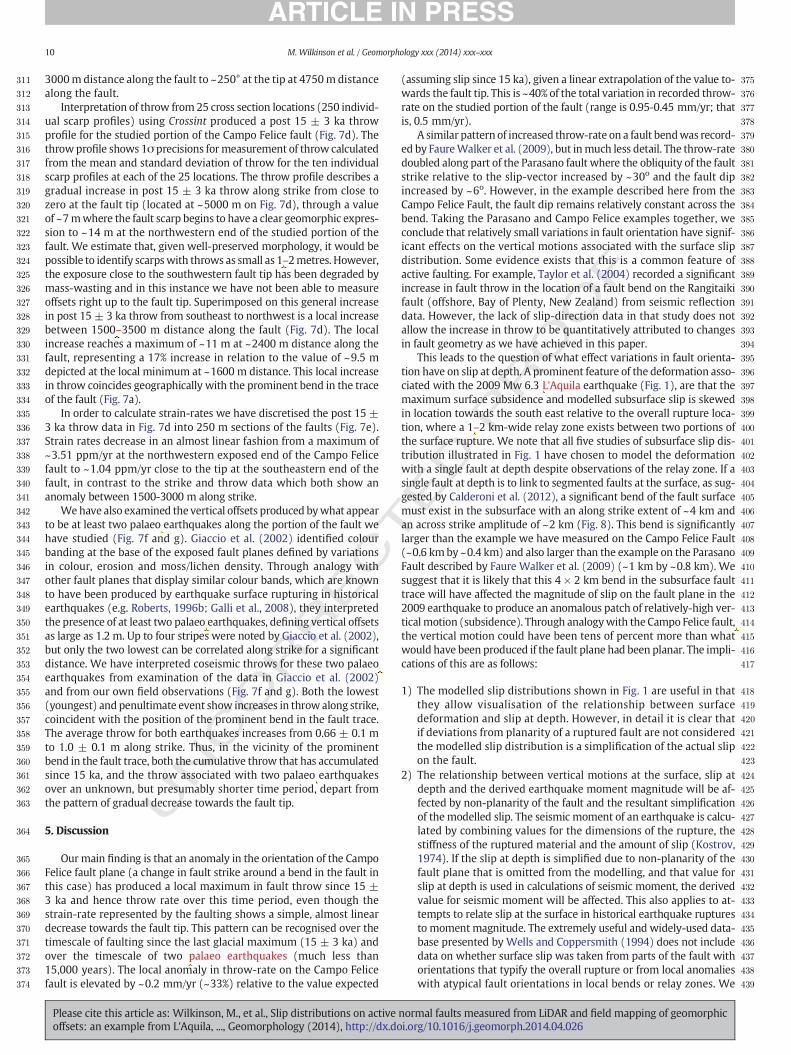
Interpretation of throw from 25 cross section locations (250 individ-ual scarp profiles) using Crossint produced a post 15 ± 3 ka throwprofile for the studied portion of the Campo Felice fault (Fig. 7d). Thethrowprofile shows 1σ precisions formeasurement of throw calculatedfrom the mean and standard deviation of throw for the ten individualscarp profiles at each of the 25 locations. The throw profile describes agradual increase in post 15 ± 3 ka throw along strike from close tozero at the fault tip (located at ~5000 m on Fig. 7d), through a valueof ~7mwhere the fault scarp begins to have a clear geomorphic expres-sion to ~14 m at the northwestern end of the studied portion of thefault. We estimate that, given well-preserved morphology, it would bepossible to identify scarpswith throws as small as 1–2metres. However,the exposure close to the southwestern fault tip has been degraded bymass-wasting and in this instance we have not been able to measureoffsets right up to the fault tip. Superimposed on this general increasein post 15 ± 3 ka throw from southeast to northwest is a local increasebetween 1500–3500 m distance along the fault (Fig. 7d). The localincrease reaches a maximum of ~11 m at ~2400 m distance along thefault, representing a 17% increase in relation to the value of ~9.5 mdepicted at the local minimum at ~1600 m distance. This local increasein throw coincides geographically with the prominent bend in the traceof the fault (Fig. 7a).

In order to calculate strain-rates we have discretised the post 15 ±3 ka throw data in Fig. 7d into 250 m sections of the faults (Fig. 7e).Strain rates decrease in an almost linear fashion from a maximum of~3.51 ppm/yr at the northwestern exposed end of the Campo Felicefault to ~1.04 ppm/yr close to the tip at the southeastern end of thefault, in contrast to the strike and throw data which both show ananomaly between 1500-3000 m along strike.

We have also examined the vertical offsets produced bywhat appearto be at least two palaeo earthquakes along the portion of the fault wehave studied (Fig. 7f and g). Giaccio et al. (2002) identified colourbanding at the base of the exposed fault planes defined by variationsin colour, erosion and moss/lichen density. Through analogy withother fault planes that display similar colour bands, which are knownto have been produced by earthquake surface rupturing in historicalearthquakes (e.g. Roberts, 1996b; Galli et al., 2008), they interpretedthe presence of at least two palaeo earthquakes, defining vertical offsetsas large as 1.2 m. Up to four stripes were noted by Giaccio et al. (2002),but only the two lowest can be correlated along strike for a significantdistance. We have interpreted coseismic throws for these two palaeoearthquakes from examination of the data in Giaccio et al. (2002)and from our own field observations (Fig. 7f and g). Both the lowest(youngest) and penultimate event show increases in throw along strike,coincident with the position of the prominent bend in the fault trace.The average throw for both earthquakes increases from 0.66 ± 0.1 mto 1.0 ± 0.1 m along strike. Thus, in the vicinity of the prominentbend in the fault trace, both the cumulative throw that has accumulatedsince 15 ka, and the throw associated with two palaeo earthquakesover an unknown, but presumably shorter time period, depart fromthe pattern of gradual decrease towards the fault tip.

5. Discussion

Ourmain finding is that an anomaly in the orientation of the CampoFelice fault plane (a change in fault strike around a bend in the fault inthis case) has produced a local maximum in fault throw since 15 ±3 ka and hence throw rate over this time period, even though thestrain-rate represented by the faulting shows a simple, almost lineardecrease towards the fault tip. This pattern can be recognised over thetimescale of faulting since the last glacial maximum (15 ± 3 ka) andover the timescale of two palaeo earthquakes (much less than15,000 years). The local anomaly in throw-rate on the Campo Felicefault is elevated by ~0.2 mm/yr (~33%) relative to the value expected

Please cite this article as: Wilkinson, M., et al., Slip distributions on activeoffsets: an example from L'Aquila, ..., Geomorphology (2014), http://dx.do

ED P

RO

OF

(assuming slip since 15 ka), given a linear extrapolation of the value to-wards the fault tip. This is ~40% of the total variation in recorded throw-rate on the studied portion of the fault (range is 0.95-0.45 mm/yr; thatis, 0.5 mm/yr).

A similar pattern of increased throw-rate on a fault bendwas record-ed by FaureWalker et al. (2009), but inmuch less detail. The throw-ratedoubled along part of the Parasano fault where the obliquity of the faultstrike relative to the slip-vector increased by ~30o and the fault dipincreased by ~6o. However, in the example described here from theCampo Felice Fault, the fault dip remains relatively constant across thebend. Taking the Parasano and Campo Felice examples together, weconclude that relatively small variations in fault orientation have signif-icant effects on the vertical motions associated with the surface slipdistribution. Some evidence exists that this is a common feature ofactive faulting. For example, Taylor et al. (2004) recorded a significantincrease in fault throw in the location of a fault bend on the Rangitaikifault (offshore, Bay of Plenty, New Zealand) from seismic reflectiondata. However, the lack of slip-direction data in that study does notallow the increase in throw to be quantitatively attributed to changesin fault geometry as we have achieved in this paper.

This leads to the question of what effect variations in fault orienta-tion have on slip at depth. A prominent feature of the deformation asso-ciated with the 2009 Mw 6.3 L'Aquila earthquake (Fig. 1), are that themaximum surface subsidence and modelled subsurface slip is skewedin location towards the south east relative to the overall rupture loca-tion, where a 1–2 km-wide relay zone exists between two portions ofthe surface rupture. We note that all five studies of subsurface slip dis-tribution illustrated in Fig. 1 have chosen to model the deformationwith a single fault at depth despite observations of the relay zone. If asingle fault at depth is to link to segmented faults at the surface, as sug-gested by Calderoni et al. (2012), a significant bend of the fault surfacemust exist in the subsurface with an along strike extent of ~4 km andan across strike amplitude of ~2 km (Fig. 8). This bend is significantlylarger than the example we have measured on the Campo Felice Fault(~0.6 kmby ~0.4 km) and also larger than the example on the ParasanoFault described by Faure Walker et al. (2009) (~1 km by ~0.8 km). Wesuggest that it is likely that this 4 × 2 km bend in the subsurface faulttrace will have affected the magnitude of slip on the fault plane in the2009 earthquake to produce an anomalous patch of relatively-high ver-ticalmotion (subsidence). Through analogywith the Campo Felice fault,the vertical motion could have been tens of percent more than whatwould have been produced if the fault plane had been planar. The impli-cations of this are as follows:

1) The modelled slip distributions shown in Fig. 1 are useful in thatthey allow visualisation of the relationship between surfacedeformation and slip at depth. However, in detail it is clear thatif deviations from planarity of a ruptured fault are not consideredthe modelled slip distribution is a simplification of the actual slipon the fault.

2) The relationship between vertical motions at the surface, slip atdepth and the derived earthquake moment magnitude will be af-fected by non-planarity of the fault and the resultant simplificationof themodelled slip. The seismic moment of an earthquake is calcu-lated by combining values for the dimensions of the rupture, thestiffness of the ruptured material and the amount of slip (Kostrov,1974). If the slip at depth is simplified due to non-planarity of thefault plane that is omitted from the modelling, and that value forslip at depth is used in calculations of seismic moment, the derivedvalue for seismic moment will be affected. This also applies to at-tempts to relate slip at the surface in historical earthquake rupturesto moment magnitude. The extremely useful and widely-used data-base presented by Wells and Coppersmith (1994) does not includedata on whether surface slip was taken from parts of the fault withorientations that typify the overall rupture or from local anomalieswith atypical fault orientations in local bends or relay zones. We

normal faults measured from LiDAR and field mapping of geomorphici.org/10.1016/j.geomorph.2014.04.026

T

OO

F

440

441

442

443

444

445

446

447

448

449

450

451

452

453

454

455

456

457

458

459

460

461

462

463

464

465

466

467

468

469

470

471

472

473

474

475

476

477

478

479

480

481

482

483

484

485

486

487

488

489

490

491

492

493

494

495

496

497

498

499

500

501

502

503

504

505

506

507

508

509

510

511

512

513

514

515

516

517

518

13o20’ 13o25’ 13o30’

42o25’

42o20’

42o15’5 km

-140

-100

-60

-20

(a)

R

-5 km-10 km-15 km (b)

Map with schematic contours drawn on the fault plane at depth

Schematic view of the Paganica fault geometry

viewed obliquely from the west

Single, curved fault at depth

Segmented faultat the surface

Fig. 8. Summary cartoon showinghow the location ofmaximumcoseismic subsidence associatedwith the 2009 L'Aquila Earthquake (Ms 6.3)may relate to the subsurface geometry of thefault.We speculate that the segmented fault at surface coalesces into a single curved fault at depth, and the along-strike bend in the fault requires high values for vertical motion followingthe relationships quantified by Faure Walker et al. (2009).

11M. Wilkinson et al. / Geomorphology xxx (2014) xxx–xxx

UNCO

RREC

suggest thismay be one of the reasons for scatter in the relationshipsbetween rupture length, slip and moment magnitudes in the data-base ofWells and Coppersmith (1994). Thus, the role of geometricalcomplexity is important and will influence the slip distribution (seeWesnousky, 2008).

3) Stress transfer modelling depends on using the slip distribution atdepth from an earthquake to model the stress transfer to so-called“receiver faults” (e.g.Walters et al., 2009). If themodelled slip distri-bution is a simplification, the stress transfer will also be a simplifica-tion. If the modelled slip distribution on a planar fault hasconcentrations of high slip, that are an artefact of inverting mea-sured anomalies in ground deformation at the surface with a simpleplanar fault, when in fact the fault is not a single plane, then themodelled concentrations of high stress will in turn be artefacts –yet it is these modelled concentrations of high stress on receiverfaults thatmay cause concern in terms of the possibility of imminentslip in a triggered earthquake.

4) Palaeo seismological studies of past earthquakes commonlymeasurethe throw per event and throw-rate associated with past events(Galli et al., 2008). However, it is rare for such studies to record thespatial variation in fault orientation around the palaeo seismic site,usually because the fault plane is poorly-exposed in the unconsoli-dated material associated with sites suitable for trenching. Impor-tantly, we have shown that defining fault orientations is essential ifthe significance of the throw per event and throw-rate values areto be fully understood. For example, the coseismic throw impliedby colour stripes on the Campo Felice Fault may be overestimatedby ~30% compared to values outside the local fault bend (Fig. 7);using the maximum value without understanding that it is generat-ed by a local anomaly in fault orientation leads to overestimation ofthe moment magnitude and hence the rupture length. As rupturedimensions and maximum earthquake magnitudes are used forseismic hazard and engineering design purposes, local changes infault orientation should be taken into account.

The implications listed above are profound for our understanding ofthe earthquake process, yet to date we only have two examples wherethe anomalous slip produced by bends in a fault plane have been quan-tified (this study and Faure Walker et al., 2009). We suggest that morestudies of the geomorphology and structural geology of active faultsare needed to produce an empirical relationship between the dimen-sions of bends in fault planes and the amplitude of vertical deformation.

Please cite this article as: Wilkinson, M., et al., Slip distributions on activeoffsets: an example from L'Aquila, ..., Geomorphology (2014), http://dx.do

ED P

R

6. Conclusions

A study of the structural geology and geomorphology of the well-exposed Campo Felice active normal fault shows that despite a sim-ple linear decrease in strain-rate along strike from the fault centreto tip, a change in fault strike has produced a localised anomaly invertical motion, with the throw-rate increasing by ~30-40% close tothe fault bend. The throw anomaly can be resolved both over a time-scale of multiple seismic cycles (15 ± 3 ka in this case) or over thetimescale of two individual palaeo earthquakes (b15 kyrs). Thisexample is well explained by theoretical considerations advancedby Faure Walker et al. (2009), who show that horizontal strain-rates and rates of vertical and horizontal deformation are linked byvariables that include fault slip vectors and fault orientations. A 4 ×2 km relay zone in the surface ruptures to the 2009 L'Aquila earth-quake (Mw 6.3) on the neighbouring Paganica fault is likely to be un-derlain by a bend in the fault trace at depth of similar dimensions.The theory of Faure Walker et al. (2009) suggests that a bend ofthis size will produce a significant local anomaly in throw per eventand throw-rate on the fault. Surface deformation for this earthquakeis skewed towards the southeastern end of the rupture trace, with amaximum in the vicinity of the aforementioned relay zone. Existingattempts to model this deformation have used a planar fault, butwe suggest that improvedmodels of the subsurface slip distributionswill be achieved if a non-planar fault with a change in strike isutilised. Surface and subsurface slip distributions are used to modelstress transfer and calculate maximummagnitudes for palaeo earth-quakes. We suggest the orientation of the fault plane in questionshould be considered with care as uncertainty in fault plane orienta-tion relative to the slip-vector will produce uncertainty in derivedstress transfer andmaximummagnitude estimates. Study of the geo-morphology and structural geology of faults at surface is therefore akey input in order to properly define fault activity for the purpose ofaccurate seismic hazard assessment.

Acknowledgements

This workwas funded byNERCGrants NE/H003266/1, NE/E01545X/1, NE/B504165/1, GR9/02995 and NE/I024127/1, a studentship to J.P.Faure Walker (NER/S/A/2006/14042) and the Doctoral Fellowshipscheme at Durham University.

normal faults measured from LiDAR and field mapping of geomorphici.org/10.1016/j.geomorph.2014.04.026

T

519

520

521

522

523524525526527528529530531532533534535536537538539540541542543544545546547548549Q5550551552553554555556557558559560561562563564565566567568569570571572573574575576577578579580581582583584

585586587588589590591592593594595596597598599600601602603604605606607608609610611612613614615616617618619620621622623624625626627628629630631632633634635636637638639640641642643644645646647648649650

12 M. Wilkinson et al. / Geomorphology xxx (2014) xxx–xxx

UNCO

RREC

Appendix A. Supplementary data

Supplementary data to this article can be found online at http://dx.doi.org/10.1016/j.geomorph.2014.04.026.

References

Atzori, S., Hunstad, I., Chini, M., Salvi, S., Tolomei, C., Bignami, C., Stramondo, S., Trasatti, E.,Antonioli, A., Boschi, E., 2009. Finite fault inversion of DInSAR coseismic displacementof the 2009 L'Aquila earthquake (central Italy). Geophys. Res. Lett. 36. http://dx.doi.org/10.1029/2009GL039293 (L15305).

Boncio, P., Pizzi, A., Brozzetti, G., Pomposo, G., Lavecchia, G., Di Naccio, D., Ferrarini, F., 2010.Coseismic ground deformation of the 6 April 2009 L'Aquila earthquake (central Italy,Mw6.3). Geophys. Res. Lett. 37, L06308. http://dx.doi.org/10.1029/2010GL042807.

Calderoni, G., Di Giovambattista, R., Vannoli, P., Pucillo, S., Rovelli, A., 2012. Fault-trappedwaves depict continuity of the fault system responsible for the 6 April 2009 Mw 6.3 L'Aquila earthquake, central Italy. Earth Planet. Sci. Lett. 323–324, 1–8.

Chan, Y.-C., Chen, Y.-G., Shih, T.-Y., Huang, C., 2007. Characterizing the Hsincheng activefault in northern Taiwan using airborne LiDAR data: Detailed geomorphic featuresand their structural implications. J. Asian Earth Sci. 31, 303–316. http://dx.doi.org/10.1016/j.jseaes.2006.07.029.

Cheloni, D., D'Agostino, N., D'Anastasio, E., Avallone, A., Mantenuto, S., Giuliani, R.,Mattone, M., Calcaterra, S., Gambino, P., Dominici, D., Radicioni, F., Fastellini, G.,2010. Coseismic and initial post-seismic slip of the 2009 Mw6.3 L'Aquila earthquake,Italy, from GPS measurements. Geophys. J. Int. 181, 1539–1546. http://dx.doi.org/10.1111/j.1365-246X.2010.04584.x.

Cirella, A., Piatanesi, A., Cocco, M., Tinti, E., Scognamiglio, L., Michelini, A., Lomax, A.,Boschi, E., 2009. Rupture history of the 2009 L'Aquila (Italy) earthquake fromnon-linear joint inversion of strong motion and GPS data. Geophys. Res. Lett. 36.http://dx.doi.org/10.1029/2009GL039795 (L19304).

Cowie, P.A., Scholz, C.H., Roberts, G.P., Faure Walker, J.P., Steer, P., 2013. Viscous roots ofactive seismogenic faults revealed by geologic slip rate variations. Nat. Geosci. 6,1036–1040. http://dx.doi.org/10.1038/NGEO1991 (3rd November 2013).

Crosby, C.J., Krishnan, S., Arrowsmith, J.R., Kim, H.S., Colunga, J., Alex, N., Baru, B., 2014w.Points2Grid: An Efficient Local GriddingMethod for DEMGeneration from Lidar PointCloud Data. Geosphere special issue on Applications of Lidar in the Earth Sciences (inreview).

D'Agostino, N., Jackson, J., Dramis, F., Funiciello, R., 2001. Interactions between mantleupwelling, drainage evolution and active normal faulting: an example from thecentral Apennines (Italy). Geophys. J. Int. 147, 475–497.

D'Agostino, N., Cheloni, D., Fornaro, G., Giuliani, R., Reale, D., 2012. Space-time distributionof afterslip following the 2009 L'Aquila earthquake. J. Geophys. Res. 117. http://dx.doi.org/10.1029/2011JB008523 (B02402).

Delaunay, B., 1934. Sur la sphère vide. Izvestia Akademii Nauk SSSR, 7. OtdelenieMatematicheskikh i Estestvennykh Nauk pp. 793–800.

Faure Walker, J.P., Roberts, G.P., Cowie, P.A., Papanikolaou, I., Sammonds, P.R., Michetti,A.M., Phillips, R.J., 2009. Horizontal strain-rates and throw-rates across breachedrelay zones, central Italy: Implications for the preservations of throw deficits at pointsof normal fault linkage. J. Struct. Geol. 31, 1145–1160.

Faure Walker, J.P., Roberts, G.P., Sammonds, P., Cowie, P.A., 2010. Comparison of earth-quakes strains over 102 and 104 year timescales: insights into variability in theseismic cycle in the central Apennines, Italy. J. Geophys. Res. 115. http://dx.doi.org/10.1029/2009JB006462 (B10418).

FaureWalker, J.P., Roberts, G.P., Cowie, P.A., Papanikolaou, I., Michetti, A.M., Sammonds, P., Wilkinson, M., McCaffrey, K.J.W., Phillips, R., 2012. Relationship between topographyand strain-rate in the actively-extending Italian Apennines. Earth Planet. Sci. Lett.325–326, 76–84. http://dx.doi.org/10.1016/j.epsl.2012.01.028.

Galadini, F., Galli, P., 2000. Active Tectonics in the Central Apennines (Italy) - Input Datafor Seismic Hazard Assessment. Nat. Hazards 22, 225–270.

Galli, P., Galadini, F., Pantosti, D., 2008. Twenty years of paleoseismology in Italy. Earth-Sci.Rev. 88, 89–117.

Giaccio, B., Galadini, F., Sposato, A., Messina, P., Moro, M., Zreda, M., Cittadini, A., Salvi, S.,Todero, A., 2002. Image processing and roughness analysis of exposed bedrock faultplanes as a tool for paleoseismological analysis: results from the Campo Felice fault(central Apennines, Italy). Geomorphology 49, 281–301.

Gold, R., Cowgill, E., Arrowsmith, J.R., Chen, X., Sharp,W.D., Cooper, K.M., Wang, X.F., 2011.Faulted terrace risers place new constraints on the late Quaternary slip rate for thecentral Altyn Tagh Fault, northwest Tibet. Geol. Soc. Am. Bull. 123, 958–978. http://dx.doi.org/10.1130/B30207.1.

Please cite this article as: Wilkinson, M., et al., Slip distributions on activeoffsets: an example from L'Aquila, ..., Geomorphology (2014), http://dx.do

ED P

RO

OF

Gold, P.O., Cowgill, E., Kreylos, O., Gold, R.D., 2012. A terrestrial lidar-based workflow fordetermining three-dimensional slip vectors and associated uncertainties. Geosphere8, 431–442.

Kostrov, V.V., 1974. Seismic Moment and Energy of Earthquakes, and Seismic Flow ofRock, Izv. Earth Phys. 1, 23–40 (translation UDC 550.341, 13-21).

Michetti, A.M., Brunamonte, F., Serva, L., Vittori, E., 1996. Trench investigations of the1915 Fucino earthquake fault scarps (Abruzzo, Central Italy): geological evidence oflarge historical events. J. Geophys. Res. 101 (B3), 5921–5936.

Oldow, J.S., Singleton, E.S., 2008. Application of Terrestrial Laser Scanning in determiningthe pattern of late Pleistocene and Holocene fault displacement from the offset of plu-vial lake shorelines in the Alvord extensional basin, northern Great Basin, USA.Geosphere 4, 536–563.

Pace, B., Peruzza, L., Lavecchia, G., Boncio, P., 2006. Global seismogenic source modellingand probabilistic seismic hazard analysis in Central Italy. Bull. Seismol. Soc. Am. 96,107–132.

Papanikolaou, I.D., Foumelis, M., Paracharidis, E.L., Lekkas, J., Fountoulis, G., 2010. Defor-mation pattern of the 6 and 7 April 2009, M = 6.3 and Mw 5.6 earthquakes inL'Aquila (central Italy) revealed by ground and space observations. Nat. HazardsEarth Syst. 10, 73–87.

Roberts, G.P., 1996a. Variation in fault-slip directions along active normal faults. J. Struct.Geol. 18, 835–845.

Roberts, G.P., 1996b. Noncharacteristic earthquake ruptures from the Gulf of Corinth,Greece. J. Geophys. Res. 101, 25255–25267.

Roberts, G.P., 2007. Fault orientation variations along the strike of active normal fault sys-tems in Italy and Greece: Implications for predicting the orientations of subseismic-resolution faults in hydrocarbon reservoirs. Am. Assoc. Pet. Geol. Bull. 91 (1), 1–20.

Roberts, G.P., Michetti, A.M., 2004. Spatial and temporal variations in growth rates alongactive normal fault systems: an example from the Lazio-Abruzzo Apennines, centralItaly. J. Struct. Geol. 26, 339–376.

Roberts, G.P., Raithatha, B., Sileo, G., Pizzi, A., Pucci, S., Faure Walker, J., Wilkinson, M.,McCaffrey, K., Phillips, R.J., Michetti, A.M., Guerrieri, L., Blumetti, A.M., Vittori, E.,Cowie, P.A., Sammonds, P., Galli, P., Boncio, P., Bristow, C., Walters, R., 2010. Shallowsub-surface structure of the 6th April 2009 Mw 6.3 L'Aquila earthquake surfacerupture at Paganica, investigated with Ground Penetrating Radar. Geophys. J. Int.183, 774–790. http://dx.doi.org/10.1111/j.1365-246X.2010.04713.x.

Taylor, S., Bull, B., Lamarche, G., Barnes, P., 2004. Normal fault growth and linkage in theWhakatane Graben, New Zealand, during the last 1.3 Myr. J. Geophys. Res. 109,B02408. http://dx.doi.org/10.1029/2003JB002412.

Vezzani, L., Ghisetti, F., 1998. Carta Geologica Dell’Abruzzo, 1:100000, SELCA, Firenze.Vittori, E., Di Manna, P., Blumetti, A.M., Comerci, V., Guerrieri, L., Esposito, E., Michetti,

A.M., Porfido, S., Piccardi, L., Roberts, G., Berlusconi, A., Livio, F., Sileo, G., Wilkinson,M., McCaffrey, K., Phillips, R., Cowie, P.A., 2011. Surface faulting of the April 6, 2009,Mw 6.3 L'Aquila earthquake in Central Italy. Bull. Seismol. Soc. Am. 101,1507–1530. http://dx.doi.org/10.1785/0120100140.

Walters, R.J., Elliott, J.R., D'Agostino, N., England, P.C., Hunstad, I., Jackson, J.A., Parsons, B.,Phillips, R.J., Roberts, G.P., 2009. The 2009 L'Aquila earthquake (central Italy): Asource mechanism and implications for seismic hazard. Geophys. Res. Lett. 36.http://dx.doi.org/10.1029/2009GL039337 (L17312).

Wells, D.L., Coppersmith, K.J., 1994. New empirical relationships among magnitude, rup-ture length, rupture width, rupture area and surface displacement. Bull. Seismol. Soc.Am. 84, 974–1002.

Wesnousky, S.G., 2006. Predicting the endpoints of earthquake ruptures. Nature 444,358–360. http://dx.doi.org/10.1038/nature05275.

Wesnousky, S.G., 2008. Displacement and geometrical characteristics of earthquake sur-face ruptures: issues and implications for seismic-hazard analysis and the processof earthquake rupture. Bull. Seismol. Soc. Am. 98 (4), 1609–1632. http://dx.doi.org/10.1785/0120070111.

Wiatr, Τ., Reicherter, Κ., Papanikolaou, Ι., Fernández-Steeger, Τ., Mason, J., 2013. Slip vectoranalysis with high resolution t-LiDAR scanning. Tectonophysics 608, 947–957.

Wilkinson, M.W., 2012. The use of Terrestrial Laser Scanning in characterizing active tec-tonic processes from postseismic slip to the long term growth of normal faults. (Doc-toral thesis) Durham University (http://etheses.dur.ac.uk/5573/).

Zielke, O., Arrowsmith, J.R., 2012. LaDiCaoz and LiDARimager -MATLAB GUIs for LiDARdata handling and lateral displacement measurement. Geosphere 8 (1), 206–221.http://dx.doi.org/10.1130/GES00686.1.

Zielke, O., Arrowsmith, J.R., Grant-Ludwig, L.B., Akciz, O.S., 2010. Slip in the 1857 and ear-lier large earthquakes along the Carrizo segment, San Andreas Fault. Science 327,1119–1122. http://dx.doi.org/10.1126/science.1182781.

normal faults measured from LiDAR and field mapping of geomorphici.org/10.1016/j.geomorph.2014.04.026