Utah State University Utah State University

DigitalCommons@USU DigitalCommons@USU

Reports Utah Water Research Laboratory

January 1969

Simulation of the Hydrologic-Economic Flow System in an Simulation of the Hydrologic-Economic Flow System in an

Agricultural Area Agricultural Area

Murland R. Packer

J. Paul Riley

Harold H. Hiskey

Eugene K. Israelsen

Follow this and additional works at: https://digitalcommons.usu.edu/water_rep

Part of the Civil and Environmental Engineering Commons, and the Water Resource Management

Commons

Recommended Citation Recommended Citation Packer, Murland R.; Riley, J. Paul; Hiskey, Harold H.; and Israelsen, Eugene K., "Simulation of the Hydrologic-Economic Flow System in an Agricultural Area" (1969). Reports. Paper 169. https://digitalcommons.usu.edu/water_rep/169

This Report is brought to you for free and open access by the Utah Water Research Laboratory at DigitalCommons@USU. It has been accepted for inclusion in Reports by an authorized administrator of DigitalCommons@USU. For more information, please contact digitalcommons@usu.edu.

SIMULATION OF THE HYDROLOGIC-

ECONOMIC FLOW SYSTEM IN

AN AGRICULTURAL AREA

by

Mur1and R. Packer J. Paul Riley

Harold H. Hiskey Eugene K. Israe1sen

The work reported by this project com.p1etion report was supported in part with funds provided by the Departm.ent of the Interior,

Office of Water Resources Research under P. L. 88-379, Project Num.ber-B-017-Utah, Agreem.ent Num.ber-

14-01-0001-1564, Investigation Period-July 1 1967 to June 30, 1969

Utah Water Research Laboratory College of Engineering Utah State Univer sity

Logan, Utah

July 1969 PRWG 57-1

ACKNOW LEDGMENTS

This publication represents the final report of a project which was supported in part with funds provided by the Office of Water Resources Research of the United States DepartITlent of the Interior as authorized under the Water Resources Research Act of 1964, Public Law 88 -379. The work was accoITlplished by pers onnel of the Utah Water Research Laboratory in accordance with a research proposal which was subITlitted to the Office of Water Resources Re­search through the Utah Center for Water Resources Research at Utah State University. This University is the institution designated to adITlinister the prograITls of the Office of Water Resources Re­search in Utah.

The authors express gratitude to all others who contributed to the success of this study. In particular, special thanks are extended to Dr. N. Keith Roberts, Dr. Darwin B. Nielsen, and Dr. V. V. Dhruva Narayana froITl Utah State University for their critique and suggestions concerning the project. Special thanks are also extended to the irrigation cOITlpanies and the federal agencies who as sisted in obtaining the data required for the hydro -econoITlic ITlodel.

Special thanks are extended to Dr. Jay M. Bagley, Director of the Utah Water Research Laboratory, for the as sistance of funds and facilities to cOITlplete this research effort.

iv

Murland R. Packer J. Paul Riley Harold H. Hiskey Eugene K. Israelsen

T ABLE OF CONTENTS

Chapter I

INTRODUCTION .

Chapter II

General . The Experimental Area .

Location Boundary Topography Vegetative cover Climate. Geology. Ground water. Soils .

SYSTEMS MODELING •

Chapter III

Modeling Techniques .

Physical models Mathematical models

Analytical models. Simulation models

Simulation Methods.

THE HYDROLOGIC MODEL.

Formulation of a Hydrologic Model

Model requirements . The conceptual model The hydrologic balance • Time and space

increments

System Processes

Surface inflows Interflow Groundwater inflow Total inflow Temperature Precipiation Snowmelt Canal diversions Available soil moisture

Source s of available water.

1 2

3 3 3 4 5 6 6 6

9

9

9 9

10 10

10

11

11

11 11 11

12

12

12 15 15 16 16 16 17 18 19

19

v

Chapter IV

Available soil mois­ture quantitiie s

Infiltration. Evapotranspiration

Effects of soil mois­ture on evapotranspi­ration.

Effects of slop and elevation on evapo­transpiration .

Deep percolation River outflow.

ECONOMIC SYSTEM

Chapter V

Hydrologic Contribution . Economic Unit

Crop cost functions Crop market prices

Economic Evaluation Function Economic System

Inputs Outputs .

LINKING THE HYDROLOGIC AND ECONOMIC SYSTEMS

Crop Production Functions

Chapter VI

COMPUTER PROGRAMMING •

Analog Computer Program.

Scaling •

Time scaling Amplitude scaling.

Digital Computer Program.

Hydrologic model .

Precipitation Snowmelt and snow

storage •

19

20 20

22

22

22 23

25

25 25

25 28

28 29

29 29

31

32

37

37

37

37 37

38

38

38

38

Chapter VII

Evapotranspiration Available soil

ITloisture storage. Irrigation . TiITle delay

(routing) . COITlputer output

EconoITlic Model AssuITlptions •

Spatial hOITlogeneity T eITlpo ral hOITlo geneity

The Production Function •

MODEL VERlFICATION •

Analog Verification of the Hydrologic Model.

Verification of the EconoITlic Model •

Verifying the Hydrologic­EconoITlic Model .

Chapter VIII

RESULTS AND DISCUSSION.

Analog Hydrologic Model.

Soil ITloisture storage. Evapotranspiration. Groundwater Snow storage •

38

40 40

40 41

41

41 41

41

43

43

44

46

49

49

49 49 49 49

vi

Digital Hydrologic­EconoITlic Model

Total value s of net farITl incoITle

Typical ITlanageITlent application of the ITlodel

Evaluation of vari-ous cropping pat­terns .

Evaluating reser­voir storage quan-

53

55

55

55

tities . 57 Evaluating water

exports and iITlports . 57

Evaluating the effects of technological advances.

Chapter IX

SUMMAR Y AND CONCLUSIONS

LITERATURE CITED.

Appendix A: Hydrologic Data for Cache Valley •

57

59

61

65

Appendix B: Analog COITlputer Output. 70

Appendix C: EconoITlic Data for Cache Valley .

Appendix D: Digital COITlputer PrograITl and Output •

72

81

Figure

1.1 General location of the Cache Valley subbasin

1. 2 Location of Cache Valley within the Bear River drainage.

1.3

1.4

1.5

3. 1

3.2

4. 1

4.2

5. 1

5.2

5. 3

5.4

5.5

6. 1

7. 1

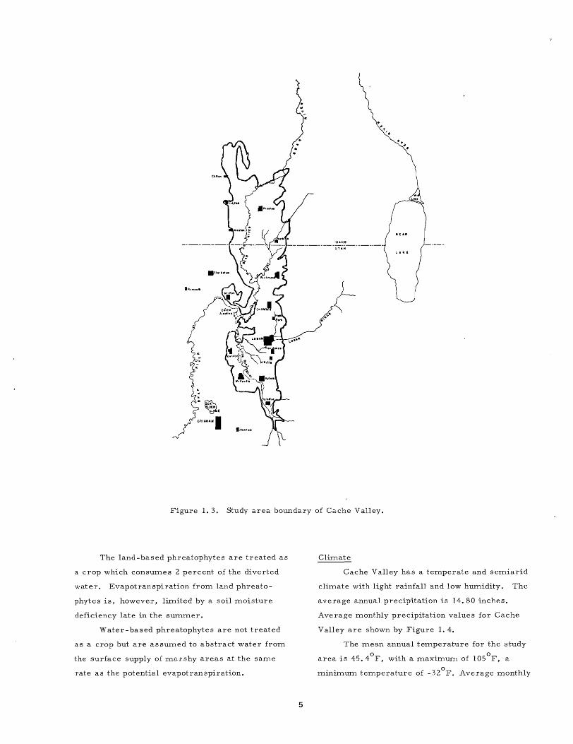
Study area boundary of Cache Valley.

Average monthly precipitation for the irrigated crop land of Cache Valley (1931-1965)

Average monthly temperature for the irrigated crop land of Cache Valley (1931-1965)

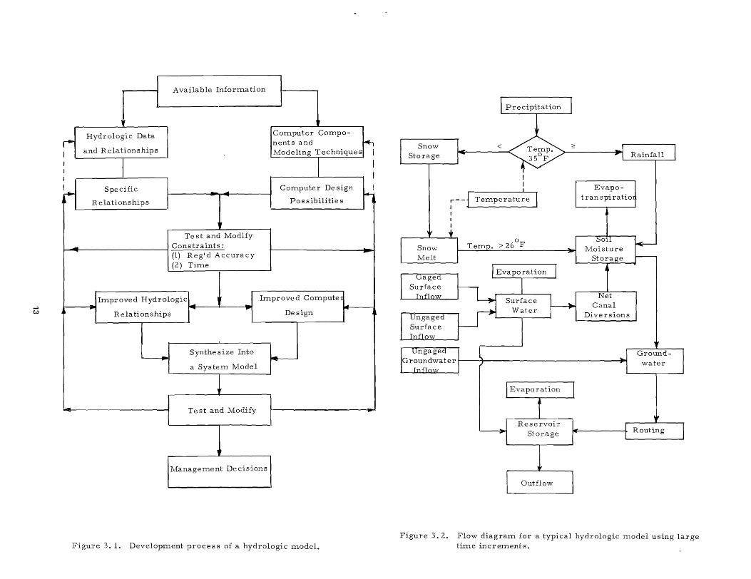
Development proces s of a hydrologic model

Flow diagram for a typical hy­drologic model using large time increments.

Flow diagram of economic system

Cost - -yield relationship for alfalfa.

A general flow chart of a typ­ical hydrologic -economic sys­tem.

Period of seasonal evapotran­spiration accumulatio for growth season of corn.

Typical short-run production function of an agricultural crop

Seasonal evapotranspiration­yield relationship for alfalfa

The production function as the link between the hydrologic and economic models

Analog program for the hy­drologic model

Typical analog computed and observed monthly outflow (acre feet) for Cache Valley, 1944

LIST OF FIGURES

Page

3

4

5

7

7

13

13

26

29

31

32

33

34

35

39

44

vii

Figure

7.2

7.3

8. 1

Summary of basic hydrologic parameters used for hydro­logic -economic model

Predicted digital and analog out­flows from Cache Valley com­pared to the measured outflow for 1944 and 1945 •

Computed available soil mois­ture content in inches, 1944.

8.2 Phreatophyte evapotranspira­tion in inches

8.3

8.4

8.5

8.6

8.7

8.8

8.9

Bl

B2

B3

B4

Crop evapotranspiration (in inches over the entire area) .

Analog calculated groundwater inflow (in inches over the entire area), 1944

Analog computed snow storage equivalent (in inches over the entire area), 1944

Analog calculated snowmelt in inches for Cache Valley

Marginal value of net return to farm management related to the amount of irrigation water di­verted

Total net return to farm manage­ment for various cropping pat­terns and levels of available irrigation water

Total net farm income as it is related to different levels of temperature.

Typical analog computed and observed

Analog computed available soil moisture content in inches, 1945 .

Analog calculated groundwater inflow (in inches over the entire area), 1945

Analog computed snow storage equivalent (in inches over the entire area), 1945

Page

45

48

50

50

51

51

52

52

54

56

56

70

70

71

71

LIST OF FIGURES (Continued)

Figure Page Figure Page

Cl Seasonal evapotranspiration-- C5 Cost - -yield relationship for yield relationship for barley. 72 corn silage . 74

C2 Seasonal evapotranspiration--yield relationship for pasture 72 C6 Cost - -yield relationship for

barl~y . 74 C3 Seasonal evapotranspiration--

yield relationship for sugar C7

beets 73 Cost- -yield relationship for sugar beets. 75

C4 Seasonal evapotranspiration--yield relationship for corn C8 Cost - -yield relationship for silage 73 pasture 75

viii

Table

4.l(a)

4.l(b)

4.2

6. 1

7. 1

7.2

7.3

8. 1

Al

A2

A3

A4

AS

A6

Typical costs of alfalfa pro­duction

Estimated net return for alfal­fa production at various levels of yield.

Market prices for various ag­ricultural crops.

Irrigation priority list of crops.

Values of analog program pa­rameters for Cache Valley hydrologic model

Digital computer model out­put of hydrologic values, 1944

Digital computer model out­put of economic values, 1944.

Various cropping patterns used in this study

Average monthly precipita­tion (inches) for the irrigated crop land of Cache Valley.

Average monthly tempera­tures (oF) for irrigated lands of Cache Valley •

Measured surface inflow to Cache Valley (ac-ft), 1944.

Measured surface inflow to Cache Valley (ac -it), 1945.

Crop growth stage coefficients, k , used in this model for the

c . varIOUS crops

Values of trr climatic coeffi­cient, k , - for various

.t mean aIr temperatures, t •

LIST OF TABLES

Page Table

A7 27

27 CIa

29 Clb

40 C2a

45 C2b

47 C3a

48 C3b

54 C4a

65 Dl

D2 65

D3 66

67 D4

68 D5

D6 68

ix

Monthly percentage of day­time hours &1) of the year for latitudes 18 to 65

0 north of

the equator

Typical costs of corn silage production.

Estimated net return for corn silage production at various levels of yield

Typical costs of sugar beets production

Estimated net return for sugar beet production at various levels of yield

Typical costs of small grains production

Estimated net return for small grains production at various level s of yield

Typical costs of pasture pro­duction •

Digital computer program list of symbols

Flow diagram of digital pro­gram

Digital computer program list­ing for the hydrologic -economic model

Constant input hydrologic values for digital Cache Valley simu­lation model.

Digital computer model output of hydrologic values, 1945

Digital computer model output of economic values, 1945.

Page

69

76

76

77

77

78

79

80

81

82

86

90

91

92

CHAPTER I

INTRODUCTION

General

Future planning and ITlanageITlent of natural

resources ITlust be based upon optiITlUITl use con­

siderations which are highly dependent upon the

concept of econoITlic efficiency. EconoITlic efficien­

cy ITlay be defined as the relationship between

the cost of particular inputs and the return of the

resulting outputs. Therefore, econoITlic efficiency

in the ITlanageITlent of a resource systeITl is con­

cerned with ITlaxiITlizing net benefits.

OptiITlizing the beneficial use of an existing

water resource systeITl depends upon an accurate

quantitative asseSSITlent of the net benefits of vari­

ous ITlanageITlent alternatives. Planning for water

resource use is a cOITlplex operation requiring

careful consideration of the entire systeITl, which

is a function of the as sociated hydrologic flow sys­

tern and the related econoITlic production functions.

An appropriate description of a water resource

systeITl, therefore, includes the hydrologic systeITl,

the econoITlic systeITl, and the functions which re­

late the hydrologic and econoITlic systeITls.

SiITlulation is a useful technique in water

resources planning and ITlanageITlent. Application

of this technique involves synthesis of fundaITlen-

tal ITlatheITlatical relationships for hydrologic and

econoITlic processes into a working ITlodel of the

systeITl. COITlprehensive ITlodeling of the hydrol­

ogy of a river basin began in 1956 with the Harvard

Water Resources PrograITl (HufschITlidt and Fiering,

1966). The purpose of that prograITl was to iITlprove

the ITlethodology for ITlanaging water resource sys­

teITl s.

SiITlulation of econoITlic systeITls has been

atteITlpted in the forITl of business cycle econoITlics

ITlodeled froITl historical records. Holland and

Gillespie (1963) siITlulated the recent history of the

econoITlY of India and used their ITlodel to test vari­

ous alternative developITlent prograITls. Manetsch

(1965) applied the siITlulation technique to an analy­

sis of the econoITlic systeITl within the softwood­

plywood industry of the United States.

In the study presented herein, a procedure for

siITlultaneous ITlodeling of the hydrologic and agri­

cultural econoITlic systeITls within a study area is

developed. The objectives of this study are to:

1. Develop, iITlprove, and evaluate basic

relationships which link the hydrologic

and econoITlic flow systeITls.

2. Develop a cOITlprehensive ITlodel consist­

ing of the linked hydrologic and econoITlic

flow systeITls and to synthesize this ITlodel

on an electronic cOITlputer.

3. Apply the cOITlputer ITlodel to a study of

4.

water values within a particular drainage

basin.

DeITlonstrate through a sensitivity analy­

sis the ability of the ITlodel to indicate

the relative iITlportance of various param­

eters and processes within the systeITl.

5. DeITlonstrate the usefulness of the ITlodel

in deterITlining the effects of various

ITlanageITlent practices on systeITl paraITl­

eters and output functions.

The general hydrologic ITlodel with SOITle ITlodi­

fications developed by Riley et al. (1966) for Circle

Valley, Utah, was adopted. The hydrologic ITlodel

was prograITlITled and verified on an analog cOITlputer,

The verified cOITlputer prograITl was then written in

Fortran IV Language for operation on a digital COITl­

puter. An econoITlic ITlodel pertaining to agricultural

production within the area was forITlulated and pro­

graITlITled on the digital cOITlputer. The two ITlodels

were linked by production functions as sociated with

each agricultural crop.

Through the comprehensive hydro-economic

model, the consequences of various management

alternatives under a variety of constraining assump­

tions were traced through time. For example,

water values were investigated by diverting water

to alternate uses from particular phases of agri­

culture and determining change in net income.

The technique developed under this study rep­

resents a valuable asset to those faced with deci­

sions regarding the utilization of existing water

resources. Specifically, some of the benefits to

be realized are:

1. The model substantially aids in evaluat­

ing and understanding the basic processes

which link the hydrologic and economic

flow systems.

2.

3.

4.

5.

6.

Because it is based on fundamental

relationships, the model has wide appli-

cation to the problems of water resources

planning and management.

The model provides insight into the rela­

tive importance of the various proces ses

within the hydrologic -economic flow

system. In addition, interactions between

the different proces ses in the systems

are examined.

The relative importance of data and other

available knowledge with respect to the

various parts of the entire system can be

objectively as ses sed. For example, the

study indicated that additional research

is needed to completely define agricul­

tural production functions under various

conditions of soil, water, and manage­

ment.

The marginal value of water for agri­

culture under various conditions and

constraints is readily estimated.

A ITleans is provided for predicting the

econoITlic impact on the farm unit due to

changes in the water supply. This anal-

2

ysis can be applied for both short and long

run economic considerations.

The ExperiITlental Area

The mathematical model of the hydrologic­

econoITlic systeITl was tested and verified with data

froITl Cache Valley, located in Cache County, Utah,

and Franklin County, Idaho. Cache Valley was

selected as the study area for the following reasons.

1. Cache Valley has three important facili­

ties required for a study of this nature:

(a) convenience of easy and frequent in­

spection; (b) availability of data; and (c)

the results of any study conducted in the

area are readily applicable over a wide

surrounding region and to areas with

similar features.

2.

3.

4.

5.

6.

The study area is well defined frOITl physi-

cal and econoITlic standpoints.

Basic hydrologic and economic data are

available from records such as the U. S.

Bureau of ReclaITlation (1962a and 1962b),

and studies by Hiskey (1968).

The Utah Water Research Laboratory and

Utah State University lie within the study

area. This facilitated ready and frequent

consultations with those who earlier con­

ducted relevent inve stigations in the study

area and with the experts in the field.

A variety of agricultural crops are grown

in the area. Such variety allowed the

model to be tested and the results evalu­

ated under ITlore general conditions.

The Cache Valley study of DeTray (1967)

has given a good initial grounding for this

study. This present study was actually

planned as a follow-up investigation of

the study by DeTray.

DeTray made a ITlethodological study of the

siITlulation techniques of analysis with special ref-

erence to developing econOlnic -hydrologic models

of real but complex water resource systems. He

studied the utility of various techniques of simula­

tion in predicting the economic impact of changes in

water supply and of developing aggregate social

values for water. DeTray concluded from his

study that the simulation approach is well suited for

analyzing and studying large complex water re­

source systems, including Cache Valley. Actual

simulation of Cache Valley is, therefore, attempted

in this study.

Location

Cache Valley is a small contiguous unit locat­

ed in northern Utah and neighboring southeastern

Idaho (Figure 1. 1). The study area is situated

roughly between 410

30 ' and 420

15' north latitudes

and between 1110

50 ' and 1120

05' west longitudes

and forms a part of the Bear River drainage (Fig-

ure 1. 2). Cache Valley is oriented in a general

north-south direction and is approximately 60 miles

long and 15 miles wide. The actual modeled area of

Cache Valley is 333 square miles.

Boundary

The hydrologic -economic investigation was

primarily concerned with agriculturally related

economics which are affected by natural and arti­

ficially imposed hydrologic conditions. The model­

ed area (Figure 1. 3) included the irrigated cropland

and lower lands dominated by phreatophytes. The

entire valley floor was considered as a single space

unit in the model. A small portion of the unculti­

vated area is included in Logan City and other urban

areas. The urban areas are assumed to consume

about half the water used by the same area of pas­

ture land (Narayana et al., 1968). The pervious

portion of the city area is usually in the form of

irrigated lawns.

3

"> .. , \.

'''''''J

i ~ ~v",\

\ ~\ ", "' .. -:-.. ~ .

D A H 0

. Boil.

·Po.crt.".

L ___ . __ .. -"I" - .. -l\.-~~~ I ~L~an I I ~'Brieh.'" I Gr"at I

I SoH.. ·Ogd.. 'L l~.('\ ------l v. Soft

• Lok. CI!, :

\

W SIlIdy "rea

i

u T H

\ :

\ I

\

L ______ .-----.-~ Figure 1. 1. General location of the Cache

Valley subbasin.

Topography

Cache Valley is generally flat with an average

elevation of about 4,500 feet and is surrounded by

mountains which exceed 9,000 feet and comprise a

large portion of the total watershed. Runoff frpm

the Cache Valley is discharged into Cutler Reser­

voir by the major drainages which include the Bear,

Figure 1. 2. Location of Cache Valley within the Bear River drainage.

Logan, Cub, and Little Bear Rivers. Bear River

is the largest stream. in the watershed and flows

southward from. Idaho.

Vegetative cover

The cropping pattern used for m.odel verifi­

cation is taken from. land use inventory m.aps pre­

pared by Haws (1969a). Cache Valley was m.apped

during the sum.m.er of 1966; the m.aps were com.­

pleted in 1967. The sum.m.ary of values used is

4

shown in Table 8. 1. For this study, the areas

listed as sm.all truck crops such as tom.atoes,

beans, and peas, are included with sugar beets

becaus e they require a sim.ilar am.ount of labor

and provide the sam.e range of net returns to farm.

m.anagem.ent.

The phreatophytes are divided into two groups:

(a) those growing on land (ditch banks, etc.) and

(b) those growing in water (low m.arsh lands).

Land phreatophytes com.prise about 75 percent of

the total phreatophyte area.

10AHO .. __ ._-._ .. _.-_0._ .. _.

Figure 1. 3. Study area boundary of Cache Valley.

The land-based phreatophytes are treated as

a crop which conSUITles 2 percent of the diverted

water. Evapotranspiration froITl land phreato­

phytes is, however, liITlited by a soil ITloisture

deficiency late in the SUITlITler.

Water - based phreatophytes are not treated

as a crop but are as sUITled to abstract water froITl

the surface supply of ITlarshy areas at the saITle

rate as the potential evapotranspiration.

5

CliITlate

Cache Valley has a teITlperate and seITliarid

c1iITlate with light rainfall and low hUITlidity. The

average annual precipitation is 14.80 inches.

Average ITlonthly precipitation values for Cache

Valley are shown by Figure 1. 4.

The ITlean annual teITlperature for the study

area is 45. 4o

F, with a ITlaxiITluITl of 1050

F, a

ITliniITlUITl teITlperature of _32o

F. Average ITlonthly

tem.peratures for Cache Valley are shown in Fig­

ure 1. 5.

The frost free period (consecutive days when

the tem.perature is 320

F or above) in the valley is

on the average 123 days (D. S. Bureau of Reclam.a­

tion, 1962c). The clim.ate perm.its a wide range of

tem.perate clim.ate field crops such as wheat, barley

alfalfa, pasture, field corn, -sugar beets, peas,

green beans, canning corn, and truck crops.

Geology

In a broad sense, the geology of any area

determ.ines the capacity of surface storage as well

as groundwater storage and percolation rates

(Morris and Johnson, 1967). The direction and the

rate of groundwater m.ovem.ent also depends upon

the geology of the area. The geology of Cache Val­

ley is particularly im.portant because of the com.­

paratively large subsurface inflow from. the sur­

rounding m.ountains. Geological studies related to

this area have been done by Gilbert (1890), William.s

(1958, 1962), and Beer (1967).

Bedrock of the Cache Valley watershed is

described by Beer (1967) as consisting of Precam.-

brian, Paleozoic, and Tertiary rocks of lim.estone

and dolom.ite, shale, sandstone, and conglom.erate,

quartzite and phyllite, and volcanic tuff. The valley

fill contains unconsolidated quaternary sedim.ents

of gravel, sand, silt, and clay of lacustrine and

fluvial origin.

Groundwater

The Cache Valley groundwater basin varies in

aquifer productivity, water tem.perature, and water

quality. The unusual geology of the area has been

responsible for the existence of groundwater occur­

ring under both water table and artesian conditions.

Aquifers in the Logan area are highly produc­

tive and are com.posed of well sorted gravels and

sandy gravels. Wells in this area produce up to

4,500 gallons per m.inute and obtain water from.

6

aquifers with transm.issibilities up to one m.illion/

gpd/ft and specific capacities ranging from. 100 to

350 gpm./ft (Beer, 1967). Aquifers away from. the

Logan area are less productive.

Water -table conditions in the Logan area

change to artesian conditions towards the west.

About 2,000 wells, m.ost of which are of the flow-

type, are operated in these aquifers (Bjorklund,

1968).

Soils

The soils of Cache Valley originated from. a

wide variety of rocks and m.inerals which were

transported into the valley by the Bear River and

by tributary stream.s (D. S. Bureau of Reclam.ation,

1962c). Much of the soil m.aterial was deposited

in ancient Lake Bonneville. The sand and gravel

m.aterials were deposited at the periphery of the

valley as fans and lake terraces. Finer textured

lacustrine clay sedim.ents settled in the deeper and

m.ore quiet waters of the lake. They are widely

distributed on the interior of the valley. Alluvial

sedim.ents were deposited along the m.eandering

courses of rivers and stream.s which traversed the

valley floor. Most of the land has good water trans-

m.is sion properties and adequate available m.oisture

capacity. Natural precipitation and irrigation have

generally leached m.ost of the toxic chem.ical con­

stituents from higher lands and transported them. to

the lower areas on the valley floor. The soils are

mostly silt loam.s with infiltration rates norm.ally

ranging between 0.6 and 1. 3 inches per hour.

Many of the low valley lands produce only

poor quality pasture grasses because of water-

10 g ging, salinity, and alkali. Othe r lands now

produce only light crops of wild hay and som.e are

alm.ost completely non-productive because of the

concentration of harm.ful salts. Gardner and

Israelsen (1954) estim.ate that over 20, 000 acres

of Cache Valley bottom. land can be m.ade productive

through adequate drainage.

2.0 .

til Q)

...c: u .S 1.5 I ~

c: 0

..., ~

J I .e-u Q) 1.0 '"' 0..

~ ...c: I ~ 0

E .5

Q)

I .. an ro

'" Q)

> <: Annllal average prec ipitation = 14.80 inches

. . . . . . .Tan. Feb. Mar. Apr. May June July Oct. ;\Iov.

Figure 1.4. Average m.onthly precipitation for the irrigated crop land of Cache Valley (1931-1965).

70 ° .

bO ° I J

50 ° c Ii-. I

Q.,

~ 40° ';d

'"' G.-o.. ~ (;:

0 30

;....,

...c

-~ ° lO

I I

Q.,

bJ: rd

'"' Q., ;....

10° -< -

. . . I I

Jan. Feb. \1ar. Apr. May June July Aug. Sept. Oct. ::\lov. Del.

Figure 1. 5. Average m.onthly tem.perature for the irrigated crop land of Cache Valley (1931-1965).

7

CHAPTER II

SYSTEMS MODELING

Modeling Techniques

Management of water-resource systems, as

with other types of public operations, deals with

techniques of decision making. Models used to

study the management of such systems need to con­

sider both the physical proces ses and the economic

implications involved in all stages of the prototype.

The problem of designing a model is to reproduce

or represent in space and time the physical and

economic processes associated with the system.

To this model it is possible to apply the physical

inputs, the constraints, and the theoretical appa­

ratus of production and allocation economics. In

order to chQose from alternative courses of action,

an objective or set of objectives must be specified

and developed as a guide to optimal management.

In recent years hydrologist s have attempted

to develop suitable mathematical models to repre­

sent the hydrologic system. Considerable atten­

tion has been given to the development of models

of complex water resource systems. As already

indicated, initial steps in developing a mathemati­

cal model of both the physical and the economic

flow systems of a hydrologic unit were undertaken

approximately 10 years ago under the Harvard

water resources program (Maass et al., 1962).

In general, the models commonly applied to water

resource systems design fall into two broad cate­

gories: Physical models and mathematical models.

Physical models

Physical models are normally scale repro­

ductions of the prototype but may be distorted in

the horizontal or vertical dimension. Measure­

ments or observations are made by subjecting the

model to conditions similar to those confronted by

the prototype. In the first period of physical mod-

9

el investigations, model reproduction based on the

similarity of hydraulic factors was considered

satisfactory. At a later stage fundamental laws

governing transporation of solid materials were

considered, and still further development led to the

consideration of morphological characteristics of

the water courses. Such models were used to test

the performance of various hydraulic structures,

flood and erosion control measures, and sediment

transport problems.

In recent years there has been a renewed

interest in the use of small-scale artifical drainage

basins for studying the rainfall-runoff process in

the laboratory. Some researchers (Grace and

Eagleson, 1965) have concluded that strict dynamic

similarity of a physical watershed model cOl:lld be

accomplished only for small impervious watersheds

not exceeding the size of one acre. If the problems

of economics and other associated complex factors

are also to be directly considered in the manage­

ment of a water resource system, it may be con­

cluded that physical models offer few practical

choices. For problems of this nature, it is neces­

sary to consider another type of modeling technique.

Mathematical models

A dynamic system, such as a water resource

system, is characterized by three basic components:

Input, storage, and output. These three components

may be related by one or more mathematical formu­

lation. Interdependent relationships exist among

individual physical, economic, and social system

components. A model, including the interdependent

relationships, can be conveniently developed with

the river subbasin as the basic space unit of study.

In recent years, the search for suitable models

of the water resource systems has led to the de-

velopment of two basic approaches or techniques:

Analytical models and simulation models. Both

kinds of ITlodels represent the physical systeITl

with quantitative inputs and outputs deterITlined by

ITlatheITlatical relationships.

Analytical ITlodels. An analytical ITlodel is a

set of equations intended to be solved for optiITli­

zation of the outputs in terITlS of a specified ob­

jective function. For exaITlple, the ITlost suitable

cOITlbination of factors, such as cropping patterns

and water use, ITlight be sought with the objective

of optiITlizing net incoITle. OptiITlization is aCCOITl­

plished with the aid of standard ITlethods of algebra

and calculus.

Analytical ITlodels that yield optiITlal solutions

have practical liITlitations when applied to cOITlplex

water resource systeITls. Solution of a systeITl of

equations by analytical ITlethods usually requires

both sectional ITlodeling and siITlplifying as SUITlP­

tions.

SiITlulation ITlodels. A generally accepted

solution to the probleITl of engineering analysis is

the adoption of the principles of siITlulation where­

in a physical systeITl is ITlodeled in SOITle practical

ITlanner. Through siITlulation ITlethods, nonlinear,

dynaITlic ITlodels of cOITlplex systeITls are entirely

pos sible. For this reason, siITlulation is frequent-

1y the only practical procedure available for the

analysis of water resource systeITls even though

it does not directly yield the optiITluITl solution.

The advantages of siITlulation include:

1. Insight is provided into the ITlake -up and

operation of the systeITl being ITlodeled

and the relative iITlportance of the vari­

ous cOITlponents within the systeITl.

2.

3.

4.

The systeITl can be nondestructively

tested, which is of particular interest

in the design of large daITls and flood

control ITleasures in a river basin.

Proposed ITlodifications of existing sys­

teITlS can be tested for perforITlance prior

to installation.

Various system designs ITlay be studied at

10

ITliniITluITl expense, thus avoiding the

selection of unsatisfactory alternatives.

As already indicated, an iITlportant liITlitation

to siITlulation is that it does not along five optiITlal

answers to design probleITls. A single siITlulation

run with a unique set of values for the design vari­

abIes provides an estiITlate of the systeITl perforITl­

ance. In effect it involves exploration of an n-diITlen­

sional response surface in which the results of any

single trial with a unique set of the design variables

constitutes a single point on this surface.

SiITlulating a water resource system involves

building a ITlodel that represents all of the inherent

systeITl characteristics while predicting responses

of the systeITl. The ITlodel usually includes SOITle

nonITlatheITlatical or logical processes. If desired,

systeITls can be analyzed in terITlS of their dynaITlic

response to paraITleter variation.

No reference was found in the literature to

studies wherein the hydrologic and econoITlic flow

systeITls are effectively ITlodeled and linked on a

deterministic basis such that the interactions be­

tween the two systeITls can be exaITlined and con­

sidered by the ITlodel. The study reported herein

describes an initial atteITlpt to bridge this gap in

water resource system ITlanageITlent techniques.

The probleITl is siITlplified by as E?uITling a systeITl

which involves only agricultural production.

SiITlulation Methods

SiITlulation can be perforITled by active and

passive analog systeITls or active digital systeITls.

Pas sive analog ITlodels have been applied to inve sti­

gations of groundwater phenoITlena for ITlany years.

Active siITlulation is a relatively new developITlent

and is periorITled by the analog or digital cOITlputer

solution of ITlatheITlatical relationships which describe

the systeITl. SiITlulation in this study was perforITled

by both analog and digital cOITlputer solution of the

systeITl equations.

CHAPTER III

THE HYDROLOGIC MODEL

Fornmlation of a Hydrologic Model

Model requirements

To meet the fundamental requirements of a

computer model of a hydrologic system, it must be

demonstrated that:

1. It simulates on a continuous basis all

important processes and relationships

within the system it represents.

2. It is nonunique with respect to space.

This implies that it can be applied easily

to different geographic areas with exist­

ing hydrologic data.

3. It is capable of answering questions con­

cerning perturba~ions in the system or of

accurately predicting outputs resulting

from varying input and process param­

eters.

The general research philosophy involved in

the development of a simulation model of a dynamic

system, such as a hydrologic unit, is shown by the

flow diagram of Figure 3. 1. In addition to predic­

ting system responses to particular input functions

and parameter changes, the process of model de­

velopment provides for improvement of system re­

lationships.

The conceptual model

The hydrologic model utilized in this study

is a modified version of that developed in earlier

studies involving the computer simulation of a com­

plete watershed unit (Riley et al., 1966 and 1967).

Simplification was achieved by including only the

valley bottom lands.

The basis of the hydrologic model is a funda­

mental and logical mathematical representation of

the various hydrologic processes and routing func-

11

tions. These physical processes are not specific

to any particular geography, but rather are appli­

cable to any hydrologic unit, including all of the

subbasins located within the Bear River basin. Ex­

perimental and analytical results were used whenever

possible to assist in testing and establishing some

of the mathematical relationships included within

the model. Under a model verification procedure,

equation constants are established which calibrate

or fit the model for a particular drainage area.

Average values of hydrologic quantities needed for

model verification were estimated from available

data, by statistical correlation techniques, and

through verification of the model.

A flow diagram of the hydrologic system is

shown by Figure 3.2. As this flow chart indicates,

the total input to a subbasin is the combination of

surface and subsurface inflows of water obtained by

summing river and tributary inflows, precipitation,

groundwater, and imports from other subbasins.

Depletions from the subbasins occur through evapo­

transpiration, municipal and industrial consumption,

exports, plus surface and subsurface outflows. As

water pas ses through this system, storage changes

occur on the land surface, in the soil moisture zone,

in the groundwater zone, and in the stream channels.

These changes occur rapidly in surface locations

and more slowly in the subsurface zones. Subsur­

face flows undergo various time delays as they

move through the system. Each parameter and

process depicted by Figure 3.2 is discussed in

some detail in the following sections.

The hydrologic balance

A dynamic system consists of three basic

components, namely the medium or media acted

upon, a set of constraints. and an energy supply or

driving force. In a hydrologic systeITl, water in any

one of its three physical states is the ITlediuITl of

interest. The constraints are applied by the physi­

cal nature of the hydrologic basin, and the driving

forces are supplied by direct solar energy, gravity,

and capillary potential fields. The various func­

tions and operations of the different parts of the

systeITl are interrelated by the concepts of continu­

ity of ITlass and ITlOITlentUITl. Unless relatively high

velocities are encountered, such as in channel flow,

the effects of ITlOITlentUITl are negligible, and the

continuity of ITlas s becoITles the only link between

the various processes within the systeITl.

Continuity of ITlass is expressed by the gen­

eral equation:

Output Input ±. Change in storage

A hydrologic balance is the application of this

equation to achieve an accounting of physical, hy­

drologic ITleasureITlents within a particular unit.

Through this ITleans and the application of appro­

priate translation or routing functions, it is possi­

ble to predict the ITloveITlent of water within a

systeITl in terITls of its occurrence in space and

tiITle.

In the course of ITlodel developITlent, each

of the systeITl processes ITlust be described

ITlatheITlatically as cOITlpletely as possible and

related to the other proces ses as de scribed in the

above flow chart. Each box and connecting line in

the flow chart is repres ented by a ITlatheITlatical

expres sion in the ITlodel.

TiITle and space increITlents

Practical data liITlitations and probleITl con­

straints require that increITlents of tiITle and space

be considered during ITlodel design. Data, such as

teITlperature and precipitation readings, are usually

available as point ITleasureITlents in terITlS of tiITle

and space; and integration in both diITlensions is

12

usually accoITlplished by the ITlethod of finite incre­

ITlents.

The cOITlplexity of a ITlodel designed to repre­

sent a hydrologic systeITl largely depends upon the

ITlagnitude of the tiITle and spatial increITlents utilized

in the ITlodel. In particular, when large increITlents

are applied, the scale ITlagnitude is such that the

phenoITlena which change over relatively sITlall incre­

ITlents of space and tiITle are ITlasked. For instance,

on a ITlonthly tiITle increITlent, interception rates and

changing snowpack teITlperatures are neglected. In

addition, the tiITle increITlent chosen ITlight coincide

"With the period of cyclic changes in certain hydro­

logic phenoITlena. In this event net changes in these

phenoITlena during the tiITle interval are usually

negligible. For exaITlple, on an annual basis, stor­

age changes within a hydrologic systeITl are often

insignificant, whereas on a ITlonthly basis, the ITlag­

nitude of these changes is frequently appreciable and

needs to be considered. As tiITle and spatial incre­

ITlents decrease, iITlproved definition of the hydro­

logic processes is required. No longer can short­

terITl transient effects or appreciable variations in

space be neglected, and the ITlatheITlatical ITlodel,

therefore, becoITles increasingly cOITlplex with an

accoITlpanying increase in the requirITlents of COITl­

puter capacity and capability.

For the study of the Cache Valley subbasin

discussed in this report, a ITlonthly tiITle increITlent

and large space unit (subbasin) were adopted. Se­

lection of the subbasin was based on hydrologic

boundaries and points of data collection. It was

felt that the selection of the subbasin and the ITlonth­

ly tiITle increITlent could satisfy the requireITlents

of a general hydro -econoITlic ITlodel.

SysteITl Proces se s

Surface inflows

The basic inflow or input of water into any hy­

drologic systeITl originates as a forITl of precipitation.

Available InforTIlation

Hydrologic Data COTIlputer COTIlPO-... nents and

and Relationships Modeling Techniques

I

! Specific COTIlputer De sign ... - ... ... ~ Relationships Pos sibilitie s

Ir

Te stand Modify

- Constraints: (1) Reg'd Accuracy (2) TiTIle

... ITIlproved Hydrologic l- . ITIlproved COTIlputel

... w Relationships Design

- Synthe size Into ~

a SysteTIl Model

- Te st and Modify

1

ManageTIlent Decisions

Figure 3. 1. DevelopTIlent proces s of a hydrologic TIlodel.

14-

..

..

I

I

ro

Snow Storage

Figure 3.2.

~--j TeTIl;e~t~r~

Rainfall

Evapo-t ran spi ratio

Net Canal

Diversions

Flow diagraTIl for a typical hydrologic TIlodel using large tiTIle increTIlents.

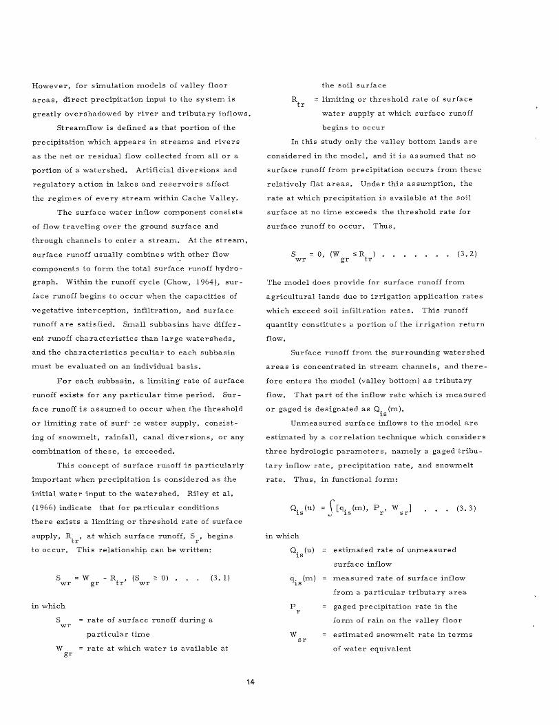
However, for simulation models of valley floor

areas, direct precipitation input to the system is

greatly overshadowed by river and tributary inflows.

Streamflow is defined as that portion of the

precipitation which appears in streams and rivers

as the net or residual flow collected from all or a

portion of a watershed. Artificial diversions and

regulatory action in lakes and reservoirs affect

the regimes of every stream within Cache Valley.

The surface water inflow component consists

of flow traveling over the ground surface and

through channels to enter a stream. At the stream,

surface runoff usually combines with other flow

components to form the total surface runoff hydro­

graph. Within the runoff cycle (Chow, 1964), sur-

face runoff begins to occur when the capacities of

vegetative interception, infiltration, and surface

runoff are satisfied. Small subbasins have differ-

ent runoff characteristics than large watersheds,

and the characteristics peculiar to each subbasin

must be evaluated on an individual basis.

For each subbasin, a limiting rate of surface

runoff exists for any particular time period. Sur­

face runoff is assumed to occur when the threshold

or limiting rate of surf- ::e water supply, consist-

ing of snowmelt, rainfall, canal diversions, or any

combination of these, is exceeded.

This concept of surface runoff is particularly

important when precipitation is considered as the

initial water input to the watershed. Riley et al.

(1966) indicate that for particular conditions

there exists a limiting or threshold rate of surface

supply, Rtr

, at which surface runoff, S r' begins

to occur. This relationship can be written:

S wr

in which

S wr

W. gr

W gr

(S ~ 0) • wr

(3. 1)

rate of surface runoff during a

particular time

rate at which water is available at

14

R tr

the soil surface

limiting or threshold rate of surface

water supply at which surface runoff

begins to occur

In this study only the valley bottom lands are

considered in the model, and it is as sumed that no

surface runoff from precipitation occurs from these

relatively flat areas. Under this assumption, the

rate at which precipitation is available at the soil

surface at no time exceeds the threshold rate for

surface runoff to occur. Thus,

S 0, (W ~R). gr tr

(3.2) wr

The model does provide for surface runoff from

agricultural lands due to irrigation application rates

which exceed soil infiltration rates. This runoff

quantity constitute s a portion of the irrigation return

flow.

Surface runoff from the surrounding watershed

areas is concentrated in stream channels, and there-

fore enters the model (valley bottom) as tributary

flow. That part of the inflow rate which is measured

or gaged is designated as Qis (m).

Unmeasured surface inflows to the model are

estimated by a correlation technique which considers

three hydrologic parameters, namely a gaged tribu­

tary inflow rate, precipitation rate, and snowmelt

rate. Thus, in functional form:

Q. (u) = \' [q. (m), Pr

, Wsr

] IS ..J IS

(3.3)

in which

Q. (u) IS

p r

W sr

estimated rate of unmeasured

surface inflow

measured rate of surface inflow

from a particular tributary area

gaged precipitation rate in the

form of rain on the valley £loor

estimated snowmelt rate in terms

of water equivalent

froITl the plant and surrounding environITlent such as

adjacent soil surfaces. Potential evapotranspiration

is defined as that rate of consuITlptive use by active-

1y growing plants which occurs under conditions of

cOITlplete crop cover and non-liITliting soil ITloisture

supply.

The evapotranspiration proces s depends upon

ITlany interrelated factors whose individual effects

are difficult to deterITline. Included aITlong these

factors are type and density of crop, soil ITloisture

supply, soil salinity, and cliITlate. CliITlatological

paraITleters usually considered to influence evapo-

transpiration rates are precipitation, teITlperature,

daylight hours, solar radiation, hUITlidity, wind

velocity, cloud cover, and length of growing season.

NUITlerous relationships have been developed for

estiITlating the potential evapotranspiration rate.

Perhaps one of the ITlost universally applied

evapotranspiration equations is that proposed by

Blaney and Criddle (1950). This equation is written

as:

D kf. (3. 19)

in which

D ITlonthly crop potential consuITlptive

use in inches

k ITlonthly coefficient which varies with

type of crop

f ITlonthly consuITlptive use factor

and is given by the following equation:

_!L f - 100 . (3.20)

in which

p

ITlean ITlonthly teITlperature in OF

ITlonthly percentage of daylight hours

of the year

A ITlodification of the Blaney-Criddle forITlula was

proposed by Phelan (1962), wherein the ITlonthly

coefficient, k, is subdivided into two parts, a crop

coefficient, k c' and a teITlperature coefficient, kt

•

21

The relationships des cribing kt

is an eITlpirical one,

depending upon only teITlperature, and is expres sed as:

(0.0173 T - 0.314) . a

(3. 21)

where T is the ITlean ITlonthly teITlperature in of. a

The crop coefficient, kc' is basically a function of

the physiology and stage of growth of the crop. Typ­

ical curves which indicate values of kc throughout

the growth cycle of particular crops are shown by

Figure 3.3 which is for alfalfa. SiITlilar k curves c

are available for ITlany agriculture crops (D. S. Soil

Conservation Service, 1964).

Thus, the ITlodified Blaney-Criddle equation

for estiITlating potential evapotranspiration rates is

written:

ET cr

T P k k _a_

c t 100 (3.22)

Because of its siITlplicity, low data require­

ITlents (only surface air teITlperature is needed), and

applicability to the irrigated areas of the Western

Dnited States, Equation 3.22 was adopted for this

study ITlodel. Since the tiITle increITlent selected for

use was one ITlonth, the variables on the right of

Equation 3.22 represent ITlean ITlonthly values, al­

though these paraITleters could be expressed as con­

tinuous functions instead of the indicated step func­

tions. Thus, Equation 3.22 estiITlates the ITlean po­

tential evapotranspiration rate during each ITlonth.

The growing season was assUITled to begin and

end when the ITlean ITlonthly air teITlperature reached

a value of 32oF. Evapotranspiration losses froITl

the agriculture area during the non-cropping season

were estiITlated froITl Equation 3.22. For ITlany

crops it was neces sary to extend the k curves to c

include the non- growing season (West, 1959). Be-

cause the kc curve for grass pasture seeITlS to rep­

resent a reasonable set of values for native vegeta-

tion (Riley et al., 1967), this curve was used as a

guide in the developITlent of a siITlilar k c curve for

phreatophytes.

Effects of soil moisture on evapotranspiration.

As the moisture content of a soil is reduced by

evapotranspiration, the moisture tension which

plants must overcome to obtain sufficient water for

growth is increased. It is generally conceded that

some reduction in the evapotranspiration rate occurs

as the available quantity of water decreases in the

plant root zone. Recent studies by the U. S. Salin­

ity Laboratory in California (Gardner and Ehlig,

1963) indicate that transpiration occurs at the full

potential rate through approximately the first one­

third of the available soil moisture range, and that

thereafter the actual evapotranspiration rate lags

the potential rate. When this critical point in the

available moisture range is reached, the plants

begin to wilt because soil moisture becomes a

limiting factor. Thereafter, an essentially linear

relationship exists between the available soil mois­

ture and the actual transpiration rate. The actual

evapotranspiration rate is expres sed by Riley et al.

(1966) in accordance with the end conditions which

accompany the two following equations:

ET r

and

ET r

in which

ET r

ET cr

M eS

M (t) s

ET , [M < M (t):-SM ] (3.23 ) cr es s cs

M (t) ET

s M

(0 ~M (t) ~ M ) (3. 24) cr s es

es

actual evapotranspiration rate

potential evapotranspiration rate

limiting or threshold content of

available water within the root

zone below which the actual be-

comes les s than the potential

evapotranspiration rate

quantity of water available for

plant consumption which is stored

in the root zone at any instant of

time

22

M root zone storage capacity of cs

water available to plants

Because they are differential with respect to

time, both Equations 3.23 and 3.24 are easily pro­

grammed on the computer. In the integrated form

Equation 3. 24 appears as:

M (2) s

ET cr

M es

(3.25 )

in which M (1) and M (2) are the soil moisture s s

storage values at time tl and t2

, respectively.

Hence, when conditions are such that the available

soil moisture storage reduces the potential evapo­

transpiration rate, the actual consumptive us e rate

can be expressed by combining Equations 3.22 and

3.24 to read:

ET r

M s

M es

T P k k _a_

c t 100 (3.26)

Equation 3. 26 is programmed on the computer to

estimate the actual evapotranspiration rate. The

equation reduces to Equation 3.22 when Ms > Mes

so that ET = ET r cr

Effects of slope and elevation on evapotrans-

piration. In that they affect the available energy

supply, land slope (degree and aspect) and elevation

influence the evapotranspiration proces s. Riley and

Chadwick (1967) considered the effects of slope by

introducing a radiation index parameter. These

same authors also introduced an elevation correction

into Equation 3,26. This adjustment is necessary

for watershed studies since surface air temperature

becomes a less reliable index of the available energy

with increased elevation above the valley floor. How­

ever, because the model of this study was confined

to the relatively flat valley floor areas, the effect

of both slope and elevation on the evapotranspiration

rate was neglected.

Deep percolation

The final independent term, G r' of Equation

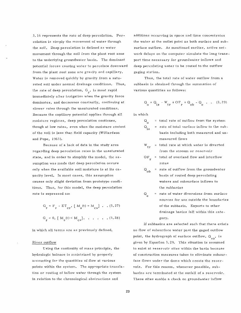
3. 16 represents the rate of deep percolation. Per­

colation is simply the movement of water through

the soil. Deep percolation is defined as water

movement through the soil from the plant root zone

to the underlying groundwater basin. The dominant

potential forces causing water to percolate downward

from the plant root zone are gravity and capillary.

Water is removed quickly by gravity from a satu­

rated soil under normal drainage conditions. Thus,

the rate of deep percolation, Gr

, is most rapid

immediately after irrigation when the gravity force

dominates, and decreases constantly, continuing at

slower rates through the unsaturated conditions.

Because the capillary potential applies through all

moisture regimes, deep percolation continues,

though at low rates, even when the moisture content

of the soil is les s than field capacity (Willardson

and Pope, 1963).

Because of a lack of data in the study area

regarding deep percolation rates in the unsaturated

state, and in order to simplify the model, the as­

sumption was made that deep percolation occurs

only when the available soil moisture is at its ca­

pacity level. In most cases, this assumption

causes only slight deviation from prototype condi­

tions. Thus, for this model, the deep percolation

rate is expressed as:

G r

G r

F r

ET , cr

[ M (t) s

0, [ M (t) < M ]. s cs

M ] . cs

• (3.27)

• (3.28)

in which all terms are as previously defined.

River outflow

U sing the continuity of mas s principle, the

hydrologic balance is maintained by properly

accounting for the quantities of flow at various

points within the system. The app1."opriate transla­

tion or routing of inflow water through the system

in relation to the chronological abstractions and

23

additions occurring in space and time concentrates

the water at the outlet point as both surface and sub-

surface outflow. As mentioned earlier, active net-

work delays on the computer simulate the long trans­

port time neces sary for groundwater inflows and

deep percolating water to be routed to the outflow

gaging station.

Thus, the total rate of water outflow from a

subbasin is obtained through the summation of

various quantities as follows:

Q o

in which

Q o

Q. IS

W tr

OF r

Q e

Q. IS

W + OF + Q - Q • tr r ob e

(3.29)

total rate of outflow from the system

rate of total surface inflow to the sub-

basin including both measured and un­

mea sured flows

total rate at which water is diverted

from the stream or reservoir

total of overland flow and interflow

rates

rate of outflow from the groundwater

basin of routed deep percolating

waters and subsurface inflows to

the subbasins

rate of water diversions from surface

sources for use outside the boundaries

of the subbasin. Exports to other

drainage basins fall within this cate-

gory.

If subbasins are selected such that there exists

no flow of subsurface water past the gaged outflow

point, the hydrograph of surface outflow, Q ,is so

given by Equation 3.29. This situation is assumed

to exist at reservoir sites within the basin because

of construction measures taken to eliminate subsur-

face flows under the dams which create the reser-

voir. For this reason, whenever possible, sub-

basins are terminated at the outfall of a reservoir.

These sites enable a check on groundwater inflow

rates to the subbasin as predicted from verification

studies involving models for one or more upstream

subbasins.

For many subbasins the termination or outlet

point is taken at a Geological Survey gaging station,

and in some of these cases groundwater flow

occurs in the streambed alluvium beneath the sur-

face channel. For these basins, the total system

outflow can be written as:

in which

Q so

Q go

Q + Q . (3.30) so go

rate of surface outflow from the

subbasin

rate of subsurface or groundwater

outflow from the subba sin

Surface outflow rates, Q so' can be compared to the

recorded values, but subsurface outflow rates,

Q ,are unmeasured and must be predicted or go

estimated. It can be as surned that the subsurface

outflow rates are directly proportional to the total

outflow rates, and Q is therefore estimated by go

24

the following relationship:

Q go

in which

(3.31 )

a coefficient determined by model

verification representing the percentage

of total outflow which leaves the basin

as subsurface flow

Because of storage and permeability effects,

fluctuations in groundwater flow rates tend to be

much les s extreme than in the case of surface

flows. The value of kd in Equation 3.31 is,

therefore, not maintained as a constant, but is

expressed as an inverse function of the surface

flow rate, Qso

• During the spring runoff period,

for example, the predicted increases in subsurface

outflow rate, Q ,from Equation 3.31 are con-go

siderably less extreme than the increase in observed

or computer surface flow rate, Qso

• Relationships

expressing kd as a function of Qso

can be develop­

ed for any subbasin through the model verification

process. However, since the outflow boundary

coincided with the location of a darn; the ungaged

groundwater outflow rate was assumed negligible.

CHAPTER IV

ECONOMIC SYSTEM

The theory involved in the formation of the

economic model for this study does not attempt to

describe the agricultural economic system in de­

tail. It does, however, attempt to predict the

average economic conditions which can be expect­

ed to occur under a given set of conditions and

constraints. The economic model described here,

in conjunction with the hydrologic model, provides

a means of establishing guides for planning and

developing existing land and water resources. The

economic system includes the crops produced on

irrigated farm land and their relationship to the

hydrologic system, but does not directly consider

live stock or municipal uses. A simplified flow

diagram of the agricultural economic unit is shown

in Figure 4. 1. The basic economic unit of the

study ITlay be an individual farm or a river subbasin.

The economic returns to agricultural crops

are basically ·related to the yield of the correspond­

ing crops. Higher yields are associated with high­

er gross returns to the farm, higher costs, and

normally higher net returns. The connecting link

between the hydrologic and economic flow systeITls

of an agricultural complex is dependent upon such

factors as water availability, water requirements,

and production per unit of water consumed. How­

ever, water is only one of many factors which in­

fluence production in agriculture. Production is

also a function of ITlanagement, capital, labor,

crop variety, soil type, and soil fertility. By

maintaining these other factors at relatively con­

stant levels, it is pos sible to estimate production

(yield) as a function of water consumed.

Hydrologic Contribution

The hydrologic system is related indirectly

to the economic system by the amount of water

25

which is applied to the crops, both artificially and

naturally, to sustain crop growth. Yield is ITlore

directly a result of water use than application rates.

Some sources (Wilson, 1967; Johnson, 1967;

Miller, 1965; and Widstoe and Merrill, 1912) have

used the total water applied to crops as an estimate

of crop yield. This approach is usually adopted

because adequate data on consumptive use of water

by crops are not available. An error is introduced

by consideration of total water applied due to the

great variation in application efficiency and storage

capacity of the soils from one farm unit to another.

The approach, suggested by Stewart and Hagan

(1968), that the crop yield is a nonlinear function of

evapotranspiration during the growing season was

adopted for this study. Seasonal evapotranspiration,

then, is the hydrologic contribution to the estiITlation

of crop yield.

EconoITlic Unit

Economics of agricultural crops on a total

valley basis are as sumed to be related to the avail­

able moisture. The economic unit deals with the

agricultural crop, production, marketing, and the

related costs and benefits within Cache Valley.

Since the irrigated land of Cache Valley is included

in the study area for the ITlodel, there is a direct

correspondence between the hydrologic and econOITl­

ic systems.

Crop cost functions

There are fixed and variable costs associated

with the production of each crop. Fixed costs (also

called overhead costs) do not vary with the level of

output during the tiITle period under study, norITlally

one year. Real estate taxes are an exaITlple of fixed

costs of production because they will not change with

Seasonal E. T. from

Hydrologic Model

, Economic Production Function

Crop Prices ~ Unit 4---- for Each Crop

~W'

Gross Farm Crop Cost Crop Acreages f----+o Income ~ Functions

11,

Net Farm Income Per Acre

Figure 4. 1. Flow diagram of economic system.

the level of farm production in any particular year.

Variable costs, on the other hand, vary with

the level of output. An example of variable cost

is the cost of fertilizers. If more fertilizer is

. applied to increase the crop yield, then the cost

of fertilizer will increase. Variable costs may

also change due to scale economies such as higher

yields related to efficiency of large farm units.

Average costs decline as the scale of operations

increase. This is due primarily to the us e of

larger and more specialized machinery and

buildings. Marginal costs are the change in total

costs as sociated with an incremental change of

inputs. The cost data used for this study were

taken from a report by Hiskey (1968).

26

Table 4. I may be referred to for the costs

as sociated with alfalfa production. The costs

associated with other crops appear in Appendix C.

The capital cost associated with agricultural pro­

duction for this study was included as a fixed cost

(Table 4. I (a)). It was as sumed that there would

be an interest due on money borrowed, or an

opportunity cost as sociated with money invested

in land and other factors of production.

The C03t of production has been itemized in

Table 4. I (a). For example, requirements for a

farm tractor are expected to be 1. 8 hours per acre

at a cost of $1. 69 per hour on a 60 acre alfalfa field.

Table 4. l(b) indicates the total costs per acre and

returns per acre that can be expected at various

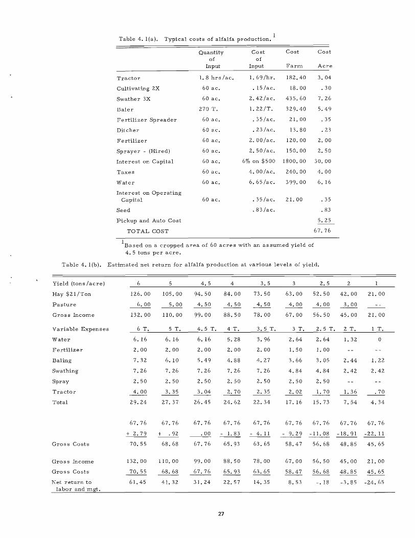
Table 4. l(a). Typical costs of alfalfa production. 1

Quantity Cost Cost Cost of of

Input Input Farm Acre

Tractor 1. 8 hrs/ac. 1. 69/hr. 182.40 3.04

Culti vating 2X 60 ac. · 15 lac. 18.00 .30

Swather 3X 60 ac. 2.42 lac. 435.60 7.26

Baler 270 T. 1. 22/T. 329.40 5.49

Fertilizer Spreader 60 ac. · 35 lac. 21. 00 .35

Ditcher 60 ac. · 23 lac. 13.80 .23

Fertilizer 60 ac. 2. 00 lac. 120.00 2.00

Sprayer - (Hired) 60 ac. 2.50/ac. 150.00 2.50

Interest on Capital 60 ac. 6% on $500 1800.00 30.00

Taxes 60 ac. 4. 00 lac. 240.00 4.00

Water 60 ac. 6. 65 lac. 399.00 6. 16

Interest on Operating Capital 60 ac. .35 lac. 21. 00 .35

Seed .83 lac. .83

Pickup and Auto Cost 5.25

TOTAL COST 67.76

IBased on a cropped area of 60 acres with an assumed yield of 4.5 tons per acre.

Table 4. l(b). Estimated net return for alfalfa production at various levels of yield.

Yield (tons lacre) 6 5 4.5 4 3.5 3 2.5 2

Hay $21/Ton 126.00 105.00 94.50 84.00 73.50 63.00 52.50 42.00 21. 00

Pasture 6.00 5.00 4.50 4.50 4.50 4.00 4.00 3.00

Gro s s Income 132. 00 1l0.00 99.00 88.50 78.00 67.00 56.50 45.00 21. 00

Variable Expenses 6 T. 5 T. 4.5 T. 4 T. 3.5 T. 3 T. 2.5 T. 2 T. T.

Water 6. 16 6.16 6. 16 5.28 3.96 2.64 2.64 1. 32 0

Fertilizer 2.00 2.00 2.00 2.00 2.00 1. 50 1. 00

Baling 7.32 6.10 5.49 4.88 4.27 3.66 3.05 2.44 1. 22

Swathing 7.26 7.26 7.26 7.26 7.26 4.84 4.84 2.42 2.42

Spray 2.50 2.50 2.50 2.50 2.50 2.50 2.50

Tractor 4.00 3.35 3.04 2.70 2.35 2.02 1. 70 1. 36 .70

Total 29.24 27.37 26.45 24.62 22.34 17.16 15. 73 7.54 4.34

67.76 67.76 67.76 67.76 67.76 67.76 67.76 67.76 67.76

+ 2.79 + .92 .00 - 1. 83 - 4.11 - 9.29 -11. 08 -18.91 -22.11 --- --- ---Gross Costs 70.55 68.68 67.76 65.93 63. 65 58.47 56.68 48.85 45.65

Gro s s Income 132.00 110.00 99.00 88.50 78.00 67.00 56.50 45.00 21. 00

Gross Costs 70.55 68.68 67.76 65.93 63.65 58.47 56.68 48.85 45.65 ---Net return to 61. 45 41. 32 31.24 22.57 14.35 8.53 -. 18 -3.85 -24. 65

labor and mgt.

27

levels of production.

Production cost data are plotted in Figure 4. 2

and Appendix C as quadratic curves which repre­

sent the costs as sociated with various levels of

farll1 production.

Crop ll1arket price s

The value of agricultural production is ll1eas-

ured by the ll1arket prices of the crops produced.

The prices used in this study are averages of the

local 1968 prices. This ll10del was assull1ed to

sill1ulate only the short - run econoll1ics, and de­

ll1and was as sUll1ed to have no effect on the fixed

prices. The values used in this study for ll1arket

prices of various crops are listed in Table 4.2.

If long-run conditions were studied, variable

prices would be introduced according to a record-

ed or predicted schedule.

Gross returns for each crop were found by

multiplying the crop yield per acre, crop area in

acres, and the ll1arket price of the crop. All

crops produced were as sumed to be sold at the

till1e of harvest at the current market prices.

Econoll1ic Evaluation Function

Once the physical productivity of water is

established for each crop, the economic produc­

tivity of each crop can be deterll1ined by attaching

ll10netary values to the output and resource inputs.

Net returns are then deterll1ined by the ll10del £rOll1

the production function of each crop and the cost

as sodated with each crop production process.

In any particular year, farll1ers report a

wide range in yields of crops per acre. Many

factors are responsible for this situation. SOll1e

farll1ers are ll10re skilled than others in using

identical production techniques. There is also a

substantial variation in the inherent production

capacity of the land froll1 one farll1 to another.

In econoll1ic analysis, the benefits and costs

are expressed in monetary terll1S on an annual

28

basis for each crop. The annual gros s benefits per

acre less the total annual costs per acre is the

annual net farm incoll1e per acre o( production. The

total net farm income is the SUll1 of the products of

the total area under each crop and the net farm in­

come per acre for each crop. Mathell1atically, the

total net farll1 income is expre s sed by:

NI

in which

NI

Y

P

o

F. 1

1. 1

A. 1

n n

~

i= 1 (Y.

1 P

i A.)

1 ~ [(Oi+Fi+Ii)AJ i= 1

(4.1)

net farll1 incoll1e

annual yield per acre for crop (i)

price per unit of yield for crop (i)

annual operating costs per acre for

crop (i)

annual fixed costs per acre for crop (i)

annual interest costs on investll1ent

per acre for crop (i)

nUll1ber of acres of crop (i)

The total net farm income is the ll1easure of

actual profit to the farmer and, for different levels

of wate r use, is an es sential econoll1ic ll1easure

of productivity in determining the ll10st efficient use

of the available water supply. In order to ll1axill1ize

net return, the farll1er attell1pts to find the most

profitable combination of variable factors and fixed

factors involved in the operation. For a given level

of technology and fixed production factors, the

farmer varies those inputs that can be changed in

order to equate ll1arginal revenue and ll1arginal cost.

If the farll1er takes each crop price as deterll1ined

by the market, since the farll1er is a price-taker,

and equates ll1arginal revenue with ll1arginal cost

for each crop, he is ll1axill1izing the net return £rOll1

the farll1 (Wilcox and Cochrane, 1960).

One ll1ight reason that, when a farll1er has

found a particular cropping pattern which maxi-

ll1izes his net returns under the given conditions,

he has found a perll1anent solution. But this is not

so, ll1ainly because the "given conditions" are

7.0

Cost . ~

0.77392 x Yleld ... 10.89453 x yield - 33. n7~·{

6.0

(I..j 5.0 0::; U <t:

~.O U)

Z 0 ~ 3.0

Q ~ (I..j ~. 0 >-i

>--

1.0

0.0

30 40 50 bO 70 kO

COST (DOLLARS / ACRE)

Figure 4.2. Cost--yield relationship for alfalfa.

constantly changing. Changes may occur for the

followirig reasons:

1. Changes in a natural resource such as

2.

3.

4.

5.

6.

water supply.

Changes in consumer supply or demand,

and therefore prices.

Changes in transportation to market

costs, which makes areas more distant

from markets either more or less

competitive.

Changes in infestations of crops by pests

and diseases.

Changes in farm machinery.

Changes in seed varieties.

Economic System

The inputs to the economic model are:

1.

2.

Seasonal evapotranspiration from each

crop (as an index of crop yield).

Production cost-yield relationships.

29

3. Market prices of the crop yields which

are considered constant for one year.

Outputs

The output values from the economic model

are dependent upon both the input functions and the

constraints as sociated with the physical and econom­

ic system. Output values include several important

indexes which indicate the success or failure or

particular farm management policies. Typical of

these indexes are:

Crop yield per acre.

Gross returns per acre.

1.

2.

3. Actual costs incurred per acre.

4. Net returns per acre.

Table 4. 2. Market prices for various agricultural crops.

Crop (unit)

Market

Sugar beets (ton)

Price 16.60 ($/unit)

Corn (ton)

7.00

Small Grains (bushels)

1. 05

Al- Pas­falfa ture (ton) (ADM)

21. 00 5.50

CHAPTER V

LINKING THE HYDROLOGIC AND ECONOMIC SYSTEMS

In the developITlent of a hydrologic -econoITlic

ITlodel, it is nece s sary to give careful consideration

to the nature of the relationships between hydro­

logic and econoITlic systeITls. A hydrologic -eco­

nOITlic ITlodel is an integrated unit of the physical

processes and quantitative econoITlic phenoITlena.

Since a strong interrelationship exists between the

physical and econoITlic systeITls, it is necessary to

develop a unified treatITlent in the synthesis of the

ITlodel.

Figure 5. I presents the basic cOITlponents of

the hydrologic and econoITlic systeITls and the re­

lationships existing between theITl. The various

cOITlponents of these systeITls are discussed in

previous chapters.

The link between the hydrologic and econoITlic

systeITls is the production function for each crop.

A production function is the relationship between

the crop yield and the seasonal evapotranspiration

of the crop, for the assuITled constant or near con­

stant levels of fertility, ITlanageITlent, and other

conditions.

Seasonal evapotranspiration is the hydrologic

input to the production function. The ITlonthly value

of the evapotranspiration coefficient k and the c

ITlonthly average teITlperature deterITline the ITlonthly

evapotranspiration. If the value of kc is greater

than o. 26 the evapotranspiration is accuITlulated

for that ITlonth and crop. If it is equal to or less

than 0.26, the evapotranspiration is assuITled to

Prec ip itat ion

\1arket Value

Income Frorn

Otllf'r Prodllcts

(-mnf'aSllreo

SllriacE'

Inflow

GrOllnciwalE'r

Inflow

(-n i 1

Inl'OIlH'

Prodllct

Deep

p, rl'olat [()n

PClrnped

Water

£conomic (- n It

GroLlndwater

Bas In

l}nit

Expense

Surfacf'

Rll.t1off

Cost of

Prodllction

ExpensE' OJ

Oth(-r Pr,)d'll Is

Surracf' Watv]-

~;rUlll1(!\,,:atf'r

Olltdo\\'

Figure 5.1. A general flow chart of a typical hydrologic-econoITlic system.

31

occur from the soil alone. Thus, at the end of the

growing period the seasonal or the accumulated

evapotranspiration of each crop is computed and

is introduced as the basic input to the economic

model from the hydrologic system. Figure 5. 2

shows the period for which evapotranspiration

would be accumulated for corn.

Irrigation of the crops was based on a se-

1ected priority. If the water supply was insuffi­

cient to meet the crop demands and a crop did not

receive water during an irrigation period, that

crop was deleted from subsequent irrigation; be­

cause a water shortage at a critical growth level'

will stunt the crop and alter the production func­

tion. The as sumption that a stunted crop has no

yield is true for cash crops such as sugar beets

and small truck crops but is less accurate for

alfalfa and grains. The practice of excluding the

crop from irrigation once it is shorted is quite

realistic since irrigation supplies seldom recover

sufficiently in the same year the shortage occurs.

Crop Production Functions

Productivity is one measure of the success

of a farm operation. It may be defined in either

physical or economic terms. With respect to

agriculture, the physical productivity is the annual

yield of crops grown on the farm. Economic pro­

ductivity is the gro s s annual monetary return

received from selling the crops produced.

A production function dete rmine s the rela­

tionship between the variation in yields of several

crops resulting from a variable input of water,

which is estimated in this study by assuming that

all inputs required for crop growth, except water,

GROWTH SEASON

<I! 1-< U 7 CI!

CIJ <I!

6 ..r:: u

.5 r::: 5 0

.j....)

CI! ::

4 0... CIJ c CI! 1-<

3 0

. 0... CI! :>

iJ.1 2 ~

:>.

..r:: G 0

~

0 . . . L . . Jan. Feb. Mar. Apr. ~ay June July Aug. Sept. Oct, Nov. Dec.

Figure 5.2. Period of seasonal evapotranspiration accumulation for growth season of corn.-

32

have been held constant. The inputs such as fer­

tility level, management, and machinery will re-

main almost constant from one year to the next

because the study farm represents an aggregation

of all farms within the area. These inputs may

change gradually over several years, but water

will fluctuate from one year to the next.

Figure 5.3 shows the theoretical short-run

production function for an agricultural crop. The

curve TPP shows the total physical productivity

per acre for a crop resulting from various quanti­

ties of seasonal evapotranspiration. The marginal

physical product (MPP) corresponding to any point

on the total yield curve is given by the slope of the

tangent to the curve at that point. The average

I

physical product (APP) corresponding to any point

on the total physical product curve is equal to the

slope of a ray from the origin to the point in que s­

tion. The average physical product attains its

maximum value when this ray is tangent to the total

product curve. The marginal physical product is

equal to the average yield at the maximum average

yield value.

The relationships among total, average, and

marginal yields are used to define three stages of

production, as illustrated in Figure 5.3. A rational

producer would never produce in stage I becaus e

the fixed inputs are present in uneconomically large

proportions to the variable inputs. To produce here

would sacrifice a greater average product per unit

STAGE I I

STAGE II

STACiE III

I I / I I I

VARIABLE INPUT (SEASONAL EVAPO­TRANSPIRATION) PER ACRE

Figure 5. 3. Typical short- run production function of an agricultural crop.

33

of input. Increasing average returns to the variable

input are as sociated with negative ITlarginal returns

to the fixed input. For siITlilar reasons rational

production would not occur in stage III; additional

units of inputs will decrease total yield.

The econoITlical point of production will be de­

terITlined by the price s and lor scarcity of inputs. In

Cache Valley the variable factor for irrigation water

is the supply rather than the price. If the water sup­

ply is insufficient to ITleet requireITlents of production

in the rational range for a given farITl, a portion of

the acreage will be dry farITled or left idle so that the

reITlaining acreage can receive adequate irrigation

and produce in the rational range. If the supply ex-

ceeds the rational production requireITlent, the ex­

cess water is either sold or wasted; since the appli­

cation of additional water will reduce rather than

increase per acre yields.

70

The production functions used to represent the

whole study area are intended to reflect averages for

each crop for the entire area. Individual farms will

produce higher or lower yields than those indicated by

the production functions. In any case, there is a point

of maximum yield for a farm and a set of conditions

where additional water will not increase and may re-

duce yield. If yield is to be increased beyond this

point, fixed factors, such as fertility, mustbe increased.

The quadratic curve s that are as sumed to de­

fine the production functions are shown in Figure 5.4

and Appendix C. Using these curves, it is possible

to find the estimated yield from a particular crop once

the seasonal evapotranspiration is known, as suming

that the production functions have been established

correctly for the existing conditions. The importance

of the crop production function in linking hydrologic

to economic systems is illustrated in Figure 5.5.

60 Yield O. II 7 x Sea s 0 na l E. T. + O. 73

,', u ro 50

:n

2 40

'-cJ

20 "-

10

6 lO 14 18 22 2.6 30

Seasonal "vapotranspiration (in. /acre)

Figure 5.4. Seasonal evapotranspiration-yield relationship for alfalfa.

34

w U'1

Diversion

Subsurface Inflow From Outside Study

Area

Gaged Surface Inflow

Ungaged Surface Inflow

HYDROLOGIC SYSTEM LINK ECONOMIC SYSTEM I I I

Surface Water

2 Month Time Delay

Change in

Reser voi r Storage

II II

Production Function For Each Crop

~lC Seasonal E. T

Yield Per Acre

of Each Crop

Cost Curves of Each Crop

~L Cost

I---------il Gross Farm Income

Net Farm Income

For Each Crop

Figure 5.5 0 The production function as the link between the hydrologic

and econom.ic m.odels.

CHAPTER VI

COMPUTER PROGRAMMING

The ITlatheITlatical ITlodel of the hydrologic

systeITl was prograITlITled on the analog cOITlputer

for testing and verification. By analog cOITlputer

verification, the ITlodel or basin paraITleters which

establish the uniqueness of the ITlodel are deter­

ITlined. In this phase of establishing ITlodel unique­

nes s, the analog cOITlputer has an advantage in the

fact that the ITlodel builder gains a keen insight

into the physical systeITl proces ses and an under­

standing of systeITl responses to induced changes.

The hydrologic systeITl ITlodel, rendered

unique by the analog cOITlputer verification, was

then prograITlITled in Fortran IV language for digital

cOITlputer cOITlputations. The econoITlic ITlodel

was originally prograITlITled in Fortran IV. Addi­

tional analysis consisted of testing and verifying

the total hydrologic-econoITlic ITlodel. The various

assuITlptions ITlade at different stages of cOITlputer

prograITlITling are discussed in this chapter.

Analog COITlputer PrograITl

The fir st step in developing the analog

cOITlputer prograITl of the hydrologic systeITl is to

express the various hydrologic processes by a

set of algebraic or differential equations.

TiITle is the independent variable in analog

cOITlputer prograITls. All dependent variables

ITlust, therefore, be functions of tiITle, and their

derivatives will be with respect to tiITle. PrograITl­

ITling of the physical probleITl ITlakes use of this

characteristic tiITle dependent behavior of the

analog variable. Physical variables are repre­

sented with suitable scales in terITlS of the depend­

ent analog variable, voltage, and the independent

analog variable tiITle. The various phases of the

hydrologic systeITl are interrelated by the concept

of continuity of ITlass.

37

Scaling

PrograITlITling an analog cOITlputer requires

the scaling of tiITle and ITlagnitude in order to operate

within the capabilities of the cOITlputer. Scaling of

tiITle corresponds to scaling the independent variable.

Scaling of ITlagnitude corresponds to scaling the

dependent variable of the probleITl (voltage) which

is related to the various hydrologic values such as

precipitation and surface inflow.

TiITle scaling. Selection of a suitable tiITle

scale for the analog cOITlputer prograITl depends

upon the nature of the ITlatheITlatical expres sions,

the input data, and the nature of the probleITl

objectives. In the present ITlodel, the ITlatheITlatical

expres sions dp not involve any periodic functions

and so the liITlitations iITlposed by the frequency

responses need not be considered in selecting a

tiITle scale. The probleITl nature and its objectives

are concerned with ITlonthly or sOITletiITles even

yearly changes in the phenoITlena such as annual

evapotranspiration and econoITlic returns. The

input data such as precipitation and teITlperature

are available in average ITlonthly values. For these

reasons, a tiITle scale of one ITlonth of real tiITle

equal to one second of the cOITlputer tiITle is adopted.

The inputs of the ITlodel are step functions

where each step or value corresponds to the variable

occurring in any tiITle increITlent, .6. t, of one ITlonth

in real tiITle or one second of cOITlputer tiITle.

For studies requiring ITlore accuracy, sITlaller

values of.6.t are desirable. The value of 6..t

should be as sITlall as pos sible within the reasonable

liITlitations of related data, tiITle, and expenses

involved.

AITlplitude scaling. The choice of a proper

aITlplitude scale factor is iITlportant to the accuracy

of the analog cOITlputer prograITl. AITlplitude scaling

is done with the following considerations.

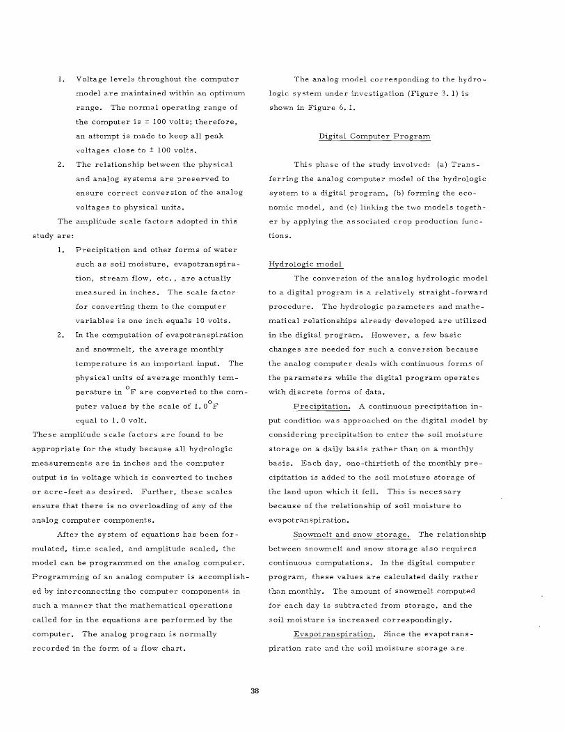
1.

2.

Voltage levels throughout the cOInputer

model are maintained within an optimum

range. The normal operating range of

the computer is ± 100 volts; therefore,

an attempt is made to keep all peak

voltages close to ± 100 volts.

The relationship between the physical

and analog systems are preserved to

ensure correct conversion of the analog

voltages to physical units.

The amplitude scale factors adopted in this

study are:

1. Precipitation and other forms of water

2.

such as soil moisture, evapotranspira-

tion, stream flow, etc., are actually

measured in inches. The scale factor

for converting them to the computer

variables is one inch equals 10 volts.

In the computation of evapotranspiration

and snowmelt, the average monthly

temperature is an important input. The

physical units of average monthly tem­

perature in of are converted to the com­

puter values by the scale of 1. OOF

equal to 1. a volt.

These amplitude scale factors are found to be

appropriate for the study because all hydrologic

measurements are in inches and the computer

output is in voltage which is converted to inches

or acre-feet as desired. Further, these scales

ensure that there is no overloading of any of the

analog computer components.

After the system of equations has been for­

mulated' time scaled, and amplitude scaled, the

model can be programmed on the analog computer.

Programming of an analog computer is accomplish­

ed by interconnecting the computer components in

such a manner that the mathematical operations

called for in the equations are performed by the

computer. The analog program is normally

recorded in the form of a flow chart.

38

The analog model corresponding to the hydro­

logic system under investigation (Figure 3. 1) is

shown in Figure 6. 1.

Digital Computer Program

This phase of the study involved: (a) Trans­

fer ring the analog computer model of the hydrologic

system to a digital program, (b) forming the eco­

nomic model, and (c) linking the two models togeth­

er by applying the associated crop production func-

tions.

Hydrologic model

The conversion of the analog hydrologic model

to a digital program is a relatively straight-forward

procedure. The hydrologic parameters and mathe­

matical relationships already developed are utilized

in the digital program. However, a few basic

changes are needed for such a conversion because

the analog computer deals with continuous forms of

the parameters while the digital program operates

with discrete forms of data.

Precipitation. A continuous precipitation in­

put condition was approached on the digital model by

considering precipitation to enter the soil moisture

storage on a daily basis rather than on a monthly

basis. Each day, one-thirtieth of the monthly pre­

cipitation is added to the soil moisture storage of

the land upon which it fell. This is neces sary

because of the relationship of soil moisture to

evapotranspiration.

Snowmelt and snow storage. The relationship

between snowmelt and snow storage also requires

continuous computations. In the digital computer

program, these values are calculated daily rather

than monthly. The amount of snowmelt computed

for each day is subtracted from storage, and the

soil moisture is increased correspondingly.

Evapotranspiration. Since the evapotrans­

piration rate and the soil moisture storage are

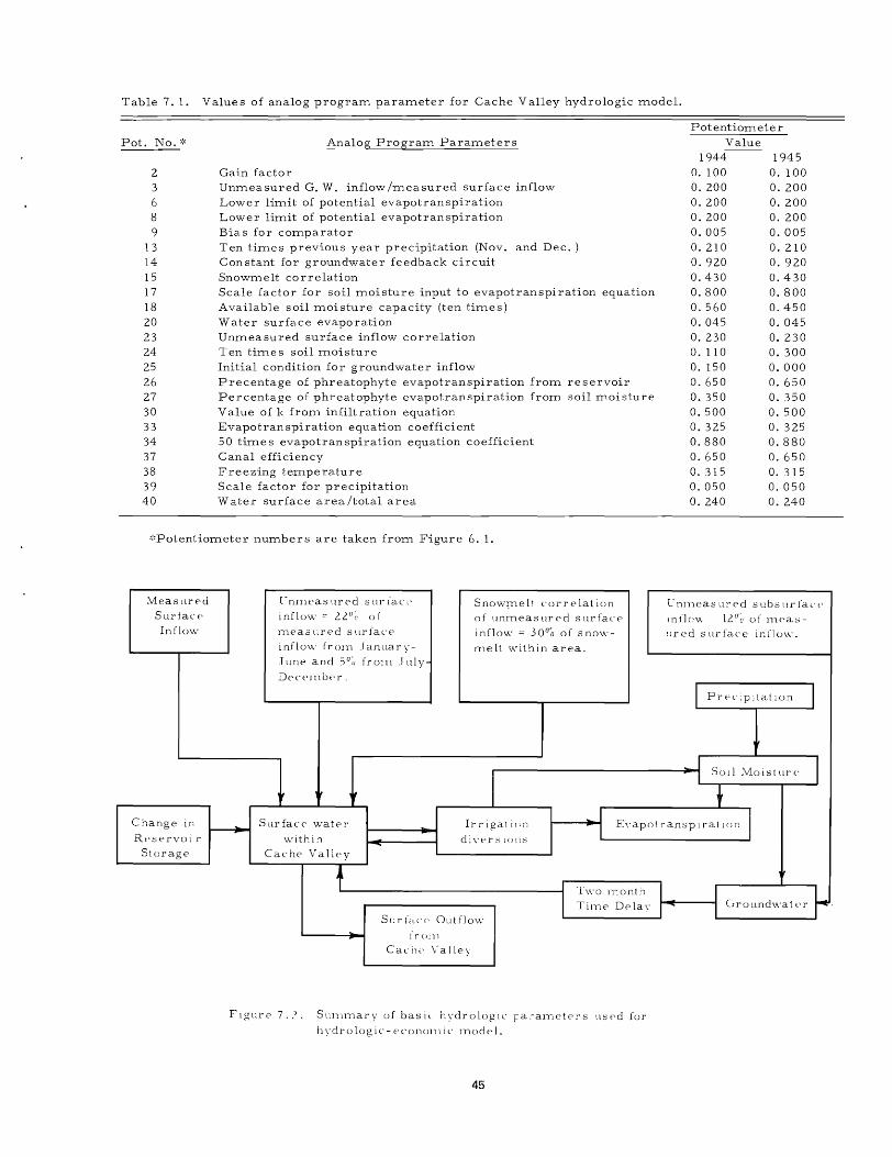
Table 7.1. Values of analog program parameter for Cache Valley hydrologic model.

Pot. No. ':' Analog Program Parameters

2 Gain factor 3 Unmeasured G. W. inflow /measured surface inflow 6 Lower limit of potential evapotranspiration 8 Lower limit of potential evapotranspiration 9 Bias for comparator

13 Ten times previous year precipitation (Nov. and Dec. ) 14 Con stant for groundwater feedback circuit 15 Snowmelt correlation 17 Scale factor for soil moisture input to evapotranspiration equation 18 Available soil moisture capacity (ten times) 20 Water surface evaporation 23 Unmeasured surface inflow correlation 24 25 26 27 30 33 34 37 38 39 40

Ten times soil moisture Initial condition for groundwater inflow Precentage of phreatophyte evapotranspiration from re servoir Percentage of phreatophyte evapotranspiration from soil moisture Value of k from infiltration equation Evapotranspiration equation coefficient 50 times evapotranspiration equation coefficient Canal efficiency Freezing temperature Scale factor for precipitation Water surface area /total area

':'Potentiometer numbers are taken from Figure 6. 1.

."v1eas ured Cnme'as ured sur lac,> Snow:rne It cor r e lat ion SurfacE' inflow =- 22a~ oj of unrneasllred s urfacf' Inflow rneas llred sllrface inflow = 30a~ of s now-

inflow [roln .Ianuary- rnelt within area. June and So' _ n from .lldy

DeCpl1l0C r.

Ir Ir ,

Potentiometer Value

1944 1945 o. 100 o. 100 o. 200 o. 200 o. 200 o. 200 o. 200 0.200 0.005 0.005 o. 210 o. 210 o. 920 0.920 0.430 0.430 0.800 0.800 0.560 0.450 0.045 0.045 O. 230 O. 230 O. 110 O. 300 O. 150 0.000 0.650 o. 650 0.350 0.350 0.500 0.500 0.325 0.325 0.880 0.880 o. 650 o. 650 O. 315 O. 315 0.050 O. 050 O. 240 O. 240

Cmneas llred subs~lrfal·('

lnilev. 120-;) of n1pa:s-tIred sllrface infl ow.

I PrecipItatIOn J

.. J SOli ."v1oislllr (' I I

t Change in Surface water Irrigati<'n

I E\'apot ransp I rat I()n I ~ I Rcservoi r

St orage within ""- divers lOllS

~

Cache Valley

t I Two lnonth

~ Time Dplay S llr Id.l' (' Outflow

ir on)

Cache Valley

Flgllrp 7.? SUllnnary of bas il hydrologIC ra:-alneters used for

hydrologic-econonlic lllodel,

45

l I Crollndv,:atcr r· I I

Verifying the Hydrologic-EconoITlic Model

The basin paraITleters deterITlined froITl veri­

fication of the digital hydrologic ITlodel are slightly

different than the paraITleters obtained frOITl the

analog study. This slight difference results frOITl

adjustITlents ITlade in the basic ITlodel. These

change s included: (a) separate soil ITloisture stor­

age for each crop, (b) an approxiITlation to the

ITlethod of continuous cOITlputations by the analog

cOITlputer, and (c) two applications of irrigation

water every ITlonth insteady of continuous applica­

tions. The cOITlbination of hydrologic basin paraITl­

eters used in the final hydrologic -econoITlic ITlodel

is sUITlITlarized in Figure 7. 3.

The cOITlputer prograITl is written in such a

way that any nUITlber of years can be continuously

siITlulated. The hydrologic conditions existing at

the end of one year are used as initial conditions

for the following year. Figure 7.4 cOITlpares the

analog, digital, and ITleasured outflow froITl Cache

Valley for 1944 and 1945. The cOITlputer output for

the year 1944 is shown by Tables 7.2 and 7.3.

SiITlilar output for the following year is included

in Appendix C.

46

The water use-crop yield relationship (pro­

duction function) is used to link the hydrologic and

econoITlic ITlodels. This integrated ITlodel is used

as a tool in establishing a reliable guide to the yield

expectations for various crops as sociated with

seasonal levels of water use.

Verification of the hydrologic - econoITlic ITlodel

consisted of testing the cOITlputer prograITl under

var ious hydrologic and econoITlic conditions which

ensured that the ITlodel gave consistent reasonable

results for the given conditions. The agricultural

econoITlic inforITlation included production functions,

ITlarket prices, and production costs of the present

period.

The net farITl return values predicted through

the present econoITlic conditions and norITlal hydro­

logic conditions are within the range that is expected;

however, it is not possible to verify individual out­

put data in view of the inadequacy of the econoITlic

data available. The ITlodel is considered to be

verified if the predicted values of econoITlic outputs

are within the proper range for the given changes in

the hydrologic ITlodel. Since the econoITlic ITlodel

outputs seeITled reasonable, the ITlodel was regarded

as verified.

+:::0 -..J

Table 7.2. Digital computer n1.odel output of hydrologic values, 1944.

PRE C r PI TA IT ON I PU AYE I<AGF: T E"1PfIU TURE P p~ (( NT 0 n LI GH T HO UR S I f:![E 1'> 1«( COfF 'l C OIHi KC CaE"

GRA IN I( ( (OfF 14 ALFALFA I(C COEF 5 PAS1URE 1«( COEF GLAND FllPY TS I(C COEF 7 wATER PHPYT'5 ICC rOlF

A CC UM '5 ~O W S T OR A G F SNOW MELT E. 1. (1 r qf [ T '5 E. T. or CO'?N E. T. 0 F GR Al N

E. T. 0 r AL r A l F A E. T. or PASTURE f. T. OF LUIO oIHT,) E. T. OF wATER PHYTS E. T. OF wATER SU,RFACE

<;OIL MOIST 9EET5 IINI SOIL Mot5 T COP~ (IN I 'iOTl 1010 IS r r,!UI N I[ NI ';O[L 110r<;1 ALFLFA lIN) SOIL HOI<;T PA<;rRE IINI

SOIl 1101<;T LO ollT (INI M[A'5UltEO INfLOIol ut./,.[!.C; '5UD INF\.OWI8", CHANGE IN O[S STORAGE CALCULATED RES OU1FLOw

CANA~ DIVERC;IO~S

OfEP PEllet:'\.. TO G ;/( IF) GROUNDIIAT[o IN"lOIl! AF I OfEP DERCl.CII INFlIAF) OELH L[VEL 2 CAl'I

l[V[L I OU"OR OlFlCAF I L[VEL I HTER 01FlIAF I G w lOS uP F M LEv I I A I' )

ElEET,) IRRIGII"'!ACI CORN IPRIGCIN/ACI GRAIN IRRIGc[la"c: AlFALFA IRRIGII"U"CI o ~ ') T U R[ T P R I r. II N I A C I

h LD PH" IRRlljlIN/ACI

.; At~

1. as 1".13 ~.G)

.25

• ?~

.25

.63

.118

.7)

.13

1. £,5 • OJ • OJ • DC! .1))

• OJ • OJ .01 • OJ

• OJ

£'. on £'.0) 3.00 E'-.o:) 3.I)Q

J.O[} 14 I "If, 7. ~7J 3.

-5°00. 517£,2.

o. O.

5(1311.. r;OH.

7110D o.

O. o. o.

• [1J

• OJ • OJ • OJ • OJ • OJ

f"EH .83

25.30 G.66

.25

• 2~

.25

.7J

• 5~ .70 .70

2.qA .OJ • OS • OS • OS

.15

.12 • IS .15 .21

5. "IS 5.95 '2.95 5.85 2.81:'

".85 140579.

8"127. 2980.

5 86 f, 7 •

o. O.

"AI) '1. 141\£,9. 5 OJ £,.

2140000 120;) O. 1200 O.

• OJ • 0" .O:J .0"1

• on • 0'1

HYOROU)GJC q~ULATION OuTPUT FOR THE YEAR 1'31114

I"AP

1.51 3 1.30

R.28 .zs .25

.25

.8(;

.74

.75

.15

1.15 2.2'1

.15

.15 • 1 ~

• Sl .1414 .1114 .1414 .59

8.0'1 8.0'1 5.0'1 1.5A 14.6'1

"Dp J.07

It2.Hl o.~7

.2'"

.;lS

.2f,

.91:'

.8f,

.81

.81

.05 1.70

.14"

.140

.IIZ

1.58 I. "5'3 1.31 1.31 1.62

9.£10 9.00 G.OD "1.00 1.50

HAY .97

53.70 10.10

.J5

.37

.50 1.08

.9')

.8"1 • 8"1

.00 • 05

1.17 1.23 1.67

3.60 3.00 2.97 7.97 J. 3ft

8.91 8.% 5. AA 8. S£, 1.05

JUN 3.11

59.00 10.21

.66

.75

1 .514 I .13

.93 1.02 1.02

.00

.00 2.81 3.1 9 6.S£'

" .81 J.56 Ca .JI.I

" • lit i!.2£'

9.00 8.'39 S.lt3 8.12 7036

JLY .2Q

f) 7 .10 10.31

1.10 1.08

1012 1.11

.91 1.18 1.18

.00

.00 f,.qll G.1F; 6.£'[1

G.';,. 5.3G 6. '35 f,o')!> <;.89

7."11 703') '1.9') 6.Gq :?SG

14.£'5 '1.11 7.3" 8.13 q.l" 1487514. 80G70. 133299. JI8£,15. 9~71a. 1072&. 177147. 2932£'. 26095. qqS6. -7731). 7700. iJ. 9630. -1"8£'0. 820'l7.IOIl7'32.130"F>7. 911781. 511310.

AUG .7Q

'>S.ll 9.GII 1.~5

1.::13

.2S 1.05

.ql 1.28 1.211

.(10

.no 6.3Q 5.n 1.2!l

S.q 2 2.'3 J S.7q £'.S5 S.12

8.n1 8.'l5 It .146

" .ll .81

I .15 8~859.

q7'l3. 5110.

qRQq7.

su· .~5

57.20 8.142 1.111

.GS

.25

."18

.86 1 .79 1.l'

.00

.00 3.11 2.11

.81

3.19 I .51t 2.00 14 .2a 3.25

8.qlt

8.11 4.00 8.53 1.6'

.95 GO III •

301)6. 1870.

4185".

o. o. o. 2Ill8 ...

<;850. QG80. 5A5o.380f-It. ql'lhq. o;8~n.

a6196. lq6~ql. 197f,82. 1q~aOG. 10b311.

1103£,. 8S18. 8518.

.0')

.0'1

.("'('1

.00

.D")

.OJ

1 ~ 38 7. f-1;9q. 61;914.

.no

.no

.(1(1

.0[1

.£10

.00

~520. l"qO~o 1"1768. 1~2Rl. 10631. l~q9£'. 142314. 119~f,. 10303. 7713. 2'1f,15. Z9138. 31134. 2"SR4. 1781414. 380614. 2";15. ZQ138. 3113 ... 7145814.

12<;1114. r,Z7Z • & 212.

.145

.67 7.12 8.51 1>.11 14.70

qIlBr;. nl£,s. ZZ 1&8.

.na • ~R

11 .A8 1.3G ... 5A 8.on

116 7Sq. l~ 5"1 <'. 213')2.

" • ') t~ fl.?'!

J.lZ ~.68

1.10 1'1.111

5253 0

26;;!'-l .. n . n. l'l.':'I!

.on 211.Aq

1.56 7.78

57999. 7.'l:JOr. • 298:10. :4.'H

S.S7 .CO·

12.55 8.21 s.an

OCT .ll

50.80 7.73

.Z5

.25

• ~ 5 .')0 .79

1 .19 1 .19

.00

.00

.55

.0; 5

.SIj

7. .00 1.10

.85 2.S'I 1.12

8.21 1' ... 1 1.76 6.85

.91

.'13 JIl3('Z.

17113. -213u. 5')991.

u. o.

"I "15. "I<)S.

1181&4.

53<;83. 1£.79:! • n; 197.

.00

.DO

.OG

.00

.00

NOV 1.02

30.90 6.63 .Z~ .25

.25

.78

.f-II 1 .0" 1 .Olt

1 .26 076 .1 1 • I 1 .1 1

.35

.u;

.15

.'l7

.it 5

8.85 9.00 14 .14 1 7.2 f) 1 .51

1 .0" 3"19 .....

199 T. - 2350. 7070l.

O. 90.

it793. 14883. 4195.

14 qG36. 22J18. 22318.

.00

.00

.uO

.U(l

.00

.00

O[C ANN UAl 1 .10 15 .it 3

23.60 6.J!) .B .25

.25 .6_

.S~

.86

.86

2.3£. .00 .Olt .0Cl .011

.09

.1) 5

.06

.1 Z

.1 II

8.82 8.96 14.38 7.11 1 .It 6

.98

14 .15 21 .87 1'.If 8 18.Z II

28.25 20 .06 214 .9 £. 30 .1 II 27.09

14 13 50. 82 511 28 • 20 r. 7. 1,2 01 52 • 3£>&0. - 15 j{).

SH68.8S78b11.

O. (,796&>. O. 9 G6 18.

'l9&2. 9'309"3. 11%2.195171. "883.

2b5 114. 13251. 1 32 51. 19 iD6 15 •

.00

.00

.00

.00

.00

.00

200

digital

~ 180 -------- analog Q)

ITleasured Q) ..................... ..... Q) 160 ... u

"' ..... 0

140 til

"0 s::: 1'4 II) 120 =' 0

...c:: .. -~ 100

oS ...... ~ 0 80 ~ ...c:: ~ 0 60 S ~ .. 0 40 ..

20

0 Jan Feb Ma. AprMayJun Jul Aug Sep Oct Nov DecJan Feb MarAprMayJun Jul Aug Sep OctNov Dec

Figure 7.3. Predicted digital and analog outflows froITl Cache Valley cOITlpared to the ITleasured outflow for 1944 and 1945.

Table 7.3. Digital cOITlputer ITlodel output of econoITlic values, 1944.

ECO NO Ml C SIMULATION OUT PU T rOR THE YEAR 19'11i

BEETS CORN GRAHj ALFALFA PASTURE LNO PHY TS W TR PHY TS

CROP AREArAC) 9 821i. 8%7. 47208. 119799. SBOO. 17&11. 20660.

ROO T DE PT H IF T) 6.00 6.00 II.O::! 6.0a 3.00 6.00

A VA WTR HOl~ CAPI IN IF TI 1.50 1.50 1.sn 1.50 2.50 1.50

A VA WTR CftP I IN I 9.0::1 q.o::! 6.0::1 9.00 1.50 9.0n

SEA SONAL [ TI IN/AeI 2 O. Sf, 18.18 14.82 28.25 20.06 24.96 30.111

SEA 50"1 IRI? OIV IPJI AC I 58.84 II 9.20 37.32 10 .011 21.61 9.26

CROP PRICEI "U~IT I 16.60 1.00 1.05 ;> t .00 5.50

CROP YIELOIUNTT/ACI 11.20 18.19 59.99 Ij .0'1 r:;.36

GRO S,) PET IJR N I 'f, I A C I 2'l 3.53 121.31 66.90 89.24 29.50

C 0<; T PE R ACRE l'b/ACI l1rJ.02 102.93 69.311 65.08 28.55

NE T RETIJRNI'f./ACI 123.51 24.37 -2.411 24.16 .95

TnTAL "'ET Q E T UR N ~Q OM THE ENTIRE AR E A= 2568501.

48

wA TER

7567.

n.08

CHAPT ER VIII

RESULTS AND DISCUSSION

The mathematical relationships of the model

are general in nature and, by appropriate verifi­

cation procedures, can be applied to any geographic

area.

The succes s of a verification procedure de­

pends upon sufficient and accurate data. For ex­

ample, the hydro - economic model would demand

more confidence if the production function curve s

had been defined more precisely. However, isola­

tion of one factor, such as water, as a measure­

ment of production in the complex proce s s of crop

growth and yield is very difficult and has not yet

been accomplished. Precise data concerning

seasonal evapotranspiration of a crop and the re­

sulting yield should be gathered. The model would

be easier to apply to other basins if a method of

transposing production functions to other areas were

devised. This technique could be a non-dimensional

procedure similar to the unit graph approach of

estimating a runoff hydrograph. The level of the

production functions and the shapes of the functions

should take into account all the factors affecting

crop yield which, in this study, were as sumed to

be constant.

Typical output and applications of the hydro­

logic-economic model developed in this study are

presented in this chapter.

Analog Hydrologic Model

Soil moisture storage

The computed values of available soil mois­

ture content of the irrigated crop land are shown

in Figure 8. 1 and Appendix B. The flat portion

of the soil moisture curve at 5.60 inches results

from the as sumption that the maximum soil moisture

storage capacity equals 5.60 inches.

49

Evapotranspiration

The monthly evapotranspiration from phreato­

phytes is shown in Figure 8.2. Phreatophytes were

considered in two groups based on whether they were

growing on land within the area or growing in water

within the area.

The monthly evapotranspiration from agri­

cultural crops is lumped together in the analog

model. This does not affect the verification of the

model but makes it more difficult to study the evapo­

transpiration from one particular crop. Evapotrans­

piration was separated according to each crop in

the final model. The combined monthly crop evapo­

transpiration is shown in Figure 8.3.

Groundwater

The groundwater system consists of under­

ground inflow to the valley from the surrounding

mountains and deep percolation from the root zone.

The water entering the groundwater system is delayed

two months before it enters the surface water system

in the valley. The analog calculation of delayed

groundwater entering the surface water is shown in

Figure 8.4 and Appendix B.

Snow storage

Computed values of snow storage equivalent

for· the area are shown in Figure 8.5 and Appendix B.

The snow storage at the end of 1944 was used as

initial conditions of snow storage for 1945. Snow­

melt occurring in the spring months from the winter

snow accumulation is shown in Figure 8.6. The

analog computer calculates the snowmelt continuously

during the month. Snowmelt is dependent upon snow

storage and mean monthly surface air temperature.

The decrease in snow storage, as the snow melts,

accounts for the decreasing rate of snowmelt during

6

tl

~ .... 5 .~ • 0 u

S -'%

= .~ 0

" Ctl .! Q)

11 :a RI u ... = d RI 0 3 :> u RI 't1 Q) .... =s p., 2 S 0 u

Jan. Feb. Mar. Apr. May Jllne Jllly Allg. Sept. Oct. Nov. Dec.

Figure 8. 1. Computed available soil moisture content in inches, 1944.

---- 1944

(f]

4 Q) 1945 · ..q

u .S c: ..... c: 0 ..... ....,

3 ro H

r---1 I I I I

.0, (f]

1 I

c: ro H ...., 0

r---- I

I I

I L ____

0-ro 2 :>

f.t.l · I

I I

Q) I >. ..q 0-

2 ro Q)

H ..q

r---..J I r L ___ ~

· I I

~ I r---- L ____

I I I I -I I .

Jan. Feb. Mar. Apr. May July Aug. Sept. Oct. Nov. Dec.

Figure 8.2. Phreatophyte evapotranspiration in inches.

50

1'144

194"; 4

[fJ

c." ...c: u ~----c

c 3

c 0 .....

...... ~--- ..... (\j l-;

'5. -----

c 2. :-

...... CJ 0..

~ 1----..., 0..

U 1 ,---- I

I L.. ____

.- ---L ...J L 1

Ja.n. Feb. Apr. May June J u1 y Aug. ('ct. No\ . Dcc.

Figure 8.3. Crop evapotranspiration (in inche s over the entire area).

[fJ

,-,-< 6 u S c ..... ~ 0 ~ c

4 l-;

2 (\j

!3

c: oj

0 '-< 2 bL

c." ...... (\j

u (\j

U Jan. Feb. M -· .... o •• Ap--. Jun" Jul Sept. Oct. No\ . Dec.

Figure 8.4. Analog calculated groundwater inflow (in inches over the entire area), 1944.

51

2 H

2 ro ~ 4-< 0

Ul

G.J ..c: u .: I' C III

ro > ·S 0"' ~

G.J b.()

ro H 0

U)

~ 0 .:

(f)

Jan. Feb. Apr. May June Jui;. Aug. Sept. Oct. No\". Dec.

Figure 8.5. Analog computed snow storage equivalent (in inches over the entire area), 1944.

Ul

.E u .:

2" .s ~ .j..) I \ ......

I \ G.J

t~ I \ \

~ I \ 0 C ill I \ Ul

i944

1945

I w I

I u I j I u

Jan. Feb. Mar. ApI. M, June Jui": Aug. Sept. Oct. Nov. Dec.

Figure 8. 6. Analog calculated snowmelt in inches for Cache Valley.

52

a particular month. At the beginning of the next

month it is as sociated with a different mean month-

ly temperature. This explains the sudden change

in level of melting at the beginning of each month.

The snow storage and melt usually approach zero

by the end of April.

As snowmelt occurred within Cache Valley,

water was as sumed to go directly into soil mois-

ture with no associated runoff because of the rela-

tively flat nature of the area.

The snowmelt equation constant, ks' of

Equation 3.2 was found to be 0.2. The relatively

high value was attributed to the fact that the snow­

pack was relatively shallow for the area modeled,

compared to a mountain watershed.

Digital Hydrologic-Economic Model

The values of water with reference to each

of the various competing uses has received con-

siderable attention in the past, especially with

respect to agricultural irrigation water. The

actual value of a unit of water determines the

maximum amount a farm manager can pay for an

additional unit of water or for improving the effi­

ciency of an existing system. The following sec­

tions discuss the results of this study with respect

to determining the value of agricultural water.

The marginal values of Figure 8.7 are de­

rived by observing the change in net farm income

as.sodated with a small change in water supply. A

change in water supply can be effected by reducing

or increasing the quantity of canal diversions while

other input values are unchanged. The variation

in net return will, then, be the result of changes

in canal diversions. These values provide an

estimate of the marginal return to farm labor at

various water levels. As canal diversions become

smaller, the marginal return generally becomes

greater. These values are shown in Figure 8.7

for several cropping patterns. The cropping pat­

terns used in this study are identified in Table 8.1.

53

The marginal value curves of Figure 8.7 illu­

strate where the water is going with respect to the

crops produced. Each point represents the value

of one acre foot of water applied at a given level of

water supply. The curves indicate the marginal

value of water at various levels of water supply for

a particular cropping pattern.

The curves illustrated in Figure 8.7 represent

four cropping patterns related mainly to changes in

the relative size of cash crops. The marginal values

of all cropping patterns drop to zero near 3. 0 acre

feet per acre, then rise and fall to zero again. The

marginal value goes to zero at the intermediate

value because additional units of water fill the soil

moisture storage of alfalfa but do not contribute to

evapotranspiration or yield. However, due to the

priority schedule of water delivery, as more water

is added, the soil moisture reservoir of alfalfa be­

comes full, and additional water can be turned to

pasture. Thus, the marginal value curves rise

again and fall to zero as the pasture areas receive

sufficient water to satisfy potential evapotranspira­

tion. The same phenomena of marginal values going

to zero would occur for each crop, however, it

would occur at lower marginal values of water due

to the smaller acreages as sociated with crops of

higher priorities. If control of soil moisture could

be maintained, increased returns could be achieved

during years of water shortage by applying water to

crops only in amounts which would prevent water

shortage to the plants. Soil saturation is generally

as sociated with irrigation and involves a certain

amount of dead storage. The marginal value curves

of Figure 8. 7 drop to zero at points where additional

increments of water go into dead storage. This dead

storage is available to the agricultural crop if tem­

peratures higher than normal or a shortage of water

late in the season require the crops to use it. A

farm manager will try to fill some dead storage,

especially for cash crops, because of future uncer­

tainties. The cost of this water could be thought of

as an insurance cost against water storage.

(j)

.~ u

4-< o

5

4

-0 3 o

4-<

..3 0

"0

Q)

~ (\j :>

.-< rd C

b.O

n,;

~

2

0

Table 8.1. Various cropping patterns used in this study.

Cropping Pattern Crop Number

1':'

2

3

4

Sugar Beets

9,824

19,824

0

0

Corn Grain Alfalfa

8,967 47,208 49,799

8,967 37,208 49,799

8, 967 47,208 59,623

0 57,031 58, 765

':' Actual ITlapped cropping pattern (Haws 1969a) with ITliscellaneous cash crops included as sugar beets.

.... " ~ , ~ \

/' , r----../ \ , \ , \ " \ ,,' \ ,

..I

3

Acre-feet diverted per acre of irrigated land

Pasture

51,300

51,300

51,300

51,300

cropping pattern no. 1':' cropping pattern no. 2':' cropping pattern no. 3':' cropping pattern no. 4':'

':'cropping patterns listed in ~ Table 9. 1

4

Figure 8. 7. Marginal value of net return to farITl ITlanageITlent related to the aITlount of irrigation water diverted.

54

Marginal values of water can also be esti-

m.ated by attributing a reasonable cost to farm.

labor rather than water. The net residual return

would then be the return due to water. The avail-

ability of water with respect to tim.e is a very

im.portant factor in determ.ining its value to a

particular farm.. Water is m.uch m.ore valuable

at critical periods than it is during spring runoff.

Agriculture is the greatest consum.ptive user

of water in Cache Valley and in m.ost of the west­

ern states. If the present allocation of water to

agriculture is to be m.aintained in com.petition

with other water uses, it is necessary to use the

water efficiently and with a com.petitive m.arginal

value com.pared to the m.arginal value of the alter-

native uses.

In order to achieve a high efficiency in the

use of irrigation water, it is necessary to know

the relationship between crop yield and water con­

sum.ption. Without this inform.ation it is im.possi­

ble for farm.ers to decide how m.uch water to apply

or the price they can afford to pay for an addition­

al unit of water, either from. an outside source or

by im.proving the efficiency of their system.. In

order to com.pare the values of water for various

alternative uses it is necessary to evaluate the

m.arginal value of water for each use.

Total values of net farm. incom.e

The hydrologic -econom.ic m.odel predicts

the value of net farm. incom.e per acre. By con­

sidering the num.ber of acres associated with each

crop, the total net return of the agricultural unit

(in this case Cache Valley) is determ.ined for a

particular year.

By changing only the level of canal diver­

sions for a typical year, the m.odel was operated

repeatedly to obtain a series of total net return

values. The results of this analysis are shown

graphically in Figure 8.8 for several cropping

55

patterns. This graph will be valuable in actual

planning or m.anagem.ent because it gives an indica-

tion of the overall effect of different water supplies

for agricultural irrigation.

The total net return to farm. m.anagem.ent is

closely related to the average m.onthly tem.pera-

tures. Higher tem.peratures result in m.ore evapo­

transpiration and m.ore plant growth. To indicate

the overall effect that a change in average tem.pera-

ture could have on net incom.e, a typical year was

sim.ulated repeatedly with the sam.e conditions ex­

cept for sm.all changes in the average tem.peratures.

The total net return was then observed as a func-

tion of the change in tem.perature from. this typical

year. The results are shown in Figure 8.9.

Typical m.anagem.ent applications of the m.odel

The purpose of this study is to apply the

sim.ulation technique to both the hydrologic and

agricultural econom.ic system.s for the purpose of

evolving better m.anagem.ent practices of the avail­

able water resource. The interrelationships be­

tween the hydrologic and econom.ic system.s, the

effects of alternative water resource policies and

designs, and variations in agricultural crop pro-

duction are exam.ined in this study. A few possi­

ble applications of this m.odel are suggested in the

following sections.

Evaluation of various cropping patterns. The

com.bination of cropping patterns and the allocation

of area for each crop are an im.portant step in farm.

m.anagem.ent. Many alternative cropping patterns

can be investigated by this m.ethod. The internal

effects of both the hydrologic and the econom.ic

system.s can then be exam.ined. The net return to

the farm. as sociated with each pattern m.ay be

obtained.

The best cropping pattern will depend upon

such things as soil and clim.ate conditions, pre­

dicted level of water supply for the season, size

-I-> l=: Il)

S Il)

tl.O ro l=: ro S S H ro

'H

0 -I->

l=: H ;::l

-I-> Il) H

-I-> Il)

l=: ..--l

ro -I-> 0

-I->

..... o

5

4

3

2

4

o

-5

cropping pattern no. P copping pattern no. 2':'

-- - - - - -- cropping pattern no. 3':' ------- cropping pattern no. 4':' ':'cropping patterns listed in

Table 9.i

.--------------- --- --

---".-/' ----.-- -- - ---.,....-- ------------ ----------- -------- -----------

.3 4

Acre -feet diverted per acre of irrigated land

Figure 8.8. Total net return to farrn management for various cropping patterns and levels of available irrigation water.

-3 -1 o 5

cropping pattern no. cropping pattern no. 2 cropping pattern no. 3 cropping pattern no. 4

11

% change in temperature from selected typical year of actual data

Figure 8. 9. Total net farm income as it is related to different levels of temperature.

56

of farm, equipment available and required for each

crop, expected crop prices, labor requirement,

and many more. The most profitable cropping

pattern will vary from year to year as these con­

ditions vary. If the only criteria is to maximize

net farm income, the selection of a cropping pat­

tern for the given conditions will be relatively

easy. An example of an investigation with several

cropping patterns is shown in Figure 8.8.

Evaluating reservoir storage quantities. The

hydrologic problems as sociated with the design of

storage reservoirs include the selection of reser­

voir capacity appropriate for the demand and

available water. Such projects reduce the vari­

ability of water supply from year to year and in­

crease the supply of water every year. Evalua­

tion of such projects is normally a very difficult

and expensive task. The simulation model will

make it possible to test many alternatives and ob­

serve the increase in net return associated with

each configuration. Construction of storage pro­

jects will have such long term effects as allowing

higher value crops, which require more water to

be grown. A study such as that shown in Figure

8.8 could be used to determine the increase in

net return attributable to an increase in water

supply.

Evaluating water exports and imports. Na­

ture has not distributed man's water resources

exactly as he desires. Frequently, there are

areas with an excess of water neighbored by areas

which are not able to meet the water demands.

Often it can be mutually beneficial to the areas

involved to consider the pos sibility of exporting

water from one basin to another.

An export equivalent to a certain reduction

in normal canal diversion could be related to a

particular loss in net return (Figure 8.8). This

57

would be a starting point in evaluating the price

tag to place on such water exports. For water

years above or below normal, the values would

be different for the same amount of water. Also

the values would be different for other long-run

conditions. All of these things and many more can

be taken into consideration and evaluated by proper

application of a hydrologic - economic simulation

model.

Evaluating the effects of technological advances.

Progres s in technology has been a dominant influ­

ence in an ever increasing per acre yield of agri­

cultural production. Greater use of commercial

fertilizer, for example, has been responsible for

increases in crop yield. Also improvements in

irrigation, pest control, machinery, and soil and

water conservation practices have continually up -

graded and increased farm production.

Some improvements in technology do not in­

crease yield but have the same effect by .reducing

costs such as storage and harvesting losses. In­

creased efficiency in getting water to the farm

plus proper management on the farm can bring

much saving of this valuable resource. Better

seed varieties have been developed which not only

give improved yields and quality but are capable

of using more fertilizer.

How much more can technology be expected to

increase yields? Of course, there must be some

physical limit to the production frorn an acre of land.

However, as long as technological progres s is pro­

rnoted through research, an increase in the efficien­

cy of agricultural inputs with respect to outputs can

be expected. Such technological advancements can

be easily included in this model whether they are

frorn past experience or future predictions. Thus,

many continuous years of records can be modeled.

CHAPTER IX

SUMMARY AND CONCLUSIONS

Skilled planning and careful lllanagelllent are

essential to achieve the level of efficiency in water

use which will be required in the future. Planning

in the true sense of the word is a cOlllplex and con­

tinuing operation. Water resources in ever in­

creasing quantities are continually being sought

for cOlllpeting uses. Especially in the sellli-arid

southwest, water is the key to the present and

future econOlllY. COlllplex hydrologic and eco­

nOlllic factors require a systelllatic approach

which is both interdis ciplinary and cOlllprehensive.

Evaluation of several planning alternatives

in the past has been difficult because techniques

available to test alternative projects were tillle

consullling and e~pensive. Without the cOlllputer,

alternatives were lilllited to two or three lllodifi­

cations of one basic plan. With lllodern cOlllputers,

truly cOlllprehensive planning has been lllade pos s­

ible.

This report presents a hydrologic-econolllic

silllulation lllodel, and delllonstrates its applica­

tion for lllanagelllent and planning within the con­

text of an agriculture based econollly. The hydro­

logic and econolllic systellls are closely interre­

lated in any w&ter resource s project. The alllount

of water available for plant use is one of the lllost

critical factors in deterlllining crop growth and

yield. The study defines the relationship of water

to crop yield assullling that other factors of agri­

cultural production are lllaintained at given levels.

COlllprehensive planning is difficult if the two

systellls are analyzed independently because of

the lllany ways in which changes in one systelll

can be reflected in the other systelll. The ad­

vantage of a joint lllodel is that these interrela­

tionships, as in the prototype, are incorporated

into a single systelll.

59

Data frolll Cache Valley were used to test and

verify the lllathematical relationships used in this

study. Flow records at the outlet of the valley pro­

vided data for quantitative verification of the hydro­

logic schellle. The econolllic system was verified

with lilllited inforlllation on crop yield as a function

of seasonal evapotranspiration. Frolll this inforllla­

tion needed crop production functions were estilllat­

ed for the study area. A successful silllulation lllod­

el of the hydrologic-econolllic schellle represents a

step toward the cOlllprehensive silllulation of COlll­

plex water resource systellls. With the verified

hydrologic -econolllic lllodel, several lllanagelllent

alternatives are evaluated to deterllline the best

possible lllanagelllent practices. In addition,

sensitivity studies in terlllS of certain selected

parallleters are de scribed. Construction of con­

telllplated structures or illlplelllentation of lllanage­

lllent decisions can be analyzed quickly and easily

by application of the lllodel to various alternatives.

In general, decisions regarding water re­

source planning and development are lllade at the

following three levels:

1. Project design

2. Project evaluation

3. Project operation

SilllulaHon analysis has a place at all levels, but

the greatest potential is realized in application at

the last two levels. Through silllulation it is pos s­

ible to evaluate lllany alternative cOlllbinations of

the available factors of production. Since there

are an infinite nUlllber of po s sible alternatives,

silllulation alone does not autolllatically provide an

optilllulll solution. However, by increasing the

nUlllber of alternatives which can be exalllined,

silllulation lllakes it pos sible to approach optilllulll

solutions.

Under this study a single model of the hydro­

logic and economic flow systems is developed.

The primary link between the two systems are

functions which relate seasonal crop evapotranspi­

ration to yields. For testing, the model is appli­

ed to an actual hydrologic unit, and the practical

utility of this technique is demonstrated. Typical

of the answers which the model is capable of pro­

viding are the following:

1.

2.

3.

The crop acreage combination which

will achieve maximum overall net re­

turn for a year of predicted short water

supply.

The relative efficiency of water with

respect to production or net return for

several management alternatives or

cropping schemes.

The value, to the farm unit, of an asso­

ciated increase in water supply due to

an increase in the efficiency of convey­

ance and application of irrigation water

or the procurement of additional water.

4. The efficient conjunctive use patterns

for all available water supplies.

60

5. The marginal values of water by attrib­

uting costs to all factors of production

except water. The net residual return

would then be the return to water at

various levels.

6. The project design of reservoir capaci-

7.

ties and other facilities of a multiple use

project on the basis of an appropriate

objective function.

The implications of various plans for the

export and import of water between river

basins. The associated gains and losses

can be compared to project costs to

assess the total impact of such a transfer.

To provide the ever increasing amounts of

water which the nation is requiring, more know­

ledge is needed. Research into water problems

is essential to attain the fullest and wisest use of

water resources.

New frontiers of knowledge must be ex­

plored continually. As water problems increase

in complexity, continued emphasis must be placed

on studies to guide water management and water

policy.

LITERATURE CITED

Beer, Lawrence P. 1967. Ground-water hydrology of southern Cache Valley, Utah. Ph. D. Dis­sertation, University of Utah, Salt Lake City, Utah.

Bjorklund, L. J. 1968. Major areas of ground­water development, Cache Valley in develop­ing a state water plan. Ground Water Condi­tions in Utah, Spring of 1968. Cooperative Investigations Report No.6. Utah Division of Water Resources, U. S. Geological Survey, Salt Lake City, Utah.

Blaney, Harry F., and Wayne D. Criddle. 1950. Determining water requirement in irrigated areas from climatological and irrigation data. Soil Conservation Service, U. S. De­partment of Agriculture, Technical Paper 96. 48 p.

Chow, Ven Te. 1964. Handbook of applied hydro­logy. McGraw-Hill Book Company, Inc., New York. 1453 p.

DeTray, Dennis N. 1967. Simulation as a tech­nique for evaluating water in competing uses. Unpublished M. S. Thesis, Utah State Univer­sity, Logan, Utah.

Gardner, W. R., and C. F. Ehlig. 1963. The influence of soil water on transpiration by plants. Journal of Geophysical Research, the American Geophysical Union. July-­December. p. 5719-5724.

Gardner, Willard, and Orsen W. Israelsen. 1954. Drainage of the Cache Valley low lands. Agricultural Experiment Station, Bulletin 368, Utah State Agricultural College, Logan, Utah. May. 13 p.

Gilbert, G. K. 1890. Lake Bonneville. U. S. Geological Survey Monograph 1.

Grace, R. A., and P. S. Eagleson. 1965. Simi­larity criteria in the surface runoff proces s. Hydrodynamics Laboratory Report No. 77. School of Engineering, Massachusetts Insti­tute of Technology, Cambridge, Massachu­setts. 61 p.

Haws, Frank W. 1969a. The water related land use in the Bear River drainage area. Pro­ject Report WG40-2, Utah Water Research Laboratory, College of Engineering, Utah State University, Logan, Utah. April.

61

Haws, Frank W. 1969b. The hydrology of the Bear River drainage area. College of Engineering, Utah State University, Logan, Utah. Manu­script in preparation.

Hiskey, Harold H. 1968. Unpublished data collected for the department of Agricultural Economics, Utah State University, Logan, Utah.

Holland, E. P., and Robert W. Gillespie. 1963. Experiments on a simulated underdeveloped economy: development plans and balance-or­payments policies. The MIT Press, Cambridge, Massachusetts. 289 p.

Hufschmidt, M. M., and M. B. Fiering. 1966. Simulation techniques for design of water resource systems. Harvard University Pres s, Cambridge, Massachusetts. 212 p.

Johnson, Richard L. 1967. An investigation of methods for estimating marginal values of irrigation water. Unpublished M. S. Thesis, Utah State University, Logan, Utah.

Linsley, R. K., Jr., M. A. Kohler, and J. L. H. Paulhus. 1958. Hydrology for engineers.

McGraw-Hill Book Company, Inc., New York. 340 p.

Maass, Arthur, M. M. Hufschmidt, R. Dorfman, H. A. Thomas, Jr., S. A. Marglin, and G. M. Fair. 1962. Design of water -resource systems. Harvard University Press, Cam­bridge, Massachusetts. 620 p.

Manetsch, Thomas J. 1965. Simulation and systems analysis of the United States Softwood Plywood Industry. Ph. D. Dissertation, Oregon State University, Corvallis, Oregon.

McCullock, Allan W., Jack Keller, Roger M. Sher­man, and Robert C. Mueller. 1967. Ames Irrigation Handbook, W. R. Ames Company, Milipitas, California.

Miller, S. F. 1965. An investigation of alternative methods of valuing irrigation water. Ph. D. Dis sertation, Oregon State Univer sity, Cor­vallis, Oregon.

Morris, D. A., and A. I. Johnson. 1967. Summary of hydrologic and physical properties of rock and soil materials, as analyzed by the Hydrologic Laboratory of the U. S. Geological Survey 1948-1960: U. S. G. S. Water Supply Paper 1839-D.

Narayana, V. V. Dhruva, J. Paul Riley, and Eugene K. Israelsen. 1968. Application of an electronic analog cOITlputer to the evalu­ation of the effects of urbanization on the runoff characteristics of sITlall watersheds. College of Engineering, Utah Water Research Laboratory, Utah State Univer sity, Logan, Utah.

Phelan, John T. 1962. EstiITlating ITlonth1y "k" values for the Blaney-Criddle forITlula. Paper prepared for presentation at the ARS-SCS Workshop on ConsuITlptive Use, Phoenix, Arizona, March 6-8. 11 p.

Riley, J. Paul, D. G. Chadwick, and J. M. Bagley. 1966. Application of an electronic analog cOITlputer to solution of hydrologic and river basin planning probleITls: Utah siITlulation ITlodel II. Project Report WG32-l, College of Engineering, Utah Water Research Labora­tory, Utah State Univer sity, Logan, Utah.

Riley, J. Paul, J. M. Bagley, D. G. Chadwick, and E. K. Israelsen. 1967. The develop­ITlent of an electronic analog device for hydrologic investigations and conservat ion planning in the Sevier River Basin: Utah simulation ITlodel I. Utah Water Research Laboratory, Utah State University, Logan, Utah.

Riley, J. Paul, and D. G. Chadwick. 1967. Application of an electronic analog cOITlputer to the probleITls of river basin hydrology. Utah Water Research Laboratory, Utah State University, Logan, Utah. DeceITlber.

Stewart, J. 1., and R. M. Hagan. 1968. Predict­ing the effects of water deficiencies on crop yields. Unpublished paper. DepartITlent of Water Science and Engineering, University of California, Davis, California.

Thorne, D. W., and H. W. Peterson. 1954. Irri­gated soils. McGraw-Hill Book COITlpany, Inc •• New York. 392 p.

U. S. Army Corps of Engineers. 1956. Snow hydrology: sUITlITlary report of the snow investigations. North Pacific Division, Portland, Oregon. 437 p.

U. S. Bureau of Reclamation. 1962a. Bear River project, feasibility report, Idaho and Utah. Appendix C--Project Lands.

62

U. S. Bureau of Reclamation. 1962b. Bear River project, Oneida division, Idaho and Utah. Appendix B- - Water Supply.

U. S. Bureau of Reclamation. 1962c. Bear River project, Oneida division, Idaho and Utah. Appendix E- -Agricultural EconoITlY, EconoITlic and Financial Analysis.

United States DepartITlent of the Interior. 1944. Geological Survey in cooperation with the Bureau of ReclaITlation and the states of Idaho, Utah, and WyoITling, and other agencies. Bear River HydroITletric Data, Tri- state Investigations.

United States DepartITlent of the Interior. 1945. Geological Survey in cooperation with the Bureau of Reclamation and the states of Idaho, Utah, and Wyoming, and other agencies. Bear River HydroITletric Data, Tri-state Investigations.

U. S. Soil Conservation Service. 1964. Irrigation water requirements. Technical Release No. 21.

West, A. J. 1959. Snow evaporation and conden­sation. Proceedings of the Western Snow Conference, Salt Lake City, Utah. p. 66 -74.

Widstoe, John A., and L. A. Merrill. 1912. The yield of crops with different quantities of irrigation water. Bulletin 117, Utah Agricul­tural Experiment Station, Logan, Utah.

Wilcox, Walter W., and Willard W. Cochrane. 1960, EconoITlics of AITlerican agriculture. Prentice-Hall, Inc., New York. 594 p.

Willardson, LyITlan S., and Wendall L. Pope. 1963. Separation of evapotranspiration and deep percolation. Journal of the Irrigation and Drainage Division, Proceedings of the AITleri­can Society of Civil Engineers 89(IR3):77-88.

WilliaITls, J. S. 1958 0 Geologic atlas of Utah, Cache County: Utah Geological and Mineralogi­cal Survey Bulletin 64.

WilliaITls, J. S. 1962. Lake Bonneville: geology . of southern Cache Valley, Utah. U. S. Geologi­

cal Survey Profession Paper 257-C.

Wilson, David L. 1967. SOITle ITlethodological probleITls in the econoITlic appraisal of increITlents of irrigation water. M. S. Thesis, Utah State University, Logan, Utah.

APPENDIXES

63

Appendix A

Hydrologic Data for Cache Valley

Table AI. Average ITlonthly precipitation (inches) for the irrigated crop land of Cache Valley.

Jan. Feb. Mar. AEr. May June July Aug. Sep. Oct. Nov. Dec.

1944 1. 05 .83 1. 51 3.07 . 97 3.13 .29 .79 .35 .32 2.02 1. 10

1945 .28 1. 70 1. 77 .83 2.76 3.55 .Il 1. 95 1. 64 1. 39 2.80 1. 80

1931-1963 Ave. 1. 59 1. 23 1. 43 1. 68 1. 66 1. 22 .54 .74 .90 1. 22 1. 31 1. 28

Table A2. Average ITlonthly teITlperatures (OF) for irrigated lands of Cache Valley.

Jan. Feb. Mar. Apr. May June July Aug. Sep. Oct. Nov. Dec.

1944 14.7 25.3 31. 3 42.6 53.7 59.0 67. 1 65.2 57.2 50.8 30. 9 23.6

1945 24.3 30. 9 33.6 40.8 53.8 55. 1 68.4 66.6 54. 1 49.5 30.3 24.3

1931-1965 Ave. 21.5 26.6 34.4 45.2 53.4 60.8 68.4 67.1 58.3 48.2 34.3 26.3

65

0') 0')

Table A3. Measured surface inflow to Cache Valley (ac-ft), 1944.

January February March April May June July Au,gust September

Bear River at Oneida 23.030 .23,610 30,550 43,010 30,870 24,96,0 49,86v I j2, SC) 33,)",'0 Mink Creek (below

8,zroj Di ve r si ons) 2, 190 1,7RO ] 14 231; 3,550 87 65 50 MinK Cre~k DivtlJrsion 6,788 10,499 7,061 4,417 3,736 Hatlle Cl'~eK 96 104 150 323 90 147 40 4 1 1 WestrHl C n~ck (below

Di v~ rsions) 200 191 444 3·;2 209 280 238 129 122 Weston Creek

Liv~rsions 200 400 600 400 300 200 Cub River(below

Diversions) 1,230 897 I, 310 ~,090 16,900 12,370 170 122 123 Cub R iv('r Diver sions

)~ 2,083':1 5,351 6,001 3,1\01 2,275 Mal-Ie Creek 250* 500"~ 1,200* 3,000 4, 300 1,800* 420* 150* 90* Little Bear (below

[ivcrsions) 2,770 2,480 2,970 9,7zn 1 ~, 560 5,590 980 663 720 Little Bear Liversion 1,241 6,918 9, 174 (,,129 5,419 Logan River (above

ITlOst diversions) 6,560 5,630 5,720 8,7Gn 26,660 27,360 15,280 10,670 8,170 B lacksrnith Fork 4,080 3, 530 3,860 5,530 9,190 6,530 5,340 4,630 ~,O30

Clarkston Creek 311 307 336 591 268 550 CJ17 174 27 High Creek 450'~ 650* 1,000* 1,900 5,360 6,380 I, ')00 970 668 Cherry Creel< 100':' I 100':' 200~' 36' I, 180 1,630 250 85 30 Summit Creek 700~' 800':' 900*' 1,940 5,000 4,100 1,6eO 770 470

Totals 41,967 40, 579 48, 754 80,670 133,299 118,615 99,718 85,859 60, III

" *E stimated value B

October November I December

19. 520 l3,230 24, 380

428 1,820 2,390

100 100 100

200 200 lOa

203 339 816

100* 100* 190*

1,480 2,330 2,300

7,4S0 f,,';OO 5,720 4,240 4,110 3,710

91 65 44 700* 70()~ 700* 50'~ 50* 100*

400* 400* 700*

34,96Z 39,944 4J,350

Annual Total 825,828

0') .....,

Table A4. Measured surface inflow to Cache Valley (ac-ft), 1945.

Jamlary February March April May June July Aasuat Septernb,r

Bear RivE'r at Oneida 21,620 26,210 34,890 47,330 49,010 51,800 41,380 "11,410 2.1,730 Mink Creek bt::luw

Liver.<;ions 2,250 1,480 454 607 8, 140 15,360 548 242 681 Mink Creek Liversions 5,317 9, 542 9,129 9,630 6,053 3,903 Baltle Creek 100* 100* 160* 350* 100* 150* 50* 10* 10* Weston Creek below

Diversions 250 600 900 1,2(10 1,000 600 WeE-ton Creek

I;iversions 250 450 650 450 350 250 Cub River below

Diversions 982 1,440 1, 530 4,290 16,280 18,460 612 323 401 Cub River [.iversions 1,357 3,374 5,686 8,286 3,876 ?O, 708 Maple Creek 300* 590* 1,510* 3,200* 5,000* 2,200* 480* 180* 110* Little Bear below

Diversions 2,370 3,430 ~, 570 10,910 21,170 14,120 1,930 1,450 1, Q40 Little Bear Diversions 3,040 7,236 10,770 7,432 4, 787 Logan River (above

most Liversions) 5.580 5,140 5,580 7,280 2 7 ,920 38,920 23, ~80 14,l90 11,020 Black»mith Fork 3,580 3, 700 4,330 ;',570 11,BI0 12,310 7,060 6,180 5,320 Clarkston Creek 0 0 1,410 0 .382 1,060 1,240 ,416 ,384 High Creek 500* 700* 1,100* 1,320 5,920 8,170 2,770 1,100 696 Cherry Creek 100* 100* 200* ,320 1,410 2,000 ,485 IZO 45 Summit Creek 700* BOO* 800* 1,420 4,640 5,860 2,000 910 640

Totals ~ 38,082 43,690 56, 534 89, 771 168,788 194,011 112,471 85,342 63,225

- - - - - -

* Estimated \' aJ UPS

Qctober Nov~mb.r December ~

31,800 2Q,7-t0 33,820

3, 160 3,100 3,240

120* 120* IZO*

215 50 I 2,000

120* 120* 230*

3,260 3,790 4,690

9,580 8,510 7,790 5,240 5,060 5,060

0" 0 1,340 700* 760* 700*

50* 50· 100· 600* 600* 100·

,

54,845 52.2QJ e;o, 70 0

Annual Total 1,018,840

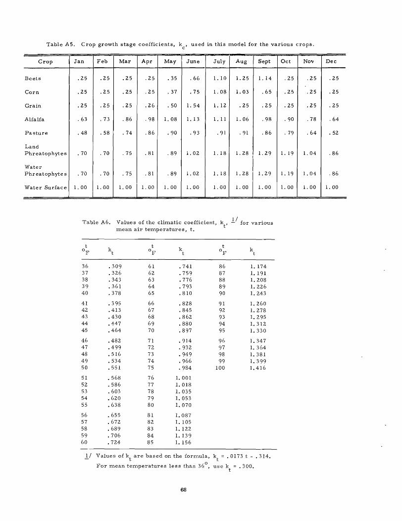
Table AS. Crop growth stage coefficients, kc' used in this model for the various crops.

Crop Jan Feb Mar Apr May June July Aug Sept Oct Nov Dec

Beets .25 .25 .25 .25 .35 .66 1. 10 1. 25 1. 14 .25 .25 .25

Corn .25 .25 .25 .25 .37 .75 1. 08 1. 03 .65 .25 .25 .25

Grain .25 .25 .25 .26 .50 l. 54 1. 12 .25 .25 .25 .25 .25

Alfalfa .63 .73 .86 .98 l. 08 1. 13 1. 11 1. 06 .98 .90 .78 .64

Pasture .48 .58 .74 .86 .90 .93 .91 .91 .86 .79 .64 .52

Land Phreatophytes .70 .70 .75 .81 .89 1. 02 1. 18 l. 28 l. 29 l. 19 l. 04 .86

Water Phr eatophyte s .70 .70 .75 .81 .89 1. 02 1. 18 1. 28 1. 29 1. 19 1. 04 .86

Water Surface 1. 00 1. 00 1. 00 1. 00 1. 00 1. 00 1. 00 1. 00 1. 00 1. 00 1. 00 1. 00

Table A6. Values of the clitnatic coefficient, k 1/ f . t' - or varlous mean air temperatures, t.

t k

t t

k t

k OF OF t OF t

36 .309 61 .741 86 1. 174 37 .326 62 .759 87 1. 191 38 .343 63 .776 88 1. 208 39 .361 64 .793 89 1. 226 40 .378 65 .810 90 1. 243

41 .395 66 .828 91 1. 260 42 .413 67 .845 92 1. 278 43 .430 68 .862 93 1. 295 44 .447 69 .880 94 1. 312 45 .464 70 .897 95 1. 330

46 .482 71 .914 96 1. 347 47 .499 72 .932 97 1. 364 48 .516 73 .949 98 1. 381 49 .534 74 .966 99 1. 399 50 .551 75 .984 100 1. 416

51 .568 76 1. 001 52 .586 77 1. 018 53 .603 78 1. 035 54 .620 79 1. 053 55 .638 80 1.070

56 .655 81 1. 087 57 .672 82 1. 105 58 .689 83 1. 122 59 .706 84 1. 139 60 .724 85 1. 156

]j Values of kt

are based on the formula, \ = .0173 t - .314.

For mean temperatures less than 36°, use k = .300. t

68

Table A 7. Monthly percentage of daytim.e hours (p) of the year for latitude s 18 0 to 65 0 north of the equator.

Latitude Jan. Feb. Mar. Apr. May June July A\J..B. Sept. Oct.

North

0

65 --------- 3 .. 45 5.14 7.90 9,92 12.65 14.12 13. 66 11. 2. 5 8. 55 6.60 64° _________ 3. 75 5.30 7.93 9.87 12.42 13.60 13. 31 1 1. 1 5 8.58 6.70 63° _________ 4. 01 5.40 7.95 9.83 12.22 13.22 1 :. 02 11. .04 R.60 6.79

62°---~----~ 4.25 5.52 7.99 9.75 12.03 12. J I ! 2.79 10 .. 92 S.50 6.86 61° _________ 4.46 5. 61 8.01 9.71 11.88 12.63 t2.55 10.84 8. 55 6.94 60° _________ 4.67 5.70 B.05 9.66 11.72 12.39 12. 33 10 .. 72 8. 57 7.00

59° _________ 4.·tU 5. 78 8.05 9.60 11. 61 12.23 12.21 10.60 8.56 7.07

58° _________ 4.99 5.85 8.06 9.55 11.44 12.00 12.00 10. 56 8.56 7. 13 57° _________ 5. 14 5.93 8.07 9. 51 11. 32 11. 77 11. 87 10.47 8. 54 7. 19

56° _________ 5.29 6.00 8. 10 9.45 11. 20 11. 67 11. 69 10.40 8.52 7.25

55° _________ 5. 39 6.06 8. 12 9.41 11. 11 11. 53 11. 59 10.32 8. 51 7.30 54° _________ 5.53 6.12 8.15 9.36 11.00 11.40 Ii. 43 10.27 8.50 7.33

53° _________ 5.64 6. 19 8. 16 9.32 10.88 11. 31 11. 34 10. 19 8.52 7.38

52° _________ 5. 75 6.23 8.17 9.28 10.81 11. 13 11. 22 10. 15 8.49 7.40

51° _________ 5.87 6.25 8.21 9.26 10.76 11. 07 11. 13 10.05 8.48 7.41

50° _________ 5.98 6.32 8.25 9.25 10.69 10.93 10.99 10.00 8.44 7.43 48° _________ 6. 13 6.42 8.22 9. 15 10. 50 10,72 10.83 9 .. 92 8.45 7.56

46° _________ 6. 30 6.50 8.24 9.09 10.37 10.54 10.66 9.82 8.44 7.61

44° _________ 6.45 6.59 8.25 9.04 10.22 10.38 10.50 9. 73 8.43 7.67

42° _________ 6.60 6.66 8.28 8.97 10. 10 10.21 10. 37 9~ 64 8.42 '7.73 40° _________ 6.73 6.73 8.30 8.92 9.99 10.08 10. 24

tl, 9.56 8.41 7.78 38° _________

6.87 6.79 8.34 8.90 9.92 9.95 10. 10 9.47 8.38 7.80 36° _________ 6.99 6.86 8. 35 8.85 9.81 9.83 9.99 9~ 40 8.36 7.85

34° _________ 7. 10 6.91 8.36 8.80 9.72 9.70 9.88 9. 33 8. 36 7.90

32° _________ 7.20 6.97 8.37 8. 72 9.1)3 9.60 9.77 9.28 8. 34 7.93

30° _________ 7.30 7.03 8. 38 8.72 9.53 9.49 9.67 9.22 8.34 7.99

28° _________ 7.40 7.02 8.39 8.68 9.46 9.38 9.58 9. 16 8.32 8.02 26° _________ 7.49 7.12 8.40 8.64 9.37 9. 30 9.49 9.10 8.32 8.06 24° _________

7.58 7.17 8.40 8.60 9.30 9. 19 9.41 9.05 8. 31 8. 10 22° _________

7.76 7.22 8.41 8.57 9.22 9.12 9. 31 9.00 8.30 8.13 20° _________ /I

7.73 7.26 8.40' 8.52 9.14 9.02 9.25 8.. 95 8.30 8. 19 I 18° _________ 7.88 7.26 8.40 8.46 9.66 I R.99 9.20 8.81 8.29 8.24

~ K

69

Nov. Dec •.

4. 12 2.64 4. 35 3.04 4. 55 3.37 4. 72 ~;, 67 4.89 3.93 5.04 4.15 5.09 4.31 5. 13 4.55 5.27 4.69 5.54 4.89 5.62 5.01 5.74 5.17 5.83 5. 31 5.94 5.43 5.97 5.46 6.07 5.65 6.24 5.86 6. 38 6.05 6. 51 6.23 6.63 6.39 6.73 6.53 6.82 6.66 6.92 6.79 7.02 6.92 7.11 7.05 7. 19 7.14 7.27 7.27 7.36 7.35 7.43 7.46 7. 50 7.56 7. 58 7.88 7.67 7.R9

Appendix B

Analog Computer Output

200

Computed

180 Observed

160

140

120

100

80

60

40

20

Jan. Feb. Mar. Apr. May June July Aug. Sept. Oct. Nov. Dec.

Figure Bl. Typical analog computed and ob served monthly outflow (acre-feet) for Cache Valley J 1945.

C/l (j) 6

.£! u .S .s c 5 (j)

C 0 u (j) 4 H

E C/l

·0 B 3

...... ...... 0 C/l

<l.) ...... 2 _Q

~ (Ij :> (Ij

'lj (j)

":j 0..

B 0 u

Jan. Feb. Ma-. Apr. May June July Aug. Sept. Oct. Nov. Let.

Figure B2. Analog computed available soil moisture content in incnes, 1945.

70

8

[fJ

CJ ...c: u 6 c ..... c ....

i3 0

'+-< C

H 4 c:-..., (0 i3 c C :J 0 H tlIJ 2 0

~ (\j

:J u rt: U

Jan. Ap:-. June July Aug. Oct. Nov. Dec.

Figure B3. Analog calculated groundwater inflow (in inches 0 e- t.:' .. f' f'nti'-p a'""ca), 1S!4S.

3

' .. j

(J ...., c;j

~ '+-< 0

[fJ

2 G;

.c: u C

.--l

i I

~ (j)

~ .~ 0" ~ (, bJ) (\j H 0 (j)

i3 0 c

(/)

Jan. Fer,. Ma. Apt. IvL June .lui ~, Aug. Sept. Nov. Dec.

Figure, B4. Analog camputee snow :"tol'age cgni\'al,'nt (in inc:,: 'S 0\',':' Ln( nti,,"" a' 'a), 1'-)-:.').

71

G.J H

G.J H U C1l

rn ...... G.J

..c rn ::J ~

::s G.J

~

6

~ 5 --....

rn

4

3

Appendix C

EconOlnic Data for Cache Valley

100

Yield ·-.15 x Seasonal E. T. - 46.0

80

60

40

20 10 12 14 16 18 20

Seasonal evapotranspiration (in. / acre)

Figure Cl. Seasonal evapotranspiration--yielcl ~plationship for barley.

Yield 0.219 x Seasonal E. T. + O.oi

7 9 11 13 15 17 19 7 31

Seasonal evapotranspiration (in. / Acre)

Figure C2. Seasonal evapotranspiration--yield relationship for pasture.

72

Yield 0.22836 x Seasonal E. T. 2 18

16 CJ H U ro

{/]

~ 14 3

:s .~ ><

12

10 17 18 19 20 21

Seasonal evapotranspiration (in. / ac re)

Figure C3. Seasonal evapotranspiration--yie1d relationship for sugar beets.

20

18

(J ;, U ro 16

{/]

~

2-Yield - 0.12755 x Seasonal E. T. + S.69881 .. Seasonal E. T.

0 ...., -4\.25543

:3 14

.~ ><

12

10 14 19 20 21

Seasonal evapotranspiration (in. I acre')

Fi SLU(' C4. S('a sona1 evapotranspiration- -yield relationship for corn silage.

73

-U) ;z; o f-t

22

20

Cost - 1. 25 x yield + 80.2

18

16

14

12 90 95 100 105

COST (DOLLARS / ACRE)

Figure C5. Cost--yield relationship for corn silage.

100

90 . 2

Cost = -0.00297636 x Yleld + 0.54329 x yield + 47.45877

70

60

50

40

30 +---.,----~----~--~----~----r_--~----~--~~--_r----T_--~----~ 60 65 70

COST (DOLLARS / ACRE)

Figure C6. Cost--yield :-elationship for barley.

74

18

17

~ p:; Cost 2.885 x Yield + 120.4 U -ex: 16 -CI)

Z 0 15 ~

q ....4

~ 14 :>-<

l3

12 155 160 165 170

COST (DOLLARS / ACRE)

Figure C7. Cost--yield relationship for sugar beets.

6

Yield 1. 345 x costs - 34.9

2 25 26 27 28 29

COST (DOLLARS / ACRE)

Figure C8. Cost--yield relationship for pasture.

75

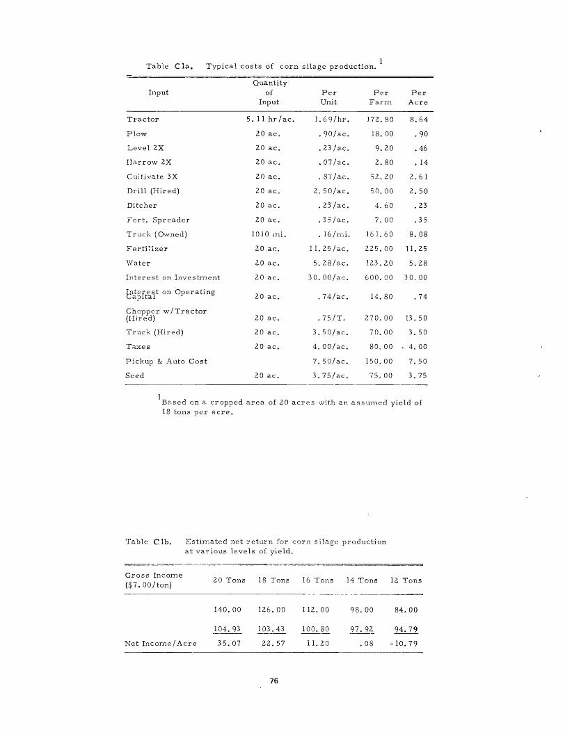
Table CIa. T . 1 f ·1 d· 1 yplca. costs a corn Sl age pro ucbon.

Quantity Input of Per Per Per

Input Unit Farm Acre

Tractor 5. 11 hr / ac. 1.69/hr. 172. SO 8.64

Plow 20 ac. .90/ac. IS. 00 .90

Level 2X 20 ac. .23/ac,.. 9.20 .46

Harrow 2X 20 ac. .07/ac. 2.80 . 14

Cultivate 3X 20 ac. . S-I/ac. 52.20 2.61

Drill (Hired) 20 ac. 2.50/ac. 50.00 2.50

Ditcher 20 ac. .23/ac. 4.60 .23

Fert. Spreader 20 ac. .35/ac. 7.00 .35

Truck (Owned) 1010 ITli. . 16/m.i. 161.60 8.08

Ferti1 izer 20.ac. 11.25/ac. 225.00 11. 25

1Nater 20 ac. 5.28/ac. 123.20 5.28

Interest on Investm.ent 20 ac. 30.00/ac. 600.00 30.00

e1tcrelt on 'operating aplta 20 ac. .74/ac. 14.80 .74

Chopper w/Tractor (Hired) 20 ac. .75/T. 270.00 13. 50

Truck (Hired) 20 ac. 3.50/ac. 70.00 3.50

Taxes 20 ac. 4.00/ac. 80.00 4.00

Pickup & Auto Cost 7.50/ac. 150.00 7.50

Seed 20 ac. 3.75/ac. 75.00 3.75 ._---------

1 Based on a cropped area of 20 acres with an assumed yield of 18 tons per acre.

Table C lb. EstiITlated net return for corn silage production at various levels of yield.

Gross Income ($7.00/ton)

Net Incorne / Acre

20 TOllS

140.00

104. 93

35.07

18 Tons

126.00

103.43

22.57

76

16 Tons

112.00

100.80 ---11. 20

14 Tons

98.00

17.9~

.08

12 Tons

84.00

94.79

-10.79

Table C2a. Typical costs of sugar beets production. 1

Quantity Input of Per Per Per

Input Unit Farm Acre

Plow 20 ac. .90/ac. 18.00 .90

Cultivate 5X 20 ac. .87/ac. 87.00 4.35

Truck 1010 mi- . 16/mi. 161.60 8.08

Fertilizer Spr eader 2X 20 ac. .35/ac. 14.00 .70

Leve12X 20 ac. .23/ac. 9.20 .46

Harrow 4X 20 ac. . 07/ac. 5.60 .28

Ditcher 20 ac. .23/ac. 4.60 .23

Drill (Hired) 20 ac. 2.50/ac. 50.00 2.50

Topping (Hired) 16 T. 1. 75/ac. 560.00 28.00

Fertilizer 20 ac. 20. OO/ac. 400.00 20. 00

Seed 20 ac. 2.25/ac. 45.00 2.25

Water 20 ac. 5.72/ac. ;; 4/40 5.72

Thinning 20 ac. 20.00/ac. 400.00 20.00

Howing 20 ac. 12.00/ac. 240.00 12.00

Interest on Investment 20 ac. 60/0 of 500.00 600.00 3 0.00

Tractor 7.56 hr lac. 169/ac. 279.20 12.77

Truck (Hired) 400/0 of crop 100/T. 128. 00 6.40

Intere st on Operating Capital 20 ac. 3.02/ac. 60.40 3. 02

Pickup & Auto Cost 9.25

166. 91

IBased on a cropped area of 20 acres with an assumed yield of 18 tons per acre.

Table C2b. Estimated net return for sugar beet production at various levels of yield.

Gross Income/Acre 18 Tons 17 Tons 16 Tons 15 Tons ]4 Tons 13 Tons

$16.60/ Ton 298.80 282.20 265.60 249.00 232.40 215.80

Value of Tops 8.00 8.00 8.00 8.00 8.00 7.00

306. 80 290.20 273.60 257.00 240.40 222.80

Costs/ Acre 171. 91 169.41 166. 91 163. 97 161. 03 158.09

Net Income/Acre 134. 89 120.79 106.69 93. 03 79.37 64.71

77

12 Tons

199.20

6.00

205.20

155.15

50.05

Table C3a. Typical costs of sITlall grains production. 1

Input

Tractor

Plow

Harrow

Level

Fertilizer Spreader

Grain Drill

Ditcher

Sprayer

Truck

Cornbine (Hired) Anline

Spray (1 pt. lac. 24D)

Seed

Fertilizer

Water

Interest on Capital

Taxes

Interest on Operating Capital

Pickup & Car costs

Total costs /acre

Quantity of

Input

2.86 hr/aco

30 ac.

30 ac. 3X

30 ac. 2X

30 ac.

30 ac.

30 ac.

30 ac.

375 rni.

30 aCe

30 ac.

30 ac ..

30 ac.

30 ac.

Costs of

Input

1.69/hr.

.90/ac.

.07/ac.

.23/ac.

.35/ac.

.90/ac.

.23/ac.

.40/ac.

.16/ITli.

6. SO/ac.

.40/ac.

4.00/ac.

7.00/ac.

4.00/ac.

6% on 500. OO/ac. 30.00/ac.

30 ac. 4.00/ac.

30 ac. .43/ac.

Costs Per

FarITl

144.90

27.00

6.30

13. 80

10. 50

27.00

6.90

12. 00

60.00

12. 00

120.00

240.00

120.00

Cost Per Acre

4.83

• 90

.21

.35

· 90

· 23

.40

2.00

.40

4.00

7.00

4.00

900.00 30.00

120.00 4.00

• 43

4.00

70.61

1 Based on a. cropped area of 30 acres \\tith an assuITled yield of 18 tons per acre.

78

Tahle C3b. Estilnated net return for small grains production at various levels of yield.

Variable Incorne 100 Bu. 90 Bu. SO Bu. 70 Bu. 60 Bn. 50 Bu. 40 Bu. 30 Bu.

Barley at 1. 05/Bu. 105. 00 94.50 84.00 73.50 63.00 52.50 4l.00 31.50

Straw 5.40 4.80 4.20 3.60 3.00 2.40

Pasture 1. 00 1. 00 1. 00 i. 00 1. 00 1. 00 1. 00 1. 00 --- --- ---Total Ill. 40 100.30 89.20 78, 10 67.00 55.90 43.00 32.50

Variable Costs 100 Bu. 90 Bu. 80 Bu. 70 Bu. 60 Bu. 50 Bu. 40 Bu. 30 Bu.

vVate r 4.00 4.00 4.00 4.00 3.08 2.20 I. 32 0

Fertilizer 7.00 7.00 7.00 7.00 7.00 7.00 5.00 3.00

'-I Harvest e.g

8.50 7.50 7.50 6.50 6.50 5.50 5.50 4.50

Seed 4.00 4.00 4.00 4.00 4.00 4.00 3.50 3.00

Interest on Operating Capital .43 .43 .43 .43 .43 .43 .35 .28

Total 23. ')3 22.93 22.93 21.93 21. 01 19. 13 15.67 10.78

+ 2.00 + 1. 00 + 1. 00 0 • 92 - 2.80 - 6.26 - 9.82

70.61 70.61 70.61 70.61 70.61 70.61 70.61 70.61

-I- 2.00 + 1. 00 + 1. 00 0 • 92 - 2.80 - 6.26 - 9.8l ---Total Costs 72.61 71. 6 1 71. 61 70.61 69.69 67.81 64.35 60.79

Gross InC0111e Ill. 40 100.30 89.20 78. 10 67.00 55.90 43.00 32.50

To ta 1 Cos t s / A ere 72.61 61. 71 61. 61 70.61 69.69 67,81 64.35 60.79

Net Incorne per ACI'e .j8.79 28.69 17.59 7.49 - 2.69 -11.91 -21. 35 -28.29

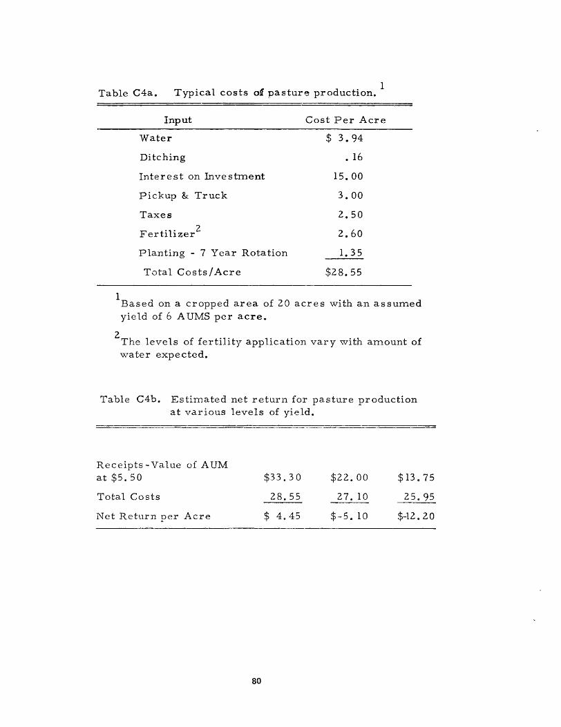
Table C4a. Typical costs of pasture production. 1

Input

Water

Ditching

Interest on Investment

Pickup & Truck

Taxes

Fertilizer2

Planting - 7 Year Rotation

Total Costs/Acre

Cost Per Acre

$ 3.94

• 16

15. 00

3.00

2.50

2.60

1. 35

$28.55

lBased on a cropped area of 20 acres with an assumed yield of 6 A DMS per acre.

2 The levels of fertility application vary ·with amount of v;.ra ter expected.

Table C4b. Estimated net return for pasture production at var ious levels of yield.

Receipts - Va lue of ADM at $5.50 $33.30 $22.00 $13 0 75

Total Costs 28.55 27. 10 25.95 ---Net Return per Acre $ 4.45 $-5" 10 $-12020

80

I' ~.

l' ~.

',' ". 70 ~.

~.

10' II' 17' I ~. I ~. 10;· 1'"

00 17. ....lo 1 ~.

I'h 7r}·

2 I' ? .,. :> 1-lq· 2 S. ?f,' 7 7 •

7 ~. ; Q.

Jr}. ~ ,. , ,,-3,· 3 q.

J ~. Jr,. 1"'. J q. , q.

.. ". .. ,. .. ,. II ,. II ,,_

.. ~. q .,. r. .. 7· C .. ~. C " a. 5 '1' 5 ,. e; ~. ,10 <; q. .,<,. 0;".

Appendix D

Digital COITlputer PrograITl and Output

Table Dl. Digital computer program. list of sym.bols.

H'OPOI~~IC ~1~ULATI0N MonEL OF C~CH[ VALLEY

ACCEI If J:AC(lJMULAlr" fVAPOHHNSPllIATTON PURRING EACH MONTH CCROP II lC«,"':4~CUMlILlTfO "'''C'I/HrL T DlJlIlI)Nr, [ACIl "'ONI~

IOJJ>P:anJI,sTEO P'HCIP rOI rON 10 PIIEHNI SNowrAlL r~OM AOOhG 10 SOIL 1'101<; TUIIF I rNCyr<; 1'[11 lCII[1

aI(C([I-'''lNTHLY VAlUES OF K( FOR <"AC~ (ROp FOR [VAPORAllON ~J'i"'lll:10JUSHr, SOIL MOISrUllr CONTENT FOR (ROP I CINCHES PER ACR£I lIRIlI:"ElSONlL I 1111 TGAl ION WAI['1 APpLiED FOR CROP I AJlllI"nl:IIlIlIr,AlrON or CpOP I rrlo ~ONTH HOIIN/MONTH! lP'flH II :IPqIGAT ION apPL J(O TO CliOI'I FOP A pAIH ICUL All HONTH

lPH:: FIIACT ION or CANAL OIVrll;ION', !lEING lpPL lEO TO LA"'O PHREUOPHT 1S APIlJCIJ':SEllING Plltrr OF CPOP I PfR UNIT lIIEYIj:IIlPIGAHO ARtA IN lCIHS A~EAIII :THE AIIEl IN AClIl<; Or (ROp I

AREll:TOTAL lREI IN HilES lWITI:MAIIMUM AliHLABL( I/AT(II FOR CROP I IIN(HE'). = ROIII'WH(1I1 AWS~C:~C FOR WAT['1 <'UIlFAC[ r:op:prpr[NT or (.",AL OIY[!?SION') WHICH DHP pn?COLAT[ TO GROUNDwATER C Q S II 1\ : CO", TIN n OLl AilS P ( R I CR [ r 0 P PROD U C I N Ii CROP I CGw:CON';TINT fOR DETERMINING IjNGH;rO GROUNOWAT[R INFLOW (1(<;:CON<;TANl FOil SNOwMELT FOliATION

('0 -(ON<'TAN' IN F" VAPOTRANSP 111 AT ION EDUATION C"[LT:S~OW'1[LT rORQfLHION C(l(H-I([[NT

CPH:DfoCENT OF PHllfArOPH'TE rVApOTRINSPIRITION TA~rN FRO" SOIL. II-rPH:FIIAcr ION OF f.T. fllOM IH';[RVOJRI

CSI :l'rPr.rNI or THE <;ullr~c[ INFLOW THIT I') ASSU"ED TO "AKf UP TIff UN'1r "SUR[D <; lJllf ICE INFLOW

nlIRS:CHANGE IN R(5fRVOIR STORAr,E IICRE-fEfTI

OPGWIIMOI:GROUNOI/AHR O[LIY L[VfL I AfTfR LO'iING WI'fR TO SlIIHaC[ [II1MOI:fT Of CROP I FOR MONTH MOctNI

[TlI!:fvapOTPANWIRITION FOR [ArH CROP IINCI-£5 PER ACR[I

[TPHs:rVIPOTRANSPIRaTION or PI-R[ATOPHYT"; THAT ARE GROWING ON 1Hr LaND IINCHr~ PEII ACR[I

E TPHW:rVIPOTlUN<,P IRH ION OF PHIlfOOPHYT<' 1HAT ARE GROwING IN WATER IINCHf.'i P(R lcofl

()Il:[)([p P[IlCOI.ITION FRO" IIlPIGATE(1 lA.,O IlCR[-FErTI t;wll.?oll :GROtJN(lwaT fll INFLOWS FOR nIfrrlHNT MONTH> PLUS 0[(1'

pfRI"'OLATION UCpr-FEfT'

f:l/llcr;JH1\JNf)I/ATf'l HI D£LU LEVU I RfFO~ LOSI"'G SOME TO ')URFACE G~Zll~a':GRnUNOWAT~Q IN (l[LAT LfvEL 2 FOR T~( "ONTH

rW311'101:MONPIl' VAlUE OF GROUN(lWJl[1I INFLOW PLU'i DE(P PERCOLATlO'" rWA 11'1(1' :~MOUNT or I/ATfll OEEP PERCOlAT~O TO GROUNDWATER <;lUSI :tll[ <;U""'P UN"[lo;uR£n SU'FACf INFLOIJ COEfF ICIENT "CT:NU~A[Q OF MONTH" OF ~ATA WHICH ARE TO Bf CALCULATED "O:HONTH OF Y[AR

N'P:'fAo OF R[CORO T(, R(GIN COMPIlTaTlONS P:~ON1HlY PERctNTI()( Of ~lYLrGHT ~OURS or !HE Y(AR pR:PJlrCTP{TlTION CINCH[S P[11 AC"fl "C:(A.,IL :.llv[P<; ION,) 'ICQ[ -rCfTl

IlCfrF :Dr"crNT or ("A'IAL [1IV['l<; 101115 THAT t;0[e; INTO THE !"JOIL 11-0C[Ff r<; "rTUIIN rlOIi rn PE<;(RVOIOI

n(FIIT:CINAL DlvrPSlrllJ.., Jlv[~TfO TO Tf.IlT CIIOP CIN(HES POI ACRE I Orr:THr I~OUN' or (ANll OlV[PSION<; WHICH HAS 1.101 B[[N IlIVERlrO TO I

rp"p fOR THIT PIPTICULAP '40IlJTt-' I ArRf-Fr£ll

S 7. ., q.

5 '1' 60' 61· 6;>.

63.

6'" 6<;.

"". 6 7. 6 ~. ,,~. 7,.,. 7 I' 7 ~.

73-1". 7 <;. 71;. 71' 7 q.

1 ". 8 '1' 8 I' I! .,.

A J. 8 ... 110;.

~6' 87. !I ~. 8 q.

'JO. '3 I. 'J 7. q J. q II. '30;. 'Jr. • '37 • 'J ~. ~ q~

I no.

101' I O~. 10 J. 11'1,,· 10<;· IOf;· 107. lOll­I nq.

III)·

111' 117'

IlIN:T4f CURR[NT VILUI" OF DEF IN IN(HfS OYER THAT pIRTlrulAR CROP POI I J : Pi'll) T 0 f P T 1-1 lor CROP I I f [ (r I P[TGCII:GQOO;<; R[TUQN IN nOLLARS PEP ICR£ fOR SfLLJI!G CROP I

"'[TNI11:NfT R[TURN IN nOLLAP,) PER ~(R[ Of CQOP I D[TNY:TOTal NO II[TURN IN OOlLaP'; FROM TH[ [NTIRE ARfA

POUT:OU"'-LOW fRO~ TH[ VAllE' UCR(- r!:[T I

S:TH[ o;TO"'AG£ COErFlCIrNT wHrCH OETfRMIN(<; HOII 'AST TH( WlT£I~ wiLL COME ""0" THr GPOU'In WII£P RrsrRvoIR JPHO TH,. SURfACE RE'i(RyoIR IS:l WOULD M['N lHIT IT WOlA.O rOME OIPfr.Tl. INTO THE SURFACE RESERVOIR EACH MON1H. O[IATfD BUT NOT SMOOTH[nl

<;!iw 1 = ':i' Gw I c; I : 11[ A 5 UII [0 S UP F' C [ r 'IF LOW I I CII [ - H [T I ')Mlr~IHE ~ArIMUM _MOu.,T OF SOIL ~OISTUR[ lHAT C~N B[ HELD 'GAIN,)1

[opAVII' rop [ICH CROP INOT SlTU!!arrOI IN INCH[S PER 'CRE r. S~[lT:<;NOII"lL T IN TfRHS OF IIIT(II rOUIY'lr .. 1 I INCHES PCR ACR[I

( S"ES=LI"ITING ROOT lONE AVAILABLE "OISTURE CO"'T£NT BELOW WHICH 1HE ( ICTU.l ['lAPOTRAN,)PIRATION IlH£ B[(O"E5 LESs 1HAN Ufr POT[N'lAl C RATr IINCHfo; PfR ACRr! ( S~IJl:QUANTI'" OF 1/11[11 ~TOREO WITHIN THE ROOT lON£ AND AVAILABLE C FO!? PllNT IJ')[ ":1.6 II[PRE')[NTTN(, TH[ ')TORAGE fOR rACH . C rROp I '1[A5UII[0 IN INCH[S PEII ACRE C "=MfAN SURFACE AIR T[MpfRATURE IN DEGREES F C T[lTRS:NfT ANNUl' CHINGE IN P[SEPYOIR STORAG[ ( T(T\:IN'IIIAL [. T. OF B[[TS C T[ T;>: AN"IlAL (. T. or COliN C TET,:INIIIUAL E. T. or GRAIN'

C T[T~=.NNlJAL [. T. OF lLFAlFA

C TET5: ANNUAL [. T. Of ".')TUR[

C T(T6:ANNUAL E. T. OF LANO-BASro PHR[aTOPHTT5 TfTPH:ANNUAL [.T. OF WAI[P-BA'i[O pHR[l!OPH'TS

C TtRR:TOTlL <,£Ao;ONAL IPRIGATION IN ACR[-r[[T C TPR:ANNUlL F'R[CIPITlTION

C TGWA:TOTAL ANNUAL wITfll fNTEPINt; GIlOUNOWATER C TGIIA:ANNlJlL OE[P p[PCOLAT ION

C U[,I/AC 1'10 I:TOTIL '''OUNT O~ wAT[R [NTfRING O[LAY L[V[l 3 rOR 1HE "ONTH C TC,1/3:lN"UAl r,rIOUNDwlT[R INFlOI/

TOC :ANNUAL CANAL OlVU~SIONS r. TROUT:CONPlJTfO ANI:Ull AR£I OIJTFLl)w C I w'> fT : ANN U A L f. I. 0 r W A T( R SU RF A C r C T <;(,WI: A'MUAl GPOUNOWAT[II THolT COI1[') TO SURfACf C T '; T : A IIIN U A l 11 [ 10; till [D <; UR ric [ I NFL 0 W C TSMU :ANNUll ACCUMULITEO SNOIJI1ELl C TU5I:AN.,UlL UNMrA~uII[r SURFAcr INFLCW C TW'i:ANNllftl ICCUMUlATfO SNOW <; TODlG[ C U,)f1IMOJ:1I0NTHL' UNr,AG[() SURFlcr INFLOW C UGI/:UNNrA<;UQEO GROUNO-WATER INFLOW INfO THE VAllEY CACRE-f[ET!

\lSI :U'IMreWIH,n SUPfArE INrLOI/ IICRE -f£ETI

W~CIII:'VAIl'Rl[ WATfR HOLOIN5 CAPACITY Of SOIL fOR CROP 1 IINCH[C; OF WAT(II P[R FOOT OF 'iOILI

wS:o;HOw <;TORAr,r. IN T(RI1~ OF WnER [QUnALENT IINr...:S PER ACR[ I wSAR:wATfR SURFI([ 10[A lA-f"I

C W')[T:fVA"OTIIANSPIPATION fROM wATfOP ')UII"IC£ tINCHE., PfR ACRE I C YlTIlI:THf ICCU/OlJlAHO <;[A,)ONAL rVADOTR'N"PIRlTION FOR CROP I r. '111 0 11 INC, lHE GROW ING !of AS ON

( 'I£LO!lI:TH( Yl(lO of CPOP r PEII lfR[. l~ THE R[GULAP UNIT') Of ( "rAo;Uol[MfNT roP THAl CROP

Table D2. Flow diagraITl of digital program.

00 10 J = 10 MeT

GT or

~L-______ '-______ ~

D~ 40 N=I,30

L T or EO GT (Snow) (Rain)

@! SMELT=CKS-;~:.TA-26.0)*WS/30.0

GT Of EO

82

~.---------------~ WS=WS-SMELT

Table D2. Continued.

~~----~~----~~----------, ~~------------~ ~...:.----....;~

~L-~E~T~(~J)~=~(~A~J~SM~(I~)/~S~M~E_S~)_*_A~K~C~<r~)_*~C~K~T_*~(T~A_*_P~/~10~O~.~O~)/~3~O~.O~ __ ~

~~----~------~~----------~

~L-________ ~ ___________ ~

~~------~----~ @ I [ SM(6)= SM(S)+QC.APH/2.0*12.0/AREA(6)

AIR(6) = AIR(6)+ QC* APH /2.0.12.0/ AREA(S)

@CGW=GW+QEF

I

@ '-----~------'

~~------------~ ).-..------~

~~------~----~ SM(I) = SMCI)-OCFRT

I [ AIR (I) = AIR(I)+QCFRT

QEF=( erN -QCFRT) .AREA(I)/12.0

~~-----~----~~------------~

83

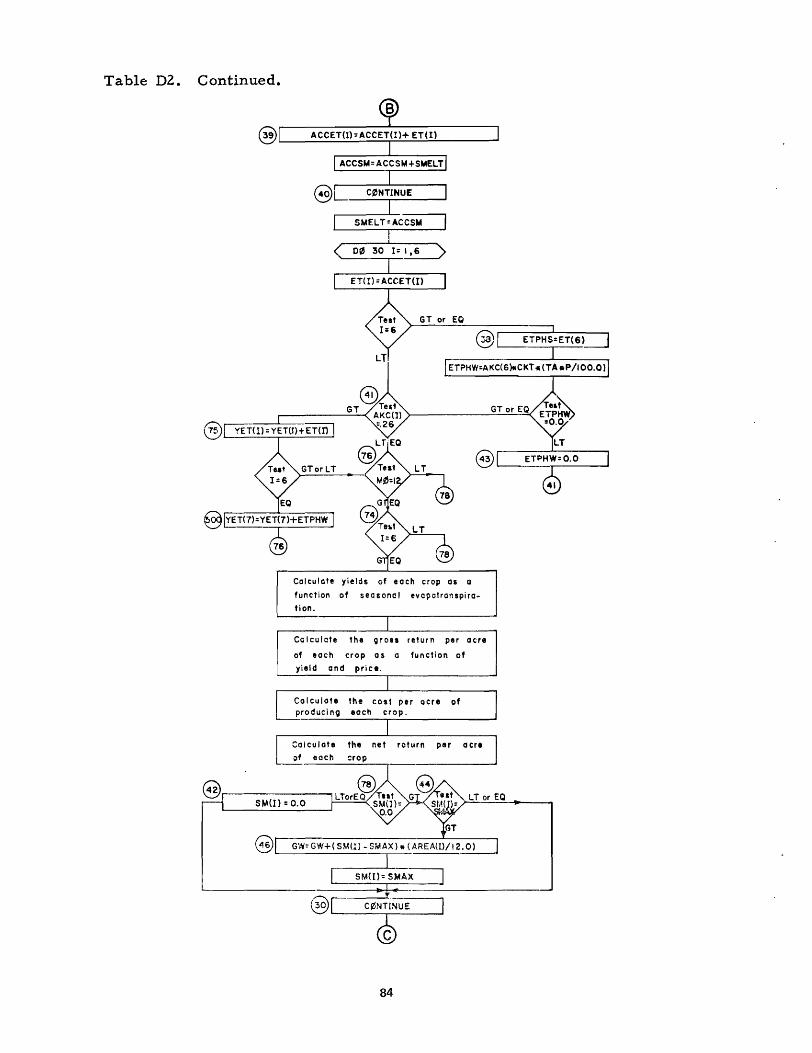
Table D2. Continued.

@ ~TPHS=ET(6)=-:J

~~------.-------~ @ L---____ .-______ ~

Calculate yields of each crop as a

function of seasonal evapotranspira­

tion.

Calculate the groll return per acre

of each crop as a function of

yield and price.

Calculate the cost per acre of produci ng each crop.

Calculate the net return per Clcre

of each

@r--------. SM(1) = 0.0

@ ~----------------.-----------------~

~L---_____ '-______ ~

84

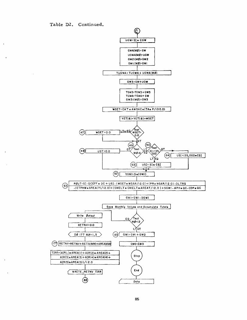
Table D2. Continued.

GWA(M~)=GW

UGWA(M~)= UGW

GW21(M~)=GW2

GWII (M~)=GWI

TUGWA= TUGWA+ UGWA(MQI)

TGW3=TGW3 + GW3

TGWA=TGWA+ GW GW31(M0)=GW3

WSET= CKT"* AWSKC*(TA* P/IOO.O)

~L-______ ~ ______ ~

R0UT=SI-QCEFF .. (;IC + USI - {WSET* WSAR/12.OH (PR* WSAR/12.0) -DL TRS

-( ETPHW.AREA(7)/ 12.0)+ (SMELT .. CM E:L T .. AREAT /12.0) +SG'NI - APH .. QC-CDP*QC

Monthly Voluu and Accumulafe Tetol.

@ '--------. @ [RETN~=RETNV+ RETrHMM)+AREAW"~

TIRR=(AIR( I ) .. AREA( I )+AIR(2). AREA(2)+ -------AIR( 3).,. AREA(3)+ AIR (4)* AREA(4)+

AIR(5)",AREA(5»/12.0

Data

85

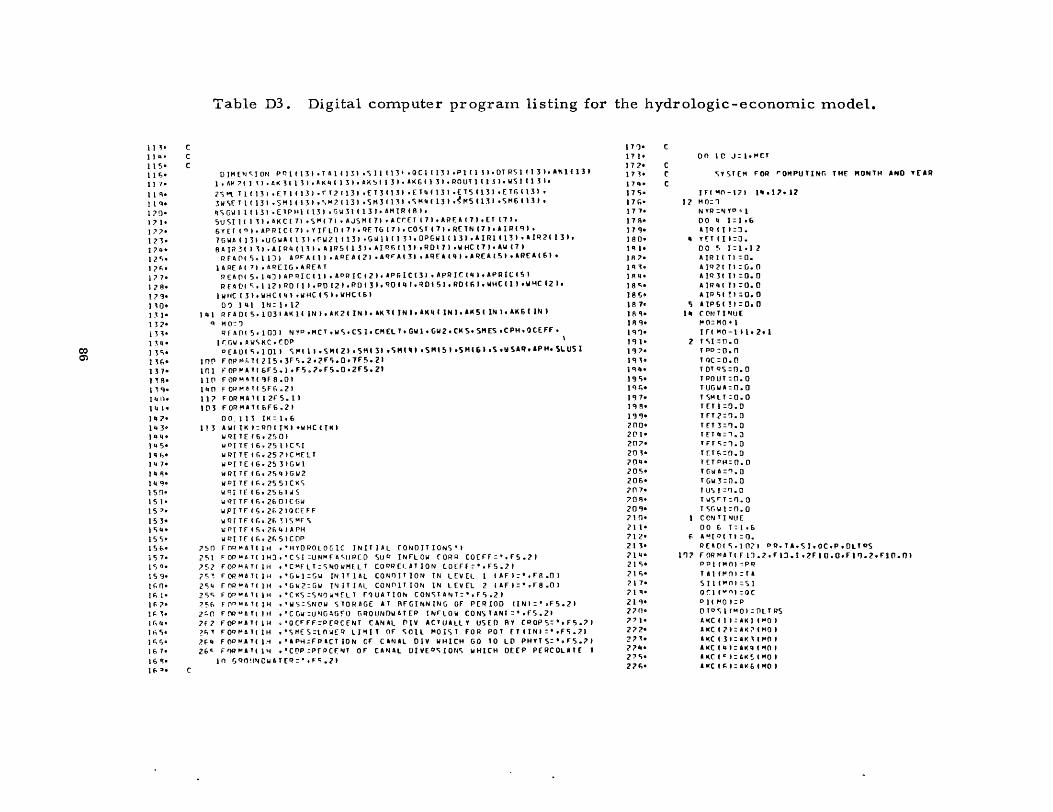
I 1 ~. C II'" C 1 I 5' C 1 1 ",. 11 7.

1 I 'I' I I q.

17Do Ill· I? l' 1 <' 1. )7'" 12 c;.

17~'

117' 17!h 179' 1'0· 1,' l' I J]. i J ,. I 311-

00 1 J <;. (j)

111',' ) :J 7-) ~ ,,-I ~ q. III 11. ) Ii \.

1117-1 .. J.

I .... • I" S' 1 ~ h' I" 7-111 !j. III q. 15 !l-IS l-IS ::0-

) 5 Jo 1 'i II. 150;· 15 G' 10;7.

\'i'h

159' 1£;0' If.: • If, 1-1 f, ,-I r, II' I h 0;. 1'; r,-If. 7-

I G '!-1 f, 'I-

Table D3. Digital cotnputer prograln listing for the hydrologic-econom.ic tnodel.

o 1M [N <; r ON P ~ 1 I 131 • Till C 131 • '; 1 1 C 13 1 • () C I C 13 , • PIC 1 J , • OT 1'15 I , 1 3 I. A!\ 1 ( 1] t 1 • All 'Ill J • A I( "5 I 1 J ) • A K .. I 1 3 ) • II K 5 C 1 3 ) • A I( G C I :5 ) .1'10 U1 1 , 1 J I , w'; 1 ( 1 :5 ,.

2'; "'I. T 1 « 13) • E 1 I I 13' • r T 2 C 131 • [1:5 , 13 I ,[ Til C I J I • E 15 113' • E 16 , 1] I • 3 II <;r 1 I C 1 J I • S M 1 C 13 I • <, M l , 131 • '; M J I 131 • '; Mil I 1] I • ~ M 5 I 13 , ,'; M 6 I 1] I , '1 <; Gill 1 I 1 3 I • E 1 PHI C 13 I • G w J 1 , 1 J J. A M I R ,8 I , 5U';llC I H,IIKCI7I.SP4'71.AJSMI1I,ACfET 17I,AR(AC11,ET 111. 6'1' [f I" I • AP RIC' 71 • Y I [LO C 1 I ,q( 1G ,71. co 5 T ,71 • RE TN (7 I , A II?! <J I , 1 G WII I 131 , U GilA ( t J I • (';111 1 I 13 I • G W 11 C I 3 I, DP Gill: 131 ,A I R 1 ( 13 I • I I R 2 C 13 t , 8 A I R 3 I I , I • A I R II « \ 3 I • A I R 5 I I 3 I , A I R f. ( 1 3 I ,R 0 I 7 I • II HC ( 1 I , A II ( 1 I

REA[11 0;. 1 iJl APrAll I .AREAI11 .ARt'AI31 ,ARfAllfl •• RElt51.AREAI61.

1 A RE A' 71 • ~ RE I G , A RE AT REA ("1 I 5, 1 .. ] I APR I C I 1 I , A PR I C 12 I , 'P I< 1 C 13 I • APR I C I If I , APR I t 151 R f ~ VI <;.1 III RO I 1 I • PO IZI ,PO 13 I, qo III I, Q 0 15 I, RO C r; I, WHC 11 I .11 ~C 12 I.

I W HC I :5 I , WH C III 1 ,W HC C C; I. IIHC (61

D'J)IiIIN:ltlZ I Ii 1 R fAD I '), 1 D 3 I A ~ 1 C I N I • A K Z ( IN) • AK ~ ( J N , , 'K II « 1 N I • AM 5 ( IN I , AM Gil N 1

q M 0::1 Q fA [11 ~, 1 DJ I N '!'P ,M(T ,w'), CS I, CMEL T, Gill. GWZ. C~ S. SMES .CPH .QCEFT,

Ir:riW,AW<;KC.r.OP \ DEAUI 5.1 DII <;,.., II.SH( 21.SM( 31.')11"41 ,5"'51.SI1(&1.5 ,IISAR •• PH. SLU51

Inp FOPM~tllI5.3F5.2.1F5_0.7F~.21 101 .... OPP4AlI £,F5.I,F5.1.F5.0.2F5.21 1 1 (l F OR M ~ 1 I 'l [ 8 • 0 I 1 q n F OP 1'18 T C 5 F h • 2 I 117 FOR M 1\ tIl 2.5. 1 1 I 0 1 F OR P4 • l( £, F 6 • :1I

DO, 113 l~: 1.6 l!J AWIIKI:POIPO'WHCCTKI

wQ[ tE 16, 2',01 .,°11fI6.251IC<;1 W PI t f 1 h. 15 71 C ~E l T w 0 r TEl G. 2~ 31 Gill wRITrlG.2S .. IGwl lIoITrlr;.255ICI(,) w'H 1 f '6.25 G 101 S WI?ITflfj,2£,OICGW wprTrlS.2~21()(EFF

W R rTf 1 fj. If. ~ 1 <; I"f S Wf'ITfl5.ZGItIAf'H W P rTf 1 I:; • If. 5 I C OP

7511 FOQP4ATllrl ,'HYDROLOGIC INITIAL rONOITION5'1 751 FOP"ATllHJ.·CSI=UNI"FA<;IJRED ';UR INfLOIi (ORR COEFF:',F5.1I 152 FOPI"'TC IH ,'CMfLT:';t.lOWM[LT CORP[I_AlION C.OEFF:'.FS.ZI 2"~ F()RMATlIH ,'Gwl:Gw INITIAL (ONfllfION IN L[V[L IIAFI:',f8.01 20;~ r(,)R"ArtlH .'Gwl:Gw INITIlll CONnITION IN LEvEL 21A[I:',f8.01 ZO;c; FOPMATlIH ,'CI(S=<;OJOI/'HLT r'lUATIO'" CON<;TANT:',F'l.ZI 251:; FO""ATllH ,'IIS:SN('W ';TORAGE AT AfGINNtNG OF P[RIOO IINI:t.F5.2I 2~n FM"ATIIH ,'CGW:U~IGAGfO GROUNOWI.TEP INfLOw CON,)TUIT:',F').21 2fl FOIH'AT(IH ,'ocrFF:p[RCfNT (ANAL r'lIV ACTUALLY U,)EO R'f' (POPS:',F5.2I ?~~ FOO,.A1IIH ,'<;MES:lO:./[t1 lPIIT or "Oil 1'101<;1 rOR POl [TCINI:',F<;.:n ?fll FOPI"ATIIH o'APH;:[P&CTION CF CANAL DIY WHICH GO 10 LD PHTTS;:""S.7) ZGc:. FrJP"'AlIl\.j ,'C[lP:PfPcpn OF CA"IAL DIYEo"IOt4<; WHICH OE[P P[R(OLAT[ ,

In t;'?O!',",OwAT[R:",F<;.ll

17 'J-17 l' 112-11.,. 17.,-170;· 11 f;. 111. 11 g-17 q. 180-1'1 1. 1 R 7-lll'h

1 RII' 18 C;.

J 8 c;,. 181. 18 q­IRq. 1 q,).

I 'l l' I q 1. I q~. 1 q If­I q <;. Iq~·

I 'l 7. 191\-19 q. 7.no· 2(11-Z07-lO .,-7011-20 S. 20G-7n 1. 10 ,,-10'l· 710-711-712' 21 l' 7111 0

21 'i'

21 "'. 7.17-71 q.

21 q. 27 flo

7'1-272-:? 7~' 77q· 2'<;· 27f.·

00 Ie J::loI'ICT C C <;YST[M FOR rOMPUTINr. THE MONTH AND Y[AR

C IF! '10-121 1",17.17

12 MO:: 1 N YP::t.I YO->1 DO II I:: I,£, alqlll;:J.

I! yn I I l:iJ. 005I:lo1Z _ IR l' I I:: O.

Al02111:0.0 AIRJI II::O.O AIRIIIII:O.O AIP'd TI ::0.0

S AlP G ( ! I : O. n II! eNI TI t.lu[

,..O:MO·1 IflI'I0-lI1.Z.1

2 T<;I:0.0 T PO: O. n T QC: 0, (1

TOTP';:O.O T POU1:0. 0 T UGWJl:O. 0 TSMlT:O.O HTl:O.O TfT2:'l.O Tfl3:"J.0 T fT 1I:1.:l TFf<;:1.0 T[Tf.:O.O T[TPH:O.O fGwA:'1.0 T GII:3: 0.0 T us J : '1.0 T I/S r T : fJ. 0 T <;r, W 1 =0. 0 C eN T I "'LI[ DO (; T: 1, £,

f • "![ O( T I: 11. R[a[ll5.1n~I PR.TA.SJ,OC.P,OlToS

1 n 7 [OR P4 All F 1 J .2, F 1:J.1 ,2F 1 000. FIr). Z. fI O. 0 I PPlfMOI:PQ TI11,..!'),:fA

51l1P401:51 Or.l ""'1 :OC P 11 P40 I::P o 1 0 <; 1 f" 0 I ;: n L T PS A I(C I I I.: A~ 1 I "'0 I 4KCI2I:AI(;>IMOI a I(C I J I: II I( ~ ( P40 I 11«( I" I: AI( II ( ""0 I 'K( I 0: ,: AI( 5 1"10 1 'IIC If,,: AI( 6 ( ""0 I

? 'J 7. "')? ~. ? ") q.

? ~!l-711' 7J7· 2 J ~.

:? ~ 'I-7 ~ I)-?l;ft-

l' h ~ 1 q.

2't"h

i ~I ,h

2~ I' 7U ?

2U 1-

Zl4'" 2'''-;. 7U c,.

747. Z~ A.

?4 .~.

75'1· 25' • 25 ?

253' 25 II' 75 ~. 75 f;. 7'i -,.

00 7<;/1· -..J 25 q.

,,~ '].

.?f>l· 762' 26 J. 26 II· 76 c,. 26 f,. -zr,7. ?6 ~. 76 .,. 77 f).

21 ~. 27 7 •

? 7 ~.

27 u. 77.,. 27 c,.

1770 77 q. ", q. :'A "0 JA I" 711 7' ? ~ ~.

1R'" .? a E).

?" ~. ;' A 7.

7A A_

?q'i.

~Q". ~., 1·

7q '.

Table D3. Continued.

rftlCULATION or <;I\jOWH[LT lfojl'l ')~ow SlNlAGr

A CC <; .. : f). C

LJ" '0;; (: I. {; ,C; ft (C < T , r I:) • n

(III :r.(ll n. IA-O.lI" I' QH:Io".ocrrrll~.'

:J 0 U (1 N: \. 31 I r I "J- ?" Ifl. 7. /I

7 orF:I(lr'QCfrFII2.~ II r O~ rr ~I'J(

IiI B-J".JI 16<16.IR I~ ':'1JP,,:oIl/JO.O

GO T(' 73 1'- w<,=W<,.PIl/30.0

ADJPIl=f'.O 11 IFlTI-'h.J1 19.<'3.73 73 IfIW<'-O.O' 21.7.1.?7 21 S~[1I:1'1.0

GO TO 7J 77 ') ~r l T = C II ') • I Tl - 26 • 0 I • W ,>, 3 0 .0

II'IW'>-<;HELTI ?6.2".2" 71; ') Hf 1I =w <, 20 \I '>=".1

G (l 10 78

211 w,,=wS-SHEl T GO TO :>11

1° 'iHFlT='l.O 7~ CONTIOjUE

G w= '1. n. 00 3q 1=1.6

T =1.7 prPIl(<,fOjl., EICH or THE 1 CPOPS (P~PIII:<'UGIR qf[T<, c: P no I ;> , = C 0 Pfoj

(POP 131 'iHAll GRATN5 r.1l OP I '" Il r Il r I HAY (POP 151 Pl51 UPf

CflOPI." TH[ P"PEIIOPHY1'i GIIOWIOjG orj LAND cpno l71 TH[ PH"fAfOPH,T'i GPOWING IN IIIT[R

CAlCULATION OF fVI P01RAN5PTQUION

IfI5"'''-S~fS' 32.~2,J1I ~;> 1J)~Ir':'>"'IIJ

G:> T(, ~6

l" A J> "" I' : <, H[ ') ~ 6 [II I' = I IJ <; '" I I ., S~ [S ,. I II C I II • C I( T • IT •• P 1\ 0 0 .0 II j 0 .0

Iflfrll'-J.O' 3o;.l1.37 3'5 I 11 II: 0.0 J7,"ITI=<;MII,.s"rlT-[TlII.ADJPR qr; CO ... IINII[

"l?nSPA" TO APPl' P!DIGI"ON WAT[R TO CIlOpe; C'N I t'IIIORIT' :lISI'> lin <,T4TrMr~jl _<;,

Ifl~ 1'1' ""7'!.II-) pq IftN-7~1~<;071.~0;

7Q C n ... 11 ~',r rrll-f,,~[).RI.8r

PI,"',r.':""'If".tIOC'""HII;:.rl·17.'1'ARfltf,' ."1 0 16' :11(l(.tD".':> .... "1 ?'1/IDr'161 I IP I r. I: I I II' [, I • A" I P, "'. GO Tr) 'H

7° J. ?q~.

Zq c.. ,Qc;. 7 0 7_ ",:,q ,,­

;>q '" 3{1'1' 30 I' 3 (,;>.

3{1 ;' 3nll' 300;·

30"" ~f' 7' 3011-Jf''l' 31 n. J I I· 117' 3 I ,. 31 It· 31 'j. 31 r.. 3110 31 Ao

3 I q. ! l '1.

37 ,.

J? 7' 321' 3;> ~.

37')' 32 r.. 377. 32 B' 37 ~.

33 n· 33\'

J J ". 3:q· 33"· l15' 3~ (;.

3' 7' 'J!IlI.. 3 ~ 9' 3~ n· JU I' 31! ? !~ 3' 3" II. ll! ..,. J/ .. f,.

107.

~" t:\. 3u'1. !s,,· 35 I' 3'; ;>. 30, 3. Jr, ... lSr,·

~S r.. 3!l 7.

~r, ".

'1'1 If, Hrl 1I-.?61"5.~'5.S9 "Q 1Ft <; .. " I-~W" 1I;0."",q5 f.O 'J cr n T : A W I I I -, ,. r I •

Q:NoOf'-·17.D/AIl[1111 I r I r. c rOT - 0 I N I 6 I ,; ? 67

61 e;"'II:<;"IT,·o~rJlI

AMI'" 11 =Orflll A :P I I I: ~ I P ! I •• Q C F P' • I I .01 (l C ~ f r • orr:I'l!,j-fl("fQT •• APF:.'JI/I?O GO III b.,

f'l (lrFDT:OIN "''''1 !I :':;MI p"H:rI'!T I III I I I = A I P C t, .0 r:F Jl T • I I • ~ lOt [FJ ,

AHIr:lI" =OCFIlT Q fF = C. n Gn !O US

01 Gw:Gw''l[ Jl AIQII"OI .11l11l'01 .... IQI1I.II.O/OC(FfJ

A III ? I .. 0 I A I R ;> I HOI •.• '" I II I ;>, • I I • III (l C [r r , • J Il 1t "r" I I P HMO to I HIli I lJ 0" .0' (l C E F F , A 1<l"I"O' I II1IIIHOI .IMIQII"ol 1.Dloc£rQ • t" <; I "0' • I II '5 1M 0' • I'" [ Q I S I 0 I 1 • 0 I (l C £ r r I I J P 1; I ~o I I III 6 tHO I • un Q I Eo I 0 I 1 • '" Q cr r r ,

00 q" HP:l.r. 9{; I"'IPI"'P':).

lie; C "N T I HUE

~9 ACCETII'=ACCElIlI.[TltJ A cr e;t' = A CC ~M'S ME L T

110 CON T I >lU£ 5'1fLT :6(:("<," 00 10 [:10(; Ell ,,:ICCE"I'

THIS C;EC'JON [e; r~ rILCULI,r [ T.'~[H 'I[LD. TH[N N[T R£TU~N PEA ICA£

I FI 1-(;1 '11038.38 3~ ETPH<;=ETl6.

£TPHW:II(CI"'·CKJ·ITIoP/100.0' IflETPHW-J.!11 ~J'''10-1

,,~ £TPHW:O.O II 1 C ON II Nur

I r I • I< r I I , - • ? 6 11£,.7 F • 7S 7" Y(TII'=,[T"'.f!IJ'

I r I J - ',J 7 6. SO 0 • n 50" T~II1I=YETl7'.!'IPHW

H IF( HO - I ZI '8. 711 01" 7_ Iftl-f;179.72.7;> 7;> 'I E lO I I , : - .;> 7 e"F, 3[1 7' T( T I I ,. f[ " I' • 1 n. 5 II 0; 8 211 _ 0 .[ , I J I - PH. 'II C; I Jq

T I[ I [1 I .' , = -. I n 5~ 9~ q. T ( T 12 , •• [ II ;,> 1 .5.69880(;60 Y [ T 12 1-" 3 • 25 5- 11 TI~lOI3'=7.15.Y[T 13,-~r;.0

TIElf'IU'=.1I7oT[I 1.".73 T I( l" 15' =.219" [ T 10;,· • 'H

7'00 7r 1<:1.') 7'1 PrTGI 1<1:' IElt'IK ,.APllrclll'

Il[TGt)l:Il[IGI)I·8.n Il £ T C' " = 11 ( T G I lJ - .0 f''161 1'5') oy 1[( (1 I 3 ,. Y [£L 0 I ) I •• I 61" 99" q., IE LO I J ,-

13.6"'1Q'19 q

o [T G, I" : P £ , I: I II I • o. c;n r (\') T I \ , : ;>. q A r; ., 1 [l ,., I 1 I. I 21. " co') T I 7' : I • 750 , I [L 0 I 7' o!l~, 7 C 0') TI H : - • r.J 2 <> 7r, 3~. , Tf UJI " " If l r t ~ , •• C;q J <' q 1 2 '1 0 TIE l 0 I 3' • I! 7. " 5" 11

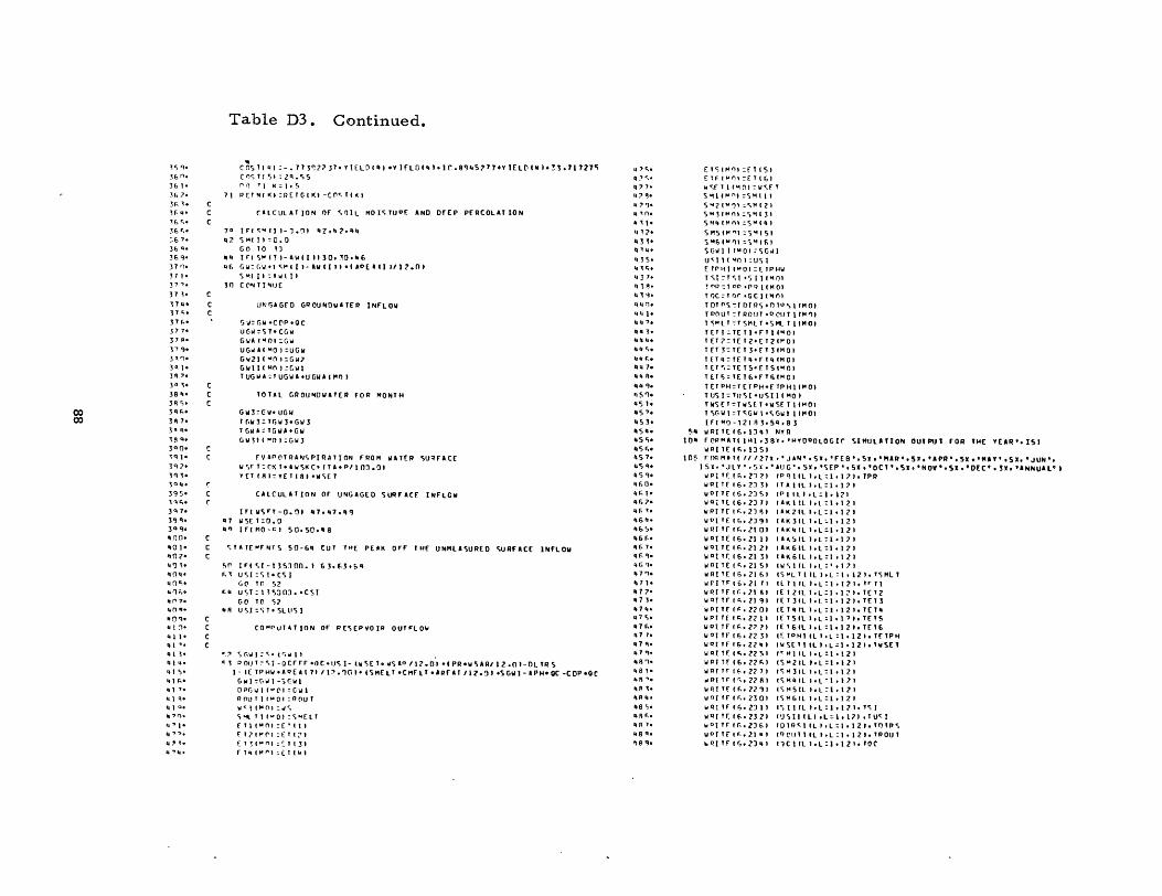
~s 'h

~& n. 3& ,. 3& ;>. 3rl ~. ~f; ",

~b '"'I. 3E. C, •

:.G 7.

3& q.

31;9' 37 q.

~ 7 , •

'3 7 ". J 7 ,.

J 7 ... ~7 ... 37 fo. J 77. J 7~' ~7 q. ~ q.,. Jq ,. 3q ~. 3 Q ~. 38 _.

3 ~ ~.

00 3'1 ",. 00 J'I70

3 ~ q.

~8 'l. Jao· ~'l I' J'l ;>. J'l Jo '1Q ... 39 S' 1'1 c,. 3'17. 39 '\. Ja 9' ~ no· "0 I' It07' .. '11' 110 .. • Lln~· ~n;;o

"I" 7.

&tn .. • ~ (') 'l.

",:l-'III' ett .,.

"' 3' II I'" "IS' .. , ",. q 1 7.

II \ ~.

"t Q. .. ..,,,. 4 ~ ,-

It""'· "' ,. ""'II-

Table D3. Continued •

.. C 05' I II I -. 11 J'! n 310 Y IE L[H" I .y If L 0"4 I. I r.. 8'1 .. 5 ;>17 oy IE L£llil lo! J .117270; C"" 1: Ij I Z'I." 5 I".J 1J ~ I. <;

71 P[TNI~I RETGIKI-Cfl«;TlO

(aLCUL'T ION Of <;~IL HOl"TUP[ AND OrEP PERCOLU ION

7 A Ifl""'IJI-J.'11 IIZ'''"'''4 II '7 '5 HI T I " 0 • 0

GO TO 'J .... Iq""I!I-AIIII1I30.~0."G

11& GW=r.\I'I"HIII-AWIIII'I'PEAIlIII?nl 5 HI II: a II I T I

3n C(''1Tt'lI)E

UNGAGfO GROUNOWITER IN"LOW

Gw:r,w·CPP·QC UGw:';T'CGw GwA IHOI =Gw UGw" HO I =UGw 6w211"01=6w7 6WII I '411 I ;Gwl TUr;WA"TUGWA'UGWAUHJ I

TOTAL GROUNDWATER fOR HONTH

6wJ:(w. UGW Tr,wJ=Tr,w3'6W3 T GW , : T G W A • G W

6 W J I I "0 I = G w J

fVAP('TRANSPIRATION fROM WATER ';U~fACE

w <;f T: (K T. l W ';1( C. I TAo P I I 01 • n I Y (T , II I: YET 181 • W <,[ ,

CAlCULATION Of UNG.GEO SUIHAC( (Nflew

IflW';J"T-0.nl·17,1I1.IIO) II 7 W 'i[ T =0. ° " .. IfIHO-1;! 50.50.118

"TAlf""NT'; 50-Gil CUT ,~[ POll 01''' THf UNl1lASUREO '>URfACf INflOW

51" IQ<,I-13SJOO.1 G30f;J.£," '" ~ U <;I :<; 10 C'; I

G(I TO Sl ':c, u<,T:IPi:)OJ •• CS1

GO TO ~7

-1'1 U SI:O; T. Slll'; J

CO"f'UTlTION Of P[C;(PVOJ~ OUT'"lOW

<;;> Sr,WI:<;·l r .lI11 . ~ 1 POUT c<'[ -OCfff ·ClCol/<; J- IW<;[ T. II'; AP Ill.OI.1 PR'WS'1I1 J 2.n I-DL TR S

1- I( TP HW' A R [, 171 I P. ')(11. I SI1E l T 'C I1F l T • 'IIr AT 112. ~ I .S GW I - A PH- QC -C OP oClt 6wl :GIII-,[Wl o pr, II \ 1"(11: Gw I

P IIU I I '" 0 I : P flU T W < I I "'III =.'; <; "'- T I 1"01 :""ELl fTIIHOI:('1\1 ~ T71"1'1 :(Tln (TH"nl:cTl31

FTcc"'''I:(''''1

u ?t;. q:, ":,. q, 7·

"' ~. .., '}. .. 'tn.

- ~ I' cc ,,,.

"J ,. q '"(ii­

ceJ!). ",c,. "31. .. 1 A. ..1 q.

"""I. CC .. 1. .. q 7.

". 3· "" ce. .. ...... ..... r .• "ce 7.

"" 1\. " .. q. ~S"',

"5 \0 'IS ". "53. "5 II. liS ...

"5"'. "51. ceS q.

"5 q. 1160. .. 6 ,.

46 ". "f, l.

"6 ~. III> .,.

116"'· 'If, 1. 1If, q.

46 'l' ,,7 '1.

,,7 I' "77' _7 Jo

.7 ce'

.. 7",

.. 76. ,,1 ,. .7 q. 41 q.

"8 '1. 48,0 IIR .,.

q~ 1. IIA ...

"e ". q.~ ...

etR'1.

liS Ch

'IlIq·

(1"1,,"1 fTl51 ETFI"n, Elll>l .. <;[ T I I HI: W <, f , 5~""'" <;HI \I S "2 I" '11 :" .. 121 ';"31 .. '" =')~I 31 '; H .. I"'''' :';'" III ';HSI"'''I :,"ISI S HI; II" '11 =';" If" SGIIII rHOI :SG,j1

U<JII"OI:USI E TP HI' HOI = ( 1 P ~W T <;1 :T <; 1'<; II I HOI ! np"T PI:' .f'Q 11 .. 01 T 'lC : T 1')" • G C I 1''' 0 I TOT P<, ~I OT R';'I') TI) <, I 11"01 T PO U T "T II 0 U T oil CU T I I" '11 T ';"l T ~ T Sl1l T 05 t1l T I I HOI T (II = TE Tlo r Til" 0 I T(T7:1ET2'[T21"OI T [T 3= TE T Jo f' J II" 0 I

T [T": Tf T ... r T .. 111 0 I T [T ... : T[ T 5' r. T 51'1 0 I TUC;:TETGorT6IHOI T (T PH = T E T PH. [ 'rp H I I" 01 T U'; (: TI) S I. U S I I I HO I , W5 fT : T W <, [ T • W Sf , I I'" 0 I T ')r,w I:T <;Gw \oS Gw I ""0' [FI H,)-121 A 3.5".8 3

5" IIRI T[lGoIJ'" NVR 10. FOIB'lTIlHI 038X. 'HYOIIOl061r SII1UlA"O" OUTPUt fOR THE YEAR'.ISI

1/111 'E Il;o1JSI I D ~ fOR HIT I I I I 271 •• JAN· • 51 •• F [ B •• 5 I • • I1AII • • 5 J • "PR •• 5 I • 'I1A Y , ,5', • J UN '.

151. 'Jl Y' .sx. ·IUG·. SI. ·';[P·. 51. 'OCT' .51. 'HOV·.51.'OEC'. 3r, 'ANNUAL" I IIP\T(I!;.Zl;>J IPI1I1LI.L=loln.fPR 1111 IT f , 6. 2J 31 IT, I I L I. L : I 01 ;> I WP['fl6.2)SI IPIIU.L:l.l?l 1111; Tl 1&. 2J 11 I A 1\ I Il 1.1 : I 01 2 I \illl 'f I"'. 21 ~I IAII21L I.l =10121 \/1'11 T[ 1&.2)91 IAK3Cll.L~1 0121 WRITrIl;.210IllKIICLI.L=10I21 will' [ 1&.21 \I I A II ~ Il 10 l : 1 • I 2 I l/'1IT[I6.21211lI\6CLI.l:10I21 WP1T(I6.2131 IlM&IL I.L:I 0121 \/1I[T[I"'.2151 IIISIIL I.L:'0171 \/ II I TEl 6 • 21 & I IS HL T I I L I • L : I • I 2 I • T'5 I1L T wPITfl&.2171 !lTIIL I.L:loIll.Trll II II [ Tf I ~ • 2 I 8 I lEI 21l I.l: I 01 ;> I. 'E T 2 w'1[Tf,I;.21911[TJlLI.\.:).121.Tf'1 \/ 1'1 T ,r f ~ • Z Z 0' I [ T .. Il I. L : I • I Z I • T ( T .. \/IIT1[II';.2211 I[T5IL Iol=IoI?I.TfTS \/IlIT(I"'.27?1 I[T61ll.L=lol21.TfT6 1/'1[Trl6.2231 Ir.IPHIILI.L:lol2IoT(TPH WI1IHI&.21 .. 1 IW5[Tllll.L:lol21.TwSET 11111 Tf I"'.ZZSI I~H"L I'L:loI21 I/I1IHI6.ZZI;, 15HZIL I.L=10I21 WRTTf'I~.n71 I<;HJIL I.L:loIZI .II{T"I'"Z?RI I,H"Il IoL=1 0121 IlIlT Tf I"'. U'H I<;H~'''L I.L:I 01 21 IInllrl"'.2301 I';H61ll.L=loI21 w'1rHI6.2JII I <,I ilL I.L:lolll.T<;! W '1 I T ( If,. 23 2 I I'J ') II I II • L :: 1 • 171 • T U" I .,°ITflr..2)&1 IDTP"IIll.L:I.121.TI')TPS W D T T r I '" • 2 I - I 1'1 t'''' I C L I • L = I • I 2 I • Til OU T "I1IHIG.2l .. 111CIIll.l:lol2IoTQC

Table D3. Continued.

'''In. II O lTE16.2311 I G II a Il I. L =) • ) ;> I • 1 r; II A

4'J1' II" 1 'f II:. 13 It I IUGwAILI.l=I.I2I.rU[,IIA ". q.,. I/PIT[I':'.2351 I r; W J I I LI • l = I • I 2 I • r Gil 3 "'l ~. wRITfIr;.2~51 Ir,wZlILI.l:I.IZI

"')". 11011(11;.2371 IGIIIIILI.L=loIZI 4'1<;' wPflf1G.2381 fl)Pr,lIlllJ.l~I.I?1

4'l1:.. lI o 1Tfll;.2311 I,)GIoIIll I.l=l.IZI. T<:r;1:1 It'lT. .PITrl!;.?711 IAIQllll.l:I.I?1 £.fq q. W"IT[16·2721 IAIQ?ILI.L=lol21 q~ q. wRllrI6,27~1 1 A IP~ ILl 'L= I 0121 son. 11[11 Tf H ,27'01 IAI""ILI.l=I·IZI 50 I. IIRIr[16,2151 18 IRo; 1 L I 'l = I. 121 5'17' w1iITE16.Z761 I&\Rblll,l:I,171 50 ,. 2 ~ I F OR "A 1 1 I H " IRE E T <; I RR If. 1 I Nt A C 1 •• IZ I' 8. Z I ~f"I' Z ~? F I"lf1 ~ I TIl H .'? r. OR N I RR 1 Gil Nt I C I " Il FR. 7 I sa c,. Z71 Fno"lAl1IH ,'3 GRAIN I RR I G II NI A C I •• IZ I' S • l I 5f' F,. 2 7 " FOP"aTlIH ,.q ALFALFA IPRIGIlN/ICI",17F8.ZI 50 7. 2~<; F()Q"aTIIH ,'5 PA,TURE IIIRIG(fN/aCI·oIZFA.ll S(1 a. 2 7e FnPMlTlIH ,'6 lD DHTI I RR I GIl Nt I C I • , 1'1' S. 11

C)fiCJ· znz FOIH'AlIIH ,·PR[CIPITITIONIlNI·.<lo\3~R.71

51 '1. ,03 FOP"AlI IH .·AvrRAGr rUIPEI1AluR, '.171'8. Z I ~ 1 i' zn4 FOP"aTIIHJ,'CANll OIVfP!>ION<;·.l;rolJr8.01

5' 7' ZOS FOP"A1IIH ,'P[OCENI OAYLIGHT HOIJPO:;·O\lFe.ZI 51 l' zr17 FoP"ATlIH .'1 BE[TS lie (0[F',7rolZF8.21 ~ I II. 70~ FnoNATlIH ,'Z rORN IIC r.OEr'.Ry,,<,Fe.21

00 ',1 S. 2f''l FOPM'TlIH1.·3 GRAIN 1If: COEF'.7xolZF8.71 to ,)11;· no FOO"AIIIH .... ALFALFA KC CO(F'.~XolZFB.21

<;170 211 F()PMITlIH ,'S PAS1U'If KC COEF'.o;x.11Fq.;>1 51 q. 21? FOP'UTlIH .'6 lANO PHllYl<; I(C (0[1' 'oIlF8.?1 519. n' FOPI'IITIIH ," wATER PHOYT') KC COEf·0I7.f9.?1 5l0' 21<; rOO'HI( IHJ.'A(CUII <;NOw <;rOQAGE',~Jol3'8.21

521' 7. 1 f, F OP HAT I I H ." NO II .. E l r ' oJ J x • I J ~ R • l I 572' 71' F()iI"~TIIH .'''. T. fOF 8([T<;',8xol3FR.7.1 5? l' 7. I ~ F 0 0 "A 1 I I H .' r. T. (' J CORN'.'1XoI3f8.;n 5lq· ?Iq FOO"A1IIH ,'r. T. n~ GPaIN',Rr., 31'8.21 <;2 <;. 7?O (op,"aI(IHJ.". T. Of AlfAlrA·.6Iol3fB.,l1 52 r,. Z;» fOP" A T I I 4 " r. 1. n f PAS T Ull f ' , F, x 01 3f 8 • 7. 1 527. Z ? 7 F OP ... A T { I H .' r • T. ('I' LAND PHYT<;',Jl0l3F8.:n <; 2 q. '? I' 0'1 " ~ TIl H .' [. T. C I' '" AlE 0 PH Y T <; • , 2 x • I 3 I' B .;> 1 52 qo 2;>~ FOPMATI JH .·E. T. (If IoIIT[1; ')UDFACr'oI,FA,?! 5J O' 27" fIlRMllIIH).·Sr'Il "OI<;T B~[TS IINI '.llF8.?! c; 3 I' 2?F ,OP"AT{J'" .";(liL '1111,' COPN IINI ',121'8.71 53 ? 77.' f'lQ".11 14 .·')OIL "('[';I GRAIN I TNI ',17 Fa.l' <;31- 27.,~ roo'uTll4 .·C;"lL "(1 1<, I AlfLfA IINI'0I7F8.71

~ 1'" ;p'~ FOO"AT(IH .·<;OIL "~I<;T PA<.fRf IINI'0I7fS.21 ') J 0;. 7'f' FI'Q"ATlIH).·,f'IL "OIST LO PHT I IN J', I ?F9. 2' I 5 j.;. ?'ll Foo"41(1H •• .. [A<;UJ;'[O INfLOw',7X,nF8.JI 5 ~ 7. 20F fOO"AT{ IH ,'CHANG[ IN R[<) <; TOIHGE •• I ~FB .lll 53 q. n ~ I' OP "A 1 1 I H .' C AL C U l AT" 0 R l C; au T F LI' W • 01 J I' ~ • :J I 53 "I. 2 ~ ~ F OD .. A 'I I H .' U "''' [ A < <;U D I'" I' L 0 .. I A F I '. 1'1' R. CJ I r',4 f)- ?~! F('IQ"A"IH .oO[EP DfQCOl TO u III.rl·,11F8.11

<;"1' 1 !" F OP .. I Til Ii .' G PO UN" W A I [P I 0; FLO II 1 a F I ' 01 ! F " • 0 I

S" ?* 5" ~. 5" ~. SU S' c;"r,. 5" 7-

S" R' ';11 q.

5') Q.

fj5 I. 5c Z· ',S 3' <;S'" !:IS"'· 551;' 5<; 7.

5<; Il' 55 Q.

56n. 56 ). <;6 ?

'\63' 56"· 5f '). 5& b' 567. 56 q. ')6 'j.

570' S 7 ). 57l' 0; 71· 'i 7 ...

57 ". 571;· 577. 57 Il' 57 'l' 'iR n.

58 I' 'ill ,. 5~ l.

58 ". 5" S'

2'<:' FOD"ATlIY .'Uf(P PERCL+GW INFLIAFI'o\3FB.rll l~F FOO"ATIIH .'OElAY LEVr.l 2 IAF I'.',xol2F8.01 2~7 FO"UITIIH).·lFVfl J 6["OP OT"LIAFI'oIlFA.OI 23~ FOPf-"AT(IH ,'L[V[L I AFIlR OlFUAFJ'o\,FB.nl 2 3 I F 00 "l f I l;.t .' GilT 0 <; IJR I' '1 l [\I I 1 I F J ' • I 3 F 9 • 0 I

117 WOTTFlf..Z"'11 NVO

l<q F('0'l41{ IHI.38x. '[roo;OMIC Sl'1IJlIIION ourpUT FOR THE ,[aR',151 wPIHfl:ol?DI

11n Fr<>"Bfl IHJ.2ex,'ScfT<; 'oE;X.' CORN ',6X,'GRAIN ·,5X,'ALFAlFA',,,,.,· I P 4, ~ U RF ' .4 X •• lO; f' PH" ~ , • 3 J • 0 W To P HY TO:;' • ~ x , ' II' T [R' I

1/ II I 1 E { I; , J 7: I; I A RF A 1 I I • I RE I , ? I • A Q" A , 31 , A '1 F II q I • I R[ A , 5 I ,a PI' AI Ed , I • fiE l( 71 .11 <, A R IIPII['''.II''IROIII.POIZI.ROI31.oDIQI,RO{51.RO'61 W Ri T ( , 6. II 5 I W "r. I I I • WHC I 7: I • W He , J I • WH I: 1 ~ I ,II HC 1 C; J , IIHC 1 6 I wIlITf.{I;.116IAWIII,AIII7:J.AII131.IWIIII,IIIC51.IWI61 W 0 I TEl 6, 12 I I f [T { 1 I • '[ T 1 7: I • Y E I I J I • Y r T { _ 1 • , [T I 5 I • Y [ T { 6 1 , T [ T PH •

IT 11<; r T \I R I T r 1 6 , 13 I J ~ II? f I I • AT R 1 1 I • AIR 1 1 I , A T R { II I • A I R I 5 I , a I R 1 6 1 WI? 1 T fIG, I Z II A PP I C , I I • Ar I? I C 1 2 I • APR 1 C , 3 I • I P RIC' II I • A PR I C 15 I W R I T E , 1;. 12 11 Y IE lD , \ I • , I [ lO 1 2 I • Y I r lO { 3 I • , I [L 0 I " 1 , , I (L 0 I., I W PI Tf {F,. 12" 'P [T G { I I .11 [T G { ;> J ,R [T ~ I J 1 • R [T GIll I , R (T G { 51 II R I T f { <; , 17 SIr: no; III I • ( 05 T , ? 1 , C OS T { 3 I • COO:; I'" I , COS TIS 1 II R I 1£ lb' 12 ., J Q [T N { I I • Q El N' 21 ,R rr N I 31 .IH I N I" I ,R £T NI 51

1:'1:. FOR"1PIIHJ.·cpor AO(AIIO ',8H7:.'ll II" FORIHTI 14).·R(1OT D[PIH 'FTJ ',6fIZ.7:1 115 FonMATllHJ.'Ava wTI? HOLD CAP{IN/FTI'.FII.2,5FJ2.21 III; FOQ~ATIIHJ.·AVA wTP CIP {INI ',61'1<'.;>1 In FoP"PI1HJ.'<;[A<;ONIL E TIINIACI ·,8FI2.ZI I~I F()P~ATllH).'S(ASON IQR 01'11 IINtaCI',6FI2.11 177 FOP"ITI IH),'CT!OP PRJC["/lINIr I ',5F12.?1 I ? 3 I' GO MAT! I H J • ' C RO P y! [l 0 , UNIT 1 A C 1 ' , 5 r I 2 • 1 1

I'" rOQ"ATfIH).'GROSS o[TURNI"ACI 17e rOP"ITIIHJ.'CO<;T Pfl? ICRE""CI

" 5f' 17:.2' 1 ',Sft2.21

IlO: FOP~ITlIHJ.' N[I R[rUI?NI"ACI ·,5FIZ.;" RETo;v=[1. DO 177 I1H:I.5

\77 R[TNV=P[INV+R£TNPlfHI'IR[ICHHI WRITEIf,ol27JPETNV

I 77 I' nil " .. 11 I H J " or (' TAL N .. T RET UP N F P 0 H T H[ EN I I R [ I R [ A = ' ,F'I 7. 0 1 T IR P = I A III { I .. AP [A II I •• 1 R« 11 '1 f!f II ZI oil P « 31 • III E I 13,01 I R (II I .a ~E ., "I •

)11PI51'AR[11511/17.0 . II PIT f f "', Z~ q IT If! II

2,,0 FOR"ITIIH).'lOIll If!QIGlTlON WIT[R OIvERI[O lACRE-F[[TI:',FI2.01

58f,. GprUNOWU[P onn S87. SSq. IIJ GWloGwloGwl 0;8'!' In GW7:GII~ !'>q,.,. qqQ C (1N TI Nil [ <;q)o S TO P O;Q7. ('40

fNO OF u"IhlC lire FORlf!AN v Co"pILlrrON. o • OIACNOST IC' Mf S'iIGf' q

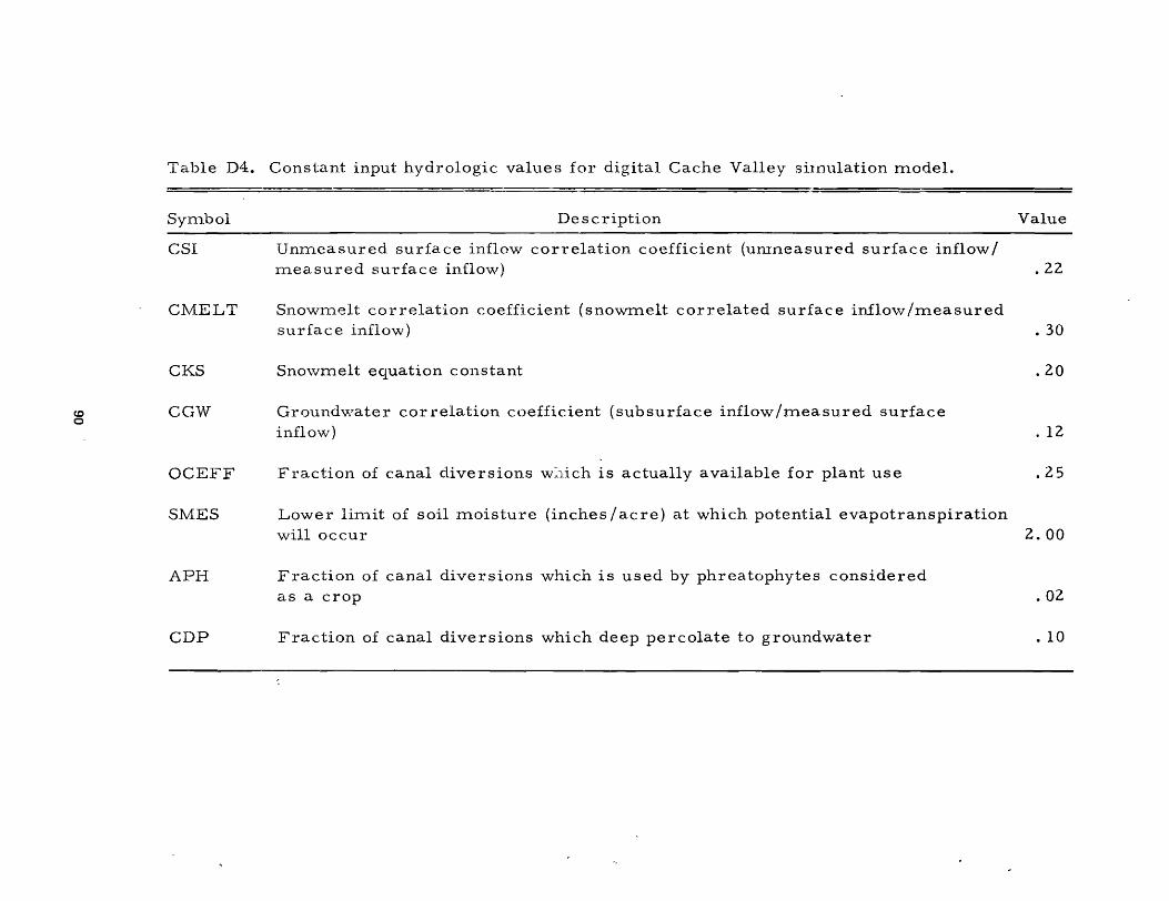
(g o

Table D4. Constant input hydrologic values for digital Cache Valley shnulation rnodel.

Syn1.bol

CSI

CMELT

CKS

CGW

OCEFF

SMES

API-I

CDP

Description

Unmeasured surface inflow correlation coefficient (um-neasured surface inflow / measured surface inflo\\')

Snowmelt correlation coefficient (snowmelt correlated surface inflo\v /rneasured surface inflow)

Sno\vrnelt equation constant

Groundv.'ater cor relation coefficient (subsurface inflow /llleasured surface inflow)

Fraction of canal diversions w:l.ich is actually available for plant use

Lower lin1.it of soil moisture (inches / acre) at \\7hich potential evapotranspiration will occur

Fraction of canal diversions which is used by phreatophytes considered as a crop

Fraction of canal diversions which deep percolate to groundwater

Value

.22

· 30

.20

· 12

.25

2.00

· 02

· 10

Table D5. Digital com.puter m.odel output of hydrologic values, 1945.

HYDROLOGIC SIMULATION OUTPUT FOR THE YOR I'JIf 5

J4N F( B HAR APR HAY '"'UN JLY Au;, SEP OCT NOV DEC ANN UAl P R[ C I ~ r T.I T I ON II N I .28 1.10 1.77 .83 'l.76 3.55 • I I 1.9S 1.611 1 .3q 2.80 1.80 20.58 AVE RA GE T["PEPATURE 211. J~ 30.9[1 33.60 "0.80 5 3. 80 55.10 (;8.1111 66.60 5" .111 "9.50 ]0.10 211 .]0 PERCENT OAf LIGHT HOURS ~.6J (; .66 f'.28 11.97 In.l0 10.21 10.11 9.6_ 8.112 7.7] 6.63 I; .39 1 BUTS I(C COEF .25 .25 .25 .7"; • JS .• 66 1.10 1.25 1 .1" .25 .25 .25

C OIHI I(C C Of F .75 .25 .25 .l5 .37 .75 1.08 1.03 .~5 .zs .25 .25

GRAIN IIC COEF .25 .25 • Z5 .26 .50 1 .511 1.12 .25 .l5 .25 .25 .25 It ALFALFA IIC CO[F .153 .n .86 .98 I.oe 1.1 ] 1 • 11 1.01> .'38 .90 .78 .6" 5 PAS lU RE I( C CO [f • ,.8 .5" • 71t .86 .9:1 .93 .'31 .91 .86 .7'3 .611 .52 G LANO PUPYTS !(C CO(F .n .7n .15 .81 .89 1.02 1.18 l.l8 1 .29 1 .1 '3 1.0- .86 7 WAr E R PloP Y T S M C C DE r .7J .70 .15 .81 .8,) 1 .02 1 .18 1.28 I .2'3 1.19 1.0 II .86

A CC UI'! S NO W STOP AG r 2.611 2.03 1.10 .06 .00 .00 .00 • 00 .00 .00 1.8 .. J.G_ SHO W ME LT • OJ 2.31 2.50 1.211 .06 .00 .00 .00 .00 .00 .'36 .00 7.01 E. T. OF qrnc; .Olt .ll .1<) .36 1.17 2.37 6.7A 6.13 J.2] .52 .1 1 .Olf 21 .65 E. T. or COR .... • Oil .11 .1'3 • ]f; 1.21t Z.70 6.66 5.511 1.811 .52 .1 1 .011 l~.] 5 E. T. cr GRAIN .Olt .11 .1'3 .17 1. &11 5.511 6.'11 I.JS .71 .52 .11 .011 U.SS

E. T. 0" At F AlF" .tl .33 .611 ).11] J.62 11.06 6.811 5.70 2.78 1.81 .J] .1 1 21.7') E. T. or PASTURE .06 .25 .55 1.2] 3.02 ] .311 5.6) II .88 2.11" I .611 .21 .09 23.38 E. T. or LAND PHYTS .06 .2e .515 1.16 2.98 ].67 7.lP. 6.8') 3.38 1.86 .33 .13 28.51

to E. T. or liATER PHYTS .12 .3? .5f; I.lf; 7.98 ].67 7.28 6.8') J.65 2.117 ." II .lIt 2').68 ...10 E. T. or VATEq suprACE .17 .115 .7" l.lt3 3.]5 3.60 6.17 5.38 2.83 Z .08 ... 2 .1 7 26 .19

SOIL HOIST BE[TS II NI ~. 78 9.00 ,).00 9.00 'J.OO 9.00 7.8'1 8.20 8.711 g .00 9.00 8.'H. 50IL HOIST CORN flNI ~. 92 9.00 9.00 9.no 9.00 9.00 7.91 8.1t0 8.91 ') .00 ,).00 8.96 SOIL MOI'.>T GRA[N If NI II. J3 f..00 6.00 f..oo 6.0n 5.61 ".87 5.11 1 6.00 f. .00 6.00 5.9" SOIl ~OIST "U'LrA fINI 7.06 9.00 9.00 9.00 8.86 8.91 7.2'i 8.17 8.8] 8.JJ 8.96 8.86 SOIL HOIST PASTRE fINI 1.1t~ 3.115 5."0 6.l11 7.lt6 7.50 J.511 3.1'1 5.93 5.68 6.37 &.29

SOIL MO IS T ... 0 PHT « IN I • 92 Z.95 It .90 5.81 6.96 8.96 5.0S 2.71 1.79 1.11 1.911 1.81 MEA SURE 0 I .. FLOW 3A082. 1136"10. 565311. 8'1711. 168J88. 1'311011. 112lt71. 85311Z. 632Z5. 5118lt5. SZZ91. 59190.101 88/fO • U"'M["S SUQ ]N"LOWIAFI ~H8. %12. 1 2lfJ7. lQ750. Z9700. Z9 700. 562,. • IIZ67. J 161 • 27'42. 2615. 2989. 11 0'375 • CHANGE IN R[S STOP.AGE 70~O. - 3920. -9111 o. 77'10. Sfl70. 2200. -7550. 11500. -10200. 101 itO. -1960. 11 itO • 5] 30. CALCULATEn PES OUTFLOW II11B 3. 7GllJ. '3I;IIJ8. 113950. 170783. 177911. 119"J68. 1t8982. 7020] • 73662. 87166. 802U8.109301".

C"NAL DIVERSIONS o. O. O. o. 9£'375.155625.239319.1511011. 95')28. o. o. o. 711 1258 • DEE P PE R(('IL TOGWfArl o. 5"0 It. nltl>8. 121'JO. 16655. 11861 • 2"Jq32. ISltOI. 11181. 11550. 1t6 '3 It • o. 112286. 6ROUNOwA TEO I NFLOwC Ar I • ~ 5 70. 52,. 3. 67811. lO173. 2n 25 5. 23281. IJ1t97. 10 211 I • 7587. 6581. 6275. 7115. 122261 • DEEP PEPCl-GW INFLI H I 1t<;70. 10f;Q 7. 27J53. 27qlJ. J£, 90'3. It 11 .. 2. 17lt28. 20:;':;112. 18768. 11131. 10969. 7175.25115117. OfL A Y LEV EL 2 (AF, 11"162. 1t570. 10"" 1. 217~ 3. 22913. 36909. II 11" 2. ]71128. 256112. 18768. 11131. 10969.

LEVEL 1 BErOR 0 TFLI AIr I 181"0. Ilt032. 11 '586. 1611110. 35 1t72. "0611 '). 5723 ... 6975') • 72308. 6]796. 11961>15. 3 S')(;It. LfvEL 1 ArTER OTFtfAFI ,070. 1016. 5793. 8710. 1713f,. 20325. 28617. JII fl8!'. 31> 154. 3DA98. 211831 • 17982. G W lOS UP r I'! L [" VIC A r I "1070. 70115. 57"13. 8nD. 17716. 20325. 71161J. ]11880. 3615 ... 30898. 2118]] • 1 7982. 2" IS 23 • I B E[ TS I RR TG If ~I AC I • '1J .00 .00 .00 .00 .00 ~ 2 .211 20.17 8.lt8 .00 .00 .00 2 C ORI~ I1?R IG cr "" AC , • OJ • on .00 .on .00 .00 71.83 16. Jq 1.07 .00 .00 .00 3 GRAIN I RR 16 I I "" AC I .0:1 .on .on .00 .00 6.63 ll.ge .O!) .00 .00 .00 .00 "ALFALFA IRRIGIINfflCI • OJ • DO .03 .00 1.1>11 2.18 ~n • .?8 19.51 6.2q .00 .00 .00 '5 PAS TUP[ I RR IG ([ NI Ar I • OJ .0!1 .O~ .00 5.6'5 .00 6.15 10.31 III .17 .00 .00 .00 f, L D PH" I PR IG (( NI AC I • OJ .O~ .O~ .00 5.25 8.q8 Il.OS 8.110 5.13 .00 .00 .uo

Table D6. Digital computer model output of economic values, 1945.

[ co NO HIe S I HlJ LA 1 ION 0 U T PU T FOR THE Y [ A R 1945

BEETS CORN GRAIN ALFALFA PASTURE LND PHY 15 WIR PHY1S wA1ER

C PO P A ~ E A U C ) 9824. 8967. en20B. 49799. 51300. 17611. 20660. 7567.

ROOT OEPT4 eFT) 6.00 6.0n ... 01 6.00 3.00 6.00

A VA WTP HOlD CAP( IN/FTI 1.50 1. SO 1.50 1.50 2.50 1.50

A VA W 1R C lP C IN) 9.00 9.00 6. 00 9.00 7.50 43.00

c.o 5EA50NAL [ llIN/AC) 20.29 17.98 14.12 27.79 23.38 28.57 24).68 26.79 N

5EA SON IR Q 01 V fIN/ACI 51.10 It 1. 21t 30.61 51.00 36.]0 10.10

C RO P PR Ie (( ~/ UN IT ) 16.60 1.00 1.05 21.00 5.5r)

CROP vIELnCUNIT/ACJ 16.85 11.98 54.9£,. 3.98 6.09

GR(lSS R(TIPNC ~/AC J 2R 7.74 125.H3 (;1.11 88.1'2 :n.49

C051 PER ACR[U/ACt 1& 9. 02 102.67 6B.33 £"4.83 28.55

NE T PET IJQ N ( $1 AC I 11 A. 7'1 23.113 -1. U; 23.29 4.9"

1 01 A L NET D [ l' UP N - r!~ 0 PI: THE (N T 1 R [ ARE A = Z" 49 798.