Simulation of Fluid Flow Through Porous Rocks on Modern ...

July 2009Anne Cathrine Elster, IDI

Master of Science in Computer ScienceSubmission date:Supervisor:

Norwegian University of Science and TechnologyDepartment of Computer and Information Science

Simulation of Fluid Flow ThroughPorous Rocks on Modern GPUs

Eirik Ola Aksnes

Problem DescriptionThis project evaluates how Graphical Processing Units (GPUs) may be utilized to offloadcomputations i large petroleum engineering applications. In particular, the task is to develope andimplement a parallelized version of the Lattice Boltzman Method (LBM) for simulation fluid flowthrough porous rocks for modern GPUs taking advantage of NVIDIA's CUDA environment. Testingwill be done using datasets provided by the oil industry on HPC-LAB's new NVIDIA Quadro FX 5800graphics card, the NVIDIA Tesla s1070 and/or other appropriate systems.

Assignment given: 26. January 2009Supervisor: Anne Cathrine Elster, IDI

Master Thesis

Simulation of Fluid Flow ThroughPorous Rocks on Modern GPUs

Eirik Ola [email protected]

Department of Computer and Information ScienceNorwegian University of Science and Technology, Trondheim

(Norway)

July 2009

SupervisorDr. Anne C. Elster

Abstract

It is important for the petroleum industry to investigate how fluids flow insidethe complicated geometries of porous rocks, in order to improve oil produc-tion. The lattice Boltzmann method can be used to calculate the porousrock’s ability to transport fluids (permeability). However, this method iscomputationally intensive and hence begging for High Performance Comput-ing (HPC). Modern GPUs are becoming interesting and important platformsfor HPC. In this thesis, we show how to implement the lattice Boltzmannmethod on modern GPUs using the NVIDIA CUDA programming environ-ment. Our work is done in collaborations with Numerical Rocks AS and theDepartment of Petroleum Engineering at the Norwegian University of Sci-ence and Technology.

To better evaluate our GPU implementation, a sequential CPU imple-mentation is first prepared. We then develop our GPU implementation andtest both implementation using three porous data sets with known perme-abilities provided by Numerical Rocks AS. Our simulations of fluid flow gethigh performance on modern GPUs showing that it is possible to calculatethe permeability of porous rocks of simulations sizes up to 3683, which fit intothe 4 GB memory of the NVIDIA Quadro FX 5800 card. The performancesof the CPU and GPU implementations are measured in MLUPS (million lat-tice node updates per second). Both implementations achieve their highestperformances using single floating-point precision, resulting in the maximumperformance equal to 1.59 MLUPS and 184.30 MLUPS. Techniques for re-ducing round-off errors are also discussed and implemented.

i

Acknowledgements

This master thesis was written at the Department of Computer and Infor-mation Science at the Norwegian University of Science and Technology incollaboration with Numerical Rocks AS and the Department of PetroleumEngineering.

This thesis would not have been possible without the support of numer-ous people. I wish to thank my supervisor Dr. Anne C. Elster who wasincredibly helpful and offered invaluable assistance and guidance with herextensive understanding of the field. She has been a source of great inspira-tion, with her always encouraging attitude and generosity through providingresources needed for this project from her own income. I wish to thankStale Fjeldstad, and Atle Rudshaug at Numerical Rocks AS for providingme with three porous data sets to evaluate my implementations, valuableassistance, and giving me the possibility to work on this subject, which hasbeen an outstanding experience. I wish to thank Egil Tjaland at the De-partment of Petroleum Engineering and Applied Geophysics, and the Centerfor Integrated Operations in the Petroleum Industry for letting me use theirmicrocomputed tomography device. I wish to thank Pablo M. Dupuy atthe Department of Chemical Engineering at the Faculty of Natural Sciencesand Technology, without his valuable advice-giving and guidance in compu-tational fluid dynamics this thesis would not have been successful. I wish tothank Jan Christian Meyer for guidance, technical support, and many inter-esting discussions during this project. I wish to thank Thorvald Natvig foradvice-giving and guidance throughout the process. I wish to thank fellowco-student Rune Erlend Jensen for many interesting discussions, and ideas tothis thesis work. I also with to thank my fellow co-students: Henrik Hesland,Rune Johan Hovland, Asmund Herikstad, Safurudin Mahic, Robin Eidissen,Daniele Giuseppe Spampinato, and many other peoples for many interest-

iii

ing and entertaining discussions throughout the semester. Finally, I wish tothank NVIDIA for providing several GPUs to Dr. Anne C. Elster and herHPC-lab through her membership in the NVIDIA’s professor partnershipprogram.

Eirik Ola AksnesTrondheim, Norway, July 12, 2009

iv

Contents

Abstract i

Acknowledgements iii

1 Introduction 11.1 Project Goals . . . . . . . . . . . . . . . . . . . . . . . . . . . 21.2 Outline . . . . . . . . . . . . . . . . . . . . . . . . . . . . . . . 3

2 Parallel Computing and The Graphics Processing Unit 52.1 Parallel Computing . . . . . . . . . . . . . . . . . . . . . . . . 5

2.1.1 Forms of parallelism . . . . . . . . . . . . . . . . . . . 72.2 The Graphics Processing Unit . . . . . . . . . . . . . . . . . . 8

2.2.1 NVIDIA CUDA Programming Model . . . . . . . . . . 102.2.2 NVIDIA Tesla Architecture . . . . . . . . . . . . . . . 15

3 Computational Fluid Dynamics and Porous Rocks 233.1 Computational Fluid Dynamics . . . . . . . . . . . . . . . . . 233.2 The Lattice Boltzmann Method . . . . . . . . . . . . . . . . . 24

3.2.1 Previous And Related Work . . . . . . . . . . . . . . . 263.2.2 Fundamentals . . . . . . . . . . . . . . . . . . . . . . . 283.2.3 Boundary Conditions . . . . . . . . . . . . . . . . . . . 293.2.4 Basic Algorithm . . . . . . . . . . . . . . . . . . . . . . 30

3.3 Porous Rocks . . . . . . . . . . . . . . . . . . . . . . . . . . . 323.3.1 Porosity . . . . . . . . . . . . . . . . . . . . . . . . . . 333.3.2 Permeability . . . . . . . . . . . . . . . . . . . . . . . . 33

4 Implementations 354.1 Platforms, Libraries, and Languages . . . . . . . . . . . . . . . 35

v

4.2 Visualization . . . . . . . . . . . . . . . . . . . . . . . . . . . 364.2.1 Graphics Rendering . . . . . . . . . . . . . . . . . . . . 364.2.2 Porous Rock Visualization . . . . . . . . . . . . . . . . 374.2.3 Fluid Flow Visualization . . . . . . . . . . . . . . . . . 38

4.3 Simulation Model . . . . . . . . . . . . . . . . . . . . . . . . . 384.3.1 Memory Usage . . . . . . . . . . . . . . . . . . . . . . 394.3.2 Simulation Model Details . . . . . . . . . . . . . . . . . 404.3.3 Calculate Permeability . . . . . . . . . . . . . . . . . . 46

4.4 Floating-point Precision . . . . . . . . . . . . . . . . . . . . . 494.5 Data Structure . . . . . . . . . . . . . . . . . . . . . . . . . . 504.6 CPU Implementation . . . . . . . . . . . . . . . . . . . . . . . 51

4.6.1 Optimizations Guidelines . . . . . . . . . . . . . . . . . 514.6.2 Details . . . . . . . . . . . . . . . . . . . . . . . . . . . 52

4.7 GPU Implementation . . . . . . . . . . . . . . . . . . . . . . . 534.7.1 Optimizations Guidelines . . . . . . . . . . . . . . . . . 534.7.2 Profiling . . . . . . . . . . . . . . . . . . . . . . . . . . 534.7.3 Details . . . . . . . . . . . . . . . . . . . . . . . . . . . 57

5 Benchmarks 635.1 Test Environment and Methodology . . . . . . . . . . . . . . . 635.2 Poiseuille Flow . . . . . . . . . . . . . . . . . . . . . . . . . . 655.3 Kernel Profiling . . . . . . . . . . . . . . . . . . . . . . . . . . 685.4 Simulation Size Restrictions . . . . . . . . . . . . . . . . . . . 695.5 Performance Measurements . . . . . . . . . . . . . . . . . . . 705.6 Porous Rock Measurements . . . . . . . . . . . . . . . . . . . 74

5.6.1 Symmetrical Cube . . . . . . . . . . . . . . . . . . . . 765.6.2 Square Tube . . . . . . . . . . . . . . . . . . . . . . . . 775.6.3 Fontainebleau . . . . . . . . . . . . . . . . . . . . . . . 795.6.4 Discussion . . . . . . . . . . . . . . . . . . . . . . . . . 80

5.7 Visual Results . . . . . . . . . . . . . . . . . . . . . . . . . . . 82

6 Conclusions and Future Work 876.1 Future Work . . . . . . . . . . . . . . . . . . . . . . . . . . . . 89

Bibliography 96

A D3Q19 Lattice 97

vi

B Annotated Citations 99B.1 GPU and GPGPU . . . . . . . . . . . . . . . . . . . . . . . . 99B.2 Lattice Boltzmann Method . . . . . . . . . . . . . . . . . . . . 99B.3 Porous Rocks . . . . . . . . . . . . . . . . . . . . . . . . . . . 100

C Notur 09 Poster 101

vii

List of Figures

1.1 Porous rock. . . . . . . . . . . . . . . . . . . . . . . . . . . . . 3

2.1 SPMD support control flow, and SIMD does not. . . . . . . . 82.2 Transistors dedicated for data processing: CPU vs. GPU. . . . 92.3 NVIDIA CUDA thread hierarchy. . . . . . . . . . . . . . . . . 122.4 NVIDIA Tesla architecture. . . . . . . . . . . . . . . . . . . . 162.5 Coalesced and non-coalesced global memory access patterns. . 192.6 Shared memory access patterns without bank conflicts. . . . . 202.7 Shared memory access patterns with bank conflicts. . . . . . . 21

3.1 The three phases of the lattice Boltzmann method. . . . . . . 253.2 The streaming step of the lattice Boltzmann method. . . . . . 263.3 The collision step of the lattice Boltzmann method. . . . . . . 263.4 Bounce back boundary: Lattice node before streaming. . . . . 303.5 Bounce back boundary: Lattice node after streaming. . . . . . 303.6 Basic algorithm of the lattice Boltzmann method. . . . . . . . 313.7 Example of low and high permeability of porous rock. . . . . . 32

4.1 Visualization of porous rock . . . . . . . . . . . . . . . . . . . 374.2 The Marching Cubes algorithm used. . . . . . . . . . . . . . . 394.3 The main phases of the simulation model used. . . . . . . . . 414.4 Expansion of the simulation model for permeability calculations. 474.5 Configurations of the boundaries in permeability calculations. 494.6 Structure-of-arrays. . . . . . . . . . . . . . . . . . . . . . . . . 504.7 Section from Cubin file. . . . . . . . . . . . . . . . . . . . . . 544.8 NVIDIA CUDA occupancy calculator. . . . . . . . . . . . . . 564.9 NVIDIA CUDA occupancy calculator. . . . . . . . . . . . . . 574.10 One-to-one mapping between threads and lattice nodes. . . . . 584.11 Number of thread blocks with varying cubic lattice size. . . . . 59

ix

4.12 The configurations of grids and thread blocks in kernels . . . . 61

5.1 Fluid flow between two parallel plates. . . . . . . . . . . . . . 655.2 Comparison of numerical and analytical velocity profiles. . . . 675.3 GPU implementation processing time of the collision phase

and streaming phase. . . . . . . . . . . . . . . . . . . . . . . . 685.4 Memory requirements with varying cubic lattice sizes. . . . . . 705.5 Performance results in MLUPS. . . . . . . . . . . . . . . . . . 725.6 Overall execution time of performance measurements. . . . . . 725.7 GPU 32 occupancy with varying registers count. . . . . . . . . 735.8 GPU 64 occupancy with varying registers count. . . . . . . . . 735.9 GPU 32 occupancy with varying block size. . . . . . . . . . . 755.10 Fluid flow through the symmetrical cube. . . . . . . . . . . . . 765.11 Symmetrical Cube performance and computed permeability

results. . . . . . . . . . . . . . . . . . . . . . . . . . . . . . . . 775.12 Fluid flow through the Square Tube. . . . . . . . . . . . . . . 775.13 Square Tube performance and computed permeability results. 785.14 Fluid flow through the Fontainebleau. . . . . . . . . . . . . . . 795.15 Fontainebleau performance and computed permeability results. 805.16 Symmetrical Cube: with and without reduced rounding error. 815.17 Symmetrical Cube: with and without reduced rounding error,

last 20 iterations. . . . . . . . . . . . . . . . . . . . . . . . . . 815.18 Fluid flow direction in visual results. . . . . . . . . . . . . . . 825.19 The first 4 iterations of fluid flow through Fontainebleau. . . . 835.20 The 5th to 8th iterations of fluid flow through Fontainebleau. . 845.21 The first 4 iterations of fluid flow inside Fontainebleau. . . . . 855.22 The 5th to 8th iterations of fluid flow inside Fontainebleau. . . 86

x

List of Tables

2.1 GPUs from NVIDIA based on the NVIDIA Tesla architecture. 152.2 NVIDIA’s GPUs general compute capability. . . . . . . . . . . 172.3 NVIDIA’s GPUs points of distinction in compute capability. . 17

3.1 Typical porosity of some representative real materials. . . . . . 33

4.1 Memory usage D3Q19 model with temporary storage. . . . . . 40

5.1 The test machine that was used to obtain the measurements. . 645.2 Measurements abbreviations. . . . . . . . . . . . . . . . . . . . 655.3 Parameter values used in the Poiseuille Flow. . . . . . . . . . 665.4 Measured deviation in the Poiseuille Flow. . . . . . . . . . . . 675.5 Registers available with varying block size. . . . . . . . . . . . 695.6 Maximum simulation sizes in the x-direction due to register

and shared memory usage per thread. . . . . . . . . . . . . . . 705.7 Performance results in MLUPS. . . . . . . . . . . . . . . . . . 715.8 Parameter values used in the porous rocks measurements. . . . 755.9 Symmetrical Cube performance and computed permeability

results. . . . . . . . . . . . . . . . . . . . . . . . . . . . . . . . 765.10 Square Tube performance and computed permeability results. 785.11 Fontainebleau performance and computed permeability results. 79

A.1 The discrete velocities ei for the D3Q19 lattice that was used . 97

xi

List of Algorithms

1 Definition and execution of NVIDIA CUDA kernels. . . . . . . 132 Build-in variables in NVIDIA CUDA kernels. . . . . . . . . . . 143 Memory access pattern without bank conflicts. . . . . . . . . . 204 Pseudo code of the initialization phase. . . . . . . . . . . . . . 435 Pseudo code of the collision phase. . . . . . . . . . . . . . . . 446 Pseudo code of the streaming phase. . . . . . . . . . . . . . . 457 Pseudo code for the find neigbhbor algorithm. . . . . . . . . . 468 CPU implementation pseudo code. . . . . . . . . . . . . . . . 529 The configurations of grids and thread blocks in kernels. . . . 60

xiii

List of Abbreviations

CFD Computational Fluid DynamicsHPC High Performance ComputingCPU Central Processing UnitGPU Graphics Processing UnitGPGPU General-Purpose Computation On Graphics Processing UnitsCUDA Compute Unified Device ArchitectureOpenCL Open Computing LanguageUMA Uniform Memory AccessNUMA Non Uniform Memory AccessMIMD Multiple-Instruction Multiple-DataSIMD Single-Instruction Multiple-DataSPMD Single-Program Multiple-DataILP Instruction Level ParallelismSM Streaming MultiprocessorsSP Stream ProcessorsSFU Special Function UnitsLBM Lattice Boltzmann MethodLGCA Lattice Gas Cellular AutomataBGK Bhatnagar-Gross-KrookVBO Vertex Buffer ObjectGLEW OpenGL Extension Wrangler LibraryGLUT The OpenGL Utility Toolkit

xv

Nomenclature

τ Single relaxation parameterρ Mass density of a fluid particleux Velocity in the x direction of a fluid particleuy Velocity in the y direction of a fluid particleuz Velocity in the z direction of a fluid particlef eq Equilibrium distribution functionf eqi Discrete equilibrium distribution function in the i directionu Average fluid velocitydx Lattice dimension in the x directiondy Lattice dimension in the y directiondz Lattice dimension in the z directionf Particle distribution functionfi Discrete particle distribution function in the i directionwi Discrete weight factor in the i directione Particle velocityei Discrete particle velocity in the i directioncs Speed of SoundFx External force in the x directionFy External force in the y directionFz External force in the z directionν Kinematic viscosityΩ Collision operatorR Universal gas constantD Dimension of the spaceT Temperatureq Volumetric fluid flux

xvii

k Permeability∆PL

Pressure drop along the sample length Lφ PorosityVp Volume of pore spaceVt Total volume of the porous media

xviii

Chapter 1

Introduction

A great many problems in science and engineering are too difficult to solveanalytically in practice, but with today’s powerful computers it is possibleto analyze and solve those problems numerically. Computer simulations areimportant to the field of fluid dynamics, as their equations are often com-plicated referred to as Computational Fluid Dynamics (CFD). To solve themost complex problems in fluid dynamics, computer simulations performedby systems with huge performance capability are necessary. In the fieldof High Performance Computing (HPC), researchers are interested in max-imizing the computing power available in systems with huge performancecapability. Systems are typically made from clusters of workstations, largeexpensive supercomputers, or Graphics Processing Units (GPUs), to be ableto solve complex problems in science and engineering.

With the recent introduction of NVIDIA’s Compute Unified Device Archi-tecture (CUDA) programming environment for the NVIDIA Tesla architec-ture, as well as heterogeneous programming standards such as Open Comput-ing Language (OpenCL), GPUs are becoming interesting and important plat-forms for HPC. Modern GPUs have typically their own dedicated memory 1,and are optimized for performing floating-point operations in parallel, whichare much used in games, multimedia, and scientific applications. Today, evencommercial GPUs can have very high floating-point compute capacity at verylow cost, available as off-the-shelf products. The state-of-the-art in GPUs canprovide computing power equal to small supercomputers 2. Compared with

1NVIDIA Quadro FX 5800 have total memory size of whole 4 GB.2NVIDIA has recently released the NVIDIA Tesla s1070 Computing System, that’s

1

an up-to-date Central Processing Unit (CPU), modern GPUs utilize a largerportion of their transistors for floating-point arithmetic, and has higher mem-ory bandwidth. With the recent developments and improvements in GPUhardware and software, many difficulties are eliminated, allowing GPUs tobe used as accelerators for a wide range of scientific applications. Today,much attention is focused on how to utilize the GPUs huge performance ca-pability for more than just graphics rendering, to accelerate computationallyintensive problems, referred to as General-Purpose computation on GraphicsProcessing Units (GPGPU).

1.1 Project Goals

For the petroleum industry it is important to quantify the petrophysicalproperties of porous rocks, such as the rock illustrated in Figure 1.1, to gainbetter understanding of conditions that affect oil production [5]. It wouldbe of great value for the petroleum industry if the petrophysical propertiesof porous rocks, such as the porosity and permeability, could be obtaineddirectly through computer simulations, capable of fast and accurate analysis.

The main objective in this thesis is to investigate the use of the graphicsprocessing unit for simulations of fluid flows through the internal pore geom-etry of natural and computer generated rocks, in order to compute the rock’sability to transport fluids (permeability).

In this thesis, we have chosen to look at the lattice Boltzmann method forthe simulation of fluid flow through porous rocks, offloaded to the GPU. Thepermeability of porous rocks is obtained directly from the generated velocityfields of the lattice Boltzmann method, together with using Darcy’s law forthe flow of fluids through porous media [24].

provide parallelism of total 960 streaming processor cores across 4 GPUs, with total of 4teraflops compute capability [13].

2

Figure 1.1: Porous rock.

1.2 Outline

This thesis is structured in the following manner:

In Chapter 2, Parallel Computing and The Graphics ProcessingUnit, we will highlight several advantages with parallel computing, and de-scribe various forms of parallelism. We will describe modern GPUs, whattasks that suit GPUs, and explain some differences between GPUs and CPUs.We will also give a brief introduction to the NVIDIA CUDA programmingmodel and the NVIDIA Tesla architecture.

In Chapter 3, Computational Fluid Dynamics and Porous Rocks,we will present and explain the necessary background theory for fluid flowthrough porous rocks using the lattice Boltzmann method. We will also givea brief description of porous rocks, and how to calculate their permeability.

In Chapter 4, Implementations, we will describe how the lattice Boltz-mann method has been implemented. We will also give a brief description of

3

the Marching Cubes algorithm, used for visual analysis of how the fluid willflow through the internal pore geometry of porous rocks.

In Chapter 5, Benchmarks, we will present performance benchmarksof our implementation of the lattice Boltzmann method, and estimations ofporous rock’s ability to transmit fluids. We will compare differences betweenboth performance and permeability estimations using NVIDIA GPUs andCPUs, with both single and double floating-point precision.

In Chapter 6, Conclusions and Future Work, we will summarize theresults we achieved, and discuss future work to improve our implementationsof the lattice Boltzmann method.

4

Chapter 2

Parallel Computing and TheGraphics Processing Unit

The topics covered in this chapter were also covered by the author and HenrikHesland in [3], the joint fall upon which this project was built. It describessome of the basic concept of parallel computing as well as the Graphics Pro-cessing Unit (GPU).

In particular, Section 2.1 gives a brief introduction to parallel comput-ing, and explains different forms of parallelism. Section 2.2 explains modernGPUs and what tasks they are suited for, and motivates for why one shoulduse GPUs instead of the CPUs for some compute intensive tasks. At the endof this chapter, the NVIDIA CUDA programming model and the NVIDIATesla architecture are presented.

2.1 Parallel ComputingMoore’s law predicts that integration of transistors doubles in 18 months.Today, to double the number of transistors placed on integrated circuits in18 months has become difficult. We have already hit the Power and Fre-quency Walls. Whatever the peak performance of today’s processors, therewill always be some problems that require or benefit from better processorspeed. As explained in [6], there is a recent renaissance in parallel computingdevelopment. Due to the Power Wall, increasing clock frequency is no longer

5

the primary method of improving processor performance. Today, parallelismhas become the standard way to increase overall performance for both theCPU and GPU. Both modern GPUs and CPUs are concerned with increasingpower dissipation, and want to increase absolute performance, but also im-prove efficiency through architectural improvements by means of parallelism.

Parallel computing often permits a larger problem or a more precise solu-tion of a problem to be found within a practical time. Parallel computing isthe concept of breaking up a larger problem into smaller units of tasks thatcan be solved. However, problems often cannot be broken up perfectly intoindependent parts, so interactions are needed among the parts, both for datatransfer and synchronization. The problem characteristicts affects how easyit is to parallelize. If possible, there would be no interaction between theseparate processes, each process requiring different data and produce resultsfrom its input data without need for results from the other processes. How-ever many problems are to be found in the middle, neither fully independentnor synchronized [54].

There are two basic types of parallel computers, when categorized bytheir memory architecture [54]:

• Shared memory systems that have a single address space, which meansthat all processing elements can access the same global memory. It canbe very hard to implement the hardware to achieve Uniform MemoryAccess (UMA) by all the processors with a larger number of proces-sors, and therefore many systems have Non Uniform Memory Access(NUMA).

• Distributed memory systems that are created by connecting computerstogether through an interconnection network, where each computer hasits own local memory that cannot be accessed by the other processors.The access time to the local memory is faster than the access time tothe non-local memory.

Distributed memory will physically scale more easily than shared mem-ory, as its memory is scalable with the increased number of processors.

6

2.1.1 Forms of parallelism

Most of the information found in this section is based on ref by Mccool [37].

There are several ways to do parallel computing. Two frequently usedmethods are task parallelism and data parallelism. Task parallelisms, alsocalled Multiple-Instruction Multiple-Data (MIMD), focus on distributing sep-arate tasks across different parallel computing nodes that operate on separatedata in parallel. It can typically be difficult to find independently tasks ina program and therefore task parallelism can have limited scalability abil-ity. The interaction between different tasks occurs through either messagepassing or shared memory regions. Communication through shared memoryregions poses the problem of maintaining memory cache coherency with in-creased number of cores, as most modern multi core CPUs use caches formemory latency hiding. Ordinary sequential execution of a single thread isdeterministic, making it understandable. Task parallelism on the other handis not even if the program is correct. Task parallelism is subject to errorssuch as race conditions and deadlocks, as correct synchronization is diffi-cult. Such faults are difficult to identify, which can make development timeoverwhelming. Multicore CPUs are capable of running entirely independentthreads of control, and are therefore great for task parallelism [37].

Data parallelism is a form of computation that implicitly has synchro-nization requirements. In a data parallel computation, the same operation isperformed on different data elements concurrently. Data parallel program-ming is very convenient for two reasons. It can be easy to program andit can scale easily to large problems. The Single-Instruction Multiple-Data(SIMD) is the simplest type of data parallelism. It operates by having thesame instruction execute in parallel on different data elements concurrently.It is convenient from a hardware standpoint. It gives an efficient hardwareimplementation, because it only needs to replicate the data path. However, ithas difficulty of balance variable work load, since it does not support efficientcontrol flow. The SIMD models have been generalized to the Single-ProgramMultiple-Data (SPMD), which include some control flow. With the SPMD itis possible to avoid and adjust the work load if there are variable amounts ofcomputation in the different parts of a program [37], as illustrated in Figure2.1. Data parallelism is essential for the modern GPU as a parallel processor,as it is optimized to carry out the same operations on a lot of data in parallel.

7

SIMD SPMD

Figure 2.1: SPMD support control flow, and SIMD does not. Based on [37].

2.2 The Graphics Processing UnitThe Graphics Processing Unit (GPU) is a special-purpose processor dedi-cated to rendering computer graphics. With their potential for computingseveral hundred instructions simultaneously, these accelerators are becomingvery interesting architectures also for High Performance Computing (HPC).As special-purpose accelerators, the GPUs are primarily designed to accel-erate graphics rendering, and most development has been targeted towardsimproved graphics for game consoles, personal computers, and workstations.Over the last 40 years, the GPU has undergone significant changes in itsfunctionality and capability, driven primarily by an ever increasing demandfor more realistic graphics in computer games. The GPU has evolved from afixed processor only capable of doing restricted graphics rendering, into a ded-icated programmable processor with huge performance capability. ModernGPU’s theoretical floating-point processing power and memory bandwidth,has exceeded the Central Processing Units (CPUs) [12].

8

Figure 2.2: Transistors dedicated for data processing: CPU vs. GPU. Figureis taken with permission from [12].

The CPU is designed to maximize the performance of a single thread ofsequential instructions. It operates on different data types, performs randommemory accesses, and branching. Instruction Level Parallelism (ILP) allowsthe CPU to execute several instructions at the same time or even alter theorder in which the instructions are executed. To increase performance, theCPU uses many of its transistors to avoid memory latency with data caching,sophisticated flow control, and to extract as much ILP as possible. There isa limited amount of ILP that is possible to identify and take advantage of ina sequential stream of instructions, to keep the execution units active. Thisis also known as the ILP Wall, and ILP causes tremendous increase in hard-ware complexity and related power consumption, without linear speedup inapplication performance [36].

The GPU is dedicated to rendering computer graphics, and the primi-tives, pixel fragments and pixels can largely be processed independently inparallel (the fragment stage is typically the most computationally demandingstage [39]). The GPU differs from the CPU in the memory access pattern, asmemory access in the GPU is very coherent. When a pixel is read or written,the neighboring pixel will be read or write a few cycles later. By organiz-ing memory correctly and hide memory access latency by doing calculationsinstead, there is no need for big data caches. GPUs are designed such thatthe same instruction operates on collections of data, and therefore only needsimple flow control. GPUs may therefore dedicate more of its transistors todata processing than the CPU, as illustrated in Figure 2.2.

9

The modern GPU is a mixture of programmable and fixed function units,allowing programmers to write vertex, fragment and geometry programs forsophisticated surface shading, and lighting effects. The instruction sets of thevertex and fragment programs have converged, now all programmable unitsin the graphics pipeline share a single programmable hardware unit. Into theunified shader architecture, where the programmable units share their timeamong vertex work, fragment work, and geometry work [39]. GPUs differenti-ate themselves from traditional CPU designs by prioritizing high-throughputprocessing of many parallel operations over the low-latency execution of a sin-gle thread. Quite often in scientific and multimedia applications there is aneed to do the same operation on a lot of different data elements. GPUssupport a massive number of threads, typically 61440 on a NVIDIA GeForceGTX 295, running concurrently and support the SPMD model to be able tosuspend and use threads to hide the latency with uneven workloads in theprograms. The combination of high performance, low-cost, and programma-bility has made the modern GPU attractive for applications traditionally ex-ecuted by the CPU, for General-Purpose Computation On GPUs (GPGPU).With the unified shader architecture, the GPGPU programmers can targetthe programmable units directly, rather than split up task to different hard-ware units.

Since GPUs are first and foremost made for graphics rendering, it is nat-ural that the first attempts of programming GPUs for non-graphics wherethrough graphics APIs. This makes it tougher to use as a HPC platformsince programmers have to master the graphics APIs and languages. To sim-plify this programming task and to hide the graphics APIs overhead, severalprogramming models have recently been created. The latest release from theGPU supplier NVIDIA is NVIDIA’s Compute Unified Device Architecture(CUDA), initially released in November 2006 [12].

2.2.1 NVIDIA CUDA Programming ModelMost of the information found in this section is based on NVIDIA’s program-ming guide for NVIDIA CUDA [12].

There are a few difficulties with the traditional way of doing GPGPU,with the graphics API overhead that are making unnecessary high learning

10

curve and the difficult to debugging. In NVIDIA CUDA, programmers donot need to think in terms of the graphics APIs for developing applications torun on the GPU. It also reveals the hardware functions of the GPUs directly,giving the programmer better control. NVIDIA CUDA is a programmingmodel that focuses on low learning curve for developing applications that arescalable with the increase number of processor cores. It is based on a smallextension to the C programming language, making it easier to get startedwith for developers familiar with the C language. Since there are currentlymillions of PCs and workstations with NVIDIA CUDA enabled GPUs, de-veloping techniques to harvest the GPUs power make it feasible to accelerateapplications for a broad range of users. Parts of programs that have lit-tle parallelism execute on the CPU, while parts that have rich parallelismexecute on the GPU. To a programmer, a system in the NVIDIA CUDAprogramming model consists of a host that is a traditional CPU, and one ormore compute devices that are massively data-parallel coprocessors. Eachdevice is equipped with a large number of arithmetic execution units, has itsown DRAM, and runs many threads in parallel.

Kernels And Execution

In NVIDIA CUDA, programmers are allowed to define data-parallel func-tions, called kernels, that run in parallel on many threads [43]. These kernelsare invoked from the host, and are defined using a special syntax, whichindicates how they are executed on the GPU. To invoke a kernel, program-mers need to specify the number of thread blocks, and threads within thesethread blocks, between triple angle brackets, and to define the kernels usingthe global declaration sign. This is illustrated in Algorithm 1. In NVIDIACUDA, there exist several qualifiers for functions:

• global defines functions that can only be called from the host, andthat execute on the device.

• device defines functions that can only be called from the device, andthat execute on the device.

• host defines functions that can only be called from the host, andthat execute on the host.

11

Figure 2.3: NVIDIA CUDA thread hierarchy. Figure is taken with permissionfrom [12].

12

Algorithm 1 Definition and execution of NVIDIA CUDA kernels.

// Kernel definition__global__ void kernelName()

...

void main()

// Defines how the GPU kernel is executedkernelName<<<gridDim,blockDim>>>();

Threads are grouped into a three level hierarchy during execution, as il-lustrated in Figure 2.3. Every kernel executes as a grid of thread blocks inone or two dimensions, where each thread block has a unique identificationindex in the grid. Each thread block is an array of threads, in one, two orthree dimensions, where each individual thread has a unique identificationindex in the thread block. Threads within the same thread block can syn-chronize, by calling syncthreads(). To help programmers, several built-invariables are available:

• gridDim, which holds the dimension of the grid.

• blockDim, which holds the dimension of the thread block.

• threadIdx, which contains the index to the current thread within thecurrent thread block.

• blockIdx, which contains the index to the current thread block withinthe grid.

How to use the build-in variables to calculate the index of a thread in atwo-dimensional block is illustrated in Algorithm 2.

13

Algorithm 2 Build-in variables in NVIDIA CUDA kernels.


int x = blockIdx.x * blockDim.x + threadIdx.x;int y = blockIdx.y * blockDim.y + threadIdx.y;

int i = x + y * blockDim.x;

...

Memory

All threads in a GPU kernel can access data from diverse places during exe-cution. Each thread has its private local memory, and the architecture allowseffective sharing of data between threads within a thread block by using thelow latency shared memory. There are also two additional read-only memo-ries accessible by all threads, the texture memory and constant memory. Thetexture memory is optimized for various memory accesses patterns. Finally,all threads have access to the same large, high latency global memory, andit is possible to transfer data to and from the GPUs global memory and thehosts memory using different API calls.

Variables may also have different qualifiers, used to differentiate where inthe memory the variables should be stored:

• device defines a variable to be stored in the global memory, availablefrom all threads, and available to the host through API calls.

• constant defines a variable to be stored in the constant memory,available from all threads, and available to the host through API calls.

• shared defines a variables to be stored in the shared memory fora current thread block, available only to the threads within the samethread block.

In addition, with the device and constant declarations the variable has

14

the life time of the application, and with the shared declaration the vari-able has the life time of the current block.

2.2.2 NVIDIA Tesla ArchitectureMost of the information found in this section is based on NVIDIA’s program-ming guide for NVIDIA CUDA [12].

For high performance, knowledge of NVIDIA’s GPUs hardware archi-tecture is important. The latest generations of NVIDIA’s GPUs are basedon the NVIDIA Tesla architecture that supports the NVIDIA CUDA pro-gramming model. The NVIDIA Tesla architecture is built around a scalablearray of Streaming Multiprocessors (SMs), and each SM consists of severalStream Processors (SPs), two Special Function Units (SFU) for complex cal-culations (sine, cosine and square root), a multithreaded instruction unit,on-chip shared memory, texture cache, some registers, and a constant cache[12], as illustrated in the Figure 2.4. GPUs from NVIDIA based on theNVIDIA Tesla architecture have the same architectural foundation, but sup-port different degree of parallelism equal to the number of SM. Some of thelatest generations of desktop GPUs from NVIDIA, based on the NVIDIATesla architecture are listed in Table 2.1.

Table 2.1: NVIDIA GPUs based on the NVIDIA Tesla architecture. Takenfrom [13] and [12].

GPU Model 8800 GT 9800 GX2 GTX 295Number of GPUs 1 2 2

Streaming Multiprocessors 14 32 60Stream Processors 112 256 480

Graphics Clock 600 MHz 600 MHz 576 MHzProcessor Clock 1500 MHz 1500 MHz 1242 MHz

Memory 512 MB 1 GB 1792 MBMemory Bandwidth 57.6 GB/s 128 GB/s 223.8 GB/sCompute Capability 1.1 1.1 1.3

15

Figure 2.4: NVIDIA Tesla architecture. Figure is taken with permission from[12].

Compute Capability

The GPUs from NVIDIA based on the NVIDIA Tesla architecture have dif-ferent compute capability. As of April 2009, indicated by a version numberfrom 1.0 to 1.4, which describes the NVIDIA’s GPUs technical specificationsand features supported, for among other things it can indicate support fordouble precision floating-point numbers. Today, GPUs from NVIDIA havea number of general features and technical specifications listed in Table 2.2,but also some differences listed in Table 2.3.

16

Table 2.2: NVIDIA’s GPUs general compute capability. Taken from [12].

Compute capability 1.1-1.4.Maximum size of the x dimension of a thread block 512Maximum size of the y dimension of a thread block 512Maximum size of the z dimension of a thread block 64Maximum number of threads per thread block 512Maximum number of active thread blocks per SM 8Amount of shared memory available per SM 16 KBTotal amount of constant memory 64 KBMaximum number of thread blocks per grid 65535

Table 2.3: NVIDIA’s GPUs points of distinction in compute capability.Taken from [12].

Compute capability 1.1 1.4Double-precision float-point support no yesMaximum number of active threads per SM 768 1024Maximum number of active warps per SM 24 32Maximum number of threads per thread block 512 1024Number of registers per SM 8192 16384Support for atomic functions no yes

Execution

For high performance, NVIDIA’s GPUs exploit massive multithreading, ahardware technique which executes thousands of threads simultaneously, toutilize the large number of computational cores and overlap memory trans-actions with computation. This is possible because NVIDIA’s GPUs threadshave very little creation overhead, and it is possible to switch between threadsthat execute with near zero cost [48]. When a GPU kernel is invoked, threadblocks from the kernel grid are distributed to SMs with available executioncapacity. As one thread block terminates, new thread blocks are lunchedon the SM [12]. Therefore to keep the SM busy, one needs to have enoughthread blocks in the grid, and threads in thread blocks. There is, however, a

17

limit on how many thread blocks a SM can process at once, one need to findthe right balance between how many registers per thread, how much sharedmemory per thread block and what number of simultaneously active threadsare required for a given kernel [48]. The programming guide for NVIDIACUDA states that the minimum number of blocks should be at least twicethe number of SMs in the device, preferably larger than 100, and that 64 isthe minimum of threads within a block. During execution, threads withina thread block are grouped into warps, which are 32 threads from continu-ous sections of a thread block. Even though warps are not explicit declared,knowledge of them may improve performance. NVIDIA’s GPUs support theSPMD model where all threads execute the same program although theydon’t need to follow the same path of execution. The SM executes the sameinstruction for every thread in a warp, so only threads that follow the sameexecution path can be executed in parallel. If none of the threads in a warphave the same execution path, all of them must be executed sequentially [48].There are several memory types with different latency available through theNVIDIA Tesla architecture, such as the global memory and the shared mem-ory. For high performance, it is essential to know some details of the differentmemory types.

Global Memory

For maximum global memory bandwidth, which can be very high, it is im-portant to to access the global memory with the right access pattern. Thisis achieved through coalescing, and result in a single memory transaction forsimultaneous accesses against the global memory by threads in a half-warp.To achieve coalescing, the programming guide for NVIDIA CUDA state someconditions that must be met. For NVIDIA GPUs with compute capability1.0 and 1.1, there are four conditions that global memory access must meetto achieve coalescing, which are illustrated in Figure 2.5:

• Threads must access:4-byte words, resulting in one 64-byte memory transaction.8-byte words, resulting in one 128-byte memory transaction.16-byte words, resulting in two 128-byte memory transactions.

• Every 16 words stand in the same segment in global memory.

18

Thread

0

Base

address

128

Thread

1

Base

address

132

Thread

2

Base

address

136

Thread

3

Base

address

140

...

Coalesced memory access

Thread

0

Base

address

128

Thread

1

Base

address

132

Thread

2

Base

address

136

Thread

3

Base

address

140

...

Non-coalesced memory access,

starting address wrong

Thread

0

Base

address

128

Thread

1

Base

address

140

Thread

2

Base

address

152

Thread

3

Base

address

164

...


wrong size of word

Thread

0

Base

address

128

Thread

1

Base

address

132

Thread

2

Base

address

136

Thread

3

Base

address

140

...


the access is non sequential

Figure 2.5: Examples of coalesced and non-coalesced global memory accesspatterns. Reproduced from [12].

• Threads must access the words in sequence, the kth thread must accessthe kth word.

With compute capability 1.2 and higher, threads do not need to access globalmemory in sequence to achieve coalescing, and access to the global memoryover one segment will not directly result in 16 separate accesses. To achievecoalescing:

• Thread access the global memory with words stand in the same alignedsegment of required size:

32-bytes for threads access 2-byte words64-bytes for threads access 4-byte words

19

128-bytes for threads access 8-byte or 16-bytes words

Shared Memory

The 16 KB of on-chip shared memory is divided into 16 banks, where accessto the same bank only can be done sequentially, but access to different bankscan be done in parallel. To get the maximum performance, the addressesof memory requests must fall into separate banks, or bank conflicts willarise. The shared memory is organized so that a sequence of four byteswords is assigned to different banks, as illustrated in Figure 2.6. A commonaccess pattern organized to avoid memory bank conflicts, are illustrated inAlgorithm 3, where tid is the thread index and s some stride. To ensure thatthere will be no bank conflicts, the programming guide for NVIDIA CUDAstate that s must be odd [12], or bank conflicts will aris as illustrated inFigure 2.7.

Algorithm 3 Memory access pattern without bank conflicts. Taken from[12].

__shared__ float shared[32];float data = shared[BaseIndex + s * tid];

Thread

0

Bank

0

Thread

1

Bank

1

Thread

2

Bank

2

Thread

3

Bank

3

...

No bank conflicts with a stride

of one four byte word

Thread

0

Thread

1

Thread

2

Thread

3...

No bank conflicts with random

1:1 relations

No

Bank

0

No bank confliNo ban

Bank

1

licts with random licts wi

Bank

2

m dom

Bank

3

Figure 2.6: Examples of shared memory access patterns without bank con-flicts. Reproduced from [12].

20

Thread 0

Thread 1

Thread 2

Thread 3

Thread 4

Thread 5

Thread 6

Thread 7

Thread 8

Thread 9

Thread 10

Thread 11

Thread 12

Thread 13

Thread 14

Thread 15

Bank 0

Bank 1

Bank 2

Bank 3

Bank 4

Bank 5

Bank 6

Bank 7

Bank 8

Bank 9

Bank 10

Bank 11

Bank 12

Bank 13

Bank 14

Bank 15

Bank conflicts with linear addressing

with a stride of two four byte words

Thread 0

Thread 1

Thread 2

Thread 3

Thread 4

Thread 5

Thread 6

Thread 7

Thread 8

Thread 9

Thread 10

Thread 11

Thread 12

Thread 13

Thread 14

Thread 15

Bank 0

Bank 1

Bank 2

Bank 3

Bank 4

Bank 5

Bank 6

Bank 7

Bank 8

Bank 9

Bank 10

Bank 11

Bank 12

Bank 13

Bank 14

Bank 15

Bank conflicts with linear addressing

with a stride of eight four byte words

Figure 2.7: Examples of shared memory access patterns with bank conflicts.Reproduced from [12].

21

Chapter 3

Computational Fluid Dynamicsand Porous Rocks

This chapter highlights the background theory we used for simulating fluidflow through porous rocks, including the lattice Boltzmann method.

In particular, Section 3.1 gives a brief introduction to computational fluiddynamics. Section 3.2 presents the theory of the lattice Boltzmann methodand explains the meaning of the most important equations of the method.Section 3.3 gives a brief description of porous rocks, and how to calculate theporosity and permeability in these.

3.1 Computational Fluid DynamicsIn the field of fluid dynamics, researchers study fluid flows. Similar to a lot ofphysical phenomena in classical mechanics, fluid flows must satisfy the prin-ciples of conservation of mass and momentum, together with energy, whichare expressed in terms of mathematical equations in form of differential equa-tions. These equations are known as the conservation equations. Analyticalsolutions to these equations are of interest, but given that these equations canbe very complex to describe mathematically, and therefore can be difficult tosolve analytically, it is useful to use computers to solve these equations nu-merically. Computational Fluid Dynamics (CFD) is the process of analyzingand solving different equations describing fluid flow, and other related phe-

23

nomena numerically on a computer [17]. Fluid flows through porous rocksare of importance to the petroleum industry, and with CFD analysis it ispossible to investigate how the fluids behave inside the complicated geome-tries of porous rocks. This gives a better understanding of how to harvestthe oil.

The fundamental equations for CFD are the Navier-Stokes equations.The Navier-Stokes equations are nonlinear partial differential equations thatare too difficult to solve analytically in practice, but with today’s power-ful computers it is possible to analyze and solve approximations to theseequations. In order to solve the Navier-Stokes equations numerically, theequations needs to be discretized using finite differences, finite elements, fi-nite volumes or spectral methods [55].

In this thesis, the lattice Boltzmann method is used for simulating fluidflow through porous rocks, which is an alternative CFD approach to theNavier-Stokes equations, based on microscopic models and the Boltzmannequation [27]. The lattice Boltzmann method might be considered meso-scopic CFD approach, and has several desired properties for performing CFDsimulations of fluid flows through porous media, particularly the ability todeal with complex geometries without significant penalty in speed and effi-ciency [45].

3.2 The Lattice Boltzmann MethodThe intention of this section is to give a brief introduction to the theory ofthe lattice Boltzmann method applied in this thesis. For a more comprehen-sive overview of the method we refer to [47] and [55].

The Boltzmann equation, formulated by Ludwig Boltzmann, uses classi-cal mechanics and statistical physics, to describe the evolution of a particledistribution function. The lattice Boltzmann method is a solver of the Boltz-mann equation in a fixed lattice. The particle distribution function gives theprobability of finding a fluid particle located at the location x, with velocitye, at time t [4]. The complex interactions of all these particles manifest asa fluid on a macroscopic scale. The Boltzmann equation without external

24

forces, can be written as Equation 3.1 [27].∂f

∂t+ e∇f = Ω (3.1)

where f is the particle distribution function, e is the particle velocity, and Ωis the collision operator that describes the interaction of collided particles.

The basic idea in the lattice Boltzmann method is that fluid flows canbe simulated by interacting particles within a lattice in one, two or threedimensions. These particles perform successive streaming and collision overthe lattice in discrete time steps. Instead of taking into consideration ev-ery individual particle’s position and velocity as in microscopic models, fluidflows are described by tracking the evolution of the particle distribution func-tions [44, 41]. The statistical treatment in the lattice Boltzmann method isnecessary because of the large number of particles interacting in a fluid [47].It leads to substantial gain in computational efficiency compared to the mi-croscopic models (molecular dynamics). The macroscopic density, pressureand velocity can be obtained from these particle distribution functions [18],and it has been shown [42], [55] that the macroscopic properties of the fluidobtained through the lattice Boltzmann method is equivalent to solving theNavier-Stokes equations [4].

Collision

StreamingNext

time step

Boundary conditions

Figure 3.1: The three phases of the lattice Boltzmann method.

In the lattice Boltzmann method, fluids flows are simulated by the stream-

25

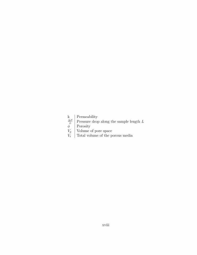
ing and collision of particles within the lattices, often together with someboundary conditions that must be fulfilled. As illustrated in Figure 3.1 theseoperations must be carried out for each discrete time step. The particleswithin the lattices can move within certain discrete velocities from one dis-crete lattice location to another. The discrete lattice locations correspond tovolume elements that contain a collection of particles [18], and represents aposition in space that holds either fluid or solid [35]. In the streaming phase,particles move to the nearest neighbor along their path of motion, as canbe seen in Figure 3.2, where they collide with other arrived particles, as canbe seen in Figure 3.3. The outcome of the collision is designed so that it isconsistent with the conservation of mass, energy and momentum [45]. Theyare collision invariant. After each iteration, only the particle distributionchanges, while the particle distribution function in the center of each latticelocations remains unchanged.

Figure 3.2: The streaming step:Particles spread out to their nearestnodes in the lattice [19].

Figure 3.3: The collision step: Exist-ing and entry particles are weighted[19].

3.2.1 Previous And Related WorkHistorically, the lattice Boltzmann method is an outcome from the attemptsto improve the Lattice Gas Cellular Automata (LGCA), even though the lat-tice Boltzmann method can be derived directly from the Boltzmann equation[27].

26

The first LGCA model named HPP was introduced in 1973 by Hardy,Pomeau and de Pazzis. In this model the lattice applied was square, andparticles could not move diagonally. Because of this the model suffered fromlack of rotational invariance [26]. In 1986, over 10 years later, the LGCAmodel named FHP was introduced by Frisch, Hasslacher, and Pomeua [23],who discovered the lattice symmetry. In this model the lattice applied wastriangular and therefore did not suffer from lack of rotational invariance[55]. The main motivation for further development was to remove the staticnoise in the LGCA models, which makes computational precision difficult toachieve [8]. In 1988, two year later, McNamara and Zanetti introduced thelattice Boltzmann method [38], which completely removed the static noisefound in the LGCA models, by replacing the Boolean representation of aparticle by the particle distribution function. Further development and im-provements where proposed by Chen[10] and Qian[42], with the use of theBhatnagar-Gross-Krook (BGK) simplified collision operator.

Today, the lattice Boltzmann method has been applied on CPUs for fluidflows through porous media to determine the permeability of porous media[2, 24]. For a comprehensive overview of efficient implementations of the lat-tice Boltzmann method for CPUs we refer to [53], in view of the fact that thearchitecture of the GPU is quite different. The lattice Boltzmann methodhas been applied on GPUs using NVIDIA CUDA [25, 40, 50, 51]. Perfor-mance of lattice Boltzmann implementations is often measured in MLUPS(million lattice nodes updates per second). Tolke and Krafczyk [51], imple-mented the lattice Boltzmann method using the D3Q13 model on a NVIDIAGeForce 8800 Ultra card, which achieved the total of 592 MLUPS. Habich[25], implemented the lattice Boltzmann method using the D3Q19 model ona NVIDIA GeForce 8800 GTX card, which achieved the total of 250 MLUPS.Bailey, Myre, Walsh, Lilja, and Saar [40] implemented the lattice Boltzmannmethod using the D3Q19 model on a NVIDIA GeForce 8800 GTX card,which achieved the total of 300 MLUPS. The higher performance of Tolkeand Krafczyk can to some extent be explained because the D3Q13 is a sim-pler lattice, compared to the D3Q19.

27

3.2.2 FundamentalsIn what follows, the starting point is the lattice Boltzmann equation withthe Bhatnagar-Gross-Krook (BGK) simplified collision operator, that can bewritten as Equation 3.2.

∂f

∂t+ e∇f = −1

τ(f − f eq) (3.2)

where τ is the single relaxation time, and f eq is the equilibrium distribu-tion function, that can be written as Equation 3.3.

f eq = ρ

(2πRT )D/2 exp[−(e− u)2

2RT

](3.3)

where R is the universal gas constant, D is the dimension of the space, ρis the macroscopic density, u is the macroscopic velocity, and T is the macro-scopic temperature [27].

In order to solve the Boltzmann equation numerically, the physical spaceis limited to a discrete lattice, only a discrete set of velocities are allowed,and the time is limited to discrete time steps. A widespread classificationsystem used for the different lattices that exist is DaQb, where Da is thenumber of dimensions and Qb is the number of distinct discrete lattice ve-locities ~ei. In the lattice Boltzmann method, the underlying lattice musthave enough symmetry to ensure isotropy, and typically lattices are D2Q9,D3Q13, D3Q15, and D3Q19.

In the lattice Boltzmann method, the time evolution of the particle dis-tribution function is obtained, by solving the discrete Boltzmann equation,that can be written as Equation 3.4 [4].

fi(~x+ ~ei, t+ 1)− fi(~x, t) = Ω (3.4)

where ~ei are discrete lattice velocities, Ω is the collision operator, andfi(~x, t) is the discrete particle distribution function in the i direction. Thesimplified BGK collision operator is often used, that can be written as Equa-tion 3.5 [42].

ΩBGK = −1τ

(fi(~x, t)− f eqi (ρ(~x, t), ~u)) (3.5)

28

where τ is the single relaxation parameter, and f eqi (ρ(~x, t), ~u) is the equi-librium distribution functions in the i direction (also often called for theMaxwell-Boltzmann distribution function). The equilibrium distribution func-tion can be written as Equation 3.6 [42].

f eqi (ρ(~x, t), ~u) = wiρ(

1 + 3c2 (~ei · ~u) + 9

2c4 (~ei · ~u)2 − 32c2~u

2)

(3.6)

where c is equal to ∆x/∆t, which are often normalized to 1, and wi isweight factors that depends on the lattice model. The macroscopic kinematicviscosity ν of the fluids, can be found with Equation 3.7 [31].

ν = 2τ − 16 (3.7)

The macroscopic properties of the fluids can be computed from the par-ticle distribution functions, such as the mass density ρ(~x, t), momentumρ(~x, t)u(~x, t) and velocity ~u(~x, t) of a fluid particle as Equations 3.8, 3.9,and 3.10 [18].

ρ(~x, t) =q∑i=0

fi(~x, t) (3.8)

ρ(~x, t)u(~x, t) =q∑i=0

~eifi(~x, t) (3.9)

~u(~x, t) = 1ρ(~x, t)

q∑i=0

~eifi(~x, t) (3.10)

where q is the number of distinct lattice velocities ~ei.

3.2.3 Boundary ConditionsThe standard boundary condition applied at solid-fluid interfaces is the no-slip boundary condition (also called bounce back boundary condition), thatcan be written as Equation 3.11 [31].

f ini (~x+ ~ei, t+ 1) = f outi (~x, t) = f ini (~x, t) (3.11)With this boundary condition applied, the particles close to solid bound-

aries do not move at all, resulting in zero velocity. The particles at the

29

solid-fluid interfaces are reflected [49], as illustrated in Figures 3.4 and 3.5.Periodic boundary condition is also common, and allows particles to be cir-culated within the fluid domain. With the periodic boundary conditions,outgoing particles at the exit boundaries will come back again into the fluiddomain through the entry boundaries on the opposed side.

Figure 3.4: Bounce back boundary:Lattice node before streamin [49].

Figure 3.5: Bounce back boundary:Lattice node after streaming [49].

3.2.4 Basic AlgorithmEquations 3.4 and 3.5 can be split up into the two following Equations 3.12and 3.13 [31].

f outi (~x, t) = f ini (~x, t)− 1τ

(f ini (~x, t)− f eqi (ρ(~x, t), ~u)

)(3.12)

f ini (~x+ ~ei, t+ 1) = f outi (~x, t) (3.13)

where f outi represents the particle distribution value after collision, andf ini is the value after both the streaming and collision operations are finished.Equations 3.12 and 3.13 implement the collide-stream system, also known asthe push method, described by [31]. The basic algorithm using the collide-stream system is illustrated in Figure 3.6.

30

Initialization

phase

Initialize the single relaxation paramter τ

Initialize the particle distribution functions ( , ) to equilibriumif x t

Collision

phase

Streaming

phase

Streaming of the particle distributions depending

on their travel direction

Boundary

condition

phase

Bounce back bounda ry condition at solids

Compute the equilibrium distribution functions f using and ueq ρ

Relaxation of the particles distributions

against equilibrium condition

Compute the macroscopic density ρ and velocity u

Next

time step

Initialize the macroscopic density ρ and velocity u

Periodic boundary condition

0 0

1( , ) ( , ) ( , ) ( , )

( , )

q q

i i i

i i

x t f x t u x t e f x tx t

ρρ= =

= =∑ ∑r r r r r r

r

2 2

2 4 2

3 9 3( ( , ), ) 1 ( · ) ( · )

2 2

eq

i i i if x t u w e u e u uc c c

ρ ρ = + + −

r r r r r r r

( )1( , ) ( , ) ( , ) ( ( , ), )

out in in eq

i i i if x t f x t f x t f x t uρτ

= − −r r r r r

( , 1) ( , )in out

i i if x e t f x t+ + =r r r

( , 1) ( , ) ( , )in out in

i i i if x e t f x t f x t+ + = =r r r r

Figure 3.6: Basic algorithm of the lattice Boltzmann method. Based on [31].

31

3.3 Porous Rocks

This section about porous rocks is taken from earlier work made by EirikOla Aksnes and Henrik Hesland [3], and used with some changes.

The word petroleum, meaning rock oil, is important to humankind asit is the primary source of energy. Petroleum does not typically lie in hugepools or are found in underground rivers, but refers to the naturally occurringhydrocarbons that are found in porous rock formations beneath the surface ofthe earth. A petroleum reservoir or an oil and gas reservoir is an undergroundaccumulation of oil and gas that is located within pore spaces of porous rocks.Not all rocks are capable of holding oil and gas. Reservoir rocks, which arecapable of holding oil and gas, are characterized by having sufficient porosityand permeability, meaning that is has sufficient storage capacity for oil andgas, and has the ability to transmit fluids. The challenge is how to extractthe oil and gas out from the porous rocks, and it is vital for the oil industryto analyze the petrophysical properties of reservoir rocks to gain improvedunderstanding of oil production. Figure 3.7 illustrates the influence the poregeometry of porous rocks has on how the fluid will flow inside the porousrocks. In Figure 3.7 fluid will flow more slowly through the left rock, becauseof the lack of interconnected pore spaces within the rock, as the pore spacesare isolated from each other, and that the existing pore spaces are narrow[22].

High permeabilityLow permeability

Figure 3.7: The left rock has low permeability, in contrast to the right rock,which allows fluid to flow easily.

32

3.3.1 Porosity

The porosity is defined as Equation 3.14 [8].

φ = VpVt

(3.14)

where Vp is the volume of pore space and Vt is total volume of the porousmedium. Some actual material porosities are listed in Table 3.1.

Table 3.1: Typical porosity of some representative real materials. Taken from[8].

Material PorositySandstone 10-20 %Clay 45-55 %Gravel 30-40 %Soils 50-60 %Sand 30-40 %

3.3.2 Permeability

Darcy’s law for the flow of fluids through porous media can be written asEquation 3.15 [24].

q = − k

ρν

∆PL

(3.15)

where q is the volumetric fluid flux through the porous media, k is thepermeability of the porous medium, ∆P

Lis the total pressure drop along the

sample length L, ρ is the fluid density, and ν is the fluid kinematic viscosity.In porous media, fluid will flow only through pores capable of transportingfluid, therefore the volumetric flux q is considered as Equation 3.16 [24].

q = uφ (3.16)

33

where u is the average velocity of the fluid and φ is the porosity of theporous medium. The permeability can be found with Equation 3.17.

k = uφρν∆PL

(3.17)

34

Chapter 4

Implementations

This chapter describes how we implemented the lattice Boltzmann methodpresented in the previous chapter on modern GPU hardware. Our simula-tion model is baded on [31]. On order to better analyze our results, bothparallel CPU and GPU implementations of the lattice Boltzmann methodwere developed.

In particular, Section 4.1, describes the target platforms, libraries, andlanguages used for both our implementations. Section 4.2 describes supportfor porous rocks visualization, and of the Marching Cubes algorithm used togenerate three dimensional models of porous rocks. Section 4.3 describes thesimulation model used in both our implementations. Section 4.4 describesan approach used to reduce the rounding error in the simulation model used.Section 4.5 describes the data structure used to store the particle distribu-tion functions for both our implementations. Sections 4.6 and 4.7 describethe CPU and GPU implementations of the lattice Boltzmann method, withoptimization guidelines for high performance.

4.1 Platforms, Libraries, and LanguagesBoth the CPU and GPU implementation are programmed in C++. Forthe GPU implementation, NVIDIA GPUs are used to accelerate the latticeBoltzmann method, due to the well developed hardware and software sup-port from NVIDIA GPUs for general purpose computation. With the latestgenerations of NVIDIA GPUs that supports the NVIDIA CUDA program-

35

ming model, several unnecessary difficulties with the traditional way of doingGPGPU are eliminated. The NVIDIA CUDA1 are a natural choice, since itexposes the hardware functions of the NVIDIA GPUs, making it possible totarget the programmable units directly for improved control. The OpenCLframework are also considered due to it’s heterogeneous platform support,but NVIDIA CUDA are used, because OpenCL is still new. For graphics ren-dering, NVIDIA CUDA supports both the Direct3D and OpenGL graphicslibrary. Since the Direct3D graphics library is only supported on the Mi-crosoft Windows operating systems, the OpenGL2 graphics library are usedfor platform independence. To access the expansions to the OpenGL graph-ics library for efficient graphics rendering, the OpenGL Extension WranglerLibrary3 (GLEW) are used. The OpenGL Utility Toolkit (GLUT) are usedto handle mouse, keyboard, and window management. The OpenGL Shad-ing Language (GLSL) are used to be able to use the programmable pipelinewith vertex and fragment shaders. The CPU implementation also uses theOpenGL, GLEW, GLUT and GLSL library.

4.2 VisualizationVisualization of the pore geometry and how fluids flow inside the pore geom-etry of rocks are implemented for both our implementations, as illustrated inFigure 4.1. The yellow color indicates high velocity and the black color indi-cates low velocity. Visualization are implemented to ease debugging duringdevelopment, and for visual analysis of the pore geometry of rocks. Since thepore geometry of rocks, how the pore spaces within the rocks are intercon-nected, and the size of the pore spaces have major influence on permeability[22].

4.2.1 Graphics RenderingVertex Buffer Object (VBO), which is an OpenGL extension provided throughGLEW are used for graphics rendering. The traditional way of rendering ge-ometric data is to transfer single data elements to the memory of the GPU.With VBO, it is possible to upload multiple data elements to the memory

1www.nvidia.com/cuda2http://www.opengl.org/3http://glew.sourceforge.net/

36

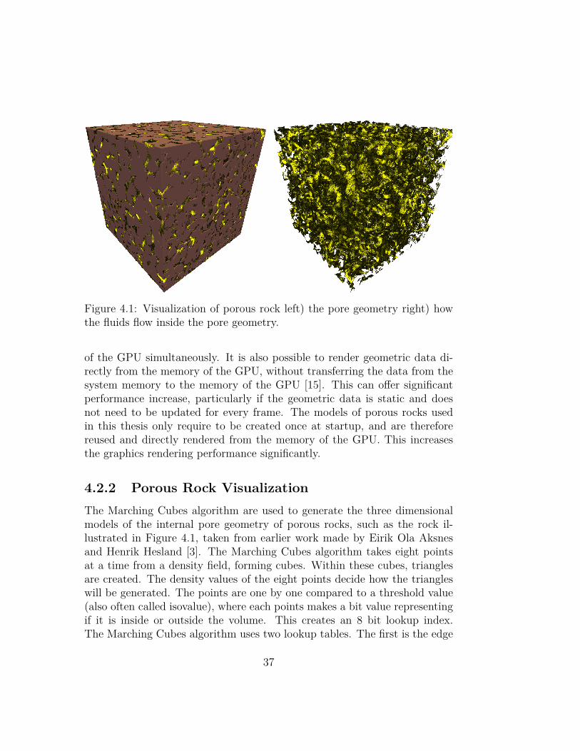
Figure 4.1: Visualization of porous rock left) the pore geometry right) howthe fluids flow inside the pore geometry.

of the GPU simultaneously. It is also possible to render geometric data di-rectly from the memory of the GPU, without transferring the data from thesystem memory to the memory of the GPU [15]. This can offer significantperformance increase, particularly if the geometric data is static and doesnot need to be updated for every frame. The models of porous rocks usedin this thesis only require to be created once at startup, and are thereforereused and directly rendered from the memory of the GPU. This increasesthe graphics rendering performance significantly.

4.2.2 Porous Rock VisualizationThe Marching Cubes algorithm are used to generate the three dimensionalmodels of the internal pore geometry of porous rocks, such as the rock il-lustrated in Figure 4.1, taken from earlier work made by Eirik Ola Aksnesand Henrik Hesland [3]. The Marching Cubes algorithm takes eight pointsat a time from a density field, forming cubes. Within these cubes, trianglesare created. The density values of the eight points decide how the triangleswill be generated. The points are one by one compared to a threshold value(also often called isovalue), where each points makes a bit value representingif it is inside or outside the volume. This creates an 8 bit lookup index.The Marching Cubes algorithm uses two lookup tables. The first is the edge

37

table that holds an overview (256 different combinations) over which of the12 edges we have to interpolate. The second is the triangle table that deter-mines the quantity (maximum five) and how the triangles inside each cubeshould be drawn for correct representation of the isosurface. The March-ing Cubes algorithm repeats the treatment of cubes until the entire densityfield is treated. Figure 4.2 shows the main phases of the Marching Cubesalgorithm used, with the value of the corner 3 above the selected isovalue.

4.2.3 Fluid Flow Visualization

In fluid simulations, velocity fields are represented as vector fields. Visu-alization of vector fields is used to describe the motion of fluids inside thepore geometry of porous rocks. To visualize vector fields, shader code andan NVIDIA CUDA kernel provided by Robin Eidissen were used, with somemodifications [20]. For each lattice node, a single line segment is created,by representing the position and direction using two four-component vec-tors. The length of line segments represents flow velocity. The first threecomponents of vectors are x, y, and z coordinates. The last component ofvectors holds the flow velocity, which is used to determine the color of theline segment. A GLSL shader colors the line segments based on the flowvelocity, with yellow color indicating high velocity and black color indicatinglow velocity.

4.3 Simulation Model

The lattice Boltzmann method with the simplified Bhatnagar-Gross-Krookcollision operator is used as simulation model for the CPU and GPU im-plementations [42]. In this thesis, large portions of the simulations will bebetween solid-fluid interfaces, inside the complex geometries of porous rocks.One of the most cited benefits of the lattice Boltzmann method is that it canhandle complex flow geometries without significant drop in computationalspeed and efficiency [46] and [45]. The method is therefore suitable for thesimulations of fluid flows through the complex geometries of porous rocks(although simulating fluid flow through porous rocks is still very complex,including the flow of single-phase fluid).

38

Create 8 bit index

Use index to lookup into the

edge table to find edges

crossed by the isosurface

Use edges to find

intersections points with

linear interpolation

Use index to lookup into the

triangle table to find out how

to draw the triangle

Calculate normals

Store the triangle

vertices and vertex

normals

User specify isovalue

Next cube

| V7 | V6 | V5 | V4 | V3 | V2 | V1 | V0 | =

| 0 | 0 | 0 | 0 | 1 | 0 | 0 | 0 |

edgetable[00001000] = edgetable[8] = 1000 0000 1100 =

edge 11, 2 and 3 are crossed by the isosurface

use edge 11, 2, and 3 to find the intersections points by

linear interpolation, P=P1+(Isovalue-V1)(P2-P1)/(V2-V1),

where p1 and p2 are vertices of a cut edge

and V1 and V2 are the density values

triangletable[8] =

3, 11, 2, -1, -1, -1, -1, -1, -1, -1, -1, -1, -1, -1, -1, -1 =

draw the triangle between the intersection points

along the edge 3,11 and 2, in that sequence.

Figure 4.2: The Marching Cubes algorithm used. Based on [7] and [34].

4.3.1 Memory Usage

The simulation model makes use of the D3Q19 lattice, which is a three di-mensional lattice with 19 discrete lattice velocities. Appendix A shows theconfiguration of the D3Q19 lattice used. Relatively large models of the inter-nal pore geometry of porous rocks are often required to get accurate estimates

39

of their permeability. For every node in the lattice, implementations usingthe D3Q19 model often stores and uses 19 values for the particle distribu-tion functions and 19 temporary values for the streaming phase, so that theparticle distribution functions are not overwritten during the exchange phasebetween neighbor lattice nodes. Table 4.1 lists the memory consumption ofthe lattice Boltzmann method using temporary storage with varying latticesizes, and with single and double floating-point precision. One can see howthe memory consumption becomes gigabytes of memory with large latticesizes, making the growth in memory requirements with lattice size visible.

Table 4.1: Memory usage D3Q19 model with temporary storage.

Lattice Single Doublesize precision precision323 4 MB 10 MB643 38 MB 76 MB1283 304 MB 608 MB2563 2.4 GB 4.8 GB5123 19.4 GB 38.8 GB

Since the lattice Boltzmann method uses a lot of memory resources, itis important to allocate and use the minimal amount of memory possible.This is particularly important for the GPU implementation, since memorycapacity is limited and memory cannot simply be added. Therefore insteadof duplicating the particle distribution functions to temporary storage in thestreaming phase, another approach described by Latt [32] is used in boththe implementations, where the source and destination particle distributionfunctions are instead swapped between neighbor lattice nodes. This approachreduces the memory requirements by 50 %, compared to using temporarystorage.

4.3.2 Simulation Model DetailsThe details of how the lattice Boltzmann method is realized in our CPU andGPU implementation are discussed here. Figure 4.4 shows the main phases

40

Initialization

phase


Initialize the particle distribution functions to equilibriumif

Collision

phase

Streaming

phase

Swap the particle distributions functions depending

on their travel direction


Relaxation of the particles distributions against

equilibrium condition


Next

time step


Set the fluid in motion with constant body force

Swap the particle distribution functions locally

9( ( , ), ( , ))i iSwap f x t f x t+

r r

9( ( , 1), ( , )i i iSwap f x t f x e t+ + +

r r r

2 2

2 4 2

3 9 3( ( , ), ) 1 ( · ) ( · )

2 2

eq

i i i if x t u w e u e u uc c c

ρ ρ = + + −

r r r r r r r

0

( , ) ( , )

q

i

i

x t f x tρ=

= ∑r r

0

1( , ) ( , )

( , )

q

i i

i

u x t e f x tx tρ =

= ∑r r r r

r

( )1( , ) ( , ) ( , ) ( ( , ), )

eq

i i i if x t f x t f x t f x t uρτ

= − −r r r r r

2

( )( , ) ( , )

( , )

eq

i ii i

s

e u f Ff x t f x t

x t cρ− × ×

= +

r

r r

r r

r

Figure 4.3: The main phases of the simulation model used. Based on [31].

41

of the simulation model. In the simulation model, the collisions of particlesare evaluated first, and then particles streams to the lattice neighbors alongthe discrete lattice velocities.

Two types of boundary conditions are implemented: the standard bounceback boundary condition to handle solid-fluid interfaces, and periodic bound-ary condition to allow fluids to be circulated within the fluid domain. Theperiodic boundary condition is built into the streaming phase, and the bounceback boundary condition is built into the streaming and collision phase. Thebounce back boundary condition emerges from swapping particle distributionfunctions between neighbors, because neighbors in the lattices only exchangeparticle distribution functions with other neighbors that are fluid elements.The different phases of the simulation model will now be discussed further,accompany by pseudo-code.

Initialization Phase

A common practice in the initialization phase is to initialize the lattice nodesusing the equilibrium distribution function with the wanted initial macro-scopic density ρ and macroscopic velocity ~u. In this thesis, when estimatingthe permeability of porous rocks, the steady state of the velocity fields isimportant. Therefore is the lattice initialized with the density ρ equal to1.0 and the velocity ~u equal to 0.0 for each node in the lattice that is fluidelement (Algorithm 4: Line 7). The velocity ~u becomes 0.0 with each nodein the lattice initialized with the density ρ equal to 1.0.

Collision Phase

The collision phase is, in contrast to the streaming phase, completely local,but it is also the most computational demanding phase. In the collisionphase, the macroscopic density ρ (Algorithm 5: Line 7) and the macroscopicvelocity ~u (Algorithm 5: Line 8-10) need to be computed, together withthe equilibrium distribution functions that need to be solved (Algorithm 5:Line 13), and the relaxation of the particles distributions against equilibriumcondition (Algorithm 5: Line14). In the collision phase, the fluids are setin motion, with some constant external force that is added to every fluid

42

Algorithm 4 Pseudo code of the initialization phase.1: for z = 0 to dz do2: for y = 0 to dy do3: for x = 0 to dx do4: current← x+ y × dx + z × dx × dy5: if fi[current] is fluid then6: for i = 0 to 18 do7: fi[current]← 1.08: end for9: end if

10: end for11: end for12: end for

element in the lattice (Algorithm 5: Line 15), using equation 4.1.

fi(~x, t) = fi(~x, t) + (~ei − ~u)× f eqi × ~F

ρ(~x, t)c2s

(4.1)

~F is the external force, and c2s is the speed of sound, given the value of√

(1/3) [28]. The external force will add some constant value to the particledistribution functions moving along the fluid flow direction, and subtractinga corresponding value from the particle distribution functions moving exactlythe opposite direction [24]. At the end in the collision phase, the particle dis-tribution functions are swapped locally (Algorithm 5: Line 17).

The collision phase is responsible for approximating the particle collisionsthat happen in real fluids. The rate of change toward equilibrium is controlledby the relaxation time τ , and determines the viscosity 4 of the fluids [45].In the lattice Boltzmann method, the relaxation time τ is normally chosenbetween 0.51 ≤ τ ≤ 2.5 [49], due to the requirements of numerical stabilityfor the simulations [24].

4Viscosity is the measure of a fluid’s resistance to flow.

43

Algorithm 5 Pseudo code of the collision phase.1: for z = 0 to dz do2: for y = 0 to dy do3: for x = 0 to dx do4: current← x+ y × dx + z × dx × dy5: if fi[current] is fluid then6: for i = 0 to 18 do7: ρ← ρ+ fi[current]8: ux ← ux + fi[current]× eix9: uy ← uy + fi[current]× eiy

10: uz ← uz + fi[current]× eiz11: end for12: for i = 0 to 18 do13: f eqi ← wi× ρ× (1.0 + 3.0× (eix × ux + eiy × uy + eiz × uz)

+ 4.5× (eix × ux + eiy × uy + eiz × uz)2

− 1.5× (ux × ux + uy × uy + uz × uz))14: fi[current]← fi[current]− 1

τ× (fi[current]− f eqi )

15: fi[current]← fi[current] + (eix − ux)× f eqiρ× c2

s

× Fx

+ (eiy − uy)× f eqiρ× c2

s

× Fy

+ (eiz − ux)× f eqiρ× c2

s

× Fz16: for i = 1 to 9 do17: swap(fi[current], fi+9[current])18: end for19: end for20: end if21: end for22: end for23: end for

Streaming Phase

The streaming phase is responsible for the movements of particle distribu-tion functions within the lattice. In the streaming phase, lattice nodes need

44

to interact with neighbors in the lattice to exchange particle distributionfunctions. In the simulation model, this is mostly swapping of particle dis-tribution functions between memory locations (Algorithm 6: Line 9). Beforethe exchange of particle distribution functions, the lattice nodes need to findthe neighbors in the lattice (Algorithm 6: Line 7).

Algorithm 6 Pseudo code of the streaming phase.1: for z = 0 to dz do2: for y = 0 to dy do3: for x = 0 to dx do4: current← x+ y × dx + z × dx × dy5: if fi[current] is fluid then6: for i = 1 to 9 do7: neighbor ← getNeighbor(x, y, z, i, px, py, pz)8: if fi[neighbor] is fluid then9: swap(fi+9[current], fi[neighbor])

10: end if11: end for12: end if13: end for14: end for15: end for

To find the coordinates to neigbors in the lattice, the coordinates of thecurrent lattice nodes are used (Algorithm 7: Line 1-3).

neighborx = currentx + eix

neighbory = currenty + eiy

neighborz = currentz + eiz

(4.2)

In our two implementations, the periodic boundary condition is built intothe finding of neighbors, by allowing or denying the lattice nodes to interactwith the opposite side of the lattice when they come close to the borders(Algorithm 7: Line 5-27).

45

Algorithm 7 Pseudo code for the find neigbhbor algorithm.getNeighbor(x,y,z,i,px,py,pz)

1: neighborx ← x+ eix2: neighbory ← y + eiy3: neighborz ← z + eiz4: if px then5: if neighborx is −1 then6: neighborx ← dx − 17: if neighborx is dx then8: neighborx ← 09: end if

10: end if11: end if12: if py then13: if neighbory is −1 then14: neighbory ← dy − 115: if neighbory is dy then16: neighbory ← 017: end if18: end if19: end if20: if pz then21: if neighborz is −1 then22: neighborz ← dz − 123: if neighborz is dz then24: neighborz ← 025: end if26: end if27: end if28: return neighborx + neighbory × dx + neighborz × dx × dy

4.3.3 Calculate Permeability

The approach used to calculate the permeability of porous rocks and mostof the information found in this section is taken from [24].

The details of how the calculation of the permeability of porous rocks is

46

realized in our CPU and GPU implementation is discussed in this section.Figure 4.4 shows the expansion of the simulation model for the calculationof permeability of porous rocks.

Initialization

phase

Collision

phase

Streaming

phase

Next

time step

Calculate

permeability

Compute the average velocity

Compute the permeability

0

( , )N

j

u x tu

N=

=∑r r

2 uk aF

ρ φ ν= −

( , 1) ( , )u x t u x t+ − < ε

Check for convergence

2 1

6

τν

−=

Compute the kinematic viscosity

Compute the porosity

p

t

V

Vφ =

Check

velocity field

Simulation

model

Expansion Figure 4.4: Expansion of the simulation model for permeability calculations.

The permeability of the porous rocks is obtained directly from the gen-erated velocity fields of the lattice Boltzmann method, together with using

47

Darcy’s law for the flow of fluids through porous media [24]. The fluid flowis driven by some external force in the simulation model, but it could also bedriven by pressure on the boundaries. The external force is expected to givethe same change in momentum as the true ∆P

L, which is the total pressure

drop along the sample length L. By adapting Equation 3.17 the permeabilityof porous rocks are directly obtained from the lattice Boltzmann simulations,using Equation 4.3 [24].

k = −a2 uρφν

F(4.3)

where a is the node resolution equivalent to the lattice spacing. Driven bysome external force, the permeability is always obtained when the velocityfield is at steady state. The simulations is considered to have converged ifthe change of the average velocity meets the condition described in Equation4.4.

|u(x, t+ 1)− u(x, t)| < ε (4.4)where the convergence threshold ε is chosen to be 10−9. The average

velocity is computed using Equation 4.5.

u =N∑j=0

~u(~x, t)N

=N∑j=0

∑qi=0 ~eifi(~x, t)/ρ(~x, t)

N(4.5)

where N is the number of fluid elements within the lattice.

Figure 4.5 illustrates the two types of boundary conditions that are usedin the calculation of the permeability of porous rocks. In the calculations ofthe permeability, the boundaries parallel to the flow direction are made solid,and with bounce back boundary conditions. The entry and exit boundariesare applied with periodic boundary conditions. In order for the periodicboundary condition to be correct in the simulations, it is common practiceto add some extra empty layers at both the entry and exit boundaries [24].

Only the interconnected (percolated) pore spaces within porous rockstransport fluid. In the expansion of the simulation model for porosity calcu-lations, both the disconnected and interconnected pore spaces are considered.There is possible to identify the percolating pore spaces within porous rockswith the Hoshen-Kopelman algorithm [24].

48

Bounce Back

Boundary

Bounce Back

Boundary

Bounce Back

Boundary

Bounce Back

Boundary

Periodic

Boundary

x

z

y

Figure 4.5: Configurations of the boundaries in permeability calculations.

4.4 Floating-point PrecisionThe Institute of Electrical and Electronics Engineers (IEEE) standard 754,defines a standard for floating-point arithmetic. The standard specifies theformat of the numbers, the results of the basic floating-point operations andcomparisons, and the rounding to nearest rule among many other things [29].Since computers represent real numbers with a limited number of bits, ap-proximations and rounding errors occur [52]. Large rounding errors occurbetween two very different numbers that are added or subtracted [29]. In thecollision phase of the simulation model, the equilibrium distribution func-tion needs to be computed with a mixture of large and small numbers thatoften leads to large amount of rounding error. It was necessary to reducethe rounding error in the simulation model when using single floating-pointprecision, to get precise permeability of porous rocks. The approach usedto reduce the rounding errors used in the simulation model is taken from[11] 5. It was left out from the previous descriptions and pseudo codes ofthe simulation model, due to readability. In this approach the simplifiedBhatnagar-Gross-Krook collision operator becomes as Equation 4.6.

houti = hi + ω(heqi − hi) (4.6)where houti = f outi −wip0, hi = fi−wip0, and heqi −wip0. The equilibrium

5www.lbmethod.org

49

distribution function becomes as Equation 4.7.

heqi = wi∆p+ wi(po + ∆p)( 3c2 (~ei · ~u) + 9

2c4 (~ei · ~u)2 − 32c2~u

2)

(4.7)

The macroscopic density ρ and the macroscopic velocity ~u becomes asEquations 4.8 and 4.10.

ρ = p0 + ∆p (4.8)

∆p =q∑i=0

hi (4.9)

~u =∑qi=0 hi~ei

p0 + ∆p (4.10)

4.5 Data StructureA structure-of-arrays are used to store the particle distribution functions forboth our implementations. There are 19 arrays in the structure, since thereare 19 discrete directions in the D3Q19 lattice, as illustrated in Figure 4.6.Each array stores one discrete direction of the particle distributions functions.

Array 0

Array 1

Array 17

Array 18

Figure 4.6: Structure-of-arrays.

50

4.6 CPU ImplementationBefore describing the CPU implementation, we will present some optimiza-tion guidelines for high performance.

4.6.1 Optimizations GuidelinesThis section is taken from earlier work made by Eirik Ola Aksnes and HenrikHesland [3], and used with only some minor changes.

There are some general optimization techniques which programmers shouldbe acquainted with for obtaning the highest possible performance. A veryimportant technique for high performance is to avoid cache misses, sincemost modern CPUs uses fast cache memory to reduce average time to accessmain memory. The CPU will first check for the data needed in the cachememory, and if the data is not there, it must wait for the data to be fetchedfrom the much slower main memory. Many programs are waiting for data tobe fetched from main memory, and therefore waste much of their executiontime. Caches rely on both spatial and temporal locality, items near a useditem might be used soon, and recently used items will likely be used again inthe near feature [30]. Data structures must therefore be set up so that themain memory is accessed in contiguous memory segments, and data elementsneed to be reused in a loop as frequently as possible [33]. Loop optimizationtechniques can have huge effect on cache performance, since most of the exe-cution time in scientific applications is used on loops. Matrix multiplicationis one example that can gain performance if the sequence of for loops is cor-rectly arranged, by allowing an optimal data array access pattern. If the dataneeded is in continuous memory, the next elements needed are more likelyto be in the cache. Cache locality can be improved by dividing the matrixinto smaller sub matrixes, and chosing the optimal block size that will fitinto cache. The size of the sub matrix will be system dependent, since thedifferent systems have different cache size.

Another feature of today’s processor architectures is the long executionpipeline, which offers significant execution speedups when kept full. Bypipelining, several instructions can be overlapped in parallel. Branch predi-cation is used to ensure that the pipeline is kept full, by guessing which waythe branch is most likely to go. It has significant impact on performance, by

51

letting processors fetch and start instructions without waiting for the branchto be determined. A conditional branch is a branch instruction that can beeither taken or not taken. If the processor makes the wrong guess in a con-ditional branch, the pipeline needs to be flushed, and all computation beforethe branch point becomes unnecessary. It can therefore be advantageous toeliminate such conditional branches in performance critical code. One tech-nique that can be used to eliminate branches and data dependencies is tounroll loops [1]. One should also try to reduce the use of if-statements asmuch as possible inside the inner loops.

4.6.2 Details

The CPU implementation is similar to the pseudo code described in Section4.7.3. It uses only one processor core, and are made to evaluate the computa-tional exactness and performance of the GPU implementation. Algorithm 8shows pseudo code of the CPU implementation. In the CPU implementationthe lattice nodes are accessed sequential.

Algorithm 8 CPU implementation pseudo code.1: Initialize lattice2: Load porous dataset3: Set boundaries on porous dataset4: while new time step is needed do5: for all n nodes in lattice do6: n.collide()7: n.stream()8: end for9: Compute the average velocity

10: Check for convergence11: end while12: Compute the kinematic viscosity13: Compute the porosity14: Compute the permeability

52

4.7 GPU ImplementationBefore we describing the GPU implementation, we present some optimizationguidelines for high performance.

4.7.1 Optimizations GuidelinesThis section is taken from earlier work made by Eirik Ola Aksnes and HenrikHesland [3], and used with only some minor changes.

For high performance of applications on NVIDIA GPUs using NVIDIACUDA, the knowledge of the hardware architecture is important. The pri-mary performance element of the GPU is the large number of computationcores. To exploit this, a massive multithreaded program should be imple-mented. The number of thread blocks used simultaneously on a StreamingMultiprocessor (SM) is restricted by the number of registers, shared memory,maximum number of active threads per SM, and number of thread blocks prSM at a time should therefore be configured carefully in proportion to these.One of the problems with a GPU implementation is the communication la-tency. For computations, there should be as little communication as possiblebetween the CPU and GPU, and often some time can be saved by doingthe same computation several times, before loading the answers between theCPU and GPU. The massive parallelization of threads is also important forhiding latency. A modern GPU contains several types of memory, with dif-fernt latiencies. To reduce bandwidth usage, it is recommended to use sharedmemory where it is possible. Shared memory is divided into banks, whereaccess to the same bank only can be done sequentially, but access to differentbanks can be done in parallel. The threads should therefore be grouped toavoid this memory conflict. Another function that should be used as littleas possible is synchronization. This can cause many threads to wait a longtime for another thread to finish up, and can slow down the computationsignificantly.

4.7.2 ProfilingMost of the information found in this section is based on NVIDIA’s program-ming guide for NVIDIA CUDA [12].

53

code name =__globfunc__Z23streamAndSwapGPU_kernel14cudaPitchedPtr3PDFjiiilmem = 0smem = 124reg = 9

Figure 4.7: Section from Cubin file.

Several helpful profiling tools are available to gather information aboutthe performance critical parts of the GPU kernels to achieve high perfor-mance.

NVIDIA CUDA Visual Profiler

With the NVIDIA CUDA Visual Profiler, it is possible to generate visualprofiles of the kernel’s resource usage during execution. The NVIDIA CUDAVisual Profiler is capable of giving precise statistics of several performancecritical aspects. Some of the most useful statistics for high performance are[14]:

• Number of coalesced global memory loads and stores• Number of non-coalesced global memory loads and stores• Number of local memory loads and stores• Kernel occupancy• Number of divergent branches• Number of warps serialized

Cubin Files

By adding the extra parameter -cubin to the compiler, there is possible togenerate so-called Cubin files from the NVIDIA CUDA source files. Thegenerated files can be opened in regular text editors, and provide helpfulinformation about kernel resource usage of particularly interest are the num-ber of registers, shared memory and local memory used per thread [16, 12].Figure 4.7 shows an example of section found in generated Cubin file.

54

In the Cubin file the lmen is the amount of local memory, smen is theamount of shared memory, and reg is the number of registers used per threadin the kernel streamAndSwapGPU kernel.

NVIDIA CUDA Occupancy Calculator

The NVIDIA CUDA occupancy calculator is a spreadsheet provided byNVIDIA, which can be used to calculate the multiprocessor occupancy. Themultiprocessor occupancy is the ratio of active warps per multiprocessor tothe maximum number of active warps. The NVIDIA Quadro FX 5800 usedin this thesis contains 16384 registers per streaming multiprocessor, and 16KB of shared memory shared among all threads during execution. With theNVIDIA CUDA occupancy calculator, is possible to determine the maximumnumber of active threads given the limited number of registers and sharedmemory available. Higher multiprocessor occupancy results in more warpsactive, which can be used to hide the global memory latency [16, 12]. TheNVIDIA CUDA occupancy calculator takes the number of registers, amountof shared memory and local memory used per thread in your kernel as input,which can be seen in the orange field of Figure 4.8. This information can befound within generated Cubin files. To achieve the highest possible multipro-cessor occupancy, one must use the minimal amount of shared memory andregisters. The NVIDIA CUDA occupancy calculator provides three graphsshowing the changes in occupancy of kernels, due to changes in block size,register count, and shared memory usage, as illustrated in Figure 4.9.

55

1.) Select Compute Capability (click): 1,0

2.) Enter your resource usage:

Threads Per Block 256

Registers Per Thread 8

Shared Memory Per Block (bytes) 2048

(Don't edit anything below this line)

3.) GPU Occupancy Data is displayed here and in the graphs:

Active Threads per Multiprocessor 768

Active Warps per Multiprocessor 24

Active Thread Blocks per Multiprocessor 3

Occupancy of each Multiprocessor 100 %

Physical Limits for GPU: 1

Threads / Warp 32

Warps / Multiprocessor 24

Threads / Multiprocessor 768

Thread Blocks / Multiprocessor 8

Total # of 32-bit registers / Multiprocessor 8192

Register allocation unit size 256

Shared Memory / Multiprocessor (bytes) 16384

Warp allocation granularity (for register allocation) 2

Allocation Per Thread Block

Warps 8

Registers 2048

Shared Memory 2048

These data are used in computing the occupancy data in blue

Maximum Thread Blocks Per Multiprocessor Blocks

Limited by Max Warps / Multiprocessor 3

Limited by Registers / Multiprocessor 4

Limited by Shared Memory / Multiprocessor 8

Thread Block Limit Per Multiprocessor highlighted RED

CUDA Occupancy Calculator

Version: 1,5

Copyright and License

Just follow steps 1, 2, and 3 below! (or click here for help)

Figure 4.8: NVIDIA CUDA occupancy calculator.

56

My Block

Size 256

Max

Occupancy

0

8

16

24

32

16 80 144 208 272 336 400 464

Mult

iprocessor

Warp O

ccupancy

Threads Per Block

Varying Block Size

My

Register

Count 8

Max

Occupancy

0

8

16

24

32

0 4 8 12 16 20 24 28 32

Mult

iprocessor

Warp O

ccupancy

Registers Per Thread

Varying Register Count

My Shared

Memory

2048

Max

Occupancy

0

8

16

24

32

0 1024

2048

3072

4096

5120

6144

7168

8192

9216

10240

11264

12288

13312

14336

15360

16384

Mult

iprocessor

Warp O

ccupancy

Shared Memory Per Thread

Varying Shared Memory Usage

Figure 4.9: NVIDIA CUDA occupancy calculator.

4.7.3 Details

In the GPU implementation, every thread created during execution is re-sponsible for performing the collision and streaming for a single lattice node.Figure 4.10 illustrates this one-to-one mapping between threads and latticenodes.

To get high utilization of global memory bandwidth, the access patternto the global memory must be correctly aligned to achieve coalescing. Astructure-of-arrays has been proven by Habich [25] to be useful to achieve co-alescing. Threads access the arrays in contiguous memory segments to obtaincoalescing. This enables efficient reading and writing of particle distributionfunctions. Each array contains one discrete direction of the particle distribu-tions functions. Arrays in the structure are three-dimensional, allocated as

57

GPU Thread 1

GPU Thread 2

Lattice node 1

Lattice node 2

GPU Thread n-1

GPU Thread n

Lattice node n-1

Lattice node n

Figure 4.10: One-to-one mapping between threads and lattice nodes.

contiguous memory on the device using cudaMalloc3D. This function takesthe width, height, and depth of simulations as input, and pads the allocationto meet the alignment requirements to achieve coalescing. The function re-turns a pitch (or stride), which is the width in bytes of the allocation. Thispitch is used in the access of array elements [12].

The configuration of grids and thread blocks used to get coalesced globalmemory access, and to have simulations with large lattices are shown in theAlgorithm 9 and Figure 4.12. Kernels execute as two dimensional grids ofthread blocks, with the width and height of the grids equal to the simulationsize in the y- and z- direction. Two-dimensional grids were necessary in or-der to simulate large lattices, due to NVIDIA’s restriction of the maximumnumber of threads blocks to be 65535 in one direction of the grid. Figure4.11 shows the number of thread blocks with varying cubic lattice sizes, andthe largest lattice possible with one dimensional grid.

Thread blocks are one dimensional, with the number of threads equal tothe simulation size in the x-direction. This configuration of thread blocks re-sults in a maximum simulation size of 512 in the x-direction, due to NVIDIA’srestriction of the maximum number of threads within thread blocks to be 512in the x-direction. However, the memory usage of simulations will dominatethe limitation of the number of threads per threads blocks in the x-direction.Simulation sizes of 5123 without using temporary storage and with singlefloating-point precision, result in a memory consumption of 9.5 Gigabyte.

58

128 144 160 176 192 208 224 240 256 272 288 304 320 336 352 368 384 4000

20 000

40 000

60 000

80 000

100 000

120 000

140 000

160 000

Cubic Lattice Size

Num

ber

Of

Th

read

Blo

cks

The limit with one dimensional grids of thread blocks

Figure 4.11: Number of thread blocks with varying cubic lattice size.

An additional GPU implementation using shared memory was made,where entire thread blocks load data into shared memory for re-use. Thecurrent maximum size of the shared memory available per multiprocessor is16 KB, as explained in 2.2.2. This relation between the shared memory andthe number of threads within thread blocks results in the maximum simula-tion size in the x-direction being no more than 210 lattice nodes for singlefloating-point precision and 105 lattice nodes for double floating-point preci-sion. Because of this restriction, we decided not to continue the developmentand testing using shared memory.

59

Algorithm 9 The configurations of grids and thread blocks in kernels.


// Increase in the order x, y, and z to the global memory.int x = threadIdx.x;int grid_y = __mul24(blockIdx.y, gridDim.x);int z = (blockIdx.x + grid_y) / height;int y = (blockIdx.x + grid_y) - z * height;

...

void main()

dim3 blockSize(dimX);dim3 nBlocks(dimY,dimZ);

// Defines how the GPU kernel is executedkernelName<<<nBlocks,blockSize>>>();

60

C code

sequential

execution

GPU kernel

Grid 0Grid 0

Thread block

0,0

Thread block

1,0

Thread block

dimY, dimZ

Device

Thread block 0Thread block 0ck 0

Thread

0

Thread

1

Thread

2

Thread

dimX-1

Thread

dimX

XZ

Y

Thread

0

Thread

dimX

Next thread block

Thread block

dimY-1, dimZ-1

Figure 4.12: The configurations of grids and thread blocks in kernels.Adapted from [12].

61

Chapter 5

Benchmarks

This chapter presents and discusses several measurements of our implemen-tations of the lattice Boltzmann method, described in the previous chapter.

In particular, Section 5.1 describes the software and hardware config-uration of the machine that was used to obtain the measurements of ourimplementations, and the testing methodology. Section 5.2 validates the nu-merical exactness and correctness of our implementations, by comparing thenumerical results of fluid flow between two parallel plates to known analyticalsolutions. Section 5.3 presents and discusses profiling results of the collisionphase and streaming phase. Section 5.4 discusses several restrictions to thesimulations sizes. Section 5.5 presents and discusses performance results ofrunning our implementations with different cubic lattice sizes ranging from83 up to 3683. Section 5.6 discusses our implementations ability to calculatethe permeability of porous rocks. Section 5.7 present visual results from ourimplementations of the lattice Boltzmann method.

5.1 Test Environment and MethodologyThe machine that was used to obtain the measurements of our implemen-tations is shown in Table 5.1. The NVIDIA Quadro FX 5800 GPU used istargeted towards professional graphics solutions, and provides high memorybandwidth, and large memory size. The NVIDIA Quadro FX 5800 is de-signed to handle the most demanding challenges for geophysicists, scientists,designers, engineers, and others that need ultra-high-end graphics solutions

63

[13].

Table 5.1: The test machine that was used to obtain the measurements.

CPU Intel Core 2 Quad Processor Q9550Processor Clock 2.83 GHzBus Speed 1333 MHzL2 Cache Size 12 MBL2 Cache Speed 2.83 GHzGPU NVIDIA Quadro FX 5800Streaming Multiprocessors 30Stream Processors 240Processor Clock 1.3 GHzMemory Size 4 GBMemory Bandwidth 102 GB/sCompute Capability 1.3Memory Corsair XMS3 DHXQuantity 8 GBMemory Type DDR3 SDRAMMemory Speed 1333 MHzMemory Latency 9-9-9-24Motherboard ASUS P5E3 Premium

Measurements of our implementations were obtained using the MicrosoftWindows XP 64-bit operating system. We had exclusive access to the systemwhile collecting the measurements. Since graphics rendering is not vital toeither performance measurements or the calculation of the permeability ofporous rocks, it was disabled during the measurements. This avoided graph-ics rendering interference with the measurements results.

The performance of our implementations is measured in MLUPS (millionlattice nodes updates per second), to an average of two decimal of precision.This metric indicates the number of lattice nodes that is updated in onesecond [40]:

MLUPS = n

tstreaming + tcollision(5.1)

64

where n is the number of million lattice nodes, tstreaming is the time usedfor the streaming phase and tcollision is the time used for the collision phaseof the lattice Boltzmann method. The QueryPerformanceCounter is usedto measure in high-resolution the time used for the collision phase and thestreaming phase of the lattice Boltzmann method. Presented performancemeasurements are based on the arithmetic average over 25 iterations.

To distinguish between the different implementations and the floating-point precision used in the measurements, abbreviations will be used hence-forth, which are listed in Table 5.2.

Table 5.2: Measurements abbreviations.

Abbreviation DescriptionCPU Measurement of the the CPU implementationGPU Measurement of the the GPU implementation32 32-bit floating-point precision used.64 64-bit floating-point precision used.

5.2 Poiseuille Flow

Figure 5.1: Fluid flow between two parallel plates.

In Poiseuille Flow the analytical solutions of the velocity profile are known.To validate the numerical correctness and exactness of our two implementa-tions, the numerical velocity profile of fluid flow between two parallel plates

65

was compared to known analytical solutions. The fluid flow between twoparallel plates that are shown in Figure 5.10, has the lattice dimension of323. The analytical velocity profile of the fluid flow between two parallelplates, which is parabolic and with the flow highest in the middle, can befound with Equation 5.2 [55, 21].

ux(y) = G

2µ(L2 − y2) (5.2)

where G is some constant external force that accelerate the fluid, µ is thedynamic viscosity of the fluid, and L is half the size of the lattice dimensionin the y direction. In the Poiseuille Flow simulation, two types of boundaryconditions were used: bounce back boundaries along the two parallel platesand periodic boundaries in the x, y, and z direction for conservation of fluidparticles. The values of the parameters that were used in the Poiseuille Flow,for the single relaxation parameter and the external force are listed in Table5.3.

Table 5.3: Parameter values used in the Poiseuille Flow.

Parameter Valueτ 0.65Fx 0.00001Fy 0.0Fz 0.0

The Poiseuille Flow simulations were performed with single and doubleprecision. Figure 5.2 compares the velocity profile of the correct analyticalsolutions to the numerical solutions, showing that the fluid flows are recov-ered with great accuracy. The solid lines show the analytical solution, andthe circles are the numerical results obtained from the Poiseuille Flow simu-lations. Table 5.4 shows the measured deviations between the numerical andanalytical solutions.

66

5 10 15 20 25 300

0.2

0.4

0.6

0.8

1

1.2

1.4x 10

−3

ux(y)

ux

CPU 32

5 10 15 20 25 300

0.2

0.4

0.6

0.8

1

1.2

1.4x 10

−3 GPU 32

ux(y)

ux

5 10 15 20 25 300

0.2

0.4

0.6

0.8

1

1.2

1.4x 10

−3 CPU 64

ux(y)

ux

5 10 15 20 25 300

0.2

0.4

0.6

0.8

1

1.2

1.4x 10

−3 GPU 64

ux(y)

ux

Figure 5.2: Comparison of numerical and analytical velocity profiles.

Table 5.4: Measured deviation in the Poiseuille Flow.

Implementation DeviationCPU 32 1.680030e-006CPU 64 1.622238e-006GPU 32 1.680030e-006GPU 64 1.622254e-006

67

5.3 Kernel ProfilingThe GPU implementation was profiled to find the processing time of thecollision phase and streaming phase with single floating-point precision. Weused a cubic lattice of size 803, filled only with fluids elements. Only theinitial phase, collision phase, and the streaming phase were enabled duringprofiling. Figure 5.3 shows the results of the relative distribution of theprocessing time between the collision phase and the streaming phase. Thestreaming phase used almost 36% of the processing time, which is becausethe lattice nodes interact with neighbors in the lattice to exchange particledistribution functions. The collision phase used almost 63% of the process-ing time, due to the calculations that takes places with the relaxation of theparticles distributions against equilibrium condition. The memory copyingused almost 1% of the processing time, which is because of the transfer of theinitial lattice configuration to GPU memory once at startup. This memorycopying is unnecessary, and the lattice could have been initialized directly onthe GPU.

Streaming Phase 36%

Collision Phase 63%

Memory Copying 1%

Figure 5.3: GPU implementation processing time of the collision phase andstreaming phase.

68

5.4 Simulation Size RestrictionsThe NVIDIA Quadro FX 5800 card used has 16384 registers and 16 KBshared memory available per multiprocessor. Threads of all thread blocksrunning on a multiprocessor must share these registers and shared memoryduring execution [25]. Kernels will fail to lunch if threads uses more registersor shared memory than available per multiprocessor [12]. Table 5.5 showsthe number of available registers per thread with varying block size.

Table 5.5: Registers available with varying block size.

Block size 256 320 384 448 512 576 640 704 768Registers available 64 51 42 36 32 28 25 23 21

In the stream and collide kernels, thread blocks are one dimensional withthe number of threads equal to simulation size in the x-direction. To findthe amount of local memory, shared memory and number of registers usedper thread in the stream and collide kernels, we generated Cubin files fromthe NVIDIA CUDA source files. The registers count and shared memoryusage of the stream and collide kernels have been minimized to support largesimulations sizes in the x-direction. Table 5.6 shows the resulting maximumsimulations sizes in the x-direction, due to the stream and collide kernelsamount of local memory, shared memory and number of registers used perthread.

The most memory demanding parts of the implementations is the structure-of-arrays used to store the particle distribution functions, together with thearray used to store the porous rocks models. Table 5.4 shows the growth inmemory requirements with varying cubic lattice sizes, and the largest cubiclattice sizes that can be run with single and double precision without runningout of global memory.

69

Table 5.6: Maximum simulation sizes in the x-direction due to register andshared memory usage per thread.

Local Shared Registers MaximumImplementation Memory Memory Count SizeGPU 32 stream 0 byte 128 bytes 13 Above 768GPU 64 stream 0 byte 128 bytes 16 Above 768GPU 32 collide 0 byte 144 bytes 20 Above 768GPU 64 collide 56 bytes 144 bytes 30 Up to 576

128 144 160 176 192 208 224 240 256 272 288 304 320 336 352 368 384 4000

1000

2000

3000

4000

5000

6000

7000

8000

9000

10000

X: 11

Y: 3645

Cubic Lattice Sizes

MB

Memory Usage

X: 16

Y: 3802

Single precision Double precision

Maximum cubic lattice size

double precision

Maximum cubic lattice size

single precision

Figure 5.4: Memory requirements with varying cubic lattice sizes.

5.5 Performance Measurements

In order to measure the performance of our CPU and GPU implementation,cubic lattice sizes ranging from 83 up to 3683 were used. The cubic lattices

70

were filed only with fluid elements, so that no extra work was required forsolid-fluid interfaces. Table 5.7 and Figure 5.5 show the results of the per-formance measurements of our CPU and GPU implementations, which arebased on the arithmetic mean over 25 iterations. Figure 5.6 shows the totaltime used to complete the 25 iterations.

Table 5.7: Performance results in MLUPS.

Lattice CPU CPU GPU GPUSize 32 64 32 64

8 1.59 1.37 2.38 2.0616 1.58 1.40 15.90 12.1932 1.42 1.22 74.40 38.9248 1.54 1.34 125.64 53.0864 1.27 1.15 91.99 55.6780 0.95 1.15 83.97 60.1796 1.27 1.15 171.40 61.25112 1.16 1.09 171.61 61.47128 1.24 1.14 112.32 60.41144 1.26 1.15 178.81 62.10160 1.25 1.13 180.34 62.54176 1.25 1.11 178.04 63.00192 1.34 1.13 121.86 61.97208 1.31 1.12 178.23 62.60224 1.36 1.13 183.08 63.35240 1.28 1.09 149.06 60.67256 1.31 1.14 112.05 61.27272 1.31 1.13 181.28 61.53288 1.35 1.14 182.79 61.87304 1.34 - 180.35 -320 1.34 - 115.41 -336 1.31 - 155.83 -352 1.33 - 184.30 -368 1.30 - 180.19 -

71

8 16 32 48 64 80 96 112 128 144 160 176 192 208 224 240 256 272 288 304 320 336 352 368

1

2

10

50

100

150

200

Cubic Lattice Size

ML

UP

S

GPU 32 GPU 64 CPU 32 CPU 64

Figure 5.5: Performance results in MLUPS.

8 16 32 48 64 80 96 112 128 144 160 176 192 208 224 240 256 272 288 304 320 336 352 3680

100

200

300

400

500

600

700

800

900

1000

Cubic Lattice Size

Seconds

GPU 32 GPU 64 CPU 32 CPU 64

Figure 5.6: Overall execution time of performance measurements.

As we can see from Table 5.7 and Figure 5.5, the GPU implementationclearly outperforms the CPU implementation in performance. Both CPUand GPU implementations achieved their highest performance using single

72

GPU 32 Register

Count 20

0

8

16

24

32

0 4 8 12 16 20 24 28 32

Mult

ipro

cessor

Warp

Occupancy


GPU 32


Figure 5.7: GPU 32 occupancy with varying registers count, generated withthe NVIDIA CUDA occupancy calculator.

GPU 64 Register

Count 30

0

8

16

24

32

0 4 8 12 16 20 24 28 32

Mult

ipro

cessor

Warp

Occupancy


GPU 64


Figure 5.8: GPU 64 occupancy with varying registers count, generated withthe NVIDIA CUDA occupancy calculator.

floating-point precision. CPU 32 and GPU 32 achieved the maximum per-formance equal to 1.59 MLUPS and 184.30 MLUPS. CPU 64 and GPU 64achieved maximum performance equal to 1.40 MLUPS and 63.35 MLUPS.Highest performance of the CPU 32 and CPU 64 was with lattice sizes smaller

73

than 643 and 483, since the lattices fits into cache memory. GPU 32 and GPU64 performance increased quickly with lattice sizes up to 963 and 483, sincethere was available computing capacity.

The performance difference between the GPU 32 and GPU 64 is becauseNVIDIA GPUs have more capacity for computing with single precision thanwith double precision, and because the GPU 32 and GPU 64 have some dif-ferences in occupancy. We used the NVIDIA CUDA occupancy calculator tocalculate the maximum multiprocessor occupancy of the collide and streamkernels, using the number of registers, amount of shared memory and localmemory used per thread as input. The GPU 32 stream kernel has maximumoccupancy of 100%. The GPU 64 stream kernel has maximum occupancyof 100%. The GPU 32 collide kernel has maximum occupancy of 75%. TheGPU 64 collide kernel has maximum occupancy of 50%.

Occupancy is important, because there is not enough computational workin the collision phase and the streaming phase to keep the multiprocessorsbusy without sufficient occupancy. With 100 % occupancy more warps areprocessed, which can be used to hide global memory latency. To get thehighest possible occupancy, the number of registers must be restricted andshared memory usage per thread must be minimized to be able to run morethread blocks in parallel. Figure 5.9 shows the current amount of registersused by the CPU 32 and GPU 64 collide kernel, and the amount needed toget better occupancy. A better occupancy would be possible for the CPU 32and GPU 64 collide kernel if the number of registers were reduced to 16 and20. This would give the CPU 32 and GPU 64 collide kernel with the rightblock size 100% and 75% occupancy. The local memory usage of the GPU 64should also be removed to increase performance. The turbulent performanceof the GPU 32 is caused of the changes in occupancy of the collide kernel,due to changes in thread block sizes, as illustrated in Figure 5.9.

5.6 Porous Rock MeasurementsIn order to evaluate our implementations ability to calculate the permeabilityof porous rocks, three porous datasets with the known permeability providedby Numerical Rocks AS were used. Porosity that reflects only the intercon-nected pore spaces within the three porous datasets calculated by Numerical

74

0

8

16

24

32

16 80 144 208 272 336 400 464

Mult

ipro

cessor

Warp

Occupancy

Threads Per Block

GPU 32

Varying Block Size

Figure 5.9: GPU 32 occupancy with varying block size, generated with theNVIDIA CUDA occupancy calculator.

Rocks AS was also used. The values of the single relaxation parameter andthe external force used in the calculations of the permeability of the threeporous datasets, are listed in Table 5.8.

Table 5.8: Parameter values used in the porous rocks measurements.

Parameter Valueτ 0.65Fx 0.00001Fy 0.0Fz 0.0

In the simulations, the configurations of the boundaries parallel to the flowdirection were made solid, and with bounce back boundary conditions. Theentry and exit boundaries were given periodic boundary conditions. Therewere also 3 empty layers of void space added at both the entry and exitboundaries. Simulations were run until velocity fields reached a steady state,before calculating the permeability of the three porous datasets.

75

5.6.1 Symmetrical Cube

Figure 5.10: Fluid flow through the symmetrical cube.

The symmetrical cube dataset shown in Figure 5.10 has the lattice sizeof 803, with known permeability equal to 22 mD. The symmetrical cubedataset porosity is 16 %. Table 5.9 shows the results of our performancemeasurements and calculated permeability. Figure 5.11 compare our resultsin bar graphs.

Table 5.9: Symmetrical Cube performance and computed permeability re-sults.

Implementation Average Maximum Total Number Of PermeabilityMLUPS MLUPS Time Iterations Obtained

CPU 32 0.97 0.98 16.2 s 131 22.37 mDGPU 32 28.90 30.53 0.5 s 131 22.37 mDCPU 64 0.96 0.98 16.3 s 131 22.37 mDGPU 64 14.55 14.98 1.0 s 131 22.37 mD

GPU 32 was the fastest of the implementations with the total simulationtime equal to 0.5 seconds. All of the implementations calculated the per-meability within reasonable deviation, with the relative error equal to 1.6%and the absolute error equal to 0.37. GPU 32 obtained the highest averageperformance at 28.90 MLUPS.

76

0

5

10

15

20

25

30

0

5

10

15

20

Average MLUPS

SecondsMLUPS

CPU 32

GPU 32

CPU 64

GPU 64

Total Time

CPU 32

GPU 32

CPU 64

GPU 64

Figure 5.11: Symmetrical Cube performance and computed permeability re-sults.

5.6.2 Square Tube

Figure 5.12: Fluid flow through the Square Tube.

The square tube dataset demonstrated handling of free fluid flow. Thesquare tube dataset shown in Figure 5.12 has the lattice size of 200×100×100,with the known permeability equal to 216 D. The square tube dataset poros-ity is 81 %. Table 5.10 shows the results of our performance measurementsand computed permeability’s. Figure 5.13 compare our results in bar graphs.

77

Table 5.10: Square Tube performance and computed permeability results.


CPU 32 1.35 1.36 1284.3 min 62221 233.52 DGPU 32 166.14 167.58 10.4 min 61893 233.39 DCPU 64 1.08 1.09 1597.1 min 61957 233.44 DGPU 64 58.40 59.33 29.7 min 61957 233.44 D

GPU 32 was the fastest of the implementations, with the total simulationtime equal to 10.4 minutes. All of the implementations calculated the per-meability within deviation, with the maximum relative error equal to 7.1%and the absolute error equal to 15.52. GPU 32 obtained the highest averageperformance equal to 166.14 MLUPS. CPU 32 used 62221 iterations beforeit converged, which was the highest number of iterations.

0

50

100

150

200

0

500

1000

1500

2000

Average MLUPS

SecondsMLUPS

CPU 32

GPU 32

CPU 64

GPU 64

Total Time

CPU 32

GPU 32

CPU 64

GPU 64

Figure 5.13: Square Tube performance and computed permeability results.

78

5.6.3 Fontainebleau

Figure 5.14: Fluid flow through the Fontainebleau.

The Fontainebleau dataset shown in Figure 5.14 has the lattice dimensionof 3003, with the known permeability equal to 1300 mD. The Fontainebleaudataset porosity is 16 %. Note that the Fontainebleau data set was too largeto allocate with double precision on the GPU. Table 5.11 shows the resultsof our performance measurements and computed permeability. Figure 5.15compare our results in bar graphs.

Table 5.11: Fontainebleau performance and computed permeability results.


CPU 32 1.03 1.04 2152 s 445 1247.80 mDGPU 32 58.81 59.15 38.0 s 445 1247.81 mDCPU 64 0.94 0.94 2375.4 s 445 1247.80 mD

GPU 32 was the fastest of the implementations with the total simula-tion time equal to 38.0 seconds. All of the implementations calculated thepermeability within deviation, with the relative error equal to 4.0% and theabsolute error equal to 53. GPU 32 obtained the highest average performanceequal to 58.81 MLUPS.

79

0

10

20

30

40

50

60

0

500

1000

1500

2000

2500

Average MLUPS

SecondsMLUPS

CPU 32

GPU 32

CPU 64

Total Time

CPU 32

GPU 32

CPU 64

Figure 5.15: Fontainebleau performance and computed permeability results.

5.6.4 DiscussionTo obtain matching calculations of porous rock permeability from the CPUand GPU implementations with single and double floating-point precision itwas necessary to reduce the rounding errors that occurred in the simulationmodel. Figure 5.16 shows permeability progression with and without reducedrounding error for the Symmetrical Cube dataset. Figure 5.17 shows in detailthe last 20 iterations of the permeability progression, to see that the CPUand GPU implementations with reduced rounding error and single precisionare matching.

80

0 200 400 600 800 1000 1200 1400 160020

20.5

21

21.5

22

22.5

23

23.5

24

Iteration

k [

mD

]

GPU 32

CPU 64

CPU 32

GPU 32 Reduced Rounding Error

CPU 32 Reduced Rounding Error

Figure 5.16: Symmetrical Cube: with and without reduced rounding error.

1491 1492 1493 1494 1495 1496 1497 1498 1499 1500

21.96

21.97

21.98

21.99

22

22.01

22.02

Iteration

k [

mD

]

GPU 32

CPU 64

CPU 32

GPU 32 Reduced Rounding Error

CPU 32 Reduced Rounding Error

Figure 5.17: Symmetrical Cube: with and without reduced rounding error,last 20 iterations.

81

5.7 Visual ResultsIn this section, we present visual results from our implementations of the lat-tice Boltzmann method. The Fontainebleau is used to show the implementedvisual support, with 3 extra empty layers of void space at both the entry andexit boundaries. The configurations of the boundaries parallel to the flowdirection were made solid, and with bounce back boundary conditions. Theentry and exit boundaries were given periodic boundary conditions. Openpores parallel to the flow direction was made visible in the visualization ofthe Fontainebleau. Figure 5.18 shows the fluid flow direction. Figures 5.19and 5.20 show the first 8 iterations of fluid flows through the pore geometryof the Fontainebleau. Figures 5.19 and 5.20 show the first 8 iterations of howfluids flow inside the pore geometry.

Flow direction

(x-direction)

Figure 5.18: Fluid flow direction in visual results.

82

Figure 5.19: The first 4 iterations of fluid flow through Fontainebleau.

83

Figure 5.20: The 5th to 8th iterations of fluid flow through Fontainebleau.

84

Figure 5.21: The first 4 iterations of fluid flow inside Fontainebleau.

85

Figure 5.22: The 5th to 8th iterations of fluid flow inside Fontainebleau.

86

Chapter 6

Conclusions and Future Work

State-of-the-art Graphics Processing Units (GPUs) offer applications the po-tential to harvest amazing amounts of compute power, by computing severalhundred instructions simultaneously. Because of this highly parallel archi-tecture, modern GPUs are used to accelerate a wide range of scientific ap-plications which earlier required clusters of workstations or large expensivesupercomputers. Since it would be very valuable for the petroleum industryto analyze petrophysical properties of porous rocks, such as the porosity andpermeability, through computer simulations, the goal of this thesis was tosee if such simulations could benefit from GPU acceleration.

In this thesis, we accelerated the previously paralellized lattice Boltzmannmethod for the GPU, using the NVIDIA CUDA programming environment.The method is used to estimate porous rock’s ability to transmit fluids. Inorder to better analyze our results, both parallel CPU and GPU implemen-tations of the lattice Boltzmann method were developed and benchmarkedusing three porous datasets provided by Numerical Rocks AS 1 where thepermeability of each dataset was known. This also allowed us to evaluatethe accuracy of our results.

To be able to support as large lattice sizes, the register count and sharedmemory usage of the kernels were minimized. The configuration of gridsand thread blocks of the kernels were properly configured. The sizes of thelattices in our simulations were limited by the memory size of the current

1http://www.numericalrocks.com/

87

GPUs. Our GPU implementation supported lattice sizes up to 3683 (with sin-gle floating-point precision), which fit into the 4 GB memory of the NVIDIAQuadro FX 5800 card. Current GPUs have 32-bit addressing, indicating thataddressing much more memory than we did for this thesis would require amajor architectural change, but will inevitably happen. Future GPUs withmore memory should then be able to alleviate our memory size problem. Seeour next section for suggestion to obtain more memory with clusters of GPUs.

Using single floating-point precision helped the memory situation some,but was also particularly advantageous for our GPU implementation, sincethe NVIDIA GPUs provided about 4 times more cores with single floating-point precision than with double floating-point precision. However, withsingle floating-point precision, our implementations were prone to round-offerrors. This influenced the accuracy and stability of our simulations, andhence the quality of the permeability estimates of porous rocks. However,for the petroleum industry it is important to get permeability estimates ofporous rocks as close to the real-world conditions as possible.

We reduced these round-off errors by looking at the calculations. In thecollision phase of the lattice Boltzmann method, the equilibrium distribu-tion function needed to be evaluated with typically a mixture of large andsmall numbers that are added and subtracted. Large round-off errors occurbetween two very different numbers that are added or subtracted. To reducethe round-off errors in our implementation, we hence used an approach thatevaluates an equilibrium distribution function without the mixture of largeand small numbers [11] 2. This allowed us to obtain the matching estimatesof porous rock’s permeability with both single and double floating-point pre-cision.

Our development efforts showed that it is possible to simulate fluid flowthrough the complicated geometries of porous rocks with high performanceon modern GPUs. Our GPU implementations clearly outperformed ourCPU implementation, in both single and double floating-point precision.Both implementations achieved their highest performances when using sin-gle floating-point precision, resulting in their maximum performance equal to1.59 MLUPS and 184.30 MLUPS, respectively for datsets of size 83 by 3523,

2www.lbmethod.org

88

where MLUPS is the measurement of million lattice nodes updates per sec-ond (indicating the number of lattice nodes that is updated in one second).Suggestions for improving these results are include in the next section.

6.1 Future WorkThere are several extensions that can be made to this thesis:

• Maximum simulation lattice size in the simulations is limited by thememory capacity of the system. The 32-bit architecture of currentGPUs limit the maximum size of the memory that can be referencedto 4 GB. One way to compensate for this is to use multiple GPUs.One such system is the rackmounted NVIDIA s1070 which has 4 GPUssimilar to the FX8800 we tested with 16GB of mememory on eachGPU.• Use of grid refinement for the improved analysis of the fluid flow inside

the narrow pore geometry of the porous rocks.• Storing only fluid elements, this will reduce memory usage, since the

porous rocks of interest often have small pore geometries.• Extenting the lattice Boltzmann simulation model to perform multi-

phase fluid dynamics.

Given the importance for the petroleum industry of getting good fluidsimulations of porous rocks, we expect that this will continue to be a greatarea of research. Flows through porous materials are also be of interest toother fields, including medicine.

89

Bibliography

[1] IA-32 Intel Architecture Optimization. http://www.parallel.ru/ftp/computers/intel/optimization/ia32_optimization_ref_manual.pdf Last retrived 03.04.2009, 2003. Intel corporation. ReferenceManual.

[2] Urpo Aaltosalmi. Fluid Flows In Porous Media With TheLattice-Botlzmann Method. http://www.jyu.fi/static/fysiikka/vaitoskirjat/2005/urpo_aaltosalmi.pdf, 2005. University ofJyvaskyla.

[3] Eirik Ola Aksnes and Henrik Hesland. GPU Techniques for Porous RockVisualization. http://www.idi.ntnu.no/˜elster/master-studs/aksnes-hesland-MSproj.pdf Last retrived 15.06.2009, January 2009.Norwegian University of Science and Technology.

[4] Usman R. Alim, Alireza Entezari, and Torsten Moller. The Lattice-Boltzmann Method on Optimal Sampling Lattices. IEEE Transactionson Visualization and Computer Graphics, 15(4):630–641, 2009.

[5] Mark Knackstedt Andreas Kayser and Murtaza Ziauddin. A Closer Lookat Pore Geometry. Schlumberger Oilfield Review, 2006.

[6] Krste Asanovic, Ras Bodik, Bryan Christopher Catanzaro,Joseph James Gebis, Parry Husbands, Kurt Keutzer, David A.Patterson, William Lester Plishker, John Shalf, Samuel Webb Williams,and Katherine A. Yelick. The Landscape of Parallel ComputingResearch: A View from Berkeley. Technical Report UCB/EECS-2006-183, EECS Department, University of California, Berkeley,Dec 2006. http://www.eecs.berkeley.edu/Pubs/TechRpts/2006/EECS-2006-183.html Last retrived 15.06.2009.

91

http://www.parallel.ru/ftp/computers/intel/optimization/ia32_optimization_ref_manual.pdf



http://www.jyu.fi/static/fysiikka/vaitoskirjat/2005/urpo_aaltosalmi.pdf

http://www.jyu.fi/static/fysiikka/vaitoskirjat/2005/urpo_aaltosalmi.pdf

http://www.idi.ntnu.no/~elster/master-studs/aksnes-hesland-MSproj.pdf

http://www.idi.ntnu.no/~elster/master-studs/aksnes-hesland-MSproj.pdf

http://www.eecs.berkeley.edu/Pubs/TechRpts/2006/EECS-2006-183.html

http://www.eecs.berkeley.edu/Pubs/TechRpts/2006/EECS-2006-183.html

[7] P. Bourke. Polygonising a scalar field. http://local.wasp.uwa.edu.au/˜pbourke/geometry/polygonise/ Last retrived 30.12.2008, May1994.

[8] D. A. Caughey and M. M. Hafez, editors. Frontiers of ComputationalFluid Dynamics 2002. World Scientific Publishing Co. Pte. Ltd., 2002.

[9] Shuai Che, Michael Boyer, Jiayuan Meng, David Tarjan, Jeremy W.Sheaffer, and Kevin Skadron. A performance study of general-purposeapplications on graphics processors using cuda. J. Parallel Distrib. Com-put., 68(10):1370–1380, 2008.

[10] Hudong Chen, Shiyi Chen, and William H. Matthaeus. Recovery of theNavier-Stokes equations using a lattice-gas Boltzmann method. Phys.Rev. A, 45(8):R5339–R5342, Apr 1992.

[11] Bastien Chopard. How to improve the accuracy of Lattice Boltzmanncalculations. http://www.lbmethod.org/ Last retrived 23.05.2009,May 2008. www.lbmethod.org.

[12] NVIDIA Corporation. NVIDIA CUDA Compute Unified De-vice Architecture. Programming Guide Version 2.0. http://developer.download.nvidia.com/compute/cuda/2_0/docs/NVIDIA_CUDA_Programming_Guide_2.0.pdf Last retrived 15.06.2009.

[13] NVIDIA Corporation. Product Overview. http://www.nvidia.com/page/products.html Last retrived 01.04.2009.

[14] NVIDIA Corporation. Readme for NVIDIA CUDA Visual Pro-filer Version 2.2. http://developer.download.nvidia.com/compute/cuda/2_2/toolkit/docs/cudaprof_1.2_readme.html Last retrived01.04.2009.

[15] NVIDIA Corporation. Using Vertex Buffer Objects. http://developer.nvidia.com/attach/6427 Last retrived 01.04.2009, Octo-ber 2003. White Paper.

[16] NVIDIA Corporation. The CUDA Compiler Driver NVCC. http://moss.csc.ncsu.edu/˜mueller/cluster/nvidia/2.0/nvcc_2.0.pdfLast retrived 01.04.2009, April 2008.

92

http://local.wasp.uwa.edu.au/~pbourke/geometry/polygonise/

http://local.wasp.uwa.edu.au/~pbourke/geometry/polygonise/

http://www.lbmethod.org/

www.lbmethod.org

http://developer.download.nvidia.com/compute/cuda/2_0/docs/NVIDIA_CUDA_Programming_Guide_2.0.pdf



http://www.nvidia.com/page/products.html

http://www.nvidia.com/page/products.html

http://developer.download.nvidia.com/compute/cuda/2_2/toolkit/docs/cudaprof_1.2_readme.html

http://developer.download.nvidia.com/compute/cuda/2_2/toolkit/docs/cudaprof_1.2_readme.html

http://developer.nvidia.com/attach/6427

http://developer.nvidia.com/attach/6427

http://moss.csc.ncsu.edu/~mueller/cluster/nvidia/2.0/nvcc_2.0.pdf

http://moss.csc.ncsu.edu/~mueller/cluster/nvidia/2.0/nvcc_2.0.pdf

[17] David Lee Davidson. The Role of Computational Fluid Dynamics inProcess Industries. The Bridge, 32(4), 2002.

[18] Stefan Donath. On Optimized Implementations of the Lattice Boltz-mann Method on Contemporary High Performance Architectures.http://www.rrze.uni-erlangen.de/dienste/arbeiten-rechnen/hpc/Projekte/Donath.pdf Last retrived 15.06.2009, 2004. Universityof Erlangen-Nuremberg.

[19] Alexander Dreweke. Implementation and Optimization ofthe Lattice Boltzmann Method for the Jackal DSM System.http://www10.informatik.uni-erlangen.de/Publications/Theses/2005/Dreweke_BA_05.pdf Last retrived 15.06.2009, 2005.Friedrich-Alexander-Universitat.

[20] Robin Eidissen. Utilizing GPUs for Real-Time Visualization of Snow.http://daim.idi.ntnu.no/masteroppgave?id=4327, 2009. Norwe-gian University of Science and Technology.

[21] Simon T. Engler. Benchmarking the 2D Lattice Boltzmann BGK Model.

[22] Alphonsus Fagan. An introduction to the petroleum industry. http://www.nr.gov.nl.ca/mines&en/education/intro.pdf Last retrived04.02.2009, November 1991. Goverment of newfoundland and labradorDepartment of Mines and Energy.

[23] U. Frisch, B. Hasslacher, and Y. Pomeau. Lattice-Gas Automata for theNavier-Stokes Equation. Phys. Rev. Lett., 56(14):1505–1508, Apr 1986.

[24] Dmitry B. Silin Guodong Jin, Tad W. Patzek. Direct Prediction Of TheAbsolute Permeability of Unconsolidated and Consolidated ReservoirRock. SPE 90084, September 2004.

[25] J Habich. Performance Evaluation of Numeric Compute Kernelson nVIDIA GPUs. http://www10.informatik.uni-erlangen.de/Publications/Theses/2008/Habich_MA08.pdf, June 2008. Friedrich-Alexander-Universitat.

[26] J. Hardy, Y. Pomeau, and O. de Pazzis. Time evolution of a two-dimensional model system. I. Invariant states and time correlation func-tions. Journal of Mathematical Physics, 14(12):1746–1759, 1973.

93

http://www.rrze.uni-erlangen.de/dienste/arbeiten-rechnen/hpc/Projekte/Donath.pdf

http://www.rrze.uni-erlangen.de/dienste/arbeiten-rechnen/hpc/Projekte/Donath.pdf

http://www10.informatik.uni-erlangen.de/Publications/Theses/2005/Dreweke_BA_05.pdf

http://www10.informatik.uni-erlangen.de/Publications/Theses/2005/Dreweke_BA_05.pdf

http://daim.idi.ntnu.no/masteroppgave?id=4327

http://www.nr.gov.nl.ca/mines&en/education/intro.pdf

http://www.nr.gov.nl.ca/mines&en/education/intro.pdf

http://www10.informatik.uni-erlangen.de/Publications/Theses/2008/Habich_MA08.pdf

http://www10.informatik.uni-erlangen.de/Publications/Theses/2008/Habich_MA08.pdf

[27] Xiaoyi He and Li-Shi Luo. Theory of the lattice Boltzmann method:From the Boltzmann equation to the lattice Boltzmann equation. Phys.Rev. E, 56(6):6811–6817, Dec 1997.

[28] Xiaoyi He, Xiaowen Shan, and Gary D. Doolen. Discrete boltzmannequation model for nonideal gases. Phys. Rev. E, 57(1):R13–R16, Jan1998.

[29] Nicholas J. Higham. Accuracy and Stability of Numerical Algorithms.Society for Industrial and Applied Mathematics, Philadelphia, PA, USA,second edition, 2002.

[30] Bruce Jacob. Cache Design for Embedded Real-Time Systems. ElectricalAnd Computer Engineering Department, 1999.

[31] C. Korner, T. Pohl, U. Rude, N. Thurey, and T. Zeiser. Parallel Lat-tice Boltzmann Methods for CFD Applications. Numerical Solution ofPartial Differential Equations on Parallel Computers, 51:439–465, 2006.

[32] Jonas Latt. Technical report: How to implement your DdQq dynamicswith only q variables per node (instead of 2q). http://www.lbmethod.org/openlb/downloads/olb-tr1.pdf Last retrived 15.03.2009, 2007.Tufts University.

[33] Borje Lindh. Application Performance Optimization. http://www.sun.com/blueprints/0302/optimize.pdf Last retrived 01.06.2009, March2002. Sun Microsystems AB. Sun Blueprints Online.

[34] Mats Lindh. Marching cubes. http://www.ia.hiof.no/˜borres/cgraph/explain/marching/p-march.html Last retrived 30.12.2008,March 2003. Computer Graphics Østfold University College.

[35] E. W. Llewellin. LBflow: an extensible lattice Boltzmann framework forthe simulation of geophysical flows. Part I: theory and implementation.2006.

[36] J.L. Manferdelli, N.K. Govindaraju, and C. Crall. Challenges andOpportunities in Many-Core Computing. Proceedings of the IEEE,96(5):808–815, May 2008.

94

http://www.lbmethod.org/openlb/downloads/olb-tr1.pdf

http://www.lbmethod.org/openlb/downloads/olb-tr1.pdf

http://www.sun.com/blueprints/0302/optimize.pdf

http://www.sun.com/blueprints/0302/optimize.pdf

http://www.ia.hiof.no/~borres/cgraph/explain/marching/p-march.html

http://www.ia.hiof.no/~borres/cgraph/explain/marching/p-march.html

[37] M. D. Mccool. Scalable Programming Models for Massively MulticoreProcessors. Proceedings of the IEEE, 96(5):816–831, 2008.

[38] Guy R. McNamara and Gianluigi Zanetti. Use of the Boltzmann Equa-tion to Simulate Lattice-Gas Automata. Phys. Rev. Lett., 61(20):2332–2335, Nov 1988.

[39] J. D. Owens, M. Houston, D. Luebke, S. Green, J. E. Stone, and J. C.Phillips. GPU Computing. Proceedings of the IEEE, 96(5):879–899,2008.

[40] Stuart D. C. Walsh David J. Lilja Peter Bailey, Joe Myre and Martin O.Saar. Accelerating Lattice Boltzmann Fluid Flow Simulations UsingGraphics Processors. 2008.

[41] G Pontrelli, S Ubertini, and S Succi. The unstructured lattice boltzmannmethod for non-newtonian flows. Journal of Statistical Mechanics: The-ory and Experiment, 2009(06):P06005 (13pp), 2009.

[42] Y. H. Qian, D. D’Humieres, and P. Lallemand. Lattice BGK Modelsfor Navier-Stokes Equation. EPL (Europhysics Letters), 17(6):479–484,1992.

[43] Shane Ryoo, Christopher Rodrigues, Sara Baghsorkhi, Sam Stone,David Kirk, and Wen mei Hwu. Optimization Principles and Appli-cation Performance Evaluation of a Multithreaded GPU Using CUDA.In Proceedings of the 13th ACM SIGPLAN Symposium on Principlesand Practice of Parallel Programming, pages 73–82, February 2008.

[44] E. Shirani and S. Jafari. Application of LBM in Simulation of Flowin Simple Micro-Geometries and Micro Porous Media. African PhysicalReview, 1(1), 2007.

[45] Gary D. Doolen Shiyi Chen and Kenneth G. Eggert. Lattice-BoltzmannFluid Dynamics: A Versatile Tool for Multiphase and Other Compli-cated Flows. Los Alamos Science, 22, 1994.

[46] S. Succi, E. Foti, and F. Higuera. Three-Dimensional Flows in ComplexGeometries with the Lattice Boltzmann Method. EPL (EurophysicsLetters), 10(5):433–438, 1989.

95

[47] Michael C. Sukop and Daniel T. Thorne Jr. Lattice Boltzmann Model-ing, An Introduction for Geoscientists and Engineers. Springer, Berlin,Heidelberg, 2007.

[48] David Tarjan and Kevin Skadron. Multithreading vs. Streaming.MSPC’08, 2, March 2008.

[49] Nils Thurey. A single-phase free-surface Lattice BoltzmannMethod. http://www10.informatik.uni-erlangen.de/˜sinithue/public/nthuerey_030602_da.pdf Last retrived 15.06.2009, 2002.Friedrich-Alexander-Universitat.

[50] J Tolke. Implementation of a Lattice Boltzmann kernel using the Com-pute Unified Device Architecture developed by nVIDIA. Computing andVisualization in Science, July 2008.

[51] J. Tolke and M. Krafczyk. TeraFLOP computing on a desktop PC withGPUs for 3D CFD. Int. J. Comput. Fluid Dyn., 22(7):443–456, 2008.

[52] Charles F. Van Loan. Introduction to scientific computing: a matrix-vector approach using MATLAB. Prentice-Hall, Inc., Upper SaddleRiver, NJ, USA, 2000.

[53] G. Wellein, T. Zeiser, G. Hager, and S. Donath. On the single proces-sor performance of simple lattice Boltzmann kernels. Computers andFluids, 35(8-9):910 – 919, 2006. Proceedings of the First InternationalConference for Mesoscopic Methods in Engineering and Science.

[54] Barry Wilkinson and Michael Allen. Parallel Programming: Techniquesand Applications Using Networked Workstations and Parallel Computers(2nd Edition). Prentice-Hall, Inc., Upper Saddle River, NJ, USA, 2004.

[55] Dieter A. Wolf-Gladrow. Lattice-Gas, Cellular Automata and LatticeBoltzmann Models, An Introduction. Lecture Notes in Mathematics.Springer, Heidelberg, Berlin, 2000.

96

http://www10.informatik.uni-erlangen.de/~sinithue/public/nthuerey_030602_da.pdf

http://www10.informatik.uni-erlangen.de/~sinithue/public/nthuerey_030602_da.pdf

Appendix A

D3Q19 Lattice

A D3Q19 lattice was used for both the implementations, with the configura-tion of the weight factors wi and the discrete velocities ei shown in EquationA.1 and Table A.1, taken from [32].

wi =

1/3 i = 0,1/18 i = 1− 3, 10− 12,1/36 i = 4− 9, 13− 18.

(A.1)

Table A.1: The discrete velocities ei for the D3Q19 lattice that was used

e0=(0,0,0)e1=(-1,0,0) e2=(0,-1,0) e3=(0,0,-1)e4=(-1,-1,0) e5=(-1,1,0) e6=(-1,0,-1)e7=(-1,0,1) e8=(0,-1,-1) e9=(0,-1,1)e10=(1,0,0) e11=(0,1,0) e12=(0,0,1)e13=(1,1,0) e14=(1,-1,0) e15=(1,0,1)e16=(1,0,-1) e17=(0,1,1) e18=(0,1,-1)

97

Appendix B

Annotated Citations

B.1 GPU and GPGPU[12] describes how to implement NVIDIA CUDA applications, which can beexecuted on NVIDIA GPUs. It contains several fundamental optimizationguidelines for high performance using NVIDIA CUDA.

[9] describes several important implementations considerations that must bemet for high performance using NVIDIA CUDA.

[39] gives an introduction to both the history and the current of GPGPU, bydescribing the background, hardware, and programming models.

B.2 Lattice Boltzmann Method[45] gives a very accurate and brief introduction to the lattice Boltzmannmethod. It presents a lot of valuable insight into some of the benefits withthe method, also concerning fluid flow through complicated geometries.

[40] and [25] describes D3Q19 model of the Lattice Boltzmann method of-floaded to NVIDIA GPUs using NVIDIA CUDA, with several importantoptimizing considerations for high performance.

[32] describes how to reduce the memory requirements by 50 %, by swapping

99

instead of duplicating the particle distribution functions to temporary stor-age in the streaming phase.

[11] describes an approach that can be used to reduce the rounding errors ofthe lattice Boltzmann calculations to improve the accuracy.

[50] describes D2Q9 model of the lattice Boltzmann method offloaded toNVIDIA GPUs using NVIDIA CUDA, with several important optimizingconsiderations for high performance.

[51] describes D3Q13 model of the lattice Boltzmann method offloaded toNVIDIA GPUs using NVIDIA CUDA, with several important optimizingconsiderations for high performance.

B.3 Porous Rocks[2] presents valuable insights into simulations of fluid flow through porousrocks using the lattice Boltzmann method, and how to obtain the permeabil-ity of porous materials, and its dependence on other macroscopic materialparameters.

[24] presents a method for the direct estimation of the absolute permeabilityof porous rocks using the lattice Boltzmann method.

100

Appendix C

Notur 09 Poster

101

Test Case - Square Tube

Dimension of lattice: 200x100x100

Analytical permeability: 216 D Numerical permeability: 233 D

Processing of Porous Rocks on Modern GPUsEirik Ola Aksens, Master Student Advisor: Anne C. Elster

Norwegian University of Science and Technology, Department of Computer and Information Science

It is important for the petroleum industry to be able to quantify petro-physical properties of porous rocks to gain improvedunderstanding of conditions that affect oil production.

Modern GPUs (Graphical Processing Units) offer with theirseveral hundred cores, applications the potential toharvest amazing amounts of compute power.

In our work, we implement the Lattice Boltzmann Method (LBM)on the GPU. This method is used to estimate the porous rocks’ability to transmit fluid (permeability).

Simulation Setup

The fluids are set in motion with some constant body force. Bound-aries parallel to the flow direction are set to solids and with bounce back boundary condition applied, and with the entry and exit bound-aries applied with periodic boundary condition.

Permeability Calculation

The permeability of the porous rocks can be obtained directly from the generated velocity fields of the LBM, together with using the Darcy’s law for the flow of fluids through porous media.

Simulation Model

Fluid flows are simulated by two main operations, the streaming and collision of fluids particles within the lattices, together with some boundary conditions that must be satisfied.

Bounce Back Boundary




PeriodicBoundary

x

z

y

Initializationphase


Initialize the particle distribution functions ( , ) to equilibriumif x t

Collisionphase

Streamingphase

Streaming of the particle distributions depending on their travel direction

Boundarycondition

phase

Bounce back bounda ry condition at solids


Relaxation of the particles distributions against equilibrium condition


Nexttime step


Periodic boundary condition

0 0

1( , ) ( , ) ( , ) ( , )( , )

q q

i i ii i

x t f x t u x t e f x tx t

ρρ= =

= =∑ ∑

2 22 4 2

3 9 3( ( , ), ) 1 ( · ) ( · )2 2

eqi i i if x t u w e u e u u

c c cρ ρ = + + −

( )1( , ) ( , ) ( , ) ( ( , ), )out in in eqi i i if x t f x t f x t f x t uρ

τ= − −

( , 1) ( , )in outi i if x e t f x t+ + =

( , 1) ( , ) ( , )in out ini i i if x e t f x t f x t+ + = =

q k P PL

b a= --

ρν

Acknowledgements: This projects is done in collaborations with Numerical Rocks AS and the Dept. of Petroleum Engineering (IPT) at NTNU.We would like to thank NVIDIA for providing several of the graphics cards used in this project through Dr. Elster’s membership in their Profes-sor Afiliates Program.

CPU GPU0

50

100

150

200

MLUPS

Performancecharacteristic

MLUPS (million lattice nodes up-

dates per second)

102

Simulation of Fluid Flow Through Porous Rocks on Modern ...

Documents

Transcript of Simulation of Fluid Flow Through Porous Rocks on Modern ...