Simulation and Optimization of Material and Energy Flow Systems

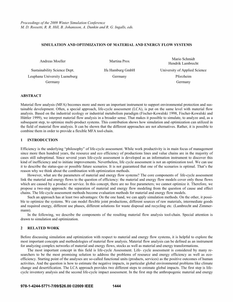
Proceedings of the 2009 Winter Simulation Conference M. D. Rossetti, R. R. Hill, B. Johansson, A. Dunkin and R. G. Ingalls, eds.

SIMULATION AND OPTIMIZATION OF MATERIAL AND ENERGY FLOW SYSTEMS

Andreas Moeller Martina Prox Mario Schmidt Hendrik Lambrecht

Sustainability Science Dept. Ifu Hamburg GmbH University of Applied Science Leuphana University Lueneburg Germany Pforzheim

Germany Germany ABSTRACT

Material flow analysis (MFA) becomes more and more an important instrument to support environmental protection and sus-tainable development. Often, a special approach, life-cycle assessment (LCA), is put on the same level with material flow analysis. Based on the industrial ecology or industrial metabolism paradigm (Fischer-Kowalski 1998, Fischer-Kowalski and Hüttler 1999), we interpret material flow analysis in a broader sense. That makes it possible to simulate, to analyze and, as a subsequent step, to optimize multi-product systems. This contribution shows how simulation and optimization can utilized in the field of material flow analysis. It can be shown that the different approaches are not alternatives. Rather, it is possible to combine them in order to provide a flexible MFA tool-chain.

1 INTRODUCTION

Efficiency is the underlying “philosophy” of life-cycle assessment. While work productivity is in main focus of management since more then hundred years, the resource and eco efficiency of productions lines and value chains are in the majority of cases still suboptimal. Since several years life-cycle assessment is developed as an information instrument to discover this kind of inefficiency and to initiate improvements. Nevertheless, life cycle assessment is not an optimization tool. We can use it to describe the status-quo or possible future scenarios. It is not guaranteed that one of the scenarios is optimal. That’s the reason why we think about the combination with optimization methods.

However, what are the parameters of material and energy flow systems? The core components of life-cycle assessment link the material and energy flows to the question of efficiency: the material and energy flow models cover only those flows which are caused by a product or service. In this concept, there are no free parameters; we cannot optimize it. Therefore, we propose a two-step approach: the separation of material and energy flow modeling from the question of cause and effect chains. The life-cycle assessment methods become evaluation methods for material and energy flow models.

Such an approach has at least two advantages: On the one hand, we can apply simulation methods. On the other, it possi-ble to optimize the systems. We can model flexible joint productions, different sources of raw materials, intermediate goods and required energy, different use phases, different solutions for waste disposal and recycling etc. (Lambrecht and Zimmer-mann).

In the following, we describe the components of the resulting material flow analysis tool-chain. Special attention is drawn to simulation and optimization.

2 RELATED WORK

Before discussing simulation and optimization with respect to material and energy flow systems, it is helpful to explore the most important concepts and methodologies of material flow analysis. Material flow analysis can be defined as an instrument for analyzing complex networks of material and energy flows, stocks as well as material and energy transformations.

The most important concept in this field is life-cycle Assessment. Life- cycle assessment is considered by many re-searchers to be the most promising solution to address the problems of resource and energy efficiency as well as eco-efficiency. Starting point of the analyses are so-called functional units (products, services) as the positive outcomes of human activities. And the question is how to estimate the negative impacts, in particular global environmental problems like climate change and desertification. The LCA approach provides two different steps to estimate global impacts. The first step is life-cycle inventory analysis and the second life-cycle impact assessment. In the first step the anthropogenic material and energy

1444978-1-4244-5771-7/09/$26.00 ©2009 IEEE

Moeller, Prox, Lambrecht and Schmidt

flows, connected to the functional unit, are calculated. The second estimates the impacts in the natural environment. To mod-el anthropogenic material and energy flows, so-called flow charts are used. They consist of linear process specifications and links between them. The flow chart represents nothing else than a set of linear equations (Hejungs 1994; Heijungs and Suh 2002). The solution of these equations are process levels: contributions of the processes. The process levels allow calculating the life-cycle inventory, the exchange of material and energy flows with the natural environment. So, the life-cycle inventory is an “interface” to life-cycle impact assessment. To cover really all relevant material and energy flows it is important to in-clude the whole product life-cycle: from raw material extraction to waste disposal.

Conceptual limitations of life-cycle assessment result from special interpretations of the principle of cause and effect. The cost accounting expert Riebel discusses three different interpretations: the causal interpretation, the final interpretation (or means-end relationship), and the identity principle (Riebel 1990). Life-cycle assessment follows the most common inter-pretation in cost accounting and analyses means-end relationships. Consequently, the first modeling step to determine life-cycle inventories starts with a functional unit or a reference flow. The challenge of this step is to determine all material and energy flows associated with the reference flow. Here another interpretation of the principle of cause and effect comes into play: the causal interpretation (Riebel 1990). The challenge for life-cycle assessment is to bring together these two interpreta-tions. To do so, life-cycle assessment looks at networks of material and energy flows, stocks and transformation processes in a specific perspective: stocks are not allowed, processes are specified in a linear manner by production coefficients, and joint productions are divided into single product processes. So, life-cycle assessment decomposes complex, joint networks of ma-terial and energy flows and stocks into several disjoint models, represented by flow charts, one for each product or functional unit.

Figure 1: Material flow network: de-inking and paper production

The most important conclusion of this examination of LCA concepts is that the most methods are focused on the prob-

lem of causation in material and energy flow networks. This requires to know the flows or processes. Today, several databas-es are in development that provide us with so-called process datasets, e.g. for fuel production, transport, waste treatment, which help to close data gaps (e.g. the Swiss EcoInvent database (Frischknecht 2004)). Despite the attempt to close data gaps by using these databases, data collection remains a big challenge. Whereas the process databases provide in particular data-sets for modeling pre and post chains which is required to represent the whole product life-cycle, internal data is missing. Wohlgemuth proposes the use of simulation approaches to close the internal data gap (Wohlgmuth 2005), and several pro-posals have been made to combine the MFA instruments with enterprise resource planning systems (ERP systems). In the perspective of environmental management accounting (Burritt et al. 2002), the different propositions are complementary: the ERP approach is past-oriented whereas the simulation methods can be used to represent future developments.

1445

Moeller, Prox, Lambrecht and Schmidt In this paper we discuss future-oriented instruments, and the question is how to combine the different components. In

this regard, we recommend the material flow network approach. Material flow networks are based on Petri Nets. They are used to represent period-oriented material and energy flows and stocks. In the perspective of simulation, Petri nets are an dis-crete event simulation approach. Here, the Petri nets are interpreted in a special way: They are as well useful to aggregate all activities within a time period. So, the material flow networks become an accounting system. Its purpose is to trace the ma-terial and energy flows and stocks within a company or between different companies within a value chain (Schmidt et al. 1997). Like Petri nets, material flow networks consist of three different types of model elements. The nodes in the network may be either transitions, visualized as squares, or places, represented by circles. Between these nodes there are arrows as linking elements. Transitions are those objects in a material flow network, where material and energy transformation processes occur. Each transition can, on the one hand, be connected to places from which it is supplied with materials and/or energy (input), and on the other hand be connected to places to which it delivers materials and/or energy (output). Places represent storages in which time transformations take place. As a result a period-oriented material and energy flow model is obtained.

Such a model can be evaluated directly by means of input/output balances. A table lists inputs and outputs of all material and energy flows of the system within the accounting period. It is also possible to analyze only parts of a system, for example single production plants within a value chain. Therefore, input/output balances provide important indicators which character-ize the “metabolic throughput” (Fischer-Kowalski and Hüttler 1999) of systems, relating to a specific time period. Time se-ries of input/output balances can provide information about the development of the material and energy flows of a material and energy flow system, but this approach does not emphasize the dynamic behavior of material and energy flows. Thus, ma-terial flow networks can be characterized as a static material flow analysis method. Nevertheless, the concept of places pro-vides an ideal interface to different simulation methods.

The period-oriented approach helps to overcome two shortcomings of conventional life-cycle inventory analysis: (1) In LCA is not allowed to use non-linear process specifications and (2) the material and energy flows are modeled for exactly for one purpose or functional unit. In the end, multi-product systems are not allowed. Nevertheless, causation is the final purpose of the instruments. It is desirable to combine the two concepts: The material flow networks serve as a data provider of life-cycle assessment (Moeller 2005). In fact, it has been shown that it is possible to extract life-cycle inventories from material flow networks.

Life-cycle inventory analysis requires input data in a specific format. If material flow model should serve as a data pro-vider of life-cycle assessment, it is necessary to transform the period-oriented data into a specific format:

• Identification of all functional units or reference flows, in other words products and services, in the material and energy flow model.

• Input and output flows of all processes (transitions) are interpreted as linear production coefficients. • The reference flows of the processes, mainly the products, must be identified. In case of joint productions allocation

rules have to be applied to obtain single product processes. • On the basis of the network, a flow chart has to be constructed. This graph contains only single product processes. As mentioned above, the flow chart provides the data input of common matrix methods. These methods calculate the

process levels of all involved processes; thereafter, the production coefficients are used to calculate the life cycle inventories.

Period-oriented MFA Material Flow Networks

Life-Cycle Inventory Analysis

Life-Cycle Impact Assessment

Figure 2: A material flow analysis tool-chain

The combination of period- and product-oriented analyses requires some preparations in the material flow model. It must

be possible to identify the reference flows, joint productions and so on. In this regard the production theory of Dyckhoff is of special importance (Dyckhoff 1994, Schmidt 2005). In particular, the categorization of all material and energy flows into 'goods', so-called 'bads' and 'neutrals' links two levels, the object level of material and energy flows, and the level of econom-ic revenues and economic and/or ecological expenditures. In other words, this concept links the two interpretations of the cause-and-effect relationship mentioned above: the causal interpretation on the level of material and energy flows and stocks, and the means-end relationship on the level of revenues and expenditures.

1446


3 THE ROLE OF SIMULATION IN THE MFA TOOL-CHAIN

There are at least two fundamental ways in which simulation can be used in the field of material and energy flow analysis: Discrete event simulation and continuous simulation. The combination of simulation methods and material flow networks be-comes a dynamic material flow analysis approach. The term ‘dynamic’ indicates that these models are focused on the tem-poral dimension of material and energy flows and stocks.

Even though dynamic material flow analysis provides new insights, simulation can as well serve as an important data provider for material flow networks and subsequent life cycle assessment (Wohlgemuth et al. 2001, Mäusbacher et al. 2003). In this regard, the simulation components play an analogous role as workflow management modules in enterprise resource planning systems. An ERP system has to cover and to observe all relevant daily operations so that it can fulfill it purpose as an integrated system that represents all relevant aspects and processes within the company. In other words, the workflow management component is the most important data source for the ERP system (Moeller et al. 2006). Here, it is the same with simulation components: This component replaces the workflow management module to provide future-oriented data.

Several different simulation methods can be applied in the field of material flow analysis. In the following, we present two examples which are close to material flow networks so that the resulting tool-chain provides a consistent modeling envi-ronment.

3.1 Continuous Simulation Example

Continuous simulation is used mainly in chemical industry. Based on the image of “Verbund” optimization, companies try to optimize the complex network chemical processes so that the company can produce the optimal mix of chemical substances. A well-known and not too complex modeling technique in the field of continuous simulation is system dynamics (Hannon and Ruth 2001). System dynamics models contain a number of stocks, shown in diagrams as rectangles, and flows, displayed as double-lined arrows. Any flow directed to the stock increases its level, and the flow going out of the stock decreases its level. The amount of flow in and out is regulated by rates, visualized as “water valves”. So-called connectors, visualized as circles, are used as helper elements to specify user-defined functions and parameters. They are linked to other nodes in the diagram and serve as “information flows”. The information flows control the water valves, and often the stocks in the model are the origin of the information flows. By this means, the modeling approach makes it easy to represent and simulate feed-back systems.

A drawback of system dynamics in the application area of material flow analysis is that it is practically almost impossi-ble to represent material and energy transformations. As well, it is a challenge to deal with a multitude of material and energy flows in system dynamics models. Consequently, system dynamics is indeed discussed in literature, but scarcely applied in practice.

Figure 3: Comparison of material flow networks and system dynamics

But enhancements are possible. Whereas in traditional system dynamics models the water valves control exactly one

flow, the transition specifications in material flow network models allow several input and output flows to be incorporated, and mappings between inputs and outputs can be specified. This approach can be applied in system dynamics models, too (Figure 3). Consequently, such a modeling approach has to deal with more internal flows, new input/output flows, and more stocks. Nevertheless, the underlying simulation methods, in particular the integration methods, are not significantly affected by this extension (Moeller 2005). The material flow network serves as well as an accounting system: It records all flows and stock changes and provides in the end a period-oriented material and energy flow model.

1447


3.2 Discrete Event Simulation Example

However, in many industry sectors different approaches are required. In today’s dynamic business environments “selling a single product is not the goal for most manufacturing organizations. Rather, most enterprises are selling a complete portfolio of products and providing related services and operations over the entire life cycle of those products” (Jones and Deshmukh 2005). MFA concepts and software applications have support these organizations; with regard to environmental protection and sustainability they have to support the analysis of material and energy flows of flexible manufacturing systems. In typical cases of manufacturing organizations, the databases of ERP systems include orders of customers, materials master data, pro-duction jobs, bill of materials (BOM), process plans, production batches and so on. Obviously, all these data categories are relevant determinants of material and energy flows and stocks. But it is not possible to derive material and energy flow data directly. Rather, a data mapper is required: a simulation component which use the data of ERP systems as data input.

One approach to realize such a component is to use Petri nets for the simulation of workshop models. But it is not possi-ble to use them in their original form. In the first phase of Petri net development mathematical foundations and logical analy-sis of concurrent computer systems were in the main focus: liveliness, deadlocks, synchronization etc. However, the analysis of dynamics of complex systems came from a different context – simulation of flexible manufacturing systems: throughput, bottle necks, conflicting requirements etc. A new category of Petri nets, in development since the early 1980s, combine the different approaches. “Time can be incorporated into Petri nets by introducing a delay after a transition is enabled. This re-sults in a timed transition that will have the ability to model tasks or activities. Such a Petri net is known as a Timed Petri net” (Sawhney 1997, Gile and DiCesare 1997) or, more precisely, a timed-transition Petri net. In real systems not all events require delays. To model these events in Petri nets, one would use classical, so-called immediate transitions. Petri net models which consist of exponentially timed transitions and immediate transitions are called generalized stochastic Petri nets (Mar-san et al. 1995). Main attention in the analyses is directed on the dynamics of complex concurrent systems and quantitative performance measures, without disregarding previously researched mathematical foundations.

In context of material flow analysis timed Petri nets cannot serve directly as an underlying concept for the simulation component. How can the conceptual ideas behind workshop models, process plans and BOMs be reformulated in Petri net languages? Valk presented one possible way by introducing object systems. He defines object systems as a pair of two types of Petri nets: the system net and the object net. The object nets replace anonymous tokens in common Petri nets (Valk 1996).

This new kind of Petri nets allows an explicit disjunction of processes and systems. This, in turn, facilitates the applica-tion of Petri nets in today’s organizational structures. With respect to flexible manufacturing systems, the system nets can serve as a conceptual foundation of workshop models, and the object nets can be applied to represent process plans. In such a way, it is possible to bring together two different directions of abstraction: process orientation and systems orientation.

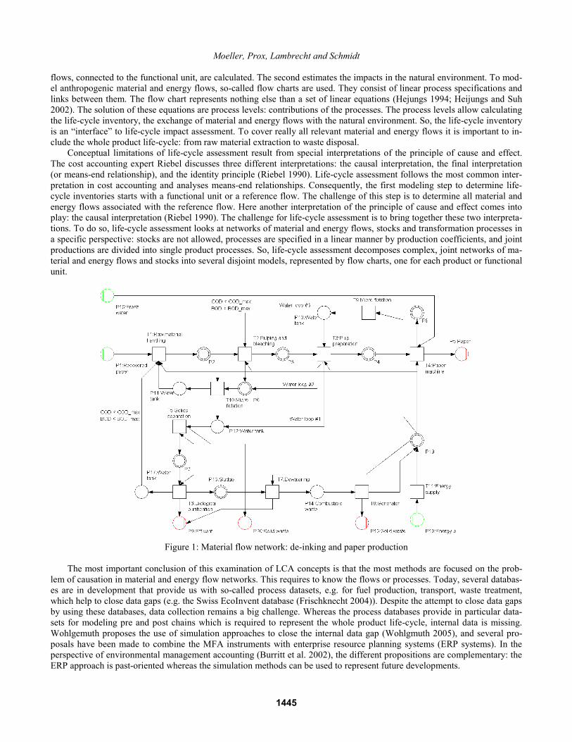
Figure 4: An object net “process plan #1” as a token in a system net “production system” (Moeller 2007)

One remaining question to ask when considering object systems is simply “What’s with material and energy flows?” –

There is a quite simple answer. BOMs are assigned to processes in the process plan or object net respectively. In this setting, the process plan is a dynamic object within a system net. It is possible in such a model to separate material and energy flow

1448


specifications from the location, where they possibly occur. Transition can be specified not only in the system net but also in the object nets, primarily on the basis of BOMs. Firing of transitions in the Petri net simulation is associated with an applica-tion of BOMs.

Data input of object system based simulations include: • A system net – this Petri net represents the workshop model, value chain or similar. The system net consists of sev-

eral functional units (e.g. processors), paths and stocks. To facilitate future-oriented analyses, in particular timed Pe-tri net approaches come into consideration.

• At least one object net – the object nets represent the corresponding process plans in the ERP system. • Loads – the loads stand for production job, the parts to be produced (products or subassemblies), an arrival object,

that specifies the release time of the load, the entry points etc. Each load is associated with an object net as its process plan.

• BOMs – BOMs are assigned to single transitions (processes) in the object net (process plan). Because the bill of ma-terials does not contain physical input and output materials, e.g. waste and emissions, it is necessary to combine them with life cycle inventory datasets.

Petri net simulation is applied to trace the paths of process plans within the workshop model. Firings of conjoint transi-tions within the simulation runs facilitate the application of BOMs and therefore the calculation of material and energy flows. The resulting aggregated data sets serve as a direct data input of the material flow network: the system net becomes a material flow network. After the simulation run, still missing data in the material flow network can be determined by using common calculation procedures for material flow networks, e.g. in case of pre chains and post chains (Moeller 2000).




Petri net based Simulation

Figure 5: Discrete event simulation as a data provider in the material flow analysis tool-chain

The extension of the life-cycle assessment tool-chain by a simulation component allows to presented complex flexible

manufacturing systems. The resulting material and energy flow model can be characterized as descriptive and explanatory models. They describe a status quo, possible a scenario, of the manufacturing system, extended maybe by pre and post chains (Schmidt et al. 2007: 271, Tillman 2000). However, they only describe a selection from possible system states. In particular, the models provide no information about those system conditions under which the system runs optimally to achieve a specific target specification; it says nothing about optimal efficiency. This represent an essential obstacle to implement resource and energy efficient manufacturing systems, as post evaluations have shown (LfU 2004).

Based on these models, the effects of possible improvements can be simulated and evaluated in “what-if” scenarios. The modeling expert has to find the optimal mix of parameters. It makes sense to think about a complementary modeling ap-proach. Here, optimization comes into play.

4 OPTIMAZITION OF MATERIAL AND ENERGY FLOW SYSTEMS

Since a long time, optimization methods are integrated into the canon of decision support instruments, e.g. linear program-ming, non-linear programming or dynamic programming. The methods are used mainly to support decisions in the operative planning sector. For example, linear programming is used to find optimal production programs. The objective function and the constraints can be formulated in a linear form. While there are available algorithms for linear programming which can be used straightforward for example in ERP system modules, solving problems with non-linear objective functions or con-straints are still not a trivial matter.

Normally, the objective function and the constraints are given in a “mathematical” form. In combination with material flow analysis the objective function Z is given by the formalized material and energy flow models presented above. The last step in the tool-chain, life-cycle impact assessment, serves not only as an impact assessment component. The software design process for such a component results in a software specification that allows to specify indicators in a flexible way: In other words, this modeling step is supported by a flexible valuation system component which allows specifying not only indicators which allow estimating e.g. the contribution to climate change but also indicators which can be used to determine e.g. re-source efficiency indicators. In fact, that characterized the relationship between optimization methods and material and ener-gy flow models: The formalized material and energy flow models become a helper function to specify the objective function.

1449


The same applies to the constraints. Within the material and energy flow model, it is possible to specify constraints like max-imum flows, the limits of flexible joint productions etc.




Petri Net-based Simulation

Optimization Cockpit

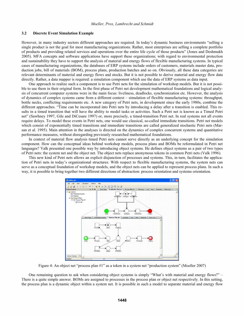
Figure 6: Optimization in the material flow analysis tool-chain

So, the interface between material flow analysis and optimization can be described in the following way: • The material flow model including the evaluation steps life-cycle inventory analysis and life cycle impact assess-

ment specify the objective function of the optimization problem. • Relevant parameters of the material flow network (so-called network parameters) are interpreted as decision va-

riables of the optimization problem. • The material flow model as well allows to specify the constraints. By specifying maximum or minimum flows, the

limits of parameters etc. The optimization algorithm can check whether the selected parameter vector complies with the constraints.

• The optimization can trigger the calculation procedures for the material flow model and it has access to the result of the calculations.

We call the this piece of software an optimization cockpit because it is more than an software adapter. The modeling ex-perts have to specify the co-operation of material flow models and optimization routines.

An optimization run consists of an iterative sequential call of the optimization algorithm, the subsequent recalculation of the material flow network and the evaluation of the new solution. The algorithm has access only to the decision variables / parameters of the model with their constraints and the evaluations of previously found solutions. With this data the algorithm must be able to generate a new solution vector. Whether a new solution vector is actually valid can only decided after recal-culation of the material flow model. Therefore, an optimization run is always simulation based. As a result, in the perspective of the optimization algorithm, the objective function and the constraints become black-boxes. It is a computable function but it is not possible to specify the derivative of the objective function in a direct way.

This constraint is the major reason why not any algorithm can be applied to the optimization problem (Lambrecht and Zimmermann 2008). The optimization algorithms have to provide iterative procedures, and it must be a differentiation free procedure because derivatives cannot be provided by the material flow model. Three different algorithms are already tested: complex procedure, evolution strategy and particle swarm optimization.

4.1 Complex Procedure

The first approach is the complex algorithm presented by Box (Box 1965). The tested variant differs from the original in creating the starting polyhedron and the treatment and evaluation of the constraints.

Starting point for generating the starting polyhedron is a valid solution in the material flow model. The values of the de-cision variables are committed to the algorithm as a vector. The corners (vectors) of the Polyhedron are calculated sequential-ly according to the following schedule: the first vector is the solution vector that is committed to the algorithm. The next vec-tor is obtained by varying the start vector in one dimension. For that purpose the difference between the upper and lower limit is computed in that dimension. This difference is added to the lower limit, factored with a random number from 0 to 1. This ensures that the new vector always hold the explicit constraints of the decision variables. Should be the upper limit positive infinite, the lower limit systemic can never be less than 0, then as the difference the value from the start vector, multiplied by 1.5, is chosen. The factor of 1.5 is an empirical value that should hold the balance between the exploration of the solution area and dispersing of the Polyhedron. The next vector is generated with the same role from the last constructed vector, but with a different dimension. Each dimension is changed at least once during the construction of the Polyhedron.

The advantage of this role of constructing the polyhedron is clear if the constraints, as dependencies between network parameters, are checked during the validation of starting polyhedron. The review of these constraints is not happened in the algorithm, but in the optimization cockpit. If a constraint injured, a value is committed to the algorithm which indicates that

1450


the final solution vector is not a valid solution within the meaning of material flow model. This can also occur if the material flow network is not recalculated correctly with the solution vector because some „hidden“ constraints within the material flow network are being violated.

The previously validated solution vector already contains a valid solution within the meaning of material flow model; at least the first vector is defined as a valid. The invalid solution vector is moved in the dimension in which it differs only from the previous valid solution vector, in a way that the gap in this dimension is halved to the valid vector. This is as long as ap-plied until the vector is seated in a valid area.

The review of the constraints is in the Complex algorithm to Box part of the algorithm. In this implemented variant only the constraints which represent the dependencies between decision variables, and the explicit constraints of decision variables are reviewed from the algorithm. The other constraints are unknown to the algorithm. It is only committed whether a con-straint has been violated, but not which has been violated.

4.2 Evolution Strategy

As another algorithm is the evolutionary strategy to Rechenberg (Rechenberg 1973). It is the (μ + λ) - ES applied, i.e. a gen-eration consists of μ individuals who conceive λ children with λ ≥ μ. After initialization a generational succession co nsists of the steps recombination, mutation, evaluation, correction, and selection. The steps are explained below.

In the initialization, the first generation is generated same role as the starting polyhedron in the Complex. The size of the generation is provided by the user in optimization cockpit. Beginning from the start vector of a valid solution in the material flow model, the other individuals are derived sequentially by random variation of one dimension. Each individual is eva-luated that means the fitness identified, and a solution vector is corrected like done in Complex algorithm, if needed.

The first step to a new generation is the recombination, the conceiving of children. Two individuals from the population as parents are to be recombined to two children. This is repeated until it is at least as many children as individuals in the pop-ulation. The selection of two parents carried out according to the roulette wheel selection. In this method, each individual is assigned with a probability value that is in pro-portion to his fitness. The probability to be selected as parent is most for the individual with the largest fitness. On the other hand, even individuals with low fitness have the chance to be selected as par-ent. Therefore, the genetic diversity is conserved.

The mutation is one of the most important steps in the evolution strategy, because the recombination only mix already known values to new vectors together. Only the mutation creates new values and thus it enables the exploration of the entire solution space. 2/3 of children are randomly selected and mutated. In the evolutionary strategies only a small number is usually added or subtracted to a solution vector. Adding a Gaussian value with the average of 0 and the standard deviation σ to the vector from the recombination νr uses to the mutated vector νm: νm = νr + N(0,σ). The standard deviation is the stan-dard deviation of the parent generation to their average (Nissen 1997).

The children of a generation are valued, i.e. the fitness determined, by recalculating the material flow network with the new vectors and evaluating the objective function subsequently. If a vector is out of bounds, the solution vector is resolved. The point on which the vector shows, is moved in the direction of the center of parents' generation, so that the gap between the vector and the center is shortened about 2/3. This procedure is applied as long as the vector is inside the valid area.

The next generation is chosen by the selection procedure. The μ individuals from the group of parents' generation and their children that have the best fitness are individuals of the new generation.

4.3 Particle Swarm Optimization

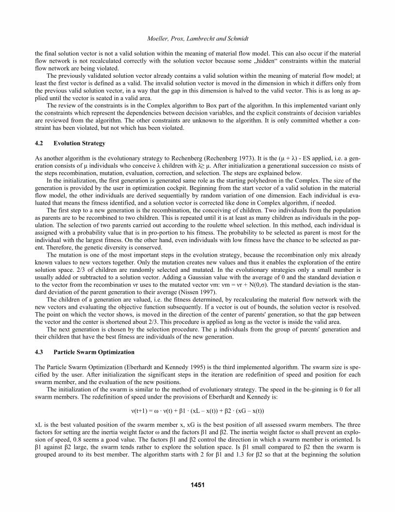
The Particle Swarm Optimization (Eberhardt and Kennedy 1995) is the third implemented algorithm. The swarm size is spe-cified by the user. After initialization the significant steps in the iteration are redefinition of speed and position for each swarm member, and the evaluation of the new positions.

The initialization of the swarm is similar to the method of evolutionary strategy. The speed in the be-ginning is 0 for all swarm members. The redefinition of speed under the provisions of Eberhardt and Kennedy is:

ν(t+1) = ω ∙ ν(t) + β1 ∙ (xL – x(t)) + β2 ∙ (xG – x(t))

xL is the best valuated position of the swarm member x, xG is the best position of all assessed swarm members. The three factors for setting are the inertia weight factor ω and the factors β1 and β2. The inertia weight factor ω shall prevent an explo-sion of speed, 0.8 seems a good value. The factors β1 and β2 control the direction in which a swarm member is oriented. Is β1 against β2 large, the swarm tends rather to explore the solution space. Is β1 small compared to β2 then the swarm is grouped around to its best member. The algorithm starts with 2 for β1 and 1.3 for β2 so that at the beginning the solution

1451


space is explored. About iteration steps, the relationship reversed so that the algorithm is a global search in the beginning and switches to a more local search in the end. The redefinition of the position is determined by:

x(t+1) = ν(t) + x(t)

If the new position is invalid after evaluation, the vector is moved in the direction to the old location. The distance between the new and old position is reduced to half. The procedure will be applied to as long as the vector is still in the invalid area.

4.4 Evaluation

Evaluations of the optimization algorithms have to incorporate not only mathematical aspects: complexity of the algorithms, termination etc. Usability has to be considered too. Is it necessary to be an expert in that field? Or is it possible that life cycle assessment experts can treat optimization as a next steps without learning a completely new modeling paradigm?

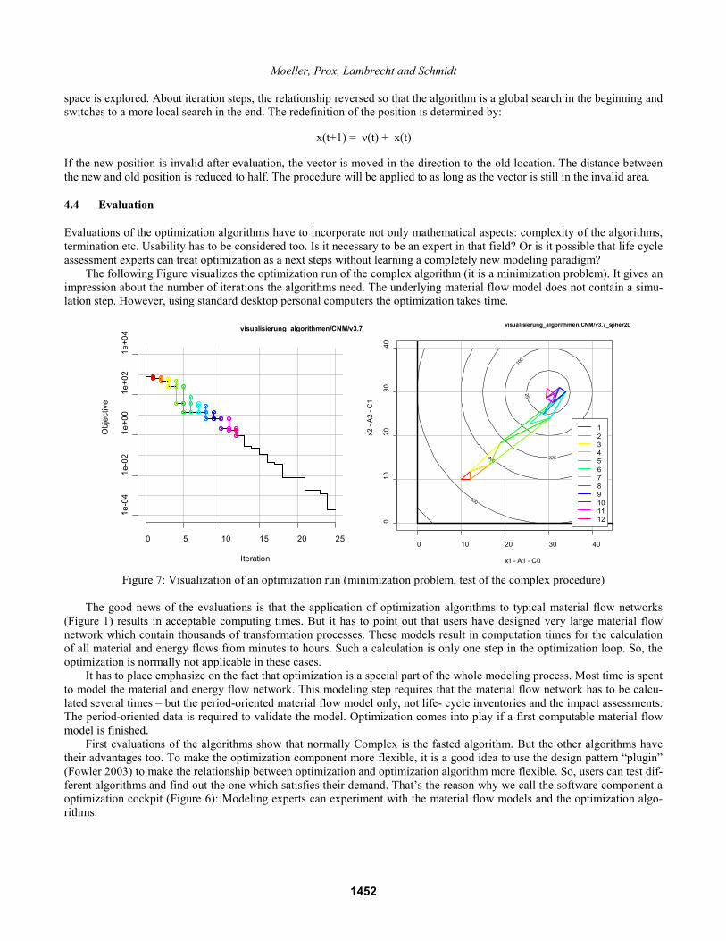
The following Figure visualizes the optimization run of the complex algorithm (it is a minimization problem). It gives an impression about the number of iterations the algorithms need. The underlying material flow model does not contain a simu-lation step. However, using standard desktop personal computers the optimization takes time.

0 5 10 15 20 25

1e-0

41e

-02

1e+0

01e

+02

1e+0

4 visualisierung_algorithmen/CNM/v3.7_

Iteration

Obj

ectiv

e

25

100

225 400

900

0 10 20 30 40

010

2030

40

x1 - A1 - C0

x2 -

A2

- C1

123456789101112

visualisierung_algorithmen/CNM/v3.7_spher2D

Figure 7: Visualization of an optimization run (minimization problem, test of the complex procedure)

The good news of the evaluations is that the application of optimization algorithms to typical material flow networks

(Figure 1) results in acceptable computing times. But it has to point out that users have designed very large material flow network which contain thousands of transformation processes. These models result in computation times for the calculation of all material and energy flows from minutes to hours. Such a calculation is only one step in the optimization loop. So, the optimization is normally not applicable in these cases.

It has to place emphasize on the fact that optimization is a special part of the whole modeling process. Most time is spent to model the material and energy flow network. This modeling step requires that the material flow network has to be calcu-lated several times – but the period-oriented material flow model only, not life- cycle inventories and the impact assessments. The period-oriented data is required to validate the model. Optimization comes into play if a first computable material flow model is finished.

First evaluations of the algorithms show that normally Complex is the fasted algorithm. But the other algorithms have their advantages too. To make the optimization component more flexible, it is a good idea to use the design pattern “plugin” (Fowler 2003) to make the relationship between optimization and optimization algorithm more flexible. So, users can test dif-ferent algorithms and find out the one which satisfies their demand. That’s the reason why we call the software component a optimization cockpit (Figure 6): Modeling experts can experiment with the material flow models and the optimization algo-rithms.

1452


5 CONCLUSION

This line of investigation represents a flow of ideas between optimization, simulation and material flow analysis that goes in all three directions: (1) Optimization algorithms help to really support the improvement of material and energy flow systems. (2) Simulation can be utilized in two different ways. (2a) The simulation approaches allow analyzing the dynamic behavior of material and energy flows and stock.. This is discussed as dynamic material flow analysis (Müller et al. 2004). (2b) In a MFA tool-chain simulation becomes an important data provider the assessment of possible future material and energy flows. (3) Finally, the concepts of material flow analysis provide an attractive new application area of operations research methods and algorithms.

So, its attractive to combine all these research fields to develop new flexible tool sets. The resulting research questions arise from a coming-together of highly different modeling approaches. One is about flexible software environments: plug-in frameworks like Eminia (Wohlgemuth et al. 2008) or openLCA (Ciroth 2008). In this perspective , this article shows how to bring together different plug-ins in such a framework.

Based on more than ten years of experiences in the field of material flow analysis, we believe the road ahead for the wide-spread application of MFA in our societies is quite challenging. There are two fundamental ways to improve the useful-ness of the concepts: firstly by reducing the effort of data gathering and secondly by the enhancement of the capabilities of the tools. Simulation can improve the usefulness in both regards: data gathering and new insights (Dynamic Material Flow Analysis). Optimization is one of the finals step to achieve the underlying purpose of all these efforts. The MFA instruments should be considered and used for one reason only: the improvement of the efficiency and effectiveness of material and ener-gy flow systems.

REFERENCES

Box, M. J. 1965. A new method of constrained optimization and a comparison with other methods. In Comp. J. 8: 42-52. Burritt R., Hahn T. and S. Schaltegger. 2002. Towards a Comprehensive Framework for Environmental Management Ac-

counting. Links Between Business Actors and Environmental Management Accounting Tools. In Australian Accounting Review 12 (2): 39-50.

Ciroth, A., M. Srocka and J. Hildenbrand. 2008. openLCA – Implications of an Emerging Open Source Software for Sustai-nability Assessment. In Environmental Informatics and Industrial Ecology, ed. A. Moeller, B. Page and M. Schreiber. Aachen, Germany: Shaker.

Dyckhoff H. 1994. Betriebliche Produktion (Corporate Production). 2nd ed., Berlin, Heidelberg, New York: Springer (in German).

Eberhardt, R. C. and J. Kennedy. 1995. Particle swarm optimization. Proceedings of IEEE International Conference on Neural Networks, Piscataway, NJ: 1942-1948.

Fischer-Kowalski, M. 1998. Society’s Metabolism – The Intellectual History of Material Flow Analysis, Part I, 1860 – 1970. In Journal of Industrial Ecology 2 (1): 61-78.

Fischer-Kowalski, M. and W. Hüttler. 1999. Society’s Metabolism – The Intellectual History of Material Flow Analysis, Part II, 1970 – 1998. In Journal of Industrial Ecology 2 (4): 107-136.

Fowler, M. 2003. Patterns of Enterprise Application Architecture. Boston et al.: Addison-Wesley. Frischknecht, R. 2004. Ecoinvent Database: Quality Control and User Interfaces for a Web-based Life Cycle Assessment Da-

tabase. In Information Systems for Sustainable Development, ed. L.M. Hilty et al. Hershey, London, Melbourne, Singa-pore: Idea Group Publishing.

Gile, M.R. and F. DiCesare. 1997. Towards Distributed Simulation of Complex Discrete Event Systems Represented by Co-lored Petri Nets: A Review. In Manufacturing and Petri Nets – A workshop within the XVIII International Conference on Applications and Theory of Petri Nets. Toulouse.

Hannon B. and M. Ruth. 2001. Dynamic Modeling. 2nd ed., Berlin, Heidelberg, New York: Springer-Verlag. Heijungs, R. 1994. A generic method for the identification of options for cleaner products. In Ecological Economics 10: 69-

81. HeijungsR. and S. Suh. 2004. The Computational Structure of Life Cycle Assessment. Dordrecht et a.: Kluwer. Jones, A. and A. Deshmukh. 2005. Test Beds for Complex Systems. In Communications of the ACM 48 (5): 45 – 50. Lambrecht, H. and M. Zimmermann. 2008. Combination of Optimization Methods and Material Flow Analysis for Improve-

ment of Operational Material Use (KOMSA): Concept and its Implementation. In Environmental Informatics and Indus-trial Ecology, ed. A. Moeller, B. Page and M. Schreiber. Aachen, Germany: Shaker.

LfU Landesanstalt für Umweltschutz Baden-Württemberg. 2004. Energie- und Stoffstrommanagement. Industrie und Ge-werbe 11 (Energy and material flow management. Industry and business 11). Karlsruhe (in German).

1453


Mäusbacher, M., D. Panic, B. Page, P. Staudt-Fischbach and V. Wohlgemuth. 2003. Kopplung von Stoffstromnetzen mit ei-nem Simulationsmodell der Produktionsendstufe eines Halbleiter-Herstellers. In Simulation in Umwelt- und Geowissen-schaften, ed. J. Wittmann and J. Maretis. Aachen: Shaker (in German).

Marsan M.A. et al. 1995. Modelling with Generalized Stochastic Petri Nets. Chichester, New York: John Wiley and Sons. Moeller, A. 2005. Dynamic Material Flow Analysis as Part of a Life Cycle Assessment Tool Chain. In Challenges for Indus-

trial Production, ed. J. Geldermann, M. Treitz and O. Rentz. Karlsruhe: Universitaetsverlag Karlsruhe. Moeller, A. 2000. Grundlagen stoffstrombasierter Betrieblicher Umweltinformationssysteme (Fundations of material flow

based environmental management information systems). Bochum, Germany: Projekt-Verlag (in German). Moeller, A., Prox, M. and T. Viere. 2006. Computer Support for Environmental Management Accounting. In Sustainability

Accounting and Reporting, ed. S. Schaltegger, M. Bennett and R. Burritt. Dordrecht: Springer. Müller, D.B., H.-P. Bader and P. Baccini. 2004. Long-term Coordination of Timber Production and Consumption Using a

Dynamic Material and Energy Flow Analysis. In Jounral of Industrial Ecology 8 (3): 65-87. Nelder, J. A. and R. A. Mead. 1965. A Simplex Method for Function Minimization. In Computer Journal 7: 308-313. Nissen, V. 1997. Einführung in evolutionäre Algorithmen: Optimierung nach dem Vorbild der Evolution, Braunschweig,

Germany: Vieweg (in German). Rechenberg, I. 1973. Evolutionsstrategie – Optimierung technischer Systeme nach Prinzipien der biologischen Evolution.

Stuttgart: Fommann-Holzboog (in German). Riebel P. 1990. Einzelkosten- und Deckungsbeitragsrechnung (Direct Costing). 6. ed., Wiesbaden, Germany: Gabler (in

German). Sawhney A. 1997. Petri Net based Simulation of Construction Schedules. In Proceedings of the 1997 Winter Simulation Con-

ference, ed. S. Andratottir et al. Atlanta: 1111 – 1118. Schmidt M. 2005. A production-theory-based framework for analysing recycling systems in the e-waste sector. In Environ-

mental Impact Assessment Review 25 (5): 505-524. Schmidt M., A. Möller, J. Hedemann and P. Müller-Beilschmidt. 1997. Environmental Material Flow Analysis by Network

Approach. In Umweltinformatik’97, ed. W. Geiger et al. Marburg: Metropolis. Schmidt, M., H. Lambrecht and A. Möller. 2007. Opimisation Approaches in Material Flow Models of Manufacturing Sys-

tems. In Environmental Informatics and Systems Research, ed. O. Hryniewicz, J. Studzinski and M. Romaniuk. Aachen: Shaker.

Tillman, A. 2000. Significance of decision-making for LCA methodology. In Environ. Impact Assessment Rev. 20 (1): 113-123.

Valk, R. 1996. On Processes of Object Petri Nets. Report No. 185/96 of the Department of Informatics, University of Ham-burg, Germany.

Wohlgemuth, V. 2005. Komponentenbasierte Unterstützung von Methoden der Modellbildung und Simulation im Einsatzkon-text des betrieblichen Umweltschutzes (Component-based software support of modeling and simulation methods in the context of corporate environmental protection). Aachen: Shaker (in German).

Wohlgemuth, V., L. Bruns and B. Page. 2001. Simulation als Ansatz zur ökologischen und ökonomischen Planungsun-terstützung im Kontext betrieblicher Umweltinformationssysteme (BUIS). In Sustainability in the Information Society, ed. L. M. Hilty and P. W. Gilgen. Marburg: Metropolis (in German).

Wohlgemuth, V., T. Schnackenbeck, D. Panic and R.-L. Barling. 2008. Development of an Open Source Framework as a Ba-sis for Implementing Plugin-Based Environmental Management Information Systems (EMIS). In Environmental Infor-matics and Industrial Ecology, ed. A. Moeller, B. Page and M. Schreiber. Aachen: Shaker.

AUTHOR BIOGRAPHIES

ANDREAS MOELLER is a Professor for environmental informatics and digital media within the sustainability sciences department of the Leuphana University Lueneburg, Germany. His Ph.D. is from the University of Hamburg in 2000. His re-search interests include material flow analysis methods and concepts, in particular around material flow networks, computer support for material flow analysis and the role of these instruments in communication processes. His email is <[email protected]> MARTINA PROX is marketing director and member of the research staff of the institute for environmental informatics, Hamburg. Her research interests include the standardization of material and energy flow based cost accounting systems like material flow cost accounting. Main focus of attention is on learning and knowledge acquisition. Her email is <m.prox@ifu>

1454


MARIO SCHMIDT is a Professor for Operations Research in the Institute for Applied Research (IAF) – Team “Material Flow and Environmental Management”, University of Applied Science, Pforzheim. Research interests: The analysis of ma-terial and energy flows in operational production or product systems and the optimization concerning economic and ecologi-cal effects,. efficient use of resources – from both a financial and an environmental perspective, energy and material flow management. He and his research group are involved in numerous research projects, e.g., for the German Federal Ministry of Education and Research (BMBF) and for the State of Baden-Wuerttemberg, and occasionally lead larger research groups. In addition, he cooperates with large companies as well as small and medium enterprises, having successfully consulted on many projects. His email is <[email protected]> HENDRIK LAMBRECHT is PhD student at the Institute for Applied Research, University of Applied Science (IAF) – Team “Material Flow and Environmental Management”, Pforzheim. His research interest is in the area of optimization of ma-terial and energy flow systems. His email is <[email protected]>

1455

Simulation and Optimization of Material and Energy Flow Systems

Documents

Transcript of Simulation and Optimization of Material and Energy Flow Systems