Simulation Modelling Practice and Theory 19 (2011) 911–923

Contents lists available at ScienceDirect

Simulation Modelling Practice and Theory

journal homepage: www.elsevier .com/ locate/s impat

A risk-averse approach to simulation optimization with multiple responses

Ebru AngünDept. of Industrial Engineering, Galatasaray University, Ortaköy 34357, _Istanbul, Turkey

a r t i c l e i n f o

Article history:Received 19 November 2009Received in revised form 20 November 2010Accepted 1 December 2010Available online 15 December 2010

Keywords:Average Value-at-RiskDiscrete-event dynamic simulationTaguchi’s robustnessMultivariate robust parameter designLinear regression

1569-190X/$ - see front matter � 2010 Elsevier B.Vdoi:10.1016/j.simpat.2010.12.006

E-mail address: eangun@gsu.edu.tr

a b s t r a c t

This article considers risk-averse simulation optimization problems, where the risk mea-sure is the well-known Average Value-at-Risk (also known as Conditional Value-at-Risk).Furthermore, this article combines Taguchi’s robustness with Response Surface Methodol-ogy (RSM), which results in a novel, robust RSM to solve such risk-averse problems. In casethe risk-averse problem is convex, the conic quadratic reformulation of the problem is pro-vided, which can be solved very efficiently. The proposed robust RSM is applied to both aninventory optimization problem with a service-level constraint and a call-center problem;the results obtained for the risk-averse problem and its benchmark problem, where the riskmeasure is the variance, are intuitively sound and interesting.

� 2010 Elsevier B.V. All rights reserved.

1. Introduction

Robust Parameter Design (RPD) has been successfully applied to improve the quality of products since the mid 1980s,particularly after the work of G. Taguchi in US companies; see Taguchi [30,31]. In his RPD, Taguchi focuses on physical exper-iments, and he distinguishes between two types of variables, namely decision and environmental variables, among thosevariables that contribute to the experiments. His technique consists of determining the levels of the decision variables thatreduce the sensitivity of the process to variations in the environmental variables, thus increasing the robustness of theprocess.

Although Taguchi’s approach to RPD has become popular, his statistical techniques have received considerable criticismfrom many statisticians including Nair [22] and Myers et al. [20]; in particular, Vining and Myers [32] show inefficiency ofTaguchi’s signal-to-noise ratios under certain conditions; i.e., regression metamodels may provide statistically more rigorousalternatives to signal-to-noise ratios.

Classic Response Surface Methodology (RSM) focuses on the optimization of the mean of a single random response ofindustrial processes; see, for example, Myers et al. [20]. This approach is known to be risk-neutral, since the mean perfor-mance measure is optimized on average without taking into account, for example, its estimated variance. In RSM, thisrisk-neutrality problem is first detected by Myers and Carter [19], who introduce the Dual Response Surface (DRS) approach.The DRS approach is further extended by Vining and Myers [32]. Basically, in the DRS approach, two regression metamodelsare fitted for the mean and the variance of a single random response, and then the two fitted regression metamodels areoptimized simultaneously in a region of interest. Furthermore, the DRS approach uses Lagrange multipliers to explore can-didate solutions in a manner similar to ridge regression.

The DRS approach has received a great deal of attention from researchers. Fan and Del Castillo [7] present a methodologyfor building a so-called optimal region for the global optimal operating conditions to address the inherent sampling errors inDRS. Ross et al. [28] extend the DRS such that the decision-makers’ preferences can be incorporated into the selection of the

. All rights reserved.

912 E. Angün / Simulation Modelling Practice and Theory 19 (2011) 911–923

Lagrange multipliers. Myers et al. [21] consider a general DRS in which the performance measure is a nonnormal response.Rajagopal et al. [24] provide a Bayesian approach to DRS. Lee and Park [17] obtain the robust optimal operating conditionsusing both fully and partially observed real-life data. Lee et al. [18] construct a robust design model which is resistant tocontaminated data and to departures from the normality, and Köksoy and Yalcinoz [16] use a genetic algorithm with arith-metic crossover to solve their DRS problem.

Classic RPD assumes physical experiments. Then, experimental designs have been devised for physical settings, but inpractical situations environmental variables are difficult, if not impossible, to control. Thus only a few of them, and withfew levels, are usually included in the design. Recently, Dellino et al. [4] extend the robust RSM in Myers et al. [20] in manydirections including the use of simulation outputs. This is an important contribution since simulation experiments enablethe exploration of many values for the decision and environmental variables, and many combinations of these values. There-fore, the major purpose of this article is to contribute to the robust RSM methodology in Dellino et al. [4] in the followingthree directions:

� Dellino et al. [4] have a mean-risk approach where they consider standard deviation as their risk measure. The standarddeviation (and variance), however, considers both the upper and lower deviations from the mean, whereas in many casesonly one-sided deviation is important; see Yin et al. [34]. Hence, this article replaces the standard deviation by the AverageValue-at-Risk (also known as the Conditional Value-at-Risk) from the financial engineering literature, which is known toconsider only one-sided deviations. Furthermore, variance is considered as the risk measure of the benchmark problem.� Dellino et al. [4] solve their risk-averse problem through MATLAB’s fmincon function without investigating its convexity.

This article, however, provides a very practical way to check for the convexity. Furthermore, in case the risk-averse prob-lem is found to be convex, it provides a conic quadratic reformulation, which can then be solved very efficiently through,for example, CVX (a free-of-charge, structured convex programming solver).� Dellino et al. [4] consider deterministic simulation whereas this article considers discrete-event dynamic (and hence sto-

chastic) simulation. The use of stochastic simulation enables to observe many times the outputs of the multiple responsesat the same input combinations through replicates, which is not meaningful for deterministic simulation. This is impor-tant since the average outputs of the multiple responses follow asymptotically a multivariate normal distribution becauseof the classic Central Limit Theorem, provided that the multiple responses have finite variances.

The proposed robust RSM is applied to the problem with the Average Value-at-Risk as its risk measure and the benchmarkproblem with variance as its risk measure on two classic cases, namely an (s, S) inventory optimization case with a service-level constraint and a call-center case, which are originally investigated by Bashyam and Fu [2] and Kelton et al. [11],respectively.

The remainder of this article is organized as follows. Section 2 introduces the problem formulation which considers Aver-age Value-at-Risk as its risk measure. Section 3 presents the steps of the robust RSM; the emphasis in this section is on theoptimization step where the benchmark problem and the conic quadratic reformulation are introduced. Section 4 givesnumerical results of the risk-averse problem with the Average Value-at-Risk and its benchmark on the inventory optimiza-tion and the call-center optimization. Section 5 gives conclusions and possible future research directions.

2. The risk-averse problem formulation

This article considers the following optimization problem:

minimized2Rk

E½f0ðd; e;xÞ�

subject to E½fjðd; e;xÞ� 6 aj j ¼ 1; . . . ; rð1Þ

where E denotes the expectation operator, the fi (i = 0, . . . ,r) are r + 1 simulation outputs (responses), d = (d1, . . . ,dk)T is thek � 1 vector of decision variables, e = (e1, . . . ,eh)T is the h � 1 vector of environmental variables, x is the simulation’s seedvector, and the aj are r deterministic threshold levels. The multivariate distribution of e is assumed to be known (i.e., esti-mated from historical data) with mean vector le—which is not necessarily a zero-vector—and covariance matrix Re—whichis not necessarily a scaled identity matrix.

The following assumptions, which are common in black-box simulation optimization, are made for the problem in (1): (i)The fi are continuous and continuously differentiable with respect to d for almost all x in the interior of the feasible regiondefined by the constraints. (ii) The mathematical formulations of the fi are unknown to the decision-maker; at a given d, e,and x, only their evaluations can be obtained through a simulation program. (iii) The expectations and the variances of the fi

are finite.The drawback of the stochastic optimization problem in (1) is that it minimizes the random response f0 on average, which

is usually called a risk-neutral approach. A classic approach that takes risk into account is the expected utility theory, whichminimizes E½uðf0ðd; e;xÞÞ� where u is assumed to be a convex and nondecreasing disutility function. The obvious difficultywith this approach is to elicit an appropriate u.

E. Angün / Simulation Modelling Practice and Theory 19 (2011) 911–923 913

Yet another way of accounting for risk is to use a mean-risk approach, where the variance or the standard deviation isusually considered as the risk measure; see, for example, the recent article by Dellino et al. [4] which uses a mean-standarddeviation approach. A deficiency of variance (and also of standard deviation) as a risk measure is that it treats the excess overthe mean equally as the shortfall (‘‘shortfall’’ is the term used in financial engineering; see, for example, Rockafellar andUryasev [27]).

To deal with risk, this article adopts a mean-risk approach, but as the risk measure, it uses the Average Value-at-Risk (alsoknown as the Conditional Value-at-Risk) from financial engineering, which is defined as follows. Let Z be a random variablerepresenting the losses. Then, the Average Value-at-Risk at reliability level (1 � s) with s 2 (0,1)—denoted by AV@R1�s—isdefined by

AV@R1�sðZÞ :¼ inft2Rft þ s�1E½ðZ � tÞþ�g ð2Þ

where inf denotes the greatest lower bound (infimum), and (x)+ denotes max{x,0}; see Shapiro et al. [29, p. 262].Taking into account the risk-aversion, the problem in (1) is reformulated as

minimized2Rk

E½f0ðd; e;xÞ� þ kAV@R1�s½f0ðd; e;xÞ�

subject to E½fjðd; e;xÞ� 6 aj j ¼ 1; . . . ; rð3Þ

where k 2 [0,1] is a scalar reflecting the degree of risk-aversion of the decision-maker; i.e., k = 0 implies total risk-neutralityand k = 1 implies risk-aversion at the full extent.

Remark 1. It is well-known that AV@R1�s(.) is convex and monotone [29, p. 261]. Hence, the superposition AV@R1�s[f0(d, e,x)] is convex in d, if f0(d, e, x) is convex in d for almost all x.

The convexity issue in Remark 1 is important in the optimization phase, and it will determine the type of the algorithm tobe used to optimize (3).

3. The robust RSM heuristic for multiple responses

This section summarizes the steps of the proposed robust RSM for multiple responses, which consist of: (i) approximatingthe unknown functions fi in (3) through second-order polynomial metamodels; (ii) estimating the unknown coefficients,testing for lack-of-fit, and halving the experimental area size and redoing all estimations if lack-of-fit is found; (iii) replacingthe fi by their approximations and minimizing the resulting problem through conic quadratic programming or global optimi-zation, depending on the convexity of the fitted metamodels. Most of the procedures in the first two steps are standard in therobust RSM; hence, they are presented only for the sake of completeness and not in full detail, and the author refers to otherworks in this field for further details. The third step, however, presents one of the contributions of this article to the robustRSM; hence, it is fully detailed.

3.1. Approximations by second-order metamodels and design of experiments

In Step 1, analogous to Myers et al. [20] and Dellino et al. [4], the fi are approximated through the following second-orderregression metamodels

yiðd; e; �iÞ ¼ bi;0 þ bTi dþ cT

i eþ dT Bidþ dTDieþ �i i ¼ 0; . . . ; r � 1 ð4Þ

where yi is the regression predictor of the ith output, bi;0 is the unknown intercept of the ith metamodel, bi = (bi;1, . . . ,bi;k)T

and ci = (ci;1, . . . ,ci;h)T are k � 1 and h � 1 vectors of the unknown coefficients of the ith metamodel, Bi is the k � k symmetricmatrix (i.e., Bi ¼ BT

i ) with the main quadratic effects bi;k0 ;k0 (k0 = 1, . . . ,k) of the ith metamodel on the main diagonal and half ofits interaction effects bi;k0 ;k00=2 (k00 = 1, . . . ,k and k00 – k0) on the off-diagonal, Di is the k � h matrix which has the control-by-noise interaction effects of the ith metamodel as its entries, and �i is the residual of the ith metamodel. The vector of r + 1residuals � = (�0, . . . ,�r)T is usually assumed to be multivariate normal with mean vector l� = 0 and covariance matrix R�.

To fit the metamodel in (4), classic RSM uses a central composite design (CCD), which consists of a resolution-V designaugmented by a central point and 2(k + h) positive and negative axial points. This CCD enables the unbiased least-squaresestimation of all unknown coefficients in (4), provided that (4) is a valid metamodel (i.e., l�i

¼ 0); the validity of the meta-model i is tested in Section 3.2. For more details on the CCD, the author refers to Kleijnen [13, pp. 50–51] and Myers et al.[20].

Let n denote the number of distinct scenarios (input combinations), and let ml denote the number of replicates at scenariol (l = 1, . . . ,n), which means that the scenario l is simulated ml times using non-overlapping streams of pseudo-random num-bers (PRN). These ml can take large values (i.e., ml P 30) if the simulation program is not time-consuming and the compu-tational budget is not tight. Then, the total number N of runs is given by N = m1 + � � � + mn. In this article, it is assumed thatml = m is fixed for all scenarios and m P 30.

914 E. Angün / Simulation Modelling Practice and Theory 19 (2011) 911–923

3.2. Estimation of the unknown parameters and lack-of-fit tests

To estimate the unknown coefficients of all r + 1 metamodels simultaneously, the decision-maker uses generalized least-squares (GLS). However, under some conditions, Rao [25] proves that the GLS estimator reduces to the following ordinaryleast-squares (OLS) estimator per response i

fi ¼ ðXT XÞ�1XT �f i i ¼ 0; . . . ; r ð5Þ

where fi is the q � 1 vector of all unknown coefficients in the ith metamodel, q = 1 + k + h + (k2 + k)/2 + kh, X is the n � q ma-trix of explanatory variables common to all r + 1 responses, and �f i is the n � 1 vector of averaged simulation outputs; i.e., thefirst component is the average of the m independent, identically distributed (IID) outputs at scenario 1, the second compo-nent is the average of the m IID outputs at scenario 2, and so on.

The covariance matrix Rfiof fi is given by

Rfi¼ �ri;iðXT XÞ�1 i ¼ 0; . . . ; r ð6Þ

where �ri;i ¼ ri;i=m is the variance of �f i. Classic RSM usually estimates the covariances ri;i0 between the responses i and i0

(i0 = 0, . . . ,r) through mean squared residuals; see Khuri [12, p. 385]. An alternative is to estimate ri;i0 through the samplecovariance, which requires replicates but does not depend on the metamodel. The sample covariance ri;i0 ;l at scenario l is gi-ven by

ri;i0 ;l ¼Pm

p¼1ðf i;l;p ��f i;lÞðf i0 ;l;p �

�f i0 ;lÞ

m� 1ð7Þ

where f i;l;p and f i0 ;l;p are the pth replicates of the outputs simulated at scenario l of the responses i and i0, and �f i;l and �

f i0 ;l are thelth components of �f i and �f i0 . Because of the assumed constant covariances across the n scenarios, the estimators in (7) arepooled to obtain ri;i0 , which estimates ri;i0 [13, p. 25]:

ri;i0 ¼Pn

l¼1ðm� 1Þri;i0 ;lPnl¼1ðm� 1Þ

¼Pn

l¼1ri;i0 ;l

nð8Þ

Now, �ri;i0 ¼ ri;i0=m and �ri;i in (6) can be estimated by setting i = i0.After fitting the metamodels, classic RSM generally tests for lack-of-fit. This is usually achieved through classic F lack-of-

fit test; see Myers et al. [20]. This F test requires the normality assumption for the random responses fi. On the other hand, totest for lack-of-fit, Dellino et al. [4] use one-leave-out cross-validation in addition to t-test combined with Bonferroni’sinequality. The former test does not require normality assumption for the fi, and the latter test is known to be robust againstnon-normality. Hence, their approach is more generally applicable than classic F test.

To test for lack-of-fit, this article uses classic F test combined with Bonferroni’s inequality. Note that the variances ri;i ofthe fi are assumed to be finite (see page 4), and each component of the �f i is the average of a large (i.e., m) number of IID out-puts. Then, the classic Central Limit Theorem concludes that the �f i is asymptotically multivariate normal and so is the fi withthe mean vector estimated through (5) and the covariance matrix estimated through (6). However, to use (9), the vector f i

whose components are the individual replicates f i;l;p in (7) has to be multivariate normal. This holds either when the f i;l;p arelong-run averages of simulation outputs—then, f i is asymptotically multivariate normal because of the Functional CentralLimit Theorem [13, p. 79]—(see also the numerical examples), or when the vector f = (f0, . . . , fr)T is assumed to be multivariatenormal. Then, under H0 : l�i

¼ 0, the following statistic has an F-distribution with n � q and n(m � 1) degrees of freedom:

Fi;n�q;nðm�1Þ ¼nðm� 1Þðn� qÞ

ð�f i � yiÞTð�f i � yiÞ

�ri;i

ð9Þ

where yi ¼ Xfi. The type-I error rate of each response i is chosen as ai = a/(r + 1), and according to Bonferroni’s inequality, thisa constitutes an upper bound on the actual type-I error rate of all r + 1 tests.

Now, if the p-value of at least one test in (9) does not exceed ai, then this article first halves the size of the previous exper-imental area to reduce bias, then repeat all estimations from (5) to (8), and tests for lack-of-fit again through (9) until all r + 1metamodels are valid. An alternative approach would be to fit more complicated metamodels such as Kriging metamodels[5], but this issue is left for future research. On the other hand, if lack-of-fit is not found (i.e., the p-value exceeds ai for allr + 1 tests), then robust RSM proceeds to the optimization phase in Step 3.

3.3. Optimization

Analogous to Dellino et al. [4] and Myers et al. [20], instead of using directly the metamodel in (4), its expectation andvariance are obtained:

E. Angün / Simulation Modelling Practice and Theory 19 (2011) 911–923 915

EðyiÞ ¼ bi;0 þ bTi dþ cT

i le þ dT Bidþ dTDile

varðyiÞ ¼ var½ðcTi þ dTDiÞe� þ r2

�i

¼ ðcTi þ dTDiÞReðci þ DT

i dÞ þ r2�i

ð10Þ

where the unknown bi;0, bi, ci, Bi, and Di are estimated through (5), and r2�i

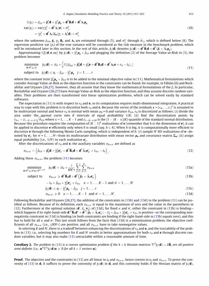
through �ri;i, which is defined below (8). Theregression predictor var (yi) of the true variance will be considered as the risk measure in the benchmark problem, whichwill be introduced later in this section. In the rest of this article, yiðdÞ denotes yiðdÞ ¼ dT bBidþ dTðbi þ bDileÞ.

Approximating E½fiðd; e;xÞ� by yiðdÞ þ cTi le þ bi;0 and plugging the definition (2) of the Average Value-at-Risk in (3), the

problem becomes

minimized2Rk ;t02R

y0ðdÞ þ kt0 þks

E½ðb0;0 þ bT0dþ cT

0eþ dT B0dþ dTD0eþ �0 � t0Þþ�

subject to yjðdÞ 6 aj � bj;0 � cTj le j ¼ 1; . . . ; r

ð11Þ

where the constant term cT0le þ b0;0 is to be added to the minimal objective value in (11). Mathematical formulations which

consider Average Value-at-Risk as the objective function or the constraints can be found, for example, in Fábián [6] and Rock-afellar and Uryasev [26,27]; however, they all assume that they know the mathematical formulations of the fi. In particular,Rockafellar and Uryasev [26,27] have Average Value-at-Risk as the objective function, and they assume discrete random vari-ables. Their problems are then transformed into linear optimization problems, which can be solved easily by standardsoftwares.

The expectation in (11) is with respect to �0 and e, so its computation requires multi-dimensional integration. A practicalway to cope with this problem is to discretize both �0 and e. Because the vector of the residuals � = (�0, . . . ,�r)T is assumed tobe multivariate normal and hence �0 is normal with mean l0 = 0 and variance �r0;0, �0 is discretized as follows: (i) divide thearea under the normal curve into K intervals of equal probability 1/K; (ii) find the discretization points by�0;j ¼ z1�ðK�jÞ=K

ffiffiffiffiffiffiffiffi�r0;0

qwhere j = 1, . . ., K � 1 and z1�(K�j)/K is the (1 � (K � j)/K)-quantile of the standard normal distribution.

Because this procedure requires the computation of (K � 1)h realizations of e (remember that h is the dimension of e), it canbe applied to discretize e efficiently only when h is small (say, h 6 4). When h is big, it is computationally more efficient todiscretize e through the following Monte Carlo sampling, which is independent of h: (i) sample N0 IID realizations of e—de-noted by e�n0 for n0 = 1, . . ., N0—from its multivariate distribution with mean vector le and covariance matrix Re; (ii) assignequal probability (i.e., 1/N0) to each realization e�n0 .

After the discretizations of �0 and e, the auxiliary variables v0;j;n0 are defined as

v0;j;n0 ¼ b0;0 þ bT0dþ cT

0e�n0 þ dT bB0dþ dT bD0e�n0 þ �0;j � t0

� �þ: ð12Þ

Adding these v0;j;n0 , the problem (11) becomes

minimized2Rk ;t02R;v02RðK�1ÞN0

y0ðdÞ þ kt0 þk

KN0sXK�1

j¼1

XN0n0¼1

v0;j;n0 ð13aÞ

subject to v0;j;n0 P dT bB0dþ dTb0 þ bD0e�n0� �

ð13bÞ

� t0 þ b0;0 þ cT0e�n0 þ �0;j j ¼ 1; . . . ;K � 1 and n0 ¼ 1; . . . ;N0

yjðdÞ 6 aj � cTj le � bj;0 j ¼ 1; . . . ; r ð13cÞ

v0;j;n0 P 0 j ¼ 1; . . . ;K � 1 and n0 ¼ 1; . . . ;N0: ð13dÞ

Following Rockafellar and Uryasev [26,27], the addition of the constraints in (13b) and (13d) to the problem (11) can be jus-tified as follows. Because of its definition, each v0;j;n0 is equal to the maximum of zero and the value in the parenthesis in(12). Furthermore at the optimal solution ðd�; t�0;v�0Þ of (13d), for fixed j and n0, either the constraint in (13b) is binding—which happens if its right-hand-side d�T bB0d� þ d�Tðb0 þ bD0e�n0 Þ � t�0 þ b0;0 þ cT

0e�n0 þ �0;j is positive—or the corresponding non-negativity constraint in (13d) is binding (or both constraints are binding if the right-hand-side in (13b) equals zero), and thishas to hold for all j and n0. This last result follows from the facts that (13d) is a minimization problem, the objective coef-ficients of all v0;j;n0 (i.e., k/KN0s) are positive, and all v0;j;n0 have to take nonnegative values.

In selecting K and N0, there is a tradeoff between enhancing the discretizations of �0 and e, and the tractability of the prob-lem in (13); i.e., selecting big numbers for K and N0 results in better approximations for both �0 and e through discrete ran-dom variables, but it may also make (13) untractable within a reasonable amount of time.

Corollary 2. The problem in (13) is a convex optimization problem if the k � k Hessian matrices r2yiðdÞ ¼ 2bBi are all positivesemi-definite (i.e., uTr2yiðdÞu P 0 for all k � 1 vectors u).

Proof. The objective and the constraints in (13) are all linear in t0 and v0;j;n0 , hence convex in t0 and v0;j;n0 . To prove the con-vexity of (13) in d, it suffices to prove the convexity of yiðdÞ in d, and this convexity holds if the Hessian matrix of yiðdÞ,

916 E. Angün / Simulation Modelling Practice and Theory 19 (2011) 911–923

namely r2yiðdÞ ¼ bBi þ bBTi ¼ 2bBi is positive semi-definite. Now the convexity of (13) follows from the fact that the intersec-

tion of an arbitrary number of convex sets is convex. h

In the following theorem, one of the main results of this article is presented, namely the reformulation of (13) as a conicquadratic problem; i.e., a problem with a linear objective function and finitely many conic constraints, where these con-straints are u-dimensional Lorentz cones defined by Lu :¼ x ¼ ðx1; . . . ; xuÞ 2 Ru : xu P

ffiffiffiffiffiffiffiffiffiffiffiffiffiffiffiffiffiffiffiffiffiffiffiffiffiffiffiffiffiffiffiffix2

1 þ � � � þ x2u�1

qn oBen-Tal and

Nemirovski [3, p. 79].

Theorem 3. Suppose that all Hessian matricesr2yiðdÞ are positive semi-definite. Then, the problem in (13) can be reformulated asthe following conic quadratic optimization problem

minimizex02Rkþ1þN0 ðK�1Þ ;z12R

z1 ð14aÞ

subject to

ffiffiffiffiffiffiffiffiffiffiffiffiffiffiffiffiffiffiffiffiffiffiffiffiffiffiffiffiffiffiffiffiffiffiffiffiffiffiffiffiffiffiffiffiffiffiffiffiffiffiffiffidT

0d0 þz1 � xT

0q0 � 1� �2

4

s6

ffiffiffiffiffiffiffiffiffiffiffiffiffiffiffiffiffiffiffiffiffiffiffiffiffiffiffiffiffiffiffiffiffiffiffiz1 � xT

0q0 þ 1� �2

4

sð14bÞffiffiffiffiffiffiffiffiffiffiffiffiffiffiffiffiffiffiffiffiffiffiffiffiffiffiffiffiffiffiffiffiffiffiffiffiffiffiffiffiffiffiffiffiffiffiffiffiffiffiffiffiffiffiffiffiffiffiffiffiffiffiffiffiffiffi

dT0d0 þ

xT0q00;j;n0 � c0;j;n0 � 1

� �2

4

vuut6

ffiffiffiffiffiffiffiffiffiffiffiffiffiffiffiffiffiffiffiffiffiffiffiffiffiffiffiffiffiffiffiffiffiffiffiffiffiffiffiffiffiffiffiffiffiffiffiffiffiffixT

0q00;j;n0 � c0;j;n0 þ 1� �2

4

vuutj ¼ 1; . . . ;K � 1 and n0 ¼ 1; . . . ;N0 ð14cÞffiffiffiffiffiffiffiffiffiffiffiffiffiffiffiffiffiffiffiffiffiffiffiffiffiffiffiffiffiffiffiffiffiffiffiffiffiffiffiffiffiffiffiffiffiffiffiffiffi

dTj dj þ

ðcj þ dT qj � 1Þ2

4

s6

ffiffiffiffiffiffiffiffiffiffiffiffiffiffiffiffiffiffiffiffiffiffiffiffiffiffiffiffiffiffiffiffiffiffiðcj þ dT qj þ 1Þ2

4

sj ¼ 1; . . . ; r ð14dÞ

v0;j;n0 P 0 j ¼ 1; . . . ;K � 1 and n0 ¼ 1; . . . ;N0 ð14eÞ

where x0 ¼ ðdT; t0; ðv0;1;1;v0;1;2; . . . ;v0;K�1;N0 ÞÞT ;di ¼ bB1=2

i d where bB1=2i is the unique matrix such that bB1=2

ibB1=2

i ¼ bBi,q0 ¼ ðbT

0 þ lTebDT

0; k; ðk=KN0s; . . . ; k=KN0sÞÞT where (k/KN0s, . . . ,k/KN0s) is the 1 � (N0(K � 1)) subvector with all components equalto k/KN0s, q00;j;n0 ¼ ð�bT

0 � e�Tn0bDT

0;1;gTj;n0 Þ

T where gj;n0 is the (N0(K � 1)) � 1 vector of zeros except a one in the j n0th position,

qj ¼ �bj � bDjle, and c0;j;n0 ¼ cT0east

n0 þ b0;0 þ �0;j and cj ¼ aj � cTj le � bj;0 are constant terms.

Proof. To linearize the objective function, (13a) is replaced by the free variable z1 and the constrainty0ðdÞ þ kt0 þ k=ðKN0sÞ

PK�1j¼1

PN0

n0¼1v0;j;n0 6 z1 is added to the problem. Using y0ðdÞ ¼ dT bB0dþ dTðb0 þ bD0leÞ and defining x0

and q0 as in Theorem 3, this constraint can be rewritten as dT bB0d 6 z1 � xT0q0. The left-hand-side of this constraint can be

further written as dT bB1=20bB1=2

0 d 6 z1 � xT0q0 because bBi is symmetric and positive semi-definite, and hence bB1=2

i exists, andit is unique and symmetric [10, p. 405]. Defining d0 as in Theorem 3, Ben-Tal and Nemirovski [3, p. 88] show the followingequivalence: dT

0d0 6 z1 � xT0q0 () dT

0d0 þ ðz1 � xT0q0 � 1Þ2=4 6 ðz1 � xT

0q0 þ 1Þ2=4, which gives (14b). (14c) and (14d) areobtained similarly from (13b) and (13c), respectively. For the nonnegativity constraints (14e), note that v0;j;n0 P 0 is equiv-alent to v0;j P

ffiffiffiffiffi02

p. h

Despite the problem mentioned in Section 2, the variance and the standard deviation are most commonly used risk mea-sures; hence, in the numerical examples, it makes sense to compare the results of (11) against those of the following bench-mark problem:

minimized2Rk

y0ðdÞ þ kdvar½y0ðdÞ�

subject to yjðdÞ 6 aj � bj;0 � cTj le j ¼ 1; . . . ; r

ð15Þ

where dvar½y0ðdÞ� ¼ ðcT0 þ dT bD0ÞReðc0 þ bDT

0dÞ þ �r0;0 follows from (10), and the constant term cT0le þ b0;0 is to be added to the

minimal objective value in (15).The variance predictor dvar½y0ðdÞ� is convex in d because Re is the covariance matrix of the vector e (hence, Re is positive

definite; i.e., uTReu > 0 for every u 2 Rh such that u – 0). Therefore, under the conditions in Corollary 2, the problem in (15) isa convex optimization problem; its objective function is simply the sum of two positively weighted (i.e., k 2 [0,1]) convexfunctions in d, and hence it is convex in d. Furthermore, the conic quadratic reformulation of (15) is given in the followingcorollary.

Corollary 4. Suppose that all Hessian matrices r2yiðdÞ are positive semi-definite. Then, the problem in (15) can be reformulatedas the following conic quadratic optimization problem

minimized2Rk ;z22R

z2

subject to

ffiffiffiffiffiffiffiffiffiffiffiffiffiffiffiffiffiffiffiffiffiffiffiffiffiffiffiffiffiffiffiffiffiffiffiffiffiffiffiffiffiffiffiffiffiffiffiffiffiffiffiffiffiffiffiffiffiffiffiffiffiffiffiffiffiffiffiffiffiffiffid0T0 d00 þ

ðz2 � dT q0 � c bench � 1Þ2

4

s6

ffiffiffiffiffiffiffiffiffiffiffiffiffiffiffiffiffiffiffiffiffiffiffiffiffiffiffiffiffiffiffiffiffiffiffiffiffiffiffiffiffiffiffiffiffiffiffiffiffiffiffiffiffiðz2 � dT q0 � cbench þ 1Þ2

4

sffiffiffiffiffiffiffiffiffiffiffiffiffiffiffiffiffiffiffiffiffiffiffiffiffiffiffiffiffiffiffiffiffiffiffiffiffiffiffiffiffiffiffiffiffiffiffiffiffidT

j dj þðcj þ dT qj � 1Þ2

4

s6

ffiffiffiffiffiffiffiffiffiffiffiffiffiffiffiffiffiffiffiffiffiffiffiffiffiffiffiffiffiffiffiffiffiffiðcj þ dT qj þ 1Þ2

4

sj ¼ 1; . . . ; r

ð16Þ

E. Angün / Simulation Modelling Practice and Theory 19 (2011) 911–923 917

where d00 ¼ bW1=20 d, bW0 ¼ bB0 þ kbD0Re

bDT0; q0 ¼ b0 þ bD0le þ 2kbD0Rec0, the constant term c bench ¼ kðcT

0Rec0 þ �r0;0Þ, and cj and qj

were defined in Theorem 3.After noticing that the matrix bD0Re

bDT0 is positive definite, so bW0 is positive semi-definite, the proof is very similar to the

one of Theorem 2, hence it is skipped.From a practical point of view, the cone representations in (14) and (16) are important because these conic constraints

can be coded very compactly in CVX—a package for specifying and solving convex programs [8,9]; there is the commandlorentz(u) to denote the u-dimensional Lorentz cone. Furthermore, a practical way of determining the positive semi-def-initeness of a matrix, say the Hessian matrix r2yiðdÞ, is to check whether all its eigenvalues are nonnegative [10, p. 402];finding the eigenvalues can be accomplished through the MATLAB’s built-in function eig. Moreover, the square root matrix,say bW1=2

0 , can be found through the MATLAB’s built-in function sqrtm.

4. Numerical examples

In this section, the (s, S) inventory problem with a service-level constraint investigated by several authors including Bash-yam and Fu [2], Kleijnen and Wan [14], and Wan and Li [33], and the call-center problem investigated by Kelton et al. [11, p.168] and Kleijnen et al. [15] are summarized. Both problems are important since they have constraints on the random out-puts of simulation, which makes them rare examples in simulation optimization literature. Then, the steps of robust RSM formultiple responses introduced in Sections 3.1, 3.2, 3.3 are applied to both problems. The emphasis is on the results of theoptimization problems which use different risk measures, namely the Average Value-at-Risk and variance.

Despite the fact that MATLAB is known to be slow, the program for the inventory simulation and optimization is coded inMATLAB for the following reasons: (i) the slow performance of MATLAB can be very much enhanced by the use of mex files; (ii)CVX uses MATLAB as its interface, so in case the problem is convex, it can be solved through CVX without any interruption;(iii) MATLAB has many built-in functions such as eig, sqrtm used through the steps of the robust RSM; and (iv) in case theproblem is non-convex, it is possible to solve it through MATLAB’s Genetic Algorithm and Direct Search Toolbox without anyinterruption. The choice for a better global optimization algorithm, however, is considered out of the scope of this article, andthe author refers to Neumaier et al. [23] for a detailed comparison of global optimization solvers.

Kleijnen and Wan [14] compare the performance of the generalized RSM developed in Angün et al. [1] with the perfor-mance of OptQuest, which is the popular commercial off-the-shelf simulation optimization software; they conjecture thatbecause the generalized RSM estimates gradients from small local experiments, and uses these gradients to estimate thesearch direction, the generalized RSM finds the optimum in less time than OptQuest does. Such a comparison for the robustRSM, however, is more difficult because the robust RSM does not impose a specific global or convex optimization solver, andits performance may depend on this choice; this issue is left for future research.

4.1. (s, S) inventory optimization problem with a service-level constraint

Bashyam and Fu [2] assume infinite horizon, periodic review inventory system with continuous-valued and IID demands,and full backlogging of orders. The basic sequence of events in each period is: (i) orders are received at the beginning of theperiod; (ii) the demand for the period is subtracted; (iii) order review is done at the end of the period; (iv) an order is placedwhen the inventory position (stock on hand plus outstanding suppliers’ orders minus customers’ back-orders) falls below thereorder level s; the order amount is the difference between the order up to level S and the current inventory position. Theyfurther assume that suppliers’ orders can cross in time, which makes an analytical solution impossible. Therefore, their prob-lem is optimized through a simulation optimization procedure.

In their problem, there are two responses, namely the steady-state expected total costs (considered as the objective)—which is the sum of order setup, ordering, and holding costs—and the expected steady-state fill rate (considered as the con-straint)—which is the long-run fraction of demand directly met from stock on hand. Their target fill rate is 0.90.

They assume that demands are exponential with mean ldemand = 100, and order lead times are Poisson with mean llead-

time = 6. They set the setup cost to 36 per order, the order cost to 2 per unit, and the holding cost to 1 per period per unit.Analogous to Bashyam and Fu [2], the objective E½f0ðd; e;xÞ� in (3) is the steady-state expected total costs, and analogous

to Kleijnen and Wan [14], one of the constraints is the steady-state expected disservice level E½f1ðd; e;xÞ�, where the upperbound on the disservice level is 0.1; i.e., a1 = 0.1 in (3). Additionally, there is a constraint on the decision variables d = (s, S)T,namely s 6 S, and there are box constraints, namely 1000 6 s 6 3000 and 1020 6 S 6 3500. The s in (3) is selected as s = 0.1,which results in 90% reliability level for the Average Value-at-Risk in (2). Moreover, the results are obtained for three differ-ent values of k, namely k = 0.25, k = 0.50, and k = 0.75 (the bigger the k is, the more risk-averse the decision-maker becomes).

The environmental variables are e = (ldemand,lleadtime)T, and this e is assumed to be multivariate normal with mean vectorle = (100, 6)T. For the covariance matrix Re, the following four cases are considered: (i) high noise with correlation; (ii) lownoise with correlation; (iii) high noise with no correlation; and (iv) low noise with no correlation. Re for cases (i) and (ii) aregiven respectively by

Re ¼25 �0:7071

�0:7071 2

� �and Re ¼

10 �0:3162�0:3162 1

� �ð17Þ

918 E. Angün / Simulation Modelling Practice and Theory 19 (2011) 911–923

where the correlation coefficient qdemand;leadtime is assumed to be qdemand;leadtime = �0.1; i.e., when the demand increases thelead time decreases, and vice versa. For cases (iii) and (iv), the variances in the respective Re’s in (17) remain the same; onlythe off-diagonal entries are zero.

In the numerical examples, the same cost values and distribution types for demand and lead times as in Bashyam and Fu[2] are used. Furthermore, each run is simulated for 5000 periods, and the simulation program starts with the inventory po-sition and the inventory level (stock on hand) at 1000 without any outstanding suppliers’ orders (as in [33]).

The upper bound a is selected as a = 0.1, so the type-I error rate of each of the two lack-of-fit tests in (9) is a/2 = 0.05.Moreover, the number of discretization points K and the size of the Monte Carlo sample N0 in (13) are selected as K = 20and N0 = 30, which implies 570 extra variables v0;j;n0 , 570 extra constraints in (13b), and 570 extra nonnegativity constraintsin (13d).

Using ldemand = 100 and lleadtime = 6, Kleijnen and Wan [14] and Wan and Li [33] find by brute-force simulation experi-ments s ¼ 1020 and bS ¼ 1075 as the best estimate of (s⁄, S⁄). Therefore, the point (1020, 1075, 100, 6) is considered as thecentral point of the CCD. Additionally, there are factorial points from a 24 design, and four positive and four negative axialpoints; see Table 1. Hence, there are all together n = 25 distinct scenarios, each replicated m = 30 times, which makes thetotal number of runs N = 750. The factorial points in Table 1 are obtained by changing arbitrarily the coordinates of the cen-tral point by 5%. To find the axial points, first the Euclidean distance of one of the factorial points to the central point is found,which gives the radius. Then, this radius is multiplied by 0.05 (since ldemand and lleadtime should be positive), and added toand subtracted from the coordinates of the central point to obtain the positive and negative axial points in Table 1 respec-tively. The last two columns in Table 1 are the averages of m = 30 IID total costs and disservice levels.

The results in Tables 2–5 are obtained as follows. The simulation is run at the scenarios in Table 1 (5000 periods, 30 rep-licates per scenario). The fi and the bR fi

are estimated through (5), (7), (8) and (6); these estimates are used as the mean vectorand the covariance matrix for the parametric bootstrapping to sample 100 fi—denoted by f�i —from the multivariate normaldistribution. For each vector f�i , lack-of-fit is tested through (9), and the eigenvalues of B0 and B1 are checked through theMATLAB’s built-in function eig. If the problem is found to be convex, the conic quadratic programming problem in (14)and its benchmark problem in (16) are solved through CVX. Otherwise, the problems in (13) and (15) are solved throughMATLAB’s built-in function ga (genetic algorithm) in Genetic Algorithm and Direct Search Toolbox. The estimated optimalobjective values are then sorted, and only the first three quartiles are shown in Tables 2–5. In these tables, ðs; bSÞ is the esti-mated robust optimal solution found by CVX or ga, ‘‘risk-averse opt. obj.’’ abbreviates its estimated optimal objective valuefound by CVX or ga, and ‘‘est. cost’’ and ‘‘est. disservice’’ abbreviate the cost and disservice level estimated through simula-tion at the corresponding ðs; bSÞ (20,000 periods and 10 replicates). These same f�i are used in all 12 cases, which consist of thecombinations of Re in (17) (with and without correlations) and the values of k (i.e., k = 0.25, 0.50, 0.75).

Among these 100 optimization problems, ten problems (on average) are found infeasible by either CVX or MATLAB’s Tool-box; the objective values of these infeasible problems are assigned +1. The following comments are offered for the results inTables 2–5.

Table 1Simulation inputs and outputs for the (s, S) inventory optimization problem.

Scenario s S ldemand lleadtime Average total costs Average disservice level

1 1071.0 1128.7 105.0 6.3 615.55 0.13072 1071.0 1128.7 105.0 5.7 667.95 0.09503 1071.0 1128.7 95.0 6.3 653.46 0.07684 1071.0 1021.3 105.0 6.3 544.68 0.19445 969.0 1128.7 105.0 6.3 575.13 0.16366 1071.0 1128.7 95.0 5.7 703.39 0.05497 1071.0 1021.3 105.0 5.7 594.39 0.14248 1071.0 1021.3 95.0 6.3 577.61 0.12699 969.0 1128.7 105.0 5.7 627.61 0.123310 969.0 1128.7 95.0 6.3 610.37 0.106811 969.0 1021.3 105.0 6.3 527.35 0.198812 969.0 1021.3 95.0 6.3 557.11 0.131913 969.0 1021.3 105.0 5.7 576.86 0.147514 969.0 1128.7 95.0 5.7 659.14 0.080215 1071.0 1021.3 95.0 5.7 626.59 0.088816 969.0 1021.3 95.0 5.7 606.13 0.092217 1020.0 1075.0 100.0 6.0 623.70 0.100118 1023.7 1075.0 100.0 6.0 612.57 0.110919 1020.0 1078.7 100.0 6.0 613.31 0.112420 1020.0 1075.0 103.7 6.0 600.66 0.133121 1020.0 1075.0 100.0 9.7 364.46 0.463022 1016.3 1075.0 100.0 6.0 609.72 0.114523 1020.0 1071.3 100.0 6.0 609.44 0.113024 1020.0 1075.0 96.3 6.0 626.46 0.091025 1020.0 1075.0 100.0 2.3 960.36 0.0039

Table 2Optimization results for the inventory problem: low noise and correlated case.

Quantiles Problem with AV@R Benchmark problem

ðs; bSÞ Risk-averseopt. obj.

Est. cost Est. disservice ðs; bSÞ Risk-averseopt. obj.

Est. cost Est. disservice

k = 0.250.25 (1000.0, 1095.8) 830.4 611.7 0.1120 (1000.0, 1074.5) 1896.6 603.6 0.11600.50 (1000.0, 1054.6) 857.6 591.6 0.1224 (1000.0, 1073.3) 2155.7 602.9 0.11490.75 (1000.0, 1055.7) 931.8 592.9 0.1222 (1011.5, 1078.1) 2388.0 610.2 0.1164

k = 0.500.25 (1000.0, 1055.6) 1007.2 592.9 0.1222 (1000.0, 1055.0) 3334.2 592.7 0.12490.50 (1138.2, 1199.7) 1078.7 721.9 0.0619 (1000.0, 1054.6) 3711.2 592.8 0.12400.75 (1000.0, 1053.0) 1168.6 592.8 0.1235 (1000.0, 1071.4) 4089.3 602.2 0.1179

k = 0.750.25 (1000.0, 1054.8) 1177.8 593.9 0.1227 (1041.8, 1050.3) 4709.4 606.4 0.12030.50 (1000.0, 1095.7) 1300.2 613.9 0.1120 (1000.0, 1042.4) 5387.1 586.2 0.12730.75 (1001.3, 1058.0) 1476.9 593.6 0.1192 (1028.6, 1059.8) 6001.2 605.9 0.1158

Table 3Optimization results for the inventory problem: low noise and uncorrelated case.

Quantiles Problem with AV@R Benchmark problem

ðs; bSÞ Risk-averseopt. obj.

Est. cost Est. disservice ðs; bSÞ Risk-averseopt. obj.

Est. cost Est. disservice

k = 0.250.25 (1000.0, 1094.4) 796.1 613.5 0.1137 (1000.0, 1088.7) 1933.8 608.7 0.11490.50 (1000.7, 1054.0) 851.9 596.7 0.1221 (1000.0, 1054.3) 2164.2 593.1 0.12410.75 (1000.1, 1052.3) 909.9 592.4 0.1234 (1005.2, 1060.8) 2421.0 597.7 0.1210

k = 0.500.25 (1000.0, 1085.5) 984.8 607.7 0.1145 (1000.0, 1076.2) 3397.4 604.8 0.11680.50 (1003.1, 1054.9) 1071.1 596.5 0.1196 (1000.0, 1054.4) 3923.4 592.5 0.12580.75 (1002.3, 1055.9) 1225.4 594.3 0.1217 (1002.6, 1056.1) 4357.4 596.7 0.1198

k = 0.750.25 (1000.0, 1095.3) 1243.2 613.6 0.1132 (1000.0, 1079.8) 4782.5 605.2 0.11790.50 (1003.2, 1056.4) 1324.6 595.2 0.1232 (1028.1, 1052.2) 5427.0 603.9 0.11500.75 (1034.2, 1072.1) 1502.3 616.4 0.1119 (1015.5, 1076.0) 5897.1 611.4 0.1123

E. Angün / Simulation Modelling Practice and Theory 19 (2011) 911–923 919

� First, the effects of the negative correlation are investigated. For the problem with AV@R, considering the negative cor-relation does not reduce the risk-averse optimal objectives (i.e., column 4) in Tables 2–5. The objective values in Table 2(correlated case) tend to be bigger than those in Table 3 (uncorrelated case) for k = 0.25 and k = 0.5; for k = 0.75, however,the objective values in Table 3 are bigger than those in Table 2. For the objective values in column 4 of Tables 4 and 5, sucha pattern is not observed. For the benchmark problem, however, considering the negative correlation does reduce therisk-averse optimal objectives; i.e., the objective values in column 8 of Table 2are smaller than those in Table 3, andthe objective values in Table 4 are smaller than those in Table 5.� Second, the effects of increasing noises are investigated. For the problem with AV@R, the objective values in column 4 of

Table 4 (high noise with correlation) are slightly bigger than those in Table 2(low noise with correlation). Similar obser-vations can be made for the objective values in Tables 3 and 5. For the benchmark problem, however, increasing the vari-ances has almost double the objective values; the objective values in column 8 of Table 4 are much bigger than those inTable 2 and the same is true for the objective values in Tables 3 and 5.� Third, the effects of increasing the risk-aversion parameter k are investigated. The objective values (i.e., columns 4 and 8)

of both the problem with AV@R and the benchmark problem increase as k increases, which should hold intuitively; thiscan be called the price of risk-aversion.� Fourth, the effects of introducing risk measures on the estimated costs and disservice levels are investigated. Remember

that the risk-neutral optimal cost and disservice level found in Kleijnen and Wan [14] are 623.7 and 0.1001, respectively.The estimated costs in columns 5 and 9 in Tables 2–5 are all below 623.7 (except 721.9 in row 5 of Table 2), but the esti-mated disservice levels in columns 6 and 10 all exceed 0.1001 (except 0.0619 in row 5 of Table 2). This is because extraemphasis is placed on the minimization of the total cost at the expense of increasing the disservice level; the importantissue of considering risk measures for the constraints is left for future research. Furthermore, as a risk measure, AV@R isnot preferable to variance (and vice versa) because the estimated robust optimal solution ðs; bSÞ of the problem with AV@R

do not provide lower estimated costs and disservice levels than those of the benchmark problem for all k (and vice versa).

Table 4Optimization results for the inventory problem: high noise and correlated case.

Quantiles Problem with AV@R Benchmark problem

ðs; bSÞ Risk-averseopt. obj.

Est. cost Est. disservice ðs; bSÞ Risk-averseopt. obj.

Est. cost Est. disservice

k = 0.250.25 (1000.0, 1093.0) 829.9 609.4 0.1162 (1019.8, 1020.0) 3170.3 582.3 0.13670.50 (1034.5, 1058.5) 886.9 609.3 0.1170 (1000.0, 1066.7) 3593.3 601.9 0.12060.75 (1010.7, 1067.2) 980.6 603.8 0.1170 (1016.3, 1075.4) 4040.6 611.1 0.1150

k = 0.500.25 (1000.2, 1054.7) 1060.1 592.9 0.1234 (1042.6, 1050.0) 5975.8 607.3 0.12110.50 (1000.0, 1074.7) 1180.5 601.6 0.1165 (1013.9, 1073.6) 6594.3 607.8 0.11370.75 (1010.4, 1061.5) 1352.0 600.9 0.1181 (1000.0, 1072.1) 7369.7 601.9 0.1176

k = 0.750.25 (1000.0, 1090.7) 1247.5 611.2 0.1133 (1000.0, 1078.2) 8496.8 606.5 0.11630.50 (1000.0, 1092.6) 1432.0 611.7 0.1140 (1000.0, 1054.7) 9788.6 594.7 0.12330.75 (1000.0, 1054.7) 1675.8 592.9 0.1236 (1015.5, 1075.6) 10763.0 609.6 0.1151

Table 5Optimization results for the inventory problem: high noise and uncorrelated case.

Quantiles Problem with AV@R Benchmark problem

ðs; bSÞ Risk-averseopt. obj.

Est. cost Est. disservice ðs; bSÞ Risk-averseopt. obj.

Est. cost Est. disservice

k = 0.250.25 (1000.0, 1095.5) 832.2 614.5 0.1096 (1000.0, 1081.0) 3344.6 605.8 0.11730.50 (1000.0, 1054.8) 865.9 594.8 0.1221 (1000.0, 1054.4) 3748.7 594.8 0.12280.75 (1000.0, 1050.5) 1012.4 589.9 0.1252 (1004.9, 1058.5) 4166.6 596.3 0.1230

k = 0.500.25 (1000.0, 1095.7) 1058.9 614.5 0.1096 (1000.0, 1092.6) 5996.4 610.8 0.11620.50 (1005.6, 1020.0) 1143.1 579.3 0.1368 (1000.0, 1064.0) 6890.9 596.2 0.12090.75 (1000.7, 1056.2) 1301.2 595.4 0.1218 (1000.0, 1072.6) 7301.7 602.1 0.1193

k = 0.750.25 (1000.0, 1095.5) 1268.3 614.5 0.1096 (1043.2, 1049.2) 8559.0 605.3 0.11690.50 (1001.3, 1059.8) 1389.1 594.9 0.1228 (1000.0, 1077.5) 10047.0 603.6 0.11490.75 (1043.4, 1052.0) 1514.7 609.5 0.1177 (1034.6, 1056.5) 10774.0 607.4 0.1168

920 E. Angün / Simulation Modelling Practice and Theory 19 (2011) 911–923

� Fifth, the effects of changing k, the magnitude of noise Re, and introducing the negative correlation qdemand;leadtime on therobust estimated optimal solutions ðs; bSÞ are investigated. For both the problem with AV@R and the benchmark problem,different from objective values, ðs; bSÞ change only slightly with the changes in k, Re, and qdemand;leadtime.

4.2. Call-center problem

The call-center provides a central telephone number which feeds 26 trunk lines. If all these 26 trunk lines are busy, a call-er gets a busy signal. An answered caller hears a recording offering three options, namely technical support, sales informa-tion, and order-status information. The time for this recording is uniform U(0.1, 0.6), where all times are given in minutes,and the percent demands for these three options are 76%, 16%, and 8%, respectively. The caller who chooses technical supporthears a second recording inquiring about the product types. This second recording is uniform U(0.1, 0.5), and the percentdemands for product types 1, 2, and 3 are 25%, 34%, and 41%, respectively. If a qualified technical person is available, thecaller is routed to that person. Otherwise, the caller is placed in an electronic queue. The time for all technical support callsis triangular TRIA(3, 6, 18), independent of the product type. The caller who chooses sales information is automatically routedto the sales staff, if one is available. The time for the sales calls is triangular TRIA(4, 15, 45). The caller who requests for order-status information is automatically handled by the phone system. The time for this transaction is triangular TRIA(2, 3, 4).Upon completion of the call, the caller exits the system.

Kelton et al. [11] consider two responses; their objective E½f0ðd; e;xÞ� in (3) is the expected total costs of hiring new tech-nical people—qualified for product types 1, 2, and 3, and for all product types—and new sales staff, and acquiring new trunklines. One of their constraint E½f1ðd; e;xÞ� is the expected percentage of the incoming calls who get a busy signal; this per-centage should not exceed 5%. They also have box constraints on the decision variables. After 12 h of computing, Kelton et al.[11, p. 249] find that five new technical people qualified for all product types and four new sales staff have to be hired, whichresults in $ 24679 as the minimum cost. The number of trunk lines required to obtain this cost is 26.

E. Angün / Simulation Modelling Practice and Theory 19 (2011) 911–923 921

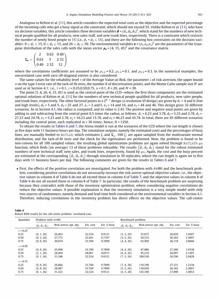
Analogous to Kelton et al. [11], this article considers the expected total costs as the objective and the expected percentageof the incoming calls who get a busy signal as the constraint, which should not exceed 5%. Unlike Kelton et al. [11], who havesix decision variables, this article considers three decision variables d = (d1,d2,d3)T, which stand for the numbers of new tech-nical people qualified for all products, new sales staff, and new trunk lines, respectively. There is a constraint which restrictsthe number of newly hired people to 15 (i.e., d1 + d2 6 15), and there are the following box constraints on the decision vari-ables: 0 6 d1 6 15, 0 6 d2 6 15, and 26 6 d3 6 50. The environmental variables e = (e1,e2,e3)T are the parameters of the trian-gular distribution of the sales calls with the mean vector le = (4, 15, 45)T and the covariance matrix

Table 6Robust

Quan

k = 00.250.500.75

k = 00.250.500.75

k = 00.250.500.75

Re ¼2 0:63 0:49

0:63 5 2:320:49 2:32 12

0B@1CA

where the correlations coefficients are assumed to be q1;2 = 0.2, q1;3 = 0.1, and q2;3 = 0.3. In the numerical examples, theuncorrelated case with zero off-diagonal entries is also considered.

The same values for the reliability level s of the Average Value-at-Risk, the parameter k of risk-aversion, the upper bounda on the type-I error rate of the lack-of-fit tests, the number K of discretization points, and the Monte Carlo sample size N0 areused as in Section 4.1; i.e., s = 0.1, k = 0.25,0.50,0.75, a = 0.1, K = 20, and N0 = 30.

The point (5, 4, 26, 4, 15, 45) is used as the central point of the CCD—where the first three components are the estimatedoptimal solutions of Kelton et al. [11] for the numbers of new technical people qualified for all products, new sales people,and trunk lines, respectively. The other factorial points in a 26�1 design (a resolution-VI design) are given by d1 = 4 and 6 (lowand high levels), d2 = 3 and 5, d3 = 25 and 27, e1 = 3 and5, e2 = 14 and 16, and e3 = 44 and 46. This design gives 32 differentscenarios. As in Section 4.1, the radius is computed, and its value is 2.45. The positive and negative axial points are given byadding to and subtracting from the central point 0.5 times the radius, as follows: d1 = 6.23 and 3.78, d2 = 5.23 and 2.78, d3 =27.23 and 24.78, e1 = 5.23 and 2.78, e2 = 16.23 and 13.78, and e3 = 46.23 and 43.78. In total, there are 45 different scenariosincluding the central point, each replicated m = 30 times; hence, N = 1350.

To obtain the results in Tables 6 and 7, the Arena model is run at the scenarios of the CCD where the run length is chosenas five days with 11 business hours per day. The simulation outputs, namely the estimated costs and the percentages of busylines, are manually feeded to MATLAB, which estimates fi and bR fi

. 100 f�i are again sampled from the multivariate normaldistribution, and the lack-of-fit tests and the check for the eigenvalues are performed. Now, the problem is found to benon-convex for all 100 sampled values; the resulting global optimization problems are again solved through MATLAB’s gafunction, which finds (on average) 13 of these problems infeasible. The results d1; d2; d3

� �stand for the robust estimated

numbers of new technical staff, new sales, and trunk lines, respectively, found by ga. Again, the cost and the busy percentare estimated at the corresponding d1; d2; d3

� �through simulation in 30 replicates, where the run length is again set to five

days with 11 business hours per day. The following comments are given for the results in Tables 6 and 7.

� First, the effects of the positive correlation are investigated. For both the problem with AV@R and the benchmark prob-lem, considering positive correlations do not necessarily increase the risk-averse optimal objective values; i.e., the objec-tive values in column 4 of Table 6 do not all exceed those in column 4 of Table 7, and the objective values in column 8 ofTable 6 do not all exceed those in column 8 of Table 7. In particular, the results of the benchmark problem are surprisingbecause they contradict with those of the inventory optimization problem, where considering negative correlations doreduce the objective values. A possible explanation is that the inventory simulation is a very simple model with onlytwo sources of randomness, namely demand and lead time both considered as the environmental variables in Section 4.1.Therefore, inducing correlations in the inventory problem has direct effects on the objective values. The call-center

RSM results for the call-center problem: correlated case.

tiles Problem with AV@R Benchmark problem

ðd1; d2; d3Þ Risk-averse opt. obj. Est. cost Est. % busy ðd1; d2; d3Þ Risk-averse opt. obj. Est. cost Est. % busy

.25(0, 1, 26) 26,463 32,524 9.9121 (5, 3, 29) 55,875 26,929 1.0587(0, 3, 26) 27,772 32,441 9.7197 (5, 5, 26) 59,333 26,182 2.3897(0, 0, 26) 30,074 33,760 9.7899 (4, 4, 26) 63,969 26,118 2.8666

.50(0, 0, 26) 25,998 33,760 9.7899 (4, 4, 28) 87,086 27,280 1.9338(2, 1, 26) 28,494 28,061 4.8371 (6, 4, 26) 95,210 26,097 2.1497(0, 1, 26) 31,348 32,524 9.9121 (7, 5, 26) 100,530 26,596 2.0428

.75(0, 0, 26) 26,866 33,760 9.7899 (7, 4, 28) 118,190 27,331 1.2334(0, 0, 26) 28,987 33,760 9.7899 (5, 5, 26) 130,920 26,182 2.3897(0, 1, 26) 31,323 32,524 9.9121 (6, 5, 28) 143,180 27,090 1.4053

Table 7Robust RSM results for the call-center problem: uncorrelated case.

Quantiles Problem with AV@R Benchmark problem

ðd1; d2; d3Þ Risk-averse opt. obj. Est. cost Est. % busy ðd1; d2; d3Þ Risk-averse opt. obj. Est. cost Est. % busy

k = 0.250.25 (2, 0, 26) 26,357 29,750 5.5549 (0, 3, 30) 56,440 39,182 8.30800.50 (1, 2, 26) 28,301 29,570 7.1330 (0, 2, 30) 60,395 38,936 8.27740.75 (1, 1, 26) 30,486 29,813 7.1519 (5, 4, 26) 65,753 26,155 2.5487

k = 0.500.25 (2, 0, 26) 26,479 29,750 5.5549 (5, 5, 28) 86,845 26,678 1.42120.50 (0, 0, 26) 28,461 33,760 9.7899 (5, 4, 26) 94,633 26,155 2.54870.75 (3, 0, 26) 30,524 29,328 4.0104 (6, 5, 26) 104,470 26,261 2.1189

k = 0.750.25 (2, 1, 26) 25,667 28,061 4.8371 (5, 4, 27) 120,320 26,109 1.77210.50 (0, 2, 26) 28,533 32,848 9.7861 (6, 5, 26) 131,750 26,155 2.11890.75 (0, 1, 26) 30,417 32,524 9.9121 (6, 4, 27) 138,930 26,395 1.7459

922 E. Angün / Simulation Modelling Practice and Theory 19 (2011) 911–923

problem, however, has a more complicated simulation model with many sources of randomness, where only a few ofthem are considered as the environmental variables, and thus inducing correlations has no directly observable effectson the estimated simulation outputs.� Second, the effects of increasing the risk-aversion parameter k are investigated. Different from the results in Section 4.1,

the risk-averse objective values of the problem with AV@R do not necessarily increase as k increases, whereas the risk-averse objective values of the benchmark problem do. This issue needs to be further investigated taking into account thatthe objective function of the call-center problem is highly non-convex.� Third, the effects of introducing risk measures on the estimated costs and percentage of the busy lines are investigated.

Remember that the risk-neutral optimal cost found in Kelton et al. [11] is $ 24679. The estimated costs in columns 5 and 9in Tables 6 and 7 all exceed 24679. Furthermore, all busy percentages except row 5 (i.e., 4.8371) in Table 6 and rows 6 and7 (i.e., 4.0104 and 4.8371) in Table 7 exceed the acceptable busy percentage (i.e., 5%) for the problem with AV@R, whereasall busy percentages except rows 1 and 2 (i.e., 8.3080 and 8.2774) in Table 7 are below 5 for the benchmark problem.Different from the inventory case, as a risk measure, variance gives usually preferable results to AV@R because the esti-mated robust optimal solution ðd1; d2; d3Þ of the benchmark problem provide acceptable results (i.e., estimated %busy lessthan 5) with lower estimated costs.� Fourth, the effects of changing k and introducing the positive correlations on the robust estimated optimal solutionsðd1; d2; d3Þ are investigated. Analogous to the results in Section 4.1, for both problems, the robust estimated optimal solu-tions ðd1; d2; d3Þ change only slightly with the changes in k and the positive correlations. In particular, the benchmarkproblem gives closer solutions to the one found in Kelton et al. [11], namely (5, 4, 26), than the problem with AV@R does.

5. Conclusions and future research

This article extends the risk-averse formulation and the robust RSM introduced in Dellino et al. [4] in the following threedirections: (i) in the risk-averse formulation, this article uses the Average Value-at-Risk as the risk measure instead of thestandard deviation in Dellino et al. [4]. The Average Value-at-Risk is a one-sided risk measure, which considers only the up-side deviation as risky in a minimization problem. Hence, in case the expected total cost is minimized, it may be a moreappropriate risk measure than the standard deviation, which considers both the upside and downside deviations from themean as important. (ii) In the optimization step of the robust RSM, a practical way of checking for the convexity of therisk-averse problem is explained, and in case this problem is found to be convex, its conic quadratic reformulation is pro-vided. Also, the problem where the variance is considered as the risk measure (the benchmark problem) and its conic qua-dratic reformulation are presented in the optimization step. These conic quadratic programming problems can be optimizedthrough CVX, which is a free-of-charge software for structured convex programming, much more efficiently than MATLAB’sfmincon function used by Dellino et al. [4]. (iii) The proposed robust RSM considers discrete-event dynamic (hence, stochas-tic) simulation instead of deterministic simulation in Dellino et al. [4]. Stochastic simulation enables to obtain large numberof replicates of multiple random responses at the same scenario through the use of non-overlapping PRNs. Then, under fairlygeneral conditions, the averages of these multiple responses have a multivariate normal distribution, which further enablesto use classic statistical tests. Hence, to apply the proposed RSM in this article, normality assumption is not required on therandom responses or environmental variables if these random responses are estimated through long-run averages of thesimulation outputs.

The proposed robust RSM is applied to an (s, S) inventory optimization with a service-level constraint and a call-center,where these problems are formulated by using the Average Value-at-Risk (problem with AV@R) and variance as the riskmeasures. For the inventory case, neither of the risk measures is found preferable to the other whereas for the call-center

E. Angün / Simulation Modelling Practice and Theory 19 (2011) 911–923 923

problem, the benchmark problem gives preferable results to the problem with AV@R. Furthermore, in both cases, the esti-mated optimal values of the decision variables are found to be not very sensitive to the environments; different environ-ments, however, do give different estimated optimal costs. These numerical studies are repeated for three differentvalues of the risk-aversion parameter, and the solutions are intuitively justifiable.

Future research may address the following issues. The simple second-order regression metamodels may be replaced byKriging metamodels in the problem with AV@R and its benchmark problem; Dellino et al. [5] already use Kriging metamod-els in their mean-risk approach, where they use standard deviation as their risk measure. Alternative one-sided risk mea-sures such as semi-variance, absolute mean semi-deviation may be used instead of the Average Value-at-Risk. The riskinvolving the constraints may be considered. Based on Neumaier et al. [23], a detailed study for the selection of global opti-mization solvers may be done, and then a proper comparison of the robust RSM with OptQuest may be performed.

Acknowledgments

I thank Professor Jack Kleijnen (Tilburg University) for his technical comments on a previous version of this article. More-over, I thank two anonymous reviewers for their comments on two earlier versions, which lead to the present article.

References

[1] E. Angün, J.P.C. Kleijnen, D. den Hertog, G. Gürkan, Response surface methodology with stochastic constraints for expensive simulation, Journal of theOperational Research Society 60 (6) (2009) 735–746.

[2] S. Bashyam, M.C. Fu, Optimization of (s, S) inventory systems with random lead times and a service level constraint, Management Science 44 (1998)S243–S256.

[3] A. Ben-Tal, A. Nemirovski, Lectures on modern convex optimization: analysis, algorithms, and engineering applications, in: MPS-SIAM Series onOptimization, SIAM, Philadelphia, PA, 2001.

[4] G. Dellino, J.P.C. Kleijnen, C. Meloni, Robust optimization in simulation: Taguchi and response surface methodology, International Journal of ProductionEconomics 125 (2010) 52–59.

[5] G. Dellino, J.P.C. Kleijnen, C. Meloni, Robust optimization in simulation: Taguchi and Krige combined, Working Paper, Tilburg University, Tilburg,Netherlands, 2010b.

[6] C.I. Fábián, Handling CVar objectives and constraints in two-stage stochastic models, European Journal of Operational Research 191 (2008) 888–911.[7] S.-K.S. Fan, E. Del Castillo, Calculation of an optimal region of operation for dual response systems fitted from experimental data, Journal of the

Operational Research Society 50 (1999) 826–836.[8] M. Grant, S. Boyd, Graph implementations for nonsmooth convex programs, in: V. Blondel, S. Boyd, H. Kimura (Eds.), Recent Advances in Learning and

Control, Lecture Notes in Control and Information Sciences, Springer, 2008, pp. 95–110. <http://stanford.edu/boyd/graph_dcp.html>.[9] M. Grant, S. Boyd, CVX: Matlab software for disciplined convex programming (web page and software), June 2009, <http://stanford.edu/boyd/cvx>.

[10] R.A. Horn, C.R. Johnson, Matrix Analysis, Cambridge University Press, Cambridge, 1999.[11] W.D. Kelton, R.P. Sadowski, D.A. Sadowski, Simulation with Arena, second ed., Mc-Graw-Hill, New York, NY, 2002.[12] A.I. Khuri, Multiresponse surface methodology, in: S. Ghosh, C.R. Rao (Eds.), Handbook of Statistics, vol. 13, Elsevier, Amsterdam, 1996.[13] J.P.C. Kleijnen, Design and Analysis of Simulation Experiments, Springer Science + Business Media, New York, NY, 2008.[14] J.P.C. Kleijnen, J. Wan, Optimization of simulated systems: OptQuest and alternatives, Simulation Modelling Practice and Theory 15 (2007) 354–362.[15] J.P.C. Kleijnen, W. van Beers, I. van Nieuwenhuyse, Constrained optimization in simulation: a novel approach, European Journal of Operational

Research 202 (2010) 164–174.[16] O. Köksoy, T. Yalcinoz, Robust design using Pareto type optimization: a genetic algorithm with arithmetic crossover, Computers & Industrial

Engineering 55 (2008) 208–218.[17] S.B. Lee, C. Park, Development of robust design optimization using incomplete data, Computers & Industrial Engineering 50 (2006) 345–356.[18] S.B. Lee, C. Park, B-R. Cho, Development of a highly efficient and resistant robust design, International Journal of Production Research 45 (1) (2007)

157–167.[19] R.H. Myers, W.H. Carter, Response surface techniques for dual response systems, Technometrics 15 (1973) 301–317.[20] R.H. Myers, D.C. Montgomery, C.M. Anderson-Cook, Response Surface Methodology: Process and Product Optimization Using Designed Experiments,

third ed., John Wiley & Sons, New York, NY, 2009.[21] W.R. Myers, W.A. Brenneman, R.H. Myers, A dual response approach to robust parameter design for a generalized linear model, Journal of Quality

Technology 37 (2) (2005) 130–138.[22] V.N. Nair (Ed.), Taguchi’s parameter design: a panel discussion, Technometrics 34 (2) (1992) 127–161.[23] A. Neumaier, O. Shcherbina, W. Huyer, T. Vinkò, A comparison of complete global optimization solvers, Mathematical Programming Series B 103 (2005)

335–356.[24] R. Rajagopal, E. Del Castillo, J.J. Peterson, Model and distribution-robust process optimization with noise factors, Journal of Quality Technology 37 (3)

(2005) 210–222.[25] C.R. Rao, Least squares theory using an estimated dispersion matrix and its application to measurement of signals, in: Proceedings of the Fifth Berkeley

Symposium on Mathematical Statistics and Probability, vol. I, 1967, pp. 355–372.[26] R.T. Rockafellar, S. Uryasev, Optimization of conditional value-at-risk, Journal of Risk 2 (2000) 21–41.[27] R.T. Rockafellar, S. Uryasev, Conditional value-at-risk for general loss distributions, Journal of Banking & Finance 26 (2002) 1443–1471.[28] D.L. Ross, D.M. Osborne, J.H. George, Decision criteria in dual response, Structural and Multidisciplinary Optimization 23 (2002) 460–466.[29] A. Shapiro, D. Dentcheva, A. Ruszczynski, Lectures on stochastic programming: modeling and theory, MPS-SIAM Series on Optimization (2009).[30] G. Taguchi, Introduction to Quality Engineering: Designing Quality into Products and Processes, Kraus International Publications, New York, NY, 1986.[31] G. Taguchi, System of experimental design: engineering methods to optimize quality and minimize cost, White Plains, New York, Quality Resources,

1987.[32] G.G. Vining, R.H. Myers, Combining Taguchi and response surface philosophies: a dual response approach, Journal of Quality Technology 22 (1990) 38–

45.[33] J. Wan, L. Li, Simulation for constrained optimization of inventory system by using Arena and OptQuest, in: Proceedings of the 2008 International

Conference on Computer Science and Software Engineering, 2008, pp. 202–205 (doi:10.1109/CSSE.2008.1217).[34] Y. Yin, S.M. Madanat, X.-Y. Lu, Robust improvement schemes for road networks under demand uncertainty, European Journal of Operational Research

198 (2) (2009) 470–479.