
Online interval scheduling on a single machine with finite lookahead
Upload
khangminh22Category
view
1download
0
Online Optimization with Lookahead
Zur Erlangung des akademischen Grades eines
Doktors der Wirtschaftswissenschaften
(Dr. rer. pol.)
von der Fakultät für Wirtschaftswissenschaften
des Karlsruher Instituts für Technologie (KIT)
genehmigte
DISSERTATION
vonDipl.-Wi.-Ing. Fabian Dunke
Tag der mündlichen Prüfung: 24. Juli 2014
Referent: Prof. Dr. Stefan Nickel
Korreferent: Prof. Dr.-Ing. Kai Furmans
Karlsruhe, 2014


I
Acknowledgements
The work you are looking at is my thesis, but it would definitely not have been possible
without the help, support and guidance of others. I first would like to thank those people.
To Prof. Dr. Stefan Nickel:
For your farsighted mentoring, for your valuable ideas throughout supervising this thesis,
and for giving me the opportunity to work in OR.
To Prof. Dr.-Ing. Kai Furmans:
For your kind interest in this work and for co-supervising it, and not to forget, for the first
steps that I could take in logistics when I was a student.
To Prof. Dr. Oliver Stein:
For your long-lasting and careful attention, for arousing my interest in optimization, and for
teaching me how to work precisely.
To Prof. Dr. J. Philipp Reiss:
For your sincere and friendly conduct as the chairman of the examination committee.
To Prof. Dr. Gerhard Woeginger:
For your lucid recommendations with regard to the realization of mathematical concepts and
for your gracious hospitality.
To Alex, Anne, Brita, Eric, Ines, Jorg and Melanie:
For the amicable working atmosphere which makes work a pleasant duty and for the com-
ments on this thesis which doubtlessly helped me improve the quality of this work.
To Marcel and Lars:
For calling me over the last five years to have an always delicious meal at mensa.
To My Family:
For the support and encouragement that you have given to me all my life.
Fabian Dunke


III
Abstract
Online optimization with lookahead deals with sequential decision making under incomplete
information where each decision must be made on the basis of a limited, but certain preview
(lookahead) of future input data. In many applications, this optimization paradigm provides
a better description of a decision maker’s informational state than the well-established dis-
ciplines of offline and online optimization since not all may be known about the future, but
also not nothing.
Despite the growing importance of the resource information as a result of technological
advances, lookahead is often still only deemed an add-on to online optimization in problem-
specific contexts. We argue that in order to understand how algorithm performance can
be enhanced by additional information, it requires a common understanding of lookahead
and its implications on instance processing by algorithms. The main contributions of this
thesis consist of the development of a systematic groundwork for comprehensive performance
evaluation of algorithms in online optimization with lookahead and the subsequent validation
of the presented approaches in theoretical analysis and computational experiments.
In the first part, we embed the paradigm of online optimization with lookahead into the
theory of optimization and develop a precise definition of the term lookahead. We find
that the lookahead effect on the objective value can be subdivided into an informational
and a processual component: The former yields the improvement attainable by forwarded
information release, while the latter expresses the improvement attainable by the change in a
problem’s “rules” immanent to lookahead. Since it is widely acknowledged that competitive
analysis – still the standard gauge for performance measurement of online algorithms – fails
to display the typical behavior of algorithms, we lay out a holistic distributional approach of
performance analysis which takes into account both the absolute behavior of an algorithm as
well as its behavior relative to some reference algorithm. This approach facilitates an explicit
consideration of different information regimes. Further, we establish the link to discrete event
systems which finally leads to the formulation of a generic modeling framework for online
optimization with lookahead.

IV
The second part applies the proposed method of distributional performance analysis to on-
line algorithms endowed with various degrees of information preview and provides structural
insights with regard to observable lookahead effects in the respective problem settings: We
first perform an exact analysis in basic settings of the ski rental, bin packing and traveling
salesman problem. From the proofs, we obtain explanations for the fact that lookahead
leads to different magnitudes of improvement depending on the respective problem types.
Subsequently, we expand our analysis to more general settings of the above problems and
additionally to the paging and scheduling problem: Extensive sample-based numerical ex-
periments are conducted to examine the algorithms’ reactions to different levels of supplied
information. Obtained results are gathered in an information pool concerning the impact of
additional information in several standard problems of online optimization. Results on the
lookahead effect from these problems can conditionally be transferred to more complex set-
tings as seen in simulation studies on the real world applications of an order picking system
in a warehouse and a pickup and delivery service in a road network. We conclude that our
approach to performance analysis of algorithms in online optimization with lookahead can
be employed in problem settings of various complexities to assess the value of information
and to determine the most suitable algorithm from a set of potential algorithm candidates
for different lookahead levels.

V
Contents
1 Introduction 1
1.1 Problem Statement and Scope of the Thesis . . . . . . . . . . . . . . . . . . 5
1.2 Applications of Online Optimization with Lookahead . . . . . . . . . . . . . 7
1.3 Overview of the Thesis . . . . . . . . . . . . . . . . . . . . . . . . . . . . . . 13
2 Analysis of Optimization Algorithms 15
2.1 Optimization Paradigms . . . . . . . . . . . . . . . . . . . . . . . . . . . . . 15
2.1.1 Offline Optimization . . . . . . . . . . . . . . . . . . . . . . . . . . . 20
2.1.2 Online Optimization . . . . . . . . . . . . . . . . . . . . . . . . . . . 20
2.1.3 Online Optimization with Lookahead . . . . . . . . . . . . . . . . . . 21
2.2 Algorithm Analysis . . . . . . . . . . . . . . . . . . . . . . . . . . . . . . . . 24
2.2.1 Complexity of Problems and Algorithms . . . . . . . . . . . . . . . . 25
2.2.2 Classification of Optimization Algorithms . . . . . . . . . . . . . . . 29
2.2.3 Algorithms and Lookahead . . . . . . . . . . . . . . . . . . . . . . . . 31
2.3 Performance of Optimization Algorithms . . . . . . . . . . . . . . . . . . . . 36
2.3.1 Performance Measures for Online Optimization Algorithms . . . . . . 36
2.3.1.1 Deterministic Worst-Case Performance Measures . . . . . . 39
2.3.1.2 Probabilistic Worst-Case Performance Measures . . . . . . . 44
2.3.1.3 Average-Case Performance Measures . . . . . . . . . . . . . 45
2.3.1.4 Distributional Performance Measures . . . . . . . . . . . . . 47
2.3.2 Performance Comparison of Optimization Algorithms . . . . . . . . . 50
2.4 Optimization Algorithms and Discrete Event Systems . . . . . . . . . . . . . 62
2.4.1 Discrete Event Systems . . . . . . . . . . . . . . . . . . . . . . . . . . 62
2.4.2 Automata . . . . . . . . . . . . . . . . . . . . . . . . . . . . . . . . . 65
2.4.3 Markov Chains . . . . . . . . . . . . . . . . . . . . . . . . . . . . . . 68
2.4.4 Discrete Event Simulation . . . . . . . . . . . . . . . . . . . . . . . . 69
2.5 Concluding Discussion . . . . . . . . . . . . . . . . . . . . . . . . . . . . . . 71
VI Contents
3 A Modeling Framework for Online Optimization with Lookahead 73
3.1 Modeling Prototypes . . . . . . . . . . . . . . . . . . . . . . . . . . . . . . . 73
3.2 Modeling Framework Components . . . . . . . . . . . . . . . . . . . . . . . . 75
3.2.1 Basic Modeling Elements . . . . . . . . . . . . . . . . . . . . . . . . . 75
3.2.2 Lookahead Type . . . . . . . . . . . . . . . . . . . . . . . . . . . . . 79
3.2.3 Processing Mode and Order . . . . . . . . . . . . . . . . . . . . . . . 83
3.2.4 Processing Accessibility . . . . . . . . . . . . . . . . . . . . . . . . . 85
3.2.5 Algorithm Execution Mode . . . . . . . . . . . . . . . . . . . . . . . 86
3.3 A Classification Scheme . . . . . . . . . . . . . . . . . . . . . . . . . . . . . 87
3.4 Discrete Event Process Model . . . . . . . . . . . . . . . . . . . . . . . . . . 90
3.5 Relation to Markov Chains . . . . . . . . . . . . . . . . . . . . . . . . . . . . 91
3.6 Instantiations of the Framework . . . . . . . . . . . . . . . . . . . . . . . . . 93
3.7 Concluding Discussion . . . . . . . . . . . . . . . . . . . . . . . . . . . . . . 99
4 Theoretical Analysis of Algorithms for Online Optimization with Lookahead 101
4.1 Online Ski Rental with Lookahead . . . . . . . . . . . . . . . . . . . . . . . . 101
4.2 Online Bin Packing with Lookahead . . . . . . . . . . . . . . . . . . . . . . . 111
4.3 Online Traveling Salesman Problem with Lookahead . . . . . . . . . . . . . . 134
4.4 Concluding Discussion . . . . . . . . . . . . . . . . . . . . . . . . . . . . . . 144
5 Experimental Analysis of Algorithms for Online Optimization with Lookahead 147
5.1 Online Ski Rental with Lookahead . . . . . . . . . . . . . . . . . . . . . . . . 148
5.1.1 Average Results . . . . . . . . . . . . . . . . . . . . . . . . . . . . . . 148
5.1.2 Distributional Results . . . . . . . . . . . . . . . . . . . . . . . . . . 150
5.2 Online Paging with Lookahead . . . . . . . . . . . . . . . . . . . . . . . . . . 154
5.2.1 Average Results . . . . . . . . . . . . . . . . . . . . . . . . . . . . . . 156
5.2.2 Distributional Results . . . . . . . . . . . . . . . . . . . . . . . . . . 158
5.2.3 Markov Chain Results . . . . . . . . . . . . . . . . . . . . . . . . . . 162
5.3 Online Bin Packing with Lookahead . . . . . . . . . . . . . . . . . . . . . . . 165
5.3.1 Classical Bin Packing . . . . . . . . . . . . . . . . . . . . . . . . . . . 166
5.3.1.1 Average Results . . . . . . . . . . . . . . . . . . . . . . . . 169
5.3.1.2 Distributional Results . . . . . . . . . . . . . . . . . . . . . 171
5.3.2 Bounded-Space Bin Packing . . . . . . . . . . . . . . . . . . . . . . . 176
5.3.2.1 Average Results . . . . . . . . . . . . . . . . . . . . . . . . 180
5.3.2.2 Distributional Results . . . . . . . . . . . . . . . . . . . . . 182
5.3.2.3 Markov Chain Results . . . . . . . . . . . . . . . . . . . . . 186

Contents VII
5.4 Online Traveling Salesman Problem with Lookahead . . . . . . . . . . . . . . 188
5.4.1 Average Results . . . . . . . . . . . . . . . . . . . . . . . . . . . . . . 193
5.4.2 Distributional Results . . . . . . . . . . . . . . . . . . . . . . . . . . 195
5.4.3 Markov Chain Results . . . . . . . . . . . . . . . . . . . . . . . . . . 199
5.5 Online Scheduling with Lookahead . . . . . . . . . . . . . . . . . . . . . . . 201
5.5.1 Online Single Machine Scheduling . . . . . . . . . . . . . . . . . . . . 203
5.5.1.1 Average Results . . . . . . . . . . . . . . . . . . . . . . . . 205
5.5.1.2 Distributional Results . . . . . . . . . . . . . . . . . . . . . 207
5.5.1.3 Markov Chain Results . . . . . . . . . . . . . . . . . . . . . 208
5.5.2 Online Parallel Machines Scheduling . . . . . . . . . . . . . . . . . . 210
5.5.2.1 Average Results . . . . . . . . . . . . . . . . . . . . . . . . 212
5.5.2.2 Distributional Results . . . . . . . . . . . . . . . . . . . . . 215
5.6 Concluding Discussion . . . . . . . . . . . . . . . . . . . . . . . . . . . . . . 215
6 Simulation of Real World Applications 219
6.1 Online Order Picking with Lookahead . . . . . . . . . . . . . . . . . . . . . . 220
6.1.1 Average Results . . . . . . . . . . . . . . . . . . . . . . . . . . . . . . 228
6.1.2 Distributional Results . . . . . . . . . . . . . . . . . . . . . . . . . . 231
6.2 Online Pickup and Delivery with Lookahead . . . . . . . . . . . . . . . . . . 239
6.2.1 Average Results . . . . . . . . . . . . . . . . . . . . . . . . . . . . . . 246
6.2.2 Distributional Results . . . . . . . . . . . . . . . . . . . . . . . . . . 250
6.3 Concluding Discussion . . . . . . . . . . . . . . . . . . . . . . . . . . . . . . 257
7 Conclusion and Outlook 261
7.1 Conclusion . . . . . . . . . . . . . . . . . . . . . . . . . . . . . . . . . . . . . 261
7.2 Outlook . . . . . . . . . . . . . . . . . . . . . . . . . . . . . . . . . . . . . . 265
A Appendix 269
A.1 Additional Proofs from Chapter 4 . . . . . . . . . . . . . . . . . . . . . . . . 269
A.1.1 Proof of Lemma 4.4 . . . . . . . . . . . . . . . . . . . . . . . . . . . . 269
A.1.2 Proof of Lemma 4.9 . . . . . . . . . . . . . . . . . . . . . . . . . . . . 270
A.2 Numerical Results from Chapter 5 . . . . . . . . . . . . . . . . . . . . . . . . 272
A.2.1 Online Ski Rental with Lookahead . . . . . . . . . . . . . . . . . . . 273
A.2.2 Online Paging with Lookahead . . . . . . . . . . . . . . . . . . . . . 276
A.2.3 Online Bin Packing with Lookahead . . . . . . . . . . . . . . . . . . . 285
A.2.3.1 Classical Problem . . . . . . . . . . . . . . . . . . . . . . . . 285
A.2.3.2 Bounded-Space Problem . . . . . . . . . . . . . . . . . . . . 294
A.2.4 Online Traveling Salesman with Lookahead . . . . . . . . . . . . . . . 303

VIII Contents
A.2.5 Online Scheduling with Lookahead . . . . . . . . . . . . . . . . . . . 315
A.2.5.1 Single Machine Problem . . . . . . . . . . . . . . . . . . . . 315
A.2.5.2 Parallel Machines Problem . . . . . . . . . . . . . . . . . . . 319
A.3 Numerical Results from Chapter 6 . . . . . . . . . . . . . . . . . . . . . . . . 323
A.3.1 Online Order Picking with Lookahead . . . . . . . . . . . . . . . . . . 323
A.3.2 Online Pickup and Delivery with Lookahead . . . . . . . . . . . . . . 347
References 357
List of Figures 373
List of Tables 379

1
1 Introduction
Although there is undisputed agreement on the importance of coping with unexpected events
in today’s systems for production and logistics ([78], [148], [154]), recent implementations
of planning and scheduling systems such as Advanced Planning Systems (APS) still suffer
from their deficiency in dealing with uncertainty over time: In a rolling time horizon, fu-
ture plans are determined on the basis of forecasted data by offline optimization methods
([154]). However, since only decisions of the next period are implemented before the problem
gets resolved with updated forecasts, this approach exhibits a high degree of redundancy.
Additionally, predictions are destined to be wrong, and it is only a matter of time before
deviations between plan and reality will occur.
On the other hand, the number of problem settings where input data can be collected and
processed in real time is continuously increasing due to technological advances ([78]). Since
planning systems built for these environments are subject to steady information disclosure,
they are said to be online. Optimization problems arising in this context are called online
optimization problems and algorithms for them have to operate dynamically. This paradigm
is completely opposite to that of classical offline optimization where all input data is assumed
to be known in advance. Between these two extremes, there is an intermediate setting which
we will call online optimization with lookahead. Here, the amount of accessible information
is governed by some lookahead mechanism. Online optimization with lookahead represents
an alternative approach for dealing with unpredictable events: Instead of having to rely on
forecasted data, uncertainty is tackled by sequential decision making where each decision is
made based only on the small, but certain part of the future known at that time.
In an organizational context, the task of solving online optimization problems (with look-
ahead) is a recurring pattern needed to operate and control industrial applications. The
functional logic of a dynamic system repeatedly requires decision making in order to continue
([135]). For each of these decisions, an online algorithm is called as a subroutine. It has to
determine partial solutions based on the currently available input data such that the overall
solution which will be composed of all partial solutions will be as good as possible.

2 1 Introduction
Figure 1.1 sums up the hierarchical relation between the logic in a dynamic system and the
online optimization module needed therein (see also [119]).
Operations and control
Input update(lookahead set)
Online optimizationwith lookahead
Figure 1.1: Hierarchical relation between operations and control of a dynamic system and onlineoptimization with lookahead.
Whether the assumption of complete or incomplete information applies, depends on the
application: On the strategic level, almost all problems are offline, e.g., facility location,
supplier selection or distribution channel selection. On the operational level, problems are
often intrinsically online, e.g., order picking, scheduling or transportation planning. Problems
on the tactical planning level, such as capacity planning or distribution planning, appear
to be of either kind. A variety of problems is solved by concatenating offline and online
optimization methods: In the first stage, offline optimization is carried out with all data
available at the start of the planning horizon; in the second stage, input data is collected
and processed repeatedly in an online manner where fixed decisions from the first stage are
respected (cf. also [88]). We conclude that online optimization problems with lookahead are
encountered primarily on the operational and occasionally on the tactical level of control.
Algorithms for solving online optimization problems – both with and without lookahead –
have to obey regimes of incomplete information while making their choices. Contrarily, offline
optimization algorithms are privileged to resort to complete information while computing a
solution. Solution methodologies for tackling the different types of these problems strongly
differ from each other as illustrated exemplarily in Figure 1.2 for the processing of an input
sequence consisting of input elements σ1, σ2, . . . , σn with n ∈ N. Arriving input elements are
represented by red rectangles, already processed input elements appear in green rectangles,
and already known but still unprocessed input elements are printed in blue rectangles. For
algorithm Alg and i, j,m ∈ N with i ≤ j ≤ m, we denote by Alg{σi,...,σj}[σ1, . . . , σm] the
costs incurred by Alg for processing the input elements in {σi, . . . , σj} based on information
σ1, . . . , σm.

3
σ1
σ2σ1
...
σn· · ·σ2σ1
Tim
et
Online algorithmOn
On{σ1}[σ1]
On{σ2}[σ1, σ2]
...
On{σn}[σ1, . . . , σn]
a)
σ2σ1
σ3σ2σ1
σ5σ4σ3σ2σ1
...
σn· · ·σ2σ1
Tim
et Online algorithm
with lookaheadLa
La{σ2}[σ1, σ2]
La{σ1,σ3}[σ1, σ2, σ3]
La{σ4}[σ1, . . . , σ5]
...
La{σn}[σ1, . . . , σn]
b)
σn· · ·σ2σ1Offline algorithm
OffOff{σ1,...,σn}[σ1, . . . , σn]
c)
Figure 1.2: Comparison of optimization paradigms. a) Online optimization without lookahead.b) Online optimization with lookahead. c) Offline optimization.
Significant research efforts have been put into tackling continuous online optimization prob-
lems arising in process industries (e.g., chemical production, raw materials processing) and
in control problems (e.g., regulatory control of power plants, robotics, aerospace). Related
problems are coined by continuous nonlinear dynamical systems, and the task consists of
monitoring and controlling the processes by adjusting parameters in order to keep the sys-
tem in a steady state (see, e.g., [84], [125]). To solve these problems, methods from control
theory are applied where mainly continuous decision variables appear within differential
equations.
In this thesis, we deal with discrete online optimization problems which means that decisions
can be traced back to a discrete structure ([85]). Most problems emerge from combinatorial
optimization where one searches for a best element in a discrete set of feasible solutions or

4 1 Introduction
from integer programming where one aims at solving mathematical programs with decision
variables constrained to take on integer values1. Online problems of this type occur in a
multitude of domains (see, e.g., [24], [32], [84], [74], [85]) including
• production and logistics, e.g., routing, packing, scheduling, load balancing,
• telecommunications, e.g., call admission, circuit routing,
• memory management, e.g., caching, paging, file migration,
• self-organizing data structures, e.g., list accessing, binary search trees,
• financial engineering, e.g., rent-or-buy decisions, portfolio selection, trading, and
• theoretical problems, e.g., graph coloring, graph matching, online linear programming.
Lookahead information is also encountered in plenty of situations in our everyday lives as
shown in Figure 1.3 and it has a major influence on our decision making: Dynamic passen-
ger information boards provide predictions about expected vehicle arrivals within the next
minutes; the information can be used in order to update travel routes based on the cur-
rent traffic scene. The weather forecast influences decisions concerning weather-dependent
outdoor activities and prevents us from booking them when the weather is announced to
be bad. A calendar can be seen as the ultimate embodiment of lookahead as it allows to
record all known pieces of future information which seem relevant to organize our personal
or professional schedules.
a) b) c)
Figure 1.3: Everyday life situations where decisions can be improved due to lookahead. a) Dy-namic passenger information board. b) Weather forecast. c) Organizer and calendar.
1 Combinatorial optimization and integer programming are closely related to each other due to the fact thatmany combinatorial optimization problems can be formulated as integer programs and, vice versa, manyinteger programs can be understood in terms of a combinatorial optimization problem.

1.1 Problem Statement and Scope of the Thesis 5
1.1 Problem Statement and Scope of the Thesis
Basic variants of online problems have been studied in the mathematical framework known as
competitive analysis (see, e.g., [32], [74]): Algorithms for an online optimization problem have
to compete with an optimal offline algorithm which knows the whole input in advance and
quality guarantees have to hold for arbitrary input sequences. Hence, competitive analysis
is a worst-case consideration of a worst-case analysis; results are overly pessimistic and do
not reflect an algorithm’s practical abilities to suitably deal with a given problem.
Most theoretical results were derived based on the taxonomy prevalent in a specific problem
and not based on a general notation valid for problems of all kinds. Likewise, the intermediate
setting of online optimization with lookahead has been addressed by the online optimization
community every now and then only in specific problems arising in routing and transportation
([7], [8], [11], [34], [96], [95], [155]), scheduling ([51], [123], [129], [130], [134], [161], [168],
[169]), organization of data structures ([2], [3], [41], [113], [156], [163], [164]), data transfer
([64], [93]), packing ([83], [86]), lot sizing ([1]), metrical task systems ([20], [115]) or graph
theory ([45], [87], [94]). To the best of our knowledge, there have been no attempts to
formalize different degrees of available information in a general framework.
A reason for the lack of general concepts lies in the unsettled role of the factor time. In some
problems it is just used to establish an order of events (sequential model); others intrinsically
rely upon time as a part of the instance specification (time stamp model). This issue also
accounts for various perceptions of the term lookahead: Does it mean that a certain number
of future input elements is known? Does it mean that all future input elements occurring in
a particular time window are foreseen?
Endowing an algorithm with lookahead should lead to better results due to improved planning
opportunities. Therefore, lookahead is deemed a mechanism for increasing the power of an
algorithm ([96]) and we may ask for the value of a preview on future information within the
class of online optimization problems.
Obviously, lookahead without an algorithm which can make use of it renders itself worthless.
Therefore, determining the value of lookahead and performance analysis of algorithms are
closely intertwined. By the nature of sequential decision making under incomplete informa-
tion, possible “errors” of an algorithm cannot necessarily be corrected later when one realizes
that another decision would have been better ([151]). Due to the inevitability of failure, it is
impossible to find an algorithm which solves an online optimization problem to optimality
and all we can do is to find algorithms for a certain problem which are as good as possible.
6 1 Introduction
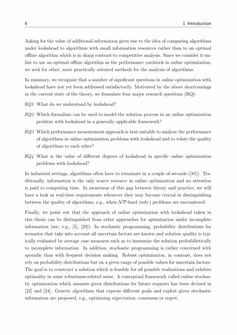
Asking for the value of additional information gives rise to the idea of comparing algorithms
under lookahead to algorithms with small information resources rather than to an optimal
offline algorithm which is in sharp contrast to competitive analysis. Since we consider it un-
fair to use an optimal offline algorithm as the performance yardstick in online optimization,
we seek for other, more practically oriented methods for the analysis of algorithms.
In summary, we recognize that a number of significant questions in online optimization with
lookahead have not yet been addressed satisfactorily. Motivated by the above shortcomings
in the current state of the theory, we formulate four major research questions (RQ):
RQ1 What do we understand by lookahead?
RQ2 Which formalism can be used to model the solution process in an online optimization
problem with lookahead in a generally applicable framework?
RQ3 Which performance measurement approach is best suitable to analyze the performance
of algorithms in online optimization problems with lookahead and to relate the quality
of algorithms to each other?
RQ4 What is the value of different degrees of lookahead in specific online optimization
problems with lookahead?
In industrial settings, algorithms often have to terminate in a couple of seconds ([85]). Tra-
ditionally, information is the only scarce resource in online optimization and no attention
is paid to computing time. In awareness of this gap between theory and practice, we will
have a look at real-time requirements whenever they may become crucial in distinguishing
between the quality of algorithms, e.g., when NP-hard (sub-) problems are encountered.
Finally, we point out that the approach of online optimization with lookahead taken in
this thesis can be distinguished from other approaches for optimization under incomplete
information (see, e.g., [5], [29]): In stochastic programming, probability distributions for
scenarios that take into account all uncertain factors are known and solution quality is typ-
ically evaluated by average case measures such as to immunize the solution probabilistically
to incomplete information. In addition, stochastic programming is rather concerned with
sporadic than with frequent decision making. Robust optimization, in contrast, does not
rely on probability distributions but on a given range of possible values for uncertain factors.
The goal is to construct a solution which is feasible for all possible realizations and exhibits
optimality in some robustness-related sense. A conceptual framework called online stochas-
tic optimization which assumes given distributions for future requests has been devised in
[22] and [24]. Generic algorithms that express different goals and exploit given stochastic
information are proposed, e.g., optimizing expectation, consensus or regret.

1.2 Applications of Online Optimization with Lookahead 7
Online optimization with lookahead as treated in this thesis differs from the previous ap-
proaches by its perception of uncertainty: Rather than presuming a particular probability
model or possible value ranges, it strives for a more holistic analysis of uncertainty as justified
by increased volatilities in today’s markets. We opt for a method of performance analysis
which incorporates typical and worst-case behavior of an algorithm as well as its overall
performance range in an equal measure. Although the traditional focus of online optimiza-
tion is on hedging against worst-case scenarios, recent application-driven developments show
that in a more comprehensive view on the topic also aspects like sensitivity to additional
lookahead or integration into simulation environments need to be addressed.
1.2 Applications of Online Optimization with Lookahead
Online optimization problems with lookahead arise in applications of different domains. The
following examples suggest that lookahead is polymorphic depending on the context.
Online Routing with Lookahead
A recurring task in transportation and logistics is vehicle routing ([118]). As a result of
increased usage of geographic information systems (GIS) and global positioning systems
(GPS), the research focus has shifted from the static to the dynamic version of the problem
([139]); these variants refer to the offline and online version, respectively. Applications can
be found in emergency, taxi and repair services as well as in order picking.
A number of requests has to be served by a set of vehicles each starting and ending in a given
depotO with the aim of optimizing some costs such as the total travel distance. Every request
has a release time representing the earliest time for service. Providing lookahead makes both
locations and release times of the requests known earlier. In Figure 1.4, the offline situation
is compared to the online situation. In the latter case, dots in gray correspond to unknown
requests at snapshot time and numbers indicate the request revelation order.
Providing additional lookahead is expected to lead to enhanced performance by incorporat-
ing more requests into an algorithm’s strategy. However, based on customer requirements it
needs to be clarified first whether earlier notification due to lookahead also facilitates earlier
customer service, or whether earliest service times from the online problem without looka-
head are retained. This requirement strongly impacts the optimization potential induced by
lookahead. We point out three notions of lookahead known from literature:

8 1 Introduction
O
x1
x2
a)
1
4
2
7
3
5
6
8
10
9
11
12
O
x1
x2
b)
Figure 1.4: Vehicle routing. a) Offline (static) version. b) Online (dynamic) version.
• Request lookahead allows an algorithm to foresee a fixed number of upcoming requests
([7], [8]).
• Time lookahead as discussed by Allulli et al. ([7], [8]) and Ausiello et al. ([11]) allows
an algorithm to foresee all requests having a release time within a fixed time window
starting at the current time.
• Disclosure times of requests introduced by Jaillet and Wagner ([96]) explicitly specify
the notification times of requests and differ from their earliest service times.
Request lookahead is probably the most unrealistic among these concepts ([11]), whereas
disclosure times allow for a customer-specific model of lookahead ([96]). Time lookahead
sets the same temporal offset between notification and release of a request for all customers.
Competitive analysis in [7] and [96] yields that time lookahead and disclosure dates may lead
to (slight) improvements depending on the objective function and metric space.
We mention that there are numerous refinements and generalizations of the vehicle routing
problem with industrial relevance ([158]), e.g., pickup and delivery problems or inventory
routing problems, which all lend themselves to an integration of additional lookahead infor-
mation. The design of real-time compliant algorithms has to take into account the computa-
tional complexity of vehicle routing problems2, e.g., by devising decomposition methods such
as cluster-first route-second strategies ([101]). Moreover, one has to be aware of counterintu-
itive problem features such as the fact that waiting for requests located in spatial proximity
may be beneficial although there are still unserved requests.
2 The vehicle routing problem is NP-hard because its decision version contains Hamiltonian Circuit
which is known to be an NP-complete problem.

1.2 Applications of Online Optimization with Lookahead 9
Online Bin Packing with Lookahead
Packing comprises the task of combining objects from a set of small items in order to pack
them into elements of large objects such that some objective function is optimized ([69]). The
practical scope of packing is twofold: First, it includes the combinatorial task of grouping
small items into subsets and assigning each of them to a large object; second, it includes
the geometric task of ensuring that within each large object the small items are laid out
such that they are entirely contained in the large object without overlapping. Applications
include packaging logistics, assembly line balancing, memory allocation and layout design.
A fundamental packing problem is the (one-dimensional) bin packing problem ([77]) where
a number of items σ1, σ2, . . . , σn for n ∈ N with sizes si ∈ (0, 1] for i = 1, . . . n is given and
the task is to pack them into a minimum number of unit-capacitated bins. We seek to find
a partition of {σ1, σ2, . . . , σn} into a minimum number m of subsets B1, B2, . . . , Bm such
that ∑σi∈Bj
si ≤ 1
for all j = 1, . . . ,m. The problem is computationally complex3.
The problem instance in Figure 1.5 shows why it is important to have a look at different
modes of information disclosure. In the pure online setting, items arrive and have to be
packed one after another without knowledge of any other future item. In an exemplary
lookahead setting, two items to be packed are known at each time except when only one
item remains to be packed. While an optimal offline algorithm needs only six bins, all online
algorithms without lookahead which do not open a new bin when the item to be packed fits
in an already open bin end up with eight bins. Seven bins are needed by all online algorithms
with lookahead of two items which try to generate bins occupied as much as possible.
The input sequence in Figure 1.5 is somewhat pathologic with respect to the item sizes and
the input sequence length. If the input sequence was much longer, the unoccupied space
of the depicted bins would probably be filled. Thus, the performance degradation due to
incomplete information is expected to be small for sufficiently long item sequences.
In contrast to the assumptions of the basic bin packing problem, there will be bounds on
the number of open bins as a result of space restrictions in practice: In packaging logistics
one would have to obey the number of packaging stations or loading docks; in memory
allocation one would have to respect storage capacities ([83]). This problem is called the
3 Bin packing is NP-hard because its decision version can be reduced from Partition which is known tobe an NP-complete problem.

10 1 Introduction
0.5
σ1
0.4
σ2
0.5
σ3
0.4
σ4
0.5
σ5
0.4
σ6
0.5
σ7
0.4
σ80.6
σ9
0.6
σ10
0.6
σ11
0.6
σ12
a)
0.6
0.4
1
0.6
0.4
2
0.6
0.4
3
0.6
0.4
4
0.5
0.5
5
0.5
0.5
6
b)
0.5
0.4
1
0.5
0.4
2
0.5
0.4
3
0.5
0.4
4
0.6
5
0.6
6
0.6
7
0.6
8
c)
0.5
0.5
1
0.4
0.5
2
0.4
0.5
3
0.4
0.6
4
0.6
0.4
5
0.6
6
0.6
7
d)
Figure 1.5: Bin packing. a) Item sequence. b) Optimal offline solution. c) Solution of an onlinealgorithm without lookahead. d) Solution of an online algorithm with lookahead.
(one-dimensional) bounded-space bin packing problem: Each time a new bin needs to be
opened, one of the K open bins has to be closed first. In packaging logistics this means
to send a bin or truck away; in memory allocation this amounts to deleting the contents
of some memory module. Because bins cannot remain open arbitrarily long and may be
sent away although not fully laden, the improvement to be expected by lookahead in the
bounded-space problem should be bigger than in the unbounded case.
Apart from informational benefits, lookahead in packing may serve as a buffer for input el-
ements. In a warehouse, items can be consolidated before their assignment to a destination
container ([83], [101]). Thus, lookahead equips the decision maker with more alternatives
through the accumulation of items. Clearly, this only holds if the processing order of known
items is arbitrary. We require to define lookahead always in conjunction with a specification
of a corresponding processing mode which tells us whether permuting input elements is al-

1.2 Applications of Online Optimization with Lookahead 11
lowed (e.g., by sorting physically small items in a buffer) or not (e.g., by enqueuing physically
large items in a job sequence).
We mention two types of lookahead from literature applicable to packing problems:
• In (conventional) request lookahead, a fixed number of future objects to be packed is
seen at any time ([83]).
• In property lookahead, the lookahead consists of those items which jointly fulfill a given
property ([83], [155]).
An instantiation of property lookahead has been laid out by Grove ([83]) for bin packing:
The lookahead consists of those items which jointly do not exceed a threshold cost value
when being processed by some algorithm. Another instantiation, due to Tinkl ([155]), is
to collect those elements in the lookahead which do not exceed a given threshold weight or
size. With respect to practical considerations, we need to guarantee that no item stays in
the buffer and no bin stays in the warehouse for too long in order to prevent starvation.
The aforementioned problems can be generalized to two or three spatial dimensions and
there are numerous additional problem variants (see, e.g., [55]) of which we mention batch
bin packing where items become available in blocks, dynamic bin packing where possible
events include departures and variable-sized bin packing where bin sizes may vary.
Online Paging with Lookahead
Memory management and data organization intrinsically feature an online character due to
data communication over time. Algorithms try to organize memory or data structures such
that the total costs for access are lowest possible. The paging problem is a fundamental
problem in computer science ([32]) and gave rise to competitive analysis in the 1980s ([149]).
It is concerned with efficiently managing a two-level store of memory consisting of a small
fast cache memory of size k and a large slow memory of unbounded size. The input sequence
corresponds to a sequence of requested pages and a requested page can only be accessed
when it is in the cache. Thus, whenever the request is on a page already in the cache, no
cost is incurred (cache hit), but whenever an algorithm has to bring the requested page to
the cache first, a unit cost is charged (page fault, cache miss). The problem is to decide
which cache page to evict upon a page fault. As opposed to the previous applications, there
is a polynomial-time optimal offline algorithm: Algorithm LongestForwardDistance
(Lfd, Belady’s optimal replacement algorithm in [17]) serves every request sequence with
the minimum number of faults by evicting the page in the cache which will be requested

12 1 Introduction
farthest in the future when a page fault occurs. An online algorithm knows nothing about
future requests. Unfavorably, this may escalate to every request producing a cache miss.
Consider a cache of size 3 and a slow memory containing all 26 letters of the standard
alphabet. Initially, the cache is filled with {a, b, c} as displayed in Figure 1.6, and the
sequence of requested pages is σ = (f, a, b, i, a, n). Offline algorithm Lfd incurs three page
faults. Online algorithm LeastRecentlyUsed (Lru) evicts a page whose last request was
earliest, i.e., least recently, among the cache pages. Lru incurs five page faults on σ.
a
b
c
a
b
f
a
b
f
a
b
f
a
i
f
a
i
f
n
i
f
a)
a
b
c
f
b
c
f
a
c
f
a
b
i
a
b
i
a
b
i
a
n
b)
Figure 1.6: Paging. Offline algorithm Lfd in a) and online algorithm Lru in b) lead to a differentnumber of page faults on input sequence σ = (f, a, b, i, a, n).
Requests usually arrive in fixed-size blocks in data communications, thereby giving a natural
preview of requests. The model of conventional request lookahead where a fixed number
of pages is seen at each time has been repelled because of its ineffectiveness in competitive
analysis ([164]): Denote by σki a request on page σi for k times in a row. Then the ratio of
the costs incurred by online algorithm Alg1 to the costs incurred by Lfd on page sequence
(σ1, σ2, . . . , σn) is the same as the ratio incurred by an online algorithm Algk with lookahead
k to the costs incurred by Lfd on page sequence (σk1 , σk2 , . . . , σ
kn) when Algk mimics Alg1
on the first of each σki with i = 1, . . . , n. Lookahead becomes useless in this case since it hides
new future requests. To eliminate this shortcoming, we give three alternatives of lookahead
that have been devised in literature:
• Strong lookahead of size k as introduced by Albers ([2]) consists of the current request
and k additional pairwise different pages which also have to differ from the current
request.
• Resource-bounded lookahead of size k as suggested by Young ([164]) consists of those
upcoming pages that fulfill the property that no more than k+ 1 page faults will occur
when processed by the online algorithm under consideration.
• By natural lookahead of size k as devised by Breslauer ([41]), we understand the knowl-
edge of k + 1 distinct pages which in contrast to strong lookahead collectively are not
in the cache.

1.3 Overview of the Thesis 13
Note that strong lookahead is independent of an algorithm, resource-bounded lookahead de-
pends both on an algorithm’s past and future behavior which makes it admittedly unrealistic
for use, and natural lookahead relies on an algorithm’s past behavior. It is shown for each of
these lookahead types that mild improvements in competitive analysis are achieved because
pathological cases as described above are bypassed. Paging algorithms turn out to strongly
benefit already from conventional request lookahead in empirical studies ([41]).
1.3 Overview of the Thesis
The overall structure of this thesis is divided into seven chapters as shown in Figure 1.7.
1 Introduction
Motivation
2 Analysis of Optimization Algorithms
3 A Modeling Framework for Online Optimization with Lookahead
Background and Modeling
4 Theoretical Analysis of Algorithms for Online Optimization with Lookahead
5 Experimental Analysis of Algorithms for Online Optimization with Lookahead
6 Simulation of Real World Applications
Analysis of Algorithms for Online Optimization with Lookahead
7 Conclusions and Outlook
Recap and Recommendations
Figure 1.7: Structure of the thesis.

14 1 Introduction
Chapter 1 introduced the subject of online optimization with lookahead, motivated desired
research outcomes and laid out some application examples.
The following two chapters are devoted to the definition of a general modeling framework
for online optimization problems with lookahead: In Chapter 2, we take a closer look at
different optimization paradigms with respect to the amount of information provided, and
we discuss different concepts for performance analysis of optimization algorithms, especially
in the context of online optimization under varying degree of informational preview. Finally,
we interrelate different modeling techniques for discrete event systems and find that methods
for solving online optimization problems with lookahead adhere to these techniques as well
due to their sequential decision making character. Chapter 3 focuses on the modeling of
online optimization problems with lookahead: We collect basic definitions for lookahead
and look at their peculiarities. Since one of our main goals is to analyze the performance
of algorithms in different applications using unified concepts and a common taxonomy, we
propose a generic process model which all online algorithms using lookahead have to obey.
In the remainder of this thesis, we continue by instantiating this framework for a variety
of important applications and by applying the proposed methods of algorithm analysis to
assess the value of lookahead.
Chapters 4 to 6 delve into the analysis of online optimization algorithms endowed with
various degrees of lookahead in particular problem settings: In Chapter 4, a theoretical
analysis is conducted for basic academic problem settings. First hints are found concerning
the role of lookahead as a promoter of improved algorithm performance. In Chapter 5, we
explore the effects of lookahead in classic online optimization problems. Detailed numerical
experiments are conducted from a sampling-based point of view. The results indicate that the
behavior of online algorithms in practice depends on the amount of lookahead, but also that
the extent of the lookahead value strongly relies on the problem itself. Online optimization
algorithms exploiting lookahead information are used within simulation models of two real
world applications in Chapter 6. We learn that due to the higher number of restrictions in
practical settings, the lookahead effect is mitigated to a certain extent.
Chapter 7 subsumes the findings of this thesis and recurs to the four central research questions
that were specified previously in this introduction. Likewise, we point out limitations of our
approach and provide starting points for possible future research directions.

15
2 Analysis of Optimization Algorithms
Algorithms are computational methods to solve any kind of computational problem, i.e., to
provide the correct output for any input ([54]). Optimization algorithms face the task of
determining a best possible element out of a set of solution candidates. Unfortunately, in
online optimization – both with and without lookahead – the input is revealed only gradually,
and due to the inevitability of failure in decision making under incomplete information, it is
impossible for any algorithm operating in an online manner to halt with the correct, i.e., best
possible, output on any input. This chapter clarifies and resolves the relationships between
the different modes of information disclosure and discusses the role of algorithms in this
context. In particular, we provide a clear definition of the optimization paradigm online
optimization with lookahead and decompose the effect of lookahead into an informational
and a processual component. To facilitate an analysis of the lookahead impact on solution
quality, we develop a holistic approach to performance measurement of algorithms. Finally,
general analogies between the solution process in an online optimization problem and discrete
event systems are deduced.
2.1 Optimization Paradigms
In online optimization, input data is revealed sequentially. Optimization problems arising
in practice often exhibit this type of information disclosure as opposed to standard offline
optimization where all data is known in advance4. Essentially, offline and online optimiza-
tion differ in the amount of accessible informational content: Offline optimization assumes
complete information, online optimization assumes incomplete information. The definition
of complete is unique in terms of representing 100 %, but the definition of incomplete admits
an infinite number of levels representing t % with t ∈ [0, 100). This leads to the definition of
4 According to [74], the terms online and offline are likely to origin from cryptographic systems wheredecryption was either done continuously during data transfer (on the communication line) or after alldata were transferred (off the communication line).

16 2 Analysis of Optimization Algorithms
a more profound notion which we will refer to as online optimization with lookahead. Here,
we can quantify the amount of information which is available to any algorithm operating in
this information regime. We start with a series of definitions in order to ensure a common
taxonomical and notational basis. The first definitions are based on Garey and Johnson ([77])
as well as on Ausiello et al. ([12]); subsequent definitions for online optimization problems –
both with and without lookahead – are introduced first in this thesis.
Definition 2.1 (Problem ([77])).
A problem is a general question containing a set of parameters. 4
Definition 2.2 (Instance of a problem ([77])).
An instance of a problem is a set of parameter values describing a concrete version of the
problem. 4
We remark that the term input is often used as a synonym for the term instance.
Definition 2.3 (Solution ([77])).
A solution to a given instance of a problem is an adequate answer to the concrete version of
the problem obtained by replacing the parameters in the general question with the provided
parameter values of the instance. 4
There are several types of problems requiring different kinds of answers: Decision problems
and search problems require yes-/no-answers, counting problems require integer answers,
and optimization problems require answers encoding the best solution. In order to give a
concise definition of the class of optimization problems, we first need an underlying concept
of optimality which allows us to judge on the quality of solutions.
Definition 2.4 (Optimality concept).
An optimality concept is a correspondence returning for each set of solutions to a given
instance of a problem a subset of this set to be considered best. 4
A natural form of an optimality concept is based on a scalar-valued objective function f
which assigns each solution s a number f(s) ∈ R, the ≤-relation on R and an optimization
goal opt ∈ {min,max}. There are other concepts of optimality, e.g., Pareto optimality in
multicriteria optimization, but for us the above optimality concept induced by (f,≤, opt)
will do. We are in a position to give a formal definition of an optimization problem which
implicitly subsumes the previous concepts.
2.1 Optimization Paradigms 17
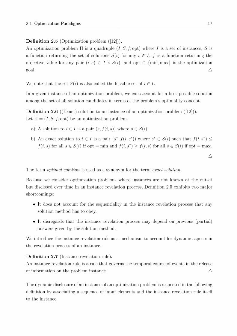
Definition 2.5 (Optimization problem ([12])).
An optimization problem Π is a quadruple (I, S, f, opt) where I is a set of instances, S is
a function returning the set of solutions S(i) for any i ∈ I, f is a function returning the
objective value for any pair (i, s) ∈ I × S(i), and opt ∈ {min,max} is the optimization
goal. 4
We note that the set S(i) is also called the feasible set of i ∈ I.
In a given instance of an optimization problem, we can account for a best possible solution
among the set of all solution candidates in terms of the problem’s optimality concept.
Definition 2.6 ((Exact) solution to an instance of an optimization problem ([12])).
Let Π = (I, S, f, opt) be an optimization problem.
a) A solution to i ∈ I is a pair (s, f(i, s)) where s ∈ S(i).
b) An exact solution to i ∈ I is a pair (s∗, f(i, s∗)) where s∗ ∈ S(i) such that f(i, s∗) ≤f(i, s) for all s ∈ S(i) if opt = min and f(i, s∗) ≥ f(i, s) for all s ∈ S(i) if opt = max.
4
The term optimal solution is used as a synonym for the term exact solution.
Because we consider optimization problems where instances are not known at the outset
but disclosed over time in an instance revelation process, Definition 2.5 exhibits two major
shortcomings:
• It does not account for the sequentiality in the instance revelation process that any
solution method has to obey.
• It disregards that the instance revelation process may depend on previous (partial)
answers given by the solution method.
We introduce the instance revelation rule as a mechanism to account for dynamic aspects in
the revelation process of an instance.
Definition 2.7 (Instance revelation rule).
An instance revelation rule is a rule that governs the temporal course of events in the release
of information on the problem instance. 4
The dynamic disclosure of an instance of an optimization problem is respected in the following
definition by associating a sequence of input elements and the instance revelation rule itself
to the instance.

18 2 Analysis of Optimization Algorithms
Definition 2.8 (Instance of an optimization problem).
An instance of an optimization problem consists of a set of parameter values including a
sequence σ = (σ1, σ2, . . .) and an instance revelation rule r. 4
The sequence σ in an instance of an optimization problem is called input sequence; its
elements σ1, σ2, . . . are called input elements. We say that the elements of σ await processing
by some solution method. Once an input element has been processed, it is considered finished.
We give three examples of general nature for an instance revelation rule:
• σi+1 with i = 1, 2, . . . is revealed when σi is considered finished.
• σ1, σ2, . . . are revealed at prescribed release times τ1, τ2, . . .
• σ is known completely at time 0.
Observe that choosing different instance revelation rules r and r′ on the same input sequence
σ establishes two different problem instances. Since different instance revelation rules may
be used for the same problem, we need a possibility to settle all sources of unclarity with
respect to the dynamic processing of the input elements which may inherently arise by the
introduction of lookahead. To this end, we associate a set of rules with a problem Π.
Definition 2.9 (Rule set).
A rule set of a problem is a set of restrictions on the solution to an instance of the problem.
4
Observe that choosing two different rule sets P and P ′ establishes two different problems.
We list three examples which may appear as elements of a rule set. Note that the first rule
cannot be used in conjunction with the second or third rule, respectively.
• σi with i = 1, 2, . . . has to be finished before σj with j > i can be finished.
• The finishing order of the input elements in σ is arbitrary.
• At most m ∈ N input elements with m > 1 can be finished at the same time.
The instance revelation rule and the rule set allow us to make a clear distinction between
the informational implications caused by lookahead and the consequences on processing of
the input elements inherent to lookahead. Regrettably, except for [155], none of the existing
literature on online optimization in conjunction with lookahead is concerned with this kind
of split of lookahead into forwarded information and implied processing requirements. As
a result, it is not clear which of the mechanisms is responsible for improvements when
additional lookahead is granted.

2.1 Optimization Paradigms 19
Whenever we want to make the rule set P of an optimization problem Π explicit, we may
write ΠP instead of Π and provide a specification of P ; whenever we want to make the
instance revelation process of an instance explicit, we specify the input sequence σ and the
revelation rule r in a pair (σ, r) along with the parameter values of the problem instance.
Example 2.10 (Paging).
Consider the paging problem introduced in Chapter 1.2 with page alphabet A, cache size k,
an initially filled cache, and denote by C = {c1, c2, . . . , ck} a cache configuration, i.e., a set
containing the k cache pages. We identify the elements of ΠP = (I, S, f, opt).
Rule set P may contain the following restrictions:
• Elements from σ = (σ1, σ2, . . .) are requested in ascending order of their index.
• Only one non-cache page can be brought into the cache at a time.
• A requested non-cache page has to be brought into the cache as soon as possible.
I is the set of all instances i = (σ, r) where σ = (σ1, σ2, . . .) with σi ∈ A for i = 1, 2, . . . is
the sequence of requested pages and r is an instance revelation rule such as:
• All elements of σ are known at the outset (offline optimization problem).
• Elements of σ become available one after another in equidistant intervals (online opti-
mization problem with independent release).
• One input element is known at a time; the next input element is revealed when
the previous one has been brought into the cache (online optimization problem with
processing-dependent release).
• Exactly k ∈ N input elements are known at a time; a new input element is revealed
when a known one has been brought into the cache (online optimization problem with
lookahead and processing-dependent release).
The set of solution candidates S contains all sequences of cache configurations which comply
with r and P , i.e.,
S ={
(C1, C2, . . .) |Ci for i = 1, 2, . . . respects r and P}.
The objective function
f =∑j>1
|Cj\Cj−1|
maps a sequence of cache configurations to the total number of page evictions. opt = min
demands to minimize the total number of page evictions. ♦

20 2 Analysis of Optimization Algorithms
2.1.1 Offline Optimization
The key characteristic of an offline optimization problem is that there is no uncertainty about
any of its instances.
Definition 2.11 (Offline optimization problem).
An offline optimization problem is an optimization problem where in each instance the input
sequence is known at time 0. 4
Example 2.12 (Offline paging).
Paging is a sequential problem by nature, i.e., although all page requests are known at the
outset, it is forbidden to permute them when bringing them into the cache. This is reflected
by the specification of rule set P = {p1, p2, p3} with
• p1 := σi has to be brought into the cache before σj if i < j,
• p2 := Two successive cache configurations have to differ in exactly one page, and
• p3 := A page has to be brought into the cache as soon as it is available.
♦
2.1.2 Online Optimization
The key characteristic of an online optimization problem is that there is uncertainty with
respect to the input sequence in at least one instance of that problem.
Definition 2.13 (Online optimization problem).
An online optimization problem is an optimization problem where at least one instance exists
for which the input sequence is not known completely at time 0. 4
We next specify two refinements of online optimization problems frequently addressed in
literature ([85], [116], [157]). In the sequential model of online optimization, new input
elements are revealed in a processing-dependent fashion.
Definition 2.14 (Online optimization problem in the sequential model).
An online optimization problem in the sequential model is an optimization problem where
any instance of the problem has an instance revelation rule which says that a new input
element only becomes known when another one has finished processing. 4

2.1 Optimization Paradigms 21
In the time stamp model of online optimization, input elements are released by an inde-
pendent external input element generator irrespective of any processing. The release times
correspond to time stamps. In contrast to the sequential model, input elements can be
accumulated in the time stamp model.
Definition 2.15 (Online optimization problem in the time stamp model).
An online optimization problem in the time stamp model is an optimization problem where
any instance of the problem has an instance revelation rule which assigns each input element
an independent release time. 4
Example 2.16 (Online paging).
Online paging is classically understood in the sequential model. Hence, we have for each
instance an instance revelation rule in the form
r := At time 0, only σ1 is seen; the next page of σ is revealed when the
currently known unprocessed page is in the cache.
Concerning rule set P , we can drop rules p1 and p2 from the offline problem in Example 2.12
because they are implied automatically as a consequence of r and we obtain
P := {A page has to be brought into the cache as soon as it is available}.
In the (barely known) time stamp model of paging, page requests pop up independently at
their release times and the restriction of sequential processing is dropped. Hence, we have
another instance revelation rule, namely
r := A page becomes available when its release time is reached.
We demand page evictions after time intervals of a given length have elapsed by rule set
P := {The cache is updated after a given amount of time has elapsed}.
In implementations, we have to think of resolution strategies for the case of too many page
arrivals in a short period of time (buffer overflow). ♦
2.1.3 Online Optimization with Lookahead
Online optimization problems with lookahead are online optimization problems. Their sep-
arate discussion results from the significant research question of how much the outcome in
22 2 Analysis of Optimization Algorithms
an online optimization problem can be enhanced through the provision of input elements at
an earlier point in time. Since lookahead makes information available earlier, an equivalent
approach would be to speak of preponed or forwarded information release.
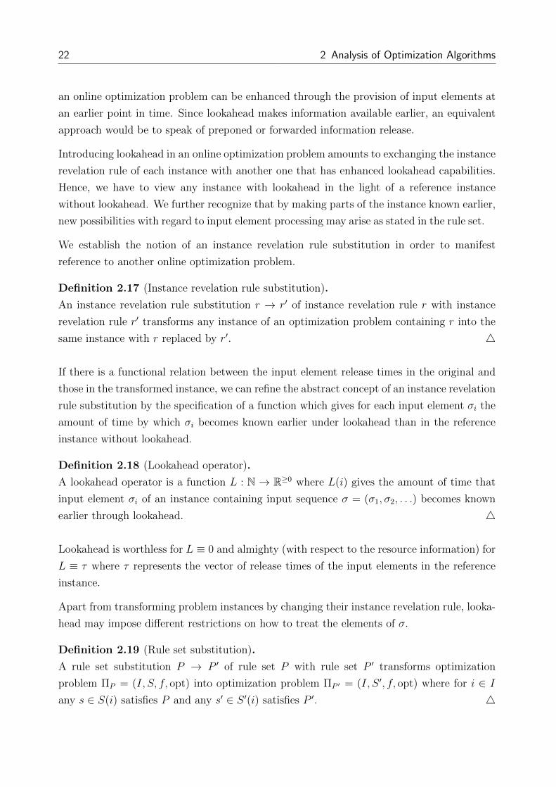
Introducing lookahead in an online optimization problem amounts to exchanging the instance
revelation rule of each instance with another one that has enhanced lookahead capabilities.
Hence, we have to view any instance with lookahead in the light of a reference instance
without lookahead. We further recognize that by making parts of the instance known earlier,
new possibilities with regard to input element processing may arise as stated in the rule set.
We establish the notion of an instance revelation rule substitution in order to manifest
reference to another online optimization problem.
Definition 2.17 (Instance revelation rule substitution).
An instance revelation rule substitution r → r′ of instance revelation rule r with instance
revelation rule r′ transforms any instance of an optimization problem containing r into the
same instance with r replaced by r′. 4
If there is a functional relation between the input element release times in the original and
those in the transformed instance, we can refine the abstract concept of an instance revelation
rule substitution by the specification of a function which gives for each input element σi the
amount of time by which σi becomes known earlier under lookahead than in the reference
instance without lookahead.
Definition 2.18 (Lookahead operator).
A lookahead operator is a function L : N → R≥0 where L(i) gives the amount of time that
input element σi of an instance containing input sequence σ = (σ1, σ2, . . .) becomes known
earlier through lookahead. 4
Lookahead is worthless for L ≡ 0 and almighty (with respect to the resource information) for
L ≡ τ where τ represents the vector of release times of the input elements in the reference
instance.
Apart from transforming problem instances by changing their instance revelation rule, looka-
head may impose different restrictions on how to treat the elements of σ.
Definition 2.19 (Rule set substitution).
A rule set substitution P → P ′ of rule set P with rule set P ′ transforms optimization
problem ΠP = (I, S, f, opt) into optimization problem ΠP ′ = (I, S ′, f, opt) where for i ∈ Iany s ∈ S(i) satisfies P and any s′ ∈ S ′(i) satisfies P ′. 4

2.1 Optimization Paradigms 23
Essentially, as a result of a rule set substitution, the feasible sets of ΠP and ΠP ′ no longer
coincide because P ′ imposes different requirements on a solution than P .
We are in a position to give a definition of lookahead in online optimization:
Definition 2.20 (Lookahead).
A lookahead is a pair (r → r′, P → P ′) consisting of an instance revelation rule substitution
r → r′ and a rule set substitution P → P ′. 4
The following definition accounts for the transformation of a given reference online opti-
mization problem induced by lookahead: On the one hand, transformation affects problem
instances due to the instance revelation rule substitution; on the other hand, problem re-
strictions may be updated as a result of the rule set substitution.
Definition 2.21 (Online optimization problem with lookahead).
An online optimization problem with lookahead is an online optimization problem which is
obtained from a reference online optimization problem by applying the instance revelation
rule substitution and the rule set substitution of a given lookahead to the instances and to
the feasible set of the reference online optimization problem, respectively. 4
Figure 2.1 illustrates the decomposition of lookahead into an informational and a processual
component.
Online optimization problem
ΠP = (I, S, f, opt)i = (σ, r) ∈ I
Online optimization problemwith lookahead
Π′P = (I ′, S, f, opt)i′ = (σ, r′) ∈ I ′
Online optimization problemwith lookahead
Π′P ′ = (I ′, S ′, f, opt)i′ = (σ, r′) ∈ I ′
(r → r′, P → P )
Instance revelation
rule substitution
(r′ → r′, P → P ′)Rule set
substitution
(r → r′, P → P ′)Lookahead
Figure 2.1: Change of problem instances and problem through application of lookahead.

24 2 Analysis of Optimization Algorithms
Example 2.22 (Online paging with lookahead).
First, recall the instance revelation rule in the reference online optimization problem from
Example 2.16 as
r := At time 0, only σ1 is seen; the next page of σ is revealed when the
currently known unprocessed page is in the cache.
Consider now lookahead where essentially a fixed number k of pages is known at each time,
but pages are still required to be processed in their order of release (request lookahead
without permutation); we have instance revelation rule
r′ := At time 0, σ1, . . . , σk are seen; the next page of σ is revealed when the
currently known unprocessed page with smallest index is in the cache.
Rule set P of the reference online optimization problem remains valid after introduction of
lookahead, i.e., the lookahead is of the form (r → r′, P → P ).
We also give the instance revelation rule for the strong type of lookahead as introduced by
Albers ([2]) where one can foresee additionally the next k different pages.
r′ := At time 0, σ1, . . . , σk′ with |{σ1, . . . , σk′}| = k + 1 are seen; whenever a
page from the lookahead is served for the last time among the lookahead
requests, the remaining pages of σ are revealed such that there are k + 1
pairwise different pages in the lookahead again.
♦
Because of the absence of a neutral performance benchmark in any optimization problem
under incomplete information (in contrast to the existence of exact solutions in offline opti-
mization), we recognize that we cannot derive any statement about the value of lookahead in
online optimization without specifying the solution method on which any of these statements
would depend.
2.2 Algorithm Analysis
Since we cannot expect a given instance of a problem to be solved by mere intuition or
clairvoyance, we are in need of a structured computational method for solution retrieval.

2.2 Algorithm Analysis 25
Definition 2.23 (Algorithm ([54], [77])).
An algorithm is a list of computational statements designed to find an adequate answer for
any instance of a given problem. 4
Algorithms take a set of values as initial input, optionally collect values as additional in-
put during execution of the statements and produce another set of values as output. In
optimization problems, algorithms return an element from the set of solutions.
Definition 2.24 ((Exact) algorithm for an optimization problem ([12], [54])).
Let Π = (I, S, f, opt) be an optimization problem.
a) An algorithm is a function Alg : I → S which assigns every i ∈ I a solution
sAlg(i) ∈ S(i).
b) An exact algorithm is a function Alg : I → S which assigns every i ∈ I an exact
solution sAlg(i) ∈ S(i).
4
The term optimal algorithm is used as a synonym for the term exact algorithm.
For problems under incomplete information, exact algorithms do not exist by nature; for
hard offline optimization problems, they may exceed available computing resources on some
instances. We conclude that in either situation, we have to be satisfied with algorithms which
produce possibly good solutions in favor of the decision maker. Moreover, data in applications
is often fuzzy or inaccurate, rendering the usage of exact algorithms inexpedient.
The two main pillars in the field of algorithms are design and analysis. We are concerned
with the latter since we intend to decide for a given set of algorithm candidates which one is
most promising. Concerning algorithms for online optimization problems under lookahead,
the resource information represents the biggest asset of an algorithm, and we seek to analyze
the influence of this resource on obtainable solution quality.
2.2.1 Complexity of Problems and Algorithms
Motivated by the resource boundedness of computers, complexity analysis of algorithms opts
at investigating resource utilization such as run time, memory or bandwidth consumption of
algorithms. The primary yardstick for algorithm complexity is run time which stems from
the desire to measure efficiency in terms of speed. Transferring the tractability of problems
through (known) algorithms, problems are also categorized in complexity classes.

26 2 Analysis of Optimization Algorithms
The underlying computational model of the following discussion is the unit-cost random ac-
cess machine where only the number of elementary steps is counted ([54]): Each elementary
step takes O(1) time independent of the length of involved operands. Elementary steps com-
prise arithmetic, data and control operations. Memory hierarchies and multi-core processors
are neglected in this model of computation as well. However, it gives suitable run time
predictions of algorithms on computers. We recall that a polynomial-time algorithm for a
problem is an algorithm which terminates for any instance of size n ∈ N in O(nk) time with
k ∈ N0.
In order to organize optimization problems in complexity classes, we have to make one step
back and consider a class of problems related to optimization problems.
Definition 2.25 (Decision problem ([77])).
A decision problem is a problem where the answer to each instance is either yes or no. 4
Any optimization problem Π = (I, S, f, opt) can be associated to a corresponding decision
problem by equipping it with a bound b ∈ R on the objective value and asking for instance
i ∈ I whether s ∈ S(i) with f(s) ≤ b if opt = min or f(s) ≥ b if opt = max exists. It follows
that an optimization problem is at least as hard as the related decision version. Fortunately,
decision problems can be organized in complexity classes.
Definition 2.26 (Complexity class P ([77])).
The complexity class P consists of all decision problems for which an algorithm exists which
determines the correct solution to any instance in polynomial time. 4
Unfortunately, for plenty of decision problems no polynomial-time algorithm has been found
until today. In order to admit a classification of these problems with respect to their tractabil-
ity as well, we merely demand that verification of an answer to a problem instance is compu-
tationally tractable when a certificate for the answer is provided. Verification is accomplished
by a verification algorithm which outputs yes upon receival of an instance and a certificate
if and only if the instance is indeed a yes-instance. Because it is unclear how many of these
certificates need to be supplied until a yes-instance is encountered, the N in the following
definition stands for non-deterministic.
Definition 2.27 (Complexity class NP ([77])).
The complexity class NP consists of all decision problems for which any yes-answer along
with a certificate can be verified as a yes-instance in polynomial time. 4
The majority of the decision versions of real world computational problems belongs to the
hardest problems in NP . To characterize them, we need polynomial-time reducibility.

2.2 Algorithm Analysis 27
Definition 2.28 (Polynomial-time reducibility ([77])).
A decision problem Π′ is called polynomial-time reducible to decision problem Π if there is
a polynomial-time algorithm with respect to the size of i′ ∈ IΠ′ such that
1. i′ ∈ IΠ′ is transformed into i ∈ IΠ,
2. i′ is a yes-instance if and only if i is a yes-instance.
4
Clearly, any algorithm for Π can be used as a subroutine for Π′. If there is no polynomial-time
algorithm for Π′, then there cannot be a polynomial-time algorithm for Π since otherwise
the polynomial-time algorithm for Π could be used for Π′ along with polynomial-time re-
ducibility.
Definition 2.29 (Complexity class NP-complete ([77])).
The complexity class NP-complete consists of all decision problems Π which fulfill the
following two properties:
1. Π ∈ NP ,
2. Π′ is polynomial-time reducible to Π for any Π′ ∈ NP .
4
It follows that if one NP-complete problem can be solved in polynomial time, then all
problems in NP can be solved in polynomial time, i.e., P = NP ; also, if for any NP-
complete problem no polynomial-time algorithm exists, then there is no such algorithm for
all NP-complete problems. This is why NP-complete problems are considered the hardest
problems in NP . Starting with the satisfiability problem ([52]), the existence of numerous
NP-complete problems could be established. Recalling that P , NP and NP-complete are
defined only for decision problems, we extend the classification to general problems next. For
polynomial-time reductions between different problem classes, we refer the reader to [12].
Definition 2.30 (Complexity class NP-hard ([77])).
The complexity classNP-hard consists of all problems Π for which it holds that any Π′ ∈ NPis polynomial-time reducible to Π. 4
If already the decision problem version of an optimization problem is NP-complete, then
the optimization problem itself has to be at least as hard as all problems in NP . Figure 2.2
summarizes the relations between the complexity classes.

28 2 Analysis of Optimization Algorithms
P
NP
NP-complete NP-hard
a)
P = NP= NP-complete
NP-hard
b)
Figure 2.2: Relations between complexity classes. a) P 6= NP. b) P = NP.
The extensive list of NP-complete problems in [77] including settings from graph theory,
network design, partitioning, storage and retrieval, and mathematical programming contains
numerous elementary problems which can be identified as subproblems in thousands of prac-
tical applications, making them intrinsically difficult. Although the vast majority of known
algorithms for NP-hard problems run in exponential time and we cannot fare better than
super-polynomial (given P 6= NP), for some problems faster exact algorithms are known
than for others. Over the last years, researchers have fostered interest in determining the
exact complexity ofNP-hard problems to distinguish between different exponential run-time
behaviors of algorithms. We refer the interested reader to the survey of Woeginger ([160]).
Complexity classes for optimization problems are established in relation to P and NP .
NPO comprises all optimization problems whose decision version is in NP ; PO consists of
all NPO problems which can be solved exactly in polynomial time.
Definition 2.31 (Complexity class NPO ([12])).
The complexity class NPO consists of all optimization problems Π = (I, S, f, opt) which
fulfill the following properties:
1. i ∈ I is recognizable as an instance of the problem in polynomial time.
2. For any i ∈ I, it is decidable in polynomial time whether a given s ∈ S(i), and the size
of any s ∈ S(i) is bounded by O(|s|k) for some k ∈ N0.
3. f is computable in polynomial time.
4
Definition 2.32 (Complexity class PO ([12])).
The complexity class PO consists of all optimization problems Π = (I, S, f, opt) ∈ NPOsuch that there exists an exact polynomial-time algorithm for Π. 4

2.2 Algorithm Analysis 29
In the sequel, we discuss how complexity arises in online optimization problems. Due to
successive instance revelation, no optimization algorithm can be exact and not even an
exponential-time algorithm with infinite capacities is able to determine an exact solution.
Thus, any online optimization problem is NP-hard. Yet, because solving an instance of an
online optimization problem comprises solving a series of subproblems, we have to be more
concerned about the complexity of the subproblems.
Whenever lookahead implies that the informational preview in terms of future input ele-
ments is bounded, subproblems occurring over time can be solved in fixed polynomial time.
Whenever lookahead admits an arbitrary number of input elements to be foreseen, the sizes
of the subproblems may become arbitrarily large such that their complexity equals that of
the offline variant of the subproblem. Irrespective of a polynomial-time upper bound on run
time, solving medium to large scale instances of NP-hard optimization problems represents
a computational burden for any online procedure in case of real-time requirements.
Since future information is uncertain anyway, finding exact solutions to the subproblems does
not automatically imply better solutions for the overall problem. We will see in Chapters 5
and 6 that there are counterexample instances in some problems where exact reoptimization
turns out disadvantageous due to myopic decision making based on current data because fu-
ture (currently unknown) data is likely to necessitate deviating from once computed plans.
We remark that it is not clear (i.e., it is not exogenously given) how optimization goal and
constraints have to look like in the subproblems. One expects them to coincide with those
of the overall problem, but perhaps it may be more advantageous to include additional or
different criteria and restrictions in the subproblems (see also Chapters 5.3, 5.4 and 7.2).
2.2.2 Classification of Optimization Algorithms
Besides classifying algorithms according to their run time, we have to account for solution
quality when dealing with optimization algorithms. Among the set of algorithms which do
not necessarily provide an exact solution to an optimization problem, we distinguish between
different aspiration levels ([12], [54]). To this end, let sAlg(i) ∈ S(i) be the solution computed
by algorithm Alg for instance i ∈ I in an optimization problem Π = (I, S, f, opt).
Approximation algorithms find a solution to an offline optimization problem with provable
solution quality. If opt = min, Alg is called c-approximative if for all i ∈ I it holds
that
f(i, sAlg(i)) ≤ c · mins∈S(i)
f(i, s).

30 2 Analysis of Optimization Algorithms
If opt = max, Alg is called a c-approximation algorithm if for all i ∈ I it holds that
c · f(i, sAlg(i)) ≥ maxs∈S(i)
f(i, s).
Approximation algorithms5 are used when the limiting resource is computing time.
Competitive algorithms find a solution to an online optimization problem with provable
solution quality with respect to a hypothesized offline algorithm. If opt = min, Alg
is called c-competitive if for all i ∈ I it holds that
f(i, sAlg(i)) ≤ c · mins∈S(i)
f(i, s).
If opt = max, Alg is called c-competitive if for all i ∈ I it holds that
c · f(i, sAlg(i)) ≥ maxs∈S(i)
f(i, s).
The limiting resource is scarce information ([32]) and not computing time.
Heuristics find a good, but not necessarily optimal solution to an (offline or online) op-
timization problem without assuring any guarantee of solution quality. Nonetheless,
computational experiments show that a large number of heuristic algorithms perform
considerably well for instances of practical problems.
Example 2.33 (Algorithms in a practical problem).
Consider a repair service which has to send a technician to customers upon their request.
To save costs, the optimization problem consists of selecting a customer order that causes a
minimum length of the service technician’s tour starting and ending at the company building.
How can the problem be tackled? Realizing that at each day the company faces an online
version of the NP-hard traveling salesman problem (TSP), there are several possibilities:
• The company ignores that customer requests arrive online and puts their requests off
to be served at the next day. This day-ahead scheduling approach amounts to solving
instances of the offline TSP over night such that customers will be served according to
the obtained plan the next day. If the company possesses two computers, it can try to
solve a mathematical programming formulation ([19], [42]) of the instance with an exact
algorithm on one computer, whilst on the other it uses Christofides’ 32-approximation
5 The definitions for opt ∈ {min,max} can be collapsed into one by max
{f(i,sAlg(i))
f(i,s∗) , f(i,s∗)f(i,sAlg(i))
}≤ c with
exact solution s∗ on any instance i; the maximum is attained by the first term in a minimization problemand by the second term in a maximization problem.

2.2 Algorithm Analysis 31
algorithm ([44]) for the TSP or the k-opt-heuristic with k ∈ {2, 3, 4} ([124]) which is
known to produce sufficiently good results for practical needs.
• Arriving customer requests are served in an online manner. Suitable objectives are to
minimize the makespan, i.e., the time to finish all requests, or to minimize the latency,
i.e., the sum of all completion times of the customers. For minimizing the makespan
a 2-competitive algorithm PlanAtHome is known ([13]), while for minimizing the
latency only a 6-competitive algorithm Interval is available ([117]). We mention two
generic algorithms for solving online optimization problems ([116]): Replan computes
an optimal tour for all known requests whenever a new request arrives and follows this
tour until either it returns to the origin or a new request arrives; Ignore computes
an optimal tour for all known requests and follows this tour until it returns to the
origin where it computes a new optimal tour for those requests that have arrived in
the meantime. Both algorithms are 52-competitive for minimizing the makespan.
• Customer requests are assumed to pop up some time ahead of earliest possible visit
(e.g., due to contractually prescribed durations between service request and delivery),
giving an algorithm a form of time lookahead. It is shown in [7] that lookahead leaves
the competitive factor at 2 which means that no better algorithm with respect to the
optimal offline solution is found in the competitive analysis framework.
♦
2.2.3 Algorithms and Lookahead
With algorithms as solution procedures for online optimization problems, we are led to the
question of what can be achieved by them upon provision of additional lookahead. For most
problem instances, lookahead is expected to change the instance and the underlying rules
in favor of the decision maker. Yet, there are situations where decisions of an algorithm
based on lookahead are worse than those that would have been taken without lookahead. To
quantify the impact of lookahead in terms of a change in the objective value, we introduce the
lookahead value which we further decompose into two components according to the instance
revelation rule and rule set substitutions of a lookahead.
Definition 2.34 (Lookahead value).
Let ΠP = (I, S, f, opt) and ΠP ′ = (I ′, S ′, f, opt) be online optimization problems where the
instances i′ ∈ I ′ result from applying lookahead (r → r′, P → P ′) to the instances i ∈ I, and
let sAlg ∈ S(i) and sAlg′ ∈ S ′(i′) be the solution candidates obtained by Alg and Alg′,
respectively.

32 2 Analysis of Optimization Algorithms
• If opt = max, then
∆f r,r′,P,P ′
Alg,Alg′(i) := f(i′, sAlg′)− f(i, sAlg)
is called the lookahead value of (r → r′, P → P ′) on input sequence i with respect to
algorithm pair (Alg,Alg′).
• If opt = min, then
∆f r,r′,P,P ′
Alg,Alg′(i) := f(i, sAlg)− f(i′, sAlg′)
is called the lookahead value of (r → r′, P → P ′) on i with respect to algorithm pair
(Alg,Alg′).
4
We artificially decompose the lookahead value to account for the partial improvements due
to the instance revelation rule substitution and due to the rule set substitution, respectively.
The decomposition is artificial because it relies on the members of the set ALG of admissible
algorithms for problems that have to operate under rule set P .
Definition 2.35 (Partial lookahead value due to instance revelation rule substitution).
Let ΠP = (I, S, f, opt) be an online optimization problem, let Alg be an algorithm for ΠP ,
and let ALG be a set of admissible algorithms for ΠP . Further, let i′′ be the instance which
results from applying lookahead (r → r′, P → P ′) to instance i ∈ I, and let sAlg ∈ S(i) and
sAlg′′ ∈ S(i′′) be the solutions obtained by Alg and Alg′′ ∈ ALG, respectively.
• If opt = max, then
∆f r,r′
Alg(i) := maxAlg′′∈ALG
{f(i′′, sAlg′′)
}− f(i, sAlg)
is called the partial lookahead value of (r → r′, P → P ′) due to instance revelation
rule substitution r → r′ on i with respect to Alg and ALG.
• If opt = min, then
∆f r,r′
Alg(i) := f(i, sAlg)− minAlg′′∈ALG
{f(i′′, sAlg′′)
}is called the partial lookahead value of (r → r′, P → P ′) due to instance revelation
rule substitution r → r′ on i with respect to Alg and ALG.
4

2.2 Algorithm Analysis 33
Note that in the previous definition Alg′′ has to operate under P although the lookahead
(r → r′, P → P ′) also comprises a rule set substitution to P ′. However, to determine the
partial lookahead value attributable to the instance revelation rule substitution, we have to
maintain algorithm processing under rule set P . The value of ∆f r,r′
Alg(i) specifies the absolute
improvement attainable for a given set ALG of algorithm candidates operating under P .
Definition 2.36 (Partial lookahead value due to rule set substitution).
Let ΠP = (I, S, f, opt) and ΠP ′ = (I ′, S ′, f, opt) be online optimization problems, let Alg
and Alg′ be algorithms for ΠP and ΠP ′ , respectively. Further, let i′ be the instance which
results from applying instance revelation rule substitution (r → r′) to instance i ∈ I, and
let sAlg′ ∈ S(i′) be the solution obtained by Alg′. The value
∆fP,P′
Alg,Alg′(i) := ∆f r,r′,P,P ′
Alg,Alg′(i)−∆f r,r′
Alg(i)
is called the partial lookahead value of (r → r′, P → P ′) due to rule set substitution P → P ′
on i with respect to algorithm pair (Alg,Alg′). 4
By definition, the lookahead value is decomposed into the two components, i.e., for lookahead
(r → r′, P → P ′) it holds that
∆f r,r′,P,P ′
Alg,Alg′(i) = ∆f r,r′
Alg(i) + ∆fP,P′
Alg,Alg′(i).
It deserves mentioning that the partial lookahead value due to rule set substitution implicitly
presumes that additional information is made known earlier. Hence, it can be seen as the
part of the lookahead effect that could not be elicited just by making use of the additional
information. In a similar form, [155] considers lookahead to be either a means of information
preview or a means of selection.
The following two examples show that – depending on the application – both partial look-
ahead values can be prevalent.
Example 2.37 (Online bin packing with lookahead).
Consider bin packing with two item sizes {0.4, 0.6} and item sequence σ = (σ1, σ2, σ3, σ4) =
(0.4, 0.4, 0.6, 0.6). For the pure online version, we have instance revelation rule r as
r := σ1 is known at the beginning;σi+1 is revealed after σi has been assigned
and rule set P as
P := {σi has to be assigned before σi+1}.

34 2 Analysis of Optimization Algorithms
For the lookahead version, we assume request lookahead of size 2, i.e., we have instance
revelation rule r′ as
r′ := σ1, σ2 are known at time 0; an item is revealed when another one has been assigned
and rule set P ′ as
P ′ := {Any previously revealed item can be assigned when it has not yet been assigned}.
Let instances i and i′ correspond to σ as revealed under r and r′, respectively. We use
algorithm BestFit (Bf) in the pure online setting and algorithm BestFitDecreasing
(Bfd) in the setting with lookahead. Bf puts the next item into the fullest bin available,
whereas Bfd first sorts the known unassigned items by non-increasing sizes and assigns the
largest of them to the fullest bin available. Both algorithms comply with rule sets P and P ′,
respectively. Moreover, we let intermediary algorithm BestFitModified (Bfm) operate
under rule set P , i.e., it puts the items into the bins in their order of appearance. However,
Bfm bases its decision on all available information: When Bfm is supplied with information
according to r′ it operates identically to Bf except for the case where an open bin at level
0.4 exists and two unassigned items with sizes 0.4 and 0.6 have to be assigned in this order
(as required by P ). In this case, the item of size 0.4 is put in a new bin and the item of size
0.6 is packed afterwards in one of the two bins at level 0.4.
Applying Bf yields one bin at level 0.8 and two bins at level 0.6, i.e., sBf(i) =((0.4, 0.4), (0.6),
(0.6))
and f(i, sBf(i)) = 3. Applying Bfd yields two fully laden bins, i.e., sBfd(i′) =((0.4, 0.6), (0.6, 0.4)
)and f(i′, sBfd(i′)) = 2. We therefore observe a lookahead value of
∆f r,r′,P,P ′
Bf,Bfd (i) = 3 − 2 = 1. Applying Bfm yields sBfm(i′) =((0.4, 0.6), (0.4, 0.6)
)in compli-
ance with P and f(i′, sBfm(i′)) = 2. Moreover, f(i′, s) ≥ 2 for any solution s ∈ S(i′). Thus, we
have a lookahead value due to instance revelation rule substitution of ∆f r,r′
Bf (i) = 3−2 = 1 on
i. There is no lookahead value due to rule set substitution because ∆fP,P′
Bf,Bfd(i) = 3−2−1 = 0.
In this example, the improvement is a result of provision of information at an earlier point
in time; allowing to permute the items is of no value. We can think of this as an algorithm
fictively processing lookahead information and reserving spaces according to the lookahead
case, whilst factually still adhering to the original release order during item packing. ♦
Example 2.38 (Online traveling salesman with lookahead).
Consider a traveling salesman problem with two locations {0, 1} and request sequence σ =
(σ1, σ2, σ3, σ4, σ5) = (0, 1, 0, 1, 0). The server starts in 0. For the pure online version, we have

2.2 Algorithm Analysis 35
instance revelation rule r as
r = σ1 is known at the beginning;σi+1 is revealed after σi has been visited
and rule set P as
P = {σi has to be visited before σi+1}.
For the lookahead version, we assume request lookahead of size 2, i.e., we have instance
revelation rule r′ as
r′ = σ1, σ2 are known initially; a request is revealed when another one has been visited
and rule set P ′ as
P ′ := {Any previously revealed request can be visited when it has not yet been visited}.
Let instances i and i′ correspond to σ as revealed under r and r′, respectively. Note that
rule set P ′ makes some locations visitable at an earlier time, e.g., at time 0, both σ1 and
σ2 can be visited, whilst under P only σ1 can be visited. Due to P , we must use algorithm
FirstComeFirstServed (Fcfs) in the pure online setting; in the setting with lookahead,
we use algorithm NearestNeighbor (Nn). Fcfs visits the requests in their order of
release, whereas Nn stays in the current location when this location is contained in the two
unvisited known requests. Both algorithms comply with rule sets P and P ′, respectively.
Moreover, there is no algorithm other than Fcfs to operate under P , i.e., we must choose
Fcfs as an intermediary algorithm that is supplied with information according to r′, but
obviously cannot capitalize from it.
Applying Fcfs on i yields the visiting order sFcfs(i) = (0, 1, 0, 1, 0) and f(i, sFcfs(i)) = 4.
Applying Nn on i′ yields the visiting order sNn(i′) = (0, 0, 1, 1, 0) and f(i′, sNn) = 2. We
therefore observe a lookahead value of ∆f r,r′,P,P ′
Fcfs,Nn (i) = 4 − 2 = 2. Applying “intermediary”
algorithm Fcfs on i′ yields sFcfs(i′) = (0, 1, 0, 1, 0) in compliance with P and f(i′, sFcfs) = 4.
Moreover f(i′, s) = 4 for any solution s ∈ S(i′). Thus, we have a lookahead value due
to instance revelation rule substitution of ∆f r,r′
Fcfs(i) = 4 − 4 = 0 on i. The complete
lookahead value is made up of the lookahead value due to rule set substitution because
∆fP,P′
Fcfs,Nn(i) = 4− 2− 0 = 2.
In this example, the improvement is a result of the change of circumstances under which
requests have to be visited; allowing to permute the release order of the known requests in
the visiting order is responsible for the complete lookahead value and it enables us to get

36 2 Analysis of Optimization Algorithms
rid of Fcfs which is ultimately susceptible to detours. Without this allowance we could not
make use of any additional information no matter at which time it is given. ♦
2.3 Performance of Optimization Algorithms
There are many different perspectives on assessing algorithm performance, and to our mind,
a holistic judgement can only be obtained by intermixing them: Worst-case analysis gives
strong worst-case guarantees of algorithm quality, but lacks in displaying the overall behavior.
Average-case analysis addresses an algorithm’s overall behavior, but it assumes distributions
on the instances to be given and provides no guarantee in form of a maximum deviation
from an (offline) optimum. Distributional analysis intends to illustrate the spectrum of
an algorithm’s behavior over all input instances, thereby eliminating weaknesses of worst-
case and average-case analysis; yet, distributional results are hard to obtain. We desire the
following properties for an ideal performance measure:
Generality The performance measure can be formulated regardless of a specific problem.
Applicability The performance measure can be applied to all types of problem settings.
Representativeness The performance measure allows for a statement about the overall be-
havior of an algorithm over all instances.
Comparability Algorithms can be compared directly using the performance measure.
Analyzability and computability The performance measure can be expressed analytically
or at least calculated in a sample-based method.
It is hardly possible for a performance measure to fulfill all criteria at once. Subsequently, we
first study performance measures for online algorithms suggested in literature along with their
strengths and weaknesses (Chapter 2.3.1), before we present our approach to performance
assessment of algorithms in online optimization that allows for the consideration of different
information regimes (Chapter 2.3.2).
2.3.1 Performance Measures for Online Optimization Algorithms
Analyzing the relation between an online algorithm (with absent or present lookahead) and
an optimal offline algorithm from a worst-case perspective has become the standard tool,
called competitive analysis, for analyzing online algorithms. However, this approach comes
along with some notable disadvantages and limitations ([65], [73]):

2.3 Performance of Optimization Algorithms 37
• Results are overly pessimistic because single worst-case instances, often pathologically
construed, decide upon the quality of an algorithm.
• Competitive analysis is oblivious to overall algorithm performance.
• Algorithm performance is reduced to a single, worst-case-related key figure.
• Discriminating between algorithms with equivalent worst-case, but differing average-
case behavior is impossible.
• Competing with an omniscient offline algorithm may be irrelevant in practice because
only short previews of future information are eligible.
• Direct comparison between two candidate algorithms is impossible.
• Although suggested by computational experiments, competitive analysis often fails to
reproduce the beneficial impact of lookahead.
• If the generation of input elements depends on algorithm processing, it is impossible
to formulate an offline counterpart of an online optimization problem.
• Competitive analysis is only amenable for academic problems, but not for real world
applications.
In order to mitigate these effects, several enhancements to competitive analysis were proposed
(see, e.g., the surveys in [38], [65], [91]) such as increasing the power of the online algorithm,
reducing the power of the offline algorithm, restricting the instance space, applying alter-
native objective functions, or randomizing the online processing. Other approaches intend
to eliminate the weaknesses of competitive analysis, e.g., by comparing algorithms directly,
assuming some distribution for the input sequences, or expanding performance assessment
from a single number to distribution functions. Table 2.1 gives a systematical overview of
the performance measures found in literature used for the analysis of online optimization
algorithms.
To harmonize notation with literature, we will denote the objective value f(i, sAlg(i)) of
online algorithm Alg on instance i containing input sequence σ as Alg[σ] := f(i, sAlg(i));
instead of instance set I, we use the set of all input sequences Σ. Moreover, we assume
minimization as optimization goal and denote an optimal (hypothesized) offline algorithm
by Opt. Except for the competitive ratio, none of the developed alternatives is widely
accepted and recognized as a performance measure. The reason for this is that the measures
were mainly developed in a problem-specific context in order to unfold some special property
of an algorithm that has been observed empirically.

38 2 Analysis of Optimization Algorithms
Deterministic worst-case analysis
Competitive analysis and refinements
• Competitive ratio ([80], [32], [99], [100], [104], [149], [150])
• Competitive ratio under resource augmentation (On ↑) ([56], [71], [102], [149])
• Competitive ratio under fair adversaries (Off ↓) ([11], [31])
• Competitive ratio under locality of reference (Off ↓) ([4], [33])
• Loose competitive ratio (Off ↓) ([165], [167])
• Accommodating function (Off ↓) ([37], [39])
• Cooperative ratio ([66])
Other approaches
• Comparative ratio ([115])
• Max/Max ratio ([20])
• Relative worst-order ratio ([35])
Probabilistic worst-case analysis
Competitive analysis and refinements
• Smoothed competitive ratio (Off ↓) ([16], [153])
• (Randomized algorithms (Off ↓) ([21], [32])
Other approaches
• Random order ratio ([108])
Average-case analysis
Competitive analysis and refinements
• Expected competitive ratio ([151])
• Expected performance ratio ([136], [145], [151])
• Expected competitive ratio under diffuse adversaries ([115], [15], [166])
Distributional analysis
Other approaches
• Relative interval analysis ([67])
• Stochastic dominance ([90])
• Bijective analysis ([9], [10])
• Average analysis ([9], [10])
• Counting distribution of objective value ([68])
• Counting distribution of performance ratio ([68])
Table 2.1: Performance measures for algorithms in online optimization problems. Decreased (in-creased) power of an offline (online) algorithm is denoted by Off ↓ (On ↑).

2.3 Performance of Optimization Algorithms 39
2.3.1.1 Deterministic Worst-Case Performance Measures
Competitive analysis has become the standard for measuring performance of online algo-
rithms since its advent in the 1970s and 1980s6. The idea of competitive analysis is to
directly compare the performance of Alg to that of Opt. Alg is called c-competitive if
there is a constant a such that
Alg[σ] ≤ c ·Opt[σ] + a, σ ∈ Σ. (2.1)
The role of the additive constant a is to facilitate an asymptotic analysis and to make results
independent of initial conditions for finite input sequences. In the case a = 0, Alg is called
strictly c-competitive ifAlg[σ]
Opt[σ]≤ c, σ ∈ Σ. (2.2)
A c-competitive algorithm is a c-approximation algorithm with the additional restriction
that it has to compute online ([32]). The competitive ratio cr of Alg is the greatest lower
bound over all c such that Alg is c-competitive, i.e.,
cr = inf{c ≥ 1 |Alg[σ] ≤ c ·Opt[σ] + a, σ ∈ Σ} (2.3)
= inf{c ≥ 1 |Alg is c-competitive}. (2.4)
The competitive ratio states how much the performance of Alg degrades with respect to Opt
due to the lack of information in the worst-case. If Alg can be shown to be c-competitive,
but c cannot be shown to be the competitive ratio because we only have a lower bound c for
the competitive ratio, there is a competitiveness gap of c−c for Alg. The competitive ratio’s
worst-case nature leads to the critique mentioned in the introduction of this section. The
first competitive analysis is probably due to Graham ([80]) who analyzed the List algorithm
for minimum makespan scheduling on m parallel machines showing that cr = 2− 1m
.
The weakness of Alg compared to Opt can partially be overcome by tuning instance para-
meters in favor of Alg and leaving them unchanged for Opt. Since informational nescience
is compensated with additional resources, this is called resource augmentation. It was intro-
duced for scheduling ([102]) where machines are allowed to process tasks at a higher speed
in the online problem. Generalizations to other problems are apparent: In paging, the cache
size is increased ([149]); in bin packing, larger bins are used ([56], [71]). The performance
6 Graham’s guarantee for the List scheduling algorithm ([80]) from 1966 and Johnson’s work on approxi-mation algorithms for bin packing ([99], [100]) in the 1970s fostered research interest in worst-case perfor-mance measurement of online algorithms. In the mid 1980s, the papers by Sleator and Tarjan ([149], [150])continued this flourishing interest which led to the term competitive analysis in 1988 by Karlin ([104]).

40 2 Analysis of Optimization Algorithms
measure depends on the amount ε of extra resource that is given to Alg which now operates
with resource amount (1 + ε) · 100% (denoted by Alg1+ε). Alg is c-competitive7 under
resource augmentation ε if it holds that
Alg1+ε[σ]
Opt[σ]≤ c, σ ∈ Σ.
Similarly to augmenting resources of Alg, we can diminish those of Opt. A realization of
this idea is to restrict the behavior of Opt to acting as a fair adversary ([11], [31]) in a sense
to be specified in the problem: In the traveling salesman problem, the server has to move
within the convex hull of the requests known to Alg so far to prevent cheap capitalizing
by moving to a future request which Alg cannot see; a fair adversary in bin packing has
to pack items in the same order as Alg. Let Opt′ be an optimal algorithm for the offline
problem under fairness constraints, then Alg is called c-competitive under fair adversaries
if Condition 2.1 holds with Opt substituted by Opt′.
Restricting instances to typical input patterns encountered in practice narrows the gap be-
tween Alg’s and Opt’s power. An application prototype is paging where it is observed that
over a short time only pages from a local neighborhood of the current cache content are
referenced (locality of reference). Numerous models of locality were proposed ([4], [33]): In
the access graph model, a graph G whose vertices correspond to page requests is used; edges
are established between two vertices corresponding to two requests when these can be re-
quested consecutively. Any feasible input sequence corresponds to a walk in G. The concave
function model ([4]) is based on the idea that the number of distinct pages in a subsequence
has to grow slower than linear in the size of the subsequence. This concept coincides with
the working set model in memory management ([59], [60]) where a function f : N→ R>0 is
concave if and only if f(1) = 1 and f(n + 1) − f(n) ≥ f(n + 2) − f(n + 1) for all n ∈ N.
An input sequence in the max-model of concave analysis is admissible if for all subsequences
of length n at most f(n) distinct pages are in the subsequence; an input sequence in the
average-model of concave analysis is admissible if the average number of distinct pages in
all subsequences of length n is at most f(n). Denote the set of input sequences consistent
with the chosen model of locality by Σloc, then Alg is called c-competitive under locality of
reference if Condition 2.1 holds with Σ replaced by Σloc.
Loose competitiveness has been introduced in [165] for two reasons: First, worst-case in-
stances in competitive analysis are often tailored to specific problem parameters. Second, it
is arguable whether input sequences with small cost shall be considered in the same way as
7 Most publications do not differentiate between competitive and strictly competitive; the case a = 0 inCondition 2.1 is often tacitly assumed.

2.3 Performance of Optimization Algorithms 41
costly ones because of setup and overhead. We pay attention to one problem parameter k,
and let K be the set of possible values for k. Alg is (ε, δ,K)-loosely c-competitive if for any
σ ∈ Σ at least (1− δ) · 100 % of the |K| parameter values for k satisfy
Algk[σ] ≤ max{c ·Opt[σ], ε · |σ|}
where Algk[σ] is the objective value of Alg on σ when the parameter is k. Hence, input
sequences with costs no larger than ε · |σ| are ignored for appropriate constant ε. Parameter
k corresponds to the cache size in paging and to the bin capacity in bin packing. Using loose
competitiveness in paging, deviations between empirical performance ratios and the lower
bound of the competitive ratio can be explained ([167]).
The accommodating function ([37], [39]) is defined for online optimization problems with a
limited resource which comes in a default amount, say k, but may be varied. Similar to
locality of reference, we restrict input sequences: Let Optk[σ] denote the costs of Opt on
σ when Opt has a resource level of k, then an input sequence σ is called an α-sequence if
Optαk[σ] = Optk′ [σ] for all k′ ≥ αk. Clearly, for 1-sequences the default amount of the
resource is enough for Opt to find the optimal solution. Let Σα be the set of all α-sequences,
then Alg is c-competitive under α-sequences if Condition 2.1 holds with Σ replaced by Σα;
Alg has competitive ratio cr(α) under α-sequences if Condition 2.3 holds with Σ replaced by
Σα. Plotting cr(α) over α yields the accommodating function A(α) = cr(α). A(1) is called
accommodating ratio of Alg and it expresses the worst-case ratio on those input sequences
which are easy enough for Opt to produce an optimal solution given the default amount of
resources. The accommodating function has been applied to resource-constrained problems
such as seat reservation, fair bin packing, unrestricted bin packing and paging. The authors
claim that only small values α ≥ 1 should be considered in order to get rid of those input
sequences leading to the conventional competitive ratio.
The cooperative ratio ([66]) replaces Opt[σ] with some modified cost value Opt′[σ] that
implicitly accounts for the difficulty of σ: On a difficult input sequence, Alg is explicitly
allowed to incur a higher cost. Let Opt′ : Σ→ R be a function with Opt′[σ] ≥ Opt[σ] for
all σ ∈ Σ, then Alg has cooperative ratio cr if Condition 2.3 holds with Opt[σ] replaced
by Opt′[σ]. The idea is to reduce the impact of badly behaving input sequences on the per-
formance ratio. In applications, difficult instances are expected to be isolated in the input
sequence space, e.g., requests in paging are expected to be generated according to some local-
ity property. Hence, the adversary is trusted to cooperate with and not to sabotage Alg. It
has been shown that the cooperative ratio leads to a better separation between performances
of different paging and list update algorithms compared to competitive analysis.

42 2 Analysis of Optimization Algorithms
Comparative analysis ([115]) differs from competitive analysis in that the latter relates Alg’s
objective value to that of Opt, whereas the former relates the best objective value of a class
of algorithm candidates to that of another class of algorithm candidates which are weaker
than Opt, but stronger than those in the first class. Let A,B be two algorithm classes
where B is more powerful than A, e.g., due to more computational resources or due to more
available information, then the comparative ratio ccompr is defined as
ccompr := maxB∈B
minA∈A
maxσ∈Σ
A[σ]
B[σ].
In order to maximize ccompr , B chooses candidate B, whereupon A answers with candidate
A, whereupon B chooses the worst instance σ ∈ Σ for A. The idea of comparative analysis
is also the foundation of our approach in Chapter 2.3.2: Compare algorithm classes with
varying lookahead levels to each other. Its advantages become apparent in the possibility to
compare algorithms without reference to Opt. Whereas competitive analysis fails to capture
the benefit of (request) lookahead of size l in paging with cache size k, it has been shown
in [115] that lookahead leads to a comparative ratio of ccompr = min{k, l + 1} as opposed to
cr = k for algorithms both with and without lookahead in competitive analysis.
Rather than comparing Alg with Opt on the same worst-case instance, the max/max ratio
([20]) compares the (amortized) behavior of both algorithms on their respective worst-case
instances. Amortization refers to the costs per input element: The amortized costs AAlg,n
of Alg over all input sequences σ = (σ1, σ2, . . . , σn) of length n are the worst-case costs per
input element over all input sequences of length n, i.e.,
AAlg,n = maxσ∈Σ,|σ|=n
Alg[σ]
n
The max/max ratio cmaxr of Alg is defined as
cmaxr := lim sup
n→∞
AAlg,n
AOpt,n
= lim supn→∞
maxσ∈Σ,|σ|=n
Alg[σ]
maxσ∈Σ,|σ|=n
Opt[σ].
Direct comparison of algorithms Alg1 and Alg2 is possible by replacing Alg with Alg1
and Opt with Alg2. Using the max/max ratio, non-competitive algorithms in compet-
itive analysis are deemed competitive in the framework of the max/max ratio: Consider
an insurance against (repeated) theft where the only option is to buy or not to buy ([20]).
Any algorithm that wants to be competitive has to buy; hence, the malicious adversary in
competitive analysis never presents a theft. Likewise, when the algorithm never buys, the
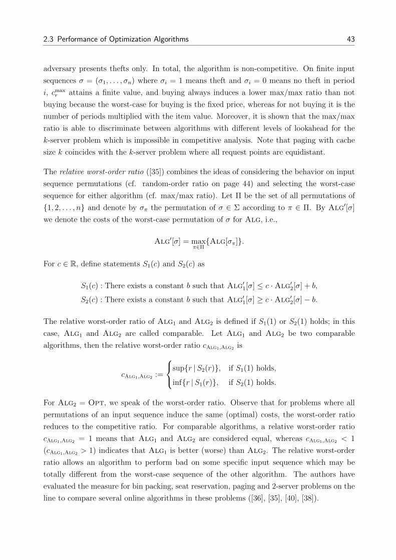
2.3 Performance of Optimization Algorithms 43
adversary presents thefts only. In total, the algorithm is non-competitive. On finite input
sequences σ = (σ1, . . . , σn) where σi = 1 means theft and σi = 0 means no theft in period
i, cmaxr attains a finite value, and buying always induces a lower max/max ratio than not
buying because the worst-case for buying is the fixed price, whereas for not buying it is the
number of periods multiplied with the item value. Moreover, it is shown that the max/max
ratio is able to discriminate between algorithms with different levels of lookahead for the
k-server problem which is impossible in competitive analysis. Note that paging with cache
size k coincides with the k-server problem where all request points are equidistant.
The relative worst-order ratio ([35]) combines the ideas of considering the behavior on input
sequence permutations (cf. random-order ratio on page 44) and selecting the worst-case
sequence for either algorithm (cf. max/max ratio). Let Π be the set of all permutations of
{1, 2, . . . , n} and denote by σπ the permutation of σ ∈ Σ according to π ∈ Π. By Alg′[σ]
we denote the costs of the worst-case permutation of σ for Alg, i.e.,
Alg′[σ] = maxπ∈Π{Alg[σπ]}.
For c ∈ R, define statements S1(c) and S2(c) as
S1(c) : There exists a constant b such that Alg′1[σ] ≤ c ·Alg′2[σ] + b,
S2(c) : There exists a constant b such that Alg′1[σ] ≥ c ·Alg′2[σ]− b.
The relative worst-order ratio of Alg1 and Alg2 is defined if S1(1) or S2(1) holds; in this
case, Alg1 and Alg2 are called comparable. Let Alg1 and Alg2 be two comparable
algorithms, then the relative worst-order ratio cAlg1,Alg2 is
cAlg1,Alg2 :=
sup{r |S2(r)}, if S1(1) holds,
inf{r |S1(r)}, if S2(1) holds.
For Alg2 = Opt, we speak of the worst-order ratio. Observe that for problems where all
permutations of an input sequence induce the same (optimal) costs, the worst-order ratio
reduces to the competitive ratio. For comparable algorithms, a relative worst-order ratio
cAlg1,Alg2 = 1 means that Alg1 and Alg2 are considered equal, whereas cAlg1,Alg2 < 1
(cAlg1,Alg2 > 1) indicates that Alg1 is better (worse) than Alg2. The relative worst-order
ratio allows an algorithm to perform bad on some specific input sequence which may be
totally different from the worst-case sequence of the other algorithm. The authors have
evaluated the measure for bin packing, seat reservation, paging and 2-server problems on the
line to compare several online algorithms in these problems ([36], [35], [40], [38]).

44 2 Analysis of Optimization Algorithms
2.3.1.2 Probabilistic Worst-Case Performance Measures
Probabilistic worst-case analysis is based on the use of some randomization mechanism. In
contrast to average-case analysis, randomness is not used to impute probabilities on the
occurrence of input sequences, but to blur worst-case instances.
Smoothed competitive analysis ([16]) origins from smoothed (complexity) analysis ([153])
where it was introduced to explain why the observed complexity of the simplex algorithm
is polynomial-time, whereas its worst-case complexity is exponential-time. The basic idea
to confirm these observations is to show that worst-case inputs are fragile in the sense that
the worst-case character vanishes under small (smoothing) perturbations. The idea has been
transferred to the analysis of online optimization algorithms by slightly perturbing instances
according to some probability distribution and analyzing the expected competitive ratio on
the perturbed sequences. Let p be some probability distribution and let Σp(σ) ⊂ Σ be the
set of input instances that are obtained by smoothening σ ∈ Σ according to p, then the
smoothed competitive ratio csr of Alg under p is given by
csr := supσ∈Σ
Ep(Alg[σp]
Opt[σp]
)where Ep is the expectation taken over all input sequences σp ∈ Σp(σ)8. For processor
scheduling in a time-sharing multitasking operating system, some algorithm is shown to
behave better under smoothed instances than its competitive ratio would suggest ([16]).
The random-order ratio ([108]) works similar to the smoothed competitive ratio. It con-
siders the neighborhood ΣΠ(σ) of an input sequence σ = (σ1, σ2, . . . , σn) as the set of all
permutations of σ, i.e.,
ΣΠ(σ) = {(σπ−1(1), σπ−1(2), . . . , σπ−1(n)) |π is a permutation of {1, 2, . . . , n}}.
The random-order ratio cror of Alg is given by
cror := lim supOpt[σ]→∞
EΣΠ(σ)(Alg[σ])
EΣΠ(σ)(Opt[σ])
where Opt[σ]→∞ (as given in [108]) characterizes the set of all input instances with length
tending to infinity and all permutations of an input sequence are considered equally likely,
i.e., uniformly distributed. For some applications, such as bin packing, this assumption is
8 Instead of the expectation of the ratio, also the ratio of expectations could be used; however, the instance-wise perspective is preferred in [16] because of its stronger notion of competitiveness.

2.3 Performance of Optimization Algorithms 45
appropriate, whereas for others, such as paging with locality of reference, it is not. In [108],
it is shown that BestFit outperforms other online bin packing algorithms: The algorithm
is shown to have cror ∈ [1.08, 1.5], whereas the competitive ratio is 1.7.
We only mention the use of randomized algorithms in order to improve worst-case results:
A randomized online algorithm RandAlg is a probability distribution over a set of deter-
ministic online algorithms {Alg1,Alg2, . . . ,Algm} which will be drawn at random. The
objective value of RandAlg[σ] on input sequence σ then becomes a random variable. The
strength of a randomized algorithm arises as a result of its uncertain realization that the
malicious adversary has to cope with. We will not go into detail as we seek for an assessment
of the behavior of a single deterministic algorithm and refer the reader to [21] and [32].
2.3.1.3 Average-Case Performance Measures
In average-case analysis, stochasticity refers to probabilities for input sequence occurrences.
The notion of competitiveness has been transferred to stochastic settings ([136], [151]). Let
D be a probability distribution over all input sequences, then Alg is called c-competitive
under D if there is a constant a such that
ED(Alg[σ]) ≤ c · E(Opt[σ]) + a.
In the case a = 0, Alg is called strictly c-competitive under D if
ED(Alg[σ])
ED(Opt[σ])≤ c.
The expected competitive ratio cr of Alg under D is
cDr = inf{c ≥ 1 |ED(Alg[σ]) ≤ c · ED(Opt[σ]) + a}= inf{c ≥ 1 |Alg is c-competitive under D}.
In the same way, the expectation can be taken instance-wise over all ratios between Alg’s
and Opt’s costs: The expected performance ratio c′Dr of Alg under D is
c′Dr = inf{c ≥ 1 |ED
(Alg[σ]
Opt[σ]
)≤ c}.
The author in [151] concludes that the expected performance ratio should be favored over
the expected competitive ratio because sequences with small (large) objective value would

46 2 Analysis of Optimization Algorithms
be underrepresented (overrepresented) in the isolated expectations. Moreover, the expected
performance ratio indicates which algorithm performs better on most of the sequences, and
using Markov’s inequality the probability for a sequence whose ratio is far from the expec-
tation can be bounded. Several publications consider an asymptotic version of the expected
performance ratio where one restricts attention to input sequences of infinite length (see, e.g.,
[26], [50], [106], [121]): Let Σn comprise the set of all input sequences of length n, σn ∈ Σn
and
RD(n) := ED(Alg[σn]
Opt[σn]
),
then the asymptotic expected performance ratio R(∞) of algorithm Alg is
RD(∞) = limn→∞
RD(n).
Expected competitiveness has been extensively studied in the context of bin packing with a
focus on the asymptotic expected performance ratio: RD(∞) is derived for NextFit under
uniformly distributed item sizes ([50], [106], [142]); Harmonic has RD(∞) = π2
3−2 ≈ 1.289
([121]). In [26], FirstFit is shown to be asymptotically optimal, i.e., RD(∞) = 1. [147]
introduced the expected waste as a subsitute performance measure and succeeded in sepa-
rating BestFit and FirstFit: In the limit both perform equally good, whereas BestFit
converges faster. Results for discrete item size distributions are given in [49]. [6] and [109]
adopt similar techniques to determine whether BestFit, FirstFit and RandomFit are
stable, i.e., whether the expected waste remains asymptotically bounded. Results for dis-
crete item sizes in the bounded-space bin packing problem are due to [136]. Surveys including
average-case results in bin packing can be found in [46], [47] and [55]. In paging with locality
of reference, [105] extends the access graph model with edge probabilities such that input
sequences are generated by a Markov chain. The asymptotic expected fault rate is used to
characterize an algorithm that achieves an optimal asymptotic expected fault rate on any
Markov chain. Moreover, a procedure to determine an online algorithm whose asymptotic
expected fault rate is bounded with respect to Opt is devised. However, in [75] it has been
shown previously that none of the famous algorithms such as Lru or Fifo can have an
asymptotic expected fault rate that is bounded with respect to Opt. In [76], c′Dr is analyzed
for the ski rental problem where skiing ends after any period with probability λ ∈ [0, 1].
Upper bounds on c′Dr for List in makespan scheduling were derived in [48] under several
distributions; for completion time scheduling, c′Dr ∈ O(1) was proven in [145] for Shortest-
ExpectedProcessingTime under a class of distributions with known expected processing
time. Bounds on c′Dr are found in [144], [151], [152] for minimum spanning trees, paging and
completion time scheduling.

2.3 Performance of Optimization Algorithms 47
The diffuse adversary model introduced in [115] decreases adversary power by restricting
instances to a class of admissible distributions ∆ whereof a worst distribution D ∈ ∆ is
selected to determine the value of the performance measure. Alg is said to have expected
competitive ratio cdr(∆) under diffuse adversaries with distribution class ∆ if
cdr(∆) = inf{c ≥ 1 | ED(Alg[σ])
ED(Opt[σ])≤ c,D ∈ ∆
}.
Alg is said to have expected performance ratio c′dr (∆) under diffuse adversaries with distri-
bution class ∆ if
c′dr (∆) = inf{c ≥ 1 |ED
(Alg[σ]
Opt[σ]
)≤ c,D ∈ ∆
}.
The diffuse adversary model was first proposed in [115] to improve competitive analysis re-
sults on paging where a class of distributions ∆ε is given to model the opposite of locality
of reference: For any given history of previously requested pages and any page p, the prob-
ability that p will be requested next is not larger than ε. It is shown that Lru attains the
optimal expected performance ratio under diffuse adversaries with distribution class ∆ε. The
computation of c′dr (∆ε) has been achieved in [166] showing Lru’s superiority over Fwf and
Fifo. A diffuse adversary to model locality of reference is proposed in [15]: Given some
history of previous pages, the probability of requesting page p is a non-increasing function of
the last point in time when p was requested. The observed superiority of Lru is confirmed
because c′dr (∆) ∈ O(1) when distributions exhibit a sufficiently large degree of locality.
2.3.1.4 Distributional Performance Measures
The main advantage of distributional performance analysis is that an algorithm is judged by
a distribution instead of a single key figure. Although no probabilistic assumptions are made
in online optimization, we recognize that we obtain deterministic counting results when we
impute a uniform distribution over all instances ([90]).
Relative interval analysis ([67]) is a preliminary stage of distributional analysis since it only
considers the extreme values of a distribution for two algorithms. Define
MinAlg1,Alg2(n) := min|σ|=n{Alg1[σ]−Alg2[σ]},
MaxAlg1,Alg2(n) := max|σ|=n{Alg1[σ]−Alg2[σ]},

48 2 Analysis of Optimization Algorithms
then the relative interval of Alg1 and Alg2 is
IAlg1,Alg2 =[lim infn→∞
MinAlg1,Alg2(n)
n, lim sup
n→∞
MaxAlg1,Alg2(n)
n
].
The relative interval of an algorithm pair corresponds to its asymptotic range of amortized
costs. For IAlg1,Alg2 = [0, c] with c ≥ 0, Alg2 dominates Alg1 in the sense that Alg2 never
incurs larger (asymptotic) amortized costs than Alg1. Analogously, for IAlg1,Alg2 = [−c, 0]
with c ≥ 0, Alg1 dominates Alg2. Relative interval analysis allows for a direct comparison
between two algorithms without reference to Opt. In [67], relative interval analysis facilitates
a distinction between paging algorithms Lru and Fifo on the one side and Fwf on the other
side; moreover, it also reflects the positive influence of lookahead on Lru.
Stochastic dominance (see, e.g., [133]) origins from statistics where it is used to establish an
order relation between distributions of two random variables. By interpreting the objective
value obtained by an algorithm as a random variable, this concept has been transferred to
the analysis of online optimization algorithms in [90] where the objective value distributions
of two algorithms Alg1 and Alg2 are related to each other using stochastic dominance9. Let
FAlg : R→ [0, 1] be the cumulative distribution function of the objective value of Alg:
• Alg1 dominates Alg2 stochastically at zeroth order if and only if Alg1[σ] ≥ Alg2[σ]
for all σ ∈ Σ (instance-wise dominance).
• Alg1 dominates Alg2 stochastically at first order (Alg1 ≥st Alg2) if the probability
for achieving an objective value larger than or equal to v is higher for Alg1 than for
Alg2 for all v ∈ R, i.e., Alg1 has more mass on high values than Alg2:
Alg1 ≥st Alg2 :⇔ P (Alg1[σ] ≥ v) ≥ P (Alg2[σ] ≥ v), v ∈ R
⇔ FAlg2(v) ≥ FAlg1(v), v ∈ R.
• Alg1 dominates Alg2 stochastically at second order (Alg1 ≥st2 Alg2) if the cumula-
tion of all probability densities for achieving an objective value larger than or equal to
v is higher for Alg1 than for Alg2 for all x ∈ R, i.e., Alg1 has more mass on [x,+∞]
than Alg2:
Alg1 ≥st2 Alg2 :⇔∫ x
−∞P (Alg1[σ] ≥ v)dv ≥
∫ x
−∞P (Alg2[σ] ≥ v)dv, x ∈ R
⇔∫ x
−∞(FAlg2(v)− FAlg1(v))dv ≥ 0, x ∈ R.
9 Note that in a minimization problem Alg1[σ] ≥ Alg2[σ] means that Alg2 is better than Alg1 on σ.

2.3 Performance of Optimization Algorithms 49
Graphically, Alg1 ≥st Alg2 yields FAlg1(v) ≤ FAlg2(v) and Alg1 ≥st2 Alg2 means that the
area from −∞ to v under FAlg2 is larger than that of FAlg1 for v ∈ R. Figure 2.3 exemplifies
stochastic dominance between the objective value distributions of three algorithms.
0
1
v
FA
lgi(v)
Alg1
Alg2
Alg3
Figure 2.3: Stochastic dominance relations between Alg1,Alg2,Alg3. Alg1 ≥st Alg2 andAlg1 ≥st Alg3, but neither Alg2 ≥st Alg3 nor Alg3 ≥st Alg2. Alg1 ≥st2 Alg2
and Alg1 ≥st2 Alg3, and from the shaded area we see that Alg2 ≥st2 Alg3.
If Alg1 stochastically dominates Alg2 at first order, then E(Alg1) ≥ E(Alg2). It is
easy to see that stochastic dominance at a given order implies stochastic dominance at all
subsequent orders. Unfortunately, no order of stochastic dominance admits a total ordering
among all distributions and we cannot expect stochastic dominance to hold for arbitrary
algorithms. However, when comparing an algorithm without lookahead Alg1 to one with
lookahead Alg2 in a minimization problem, Alg1 ≥st Alg2 would illustrate the benefit of
lookahead because Alg2 attains smaller objective values on more instances than Alg1. In
this case, Alg2 is said to be stochastically better than Alg1. In [90], stochastic dominance
is analyzed for paging and bin coloring: Lru can be shown to be stochastically optimal for
paging with locality of reference under three different models of locality; in bin coloring,
the reasonable GreedyFit algorithm is shown to be stochastically better than the trivial
OneBin algorithm, whereas competitive analysis fails to discriminate them.
Bijective analysis ([9]) is a special case of stochastic dominance where input sequences are
uniformly distributed. The basic idea is to find a bijection b : Σn ↔ Σn between the
input sequences for Alg1 and Alg2 such that in a minimization problem, the objective
value Alg1[σ] of Alg1 on σ is never worse than that of Alg2 on the image b(σ) of σ,
i.e., Alg2[b(σ)]. Essentially, the approach consists in establishing an order of the elements
in Σn such that Alg1 outperforms Alg2 on every pair (σ, b(σ)). Alg1 is called no worse
than Alg2 according to bijective analysis (Alg1 � Alg2) if for all n ≥ n0 ≥ 1 with some
n0 ∈ N there exists b : Σn ↔ Σn with Alg1[σ] ≤ Alg2[b(σ)] for all σ ∈ Σn. Alg1 is called

50 2 Analysis of Optimization Algorithms
better than Alg2 according to bijective analysis if Alg1 � Alg2 and not Alg2 � Alg1.
Hence, Alg1 does not have to outperform Alg2 on each input sequence, but there has to
be a relabeling of the input sequences such that this relation holds between the original and
relabeled sequences. The authors applied bijective analysis to the paging and list update
problem in [9] and [10]: Lru is better than Fwf according to bijective analysis. Moreover,
lookahead is shown to be beneficial by Lru(l) � Lru where l is the lookahead size.
The authors of [9] themselves consider bijective analysis as too strong to establish a relation
between algorithms in many problems and propose a substantially weaker concept called
average analysis ([65]) which compares the average cost of two algorithms over all requests
of the same length. Alg1 is called no worse than Alg2 according to average analysis if for
all n ≥ n0 ≥ 1 with some n0 ∈ N we have∑σ∈Σn
Alg1[σ] ≤∑σ∈Σn
Alg2[σ].
For paging with locality of reference as defined in concave analysis, Lru is strictly separated
from all other strategies as the unique optimal strategy according to average analysis.
We point out the advantages given in [10] for bijective analysis that can be transferred to
any distributional performance measure:
• The performance measure is simple and intuitive, yet powerful.
• Algorithms can be compared directly without reference to a hypothetical algorithm.
• Typical properties of algorithms are likely to be uncovered.
We will adopt the idea of looking at distribution functions for assessing algorithm per-
formance in our approach presented in the following section. We note that none of the
distributional performance measures proposed in literature sticks to the idea of comparing
algorithms on an instance-wise basis in form of a performance ratio.
2.3.2 Performance Comparison of Optimization Algorithms
The behavior of an algorithm with respect to the obtained objective value may differ strongly
from instance to instance. We seek for an approach which summarizes the global behavior of
an algorithm over all instances, but also does not lose sight of local quality, i.e., with respect
to a particular instance. We wish to present algorithm behavior free of risk preferences
such that the decision maker can choose the most suitable algorithm according to personal
preferences, and we desire to analyze the impact of lookahead on algorithm performance.

2.3 Performance of Optimization Algorithms 51
Definition 2.39 (Objective value).
Let Π = (I, S, f, opt) be an optimization problem, let i ∈ I be an instance of Π, and let Alg
be an algorithm for Π choosing sAlg(i) ∈ S(i) on i.
a) vAlg(i) := f(i, sAlg(i)) is called objective value of Alg with respect to i.
b) vAlg(I) := maxi∈I{vAlg(i)} is called upper objective value of Alg with respect to I.
c) vAlg(I) := mini∈I{vAlg(i)} is called lower objective value of Alg with respect to I.
4Since in online optimization, traditionally no probabilistic information on instance occur-
rences is given, choosing the maximum entropy distribution emulates the state of informa-
tional nescience best by minimizing the amount of a-priori information in the distribution
([97], [98]). The uniform distribution over I is the maximum entropy distribution among all
distributions with support I (which follows from Langrangian relaxation by the definition
of the entropy together with the constraint that the sum over all probabilities equals 1).
For finite I, imposing a uniform distribution leads to counting results saying how many out
of all instances yield a certain objective value ([90]). We define the counting distribution
function10 in order to subsume these frequency information of objective values over I:
Definition 2.40 (Counting distribution function of objective value).
Let Π = (I, S, f, opt) be an optimization problem, let i ∈ I be an instance of Π, let Alg be
an algorithm for Π, and let vAlg(i) be the objective value of Alg on i.
a) If I is a discrete set, then the function FAlg : R→ [0, 1] with
FAlg(v) :=
∑i∈I
1[−∞,v](vAlg(i))
|I|
is called counting distribution function of the objective value of Alg over I.
b) If I is an uncountable set, then the function FAlg : R→ [0, 1] with
FAlg(v) :=
∫i∈I
1[−∞,v](vAlg(i))
|I|
is called counting distribution function of the objective value of Alg over I.
410The indicator function 1A(x) is 1 if x ∈ A and 0 otherwise.

52 2 Analysis of Optimization Algorithms
Comparing two algorithms by means of their counting distribution functions of the objective
value is done by examining their relative positions to each other. Assuming minimization
in Figure 2.4 a), Alg1 exhibits a more volatile behavior than Alg2 with objective values
ranging in a broader interval; likewise, chances for a low objective value are higher.
0
1
vAlg1vAlg2 vAlg2 vAlg1
v
FA
lgi(v)
Alg1
Alg2
a)
0
1
rAlg1,Alg2 1 rAlg1,Alg2
r
FA
lg1,A
lg2(r)
Alg1/Alg2
b)
Figure 2.4: Counting distribution functions. a) Of objective value of Alg1 and Alg2. b) Ofperformance ratio of Alg1 relative to Alg2.
The following definitions account for the relative performance of two algorithms to each other
when both are restricted to operate on the same problem instance:
Definition 2.41 (Performance ratio).
Let Π = (I, S, f, opt) be an optimization problem, let i ∈ I be an instance of Π, and let
Alg1, Alg2 be two algorithms for Π choosing sAlg1(i), sAlg2(i) ∈ S(i) on i, respectively.
a) rAlg1,Alg2(i) :=f(i,sAlg1
(i))
f(i,sAlg2(i))
is called performance ratio of Alg1 relative to Alg2 with
respect to i.
b) rAlg1,Alg2(I) := maxi∈I{rAlg1,Alg2(i)} is called upper performance ratio of Alg1 relative
to Alg2 with respect to I.
c) rAlg1,Alg2(I) := min
i∈I{rAlg1,Alg2(i)} is called lower performance ratio of Alg1 relative
to Alg2 with respect to I.
4
rAlg1,Alg2(I) coincides with the competitive ratio if Π is an online optimization problem,
Alg1 is an online algorithm and Alg2 equals Opt. It coincides with the approximation
ratio if Π is an offline optimization problem, Alg1 is an offline algorithm and Alg2 equals
Opt. For online algorithms Alg1 and Alg2 with and without lookahead, respectively, the
performance ratio expresses how much Alg1 benefits from lookahead compared to Alg2.

2.3 Performance of Optimization Algorithms 53
Definition 2.42 (Counting distribution function of performance ratio).
Let Π = (I, S, f, opt) be an optimization problem, let i ∈ I be an instance of Π, let Alg be
an algorithm for Π, and let rAlg1,Alg2(i) be the performance ratio of Alg1 relative to Alg2
on i.
a) If I is a discrete set, then the function FAlg1,Alg2 : R→ [0, 1] with
FAlg1,Alg2(r) :=
∑i∈I
1[−∞,r](rAlg1,Alg2(i))
|I|
is called counting distribution function of the performance ratio of Alg1 relative to
Alg2 over I.
b) If I is an uncountable set, then the function FAlg1,Alg2 : R→ [0, 1] with
FAlg1,Alg2(r) :=
∫i∈I
1[−∞,r](rAlg1,Alg2(i))
|I|
is called counting distribution function of the performance ratio of Alg1 relative to
Alg2 over I.
4
Assuming minimization, comparing two algorithms Alg1 and Alg2 by means of their count-
ing distribution function of the performance ratio is done by partitioning the set of all in-
stances into those with performance ratio smaller than or equal to 1 (favoring Alg1) and into
those with performance ratio larger than 1 (favoring Alg2). In Figure 2.4 b), Alg1 attains
an objective value at least as large as that of Alg2 on the majority of the instances.
We mention advantages of our two-sided approach which consists of using distribution func-
tions of the objective value and the performance ratio for assessing an algorithm’s quality:
• The distribution function of the objective value gives a global view on the quality of
an algorithm over all instances.
• The distribution function of the performance ratio of an algorithm pair offers a local
view on the quality of both algorithms relative to each other on the same instance.
• Distribution-based analysis also yields information about ranges and variability.
• Algorithms with arbitrary lookahead levels can be compared to each other.

54 2 Analysis of Optimization Algorithms
Example 2.43 (Counting distributions of objective value and performance ratio).
Consider an optimization problem Π = (I, S, f,max) where the instance set I is defined by
I = {x ∈ R2 |x1 + x2 ≤ 5, 0.75x1 + x2 ≤ 4.5, x1 ≤ 3, x1 ≥ 0, x2 ≥ 0} ⊂ R2
as illustrated in Figure 2.5 with a total volume |I| = 10.
0 1 2 3 4 5 6
0
1
2
3
4
5
vAlg1(x) = 2
vAlg2(x) = 1.5
vAlg3(x) = 1.5
I
x1
x2
Figure 2.5: Graphical illustration of instance set I.
The set of feasible solutions for each i ∈ I is given by
S(i) = S(x1, x2) = {c1x1 + c2x2 | c1, c2 ∈ R} = R
and a feasible solution s ∈ S(i) is evaluated as its identity, i.e., f(i, s) = s. For some
(intransparent) reason, we have three algorithms Alg1, Alg2, Alg3 which choose
sAlg1(i) = sAlg1(x1, x2) = x1 + x2,
sAlg2(i) = sAlg2(x1, x2) = 1.5x1 + 0.5x2,
sAlg3(i) = sAlg3(x1, x2) = 0.5x1 + 1.5x2,
respectively. Which of the three algorithms is most promising when some instance i ∈ I will
be revealed to the decision maker?
In contrast to linear programming, we do not want to maximize sAlgj(i) for j = 1, 2, 3 over
I but rather would like to obtain the objective value distribution over I for each of the
algorithms (cf. Figure 2.6 for Alg1). One can think of a decision maker who has to choose

2.3 Performance of Optimization Algorithms 55
one of the algorithms before being presented with some point i = (x1, x2) ∈ I. How should
the decision maker behave in order to obtain a high objective value?
01
23 0
2
4
0
2
4
I
x1 x2
v Alg1(x)
0
1
2
3
4
5
Figure 2.6: Objective value of Alg1 over instance set I.
To find an expression for the counting distribution function FAlgj(v) with j = 1, 2, 3, we
first compute the area V jv := |{x ∈ I | f(x, sAlgj
(x)) ≤ v}| of all points x ∈ I with objective
function value of Algj smaller than or equal to v.
• f(x, sAlg1(x)) = x1 + x2:
– v ∈ [0, 3]: V 1v =
v∫0
(v − x1)dx1 = 0.5v2
– v ∈ [3, 4.5]: V 1v =
3∫0
(v − x1)dx1 = 3v − 4.5
– v ∈ [4.5, 5]: V 1v =
4v−18∫0
(4.5− 0.75x1)dx1 +3∫
4v−18
(v − x1)dx1 = −2v2 + 21v − 45
• f(x, sAlg2(x)) = 1.5x1 + 0.5x2:
– v ∈ [0, 2.25]: V 2v =
23v∫
0
(2v − 3x1)dx1 = 23v2
– v ∈ [2.25, 4.5]: V 2v =
89v−2∫0
(4.5− 0.75x1)dx1 +
23v∫
89v−2
(2v− 3x1)dx1 = −29v2 + 4v− 4.5
– v ∈ [4.5, 5.5]: V 2v =
2∫0
(4.5− 0.75x1)dx1 +v−2.5∫
2
(5− x1)dx1 +3∫
v−2.5
(2v − 3x1)dx1
= −v2 + 11v − 20.25

56 2 Analysis of Optimization Algorithms
• f(x, sAlg3(x)) = 0.5x1 + 1.5x2:
– v ∈ [0, 1.5]: V 3v =
2v∫0
(23v − 1
3x1)dx1 = 2
3v2
– v ∈ [1.5, 4.5]: V 3v =
3∫0
(23v − 1
3x1)dx1 = 2v − 1.5
– v ∈ [4.5, 5.5]: V 3v =
7.5−v∫0
(23v − 1
3x1)dx1 +
3∫7.5−v
(5− x1)dx1
= −13v2 + 5v − 8.25
– v ∈ [5.5, 6.75]: V 3v =
10.8−1.6v∫0
(23v− 1
3x1)dx1+
2∫10.8−1.6v
(4.5−0.75x1)dx1+3∫2
(5−x1)dx1
= − 815v2 + 7.2v − 14.3
With V jv for j ∈ {1, 2, 3} and I’s total volume of 10, we have that the percentage of all x ∈ I
with objective value of Algj smaller than or equal to v is V jv
10. We can interpret this value as
the probability that the objective value will be no more than v when we pick a point x ∈ Iat random, i.e., when we assume a uniform distribution over the elements of I. We obtain
the counting distribution functions of the objective value (cf. Figure 2.7) as follows:
FAlg1(v) =
0, if v < 0
110
(0.5v2), if 0 ≤ v < 3,
110
(3v − 4.5), if 3 ≤ v < 4.5,
110
(−2v2 + 21v − 45), if 4.5 ≤ v < 5,
1, else.
FAlg2(v) =
0, if v < 0,
110
(23v2), if 0 ≤ v < 2.25,
110
(−29v2 + 4v − 4.5), if 2.25 ≤ v < 4.5,
110
(−v2 + 11v − 20.25), if 4.5 ≤ v < 5.5,
1, else.

2.3 Performance of Optimization Algorithms 57
0 1 2 3 4 5 6 7
0
1
v
FA
lgi(v)
Alg1
Alg2
Alg3
Figure 2.7: Distributions of objective value of Alg1, Alg2, Alg3 over I.
FAlg3(v) =
0, if v < 0,
110
(23v2), if 0 ≤ v < 1.5,
110
(2v − 1.5), if 1.5 ≤ v < 4.5,
110
(−13v2 + 5v − 8.25), if 4.5 ≤ v < 5.5,
110
(− 815v2 + 7.2v − 14.3), if 5.5 ≤ v < 6.75,
1, else.
Because of FAlg2(v) ≥ FAlg3(v) for v ∈ R, Alg3 dominates Alg2. No dominance relation
involves FAlg1 . However, when we compare FAlg1 and FAlg2 , we see that FAlg1(v) ≤ FAlg2(v)
for v ∈ [0, 4.5] making Alg1 comparably attractive.
We next seek to derive an expression for the counting distribution function of the performance
ratio of one algorithm relative to another one. Exemplarily, Figure 2.8 shows the graph of
the performance ratio rAlg1,Alg2(x) over all instances.
Considering performance ratio rAlg1,Alg2(i) =f(i,sAlg1
(i))
f(i,sAlg2(i))
= x1+x2
1.5x1+0.5x2, we first recognize that
every ray emanating from the origin consists of points with equal performance ratio: Let
x2 = mx1 be such a ray, then it follows that
f(i, sAlg1(i))
f(i, sAlg2(i))=
x1 +mx1
1.5x1 + 0.5mx1
=x1(1 +m)
x1(1.5 + 0.5m)= const.
As displayed in Figure 2.9, we subdivide I into three regions A1 with rAlg1,Alg2(i) ∈ [23, 10
11],
A2 with rAlg1,Alg2(i) ∈ [1011, 10
9], and A3 with rAlg1,Alg2(i) ∈ [10
9, 2].

58 2 Analysis of Optimization Algorithms
01
23 0
2
4
0
1
2
I
x1 x2
v Alg1(x)
0.8
1
1.2
1.4
1.6
1.8
2
Figure 2.8: Performance ratio rAlg1,Alg2(x) over instance set I.
Observe that for two rays x2 = m2x1 and x2 = m1x1 with m2 > m1 it follows that all points
on x2 = m2x1 have a larger performance ratio than all points on x2 = m1x1:
x1 +m2x1
1.5x1 + 0.5m2x1
>x1 +m1x1
1.5x1 + 0.5m1x1
⇔ 1 +m2
1.5 + 0.5m2
>1 +m1
1.5 + 0.5m1
⇔ m2 > m1.
0 1 2 3 4 5 6
0
1
2
3
4
5
A2
A3
A1
r(x) = 23
r(x) = 1011
r(x) = 109
r(x) = 2
α2
α3
·
x1
x2
Figure 2.9: Instance set I with regions A1, A2, A3.
In order to find an expression for FAlg1,Alg2(r), we have to characterize the amount of the
volume of I where performance ratios not larger than r are attained for each r ∈ R. We
have from the previous discussion that FAlg1,Alg2(r) = 0 for r < 23
and FAlg1,Alg2(r) = 1
for r ≥ 2. For the remaining values of r, we analyze areas A1, A2 and A3: By A≤i (r)

2.3 Performance of Optimization Algorithms 59
(i = 1, 2, 3) we denote the (triangular) subregion in Ai where each point x of this sub-
region has rAlg1,Alg2(x) ≤ r, by x(r) = (x1(r), x2(r)) we denote the point on the face of
I with rAlg1,Alg2(x) = r, and by h(x(r)) we denote the height of triangle A≤i (r) when
the ray emanating from 0 intersects x(r). As the bases of A≤1 (r), A≤2 (r), A≤3 (r), we take
[0, (3, 0)], [0, (3, 2)], [0, (2, 3)], respectively.
• For A1, we have that |A≤1 (23)| = 0 and |A≤1 (10
11)| = 3. Exploiting the relation
r =3 + x2
4.5 + 0.5x2
⇔ x2 =3− 4.5r
0.5r − 1⇔ x2 =
6− 9r
r − 2
which follows from x1 = 3 on the face of I in A1 coinciding with the height of the
triangle for computing A≤1 (r), we obtain
|A≤1 (r)| = 1
2· 3 · h(x(r)) =
1
2· 3 · x2(r) =
3
2
(6− 9r
r − 2
).
Relating |A≤1 (r)| to |I| = 10, we get for r ∈ [23, 10
11] that
FAlg1,Alg2(r) =3
20
(6− 9r
r − 2
).
• For A2, we have that |A≤2 (1011
)| = 0 and |A≤2 (109
)| = 2.5. Using the values of the slopes
of x2 = 5− x1 and x2 = 23x1 we have
tanα2 =∣∣∣−1− 2
3
1− 23
∣∣∣ = 5⇒ α2 = tan−1(5) ≈ 78.69◦.
Exploiting the relation
r =5
7.5− x2
⇔ x2 = 7.5− 5
r⇔ x2 =
15
2− 5
r
which follows from x1 = 5− x2 on the face of I in A2 needed to determine the height
of the triangle for computing A≤2 (r), we obtain
|A≤2 (r)| = 1
2·√
13 · h(x(r))
=1
2·√
13 · sin(tan−1(5)) ·√
((5− x2)− 3)2 + (x2 − 2)2
=1
2·√
13 · sin(tan−1(5)) ·√
2 · (x2 − 2)
=5
2· (x2 − 2) =
5
2·((15
2− 5
r
)− 2)
=5
2·(11
2− 5
r
).

60 2 Analysis of Optimization Algorithms
Relating |A≤2 (r)| to |I| = 10 and considering that |A1| = 3, we get for r ∈ [1011, 10
9] that
FAlg1,Alg2(r) = 0.3 +5
20
(11
2− 5
r
)=
67
40− 5
4r.
• For A3, we have that |A≤3 (109
)| = 0 and |A≤3 (2)| = 4.5. Using the values of the slopes
of x2 = 4.5− 0.75x1 and x2 = 1.5x1 we have
tanα3 =∣∣1.5 + 0.75
1− 98
∣∣ = 18⇒ α3 = tan−1(18) ≈ 86.82◦.
Exploiting the relation
r =36− 2x2
54− 9x2
⇔ x2 = 6− 24
9r − 2
which follows from x1 = 6− 43x2 on the face of I in A3 needed to determine the height
of the triangle for computing A≤3 (r), we obtain
|A≤3 (r)| = 1
2·√
13 · h(x(r))
=1
2·√
13 · sin(tan−1(18)) ·√
((6− 4
3x2)− 2)2 + (x2 − 3)2
=1
2·√
13 · sin(tan−1(18)) · 5
3· (x2 − 3)
= 3 · (x2 − 3) = 3((
6− 24
9r − 2
)− 3)
= 9− 72
9r − 2.
Relating |A≤3 (r)| to |I| = 10 and considering that |A1| = 3, |A1| = 2.5, we get for
r ∈ [109, 2] that
FAlg1,Alg2(r) = 0.55 +9
10
(1− 8
9r − 2
)=
29
20− 36
5(9r − 2).
We obtain the counting distribution function for the performance ratio of Alg1 relative to
Alg2 as
FAlg1,Alg2(r) =
0, if r < 23,
320
(6−9rr−2
), if 2
3≤ r < 10
11,
6740− 5
4r, if 10
11≤ r < 10
9,
2920− 36
5(9r−2), if 10
9≤ r < 2,
1, if r ≥ 2.

2.3 Performance of Optimization Algorithms 61
A similar analysis applies to determine the distribution functions of the performance ratio
of Alg1 relative to Alg3 and of Alg2 relative to Alg3, respectively:
FAlg1,Alg3(r) =
0, if r < 23,
2720− 54−27r
5(5r+2), if 2
3≤ r < 10
11,
7340− 5
4r, if 10
11≤ r < 10
9,
1− 18−9r10(6r−4)
, if 109≤ r < 2,
1, if r ≥ 2.
FAlg2,Alg3(r) =
0, if r < 13,
2720− 81−27r
5(5r+9), if 1
3≤ r < 9
11,
65− 15−5r
8(1+r), if 9
11≤ r < 11
9,
1− 27−9r20(3r−1)
, if 119≤ r < 3,
1, if r ≥ 3.
Figure 2.10 plots the distribution functions of the performance ratio of the three algorithms
relative to each other.
0 0.5 1 1.5 2 2.5 3
0
0.2
0.4
0.6
0.8
1
r
FA
lgi,A
lgj(r)
Alg1/Alg2
Alg1/Alg3
Alg2/Alg3
Figure 2.10: Distribution of performance ratio of Algi relative to Algj for (i, j) = (1, 2),(i, j) = (1, 3) and (i, j) = (2, 3) over I.
Because of maximization, it would be more desirable to choose Alg1 over Alg2: The per-
formance ratio range [23, 2] reveals that Alg1 can be up to twice as good as Alg2, whereas
Alg2 can only be 32
as good as Alg1; at the same time more than 50 % of the instances incur
a ratio larger than 1. Consider FAlg1,Alg3 : On the one hand, Alg1 loses to Alg3 on having
more instances with a ratio larger than 1; on the other hand, Alg1 beats Alg3 in potentially

62 2 Analysis of Optimization Algorithms
being twice as good, whereas Alg3 can only be 32
as good as Alg1. For FAlg2,Alg3 , the ratio
ranges in [13, 3] and less than 50 % of the instances incur a ratio larger than 1. In this sense,
Alg3 should be favored over Alg2. From the discussion it follows that Alg2 is not to be
recommended in the first place.
We remark that in general computing the volume of a polytope is #P-hard11. For further
details, the interested reader is referred to [110], [111], [112]. ♦
2.4 Optimization Algorithms and Discrete Event Systems
So far we were only concerned with the outcome of an algorithm for a given instance of an
online optimization problem but did not pay attention to the solution process that is under-
gone in order to obtain the outcome. Now we concentrate on the modeling of that solution
process: Interpreting the release of an input element of input sequence σ = (σ1, σ2, . . .) as the
occurrence of an event allows us to recast the solution process in online optimization using
the terminology from discrete event systems. In the following Chapters 2.4.1 to 2.4.4, differ-
ent modeling concepts are discussed based on the standard works [43] and [126] on discrete
event systems as well as on the guidelines of the Association of German Engineers (VDI,
Verein Deutscher Ingenieure) on simulation in [159]; alongside the discussion we transfer
these concepts to online optimization with lookahead.
2.4.1 Discrete Event Systems
Define a process as a transformation, transportation or storage of some energetic, material or
informational resource, then a system is a fragment of the real world in which all processes
relevant to the user take place. As such, a system is a reduction from the real world to
those entities which influence these processes and satisfy the user’s wish to duplicate them.
Models are used to describe systems: A model is a formal description of a system which
captures the relevant aspects of the system along with all related processes in a sufficient
level of detail. Systems with time-dependent behavior are called dynamic systems and they
are usually described by an input-output model.
11A counting problem Π (asking for the number of solutions to an instance with a given property) is incomplexity class #P if its associated decision problem is in NP. A problem in #P is at least as hardas its decision problem version in NP. A counting problem Π is in complexity class #P-complete if itis in #P and all other problems in #P can be transformed to it in polynomial time. A problem Π is incomplexity class #P-hard if it is at least as hard as any problem in #P.

2.4 Optimization Algorithms and Discrete Event Systems 63
Processes in dynamic systems are stimulated by an input function v : T → V from the set
T of time instants to the set V of input values. In discrete time systems, we typically have
T = N0; in continuous time systems, usually T = R≥0. The system responds to the values
provided by v over time with an output function w : T → W from T to the setW of output
values. Let Fv and Fw be the set of all input and output functions, respectively. Then we
can view a (model of a) system as an operator S : Fv → Fw and S can be described by the
input-output relation
(w(0), w(1), w(2), . . . , w(k)) = S ◦ (v(0), v(1), v(2), . . . , v(k)).
It has proven useful to bypass the input-output relation by using the concept of a state. A
state s(k) of a system at time k comprises all information needed to determine w(k′) for k′ ≥ k
based on v(k′). The state space S of a system is the set of all possible states of the system.
Using a state transition function f : S × V → S and an output function h : S × V → W ,
we substitute the input-output relation with a recursive state space representation of the
system in discrete time by
s(k + 1) = f(s(k), v(k)), s(0) = s0,
w(k) = h(s(k), v(k))
where s0 is the initial state of the system.
Let an event be a spontaneous occurrence triggered by some external entity (event generator,
nature) or by fulfillment of all conditions of a switching rule (event generation rule). Because
events can be used to submit changes of the input function value to the system over time,
the following definition is obtained:
Definition 2.44 (Discrete event system ([43], [126])).
A discrete event system (DES) is an event-driven system whose state trajectory depends
only on the occurrence of discrete events over time. 4
Figure 2.11 subsumes the causal relationships in a discrete event system. Note that events
may result from the output function and feed back as an event to the input function.
In online optimization, the release of input elements occurs at discrete points in time and an
online algorithm operates as part of a reactive planning system. Hence, the solution process
in online optimization can be modeled as a DES. Because we associate an objective value to
an input sequence processed by an algorithm, we embed an entry for the objective value of

64 2 Analysis of Optimization Algorithms
Inputgeneration
ProcessEvent
generation
Input v(k)
v1(k)
v2(k)
v3(k)
Output w(k)
w1(k)
w2(k)
w3(k)
Eventsequence
Figure 2.11: Event-based input-output model of discrete event systems. (Source: [126])
the current state into the state encoding scheme. Table 2.2 summarizes analogies between
the solution procedure in online optimization and the behavior of discrete event systems.
Online optimization Discrete event system
Input element EventInput sequence Event sequence
Input element release Event occurrenceReleases occur at discrete times Events occur at discrete times
Algorithm reacts to input element releases System reacts to event occurrencesOnline algorithm State transition functionObjective value Entry in state encoding scheme
Table 2.2: Analogies between online optimization and discrete event systems.
As a result of their similarities, both online algorithms and discrete event systems can be
tackled using the same arsenal of analytical methods.
Automata are the basic logical model to replicate discrete system behavior over time. They
allow to track state transitions and resulting state trajectories over time. However,
they do not provide information on frequencies for transitions or trajectories leading
to a certain state.
Markov chains extend logical models with stochastic information. Their analysis gives in-
formation about state frequencies and yields mathematical expressions for quantities of
interest. Recall that by imposing a uniform distribution over the set of input elements
(as the maximum entropy distribution), we obtain deterministic counting results.
Discrete event simulation is applied for most real world problem settings since it is impossi-
ble to use exact methods like automata or Markov chains due to intractable complexity
and state space explosion for increased problem size and level of detail.

2.4 Optimization Algorithms and Discrete Event Systems 65
Due to their logical character with regard to the order of events, both basic automata and
Markov chains are restricted to the analysis of online optimization algorithms in the sequen-
tial model. In order to comply with the time stamp model, timed versions of automata and
Markov chains are needed. These are obtained by additionally imposing a clock structure
on the DES. We will not further discuss this topic in the sequel.
2.4.2 Automata
Automata theory provides a formal means to study the behavior of a discrete event system
over time. The set of all events can be regarded as an alphabet and event sequences cor-
respond to words which form the input to an automaton. The set of all words that can be
processed by an automaton is called the language of this automaton. Informally, an automa-
ton is a device capable of processing the words of its language. An automaton is the simplest
representation of an event-driven state transition mechanism.
Definition 2.45 (Deterministic automaton ([43], [126])).
A deterministic automaton A is a quintuple (S, E , f, s0,SF ) where S is the set of states, Eis the set of events, f : S × E → S is the state transition function, s0 ∈ S is the initial state
and SF ⊆ S is the set of final states. 4
A deterministic automaton can be represented by a graph: Nodes correspond to the states
of the automaton; edges represent transitions between states and are labeled with the events
which induce the state transition. The event-driven approach becomes apparent by using
automata to process an event sequence resulting in a state sequence as seen in Figure 2.12.
A
e1
e2
e3
s1
s2
s3
Tim
et
Figure 2.12: Automaton as a formal means to process elements of an event sequence. (Source:[126])
The behavior of an automaton for a given event sequence (e0, e1, e2, . . . , eK) with K ∈ Nwhen starting in initial state s0 ∈ S is specified by the sequence of state transitions
sk+1 = f(sk, ek), ek ∈ {e ∈ E | f(sk, e) is defined}, k = 0, 1, . . . , K.

66 2 Analysis of Optimization Algorithms
Although instances in online optimization are uncertain, a deterministic online algorithm
processes any instance deterministically. Thus, it suffices to restrict attention to deterministic
automata. In order to describe the behavior of an online algorithm during input element
processing by a deterministic automaton, we have to perform the following steps:
1. Define the set of input elements which are translated into event set E .
2. Find a representation of the system state which is translated into state space S.
3. Determine the behavior of the online algorithm when it encounters a given input ele-
ment in a given state which is translated into state transition function f .
4. Determine the initial system state s0 and, if necessary, the set of final states SF .
Analysis methods focus on properties that can be inferred from reachability between states:
Given an automaton A with initial state si, it is asked for the set of reachable states SR where
state sj is called reachable from si if there exists an event sequence such that the sequence
of induced state transitions leads from si to sj. The concept of reachability coincides with
reachability in graph theory and can be reduced to finding a path between si and sj in the
graph representation of A. Introduce the adjacency matrix A = (aij) with i, j ∈ S as
aij =
1, if there exists e ∈ E with f(i, e) = j
0, else,
and denote by Ak = (akij) the kth power of A for k ∈ N. Because in a connected graph
with N nodes any node can be reached traversing at most N − 1 edges, we have that by
determining AN−1 all reachability relations between states of the automaton are known: sj
is reachable from si if and only if aN−1ij 6= 0.
With regard to the performance ratio analysis of online optimization algorithms, we consider
the product coupling A× = A1 ×A2 of two automata A1,A2. The product coupling of two
automata is used when both automata are synchronized, i.e., they have to respond to a
common sequence of events (cf. Figure 2.13). Comparing two online algorithms on the same
input sequence, this condition is given whenever the input sequence does not depend on
previous decisions.
Formally, the product couplingA× ofA1 = (S1, E , f1, s0,1,SF,1) andA2 = (S2, E , f2, s0,2,SF,2)
is given as A× = (S1×S2, E , f×, (s0,1, s0,2),SF,1×SF,2) where a state is a pair (s1, s2) ∈ S1×S2
and the state transition function f× is recast as

2.4 Optimization Algorithms and Discrete Event Systems 67
A1 = (S1, E , f1, s0,1,SF,1)
A2 = (S2, E , f2, s0,2,SF,2)
e = (e1, e2, . . .)
Figure 2.13: Coupling of two automata. (Source: [126])
f×((s1, s2), e) =
(f1(s1, e), f2(s2, e)
)if f1(s1, e) and f2(s2, e) are defined,
undefined, otherwise.
Applying the product-coupling on two online algorithms permits a simultaneous tracking of
the state evolution over time.
In preparation for the discussion of Markov chains, we introduce the notions of an au-
tonomous deterministic automaton and an autonomous nondeterministic automaton.
Definition 2.46 (Autonomous deterministic automaton ([43], [126])).
An autonomous deterministic automaton A is a quadruple (S, f, s0,SF ) where S, s0, SF are
the same as in a deterministic automaton and f : S → S is the state transition function. 4
State transitions of an autonomous automaton are not associated to the occurrence of events
but rather happen without a certain reason out of nowhere.
Definition 2.47 (Autonomous nondeterministic automaton ([43], [126])).
An autonomous nondeterministic automaton A is a quadruple (S, frel, s0,SF ) where S, s0,
SF are the same as in an autonomus deterministic automaton and frel : S → 2S is the state
transition relation. 4
The state transition relation frel(·) of a nondeterministic automaton gives a set of possible
successor states from the power set 2S of S for some given state. Notice that we obtain an
autonomous nondeterministic automaton from any deterministic automaton simply by omit-
ting the set of events Σ in the definition of the state transition function. In the automaton
graph this amounts to removing the edge labels (events) suggesting that the state transition
is carried out as a result of some random mechanism rather than as a result of an event.

68 2 Analysis of Optimization Algorithms
2.4.3 Markov Chains
Besides analyzing state reachability, Markov chains allow for analyzing the frequency of
encountering a given state by incorporating probabilistic information on state transitions.
This approach is particularly meaningful for representing the performance distribution of
algorithms as it allows to track the objective value and performance ratio distribution.
Let P (A) denote the probability of some event A and let Sk be a random variable for the
state at time k in a discrete event system with time instants N0. A Markov chain is obtained
from an autonomous nondeterministic automaton by replacing the state transition relation
frel with a probability distribution Gprob : S × S → [0, 1] such that
gss′ := Gprob(s, s′) = P (Sk+1 = s′ |Sk = s)
gives the conditional probability that the system reaches state s′ at time k + 1 when it has
already reached state s at time k. We have to impose that∑s′∈S
gss′ = 1, s ∈ S,
to ensure that Gprob(s, ·) is a probability distribution. In a discrete event system, uncertainty
is quantified by stochastic information on the occurrence of events leading to a state tran-
sition. When no stochastic information is given, imputing the uniform distribution yields
deterministic counting results ([90]).
Definition 2.48 (Markov chain ([43], [126])).
A Markov chain A is a quadruple (S, Gprob, p0,SF ) where S, SF are the same as in an
autonomous deterministic automaton, Gprob : S×S → [0, 1] is the state transition probability
distribution and p0 is a probability distribution on the initial state. 4
A Markov chain is also called an autonomous stochastic automaton.
Denote by p(k) the vector whose ith element pi(k) := P (Sk = i) gives the probability that
the system takes on state i at time k. Using matrix G = (gij) with
gij := P (Sk+1 = j |Sk = i),
we obtain the recursive relation
p(k + 1) = Gp(k)

2.4 Optimization Algorithms and Discrete Event Systems 69
known as the Chapman-Kolmogorow equation. Hence, a Markov chain models a discrete time
linear system and with the initial state probability distribution p0 we have that pk = Gkp0
computes the state probabilities at time k. Using the uniform distribution over all events or
state transitions, respectively, we obtain deterministic counting results with regard to how
often a state is reached after a fixed amount of time has expired.
A system is said to have the Markov property if it holds that
P (Sk+1 = sk+1 |Sk = sk, . . . , S0 = s0) = P (Sk+1 = sk+1 |Sk = sk)
for all k ≥ 0. The Markov property states that the successor state solely depends on the
current state, but on none of the states prior to that. It can be shown that a system has to
fulfill the Markov property in order to establish a recursion in the form of the Kolmogorow-
Chapman equation which gives rise to the term Markov chain as a synonym for autonomous
stochastic automaton. The Markov property has also coined the notion of a memoryless
system due to the system’s oblivion to past states before the current state.
Classical Markov chain analysis is concerned with finding the steady state distribution, if it
exists. We are interested in a Markov chain’s transient behavior which yields information
about the state distribution after a given number of time steps ([90]). In most Markov chain
models of online optimization, no steady state distribution exists due to the objective value
being a part of the state encoding. We use Markov chains to obtain frequency information
concerning states with a prescribed objective value. For the performance ratio of an algorithm
relative to another, the state space of an associated Markov chain would need to comprise
the Cartesian product of the state space used for the analysis of the objective value of one
algorithm as outlined in Chapter 2.4.2.
2.4.4 Discrete Event Simulation
According to [159], “simulation is the reproduction of a system along with its dynamic
processes in an executable model in order to retrieve results which are transferable to reality”.
An execution of the simulation with specified input parameters is called simulation run or
replication. Results on system performance are derived from first collecting data over a
sufficient number of simulation runs which then serve as the computational basis so as to
determine (point, interval or distributional) estimates for several performance measures of
interest. In an experiment, we define a sufficiently large replication set to increase the
likelihood for results of high representativeness. Besides experiment design, we have to take

70 2 Analysis of Optimization Algorithms
into account in the model design that each involved stochastic process is associated with a
separate stream of random numbers such that any sort of dependency is ruled out.
Whenever a real world system shall be analyzed but exact analysis is out of reach due to a
high degree of complexity and a large number of dependent stochastic processes, simulation
represents an appropriate tool to provide estimates for desired performance measures. Al-
though the approximation character in the outcomes may be deprecating, there are quite a
number of advantages:
• Simulation may be the only way to analyze the behavior of complex systems with mul-
tiple dependent random variables and manifold types of events such as input element
releases, machine breakdowns, occurrence of erroneous data or erroneous operations.
• Sufficiently many simulation runs allow to obtain statistically sound results.
• Simulation allows to track manifold quantities of interest as intended by multicriteria
approaches in optimization.
• Simulation as an abstract model of reality is comparatively risk-free and cheap.
The event calendar is the pivotal element of a discrete event simulation model. It can
be thought of as a list of pending events that are fed into the discrete event system over
the course of a simulation run. Hence, the event calendar at time t is a list of events
ek, ek+1, . . . , ekmax
Lt =((ek, tk), (ek+1, tk+1), . . . , (ekmax , tkmax)
)with elements ordered according to non-decreasing occurrence times tk, tk+1, . . . , tkmax . We
take care of state trajectories by using a state transition function f : S × E → S where Scorresponds to the state space and E corresponds to the event set.
A run of a discrete event simulation model comprises the steps displayed in Algorithm
2.1 and any implementation of a discrete event simulation software amounts to a generic
implementation of these steps. A simulation study then consists of building a model for the
simulation and executing Algorithm 2.1 with respect to the simulation model for a sufficient
number of times with independent seeds. Clearly, the main contribution in a simulation
study consists in building the right model for the right purpose. Therefore, modeling requires
continuous surveillance using validation and verification methods ([141]).
There are two possible hierarchical relations between simulation and optimization ([135],
[119]): First, optimization appears as a subroutine module in the simulation; second, sim-
ulation is used as a multi-criteria evaluation function for an optimization method. Due
to incremental decision making in online optimization, we are concerned with the former

2.5 Concluding Discussion 71
Algorithm 2.1 Discrete event simulation run
Input: Seed value list S, initial state s, initial event list E, set of statistics, ending condition
1: Initialize random number generators with seed values from S2: Initialize system state with s3: Initialize event calendar with initial event list E4: while ending condition not fulfilled do5: Remove first entry (e, t) from event calendar6: Advance to time t7: Update system state according to state transition function s := f(s, e)8: Update statistics9: Delete (e, t) and all infeasible events from event calendar
10: Generate new events and add them to event calendar11: Reorder elements in the event calendar by non-decreasing event times12: end while
Output: Terminal state s, values of statistics
relation where decisions from an optimization module are iteratively requested within the
simulation model at the corresponding decision points of the function logic in the real world
model. In Algorithm 2.1, a decision elicited from an optimization method is manifested in
the discrete event simulation run by a state transition according to that decision in line 7.
Real world systems from production and logistics are inherently complex and contain opti-
mization problems exhibiting an online character at several control points. Discrete event
simulation combined with methods from online optimization represents a powerful tool in
the design (or reorganization) phase of such systems as it allows to evaluate the performance
of algorithms and to identify the most promising algorithm with respect to the user’s require-
ments on system performance. As a major disadvantage, it is much more difficult to gain
structural insights on why a system behaves the way it does from simulation experiments
than from exact analysis methods. After the simulation model is finished, it is often just
used as a black box to evaluate sample state trajectories of the system.
2.5 Concluding Discussion
This chapter provided a clear definition of the term online optimization with lookahead in
order to ensure a common understanding of this optimization concept not only through-
out this thesis but also throughout different problem settings in general. We clarified the
relations between the different optimization paradigms and examined their implications on
computational complexity as well as on algorithm analysis. It became evident that – due
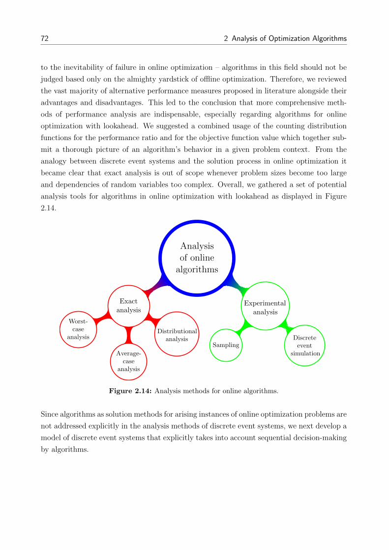
72 2 Analysis of Optimization Algorithms
to the inevitability of failure in online optimization – algorithms in this field should not be
judged based only on the almighty yardstick of offline optimization. Therefore, we reviewed
the vast majority of alternative performance measures proposed in literature alongside their
advantages and disadvantages. This led to the conclusion that more comprehensive meth-
ods of performance analysis are indispensable, especially regarding algorithms for online
optimization with lookahead. We suggested a combined usage of the counting distribution
functions for the performance ratio and for the objective function value which together sub-
mit a thorough picture of an algorithm’s behavior in a given problem context. From the
analogy between discrete event systems and the solution process in online optimization it
became clear that exact analysis is out of scope whenever problem sizes become too large
and dependencies of random variables too complex. Overall, we gathered a set of potential
analysis tools for algorithms in online optimization with lookahead as displayed in Figure
2.14.
Analysisof onlinealgorithms
Exactanalysis
Worst-case
analysis
Average-case
analysis
Distributionalanalysis
Experimentalanalysis
SamplingDiscreteevent
simulation
Figure 2.14: Analysis methods for online algorithms.
Since algorithms as solution methods for arising instances of online optimization problems are
not addressed explicitly in the analysis methods of discrete event systems, we next develop a
model of discrete event systems that explicitly takes into account sequential decision-making
by algorithms.

73
3 A Modeling Framework for Online
Optimization with Lookahead
In this chapter, we consider how a system whose function logic iteratively requires solving
subproblems of an online optimization problem instance can be tackled formally. We propose
a generic framework in order to harmonize concepts and notation throughout problems and
applications. Its instantiations specify the constraints and the potential workflow that the
system under consideration has to undergo while processing an input sequence using an algo-
rithm with lookahead capabilities. The framework intends to facilitate systematic algorithm
analysis based on a common understanding of the solution process paradigm and lookahead
mechanism. In contrast to discrete event systems, our framework explicitly accounts for an
integration of an algorithm’s decision making and available lookahead.
3.1 Modeling Prototypes
A first attempt to model online optimization problems generically were request answer games
as introduced at the beginning of the previous millenium’s last decade by Ben-David et al.
([21]). A sequence of requests is presented online and each time a new request arrives, an
adequate answer has to be given incurring some cost.
Formally, a request answer game over time horizon n ∈ N is a triple (R,A, C) where Ris a set of requests, A is a set of answers and C = {cn |n ∈ N} is a set of cost functions
with cn : Rn × An → R ∪ {∞}. In this model, a deterministic online algorithm Alg =
(Alg1,Alg2, . . . ,Algn) is a sequence of functions with Algi : Ri → A for i = 1, 2, . . . , n.
The output of an algorithm upon request sequence r = (r1, r2, . . . , rn) ∈ Rn is a sequence of
answers a = (a1, a2, . . . , an) ∈ An with ai = Algi(r1, r2, . . . , ri) for i = 1, 2, . . . , n. The costs
incurred by Alg upon processing r are given by cn(r, a).

74 3 A Modeling Framework for Online Optimization with Lookahead
Although request and answer games cover many online optimization problems, the concept
could not be established as a modeling standard due to its lacking ability to account for the
rationale in an algorithm’s decision making. Clearly, the concept of a state is needed for this
purpose. Request and answer games are mainly used in order to distinguish between several
types of adversaries in competitive analysis of randomized online algorithms ([21], [32]).
Another proposition for a generic model of online optimization origins from the priority
programme Online Optimization of Large Scale Systems of the German Research Foundation
(DFG, Deutsche Forschungsgemeinschaft) from 1996 to 2001 ([84]). On an informal basis,
Grotschel et al. ([85]) propose the sequential model and the time stamp model of online
optimization as refurbished in Definitions 2.14 and 2.15, respectively.
In both models, an input sequence σ = (σ1, σ2, . . .) is revealed over time and an algorithm
has to serve each of the input elements. In the sequential model, σi+1 is presented only when
σi has just been served, i.e., input elements are processed according to the first-in first-out
priority rule. In the time stamp model, each input element σi comes along with a release time
τi which is independent of an algorithm’s previous actions. The release time represents the
earliest point in time where σi may be served. Hence, in complete opposite to the sequential
model, the order of service is not fixed initially. Under the time stamp model, decisions
have a tentative character as long as they have not been executed and may be revoked until
then. As a result of an inclusion of the factor time, different solution strategies arise for an
algorithm: Waiting may become lucrative and decisions may be made at arbitrary points in
time.
Both for the sequential and time stamp model, no extension to the lookahead case was
suggested. In particular, incorporation of lookahead would require a more concise statement
about the restrictions on the service order and on the earliest possible times for service
which would arise due to lookahead. A subdivision of lookahead into an informational and
a processual component as outlined in Chapter 2.1.3 would be the logical consequence.
For classical disciplines in optimization, the working schemes of exact algorithms are known:
In mixed integer linear programming, the branch and bound method is established and
research concentrates on improving or extending the method by valid inequalities or branch
and cut procedures. In dynamic programming, value iteration, policy iteration or linear
programming are known to work as a result of the Bellman equation and research focuses
on how to apply the methods in practice, e.g., by approximative approaches. In contrast, no
online optimization algorithm can be exact; as a result, there is no basic starting point for
further research as outlined for the other fields. We believe that the introduction of a formal
modeling framework is at least a first step to find a common basis of understanding.

3.2 Modeling Framework Components 75
3.2 Modeling Framework Components
We recognize that previous models of online optimization lack an integration of lookahead
and a representation of the solution process for a given problem instance. In particular, the
sequential character of decision making by an algorithm in form of reactive planning upon
notification of new input elements needs a dedicated formulation. In the following sections,
we build a generic modeling framework for online optimization problems with lookahead; it
comprises four building blocks:
• The basic modeling elements provide an abstract view on the infrastructure of infor-
mation flows needed to model the solution process.
• The lookahead type specifies the instance revelation rule that an algorithm under look-
ahead has to obey in contrast to the reference online case.
• The processing characteristics specify the processing rules that an algorithm under
lookahead has to obey in its decision making on how to serve the input elements in
contrast to the reference online case.
• The algorithm execution mode defines the time instants at which algorithm evaluation
is scheduled over the course of the solution process.
Instantiations of the four building blocks are combined in a generic process model which
describes the interaction of the modeling elements over time as a result of the specific forms
of lookahead type, implied processing characteristics and prescribed algorithm execution
mode. The process model is of a discrete event nature because an algorithm has to respond
to a sequence of input elements arriving at discrete points in time ([68]).
3.2.1 Basic Modeling Elements
We first identify the constituting elements which are needed in each model of an online
optimization problem with lookahead. To this end, we consider the problem as part of a
dynamic system: We let the system under consideration be the abstracted collection of all
real world entities needed to describe the optimization problem, and we embed the system
in a time horizon with current time denoted by t.

76 3 A Modeling Framework for Online Optimization with Lookahead
Input element and input sequence
The smallest unit of information is given by an input element from the set of all possible input
elements Σ1 (which is the set of all input sequences of length 1). The input appears in form of
an input sequence σ = (σ1, σ2, . . .) consisting of input elements σi ∈ Σ1 for i = 1, 2, . . . These
are invisible at first, but then revealed successively according to the lookahead mechanism.
Each input element awaits some processing during the solution process. The processing of
an input element can be understood as the result of a decision (e.g., in form of a decision
variable assignment) on what to do with it in order to comply with all restrictions and to
contribute to the optimization goal.
An input element σi is a data record containing all relevant information needed by an algo-
rithm to decide on the processing of σi. On the most granular level, it is associated with the
following atomic parts:
• Release time τi := τ(σi) in the reference online optimization problem
• Release time τ ′i := τ ′(σi) in the online optimization problem with lookahead
• Processing time interval [T i, T i] := [T (σi), T (σi)] in the reference online optimization
problem
• Processing time interval [T ′i, T′i] := [T ′(σi), T
′(σi)] in the online optimization problem
with lookahead
• Input element information ri := r(σi)
The only requirement on release times is τ ′i ≤ τi. The processing time intervals [T i, T i] and
[T ′i, T′i] give the times at which input element σi is allowed to be (physically) processed in
the absence and presence of lookahead, respectively. Many combinatorial online optimization
problems have T i = T i and T ′i = T′i; in this case, we can also use Ti and T ′i as the time
instants where processing is due to be executed. ri carries the essential information of σi
which is needed for decision making (e.g., the size of an item in bin packing or the location
of a request in the traveling salesman problem).
We associate two time-dependent variables with each input element σi:
• Processing status pi(t) := p(σi, t) ∈ {unprocessed, processing, finished}
• Action ai(t) := a(σi, t)

3.2 Modeling Framework Components 77
Processing status pi(t) gives the state of σi at time t and rules membership to the sets of
still unprocessed, currently processing or already finished input elements. Action ai(t) is a
data record with all information concerning how σi is, was, or is planned to be processed.
ai(t) is determined by an algorithm; if no action has been determined yet at time t, we set
ai(t) = Null. Whenever ai(t) 6= Null, we have that ai(t) contains at least the elements
ta,starti and ta,finishi denoting the time instants when processing of σi is (planned to be) started
and finished, respectively. Decisions made previously may be revoked until the current time
t reaches ta,starti . The set of all possible actions for an input element is denoted by A.
There are no additional sources of incomplete information with respect to σi once it has
been notified, i.e., it is given in its entirety as soon as its existence emerges. Each input
element experiences two steps with respect to its information: First, all information of an
input element is announced at its release time. Second, this information is exploited by an
algorithm to determine how an input element will be processed. The processing itself, of
course, takes place between ta,starti and ta,finishi without any further ado.
We remark that there are different types of events besides the arrival of new input elements
in real world applications such as system breakdowns, erroneous inputs or other kinds of
unforeseeable disturbances. In these cases, it must be ensured that input sequence σ can
accommodate input elements of different event classes.
Lookahead set
At each time t, the processing statuses of the known input elements establish a partition
of all available input elements into sets Ut, Pt and Ft of unprocessed, currently processing
and finished input elements, respectively. In the reference online optimization problem, we
have
• Ut := {σi | τi ≤ t, pi(t) = unprocessed}
• Pt := {σi | τi ≤ t, pi(t) = processing}
• Ft := {σi | τi ≤ t, pi(t) = finished}
In an online optimization problem with lookahead, τi is replaced with τ ′i . The following
equivalences rule membership of σi to these sets:
• pi(t) = unprocessed ⇔ ai(t) = Null ∨ ta,starti > t
• pi(t) = processing ⇔ ta,starti ≤ t < ta,finishi
• pi(t) = finished ⇔ ta,finishi ≤ t

78 3 A Modeling Framework for Online Optimization with Lookahead
The lookahead set Lt at time t is the collection of those input elements which have been
revealed, but still require (some amount of) processing, i.e., Lt := Ut∪Pt. Thus, Lt depends
on previous decisions and actions caused by an algorithm and not on a distinction between
the release times in the cases of absent and present lookahead. Although it might be tempting
to define lookahead as the set difference between the input elements known in the reference
online case and those known in the lookahead case, this approach has no practical benefit as
it is oblivious to the input elements which are at an algorithm’s disposal. Note that an input
element can stay in Lt arbitrarily long and suffer starvation if its processing is continuously
rejected in favor of another input element.
State space
For a better representation of the dependencies between an algorithm’s decision and the
current state, we decompose each state s from the set of all states S into three components
s = (sin, ssys, sobj) with input state sin, system state ssys and objective state sobj. All
information concerning the input of the problem at time t is collected in input state sint =
(Ut, Pt, Ft); the set of all input states is denoted by S in. Because sint contains all σi with
τi ≤ t or τ ′i ≤ t, it also contains all action variables ai(t) for these input elements. To
describe external circumstances which have to be taken into account by an algorithm, the
system state ssyst at time t is a data record containing all information to describe the system
configuration (e.g., bin configurations in bin packing or the current server position in the
traveling salesman problem) at time t; the set of all system states is denoted by Ssys. In the
context of optimization, we have to use valued states to keep track of the current objective
value during the solution process. At time t, we extract all information relevant to the future
development of the objective value (e.g., the plain current objective value) in objective
state sobjt ; the set of all objective states is denoted by Sobj. The set of all states is S =
S in × Ssys × Sobj; concerning the solution process of an online optimization problem with
lookahead, we are interested in the state trajectory evolution (st)t≥0 with st ∈ S for t ≥ 0.
Event space
Because in online optimization an algorithm has to respond to arriving input elements, we
classify the arrival of a new input element as an event. Likewise, finished processing may
change the objective state such that the end of an input element’s processing also represents
an event. In total, all state transitions which are of interest in monitoring the solution
process of an online optimization problem are triggered by the occurrence of an event. We

3.2 Modeling Framework Components 79
subsume all possible events in the event set E . Events occur at discrete time instants and
have a duration of zero. In our framework, events are the only source of uncertainty which an
algorithm has to cope with. Note that both the sequential and time stamp model of online
optimization only know two types of events referring either to finished processing of an input
element or to notification of a new input element; both types coincide in the sequential model
because a new element only becomes available when a known one finishes processing.
Algorithm
Input element processing is controlled by the decisions of an algorithm, ultimately causing
changeovers of input elements between sets Ut, Pt and Ft as imputed by the algorithm’s
decisions. Recalling that in online optimization the overall solution is composed of a sequence
of partial solutions, an algorithm Alg is used to successively produce partial solutions by
determining the values of the input elements’ action variables. Let nt := |Ut ∪ Pt| = |Lt| be
the number of unfinished known input elements, then an online algorithm Alg is a family
of functions Alg := (Algt)t≥0 where Algt : S ×E → Ant is a function determining for each
of the nt known and yet unfinished input elements an action from the action space A based
on current state s ∈ S and occurring event e ∈ E . Hence, our definition of an algorithm
generalizes that of the request answer games from Chapter 3.1 in terms of the dependency
on the current state and the multidimensionality of the codomain. Algt is evaluated at each
time instant t where an event occurs.
State transition
The state transition function f : S × E → S determines for a given state s ∈ S and an
occurring event e ∈ E the successor state s′ ∈ S. It only needs to be evaluated at the
discrete time instants where an event occurs because for all other times the state trajectory
is assumed to advance deterministically, i.e., it can be precomputed.
3.2.2 Lookahead Type
The lookahead type specifies the mechanism under which the membership of input elements
to lookahead set Lt is governed for all t. According to the taxonomy from Chapter 2.1.3,
it corresponds to the instance revelation rule of online optimization with lookahead. Which
lookahead type is employed depends on the application under consideration and on the tech-
nical possibilities. We give some frequently used types of lookahead in literature, harmonize

80 3 A Modeling Framework for Online Optimization with Lookahead
them with our notation and introduce property lookahead as a generalization of all instance
revelation rules which allow for a property-related characterization of all known input ele-
ments. Recall that a key characteristic in the sequential model is the processing-dependent
release of input elements: Only when an input element finishes processing, a new one be-
comes known; in the time stamp model, input elements become known independently of
previous decisions and an online algorithm is allowed to wait and revoke decisions as long
as they have not been implemented. Despite of that, also the sequential model can incor-
porate temporal aspects in the specification of input element σi. A similar classification of
lookahead types as described subsequently has also been given by Tinkl ([155]).
Request lookahead
Request lookahead of size k ∈ N ([155]) is defined to have access to a fixed number k of
unprocessed or currently processing input elements, or to all of the remaining unprocessed
and currently processing input elements if there are less than k of them. The first of these
input elements is also known in the pure online situation, but the remaining k − 1 input
elements or all remaining input elements if there are less than k of them are known due to
the lookahead capability. Request lookahead construes the lookahead set dependent on the
processing statuses of the input elements and not in an independent process of release. We
obtain the release times recursively from
τi :=
0, if i = 1,
min{ta,finishj |σj ∈ Lτi−1}, if i = 2, 3, . . .
in the case without lookahead and
τ ′i :=
0, if i = 1, . . . , k,
min{ta,finishj |σj ∈ Lτ ′i−1}, if i = k + 1, k + 2, . . .
in the case with lookahead. Request lookahead origins from applications where time is not
modeled explicitly such that request lookahead is understood only in the sequential model.
Request lookahead is not possible in the time stamp model because an arbitrary number of
input elements may be released at any time contradicting the requirement to hold at most
k input elements. For applications which adhere to capacities, such as storage devices or
inventory spaces, request lookahead is realistic, whereas for applications which deal with
immaterial requests, such as emergency calls or customer demands, it is unrealistic.
Under request lookahead, input elements are revealed in a rolling time horizon. However, one

3.2 Modeling Framework Components 81
can also think of situations where information is released rather in batches or blocks than
steadily over time: A new batch is only given when all elements of the previous one have
finished processing. This gives rise to a batched version of this lookahead variant. In batched
request lookahead of size k, input elements are always revealed in blocks of k elements if
there are more than k elements left, otherwise the remaining input elements are revealed. In
this case, we have
τ ′i :=
0, if i = 1, . . . , k,
max{ta,finishj |σj ∈ Lτ ′ck}, if i = ck + 1, ck + 2, . . . , ck + k with c ∈ N.
Time lookahead
Time lookahead of length D ∈ R>0 ([155]) essentially makes input element σi known D time
units earlier in the online setting with lookahead than in the setting without lookahead.
Hence, except for input sequences which are released before t = D, there is a fixed offset
D between an input element’s release time in the cases of present and absent lookahead.
Release times τi in the pure online setting are assumed to be independent of an algorithm’s
processing and we obtain that τ ′i := max{τi − D, 0}. Time lookahead can be seen as an
artificial preponement of the moment at which an input element is notified by D time units.
It is not admissible in the sequential model because the generation of input elements is an
independent process. A drawback of time lookahead is that arbitrarily many input elements
may reside in the lookahead set: When processing of a single input element extends over time,
the workload may collapse in the long run. Thus, it is reasonable to see time lookahead in
connection with stability enforcing constraints similar to those in queuing systems where the
occupation rate is used to measure server utilization. It deserves mentioning that artificially
diminishing the release time of an input element is conceptually different from allowing an
algorithm to wait in order to accumulate input elements as we nominally make information
available earlier in time. Though, the consequences and positive effects of delaying processing
decisions to a later point in time are similar because the planning basis, i.e., the available
data for a set of decisions, is extended in both situations (cf. also [7]).
Collective property lookahead
Collective property lookahead has been first introduced as a general concept in [155] although
in bin packing (see, e.g., [83]) and paging (see, e.g., [2]) it had already been instantiated

82 3 A Modeling Framework for Online Optimization with Lookahead
before. Let c-prop be a time variant property of an arbitrary subset σ≤j(t) of the elements
in input sequence σ where
σ≤j(t) := {σi | i ∈ {1, 2, . . . , j}, pi(t) 6= finished}.
Write c-propj(t) := c-prop(σ≤j, t) if σ≤j(t) fulfills c-prop at time t and ¬c-propj(t) otherwise.
In addition, we assume for σi, σj, σk ∈ Lt that ¬c-propk(t) holds for all k > j whenever
¬c-propj(t) and that c-propi(t) holds for all i < j whenever c-propj(t). Without a collective
property lookahead device for c-prop, any algorithm is oblivious to c-prop and σi is released
according to the instance revelation rule in the online case; collective property lookahead
makes all input elements that comply with c-prop visible to an algorithm. Collective property
lookahead is defined to have access at time t to a largest possible subsequence of unfinished
input elements such that all input elements of this subsequence collectively fulfill property
c-prop at time t. The first time t where c-propi(t) is fulfilled is set to be the preponed release
time of σi. Thus, in the online setting with lookahead, we have τ ′i := min{t | c-propi(t)}.The instance revelation rule of the pure online setting has to ensure that τ ′i ≤ τi. Collective
property lookahead can be admissible both in the sequential model and time stamp model
depending on the definition of c-prop itself. Collective property lookahead is used when input
elements collectively influence which part of the input sequence is seen, e.g., due to their
combined size or weight.
Property lookahead
We introduce this type of lookahead as a generalization of all lookahead types that can
be described explicitly. Let prop be a time variant property of each input element. Write
propi(t) := prop(σi, t) if σi fulfills prop at time t and ¬propi(t) otherwise. Without a property
lookahead device for prop, any algorithm is oblivious to prop and σi is released according to
the instance revelation rule in the online case; property lookahead makes all input elements
that comply with prop visible to an algorithm. The first time t where propi(t) is fulfilled
is set to be the preponed release time of σi. Thus, in the online setting with lookahead,
we have τ ′i := min{t | propi(t)}. The instance revelation rule of the pure online setting has
to ensure that τ ′i ≤ τi. Property lookahead can be admissible both in the sequential model
and time stamp model depending on the definition of prop itself. Property lookahead is
used whenever there is some device that allows to recognize input elements which fulfill the
property. Note that property lookahead is a generalization of all lookahead types that rely
on some rule which governs membership of input elements to the lookahead set.

3.2 Modeling Framework Components 83
Free lookahead
Free lookahead is applied whenever it is observed that input elements become known earlier
than in the reference online setting, but the mechanism of preponed release of input elements
is unknown or hidden to the user. The fundamental feature of free lookahead is that there
is no relation known between τi and τ ′i other than τ ′i ≤ τi.
3.2.3 Processing Mode and Order
According to Chapter 2.1.3, when input elements are processed, they are subject to the rules
specified in (processing) rule sets P and P ′ of the online optimization problem in absence
and presence of lookahead, respectively. Unfortunately, in literature it is never specified
how P and P ′ exactly look like but tacitly assumed according to the problem context. We
provide a classification which verbally expresses the essential difference between P and P ′.
By definition, the decisions of an algorithm on processing start and end times have to obey
T i ≤ ta,starti ≤ ta,finishi ≤ T i in the pure online setting; in the online case with lookahead, T i
and T i have to be replaced by T ′i and T′i, respectively.
Under lookahead, we have to deal with the questions whether we have to adhere to the order
in the input element sequence also in processing (processing order) and whether more than
one input element can be processed at a time (processing mode).
We explain combinations of the four possible processing modes
• single processing,
• parallel processing,
• limited parallel processing,
• property processing
with the two possible processing orders
• in-order processing,
• random-order processing.

84 3 A Modeling Framework for Online Optimization with Lookahead
Single in-order processing
In single in-order processing, we have to obey the given order of input element releases also
when processing the input elements and we have to process them one after another. For the
decisions of an algorithm on input element σi it has to hold that ta,finishi ≤ ta,starti+1 .
Single random-order processing
In single random-order processing, we are allowed to choose any available unfinished input
element for being processed next at any time, but have to respect that only one input element
can be processed at a time. For the decisions of an algorithm on two input elements σi and
σj with i 6= j it has to hold that [ta,starti , ta,finishi ) ∩ [ta,startj , ta,finishj ) = ∅.
Parallel in-order processing
In parallel in-order processing, we have to obey the given order of input element releases
also when processing the input elements, but we may process more than one input element
at a time. For the decisions of an algorithm on input element σi it has to hold that ta,starti ≤ta,starti+1 .
Parallel random-order processing
In parallel random-order processing, we are allowed to choose any available unfinished input
element for being processed next at any time and we may process more than one input
element at a time. There are no temporal restrictions on processing times which have to
hold for the decisions of an algorithm on the input elements.
Limited parallel in-order processing
Limited parallel in-order processing is similar to parallel in-order processing, but additionally
imposes that at most m input elements can be processed at a time. For the decisions of an
algorithm on input element σi it has to hold that ta,starti ≤ ta,starti+1 and additionally for t ≥ 0
that |{σj | t ∈ [ta,startj , ta,finishj )}| ≤ m.

3.2 Modeling Framework Components 85
Limited parallel random-order processing
Limited parallel random-order processing is similar to parallel random-order processing, but
additionally imposes that at most m input elements can be processed at a time, i.e., for the
decisions of an algorithm it has to hold for t ≥ 0 that |{σj | t ∈ [ta,startj , ta,finishj )}| ≤ m.
Property processing
In property processing, input elements eligible to be processed at time t are marked. Let
proc be a time-dependent property of each input element; write proci(t) := proc(σi, t) if σi
fulfills proc at time t and ¬proci(t) otherwise. Processing start times are coordinated such
that proci(t) is fulfilled when ta,starti = t is chosen. For the decisions of an algorithm on input
element σi it has to hold that ta,starti ∈ {t ≥ 0 | proci(t)}. All previous processing modes and
orders can be emulated by property processing using an adequate specification of proc.
3.2.4 Processing Accessibility
We address the question of when input elements are ready to be processed once they have
been disclosed. Exact specifications of instance revelation rules r and r′ as well as of rule sets
P and P ′ according to the taxonomy in Chapter 2.1.3 would resolve this issue automatically.
However, these specifications are rarely given explicitly in publications such that we provide
a classification which verbally expresses the processing permissions arising by lookahead.
The task is to specify whether earlier disclosure of input element information only means
that the information is known earlier or also that the input element itself is ready to be
processed earlier (cf. also [155]). In the first case, there can only be an informational benefit
of lookahead, but there may additionally be a processual benefit in the latter case.
Immediate accessibility
Processing input element σi is possible directly upon receiving it, i.e., we have T i := τi in
the online setting without lookahead and T ′i := τ ′i in the online setting with lookahead.
Regular accessibility
Processing input element σi is possible only when the regular earliest processing time is
reached, i.e., we have T ′i := T i.

86 3 A Modeling Framework for Online Optimization with Lookahead
Delayed accessibility
Processing input element σi is not possible directly upon receiving its information, but may
be possible at some time before the regular earliest processing time, i.e., we have T i > τi in
the online setting without lookahead and T ′i > τ ′i in the online setting with lookahead. A
typical case is to impose a fixed offset toff between information release and earliest possible
processing, i.e., T i = τi + toff and T ′i = τ ′i + toff .
3.2.5 Algorithm Execution Mode
The algorithm execution mode controls at which time instants an algorithm is executed
in order to determine the values of the action variables of known input elements. Recall
that algorithm execution and action execution (physical processing) are different: Algorithm
execution refers to the computational steps needed to determine actions for input elements,
whereas action execution is the realization of the decisions which have been determined by
algorithm execution before. Action execution runs automatically, but algorithm execution
needs initiation.
We present three intuitive algorithm execution modes which are applicable to algorithms
in online optimization problems with absent or present lookahead. Computing time of al-
gorithms is not a scarce resource in the online optimization paradigm by definition; the
only scarce resource is information ([32]). However, when exact algorithms are applied to
instances of NP-hard optimization problems, we have to ensure that prescribed real-time
requirements are not violated.
Cyclic Execution
Algorithm execution is carried out cyclically, i.e., at all times texeci = i · tcycle for i = 0, 1, 2, . . .
where tcycle is the base time interval between two algorithm executions. It is possible that an
arbitrary large number of new input elements accumulates during two algorithm executions
or that no new input element arrives at all. Execution may still be worthwhile because
actions different from Null may be determined for known input elements which have not
yet been assigned an action so far.

3.3 A Classification Scheme 87
Full Buffer Execution
Algorithm execution is performed every time that the number of elements in the lookahead
set reaches a prescribed limit c ∈ N, i.e., at all times in
{texec ≥ 0
∣∣ |Ltexec | = c, |Ltexec−ε| < c}
with sufficiently small ε > 0. At the end of the input sequence, it has to be assured that none
of the input elements σi exhibits ai(t) = Null so as to guarantee that each input element
will be processed.
Discrete Event Execution
Execution of an algorithm is triggered by events occurring at discrete time instants. From
a technical point of view, an event detecting device must be installed in order to monitor
incoming events. Release of a new input element and finished processing of an input element
serve as typical events in basic online optimization problems. In more complex settings,
additional events such as any type of system breakdown or failure can also be considered as
events. Denote by (tei )i∈N the sequence of time instants at which events are notified, then
algorithm execution takes place at times texeci = tei + ε for i ∈ N with sufficiently small ε > 0.
Note that practically all types of relevant algorithm execution modes can be traced back to
the case of discrete event execution by appropriate definition of the set of events.
3.3 A Classification Scheme
Similar to the classification scheme of Graham et al. for scheduling problems ([81]), we pro-
vide a classification scheme for the modeling of online optimization problems with lookahead
that takes into account their characteristics as identified in the previous sections. Given an
instance of an online optimization problem with lookahead, the components of the modeling
framework need to be specified in order to implement a solution procedure: Basic modeling
elements as introduced in Chapter 3.2.1 are specific to the problem under investigation such
that an associated modeling effort is unavoidable; restrictions concerning the release pro-
cess, the processing characteristics and the algorithm execution mode from Chapters 3.2.2
to 3.2.5 work in a similar way for different problem settings, and they characterize the form
of the instance revelation rule substitution and rule set substitution that comes along with
lookahead.

88 3 A Modeling Framework for Online Optimization with Lookahead
We propose a four-position classification scheme of the form α | β | γ | δ for online optimiza-
tion problems with lookahead in order to quickly indicate the qualitative characteristics of
a problem under lookahead as compared to the online problem without lookahead:
Lookahead type α Frequently used entries for α are:
• req for request lookahead
• req-b for request lookahead in batches
• time for time lookahead
• col for collective property lookahead
• prop for property lookahead
• free for free lookahead
Processing mode and order β Frequently used entries for β are:
• sngl/ord for single in-order processing
• sngl/rnd for single random-order processing
• prl/ord for parallel in-order processing
• prl/rnd for parallel random-order processing
• prl-ltd/ord for parallel limited in-order processing
• prl-ltd/rnd for parallel limited random-order processing
• pp for property processing
Processing accessibility γ Frequently used entries for γ are:
• im for immediate accessibility
• reg for regular accessibility
• dly for delayed accessibility
Algorithm execution mode δ Frequently used entries for δ are:
• cyc for cyclic algorithm execution
• full for full buffer algorithm execution
• discr for discrete event algorithm execution
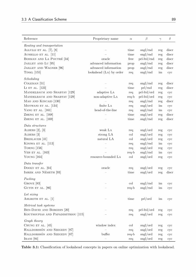
3.3 A Classification Scheme 89
Reference Proprietary name α β γ δ
Routing and transportation
Allulli et al. [7], [8] – time sngl/rnd reg discr
Ausiello et al. [11] – time sngl/rnd reg discr
Bosman and La Poutre [34] oracle free prl-ltd/rnd reg discr
Jaillet and Lu [95] advanced information prop sngl/rnd reg discr
Jaillet and Wagner [96] advanced information prop sngl/rnd reg discr
Tinkl [155] lookahead (La) by order req sngl/rnd im cyc
Scheduling
Coleman [51] – req sngl/rnd reg discr
Li et al. [123] – time prl/rnd reg discr
Mandelbaum and Shabtay [129] adaptive La req prl-ltd/ord reg cyc
Mandelbaum and Shabtay [129] non-adaptive La req-b prl-ltd/ord reg cyc
Mao and Kincaid [130] – req sngl/rnd reg discr
Motwani et al. [134] finite La req sngl/ord im cyc
Yang et al. [161] head-of-the-line req sngl/rnd im cyc
Zheng et al. [168] – time sngl/ord reg discr
Zheng et al. [169] – time sngl/rnd reg discr
Data structures
Albers [2], [3] weak La req sngl/ord reg cyc
Albers [3] strong LA col sngl/ord reg cyc
Breslauer [41] natural LA col sngl/ord reg cyc
Kiniwa et al. [113] – req sngl/rnd im cyc
Torng [156] – req sngl/ord reg cyc
Yeh et al. [163] – req-b sngl/rnd im cyc
Young [164] resource-bounded La col sngl/ord reg cyc
Data transfer
Dooly et al. [64] oracle req sngl/ord reg cyc
Imrek and Nemeth [93] – time sngl/ord reg discr
Packing
Grove [83] – col sngl/rnd im cyc
Gutin et al. [86] – req-b sngl/rnd im cyc
Lot sizing
Ahlroth et al. [1] – time prl/ord im cyc
Metrical task systems
Ben-David and Borodin [20] – req prl-ltd/ord reg cyc
Koutsoupias and Papadimitriou [115] – req sngl/ord reg cyc
Graph theory
Chung et al. [45] window index col sngl/ord reg cyc
Halldorsson and Szegedy [87] – req sngl/ord reg cyc
Halldorsson and Szegedy [87] buffer req-b sngl/ord reg cyc
Irani [94] – req sngl/ord reg cyc
Table 3.1: Classification of lookahead concepts in papers on online optimization with lookahead.

90 3 A Modeling Framework for Online Optimization with Lookahead
As an example, the sequential model of online optimization endowed with request lookahead
as encountered in the paging problem may be represented both by req | sngl/ord | im | discrand req | sngl/ord | im | cyc.
In literature, lookahead is mainly defined with respect to the topic of a paper; often an explicit
specification of processing characteristics is missing but implicitly assumed. Table 3.1 on the
previous page classifies the lookahead concepts and their requirements on processing and
algorithm execution as described in papers on online optimization with lookahead.
Finally, we relate the classification scheme to Definitions 2.13 and 2.21 of online optimization
problems in absence and presence of lookahead, respectively: The lookahead type α indicates
the instance revelation rule substitution from r to r′. The processing mode and order β as
well as the processing accessibility γ are established by rule set P ′ which constitutes the
conditions for the processing of the input elements such that compliance with the feasible
set of the problem under lookahead is ensured. The algorithm execution mode δ as part of
the solution routine is unaffected by the problem formulation.
3.4 Discrete Event Process Model
The generic process model for online optimization with lookahead describes the interaction of
the basic modeling elements over time in order to reproduce the function logic of a dynamic
system. Because we basically impute a discrete-event-triggered algorithm execution, we also
speak of a discrete event process model. In order to keep track of the solution process in
an instance of an online optimization problem with lookahead, we need instantiations of the
lookahead type, the processing mode and order, and the processing accessibility as specified
by the (instance revelation rule and the rule set of the) application.
The system is assumed to operate on an event-driven basis. Starting with initial state s0 ∈ S,
Figure 3.1 schematically illustrates how the system’s state trajectory (s0, s1, s2, . . .) evolves
as a result of events arriving in the event sequence (e0, e1, e2, . . .) and related computations
of algorithm Alg: Upon arrival of an event e ∈ E , the system proceeds from its current state
s ∈ S to successor state s′ ∈ S by evaluating the state transition function f(s, e). However,
computing the successor state at time t as f(s, e) implicitly requires a preceding evaluation
of Algt(s, e) ∈ Ant where nt is the number of known unfinished input elements at time t
because the successor state also contains a specification of the action variables for the yet
unfinished input elements. Upon reaching the successor state, the system awaits the arrival
of a new event causing the system to undergo the same sequence of steps again.

3.5 Relation to Markov Chains 91
s0 ∈ S Alg0(s0, e0)
s1 ∈ S Alg1(s1, e1)
s2 ∈ S · · ·
e0 ∈ E
f(s0, e0)
e1 ∈ E
f(s1, e1)
e2 ∈ E
Figure 3.1: State trajectory with associated state transition function and algorithm evaluationsin the process model for online optimization with lookahead.
The computational effort of an algorithm caused by a state transition typically depends on
the type of the event e that is encountered: The arrival of a new input element suggests
to solve a snapshot optimization problem in order to determine the action variable for the
new input element and to redetermine the action variables for still unfinished input elements;
finished processing of an input element will not cause an algorithm to spend excessive compu-
tational resources since no additional action for a new input element needs to be determined
and all remaining actions are expected to remain the same as they have been computed
previously on the same informational basis.
Information about the evolution of the objective value which is incurred by processing the
elements of the input sequence can be tracked by monitoring the objective state component
sobj of each attained state s = (sin, ssys, sobj). Typically, when an event corresponds to a
finished processing of an input element, a change in the objective value can be observed as a
result of the associated state transition, whereas when an event corresponds to a new input
element release, no immediate change in the objective value will occur since processing of
this input element is still pending.
3.5 Relation to Markov Chains
In a Markov chain, state transitions occur at discrete time instants i ∈ N irrespective of
all past states other than the current state resulting in an associated random (stochastic)
process exhibiting the memoryless property. That is why Markov chains are an equivalent
type of description for autonomous stochastic automata (see also Chapter 2.4.3). A Markov

92 3 A Modeling Framework for Online Optimization with Lookahead
chain can be modeled by identifying the state space S, the initial state probabilities p0(s)
which give the probability that the initial state of the system is s ∈ S, the state transition
probabilities gss′ which give the probability that the successor state of s ∈ S is s′ ∈ S, and a
set SF ⊆ S of terminal states for which we would like to obtain frequency information. For
a fixed initial state s0 ∈ S, the state of the Markov chain is assumed to evolve autonomously
according to the state transition probabilities; after n ∈ N transition steps, a probability
distribution over the states reached after n transitions starting from s0 is obtained. Our
discrete event process model is somewhat different from this perspective because it neither
specifies initial state probabilities nor state transition probabilities. Moreover, upon receiv-
ing a new event from event set E , an algorithm decides deterministically which successor
state will be attained. However, with the sequence of occurring events (e0, e1, e2, . . .), we can
identify a source of randomness also in the discrete event process model. We translate our
nescience of probabilities for occurring events into the assumption of a uniform distribution
for the occurring events: According to the principle of maximum entropy, the largest entropy
distribution, which is the discrete uniform distribution in this case, should be chosen repre-
sentatively in order to ensure that no unjustified assumptions are introduced ([97], [98]). As
a major side effect of this approach, we can use a Markov chain to model the evolution of
the state trajectory in online optimization with lookahead: The state space S of the Markov
chain coincides with the state space of the discrete event process model, the distribution
of the initial state probabilities is degenerated by p0(s0) = 1 for s0 ∈ S and p0(s) = 0 for
s ∈ S with s 6= s0, and the state transition probabilities are chosen as gss′ := e(s,s′)|E| where
e(s, s′) :=∣∣ {e ∈ E | fAlg(s, e) = s′}
∣∣ is the number of events in E leading from state s ∈ Sto state s′ ∈ S by applying algorithm Alg. The choice of gss′ in this Markov chain accounts
for the discrete uniform distribution over the elements of event set E . We note that because
of the objective state component sobj in state s = (sin, ssys, sobj) ∈ S holding information
about the valuation of a state, we implicitly model a valued Markov chain with the above
specifications.
A requirement to adopt Markov chains to online optimization with lookahead is that the
state space S is a finite or countable set. Hence, for time lookahead or continuous state
space information this method of evaluation would be inapplicable and a discretization of
the respective dimensions is required first. However, analyzing an algorithm for an online
optimization problem with lookahead by means of an associated Markov chain suffers the
same computational burdens as the analysis of any Markov chain when the size of the state
space explodes for increased values of the problem parameters ([18]).
We note that the set up of a Markov decision process ([140]) is different from ours: State tran-
sitions occur probabilistically once a control action has been chosen, whereas in our setting

3.6 Instantiations of the Framework 93
they occur deterministically based on an algorithm’s deterministic decision. Markov decision
processes are used as a modeling formalism to determine an optimal strategy, i.e., the deci-
sions of an optimal algorithm with respect to some expected objective value, using dynamic
programming. Stochastic assumptions concerning transition probabilities depending on the
control action are given a-priori: p(s, a, s′) with s, s′ ∈ S and a ∈ A is the probability that
the successor state of s is s′ if action a is chosen. In contrast to this, our analysis merely
intends to evaluate the quality of a given algorithm in a setting of complete nescience of
stochastic information. In particular, we do not seek for an optimal algorithm.
3.6 Instantiations of the Framework
We instantiate the generic modeling framework for online optimization with lookahead in
three exemplary applications by specifying its components.
Online Bin Packing with Lookahead
Consider a version of the online bin packing problem whose lookahead and processing char-
acteristics are classified according to
req | sngl/ord | reg | discr.
Lookahead type Request lookahead of size k.
Processing Mode and Order Items have to be packed in their order of appearance one af-
ter another. As a result, the advantage accrued by lookahead is merely informational.
However, as seen in Example 2.37 and confirmed by the computational results in Chap-
ter 5.3, the value of permuting the item order in physical processing turns out to be 0
anyway when an unbounded number of open bins is allowed.
Processing Accessibility Although lookahead makes items known earlier in time, their pro-
cessing time in the lookahead setting coincides with the processing time in the setting
without lookahead due to required sequentiality. This type of restriction may arise due
to the physical dimensions of the objects which have to be packed.
Algorithm Execution Mode Since assignment decisions are invariant as long as no event
(arrival of new item or packing of item into a bin) occurs, they only need to be (re-)
determined by evaluating Alg whenever an event takes place.

94 3 A Modeling Framework for Online Optimization with Lookahead
Input element and input sequence Denote the set of items by Σ1. An element σi ∈ Σ1 of
the input sequence σ = (σ1, σ2, . . .) corresponds to an item and comprises the following
data:
• Release time τi = i− 1 in the reference problem without lookahead
• Release time τ ′i = max{0, i− k} in the problem with lookahead
• Processing time Ti = i− ε in the reference problem without lookahead
• Processing time T ′i = i− ε in the problem with lookahead
• Input element information ri = si where si is the size of item σi
Lookahead set The lookahead set essentially contains those k items which have not yet
been put into a bin, i.e., Lt = {σi | pi(t) = unprocessed, τi ≤ t} in the setting without
lookahead and Lt = {σi | pi(t) = unprocessed, τ ′i ≤ t} in the setting with lookahead.
State space The state space is given as S = {(U, c1, c2, . . . , cm,m)} where U is the set of
items which have not yet been physically assigned to a bin with U ∈ Σ1∪∅ in the case
without lookahead and U ∈ ⋃k′≤k
{{σ1, σ2, . . . , σk′} |σi ∈ Σ1, i = 1, 2, . . . , k′
}in the case
with lookahead and (c1, c2, . . . , cm) are the fill levels of the m bins used.
Event space The set of events comprises two event types. Events of the first type are of the
form e1(σi) := Arrival of new item σi and events of the second type are of the form
e2(σi, j) := Physical assignment of item σi to bin j. Hence, the event set is given as
E = {e1(σi) |σi ∈ Σ1} ∪ {e2(σi, j) |σi ∈ Σ1, j ∈ N}.
Algorithm An algorithm has to decide into which bin an item has to be put such that no bin
capacity is ever exceeded. Thus, with nt = |Lt| as the number of unprocessed items at
time t, Algt : S×E → {N∪Null}nt is a function which assigns each item in Lt either
the number of the bin into which it is planned to be put at its respective processing
time or leaves the destination bin undetermined.
State transition function Let the current state at time t be s = (U, c1, c2, . . . , cm,m) and
let an event of the form e = e1(σi) occur at t, then the successor state s′ computed
by the state transition function is f(s, e) = (U ′, c1, c2, . . . , cm,m) where U ′ corresponds
to U expanded with σi. Upon event e = e2(σi, j), the successor state s′ is f(s, e) =
(U ′, c′1, c′2, . . . , c
′m′ ,m
′) where U ′ corresponds to U diminished by σi, c′j = cj+si, c
′k = ck
for k = 1, . . . ,m with k 6= j and m′ ∈ {m,m + 1} gives the number of occupied bins
after σi has been packed.

3.6 Instantiations of the Framework 95
Online Traveling Salesman Problem with Lookahead
Consider a version of the online traveling salesman problem whose lookahead and processing
characteristics are classified according to
time | sngl/rnd | im | discr.
Due to the infinite state space as a result of continuous time, the elements of the state space
are uncountable and Markov chain analysis is computationally prohibitive. Nonetheless, the
discrete event process model can be utilized in sample-based analysis or simulation.
Lookahead type Time lookahead of length D.
Processing Mode and Order Locations have to be visited one after another, but not nec-
essarily in their order of appearance. As a result, the advantage from lookahead is
both related to earlier information and possibilities of earlier processing. As seen in
Example 2.37 and confirmed by the computational results in Chapter 5.4, algorithms
benefit from lookahead by visiting spatially proximate locations in temporal proximity.
Processing Accessibility Positive effects in terms of increased degrees of freedom due to
permutability of locations in the visiting sequence are further enhanced by immediate
processing accessibility of the locations, i.e., once a location is known, it is allowed to be
visited immediately. Unrestricted visitation opportunities of this kind may arise when-
ever the requesting entity has no temporal preferences which is the case for physical
or virtual objects, but not for animate beings.
Algorithm Execution Mode Because sequencing decisions are invariant as long as no event
(arrival of new request or finished service) occurs, they only need to be (re-) deter-
mined by evaluating Alg whenever an event takes place. Due to continuous time,
the state trajectory is a continuous path in the state space. However, events can be
ordered such that discrete event algorithm execution applies, and the evolution of the
state trajectory can be (analytically) reproduced based on the event occurrences and
associated decisions of the algorithm.
Input element and input sequence Denote the set of locations by Σ1. An element σi ∈ Σ1
of the input sequence σ = (σ1, σ2, . . .) corresponds to a location to be visited and
comprises the following data:
• Release time τi ∈ [0,∞) in the reference problem without lookahead
• Release time τ ′i = max{0, τi −D} in the problem with lookahead

96 3 A Modeling Framework for Online Optimization with Lookahead
• Processing time Ti ∈ [τi,∞) in the reference problem without lookahead
• Processing time T ′i ∈ [τ ′i ,∞) in the problem with lookahead
• Input element information ri = xi where xi gives the spatial position of σi
Lookahead set Set p(σi) := processing if location σi is currently approached and p(σi) :=
unprocessed otherwise. The lookahead set contains all known locations which have not
yet been reached by the server, i.e., Lt = {σi | pi(t) ∈ {unprocessed, processing}, τi ≤ t}in the case without lookahead and Lt = {σi | pi(t) = {unprocessed, processing}, τ ′i ≤ t}in the case with lookahead.
State space Let n be the maximum number of locations to be visited by the server. The
state space is given as S = {(U, P, t, xs, tlast)} where U ∈ ⋃n′≤n
{{σ1, σ2, . . . , σn′} |σi ∈
Σ1, i = 1, 2, . . . , n′}
is the set of unprocessed locations, P ∈ Σ1 ∪ ∅ is the currently
approached location, t is the current time, xs is the current server location and tlast is
the last time instant where a request location has been visited.
Event space The server moves autonomously to its destinations as prescribed in the action
variables of the locations. The set of events only comprises two event types. Events
of the first type are of the form e1(σi) := Arrival of new location σi and events of the
second type are of the form e2(σi) := Server has reached location σi. Hence, the event
set is given as E = {e1(σi) |σi ∈ Σ1} ∪ {e2(σi) |σi ∈ Σ1}.
Algorithm An algorithm has to decide upon the order in which the locations in Lt have to
be visited. It suffices at each time if the server knows which location to approach next;
note that the current destination may be revised upon announcement of a new location.
Thus, with nt = |Lt| as the number of unvisited locations at time t, Algt : S × E →{N∪Null}nt is a function which assigns each location in Lt either the position in the
visiting order of the unvisited locations or leaves the position undetermined.
State transition function Let the current state at time t be s = (U, P, t, xs, tlast) and let
an event of the form e = e1(σ) occur at t, then the successor state s′ computed
by the state transition function is f(s, e) = (U ′, P ′, t, xs, tlast) where P ′ contains the
location from U ∪ P ∪ {σi} which Algt decides to approach next and U ′ contains the
remaining unvisited locations. Upon event e = e2(σi) at time t, the successor state s′
is f(s, e) = (U ′, P ′, t, x′s, t′last) where x′s = xi, t
′last = t, and for U ′ and P ′ there are two
cases. First, if all known locations have been visited, then U ′ = P ′ = ∅. Second, if
at least one location is still to be visited, then P ′ contains the location determined by
Algt(s, e) to be visited next and U ′ contains the remaining unvisited locations.

3.6 Instantiations of the Framework 97
Online Linear Programming with Lookahead
Consider for m,n ∈ N a linear program with n-dimensional decision variable x ∈ [0, 1]n of
the form
max cᵀx s.t. Ax ≤ b, 0 ≤ xi ≤ 1, i = 1, . . . , n
where c ∈ Rn, b ∈ Rm, and A = (aij) is a (m,n)-matrix with aij ∈ R for all i = 1, . . . ,m and
j = 1, . . . , n. In the online linear programming problem ([162]), the number of variables n
and the right-hand side b are given in advance, but the objective function coeffients cj and
the columns aj = (a1j, . . . , amj) of A are revealed one after another for j = 1, . . . , n. The
goal is to assign a value from [0, 1] to xj when (cj, aj) is disclosed. In the case of lookahead,
more than one variable with unassigned value may be known at a time.
Consider a version of the online linear programming problem whose lookahead and processing
characteristics are classified according to
req | prl/rnd | im | cyc.
Lookahead type Request lookahead of size k.
Processing Mode and Order Processing a revealed variable amounts to irrevocably set its
value.
Processing Accessibility Because variables are abstract entities, there are no restrictions
on their processing and variables can be assigned values as soon as their respective
column data is known.
Algorithm Execution Mode Because value assignment decisions are invariant as long as no
event (release of a new column or value assignment to a variable) occurs, they only need
to be (re-) determined by evaluating Alg whenever a new variable’s data is revealed
(which is assumed to happen cyclically).
Input element and input sequence Denote the set of variables by Σ1. An element σi ∈ Σ1
of the input sequence σ = (σ1, σ2, . . .) corresponds to a variable xi and comprises the
following data:
• Release time τi = i− 1 in the reference problem without lookahead
• Release time τ ′i = max{0, i− k} in the problem with lookahead
• Processing time Ti = i− ε in the reference problem without lookahead
• Processing time T ′i = i− ε in the problem with lookahead

98 3 A Modeling Framework for Online Optimization with Lookahead
• Input element information ri = (ci, ai) where ci is the objective function coefficient
of xi and ai is the vector of the coefficients (a1i, . . . , ami) in the ith column of the
coefficient matrix A
Lookahead set The lookahead set essentially contains those k variables which have not yet
been assigned an irrevocable value, i.e., Lt = {σi | pi(t) = unprocessed, τi ≤ t} in the
setting without lookahead and Lt = {σi | pi(t) = unprocessed, τ ′i ≤ t} in the setting
with lookahead.
State space The state space is given as S = {(U, F, x, o)} where U is the set of variables
which have not yet been assigned an irrevocable value with U ∈ Σ1 ∪ ∅ in the case
without lookahead and U ∈ ⋃k′≤k
{{σ1, σ2, . . . , σk′} |σi ∈ Σ1, i = 1, 2, . . . , k′
}in the case
with lookahead, F is the tuple of variables which have already been assigned a final
value with F ∈ ⋃n′≤n
{{σ1, σ2, . . . , σn′} |σi ∈ Σ1, i = 1, 2, . . . , n′
}for n′ = 0, 1, . . . , n,
x ∈{R ∪ {Null}
}nis the vector of values assigned to the variables and
o :=n∑i=1,σi∈F
cixi
is the objective value incurred so far.
Event space The set of events comprises two event types. Events of the first type are of
the form e1(σi) := Release of a new column σi and events of the second type are of the
form e2(σi, v) := The variable of column σi has been assigned the irrevocable value v.
Hence, the event set is given as E = {e1(σi) |σi ∈ Σ1} ∪ {e2(σi, v) |σi ∈ Σ1, v ∈ [0, 1]}.
Algorithm An algorithm has to decide which values to assign to the revealed variables and in
which order of the variables the value assignment will take place. Thus, with nt = |Lt|as the number of variables without fixed value assignment at time t, Algt : S × E →{[0, 1]∪Null}nt ×{N∪Null}nt is a function which assigns each variable in Lt a pair
(v, p) where v gives the planned value of the variable and p gives the planned position
in the sequence of upcoming assignments; if no value and no position for a variable
have been determined yet, the pair (Null,Null) can be used tentatively. Algorithms
may strongly rely on the theory of linear programming and the concepts introduced
for column generation in order to check profitability of a new column ([61], [162]), e.g.,
by making use of the value of the dual variables from the preceding snapshot linear
program in order to decide on the value of the next variables.

3.7 Concluding Discussion 99
State transition function Let the current state at time t be s = (U, F, x, o) and let an event
of the form e = e1(σi) occur at t, then the successor state s′ computed by the state
transition function is f(s, e) = (U ′, F, x, o) where U ′ corresponds to U expanded with
the additional column σi that has been released at time t. Upon event e = e2(σi, v),
the successor state s′ is f(s, e) = (U ′, F ′, x′, o′) where U ′ corresponds to U diminished
by σi, F′ corresponds to F expanded with σi, x
′ contains the same elements as x except
for the element corresponding to σi, the element corresponding to σi in x′ is set to v
and o′ = o+ civ.
3.7 Concluding Discussion
The discussion of previous attempts to model online optimization problems in a general
fashion showed that these suffer from several shortcomings with respect to practical pur-
poses. Amongst them, the lack of integration of lookahead and of the solution routine itself
indicated the need for a more comprehensive framework for online optimization with looka-
head. Taking advantage of the analogies between the solution process in sequential decision
making and discrete event systems trajectories, we derived a general framework for online
optimization with lookahead which can easily be instantiated in arbitrary applications. We
accounted for the multitude of different lookahead forms encountered in theory and practice
by introducing a classification scheme which allows for a quick categorization of a looka-
head setting on hand, including the restrictions that arise for any solution process due to
the provision of lookahead. Table 3.1 on page 89 gave a classification of the lookahead set-
tings encountered in publications on online optimization with lookahead according to the
proposed classification scheme. Furthermore, as a result of the close relationship between
discrete event systems and Markov chains, we transferred Markov chain analysis to online op-
timization with lookahead. The final section of this chapter exemplified three instantiations
of the modeling framework.


101
4 Theoretical Analysis of Algorithms for
Online Optimization with Lookahead
In this chapter, we investigate the question of what can be achieved by the provision of
additional lookahead relative to the pure online case where no lookahead is available from a
theoretical point of view. The exact analysis comprises the derivation of exact expressions
for the counting distribution functions of the objective value and the performance ratio (see
Definitions 2.40 and 2.42). We stick to base cases of three academic problems:
• Online Ski Rental with Lookahead
• Online Bin Packing with Lookahead
• Online Traveling Salesman Problem with Lookahead
In the first problem, we allow for arbitrary additional lookahead, whereas for the two latter
problems only one additional input element is considered. Theoretical analysis is possible
because the implications of lookahead on the objective can be traced back to combinatorics.
4.1 Online Ski Rental with Lookahead
In the ski rental problem ([103], [128]), a novice to skiing needs to procure a pair of skis for
an unknown number of days. As long as the skis have not been bought, the skier has to
choose before each period whether to rent the skis for that day and thereby repeatedly incur
renting costs, or to buy the skis and incur buying costs on that day with no additional future
costs. The ski rental problem can be generalized to a decision maker in need of a resource
for a time horizon of unknown length with two possibilities for procurement as long as the
resource has not yet been bought: Either by paying a one-time cost (buy option) and using
the resource without additional future costs, or by paying a pay-per-period cost granting
right of use on that day (renting option).
102 4 Theoretical Analysis of Algorithms for Online Optimization with Lookahead
In the offline version, the skier knows the number of skiing days in advance.
Problem 4.1 (Offline Ski Rental).
Instance Number n of skiing days, buying cost B, daily renting costs r.
Task Decide on which day i ∈ {1, 2, . . . n} ∪ {∞} to buy skis where i = ∞ means
that they are never bought such that total skiing costs are minimized.
In the online version, the skier knows at the beginning of each day whether skiing will occur
on this day or not, i.e., whether the end of the skiing period has been reached or not.
Problem 4.2 (Online Ski Rental).
Instance Sequence of bits σ = (σ1, σ2, . . . , σn, σn+1) with σ1 = . . . = σn = 1 and σn+1 = 0
where σi indicates whether the skier will go skiing on day i (σi = 1) or not
(σi = 0) for i = 1, . . . , n + 1, buying cost B, daily renting costs r, instance
revelation rule r for the online case.
Task Sequentially decide for each i = 1, 2, . . . , n without knowing σj for j > i whether
to rent or buy skis on day i such that total skiing costs are minimized.
In the online version with lookahead of size l ∈ N, the skier knows at the beginning of each
day whether skiing will occur on this day and the consecutive l− 1 days or not, i.e., whether
the end of the skiing period has been or will be reached during this and the next l−1 days.
Problem 4.3 (Online Ski Rental with Lookahead).
Instance Sequence of bits σ = (σ1, σ2, . . . , σn, σn+1) with σ1 = . . . = σn = 1 and σn+1 = 0
where σi indicates whether the skier will go skiing on day i (σi = 1) or not
(σi = 0) for i = 1, . . . , n + 1, buying cost B, daily renting costs r, instance
revelation rule r′ for the lookahead case.
Task Sequentially decide for each i = 1, 2, . . . , n without knowing σj for j > i+ l− 1
whether to rent or buy skis on day i such that total skiing costs are minimized.
The instance revelation rule in the online case is
r := At the start of day i, σi is revealed
and in the lookahead case
r′ := At the start of day i, unknown elements of σi, σi+1, . . . , σmin{i+l−1,n+1} are revealed.
The rule set is trivial and coincides in both cases with
P = P ′ := {At any day i, go skiing if σi = 1, otherwise do not go skiing}.

4.1 Online Ski Rental with Lookahead 103
According to the modeling framework from Chapter 3, the lookahead setting is
req | sngl/ord | reg | discr or equivalently req | sngl/ord | reg | cyc.
The input information of an input element is given by σi. In the online case, we have
τi = i and Ti = i + ε; in the lookahead case, we have τ ′i = max{1, i − l + 1} and T ′i =
max{1, i− l + 1}+ ε with sufficiently small ε > 0.
The offline problem is solved easily: Buy at the beginning of the first period if B ≤ rn,
otherwise rent the pair of skis in all periods yielding costs of rn < B. Thus, we have
Optimal[(σ1, σ2, . . . , σn, σn+1)] = min{B, rn}.
In Algorithm 4.1, we denote the time of purchase by k and interpret k = ∞ as the option
to never buy.
Algorithm 4.1 Optimal offline algorithm Optimal for ski rental
Input: Input sequence σ = (σ1, σ2, . . . , σn, σn+1), renting cost r > 0, buying cost B
1: if B ≤ rn (⇔ n ≥ Br
) then2: k := 1, C := B3: else4: k :=∞, C := rn5: end if
Output: Time of purchase k, optimal skiing costs C
A generic algorithm for the online problem buys in a prescribed period k if n ≥ k. We will
denote this algorithm by Buyk (cf. Algorithm 4.2 and [128]) and its payment profile is given
by
Buyk[(σ1, σ2, . . . , σn, σn+1)] =
rn if n < k,
r(k − 1) +B otherwise.
Because of rbBrc ≤ B ≤ rdB
re, dB
re gives the minimum number of days for which buying
induces costs not higher than for renting. Thus, in the lookahead case with l ≥ dBre (recall
that additional l− 1 periods can be overseen besides the current period), we see at the first
day whether buying at the first day excels renting and any reasonable algorithm would buy
at the first day if σdBre = 1. The payment profile of such an algorithm coincides with that of
Optimal. Thus, there is no need for further discussion of the case l ≥ dBre and we turn to
the case l < dBre where we cannot see in the first period whether buying will excel renting
because the overseen time horizon is too short.

104 4 Theoretical Analysis of Algorithms for Online Optimization with Lookahead
Algorithm 4.2 Online algorithm Buyk for ski rental
Input: First element σ1 of input sequence σ, renting cost r > 0, buying cost B, intendedtime of purchase k
1: i := 1, k :=∞, C := 02: while σi = 1 and i ≤ k do3: if i = k then4: k := k, C := r(k − 1) +B5: else6: C := ri7: additional input: (i+ 1)st element σi+1 of input sequence σ8: i := i+ 19: end if
10: end while
Output: Realized time of purchase k, skiing costs C
Algorithm 4.3 Online algorithm ConditionalBuyk,l with lookahead for ski rental
Input: Lookahead l (in days), first l elements σ1, σ2, . . . , σl of input sequence σ, renting costr > 0, buying cost B, intended time of purchase k
1: i := 1, k :=∞, C := 02: if l < dB
re then
3: while σi = 1 and i ≤ k do4: if i = k and σi+l−1 = 1 then5: k := k, C := r(k − 1) +B6: else7: C := ri8: if σi+l−1 = 1 then9: additional input: (i+ l)th element σi+l of input sequence σ
10: end if11: i := i+ 112: end if13: end while14: else15: if σdB
re = 1 then
16: k := 1, C := B17: else18: C := r ·max{i ∈ {1, . . . , l} |σi = 1}19: end if20: end if
Output: Realized time of purchase k, skiing costs C

4.1 Online Ski Rental with Lookahead 105
On the previous page, we introduce generic online algorithm ConditionalBuyk,l (cf. Al-
gorithm 4.3) for the lookahead setting; it exploits lookahead by the following decision rule:
Buy in period k if n ≥ k + l − 1. The algorithm coincides with Buyk for l = 1 and its
payment profile is given by
ConditionalBuyk,l[(σ1, σ2, . . . , σn, σn+1)] =
min{B, rn} if l ≥ dB
re,
rn if l < dBre, n < k + l − 1,
r(k − 1) +B otherwise.
We compare algorithms Optimal, Buyk and ConditionalBuyk,l in order to evaluate the
benefit of lookahead in the ski rental problem. The costs of all mentioned algorithms are
summarized in Table 4.1 depending on the relation between k, k + l − 1 and dBre, and we
can already conclude that lookahead in the ski rental problem induces stochastic dominance
of all orders.
n Optimal Buyk ConditionalBuyk,l
1, 2, . . . , k − 1 rn rn rnk, k + 1, . . . , k + l − 2 rn r(k − 1) +B rn
k + l − 1, k + l, . . . , dBre − 1 rn r(k − 1) +B r(k − 1) +B
dBre, dB
re+ 1, . . . , nmax B r(k − 1) +B r(k − 1) +B
a)
n Optimal Buyk ConditionalBuyk,l
1, 2, . . . , k − 1 rn rn rnk, k + 1, . . . , dB
re − 1 rn r(k − 1) +B rn
dBre, dB
re+ 1, . . . , k + l − 2 B r(k − 1) +B rn
k + l − 1, k + l, . . . , nmax B r(k − 1) +B r(k − 1) +B
b)
n Optimal Buyk ConditionalBuyk,l
1, 2, . . . , dBre − 1 rn rn rn
dBre, dB
re+ 1, . . . , k − 1 B rn rn
k, k + 1, . . . , k + l − 2 B r(k − 1) +B rnk + l − 1, k + l, . . . , nmax B r(k − 1) +B r(k − 1) +B
c)
Table 4.1: Costs in the ski rental problem with l < dBr e. a) k < k + l − 1 ≤ dBr e. b) k ≤ dBr e <k+ l− 1. c) dBr e ≤ k < k+ l− 1. In a), the third line vanishes for dBr e = k+ l− 1; inb) and c), the second line vanishes for dBr e = k.

106 4 Theoretical Analysis of Algorithms for Online Optimization with Lookahead
Note that ConditionalBuyk,l never achieves higher costs than Buyk because of
rn ≤ r(k − 1) +B for n = k, . . . , k + l − 2 ⇔ rn ≤ r(k − 1) +B for n = k + l − 2
⇔ r(l − 1) ≤ B
⇔ l ≤ B
r+ 1
where the last inequality is certainly true when l < dBre. For l ≥ dB
re, recall that Opt and
ConditionalBuyk,l behave identically.
We now analyze the counting distribution functions of the objective value and the perfor-
mance ratio for the set of input sequences corresponding to at most nmax ∈ N skiing days,
i.e., for
Σ≤nmax ={σ = (σ1, σ2, . . . , σn, σn+1) |n ∈ {1, 2, . . . , nmax}
}.
The dominance relations between Optimal, ConditionalBuyk,l over Buyk can be seen in
the resulting counting distribution functions for the objective value in Figure 4.1 and Table
4.2 (for a simplified exposition we only give the values at the breakpoints) where for all v ∈ Rwe have FOptimal(v) ≥ FConditionalBuyk,l
(v) ≥ FBuyk(v).
r 2r B (k − 1)r (k + l − 2)r (k − 1)r + B
0
1/nmax
2/nmax
bB/rcnmax
k−1nmax
k+l−2nmax
1
v
F(v)
Buyk
ConditionalBuyk,l
Optimal
Figure 4.1: Counting distribution functions of costs in the ski rental problem with k ≥ Br .
We note that no special relation has to be enforced on B, r and k: Choosing k < Br
may be
justified by the fact that if buying is carried out, then it should be beneficial in the outset.
Choosing k ≥ Br
may be justified by the fact that the decision maker wants to try skiing for
a certain time first before buying skis.

4.1 Online Ski Rental with Lookahead 107
v FBuyk(v) FConditionalBuyk,l
(v) FOptimal(v)
r 1nmax
1nmax
{1
nmaxif r < B,
1 else
2r 2nmax
2nmax
{2
nmaxif 2r < B,
1 else...
......
...
(k − 1)r k−1nmax
k−1nmax
{k−1nmax
if (k − 1)r < B,
1 else
kr k−1nmax
knmax
{k
nmaxif kr < B,
1 else
(k + 1)r k−1nmax
k+1nmax
{k+1nmax
if (k + 1)r < B,
1 else...
......
...
(k + l − 2)r k−1nmax
k+l−2nmax
{k+l−2nmax
if (k + l − 2)r < B,
1 else
(k + l − 1)r k−1nmax
k+l−2nmax
{k+l−1nmax
if (k + l − 1)r < B,
1 else...
......
...
(k − 1)r +B 1 1 1
Table 4.2: Counting distribution functions of costs in the ski rental problem with l < dBr e.
When we consider an instance-wise comparison of Buyk and ConditionalBuyk,l, we find
that for all but l − 1 input sequences there is no difference in the objective value, resulting
in performance ratio Buyk[σ]ConditionalBuyk,l[σ]
= 1 for these input sequences σ. The remaining l− 1
input sequences exhibit improved performance of ConditionalBuyk,l over Buyk due to
lookahead. Performance ratios for these inputs range in the interval[r(k − 1) +B
r(k + l − 2),r(k − 1) +B
rk
]=
[1 +
B + r − rlr(k + l − 2)
, 1 +B − rrk
]
which can be seen by considering the extreme cases n = k + l − 2 and n = k. The resulting
values of the counting distribution function for the performance ratio of Buyk relative to
ConditionalBuyk,l are graphically illustrated in Figure 4.2 and shown in Table 4.3.
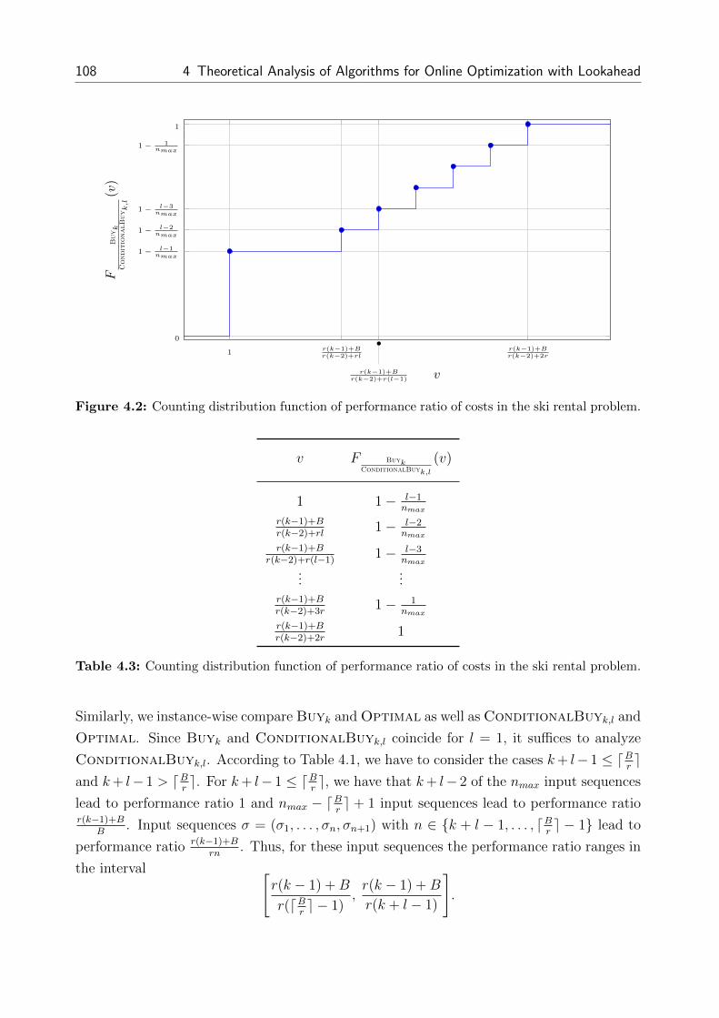
108 4 Theoretical Analysis of Algorithms for Online Optimization with Lookahead
1r(k−1)+Br(k−2)+rl
r(k−1)+Br(k−2)+2r
0
1 − l−1nmax
1 − l−2nmax
1 − l−3nmax
1 − 1nmax
1
v
FB
uyk
Condit
ionalB
uyk,l
(v)
r(k−1)+Br(k−2)+r(l−1)
Figure 4.2: Counting distribution function of performance ratio of costs in the ski rental problem.
v F BuykConditionalBuyk,l
(v)
1 1− l−1nmax
r(k−1)+Br(k−2)+rl
1− l−2nmax
r(k−1)+Br(k−2)+r(l−1)
1− l−3nmax
......
r(k−1)+Br(k−2)+3r
1− 1nmax
r(k−1)+Br(k−2)+2r
1
Table 4.3: Counting distribution function of performance ratio of costs in the ski rental problem.
Similarly, we instance-wise compare Buyk and Optimal as well as ConditionalBuyk,l and
Optimal. Since Buyk and ConditionalBuyk,l coincide for l = 1, it suffices to analyze
ConditionalBuyk,l. According to Table 4.1, we have to consider the cases k+ l− 1 ≤ dBre
and k+ l− 1 > dBre. For k+ l− 1 ≤ dB
re, we have that k+ l− 2 of the nmax input sequences
lead to performance ratio 1 and nmax − dBr e + 1 input sequences lead to performance ratior(k−1)+B
B. Input sequences σ = (σ1, . . . , σn, σn+1) with n ∈ {k + l − 1, . . . , dB
re − 1} lead to
performance ratio r(k−1)+Brn
. Thus, for these input sequences the performance ratio ranges in
the interval [r(k − 1) +B
r(dBre − 1)
,r(k − 1) +B
r(k + l − 1)
].

4.1 Online Ski Rental with Lookahead 109
1r(k−1)+B
Br(k−1)+B
r(dBre−1)
r(k−1)+Br(k+l−1)
0
k+l−2nmax
nmax+k+l−dBre−1
nmax
1 − dBre−k−l
nmax
1 − dBre−k−l−1
nmax
1 − 1nmax
1
v
FC
ondit
ionalB
uyk,l
Optim
al
(v)
r(k−1)+B
r(dBre−2)
Figure 4.3: Counting distribution function of performance ratio of costs in the ski rental problemwith k + l − 1 ≤ dBr e.
v FConditionalBuyk,lOptimal
(v) v FConditionalBuyk,lOptimal
(v)
1 k+l−2nmax
1dB
re−1
nmax
r(k−1)+BB
nmax+k+l−dBre−1
nmax
rdBre
B
dBre
nmax
r(k−1)+B
r(dBre−1)
1− dBre−k−lnmax
r(dBre+1)
B
dBre+1
nmax
r(k−1)+B
r(dBre−2)
1− dBre−k−l−1
nmax
......
...... r(k+l−3)
Bk+l−3nmax
r(k−1)+Br(k+l−2)
1− 1nmax
r(k+l−2)B
k+l−2nmax
r(k−1)+Br(k+l−1)
1 r(k−1)+BB
1
a) b)
Table 4.4: Counting distribution functions of performance ratio of costs in the ski rental problem.a) k + l − 1 ≤ dBr e and b) k + l − 1 > dBr e.

110 4 Theoretical Analysis of Algorithms for Online Optimization with Lookahead
The resulting counting distribution function of the performance ratio is illustrated in Figure
4.3 and Table 4.4 a) on the previous page.
For k + l− 1 > dBre, we have that dB
re − 1 of the nmax input sequences lead to performance
ratio 1 and nmax − k − l + 2 input sequences lead to performance ratio r(k−1)+BB
. Input
sequences σ = (σ1, . . . , σn, σn+1) with n ∈ {dBre, . . . , k+ l− 2} lead to performance ratio rn
B.
Thus, for these input sequences the performance ratio ranges in the interval[rdB
re
B,r(k + l − 2)
B
].
The resulting counting distribution function of the performance ratio is illustrated in Figure
4.4 and Table 4.4 b).
1rdB/re
Br(k+l−2)
Br(k−1)+B
B
0
dBre−1
nmax
dBre
nmax
dBre+1
nmax
k+l−2nmax
1
v
FC
ondit
ionalB
uyk,l
Optim
al
(v)
r(dB/re+1)B
Figure 4.4: Counting distribution function of performance ratio of costs in the ski rental problemwith k + l − 1 > dBr e.
For l1 > l2, ConditionalBuyk,l1 instance-wise outperforms ConditionalBuyk,l2 , i.e., no
algorithm of this family ever fails to interpret lookahead to its advantage. The explanation

4.2 Online Bin Packing with Lookahead 111
for this can be traced back to the one-shot decision character: Because there is only one
decision, there is no possibility that its profitability could be undone by a future decision.
In this section, we underlined by exact analysis that in the ski rental problem it is possible
to incur considerable improvement (for typical parameter values of B, r, k and l) when ad-
ditional lookahead information concerning the plan on skiing over the next days is provided.
The improvement is due to the avoidance of mispurchases when a short time later the skier
ends the skiing trip.
4.2 Online Bin Packing with Lookahead
The bin packing problem is a fundamental combinatorial problem from the class of cutting
and packing ([55]). It has attracted research attention as an abstract problem of packing a
set of small objects into a set of larger objects under some objective function.
Problem 4.4 (Offline Bin Packing).
Instance Bin capacity C, set of items {σi | i ∈ {1, . . . , n}} where item σi has size si for
i = 1, . . . , n.
Task Assign each item to a bin such that the sum of item sizes assigned to a bin does
not exceed C and the number of bins used is minimal.
In the online version, the items have to be packed one after another without knowledge of
items other than the next one.
Problem 4.5 (Online Bin Packing).
Instance Bin capacity C, sequence of items (σ1, . . . , σn) where item σi has size si for
i = 1, . . . , n, instance revelation rule r for the online case.
Task Sequentially assign each item σi to a bin without having any information about
items σj with j > i such that the sum of item sizes assigned to a bin does not
exceed C and the number of bins used is minimal.
In the online version with lookahead, the items have to be packed one after another with
limited knowledge about future items.
Problem 4.6 (Online Bin Packing with Lookahead).
Instance Bin capacity C, sequence of items (σ1, . . . , σn) where item σi has size si for
i = 1, . . . , n, instance revelation rule r′ for the lookahead case.
Task Sequentially assign an unpacked item which is known as part of the lookahead
information to a bin such that the sum of item sizes assigned to a bin does not
exceed C and the number of bins used is minimal.

112 4 Theoretical Analysis of Algorithms for Online Optimization with Lookahead
Different types of lookahead are possible in bin packing, and we make the type to be inves-
tigated subsequently more concrete. The instance revelation rule in the online case is
r := At the beginning, σ1 is known; a new item is revealed when a known one is packed
and in the lookahead case with l ∈ N
r′ := At the beginning, σ1, . . . , σl are known; a new item is revealed when a known one is
packed.
The rule set in the online case is trivial, i.e.,
P := {Pack the known item};
permutations are allowed in the lookahead case, i.e.,
P ′ := {Pack one of the known items}.
According to the modeling framework from Chapter 3, the lookahead setting is
req | sngl/rnd | im | discr or equivalently req | sngl/rnd | im | cyc.
The input information of an input element is given by si. In the online case, we have τi = i
and Ti = i+ ε; in the lookahead case, we have τi = max{1, i− l} and T ′i = max{1, i− l}+ ε,
T′i =∞ with sufficiently small ε > 0.
We now compare the pure online setting with the setting enhanced by lookahead: Online
algorithm BestFit puts the known item into the fullest open bin that can accommodate
it, if any; otherwise a new bin is opened and the item put in it (cf. Algorithm 4.4 and [55]).
Online algorithm BestFitl with request lookahead l first sorts the known items in order of
non-increasing sizes and fictively packs them using BestFit; the largest known item is then
put into the fullest open bin that can accommodate it, if any; otherwise a new bin is opened
and the largest known item put in it (cf. Algorithm 4.5 and [55]).
Under additional lookahead of one item (l = 2), we derive exact expressions for the counting
distribution functions of the objective value and the performance ratio for the case of two
item sizes 0.5 + ε and 0.5− ε with arbitrary ε ∈ (0, 16) and C = 1. Under these conditions at
most two items fit into a single bin. Despite the simple setting, the exact analysis is rather
intricate and relies upon the combinatorial structure imposed to the problem. We conclude
that there is no general recipe for exact analysis in online optimization with lookahead.

4.2 Online Bin Packing with Lookahead 113
Algorithm 4.4 Online algorithm BestFit for bin packing
Input: First element σ1 of input sequence σ with size s1, bin capacity C
1: i := 1, J := ∅2: while i ≤ n do3: Determine the fill levels fj of all open bins j ∈ J4: if J ′ := {j ∈ J | fj + si ≤ C} 6= ∅ then5: Determine j′ ∈ J ′ such that fj′ = max{fj | j ∈ J ′}6: else7: Open a new bin j′, J := J ∪ {j′}8: end if9: Assign item σi to bin j′
10: if i < n then11: additional input: (i+ 1)st element σi+1 of input sequence σ with size si+1
12: end if13: i := i+ 114: end while
Output: Number of bins used |J |
Algorithm 4.5 Online algorithm BestFitl with lookahead for bin packing
Input: First l elements σ1, . . . , σl of input sequence σ with sizes s1, . . . , sl, bin capacity C
1: i := 1, J := ∅2: while i ≤ n do3: Determine the fill levels fj of all open bins j ∈ J4: Sort the unpacked known items obtaining list σ(1), σ(2), . . . with s(1) ≥ s(2) ≥ . . .5: if J ′ := {j ∈ J | fj + s(1) ≤ C} 6= ∅ then6: Determine j′ ∈ J ′ such that fj′ = max{fj | j ∈ J ′}7: else8: Open a new bin j′, J := J ∪ {j′}9: end if
10: Assign item σ(1) to bin j′
11: if i ≤ n− l then12: additional input: (i+ l)th element σi+l of input sequence σ with size si+l13: end if14: i := i+ 115: end while
Output: Number of bins used |J |

114 4 Theoretical Analysis of Algorithms for Online Optimization with Lookahead
From now on, we refer to BestFit as Bf and to BestFit2 as Bfd because BestFit2
emulates BestFit with the additional feature that the two known items are always sorted
by decreasing size. We set C := 1, let ε ∈ (0, 16) and use the following additional notation:
• Large / small item: Item of size 0.5 + ε / 0.5− ε
• nl(σ) / ns(σ): Number of large / small items in σ
• Bf(n,m) / Bfd(n,m): Number of item sequences of length n which need m bins under
BestFit / BestFit2
• Ci: ith Catalan number given by Ci =(
2ii
)−(
2ii+1
)= 1
i+1
(2ii
)12
Theorem 4.1. For any item sequence σ = (σ1, σ2, . . .) with σi ∈ {0.5 + ε, 0.5 − ε} it holds
that Bf[σ]−Bfd[σ] ∈ {0, 1}.
Proof. The first difference in the packings of Bf and Bfd occurs when item subsequence
(0.5− ε, 0.5− ε, 0.5+ ε) appears and there is no bin to accommodate any of these items. Bfd
packs the first and third item into a single bin at full capacity and keeps the second (small)
item unpacked in the lookahead until the end of the sequence (since items are homogenous),
whereas Bf packs the first two items in a bin at capacity 1 − 2ε and the third item in a
second bin. Thus, Bfd leads with one bin less used, but also one small item less packed.
Bfd also loses its lookahead power as it holds the small item in the lookahead and will not
change orders of two lookahead items ever again. Thus, both Bfd and Bf will process the
remaining items in parallel, but starting from a different bin configuration. The number of
upcoming new bins for the remaining items by Bf can only be the same or one less than
that of Bfd (without considering the left-over small item) because items have to be packed
in the same order and Bf can pack one small item without opening a new bin, whereas Bfd
has to open a new bin immediately. Finally, Bfd has to pack the left-over small item: When
the number of new bins in the previous step is the same for Bfd and Bf and in the packing
of Bfd there is room for a small item, Bfd will end up with one bin less than Bf, otherwise
Bfd will have to open a new bin resulting in a tie for the numbers of bins used.
From Theorem 4.1 it follows that Bfd dominates Bf in the sense that for each item sequence
it produces the same number of bins or even needs one bin less. As a result, Bfd never makes
a decision which will have worse consequences than that of Bf in the given setting.
12The Catalan numbers (see, e.g., [146]) are a sequence of natural numbers discovered by Eugene CharlesCatalan (1814-1894) which appear in an enormous number of counting problems. The Catalan numbers(Ci)i∈N0
start with 1, 1, 2, 5, 14, 42, 132, 429, 1430, 4862, . . .

4.2 Online Bin Packing with Lookahead 115
Definition 4.1 (Condensation of an input sequence).
Let σ = (σ1, σ2, . . .) be an input sequence with σi ∈ {0.5 + ε, 0.5 − ε}. The condensation
σc of σ is the input sequence that arises by repetitively removing all pairs (0.5− ε, 0.5− ε)starting in an odd position if the number of large items encountered previously is not larger
than the number of small items encountered previously. 4
A pair of removed small items in Definition 4.1 is also referred to as a condensed pair or as
a condensation in an input sequence.
Example 4.2 (Condensation of an input sequence).
Consider for ε = 0.1 the item sequences σ1 = (0.4, 0.4, 0.6, 0.6, 0.4, 0.6) and σ2 = (0.6, 0.4, 0.4,
0.6, 0.4, 0.4, 0.6, 0.4, 0.4, 0.4). The condensation of σ1 is σc1 = (0.6, 0.6, 0.4, 0.6); the conden-
sation of σ2 is σc2 = (0.6, 0.4, 0.4, 0.6, 0.6, 0.4). ♦
The condensation σc of an input sequence σ can be computed by Algorithm 4.6.
Algorithm 4.6 Determining the condensation of an item sequence
Input: Input sequence σ = (σ1, σ2, . . .) with σj ∈ {0.5− ε, 0.5 + ε}1: σc := σ, i := 12: while i ≤ |σc| − 1 do3: if σci = σci+1 = 0.5− ε and nl(σcj)j=1,...,i−1 ≤ ns(σcj)j=1,...,i−1 then4: Delete σci and σci+1 from σc by removal (successive elements are shifted forwards)5: i := i− 26: end if7: i := i+ 28: end while
Output: Condensation σc of σ
Theorem 4.2. For any item sequence σ = (σ1, σ2, . . . , σn) with σi ∈ {0.5 + ε, 0.5 − ε} and
n ∈ N it holds that Bf[σ] − Bfd[σ] = 1 if and only if there is an odd j ∈ N such that the
following conditions are satisfied:
i) nl((σ1, . . . , σj−1)) = ns((σ1, . . . , σj−1)c)
ii) (σj, σj+1, σj+2) = (0.5− ε, 0.5− ε, 0.5 + ε)
iii) ns((σj+3, . . . , σn)) = ns((σj+3, . . . , σn)c)
iv) nl((σj+3, . . . , σn)) ≥ ns((σj+3, . . . , σn)) + 1
116 4 Theoretical Analysis of Algorithms for Online Optimization with Lookahead
Proof. ⇒: Let Bf[σ] − Bfd[σ] = 1 for σ = (σ1, . . . , σn). Then σ can be split into σi =
(σ1, . . . , σj−1) and σii = (σj, . . . , σn) such that Bf[σi]−Bfd[σi] = 0, Bf[σii]−Bfd[σii] = 1
and both algorithms produce the same bin configurations (albeit in a different order) for σi.
Among all these splits there exists one with longest σi which we refer to as σi from now on.
Recall that the first difference in the packings of Bf and Bfd occurs when item subsequence
(0.5− ε, 0.5− ε, 0.5 + ε) appears and no open bin can accommodate any of these items. By
definition, σi immediately precedes this subsequence. If |σi| was odd, any algorithm would
leave a bin with space at least 0.5− ε after packing the odd number of items in σi. Hence,
the first (small) item of the subsequence could also be added contradicting that no open bin
can accommodate any of the items. Thus, |σi| is even and j is odd.
From Definition 4.1, it follows that nl((σi)) ≥ ns((σi)c) because any pair of small items
that would lead to more small than large items immediately after this pair has been deleted
in ns((σi)c) and |σi| is even. For nl((σi)) = ns((σi)c), each large item has a matching
small item which comes after or immediately before the large item. Thus, the configuration
determined by Bf is composed of nl((σi)) completely filled bins and |σi|−2nl((σi))2
bins with
two small items. Clearly, this number of bins is optimal. From the proof of Theorem 4.1,
both Bfd and Bf attain the optimal number of bins by the same bin configurations for
nl((σi)) = ns((σi)c). For nl((σi)) > ns((σi)c), we show by contradiction that σi cannot be
a longest possible subsequence such that Bfd and Bf produce the same bin configurations:
Assume that σi is a longest possible subsequence such that Bfd and Bf produce the same
bin configurations and nl((σi)) > ns((σi)c). Then there is at least one bin containing a large
item without a matching small item. An additional small item will be put into such a bin,
an additional large item will need a new bin, but the configurations of both algorithms will
remain the same contradicting the definition of σi. Thus, nl((σi)) = ns((σi)c) which is i).
According to i) and the definition of σi, there must be an odd j such that Bfd starts to
exhibit an advantage over Bf on σii = (σj, σj+1, σj+2, . . .) after σi has been packed resulting
in the same bin configurations with no space left by both algorithms. Only (σj, σj+1) =
(0.5 − ε, 0.5 − ε) potentially produces a difference. To make this happen, Bfd need not
pack these two items into the same bin, whereas Bf has to. This happens if and only if
σj+2 = 0.5 + ε: Bfd will not pack σj+1 immediately, but delay it until the end of the item
sequence, whereas σj+2 will be matched with σj. This establishes ii).
To see iii), note that the processing of Bfd on σii = (0.5 − ε, 0.5 − ε, 0.5 + ε, σj+3, . . . , σn)
is emulated by Bf on σii = (0.5 − ε, 0.5 + ε, σj+3, . . . , σn, 0.5 − ε). Assume there is a con-
densed pair of small items in the subsequence starting with σj+3; if there is more than one
condensation, consider the first one. Let σj′ be the first small item of this condensation. Bf

4.2 Online Bin Packing with Lookahead 117
produces a bin with two small items for σj and σj+1, but not for σj′ and σj′+1 since two small
items starting in an even position of the original sequence cannot be put in the same bin by
Bf. Bfd processes (σj, σj+1, σj+2, . . . , σn−1, σn) as (σj, σj+2, . . . , σn−1, σn, σj+1) emulated by
Bf, i.e., it does not produce a bin with two small items for σj and σj+2, but for σj′ and σj′+1
since in (σi, σii) these items are condensed items. Between σj+3 and σj′ , neither algorithm
produces another bin with two small items since we consider the first condensation in the
subsequence starting from σj+3. Hence, both Bf and Bfd produce one additional bin with
two small items for σi = (σ1, . . . , σj−1, σj, σj+1, σj+2, . . . , σj′) as compared to σi, and σi could
not have been the longest possible first part among all splits of σ.
From i), ii), iii), we know that in Bfd’s processing there is no bin with two small items from
σj onwards, whereas Bf creates such a bin for (σj, σj+1). Hence, in order to pack σj+1 at the
end of Bfd’s processing into an already open bin and to save a bin as compared to Bf, we
need an open bin with a large item only. This is the case if and only if in the subsequence
starting from σj+3 at least one more large item exists, i.e., iv).
⇐: We have that for item sequence σ there is an odd j ∈ N such that conditions i) to iv)
are fulfilled. In the sequel, a bin is called matched if it contains a large and small item,
otherwise it is called unmatched. From iii), we know that Bfd will not produce a bin with
two small items from σj onwards, whereas Bf creates such a one for (σj, σj+1). From iv),
we conclude that the number of matched bins in Bfd is two higher than in Bf. From the
pigeonhole principle, it follows that the number of unmatched bins in Bf is three higher
than in Bfd. Thus, Bf[(σj, σj+1, . . . , σn)]− Bfd[(σj, σj+1, . . . , σn)] = 1. i) guarantees that
in the bin configurations induced both by Bfd and Bf there is a matching small item for
any large item such that there is no bin with a large item only after (σ1, . . . , σj−1) have
been processed. Since |(σ1, . . . , σj−1)| is even, there is no bin with a small item only after
(σ1, . . . , σj−1) has been packed. Hence, the initial position for processing (σj, σj+1, . . . , σn)
is the same for Bfd and Bf and can be viewed as restarting with no bins used so far. In
particular, Bf[(σ1, σ2, . . . , σj−1)]−Bfd[(σ1, σ2, . . . , σj−1)] = 0.
We are in a position to characterize the number of item sequences of given length which lead
to a a saving of one bin by applying Bfd instead of Bf.
Theorem 4.3.
a) The number of item sequences σ of odd length |σ| = 2n + 1 for n ∈ N with Bf[σ] −Bfd[σ] = 1 is given by

118 4 Theoretical Analysis of Algorithms for Online Optimization with Lookahead
n−1∑p=1
(22(p−1) −
p−1∑i=1
Ci · 22(p−1−i))(
22(n−p) −n−p∑i=1
Ci · 22(n−p−i) − Cn−p+1
).
b) The number of item sequences σ of even length |σ| = 2n for n ∈ N with Bf[σ] −Bfd[σ] = 1 is given by
n−1∑p=1
(22(p−1) −
p−1∑i=1
Ci · 22(p−1−i))(
22(n−p)−1 −n−p−1∑i=1
Ci · 22(n−p−i)−1 − Cn−p).
Proof.
a) We compute the number of item sequences σ which can be brought into the form
σ = (σ1, . . . , σj−1, σj, σj+1, σj+2, σj+3, . . . , σ2n+1) fulfilling i) to iv) from Theorem 4.2
with odd j. We can choose j to be every odd number with |(σj, σj+1, σj+2, . . . , σ2n+1)| ≥4. The largest j fulfilling this condition is j = 2(n − 1) − 1 such that five items
(σ2(n−1)−1, σ2(n−1), σ2n−1, σ2n, σ2n+1) remain. Hence, in the first sum, p runs from 1 to
n− 1 indicating that j runs from 2 · 1− 1 = 1 to 2 · (n− 1)− 1 with even j’s omitted.
We first consider the first pair of parentheses: For fixed p, the number of item (sub-)
sequences of length 2(p− 1) satisfying condition i) from Theorem 4.2, i.e.,
nl((σ1, . . . , σj−1)) = ns((σ1, . . . , σj−1)c) (?)
with j − 1 = 2(p− 1) is n0 = 22(p−1)−p−1∑i=1
Ci · 22(p−1−i) which can be seen as follows: It
holds that n0 = 22(p−1)−nviol where nviol is the number of sequences of length 2(p−1) vi-
olating (?). Since by definition nl((σ1, . . . , σj−1)) ≥ ns((σ1, . . . , σj−1)c), we have nviol =
|Σviol| with Σviol := {(σ1, . . . , σj−1) |nl((σ1, . . . , σj−1)) > ns((σ1, . . . , σj−1)c)}. From
the pigeonhole principle, we can only have nl((σ1, . . . , σj−1)) = ns((σ1, . . . , σj−1)c) + d
where d = 2, 4, 6, . . . for (σ1, . . . , σj−1) ∈ Σviol because |(σ1, . . . , σj−1)c| is even. Thus,
a pair of large items has to occur at positions 2(p− 1− i) + 1 and 2(p− 1− i) + 2 for
i ∈ {1, 2, . . . , p−1} which will be responsible for nl((σ1, . . . , σj−1)) > ns((σ1, . . . , σj−1)c)
under conditions
• nl((σ2(p−1−i)+3, . . . , σ2(p−1))) = ns((σ2(p−1−i)+3, . . . , σ2(p−1))) and
• ns((σ2(p−1−i)+3, . . . , σ2(p−1))) = ns((σ2(p−1−i)+3, . . . , σ2(p−1))c)
regardless of σ1, . . . , σ2(p−1−i) . Thus, we can choose σ1, . . . , σ2(p−1−i) freely giving the
factor 22(p−1−i). Note that the first condition is necessary to ensure that the two

4.2 Online Bin Packing with Lookahead 119
large items σ2(p−1−i)+1 and σ2(p−1−i)+2 can be held responsible for nl((σ1, . . . , σj−1)) >
ns((σ1, . . . , σj−1)c); the second condition is sufficient to make them responsible for
nl((σ1, . . . , σj−1)) > ns((σ1, . . . , σj−1)c) because if there was a condensed pair of small
items, then at least one pair of two large items would follow which would be responsible
for nl((σ1, . . . , σj−1)) > ns((σ1, . . . , σj−1)c). For fixed i, it remains to show that the
number of item sequences of length 2(i− 1) fulfilling the two itemized conditions is Ci.
To this end, we make use of the concept of (recurring) unit-sloped paths ([131]):
Definition 4.3 ((Recurring) unit-sloped path).
A unit-sloped path of length 2i is a path in R2 from (0, 0) to (2i, s2i) consisting only of
line segments between (k− 1, sk−1) and (k, sk) for k = 1, 2, . . . , 2i where sk = sk−1 + 1
or sk = sk−1 − 1 and s0 = 0. A recurring unit-sloped path of length 2i is a unit-sloped
path of length 2i that ends in (2i, 0), i.e., it has s2i = 0. 4
Note that if we restrict sk ≥ 0 for all k = 0, 1, 2, . . . , 2i, this definition coincides with
that of the well-known Dyck path (see, e.g., [62], [63]). Figure 4.5 shows an example
for a recurring unit-sloped path and a Dyck path, respectively.
1 2i
1
a)
1 2i
1
b)
Figure 4.5: Recurring unit sloped paths. a) General path. and b) Dyck path.
Lemma 4.4.
a) The number of recurring unit-sloped paths of length 2i which have sk ≥ 0 for all
k = 0, 1, 2, . . . , 2i is Ci.
b) The number of recurring unit-sloped paths of length 2i which have sk ≥ −1 for all
k = 0, 1, 2, . . . , 2i is Ci+1.
Proof. See Appendix A.1.1.
In order to fulfill the first itemized condition, observe the correspondences between the
appearance of a large item and an up-move (sk = sk−1+1) and between the appearance
of a small item and a down-move (sk = sk−1 − 1) in a unit-sloped path. Because the
number of large items equals the number of small items, this path is also recurring.

120 4 Theoretical Analysis of Algorithms for Online Optimization with Lookahead
The second itemized condition expresses that there are never two small items such that
the number of large items minus the number of small items up to an arbitrary position
in the item sequence would drop down to −2. Hence, the number of item sequences of
length 2(i−1) fulfilling both conditions is equal to the number of recurring unit-sloped
paths with sk ≥ −1 for all k. According to Lemma 4.4 b), this number is Ci.
We now consider the second pair of parentheses: For fixed p, the number of item
sequences of length 2(n−p) which fulfill conditions iii) and iv) from Theorem 4.2, i.e.,
• ns((σj+3, . . . , σ2n+1)) = ns((σj+3, . . . , σ2n+1)c) and
• nl((σj+3, . . . , σ2n+1)) ≥ ns((σj+3, . . . , σ2n+1)) + 1
with j = 2p − 1 can be characterized as 22(n−p) − n1 − n2 where n1 is the number of
item sequences of length 2(n− p) with at least one condensation and n2 is the number
of item sequences of length 2(n− p) without condensation that has the same number
of small and large items.
For n1, let i ∈ {1, . . . , n−p} be fixed such that the first condensation consists of σ2(p+i)
and σ2(p+i)+1, then we need to have nl(σj+3, . . . , σ2(p+i)−1) = ns(σj+3, . . . , σ2(p+i)−1) and
no condensation is allowed in (σj+3, . . . , σ2(p+i)−1). Structurally, we obtain the same
two conditions as the two itemized conditions for the first pair of parentheses, i.e.,
• nl((σ2(p+1), . . . , σ2(p+i)−1)) = ns((σ2(p+1), . . . , σ2(p+i)−1)) and
• ns((σ2(p+1), . . . , σ2(p+i)−1)) = ns((σ2(p+1), . . . , σ2(p+i)−1)c)
regardless of σ2(p+i)+2, . . . , σ2n+1 because once a condensation occurs the rest is irrele-
vant. Since σ2(p+i)+2, . . . , σ2n+1 are free, the factor 22(n−p−i) follows, and from Lemma
4.4, the number of item sequences of length 2(i− 1) fulfilling the two itemized condi-
tions is Ci. Thus, we obtain n1 =n−p∑i=1
Ci · 22(n−p−i). Also from Lemma 4.4, it follows
that n2 = Cn−p+1 gives the number of item sequences of length 2(n − p) where the
number of large items equals the number of small items and no condensations occur.
b) The proof is analogous to part a) with the only difference that the decomposition into
σ = (σ1, . . . , σj−1, σj, σj+1, σj+2, σj+3, . . . , σ2n+1) now has odd |(σj+3, . . . , σ2n)|. Thus,
for a given p ∈ {1, . . . , n−1}, the subsequence (σj+3, . . . , σ2n) now only has 2(n−p)−1
elements, and the number of sequences of (longest possible even) length 2(n − p − 1)
without condensation and balanced number of small and large items is Cn−p.

4.2 Online Bin Packing with Lookahead 121
The previous result yielded the number of item sequences of given length for which Bfd
saves a bin as compared to Bf. Although this cannot be used directly for the counting
distribution functions of the objective value or performance ratio, many proof ideas are
reused subsequently.
Lemma 4.5.
a) The number an,k of unit-sloped paths of length 2n with sk′ ≥ −1 for all k′ = 0, 1, 2, . . . , 2n
which end at position (2n, 2k), i.e., at height 2k, is given by
an,k =k + 1
n+ 1
(2n+ 2
n− k
).
b) The number of item sequences σ of length 2n without condensations where Bf[σ] = m
for m ∈ {n, n+ 1, . . . , 2n} is given by an,m−n.
Proof.
a) The proof is an immediate consequence of the bijection between Dyck paths of length
2n+ 2 and path pairs of length n given in [63] and the included remark concerning the
relaxation of the restriction of path pairs having to end in the same point. To this end,
we first modify the bijection by omitting the appended u-step at the beginning and the
appended d-step at the end of the Dyck path in order to facilitate recurring unit-sloped
paths that are allowed to hit the level of −1. Moreover, since the number of path pairs
of length n having endpoints k√
2 apart is an,k13, it follows from the bijection that the
number of unit-sloped paths ending at height 2k is an,k.
b) A total number of m bins with m ∈ {n, n + 1, . . . , 2n} is obtained when in an item
sequence without condensations m− n out of the n pairs of successive items are pairs
of large items for which no matching small items can be found afterwards. Each
such item sequence corresponds to a unit-sloped path of length 2n with sk ≥ −1
for k = 0, 1, 2, . . . , 2n ending at height 2(m − n) because each pair of large items
contributes an amount of 2 to the total height achieved at the end of the path, and
the result follows.
13 It also holds that an,k =∑
i1+i2+...+ik=n
Ci1Ci2 · · ·Cik , i.e., an,k is the sum of products of Catalan numbers
which is why the resulting table for n, k ∈ N with k ≤ n is called Catalan triangle ([146]).

122 4 Theoretical Analysis of Algorithms for Online Optimization with Lookahead
Theorem 4.6.
a) The number of item sequences σ of length 2n where Bf[σ] = m is given by
Bf(2n,m) =
n∑
k=m−nan,k =
n∑k=m−n
k + 1
n+ 1
(2n+ 2
n− k
)if n ≤ m ≤ 2n,
0 otherwise.
b) The number of item sequences σ of length 2n+ 1 where Bf[σ] = m is given by
Bf(2n+ 1,m) =
2n∑
k=m−nan,k + an,m−1−n if n+ 1 < m ≤ 2n+ 1,
3n∑k=0
an,k − an,0 if m = n+ 1,
0 otherwise.
Proof.
a) Since for 2n items at least n and at most 2n bins are needed, Bf(2n,m) = 0 for m < n
and m > 2n. For the remaining m, we perform a reverse induction on m. The base
case m = 2n is valid because the only item sequence which needs 2n bins has 2n large
items and it holds that
n∑k=2n−n
an,k = an,n =n+ 1
n+ 1
(2n+ 2
0
)= 1.
For the inductive step, let Bf(2n,m) =n∑
k=m−nan,k be valid for some m with 2n ≥ m >
n. We show that Bf(2n,m − 1) =n∑
k=m−1−nan,k. Because of m > n, there must be a
pair of large items starting at an odd position for which no matching small items follow
in every item sequence with objective value m since otherwise these large items could
be matched with small items and would fit into a bin contradicting m > n. Hence, we
obtain for any item sequence with objective value m an item sequence with objective
value m − 1 by replacing the first pair of large items starting at an odd position for
which no matching small items follow with a pair of small items which in turn lead
to a condensation. As a result, we have Bf(2n,m − 1) = Bf(2n,m) + |Σadd| where
Σadd are the additional item sequences leading to objective value m − 1 which have
not resulted from establishing a condensation in an item sequence with objective value

4.2 Online Bin Packing with Lookahead 123
m. These item sequences can be mapped to a unit-sloped path of length 2n not going
below level −1 and ending at height 2(m − 1 − n). From Lemma 4.5, we have that
|Σadd| = an,m−n−1. Together with the induction hypothesis we conclude that
Bf(2n,m− 1) = Bf(2n,m) + |Σadd| =n∑
k=m−nan,k + an,m−n−1 =
n∑k=m−n−1
an,k.
b) Since for 2n+1 items at least n+1 and at most 2n+1 bins are needed, Bf(2n+1,m) = 0
for m < n+ 1 and m > 2n+ 1. Notice that whenever m > n+ 1 for an item sequence
of length 2n + 1, we have m > n for the same item sequence where the last item is
deleted. Thus, there must be a pair of large items beginning at an odd position in the
truncated sequence from the same reasoning as in part a) of the proof. Objective value
m with n + 1 < m ≤ 2n + 1 for an item sequence of length 2n + 1 can be attained in
two ways: First, Bf needed m−1 bins after 2n items and the 2n+1st item leads to the
mth bin. Second, Bf needed m bins after 2n items and the 2n+1st item needs no new
bin. In the first case, we have Bf(2n,m− 1) item sequences which must incur a new
bin upon appending a large item; appending a small item would leave the objective
value at m because there are at least two large items which could be matched with
the small item. In the second case, Bf(2n,m) item sequences will not incur a new bin
upon appending a small item as this item can be matched with one of the large items;
appending a large item would lead to objective value m+ 1 since after 2n items there
can never be a bin with a small item only.
We obtain
Bf(2n+ 1,m) = Bf(2n,m− 1) + Bf(2n,m)
=n∑
k=m−1−nan,k +
n∑k=m−n
an,k = 2n∑
k=m−nan,k + an,m−1−n.
Objective value n+ 1 can be attained in three ways: First, Bf needed n bins after 2n
items and the 2n + 1st item is large leading to the n + 1st bin. Second, Bf needed n
bins after 2n items and the 2n + 1st item is small leading to the n + 1st bin. Third,
Bf needed n+ 1 bins after 2n items and the 2n+ 1st item is small, but does not lead
to a new bin. The first case is trivial. In the second case, we seek for the same item
sequences because neither of them can exhibit a pair of large items starting in an odd
position. In the third case, we seek for the item sequences of length 2n with objective
value n + 1 which have at least one pair of large items beginning at an odd position

124 4 Theoretical Analysis of Algorithms for Online Optimization with Lookahead
such that the appended small item does not incur a new bin. These item sequences
are counted by Bf(2n, n+ 1). We obtain
Bf(2n+ 1, n+ 1) = Bf(2n, n) + Bf(2n, n) + Bf(2n, n+ 1)
=n∑k=0
an,k +n∑k=0
an,k +n∑k=1
an,k = 3n∑k=0
an,k − an,0.
We now give another formula to compute the numbers Bf(2n,m) and Bf(2n+ 1,m).
Theorem 4.7.
a) The number of item sequences σ of length 2n where Bf[σ] = m is given by
Bf(2n,m) =
(
2n+1m+1
)=(
2nm
)+(
2nm+1
)if n ≤ m ≤ 2n,
0 otherwise.
b) The number of item sequences σ of length 2n+ 1 where Bf[σ] = m is given by
Bf(2n+ 1,m) =
(
2n+2m+1
)=(
2n+1m
)+(
2n+1m+1
)if n+ 1 < m ≤ 2n+ 1,(
2n+3n+2
)−(
2n+1n+1
)if m = n+ 1,
0 otherwise.
Proof.
a) We show by two-dimensional induction on n and m that
n∑k=m−n
an,k =
(2n+ 1
m+ 1
).
Recall that n = 1, 2, . . . and m = n, n+ 1, . . . , 2n. The base case n = 1 and m = n = 1
is valid because it holds that
1∑k=0
a1,k = a1,0 + a1,1 = 2 + 1 = 3 =
(2 · 1 + 1
1 + 1
)=
(3
2
)= 3.

4.2 Online Bin Packing with Lookahead 125
In the first inductive step (on n with fixed m = n), we show thatn∑k=0
an,k =(
2n+1n+1
)holds. From [146], we know that 1
2
(2(n+1)n+1
)=
n∑k=0
an,k. The result follows from
1
2
(2(n+ 1)
n+ 1
)=
1
2
(2n+ 2)!
(n+ 1)!(n+ 1)!=
(2n+ 2)(2n+ 1)!
2(n+ 1)n!(n+ 1)!=
(2n+ 1
n+ 1
).
In the second inductive step (on m with arbitrary n), we show thatn∑
k=m−nan,k =
(2n+1m+1
)implies
n∑k=m+1−n
an,k =(
2n+1m+2
). This can be seen by the following calculations:
n∑k=m+1−n
an,k =n∑
k=m−nan,k − an,m−n =
(2n+ 1
m+ 1
)− m− n+ 1
n+ 1
(2n+ 2
2n−m
)
=(2n+ 1)!
(m+ 1)!(2n−m)!− m− n+ 1
n+ 1
(2n+ 2)!
(2n−m)!(m+ 2)!
=(2n+ 1)!(n+ 1)(m+ 2)− (m− n+ 1)(2n+ 2)!
(2n−m)!(m+ 2)!(n+ 1)
=(2n+ 1)!
(m+ 2)!(2n−m− 1)!
(n+ 1)(m+ 2)− (m− n+ 1)(2n+ 2)
(2n−m)(n+ 1)
=(2n+ 1)!
(m+ 2)!(2n−m− 1)!· 1 =
(2n+ 1
m+ 2
).
b) For m = n+ 1, we have
3n∑k=0
an,k − an,0a)= 3
(2n+ 1
n+ 1
)− 1
n+ 1
(2n+ 2
n
)= 3
(2n+ 1)!
(n+ 1)!n!− 1
n+ 1
(2n+ 2)!
n!(n+ 2)!
=(2n+ 1)!
(n+ 2)!(n+ 1)!(3(n+ 2)(n+ 1)− (2n+ 2))
=(2n+ 1)!
(n+ 2)!(n+ 1)!(3n2 + 7n+ 4)

126 4 Theoretical Analysis of Algorithms for Online Optimization with Lookahead
and (2n+ 3
n+ 2
)−(
2n+ 1
n+ 1
)=
(2n+ 3)!
(n+ 2)!(n+ 1)!− (2n+ 1)!
(n+ 1)!n!
=(2n+ 1)!
(n+ 2)!(n+ 1)!((2n+ 3)(2n+ 2)− (n+ 2)(n+ 1))
=(2n+ 1)!
(n+ 2)!(n+ 1)!(3n2 + 7n+ 4).
which together yields the desired relation for m = n+ 1.
For n+ 1 < m ≤ 2n+ 1, we have
2n∑
k=m−nan,k + an,m−n−1
a)= 2
(2n+ 1
m+ 1
)+m− nn+ 1
(2n+ 2
2n−m+ 1
)
= 2(2n+ 1)!
(m+ 1)!(2n−m)!+m− nn+ 1
(2n+ 2)!
(2n−m+ 1)!(m+ 1)!
=(2n+ 2)!
(m+ 1)!(2n−m+ 1)!
(2(2n−m+ 1)
2n+ 2+m− nn+ 1
)
=(2n+ 2)!
(m+ 1)!(2n−m+ 1)!
(2n+ 2
2n+ 2
)=
(2n+ 2
m+ 1
).
Theorem 4.8. The number of item sequences σ of length n where Bf[σ] = m and
Bfd[σ] = m− 1 is given by(
nm+1
)for m = dn
2e+ 1, . . . , n− 1.
Proof. From [143], we have for 1 ≤ q ≤ p ≤ 2q − 1 the following expression for the binomial
coefficient: (p
q
)=∑i≥0
Ci
(p− 1− 2i
q − 1− i
)
For item sequence σ, assume that |σ| = 2n and that σ fulfills the conditions stated in
Theorem 4.2. We further decompose σ into three parts: For some i ∈ {1, . . . , n − 1},let (σ1, σ2, . . . , σ2(i−1)) correspond to a recurring unit-sloped path with sk ≥ −1 for all
k = 1, 2, . . . , 2(i − 1), let σ2i−1, σ2i be the first two small items which would be condensed,

4.2 Online Bin Packing with Lookahead 127
and let (σ2i+1, σ2(i+1), . . . , σ2n) be the rest of σ. Note that σ2i−1, σ2i are not necessarily
responsible for the saving which can be accrued by Bfd over Bf.
According to Lemma 4.4, the number of item sequences fulfilling the properties of the first
subsequence is Ci. The number of item subsequences (σ2i+1, σ2(i+1), . . . , σ2n) leading to overall
m bins for Bf and overall m − 1 bins for Bfd is(
2n−2im−i
)which can be seen as follows: For
(σ1, σ2, . . . , σ2(i−1)), i− 1 bins were needed such that for (σ2i−1, σ2i, . . . , σ2n), m− i + 1 and
m− i additional bins will be needed by Bf and Bfd, respectively. Since σ2i−1, σ2i are small
items, m− i bins will be needed by Bf for (σ2i+1, σ2(i+1), . . . , σ2n) and in addition, conditions
ii), iii) and iv) of Theorem 4.2 have to hold for some j ≥ 2i−1 to realize the saving of Bfd.
Because condition iv) of Theorem 4.2 has to hold, objective value m is attained by Bf when
m− i out of the 2n−2i items (σ2i+1, σ2(i+1), . . . , σ2n) are large. However, this choice does not
necessarily fulfill conditions ii) and iii) of Theorem 4.2 because it may be that (σ2i+1, σ2i+2) =
(0.5 − ε, 0.5 + ε) or that condensations can be found in (σ2i+2, σ2i+3, . . . , σ2n). These two
cases are resolved as follows: Whenever (σ2i+1, σ2i+2) = (0.5− ε, 0.5 + ε), we find a bijective
mapping from σ to some σ′ where σ′ is identical to σ except for (σ2i+1, σ2i+2) now being
(σ2i+1, σ2i+2) = (0.5 − ε, 0.5 − ε). Hereby, another condensation is established which erases
responsibility of the first condensation for the saving of Bfd and claims responsibility itself
(by setting j = 2i+1). Whenever we have another condensation in (σ2i+2, σ2i+3, . . . , σ2n), we
recognize that it erases responsibility for the saving of Bfd of a previous condensation and
claims responsibility itself (by setting j accordingly). Thus, for some i such that (σ2i−1, σ2i)
is the first condensation, there are(
2n−2im−i
)item subsequences (σ2i+1, σ2(i+1), . . . , σ2n) fulfilling
conditions ii), iii) and iv) of Theorem 4.2.
Lemma 4.9. For n ≤ m ≤ 2n it holds that
∑i≥1
Ci
(2n− 2i
m− i
)=∑i≥1
Ci−1
(2n− 2i+ 1
m− i+ 1
).
Proof. See Appendix A.1.2.
We complete the proof for even length 2n of σ with the following calculation:
∑i≥1
Ci
(2n− 2i
m− i
)=∑i≥1
Ci−1
(2n− 2i+ 1
m− i+ 1
)=∑i≥1
1
i
(2i− 2
i− 1
)(2n− 2i+ 1
m− i+ 1
)=∑i≥0
1
i+ 1
(2i
i
)(2n− 2i− 1
m− i
)=∑i≥0
Ci
(2n− 2i− 1
m− i
)=
(2n
m+ 1
).

128 4 Theoretical Analysis of Algorithms for Online Optimization with Lookahead
where the the last equality follows for n < m ≤ 2n− 1 from the proof of Lemma 9 in [143]
and condition iv) from Theorem 4.2. For odd length 2n+ 1 of σ, the proof is analogous with
2n− 2i replaced by 2n− 2i+ 1.
Corollary 4.10. The number of item sequences σ of length n with Bf[σ] = m and Bfd[σ] =
m is given by(nm
)for m = dn
2e+ 1, . . . , n.
Proof. From Theorem 4.1, we know that Bfd[σ] ∈ {m,m − 1} whenever Bf[σ] = m; from
the previous Theorem 4.8, we know that |{σ | |σ| = n,Bfd[σ] = m−1,Bf[σ] = m}| =(
nm+1
)for m = dn
2e+1, . . . , n−1. Hence, from Theorem 4.7 it immediately follows for these m that
|{σ | |σ| = n,Bfd[σ] = m}| =(n+ 1
m+ 1
)−(
n
m+ 1
)=
(n
m
).
Clearly, |{σ | |σ| = n,Bf[σ] = n}| = |{σ | |σ| = n,Bfd[σ] = n}| = 1.
We are in a position to state the central relation between the objective values attained by
Bfd and Bf.
Theorem 4.11. The number of item sequences σ of length n where Bfd[σ] = m is given by
Bfd(n,m) =
1 if m = n,
Bf(n,m) + Bf(n,m+ 1)− 2(
nm+1
)if m = dn
2e+ 1, . . . , n− 1,
Bf(n,m) + Bf(n,m+ 1)−(
nm+1
)if m = dn
2e,
0 if m ≤ dn2e − 1.
Proof. Because of item sizes in {0.5− ε, 0.5 + ε}, at most two items can be packed in a bin
so that packing n items in less than dn2e bins is infeasible. Likewise, each item of σ is packed
separately if and only if each item is large, and there is only one such item sequence σ.
The number of item sequences of length n for which Bfd attains objective value m can be
computed as n1 + n2− n3− n4 where n1 is the number of item sequences σ of length n with
Bf[σ] = m, n2 is the number of item sequences σ of length n with Bf[σ] = m+ 1, n3 is the
number of item sequences σ of length n with Bf[σ] = m, Bfd[σ] = m − 1, and n4 is the
number of item sequences σ of length n with Bf[σ] = m+ 1, Bfd[σ] = m+ 1.
From Theorem 4.8, we have that the number of all item sequences σ of length n with
Bf[σ] = m and Bfd[σ] = m − 1 is n3 =(
nm+1
)for m = dn
2e + 1, . . . , n − 1; from Corollary
4.10, we have that the number of all item sequences σ of length n with Bf[σ] = m + 1 and
Bfd[σ] = m+ 1 is n4 =(
nm+1
)for m = dn
2e, . . . , n− 1, and the result follows.

4.2 Online Bin Packing with Lookahead 129
From the previous results, we immediately obtain expressions for the counting distribution
functions of the objective value FBf(v) and FBfd(v), respectively. We now restrict ourselves
to item sequences of even length because from the previous results analogous conclusions
can be drawn immediately for item sequences of odd length.
Corollary 4.12. The counting distribution functions of the objective value FBf(v) and
FBfd(v) of Bf and Bfd for item sequences of length 2n are given by
FBf(v) =
0 if v < n,
2−2n
bvc∑m=n
(2n+1m+1
)if n ≤ v < 2n,
1 if v ≥ 2n,
and
FBfd(v) =
0 if v < n,
2−2n
( bvc∑m=n
((2n+1m+1
)+(
2n+1m+2
)− 2(
2nm+1
))+(
2nm+1
))if n ≤ v < 2n,
1 if v ≥ 2n.
Proof. Direct consequence of Theorems 4.7 and 4.11.
The following corollary expresses Bfd’s dominance over Bf. As could already be seen from
Theorem 4.1, stochastic dominance of all orders is established.
Theorem 4.13. For item sequences of length 2n, we have FBfd(v) ≥ FBf(v) for all v ∈ Rand FBfd(v)− FBf(v) > FBfd(v + 1)− FBf(v + 1) for all v < 2n− 1.
Proof. For v < n and v ≥ 2n− 1, FBf(v) = FBfd(v). For n ≤ v < 2n− 1
FBfd(v)− FBf(v) =
( bvc∑m=n
((2n+1m+2
)− 2(
2nm+1
))+(
2nn+1
))· (2−2n)
=
( bvc∑m=n
((2n+1m+2
)−(
2nm+1
)−(
2nm+1
))+(
2nn+1
))· (2−2n)
=
( bvc∑m=n
((2nm+2
)−(
2nm+1
))+(
2nn+1
))· (2−2n)
=((
2nbvc+2
)−(
2nn+1
)+(
2nn+1
))· (2−2n) =
(2nbvc+2
)· (2−2n) > 0.

130 4 Theoretical Analysis of Algorithms for Online Optimization with Lookahead
The second part follows immediately from Pascal’s triangle as a result of(
2nv+2
)>(
2nv+3
)for
v = n, n+ 1, . . . , 2n− 3.
Theorem 4.14. For item sequences of length 2n, we have supv∈R |FBfd(v)−FBf(v)| → 0 as
n→∞.
Proof. Using the formula of Stirling (n! ≈√
2πn(ne)n; see, e.g., [114]), we get for n → ∞
that
FBfd(n)− FBf(n) =
(2n
n+ 2
)· 2−2n
=(2n)!
(n+ 2)!(n− 2)!· 2−2n
≈√
4πn(2ne
)2n√2π(n+ 2)(n+2
e)n+2
√2π(n− 2)(n−2
e)n−2
· 2−2n
=
√n(2n
e)2n√
π(n2 − 4)(n+2e
)n+2(n−2e
)n−2· 2−2n
=
√n(2n)2n√
π(n2 − 4)(n+ 2)n+2(n− 2)n−2· 2−2n
=
√n22nn2n√
π(n2 − 4)(n+ 2)n+2(n− 2)n−2· 2−2n ∈ Θ(
1√n
).
In addition,(
2nv
)>(
2nv+1
)for v ∈ N with v ≥ n, i.e., FBfd(v)−FBf(v) monotonously decreases
for v ≥ n. Since also FBfd(v) = FBf(v) for v < n and v ≥ 2n− 1, the result follows.
As a consequence of Theorem 4.14, one additional lookahead item is worthless in the limit for
Bfd in comparison to Bf. Taking into account Theorem 4.1, this result was to be expected.
The reason for this ineffectiveness lies in the total forfeiture of the power of the lookahead
capability once a small item occurs and occupies the lookahead set.
Figure 4.6 exemplarily plots FBf(v) and FBfd(v) for all item sequences of length n =
10, 50, 100, 500. We observe a rather small lookahead effect as a result of the conditions
in Theorem 4.2 which are collectively found only in a minor fraction of all item sequences.
We next derive an expression for the counting distribution function of the performance ratio
F BfBfd
(v) of Bf relative to Bfd.

4.2 Online Bin Packing with Lookahead 131
10 11 12 13 14 15 16 17 18 19 200
0.2
0.4
0.6
0.8
1
v
F(v)
Bf
Bfd
a)
50 55 60 65 70 75 80 85 90 95 1000
0.2
0.4
0.6
0.8
1
v
F(v)
Bf
Bfd
b)
100 110 120 130 140 150 160 170 180 190 2000
0.2
0.4
0.6
0.8
1
v
F(v)
Bf
Bfd
c)
500 550 600 650 700 750 800 850 900 950 1,0000
0.2
0.4
0.6
0.8
1
v
F(v)
Bf
Bfd
d)
Figure 4.6: Counting distribution functions of costs in the bin packing problem. a) 2n = 20.b) 2n = 100. c) 2n = 200. d) 2n = 1000.

132 4 Theoretical Analysis of Algorithms for Online Optimization with Lookahead
Corollary 4.15. The counting distribution function of the performance ratio F BfBfd
(v) of Bf
relative to Bfd for item sequences of length 2n is given by
F BfBfd
(v) =
0 if v < 1,
12
+12(2n
n )+( 2nn+1)
22n if 1 ≤ v < 2n−12n−2
= 1 + 12n−2
,
12
+
12(2n
n )+( 2nn+1)+
n−2−k∑i=0
( 2n2n−i)
22n if n+k+1n+k
= 1 + 1n+k≤ v < n+k
n+k−1= 1 + 1
n+k−1
for k = 1, . . . , n− 2,
1 else.
Proof. According to Theorem 4.8, we have:
•(
2nn+2
)is the number of sequences of length 2n with Bf[σ] = n+ 1, Bfd[σ] = n
•(
2nn+3
)is the number of sequences of length 2n with Bf[σ] = n+ 2, Bfd[σ] = n+ 1
• . . .
•(
2n2n
)is the number of sequences of length 2n with Bf[σ] = 2n− 1, Bfd[σ] = 2n− 2
Apart from these item sequences, no other sequences change their objective due to application
of Bfd instead of Bf. Thus, the performance ratio ranges in [1, n+1n
] and the number of item
sequences of length 2n which leave the number of bins unchanged in both algorithms is
22n −(
2nn+2
)−(
2nn+3
)− . . .−
(2n2n
)=(
2n0
)+(
2n1
)+ . . .+
(2nn+1
)= 22n−1 +
1
2
(2nn
)+(
2nn+1
).
Exploiting this relation, we immediately get the given expression for the counting distribution
function of the performance ratio as F BfBfd
(v).
In Figure 4.7, exemplary plots of F BfBfd
(v) are given for input sequences of length n =
10, 50, 100, 500 confirming that the lookahead effect is also relatively small with respect to
an instance-wise comparison of both algorithms to each other.
The only pair of items where algorithm Bfd changes the packing order in contrast to the
revelation order is σsub = (0.5− ε, 0.5 + ε). Assume now that Bfd is prohibited to permute
the item order during packing. Define algorithm Bfd′ which fictively operates as Bfd, i.e.,
it does not put the small item of σsub into an open bin with a small item but in a new bin
because it reserves the space in the already open bin for the large item of σsub. Since Bfd′
emulates Bfd and leads to the same outcome, it is seen easily that the value of being allowed
to permute the items is zero. The attainable benefit out of the additional lookahead item is
entirely due to the information about the size of this item.
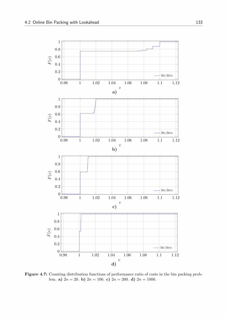
4.2 Online Bin Packing with Lookahead 133
0.98 1 1.02 1.04 1.06 1.08 1.1 1.120
0.2
0.4
0.6
0.8
1
v
F(v)
Bf/Bfd
a)
0.98 1 1.02 1.04 1.06 1.08 1.1 1.120
0.2
0.4
0.6
0.8
1
v
F(v)
Bf/Bfd
b)
0.98 1 1.02 1.04 1.06 1.08 1.1 1.120
0.2
0.4
0.6
0.8
1
v
F(v)
Bf/Bfd
c)
0.98 1 1.02 1.04 1.06 1.08 1.1 1.120
0.2
0.4
0.6
0.8
1
v
F(v)
Bf/Bfd
d)
Figure 4.7: Counting distribution functions of performance ratio of costs in the bin packing prob-lem. a) 2n = 20. b) 2n = 100. c) 2n = 200. d) 2n = 1000.

134 4 Theoretical Analysis of Algorithms for Online Optimization with Lookahead
The derivation of expressions for the counting distribution functions of the objective value
and of the performance ratio for the case of two item sizes showed that the improvement
to be expected from an additional lookahead item is very small as a result of a number of
(restrictive) conditions that have to be fulfilled by the structure of an item sequence (cf.
Theorem 4.2). We also found that the lookahead effect vanishes in the sense of converging
distribution functions for Bf and Bfd as the number of items tends to infinity; vice versa,
the impact of lookahead is more likely to be observed on item sequences which are of rather
short length. Moreover, it is irrelevant whether one is allowed to change the order of the
items during their packing or not.
4.3 Online Traveling Salesman Problem with Lookahead
The traveling salesman problem (TSP) lies at the core of nearly every transportation or
routing problem as it seeks to find a round trip (also called tour) for a given set of locations
to be visited (also called requests) such that some cost function depending on the total travel
distance is minimized ([122]). Hence, the TSP is a pure sequencing problem.
For input sequence σ = (σ1, σ2, . . .), let a request σi with i ∈ N correspond to a point xi in
a space M with metric d :M×M→ R, then the TSP consists of visiting the points of all
requests with a server in a tour of minimum length starting and ending in some distinguished
origin o ∈M.
A permutation π(σ) = (π1(σ), π2(σ), . . . , πn(σ)) of the set {σ1, σ2, . . . , σn} of requests repre-
sents a tour (o, xπ1(σ), xπ2(σ), . . . , xπn(σ), o), i.e., a feasible solution to an instance of the TSP.
The value of
D(π(σ)) := d(o, xπ1(σ)) +n−1∑i=1
d(xπi(σ), xπi+1(σ)) + d(xπn(σ), o)
is called the tour length of π(σ).
Problem 4.7 (Offline Traveling Salesman).
Instance Metric space (M, d), origin o ∈ M, set of requests σ = {σi | i ∈ {1, . . . , n}}where σi is a request at xi ∈M.
Task Find a permutation π(σ) of σ with minimum tour length.
Because we neglect temporal aspects, the online versions are considered in the sequential
model. The online version without lookahead is trivial because the requests have to be
visited in their order of appearance.

4.3 Online Traveling Salesman Problem with Lookahead 135
Problem 4.8 (Online Traveling Salesman).
Instance Metric space (M, d), origin o ∈ M, sequence of requests σ = (σ1, σ2, . . . , σn)
where σi is a request at xi ∈M, instance revelation rule r for the online case.
Task Sequentially set πi(σ) := σi when σi is revealed.
In the online version with lookahead, there is limited knowledge about a number of requests
to be visited.
Problem 4.9 (Online Traveling Salesman with Lookahead).
Instance Metric space (M, d), origin o ∈ M, sequence of requests σ = (σ1, σ2, . . . , σn)
where σi is a request at xi ∈ M, instance revelation rule r′ for the lookahead
case.
Task Sequentially choose πi(σ) as one of the unvisited requests which are known as
part of the lookahead information such that the tour length of π(σ) is minimized.
As a result of the irrelevance of the factor time, the instance revelation rule in the online
case is
r := At the beginning, σ1 is known; a new request is revealed when the known one is visited
and in the lookahead case with l ∈ N
r′ := At the beginning, σ1, . . . , σl are known; a new request is revealed when a known one
is visited.
The rule set in the online case is trivial and does not give any degrees of freedom to the
decision maker, i.e.,
P := {Visit the known request};
permutations are allowed in the lookahead case, i.e.,
P ′ := {Visit one of the known requests}.
According to the modeling framework from Chapter 3, the lookahead setting is
req | sngl/rnd | im | discr or equivalently req | sngl/rnd | im | cyc.
The input information of an input element is given by xi. In the online case, we have τi = i
and Ti = i+ ε; in the lookahead case, we have τi = max{1, i− l} and T ′i = max{1, i− l}+ ε,
T′i = ∞ with sufficiently small ε > 0. Hence, the server is assumed to travel at infinite
speed.

136 4 Theoretical Analysis of Algorithms for Online Optimization with Lookahead
We now compare the pure online setting with the setting enhanced by lookahead: Online
algorithm FirstComeFirstServed has no choices, i.e., the server has to visit the requests
in their order of appearance in a first-come first-served manner (cf. Algorithm 4.7). Online
algorithm NearestNeighborl with request lookahead l always moves the server to the
closest known point in terms of distance from its current location (cf. Algorithm 4.8).
Algorithm 4.7 Online algorithm FirstComeFirstServed for the TSP
Input: Metric space (M, d), origin o ∈M, first element σ1 of input sequence σ with requestat x1
1: D := d(o, xσ1), i := 1, π1(σ) := σ1
2: while i < n do3: additional input: (i+ 1)st element σi+1 of input sequence σ with request at xi+1
4: D := D + d(xσi , xσi+1), πi+1(σ) := σi+1
5: i := i+ 16: end while7: D := D + d(xσn , o)
Output: (Identity) Permutation π(σ), total distance D of π(σ)
Algorithm 4.8 Online algorithm NearestNeighborl with lookahead for the TSP
Input: Metric space (M, d), origin o ∈ M, first l elements σ1, σ2, . . . , σl of input sequenceσ with requests at x1, x2, . . . , xl
1: x := o,D := 0, i := 1, J := {1, 2, . . . , l}2: while i ≤ n do3: k := arg minj∈J d(x, xσj), J := J\{k}, x′ := xσk4: D := D + d(x, x′), πi(σ) := σk5: if i ≤ n− l then6: additional input: (i+ l)th element σi+l of input sequence σ with request at xi+l7: J := J ∪ {i+ l}8: end if9: i := i+ 1, x := x′
10: end while11: D := D + d(x, o)
Output: Permutation π(σ), total distance D of π(σ)
Under additional lookahead of one request (l = 2), we derive exact expressions for the
counting distribution functions of the objective value and the performance ratio for the case
of a metric space consisting of two points only, i.e., M = {0, 1} with d(0, 1) = d(1, 0) = 1,
d(0, 0) = d(1, 1) = 0 and o = 0.
From now on, we refer to FirstComeFirstServed as Fcfs and to NearestNeighbor2
as Nn. We use the following additional terminology:

4.3 Online Traveling Salesman Problem with Lookahead 137
• A pass is the transition between two successive requests.
• A change pass is a pass between two requests (σi, σi+1) with xi = 1, xi+1 = 0 or
xi = 0, xi+1 = 1.
• A remain pass is a pass between two requests (σi, σi+1) with xi = xi+1.
• A request subsequence (σi, σi+1, σi+2) is a pass pair.
• A free point at a given time is a point which is not occupied by the server at that time.
The main advantage of Nn over Fcfs is its ability to crack pass pairs (0, 1, 0) or (1, 0, 1) in
order to build pass pairs (0, 0, 1) or (1, 1, 0). Note that because of the return to o, only even
overall tour lengths are possible.
Theorem 4.16.
a) The number of request sequences σ of length n where Fcfs[σ] = m and m is even is
given by
Fcfs(n,m) =
(n+ 1
m
).
b) The number of request sequences σ of length n where Nn[σ] = m and m is even is
given by
Nn(n,m) =
(n+ 1
2m− 2
)+
(n+ 1
2m
).
Proof. A sequence of n points starting and ending in o has n+ 2 requests including the two
dummy requests at o and encounters n+ 1 passes to either the current or the free point.
a) For Fcfs in order to result in objective value m, a request sequence has to exhibit
exactly m change passes out of the n+ 1 passes.
b) For m = 0, the formula obviously holds. For m > 0, first observe that each resulting
sequence after being processed by Nn exhibits a last change from 0 to 1 and a last
change from 1 to 0 in the visiting order of requests which together contribute a total
of 2 to the objective value. We conclude that a contribution of m − 2 is due to all
previous passes that do not involve the 1 of the last change from 0 to 1. There are two
cases how this 1 could be obtained: Either it was at the same position originally and
remained there also under processing of Nn (case 1), or it had been shifted to that
position as a result of the processing of Nn (case 2).
Denote by σ the original request sequence and by σ′ the visiting order under Nn. For
n = 9 and m = 4, we give an example of case 1 by
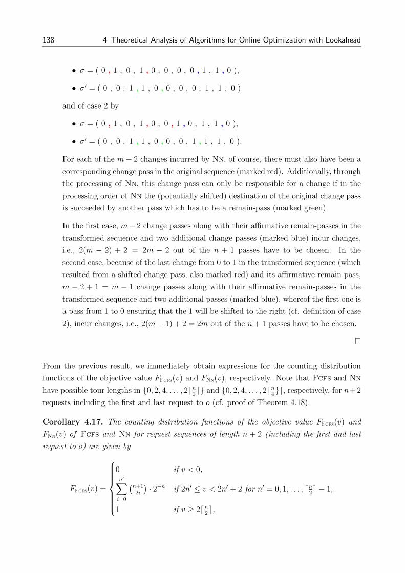
138 4 Theoretical Analysis of Algorithms for Online Optimization with Lookahead
• σ = ( 0 , 1 , 0 , 1 , 0 , 0 , 0 , 0 , 1 , 1 , 0 ),
• σ′ = ( 0 , 0 , 1 , 1 , 0 , 0 , 0 , 0 , 1 , 1 , 0 )
and of case 2 by
• σ = ( 0 , 1 , 0 , 1 , 0 , 0 , 1 , 0 , 1 , 1 , 0 ),
• σ′ = ( 0 , 0 , 1 , 1 , 0 , 0 , 0 , 1 , 1 , 1 , 0 ).
For each of the m− 2 changes incurred by Nn, of course, there must also have been a
corresponding change pass in the original sequence (marked red). Additionally, through
the processing of Nn, this change pass can only be responsible for a change if in the
processing order of Nn the (potentially shifted) destination of the original change pass
is succeeded by another pass which has to be a remain-pass (marked green).
In the first case, m− 2 change passes along with their affirmative remain-passes in the
transformed sequence and two additional change passes (marked blue) incur changes,
i.e., 2(m − 2) + 2 = 2m − 2 out of the n + 1 passes have to be chosen. In the
second case, because of the last change from 0 to 1 in the transformed sequence (which
resulted from a shifted change pass, also marked red) and its affirmative remain pass,
m − 2 + 1 = m − 1 change passes along with their affirmative remain-passes in the
transformed sequence and two additional passes (marked blue), whereof the first one is
a pass from 1 to 0 ensuring that the 1 will be shifted to the right (cf. definition of case
2), incur changes, i.e., 2(m− 1) + 2 = 2m out of the n+ 1 passes have to be chosen.
From the previous result, we immediately obtain expressions for the counting distribution
functions of the objective value FFcfs(v) and FNn(v), respectively. Note that Fcfs and Nn
have possible tour lengths in {0, 2, 4, . . . , 2dn2e} and {0, 2, 4, . . . , 2dn
4}e, respectively, for n+2
requests including the first and last request to o (cf. proof of Theorem 4.18).
Corollary 4.17. The counting distribution functions of the objective value FFcfs(v) and
FNn(v) of Fcfs and Nn for request sequences of length n + 2 (including the first and last
request to o) are given by
FFcfs(v) =
0 if v < 0,n′∑i=0
(n+12i
)· 2−n if 2n′ ≤ v < 2n′ + 2 for n′ = 0, 1, . . . , dn
2e − 1,
1 if v ≥ 2dn2e,

4.3 Online Traveling Salesman Problem with Lookahead 139
FNn(v) =
0 if v < 0,n′∑i=0
((n+14i
)+(n+14i−2
))· 2−n if 2n′ ≤ v < 2n′ + 2 for n′ = 0, 1, . . . , dn
4e − 1,
1 if v ≥ 2dn4e.
Figure 4.8 exemplarily plots FFcfs(v) and FNn(v) for all item sequences of length n =
5, 10, 50, 100, 500, 1000. We observe a significant lookahead effect as a result of permut-
ing request triples with two sucessive change passes such that these turn into one change
pass and one remain pass.
We next derive an expression for the counting distribution function of the performance ratio
F NnFcfs
(v) of Nn relative to Fcfs.
Theorem 4.18. Let mNn(σ) and mFcfs(σ) denote the objective values of algorithms Nn
and Fcfs on request sequence σ, respectively, and let n NnFcfs
(n, a, b) be the number of request
sequences σ of length n + 2 (including the first and last request to o) with mNn(σ) = a and
mFcfs(σ) = b for a = 0, 2, 4, . . . , 2dn4e and b = 0, 2, 4, . . . , 2dn
2e, then it holds that
n NnFcfs
(n, a, b) =
1 if b = a = 0(n+3−a
a
)if b = a 6= 0(
n+1−a2a
)if b = 3a(
n+2−a2a−1
)+ (a− 1)
(n+1−a2a−1
)if b = 3a− 2(
a−2b−a
2
)(n+3−a
a+b2
)+(a−2
b−a2−1
)(n+2−a
a+b2
)+(a−1
b−a2−1
)(n+1−a
a+b2
)if b = a+ 2, a+ 4, . . . ,
3a− 4
0 else.
Proof. Notice that Nn can never be worse than Fcfs because whenever Nn changes the
order, a saving occurs without future drawbacks. Nn needs at least a third of the distance of
Fcfs which can be seen by (0, 1, 0, 1, 0, 1, 0) which requires two units from Nn and six units
from Fcfs. There are no sequences with a larger percentage of savings because at the end
of this sequence only two requests on 0 are seen by Nn, i.e., there is no value of lookahead
in this moment, and modifying the above sequence by additional requests cannot improve
the advantage of Nn over Fcfs any further. For a request sequence with n points (apart
from the dummy requests at the beginning and end), b can attain values up to 2dn2e which is
seen by the worst-case sequences for Fcfs: Sequences of odd length consist only of change
passes; sequences of even length consist only of change passes except for one remain pass.
For a request sequence with n points (apart from the dummy requests at the beginning and

140 4 Theoretical Analysis of Algorithms for Online Optimization with Lookahead
0 2 4 60
0.2
0.4
0.6
0.8
1
v
F(v)
Fcfs
Nn
a)
0 2 4 6 8 100
0.2
0.4
0.6
0.8
1
v
F(v)
Fcfs
Nn
b)
0 10 20 30 40 500
0.2
0.4
0.6
0.8
1
v
F(v)
Fcfs
Nn
c)
0 20 40 60 80 1000
0.2
0.4
0.6
0.8
1
v
F(v)
Fcfs
Nn
d)
0 100 200 300 400 5000
0.2
0.4
0.6
0.8
1
v
F(v)
Fcfs
Nn
e)
0 200 400 600 800 10000
0.2
0.4
0.6
0.8
1
v
F(v)
Fcfs
Nn
f)
Figure 4.8: Counting distribution functions of costs in the TSP. a) n = 5. b) n = 10. c) n = 50.d) n = 100. e) n = 500. f) n = 1000.

4.3 Online Traveling Salesman Problem with Lookahead 141
end), a can attain values up to 2dn4e which is seen by the worst-case sequences for Nn of the
forms (0, (1, 1, 0, 0)c, 1, 0), (0, (1, 1, 0, 0)c, 1, 1, 0) or (0, (1, 1, 0, 0)c, 1, 1, 0, 0) for c ∈ N where
(1, 1, 0, 0)c means that (1, 1, 0, 0) is requested c times in a row. Hence, every four requests
contribute at most two units to the objective value (except for the last, the two last or the
three last requests). The only sequence with a = b = 0 has σi = 0 for i = 1, . . . , n.
For a = b 6= 0, the visiting order of the points in σ is identical for Fcfs and Nn because Nn
has a lookahead of one additional request. In particular, we know that the pass immediately
following each of the first a − 2 change passes has to be a remain pass since otherwise Nn
would have reorganized the order. (The last two change passes do not have to exhibit this
structure because these changes cannot be extinguished by Nn due to the forced return to
the origin.) Thus, since for a− 2 passes we know the type of the immediate successor pass,
we only have to choose the a change passes out of n+ 1− (a− 2) = n+ 3− a passes.
For b = 3a, it follows from the definition of the request lookahead mechanism with one
additional request that the request sequence has to consist only of disjunct subsequences of
the form (0c0 , 1, 0c1 , 1c2 , 0, 1c3 , 0c4) with ci ∈ N for i = 0, 1, 2, 3, 4 where xc stands for a request
on x ∈ {0, 1} for c times in a row. The requests of each such subsequence will be visited in
the order (0c0 , 0c1 , 1, 1c2 , 1c3 , 0, 0c4) by Nn producing two moves, whereas Fcfs needs six. In
particular, we know that in the original sequence after the first pass from 0 to 1 a pass to 0
immediately follows and that the pass from 0 to 1c3 is immediately preceded by a 1. Hence,
for each pass in σ that leads to one of the a moves of Nn, there is also another associated
pass known in σ. Thus, we choose out of n + 1 − a passes rather than out of n + 1 passes.
Within each such subsequence, we have to choose the ends of 0c0 , 0c1 , 1c2 , 1c3 by selecting
c0, c1, c2, c3. Since there are a2
such subsequences for objective value a, in total we have to
choose 4 · a2
= 2a out of n+ 1− a passes.
In the sequel, we call a subsequence (0, 1, 0) or (1, 0, 1) a change-change pass pair (c/c-pair)
and a subsequence (0, 1, 1) or (1, 0, 0) a change-remain pass pair (c/r-pair).
For a difference of b − a in the outcome, one has to encounter exactly b−a2
non-overlapping
c/c-pairs before the final return to o. Hence, for b = 3a − 2, we need 3a−2−a2
= a − 1 non-
overlapping c/c-pairs. Moreover, one additional (isolated) change pass has to occur within σ
because a−1 is odd and the server has to return to o. For each of the a−1 c/c-pairs (0, 1, 0)
or (1, 0, 1), we also have to specify the position until which the sequence continues with 0
and 1, respectively. Hence, we have to choose (a − 1) + 1 + (a − 1) = 2a − 1 passes. Now
there are two cases which lead to(n+2−a2a−1
)+ (a− 1)
(n+1−a2a−1
)sequences exhibiting b = 3a− 2:
• The isolated change pass occurs after all non-overlapping c/c-pairs. Then we have to

142 4 Theoretical Analysis of Algorithms for Online Optimization with Lookahead
choose the non-overlapping c/c-pairs and the isolated change pass out of n+1−(a−1) =
n+ 2− a passes.
• The isolated change pass occurs prior to all or within the sequence of non-overlapping
c/c-pairs. Then we have to choose the non-overlapping c/c-pairs and the isolated
change pass out of n + 1 − (a − 1) − 1 = n + 1 − a passes because we know that the
isolated change pass is succeeded by a remain pass since otherwise it would not be an
isolated change pass. Clearly, there are a− 1 positions to locate the change pass prior
to all or within the sequence of the a− 1 non-overlapping c/c-pairs.
For b = a + 2i with i = 1, 2, . . . , a− 2, exactly i non-overlapping c/c-pairs occur before the
final return to o because each such pair gives a saving of two. We conclude that at least
(a− 2)− i pairs have to be c/r-pairs and two additional change passes are left over (which
may come in arbitrary form, i.e., as a c/c-pair or as two c/r-pairs). We distinguish whether
these two left-over change passes appear at the end of σ (case 1) or not (cases 2 and 3):
• First, assume the two left-over change passes to appear at the end of σ, i.e., when all
of the a−2 c/c- and c/r-pairs have occurred. Hence, we choose out of n+1− (a−2) =
n + 3 − a rather than out of n + 1 passes. Recall that for a difference of b − a one
has to encounter exactly b−a2
non-overlapping c/c-pairs before the final return to o. In
total, in order to obtain objective value pair (a, b) one has to choose b−a2
+ a = a+b2
change passes. Since the two left-over change passes appear at the end of σ, we have
that the b−a2
non-overlapping c/c-pairs appear somewhere among the a− 2 known c/c-
and c/r-pairs, i.e., we have to choose b−a2
out of a− 2.
• Second, assume one additional c/r-pair (containing a left-over change pass) is inserted
before the last of the known a−2 c/c- and c/r-pairs, i.e., within the first a−1 c/c- and
c/r-pairs. Then we have to choose a+b2
change passes out of n+1−(a−2)−1 = n+2−apasses. Due to the additional c/r-pair, there are only b−a
2− 1 c/c-pairs among the first
a− 2 c/c- and c/r-pairs, i.e., we have to choose b−a2− 1 out of a− 2.
• Third, assume two additional c/r-pairs (each containing a left-over change pass) are
inserted before the last of the known a−2 c/c- and c/r-pairs, i.e., within the first a c/c-
and c/r-pairs. Then we have to choose a+b2
change passes out of n+ 1− (a− 2)− 2 =
n + 1 − a passes. Due to the additional c/r-pairs, there are only b−a2− 2 or b−a
2− 1
c/c-pairs among the first a− 2 c/c- and c/r-pairs, i.e., we have to choose b−a2− 2 out
of a− 2 or b−a2− 1 out of a− 2, i.e.,
(a−2
b−a2−2
)+(a−2
b−a2−1
)=(a−1
b−a2−1
).

4.3 Online Traveling Salesman Problem with Lookahead 143
0 0.2 0.4 0.6 0.8 1 1.20
0.2
0.4
0.6
0.8
1
v
F(v)
Nn/Fcfs
a)
0 0.2 0.4 0.6 0.8 1 1.20
0.2
0.4
0.6
0.8
1
v
F(v)
Nn/Fcfs
b)
0 0.2 0.4 0.6 0.8 1 1.20
0.2
0.4
0.6
0.8
1
v
F(v)
Nn/Fcfs
c)
0 0.2 0.4 0.6 0.8 1 1.20
0.2
0.4
0.6
0.8
1
v
F(v)
Nn/Fcfs
d)
0 0.2 0.4 0.6 0.8 1 1.20
0.2
0.4
0.6
0.8
1
v
F(v)
Nn/Fcfs
e)
0 0.2 0.4 0.6 0.8 1 1.20
0.2
0.4
0.6
0.8
1
v
F(v)
Nn/Fcfs
f)
Figure 4.9: Counting distributions functions of performance ratio of costs in the TSP. a) n = 5.b) n = 10. c) n = 50. d) n = 100. e) n = 500. f) n = 1000.

144 4 Theoretical Analysis of Algorithms for Online Optimization with Lookahead
Corollary 4.19. The counting distribution function of the performance ratio F NnFcfs
(v) of
Fcfs and Nn for request sequences of length n+ 2 (including the first and last request to 0)
is given by
F NnFcfs
(v) = 2−n ·∑
j=0,2,...,2dn2e
∑i=0,2,...,min{j,2dn
4e},
ij≤v
n NnFcfs
(n, i, j)
with n NnFcfs
(n, i, j) from Theorem 4.18.
In Figure 4.9 on the previous page, exemplary plots of F NnFcfs
(v) are given for input sequences
of length n = 5, 10, 50, 100, 500, 1000 confirming that the lookahead effect is also enormous
with respect to an instance-wise comparison of both algorithms to each other.
For the online TSP with two locations, we showed that the provision of only one additional
location already leads to huge improvements in the total distance to be traveled by the server
as a result of the immediate savings that can be accrued without future obligations whenever
the second of the two known locations coincides with the current server position and the first
one does not. The benefit is exclusively due to the allowance to visit the known requests in
any order. Hence, the lookahead effect is entirely made up of its processual component.
4.4 Concluding Discussion
In this chapter, we carried out an exact theoretical analysis of algorithm performance in
online optimization with lookahead for three academic problem classes. In each of the set-
tings, we characterized the improvement attainable by additional information in terms of
the resulting counting distribution functions of the objective value and of the performance
ratio. The analysis reproduced an exact image of algorithm behavior over all input sequences
(including also competitive analysis results).
In all three problems, we found that lookahead has a positive influence on solution quality,
albeit the magnitude of the impact differs strongly from one problem to another. Explana-
tions and reasons for these differences in the value of information could mainly be identified
in the proofs of the results: The ski rental problem – representing the class of rent-or-buy
problems – exhibits a remarkable lookahead effect as a result of improved one-shot decision
making. The bin packing problem – representing the class of packing problems – only admits
small improvements because a number of restrictive conditions on combined item sizes would
need to be fulfilled such there is potential for saving a bin at all. In contrast to that, in the

4.4 Concluding Discussion 145
TSP – representing the class of routing problems – the largest improvement is observed be-
cause permuting the visiting order directly pays off in form of savings in the travel distance
without future drawbacks. Note that permutations were allowed in bin packing, too; yet,
the considered algorithm could not capitalize from it.
Table 4.5 sums up at a coarse-grained level the qualitative findings of the exact analysis
in the three problem settings from this chapter: While in the ski rental and bin packing
problem the lookahead effect (column ∆f r,r′,P,P ′
Alg,Alg′) was entirely made up of its informational
component (column ∆f r,r′
Alg), the benefit attained in the TSP was facilitated by the rule
set substitution (column ∆fP,P′
Alg,Alg′) in form of the allowance to visit the locations in an
arbitrary order. Observe from the last column (Deterioration) that in no problem it was
possible to incur a deterioration upon obtaining additional lookahead information.
The derivation of the expressions for the counting distribution functions of the performance
ratio and of the objective value showed that an exact analysis of combinatorial online opti-
mization problems is strongly interconnected to the combinatorial structure which is injected
to the problem setting by the processing of an algorithm and the choice of problem param-
eters. Clearly, these structures are recognizable by human thinking capabilities only when
algorithms apply simple decision rules. However, even under this assumption the analysis
became quite involved. We recognize that for larger lookahead and general settings it is
virtually impossible to track the effects of lookahead in the processing of an algorithm over
all input sequences. Hence, we are led to conducting experimental analysis in more realistic
problem settings which will be our agenda for the next two chapters.
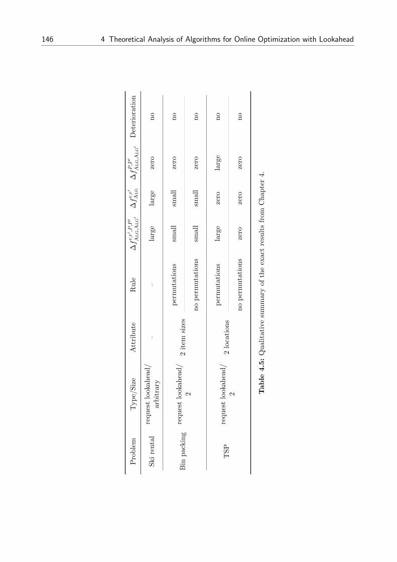
146 4 Theoretical Analysis of Algorithms for Online Optimization with Lookahead
Pro
ble
mT
yp
e/Siz
eA
ttri
bu
teR
ule
∆fr,r′ ,P,P′
Alg,A
lg′
∆fr,r′
Alg
∆fP,P′
Alg,A
lg′
Det
erio
rati
on
Ski
renta
lre
ques
tlo
oka
hea
d/
arb
itra
ry–
–la
rge
larg
eze
ron
o
Bin
pack
ing
reques
tlo
okahea
d/
22
item
size
sp
erm
uta
tion
ssm
all
smal
lze
rono
no
per
mu
tati
ons
smal
lsm
all
zero
no
TSP
reques
tlo
okah
ead/
22
loca
tion
sp
erm
uta
tion
sla
rge
zero
larg
eno
no
per
mu
tati
ons
zero
zero
zero
no
Table
4.5:
Qu
alita
tive
sum
mar
yof
the
exac
tre
sult
sfr
omC
hap
ter
4.

147
5 Experimental Analysis of Algorithms for
Online Optimization with Lookahead
Complementing the theoretical results derived in the previous chapter, we now conduct a
series of numerical experiments on five standard online optimization problems in order to
examine the impact of lookahead on solution quality for algorithms specifically tailored to
take advantage of lookahead. We observe significant differences in the magnitude of the
lookahead effect depending on the respective problem settings and give explanations for
varying algorithm behavior under additional lookahead. The study of this chapter enables
us to preestimate the magnitude of the lookahead effect based on the problem characteristics
provided. We consider two additional problems alongside those of the previous chapter:
• Online Paging with Lookahead
• Online Scheduling with Lookahead
For each problem, three different types of analysis are applied in order to ensure a compre-
hensive view on algorithm behavior under different information regimes:
1. Average results portray the overall behavior of algorithms under different amounts of
lookahead for a prescribed number of independent random input sequences.
2. Distributional results submit a more precise picture by including frequency information
on observed objective values and performance ratios, respectively.
3. Markov chain results serve as an exact underpinning for the sampled results. Because
of the curse of dimensionality, we restrict ourselves to small parameter values.
Computational experiments were performed on a personal computer with AMD Phenom II
X6 1100T 3.31 GHz processor and 16 GB RAM under Microsoft Windows 7 (64-bit). All
algorithms were implemented in C++ and arising instances of IP and MIP formulations were
solved using IBM ILOG CPLEX 12.5 with a prescribed time limit of 120 seconds. A detailed
summary of statistical key figures for each experiment is given in Appendix A.2.

148 5 Experimental Analysis of Algorithms for Online Optimization with Lookahead
5.1 Online Ski Rental with Lookahead
A specification of the online ski rental problem with lookahead and corresponding algorithms
is given in Chapter 4.1. Because exact expressions for the counting distribution functions
of the objective value and the performance ratio have been derived, we only present a brief
(exact) numerical analysis for fixed parameters nmax = 100, B = 50, r = 1 to see the magni-
tude of the lookahead impact. Recall that an input sequence σ corresponds to a prescribed
number of skiing days n ∈ {1, 2, . . . , nmax}. For better readability, we denote algorithm
ConditionalBuyk,l as Algk,l; the optimal offline algorithm is called Opt. Observe that
Algk,l coincides with Opt for l ≥ dBre = d50
1e = 50 and with Buyk for l = 1. Algorithms
are tested with variable purchase time k ∈ {1, 25, 50, 75, 100} and variable lookahead sizes
l ∈ {1, 5, 10, 20, . . . , 100}.
5.1.1 Average Results
From Figure 5.1, we see that lookahead leads to drastic reductions in the average costs
required for skiing over all input sequences when each of the nmax = 100 days is equally
probable to be the last skiing day. Comparing the online and offline situation, average cost
reductions vary between 24.5 % and 39.8 % depending on the appointed day of purchase.
0 10 20 30 40 50 60 70 80 90 100
40
45
50
55
60
65
Lookahead size l
Averagecosts
Alg1,l
Alg25,l
Alg50,l
Alg75,l
Alg100,l
Figure 5.1: Average costs for different lookahead sizes and nmax = 100 in the ski rental problem.
For fixed k, consider two lookahead levels l1, l2 with l1 < l2 and l1, l2 < dBr e = 50. From
the cost profile of Algk,l it follows that Algk,l1 [σ] ≥ Algk,l2 [σ] for all input sequences σ.

5.1 Online Ski Rental with Lookahead 149
Hence, additional lookahead proves exclusively beneficial and the average savings is
∑σ
Algk,l1 [σ]−Algk,l2 [σ]
nmax=
k+l2−2∑t=k+l1−1
r(k − 1) +B − rtnmax
=
k+l2−2∑t=k+l1−1
k + 49− t100
≥ 0.
For fixed lookahead l, the relation of the average costs incurred by Algk1,l and Algk2,l with
k1 < k2 is determined by the value
∑σ
Algk1,l[σ]−Algk2,l[σ]
nmax=
k2+l−2∑t=k1+l−1
(r(k1 − 1) +B − rt)−nmax∑
t=k2+l−1
r(k2 − k1)
nmax
=
k2+l−2∑t=k1+l−1
(k1 + 49− t)− (102− k2 − l)(k2 − k1)
100
whose sign depends on the choices of k1 and k2. For the given parameters, the average
of Alg1,l, i.e., k1 = 1, is not larger than that of Algk2,l for all k2 ∈ {2, . . . , 100} and
all l as indicated by the red line in Figure 5.1: The savings of Alg1,l for all σ = {1}nwith n ≥ k2 + l − 1 cannot be exceeded by its excess expenditures for all σ = {1}n with
k1 + l − 1 = l ≤ n ≤ k2 + l − 2. This can be seen by
k2+l−2∑t=l
(50− t)− (102− k2 − l)(k2 − 1) = 50(k2 − 1)−k2+l−2∑t=l
t− (102− k2 − l)(k2 − 1)
=k2
2(k2 − 103) + 51
which is smaller than 0 for k2 ≤ 100. We remark that the order relation between the average
of Algk,l[σ] for varying k and fixed l is strongly affected by the skier’s expectation for the
length of the skiing trip: Buying early should pay off whenever skis are expected to be in
need for a long time; vice versa, buying late should pay off whenever skis are expected to
be in need only shortly. Incorporating these considerations by weighting of input sequences,
superiority of Alg1,l as displayed in Figure 5.1 is obtained by attributing equal weights 1nmax
to all input sequences. Because of the parameter choices, this weighting already suffices to
suggest earliest possible buying. Weightings which favor ski trips of short duration tend to
shift lower costs to algorithms which buy late; vice versa, weightings which favor ski trips of
long duration tend to shift lower costs to algorithms which buy early.

150 5 Experimental Analysis of Algorithms for Online Optimization with Lookahead
5.1.2 Distributional Results
Figure 5.2 displays the counting distribution functions of the objective value for Algk,l
and benchmarks them with the objective value distribution of Opt. Since for l ≥ 50, the
distributions of Algk,l coincide with that of Opt, their plots are omitted.
Note that it is not possible for any of the algorithms to incur a deterioration in the objective
value when more information is provided. In each of the diagrams, this can be seen from the
perfect (stochastic) ordering of the counting distribution functions for prescribed purchase
time k. Since Alg1,l is the only family of algorithms which considers buying at the outset of
the dynamic problem, it is the only algorithm family which approximates Opt for increasing
l. For all other Algk,l with k > 1, a gap remains for increasing l with l < 50 due to
non-optimal buying decisions before day k. Clearly, for l ≥ 50 the plot of any algorithm
Algk,l would snap to that of Opt. For fixed lookahead l, the range of occurring objective
values broadens to larger values for increased k, thereby confirming the previously described
superiority of Alg1,l in the given parameter constellation.
Although the average objective values and the objective value distributions suggest to buy
at the very beginning of the planning horizon, the counting distribution functions of the
performance ratio of each algorithm relative to Opt in Figure 5.3 show that there is a high
risk of incurring large multiples of the optimal objective value for these algorithms. For
instance, on the input sequence σ corresponding to one skiing day, Alg1,1[σ] charges costs
of 50, whereas Opt only incurs a unit cost. Hence, the performance ratio is 50, emphasizing
the potential risk of buying too early. This result is also confirmed by the comparatively
large coefficients of variation for the performance ratios when k is small and the reduction
in the confidence interval width for increasing k as shown in Table A.2 of Appendix A.2.1.
Similar conclusions as found previously are discovered regarding the benefit of lookahead
within an algorithm family Algk,l with fixed k and variable l. Additional information leads
to a considerable risk mitigation in form of a diminished competitive ratio that is attained
by Algk,l for increasing values of l. Note that in general no deterministic algorithm can be
better than (2− 1B
= 1.98)-competitive ([107]).
In case of comparing to the pure online versions Algk,1 of the algorithms rather than to Opt,
the variability of performance ratios for small k becomes evident in the immense width of
their range for k = 1 as compared to larger values of k (see Figure 5.4 and Table A.3 of
Appendix A.2.1). From this point of view, we also find that additional lookahead exclusively
leads to lower costs as reflected by all performance ratios being smaller than 1 and confidence
intervals shifting to regions with smaller values for increasing l.

5.1 Online Ski Rental with Lookahead 151
0 20 40 60 80 100 120 140 1600
0.2
0.4
0.6
0.8
1
v
F(v)
Alg1,1 Alg1,5
Alg1,10 Alg1,20
Alg1,30 Alg1,40
Alg1,50 = Opt
0 20 40 60 80 100 120 140 1600
0.2
0.4
0.6
0.8
1
v
F(v)
Alg25,1 Alg25,5
Alg25,10 Alg25,20
Alg25,30 Alg25,40
Alg25,50 = Opt
0 20 40 60 80 100 120 140 1600
0.2
0.4
0.6
0.8
1
v
F(v)
Alg50,1 Alg50,5
Alg50,10 Alg50,20
Alg50,30 Alg50,40
Alg50,50 = Opt
0 20 40 60 80 100 120 140 1600
0.2
0.4
0.6
0.8
1
v
F(v)
Alg75,1 Alg75,5
Alg75,10 Alg75,20
Alg75,30 Alg75,40
Alg75,50 = Opt
0 20 40 60 80 100 120 140 1600
0.2
0.4
0.6
0.8
1
v
F(v)
Alg100,1 Alg100,5
Alg100,10 Alg100,20
Alg100,30 Alg100,40
Alg100,50 = Opt
Figure 5.2: Counting distribution functions of costs for nmax = 100 in the ski rental problem.

152 5 Experimental Analysis of Algorithms for Online Optimization with Lookahead
0 10 20 30 40 500
0.2
0.4
0.6
0.8
1
v
F(v)
Alg1,1 Alg1,5
Alg1,10 Alg1,20
Alg1,30 Alg1,40
Alg1,50 = Opt
0 1 2 3 40
0.2
0.4
0.6
0.8
1
v
F(v)
0 10 20 30 40 500
0.2
0.4
0.6
0.8
1
v
F(v)
Alg25,1 Alg25,5
Alg25,10 Alg25,20
Alg25,30 Alg25,40
Alg25,50 = Opt
0 1 2 3 40
0.2
0.4
0.6
0.8
1
v
F(v)
0 10 20 30 40 500
0.2
0.4
0.6
0.8
1
v
F(v)
Alg50,1 Alg50,5
Alg50,10 Alg50,20
Alg50,30 Alg50,40
Alg50,50 = Opt
0 1 2 3 40
0.2
0.4
0.6
0.8
1
v
F(v)
0 10 20 30 40 500
0.2
0.4
0.6
0.8
1
v
F(v)
Alg75,1 Alg75,5
Alg75,10 Alg75,20
Alg75,30 Alg75,40
Alg75,50 = Opt
0 1 2 3 40
0.2
0.4
0.6
0.8
1
v
F(v)
0 10 20 30 40 500
0.2
0.4
0.6
0.8
1
v
F(v)
Alg100,1 Alg100,5
Alg100,10 Alg100,20
Alg100,30 Alg100,40
Alg100,50 = Opt
0 1 2 3 40
0.2
0.4
0.6
0.8
1
v
F(v)
Figure 5.3: Counting distribution functions of performance ratio of costs relative to Opt fornmax = 100 in the ski rental problem.
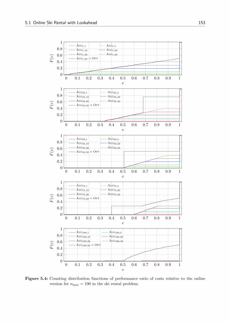
5.1 Online Ski Rental with Lookahead 153
0 0.1 0.2 0.3 0.4 0.5 0.6 0.7 0.8 0.9 10
0.2
0.4
0.6
0.8
1
v
F(v)
Alg1,1 Alg1,5
Alg1,10 Alg1,20
Alg1,30 Alg1,40
Alg1,50 = Opt
0 0.1 0.2 0.3 0.4 0.5 0.6 0.7 0.8 0.9 10
0.2
0.4
0.6
0.8
1
v
F(v)
Alg25,1 Alg25,5
Alg25,10 Alg25,20
Alg25,30 Alg25,40
Alg25,50 = Opt
0 0.1 0.2 0.3 0.4 0.5 0.6 0.7 0.8 0.9 10
0.2
0.4
0.6
0.8
1
v
F(v)
Alg50,1 Alg50,5
Alg50,10 Alg50,20
Alg50,30 Alg50,40
Alg50,50 = Opt
0 0.1 0.2 0.3 0.4 0.5 0.6 0.7 0.8 0.9 10
0.2
0.4
0.6
0.8
1
v
F(v)
Alg75,1 Alg75,5
Alg75,10 Alg75,20
Alg75,30 Alg75,40
Alg75,50 = Opt
0 0.1 0.2 0.3 0.4 0.5 0.6 0.7 0.8 0.9 10
0.2
0.4
0.6
0.8
1
v
F(v)
Alg100,1 Alg100,5
Alg100,10 Alg100,20
Alg100,30 Alg100,40
Alg100,50 = Opt
Figure 5.4: Counting distribution functions of performance ratio of costs relative to the onlineversion for nmax = 100 in the ski rental problem.

154 5 Experimental Analysis of Algorithms for Online Optimization with Lookahead
Since there is only one input sequence of a given length n and an expression for the costs on
a given input sequence is known for all algorithms, Markov chain analysis becomes obsolete;
all results are already included in the theoretical analysis in Chapter 4.1.
We conclude this section by pointing out that the computational experiments on the ski
rental problem merely serve as an illustration for the results obtained by the exact analysis
in Chapter 4.1. For nmax = 100, the exclusive benefit from lookahead is apparent from the
clear-cut gaps between the counting distribution function plots of successive lookahead levels.
Advantages arise by the fact that the ski rental problem is a one-shot decision problem where
more information never leads to worse decisions.
5.2 Online Paging with Lookahead
Paging deals with the organization of a two-level memory system for sequential requests on
elements (pages) of an alphabet A ([74], [164]). The large and slow main memory holds
all pages of A, whereas the small and fast cache memory can only hold k < |A| pages (or
pointers to them). A requested page currently not in the cache produces a page fault, and
whenever a page fault occurs, the page has to be brought to the cache first before it can be
accessed. The goal is to minimize the number of page faults. For fixed n ∈ N, the set of all
input sequences is given by
Σn ={
(σ1, σ2, . . . , σn) |σi ∈ A, i = 1, . . . , n}
and comprises all page sequences of length n. Typically, pages must be brought to the
cache in their order of appearance in the input sequence – regardless of the type and size of
lookahead. In the online version, only σi with i = 1, . . . , n is known when σi is requested. In
the online version with lookahead of size l, σi with i = 1, . . . , n and l− 1 successive requests
σi+1, . . . , σi+l−1 are known if i + l − 1 ≤ n, otherwise σi and additional n − i successive
requests σi+1, . . . , σn are known. In the offline version, all requested pages are known at the
beginning. Subsequently, a page that is already in the cache is called a cache page.
In our experiment, we draw m = 1000 independent request sequences where each one of
them consists of n = 100 pages. The cache has a capacity of k = 10 pages and the alphabet
corresponds to the 26 standard letters, i.e., A = {A,B, . . . , Z}. Lookahead sizes l are chosen
from {1, 5, 10, 20, 40, . . . , 100}. In accordance with mainstream research on paging (see, e.g.,
[4], [33]), also our analysis takes into account different levels of locality of reference in the
input sequence:

5.2 Online Paging with Lookahead 155
• No locality at all, i.e., at any time each page is equally probable.
• Locality by generating input sequences according to an access graph, i.e., page se-
quences are generated by traversing the edges of a graph whose vertices are labeled
with the pages. Pages could, for instance, be understood as the subpages of an internet
homepage, i.e., the access graph amounts to the homepage navigation scheme.
• Locality by assigning each page a fixed probability for occurring next based on relative
letter frequencies in texts as elicited by statistical evaluations.
We restrict the discussion to the first two cases and refer to Appendix A.2.2 for more infor-
mation on the third case.
A decision by an algorithm is required only when a page fault occurs and merely consists of
selecting the cache page to be evicted in order to make way for the current request.
Online algorithms
• FirstInFirstOut (Fifo): In case of a page fault, evict a cache page which entered
the cache first ([149]).
• LastInFirstOut (Lifo): In case of a page fault, evict a cache page which entered
the cache last ([149]).
• LeastFrequentlyUsed (Lfu): In case of a page fault, evict a cache page which has
been requested least frequently ([149]).
• LeastRecentlyUsed (Lru): In case of a page fault, evict a cache page which has
been requested least recently ([149]).
Online algorithms with lookahead of size l
• FirstInFirstOutl (Fifol): In case of a page fault, if there are cache pages which
are not requested in the lookahead, evict a cache page which entered the cache first
among these pages; otherwise evict a cache page whose next request is farthest ahead.
• LastInFirstOutl (Lifol): In case of a page fault, if there are cache pages which are
not requested in the lookahead, evict a cache page which entered the cache last among
these pages; otherwise evict a cache page whose next request is farthest ahead.
• LeastFrequentlyUsedl (Lful): In case of a page fault, if there are cache pages
which are not requested in the lookahead, evict a cache page which has been requested
least frequently among these pages; otherwise evict a cache page whose next request
is farthest ahead.

156 5 Experimental Analysis of Algorithms for Online Optimization with Lookahead
• LeastRecentlyUsedl (Lrul): In case of a page fault, if there are cache pages which
are not requested in the lookahead, evict a cache page which has been requested least
recently among these pages; otherwise evict a cache page whose next request is farthest
ahead.
Optimal offline algorithm
• Optimal (Opt): In case of a page fault, evict a cache page whose next request is
farthest ahead (Belady’s optimal replacement algorithm in [17]).
Note that Fifol, Lifol, Lful and Lrul all coincide with Opt for l = n = 100 and with
Fifo, Lifo, Lfu and Lru, respectively, for l = 1.
Besides regular request lookahead, we also include batched request lookahead of size l into
our experiment to find out whether a steady supply with input elements is really needed
or whether input element release in blocks suffices to obtain satisfying results: During the
processing of a batch of input elements, the number of pages seen by the algorithm gradually
reduces by one in each processing step. Since data is often organized in blocks or packages,
batched lookahead is realistic for practical applications. If algorithms operate under batched
lookahead, we indicate them with an added suffix B in the algorithm name.
5.2.1 Average Results
Figure 5.5 displays that each algorithm class performs equally good under the same lookahead
regime when each page is equally probable to be the next one encountered in an input
sequence. Because of this assumption, the probability for a page fault is identical for each
possible current cache configuration, i.e., irrespective of an algorithm’s previous organization
of the cache. Lookahead leads to a substantial decrease in the number of page faults: Between
the extreme cases of online and offline optimization, average page fault reductions of 36.7 %
are observed. However, the marginal benefit of lookahead is strictly decreasing, i.e., the first
lookahead units are the most valuable. Because all algorithms collapse into Opt for l = 100,
every algorithm yields the optimal number of average page faults in this case. Applying
regular lookahead instead of batched lookahead pays off by up to 15.4 % for l = 20.
When a (non-trivial) stochastic model about page occurrences is imputed by locality of
reference in form of an access graph, algorithms behave differently as can be seen in Figure
5.6. Algorithm Lrul now outperforms the other algorithms for fixed l because construing
input sequences according to the access graph implies that recently requested pages are more
likely for being next than pages requested a long time ago as a result of their (shortest path)

5.2 Online Paging with Lookahead 157
0 10 20 30 40 50 60 70 80 90 100
40
45
50
55
60
65
Lookahead size l
Average
costs
Fifol
Lifol
Lful
Lrul
Fifol,B
Lifol,B
Lful,B
Lrul,B
Figure 5.5: Average costs for different lookahead sizes and n = 100 in the paging problem wheneach page is equally probable.
distance to the vertex labeled with the current page. This is in line with Lrul’s behavior of
keeping recent requests and evicting requests from long ago. Likewise, Fifol fares relatively
good as it also sticks to deleting older pages first. Quite contrary, both Lifol and Lful
counteract the rationale of locality of reference imputed by an access graph: Because they
evict pages that just joined the cache or yet have a small frequency count since they have
just joined the cache, they make page faults much more likely as the evicted pages are near
to the current page in terms of the distance in the access graph.
0 10 20 30 40 50 60 70 80 90 100
20
25
30
35
40
45
Lookahead size l
Averagecosts
Fifol
Lifol
Lful
Lrul
Fifol,B
Lifol,B
Lful,B
Lrul,B
Figure 5.6: Average costs for different lookahead sizes and n = 100 in the paging problem whenpage sequences are generated according to an access graph.

158 5 Experimental Analysis of Algorithms for Online Optimization with Lookahead
The positive effect of lookahead is retained also under locality of reference, albeit for Lrul and
Fifol its magnitude is diminished strongly as a result of the already satisfying performance
of the pure online algorithms. For these two algorithms, the lookahead effect is up to 11.5 %
and 18.4 %, respectively, when online and offline optimization are compared. We conclude
that locality of reference makes the future more predictive such that suitable algorithms can
capitalize already from this circumstance substantially. For these algorithms, it is nearly
irrelevant whether lookahead is provided on a rolling time horizon or in batches.
We remark that in locality of reference with preassigned page probabilities, Lful excels
the other algorithms for fixed l because it bases its decision on frequency counts which are
expected to comply with prescribed page probabilities that have been derived from letter
frequencies. This result is in sharp contrast to competitive analysis where Lfu and Lifo are
known to be non-competitive, whilst Fifo and Lru are (k = 10)-competitive.
The impact of lookahead on the given algorithms is exclusively beneficial in case of regular
lookahead which is seen by two arguments: First, evicting a page seen in the lookahead
would lead to a guaranteed page fault within the time window of the lookahead size, whereas
evicting one that is not seen does not lead to a page fault in the same time window. Sec-
ond, the worst-case concerning the obtained cache configuration would be that the evicted
page would be needed immediately after the lookahead time window. However, the needed
cache configuration could then be produced with one page fault in total by reinserting the
evicted page in the cache again. In summary, evicting a page not seen in the lookahead
can never be worse than evicting a page seen in the lookahead, and it maintains the chance
of avoiding unnecessary page faults. In case of batched lookahead, there may be instances
with degradations in the objective value although more lookahead was provided as seen in
the last column of Table A.7 in Appendix A.2.2. This effect is due to the variable size of
the information preview window under batched lookahead where algorithms operate under
successively tightened lookahead within each batch.
5.2.2 Distributional Results
Because algorithms behave identically when each page is equally probable and due to the
small width of confidence intervals as seen in Tables A.4 to A.6 of Appendix A.2.2, we omit
a discussion of this case and concentrate on the results found under locality of reference in
the access graph model.
In Figure 5.7, the stable and superior performance of Lrul and Fifol is seen by the narrow
interval of observed objective intervals for each lookahead level and the relative closeness of

5.2 Online Paging with Lookahead 159
20 40 60 800
0.2
0.4
0.6
0.8
1
v
F(v)
Fifo1
Fifo5
Fifo10
Fifo20
Fifo40
Fifo60
Fifo80
Fifo100 = Opt
20 40 60 800
0.2
0.4
0.6
0.8
1
v
F(v)
Fifo1,B
Fifo5,B
Fifo10,B
Fifo20,B
Fifo40,B
Fifo60,B
Fifo80,B
Fifo100,B = Opt
20 40 60 800
0.2
0.4
0.6
0.8
1
v
F(v)
Lifo1
Lifo5
Lifo10
Lifo20
Lifo40
Lifo60
Lifo80
Lifo100 = Opt
20 40 60 800
0.2
0.4
0.6
0.8
1
v
F(v)
Lifo1,B
Lifo5,B
Lifo10,B
Lifo20,B
Lifo40,B
Lifo60,B
Lifo80,B
Lifo100,B = Opt
20 40 60 800
0.2
0.4
0.6
0.8
1
v
F(v)
Lfu1
Lfu5
Lfu10
Lfu20
Lfu40
Lfu60
Lfu80
Lfu100 = Opt
20 40 60 800
0.2
0.4
0.6
0.8
1
v
F(v)
Lfu1,B
Lfu5,B
Lfu10,B
Lfu20,B
Lfu40,B
Lfu60,B
Lfu80,B
Lfu100,B = Opt
20 40 60 800
0.2
0.4
0.6
0.8
1
v
F(v)
Lru1
Lru5
Lru10
Lru20
Lru40
Lru60
Lru80
Lru100 = Opt
20 40 60 800
0.2
0.4
0.6
0.8
1
v
F(v)
Lru1,B
Lru5,B
Lru10,B
Lru20,B
Lru40,B
Lru60,B
Lru80,B
Lru100,B = Opt
Figure 5.7: Empirical counting distribution functions of costs for n = 100 in the paging problemwhen page sequences are generated according to an access graph.

160 5 Experimental Analysis of Algorithms for Online Optimization with Lookahead
1 2 3 4 50
0.2
0.4
0.6
0.8
1
v
F(v)
Fifo1
Fifo5
Fifo10
Fifo20
Fifo40
Fifo60
Fifo80
Fifo100 = Opt
1 2 3 4 50
0.2
0.4
0.6
0.8
1
v
F(v)
Fifo1,B
Fifo5,B
Fifo10,B
Fifo20,B
Fifo40,B
Fifo60,B
Fifo80,B
Fifo100,B = Opt
1 2 3 4 50
0.2
0.4
0.6
0.8
1
v
F(v)
Lifo1
Lifo5
Lifo10
Lifo20
Lifo40
Lifo60
Lifo80
Lifo100 = Opt
1 2 3 4 50
0.2
0.4
0.6
0.8
1
v
F(v)
Lifo1,B
Lifo5,B
Lifo10,B
Lifo20,B
Lifo40,B
Lifo60,B
Lifo80,B
Lifo100,B = Opt
1 2 3 4 50
0.2
0.4
0.6
0.8
1
v
F(v)
Lfu1
Lfu5
Lfu10
Lfu20
Lfu40
Lfu60
Lfu80
Lfu100 = Opt
1 2 3 4 50
0.2
0.4
0.6
0.8
1
v
F(v)
Lfu1,B
Lfu5,B
Lfu10,B
Lfu20,B
Lfu40,B
Lfu60,B
Lfu80,B
Lfu100,B = Opt
1 2 3 4 50
0.2
0.4
0.6
0.8
1
v
F(v)
Lru1
Lru5
Lru10
Lru20
Lru40
Lru60
Lru80
Lru100 = Opt
1 2 3 4 50
0.2
0.4
0.6
0.8
1
v
F(v)
Lru1,B
Lru5,B
Lru10,B
Lru20,B
Lru40,B
Lru60,B
Lru80,B
Lru100,B = Opt
Figure 5.8: Empirical counting distribution functions of performance ratio of costs relative to Optfor n = 100 in the paging problem when page sequences are generated according toan access graph.

5.2 Online Paging with Lookahead 161
0.2 0.4 0.6 0.8 10
0.2
0.4
0.6
0.8
1
v
F(v)
Fifo1
Fifo5
Fifo10
Fifo20
Fifo40
Fifo60
Fifo80
Fifo100 = Opt
0.2 0.4 0.6 0.8 10
0.2
0.4
0.6
0.8
1
v
F(v)
Fifo1,B
Fifo5,B
Fifo10,B
Fifo20
Fifo40,B
Fifo60,B
Fifo80,B
Fifo100,B = Opt
0.2 0.4 0.6 0.8 10
0.2
0.4
0.6
0.8
1
v
F(v)
Lifo1
Lifo5
Lifo10
Lifo20
Lifo40
Lifo60
Lifo80
Lifo100 = Opt
0.2 0.4 0.6 0.8 10
0.2
0.4
0.6
0.8
1
v
F(v)
Lifo1,B
Lifo5,B
Lifo10,B
Lifo20,B
Lifo40,B
Lifo60,B
Lifo80,B
Lifo100,B = Opt
0.2 0.4 0.6 0.8 10
0.2
0.4
0.6
0.8
1
v
F(v)
Lfu1
Lfu5
Lfu10
Lfu20
Lfu40
Lfu60
Lfu80
Lfu100 = Opt
0.2 0.4 0.6 0.8 10
0.2
0.4
0.6
0.8
1
v
F(v)
Lfu1,B
Lfu5,B
Lfu10,B
Lfu20,B
Lfu40,B
Lfu60,B
Lfu80,B
Lfu100,B = Opt
0.2 0.4 0.6 0.8 10
0.2
0.4
0.6
0.8
1
v
F(v)
Lru1
Lru5
Lru10
Lru20
Lru40
Lru60
Lru80
Lru100 = Opt
0.2 0.4 0.6 0.8 10
0.2
0.4
0.6
0.8
1
v
F(v)
Lru1,B
Lru5,B
Lru10,B
Lru20,B
Lru40,B
Lru60,B
Lru80,B
Lru100,B = Opt
Figure 5.9: Empirical counting distribution functions of performance ratio of costs relative to theonline version for n = 100 in the paging problem when page sequences are generatedaccording to an access graph.

162 5 Experimental Analysis of Algorithms for Online Optimization with Lookahead
the plots to each other for all pairs of lookahead levels. This is also confirmed by the widths
and positions of the confidence intervals in Table A.7 of Appendix A.2.2. Lookahead leads
to improvement as seen by the ordering of the empirical counting distribution functions,
although not as drastically as for Lifol and Lful. For these algorithms, stable behavior
is reached only if there is a (real) lookahead of size larger than 1. Accordingly, additional
lookahead leads to a much higher percentage of decrease in the objective value than for Lrul
and Fifol.
Experimental competitive ratios as displayed in Figure 5.8 and indicated in the column for
the maximum observed value in Table A.8 of Appendix A.2.2 are consistently smaller than
2 for Fifo1 and Lru1; hence, they are much better than the theoretical value of k = 10
would suggest. Already for Lru1 and Fifo1 the fraction of admissible input sequences with
the minimum number of page faults amounts to 20.2 % and 28 %, respectively. Yet, even
under locality of reference, instances are encountered where Lru1 and Fifo1 miss optimality
by 50 % and 94 %, respectively. For l = 80, the worst observed performance ratio drops
to 1.06 for both algorithms. For high lookahead values, the empirical counting distribution
functions of the performance ratios are moving closer to 1 and become steeper, i.e., with
a fair amount of lookahead the deviation from optimality can be preestimated. From the
(local) optimality of evicting a cache page which lies farthest in the future, it follows that
for l tending to n = 100 the number of page sequences with performance ratio larger than 1
is non-increasing.
Comparing algorithms to their respective online version as illustrated in Figure 5.9 approves
the exclusive benefit of additionally provided information under regular lookahead because all
performance ratios encountered are smaller than 1. For Lrul and Fifol, there are instances
where full lookahead leads to a reduction to only 67 % and 52 % of the number of page
faults from the online case, respectively. For batched lookahead, improvements are slightly
smaller; instances sporadically experience an objective value degradation upon additional
information.
5.2.3 Markov Chain Results
The elements of the state space S subsume the cache configuration c = (c1, . . . , ck) whose el-
ements are ordered lexicographically, the lookahead pages p = (p1, . . . , pl), the page attribute
configurations a = (a1, . . . , a|A|) and the number of page faults v so far, i.e.,
S ={
(c, p, a, v) | c ∈ Ak, p ∈ Al, a ∈ N|A|, v ∈ N0
}.

5.2 Online Paging with Lookahead 163
Page attribute aj with j ∈ {1, 2, . . . , |A|} holds information concerning page j relevant to
successive algorithm computations. For instance, aj may hold the last time that j entered
the cache, the number of requests on j so far or the number of requests that lie between the
current and the last request on j. Upon arrival of a new page, each algorithm Alg decides
which page to evict from the cache – if necessary – in order to bring p1 into the cache. Hence,
Alg is a function
Alg : S ×A → {0, 1, 2, . . . , k}
which gives the cache position to be evicted where Alg(·) = 0 means that no page needs
to be evicted. The successor state of s = (c, p, a, v) upon arrival of page pnew is given by
s′ = (c′, p′, a′, v′) where c′ arises from c by removing element cAlg(s,pnew), appending element
p1 and ordering lexicographically, p′ arises from p by removing p1 and appending pnew,
a′j =
aj if Alg ∈ {Fifo,Lifo},Alg(s, pnew) = 0,
aj if Alg ∈ {Fifo,Lifo},Alg(s, pnew) 6= 0, p1 6= j,
max{ai}+ 1 if Alg ∈ {Fifo,Lifo},Alg(s, pnew) 6= 0, p1 = j,
aj if Alg = Lfu, p1 6= j,
aj + 1 if Alg = Lfu, p1 = j,
aj + 1 if Alg = Lru, p1 6= j,
0 if Alg = Lru, p1 = j.
for j = 1, . . . , |A| and
v′ =
v if Alg(s, pnew) = 0,
v + 1 otherwise.
Finally, we have to specify the initial state of the cache.
Since all algorithms include past information into their decision making, the Markov property
is lost in the ordinary sense. We artificially make Markov chain analysis applicable by
integrating all necessary information from the past in form of the page attributes a into the
state space. For this trick, we have to pay the price of an increased state space size, namely
|S| =(|A|k
)· |A|l · (n+ 1)|A| · (n+ 1).
For Alg ∈ {Fifol,Lifol,Lful,Lrul} and selected lookahead level l, we now determine the
successor for each state and each new page request to obtain the one-step frequency matrix

164 5 Experimental Analysis of Algorithms for Online Optimization with Lookahead
FAlg = (fAlgij ) of the Markov chain. Entry fAlg
ij gives the number of page requests which
lead from state i ∈ S to state j ∈ S by applying Alg in i. We get the n-step frequency
matrix FAlg,n = (fAlg,nij ) as the nth power of FAlg, i.e., FAlg,n = (FAlg)n. Entry fAlg,n
ij
gives the number of permutations of n page requests, i.e., the number of input sequences
of length n which lead from state i ∈ S to state j ∈ S by applying Alg n times in a row
starting in i.
In our numerical experiment, we use the parametrization n = 5, A = {A,B,C}, k = 2 and
l ∈ {1, 2, . . . , 5}. For this small exemplary setting, the state space size already amounts to(32
)·35 ·63 ·6 = 944 784 elements for l = 5 which is mainly due to the artificial extension of the
state space in order to include information concerning the past behavior of the algorithms.
Since we consider no locality of reference, we have that Fifol,Lifol,Lful,Lrul all lead to
identical objective value distributions for fixed l. Therefore, we speak of Algl in the sequel
and refer to each of the algorithms.
In consonance with Figure 5.5, also Figure 5.10 affirms the positive impact of lookahead on
the number of page faults encountered. From the area between the plots of two successive
lookahead levels, we find that already for relatively short input sequences it is seen that the
first lookahead units prove most valuable.
0 1 2 3 4 50
0.2
0.4
0.6
0.8
1
v
F(v)
Alg1
Alg2
Alg3
Alg4
Alg5
Figure 5.10: Exact distribution functions of costs for n = 5 in the paging problem when pagesare equally distributed.
We conclude that the positive effect of lookahead has its roots in the immediate reduction
of the number of page faults by not deleting a page whenever it is seen in the lookahead as
compared to the case where it may be deleted as it cannot be seen due to a more limited
information preview window. Hence, lookahead can never be harmful in the paging problem.
Observe that there is no change in the rule set of paging under additional lookahead due
to the sequential character of page requests; all improvements are a result of advanced
information.

5.3 Online Bin Packing with Lookahead 165
5.3 Online Bin Packing with Lookahead
A specification of the online bin packing problem with lookahead and algorithms BestFit
and BestFitl is given in Chapter 4.2. In the numerical analysis, we take into account
further algorithms and consider two cases with respect to the rule set: Item permutations
may be allowed when items have small physical dimensions such that sorting is done easily,
or item permutations may be forbidden when items are physically too large to be rearranged.
In applications, the restriction of a bounded number of open bins at a time is encountered
frequently due to capacity or space limitations. The latter problem is called the bounded-
space bin packing problem with lookahead. We obtain four problem settings:
• Classical bin packing with item permutations
• Classical bin packing without item permutations
• Bounded-space bin packing with item permutations
• Bounded-space bin packing without item permutations
For fixed n ∈ N, the set of all input sequences of length n is given by
Σn ={
(σ1, σ2, . . . , σn) |σi := si ∈ (0, 1], i = 1, . . . , n}
and comprises all item sequences of length n where σi is identified with the size of the ith
item. In the online version, only σi with i = 1, . . . , n is known when σi has to be packed.
When σi with i = 1, . . . , n has to be packed in the online version with lookahead of size l
under order preservation, also l−1 successive items σi+1, . . . , σi+l−1 are known if i+l−1 ≤ n,
otherwise σi and additional n−i successive items σi+1, . . . , σn are known. When known items
may be packed in arbitrary order, then at the ith packing time, the l unpacked items from
σ1, σ2, . . . , σi+l−1 with i = 1, . . . , n are known if i + l − 1 ≤ n, otherwise the n − i + 1
unpacked items from σ1, σ2, . . . , σn are known. In the offline version, all items are known at
the beginning.
We select two settings for our numerical experiments which both feature m = 1000 indepen-
dently drawn item sequences: In the first setting, we have n = 25 items per item sequence;
in the second setting, an item sequence consists of n = 100 items. Item sizes are drawn from
(0, 1] and each bin has unit capacity. In the bounded-space version, only k = 3 bins are
allowed to be open at the same time. For n = 25, lookahead sizes are l ∈ {1, 5, 10, . . . , 25};for n = 100, we have l ∈ {1, 5, 10, 20, 40, . . . , 100}. We discuss results for n = 25 and refer
the reader to Appendix A.2.3 for n = 100.

166 5 Experimental Analysis of Algorithms for Online Optimization with Lookahead
We consider both regular and batched request lookahead of size l in order to see whether
a steady information about future items leads to mentionable improvements or whether it
suffices to release the items in batches in order to obtain satisfactory results. If algorithms
operate under batched lookahead, we indicate them with an added suffix B in the algorithm
name.
A decision by an algorithm is required for every item that has to be packed and consists of
selecting the bin in which this item should be put.
5.3.1 Classical Bin Packing
Because a bin once opened is never closed again, each of the following algorithms can be used
irrespective of whether item permutations are allowed or not: An item to bin assignment
determined by any of the algorithms can be realized also in case of forbidden permutations
by fictively rearranging all items assigned to the same bin such that their order in a bin
complies with their release order.
Online algorithms
• FirstFit (Ff): If there is at least one open bin that can accommodate the item to
be packed, put the item in the bin that was opened first among these bins; otherwise
open a new bin and put the item in ([55]).
• BestFit (Bf): If there is at least one open bin that can accommodate the item to be
packed, put the item in the fullest among these bins; otherwise open a new bin and
put the item in ([55]).
Online algorithms with lookahead of size l
• FirstFitl (Ffl): Sort the items in the lookahead by non-increasing size and fictively
pack them with Ff. If the item to be packed is put in a new bin, open a new bin and
put the item in; otherwise put the item in the bin from the fictive assignment ([55]).
• BestFitl (Bfl): Sort the items in the lookahead by non-increasing size and fictively
pack them with Bf. If the item to be packed is put in a new bin, open a new bin and
put the item in; otherwise put the item in the bin from the fictive assignment ([55]).
• Optimall (Optl): In Figure 5.11, set N,N o, s and f according to the current bin
configuration and items seen in the lookahead. Solve the resulting IP formulation in
Figure 5.12. If the item to be packed is put in a new bin, open a new bin and put the
item in; otherwise put the item in the bin from the obtained assignment.

5.3 Online Bin Packing with Lookahead 167
Sets
I set of items with I = {1, . . . , N}J set of potential new bins with J = {1, . . . , N}Jo set of already used bins with Jo = {1, . . . , N o}L set of fill levels ` with L = {0.7, 0.75, 0.8, 0.85, 0.9, 0.95}
Parameters
N number of items and potential new binsN o number of bins already usedsi size of item i ∈ Ifjo fill level of already used bin jo ∈ Jow` weight of fill level ` ∈ L with w0.7 = 0.01, w0.75 = 0.02,
w0.8 = 0.04, w0.85 = 0.08, w0.9 = 0.16, w0.95 = 0.32
Variables
xij =
{1 if item i ∈ I is put in bin j ∈ J,0 else
xoijo =
{1 if item i ∈ I is put in already used bin jo ∈ Jo,0 else
yj =
{1 if bin j ∈ J is used,
0 else
αj` =
1 if bin j ∈ J has fill level in [`, `+ 0.05) for ` ∈ L with ` 6= 0.95,
or [`, `+ 0.05] for ` = 0.95,
0 else
αojo` =
1 if already used bin jo ∈ Jo has fill level in [`, `+ 0.05) for ` ∈ L
with ` 6= 0.95, or [`, `+ 0.05] for ` = 0.95,
0 else
Figure 5.11: Sets, parameters and variables in the IP formulation of the bin packing problems(see also [72]).
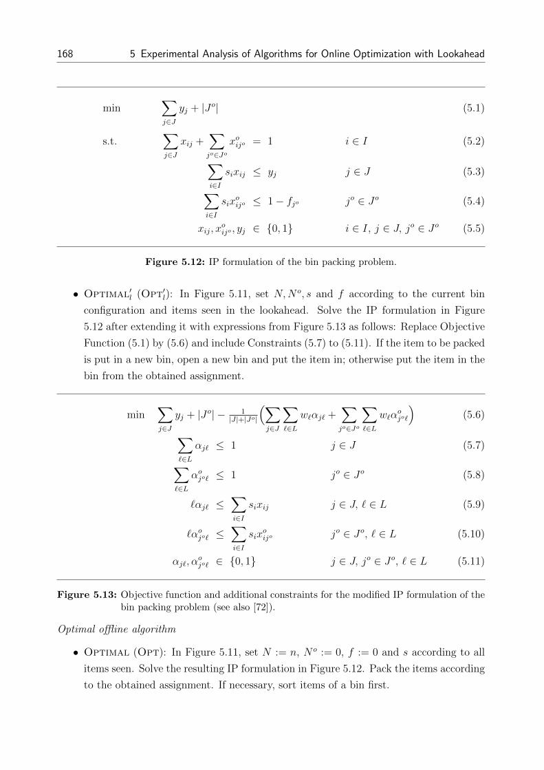
168 5 Experimental Analysis of Algorithms for Online Optimization with Lookahead
min∑j∈J
yj + |Jo| (5.1)
s.t.∑j∈J
xij +∑jo∈Jo
xoijo = 1 i ∈ I (5.2)∑i∈I
sixij ≤ yj j ∈ J (5.3)∑i∈I
sixoijo ≤ 1− fjo jo ∈ Jo (5.4)
xij, xoijo , yj ∈ {0, 1} i ∈ I, j ∈ J, jo ∈ Jo (5.5)
Figure 5.12: IP formulation of the bin packing problem.
• Optimal′l (Opt′l): In Figure 5.11, set N,N o, s and f according to the current bin
configuration and items seen in the lookahead. Solve the IP formulation in Figure
5.12 after extending it with expressions from Figure 5.13 as follows: Replace Objective
Function (5.1) by (5.6) and include Constraints (5.7) to (5.11). If the item to be packed
is put in a new bin, open a new bin and put the item in; otherwise put the item in the
bin from the obtained assignment.
min∑j∈J
yj + |Jo| − 1|J |+|Jo|
(∑j∈J
∑`∈L
w`αj` +∑jo∈Jo
∑`∈L
w`αojo`
)(5.6)∑
`∈Lαj` ≤ 1 j ∈ J (5.7)∑
`∈Lαojo` ≤ 1 jo ∈ Jo (5.8)
`αj` ≤∑i∈I
sixij j ∈ J, ` ∈ L (5.9)
`αojo` ≤∑i∈I
sixoijo jo ∈ Jo, ` ∈ L (5.10)
αj`, αojo` ∈ {0, 1} j ∈ J, jo ∈ Jo, ` ∈ L (5.11)
Figure 5.13: Objective function and additional constraints for the modified IP formulation of thebin packing problem (see also [72]).
Optimal offline algorithm
• Optimal (Opt): In Figure 5.11, set N := n, N o := 0, f := 0 and s according to all
items seen. Solve the resulting IP formulation in Figure 5.12. Pack the items according
to the obtained assignment. If necessary, sort items of a bin first.

5.3 Online Bin Packing with Lookahead 169
While Optl only considers the number of bins in the objective, Opt′l secondarily searches
for an item to bin assignment with bins as full or empty as possible, but not with medium
fill levels. This is done by promoting bins with large fill levels in Objective Function 5.6
in such a way that the total number of bins used stays unaffected. Constraints 5.7 to 5.11
ensure that at most one fill level is attained according to the combined item sizes in a bin.
Thereby, the initial position for successive items is improved because in case of large item
sizes, empty bins are more valuable. This approach of using a surrogate objective function
in order to improve the initial position for future steps is due to Esen ([72]).
5.3.1.1 Average Results
Average algorithm behavior is displayed in Figures 5.14 and 5.15 for the cases of allowed and
forbidden item permutations, respectively. The positive effect of allowing item permutations
is virtually non-existent as compared to forbidden item permutations as can be seen from
the nearly identical shapes of the corresponding plots in both diagrams.
2 4 6 8 10 12 14 16 18 20 22 24
14.2
14.4
14.6
14.8
Lookahead size l
Average
costs
BflFflOptl
Opt′l
Bfl,BFfl,BOptl,B
Opt′l,B
Figure 5.14: Average costs for different lookahead sizes and n = 25 in the classical bin packingproblem when item permutations are allowed.
Recall that in Example 2.37 there was no value of permuting items at all in online bin
packing with two item sizes. Moreover, as pointed out earlier, all algorithms under allowed
item permutations can also be applied under forbidden item permutations to first determine
a fictive assignment before packing an item. However, due to new items, the obtained bin
configurations are not necessarily identical; yet, in both cases algorithms combine items to
fit a bin, and the overall character of the bin configurations is approximately the same.

170 5 Experimental Analysis of Algorithms for Online Optimization with Lookahead
2 4 6 8 10 12 14 16 18 20 22 24
14.2
14.4
14.6
14.8
Lookahead size l
Average
costs
BflFflOptl
Opt′l
Bfl,BFfl,BOptl,B
Opt′l,B
Figure 5.15: Average costs for different lookahead sizes and n = 25 in the classical bin packingproblem when item permutations are forbidden.
From Tables A.13 and A.14 of Appendix A.2.3, we conclude that it may be slightly beneficial
to be allowed to pack large items earlier, but we consider the overall effect as negligible, e.g.,
Opt15 needs an average of 14.12 bins in case of allowed item permutations as opposed to
14.2 bins in case of no item permutations which is a relative advantage of less than 1 %.
For this reason, we will restrict our discussion only to the case of allowed item permutations
from now on.
In accordance with the theoretical analysis in Chapter 4.2, also for arbitrary item sizes only
small gains can be achieved by additional lookahead. Between the pure online and offline
situations only 0.53 to 0.7 bins could be saved on average depending on the algorithm used
which amounts to an improvement of 3.6 % to 4.7 %. Moreover, we find that relatively simple
algorithms like Bfl and Ffl outperform exact reoptimization methods for all lookahead sizes
l with l < 15. Bfl produces the best overall results in this information regime. Algorithms
Optl and Opt′l beat the rule-based algorithms only for sufficiently large lookahead l ≥ 15 by
a rather slight margin. Hence, we infer that exact reoptimization is not needed in bin packing
problems when a too large part of the future is unseen. The stability granted by Bfl and Ffl
for small to medium lookahead sizes which is achieved by packing large items first proves
advantageous over the “local” optimality of exact solutions to snapshot problems; these
solutions are fragile once the situation changes due to newly announced lookahead items.
Optimality of partial solutions becomes important only if their benefit cannot be undone
by future decisions on upcoming items. Algorithms collectively show a decreasing marginal
benefit from lookahead, i.e., the first lookahead units are most valuable and sufficient to

5.3 Online Bin Packing with Lookahead 171
drive item to bin assignments towards an optimal solution. In order to take full advantage of
possible improvements due to additional information, it is recommended to use the regular
type of lookahead rather than the batched type: For instance, Bf10 shows an improvement
of 3.5 % compared to the online case, whilst Bf10,B accounts for an improvement of 2.1 %.
From the percentage of item sequences with degraded objective value in case of additional
lookahead in Tables A.13 and A.14 of Appendix A.2.3, we find that exclusive benefit from
lookahead cannot be guaranteed. However, instances with a deterioration are encountered
rarely. For n = 100 items per sequence, the picture remains the same and improvements are
between 3.8 % and 4.9 %; for details, see Appendix A.2.3.
5.3.1.2 Distributional Results
The distributional results with respect to obtained objective values as shown in Figure 5.16
are affirmative to the minor positive effect of lookahead. This can be seen from the relative
closeness of the plots of two successive lookahead levels to each other. For medium to large
lookahead, differences in the counting distribution functions are even hardly perceivable.
The small lookahead impact is further witnessed by the position of the confidence intervals
(cf. Tables A.13 and A.14 of Appendix A.2.3): For two successive lookahead levels, they
lie intimately close to each other on the objective value axis, sometimes even overlapping.
Moreover, the width of all confidence intervals is smaller than 0.3 irrespective of the algorithm
and lookahead level used which implies that results can be considered representative for
typical item sequences. From the left column in Figure 5.16, we see that under regular
request lookahead the effect of the first lookahead units is stronger than those of successive
lookahead levels, whereas for algorithms using the batched type of lookahead on the right
column the impact of further lookahead units appears more evenly distributed.
The most striking conclusion that can be drawn from the empirical counting distribution
functions of the performance ratios relative to Opt in Figure 5.17 is that there is an im-
mense fraction of item sequences which already lead to a performance ratio of 1 even if
the algorithm that has to compete with Opt is not supplied any lookahead item at all. In
this category, Bf performs best with nearly half of all item sequences leading to an optimal
number of bins used. The worst deviation from optimality as a result of informational ne-
science is approximately 23 % attained on an item sequence by Opt1. Confidence intervals
of the performance ratios (see Tables A.15 and A.16 of Appendix A.2.3) reduce to one point
if rounded to two decimal places for all algorithms and lookahead levels. The largest en-
countered performance ratio in a confidence interval is 1.05 obtained for Bf1,B, Ff1, Ff1,B,
Opt1, Opt1,B, Opt′1 and Opt′1,B. More than 90 % of all experimental competitive ratios

172 5 Experimental Analysis of Algorithms for Online Optimization with Lookahead
10 15 20 250
0.2
0.4
0.6
0.8
1
v
F(v)
Bf1
Bf5
Bf10
Bf15
Bf20
Bf25
Opt
10 15 20 250
0.2
0.4
0.6
0.8
1
v
F(v)
Bf1,BBf5,BBf10,BBf15,BBf20,BBf25,BOpt
10 15 20 250
0.2
0.4
0.6
0.8
1
v
F(v)
Ff1
Ff5
Ff10
Ff15
Ff20
Ff25
Opt
10 15 20 250
0.2
0.4
0.6
0.8
1
v
F(v)
Ff1,BFf5,BFf10,BFf15,BFf20,BFf25,BOpt
10 15 20 250
0.2
0.4
0.6
0.8
1
v
F(v)
Opt1
Opt5
Opt10
Opt15
Opt20
Opt25 = Opt
Opt
10 15 20 250
0.2
0.4
0.6
0.8
1
v
F(v)
Opt1,B
Opt5,B
Opt10,B
Opt15,B
Opt20,B
Opt25,B = Opt
Opt
10 15 20 250
0.2
0.4
0.6
0.8
1
v
F(v)
Opt′1
Opt′5
Opt′10
Opt′15
Opt′20
Opt′25 = Opt
Opt
10 15 20 250
0.2
0.4
0.6
0.8
1
v
F(v)
Opt′1,B
Opt′5,B
Opt′10,B
Opt′15,B
Opt′20,B
Opt′25,B = Opt
Opt
Figure 5.16: Empirical counting distribution functions of costs for n = 25 in the classical binpacking problem when item permutations are allowed.

5.3 Online Bin Packing with Lookahead 173
0.95 1 1.05 1.1 1.15 1.20
0.2
0.4
0.6
0.8
1
v
F(v) Bf1
Bf5
Bf10
Bf15
Bf20
Bf25
0.95 1 1.05 1.1 1.15 1.20
0.2
0.4
0.6
0.8
1
v
F(v) Bf1,B
Bf5,BBf10,BBf15,BBf20,BBf25,B
0.95 1 1.05 1.1 1.15 1.20
0.2
0.4
0.6
0.8
1
v
F(v) Ff1
Ff5
Ff10
Ff15
Ff20
Ff25
0.95 1 1.05 1.1 1.15 1.20
0.2
0.4
0.6
0.8
1
v
F(v) Ff1,B
Ff5,BFf10,BFf15,BFf20,BFf25,B
0.95 1 1.05 1.1 1.15 1.20
0.2
0.4
0.6
0.8
1
v
F(v) Opt1
Opt5
Opt10
Opt15
Opt20
Opt25 = Opt
0.95 1 1.05 1.1 1.15 1.20
0.2
0.4
0.6
0.8
1
v
F(v) Opt1,B
Opt5,B
Opt10,B
Opt15,B
Opt20,B
Opt25,B = Opt
0.95 1 1.05 1.1 1.15 1.20
0.2
0.4
0.6
0.8
1
v
F(v) Opt′
1
Opt′5
Opt′10
Opt′15
Opt′20
Opt′25 = Opt
0.95 1 1.05 1.1 1.15 1.20
0.2
0.4
0.6
0.8
1
v
F(v) Opt′
1,B
Opt′5,B
Opt′10,B
Opt′15,B
Opt′20,B
Opt′25,B = Opt
Figure 5.17: Empirical counting distribution functions of performance ratio of costs relative toOpt for n = 25 in the classical bin packing problem when item permutations areallowed.
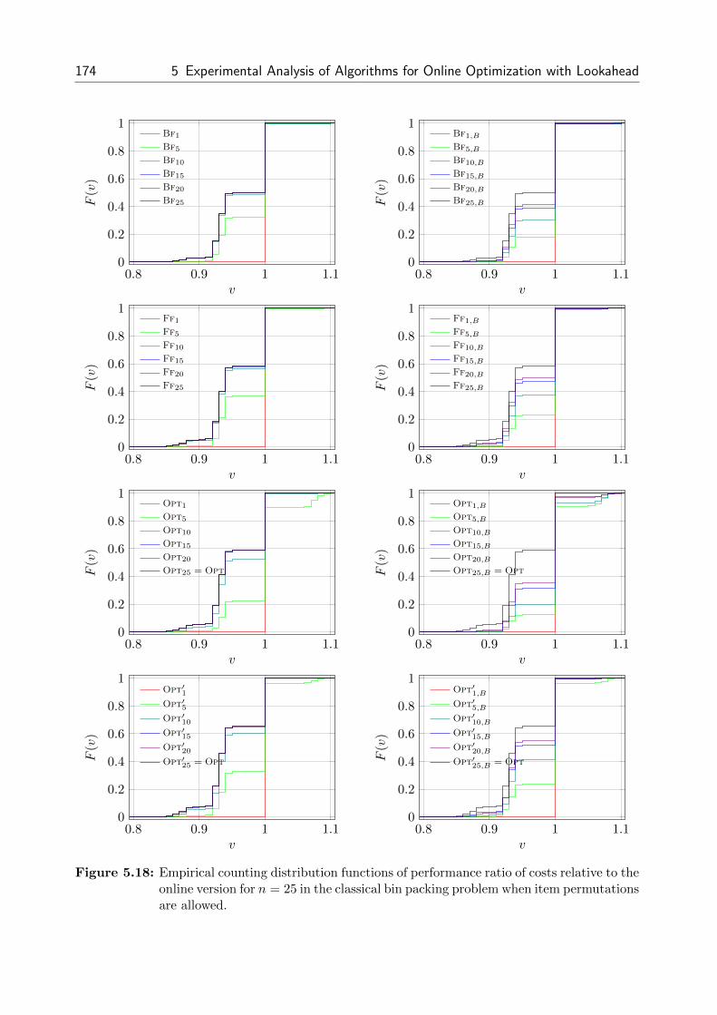
174 5 Experimental Analysis of Algorithms for Online Optimization with Lookahead
0.8 0.9 1 1.10
0.2
0.4
0.6
0.8
1
v
F(v)
Bf1
Bf5
Bf10
Bf15
Bf20
Bf25
0.8 0.9 1 1.10
0.2
0.4
0.6
0.8
1
v
F(v)
Bf1,BBf5,BBf10,BBf15,BBf20,BBf25,B
0.8 0.9 1 1.10
0.2
0.4
0.6
0.8
1
v
F(v)
Ff1
Ff5
Ff10
Ff15
Ff20
Ff25
0.8 0.9 1 1.10
0.2
0.4
0.6
0.8
1
v
F(v)
Ff1,BFf5,BFf10,BFf15,BFf20,BFf25,B
0.8 0.9 1 1.10
0.2
0.4
0.6
0.8
1
v
F(v)
Opt1
Opt5
Opt10
Opt15
Opt20
Opt25 = Opt
0.8 0.9 1 1.10
0.2
0.4
0.6
0.8
1
v
F(v)
Opt1,B
Opt5,B
Opt10,B
Opt15,B
Opt20,B
Opt25,B = Opt
0.8 0.9 1 1.10
0.2
0.4
0.6
0.8
1
v
F(v)
Opt′1
Opt′5
Opt′10
Opt′15
Opt′20
Opt′25 = Opt
0.8 0.9 1 1.10
0.2
0.4
0.6
0.8
1
v
F(v)
Opt′1,B
Opt′5,B
Opt′10,B
Opt′15,B
Opt′20,B
Opt′25,B = Opt
Figure 5.18: Empirical counting distribution functions of performance ratio of costs relative to theonline version for n = 25 in the classical bin packing problem when item permutationsare allowed.

5.3 Online Bin Packing with Lookahead 175
are smaller than 1.1 for all algorithms and lookahead levels which additionally shows that
lookahead benefits are of a rather small magnitude. The satisfactory behavior of the online
algorithms can be explained by two reasons: First, since any bin is left open forever, a solid
utilization of each bin is probable in the long term also in the online setting and the impli-
cations of bad decisions are either unnoticeable or rather small. Second, it is known that
the competitive ratio of Bf and Ff is 1710
and that of Bfn and Ffn is 119
([14], [147]). Thus,
algorithms endowed with lookahead cannot deviate more from optimality than suggested
by these ratios, especially not under representative item sequences that look significantly
different from pathologic worst-case sequences for which the above ratios were derived. Note
that some few of the m = 1000 instances could not be solved to optimality in the prescribed
time limit of 120 seconds. However, their proportion is so tiny such that performance ratios
smaller than 1 are nearly unnoticeable in Figure 5.17 (cf. also Tables A.15 and A.16 of
Appendix A.2.3).
Figure 5.18 yields plots of the empirical counting distributions functions for the performance
ratio that result from comparing the algorithms to their respective online versions without
lookahead. We derive two distinctive features of online bin packing with lookahead from these
diagrams: First, it is seen from the plots of Ff5,B and all exact reoptimization approaches
that additional information may also lead to a deterioration in the objective value if item
sequences were leading algorithms to disadvantageous decisions that cannot necessarily be
corrected later. Second, the largest part of the item sequences leads to performance ratios
in the range between 0.9 and 1 irrespective of the chosen algorithm, lookahead type and
batching mode. The counting distributions of attained performance ratios for the respective
algorithms mostly differ within this group of item sequences depending on the lookahead level
l. Confidence intervals and coefficients of variations of the performance ratios are negligibly
small and collectively have lower bounds larger than 0.95 as listed in Tables A.17 and A.18
of Appendix A.2.3. Hence, there is also no great potential for improving the outcome of
online algorithms by providing additional lookahead with respect to the performance ratio
on typical item sequences.
We left out an experiment on Markov chains for the classical bin packing problem because of
state space considerations: Since a bin once opened remains open for the rest of the packing
process, the state space representation would have to account for that by including each
possible bin configuration of up to n bins. In the bounded-space bin packing problem, this
issue is mitigated due to the limited number of bins. Therefore, we include a Markov chain
analysis in the following section on numerical experiments for the bounded-space bin packing
problem.

176 5 Experimental Analysis of Algorithms for Online Optimization with Lookahead
5.3.2 Bounded-Space Bin Packing
Recall that k ∈ N gives the number of maximum allowed open bins and that whenever a
new bin would need to be opened, one of the k open bins has to be closed first. A fictive
assignment of the l lookahead items to bins based on an item list sorted by non-increasing
item sizes only guarantees feasibility under allowed item permutations. When the item
appearance order has to be respected also during packing, such a fictive assignment only
guarantees feasibility for the first k items of the list of items sorted by non-increasing sizes:
From the pigeonhole principle, it follows for l ≤ k that for each of the l items which requires
a new bin, one of the already open bins will not be occupied with any of the l − 1 other
items. For l > k, it could occur that the list assignment would put an item in a bin which
had to be closed already before. The fullest of the k open bins is closed whenever a new
bin is required. As a result, the algorithms with lookahead which rely on reordering items
according to their sizes can exploit only min{k, l} lookahead units.
Online algorithms
• FirstFitBounded (Ffb): If there is at least one open bin that can accommodate the
item to be packed, put it in the bin that was opened first among these bins; otherwise
close the fullest open bin if k bins are open, open a new bin and put the item in ([55]).
• BestFitBounded (Bfb): If there is at least one open bin that can accommodate the
item to be packed, put the item in the fullest among these bins; otherwise close the
fullest open bin if k bins are open, open a new bin and put the item in ([55]).
Online algorithms with lookahead of size l
• FirstFitBoundedl (Ffbl):
Item permutations allowed
Sort the items in the lookahead by non-increasing size and fictively pack them with
Ff. If the item to be packed is put in a new bin, close the fullest open bin if k bins
are open, open a new bin and put the item in; otherwise put the item in the bin from
the fictive assignment.
Item permutations forbidden
Sort the first min{k, l} items in the lookahead by non-increasing size and fictively pack
them with Ff. If the item to be packed is put in a new bin, close the fullest open bin
if k bins are open, open a new bin and put the item in; otherwise put the item in the
bin from the fictive assignment.
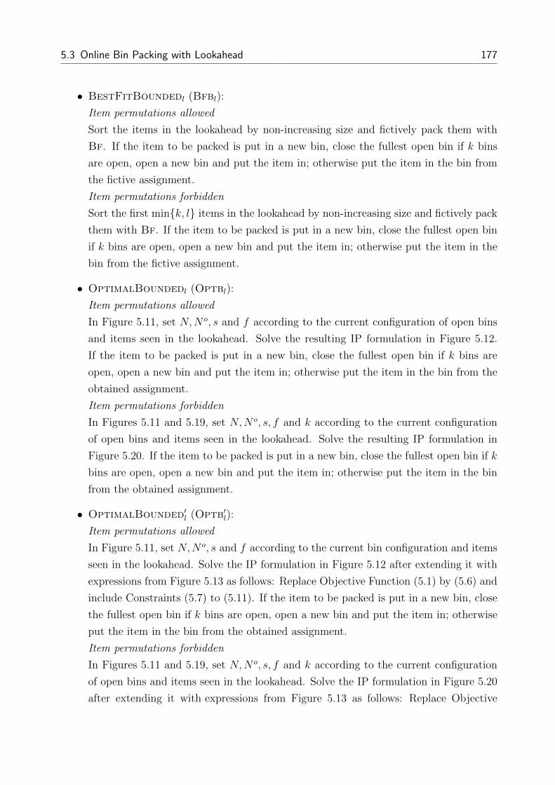
5.3 Online Bin Packing with Lookahead 177
• BestFitBoundedl (Bfbl):
Item permutations allowed
Sort the items in the lookahead by non-increasing size and fictively pack them with
Bf. If the item to be packed is put in a new bin, close the fullest open bin if k bins
are open, open a new bin and put the item in; otherwise put the item in the bin from
the fictive assignment.
Item permutations forbidden
Sort the first min{k, l} items in the lookahead by non-increasing size and fictively pack
them with Bf. If the item to be packed is put in a new bin, close the fullest open bin
if k bins are open, open a new bin and put the item in; otherwise put the item in the
bin from the fictive assignment.
• OptimalBoundedl (Optbl):
Item permutations allowed
In Figure 5.11, set N,N o, s and f according to the current configuration of open bins
and items seen in the lookahead. Solve the resulting IP formulation in Figure 5.12.
If the item to be packed is put in a new bin, close the fullest open bin if k bins are
open, open a new bin and put the item in; otherwise put the item in the bin from the
obtained assignment.
Item permutations forbidden
In Figures 5.11 and 5.19, set N,N o, s, f and k according to the current configuration
of open bins and items seen in the lookahead. Solve the resulting IP formulation in
Figure 5.20. If the item to be packed is put in a new bin, close the fullest open bin if k
bins are open, open a new bin and put the item in; otherwise put the item in the bin
from the obtained assignment.
• OptimalBounded′l (Optb′l):
Item permutations allowed
In Figure 5.11, set N,N o, s and f according to the current bin configuration and items
seen in the lookahead. Solve the IP formulation in Figure 5.12 after extending it with
expressions from Figure 5.13 as follows: Replace Objective Function (5.1) by (5.6) and
include Constraints (5.7) to (5.11). If the item to be packed is put in a new bin, close
the fullest open bin if k bins are open, open a new bin and put the item in; otherwise
put the item in the bin from the obtained assignment.
Item permutations forbidden
In Figures 5.11 and 5.19, set N,N o, s, f and k according to the current configuration
of open bins and items seen in the lookahead. Solve the IP formulation in Figure 5.20
after extending it with expressions from Figure 5.13 as follows: Replace Objective

178 5 Experimental Analysis of Algorithms for Online Optimization with Lookahead
Sets
T set of time instants with T = {1, . . . , N}
Parameters
k maximum number of open bins at a time
Variables
xijt =
{1 if item i ∈ I is put in bin j ∈ J at time t ∈ T,0 else
xoijot =
{1 if item i ∈ I is put in already used bin jo ∈ Jo at time t ∈ T,0 else
yjt =
{1 if bin j ∈ J is open at time t ∈ T,0 else
yojot =
{1 if already used bin jo ∈ Jo is still open at time t ∈ T,0 else
zopenjt =
{1 if bin j ∈ J is opened at time t ∈ T,0 else
zclosejt =
{1 if bin j ∈ J is closed at time t ∈ T,0 else
zo,closejot =
{1 if already used bin jo ∈ Jo is closed at time t ∈ T,0 else
Figure 5.19: Additional sets, parameters and variables in the IP formulation of the bounded-spacebin packing problem when item permutations are forbidden.
Function (5.12) by (5.6) and include Constraints (5.7) to (5.11). If the item to be
packed is put in a new bin, close the fullest open bin if k bins are open, open a new bin
and put the item in; otherwise put the item in the bin from the obtained assignment.
Optimal offline algorithm
• OptimalBounded (Optb):
Item permutations allowed
In Figure 5.11, set N := n, N o := 0, f := 0 and s according to all items seen. Solve
the resulting IP formulation in Figure 5.12. Pack the items according to the obtained
assignment bin after bin.
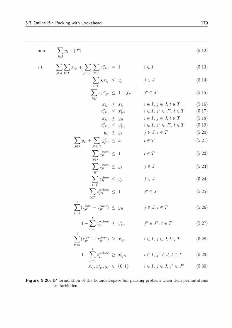
5.3 Online Bin Packing with Lookahead 179
min∑j∈J
yj + |Jo| (5.12)
s.t.∑j∈J
∑t∈T
xijt +∑jo∈Jo
∑t∈T
xoijot = 1 i ∈ I (5.13)∑i∈I
sixij ≤ yj j ∈ J (5.14)∑i∈I
sixoijo ≤ 1− fjo jo ∈ Jo (5.15)
xijt ≤ xij i ∈ I, j ∈ J, t ∈ T (5.16)
xoijot ≤ xoijo i ∈ I, jo ∈ Jo, t ∈ T (5.17)
xijt ≤ yjt i ∈ I, j ∈ J, t ∈ T (5.18)
xoijot ≤ yojot i ∈ I, jo ∈ Jo, t ∈ T (5.19)
yjt ≤ yj j ∈ J, t ∈ T (5.20)∑j∈J
yjt +∑jo∈Jo
yojot ≤ k t ∈ T (5.21)∑j∈J
zopenjt ≤ 1 t ∈ T (5.22)∑t∈T
zopenjt ≤ yj j ∈ J (5.23)∑t∈T
zclosejt ≤ yj j ∈ J (5.24)∑t∈T
zo,closejot ≤ 1 jo ∈ Jo (5.25)
t∑t′=1
(zopenjt′ − zclosejt′ ) ≤ yjt j ∈ J, t ∈ T (5.26)
1−t∑
t′=1
zo,closejt′ ≤ yojot jo ∈ Jo, t ∈ T (5.27)
t∑t′=1
(zopenjt′ − zclosejt′ ) ≥ xijt i ∈ I, j ∈ J, t ∈ T (5.28)
1−t∑
t′=1
zo,closejt′ ≥ xoijot i ∈ I, jo ∈ J, t ∈ T (5.29)
xij, xoijo , yj ∈ {0, 1} i ∈ I, j ∈ J, jo ∈ Jo (5.30)
Figure 5.20: IP formulation of the bounded-space bin packing problem when item permutationsare forbidden.

180 5 Experimental Analysis of Algorithms for Online Optimization with Lookahead
Item permutations forbidden
In Figures 5.11 and 5.19, set N := n, N o := 0, f := 0, k and s according to all items
seen. Solve the resulting IP formulation in Figure 5.20. Pack the items according to
the obtained assignment item after item.
In the IP formulation for forbidden item permutations in Figure 5.20, we have to account
for the time dimension to make sure that an item is put into a bin that is open at packing
time: In addition to xij, xoijo and yj, y
ojo , we introduce decision variables xijt, x
oijot and yjt, y
ojot
where t refers to the time instant. Constraints 5.13 to 5.21 ensure that each item is packed in
a bin, that each bin capacity is not exceeded and that at each time at most k bins are open.
To facilitate the operations of openening and closing a bin at time t, we introduce variables
zopenjt , zclosejt and zo,closejot . Constraints 5.22 to 5.25 take care that at each time and for each bin
only one respective operation is carried out. Constraints 5.26 to 5.29 guarantee that opening
and closing operations are consistent with bin statuses and packing operations.
5.3.2.1 Average Results
In Figures 5.21 and 5.22, the average algorithm behavior in the cases of allowed and forbidden
permutations shows that although we are restricted to keep at most k = 3 bins open at a
time there is no significant surplus of lookahead as opposed to classical bin packing. Our first
intuition was that being forced to close a bin upon opening a new one would lead to a higher
value of information since for late items not all but only the currently open bins are ready to
accept an item such that careful decision making should pay off. While this is probable to
be the reason for the slight boost in the lookahead effect under allowed item permutations,
computational results show that the magnitude of this effect is rather small.
In classical bin packing, maximum improvements between online and offline situations were
between 3.6 % and 4.7 % irrespective of item permutations. Now, in bounded-space bin
packing, the improvement increases to levels between 4.6 % and 5.6 % under allowed per-
mutations; under forbidden permutations, the benefit of lookahead drops to at most 3.7 %
due to the additional restriction on the number of open bins. For l = n = 25, the optimal
number of bins coincides with that of the classical problem for allowed item permutations. In
case of forbidden item permutations, this value augments to 14.41, while in the unbounded
case it was 14.12. The average number of bins also slightly increases under forbidden item
permutations for small lookahead levels l < n = 25. Hence, we judge the delimiting influence
of the bounded-space feature in bin packing as rather modest. Confidence intervals, coef-
ficients of variation and objective deterioration under additional lookahead have analogous
dimensions as in classical bin packing (cf. Tables A.25 and A.26 of Appendix A.2.3).
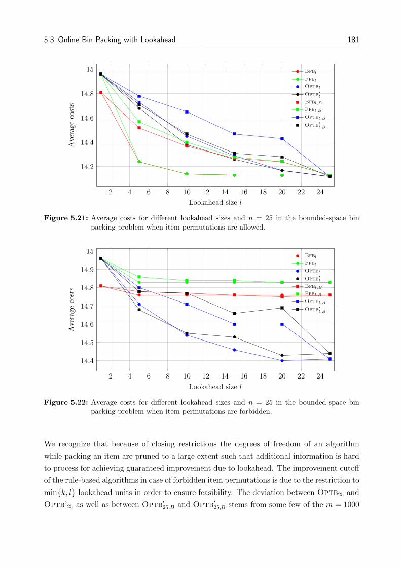
5.3 Online Bin Packing with Lookahead 181
2 4 6 8 10 12 14 16 18 20 22 24
14.2
14.4
14.6
14.8
15
Lookahead size l
Average
costs
Bfbl
Ffbl
Optbl
Optb′l
Bfbl,B
Ffbl,B
Optbl,B
Optb′l,B
Figure 5.21: Average costs for different lookahead sizes and n = 25 in the bounded-space binpacking problem when item permutations are allowed.
2 4 6 8 10 12 14 16 18 20 22 24
14.4
14.5
14.6
14.7
14.8
14.9
15
Lookahead size l
Average
costs
Bfbl
Ffbl
Optbl
Optb′l
Bfbl,B
Ffbl,B
Optbl,B
Optb′l,B
Figure 5.22: Average costs for different lookahead sizes and n = 25 in the bounded-space binpacking problem when item permutations are forbidden.
We recognize that because of closing restrictions the degrees of freedom of an algorithm
while packing an item are pruned to a large extent such that additional information is hard
to process for achieving guaranteed improvement due to lookahead. The improvement cutoff
of the rule-based algorithms in case of forbidden item permutations is due to the restriction to
min{k, l} lookahead units in order to ensure feasibility. The deviation between Optb25 and
Optb’25 as well as between Optb′25,B and Optb′25,B stems from some few of the m = 1000

182 5 Experimental Analysis of Algorithms for Online Optimization with Lookahead
instances whose IP formulation in Figure 5.20 could not be solved to optimality within the
prescribed time limit of 120 seconds.
We note that for item sequences of length n = 100, the improvement as a result of full
lookahead amounts to values between 7.9 % and 9.1 % depending on the algorithm used
when item permutations are allowed. Because we only consider the rule-based algorithms
which are restricted to min{k, l} lookahead units for n = 100, improvement due to lookahead
vanishes in the case of forbidden item permutations; for details, see Appendix A.2.3. We
will restrict our discussion only to allowed item permutations from now on.
5.3.2.2 Distributional Results
The gap between the red and green curve in the plots of algorithm families Bfbl and Ffbl
in Figure 5.23 implies that for the rule-based algorithms the first lookahead units are most
valuable in terms of a reduction of the number of bins used. From Figure 5.21, we already
knew that especially under these lookahead sizes the rule-based algorithms outperform the
exact reoptimization strategies. Hence, we come to the overall recommendation to relinquish
exact reoptimization methods in favor of stability-oriented rule-based algorithms in bounded-
space bin packing. All plots in Figure 5.23 underline the small positive effect to be expected
through additional lookahead by the ordering of the empirical counting distribution functions
depending on the lookahead size l for each algorithm family. Under batched lookahead, the
positive effect is acquired more evenly among additional lookahead units as opposed to the
regular type of lookahead where the effect is mainly attributable to the first units. Confidence
intervals of width smaller than 0.3 for all algorithms and lookahead levels in Tables A.25 and
A.26 of Appendix A.2.3 provide sufficient statistical evidence for the validity of the observed
algorithm performance on random input sequences. As seen from the percentage of item
sequences with a deterioration between successive lookahead levels, exact reoptimization
is more susceptible to misinterpretation of additional lookahead than rule-based heuristics
are.
Figures 5.24 and 5.25 show the empirical counting distributions of the performance ratio rel-
ative to Opt and the online variants of the algorithms, respectively. Both from a qualitative
and quantitative point of view, we draw the same conclusions as in classical bin packing:
• A large fraction of all item sequences already leads to an optimal number of bins even
if no lookahead or few lookahead units are given.
• The maximum deviation from optimality is below 20 % for all algorithms.
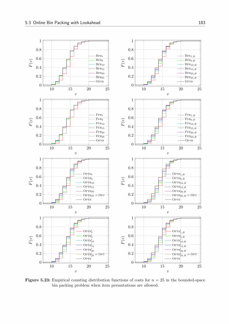
5.3 Online Bin Packing with Lookahead 183
10 15 20 250
0.2
0.4
0.6
0.8
1
v
F(v)
Bfb1
Bfb5
Bfb10
Bfb15
Bfb20
Bfb25
Optb
10 15 20 250
0.2
0.4
0.6
0.8
1
v
F(v)
Bfb1,B
Bfb5,B
Bfb10,B
Bfb15,B
Bfb20,B
Bfb25,B
Optb
10 15 20 250
0.2
0.4
0.6
0.8
1
v
F(v)
Ffb1
Ffb5
Ffb10
Ffb15
Ffb20
Ffb25
Optb
10 15 20 250
0.2
0.4
0.6
0.8
1
v
F(v)
Ffb1,B
Ffb5,B
Ffb10,B
Ffb15,B
Ffb20,B
Ffb25,B
Optb
10 15 20 250
0.2
0.4
0.6
0.8
1
v
F(v)
Optb1
Optb5
Optb10
Optb15
Optb20
Optb25 = Opt
Optb
10 15 20 250
0.2
0.4
0.6
0.8
1
v
F(v)
Optb1,B
Optb5,B
Optb10,B
Optb15,B
Optb20,B
Optb25,B = Opt
Optb
10 15 20 250
0.2
0.4
0.6
0.8
1
v
F(v)
Optb′1
Optb′5
Optb′10
Optb′15
Optb′20
Optb′25 = Opt
Optb
10 15 20 250
0.2
0.4
0.6
0.8
1
v
F(v)
Optb′1,B
Optb′5,B
Optb′10,B
Optb′15,B
Optb′20,B
Optb′25,B = Opt
Optb
Figure 5.23: Empirical counting distribution functions of costs for n = 25 in the bounded-spacebin packing problem when item permutations are allowed.

184 5 Experimental Analysis of Algorithms for Online Optimization with Lookahead
1 1.1 1.20
0.2
0.4
0.6
0.8
1
v
F(v) Bfb1
Bfb5
Bfb10
Bfb15
Bfb20
Bfb25
1 1.1 1.20
0.2
0.4
0.6
0.8
1
v
F(v) Bfb1,B
Bfb5,B
Bfb10,B
Bfb15,B
Bfb20,B
Bfb25,B
1 1.1 1.20
0.2
0.4
0.6
0.8
1
v
F(v) Ffb1
Ffb5
Ffb10
Ffb15
Ffb20
Ffb25
1 1.1 1.20
0.2
0.4
0.6
0.8
1
v
F(v) Ffb1,B
Ffb5,B
Ffb10,B
Ffb15,B
Ffb20,B
Ffb25,B
1 1.1 1.20
0.2
0.4
0.6
0.8
1
v
F(v) Optb1
Optb5
Optb10
Optb15
Optb20
Optb25 = Optb
1 1.1 1.20
0.2
0.4
0.6
0.8
1
v
F(v) Optb1,B
Optb5,B
Optb10,B
Optb15,B
Optb20,B
Optb25,B = Optb
1 1.1 1.20
0.2
0.4
0.6
0.8
1
v
F(v) Optb′1
Optb′5
Optb′10
Optb′15
Optb′20
Optb′25 = Optb
1 1.1 1.20
0.2
0.4
0.6
0.8
1
v
F(v) Optb′
1,B
Optb′5,B
Optb′10,B
Optb′15,B
Optb′20,B
Optb′25,B = Optb
Figure 5.24: Empirical counting distribution functions of performance ratio of costs relative toOpt for n = 25 in the bounded-space bin packing problem when item permutationsare allowed.

5.3 Online Bin Packing with Lookahead 185
0.8 0.9 1 1.10
0.2
0.4
0.6
0.8
1
v
F(v)
Bfb1
Bfb5
Bfb10
Bfb15
Bfb20
Bfb25
0.8 0.9 1 1.10
0.2
0.4
0.6
0.8
1
v
F(v)
Bfb1,B
Bfb5,B
Bfb10,B
Bfb15,B
Bfb20,B
Bfb25,B
0.8 0.9 1 1.10
0.2
0.4
0.6
0.8
1
v
F(v)
Ffb1
Ffb5
Ffb10
Ffb15
Ffb20
Ffb25
0.8 0.9 1 1.10
0.2
0.4
0.6
0.8
1
v
F(v)
Ffb1,B
Ffb5,B
Ffb10,B
Ffb15,B
Ffb20,B
Ffb25,B
0.8 0.9 1 1.10
0.2
0.4
0.6
0.8
1
v
F(v)
Optb1
Optb5
Optb10
Optb15
Optb20
Optb25 = Optb
0.8 0.9 1 1.10
0.2
0.4
0.6
0.8
1
v
F(v)
Optb1,B
Optb5,B
Optb10,B
Optb15,B
Optb20,B
Optb25,B = Optb
0.8 0.9 1 1.10
0.2
0.4
0.6
0.8
1
v
F(v)
Optb′1
Optb′5
Optb′10
Optb′15
Optb′20
Optb′25 = Optb
0.8 0.9 1 1.10
0.2
0.4
0.6
0.8
1
v
F(v)
Optb′1,B
Optb′5,B
Optb′10,B
Optb′15,B
Optb′20,B
Optb′25,B = Optb
Figure 5.25: Empirical counting distribution functions of performance ratio of costs relative tothe online version for n = 25 in the bounded-space bin packing problem when itempermutations are allowed.

186 5 Experimental Analysis of Algorithms for Online Optimization with Lookahead
• Algorithms may interpret lookahead disadvantageously; however, this happens only
very rarely.
• Most item sequences experience a lookahead effect of at most 10 %.
For a detailed statistical summary, see Tables A.27 to A.30 of Appendix A.2.3.
5.3.2.3 Markov Chain Results
Consider the online bounded-space bin packing problem with lookahead l and a maximum
number k of open bins at a time under allowed item permutations. The elements of the state
space S subsume the fill levels f = (f1, . . . , fk) of the k open bins, the sizes s = (s1, . . . , sl)
of the lookahead items which are ordered non-increasingly and the number of bins v used so
far, i.e.,
S ={
(f, s, v) | f ∈ [0, 1]k, s ∈ (0, 1]l, v ∈ N0
}.
Upon arrival of a new item, each algorithm Alg assigns the largest item in the current
lookahead to one of the k open bins or to a new bin. In the latter case, an open bin is closed
first and the objective value increases by one unit. Hence, Alg is a function
Alg : S × (0, 1]→ {1, 2, . . . , k + 1}
which gives the bin into which the largest item will be put where Alg(s, snew) = k+1 means
that a new bin needs to be opened. The successor state of s = (f, s, v) upon arrival of an item
with size snew is given by s′ = (f ′, s′, v′) where f ′ arises from f by adding s1 to fAlg(s,snew) if
Alg(s, snew) 6= k+1 or replacing the largest component of f with s1 if Alg(s, snew) = k+1,
s′ arises from s by removing s1, appending snew and ordering non-increasingly, and
v′ =
v if Alg(s, snew) ∈ {1, . . . , k},v + 1 otherwise.
In order to obtain a finite state space representation, we have to discretize item sizes: To
this end, denote the number of possible item sizes by ns and the resulting number of item
size combinations with total size not larger than 1 by nc, then the state space size amounts
to |S| = nkc ·(ns+l−1
l
)· (n+ 1)14.
14The number of combinations with repetition where n is the number of elements to choose from and relements have to be chosen is
(n+r−1
r
)([137]).

5.3 Online Bin Packing with Lookahead 187
For Alg ∈ {Bfbl,Ffbl,Optbl} and selected lookahead level l, we determine the successor
for each state and each new item to obtain the one-step frequency matrix and the n-step
frequency matrix of the Markov chain.
In our numerical experiment, we use the parametrization n = 25, k = 3, l ∈ {1, 2, . . . , 5}and restrict item sizes to {0.4, 0.5, 0.6}. Hence, we have ns = 3 and nc = |{0.4, 0.5, 0.6, 0.4 +
0.4, 0.4 + 0.5, 0.4 + 0.6}| = 6. For this small exemplary setting, the state space size amounts
to 63 ·(
3+5−15
)· 26 = 117 936 elements for l = 5.
The resulting exact distribution functions in Figure 5.26 are affirmative to the main result
found for bin packing, namely that lookahead has a benefit, albeit a rather small one.
14 16 18 20 22 240
0.2
0.4
0.6
0.8
1
v
F(v)
Bfb1
Bfb2
Bfb3
Bfb4
Bfb5
14 16 18 20 22 240
0.2
0.4
0.6
0.8
1
v
F(v)
Ffb1
Ffb2
Ffb3
Ffb4
Ffb5
14 16 18 20 22 240
0.2
0.4
0.6
0.8
1
v
F(v)
Optb1
Optb2
Optb3
Optb4
Optb5
Figure 5.26: Exact distribution functions of costs for n = 25 in the bounded-space bin packingproblem.
Moreover, we see that already in the case of no or few lookahead units the number of item
sequences which lead to the smallest objective value of 13 is consistently larger than 25 %
of the number of all item sequences. We conclude that online bin packing algorithms have
quite a good chance of obtaining an optimal number of bins and that maximum deviations
from optimality as suggested by (asymptotic) competitive ratios in both types of bin packing
problems of 70 % ([55]) are quite untypical.

188 5 Experimental Analysis of Algorithms for Online Optimization with Lookahead
We conclude this section by pointing out that the results of the computational experiments on
the bin packing problem are in line with the minor positive effect of lookahead as determined
by exact analysis in Chapter 4.2 for a basic setting with two item sizes and l = 2. Hence,
significant savings in the number of bins used can also not be expected for arbitrary item
sizes. Nonetheless, the impact of lookahead is slightly stronger as a result of the increased
number of item combinations which lead to a saving of a bin.
5.4 Online Traveling Salesman Problem with Lookahead
A specification of the online traveling salesman problem (TSP) with lookahead and algo-
rithms FirstComeFirstServed and NearestNeighborl is given in Chapter 4.3. Fur-
ther algorithms for the online version with lookahead will be introduced in the sequel. For
fixed n ∈ N and metric space (M, d), the set of all input sequences of length n is given by
Σn ={
(σ1, σ2, . . . , σn) |σi := xi ∈M, i = 1, . . . , n}
and comprises all request sequences of length n where σi is identified with point xi ∈ M to
be visited. Because in an optimal solution to an instance of the offline problem, all points
will be approached exactly once, all σi are assumed pairwise different in the offline TSP. In
the dynamic setting, of course, we have to allow multiple requests on the same location. In
the online version, only σi with i = 1, . . . , n is known when σi has to be visited. In the online
version with lookahead of size l, when for the ith time it has to be decided which location
to be visited, the l unvisited locations from σ1, σ2, . . . , σi+l−1 with i = 1, . . . , n are known if
i+ l− 1 ≤ n, otherwise the n− i+ 1 unvisited locations from σ1, σ2, . . . , σn are known15. In
the offline version, all locations are known at the beginning.
Computational experiments feature two problem settings each of which underlies m = 1000
independently drawn request sequences. In the first setting, each sequence consists of n = 25
requests, while the second setting has n = 100 requests per sequence. Requests are located
in the planar unit squareM = [0, 1]× [0, 1] ⊂ R2 and distance is measured by the Euclidean
metric. A set of requests establishes a complete graph consisting of vertices labeled with the
requests as well as additional vertices for the current server location and the origin; edge
weights correspond to distances between respective locations. For n = 25, lookahead sizes
are l ∈ {1, 5, 10, . . . , 25}; for n = 100, we have l ∈ {1, 5, 10, 20, 40, . . . , 100}. We discuss
results for n = 25 and refer the reader to Appendix A.2.4 for n = 100.
15 In Chapter 6, we take into account time lookahead for the pickup and delivery problem with time windows– a problem closely related to the TSP.

5.4 Online Traveling Salesman Problem with Lookahead 189
A decision by an algorithm is required when the server starts initially or a request is reached;
it consists of selecting the request to be visited next from the set of known requests. Note
that any online algorithm without lookahead is trivial since it only sees the current request
and has to visit it, i.e., it has no degrees of freedom at all.
Online algorithm
• FirstComeFirstServed (Fcfs): Choose the only unvisited known request next.
Online algorithms with lookahead of size l
• NearestNeighborl (Nnl): From the requests in the lookahead, choose a request
closest to the server’s current location next (see also [120]).
• Insertionl (Insl): Construct a Hamiltonian path H visiting each of the requests in the
lookahead starting in the server’s current location and ending in the origin as follows:
1. At the beginning, H consists of the invariant starting and ending point only.
2. Insert a request whose distance to the starting point is largest possible into H.
3. Successively insert requests by choosing in each iteration a request whose smallest
distance to a request in H is largest and insert it at a best possible position in
terms of a smallest tour length increase.
Choose the first request from H following the starting point next (see also [120]).
• 2Optl: Construct a Hamiltonian path H visiting each of the requests in the lookahead
starting in the server’s current location and ending in the origin as follows:
1. Obtain H initially by applying Nnl or Insl.
2. Choose two requests from H and reverse the order of requests between them to
obtain H ′.
3. If H ′ is shorter than H, set H := H ′.
4. Return to step 2 until no further improvement is possible.
Choose the first request from H following the starting point next (see also [120]).
• 3Optl: Construct a Hamiltonian path H visiting each of the requests in the lookahead
starting in the server’s current location and ending in the origin as follows:
1. Obtain H initially by applying Nnl or Insl.

190 5 Experimental Analysis of Algorithms for Online Optimization with Lookahead
2. Choose three edges from H such that neither of them is incident to the starting
or ending point and reorganize H as follows:
– Form three new edges using the requests incident to the three edges.
– Choose an order for the three new edges.
– Adjust the order of the requests between the edges such that a feasible Hamil-
tonian path H ′ starting in the server’s current location and ending in the
origin is obtained if possible at all.
– If H ′ is feasible and shorter than H, set H := H ′.
3. Return to step 2 until no further improvement is possible.
Choose the first request from H following the starting point next (see also [120]).
• SimulatedAnnealingl (Sal): Construct a Hamiltonian path H visiting each of the
requests in the lookahead starting in the server’s current location and ending in the
origin as follows:
1. Obtain H initially by applying Nnl or Insl.
2. Select initial temperature T0 ∈ R, minimum temperature Tmin ∈ R with Tmin <
T0, maximum number of iterations Lmax ∈ N with unchanged temperature and
set T := T0, L := 0.
3. If L = Lmax, set T := 0.9 · T and L := 1; else set L := L+ 1.
4. Choose two requests from H and reverse the order of requests between them to
obtain H ′.
5. If H ′ is shorter than H, set H := H ′; else set H := H ′ with probability exp(−∆T
)
where ∆ is the difference between the length of H ′ and the length of H.
6. Return to step 3 until T < Tmin.
Choose the first request following the starting point from the shortest Hamiltonian
path obtained throughout the procedure next (see also [120]).
• TabuSearchl (Tsl): Construct a Hamiltonian path H visiting each of the lookahead
points starting in the server’s current location and ending in the origin as follows:
1. Obtain H initially by applying Nnl or Insl.
2. Select tabu time T ∈ N, maximum number Dmax of diversifications, number of
swaps s per diversification and set D := 0.

5.4 Online Traveling Salesman Problem with Lookahead 191
3. Choose two requests from H and swap them to obtain H ′.
4. If H ′ is shorter than H and the swapped request pair is not included in the tabu
list, set H := H ′ and add the swapped request pair to the tabu list with remaining
tabu time T ; else if H ′ is shorter than the best Hamiltonian path obtained so far
and the swapped request pair is tabu, set H := H ′ (aspiration).
5. For all tabu list entries except the new one, decrease the remaining tabu time by
one iteration; return to step 3 until all pairs of points have been examined.
6. Perform a swap of two random points in H ′ for s times (diversification), set
H := H ′, D := D + 1.
7. Return to step 3 until D ≥ Dmax.
Choose the first request following the starting point from the shortest Hamiltonian
path obtained throughout the procedure next (see also [79]).
Sets
J set of requests with J = {1, . . . , N}
Parameters
N number of requestscij distance between requests i, j ∈ Jcstartj distance of request j ∈ J to current server positioncendj distance of request j ∈ J to originM sufficiently large constant (big M)
Variables
xij =
{1 if request i ∈ J immediately precedes request j ∈ J,0 else
xstartj =
{1 if request j ∈ J is visited first,
0 else
xendj =
{1 if request j ∈ J is visited last,
0 else
Tj ≥ 0 start time of request j ∈ J
Figure 5.27: Sets, parameters and variables in the MIP formulation of the Hamiltonian pathproblem with fixed starting and ending point.

192 5 Experimental Analysis of Algorithms for Online Optimization with Lookahead
• Optimall (Optl): In Figure 5.27, set N , c, cstart and cend according to the distances
between current lookahead requests to each other and to the current server location.
Solve the MIP formulation in Figure 5.28. Choose the first request following the
starting point in the obtained solution next.
min∑i∈J
∑j∈J
cijxij +∑j∈J
cstartj xstartj +∑j∈J
cendj xendj (5.31)
s.t.∑j∈J,j 6=i
xij + xendi = 1 i ∈ J (5.32)
∑i∈J,i 6=j
xij + xstartj = 1 j ∈ J (5.33)
∑j∈J
xstartj = 1 (5.34)∑j∈J
xendj = 1 (5.35)
Ti + 1 ≤ Tj + M · (1− xij) i, j ∈ J (5.36)
xij, xstartj , xendj ∈ {0, 1} i, j ∈ J (5.37)
Tj ≥ 0 j ∈ J (5.38)
Figure 5.28: MIP formulation of the Hamiltonian path problem with fixed starting and endingpoint.
Optimal offline algorithm
• Optimal (Opt): In Figure 5.27, set N , c, cstart and cend according to the distances
between all requests to each other and to the initial server location. Solve the MIP
formulation in Figure 5.28. Visit the requests according to the obtained solution.
Note that all algorithms with lookahead collapse into Fcfs for l = 1. There are plenty of
IP and MIP formulations for the TSP (see, e.g., [120]); in the MIP formulation in Figure
5.28, we decide to get rid of the subtour elimination constraints by establishing precedence
relations in Constraint 5.36 between requests based on decision variables for time instants
at which requests are served ([132]).
Similar to the previous problems, we check whether regular request lookahead of size l leads
to significantly better algorithm behavior as opposed to batched provision of lookahead units.
If algorithms operate under batched lookahead, we indicate them with an added suffix B in
the algorithm name.

5.4 Online Traveling Salesman Problem with Lookahead 193
5.4.1 Average Results
As Figure 5.29 shows for four requests with origin in request 1, providing an algorithm with
only one additional unit of lookahead already leads to an order readjustment which avoids
frequent detours. We recognize that – in contrast to bin packing – the objective value is
immediately and heavily affected by the selected order of input element processing. We
conclude that there should be a substantial effect of lookahead which results from visiting
requests in an order different from their release order, i.e., from a rule set substitution.
1
2
4
3
x1
x2
a)
1
2
4
3
x1
x2
b)
Figure 5.29: Comparison of routes obtained in the TSP. a) Without lookahead (l = 1). b) Withlookahead of only one additional request (l = 2).
Figure 5.30 confirms the huge benefit attainable by providing the server with lookahead in
form of a preview of future requests and allowing it to visit known requests in arbitrary
order. Comparing the online with the offline case, reductions in the overall tour length
of 60.5 % to 67.8 % are achieved depending on the algorithm used. Lookahead positively
affects all algorithms in the same order of magnitude. Confidence interval widths smaller
than 0.2 for all algorithms and lookahead levels as well as comparatively small coefficients
of variation in Table A.37 of Appendix A.2.4 support the statistical validity of the results
on lookahead improvements found over the randomly chosen input instances. The marginal
benefit of an additional lookahead unit is strictly decreasing for all algorithms. In this sense,
already provisioning an algorithm with small lookahead leads to considerable improvement.
For instance, already for l = 5 overall tour lengths are reduced to between 57.5 % and 74.1 %
of the online tour length depending on the algorithm used. Finally, we observe improved
behavior of algorithms with regular request lookahead over those which have to adhere to
batched lookahead as a result of the potential for tour length reduction that any additional
lookahead unit has.

194 5 Experimental Analysis of Algorithms for Online Optimization with Lookahead
2 4 6 8 10 12 14 16 18 20 22 24
4
6
8
10
12
14
Lookahead size l
Average
costs
Nnl Nnl,B
Insl Insl,B2Optl 2Optl,B
3Optl 3Optl,B
Sal Sal,B
Tsl Tsl,BOptl Optl,B
Figure 5.30: Average costs for different lookahead sizes and n = 25 in the TSP.
In a more detailed view, it is seen that for information regimes corresponding to small
lookahead the simple algorithm Nnl fares best; only for large lookahead sizes the more
sophisticated algorithms exhibit superior performance. We conclude that a surplus of using
refined algorithms rather than simple algorithms can only be realized when the overseen time
horizon is as large as to guarantee that no severe deviations between previously calculated
routes and recalculated routes upon additional request arrivals will occur. Clearly, for small
lookahead this requirement is likely to be violated due to newly arriving requests rendering
once calculated “locally optimal” plans obsolete.
We illustrate this result by contrasting Nnl and Optl: Nnl proves superior for small and
medium lookahead sizes l because of its consistent behavior which results from always choos-
ing the closest known request next, whereas Optl may choose a request from a distant region
next if suggested by an optimal solution of the snapshot problem. Hence, the danger of a
zigzag route is increased for Optl. Consider Figure 5.31 with n = 10 requests where requests
are labeled as (1, 2, . . . , 10) and also released in that order, current server position and origin
in request 1, and lookahead l = 2. After arrival in request 2, the lookahead comprises re-
quests 3 and 4 for both algorithms. Opt2 (in Figure 5.31 b)) next chooses request 3 because
route (2, 3, 4, 1) is shorter than (2, 4, 3, 1). Later, when request 6 is reached, the lookahead
consists of requests 4 and 7 such that a distant region has to be revisited although the server
had initially been there. Contrarily, Nn2 (in Figure 5.31 a)) avoids revisiting this region by
choosing request 4 as successor of request 2. Hence, the probability for zigzagging is reduced
under Nnl compared to Optl, albeit returning to previously seen regions cannot be excluded
in general because of future requests.

5.4 Online Traveling Salesman Problem with Lookahead 195
1
23
4
5
6
7
8 9 10
x1
x2
a)
1
23
4
5
6
7
8 9 10
x1
x2
b)
Figure 5.31: Threat of bad decisions in the TSP. a) Low risk for stability-oriented algorithm Nn2.b) High risk for exact reoptimization algorithm Opt2.
For n = 100 items per sequence, the same qualitative effects are observed: The simple al-
gorithm Nnl excels the sophisticated algorithms for small lookahead; for medium to large
lookahead it is recommended to use the elaborated algorithms. The marginal benefit of
additional lookahead is strictly decreasing. Comparing the online and offline situation, im-
provements are even higher – between 81.3 % and 84.6 % depending on the algorithm – than
for n = 25; for details, see Appendix A.2.4.
5.4.2 Distributional Results
Empirical counting distribution functions of objective values and performance ratios as shown
in Figures 5.32 to 5.34 appear clearly segregated from each other for successive lookahead
levels of small to medium size with decreasing gap for increasing lookahead level. Moreover,
confidence intervals both of objective values and performance ratios as listed in Tables A.37
to A.39 of Appendix A.2.4 are predominantly disjunct and have small width. Conjointly,
these findings are affirmative both to the huge magnitude of lookahead and the decreasing
marginal value of information.
From Figure 5.32, it is seen that the absolute value of tour lengths reduces drastically under
lookahead. The reduction is as substantial as to cause the supports of the density functions
related to the given plots not to come to an overlap for l = 1 and l = 10. Moreover, we
recommend to exclude algorithm family Insl from further consideration by cause of poor
behavior over all lookahead levels l as compared to Nnl on small to medium lookahead
levels and compared to the sophisticated algorithms on medium to large lookahead levels.

196 5 Experimental Analysis of Algorithms for Online Optimization with Lookahead
5 10 15 200
0.20.40.60.81
v
F(v)
Nn1 Nn5
Nn10 Nn15
Nn20 Nn25
Opt
5 10 15 200
0.20.40.60.81
v
F(v)
Nn1,B Nn5,B
Nn10,B Nn15,B
Nn20,B Nn25,B
Opt
5 10 15 200
0.20.40.60.81
v
F(v)
Ins1 Ins5
Ins10 Ins15
Ins20 Ins25
Opt
5 10 15 200
0.20.40.60.81
v
F(v)
Ins1,B Ins5,BIns10,B Ins15,BIns20,B Ins25,BOpt
5 10 15 200
0.20.40.60.81
v
F(v)
2Opt1 2Opt5
2Opt10 2Opt15
2Opt20 2Opt25
Opt
5 10 15 200
0.20.40.60.81
v
F(v)
2Opt1,B 2Opt5,B
2Opt10,B 2Opt15,B
2Opt20,B 2Opt25,B
Opt
5 10 15 200
0.20.40.60.81
v
F(v)
3Opt1 3Opt5
3Opt10 3Opt15
3Opt20 3Opt25
Opt
5 10 15 200
0.20.40.60.81
v
F(v)
3Opt1,B 3Opt5,B
3Opt10,B 3Opt15,B
3Opt20,B 3Opt25,B
Opt
5 10 15 200
0.20.40.60.81
v
F(v)
Sa1 Sa5
Sa10 Sa15
Sa20 Sa25
Opt
5 10 15 200
0.20.40.60.81
v
F(v)
Sa1,B Sa5,B
Sa10,B Sa15,B
Sa20,B Sa25,B
Opt
5 10 15 200
0.20.40.60.81
v
F(v)
Ts1 Ts5
Ts10 Ts15
Ts20 Ts25
Opt
5 10 15 200
0.20.40.60.81
v
F(v)
Ts1,B Ts5,BTs10,B Ts15,BTs20,B Ts25,BOpt
5 10 15 200
0.20.40.60.81
v
F(v)
Opt1 Opt5
Opt10 Opt15
Opt20 Opt25 = Opt
Opt
5 10 15 200
0.20.40.60.81
v
F(v)
Opt1,B Opt5,B
Opt10,B Opt15,B
Opt20,B Opt25,B = Opt
Opt
Figure 5.32: Empirical counting distribution functions of costs for n = 25 in the TSP.

5.4 Online Traveling Salesman Problem with Lookahead 197
1 2 3 4 50
0.20.40.60.81
v
F(v)
Nn1 Nn5
Nn10 Nn15
Nn20 Nn25
1 2 3 4 50
0.20.40.60.81
v
F(v)
Nn1,B Nn5,B
Nn10,B Nn15,B
Nn20,B Nn25,B
1 2 3 4 50
0.20.40.60.81
v
F(v)
Ins1 Ins5
Ins10 Ins15
Ins20 Ins25
1 2 3 4 50
0.20.40.60.81
v
F(v)
Ins1,B Ins5,BIns10,B Ins15,BIns20,B Ins25,B
1 2 3 4 50
0.20.40.60.81
v
F(v)
2Opt1 2Opt5
2Opt10 2Opt15
2Opt20 2Opt25
1 2 3 4 50
0.20.40.60.81
v
F(v)
2Opt1,B 2Opt5,B
2Opt10,B 2Opt15,B
2Opt20,B 2Opt25,B
1 2 3 4 50
0.20.40.60.81
v
F(v)
3Opt1 3Opt5
3Opt10 3Opt15
3Opt20 3Opt25
1 2 3 4 50
0.20.40.60.81
v
F(v)
3Opt1,B 3Opt5,B
3Opt10,B 3Opt15,B
3Opt20,B 3Opt25,B
1 2 3 4 50
0.20.40.60.81
v
F(v)
Sa1 Sa5
Sa10 Sa15
Sa20 Sa25
1 2 3 4 50
0.20.40.60.81
v
F(v)
Sa1,B Sa5,B
Sa10,B Sa15,B
Sa20,B Sa25,B
1 2 3 4 50
0.20.40.60.81
v
F(v)
Ts1 Ts5
Ts10 Ts15
Ts20 Ts25
1 2 3 4 50
0.20.40.60.81
v
F(v)
Ts1,B Ts5,BTs10,B Ts15,BTs20,B Ts25,B
1 2 3 4 50
0.20.40.60.81
v
F(v)
Opt1 Opt5
Opt10 Opt15
Opt20 Opt25 = Opt
1 2 3 4 50
0.20.40.60.81
v
F(v)
Opt1,B Opt5,B
Opt10,B Opt15,B
Opt20,B Opt25,B = Opt
Figure 5.33: Empirical counting distribution functions of performance ratio of costs relative toOpt for n = 25 in the TSP.

198 5 Experimental Analysis of Algorithms for Online Optimization with Lookahead
0.4 0.6 0.8 10
0.20.40.60.81
v
F(v)
Nn1 Nn5
Nn10 Nn15
Nn20 Nn25
0.4 0.6 0.8 10
0.20.40.60.81
v
F(v)
Nn1,B Nn5,B
Nn10,B Nn15,B
Nn20,B Nn25,B
0.4 0.6 0.8 10
0.20.40.60.81
v
F(v)
Ins1 Ins5
Ins10 Ins15
Ins20 Ins25
0.4 0.6 0.8 10
0.20.40.60.81
v
F(v)
Ins1,B Ins5,BIns10,B Ins15,BIns20,B Ins25,B
0.4 0.6 0.8 10
0.20.40.60.81
v
F(v)
2Opt1 2Opt5
2Opt10 2Opt15
2Opt20 2Opt25
0.4 0.6 0.8 10
0.20.40.60.81
v
F(v)
2Opt1,B 2Opt5,B
2Opt10,B 2Opt15,B
2Opt20,B 2Opt25,B
0.4 0.6 0.8 10
0.20.40.60.81
v
F(v)
3Opt1 3Opt5
3Opt10 3Opt15
3Opt20 3Opt25
0.4 0.6 0.8 10
0.20.40.60.81
v
F(v)
3Opt1,B 3Opt5,B
3Opt10,B 3Opt15,B
3Opt20,B 3Opt25,B
0.4 0.6 0.8 10
0.20.40.60.81
v
F(v)
Sa1 Sa5
Sa10 Sa15
Sa20 Sa25
0.4 0.6 0.8 10
0.20.40.60.81
v
F(v)
Sa1,B Sa5,B
Sa10,B Sa15,B
Sa20,B Sa25,B
0.4 0.6 0.8 10
0.20.40.60.81
v
F(v)
Ts1 Ts5
Ts10 Ts15
Ts20 Ts25
0.4 0.6 0.8 10
0.20.40.60.81
v
F(v)
Ts1,B Ts5,BTs10,B Ts15,BTs20,B Ts25,B
0.4 0.6 0.8 10
0.20.40.60.81
v
F(v)
Opt1 Opt5
Opt10 Opt15
Opt20 Opt25 = Opt
0.4 0.6 0.8 10
0.20.40.60.81
v
F(v)
Opt1,B Opt5,B
Opt10,B Opt15,B
Opt20,B Opt25,B = Opt
Figure 5.34: Empirical counting distribution functions of performance ratio of costs relative tothe online version for n = 25 in the TSP.

5.4 Online Traveling Salesman Problem with Lookahead 199
Furthermore, exact reoptimization approach Optl is outperformed by 2Optl, 3Optl, Sal
and Tsl for all lookahead levels l except for the state of full informational knowledge (l =
25). The latter algorithms are considered to have equal performance. However, from the
percentage of request sequences with a deterioration between two successive lookahead levels
in the last column of Table A.37 of Appendix A.2.4, we see that there are sporadic instances
where additional lookahead was misleading for an algorithm.
While performance ratios relative to Opt were below 1.25 for all instances of the bin pack-
ing problems, the picture remarkably changes in the TSP as seen in Figure 5.33. Here,
performance ratios larger than 4.5 are encountered. However, already for l = 10 none of
the algorithms endowed with regular request lookahead except for Insl incurred a perfor-
mance ratio larger than 2 on any instance which points towards the huge impact of the
first lookahead requests and the decreasing marginal benefit of additional lookahead units.
The proportion of instances which lead to a performance ratio of 1 is rather modest for all
lookahead levels smaller than l = n = 25. Thus, each additional lookahead request tends
to unfold its potential for tour length reduction over the course of requests revealed in a
sequence. As can be seen from the minimum performance ratios and the percentage with
performance ratio smaller than 1 in Table A.38 of Appendix A.2.4, not all of the m = 1000
instances could be solved to optimality within 120 seconds. Hence, in some few cases Opt
could be outperformed by some of the other algorithms.
The empirical counting distribution functions relative to the respective online versions of
the algorithms in Figure 5.34 lead to the same conclusions that could be drawn from the
previous figures. Note that no instance exists for which the provision of lookahead leads to
a deterioration in the resulting tour length of any algorithm when compared to the online
case without lookahead. Confidence intervals shrink to a single point when the bounds are
rounded to two decimal places (cf. also Table A.39 of Appendix A.2.4).
Observe that for large lookahead all counting distribution functions are relatively steep in
a characteristic interval which illustrates the homogenous positive effect of additional infor-
mation on all kinds of request sequences.
5.4.3 Markov Chain Results
Assume all requests inM are given a name which allows to establish a lexicographical order
among them. The elements of the state space S subsume the current server location xs, the
requests x = (x1, . . . , xl) in the lookahead in lexicographical order of their name and the

200 5 Experimental Analysis of Algorithms for Online Optimization with Lookahead
distance v traveled by the server so far, i.e.,
S ={
(xs, x, v) |xs ∈M, x ∈Ml, v ∈ R≥0}.
Upon arrival of a new request to be visited, each algorithm Alg decides which one of the
requests in the lookahead is visited next. Hence, Alg is a function
Alg : S ×M→ {1, . . . , l}
which gives the position of the request to be visited next in the lookahead. The successor state
of s = (xs, x, v) upon arrival of request xnew is given by s′ = (x′s, x′, v′) where x′s = xAlg(s,xnew),
x′ arises from x by removing element xAlg(s,xnew), appending element xnew and ordering
lexicographically, and v′ = v + d(xs, xAlg(s,xnew)) with distance function d on M.
In order to obtain a finite state space representation, we have to ensure that M is a finite
metric space and that the possible values for v form a finite set: To this end, denote the
diameter of M by dmax, then for integer distances the state space size amounts to
|S| = |M| ·(|M|+ l − 1
l
)·((n+ 1) · dmax
).
For Alg ∈ {Nnl, Insl, 2Optl,Optl} and selected lookahead level l, we determine the suc-
cessor for each state and each new request to obtain the one-step frequency matrix and the
n-step frequency matrix of the Markov chain.
In our numerical experiment, we use the parametrization n = 25, |M| = 4, dmax = 3
and l ∈ {1, 2, . . . , 5}. For this small exemplary setting, the state space size amounts to
4 ·(
4+5−15
)· (26 · 3) = 17 472 elements for l = 5.
Figure 5.35 displays the exact distribution functions of the objective values obtained for the
four algorithm families. The overall picture shows that each additional lookahead unit corre-
sponds to a decrease in the objective value for the vast majority of all request sequences.
Algorithms Nnl, Insl and 2Optl exhibit exclusive improvement due to lookahead which is
seen by the perfect ordering of the plots corresponding to different lookahead levels. For
exact reoptimization algorithms in Optl, we realize that the provided lookahead levels l ∈{1, 2, . . . , 5} are too small to be exploited more advantageously than by the other algorithms.
Moreover, we find that the distribution functions for Opt4 and Opt5 intersect such that no
exclusive benefit of lookahead can be attested. Opt2 if found to score poorly compared to
Opt1 considering that it is provided an additional lookahead request.

5.5 Online Scheduling with Lookahead 201
0 20 40 60 800
0.2
0.4
0.6
0.8
1
v
F(v)
Nn1
Nn2
Nn3
Nn4
Nn5
0 20 40 60 800
0.2
0.4
0.6
0.8
1
v
F(v)
Ins1
Ins2
Ins3
Ins4
Ins5
0 20 40 60 800
0.2
0.4
0.6
0.8
1
v
F(v)
2Opt1
2Opt2
2Opt3
2Opt4
2Opt5
0 20 40 60 800
0.2
0.4
0.6
0.8
1
v
F(v)
Opt1
Opt2
Opt3
Opt4
Opt5
Figure 5.35: Exact distribution functions of costs for n = 25 in the TSP.
We conclude this section by pointing out that the computational experiments on the TSP
confirm the large positive effect of lookahead on the objective value as determined by exact
analysis for a basic setting with two request locations and l = 2 in Chapter 4.3. Hence,
significant savings in the total distance can also be obtained in R2, although the impact of
lookahead – in comparison to the case of M = {0, 1} from Chapter 4.3 – is mitigated to a
certain extent by requests now being scattered over R2 rather than over {0, 1}.
5.5 Online Scheduling with Lookahead
Scheduling deals with the allocation of tasks to a set of resources over a given time horizon
in order to meet some objective ([30], [138]). In the sequel, resources are called machines and
tasks are referred to as jobs. Problem types differ in the machine environment, the processing
restrictions and the objective(s) to be optimized. Frequent machine environments are a single
machine, parallel machines, flow shops or job shops; processing restrictions may include
precedence constraints, preemptions, release times or due dates; and common objectives are
to minimize the maximum completion time (makespan), the total completion time or the

202 5 Experimental Analysis of Algorithms for Online Optimization with Lookahead
maximum lateness. A problem can be classified using the three position scheme α | β | γ of
Graham ([81]) with α indicating the machine environment, β the processing restrictions and
γ the objective.
Since our analysis encompasses online scheduling with lookahead, we face online counterparts
of offline scheduling problems; we indicate this with an additional entry on in β. Moreover,
we distinguish whether a job is allowed to be processed immediately when it becomes known
due to lookahead or whether it has to wait until its time of notification in the case without
lookahead. The latter time is called the release time rj of a job j. For job set J , the required
processing time of job j ∈ J is given as pj; the completion time of j is denoted by Cj. The
total completion time of all jobs in J is denoted symbolically by∑Cj :=
∑j∈J Cj and the
makespan by Cmax := max{Cj | j ∈ J}. We study problems for a single machine (α = 1)
and two identical parallel machines (α = P2). Overall, we obtain four problem settings:
• Online single machine with total completion time objective: 1 | on | ∑Cj
• Online single machine with release times and total completion time objective:
1 | on, rj |∑Cj
• Online parallel machines with makespan objective: P2 | on |Cmax
• Online parallel machines with release times and makespan objective: P2 | on, rj |Cmax
Under total completion time objective, a job sequence has to be found which schedules short
jobs as early as possible; under makespan objective, machines have to cooperate so as to find
balanced workloads over the machines ([138]).
For fixed n ∈ N, the set of all input sequences of length n is given by
Σn ={
(σ1, σ2, . . . , σn) |σi := pi ∈ R>0, i = 1, . . . , n}
and comprises all job sequences of length n where σi is identified with the processing time
pi of the ith job. In the online version, σi with i = 1, . . . , n is known when the current
time reaches release time ri. In the online version with lookahead of duration D, σi with
i = 1, . . . , n is known when the current time reaches its forwarded release time max{0, ri−D}.In the offline version, all jobs are known at the beginning.
Our numerical experiments examine two problem settings each of which features m = 1000
independently drawn job sequences. In the first setting, each sequence consists of n = 25
jobs, while the second setting has n = 100 jobs per sequence. Jobs are assumed to have a
regular release time in time interval [0, 100] and a processing time from (0, 4]. Lookahead

5.5 Online Scheduling with Lookahead 203
levels correspond to lookahead durations of D ∈ {0, 5, 10, 25, 50, 100} time units. We discuss
results for n = 25 and refer the reader to Appendix A.2.5 for n = 100.
A decision by an algorithm is required in two situations: First, a machine is freed and
processable jobs are available; second, the machine is idle and a job becomes processable.
The decision amounts to selecting a known processable job to be started on a free machine.
The earliest start time of a job is the earliest time where it is allowed to go on a machine: In
the case of allowed immediate processing, the earliest start time of a job coincides with its
notification time; in the case of forbidden immediate processing, the earliest start time of a
job is its (regular) release time from the case without lookahead.
5.5.1 Online Single Machine Scheduling
For the offline problem without release times (1 | | ∑Cj), it is optimal to schedule jobs in
order of non-decreasing processing times as can be shown easily by contradiction ([138]).
The following algorithms mimic this behavior on the known jobs in the lookahead set.
Online algorithm
• ShortestProcessingTime (Spt): If a new job arrives at time rj and the machine
is idle, start the shortest job with release time rj; if the machine finishes a job and
unprocessed jobs are known, start a job with shortest processing time among these
jobs ([138]).
Online algorithms with lookahead of duration D
• ShortestProcessingTimeD (SptD):
If the earliest start time of a job is reached and the machine is idle, start the shortest
job whose earliest start time is reached; if the machine finishes a job and there are
unprocessed jobs whose earliest start time has already been reached, start a job with
shortest processing time among these jobs.
• OptimalD (OptD): If the earliest start time of a job is reached and the machine is
idle or if the machine finishes a job and unprocessed jobs are known whose earliest start
time has already been reached, then in Figure 5.36, set M := 1 and N, e, p according
to the current jobs in the lookahead set. Solve the MIP formulation in Figure 5.37.
Start the first processable job as suggested by the obtained schedule.
Optimal offline algorithm
• Optimal (Opt): In Figure 5.36, set N := n,M := 1 and e, p according to the known
jobs. Solve the MIP formulation in Figure 5.37. Execute the obtained schedule.

204 5 Experimental Analysis of Algorithms for Online Optimization with Lookahead
Sets
J set of jobs with J = {1, . . . , N}K set of machines with K = {1, . . . ,M}
Parameters
N number of jobsM number of machinesej earliest start time of job j ∈ Jpj processing time of job j ∈ Jck next completion time of machine k ∈ KM sufficiently large constant (big M)
Variables
xij =
{1 if job i ∈ J precedes job j ∈ J,0 else
xijk =
{1 if job i ∈ J precedes job j ∈ J on machine k ∈ K,0 else
zjk =
{1 if job j ∈ J is scheduled on machine k ∈ K,0 else
sj ≥ 0 start time of job j ∈ Jsjk ≥ 0 start time of job j ∈ J on machine k ∈ K
Figure 5.36: Sets, parameters and variables in the MIP formulations of the scheduling problems.
min∑j∈J
(sj + pj) (5.39)
s.t. xij + xji = 1 i, j ∈ J, i 6= j (5.40)
xjj = 0 j ∈ J (5.41)
sj ≥ ej j ∈ J (5.42)
si + pi ≤ sj + M · (1− xij) i, j ∈ J, i 6= j (5.43)
xij ∈ {0, 1} i, j ∈ J (5.44)
sj ≥ 0 j ∈ J (5.45)
Figure 5.37: MIP formulation of the scheduling problem 1 | ej |∑Cj .

5.5 Online Scheduling with Lookahead 205
In case of allowed immediate processing, we expect SptD and OptD to coincide because in
a reoptimization step it should never be advantageous for∑Cj to schedule a long job before
a short one when both may be scheduled. In case of forbidden immediate processing, we
do not expect much: SptD collapses into Spt for arbitrary D because it has to wait until
the regular release time of a job to start processing; OptD may only profit from lookahead
when jobs accumulate while the machine is idle and it is “locally” advantageous to delay a
job although it could be scheduled because a shorter job reaches its release date soon. This
situation is displayed in Figure 5.38 where it is better not to schedule job 1 at time 0 but to
wait for job 2 to start it at time 1; observe also that for all successive jobs the initial position
as incurred by OptD is worse than that incurred by SptD.
0 1 2 3 4 5 6
Optl
Sptl
Time
Figure 5.38: Local improvement of OptD over SptD. For two jobs with (r1, p1) = (0, 4)and (r2, p2) = (1, 1), we have that C1(SptD) + C2(SptD) = 9 > C1(OptD) +C2(OptD) = 8.
5.5.1.1 Average Results
From the average total completion times in Figures 5.39 and 5.40, we conclude that for the
algorithms under investigation mentionable improvements in the objective value can only be
realized when immediate processing is allowed. In this case, SptD and OptD yield identical
schedules as expected and there is no necessity of applying exact reoptimization. Comparing
the extreme cases of the online and offline setting, improvements of up to 60.8 % are possible
if all jobs were known at the beginning. The marginal benefit of an additional time unit of
lookahead appears nearly constant over the first lookahead time units; for higher lookahead
levels the marginal benefit decreases more and more. Considering the small coefficients of
variation and the relatively small width of confidence intervals in Table A.43 of Appendix
A.2.5, we regard the results as representative for randomly drawn job sequences. Also note
that no instances can occur where additional lookahead leads to a larger total completion
time.

206 5 Experimental Analysis of Algorithms for Online Optimization with Lookahead
0 10 20 30 40 50 60 70 80 90 100
600
800
1000
1200
Lookahead duration D
Average
costs
SptD
OptD
Figure 5.39: Average costs for different lookahead durations and n = 25 in the single machinescheduling problem when immediate processing is allowed.
0 10 20 30 40 50 60 70 80 90 100
1317.61
1317.62
1317.63
1317.64
1317.65
Lookahead duration D
Average
costs
SptD
OptD
Figure 5.40: Average costs for different lookahead durations and n = 25 in the single machinescheduling problem when immediate processing is forbidden.
For algorithm family SptD it was already clear from the algorithm description that additional
lookahead cannot be exploited at all when immediate processing is prohibited, whereas for
algorithm family OptD there was hope that deciding to delay a job although it was available
to be processed could pay off when another shorter job jumps in quickly after that decision (cf.
Figure 5.38). Regrettably, this approach leads for the given parameters only to an average
improvement of 0.04 time units, i.e., 0.003 %, when Opt100 is used instead of Opt0.
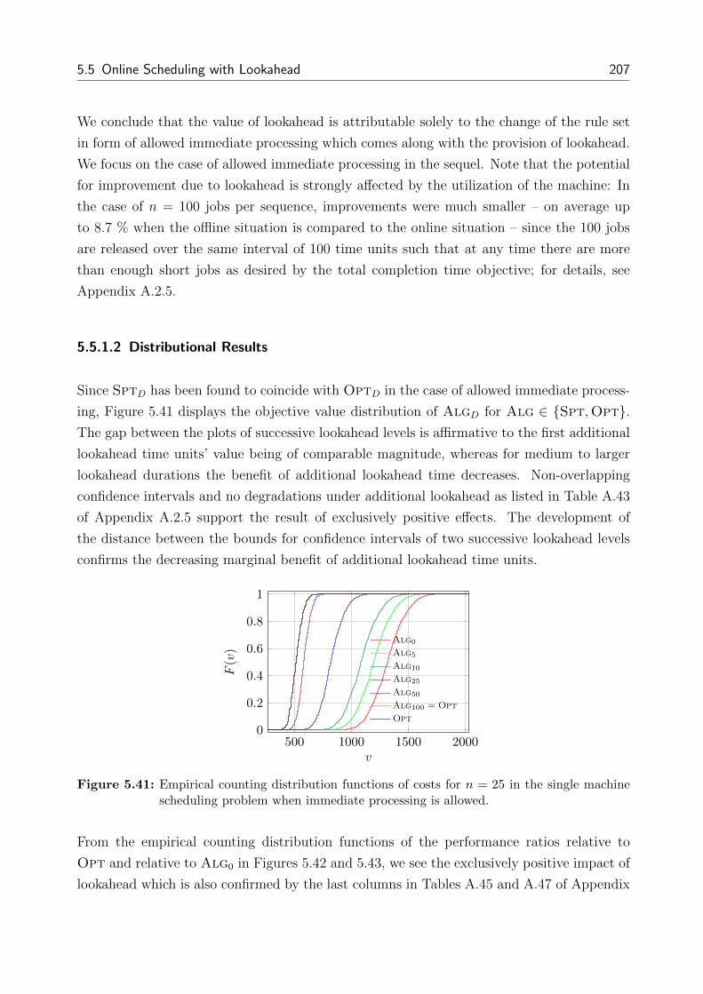
5.5 Online Scheduling with Lookahead 207
We conclude that the value of lookahead is attributable solely to the change of the rule set
in form of allowed immediate processing which comes along with the provision of lookahead.
We focus on the case of allowed immediate processing in the sequel. Note that the potential
for improvement due to lookahead is strongly affected by the utilization of the machine: In
the case of n = 100 jobs per sequence, improvements were much smaller – on average up
to 8.7 % when the offline situation is compared to the online situation – since the 100 jobs
are released over the same interval of 100 time units such that at any time there are more
than enough short jobs as desired by the total completion time objective; for details, see
Appendix A.2.5.
5.5.1.2 Distributional Results
Since SptD has been found to coincide with OptD in the case of allowed immediate process-
ing, Figure 5.41 displays the objective value distribution of AlgD for Alg ∈ {Spt,Opt}.The gap between the plots of successive lookahead levels is affirmative to the first additional
lookahead time units’ value being of comparable magnitude, whereas for medium to larger
lookahead durations the benefit of additional lookahead time decreases. Non-overlapping
confidence intervals and no degradations under additional lookahead as listed in Table A.43
of Appendix A.2.5 support the result of exclusively positive effects. The development of
the distance between the bounds for confidence intervals of two successive lookahead levels
confirms the decreasing marginal benefit of additional lookahead time units.
500 1000 1500 20000
0.2
0.4
0.6
0.8
1
v
F(v)
Alg0
Alg5
Alg10
Alg25
Alg50
Alg100 = Opt
Opt
Figure 5.41: Empirical counting distribution functions of costs for n = 25 in the single machinescheduling problem when immediate processing is allowed.
From the empirical counting distribution functions of the performance ratios relative to
Opt and relative to Alg0 in Figures 5.42 and 5.43, we see the exclusively positive impact of
lookahead which is also confirmed by the last columns in Tables A.45 and A.47 of Appendix
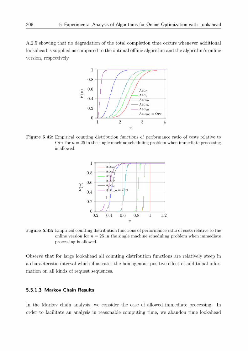
208 5 Experimental Analysis of Algorithms for Online Optimization with Lookahead
A.2.5 showing that no degradation of the total completion time occurs whenever additional
lookahead is supplied as compared to the optimal offline algorithm and the algorithm’s online
version, respectively.
1 2 3 40
0.2
0.4
0.6
0.8
1
v
F(v) Alg0
Alg5
Alg10
Alg25
Alg50
Alg100 = Opt
Figure 5.42: Empirical counting distribution functions of performance ratio of costs relative toOpt for n = 25 in the single machine scheduling problem when immediate processingis allowed.
0.2 0.4 0.6 0.8 1 1.20
0.2
0.4
0.6
0.8
1
v
F(v)
Alg0
Alg5
Alg10
Alg25
Alg50
Alg100 = Opt
Figure 5.43: Empirical counting distribution functions of performance ratio of costs relative to theonline version for n = 25 in the single machine scheduling problem when immediateprocessing is allowed.
Observe that for large lookahead all counting distribution functions are relatively steep in
a characteristic interval which illustrates the homogenous positive effect of additional infor-
mation on all kinds of request sequences.
5.5.1.3 Markov Chain Results
In the Markov chain analysis, we consider the case of allowed immediate processing. In
order to facilitate an analysis in reasonable computing time, we abandon time lookahead

5.5 Online Scheduling with Lookahead 209
and switch to request lookahead of size l. The elements of the state space S subsume the
last completion time c of a job scheduled on the machine, the processing times p = (p1, . . . , pl)
of the lookahead jobs in non-decreasing order and the current objective value v of the total
completion time, i.e.,
S ={
(c, p, v) | c ∈ R≥0, p ∈ (R>0)l, v ∈ R≥0}.
Note that completion of a job and arrival of a new job coincide under request lookahead.
Upon arrival of a new job, each algorithm Alg chooses a job from the lookahead to be
scheduled next on the machine. Hence, Alg is a function
Alg : S × R>0 → {1, 2, . . . , l}
which gives the position of the selected job in the lookahead. The successor state of s =
(c, p, v) upon arrival of a job with processing time pnew is given by s′ = (c′, p′, v′) where
c′ = c + pAlg(s,pnew), p′ arises from p by removing element pAlg(s,pnew), appending pnew and
ordering non-decreasingly, and v′ = v + c′.
In order to obtain a finite state space representation, we have to discretize job processing
times: To this end, denote the number of possible processing times by np and the maximum
possible processing time by pmax, then the state space size amounts to
|S| = (npmax + 1) ·(np + l − 1
l
)·(n(n+ 1)
2pmax + 1
).
When immediate processing is allowed, deviating from the shortest processing time first rule
would lead to a deterioration in the objective value as shown easily by a job interchange
argument. Hence, Sptl and Optl coincide. For Algl with Alg ∈ {Spt,Opt} and selected
lookahead level l, we determine the successor for each state and each new job to obtain the
one-step frequency matrix and the n-step frequency matrix of the Markov chain.
In our numerical experiment, we use the parameterization n = 25, np = 2, pmax = 2
and l ∈ {1, 2, . . . , 5}. For this small exemplary setting, the state space size amounts to
(25 · 2 + 1) ·(
2+5−15
)· (25·26
2· 2 + 1) = 199 206 elements for l = 5.
The exclusively beneficial effect of lookahead for the resulting objective value distributions is
presented in Figure 5.44. The horizontal distance between the plots of two successive looka-
head levels suggests that the marginal improvement attainable by an additional lookahead
unit remains the same for increasing lookahead size.

210 5 Experimental Analysis of Algorithms for Online Optimization with Lookahead
400 500 6000
0.2
0.4
0.6
0.8
1
v
F(v)
Alg1
Alg2
Alg3
Alg4
Alg5
Figure 5.44: Exact distribution functions of costs for n = 25 in the single machine schedulingproblem when immediate processing is allowed.
5.5.2 Online Parallel Machines Scheduling
Similar to ordering items by non-increasing size in bin packing, ordering jobs by non-
increasing processing times is a reasonable strategy to balance workload among parallel
machines. For the offline problem without release times (Pm | |Cmax), this strategy is a
(43− 1
3m)-approximation algorithm as shown easily by contradiction ([138]). For m = 2,
we get a 76-approximation algorithm. The following algorithms mimic this behavior on the
known jobs in the lookahead set. Note that the problem is NP-hard for m ≥ 2 by reduction
from NP-complete problem Partition.
Online algorithm
• LongestProcessingTime (Lpt): If a new job j arrives at time rj and a machine is
idle, start the longest job with release time rj on this machine; if a machine finishes a
job and unprocessed jobs are known, start a job with longest processing time among
these jobs on this machine ([138]).
Online algorithms with lookahead of duration D
• LongestProcessingTimeD (LptD):
If the earliest start time of a job is reached and the machine is idle, start the longest
job whose earliest start time is reached; if a machine finishes a job and there are
unprocessed jobs whose earliest start time has already been reached, start a job with
longest processing time among these jobs on this machine.
• OptimalD (OptD): If the earliest start time of a job is reached and a machine is
idle or if a machine finishes a job and unprocessed jobs are known whose earliest start
time has already been reached, then in Figure 5.36, set M := 2 and N, e, p, c according

5.5 Online Scheduling with Lookahead 211
to the current jobs in the lookahead set and the current machine statuses. Solve the
MIP formulation in Figure 5.45. Start the first processable job on the free machine as
suggested by the obtained schedule.
min Cmax (5.46)
s.t. xijk + xjik ≤ zik i, j ∈ J, i 6= j, k ∈ K (5.47)
xijk + xjik ≥ zik + zjk − 1 i, j ∈ J, i 6= j, k ∈ K (5.48)
xjjk = 0 j ∈ J, k ∈ K (5.49)∑k∈K
zjk = 1 j ∈ J (5.50)
sjk ≥ max{ej, ck}zjk j ∈ J, k ∈ K (5.51)
sik + pi ≤ sjk + M · (1− xijk) i, j ∈ J, i 6= j, k ∈ K (5.52)
Cmax ≥ sjk + pj j ∈ J, k ∈ K (5.53)
xijk, zjk ∈ {0, 1} i, j ∈ J, k ∈ K (5.54)
sjk ≥ 0 j ∈ J, k ∈ K (5.55)
Figure 5.45: MIP formulation of the scheduling problem Pm | ej |Cmax.
Optimal offline algorithm
• Optimal (Opt): In Figure 5.36, set N := n,M := 2, c := 0 and e, p according to the
known jobs. Solve the MIP formulation in Figure 5.45. Execute the obtained schedule.
In the MIP formulation in Figure 5.45, we use additional decision variables zik in order to
express on which machine k job i is processed. Cmax is used as an auxiliary variable to indicate
the end of the schedule. All other variables are also extended with an additional index
referring to the machine. In particular, Constraint 5.48 ensures that there is a precedence
relation between each pair of jobs that goes on the same machine.
In case of forbidden immediate processing, we do not expect lookahead to be exploited
much: LptD cannot take advantage of lookahead at all because it collapses into Lpt; for
OptD in order to excel LptD, job processing times have to be such that arranging them
“locally” optimal on the two machines leads to a deviation from LptD as shown in Figure
5.46. Clearly, the probability for such a pathologic construction is not too high. Note that
this effect also occurs under allowed immediate processing. However, the lookahead effect
there is mainly attributed to the rule set substitution, whereas under forbidden immediate
processing could only be attributed to OptD’s farsightedness.

212 5 Experimental Analysis of Algorithms for Online Optimization with Lookahead
0 1 2 3 4 5 6 7
Optl
Lptl
machine 1
machine 2
machine 1
machine 2
Time
Figure 5.46: Local improvement of OptD over LptD. For five jobs with (r1, p1) = (r2, p2) =(0, 3), (r3, p3) = (r4, p4) = (r5, p5) = (0, 2), we have that Cmax(LptD) = 7 >Cmax(OptD) = 6.
5.5.2.1 Average Results
We find massive makespan reductions when immediate processing is allowed and virtually
no effect when immediate processing is forbidden as depicted in Figures 5.47 and 5.48. In
case of allowed immediate processing, the makespan can be drastically reduced as a result
of avoided idle times on the machines and the privilege of not having to wait until regular
release times. Between online and offline situations, algorithm performance can be enhanced
such that makespan reductions of up to 74.5 % are incurred. Additionally, the potential
of sophisticated exact reoptimization in order to capitalize from situations as displayed in
Figure 5.46 is considered insignificant. Small coefficients of variation and tight confidence
intervals indicate statistical validity of the obtained results (cf. also Table A.55 of Appendix
A.2.5). As in the single machine problem, no instance encountered exhibits a deterioration
in the objective value when algorithms are provided additional lookahead time.
Contrarily, under forbidden immediate processing the makespan is by definition crucially
determined by the release times of the last jobs to finish processing on the machines; this
holds especially true in case of low to moderate machine utilization as given for n = 25 with
an overall horizon of 100 time units: Looking at the scale in Figure 5.48, we declare the
improvement under forbidden immediate processing as negligible. For LptD it was already
clear from the algorithm description that no lookahead value exists at all; whereas for OptD
we found that there are too few situations that would allow to determine an elaborate partial
schedule by applying exact reoptimization techniques similar to the one shown in Figure 5.46
so as to influence the overall makespan attained at the end of the time horizon.

5.5 Online Scheduling with Lookahead 213
0 10 20 30 40 50 60 70 80 90 10020
40
60
80
100
Lookahead duration D
Average
costs
LptD
OptD
Figure 5.47: Average costs for different lookahead durations and n = 25 in the parallel machinesscheduling problem when immediate processing is allowed.
0 10 20 30 40 50 60 70 80 90 100
98.79
98.79
98.79
98.8
98.8
98.8
Lookahead duration D
Average
costs
LptD
OptD
Figure 5.48: Average costs for different lookahead durations and n = 25 in the parallel machinesscheduling problem when immediate processing is forbidden.
In summary, makespan reductions are achieved only as a result of a changed problem setting
in favor of the decision maker by allowing immediate processing. Hence, we concentrate on
this setting subsequently. As seen in Appendix A.2.5, also for n = 100 jobs per sequence
makespan reductions are achieved. However, as in the single machine problem, the reduction
is sharply constricted by the high machine utilization which makes sure that most of the times
when a machine is freed there are plenty of long jobs to go on that machine.

214 5 Experimental Analysis of Algorithms for Online Optimization with Lookahead
20 40 60 80 1000
0.2
0.4
0.6
0.8
1
v
F(v)
Lpt0
Lpt5
Lpt10
Lpt25
Lpt50
Lpt100
Opt
20 40 60 80 1000
0.2
0.4
0.6
0.8
1
v
F(v)
Opt0
Opt5
Opt10
Opt25
Opt50
Opt100 = Opt
Opt
Figure 5.49: Empirical counting distribution functions of costs for n = 25 in the parallel machinesscheduling problem when immediate processing is allowed.
1 2 3 4 5 60
0.2
0.4
0.6
0.8
1
v
F(v) Lpt0
Lpt5
Lpt10
Lpt25
Lpt50
Lpt100
1 2 3 4 5 60
0.2
0.4
0.6
0.8
1
v
F(v) Opt0
Opt5
Opt10
Opt25
Opt50
Opt100 = Opt
Figure 5.50: Empirical counting distribution functions of performance ratio of costs relative toOpt for n = 25 in the parallel machines scheduling problem when immediate pro-cessing is allowed.
0.2 0.4 0.6 0.8 10
0.2
0.4
0.6
0.8
1
v
F(v)
Lpt0
Lpt5
Lpt10
Lpt25
Lpt50
Lpt100
0.2 0.4 0.6 0.8 10
0.2
0.4
0.6
0.8
1
v
F(v)
Opt0
Opt5
Opt10
Opt25
Opt50
Opt100 = Opt
Figure 5.51: Empirical counting distribution functions of performance ratio of costs relative tothe online version for n = 25 in the parallel machines scheduling problem whenimmediate processing is allowed.

5.6 Concluding Discussion 215
5.5.2.2 Distributional Results
Figure 5.49 illustrates the huge benefit of lookahead when immediate processing is allowed
in terms of a left shift of the plots of the empirical counting distribution functions of the
objective value when additional time units of lookahead are supplied. Algorithm families
LptD and OptD lead to schedules of the same quality such that it is not necessary to
apply exact reoptimization methods. From the large slope value of the empirical counting
distribution functions in a characteristic interval for each combination of algorithm and
lookahead level as well as from the width of all confidence intervals being smaller than one
time unit (cf. Table A.55 of Appendix A.2.5), we infer that the sampled results give a
profound impression of the performance of the respective algorithms. From the distance
of the curves to each other, we see that for small to medium lookahead levels the marginal
benefit of an additional time unit of lookahead stays constant and that it gradually decreases
for larger lookahead durations.
Figures 5.50 and 5.51 display the empirical counting distribution functions of the performance
ratios relative to Opt and the online versions of the algorithms, respectively. Confidence
interval widths collectively smaller than 0.04 in the case relative to Opt and even coinciding
at the second decimal place in the case relative to the online version imply the characteristic
improvement for each lookahead level (cf. Tables A.57 and A.59 of Appendix A.2.5). No
algorithm exhibits worsened performance on any instance when lookahead is supplied.
We conclude this section by pointing out the similarities between the computational results
for the scheduling problem and those for the TSP. In both cases, being allowed to process
an input element as soon as its existence emerges leads to the major impact of lookahead.
5.6 Concluding Discussion
The computational experiments from this chapter covered different problem classes:
• In the ski rental problem, an instance of a one-shot rent-or-buy problem was solved.
• In paging, instances of replacement problems were solved repetitively.
• In bin packing, instances of packing problems were solved repetitively.
• In the TSP, instances of sequencing problems were solved repetitively.
• In scheduling, instances of (combined) packing, sequencing and timing problems were
solved repetitively.

216 5 Experimental Analysis of Algorithms for Online Optimization with Lookahead
Numerical results in each problem setting suggest that there is an overall positive effect on
the objective value that can be obtained if algorithms are designed and allowed to take ad-
vantage of lookahead. However, the magnitude of the effect is strongly problem-specific: In
the TSP and in scheduling with allowed immediate processing, exploiting additional looka-
head directly paid off upon changing the processing order of input elements because of the
direct impact on the objective value. In bin packing, the observed effect was much smaller as
a result of the indirect impact of item assignments on the objective value: An item occupies
the same bin capacity no matter in which bin it lies and at which time it is packed. More-
over, we found that improvements in packing problems could only be attained by a clever
arrangement of the small objects that have to be put in the large objects. Unfortunately,
constellations where such improvements can be made are encountered rarely in typical item
or job sequences. Lookahead in the paging and ski rental problem was also found to have
a major positive impact on the costs incurred by respective algorithms. The explanation
lies in the risk-free exploitation of additional lookahead based on a larger part of the time
horizon that is overseen. The additional knowledge allows an algorithm to make a decision
that is guaranteed to have no future ramifications as compared to a decision made under
fewer available lookahead information. Hence, in these types of problems there is no threat
of bad decisions.
In some problem settings, it was possible to devise algorithms such that additional lookahead
proved exclusively beneficial, whereas in others there were instances with degraded algorithm
performance for any of the devised algorithms since lookahead was leading them towards a
wrong direction as discovered only later in the processing of the input sequence. Yet, such
instances were encountered only sporadically in all problem settings.
Concerning the usage of exact reoptimization algorithms for the subproblems, we found that
the role of exact reoptimization methods to unveil improvement by lookahead is smaller than
previously expected: Although in some problems these methods led to a slight performance
enhancement especially for large lookahead sizes, they also tended to be of nearly no benefit
for small lookahead sizes when compared to heuristic reoptimization strategies: Optimality
of a partial solution often does not migrate to the overall solution because substructures in
partial solutions with a positive influence on the objective value are likely to be relinquished
during the future solution process. In the case of the TSP, we also discovered that applying
sophisticated reoptimization methods could be harmful since stability as imposed by simple
algorithms may get lost; for small to medium lookahead sizes, exact reoptimization was
frequently beaten by much simpler heuristic approaches. It is up to the decision maker to
figure out whether the computationally intense usage of exact reoptimization methods is
worth the effort or not.

5.6 Concluding Discussion 217
Table 5.1 subsumes the findings from this chapter on a granular level: The column for the
total lookahead effect (∆f r,r′,P,P ′
Alg,Alg′) admits that observed lookahead effects strongly relied on
the problem settings themselves. The two columns for the partial lookahead effects due to
instance revelation rule substitution (∆f r,r′
Alg) and due to rule set substitution (∆fP,P′
Alg,Alg′)
show that in the ski rental, paging and bin packing problem merely the additional information
was responsible for improvements, whereas in the TSP and the scheduling problem the
change of the rule set lead to improved objective values in the first place. Column Alg∗
tells us whether there was one algorithm (or several comparably good algorithms) that
could be considered the champion over all lookahead levels. Although this happened only
rarely, we often observed that heuristics did especially well for small lookahead sizes, whereas
exact reoptimization approaches outperformed heuristics by a very slight margin for large
lookahead sizes, i.e., when the problem approaches its offline version. Column Opt indicates
whether exact reoptimization lead to significant improvements. As shown before, only minor
improvements were observed such that exact reoptimization is not deemed a must-have in
online optimization. There was no homogeneous picture about whether additional lookahead
can also lead to objective value deterioration or not (column Deterioration).
We remark that the computational results from this chapter are affirmative to the findings of
the exact analysis in the previous chapter concerning the magnitude of the lookahead impact
as well as its primarily responsible factors.
Our approach of evaluating algorithm performance in the context of a potential provision
of lookahead encompassed two stages: In the first stage, an average-case analysis allowed
us to find the most promising algorithm candidates for a given lookahead level in terms
of expected algorithm behavior. In the second stage, distributional analysis lead to a fine-
grained assessment of each candidate’s individual risk profile with respect to attainable
objective values and performance ratios.

218 5 Experimental Analysis of Algorithms for Online Optimization with Lookahead
Pro
ble
mT
yp
eA
ttri
bute
Rule
∆fr,r′ ,P,P′
Alg,A
lg′
∆fr,r′
Alg
∆fP,P′
Alg,A
lg′
Alg∗
Opt
Det
erio
rati
on
Ski
renta
lre
ques
tlo
oka
hea
d–
–la
rge
larg
eze
roye
s–
no
Pagin
gre
ques
tlo
oka
hea
d
equal
pro
babilit
ies
–la
rge
larg
eze
rono
–n
o/ye
s*
acce
ssgra
ph
–m
ediu
mm
ediu
mze
roye
s–
no/y
es*
page
freq
uen
cies
–la
rge
larg
eze
roye
s–
no/
yes*
Bin
pack
ing
reques
tlo
oka
hea
d
clas
sica
lp
erm
uta
tion
ssm
all
smal
lze
rono
no
yes
no
per
mu
tati
ons
smal
lsm
all
zero
no
no
yes
bou
nd
ed-
spac
e
per
muta
tion
ssm
all
smal
ln
egligib
leye
sno
yes
no
per
mu
tati
ons
smal
lsm
all
neg
ligi
ble
no
no
yes
TSP
reques
tlo
oka
hea
d–
–la
rge
zero
larg
eno
no
yes
Sch
edu
ling
tim
elo
oka
hea
d
singl
em
ach
ine
imm
edia
tepro
cess
ing
larg
en
egligi
ble
larg
eno
no
no
no
imm
edia
tepro
cess
ing
neg
ligi
ble
neg
ligi
ble
zero
no
no
yes
par
alle
lm
ach
ines
imm
edia
tepro
cess
ing
larg
en
egligi
ble
larg
eno
no
no
no
imm
edia
tepro
cess
ing
neg
ligi
ble
neg
ligi
ble
zero
no
no
no
*Inst
ance
sw
ith
det
erio
rate
dob
ject
ive
valu
ein
the
pag
ing
pro
ble
mw
ere
only
obse
rved
for
bat
chin
galg
ori
thm
s.
Table
5.1:
Qu
alita
tive
sum
mar
yof
the
exp
erim
enta
lre
sult
sfr
omC
hap
ter
5.

219
6 Simulation of Real World Applications
In the previous two chapters, we studied the influence of lookahead on solution quality in
standard online optimization problems. This chapter extends our analysis to more complex
dynamic systems. We consider two real world applications which reveal their online character
not only in form of an input element disclosure over time but also in form of additional
unforeseeable events:
• Online Order Picking with Lookahead
• Online Pickup and Delivery with Lookahead
Examples for additional random events are breakdowns, no-shows or processing time varia-
tions. Since future implications of these event types are uncertain due to our non-clairvoyance,
it is now not even possible to provide an exact formulation of the snapshot problem at a
given time. Moreover, since applications originate from practice, typically not only one but
a set of objectives is relevant to the decision maker. Accordingly, we find ourselves in the
intrinsically more difficult setting of multicriteria optimization. We are concerned with the
question whether endowing algorithms with lookahead proves beneficial to their outcome
given that we have to regard several optimization goals and additional random influences.
Due to the high complexity incurred by a large number of dependent random variables and
the existence of several optimization goals, we use simulation models to derive statements
about algorithm performance. Optimization algorithms are integrated into the simulation
environment such that whenever the logic of the simulation requires a decision, a correspond-
ing algorithm is invoked to deliver that decision (see also Chapter 2.4.4 and [68]).
Computational experiments were performed on the same hardware as specified at the be-
ginning of Chapter 5. All simulation models were developed in AnyLogic 6.9.0 as discrete
event models. Algorithms were implemented in the native Java environment of AnyLogic
and arising instances of IP and MIP formulations were solved using IBM ILOG CPLEX 12.5
with a prescribed time limit of 120 seconds. A detailed summary of statistical key figures
for each experiment is given in Appendix A.3.

220 6 Simulation of Real World Applications
6.1 Online Order Picking with Lookahead
In a manual order picking system, pickers move through the aisles of a warehouse to retrieve
items packed in boxes as demanded by the orders from external customers. When a picker
has collected all boxes assigned to him, he returns to a depot to unload the boxes and wait
for the next assignment of boxes to be picked ([89], [92]).
Efficiently managing an order picking system is a crucial task both in manufacturing and
distribution logistics which is underlined by the fact that more than the half of all warehouse
operating costs can be attributed to order picking ([57]).
Typically, customer orders arrive throughout the day and the objective is to make the pickers
collect all boxes of the customer orders in a way that meets the decision maker’s goal system
best. Figure 6.1 displays the warehouse under consideration along with charts for some
performance indicators of interest.
Figure 6.1: Animation of the simulation model for an order picking system in AnyLogic.

6.1 Online Order Picking with Lookahead 221
The warehouse layout consists of ten aisles arranged in a lower and an upper block of five
aisles each. Each aisle has 20 storage locations, ten to the left and right, respectively. Depot
and break location are positioned in the lower left corner of the warehouse. The length of
each aisle amounts to 30 meters, the horizontal (vertical) distance between two aisles is 8
(2.5) meters. On average, pickers move at a speed of 1 meter per second. When a picker
is not working and absent without leave, he is displayed in the no-show area. Five pickers
have to commission n = 625 orders over a work day of 600 minutes plus potential overtime.
An order may consist of up to three boxes and the picker capacity amounts to ten boxes.
Aisle traversal is subject to blocking effects ([92]), e.g., because of security or space consid-
erations: Only one picker is allowed inside an aisle at a time. For this reason, each aisle has
a traffic light at its front and rear entry (cf. Figure 6.1) to signal that the aisle is acces-
sible (green light) or inaccessible (red light) at the moment. Pickers that need to enter an
inaccessible aisle have to enqueue at an aisle entry point and wait until the aisle is freed.
Order arrival and data are random, i.e., release time, number of boxes, pick time, drop
time and location of an order are realizations of random variables that are unknown to
the algorithms which have to determine pick lists and routes. In addition, order picking
operations underlie the following random influences:
• Picker velocity profile
• Picker break start and end time
• Picker no-show occurrence
• If applicable, picker no-show start and end time
Because of blocking effects and the large number of random processes, it is out of scope to
give an exact formulation of an optimization problem that takes into account all of these
features. Hence, simulation is deemed a suitable method of analysis.
At the end of a run of an independent simulation replication, the decision maker is supplied
with the following quality indicators for the pick lists and routes which are used to judge on
the quality of the responsible algorithm:
• Makespan, i.e., the time when the last box is unloaded at the depot
• Total distance covered by all pickers
• Picker utilization, i.e., the mean percentage of working pickers over the time horizon
• Box throughput, i.e., the box delivery rate at the depot

222 6 Simulation of Real World Applications
Lookahead appears as time lookahead of duration D ∈ {0, 60, 120, . . . , 600} minutes. We
assume that the warehouse initially contains all items in a quantity sufficient to satisfy all
customer orders arriving over the day such that no additional storage operations are required
in the course of a day. Once an order arrives, its contents are ready to be picked by a picker.
Hence, lookahead forwards the earliest start time of an order, and waiting until the regular
release time from the pure online case is not necessary. In this way, lookahead implies a
change of the rule set in favor of the decision maker.
In our computational experiments, we draw m = 50 independent simulation replications by
initializing the random number generator with a different seed and ensuring independence
of all stochastic processes in each replication.
An algorithm is required to determine the pick lists and routes for all pickers available at
that time so as to fulfill the known and yet unfulfilled customer orders in a way that best
matches the decision maker’s preferences with respect to the quality criteria specified above.
We agree upon algorithm execution whenever the current situation changes as a result of a
customer order arrival, a picker’s re-entry in the system after a break or no-show, or a picker
becoming available upon finished unloading at the depot.
Commonly, all boxes of an order are picked by the same picker in a single route such that
no sorting device needs to be installed. Hence, managing an order picking system consists
of repetitively solving two interrelated subproblems for yet unserved orders:
1. Assignment of orders to pickers such that the total number of boxes of assigned orders
does not exceed the picker capacity (batching).
2. Route calculation16 for each picker such that all boxes of assigned orders are visited
and the route starts and ends at the depot (routing).
Algorithms solve these tasks either sequentially or simultaneously. Sequential methods cope
with the complexity of the problem by decoupling the subproblems from each other similar
to cluster-first route-second approaches for vehicle routing ([101]); the batching algorithm
first assigns orders to pickers; afterwards the routing algorithm determines picker traversal
paths through the aisles including aisle entry and exit points. Note that some batching
algorithms take potential routes as determined by a routing algorithm into account. Due to
the multitude of different batching and routing algorithms, our computational experiments
check which combination of a batching and routing policy is most promising. Simultaneous
methods solve the batching and routing problem at the same time. Only simultaneous
16Because a route in an order picking system has to start and end in the depot, the decision version of the“problem” contains Hamiltonian Circuit which is known to be an NP-complete problem.

6.1 Online Order Picking with Lookahead 223
methods provide exact solutions to snapshot problem instances. Unfortunately, when many
customer orders are known, e.g., due to lookahead of large duration, problem instances
become huge and solving them almost surely exceeds the prescribed time limit of 120 seconds.
In this case, a substitute solution is retrieved by applying a sequential method. Except for
the exact reoptimization approaches, all of the following algorithms represent well-known
and commonly accepted algorithms for order picking systems (see the survey in [89] and the
included references).
Batching Algorithms
• PriorityBatching (Prio): Sort orders according to a criterion, e.g., non-increasingly
according to their number of boxes. Assign orders successively to batches in a first fit
manner ([89]).
• SeedBatching (Seed): Batches are built sequentially: Initialize each batch with a
seed order, e.g., by selecting an order with the largest number of boxes; fill the batch
with additional orders according to an order congruency rule, e.g., select an order with
the smallest number of additional aisles ([89]).
• SavingsBatching (Svgs): Batches are built simultaneously: Initialize the batch
building process with each order forming a separate batch. In the improvement phase,
combine orders of two batches into one batch if the total distance is reduced according
to the routing algorithm applied until no further improvement is possible ([89]).
• LocalSearchBatching (Ls): Let the neighborhood of a batch set be given by all
batch sets which are obtained by a swap or shift move. A swap move exchanges one
selected order per batch between two batches; a shift move transfers a selected order
from one batch to another. A perturbation of a batch set consists of transferring a
random number of orders from one batch to another if the receiving batch remains
feasible. Execute the following two steps until the total distance of all batches cannot
be reduced in either step: Search within the neighborhood of the current batch set
for a batch set with smaller total distance. Perturb the current batch set for a fixed
number of times to find a batch set with smaller total distance ([89]).
• TabuSearchBatching (Ts): Apply Ls with the modifications that a swap or shift
move that has just been carried out is forbidden along with its inverse move for a pre-
scribed number of iterations and that always the best solution within the neighborhood
of the current batch set is selected even if it leads to a longer total distance ([89]).

224 6 Simulation of Real World Applications
Routing Algorithms
• ReturnRouting (Ret): Lower aisles with boxes are visited first from left to right;
upper aisles with boxes are visited afterwards from right to left. Each aisle except for
the last lower aisle with a box is entered and exited at its front entry; the last lower
aisle with a box is traversed entirely ([89]).
• S-ShapedRouting (S): First, the two leftmost aisles with boxes of both blocks are
traversed upwards entirely. Second, upper aisles with boxes are visited from left to
right where each aisle except for the rightmost is traversed entirely in the direction
opposite to that of the previous aisle; the rightmost aisle is traversed entirely if it is
entered at its rear entry, otherwise it is entered and exited at its front entry. Third,
lower aisles with boxes are visited from right to left where each aisle except for the
rightmost is traversed entirely in the direction opposite to that of the previous aisle;
the rightmost aisle is traversed downwards entirely ([89]).
• LargestGapRouting (Gap): The largest gap of an aisle is its largest segment that
contains no box, i.e., either the segment between two adjacent boxes, between front
entry and lowermost box, or between rear entry and uppermost box. The largest gap
of an aisle separates two parts of the aisle from each other: The lower (upper) part
starts at the front (rear) entry and finishes at the lowermost (uppermost) point of the
largest gap. First, lower parts of lower aisles with boxes are visited from left to right.
Second, upper parts of lower aisles with boxes are visited from right to left. Third,
lower parts of upper aisles with boxes are visited from left to right. Fourth, upper
parts of upper aisles with boxes are visited from right to left. The rightmost aisle of
each block is traversed entirely; in all other aisles, lower (upper) parts are entered and
exited at the front (rear) entry ([89]).
• OptimalRouting (Opt): In Figure 6.2, set N according to the number of boxes in
the batch assigned to the picker and c according to the distances between the boxes to
each other and to the depot. Solve the MIP formulation in Figure 6.3. Visit the boxes
in the order suggested by the obtained solution.
Simultaneous Batching and Routing Algorithm
• Optimal,Optimal (Opt,Opt): In Figure 6.4, set K,M,N, s, κ, u according to the
available pickers and orders in the lookahead and c according to the distances between
the boxes to each other and to the depot. Solve the MIP formulation in Figure 6.5.
Assign orders to pickers and apply for each picker’s boxes the visiting order as suggested
by the obtained solution.

6.1 Online Order Picking with Lookahead 225
Sets
V set of boxes and box locations with V = {1, . . . , N}Parameters
N number of boxescij travel costs between boxes i ∈ V and j ∈ Vc0j travel costs between depot and box j ∈ Vcj0 travel costs between box j ∈ V and depotM sufficiently large constant (big M)
Variables
xij =
{1 if box i ∈ V is picked immediately before box j ∈ V,0 else
x0j =
{1 if box j ∈ V is the first box picked,
0 else
xj0 =
{1 if box j ∈ V is the last box picked,
0 else
Tj ≥ 0 picking start time of box j ∈ V
Figure 6.2: Sets, parameters and variables in the MIP formulation of the order routing problem.
min∑i∈V
∑j∈V
cijxij +∑j∈V
c0jx0j +∑j∈V
cj0xj0 (6.1)
s.t.∑j∈V,j 6=i
xij + xi0 = 1 i ∈ V (6.2)
∑i∈V,i 6=j
xij + x0j = 1 j ∈ V (6.3)
∑j∈V
x0j = 1 (6.4)∑j∈V
xj0 = 1 (6.5)
Ti + 1 ≤ Tj + M · (1− xij) i, j ∈ V (6.6)
xij ∈ {0, 1} i, j ∈ V (6.7)
x0j, xj0 ∈ {0, 1} j ∈ V (6.8)
Tj ≥ 0 j ∈ V (6.9)
Figure 6.3: MIP formulation of the order routing problem.

226 6 Simulation of Real World Applications
Sets
P set of pickers including dummy picker with P = {1, . . . , K + 1}V set of boxes and box locations with V = {1, . . . , N}O set of orders with O = {1, . . . ,M}
Parameters
K number of pickersM number of ordersN number of boxessi number of boxes in order i ∈ Oκk capacity of picker k ∈ Pcj1j2k travel costs of picker k ∈ P between boxes j1 ∈ V and j2 ∈ Vc0jk travel costs of picker k ∈ P between depot and box j ∈ Vcj0k travel costs of picker k ∈ P between box and depot j ∈ VM sufficiently large constant (big M)
uij =
{1 if box j belongs to order i,
0 else
Variables
xj1j2k =
1 if box j1 ∈ V is picked immediately before box j2 ∈ V
by picker k ∈ P,0 else
x0jk =
{1 if box j ∈ V is the first box picked by picker k ∈ P,0 else
xj0k =
{1 if box j ∈ V is the last box picked by picker k ∈ P,0 else
yik =
{1 if order i ∈ V is served by picker k ∈ P,0 else
zjk =
{1 if box j ∈ V is picked by picker k ∈ P,0 else
Tjk ≥ 0 picking start time of box j ∈ V for picker k ∈ P
Figure 6.4: Sets, parameters and variables in the MIP formulation of the order batching androuting problem.

6.1 Online Order Picking with Lookahead 227
min∑k∈P
∑j1∈V
∑j2∈V
cj1j2kxj1j2k +∑k∈P
∑j∈V
c0jkx0jk +∑k∈P
∑j∈V
cj0kxj0k (6.10)
s.t.∑k∈K1
∑j2∈V,j2 6=j1
xj1j2k +∑k∈P
xj10k = 1 j1 ∈ V (6.11)
∑k∈P
∑j1∈V,j1 6=j2
xj1j2k +∑k∈P
x0j2k = 1 j2 ∈ V (6.12)
∑j1∈V
xj1jk + x0jk =∑j2∈V
xjj2k + xj0k j ∈ V, k ∈ P (6.13)∑j∈V
x0jk ≤ 1 k ∈ P (6.14)∑j∈V
xj0k ≤ 1 k ∈ P (6.15)∑j∈V
x0jk = yik i ∈ O, k ∈ P (6.16)∑j∈V
xj0k = yik i ∈ O, k ∈ P (6.17)∑i∈O
siyik ≤ κk k ∈ P (6.18)∑j2∈V
xj1j2k ≤ zj1k j1 ∈ V, k ∈ P (6.19)∑j1∈V
xj1j2k ≤ zj2k j2 ∈ V, k ∈ P (6.20)∑j∈V
uijzjk = siyik i ∈ O, k ∈ P (6.21)∑k∈P
yik = 1 i ∈ O (6.22)
Tj1k + 1 ≤ Tj2k + M · (1− xj1j2k) j1, j2 ∈ V, k ∈ P (6.23)
xj1j2k ∈ {0, 1} j1, j2 ∈ V, k ∈ P (6.24)
x0jk, xj0k, zjk ∈ {0, 1} j ∈ V, k ∈ P (6.25)
yik ∈ {0, 1} i ∈ O, k ∈ P (6.26)
Tjk ≥ 0 j ∈ V, k ∈ P (6.27)
Figure 6.5: MIP formulation of the order batching and routing problem.

228 6 Simulation of Real World Applications
In the MIP formulations in Figures 6.3 and 6.5, we decide to get rid of the subtour elimination
constraints by establishing precedence relations between pick operations based on decision
variables for time instants at which boxes are picked in Constraints 6.6 and 6.23, respectively
([132]). In the order batching and routing problem (cf. Figure 6.5), we have to introduce
additional variables yik and zjk to express the (exclusive) assignment of order i (i.e., all of
its associated boxes j) to picker k. In particular, Constraints 6.18 to 6.22 ensure that picker
capacities are respected and that all boxes of an order are picked by the same picker.
6.1.1 Average Results
All combinations of batching and routing algorithms as well as the simultaneous algorithm
were tested. We preface the discussion by noting that rule-based routing policies like Ret, S
or Gap are commonly accepted in practice because of their simplicity, whilst optimal routes
as calculated by Opt or the simultaneous approach in general yield shapelessness routes
which my be hard to follow for a picker and thereby represent an additional source of failure.
A summary of the simulation results obtained for all considered performance criteria is given
in Appendix A.3.1; we restrict attention to two selected performance criteria:
• Total travel distance in kilometers
• Box throughput in boxes per hour
Figure 6.6 shows that – apart from algorithms which rely on a batching determined by Prio
– a substantial reduction in the total distance covered by all pickers is achieved as a result
of providing time lookahead. For lookahead durations D ≥ 300, the optimization potential
appears satiated and the marginal benefit of an additional minute of lookahead becomes
approximately zero.
The positive effect is explained by the same change of the rule set as experienced already
in the TSP in Chapters 4.3 and 5.4: Since a box may be picked up as soon as it becomes
known, increasing the lookahead duration leads to increased probabilities for encountering
spatially proximate boxes which then can be consolidated in a tour. Hence, distance savings
as observed in the TSP carry over to this realistic problem setting which takes random
disturbances into account. However, there are slight differences: Because of the bounded
picker capacity, lookahead cannot be exploited as excessively as in the unrestricted case.
Pickers must return to the depot after ten boxes have been picked; if picker capacities were
unlimited, they could pick all boxes assigned to them in a single tour if full a-priori knowledge
was provided.

6.1 Online Order Picking with Lookahead 229
0 50 100 150 200 250 300 350 400 450 500 550 600
60
70
80
90
100
Lookahead duration D
Averagedistance
Prio,RetD Prio,SD Prio,GapD Prio,OptD
Seed,RetD Seed,SD Seed,GapD Seed,OptD
Svgs,RetD Svgs,SD Svgs,GapD Svgs,OptD
Ls,RetD Ls,SD Ls,GapD Ls,OptD
Ts,RetD Ts,SD Ts,GapD Ts,OptD
Opt,OptD
Figure 6.6: Average distances for different lookahead sizes and n = 625 in the order pickingsystem.
Batching by Prio suffers poor overall performance regardless of the lookahead level and is
eliminated from further consideration; Svgs is also considered inferior and repelled as it
consistently loses to all remaining batching policies; these two batching algorithms are also
outperformed on the other objectives (see Appendix A.3.1). We recognize that the right
batching decision is an essential first step to capitalize from the potential of lookahead.
Batching policies Seed, Ls and Ts exhibit comparable but not identical behavior. We draw
a more precise picture based on the selected routing strategy: Routing policy Ret fails
in comparison to the other routing strategies by cause of its naive approach. Concerning
routing policy Opt, all three batching algorithms are considered equal. Under Gap routing
and small lookahead, Ls batching has slight advantages over the two other batching rules,
whereas in case of medium to large information preview Ts excels Ls and Seed. Under
routing policy S, all algorithms exhibit the same quality; however, performance is degraded
as compared to Opt’s routing for small lookahead. Note that there are no deadheads after
all boxes in an aisle have been collected in S’s routing as opposed to Gap’s routing.
Simultaneously solving the batching and routing problem as targeted by Opt,Opt is found
computationally impracticable to obtain solutions quickly: Whenever more than ten orders,

230 6 Simulation of Real World Applications
i.e., up to 30 boxes, are open, we had to forfeit almost always the exact reoptimization
approach in favor of applying Seed,Gap as a substitute to keep computational efforts low.
For this reason, the plots of Opt,Opt and Seed,Gap coincide for D ≥ 180. This means
that under a three-hour lookahead too many orders and boxes are known as to guarantee
that Opt,Opt could terminate within less than 120 seconds. For the order routing problem
alone, computing time is uncritical because of picker capacities delimiting problem sizes.
Based on the total distance objective function only, we come to the interim conclusion that
Ts, Ls and Seed are deemed the most promising batching policies along with either S or Opt
as recommendable routing strategies. Exact reoptimization is found to be computationally
too hard so as to elicit its full potential.
Before we proceed with the assessment of the results on the box throughput, we first note that
total travel distance and box throughput are no competing optimization goals by definition.
Thus, we do not expect throughput to be negatively affected by the implicit rationale of all
batching and routing policies which lies in finding routes as short as possible. Note that
throughput is to be maximized and used as a frequent key performance indicator for chief
operating officers in warehouses to estimate the overall efficiency of the system consisting of
pickers, orders and the warehouse configuration.
0 50 100 150 200 250 300 350 400 450 500 550 600
120
130
140
150
160
Lookahead duration D
Average
through
put
Prio,RetD Prio,SD Prio,GapD Prio,OptD
Seed,RetD Seed,SD Seed,GapD Seed,OptD
Svgs,RetD Svgs,SD Svgs,GapD Svgs,OptD
Ls,RetD Ls,SD Ls,GapD Ls,OptD
Ts,RetD Ts,SD Ts,GapD Ts,OptD
Opt,OptD
Figure 6.7: Average throughput for different lookahead sizes and n = 625 in the order pickingsystem.

6.1 Online Order Picking with Lookahead 231
The box throughput attained by the pickers as imputed by the decisions of respective al-
gorithms is entirely affirmative to the previously found ranking of batching and routing
algorithms based on the total distance objective as can be seen in Figure 6.7.
While differences in throughput as accomplished by the different algorithms are virtually
non-existent for small lookahead durations, batching algorithms Ts, Ls and Seed unfold
their potential and consistently outperform all other batching policies as well as the exact
reoptimization method for medium to large lookahead window. Routings determined by S
and Opt clearly outperform the other routing strategies.
6.1.2 Distributional Results
Since routing policy Opt intrinsically leads to the shortest route for a given batch, we restrict
the discussion to this routing strategy. Analogous results can be derived for all other routing
policies by consulting Appendix A.3.1. Because batching algorithm Ts has been identified
as one of the top candidates, we select the combined batching and routing policy Ts,Opt600
to be the reference for performance ratios relative to the “best” offline algorithm.
Figure 6.8 confirms the positive effect of lookahead on the total distance. Concerning batch-
ing algorithm candidates Ts, Ls and Seed, a perfect ordering of the empirical counting
distribution functions is observed for successive lookahead durations when the larger one of
them is at most D = 240. Hence, the results point to an exclusive lookahead effect for these
information regimes. For lookahead durations D ≥ 300, we find that empirical counting
distribution functions intransparently cross each other for countless times; hence, no exclu-
sive benefit can be attested for these lookahead durations and the marginal benefit of an
additional time unit of lookahead is approximately zero. Each of the plots has a large steep-
ness in a characteristic interval of total distance values and nearly no steepness elsewhere
indicating that each algorithm corresponds to a specific range of total distances. From the
small confidence intervals with widths collectively smaller than 1 kilometer for each com-
bination of algorithm and lookahead level as well as from the tiny coefficients of variation
collectively not larger than 0.03 in Table A.70 of Appendix A.3.1, we infer representativeness
of the obtained total distances for the given warehouse and picker configuration. However,
we also discover in the table that for larger lookahead durations, instances where additional
lookahead leads to a degradation in the objective value are encountered every now and then.
Yet, since the marginal benefit of lookahead in this information regime is negligible anyway,
this effect is considered unimportant. In fact, the numerous intersection points of the plots
corresponding to these lookahead durations are explained by this observation.

232 6 Simulation of Real World Applications
The empirical counting distribution functions of the performance ratio for the total distance
relative to Ts,Opt600 and relative to the online version of the algorithms are displayed in
Figures 6.9 and 6.10, respectively. Experimental competitive ratios are not larger than 1.33
for batching algorithms Ts, Ls and Seed as also seen in Table A.71 of Appendix A.3.1.
The distance of the plots for two successive lookahead levels to each other admits the same
conclusions as already drawn from the total distance distributions. For lookahead durations
D ≥ 300, performance ratios relative to Ts,Opt600 appear centered around the value 1, i.e.,
deterioration – albeit only at a small magnitude – in consequence of additional lookahead is
encountered on a regular basis. Relative to the pure online version of an algorithm, additional
lookahead leads to performance ratios smaller than 1 for batching algorithm candidates Ts,
Ls and Seed on the largest part of input sequences (cf. Table A.71 of Appendix A.3.1).
Figures 6.11 to 6.13 illustrate the distributional results for the box throughput. For the em-
pirical counting distribution functions of the throughput it is desirable to have larger parts
of the distribution on larger values, i.e., by lookahead we intend to shift the plots to the
right. We observe a qualitative difference compared to the distributional results of the total
distance: The variability of the throughput as well as of performance ratios relative to the
online versions of the algorithms increases considerably for increasing lookahead durations
as confirmed by the coefficients of variation and confidence intervals in Tables A.76 and A.78
of Appendix A.3.1; likewise, the variability of performance ratios relative to Ts,Opt600 de-
creases considerably for increasing lookahead durations (see Table A.77 of Appendix A.3.1):
In the pure online case, orders arrive over the whole time horizon of 600 minutes and the
throughput is considerably influenced by the arrival process, particularly by the last orders;
under full lookahead the throughput is a sole consequence of the pickers’ efficiency on coping
with the input sequence that was revealed at the outset. Hence, throughput is inherently
throttled and regulated in the online case leading to a much more invariant behavior as when
the system is allowed to unfold its throughput freely. This explains the high throughput vari-
ability in the case of large lookahead as opposed to small informational preview.
We conclude this section by pointing out that in order picking where boxes can be picked
up once they are known, massive improvements in all goals could be observed as a result of
an enlarged planning basis for pick list and route generation when additional information is
provided. Since objectives are not conflicting, all goals can be improved and no trade-offs
between different goals have to be taken into account by the algorithms. From a managerial
point of view, we recommend to install technical devices which allow for the retrieval of
lookahead information and to check whether operating strategies currently implemented in
the warehouse are conform with potential warehouse efficiency as extracted by simulation
under batching policies Ts, Ls and Seed combined with routing policies S and Opt.

6.1 Online Order Picking with Lookahead 233
50 60 70 800
0.20.40.60.81
v
F(v)
Prio,Opt0 Prio,Opt60
Prio,Opt120 Prio,Opt180
Prio,Opt240 Prio,Opt300
Prio,Opt360 Prio,Opt420
Prio,Opt480 Prio,Opt540
Prio,Opt600 Ts,Opt600
50 60 70 800
0.20.40.60.81
v
F(v)
Seed,Opt0 Seed,Opt60
Seed,Opt120 Seed,Opt180
Seed,Opt240 Seed,Opt300
Seed,Opt360 Seed,Opt420
Seed,Opt480 Seed,Opt540
Seed,Opt600 Ts,Opt600
50 60 70 800
0.20.40.60.81
v
F(v)
Svgs,Opt0 Svgs,Opt60
Svgs,Opt120 Svgs,Opt180
Svgs,Opt240 Svgs,Opt300
Svgs,Opt360 Svgs,Opt420
Svgs,Opt480 Svgs,Opt540
Svgs,Opt600 Ts,Opt600
50 60 70 800
0.20.40.60.81
v
F(v)
Ls,Opt0 Ls,Opt60
Ls,Opt120 Ls,Opt180
Ls,Opt240 Ls,Opt300
Ls,Opt360 Ls,Opt420
Ls,Opt480 Ls,Opt540
Ls,Opt600 Ts,Opt600
50 60 70 800
0.20.40.60.81
v
F(v)
Ts,Opt0 Ts,Opt60
Ts,Opt120 Ts,Opt180
Ts,Opt240 Ts,Opt300
Ts,Opt360 Ts,Opt420
Ts,Opt480 Ts,Opt540
Ts,Opt600 Ts,Opt600
50 60 70 800
0.20.40.60.81
v
F(v)
Opt,Opt0 Opt,Opt60
Opt,Opt120 Opt,Opt180
Opt,Opt240 Opt,Opt300
Opt,Opt360 Opt,Opt420
Opt,Opt480 Opt,Opt540
Opt,Opt600 Ts,Opt600
Figure 6.8: Empirical counting distribution functions of distance for n = 625 in the order pickingsystem.

234 6 Simulation of Real World Applications
1 1.1 1.2 1.3 1.40
0.20.40.60.81
v
F(v)
Prio,Opt0 Prio,Opt60
Prio,Opt120 Prio,Opt180
Prio,Opt240 Prio,Opt300
Prio,Opt360 Prio,Opt420
Prio,Opt480 Prio,Opt540
Prio,Opt600
1 1.1 1.2 1.3 1.40
0.20.40.60.81
v
F(v)
Seed,Opt0 Seed,Opt60
Seed,Opt120 Seed,Opt180
Seed,Opt240 Seed,Opt300
Seed,Opt360 Seed,Opt420
Seed,Opt480 Seed,Opt540
Seed,Opt600
1 1.1 1.2 1.3 1.40
0.20.40.60.81
v
F(v)
Svgs,Opt0 Svgs,Opt60
Svgs,Opt120 Svgs,Opt180
Svgs,Opt240 Svgs,Opt300
Svgs,Opt360 Svgs,Opt420
Svgs,Opt480 Svgs,Opt540
Svgs,Opt600
1 1.1 1.2 1.3 1.40
0.20.40.60.81
v
F(v)
Ls,Opt0 Ls,Opt60
Ls,Opt120 Ls,Opt180
Ls,Opt240 Ls,Opt300
Ls,Opt360 Ls,Opt420
Ls,Opt480 Ls,Opt540
Ls,Opt600
1 1.1 1.2 1.3 1.40
0.20.40.60.81
v
F(v)
Ts,Opt0 Ts,Opt60
Ts,Opt120 Ts,Opt180
Ts,Opt240 Ts,Opt300
Ts,Opt360 Ts,Opt420
Ts,Opt480 Ts,Opt540
Ts,Opt600
1 1.1 1.2 1.3 1.40
0.20.40.60.81
v
F(v)
Opt,Opt0 Opt,Opt60
Opt,Opt120 Opt,Opt180
Opt,Opt240 Opt,Opt300
Opt,Opt360 Opt,Opt420
Opt,Opt480 Opt,Opt540
Opt,Opt600
Figure 6.9: Empirical counting distribution functions of performance ratio of distance relative toTs,Opt600 for n = 625 in the order picking system.

6.1 Online Order Picking with Lookahead 235
0.8 0.9 10
0.20.40.60.81
v
F(v)
Prio,Opt0 Prio,Opt60
Prio,Opt120 Prio,Opt180
Prio,Opt240 Prio,Opt300
Prio,Opt360 Prio,Opt420
Prio,Opt480 Prio,Opt540
Prio,Opt600
0.8 0.9 10
0.20.40.60.81
v
F(v)
Seed,Opt0 Seed,Opt60
Seed,Opt120 Seed,Opt180
Seed,Opt240 Seed,Opt300
Seed,Opt360 Seed,Opt420
Seed,Opt480 Seed,Opt540
Seed,Opt600
0.8 0.9 10
0.20.40.60.81
v
F(v)
Svgs,Opt0 Svgs,Opt60
Svgs,Opt120 Svgs,Opt180
Svgs,Opt240 Svgs,Opt300
Svgs,Opt360 Svgs,Opt420
Svgs,Opt480 Svgs,Opt540
Svgs,Opt600
0.8 0.9 10
0.20.40.60.81
v
F(v)
Ls,Opt0 Ls,Opt60
Ls,Opt120 Ls,Opt180
Ls,Opt240 Ls,Opt300
Ls,Opt360 Ls,Opt420
Ls,Opt480 Ls,Opt540
Ls,Opt600
0.8 0.9 10
0.20.40.60.81
v
F(v)
Ts,Opt0 Ts,Opt60
Ts,Opt120 Ts,Opt180
Ts,Opt240 Ts,Opt300
Ts,Opt360 Ts,Opt420
Ts,Opt480 Ts,Opt540
Ts,Opt600
0.8 0.9 10
0.20.40.60.81
v
F(v)
Opt,Opt0 Opt,Opt60
Opt,Opt120 Opt,Opt180
Opt,Opt240 Opt,Opt300
Opt,Opt360 Opt,Opt420
Opt,Opt480 Opt,Opt540
Opt,Opt600
Figure 6.10: Empirical counting distribution functions of performance ratio of throughput relativeto the online version for n = 625 in the order picking system.
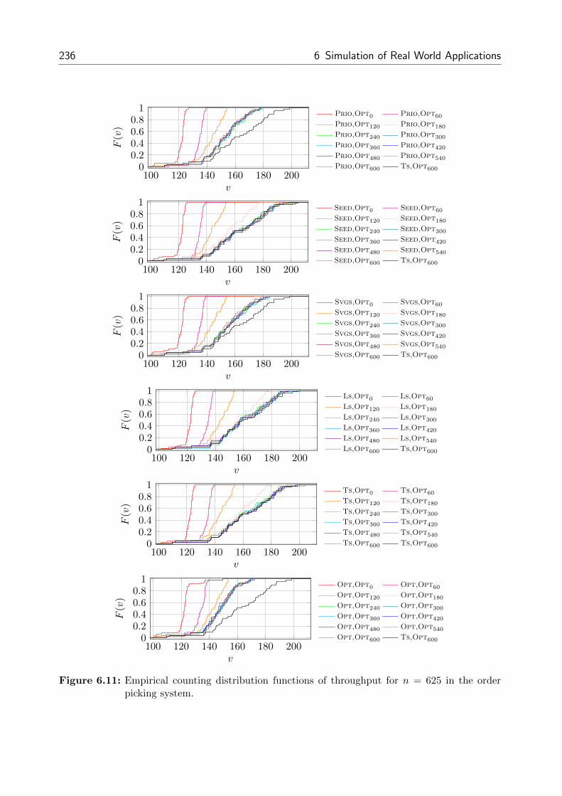
236 6 Simulation of Real World Applications
100 120 140 160 180 2000
0.20.40.60.81
v
F(v)
Prio,Opt0 Prio,Opt60
Prio,Opt120 Prio,Opt180
Prio,Opt240 Prio,Opt300
Prio,Opt360 Prio,Opt420
Prio,Opt480 Prio,Opt540
Prio,Opt600 Ts,Opt600
100 120 140 160 180 2000
0.20.40.60.81
v
F(v)
Seed,Opt0 Seed,Opt60
Seed,Opt120 Seed,Opt180
Seed,Opt240 Seed,Opt300
Seed,Opt360 Seed,Opt420
Seed,Opt480 Seed,Opt540
Seed,Opt600 Ts,Opt600
100 120 140 160 180 2000
0.20.40.60.81
v
F(v)
Svgs,Opt0 Svgs,Opt60
Svgs,Opt120 Svgs,Opt180
Svgs,Opt240 Svgs,Opt300
Svgs,Opt360 Svgs,Opt420
Svgs,Opt480 Svgs,Opt540
Svgs,Opt600 Ts,Opt600
100 120 140 160 180 2000
0.20.40.60.81
v
F(v)
Ls,Opt0 Ls,Opt60
Ls,Opt120 Ls,Opt180
Ls,Opt240 Ls,Opt300
Ls,Opt360 Ls,Opt420
Ls,Opt480 Ls,Opt540
Ls,Opt600 Ts,Opt600
100 120 140 160 180 2000
0.20.40.60.81
v
F(v)
Ts,Opt0 Ts,Opt60
Ts,Opt120 Ts,Opt180
Ts,Opt240 Ts,Opt300
Ts,Opt360 Ts,Opt420
Ts,Opt480 Ts,Opt540
Ts,Opt600 Ts,Opt600
100 120 140 160 180 2000
0.20.40.60.81
v
F(v)
Opt,Opt0 Opt,Opt60
Opt,Opt120 Opt,Opt180
Opt,Opt240 Opt,Opt300
Opt,Opt360 Opt,Opt420
Opt,Opt480 Opt,Opt540
Opt,Opt600 Ts,Opt600
Figure 6.11: Empirical counting distribution functions of throughput for n = 625 in the orderpicking system.

6.1 Online Order Picking with Lookahead 237
0.6 0.8 1 1.2 1.40
0.20.40.60.81
v
F(v)
Prio,Opt0 Prio,Opt60
Prio,Opt120 Prio,Opt180
Prio,Opt240 Prio,Opt300
Prio,Opt360 Prio,Opt420
Prio,Opt480 Prio,Opt540
Prio,Opt600
0.6 0.8 1 1.2 1.40
0.20.40.60.81
v
F(v)
Seed,Opt0 Seed,Opt60
Seed,Opt120 Seed,Opt180
Seed,Opt240 Seed,Opt300
Seed,Opt360 Seed,Opt420
Seed,Opt480 Seed,Opt540
Seed,Opt600
0.6 0.8 1 1.2 1.40
0.20.40.60.81
v
F(v)
Svgs,Opt0 Svgs,Opt60
Svgs,Opt120 Svgs,Opt180
Svgs,Opt240 Svgs,Opt300
Svgs,Opt360 Svgs,Opt420
Svgs,Opt480 Svgs,Opt540
Svgs,Opt600
0.6 0.8 1 1.2 1.40
0.20.40.60.81
v
F(v)
Ls,Opt0 Ls,Opt60
Ls,Opt120 Ls,Opt180
Ls,Opt240 Ls,Opt300
Ls,Opt360 Ls,Opt420
Ls,Opt480 Ls,Opt540
Ls,Opt600
0.6 0.8 1 1.2 1.40
0.20.40.60.81
v
F(v)
Ts,Opt0 Ts,Opt60
Ts,Opt120 Ts,Opt180
Ts,Opt240 Ts,Opt300
Ts,Opt360 Ts,Opt420
Ts,Opt480 Ts,Opt540
Ts,Opt600
0.6 0.8 1 1.2 1.40
0.20.40.60.81
v
F(v)
Opt,Opt0 Opt,Opt60
Opt,Opt120 Opt,Opt180
Opt,Opt240 Opt,Opt300
Opt,Opt360 Opt,Opt420
Opt,Opt480 Opt,Opt540
Opt,Opt600
Figure 6.12: Empirical counting distribution functions of performance ratio of throughput relativeto Ts,Opt600 for n = 625 in the order picking system.

238 6 Simulation of Real World Applications
1 1.2 1.4 1.60
0.20.40.60.81
v
F(v)
Prio,Opt0 Prio,Opt60
Prio,Opt120 Prio,Opt180
Prio,Opt240 Prio,Opt300
Prio,Opt360 Prio,Opt420
Prio,Opt480 Prio,Opt540
Prio,Opt600
1 1.2 1.4 1.60
0.20.40.60.81
v
F(v)
Seed,Opt0 Seed,Opt60
Seed,Opt120 Seed,Opt180
Seed,Opt240 Seed,Opt300
Seed,Opt360 Seed,Opt420
Seed,Opt480 Seed,Opt540
Seed,Opt600
1 1.2 1.4 1.60
0.20.40.60.81
v
F(v)
Svgs,Opt0 Svgs,Opt60
Svgs,Opt120 Svgs,Opt180
Svgs,Opt240 Svgs,Opt300
Svgs,Opt360 Svgs,Opt420
Svgs,Opt480 Svgs,Opt540
Svgs,Opt600
1 1.2 1.4 1.60
0.20.40.60.81
v
F(v)
Ls,Opt0 Ls,Opt60
Ls,Opt120 Ls,Opt180
Ls,Opt240 Ls,Opt300
Ls,Opt360 Ls,Opt420
Ls,Opt480 Ls,Opt540
Ls,Opt600
1 1.2 1.4 1.60
0.20.40.60.81
v
F(v)
Ts,Opt0 Ts,Opt60
Ts,Opt120 Ts,Opt180
Ts,Opt240 Ts,Opt300
Ts,Opt360 Ts,Opt420
Ts,Opt480 Ts,Opt540
Ts,Opt600
1 1.2 1.4 1.60
0.20.40.60.81
v
F(v)
Opt,Opt0 Opt,Opt60
Opt,Opt120 Opt,Opt180
Opt,Opt240 Opt,Opt300
Opt,Opt360 Opt,Opt420
Opt,Opt480 Opt,Opt540
Opt,Opt600
Figure 6.13: Empirical counting distribution functions of performance ratio of throughput relativeto the online version for n = 625 in the order picking system.

6.2 Online Pickup and Delivery with Lookahead 239
6.2 Online Pickup and Delivery with Lookahead
In a pickup and delivery service, customers specify transportation orders between individual
origins and destinations in a road network. In addition, customers provide preferred time
windows for their pickup and delivery time. Transportation orders are served by a fleet of
vehicles and each vehicle has to start and end its routes at an individual depot ([27], [53]).
Dial-a-ride problems are special types of pickup and delivery problems where apart from
travel costs also user convenience in the sense of service quality matters ([53]). While this
may not be relevant to the transportation of goods, it definitely is for the transportation of
persons or perishable freight, e.g., in patient ambulance, taxi services, school bus routing,
or food provision ([158]). Real world pickup and delivery services have to take into account
multiple criteria as intended by dial-a-ride problems due to customer requirements.
Typically, transportation orders arrive throughout the day and the objective is to make the
vehicles pick up and deliver all transportation orders in a way that meets the decision maker’s
goal system best. Figure 6.14 shows the road network under consideration along with charts
for some performance indicators of interest.
Figure 6.14: Animation of the simulation model for a pickup and delivery service in AnyLogic.

240 6 Simulation of Real World Applications
The network represents the urban and suburban region of Karlsruhe and consists of 269
central points and 449 major roads between them. The diameter of the network is 28.5
kilometers; each road is prescribed a specific maximum allowed speed limit. Three vehicles
have to serve n = 50 customer orders arriving over a work day of 600 minutes plus potential
overtime. When a vehicle is not working because of a break or absence without leave (no-
show), its loading space is displayed in gray (cf. Figure 6.14). An order may consist of up
to two units to be transported and the vehicle capacity amounts to five units.
Vehicles are subject to the traffic scene encountered during their service rides, i.e., they have
to adapt to reduced speed limits whenever a traffic jam forbids traveling at regular speed on
a road. Hence, traffic jams represent additional random events in our simulation model.
Order arrival and data are random, i.e., release time, number of units to be transported,
pickup time, delivery time, pickup time window, delivery time window, pickup location and
delivery location of an order are realizations of random variables that are unknown to the
algorithms which have to determine the routes of the vehicles. Pickup and delivery time
windows refer to the preferred service start times of pickups and deliveries, respectively. In
addition, pickup and delivery operations underlie the following random influences:
• Vehicle break start and end time
• Vehicle no-show occurrence
• If applicable, vehicle no-show start and end time
Because of traffic jams and the large number of random processes, it is out of scope to give
an exact formulation of an optimization problem that takes into account all of these features.
Hence, simulation is deemed a suitable method of analysis.
At the end of a run of an independent simulation replication, the decision maker is supplied
with the following quality indicators for the routes which are used to judge on the quality of
the responsible algorithm:
• Makespan, i.e., the time when the last vehicle returns to its depot
• Total distance covered by all vehicles
• Tardiness, i.e., the mean tardiness over all pickup and delivery orders
• Maximum tardiness, i.e., the maximum tardiness over all pickup and delivery orders
• Vehicle utilization, i.e., the mean percentage of working vehicles over the time horizon
• Order throughput, i.e., order fulfillment rate

6.2 Online Pickup and Delivery with Lookahead 241
Lookahead appears as time lookahead of duration D ∈ {0, 60, 120, . . . , 600} minutes. Once
a transportation request arrives, it has to be waited until the corresponding time window
starts before the order can be picked up or delivered, respectively: It is not allowed to incur
an earliness both in the pickup and delivery of an order. Hence, earliest start times of
transportation orders under lookahead are preserved from the pure online case. Lookahead
does not imply a change of the rule set in favor of the decision maker and only serves as a
means of forwarded information release.
In our computational experiments, we draw m = 100 independent simulation replications by
initializing the random number generator with a different seed and ensuring independence
of all stochastic processes in each replication.
An algorithm is required to determine the routes for all vehicles available at that time so
as to fulfill the known and yet unfulfilled transportation orders in a way that best matches
the decision maker’s preferences with respect to the quality criteria specified above. We
agree upon algorithm execution whenever the current situation changes as a result of a
transportation order arrival or a vehicle’s re-entry in the system after a break or no-show.
Despite obvious similarities to the order picking system, some features make the pickup and
delivery service substantially different and demand for other algorithmic approaches:
• Temporal restrictions have to be regarded.
• Earliest start times for pickups and deliveries are not forwarded but retained from the
pure online setting.
• Assignment decisions may be revoked as long as an order has not yet been picked up,
i.e., a route assigned to a vehicle is not fixed when the vehicle leaves the depot.
Managing a pickup and delivery service comprises solving the two interrelated subproblems
of assigning each customer order to a vehicle (batching) and calculating scheduled routes17
for each vehicle according to the assigned orders (routing). Because of the factor time,
not only spatial proximity of locations with respect to a vehicle’s current position but also
temporal proximity of time windows with respect to the current time has to be taken into
account by an algorithm both in its batching and routing decisions. Moreover, each pickup
of an order has to be seen in logical conjunction with the corresponding delivery operation.
Therefore, the variety of solution methods is more limited than for similar problems without
time windows and there is no a-priori subdivision into batching and routing algorithms as
outlined in the order picking system (cf. Chapter 6.1).
17Because a route in a pickup and delivery service has to start and end in the vehicle’s depot, the decisionversion of the “problem” contains Hamiltonian Circuit which is known to be an NP-complete problem.
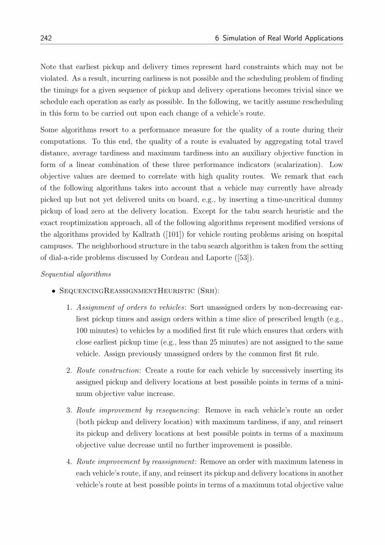
242 6 Simulation of Real World Applications
Note that earliest pickup and delivery times represent hard constraints which may not be
violated. As a result, incurring earliness is not possible and the scheduling problem of finding
the timings for a given sequence of pickup and delivery operations becomes trivial since we
schedule each operation as early as possible. In the following, we tacitly assume rescheduling
in this form to be carried out upon each change of a vehicle’s route.
Some algorithms resort to a performance measure for the quality of a route during their
computations. To this end, the quality of a route is evaluated by aggregating total travel
distance, average tardiness and maximum tardiness into an auxiliary objective function in
form of a linear combination of these three performance indicators (scalarization). Low
objective values are deemed to correlate with high quality routes. We remark that each
of the following algorithms takes into account that a vehicle may currently have already
picked up but not yet delivered units on board, e.g., by inserting a time-uncritical dummy
pickup of load zero at the delivery location. Except for the tabu search heuristic and the
exact reoptimization approach, all of the following algorithms represent modified versions of
the algorithms provided by Kallrath ([101]) for vehicle routing problems arising on hospital
campuses. The neighborhood structure in the tabu search algorithm is taken from the setting
of dial-a-ride problems discussed by Cordeau and Laporte ([53]).
Sequential algorithms
• SequencingReassignmentHeuristic (Srh):
1. Assignment of orders to vehicles : Sort unassigned orders by non-decreasing ear-
liest pickup times and assign orders within a time slice of prescribed length (e.g.,
100 minutes) to vehicles by a modified first fit rule which ensures that orders with
close earliest pickup time (e.g., less than 25 minutes) are not assigned to the same
vehicle. Assign previously unassigned orders by the common first fit rule.
2. Route construction: Create a route for each vehicle by successively inserting its
assigned pickup and delivery locations at best possible points in terms of a mini-
mum objective value increase.
3. Route improvement by resequencing : Remove in each vehicle’s route an order
(both pickup and delivery location) with maximum tardiness, if any, and reinsert
its pickup and delivery locations at best possible points in terms of a maximum
objective value decrease until no further improvement is possible.
4. Route improvement by reassignment : Remove an order with maximum lateness in
each vehicle’s route, if any, and reinsert its pickup and delivery locations in another
vehicle’s route at best possible points in terms of a maximum total objective value

6.2 Online Pickup and Delivery with Lookahead 243
decrease until no further improvement is possible. In order to choose the vehicle
which receives the order, check all vehicles and select one that leads to smallest
total objective value.
5. Route improvement by resequencing : See step 3 ([101]).
• 2Opt (2Opt): Obtain initial routes for each available vehicle by applying Srh. Apply
to each vehicle’s route algorihm 2Optl as outlined in Chapter 5.4 for the TSP without
the first step where l equals the number of pickup and delivery locations; use route
quality as the objective and ensure that feasible sequences of pickup and delivery
locations are obtained (see also [101], [120]).
• SimulatedAnnealing (Sa): A swap move in a route consists of exchanging the
positions of two locations if a feasible sequence of pickup and delivery locations is
obtained; a shift move in a route consists of shifting a number of successive locations
to another position in the route if a feasible sequence of pickup and delivery locations
is obtained. Obtain initial routes for each available vehicle by applying Srh. Apply to
each vehicle’s route algorihm Sal as outlined in Chapter 5.4 for the TSP without the
first step and step 4 replaced by
4. Obtain H ′ by performing a swap or shift move on H at random.
where l equals the number of pickup and delivery locations; use route quality as the
objective ([101])
• TabuSearch (Ts): Let the neighborhood of a route set consist of all route sets which
emanate from removing the pickup and delivery locations of an order from a first route
and inserting them at the best possible points of a second route in terms of a minimum
objective value increase. In Ts, the auxiliary objective function for route quality is
modified by adding a penalty term proportional to the number of times that the move
resulting in the neighboring route set has been applied previously. A route is called
tabu if it results from reinserting an order which has been removed from it within a
prescribed maximum number of immediately preceding iterations. Obtain initial routes
for each available vehicle by applying Srh and set the current route set to this solution.
Repeatedly set the current route set to a route set with minimum total objective value
among all route sets in the neighborhood of the current route set such that each of the
contained routes is non-tabu until no further improvement is made over a prescribed
number of iterations ([53]).

244 6 Simulation of Real World Applications
Simultaneous algorithm
• Optimal (Opt): In Figure 6.15, set K, N , s, l, a, b, κ, linit according to the available
vehicles and orders in the lookahead and c, t according to the distances and travel times
between the locations to each other, to the depots and to the current vehicle locations.
Solve the MIP formulation in Figure 6.16. Assign orders to vehicles and route them as
suggested by the obtained solution.
Sets
C set of vehicles and current vehicle locations with C = {1, . . . , K}P set of pickup locations with P = {K + 1, . . . , K +N}C ′ set of vehicle depot locations with C ′ = {K +N + 1, . . . , 2K +N}D set of delivery locations with D = {2K +N + 1, . . . , 2K + 2N}V set of all locations with V = C ∪ C ′ ∪ P ∪D
Parameters
K number of vehiclesN number of transportation orderscijk travel costs (e.g., distance) between locations i ∈ V and j ∈ Vtijk travel time between locations i ∈ V and j ∈ Vsi service time at location i ∈ Vli load to be picked up / delivered at location i ∈ V ;
delivery loads are the negative value of corresponding pickup loadsai earliest possible service start time at location i ∈ Vbi latest possible service start time at location i ∈ Vκk capacity of vehicle k ∈ Clinitk initial load of vehicle k ∈ Cα1, α2, α3 weights for distance (α1), tardiness (α2), maximum tardiness (α3)M sufficiently large constant (big M)
Variables
xijk =
{1 if vehicle k ∈ C visits location j ∈ V immediately after location i ∈ V,0 else
Tik ≥ 0 service start time of vehicle k ∈ C at location i ∈ VT tardyik ≥ 0 tardiness of service start time of vehicle k ∈ C at location i ∈ Vdmax ≥ 0 maximum tardiness of service start timesLik ≥ 0 load of vehicle k ∈ C after service at location i ∈ V
Figure 6.15: Sets, parameters and variables in the MIP formulation of the pickup and deliveryproblem.
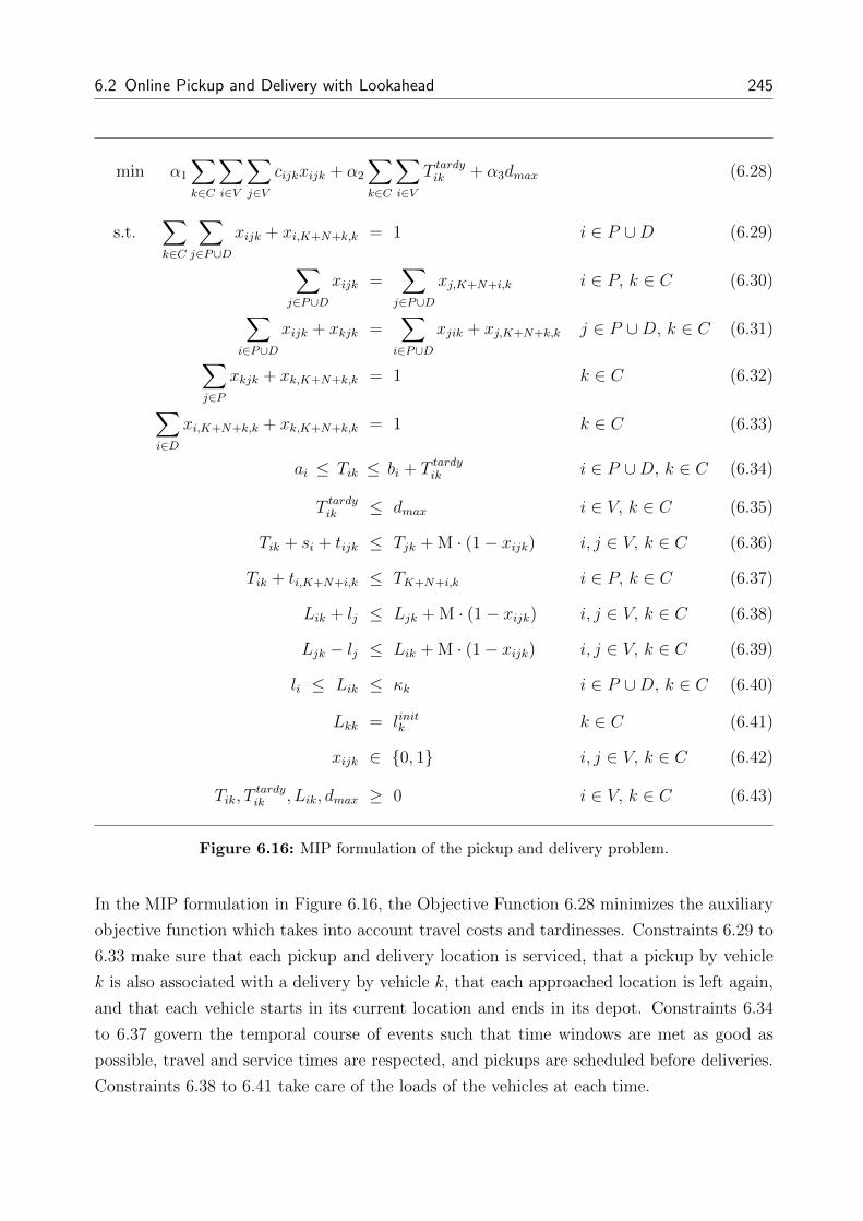
6.2 Online Pickup and Delivery with Lookahead 245
min α1
∑k∈C
∑i∈V
∑j∈V
cijkxijk + α2
∑k∈C
∑i∈V
T tardyik + α3dmax (6.28)
s.t.∑k∈C
∑j∈P∪D
xijk + xi,K+N+k,k = 1 i ∈ P ∪D (6.29)∑j∈P∪D
xijk =∑
j∈P∪Dxj,K+N+i,k i ∈ P, k ∈ C (6.30)∑
i∈P∪Dxijk + xkjk =
∑i∈P∪D
xjik + xj,K+N+k,k j ∈ P ∪D, k ∈ C (6.31)∑j∈P
xkjk + xk,K+N+k,k = 1 k ∈ C (6.32)∑i∈D
xi,K+N+k,k + xk,K+N+k,k = 1 k ∈ C (6.33)
ai ≤ Tik ≤ bi + T tardyik i ∈ P ∪D, k ∈ C (6.34)
T tardyik ≤ dmax i ∈ V, k ∈ C (6.35)
Tik + si + tijk ≤ Tjk + M · (1− xijk) i, j ∈ V, k ∈ C (6.36)
Tik + ti,K+N+i,k ≤ TK+N+i,k i ∈ P, k ∈ C (6.37)
Lik + lj ≤ Ljk + M · (1− xijk) i, j ∈ V, k ∈ C (6.38)
Ljk − lj ≤ Lik + M · (1− xijk) i, j ∈ V, k ∈ C (6.39)
li ≤ Lik ≤ κk i ∈ P ∪D, k ∈ C (6.40)
Lkk = linitk k ∈ C (6.41)
xijk ∈ {0, 1} i, j ∈ V, k ∈ C (6.42)
Tik, Ttardyik , Lik, dmax ≥ 0 i ∈ V, k ∈ C (6.43)
Figure 6.16: MIP formulation of the pickup and delivery problem.
In the MIP formulation in Figure 6.16, the Objective Function 6.28 minimizes the auxiliary
objective function which takes into account travel costs and tardinesses. Constraints 6.29 to
6.33 make sure that each pickup and delivery location is serviced, that a pickup by vehicle
k is also associated with a delivery by vehicle k, that each approached location is left again,
and that each vehicle starts in its current location and ends in its depot. Constraints 6.34
to 6.37 govern the temporal course of events such that time windows are met as good as
possible, travel and service times are respected, and pickups are scheduled before deliveries.
Constraints 6.38 to 6.41 take care of the loads of the vehicles at each time.

246 6 Simulation of Real World Applications
6.2.1 Average Results
All sequential algorithms as well as the simultaneous algorithm were tested. A summary of
the simulation results obtained for all considered performance criteria is given in Appendix
A.3.2; we restrict attention to three selected performance criteria which already illustrate
the trade-offs between competing goals:
• Total travel distance in kilometers
• Tardiness of pickup and delivery operations in minutes
• Order throughput in orders per hour
Figure 6.17 shows the average total distance covered by all vehicles for different lookahead
durations. Apart from Opt, all algorithms possess the potential to acquire reductions in
the total travel distance by providing additional lookahead time. However, because of time
windows, improvement through lookahead in the total travel distance appears neither as
drastic nor as reliable as in all previously considered problem settings that were based on
the TSP with allowed immediate service of requests. We attribute the major degree of
unpredictability concerning the travel distance to the algorithms’ rationale which also opts at
minimizing average and maximum tardiness by means of the auxiliary objective function.
0 50 100 150 200 250 300 350 400 450 500 550 600
1600
1650
1700
1750
Lookahead duration D
Averagedistance
SrhD = 2OptD = SaD TsD OptD
Figure 6.17: Average distances for different lookahead sizes and n = 50 in the pickup and deliveryservice.

6.2 Online Pickup and Delivery with Lookahead 247
Srh, 2Opt and Sa are found to fare best. These algorithms exhibit identical behavior which
means that applying edge exchanging moves as well as swap and shift moves on the route set
determined by Srh did not result in a single route improvement. Hence, algorithms 2Opt
and Sa which are focused on intra-route improvement ([101]) offer no additional benefit. This
is explained by the already elaborate route construction of Srh based on a best insertion
policy and the problem-related difficulty of obtaining feasible routes upon route modifications
due to time windows in conjunction with logical precedence restrictions between pickup and
delivery operations. Although Ts also resorts to routes initially determined by Srh, the
added possibility of order reassignments from one route to another – which was not taken
into account by 2Opt and Sa – leads to structurally different routes that are obviously
worse for the total distance criterion. Yet, for other objective functions we will see that the
inter-route improvement ([101]) approach of Ts is profitable. Concerning the behavior of
exact reoptimization by Opt, we observe that lookahead seems to lead to unstable routings as
already figured out for the TSP in Chapter 5.4: Partial solutions which may be advantageous
for the given snapshot situation may turn out disastrous whenever the current situation
changes as new transportation orders pop up; as a result, subsequent partial solutions may
exhibit a substantially different character.
0 50 100 150 200 250 300 350 400 450 500 550 600
22
24
26
28
Lookahead duration D
Average
tardiness
SrhD = 2OptD = SaD TsD OptD
Figure 6.18: Average tardinesses for different lookahead sizes and n = 50 in the pickup anddelivery service.
The drawn picture of algorithm quality overly changes when the average tardiness of the
vehicles over all pickup and delivery operations is deemed the predominant performance
yardstick: Figure 6.18 suggests algorithms Ts and Opt as the most promising algorithm

248 6 Simulation of Real World Applications
candidates in order to keep tardiness low which is in sharp contrast to superiority of Srh-
based algorithms with respect to the total distance criterion. At this point, we recall that
route quality is assessed by an auxiliary objective function that takes on the form of a linear
combination of total distance, mean tardiness and maximum tardiness. Hence, algorithms
tend to shift their focus on whatever optimization goal can be addressed best by their ra-
tionale. In this sense, algorithm Ts fares best with respect to tardiness-related objectives
by trading an increase in the total distance for a decrease in the average (and maximum)
tardiness. We note that with respect to our selected objective function, Ts yielded routes
with lower aggregated objective value; however, we refrain from drawing general conclusions
upon the objective value dimension due to the drawbacks of scalarization in multicriteria
optimization (see also [70]).
Unfortunately, none of the algorithms is found to benefit from lookahead with respect to
tardiness-related goals. Quite to the contrary, even sophisticated algorithms like Ts and Opt
have to struggle with the instability of “locally” good solutions whose advantages are likely
to be relinquished in the upcoming part of the request sequence. Instead, ad-hoc planning
without taking into account any additionally provided future information is advisable because
large deviations between previously calculated routes and actual travel routes are likely to
occur anyway as a result of changed circumstances once new orders arrive. Because already in
the pure online setting, at each time there are enough unfulfilled orders to induce high vehicle
utilization (cf. Table A.91 of Appendix A.3.2), it suffices to consider the transportation orders
known in this case. The parallel behavior of Ts and Opt is due to our stipulation to use
Ts as a substitute for Opt in case of more than ten orders so as to guarantee reasonable
computational effort. After a closer look at the average distance in Figure 6.17, we also
recognize the parallel behavior of Ts and Opt in this objective for D ≥ 180. Hence, we
draw the same conclusion as in the order picking system: When the lookahead duration
exceeds three hours, problem sizes become too large as to guarantee that instances of Opt
can be solved within the prescribed computing time limit of 120 seconds. Observe that the
parallel but shifted behavior also illustrates the different trade-offs of the algorithms.
After a glance at the first two objectives, we come to the interim conclusion that the general
dilemma of multicriteria optimization is preserved even if large lookahead capabilities are
provided and that it is not as easy to design algorithms compliant with all objectives in a
system of conflicting goals as in a system of complementing or independent goals like in the
order picking system in Chapter 6.1. Since creating short distance routes may only come
along with the price of large violations in the time window constraints, we recognize that in
the application under consideration the decision maker has to be aware of his own trade-off
relations for different goals in order to reach a final decision on algorithm quality.

6.2 Online Pickup and Delivery with Lookahead 249
The average throughput of transportation orders as achieved by the different algorithms is
shown in Figure 6.19.
0 50 100 150 200 250 300 350 400 450 500 550 600
3.66
3.67
3.68
3.69
3.7
3.71
Lookahead duration D
Averagethrough
put
SrhD = 2OptD = SaD TsD OptD
Figure 6.19: Average throughput for different lookahead sizes and n = 50 in the pickup anddelivery service.
Looking at the scale of the diagram, we find that differences between the algorithms are only
of minor magnitude. This observation is explained by the hard restriction on the earliest
possible start time of pickup and delivery operations at the lower bound of coresponding time
window intervals that any algorithm has to respect. Thus, we refrain from deriving further
judgments on algorithm quality based upon the throughput attained by the vehicles.
We come to the overall conclusion that in the problem setting under consideration with
time windows and multiple types of unpredictable events, there is no essential benefit from
lookahead in terms of major improvements in the overall route plan. Immediate planning
upon arrival of transportation orders that does not account for too much future information
proves to be a sufficient methodology to determine feasible routes of fair quality. However,
this recommendation only holds true for the investigated setting with an order dispatching
of n = 50 orders which leads to almost full vehicle utilization (cf. also Table A.91 of
Appendix A.3.2). The decision maker is left over with the task of choosing the algorithm
candidate most consonant with his individual preferences: If goals are equally important,
Opt leads to balanced results concerning several objectives; if travel distance (tardiness and
maximum tardiness) minimization is considered the most important goal, Srh (Ts) is the
most promising candidate.

250 6 Simulation of Real World Applications
6.2.2 Distributional Results
The empirical counting distribution functions incurred by the algorithms with respect to the
total travel distance and tardiness are displayed in Figures 6.20 to 6.22 and in Figures 6.23
to 6.25, respectively. A discussion of the distributional results for the order throughput is
omitted because of the criterion’s irrelevance to the decision making process concerning the
selection of a most appropriate algorithm in the given setting.
In Figure 6.20, the empirical counting distribution functions of the total distance are found to
lie close to each other for different lookahead durations and there are countless intersections
of the plots contradicting an exclusively positive benefit from lookahead. Table A.82 of Ap-
pendix A.3.2 also shows that instances with deteriorated total distance value are encountered
every now and then, even if more lookahead was provided. Nevertheless, the slight positive
influence of lookahead can clearly be seen by the relative position of the plots of successive
lookahead levels to each other. Medium widths of confidence intervals and coefficients of
variation admit that the distance to be expected cannot be preestimated as accurately as
in the simulation of the order picking system in Chapter 6.1. Yet, results are representative
because of a fair average deviation of 70 meters per kilometer of the average total distance.
Performance ratios of the total distance incurred by the online algorithms under lookahead
relative to Ts,Opt600 in Figure 6.21 appear centered around the value of 1. This means that
– albeit their informational state is worse – online algorithms under lookahead lead to shorter
routes on a considerable proportion of instances as compared to the routes determined under
complete information. The plots of the empirical counting distribution functions exhibit
numerous intersection points with each other, yet allow to establish an approximate order
by their relative positions to each other for different lookahead durations. Table A.83 of
Appendix A.3.2 confirms that a significant fraction of input instances has experimental
competitive ratio smaller than 1. Analogous statements are derived for the performance
ratio of the total distance relative to the online version of an algorithm (cf. Figure 6.22 and
Table A.84 of Appendix A.3.2).
Concerning the distributional results with respect to the tardiness over all pickup and delivery
operations as incurred by the different algorithms, Figures 6.23 to 6.25 in combination with
Tables A.85 to A.87 of Appendix A.3.2 are affirmative to the ineffectiveness of additional
time units of lookahead: Plots of all different lookahead durations intersect with each other
in a disordered fashion for countless times such that no order relation between any of the
empirical counting distribution functions from different information regimes is recognizable
at all.

6.2 Online Pickup and Delivery with Lookahead 251
1400 1600 1800 2000 22000
0.2
0.4
0.6
0.8
1
v
F(v)
Srh0 Srh60
Srh120 Srh180
Srh240 Srh300
Srh360 Srh420
Srh480 Srh540
Srh600 Opt600
1400 1600 1800 2000 22000
0.2
0.4
0.6
0.8
1
v
F(v)
2Opt0 2Opt60
2Opt120 2Opt180
2Opt240 2Opt300
2Opt360 2Opt420
2Opt480 2Opt540
2Opt600 Opt600
1400 1600 1800 2000 22000
0.2
0.4
0.6
0.8
1
v
F(v)
Sa0 Sa60
Sa120 Sa180
Sa240 Sa300
Sa360 Sa420
Sa480 Sa540
Sa600 Opt600
1400 1600 1800 2000 22000
0.2
0.4
0.6
0.8
1
v
F(v)
Ts0 Ts60
Ts120 Ts180
Ts240 Ts300
Ts360 Ts420
Ts480 Ts540
Ts600 Opt600
1400 1600 1800 2000 22000
0.2
0.4
0.6
0.8
1
v
F(v)
Opt0 Opt60
Opt120 Opt180
Opt240 Opt300
Opt360 Opt420
Opt480 Opt540
Opt600 Opt600
Figure 6.20: Empirical counting distribution functions of distance for n = 50 in the pickup anddelivery service.

252 6 Simulation of Real World Applications
0.8 1 1.20
0.2
0.4
0.6
0.8
1
v
F(v)
Srh0 Srh60
Srh120 Srh180
Srh240 Srh300
Srh360 Srh420
Srh480 Srh540
Srh600
0.8 1 1.20
0.2
0.4
0.6
0.8
1
v
F(v)
2Opt0 2Opt60
2Opt120 2Opt180
2Opt240 2Opt300
2Opt360 2Opt420
2Opt480 2Opt540
2Opt600
0.8 1 1.20
0.2
0.4
0.6
0.8
1
v
F(v)
Sa0 Sa60
Sa120 Sa180
Sa240 Sa300
Sa360 Sa420
Sa480 Sa540
Sa600
0.8 1 1.20
0.2
0.4
0.6
0.8
1
v
F(v)
Ts0 Ts60
Ts120 Ts180
Ts240 Ts300
Ts360 Ts420
Ts480 Ts540
Ts600
0.8 1 1.20
0.2
0.4
0.6
0.8
1
v
F(v)
Opt0 Opt60
Opt120 Opt180
Opt240 Opt300
Opt360 Opt420
Opt480 Opt540
Opt600
Figure 6.21: Empirical counting distribution functions of performance ratio of distance relativeto Ts,Opt600 for n = 50 in the pickup and delivery service.
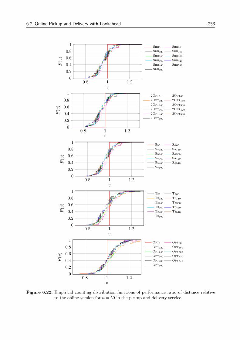
6.2 Online Pickup and Delivery with Lookahead 253
0.8 1 1.20
0.2
0.4
0.6
0.8
1
v
F(v)
Srh0 Srh60
Srh120 Srh180
Srh240 Srh300
Srh360 Srh420
Srh480 Srh540
Srh600
0.8 1 1.20
0.2
0.4
0.6
0.8
1
v
F(v)
2Opt0 2Opt60
2Opt120 2Opt180
2Opt240 2Opt300
2Opt360 2Opt420
2Opt480 2Opt540
2Opt600
0.8 1 1.20
0.2
0.4
0.6
0.8
1
v
F(v)
Sa0 Sa60
Sa120 Sa180
Sa240 Sa300
Sa360 Sa420
Sa480 Sa540
Sa600
0.8 1 1.20
0.2
0.4
0.6
0.8
1
v
F(v)
Ts0 Ts60
Ts120 Ts180
Ts240 Ts300
Ts360 Ts420
Ts480 Ts540
Ts600
0.8 1 1.20
0.2
0.4
0.6
0.8
1
v
F(v)
Opt0 Opt60
Opt120 Opt180
Opt240 Opt300
Opt360 Opt420
Opt480 Opt540
Opt600
Figure 6.22: Empirical counting distribution functions of performance ratio of distance relativeto the online version for n = 50 in the pickup and delivery service.

254 6 Simulation of Real World Applications
0 20 40 60 80 100 1200
0.2
0.4
0.6
0.8
1
v
F(v)
Srh0 Srh60
Srh120 Srh180
Srh240 Srh300
Srh360 Srh420
Srh480 Srh540
Srh600 Opt600
0 20 40 60 80 100 1200
0.2
0.4
0.6
0.8
1
v
F(v)
2Opt0 2Opt60
2Opt120 2Opt180
2Opt240 2Opt300
2Opt360 2Opt420
2Opt480 2Opt540
2Opt600 Opt600
0 20 40 60 80 100 1200
0.2
0.4
0.6
0.8
1
v
F(v)
Sa0 Sa60
Sa120 Sa180
Sa240 Sa300
Sa360 Sa420
Sa480 Sa540
Sa600 Opt600
0 20 40 60 80 100 1200
0.2
0.4
0.6
0.8
1
v
F(v)
Ts0 Ts60
Ts120 Ts180
Ts240 Ts300
Ts360 Ts420
Ts480 Ts540
Ts600 Opt600
0 20 40 60 80 100 1200
0.2
0.4
0.6
0.8
1
v
F(v)
Opt0 Opt60
Opt120 Opt180
Opt240 Opt300
Opt360 Opt420
Opt480 Opt540
Opt600 Opt600
Figure 6.23: Empirical counting distribution functions of tardiness for n = 50 in the pickup anddelivery service.
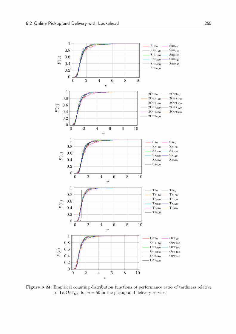
6.2 Online Pickup and Delivery with Lookahead 255
0 2 4 6 8 100
0.2
0.4
0.6
0.8
1
v
F(v)
Srh0 Srh60
Srh120 Srh180
Srh240 Srh300
Srh360 Srh420
Srh480 Srh540
Srh600
0 2 4 6 8 100
0.2
0.4
0.6
0.8
1
v
F(v)
2Opt0 2Opt60
2Opt120 2Opt180
2Opt240 2Opt300
2Opt360 2Opt420
2Opt480 2Opt540
2Opt600
0 2 4 6 8 100
0.2
0.4
0.6
0.8
1
v
F(v)
Sa0 Sa60
Sa120 Sa180
Sa240 Sa300
Sa360 Sa420
Sa480 Sa540
Sa600
0 2 4 6 8 100
0.2
0.4
0.6
0.8
1
v
F(v)
Ts0 Ts60
Ts120 Ts180
Ts240 Ts300
Ts360 Ts420
Ts480 Ts540
Ts600
0 2 4 6 8 100
0.2
0.4
0.6
0.8
1
v
F(v)
Opt0 Opt60
Opt120 Opt180
Opt240 Opt300
Opt360 Opt420
Opt480 Opt540
Opt600
Figure 6.24: Empirical counting distribution functions of performance ratio of tardiness relativeto Ts,Opt600 for n = 50 in the pickup and delivery service.

256 6 Simulation of Real World Applications
0 2 4 60
0.2
0.4
0.6
0.8
1
v
F(v)
Srh0 Srh60
Srh120 Srh180
Srh240 Srh300
Srh360 Srh420
Srh480 Srh540
Srh600
0 2 4 60
0.2
0.4
0.6
0.8
1
v
F(v)
2Opt0 2Opt60
2Opt120 2Opt180
2Opt240 2Opt300
2Opt360 2Opt420
2Opt480 2Opt540
2Opt600
0 2 4 60
0.2
0.4
0.6
0.8
1
v
F(v)
Sa0 Sa60
Sa120 Sa180
Sa240 Sa300
Sa360 Sa420
Sa480 Sa540
Sa600
0 2 4 60
0.2
0.4
0.6
0.8
1
v
F(v)
Ts0 Ts60
Ts120 Ts180
Ts240 Ts300
Ts360 Ts420
Ts480 Ts540
Ts600
0 2 4 60
0.2
0.4
0.6
0.8
1
v
F(v)
Opt0 Opt60
Opt120 Opt180
Opt240 Opt300
Opt360 Opt420
Opt480 Opt540
Opt600
Figure 6.25: Empirical counting distribution functions of performance ratio of tardiness relativeto the online version for n = 50 in the pickup and delivery service.

6.3 Concluding Discussion 257
We conclude this section by pointing out that hard constraints, such as retained earliest
service times, and competing objectives, such as distance and tardiness, make it considerably
harder for algorithms to elicit any improvement out of additional information preview at all.
In particular, straight-forward extensions of pure online algorithms to the lookahead case are
of no use. From a managerial point of view, we recommend not to blindly install technical
devices for the retrieval of lookahead information and not to hope for improvement without
having an algorithm at hand which could reliably make use of lookahead in the face of
competing objectives. Instead of that, it is advisable to spend more money on research for
algorithms that align their rationale with lookahead and multiple goals.
6.3 Concluding Discussion
We analyzed the effect of lookahead on the quality of solutions obtained by several algorithm
candidates in two real world applications by means of simulation studies. In contrast to
the standard online optimization problems examined in Chapters 4 and 5, the settings are
characterized by a higher degree of complexity as a result of additional random events,
realistic restrictions upon system operations and relevance of multiple performance criteria.
We found that lookahead can be exploited to a fair extent similar as in the underlying
standard problems whenever goals are complementary to each other. Under conflicting ob-
jectives, however, we discovered that the positive effects of lookahead found in corresponding
standard problems with only one objective could not be adapted to the multicriteria case.
The future challenge in this field mainly lies in designing algorithms which are able to cope
with the relations of several objectives to each other and also capitalize from lookahead.
Concerning the transferability of statements about the lookahead effect from standard prob-
lems to complex dynamic settings, we recognize that a one-to-one mapping is not possible.
Yet, the standard problems still deliver the vast majority of explanations for the effects that
are observed also in the more realistic settings. For instance, the large difference in the
impact of lookahead in the two applications from this chapter is mainly attributable to the
rule set exchange in form of allowed immediate processing that was invoked in the order
picking system but not in the pickup and delivery service because of time windows.
Added practical features may counteract the effects from the standard problems: The set of
constraints in an application determines the degrees of freedom that an algorithm can take
advantage of to calculate its solution proposal. As a result, a problem’s constraint set already
implies the optimization potential that may be exploited by appropriate algorithms. In this

258 6 Simulation of Real World Applications
context, specified time windows in the pickup and delivery service which are retained under
lookahead appeared as the major spoiler for performance improvement upon provision of
additional information by pruning the problem’s optimization potential already in advance.
Blocking effects in the order picking system had no influence on the total distance objective,
but lead to minor degradations in the throughput and makespan objectives.
Algorithms based on exact reoptimization showed no additional benefit compared to heuristic
methods. In particular, the computing time limit of 120 seconds per snapshot problem as
prescribed by real-time requirements in both applications was exceeded almost surely for
lookahead duration D ≥ 180 minutes due to the size of the resulting IP and MIP models
such that substitute solutions had to be determined by heuristic approaches anyway.
Table 6.1 displays the results of the simulation studies in a condensed form: For the order
picking system, we found considerable improvement in all goals through additional lookahead
(column ∆f r,r′,P,P ′
Alg,Alg′). The benefit is accrued through allowed immediate processing of boxes
and not having to wait for their arrivals (column ∆fP,P′
Alg,Alg′). As a consequence, the mere
benefit of information is deemed negligible (column ∆f r,r′
Alg). Quite to the contrary, in the
pickup and delivery service hardly any improvement occurred because of the algorithms’
incapability to deal with competing objectives in general. Since time windows were retained,
the minor lookahead effects are attributed to their informational component. The column
Alg∗ indicates whether there was some algorithm or a group of comparably good algorithms
that outperformed the remaining algorithms. In the order picking system, routing strategies
Opt and S along with batching algorithms Ls, Ts and Seed excelled remaining strategy
combinations for three of the four objectives; in the remaining objective there were no
remarkable differences. In the pickup and delivery service, each algorithm exhibited a trade-
off between competing objectives. While Srh, 2Opt and Sa lead to shorter total distances
than Ts and Opt, the latter group did considerably better with respect to the objectives
related to tardiness. In both applications, exact reoptimization did not result in significant
advantages compared to heuristics (column Opt) and deterioration in the objective value
could occur although additional lookahead was provided (column Deterioration).
While in standard problems viable algorithms often perform at comparable quality levels,
the simulation studies revealed that algorithms may exhibit fundamentally different perfor-
mance in realistic settings. Hence, the first step towards efficient logistics operations consists
of selecting the right algorithm which matches the decision maker’s preferences best. We
conclude that simulation is a suitable method to elicit the information (e.g., key performance
indicators or counting distributions of algorithm performance for multiple goals) needed by
managers of real world systems to successfully deploy their decision making processes.

6.3 Concluding Discussion 259
App
lica
tion
Ru
les
Typ
eO
bje
ctiv
e∆fr,r′ ,P,P′
Alg,A
lg′
∆fr,r′
Alg
∆fP,P′
Alg,A
lg′
Alg∗
Opt
Det
erio
rati
on
Ord
erpic
kin
gp
erm
uta
tion
s,blo
ckin
gti
me
look
ah
ead
mak
espan
larg
eneg
ligi
ble
larg
eno
no
yes
dis
tan
cela
rge
neg
ligi
ble
larg
eyes
no
yes
uti
liza
tion
larg
eneg
ligi
ble
larg
eyes
yes
yes
thro
ugh
put
larg
en
egligi
ble
larg
eye
sno
yes
Pic
ku
pan
ddel
iver
yti
me
win
dow
s,tr
affi
csc
ene
tim
elo
okah
ead
mak
espan
neg
ligi
ble
neg
ligi
ble
zero
yes
no
yes
dis
tan
cesm
all
smal
lze
royes
no
yes
tard
ines
sze
roze
roze
roye
sno
yes
max
imum
tard
ines
sze
roze
roze
roye
sno
yes
uti
liza
tion
med
ium
med
ium
zero
no
no
yes
thro
ugh
put
neg
ligi
ble
neg
ligi
ble
zero
yes
no
yes
Table
6.1:
Qu
alit
ativ
esu
mm
ary
ofth
esi
mula
tion
resu
lts
from
Chap
ter
6.


261
7 Conclusion and Outlook
In this thesis, the topic of online optimization with lookahead was addressed from a multi-
faceted point of view with the intention to lay out generically applicable methodologies for
the analysis of algorithms and to demonstrate their applicability in different problem settings.
We close this thesis by summarizing the main contributions, relating them to the research
questions introduced in Chapter 1 and pointing out to directions for future research.
7.1 Conclusion
Catalyzed by dozens of applications featuring online optimization problems with lookahead
on the one hand, but given the poor set of comprehensive methods for algorithm analysis
in this optimization paradigm on the other hand, we started our research in the fundamen-
tals of the concepts of online optimization and lookahead information. Since both terms
are understood and used in a versatile fashion, we first established clear, but yet flexible
definitions for these terms which facilitate a modeling of lookahead in different online opti-
mization problems using the same taxonomy and notation. Additionally, we subdivided the
mechanism of lookahead into an informational and a processual component. Referring to
Chapter 2, this leads us to the answer of the first research question:
RQ1 What do we understand by lookahead?
Lookahead is a mechanism of information release that specifies the difference in the
process of information disclosure as compared to a reference online optimization prob-
lem (instance revelation rule substitution) and that might impose a set of constraints
differing from the set of constraints in the reference online optimization problem upon
the processing of the input elements (rule set substitution).
In conjunction with the answer of this question, we emphasize that lookahead – both the
way it leads to forwarded information release and also the way it affects processing of input
262 7 Conclusion and Outlook
elements – is defined in existing literature only in problem-specific contexts of publications
which prohibits a structurally-oriented view on the effects caused by it. Using the approach
outlined in this thesis, we are able to attribute a reason to lookahead effects observed in
problems and to transfer that knowledge also to other settings.
We realized that in order to design algorithms for online optimization problems with looka-
head, we first need to understand how they should act within the solution process of an
instance. Driven by the sequentiality in the information element release process, we found a
large number of analogies to the control of discrete event dynamic systems (cf. Chapter 2).
As a result, we adapted the concepts from this domain and coined them towards the needs of
the solution process in an instance of an online optimization problem with lookahead. This
allows us to address research question RQ2 based on the general modeling framework for
online optimization with lookahead developed in Chapter 3:
RQ2 Which formalism can be used to model the solution process in an online optimization
problem with lookahead in a generally applicable framework?
The solution process is abstractly emulated as the state trajectory of our state-based
discrete event modeling framework. The evolution of the state trajectory over time
is induced by the decisions of an algorithm for the snapshot problems of the online
optimization problem under consideration. Algorithm execution occurs whenever the
state is stimulated to advance, e.g., upon an external trigger in form of an event such
as the release of a new input element.
A particular emphasis in the modeling framework is put on lookahead-related issues such
as processing modes, orders and accessibilities. Hence, devising algorithms for online opti-
mization with lookahead is no more seen as a problem-specific task independent of a general
optimization paradigm, but closely intertwined with the abstract concept of lookahead as
introduced in Chapter 2 and the framework from Chapter 3. Moreover, solution concepts can
now be described independent of domains in an abstract way using a unified taxonomy.
The commonly used standard performance yardstick for online algorithms is competitive
analysis although there is undisputed agreement that this worst-case analysis lacks display-
ing the typical behavior of an algorithm over all input sequences and has numerous other
drawbacks ([65], [73]). We are lead to the conclusion that other, more comprehensive anal-
ysis methods are required in practice: According to the very nature of online optimization,
no stochastic information is given, i.e., one has to hedge against all possible scenarios. As
a consequence, we impute the uniform distribution as the distribution of maximum entropy
(or analogously of minimum prior information) on the release of input elements ([97], [98]).

7.1 Conclusion 263
What we obtain are counting results yielding frequency information about the occurrences
of specific objective function or performance ratio values. We called the corresponding dis-
tribution functions the counting distribution functions of the objective value and of the
performance ratio, respectively (see Chapter 2); they form the basis of our approach to
performance measurement in online optimization with lookahead as addressed in RQ3 and
conducted in Chapters 4 to 6:
RQ3 Which performance measurement approach is best suitable to analyze the performance
of algorithms in online optimization problems with lookahead and to relate the quality
of algorithms to each other?
Algorithm performance is not measured based on a single performance indicator. Algo-
rithm performance is evaluated by the decision maker with his individual preferences
based on the counting distribution functions of the objective value and of the per-
formance ratio for candidate algorithms relative to each other. The objective value
distribution yields global information concerning the absolute performance achieved
by individual algorithms, whereas performance ratio distributions indicate the relative
performance of algorithms to each other on the same input instance, i.e., a type of local
information. Different lookahead regimes are accounted for by relating algorithm per-
formance to some reference information regime which yields the baseline for counting
distributions both of the objective value and of the performance ratio.
Presenting a decision maker with the counting distribution functions instead of single per-
formance indicators puts the burden of defining trade-offs between worst case, best case and
average case off our shoulders. The decision maker is equipped with all possible information
except for the direct mapping of objective values and performance ratios to input instances.
For holistic decision making, we cannot think of a more comprehensive way to supply a
decision maker with information about algorithm behavior. In case of a high number of
algorithm alternatives, one can conduct an average-case analysis in the first step to filter out
algorithms which shall be investigated by distributional analysis in the second step.
Knowing the magnitude of the lookahead impact on solution quality for different algorithms
in a given application is important to practitioners when they have to decide whether it
would be beneficial to invest in new machinery with lookahead devices, and if so, what
level of lookahead capability should be selected. From an academic point of view, it is of
interest which kinds of problems are amenable to lookahead in terms of improved algorithm
performance and which are not. We studied the impact of lookahead in theory (cf. Chapter
4), in basic practical settings (cf. Chapter 5), and in real world applications (cf. Chapter 6)
which brings us in a position to answer the last research question:

264 7 Conclusion and Outlook
RQ4 What is the value of different degrees of lookahead in specific online optimization
problems with lookahead?
The extent of the lookahead effect clearly depends on the problem setting under in-
vestigation. Overall, we found that there is a positive effect on objective values and
on performance ratios when algorithms are supplied with lookahead. However, the
magnitude of the effect depends on several key characteristics of the problem such as:
• Allowance of algorithms to take advantage of lookahead by rule set substitution
• Admissible degrees of freedom for algorithms as imposed by problem constraints
• Possibility of bad decisions and risk of deterioration upon lookahead provision
• Performance quality gap between offline algorithms and pure online algorithms
without lookahead
Details on the magnitude of the lookahead effects for different levels of information
preview as determined for a large number of problem classes can be looked up in
Chapters 4 to 6 along with corresponding explanations. We remark that problems
where solution quality is strongly affected by permuting the input element release
order during processing and where algorithms are allowed to change that order have a
high potential for significant benefits from lookahead as long as the feasible set of the
instance admits the necessary degrees of freedom. Moreover, there are problem types
where more information never leads to a degradation in performance, but also problem
types where “wrong” decisions may be made although more information was provided.
To the best of our knowledge, our exact analyses in Chapter 4 are the first to give an exact
image reproducing algorithm behavior over all input sequences in the respective problems.
Despite the small size of the basic settings, as a byproduct, the proofs already provided
explanations for the lookahead effects which were also encountered in the more realistic
settings. The computational results of Chapter 5 may serve to future works in the field of
online optimization as an information pool concerning the impact of lookahead in several
standard problems. In Chapter 6, we already took advantage of this information pool by
easily delivering explanations for the effects of lookahead in two real world applications.
Nonetheless, in this context it became clear that results can never be transferred in a one-
to-one fashion due to additional constraints in practical problems. We recognized that in
real world applications there is an additional dimension of onlineness in form of random
occurrences that are out of control in operations and hardly calculable at all. Due to the
complexity of the settings, we used simulation models to study the influence of lookahead with
respect to the input element disclosure when systems are additionally subject to unforeseeable

7.2 Outlook 265
random events. We recommend to make use of simulation studies in order to determine the
lookahead effect prior to operating a system whenever an algorithm needs to be selected but
the number of dependent random variables – whose realizations taken together lead to the
realization of the random variable for the attained objective value – is too large.
Algorithms in online optimization are required to respond to the arrival of input data within
few seconds, i.e., they have to be real-time compliant. Throughout our computational experi-
ments, we could not observe an advantage of exact reoptimization over heuristic methods in
solving the snapshot problems: “Locally” optimal solutions lost their efficacy once the situa-
tion changed upon arrival of new input elements. Quite to the contrary, computational effort
is out of scale compared to heuristics such that no need is seen for exact reoptimization.
Overall, this thesis
• provided a clear and versatile definition of the optimization paradigm of online opti-
mization with lookahead,
• related it to the established paradigms of online and offline optimization,
• characterized components of the lookahead effect,
• presented a holistic approach to performance assessment of candidate algorithms which
may resort to different information regimes,
• developed a generic modeling framework for online optimization with lookahead, and
• determined the value of information using exact analysis in basic problem settings,
extensive sample-based analysis in standard problem settings and simulation studies
in real world applications.
7.2 Outlook
Future research directions in the field of online optimization with lookahead emerge from
limitations of the presented approaches on the one hand and from related topics that were
not addressed in this thesis on the other hand.
The derivation of exact expressions for the counting distribution functions in Chapter 4
showed that already in basic settings it is hard to gain access to the combinatorial structures
that govern the behavior of algorithms during input element processing. We recognize that
for more complex settings an analysis of this type is likely to be out of scope such that the
approach has to be transferred to sample-based methods (cf. Chapters 5 and 6) or reduced

266 7 Conclusion and Outlook
to order relations between objective value distributions of algorithms (cf. also [9], [10], [90]).
With respect to the first direction, we identify the need for a thorough examination of how to
propagate methods of distributional analysis to experimental algorithm analysis in general
and especially in settings which involve multicriteria online optimization with lookahead;
concerning the second direction, it has to be checked which types of mathematical statements
are realistic to be elicited in further exact analysis.
Because the provision of lookahead may intrinsically yield an altered set of constraints as a
consequence of a rule set substitution, we argue that defining the snapshot problem to be
solved in each reoptimization step in a way different from just adapting the overall problem
to the current lookahead set could contribute to enhanced algorithm performance. The
rationale behind this idea is to bring the algorithm in a best possible position for future
steps at the end of each reoptimization step. As an example, we suggest in the snapshot
problems of the TSP not to compute a Hamiltonian path that returns to the origin but
to a point that minimizes the (expectation of the) total distance of all locations to that
point (median); likewise, one could avoid zig-zagging in routes by additionally incorporating
enforced stability constraints which forbid frequent moves to distant regions. For the bin
packing problem, we carried out this approach by modifying the objective function such
that not only the total number of bins is minimized but also that bins as full and empty
as possible are generated and not bins at medium capacity (see also [72]). The stream of
publications on online stochastic combinatorial optimization by Bent and Van Hentenryck
([22], [23], [24], [25]) represents a first step in this direction by taking into account several
alternative objective functions. Future research could also consider variable forms of the
snapshot problem as input to algorithms already in their design phase, and the goal would
be to determine the snapshot problem type which yields the best algorithm performance.
In the same line of argumentation, we point out that stability (in the sense of consistency over
time) of the partial solutions with regard to some problem-related criterion could be a major
contributor to solid decision making: For instance, in the TSP, “nearness”-oriented algorithm
NearestNeighbor lead to routes that were more robust under future scenarios than those
determined by exact reoptimization. Similar results are also known for (reactive) project
scheduling ([58]) where it is recommended to insert time buffers in schedules to make them
robust for future deviations. Hence, we conclude that the inclusion of stability-enforcing
constraints into subproblem formulations should be addressed in future works.
Throughout this thesis, we were only concerned with the value of lookahead but not with
the costs that are related to it. Realizing lookahead in practice amounts to the installation
of costly technical devices such as barcode or radio-frequency identification (RFID) tag

7.2 Outlook 267
scanners which facilitate transmitting information about input elements at an earlier point
in time. Installation and operation of such machinery induces a fair amount of costs, and it
needs to be checked whether the benefits of lookahead exceed the costs of lookahead device
installation and operations. To this end, economic models and methods that translate the
value of lookahead into a monetary equivalent are still needed.
Real world applications typically feature multiple, oftentimes conflicting optimization goals.
As figured out in Chapter 6, the task of designing algorithms which are able to exploit looka-
head in more than one goal at the same time is not trivial and requires more sophisticated
approaches than mere adaptation of pure online algorithms to the lookahead case. Future re-
search in this direction would comprise devising algorithms for practical settings specifically
tailored towards lookahead utilization that take several objectives as well as their trade-offs
into account in their rationale.
With the paging and ski rental problem, we identified two problem classes where algorithms
could not go wrong by using additional information. Contrarily, in all other problems we
encountered instances with objective value degradation although lookahead capabilities were
enlarged. It is of general interest to find characterizations for problem settings where it can
be guaranteed that additional information never leads to worse decisions (similar to matroid
structures ensuring optimality of greedy choices in offline optimization ([82])). We conjecture
that properties akin to those required for employing dynamic programming upon a given
problem, namely optimality of subsolutions and independence of substructures ([54]), are
required in order to assure no threat by providing additional lookahead information. We
leave a detailed examination of this question to future research.
Another interesting research question encompasses the relation between resource augmenta-
tion and lookahead: We might ask whether physical resources and informational resources
are interchangeable. In the framework of competitive analysis, it has been shown for two
single machine scheduling problems that increasing processor speed is more valuable than
allowing an algorithm to foresee the future ([28], [102]). The effect of resource augmen-
tation on competitive ratios has also been investigated in paging (by increased cache size
([149])) and bin packing (by increased bin sizes ([56], [71])). In these problems, the connec-
tion of resource augmentation to lookahead – not only in competitive analysis but also in
distributional analysis – remains an open question.
Although tremendous research effort has been spent on online optimization over the past two
decades, it is still widely believed that the state of the art is yet far from reaching maturity
([84], [85]). In particular, there is no agreed groundwork of methods and tools for compre-
hensive algorithm analysis in online optimization, not to mention in online optimization with

268 7 Conclusion and Outlook
lookahead. This thesis aimed at contributing towards the elimination of this deficiency by
providing a commonly agreeable basis for the modeling and the analysis of algorithms in this
optimization paradigm in order to establish a harmonized understanding of the mechanism
of information preview and to foster the use of holistic algorithm assessment methods across
application domains. We recognize that there is still a long way to go in this direction,
but we hope for future research to revisit, foster or extend some of the ideas and concepts
brought up in this thesis.

269
A Appendix
A.1 Additional Proofs from Chapter 4
A.1.1 Proof of Lemma 4.4
a) See [131], chapter 7, pages 115 and 116.
b) The proof is a modification of [127]: The number of recurring unit-sloped paths of
length 2i with sk ≥ −1 for k = 0, 1, 2, . . . , 2i is the number of all recurring unit-sloped
paths of length 2i minus the number of all recurring unit-sloped paths of length 2i
which hit the number −2 at least once.
For each of these paths hitting −2 at least once, define T as the first time −2 is hit by
the path (see Figure A.1). According to the reflection principle, we can start a mirror
path at T with respect to the horizontal axis with ordinate −2 that necessarily ends
at height −4 at time 2k (the mirror position of 0 with respect to −2).
1 T 2i
1
Figure A.1: Reflection principle.
Thus, counting the paths from (0, 0) to (2k, 0) hitting −2 at least once is the same
as counting the paths from (0, 0) to (2k,−4) hitting −2 at least once. But any such
path must hit −2 at some point, i.e., we are computing the total number of paths from
(0, 0) to (2k,−4).

270 A Appendix
In total, we obtain that the number of recurring unit-sloped paths of length 2i with
sk ≥ −1 for k = 0, 1, 2, . . . , 2i is equal to the total number of paths from (0, 0) to
(2k, 0) minus the total number of paths from (0, 0) to (2k,−4) which is equal to(2k
k
)−(
2k
k + 2
)=
(2k)!
(k!)2− (2k)!
(k + 2)!(k − 2)!
=(2k)!
(k!)2
(1− k(k − 1)
(k + 1)(k + 2)
)
=(2k)!
(k!)2
(k + 1)(k + 2)− k(k − 1)
(k + 1)(k + 2)
=(2k)!
(k!)2
4k + 2
(k + 1)(k + 2)
=1
k + 2
1
(k + 1)!
(2k)!(4k + 2)
k!
=1
k + 2
1
(k + 1)!
(2k)!(4k + 2)(k + 1)
(k + 1)!
=1
k + 2
1
(k + 1)!
(2k)!(4k2 + 6k + 2)
(k + 1)!
=1
k + 2
1
(k + 1)!
(2k)!(2k + 1)(2k + 2)
(k + 1)!
=1
k + 2
(2k + 2
k + 1
)= Ck+1.
A.1.2 Proof of Lemma 4.9
We show that ∑i≥1
Ci
(2n− 2i
m− i
)−∑i≥1
Ci−1
(2n− 2i+ 1
m− i+ 1
)= 0.
Notice that from the definition of the binomial coefficient, i ranges in {1, 2, . . . , 2n−m} in
both terms.

A.1 Additional Proofs from Chapter 4 271
Hence,
∑i≥1
Ci
(2n− 2i
m− i
)−∑i≥1
Ci−1
(2n− 2i+ 1
m− i+ 1
)
= C1
(2n− 2
m− 1
)+ C2
(2n− 4
m− 2
)+ C3
(2n− 6
m− 3
)+ . . .+ C2n−m
(2m− n2m− n
)
−(C0
(2n− 1
m
)+ C1
(2n− 3
m− 1
)+ C2
(2n− 5
m− 2
)+ . . .+ C2n−m−1
(2m− n+ 1
2m− n+ 1
))
= C1
(2n− 3
m− 2
)+ C2
(2n− 5
m− 3
)+ . . .+ C2n−m−1
(2m− n+ 1
2m− 2n
)+ C2n−m −
(2n− 1
m
)
=2n−m−1∑i=1
Ci
(2n− 2i− 1
m− i− 1
)+ C2n−m −
(2n− 1
m
)
=2n−m−1∑i=0
Ci
(2n− 2i− 1
m− i− 1
)−(
2n− 1
m− 1
)+ C2n−m −
(2n− 1
m
)
=2n−m∑i=0
Ci
(2n− 2i− 1
m− i− 1
)− C2n−m
(2m− 2n− 1
2m− 2n− 1
)−(
2n− 1
m− 1
)+ C2n−m −
(2n− 1
m
)
=∑i≥0
Ci
(2n− 2i− 1
m− i− 1
)− C2n−m −
(2n− 1
m− 1
)+ C2n−m −
(2n− 1
m
)
=
(2n
m
)−(
2n− 1
m− 1
)−(
2n− 1
m
)=
(2n
m
)−(
2n
m
)= 0.

272 A Appendix
A.2 Numerical Results from Chapter 5
This section contains a detailed statistical summary of the numerical results gathered during
the experimental analysis in Chapter 5. For each problem, we give three tables:
• The first table subsumes in one line per algorithm and lookahead level the key figures
with respect to the objective values incurred over the set of sampled input instances.
• The second table subsumes in one line per algorithm and lookahead level the key
figures with respect to the performance ratio relative to an optimal offline algorithm if
available, or relative to the best offline algorithm applied.
• The third table subsumes in one line per algorithm and lookahead level the key figures
with respect to the performance ratio relative to an online algorithm from the same
class of algorithms.
The following key figures were calculated from the samples of random input instances:
µ Average of objective value or performance ratio
CV Coefficient of variation of objective value or performance ratio
95 % CI 95 % confidence interval of objective value or performance ratio
min Minimum objective value or performance ratio
max Maximum objective value or performance ratio
q0.01 First percentile of objective value or performance ratio counting distribution
q0.5 Median of objective value or performance ratio counting distribution
q0.99 99th percentile of objective value or performance ratio counting distribution
% det. Fraction of samples with deterioration in the objective value when compared to the
same algorithm with the lookahead level preceding the algorithm’s lookahead level
F (1) Fraction of samples with performance ratio smaller than 1 relative to the optimal
offline algorithm if available, or relative to a best possible offline algorithm among
those offline algorithms which terminated
1 − F (1) Fraction of samples with performance ratio larger than 1 relative to an online
algorithm from the same class of algorithms

A.2 Numerical Results from Chapter 5 273
A.2.1 Online Ski Rental with Lookahead
Costs for nmax = 100
Algorithm µ CV 95% CI min max q0.01 q0.5 q0.99 % det.
Alg1,1 50 0 [50, 50] 50 50 50 50 50Alg1,5 48.1 0.19 [46.3, 49.9] 1 50 1.5 50 50 0Alg1,10 45.95 0.28 [43.42, 48.48] 1 50 1.5 50 50 0Alg1,20 42.4 0.37 [39.31, 45.49] 1 50 1.5 50 50 0Alg1,30 39.85 0.41 [36.63, 43.07] 1 50 1.5 50 50 0Alg1,40 38.3 0.42 [35.13, 41.47] 1 50 1.5 50 50 0
Alg1,50...100 37.75 0.42 [34.63, 40.87] 1 50 1.5 50 50 0Alg25,1 59.24 0.45 [53.99, 64.49] 1 74 1.5 74 74Alg25,5 57.34 0.47 [52.03, 62.65] 1 74 1.5 74 74 0Alg25,10 55.19 0.5 [49.75, 60.63] 1 74 1.5 74 74 0Alg25,20 51.64 0.52 [46.35, 56.93] 1 74 1.5 74 74 0Alg25,30 49.09 0.53 [43.96, 54.22] 1 74 1.5 50.5 74 0Alg25,40 47.54 0.52 [42.67, 52.41] 1 74 1.5 50.5 74 0
Alg25,50...100 37.75 0.42 [34.63, 40.87] 1 50 1.5 50 50 0Alg50,1 62.74 0.61 [55.2, 70.28] 1 99 1.5 99 99Alg50,5 60.84 0.62 [53.41, 68.27] 1 99 1.5 50.5 99 0Alg50,10 58.69 0.62 [51.52, 65.86] 1 99 1.5 50.5 99 0Alg50,20 55.14 0.62 [48.41, 61.87] 1 99 1.5 50.5 99 0Alg50,30 52.59 0.6 [46.37, 58.81] 1 99 1.5 50.5 99 0Alg50,40 51.04 0.58 [45.21, 56.87] 1 99 1.5 50.5 99 0
Alg50,50...100 37.75 0.42 [34.63, 40.87] 1 50 1.5 50 50 0Alg75,1 59.99 0.7 [51.72, 68.26] 1 124 1.5 50.5 124Alg75,5 58.09 0.69 [50.19, 65.99] 1 124 1.5 50.5 124 0Alg75,10 55.94 0.67 [48.56, 63.32] 1 124 1.5 50.5 124 0Alg75,20 52.39 0.62 [45.99, 58.79] 1 124 1.5 50.5 124 0Alg75,30 50.5 0.57 [44.83, 56.17] 1 100 1.5 50.5 99.5 0Alg75,40 50.5 0.57 [44.83, 56.17] 1 100 1.5 50.5 99.5 0
Alg75,50...100 37.75 0.42 [34.63, 40.87] 1 50 1.5 50 50 0Alg100,1 50.99 0.59 [45.06, 56.92] 1 149 1.5 50.5 124Alg100,5 50.5 0.57 [44.83, 56.17] 1 100 1.5 50.5 99.5 0Alg100,10 50.5 0.57 [44.83, 56.17] 1 100 1.5 50.5 99.5 0Alg100,20 50.5 0.57 [44.83, 56.17] 1 100 1.5 50.5 99.5 0Alg100,30 50.5 0.57 [44.83, 56.17] 1 100 1.5 50.5 99.5 0Alg100,40 50.5 0.57 [44.83, 56.17] 1 100 1.5 50.5 99.5 0
Alg100,50...100 37.75 0.42 [34.63, 40.87] 1 50 1.5 50 50 0
Table A.1: Costs in the ski rental problem.

274 A Appendix
Performance ratios of costs relative to Opt for nmax = 100
Algorithm µ CV 95% CI min max q0.01 q0.5 q0.99 F (1)
Alg1,1 2.75 2.11 [1.61, 3.89] 1 50 1 1 37.5 0Alg1,5 1.75 0.91 [1.44, 2.06] 1 10 1 1 9.17 0Alg1,10 1.43 0.58 [1.27, 1.59] 1 5 1 1 4.77 0Alg1,20 1.17 0.29 [1.1, 1.24] 1 2.5 1 1 2.44 0Alg1,30 1.06 0.14 [1.03, 1.09] 1 1.67 1 1 1.64 0Alg1,40 1.01 0.04 [1, 1.02] 1 1.25 1 1 1.23 0
Alg1,50...100 1 0 [1, 1] 1 1 1 1 1 0Alg25,1 1.52 0.29 [1.43, 1.61] 1 2.96 1 1.48 2.9 0Alg25,5 1.44 0.25 [1.37, 1.51] 1 2.55 1 1.48 2.51 0Alg25,10 1.37 0.22 [1.31, 1.43] 1 2.18 1 1.48 2.15 0Alg25,20 1.28 0.19 [1.23, 1.33] 1 1.68 1 1.48 1.66 0Alg25,30 1.23 0.19 [1.18, 1.28] 1 1.48 1 1.01 1.48 0Alg25,40 1.2 0.19 [1.16, 1.24] 1 1.48 1 1.01 1.48 0
Alg25,50...100 1 0 [1, 1] 1 1 1 1 1 0Alg50,1 1.5 0.33 [1.4, 1.6] 1 1.98 1 1.98 1.98 0Alg50,5 1.46 0.33 [1.37, 1.55] 1 1.98 1 1.01 1.98 0Alg50,10 1.42 0.34 [1.32, 1.52] 1 1.98 1 1.01 1.98 0Alg50,20 1.35 0.33 [1.26, 1.44] 1 1.98 1 1.01 1.98 0Alg50,30 1.3 0.3 [1.22, 1.38] 1 1.98 1 1.01 1.98 0Alg50,40 1.27 0.27 [1.2, 1.34] 1 1.98 1 1.01 1.98 0
Alg50,50...100 1 0 [1, 1] 1 1 1 1 1 0Alg75,1 1.44 0.43 [1.32, 1.56] 1 2.48 1 1.01 2.48 0Alg75,5 1.41 0.42 [1.29, 1.53] 1 2.48 1 1.01 2.48 0Alg75,10 1.36 0.4 [1.25, 1.47] 1 2.48 1 1.01 2.48 0Alg75,20 1.29 0.33 [1.21, 1.37] 1 2.48 1 1.01 2.48 0Alg75,30 1.25 0.26 [1.19, 1.31] 1 2 1 1.01 1.99 0Alg75,40 1.25 0.26 [1.19, 1.31] 1 2 1 1.01 1.99 0
Alg75,50...100 1 0 [1, 1] 1 1 1 1 1 0Alg100,1 1.26 0.29 [1.19, 1.33] 1 2.98 1 1.01 2.48 0Alg100,5 1.25 0.26 [1.19, 1.31] 1 2 1 1.01 1.99 0Alg100,10 1.25 0.26 [1.19, 1.31] 1 2 1 1.01 1.99 0Alg100,20 1.25 0.26 [1.19, 1.31] 1 2 1 1.01 1.99 0Alg100,30 1.25 0.26 [1.19, 1.31] 1 2 1 1.01 1.99 0Alg100,40 1.25 0.26 [1.19, 1.31] 1 2 1 1.01 1.99 0
Alg100,50...100 1 0 [1, 1] 1 1 1 1 1 0
Table A.2: Performance ratios of costs relative to Opt in the ski rental problem.

A.2 Numerical Results from Chapter 5 275
Performance ratios of costs relative to online version for nmax = 100
Algorithm µ CV 95% CI min max q0.01 q0.5 q0.99 1− F (1)
Alg1,1 1 0 [1, 1] 1 1 1 1 1 0Alg1,5 0.96 0.19 [0.92, 1] 0.02 1 0.03 1 1 0Alg1,10 0.92 0.28 [0.87, 0.97] 0.02 1 0.03 1 1 0Alg1,20 0.85 0.37 [0.79, 0.91] 0.02 1 0.03 1 1 0Alg1,30 0.8 0.41 [0.74, 0.86] 0.02 1 0.03 1 1 0Alg1,40 0.77 0.42 [0.71, 0.83] 0.02 1 0.03 1 1 0
Alg1,50...100 0.76 0.42 [0.7, 0.82] 0.02 1 0.03 1 1 0Alg25,1 1 0 [1, 1] 1 1 1 1 1 0Alg25,5 0.97 0.13 [0.95, 0.99] 0.34 1 0.34 1 1 0Alg25,10 0.95 0.18 [0.92, 0.98] 0.34 1 0.34 1 1 0Alg25,20 0.9 0.24 [0.86, 0.94] 0.34 1 0.34 1 1 0Alg25,30 0.86 0.26 [0.82, 0.9] 0.34 1 0.34 1 1 0Alg25,40 0.84 0.26 [0.8, 0.88] 0.34 1 0.34 1 1 0
Alg25,50...100 0.71 0.26 [0.67, 0.75] 0.34 1 0.34 0.68 1 0Alg50,1 1 0 [1, 1] 1 1 1 1 1 0Alg50,5 0.98 0.1 [0.96, 1] 0.51 1 0.51 1 1 0Alg50,10 0.96 0.14 [0.93, 0.99] 0.51 1 0.51 1 1 0Alg50,20 0.92 0.17 [0.89, 0.95] 0.51 1 0.51 1 1 0Alg50,30 0.9 0.19 [0.87, 0.93] 0.51 1 0.51 1 1 0Alg50,40 0.88 0.19 [0.85, 0.91] 0.51 1 0.51 1 1 0
Alg50,50...100 0.75 0.33 [0.7, 0.8] 0.51 1 0.51 0.51 1 0Alg75,1 1 0 [1, 1] 1 1 1 1 1 0Alg75,5 0.98 0.08 [0.96, 1] 0.6 1 0.61 1 1 0Alg75,10 0.97 0.11 [0.95, 0.99] 0.6 1 0.61 1 1 0Alg75,20 0.94 0.14 [0.91, 0.97] 0.6 1 0.61 1 1 0Alg75,30 0.92 0.14 [0.89, 0.95] 0.6 1 0.61 1 1 0Alg75,40 0.92 0.14 [0.89, 0.95] 0.6 1 0.61 1 1 0
Alg75,50...100 0.8 0.31 [0.75, 0.85] 0.4 1 0.4 0.99 1 0Alg100,1 1 0 [1, 1] 1 1 1 1 1 0Alg100,5 1 0.03 [0.99, 1.01] 0.67 1 0.84 1 1 0Alg100,10 1 0.03 [0.99, 1.01] 0.67 1 0.84 1 1 0Alg100,20 1 0.03 [0.99, 1.01] 0.67 1 0.84 1 1 0Alg100,30 1 0.03 [0.99, 1.01] 0.67 1 0.84 1 1 0Alg100,40 1 0.03 [0.99, 1.01] 0.67 1 0.84 1 1 0
Alg100,50...100 0.84 0.22 [0.8, 0.88] 0.34 1 0.42 0.99 1 0
Table A.3: Performance ratios of costs relative to the online version of an algorithm in the skirental problem.
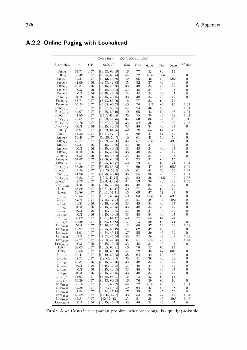
276 A Appendix
A.2.2 Online Paging with Lookahead
Costs for n = 100 (1000 samples)
Algorithm µ CV 95% CI min max q0.01 q0.5 q0.99 % det.
Fifo1 63.71 0.07 [63.43, 63.99] 46 77 52 64 74Fifo5 56.49 0.07 [56.24, 56.74] 44 72 46.5 56.5 66 0Fifo10 50.34 0.07 [50.12, 50.56] 40 66 42 50 58.5 0Fifo20 42.69 0.06 [42.53, 42.85] 35 52 37 43 49 0Fifo40 40.31 0.06 [40.16, 40.46] 33 48 34 40 47 0Fifo60 40.3 0.06 [40.15, 40.45] 33 48 34 40 47 0Fifo80 40.3 0.06 [40.15, 40.45] 33 48 34 40 47 0Fifo100 40.3 0.06 [40.15, 40.45] 33 48 34 40 47 0Fifo1,B 63.71 0.07 [63.43, 63.99] 46 77 52 64 74Fifo5,B 60.29 0.07 [60.03, 60.55] 46 76 49.5 60 70 0.01Fifo10,B 56.11 0.07 [55.87, 56.35] 44 74 46 56 66 0.04Fifo20,B 49.97 0.07 [49.75, 50.19] 40 65 42 50 58 0.01Fifo40,B 44.89 0.07 [44.7, 45.08] 35 55 38 45 52 0.01Fifo60,B 42.57 0.07 [42.39, 42.75] 34 53 36 42 49 0.1Fifo80,B 42.76 0.07 [42.57, 42.95] 35 52 36 43 50 0.43Fifo100,B 40.3 0.06 [40.15, 40.45] 33 48 34 40 47 0
Lifo1 63.97 0.07 [63.69, 64.25] 52 78 53 64 75Lifo5 56.82 0.07 [56.57, 57.07] 45 69 47 57 67 0Lifo10 50.48 0.07 [50.26, 50.7] 40 61 43 50 59 0Lifo20 42.77 0.07 [42.58, 42.96] 35 51 36.5 43 49.5 0Lifo40 40.31 0.06 [40.16, 40.46] 33 48 34 40 47 0Lifo60 40.3 0.06 [40.15, 40.45] 33 48 34 40 47 0Lifo80 40.3 0.06 [40.15, 40.45] 33 48 34 40 47 0Lifo100 40.3 0.06 [40.15, 40.45] 33 48 34 40 47 0Lifo1,B 63.97 0.07 [63.69, 64.25] 52 78 53 64 75Lifo5,B 60.51 0.07 [60.25, 60.77] 49 73 51 60 71 0.04Lifo10,B 56.39 0.07 [56.15, 56.63] 44 69 47 56 65.5 0.04Lifo20,B 49.98 0.07 [49.76, 50.2] 40 61 42 50 58 0.01Lifo40,B 44.96 0.07 [44.76, 45.16] 36 55 38 45 52 0.01Lifo60,B 42.58 0.07 [42.4, 42.76] 33 52 36 42.5 49 0.08Lifo80,B 42.79 0.07 [42.6, 42.98] 34 53 36 43 49 0.45Lifo100,B 40.3 0.06 [40.15, 40.45] 33 48 34 40 47 0
Lfu1 63.89 0.07 [63.61, 64.17] 50 77 53 64 74Lfu5 56.86 0.07 [56.61, 57.11] 45 69 47 57 67 0Lfu10 50.53 0.07 [50.31, 50.75] 40 63 42.5 50 59.5 0Lfu20 42.75 0.07 [42.56, 42.94] 34 51 36 43 49.5 0Lfu40 40.31 0.06 [40.16, 40.46] 33 48 34 40 47 0Lfu60 40.3 0.06 [40.15, 40.45] 33 48 34 40 47 0Lfu80 40.3 0.06 [40.15, 40.45] 33 48 34 40 47 0Lfu100 40.3 0.06 [40.15, 40.45] 33 48 34 40 47 0Lfu1,B 63.89 0.07 [63.61, 64.17] 50 77 53 64 74Lfu5,B 60.59 0.07 [60.33, 60.85] 47 73 50 60 71 0Lfu10,B 56.4 0.07 [56.16, 56.64] 43 69 47 56 66 0.03Lfu20,B 49.97 0.07 [49.75, 50.19] 41 62 42 50 59 0Lfu40,B 44.94 0.07 [44.74, 45.14] 37 55 39 45 52 0Lfu60,B 42.5 0.07 [42.32, 42.68] 33 52 36 42 49 0.08Lfu80,B 42.77 0.07 [42.58, 42.96] 34 51 36.5 43 50 0.44Lfu100,B 40.3 0.06 [40.15, 40.45] 33 48 34 40 47 0
Lru1 63.63 0.07 [63.35, 63.91] 46 78 52 64 74Lru5 56.68 0.07 [56.43, 56.93] 44 72 48 57 66.5 0Lru10 50.41 0.07 [50.19, 50.63] 38 64 42 50 58 0Lru20 42.71 0.07 [42.52, 42.9] 35 51 36 43 49 0Lru40 40.31 0.06 [40.16, 40.46] 33 48 34 40 47 0Lru60 40.3 0.06 [40.15, 40.45] 33 48 34 40 47 0Lru80 40.3 0.06 [40.15, 40.45] 33 48 34 40 47 0Lru100 40.3 0.06 [40.15, 40.45] 33 48 34 40 47 0Lru1,B 63.63 0.07 [63.35, 63.91] 46 78 52 64 74Lru5,B 60.39 0.07 [60.13, 60.65] 46 76 50 60 70 0Lru10,B 56.15 0.07 [55.91, 56.39] 44 72 46.5 56 66 0.01Lru20,B 49.86 0.07 [49.64, 50.08] 39 64 42 50 58 0Lru40,B 44.94 0.07 [44.74, 45.14] 37 55 38 45 52 0Lru60,B 42.52 0.07 [42.34, 42.7] 33 54 36 42 49 0.04Lru80,B 42.81 0.07 [42.62, 43] 35 51 36 43 49.5 0.45Lru100,B 40.3 0.06 [40.15, 40.45] 33 48 34 40 47 0
Table A.4: Costs in the paging problem when each page is equally probable.

A.2 Numerical Results from Chapter 5 277
Performance ratios of costs relative to Opt for n = 100 (1000 samples)
Algorithm µ CV 95% CI min max q0.01 q0.5 q0.99 F (1)
Fifo1 1.58 0.05 [1.58, 1.58] 1.29 1.86 1.39 1.58 1.79 0Fifo5 1.4 0.05 [1.4, 1.4] 1.18 1.6 1.24 1.4 1.55 0Fifo10 1.25 0.04 [1.25, 1.25] 1.07 1.42 1.12 1.25 1.38 0Fifo20 1.06 0.03 [1.06, 1.06] 1 1.21 1 1.05 1.16 0Fifo40 1 0 [1, 1] 1 1.03 1 1 1 0Fifo60 1 0 [1, 1] 1 1 1 1 1 0Fifo80 1 0 [1, 1] 1 1 1 1 1 0Fifo100 1 0 [1, 1] 1 1 1 1 1 0Fifo1,B 1.58 0.05 [1.58, 1.58] 1.29 1.86 1.39 1.58 1.79 0Fifo5,B 1.5 0.05 [1.5, 1.5] 1.28 1.73 1.32 1.5 1.66 0Fifo10,B 1.39 0.05 [1.39, 1.39] 1.16 1.61 1.23 1.39 1.55 0Fifo20,B 1.24 0.05 [1.24, 1.24] 1.07 1.41 1.11 1.24 1.38 0Fifo40,B 1.11 0.04 [1.11, 1.11] 1 1.32 1.02 1.11 1.23 0Fifo60,B 1.06 0.03 [1.06, 1.06] 1 1.17 1 1.05 1.13 0Fifo80,B 1.06 0.03 [1.06, 1.06] 1 1.18 1 1.05 1.14 0Fifo100,B 1 0 [1, 1] 1 1 1 1 1 0
Lifo1 1.59 0.08 [1.58, 1.6] 1.2 2.14 1.31 1.59 1.95 0Lifo5 1.41 0.07 [1.4, 1.42] 1.14 1.74 1.21 1.41 1.69 0Lifo10 1.25 0.06 [1.25, 1.25] 1.07 1.51 1.11 1.25 1.44 0Lifo20 1.06 0.03 [1.06, 1.06] 1 1.19 1 1.05 1.15 0Lifo40 1 0 [1, 1] 1 1.03 1 1 1 0Lifo60 1 0 [1, 1] 1 1 1 1 1 0Lifo80 1 0 [1, 1] 1 1 1 1 1 0Lifo100 1 0 [1, 1] 1 1 1 1 1 0Lifo1,B 1.59 0.08 [1.58, 1.6] 1.2 2.14 1.31 1.59 1.95 0Lifo5,B 1.5 0.08 [1.49, 1.51] 1.2 1.89 1.26 1.5 1.81 0Lifo10,B 1.4 0.07 [1.39, 1.41] 1.16 1.8 1.2 1.4 1.67 0Lifo20,B 1.24 0.05 [1.24, 1.24] 1.04 1.49 1.1 1.24 1.41 0Lifo40,B 1.12 0.04 [1.12, 1.12] 1 1.29 1.02 1.11 1.23 0Lifo60,B 1.06 0.03 [1.06, 1.06] 1 1.19 1 1.05 1.14 0Lifo80,B 1.06 0.03 [1.06, 1.06] 1 1.19 1 1.06 1.14 0Lifo100,B 1 0 [1, 1] 1 1 1 1 1 0
Lfu1 1.59 0.07 [1.58, 1.6] 1.3 1.89 1.36 1.59 1.85 0Lfu5 1.41 0.06 [1.4, 1.42] 1.15 1.72 1.22 1.41 1.62 0Lfu10 1.25 0.05 [1.25, 1.25] 1.07 1.49 1.11 1.25 1.42 0Lfu20 1.06 0.03 [1.06, 1.06] 1 1.19 1 1.05 1.15 0Lfu40 1 0 [1, 1] 1 1.03 1 1 1 0Lfu60 1 0 [1, 1] 1 1 1 1 1 0Lfu80 1 0 [1, 1] 1 1 1 1 1 0Lfu100 1 0 [1, 1] 1 1 1 1 1 0Lfu1,B 1.59 0.07 [1.58, 1.6] 1.3 1.89 1.36 1.59 1.85 0Lfu5,B 1.51 0.06 [1.5, 1.52] 1.24 1.79 1.29 1.51 1.72 0Lfu10,B 1.4 0.06 [1.39, 1.41] 1.13 1.69 1.22 1.4 1.61 0Lfu20,B 1.24 0.05 [1.24, 1.24] 1.07 1.51 1.11 1.24 1.41 0Lfu40,B 1.12 0.04 [1.12, 1.12] 1 1.26 1.02 1.11 1.23 0Lfu60,B 1.05 0.03 [1.05, 1.05] 1 1.19 1 1.05 1.14 0Lfu80,B 1.06 0.03 [1.06, 1.06] 1 1.18 1 1.05 1.15 0Lfu100,B 1 0 [1, 1] 1 1 1 1 1 0
Lru1 1.58 0.05 [1.58, 1.58] 1.3 1.82 1.41 1.58 1.77 0Lru5 1.41 0.04 [1.41, 1.41] 1.21 1.61 1.26 1.41 1.54 0Lru10 1.25 0.04 [1.25, 1.25] 1.08 1.43 1.14 1.25 1.37 0Lru20 1.06 0.03 [1.06, 1.06] 1 1.17 1 1.05 1.15 0Lru40 1 0 [1, 1] 1 1.03 1 1 1 0Lru60 1 0 [1, 1] 1 1 1 1 1 0Lru80 1 0 [1, 1] 1 1 1 1 1 0Lru100 1 0 [1, 1] 1 1 1 1 1 0Lru1,B 1.58 0.05 [1.58, 1.58] 1.3 1.82 1.41 1.58 1.77 0Lru5,B 1.5 0.05 [1.5, 1.5] 1.23 1.7 1.34 1.5 1.65 0Lru10,B 1.39 0.04 [1.39, 1.39] 1.21 1.57 1.24 1.39 1.53 0Lru20,B 1.24 0.04 [1.24, 1.24] 1.1 1.39 1.12 1.24 1.35 0Lru40,B 1.12 0.03 [1.12, 1.12] 1.02 1.24 1.03 1.12 1.22 0Lru60,B 1.06 0.03 [1.06, 1.06] 1 1.15 1 1.05 1.12 0Lru80,B 1.06 0.03 [1.06, 1.06] 1 1.15 1 1.07 1.14 0Lru100,B 1 0 [1, 1] 1 1 1 1 1 0
Table A.5: Performance ratios of costs relative to Opt in the paging problem when each page isequally probable.

278 A Appendix
Performance ratios of costs relative to online version for n = 100 (1000 samples)
Algorithm µ CV 95% CI min max q0.01 q0.5 q0.99 1− F (1)
Fifo1 1 0 [1, 1] 1 1 1 1 1 0Fifo5 0.89 0.05 [0.89, 0.89] 0.73 1 0.77 0.89 0.98 0Fifo10 0.79 0.06 [0.79, 0.79] 0.66 0.93 0.69 0.79 0.9 0Fifo20 0.67 0.06 [0.67, 0.67] 0.56 0.81 0.59 0.67 0.77 0Fifo40 0.63 0.05 [0.63, 0.63] 0.54 0.78 0.56 0.63 0.72 0Fifo60 0.63 0.05 [0.63, 0.63] 0.54 0.78 0.56 0.63 0.72 0Fifo80 0.63 0.05 [0.63, 0.63] 0.54 0.78 0.56 0.63 0.72 0Fifo100 0.63 0.05 [0.63, 0.63] 0.54 0.78 0.56 0.63 0.72 0Fifo1,B 1 0 [1, 1] 1 1 1 1 1 0Fifo5,B 0.95 0.04 [0.95, 0.95] 0.76 1.04 0.83 0.95 1 0.01Fifo10,B 0.88 0.06 [0.88, 0.88] 0.7 1 0.77 0.88 0.98 0Fifo20,B 0.79 0.06 [0.79, 0.79] 0.65 0.96 0.68 0.78 0.9 0Fifo40,B 0.71 0.06 [0.71, 0.71] 0.59 0.87 0.61 0.7 0.81 0Fifo60,B 0.67 0.06 [0.67, 0.67] 0.56 0.8 0.59 0.67 0.76 0Fifo80,B 0.67 0.06 [0.67, 0.67] 0.54 0.8 0.59 0.67 0.77 0Fifo100,B 0.63 0.05 [0.63, 0.63] 0.54 0.78 0.56 0.63 0.72 0
Lifo1 1 0 [1, 1] 1 1 1 1 1 0Lifo5 0.89 0.05 [0.89, 0.89] 0.74 1.02 0.77 0.89 1 0Lifo10 0.79 0.07 [0.79, 0.79] 0.62 1 0.67 0.79 0.92 0Lifo20 0.67 0.08 [0.67, 0.67] 0.52 0.85 0.56 0.67 0.8 0Lifo40 0.63 0.08 [0.63, 0.63] 0.47 0.83 0.51 0.63 0.76 0Lifo60 0.63 0.08 [0.63, 0.63] 0.47 0.83 0.51 0.63 0.76 0Lifo80 0.63 0.08 [0.63, 0.63] 0.47 0.83 0.51 0.63 0.76 0Lifo100 0.63 0.08 [0.63, 0.63] 0.47 0.83 0.51 0.63 0.76 0Lifo1,B 1 0 [1, 1] 1 1 1 1 1 0Lifo5,B 0.95 0.04 [0.95, 0.95] 0.8 1.05 0.85 0.95 1.03 0.04Lifo10,B 0.88 0.06 [0.88, 0.88] 0.68 1.03 0.76 0.88 1 0Lifo20,B 0.78 0.07 [0.78, 0.78] 0.63 0.96 0.65 0.78 0.9 0Lifo40,B 0.71 0.08 [0.71, 0.71] 0.55 0.89 0.58 0.7 0.85 0Lifo60,B 0.67 0.08 [0.67, 0.67] 0.5 0.87 0.54 0.67 0.8 0Lifo80,B 0.67 0.09 [0.67, 0.67] 0.51 0.89 0.55 0.67 0.81 0Lifo100,B 0.63 0.08 [0.63, 0.63] 0.47 0.83 0.51 0.63 0.76 0
Lfu1 1 0 [1, 1] 1 1 1 1 1 0Lfu5 0.89 0.04 [0.89, 0.89] 0.76 1 0.79 0.89 0.97 0Lfu10 0.79 0.05 [0.79, 0.79] 0.65 0.95 0.7 0.79 0.9 0Lfu20 0.67 0.06 [0.67, 0.67] 0.54 0.8 0.58 0.67 0.78 0Lfu40 0.63 0.07 [0.63, 0.63] 0.53 0.77 0.54 0.63 0.73 0Lfu60 0.63 0.07 [0.63, 0.63] 0.53 0.77 0.54 0.63 0.73 0Lfu80 0.63 0.07 [0.63, 0.63] 0.53 0.77 0.54 0.63 0.73 0Lfu100 0.63 0.07 [0.63, 0.63] 0.53 0.77 0.54 0.63 0.73 0Lfu1,B 1 0 [1, 1] 1 1 1 1 1 0Lfu5,B 0.95 0.03 [0.95, 0.95] 0.82 1.03 0.87 0.95 1 0Lfu10,B 0.88 0.04 [0.88, 0.88] 0.75 1 0.79 0.89 0.97 0Lfu20,B 0.78 0.06 [0.78, 0.78] 0.65 0.93 0.68 0.78 0.89 0Lfu40,B 0.71 0.06 [0.71, 0.71] 0.57 0.85 0.6 0.7 0.81 0Lfu60,B 0.67 0.07 [0.67, 0.67] 0.53 0.8 0.57 0.67 0.77 0Lfu80,B 0.67 0.07 [0.67, 0.67] 0.55 0.82 0.58 0.67 0.78 0Lfu100,B 0.63 0.07 [0.63, 0.63] 0.53 0.77 0.54 0.63 0.73 0
Lru1 1 0 [1, 1] 1 1 1 1 1 0Lru5 0.89 0.04 [0.89, 0.89] 0.78 0.98 0.81 0.89 0.97 0Lru10 0.79 0.05 [0.79, 0.79] 0.66 0.92 0.7 0.79 0.9 0Lru20 0.67 0.06 [0.67, 0.67] 0.57 0.83 0.59 0.67 0.77 0Lru40 0.63 0.05 [0.63, 0.63] 0.55 0.77 0.57 0.63 0.71 0Lru60 0.63 0.05 [0.63, 0.63] 0.55 0.77 0.57 0.63 0.71 0Lru80 0.63 0.05 [0.63, 0.63] 0.55 0.77 0.57 0.63 0.71 0Lru100 0.63 0.05 [0.63, 0.63] 0.55 0.77 0.57 0.63 0.71 0Lru1,B 1 0 [1, 1] 1 1 1 1 1 0Lru5,B 0.95 0.03 [0.95, 0.95] 0.86 1 0.88 0.95 1 0Lru10,B 0.88 0.04 [0.88, 0.88] 0.77 0.98 0.79 0.88 0.97 0Lru20,B 0.78 0.05 [0.78, 0.78] 0.66 0.9 0.69 0.78 0.89 0Lru40,B 0.71 0.05 [0.71, 0.71] 0.59 0.83 0.63 0.71 0.8 0Lru60,B 0.67 0.05 [0.67, 0.67] 0.58 0.81 0.6 0.67 0.75 0Lru80,B 0.67 0.05 [0.67, 0.67] 0.57 0.79 0.6 0.68 0.76 0Lru100,B 0.63 0.05 [0.63, 0.63] 0.55 0.77 0.57 0.63 0.71 0
Table A.6: Performance ratios of costs relative to the online version of an algorithm in the pagingproblem when each page is equally probable.

A.2 Numerical Results from Chapter 5 279
Costs for n = 100 (1000 samples)
Algorithm µ CV 95% CI min max q0.01 q0.5 q0.99 % det.
Fifo1 22.77 0.26 [22.4, 23.14] 6 42 10 23 37Fifo5 21.78 0.25 [21.44, 22.12] 6 40 10 22 35 0Fifo10 21.05 0.25 [20.72, 21.38] 6 35 10 21 33.5 0Fifo20 19.91 0.23 [19.63, 20.19] 6 35 10 20 30 0Fifo40 18.88 0.21 [18.63, 19.13] 6 31 10 19 28 0Fifo60 18.64 0.2 [18.41, 18.87] 6 29 10 19 27 0Fifo80 18.6 0.2 [18.37, 18.83] 6 29 10 19 27 0Fifo100 18.59 0.2 [18.36, 18.82] 6 29 10 19 27 0Fifo1,B 22.77 0.26 [22.4, 23.14] 6 42 10 23 37Fifo5,B 22.28 0.26 [21.92, 22.64] 6 42 10 22 36 0Fifo10,B 21.84 0.25 [21.5, 22.18] 6 40 10 22 34.5 0.05Fifo20,B 21.02 0.24 [20.71, 21.33] 6 35 10 21 33 0.03Fifo40,B 20.26 0.23 [19.97, 20.55] 6 35 10 20 31 0.05Fifo60,B 19.66 0.22 [19.39, 19.93] 6 32 10 20 29 0.15Fifo80,B 19.6 0.22 [19.33, 19.87] 6 33 10 20 29 0.27Fifo100,B 18.59 0.2 [18.36, 18.82] 6 29 10 19 27 0
Lifo1 45.08 0.41 [43.93, 46.23] 6 90 10 46 86Lifo5 23.92 0.27 [23.52, 24.32] 6 46 10 24 39 0Lifo10 21.67 0.25 [21.33, 22.01] 6 36 10 22 33 0Lifo20 19.97 0.22 [19.7, 20.24] 6 33 10 20 30 0Lifo40 18.88 0.21 [18.63, 19.13] 6 30 10 19 27.5 0Lifo60 18.63 0.2 [18.4, 18.86] 6 29 10 19 27 0Lifo80 18.59 0.2 [18.36, 18.82] 6 29 10 19 27 0Lifo100 18.59 0.2 [18.36, 18.82] 6 29 10 19 27 0Lifo1,B 45.08 0.41 [43.93, 46.23] 6 90 10 46 86Lifo5,B 27.45 0.3 [26.94, 27.96] 6 52 10 28 46.5 0.01Lifo10,B 24.53 0.28 [24.1, 24.96] 6 49 10 25 40.5 0.1Lifo20,B 22.03 0.25 [21.69, 22.37] 6 37 10 22 35 0.08Lifo40,B 20.66 0.23 [20.37, 20.95] 6 34 10 21 32 0.08Lifo60,B 19.84 0.22 [19.57, 20.11] 6 32 10 20 29 0.19Lifo80,B 19.71 0.21 [19.45, 19.97] 6 31 10 20 29 0.28Lifo100,B 18.59 0.2 [18.36, 18.82] 6 29 10 19 27 0
Lfu1 30.55 0.32 [29.94, 31.16] 6 55 10 31 51Lfu5 22.6 0.26 [22.24, 22.96] 6 38 10 23 35 0Lfu10 21.09 0.24 [20.78, 21.4] 6 36 10 21 32 0Lfu20 19.79 0.22 [19.52, 20.06] 6 33 10 20 29 0Lfu40 18.83 0.21 [18.58, 19.08] 6 29 10 19 27 0Lfu60 18.63 0.2 [18.4, 18.86] 6 29 10 19 27 0Lfu80 18.6 0.2 [18.37, 18.83] 6 29 10 19 27 0Lfu100 18.59 0.2 [18.36, 18.82] 6 29 10 19 27 0Lfu1,B 30.55 0.32 [29.94, 31.16] 6 55 10 31 51Lfu5,B 24.85 0.28 [24.42, 25.28] 6 44 10 25 39 0Lfu10,B 23.16 0.26 [22.79, 23.53] 6 40 10 23 36.5 0.11Lfu20,B 21.52 0.24 [21.2, 21.84] 6 36 10 22 33 0.08Lfu40,B 20.45 0.23 [20.16, 20.74] 6 33 10 21 31 0.08Lfu60,B 19.72 0.22 [19.45, 19.99] 6 31 10 20 29 0.19Lfu80,B 19.67 0.22 [19.4, 19.94] 6 31 10 20 29 0.28Lfu100,B 18.59 0.2 [18.36, 18.82] 6 29 10 19 27 0
Lru1 21 0.24 [20.69, 21.31] 6 38 10 21 33Lru5 20.61 0.24 [20.3, 20.92] 6 37 10 21 32 0Lru10 20.18 0.23 [19.89, 20.47] 6 34 10 20 31 0Lru20 19.47 0.22 [19.2, 19.74] 6 32 10 20 29 0Lru40 18.78 0.21 [18.54, 19.02] 6 29 10 19 27.5 0Lru60 18.61 0.2 [18.38, 18.84] 6 29 10 19 27 0Lru80 18.6 0.2 [18.37, 18.83] 6 29 10 19 27 0Lru100 18.59 0.2 [18.36, 18.82] 6 29 10 19 27 0Lru1,B 21 0.24 [20.69, 21.31] 6 38 10 21 33Lru5,B 20.83 0.24 [20.52, 21.14] 6 37 10 21 33 0Lru10,B 20.56 0.24 [20.25, 20.87] 6 36 10 21 32 0.02Lru20,B 20.14 0.23 [19.85, 20.43] 6 36 10 20 31 0.04Lru40,B 19.65 0.22 [19.38, 19.92] 6 34 10 20 30 0.03Lru60,B 19.29 0.22 [19.03, 19.55] 6 31 10 19 28.5 0.15Lru80,B 19.17 0.21 [18.92, 19.42] 6 30 10 19 28.5 0.2Lru100,B 18.59 0.2 [18.36, 18.82] 6 29 10 19 27 0
Table A.7: Costs in the paging problem when page sequences are generated according to an accessgraph.

280 A Appendix
Performance ratios of costs relative to Opt for n = 100 (1000 samples)
Algorithm µ CV 95% CI min max q0.01 q0.5 q0.99 F (1)
Fifo1 1.22 0.14 [1.21, 1.23] 1 1.94 1 1.21 1.69 0Fifo5 1.16 0.11 [1.15, 1.17] 1 1.65 1 1.16 1.49 0Fifo10 1.13 0.1 [1.12, 1.14] 1 1.5 1 1.11 1.4 0Fifo20 1.07 0.07 [1.07, 1.07] 1 1.33 1 1.05 1.28 0Fifo40 1.01 0.03 [1.01, 1.01] 1 1.19 1 1 1.15 0Fifo60 1 0.01 [1, 1] 1 1.16 1 1 1.06 0Fifo80 1 0 [1, 1] 1 1.06 1 1 1 0Fifo100 1 0 [1, 1] 1 1 1 1 1 0Fifo1,B 1.22 0.14 [1.21, 1.23] 1 1.94 1 1.21 1.69 0Fifo5,B 1.19 0.13 [1.18, 1.2] 1 1.76 1 1.18 1.58 0Fifo10,B 1.17 0.12 [1.16, 1.18] 1 1.58 1 1.16 1.5 0Fifo20,B 1.12 0.1 [1.11, 1.13] 1 1.53 1 1.11 1.39 0Fifo40,B 1.09 0.08 [1.08, 1.1] 1 1.39 1 1.06 1.31 0Fifo60,B 1.05 0.07 [1.05, 1.05] 1 1.33 1 1.04 1.27 0Fifo80,B 1.05 0.06 [1.05, 1.05] 1 1.35 1 1.04 1.24 0Fifo100,B 1 0 [1, 1] 1 1 1 1 1 0
Lifo1 2.38 0.35 [2.33, 2.43] 1 5.47 1 2.31 4.63 0Lifo5 1.28 0.16 [1.27, 1.29] 1 2.18 1 1.24 1.89 0Lifo10 1.16 0.12 [1.15, 1.17] 1 1.76 1 1.14 1.53 0Lifo20 1.07 0.07 [1.07, 1.07] 1 1.47 1 1.05 1.3 0Lifo40 1.01 0.03 [1.01, 1.01] 1 1.22 1 1 1.16 0Lifo60 1 0.01 [1, 1] 1 1.19 1 1 1.06 0Lifo80 1 0 [1, 1] 1 1 1 1 1 0Lifo100 1 0 [1, 1] 1 1 1 1 1 0Lifo1,B 2.38 0.35 [2.33, 2.43] 1 5.47 1 2.31 4.63 0Lifo5,B 1.46 0.2 [1.44, 1.48] 1 2.6 1 1.44 2.3 0Lifo10,B 1.31 0.16 [1.3, 1.32] 1 2.33 1 1.28 1.89 0Lifo20,B 1.18 0.12 [1.17, 1.19] 1 1.76 1 1.15 1.58 0Lifo40,B 1.11 0.08 [1.1, 1.12] 1 1.59 1 1.1 1.38 0Lifo60,B 1.07 0.07 [1.07, 1.07] 1 1.41 1 1.05 1.26 0Lifo80,B 1.06 0.06 [1.06, 1.06] 1 1.36 1 1.05 1.25 0Lifo100,B 1 0 [1, 1] 1 1 1 1 1 0
Lfu1 1.61 0.19 [1.59, 1.63] 1 2.45 1 1.62 2.3 0Lfu5 1.2 0.11 [1.19, 1.21] 1 1.71 1 1.2 1.53 0Lfu10 1.13 0.08 [1.12, 1.14] 1 1.5 1 1.12 1.35 0Lfu20 1.06 0.06 [1.06, 1.06] 1 1.29 1 1.05 1.24 0Lfu40 1.01 0.03 [1.01, 1.01] 1 1.19 1 1 1.13 0Lfu60 1 0.01 [1, 1] 1 1.12 1 1 1.06 0Lfu80 1 0 [1, 1] 1 1.06 1 1 1 0Lfu100 1 0 [1, 1] 1 1 1 1 1 0Lfu1,B 1.61 0.19 [1.59, 1.63] 1 2.45 1 1.62 2.3 0Lfu5,B 1.32 0.14 [1.31, 1.33] 1 2.05 1 1.3 1.77 0Lfu10,B 1.23 0.11 [1.22, 1.24] 1 1.71 1 1.22 1.6 0Lfu20,B 1.15 0.09 [1.14, 1.16] 1 1.5 1 1.14 1.42 0Lfu40,B 1.1 0.07 [1.1, 1.1] 1 1.44 1 1.09 1.33 0Lfu60,B 1.06 0.06 [1.06, 1.06] 1 1.26 1 1.05 1.22 0Lfu80,B 1.06 0.06 [1.06, 1.06] 1 1.31 1 1.05 1.23 0Lfu100,B 1 0 [1, 1] 1 1 1 1 1 0
Lru1 1.12 0.1 [1.11, 1.13] 1 1.5 1 1.11 1.4 0Lru5 1.1 0.09 [1.09, 1.11] 1 1.43 1 1.08 1.35 0Lru10 1.08 0.08 [1.07, 1.09] 1 1.36 1 1.06 1.3 0Lru20 1.04 0.06 [1.04, 1.04] 1 1.32 1 1 1.22 0Lru40 1.01 0.03 [1.01, 1.01] 1 1.19 1 1 1.12 0Lru60 1 0.01 [1, 1] 1 1.12 1 1 1.05 0Lru80 1 0 [1, 1] 1 1.06 1 1 1 0Lru100 1 0 [1, 1] 1 1 1 1 1 0Lru1,B 1.12 0.1 [1.11, 1.13] 1 1.5 1 1.11 1.4 0Lru5,B 1.11 0.09 [1.1, 1.12] 1 1.5 1 1.1 1.39 0Lru10,B 1.1 0.09 [1.09, 1.11] 1 1.41 1 1.09 1.33 0Lru20,B 1.08 0.07 [1.08, 1.08] 1 1.36 1 1.06 1.3 0Lru40,B 1.05 0.06 [1.05, 1.05] 1 1.33 1 1.04 1.25 0Lru60,B 1.04 0.05 [1.04, 1.04] 1 1.33 1 1 1.21 0Lru80,B 1.03 0.05 [1.03, 1.03] 1 1.25 1 1 1.2 0Lru100,B 1 0 [1, 1] 1 1 1 1 1 0
Table A.8: Performance ratios of costs relative to Opt in the paging problem when page sequencesare generated according to an access graph.

A.2 Numerical Results from Chapter 5 281
Performance ratios of costs relative to online version for n = 100 (1000 samples)
Algorithm µ CV 95% CI min max q0.01 q0.5 q0.99 1− F (1)
Fifo1 1 0 [1, 1] 1 1 1 1 1 0Fifo5 0.96 0.06 [0.96, 0.96] 0.7 1.04 0.73 1 1 0Fifo10 0.93 0.08 [0.93, 0.93] 0.59 1.04 0.69 0.95 1 0Fifo20 0.89 0.11 [0.88, 0.9] 0.59 1 0.64 0.91 1 0Fifo40 0.85 0.14 [0.84, 0.86] 0.52 1 0.59 0.85 1 0Fifo60 0.84 0.14 [0.83, 0.85] 0.52 1 0.59 0.83 1 0Fifo80 0.84 0.14 [0.83, 0.85] 0.52 1 0.59 0.83 1 0Fifo100 0.84 0.14 [0.83, 0.85] 0.52 1 0.59 0.83 1 0Fifo1,B 1 0 [1, 1] 1 1 1 1 1 0Fifo5,B 0.98 0.04 [0.98, 0.98] 0.71 1.12 0.78 1 1 0Fifo10,B 0.96 0.06 [0.96, 0.96] 0.67 1.05 0.74 1 1 0Fifo20,B 0.93 0.09 [0.92, 0.94] 0.62 1.04 0.68 0.96 1 0Fifo40,B 0.9 0.11 [0.89, 0.91] 0.6 1 0.64 0.92 1 0Fifo60,B 0.88 0.12 [0.87, 0.89] 0.52 1.05 0.62 0.89 1 0Fifo80,B 0.88 0.12 [0.87, 0.89] 0.57 1 0.62 0.89 1 0Fifo100,B 0.84 0.14 [0.83, 0.85] 0.52 1 0.59 0.83 1 0
Lifo1 1 0 [1, 1] 1 1 1 1 1 0Lifo5 0.59 0.29 [0.58, 0.6] 0.24 1.06 0.29 0.56 1 0Lifo10 0.54 0.33 [0.53, 0.55] 0.22 1 0.26 0.51 1 0Lifo20 0.51 0.36 [0.5, 0.52] 0.2 1 0.24 0.47 1 0Lifo40 0.48 0.38 [0.47, 0.49] 0.18 1 0.22 0.44 1 0Lifo60 0.48 0.39 [0.47, 0.49] 0.18 1 0.22 0.43 1 0Lifo80 0.48 0.39 [0.47, 0.49] 0.18 1 0.22 0.43 1 0Lifo100 0.48 0.39 [0.47, 0.49] 0.18 1 0.22 0.43 1 0Lifo1,B 1 0 [1, 1] 1 1 1 1 1 0Lifo5,B 0.66 0.25 [0.65, 0.67] 0.3 1.28 0.35 0.64 1 0.01Lifo10,B 0.6 0.29 [0.59, 0.61] 0.26 1.06 0.3 0.58 1 0Lifo20,B 0.55 0.32 [0.54, 0.56] 0.2 1 0.26 0.52 1 0Lifo40,B 0.52 0.35 [0.51, 0.53] 0.2 1 0.24 0.48 1 0Lifo60,B 0.51 0.36 [0.5, 0.52] 0.2 1 0.23 0.46 1 0Lifo80,B 0.5 0.37 [0.49, 0.51] 0.18 1 0.23 0.46 1 0Lifo100,B 0.48 0.39 [0.47, 0.49] 0.18 1 0.22 0.43 1 0
Lfu1 1 0 [1, 1] 1 1 1 1 1 0Lfu5 0.77 0.14 [0.76, 0.78] 0.51 1 0.55 0.75 1 0Lfu10 0.72 0.17 [0.71, 0.73] 0.46 1 0.51 0.7 1 0Lfu20 0.68 0.19 [0.67, 0.69] 0.43 1 0.48 0.66 1 0Lfu40 0.65 0.21 [0.64, 0.66] 0.41 1 0.44 0.63 1 0Lfu60 0.65 0.21 [0.64, 0.66] 0.41 1 0.43 0.62 1 0Lfu80 0.65 0.21 [0.64, 0.66] 0.41 1 0.43 0.62 1 0Lfu100 0.65 0.21 [0.64, 0.66] 0.41 1 0.43 0.62 1 0Lfu1,B 1 0 [1, 1] 1 1 1 1 1 0Lfu5,B 0.83 0.12 [0.82, 0.84] 0.55 1 0.63 0.83 1 0Lfu10,B 0.78 0.14 [0.77, 0.79] 0.48 1 0.57 0.77 1 0Lfu20,B 0.74 0.16 [0.73, 0.75] 0.49 1 0.53 0.72 1 0Lfu40,B 0.7 0.18 [0.69, 0.71] 0.46 1 0.49 0.68 1 0Lfu60,B 0.68 0.19 [0.67, 0.69] 0.42 1 0.47 0.66 1 0Lfu80,B 0.68 0.19 [0.67, 0.69] 0.44 1 0.46 0.66 1 0Lfu100,B 0.65 0.21 [0.64, 0.66] 0.41 1 0.43 0.62 1 0
Lru1 1 0 [1, 1] 1 1 1 1 1 0Lru5 0.98 0.03 [0.98, 0.98] 0.79 1 0.86 1 1 0Lru10 0.97 0.05 [0.97, 0.97] 0.74 1 0.8 1 1 0Lru20 0.94 0.07 [0.94, 0.94] 0.71 1 0.75 0.95 1 0Lru40 0.91 0.09 [0.9, 0.92] 0.67 1 0.71 0.92 1 0Lru60 0.9 0.1 [0.89, 0.91] 0.67 1 0.71 0.9 1 0Lru80 0.9 0.1 [0.89, 0.91] 0.67 1 0.71 0.9 1 0Lru100 0.9 0.1 [0.89, 0.91] 0.67 1 0.71 0.9 1 0Lru1,B 1 0 [1, 1] 1 1 1 1 1 0Lru5,B 0.99 0.02 [0.99, 0.99] 0.83 1 0.89 1 1 0Lru10,B 0.98 0.04 [0.98, 0.98] 0.79 1 0.85 1 1 0Lru20,B 0.96 0.05 [0.96, 0.96] 0.71 1 0.8 1 1 0Lru40,B 0.94 0.07 [0.94, 0.94] 0.68 1 0.75 0.96 1 0Lru60,B 0.93 0.08 [0.93, 0.93] 0.67 1 0.72 0.95 1 0Lru80,B 0.92 0.09 [0.91, 0.93] 0.67 1 0.74 0.95 1 0Lru100,B 0.9 0.1 [0.89, 0.91] 0.67 1 0.71 0.9 1 0
Table A.9: Performance ratios of costs relative to the online version of an algorithm in the pagingproblem when page sequences are generated according to an access graph.

282 A Appendix
Costs for n = 100 (1000 samples)
Algorithm µ CV 95% CI min max q0.01 q0.5 q0.99 % det.
Fifo1 44.55 0.12 [44.22, 44.88] 27 60 33 44.5 56.5Fifo5 39.3 0.11 [39.03, 39.57] 26 52 29 39 49.5 0Fifo10 34.46 0.11 [34.22, 34.7] 23 46 26 34 43 0Fifo20 28.87 0.1 [28.69, 29.05] 18 37 22 29 36 0Fifo40 26.62 0.1 [26.45, 26.79] 18 35 21 27 33 0Fifo60 26.59 0.1 [26.43, 26.75] 18 35 21 27 33 0Fifo80 26.59 0.1 [26.43, 26.75] 18 35 21 27 33 0Fifo100 26.59 0.1 [26.43, 26.75] 18 35 21 27 33 0Fifo1,B 44.55 0.12 [44.22, 44.88] 27 60 33 44.5 56.5Fifo5,B 42.16 0.11 [41.87, 42.45] 25 56 31 42 53 0.03Fifo10,B 39 0.11 [38.73, 39.27] 24 53 29 39 50 0.05Fifo20,B 34.16 0.11 [33.93, 34.39] 23 45 26 34 43 0.01Fifo40,B 30.69 0.11 [30.48, 30.9] 21 40 23 31 38 0.02Fifo60,B 28.55 0.11 [28.36, 28.74] 19 37 22 28 36 0.1Fifo80,B 28.88 0.11 [28.68, 29.08] 18 37 22 29 36 0.45Fifo100,B 26.59 0.1 [26.43, 26.75] 18 35 21 27 33 0
Lifo1 41.78 0.16 [41.37, 42.19] 25 67 28 41 59Lifo5 36.28 0.13 [35.99, 36.57] 24 54 26 36 48 0Lifo10 32.4 0.12 [32.16, 32.64] 21 47 24 32 42 0Lifo20 28.19 0.1 [28.02, 28.36] 19 36 22 28 35 0Lifo40 26.61 0.1 [26.44, 26.78] 18 35 21 27 33 0Lifo60 26.59 0.1 [26.43, 26.75] 18 35 21 27 33 0Lifo80 26.59 0.1 [26.43, 26.75] 18 35 21 27 33 0Lifo100 26.59 0.1 [26.43, 26.75] 18 35 21 27 33 0Lifo1,B 41.78 0.16 [41.37, 42.19] 25 67 28 41 59Lifo5,B 38.94 0.14 [38.6, 39.28] 24 60 27 39 52 0.08Lifo10,B 35.9 0.13 [35.61, 36.19] 23 52 26 36 47.5 0.07Lifo20,B 31.89 0.11 [31.67, 32.11] 21 43 24 32 40 0.02Lifo40,B 29.27 0.1 [29.09, 29.45] 19 38 22.5 29 36 0.04Lifo60,B 27.69 0.1 [27.52, 27.86] 20 37 22 28 34 0.1Lifo80,B 27.92 0.1 [27.75, 28.09] 19 37 22 28 35 0.44Lifo100,B 26.59 0.1 [26.43, 26.75] 18 35 21 27 33 0
Lfu1 37.46 0.13 [37.16, 37.76] 23 54 27 37 50Lfu5 34.18 0.12 [33.93, 34.43] 22 45 25 34 44 0Lfu10 31.27 0.11 [31.06, 31.48] 22 42 24 31 39.5 0Lfu20 27.88 0.1 [27.71, 28.05] 20 36 21.5 28 34.5 0Lfu40 26.62 0.1 [26.45, 26.79] 18 35 21 27 33 0Lfu60 26.59 0.1 [26.43, 26.75] 18 35 21 27 33 0Lfu80 26.59 0.1 [26.43, 26.75] 18 35 21 27 33 0Lfu100 26.59 0.1 [26.43, 26.75] 18 35 21 27 33 0Lfu1,B 37.46 0.13 [37.16, 37.76] 23 54 27 37 50Lfu5,B 35.93 0.13 [35.64, 36.22] 23 50 26.5 36 46.5 0Lfu10,B 33.99 0.12 [33.74, 34.24] 22 46 26 34 43.5 0.06Lfu20,B 31.15 0.11 [30.94, 31.36] 23 43 24 31 39.5 0.03Lfu40,B 28.96 0.1 [28.78, 29.14] 20 37 22.5 29 36 0.04Lfu60,B 27.58 0.1 [27.41, 27.75] 20 37 21.5 27 34 0.1Lfu80,B 27.76 0.1 [27.59, 27.93] 19 36 21 28 34 0.39Lfu100,B 26.59 0.1 [26.43, 26.75] 18 35 21 27 33 0
Lru1 41.49 0.13 [41.16, 41.82] 25 61 30 41 53Lru5 36.65 0.12 [36.38, 36.92] 20 51 27 37 47 0Lru10 32.77 0.11 [32.55, 32.99] 20 44 25 33 41 0Lru20 28.37 0.1 [28.19, 28.55] 18 36 22 28 35 0Lru40 26.62 0.1 [26.45, 26.79] 18 35 21 27 33 0Lru60 26.59 0.1 [26.43, 26.75] 18 35 21 27 33 0Lru80 26.59 0.1 [26.43, 26.75] 18 35 21 27 33 0Lru100 26.59 0.1 [26.43, 26.75] 18 35 21 27 33 0Lru1,B 41.49 0.13 [41.16, 41.82] 25 61 30 41 53Lru5,B 39.16 0.12 [38.87, 39.45] 23 56 29 39 49 0Lru10,B 36.47 0.12 [36.2, 36.74] 22 51 26.5 36 47 0.03Lru20,B 32.55 0.11 [32.33, 32.77] 21 44 25 32.5 41 0.01Lru40,B 29.73 0.11 [29.53, 29.93] 20 40 23 30 37 0.01Lru60,B 27.98 0.1 [27.81, 28.15] 18 37 22 28 34 0.08Lru80,B 28.21 0.1 [28.04, 28.38] 19 37 22 28 35 0.41Lru100,B 26.59 0.1 [26.43, 26.75] 18 35 21 27 33 0
Table A.10: Costs in the paging problem when pages are stochastically distributed.

A.2 Numerical Results from Chapter 5 283
Performance ratios of costs relative to Opt for n = 100 (1000 samples)
Algorithm µ CV 95% CI min max q0.01 q0.5 q0.99 F (1)
Fifo1 1.68 0.07 [1.67, 1.69] 1.32 2.04 1.42 1.68 1.96 0Fifo5 1.48 0.06 [1.47, 1.49] 1.12 1.78 1.27 1.48 1.7 0Fifo10 1.3 0.06 [1.3, 1.3] 1.08 1.56 1.13 1.3 1.46 0Fifo20 1.09 0.05 [1.09, 1.09] 1 1.29 1 1.08 1.22 0Fifo40 1 0.01 [1, 1] 1 1.09 1 1 1.04 0Fifo60 1 0 [1, 1] 1 1.04 1 1 1 0Fifo80 1 0 [1, 1] 1 1 1 1 1 0Fifo100 1 0 [1, 1] 1 1 1 1 1 0Fifo1,B 1.68 0.07 [1.67, 1.69] 1.32 2.04 1.42 1.68 1.96 0Fifo5,B 1.59 0.06 [1.58, 1.6] 1.28 1.88 1.36 1.58 1.83 0Fifo10,B 1.47 0.06 [1.46, 1.48] 1.19 1.74 1.28 1.46 1.69 0Fifo20,B 1.29 0.06 [1.29, 1.29] 1.05 1.52 1.11 1.29 1.46 0Fifo40,B 1.16 0.05 [1.16, 1.16] 1 1.41 1.03 1.15 1.32 0Fifo60,B 1.07 0.04 [1.07, 1.07] 1 1.25 1 1.07 1.2 0Fifo80,B 1.09 0.04 [1.09, 1.09] 1 1.24 1 1.08 1.21 0Fifo100,B 1 0 [1, 1] 1 1 1 1 1 0
Lifo1 1.57 0.14 [1.56, 1.58] 1.1 2.79 1.16 1.55 2.21 0Lifo5 1.37 0.1 [1.36, 1.38] 1.07 1.83 1.11 1.36 1.72 0Lifo10 1.22 0.08 [1.21, 1.23] 1.03 1.62 1.04 1.21 1.45 0Lifo20 1.06 0.04 [1.06, 1.06] 1 1.27 1 1.05 1.2 0Lifo40 1 0.01 [1, 1] 1 1.1 1 1 1.04 0Lifo60 1 0 [1, 1] 1 1 1 1 1 0Lifo80 1 0 [1, 1] 1 1 1 1 1 0Lifo100 1 0 [1, 1] 1 1 1 1 1 0Lifo1,B 1.57 0.14 [1.56, 1.58] 1.1 2.79 1.16 1.55 2.21 0Lifo5,B 1.47 0.12 [1.46, 1.48] 1.08 2.13 1.13 1.45 1.96 0Lifo10,B 1.35 0.1 [1.34, 1.36] 1.07 1.83 1.11 1.34 1.72 0Lifo20,B 1.2 0.07 [1.19, 1.21] 1 1.5 1.04 1.19 1.42 0Lifo40,B 1.1 0.05 [1.1, 1.1] 1 1.29 1 1.1 1.24 0Lifo60,B 1.04 0.03 [1.04, 1.04] 1 1.2 1 1.04 1.14 0Lifo80,B 1.05 0.04 [1.05, 1.05] 1 1.21 1 1.04 1.16 0Lifo100,B 1 0 [1, 1] 1 1 1 1 1 0
Lfu1 1.41 0.09 [1.4, 1.42] 1.07 1.84 1.13 1.41 1.77 0Lfu5 1.29 0.08 [1.28, 1.3] 1 1.64 1.08 1.28 1.55 0Lfu10 1.18 0.06 [1.18, 1.18] 1 1.5 1.03 1.17 1.36 0Lfu20 1.05 0.04 [1.05, 1.05] 1 1.27 1 1.04 1.17 0Lfu40 1 0.01 [1, 1] 1 1.05 1 1 1.04 0Lfu60 1 0 [1, 1] 1 1.04 1 1 1 0Lfu80 1 0 [1, 1] 1 1 1 1 1 0Lfu100 1 0 [1, 1] 1 1 1 1 1 0Lfu1,B 1.41 0.09 [1.4, 1.42] 1.07 1.84 1.13 1.41 1.77 0Lfu5,B 1.35 0.09 [1.34, 1.36] 1.07 1.8 1.12 1.35 1.65 0Lfu10,B 1.28 0.08 [1.27, 1.29] 1.03 1.6 1.08 1.27 1.54 0Lfu20,B 1.17 0.06 [1.17, 1.17] 1 1.44 1.02 1.17 1.36 0Lfu40,B 1.09 0.05 [1.09, 1.09] 1 1.29 1 1.08 1.21 0Lfu60,B 1.04 0.03 [1.04, 1.04] 1 1.18 1 1.04 1.14 0Lfu80,B 1.04 0.03 [1.04, 1.04] 1 1.21 1 1.04 1.13 0Lfu100,B 1 0 [1, 1] 1 1 1 1 1 0
Lru1 1.56 0.07 [1.55, 1.57] 1.25 2 1.32 1.56 1.81 0Lru5 1.38 0.06 [1.37, 1.39] 1.11 1.61 1.2 1.38 1.55 0Lru10 1.23 0.05 [1.23, 1.23] 1.08 1.38 1.11 1.23 1.37 0Lru20 1.07 0.04 [1.07, 1.07] 1 1.21 1 1.07 1.18 0Lru40 1 0.01 [1, 1] 1 1.1 1 1 1.04 0Lru60 1 0 [1, 1] 1 1.04 1 1 1 0Lru80 1 0 [1, 1] 1 1 1 1 1 0Lru100 1 0 [1, 1] 1 1 1 1 1 0Lru1,B 1.56 0.07 [1.55, 1.57] 1.25 2 1.32 1.56 1.81 0Lru5,B 1.47 0.06 [1.46, 1.48] 1.17 1.75 1.26 1.47 1.69 0Lru10,B 1.37 0.06 [1.36, 1.38] 1.15 1.67 1.19 1.37 1.56 0Lru20,B 1.22 0.05 [1.22, 1.22] 1.04 1.42 1.08 1.22 1.38 0Lru40,B 1.12 0.05 [1.12, 1.12] 1 1.32 1.02 1.12 1.25 0Lru60,B 1.05 0.03 [1.05, 1.05] 1 1.18 1 1.04 1.14 0Lru80,B 1.06 0.03 [1.06, 1.06] 1 1.2 1 1.06 1.15 0Lru100,B 1 0 [1, 1] 1 1 1 1 1 0
Table A.11: Performance ratios of costs relative to Opt in the paging problem when pages arestochastically distributed.

284 A Appendix
Performance ratios of costs relative to online version for n = 100 (1000 samples)
Algorithm µ CV 95% CI min max q0.01 q0.5 q0.99 1− F (1)
Fifo1 1 0 [1, 1] 1 1 1 1 1 0Fifo5 0.88 0.07 [0.88, 0.88] 0.67 1.03 0.74 0.89 1 0Fifo10 0.78 0.07 [0.78, 0.78] 0.6 0.94 0.64 0.78 0.9 0Fifo20 0.65 0.08 [0.65, 0.65] 0.49 0.86 0.55 0.65 0.78 0Fifo40 0.6 0.07 [0.6, 0.6] 0.49 0.76 0.51 0.6 0.71 0Fifo60 0.6 0.07 [0.6, 0.6] 0.49 0.76 0.51 0.6 0.71 0Fifo80 0.6 0.07 [0.6, 0.6] 0.49 0.76 0.51 0.6 0.71 0Fifo100 0.6 0.07 [0.6, 0.6] 0.49 0.76 0.51 0.6 0.71 0Fifo1,B 1 0 [1, 1] 1 1 1 1 1 0Fifo5,B 0.95 0.05 [0.95, 0.95] 0.76 1.09 0.8 0.96 1.03 0.03Fifo10,B 0.88 0.07 [0.88, 0.88] 0.65 1 0.73 0.88 1 0Fifo20,B 0.77 0.08 [0.77, 0.77] 0.59 0.97 0.64 0.77 0.91 0Fifo40,B 0.69 0.08 [0.69, 0.69] 0.54 0.89 0.57 0.69 0.83 0Fifo60,B 0.64 0.08 [0.64, 0.64] 0.5 0.85 0.54 0.64 0.77 0Fifo80,B 0.65 0.08 [0.65, 0.65] 0.51 0.81 0.54 0.65 0.78 0Fifo100,B 0.6 0.07 [0.6, 0.6] 0.49 0.76 0.51 0.6 0.71 0
Lifo1 1 0 [1, 1] 1 1 1 1 1 0Lifo5 0.88 0.09 [0.88, 0.88] 0.6 1.07 0.66 0.88 1.03 0Lifo10 0.79 0.11 [0.78, 0.8] 0.46 1.03 0.57 0.79 0.97 0Lifo20 0.69 0.13 [0.68, 0.7] 0.39 0.97 0.48 0.68 0.89 0Lifo40 0.65 0.14 [0.64, 0.66] 0.36 0.93 0.45 0.65 0.86 0Lifo60 0.65 0.14 [0.64, 0.66] 0.36 0.91 0.45 0.65 0.86 0Lifo80 0.65 0.14 [0.64, 0.66] 0.36 0.91 0.45 0.65 0.86 0Lifo100 0.65 0.14 [0.64, 0.66] 0.36 0.91 0.45 0.65 0.86 0Lifo1,B 1 0 [1, 1] 1 1 1 1 1 0Lifo5,B 0.94 0.07 [0.94, 0.94] 0.63 1.13 0.75 0.95 1.07 0.08Lifo10,B 0.87 0.1 [0.86, 0.88] 0.55 1.07 0.67 0.87 1.03 0.02Lifo20,B 0.77 0.12 [0.76, 0.78] 0.48 1 0.55 0.77 0.97 0Lifo40,B 0.71 0.13 [0.7, 0.72] 0.44 1 0.48 0.71 0.92 0Lifo60,B 0.67 0.14 [0.66, 0.68] 0.37 0.94 0.46 0.67 0.89 0Lifo80,B 0.68 0.14 [0.67, 0.69] 0.4 0.97 0.47 0.68 0.91 0Lifo100,B 0.65 0.14 [0.64, 0.66] 0.36 0.91 0.45 0.65 0.86 0
Lfu1 1 0 [1, 1] 1 1 1 1 1 0Lfu5 0.91 0.05 [0.91, 0.91] 0.72 1.04 0.8 0.92 1 0Lfu10 0.84 0.07 [0.84, 0.84] 0.67 1 0.71 0.83 0.97 0Lfu20 0.75 0.09 [0.75, 0.75] 0.57 0.96 0.6 0.75 0.91 0Lfu40 0.72 0.09 [0.72, 0.72] 0.54 0.94 0.57 0.71 0.89 0Lfu60 0.72 0.09 [0.72, 0.72] 0.54 0.94 0.57 0.71 0.89 0Lfu80 0.72 0.09 [0.72, 0.72] 0.54 0.94 0.57 0.71 0.89 0Lfu100 0.72 0.09 [0.72, 0.72] 0.54 0.94 0.57 0.71 0.89 0Lfu1,B 1 0 [1, 1] 1 1 1 1 1 0Lfu5,B 0.96 0.04 [0.96, 0.96] 0.81 1.1 0.86 0.97 1 0Lfu10,B 0.91 0.06 [0.91, 0.91] 0.72 1 0.78 0.91 1 0Lfu20,B 0.84 0.07 [0.84, 0.84] 0.62 1 0.69 0.84 0.97 0Lfu40,B 0.78 0.09 [0.78, 0.78] 0.58 1 0.63 0.78 0.94 0Lfu60,B 0.74 0.09 [0.74, 0.74] 0.55 0.96 0.6 0.74 0.89 0Lfu80,B 0.75 0.09 [0.75, 0.75] 0.56 0.97 0.59 0.74 0.91 0Lfu100,B 0.72 0.09 [0.72, 0.72] 0.54 0.94 0.57 0.71 0.89 0
Lru1 1 0 [1, 1] 1 1 1 1 1 0Lru5 0.89 0.05 [0.89, 0.89] 0.74 1 0.77 0.89 0.98 0Lru10 0.79 0.07 [0.79, 0.79] 0.64 0.94 0.67 0.79 0.93 0Lru20 0.69 0.08 [0.69, 0.69] 0.54 0.87 0.58 0.68 0.83 0Lru40 0.65 0.07 [0.65, 0.65] 0.5 0.8 0.55 0.64 0.76 0Lru60 0.64 0.07 [0.64, 0.64] 0.5 0.8 0.55 0.64 0.76 0Lru80 0.64 0.07 [0.64, 0.64] 0.5 0.8 0.55 0.64 0.76 0Lru100 0.64 0.07 [0.64, 0.64] 0.5 0.8 0.55 0.64 0.76 0Lru1,B 1 0 [1, 1] 1 1 1 1 1 0Lru5,B 0.94 0.04 [0.94, 0.94] 0.81 1 0.85 0.95 1 0Lru10,B 0.88 0.05 [0.88, 0.88] 0.7 1 0.77 0.88 0.97 0Lru20,B 0.79 0.07 [0.79, 0.79] 0.63 0.97 0.65 0.79 0.92 0Lru40,B 0.72 0.07 [0.72, 0.72] 0.58 0.9 0.6 0.72 0.85 0Lru60,B 0.68 0.07 [0.68, 0.68] 0.54 0.84 0.57 0.68 0.8 0Lru80,B 0.68 0.07 [0.68, 0.68] 0.52 0.87 0.58 0.68 0.8 0Lru100,B 0.64 0.07 [0.64, 0.64] 0.5 0.8 0.55 0.64 0.76 0
Table A.12: Performance ratios of costs relative to the online version of an algorithm in the pagingproblem when pages are stochastically distributed.

A.2 Numerical Results from Chapter 5 285
A.2.3 Online Bin Packing with Lookahead
A.2.3.1 Classical Problem
Costs for n = 25 (1000 samples)
Algorithm µ CV 95% CI min max q0.01 q0.5 q0.99 % det.
Bf1 14.66 0.13 [14.54, 14.78] 9 21 11 15 19Bf5 14.33 0.13 [14.21, 14.45] 9 21 10 14 19 0Bf10 14.14 0.14 [14.02, 14.26] 9 21 10 14 19 0Bf15 14.13 0.14 [14.01, 14.25] 9 21 10 14 19 0Bf20 14.13 0.14 [14.01, 14.25] 9 21 10 14 19 0Bf25 14.13 0.14 [14.01, 14.25] 9 21 10 14 19 0Bf1,B 14.66 0.13 [14.54, 14.78] 9 21 11 15 19Bf5,B 14.48 0.13 [14.36, 14.6] 9 21 11 14 19 0.01Bf10,B 14.35 0.13 [14.23, 14.47] 9 21 10.5 14 19 0Bf15,B 14.26 0.13 [14.15, 14.37] 9 21 10 14 19 0.04Bf20,B 14.23 0.14 [14.11, 14.35] 9 21 10 14 19 0.05Bf25,B 14.13 0.14 [14.01, 14.25] 9 21 10 14 19 0
Ff1 14.76 0.13 [14.64, 14.88] 9 21 11 15 19Ff5 14.39 0.13 [14.27, 14.51] 9 21 10.5 14 19 0Ff10 14.15 0.14 [14.03, 14.27] 9 21 10 14 19 0Ff15 14.13 0.14 [14.01, 14.25] 9 21 10 14 19 0Ff20 14.13 0.14 [14.01, 14.25] 9 21 10 14 19 0Ff25 14.13 0.14 [14.01, 14.25] 9 21 10 14 19 0Ff1,B 14.76 0.13 [14.64, 14.88] 9 21 11 15 19Ff5,B 14.54 0.13 [14.42, 14.66] 9 21 11 15 19 0.01Ff10,B 14.38 0.13 [14.26, 14.5] 9 21 11 14 19 0Ff15,B 14.27 0.13 [14.15, 14.39] 9 21 10 14 19 0.04Ff20,B 14.24 0.13 [14.13, 14.35] 9 21 10 14 19 0.05Ff25,B 14.13 0.14 [14.01, 14.25] 9 21 10 14 19 0Opt1 14.76 0.13 [14.64, 14.88] 9 21 11 15 19Opt5 14.63 0.12 [14.52, 14.74] 10 21 11 15 19 0.11Opt10 14.21 0.13 [14.1, 14.32] 9 21 10 14 19 0Opt15 14.12 0.14 [14, 14.24] 9 21 10 14 19 0Opt20 14.12 0.14 [14, 14.24] 9 21 10 14 19 0Opt25 14.12 0.14 [14, 14.24] 9 21 10 14 19 0Opt1,B 14.76 0.13 [14.64, 14.88] 9 21 11 15 19Opt5,B 14.73 0.13 [14.61, 14.85] 9 21 11 15 19.5 0.09Opt10,B 14.63 0.13 [14.51, 14.75] 10 21 11 15 19 0.07Opt15,B 14.46 0.13 [14.34, 14.58] 9 21 10 14 19 0.06Opt20,B 14.42 0.13 [14.3, 14.54] 10 21 11 14 19 0.11Opt25,B 14.12 0.14 [14, 14.24] 9 21 10 14 19 0
Opt′1 14.84 0.13 [14.72, 14.96] 10 21 11 15 19Opt′5 14.54 0.13 [14.42, 14.66] 9 21 11 15 19 0.04Opt′10 14.19 0.13 [14.08, 14.3] 9 21 10 14 19 0Opt′15 14.12 0.14 [14, 14.24] 9 21 10 14 19 0Opt′20 14.12 0.14 [14, 14.24] 9 21 10 14 19 0Opt′25 14.12 0.14 [14, 14.24] 9 21 10 14 19 0Opt′1,B 14.84 0.13 [14.72, 14.96] 10 21 11 15 19
Opt′5,B 14.64 0.13 [14.52, 14.76] 10 21 11 15 19 0.04
Opt′10,B 14.42 0.13 [14.3, 14.54] 9 21 10 14 19 0.02
Opt′15,B 14.29 0.13 [14.17, 14.41] 9 21 10 14 19 0.04
Opt′20,B 14.27 0.13 [14.15, 14.39] 9 21 10 14 19 0.07
Opt′25,B 14.12 0.14 [14, 14.24] 9 21 10 14 19 0
Table A.13: Costs in the classical bin packing problem when item permutations are allowed.

286 A Appendix
Costs for n = 25 (1000 samples)
Algorithm µ CV 95% CI min max q0.01 q0.5 q0.99 % det.
Bf1 14.66 0.13 [14.54, 14.78] 9 21 11 15 19Bf5 14.34 0.13 [14.22, 14.46] 9 21 10.5 14 19 0Bf10 14.2 0.14 [14.08, 14.32] 9 21 10 14 19 0.01Bf15 14.16 0.14 [14.04, 14.28] 9 21 10 14 19 0.01Bf20 14.15 0.14 [14.03, 14.27] 9 21 10 14 19 0Bf25 14.15 0.14 [14.03, 14.27] 9 21 10 14 19 0Bf1,B 14.66 0.13 [14.54, 14.78] 9 21 11 15 19Bf5,B 14.48 0.13 [14.36, 14.6] 9 21 11 14 19 0.01Bf10,B 14.37 0.13 [14.25, 14.49] 9 21 11 14 19 0.01Bf15,B 14.28 0.13 [14.16, 14.4] 9 21 10 14 19 0.04Bf20,B 14.25 0.13 [14.14, 14.36] 9 21 10 14 19 0.06Bf25,B 14.15 0.14 [14.03, 14.27] 9 21 10 14 19 0.01
Ff1 14.76 0.13 [14.64, 14.88] 9 21 11 15 19Ff5 14.42 0.13 [14.3, 14.54] 9 21 10 14 19 0.01Ff10 14.24 0.14 [14.12, 14.36] 9 21 10 14 19 0.01Ff15 14.17 0.14 [14.05, 14.29] 9 21 10 14 19 0.01Ff20 14.14 0.14 [14.02, 14.26] 9 21 10 14 19 0.01Ff25 14.13 0.14 [14.01, 14.25] 9 21 10 14 19 0Ff1,B 14.76 0.13 [14.64, 14.88] 9 21 11 15 19Ff5,B 14.54 0.13 [14.42, 14.66] 9 21 11 15 19 0.01Ff10,B 14.38 0.13 [14.26, 14.5] 9 21 11 14 19 0Ff15,B 14.27 0.13 [14.15, 14.39] 9 21 10 14 19 0.04Ff20,B 14.24 0.13 [14.13, 14.35] 9 21 10 14 19 0.05Ff25,B 14.13 0.14 [14.01, 14.25] 9 21 10 14 19 0Opt1 14.76 0.13 [14.64, 14.88] 9 21 11 15 19Opt5 14.63 0.13 [14.51, 14.75] 10 21 11 15 19 0.07Opt10 14.36 0.13 [14.24, 14.48] 9 21 10 14 19 0.02Opt15 14.2 0.14 [14.08, 14.32] 9 21 10 14 19 0.02Opt20 14.13 0.14 [14.01, 14.25] 9 21 10 14 19 0.01Opt25 14.12 0.14 [14, 14.24] 9 21 10 14 19 0Opt1,B 14.76 0.13 [14.64, 14.88] 9 21 11 15 19Opt5,B 14.73 0.13 [14.61, 14.85] 9 21 11 15 19.5 0.09Opt10,B 14.63 0.13 [14.51, 14.75] 10 21 11 15 19 0.07Opt15,B 14.46 0.13 [14.34, 14.58] 9 21 10 14 19 0.06Opt20,B 14.42 0.13 [14.3, 14.54] 10 21 11 14 19 0.11Opt25,B 14.12 0.14 [14, 14.24] 9 21 10 14 19 0
Opt′1 14.84 0.13 [14.72, 14.96] 10 21 11 15 19Opt′5 14.52 0.13 [14.4, 14.64] 10 21 11 15 19 0.02Opt′10 14.29 0.13 [14.17, 14.41] 9 21 10.5 14 19 0.02Opt′15 14.18 0.14 [14.06, 14.3] 9 21 10 14 19 0.02Opt′20 14.13 0.14 [14.01, 14.25] 9 21 10 14 19 0.01Opt′25 14.12 0.14 [14, 14.24] 9 21 10 14 19 0Opt′1,B 14.84 0.13 [14.72, 14.96] 10 21 11 15 19
Opt′5,B 14.64 0.13 [14.52, 14.76] 10 21 11 15 19 0.04
Opt′10,B 14.42 0.13 [14.3, 14.54] 9 21 10 14 19 0.02
Opt′15,B 14.29 0.13 [14.17, 14.41] 9 21 10 14 19 0.04
Opt′20,B 14.27 0.13 [14.15, 14.39] 9 21 10 14 19 0.07
Opt′25,B 14.12 0.14 [14, 14.24] 9 21 10 14 19 0
Table A.14: Costs in the classical bin packing problem when item permutations are forbidden.

A.2 Numerical Results from Chapter 5 287
Performance ratios of costs relative to Opt for n = 25 (1000 samples)
Algorithm µ CV 95% CI min max q0.01 q0.5 q0.99 F (1)
Bf1 1.04 0.04 [1.04, 1.04] 1 1.2 1 1.06 1.15 0Bf5 1.02 0.03 [1.02, 1.02] 0.94 1.17 1 1 1.1 0Bf10 1 0.02 [1, 1] 0.94 1.11 1 1 1.09 0Bf15 1 0.01 [1, 1] 0.94 1.11 1 1 1.08 0Bf20 1 0.01 [1, 1] 0.94 1.11 1 1 1.08 0Bf25 1 0.01 [1, 1] 0.94 1.11 1 1 1.08 0Bf1,B 1.04 0.04 [1.04, 1.04] 1 1.2 1 1.06 1.15 0Bf5,B 1.03 0.04 [1.03, 1.03] 1 1.2 1 1 1.12 0Bf10,B 1.02 0.03 [1.02, 1.02] 1 1.2 1 1 1.1 0Bf15,B 1.01 0.03 [1.01, 1.01] 0.94 1.15 1 1 1.09 0Bf20,B 1.01 0.03 [1.01, 1.01] 0.94 1.17 1 1 1.09 0Bf25,B 1 0.01 [1, 1] 0.94 1.11 1 1 1.08 0
Ff1 1.05 0.04 [1.05, 1.05] 1 1.23 1 1.07 1.17 0Ff5 1.02 0.04 [1.02, 1.02] 0.94 1.2 1 1 1.1 0Ff10 1 0.02 [1, 1] 0.94 1.11 1 1 1.09 0Ff15 1 0.01 [1, 1] 0.94 1.11 1 1 1.08 0Ff20 1 0.01 [1, 1] 0.94 1.11 1 1 1.08 0Ff25 1 0.01 [1, 1] 0.94 1.11 1 1 1.08 0Ff1,B 1.05 0.04 [1.05, 1.05] 1 1.23 1 1.07 1.17 0Ff5,B 1.03 0.04 [1.03, 1.03] 1 1.2 1 1 1.14 0Ff10,B 1.02 0.03 [1.02, 1.02] 1 1.2 1 1 1.1 0Ff15,B 1.01 0.03 [1.01, 1.01] 0.94 1.15 1 1 1.09 0Ff20,B 1.01 0.03 [1.01, 1.01] 0.94 1.17 1 1 1.09 0Ff25,B 1 0.01 [1, 1] 0.94 1.11 1 1 1.08 0Opt1 1.05 0.04 [1.05, 1.05] 1 1.23 1 1.07 1.17 0Opt5 1.04 0.04 [1.04, 1.04] 0.94 1.2 1 1 1.18 0Opt10 1.01 0.02 [1.01, 1.01] 0.94 1.11 1 1 1.09 0Opt15 1 0 [1, 1] 0.94 1.08 1 1 1 0Opt20 1 0 [1, 1] 0.94 1.08 1 1 1 0Opt25 1 0 [1, 1] 1 1 1 1 1 0Opt1,B 1.05 0.04 [1.05, 1.05] 1 1.23 1 1.07 1.17 0Opt5,B 1.05 0.04 [1.05, 1.05] 1 1.2 1 1.06 1.17 0Opt10,B 1.04 0.04 [1.04, 1.04] 1 1.2 1 1 1.15 0Opt15,B 1.03 0.04 [1.03, 1.03] 1 1.18 1 1 1.14 0Opt20,B 1.02 0.04 [1.02, 1.02] 1 1.17 1 1 1.1 0Opt25,B 1 0 [1, 1] 1 1 1 1 1 0
Opt′1 1.05 0.04 [1.05, 1.05] 1 1.2 1 1.07 1.17 0Opt′5 1.03 0.04 [1.03, 1.03] 0.94 1.18 1 1 1.15 0Opt′10 1.01 0.02 [1.01, 1.01] 0.94 1.11 1 1 1.09 0Opt′15 1 0.01 [1, 1] 0.94 1.11 1 1 1 0Opt′20 1 0 [1, 1] 0.94 1.08 1 1 1 0Opt′25 1 0 [1, 1] 0.94 1.08 1 1 1 0Opt′1,B 1.05 0.04 [1.05, 1.05] 1 1.2 1 1.07 1.17 0
Opt′5,B 1.04 0.04 [1.04, 1.04] 1 1.2 1 1 1.15 0
Opt′10,B 1.02 0.04 [1.02, 1.02] 0.94 1.2 1 1 1.1 0
Opt′15,B 1.01 0.03 [1.01, 1.01] 0.94 1.15 1 1 1.09 0
Opt′20,B 1.01 0.03 [1.01, 1.01] 0.94 1.17 1 1 1.09 0
Opt′25,B 1 0 [1, 1] 0.94 1.08 1 1 1 0
Table A.15: Performance ratios of costs relative to Opt in the classical bin packing problem whenitem permutations are allowed.

288 A Appendix
Performance ratios of costs relative to Opt for n = 25 (1000 samples)
Algorithm µ CV 95% CI min max q0.01 q0.5 q0.99 F (1)
Bf1 1.04 0.04 [1.04, 1.04] 1 1.2 1 1.06 1.15 0Bf5 1.02 0.03 [1.02, 1.02] 0.94 1.15 1 1 1.1 0Bf10 1.01 0.02 [1.01, 1.01] 0.94 1.11 1 1 1.09 0Bf15 1 0.02 [1, 1] 0.94 1.11 1 1 1.09 0Bf20 1 0.02 [1, 1] 0.94 1.11 1 1 1.09 0Bf25 1 0.02 [1, 1] 0.94 1.11 1 1 1.09 0Bf1,B 1.04 0.04 [1.04, 1.04] 1 1.2 1 1.06 1.15 0Bf5,B 1.03 0.04 [1.03, 1.03] 1 1.2 1 1 1.12 0Bf10,B 1.02 0.03 [1.02, 1.02] 1 1.2 1 1 1.1 0Bf15,B 1.01 0.03 [1.01, 1.01] 0.94 1.14 1 1 1.09 0Bf20,B 1.01 0.03 [1.01, 1.01] 1 1.17 1 1 1.09 0Bf25,B 1 0.02 [1, 1] 0.94 1.11 1 1 1.09 0
Ff1 1.05 0.04 [1.05, 1.05] 1 1.23 1 1.07 1.17 0Ff5 1.02 0.04 [1.02, 1.02] 0.94 1.15 1 1 1.1 0Ff10 1.01 0.03 [1.01, 1.01] 0.94 1.1 1 1 1.09 0Ff15 1 0.02 [1, 1] 0.94 1.1 1 1 1.09 0Ff20 1 0.01 [1, 1] 0.94 1.11 1 1 1.09 0Ff25 1 0.01 [1, 1] 0.94 1.11 1 1 1.08 0Ff1,B 1.05 0.04 [1.05, 1.05] 1 1.23 1 1.07 1.17 0Ff5,B 1.03 0.04 [1.03, 1.03] 1 1.2 1 1 1.14 0Ff10,B 1.02 0.03 [1.02, 1.02] 1 1.2 1 1 1.1 0Ff15,B 1.01 0.03 [1.01, 1.01] 0.94 1.15 1 1 1.09 0Ff20,B 1.01 0.03 [1.01, 1.01] 0.94 1.17 1 1 1.09 0Ff25,B 1 0.01 [1, 1] 0.94 1.11 1 1 1.08 0Opt1 1.05 0.04 [1.05, 1.05] 1 1.23 1 1.07 1.17 0Opt5 1.04 0.04 [1.04, 1.04] 1 1.2 1 1 1.16 0Opt10 1.02 0.03 [1.02, 1.02] 0.94 1.15 1 1 1.09 0Opt15 1.01 0.02 [1.01, 1.01] 0.94 1.15 1 1 1.09 0Opt20 1 0.01 [1, 1] 0.94 1.1 1 1 1.07 0Opt25 1 0 [1, 1] 1 1 1 1 1 0Opt1,B 1.05 0.04 [1.05, 1.05] 1 1.23 1 1.07 1.17 0Opt5,B 1.05 0.04 [1.05, 1.05] 1 1.2 1 1.06 1.17 0Opt10,B 1.04 0.04 [1.04, 1.04] 1 1.2 1 1 1.15 0Opt15,B 1.03 0.04 [1.03, 1.03] 1 1.18 1 1 1.14 0Opt20,B 1.02 0.04 [1.02, 1.02] 1 1.17 1 1 1.1 0Opt25,B 1 0 [1, 1] 1 1 1 1 1 0
Opt′1 1.05 0.04 [1.05, 1.05] 1 1.2 1 1.07 1.17 0Opt′5 1.03 0.04 [1.03, 1.03] 0.94 1.18 1 1 1.11 0Opt′10 1.01 0.03 [1.01, 1.01] 0.94 1.18 1 1 1.1 0Opt′15 1.01 0.02 [1.01, 1.01] 0.94 1.15 1 1 1.09 0Opt′20 1 0.01 [1, 1] 0.94 1.09 1 1 1.07 0Opt′25 1 0 [1, 1] 0.94 1.08 1 1 1 0Opt′1,B 1.05 0.04 [1.05, 1.05] 1 1.2 1 1.07 1.17 0
Opt′5,B 1.04 0.04 [1.04, 1.04] 1 1.2 1 1 1.15 0
Opt′10,B 1.02 0.04 [1.02, 1.02] 0.94 1.2 1 1 1.1 0
Opt′15,B 1.01 0.03 [1.01, 1.01] 0.94 1.15 1 1 1.09 0
Opt′20,B 1.01 0.03 [1.01, 1.01] 0.94 1.17 1 1 1.09 0
Opt′25,B 1 0 [1, 1] 0.94 1.08 1 1 1 0
Table A.16: Performance ratios of costs relative to Opt in the classical bin packing problem whenitem permutations are forbidden.

A.2 Numerical Results from Chapter 5 289
Performance ratios of costs relative to online version for n = 25 (1000 samples)
Algorithm µ CV 95% CI min max q0.01 q0.5 q0.99 1− F (1)
Bf1 1 0 [1, 1] 1 1 1 1 1 0Bf5 0.98 0.03 [0.98, 0.98] 0.88 1.1 0.92 1 1 0Bf10 0.97 0.04 [0.97, 0.97] 0.83 1.1 0.87 1 1 0Bf15 0.96 0.04 [0.96, 0.96] 0.83 1 0.87 1 1 0Bf20 0.96 0.04 [0.96, 0.96] 0.83 1 0.87 1 1 0Bf25 0.96 0.04 [0.96, 0.96] 0.83 1 0.87 1 1 0Bf1,B 1 0 [1, 1] 1 1 1 1 1 0Bf5,B 0.99 0.03 [0.99, 0.99] 0.91 1.1 0.92 1 1 0.01Bf10,B 0.98 0.03 [0.98, 0.98] 0.87 1.1 0.92 1 1 0Bf15,B 0.97 0.04 [0.97, 0.97] 0.85 1.1 0.9 1 1 0Bf20,B 0.97 0.04 [0.97, 0.97] 0.83 1.09 0.88 1 1 0Bf25,B 0.96 0.04 [0.96, 0.96] 0.83 1 0.87 1 1 0
Ff1 1 0 [1, 1] 1 1 1 1 1 0Ff5 0.98 0.03 [0.98, 0.98] 0.88 1.09 0.92 1 1 0Ff10 0.96 0.04 [0.96, 0.96] 0.81 1 0.87 0.94 1 0Ff15 0.96 0.04 [0.96, 0.96] 0.81 1 0.86 0.94 1 0Ff20 0.96 0.04 [0.96, 0.96] 0.81 1 0.86 0.94 1 0Ff25 0.96 0.04 [0.96, 0.96] 0.81 1 0.86 0.94 1 0Ff1,B 1 0 [1, 1] 1 1 1 1 1 0Ff5,B 0.99 0.03 [0.99, 0.99] 0.85 1.08 0.92 1 1 0.01Ff10,B 0.97 0.04 [0.97, 0.97] 0.85 1.08 0.91 1 1 0Ff15,B 0.97 0.04 [0.97, 0.97] 0.83 1.08 0.88 1 1 0Ff20,B 0.96 0.04 [0.96, 0.96] 0.83 1.08 0.87 1 1 0Ff25,B 0.96 0.04 [0.96, 0.96] 0.81 1 0.86 0.94 1 0Opt1 1 0 [1, 1] 1 1 1 1 1 0Opt5 0.99 0.04 [0.99, 0.99] 0.88 1.11 0.92 1 1.09 0.11Opt10 0.96 0.04 [0.96, 0.96] 0.81 1.1 0.87 0.94 1 0Opt15 0.96 0.04 [0.96, 0.96] 0.81 1 0.86 0.94 1 0Opt20 0.96 0.04 [0.96, 0.96] 0.81 1 0.86 0.94 1 0Opt25 0.96 0.04 [0.96, 0.96] 0.81 1 0.86 0.94 1 0Opt1,B 1 0 [1, 1] 1 1 1 1 1 0Opt5,B 1 0.03 [1, 1] 0.89 1.1 0.92 1 1.08 0.09Opt10,B 0.99 0.04 [0.99, 0.99] 0.88 1.11 0.92 1 1.08 0.07Opt15,B 0.98 0.04 [0.98, 0.98] 0.85 1.09 0.91 1 1.07 0.02Opt20,B 0.98 0.04 [0.98, 0.98] 0.85 1.11 0.89 1 1.08 0.03Opt25,B 0.96 0.04 [0.96, 0.96] 0.81 1 0.86 0.94 1 0
Opt′1 1 0 [1, 1] 1 1 1 1 1 0Opt′5 0.98 0.04 [0.98, 0.98] 0.87 1.1 0.91 1 1.08 0.04Opt′10 0.96 0.04 [0.96, 0.96] 0.85 1 0.86 0.94 1 0Opt′15 0.95 0.04 [0.95, 0.95] 0.83 1 0.86 0.94 1 0Opt′20 0.95 0.04 [0.95, 0.95] 0.83 1 0.86 0.94 1 0Opt′25 0.95 0.04 [0.95, 0.95] 0.83 1 0.86 0.94 1 0Opt′1,B 1 0 [1, 1] 1 1 1 1 1 0
Opt′5,B 0.99 0.03 [0.99, 0.99] 0.88 1.09 0.92 1 1.08 0.04
Opt′10,B 0.97 0.04 [0.97, 0.97] 0.85 1.08 0.89 1 1 0.01
Opt′15,B 0.96 0.04 [0.96, 0.96] 0.85 1.07 0.87 0.94 1 0
Opt′20,B 0.96 0.04 [0.96, 0.96] 0.85 1.07 0.88 0.94 1 0
Opt′25,B 0.95 0.04 [0.95, 0.95] 0.83 1 0.86 0.94 1 0
Table A.17: Performance ratios of costs relative to the online version of an algorithm in theclassical bin packing problem when item permutations are allowed.

290 A Appendix
Performance ratios of costs relative to online version for n = 25 (1000 samples)
Algorithm µ CV 95% CI min max q0.01 q0.5 q0.99 1− F (1)
Bf1 1 0 [1, 1] 1 1 1 1 1 0Bf5 0.98 0.03 [0.98, 0.98] 0.85 1.1 0.92 1 1 0Bf10 0.97 0.04 [0.97, 0.97] 0.83 1.1 0.87 1 1 0.01Bf15 0.97 0.04 [0.97, 0.97] 0.85 1.09 0.87 1 1 0Bf20 0.97 0.04 [0.97, 0.97] 0.83 1.09 0.87 1 1 0Bf25 0.97 0.04 [0.97, 0.97] 0.83 1.09 0.87 1 1 0Bf1,B 1 0 [1, 1] 1 1 1 1 1 0Bf5,B 0.99 0.03 [0.99, 0.99] 0.91 1.1 0.92 1 1 0.01Bf10,B 0.98 0.03 [0.98, 0.98] 0.87 1.1 0.92 1 1 0Bf15,B 0.97 0.04 [0.97, 0.97] 0.85 1.1 0.89 1 1 0.01Bf20,B 0.97 0.04 [0.97, 0.97] 0.83 1.09 0.9 1 1 0Bf25,B 0.97 0.04 [0.97, 0.97] 0.83 1.09 0.87 1 1 0
Ff1 1 0 [1, 1] 1 1 1 1 1 0Ff5 0.98 0.04 [0.98, 0.98] 0.85 1.09 0.91 1 1 0.01Ff10 0.97 0.04 [0.97, 0.97] 0.83 1.08 0.87 1 1 0Ff15 0.96 0.04 [0.96, 0.96] 0.81 1 0.86 0.94 1 0Ff20 0.96 0.04 [0.96, 0.96] 0.81 1.08 0.86 0.94 1 0Ff25 0.96 0.04 [0.96, 0.96] 0.81 1 0.86 0.94 1 0Ff1,B 1 0 [1, 1] 1 1 1 1 1 0Ff5,B 0.99 0.03 [0.99, 0.99] 0.85 1.08 0.92 1 1 0.01Ff10,B 0.97 0.04 [0.97, 0.97] 0.85 1.08 0.91 1 1 0Ff15,B 0.97 0.04 [0.97, 0.97] 0.83 1.08 0.88 1 1 0Ff20,B 0.96 0.04 [0.96, 0.96] 0.83 1.08 0.87 1 1 0Ff25,B 0.96 0.04 [0.96, 0.96] 0.81 1 0.86 0.94 1 0Opt1 1 0 [1, 1] 1 1 1 1 1 0Opt5 0.99 0.04 [0.99, 0.99] 0.87 1.11 0.92 1 1.08 0.07Opt10 0.97 0.04 [0.97, 0.97] 0.83 1.08 0.88 1 1.03 0.01Opt15 0.96 0.04 [0.96, 0.96] 0.83 1.07 0.87 0.94 1 0Opt20 0.96 0.04 [0.96, 0.96] 0.81 1 0.86 0.94 1 0Opt25 0.96 0.04 [0.96, 0.96] 0.81 1 0.86 0.94 1 0Opt1,B 1 0 [1, 1] 1 1 1 1 1 0Opt5,B 1 0.03 [1, 1] 0.89 1.1 0.92 1 1.08 0.09Opt10,B 0.99 0.04 [0.99, 0.99] 0.88 1.11 0.92 1 1.08 0.07Opt15,B 0.98 0.04 [0.98, 0.98] 0.85 1.09 0.91 1 1.07 0.02Opt20,B 0.98 0.04 [0.98, 0.98] 0.85 1.11 0.89 1 1.08 0.03Opt25,B 0.96 0.04 [0.96, 0.96] 0.81 1 0.86 0.94 1 0
Opt′1 1 0 [1, 1] 1 1 1 1 1 0Opt′5 0.98 0.04 [0.98, 0.98] 0.85 1.09 0.91 1 1.07 0.02Opt′10 0.96 0.04 [0.96, 0.96] 0.85 1.08 0.87 0.94 1 0Opt′15 0.96 0.04 [0.96, 0.96] 0.83 1.08 0.86 0.94 1 0Opt′20 0.95 0.04 [0.95, 0.95] 0.83 1 0.86 0.94 1 0Opt′25 0.95 0.04 [0.95, 0.95] 0.83 1 0.86 0.94 1 0Opt′1,B 1 0 [1, 1] 1 1 1 1 1 0
Opt′5,B 0.99 0.03 [0.99, 0.99] 0.88 1.09 0.92 1 1.08 0.04
Opt′10,B 0.97 0.04 [0.97, 0.97] 0.85 1.08 0.89 1 1 0.01
Opt′15,B 0.96 0.04 [0.96, 0.96] 0.85 1.07 0.87 0.94 1 0
Opt′20,B 0.96 0.04 [0.96, 0.96] 0.85 1.07 0.88 0.94 1 0
Opt′25,B 0.95 0.04 [0.95, 0.95] 0.83 1 0.86 0.94 1 0
Table A.18: Performance ratios of costs relative to the online version of an algorithm in theclassical bin packing problem when item permutations are forbidden.

A.2 Numerical Results from Chapter 5 291
Costs for n = 100 (1000 samples)
Algorithm µ CV 95% CI min max q0.01 q0.5 q0.99 % det.
Bf1 54.94 0.07 [54.7, 55.18] 44 68 47 55 64.5Bf5 54.73 0.07 [54.49, 54.97] 44 67 47 55 64.5 0.02Bf10 54.37 0.07 [54.13, 54.61] 44 67 46 54 64 0.01Bf20 53.65 0.07 [53.42, 53.88] 43 66 46 54 63 0Bf40 52.88 0.07 [52.65, 53.11] 43 66 45 53 63 0Bf60 52.85 0.07 [52.62, 53.08] 43 66 45 53 63 0Bf80 52.85 0.07 [52.62, 53.08] 43 66 45 53 63 0Bf100 52.85 0.07 [52.62, 53.08] 43 66 45 53 63 0Bf1,B 54.94 0.07 [54.7, 55.18] 44 68 47 55 64.5Bf5,B 54.68 0.07 [54.44, 54.92] 44 67 46 55 64.5 0.02Bf10,B 54.42 0.07 [54.18, 54.66] 44 67 46 54 64 0.02Bf20,B 54.03 0.07 [53.8, 54.26] 44 67 46 54 64 0Bf40,B 53.62 0.07 [53.39, 53.85] 43 67 46 54 63 0Bf60,B 53.38 0.07 [53.15, 53.61] 43 66 46 53 63 0.09Bf80,B 53.22 0.07 [52.99, 53.45] 43 66 45 53 63 0.1Bf100,B 52.85 0.07 [52.62, 53.08] 43 66 45 53 63 0
Ff1 55.61 0.07 [55.37, 55.85] 45 68 48 56 65Ff5 55.34 0.07 [55.1, 55.58] 45 67 47 55 65 0.01Ff10 54.89 0.07 [54.65, 55.13] 45 67 47 55 64 0Ff20 53.89 0.07 [53.66, 54.12] 44 66 46 54 63 0Ff40 52.9 0.07 [52.67, 53.13] 43 66 45 53 63 0Ff60 52.85 0.07 [52.62, 53.08] 43 66 45 53 63 0Ff80 52.85 0.07 [52.62, 53.08] 43 66 45 53 63 0Ff100 52.85 0.07 [52.62, 53.08] 43 66 45 53 63 0Ff1,B 55.61 0.07 [55.37, 55.85] 45 68 48 56 65Ff5,B 55.14 0.07 [54.9, 55.38] 44 68 47 55 65 0.01Ff10,B 54.69 0.07 [54.45, 54.93] 44 68 47 55 64 0.01Ff20,B 54.14 0.07 [53.9, 54.38] 44 67 46 54 64 0Ff40,B 53.64 0.07 [53.41, 53.87] 43 67 46 54 63 0Ff60,B 53.39 0.07 [53.16, 53.62] 43 66 46 53 63 0.08Ff80,B 53.23 0.07 [53, 53.46] 43 66 45.5 53 63 0.1Ff100,B 52.85 0.07 [52.62, 53.08] 43 66 45 53 63 0
Table A.19: Costs in the classical bin packing problem when item permutations are allowed.
Costs for n = 100 (1000 samples)
Algorithm µ CV 95% CI min max q0.01 q0.5 q0.99 % det.
Bf1 54.94 0.07 [54.7, 55.18] 44 68 47 55 64.5Bf5 54.4 0.07 [54.16, 54.64] 44 67 46 54 64 0.01Bf10 53.93 0.07 [53.7, 54.16] 44 67 46 54 64 0.02Bf20 53.41 0.07 [53.18, 53.64] 43 66 46 53 63 0Bf40 53.05 0.07 [52.82, 53.28] 43 66 45 53 63 0Bf60 52.96 0.07 [52.73, 53.19] 43 66 45 53 63 0.01Bf80 52.93 0.07 [52.7, 53.16] 43 66 45 53 63 0.01Bf100 52.93 0.07 [52.7, 53.16] 43 66 45 53 63 0Bf1,B 54.94 0.07 [54.7, 55.18] 44 68 47 55 64.5Bf5,B 54.67 0.07 [54.43, 54.91] 44 67 46 55 64.5 0.02Bf10,B 54.43 0.07 [54.19, 54.67] 44 67 46 54 64 0.02Bf20,B 54.09 0.07 [53.86, 54.32] 43 67 46 54 64 0.01Bf40,B 53.7 0.07 [53.47, 53.93] 43 67 46 54 63 0.01Bf60,B 53.46 0.07 [53.23, 53.69] 43 66 46 53 63 0.09Bf80,B 53.3 0.07 [53.07, 53.53] 43 66 46 53 63 0.1Bf100,B 52.93 0.07 [52.7, 53.16] 43 66 45 53 63 0.01
Ff1 55.61 0.07 [55.37, 55.85] 45 68 48 56 65Ff5 54.85 0.07 [54.61, 55.09] 44 68 47 55 64 0Ff10 54.23 0.07 [53.99, 54.47] 44 67 46 54 64 0.01Ff20 53.52 0.07 [53.29, 53.75] 43 67 46 53 63 0Ff40 53.07 0.07 [52.84, 53.3] 43 66 45.5 53 63 0.01Ff60 52.96 0.07 [52.73, 53.19] 43 66 45 53 63 0.02Ff80 52.9 0.07 [52.67, 53.13] 43 66 45 53 63 0.02Ff100 52.85 0.07 [52.62, 53.08] 43 66 45 53 63 0Ff1,B 55.61 0.07 [55.37, 55.85] 45 68 48 56 65Ff5,B 55.14 0.07 [54.9, 55.38] 44 68 47 55 65 0.01Ff10,B 54.69 0.07 [54.45, 54.93] 44 68 47 55 64 0.01Ff20,B 54.14 0.07 [53.9, 54.38] 44 67 46 54 64 0Ff40,B 53.64 0.07 [53.41, 53.87] 43 67 46 54 63 0Ff60,B 53.39 0.07 [53.16, 53.62] 43 66 46 53 63 0.08Ff80,B 53.23 0.07 [53, 53.46] 43 66 45.5 53 63 0.1Ff100,B 52.85 0.07 [52.62, 53.08] 43 66 45 53 63 0
Table A.20: Costs in the classical bin packing problem when item permutations are forbidden.

292 A Appendix
Performance ratios of costs relative to Bf100 for n = 100 (1000 samples)
Algorithm µ CV 95% CI min max q0.01 q0.5 q0.99 F (1)
Bf1 1.04 0.02 [1.04, 1.04] 1 1.12 1 1.04 1.1 0Bf5 1.04 0.02 [1.04, 1.04] 1 1.12 1 1.04 1.1 0Bf10 1.03 0.02 [1.03, 1.03] 1 1.1 1 1.02 1.09 0Bf20 1.02 0.02 [1.02, 1.02] 1 1.08 1 1.02 1.06 0Bf40 1 0 [1, 1] 1 1.02 1 1 1.02 0Bf60 1 0 [1, 1] 1 1 1 1 1 0Bf80 1 0 [1, 1] 1 1 1 1 1 0Bf100 1 0 [1, 1] 1 1 1 1 1 0Bf1,B 1.04 0.02 [1.04, 1.04] 1 1.12 1 1.04 1.1 0Bf5,B 1.04 0.02 [1.04, 1.04] 1 1.1 1 1.04 1.09 0Bf10,B 1.03 0.02 [1.03, 1.03] 1 1.1 1 1.02 1.08 0Bf20,B 1.02 0.02 [1.02, 1.02] 1 1.1 1 1.02 1.06 0Bf40,B 1.02 0.02 [1.02, 1.02] 1 1.07 1 1.02 1.06 0Bf60,B 1.01 0.01 [1.01, 1.01] 1 1.08 1 1 1.05 0Bf80,B 1.01 0.01 [1.01, 1.01] 1 1.06 1 1 1.04 0Bf100,B 1 0 [1, 1] 1 1 1 1 1 0
Ff1 1.05 0.02 [1.05, 1.05] 1 1.14 1.02 1.05 1.11 0Ff5 1.05 0.02 [1.05, 1.05] 1 1.12 1 1.04 1.1 0Ff10 1.04 0.02 [1.04, 1.04] 1 1.12 1 1.04 1.1 0Ff20 1.02 0.02 [1.02, 1.02] 1 1.08 1 1.02 1.07 0Ff40 1 0 [1, 1] 1 1.02 1 1 1.02 0Ff60 1 0 [1, 1] 0.98 1.02 1 1 1 0Ff80 1 0 [1, 1] 1 1.02 1 1 1 0Ff100 1 0 [1, 1] 1 1.02 1 1 1 0Ff1,B 1.05 0.02 [1.05, 1.05] 1 1.14 1.02 1.05 1.11 0Ff5,B 1.04 0.02 [1.04, 1.04] 1 1.12 1 1.04 1.1 0Ff10,B 1.04 0.02 [1.04, 1.04] 1 1.1 1 1.04 1.08 0Ff20,B 1.02 0.02 [1.02, 1.02] 1 1.1 1 1.02 1.07 0Ff40,B 1.02 0.02 [1.02, 1.02] 1 1.07 1 1.02 1.06 0Ff60,B 1.01 0.01 [1.01, 1.01] 1 1.08 1 1 1.05 0Ff80,B 1.01 0.01 [1.01, 1.01] 1 1.06 1 1 1.04 0Ff100,B 1 0 [1, 1] 1 1.02 1 1 1 0
Table A.21: Performance ratios of costs relative to Bf100 in the classical bin packing problemwhen item permutations are allowed.
Performance ratios of costs relative to Bf100 for n = 100 (1000 samples)
Algorithm µ CV 95% CI min max q0.01 q0.5 q0.99 F (1)
Bf1 1.04 0.02 [1.04, 1.04] 1 1.12 1 1.04 1.1 0Bf5 1.03 0.02 [1.03, 1.03] 1 1.1 1 1.02 1.08 0Bf10 1.02 0.02 [1.02, 1.02] 0.98 1.08 1 1.02 1.06 0Bf20 1.01 0.01 [1.01, 1.01] 0.98 1.08 1 1 1.04 0Bf40 1 0.01 [1, 1] 0.98 1.04 1 1 1.02 0.01Bf60 1 0 [1, 1] 0.98 1.02 1 1 1.02 0.01Bf80 1 0 [1, 1] 0.98 1.02 1 1 1 0Bf100 1 0 [1, 1] 1 1 1 1 1 0Bf1,B 1.04 0.02 [1.04, 1.04] 1 1.12 1 1.04 1.1 0Bf5,B 1.03 0.02 [1.03, 1.03] 1 1.1 1 1.04 1.08 0Bf10,B 1.03 0.02 [1.03, 1.03] 1 1.1 1 1.02 1.08 0Bf20,B 1.02 0.02 [1.02, 1.02] 0.98 1.1 1 1.02 1.07 0Bf40,B 1.01 0.02 [1.01, 1.01] 0.98 1.07 1 1.02 1.06 0Bf60,B 1.01 0.01 [1.01, 1.01] 0.98 1.08 1 1 1.06 0.01Bf80,B 1.01 0.01 [1.01, 1.01] 0.98 1.06 1 1 1.04 0.01Bf100,B 1 0 [1, 1] 1 1 1 1 1 0
Ff1 1.05 0.02 [1.05, 1.05] 1 1.14 1.02 1.05 1.1 0Ff5 1.04 0.02 [1.04, 1.04] 1 1.1 1 1.04 1.08 0Ff10 1.02 0.02 [1.02, 1.02] 1 1.1 1 1.02 1.06 0Ff20 1.01 0.01 [1.01, 1.01] 0.98 1.06 1 1.02 1.04 0Ff40 1 0.01 [1, 1] 0.98 1.04 0.98 1 1.02 0.02Ff60 1 0.01 [1, 1] 0.98 1.04 0.98 1 1.02 0.03Ff80 1 0.01 [1, 1] 0.98 1.02 0.98 1 1.02 0.06Ff100 1 0.01 [1, 1] 0.98 1.02 0.98 1 1 0.09Ff1,B 1.05 0.02 [1.05, 1.05] 1 1.14 1.02 1.05 1.1 0Ff5,B 1.04 0.02 [1.04, 1.04] 1 1.1 1 1.04 1.1 0Ff10,B 1.03 0.02 [1.03, 1.03] 1 1.1 1 1.04 1.08 0Ff20,B 1.02 0.02 [1.02, 1.02] 0.98 1.1 1 1.02 1.07 0Ff40,B 1.01 0.01 [1.01, 1.01] 0.98 1.07 1 1.02 1.06 0Ff60,B 1.01 0.01 [1.01, 1.01] 0.98 1.08 0.98 1 1.05 0.02Ff80,B 1.01 0.01 [1.01, 1.01] 0.98 1.06 0.98 1 1.04 0.02Ff100,B 1 0.01 [1, 1] 0.98 1.02 0.98 1 1 0.09
Table A.22: Performance ratios of costs relative to Bf100 in the classical bin packing problemwhen item permutations are forbidden.

A.2 Numerical Results from Chapter 5 293
Performance ratios of costs relative to online version for n = 100 (1000 samples)
Algorithm µ CV 95% CI min max q0.01 q0.5 q0.99 1− F (1)
Bf1 1 0 [1, 1] 1 1 1 1 1 0Bf5 1 0.01 [1, 1] 0.98 1.02 0.98 1 1.02 0.02Bf10 0.99 0.01 [0.99, 0.99] 0.95 1.02 0.96 0.98 1 0.01Bf20 0.98 0.01 [0.98, 0.98] 0.93 1 0.94 0.98 1 0Bf40 0.96 0.02 [0.96, 0.96] 0.89 1 0.91 0.96 1 0Bf60 0.96 0.02 [0.96, 0.96] 0.89 1 0.91 0.96 1 0Bf80 0.96 0.02 [0.96, 0.96] 0.89 1 0.91 0.96 1 0Bf100 0.96 0.02 [0.96, 0.96] 0.89 1 0.91 0.96 1 0Bf1,B 1 0 [1, 1] 1 1 1 1 1 0Bf5,B 1 0.01 [1, 1] 0.97 1.02 0.98 1 1.02 0.02Bf10,B 0.99 0.01 [0.99, 0.99] 0.96 1.02 0.96 0.99 1 0.01Bf20,B 0.98 0.01 [0.98, 0.98] 0.94 1.02 0.95 0.98 1 0Bf40,B 0.98 0.01 [0.98, 0.98] 0.93 1 0.94 0.98 1 0Bf60,B 0.97 0.02 [0.97, 0.97] 0.91 1 0.93 0.97 1 0Bf80,B 0.97 0.02 [0.97, 0.97] 0.91 1 0.93 0.97 1 0Bf100,B 0.96 0.02 [0.96, 0.96] 0.89 1 0.91 0.96 1 0
Ff1 1 0 [1, 1] 1 1 1 1 1 0Ff5 1 0.01 [1, 1] 0.98 1.02 0.98 1 1 0.01Ff10 0.99 0.01 [0.99, 0.99] 0.95 1.02 0.96 0.98 1 0Ff20 0.97 0.01 [0.97, 0.97] 0.93 1 0.94 0.97 1 0Ff40 0.95 0.02 [0.95, 0.95] 0.89 1 0.91 0.95 0.98 0Ff60 0.95 0.02 [0.95, 0.95] 0.88 1 0.9 0.95 0.98 0Ff80 0.95 0.02 [0.95, 0.95] 0.88 1 0.9 0.95 0.98 0Ff100 0.95 0.02 [0.95, 0.95] 0.88 1 0.9 0.95 0.98 0Ff1,B 1 0 [1, 1] 1 1 1 1 1 0Ff5,B 0.99 0.01 [0.99, 0.99] 0.96 1.02 0.96 1 1 0.01Ff10,B 0.98 0.01 [0.98, 0.98] 0.94 1 0.96 0.98 1 0Ff20,B 0.97 0.01 [0.97, 0.97] 0.93 1 0.94 0.98 1 0Ff40,B 0.96 0.02 [0.96, 0.96] 0.92 1 0.93 0.96 1 0Ff60,B 0.96 0.02 [0.96, 0.96] 0.91 1 0.92 0.96 1 0Ff80,B 0.96 0.02 [0.96, 0.96] 0.91 1 0.92 0.96 0.98 0Ff100,B 0.95 0.02 [0.95, 0.95] 0.88 1 0.9 0.95 0.98 0
Table A.23: Performance ratios of costs relative to the online version of an algorithm in theclassical bin packing problem when item permutations are allowed.
Performance ratios of costs relative to online version for n = 100 (1000 samples)
Algorithm µ CV 95% CI min max q0.01 q0.5 q0.99 1− F (1)
Bf1 1 0 [1, 1] 1 1 1 1 1 0Bf5 0.99 0.01 [0.99, 0.99] 0.96 1.02 0.96 0.98 1 0.01Bf10 0.98 0.01 [0.98, 0.98] 0.94 1.02 0.95 0.98 1 0Bf20 0.97 0.02 [0.97, 0.97] 0.92 1.02 0.93 0.98 1 0Bf40 0.97 0.02 [0.97, 0.97] 0.89 1 0.92 0.96 1 0Bf60 0.96 0.02 [0.96, 0.96] 0.89 1 0.91 0.96 1 0Bf80 0.96 0.02 [0.96, 0.96] 0.89 1 0.91 0.96 1 0Bf100 0.96 0.02 [0.96, 0.96] 0.89 1 0.91 0.96 1 0Bf1,B 1 0 [1, 1] 1 1 1 1 1 0Bf5,B 1 0.01 [1, 1] 0.96 1.02 0.98 1 1.02 0.02Bf10,B 0.99 0.01 [0.99, 0.99] 0.96 1.02 0.96 1 1 0.01Bf20,B 0.98 0.01 [0.98, 0.98] 0.94 1.02 0.96 0.98 1 0.01Bf40,B 0.98 0.01 [0.98, 0.98] 0.93 1 0.94 0.98 1 0Bf60,B 0.97 0.02 [0.97, 0.97] 0.91 1 0.93 0.98 1 0Bf80,B 0.97 0.02 [0.97, 0.97] 0.91 1 0.93 0.97 1 0Bf100,B 0.96 0.02 [0.96, 0.96] 0.89 1 0.91 0.96 1 0
Ff1 1 0 [1, 1] 1 1 1 1 1 0Ff5 0.99 0.01 [0.99, 0.99] 0.96 1.02 0.96 0.98 1 0Ff10 0.98 0.01 [0.98, 0.98] 0.93 1 0.94 0.98 1 0Ff20 0.96 0.02 [0.96, 0.96] 0.91 1 0.92 0.96 1 0Ff40 0.95 0.02 [0.95, 0.95] 0.89 1 0.91 0.96 0.99 0Ff60 0.95 0.02 [0.95, 0.95] 0.89 1 0.91 0.95 0.98 0Ff80 0.95 0.02 [0.95, 0.95] 0.89 1 0.91 0.95 0.98 0Ff100 0.95 0.02 [0.95, 0.95] 0.88 1 0.9 0.95 0.98 0Ff1,B 1 0 [1, 1] 1 1 1 1 1 0Ff5,B 0.99 0.01 [0.99, 0.99] 0.96 1.02 0.96 1 1 0.01Ff10,B 0.98 0.01 [0.98, 0.98] 0.94 1 0.96 0.98 1 0Ff20,B 0.97 0.01 [0.97, 0.97] 0.93 1 0.94 0.98 1 0Ff40,B 0.96 0.02 [0.96, 0.96] 0.92 1 0.93 0.96 1 0Ff60,B 0.96 0.02 [0.96, 0.96] 0.91 1 0.92 0.96 1 0Ff80,B 0.96 0.02 [0.96, 0.96] 0.91 1 0.92 0.96 0.98 0Ff100,B 0.95 0.02 [0.95, 0.95] 0.88 1 0.9 0.95 0.98 0
Table A.24: Performance ratios of costs relative to the online version of an algorithm in theclassical bin packing problem when item permutations are forbidden.

294 A Appendix
A.2.3.2 Bounded-Space Problem
Costs for n = 25 (1000 samples)
Algorithm µ CV 95% CI min max q0.01 q0.5 q0.99 % det.
Bfb1 14.81 0.13 [14.69, 14.93] 9 21 11 15 19Bfb5 14.24 0.13 [14.13, 14.35] 9 21 10 14 19 0Bfb10 14.14 0.14 [14.02, 14.26] 9 21 10 14 19 0Bfb15 14.13 0.14 [14.01, 14.25] 9 21 10 14 19 0Bfb20 14.13 0.14 [14.01, 14.25] 9 21 10 14 19 0Bfb25 14.13 0.14 [14.01, 14.25] 9 21 10 14 19 0Bfb1,B 14.81 0.13 [14.69, 14.93] 9 21 11 15 19Bfb5,B 14.52 0.13 [14.4, 14.64] 9 21 11 15 19 0Bfb10,B 14.37 0.13 [14.25, 14.49] 9 21 10.5 14 19 0Bfb15,B 14.27 0.13 [14.15, 14.39] 9 21 10 14 19 0.05Bfb20,B 14.24 0.14 [14.12, 14.36] 9 21 10 14 19 0.06Bfb25,B 14.13 0.14 [14.01, 14.25] 9 21 10 14 19 0
Ffb1 14.96 0.13 [14.84, 15.08] 9 21 11 15 20Ffb5 14.24 0.13 [14.13, 14.35] 9 21 10 14 19 0Ffb10 14.14 0.14 [14.02, 14.26] 9 21 10 14 19 0Ffb15 14.13 0.14 [14.01, 14.25] 9 21 10 14 19 0Ffb20 14.13 0.14 [14.01, 14.25] 9 21 10 14 19 0Ffb25 14.13 0.14 [14.01, 14.25] 9 21 10 14 19 0Ffb1,B 14.96 0.13 [14.84, 15.08] 9 21 11 15 20Ffb5,B 14.57 0.13 [14.45, 14.69] 9 21 11 15 19 0Ffb10,B 14.4 0.13 [14.28, 14.52] 9 21 11 14 19 0Ffb15,B 14.28 0.13 [14.16, 14.4] 9 21 10 14 19 0.04Ffb20,B 14.24 0.13 [14.13, 14.35] 9 21 10 14 19 0.06Ffb25,B 14.13 0.14 [14.01, 14.25] 9 21 10 14 19 0Optb1 14.96 0.13 [14.84, 15.08] 9 21 11 15 20Optb5 14.73 0.13 [14.61, 14.85] 9 21 11 15 19 0.05Optb10 14.45 0.13 [14.33, 14.57] 9 21 10.5 14 19 0.03Optb15 14.29 0.14 [14.17, 14.41] 9 21 10 14 19 0.04Optb20 14.17 0.14 [14.05, 14.29] 9 21 10 14 19 0.03Optb25 14.12 0.14 [14, 14.24] 9 21 10 14 19 0Optb1,B 14.96 0.13 [14.84, 15.08] 9 21 11 15 20Optb5,B 14.78 0.13 [14.66, 14.9] 10 21 11 15 19.5 0.06Optb10,B 14.65 0.13 [14.53, 14.77] 10 21 11 15 19 0.06Optb15,B 14.47 0.13 [14.35, 14.59] 9 21 10 15 19 0.06Optb20,B 14.43 0.13 [14.31, 14.55] 10 21 11 14 19 0.11Optb25,B 14.12 0.14 [14, 14.24] 9 21 10 14 19 0
Optb′1 14.96 0.13 [14.84, 15.08] 9 21 11 15 19.5Optb′5 14.68 0.13 [14.56, 14.8] 9 21 10.5 15 19 0.03Optb′10 14.38 0.14 [14.26, 14.5] 9 21 10 14 19 0.03Optb′15 14.26 0.14 [14.14, 14.38] 9 21 10 14 19 0.04Optb′20 14.17 0.14 [14.05, 14.29] 9 21 10 14 19 0.02Optb′25 14.12 0.14 [14, 14.24] 9 21 10 14 19 0Optb′1,B 14.96 0.13 [14.84, 15.08] 9 21 11 15 19.5
Optb′5,B 14.71 0.13 [14.59, 14.83] 10 21 11 15 19.5 0.04
Optb′10,B 14.47 0.13 [14.35, 14.59] 9 21 10 14 19 0.02
Optb′15,B 14.31 0.13 [14.19, 14.43] 9 21 10 14 19 0.05
Optb′20,B 14.28 0.13 [14.16, 14.4] 9 21 10 14 19 0.08
Optb′25,B 14.12 0.14 [14, 14.24] 9 21 10 14 19 0
Table A.25: Costs in the bounded-space bin packing problem when item permutations are allowed.

A.2 Numerical Results from Chapter 5 295
Costs for n = 25 (1000 samples)
Algorithm µ CV 95% CI min max q0.01 q0.5 q0.99 % det.
Bfb1 14.81 0.13 [14.69, 14.93] 9 21 11 15 19Bfb5 14.76 0.14 [14.63, 14.89] 9 21 10.5 15 20 0.12Bfb10 14.76 0.14 [14.63, 14.89] 9 21 10.5 15 20 0Bfb15 14.76 0.14 [14.63, 14.89] 9 21 10.5 15 20 0Bfb20 14.76 0.14 [14.63, 14.89] 9 21 10.5 15 20 0Bfb25 14.76 0.14 [14.63, 14.89] 9 21 10.5 15 20 0Bfb1,B 14.81 0.13 [14.69, 14.93] 9 21 11 15 19Bfb5,B 14.78 0.13 [14.66, 14.9] 9 21 11 15 20 0.11Bfb10,B 14.77 0.14 [14.64, 14.9] 9 21 11 15 20 0.03Bfb15,B 14.76 0.14 [14.63, 14.89] 9 21 10.5 15 20 0.05Bfb20,B 14.75 0.14 [14.62, 14.88] 9 21 11 15 20 0.03Bfb25,B 14.76 0.14 [14.63, 14.89] 9 21 10.5 15 20 0.02
Ffb1 14.96 0.13 [14.84, 15.08] 9 21 11 15 20Ffb5 14.83 0.14 [14.7, 14.96] 9 21 11 15 20 0.09Ffb10 14.83 0.14 [14.7, 14.96] 9 21 11 15 20 0Ffb15 14.83 0.14 [14.7, 14.96] 9 21 11 15 20 0Ffb20 14.83 0.14 [14.7, 14.96] 9 21 11 15 20 0Ffb25 14.83 0.14 [14.7, 14.96] 9 21 11 15 20 0Ffb1,B 14.96 0.13 [14.84, 15.08] 9 21 11 15 20Ffb5,B 14.86 0.13 [14.74, 14.98] 9 21 11 15 20 0.08Ffb10,B 14.84 0.13 [14.72, 14.96] 9 21 11 15 20 0.02Ffb15,B 14.84 0.14 [14.71, 14.97] 9 21 11 15 20 0.05Ffb20,B 14.83 0.13 [14.71, 14.95] 9 21 11 15 20 0.03Ffb25,B 14.83 0.14 [14.7, 14.96] 9 21 11 15 20 0.02Optb1 14.96 0.13 [14.84, 15.08] 9 21 11 15 20Optb5 14.71 0.13 [14.59, 14.83] 10 21 11 15 19.5 0.02Optb10 14.54 0.13 [14.42, 14.66] 9 21 11 15 19 0.02Optb15 14.46 0.13 [14.34, 14.58] 9 21 11 14 19 0.02Optb20 14.4 0.13 [14.28, 14.52] 9 21 10 14 19 0.01Optb25 14.41 0.13 [14.29, 14.53] 9 21 10 14 19 0.05Optb1,B 14.96 0.13 [14.84, 15.08] 9 21 11 15 20Optb5,B 14.8 0.13 [14.68, 14.92] 10 21 11 15 19.5 0.03Optb10,B 14.71 0.13 [14.59, 14.83] 10 21 11 15 19 0.06Optb15,B 14.6 0.13 [14.48, 14.72] 9 21 10.5 15 19 0.07Optb20,B 14.6 0.13 [14.48, 14.72] 10 21 11 15 19.5 0.12Optb25,B 14.41 0.13 [14.29, 14.53] 9 21 10 14 19 0.03
Optb′1 14.96 0.13 [14.84, 15.08] 9 21 11 15 20Optb′5 14.68 0.13 [14.56, 14.8] 10 21 11 15 19 0.01Optb′10 14.55 0.13 [14.43, 14.67] 9 21 10.5 15 19 0.03Optb′15 14.53 0.13 [14.41, 14.65] 9 21 10.5 15 19 0.08Optb′20 14.43 0.13 [14.31, 14.55] 9 21 10 14 19.5 0.04Optb′25 14.44 0.14 [14.31, 14.57] 9 21 10 14 19 0.06Optb′1,B 14.96 0.13 [14.84, 15.08] 9 21 11 15 20
Optb′5,B 14.78 0.13 [14.66, 14.9] 10 21 11 15 20 0.04
Optb′10,B 14.77 0.13 [14.65, 14.89] 10 21 11 15 20 0.12
Optb′15,B 14.66 0.13 [14.54, 14.78] 9 21 10 15 19 0.11
Optb′20,B 14.69 0.13 [14.57, 14.81] 10 21 11 15 19.5 0.18
Optb′25,B 14.44 0.14 [14.31, 14.57] 9 21 10 14 19 0.05
Table A.26: Costs in the bounded-space bin packing problem when item permutations are forbid-den.

296 A Appendix
Performance ratios of costs relative to Opt for n = 25 (1000 samples)
Algorithm µ CV 95% CI min max q0.01 q0.5 q0.99 F (1)
Bfb1 1.05 0.04 [1.05, 1.05] 1 1.2 1 1.07 1.17 0Bfb5 1.01 0.03 [1.01, 1.01] 0.94 1.11 1 1 1.09 0Bfb10 1 0.01 [1, 1] 0.94 1.11 1 1 1.09 0Bfb15 1 0.01 [1, 1] 0.94 1.11 1 1 1.08 0Bfb20 1 0.01 [1, 1] 0.94 1.11 1 1 1.08 0Bfb25 1 0.01 [1, 1] 0.94 1.11 1 1 1.08 0Bfb1,B 1.05 0.04 [1.05, 1.05] 1 1.2 1 1.07 1.17 0Bfb5,B 1.03 0.04 [1.03, 1.03] 1 1.2 1 1 1.12 0Bfb10,B 1.02 0.03 [1.02, 1.02] 1 1.2 1 1 1.1 0Bfb15,B 1.01 0.03 [1.01, 1.01] 0.94 1.15 1 1 1.09 0Bfb20,B 1.01 0.03 [1.01, 1.01] 0.94 1.17 1 1 1.09 0Bfb25,B 1 0.01 [1, 1] 0.94 1.11 1 1 1.08 0
Ffb1 1.06 0.04 [1.06, 1.06] 1 1.23 1 1.07 1.18 0Ffb5 1.01 0.03 [1.01, 1.01] 0.94 1.11 1 1 1.09 0Ffb10 1 0.01 [1, 1] 0.94 1.11 1 1 1.09 0Ffb15 1 0.01 [1, 1] 0.94 1.11 1 1 1.08 0Ffb20 1 0.01 [1, 1] 0.94 1.11 1 1 1.08 0Ffb25 1 0.01 [1, 1] 0.94 1.11 1 1 1.08 0Ffb1,B 1.06 0.04 [1.06, 1.06] 1 1.23 1 1.07 1.18 0Ffb5,B 1.03 0.04 [1.03, 1.03] 1 1.2 1 1 1.14 0Ffb10,B 1.02 0.03 [1.02, 1.02] 1 1.2 1 1 1.1 0Ffb15,B 1.01 0.03 [1.01, 1.01] 0.94 1.15 1 1 1.09 0Ffb20,B 1.01 0.03 [1.01, 1.01] 0.94 1.17 1 1 1.09 0Ffb25,B 1 0.01 [1, 1] 0.94 1.11 1 1 1.08 0Optb1 1.06 0.04 [1.06, 1.06] 1 1.23 1 1.07 1.18 0Optb5 1.05 0.04 [1.05, 1.05] 1 1.2 1 1.06 1.17 0Optb10 1.02 0.04 [1.02, 1.02] 1 1.15 1 1 1.1 0Optb15 1.01 0.03 [1.01, 1.01] 0.94 1.14 1 1 1.09 0Optb20 1 0.02 [1, 1] 0.94 1.1 1 1 1.09 0Optb25 1 0 [1, 1] 1 1 1 1 1 0Optb1,B 1.06 0.04 [1.06, 1.06] 1 1.23 1 1.07 1.18 0Optb5,B 1.05 0.04 [1.05, 1.05] 1 1.2 1 1.07 1.17 0Optb10,B 1.04 0.04 [1.04, 1.04] 1 1.2 1 1.06 1.15 0Optb15,B 1.03 0.04 [1.03, 1.03] 1 1.18 1 1 1.14 0Optb20,B 1.02 0.04 [1.02, 1.02] 1 1.17 1 1 1.1 0Optb25,B 1 0 [1, 1] 1 1 1 1 1 0
Optb′1 1.06 0.04 [1.06, 1.06] 1 1.2 1 1.07 1.18 0Optb′5 1.04 0.04 [1.04, 1.04] 1 1.2 1 1.06 1.15 0Optb′10 1.02 0.03 [1.02, 1.02] 0.94 1.14 1 1 1.1 0Optb′15 1.01 0.03 [1.01, 1.01] 0.94 1.14 1 1 1.09 0Optb′20 1 0.02 [1, 1] 0.94 1.11 1 1 1.09 0Optb′25 1 0 [1, 1] 0.94 1.08 1 1 1 0Optb′1,B 1.06 0.04 [1.06, 1.06] 1 1.2 1 1.07 1.18 0
Optb′5,B 1.04 0.04 [1.04, 1.04] 1 1.2 1 1.06 1.15 0
Optb′10,B 1.03 0.04 [1.03, 1.03] 0.94 1.2 1 1 1.11 0
Optb′15,B 1.02 0.03 [1.02, 1.02] 0.94 1.17 1 1 1.1 0
Optb′20,B 1.01 0.03 [1.01, 1.01] 0.94 1.17 1 1 1.09 0
Optb′25,B 1 0 [1, 1] 0.94 1.08 1 1 1 0
Table A.27: Performance ratios of costs relative to Optb in the bounded-space bin packing prob-lem when item permutations are allowed.

A.2 Numerical Results from Chapter 5 297
Performance ratios of costs relative to Opt for n = 25 (1000 samples)
Algorithm µ CV 95% CI min max q0.01 q0.5 q0.99 F (1)
Bfb1 1.03 0.04 [1.03, 1.03] 0.89 1.18 0.94 1 1.1 0.01Bfb5 1.02 0.04 [1.02, 1.02] 0.88 1.15 0.94 1 1.12 0.02Bfb10 1.02 0.04 [1.02, 1.02] 0.88 1.15 0.94 1 1.12 0.02Bfb15 1.02 0.04 [1.02, 1.02] 0.88 1.15 0.94 1 1.12 0.02Bfb20 1.02 0.04 [1.02, 1.02] 0.88 1.15 0.94 1 1.12 0.02Bfb25 1.02 0.04 [1.02, 1.02] 0.88 1.15 0.94 1 1.12 0.02Bfb1,B 1.03 0.04 [1.03, 1.03] 0.89 1.18 0.94 1 1.1 0.01Bfb5,B 1.03 0.04 [1.03, 1.03] 0.88 1.15 0.94 1 1.13 0.01Bfb10,B 1.03 0.04 [1.03, 1.03] 0.88 1.15 0.94 1 1.13 0.02Bfb15,B 1.02 0.04 [1.02, 1.02] 0.88 1.15 0.94 1 1.12 0.02Bfb20,B 1.02 0.04 [1.02, 1.02] 0.88 1.15 0.94 1 1.13 0.02Bfb25,B 1.02 0.04 [1.02, 1.02] 0.88 1.15 0.94 1 1.12 0.02
Ffb1 1.04 0.04 [1.04, 1.04] 0.89 1.2 0.94 1.06 1.14 0.01Ffb5 1.03 0.04 [1.03, 1.03] 0.93 1.2 0.94 1 1.13 0.01Ffb10 1.03 0.04 [1.03, 1.03] 0.93 1.2 0.94 1 1.13 0.01Ffb15 1.03 0.04 [1.03, 1.03] 0.93 1.2 0.94 1 1.13 0.01Ffb20 1.03 0.04 [1.03, 1.03] 0.93 1.2 0.94 1 1.13 0.01Ffb25 1.03 0.04 [1.03, 1.03] 0.93 1.2 0.94 1 1.13 0.01Ffb1,B 1.04 0.04 [1.04, 1.04] 0.89 1.2 0.94 1.06 1.14 0.01Ffb5,B 1.03 0.04 [1.03, 1.03] 0.92 1.2 0.94 1 1.13 0.01Ffb10,B 1.03 0.04 [1.03, 1.03] 0.93 1.2 0.94 1 1.13 0.01Ffb15,B 1.03 0.04 [1.03, 1.03] 0.92 1.2 0.94 1 1.13 0.01Ffb20,B 1.03 0.04 [1.03, 1.03] 0.93 1.2 0.94 1 1.13 0.01Ffb25,B 1.03 0.04 [1.03, 1.03] 0.93 1.2 0.94 1 1.13 0.01Optb1 1.04 0.04 [1.04, 1.04] 0.89 1.2 0.94 1.06 1.14 0.01Optb5 1.02 0.04 [1.02, 1.02] 0.89 1.17 0.94 1 1.09 0.02Optb10 1.01 0.03 [1.01, 1.01] 0.89 1.1 0.93 1 1.09 0.03Optb15 1 0.03 [1, 1] 0.88 1.1 0.93 1 1.09 0.04Optb20 1 0.02 [1, 1] 0.88 1.1 0.93 1 1.08 0.05Optb25 1 0 [1, 1] 1 1 1 1 1 0Optb1,B 1.04 0.04 [1.04, 1.04] 0.89 1.2 0.94 1.06 1.14 0.01Optb5,B 1.03 0.04 [1.03, 1.03] 0.89 1.2 0.94 1 1.09 0.02Optb10,B 1.02 0.04 [1.02, 1.02] 0.88 1.2 0.93 1 1.09 0.03Optb15,B 1.01 0.03 [1.01, 1.01] 0.88 1.1 0.93 1 1.09 0.03Optb20,B 1.01 0.03 [1.01, 1.01] 0.88 1.11 0.93 1 1.09 0.03Optb25,B 1 0.01 [1, 1] 0.88 1.07 1 1 1 0
Optb′1 1.04 0.04 [1.04, 1.04] 0.89 1.2 0.94 1.06 1.14 0.01Optb′5 1.02 0.03 [1.02, 1.02] 0.89 1.11 0.94 1 1.09 0.02Optb′10 1.01 0.03 [1.01, 1.01] 0.89 1.1 0.93 1 1.09 0.03Optb′15 1.01 0.03 [1.01, 1.01] 0.88 1.13 0.93 1 1.09 0.03Optb′20 1 0.03 [1, 1] 0.88 1.17 0.93 1 1.08 0.05Optb′25 1 0.01 [1, 1] 0.88 1.13 1 1 1.07 0.01Optb′1,B 1.04 0.04 [1.04, 1.04] 0.89 1.2 0.94 1.06 1.14 0.01
Optb′5,B 1.03 0.04 [1.03, 1.03] 0.89 1.18 0.94 1 1.11 0.02
Optb′10,B 1.03 0.04 [1.03, 1.03] 0.89 1.2 0.93 1 1.12 0.03
Optb′15,B 1.02 0.04 [1.02, 1.02] 0.89 1.14 0.93 1 1.09 0.03
Optb′20,B 1.02 0.04 [1.02, 1.02] 0.88 1.15 0.93 1 1.1 0.04
Optb′25,B 1 0.01 [1, 1] 0.88 1.13 1 1 1.07 0.01
Table A.28: Performance ratios of costs relative to Optb in the bounded-space bin packing prob-lem when item permutations are forbidden.

298 A Appendix
Performance ratios of costs relative to online version for n = 25 (1000 samples)
Algorithm µ CV 95% CI min max q0.01 q0.5 q0.99 1− F (1)
Bfb1 1 0 [1, 1] 1 1 1 1 1 0Bfb5 0.96 0.04 [0.96, 0.96] 0.85 1 0.87 0.94 1 0Bfb10 0.95 0.04 [0.95, 0.95] 0.83 1 0.86 0.94 1 0Bfb15 0.95 0.04 [0.95, 0.95] 0.83 1 0.86 0.94 1 0Bfb20 0.95 0.04 [0.95, 0.95] 0.83 1 0.86 0.94 1 0Bfb25 0.95 0.04 [0.95, 0.95] 0.83 1 0.86 0.94 1 0Bfb1,B 1 0 [1, 1] 1 1 1 1 1 0Bfb5,B 0.98 0.03 [0.98, 0.98] 0.85 1.08 0.92 1 1 0Bfb10,B 0.97 0.04 [0.97, 0.97] 0.85 1 0.88 1 1 0Bfb15,B 0.96 0.04 [0.96, 0.96] 0.85 1 0.87 0.95 1 0Bfb20,B 0.96 0.04 [0.96, 0.96] 0.83 1.05 0.87 0.94 1 0Bfb25,B 0.95 0.04 [0.95, 0.95] 0.83 1 0.86 0.94 1 0
Ffb1 1 0 [1, 1] 1 1 1 1 1 0Ffb5 0.95 0.04 [0.95, 0.95] 0.81 1 0.86 0.94 1 0Ffb10 0.94 0.04 [0.94, 0.94] 0.81 1 0.85 0.94 1 0Ffb15 0.94 0.04 [0.94, 0.94] 0.81 1 0.85 0.93 1 0Ffb20 0.94 0.04 [0.94, 0.94] 0.81 1 0.85 0.93 1 0Ffb25 0.94 0.04 [0.94, 0.94] 0.81 1 0.85 0.93 1 0Ffb1,B 1 0 [1, 1] 1 1 1 1 1 0Ffb5,B 0.97 0.04 [0.97, 0.97] 0.85 1.08 0.89 1 1 0Ffb10,B 0.96 0.04 [0.96, 0.96] 0.85 1 0.87 0.94 1 0Ffb15,B 0.95 0.04 [0.95, 0.95] 0.83 1 0.86 0.94 1 0Ffb20,B 0.95 0.04 [0.95, 0.95] 0.83 1 0.86 0.94 1 0Ffb25,B 0.94 0.04 [0.94, 0.94] 0.81 1 0.85 0.93 1 0Optb1 1 0 [1, 1] 1 1 1 1 1 0Optb5 0.98 0.04 [0.98, 0.98] 0.85 1.1 0.91 1 1.08 0.05Optb10 0.97 0.04 [0.97, 0.97] 0.85 1.08 0.87 1 1 0.01Optb15 0.95 0.04 [0.95, 0.95] 0.83 1.1 0.86 0.94 1 0Optb20 0.95 0.04 [0.95, 0.95] 0.83 1.08 0.85 0.94 1 0Optb25 0.94 0.04 [0.94, 0.94] 0.81 1 0.85 0.93 1 0Optb1,B 1 0 [1, 1] 1 1 1 1 1 0Optb5,B 0.99 0.04 [0.99, 0.99] 0.86 1.11 0.92 1 1.08 0.06Optb10,B 0.98 0.04 [0.98, 0.98] 0.85 1.11 0.9 1 1.08 0.03Optb15,B 0.97 0.04 [0.97, 0.97] 0.85 1.09 0.87 1 1.06 0.01Optb20,B 0.96 0.04 [0.96, 0.96] 0.85 1.11 0.87 0.94 1.07 0.02Optb25,B 0.94 0.04 [0.94, 0.94] 0.81 1 0.85 0.93 1 0
Optb′1 1 0 [1, 1] 1 1 1 1 1 0Optb′5 0.98 0.04 [0.98, 0.98] 0.86 1.09 0.91 1 1.07 0.03Optb′10 0.96 0.04 [0.96, 0.96] 0.85 1.07 0.86 0.94 1.03 0.01Optb′15 0.95 0.04 [0.95, 0.95] 0.83 1.07 0.86 0.94 1 0Optb′20 0.95 0.04 [0.95, 0.95] 0.83 1 0.86 0.94 1 0Optb′25 0.94 0.04 [0.94, 0.94] 0.83 1 0.85 0.93 1 0Optb′1,B 1 0 [1, 1] 1 1 1 1 1 0
Optb′5,B 0.98 0.04 [0.98, 0.98] 0.87 1.11 0.91 1 1.08 0.04
Optb′10,B 0.97 0.04 [0.97, 0.97] 0.85 1.08 0.88 1 1 0.01
Optb′15,B 0.96 0.04 [0.96, 0.96] 0.85 1 0.86 0.94 1 0
Optb′20,B 0.95 0.04 [0.95, 0.95] 0.85 1.07 0.86 0.94 1 0
Optb′25,B 0.94 0.04 [0.94, 0.94] 0.83 1 0.85 0.93 1 0
Table A.29: Performance ratios of costs relative to the online version of an algorithm in thebounded-space bin packing problem when item permutations are allowed.

A.2 Numerical Results from Chapter 5 299
Performance ratios of costs relative to online version for n = 25 (1000 samples)
Algorithm µ CV 95% CI min max q0.01 q0.5 q0.99 1− F (1)
Bfb1 1 0 [1, 1] 1 1 1 1 1 0Bfb5 1 0.04 [1, 1] 0.87 1.13 0.92 1 1.08 0.12Bfb10 1 0.04 [1, 1] 0.87 1.13 0.92 1 1.08 0.12Bfb15 1 0.04 [1, 1] 0.87 1.13 0.92 1 1.08 0.12Bfb20 1 0.04 [1, 1] 0.87 1.13 0.92 1 1.08 0.12Bfb25 1 0.04 [1, 1] 0.87 1.13 0.92 1 1.08 0.12Bfb1,B 1 0 [1, 1] 1 1 1 1 1 0Bfb5,B 1 0.03 [1, 1] 0.91 1.11 0.92 1 1.08 0.11Bfb10,B 1 0.04 [1, 1] 0.87 1.13 0.92 1 1.08 0.11Bfb15,B 1 0.04 [1, 1] 0.87 1.13 0.92 1 1.08 0.12Bfb20,B 1 0.04 [1, 1] 0.87 1.13 0.92 1 1.08 0.11Bfb25,B 1 0.04 [1, 1] 0.87 1.13 0.92 1 1.08 0.12
Ffb1 1 0 [1, 1] 1 1 1 1 1 0Ffb5 0.99 0.04 [0.99, 0.99] 0.87 1.13 0.92 1 1.08 0.09Ffb10 0.99 0.04 [0.99, 0.99] 0.87 1.13 0.92 1 1.08 0.09Ffb15 0.99 0.04 [0.99, 0.99] 0.87 1.13 0.92 1 1.08 0.09Ffb20 0.99 0.04 [0.99, 0.99] 0.87 1.13 0.92 1 1.08 0.09Ffb25 0.99 0.04 [0.99, 0.99] 0.87 1.13 0.92 1 1.08 0.09Ffb1,B 1 0 [1, 1] 1 1 1 1 1 0Ffb5,B 0.99 0.03 [0.99, 0.99] 0.89 1.08 0.92 1 1.07 0.08Ffb10,B 0.99 0.04 [0.99, 0.99] 0.87 1.13 0.92 1 1.08 0.08Ffb15,B 0.99 0.04 [0.99, 0.99] 0.87 1.13 0.92 1 1.08 0.09Ffb20,B 0.99 0.04 [0.99, 0.99] 0.87 1.13 0.92 1 1.08 0.08Ffb25,B 0.99 0.04 [0.99, 0.99] 0.87 1.13 0.92 1 1.08 0.09Optb1 1 0 [1, 1] 1 1 1 1 1 0Optb5 0.98 0.03 [0.98, 0.98] 0.88 1.11 0.92 1 1.08 0.02Optb10 0.97 0.04 [0.97, 0.97] 0.85 1.08 0.89 1 1 0Optb15 0.97 0.04 [0.97, 0.97] 0.85 1.08 0.88 1 1 0Optb20 0.96 0.04 [0.96, 0.96] 0.85 1.08 0.88 0.94 1 0Optb25 0.96 0.04 [0.96, 0.96] 0.83 1.13 0.88 0.94 1.06 0.01Optb1,B 1 0 [1, 1] 1 1 1 1 1 0Optb5,B 0.99 0.03 [0.99, 0.99] 0.88 1.11 0.92 1 1.08 0.03Optb10,B 0.98 0.04 [0.98, 0.98] 0.87 1.11 0.92 1 1.08 0.03Optb15,B 0.98 0.04 [0.98, 0.98] 0.85 1.09 0.88 1 1.08 0.02Optb20,B 0.98 0.04 [0.98, 0.98] 0.85 1.11 0.91 1 1.07 0.03Optb25,B 0.96 0.04 [0.96, 0.96] 0.83 1.13 0.88 0.94 1.06 0.01
Optb′1 1 0 [1, 1] 1 1 1 1 1 0Optb′5 0.98 0.03 [0.98, 0.98] 0.86 1.11 0.91 1 1.03 0.01Optb′10 0.97 0.04 [0.97, 0.97] 0.85 1.08 0.88 1 1.03 0.01Optb′15 0.97 0.04 [0.97, 0.97] 0.85 1.09 0.89 1 1.07 0.02Optb′20 0.96 0.04 [0.96, 0.96] 0.85 1.08 0.88 0.94 1.06 0.01Optb′25 0.96 0.04 [0.96, 0.96] 0.83 1.13 0.88 0.94 1.07 0.02Optb′1,B 1 0 [1, 1] 1 1 1 1 1 0
Optb′5,B 0.99 0.03 [0.99, 0.99] 0.88 1.11 0.92 1 1.08 0.04
Optb′10,B 0.99 0.04 [0.99, 0.99] 0.87 1.11 0.92 1 1.08 0.07
Optb′15,B 0.98 0.04 [0.98, 0.98] 0.86 1.09 0.88 1 1.08 0.04
Optb′20,B 0.98 0.04 [0.98, 0.98] 0.85 1.13 0.88 1 1.08 0.06
Optb′25,B 0.96 0.04 [0.96, 0.96] 0.83 1.12 0.88 0.94 1.07 0.02
Table A.30: Performance ratios of costs relative to the online version of an algorithm in thebounded-space bin packing problem when item permutations are forbidden.
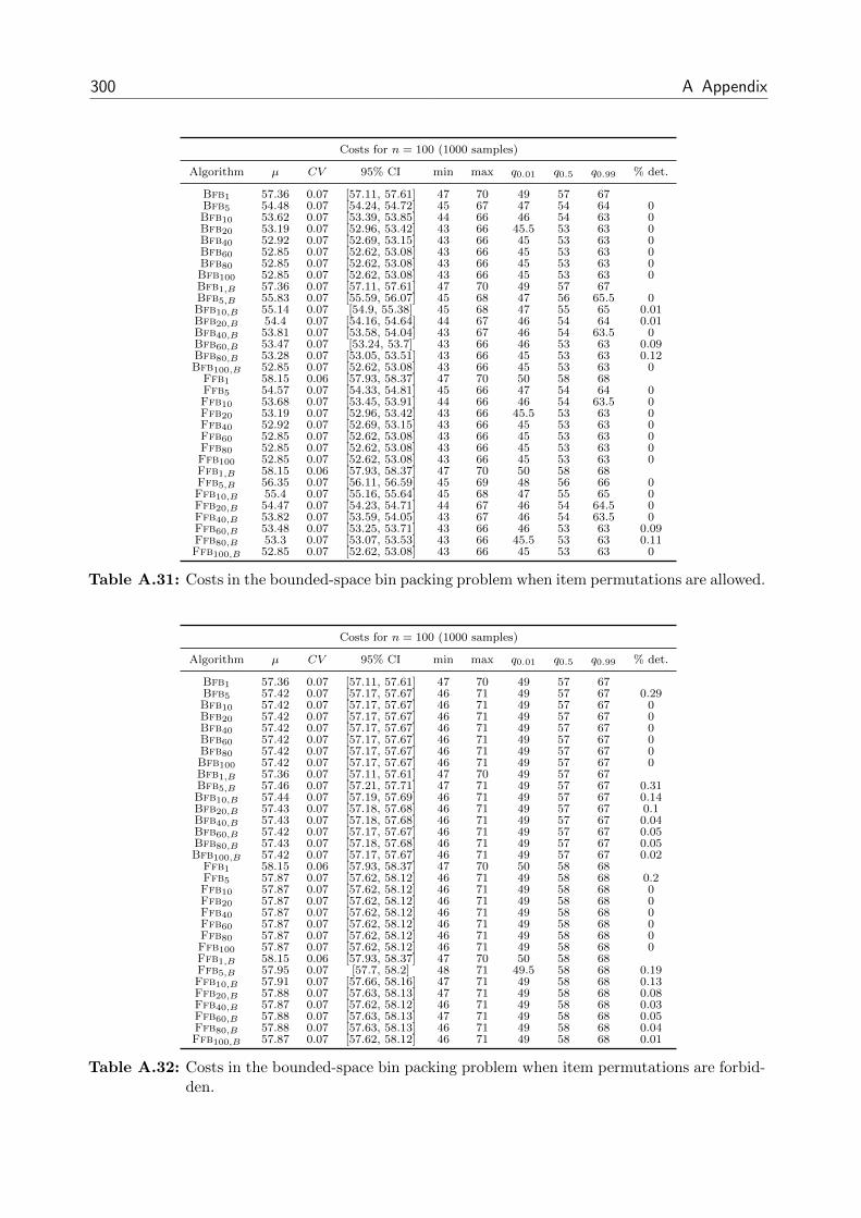
300 A Appendix
Costs for n = 100 (1000 samples)
Algorithm µ CV 95% CI min max q0.01 q0.5 q0.99 % det.
Bfb1 57.36 0.07 [57.11, 57.61] 47 70 49 57 67Bfb5 54.48 0.07 [54.24, 54.72] 45 67 47 54 64 0Bfb10 53.62 0.07 [53.39, 53.85] 44 66 46 54 63 0Bfb20 53.19 0.07 [52.96, 53.42] 43 66 45.5 53 63 0Bfb40 52.92 0.07 [52.69, 53.15] 43 66 45 53 63 0Bfb60 52.85 0.07 [52.62, 53.08] 43 66 45 53 63 0Bfb80 52.85 0.07 [52.62, 53.08] 43 66 45 53 63 0Bfb100 52.85 0.07 [52.62, 53.08] 43 66 45 53 63 0Bfb1,B 57.36 0.07 [57.11, 57.61] 47 70 49 57 67Bfb5,B 55.83 0.07 [55.59, 56.07] 45 68 47 56 65.5 0Bfb10,B 55.14 0.07 [54.9, 55.38] 45 68 47 55 65 0.01Bfb20,B 54.4 0.07 [54.16, 54.64] 44 67 46 54 64 0.01Bfb40,B 53.81 0.07 [53.58, 54.04] 43 67 46 54 63.5 0Bfb60,B 53.47 0.07 [53.24, 53.7] 43 66 46 53 63 0.09Bfb80,B 53.28 0.07 [53.05, 53.51] 43 66 45 53 63 0.12Bfb100,B 52.85 0.07 [52.62, 53.08] 43 66 45 53 63 0
Ffb1 58.15 0.06 [57.93, 58.37] 47 70 50 58 68Ffb5 54.57 0.07 [54.33, 54.81] 45 66 47 54 64 0Ffb10 53.68 0.07 [53.45, 53.91] 44 66 46 54 63.5 0Ffb20 53.19 0.07 [52.96, 53.42] 43 66 45.5 53 63 0Ffb40 52.92 0.07 [52.69, 53.15] 43 66 45 53 63 0Ffb60 52.85 0.07 [52.62, 53.08] 43 66 45 53 63 0Ffb80 52.85 0.07 [52.62, 53.08] 43 66 45 53 63 0Ffb100 52.85 0.07 [52.62, 53.08] 43 66 45 53 63 0Ffb1,B 58.15 0.06 [57.93, 58.37] 47 70 50 58 68Ffb5,B 56.35 0.07 [56.11, 56.59] 45 69 48 56 66 0Ffb10,B 55.4 0.07 [55.16, 55.64] 45 68 47 55 65 0Ffb20,B 54.47 0.07 [54.23, 54.71] 44 67 46 54 64.5 0Ffb40,B 53.82 0.07 [53.59, 54.05] 43 67 46 54 63.5 0Ffb60,B 53.48 0.07 [53.25, 53.71] 43 66 46 53 63 0.09Ffb80,B 53.3 0.07 [53.07, 53.53] 43 66 45.5 53 63 0.11Ffb100,B 52.85 0.07 [52.62, 53.08] 43 66 45 53 63 0
Table A.31: Costs in the bounded-space bin packing problem when item permutations are allowed.
Costs for n = 100 (1000 samples)
Algorithm µ CV 95% CI min max q0.01 q0.5 q0.99 % det.
Bfb1 57.36 0.07 [57.11, 57.61] 47 70 49 57 67Bfb5 57.42 0.07 [57.17, 57.67] 46 71 49 57 67 0.29Bfb10 57.42 0.07 [57.17, 57.67] 46 71 49 57 67 0Bfb20 57.42 0.07 [57.17, 57.67] 46 71 49 57 67 0Bfb40 57.42 0.07 [57.17, 57.67] 46 71 49 57 67 0Bfb60 57.42 0.07 [57.17, 57.67] 46 71 49 57 67 0Bfb80 57.42 0.07 [57.17, 57.67] 46 71 49 57 67 0Bfb100 57.42 0.07 [57.17, 57.67] 46 71 49 57 67 0Bfb1,B 57.36 0.07 [57.11, 57.61] 47 70 49 57 67Bfb5,B 57.46 0.07 [57.21, 57.71] 47 71 49 57 67 0.31Bfb10,B 57.44 0.07 [57.19, 57.69] 46 71 49 57 67 0.14Bfb20,B 57.43 0.07 [57.18, 57.68] 46 71 49 57 67 0.1Bfb40,B 57.43 0.07 [57.18, 57.68] 46 71 49 57 67 0.04Bfb60,B 57.42 0.07 [57.17, 57.67] 46 71 49 57 67 0.05Bfb80,B 57.43 0.07 [57.18, 57.68] 46 71 49 57 67 0.05Bfb100,B 57.42 0.07 [57.17, 57.67] 46 71 49 57 67 0.02
Ffb1 58.15 0.06 [57.93, 58.37] 47 70 50 58 68Ffb5 57.87 0.07 [57.62, 58.12] 46 71 49 58 68 0.2Ffb10 57.87 0.07 [57.62, 58.12] 46 71 49 58 68 0Ffb20 57.87 0.07 [57.62, 58.12] 46 71 49 58 68 0Ffb40 57.87 0.07 [57.62, 58.12] 46 71 49 58 68 0Ffb60 57.87 0.07 [57.62, 58.12] 46 71 49 58 68 0Ffb80 57.87 0.07 [57.62, 58.12] 46 71 49 58 68 0Ffb100 57.87 0.07 [57.62, 58.12] 46 71 49 58 68 0Ffb1,B 58.15 0.06 [57.93, 58.37] 47 70 50 58 68Ffb5,B 57.95 0.07 [57.7, 58.2] 48 71 49.5 58 68 0.19Ffb10,B 57.91 0.07 [57.66, 58.16] 47 71 49 58 68 0.13Ffb20,B 57.88 0.07 [57.63, 58.13] 47 71 49 58 68 0.08Ffb40,B 57.87 0.07 [57.62, 58.12] 46 71 49 58 68 0.03Ffb60,B 57.88 0.07 [57.63, 58.13] 47 71 49 58 68 0.05Ffb80,B 57.88 0.07 [57.63, 58.13] 46 71 49 58 68 0.04Ffb100,B 57.87 0.07 [57.62, 58.12] 46 71 49 58 68 0.01
Table A.32: Costs in the bounded-space bin packing problem when item permutations are forbid-den.

A.2 Numerical Results from Chapter 5 301
Performance ratios of costs relative to Bfb100 for n = 100 (1000 samples)
Algorithm µ CV 95% CI min max q0.01 q0.5 q0.99 F (1)
Bfb1 1.09 0.02 [1.09, 1.09] 1.02 1.15 1.03 1.09 1.14 0Bfb5 1.03 0.02 [1.03, 1.03] 1 1.1 1 1.04 1.07 0Bfb10 1.01 0.01 [1.01, 1.01] 1 1.08 1 1.02 1.04 0Bfb20 1.01 0.01 [1.01, 1.01] 1 1.04 1 1 1.04 0Bfb40 1 0.01 [1, 1] 1 1.02 1 1 1.02 0Bfb60 1 0 [1, 1] 1 1.02 1 1 1 0Bfb80 1 0 [1, 1] 1 1 1 1 1 0Bfb100 1 0 [1, 1] 1 1 1 1 1 0Bfb1,B 1.09 0.02 [1.09, 1.09] 1.02 1.15 1.03 1.09 1.14 0Bfb5,B 1.06 0.02 [1.06, 1.06] 1 1.13 1.02 1.06 1.1 0Bfb10,B 1.04 0.02 [1.04, 1.04] 1 1.1 1 1.04 1.1 0Bfb20,B 1.03 0.02 [1.03, 1.03] 1 1.1 1 1.02 1.08 0Bfb40,B 1.02 0.01 [1.02, 1.02] 1 1.08 1 1.02 1.06 0Bfb60,B 1.01 0.01 [1.01, 1.01] 1 1.08 1 1.02 1.05 0Bfb80,B 1.01 0.01 [1.01, 1.01] 1 1.06 1 1 1.04 0Bfb100,B 1 0 [1, 1] 1 1 1 1 1 0
Ffb1 1.1 0.02 [1.1, 1.1] 1.03 1.19 1.05 1.1 1.16 0Ffb5 1.03 0.02 [1.03, 1.03] 1 1.1 1 1.04 1.08 0Ffb10 1.02 0.01 [1.02, 1.02] 1 1.06 1 1.02 1.04 0Ffb20 1.01 0.01 [1.01, 1.01] 1 1.04 1 1 1.04 0Ffb40 1 0.01 [1, 1] 1 1.02 1 1 1.02 0Ffb60 1 0 [1, 1] 1 1.02 1 1 1 0Ffb80 1 0 [1, 1] 1 1.02 1 1 1 0Ffb100 1 0 [1, 1] 1 1.02 1 1 1 0Ffb1,B 1.1 0.02 [1.1, 1.1] 1.03 1.19 1.05 1.1 1.16 0Ffb5,B 1.07 0.02 [1.07, 1.07] 1 1.14 1.02 1.07 1.12 0Ffb10,B 1.05 0.02 [1.05, 1.05] 1 1.12 1.02 1.05 1.1 0Ffb20,B 1.03 0.02 [1.03, 1.03] 1 1.1 1 1.03 1.08 0Ffb40,B 1.02 0.01 [1.02, 1.02] 1 1.08 1 1.02 1.06 0Ffb60,B 1.01 0.01 [1.01, 1.01] 1 1.08 1 1.02 1.05 0Ffb80,B 1.01 0.01 [1.01, 1.01] 1 1.06 1 1 1.04 0Ffb100,B 1 0 [1, 1] 1 1.02 1 1 1 0
Table A.33: Performance ratios of costs relative to Bfb100 in the bounded-space bin packingproblem when item permutations are allowed.
Performance ratios of costs relative to Bfb100 for n = 100 (1000 samples)
Algorithm µ CV 95% CI min max q0.01 q0.5 q0.99 F (1)
Bfb1 1 0.02 [1, 1] 0.95 1.05 0.96 1 1.04 0.29Bfb5 1 0 [1, 1] 1 1 1 1 1 0Bfb10 1 0 [1, 1] 1 1 1 1 1 0Bfb20 1 0 [1, 1] 1 1 1 1 1 0Bfb40 1 0 [1, 1] 1 1 1 1 1 0Bfb60 1 0 [1, 1] 1 1 1 1 1 0Bfb80 1 0 [1, 1] 1 1 1 1 1 0Bfb100 1 0 [1, 1] 1 1 1 1 1 0Bfb1,B 1 0.02 [1, 1] 0.95 1.05 0.96 1 1.04 0.29Bfb5,B 1 0.01 [1, 1] 0.96 1.05 0.97 1 1.04 0.2Bfb10,B 1 0.01 [1, 1] 0.96 1.04 0.98 1 1.02 0.14Bfb20,B 1 0.01 [1, 1] 0.96 1.04 0.98 1 1.02 0.07Bfb40,B 1 0 [1, 1] 0.98 1.02 0.98 1 1.02 0.03Bfb60,B 1 0 [1, 1] 0.97 1.02 0.98 1 1.02 0.02Bfb80,B 1 0 [1, 1] 0.98 1.02 0.98 1 1.02 0.02Bfb100,B 1 0 [1, 1] 1 1 1 1 1 0
Ffb1 1.01 0.02 [1.01, 1.01] 0.96 1.08 0.97 1.02 1.06 0.1Ffb5 1.01 0.01 [1.01, 1.01] 0.96 1.06 0.98 1 1.04 0.03Ffb10 1.01 0.01 [1.01, 1.01] 0.96 1.06 0.98 1 1.04 0.03Ffb20 1.01 0.01 [1.01, 1.01] 0.96 1.06 0.98 1 1.04 0.03Ffb40 1.01 0.01 [1.01, 1.01] 0.96 1.06 0.98 1 1.04 0.03Ffb60 1.01 0.01 [1.01, 1.01] 0.96 1.06 0.98 1 1.04 0.03Ffb80 1.01 0.01 [1.01, 1.01] 0.96 1.06 0.98 1 1.04 0.03Ffb100 1.01 0.01 [1.01, 1.01] 0.96 1.06 0.98 1 1.04 0.03Ffb1,B 1.01 0.02 [1.01, 1.01] 0.96 1.08 0.97 1.02 1.06 0.1Ffb5,B 1.01 0.01 [1.01, 1.01] 0.97 1.06 0.98 1 1.04 0.08Ffb10,B 1.01 0.01 [1.01, 1.01] 0.97 1.06 0.98 1 1.04 0.06Ffb20,B 1.01 0.01 [1.01, 1.01] 0.96 1.06 0.98 1 1.04 0.05Ffb40,B 1.01 0.01 [1.01, 1.01] 0.96 1.06 0.98 1 1.04 0.04Ffb60,B 1.01 0.01 [1.01, 1.01] 0.96 1.06 0.98 1 1.04 0.04Ffb80,B 1.01 0.01 [1.01, 1.01] 0.96 1.06 0.98 1 1.04 0.04Ffb100,B 1.01 0.01 [1.01, 1.01] 0.96 1.06 0.98 1 1.04 0.03
Table A.34: Performance ratios of costs relative to Bfb100 in the bounded-space bin packingproblem when item permutations are forbidden.

302 A Appendix
Performance ratios of costs relative to online version for n = 100 (1000 samples)
Algorithm µ CV 95% CI min max q0.01 q0.5 q0.99 1− F (1)
Bfb1 1 0 [1, 1] 1 1 1 1 1 0Bfb5 0.95 0.02 [0.95, 0.95] 0.9 1 0.91 0.95 0.98 0Bfb10 0.93 0.02 [0.93, 0.93] 0.88 0.98 0.89 0.93 0.97 0Bfb20 0.93 0.02 [0.93, 0.93] 0.87 0.98 0.88 0.93 0.97 0Bfb40 0.92 0.02 [0.92, 0.92] 0.87 0.98 0.88 0.92 0.97 0Bfb60 0.92 0.02 [0.92, 0.92] 0.87 0.98 0.88 0.92 0.97 0Bfb80 0.92 0.02 [0.92, 0.92] 0.87 0.98 0.88 0.92 0.97 0Bfb100 0.92 0.02 [0.92, 0.92] 0.87 0.98 0.88 0.92 0.97 0Bfb1,B 1 0 [1, 1] 1 1 1 1 1 0Bfb5,B 0.97 0.01 [0.97, 0.97] 0.93 1.02 0.94 0.97 1 0Bfb10,B 0.96 0.02 [0.96, 0.96] 0.92 1 0.93 0.96 1 0Bfb20,B 0.95 0.02 [0.95, 0.95] 0.89 1 0.91 0.95 0.98 0Bfb40,B 0.94 0.02 [0.94, 0.94] 0.89 0.98 0.89 0.94 0.98 0Bfb60,B 0.93 0.02 [0.93, 0.93] 0.87 0.98 0.89 0.93 0.97 0Bfb80,B 0.93 0.02 [0.93, 0.93] 0.87 0.98 0.88 0.93 0.97 0Bfb100,B 0.92 0.02 [0.92, 0.92] 0.87 0.98 0.88 0.92 0.97 0
Ffb1 1 0 [1, 1] 1 1 1 1 1 0Ffb5 0.94 0.02 [0.94, 0.94] 0.88 0.98 0.9 0.94 0.97 0Ffb10 0.92 0.02 [0.92, 0.92] 0.85 0.98 0.88 0.92 0.97 0Ffb20 0.91 0.02 [0.91, 0.91] 0.84 0.97 0.87 0.92 0.96 0Ffb40 0.91 0.02 [0.91, 0.91] 0.84 0.97 0.86 0.91 0.95 0Ffb60 0.91 0.02 [0.91, 0.91] 0.84 0.97 0.86 0.91 0.95 0Ffb80 0.91 0.02 [0.91, 0.91] 0.84 0.97 0.86 0.91 0.95 0Ffb100 0.91 0.02 [0.91, 0.91] 0.84 0.97 0.86 0.91 0.95 0Ffb1,B 1 0 [1, 1] 1 1 1 1 1 0Ffb5,B 0.97 0.02 [0.97, 0.97] 0.92 1 0.93 0.97 1 0Ffb10,B 0.95 0.02 [0.95, 0.95] 0.89 1 0.91 0.95 0.98 0Ffb20,B 0.94 0.02 [0.94, 0.94] 0.87 1 0.89 0.93 0.98 0Ffb40,B 0.93 0.02 [0.93, 0.93] 0.86 0.98 0.88 0.93 0.97 0Ffb60,B 0.92 0.02 [0.92, 0.92] 0.84 0.97 0.87 0.92 0.96 0Ffb80,B 0.92 0.02 [0.92, 0.92] 0.85 0.97 0.87 0.92 0.96 0Ffb100,B 0.91 0.02 [0.91, 0.91] 0.84 0.97 0.86 0.91 0.95 0
Table A.35: Performance ratios of costs relative to the online version of an algorithm in thebounded-space bin packing problem when item permutations are allowed.
Performance ratios of costs relative to online version for n = 100 (1000 samples)
Algorithm µ CV 95% CI min max q0.01 q0.5 q0.99 1− F (1)
Bfb1 1 0 [1, 1] 1 1 1 1 1 0Bfb5 1 0.02 [1, 1] 0.95 1.05 0.96 1 1.04 0.29Bfb10 1 0.02 [1, 1] 0.95 1.05 0.96 1 1.04 0.29Bfb20 1 0.02 [1, 1] 0.95 1.05 0.96 1 1.04 0.29Bfb40 1 0.02 [1, 1] 0.95 1.05 0.96 1 1.04 0.29Bfb60 1 0.02 [1, 1] 0.95 1.05 0.96 1 1.04 0.29Bfb80 1 0.02 [1, 1] 0.95 1.05 0.96 1 1.04 0.29Bfb100 1 0.02 [1, 1] 0.95 1.05 0.96 1 1.04 0.29Bfb1,B 1 0 [1, 1] 1 1 1 1 1 0Bfb5,B 1 0.02 [1, 1] 0.95 1.05 0.96 1 1.04 0.31Bfb10,B 1 0.02 [1, 1] 0.95 1.05 0.96 1 1.04 0.3Bfb20,B 1 0.02 [1, 1] 0.95 1.06 0.96 1 1.04 0.3Bfb40,B 1 0.02 [1, 1] 0.95 1.05 0.96 1 1.04 0.29Bfb60,B 1 0.02 [1, 1] 0.95 1.05 0.96 1 1.04 0.29Bfb80,B 1 0.02 [1, 1] 0.95 1.05 0.96 1 1.04 0.29Bfb100,B 1 0.02 [1, 1] 0.95 1.05 0.96 1 1.04 0.29
Ffb1 1 0 [1, 1] 1 1 1 1 1 0Ffb5 1 0.02 [1, 1] 0.95 1.05 0.95 1 1.03 0.2Ffb10 1 0.02 [1, 1] 0.95 1.05 0.95 1 1.03 0.2Ffb20 1 0.02 [1, 1] 0.95 1.05 0.95 1 1.03 0.2Ffb40 1 0.02 [1, 1] 0.95 1.05 0.95 1 1.03 0.2Ffb60 1 0.02 [1, 1] 0.95 1.05 0.95 1 1.03 0.2Ffb80 1 0.02 [1, 1] 0.95 1.05 0.95 1 1.03 0.2Ffb100 1 0.02 [1, 1] 0.95 1.05 0.95 1 1.03 0.2Ffb1,B 1 0 [1, 1] 1 1 1 1 1 0Ffb5,B 1 0.02 [1, 1] 0.93 1.05 0.96 1 1.03 0.19Ffb10,B 1 0.02 [1, 1] 0.95 1.05 0.95 1 1.03 0.21Ffb20,B 1 0.02 [1, 1] 0.95 1.05 0.95 1 1.03 0.2Ffb40,B 1 0.02 [1, 1] 0.95 1.05 0.95 1 1.03 0.2Ffb60,B 1 0.02 [1, 1] 0.95 1.05 0.95 1 1.03 0.2Ffb80,B 1 0.02 [1, 1] 0.95 1.05 0.95 1 1.03 0.2Ffb100,B 1 0.02 [1, 1] 0.95 1.05 0.95 1 1.03 0.2
Table A.36: Performance ratios of costs relative to the online version of an algorithm in thebounded-space bin packing problem when item permutations are forbidden.

A.2 Numerical Results from Chapter 5 303
A.2.4 Online Traveling Salesman with Lookahead
Costs for n = 25 (1000 samples)
Algorithm µ CV 95% CI min max q0.01 q0.5 q0.99 % det.
Nn1 14.05 0.1 [13.96, 14.14] 10.5 19.2 10.8 14.05 17.5Nn5 8.09 0.1 [8.04, 8.14] 6 10.2 6.4 8 9.95 0Nn10 6.43 0.11 [6.39, 6.47] 4.2 8.8 5 6.4 8 0.02Nn15 5.77 0.1 [5.73, 5.81] 3.8 7.9 4.5 5.8 7.3 0.13Nn20 5.48 0.1 [5.45, 5.51] 3.6 7.2 4.25 5.5 6.8 0.23Nn25 5.39 0.1 [5.36, 5.42] 3.8 7.2 4.1 5.4 6.6 0.09Nn1,B 14.05 0.1 [13.96, 14.14] 10.5 19.2 10.8 14.05 17.5Nn5,B 9.76 0.09 [9.71, 9.81] 7 13 7.65 9.8 11.95 0Nn10,B 8.06 0.1 [8.01, 8.11] 5.6 10.8 6.25 8.1 10 0.02Nn15,B 6.94 0.1 [6.9, 6.98] 5 9 5.45 6.9 8.5 0.08Nn20,B 6.57 0.1 [6.53, 6.61] 4.4 9 5.2 6.6 8.1 0.26Nn25,B 5.39 0.1 [5.36, 5.42] 3.8 7.2 4.1 5.4 6.6 0.03
Ins1 14.05 0.1 [13.96, 14.14] 10.5 19.2 10.8 14.05 17.5Ins5 8.61 0.11 [8.55, 8.67] 6.1 11.9 6.6 8.6 11 0Ins10 6.93 0.12 [6.88, 6.98] 4.1 10.1 5.15 6.9 9.1 0.06Ins15 5.9 0.11 [5.86, 5.94] 4.2 8.4 4.5 5.9 7.5 0.13Ins20 5.56 0.08 [5.53, 5.59] 4.2 7 4.5 5.5 6.6 0.28Ins25 5.55 0.06 [5.53, 5.57] 4.4 6.5 4.7 5.6 6.3 0.46Ins1,B 14.05 0.1 [13.96, 14.14] 10.5 19.2 10.8 14.05 17.5Ins5,B 9.91 0.1 [9.85, 9.97] 7.1 13 7.8 9.9 12.3 0Ins10,B 8.29 0.09 [8.24, 8.34] 6 10.4 6.55 8.3 10.05 0.02Ins15,B 6.52 0.08 [6.49, 6.55] 4.4 8.2 5.2 6.5 7.7 0.01Ins20,B 6.17 0.09 [6.14, 6.2] 4.4 8.1 5 6.2 7.45 0.19Ins25,B 5.55 0.06 [5.53, 5.57] 4.4 6.5 4.7 5.6 6.3 0.062Opt1 14.05 0.1 [13.96, 14.14] 10.5 19.2 10.8 14.05 17.52Opt5 8.81 0.12 [8.74, 8.88] 5.7 12.2 6.45 8.7 11.5 02Opt10 6.24 0.11 [6.2, 6.28] 4.2 8.8 4.85 6.2 8 0.012Opt15 5.27 0.1 [5.24, 5.3] 3.6 7.2 4.2 5.3 6.5 0.052Opt20 4.79 0.08 [4.77, 4.81] 3.6 6.2 3.95 4.8 5.7 0.12Opt25 4.66 0.07 [4.64, 4.68] 3.6 5.8 3.9 4.7 5.5 0.182Opt1,B 14.05 0.1 [13.96, 14.14] 10.5 19.2 10.8 14.05 17.52Opt5,B 9.99 0.09 [9.93, 10.05] 7.6 12.9 7.9 10 12 02Opt10,B 7.93 0.08 [7.89, 7.97] 6 9.9 6.5 7.9 9.4 02Opt15,B 6.42 0.08 [6.39, 6.45] 5 8 5.3 6.4 7.7 0.012Opt20,B 6.29 0.08 [6.26, 6.32] 4.6 7.8 4.95 6.3 7.5 0.322Opt25,B 4.66 0.07 [4.64, 4.68] 3.6 5.8 3.9 4.7 5.5 0
3Opt1 14.05 0.1 [13.96, 14.14] 10.5 19.2 10.8 14.05 17.53Opt5 8.75 0.12 [8.68, 8.82] 5.7 12.3 6.4 8.7 11.4 03Opt10 6.15 0.1 [6.11, 6.19] 4.2 8.8 4.8 6.1 7.85 03Opt15 5.16 0.09 [5.13, 5.19] 3.6 6.5 4.2 5.1 6.2 0.033Opt20 4.68 0.07 [4.66, 4.7] 3.6 6.2 3.9 4.7 5.5 0.053Opt25 4.57 0.07 [4.55, 4.59] 3.6 5.6 3.9 4.6 5.2 0.123Opt1,B 14.05 0.1 [13.96, 14.14] 10.5 19.2 10.8 14.05 17.53Opt5,B 9.96 0.09 [9.9, 10.02] 7.6 12.9 7.85 10 12 03Opt10,B 7.88 0.08 [7.84, 7.92] 6 9.8 6.5 7.9 9.3 03Opt15,B 6.36 0.07 [6.33, 6.39] 5 7.9 5.3 6.4 7.45 03Opt20,B 6.23 0.08 [6.2, 6.26] 4.6 7.7 5 6.2 7.35 0.33Opt25,B 4.57 0.07 [4.55, 4.59] 3.6 5.6 3.9 4.6 5.2 0
Sa1 14.05 0.1 [13.96, 14.14] 10.5 19.2 10.8 14.05 17.5Sa5 8.92 0.13 [8.85, 8.99] 6.1 12.9 6.6 8.8 11.95 0Sa10 6.24 0.11 [6.2, 6.28] 4.2 9.2 4.85 6.2 8.05 0Sa15 5.27 0.1 [5.24, 5.3] 3.6 7.2 4.2 5.3 6.5 0.05Sa20 4.79 0.08 [4.77, 4.81] 3.6 6.2 3.95 4.8 5.7 0.1Sa25 4.66 0.07 [4.64, 4.68] 3.6 5.8 3.9 4.7 5.5 0.18Sa1,B 14.05 0.1 [13.96, 14.14] 10.5 19.2 10.8 14.05 17.5Sa5,B 10.08 0.09 [10.02, 10.14] 7.6 13.1 8 10.1 12.25 0Sa10,B 7.92 0.08 [7.88, 7.96] 6 9.9 6.5 7.9 9.4 0Sa15,B 6.42 0.08 [6.39, 6.45] 5 8 5.3 6.4 7.7 0.01Sa20,B 6.28 0.08 [6.25, 6.31] 4.6 7.8 4.95 6.3 7.5 0.31
......
......
......
......
......

304 A Appendix
Costs for n = 25 (1000 samples)
Algorithm µ CV 95% CI min max q0.01 q0.5 q0.99 % det.
......
......
......
......
......
Sa25,B 4.66 0.07 [4.64, 4.68] 3.6 5.8 3.9 4.7 5.5 0Ts1 14.05 0.1 [13.96, 14.14] 10.5 19.2 10.8 14.05 17.5Ts5 8.9 0.12 [8.83, 8.97] 6.1 13.1 6.6 8.8 11.85 0Ts10 6.22 0.11 [6.18, 6.26] 4.2 8.6 4.8 6.2 7.95 0.01Ts15 5.21 0.09 [5.18, 5.24] 3.6 6.8 4.2 5.2 6.4 0.05Ts20 4.76 0.08 [4.74, 4.78] 3.6 6.5 3.95 4.75 5.6 0.11Ts25 4.64 0.07 [4.62, 4.66] 3.6 5.7 3.9 4.7 5.4 0.2Ts1,B 14.05 0.1 [13.96, 14.14] 10.5 19.2 10.8 14.05 17.5Ts5,B 10.07 0.09 [10.01, 10.13] 7.6 13.1 8 10.1 12.2 0Ts10,B 7.97 0.08 [7.93, 8.01] 6 9.6 6.5 8 9.4 0Ts15,B 6.42 0.08 [6.39, 6.45] 5 7.9 5.3 6.4 7.6 0Ts20,B 6.3 0.08 [6.27, 6.33] 4.6 7.9 4.95 6.3 7.45 0.33Ts25,B 4.65 0.07 [4.63, 4.67] 3.6 5.7 3.9 4.7 5.4 0Opt1 14.05 0.1 [13.96, 14.14] 10.5 19.2 10.8 14.05 17.5Opt5 9.55 0.1 [9.49, 9.61] 6.8 13 7.55 9.5 11.8 0Opt10 6.89 0.1 [6.85, 6.93] 5.1 9.6 5.3 6.9 8.5 0Opt15 5.67 0.1 [5.63, 5.71] 4.1 11.2 4.4 5.6 7.15 0.01Opt20 4.89 0.08 [4.87, 4.91] 3.6 6.5 4 4.9 5.9 0.02Opt25 4.52 0.06 [4.5, 4.54] 3.6 5.5 3.85 4.5 5.15 0.02Opt1,B 14.05 0.1 [13.96, 14.14] 10.5 19.2 10.8 14.05 17.5Opt5,B 10.41 0.09 [10.35, 10.47] 7.4 13.8 8.35 10.4 12.6 0Opt10,B 8.13 0.08 [8.09, 8.17] 6 10 6.7 8.1 9.5 0Opt15,B 6.55 0.07 [6.52, 6.58] 5.1 7.9 5.4 6.6 7.6 0Opt20,B 6.4 0.08 [6.37, 6.43] 4.8 7.7 5 6.4 7.5 0.3Opt25,B 4.53 0.06 [4.51, 4.55] 3.6 5.4 3.85 4.5 5.2 0
Table A.37: Costs in the TSP.

A.2 Numerical Results from Chapter 5 305
Performance ratios of costs relative to Opt for n = 25 (1000 samples)
Algorithm µ CV 95% CI min max q0.01 q0.5 q0.99 F (1)
Nn1 3.11 0.11 [3.09, 3.13] 2.19 4.68 2.37 3.1 3.98 0Nn5 1.79 0.1 [1.78, 1.8] 1.25 2.49 1.4 1.78 2.21 0Nn10 1.42 0.1 [1.41, 1.43] 1.07 1.98 1.12 1.42 1.74 0Nn15 1.28 0.09 [1.27, 1.29] 1 1.78 1.05 1.27 1.56 0Nn20 1.21 0.09 [1.2, 1.22] 1 1.68 1.02 1.21 1.48 0Nn25 1.19 0.08 [1.18, 1.2] 1 1.5 1 1.19 1.43 0Nn1,B 3.11 0.11 [3.09, 3.13] 2.19 4.68 2.37 3.1 3.98 0Nn5,B 2.16 0.1 [2.15, 2.17] 1.49 2.93 1.69 2.15 2.63 0Nn10,B 1.78 0.09 [1.77, 1.79] 1.24 2.35 1.43 1.77 2.22 0Nn15,B 1.54 0.09 [1.53, 1.55] 1.14 1.93 1.25 1.53 1.85 0Nn20,B 1.45 0.09 [1.44, 1.46] 1.08 2 1.18 1.45 1.76 0Nn25,B 1.19 0.08 [1.18, 1.2] 1 1.5 1 1.19 1.43 0
Ins1 3.11 0.11 [3.09, 3.13] 2.19 4.68 2.37 3.1 3.98 0Ins5 1.91 0.11 [1.9, 1.92] 1.37 2.8 1.48 1.89 2.44 0Ins10 1.53 0.11 [1.52, 1.54] 1.11 2.2 1.18 1.52 1.97 0Ins15 1.31 0.11 [1.3, 1.32] 0.96 1.77 1.02 1.3 1.67 0Ins20 1.23 0.08 [1.22, 1.24] 0.92 1.67 1.03 1.23 1.5 0.01Ins25 1.23 0.05 [1.23, 1.23] 1.02 1.45 1.08 1.23 1.38 0Ins1,B 3.11 0.11 [3.09, 3.13] 2.19 4.68 2.37 3.1 3.98 0Ins5,B 2.19 0.1 [2.18, 2.2] 1.62 3.05 1.69 2.19 2.75 0Ins10,B 1.84 0.09 [1.83, 1.85] 1.29 2.41 1.41 1.84 2.24 0Ins15,B 1.44 0.07 [1.43, 1.45] 1.15 1.81 1.2 1.44 1.69 0Ins20,B 1.37 0.08 [1.36, 1.38] 1.09 1.67 1.14 1.36 1.62 0Ins25,B 1.23 0.05 [1.23, 1.23] 1.02 1.45 1.08 1.23 1.38 02Opt1 3.11 0.11 [3.09, 3.13] 2.19 4.68 2.37 3.1 3.98 02Opt5 1.95 0.13 [1.93, 1.97] 1.33 3.05 1.43 1.93 2.56 02Opt10 1.38 0.1 [1.37, 1.39] 1.04 2.02 1.11 1.37 1.74 02Opt15 1.17 0.08 [1.16, 1.18] 0.95 1.51 1 1.16 1.39 02Opt20 1.06 0.05 [1.06, 1.06] 0.9 1.3 0.98 1.05 1.22 0.022Opt25 1.03 0.04 [1.03, 1.03] 0.87 1.23 0.96 1.02 1.14 0.032Opt1,B 3.11 0.11 [3.09, 3.13] 2.19 4.68 2.37 3.1 3.98 02Opt5,B 2.21 0.1 [2.2, 2.22] 1.62 3.15 1.73 2.2 2.78 02Opt10,B 1.76 0.08 [1.75, 1.77] 1.31 2.25 1.43 1.75 2.12 02Opt15,B 1.42 0.07 [1.41, 1.43] 1.15 1.69 1.21 1.41 1.66 02Opt20,B 1.39 0.07 [1.38, 1.4] 1.09 1.71 1.15 1.4 1.62 02Opt25,B 1.03 0.04 [1.03, 1.03] 0.87 1.23 0.96 1.02 1.14 0.03
3Opt1 3.11 0.11 [3.09, 3.13] 2.19 4.68 2.37 3.1 3.98 03Opt5 1.94 0.13 [1.92, 1.96] 1.33 3.05 1.43 1.93 2.59 03Opt10 1.36 0.09 [1.35, 1.37] 1.04 1.91 1.09 1.35 1.7 03Opt15 1.14 0.08 [1.13, 1.15] 0.89 1.44 1 1.13 1.37 0.013Opt20 1.03 0.04 [1.03, 1.03] 0.87 1.28 0.96 1.02 1.18 0.033Opt25 1.01 0.02 [1.01, 1.01] 0.85 1.13 0.94 1 1.08 0.063Opt1,B 3.11 0.11 [3.09, 3.13] 2.19 4.68 2.37 3.1 3.98 03Opt5,B 2.21 0.1 [2.2, 2.22] 1.56 3.15 1.73 2.19 2.76 03Opt10,B 1.75 0.08 [1.74, 1.76] 1.33 2.2 1.43 1.74 2.1 03Opt15,B 1.41 0.06 [1.4, 1.42] 1.13 1.69 1.2 1.4 1.61 03Opt20,B 1.38 0.07 [1.37, 1.39] 1.06 1.71 1.15 1.38 1.6 03Opt25,B 1.01 0.02 [1.01, 1.01] 0.85 1.13 0.94 1 1.08 0.06
Sa1 3.11 0.11 [3.09, 3.13] 2.19 4.68 2.37 3.1 3.98 0Sa5 1.98 0.13 [1.96, 2] 1.4 3.05 1.48 1.95 2.75 0Sa10 1.38 0.1 [1.37, 1.39] 1.04 2.02 1.11 1.37 1.74 0Sa15 1.17 0.08 [1.16, 1.18] 0.95 1.51 1 1.16 1.39 0Sa20 1.06 0.05 [1.06, 1.06] 0.9 1.3 0.98 1.05 1.22 0.02Sa25 1.03 0.04 [1.03, 1.03] 0.87 1.23 0.96 1.02 1.14 0.03Sa1,B 3.11 0.11 [3.09, 3.13] 2.19 4.68 2.37 3.1 3.98 0Sa5,B 2.23 0.1 [2.22, 2.24] 1.6 2.98 1.74 2.23 2.75 0Sa10,B 1.75 0.08 [1.74, 1.76] 1.33 2.25 1.43 1.74 2.12 0Sa15,B 1.42 0.07 [1.41, 1.43] 1.15 1.69 1.21 1.41 1.66 0Sa20,B 1.39 0.07 [1.38, 1.4] 1.06 1.71 1.15 1.39 1.62 0Sa25,B 1.03 0.04 [1.03, 1.03] 0.87 1.23 0.96 1.02 1.14 0.03
Ts1 3.11 0.11 [3.09, 3.13] 2.19 4.68 2.37 3.1 3.98 0Ts5 1.97 0.13 [1.95, 1.99] 1.4 3.05 1.48 1.95 2.72 0Ts10 1.38 0.1 [1.37, 1.39] 1.02 1.87 1.1 1.36 1.71 0
......
......
......
......
......
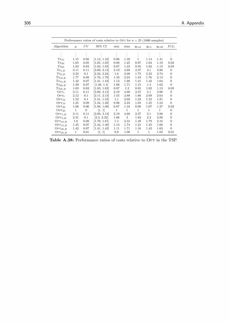
306 A Appendix
Performance ratios of costs relative to Opt for n = 25 (1000 samples)
Algorithm µ CV 95% CI min max q0.01 q0.5 q0.99 F (1)
......
......
......
......
......
Ts15 1.15 0.08 [1.14, 1.16] 0.96 1.49 1 1.14 1.41 0Ts20 1.05 0.05 [1.05, 1.05] 0.88 1.25 0.97 1.04 1.19 0.02Ts25 1.03 0.03 [1.03, 1.03] 0.87 1.23 0.95 1.02 1.13 0.03Ts1,B 3.11 0.11 [3.09, 3.13] 2.19 4.68 2.37 3.1 3.98 0Ts5,B 2.23 0.1 [2.22, 2.24] 1.6 2.98 1.75 2.22 2.74 0Ts10,B 1.77 0.08 [1.76, 1.78] 1.33 2.24 1.43 1.76 2.13 0Ts15,B 1.42 0.07 [1.41, 1.43] 1.13 1.68 1.21 1.42 1.64 0Ts20,B 1.39 0.07 [1.38, 1.4] 1.06 1.71 1.15 1.4 1.62 0Ts25,B 1.03 0.03 [1.03, 1.03] 0.87 1.2 0.95 1.02 1.13 0.03Opt1 3.11 0.11 [3.09, 3.13] 2.19 4.68 2.37 3.1 3.98 0Opt5 2.12 0.1 [2.11, 2.13] 1.55 2.88 1.66 2.09 2.64 0Opt10 1.52 0.1 [1.51, 1.53] 1.1 2.02 1.23 1.52 1.91 0Opt15 1.25 0.09 [1.24, 1.26] 0.96 2.24 1.04 1.25 1.54 0Opt20 1.08 0.06 [1.08, 1.08] 0.87 1.34 0.98 1.07 1.27 0.02Opt25 1 0 [1, 1] 1 1 1 1 1 0Opt1,B 3.11 0.11 [3.09, 3.13] 2.19 4.68 2.37 3.1 3.98 0Opt5,B 2.31 0.1 [2.3, 2.32] 1.66 3 1.82 2.3 2.89 0Opt10,B 1.8 0.08 [1.79, 1.81] 1.4 2.34 1.48 1.79 2.16 0Opt15,B 1.45 0.07 [1.44, 1.46] 1.13 1.74 1.21 1.45 1.66 0Opt20,B 1.42 0.07 [1.41, 1.43] 1.11 1.71 1.16 1.42 1.63 0Opt25,B 1 0.01 [1, 1] 0.9 1.08 1 1 1.02 0.01
Table A.38: Performance ratios of costs relative to Opt in the TSP.

A.2 Numerical Results from Chapter 5 307
Performance ratios of costs relative to online version for n = 25 (1000 samples)
Algorithm µ CV 95% CI min max q0.01 q0.5 q0.99 1− F (1)
Nn1 1 0 [1, 1] 1 1 1 1 1 0Nn5 0.58 0.11 [0.58, 0.58] 0.41 0.79 0.45 0.57 0.74 0Nn10 0.46 0.12 [0.46, 0.46] 0.29 0.66 0.33 0.46 0.6 0Nn15 0.41 0.13 [0.41, 0.41] 0.27 0.62 0.29 0.41 0.56 0Nn20 0.39 0.14 [0.39, 0.39] 0.23 0.61 0.28 0.39 0.54 0Nn25 0.39 0.13 [0.39, 0.39] 0.23 0.61 0.27 0.38 0.53 0Nn1,B 1 0 [1, 1] 1 1 1 1 1 0Nn5,B 0.7 0.1 [0.7, 0.7] 0.52 0.9 0.55 0.7 0.86 0Nn10,B 0.58 0.11 [0.58, 0.58] 0.39 0.78 0.44 0.57 0.74 0Nn15,B 0.5 0.12 [0.5, 0.5] 0.33 0.71 0.37 0.49 0.66 0Nn20,B 0.47 0.12 [0.47, 0.47] 0.31 0.68 0.36 0.47 0.62 0Nn25,B 0.39 0.13 [0.39, 0.39] 0.23 0.61 0.27 0.38 0.53 0
Ins1 1 0 [1, 1] 1 1 1 1 1 0Ins5 0.62 0.12 [0.62, 0.62] 0.44 0.87 0.46 0.61 0.79 0Ins10 0.5 0.14 [0.5, 0.5] 0.29 0.82 0.35 0.49 0.67 0Ins15 0.42 0.15 [0.42, 0.42] 0.27 0.68 0.29 0.42 0.57 0Ins20 0.4 0.12 [0.4, 0.4] 0.27 0.57 0.31 0.39 0.54 0Ins25 0.4 0.11 [0.4, 0.4] 0.29 0.57 0.32 0.4 0.52 0Ins1,B 1 0 [1, 1] 1 1 1 1 1 0Ins5,B 0.71 0.09 [0.71, 0.71] 0.51 0.92 0.56 0.71 0.86 0Ins10,B 0.59 0.1 [0.59, 0.59] 0.43 0.8 0.47 0.59 0.73 0Ins15,B 0.47 0.11 [0.47, 0.47] 0.31 0.66 0.36 0.47 0.59 0Ins20,B 0.44 0.11 [0.44, 0.44] 0.31 0.61 0.34 0.44 0.57 0Ins25,B 0.4 0.11 [0.4, 0.4] 0.29 0.57 0.32 0.4 0.52 02Opt1 1 0 [1, 1] 1 1 1 1 1 02Opt5 0.63 0.12 [0.63, 0.63] 0.42 0.85 0.47 0.63 0.81 02Opt10 0.45 0.13 [0.45, 0.45] 0.29 0.72 0.33 0.44 0.6 02Opt15 0.38 0.13 [0.38, 0.38] 0.25 0.63 0.28 0.38 0.5 02Opt20 0.34 0.12 [0.34, 0.34] 0.22 0.52 0.26 0.34 0.46 02Opt25 0.33 0.12 [0.33, 0.33] 0.22 0.49 0.26 0.33 0.44 02Opt1,B 1 0 [1, 1] 1 1 1 1 1 02Opt5,B 0.71 0.09 [0.71, 0.71] 0.54 0.95 0.57 0.71 0.87 02Opt10,B 0.57 0.1 [0.57, 0.57] 0.42 0.75 0.45 0.57 0.71 02Opt15,B 0.46 0.1 [0.46, 0.46] 0.31 0.65 0.35 0.46 0.58 02Opt20,B 0.45 0.1 [0.45, 0.45] 0.31 0.62 0.36 0.45 0.57 02Opt25,B 0.33 0.12 [0.33, 0.33] 0.22 0.49 0.26 0.33 0.44 0
3Opt1 1 0 [1, 1] 1 1 1 1 1 03Opt5 0.63 0.12 [0.63, 0.63] 0.42 0.85 0.47 0.62 0.8 03Opt10 0.44 0.12 [0.44, 0.44] 0.29 0.71 0.33 0.44 0.58 03Opt15 0.37 0.12 [0.37, 0.37] 0.25 0.55 0.28 0.37 0.48 03Opt20 0.34 0.11 [0.34, 0.34] 0.22 0.47 0.26 0.33 0.45 03Opt25 0.33 0.11 [0.33, 0.33] 0.22 0.46 0.25 0.33 0.43 03Opt1,B 1 0 [1, 1] 1 1 1 1 1 03Opt5,B 0.71 0.09 [0.71, 0.71] 0.54 0.95 0.58 0.71 0.87 03Opt10,B 0.56 0.09 [0.56, 0.56] 0.43 0.76 0.45 0.56 0.7 03Opt15,B 0.46 0.1 [0.46, 0.46] 0.31 0.65 0.35 0.45 0.57 03Opt20,B 0.45 0.1 [0.45, 0.45] 0.31 0.59 0.36 0.45 0.56 03Opt25,B 0.33 0.11 [0.33, 0.33] 0.22 0.46 0.25 0.33 0.43 0
Sa1 1 0 [1, 1] 1 1 1 1 1 0Sa5 0.64 0.12 [0.64, 0.64] 0.45 0.89 0.48 0.63 0.82 0Sa10 0.45 0.13 [0.45, 0.45] 0.29 0.72 0.33 0.44 0.6 0Sa15 0.38 0.13 [0.38, 0.38] 0.25 0.63 0.28 0.38 0.5 0Sa20 0.34 0.12 [0.34, 0.34] 0.22 0.52 0.26 0.34 0.46 0Sa25 0.33 0.12 [0.33, 0.33] 0.22 0.49 0.26 0.33 0.44 0Sa1,B 1 0 [1, 1] 1 1 1 1 1 0Sa5,B 0.72 0.09 [0.72, 0.72] 0.53 0.95 0.58 0.72 0.87 0Sa10,B 0.57 0.1 [0.57, 0.57] 0.42 0.75 0.45 0.57 0.71 0Sa15,B 0.46 0.1 [0.46, 0.46] 0.31 0.65 0.35 0.46 0.58 0Sa20,B 0.45 0.1 [0.45, 0.45] 0.3 0.62 0.35 0.45 0.57 0Sa25,B 0.33 0.12 [0.33, 0.33] 0.22 0.49 0.26 0.33 0.44 0
Ts1 1 0 [1, 1] 1 1 1 1 1 0Ts5 0.64 0.12 [0.64, 0.64] 0.43 0.88 0.47 0.63 0.82 0Ts10 0.45 0.13 [0.45, 0.45] 0.29 0.71 0.33 0.44 0.59 0
......
......
......
......
......

308 A Appendix
Performance ratios of costs relative to online version for n = 25 (1000 samples)
Algorithm µ CV 95% CI min max q0.01 q0.5 q0.99 1− F (1)
......
......
......
......
......
Ts15 0.37 0.13 [0.37, 0.37] 0.24 0.6 0.28 0.37 0.5 0Ts20 0.34 0.12 [0.34, 0.34] 0.21 0.49 0.26 0.34 0.46 0Ts25 0.33 0.11 [0.33, 0.33] 0.22 0.48 0.26 0.33 0.44 0Ts1,B 1 0 [1, 1] 1 1 1 1 1 0Ts5,B 0.72 0.09 [0.72, 0.72] 0.54 0.95 0.58 0.72 0.87 0Ts10,B 0.57 0.09 [0.57, 0.57] 0.43 0.75 0.45 0.57 0.71 0Ts15,B 0.46 0.1 [0.46, 0.46] 0.31 0.63 0.35 0.46 0.58 0Ts20,B 0.45 0.1 [0.45, 0.45] 0.3 0.6 0.35 0.45 0.57 0Ts25,B 0.33 0.11 [0.33, 0.33] 0.22 0.48 0.26 0.33 0.44 0Opt1 1 0 [1, 1] 1 1 1 1 1 0Opt5 0.68 0.09 [0.68, 0.68] 0.5 0.87 0.54 0.68 0.83 0Opt10 0.49 0.12 [0.49, 0.49] 0.35 0.7 0.37 0.49 0.64 0Opt15 0.41 0.13 [0.41, 0.41] 0.28 0.67 0.3 0.4 0.54 0Opt20 0.35 0.12 [0.35, 0.35] 0.23 0.53 0.26 0.35 0.47 0Opt25 0.32 0.11 [0.32, 0.32] 0.21 0.46 0.25 0.32 0.42 0Opt1,B 1 0 [1, 1] 1 1 1 1 1 0Opt5,B 0.74 0.09 [0.74, 0.74] 0.54 0.97 0.6 0.74 0.89 0Opt10,B 0.58 0.09 [0.58, 0.58] 0.43 0.78 0.47 0.58 0.72 0Opt15,B 0.47 0.1 [0.47, 0.47] 0.31 0.64 0.37 0.47 0.58 0Opt20,B 0.46 0.1 [0.46, 0.46] 0.33 0.59 0.36 0.46 0.57 0Opt25,B 0.32 0.11 [0.32, 0.32] 0.21 0.46 0.25 0.32 0.42 0
Table A.39: Performance ratios of costs relative to the online version of an algorithm in the TSP.

A.2 Numerical Results from Chapter 5 309
Costs for n = 100 (1000 samples)
Algorithm µ CV 95% CI min max q0.01 q0.5 q0.99 % det.
Nn1 53.11 0.05 [52.95, 53.27] 45.3 64.3 47.1 53.1 60.05Nn5 28.36 0.05 [28.27, 28.45] 24.1 34.1 25.4 28.3 31.75 0Nn10 20.93 0.05 [20.87, 20.99] 18 24.8 18.6 20.9 23.65 0Nn20 15.72 0.06 [15.66, 15.78] 13.1 18.1 13.8 15.7 17.7 0Nn40 12.22 0.06 [12.17, 12.27] 10.2 15 10.6 12.2 14.05 0Nn60 10.82 0.06 [10.78, 10.86] 8.7 13 9.5 10.8 12.3 0.05Nn80 10.15 0.06 [10.11, 10.19] 8.5 12 8.8 10.1 11.6 0.14Nn100 9.95 0.06 [9.91, 9.99] 8.5 11.9 8.7 9.9 11.3 0.2Nn1,B 53.11 0.05 [52.95, 53.27] 45.3 64.3 47.1 53.1 60.05Nn5,B 36.26 0.05 [36.15, 36.37] 31.1 43.3 32.5 36.2 40.65 0Nn10,B 27.89 0.05 [27.8, 27.98] 23.3 31.9 25 27.9 30.8 0Nn20,B 20.74 0.05 [20.68, 20.8] 17.5 24.4 18.3 20.8 23.15 0Nn40,B 16.28 0.05 [16.23, 16.33] 13.5 19 14.2 16.3 18.35 0Nn60,B 13.58 0.06 [13.53, 13.63] 11 16.2 11.9 13.6 15.4 0Nn80,B 12.92 0.06 [12.87, 12.97] 11 15.5 11.3 12.9 14.8 0.21Nn100,B 9.95 0.06 [9.91, 9.99] 8.5 11.9 8.7 9.9 11.3 0
Ins1 53.11 0.05 [52.95, 53.27] 45.3 64.3 47.1 53.1 60.05Ins5 31.14 0.06 [31.02, 31.26] 25.8 37.4 26.8 31.1 35.6 0Ins10 25.11 0.07 [25, 25.22] 19.8 31.3 21.25 25.1 29.5 0.01Ins20 19.11 0.08 [19.02, 19.2] 14.7 24.7 15.7 19.1 23.1 0.01Ins40 13.88 0.09 [13.8, 13.96] 10.9 18.3 11.5 13.8 17.4 0.01Ins60 11.24 0.08 [11.18, 11.3] 8.9 14.6 9.4 11.2 13.45 0.02Ins80 9.95 0.05 [9.92, 9.98] 8.5 11.8 8.8 9.9 11.1 0.06Ins100 9.65 0.03 [9.63, 9.67] 8.5 10.4 8.9 9.7 10.3 0.23Ins1,B 53.11 0.05 [52.95, 53.27] 45.3 64.3 47.1 53.1 60.05Ins5,B 36.37 0.05 [36.26, 36.48] 30.7 43.5 32.05 36.3 41.1 0Ins10,B 27.73 0.05 [27.64, 27.82] 23.8 32.7 24.9 27.8 31 0Ins20,B 20.31 0.04 [20.26, 20.36] 17.3 22.7 18.3 20.4 22.05 0Ins40,B 15.66 0.04 [15.62, 15.7] 14.1 17.4 14.4 15.7 16.9 0Ins60,B 11.94 0.04 [11.91, 11.97] 10.4 13.2 11 11.9 12.9 0Ins80,B 11.51 0.04 [11.48, 11.54] 10 13.6 10.5 11.5 12.6 0.14Ins100,B 9.65 0.03 [9.63, 9.67] 8.5 10.4 8.9 9.7 10.3 02Opt1 53.11 0.05 [52.95, 53.27] 45.3 64.3 47.1 53.1 60.052Opt5 42.03 0.09 [41.8, 42.26] 32.2 55.6 33.75 42 50.75 02Opt10 30.22 0.11 [30.01, 30.43] 21.1 44.6 22.95 30.15 38.9 02Opt20 19.01 0.11 [18.88, 19.14] 14.1 30.5 15.3 18.8 24.4 02Opt40 12.47 0.09 [12.4, 12.54] 9.7 16.9 10.4 12.3 15.65 02Opt60 10.08 0.06 [10.04, 10.12] 8.5 12.8 8.9 10 11.75 0.012Opt80 8.87 0.05 [8.84, 8.9] 7.7 10.4 8 8.9 9.9 0.012Opt100 8.39 0.03 [8.37, 8.41] 7.6 9.3 7.7 8.4 9.05 0.082Opt1,B 53.11 0.05 [52.95, 53.27] 45.3 64.3 47.1 53.1 60.052Opt5,B 38.31 0.05 [38.19, 38.43] 32.9 45 34.15 38.3 42.5 02Opt10,B 27.61 0.04 [27.54, 27.68] 24.2 31.1 25.1 27.6 30.4 02Opt20,B 19.39 0.04 [19.34, 19.44] 16.6 21.8 17.6 19.4 21.3 02Opt40,B 14.78 0.04 [14.74, 14.82] 13.1 16.9 13.5 14.8 16.1 02Opt60,B 11.95 0.04 [11.92, 11.98] 10.4 13.4 10.95 11.9 13 02Opt80,B 11.51 0.04 [11.48, 11.54] 10.1 13.1 10.55 11.5 12.5 0.142Opt100,B 8.39 0.03 [8.37, 8.41] 7.6 9.3 7.7 8.4 9.05 0
3Opt1 53.11 0.05 [52.95, 53.27] 45.3 64.3 47.1 53.1 60.053Opt5 41.59 0.09 [41.36, 41.82] 31.2 53.9 33.15 41.75 50.75 03Opt10 29.23 0.11 [29.03, 29.43] 20.3 40.8 22.4 29 37.95 03Opt20 18.33 0.1 [18.22, 18.44] 13.9 26.1 14.8 18.2 23.3 03Opt40 12.17 0.09 [12.1, 12.24] 10 17.4 10.2 12.1 15.15 03Opt60 9.81 0.06 [9.77, 9.85] 8.3 12 8.8 9.7 11.4 0.013Opt80 8.62 0.04 [8.6, 8.64] 7.7 9.9 7.9 8.6 9.5 0.013Opt100 8.2 0.03 [8.18, 8.22] 7.4 9 7.6 8.2 8.8 0.053Opt1,B 53.11 0.05 [52.95, 53.27] 45.3 64.3 47.1 53.1 60.053Opt5,B 38.23 0.05 [38.11, 38.35] 32.5 44.9 34.05 38.3 42.6 03Opt10,B 27.42 0.04 [27.35, 27.49] 24.2 30.8 24.9 27.4 30.1 03Opt20,B 19.07 0.04 [19.02, 19.12] 16.6 21.5 17.2 19.1 20.8 03Opt40,B 14.46 0.04 [14.42, 14.5] 13 16.2 13.35 14.5 15.6 03Opt60,B 11.66 0.03 [11.64, 11.68] 10.3 12.8 10.8 11.7 12.6 03Opt80,B 11.26 0.03 [11.24, 11.28] 10 12.9 10.4 11.25 12.2 0.13
......
......
......
......
......

310 A Appendix
Costs for n = 100 (1000 samples)
Algorithm µ CV 95% CI min max q0.01 q0.5 q0.99 % det.
......
......
......
......
......
3Opt100,B 8.2 0.03 [8.18, 8.22] 7.4 9 7.6 8.2 8.8 0Sa1 53.11 0.05 [52.95, 53.27] 45.3 64.3 47.1 53.1 60.05Sa5 41.63 0.09 [41.4, 41.86] 29.8 54.6 33.7 41.4 50.5 0Sa10 30.19 0.11 [29.98, 30.4] 21.1 44.6 22.95 30 38.55 0Sa20 19.02 0.11 [18.89, 19.15] 14.1 30.5 15.3 18.8 24.4 0Sa40 12.47 0.09 [12.4, 12.54] 9.7 16.9 10.4 12.3 15.65 0Sa60 10.08 0.06 [10.04, 10.12] 8.5 12.8 8.9 10 11.75 0.01Sa80 8.87 0.05 [8.84, 8.9] 7.7 10.4 8 8.9 9.9 0.01Sa100 8.39 0.03 [8.37, 8.41] 7.6 9.3 7.7 8.4 9.05 0.08Sa1,B 53.11 0.05 [52.95, 53.27] 45.3 64.3 47.1 53.1 60.05Sa5,B 38.34 0.05 [38.22, 38.46] 32.9 44.7 34.25 38.3 42.65 0Sa10,B 27.6 0.04 [27.53, 27.67] 24.2 31.1 25.1 27.6 30.4 0Sa20,B 19.39 0.04 [19.34, 19.44] 16.6 21.8 17.6 19.4 21.3 0Sa40,B 14.78 0.04 [14.74, 14.82] 13.1 16.9 13.5 14.8 16.1 0Sa60,B 11.95 0.04 [11.92, 11.98] 10.4 13.4 10.95 11.9 13 0Sa80,B 11.51 0.04 [11.48, 11.54] 10.1 13.1 10.55 11.5 12.5 0.14Sa100,B 8.39 0.03 [8.37, 8.41] 7.6 9.3 7.7 8.4 9.05 0
Ts1 53.11 0.05 [52.95, 53.27] 45.3 64.3 47.1 53.1 60.05Ts5 41.62 0.09 [41.39, 41.85] 31.3 54.6 33.8 41.4 50.95 0Ts10 29.84 0.11 [29.64, 30.04] 20.3 41.1 22.85 29.7 38 0Ts20 18.88 0.11 [18.75, 19.01] 14.9 26.6 15.4 18.5 24.4 0Ts40 12.46 0.09 [12.39, 12.53] 9.7 16.9 10.4 12.3 15.65 0Ts60 10.08 0.06 [10.04, 10.12] 8.5 12.8 8.9 10 11.75 0.01Ts80 8.87 0.05 [8.84, 8.9] 7.7 10.4 8 8.9 9.9 0.01Ts100 8.39 0.03 [8.37, 8.41] 7.6 9.3 7.7 8.4 9.05 0.08Ts1,B 53.11 0.05 [52.95, 53.27] 45.3 64.3 47.1 53.1 60.05Ts5,B 38.33 0.05 [38.21, 38.45] 32.9 44.7 34.15 38.3 42.7 0Ts10,B 27.48 0.04 [27.41, 27.55] 24 30.8 24.9 27.5 30.15 0Ts20,B 19.32 0.04 [19.27, 19.37] 16.6 21.7 17.6 19.3 21.1 0Ts40,B 14.76 0.04 [14.72, 14.8] 13.1 16.4 13.5 14.8 16.1 0Ts60,B 11.95 0.04 [11.92, 11.98] 10.4 13.4 10.95 11.9 13 0Ts80,B 11.5 0.04 [11.47, 11.53] 10.1 13 10.5 11.5 12.5 0.13Ts100,B 8.39 0.03 [8.37, 8.41] 7.6 9.3 7.7 8.4 9.05 0
Table A.40: Costs in the TSP.

A.2 Numerical Results from Chapter 5 311
Performance ratios of costs relative to 3Opt100 for n = 100 (1000 samples)
Algorithm µ CV 95% CI min max q0.01 q0.5 q0.99 F (1)
Nn1 6.49 0.06 [6.47, 6.51] 5.27 8.13 5.64 6.48 7.52 0Nn5 3.46 0.06 [3.45, 3.47] 2.84 4.16 3.03 3.45 3.97 0Nn10 2.56 0.06 [2.55, 2.57] 2.14 3 2.23 2.55 2.91 0Nn20 1.92 0.06 [1.91, 1.93] 1.52 2.35 1.67 1.92 2.18 0Nn40 1.49 0.06 [1.48, 1.5] 1.24 1.78 1.29 1.49 1.72 0Nn60 1.32 0.06 [1.32, 1.32] 1.1 1.56 1.16 1.32 1.49 0Nn80 1.24 0.06 [1.24, 1.24] 1.05 1.46 1.09 1.24 1.4 0Nn100 1.21 0.05 [1.21, 1.21] 1.06 1.4 1.09 1.21 1.37 0Nn1,B 6.49 0.06 [6.47, 6.51] 5.27 8.13 5.64 6.48 7.52 0Nn5,B 4.43 0.06 [4.41, 4.45] 3.74 5.28 3.9 4.42 5.09 0Nn10,B 3.41 0.05 [3.4, 3.42] 2.77 4.04 3 3.4 3.85 0Nn20,B 2.53 0.06 [2.52, 2.54] 2.08 3.03 2.21 2.53 2.88 0Nn40,B 1.99 0.05 [1.98, 2] 1.66 2.38 1.73 1.99 2.26 0Nn60,B 1.66 0.06 [1.65, 1.67] 1.38 2.01 1.45 1.65 1.88 0Nn80,B 1.58 0.06 [1.57, 1.59] 1.31 1.85 1.39 1.57 1.8 0Nn100,B 1.21 0.05 [1.21, 1.21] 1.06 1.4 1.09 1.21 1.37 0
Ins1 6.49 0.06 [6.47, 6.51] 5.27 8.13 5.64 6.48 7.52 0Ins5 3.8 0.07 [3.78, 3.82] 3.1 4.64 3.26 3.79 4.47 0Ins10 3.07 0.07 [3.06, 3.08] 2.28 3.79 2.55 3.06 3.61 0Ins20 2.33 0.09 [2.32, 2.34] 1.78 3.09 1.91 2.33 2.87 0Ins40 1.69 0.09 [1.68, 1.7] 1.34 2.3 1.4 1.68 2.14 0Ins60 1.37 0.08 [1.36, 1.38] 1.12 1.73 1.15 1.37 1.63 0Ins80 1.21 0.05 [1.21, 1.21] 1.05 1.4 1.08 1.21 1.36 0Ins100 1.18 0.03 [1.18, 1.18] 1.08 1.35 1.11 1.18 1.25 0Ins1,B 6.49 0.06 [6.47, 6.51] 5.27 8.13 5.64 6.48 7.52 0Ins5,B 4.44 0.06 [4.42, 4.46] 3.7 5.42 3.87 4.43 5.1 0Ins10,B 3.39 0.05 [3.38, 3.4] 2.83 4.03 2.98 3.38 3.83 0Ins20,B 2.48 0.05 [2.47, 2.49] 2.07 3.07 2.19 2.48 2.75 0Ins40,B 1.91 0.04 [1.91, 1.91] 1.64 2.2 1.74 1.91 2.08 0Ins60,B 1.46 0.04 [1.46, 1.46] 1.29 1.69 1.33 1.46 1.59 0Ins80,B 1.41 0.04 [1.41, 1.41] 1.19 1.62 1.27 1.41 1.54 0Ins100,B 1.18 0.03 [1.18, 1.18] 1.08 1.35 1.11 1.18 1.25 02Opt1 6.49 0.06 [6.47, 6.51] 5.27 8.13 5.64 6.48 7.52 02Opt5 5.13 0.1 [5.1, 5.16] 3.79 7.01 4.08 5.13 6.33 02Opt10 3.69 0.12 [3.66, 3.72] 2.51 5.37 2.75 3.67 4.86 02Opt20 2.32 0.11 [2.3, 2.34] 1.7 3.63 1.85 2.29 2.99 02Opt40 1.52 0.09 [1.51, 1.53] 1.2 2.14 1.28 1.51 1.9 02Opt60 1.23 0.06 [1.23, 1.23] 1.05 1.6 1.09 1.22 1.44 02Opt80 1.08 0.04 [1.08, 1.08] 0.98 1.25 0.99 1.08 1.19 0.022Opt100 1.02 0.02 [1.02, 1.02] 1 1.12 1 1.02 1.07 02Opt1,B 6.49 0.06 [6.47, 6.51] 5.27 8.13 5.64 6.48 7.52 02Opt5,B 4.68 0.06 [4.66, 4.7] 3.93 5.58 4.1 4.68 5.32 02Opt10,B 3.37 0.05 [3.36, 3.38] 2.86 4.2 3.01 3.37 3.79 02Opt20,B 2.37 0.05 [2.36, 2.38] 2.06 2.92 2.13 2.36 2.65 02Opt40,B 1.8 0.04 [1.8, 1.8] 1.6 2.06 1.63 1.8 1.99 02Opt60,B 1.46 0.04 [1.46, 1.46] 1.24 1.64 1.33 1.46 1.59 02Opt80,B 1.41 0.04 [1.41, 1.41] 1.23 1.59 1.29 1.4 1.54 02Opt100,B 1.02 0.02 [1.02, 1.02] 1 1.12 1 1.02 1.07 0
3Opt1 6.49 0.06 [6.47, 6.51] 5.27 8.13 5.64 6.48 7.52 03Opt5 5.08 0.1 [5.05, 5.11] 3.65 7.01 4.01 5.09 6.21 03Opt10 3.57 0.12 [3.54, 3.6] 2.36 5.1 2.71 3.53 4.76 03Opt20 2.24 0.1 [2.23, 2.25] 1.65 3.11 1.79 2.22 2.86 03Opt40 1.49 0.09 [1.48, 1.5] 1.19 2.1 1.26 1.47 1.85 03Opt60 1.2 0.06 [1.2, 1.2] 1.02 1.44 1.07 1.19 1.4 03Opt80 1.05 0.04 [1.05, 1.05] 0.96 1.21 0.98 1.05 1.14 0.053Opt100 1 0 [1, 1] 1 1 1 1 1 03Opt1,B 6.49 0.06 [6.47, 6.51] 5.27 8.13 5.64 6.48 7.52 03Opt5,B 4.67 0.06 [4.65, 4.69] 3.93 5.49 4.1 4.67 5.3 03Opt10,B 3.35 0.05 [3.34, 3.36] 2.92 4.16 3 3.34 3.75 03Opt20,B 2.33 0.05 [2.32, 2.34] 2.04 2.82 2.11 2.33 2.58 03Opt40,B 1.77 0.04 [1.77, 1.77] 1.57 2.01 1.61 1.77 1.92 03Opt60,B 1.42 0.04 [1.42, 1.42] 1.24 1.61 1.31 1.42 1.54 03Opt80,B 1.38 0.04 [1.38, 1.38] 1.22 1.53 1.27 1.38 1.5 0
......
......
......
......
......

312 A Appendix
Performance ratios of costs relative to 3Opt100 for n = 100 (1000 samples)
Algorithm µ CV 95% CI min max q0.01 q0.5 q0.99 F (1)
......
......
......
......
......
3Opt100,B 1 0 [1, 1] 1 1 1 1 1 0Sa1 6.49 0.06 [6.47, 6.51] 5.27 8.13 5.64 6.48 7.52 0Sa5 5.09 0.1 [5.06, 5.12] 3.47 6.83 4.05 5.07 6.31 0Sa10 3.69 0.12 [3.66, 3.72] 2.51 5.31 2.79 3.66 4.86 0Sa20 2.32 0.11 [2.3, 2.34] 1.7 3.63 1.86 2.3 2.99 0Sa40 1.52 0.09 [1.51, 1.53] 1.2 2.14 1.28 1.51 1.9 0Sa60 1.23 0.06 [1.23, 1.23] 1.05 1.6 1.09 1.22 1.44 0Sa80 1.08 0.04 [1.08, 1.08] 0.98 1.25 0.99 1.08 1.19 0.02Sa100 1.02 0.02 [1.02, 1.02] 1 1.12 1 1.02 1.07 0Sa1,B 6.49 0.06 [6.47, 6.51] 5.27 8.13 5.64 6.48 7.52 0Sa5,B 4.68 0.06 [4.66, 4.7] 3.93 5.49 4.12 4.69 5.34 0Sa10,B 3.37 0.05 [3.36, 3.38] 2.86 4.2 3.01 3.37 3.79 0Sa20,B 2.37 0.05 [2.36, 2.38] 2.06 2.92 2.13 2.36 2.65 0Sa40,B 1.8 0.04 [1.8, 1.8] 1.6 2.06 1.63 1.8 1.99 0Sa60,B 1.46 0.04 [1.46, 1.46] 1.24 1.64 1.33 1.46 1.59 0Sa80,B 1.41 0.04 [1.41, 1.41] 1.23 1.59 1.29 1.4 1.54 0Sa100,B 1.02 0.02 [1.02, 1.02] 1 1.12 1 1.02 1.07 0
Ts1 6.49 0.06 [6.47, 6.51] 5.27 8.13 5.64 6.48 7.52 0Ts5 5.08 0.1 [5.05, 5.11] 3.64 6.83 4.04 5.06 6.33 0Ts10 3.65 0.12 [3.62, 3.68] 2.42 5.14 2.8 3.62 4.69 0Ts20 2.3 0.11 [2.28, 2.32] 1.8 3.47 1.85 2.26 2.95 0Ts40 1.52 0.09 [1.51, 1.53] 1.2 2.14 1.28 1.51 1.9 0Ts60 1.23 0.06 [1.23, 1.23] 1.05 1.6 1.09 1.22 1.44 0Ts80 1.08 0.04 [1.08, 1.08] 0.98 1.25 0.99 1.08 1.19 0.02Ts100 1.02 0.02 [1.02, 1.02] 1 1.12 1 1.02 1.07 0Ts1,B 6.49 0.06 [6.47, 6.51] 5.27 8.13 5.64 6.48 7.52 0Ts5,B 4.68 0.06 [4.66, 4.7] 3.93 5.49 4.12 4.69 5.34 0Ts10,B 3.36 0.05 [3.35, 3.37] 2.9 4.11 2.99 3.35 3.75 0Ts20,B 2.36 0.05 [2.35, 2.37] 2.06 2.89 2.13 2.35 2.63 0Ts40,B 1.8 0.04 [1.8, 1.8] 1.6 2.06 1.63 1.8 1.99 0Ts60,B 1.46 0.04 [1.46, 1.46] 1.24 1.64 1.33 1.46 1.59 0Ts80,B 1.4 0.04 [1.4, 1.4] 1.23 1.58 1.29 1.4 1.53 0Ts100,B 1.02 0.02 [1.02, 1.02] 1 1.12 1 1.02 1.07 0
Table A.41: Performance ratios of costs relative to 3Opt100 in the TSP.

A.2 Numerical Results from Chapter 5 313
Performance ratios of costs relative to online version for n = 100 (1000 samples)
Algorithm µ CV 95% CI min max q0.01 q0.5 q0.99 1− F (1)
Nn1 1 0 [1, 1] 1 1 1 1 1 0Nn5 0.53 0.06 [0.53, 0.53] 0.43 0.63 0.47 0.53 0.6 0Nn10 0.39 0.07 [0.39, 0.39] 0.32 0.48 0.34 0.39 0.46 0Nn20 0.3 0.07 [0.3, 0.3] 0.24 0.37 0.25 0.3 0.35 0Nn40 0.23 0.08 [0.23, 0.23] 0.18 0.3 0.19 0.23 0.28 0Nn60 0.2 0.08 [0.2, 0.2] 0.16 0.27 0.17 0.2 0.25 0Nn80 0.19 0.08 [0.19, 0.19] 0.15 0.26 0.16 0.19 0.23 0Nn100 0.19 0.08 [0.19, 0.19] 0.14 0.24 0.16 0.19 0.22 0Nn1,B 1 0 [1, 1] 1 1 1 1 1 0Nn5,B 0.68 0.05 [0.68, 0.68] 0.59 0.79 0.61 0.68 0.76 0Nn10,B 0.53 0.06 [0.53, 0.53] 0.43 0.63 0.46 0.53 0.6 0Nn20,B 0.39 0.07 [0.39, 0.39] 0.32 0.49 0.33 0.39 0.46 0Nn40,B 0.31 0.07 [0.31, 0.31] 0.24 0.38 0.26 0.31 0.36 0Nn60,B 0.26 0.08 [0.26, 0.26] 0.2 0.33 0.21 0.26 0.31 0Nn80,B 0.24 0.08 [0.24, 0.24] 0.18 0.33 0.2 0.24 0.29 0Nn100,B 0.19 0.08 [0.19, 0.19] 0.14 0.24 0.16 0.19 0.22 0
Ins1 1 0 [1, 1] 1 1 1 1 1 0Ins5 0.59 0.06 [0.59, 0.59] 0.49 0.7 0.51 0.59 0.67 0Ins10 0.47 0.08 [0.47, 0.47] 0.36 0.63 0.4 0.47 0.56 0Ins20 0.36 0.09 [0.36, 0.36] 0.26 0.5 0.29 0.36 0.44 0Ins40 0.26 0.1 [0.26, 0.26] 0.2 0.36 0.21 0.26 0.33 0Ins60 0.21 0.09 [0.21, 0.21] 0.15 0.29 0.17 0.21 0.26 0Ins80 0.19 0.07 [0.19, 0.19] 0.15 0.23 0.16 0.19 0.22 0Ins100 0.18 0.06 [0.18, 0.18] 0.14 0.22 0.16 0.18 0.21 0Ins1,B 1 0 [1, 1] 1 1 1 1 1 0Ins5,B 0.69 0.05 [0.69, 0.69] 0.59 0.8 0.61 0.68 0.77 0Ins10,B 0.52 0.05 [0.52, 0.52] 0.44 0.64 0.46 0.52 0.6 0Ins20,B 0.38 0.06 [0.38, 0.38] 0.32 0.45 0.33 0.38 0.44 0Ins40,B 0.3 0.06 [0.3, 0.3] 0.24 0.36 0.26 0.29 0.34 0Ins60,B 0.23 0.06 [0.23, 0.23] 0.18 0.27 0.19 0.22 0.26 0Ins80,B 0.22 0.07 [0.22, 0.22] 0.17 0.26 0.19 0.22 0.25 0Ins100,B 0.18 0.06 [0.18, 0.18] 0.14 0.22 0.16 0.18 0.21 02Opt1 1 0 [1, 1] 1 1 1 1 1 02Opt5 0.79 0.07 [0.79, 0.79] 0.6 0.94 0.64 0.79 0.91 02Opt10 0.57 0.11 [0.57, 0.57] 0.4 0.79 0.45 0.57 0.72 02Opt20 0.36 0.12 [0.36, 0.36] 0.27 0.54 0.28 0.35 0.48 02Opt40 0.24 0.1 [0.24, 0.24] 0.17 0.32 0.19 0.23 0.29 02Opt60 0.19 0.08 [0.19, 0.19] 0.15 0.24 0.16 0.19 0.23 02Opt80 0.17 0.07 [0.17, 0.17] 0.13 0.21 0.14 0.17 0.2 02Opt100 0.16 0.06 [0.16, 0.16] 0.12 0.2 0.14 0.16 0.18 02Opt1,B 1 0 [1, 1] 1 1 1 1 1 02Opt5,B 0.72 0.05 [0.72, 0.72] 0.61 0.82 0.64 0.72 0.81 02Opt10,B 0.52 0.05 [0.52, 0.52] 0.45 0.61 0.46 0.52 0.58 02Opt20,B 0.37 0.06 [0.37, 0.37] 0.31 0.43 0.32 0.36 0.42 02Opt40,B 0.28 0.06 [0.28, 0.28] 0.23 0.34 0.24 0.28 0.32 02Opt60,B 0.23 0.06 [0.23, 0.23] 0.18 0.28 0.2 0.23 0.26 02Opt80,B 0.22 0.06 [0.22, 0.22] 0.18 0.26 0.19 0.22 0.25 02Opt100,B 0.16 0.06 [0.16, 0.16] 0.12 0.2 0.14 0.16 0.18 0
3Opt1 1 0 [1, 1] 1 1 1 1 1 03Opt5 0.78 0.07 [0.78, 0.78] 0.61 0.94 0.65 0.79 0.9 03Opt10 0.55 0.11 [0.55, 0.55] 0.4 0.75 0.43 0.55 0.7 03Opt20 0.35 0.11 [0.35, 0.35] 0.25 0.49 0.26 0.34 0.45 03Opt40 0.23 0.1 [0.23, 0.23] 0.17 0.33 0.19 0.23 0.3 03Opt60 0.19 0.08 [0.19, 0.19] 0.13 0.23 0.16 0.18 0.22 03Opt80 0.16 0.07 [0.16, 0.16] 0.13 0.2 0.14 0.16 0.19 03Opt100 0.15 0.07 [0.15, 0.15] 0.12 0.19 0.13 0.15 0.18 03Opt1,B 1 0 [1, 1] 1 1 1 1 1 03Opt5,B 0.72 0.05 [0.72, 0.72] 0.6 0.82 0.64 0.72 0.81 03Opt10,B 0.52 0.05 [0.52, 0.52] 0.44 0.61 0.46 0.52 0.58 03Opt20,B 0.36 0.06 [0.36, 0.36] 0.3 0.42 0.31 0.36 0.41 03Opt40,B 0.27 0.06 [0.27, 0.27] 0.22 0.33 0.24 0.27 0.31 03Opt60,B 0.22 0.06 [0.22, 0.22] 0.18 0.27 0.19 0.22 0.25 03Opt80,B 0.21 0.06 [0.21, 0.21] 0.18 0.26 0.18 0.21 0.24 0
......
......
......
......
......

314 A Appendix
Performance ratios of costs relative to online version for n = 100 (1000 samples)
Algorithm µ CV 95% CI min max q0.01 q0.5 q0.99 1− F (1)
......
......
......
......
......
3Opt100,B 0.15 0.07 [0.15, 0.15] 0.12 0.19 0.13 0.15 0.18 0Sa1 1 0 [1, 1] 1 1 1 1 1 0Sa5 0.78 0.08 [0.78, 0.78] 0.59 0.94 0.65 0.79 0.9 0Sa10 0.57 0.11 [0.57, 0.57] 0.4 0.75 0.45 0.57 0.71 0Sa20 0.36 0.12 [0.36, 0.36] 0.27 0.54 0.28 0.35 0.48 0Sa40 0.24 0.1 [0.24, 0.24] 0.17 0.32 0.19 0.23 0.29 0Sa60 0.19 0.08 [0.19, 0.19] 0.15 0.24 0.16 0.19 0.23 0Sa80 0.17 0.07 [0.17, 0.17] 0.13 0.21 0.14 0.17 0.2 0Sa100 0.16 0.06 [0.16, 0.16] 0.12 0.2 0.14 0.16 0.18 0Sa1,B 1 0 [1, 1] 1 1 1 1 1 0Sa5,B 0.72 0.05 [0.72, 0.72] 0.6 0.83 0.65 0.72 0.81 0Sa10,B 0.52 0.05 [0.52, 0.52] 0.45 0.61 0.46 0.52 0.58 0Sa20,B 0.37 0.06 [0.37, 0.37] 0.31 0.43 0.32 0.36 0.42 0Sa40,B 0.28 0.06 [0.28, 0.28] 0.23 0.34 0.24 0.28 0.32 0Sa60,B 0.23 0.06 [0.23, 0.23] 0.18 0.28 0.2 0.23 0.26 0Sa80,B 0.22 0.06 [0.22, 0.22] 0.18 0.26 0.19 0.22 0.25 0Sa100,B 0.16 0.06 [0.16, 0.16] 0.12 0.2 0.14 0.16 0.18 0
Ts1 1 0 [1, 1] 1 1 1 1 1 0Ts5 0.78 0.08 [0.78, 0.78] 0.58 0.93 0.65 0.78 0.91 0Ts10 0.56 0.11 [0.56, 0.56] 0.39 0.75 0.43 0.56 0.71 0Ts20 0.36 0.11 [0.36, 0.36] 0.26 0.52 0.28 0.35 0.47 0Ts40 0.24 0.1 [0.24, 0.24] 0.17 0.32 0.19 0.23 0.29 0Ts60 0.19 0.08 [0.19, 0.19] 0.15 0.24 0.16 0.19 0.23 0Ts80 0.17 0.07 [0.17, 0.17] 0.13 0.21 0.14 0.17 0.2 0Ts100 0.16 0.06 [0.16, 0.16] 0.12 0.2 0.14 0.16 0.18 0Ts1,B 1 0 [1, 1] 1 1 1 1 1 0Ts5,B 0.72 0.05 [0.72, 0.72] 0.6 0.84 0.65 0.72 0.81 0Ts10,B 0.52 0.05 [0.52, 0.52] 0.45 0.61 0.45 0.52 0.58 0Ts20,B 0.36 0.06 [0.36, 0.36] 0.31 0.43 0.32 0.36 0.42 0Ts40,B 0.28 0.06 [0.28, 0.28] 0.23 0.34 0.24 0.28 0.32 0Ts60,B 0.23 0.06 [0.23, 0.23] 0.18 0.28 0.2 0.23 0.26 0Ts80,B 0.22 0.06 [0.22, 0.22] 0.18 0.26 0.19 0.22 0.25 0Ts100,B 0.16 0.06 [0.16, 0.16] 0.12 0.2 0.14 0.16 0.18 0
Table A.42: Performance ratios of costs relative to the online version of an algorithm in the TSP.

A.2 Numerical Results from Chapter 5 315
A.2.5 Online Scheduling with Lookahead
A.2.5.1 Single Machine Problem
Costs for n = 25 (1000 samples)
Algorithm µ CV 95% CI min max q0.01 q0.5 q0.99 % det.
Spt0 1317.65 0.11 [1308.66, 1326.64] 838 1727 994.5 1316.5 1660Spt5 1198.64 0.12 [1189.72, 1207.56] 734 1602 877.5 1196 1538.5 0Spt10 1089.86 0.12 [1081.75, 1097.97] 666 1482 797 1083 1419 0Spt25 825.93 0.12 [819.78, 832.08] 561 1136 617.5 819 1083.5 0Spt50 584.61 0.09 [581.35, 587.87] 426 753 466 581 711.5 0Spt100 516.11 0.1 [512.91, 519.31] 359 706 399.5 514 647 0Opt0 1317.65 0.11 [1308.66, 1326.64] 838 1727 994.5 1316.5 1660Opt5 1198.64 0.12 [1189.72, 1207.56] 734 1602 877.5 1196 1538.5 0Opt10 1089.86 0.12 [1081.75, 1097.97] 666 1482 797 1083 1419 0Opt25 825.93 0.12 [819.78, 832.08] 561 1136 617.5 819 1083.5 0Opt50 584.61 0.09 [581.35, 587.87] 426 753 466 581 711.5 0Opt100 516.11 0.1 [512.91, 519.31] 359 706 399.5 514 647 0
Table A.43: Costs in the single machine scheduling problem when immediate processing is allowed.
Costs for n = 25 (1000 samples)
Algorithm µ CV 95% CI min max q0.01 q0.5 q0.99 % det.
Spt0 1317.65 0.11 [1308.66, 1326.64] 838 1727 994.5 1316.5 1660Spt5 1317.65 0.11 [1308.66, 1326.64] 838 1727 994.5 1316.5 1660 0Spt10 1317.65 0.11 [1308.66, 1326.64] 838 1727 994.5 1316.5 1660 0Spt25 1317.65 0.11 [1308.66, 1326.64] 838 1727 994.5 1316.5 1660 0Spt50 1317.65 0.11 [1308.66, 1326.64] 838 1727 994.5 1316.5 1660 0Spt100 1317.65 0.11 [1308.66, 1326.64] 838 1727 994.5 1316.5 1660 0Opt0 1317.65 0.11 [1308.66, 1326.64] 838 1727 994.5 1316.5 1660Opt5 1317.64 0.11 [1308.65, 1326.63] 838 1727 994.5 1316.5 1660 0.01Opt10 1317.61 0.11 [1308.62, 1326.6] 838 1727 994.5 1316.5 1660 0Opt25 1317.61 0.11 [1308.62, 1326.6] 838 1727 994.5 1316.5 1660 0Opt50 1317.61 0.11 [1308.62, 1326.6] 838 1727 994.5 1316.5 1660 0Opt100 1317.61 0.11 [1308.62, 1326.6] 838 1727 994.5 1316.5 1660 0
Table A.44: Costs in the single machine scheduling problem when immediate processing is for-bidden.
Performance ratios of costs relative to Opt for n = 25 (1000 samples)
Algorithm µ CV 95% CI min max q0.01 q0.5 q0.99 F (1)
Spt0 2.58 0.15 [2.56, 2.6] 1.52 3.85 1.75 2.55 3.66 0Spt5 2.35 0.15 [2.33, 2.37] 1.33 3.55 1.57 2.32 3.37 0Spt10 2.13 0.16 [2.11, 2.15] 1.21 3.25 1.44 2.11 3.07 0Spt25 1.61 0.15 [1.6, 1.62] 1.07 2.5 1.18 1.59 2.3 0Spt50 1.14 0.07 [1.14, 1.14] 1 1.52 1.02 1.13 1.41 0Spt100 1 0 [1, 1] 1 1 1 1 1 0Opt0 2.58 0.15 [2.56, 2.6] 1.52 3.85 1.75 2.55 3.66 0Opt5 2.35 0.15 [2.33, 2.37] 1.33 3.55 1.57 2.32 3.37 0Opt10 2.13 0.16 [2.11, 2.15] 1.21 3.25 1.44 2.11 3.07 0Opt25 1.61 0.15 [1.6, 1.62] 1.07 2.5 1.18 1.59 2.3 0Opt50 1.14 0.07 [1.14, 1.14] 1 1.52 1.02 1.13 1.41 0Opt100 1 0 [1, 1] 1 1.01 1 1 1 0
Table A.45: Performance ratios of costs relative to Opt in the single machine scheduling problemwhen immediate processing is allowed.

316 A Appendix
Performance ratios of costs relative to Opt for n = 25 (1000 samples)
Algorithm µ CV 95% CI min max q0.01 q0.5 q0.99 F (1)
Spt0 1 0 [1, 1] 1 1 1 1 1 0Spt5 1 0 [1, 1] 1 1 1 1 1 0Spt10 1 0 [1, 1] 1 1 1 1 1 0Spt25 1 0 [1, 1] 1 1 1 1 1 0Spt50 1 0 [1, 1] 1 1 1 1 1 0Spt100 1 0 [1, 1] 1 1 1 1 1 0Opt0 1 0 [1, 1] 1 1 1 1 1 0Opt5 1 0 [1, 1] 1 1.01 1 1 1 0.04Opt10 1 0 [1, 1] 1 1 1 1 1 0.04Opt25 1 0 [1, 1] 1 1 1 1 1 0.04Opt50 1 0 [1, 1] 1 1 1 1 1 0.04Opt100 1 0 [1, 1] 1 1 1 1 1 0.04
Table A.46: Performance ratios of costs relative to Opt in the single machine scheduling problemwhen immediate processing is forbidden.
Performance ratios of costs relative to online version for n = 25 (1000 samples)
Algorithm µ CV 95% CI min max q0.01 q0.5 q0.99 1− F (1)
Spt0 1 0 [1, 1] 1 1 1 1 1 0Spt5 0.91 0.01 [0.91, 0.91] 0.88 0.95 0.88 0.91 0.93 0Spt10 0.83 0.02 [0.83, 0.83] 0.77 0.91 0.78 0.83 0.86 0Spt25 0.63 0.05 [0.63, 0.63] 0.51 0.8 0.56 0.63 0.7 0Spt50 0.45 0.11 [0.45, 0.45] 0.32 0.68 0.35 0.44 0.6 0Spt100 0.4 0.15 [0.4, 0.4] 0.26 0.66 0.27 0.39 0.57 0Opt0 1 0 [1, 1] 1 1 1 1 1 0Opt5 0.91 0.01 [0.91, 0.91] 0.88 0.95 0.88 0.91 0.93 0Opt10 0.83 0.02 [0.83, 0.83] 0.77 0.91 0.78 0.83 0.86 0Opt25 0.63 0.05 [0.63, 0.63] 0.51 0.8 0.56 0.63 0.7 0Opt50 0.45 0.11 [0.45, 0.45] 0.32 0.68 0.35 0.44 0.6 0Opt100 0.4 0.15 [0.4, 0.4] 0.26 0.66 0.27 0.39 0.57 0
Table A.47: Performance ratios of costs relative to the online version of an algorithm in the singlemachine scheduling problem when immediate processing is allowed.
Performance ratios of costs relative to online version for n = 25 (1000 samples)
Algorithm µ CV 95% CI min max q0.01 q0.5 q0.99 1− F (1)
Spt0 1 0 [1, 1] 1 1 1 1 1 0Spt5 1 0 [1, 1] 1 1 1 1 1 0Spt10 1 0 [1, 1] 1 1 1 1 1 0Spt25 1 0 [1, 1] 1 1 1 1 1 0Spt50 1 0 [1, 1] 1 1 1 1 1 0Spt100 1 0 [1, 1] 1 1 1 1 1 0Opt0 1 0 [1, 1] 1 1 1 1 1 0Opt5 1 0 [1, 1] 1 1.01 1 1 1 0.01Opt10 1 0 [1, 1] 1 1 1 1 1 0Opt25 1 0 [1, 1] 1 1 1 1 1 0Opt50 1 0 [1, 1] 1 1 1 1 1 0Opt100 1 0 [1, 1] 1 1 1 1 1 0
Table A.48: Performance ratios of costs relative to the online version of an algorithm in the singlemachine scheduling problem when immediate processing is forbidden.
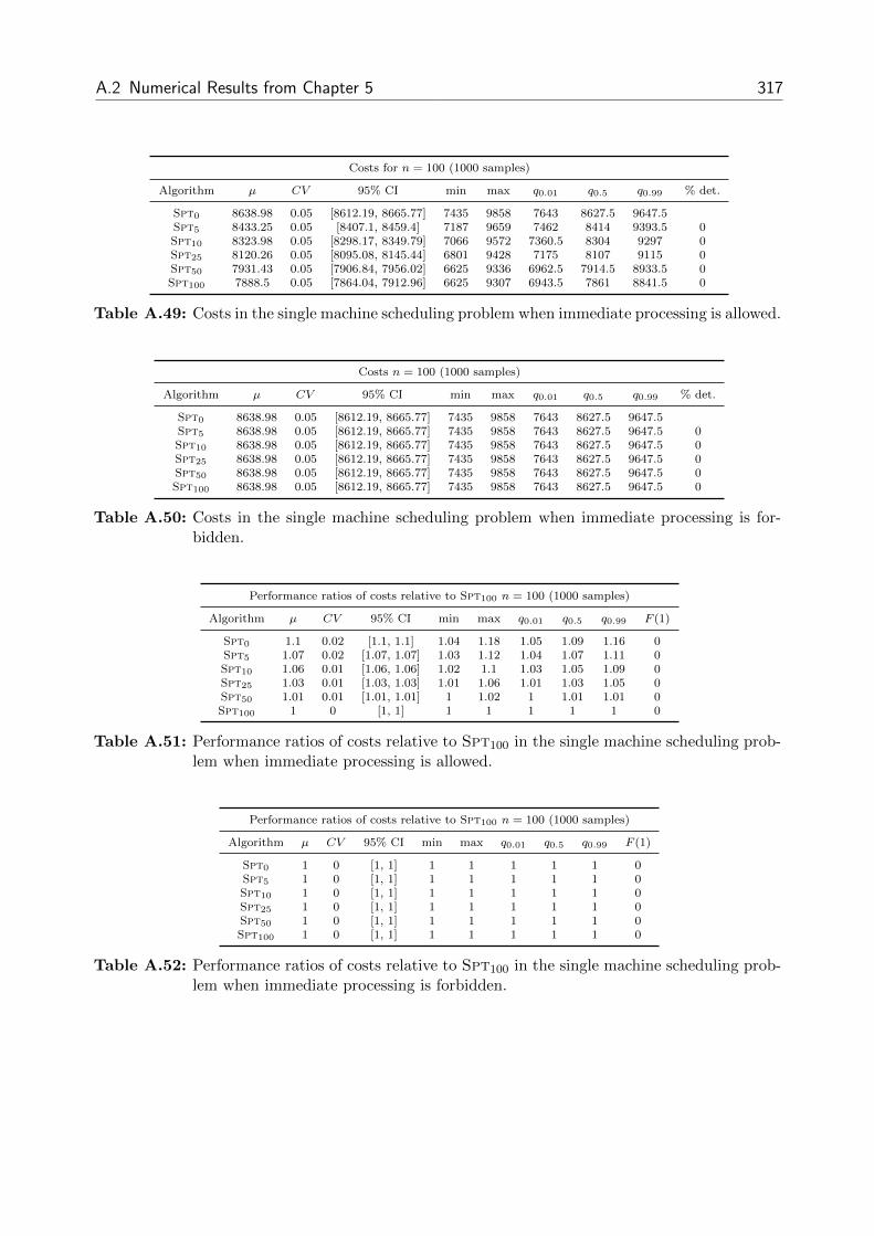
A.2 Numerical Results from Chapter 5 317
Costs for n = 100 (1000 samples)
Algorithm µ CV 95% CI min max q0.01 q0.5 q0.99 % det.
Spt0 8638.98 0.05 [8612.19, 8665.77] 7435 9858 7643 8627.5 9647.5Spt5 8433.25 0.05 [8407.1, 8459.4] 7187 9659 7462 8414 9393.5 0Spt10 8323.98 0.05 [8298.17, 8349.79] 7066 9572 7360.5 8304 9297 0Spt25 8120.26 0.05 [8095.08, 8145.44] 6801 9428 7175 8107 9115 0Spt50 7931.43 0.05 [7906.84, 7956.02] 6625 9336 6962.5 7914.5 8933.5 0Spt100 7888.5 0.05 [7864.04, 7912.96] 6625 9307 6943.5 7861 8841.5 0
Table A.49: Costs in the single machine scheduling problem when immediate processing is allowed.
Costs n = 100 (1000 samples)
Algorithm µ CV 95% CI min max q0.01 q0.5 q0.99 % det.
Spt0 8638.98 0.05 [8612.19, 8665.77] 7435 9858 7643 8627.5 9647.5Spt5 8638.98 0.05 [8612.19, 8665.77] 7435 9858 7643 8627.5 9647.5 0Spt10 8638.98 0.05 [8612.19, 8665.77] 7435 9858 7643 8627.5 9647.5 0Spt25 8638.98 0.05 [8612.19, 8665.77] 7435 9858 7643 8627.5 9647.5 0Spt50 8638.98 0.05 [8612.19, 8665.77] 7435 9858 7643 8627.5 9647.5 0Spt100 8638.98 0.05 [8612.19, 8665.77] 7435 9858 7643 8627.5 9647.5 0
Table A.50: Costs in the single machine scheduling problem when immediate processing is for-bidden.
Performance ratios of costs relative to Spt100 n = 100 (1000 samples)
Algorithm µ CV 95% CI min max q0.01 q0.5 q0.99 F (1)
Spt0 1.1 0.02 [1.1, 1.1] 1.04 1.18 1.05 1.09 1.16 0Spt5 1.07 0.02 [1.07, 1.07] 1.03 1.12 1.04 1.07 1.11 0Spt10 1.06 0.01 [1.06, 1.06] 1.02 1.1 1.03 1.05 1.09 0Spt25 1.03 0.01 [1.03, 1.03] 1.01 1.06 1.01 1.03 1.05 0Spt50 1.01 0.01 [1.01, 1.01] 1 1.02 1 1.01 1.01 0Spt100 1 0 [1, 1] 1 1 1 1 1 0
Table A.51: Performance ratios of costs relative to Spt100 in the single machine scheduling prob-lem when immediate processing is allowed.
Performance ratios of costs relative to Spt100 n = 100 (1000 samples)
Algorithm µ CV 95% CI min max q0.01 q0.5 q0.99 F (1)
Spt0 1 0 [1, 1] 1 1 1 1 1 0Spt5 1 0 [1, 1] 1 1 1 1 1 0Spt10 1 0 [1, 1] 1 1 1 1 1 0Spt25 1 0 [1, 1] 1 1 1 1 1 0Spt50 1 0 [1, 1] 1 1 1 1 1 0Spt100 1 0 [1, 1] 1 1 1 1 1 0
Table A.52: Performance ratios of costs relative to Spt100 in the single machine scheduling prob-lem when immediate processing is forbidden.

318 A Appendix
Performance ratios of costs relative to online version n = 100 (1000 samples)
Algorithm µ CV 95% CI min max q0.01 q0.5 q0.99 1− F (1)
Spt0 1 0 [1, 1] 1 1 1 1 1 0Spt5 0.98 0.01 [0.98, 0.98] 0.94 0.99 0.95 0.98 0.99 0Spt10 0.96 0.01 [0.96, 0.96] 0.9 0.99 0.92 0.97 0.99 0Spt25 0.94 0.02 [0.94, 0.94] 0.87 0.98 0.89 0.94 0.97 0Spt50 0.92 0.02 [0.92, 0.92] 0.85 0.97 0.87 0.92 0.96 0Spt100 0.91 0.02 [0.91, 0.91] 0.85 0.96 0.86 0.91 0.95 0
Table A.53: Performance ratios of costs relative to the online version of an algorithm in the singlemachine scheduling problem when immediate processing is allowed.
Performance ratios of costs relative to online version n = 100 (1000 samples)
Algorithm µ CV 95% CI min max q0.01 q0.5 q0.99 1− F (1)
Spt0 1 0 [1, 1] 1 1 1 1 1 0Spt5 1 0 [1, 1] 1 1 1 1 1 0Spt10 1 0 [1, 1] 1 1 1 1 1 0Spt25 1 0 [1, 1] 1 1 1 1 1 0Spt50 1 0 [1, 1] 1 1 1 1 1 0Spt100 1 0 [1, 1] 1 1 1 1 1 0
Table A.54: Performance ratios of costs relative to the online version of an algorithm in the singlemachine scheduling problem when immediate processing is forbidden.

A.2 Numerical Results from Chapter 5 319
A.2.5.2 Parallel Machines Problem
Costs for n = 25 (1000 samples)
Algorithm µ CV 95% CI min max q0.01 q0.5 q0.99 % det.
Lpt0 98.79 0.04 [98.54, 99.04] 78 104 85 100 103Lpt5 93.79 0.04 [93.56, 94.02] 73 99 80 95 98 0Lpt10 88.79 0.04 [88.57, 89.01] 68 94 75 90 93 0Lpt25 73.79 0.05 [73.56, 74.02] 53 79 60 75 78 0Lpt50 48.79 0.08 [48.55, 49.03] 28 54 35 50 53 0Lpt100 25.23 0.08 [25.1, 25.36] 17 31 20 25 30 0Opt0 98.79 0.04 [98.54, 99.04] 78 104 85 100 103Opt5 93.79 0.04 [93.56, 94.02] 73 99 80 95 98 0Opt10 88.79 0.04 [88.57, 89.01] 68 94 75 90 93 0Opt25 73.79 0.05 [73.56, 74.02] 53 79 60 75 78 0Opt50 48.79 0.08 [48.55, 49.03] 28 54 35 50 53 0Opt100 25.23 0.08 [25.1, 25.36] 17 31 20 25 30 0
Table A.55: Costs in the parallel machines scheduling problem when immediate processing isallowed.
Costs for n = 25 (1000 samples)
Algorithm µ CV 95% CI min max q0.01 q0.5 q0.99 % det.
Lpt0 98.79 0.04 [98.54, 99.04] 78 104 85 100 103Lpt5 98.79 0.04 [98.54, 99.04] 78 104 85 100 103 0Lpt10 98.79 0.04 [98.54, 99.04] 78 104 85 100 103 0Lpt25 98.79 0.04 [98.54, 99.04] 78 104 85 100 103 0Lpt50 98.79 0.04 [98.54, 99.04] 78 104 85 100 103 0Lpt100 98.79 0.04 [98.54, 99.04] 78 104 85 100 103 0Opt0 98.79 0.04 [98.54, 99.04] 78 104 85 100 103Opt5 98.79 0.04 [98.54, 99.04] 78 104 85 100 103 0Opt10 98.79 0.04 [98.54, 99.04] 78 104 85 100 103 0Opt25 98.79 0.04 [98.54, 99.04] 78 104 85 100 103 0Opt50 98.79 0.04 [98.54, 99.04] 78 104 85 100 103 0Opt100 98.79 0.04 [98.54, 99.04] 78 104 85 100 103 0
Table A.56: Costs in the parallel machines scheduling problem when immediate processing isforbidden.
Performance ratios of costs relative to Opt for n = 25 (1000 samples)
Algorithm µ CV 95% CI min max q0.01 q0.5 q0.99 F (1)
Lpt0 3.94 0.09 [3.92, 3.96] 2.9 5.76 3.19 3.92 4.83 0Lpt5 3.74 0.09 [3.72, 3.76] 2.73 5.47 3 3.73 4.6 0Lpt10 3.54 0.09 [3.52, 3.56] 2.57 5.18 2.82 3.54 4.36 0Lpt25 2.94 0.1 [2.92, 2.96] 2.07 4.29 2.27 2.96 3.64 0Lpt50 1.95 0.11 [1.94, 1.96] 1.12 2.82 1.32 1.96 2.44 0Lpt100 1 0 [1, 1] 1 1 1 1 1 0Opt0 3.94 0.09 [3.92, 3.96] 2.9 5.76 3.19 3.92 4.83 0Opt5 3.74 0.09 [3.72, 3.76] 2.73 5.47 3 3.73 4.6 0Opt10 3.54 0.09 [3.52, 3.56] 2.57 5.18 2.82 3.54 4.36 0Opt25 2.94 0.1 [2.92, 2.96] 2.07 4.29 2.27 2.96 3.64 0Opt50 1.95 0.11 [1.94, 1.96] 1.12 2.82 1.32 1.96 2.44 0Opt100 1 0 [1, 1] 1 1 1 1 1 0
Table A.57: Performance ratios of costs relative to Opt in the parallel machines scheduling prob-lem when immediate processing is allowed.

320 A Appendix
Performance ratios of costs relative to Opt for n = 25 (1000 samples)
Algorithm µ CV 95% CI min max q0.01 q0.5 q0.99 F (1)
Lpt0 1 0 [1, 1] 1 1.01 1 1 1 0Lpt5 1 0 [1, 1] 1 1.01 1 1 1 0Lpt10 1 0 [1, 1] 1 1.01 1 1 1 0Lpt25 1 0 [1, 1] 1 1.01 1 1 1 0Lpt50 1 0 [1, 1] 1 1.01 1 1 1 0Lpt100 1 0 [1, 1] 1 1.01 1 1 1 0Opt0 1 0 [1, 1] 1 1.01 1 1 1 0Opt5 1 0 [1, 1] 1 1 1 1 1 0Opt10 1 0 [1, 1] 1 1 1 1 1 0Opt25 1 0 [1, 1] 1 1 1 1 1 0Opt50 1 0 [1, 1] 1 1 1 1 1 0Opt100 1 0 [1, 1] 1 1 1 1 1 0
Table A.58: Performance ratios of costs relative to Opt in the parallel machines scheduling prob-lem when immediate processing is forbidden.
Performance ratios of costs relative to online version for n = 25 (1000 samples)
Algorithm µ CV 95% CI min max q0.01 q0.5 q0.99 1− F (1)
Lpt0 1 0 [1, 1] 1 1 1 1 1 0Lpt5 0.95 0 [0.95, 0.95] 0.94 0.95 0.94 0.95 0.95 0Lpt10 0.9 0 [0.9, 0.9] 0.87 0.9 0.88 0.9 0.9 0Lpt25 0.75 0.01 [0.75, 0.75] 0.68 0.76 0.71 0.75 0.76 0Lpt50 0.49 0.04 [0.49, 0.49] 0.36 0.52 0.41 0.5 0.51 0Lpt100 0.26 0.09 [0.26, 0.26] 0.17 0.34 0.21 0.25 0.31 0Opt0 1 0 [1, 1] 1 1 1 1 1 0Opt5 0.95 0 [0.95, 0.95] 0.94 0.95 0.94 0.95 0.95 0Opt10 0.9 0 [0.9, 0.9] 0.87 0.9 0.88 0.9 0.9 0Opt25 0.75 0.01 [0.75, 0.75] 0.68 0.76 0.71 0.75 0.76 0Opt50 0.49 0.04 [0.49, 0.49] 0.36 0.52 0.41 0.5 0.51 0Opt100 0.26 0.09 [0.26, 0.26] 0.17 0.34 0.21 0.25 0.31 0
Table A.59: Performance ratios of costs relative to the online version of an algorithm in the parallelmachines scheduling problem when immediate processing is allowed.
Performance ratios of costs relative to online version for n = 25 (1000 samples)
Algorithm µ CV 95% CI min max q0.01 q0.5 q0.99 1− F (1)
Lpt0 1 0 [1, 1] 1 1 1 1 1 0Lpt5 1 0 [1, 1] 1 1 1 1 1 0Lpt10 1 0 [1, 1] 1 1 1 1 1 0Lpt25 1 0 [1, 1] 1 1 1 1 1 0Lpt50 1 0 [1, 1] 1 1 1 1 1 0Lpt100 1 0 [1, 1] 1 1 1 1 1 0Opt0 1 0 [1, 1] 1 1 1 1 1 0Opt5 1 0 [1, 1] 0.99 1 1 1 1 0Opt10 1 0 [1, 1] 0.99 1 1 1 1 0Opt25 1 0 [1, 1] 0.99 1 1 1 1 0Opt50 1 0 [1, 1] 0.99 1 1 1 1 0Opt100 1 0 [1, 1] 0.99 1 1 1 1 0
Table A.60: Performance ratios of costs relative to the online version of an algorithm in the parallelmachines scheduling problem when immediate processing is forbidden.

A.2 Numerical Results from Chapter 5 321
Costs for n = 100 (1000 samples)
Algorithm µ CV 95% CI min max q0.01 q0.5 q0.99 % det.
Lpt0 107.35 0.04 [107.08, 107.62] 99 123 101 107 118Lpt5 103.01 0.04 [102.75, 103.27] 95 118 96 103 113 0Lpt10 100.73 0.04 [100.48, 100.98] 92 113 92 101 110 0Lpt25 100.14 0.04 [99.89, 100.39] 87 113 90 100 109 0Lpt50 100.14 0.04 [99.89, 100.39] 87 113 90 100 109 0Lpt100 100.14 0.04 [99.89, 100.39] 87 113 90 100 109 0
Table A.61: Costs in the parallel machines scheduling problem when immediate processing isallowed.
Costs for n = 100 (1000 samples)
Algorithm µ CV 95% CI min max q0.01 q0.5 q0.99 % det.
Lpt0 107.35 0.04 [107.08, 107.62] 99 123 101 107 118Lpt5 107.35 0.04 [107.08, 107.62] 99 123 101 107 118 0Lpt10 107.35 0.04 [107.08, 107.62] 99 123 101 107 118 0Lpt25 107.35 0.04 [107.08, 107.62] 99 123 101 107 118 0Lpt50 107.35 0.04 [107.08, 107.62] 99 123 101 107 118 0Lpt100 107.35 0.04 [107.08, 107.62] 99 123 101 107 118 0
Table A.62: Costs in the parallel machines scheduling problem when immediate processing isforbidden.
Performance ratios of costs relative to Lpt100 for n = 100 (1000 samples)
Algorithm µ CV 95% CI min max q0.01 q0.5 q0.99 F (1)
Lpt0 1.07 0.04 [1.07, 1.07] 1 1.22 1 1.07 1.18 0Lpt5 1.03 0.03 [1.03, 1.03] 1 1.16 1 1.02 1.12 0Lpt10 1.01 0.02 [1.01, 1.01] 1 1.11 1 1 1.07 0Lpt25 1 0 [1, 1] 1 1 1 1 1 0Lpt50 1 0 [1, 1] 1 1 1 1 1 0Lpt100 1 0 [1, 1] 1 1 1 1 1 0
Table A.63: Performance ratios of costs relative to Lpt100 in the parallel machines schedulingproblem when immediate processing is allowed.
Performance ratios of costs relative to Lpt100 for n = 100 (1000 samples)
Algorithm µ CV 95% CI min max q0.01 q0.5 q0.99 F (1)
Lpt0 1 0 [1, 1] 1 1 1 1 1 0Lpt5 1 0 [1, 1] 1 1 1 1 1 0Lpt10 1 0 [1, 1] 1 1 1 1 1 0Lpt25 1 0 [1, 1] 1 1 1 1 1 0Lpt50 1 0 [1, 1] 1 1 1 1 1 0Lpt100 1 0 [1, 1] 1 1 1 1 1 0
Table A.64: Performance ratios of costs relative to Lpt100 in the parallel machines schedulingproblem when immediate processing is forbidden.

322 A Appendix
Performance ratios of costs relative to online version for n = 100 (1000 samples)
Algorithm µ CV 95% CI min max q0.01 q0.5 q0.99 1− F (1)
Lpt0 1 0 [1, 1] 1 1 1 1 1 0Lpt5 0.96 0.01 [0.96, 0.96] 0.95 1 0.95 0.95 1 0Lpt10 0.94 0.03 [0.94, 0.94] 0.9 1 0.9 0.93 1 0Lpt25 0.93 0.04 [0.93, 0.93] 0.82 1 0.85 0.93 1 0Lpt50 0.93 0.04 [0.93, 0.93] 0.82 1 0.85 0.93 1 0Lpt100 0.93 0.04 [0.93, 0.93] 0.82 1 0.85 0.93 1 0
Table A.65: Performance ratios of costs relative to the online version of an algorithm in the parallelmachines scheduling problem when immediate processing is allowed.
Performance ratios of costs relative to online version for n = 100 (1000 samples)
Algorithm µ CV 95% CI min max q0.01 q0.5 q0.99 1− F (1)
Lpt0 1 0 [1, 1] 1 1 1 1 1 0Lpt5 1 0 [1, 1] 1 1 1 1 1 0Lpt10 1 0 [1, 1] 1 1 1 1 1 0Lpt25 1 0 [1, 1] 1 1 1 1 1 0Lpt50 1 0 [1, 1] 1 1 1 1 1 0Lpt100 1 0 [1, 1] 1 1 1 1 1 0
Table A.66: Performance ratios of costs relative to the online version of an algorithm in the parallelmachines scheduling problem when immediate processing is forbidden.

A.3 Numerical Results from Chapter 6 323
A.3 Numerical Results from Chapter 6
This section contains a detailed statistical summary of the numerical results gathered during
the experimental analysis in Chapter 6. The presentation is carried out in the same form as
described at the beginning of Appendix A.2. Because of space restrictions, we omit results
for lookahead durations D ∈ {180, 240, 300, 420, 480, 540} minutes and only list results for
D ∈ {0, 60, 120, 360, 600} minutes.
A.3.1 Online Order Picking with Lookahead
Makespan for n = 625 (50 samples)
Algorithm µ CV 95% CI min max q0.01 q0.5 q0.99 % det.
Prio,Ret0 624.81 0.05 [615.97, 633.65] 608.2 742.6 608.2 614.9 742.6Prio,Ret60 562.51 0.03 [557.74, 567.28] 548.9 680 548.9 556.7 680 0.02Prio,Ret120 534.27 0.07 [523.69, 544.85] 493.6 725.7 493.6 524.3 725.7 0.08Prio,Ret360 519.58 0.06 [510.76, 528.4] 445.3 664.9 445.3 517.6 664.9 0.43Prio,Ret600 519.9 0.06 [511.08, 528.72] 443.4 664.9 443.4 519.2 664.9 0.45
Prio,S0 619.17 0.04 [612.16, 626.18] 607.9 725.7 607.9 614.1 725.7Prio,S60 567.5 0.06 [557.87, 577.13] 547.7 698.5 547.7 555.6 698.5 0.06Prio,S120 534.15 0.09 [520.55, 547.75] 491.2 725.7 491.2 526.2 725.7 0.12Prio,S360 505.79 0.09 [492.91, 518.67] 430.3 664.9 430.3 502.1 664.9 0.31Prio,S600 507.94 0.09 [495.01, 520.87] 425.7 664.9 425.7 505.5 664.9 0.41Prio,Gap0 622.08 0.04 [615.04, 629.12] 606.9 742.6 606.9 615.2 742.6Prio,Gap60 568.84 0.06 [559.18, 578.5] 550.4 693 550.4 556.5 693 0.08Prio,Gap120 531.74 0.08 [519.71, 543.77] 490.2 725.7 490.2 524.4 725.7 0.08Prio,Gap360 513.43 0.08 [501.81, 525.05] 437.3 664.9 437.3 511.9 664.9 0.31Prio,Gap600 513.83 0.08 [502.2, 525.46] 434.9 664.9 434.9 510.1 664.9 0.39Prio,Opt0 619.94 0.04 [612.92, 626.96] 607.6 742.6 607.6 613.3 742.6Prio,Opt60 558.79 0.03 [554.05, 563.53] 547.1 657.6 547.1 553.6 657.6 0.02Prio,Opt120 531.51 0.09 [517.98, 545.04] 488 725.7 488 522.8 725.7 0.08Prio,Opt360 495.92 0.11 [480.49, 511.35] 419.2 669.5 419.2 486 669.5 0.37Prio,Opt600 500.44 0.11 [484.87, 516.01] 414.9 669.5 414.9 495.8 669.5 0.45Seed,Ret0 616.8 0.03 [611.57, 622.03] 608.5 725.7 608.5 614.4 725.7Seed,Ret60 563.42 0.05 [555.45, 571.39] 546 712.5 546 555.8 712.5 0.04Seed,Ret120 535.86 0.09 [522.22, 549.5] 490.2 725.7 490.2 527.5 725.7 0.12Seed,Ret360 493.33 0.12 [476.58, 510.08] 408.4 669.5 408.4 486.3 669.5 0.2Seed,Ret600 491.71 0.1 [477.8, 505.62] 408.6 664.9 408.6 490 664.9 0.35
Seed,S0 620.27 0.04 [613.25, 627.29] 609.5 725.7 609.5 613.1 725.7Seed,S60 569.04 0.07 [557.77, 580.31] 546.2 712.5 546.2 555.1 712.5 0.08Seed,S120 528.66 0.08 [516.7, 540.62] 488.3 725.7 488.3 521.4 725.7 0.04Seed,S360 465.52 0.12 [449.72, 481.32] 357.6 664.9 357.6 462.8 664.9 0.43Seed,S600 470.2 0.13 [452.91, 487.49] 373.2 669.5 373.2 462.8 669.5 0.27Seed,Gap0 619.82 0.03 [614.56, 625.08] 607.4 725.7 607.4 614.4 725.7Seed,Gap60 562.44 0.04 [556.08, 568.8] 548.4 698.5 548.4 556 698.5 0.04Seed,Gap120 533.08 0.08 [521.02, 545.14] 491.3 725.7 491.3 520.6 725.7 0.08Seed,Gap360 514.45 0.09 [501.35, 527.55] 434.4 669.5 434.4 513.7 669.5 0.35Seed,Gap600 508.14 0.08 [496.64, 519.64] 437.4 664.9 437.4 509.7 664.9 0.33Seed,Opt0 619.73 0.04 [612.72, 626.74] 606.4 725.7 606.4 613 725.7Seed,Opt60 557.79 0.03 [553.06, 562.52] 546 680 546 553.7 680 0Seed,Opt120 528.99 0.08 [517.02, 540.96] 488.8 725.7 488.8 525.1 725.7 0.08Seed,Opt360 468.29 0.13 [451.07, 485.51] 357.4 664.9 357.4 467.8 664.9 0.33Seed,Opt600 463.41 0.12 [447.68, 479.14] 374.5 664.9 374.5 458.8 664.9 0.41
Svg,Ret0 619.45 0.04 [612.44, 626.46] 607.5 741 607.5 614.7 741...
......
......
......
......
...

324 A Appendix
Makespan for n = 625 (50 samples)
Algorithm µ CV 95% CI min max q0.01 q0.5 q0.99 % det.
......
......
......
......
......
Svg,Ret60 561.11 0.03 [556.35, 565.87] 548.2 680 548.2 555.9 680 0.02Svg,Ret120 532.02 0.08 [519.98, 544.06] 492.7 725.7 492.7 527 725.7 0.06Svg,Ret360 507.09 0.1 [492.74, 521.44] 438.8 669.5 438.8 496.7 669.5 0.45Svg,Ret600 514.56 0.1 [500, 529.12] 431.3 669.5 431.3 511.6 669.5 0.37
Svg,S0 615.81 0.03 [610.58, 621.04] 607.5 725.7 607.5 613.5 725.7Svg,S60 557.53 0.02 [554.38, 560.68] 548.1 623.2 548.1 554.8 623.2 0Svg,S120 531.09 0.08 [519.07, 543.11] 488.7 725.7 488.7 525.4 725.7 0.08Svg,S360 492.56 0.12 [475.84, 509.28] 409.4 669.5 409.4 487.8 669.5 0.27Svg,S600 494.32 0.11 [478.94, 509.7] 415.1 669.5 415.1 483.3 669.5 0.24Svg,Gap0 621.23 0.04 [614.2, 628.26] 609.2 742.6 609.2 614.4 742.6Svg,Gap60 560.55 0.04 [554.21, 566.89] 549.3 712.5 549.3 555.7 712.5 0Svg,Gap120 531.5 0.08 [519.47, 543.53] 491.8 725.7 491.8 526.3 725.7 0.08Svg,Gap360 508.96 0.08 [497.44, 520.48] 430.5 664.9 430.5 505.8 664.9 0.47Svg,Gap600 514.31 0.08 [502.67, 525.95] 429.4 664.9 429.4 517.9 664.9 0.47Svg,Opt0 622.92 0.05 [614.11, 631.73] 607.6 742.6 607.6 613.8 742.6Svg,Opt60 558.43 0.04 [552.11, 564.75] 548.1 698.5 548.1 553.3 698.5 0.02Svg,Opt120 531.93 0.08 [519.89, 543.97] 491.6 725.7 491.6 525.5 725.7 0.12Svg,Opt360 489.01 0.12 [472.41, 505.61] 409.7 669.5 409.7 483.8 669.5 0.31Svg,Opt600 492.16 0.1 [478.24, 506.08] 412.4 664.9 412.4 489.4 664.9 0.39
Ls,Ret0 620.74 0.04 [613.72, 627.76] 608.6 741 608.6 614.8 741Ls,Ret60 562.53 0.05 [554.57, 570.49] 546.2 693 546.2 556.3 693 0.04Ls,Ret120 530 0.08 [518, 542] 490.8 725.7 490.8 523.4 725.7 0.06Ls,Ret360 491.63 0.12 [474.94, 508.32] 406.2 669.5 406.2 481.4 669.5 0.29Ls,Ret600 492.09 0.12 [475.38, 508.8] 407.8 669.5 407.8 487.9 669.5 0.2
Ls,S0 621.5 0.05 [612.71, 630.29] 608.7 741 608.7 613.3 741Ls,S60 557.83 0.03 [553.1, 562.56] 547.2 657.6 547.2 554.1 657.6 0.02Ls,S120 528.88 0.08 [516.91, 540.85] 488.6 725.7 488.6 525.7 725.7 0.06Ls,S360 467.4 0.12 [451.53, 483.27] 379 664.9 379 463.3 664.9 0.33Ls,S600 464.93 0.12 [449.15, 480.71] 357.7 664.9 357.7 462.8 664.9 0.33Ls,Gap0 622.76 0.05 [613.95, 631.57] 608.6 741 608.6 614.3 741Ls,Gap60 562.47 0.05 [554.51, 570.43] 547.8 712.5 547.8 554.5 712.5 0Ls,Gap120 532.31 0.09 [518.76, 545.86] 491.6 725.7 491.6 523.3 725.7 0.08Ls,Gap360 484.77 0.11 [469.68, 499.86] 404.6 664.9 404.6 480.5 664.9 0.24Ls,Gap600 487.55 0.11 [472.38, 502.72] 403.5 664.9 403.5 481 664.9 0.31Ls,Opt0 617.52 0.03 [612.28, 622.76] 607.6 725.7 607.6 613 725.7Ls,Opt60 562.69 0.05 [554.73, 570.65] 548.4 712.5 548.4 554.4 712.5 0.04Ls,Opt120 528.22 0.08 [516.27, 540.17] 489.7 725.7 489.7 520.4 725.7 0.08Ls,Opt360 467.18 0.12 [451.32, 483.04] 373.3 664.9 373.3 462.7 664.9 0.31Ls,Opt600 472.86 0.12 [456.81, 488.91] 392.7 664.9 392.7 472 664.9 0.2Ts,Ret0 619.58 0.03 [614.32, 624.84] 608.2 725.7 608.2 615 725.7Ts,Ret60 567.43 0.06 [557.8, 577.06] 547.6 712.5 547.6 556.3 712.5 0.08Ts,Ret120 530.88 0.08 [518.87, 542.89] 493.8 725.7 493.8 523.4 725.7 0.1Ts,Ret360 489.94 0.12 [473.31, 506.57] 411.7 669.5 411.7 484.4 669.5 0.29Ts,Ret600 487.26 0.1 [473.48, 501.04] 411 664.9 411 485.7 664.9 0.33
Ts,S0 622.39 0.05 [613.59, 631.19] 608.5 742.6 608.5 613.6 742.6Ts,S60 559.28 0.04 [552.95, 565.61] 549 698.5 549 554.8 698.5 0Ts,S120 527.52 0.08 [515.58, 539.46] 488.4 725.7 488.4 523.8 725.7 0.06Ts,S360 469.72 0.13 [452.45, 486.99] 371.6 669.5 371.6 462.8 669.5 0.29Ts,S600 466.62 0.12 [450.78, 482.46] 372.1 664.9 372.1 462.8 664.9 0.27Ts,Gap0 621.1 0.04 [614.07, 628.13] 608.3 742.6 608.3 614.4 742.6Ts,Gap60 563.89 0.06 [554.32, 573.46] 548.1 712.5 548.1 556.4 712.5 0.06Ts,Gap120 532.84 0.09 [519.27, 546.41] 488.7 725.7 488.7 525.1 725.7 0.1Ts,Gap360 489.69 0.12 [473.07, 506.31] 405.7 669.5 405.7 481.6 669.5 0.39Ts,Gap600 488.31 0.12 [471.73, 504.89] 414.3 669.5 414.3 476.4 669.5 0.35Ts,Opt0 614.88 0.03 [609.66, 620.1] 606.6 725.7 606.6 612.5 725.7Ts,Opt60 561.7 0.05 [553.75, 569.65] 547.4 712.5 547.4 554.2 712.5 0.04Ts,Opt120 531.77 0.09 [518.23, 545.31] 488 725.7 488 526.3 725.7 0.08Ts,Opt360 474.58 0.14 [455.78, 493.38] 357.4 669.5 357.4 469.1 669.5 0.31Ts,Opt600 469.68 0.13 [452.41, 486.95] 376.9 669.5 376.9 464.9 669.5 0.31Opt,Opt0 615.99 0.06 [605.53, 626.45] 507.7 741 507.7 613.3 741Opt,Opt60 566.2 0.06 [556.59, 575.81] 507.7 712.5 507.7 554.5 712.5 0.08Opt,Opt120 533.08 0.08 [521.02, 545.14] 489.9 725.7 489.9 525 725.7 0.14Opt,Opt360 513.23 0.09 [500.16, 526.3] 434.4 669.5 434.4 510.8 669.5 0.31Opt,Opt600 507.97 0.08 [496.47, 519.47] 436.3 664.9 436.3 509.7 664.9 0.27
Table A.67: Makespans in the order picking system.

A.3 Numerical Results from Chapter 6 325
Performance ratios of makespan relative to Ts,Opt600 for n = 625 (50 samples)
Algorithm µ CV 95% CI min max q0.01 q0.5 q0.99 F (1)
Prio,Ret0 1.35 0.13 [1.3, 1.4] 0.92 1.66 0.92 1.39 1.66 0.04Prio,Ret60 1.22 0.13 [1.18, 1.26] 0.83 1.67 0.83 1.2 1.67 0.04Prio,Ret120 1.15 0.14 [1.1, 1.2] 0.78 1.66 0.78 1.13 1.66 0.02Prio,Ret360 1.12 0.12 [1.08, 1.16] 0.77 1.39 0.77 1.06 1.39 0.02Prio,Ret600 1.12 0.12 [1.08, 1.16] 0.77 1.39 0.77 1.08 1.39 0.02
Prio,S0 1.34 0.13 [1.29, 1.39] 0.92 1.67 0.92 1.32 1.67 0.04Prio,S60 1.23 0.15 [1.18, 1.28] 0.83 1.68 0.83 1.2 1.68 0.04Prio,S120 1.15 0.13 [1.11, 1.19] 0.99 1.66 0.99 1.12 1.66 0.02Prio,S360 1.09 0.14 [1.05, 1.13] 0.73 1.61 0.73 1.02 1.61 0.04Prio,S600 1.1 0.14 [1.06, 1.14] 0.74 1.61 0.74 1.02 1.61 0.06Prio,Gap0 1.35 0.12 [1.3, 1.4] 0.92 1.66 0.92 1.37 1.66 0.04Prio,Gap60 1.23 0.14 [1.18, 1.28] 0.82 1.68 0.82 1.2 1.68 0.04Prio,Gap120 1.15 0.14 [1.1, 1.2] 0.76 1.66 0.76 1.11 1.66 0.02Prio,Gap360 1.11 0.13 [1.07, 1.15] 0.76 1.61 0.76 1.05 1.61 0.02Prio,Gap600 1.11 0.13 [1.07, 1.15] 0.76 1.61 0.76 1.04 1.61 0.04Prio,Opt0 1.34 0.13 [1.29, 1.39] 0.92 1.66 0.92 1.36 1.66 0.04Prio,Opt60 1.21 0.13 [1.17, 1.25] 0.85 1.54 0.85 1.2 1.54 0.04Prio,Opt120 1.15 0.14 [1.1, 1.2] 0.98 1.66 0.98 1.07 1.66 0.02Prio,Opt360 1.06 0.12 [1.02, 1.1] 0.99 1.61 0.99 1.02 1.61 0.1Prio,Opt600 1.08 0.12 [1.04, 1.12] 0.99 1.61 0.99 1.02 1.61 0.04Seed,Ret0 1.33 0.13 [1.28, 1.38] 0.92 1.66 0.92 1.33 1.66 0.04Seed,Ret60 1.22 0.13 [1.18, 1.26] 0.85 1.53 0.85 1.2 1.53 0.04Seed,Ret120 1.16 0.13 [1.12, 1.2] 0.99 1.66 0.99 1.12 1.66 0.02Seed,Ret360 1.06 0.12 [1.02, 1.1] 0.98 1.61 0.98 1.01 1.61 0.06Seed,Ret600 1.06 0.13 [1.02, 1.1] 0.73 1.61 0.73 1.01 1.61 0.06
Seed,S0 1.34 0.13 [1.29, 1.39] 0.92 1.68 0.92 1.36 1.68 0.04Seed,S60 1.23 0.14 [1.18, 1.28] 0.85 1.67 0.85 1.23 1.67 0.04Seed,S120 1.14 0.14 [1.09, 1.19] 0.75 1.66 0.75 1.07 1.66 0.04Seed,S360 0.99 0.05 [0.98, 1] 0.73 1.03 0.73 1 1.03 0.29Seed,S600 1 0.01 [1, 1] 0.98 1.03 0.98 1 1.03 0.31Seed,Gap0 1.34 0.13 [1.29, 1.39] 0.92 1.66 0.92 1.33 1.66 0.04Seed,Gap60 1.22 0.13 [1.18, 1.26] 0.83 1.5 0.83 1.2 1.5 0.04Seed,Gap120 1.15 0.13 [1.11, 1.19] 1 1.66 1 1.08 1.66 0Seed,Gap360 1.11 0.13 [1.07, 1.15] 0.99 1.61 0.99 1.02 1.61 0.02Seed,Gap600 1.1 0.13 [1.06, 1.14] 0.74 1.61 0.74 1.03 1.61 0.04Seed,Opt0 1.34 0.13 [1.29, 1.39] 0.91 1.68 0.91 1.32 1.68 0.04Seed,Opt60 1.21 0.13 [1.17, 1.25] 0.82 1.67 0.82 1.19 1.67 0.04Seed,Opt120 1.14 0.14 [1.09, 1.19] 0.81 1.66 0.81 1.11 1.66 0.04Seed,Opt360 1 0.11 [0.97, 1.03] 0.74 1.61 0.74 1 1.61 0.39Seed,Opt600 0.99 0.05 [0.98, 1] 0.73 1.07 0.73 1 1.07 0.43
Svg,Ret0 1.34 0.13 [1.29, 1.39] 0.92 1.66 0.92 1.32 1.66 0.04Svg,Ret60 1.21 0.13 [1.17, 1.25] 0.83 1.67 0.83 1.2 1.67 0.04Svg,Ret120 1.15 0.14 [1.1, 1.2] 0.81 1.66 0.81 1.09 1.66 0.04Svg,Ret360 1.09 0.12 [1.05, 1.13] 0.98 1.61 0.98 1.03 1.61 0.04Svg,Ret600 1.11 0.13 [1.07, 1.15] 1 1.61 1 1.03 1.61 0.02
Svg,S0 1.33 0.13 [1.28, 1.38] 0.92 1.66 0.92 1.32 1.66 0.04Svg,S60 1.21 0.13 [1.17, 1.25] 0.82 1.5 0.82 1.19 1.5 0.04Svg,S120 1.15 0.14 [1.1, 1.2] 0.81 1.66 0.81 1.09 1.66 0.04Svg,S360 1.06 0.12 [1.02, 1.1] 0.99 1.61 0.99 1 1.61 0.08Svg,S600 1.06 0.12 [1.02, 1.1] 0.98 1.61 0.98 1 1.61 0.04Svg,Gap0 1.34 0.13 [1.29, 1.39] 0.92 1.66 0.92 1.36 1.66 0.04Svg,Gap60 1.21 0.13 [1.17, 1.25] 0.82 1.53 0.82 1.2 1.53 0.04Svg,Gap120 1.15 0.14 [1.1, 1.2] 0.75 1.66 0.75 1.12 1.66 0.04Svg,Gap360 1.1 0.13 [1.06, 1.14] 0.73 1.61 0.73 1.03 1.61 0.02Svg,Gap600 1.11 0.13 [1.07, 1.15] 0.75 1.61 0.75 1.06 1.61 0.02Svg,Opt0 1.35 0.13 [1.3, 1.4] 0.91 1.67 0.91 1.36 1.67 0.04Svg,Opt60 1.21 0.13 [1.17, 1.25] 0.83 1.49 0.83 1.2 1.49 0.04Svg,Opt120 1.15 0.14 [1.1, 1.2] 0.81 1.66 0.81 1.12 1.66 0.04Svg,Opt360 1.05 0.11 [1.02, 1.08] 0.98 1.61 0.98 1.01 1.61 0.06Svg,Opt600 1.06 0.13 [1.02, 1.1] 0.73 1.61 0.73 1.01 1.61 0.1
Ls,Ret0 1.34 0.13 [1.29, 1.39] 0.92 1.66 0.92 1.36 1.66 0.04Ls,Ret60 1.22 0.14 [1.17, 1.27] 0.83 1.68 0.83 1.2 1.68 0.04Ls,Ret120 1.15 0.14 [1.1, 1.2] 0.74 1.66 0.74 1.07 1.66 0.04
......
......
......
......
......

326 A Appendix
Performance ratios of makespan relative to Ts,Opt600 for n = 625 (50 samples)
Algorithm µ CV 95% CI min max q0.01 q0.5 q0.99 F (1)
......
......
......
......
......
Ls,Ret360 1.05 0.12 [1.01, 1.09] 0.99 1.61 0.99 1 1.61 0.1Ls,Ret600 1.06 0.12 [1.02, 1.1] 0.98 1.61 0.98 1.01 1.61 0.12
Ls,S0 1.35 0.13 [1.3, 1.4] 0.92 1.67 0.92 1.36 1.67 0.04Ls,S60 1.21 0.13 [1.17, 1.25] 0.83 1.49 0.83 1.19 1.49 0.04Ls,S120 1.14 0.14 [1.09, 1.19] 0.74 1.66 0.74 1.06 1.66 0.04Ls,S360 1 0.04 [0.99, 1.01] 0.74 1.07 0.74 1 1.07 0.27Ls,S600 0.99 0.05 [0.98, 1] 0.73 1.02 0.73 1 1.02 0.31Ls,Gap0 1.35 0.13 [1.3, 1.4] 0.92 1.66 0.92 1.39 1.66 0.04Ls,Gap60 1.22 0.13 [1.18, 1.26] 0.85 1.53 0.85 1.23 1.53 0.04Ls,Gap120 1.15 0.13 [1.11, 1.19] 0.98 1.66 0.98 1.06 1.66 0.02Ls,Gap360 1.04 0.12 [1, 1.08] 0.73 1.61 0.73 1 1.61 0.12Ls,Gap600 1.05 0.13 [1.01, 1.09] 0.73 1.61 0.73 1 1.61 0.16Ls,Opt0 1.34 0.13 [1.29, 1.39] 0.91 1.67 0.91 1.32 1.67 0.04Ls,Opt60 1.22 0.13 [1.18, 1.26] 0.85 1.54 0.85 1.23 1.54 0.04Ls,Opt120 1.14 0.14 [1.09, 1.19] 0.74 1.66 0.74 1.07 1.66 0.04Ls,Opt360 1 0.04 [0.99, 1.01] 0.73 1.03 0.73 1 1.03 0.27Ls,Opt600 1.01 0.1 [0.98, 1.04] 0.73 1.61 0.73 1 1.61 0.24Ts,Ret0 1.34 0.13 [1.29, 1.39] 0.92 1.66 0.92 1.33 1.66 0.04Ts,Ret60 1.23 0.15 [1.18, 1.28] 0.83 1.68 0.83 1.2 1.68 0.04Ts,Ret120 1.15 0.14 [1.1, 1.2] 0.75 1.66 0.75 1.12 1.66 0.04Ts,Ret360 1.05 0.12 [1.01, 1.09] 0.99 1.61 0.99 1.01 1.61 0.08Ts,Ret600 1.05 0.12 [1.01, 1.09] 0.73 1.61 0.73 1.01 1.61 0.08
Ts,S0 1.35 0.13 [1.3, 1.4] 0.91 1.67 0.91 1.36 1.67 0.04Ts,S60 1.21 0.13 [1.17, 1.25] 0.83 1.49 0.83 1.19 1.49 0.04Ts,S120 1.14 0.14 [1.09, 1.19] 0.74 1.66 0.74 1.07 1.66 0.04Ts,S360 1 0.01 [1, 1] 0.97 1.02 0.97 1 1.02 0.24Ts,S600 1 0.04 [0.99, 1.01] 0.73 1.07 0.73 1 1.07 0.31Ts,Gap0 1.34 0.13 [1.29, 1.39] 0.92 1.66 0.92 1.37 1.66 0.04Ts,Gap60 1.22 0.14 [1.17, 1.27] 0.83 1.67 0.83 1.2 1.67 0.04Ts,Gap120 1.15 0.13 [1.11, 1.19] 0.99 1.66 0.99 1.08 1.66 0.02Ts,Gap360 1.05 0.12 [1.01, 1.09] 0.99 1.61 0.99 1 1.61 0.14Ts,Gap600 1.05 0.11 [1.02, 1.08] 0.97 1.61 0.97 1 1.61 0.12Ts,Opt0 1.33 0.13 [1.28, 1.38] 0.91 1.66 0.91 1.32 1.66 0.04Ts,Opt60 1.22 0.14 [1.17, 1.27] 0.82 1.68 0.82 1.2 1.68 0.04Ts,Opt120 1.15 0.13 [1.11, 1.19] 0.98 1.66 0.98 1.07 1.66 0.02Ts,Opt360 1.01 0.09 [0.98, 1.04] 0.83 1.61 0.83 1 1.61 0.31Ts,Opt600 1 0 [1, 1] 1 1 1 1 1 0Opt,Opt0 1.33 0.13 [1.28, 1.38] 0.92 1.73 0.92 1.32 1.73 0.02Opt,Opt60 1.23 0.15 [1.18, 1.28] 0.85 1.68 0.85 1.24 1.68 0.06Opt,Opt120 1.15 0.13 [1.11, 1.19] 0.92 1.66 0.92 1.11 1.66 0.04Opt,Opt360 1.11 0.13 [1.07, 1.15] 0.99 1.61 0.99 1.02 1.61 0.04Opt,Opt600 1.1 0.13 [1.06, 1.14] 0.74 1.61 0.74 1.03 1.61 0.04
Table A.68: Performance ratios of makespan relative to Ts,Opt600 in the order picking system.
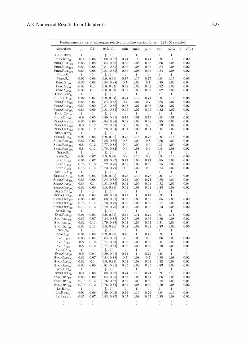
A.3 Numerical Results from Chapter 6 327
Performance ratios of makespan relative to online version for n = 625 (50 samples)
Algorithm µ CV 95% CI min max q0.01 q0.5 q0.99 1− F (1)
Prio,Ret0 1 0 [1, 1] 1 1 1 1 1 0Prio,Ret60 0.9 0.06 [0.88, 0.92] 0.74 1.1 0.74 0.9 1.1 0.02Prio,Ret120 0.86 0.08 [0.84, 0.88] 0.68 1.08 0.68 0.86 1.08 0.02Prio,Ret360 0.83 0.08 [0.81, 0.85] 0.66 1.08 0.66 0.84 1.08 0.02Prio,Ret600 0.83 0.08 [0.81, 0.85] 0.66 1.08 0.66 0.84 1.08 0.02
Prio,S0 1 0 [1, 1] 1 1 1 1 1 0Prio,S60 0.92 0.06 [0.9, 0.94] 0.77 1.15 0.77 0.9 1.15 0.06Prio,S120 0.86 0.08 [0.84, 0.88] 0.7 1.09 0.7 0.85 1.09 0.04Prio,S360 0.82 0.1 [0.8, 0.84] 0.62 1.08 0.62 0.82 1.08 0.04Prio,S600 0.82 0.1 [0.8, 0.84] 0.62 1.08 0.62 0.82 1.08 0.04Prio,Gap0 1 0 [1, 1] 1 1 1 1 1 0Prio,Gap60 0.92 0.07 [0.9, 0.94] 0.74 1.12 0.74 0.9 1.12 0.08Prio,Gap120 0.86 0.07 [0.84, 0.88] 0.7 1.07 0.7 0.85 1.07 0.02Prio,Gap360 0.83 0.09 [0.81, 0.85] 0.63 1.07 0.63 0.82 1.07 0.02Prio,Gap600 0.83 0.09 [0.81, 0.85] 0.65 1.07 0.65 0.82 1.07 0.02Prio,Opt0 1 0 [1, 1] 1 1 1 1 1 0Prio,Opt60 0.9 0.05 [0.89, 0.91] 0.74 1.07 0.74 0.9 1.07 0.02Prio,Opt120 0.86 0.08 [0.84, 0.88] 0.68 1.09 0.68 0.85 1.09 0.04Prio,Opt360 0.8 0.12 [0.77, 0.83] 0.6 1.09 0.6 0.79 1.09 0.04Prio,Opt600 0.81 0.12 [0.78, 0.84] 0.61 1.09 0.61 0.8 1.09 0.04Seed,Ret0 1 0 [1, 1] 1 1 1 1 1 0Seed,Ret60 0.91 0.05 [0.9, 0.92] 0.78 1.16 0.78 0.9 1.16 0.04Seed,Ret120 0.87 0.07 [0.85, 0.89] 0.8 1.09 0.8 0.86 1.09 0.04Seed,Ret360 0.8 0.12 [0.77, 0.83] 0.6 1.09 0.6 0.8 1.09 0.04Seed,Ret600 0.8 0.11 [0.78, 0.82] 0.6 1.08 0.6 0.8 1.08 0.02
Seed,S0 1 0 [1, 1] 1 1 1 1 1 0Seed,S60 0.92 0.07 [0.9, 0.94] 0.8 1.16 0.8 0.9 1.16 0.08Seed,S120 0.85 0.07 [0.83, 0.87] 0.71 1.09 0.71 0.85 1.09 0.02Seed,S360 0.75 0.13 [0.72, 0.78] 0.58 1.09 0.58 0.75 1.09 0.02Seed,S600 0.76 0.14 [0.73, 0.79] 0.6 1.09 0.6 0.74 1.09 0.04Seed,Gap0 1 0 [1, 1] 1 1 1 1 1 0Seed,Gap60 0.91 0.05 [0.9, 0.92] 0.78 1.14 0.78 0.9 1.14 0.04Seed,Gap120 0.86 0.08 [0.84, 0.88] 0.71 1.09 0.71 0.85 1.09 0.04Seed,Gap360 0.83 0.1 [0.81, 0.85] 0.64 1.09 0.64 0.83 1.09 0.04Seed,Gap600 0.82 0.09 [0.8, 0.84] 0.62 1.08 0.62 0.83 1.08 0.02Seed,Opt0 1 0 [1, 1] 1 1 1 1 1 0Seed,Opt60 0.9 0.04 [0.89, 0.91] 0.77 1 0.77 0.9 1 0Seed,Opt120 0.85 0.07 [0.83, 0.87] 0.69 1.08 0.69 0.85 1.08 0.02Seed,Opt360 0.76 0.14 [0.73, 0.79] 0.59 1.08 0.59 0.77 1.08 0.02Seed,Opt600 0.75 0.13 [0.72, 0.78] 0.58 1.08 0.58 0.73 1.08 0.02
Svg,Ret0 1 0 [1, 1] 1 1 1 1 1 0Svg,Ret60 0.91 0.05 [0.9, 0.92] 0.75 1.11 0.75 0.91 1.11 0.02Svg,Ret120 0.86 0.07 [0.84, 0.88] 0.67 1.08 0.67 0.86 1.08 0.02Svg,Ret360 0.82 0.11 [0.79, 0.85] 0.61 1.09 0.61 0.81 1.09 0.04Svg,Ret600 0.83 0.11 [0.8, 0.86] 0.62 1.09 0.62 0.83 1.09 0.06
Svg,S0 1 0 [1, 1] 1 1 1 1 1 0Svg,S60 0.91 0.03 [0.9, 0.92] 0.78 1 0.78 0.9 1 0Svg,S120 0.86 0.07 [0.84, 0.88] 0.8 1.08 0.8 0.86 1.08 0.02Svg,S360 0.8 0.12 [0.77, 0.83] 0.59 1.09 0.59 0.8 1.09 0.04Svg,S600 0.8 0.12 [0.77, 0.83] 0.59 1.09 0.59 0.79 1.09 0.04Svg,Gap0 1 0 [1, 1] 1 1 1 1 1 0Svg,Gap60 0.9 0.04 [0.89, 0.91] 0.74 1 0.74 0.9 1 0Svg,Gap120 0.86 0.07 [0.84, 0.88] 0.7 1.08 0.7 0.85 1.08 0.02Svg,Gap360 0.82 0.1 [0.8, 0.84] 0.62 1.08 0.62 0.82 1.08 0.02Svg,Gap600 0.83 0.09 [0.81, 0.85] 0.65 1.08 0.65 0.83 1.08 0.02Svg,Opt0 1 0 [1, 1] 1 1 1 1 1 0Svg,Opt60 0.9 0.06 [0.88, 0.92] 0.74 1.15 0.74 0.9 1.15 0.02Svg,Opt120 0.86 0.08 [0.84, 0.88] 0.67 1.08 0.67 0.86 1.08 0.02Svg,Opt360 0.79 0.13 [0.76, 0.82] 0.59 1.09 0.59 0.78 1.09 0.04Svg,Opt600 0.79 0.12 [0.76, 0.82] 0.59 1.08 0.59 0.79 1.08 0.02
Ls,Ret0 1 0 [1, 1] 1 1 1 1 1 0Ls,Ret60 0.91 0.06 [0.89, 0.93] 0.74 1.13 0.74 0.9 1.13 0.04Ls,Ret120 0.85 0.07 [0.83, 0.87] 0.67 1.08 0.67 0.85 1.08 0.02
......
......
......
......
......

328 A Appendix
Performance ratios of makespan relative to online version for n = 625 (50 samples)
Algorithm µ CV 95% CI min max q0.01 q0.5 q0.99 1− F (1)
......
......
......
......
......
Ls,Ret360 0.79 0.13 [0.76, 0.82] 0.6 1.09 0.6 0.78 1.09 0.04Ls,Ret600 0.79 0.13 [0.76, 0.82] 0.61 1.09 0.61 0.78 1.09 0.04
Ls,S0 1 0 [1, 1] 1 1 1 1 1 0Ls,S60 0.9 0.05 [0.89, 0.91] 0.75 1.07 0.75 0.9 1.07 0.02Ls,S120 0.85 0.08 [0.83, 0.87] 0.67 1.08 0.67 0.86 1.08 0.02Ls,S360 0.75 0.13 [0.72, 0.78] 0.59 1.08 0.59 0.74 1.08 0.02Ls,S600 0.75 0.13 [0.72, 0.78] 0.59 1.08 0.59 0.73 1.08 0.02Ls,Gap0 1 0 [1, 1] 1 1 1 1 1 0Ls,Gap60 0.9 0.04 [0.89, 0.91] 0.75 1 0.75 0.9 1 0Ls,Gap120 0.86 0.09 [0.84, 0.88] 0.67 1.09 0.67 0.85 1.09 0.04Ls,Gap360 0.78 0.12 [0.75, 0.81] 0.61 1.08 0.61 0.78 1.08 0.02Ls,Gap600 0.78 0.12 [0.75, 0.81] 0.59 1.08 0.59 0.78 1.08 0.02Ls,Opt0 1 0 [1, 1] 1 1 1 1 1 0Ls,Opt60 0.91 0.06 [0.89, 0.93] 0.78 1.16 0.78 0.9 1.16 0.04Ls,Opt120 0.86 0.07 [0.84, 0.88] 0.75 1.08 0.75 0.85 1.08 0.02Ls,Opt360 0.76 0.12 [0.73, 0.79] 0.6 1.08 0.6 0.76 1.08 0.02Ls,Opt600 0.77 0.13 [0.74, 0.8] 0.59 1.08 0.59 0.77 1.08 0.02Ts,Ret0 1 0 [1, 1] 1 1 1 1 1 0Ts,Ret60 0.92 0.07 [0.9, 0.94] 0.78 1.16 0.78 0.9 1.16 0.08Ts,Ret120 0.86 0.07 [0.84, 0.88] 0.71 1.08 0.71 0.85 1.08 0.02Ts,Ret360 0.79 0.12 [0.76, 0.82] 0.6 1.09 0.6 0.78 1.09 0.04Ts,Ret600 0.79 0.11 [0.77, 0.81] 0.6 1.08 0.6 0.79 1.08 0.02
Ts,S0 1 0 [1, 1] 1 1 1 1 1 0Ts,S60 0.9 0.04 [0.89, 0.91] 0.75 1 0.75 0.9 1 0Ts,S120 0.85 0.07 [0.83, 0.87] 0.69 1.09 0.69 0.85 1.09 0.02Ts,S360 0.76 0.14 [0.73, 0.79] 0.58 1.09 0.58 0.75 1.09 0.04Ts,S600 0.75 0.13 [0.72, 0.78] 0.59 1.09 0.59 0.74 1.09 0.02Ts,Gap0 1 0 [1, 1] 1 1 1 1 1 0Ts,Gap60 0.91 0.07 [0.89, 0.93] 0.74 1.16 0.74 0.9 1.16 0.06Ts,Gap120 0.86 0.08 [0.84, 0.88] 0.69 1.09 0.69 0.86 1.09 0.04Ts,Gap360 0.79 0.12 [0.76, 0.82] 0.6 1.09 0.6 0.78 1.09 0.04Ts,Gap600 0.79 0.12 [0.76, 0.82] 0.6 1.09 0.6 0.77 1.09 0.04Ts,Opt0 1 0 [1, 1] 1 1 1 1 1 0Ts,Opt60 0.91 0.06 [0.89, 0.93] 0.78 1.17 0.78 0.9 1.17 0.04Ts,Opt120 0.86 0.07 [0.84, 0.88] 0.8 1.09 0.8 0.86 1.09 0.04Ts,Opt360 0.77 0.14 [0.74, 0.8] 0.59 1.09 0.59 0.77 1.09 0.04Ts,Opt600 0.76 0.14 [0.73, 0.79] 0.6 1.09 0.6 0.76 1.09 0.04Opt,Opt0 1 0 [1, 1] 1 1 1 1 1 0Opt,Opt60 0.92 0.08 [0.9, 0.94] 0.76 1.16 0.76 0.9 1.16 0.08Opt,Opt120 0.87 0.07 [0.85, 0.89] 0.67 1 0.67 0.86 1 0.02Opt,Opt360 0.84 0.11 [0.81, 0.87] 0.59 1.09 0.59 0.84 1.09 0.04Opt,Opt600 0.83 0.09 [0.81, 0.85] 0.6 1 0.6 0.84 1 0.02
Table A.69: Performance ratios of makespan relative to the online version of an algorithm in theorder picking system.

A.3 Numerical Results from Chapter 6 329
Distance for n = 625 (50 samples)
Algorithm µ CV 95% CI min max q0.01 q0.5 q0.99 % det.
Prio,Ret0 96.91 0.02 [96.36, 97.46] 92.7 100.6 92.7 96.8 100.6Prio,Ret60 96.21 0.02 [95.67, 96.75] 92.3 99.5 92.3 95.8 99.5 0.22Prio,Ret120 95.74 0.02 [95.2, 96.28] 91.1 98.1 91.1 95.8 98.1 0.35Prio,Ret360 95.52 0.02 [94.98, 96.06] 92.1 98.7 92.1 95.3 98.7 0.61Prio,Ret600 95.29 0.02 [94.75, 95.83] 90.9 97.8 90.9 95.4 97.8 0.43
Prio,S0 86.42 0.02 [85.93, 86.91] 82.7 88.9 82.7 86.3 88.9Prio,S60 85.76 0.02 [85.27, 86.25] 82.8 88.3 82.8 85.9 88.3 0.2Prio,S120 85.13 0.02 [84.65, 85.61] 82.2 88 82.2 85 88 0.2Prio,S360 84.75 0.02 [84.27, 85.23] 81.9 87.5 81.9 84.9 87.5 0.55Prio,S600 84.56 0.02 [84.08, 85.04] 81.8 87.2 81.8 84.9 87.2 0.59Prio,Gap0 85.05 0.01 [84.81, 85.29] 82.7 87.9 82.7 84.9 87.9Prio,Gap60 84.47 0.01 [84.23, 84.71] 81.6 86.9 81.6 84.4 86.9 0.31Prio,Gap120 83.85 0.02 [83.38, 84.32] 81.5 86.8 81.5 83.9 86.8 0.2Prio,Gap360 83.61 0.02 [83.14, 84.08] 80.6 86.9 80.6 83.5 86.9 0.55Prio,Gap600 83.47 0.02 [83, 83.94] 80.8 86 80.8 83.6 86 0.51Prio,Opt0 75.56 0.01 [75.35, 75.77] 72.8 78.5 72.8 75.8 78.5Prio,Opt60 74.99 0.01 [74.78, 75.2] 72.6 76.8 72.6 75 76.8 0.16Prio,Opt120 74.51 0.01 [74.3, 74.72] 72.5 76.7 72.5 74.8 76.7 0.2Prio,Opt360 73.89 0.02 [73.47, 74.31] 71.6 76.1 71.6 74 76.1 0.47Prio,Opt600 73.73 0.01 [73.52, 73.94] 71.4 75.4 71.4 73.9 75.4 0.47Seed,Ret0 94.42 0.02 [93.89, 94.95] 89.6 98.8 89.6 94.3 98.8Seed,Ret60 89.65 0.02 [89.14, 90.16] 85.1 94 85.1 89.6 94 0.02Seed,Ret120 82.08 0.02 [81.62, 82.54] 78.5 88.3 78.5 82.1 88.3 0Seed,Ret360 67.49 0.02 [67.11, 67.87] 64.8 69.9 64.8 67.4 69.9 0.33Seed,Ret600 67.49 0.02 [67.11, 67.87] 65.4 70.1 65.4 67.3 70.1 0.49
Seed,S0 84.67 0.02 [84.19, 85.15] 79.6 87.7 79.6 85.2 87.7Seed,S60 80.39 0.02 [79.94, 80.84] 76.6 84 76.6 80.5 84 0Seed,S120 73.92 0.03 [73.29, 74.55] 69.3 79.8 69.3 74 79.8 0Seed,S360 59.62 0.02 [59.28, 59.96] 57.4 62 57.4 59.7 62 0.33Seed,S600 59.63 0.02 [59.29, 59.97] 57.1 61.8 57.1 59.9 61.8 0.49Seed,Gap0 83.25 0.02 [82.78, 83.72] 78.9 86.4 78.9 83.1 86.4Seed,Gap60 79.19 0.02 [78.74, 79.64] 76.4 83.3 76.4 79.3 83.3 0.02Seed,Gap120 72.26 0.03 [71.65, 72.87] 68.2 77.5 68.2 72.2 77.5 0Seed,Gap360 63.49 0.02 [63.13, 63.85] 61.1 66.2 61.1 63.5 66.2 0.45Seed,Gap600 63.52 0.02 [63.16, 63.88] 60.6 65.8 60.6 63.5 65.8 0.59Seed,Opt0 74.76 0.02 [74.34, 75.18] 71.5 77.5 71.5 74.8 77.5Seed,Opt60 72.01 0.02 [71.6, 72.42] 69.1 74.7 69.1 72.1 74.7 0Seed,Opt120 67.8 0.02 [67.42, 68.18] 64 71.8 64 67.9 71.8 0Seed,Opt360 57.75 0.02 [57.42, 58.08] 55.6 59.8 55.6 57.9 59.8 0.29Seed,Opt600 57.83 0.02 [57.5, 58.16] 55.5 59.8 55.5 57.9 59.8 0.47
Svg,Ret0 93.57 0.02 [93.04, 94.1] 88.5 97.9 88.5 93.3 97.9Svg,Ret60 89.19 0.02 [88.69, 89.69] 85.7 93.9 85.7 89 93.9 0.02Svg,Ret120 83.2 0.02 [82.73, 83.67] 78.6 89.1 78.6 83.3 89.1 0Svg,Ret360 78.51 0.02 [78.07, 78.95] 75.3 82.3 75.3 78.2 82.3 0.65Svg,Ret600 80.94 0.02 [80.48, 81.4] 77.1 85.6 77.1 80.8 85.6 0.59
Svg,S0 83.98 0.02 [83.5, 84.46] 80.2 88 80.2 84.2 88Svg,S60 80.46 0.02 [80, 80.92] 76.5 84 76.5 80.2 84 0Svg,S120 76.14 0.02 [75.71, 76.57] 72.8 80.9 72.8 76.3 80.9 0.02Svg,S360 70.33 0.02 [69.93, 70.73] 66.9 74.6 66.9 70.2 74.6 0.59Svg,S600 72.72 0.02 [72.31, 73.13] 69.8 76.3 69.8 72.9 76.3 0.53Svg,Gap0 82.91 0.02 [82.44, 83.38] 79.2 86.6 79.2 82.9 86.6Svg,Gap60 79.84 0.02 [79.39, 80.29] 77.1 82.7 77.1 79.9 82.7 0Svg,Gap120 76.61 0.02 [76.18, 77.04] 72.7 83.2 72.7 76.5 83.2 0.02Svg,Gap360 74.28 0.03 [73.65, 74.91] 69.1 81.9 69.1 74.2 81.9 0.59Svg,Gap600 76.74 0.03 [76.09, 77.39] 71.6 80.8 71.6 76.8 80.8 0.67Svg,Opt0 74.46 0.02 [74.04, 74.88] 71.9 77.3 71.9 74.6 77.3Svg,Opt60 72.37 0.02 [71.96, 72.78] 70.2 75.1 70.2 72.3 75.1 0.04Svg,Opt120 70.12 0.02 [69.72, 70.52] 67.1 73.5 67.1 70.1 73.5 0Svg,Opt360 67.43 0.03 [66.86, 68] 64.6 72.7 64.6 67.3 72.7 0.67Svg,Opt600 70.24 0.02 [69.84, 70.64] 66.6 72.5 66.6 70.2 72.5 0.63
Ls,Ret0 92.7 0.03 [91.91, 93.49] 85.7 97.3 85.7 92.7 97.3Ls,Ret60 87.26 0.02 [86.77, 87.75] 83.2 92 83.2 87.1 92 0.02Ls,Ret120 79.57 0.02 [79.12, 80.02] 75.7 84.7 75.7 79.4 84.7 0
......
......
......
......
......

330 A Appendix
Distance for n = 625 (50 samples)
Algorithm µ CV 95% CI min max q0.01 q0.5 q0.99 % det.
......
......
......
......
......
Ls,Ret360 66.09 0.02 [65.72, 66.46] 63.7 68.7 63.7 66.1 68.7 0.45Ls,Ret600 65.97 0.02 [65.6, 66.34] 63.8 68.6 63.8 65.9 68.6 0.37
Ls,S0 83.17 0.02 [82.7, 83.64] 79.3 87.2 79.3 83 87.2Ls,S60 78.13 0.02 [77.69, 78.57] 74.3 81.6 74.3 78.1 81.6 0Ls,S120 71.87 0.02 [71.46, 72.28] 68.4 75.2 68.4 72 75.2 0Ls,S360 58.4 0.02 [58.07, 58.73] 55.5 60.8 55.5 58.4 60.8 0.37Ls,S600 58.42 0.02 [58.09, 58.75] 56.2 60.7 56.2 58.5 60.7 0.45Ls,Gap0 81.22 0.02 [80.76, 81.68] 76.8 85 76.8 81.1 85Ls,Gap60 76.74 0.02 [76.31, 77.17] 72.9 79.9 72.9 76.8 79.9 0Ls,Gap120 70.63 0.03 [70.03, 71.23] 66.4 74.5 66.4 70.7 74.5 0Ls,Gap360 59.8 0.02 [59.46, 60.14] 57 62.4 57 59.8 62.4 0.35Ls,Gap600 59.89 0.02 [59.55, 60.23] 56.8 62.2 56.8 59.8 62.2 0.47Ls,Opt0 73.6 0.02 [73.18, 74.02] 70.3 76.4 70.3 73.8 76.4Ls,Opt60 70.86 0.02 [70.46, 71.26] 68.1 73.3 68.1 71.1 73.3 0.02Ls,Opt120 66.92 0.02 [66.54, 67.3] 64.3 69.3 64.3 67 69.3 0Ls,Opt360 58.26 0.02 [57.93, 58.59] 55.5 60.6 55.5 58.2 60.6 0.24Ls,Opt600 58.36 0.02 [58.03, 58.69] 55.7 60.4 55.7 58.2 60.4 0.49Ts,Ret0 93.23 0.03 [92.44, 94.02] 85.9 98.6 85.9 93.3 98.6Ts,Ret60 87.51 0.03 [86.77, 88.25] 82.9 92.3 82.9 87.2 92.3 0Ts,Ret120 80.27 0.03 [79.59, 80.95] 75.9 86.2 75.9 80.3 86.2 0Ts,Ret360 66.01 0.02 [65.64, 66.38] 63.3 68.6 63.3 66.1 68.6 0.39Ts,Ret600 65.99 0.02 [65.62, 66.36] 63.8 68.5 63.8 65.9 68.5 0.51
Ts,S0 83.48 0.03 [82.77, 84.19] 78.8 87.6 78.8 83.6 87.6Ts,S60 78.54 0.02 [78.1, 78.98] 75.1 82.3 75.1 78.7 82.3 0.02Ts,S120 72.38 0.03 [71.77, 72.99] 67.6 76.6 67.6 72.2 76.6 0.02Ts,S360 58.38 0.02 [58.05, 58.71] 56 60.6 56 58.4 60.6 0.37Ts,S600 58.36 0.02 [58.03, 58.69] 56.1 60.4 56.1 58.3 60.4 0.35Ts,Gap0 81.98 0.02 [81.52, 82.44] 77.3 86 77.3 81.9 86Ts,Gap60 77.41 0.02 [76.97, 77.85] 74.6 80.7 74.6 77.3 80.7 0Ts,Gap120 70.95 0.02 [70.55, 71.35] 67.5 74.9 67.5 71.2 74.9 0Ts,Gap360 59.28 0.02 [58.94, 59.62] 57 62.1 57 59.2 62.1 0.35Ts,Gap600 59.46 0.02 [59.12, 59.8] 56.9 61.8 56.9 59.4 61.8 0.43Ts,Opt0 74.12 0.02 [73.7, 74.54] 70.4 76.6 70.4 74.1 76.6Ts,Opt60 71.24 0.02 [70.84, 71.64] 68.7 73.8 68.7 71.4 73.8 0.02Ts,Opt120 67.17 0.02 [66.79, 67.55] 63.8 70.6 63.8 67.1 70.6 0Ts,Opt360 57.69 0.02 [57.36, 58.02] 55.3 60 55.3 57.9 60 0.41Ts,Opt600 57.77 0.02 [57.44, 58.1] 55 60.5 55 57.8 60.5 0.35Opt,Opt0 75 0.02 [74.58, 75.42] 69.3 78.2 69.3 75.1 78.2Opt,Opt60 73.66 0.02 [73.24, 74.08] 69.3 76.2 69.3 73.7 76.2 0.14Opt,Opt120 69.94 0.02 [69.54, 70.34] 67 74.6 67 69.8 74.6 0.06Opt,Opt360 63.37 0.02 [63.01, 63.73] 61 66 61 63.3 66 0.33Opt,Opt600 63.39 0.02 [63.03, 63.75] 60.3 65.6 60.3 63.4 65.6 0.51
Table A.70: Distances in the order picking system.

A.3 Numerical Results from Chapter 6 331
Performance ratios of distance relative to Ts,Opt600 for n = 625 (50 samples)
Algorithm µ CV 95% CI min max q0.01 q0.5 q0.99 F (1)
Prio,Ret0 1.68 0.02 [1.67, 1.69] 1.63 1.74 1.63 1.68 1.74 0Prio,Ret60 1.67 0.02 [1.66, 1.68] 1.62 1.72 1.62 1.66 1.72 0Prio,Ret120 1.66 0.01 [1.66, 1.66] 1.62 1.7 1.62 1.65 1.7 0Prio,Ret360 1.65 0.01 [1.65, 1.65] 1.59 1.72 1.59 1.65 1.72 0Prio,Ret600 1.65 0.01 [1.65, 1.65] 1.6 1.7 1.6 1.65 1.7 0
Prio,S0 1.5 0.01 [1.5, 1.5] 1.45 1.54 1.45 1.5 1.54 0Prio,S60 1.48 0.01 [1.48, 1.48] 1.45 1.54 1.45 1.48 1.54 0Prio,S120 1.47 0.01 [1.47, 1.47] 1.43 1.52 1.43 1.47 1.52 0Prio,S360 1.47 0.01 [1.47, 1.47] 1.43 1.53 1.43 1.47 1.53 0Prio,S600 1.46 0.01 [1.46, 1.46] 1.42 1.51 1.42 1.46 1.51 0Prio,Gap0 1.47 0.01 [1.47, 1.47] 1.43 1.52 1.43 1.47 1.52 0Prio,Gap60 1.46 0.01 [1.46, 1.46] 1.42 1.5 1.42 1.46 1.5 0Prio,Gap120 1.45 0.01 [1.45, 1.45] 1.4 1.5 1.4 1.45 1.5 0Prio,Gap360 1.45 0.01 [1.45, 1.45] 1.4 1.49 1.4 1.45 1.49 0Prio,Gap600 1.45 0.01 [1.45, 1.45] 1.4 1.49 1.4 1.45 1.49 0Prio,Opt0 1.31 0.01 [1.31, 1.31] 1.28 1.35 1.28 1.31 1.35 0Prio,Opt60 1.3 0.01 [1.3, 1.3] 1.27 1.33 1.27 1.3 1.33 0Prio,Opt120 1.29 0.01 [1.29, 1.29] 1.24 1.33 1.24 1.29 1.33 0Prio,Opt360 1.28 0.01 [1.28, 1.28] 1.25 1.32 1.25 1.28 1.32 0Prio,Opt600 1.28 0.01 [1.28, 1.28] 1.24 1.31 1.24 1.28 1.31 0Seed,Ret0 1.63 0.02 [1.62, 1.64] 1.54 1.71 1.54 1.63 1.71 0Seed,Ret60 1.55 0.03 [1.54, 1.56] 1.47 1.65 1.47 1.55 1.65 0Seed,Ret120 1.42 0.03 [1.41, 1.43] 1.35 1.49 1.35 1.42 1.49 0Seed,Ret360 1.17 0.01 [1.17, 1.17] 1.14 1.2 1.14 1.17 1.2 0Seed,Ret600 1.17 0.01 [1.17, 1.17] 1.14 1.19 1.14 1.17 1.19 0
Seed,S0 1.47 0.02 [1.46, 1.48] 1.38 1.54 1.38 1.47 1.54 0Seed,S60 1.39 0.02 [1.38, 1.4] 1.31 1.48 1.31 1.4 1.48 0Seed,S120 1.28 0.03 [1.27, 1.29] 1.18 1.35 1.18 1.28 1.35 0Seed,S360 1.03 0.01 [1.03, 1.03] 1.01 1.05 1.01 1.03 1.05 0Seed,S600 1.03 0.01 [1.03, 1.03] 1.02 1.05 1.02 1.03 1.05 0Seed,Gap0 1.44 0.02 [1.43, 1.45] 1.38 1.49 1.38 1.45 1.49 0Seed,Gap60 1.37 0.02 [1.36, 1.38] 1.3 1.44 1.3 1.38 1.44 0Seed,Gap120 1.25 0.03 [1.24, 1.26] 1.19 1.32 1.19 1.25 1.32 0Seed,Gap360 1.1 0.01 [1.1, 1.1] 1.07 1.12 1.07 1.1 1.12 0Seed,Gap600 1.1 0.01 [1.1, 1.1] 1.08 1.12 1.08 1.1 1.12 0Seed,Opt0 1.29 0.01 [1.29, 1.29] 1.25 1.33 1.25 1.29 1.33 0Seed,Opt60 1.25 0.02 [1.24, 1.26] 1.19 1.29 1.19 1.25 1.29 0Seed,Opt120 1.17 0.02 [1.16, 1.18] 1.11 1.21 1.11 1.18 1.21 0Seed,Opt360 1 0.01 [1, 1] 0.98 1.01 0.98 1 1.01 0.41Seed,Opt600 1 0.01 [1, 1] 0.99 1.02 0.99 1 1.02 0.43
Svg,Ret0 1.62 0.02 [1.61, 1.63] 1.53 1.68 1.53 1.63 1.68 0Svg,Ret60 1.54 0.02 [1.53, 1.55] 1.47 1.64 1.47 1.54 1.64 0Svg,Ret120 1.44 0.03 [1.43, 1.45] 1.37 1.53 1.37 1.44 1.53 0Svg,Ret360 1.36 0.02 [1.35, 1.37] 1.31 1.41 1.31 1.36 1.41 0Svg,Ret600 1.4 0.02 [1.39, 1.41] 1.35 1.44 1.35 1.41 1.44 0
Svg,S0 1.45 0.02 [1.44, 1.46] 1.39 1.51 1.39 1.45 1.51 0Svg,S60 1.39 0.02 [1.38, 1.4] 1.32 1.45 1.32 1.39 1.45 0Svg,S120 1.32 0.02 [1.31, 1.33] 1.26 1.38 1.26 1.32 1.38 0Svg,S360 1.22 0.02 [1.21, 1.23] 1.18 1.25 1.18 1.22 1.25 0Svg,S600 1.26 0.02 [1.25, 1.27] 1.21 1.31 1.21 1.26 1.31 0Svg,Gap0 1.44 0.02 [1.43, 1.45] 1.38 1.48 1.38 1.44 1.48 0Svg,Gap60 1.38 0.02 [1.37, 1.39] 1.33 1.43 1.33 1.38 1.43 0Svg,Gap120 1.33 0.02 [1.32, 1.34] 1.27 1.4 1.27 1.33 1.4 0Svg,Gap360 1.29 0.03 [1.28, 1.3] 1.23 1.38 1.23 1.28 1.38 0Svg,Gap600 1.33 0.02 [1.32, 1.34] 1.28 1.39 1.28 1.33 1.39 0Svg,Opt0 1.29 0.01 [1.29, 1.29] 1.25 1.32 1.25 1.29 1.32 0Svg,Opt60 1.25 0.01 [1.25, 1.25] 1.2 1.29 1.2 1.26 1.29 0Svg,Opt120 1.21 0.02 [1.2, 1.22] 1.16 1.25 1.16 1.22 1.25 0Svg,Opt360 1.17 0.02 [1.16, 1.18] 1.13 1.23 1.13 1.16 1.23 0Svg,Opt600 1.22 0.01 [1.22, 1.22] 1.18 1.25 1.18 1.21 1.25 0
Ls,Ret0 1.6 0.02 [1.59, 1.61] 1.48 1.67 1.48 1.61 1.67 0Ls,Ret60 1.51 0.03 [1.5, 1.52] 1.44 1.59 1.44 1.51 1.59 0Ls,Ret120 1.38 0.03 [1.37, 1.39] 1.29 1.46 1.29 1.37 1.46 0
......
......
......
......
......
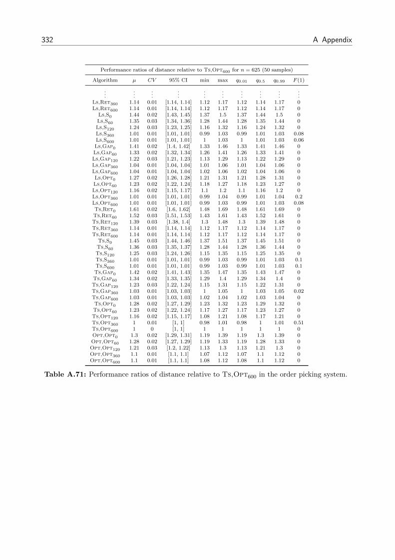
332 A Appendix
Performance ratios of distance relative to Ts,Opt600 for n = 625 (50 samples)
Algorithm µ CV 95% CI min max q0.01 q0.5 q0.99 F (1)
......
......
......
......
......
Ls,Ret360 1.14 0.01 [1.14, 1.14] 1.12 1.17 1.12 1.14 1.17 0Ls,Ret600 1.14 0.01 [1.14, 1.14] 1.12 1.17 1.12 1.14 1.17 0
Ls,S0 1.44 0.02 [1.43, 1.45] 1.37 1.5 1.37 1.44 1.5 0Ls,S60 1.35 0.03 [1.34, 1.36] 1.28 1.44 1.28 1.35 1.44 0Ls,S120 1.24 0.03 [1.23, 1.25] 1.16 1.32 1.16 1.24 1.32 0Ls,S360 1.01 0.01 [1.01, 1.01] 0.99 1.03 0.99 1.01 1.03 0.08Ls,S600 1.01 0.01 [1.01, 1.01] 1 1.03 1 1.01 1.03 0.06Ls,Gap0 1.41 0.02 [1.4, 1.42] 1.33 1.46 1.33 1.41 1.46 0Ls,Gap60 1.33 0.02 [1.32, 1.34] 1.26 1.41 1.26 1.33 1.41 0Ls,Gap120 1.22 0.03 [1.21, 1.23] 1.13 1.29 1.13 1.22 1.29 0Ls,Gap360 1.04 0.01 [1.04, 1.04] 1.01 1.06 1.01 1.04 1.06 0Ls,Gap600 1.04 0.01 [1.04, 1.04] 1.02 1.06 1.02 1.04 1.06 0Ls,Opt0 1.27 0.02 [1.26, 1.28] 1.21 1.31 1.21 1.28 1.31 0Ls,Opt60 1.23 0.02 [1.22, 1.24] 1.18 1.27 1.18 1.23 1.27 0Ls,Opt120 1.16 0.02 [1.15, 1.17] 1.1 1.2 1.1 1.16 1.2 0Ls,Opt360 1.01 0.01 [1.01, 1.01] 0.99 1.04 0.99 1.01 1.04 0.2Ls,Opt600 1.01 0.01 [1.01, 1.01] 0.99 1.03 0.99 1.01 1.03 0.08Ts,Ret0 1.61 0.02 [1.6, 1.62] 1.48 1.69 1.48 1.61 1.69 0Ts,Ret60 1.52 0.03 [1.51, 1.53] 1.43 1.61 1.43 1.52 1.61 0Ts,Ret120 1.39 0.03 [1.38, 1.4] 1.3 1.48 1.3 1.39 1.48 0Ts,Ret360 1.14 0.01 [1.14, 1.14] 1.12 1.17 1.12 1.14 1.17 0Ts,Ret600 1.14 0.01 [1.14, 1.14] 1.12 1.17 1.12 1.14 1.17 0
Ts,S0 1.45 0.03 [1.44, 1.46] 1.37 1.51 1.37 1.45 1.51 0Ts,S60 1.36 0.03 [1.35, 1.37] 1.28 1.44 1.28 1.36 1.44 0Ts,S120 1.25 0.03 [1.24, 1.26] 1.15 1.35 1.15 1.25 1.35 0Ts,S360 1.01 0.01 [1.01, 1.01] 0.99 1.03 0.99 1.01 1.03 0.1Ts,S600 1.01 0.01 [1.01, 1.01] 0.99 1.03 0.99 1.01 1.03 0.1Ts,Gap0 1.42 0.02 [1.41, 1.43] 1.35 1.47 1.35 1.43 1.47 0Ts,Gap60 1.34 0.02 [1.33, 1.35] 1.29 1.4 1.29 1.34 1.4 0Ts,Gap120 1.23 0.03 [1.22, 1.24] 1.15 1.31 1.15 1.22 1.31 0Ts,Gap360 1.03 0.01 [1.03, 1.03] 1 1.05 1 1.03 1.05 0.02Ts,Gap600 1.03 0.01 [1.03, 1.03] 1.02 1.04 1.02 1.03 1.04 0Ts,Opt0 1.28 0.02 [1.27, 1.29] 1.23 1.32 1.23 1.29 1.32 0Ts,Opt60 1.23 0.02 [1.22, 1.24] 1.17 1.27 1.17 1.23 1.27 0Ts,Opt120 1.16 0.02 [1.15, 1.17] 1.08 1.21 1.08 1.17 1.21 0Ts,Opt360 1 0.01 [1, 1] 0.98 1.01 0.98 1 1.01 0.51Ts,Opt600 1 0 [1, 1] 1 1 1 1 1 0Opt,Opt0 1.3 0.02 [1.29, 1.31] 1.19 1.39 1.19 1.3 1.39 0Opt,Opt60 1.28 0.02 [1.27, 1.29] 1.19 1.33 1.19 1.28 1.33 0Opt,Opt120 1.21 0.03 [1.2, 1.22] 1.13 1.3 1.13 1.21 1.3 0Opt,Opt360 1.1 0.01 [1.1, 1.1] 1.07 1.12 1.07 1.1 1.12 0Opt,Opt600 1.1 0.01 [1.1, 1.1] 1.08 1.12 1.08 1.1 1.12 0
Table A.71: Performance ratios of distance relative to Ts,Opt600 in the order picking system.

A.3 Numerical Results from Chapter 6 333
Performance ratios of distance relative to online version for n = 625 (50 samples)
Algorithm µ CV 95% CI min max q0.01 q0.5 q0.99 1− F (1)
Prio,Ret0 1 0 [1, 1] 1 1 1 1 1 0Prio,Ret60 0.99 0.01 [0.99, 0.99] 0.98 1.01 0.98 0.99 1.01 0.22Prio,Ret120 0.99 0.01 [0.99, 0.99] 0.97 1.01 0.97 0.99 1.01 0.14Prio,Ret360 0.99 0.01 [0.99, 0.99] 0.96 1 0.96 0.99 1 0.1Prio,Ret600 0.98 0.01 [0.98, 0.98] 0.96 1.01 0.96 0.98 1.01 0.06
Prio,S0 1 0 [1, 1] 1 1 1 1 1 0Prio,S60 0.99 0.01 [0.99, 0.99] 0.97 1.02 0.97 0.99 1.02 0.2Prio,S120 0.99 0.01 [0.99, 0.99] 0.97 1.01 0.97 0.98 1.01 0.08Prio,S360 0.98 0.01 [0.98, 0.98] 0.96 1.02 0.96 0.98 1.02 0.04Prio,S600 0.98 0.01 [0.98, 0.98] 0.95 1.01 0.95 0.98 1.01 0.06Prio,Gap0 1 0 [1, 1] 1 1 1 1 1 0Prio,Gap60 0.99 0.01 [0.99, 0.99] 0.97 1.02 0.97 0.99 1.02 0.31Prio,Gap120 0.99 0.01 [0.99, 0.99] 0.96 1.01 0.96 0.99 1.01 0.08Prio,Gap360 0.98 0.01 [0.98, 0.98] 0.96 1.01 0.96 0.98 1.01 0.04Prio,Gap600 0.98 0.01 [0.98, 0.98] 0.95 1.02 0.95 0.98 1.02 0.04Prio,Opt0 1 0 [1, 1] 1 1 1 1 1 0Prio,Opt60 0.99 0.01 [0.99, 0.99] 0.97 1.01 0.97 0.99 1.01 0.16Prio,Opt120 0.99 0.01 [0.99, 0.99] 0.96 1 0.96 0.99 1 0.02Prio,Opt360 0.98 0.01 [0.98, 0.98] 0.96 0.99 0.96 0.98 0.99 0Prio,Opt600 0.98 0.01 [0.98, 0.98] 0.96 1 0.96 0.98 1 0.02Seed,Ret0 1 0 [1, 1] 1 1 1 1 1 0Seed,Ret60 0.95 0.02 [0.94, 0.96] 0.89 1.01 0.89 0.95 1.01 0.02Seed,Ret120 0.87 0.03 [0.86, 0.88] 0.81 0.94 0.81 0.87 0.94 0Seed,Ret360 0.71 0.02 [0.71, 0.71] 0.69 0.76 0.69 0.71 0.76 0Seed,Ret600 0.71 0.02 [0.71, 0.71] 0.69 0.75 0.69 0.71 0.75 0
Seed,S0 1 0 [1, 1] 1 1 1 1 1 0Seed,S60 0.95 0.02 [0.94, 0.96] 0.89 1 0.89 0.95 1 0Seed,S120 0.87 0.03 [0.86, 0.88] 0.82 0.94 0.82 0.87 0.94 0Seed,S360 0.7 0.02 [0.7, 0.7] 0.68 0.74 0.68 0.7 0.74 0Seed,S600 0.7 0.02 [0.7, 0.7] 0.68 0.74 0.68 0.7 0.74 0Seed,Gap0 1 0 [1, 1] 1 1 1 1 1 0Seed,Gap60 0.95 0.02 [0.94, 0.96] 0.89 1 0.89 0.95 1 0.02Seed,Gap120 0.87 0.03 [0.86, 0.88] 0.81 0.93 0.81 0.87 0.93 0Seed,Gap360 0.76 0.02 [0.76, 0.76] 0.73 0.81 0.73 0.76 0.81 0Seed,Gap600 0.76 0.02 [0.76, 0.76] 0.74 0.8 0.74 0.76 0.8 0Seed,Opt0 1 0 [1, 1] 1 1 1 1 1 0Seed,Opt60 0.96 0.02 [0.95, 0.97] 0.92 1 0.92 0.97 1 0Seed,Opt120 0.91 0.02 [0.9, 0.92] 0.87 0.94 0.87 0.91 0.94 0Seed,Opt360 0.77 0.01 [0.77, 0.77] 0.75 0.79 0.75 0.77 0.79 0Seed,Opt600 0.77 0.01 [0.77, 0.77] 0.75 0.8 0.75 0.77 0.8 0
Svg,Ret0 1 0 [1, 1] 1 1 1 1 1 0Svg,Ret60 0.95 0.02 [0.94, 0.96] 0.88 1.02 0.88 0.95 1.02 0.02Svg,Ret120 0.89 0.03 [0.88, 0.9] 0.84 0.95 0.84 0.89 0.95 0Svg,Ret360 0.84 0.02 [0.84, 0.84] 0.8 0.91 0.8 0.84 0.91 0Svg,Ret600 0.87 0.02 [0.87, 0.87] 0.83 0.93 0.83 0.86 0.93 0
Svg,S0 1 0 [1, 1] 1 1 1 1 1 0Svg,S60 0.96 0.02 [0.95, 0.97] 0.91 1 0.91 0.96 1 0Svg,S120 0.91 0.03 [0.9, 0.92] 0.85 0.96 0.85 0.91 0.96 0Svg,S360 0.84 0.02 [0.84, 0.84] 0.8 0.89 0.8 0.84 0.89 0Svg,S600 0.87 0.02 [0.87, 0.87] 0.84 0.93 0.84 0.87 0.93 0Svg,Gap0 1 0 [1, 1] 1 1 1 1 1 0Svg,Gap60 0.96 0.02 [0.95, 0.97] 0.92 1 0.92 0.97 1 0Svg,Gap120 0.92 0.03 [0.91, 0.93] 0.87 0.98 0.87 0.93 0.98 0Svg,Gap360 0.9 0.03 [0.89, 0.91] 0.85 0.97 0.85 0.89 0.97 0Svg,Gap600 0.93 0.02 [0.92, 0.94] 0.89 0.97 0.89 0.92 0.97 0Svg,Opt0 1 0 [1, 1] 1 1 1 1 1 0Svg,Opt60 0.97 0.02 [0.96, 0.98] 0.93 1.01 0.93 0.97 1.01 0.04Svg,Opt120 0.94 0.02 [0.93, 0.95] 0.91 0.98 0.91 0.94 0.98 0Svg,Opt360 0.91 0.02 [0.9, 0.92] 0.88 0.96 0.88 0.9 0.96 0Svg,Opt600 0.94 0.02 [0.93, 0.95] 0.91 1 0.91 0.94 1 0
Ls,Ret0 1 0 [1, 1] 1 1 1 1 1 0Ls,Ret60 0.94 0.03 [0.93, 0.95] 0.9 1 0.9 0.95 1 0.02Ls,Ret120 0.86 0.03 [0.85, 0.87] 0.81 0.92 0.81 0.85 0.92 0
......
......
......
......
......

334 A Appendix
Performance ratios of distance relative to online version for n = 625 (50 samples)
Algorithm µ CV 95% CI min max q0.01 q0.5 q0.99 1− F (1)
......
......
......
......
......
Ls,Ret360 0.71 0.02 [0.71, 0.71] 0.68 0.77 0.68 0.71 0.77 0Ls,Ret600 0.71 0.02 [0.71, 0.71] 0.69 0.77 0.69 0.71 0.77 0
Ls,S0 1 0 [1, 1] 1 1 1 1 1 0Ls,S60 0.94 0.02 [0.93, 0.95] 0.88 0.98 0.88 0.94 0.98 0Ls,S120 0.86 0.03 [0.85, 0.87] 0.81 0.92 0.81 0.86 0.92 0Ls,S360 0.7 0.02 [0.7, 0.7] 0.68 0.74 0.68 0.7 0.74 0Ls,S600 0.7 0.02 [0.7, 0.7] 0.68 0.74 0.68 0.7 0.74 0Ls,Gap0 1 0 [1, 1] 1 1 1 1 1 0Ls,Gap60 0.95 0.02 [0.94, 0.96] 0.89 1 0.89 0.94 1 0Ls,Gap120 0.87 0.03 [0.86, 0.88] 0.81 0.94 0.81 0.87 0.94 0Ls,Gap360 0.74 0.02 [0.74, 0.74] 0.71 0.78 0.71 0.74 0.78 0Ls,Gap600 0.74 0.02 [0.74, 0.74] 0.71 0.77 0.71 0.74 0.77 0Ls,Opt0 1 0 [1, 1] 1 1 1 1 1 0Ls,Opt60 0.96 0.02 [0.95, 0.97] 0.91 1 0.91 0.96 1 0.02Ls,Opt120 0.91 0.02 [0.9, 0.92] 0.87 0.96 0.87 0.91 0.96 0Ls,Opt360 0.79 0.02 [0.79, 0.79] 0.76 0.83 0.76 0.79 0.83 0Ls,Opt600 0.79 0.02 [0.79, 0.79] 0.77 0.83 0.77 0.79 0.83 0Ts,Ret0 1 0 [1, 1] 1 1 1 1 1 0Ts,Ret60 0.94 0.03 [0.93, 0.95] 0.88 1 0.88 0.94 1 0Ts,Ret120 0.86 0.03 [0.85, 0.87] 0.81 0.93 0.81 0.86 0.93 0Ts,Ret360 0.71 0.02 [0.71, 0.71] 0.68 0.76 0.68 0.7 0.76 0Ts,Ret600 0.71 0.02 [0.71, 0.71] 0.68 0.76 0.68 0.7 0.76 0
Ts,S0 1 0 [1, 1] 1 1 1 1 1 0Ts,S60 0.94 0.03 [0.93, 0.95] 0.86 1 0.86 0.95 1 0.02Ts,S120 0.87 0.04 [0.86, 0.88] 0.78 0.94 0.78 0.87 0.94 0Ts,S360 0.7 0.02 [0.7, 0.7] 0.67 0.74 0.67 0.7 0.74 0Ts,S600 0.7 0.02 [0.7, 0.7] 0.67 0.74 0.67 0.7 0.74 0Ts,Gap0 1 0 [1, 1] 1 1 1 1 1 0Ts,Gap60 0.94 0.02 [0.93, 0.95] 0.9 1 0.9 0.94 1 0Ts,Gap120 0.87 0.03 [0.86, 0.88] 0.81 0.93 0.81 0.86 0.93 0Ts,Gap360 0.72 0.02 [0.72, 0.72] 0.7 0.77 0.7 0.72 0.77 0Ts,Gap600 0.73 0.02 [0.73, 0.73] 0.7 0.77 0.7 0.72 0.77 0Ts,Opt0 1 0 [1, 1] 1 1 1 1 1 0Ts,Opt60 0.96 0.02 [0.95, 0.97] 0.92 1 0.92 0.96 1 0.02Ts,Opt120 0.91 0.02 [0.9, 0.92] 0.86 0.95 0.86 0.9 0.95 0Ts,Opt360 0.78 0.02 [0.78, 0.78] 0.76 0.82 0.76 0.78 0.82 0Ts,Opt600 0.78 0.02 [0.78, 0.78] 0.76 0.81 0.76 0.78 0.81 0Opt,Opt0 1 0 [1, 1] 1 1 1 1 1 0Opt,Opt60 0.98 0.02 [0.97, 0.99] 0.93 1.02 0.93 0.98 1.02 0.14Opt,Opt120 0.93 0.03 [0.92, 0.94] 0.86 1 0.86 0.93 1 0Opt,Opt360 0.85 0.02 [0.85, 0.85] 0.8 0.93 0.8 0.84 0.93 0Opt,Opt600 0.85 0.03 [0.84, 0.86] 0.79 0.94 0.79 0.84 0.94 0
Table A.72: Performance ratios of distance relative to the online version of an algorithm in theorder picking system.

A.3 Numerical Results from Chapter 6 335
Utilization for n = 625 (50 samples)
Algorithm µ CV 95% CI min max q0.01 q0.5 q0.99 % det.
Prio,Ret0 0.79 0.05 [0.78, 0.8] 0.6 0.8 0.6 0.8 0.8Prio,Ret60 0.88 0.05 [0.87, 0.89] 0.7 0.9 0.7 0.9 0.9 0.02Prio,Ret120 0.92 0.09 [0.9, 0.94] 0.6 1 0.6 0.9 1 0.06Prio,Ret360 0.94 0.07 [0.92, 0.96] 0.7 1 0.7 0.9 1 0.04Prio,Ret600 0.94 0.07 [0.92, 0.96] 0.7 1 0.7 0.9 1 0.06
Prio,S0 0.73 0.07 [0.72, 0.74] 0.6 0.8 0.6 0.7 0.8Prio,S60 0.81 0.07 [0.79, 0.83] 0.6 0.9 0.6 0.8 0.9 0.04Prio,S120 0.86 0.1 [0.84, 0.88] 0.6 1 0.6 0.9 1 0.1Prio,S360 0.91 0.1 [0.88, 0.94] 0.6 1 0.6 0.9 1 0.04Prio,S600 0.91 0.1 [0.88, 0.94] 0.7 1 0.7 0.9 1 0.04Prio,Gap0 0.78 0.06 [0.77, 0.79] 0.6 0.8 0.6 0.8 0.8Prio,Gap60 0.85 0.08 [0.83, 0.87] 0.7 0.9 0.7 0.9 0.9 0.06Prio,Gap120 0.91 0.09 [0.89, 0.93] 0.6 1 0.6 0.9 1 0.08Prio,Gap360 0.92 0.09 [0.9, 0.94] 0.7 1 0.7 0.9 1 0.1Prio,Gap600 0.93 0.09 [0.91, 0.95] 0.7 1 0.7 0.9 1 0.08Prio,Opt0 0.71 0.06 [0.7, 0.72] 0.6 0.8 0.6 0.7 0.8Prio,Opt60 0.8 0.05 [0.79, 0.81] 0.7 0.9 0.7 0.8 0.9 0Prio,Opt120 0.84 0.09 [0.82, 0.86] 0.6 1 0.6 0.8 1 0.08Prio,Opt360 0.9 0.11 [0.87, 0.93] 0.6 1 0.6 0.9 1 0.02Prio,Opt600 0.89 0.11 [0.86, 0.92] 0.6 1 0.6 0.9 1 0.08Seed,Ret0 0.79 0.05 [0.78, 0.8] 0.6 0.8 0.6 0.8 0.8Seed,Ret60 0.84 0.07 [0.82, 0.86] 0.7 0.9 0.7 0.8 0.9 0.04Seed,Ret120 0.86 0.09 [0.84, 0.88] 0.6 1 0.6 0.9 1 0.2Seed,Ret360 0.88 0.12 [0.85, 0.91] 0.6 1 0.6 0.9 1 0.06Seed,Ret600 0.88 0.12 [0.85, 0.91] 0.6 1 0.6 0.9 1 0.1
Seed,S0 0.73 0.07 [0.72, 0.74] 0.6 0.8 0.6 0.7 0.8Seed,S60 0.79 0.08 [0.77, 0.81] 0.6 0.9 0.6 0.8 0.9 0.08Seed,S120 0.84 0.09 [0.82, 0.86] 0.6 0.9 0.6 0.8 0.9 0.06Seed,S360 0.89 0.13 [0.86, 0.92] 0.6 1 0.6 0.9 1 0.08Seed,S600 0.88 0.13 [0.85, 0.91] 0.6 1 0.6 0.9 1 0.02Seed,Gap0 0.77 0.06 [0.76, 0.78] 0.6 0.8 0.6 0.8 0.8Seed,Gap60 0.84 0.06 [0.83, 0.85] 0.7 0.9 0.7 0.8 0.9 0.02Seed,Gap120 0.88 0.09 [0.86, 0.9] 0.6 1 0.6 0.9 1 0.1Seed,Gap360 0.91 0.1 [0.88, 0.94] 0.7 1 0.7 0.9 1 0.12Seed,Gap600 0.92 0.09 [0.9, 0.94] 0.7 1 0.7 0.9 1 0.06Seed,Opt0 0.7 0.06 [0.69, 0.71] 0.6 0.8 0.6 0.7 0.8Seed,Opt60 0.8 0.05 [0.79, 0.81] 0.6 0.9 0.6 0.8 0.9 0Seed,Opt120 0.82 0.09 [0.8, 0.84] 0.6 0.9 0.6 0.8 0.9 0.14Seed,Opt360 0.88 0.13 [0.85, 0.91] 0.6 1 0.6 0.9 1 0.08Seed,Opt600 0.89 0.12 [0.86, 0.92] 0.6 1 0.6 0.9 1 0.08
Svg,Ret0 0.79 0.05 [0.78, 0.8] 0.6 0.8 0.6 0.8 0.8Svg,Ret60 0.85 0.06 [0.84, 0.86] 0.7 0.9 0.7 0.9 0.9 0.02Svg,Ret120 0.87 0.09 [0.85, 0.89] 0.6 1 0.6 0.9 1 0.14Svg,Ret360 0.9 0.11 [0.87, 0.93] 0.6 1 0.6 0.9 1 0.06Svg,Ret600 0.9 0.11 [0.87, 0.93] 0.6 1 0.6 0.9 1 0.1
Svg,S0 0.73 0.07 [0.72, 0.74] 0.6 0.8 0.6 0.7 0.8Svg,S60 0.8 0.04 [0.79, 0.81] 0.7 0.9 0.7 0.8 0.9 0.02Svg,S120 0.84 0.09 [0.82, 0.86] 0.6 1 0.6 0.9 1 0.06Svg,S360 0.88 0.13 [0.85, 0.91] 0.6 1 0.6 0.9 1 0.06Svg,S600 0.9 0.11 [0.87, 0.93] 0.6 1 0.6 0.9 1 0.04Svg,Gap0 0.77 0.07 [0.75, 0.79] 0.6 0.8 0.6 0.8 0.8Svg,Gap60 0.83 0.06 [0.82, 0.84] 0.7 0.9 0.7 0.8 0.9 0Svg,Gap120 0.88 0.09 [0.86, 0.9] 0.6 1 0.6 0.9 1 0.08Svg,Gap360 0.92 0.09 [0.9, 0.94] 0.7 1 0.7 0.9 1 0.08Svg,Gap600 0.92 0.08 [0.9, 0.94] 0.7 1 0.7 0.9 1 0.08Svg,Opt0 0.71 0.06 [0.7, 0.72] 0.6 0.8 0.6 0.7 0.8Svg,Opt60 0.79 0.05 [0.78, 0.8] 0.6 0.9 0.6 0.8 0.9 0.02Svg,Opt120 0.83 0.1 [0.81, 0.85] 0.6 0.9 0.6 0.8 0.9 0.1Svg,Opt360 0.88 0.12 [0.85, 0.91] 0.6 1 0.6 0.9 1 0.04Svg,Opt600 0.89 0.11 [0.86, 0.92] 0.6 1 0.6 0.9 1 0.06
Ls,Ret0 0.78 0.06 [0.77, 0.79] 0.6 0.8 0.6 0.8 0.8Ls,Ret60 0.83 0.06 [0.82, 0.84] 0.7 0.9 0.7 0.8 0.9 0.04Ls,Ret120 0.86 0.08 [0.84, 0.88] 0.6 1 0.6 0.9 1 0.16
......
......
......
......
......

336 A Appendix
Utilization for n = 625 (50 samples)
Algorithm µ CV 95% CI min max q0.01 q0.5 q0.99 % det.
......
......
......
......
......
Ls,Ret360 0.88 0.12 [0.85, 0.91] 0.6 1 0.6 0.9 1 0.02Ls,Ret600 0.88 0.13 [0.85, 0.91] 0.6 1 0.6 0.9 1 0.08
Ls,S0 0.71 0.06 [0.7, 0.72] 0.6 0.8 0.6 0.7 0.8Ls,S60 0.8 0.04 [0.79, 0.81] 0.7 0.9 0.7 0.8 0.9 0Ls,S120 0.83 0.08 [0.81, 0.85] 0.6 0.9 0.6 0.8 0.9 0.1Ls,S360 0.89 0.12 [0.86, 0.92] 0.6 1 0.6 0.9 1 0.06Ls,S600 0.88 0.13 [0.85, 0.91] 0.6 1 0.6 0.9 1 0.04Ls,Gap0 0.75 0.07 [0.74, 0.76] 0.6 0.8 0.6 0.8 0.8Ls,Gap60 0.8 0.05 [0.79, 0.81] 0.6 0.9 0.6 0.8 0.9 0.02Ls,Gap120 0.84 0.08 [0.82, 0.86] 0.6 0.9 0.6 0.8 0.9 0.1Ls,Gap360 0.89 0.13 [0.86, 0.92] 0.6 1 0.6 0.9 1 0.06Ls,Gap600 0.88 0.12 [0.85, 0.91] 0.6 1 0.6 0.9 1 0.08Ls,Opt0 0.72 0.07 [0.71, 0.73] 0.6 0.8 0.6 0.7 0.8Ls,Opt60 0.79 0.07 [0.77, 0.81] 0.6 0.9 0.6 0.8 0.9 0.04Ls,Opt120 0.82 0.09 [0.8, 0.84] 0.6 0.9 0.6 0.8 0.9 0.1Ls,Opt360 0.89 0.12 [0.86, 0.92] 0.6 1 0.6 0.9 1 0.04Ls,Opt600 0.88 0.13 [0.85, 0.91] 0.6 1 0.6 0.9 1 0.04Ts,Ret0 0.78 0.05 [0.77, 0.79] 0.6 0.8 0.6 0.8 0.8Ts,Ret60 0.84 0.07 [0.82, 0.86] 0.7 0.9 0.7 0.8 0.9 0.04Ts,Ret120 0.86 0.08 [0.84, 0.88] 0.6 1 0.6 0.9 1 0.16Ts,Ret360 0.88 0.13 [0.85, 0.91] 0.6 1 0.6 0.9 1 0.06Ts,Ret600 0.88 0.12 [0.85, 0.91] 0.6 1 0.6 0.9 1 0.06
Ts,S0 0.72 0.07 [0.71, 0.73] 0.6 0.8 0.6 0.7 0.8Ts,S60 0.8 0.05 [0.79, 0.81] 0.6 0.9 0.6 0.8 0.9 0.02Ts,S120 0.84 0.08 [0.82, 0.86] 0.6 0.9 0.6 0.8 0.9 0.06Ts,S360 0.88 0.13 [0.85, 0.91] 0.6 1 0.6 0.9 1 0.06Ts,S600 0.89 0.12 [0.86, 0.92] 0.6 1 0.6 0.9 1 0.02Ts,Gap0 0.75 0.08 [0.73, 0.77] 0.6 0.8 0.6 0.8 0.8Ts,Gap60 0.8 0.06 [0.79, 0.81] 0.6 0.9 0.6 0.8 0.9 0.04Ts,Gap120 0.84 0.09 [0.82, 0.86] 0.6 1 0.6 0.8 1 0.08Ts,Gap360 0.87 0.13 [0.84, 0.9] 0.6 1 0.6 0.9 1 0.06Ts,Gap600 0.89 0.12 [0.86, 0.92] 0.6 1 0.6 0.9 1 0.06Ts,Opt0 0.71 0.06 [0.7, 0.72] 0.6 0.8 0.6 0.7 0.8Ts,Opt60 0.79 0.06 [0.78, 0.8] 0.6 0.9 0.6 0.8 0.9 0.04Ts,Opt120 0.82 0.09 [0.8, 0.84] 0.6 0.9 0.6 0.8 0.9 0.12Ts,Opt360 0.87 0.14 [0.84, 0.9] 0.6 1 0.6 0.9 1 0.08Ts,Opt600 0.88 0.13 [0.85, 0.91] 0.6 1 0.6 0.9 1 0.04Opt,Opt0 0.72 0.09 [0.7, 0.74] 0.6 0.9 0.6 0.7 0.9Opt,Opt60 0.79 0.07 [0.77, 0.81] 0.6 0.9 0.6 0.8 0.9 0.04Opt,Opt120 0.86 0.09 [0.84, 0.88] 0.6 1 0.6 0.9 1 0.1Opt,Opt360 0.91 0.1 [0.88, 0.94] 0.7 1 0.7 0.9 1 0.08Opt,Opt600 0.92 0.09 [0.9, 0.94] 0.7 1 0.7 0.9 1 0.06
Table A.73: Picker utilizations in the order picking system.

A.3 Numerical Results from Chapter 6 337
Performance ratios of utilization relative to Ts,Opt600 for n = 625 (50 samples)
Algorithm µ CV 95% CI min max q0.01 q0.5 q0.99 F (1)
Prio,Ret0 0.91 0.16 [0.87, 0.95] 0.67 1.33 0.67 0.89 1.33 0.12Prio,Ret60 1.02 0.16 [0.97, 1.07] 0.7 1.5 0.7 1 1.5 0.37Prio,Ret120 1.07 0.17 [1.02, 1.12] 0.67 1.67 0.67 1.11 1.67 0.53Prio,Ret360 1.09 0.15 [1.04, 1.14] 0.8 1.67 0.8 1.11 1.67 0.57Prio,Ret600 1.09 0.15 [1.04, 1.14] 0.8 1.67 0.8 1.11 1.67 0.57
Prio,S0 0.85 0.2 [0.8, 0.9] 0.67 1.33 0.67 0.8 1.33 0.1Prio,S60 0.94 0.18 [0.89, 0.99] 0.6 1.5 0.6 0.9 1.5 0.2Prio,S120 1 0.14 [0.96, 1.04] 0.67 1.29 0.67 1 1.29 0.41Prio,S360 1.05 0.15 [1.01, 1.09] 0.7 1.67 0.7 1.11 1.67 0.57Prio,S600 1.05 0.16 [1, 1.1] 0.7 1.67 0.7 1.11 1.67 0.55Prio,Gap0 0.9 0.17 [0.86, 0.94] 0.67 1.33 0.67 0.89 1.33 0.12Prio,Gap60 0.99 0.18 [0.94, 1.04] 0.7 1.5 0.7 1 1.5 0.35Prio,Gap120 1.05 0.16 [1, 1.1] 0.67 1.67 0.67 1.11 1.67 0.51Prio,Gap360 1.07 0.16 [1.02, 1.12] 0.7 1.67 0.7 1.11 1.67 0.59Prio,Gap600 1.08 0.15 [1.03, 1.13] 0.7 1.67 0.7 1.11 1.67 0.59Prio,Opt0 0.82 0.17 [0.78, 0.86] 0.67 1.17 0.67 0.78 1.17 0.06Prio,Opt60 0.93 0.17 [0.89, 0.97] 0.7 1.5 0.7 0.89 1.5 0.16Prio,Opt120 0.97 0.14 [0.93, 1.01] 0.67 1.17 0.67 1 1.17 0.33Prio,Opt360 1.03 0.11 [1, 1.06] 0.7 1.25 0.7 1 1.25 0.41Prio,Opt600 1.02 0.11 [0.99, 1.05] 0.7 1.25 0.7 1 1.25 0.39Seed,Ret0 0.92 0.16 [0.88, 0.96] 0.67 1.33 0.67 0.89 1.33 0.12Seed,Ret60 0.98 0.18 [0.93, 1.03] 0.7 1.5 0.7 1 1.5 0.33Seed,Ret120 1 0.14 [0.96, 1.04] 0.67 1.29 0.67 1 1.29 0.41Seed,Ret360 1.01 0.11 [0.98, 1.04] 0.7 1.25 0.7 1 1.25 0.27Seed,Ret600 1.01 0.13 [0.97, 1.05] 0.6 1.5 0.6 1 1.5 0.27
Seed,S0 0.85 0.19 [0.8, 0.9] 0.67 1.33 0.67 0.8 1.33 0.08Seed,S60 0.92 0.19 [0.87, 0.97] 0.6 1.5 0.6 0.89 1.5 0.16Seed,S120 0.97 0.16 [0.93, 1.01] 0.67 1.5 0.67 1 1.5 0.33Seed,S360 1.01 0.07 [0.99, 1.03] 0.87 1.33 0.87 1 1.33 0.1Seed,S600 1.01 0.04 [1, 1.02] 0.89 1.14 0.89 1 1.14 0.1Seed,Gap0 0.9 0.18 [0.85, 0.95] 0.67 1.33 0.67 0.89 1.33 0.12Seed,Gap60 0.98 0.17 [0.93, 1.03] 0.78 1.5 0.78 1 1.5 0.29Seed,Gap120 1.02 0.15 [0.98, 1.06] 0.67 1.29 0.67 1 1.29 0.47Seed,Gap360 1.05 0.14 [1.01, 1.09] 0.7 1.29 0.7 1.11 1.29 0.59Seed,Gap600 1.07 0.15 [1.02, 1.12] 0.7 1.67 0.7 1.11 1.67 0.59Seed,Opt0 0.82 0.18 [0.78, 0.86] 0.6 1.33 0.6 0.78 1.33 0.04Seed,Opt60 0.93 0.16 [0.89, 0.97] 0.6 1.33 0.6 0.89 1.33 0.12Seed,Opt120 0.95 0.17 [0.9, 1] 0.67 1.5 0.67 1 1.5 0.22Seed,Opt360 1.01 0.1 [0.98, 1.04] 0.6 1.33 0.6 1 1.33 0.1Seed,Opt600 1.01 0.09 [0.98, 1.04] 0.87 1.5 0.87 1 1.5 0.12
Svg,Ret0 0.91 0.16 [0.87, 0.95] 0.67 1.33 0.67 0.89 1.33 0.12Svg,Ret60 0.99 0.17 [0.94, 1.04] 0.7 1.5 0.7 1 1.5 0.33Svg,Ret120 1.01 0.17 [0.96, 1.06] 0.67 1.67 0.67 1 1.67 0.43Svg,Ret360 1.04 0.12 [1, 1.08] 0.7 1.25 0.7 1.11 1.25 0.53Svg,Ret600 1.04 0.14 [1, 1.08] 0.7 1.29 0.7 1.11 1.29 0.57
Svg,S0 0.85 0.18 [0.81, 0.89] 0.67 1.33 0.67 0.8 1.33 0.08Svg,S60 0.93 0.16 [0.89, 0.97] 0.7 1.33 0.7 0.89 1.33 0.12Svg,S120 0.98 0.17 [0.93, 1.03] 0.67 1.5 0.67 1 1.5 0.37Svg,S360 1.01 0.11 [0.98, 1.04] 0.6 1.25 0.6 1 1.25 0.31Svg,S600 1.03 0.11 [1, 1.06] 0.7 1.25 0.7 1 1.25 0.37Svg,Gap0 0.89 0.18 [0.84, 0.94] 0.67 1.33 0.67 0.87 1.33 0.12Svg,Gap60 0.97 0.16 [0.93, 1.01] 0.78 1.5 0.78 1 1.5 0.22Svg,Gap120 1.02 0.17 [0.97, 1.07] 0.67 1.67 0.67 1 1.67 0.43Svg,Gap360 1.06 0.15 [1.02, 1.1] 0.7 1.67 0.7 1.11 1.67 0.59Svg,Gap600 1.07 0.15 [1.02, 1.12] 0.7 1.67 0.7 1.11 1.67 0.57Svg,Opt0 0.82 0.17 [0.78, 0.86] 0.67 1.33 0.67 0.78 1.33 0.04Svg,Opt60 0.92 0.16 [0.88, 0.96] 0.67 1.33 0.67 0.89 1.33 0.14Svg,Opt120 0.97 0.17 [0.92, 1.02] 0.67 1.5 0.67 1 1.5 0.31Svg,Opt360 1.01 0.1 [0.98, 1.04] 0.7 1.17 0.7 1 1.17 0.29Svg,Opt600 1.02 0.12 [0.99, 1.05] 0.7 1.5 0.7 1 1.5 0.33
Ls,Ret0 0.91 0.16 [0.87, 0.95] 0.67 1.33 0.67 0.89 1.33 0.12Ls,Ret60 0.97 0.18 [0.92, 1.02] 0.7 1.5 0.7 0.9 1.5 0.27Ls,Ret120 0.99 0.17 [0.94, 1.04] 0.67 1.67 0.67 1 1.67 0.35
......
......
......
......
......

338 A Appendix
Performance ratios of utilization relative to Ts,Opt600 for n = 625 (50 samples)
Algorithm µ CV 95% CI min max q0.01 q0.5 q0.99 F (1)
......
......
......
......
......
Ls,Ret360 1.01 0.1 [0.98, 1.04] 0.7 1.25 0.7 1 1.25 0.29Ls,Ret600 1 0.1 [0.97, 1.03] 0.6 1.17 0.6 1 1.17 0.24
Ls,S0 0.82 0.16 [0.78, 0.86] 0.67 1.17 0.67 0.78 1.17 0.04Ls,S60 0.93 0.16 [0.89, 0.97] 0.7 1.33 0.7 0.89 1.33 0.16Ls,S120 0.96 0.16 [0.92, 1] 0.67 1.5 0.67 1 1.5 0.24Ls,S360 1.02 0.08 [1, 1.04] 0.87 1.5 0.87 1 1.5 0.1Ls,S600 1.01 0.09 [0.98, 1.04] 0.87 1.5 0.87 1 1.5 0.08Ls,Gap0 0.87 0.17 [0.83, 0.91] 0.67 1.33 0.67 0.87 1.33 0.1Ls,Gap60 0.93 0.17 [0.89, 0.97] 0.67 1.5 0.67 0.89 1.5 0.14Ls,Gap120 0.97 0.15 [0.93, 1.01] 0.67 1.17 0.67 1 1.17 0.35Ls,Gap360 1.02 0.13 [0.98, 1.06] 0.6 1.5 0.6 1 1.5 0.27Ls,Gap600 1.01 0.13 [0.97, 1.05] 0.6 1.5 0.6 1 1.5 0.27Ls,Opt0 0.84 0.19 [0.79, 0.89] 0.6 1.33 0.6 0.8 1.33 0.08Ls,Opt60 0.91 0.17 [0.87, 0.95] 0.67 1.33 0.67 0.89 1.33 0.12Ls,Opt120 0.95 0.17 [0.9, 1] 0.67 1.5 0.67 1 1.5 0.24Ls,Opt360 1.01 0.08 [0.99, 1.03] 0.89 1.5 0.89 1 1.5 0.08Ls,Opt600 1.01 0.1 [0.98, 1.04] 0.6 1.5 0.6 1 1.5 0.08Ts,Ret0 0.91 0.17 [0.87, 0.95] 0.67 1.33 0.67 0.89 1.33 0.12Ts,Ret60 0.98 0.18 [0.93, 1.03] 0.7 1.5 0.7 1 1.5 0.29Ts,Ret120 1 0.17 [0.95, 1.05] 0.67 1.67 0.67 1 1.67 0.37Ts,Ret360 1.01 0.1 [0.98, 1.04] 0.7 1.25 0.7 1 1.25 0.27Ts,Ret600 1.01 0.12 [0.98, 1.04] 0.6 1.5 0.6 1 1.5 0.24
Ts,S0 0.84 0.18 [0.8, 0.88] 0.67 1.33 0.67 0.78 1.33 0.08Ts,S60 0.93 0.16 [0.89, 0.97] 0.67 1.33 0.67 0.89 1.33 0.14Ts,S120 0.97 0.17 [0.92, 1.02] 0.67 1.5 0.67 1 1.5 0.31Ts,S360 1.01 0.04 [1, 1.02] 0.9 1.13 0.9 1 1.13 0.08Ts,S600 1.01 0.08 [0.99, 1.03] 0.87 1.5 0.87 1 1.5 0.08Ts,Gap0 0.87 0.19 [0.82, 0.92] 0.67 1.33 0.67 0.87 1.33 0.12Ts,Gap60 0.93 0.17 [0.89, 0.97] 0.67 1.5 0.67 0.89 1.5 0.16Ts,Gap120 0.97 0.14 [0.93, 1.01] 0.67 1.17 0.67 1 1.17 0.35Ts,Gap360 1 0.11 [0.97, 1.03] 0.6 1.25 0.6 1 1.25 0.18Ts,Gap600 1.02 0.11 [0.99, 1.05] 0.6 1.17 0.6 1 1.17 0.33Ts,Opt0 0.83 0.17 [0.79, 0.87] 0.67 1.33 0.67 0.78 1.33 0.04Ts,Opt60 0.92 0.17 [0.88, 0.96] 0.6 1.33 0.6 0.89 1.33 0.14Ts,Opt120 0.94 0.15 [0.9, 0.98] 0.67 1.17 0.67 1 1.17 0.22Ts,Opt360 0.99 0.08 [0.97, 1.01] 0.6 1.25 0.6 1 1.25 0.06Ts,Opt600 1 0 [1, 1] 1 1 1 1 1 0Opt,Opt0 0.83 0.18 [0.79, 0.87] 0.67 1.33 0.67 0.78 1.33 0.06Opt,Opt60 0.93 0.18 [0.88, 0.98] 0.6 1.5 0.6 0.89 1.5 0.16Opt,Opt120 1 0.15 [0.96, 1.04] 0.67 1.33 0.67 1 1.33 0.41Opt,Opt360 1.05 0.14 [1.01, 1.09] 0.7 1.29 0.7 1.11 1.29 0.59Opt,Opt600 1.07 0.15 [1.02, 1.12] 0.7 1.67 0.7 1.11 1.67 0.59
Table A.74: Performance ratios of picker utilization relative to Ts,Opt600 in the order pickingsystem.

A.3 Numerical Results from Chapter 6 339
Performance ratios of utilization relative to online version for n = 625 (50 samples)
Algorithm µ CV 95% CI min max q0.01 q0.5 q0.99 1− F (1)
Prio,Ret0 1 0 [1, 1] 1 1 1 1 1 0Prio,Ret60 1.12 0.07 [1.1, 1.14] 0.87 1.33 0.87 1.13 1.33 0.02Prio,Ret120 1.17 0.09 [1.14, 1.2] 0.87 1.43 0.87 1.13 1.43 0.02Prio,Ret360 1.2 0.1 [1.17, 1.23] 0.87 1.67 0.87 1.25 1.67 0.02Prio,Ret600 1.2 0.1 [1.17, 1.23] 0.87 1.67 0.87 1.13 1.67 0.02
Prio,S0 1 0 [1, 1] 1 1 1 1 1 0Prio,S60 1.11 0.09 [1.08, 1.14] 0.86 1.33 0.86 1.14 1.33 0.04Prio,S120 1.19 0.1 [1.16, 1.22] 0.87 1.5 0.87 1.14 1.5 0.04Prio,S360 1.25 0.14 [1.2, 1.3] 0.75 1.67 0.75 1.29 1.67 0.02Prio,S600 1.25 0.13 [1.2, 1.3] 0.87 1.67 0.87 1.29 1.67 0.02Prio,Gap0 1 0 [1, 1] 1 1 1 1 1 0Prio,Gap60 1.1 0.09 [1.07, 1.13] 0.87 1.33 0.87 1.13 1.33 0.06Prio,Gap120 1.17 0.09 [1.14, 1.2] 0.87 1.43 0.87 1.13 1.43 0.02Prio,Gap360 1.2 0.11 [1.16, 1.24] 0.87 1.67 0.87 1.25 1.67 0.04Prio,Gap600 1.2 0.12 [1.16, 1.24] 0.87 1.67 0.87 1.25 1.67 0.04Prio,Opt0 1 0 [1, 1] 1 1 1 1 1 0Prio,Opt60 1.14 0.07 [1.12, 1.16] 1 1.33 1 1.14 1.33 0Prio,Opt120 1.19 0.1 [1.16, 1.22] 0.86 1.5 0.86 1.14 1.5 0.02Prio,Opt360 1.28 0.14 [1.23, 1.33] 0.86 1.67 0.86 1.29 1.67 0.02Prio,Opt600 1.26 0.13 [1.21, 1.31] 0.86 1.67 0.86 1.29 1.67 0.02Seed,Ret0 1 0 [1, 1] 1 1 1 1 1 0Seed,Ret60 1.07 0.08 [1.05, 1.09] 0.87 1.33 0.87 1.13 1.33 0.04Seed,Ret120 1.09 0.07 [1.07, 1.11] 0.87 1.25 0.87 1.13 1.25 0.04Seed,Ret360 1.12 0.14 [1.08, 1.16] 0.75 1.67 0.75 1.13 1.67 0.1Seed,Ret600 1.12 0.13 [1.08, 1.16] 0.75 1.5 0.75 1.13 1.5 0.08
Seed,S0 1 0 [1, 1] 1 1 1 1 1 0Seed,S60 1.09 0.09 [1.06, 1.12] 0.86 1.29 0.86 1.14 1.29 0.08Seed,S120 1.16 0.09 [1.13, 1.19] 0.75 1.29 0.75 1.14 1.29 0.02Seed,S360 1.23 0.16 [1.17, 1.29] 0.75 1.5 0.75 1.25 1.5 0.06Seed,S600 1.22 0.16 [1.16, 1.28] 0.75 1.5 0.75 1.25 1.5 0.06Seed,Gap0 1 0 [1, 1] 1 1 1 1 1 0Seed,Gap60 1.09 0.07 [1.07, 1.11] 0.87 1.33 0.87 1.13 1.33 0.02Seed,Gap120 1.14 0.09 [1.11, 1.17] 0.87 1.43 0.87 1.13 1.43 0.04Seed,Gap360 1.18 0.13 [1.14, 1.22] 0.87 1.67 0.87 1.13 1.67 0.04Seed,Gap600 1.2 0.11 [1.16, 1.24] 0.87 1.67 0.87 1.25 1.67 0.02Seed,Opt0 1 0 [1, 1] 1 1 1 1 1 0Seed,Opt60 1.14 0.06 [1.12, 1.16] 1 1.33 1 1.14 1.33 0Seed,Opt120 1.17 0.1 [1.14, 1.2] 0.86 1.5 0.86 1.14 1.5 0.02Seed,Opt360 1.26 0.16 [1.2, 1.32] 0.86 1.67 0.86 1.29 1.67 0.04Seed,Opt600 1.27 0.14 [1.22, 1.32] 0.86 1.67 0.86 1.29 1.67 0.02
Svg,Ret0 1 0 [1, 1] 1 1 1 1 1 0Svg,Ret60 1.09 0.07 [1.07, 1.11] 0.87 1.33 0.87 1.13 1.33 0.02Svg,Ret120 1.11 0.09 [1.08, 1.14] 0.87 1.43 0.87 1.13 1.43 0.02Svg,Ret360 1.15 0.13 [1.11, 1.19] 0.75 1.67 0.75 1.13 1.67 0.06Svg,Ret600 1.16 0.13 [1.12, 1.2] 0.75 1.67 0.75 1.13 1.67 0.08
Svg,S0 1 0 [1, 1] 1 1 1 1 1 0Svg,S60 1.11 0.07 [1.09, 1.13] 0.87 1.33 0.87 1.14 1.33 0.02Svg,S120 1.16 0.09 [1.13, 1.19] 0.86 1.43 0.86 1.14 1.43 0.04Svg,S360 1.22 0.15 [1.17, 1.27] 0.86 1.67 0.86 1.25 1.67 0.08Svg,S600 1.24 0.14 [1.19, 1.29] 0.86 1.67 0.86 1.29 1.67 0.06Svg,Gap0 1 0 [1, 1] 1 1 1 1 1 0Svg,Gap60 1.09 0.09 [1.06, 1.12] 1 1.5 1 1.13 1.5 0Svg,Gap120 1.15 0.1 [1.12, 1.18] 0.87 1.5 0.87 1.13 1.5 0.02Svg,Gap360 1.2 0.13 [1.16, 1.24] 0.87 1.67 0.87 1.25 1.67 0.04Svg,Gap600 1.21 0.12 [1.17, 1.25] 0.87 1.67 0.87 1.25 1.67 0.04Svg,Opt0 1 0 [1, 1] 1 1 1 1 1 0Svg,Opt60 1.13 0.07 [1.11, 1.15] 0.86 1.33 0.86 1.14 1.33 0.02Svg,Opt120 1.18 0.11 [1.14, 1.22] 0.86 1.5 0.86 1.14 1.5 0.02Svg,Opt360 1.26 0.14 [1.21, 1.31] 0.86 1.67 0.86 1.29 1.67 0.04Svg,Opt600 1.27 0.14 [1.22, 1.32] 0.86 1.67 0.86 1.29 1.67 0.02
Ls,Ret0 1 0 [1, 1] 1 1 1 1 1 0Ls,Ret60 1.06 0.08 [1.04, 1.08] 0.87 1.33 0.87 1 1.33 0.04Ls,Ret120 1.1 0.08 [1.08, 1.12] 0.87 1.29 0.87 1.13 1.29 0.02
......
......
......
......
......

340 A Appendix
Performance ratios of utilization relative to online version for n = 625 (50 samples)
Algorithm µ CV 95% CI min max q0.01 q0.5 q0.99 1− F (1)
......
......
......
......
......
Ls,Ret360 1.14 0.15 [1.09, 1.19] 0.75 1.67 0.75 1.13 1.67 0.12Ls,Ret600 1.12 0.15 [1.07, 1.17] 0.75 1.5 0.75 1.13 1.5 0.12
Ls,S0 1 0 [1, 1] 1 1 1 1 1 0Ls,S60 1.14 0.06 [1.12, 1.16] 1 1.33 1 1.14 1.33 0Ls,S120 1.17 0.1 [1.14, 1.2] 1 1.5 1 1.14 1.5 0Ls,S360 1.26 0.14 [1.21, 1.31] 0.86 1.5 0.86 1.29 1.5 0.02Ls,S600 1.25 0.14 [1.2, 1.3] 0.86 1.5 0.86 1.29 1.5 0.02Ls,Gap0 1 0 [1, 1] 1 1 1 1 1 0Ls,Gap60 1.07 0.08 [1.05, 1.09] 0.86 1.33 0.86 1 1.33 0.02Ls,Gap120 1.12 0.09 [1.09, 1.15] 0.87 1.29 0.87 1.13 1.29 0.02Ls,Gap360 1.19 0.15 [1.14, 1.24] 0.86 1.67 0.86 1.14 1.67 0.08Ls,Gap600 1.18 0.15 [1.13, 1.23] 0.86 1.67 0.86 1.14 1.67 0.06Ls,Opt0 1 0 [1, 1] 1 1 1 1 1 0Ls,Opt60 1.09 0.08 [1.07, 1.11] 0.86 1.33 0.86 1.14 1.33 0.04Ls,Opt120 1.14 0.1 [1.11, 1.17] 0.75 1.33 0.75 1.14 1.33 0.04Ls,Opt360 1.24 0.16 [1.18, 1.3] 0.75 1.67 0.75 1.25 1.67 0.06Ls,Opt600 1.22 0.16 [1.16, 1.28] 0.75 1.67 0.75 1.14 1.67 0.06Ts,Ret0 1 0 [1, 1] 1 1 1 1 1 0Ts,Ret60 1.07 0.08 [1.05, 1.09] 0.87 1.33 0.87 1.13 1.33 0.04Ts,Ret120 1.1 0.08 [1.08, 1.12] 0.87 1.29 0.87 1.13 1.29 0.02Ts,Ret360 1.13 0.15 [1.08, 1.18] 0.75 1.67 0.75 1.13 1.67 0.12Ts,Ret600 1.13 0.14 [1.09, 1.17] 0.75 1.5 0.75 1.13 1.5 0.1
Ts,S0 1 0 [1, 1] 1 1 1 1 1 0Ts,S60 1.11 0.07 [1.09, 1.13] 0.86 1.33 0.86 1.14 1.33 0.02Ts,S120 1.17 0.08 [1.14, 1.2] 1 1.5 1 1.14 1.5 0Ts,S360 1.23 0.16 [1.17, 1.29] 0.75 1.5 0.75 1.29 1.5 0.08Ts,S600 1.24 0.15 [1.19, 1.29] 0.86 1.5 0.86 1.29 1.5 0.04Ts,Gap0 1 0 [1, 1] 1 1 1 1 1 0Ts,Gap60 1.07 0.09 [1.04, 1.1] 0.86 1.33 0.86 1 1.33 0.04Ts,Gap120 1.12 0.12 [1.08, 1.16] 0.75 1.5 0.75 1.13 1.5 0.04Ts,Gap360 1.17 0.16 [1.12, 1.22] 0.75 1.5 0.75 1.14 1.5 0.12Ts,Gap600 1.19 0.16 [1.14, 1.24] 0.75 1.67 0.75 1.25 1.67 0.08Ts,Opt0 1 0 [1, 1] 1 1 1 1 1 0Ts,Opt60 1.11 0.07 [1.09, 1.13] 0.86 1.17 0.86 1.14 1.17 0.04Ts,Opt120 1.14 0.09 [1.11, 1.17] 0.75 1.29 0.75 1.14 1.29 0.02Ts,Opt360 1.22 0.16 [1.16, 1.28] 0.75 1.5 0.75 1.29 1.5 0.06Ts,Opt600 1.23 0.15 [1.18, 1.28] 0.75 1.5 0.75 1.29 1.5 0.04Opt,Opt0 1 0 [1, 1] 1 1 1 1 1 0Opt,Opt60 1.11 0.1 [1.08, 1.14] 0.86 1.33 0.86 1.14 1.33 0.04Opt,Opt120 1.21 0.1 [1.18, 1.24] 1 1.5 1 1.17 1.5 0Opt,Opt360 1.28 0.12 [1.24, 1.32] 0.87 1.67 0.87 1.29 1.67 0.02Opt,Opt600 1.29 0.11 [1.25, 1.33] 1 1.67 1 1.29 1.67 0
Table A.75: Performance ratios of picker utilization relative to the online version of an algorithmin the order picking system.

A.3 Numerical Results from Chapter 6 341
Throughput for n = 625 (50 samples)
Algorithm µ CV 95% CI min max q0.01 q0.5 q0.99 % det.
Prio,Ret0 120.03 0.05 [118.33, 121.73] 100.6 125.9 100.6 122.1 125.9Prio,Ret60 133.14 0.03 [132.01, 134.27] 109.2 137.7 109.2 133.9 137.7 0.02Prio,Ret120 140.71 0.07 [137.92, 143.5] 101.4 153.4 101.4 142.1 153.4 0.06Prio,Ret360 144.51 0.06 [142.06, 146.96] 109.6 164 109.6 144.3 164 0.43Prio,Ret600 144.39 0.06 [141.94, 146.84] 109.6 164.7 109.6 145 164.7 0.45
Prio,S0 120.99 0.04 [119.62, 122.36] 101.4 126.3 101.4 122.4 126.3Prio,S60 132.29 0.06 [130.04, 134.54] 105.9 138.3 105.9 134.4 138.3 0.06Prio,S120 140.96 0.08 [137.77, 144.15] 101.4 153.9 101.4 142.6 153.9 0.12Prio,S360 149.07 0.09 [145.27, 152.87] 109.6 172.2 109.6 149 172.2 0.29Prio,S600 148.47 0.09 [144.69, 152.25] 109.6 173.1 109.6 149 173.1 0.41Prio,Gap0 120.47 0.04 [119.11, 121.83] 101.4 126.5 101.4 121.5 126.5Prio,Gap60 131.93 0.05 [130.06, 133.8] 105.9 138.2 105.9 133.9 138.2 0.08Prio,Gap120 141.43 0.07 [138.63, 144.23] 101.4 154.1 101.4 143.4 154.1 0.08Prio,Gap360 146.48 0.07 [143.58, 149.38] 109.6 167 109.6 146.2 167 0.31Prio,Gap600 146.34 0.07 [143.44, 149.24] 109.6 167.9 109.6 148 167.9 0.39Prio,Opt0 120.89 0.04 [119.52, 122.26] 101.4 126.6 101.4 122.5 126.6Prio,Opt60 134 0.03 [132.86, 135.14] 112.8 139 112.8 134.7 139 0.02Prio,Opt120 141.69 0.08 [138.48, 144.9] 101.4 154.3 101.4 143.4 154.3 0.08Prio,Opt360 152.51 0.1 [148.2, 156.82] 109.6 179 109.6 154.9 179 0.37Prio,Opt600 151.01 0.1 [146.74, 155.28] 109.6 177.6 109.6 151.8 177.6 0.43Seed,Ret0 121.37 0.03 [120.34, 122.4] 101.4 125.7 101.4 122.1 125.7Seed,Ret60 133.05 0.04 [131.54, 134.56] 102.7 138.5 102.7 134.7 138.5 0.04Seed,Ret120 140.5 0.08 [137.32, 143.68] 101.4 153.6 101.4 141.9 153.6 0.12Seed,Ret360 153.43 0.1 [149.09, 157.77] 109.6 180.4 109.6 153.7 180.4 0.2Seed,Ret600 153.62 0.09 [149.71, 157.53] 109.6 180.3 109.6 153 180.3 0.35
Seed,S0 120.79 0.04 [119.42, 122.16] 101.4 126 101.4 122.1 126Seed,S60 132 0.06 [129.76, 134.24] 102.7 138.4 102.7 134.6 138.4 0.08Seed,S120 142.29 0.07 [139.47, 145.11] 101.4 154.2 101.4 143.8 154.2 0.04Seed,S360 162.96 0.11 [157.89, 168.03] 109.6 204.2 109.6 158.6 204.2 0.43Seed,S600 161.61 0.12 [156.12, 167.1] 109.6 200.3 109.6 159 200.3 0.27Seed,Gap0 120.85 0.04 [119.48, 122.22] 101.4 125.8 101.4 122.1 125.8Seed,Gap60 133.22 0.04 [131.71, 134.73] 107 137.9 107 134.6 137.9 0.04Seed,Gap120 141.21 0.07 [138.41, 144.01] 101.4 153.7 101.4 143.1 153.7 0.08Seed,Gap360 146.56 0.08 [143.24, 149.88] 109.6 170.5 109.6 147.1 170.5 0.35Seed,Gap600 148.07 0.07 [145.14, 151] 109.6 168.4 109.6 148.4 168.4 0.31Seed,Opt0 120.93 0.04 [119.56, 122.3] 101.4 126.4 101.4 122.6 126.4Seed,Opt60 134.26 0.03 [133.12, 135.4] 109.2 139.4 109.2 135.3 139.4 0Seed,Opt120 142.21 0.07 [139.39, 145.03] 101.4 154.2 101.4 143.4 154.2 0.08Seed,Opt360 162.27 0.12 [156.76, 167.78] 109.6 204.3 109.6 159.7 204.3 0.33Seed,Opt600 163.68 0.11 [158.59, 168.77] 109.6 199.6 109.6 164.5 199.6 0.39
Svg,Ret0 120.93 0.04 [119.56, 122.3] 100.6 125.9 100.6 121.9 125.9Svg,Ret60 133.46 0.03 [132.33, 134.59] 109.2 137.9 109.2 134.2 137.9 0.02Svg,Ret120 141.33 0.07 [138.53, 144.13] 101.4 153.2 101.4 142.3 153.2 0.06Svg,Ret360 148.82 0.09 [145.03, 152.61] 109.6 171.1 109.6 149.7 171.1 0.45Svg,Ret600 146.66 0.09 [142.93, 150.39] 109.6 171.9 109.6 147.4 171.9 0.37
Svg,S0 121.57 0.03 [120.54, 122.6] 101.4 126.1 101.4 122.3 126.1Svg,S60 134.26 0.03 [133.12, 135.4] 115.4 139.1 115.4 134.9 139.1 0Svg,S120 141.7 0.07 [138.89, 144.51] 101.4 154.1 101.4 143.4 154.1 0.08Svg,S360 153.73 0.1 [149.38, 158.08] 109.6 181 109.6 154.4 181 0.27Svg,S600 153.06 0.1 [148.73, 157.39] 109.6 177.5 109.6 153.7 177.5 0.24Svg,Gap0 120.63 0.04 [119.26, 122] 101.4 126.2 101.4 122.2 126.2Svg,Gap60 133.66 0.04 [132.15, 135.17] 102.7 138.3 102.7 134.7 138.3 0Svg,Gap120 141.49 0.07 [138.69, 144.29] 101.4 153.9 101.4 142.7 153.9 0.08Svg,Gap360 147.91 0.08 [144.56, 151.26] 109.6 173.4 109.6 147.4 173.4 0.45Svg,Gap600 146.27 0.07 [143.37, 149.17] 109.6 171.6 109.6 146.3 171.6 0.47Svg,Opt0 120.37 0.05 [118.67, 122.07] 100.6 126.3 100.6 122.3 126.3Svg,Opt60 134.14 0.04 [132.62, 135.66] 107 139 107 135.3 139 0.02Svg,Opt120 141.44 0.07 [138.64, 144.24] 101.4 153.6 101.4 142.6 153.6 0.12Svg,Opt360 154.87 0.11 [150.05, 159.69] 109.6 180 109.6 155 180 0.31Svg,Opt600 153.44 0.09 [149.53, 157.35] 109.6 178.6 109.6 152.8 178.6 0.39
Ls,Ret0 120.72 0.04 [119.35, 122.09] 100.6 125.9 100.6 121.9 125.9Ls,Ret60 133.25 0.04 [131.74, 134.76] 105.9 138.4 105.9 134.8 138.4 0.04Ls,Ret120 141.92 0.07 [139.11, 144.73] 101.4 153.4 101.4 142.8 153.4 0.06
......
......
......
......
......

342 A Appendix
Throughput for n = 625 (50 samples)
Algorithm µ CV 95% CI min max q0.01 q0.5 q0.99 % det.
......
......
......
......
......
Ls,Ret360 153.99 0.1 [149.63, 158.35] 109.6 181.4 109.6 154.9 181.4 0.29Ls,Ret600 153.88 0.1 [149.53, 158.23] 109.6 181.1 109.6 153.7 181.1 0.18
Ls,S0 120.62 0.05 [118.91, 122.33] 100.6 125.8 100.6 122.3 125.8Ls,S60 134.21 0.03 [133.07, 135.35] 112.8 138.8 112.8 134.7 138.8 0.02Ls,S120 142.22 0.07 [139.4, 145.04] 101.4 154.1 101.4 143.7 154.1 0.06Ls,S360 162.22 0.11 [157.17, 167.27] 109.6 197.3 109.6 159.3 197.3 0.33Ls,S600 163.22 0.12 [157.68, 168.76] 109.6 204.2 109.6 159.1 204.2 0.31Ls,Gap0 120.38 0.05 [118.68, 122.08] 100.6 126 100.6 122.2 126Ls,Gap60 133.34 0.05 [131.45, 135.23] 102.7 138.8 102.7 134.7 138.8 0Ls,Gap120 141.44 0.08 [138.24, 144.64] 101.4 153.9 101.4 142.7 153.9 0.08Ls,Gap360 155.96 0.1 [151.55, 160.37] 109.6 182.5 109.6 156.3 182.5 0.24Ls,Gap600 155 0.1 [150.62, 159.38] 109.6 183.2 109.6 156.4 183.2 0.31Ls,Opt0 121.27 0.03 [120.24, 122.3] 101.4 125.9 101.4 122.5 125.9Ls,Opt60 133.29 0.05 [131.4, 135.18] 102.7 138.8 102.7 134.9 138.8 0.04Ls,Opt120 142.41 0.07 [139.59, 145.23] 101.4 153.9 101.4 143.7 153.9 0.08Ls,Opt360 162.2 0.11 [157.15, 167.25] 109.6 200.3 109.6 158.2 200.3 0.31Ls,Opt600 160.3 0.11 [155.31, 165.29] 109.6 189.8 109.6 157.3 189.8 0.2Ts,Ret0 120.88 0.03 [119.85, 121.91] 101.4 125.8 101.4 122.1 125.8Ts,Ret60 132.31 0.06 [130.06, 134.56] 102.7 138.3 102.7 134.7 138.3 0.08Ts,Ret120 141.67 0.07 [138.86, 144.48] 101.4 153.3 101.4 142.6 153.3 0.1Ts,Ret360 154.57 0.1 [150.2, 158.94] 109.6 179 109.6 154.4 179 0.29Ts,Ret600 155.05 0.1 [150.66, 159.44] 109.6 179.4 109.6 153.8 179.4 0.33
Ts,S0 120.43 0.04 [119.07, 121.79] 101.4 125.9 101.4 122.1 125.9Ts,S60 133.93 0.03 [132.79, 135.07] 107 138.8 107 134.7 138.8 0Ts,S120 142.58 0.07 [139.76, 145.4] 101.4 154.6 101.4 143.4 154.6 0.06Ts,S360 161.82 0.12 [156.33, 167.31] 109.6 201.2 109.6 158.7 201.2 0.29Ts,S600 162.57 0.11 [157.51, 167.63] 109.6 200.9 109.6 158.6 200.9 0.27Ts,Gap0 120.65 0.04 [119.28, 122.02] 101.4 125.8 101.4 121.8 125.8Ts,Gap60 133.05 0.05 [131.17, 134.93] 102.7 139.3 102.7 135 139.3 0.06Ts,Gap120 141.32 0.08 [138.12, 144.52] 101.4 153.9 101.4 143 153.9 0.1Ts,Gap360 154.67 0.11 [149.86, 159.48] 109.6 183.3 109.6 155.1 183.3 0.37Ts,Gap600 155.08 0.1 [150.69, 159.47] 109.6 178.3 109.6 157.3 178.3 0.35Ts,Opt0 121.76 0.03 [120.73, 122.79] 101.4 126 101.4 122.6 126Ts,Opt60 133.53 0.05 [131.64, 135.42] 102.7 139.3 102.7 135.2 139.3 0.04Ts,Opt120 141.61 0.08 [138.41, 144.81] 101.4 154.3 101.4 143.3 154.3 0.08Ts,Opt360 160.41 0.13 [154.51, 166.31] 109.6 204.3 109.6 159 204.3 0.31Ts,Opt600 161.83 0.12 [156.34, 167.32] 109.6 198.4 109.6 159.8 198.4 0.31Opt,Opt0 121.91 0.06 [119.84, 123.98] 100.6 149.7 100.6 122.4 149.7Opt,Opt60 132.63 0.06 [130.38, 134.88] 102.7 149.7 102.7 134.3 149.7 0.06Opt,Opt120 141.13 0.07 [138.34, 143.92] 101.4 153.6 101.4 143.2 153.6 0.16Opt,Opt360 146.93 0.08 [143.6, 150.26] 109.6 170.1 109.6 147.6 170.1 0.33Opt,Opt600 148.13 0.07 [145.2, 151.06] 109.6 168.9 109.6 148.4 168.9 0.24
Table A.76: Box throughputs in the order picking system.

A.3 Numerical Results from Chapter 6 343
Performance ratios of throughput relative to Ts,Opt600 for n = 625 (50 samples)
Algorithm µ CV 95% CI min max q0.01 q0.5 q0.99 F (1)
Prio,Ret0 0.75 0.14 [0.72, 0.78] 0.6 1.09 0.6 0.72 1.09 0.04Prio,Ret60 0.84 0.14 [0.81, 0.87] 0.6 1.2 0.6 0.83 1.2 0.04Prio,Ret120 0.88 0.14 [0.85, 0.91] 0.6 1.29 0.6 0.89 1.29 0.02Prio,Ret360 0.9 0.12 [0.87, 0.93] 0.72 1.3 0.72 0.94 1.3 0.02Prio,Ret600 0.9 0.12 [0.87, 0.93] 0.72 1.3 0.72 0.93 1.3 0.02
Prio,S0 0.76 0.14 [0.73, 0.79] 0.6 1.09 0.6 0.75 1.09 0.04Prio,S60 0.83 0.15 [0.79, 0.87] 0.59 1.21 0.59 0.83 1.21 0.04Prio,S120 0.88 0.12 [0.85, 0.91] 0.6 1.01 0.6 0.9 1.01 0.02Prio,S360 0.93 0.13 [0.9, 0.96] 0.62 1.37 0.62 0.98 1.37 0.04Prio,S600 0.93 0.13 [0.9, 0.96] 0.62 1.35 0.62 0.98 1.35 0.06Prio,Gap0 0.76 0.14 [0.73, 0.79] 0.6 1.08 0.6 0.73 1.08 0.04Prio,Gap60 0.83 0.15 [0.79, 0.87] 0.59 1.21 0.59 0.83 1.21 0.04Prio,Gap120 0.89 0.14 [0.85, 0.93] 0.6 1.31 0.6 0.9 1.31 0.02Prio,Gap360 0.92 0.12 [0.89, 0.95] 0.62 1.31 0.62 0.96 1.31 0.02Prio,Gap600 0.92 0.12 [0.89, 0.95] 0.62 1.31 0.62 0.96 1.31 0.04Prio,Opt0 0.76 0.14 [0.73, 0.79] 0.6 1.09 0.6 0.74 1.09 0.04Prio,Opt60 0.84 0.13 [0.81, 0.87] 0.65 1.18 0.65 0.84 1.18 0.04Prio,Opt120 0.89 0.12 [0.86, 0.92] 0.6 1.02 0.6 0.93 1.02 0.02Prio,Opt360 0.95 0.09 [0.93, 0.97] 0.62 1.01 0.62 0.99 1.01 0.1Prio,Opt600 0.94 0.1 [0.91, 0.97] 0.62 1.01 0.62 0.98 1.01 0.04Seed,Ret0 0.76 0.14 [0.73, 0.79] 0.6 1.09 0.6 0.75 1.09 0.04Seed,Ret60 0.83 0.14 [0.8, 0.86] 0.65 1.18 0.65 0.84 1.18 0.04Seed,Ret120 0.88 0.12 [0.85, 0.91] 0.6 1.01 0.6 0.9 1.01 0.02Seed,Ret360 0.95 0.09 [0.93, 0.97] 0.62 1.02 0.62 0.99 1.02 0.06Seed,Ret600 0.96 0.11 [0.93, 0.99] 0.62 1.37 0.62 0.99 1.37 0.06
Seed,S0 0.76 0.14 [0.73, 0.79] 0.59 1.09 0.59 0.73 1.09 0.04Seed,S60 0.83 0.15 [0.79, 0.87] 0.6 1.18 0.6 0.81 1.18 0.04Seed,S120 0.89 0.14 [0.85, 0.93] 0.6 1.34 0.6 0.93 1.34 0.04Seed,S360 1.01 0.06 [0.99, 1.03] 0.97 1.37 0.97 1 1.37 0.29Seed,S600 1 0.01 [1, 1] 0.97 1.02 0.97 1 1.02 0.31Seed,Gap0 0.76 0.14 [0.73, 0.79] 0.6 1.09 0.6 0.75 1.09 0.04Seed,Gap60 0.84 0.14 [0.81, 0.87] 0.67 1.2 0.67 0.83 1.2 0.04Seed,Gap120 0.88 0.12 [0.85, 0.91] 0.6 1 0.6 0.92 1 0Seed,Gap360 0.92 0.11 [0.89, 0.95] 0.62 1.01 0.62 0.98 1.01 0.02Seed,Gap600 0.93 0.12 [0.9, 0.96] 0.62 1.34 0.62 0.97 1.34 0.04Seed,Opt0 0.76 0.14 [0.73, 0.79] 0.59 1.09 0.59 0.76 1.09 0.04Seed,Opt60 0.84 0.14 [0.81, 0.87] 0.6 1.21 0.6 0.84 1.21 0.04Seed,Opt120 0.89 0.13 [0.86, 0.92] 0.6 1.24 0.6 0.9 1.24 0.04Seed,Opt360 1.01 0.09 [0.98, 1.04] 0.62 1.36 0.62 1 1.36 0.39Seed,Opt600 1.01 0.06 [0.99, 1.03] 0.93 1.36 0.93 1 1.36 0.43
Svg,Ret0 0.76 0.14 [0.73, 0.79] 0.6 1.09 0.6 0.76 1.09 0.04Svg,Ret60 0.84 0.14 [0.81, 0.87] 0.6 1.2 0.6 0.84 1.2 0.04Svg,Ret120 0.89 0.13 [0.86, 0.92] 0.6 1.24 0.6 0.92 1.24 0.04Svg,Ret360 0.93 0.1 [0.9, 0.96] 0.62 1.02 0.62 0.97 1.02 0.04Svg,Ret600 0.92 0.11 [0.89, 0.95] 0.62 1 0.62 0.97 1 0.02
Svg,S0 0.76 0.14 [0.73, 0.79] 0.6 1.09 0.6 0.75 1.09 0.04Svg,S60 0.84 0.14 [0.81, 0.87] 0.67 1.21 0.67 0.84 1.21 0.04Svg,S120 0.89 0.14 [0.85, 0.93] 0.6 1.24 0.6 0.92 1.24 0.04Svg,S360 0.96 0.09 [0.94, 0.98] 0.62 1.01 0.62 1 1.01 0.08Svg,S600 0.95 0.09 [0.93, 0.97] 0.62 1.02 0.62 1 1.02 0.04Svg,Gap0 0.76 0.14 [0.73, 0.79] 0.6 1.09 0.6 0.73 1.09 0.04Svg,Gap60 0.84 0.14 [0.81, 0.87] 0.65 1.21 0.65 0.84 1.21 0.04Svg,Gap120 0.89 0.14 [0.85, 0.93] 0.6 1.33 0.6 0.89 1.33 0.04Svg,Gap360 0.93 0.12 [0.9, 0.96] 0.62 1.37 0.62 0.97 1.37 0.02Svg,Gap600 0.92 0.12 [0.89, 0.95] 0.62 1.32 0.62 0.94 1.32 0.02Svg,Opt0 0.76 0.14 [0.73, 0.79] 0.6 1.09 0.6 0.74 1.09 0.04Svg,Opt60 0.84 0.14 [0.81, 0.87] 0.67 1.21 0.67 0.83 1.21 0.04Svg,Opt120 0.89 0.13 [0.86, 0.92] 0.6 1.24 0.6 0.9 1.24 0.04Svg,Opt360 0.96 0.08 [0.94, 0.98] 0.62 1.02 0.62 0.99 1.02 0.06Svg,Opt600 0.96 0.11 [0.93, 0.99] 0.62 1.37 0.62 0.99 1.37 0.08
Ls,Ret0 0.76 0.14 [0.73, 0.79] 0.6 1.09 0.6 0.74 1.09 0.04Ls,Ret60 0.84 0.14 [0.81, 0.87] 0.59 1.21 0.59 0.84 1.21 0.04Ls,Ret120 0.89 0.14 [0.85, 0.93] 0.6 1.35 0.6 0.93 1.35 0.04
......
......
......
......
......

344 A Appendix
Performance ratios of throughput relative to Ts,Opt600 for n = 625 (50 samples)
Algorithm µ CV 95% CI min max q0.01 q0.5 q0.99 F (1)
......
......
......
......
......
Ls,Ret360 0.96 0.09 [0.94, 0.98] 0.62 1.01 0.62 1 1.01 0.1Ls,Ret600 0.96 0.09 [0.94, 0.98] 0.62 1.02 0.62 0.99 1.02 0.12
Ls,S0 0.76 0.14 [0.73, 0.79] 0.6 1.09 0.6 0.73 1.09 0.04Ls,S60 0.84 0.14 [0.81, 0.87] 0.67 1.21 0.67 0.84 1.21 0.04Ls,S120 0.89 0.14 [0.85, 0.93] 0.6 1.35 0.6 0.94 1.35 0.04Ls,S360 1 0.05 [0.99, 1.01] 0.93 1.36 0.93 1 1.36 0.24Ls,S600 1.01 0.06 [0.99, 1.03] 0.98 1.37 0.98 1 1.37 0.31Ls,Gap0 0.76 0.14 [0.73, 0.79] 0.6 1.09 0.6 0.72 1.09 0.04Ls,Gap60 0.84 0.14 [0.81, 0.87] 0.65 1.18 0.65 0.81 1.18 0.04Ls,Gap120 0.88 0.12 [0.85, 0.91] 0.6 1.02 0.6 0.94 1.02 0.02Ls,Gap360 0.97 0.1 [0.94, 1] 0.62 1.36 0.62 1 1.36 0.12Ls,Gap600 0.97 0.1 [0.94, 1] 0.62 1.36 0.62 1 1.36 0.16Ls,Opt0 0.76 0.14 [0.73, 0.79] 0.6 1.09 0.6 0.76 1.09 0.04Ls,Opt60 0.84 0.14 [0.81, 0.87] 0.65 1.18 0.65 0.82 1.18 0.04Ls,Opt120 0.89 0.14 [0.85, 0.93] 0.6 1.36 0.6 0.94 1.36 0.04Ls,Opt360 1 0.05 [0.99, 1.01] 0.97 1.37 0.97 1 1.37 0.27Ls,Opt600 1 0.08 [0.98, 1.02] 0.62 1.37 0.62 1 1.37 0.24Ts,Ret0 0.76 0.14 [0.73, 0.79] 0.6 1.09 0.6 0.75 1.09 0.04Ts,Ret60 0.83 0.15 [0.79, 0.87] 0.59 1.21 0.59 0.83 1.21 0.04Ts,Ret120 0.89 0.14 [0.85, 0.93] 0.6 1.33 0.6 0.89 1.33 0.04Ts,Ret360 0.96 0.09 [0.94, 0.98] 0.62 1.01 0.62 0.99 1.01 0.08Ts,Ret600 0.97 0.1 [0.94, 1] 0.62 1.36 0.62 0.99 1.36 0.08
Ts,S0 0.76 0.14 [0.73, 0.79] 0.6 1.09 0.6 0.73 1.09 0.04Ts,S60 0.84 0.14 [0.81, 0.87] 0.67 1.21 0.67 0.84 1.21 0.04Ts,S120 0.89 0.14 [0.85, 0.93] 0.6 1.36 0.6 0.94 1.36 0.04Ts,S360 1 0.01 [1, 1] 0.98 1.03 0.98 1 1.03 0.24Ts,S600 1.01 0.05 [1, 1.02] 0.93 1.36 0.93 1 1.36 0.31Ts,Gap0 0.76 0.14 [0.73, 0.79] 0.6 1.09 0.6 0.73 1.09 0.04Ts,Gap60 0.84 0.15 [0.8, 0.88] 0.6 1.21 0.6 0.83 1.21 0.04Ts,Gap120 0.88 0.12 [0.85, 0.91] 0.6 1.01 0.6 0.93 1.01 0.02Ts,Gap360 0.96 0.09 [0.94, 0.98] 0.62 1.02 0.62 1 1.02 0.14Ts,Gap600 0.96 0.08 [0.94, 0.98] 0.62 1.03 0.62 1 1.03 0.12Ts,Opt0 0.76 0.14 [0.73, 0.79] 0.6 1.09 0.6 0.75 1.09 0.04Ts,Opt60 0.84 0.14 [0.81, 0.87] 0.59 1.21 0.59 0.83 1.21 0.04Ts,Opt120 0.89 0.12 [0.86, 0.92] 0.6 1.02 0.6 0.94 1.02 0.02Ts,Opt360 0.99 0.07 [0.97, 1.01] 0.62 1.2 0.62 1 1.2 0.31Ts,Opt600 1 0 [1, 1] 1 1 1 1 1 0Opt,Opt0 0.76 0.14 [0.73, 0.79] 0.59 1.09 0.59 0.73 1.09 0.02Opt,Opt60 0.83 0.15 [0.79, 0.87] 0.59 1.18 0.59 0.8 1.18 0.06Opt,Opt120 0.88 0.12 [0.85, 0.91] 0.6 1.09 0.6 0.89 1.09 0.02Opt,Opt360 0.92 0.11 [0.89, 0.95] 0.62 1.01 0.62 0.98 1.01 0.04Opt,Opt600 0.93 0.12 [0.9, 0.96] 0.62 1.34 0.62 0.97 1.34 0.04
Table A.77: Performance ratios of box throughput relative to Ts,Opt600 in the order pickingsystem.

A.3 Numerical Results from Chapter 6 345
Performance ratios of throughput relative to online version for n = 625 (50 samples)
Algorithm µ CV 95% CI min max q0.01 q0.5 q0.99 1− F (1)
Prio,Ret0 1 0 [1, 1] 1 1 1 1 1 0Prio,Ret60 1.11 0.06 [1.09, 1.13] 0.91 1.34 0.91 1.11 1.34 0.02Prio,Ret120 1.17 0.08 [1.14, 1.2] 0.93 1.46 0.93 1.17 1.46 0.02Prio,Ret360 1.21 0.09 [1.18, 1.24] 0.93 1.51 0.93 1.19 1.51 0.02Prio,Ret600 1.21 0.08 [1.18, 1.24] 0.93 1.52 0.93 1.19 1.52 0.02
Prio,S0 1 0 [1, 1] 1 1 1 1 1 0Prio,S60 1.09 0.06 [1.07, 1.11] 0.87 1.29 0.87 1.11 1.29 0.06Prio,S120 1.17 0.07 [1.15, 1.19] 0.92 1.43 0.92 1.17 1.43 0.04Prio,S360 1.23 0.1 [1.2, 1.26] 0.92 1.62 0.92 1.22 1.62 0.04Prio,S600 1.23 0.1 [1.2, 1.26] 0.92 1.6 0.92 1.22 1.6 0.04Prio,Gap0 1 0 [1, 1] 1 1 1 1 1 0Prio,Gap60 1.1 0.07 [1.08, 1.12] 0.89 1.34 0.89 1.11 1.34 0.08Prio,Gap120 1.17 0.07 [1.15, 1.19] 0.93 1.43 0.93 1.18 1.43 0.02Prio,Gap360 1.22 0.09 [1.19, 1.25] 0.93 1.58 0.93 1.21 1.58 0.02Prio,Gap600 1.22 0.09 [1.19, 1.25] 0.93 1.54 0.93 1.21 1.54 0.02Prio,Opt0 1 0 [1, 1] 1 1 1 1 1 0Prio,Opt60 1.11 0.05 [1.09, 1.13] 0.93 1.35 0.93 1.11 1.35 0.02Prio,Opt120 1.17 0.08 [1.14, 1.2] 0.92 1.46 0.92 1.17 1.46 0.04Prio,Opt360 1.26 0.12 [1.22, 1.3] 0.92 1.67 0.92 1.26 1.67 0.04Prio,Opt600 1.25 0.11 [1.21, 1.29] 0.92 1.63 0.92 1.25 1.63 0.04Seed,Ret0 1 0 [1, 1] 1 1 1 1 1 0Seed,Ret60 1.1 0.04 [1.09, 1.11] 0.86 1.27 0.86 1.11 1.27 0.04Seed,Ret120 1.16 0.06 [1.14, 1.18] 0.92 1.25 0.92 1.16 1.25 0.04Seed,Ret360 1.27 0.11 [1.23, 1.31] 0.92 1.67 0.92 1.26 1.67 0.04Seed,Ret600 1.27 0.1 [1.23, 1.31] 0.93 1.66 0.93 1.25 1.66 0.02
Seed,S0 1 0 [1, 1] 1 1 1 1 1 0Seed,S60 1.09 0.06 [1.07, 1.11] 0.87 1.25 0.87 1.11 1.25 0.08Seed,S120 1.18 0.07 [1.16, 1.2] 0.92 1.42 0.92 1.17 1.42 0.02Seed,S360 1.35 0.13 [1.3, 1.4] 0.92 1.71 0.92 1.33 1.71 0.02Seed,S600 1.34 0.13 [1.29, 1.39] 0.92 1.68 0.92 1.36 1.68 0.04Seed,Gap0 1 0 [1, 1] 1 1 1 1 1 0Seed,Gap60 1.1 0.05 [1.08, 1.12] 0.87 1.29 0.87 1.11 1.29 0.04Seed,Gap120 1.17 0.07 [1.15, 1.19] 0.92 1.41 0.92 1.18 1.41 0.04Seed,Gap360 1.22 0.1 [1.19, 1.25] 0.92 1.56 0.92 1.2 1.56 0.04Seed,Gap600 1.23 0.09 [1.2, 1.26] 0.92 1.6 0.92 1.2 1.6 0.02Seed,Opt0 1 0 [1, 1] 1 1 1 1 1 0Seed,Opt60 1.11 0.04 [1.1, 1.12] 1 1.29 1 1.11 1.29 0Seed,Opt120 1.18 0.07 [1.16, 1.2] 0.92 1.44 0.92 1.17 1.44 0.02Seed,Opt360 1.35 0.14 [1.3, 1.4] 0.92 1.71 0.92 1.3 1.71 0.02Seed,Opt600 1.36 0.13 [1.31, 1.41] 0.92 1.71 0.92 1.36 1.71 0.02
Svg,Ret0 1 0 [1, 1] 1 1 1 1 1 0Svg,Ret60 1.1 0.05 [1.08, 1.12] 0.9 1.34 0.9 1.11 1.34 0.02Svg,Ret120 1.17 0.07 [1.15, 1.19] 0.93 1.49 0.93 1.17 1.49 0.02Svg,Ret360 1.23 0.1 [1.2, 1.26] 0.92 1.64 0.92 1.24 1.64 0.04Svg,Ret600 1.22 0.11 [1.18, 1.26] 0.92 1.61 0.92 1.21 1.61 0.06
Svg,S0 1 0 [1, 1] 1 1 1 1 1 0Svg,S60 1.1 0.03 [1.09, 1.11] 1 1.27 1 1.11 1.27 0Svg,S120 1.16 0.06 [1.14, 1.18] 0.92 1.25 0.92 1.17 1.25 0.02Svg,S360 1.27 0.12 [1.23, 1.31] 0.92 1.68 0.92 1.25 1.68 0.04Svg,S600 1.26 0.11 [1.22, 1.3] 0.92 1.68 0.92 1.27 1.68 0.04Svg,Gap0 1 0 [1, 1] 1 1 1 1 1 0Svg,Gap60 1.11 0.04 [1.1, 1.12] 1 1.34 1 1.11 1.34 0Svg,Gap120 1.17 0.07 [1.15, 1.19] 0.93 1.44 0.93 1.17 1.44 0.02Svg,Gap360 1.23 0.1 [1.2, 1.26] 0.93 1.62 0.93 1.22 1.62 0.02Svg,Gap600 1.22 0.09 [1.19, 1.25] 0.93 1.53 0.93 1.2 1.53 0.02Svg,Opt0 1 0 [1, 1] 1 1 1 1 1 0Svg,Opt60 1.12 0.06 [1.1, 1.14] 0.87 1.35 0.87 1.11 1.35 0.02Svg,Opt120 1.18 0.08 [1.15, 1.21] 0.92 1.5 0.92 1.17 1.5 0.02Svg,Opt360 1.29 0.12 [1.25, 1.33] 0.91 1.69 0.91 1.28 1.69 0.04Svg,Opt600 1.28 0.11 [1.24, 1.32] 0.92 1.69 0.92 1.27 1.69 0.02
Ls,Ret0 1 0 [1, 1] 1 1 1 1 1 0Ls,Ret60 1.11 0.06 [1.09, 1.13] 0.88 1.34 0.88 1.11 1.34 0.04Ls,Ret120 1.18 0.07 [1.16, 1.2] 0.92 1.5 0.92 1.18 1.5 0.02
......
......
......
......
......

346 A Appendix
Performance ratios of throughput relative to online version for n = 625 (50 samples)
Algorithm µ CV 95% CI min max q0.01 q0.5 q0.99 1− F (1)
......
......
......
......
......
Ls,Ret360 1.28 0.12 [1.24, 1.32] 0.92 1.67 0.92 1.28 1.67 0.04Ls,Ret600 1.28 0.12 [1.24, 1.32] 0.92 1.65 0.92 1.28 1.65 0.04
Ls,S0 1 0 [1, 1] 1 1 1 1 1 0Ls,S60 1.11 0.05 [1.09, 1.13] 0.94 1.34 0.94 1.11 1.34 0.02Ls,S120 1.18 0.08 [1.15, 1.21] 0.92 1.5 0.92 1.17 1.5 0.02Ls,S360 1.35 0.12 [1.3, 1.4] 0.92 1.69 0.92 1.35 1.69 0.02Ls,S600 1.36 0.13 [1.31, 1.41] 0.92 1.7 0.92 1.36 1.7 0.02Ls,Gap0 1 0 [1, 1] 1 1 1 1 1 0Ls,Gap60 1.11 0.04 [1.1, 1.12] 1 1.33 1 1.11 1.33 0Ls,Gap120 1.18 0.09 [1.15, 1.21] 0.92 1.49 0.92 1.17 1.49 0.04Ls,Gap360 1.3 0.11 [1.26, 1.34] 0.92 1.65 0.92 1.28 1.65 0.02Ls,Gap600 1.29 0.12 [1.25, 1.33] 0.92 1.69 0.92 1.28 1.69 0.02Ls,Opt0 1 0 [1, 1] 1 1 1 1 1 0Ls,Opt60 1.1 0.05 [1.08, 1.12] 0.86 1.27 0.86 1.11 1.27 0.04Ls,Opt120 1.17 0.06 [1.15, 1.19] 0.92 1.33 0.92 1.18 1.33 0.02Ls,Opt360 1.34 0.12 [1.29, 1.39] 0.92 1.68 0.92 1.32 1.68 0.02Ls,Opt600 1.32 0.12 [1.28, 1.36] 0.92 1.69 0.92 1.29 1.69 0.02Ts,Ret0 1 0 [1, 1] 1 1 1 1 1 0Ts,Ret60 1.1 0.06 [1.08, 1.12] 0.86 1.28 0.86 1.11 1.28 0.08Ts,Ret120 1.17 0.07 [1.15, 1.19] 0.92 1.41 0.92 1.18 1.41 0.02Ts,Ret360 1.28 0.12 [1.24, 1.32] 0.92 1.68 0.92 1.28 1.68 0.04Ts,Ret600 1.28 0.11 [1.24, 1.32] 0.92 1.67 0.92 1.27 1.67 0.02
Ts,S0 1 0 [1, 1] 1 1 1 1 1 0Ts,S60 1.11 0.04 [1.1, 1.12] 1 1.34 1 1.11 1.34 0Ts,S120 1.19 0.07 [1.17, 1.21] 0.92 1.45 0.92 1.17 1.45 0.02Ts,S360 1.35 0.13 [1.3, 1.4] 0.91 1.71 0.91 1.34 1.71 0.04Ts,S600 1.35 0.12 [1.3, 1.4] 0.92 1.68 0.92 1.34 1.68 0.02Ts,Gap0 1 0 [1, 1] 1 1 1 1 1 0Ts,Gap60 1.1 0.06 [1.08, 1.12] 0.86 1.35 0.86 1.11 1.35 0.06Ts,Gap120 1.17 0.08 [1.14, 1.2] 0.92 1.46 0.92 1.17 1.46 0.04Ts,Gap360 1.28 0.12 [1.24, 1.32] 0.92 1.67 0.92 1.28 1.67 0.04Ts,Gap600 1.29 0.11 [1.25, 1.33] 0.92 1.68 0.92 1.29 1.68 0.04Ts,Opt0 1 0 [1, 1] 1 1 1 1 1 0Ts,Opt60 1.1 0.05 [1.08, 1.12] 0.86 1.27 0.86 1.11 1.27 0.04Ts,Opt120 1.16 0.06 [1.14, 1.18] 0.91 1.25 0.91 1.17 1.25 0.04Ts,Opt360 1.32 0.13 [1.27, 1.37] 0.91 1.71 0.91 1.3 1.71 0.04Ts,Opt600 1.33 0.13 [1.28, 1.38] 0.91 1.66 0.91 1.32 1.66 0.04Opt,Opt0 1 0 [1, 1] 1 1 1 1 1 0Opt,Opt60 1.09 0.07 [1.07, 1.11] 0.86 1.29 0.86 1.11 1.29 0.06Opt,Opt120 1.16 0.08 [1.13, 1.19] 1 1.5 1 1.16 1.5 0.02Opt,Opt360 1.21 0.11 [1.17, 1.25] 0.92 1.67 0.92 1.2 1.67 0.04Opt,Opt600 1.22 0.1 [1.19, 1.25] 1 1.63 1 1.2 1.63 0.02
Table A.78: Performance ratios of box throughput relative to the online version of an algorithmin the order picking system.

A.3 Numerical Results from Chapter 6 347
A.3.2 Online Pickup and Delivery with Lookahead
Makespan for n = 50 (100 samples)
Algorithm µ CV 95% CI min max q0.01 q0.5 q0.99 % det.
Srh0 819.73 0.04 [813.27, 826.19] 753.3 943 755.8 814.8 928.55Srh60 819.73 0.04 [813.27, 826.19] 748.8 908.1 749.25 813.8 902.9 0.43Srh120 814.83 0.04 [808.41, 821.25] 736.8 898.8 745.05 812.9 894.6 0.38Srh360 815.41 0.04 [808.98, 821.84] 753.3 938.3 757.1 811.6 906.8 0.52Srh600 813.69 0.04 [807.28, 820.1] 757.7 891.1 758.8 810.25 884.05 0.422Opt0 819.73 0.04 [813.27, 826.19] 753.3 943 755.8 814.8 928.552Opt60 819.73 0.04 [813.27, 826.19] 748.8 908.1 749.25 813.8 902.9 0.432Opt120 814.83 0.04 [808.41, 821.25] 736.8 898.8 745.05 812.9 894.6 0.382Opt360 815.41 0.04 [808.98, 821.84] 753.3 938.3 757.1 811.6 906.8 0.522Opt600 813.69 0.04 [807.28, 820.1] 757.7 891.1 758.8 810.25 884.05 0.42
Sa0 819.73 0.04 [813.27, 826.19] 753.3 943 755.8 814.8 928.55Sa60 819.73 0.04 [813.27, 826.19] 748.8 908.1 749.25 813.8 902.9 0.43Sa120 814.83 0.04 [808.41, 821.25] 736.8 898.8 745.05 812.9 894.6 0.38Sa360 815.41 0.04 [808.98, 821.84] 753.3 938.3 757.1 811.6 906.8 0.52Sa600 813.69 0.04 [807.28, 820.1] 757.7 891.1 758.8 810.25 884.05 0.42Ts0 813.35 0.03 [808.54, 818.16] 743.9 883 750.25 810.6 878.9Ts60 812.15 0.04 [805.75, 818.55] 752.4 919.2 753.35 808.9 905.55 0.48Ts120 812.46 0.03 [807.66, 817.26] 756.7 924.6 761.15 807.35 909.85 0.49Ts360 811.49 0.03 [806.69, 816.29] 735.7 870.4 749.25 810.1 864.75 0.45Ts600 813.64 0.03 [808.83, 818.45] 735.9 921.9 739.15 812.55 895.25 0.53Opt0 819.12 0.03 [814.28, 823.96] 752.5 885.1 752.9 821.3 883.15Opt60 817.59 0.03 [812.76, 822.42] 750.6 894.4 758.5 812.9 889.8 0.48Opt120 818.08 0.04 [811.63, 824.53] 749.2 897 749.95 819.6 895.1 0.5Opt360 816.9 0.03 [812.07, 821.73] 727.6 879.1 743.3 814.85 876.95 0.56Opt600 817.7 0.03 [812.87, 822.53] 745.1 910.8 746.9 816.5 906.65 0.46
Table A.79: Makespans in the pickup and delivery service.
Performance ratios of makespan relative to Opt for n = 50 (100 samples)
Algorithm µ CV 95% CI min max q0.01 q0.5 q0.99 F (1)
Srh0 1 0.04 [0.99, 1.01] 0.91 1.12 0.92 1 1.12 0.54Srh60 1 0.04 [0.99, 1.01] 0.89 1.15 0.91 1 1.12 0.51Srh120 1 0.04 [0.99, 1.01] 0.92 1.13 0.92 0.99 1.11 0.59Srh360 1 0.03 [0.99, 1.01] 0.9 1.09 0.92 0.99 1.09 0.59Srh600 1 0.03 [0.99, 1.01] 0.88 1.08 0.91 1 1.07 0.592Opt0 1 0.04 [0.99, 1.01] 0.91 1.12 0.92 1 1.12 0.542Opt60 1 0.04 [0.99, 1.01] 0.89 1.15 0.91 1 1.12 0.512Opt120 1 0.04 [0.99, 1.01] 0.92 1.13 0.92 0.99 1.11 0.592Opt360 1 0.03 [0.99, 1.01] 0.9 1.09 0.92 0.99 1.09 0.592Opt600 1 0.03 [0.99, 1.01] 0.88 1.08 0.91 1 1.07 0.59
Sa0 1 0.04 [0.99, 1.01] 0.91 1.12 0.92 1 1.12 0.54Sa60 1 0.04 [0.99, 1.01] 0.89 1.15 0.91 1 1.12 0.51Sa120 1 0.04 [0.99, 1.01] 0.92 1.13 0.92 0.99 1.11 0.59Sa360 1 0.03 [0.99, 1.01] 0.9 1.09 0.92 0.99 1.09 0.59Sa600 1 0.03 [0.99, 1.01] 0.88 1.08 0.91 1 1.07 0.59Ts0 1 0.03 [0.99, 1.01] 0.91 1.07 0.92 1 1.06 0.59Ts60 0.99 0.03 [0.98, 1] 0.89 1.14 0.9 0.99 1.11 0.61Ts120 0.99 0.04 [0.98, 1] 0.88 1.14 0.91 0.99 1.11 0.6Ts360 0.99 0.03 [0.98, 1] 0.89 1.05 0.91 0.99 1.05 0.64Ts600 1 0.02 [1, 1] 0.88 1.05 0.91 1 1.04 0.52Opt0 1 0.03 [0.99, 1.01] 0.9 1.1 0.92 1 1.09 0.5Opt60 1 0.03 [0.99, 1.01] 0.91 1.1 0.92 1 1.09 0.51Opt120 1 0.05 [0.99, 1.01] 0.9 1.15 0.9 1 1.14 0.47Opt360 1 0.03 [0.99, 1.01] 0.89 1.07 0.92 1 1.07 0.54Opt600 1 0 [1, 1] 1 1 1 1 1 0
Table A.80: Performance ratios of makespan relative to Opt in the pickup and delivery service.
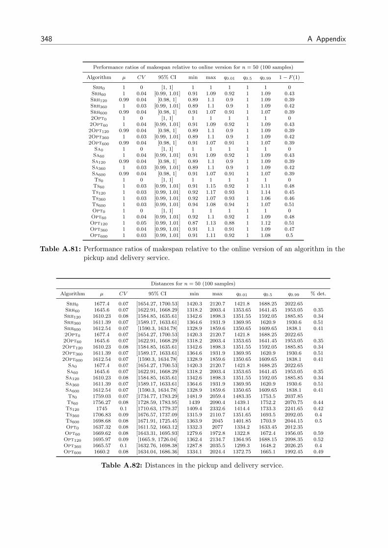
348 A Appendix
Performance ratios of makespan relative to online version for n = 50 (100 samples)
Algorithm µ CV 95% CI min max q0.01 q0.5 q0.99 1− F (1)
Srh0 1 0 [1, 1] 1 1 1 1 1 0Srh60 1 0.04 [0.99, 1.01] 0.91 1.09 0.92 1 1.09 0.43Srh120 0.99 0.04 [0.98, 1] 0.89 1.1 0.9 1 1.09 0.39Srh360 1 0.03 [0.99, 1.01] 0.89 1.1 0.9 1 1.09 0.42Srh600 0.99 0.04 [0.98, 1] 0.91 1.07 0.91 1 1.07 0.392Opt0 1 0 [1, 1] 1 1 1 1 1 02Opt60 1 0.04 [0.99, 1.01] 0.91 1.09 0.92 1 1.09 0.432Opt120 0.99 0.04 [0.98, 1] 0.89 1.1 0.9 1 1.09 0.392Opt360 1 0.03 [0.99, 1.01] 0.89 1.1 0.9 1 1.09 0.422Opt600 0.99 0.04 [0.98, 1] 0.91 1.07 0.91 1 1.07 0.39
Sa0 1 0 [1, 1] 1 1 1 1 1 0Sa60 1 0.04 [0.99, 1.01] 0.91 1.09 0.92 1 1.09 0.43Sa120 0.99 0.04 [0.98, 1] 0.89 1.1 0.9 1 1.09 0.39Sa360 1 0.03 [0.99, 1.01] 0.89 1.1 0.9 1 1.09 0.42Sa600 0.99 0.04 [0.98, 1] 0.91 1.07 0.91 1 1.07 0.39Ts0 1 0 [1, 1] 1 1 1 1 1 0Ts60 1 0.03 [0.99, 1.01] 0.91 1.15 0.92 1 1.11 0.48Ts120 1 0.03 [0.99, 1.01] 0.92 1.17 0.93 1 1.14 0.45Ts360 1 0.03 [0.99, 1.01] 0.92 1.07 0.93 1 1.06 0.46Ts600 1 0.03 [0.99, 1.01] 0.94 1.08 0.94 1 1.07 0.51Opt0 1 0 [1, 1] 1 1 1 1 1 0Opt60 1 0.04 [0.99, 1.01] 0.92 1.1 0.92 1 1.09 0.48Opt120 1 0.05 [0.99, 1.01] 0.87 1.13 0.88 1 1.12 0.51Opt360 1 0.04 [0.99, 1.01] 0.91 1.1 0.91 1 1.09 0.47Opt600 1 0.03 [0.99, 1.01] 0.91 1.11 0.92 1 1.08 0.5
Table A.81: Performance ratios of makespan relative to the online version of an algorithm in thepickup and delivery service.
Distances for n = 50 (100 samples)
Algorithm µ CV 95% CI min max q0.01 q0.5 q0.99 % det.
Srh0 1677.4 0.07 [1654.27, 1700.53] 1420.3 2120.7 1421.8 1688.25 2022.65Srh60 1645.6 0.07 [1622.91, 1668.29] 1318.2 2003.4 1353.65 1641.45 1953.05 0.35Srh120 1610.23 0.08 [1584.85, 1635.61] 1342.6 1898.3 1351.55 1592.05 1885.85 0.34Srh360 1611.39 0.07 [1589.17, 1633.61] 1364.6 1931.9 1369.95 1620.9 1930.6 0.51Srh600 1612.54 0.07 [1590.3, 1634.78] 1328.9 1859.6 1350.65 1609.65 1838.1 0.412Opt0 1677.4 0.07 [1654.27, 1700.53] 1420.3 2120.7 1421.8 1688.25 2022.652Opt60 1645.6 0.07 [1622.91, 1668.29] 1318.2 2003.4 1353.65 1641.45 1953.05 0.352Opt120 1610.23 0.08 [1584.85, 1635.61] 1342.6 1898.3 1351.55 1592.05 1885.85 0.342Opt360 1611.39 0.07 [1589.17, 1633.61] 1364.6 1931.9 1369.95 1620.9 1930.6 0.512Opt600 1612.54 0.07 [1590.3, 1634.78] 1328.9 1859.6 1350.65 1609.65 1838.1 0.41
Sa0 1677.4 0.07 [1654.27, 1700.53] 1420.3 2120.7 1421.8 1688.25 2022.65Sa60 1645.6 0.07 [1622.91, 1668.29] 1318.2 2003.4 1353.65 1641.45 1953.05 0.35Sa120 1610.23 0.08 [1584.85, 1635.61] 1342.6 1898.3 1351.55 1592.05 1885.85 0.34Sa360 1611.39 0.07 [1589.17, 1633.61] 1364.6 1931.9 1369.95 1620.9 1930.6 0.51Sa600 1612.54 0.07 [1590.3, 1634.78] 1328.9 1859.6 1350.65 1609.65 1838.1 0.41Ts0 1759.03 0.07 [1734.77, 1783.29] 1481.9 2059.4 1483.35 1753.5 2037.85Ts60 1756.27 0.08 [1728.59, 1783.95] 1439 2090.4 1439.1 1752.2 2070.75 0.44Ts120 1745 0.1 [1710.63, 1779.37] 1409.4 2332.6 1414.4 1733.3 2241.65 0.42Ts360 1706.83 0.09 [1676.57, 1737.09] 1315.9 2110.7 1351.65 1693.5 2092.05 0.4Ts600 1698.68 0.08 [1671.91, 1725.45] 1363.9 2045 1401.85 1703.9 2044.15 0.5Opt0 1637.32 0.08 [1611.52, 1663.12] 1332.3 2077 1334.2 1633.45 2012.35Opt60 1669.62 0.08 [1643.31, 1695.93] 1279.6 1972.8 1322.8 1672.4 1956.05 0.59Opt120 1695.97 0.09 [1665.9, 1726.04] 1362.4 2134.7 1364.95 1688.15 2098.35 0.52Opt360 1665.57 0.1 [1632.76, 1698.38] 1287.8 2035.5 1299.3 1648.2 2026.25 0.4Opt600 1660.2 0.08 [1634.04, 1686.36] 1334.1 2024.4 1372.75 1665.1 1992.45 0.49
Table A.82: Distances in the pickup and delivery service.

A.3 Numerical Results from Chapter 6 349
Performance ratios of distance relative to Opt for n = 50 (100 samples)
Algorithm µ CV 95% CI min max q0.01 q0.5 q0.99 F (1)
Srh0 1.01 0.07 [1, 1.02] 0.86 1.23 0.86 1.01 1.22 0.46Srh60 0.99 0.08 [0.97, 1.01] 0.78 1.17 0.81 0.98 1.16 0.57Srh120 0.97 0.08 [0.95, 0.99] 0.72 1.16 0.77 0.98 1.14 0.62Srh360 0.97 0.07 [0.96, 0.98] 0.8 1.14 0.8 0.97 1.14 0.69Srh600 0.97 0.07 [0.96, 0.98] 0.82 1.19 0.82 0.98 1.16 0.662Opt0 1.01 0.07 [1, 1.02] 0.86 1.23 0.86 1.01 1.22 0.462Opt60 0.99 0.08 [0.97, 1.01] 0.78 1.17 0.81 0.98 1.16 0.572Opt120 0.97 0.08 [0.95, 0.99] 0.72 1.16 0.77 0.98 1.14 0.622Opt360 0.97 0.07 [0.96, 0.98] 0.8 1.14 0.8 0.97 1.14 0.692Opt600 0.97 0.07 [0.96, 0.98] 0.82 1.19 0.82 0.98 1.16 0.66
Sa0 1.01 0.07 [1, 1.02] 0.86 1.23 0.86 1.01 1.22 0.46Sa60 0.99 0.08 [0.97, 1.01] 0.78 1.17 0.81 0.98 1.16 0.57Sa120 0.97 0.08 [0.95, 0.99] 0.72 1.16 0.77 0.98 1.14 0.62Sa360 0.97 0.07 [0.96, 0.98] 0.8 1.14 0.8 0.97 1.14 0.69Sa600 0.97 0.07 [0.96, 0.98] 0.82 1.19 0.82 0.98 1.16 0.66Ts0 1.06 0.07 [1.05, 1.07] 0.88 1.25 0.89 1.06 1.24 0.14Ts60 1.06 0.07 [1.05, 1.07] 0.84 1.24 0.85 1.05 1.24 0.18Ts120 1.05 0.08 [1.03, 1.07] 0.86 1.3 0.87 1.05 1.28 0.28Ts360 1.03 0.07 [1.02, 1.04] 0.9 1.22 0.9 1.02 1.21 0.39Ts600 1.02 0.02 [1.02, 1.02] 0.96 1.1 0.97 1.02 1.09 0.11Opt0 0.99 0.07 [0.98, 1] 0.83 1.15 0.83 0.99 1.15 0.56Opt60 1.01 0.08 [0.99, 1.03] 0.83 1.24 0.84 1.01 1.21 0.46Opt120 1.03 0.1 [1.01, 1.05] 0.76 1.34 0.77 1.03 1.28 0.35Opt360 1 0.07 [0.99, 1.01] 0.87 1.21 0.88 1 1.19 0.55Opt600 1 0 [1, 1] 1 1 1 1 1 0
Table A.83: Performance ratios of distance relative to Opt in the pickup and delivery service.
Performance ratios of distance relative to online version for n = 50 (100 samples)
Algorithm µ CV 95% CI min max q0.01 q0.5 q0.99 1− F (1)
Srh0 1 0 [1, 1] 1 1 1 1 1 0Srh60 0.98 0.07 [0.97, 0.99] 0.84 1.19 0.85 0.97 1.15 0.35Srh120 0.96 0.07 [0.95, 0.97] 0.78 1.17 0.8 0.96 1.14 0.27Srh360 0.96 0.06 [0.95, 0.97] 0.8 1.17 0.81 0.96 1.12 0.26Srh600 0.96 0.06 [0.95, 0.97] 0.82 1.09 0.83 0.96 1.09 0.352Opt0 1 0 [1, 1] 1 1 1 1 1 02Opt60 0.98 0.07 [0.97, 0.99] 0.84 1.19 0.85 0.97 1.15 0.352Opt120 0.96 0.07 [0.95, 0.97] 0.78 1.17 0.8 0.96 1.14 0.272Opt360 0.96 0.06 [0.95, 0.97] 0.8 1.17 0.81 0.96 1.12 0.262Opt600 0.96 0.06 [0.95, 0.97] 0.82 1.09 0.83 0.96 1.09 0.35
Sa0 1 0 [1, 1] 1 1 1 1 1 0Sa60 0.98 0.07 [0.97, 0.99] 0.84 1.19 0.85 0.97 1.15 0.35Sa120 0.96 0.07 [0.95, 0.97] 0.78 1.17 0.8 0.96 1.14 0.27Sa360 0.96 0.06 [0.95, 0.97] 0.8 1.17 0.81 0.96 1.12 0.26Sa600 0.96 0.06 [0.95, 0.97] 0.82 1.09 0.83 0.96 1.09 0.35Ts0 1 0 [1, 1] 1 1 1 1 1 0Ts60 1 0.07 [0.99, 1.01] 0.86 1.17 0.87 0.99 1.16 0.44Ts120 0.99 0.09 [0.97, 1.01] 0.85 1.28 0.85 0.98 1.25 0.44Ts360 0.97 0.08 [0.95, 0.99] 0.82 1.21 0.82 0.96 1.19 0.32Ts600 0.97 0.07 [0.96, 0.98] 0.85 1.15 0.85 0.96 1.15 0.26Opt0 1 0 [1, 1] 1 1 1 1 1 0Opt60 1.02 0.08 [1, 1.04] 0.76 1.27 0.81 1.01 1.27 0.59Opt120 1.04 0.11 [1.02, 1.06] 0.75 1.44 0.78 1.04 1.41 0.6Opt360 1.02 0.07 [1.01, 1.03] 0.83 1.19 0.84 1.01 1.18 0.62Opt600 1.02 0.07 [1.01, 1.03] 0.87 1.21 0.87 1.01 1.2 0.56
Table A.84: Performance ratios of distance relative to the online version of an algorithm in thepickup and delivery service.

350 A Appendix
Tardiness for n = 50 (100 samples)
Algorithm µ CV 95% CI min max q0.01 q0.5 q0.99 % det.
Srh0 25.8 0.48 [23.36, 28.24] 7 75.6 7.45 22.75 72.15Srh60 27.39 0.51 [24.64, 30.14] 6.8 76 7.35 24.2 72.55 0.53Srh120 26.21 0.41 [24.09, 28.33] 10.4 54.7 10.9 23.4 54.55 0.45Srh360 26.75 0.53 [23.96, 29.54] 8.3 120.9 9.15 24.85 93 0.54Srh600 26.28 0.4 [24.21, 28.35] 6.8 62.4 6.9 25.05 60 0.42Opt0 25.8 0.48 [23.36, 28.24] 7 75.6 7.45 22.75 72.152Opt60 27.39 0.51 [24.64, 30.14] 6.8 76 7.35 24.2 72.55 0.532Opt120 26.21 0.41 [24.09, 28.33] 10.4 54.7 10.9 23.4 54.55 0.452Opt360 26.75 0.53 [23.96, 29.54] 8.3 120.9 9.15 24.85 93 0.542Opt600 26.28 0.4 [24.21, 28.35] 6.8 62.4 6.9 25.05 60 0.4
Sa0 25.8 0.48 [23.36, 28.24] 7 75.6 7.45 22.75 72.15Sa60 27.39 0.51 [24.64, 30.14] 6.8 76 7.35 24.2 72.55 0.53Sa120 26.21 0.41 [24.09, 28.33] 10.4 54.7 10.9 23.4 54.55 0.45Sa360 26.75 0.53 [23.96, 29.54] 8.3 120.9 9.15 24.85 93 0.54Sa600 26.28 0.4 [24.21, 28.35] 6.8 62.4 6.9 25.05 60 0.4Ts0 21.08 0.43 [19.29, 22.87] 5.5 43.5 6.2 19.6 43.15Ts60 21.77 0.39 [20.1, 23.44] 6.3 45.9 6.85 21.4 44.4 0.51Ts120 21.66 0.42 [19.87, 23.45] 7.9 58.8 8.2 19.6 56.5 0.5Ts360 21.04 0.4 [19.38, 22.7] 8.8 55.4 8.8 19.35 50.1 0.55Ts600 21.96 0.5 [19.8, 24.12] 3.9 59 4.3 19.75 57.15 0.44Opt0 20.74 0.38 [19.19, 22.29] 7.3 48.8 7.6 20.05 43.65Opt60 20.81 0.43 [19.05, 22.57] 6.5 48.3 7 19.25 47.35 0.5Opt120 21.75 0.41 [19.99, 23.51] 8.7 58.8 9.05 20.15 55.15 0.51Opt360 21.52 0.4 [19.82, 23.22] 8.5 56.1 8.95 20.4 51.6 0.57Opt600 22.33 0.49 [20.17, 24.49] 4.3 59.3 4.5 20.15 57.2 0.46
Table A.85: Tardinesses in the pickup and delivery service.
Performance ratios of tardiness relative to Opt for n = 50 (100 samples)
Algorithm µ CV 95% CI min max q0.01 q0.5 q0.99 F (1)
Srh0 1.32 0.52 [1.18, 1.46] 0.42 3.84 0.46 1.12 3.65 0.39Srh60 1.44 0.61 [1.27, 1.61] 0.21 4.28 0.29 1.19 4.18 0.36Srh120 1.4 0.64 [1.22, 1.58] 0.3 6.16 0.4 1.21 5.84 0.37Srh360 1.34 0.49 [1.21, 1.47] 0.46 4.84 0.46 1.2 4.01 0.35Srh600 1.4 0.65 [1.22, 1.58] 0.4 5.76 0.43 1.17 5.55 0.352Opt0 1.32 0.52 [1.18, 1.46] 0.42 3.84 0.46 1.12 3.65 0.392Opt60 1.44 0.61 [1.27, 1.61] 0.21 4.28 0.29 1.19 4.18 0.362Opt120 1.4 0.64 [1.22, 1.58] 0.3 6.16 0.4 1.21 5.84 0.372Opt360 1.34 0.49 [1.21, 1.47] 0.46 4.84 0.46 1.2 4.01 0.352Opt600 1.4 0.65 [1.22, 1.58] 0.4 5.76 0.43 1.17 5.55 0.35
Sa0 1.32 0.52 [1.18, 1.46] 0.42 3.84 0.46 1.12 3.65 0.39Sa60 1.44 0.61 [1.27, 1.61] 0.21 4.28 0.29 1.19 4.18 0.36Sa120 1.4 0.64 [1.22, 1.58] 0.3 6.16 0.4 1.21 5.84 0.37Sa360 1.34 0.49 [1.21, 1.47] 0.46 4.84 0.46 1.2 4.01 0.35Sa600 1.4 0.65 [1.22, 1.58] 0.4 5.76 0.43 1.17 5.55 0.35Ts0 1.07 0.48 [0.97, 1.17] 0.33 2.68 0.33 0.94 2.53 0.57Ts60 1.11 0.46 [1.01, 1.21] 0.34 2.89 0.34 1.03 2.75 0.48Ts120 1.1 0.48 [1, 1.2] 0.4 3.98 0.41 0.97 3.2 0.54Ts360 1.1 0.6 [0.97, 1.23] 0.23 5.91 0.37 0.92 4.51 0.55Ts600 0.98 0.05 [0.97, 0.99] 0.74 1.07 0.76 0.99 1.06 0.63Opt0 1.09 0.55 [0.97, 1.21] 0.19 4.3 0.26 0.95 3.81 0.52Opt60 1.07 0.47 [0.97, 1.17] 0.12 3.38 0.16 0.94 2.9 0.54Opt120 1.25 0.8 [1.05, 1.45] 0.16 8.57 0.22 1.01 6.33 0.47Opt360 1.12 0.63 [0.98, 1.26] 0.25 6.4 0.38 0.96 4.86 0.53Opt600 1 0 [1, 1] 1 1 1 1 1 0
Table A.86: Performance ratios of tardiness relative to Opt in the pickup and delivery service.
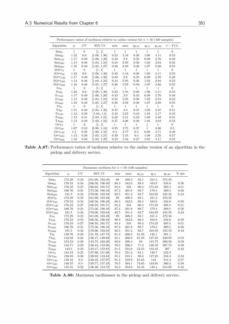
A.3 Numerical Results from Chapter 6 351
Performance ratios of tardiness relative to online version for n = 50 (100 samples)
Algorithm µ CV 95% CI min max q0.01 q0.5 q0.99 1− F (1)
Srh0 1 0 [1, 1] 1 1 1 1 1 0Srh60 1.22 0.6 [1.08, 1.36] 0.23 5.16 0.26 1.06 4.11 0.53Srh120 1.17 0.49 [1.06, 1.28] 0.33 2.9 0.35 0.99 2.76 0.49Srh360 1.14 0.46 [1.04, 1.24] 0.24 2.95 0.36 1.03 2.84 0.52Srh600 1.16 0.48 [1.05, 1.27] 0.36 2.93 0.38 1.07 2.88 0.552Opt0 1 0 [1, 1] 1 1 1 1 1 02Opt60 1.22 0.6 [1.08, 1.36] 0.23 5.16 0.26 1.06 4.11 0.532Opt120 1.17 0.49 [1.06, 1.28] 0.33 2.9 0.35 0.99 2.76 0.492Opt360 1.14 0.46 [1.04, 1.24] 0.24 2.95 0.36 1.03 2.84 0.522Opt600 1.16 0.48 [1.05, 1.27] 0.36 2.93 0.38 1.07 2.88 0.55
Sa0 1 0 [1, 1] 1 1 1 1 1 0Sa60 1.22 0.6 [1.08, 1.36] 0.23 5.16 0.26 1.06 4.11 0.53Sa120 1.17 0.49 [1.06, 1.28] 0.33 2.9 0.35 0.99 2.76 0.49Sa360 1.14 0.46 [1.04, 1.24] 0.24 2.95 0.36 1.03 2.84 0.52Sa600 1.16 0.48 [1.05, 1.27] 0.36 2.93 0.38 1.07 2.88 0.55Ts0 1 0 [1, 1] 1 1 1 1 1 0Ts60 1.15 0.48 [1.04, 1.26] 0.47 3.4 0.47 1.02 3.37 0.51Ts120 1.12 0.38 [1.04, 1.2] 0.42 2.25 0.44 1.04 2.17 0.53Ts360 1.12 0.41 [1.03, 1.21] 0.28 2.51 0.33 1.08 2.49 0.55Ts600 1.13 0.48 [1.02, 1.24] 0.37 3.06 0.38 1.04 3.04 0.53Opt0 1 0 [1, 1] 1 1 1 1 1 0Opt60 1.07 0.43 [0.98, 1.16] 0.35 2.75 0.37 1 2.66 0.5Opt120 1.2 0.58 [1.06, 1.34] 0.3 3.77 0.3 0.99 3.71 0.48Opt360 1.12 0.39 [1.03, 1.21] 0.39 2.45 0.4 1.08 2.35 0.57Opt600 1.16 0.56 [1.03, 1.29] 0.23 5.16 0.27 1.05 4.11 0.52
Table A.87: Performance ratios of tardiness relative to the online version of an algorithm in thepickup and delivery service.
Maximum tardiness for n = 50 (100 samples)
Algorithm µ CV 95% CI min max q0.01 q0.5 q0.99 % det.
Srh0 172.29 0.33 [161.09, 183.49] 89 409.3 92.1 161.3 372.35Srh60 178.52 0.34 [166.56, 190.48] 88.3 342.6 88.4 163.9 334.6 0.56Srh120 176.33 0.27 [166.95, 185.71] 94.4 316 96.4 174.25 305.5 0.51Srh360 186.76 0.31 [175.36, 198.16] 87.3 401.8 88.7 179.4 389.5 0.56Srh600 181.5 0.32 [170.06, 192.94] 82.5 351.2 82.7 164.05 345.55 0.432Opt0 172.29 0.33 [161.09, 183.49] 89 409.3 92.1 161.3 372.352Opt60 178.52 0.34 [166.56, 190.48] 88.3 342.6 88.4 163.9 334.6 0.562Opt120 176.33 0.27 [166.95, 185.71] 94.4 316 96.4 174.25 305.5 0.512Opt360 186.76 0.31 [175.36, 198.16] 87.3 401.8 88.7 179.4 389.5 0.562Opt600 181.5 0.32 [170.06, 192.94] 82.5 351.2 82.7 164.05 345.55 0.43
Sa0 172.29 0.33 [161.09, 183.49] 89 409.3 92.1 161.3 372.35Sa60 178.52 0.34 [166.56, 190.48] 88.3 342.6 88.4 163.9 334.6 0.56Sa120 176.33 0.27 [166.95, 185.71] 94.4 316 96.4 174.25 305.5 0.51Sa360 186.76 0.31 [175.36, 198.16] 87.3 401.8 88.7 179.4 389.5 0.56Sa600 181.5 0.32 [170.06, 192.94] 82.5 351.2 82.7 164.05 345.55 0.43Ts0 139.76 0.29 [131.78, 147.74] 81.3 306.3 81.95 132.1 281.1Ts60 142.93 0.24 [136.17, 149.69] 55.1 266.8 61.95 137.05 249.05 0.55Ts120 153.52 0.29 [144.75, 162.29] 82.6 298.4 83 145.75 280.95 0.59Ts360 144.71 0.29 [136.44, 152.98] 70.5 296.5 71.3 138.35 287.75 0.39Ts600 143.5 0.33 [134.17, 152.83] 51.5 353.9 52.55 133.45 307 0.42Opt0 144.53 0.23 [137.98, 151.08] 78.4 251.2 84.1 139.7 242.3Opt60 136.93 0.26 [129.92, 143.94] 55.1 243.1 69.6 127.85 234.3 0.43Opt120 149.16 0.3 [140.35, 157.97] 81.2 319.9 81.65 144 314.4 0.57Opt360 148.55 0.3 [139.77, 157.33] 70.5 304.1 74.85 143.05 300.3 0.38Opt600 145.55 0.32 [136.38, 154.72] 53.3 353.9 53.45 140.4 313.95 0.42
Table A.88: Maximum tardinesses in the pickup and delivery service.

352 A Appendix
Performance ratios of maximum tardiness relative to Opt for n = 50 (100 samples)
Algorithm µ CV 95% CI min max q0.01 q0.5 q0.99 F (1)
Srh0 1.28 0.4 [1.18, 1.38] 0.42 3.27 0.49 1.17 2.91 0.32Srh60 1.34 0.43 [1.23, 1.45] 0.27 3.23 0.36 1.22 3.08 0.3Srh120 1.35 0.52 [1.21, 1.49] 0.37 5.09 0.44 1.21 4.83 0.34Srh360 1.39 0.4 [1.28, 1.5] 0.41 3.32 0.47 1.32 3.16 0.25Srh600 1.39 0.56 [1.24, 1.54] 0.41 6.59 0.49 1.19 5.14 0.292Opt0 1.28 0.4 [1.18, 1.38] 0.42 3.27 0.49 1.17 2.91 0.322Opt60 1.34 0.43 [1.23, 1.45] 0.27 3.23 0.36 1.22 3.08 0.32Opt120 1.35 0.52 [1.21, 1.49] 0.37 5.09 0.44 1.21 4.83 0.342Opt360 1.39 0.4 [1.28, 1.5] 0.41 3.32 0.47 1.32 3.16 0.252Opt600 1.39 0.56 [1.24, 1.54] 0.41 6.59 0.49 1.19 5.14 0.29
Sa0 1.28 0.4 [1.18, 1.38] 0.42 3.27 0.49 1.17 2.91 0.32Sa60 1.34 0.43 [1.23, 1.45] 0.27 3.23 0.36 1.22 3.08 0.3Sa120 1.35 0.52 [1.21, 1.49] 0.37 5.09 0.44 1.21 4.83 0.34Sa360 1.39 0.4 [1.28, 1.5] 0.41 3.32 0.47 1.32 3.16 0.25Sa600 1.39 0.56 [1.24, 1.54] 0.41 6.59 0.49 1.19 5.14 0.29Ts0 1.04 0.38 [0.96, 1.12] 0.31 2.9 0.4 0.97 2.7 0.53Ts60 1.07 0.43 [0.98, 1.16] 0.43 3.93 0.44 1 3.08 0.5Ts120 1.15 0.44 [1.05, 1.25] 0.26 4.57 0.37 1.06 3.49 0.44Ts360 1.09 0.54 [0.97, 1.21] 0.45 5.56 0.45 0.99 3.99 0.51Ts600 0.99 0.07 [0.98, 1] 0.68 1.28 0.69 1 1.22 0.2Opt0 1.1 0.48 [1, 1.2] 0.26 4.71 0.39 0.99 3.79 0.51Opt60 1.02 0.39 [0.94, 1.1] 0.44 3.1 0.45 0.93 2.88 0.58Opt120 1.14 0.5 [1.03, 1.25] 0.4 4.57 0.42 1.05 3.95 0.44Opt360 1.12 0.53 [1, 1.24] 0.45 5.56 0.45 1.02 4.02 0.49Opt600 1 0 [1, 1] 1 1 1 1 1 0
Table A.89: Performance ratios of maximum tardiness relative to Opt in the pickup and deliveryservice.
Performance ratios of maximum tardiness relative to online version for n = 50 (100 samples)
Algorithm µ CV 95% CI min max q0.01 q0.5 q0.99 1− F (1)
Srh0 1 0 [1, 1] 1 1 1 1 1 0Srh60 1.12 0.4 [1.03, 1.21] 0.32 2.31 0.37 1.08 2.24 0.56Srh120 1.11 0.39 [1.02, 1.2] 0.36 3.06 0.41 1.01 3.01 0.52Srh360 1.16 0.35 [1.08, 1.24] 0.35 2.48 0.43 1.04 2.45 0.55Srh600 1.15 0.43 [1.05, 1.25] 0.43 3.48 0.46 1.03 2.97 0.532Opt0 1 0 [1, 1] 1 1 1 1 1 02Opt60 1.12 0.4 [1.03, 1.21] 0.32 2.31 0.37 1.08 2.24 0.562Opt120 1.11 0.39 [1.02, 1.2] 0.36 3.06 0.41 1.01 3.01 0.522Opt360 1.16 0.35 [1.08, 1.24] 0.35 2.48 0.43 1.04 2.45 0.552Opt600 1.15 0.43 [1.05, 1.25] 0.43 3.48 0.46 1.03 2.97 0.53
Sa0 1 0 [1, 1] 1 1 1 1 1 0Sa60 1.12 0.4 [1.03, 1.21] 0.32 2.31 0.37 1.08 2.24 0.56Sa120 1.11 0.39 [1.02, 1.2] 0.36 3.06 0.41 1.01 3.01 0.52Sa360 1.16 0.35 [1.08, 1.24] 0.35 2.48 0.43 1.04 2.45 0.55Sa600 1.15 0.43 [1.05, 1.25] 0.43 3.48 0.46 1.03 2.97 0.53Ts0 1 0 [1, 1] 1 1 1 1 1 0Ts60 1.08 0.32 [1.01, 1.15] 0.47 2.19 0.51 1.03 2.09 0.55Ts120 1.16 0.34 [1.08, 1.24] 0.45 2.52 0.48 1.11 2.45 0.63Ts360 1.1 0.36 [1.02, 1.18] 0.44 2.88 0.45 1.03 2.5 0.53Ts600 1.08 0.39 [1, 1.16] 0.34 3.27 0.37 0.98 2.64 0.5Opt0 1 0 [1, 1] 1 1 1 1 1 0Opt60 0.99 0.31 [0.93, 1.05] 0.36 2.08 0.39 0.94 1.99 0.43Opt120 1.08 0.35 [1.01, 1.15] 0.53 2.15 0.54 0.99 2.03 0.49Opt360 1.07 0.34 [1, 1.14] 0.47 2.03 0.48 0.99 2.02 0.49Opt600 1.06 0.41 [0.97, 1.15] 0.21 3.9 0.28 1.01 2.91 0.51
Table A.90: Performance ratios of maximum tardiness relative to the online version of an algo-rithm in the pickup and delivery service.

A.3 Numerical Results from Chapter 6 353
Utilization for n = 50 (100 samples)
Algorithm µ CV 95% CI min max q0.01 q0.5 q0.99 % det.
Srh0 0.93 0.05 [0.92, 0.94] 0.9 1 0.9 0.9 1Srh60 0.98 0.04 [0.97, 0.99] 0.9 1 0.9 1 1 0.01Srh120 0.99 0.03 [0.98, 1] 0.9 1 0.9 1 1 0.05Srh360 0.99 0.03 [0.98, 1] 0.9 1 0.9 1 1 0.04Srh600 0.99 0.04 [0.98, 1] 0.9 1 0.9 1 1 0.092Opt0 0.93 0.05 [0.92, 0.94] 0.9 1 0.9 0.9 12Opt60 0.98 0.04 [0.97, 0.99] 0.9 1 0.9 1 1 0.012Opt120 0.99 0.03 [0.98, 1] 0.9 1 0.9 1 1 0.052Opt360 0.99 0.03 [0.98, 1] 0.9 1 0.9 1 1 0.042Opt600 0.99 0.04 [0.98, 1] 0.9 1 0.9 1 1 0.09
Sa0 0.93 0.05 [0.92, 0.94] 0.9 1 0.9 0.9 1Sa60 0.98 0.04 [0.97, 0.99] 0.9 1 0.9 1 1 0.01Sa120 0.99 0.03 [0.98, 1] 0.9 1 0.9 1 1 0.05Sa360 0.99 0.03 [0.98, 1] 0.9 1 0.9 1 1 0.04Sa600 0.99 0.04 [0.98, 1] 0.9 1 0.9 1 1 0.09Ts0 0.91 0.04 [0.9, 0.92] 0.8 1 0.85 0.9 1Ts60 0.96 0.05 [0.95, 0.97] 0.9 1 0.9 1 1 0.04Ts120 0.98 0.04 [0.97, 0.99] 0.9 1 0.9 1 1 0.09Ts360 0.99 0.04 [0.98, 1] 0.9 1 0.9 1 1 0.07Ts600 0.99 0.03 [0.98, 1] 0.9 1 0.9 1 1 0.05Opt0 0.88 0.05 [0.87, 0.89] 0.8 0.9 0.8 0.9 0.9Opt60 0.91 0.04 [0.9, 0.92] 0.8 1 0.8 0.9 1 0.01Opt120 0.96 0.05 [0.95, 0.97] 0.9 1 0.9 1 1 0.02Opt360 0.96 0.05 [0.95, 0.97] 0.9 1 0.9 1 1 0.26Opt600 0.97 0.05 [0.96, 0.98] 0.9 1 0.9 1 1 0.13
Table A.91: Vehicle utilizations in the pickup and delivery service.
Performance ratios of utilization relative to Opt for n = 50 (100 samples)
Algorithm µ CV 95% CI min max q0.01 q0.5 q0.99 F (1)
Srh0 0.96 0.06 [0.95, 0.97] 0.9 1.11 0.9 1 1.11 0.04Srh60 1.01 0.06 [1, 1.02] 0.9 1.11 0.9 1 1.11 0.2Srh120 1.02 0.05 [1.01, 1.03] 0.9 1.11 0.9 1 1.11 0.22Srh360 1.02 0.05 [1.01, 1.03] 0.9 1.11 0.9 1 1.11 0.24Srh600 1.02 0.05 [1.01, 1.03] 0.9 1.11 0.9 1 1.11 0.22Opt0 0.96 0.06 [0.95, 0.97] 0.9 1.11 0.9 1 1.11 0.042Opt60 1.01 0.06 [1, 1.02] 0.9 1.11 0.9 1 1.11 0.22Opt120 1.02 0.05 [1.01, 1.03] 0.9 1.11 0.9 1 1.11 0.222Opt360 1.02 0.05 [1.01, 1.03] 0.9 1.11 0.9 1 1.11 0.242Opt600 1.02 0.05 [1.01, 1.03] 0.9 1.11 0.9 1 1.11 0.2
Sa0 0.96 0.06 [0.95, 0.97] 0.9 1.11 0.9 1 1.11 0.04Sa60 1.01 0.06 [1, 1.02] 0.9 1.11 0.9 1 1.11 0.2Sa120 1.02 0.05 [1.01, 1.03] 0.9 1.11 0.9 1 1.11 0.22Sa360 1.02 0.05 [1.01, 1.03] 0.9 1.11 0.9 1 1.11 0.24Sa600 1.02 0.05 [1.01, 1.03] 0.9 1.11 0.9 1 1.11 0.2Ts0 0.94 0.06 [0.93, 0.95] 0.8 1.11 0.85 0.9 1.11 0.03Ts60 0.99 0.06 [0.98, 1] 0.9 1.11 0.9 1 1.11 0.15Ts120 1.01 0.05 [1, 1.02] 0.9 1.11 0.9 1 1.11 0.19Ts360 1.02 0.05 [1.01, 1.03] 0.9 1.11 0.9 1 1.11 0.21Ts600 1.02 0.05 [1.01, 1.03] 0.9 1.11 0.9 1 1.11 0.2Opt0 0.91 0.07 [0.9, 0.92] 0.8 1 0.8 0.9 1 0Opt60 0.94 0.06 [0.93, 0.95] 0.8 1.11 0.8 0.9 1.11 0.02Opt120 0.99 0.07 [0.98, 1] 0.9 1.11 0.9 1 1.11 0.17Opt360 0.99 0.06 [0.98, 1] 0.9 1.11 0.9 1 1.11 0.13Opt600 1 0 [1, 1] 1 1 1 1 1 0
Table A.92: Performance ratios of vehicle utilization relative to Opt in the pickup and deliveryservice.

354 A Appendix
Performance ratios of utilization relative to online version for n = 50 (100 samples)
Algorithm µ CV 95% CI min max q0.01 q0.5 q0.99 1− F (1)
Srh0 1 0 [1, 1] 1 1 1 1 1 0Srh60 1.06 0.05 [1.05, 1.07] 0.9 1.11 0.95 1.11 1.11 0.01Srh120 1.07 0.05 [1.06, 1.08] 0.9 1.11 0.9 1.11 1.11 0.02Srh360 1.07 0.05 [1.06, 1.08] 0.9 1.11 0.9 1.11 1.11 0.02Srh600 1.07 0.06 [1.06, 1.08] 0.9 1.11 0.9 1.11 1.11 0.032Opt0 1 0 [1, 1] 1 1 1 1 1 02Opt60 1.06 0.05 [1.05, 1.07] 0.9 1.11 0.95 1.11 1.11 0.012Opt120 1.07 0.05 [1.06, 1.08] 0.9 1.11 0.9 1.11 1.11 0.022Opt360 1.07 0.05 [1.06, 1.08] 0.9 1.11 0.9 1.11 1.11 0.022Opt600 1.07 0.06 [1.06, 1.08] 0.9 1.11 0.9 1.11 1.11 0.03
Sa0 1 0 [1, 1] 1 1 1 1 1 0Sa60 1.06 0.05 [1.05, 1.07] 0.9 1.11 0.95 1.11 1.11 0.01Sa120 1.07 0.05 [1.06, 1.08] 0.9 1.11 0.9 1.11 1.11 0.02Sa360 1.07 0.05 [1.06, 1.08] 0.9 1.11 0.9 1.11 1.11 0.02Sa600 1.07 0.06 [1.06, 1.08] 0.9 1.11 0.9 1.11 1.11 0.03Ts0 1 0 [1, 1] 1 1 1 1 1 0Ts60 1.05 0.06 [1.04, 1.06] 0.9 1.13 0.9 1.11 1.12 0.04Ts120 1.08 0.05 [1.07, 1.09] 1 1.25 1 1.11 1.18 0Ts360 1.08 0.05 [1.07, 1.09] 1 1.25 1 1.11 1.18 0Ts600 1.08 0.05 [1.07, 1.09] 1 1.25 1 1.11 1.18 0Opt0 1 0 [1, 1] 1 1 1 1 1 0Opt60 1.03 0.05 [1.02, 1.04] 0.89 1.13 0.94 1 1.13 0.01Opt120 1.09 0.07 [1.07, 1.11] 1 1.25 1 1.11 1.25 0Opt360 1.1 0.06 [1.09, 1.11] 1 1.25 1 1.11 1.25 0Opt600 1.1 0.07 [1.08, 1.12] 1 1.25 1 1.11 1.25 0
Table A.93: Performance ratios of vehicle utilization relative to the online version of an algorithmin the pickup and delivery service.
Throughput for n = 50 (100 samples)
Algorithm µ CV 95% CI min max q0.01 q0.5 q0.99 % det.
Srh0 3.67 0.04 [3.64, 3.7] 3.2 4 3.25 3.7 4Srh60 3.66 0.04 [3.63, 3.69] 3.3 4 3.3 3.7 4 0.29Srh120 3.68 0.04 [3.65, 3.71] 3.3 4.1 3.35 3.7 4.05 0.2Srh360 3.69 0.04 [3.66, 3.72] 3.2 4 3.3 3.7 3.95 0.29Srh600 3.69 0.04 [3.66, 3.72] 3.4 4 3.4 3.7 3.95 0.272Opt0 3.67 0.04 [3.64, 3.7] 3.2 4 3.25 3.7 42Opt60 3.66 0.04 [3.63, 3.69] 3.3 4 3.3 3.7 4 0.292Opt120 3.68 0.04 [3.65, 3.71] 3.3 4.1 3.35 3.7 4.05 0.22Opt360 3.69 0.04 [3.66, 3.72] 3.2 4 3.3 3.7 3.95 0.292Opt600 3.69 0.04 [3.66, 3.72] 3.4 4 3.4 3.7 3.95 0.27
Sa0 3.67 0.04 [3.64, 3.7] 3.2 4 3.25 3.7 4Sa60 3.66 0.04 [3.63, 3.69] 3.3 4 3.3 3.7 4 0.29Sa120 3.68 0.04 [3.65, 3.71] 3.3 4.1 3.35 3.7 4.05 0.2Sa360 3.69 0.04 [3.66, 3.72] 3.2 4 3.3 3.7 3.95 0.29Sa600 3.69 0.04 [3.66, 3.72] 3.4 4 3.4 3.7 3.95 0.27Ts0 3.69 0.03 [3.67, 3.71] 3.4 4 3.4 3.7 4Ts60 3.7 0.04 [3.67, 3.73] 3.3 4 3.35 3.7 4 0.29Ts120 3.7 0.04 [3.67, 3.73] 3.2 4 3.3 3.7 3.95 0.21Ts360 3.7 0.03 [3.68, 3.72] 3.4 4.1 3.45 3.7 4 0.28Ts600 3.69 0.03 [3.67, 3.71] 3.3 4.1 3.4 3.7 4.05 0.34Opt0 3.67 0.03 [3.65, 3.69] 3.4 4 3.4 3.65 4Opt60 3.67 0.03 [3.65, 3.69] 3.4 4 3.4 3.7 3.95 0.36Opt120 3.67 0.04 [3.64, 3.7] 3.3 4 3.35 3.7 4 0.35Opt360 3.68 0.04 [3.65, 3.71] 3.4 4.1 3.4 3.7 4.05 0.39Opt600 3.68 0.03 [3.66, 3.7] 3.3 4 3.3 3.7 4 0.3
Table A.94: Job throughputs in the pickup and delivery service.

A.3 Numerical Results from Chapter 6 355
Performance ratios of throughput relative to Opt for n = 50 (100 samples)
Algorithm µ CV 95% CI min max q0.01 q0.5 q0.99 F (1)
Srh0 1 0.04 [0.99, 1.01] 0.89 1.09 0.89 1 1.09 0.27Srh60 1 0.04 [0.99, 1.01] 0.87 1.12 0.88 1 1.1 0.29Srh120 1 0.04 [0.99, 1.01] 0.89 1.09 0.89 1 1.09 0.37Srh360 1 0.03 [0.99, 1.01] 0.91 1.12 0.92 1 1.09 0.37Srh600 1 0.04 [0.99, 1.01] 0.92 1.15 0.93 1 1.12 0.352Opt0 1 0.04 [0.99, 1.01] 0.89 1.09 0.89 1 1.09 0.272Opt60 1 0.04 [0.99, 1.01] 0.87 1.12 0.88 1 1.1 0.292Opt120 1 0.04 [0.99, 1.01] 0.89 1.09 0.89 1 1.09 0.372Opt360 1 0.03 [0.99, 1.01] 0.91 1.12 0.92 1 1.09 0.372Opt600 1 0.04 [0.99, 1.01] 0.92 1.15 0.93 1 1.12 0.35
Sa0 1 0.04 [0.99, 1.01] 0.89 1.09 0.89 1 1.09 0.27Sa60 1 0.04 [0.99, 1.01] 0.87 1.12 0.88 1 1.1 0.29Sa120 1 0.04 [0.99, 1.01] 0.89 1.09 0.89 1 1.09 0.37Sa360 1 0.03 [0.99, 1.01] 0.91 1.12 0.92 1 1.09 0.37Sa600 1 0.04 [0.99, 1.01] 0.92 1.15 0.93 1 1.12 0.35Ts0 1 0.03 [0.99, 1.01] 0.95 1.09 0.95 1 1.09 0.36Ts60 1.01 0.03 [1, 1.02] 0.89 1.12 0.91 1 1.1 0.36Ts120 1 0.04 [0.99, 1.01] 0.86 1.12 0.89 1 1.1 0.35Ts360 1.01 0.03 [1, 1.02] 0.95 1.12 0.95 1 1.11 0.41Ts600 1 0.03 [0.99, 1.01] 0.95 1.15 0.96 1 1.11 0.28Opt0 1 0.03 [0.99, 1.01] 0.92 1.09 0.92 1 1.08 0.3Opt60 1 0.03 [0.99, 1.01] 0.92 1.09 0.92 1 1.09 0.31Opt120 1 0.05 [0.99, 1.01] 0.87 1.14 0.87 1 1.13 0.34Opt360 1 0.03 [0.99, 1.01] 0.92 1.12 0.93 1 1.09 0.34Opt600 1 0 [1, 1] 1 1 1 1 1 0
Table A.95: Performance ratios of job throughput relative to Opt in the pickup and deliveryservice.
Performance ratios of throughput relative to online version for n = 50 (100 samples)
Algorithm µ CV 95% CI min max q0.01 q0.5 q0.99 1− F (1)
Srh0 1 0 [1, 1] 1 1 1 1 1 0Srh60 1 0.04 [0.99, 1.01] 0.92 1.09 0.92 1 1.09 0.29Srh120 1.01 0.04 [1, 1.02] 0.89 1.12 0.91 1 1.12 0.25Srh360 1.01 0.03 [1, 1.02] 0.91 1.13 0.92 1 1.12 0.24Srh600 1.01 0.04 [1, 1.02] 0.92 1.12 0.92 1 1.1 0.292Opt0 1 0 [1, 1] 1 1 1 1 1 02Opt60 1 0.04 [0.99, 1.01] 0.92 1.09 0.92 1 1.09 0.292Opt120 1.01 0.04 [1, 1.02] 0.89 1.12 0.91 1 1.12 0.252Opt360 1.01 0.03 [1, 1.02] 0.91 1.13 0.92 1 1.12 0.242Opt600 1.01 0.04 [1, 1.02] 0.92 1.12 0.92 1 1.1 0.29
Sa0 1 0 [1, 1] 1 1 1 1 1 0Sa60 1 0.04 [0.99, 1.01] 0.92 1.09 0.92 1 1.09 0.29Sa120 1.01 0.04 [1, 1.02] 0.89 1.12 0.91 1 1.12 0.25Sa360 1.01 0.03 [1, 1.02] 0.91 1.13 0.92 1 1.12 0.24Sa600 1.01 0.04 [1, 1.02] 0.92 1.12 0.92 1 1.1 0.29Ts0 1 0 [1, 1] 1 1 1 1 1 0Ts60 1 0.03 [0.99, 1.01] 0.87 1.09 0.89 1 1.09 0.29Ts120 1 0.04 [0.99, 1.01] 0.84 1.09 0.88 1 1.09 0.3Ts360 1 0.03 [0.99, 1.01] 0.92 1.06 0.92 1 1.06 0.25Ts600 1 0.03 [0.99, 1.01] 0.92 1.06 0.93 1 1.06 0.29Opt0 1 0 [1, 1] 1 1 1 1 1 0Opt60 1 0.04 [0.99, 1.01] 0.92 1.11 0.92 1 1.1 0.36Opt120 1 0.05 [0.99, 1.01] 0.88 1.14 0.89 1 1.13 0.38Opt360 1 0.04 [0.99, 1.01] 0.89 1.11 0.91 1 1.1 0.29Opt600 1 0.04 [0.99, 1.01] 0.92 1.09 0.93 1 1.09 0.3
Table A.96: Performance ratios of job throughput relative to the online version of an algorithmin the pickup and delivery service.


357
References
[1] Ahlroth, L.; Schumacher, A.; Haanpaa, H.: On the power of lookahead inonline lot-sizing. In: Operations Research Letters, 38 (6), 522–526, 2010. 5, 89
[2] Albers, S.: On the influence of lookahead in competitive paging algorithms. In:Algorithmica, 18 (3), 283–305, 1997. 5, 12, 24, 81, 89
[3] Albers, S.: A competitive analysis of the list update problem with lookahead. In:Theoretical Computer Science, 197 (1-2), 95–109, 1998. 5, 89
[4] Albers, S.; Favrholdt, L.; Giel, O.: On paging with locality of reference. In:Journal of Computer and System Sciences, 70 (2), 145–175, 2005. 38, 40, 154
[5] Albers, S.; Mohring, R.; Pflug, G.; Schultz, R.: Summary. In: S. Albers;R. Mohring; G. Pflug; R. Schultz (eds.), Algorithms for Optimization withIncomplete Information, 2005. 6
[6] Albers, S.; Mitzenmacher, M.: Average-case analyses of first fit and random fitbin packing. In: Random Structures and Algorithms, 16 (3), 240–259, 2000. 46
[7] Allulli, L.; Ausiello, G.; Bonifaci, V.; Laura, L.: On the power of lookaheadin on-line server routing problems. In: Theoretical Computer Science, 408 (2-3), 116–128, 2008. 5, 8, 31, 81, 89
[8] Allulli, L.; Ausiello, G.; Laura, L.: On the power of lookahead in on-linevehicle routing problems. In: L. Wang (ed.), Computing and Combinatorics, 728–736, Springer, 2005. 5, 8, 89
[9] Angelopoulos, S.; Dorrigiv, R.; Lopez-Ortiz, A.: On the separation andequivalence of paging strategies. In: Proceedings of the 18th Annual ACM-SIAM Sym-posium on Discrete Algorithms, 229–237, 2007. 38, 49, 50, 266
[10] Angelopoulos, S.; Schweitzer, P.: Paging and list update under bijective anal-ysis. In: Journal of the ACM, 60 (2), article no. 7, 2013. 38, 50, 266
[11] Ausiello, G.; Allulli, L.; Bonifaci, V.; Laura, L.: On-line algorithms, realtime, the virtue of laziness, and the power of clairvoyance. In: J. Cai; S. Cooper;A. Li (eds.), Theory and Applications of Models of Computation, 1–20, Springer, 2006.5, 8, 38, 40, 89

358 References
[12] Ausiello, G.; Crescenzi, P.; Kann, V.; Marchetti-Spaccalema, A.; Gam-bosi, G.; Spaccamela, A.: Complexity and Approximation: Combinatorial Opti-mization Problems and their Approximability Properties. Springer, 2nd edition, 2003.16, 17, 25, 27, 28, 29
[13] Ausiello, G.; Feuerstein, E.; Leonardi, S.; Stougie, L.; Talamo, M.:Competitive algorithms for the on-line traveling salesman. In: S. Akl; F. Dehne;J. Sack; N. Santoro (eds.), Algorithms and Data Structures, 206–217, Springer,1995. 31
[14] Baker, B.: A new proof for the first-fit decreasing bin-packing algorithm. In: Journalof Algorithms, 6 (1), 49–70, 1985. 175
[15] Becchetti, L.: Modeling locality: A probabilistic analysis of LRU and FWF. In:S. Albers; T. Radzik (eds.), Algorithms ESA 2004, 98–109, Springer, 2004. 38, 47
[16] Becchetti, L.; Leonardi, S.; Marchetti-Spaccamela, A.; Schafer, G.;Vredeveld, T.: Average-case and smoothed competitive analysis of the multilevelfeedback algorithm. In: Mathematics of Operations Research, 31 (1), 85–108, 2006. 38,44
[17] Belady, L.: A study of replacement algorithms for a virtual-storage computer. In:IBM Systems Journal, 5 (2), 78–101, 1966. 11, 156
[18] Bellman, R.: Dynamic Programming. Princeton University Press, 1957. 92
[19] Bellmore, M.; Nemhauser, G.: The traveling salesman problem: A survey. In:Operations Research, 16 (3), 538–558, 1968. 30
[20] Ben-David, S.; Borodin, A.: A new measure for the study of on-line algorithms.In: Algorithmica, 11 (1), 73–91, 1994. 5, 38, 42, 89
[21] Ben-David, S.; Borodin, A.; Karp, R.; Tardos, G.; Wigderson, A.: On thepower of randomization in on-line algorithms. In: Algorithmica, 11 (1), 2–14, 1994. 38,45, 73, 74
[22] Bent, R.; Van Hentenryck, P.: Regrets only! Online stochastic optimizationunder time constraints. In: Proceedings of the 19th National Conference on ArtificialIntelligence, 501–506, 2004. 6, 266
[23] Bent, R.; Van Hentenryck, P.: The value of consensus in online stochasticscheduling. In: Proceedings of the 14th International Conference on Automated Plan-ning and Scheduling, 219–226, 2004. 266
[24] Bent, R.; Van Hentenryck, P.: Online stochastic and robust optimization. In:M. Maher (ed.), Advances in Computer Science - ASIAN 2004: Higher-Level DecisionMaking, 3237–3238, Springer, 2005. 4, 6, 266
[25] Bent, R.; Van Hentenryck, P.: Online Stochastic Combinatorial Optimization.The MIT Press, 2006. 266
References 359
[26] Bentley, J.; Johnson, D.; Leighton, F.; McGeoch, C.; McGeoch, L.: Someunexpected expected behavior results for bin packing. In: Proceedings of the 16thAnnual ACM Symposium on Theory of Computing, 279–288, 1984. 46
[27] Berbeglia, G.; Cordeau, J.; Laporte, G.: Dynamic pickup and delivery prob-lems. In: European Journal of Operational Research, 202 (1), 8–15, 2010. 239
[28] Berman, P.; Coulston, C.: Speed is more powerful than clairvoyance. In: NordicJournal of Computing, 6 (2), 181–193, 1999. 267
[29] Bertsimas, D.; Brown, D.; Caramanis, C.: Theory and applications of robustoptimization. In: SIAM Review, 53 (3), 464–501, 2011. 6
[30] B lazewicz, J.; Ecker, K.; Pesch, E.; Schmidt, G.; Weglarz, J. (eds.): Hand-book on Scheduling: From Theory to Applications. Springer, 2007. 201
[31] Blom, M.; Krumke, S.; de Paepe, W.; Stougie, L.: The online TSP against fairadversaries. In: G. Bongiovanni; R. Petreschi; G. Gambosi (eds.), Algorithmsand Complexity, 137–149, Springer, 2000. 38, 40
[32] Borodin, A.; El-Yaniv, R.: Online Computation and Competitive Analysis. Cam-bridge University Press, 1998. 4, 5, 11, 30, 38, 39, 45, 74, 86
[33] Borodin, A.; Irani, S.; Raghavan, P.; Schieber, B.: Competitive paging withlocality of reference. In: Journal of Computer and System Sciences, 50 (2), 244 – 258,1995. 38, 40, 154
[34] Bosman, P.; La Poutre, H.: Online transportation and logistics using compu-tationally intelligent anticipation. In: A. Fink; F. Rothlauf (eds.), Advances inComputational Intelligence in Transport, Logistics, and Supply Chain Management,185–208, Springer, 2008. 5, 89
[35] Boyar, J.; Favrholdt, L.: The relative worst order ratio for online algorithms. In:ACM Transactions on Algorithms, 3 (2), article no. 22, 2007. 38, 43
[36] Boyar, J.; Favrholdt, L.; Larsen, K.: The relative worst order ratio appliedto paging. In: Proceedings of the 16th Annual ACM-SIAM Symposium on DiscreteAlgorithms, 718–727, 2005. 43
[37] Boyar, J.; Favrholdt, L.; Larsen, K.; Nielsen, M.: Extending the accommo-dating function. In: Acta Informatica, 40 (1), 3–35, 2003. 38, 41
[38] Boyar, J.; Irani, S.; Larsen, K.: A comparison of performance measures for onlinealgorithms. In: Proceedings of the 11th International Symposium on Algorithms andData Structures, 119–130, 2009. 37, 43
[39] Boyar, J.; Larsen, K.; Nielsen, M.: The accommodating function: A generaliza-tion of the competitive ratio. In: SIAM Journal on Computing, 31 (1), 233–258, 2002.38, 41
[40] Boyar, J.; Medvedev, P.: The relative worst order ratio applied to seat reservation.In: ACM Transactions on Algorithms, 4 (4), article no. 48, 2008. 43

360 References
[41] Breslauer, D.: On competitive on-line paging with lookahead. In: Theoretical Com-puter Science, 209 (1–2), 365 – 375, 1998. 5, 12, 13, 89
[42] Burkard, R.: Travelling salesman and assignment problems: A survey. In: DiscreteOptimization I Proceedings of the Advanced Research Institute on Discrete Optimiza-tion and Systems Applications of the Systems Science Panel of NATO and of theDiscrete Optimization Symposium, 193–215, 1979. 30
[43] Cassandras, C.; Lafortune, S.: Introduction to Discrete Event Systems. Springer,2nd edition, 2008. 62, 63, 65, 67, 68
[44] Christofides, N.: Worst-case analysis of a new heuristic for the travelling sales-man problem. Technical Report 388, Graduate School of Industrial Administration,Carnegie Mellon University, 1976. 31
[45] Chung, F.; Graham, R.; Saks, M.: A dynamic location problem for graphs. In:Combinatorica, 9 (2), 111–131, 1989. 5, 89
[46] Coffman, Jr., E.; Courcoubetis, C.; Garey, M.; Johnson, D.; Shor, P.;Weber, R.; Yannakakis, M.: Perfect packing theorems and the average-case be-havior of optimal and online bin packing. In: SIAM Review, 44 (1), 95–108, 2002.46
[47] Coffman, Jr., E.; Garey, M.; Johnson, D.: Approximation algorithms for binpacking: A survey. In: D. Hochbaum (ed.), Approximation Algorithms for NP-HardProblems, 46–93, PWS Publishing, 1997. 46
[48] Coffman, Jr., E.; Gilbert, E.: On the expected relative performance of listscheduling. In: Operations Research, 33 (3), pp. 548–561, 1985. 46
[49] Coffman, Jr., E.; Johnson, D.; Shor, P.; Weber, R.: Markov chains, computerproofs, and average-case analysis of best fit bin packing. In: Proceedings of the 25thAnnual ACM Symposium on Theory of Computing, 412–421, 1993. 46
[50] Coffman, Jr., E.; So, K.; Hofri, M.; Yao, A.: A stochastic model of bin-packing.In: Information and Control, 44 (2), 105–115, 1980. 46
[51] Coleman, B.: Quality vs. performance in lookahead scheduling. In: Proceedings ofthe 9th International Joint Conference on Information Science, 324–327, 2006. 5, 89
[52] Cook, S.: The complexity of theorem-proving procedures. In: Proceedings of the 3rdAnnual ACM Symposium on Theory of Computing, 151–158, 1971. 27
[53] Cordeau, J.; Laporte, G.: A tabu search heuristic for the static multi-vehicle dial-a-ride problem. In: Transportation Research Part B: Methodological, 37 (6), 579–594,2003. 239, 242, 243
[54] Cormen, T.; Leiserson, C.; Rivest, R.; Stein, C.: Introduction to Algorithms.The MIT Press, 3rd edition, 2009. 15, 25, 26, 29, 267

References 361
[55] Csirik, J.; Woeginger, G.: On-line packing and covering problems. In: A. Fiat;G. Woeginger (eds.), Online Algorithms: The State of the Art, 147–177, Springer,1998. 11, 46, 111, 112, 166, 176, 187
[56] Csirik, J.; Woeginger, G.: Resource augmentation for online bounded space binpacking. In: Journal of Algorithms, 44 (2), 308–320, 2002. 38, 39, 267
[57] de Koster, R.; Le-Duc, T.; Roodbergen, K.: Design and control of warehouseorder picking: A literature review. In: European Journal of Operational Research,182 (2), 481–501, 2007. 220
[58] Demeulemeester, E.; Herroelen, W.: Project Scheduling: A Research Hand-book. Kluwer, 2002. 266
[59] Denning, P.: The working set model for program behavior. In: Communications ofthe ACM, 11 (5), 323–333, 1968. 40
[60] Denning, P.: Working sets past and present. In: IEEE Transactions on SoftwareEngineering, 6 (1), 64–84, 1980. 40
[61] Desaulniers, G.; Desrosiers, J.; Solomon, M. (eds.): Column Generation.Springer, 2005. 98
[62] Deutsch, E.: Dyck path enumeration. In: Discrete Mathematics, 204 (1–3), 167–202,1999. 119
[63] Deutsch, E.; Shapiro, L.: A survey of the Fine numbers. In: Discrete Mathematics,241 (1-3), 241–265, 2001. 119, 121
[64] Dooly, D.; Goldman, S.; Scott, S.: On-line analysis of the TCP acknowledgmentdelay problem. In: Journal of the ACM, 48 (2), 243–273, 2001. 5, 89
[65] Dorrigiv, R.: Alternative Measures for the Analysis of Online Algorithms. Ph.D.thesis, University of Waterloo, 2010. 36, 37, 50, 262
[66] Dorrigiv, R.; Lopez-Ortiz, A.: Closing the gap between theory and practice:New measures for on-line algorithm analysis. In: Proceedings of the 2nd InternationalConference on Algorithms and Computation, 13–24, 2008. 38, 41
[67] Dorrigiv, R.; Lopez-Ortiz, A.; Munro, J.: On the relative dominance of pagingalgorithms. In: Theoretical Computer Science, 410 (38-40), 3694–3701, 2009. 38, 47,48
[68] Dunke, F.; Nickel, S.: Simulative algorithm analysis in online optimization withlookahead. In: W. Dangelmaier; C. Laroque; A. Klaas (eds.), Simulationin Produktion und Logistik: Entscheidungsunterstutzung von der Planung bis zurSteuerung, 405–416, HNI-Verlagsschriftenreihe, 2013. 38, 75, 219
[69] Dyckhoff, H.; Finke, U.: Cutting and Packing in Production and Distribution: ATypology and Bibliography. Physica, 1992. 9
[70] Ehrgott, M.: Multicriteria Optimization. Springer, 2nd edition, 2005. 248

362 References
[71] Epstein, L.; van Stee, R.: Online bin packing with resource augmentation. In:G. Persiano; R. Solis-Oba (eds.), Approximation and Online Algorithms, 23–35,Springer, 2005. 38, 39, 267
[72] Esen, M.: Design, Implementation and Analysis of Online Bin Packing Problems.Master’s thesis, Technische Universitat Kaiserslautern, 2000. 167, 168, 169, 266
[73] Fiat, A.; Woeginger, G.: Competitive odds and ends. In: A. Fiat; G. Woeg-inger (eds.), Online Algorithms: The State of the Art, 385–394, Springer, 1998. 36,262
[74] Fiat, A.; Woeginger, G. (eds.): Online Algorithms: The State of the Art. Springer,1998. 4, 5, 15, 154
[75] Franaszek, P.; Wagner, T.: Some distribution-free aspects of paging algorithmperformance. In: Journal of the ACM, 21 (1), 31–39, 1974. 46
[76] Fujiwara, H.; Iwama, K.: Average-case competitive analyses for ski-rental prob-lems. In: Algorithmica, 42 (1), 95–107, 2005. 46
[77] Garey, M.; Johnson, D.: Computers and Intractability: A Guide to the Theory ofNP-Completeness. Freeman, 1979. 9, 16, 25, 26, 27, 28
[78] Ghiani, G.; Laporte, G.; Musmanno, R.: Introduction to Logistics SystemsPlanning and Control. Wiley, 2004. 1
[79] Glover, F.: Tabu search – Part I. In: ORSA Journal on Computing, 1 (3), 190–206,1989. 191
[80] Graham, R.: Bounds for certain multiprocessing anomalies. In: Bell System TechnicalJournal, 45 (9), 1563–1581, 1966. 38, 39
[81] Graham, R.; Lawler, E.; Lenstra, J.; Kan, A.R.: Optimization and approxi-mation in deterministic sequencing and scheduling: A survey. In: Discrete Optimiza-tion II Proceedings of the Advanced Research Institute on Discrete Optimization andSystems Applications of the Systems Science Panel of NATO and of the Discrete Op-timization Symposium, 287 – 326, 1979. 87, 202
[82] Gross, J.; Yellen, J. (eds.): Handbook of Graph Theory. CRC Press, 2004. 267
[83] Grove, E.: Online bin packing with lookahead. In: Proceedings of the 6th AnnualACM-SIAM Symposium on Discrete Algorithms, 430–436, 1995. 5, 9, 10, 11, 81, 89
[84] Grotschel, M.; Krumke, S.; Rambau, J. (eds.): Online Optimization of LargeScale Systems. Springer, 2001. 3, 4, 74, 267
[85] Grotschel, M.; Krumke, S.; Rambau, J.; Winter, T.; Zimmermann, U.:Combinatorial online optimization in real time. In: M. Grotschel; S. Krumke;J. Rambau (eds.), Online Optimization of Large Scale Systems, 679–704, Springer,2001. 3, 4, 6, 20, 74, 267
[86] Gutin, G.; Jensen, T.; Yeo, A.: Batched bin packing. In: Discrete Optimization,2 (1), 71–82, 2005. 5, 89

References 363
[87] Halldorsson, M.; Szegedy, M.: Lower bounds for on-line graph coloring. In:Theoretical Computer Science, 130 (1), 163–174, 1994. 5, 89
[88] Heinz, S.: The Online Target Date Assignment Problem. Master’s thesis, Konrad-Zuse-Zentrum fur Informationstechnik Berlin, 2005. 2
[89] Henn, S.; Koch, S.; Wascher, G.: Order batching in order picking warehouses:A survey of solution approaches. In: R. Manzini (ed.), Warehousing in the GlobalSupply Chain, 105–137, Springer, 2012. 220, 223, 224
[90] Hiller, B.: Online Optimization: Probabilistic Analysis and Algorithm Engineering.Ph.D. thesis, Technische Universitat Berlin, 2009. 38, 47, 48, 49, 51, 68, 69, 266
[91] Hiller, B.; Vredeveld, T.: Probabilistic alternatives for competitive analysis. In:Computer Science - Research and Development, 27 (3), 189–196, 2012. 37
[92] Huber, C.: Throughput Analysis of Manual Order Picking Systems with CongestionConsideration. Ph.D. thesis, Karlsruher Institut fur Technologie, 2011. 220, 221
[93] Imreh, C.; Nemeth, T.: On time lookahead algorithms for the online data acknowl-edgement problem. In: L. Kucera; A. Kucera (eds.), Mathematical Foundationsof Computer Science 2007, 288–297, Springer, 2007. 5, 89
[94] Irani, S.: Coloring inductive graphs on-line. In: Algorithmica, 11 (1), 53–72, 1994. 5,89
[95] Jaillet, P.; Lu, X.: Online traveling salesman problems with service flexibility. In:Networks, 58 (2), 137–146, 2011. 5, 89
[96] Jaillet, P.; Wagner, M.: Online routing problems: Value of advanced informationas improved competitive ratios. In: Transportation Science, 40 (2), 200–210, 2006. 5,8, 89
[97] Jaynes, E.: Information theory and statistical mechanics. In: Physical Review,106 (4), 620–630, 1957. 51, 92, 262
[98] Jaynes, E.: Information theory and statistical mechanics II. In: Physical Review,108 (2), 171–190, 1957. 51, 92, 262
[99] Johnson, D.: Near-Optimal Bin Packing Algorithms. Ph.D. thesis, MassachusettsInstitute of Technology, 1973. 38, 39
[100] Johnson, D.: Fast algorithms for bin packing. In: Journal of Computer and SystemSciences, 8 (3), 272–314, 1974. 38, 39
[101] Kallrath, J.: Online Storage Systems and Transportation Problems with Applica-tions: Optimization Models and Mathematical Solutions. Springer, 2005. 8, 10, 222,242, 243, 247
[102] Kalyanasundaram, B.; Pruhs, K.: Speed is as powerful as clairvoyance. In: Jour-nal of the ACM, 47 (4), 617–643, 2000. 38, 39, 267

364 References
[103] Karlin, A.: On the performance of competitive algorithms in practice. In: A. Fiat;G. Woeginger (eds.), Online Algorithms: The State of the Art, 373–384, Springer,1998. 101
[104] Karlin, A.; Manasse, M.; Rudolph, L.; Sleator, D.: Competitive snoopycaching. In: Algorithmica, 3 (1-4), 79–119, 1988. 38, 39
[105] Karlin, A.; Phillips, S.; Raghavan, P.: Markov paging. In: SIAM Journal onComputing, 30 (3), 906–922, 2000. 46
[106] Karmarkar, N.: Probabilistic analysis of some bin-packing problems. In: Proceed-ings of the 23rd Annual Symposium on Foundations of Computer Science, 107–111,1982. 46
[107] Karp, R.: On-line algorithms versus off-line algorithms: How much is it worth toknow the future? In: Proceedings of the IFIP 12th World Computer Congress onAlgorithms, Software, Architecture, 416–429, 1992. 150
[108] Kenyon, C.: Best-fit bin-packing with random order. In: Proceedings of the 7thAnnual ACM-SIAM Symposium on Discrete Algorithms, 359–364, 1996. 38, 44, 45
[109] Kenyon, C.; Rabani, Y.; Sinclair, A.: Biased random walks, Lyapunov functions,and stochastic analysis of best fit bin packing. In: Journal of Algorithms, 27 (2), 218–235, 1998. 46
[110] Khachiyan, L.: On the complexity of computing the volume of a polytope. In: En-gineering Cybernet, 3, 45–46, 1988. 62
[111] Khachiyan, L.: Computing the volume of polytopes and polyhedra is hard. In: Rus-sian Mathematical Surveys, 44 (3), 199–200, 1989. 62
[112] Khachiyan, L.: Complexity of polytope volume computation. In: New Trends inDiscrete and Computational Geometry, 3, 91–101, 1993. 62
[113] Kiniwa, J.; Hamada, T.; Mizoguchi, D.: Lookahead scheduling requests for mul-tisize page caching. In: IEEE Transactions on Computers, 50 (9), 972–983, 2001. 5,89
[114] Konigsberger, K.: Analysis 1. Springer, 5th edition, 2001. 130
[115] Koutsoupias, E.; Papadimitriou, C.: Beyond competitive analysis. In: SIAMJournal of Computing, 30 (1), 300–317, 2000. 5, 38, 42, 47, 89
[116] Krumke, S.: Online Optimization: Competitive Analysis and Beyond. Habilitation,Technische Universitat Berlin, 2002. 20, 31
[117] Krumke, S.; de Paepe, W.; Poensgen, D.; Stougie, L.: News from the onlinetraveling repairman. In: Theoretical Computer Science, 295 (1–3), 279 – 294, 2003. 31
[118] Larsen, A.; Madsen, O.; Solomon, M.: Recent developments in dynamic vehiclerouting systems. In: B. Golden; S. Raghavan; E. Wasil (eds.), The VehicleRouting Problem: Latest Advances and New Challenges, 199–218, Springer, 2008. 7

References 365
[119] Lavrov, A.; Nickel, S.: Simulation und Optimierung zur Planung von Kommis-sionierungssystemen. VDI-Seminar, 2005. 2, 70
[120] Lawler, E.; Lenstra, J.; Rinnooy Kan, A.; Shmoys, D. (eds.): The TravelingSalesman Problem: A Guided Tour of Combinatorial Optimization. Wiley, 1985. 189,190, 192, 243
[121] Lee, C.; Lee, D.: A simple on-line bin-packing algorithm. In: Journal of the ACM,32 (3), 562–572, 1985. 46
[122] Lenstra, J.; Rinnooy Kan, A.: Some simple applications of the travelling salesmanproblem. In: Operational Research Quarterly, 26 (4), 717–733, 1975. 134
[123] Li, W.; Yuan, J.; Cao, J.; Bu, H.: Online scheduling of unit length jobs on abatching machine to maximize the number of early jobs with lookahead. In: TheoreticalComputer Science, 410 (47–49), 5182–5187, 2009. 5, 89
[124] Lin, S.; Kernighan, B.: An effective heuristic algorithm for the travelling-salesmanproblem. In: Operations Research, 21 (2), 498–516, 1973. 31
[125] Lucas, K.; Roosen, P. (eds.): Emergence, Analysis and Evolution of Structures:Concepts and Strategies across Disciplines. Springer, 2010. 3
[126] Lunze, J.: Ereignisdiskrete Systeme: Modellierung und Analyse dynamischer Systememit Automaten, Markovketten und Petrinetzen. Oldenbourg, 2006. 62, 63, 64, 65, 67,68
[127] Leveque, O.: Random matrices and communication systems. Lecture Notes,Ecole Polytechnique Federale de Lausanne, available online at http://ipg.epfl.
ch/~leveque/LectureNotes/rm_lecture_notes.pdf (visited on January 2nd, 2014),2012. 269
[128] Manasse, M.: Ski rental problem. In: M. Kao (ed.), Encyclopedia of Algorithms,849–851, Springer, 2008. 101, 103
[129] Mandelbaum, M.; Shabtay, D.: Scheduling unit length jobs on parallel machineswith lookahead information. In: Journal of Scheduling, 14 (4), 335–350, 2011. 5, 89
[130] Mao, W.; Kincaid, R.: A look-ahead heuristic for scheduling jobs with release dateson a single machine. In: Computers and Operations Research, 21 (10), 1041 – 1050,1994. 5, 89
[131] Michaels, J.; Rosen, K.: Applications of Discrete Mathematics. McGraw-Hill,1991. 119, 269
[132] Miller, C.; Tucker, A.; Zemlin, R.: Integer programming formulation of travel-ing salesman problems. In: Journal of the ACM, 7 (4), 326–329, 1960. 192, 228
[133] Muller, A.; Stoyan, D.: Comparison Methods for Stochastic Models and Risks.Wiley, 2002. 48
366 References
[134] Motwani, R.; Saraswat, V.; Torng, E.: Online scheduling with lookahead:Multipass assembly lines. In: INFORMS Journal on Computing, 10 (3), 331–340, 1998.5, 89
[135] Marz, L.; Krug, W.: Kopplung von Simulation und Optimierung. In: W. Krug;O. Rose; G. Weigert (eds.), Simulation und Optimierung in Produktion und Lo-gistik: Praxisorientierter Leitfaden mit Fallbeispielen, 41–45, Springer, 2011. 1, 70
[136] Naaman, N.; Rom, R.: Average case analysis of bounded space bin packing algo-rithms. In: Algorithmica, 50 (1), 72–97, 2007. 38, 45, 46
[137] Papula, L.: Mathematische Formelsammlung. Vieweg+Teubner, 10th edition, 2009.186
[138] Pinedo, M.: Scheduling: Theory, Algorithms, and Systems. Springer, 4th edition,2012. 201, 202, 203, 210
[139] Psaraftis, H.: Dynamic vehicle routing: Status and prospects. In: Annals of Oper-ations Research, 61 (1), 143–164, 1995. 7
[140] Puterman, M.: Markov Decision Processes: Discrete Stochastic Dynamic Program-ming. Wiley, 2005. 92
[141] Rabe, M.; Spieckermann, S.; Wenzel, S.: Verifikation und Validierung fur dieSimulation in Produktion und Logistik: Vorgehensmodelle und Techniken. Springer,2008. 70
[142] Ramanan, P.: Average-case analysis of the smart next fit algorithm. In: InformationProcessing Letters, 31 (5), 221–225, 1989. 46
[143] Regev, A.: A proof of Catalan’s convolution formula. In: Integers, 12 (5), 929–934,2012. 126, 128
[144] Remy, J.; Souza, A.; Steger, A.: On an online spanning tree problem in randomlyweighted graphs. In: Combinatorics, Probability and Computing, 16 (1), 127–144, 2007.46
[145] Scharbrodt, M.; Schickinger, T.; Steger, A.: A new average case analysis forcompletion time scheduling. In: Journal of the ACM, 53 (1), 121–146, 2006. 38, 46
[146] Shapiro, L.: A Catalan triangle. In: Discrete Mathematics, 14 (1), 83–90, 1976. 114,121, 125
[147] Shor, P.: The average-case analysis of some on-line algorithms for bin packing. In:Combinatorica, 6 (2), 179–200, 1986. 46, 175
[148] Simchi-Levi, D.; Kaminsky, P.; Simchi-Levi, E.: Designing and Managing theSupply Chain: Concepts, Strategies, and Case Studies. McGraw-Hill, 3rd edition, 2008.1
[149] Sleator, D.; Tarjan, R.: Amortized efficiency of list update and paging rules. In:Communications of the ACM, 28 (2), 202–208, 1985. 11, 38, 39, 155, 267

References 367
[150] Sleator, D.; Tarjan, R.: Self-adjusting binary search trees. In: Journal of theACM, 32 (3), 652–686, 1985. 38, 39
[151] Souza, A.: Average Performance Analysis. Ph.D. thesis, Eidgenossische TechnischeHochschule Zurich, 2006. 5, 38, 45, 46
[152] Souza, A.; Steger, A.: The expected competitive ratio for weighted completiontime scheduling. In: V. Diekert; M. Habib (eds.), STACS 2004, 620–631, Springer,2004. 46
[153] Spielman, D.; Teng, S.: Smoothed analysis of algorithms: Why the simplex algo-rithm usually takes polynomial time. In: Journal of the ACM, 51 (3), 385–463, 2004.38, 44
[154] Stadtler, H.; Kilger, C. (eds.): Supply Chain Management and Advanced Plan-ning: Concepts, Models, Software, and Case Studies. Springer, 4th edition, 2008. 1
[155] Tinkl, M.: Online-Optimierung der Rundreise auf der Kreislinie mit Informationsvor-lauf. Ph.D. thesis, Universitat Augsburg, 2011. 5, 11, 18, 33, 80, 81, 85, 89
[156] Torng, E.: A unified analysis of paging and caching. In: Algorithmica, 20 (2), 175–200, 1998. 5, 89
[157] Torres, L.: Online Vehicle Routing: Set Partitioning Problems. Cuvillier, 2004. 20
[158] Toth, P.; Vigo, D. (eds.): The Vehicle Routing Problem. SIAM, 2002. 8, 239
[159] Verein Deutscher Ingenieure (VDI): VDI-Richtlinie 3633. Simulation vonLogistik-, Materialfluß- und Produktionssystemen: Begriffsdefinitionen. In: VDI-Handbuch Materialfluß und Fordertechnik, Beuth, 1996. 62, 69
[160] Woeginger, G.: Exact algorithms for NP-hard problems: A survey. In: M. Junger;G. Reinelt; G. Rinaldi (eds.), Combinatorial Optimization - Eureka, You Shrink!,185–207, Springer, 2003. 28
[161] Yang, D.; Nair, G.; Sivaramakrishnan, B.; Jayakumar, H.: Round robin withlook ahead: A new scheduling algorithm for bluetooth. In: Proceedings of the 2002International Conference on Parallel Processing Workshops, 45–50, 2002. 5, 89
[162] Ye, Y.; Agrawal, S.; Wang, Z.: A dynamic near-optimal algorithm for onlinelinear programming. Working Paper, available online at http://www.stanford.edu/
~yyye/onlineLPv4.pdf (visited on January 2nd, 2014), 2009. 97, 98
[163] Yeh, T.; Kuo, C.; Lei, C.; Yen, H.: Competitive analysis of on-line disk schedul-ing. In: T. Asano; Y. Igarashi; H. Nagamochi; S. Miyano; S. Suri (eds.),Algorithms and Computation, 356–365, Springer, 1996. 5, 89
[164] Young, N.: Competitive Paging And Dual-Guided On-Line Weighted Caching AndMatching Algorithms. Ph.D. thesis, Princeton University, 1991. 5, 12, 89, 154
[165] Young, N.: The k -server dual and loose competitiveness for paging. In: Algorithmica,11 (6), 525–541, 1994. 38, 40

368 References
[166] Young, N.: Bounding the diffuse adversary. In: Proceedings of the 9th Annual ACM-SIAM Symposium on Discrete Algorithms, 420–425, 1998. 38, 47
[167] Young, N.: On-line file caching. In: Proceedings of the 9th Annual ACM-SIAMSymposium on Discrete Algorithms, 82–86, 1998. 38, 41
[168] Zheng, F.; Cheng, Y.; Liu, M.; Xu, Y.: Online interval scheduling on a singlemachine with finite lookahead. In: Computers and Operations Research, 40 (1), 180 –191, 2013. 5, 89
[169] Zheng, F.; Xu, Y.; Zhang, E.: How much can lookahead help in online singlemachine scheduling. In: Information Processing Letters, 106 (2), 70–74, 2008. 5, 89

369
List of Figures
1.1 Hierarchical relation between operations and control of a dynamic system andonline optimization with lookahead. . . . . . . . . . . . . . . . . . . . . . . . 2
1.2 Comparison of optimization paradigms. . . . . . . . . . . . . . . . . . . . . . 31.3 Everyday life situations where decisions can be improved due to lookahead. . 41.4 Vehicle routing. . . . . . . . . . . . . . . . . . . . . . . . . . . . . . . . . . . 81.5 Bin packing. . . . . . . . . . . . . . . . . . . . . . . . . . . . . . . . . . . . . 101.6 Paging. . . . . . . . . . . . . . . . . . . . . . . . . . . . . . . . . . . . . . . . 121.7 Structure of the thesis. . . . . . . . . . . . . . . . . . . . . . . . . . . . . . . 13
2.1 Change of problem instances and problem through application of lookahead. 232.2 Relations between complexity classes. . . . . . . . . . . . . . . . . . . . . . . 282.3 Stochastic dominance relations between Alg1,Alg2,Alg3. . . . . . . . . . . 492.4 Counting distribution functions. . . . . . . . . . . . . . . . . . . . . . . . . . 522.5 Graphical illustration of instance set I. . . . . . . . . . . . . . . . . . . . . . 542.6 Objective value of Alg1 over instance set I. . . . . . . . . . . . . . . . . . . 552.7 Distributions of objective value of Alg1, Alg2, Alg3 over I. . . . . . . . . . 572.8 Performance ratio rAlg1,Alg2(x) over instance set I. . . . . . . . . . . . . . . 582.9 Instance set I with regions A1, A2, A3. . . . . . . . . . . . . . . . . . . . . . 582.10 Distribution of performance ratio of Algi relative to Algj. . . . . . . . . . . 612.11 Event-based input-output model of discrete event systems. . . . . . . . . . . 642.12 Automaton as a formal means to process elements of an event sequence. . . . 652.13 Coupling of two automata. . . . . . . . . . . . . . . . . . . . . . . . . . . . . 672.14 Analysis methods for online algorithms. . . . . . . . . . . . . . . . . . . . . . 72
3.1 State trajectory in the process model for online optimization with lookahead. 91
4.1 Counting distribution functions of costs in the ski rental problem with k ≥ Br
. 1064.2 Counting distribution function of performance ratio of costs in the ski rental
problem. . . . . . . . . . . . . . . . . . . . . . . . . . . . . . . . . . . . . . . 1084.3 Counting distribution function of performance ratio of costs in the ski rental
problem with k + l − 1 ≤ dBre. . . . . . . . . . . . . . . . . . . . . . . . . . . 109
4.4 Counting distribution function of performance ratio of costs in the ski rentalproblem with k + l − 1 > dB
re. . . . . . . . . . . . . . . . . . . . . . . . . . . 110
4.5 Recurring unit sloped paths. . . . . . . . . . . . . . . . . . . . . . . . . . . . 1194.6 Counting distribution functions of costs in the bin packing problem. . . . . . 131

370 List of Figures
4.7 Counting distribution functions of performance ratio of costs in the bin pack-ing problem. . . . . . . . . . . . . . . . . . . . . . . . . . . . . . . . . . . . . 133
4.8 Counting distribution functions of costs in the TSP. . . . . . . . . . . . . . . 140
4.9 Counting distribution functions of performance ratio of costs in the TSP. . . 143
5.1 Average costs for different lookahead sizes and nmax = 100 in the ski rentalproblem. . . . . . . . . . . . . . . . . . . . . . . . . . . . . . . . . . . . . . . 148
5.2 Counting distribution functions of costs for nmax = 100 in the ski rental problem.151
5.3 Counting distribution functions of performance ratio of costs relative to Optfor nmax = 100 in the ski rental problem. . . . . . . . . . . . . . . . . . . . . 152
5.4 Counting distribution functions of performance ratio of costs relative to theonline version for nmax = 100 in the ski rental problem. . . . . . . . . . . . . 153
5.5 Average costs for different lookahead sizes and n = 100 in the paging problemwhen each page is equally probable. . . . . . . . . . . . . . . . . . . . . . . . 157
5.6 Average costs for different lookahead sizes and n = 100 in the paging problemwhen page sequences are generated according to an access graph. . . . . . . 157
5.7 Empirical counting distribution functions of costs for n = 100 in the pagingproblem when page sequences are generated according to an access graph. . . 159
5.8 Empirical counting distribution functions of performance ratio of costs relativeto Opt for n = 100 in the paging problem when page sequences are generatedaccording to an access graph. . . . . . . . . . . . . . . . . . . . . . . . . . . 160
5.9 Empirical counting distribution functions of performance ratio of costs relativeto the online version for n = 100 in the paging problem when page sequencesare generated according to an access graph. . . . . . . . . . . . . . . . . . . 161
5.10 Exact distribution functions of costs for n = 5 in the paging problem whenpages are equally distributed. . . . . . . . . . . . . . . . . . . . . . . . . . . 164
5.11 Sets, parameters and variables in the IP formulation of the bin packing problems.167
5.12 IP formulation of the bin packing problem. . . . . . . . . . . . . . . . . . . . 168
5.13 Objective function and additional constraints for the modified IP formulationof the bin packing problem. . . . . . . . . . . . . . . . . . . . . . . . . . . . 168
5.14 Average costs for different lookahead sizes and n = 25 in the classical binpacking problem when item permutations are allowed. . . . . . . . . . . . . . 169
5.15 Average costs for different lookahead sizes and n = 25 in the classical binpacking problem when item permutations are forbidden. . . . . . . . . . . . 170
5.16 Empirical counting distribution functions of costs for n = 25 in the classicalbin packing problem when item permutations are allowed. . . . . . . . . . . 172
5.17 Empirical counting distribution functions of performance ratio of costs rel-ative to Opt for n = 25 in the classical bin packing problem when itempermutations are allowed. . . . . . . . . . . . . . . . . . . . . . . . . . . . . 173
5.18 Empirical counting distribution functions of performance ratio of costs relativeto the online version for n = 25 in the classical bin packing problem whenitem permutations are allowed. . . . . . . . . . . . . . . . . . . . . . . . . . 174
5.19 Additional sets, parameters and variables in the IP formulation of the bounded-space bin packing problem when item permutations are forbidden. . . . . . . 178

List of Figures 371
5.20 IP formulation of the bounded-space bin packing problem when item permu-tations are forbidden. . . . . . . . . . . . . . . . . . . . . . . . . . . . . . . . 179
5.21 Average costs for different lookahead sizes and n = 25 in the bounded-spacebin packing problem when item permutations are allowed. . . . . . . . . . . 181
5.22 Average costs for different lookahead sizes and n = 25 in the bounded-spacebin packing problem when item permutations are forbidden. . . . . . . . . . 181
5.23 Empirical counting distribution functions of costs for n = 25 in the bounded-space bin packing problem when item permutations are allowed. . . . . . . . 183
5.24 Empirical counting distribution functions of performance ratio of costs relativeto Opt for n = 25 in the bounded-space bin packing problem when itempermutations are allowed. . . . . . . . . . . . . . . . . . . . . . . . . . . . . 184
5.25 Empirical counting distribution functions of performance ratio of costs relativeto the online version for n = 25 in the bounded-space bin packing problemwhen item permutations are allowed. . . . . . . . . . . . . . . . . . . . . . . 185
5.26 Exact distribution functions of costs for n = 25 in the bounded-space binpacking problem. . . . . . . . . . . . . . . . . . . . . . . . . . . . . . . . . . 187
5.27 Sets, parameters and variables in the MIP formulation of the Hamiltonianpath problem with fixed starting and ending point. . . . . . . . . . . . . . . 191
5.28 MIP formulation of the Hamiltonian path problem with fixed starting andending point. . . . . . . . . . . . . . . . . . . . . . . . . . . . . . . . . . . . 192
5.29 Comparison of routes obtained in the TSP. . . . . . . . . . . . . . . . . . . . 1935.30 Average costs for different lookahead sizes and n = 25 in the TSP. . . . . . . 1945.31 Threat of bad decisions in the TSP. . . . . . . . . . . . . . . . . . . . . . . . 1955.32 Empirical counting distribution functions of costs for n = 25 in the TSP. . . 1965.33 Empirical counting distribution functions of performance ratio of costs relative
to Opt for n = 25 in the TSP. . . . . . . . . . . . . . . . . . . . . . . . . . . 1975.34 Empirical counting distribution functions of performance ratio of costs relative
to the online version for n = 25 in the TSP. . . . . . . . . . . . . . . . . . . 1985.35 Exact distribution functions of costs for n = 25 in the TSP. . . . . . . . . . . 2015.36 Sets, parameters and variables in the MIP formulations of the scheduling
problems. . . . . . . . . . . . . . . . . . . . . . . . . . . . . . . . . . . . . . 2045.37 MIP formulation of the scheduling problem 1 | ej |
∑Cj. . . . . . . . . . . . 204
5.38 Local improvement of OptD over SptD. . . . . . . . . . . . . . . . . . . . . 2055.39 Average costs for different lookahead durations and n = 25 in the single
machine scheduling problem when immediate processing is allowed. . . . . . 2065.40 Average costs for different lookahead durations and n = 25 in the single
machine scheduling problem when immediate processing is forbidden. . . . . 2065.41 Empirical counting distribution functions of costs for n = 25 in the single
machine scheduling problem when immediate processing is allowed. . . . . . 2075.42 Empirical counting distribution functions of performance ratio of costs relative
to Opt for n = 25 in the single machine scheduling problem when immediateprocessing is allowed. . . . . . . . . . . . . . . . . . . . . . . . . . . . . . . . 208
5.43 Empirical counting distribution functions of performance ratio of costs relativeto the online version for n = 25 in the single machine scheduling problem whenimmediate processing is allowed. . . . . . . . . . . . . . . . . . . . . . . . . . 208

372 List of Figures
5.44 Exact distribution functions of costs for n = 25 in the single machine schedul-ing problem when immediate processing is allowed. . . . . . . . . . . . . . . 210
5.45 MIP formulation of the scheduling problem Pm | ej |Cmax. . . . . . . . . . . 211
5.46 Local improvement of OptD over LptD. . . . . . . . . . . . . . . . . . . . . 212
5.47 Average costs for different lookahead durations and n = 25 in the parallelmachines scheduling problem when immediate processing is allowed. . . . . . 213
5.48 Average costs for different lookahead durations and n = 25 in the parallelmachines scheduling problem when immediate processing is forbidden. . . . . 213
5.49 Empirical counting distribution functions of costs for n = 25 in the parallelmachines scheduling problem when immediate processing is allowed. . . . . . 214
5.50 Empirical counting distribution functions of performance ratio of costs rela-tive to Opt for n = 25 in the parallel machines scheduling problem whenimmediate processing is allowed. . . . . . . . . . . . . . . . . . . . . . . . . . 214
5.51 Empirical counting distribution functions of performance ratio of costs relativeto the online version for n = 25 in the parallel machines scheduling problemwhen immediate processing is allowed. . . . . . . . . . . . . . . . . . . . . . 214
6.1 Animation of the simulation model for an order picking system in AnyLogic. 220
6.2 Sets, parameters and variables in the MIP formulation of the order routingproblem. . . . . . . . . . . . . . . . . . . . . . . . . . . . . . . . . . . . . . . 225
6.3 MIP formulation of the order routing problem. . . . . . . . . . . . . . . . . . 225
6.4 Sets, parameters and variables in the MIP formulation of the order batchingand routing problem. . . . . . . . . . . . . . . . . . . . . . . . . . . . . . . . 226
6.5 MIP formulation of the order batching and routing problem. . . . . . . . . . 227
6.6 Average distances for different lookahead sizes and n = 625 in the orderpicking system. . . . . . . . . . . . . . . . . . . . . . . . . . . . . . . . . . . 229
6.7 Average throughput for different lookahead sizes and n = 625 in the orderpicking system. . . . . . . . . . . . . . . . . . . . . . . . . . . . . . . . . . . 230
6.8 Empirical counting distribution functions of distance for n = 625 in the orderpicking system. . . . . . . . . . . . . . . . . . . . . . . . . . . . . . . . . . . 233
6.9 Empirical counting distribution functions of performance ratio of distancerelative to Ts,Opt600 for n = 625 in the order picking system. . . . . . . . . 234
6.10 Empirical counting distribution functions of performance ratio of throughputrelative to the online version for n = 625 in the order picking system. . . . . 235
6.11 Empirical counting distribution functions of throughput for n = 625 in theorder picking system. . . . . . . . . . . . . . . . . . . . . . . . . . . . . . . . 236
6.12 Empirical counting distribution functions of performance ratio of throughputrelative to Ts,Opt600 for n = 625 in the order picking system. . . . . . . . . 237
6.13 Empirical counting distribution functions of performance ratio of throughputrelative to the online version for n = 625 in the order picking system. . . . . 238
6.14 Animation of the simulation model for a pickup and delivery service in AnyLogic.239
6.15 Sets, parameters and variables in the MIP formulation of the pickup anddelivery problem. . . . . . . . . . . . . . . . . . . . . . . . . . . . . . . . . . 244
6.16 MIP formulation of the pickup and delivery problem. . . . . . . . . . . . . . 245

List of Figures 373
6.17 Average distances for different lookahead sizes and n = 50 in the pickup anddelivery service. . . . . . . . . . . . . . . . . . . . . . . . . . . . . . . . . . . 246
6.18 Average tardinesses for different lookahead sizes and n = 50 in the pickup anddelivery service. . . . . . . . . . . . . . . . . . . . . . . . . . . . . . . . . . . 247
6.19 Average throughput for different lookahead sizes and n = 50 in the pickupand delivery service. . . . . . . . . . . . . . . . . . . . . . . . . . . . . . . . 249
6.20 Empirical counting distribution functions of distance for n = 50 in the pickupand delivery service. . . . . . . . . . . . . . . . . . . . . . . . . . . . . . . . 251
6.21 Empirical counting distribution functions of performance ratio of distancerelative to Ts,Opt600 for n = 50 in the pickup and delivery service. . . . . . 252
6.22 Empirical counting distribution functions of performance ratio of distancerelative to the online version for n = 50 in the pickup and delivery service. . 253
6.23 Empirical counting distribution functions of tardiness for n = 50 in the pickupand delivery service. . . . . . . . . . . . . . . . . . . . . . . . . . . . . . . . 254
6.24 Empirical counting distribution functions of performance ratio of tardinessrelative to Ts,Opt600 for n = 50 in the pickup and delivery service. . . . . . 255
6.25 Empirical counting distribution functions of performance ratio of tardinessrelative to the online version for n = 50 in the pickup and delivery service. . 256
A.1 Reflection principle. . . . . . . . . . . . . . . . . . . . . . . . . . . . . . . . . 269


375
List of Tables
2.1 Performance measures for algorithms in online optimization problems. . . . . 382.2 Analogies between online optimization and discrete event systems. . . . . . . 64
3.1 Classification of lookahead concepts in papers on online optimization withlookahead. . . . . . . . . . . . . . . . . . . . . . . . . . . . . . . . . . . . . . 89
4.1 Costs in the ski rental problem with l < dBre. . . . . . . . . . . . . . . . . . . 105
4.2 Counting distribution functions of costs in the ski rental problem with l < dBre.107
4.3 Counting distribution function of performance ratio of costs in the ski rentalproblem. . . . . . . . . . . . . . . . . . . . . . . . . . . . . . . . . . . . . . . 108
4.4 Counting distribution functions of performance ratio of costs in the ski rentalproblem. . . . . . . . . . . . . . . . . . . . . . . . . . . . . . . . . . . . . . . 109
4.5 Qualitative summary of the exact results from Chapter 4. . . . . . . . . . . . 146
5.1 Qualitative summary of the experimental results from Chapter 5. . . . . . . 218
6.1 Qualitative summary of the simulation results from Chapter 6. . . . . . . . . 259
A.1 Costs in the ski rental problem. . . . . . . . . . . . . . . . . . . . . . . . . . 273A.2 Performance ratios of costs relative to Opt in the ski rental problem. . . . . 274A.3 Performance ratios of costs relative to the online version of an algorithm in
the ski rental problem. . . . . . . . . . . . . . . . . . . . . . . . . . . . . . . 275A.4 Costs in the paging problem when each page is equally probable. . . . . . . . 276A.5 Performance ratios of costs relative to Opt in the paging problem when each
page is equally probable. . . . . . . . . . . . . . . . . . . . . . . . . . . . . . 277A.6 Performance ratios of costs relative to the online version of an algorithm in
the paging problem when each page is equally probable. . . . . . . . . . . . . 278A.7 Costs in the paging problem when page sequences are generated according to
an access graph. . . . . . . . . . . . . . . . . . . . . . . . . . . . . . . . . . . 279A.8 Performance ratios of costs relative to Opt in the paging problem when page
sequences are generated according to an access graph. . . . . . . . . . . . . . 280A.9 Performance ratios of costs relative to the online version of an algorithm in
the paging problem when page sequences are generated according to an accessgraph. . . . . . . . . . . . . . . . . . . . . . . . . . . . . . . . . . . . . . . . 281
A.10 Costs in the paging problem when pages are stochastically distributed. . . . 282

376 List of Tables
A.11 Performance ratios of costs relative to Opt in the paging problem when pagesare stochastically distributed. . . . . . . . . . . . . . . . . . . . . . . . . . . 283
A.12 Performance ratios of costs relative to the online version of an algorithm inthe paging problem when pages are stochastically distributed. . . . . . . . . 284
A.13 Costs in the classical bin packing problem when item permutations are allowed.285
A.14 Costs in the classical bin packing problem when item permutations are forbidden.286
A.15 Performance ratios of costs relative to Opt in the classical bin packing prob-lem when item permutations are allowed. . . . . . . . . . . . . . . . . . . . . 287
A.16 Performance ratios of costs relative to Opt in the classical bin packing prob-lem when item permutations are forbidden. . . . . . . . . . . . . . . . . . . . 288
A.17 Performance ratios of costs relative to the online version of an algorithm inthe classical bin packing problem when item permutations are allowed. . . . 289
A.18 Performance ratios of costs relative to the online version of an algorithm inthe classical bin packing problem when item permutations are forbidden. . . 290
A.19 Costs in the classical bin packing problem when item permutations are allowed.291
A.20 Costs in the classical bin packing problem when item permutations are forbidden.291
A.21 Performance ratios of costs relative to Bf100 in the classical bin packing prob-lem when item permutations are allowed. . . . . . . . . . . . . . . . . . . . . 292
A.22 Performance ratios of costs relative to Bf100 in the classical bin packing prob-lem when item permutations are forbidden. . . . . . . . . . . . . . . . . . . . 292
A.23 Performance ratios of costs relative to the online version of an algorithm inthe classical bin packing problem when item permutations are allowed. . . . 293
A.24 Performance ratios of costs relative to the online version of an algorithm inthe classical bin packing problem when item permutations are forbidden. . . 293
A.25 Costs in the bounded-space bin packing problem when item permutations areallowed. . . . . . . . . . . . . . . . . . . . . . . . . . . . . . . . . . . . . . . 294
A.26 Costs in the bounded-space bin packing problem when item permutations areforbidden. . . . . . . . . . . . . . . . . . . . . . . . . . . . . . . . . . . . . . 295
A.27 Performance ratios of costs relative to Optb in the bounded-space bin packingproblem when item permutations are allowed. . . . . . . . . . . . . . . . . . 296
A.28 Performance ratios of costs relative to Optb in the bounded-space bin packingproblem when item permutations are forbidden. . . . . . . . . . . . . . . . . 297
A.29 Performance ratios of costs relative to the online version of an algorithm inthe bounded-space bin packing problem when item permutations are allowed. 298
A.30 Performance ratios of costs relative to the online version of an algorithm inthe bounded-space bin packing problem when item permutations are forbidden.299
A.31 Costs in the bounded-space bin packing problem when item permutations areallowed. . . . . . . . . . . . . . . . . . . . . . . . . . . . . . . . . . . . . . . 300
A.32 Costs in the bounded-space bin packing problem when item permutations areforbidden. . . . . . . . . . . . . . . . . . . . . . . . . . . . . . . . . . . . . . 300
A.33 Performance ratios of costs relative to Bfb100 in the bounded-space bin pack-ing problem when item permutations are allowed. . . . . . . . . . . . . . . . 301
A.34 Performance ratios of costs relative to Bfb100 in the bounded-space bin pack-ing problem when item permutations are forbidden. . . . . . . . . . . . . . . 301

List of Tables 377
A.35 Performance ratios of costs relative to the online version of an algorithm inthe bounded-space bin packing problem when item permutations are allowed. 302
A.36 Performance ratios of costs relative to the online version of an algorithm inthe bounded-space bin packing problem when item permutations are forbidden.302
A.37 Costs in the TSP. . . . . . . . . . . . . . . . . . . . . . . . . . . . . . . . . . 304
A.38 Performance ratios of costs relative to Opt in the TSP. . . . . . . . . . . . . 306
A.39 Performance ratios of costs relative to the online version of an algorithm inthe TSP. . . . . . . . . . . . . . . . . . . . . . . . . . . . . . . . . . . . . . . 308
A.40 Costs in the TSP. . . . . . . . . . . . . . . . . . . . . . . . . . . . . . . . . . 310
A.41 Performance ratios of costs relative to 3Opt100 in the TSP. . . . . . . . . . . 312
A.42 Performance ratios of costs relative to the online version of an algorithm inthe TSP. . . . . . . . . . . . . . . . . . . . . . . . . . . . . . . . . . . . . . . 314
A.43 Costs in the single machine scheduling problem when immediate processing isallowed. . . . . . . . . . . . . . . . . . . . . . . . . . . . . . . . . . . . . . . 315
A.44 Costs in the single machine scheduling problem when immediate processing isforbidden. . . . . . . . . . . . . . . . . . . . . . . . . . . . . . . . . . . . . . 315
A.45 Performance ratios of costs relative to Opt in the single machine schedulingproblem when immediate processing is allowed. . . . . . . . . . . . . . . . . 315
A.46 Performance ratios of costs relative to Opt in the single machine schedulingproblem when immediate processing is forbidden. . . . . . . . . . . . . . . . 316
A.47 Performance ratios of costs relative to the online version of an algorithm inthe single machine scheduling problem when immediate processing is allowed. 316
A.48 Performance ratios of costs relative to the online version of an algorithm inthe single machine scheduling problem when immediate processing is forbidden.316
A.49 Costs in the single machine scheduling problem when immediate processing isallowed. . . . . . . . . . . . . . . . . . . . . . . . . . . . . . . . . . . . . . . 317
A.50 Costs in the single machine scheduling problem when immediate processing isforbidden. . . . . . . . . . . . . . . . . . . . . . . . . . . . . . . . . . . . . . 317
A.51 Performance ratios of costs relative to Spt100 in the single machine schedulingproblem when immediate processing is allowed. . . . . . . . . . . . . . . . . 317
A.52 Performance ratios of costs relative to Spt100 in the single machine schedulingproblem when immediate processing is forbidden. . . . . . . . . . . . . . . . 317
A.53 Performance ratios of costs relative to the online version of an algorithm inthe single machine scheduling problem when immediate processing is allowed. 318
A.54 Performance ratios of costs relative to the online version of an algorithm inthe single machine scheduling problem when immediate processing is forbidden.318
A.55 Costs in the parallel machines scheduling problem when immediate processingis allowed. . . . . . . . . . . . . . . . . . . . . . . . . . . . . . . . . . . . . . 319
A.56 Costs in the parallel machines scheduling problem when immediate processingis forbidden. . . . . . . . . . . . . . . . . . . . . . . . . . . . . . . . . . . . . 319
A.57 Performance ratios of costs relative to Opt in the parallel machines schedulingproblem when immediate processing is allowed. . . . . . . . . . . . . . . . . 319
A.58 Performance ratios of costs relative to Opt in the parallel machines schedulingproblem when immediate processing is forbidden. . . . . . . . . . . . . . . . 320

378 List of Tables
A.59 Performance ratios of costs relative to the online version of an algorithm inthe parallel machines scheduling problem when immediate processing is allowed.320
A.60 Performance ratios of costs relative to the online version of an algorithm in theparallel machines scheduling problem when immediate processing is forbidden. 320
A.61 Costs in the parallel machines scheduling problem when immediate processingis allowed. . . . . . . . . . . . . . . . . . . . . . . . . . . . . . . . . . . . . . 321
A.62 Costs in the parallel machines scheduling problem when immediate processingis forbidden. . . . . . . . . . . . . . . . . . . . . . . . . . . . . . . . . . . . . 321
A.63 Performance ratios of costs relative to Lpt100 in the parallel machines schedul-ing problem when immediate processing is allowed. . . . . . . . . . . . . . . 321
A.64 Performance ratios of costs relative to Lpt100 in the parallel machines schedul-ing problem when immediate processing is forbidden. . . . . . . . . . . . . . 321
A.65 Performance ratios of costs relative to the online version of an algorithm inthe parallel machines scheduling problem when immediate processing is allowed.322
A.66 Performance ratios of costs relative to the online version of an algorithm in theparallel machines scheduling problem when immediate processing is forbidden. 322
A.67 Makespans in the order picking system. . . . . . . . . . . . . . . . . . . . . . 324A.68 Performance ratios of makespan relative to Ts,Opt600 in the order picking
system. . . . . . . . . . . . . . . . . . . . . . . . . . . . . . . . . . . . . . . . 326A.69 Performance ratios of makespan relative to the online version of an algorithm
in the order picking system. . . . . . . . . . . . . . . . . . . . . . . . . . . . 328A.70 Distances in the order picking system. . . . . . . . . . . . . . . . . . . . . . 330A.71 Performance ratios of distance relative to Ts,Opt600 in the order picking system.332A.72 Performance ratios of distance relative to the online version of an algorithm
in the order picking system. . . . . . . . . . . . . . . . . . . . . . . . . . . . 334A.73 Picker utilizations in the order picking system. . . . . . . . . . . . . . . . . . 336A.74 Performance ratios of picker utilization relative to Ts,Opt600 in the order
picking system. . . . . . . . . . . . . . . . . . . . . . . . . . . . . . . . . . . 338A.75 Performance ratios of picker utilization relative to the online version of an
algorithm in the order picking system. . . . . . . . . . . . . . . . . . . . . . 340A.76 Box throughputs in the order picking system. . . . . . . . . . . . . . . . . . 342A.77 Performance ratios of box throughput relative to Ts,Opt600 in the order pick-
ing system. . . . . . . . . . . . . . . . . . . . . . . . . . . . . . . . . . . . . 344A.78 Performance ratios of box throughput relative to the online version of an
algorithm in the order picking system. . . . . . . . . . . . . . . . . . . . . . 346A.79 Makespans in the pickup and delivery service. . . . . . . . . . . . . . . . . . 347A.80 Performance ratios of makespan relative to Opt in the pickup and delivery
service. . . . . . . . . . . . . . . . . . . . . . . . . . . . . . . . . . . . . . . . 347A.81 Performance ratios of makespan relative to the online version of an algorithm
in the pickup and delivery service. . . . . . . . . . . . . . . . . . . . . . . . . 348A.82 Distances in the pickup and delivery service. . . . . . . . . . . . . . . . . . . 348A.83 Performance ratios of distance relative to Opt in the pickup and delivery
service. . . . . . . . . . . . . . . . . . . . . . . . . . . . . . . . . . . . . . . . 349A.84 Performance ratios of distance relative to the online version of an algorithm
in the pickup and delivery service. . . . . . . . . . . . . . . . . . . . . . . . . 349

List of Tables 379
A.85 Tardinesses in the pickup and delivery service. . . . . . . . . . . . . . . . . . 350A.86 Performance ratios of tardiness relative to Opt in the pickup and delivery
service. . . . . . . . . . . . . . . . . . . . . . . . . . . . . . . . . . . . . . . . 350A.87 Performance ratios of tardiness relative to the online version of an algorithm
in the pickup and delivery service. . . . . . . . . . . . . . . . . . . . . . . . . 351A.88 Maximum tardinesses in the pickup and delivery service. . . . . . . . . . . . 351A.89 Performance ratios of maximum tardiness relative to Opt in the pickup and
delivery service. . . . . . . . . . . . . . . . . . . . . . . . . . . . . . . . . . . 352A.90 Performance ratios of maximum tardiness relative to the online version of an
algorithm in the pickup and delivery service. . . . . . . . . . . . . . . . . . . 352A.91 Vehicle utilizations in the pickup and delivery service. . . . . . . . . . . . . . 353A.92 Performance ratios of vehicle utilization relative to Opt in the pickup and
delivery service. . . . . . . . . . . . . . . . . . . . . . . . . . . . . . . . . . . 353A.93 Performance ratios of vehicle utilization relative to the online version of an
algorithm in the pickup and delivery service. . . . . . . . . . . . . . . . . . . 354A.94 Job throughputs in the pickup and delivery service. . . . . . . . . . . . . . . 354A.95 Performance ratios of job throughput relative to Opt in the pickup and de-
livery service. . . . . . . . . . . . . . . . . . . . . . . . . . . . . . . . . . . . 355A.96 Performance ratios of job throughput relative to the online version of an al-
gorithm in the pickup and delivery service. . . . . . . . . . . . . . . . . . . . 355


Erklarung
gemaß § 4, Abs. 4 der Promotionsordnung vom 15. August 2006:
Ich versichere wahrheitsgemaß, die Dissertation bis auf die in der Abhandlung angegebeneHilfe selbstandig angefertigt, alle benutzten Hilfsmittel vollstandig und genau angegebenund genau kenntlich gemacht zu haben, was aus Arbeiten anderer und aus eigenen Verof-fentlichungen unverandert oder mit Abanderungen entnommen wurde.
Eggenstein, 24. Juli 2014
Fabian Dunke
Copyright © 2022 FDOKUMEN