Computers & Operations Research 40 (2013) 180–191

Contents lists available at SciVerse ScienceDirect

Computers & Operations Research

0305-05

http://d

$This

of Chinan Corr

E-m

chengyx

yfxu@m

journal homepage: www.elsevier.com/locate/caor

Online interval scheduling on a single machine with finite lookahead$

Feifeng Zheng a,b, Yongxi Cheng a,n, Ming Liu c, Yinfeng Xu a

a School of Management, Xi’an Jiaotong University, Xi’an 710049, Chinab Glorious Sun School of Business and Management, Donghua University, Shanghai 200051, Chinac School of Economics & Management, Tongji University, Shanghai 200092, China

a r t i c l e i n f o

Available online 15 June 2012

Keywords:

Online interval scheduling

Lookahead

Preemption

Competitive ratio

48/$ - see front matter & 2012 Elsevier Ltd. A

x.doi.org/10.1016/j.cor.2012.06.003

work was partially supported by the Nationa

under Grant nos. 71172189, 11101326, 711

esponding author.

ail addresses: zhengff@mail.xjtu.edu.cn (F. Zh

@mail.xjtu.edu.cn (Y. Cheng), minyivg@gmai

ail.xjtu.edu.cn (Y. Xu).

a b s t r a c t

We study an online weighted interval scheduling problem on a single machine, where all intervals have

unit length and the objective is to maximize the total weight of all completed intervals. We investigate

how the function of finite lookahead improves the competitivities of deterministic online heuristics,

under both preemptive and non-preemptive models. The lookahead model studied in this paper is that

an online heuristic is said to have a lookahead ability of LD if at any time point it is able to foresee all

the intervals to be released within the next LD units of time. We investigate both competitive online

heuristics and lower bounds on the competitive ratio, with lookahead 0rLDr1 under the preemptive

model, and lookahead 0rLDr2 under the non-preemptive model. A method to transform a

preemptive lookahead online algorithm to a non-preemptive online algorithm with enhanced looka-

head ability is also given. Computational tests are performed to compare the practical competitivities of

the online heuristics with different lookahead abilities.

& 2012 Elsevier Ltd. All rights reserved.

1. Introduction

In the online single machine interval scheduling problem,there is one machine to schedule a set of weighted intervals withvarious arrival time, and at any time point at most one intervalcan be processed on the machine. The goal is to maximize thetotal weight of all completed intervals. The problem can beviewed as a special job scheduling problem in which each intervalis considered to be a job, and each job has, besides its weight, anarrival time and a processing time. All the information of a jobbecomes known upon its arrival, that is at the release time of thejob. If one does not start an interval immediately upon its arrival,or if one aborts an interval before its completion, that interval islost. The interval scheduling problem arises naturally fromvarious real-life applications, including the assignment of trans-ports to loading/unloading terminals, work planning for person-nel, bandwidth allocation of communication channels, etc. [1].Refer to [1,2] for recent surveys on offline and online intervalscheduling problems and their variants.

We use the concept of competitive ratio (see [3]) to measurethe performance of an online algorithm A, which is the worst case

ll rights reserved.

l Natural Science Foundation

01106, and 71071123.

eng), chengyx@gmail.com,

l.com (M. Liu),

ratio between the weight obtained by an optimal offline algo-rithm OPT and the weight obtained by A, over all possible inputinterval sequence I. More specifically, let AðIÞ and In denote theschedules produced by A and by an optimal offline algorithm OPT,on an input interval sequence I, respectively. Let 9AðIÞ9 and 9In9denote the total weight of all the intervals in AðIÞ and In,respectively. Then, the competitive ratio of A is defined asc¼ supI9I

n9=9AðIÞ9, where the supremum is taken over all possibleinput sequence I. If c is finite, then A is said to be competitive, or,to be more specific, c-competitive.

For the general online weighted interval scheduling problem,even on a single machine, Woeginger [4] showed that no deter-ministic algorithm has a finite competitive ratio. Later, Canettiand Irani [5] showed that the same also holds for randomizedalgorithms. On the other hand, randomized competitive algo-rithms do exist for special cases where there is a certain relationbetween the length of an interval and its weight [6,7].

1.1. Lookahead and preemption

Offline algorithms have all the information of all intervals fromthe very beginning, while online algorithms know nothing aboutfuture intervals. Somewhat in between are the algorithms withcertain lookahead ability, which have knowledge of the intervalsin the near future. Usually the model with a finite lookaheadability represents a more realistic situation. For example, a doctorwho responds to patients’ requests for office visits is unable toknow all requests in the future, however, it is possible for him/her

F. Zheng et al. / Computers & Operations Research 40 (2013) 180–191 181

to know the requests in the near future, say up to the next week,via an appointment system. An online algorithm is said to have alookahead ability of LDZ0, if at any time t the algorithm hasinformation of all the intervals to be released in ½t,tþLD�, includ-ing the release time and the weight of each interval.

An online interval scheduling problem is said to be underpreemptive model if it is allowed to abort the interval beingcurrently processed in order to start a new one, and in this casethe aborted interval is lost; otherwise the problem is said to beunder non-preemptive model, that is once the algorithm startsprocessing an interval it must complete that interval.

The function of lookahead has applications in various schedul-ing problems such as job-shop scheduling [8], transportation [9],page caching [10], etc. There are generally two types of lookaheadmodels in the literature. The first lookahead model considers thenumber of future jobs to be foreseen at any time. Mao and Kincaid[11] studied a special lookahead model such that an onlinescheduler foresees the next k¼1 released jobs at any time. Inthe single machine environment with the objective to minimizetotal completion time, they presented an online lookahead algo-rithm and proved that it outperforms most online and offlineheuristics. Mandelbaum and Shabtay [12] considered the moregeneral lookahead model such that at any time the onlinescheduler can foresee the next kZ1 jobs, while they consideredthe scenario where jobs are released over list but not over time.They assumed that jobs have different subsets of suitablemachines. In the multiple machine environment to minimizethe makespan, they showed that if there are only two types ofjobs then there exists an online algorithm producing the optimalschedule, otherwise no such online algorithm exists. Coleman andMao [13] studied a scheduling problem on unrelated machineswith the objective of minimizing the average wait time. Theycompared a non-lookahead algorithm with a lookahead algo-rithm, and showed by simulation that the lookahead algorithmsaves up to 35% of the average wait time.

The second lookahead model considers a limited length of timeto be foreseen. Zheng et al. [14] investigated a single machinescheduling problem with unit length jobs, such that at any timethe online algorithm can foresee the jobs to be released in thenext LDZ0 units of time. For the objective to maximize the totalnumber of completed jobs, they investigated both preemptive andnon-preemptive models and presented some upper and lowerbounds on the competitive ratio. When 1rLDo2, they gave anoptimal 3/2-competitive online algorithm for the non-preemptivemodel. Li et al. [15] studied the problem of scheduling unit lengthjobs on a parallel batching machine, aiming at maximizing thenumber of early jobs. They proved that a lookahead ability with0rLDo1 is useless, in the sense that it does not improve thecompetitive ratio of an optimal online algorithm. For 1rLDo2,they presented an online algorithm that is 4 and 5-competitive,and proved lower bounds of 100/39 and 3/2 on the competitiveratio, for unbounded and bounded batching models, respectively.Woeginger [4] studied a single machine scheduling problemwithout lookahead under the preemptive model, to maximizethe total weight of all completed jobs. In particular for the casewhere all jobs have unit length, he proved that any onlinedeterministic algorithm cannot be better than 4-competitive.Moreover, an optimal 4-competitive online algorithm is pre-sented, which preempts any currently processed job to start anewly arrived one, provided that the new job has a weight of atleast twice larger.

1.2. Our results

In this paper we study the online weighted interval schedulingproblem with the objective to maximize the total weight of all

completed intervals, and explore how limited lookaheadimproves the performances of deterministic online heuristics.We mainly focus on the second lookahead model introducedabove, and on the case where the processing time of all intervalsis of unit length.

Given an input interval sequence, let G be the set of all intervalscompleted by an online algorithm. Adopting the three field notationproposed by Graham et al. [16], we use 19rj,online,LD9

PJj AGwj to

denote the online interval scheduling problem with unit lengthintervals under the non-preemptive model, where the online algo-rithm has the ability of lookahead with LD units of time, and rj

denotes that the intervals have various release time. We use19rj,online,pmtn,LD9

PJj AGwj to denote the same problem under

the preemptive model.We investigate both competitive online algorithms and lower

bounds on the competitive ratio, with lookahead 0rLDr1 underthe preemptive model, and lookahead 0rLDr2 under the non-preemptive model. Experimental tests are performed to comparethe practical competitivities of the online algorithms with differ-ent lookahead abilities.

The rest of the paper is organized as follows. In Section 2, westudy the preemptive model. We first give a tight lower bound of4 on the competitive ratio when 0rLDo1. For LD¼1, we presenta 3-competitive online algorithm and a lower bound of

ffiffiffi2p

on thecompetitive ratio. In Section 3, we study the non-preemptivemodel. We first observe a relation between the ability of looka-head and the ability of preemption, for deterministic onlinealgorithms solving the interval scheduling problem. By applyingthis observation we transform the algorithmic results in Section 2and in [4] under the preemptive model into new online algo-rithms under the non-preemptive model with enhanced looka-head ability. We also discuss lower bounds on the competitiveratio under these models. In particular, by applying a variant andextension of the idea used in [4], we prove a tight lower bound of4 on the competitive ratio for problem 19rj,online,LD¼ 19

PJj AGwj.

In Section 4, computational experiments are performed to com-pare the practical performances of the online algorithms withdifferent lookahead abilities. We conclude our paper in Section 5.

2. The preemptive model with lookahead

In this section, we investigate two cases under the preemptivemodel: 0rLDo1 and LD¼1.

2.1. The case where 0rLDo1

For the case where the time length of lookahead is strictly lessthan one, we have the following negative result.

Theorem 2.1. For problem 19rj,online,pmtn,LD9P

Jj AGwj, if the

length of lookahead is strictly less than one, i.e., 0rLDo1, then

no deterministic online algorithm has a worst case competitive ratio

better than 4.

The theorem can be proved in almost the same way as theproof for the lower bound in Theorem 4.4 in Woeginger [4].The only difference is that for the set of intervals S1 ¼

fJ1;1, ,J1;2, . . . ,J1,n1g presented to the online algorithm in the first

step, we have an extra requirement r1,n1�r1;1o1�LD, where r1;1

and r1,n1are the release time of J1;1 and J1,n1

, respectively. Thisrequirement insures that when an online algorithm decideswhether to start processing an interval in S1, it cannot foreseethe release of any interval in set S2, which is to be released in thesecond step. It can be verified that similarly, when an onlinealgorithm decides whether to start processing an interval in Si

(to be released in Step i), it cannot foresee the release of any

F. Zheng et al. / Computers & Operations Research 40 (2013) 180–191182

interval in set Siþ1 (to be released in Step iþ1), for any iZ2. Therest of the proof is the same as that for Theorem 4.4 in [4], andthis establishes the above lower bound 4 on the competitive ratiofor 19rj,online,pmtn,0rLDo19 max

PJj AGwj. On the other hand,

with the optimal 4-competitive algorithm without lookahead in[4] under the preemptive model, we have that the lower bound of4 in Theorem 2.1 is tight, which also implies the followingconclusion.

Corollary 2.2. For problem 19rj,online,pmtn,LD9P

Jj AGwj, a looka-

head ability of LDo1 is not helpful for improving the worst case

competitive ratio.

2.2. The case where LD¼1

For the preemptive model with lookahead LD¼1, we firstpresent a 3-competitive algorithm. Compared with the tightlower bound of 4 on the competitive ratio for 0rLDo1 inTheorem 2.1, this illustrates that a stronger lookahead abilityindeed helps here. Then, we prove a lower bound of

ffiffiffi2p

on thecompetitive ratio for LD¼1.

2.2.1. A 3-competitive algorithm

We present an online algorithm ILM (Iterative Local Maximi-zation) with lookahead ability LD¼1 (i.e., at any time t algorithmILM is able to foresee all intervals to be released in ½t,tþ1�), andprove that ILM is 3-competitive. The main idea of ILM is that, foreach interval J being currently processed, ILM preempts J to start anewly released interval J0 with weight wðJ0Þ4wðJÞ, if none of thelater intervals that have to be discarded for completing J0 (i.e.,those intervals overlapping with J0 but not J) has a too largeweight, where the exact meaning of being ‘too large’ will beexplained in detail in the description of ILM presented below.

For any interval J, let dJ denote the due time (i.e., the arrivaltime plus the processing time) of J, and let MJ be the interval withthe largest weight to be released in ½rJ ,dJÞ, where ties are brokenby selecting the earliest interval. Algorithm ILM works as follows.

Algorithm ILM.

�

Step 1. ILM considers the first released interval J at thebeginning. � Step 2. There are the following two different cases for J:

J Case 1. MJ ¼ J. In this case ILM completes J withoutpreemption, and then considers the next earliest intervalJn with rJn ZdJ (if such a Jn exists) and starts over from thebeginning of Step 2, taking Jn as the new J.

J Case 2. MJ a J. In this case it must have wðMJÞ4wðJÞ. ILMgoes to Step 3 at time rJ.

�

Step 3. Let J0 be the first interval with release time in ðrJ ,rMJ�

and weight larger than w(J). Such an interval J0 exists since MJ

satisfies the requirements. ILM proceeds processing J to timepoint rJ0 . Now ILM is able to foresee all intervals to be releasedin ½dJ ,dJ0 �. There are the following two cases.J Case 1. There is no interval with release time in ½dJ ,dJ0 Þ and

weight larger than wðMJÞ. In this case, ILM preempts J to startprocessing J0 and goes back to Step 2 at time rðJ0Þ, taking J0 asthe new J (notice that MJ remains the same for this new J).

J Case 2. There is at least one interval with release time in½dJ ,dJ0 Þ and weight larger than wðMJÞ, let Jn be the first suchinterval. In this case, ILM discards J0 and completes J withoutany future preemption. After completing J, ILM starts with Jn

and goes back to Step 2 at time rJn , taking Jn as the new J.

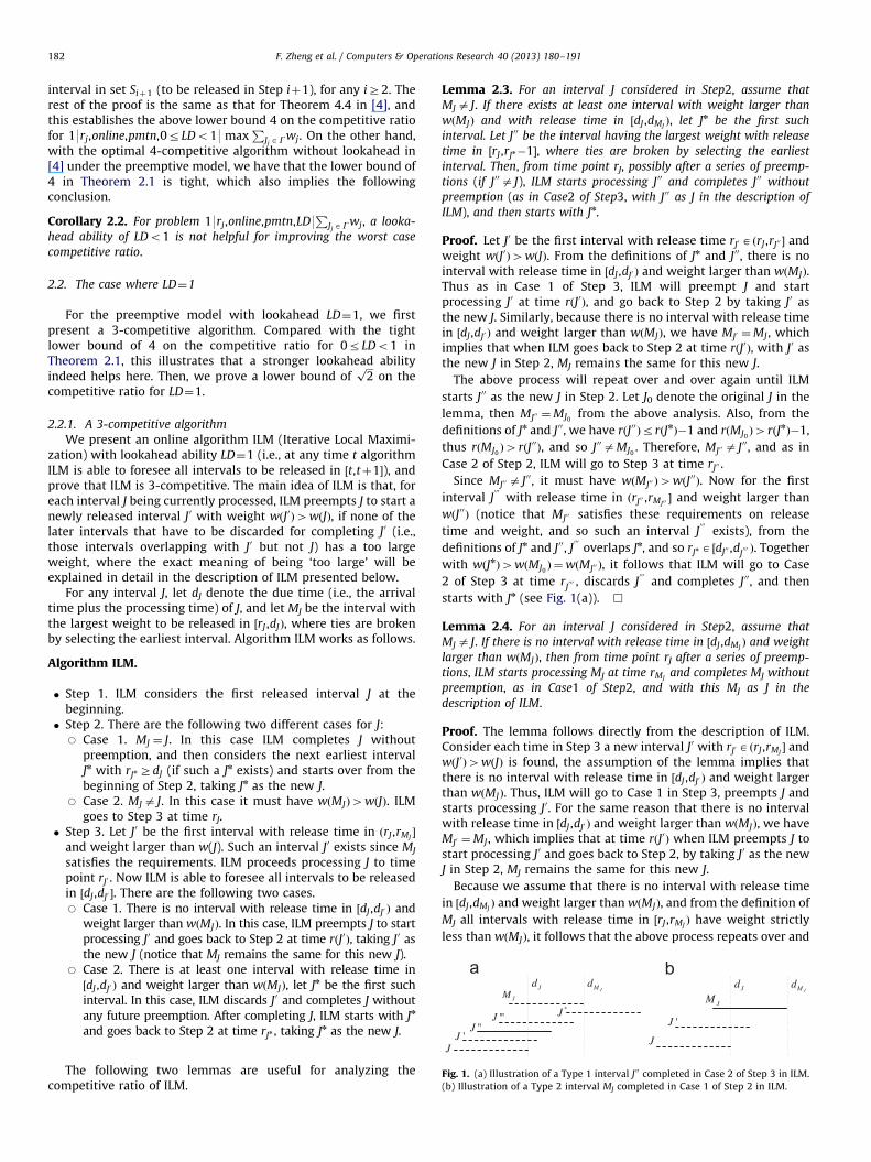
Fig. 1. (a) Illustration of a Type 1 interval J00 completed in Case 2 of Step 3 in ILM.

(b) Illustration of a Type 2 interval MJ completed in Case 1 of Step 2 in ILM.

The following two lemmas are useful for analyzing thecompetitive ratio of ILM.

Lemma 2.3. For an interval J considered in Step2, assume that

MJ a J. If there exists at least one interval with weight larger than

wðMJÞ and with release time in ½dJ ,dMJÞ, let Jn be the first such

interval. Let J00 be the interval having the largest weight with release

time in ½rJ ,rJn�1�, where ties are broken by selecting the earliest

interval. Then, from time point rJ, possibly after a series of preemp-

tions (if J00a J), ILM starts processing J00 and completes J00 without

preemption (as in Case2 of Step3, with J00 as J in the description of

ILM), and then starts with Jn.

Proof. Let J0 be the first interval with release time rJ0AðrJ ,rJ00 � andweight wðJ0Þ4wðJÞ. From the definitions of Jn and J00, there is nointerval with release time in ½dJ ,dJ0 Þ and weight larger than wðMJÞ.Thus as in Case 1 of Step 3, ILM will preempt J and startprocessing J0 at time rðJ0Þ, and go back to Step 2 by taking J0 asthe new J. Similarly, because there is no interval with release timein ½dJ ,dJ0 Þ and weight larger than wðMJÞ, we have MJ0 ¼MJ , whichimplies that when ILM goes back to Step 2 at time rðJ0Þ, with J0 asthe new J in Step 2, MJ remains the same for this new J.

The above process will repeat over and over again until ILM

starts J00 as the new J in Step 2. Let J0 denote the original J in the

lemma, then MJ00 ¼MJ0from the above analysis. Also, from the

definitions of Jn and J00, we have rðJ00ÞrrðJnÞ�1 and rðMJ0Þ4rðJnÞ�1,

thus rðMJ0Þ4rðJ00Þ, and so J00aMJ0

. Therefore, MJ00a J00, and as in

Case 2 of Step 2, ILM will go to Step 3 at time rJ00 .

Since MJ00a J00, it must have wðMJ00 Þ4wðJ00Þ. Now for the first

interval J000

with release time in ðrJ00 ,rMJ00� and weight larger than

wðJ00Þ (notice that MJ00 satisfies these requirements on release

time and weight, and so such an interval J000

exists), from the

definitions of Jn and J00, J000

overlaps Jn, and so rJn A ½dJ00 ,dJ000 Þ. Together

with wðJnÞ4wðMJ0Þ ¼wðMJ00 Þ, it follows that ILM will go to Case

2 of Step 3 at time rJ000 , discards J

000

and completes J00, and then

starts with Jn (see Fig. 1(a)). &

Lemma 2.4. For an interval J considered in Step2, assume that

MJ a J. If there is no interval with release time in ½dJ ,dMJÞ and weight

larger than wðMJÞ, then from time point rJ after a series of preemp-

tions, ILM starts processing MJ at time rMJand completes MJ without

preemption, as in Case1 of Step2, and with this MJ as J in the

description of ILM.

Proof. The lemma follows directly from the description of ILM.Consider each time in Step 3 a new interval J0 with rJ0AðrJ ,rMJ

� andwðJ0Þ4wðJÞ is found, the assumption of the lemma implies thatthere is no interval with release time in ½dJ ,dJ0 Þ and weight largerthan wðMJÞ. Thus, ILM will go to Case 1 in Step 3, preempts J andstarts processing J0. For the same reason that there is no intervalwith release time in ½dJ ,dJ0 Þ and weight larger than wðMJÞ, we haveMJ0 ¼MJ , which implies that at time rðJ0Þ when ILM preempts J tostart processing J0 and goes back to Step 2, by taking J0 as the newJ in Step 2, MJ remains the same for this new J.

Because we assume that there is no interval with release time

in ½dJ ,dMJÞ and weight larger than wðMJÞ, and from the definition of

MJ all intervals with release time in ½rJ ,rMJÞ have weight strictly

less than wðMJÞ, it follows that the above process repeats over and

F. Zheng et al. / Computers & Operations Research 40 (2013) 180–191 183

over again, until to some time point we have J0 ¼MJ . Then, ILM

preempts the interval being currently processed and starts

processing J0 ¼MJ at time rðMJÞ, and goes back to Step 2 by taking

J0 as the new J. Now in Step 2 we have J¼MJ for this new J, and so

ILM completes MJ as in Case 1 of Step 2 (see Fig. 1(b)). &

Now we are ready to prove the following theorem on thecompetitive ratio of ILM.

Theorem 2.5. ILM is3-competitive for 19rj,online,pmtn,LD¼

19P

Jj AGwj.

Proof. For an input sequence of intervals, let s¼ ðJ1,J2, . . . ,JnÞ bethe schedule produced by ILM, where J1,J2, . . . ,Jn are all theintervals completed by ILM and rðJ1ÞorðJ2Þo � � �orðJnÞ. Fromthe description of ILM, there are two types of intervals completedby ILM: those completed in Case 2 of Step 3 (Fig. 1(a)), and thosecompleted in Case 1 of Step 2 (Fig. 1(b)). If an interval iscompleted in Case 2 of Step 3 then we call it a Type 1 interval,and if an interval is completed in Case 1 of Step 2 then we call it aType 2 interval.

We partition s into subschedules fs1,s2, . . . ,skg, such that each

subschedule consists of a number of consecutive intervals in s,

and an interval JjAs is an end interval in a subschedule if and

only if it is a Type 2 interval. Thus, each subschedule consists of a

sequence of Type 1 intervals followed by one Type 2 interval.

Notice that a subschedule may contain only one interval which is

of Type 2.

Consider a subschedule si ¼ ðJi,1,Ji,2, . . . ,Ji,niÞ with rðJi,1ÞorðJi,2Þ

o � � �orðJi,niÞ completed by ILM. Regarding the behavior of ILM

on si, by Lemmas 2.3 and 2.4, there exist intervals Jni,1,Jni,2, . . . ,Jni,ni,

such that for each 1r jrni�1, rðJni,jÞrrðJi,jÞorðMðJni,jÞÞ, and

Ji,ni¼MðJni,ni

Þ (see Fig. 2). If i¼1 then ILM starts with Jn1;1 in Step

1, that is si is the first subschedule and Jn1;1 is the first interval in

the input sequence to ILM; otherwise if i41, then ILM starts with

Jni,1 (as Jn in the description of ILM) in Case 1 of Step 2. The

following process repeats for j¼ 1;2, . . . ,ni�1: after starting with

Jni,j, possibly after a series of preemptions, ILM starts with and

completes Ji,j before starting with Jni,jþ1 (as in Case 2 of Step 3). At

last, after starting with Jni,ni,possibly after a series of preemptions,

ILM starts with and completes Ji,ni¼MðJni,ni

Þ as in Case 1 of Step 2

(with Ji,nias J in the description of ILM).

Consider the time sections

½rðJn1;1Þ,dðJ1,n1ÞÞ,½rðJn2;1Þ,dðJ2,n2

ÞÞ, . . . ,½rðJnk,1Þ,dðJk,nkÞÞ:

From the description of ILM, the release time of every interval in

the input falls into one of the above sections. For each time

section ½rðJni,1Þ,dðJi,niÞÞ with 1r irk, we further partition it into the

Fig. 2. Intervals with release time in ½rðJni,1Þ,dðJi,niÞÞ, where so

following ni subsections

½rðJni,1Þ,rðJn

i,2ÞÞ,½rðJn

i,2Þ,rðJn

i,3ÞÞ, . . . ,½rðJn

i,ni�1Þ,rðJn

i,niÞÞ,½rðJni,ni

Þ,dðJi,niÞÞ:

For each of the first ni�1 subsections si,j ¼ ½rðJn

i,jÞ,rðJn

i,jþ1ÞÞ with

1r jrni�1, clearly rðJni,jþ1ÞZdðJni,jÞ, we have that the length of

si,j is rðJni,jþ1Þ�rðJni,jÞZ1. Also, since Ji,ni¼MðJni,ni

Þ and clearly

dðMðJni,niÞÞZdðJni,ni

Þ, the length of the last subsection si,ni¼

½rðJni,niÞ,dðJi,ni

ÞÞ is dðJi,niÞ�rðJni,ni

Þ ¼ dðMðJni,niÞÞ�rðJni,ni

ÞZ1. Thus the

length of every subsection si,j, 9si,j9, is at least 1, for 1r jrni. On

the other hand, since Jni,j overlaps MðJni,jÞ for each 1r jrni, and

MðJni,jÞ overlaps Jni,jþ1 for each 1r jrni�1, it follows that the

length 9si,j9 of every subsection si,j is strictly less than 2.

We further partition each subsection si,j into two smaller blocks

sð1Þi,j and sð2Þi,j , such that the first block sð1Þi,j ¼ ½rðJn

i,jÞ,rðJn

i,jÞþ9si,j9�1Þ and

the second block sð2Þi,j ¼ si,j\sð1Þi,j . Thus the length of the second block

sð2Þi,j is 1 and the length of the first block sð1Þi,j is less than 1. For each

sð1Þi,j (and sð2Þi,j ), the optimal offline algorithm OPT completes at most

one interval with release time in it, we use Oð1Þi,j (and Oð2Þi,j ) to

denote this interval. Next we bound from the above the weights

of all these intervals that are possibly completed by OPT.

For Oð1Þi,j with 1r jrni�1, since its release time rðOð1Þi,j ÞorðJni,jþ1Þ�1, Oð1Þi,j does not overlap with Jni,jþ1, which implies that

wðOð1Þi,j ÞrwðJi,jÞ (since otherwise ILM will complete Oð1Þi,j instead

of Ji,j). For Oð1Þi,ni, since its release time is in ½rðJni,ni

Þ,rðMðJni,niÞÞÞ,

wðOð1Þi,niÞowðMðJni,ni

ÞÞ ¼wðJi,niÞ.

For Oð2Þi,j with 1r jrni�1, since its release time rðOð2Þi,j ÞorðJni,jþ1Þ,

and Jni,jþ1 is the first interval with release time in ½dðJni,jÞ,dðMðJn

i,jÞÞÞ

and with weight larger than wðMðJni,jÞÞ, we have wðOð2Þi,j ÞrwðMðJni,jÞÞ,

and so wðOð2Þi,j ÞowðJni,jþ1ÞrwðJi,jþ1Þ. For Oð2Þi,ni, since its release time

is in ½rðMðJni,niÞÞ,dðMðJni,ni

ÞÞÞ and ILM completes MðJni,niÞ, wðOð2Þi,ni

Þ

rwðMðJni,niÞÞ ¼wðJi,ni

Þ.

From the above analysis, for each subschedule si with 1r irk,

the total weight of all intervals possibly completed by OPT with

release time in ½rðJni,1Þ,dðJi,niÞÞ is at most

Xni

j ¼ 1

ðwðOð1Þi,j ÞþwðOð2Þi,j ÞÞoXni�1

j ¼ 1

ðwðJi,jÞþwðJi,jþ1ÞÞþ2wðJi,niÞ

¼wðJi,1Þþ2Xni�1

j ¼ 2

wðJi,jÞþ3wðJi,niÞ

o3Xni

j ¼ 1

wðJi,jÞ:

Let w(OPT) and w(ILM) denote the total weight obtained by OPT

and ILM, respectively. Then,

lid line segments represent intervals completed by ILM.

Fig. 3. An input example to illustrate that the 3-competitiveness result for ILM in

Theorem 2.5 is tight.

F. Zheng et al. / Computers & Operations Research 40 (2013) 180–191184

wðOPTÞrXk

i ¼ 1

Xni

j ¼ 1

ðwðOð1Þi,j ÞþwðOð2Þi,j ÞÞ

o3Xk

i ¼ 1

Xni

j ¼ 1

wðJi,jÞ ¼ 3wðILMÞ,

which establishes the theorem. &

Remark. The competitive ratio 3 of ILM given in Theorem 2.5 isactually tight, and this can be seen from the following inputsequence t¼ ðJ1,J2, . . . ,J6Þ. Each interval in t is of length 1, and therelease time and weights of these intervals are as follows,rðJ1Þ ¼ 0, wðJ1Þ ¼ 1, rðJ2Þ ¼ 2=5, wðJ2Þ ¼M, rðJ3Þ ¼ 6=5, wðJ3Þ ¼Mþ1,rðJ4Þ ¼ 8=5, wðJ4Þ ¼Mþ1, rðJ5Þ ¼ 2, wðJ5Þ ¼Mþ2, rðJ6Þ ¼ 14=5, andwðJ6Þ ¼Mþ1, where Mb1. It is easy to verify that ILM willcomplete J1 and J5, obtaining a total weight of Mþ3. On the otherhand, OPT completes J2,J4, and J6, obtaining a total weight of3Mþ2. The ratio ð3Mþ2Þ=ðMþ3Þ can be arbitrarily close to3 while M approaches infinity (see Fig. 3).

2.2.2. A lower boundffiffiffi2p

on the competitive ratio

Theorem 2.6. For problem 19rj,online,pmtn,LD¼ 19P

Jj AGwj, no

deterministic online algorithm has competitive ratio less thanffiffiffi2p

.

Proof. We construct an input sequence s, which contains at mostfour intervals, to make any online algorithm A behave poorly andbe at best

ffiffiffi2p

-competitive. Let wðsÞ and wnðsÞ be the total weightobtained by A and by the optimal offline algorithm OPT on s,respectively.

The first three intervals J1,J2, and J3 in s are released at time 0,

2/3 and 4/3, respectively, with wðJ1Þ ¼ 1, wðJ2Þ ¼ 1þffiffiffi2p

, and

wðJ3Þ ¼ 1þffiffiffi2p

. A may start processing J1 at time 0. At time 2/3

A either preempts J1 to start processing J2, or goes on processing J1

and discards J2, which correspond to the following two cases.

Case 1: A preempts J1 to start processing J2 at time 2/3. In this

case, no more intervals after J3 will be released. A completes at

most one interval, either J2 or J3, and obtains a weight of at most

wðsÞ ¼ 1þffiffiffi2p

. On the other hand, since J1 and J3 do not overlap,

OPT can complete both of them and obtain wnðsÞ ¼ 1þð1þffiffiffi2pÞ¼

2þffiffiffi2p

. Thus, in this case wnðsÞ=wðsÞZ ð2þffiffiffi2pÞ=ð1þ

ffiffiffi2pÞ¼

ffiffiffi2p

.

Case 2: A goes on processing J1 and discards J2 at time 2/3. In

this case, the last interval J4 is released at time 2 with

wðJ4Þ ¼ 1þffiffiffi2p

. Since J4 overlaps J3, after completing J1, A is able

to complete at most one more interval, either J3 or J4, obtaining a

total weight of at most wðsÞ ¼ 1þð1þffiffiffi2pÞ¼ 2þ

ffiffiffi2p

. Since J2 and J4

do not overlap, OPT can complete both of them and obtain

wnðsÞ ¼ 2ð1þffiffiffi2pÞ. Thus, in this case we have wnðsÞ=wðsÞZ

2ð1þffiffiffi2pÞ=ð2þ

ffiffiffi2pÞ¼

ffiffiffi2p

.

In either case, wnðsÞ=wðsÞZffiffiffi2p

. The theorem follows. &

3. The non-preemptive model with lookahead

In this section we investigate the non-preemptive model. Wefirst give a result on the relation between the ability of lookahead

and the ability of preemption, for deterministic online heuristicssolving the interval scheduling problem.

Theorem 3.1. For an input s of intervals with various release times,if there is an upper bound L on the length (processing time) of every

interval in s, then for any deterministic preemptive online heuristics

H1 with lookahead ability LD, there is a deterministic non-preemp-

tive online heuristics H2 with lookahead ability LDþL, such that H2 is

able to simulate H1 and complete the same subset of intervals as H1

does on input s.

Proof. The proof is straightforward. Assume that at time t, H1

preempts an interval JiAs with release time riot. Since H1 haslookahead ability LD, the decision of preempting Ji is made by H1

based on the information up to time point tþLD. Because Ji is stillbeing processed at time t and the length of Ji is bounded fromabove by L, we have toriþL. On the other hand, at time ri, H2 isable to foresee the information up to time riþðLDþLÞ4tþLD, andso H2 is able to predict that H1 will preempt Ji later at time t, thusH2 can simply discard Ji at time ri in the first place. Therefore, H2 isable to choose only to start and process all the intervals com-pleted by H1, and so to complete the same subset of intervals in sas H1 does, without preemption. &

By using Theorem 3.1, in this section we transform thealgorithmic results in Section 2 and in [4] under the preemptivemodel into new online algorithms under the non-preemptivemodel, with corresponding lookahead abilities enhanced by onemore time unit. We also discuss lower bounds on the competitiveratio under these models. In what follows, we return to the case ofunit-length intervals.

3.1. The case where 0rLDo1

Under the non-preemptive model, if the lookahead ability isstrictly less than one then we have the following negative result.

Theorem 3.2. No deterministic online algorithm has bounded

competitive ratio for problem 19rj,online,0rLDo19P

Jj AGwj.

Proof. We construct an input sequence s to make any determi-nistic online algorithm A behave poorly. The first interval J1As isreleased at time 0 with weight wðJ1Þ ¼ 1. There are the followingtwo cases.

Case 1: A discards J1 at time 0. In this case s contains only J1,

i.e., no more interval is released. Then, A obtains a weight of zero,

and the optimal offline algorithm OPT can complete J1 and obtain

a weight of one. Clearly, A loses in this case.

Case 2: A starts J1 at time 0. In this case the second interval J2 is

released at time LDþE with weight M, where 0oEo1�LD, and

M40 is an arbitrarily large value. Notice that J2 cannot be

foreseen by A when A starts J1 at time 0. Since J1 and J2 overlap

with each other, A completes at most one interval J1 and gains a

weight of at most one. On the other hand, OPT can complete J2

and gain a weight of M. Then the ratio between what OPT and Again is M. Since M can be arbitrarily large, A also loses in this case.

In either case, A loses. The theorem follows. &

3.2. The case where LD¼1

In Theorem 3.2 and Remark 3.3 in [4] a preemptive heuristicH1 with no lookahead ability is proposed as follows. H1 startsprocessing the first released interval, and each time a newinterval J0 is released, if the weight of J0 is at least twice theweight of the currently processed interval J then H1 preempts J to

F. Zheng et al. / Computers & Operations Research 40 (2013) 180–191 185

start processing J0, otherwise H1 discards J0 and continues proces-sing J. H1 is proved to be 4-competitive in [4].

By Theorem 3.1, H1 can be simulated by an online non-preemptive algorithm with lookahead LD¼1. We give fulldescription of this non-preemptive algorithm as A1 below, forthe sake of clarity. Recall that for an interval J, MJ denotes theinterval with the largest weight to be released in ½rJ ,dJÞ, where tiesare broken by selecting the earliest interval.

Algorithm A1.

�

Figresu

Step 1. A1 considers the first released interval J at thebeginning.

� Step 2. There are the following two different cases for J:

J Case 1. wðMJÞo2wðJÞ. In this case A1 starts and completes J.Then, A1 considers the next earliest interval Jn withrðJnÞZdðJÞ (if such an interval Jn exists), and goes back toStep 1 at time rðJnÞ, taking Jn as the new J.

J Case 2. wðMJÞZ2wðJÞ. In this case A1 discards J. Then, attime rðMJÞ A1 goes back to Step 1 and considers MJ, takingMJ as the new J.

0

. 4.lt f

By Theorem 3.1, the 4-competitiveness result for H1 in [4]immediately implies the following 4-competitiveness result for A1.

Corollary 3.3. A1 is 4-competitive for 19rj,online,LD¼ 19P

Jj AGwj.

The competitive ratio 4 given above is tight for algorithms H1

and A1, and this can be seen from the following class of inputsequences sðkÞ, for k¼ 2;3, . . . . Input sðkÞ consists of 2k unit-lengthintervals J1,J2, . . . ,J2k, such that rðJ2i�1Þ ¼ ði�1Þð1�gÞ, wðJ2i�1Þ ¼

2i�1, rðJ2iÞ ¼ i�ð2k�iÞg, and wðJ2iÞ ¼ 2i�e, for i¼ 1;2, . . . ,k, where

0ogo1=ð2k�1Þ, and e40 is an arbitrarily small value. Then,each interval J2i�1 has an overlap of g with J2iþ1, and there is a gapof g between the due time of J2i and the start time of J2ðiþ1Þ, foreach i¼ 1;2, . . . ,k�1. When 0ogo1=ð2k�1Þ, interval J2i onlyoverlaps with J2i�1 and J2iþ1 for each i¼ 1;2, . . . ,k�1, and the lastinterval J2k only overlaps with J2k�1 for an amount of g. It is easyto verify that for very small value 0oe51, for such an inputsequence sðkÞ, algorithm H1 (and A1, since by Theorem 3.1algorithms H1 and A1 complete the same subset of intervals forany input sequence) completes only one interval J2k�1 and obtainsa weight W ¼ 2k�1, while the optimal algorithm OPT can chooseto complete intervals J2,J4, . . . ,J2k to obtain a weight Wn

¼P

ki ¼ 1ð2

i�eÞ ¼ 2kþ1

�2�ke. Then, the ratio Wn=W ¼ 4�ð2þkeÞ=2k�1

can be arbitrarily close to 4 when k-1 (see Fig. 4 for anillustration of input sequence sðkÞ with k¼4 and g¼ 1=10).

In fact, a more general result can be proved as in the followingtheorem, which gives a matching lower bound of 4 on thecompetitive ratio for problem 19rj,online,LD¼ 19

PJj AGwj. This

also implies that algorithm A1 is actually optimal.

Theorem 3.4. No deterministic online algorithm is better than

4-competitive for problem 19rj,online,LD¼ 19P

Jj AGwj.

1( ) 1w J

t1 7 1 2 6 2 2 3 5 3 3 4 4

2( ) 2w J

3( ) 2w J

4( ) 4w J

5( ) 4w J

6( ) 8w J

7( ) 8w J

8( ) 16w J

An example input sequence sð4Þ to illustrate that the 4-competitiveness

or H1 (and A1) is tight, where g¼ 1=10.

Proof. See Appendix A.

By Corollary 3.3 and Theorem 3.4, together with the optimal4-competitive algorithm (i.e., H1 as described in Section 3.2)proved in Woeginger [4] for 19rj,online,pmtn9

PJj AGwj, i.e., the

online interval scheduling problem with unit length intervalsunder preemptive model without lookahead, we have the follow-ing conclusion.

Corollary 3.5. For problem 19rj,online9P

Jj AGwj, the ability of looka-

head with one unit length time is the same powerful as the ability of

preemption, in terms of improving the performance of the optimal

online algorithms measured by the worst case competitive ratio

(from being not competitive to4-competitive).

3.3. The case where LD¼2

By Theorem 3.1, ILM can be simulated by a non-preemptiveonline algorithm ILMn with lookahead ability LD¼2, such that onany input sequence s of unit-length intervals, ILMn alwayscompletes the same subset of intervals in s as ILM does. Fromalgorithm ILM and its analysis (i.e., Theorem 2.5 and Lemmas 2.3and 2.4), ILMn can be described in the following way.

Algorithm ILMn.

�

Steps 1 and 2 of ILMn are the same as that of ILM. � Step 3. At time rJ, we have MJ a J, ILMn is able to foresee all

intervals with release time in ½rJ ,rJþ2�, and so all intervalswith release time in ½rJ ,dðMJÞ�. There are the following twocases.J Case 1. There is no interval to be released in ½dJ ,dðMJÞÞ

having weight larger than wðMJÞ. In this case, ILMn goesback to Case 1 of Step 2 and completes J ¼MJ . That is, ILMn

takes J ¼MJ as J in Case 1 of Step 2 (notice that J ¼MJ ).J Case 2. There is at least one interval with release time in½dJ ,dðMJÞÞ and weight larger than wðMJÞ, let Jn be the firstsuch interval. In this case, let J0 be the interval with thelargest weight and with release time in ½rJ ,rJn�1� (and so J0

does not overlap with Jn). ILMn starts and completes J0, andthen goes back to the beginning of Step 2 at time rJn toconsider Jn, taking Jn as the new J in Step 2.

Theorems 2.5 and 3.1 immediately imply the following 3-com-petitiveness result on ILMn.

Corollary 3.6. ILMn is 3-competitive for 19rj,online,LD¼

29P

Jj AGwj.

By Theorem 3.1, for any input sequence ILMn completes thesame subset of intervals as ILM does. Therefore the input instance(given in the remarks immediately after the proof of Theorem 2.5)is tight for ILMn as well, i.e., the input instance also demonstratesthat the above 3-competitiveness result for ILMn is tight.

The proof for the lower boundffiffiffi2p

on the competitive ratio for19rj,online,pmtn,LD¼ 19

PJj AGwj in Theorem 2.6 also applies here,

for problem 19rj,online,LD¼ 29P

Jj AGwj, with only a small mod-ification here that the release time of J4 (if J4 is in the input) is setto be 2þe instead of 2, where e40 is a very small value, so thatany online algorithm with lookahead 2 cannot foresee whether J4

is in the input or not at time 0. The proof here works in thefollowing way: Case 1 in the proof of Theorem 2.6 (where J1 ispreempted at time 2/3) corresponds to the case here that J1 isdiscarded by the online algorithm (i.e., J1 never gets started, andin this case the fourth interval J4 will not appear in the inputsequence); Case 2 in the proof of Theorem 2.6 (where J1 is notpreempted at time 2/3) corresponds to the case here that J1 is

F. Zheng et al. / Computers & Operations Research 40 (2013) 180–191186

started (and so completed) by the online algorithm, and in thiscase the fourth interval J4 will appear in the input sequence withrelease time 2þe. The rest of the proof here is the same as that forTheorem 2.6, which implies the following result.

0 200 400 600 800 1000 1200 1400 1600 1800 20001

1.02

1.04

1.06

1.08

1.1

1.12

1.14

1.16

1.18

1.2

Number of Intervals

Ave

rage

Com

petit

ivity

ILM (ILM*)H (A )

Fig. 5. Experimental competitivities on the first class of instances, where in each

instance the interval weights are uniformly sampled from ½0;100�.

0 200 400 600 800 1000 1200 1400 1600 1800 20001

1.02

1.04

1.06

1.08

1.1

1.12

1.14

1.16

1.18

1.2

Number of Intervals

Ave

rage

Com

petit

ivity

ILM (ILM*)H1 (A1)

0 200 400 600 800 1000 1200 1400 1600 1800 20001

1.02

1.04

1.06

1.08

1.1

1.12

1.14

1.16

1.18

1.2

Number of Intervals

Ave

rage

Com

petit

ivity

ILM (ILM*)H1 (A1)

Fig. 6. Experimental competitivities on the second class of instances, where in each ins

from (a) N(100, 15), (b) N(100, 20), (c) N(100, 25), and (d) N(100, 50).

Corollary 3.7. For problem 19rj,online,LD¼ 29P

Jj AGwj, no deter-

ministic online algorithm has competitive ratio less thanffiffiffi2p

.

4. Experimental results

In this section, we present experimental results on algorithmILM described in Section 2.2.1 (which always obtains the samesolution as Algorithm ILMn described in Section 3.3) and algo-rithm H1 from [4] as described in Section 3.2 (which alwaysobtains the same solution as Algorithm A1 also described inSection 3.2), to get an impression of their average case perfor-mances. Our experimental results indicate that on input instanceswhere interval weights follow normal distribution with relativelylarge standard deviations, and input instances where intervalweights grow exponentially in the release times of the intervals,Algorithm ILM (ILMn) exhibits better practical performances thanH1 (A1) does, with the help of one more unit time lookaheadability.

We perform tests on three classes of instances. In all the threeclasses, the release times of the intervals in an instance follow auniform distribution in ½0;100�. The interval weights in aninstance follow uniform distribution in the first class, follownormal distribution in the second class, and grow exponentiallywith the release times of the intervals in the third class. For theoptimal solutions of the instances in each class, it is easy to see

0 200 400 600 800 1000 1200 1400 1600 1800 20001

1.02

1.04

1.06

1.08

1.1

1.12

1.14

1.16

1.18

1.2

Number of Intervals

Ave

rage

Com

petit

ivity

ILM (ILM*)H1 (A1)

0 200 400 600 800 1000 1200 1400 1600 1800 20001

1.02

1.04

1.06

1.08

1.1

1.12

1.14

1.16

1.18

1.2

Number of Intervals

Ave

rage

Com

petit

ivity

ILM (ILM*)H1 (A1)

tance the interval weights are normally distributed. Interval weights are sampled

F. Zheng et al. / Computers & Operations Research 40 (2013) 180–191 187

that they can be obtained efficiently by an offline algorithmusing the standard dynamic programming technique. Weuse the two non-preemptive algorithms, ILMn and A1, for theimplementations.

4.1. Uniformly distributed weights

For the first class of test instances, the interval weights in eachinstance follow a uniform distribution from ½0;100�. For eachnAf10;20, . . . ,2000g where n is the number of intervals in aninstance, we sample 100 instances to calculate the averagecompetitivities of ILM (i.e., of ILMn) and of H1 (i.e., of A1). AsFig. 5 shows, the practical average competitivities of ILM (ILMn)and H1 (A1) for the first class of instances are very close to eachother. Moreover, they both have very good practical perfor-mances, with average case competitivities no greater than1.2 on any instance size tested.

4.2. Normally distributed weights

For the second class of test instances, we have four test sets S1,S2, S3, and S4. The interval weights of an instance in set Si follow anormal distribution with expected value 100 and standard devia-tion si, where s1 ¼ 15, s2 ¼ 20, s3 ¼ 25, and s4 ¼ 50. In each test

0 200 400 600 800 1000 1200 1400 1600 1800 20001

1.05

1.1

1.15

1.2

1.25

1.3

1.35

1.4

1.45

Number of Intervals

Ave

rage

Com

petit

ivity

ILM (ILM*)H1 (A1)

0 200 400 600 800 1000 1200 1400 1600 1800 20001

1.2

1.4

1.6

1.8

2

2.2

2.4

Number of Intervals

Ave

rage

Com

petit

ivity

ILM (ILM*)H1 (A1)

Fig. 7. Experimental competitivities on the third class of instances, where the interval

The weight of each interval J is (a) wðJÞ ¼ 1:5rðJÞ , (b) wðJÞ ¼ 2rðJÞ , (c) wðJÞ ¼ 2:5rðJÞ , and (d)

set Si, similarly as for the first class, for each nAf10;20, . . . ,2000gwhere n is the number of intervals in an instance, 100 instancesare sampled to calculate the average competitivities. Fig. 6 showsthe practical average competitivities of ILM (ILMn) and H1 (A1) oneach test set.

Fig. 6 shows that both ILM (ILMn) and H1 (A1) have very goodpractical performances on the second class of instances, withaverage case competitivities no greater than 1.2 on any instancesize tested. The practical performance of ILM (ILMn) is worse thanH1 (A1) if the normal distribution has a relatively small standarddeviation (Fig. 6(a)), and better than H1 (A1) if the standarddeviation is relatively large (Fig. 6(c) and (d)). For our second testset where the interval weights follow a normal distributionNð100;20Þ, the practical performances of ILM (ILMn) and H1 (A1)are very close to each other (Fig. 6(b)). For the fourth test setwhere the interval weights follow a normal distributionNð100;50Þ, the advantage of ILM (ILMn) over H1 (A1) becomesmore obvious, for example the difference on their averagecompetitivities is typically no less than 0.04 when the numberof intervals n is no less than 400.

One possible explanation for this phenomenon is that whenthe standard deviation is relatively small, the interval weightstend to be very close to each other, and it is very unlikely for twooverlapping intervals such that the weight of one is as twice large

0 200 400 600 800 1000 1200 1400 1600 1800 20001

1.05

1.1

1.15

1.2

1.25

1.3

1.35

1.4

1.45

Number of Intervals

Ave

rage

Com

petit

ivity

ILM (ILM*)H1 (A1)

0 200 400 600 800 1000 1200 1400 1600 1800 20001

1.2

1.4

1.6

1.8

2

2.2

2.4

Number of Intervals

Ave

rage

Com

petit

ivity

ILM (ILM*)H1 (A1)

weights in each instance grow exponentially in the release times of the intervals.

wðJÞ ¼ 3rðJÞ .

F. Zheng et al. / Computers & Operations Research 40 (2013) 180–191188

as the other, thus most of the time algorithm H1 (A1) simplycompletes any newly started interval. On the other hand, from thedescription of ILM (ILMn), for this kind of input sequence Algo-rithm ILM (ILMn) tends to drop a new interval for some lateroverlapping interval with slightly larger weight. The gain of moreweight from each interval in this way is very limited, but it doescreate considerably many wasted time segments (i.e., no com-pleted intervals cover these time segments), which cancels theeffect of choosing intervals with slightly larger weights andmakes the average performance of ILM (ILMn) even worse thanH1 (A1) on such inputs. However, when the standard deviationgets larger, the interval weights become more diverse, in suchcase the advantage of ILM (ILMn) with stronger lookahead abilitybecomes more obvious.

4.3. Exponentially growing weights

For the third class of test instances, we also have four test setsS01, S02, S03, and S04. In test set S0i, the weight w(J) of an interval J isarðJÞ

i , that is the weight w(J) of J is exponential in the release timer(J) of J, where a1 ¼ 1:5, a2 ¼ 2, a3 ¼ 2:5, and a4 ¼ 3. In each testset S0i, for each nAf10;20, . . . ,2000g where n is the number ofintervals in an instance, similarly as the previous two classes 100instances are randomly sampled to calculate the average compe-titivities. It is not hard to see that input instances in this classhave certain similarities with the tight instances for H1 (and A1)given right below Corollary 3.3. Fig. 7 shows the practical averagecompetitivities of ILM (ILMn) and H1 (A1) on each test set.

From Fig. 7, for the instances where interval weights growexponentially with the release times, ILM (ILMn) with the help ofone more unit time lookahead ability has better average practicalperformances than H1 (A1) does. For most of the instance sizes n

tested, there is typically a difference of about 0.1 in the averagecompetitivities with a1 ¼ 1:5 (Fig. 7(a)), and a difference of about0.2 in the average competitivities with a2 ¼ 2 (Fig. 7(b)). Theadvantage of ILM (ILMn) over H1 (A1) becomes much moreobvious with a3 ¼ 2:5 and a4 ¼ 3 (Fig. 7(c) and (d)), for thesetwo test sets with reasonably large n, say nZ1000, the averagecompetitivities of H1 (A1) become around 2 and generally grow asn grows, while the average competitivities of ILM (ILMn) staybelow 1.2 for the whole range 0rnr2000. Preliminary compu-tational tests are also performed for input instances withwðJÞ ¼ arðJÞ where a43, and the experimental results indicatethat the difference of the average competitivities between H1 (A1)and ILM (ILMn) generally decreases as the base a43 grows.

5. Discussions

For the non-preemptive model with one unit time length looka-head, our main result is that the optimal online algorithm has acompetitive ratio of 4, which is a direct conclusion from Corollary3.3 and Theorem 3.4. For the preemptive model with one unit timelength lookahead, we propose a 3-competitive online algorithm ILMand prove a lower bound of

ffiffiffi2p

on the competitive ratio.It is interesting to investigate whether there are other ways to

utilize the one unit time length lookahead ability to achievebetter worst case competitive ratio for the preemptive model, orto achieve better average practical competitivities for the pre-emptive or non-preemptive model. A more general problem forfuture study is to investigate the power of general lookaheadability LDZ0 for online interval scheduling.

For the experimental results reported in this paper, we noticethat there is a point of intersection at around n¼1000 in Fig. 5(i.e., the figure for the first class of input instances where intervalweights follow uniform distribution). We have performed the

computational tests for a number of times and find out that theintersection point does always exist. One open question we left isto give an explanation why such an intersection point exists,either based on rigorous theoretical analysis or based on intui-tively plausible arguments.

Acknowledgments

The authors are grateful to the anonymous reviewers for theirhelpful comments and suggestions.

Appendix A. Proof of Theorem 3.4

Theorem 3.4 is proved based on a variant and extension of theidea used in the proof of Theorem 4.4 in [4]. We first present auseful lemma.

Lemma A.1 (Woeginger [4, Lemma 4.3]). For 2oao4, let SðaÞ be a

strictly increasing sequence of positive numbers /v1,v2, . . .S ful-

filling the inequality

viþ2r ða�1Þviþ1�Xi

j ¼ 1

vj

for every iZ0. Then SðaÞ is finite.

Now we are ready to prove Theorem 3.4. For given 1rwrw,0r ltort, and d40, define Sðw,w,lt,rt,dÞ to be a set of intervalsfJ1,J2, . . . ,Jqg with the following properties.

�

Let wðJiÞ be the weight of interval Ji, for 1r irq. Then,wðJ1Þ ¼w, wðJqÞ ¼w, and wðJiÞowðJiþ1ÞrwðJiÞþd for1r irq�1 (here the total number q of intervals in the setdoes not really matter, as long as the above requirements aresatisfied for the given w, w, and dÞ. � Let rðJiÞ be the release time of interval Ji, for 1r irq. Then,

ltorðJ1ÞorðJ2Þo � � �orðJqÞort.

For any small value E40, we will define a list LðEÞ of interval setsand an adversary strategy to present the intervals in LðEÞ to anyonline algorithm A, to make A behave poorly and have a worstcase ratio of at least ð4�EÞ. Let a¼ 4�E=2, let d be a small valuesuch that 0odoE=2, and let di ¼ d=2i for every integer iZ1.

Next we describe the structure of the list LðEÞ of interval sets.The sets in LðEÞ are in different phases. There is only one set inPhase 1, Sð1,a,0;1,d1Þ. We use SðiÞj to denote the jth interval set inphase i, for i,jZ1. Each set in phase i has the form Sðn,n,n,n,diÞ

with di ¼ d=2i.We first specify the release time of the intervals in LðEÞ. In any

phase iZ1, for each pair of two consecutive intervals J0 and J

(with release time rJ0orJ) in each set SðiÞ in phase i, the pair ðJ0,JÞdefines a new set Sðiþ1Þ

ðn,n,dJ0 ,dJ ,diþ1Þ in phase iþ1, where dJ0 anddJ are the due time of J0 and J respectively. That is, the release timeof every interval in this new set Sðiþ1Þ is strictly between the duetime of J0 and J (see Fig. 8(a)).

For each i41, all the interval sets SðiÞj in phase i are indexed inthe same ordering as of the interval pairs (in phase i�1) definingthem. From the above it is easy to verify that the intervals in LðEÞhave the following properties: an interval always has release timelater than all the intervals in earlier phases; all intervals in thesame phase overlap with each other (we say that two intervalsoverlap with each other if they cover a common time segment oflength larger than zero), and within the same phase i, for any twointervals J1ASðiÞj and J2ASðiÞk with jok, we have rðJ1ÞorðJ2Þ; also,there exist no two intervals J,J0ALðEÞ such that rJ0 ¼ dJ , that is no

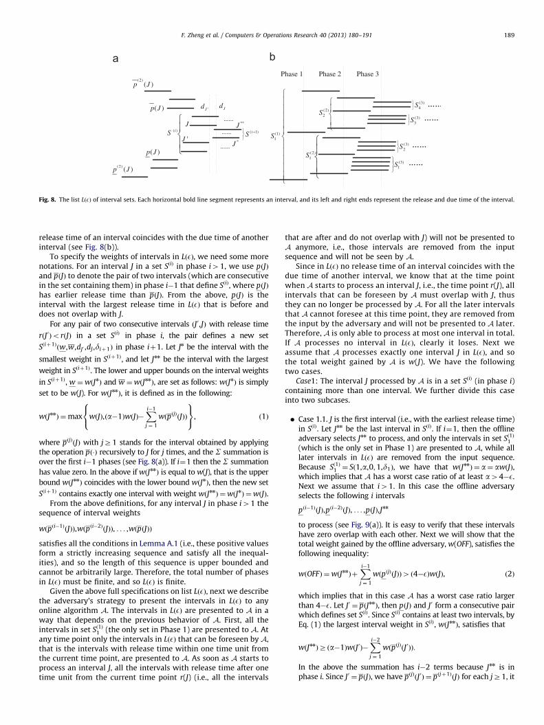
Fig. 8. The list LðEÞ of interval sets. Each horizontal bold line segment represents an interval, and its left and right ends represent the release and due time of the interval.

F. Zheng et al. / Computers & Operations Research 40 (2013) 180–191 189

release time of an interval coincides with the due time of anotherinterval (see Fig. 8(b)).

To specify the weights of intervals in LðEÞ, we need some morenotations. For an interval J in a set SðiÞ in phase i41, we use pðJÞ

and pðJÞ to denote the pair of two intervals (which are consecutivein the set containing them) in phase i�1 that define SðiÞ, where pðJÞ

has earlier release time than pðJÞ. From the above, pðJÞ is theinterval with the largest release time in LðEÞ that is before anddoes not overlap with J.

For any pair of two consecutive intervals ðJ0,JÞ with release time

rðJ0ÞorðJÞ in a set SðiÞ in phase i, the pair defines a new set

Sðiþ1Þðw,w,dJ0 ,dJ ,diþ1Þ in phase iþ1. Let Jn be the interval with the

smallest weight in Sðiþ1Þ, and let Jnn be the interval with the largest

weight in Sðiþ1Þ. The lower and upper bounds on the interval weights

in Sðiþ1Þ, w ¼wðJnÞ and w ¼wðJnnÞ, are set as follows: wðJnÞ is simply

set to be w(J). For wðJnnÞ, it is defined as in the following:

wðJnnÞ ¼max wðJÞ,ða�1ÞwðJÞ�Xi�1

j ¼ 1

wðpðjÞðJÞÞ

8<:

9=;, ð1Þ

where pðjÞðJÞ with jZ1 stands for the interval obtained by applyingthe operation pð�Þ recursively to J for j times, and the S summation is

over the first i�1 phases (see Fig. 8(a)). If i¼1 then the S summation

has value zero. In the above if wðJnnÞ is equal to w(J), that is the upper

bound wðJnnÞ coincides with the lower bound wðJnÞ, then the new set

Sðiþ1Þ contains exactly one interval with weight wðJnnÞ ¼wðJnÞ ¼wðJÞ.From the above definitions, for any interval J in phase i41 the

sequence of interval weights

wðpði�1ÞðJÞÞ,wðpði�2Þ

ðJÞÞ, . . . ,wðpðJÞÞ

satisfies all the conditions in Lemma A.1 (i.e., these positive valuesform a strictly increasing sequence and satisfy all the inequal-ities), and so the length of this sequence is upper bounded andcannot be arbitrarily large. Therefore, the total number of phasesin LðEÞ must be finite, and so LðEÞ is finite.

Given the above full specifications on list LðEÞ, next we describethe adversary’s strategy to present the intervals in LðEÞ to anyonline algorithm A. The intervals in LðEÞ are presented to A in away that depends on the previous behavior of A. First, all theintervals in set Sð1Þ1 (the only set in Phase 1) are presented to A. Atany time point only the intervals in LðEÞ that can be foreseen by A,that is the intervals with release time within one time unit fromthe current time point, are presented to A. As soon as A starts toprocess an interval J, all the intervals with release time after onetime unit from the current time point r(J) (i.e., all the intervals

that are after and do not overlap with J) will not be presented toA anymore, i.e., those intervals are removed from the inputsequence and will not be seen by A.

Since in LðEÞ no release time of an interval coincides with thedue time of another interval, we know that at the time pointwhen A starts to process an interval J, i.e., the time point r(J), allintervals that can be foreseen by A must overlap with J, thusthey can no longer be processed by A. For all the later intervalsthat A cannot foresee at this time point, they are removed fromthe input by the adversary and will not be presented to A later.Therefore, A is only able to process at most one interval in total.If A processes no interval in LðEÞ, clearly it loses. Next weassume that A processes exactly one interval J in LðEÞ, and sothe total weight gained by A is w(J). We have the followingtwo cases.

Case1: The interval J processed by A is in a set SðiÞ (in phase i)containing more than one interval. We further divide this caseinto two subcases.

�

Case 1.1. J is the first interval (i.e., with the earliest release time)in SðiÞ. Let Jnn be the last interval in SðiÞ. If i¼1, then the offlineadversary selects Jnn to process, and only the intervals in set Sð1Þ1

(which is the only set in Phase 1) are presented to A, while alllater intervals in LðEÞ are removed from the input sequence.Because Sð1Þ1 ¼ Sð1,a,0;1,d1Þ, we have that wðJnnÞ ¼ a¼ awðJÞ,which implies that A has a worst case ratio of at least a44�E.Next we assume that i41. In this case the offline adversaryselects the following i intervals

pði�1ÞðJÞ,pði�2ÞðJÞ, . . . ,pðJÞ,Jnn

to process (see Fig. 9(a)). It is easy to verify that these intervalshave zero overlap with each other. Next we will show that thetotal weight gained by the offline adversary, w(OFF), satisfies thefollowing inequality:

wðOFFÞ ¼wðJnnÞþXi�1

j ¼ 1

wðpðjÞðJÞÞ4 ð4�EÞwðJÞ, ð2Þ

which implies that in this case A has a worst case ratio largerthan 4�E. Let J0 ¼ pðJnnÞ, then pðJÞ and J0 form a consecutive pairwhich defines set SðiÞ. Since SðiÞ contains at least two intervals, byEq. (1) the largest interval weight in SðiÞ, wðJnnÞ, satisfies that

wðJnnÞZ ða�1ÞwðJ0Þ�Xi�2

j ¼ 1

wðpðjÞðJ0ÞÞ:

In the above the summation has i�2 terms because Jnn is inphase i. Since J0 ¼ pðJÞ, we have pðjÞðJ0Þ ¼ pðjþ1Þ

ðJÞ for each jZ1, it

**J

J'J

J **JJ

'J

'J( )iS

( )p J

(2) ( )p J

( )p J

(2) ( )p J

( )p J

(2) ( )p J

( 1)iS( )iS

( )iS( 1)iS ( 1)iS*J

Fig. 9. Different cases for the interval J processed by A. (a) J is the first interval in a set SðiÞ of size at least two, as in Case 1.1; (b) J is not the first interval in a set SðiÞ , as in

Case 1.2; and (c) J is the only interval in a set SðiÞ , as in Case 2.

F. Zheng et al. / Computers & Operations Research 40 (2013) 180–191190

follows that

wðJnnÞZ ða�1ÞwðJ0Þ�Xi�1

j ¼ 2

wðpðjÞðJÞÞ:

By substituting in the above equality, the total weight gained bythe offline adversary is

wðOFFÞ ¼wðJnnÞþXi�1

j ¼ 1

wðpðjÞðJÞÞ

Z ða�1ÞwðJ0Þ�Xi�1

j ¼ 2

wðpðjÞðJÞÞþXi�1

j ¼ 1

wðpðjÞðJÞÞ

¼ ða�1ÞwðJ0ÞþwðpðJÞÞ�Xi�1

j ¼ 1

ðwðpðjÞðJÞÞ�wðpðjÞðJÞÞÞ

¼ awðJÞ�Xi�1

j ¼ 1

ðwðpðjÞðJÞÞ�wðpðjÞðJÞÞÞ, ð3Þ

where the last equality is because pðJÞ ¼ J0 and wðJ0Þ ¼wðJÞ. Also,since pðjÞðJÞ and pðjÞðJÞ are two consecutive intervals in a set inphase i�j for 1r jr i�1, it follows that

wðpðjÞðJÞÞ�wðpðjÞðJÞÞrdi�j for 1r jr i�1:

Therefore,

wðOFFÞZawðJÞ�Xi�1

j ¼ 1

di�j4awðJÞ�X1k ¼ 1

dk ¼ awðJÞ�d,

where the last equality is because dk ¼ d=2k for kZ1. Sincethere is only one set Sð1,a,0;1,d1Þ in Phase 1 and the smallestinterval weight in this set is one, from the way the sets in laterphases are defined, it is easy to see that all interval weights inLðEÞ are at least one. Since doE=2 as specified at the beginning,we have doEwðJÞ=2. Thus,

wðOFFÞ4awðJÞ�d4ða�E=2ÞwðJÞ ¼ ð4�EÞwðJÞ,

and this establishes Inequality (2).

� Case 1.2. J is not the first interval in SðiÞ. This case can be analyzed

in essentially the same way as Case 1.1. Let J0 be the interval rightbefore J in SðiÞ, and let Sðiþ1Þ be the set in phase iþ1 defined bythe interval pair ðJ0,JÞ. Let Jn be the first interval in Sðiþ1Þ, and letJnn be the last interval in Sðiþ1Þ. In this case, the offline adversaryselects the following iþ1 intervals:

pði�1ÞðJÞ,pði�2ÞðJÞ, . . . ,pðJÞ,J0,Jnn

to process (see Fig. 9(b)). Since wðJÞ ¼wðJnÞ, to show that in thiscase A has a worst case ratio larger than 4�E, it suffices to provethe following inequality:

wðOFFÞ ¼wðJnnÞþwðJ0ÞþXi�1

j ¼ 1

wðpðjÞðJÞÞ4ð4�EÞwðJnÞ:

It is easy to verify that the above inequality is, by definition,essentially the same as Inequality (2) in Case 1.1, and so is correct(here the summation for w(OFF) has one more term than that inInequality (2) because in this case Jnn is in phase iþ1, seeFig. 9(a) and (b)).

Case 2: The interval J processed by A is in a set SðiÞ (in phase i)containing only one interval. In this case it must have iZ2because the only set in Phase 1, Sð1Þ1 , has more than one interval.Again, this case can be analyzed in essentially the same way asCase 1.1. The offline adversary selects the following i intervals:

pði�1ÞðJÞ,pði�2ÞðJÞ, . . . ,pðJÞ,J

to process (see Fig. 9(c)). Let J0 ¼ pðJÞ. Similarly as in Case 1.1, wecan obtain that

wðJÞZ ða�1ÞwðJ0Þ�Xi�1

j ¼ 2

wðpðjÞðJÞÞ:

Thus the total weight gained by the offline adversary is

wðOFFÞ ¼wðJÞþXi�1

j ¼ 1

wðpðjÞðJÞÞ

Z ða�1ÞwðJ0Þ�Xi�1

j ¼ 2

wðpðjÞðJÞÞþXi�1

j ¼ 1

wðpðjÞðJÞÞ

In the above the last formula is exactly the same as that in Eq. (3)in Case 1.1, and the rest of the analysis follows in the same way asin Case 1.1, which establishes that in this case A has a worst caseratio larger than 4�E.

By combining all the above cases the theorem is proved.

References

[1] Kovalyov MY, Ng CT, Cheng TCE. Fixed interval scheduling: models, applica-tions, computational complexity and algorithms. European Journal of Opera-tional Research 2007;178(2):331–42.

[2] Kolen AWJ, Lenstra JK, Papadimitriou CH, Spieksma FCR. Interval scheduling:a survey. Naval Research Logistics 2007;54:530–43.

[3] Borodin A, El-Yaniv R. Online computation and competitive analysis. Cam-bridge University Press; 1998.

[4] Woeginger GJ. On-line scheduling of jobs with fixed start and end times.Theoretical Computer Science 1994;130:5–16.

[5] Canetti R, Irani S. Bounding the power of preemption in randomizedscheduling. SIAM Journal on Computing 1998;27(4):993–1015.

[6] Seiden SS. Randomized online interval scheduling. Operations ResearchLetters 1998;22(4–5):171–7.

[7] Epstein L, Levin A. Improved randomized results for that interval selectionproblem. In: Proceedings of the 16th annual European symposium onalgorithms (ESA). Lecture notes in computer science, vol. 5193, 2008.p. 381–92.

[8] Itoh K, Huang D, Enkawa T. Twofold look-ahead search for multicriterion job-shop scheduling. International Journal of Production Research 1993;31(9):2215–34.

F. Zheng et al. / Computers & Operations Research 40 (2013) 180–191 191

[9] Mes M, van der Heijden M, van Harten A. Comparison of agent-basedscheduling to look-ahead heuristics for real-time transportation problems.European Journal of Operational Research 2007;181(1):59–75.

[10] Kiniwa J, Hamada T, Mizoguchi D. Lookahead scheduling requests formultisize page caching. IEEE Transactions on Computers 2001;50(9):972–83.

[11] Mao W, Kincaid RK. A look-ahead heuristic for scheduling jobs with releasedates on a single machine. Computers & Operations Research 1994;21:1041–1050.

[12] Mandelbaum M, Shabtay D. Scheduling unit length jobs on parallel machineswith lookahead information. Journal of Scheduling 2011;14(4):335–50.

[13] Coleman B, Mao W. Lookahead scheduling for unrelated machines. In:Proceedings of the 7th international conference on computer science andinformatics (ICCSI), 2003. p. 397–400.

[14] Zheng F, Xu Y, Zhang E. How much can lookahead help in online singlemachine scheduling. Information Processing Letters 2008;106(2):70–4.

[15] Li W, Yuan J, Cao J, Bu H. Online scheduling of unit length jobs on a batchingmachine to maximize the number of early jobs with lookahead. TheoreticalComputer Science 2009;410(47–49):5182–7.

[16] Graham RL, Lawler EL, Lenstra JK, Rinnooy Kan AHG. Optimization andapproximation in deterministic sequencing and scheduling: a survey. Annalsof Discrete Mathematics 1979;5:287–326.