Lookahead Strategies for Sequential Monte Carlo - arXiv

arX

iv:1

302.

5206

v1 [

stat

.ME

] 2

1 Fe

b 20

13

Statistical Science

2013, Vol. 28, No. 1, 69–94DOI: 10.1214/12-STS401c© Institute of Mathematical Statistics, 2013

Lookahead Strategies for SequentialMonte CarloMing Lin, Rong Chen and Jun S. Liu

Abstract. Based on the principles of importance sampling and resam-pling, sequential Monte Carlo (SMC) encompasses a large set of powerfultechniques dealing with complex stochastic dynamic systems. Many ofthese systems possess strong memory, with which future information canhelp sharpen the inference about the current state. By providing theo-retical justification of several existing algorithms and introducing severalnew ones, we study systematically how to construct efficient SMC algo-rithms to take advantage of the “future” information without creating asubstantially high computational burden. The main idea is to allow forlookahead in the Monte Carlo process so that future information can beutilized in weighting and generating Monte Carlo samples, or resamplingfrom samples of the current state.

Key words and phrases: Sequential Monte Carlo, lookahead weighting,lookahead sampling, pilot lookahead, multilevel, adaptive lookahead.

1. INTRODUCTION

Sequential Monte Carlo (SMC) methods have beenwidely used to deal with stochastic dynamic systemsoften encountered in engineering, bioinformatics, fi-nance and many other fields (Gordon, Salmond andSmith, 1993; Kong, Liu and Wong, 1994; Avitzour,1995; Hurzeler and Kunsch, 1995; Liu and Chen,1995; Kitagawa, 1996; Kim, Shephard and Chib,1998; Liu and Chen, 1998; Pitt and Shephard, 1999;Chen, Wang and Liu, 2000; Doucet, de Freitas andGordon, 2001; Liu, 2001; Fong et al., 2002; Godsill,Doucet and West, 2004). They utilize the sequen-

Ming Lin is Associate Professor, Wang Yanan Institutefor Studies in Economics, Xiamen University, Xiamen,Fujian 361005, China. Rong Chen is Professor,Department of Statistics, Rutgers University,Piscataway, New Jersey 08854, USA e-mail:[email protected]. Jun S. Liu is Professor,Department of Statistics, Harvard University,Cambridge, Massachusetts 02138, USA.

This is an electronic reprint of the original articlepublished by the Institute of Mathematical Statistics inStatistical Science, 2013, Vol. 28, No. 1, 69–94. Thisreprint differs from the original in pagination andtypographic detail.

tial nature of stochastic dynamic systems to gen-erate sequentially weighted Monte Carlo samples ofthe unobservable state variables or other latent vari-ables, and use these weighted samples for statisticalinference of the system or finding the stochastic op-timization solution. A general framework for SMCis provided in Liu and Chen (1998) and Del Moral(2004). Many successful applications of SMC in di-verse areas of science and engineering can be foundin Doucet, de Freitas and Gordon (2001) and Liu(2001).Dynamic systems often possess strong memory so

that future information is often critical for sharpen-ing the inference about the current state. For exam-ple, in target tracking systems (Godsill and Vermaak,2004; Ikoma et al., 2001), at each time point alongthe trajectory of a moving object, one observes afunction of the object’s location with noise. Such ob-servations obtained in the future contain substantialinformation about the current true location, velocityand acceleration of the object. In protein structureprediction problems, often the objective is to find anoptimal polymer conformation that minimizes cer-tain energy function. By “growing” the polymer se-quentially (Rosenbluth and Rosenbluth, 1955), theconstruction of polymer conformations can be turned

1

http://arxiv.org/abs/1302.5206v1

http://www.imstat.org/sts/

http://dx.doi.org/10.1214/12-STS401

http://www.imstat.org

mailto:[email protected]

http://www.imstat.org

http://www.imstat.org/sts/

http://dx.doi.org/10.1214/12-STS401

2 M. LIN, R. CHEN AND J. S. LIU

into a stochastic dynamic system with long mem-ory. In such cases, lookahead techniques have beenproven very useful (Zhang and Liu, 2002).To utilize the strong memory effect, Clapp and

Godsill (1999) studied fixed-lag smoothing using theinformation from the future. Independently, Chen,Wang and Liu (2000) proposed the delayed-samplemethod that generates samples of the current stateby integrating (marginalizing) out the future states,and showed that this method is effective in solvingthe problem of adaptive detection and decoding ina wireless communication problem. The computa-tional complexity of this method, however, can besubstantial when the number of future states be-ing marginalized out is large. Wang, Chen and Guo(2002) developed the delayed-pilot sampling methodwhich generates random pilot streams to partiallyexplore the space of future states, as well as thehybrid-pilot method that combines the delayed-sam-ple method and the delayed-pilot sampling method.Guo, Wang and Chen (2004) proposed a multilevelmethod to reduce complexity for the large state spacesystem. These low-complexity techniques have beenshown to be effective in the flat-fading channel prob-lem treated in Chen, Wang and Liu (2000). Doucet,Briers and Senecal (2006) proposed a block sam-pling strategy to utilize future information in gen-erating better samples of the current states. Zhangand Liu (2002) developed the pilot-exploration re-sampling method, which utilizes multiple randompilot paths for each particle of the current state togather future information, and showed that it is ef-fective in finding the minimum-energy polymer con-formation.In this paper we formalize the general principle

of lookahead in SMC. Several existing methods arethen systematically summarized and studied underthis principle, with more detailed theoretical justifi-cations. In addition, we propose an adaptive looka-head scheme. The rest of this paper is organized asfollows. In Section 2 we briefly overview the gen-eral framework of SMC. Section 3 introduces thegeneral principle of lookahead. Section 4 discussesseveral lookahead methods in detail. In Section 5we discuss adaptive lookahead. Section 6 presentsseveral applications. The proofs of all theorems arepresented in the Appendix.

2. SEQUENTIAL MONTE CARLO (SMC)

Following Liu and Chen (1998), we define a sto-chastic dynamic system as a sequence of evolving

probability distributions π0(x0), π1(x1), . . . , πt(xt),. . . , where xt is called the state variable. We focuson the case when the state variable evolves with in-creasing dimension, that is, xt = (x0, x1, . . . , xt) =(xt−1, xt), where xt can be multidimensional. Forexample, in the state space model, the latent statext evolves through state dynamic xt ∼ gt(· | xt−1),and “information” yt ∼ ft(· | xt) is observed at eachtime t. In this case,

πt(xt) = p(xt | yt)

∝ g0(x0)

t∏

s=1

gs(xs | xs−1)fs(ys | xs).

In this paper we use the notation πt(xt | xt−1) ≡p(xt | xt−1,yt) and πt−1(xt | xt−1) ≡ p(xt | xt−1,yt−1). Usually, the goal is to make inference of a cer-tain function h(xt) given all past information yt =(y1, . . . , yt).With all the information up to time t, we see that

the minimum mean squared error (MMSE) estima-

tor of h(xt), which minimizes Eπt[h−h(xt)]2, is h=

Eπt(h(xt)). When an analytic solution of Eπt(h(xt))is not available, an importance sampling Monte Carloscheme can be employed (Marshall, 1956; Liu, 2001).

Specifically, we can draw samples x(j)t , j = 1, . . . ,m,

from a trial distribution rt(xt), given that rt(xt)’ssupport covers πt(xt)’s support, then Eπt(h(xt)) canbe estimated by

1

m

m∑

j=1

w(j)t h(x

(j)t ) or

1∑m

j=1w(j)t

m∑

j=1

w(j)t h(x

(j)t ),

where w(j)t = wt(x

(j)t ) = πt(x

(j)t )/rt(x

(j)t ) is referred

to as a proper importance weight for x(j)t with re-

spect to πt(xt). Although the second estimator isbiased, it is often less variable and easier to use sincein this case wt only needs to be evaluated up to amultiplicative constant. Throughout this paper, we

will use xt and x(j)t to denote the true state and the

Monte Carlo sample, respectively.The basis of all SMC methods is the so-called

“sequential importance sampling (SIS)” (Kong, LiuandWong, 1994; Liu, 2001), which sequentially buildsup a high-dimensional sample according to the chain

rule. More precisely, the sample x(j)t is built up se-

quentially according to a series of low-dimensionalconditional distributions:

rt(xt) = q0(x0)q1(x1 | x0)q2(x2 | x1) · · ·qt(xt | xt−1).

LOOKAHEAD STRATEGIES FOR SMC 3

The importance weight for the sample can be up-dated sequentially as

wt(x(j)t ) =wt−1(x

(j)t−1)ut(x

(j)t ),

where

ut(x(j)t ) =

πt(x(j)t )

πt−1(x(j)t−1)qt(x

(j)t | x

(j)t−1)

is called the incremental weight. The choice of thetrial distribution rt (or qt) has a significant impacton the accuracy and efficiency of the algorithm. As ageneral principle, a good trial distribution should beclose to the target distribution. An obvious choiceof qt in the dynamic system setting is qt(xt | xt−1) =πt−1(xt | xt−1) (Avitzour, 1995; Gordon, Salmondand Smith, 1993; Kitagawa, 1996). Kong, Liu andWong (1994) and Liu and Chen (1998) argued thatqt(xt | xt−1) = πt(xt | xt−1) is a better trial distribu-tion because of its usage of the most “up-to-date”information to generate xt. More choices of qt(xt |xt−1) can be found in Chen and Liu (2000), Kotechaand Djuric (2003), Lin et al. (2005), Liu and Chen(1998), van der Merwe et al. (2002) and Pitt andShephard (1999).As t increases, the distribution of the importance

weight wt often becomes increasingly skewed (Kong,Liu and Wong, 1994), resulting in many unrepre-sentative samples of xt. A resampling scheme is of-ten used to alleviate this problem (Gordon, Salmondand Smith, 1993; Liu and Chen, 1995; Kitagawa,1996; Liu and Chen, 1998; Pitt and Shephard, 1999;Chopin, 2004; Del Moral, 2004). The basic idea isto imagine implementing multiple SIS procedures in

parallel, that is, to generate {x(1)t , . . . ,x

(m)t } at each

step t, with corresponding weights {w(1)t , . . . ,w

(m)t },

and resample from the set according to a certain“priority score.” More precisely, suppose we have

obtained {(x(j)t ,w

(j)t ), j = 1, . . . ,m} that is properly

weighted with respect to πt(xt), then we create anew set of weighted samples as follows:Resampling scheme.

• For each sample x(j)t , j = 1, . . . ,m, assign a prior-

ity score α(j)t > 0.

• For j = 1, . . . ,m,

– Randomly draw x∗(j)t from the set {x

(j)t , j =

1, . . . ,m} with probabilities proportional to {α(j)t ,

j = 1, . . . ,m};

– If x∗(j)t = x

(j0)t , then set the new weight associ-

ated with x∗(j)t to be w

∗(j)t =w

(j0)t /α

(j0)t .

• Return the new set of weighted samples {(x∗(j)t ,

w∗(j)t ), j = 1, . . . ,m}.

This new set of weighted samples is also approx-imately properly weighted with respect to πt(xt).

Often, α(j)t are chosen to be proportional to w

(j)t ,

so that the new samples are equally weighted. Someimproved resampling schemes can be found in Liuand Chen (1998), Carpenter, Clifford and Fearnhead(1999), Crisan and Lyons (2002), Liang, Chen andZhang (2002) and Pitt (2002).Resampling plays an important role in SMC. Cho-

pin (2004) and Del Moral (2004) provide asymp-totic results on its effect, but its finite sample ef-fects have not been fully understood. Performingresampling at every step t is usually neither neces-sary nor efficient since it induces excessive variations(Liu and Chen, 1995). Liu and Chen (1998) suggeststo use either a deterministic schedule, in which re-sampling only takes place at time T,2T,3T, . . . , or adynamic schedule, in which resampling is performedwhen the effective sample size (Kong, Liu and Wong,1994) ESS = m/(1 + vt(w)) is less than a certainthreshold, where vt(w) is the estimated coefficientof variation, that is,

vt(w) =(∑m

j=1(w(j)t −

∑mj=1w

(j)t /m)2)/m

(∑m

j=1w(j)t /m)2

.(1)

In problems that the state variable xt takes valuesin a finite set A= {a1, . . . , a|A|}, duplicated samplesproduced in sampling or resampling steps result inrepeated calculation and a waste of resources. Usingan idea related to the rejection control (Liu, Chenand Wong, 1998), Fearnhead and Clifford (2003) de-veloped a more efficient scheme that combines sam-pling and resampling in one step and guarantees togenerate distinctive samples.Most of the SMC algorithms are designed for fil-

tering and smoothing problems. It is a challengingproblem when the system has unknown fixed param-eters to be estimated and learned. Some new devel-opment can be found in Gilks and Berzuini (2001),Chopin (2002), Fearnhead (2002), Andrieu, Doucetand Holenstein (2010) and Carvalho et al. (2010). Inthis paper we assume all the parameters are known.

3. THE PRINCIPLE OF LOOKAHEAD

To formalize our argument that the “future” infor-mation is helpful for the inference about the currentstate, we assume that the dynamic system πt offersmore and more “information” of the state variables


as t increases. A simple way to quantify this con-cept is to assume that the information available attime t takes the form yt = (y1, y2, . . . , yt) and incre-ments to (yt, yt+1) at time t+ 1. The dynamic sys-tem πt(xt) simply takes the form of πt(xt) = p(xt |yt). Although this framework is not all-inclusive,it is sufficiently broad and our theoretical resultsare all under this setting. The basic lookahead prin-ciple is to use “future” information for the infer-ence of the current state. That is, we believe thatE(h(xt) | yt+∆) results in a better inference of thecurrent state h(xt) than E(h(xt) | yt) for any ∆> 0.Thus, if the added computational burden is not con-sidered, we would like to use a Monte Carlo estimateof E(h(xt) | yt+∆) to make inference on h(xt).Here we study the benefit of the lookahead strat-

egy rigorously. Let ht+∆ be a consistent Monte Carloestimator of Eπt+∆

(h(xt)) = E(h(xt) | yt+∆) and

ht+∆ is independent of the true state xt conditionalon yt+∆. The mean squared difference between h(xt)

and its estimator ht+∆, averaged over the MonteCarlo samples, the true state and the future obser-vations can be decomposed as

Eπt [ht+∆ − h(xt)]2

=Eπt [ht+∆ −E(h(xt) | yt+∆)]2

(2)+Eπt[E(h(xt) | yt+∆)− h(xt)]

2

△= I(∆) + II (∆).

As the Monte Carlo sample size tends to infinity,I(∆), which is the variance of the consistent esti-mator, tends to zero. For II (∆), we can show thefollowing:

Proposition 1. For any square integrable func-tion h(·), II (∆) decreases as ∆ increases.

The proof is given in the Appendix.When the Monte Carlo sample size is sufficiently

large, I(∆) becomes negligible relative to II (∆).Hence, the above proposition implies that a consis-tent Monte Carlo estimator of E(h(xt) | yt+∆) is al-ways more accurate with larger ∆ when the MonteCarlo sample size is sufficiently large.However, this gain of accuracy is not always de-

sirable in practice because of the additional compu-tational costs. Most of the time additional compu-tational resources are needed to obtain consistentestimators of E(h(xt) | yt+∆) with larger ∆. Fur-thermore, I(∆) sometimes increases sharply as ∆increases when the Monte Carlo sample size is fixed.More detailed analysis is shown in Section 5.

In order to achieve the goal of estimating the looka-head expectation Eπt+∆

(h(xt)) effectively using SMC,we may consider defining a new stochastic dynamicsystem with the probability distribution at step t be-ing the ∆-step lookahead (or delayed) distribution,that is,

π∗t (xt) = πt+∆(xt)(3)

=

∫πt+∆(xt+∆)dxt+1 · · ·dxt+∆.

With the system defined by {π∗0(x0), π∗1(x1), . . .}, the

same SMC recursion can be carried out.In practice, however, it is often difficult to use this

modified system directly since the analytic evalua-tion of the integration/summation in (3) is impos-sible for most systems. Even when the state vari-ables take values from a finite set so that πt+∆(xt)can be calculated exactly through summation, thenumber of terms in the summation grows exponen-tially with ∆. Nonetheless, the lookahead system{π∗0(x0), π

∗1(x1), . . .} suggests a potential direction

that we can work toward.There are three possible ways to make use of the

future information: (i) for choosing a good trial dis-tribution rt(xt) close to π∗t (xt); (ii) for calculatingand keeping track of the importance weight for xt

using π∗t (xt) as the target distribution; and (iii) forsetting up an effective resampling priority score func-tion αt(xt) using information provided by π∗t (xt).Detailed algorithms are given in the next section.We note here that lookahead (into the “future”)

strategies are mathematically equivalent to delaystrategies (i.e., making inference after seeing moredata) in Chen, Wang and Liu (2000). In our setup,we assume that the current time is t + ∆ and weobserve y1, . . . , yt+∆. In fact, some of the algorithmswe covered were initially named “delay algorithms,”under the notion that the system allows certain de-lay in estimation. The reason that we choose to usethe term “lookahead” instead of “delay” is that wefocus on sampling of xt, using information after timet (i.e., its own future). It is easier to discuss and com-pare the same xt when looking further into the fu-ture (increasing ∆), rather than a longer delay (witha fixed current time and to discuss the estimation ofxt−∆ with changing ∆).The lookahead algorithms we discuss here are clos-

ely related to the smoothing problem in state spacemodels where one is interested in making inferencewith respect to p(xt | y1, . . . , yT ) for t = 1, . . . , T .Many algorithms, some are closely related to our


approach, can be found in Godsill, Doucet and West(2004), Douc et al. (2009), Briers, Doucet and Maskell(2010), Carvalho et al. (2010), Fearnhead, Wyncolland Tawn (2010) and others. However, in this paperwe emphasize on dynamically processing of p(xt |y1, . . . , yt+∆) for t= 1, . . . , n. It has the characteris-tic of both filtering (updating as new informationcomes in) and smoothing (inference with future in-formation).Another possible benefit of the proposed looka-

head strategy is that it tends to be more robustto outliers, since the future information will correctthe misinformation from the outliers. This is par-ticularly helpful during resampling stages. With anoutlier, the “good samples” that are close to thetrue state will be mistakenly given smaller weights.Resampling according to weights will then be morelikely to remove these “good samples.” Lookaheadthat takes into account more information will bevery useful in such a situation.A “true” lookahead would utilize the expected

(but unobserved) future information in generatingsamples of current xt. The popular and powerfulauxiliary particle filter (Pitt and Shephard, 1999) isbased on such an insight, though it only looks aheadone step. Our experience shows that the improve-ment is limited with more steps of such a “true”lookahead scheme, as the information is limited toy1, . . . , yt. Here we focus on the utilization of theextra information provided by future observations.

4. BASIC LOOKAHEAD STRATEGIES

4.1 Lookahead Weighting Algorithm

Suppose at step t+∆, we obtain a set of weighted

samples {(x(j)t+∆,w

(j)t+∆), j = 1, . . . ,m} properly

weighted with respect to πt+∆(xt+∆), using the stan-

dard concurrent SMC. With the same weight w(j)t

△=

w(j)t+∆, the partial chain x

(j)t is also properly weighted

with respect to the marginal distribution πt+∆(xt).Specifically, we have the following algorithmic steps.

Lookahead weighting algorithm.

• At time t= 0, for j = 1, . . . ,m:

– Draw (x(j)0 , . . . , x

(j)∆ ) from distribution q0(x0) ·∏∆

s=1 qs(xs | xs−1).– Set

w(j)0 ∝

π∆(x(j)∆ )

q0(x0)∏∆

s=1 qs(x(j)s | x

(j)s−1)

.

• At times t= 1,2, . . . , suppose we obtained {(x(j)t+∆−1,

w(j)t−1), j = 1, . . . ,m} properly weighted with respect

to πt+∆−1(xt+∆−1).– (Optional.) Resample with probability propor-

tional to the priority scores α(j)t−1 =w

(j)t−1 to ob-

tain a new set of weighted samples.– Propagation: For j = 1, . . . ,m:

∗ (Sampling.) Draw x(j)t+∆ from distribution

qt+∆(xt+∆ | x(j)t+∆−1). Set x

(j)t+∆ = (x

(j)t+∆−1,

x(j)t+∆).

∗ (Updating weights.) Set

w(j)t ∝w

(j)t−1

πt+∆(x(j)t+∆)

πt+∆−1(x(j)t+∆−1)qt+∆(x

(j)t+∆ | x

(j)t+∆−1)

.

– Inference: Eπt+∆(h(xt)) is estimated by

m∑

j=1

w(j)t h(x

(j)t )/ m∑

j=1

w(j)t .

Because the x(j)t are still generated based on the

information up to step t, for example, qt(xt | xt−1) =πt(xt | xt−1), and the future information is utilizedonly through weight adjustments; Chen, Wang andLiu (2000) called this method the delayed-weightmethod. Clapp and Godsill (1999) called the pro-cedure sequential imputation with decision step, asinference and decisions are made separately at dif-ferent time steps.The lookahead weighting algorithm is a simple

scheme to provide a consistent estimator forEπt+∆

(h(xt)) with almost no additional computa-tional cost, except for some additional memory buffer.Hence, it is often useful in real-time filtering prob-lems (Chen, Wang and Liu, 2000; Kantas et al., 2009).However, when ∆ is large, it is well known thatsuch a forward algorithm is highly inaccurate andinefficient in approximating the smoothing distribu-tion πt+∆(xt) (e.g., Godsill, Doucet and West, 2004;Douc et al., 2009; Briers, Doucet and Maskell, 2010;Fearnhead, Wyncoll and Tawn, 2010; Carvalho et al.,2010).

4.2 Exact Lookahead Sampling

This method was proposed by Chen, Wang andLiu (2000), termed as delayed-sample method. Itskey is to use the modified stochastic dynamic sys-tem defined by π∗t (xt) = πt+∆(xt) in (3) to constructthe importance sampling distribution. At step t, the


Fig. 1. Illustration of the exact lookahead sampling method, in which the trail distribution qt(xt = i | x(j)t−1), i = 0,1, is

proportional to the summation of πt+2(xt = i, xt+1, xt+2 | x(j)t−1) for xt+1, xt+2 = 0,1.

conditional sampling distribution for x(j)t is chosen

to be

qt(xt | x(j)t−1) = π∗t (xt | x

(j)t−1) = πt+∆(xt | x

(j)t−1),(4)

and the weight is updated accordingly as

wt(x(j)t ) =wt−1(x

(j)t )

π∗t (x(j)t )

π∗t−1(x(j)t−1)π

∗t (x

(j)t | x

(j)t−1)

=wt−1(x(j)t )

πt+∆(x(j)t−1)

πt+∆−1(x(j)t−1)

.

Figure 1 illustrates the method with xt ∈A= {0,1}and ∆= 2, in which the trial distribution is

qt(xt = i | x(j)t−1)

= πt+2(xt = i | x(j)t−1)

=∑

xt+1

∑

xt+2

πt+2(xt = i, xt+1, xt+2 | x(j)t−1)

∝∑

xt+1

∑

xt+2

πt+2(x(j)t−1, xt = i, xt+1, xt+2)

for i= 0,1.The exact lookahead sampling algorithm is shown

as follows.

Exact lookahead sampling algorithm.

• At time t= 0, for j = 1, . . . ,m:

– Draw x(j)0 from distribution q0(x0).

– Set w(j)0 = π∆(x

(j)0 )/q0(x

(j)0 ).

• At times t= 1,2, . . . :

– (Optional.) Resample {x(j)t−1,w

(j)t−1, j = 1, . . . ,m}

with priority scores α(j)t−1 =w

(j)t−1.

– Propagation: For j = 1, . . . ,m:

∗ (Sampling.) Draw x(j)t from distribution

qt(xt | x(j)t−1) = πt+∆(xt | x

(j)t−1)

=πt+∆(x

(j)t−1, xt)

πt+∆(x(j)t−1)

.


w(j)t =w

(j)t−1

πt+∆(x(j)t−1)

πt+∆−1(x(j)t−1)

.


m∑

j=1

w(j)t h(x

(j)t )/ m∑

j=1

w(j)t .

Specifically, for models with finite state space, thesampling and weight update steps in the exact looka-head sampling method involve evaluation of summa-tions of the form

πt+∆(xt) =∑

xt+1,...,xt+∆

πt+∆(xt, xt+1, . . . , xt+∆)

∝∑

xt+1,...,xt+∆

g0(x0)t+∆∏

s=1

gs(xs | xs−1)(5)

· fs(ys | xs).


For continuous state space, it is more difficult toadopt this approach, as one needs to generate sam-ples from

qt(xt | x(j)t−1)

= πt+∆(xt | x(j)t−1)

(6)

∝

∫πt+∆(x

(j)t−1, xt, xt+1, . . . ,

xt+∆)dxt+1 · · ·dxt+∆

and evaluate it in order to update the weight. A slight-ly different version of the algorithm was proposed inClapp and Godsill (1999), termed as lagged time fil-tering density. Instead of calculating the exact sam-pling density (5) or (6), and sample from it, theyproposed to use forward filtering backward samplingtechniques of Carter and Kohn (1994) and Clappand Godsill (1997).As demonstrated in Chen, Wang and Liu (2000)

and Clapp and Godsill (1999), the exact lookaheadsampling method can achieve a significant improve-ment in performance compared to the concurrentSMC method. Chen, Wang and Liu (2000) providedsome heuristic justification of this method. Here weprovide a theoretical justification by showing thatthe exact lookahead sampling method generates moreeffective samples (or “particles”) than any trial dis-tribution that does not utilize the future informa-tion.To set up the analysis, we assume that {(x

(j)t−1,

w(j)t−1), j = 1, . . . ,m} is properly weighted with re-

spect to πt−1(xt−1) (not the lookahead distribution).We compare two sampling schemes. In exact looka-

head sampling, x(1,j)t is generated from πt+∆(xt |

x(j)t−1), and x

(1,j)t = (x

(j)t−1, x

(1,j)t ) is properly weighted

with respect to πt+∆(xt) by weight

w(1,j)t =w

(j)t−1

πt+∆(x(j)t−1)

πt−1(x(j)t−1)

.(7)

Let sample x(2,j)t be generated from a trial distri-

bution qt(xt | x(j)t−1) that uses no future information,

that is, qt(xt | x(j)t−1) does not depend on yt+1, . . . ,

yt+∆, then x(2,j)t = (x

(j)t−1, x

(2,j)t ) is properly weighted

with respect to πt+∆(xt) using the weight

w(2,j)t =w

(j)t−1

πt+∆(x(2,j)t )


(2,j)t | x

(j)t−1)

.(8)

Let the subscript πt+∆ indicate that the corre-sponding operations are to be taken conditional onyt+∆, and let

Eπt+∆(h(xt) | xt−1 = x

(j)t−1)

=

∫h(x

(j)t−1, xt)πt+∆(xt | x

(j)t−1)dxt.

We have the following proposition:

Proposition 2.

varπt+∆(w

(2,j)t )≥ varπt+∆

(w(1,j)t )(9)

and

varπt+∆[w

(2,j)t h(x

(2,j)t )]

(10)≥ varπt+∆

[w(1,j)t Eπt+∆

(h(xt) | xt−1 = x(j)t−1)],

varπt+∆[w

(2,j)t Eπt+∆

(h(xt) | xt−1 = x(j)t−1)]

(11)≥ varπt+∆

[w(1,j)t Eπt+∆

(h(xt) | xt−1 = x(j)t−1)].

The proof is presented in the Appendix.Note that the right-hand sides of (10) and (11)

use the Rao-Blackwellization estimator

w(1,j)t Eπt+∆

(h(xt) | xt−1 = x(j)t−1).

For finite state space, it is often achievable since

Eπt+∆(h(xt) | xt−1 = x

(j)t−1)

=

|A|∑

i=1

h(x(j)t−1, xt = ai)πt+∆(xt = ai | x

(j)t−1),

where πt+∆(xt = ai | x(j)t−1) have been computed dur-

ing the propagation step. Also note that (10) does

not provide a direct comparison between∑m

j=1w(1,j)t ·

h(x(j)t ) and

∑mj=1w

(2,j)t h(x

(j)t ). This is because the

sampling efficiency is also related to function h(·).If h(xt) does not depend on xt, then (10) indeedshows that the full lookahead sampler is always bet-ter. Otherwise, this proposition suggests to use

1∑m

j=1w(j)t

m∑

j=1

w(j)t Eπt+∆

(h(xt) | xt−1 = x(j)t−1)

for estimation in the exact lookahead sampler.As a direct consequence of Proposition 2, the fol-

lowing proposition shows that exact lookahead sam-pling is more efficient than lookahead weighting. Sup-

pose in lookahead weighting sample x(3,j)t = x

(2,j)t =


(x(j)t−1, x

(2,j)t ) is available at time t and x

(3,j)t+1:t+∆ is

generated from

t+∆∏

s=t+1

qs(xs | x(3,j)t ,xt+1:s−1)

in the next ∆ steps. Let x(3,j)t+∆ = (x

(3,j)t ,x

(3,j)t+1:t+∆),

then the weight corresponding to the lookaheadweighting algorithm is

w(3,j)t =w

(j)t−1

πt+∆(x(3,j)t+∆)

πt−1(x(j)t−1)

∏t+∆s=t qs(x

(3,j)s | x

(3,j)s−1 )

.


Proposition 3.

varπt+∆(w

(3,j)t )≥ varπt+∆

(w(2,j)t )

and for any square integrable function h(xt),

varπt+∆[w

(3,j)t h(x

(j)t−1, x

(2,j)t )]

≥ varπt+∆[w

(2,j)t h(x

(j)t−1, x

(2,j)t )].

The proof is presented in the Appendix.In the exact lookahead sampling, the incremental

weight Ut = πt+∆(xt−1)/πt+∆−1(xt−1) usually willbe close to 1 when ∆ is large, so the variance ofweights typically decreases as ∆ increases (Doucet,Briers and Senecal, 2006). The benefit of exact looka-head sampling, however, comes at the cost of in-creased analytical and computational complexitiesdue to the need of marginalizing out the future statesxt+1, . . . , xt+∆ in (3). Often, the computational costgrows exponentially as the lookahead step ∆ in-creases.

4.3 Block Sampling

Doucet, Briers and Senecal (2006) proposes a blocksampling strategy, which can be viewed as a varia-tion of lookahead. A slightly modified version (underour notation) is given as follows.

Block sampling algorithm.

• At time t= 0, for j = 1, . . . ,m:

– Draw (x(j)0 , . . . , x

(j)∆ ) from distribution q0(x0) ·∏∆

s=1 qs(xs | xs−1).– Set

w(j)0 ∝

π∆(x(j)∆ )

q0(x0)∏∆

s=1 qs(x(j)s | x

(j)s−1)

.

• At times t= 1,2, . . . :

– (Optional.) Resample {x(j)t+∆−1,w

(j)t−1, j = 1, . . . ,

m} with priority scores α(j)t−1 =w

(j)t−1.


∗ (Sampling.) Draw x∗(j)t:t+∆ from qt(x

∗(j)t:t+∆ |

x(j)t+∆−1).


w(j)t =w

(j)t−1πt+∆(x

(j)t−1,x

∗(j)t:t+∆)

· λt(x(j)t:t+∆−1 | x

(j)t−1,x

∗(j)t:t+∆)

/(πt+∆−1(x(j)t−1,x

(j)t:t+∆−1)

· qt(x∗(j)t:t+∆ | x

(j)t−1,x

(j)t:t+∆−1)).

∗ Let x(j)t+∆ = (x

(j)t−1,x

∗(j)t:t+∆).


m∑

j=1

w(j)t h(x

(j)t )/ m∑

j=1

w(j)t .

Here λt(x(j)t:t+∆−1 | x

(j)t−1,x

∗(j)t:t+∆) is called the arti-

ficial conditional distribution.Doucet, Briers and Senecal (2006) suggested that

one should choose qt(x∗(j)t:t+∆ | x

(j)t+∆−1) = qt(x

∗(j)t:t+∆ |

x(j)t−1), that is, the trial distribution does not depend

on x(j)t:t+∆−1. Then the optimal choices of qt and λt

are

qt(x∗(j)t:t+∆ | x

(j)t−1,x

(j)t:t+∆−1) = πt+∆(x

∗(j)t:t+∆ | x

(j)t−1)

and

λt(x(j)t:t+∆−1 | x

(j)t−1,x

∗(j)t:t+∆) = πt+∆−1(x

(j)t:t+∆−1 | x

(j)t−1).

Note that, in this case, the marginal trial distribu-

tion of x∗(j)t is πt+∆(x

∗(j)t | x

(j)t−1), and the weight is

updated by

w(j)t =w

(j)t−1

πt+∆(x(j)t−1)

πt+∆−1(x(j)t−1)

.

In this case, the blocking sampling method becomesthe exact lookahead sampling.In practice, we can use

qt(x∗(j)t:t+∆ | x

(j)t−1,x

(j)t:t+∆−1) = πt+∆(x

∗(j)t:t+∆ | x

(j)t−1)

and

λt(x(j)t:t+∆−1 | x

(j)t−1,x

∗(j)t:t+∆)

= πt+∆−1(x(j)t:t+∆,t−1 | x

(j)t−1),


Fig. 2. Illustration of the single-pilot lookahead sampling method, in which the pilot path for (x(j)t−1, xt = 0) is

(xt+1 = 1, xt+2 = 1) and the pilot path for (x(j)t−1, xt = 1) is (xt+1 = 0, xt+2 = 1).

which are low complexity approximations of the op-timal qt and λt.

4.4 Pilot Lookahead Sampling

Because of the desire to explore the space of futurestates with controllable computational cost, Wang,Chen and Guo (2002) and Zhang and Liu (2002)considered the pilot exploration method, in whichthe space of future states {xt+1, . . . , xt+∆} is par-tially explored by pilot “paths.” The method couldbe viewed as a low-accuracy Monte Carlo approxi-mation to the exact lookahead sampling method.The method was introduced for the case of fi-

nite state space of xt ∈ A = {a1, . . . , a|A|} in bothWang, Chen and Guo (2002) and Zhang and Liu(2002). Specifically, suppose at time t− 1 we have

a set of samples {(x(j)t−1,w

(j)t−1), j = 1, . . . ,m} prop-

erly weighted with respect to πt−1(xt−1). For each

x(j)t−1 and each possible value ai of xt, a pilot path

x(j,i)t:t+∆ = (x

(j,i)t = ai, x

(j,i)t+1 , . . . , x

(j,i)t+∆) is constructed

sequentially from distribution

t+∆∏

s=t+1

qpilots (xs | x(j)t−1, xt = ai,xt+1:s−1).(12)

Then, x(j)t can be drawn from a trial distribution

that utilizes the “future information” gathered by

the pilot samples x(j,i)t+1:t+∆, i= 1, . . . , |A|.

Figure 2 illustrates the pilot lookahead samplingoperation, with A= {0,1} and ∆ = 2, in which the

pilot path for (x(j)t−1, xt = 0) is (xt+1 = 1, xt+2 = 1)

and the pilot path for (x(j)t−1, xt = 1) is (xt+1 = 0,

xt+2 = 1); both are shown as a dark path.The single pilot lookahead algorithm is as follows.

Single pilot lookahead algorithm.

• At time t= 0, for j = 1, . . . ,m:


– Set w(j)0 = π0(x

(j)0 )/q0(x

(j)0 ).

– Generate pilot path x(j,∗)1:∆ from

∏∆s=1 q

pilots (xs |

x(j)0 ,x1:s−1) and calculate

waux(j)0 =w

(j)0

π∆(x(j)0 , x

(j,∗)1:∆ )

π0(x(j)0 )∏∆

s=1 qpilots (xs | x

(j)0 ,x1:s−1)

.

• At times t= 1,2, . . . :


(j)t−1, j = 1, . . . ,m}


aux(j)t−1 .

– Propagation: For j = 1, . . . ,m:∗ (Generating pilots.) For xt = ai, i= 1, . . . , |A|,

draw x(j,i)t+1:t+∆ from (12) and calculate

U(j,i)t = πt+∆(x

(j)t−1, xt = ai,x

(j,i)t+1:t+∆)

(13)/(πt−1(x

(j)t−1)Q

(j,i)t ),

where

Q(j,i)t =

t+∆∏

s=t+1

qpilots (x(j,i)s | x(j)t−1, xt = ai,x

(j,i)t+1:s−1).



qt(xt = ai | x(j)t−1) =

U(j,i)t∑|A|

k=1U(j,k)t

.

∗ (Updating weights.) We will keep two sets ofweights. Let

w(j)t =w

(j)t−1

πt(x(j)t )


(j)t | x

(j)t−1)

and

waux(j)t =w

(j)t−1

|A|∑

k=1

U(j,k)t .


∑mj=1w

(j)t−1

∑|A|i=1U

(j,i)t h(x

(j)t−1, xt = ai)

∑mj=1w

aux(j)t

.(14)

In the algorithm we maintain two sets of weights.

The weight w(j)t is being updated at each step, and

the sample (xt,w(j)t ) is properly weighted with re-

spect to πt(xt), but not πt+∆(xt). A second set of

weights, the auxiliary weight waux(j)t , is obtained for

resampling and making inference of Eπt+∆(h(xt)).


Proposition 4. The weighted sample (x(j)t ,

waux(j)t ) obtained by the single-pilot lookahead algo-

rithm is properly weighted with respect to πt+∆(xt),and estimator (14) is a consistent estimator ofEπt+∆

(h(xt)).

The proof is given in the Appendix.The pilot scheme can be quite flexible. For exam-

ple, multiple pilots can be used for each (x(j)t−1, xt =

ai). This would be particularly useful when the sizeof the state space A is large. Specifically, for each

(x(j)t−1, xt = ai), multiple pilots x

(j,i,k)t+1:t+∆, k = 1, . . . ,K,

are generated from distribution (12) independentlyand the corresponding cumulative incremental

weights U(j,i,k)t are calculated by

U(j,i,k)t = πt+∆(x

(j)t−1, xt = ai,x

(j,i,k)t+1:t+∆)

/(πt−1(x(j)t−1)Q

(j,i,k)t ),

where

Q(j,i,k)t =

t+∆∏

s=t+1

qpilots (x(j,i,k)s | x(j)t−1, xt = ai,x

(j,i,k)t+1:s−1).

Sample x(j)t is then generated from distribution

qt(xt = ai | x(j)t−1) =

∑Kk=1U

(j,i,k)t∑|A|

i=1

∑Kk=1U

(j,i,k)t

.(15)

The corresponding weight and auxiliary weight areupdated by

w(j)t =w

(j)t−1

πt(x(j)t )


(j)t | x

(j)t−1)

and

waux(j)t =w

(j)t−1

A∑

i=1

1

K

K∑

k=1

U(j,i,k)t ,

respectively.Similar to the conclusion of Proposition 4, samples

(x(j)t ,w

aux(j)t ) are properly weighted with respect to

πt+∆(xt). In addition, we have the following propo-sition:

Proposition 5. Suppose sample x(1,j)t is gener-

ated by the exact lookahead sampling algorithm with

weight w(1,j)t as in (7). Denote (x

(4,j)t ,w

(4,j)t ,w

aux(j)t )

as the weighted samples from the k-pilot lookahead

algorithm and U(j,i,k)t are the cumulative incremen-

tal weights, then

0≤ varπt+∆(w

aux(j)t )− varπt+∆

(w(1,j)t )

∼O(1/K)

and

0≤ varπt+∆

[w

(j)t−1

A∑

i=1

1

K

K∑

k=1

U(j,i,k)t h(x

(j)t−1, xt = ai)

]

− varπt+∆[w

(1,j)t Eπt+∆

(h(xt) | xt−1 = x(j)t−1)]

∼O(1/K).

The proof is in the Appendix.This proposition shows that the variance of the

weights under the multiple-pilot lookahead samplingmethod is larger than that under the exact looka-head sampling method, but converges to the latterat the rate of 1/K as the number of pilots K in-creases. As a consequence, the samples generated bythe multiple-pilot lookahead sampling method aremore effective than the samples generated by thelookahead weighting method when pilot number Kis reasonably large.When the state space for xt is continuous, it is

infeasible to explore all the possible values of xt.


Finding a more efficient method to carry out looka-head in continuous state space cases is a challengingproblem currently under investigation.One possible approach is the following simple al-

gorithm. For each j, draw multiple samples of x(j,i)t ,

i= 1, . . . ,A, from qt(xt | x(j)t−1) and treat this set as

the space of x(j)t (the possible values x

(j)t can take).

Then we run single or multiple pilots from each

of these values and sample x(j)t according to the

lookahead cumulative incremental weights, just asin the discrete state-space case. In the special caseof A= 1, the sampling distribution of this lookaheadmethod will be the same as that in the concurrentSMC, but one would use the lookahead weight asthe resampling priority score at time t.An improvement of this approach for the contin-

uous state-space case can be achieved if the dimen-sion of xt is relatively low and when the state-spacemodel is Markovian. That is,

gt(xt | xt−1) = gt(xt | xt−1)

and

ft(yt | xt) = ft(yt | xt).

In this case, the cumulative incremental weight U(j,i)t

of the pilot (x(j,i)t ,x

(j,i)t+1:t+∆) can be written as

U(j,i)t = πt+∆(x

(j)t−1, x

(j,i)t ,x

(j,i)t+1:t+∆)

/(πt−1(x(j)t−1)Q

(j,i)t )

∝ gt(x(j,i)t | x

(j)t−1)ft(yt | x

(j,i)t )

·t+∆∏

s=t+1

gs(x(j,i)s | x

(j,i)s−1)fs(ys | x

(j,i)s )/Q

(j,i)t

△= V

(j,i)t V

(j,i)t+1:t+∆,

where

Q(j,i)t = qt(x

(j,i)t | x

(j)t−1)

t+∆∏

s=t+1

qpilots (x(j,i)s | x(j,i)s−1),

V(j,i)t =

gt(x(j,i)t | x

(j)t−1)ft(yt | x

(j,i)t )

qt(x(j,i)t | x

(j)t−1)

and

V(j,i)t+1:t+∆ =

∏t+∆s=t+1 gs(x

(j,i)s | x

(j,i)s−1)fs(ys | x

(j,i)s )

∏t+∆s=t+1 q

pilots (x

(j,i)s | x

(j,i)s−1)

.

Standard procedure would choose x(j)t from the gen-

erated x(j,i)t , i = 1, . . . ,A, with probability U

(j,i)t /∑

lU(j,l)t . However, note that

V(j,i)t+1:t+∆

△= E(V

(j,i)t+1:t+∆ | x

(j)t−1, x

(j,i)t ,yt+∆)

=

∫g(xt+1 | x

(j,i)t )f(yt+1 | xt+1)

(16)

·t+∆∏

s=t+2

gs(xs | xs−1)

· f(ys | xs)dxt+1 · · ·dxt+∆

only depends on x(j,i)t , and

V(j,i)t V

(j,i)t+1:t+∆ ∝

πt+∆(x(j)t−1, x

(j,i)t )


(j,i)t | x

(j)t−1)

is the lookahead cumulative incremental weight in

(8), which is shown to be more efficient than U(j,i)t =

V(j,i)t V

(j,i)t+1:t+∆ as in Proposition 3.

With a Markovian model, V(j,i)t+1:t+∆ is the function

of x(j,i)t , and V

(j,i)t+1:t+∆ can be considered as a noisy

version of V t+1:t+∆(x(j,i)t ). That is, one can write

V(j,i)t+1:t+∆ = V t+1:t+∆(x

(j,i)t ) + e

(j,i)t ,

where

E(e(j,i)t | x

(j,i)t ) = 0.

Hence, if the dimension of xt is small, one can smooth

V(j,i)t+1:t+∆ in the space of xt to obtain an estimate

of V(j,i)t+1:t+∆, using all the pilot samples. The esti-

mate is then used for sampling and resampling. For

example, let V(j,i)t+1:t+∆ be a nonparametric estimate

of V(j,i)t+1:t+∆ and let U

(j,i)t = V

(j,i)t V

(j,i)t+1:t+∆. One can

choose x(j)t from x

(j,i)t , i= 1, . . . ,A, with probability

U(j,i)t /

∑l U

(j,l)t and weight it accordingly. Experi-

ence shows that a very accurate smoothing method(e.g., kernel smoothing) is not necessary, as to con-trol computational cost. Often a piecewise constantsmoother is sufficient.

4.5 Deterministic Piloting

It is also possible to use deterministic pilots inthe pilot lookahead sampling method. For example,

at time t, the pilot starting with (x(j)t−1, xt = ai) for

each ai ∈A can be a future path x(j,i)t+1:t+∆ that max-

imizes πt+∆(xt+1:t+∆ | x(j)t−1, xt = ai). Since such a


global maximum is usually difficult to obtain, aneasily obtainable local maximum is to sequentially,for s= t+1, . . . , t+∆, obtain

x(j,i)s = argmaxxs

πs(xs | x(j)t−1, xt = ai,x

(j,i)t+1:s−1).(17)

Once the pilots are drawn, the remaining stepsare similar to those in the random pilot algorithm,except that there is usually no easy way to obtaina proper weight with respect to πt+∆(xt), though aproper weight with respect to πt(xt) is easily avail-able. In order to make proper inference with respectto πt+∆(xt), one can generate an additional randompilot path to xt+∆. Specifically, we have the follow-ing scheme.

Deterministic pilot lookahead algorithm.

• At time t= 0, for j = 1, . . . ,m:


– Set w(j)0 = π0(x

(j)0 )/q0(x

(j)0 ).

– Generate deterministic pilots x(j,∗)1:∆ sequentially

by letting

x(j,∗)s = argmaxxs

πs(xs | x(j)∆ ,x

(j,∗)1:s−1)

for s = 1, . . . ,∆. Let U(j,∗)0 = π∆(x

(j)0 ,x

(j,∗)1:∆ )/

π0(x(j)0 ).

– Set wres(j)0 =w

(j)0 U

(j,∗)0 .

• At times t= 1,2, . . . :

– (Optional.) Resample {(x(j)t−1,w

(j)t−1), j = 1, . . . ,

m} with priority scores α(j)t−1 =w

res(j)t−1 .

– Propagation: For j = 1, . . . ,m:∗ (Generating deterministic pilots.) For xt =

ai, i= 1, . . . , |A|, obtain x(j,i)t+1:t+∆ sequentially

using (17) for s= t+ 1, . . . , t+∆.


qt(xt = ai | x(j)t−1) = U

(j,i)t

/ |A|∑

i=1

U(j,i)t ,

where

U(j,i)t =

πt+∆(x(j)t−1, xt = ai,x

(j,i)t+1:t+∆)

πt−1(x(j)t−1)

.

∗ (Updating weights.) We keep three sets ofweights for concurrent weighting, resamplingand estimation.

(1) Concurrent weight:

w(j)t =w

(j)t−1

πt(x(j)t )


(j)t | x

(j)t−1)

;

(2) Resampling weight

wres(j)t =w

(j)t−1

|A|∑

i=1

U(j,i)t ;

(3) Auxiliary weight: draw xaux(j)t+1:t+∆ from

t+∆∏

s=t+1

qauxs (xs | x(j)t−1, x

(j)t ,xt+1:s−1)

and calculate

waux(j)t = w

(j)t πt+∆(x

(j)t−1, x

(j)t ,x

aux(j)t+1:t+∆)

/(πt(x(j)t )Q

aux(j)t ),

where

Qaux(j)t =

t+∆∏

s=t+1

qauxs (xaux(j)s | x(j)t−1, x

(j)t ,x

aux(j)t+1:s−1).


m∑

j=1

waux(j)t h(x

(j)t )/ m∑

j=1

waux(j)t .

The above algorithm requires the generation of an

additional random pilot xaux(j)t+1:t+∆ to obtain w

aux(j)t ,

which is properly weighted with respect to πt+∆(xt).Alternatively, one can combine the deterministic pi-lot scheme and the lookahead weighting method inSection 4.1 to obtain a consistent estimate ofEπt+∆

(h(xt)).

The resampling weight wres(j)t is served as the pri-

ority score for resampling when needed. It retainsthe information from the deterministic pilot and avoidsthe additional random variation from the additionalsample path required by the auxiliary weight w

aux(j)t .

The deterministic pilots are useful because theygather future information to guide the generationof the current state xt. In some cases, the deter-ministic pilots can provide a better approximation

of the distribution πt+∆(xt | x(j)t−1) than the random

pilots, especially when we can only afford to use a

single pilot for each (x(j)t−1, xt = ai). In addition, with

some proper approximation, the deterministic pilotscheme may have lower computational complexity.The example in Section 6.1 uses a low complexitymethod to generate the deterministic pilots.


Fig. 3. Illustration of multilevel structure in a 16-QAMmodulation.

4.6 Multilevel Pilot Lookahead Sampling

In case of finite state space, when the size of thestate space A is large, the pilot lookahead sam-pling method can still be too expensive. To reducethe computational cost, we introduce a multilevelmethod, which constructs a hierarchical structurein the state space and utilizes the lookahead ideawithin the structure. Guo, Wang and Chen (2004)developed a similar algorithm.Specifically, at time t, we first divide the current

state space A of xt into disjoint subspaces on L+1different levels, that is,

A= Cl,1 ∪ Cl,2 ∪ · · · ∪ Cl,Dl, l= 0, . . . ,L.

In the division, each level-l subspace Cl,i consistsof several level-(l + 1) sets Cl+1,j . On the top level(level-0), C0,1 = A. On the lowest level (level-L),each CL,i only contains a single state value ai ∈ A.For example, in a 16-QAM wireless communicationproblem (Guo, Wang and Chen, 2004), the trans-mitted signal xt to be decoded takes values in spaceA= {ai = (ai,1, ai,2) :ai,1, ai,2 =±1,±2}. Figure 3 de-picts a multilevel scheme where the state space isdivided into three levels (L= 2),

A= C0,1 = C1,1 ∪ C1,2 ∪ C1,3 ∪ C1,4

=

16⋃

i=1

C2,i =

16⋃

i=1

{ai}.

At time t, instead of sampling x(j)t directly, we

generate a length L index sequence {I(j)t,1 , . . . , I

(j)t,L},

in which I(j)t,l indicates that x

(j)t belongs to level-l

subsets Cl,I

(j)t,l

. A valid index sequence {I(j)t,1 , . . . , I

(j)t,L}

needs to satisfy Cl,I

(j)t,l

⊂ Cl−1,I

(j)t,l−1

, l = 1, . . . ,L. The

last indicator I(j)t,L specifies the value of x

(j)t , as the

level-L subset CL,I

(j)t,L

only contains one state value.

The index sequence {I(j)t,1 , . . . , I

(j)t,L} is generated se-

quentially, starting from the highest level, followingthe trial distribution

L∏

l=1

qt,l(It,l | x(j)t−1, It,l−1).

Here we define It,0 ≡ 1, which coincides with xt ∈C0,1 ≡ A. The index sampling distribution qt,l(It,l |

x(j)t−1, It,l−1) can be constructed as follows, using a

pilot scheme.For every i such that Cl,i ⊂ Cl−1,It,l−1

, randomly

draw a pilot path (x(j,i)t , x

(j,i)t+1 , . . . , x

(j,i)t+∆) from the

trial distribution

qpilott (xt | x(j)t−1, It,l = i)

(18)

·

t+∆∏

s=t+1

qpilots (xs | x(j)t−1,xt:s−1),

where qpilott (xt | x(j)t−1, It,l = i) indicates that xt must

be a member of Cl,i, and calculate

U(j,i)t,l = πt+∆(x

(j)t−1,x

(j,i)t:t+∆)/(πt−1(x

(j)t−1)Q

pilot(j,i)t,l ),

(19)

where

Qpilot(j,i)t,l = qpilott (x

(j,i)t | x

(j)t−1, It,l = i)

·

t+∆∏

s=t+1

qpilots (x(j,i)s | x(j)t−1,x

(j,i)t:s−1).

Then sample I(j)t,l is generated from distribution

qt,l(It,l = i | x(j)t−1, I

(j)t,l−1)

(20)

=U

(j,i)t,l∑

k:Cl,k⊂Cl−1,It,l−1U

(j,k)t,l

.

Specifically, the algorithm is as follows.

Multilevel pilot algorithm.

• At time t= 0, for j = 1, . . . ,m:


– Set w(j)0 = π0(x

(j)0 )/q0(x

(j)0 ).


– Generate pilot path x(j,∗)1:∆ from

∏∆s=1 q

pilots (xs |

x(j)0 ,x1:s−1) and calculate

U(j,∗)0 =

π∆(x(j)0 , x

(j,∗)1:∆ )

π0(x(j)0 )∏∆

s=1 qpilots (xs | x

(j)0 ,x1:s−1)

.

– Set waux(j)0 =w

(j)0 U

(j,∗)0 .

• At time t= 1,2, . . . :


(j)t−1, j = 1, . . . ,m}


aux(j)t−1 .


∗ Set I(j)t,0 ≡ 1. For level l= 1,2, . . . ,L:

· (Generating pilots.) For each i such that

Cl,i ⊂ Cl−1,I

(j)t,l−1

, generate pilot (x(j,i)t ,

x(j,i)t+1:t+∆) from distribution (18) and U

(j,i)t,l

is calculated as in (19).

· (Sampling.) Draw I(j)t,l−1 from the trial dis-

tribution (20).

∗ (Updating weights.) If x(j)t = ai0 is chosen at

last, that is, CL,I

(j)t,L

= {ai0}, let

w(j)t =w

(j)t−1

πt(x(j)t )

πt−1(x(j)t−1)

∏Ll=1 qt,l(I

(j)t,l | I

(j)t,l−1,x

(j)t−1)

,

waux(j)t =w

(j)t−1

U(j,i0)t,L∏L

l=1 qt,l(I(j)t,l | I

(j)t,l−1,x

(j)t−1)

.


m∑

j=1

waux(j)t h(x

(j)t )/ m∑

j=1

waux(j)t .

The advantage of the multilevel method is that itreduces the total number of probability calculations

involved in generating x(j)t . For example, generat-

ing x(j)t directly from trial distribution qt(xt | x

(j)t−1)

requires a total of |A| evaluations of qt(xt = ai |

x(j)t−1), i = 1, . . . , |A|. On the other hand, generat-

ing {I(j)t,1 , . . . , I

(j)t,L} only requires

∑Ll=1n(I

(j)t,l−1) such

evaluations, where n(I(j)t,l−1) is the number of level-l

subsets contained in level-(l−1) subset Cl−1,I

(j)t,l−1

. In

the example illustrated by Figure 3, I(j)t,1 is chosen

from a set of four subgroups at the first step. Given

a selected I(j)t,1 , I

(j)t,2 is drawn from a set of four ele-

ments under I(j)t,1 . Hence, n(It,0) = 4 and n(It,1) = 4.

In this example, a total of 8 probabilities need to be

evaluated, reduced from 16 if x(j)t were generated

directly. More generally, if |A|= 4L, we can reducethe computation to 4L evaluations based on such amultilevel structure.As discussed in Section 4.5, a deterministic pilot

can also be used in the multilevel method. A mul-tilevel pilot lookahead sampling method using de-terministic pilots is applied to the signal detectionexample in Section 6.1.

4.7 Resampling with Lookahead and Piloting

As discussed in Liu and Chen (1995), Liu andChen (1998), although a resampling step introducesadditional Monte Carlo variations for estimating thecurrent state, it enables the sampler to focus on im-portant regions of “future” spaces and can improvethe effectiveness of samples in future steps. Liu andChen (1998) suggested that one can perform resam-pling according to either a deterministic schedule oran adaptive schedule. In the following, we considerthe problem of finding the optimal resampling pri-ority score if resampling only takes place at timeT,2T,3T, . . . (i.e., a deterministic schedule).Suppose we perform a standard SMC procedure.

At time t = nT , samples {(x(j)t ,w

(j)t ), j = 1, . . . ,m}

properly weighted with respect to πt(xt) are gener-

ated, in which x(j)t follows the distribution rt(xt),

and w(j)t = wt(x

(j)t ) = πt(x

(j)t )/rt(x

(j)t ). We perform

a resampling step with priority score b(x(j)t ), then

the new samples x∗(j)t , j = 1, . . . ,m, approximately

follow the distribution ψ(xt) that is proportional to

rt(xt)b(xt). In the following T steps, x∗(j)t+1 , . . . , x

∗(j)t+T

is generated sequentially from distribution qs(xs |

x∗(j)s−1), s = t + 1, . . . , t + T , then the corresponding

weight of x∗(j)t+T with respect to πt+T (xt+T ) is

wt+T (x∗(j)t+T )

=πt(x

∗(j)t )

ψt(x∗(j)t )

πt+T (x∗(j)t+T )

πt(x∗(j)t )

∏t+Ts=t+1 qs(x

∗(j)s | x

∗(j)s−1)

∝πt(x

∗(j)t )

rt(x∗(j)t )bt(x

∗(j)t )

·πt+T (x

∗(j)t+T )

πt(x∗(j)t )

∏t+Ts=t+1 qs(x

∗(j)s | x

∗(j)s−1)

.

The following proposition concerns the choice of pri-ority score b(xt) that minimizes the variance of weight

wt+T (x∗(j)t+T ).


Proposition 6. The variance of weight

wt+T (x∗(j)t+T ) is minimized when

bt(xt)∝wt(xt)η1/2t,T (xt),(21)

where

ηt,T (xt) =

∫ [πt+T (xt+T )

πt(xt)∏t+T

s=t+1 qs(xs | xs−1)

]2

·t+T∏

s=t+1

qs(xs | xs−1)dxt+1 · · ·dxt+T .

The proof is in the Appendix.Specifically, if we perform resampling at every step

(T = 1), and the trial distribution is qs(xs | xs−1) =πs(xs | xs−1), the optimal priority score becomes

bt(xt) =wt(xt)πt+1(xt)

πt(xt),

which is the priority score used in the sequentialimputation of Kong, Liu and Wong (1994) and Liuand Chen (1995), and the auxiliary particle filterproposed by Pitt and Shephard (1999).When T > 1, the exact value of ηt,T (xt) in (21)

is difficult to calculate. In this case, one can usethe pilot method to find an approximation. For each

sample x(j)t , multiple pilots x

(j,i)t+1:t+T , i = 1, . . . ,K,

are generated following distribution∏t+T

s=t+1 qs(xs |

x(j,i)s−1) with the cumulative incremental weight

U(j,i)t =

πt+T (x(j)t ,x

(j,i)t+1:t+T )

πt(x(j)t )∏t+T

s=t+1 qs(x(j,i)s | x

(j)t ,x

(j,i)t+1:s−1)

.

Then η(x(j)t ) can be estimated byK−1

∑Ki=1(U

(j,i)t )2.

4.8 Combined Methods

The lookahead schemes discussed so far can becombined to further improve the efficiency. For ex-ample, Wang, Chen and Guo (2002) considered acombination of the exact lookahead sampling andthe pilot lookahead sampling methods. In this ap-proach, the space of the immediate future states isexplored exhaustively, and the space of further fu-ture states is explored using pilots.

5. ADAPTIVE LOOKAHEAD

Many systems have structures with different localcomplexity. In these systems, it may be beneficialto have different lookahead schemes based on local

information. For example, in one of the wireless com-munication applications, the received signal yt canbe considered as following

yt = ξtxt + vt,

where {vt} is white noise with variance σ2, {xt} isthe transmitted discrete symbol sequence and {ξt} isthe fading channel coefficient that varies over time.Since {ξt} varies, the signal-to-noise ratio in the sys-tem also changes. When |ξt| is large, the currentobservation yt contains sufficient information to de-code xt accurately. In this case, lookahead is notneeded. When |ξt| is small, the signal-to-noise ra-tio is low and lookahead becomes very important tobring in future observations to help the estimationof ξt and xt.Lookahead strategies always result in a better es-

timator provided that the Monte Carlo sample sizeis sufficiently large so that I(∆) in (2) is negligi-ble. To control computational cost, however, MonteCarlo sample size used may not be large enough tomake I(∆) negligible. For a fixed sample size, I(∆)can increase as ∆ increases. Hence, it is possiblethat lookahead make the performance worse with fi-nite Monte Carlo sample size. The following propo-sition provides the condition under which one ad-ditional lookahead step in the pilot lookahead sam-pling method makes the estimator less accurate.Specifically, suppose in a finite state system a sam-

ple set {(x(j)t−1,w

(j)t−1), j = 1, . . . ,m} properly weighted

with respect to πt−1(xt−1) is available at time t−

1. At time t, ∆-step pilots x(j,i)t+∆ = (x

(j)t−1, xt = ai,

x(j,i)t+1:t+∆), j = 1, . . . ,m, i = 1, . . . ,A, are generated

from distribution (12) with cumulative incrementalweight

U(j,i)t,∆ =

πt+∆(x(j,i)t+∆)

πt−1(x(j)t−1)

∏t+∆s=t+1 q

pilots (x

(j,i)s | x

(j,i)s−1 ,ys)

.

Then the ∆-step pilot lookahead sampling estimatorof h(xt) is

h =1

m

m∑

j=1

w(j)t−1

A∑

i=1

U(j,i)t,∆ h(x

(j)t−1, xt = ai)

→E(h(xt) | yt+∆).

If we lookahead one more step and draw x(j,i)t+∆+1

from trial distribution qt+∆+1(xt+∆+1 | x(j,i)t+∆,yt+∆+1),


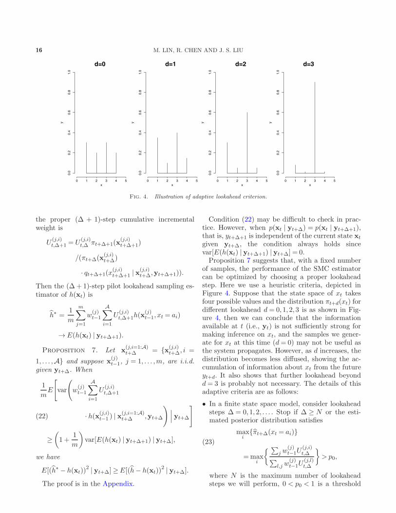
Fig. 4. Illustration of adaptive lookahead criterion.

the proper (∆ + 1)-step cumulative incrementalweight is

U(j,i)t,∆+1 = U

(j,i)t,∆ πt+∆+1(x

(j,i)t+∆+1)

/(πt+∆(x(j,i)t+∆)

· qt+∆+1(x(j,i)t+∆+1 | x

(j,i)t+∆,yt+∆+1)).

Then the (∆+ 1)-step pilot lookahead sampling es-timator of h(xt) is

h∗ =1

m

m∑

j=1

w(j)t−1

A∑

i=1

U(j,i)t,∆+1h(x

(j)t−1, xt = ai)

→E(h(xt) | yt+∆+1).

Proposition 7. Let x(j,i=1:A)t+∆ = {x

(j,i)t+∆, i =

1, . . . ,A} and suppose x(j)t−1, j = 1, . . . ,m, are i.i.d.

given yt+∆. When

1

mE

[var

(w

(j)t−1

A∑

i=1

U(j,i)t,∆+1

· h(x(j,i)t−1 ) | x

(j,i=1:A)t+∆ ,yt+∆

) ∣∣∣ yt+∆

](22)

≥

(1 +

1

m

)var[E(h(xt) | yt+∆+1) | yt+∆],

we have

E[(h∗ − h(xt))2 | yt+∆]≥E[(h− h(xt))

2 | yt+∆].

The proof is in the Appendix.

Condition (22) may be difficult to check in prac-tice. However, when p(xt | yt+∆) = p(xt | yt+∆+1),that is, yt+∆+1 is independent of the current state xt

given yt+∆, the condition always holds sincevar[E(h(xt) | yt+∆+1) | yt+∆] = 0.Proposition 7 suggests that, with a fixed number

of samples, the performance of the SMC estimatorcan be optimized by choosing a proper lookaheadstep. Here we use a heuristic criteria, depicted inFigure 4. Suppose that the state space of xt takesfour possible values and the distribution πt+d(xt) fordifferent lookahead d = 0,1,2,3 is as shown in Fig-ure 4, then we can conclude that the informationavailable at t (i.e., yt) is not sufficiently strong formaking inference on xt, and the samples we gener-ate for xt at this time (d= 0) may not be useful asthe system propagates. However, as d increases, thedistribution becomes less diffused, showing the ac-cumulation of information about xt from the futureyt+d. It also shows that further lookahead beyondd= 3 is probably not necessary. The details of thisadaptive criteria are as follows:

• In a finite state space model, consider lookaheadsteps ∆ = 0,1,2, . . . . Stop if ∆ ≥ N or the esti-mated posterior distribution satisfies

maxi

{πt+∆(xt = ai)}

(23)

=maxi

{ ∑j w

(j)t−1U

(j,i)t,∆∑

l,j w(j)t−1U

(j,l)t,∆

}> p0,

where N is the maximum number of lookaheadsteps we will perform, 0 < p0 < 1 is a threshold


close to 1, and U(j,i)t are the cumulative incre-

mental weights defined in (13).• In a continuous state space model, try lookahead

steps ∆ = 0,1,2, . . . . Stop if ∆ ≥ N or the esti-mated variance varπt+∆

(xt) satisfies

varπt+∆(xt) =

∑i,j w

(j)t−1U

(j,i)t,∆ (x

(j,i)t )2

∑i,j w

(j)t−1U

(j,i)t,∆

−

(∑i,j w

(j)t−1U

(j,i)t,∆ x

(j,i)t

∑i,j w

(j)t−1U

(j,i)t,∆

)2

(24)

< σ20 ,

where σ20 is a given threshold, x(j,i)t are samples

of current state generated from each x(j)t−1 under

the pilot scheme and U(j,i)t,∆ are the corresponding

cumulative incremental weights.

Some examples of using adaptive lookahead in fi-nite state space models and continuous state spacemodels are presented in Section 6.

6. APPLICATIONS

In this section we demonstrate the property oflookahead and make performance comparisons. Inall cases, δ, ∆ and ∆′ are used to denote the num-bers of lookahead steps in lookahead weighting, ex-act lookahead sampling and pilot lookahead sam-pling, respectively.

6.1 Signal Detection over Flat-Fading Channel

In a digital wireless communication problem (Chenand Liu, 2000; Wang, Chen and Guo, 2002), the re-ceived signal sequence {yt} is modeled as

yt = ξtxt + vt,

where {xt} is the transmitted complex digital sym-bol sequence, {vt} is the white complex Gaussiannoise with variance σ2 and independent real andcomplex components, and {ξt} is the transmittedchannel, which can be modeled as an ARMA pro-cess

ξt + φ1ξt−1 + · · ·+ φrξt−r

= θ0ut + θ1ut−1 + · · ·+ θrut−r,

where {ut} is a unit white complex Gaussian noise.In this example, we assume {ξt} follows the

ARMA(3,3) process (Guo, Wang and Chen, 2004)

ξt − 2.37409ξt−1 + 1.92936ξt−2 − 0.53208ξt−3

= 10−2(0.89409ut + 2.68227ut−1

+2.68227ut−2 +0.89409ut−3).

This system can be turned into a conditional dy-namic linear model (CDLM) as follows:

zt = Fzt−1 + gut,

yt = ξtxt + vt = hHztxt + vt,

where

F=

−φ1 −φ2 · · · −φr 01 0 · · · 0 00 1 · · · 0 0...

.... . .

......

0 0 · · · 1 0

, g=

10...0

,

h= [θ0θ1 · · ·θr]H .

Here we consider a high-constellation system witha 256-QAM modulation, thus the symbol space isA = {ai = (ai,1, ai,2) :ai,1, ai,2 = ±1,±3, . . . ,±15},where ai,1 and ai,2 are the real and imaginary partsof symbol ai, respectively. We decode {xt} from re-ceived {yt} under the framework of the mixture Kal-man filter of Chen and Liu (2000) and the “optimal-resampling” scheme of Fearnhead and Clifford (2003).Because the symbol space is large (|A| = 256),

we use a combination of the multilevel pilot looka-head sampling method and the lookahead weight-ing method. The multilevel structure used is simi-lar to that of 16-QAM presented in Figure 3. Thesymbol space is divided into subspaces of five dif-ferent levels (L= 4). Hence, at time t, we generate

(I(j)t,1 , I

(j)t,2 , I

(j)t,3 , I

(j)t,4 ) to obtain x

(j)t for given x

(j)t−1 se-

quentially.To construct the conditional trial distribution

qt,l(It,l | x(j)t−1, I

(j)t,l−1), we generate a deterministic pi-

lot (x(j,It,l)t , . . . , x

(j,It,l)t+∆′ ) for every possible It,l given

(x(j)t−1, I

(j)t,1 , . . . , I

(j)t,l−1) generated. The steps to gener-

ate the deterministic pilot are as follows:

• Predict channel ξt by ξ(j)t =E(ξt | x

(j)t−1, Yt−1). Let

x(j,It,l)t be the symbol ai ∈ Cl,It,l closest to yt/ξ

(j)t .

• For s= t+ 1, . . . , t+∆′, repeat the following:

– Predict channel ξs by ξ(j,It,l)s =E(ξs | x

(j)t−1, x

(j,It,l)t ,

. . . , x(j,It,l)s−1 ,ys−1).


– Choose symbol ai ∈ A closest to ys/ξ(j,It,l)s as

x(j,It,l)s .

Letting U(j,It,l)t = πt+∆′(x

(j)t−1, x

(j,It,l)t ,x

(j,It,l)t+1:t+∆′)/

πt−1(x(j)t−1), the trial distribution is

qt,l(It,l | x(j)t−1, I

(j)t,l−1) =

U(j,It,l)t∑

k:Cl,k⊂Cl−1,I

(j)t,l−1

U(j,k)t

.

For comparison, SMC without using the multi-level structure and lookahead pilot is also consid-ered. More computational details of this problemcan be found in Wang, Chen and Guo (2002).In the simulation, the length of transmitted sym-

bol sequences is 500. To avoid phase ambiguities,differential decoding is used. Specifically, supposethe information symbol sequence is {dt}. The actualtransmitted symbol sequence {xt} is constructed asfollows: given the 256 QAM transmitted symbol xt−1

and information symbol dt, we first map them tofour QPSK symbols (rxt−1,1, rxt−1,2, rxt−1,3, rxt−1,4)and (rdt,1, rdt,2, rdt,3, rdt,4), respectively. Let rxt,i =rdt,irxt−1,i, i= 1,2,3,4, and we map these four QPSKsymbols (rxt,1, rxt,2, rxt,3, rxt,4) back to 256-QAM asthe transmitted symbol xt. The differential receivercalculates r

dt,i= rxt,ir

∗xt−1,i

, where (xt−1, xt) are es-

timated (xt−1, xt) at the receiver, then decodes theinformation symbol dt as the 256-QAM symbol cor-responding to (r

dt,1, r

dt,2, r

dt,3, r

dt,4). To improve the

decoding accuracy of this high-constellation system,we also insert 10% symbols that are known to thereceiver into the transmitted symbol sequences peri-odically. The experiment is repeated 100 times. A to-tal of 50,000 symbols (400,000 bit information) aredecoded.Figure 5 reports the bit-error-ratio (BER) perfor-

mance of a different lookahead step δ of the looka-head weighting method with standard concurrentSMC sampling (∆ = 0,∆′ = 0). m= 200 samples areused. It is seen that the BER performance does notimprove further after δ ≥ 8 lookahead steps. We useδ = 10 in the following comparison.BER performance of pilot lookahead sampling meth-

ods with different lookahead steps ∆′ is shown inFigure 6. The number of Monte Carlo samples isadjusted so that each method takes approximatelythe same CPU time. From the result, it is seen thatthe multilevel pilot lookahead sampling method with∆′ = 1 has smaller BER than SMC without using

Fig. 5. BER performance of the lookahead weighting methodwith ∆= 0, ∆′ = 0, m= 200 and different δ in a 256-QAMsystem.

lookahead pilots. But when we use ∆′ = 2, the per-formance is worse. One of the reasons is that weuse the predicted channel to construct the pilot,which could be very different from the true chan-nel and severely mislead the sampling, especiallywhen the number of lookahead steps is large. Wealso implement the adaptive method. Here we useadaptive stop criteria (23) with p0 = 0.90. The re-sulting average number of lookahead steps is 0.195.Due to the saving in the smaller number of looka-

Fig. 6. BER performance of the multilevel pilot lookaheadsampling method with ∆= 0, δ = 10 but different ∆′ and num-ber of samples m in the 256-QAM system. The number ofsamples are chosen so that each of the methods takes approx-imately the same CPU time.


Table 1

Average RMSE1 for SMC with different lookahead methods. The same numbers of samples (m= 3000)are used in different methods. We use a single pilot lookahead (K = 1) unless stated otherwise.

Average lookahead steps in the adaptive lookahead method are reports in the parentheses

∆′ + δ

RMSE1 0 1 2 3 5 7 Time (sec.)

SMC (∆′ = 0) 3.128 1.011 0.828 0.817 0.818 0.819 0.113

SMC (∆′ = 1,A= 10,K = 16) – 1.009 0.824 0.813 0.812 0.813 5.952

SMC (∆′ = 1,A= 3) – 1.011 0.831 0.826 0.831 0.839 0.319SMC (∆′ = 2,A= 3) – – 0.838 0.844 0.860 0.876 0.405SMC (∆′ = 3,A= 3) – – – 0.846 0.885 0.913 0.504

SMC-S (∆′ = 1,A= 1) – 1.009 0.825 0.815 0.814 0.815 0.170SMC-S (∆′ = 2,A= 1) – – 0.825 0.815 0.815 0.815 0.197SMC-S (∆′ = 3,A= 1) – – – 0.816 0.816 0.816 0.224SMC-S (adpt∆′(0.244),A= 1) 0.995 0.834 0.815 0.814 0.816 0.817 0.147

SMC-S (∆′ = 1,A= 3) – 1.009 0.824 0.813 0.813 0.813 0.421SMC-S (∆′ = 2,A= 3) – – 0.824 0.813 0.813 0.813 0.498SMC-S (∆′ = 3,A= 3) – – – 0.814 0.814 0.813 0.576

head steps, larger Monte Carlo sample size is usedwith the same computational time. Its BER perfor-mance is slightly better than using the fixing pilotlookahead step ∆′ = 1.

6.2 Nonlinear Filtering

Consider the following nonlinear state space model(Gordon, Salmond and Smith, 1993):

state equation:

xt = 0.5xt−1 +25xt−1/(1 + x2t−1)

+ 8cos(1.2(t− 1)) + ut,

observation equation: yt = x2t/20 + vt,

where ut ∼ N(0, σ2), vt ∼ N(0, η2) are Gaussianwhite noise. In the simulation, we let σ = 1 andη = 1, and the length of observations is T = 100.We compare the performance of different lookaheadstrategies.In this nonlinear system, πt(xt | xt−1) cannot be

easily sampled from. Here we use the simple trialdistribution

qt(xt | xt−1) = πt−1(xt | xt−1) = gt(xt | xt−1)

and

qpilots (xs | xs−1) = gs(xs | xs−1).

We use SMC to denote the pilot lookahead samplingmethod for the continuous state space case. The im-plementation with smoothing step presented in Sec-tion 4.4 is denoted as SMC-S. A simple piecewise

constant function with interval width 0.5 is used forsmoothing. Resampling is applied at every step.We repeat the experiment 1000 times. The good-

ness-of-fit measures used are

RMSE1 =

[1

T

T∑

t=1

(xt − xt)2

]1/2

and

RMSE2 =

[1

T

T∑

t=1

(xt − Eπt+δ+∆′ (xt))2

]1/2,

where RMSE2 is a measurement of estimation vari-ance, I(δ +∆′) in (2). Here Eπδ+∆′ (xt) is obtained

by SMC (∆′ = 0) with a large number of samples(m= 200,000) and the lookahead weighting methodwith lookahead steps δ∗ = δ + ∆′. Tables 1 and 2report average RMSE1 and RMSE2 and the associ-ated CPU time of using different sampling methodsand m= 3000 samples. It can be seen that the de-layed methods can greatly reduce RMSE1 for smallδ + ∆′, but no further improvement can be foundwhen δ +∆′ ≥ 3. SMC with ∆′ = 1,A= 10,K = 16is an approximation of the exact lookahead samplingmethod with ∆ = 1. It has the smallest RMSE1 atthe cost of extensive computation, which confirmsProposition 3. The performance of SMC with a sin-gle pilot (K = 1) is poor because the future statespace cannot be efficiently explored by the small


Table 2

Average RMSE2 for SMC with different lookahead methods. The same numbers of samples (m= 3000)are used in different methods

∆′ + δ

RMSE2 0 1 2 3 5 7 Time (sec.)

SMC (∆′ = 0) 0.137 0.055 0.057 0.066 0.078 0.090 0.113

SMC (∆′ = 1,A= 10,K = 16) – 0.023 0.027 0.032 0.038 0.043 5.952

SMC (∆′ = 1,A= 3) – 0.070 0.105 0.138 0.174 0.203 0.319SMC (∆′ = 2,A= 3) – – 0.156 0.220 0.278 0.326 0.405SMC (∆′ = 3,A= 3) – – – 0.240 0.356 0.417 0.504



number of pilots. With the smoothing step, SMC-S can achieve better performance than the simplelookahead weighting method (SMC, ∆′ = 0). SMC-S with A = 3 has better performance than SMC-Swith A= 1, because when using A= 1, the pilot onlyaffects resampling and estimation, but not the sam-pling procedure. However, SMC-S with A = 3 alsotakes a longer CPU time.We also use the adaptive stop criteria (24) (adpt)

to choose the lookahead steps adaptively. In the cri-teria, we let σ20 = 4. The adaptive method has sim-ilar performance to the fixed-step pilot lookaheadsampling method, but much fewer average looka-head steps (average lookahead steps are only 0.244)and less CPU time.

For a fair comparison, Tables 3 and 4 report aver-age RMSE1 and RMSE2 of different methods withdifferent numbers of samples, which are chosen sothat each method used approximately the same CPUtime. In this table, SMC with A= 1 and the adap-tive lookahead scheme has the smallest RMSE1, whichdemonstrates the effectiveness of the adaptive looka-head strategy. It also shows that SMC-1 with ∆′ =1,A= 10,K = 16 has a large RMSE1, because of itshigh computational cost per sample.

6.3 Target Tracking in Clutter

Consider the problem of tracking a single target inclutter (Avitzour, 1995). In this example, the targetmoves with random acceleration in one dimension.

Table 3

Average RMSE1 for SMC with different lookahead methods. The numbers of samples are chosen so that each method usedapproximately the same CPU time. Average lookahead steps in the adaptive lookahead method are reports in the parentheses

∆′ + δ

RMSE1 0 1 2 3 5 7 Time (sec.)

SMC (m= 3000,∆′ = 0) 3.128 1.011 0.828 0.817 0.818 0.819 0.113

SMC (m= 60,∆′ = 1,A= 10,K = 16) – 1.079 0.911 0.906 0.912 0.920 0.125

SMC-S (m= 2000,∆′ = 1,A= 1) – 1.010 0.826 0.817 0.817 0.818 0.117SMC-S (m= 1700,∆′ = 2,A= 1) – – 0.827 0.818 0.817 0.819 0.116SMC-S (m= 1500,∆′ = 3,A= 1) – – – 0.820 0.822 0.823 0.118SMC-S (m= 2400, adpt∆′(0.245),A= 1) 0.994 0.835 0.816 0.815 0.817 0.818 0.104

SMC-S (m= 800,∆′ = 1,A= 3) – 1.015 0.832 0.821 0.821 0.822 0.108SMC-S (m= 700,∆′ = 2,A= 3) – – 0.827 0.817 0.816 0.817 0.111SMC-S (m= 600,∆′ = 3,A= 3) – – – 0.819 0.819 0.820 0.119


Table 4

Average RMSE2 for SMC with different lookahead methods. The numbers of samples are chosen so thateach method used approximately the same CPU time

∆′ + δ

RMSE2 0 1 2 3 5 7 Time (sec.)

SMC (m= 3000,∆′ = 0) 0.137 0.055 0.057 0.066 0.078 0.090 0.113

SMC (m= 60,∆′ = 1,A= 10,K = 16) – 0.228 0.254 0.277 0.306 0.334 0.125



The state equation can be written as(xt,1xt,2

)=

(1 10 1

)(xt−1,1

xt−1,2

)+

(1/21

)ut,

where xt,1 and xt,2 denote the one-dimensional lo-cation and velocity of the target, respectively; ut ∼N(0, σ2) is the random acceleration.At each time t, the target can be observed with

probability pd independently. If the target is ob-served, the observation is

zt = xt,1 + vt,

where vt ∼N(0, r2).In additional to the true observation, there are

false signals. Observation of false signals follows aspatially homogeneous Poisson process with rate λ.Suppose the observation window is wide and centersaround the predicted location of the target. Let Dbe the range of the observation window. The actualobservation yt includes nt detected signals, amongwhich at most one is the true observation. There-fore, nt follows a Bernoulli(pd) + Poisson(λD) dis-tribution.Define an indicator variable It as follows:

It =

{0, if the target is not detected at time t,k, if the kth signal in yt

is the true observation,

then we have

p(yt, It | xt)

∝

(1− pd)λ, if It = 0,

pd(2πr2)−1/2 exp{−(yt,k − xt)

2/2r2},

if It = k > 0.

In this system, given It = (I1, . . . , It), it becomes alinear Gaussian state space model. In such a system,the mixture Kalman filter (MKF) can be applied.The mixture Kalman filter only generates samples

of the indicators I(j)t and considers the state space as

discrete. Conditional on I(j)t and yt, the state vari-

able xt is normally distributed. The mean and the

variance of p(xt−δ | I(j)t ,yt) can be exactly calculated

through the Kalman filter. To perform lookaheadstrategies in MKF, suppose we can obtain samples

{(I(j)t+∆,w

jt ), j = 1, . . . ,m} properly weighted with re-

spect to πt+∆(It+∆) = p(It+∆ | yt+∆), then∑m

j=1w(j)t Eπt+∆

(xt−δ | It+∆ = I(j)t+∆)∑m

j=1w(j)t

is a consistent estimator of Eπt+∆(xt−δ), δ = 0,1, . . . .

More details of MKF and MKF with lookahead canbe found in Chen and Liu (2000) and Wang, Chenand Guo (2002).In this example, we can also use the smoothing

step presented in Section 4.4 to improve the perfor-mance of the pilot lookahead sampling method. It

can be shown that V(j,i)t+1:t+∆ =E(V

(j,i)t+1:t+∆ | I

(j)t−1, It =

i,yt+∆) in (16) only depends on the mean µ(j,i)t and

the variance Σ(j,i)t of the normal distribution p(xt |

I(j)t−1, It = i,yt). For simplicity, we approximately as-

sume V(j,i)t+1:t+∆ only depends on µ

(j,i)t = (µ

(j,i)t,1 , µ

(j,i)t,2 ),

that is,

V(j,i)t+1:t+∆ ≈ V t+1:t+∆(µ

(j,i)t ) + e

(j,i)t .

We then use the smoothed V(j,i)t+1:t+∆ to reduce the

variation introduced by random pilots. We denoted


Table 5

MAE1 and MAE2 for different lookahead methods. The same numbers of samples (m= 200) are used.The CPU time used in each experiment is 0.341 seconds for the lookahead weighting method (MKF, ∆= 0);3.554 seconds for the exact lookahead sampling method (MKF, ∆= 3); 0.783 seconds for the pilot lookahead

sampling method (MKF, ∆′ = 3), and 0.788 seconds for MKF-S (∆′ = 3)

∆+ δ/∆′ + δ

0 1 2 3 5 8 10 13 15

MAE1 MKF (∆= 0) 1.0300 0.7890 0.6560 0.5830 0.5180 0.4750 0.4590 0.4470 0.4450MKF (∆= 3) – – – 0.5780 0.5150 0.4710 0.4540 0.4410 0.4370MKF (∆′ = 3) – – – 0.5780 0.5150 0.4730 0.4560 0.4440 0.4420MKF-S (∆′ = 3) – – – 0.5730 0.5120 0.4690 0.4530 0.4410 0.4370

MAE2 MKF (∆= 0) 0.0932 0.0760 0.0618 0.0525 0.0460 0.0453 0.0467 0.0500 0.0520MKF (∆= 3) – – – 0.0463 0.0357 0.0307 0.0298 0.0298 0.0305MKF (∆′ = 3) – – – 0.0575 0.0503 0.0472 0.0480 0.0503 0.0525MKF-S (∆′ = 3) – – – 0.0490 0.0398 0.0360 0.0353 0.0365 0.0375

this method by MKF-S. We used the piecewise cons-

tant smoother to estimate V(j,i)t+1:t+∆. In the smoother,

the space [min{µ(j,i)t,1 },max{µ

(j,i)t,1 }] × [min{µ

(j,i)t,2 },

max{µ(j,i)t,2 }] is divided into 10× 10 equal parts.

In this example, we let σ2 = 0.1, r2 = 1.0, pd = 0.8,λ = 0.1, and D = 100r. The length of the observa-tion period is T = 100. We repeat the experiment500 times. The resampling step is applied when theeffective sample size is less than 0.1m.Following Avitzour (1995), we use the median ab-

solute error (MAE) as the performance measure-ment. Define

MAE1 =median{|xt,1 − xt,1|}

and

MAE2 =median{|xt,1 − Eπt+∆+δ(xt,1)|},

where xt,1 is the consistent estimation ofEπt+∆+δ

(xt,1) using different lookahead methods, and

Eπt+∆+δ(xt,1) is obtained by the lookahead weight-

ing method using a large number of samples (m=20,000).We first compare the performance of different look-

ahead methods using the same number of samples(m= 200). Table 5 reports MAE1 and MAE2 for thelookahead weighting method (MKF, ∆= 0), the ex-act lookahead sampling method (MKF, ∆= 3) andthe single pilot lookahead sampling method (MKF,∆′ = 3 and MKF-S, ∆′ = 3). From the result, MAE1

decreases as the number of lookahead steps increases,which shows the effectiveness of the lookahead strate-gies. The exact lookahead sampling method (MKF,∆= 3) has the smallest MAE2, which confirms Pro-

positions 3 and 5, although its computational costis the highest. We can also see that MKF-S (∆′ = 3)performs better than MKF (∆′ = 3).Then we compare the performance of different

methods under similar computational cost. The num-ber of samples is adjusted so that each method takesapproximately the same CPU time. Table 6 reportsthe quantiles of absolute estimation errors |xt,1 −xt,1| for different lookahead methods with lookaheadsteps ∆+ δ = 15 (or ∆′ + δ = 15). The performancedoes not improve further when ∆′ + δ ≥ 15. Underthe same CPU time, the lookahead sampling methodhas the largest absolute estimation error becauseof its high computational cost. The pilot lookaheadsampling method (MKF-S, ∆′ = 3) has better per-formance than the simple lookahead weighting meth-od (MKF, ∆= 0). We then use the stop criteria(24) to choose lookahead steps in the pilot lookaheadsampling method adaptively (MKF-S, adpt∆′).When we set σ20 = 1.5r2 in criteria (24), the averagenumber of lookahead steps is 1.572. The result showsthat the adaptive pilot lookahead sampling methodperforms the best under the same CPU time.

APPENDIX

Proof of Proposition 1. For any ∆2 >∆1 ≥0, we have

Eπt [E(h(xt) | yt+∆1)− h(xt)]2

=Eπt[E(h(xt) | yt+∆1)−E(h(xt) | yt+∆2)]2

+Eπt [E(h(xt) | yt+∆2)− h(xt)]2

+2Eπt{[E(h(xt) | yt+∆1)−E(h(xt) | yt+∆2)]

· [E(h(xt) | yt+∆2)− h(xt)]}.


Table 6

Quantiles of absolute estimation errors |xt,1 − xt,1| for different lookahead methods. The numbers of samplesare chosen so that each method used approximately the same CPU time. In the adaptive pilot lookahead

sampling method (MKF-S, adpt∆′),the average number of lookahead steps is 1.572

Quantiles (∆+ δ = 15)

0.05 0.25 0.50 0.75 0.95 Time (sec.)

MKF (m= 450,∆= 0) 0.0400 0.2040 0.4420 0.7910 1.7885 0.791MKF (m= 50,∆= 3) 0.0400 0.2080 0.4490 0.8120 2.1610 0.851MKF-S (m= 200,∆′ = 3) 0.0390 0.2030 0.4370 0.7790 1.6590 0.788MKF-S (m= 280, adpt∆′) 0.0390 0.2020 0.4340 0.7700 1.6295 0.802

Because

Eπt{[E(h(xt) | yt+∆1)−E(h(xt) | yt+∆2)]

· [E(h(xt) | yt+∆2)− h(xt)]}

=E{E{[E(h(xt) | yt+∆1)−E(h(xt) | yt+∆2)]

· [E(h(xt) | yt+∆2)− h(xt)] | yt+∆2} | yt}

= 0,

the conclusion holds. �

Proof of Proposition 2. It is easily seen that

Eπt+∆[w

(2,j)t h(x

(2,j)t ) | x

(j)t−1]

=Eπt+∆

[w

(j)t−1

πt+∆(x(2,j)t )


(2,j)t | x

(j)t−1)

· h(x(2,j)t ) | x

(j)t−1

]

=w(j)t−1

πt+∆(x(j)t−1)

πt−1(x(j)t−1)

·Eπt+∆

[h(x

(2,j)t )

πt+∆(x(2,j)t | x

(j)t−1)

qt(x(2,j)t | x

(j)t−1)

∣∣∣ x(j)t−1

]

=w(1,j)t Eπt+∆

(h(xt) | xt−1 = x(j)t−1).

Then (10) is a direct result of Rao-Blackwellization.By replacing h(xt) with Eπt+∆

(h(xt) | xt−1) andh(xt) = 1 in (10), we obtain (11) and (9), respec-tively. �

Proof of Proposition 3. Since

Eπt+∆{w

(3,j)t h(x

(j)t−1, x

(2,j)t ) | x

(j)t−1, x

(2,j)t }

=Eπt+∆

{h(x

(j)t−1, x

(2,j)t )

·

[w

(j)t−1

πt+∆(x(3,j)t+∆)

πt−1(x(j)t−1)

∏t+∆s=t qs(x

(3,j)s | x

(3,j)s−1 )

] ∣∣∣

x(j)t−1, x

(2,j)t

}

= h(x(j)t−1, x

(2,j)t )w

(j)t−1

πt+∆(x(j)t−1, x

(2,j)t )


(2,j)t | x

(j)t−1)

·Eπt+∆

{πt+∆(x

(3,j)t+1:t+∆ | x

(j)t−1, x

(2,j)t )

∏t+∆s=t+1 qs(x

(3,j)s | x

(3,j)s−1 )

∣∣∣

x(j)t−1, x

(2,j)t

}

=w(2,j)t h(x

(j)t−1, x

(2,j)t ),

we have

varπt+∆[w

(3,j)t h(x

(j)t−1, x

(2,j)t )]

≥ varπt+∆[w

(2,j)t h(x

(j)t−1, x

(2,j)t )]

according to the Rao-Blackwellization theorem. �

Proof of Proposition 4. To prove (x(j)t ,

waux(j)t ) is properly weighted with respect to dis-

tribution πt+∆(xt), we only need to prove

Eπt+∆[w

aux(j)t h(x

(j)t )] =Eπt+∆

[h(xt)].

According to the sampling distribution of the looka-

head pilot x(j,i)t+∆ and calculation of the corresponding

cumulative incremental weight U(j,i)t ,

Eπt+∆[w

aux(j)t h(x

(j)t ) | x

(j)t−1]

=Eπt+∆

[w

(j)t−1

A∑

i=1

U(j,i)t h(x

(j)t−1, xt = ai) | x

(j)t−1

]

=w(j)t−1

A∑

i=1

πt+∆(x(j)t−1, xt = ai)h(x

(j)t−1, xt = ai)

πt−1(x(j)t−1)


=w(j)t−1

πt+∆(x(j)t−1)

πt−1(x(j)t−1)

Eπt+∆[h(xt) | x

(j)t−1].

Because sample (x(j)t−1,w

(j)t−1) is properly weighted

with respect to πt−1(xt−1),

Eπt+∆

[w

(j)t−1

πt+∆(x(j)t−1)

πt−1(x(j)t−1)

Eπt+∆(h(xt) | x

(j)t−1)

]

=Eπt−1

[πt+∆(xt−1)

πt−1(xt−1)Eπt+∆

(h(xt) | xt−1)

]

=Eπt+∆[h(xt)];

the proposition follows. �

Proof of Proposition 5. Because waux(j)t and

w(1,j)t both are importance weights, we have

Eπt+∆(w

aux(j)t ) =Eπt+∆

(w(1,j)t ) = 1. Hence,

varπt+∆(w


(w(1,j)t )

=Eπt+∆(w

aux(j)t )2 −Eπt+∆

(w(1,j)t )2

=Eπt+∆{Eπt+∆

[(waux(j)t )2 | x

(j)t−1]

−Eπt+∆[(w

(1,j)t )2 | x

(j)t−1]}.

Now we consider the difference betweenEπt+∆

[(waux(j)t )2 | x

(j)t−1] and Eπt+∆

[(w(1,j)t )2 | x

(j)t−1].

Let

ε(j,i,k) =U(j,i,k)t −

πt+∆(x(j)t−1, xt = ai)

πt−1(x(j)t−1)

.

Because

Eπt+∆[U

(j,i,k)t | x

(j)t−1] =


πt−1(x(j)t−1)

,

we have Eπt+∆[ε(j,i,k) | x

(j)t−1] = 0. In addition, ε(j,i,k),

i= 1, . . . ,A, k = 1, . . . ,K are independent condition-

al on x(j)t−1, and for fixed i, ε(j,i,k), k = 1, . . . ,K, fol-

low the same distribution:

Eπt+∆[(w

aux(j)t )2 | x

(j)t−1]

= (w(j)t−1)

2Eπt+∆

[(A∑

i=1


πt−1(x(j)t−1)

+A∑

i=1

1

K

K∑

k=1

ε(j,i,k)

)2 ∣∣∣ x(j)t−1

]

= (w(j)t−1)

2Eπt+∆

[(πt+∆(x

(j)t−1)

πt−1(x(j)t−1)

)2 ∣∣∣ x(j)t−1

]

+ (w(j)t−1)

2Eπt+∆

[(A∑

i=1

1

K

K∑

k=1

ε(j,i,k)

)2 ∣∣∣ x(j)t−1

]

=Eπt+∆[(w

(1,j)t )2 | x

(j)t−1]

+1

K2(w

(j)t−1)

2A∑

i=1

K∑

k=1

Eπt+∆[(ε(j,i,k))2 | x

(j)t−1]

=Eπt+∆[(w

(1,j)t )2 | x

(j)t−1]

+1

K(w

(j)t−1)

2A∑

i=1

Eπt+∆[(ε(i,j,k=1))2 | x

(j)t−1].

Then we have

Eπt+∆[(w

aux(j)t )2 | x

(j)t−1]−Eπt+∆

[(w(1,j)t )2 | x

(j)t−1]

=1

K(w

(j)t−1)

2A∑

i=1

Eπt+∆[(ε(i,j,k=1))2 | x

(j)t−1],

hence,

0≤ varπt+∆(w


(w(1,j)t )

∼O(1/K).

With a similar method, we can prove

0≤ varπt+∆

[w

(j)t−1

A∑

i=1

1

K

K∑

k=1

U(j,i,k)t h(x

(j)t−1, xt = ai)

]

− varπt+∆[w

(1,j)t Eπt+∆

(h(x(j)t−1, xt) | x

(j)t−1)]

∼O(1/K). �

Proof of Proposition 6. Let ψt(xt)∝ rt(xt) ·bt(xt) be the distribution of samples after resam-

pling, Because Eπt+T(w

∗(j)t+T ) ≡ 1, we only consider

minimizing Eπt+T(w

∗(j)t+T )

2. We have

Eπt+T(w

∗(j)t+T )

2

=

∫π2t (xt)

ψ2t (xt)

[πt+T (xt+T )

πt(xt)∏t+T

s=t+1 qs(xs | xs−1)

]2ψt(xt)

·

t+T∏

s=t+1

qs(xs | xs−1)dxt dxt+1 · · ·dxt+T

=

∫π2t (xt)

ψt(xt)η(xt)dxt.

According to Jensen’s inequality, to minimize

Eπt+T(w

∗(j)t+T )

2, ψt(xt) needs to be proportional to

πt(xt)η1/2(xt). �


Proof of Proposition 7. For estimator h∗,because h∗ and h(xt) are independent conditionalon yt+∆+1, we have

E[(h∗ − h(xt))2 | yt+∆]

=E{E[[h∗ −E(h(xt) | yt+∆+1)

+E(h(xt) | yt+∆+1)− h(xt)]2 | yt+∆+1] | yt+∆}

=E[var(h∗ | yt+∆+1) | yt+∆]

+E[[E(h(xt) | yt+∆+1)− h(xt)]2 | yt+∆]

and for estimator h,

E[(h− h(xt))2 | yt+∆]

= var[h | yt+∆]

+E[[E(h(xt) | yt+∆)− h(xt)]2 | yt+∆].

Similar to the proof of Proposition 4, we have

E[[E(h(xt) | yt+∆)− h(xt)]2 | yt+∆]

−E[[E(h(xt) | yt+∆+1)− h(xt)]2 | yt+∆]

= var[E(h(xt) | yt+∆+1) | yt+∆].

Hence,

E[(h∗ − h(xt))2 | yt+∆]−E[(h− h(xt))

2 | yt+∆]

=E[var(h∗ | yt+∆+1) | yt+∆]− var[h | yt+∆]

− var[E(h(xt) | yt+∆+1) | yt+∆]

=1

mE

[var

(w

(j)t−1

A∑

i=1

U(j,i)t,∆+1

· h(x(j,i)t−1 ) | yt+∆+1

) ∣∣∣ yt+∆

]

−1

mvar

[w

(j)t−1

A∑

i=1

U(j,i)t,∆ h(x

(j,i)t−1 ) | yt+∆

](25)

− var[E(h(xt) | yt+∆+1) | yt+∆]

=1

m

{var

[w

(j)t−1

A∑

i=1

U(j,i)t,∆+1h(x

(j,i)t−1 ) | yt+∆

]

− var[E(h(xt) | yt+∆+1) | yt+∆]

− var

[w

(j)t−1

A∑

i=1

U(j,i)t,∆ h(x

(j,i)t−1 ) | yt+∆

]}

− var[E(h(xt) | yt+∆+1) | yt+∆]

=1

m

{var

[w

(j)t−1

A∑

i=1

U(j,i)t,∆+1h(x

(j,i)t−1 ) | yt+∆

]

− var

[w

(j)t−1

A∑

i=1

U(j,i)t,∆ h(x

(j,i)t−1 ) | yt+∆

]}

−

(1 +

1

m

)var[E(h(xt) | yt+∆+1) | yt+∆].

In the pilot lookahead sampling method, because

U(j,i)t,∆+1 = U

(j,i)t,∆ p(x

(j,i)t+∆+1 | yt+∆+1)

/(p(x

(j,i)t+∆ | yt+∆)

· qt+∆+1(x(j,i)t+∆+1 | x

(j,i)t+∆,yt+∆+1)

),

we have

E(U(j,i)t,∆+1h(x

(j,i)t ) | x

(j,i)t+∆,yt+∆)

=U(j,i)t,∆ h(x

(j,i)t )

·

∫(p(x

(j,i)t+∆+1 | yt+∆+1)

/(p(x(j,i)t+∆ | yt+∆)

· qt+∆+1(x(j,i)t+∆+1 | x

(j,i)t+∆,yt+∆+1)))

· qt+∆+1(x(j,i)t+∆+1 | x

(j,i)t+∆,yt+∆+1)

· p(yt+∆+1 | yt+∆)dx(j,i)t+∆+1 dyt+∆+1

=U(j,i)t,∆ h(x

(j,i)t ),

according to the Rao-Blackwellization theorem,

var

[w

(j)t−1

A∑

i=1

U(j,i)t,∆+1h(x

(j,i)t−1 ) | yt+∆

]

− var

[w

(j)t−1

A∑

i=1

U(j,i)t,∆ h(x

(j,i)t−1 ) | yt+∆

]

(26)

=E

[var

(w

(j)t−1

A∑

i=1

U(j,i)t,∆+1

· h(x(j,i)t−1 ) | x

(j,i=1:A)t+∆ ,yt+∆

) ∣∣∣ yt+∆

].

Combining (25) and (26), the conclusion holds. �


ACKNOWLEDGMENTS

Ming Lin’s research is supported by the NationalNature Science Foundation of China Grant 11101341and by the Fundamental Research Funds for theCentral Universities 2010221093. Rong Chen’s re-search is sponsored in part by NSF Grants DMS-08-00183, DMS-09-05076 and DMS-09-15139. JunLiu’s research was supported in part by NSF GrantsDMS-07-06989 and DMS-10-07762.

REFERENCES

Andrieu, C., Doucet, A. and Holenstein, R. (2010). Par-ticle Markov chain Monte Carlo methods. J. R. Stat. Soc.Ser. B Stat. Methodol. 72 269–342. MR2758115

Avitzour, D. (1995). Stochastic simulation Bayesian ap-proach to multitarget tracking. IEE Proceedings on Radar,Sonar and Navigation 142 41–44.

Briers, M., Doucet, A. and Maskell, S. (2010). Smooth-ing algorithms for state-space models. Ann. Inst. Statist.Math. 62 61–89. MR2577439

Carpenter, J., Clifford, P. and Fearnhead, P. (1999).An improved particle for non-linear problems. IEE Pro-ceedings on Radar, Sonar and Navigation 146 2–7.

Carter, C. K. and Kohn, R. (1994). On Gibbs sampling forstate space models. Biometrika 81 541–553. MR1311096

Carvalho, C. M., Johannes, M. S., Lopes, H. F. andPolson, N. G. (2010). Particle learning and smoothing.Statist. Sci. 25 88–106. MR2741816

Chen, R. and Liu, J. S. (2000). Mixture Kalman filters. J. R.Stat. Soc. Ser. B Stat. Methodol. 62 493–508. MR1772411

Chen, R., Wang, X. and Liu, J. S. (2000). Adaptive jointdetection and decoding in flat-fading channels via mixtureKalman filtering. IEEE Trans. Inform. Theory 46 2079–2094. MR1781368

Chopin, N. (2002). A sequential particle filter method forstatic models. Biometrika 89 539–551. MR1929161

Chopin, N. (2004). Central limit theorem for sequentialMonte Carlo methods and its application to Bayesian in-ference. Ann. Statist. 32 2385–2411. MR2153989

Clapp, T. C. and Godsill, S. J. (1997). Bayesian blinddeconvolution for mobile communications. In Proceedingsof IEE Colloqium on Adaptive Signal Processing for MobileCommunication Systems 9 1–6. IET.

Clapp, T. C. and Godsill, S. J. (1999). Fixed-lagsmoothing using sequential importance sampling. InBayesian Statistics 6 (J. M. Bernardo, J. O. Berger,A. P. Dawid and A. F. M. Smith, eds.) 743–752. OxfordUniv. Press, Oxford.

Crisan, D. and Lyons, T. (2002). Minimal entropy approx-imations and optimal algorithms. Monte Carlo MethodsAppl. 8 343–355. MR1943203

Del Moral, P. (2004). Feynman–Kac Formulae: Genealog-ical and Interacting Particle Systems with Applications.Springer, New York. MR2044973

Douc, R., Garivier, E., Moulines, E. and Olsson, J.

(2009). On the forward filtering backward smoothing par-

ticle approximations of the smoothing distribution in gen-eral state space models. Working paper, Institut Telecom,Paris.

Doucet, A., Briers, M. and Senecal, S. (2006). Efficientblock sampling strategies for sequential Monte Carlo meth-ods. J. Comput. Graph. Statist. 15 693–711. MR2280152

Doucet, A., de Freitas, N. and Gordon, N., eds. (2001).Sequential Monte Carlo Methods in Practice. Springer, NewYork. MR1847783

Fearnhead, P. (2002). Markov chain Monte Carlo, sufficientstatistics, and particle filters. J. Comput. Graph. Statist. 11848–862. MR1951601

Fearnhead, P. and Clifford, P. (2003). On-line inferencefor hidden Markov models via particle filters. J. R. Stat.Soc. Ser. B Stat. Methodol. 65 887–899. MR2017876

Fearnhead, P., Wyncoll, D. and Tawn, J. (2010). A se-quential smoothing algorithm with linear computationalcost. Biometrika 97 447–464. MR2650750

Fong, W., Godsill, S. J., Doucet, A. and West, M.

(2002). Monte Carlo smoothing with application to speekchenhancement. IEEE Trans. Signal Process. 50 438–449.

Gilks, W. R. and Berzuini, C. (2001). Following a movingtarget—Monte Carlo inference for dynamic Bayesian mod-els. J. R. Stat. Soc. Ser. B Stat. Methodol. 63 127–146.MR1811995

Godsill, S. J., Doucet, A. and West, M. (2004). MonteCarlo smoothing for non-linear time series. J. Amer.Statist. Assoc. 50 438–449.

Godsill, S. J. and Vermaak, J. (2004). Models and al-gorithms for tracking using trans-dimensional sequentialMonte Carlo. Proc. IEEE ICASSP 3 976–979.

Gordon, N. J., Salmond, D. J. and Smith, A. F. M.

(1993). Novel approach to nonlinear/non-GaussianBayesian state estimation. IEE Proceedings on Radar andSignal Processing 140 107–113.

Guo, D., Wang, X. and Chen, R. (2004). Multilevel mixtureKalman filter. EURASIP J. Appl. Signal Process. 15 2255–2266. MR2116229

Hurzeler, M. and Kunsch, H. R. (1995). Monte Carlo ap-proximations for general state space models. Research Re-port 73, ETH, Zurich.

Ikoma, N., Ichimura, N., Higuchi, T. and Maeda, H.

(2001). Maneuvering target tracking by using particle fil-ter. In Joint 9th IFSA World Congress and 20th NAFIPSInternational Conference 4 2223–2228. IEEE.

Kantas, N., Doucet, A., Singh, S. S. and Ma-

ciejowski, J. M. (2009). An overview of sequential MonteCarlo methods for parameter estimation in general state-space models. In 15th IFAC Symposium on System Identi-fication.

Kim, S., Shephard, N. and Chib, S. (1998). Stochasticvolatility: Likelihood inference and comparison with ARCHmodels. Review of Economic Studies 65 361–393.

Kitagawa, G. (1996). Monte Carlo filter and smoother fornon-Gaussian nonlinear state space models. J. Comput.Graph. Statist. 5 1–25. MR1380850

Kong, A., Liu, J. S. and Wong, W. H. (1994). Sequentialimputations and Bayesian missing data problems. J. Amer.Statist. Assoc. 89 278–288.

http://www.ams.org/mathscinet-getitem?mr=2758115



















Kotecha, J. H. and Djuric, P. M. (2003). Gaussian sum

particle filtering. IEEE Trans. Signal Process. 51 2602–

2612. MR2003067

Liang, J., Chen, R. and Zhang, J. (2002). Statistical geom-

etry of packing defects of lattice chain polymer from enu-

meration and sequential Monte Carlo method. J. Chem.

Phys. 117 3511–3521.

Lin, M. T., Zhang, J. L., Cheng, Q. and Chen, R. (2005).

Independent particle filters. J. Amer. Statist. Assoc. 100

1412–1421. MR2236451

Liu, J. S. (2001). Monte Carlo Strategies in Scientific Com-

puting. Springer, New York. MR1842342

Liu, J. S. and Chen, R. (1995). Blind deconvolution via se-

quential imputations. J. Amer. Statist. Assoc. 90 567–576.

Liu, J. S. and Chen, R. (1998). Sequential Monte Carlo

methods for dynamic systems. J. Amer. Statist. Assoc. 93

1032–1044. MR1649198

Liu, J. S., Chen, R. and Wong, W. H. (1998). Rejec-

tion control and sequential importance sampling. J. Amer.

Statist. Assoc. 93 1022–1031. MR1649197

Marshall, A. W. (1956). The use of multi-stage sampling

schemes in Monte Carlo computations. In Symposium on

Monte Carlo Methods (M. A. Meyer, ed.) 123–140. Wiley,New York.

Pitt, M. K. (2002). Smooth particle filters for likelihood andmaximisation. Technical report, Univ. Warwick.

Pitt, M. K. and Shephard, N. (1999). Filtering via simula-tion: Auxiliary particle filters. J. Amer. Statist. Assoc. 94590–599. MR1702328

Rosenbluth, M. N. and Rosenbluth, A. W. (1955). MonteCarlo calculation of the average extension of molecularchains. J. Chem. Phys. 23 356–359.

van der Merwe, R., Doucet, A., de Freitas, N. andWan, E. (2002). The unscented particle filter. In Advancesin Neural Information Processing Systems (NIPS13) (T.

K. Leen, T. G. Dietterich and V. Tresp, eds.). MITPress, Cambridge, MA.

Wang, X., Chen, R. andGuo, D. (2002). Delayed pilot sam-pling for mixture Kalman filter with application in fadingchannels. IEEE Trans. Signal Process. 50 241–264.

Zhang, J. L. and Liu, J. S. (2002). A new sequentialimportance sampling method and its application to thetwo-dimensional hydrophobic-hydrophilic model. J. Chem.Phys. 117 3492–3498.







Lookahead Strategies for Sequential Monte Carlo - arXiv

Documents

Transcript of Lookahead Strategies for Sequential Monte Carlo - arXiv