Controlled Sequential Monte Carlo - Oxford Statistics

Submitted to the Annals of StatisticsarXiv: arXiv:1708.08396

CONTROLLED SEQUENTIAL MONTE CARLO

By Jeremy Heng∗, Adrian N. Bishop†, GeorgeDeligiannidis‡ and Arnaud Doucet‡

ESSEC Business School∗, CSIRO and University of Technology Sydney†,and Oxford University‡

Sequential Monte Carlo methods, also known as particle methods,are a popular set of techniques for approximating high-dimensionalprobability distributions and their normalizing constants. These meth-ods have found numerous applications in statistics and related fields;e.g. for inference in non-linear non-Gaussian state space models, andin complex static models. Like many Monte Carlo sampling schemes,they rely on proposal distributions which crucially impact their per-formance. We introduce here a class of controlled sequential MonteCarlo algorithms, where the proposal distributions are determinedby approximating the solution to an associated optimal control prob-lem using an iterative scheme. This method builds upon a numberof existing algorithms in econometrics, physics, and statistics for in-ference in state space models, and generalizes these methods so asto accommodate complex static models. We provide a theoreticalanalysis concerning the fluctuation and stability of this methodologythat also provides insight into the properties of related algorithms.We demonstrate significant gains over state-of-the-art methods at afixed computational complexity on a variety of applications.

1. Introduction. Sequential Monte Carlo (SMC) methods have founda wide range of applications in many areas of statistics as they can beused, among others things, to perform inference for dynamic non-linear non-Gaussian state space models [32, 41, 33] but also for complex static models[39, 9, 13]; see [8, 17, 31] for recent reviews of this active area. Althoughthese methods are supported by theoretical guarantees [12], the number ofsamples required to achieve a desired level of precision of the correspondingMonte Carlo estimators can be prohibitively large in practice, especially sofor high-dimensional problems.

The present work is one means to address the computational difficultieswith SMC in offline inference settings. In particular, we leverage ideas fromoptimal control theory and we seek novel SMC methods that achieve a de-sired level of precision at a fraction of the computational cost of state-of-the-

MSC 2010 subject classifications: Primary 62M05; secondary 62F12, 62M10Keywords and phrases: State space models, annealed importance sampling, normalizing

constants, optimal control, approximate dynamic programming, reinforcement learning

1

http://www.imstat.org/aos/

http://arxiv.org/abs/arXiv:1708.08396

2 HENG ET AL.

art algorithms. We introduce a class of algorithms that will be referred to ascontrolled SMC, under which the sequence of SMC proposal distributionsare related naturally with an associated optimal control problem. The costfunctional is the Kullback–Leibler divergence from the sought after proposalsto the target distributions and we may account for an arbitrary current pro-posal estimate. With this formulation, the optimal proposal distributions arespecified by the optimal control policy of a related dynamic programmingrecursion. In general, this dynamic programming recursion is intractable.However, by making this connection, we can then exploit an array of meth-ods and procedures for so-called approximate dynamic programming (ADP).Broadly speaking, a single iteration of our proposed methodology involves:1) based on a current sequence of proposal distributions, running a SMCmethod to obtain a collection of samples that approximate the sequenceof SMC target distributions; 2) using these samples as support points, weapproximate intractable backward recursions using regression to computea new policy that specifies a new sequence of approximately optimal pro-posal distributions. Continuing in this manner allows us to further refine theproposal distributions and improve our approximation of the target distri-butions, via a novel iteration of SMC and ADP.

Prior influential work in [42] proposed a motivating method in the con-text of importance sampling, for computing the marginal likelihood in statespace models. In this contribution, the sequential structure which definesthe marginal likelihood is exploited and proposal distributions are definedby a sequence of parameterized Markov transition kernels. A criterion basedon the variance of importance weights is introduced to optimize these pa-rameters and an iterative procedure with fixed random numbers is proposed.The work of [47] extends [42] by employing these optimized proposal distri-butions within a SMC methodology. In particular, [47] identified the appro-priate importance weights one should use for resampling, which is crucialto ensure that the variance of the marginal likelihood estimator remainscontrolled. Moreover, [47] also recommends relaxing the use of common ran-dom variables across iterations. Recent work in [23], again with a focus ondiscrete time state space models, may be viewed as an extension of [47]where resampling is performed at every iteration, instead of just the last.The resulting algorithm is numerically much more stable than [42, 47]. Al-though the iterative procedures in [42, 47, 23] are similar in spirit to ourproposed methodology, the main and important difference is that all theseworks employ an optimality criterion, to learn proposal distributions, thatis not adjusted across iterations to account for any improvements made inprior iterations. Finally, we highlight related ideas in [29, 45] where the focus

CONTROLLED SEQUENTIAL MONTE CARLO 3

is partially observed diffusion models and the algorithms proposed thereinare based on other strategies to learn a parameterized additive control di-rectly. Such ideas have also been exploited in physics to perform rare eventsimulation for diffusions [40].

Our work extends these contributions in the following ways. Firstly, thesepreceding works [42, 47, 23] consider only state space models. In contrast, themethodology proposed here allows us to perform inference for static models;a direct extension of these prior methods [42, 47, 23] to static models isinfeasible, as it leads to algorithms which are not implementable.

Secondly, in contrast to the methodology in [42, 47, 23], the Kullback–Leibler optimality criterion at each iteration in our approach, is dependenton the approximately optimal proposal distributions computed at the pre-ceding iteration; i.e. we seek to minimize the residual discrepancy betweenany previously estimated proposals and the target distributions. This dif-ference allows us to elucidate the effect each iteration in our method hason refining proposal distributions and improves algorithmic performance asillustrated in Section 6.2. See also [49, 50] for related iterative procedures incontinuous-time optimal control approximation.

The controlled SMC methodology is one of the main contributions of thiswork. Another contribution is to provide a detailed theoretical analysis ofvarious aspects of our methodology. In Proposition 5.1, we provide a back-ward recursion that characterizes the error of policies estimated using ourADP procedure. This error is given naturally in terms of function approxima-tion errors with finite samples and the stability properties of the dynamicprogramming recursion defining the optimal policy, which is addressed inProposition 5.2. These results show that we can obtain good approxima-tions of the optimal policy and hence the optimal proposal distributions, ifthe function classes employed are ‘rich’ enough and the number of samplesused to learn policies is sufficiently large. In Theorem 5.1, we then establisha central limit theorem for our ADP algorithm as the number of samplesused in the policy learning goes to infinity. This reveals that the algorithmconcentrates around an idealized ADP algorithm and provides a precisecharacterization of how Monte Carlo errors correlate over time. These pre-ceding results concern a single iteration of our proposed method and may beapplied to the existing algorithms discussed above, e.g. [42, 47, 23]. Usingthe notion of iterated random functions, we introduce a novel frameworkin Theorem 5.2 to understand the asymptotic behaviour of our algorithmas the number of iterations converges to infinity. This elucidates the needfor iterating the ADP procedure and provides insight into the number of it-erations required in practice. The discussion surrounding Theorem 5.2 also

4 HENG ET AL.

emphasizes a key difference between the newly proposed method and ex-isting work in [42, 47, 23]. After the first version of this work appeared, asimilar approach was developed for generic stochastic control problems in[24]. Our results hold under strong assumptions but appear to capture ourexperimental results remarkably well.

The rest of this paper is organized as follows. We introduce SMC meth-ods in the framework of Feynman-Kac models [12] in Section 2 and twistedvariants in Section 3, as this affords us the generality to cover both statespace models and static models. We then identify the optimal policy that in-duces an optimal SMC method in Section 4.1. We describe general methodsto approximate the optimal policy in Section 4.2 and develop an iterativescheme to refine policies in Section 4.3. The proposed methodology is illus-trated on a neuroscience application in Section 4.4. We present the results ofour analysis in Section 5 and conclude with applications in Sections 6-7. Allproofs are given in the Supplementary Material which also includes threeadditional applications. MATLAB code to reproduce all numerical results isavailable online1.

2. Motivating models and sequential Monte Carlo.

2.1. Notation. We first introduce notation used throughout the article.Given integers n ≤ m and a sequence (xt)t∈N, we define the set [n : m] =n, . . . ,m and write the subsequence xn:m = (xn, . . . , xm). When n < m,we use the convention

∏nt=m xt = 1. Let (E, E) be an arbitrary measurable

space. We denote the set of all finite signed measures by S(E), the set of allprobability measures by P(E) ⊂ S(E), and the set of all Markov transitionkernels on (E, E) by M(E). Given µ, ν ∈ P(E), we write µ ν if µ is ab-solutely continuous w.r.t. ν and denote the corresponding Radon-Nikodymderivative as dµ/dν. For any x ∈ E, δx denotes the Dirac measure at x.The set of all real-valued, E-measurable, lower bounded, bounded or contin-uous functions on E are denoted by L(E), B(E) and C(E) respectively. Givenγ ∈ S(E) and M ∈ M(E), we define (γ ⊗ M)(dx, dy) = γ(dx)M(x,dy)and (M ⊗ γ)(dx,dy) = M(y,dx)γ(dy) as finite signed measures on theproduct space E × E, equipped with the product σ-algebra E × E . Givenγ ∈ S(E), M ∈M(E), ϕ ∈ B(E), ξ ∈ B(E×E), we define the integral γ(ϕ) =∫E ϕ(x)γ(dx), the signed measure γM(·) =

∫E γ(dx)M(x, ·) ∈ S(E) and

functions M(ϕ)(·) =∫E ϕ(y)M(·, dy) ∈ B(E), M(ξ)(·) =

∫E ξ(·, y)M(·,dy) ∈

B(E).

1Link: https://github.com/jeremyhengjm/controlledSMC

https://github.com/jeremyhengjm/controlledSMC


2.2. Feynman-Kac models. We begin by introducing Feynman-Kac mod-els [12] and defer a detailed discussion of their applications to Sections 2.3-2.4. Consider a non-homogeneous Markov chain of length T + 1 ∈ N on ameasurable space (X,X ), associated with an initial distribution µ ∈ P(X),and a collection of Markov transition kernels Mt ∈M(X) for t ∈ [1 : T ]. Wedenote the law of the Markov chain on path space XT+1, equipped with theproduct σ-algebra X T+1, with

(1) Q(dx0:T ) = µ(dx0)T∏t=1

Mt(xt−1,dxt)

and denote expectations w.r.t. Q by EQ, whereas we write Et,xQ for conditionalexpectations on the event Xt = x ∈ X. Given a sequence of strictly positivefunctions G0 ∈ B(X) and Gt ∈ B(X × X) for t ∈ [1 : T ], we define theFeynman-Kac path measure

(2) P(dx0:T ) = Z−1G0(x0)T∏t=1

Gt(xt−1, xt)Q(dx0:T )

where Z := EQ

[G0(X0)

∏Tt=1Gt(Xt−1, Xt)

]denotes the normalizing con-

stant. Equation (2) can be understood as the probability measure obtainedby repartitioning the probability mass of Q with the potential functions(Gt)t∈[0:T ].

To examine the time evolution of (2), we define the following sequence ofpositive signed measures γt ∈ S(X) for t ∈ [0 : T ] by

(3) γt(ϕ) = EQ

[ϕ(Xt)G0(X0)

t∏s=1

Gs(Xs−1, Xs)

]and their normalized counterparts ηt ∈ P(X) by

(4) ηt(ϕ) = γt(ϕ)/Zt

for ϕ ∈ B(X), t ∈ [0 : T ], where Zt := γt(X). Equations (3) and (4) areknown as the unnormalized and normalized (updated) Feynman-Kac mod-els respectively [12, Definition 2.3.2]. These models are determined by thetriple

µ, (Mt)t∈[1:T ], (Gt)t∈[0:T ]

, which depends on the specific application

of interest. The measure ηT is the terminal time marginal distribution of Pand Z = ZT = µ(G0)

∏Tt=1 ηt−1(Mt(Gt)).

2.3. State space models. Consider an X-valued hidden Markov chain (Xt)t∈[0:T ],

whose law on (XT+1,X T+1) is given by

H(dx0:T ) = ν(dx0)T∏t=1

ft(xt−1,dxt)

6 HENG ET AL.

where ν ∈ P(X) and ft ∈ M(X) for t ∈ [1 : T ]. The Y-valued observations(Yt)t∈[0:T ] are assumed to be conditionally independent given (Xt)t∈[0:T ] andthe conditional distribution of Yt has a strictly positive density gt(Xt, ·)with gt ∈ B(X× Y) for t ∈ [0 : T ]. Here

ν, (ft)t∈[1:T ], (gt)t∈[0:T ]

can poten-

tially depend on unknown static parameters θ ∈ Θ, but this is notationallyomitted for simplicity. Given access to a realization y0:T ∈ YT+1 of the obser-vation process, statistical inference for these models relies on the marginallikelihood of y0:T given θ,

Z(y0:T ) = EH

[T∏t=0

gt(Xt, yt)

],

and/or the smoothing distribution, i.e. the conditional distribution of X0:T

given Y0:T = y0:T and θ

(5) P(dx0:T |y0:T ) = Z(y0:T )−1T∏t=0

gt(xt, yt)H(dx0:T ).

If we set Q ∈ P(XT+1) defined in (1) equal to H, we recover the Feynman-Kac path measure representation (2) by defining Gt(xt−1, xt) = gt(xt, yt)for all t ∈ [0 : T ]. However, this representation is not unique. Indeed any Qsatisfying H Q provides a Feynman-Kac path measure representation of(2) by defining the potentials

G0(x0) =d(ν · g0)

dµ(x0), Gt(xt−1, xt) =

d(ft · gt)(xt−1,·)dMt(xt−1, ·)

(xt), t ∈ [1 : T ].

As outlined in [17], most SMC algorithms available at present correspond tothe same basic mechanism applied to different Feynman-Kac representationsof a given target probability measure. The bootstrap particle filter (BPF)presented in [22] corresponds to Q = H, i.e. Mt(xt−1,dxt) = ft(xt−1,dxt) fort ∈ [1 : T ], while the popular ‘fully adapted’ auxiliary particle filter (APF)of [41] uses Mt(xt−1,dxt) = P(dxt|xt−1, yt) ∝ ft(xt−1, dxt)gt(xt, yt).

As a motivating example, we consider a model for T + 1 = 3000 mea-surements collected from a neuroscience experiment [48]. The observationyt ∈ Y = [0 : M ] at each time instance t ∈ [0 : T ], shown in the left panel ofFigure 1, represents the number of activated neurons over M = 50 repeatedexperiments and is modelled as a binomial distribution with probabilityof success pt ∈ [0, 1]. We will write its probability mass function as yt 7→Bin(yt;M,pt). To model the time varying behaviour of activation probabili-ties, it is assumed that pt = κ(Xt) where κ(u) := (1 + exp(−u))−1 for u ∈ Ris the logistic link function and (Xt)t∈[0:T ] is a real-valued first-order autore-gressive process. This corresponds to a time homogeneous state space modelon X = R, equipped with its Borel σ-algebra X = B(R), with ν = N (0, 1),


500 1000 1500 2000 2500 3000

0

2

4

6

8

10

12

14

0 500 1000 1500 2000 2500

0

10

20

30

40

50

60

70

80

90

100

Fig 1. Number of activated neurons over M = 50 repeated experiments with time ( left)and effective sample size of bootstrap particle filter with N = 1024 particles ( right) for theneuroscience model with parameters α = 0.99 and σ2 = 0.11.

f(xt−1,dxt) = N (xt;αxt−1, σ2)dxt, and g(xt, yt) = Bin(yt;M,κ(xt)) for

t ∈ [1 : T ], where we denote the Gaussian distribution on Rd with meanvector ξ ∈ Rd and covariance matrix Σ ∈ Rd×d by N (ξ,Σ) and its Lebesguedensity by x 7→ N (x; ξ,Σ). The parameters of this model to be inferred fromdata are θ = (α, σ2) ∈ [0, 1]× R+.

2.4. Static models. Suppose we are interested in sampling from a targetdistribution η(dx) = Z−1γ(dx) ∈ P(X) and/or estimating its normalizingconstant Z = γ(X). To facilitate inference, we introduce a sequence of prob-ability measures (ηt)t∈[0:T ] in P(X) that bridges a simple distribution η0 = µto the target distribution ηT = η with η µ. Our implementation in Section7 adopts the geometric path [18, 39, 13]

(6) γt(dx) := µ(dx)

(dγ

dµ(x)

)λt, ηt(dx) := γt(dx)/Zt, t ∈ [0 : T ],

where Zt := γt(X) and (λt)t∈[0:T ] ∈ [0, 1]T+1 is an increasing sequence satis-fying λ0 = 0 and λT = 1; see [13, Section 2.3.1] for choices in other inferencesettings. In order to define Q, we introduce a sequence of ‘forward’ Markovtransition kernels Mt ∈ M(X) for t = [1 : T ] where ηt−1Mt approximatesηt. One expects the distribution η = η0M1 · · ·MT of samples drawn from anon-homogeneous Markov chain with initial distribution η0 and transitionkernels (Mt)t∈[1:T ] to be close to ηT = η. However, importance samplingcannot be employed to correct for the discrepancy between η and η, as η istypically analytically intractable.

SMC samplers described in [13] circumvent this difficulty by perform-ing importance sampling on path space (XT+1,X T+1) using an artificial

8 HENG ET AL.

extended target distribution of the form

P(dx0:T ) = η(dxT )T∏t=1

Lt−1(xt, dxt−1),

where Lt ∈ M(X) for t ∈ [0 : T − 1] is a sequence of auxiliary ‘backward’Markov transition kernels. Assuming that we have Lt−1 ⊗ γt γt−1 ⊗Mt

with strictly positive and bounded Radon-Nikodym derivative for all t ∈ [1 :T ], the Feynman-Kac path measure representation (2) can be recovered bydefining

(7) G0(x0) = 1, Gt(xt−1, xt) =d(Lt−1 ⊗ γt)d(γt−1 ⊗Mt)

(xt−1, xt), t ∈ [1 : T ].

Under these potentials, the normalized Feynman-Kac models (4) act as thesequence of bridging distributions (ηt)t∈[0:T ] in this setting. In annealed im-portance sampling (AIS) [39] and the sequential sampler proposed in [9], oneselects Mt ∈M(X) as a Markov chain Monte Carlo (MCMC) kernel that isηt-invariant and Lt−1 ∈M(X) as its time reversal, i.e. Lt−1 ⊗ ηt = ηt ⊗Mt,so the potentials in (7) simplify to

(8) G0(x0) = 1, Gt(xt−1) =γt(xt−1)

γt−1(xt−1), t ∈ [1 : T ].

3. Twisted models and sequential Monte Carlo.

3.1. Twisted Feynman-Kac models. SMC methods can perform poorlywhen the discrepancy between P and Q is large. The right panel of Fig-ure 1 illustrates that this is the case when we employ BPF on the neuro-science application in Section 2.3: the effective sample size (ESS), a com-mon criterion used to assess the quality of a particle approximation [33,p. 34–35], falls below 20% when the data change abruptly. This is becausethe kernel Mt(xt−1,dxt) = ft(xt−1,dxt) used to sample particles at timet does not take the observations into account. Better performance couldbe obtained using observation-dependent kernels. Indeed, in the contextof state space models, the smoothing distribution (5) can be written asP(dx0:T |y0:T ) = P(dx0|y0:T )

∏Tt=1 P(dxt|xt−1, yt:T ) with

P(dx0|y0:T ) =ν(dx0)ψ

∗0(x0)

ν(ψ∗0), P(dxt|xt−1, yt:T ) =

ft(xt−1, dxt)ψ∗t (xt)

ft(ψ∗t )(xt−1), t ∈ [1 : T ],

(9)

where the kernel ft(xt−1, ·) is twisted using the so-called backward informa-tion filter [5, 6], given by ψ∗t (xt) = P(yt:T |xt), for t ∈ [0 : T ].

The backward information filter can also be defined using the backward


recursion

ψ∗T (xT ) = gT (xT , yT ),

ψ∗t (xt) = gt(xt, yt)ft+1(ψ∗t+1)(xt), t ∈ [0 : T − 1].

(10)

We can exploit this to obtain an approximation ψt(xt), t ∈ [0 : T ] using re-gression [42, 47, 23]. We can then sample particles at time t using a proposal

M ψt (xt−1, dxt) ∝ ft(xt−1, dxt)ψt(xt) that approximates P(dxt|xt−1, yt:T ).Abstracting the above discussion from state space models to general

Feynman–Kac models, where the potential Gt might depend on both xt−1and xt, motivates the following definitions.

Definition 3.1. (Admissible policies) A sequence of functions ψ = (ψt)t∈[0:T ]is an admissible policy if these functions are strictly positive and satisfyψ0 ∈ B(X), ψt ∈ B(X × X) for all t ∈ [1 : T ]. The set of all admissiblepolicies will be denoted as Ψ.

Definition 3.2. (Twisted path measures) Given a policy ψ ∈ Ψ and apath measure F ∈ P(XT+1) of the form F(dx0:T ) = ν(dx0)

∏Tt=1Kt(xt−1, dxt)

for some ν ∈ P(X) and Kt ∈ M(X) for t ∈ [1 : T ], the ψ-twisted path mea-

sure of F is defined as Fψ(dx0:T ) = νψ(dx0)∏Tt=1K

ψt (xt−1,dxt) where

νψ(dx0) :=ν(dx0)ψ0(x0)

ν(ψ0), Kψ

t (xt−1,dxt) :=Kt(xt−1,dxt)ψt(xt−1, xt)

Kt(ψt)(xt−1), t ∈ [1 : T ].

(11)

For any policy ψ ∈ Ψ, since P Q Qψ by positivity of ψ, we canrewrite the measure P defined in (2) as

(12) P(dx0:T ) = Z−1Gψ0 (x0)

T∏t=1

Gψt (xt−1, xt)Qψ(dx0:T )

where the twisted potentials associated with the twisted path measure Qψ

are given by

Gψ0 (x0) :=µ(ψ0)G0(x0)M1(ψ1)(x0)

ψ0(x0),(13)

Gψt (xt−1, xt) :=Gt(xt−1, xt)Mt+1(ψt+1)(xt)

ψt(xt−1, xt), t ∈ [1 : T − 1],

GψT (xT−1, xT ) :=GT (xT−1, xT )

ψT (xT−1, xT ).

Note from (12) that Z = EQψ[Gψ0 (X0)

∏Tt=1G

ψt (Xt−1, Xt)

]by construc-

tion, whereas the tripleµψ, (Mψ

t )t∈[1:T ], (Gψt )t∈[0:T ]

induces the ψ-twisted

10 HENG ET AL.

Feynman-Kac models given by(14)

γψt (ϕ) = EQψ

[ϕ(Xt)G

ψ0 (X0)

t∏s=1

Gψs (Xs−1, Xs)

], ηψt (ϕ) = γψt (ϕ)/Zψt ,

for ϕ ∈ B(X), t ∈ [0 : T ], where Zψt := γψt (X). For t ∈ [0 : T − 1], themarginal distributions of the twisted model are given by

(15) ηψt (dxt) = ηt(dxt)Mt+1(ψt+1)(xt)Zt/Zψt

and do not generally coincide with the ones of the original model (4). How-ever, we stress that they coincide at time T as

(16) Z = ZψT = µψ(Gψ0 )

T∏t=1

ηψt−1(Mψt (Gψt )).

To illustrate the effect of twisting models in the static setting of Section2.4, rewriting the twisted potentials (13) using (15) as

Gψ0 (x0) =dηψ0dµψ

(x0), Gψt (xt−1, xt) =d(Lt−1 ⊗ γψt )

d(γψt−1 ⊗Mψt )

(xt−1, xt), t ∈ [1 : T ],

shows that this corresponds to employing the same backward kernels (Lt)t∈[0:T−1],

but altered bridging distributions (ηψt )t∈[0:T ], initial distribution µψ and for-

ward kernels (Mψt )t∈[1:T ].

3.2. Twisted sequential Monte Carlo. Consider a policy ψ ∈ Ψ such thatsampling from the initial distribution µψ ∈ P(X) and the transition ker-

nels (Mψt )t∈[1:T ] inM(X) is feasible and evaluation of the twisted potentials

(13) is tractable. We can now construct the ψ-twisted SMC method as sim-ply the standard sampling-resampling SMC algorithm applied to ψ-twistedFeynman-Kac models [17]. The resulting algorithm provides approximations

of the probability measures (ηψt )t∈[0:T ], normalizing constant Z and pathmeasure P, by simulating an interacting particle system of size N ∈ N. Analgorithmic description is detailed in Algorithm 1, where R (w1, . . . , wN )refers to a resampling operation based on a vector of unnormalized weights(wn)n∈[1:N ] ∈ RN+ . For example, this is the categorical distribution on [1 : N ]

with probabilities (wn/∑N

m=1wm)n∈[1:N ], when multinomial resampling isemployed; other lower variance and adaptive resampling schemes can alsobe considered [19]. All simulations presented in this article employ the sys-tematic resampling scheme.

Given the output of the algorithm, i.e. an array of X-valued position vari-ables (Xn

t )(t,n)∈[0:T ]×[1:N ] and an array of [1 : N ]-valued ancestor variables


Algorithm 1 ψ-twisted sequential Monte CarloInput: number of particles N ∈ N and policy ψ ∈ Ψ.

1. At time t = 0 and particle n ∈ [1 : N ]:

(a) sample Xn0 ∼ µψ;

(b) sample ancestor index An0 ∼ R(Gψ0 (X1

0 ), . . . , Gψ0 (XN0 )).

2. For time t ∈ [1 : T ] and particle n ∈ [1 : N ]:

(a) sample Xnt ∼Mψ

t (XAn

t−1t−1 , ·);

(b) sample ancestor index Ant ∼ R(Gψt (X

A1t−1

t−1 , X1t ), . . . , Gψt (X

ANt−1

t−1 , XNt ))

.

Output: trajectories (Xnt )(t,n)∈[0:T ]×[1:N ] and ancestries (Ant )(t,n)∈[0:T ]×[1:N ].

(Ant )(t,n)∈[0:T ]×[1:N ], we have a particle approximation of ηψt given by theweighted random measure

ηψ,Nt =

N∑n=1

Wψ,nt δXn

t, Wψ,n

t :=Gψt (X

Ant−1

t−1 , Xnt )∑N

m=1Gψt (X

Amt−1

t−1 , Xmt )

,

for t ∈ [1 : T ] (similar expression for t = 0) and an unbiased estimator of Zresembling the form of (16)

(17) Zψ,N =

1

N

N∑n=1

Gψ0 (Xn0 )

T∏t=1

1

N

N∑n=1

Gψt (XAnt−1

t−1 , Xnt )

.

With stored trajectories [26], we can also form a particle approximation ofP with Pψ,N = N−1

∑Nn=1 δXn

0:T, where Xn

0:T denotes the path obtained by

tracing the ancestral lineage of particle XnT , i.e. Xn

0:T := (XBntt )t∈[0:T ] with

BnT := AnT and Bn

t := ABnt+1

t for t ∈ [0 : T − 1]. Many convergence resultsare available for these approximations as the size N of the particle systemincreases [12]. However, depending on the choice of ψ ∈ Ψ, the qualityof these approximations may be inadequate for practical values of N ; forexample, the large variance of (17) often hinders its use within particleMCMC schemes [1] and the approximation Pψ,N could degenerate quicklywith T . The choice of an optimal policy is addressed in the following section.

4. Controlled sequential Monte Carlo.

4.1. Optimal policies. Suppose we have an arbitrary current policy ψ ∈Ψ, initially given by a sequence of constant functions. We would like to twistthe path measure Qψ ∈ P(XT+1) further with a policy φ ∈ Ψ, so that theresulting twisted path measure (Qψ)φ ∈ P(XT+1) is in some sense ‘closer’ to

12 HENG ET AL.

the target Feynman-Kac measure P. Note from Definition 3.2 that (Qψ)φ =Qψ·φ, where ψ · φ = (ψt · φt)t∈[0:T ] denotes element-wise multiplication, issimply the (ψ · φ)-twisted path measure of Q. From (13), the correspondingtwisted potentials are given by

Gψ·φ0 (x0) =µψ(φ0)G

ψ0 (x0)M

ψ1 (φ1)(x0)

φ0(x0),(18)

Gψ·φt (xt−1, xt) =Gψt (xt−1, xt)M

ψt+1(φt+1)(xt)

φt(xt−1, xt), t ∈ [1 : T − 1],

Gψ·φT (xT−1, xT ) =GψT (xT−1, xT )

φT (xT−1, xT ).

The choice of φ that optimally refines an arbitrary policy ψ is given bythe following optimality result.

Proposition 4.1. For any ψ ∈ Ψ, under the policy φ∗ = (φ∗t )t∈[0:T ]defined recursively as

φ∗T (xT−1, xT ) = GψT (xT−1, xT ),(19)

φ∗t (xt−1, xt) = Gψt (xt−1, xt)Mψt+1(φ

∗t+1)(xt), t ∈ [1 : T − 1],

φ∗0(x0) = Gψ0 (x0)Mψ1 (φ∗1)(x0),

the refined policy ψ∗ := ψ · φ∗ satisfies the following properties:

1. the twisted path measure Qψ∗ coincides with the Feynman-Kac pathmeasure P;

2. the normalized Feynman-Kac model ηψ∗

t is the time t-marginal distri-

bution of P and its normalizing constant Zψ∗

t = Z for all t ∈ [0 : T ];3. the normalizing constant estimator Zψ

∗,N = Z almost surely for anyN ∈ N.

Moreover, if Gψ0 ∈ B(X) and Gψt ∈ B(X× X) for t ∈ [1 : T ] then φ∗ ∈ Ψ.

This proposition implies that SMC sampling with the optimal ψ∗-twistedversion of Algorithm 1 ensures that the normalizing constant estimator isconstant over the entire time horizon, and is equal to the desired normalizingconstant. This follows because the SMC weights themselves are almost surelyconstant; one can see this by substituting the optimal choice (19) into (18).The variance of the SMC weights and the constancy of the normalizingconstant estimator can both be used (as described later) as measures ofperformance evaluation or adaptive tuning.

In a state space context, (19) corresponds to the recursion satisfied bythe backward information filter introduced in (10) when ψ ∈ Ψ are constant


functions, i.e. µψ = µ = ν and Mψt = Mt = ft, t ∈ [1 : T ]; see, e.g., [5, 6].

As it can be shown that φ∗ is the optimal policy of an associated Kullback–Leibler optimal control problem (Supplementary Material, Section 5), weshall refer to it as the optimal policy w.r.t. Qψ, although the optimalityproperties in Proposition 4.1 only identify a policy up to normalization fac-tors. An application of this result gives us the optimal policy ψ∗ = ψ·φ∗ w.r.t.Q, which is admissible if the original potentials (Gt)t∈[0:T ] are bounded2.

4.2. Approximate dynamic programming. Equation (19) may be viewedas a dynamic programming backward recursion. The optimal policy φ∗ w.r.t.Qψ will give rise to an optimally controlled SMC algorithm via a ψ∗ = (ψ ·φ∗)-twisted version of Algorithm 1. In all but simple cases, the recursion (19)defining φ∗ is intractable. We now exploit the connection to optimal controlby adapting numerical methods (i.e. approximate dynamic programming) forfinite horizon control problems [2, p. 329–331] to our setup. The resultingmethodology approximates φ∗ by combining function approximation anditerating the backward recursion (19).

In the following, we will approximate V ∗t := − log φ∗t , t ∈ [0 : T ] as thiscorresponds to learning the optimal value functions of the associated controlproblem. Compared to learning optimal policies directly, as considered in[23], the latter choice is often more desirable as computing in logarithmicscale offers more numerical stability and the minimization is additionallyanalytically tractable in important scenarios. Moreover, this allows us torelate regression errors to performance properties of the resulting twistedSMC method in the next section.

Let (Xnt )(t,n)∈[0:T ]×[1:N ] and (Ant )(t,n)∈[0:T ]×[1:N ] denote the trajectories

and ancestries, obtained by running a ψ-twisted SMC. At time T , to approx-imate V ∗T := − log φ∗T = − logGψT , we consider the least squares problem

VT = arg minϕ∈FT

N∑n=1

(ϕ(X

AnT−1

T−1 , XnT ) + logGψT (X

AnT−1

T−1 , XnT ))2,(20)

where FT is a pre-specified function class. An approximation of φ∗T can then

be obtained by taking φT := exp(−VT ). To iterate the backward recursion

φ∗T−1 = GψT−1MψT (φ∗T ), we set ξT−1 := GψT−1M

ψT (φT ) by plugging in the

2For ease of presentation, the notion of admissibility adopted in Definition 3.1 is morestringent than necessary as non-admissible optimal policies can still lead to valid optimalSMC methods.

14 HENG ET AL.

approximation φT ≈ φ∗T and consider the least squares problem

VT−1 = arg minϕ∈FT−1

N∑n=1

(ϕ(X

AnT−2

T−2 , XnT−1) + log ξT−1(X

AnT−2

T−2 , XnT−1)

)2,

(21)

where FT−1 is another function class to be specified. As before, we formthe approximation φT−1 := exp(−VT−1). Continuing in this manner untiltime 0 gives us an approximation φ = (φt)t∈[0:T ] of φ∗. We shall refer to thisprocedure as the approximate dynamic programming algorithm and providea detailed description in Algorithm 2.

Restricting the function classes (Ft)t∈[0:T ] to contain only lower bounded

functions ensures that the estimated policy φ lies in Ψ, hence the refinedpolicy ψ · φ also lies in Ψ. We defer a detailed discussion on the choice offunction classes and shall assume for now this is such that under the refinedpolicy ψ · φ ∈ Ψ, sampling from initial distribution µψ·φ ∈ P(X), transition

kernels (Mψ·φt )t∈[1:T ] inM(X) is feasible and evaluation of twisted potentials

(Gψ·φt )t∈[0:T ] is tractable.As the size of the particle system N increases, it is natural to expect

φ to converge (in a suitable sense) to a policy defined by an idealized al-gorithm that performs the least squares approximations in (20)-(21) usingL2-projections. This will be established in Section 5.2 for a common choiceof function class. It follows that the quality of φ, as an approximation of theoptimal policy φ∗, will depend on the number of particles N and the ‘rich-ness’ of chosen function classes (Ft)t∈[0:T ]. A more precise characterizationof the ADP error in terms of approximate projection errors will be given inSection 5.1.

4.3. Policy refinement. If the recursion (19) could be performed exactly,no policy refinement would be necessary as we would initialize ψ as a policyof constant functions and obtain the optimal policy ψ∗ = φ∗ w.r.t. Q. Thiswill not be possible in practical scenarios. Given a current policy ψ ∈ Ψ, weemploy ADP and obtain an approximation φ of the optimal policy φ∗ w.r.t.Qψ. The residuals from the corresponding least squares approximations (20)-(21) are given by

εψT := log φT − logGψT , εψt := log φt − logGψt − logMψt+1(φt+1), t ∈ [0 : T − 1].

From (18), these residuals are related to twisted potentials of the refinedpolicy ψ · φ via

logGψ·φ0 = logµψ(φ0)− εψ0 , logGψ·φt = −εψt , t ∈ [1 : T ].(22)


Algorithm 2 Approximate dynamic programmingInput: policy ψ ∈ Ψ and output of ψ-twisted SMC method (Algorithm 1).

1. Initialization: set MψT+1(φT+1)(Xn

T ) = 1 for n ∈ [1 : N ].

2. For time t ∈ [1 : T ]:

(a) set ξt(XAn

t−1t−1 , Xn

t ) = Gψt (XAn

t−1t−1 , Xn

t )Mψt+1(φt+1)(Xn

t ) for n ∈ [1 : N ];

(b) fit Vt = arg minϕ∈Ft∑Nn=1

(ϕ(X

Ant−1

t−1 , Xnt ) + log ξt(X

Ant−1

t−1 , Xnt ))2

;

(c) set φt = exp(−Vt).

3. At time t = 0:

(a) set ξ0(Xn0 ) = Gψ0 (Xn

0 )Mψ1 (φ1)(Xn

0 ) for n ∈ [1 : N ];

(b) fit V0 = arg minϕ∈F0∑Nn=1 (ϕ(Xn

0 ) + log ξ0(Xn0 ))2;

(c) set φ0 = exp(−V0).

Output: policy φ = (φt)t∈[0:T ] ∈ Ψ.

Using this relation, we can monitor the efficiency of ADP via the varianceof SMC weights in the (ψ · φ)-twisted version of Algorithm 1. It follows from

(22) that the Kullback–Leibler divergence from (Qψ)φ to P is at most

(23) | logµψ(φ0)− logZ|+ ‖εψ0 ‖L1(P0) +T∑t=1

‖εψt ‖L1(Pt−1,t)

where ‖ · ‖L1 denotes the L1-norm w.r.t. the one time (Pt)t∈[0:T ] and twotime (Pt,s)(t,s)∈[0:T−1]×[t+1:T ] marginal distributions of P. This shows how

performance of (ψ · φ)-twisted SMC depends on the quality of the ADPapproximation of the optimal policy w.r.t. Qψ.

If we further twist the path measure Qψ·φ by a policy ζ ∈ Ψ, the subse-quent ADP procedure defining ζ would consider the least squares problem

− log ζT := arg minϕ∈FT

N∑n=1

(ϕ(X

AnT−1

T−1 , XnT )− εψT (X

AnT−1

T−1 , XnT ))2,(24)

at time T , and for t ∈ [1 : T − 1]

− log ζt := arg minϕ∈Ft

N∑n=1

(ϕ(X

Ant−1

t−1 , Xnt )− (εψt − logMψ·φ

t+1(ζt+1))(XAnt−1

t−1 , Xnt ))2,

(25)

where (Xnt )(t,n)∈[0:T ]×[1:N ] and (Ant )(t,n)∈[0:T ]×[1:N ] denote the output of (ψ ·

φ)-twisted SMC. Equations (24)-(25) reveal that it might be beneficial to

16 HENG ET AL.

have an iterative scheme to refine policies as this allows repeated leastsquares fitting of residuals, in the spirit of L2-boosting methods [7]. More-over, it follows from (22)-(23) that errors would not accumulate over iter-ations. The resulting iterative algorithm, summarized in Algorithm 3, willbe referred to as the controlled SMC method (cSMC). The overall compu-tational complexity is of order I × T × (NCsampleCevaluate +Capprox), whereCsample(d) is the cost of sampling from each initial distribution or transitionkernel in (11), Cevaluate(d) is the cost of evaluating each twisted potentialin (13), and Capprox(N, d) is the cost of each least squares approximation3.The first iteration of the algorithm would coincide with that of [23] for statespace models, if regressions were computed on the natural scale; subsequentiterations differ in policy refinement strategy. To maintain a coherent ter-minology, we will refer to the standard SMC method and ψ∗-twisted SMCmethod as the uncontrolled and optimally controlled SMC methods respec-tively. From the output of the algorithm, we can estimate P with Pψ(I),N

and its normalizing constant Z with Zψ(I),N as explained in Section 3.2.

It is possible to consider performance monitoring and adaptive tuning forthe SMC sampling and the iterative policy refinement. Recalling the rela-tionship between residuals and twisted potentials (22), we note that moni-toring the variance of the SMC weights, using for example the ESS, allowsus to evaluate the effectiveness of the ADP algorithm and to identify timeinstances when the approximation is inadequate. We can also deduce if theestimated policy is far from optimal by comparing the behaviour of the nor-malizing constant estimates across time with those when the optimal policyis applied, as detailed in Proposition 4.1. When implementing Algorithm 3,the number of iterations I ∈ N can be pre-determined using preliminary runsor chosen adaptively until successive policy refinement yields no improve-ment in performance. For example, one can iterate policy refinement untilthe ESS across time achieves a desired minimum threshold and/or there is noimprovement in ESS across iterations; see Section 6.2 for a numerical illus-tration. In Section 5.3, under appropriate regularity assumptions, we showthat this iterative scheme generates a geometrically ergodic Markov chainon Ψ and characterize its unique invariant distribution. For all numericalexamples considered in this article, we observe that convergence happensvery rapidly, so only a small number of iterations is necessary.

3The dependence of these costs on their arguments will depend on the specific problemof interest and the choice of function classes. As an example, Capprox will depend linearlyon N in the case of linear least squares regression.


Algorithm 3 Controlled sequential Monte CarloInput: number of particles N ∈ N and iterations I ∈ N.

1. Initialization: set ψ(0) as constant one functions.

2. For iterations i ∈ [0 : I − 1]:

(a) run ψ(i)-twisted SMC method (Algorithm 1);

(b) perform ADP (Algorithm 2) with SMC output to obtain policy φ(i+1);

(c) construct refined policy ψ(i+1) = ψ(i) · φ(i+1).

3. At iteration i = I:

(a) run ψ(I)-twisted SMC method (Algorithm 1).

Output: trajectories (Xnt )(t,n)∈[0:T ]×[1:N ] and ancestries (Ant )(t,n)∈[0:T ]×[1:N ] from

ψ(I)-twisted SMC method.

4.4. Illustration on neuroscience model. We now apply our proposedmethodology on the neuroscience model introduced in Section 2.3. We takeBPF as the uncontrolled SMC method, i.e. we set µ = ν and Mt = f fort ∈ [1 : T ]. Under the following choice of function classes

(26) Ft =ϕ(xt) = atx

2t + btxt + ct : (at, bt, ct) ∈ R3

, t ∈ [0 : T ],

the policy ψ(i) = (ψ(i)t )t∈[0:T ] at iteration i ∈ [1 : I] of Algorithm 3 has the

form

ψ(i)t (xt) = exp

(−a(i)t x2t − b

(i)t xt − c

(i)t

), t ∈ [0 : T ],

where a(i)t :=

∑ij=1 a

jt , b

(i)t :=

∑ij=1 b

jt , c

(i)t :=

∑ij=1 c

jt for t ∈ [0 : T ] and

(aj+1t , bj+1

t , cj+1t )t∈[0:T ] denotes the coefficients estimated using linear least

squares at iteration j ∈ [0 : I − 1]. Exact expressions of the twisted initialdistribution, transition kernels and potentials, required to implement cSMCare given in Section 9.3 of Supplementary Material.

Figure 2 illustrates that the parameterization (26) provides a good ap-proximation of the optimal policy. We note (left panel) the significant im-provement of ESS across iterations, and see how this may be used as ameasure of performance evaluation. In the right panel, we can also deducehow far the estimated policy is from optimality by observing the behaviourof normalizing constant estimates as discussed previously. Indeed, while the

uncontrolled SMC approximates Zt = Zψ(0)

t = p(y0:t), the controlled SMC

scheme approximates Zψ∗

t = p(y0:T ) for all t ∈ [0 : T ].Moreover, we see from the left panel of Figure 3 that the improvement in

performance is reflected in the estimated policy’s ability to capture abruptchanges in the data. This plot also demonstrates the effect of policy refine-

18 HENG ET AL.

0 500 1000 1500 2000 2500

0

10

20

30

40

50

60

70

80

90

100

Uncontrolled

Iteration 1

Iteration 2

Iteration 3

0 500 1000 1500 2000 2500

-3000

-2500

-2000

-1500

-1000

-500

UncontrolledIteration 1Iteration 2Iteration 3

0 1000 2000

-3100

-3090

-3080

-3070

Fig 2. Comparison of uncontrolled and controlled SMC methods in terms of effectivesample size ( left) and normalizing constant estimation ( right) on the neuroscience modelintroduced in Section 2.3. The parameters are α = 0.99, σ2 = 0.11 and the algorithmicsettings of cSMC are I = 3, N = 128.

0 500 1000 1500 2000 2500 3000

-20

-15

-10

-5

0

5

10

15

20

25

Iteration 1

Iteration 2

Iteration 3

14 16 18 20 22 24

0

1

2

3

4

5

6

Fig 3. Applying controlled SMC method on the neuroscience model introduced in Section2.3: coefficients estimated at each iteration with N = 128 particles ( left) and invariantdistribution of coefficients with various number of particles ( right).

ment: by refitting residuals from previous iterations (24)-(25), the magni-tude of estimated coefficients decreases with iterations as the residuals canbe adequately approximated by simpler functions. Lastly, in the right panelof Figure 3, we illustrate the invariant distribution of coefficients estimatedby cSMC using a long run of I = 1000 iterations, with the first 10 iterationsdiscarded as burn-in. These plots show that the distribution concentratesas the size of the particle system N increases, which is consistent with ourfindings presented in Section 5.3.

5. Analysis. This section considers several theoretical aspects of theproposed methodology, and may be skipped without affecting the method-ological developments thus far and the experimental results that follow.


5.1. Policy learning. The goal of this section is to characterize the errorof ADP (Algorithm 2) for learning the optimal policy (19) in terms of regres-sion errors. We first define, for any µ ∈ P(E), the set L2(µ) of E-measurablefunctions ϕ : E → Rd such that ‖ϕ‖L2(µ) := (

∫E |ϕ(x)|2µ(dx))1/2 < ∞,

and L2(µ) as the set of equivalence classes of functions in L2(µ) that agreeµ-almost everywhere. To simplify notation, we introduce some operators.

Definition 5.1. (Bellman operators) Given ψ ∈ Ψ such that Gψ0 ∈ B(X)

and Gψt ∈ B(X× X) for t ∈ [1 : T ], we define the operators Qψt : L2(νψt+1)→L2(νψt ) for t ∈ [0 : T − 1] as

Qψ0 (ϕ)(x) = Gψ0 (x)Mψ1 (ϕ)(x), ϕ ∈ L2(νψ1 ),

Qψt (ϕ)(x, y) = Gψt (x, y)Mψt+1(ϕ)(y), ϕ ∈ L2(νψt+1),

where νψ0 := µψ ∈ P(X) and νψt := ηψt−1 ⊗Mψt ∈ P(X × X) for t ∈ [1 : T ].

For notational convenience define QψT (ϕ)(x, y) = GψT (x, y) for any ϕ (take

νψT+1 as an arbitrary element in P(X× X)).

Although these operators are typically used to define unnormalized pre-dictive Feynman-Kac models [12, Proposition 2.5.1], we shall adopt termi-nology from control literature and refer to them as Bellman operators. Itcan be shown that these Bellman operators are well-defined and are in factbounded linear operators – see Proposition 5.2. In this notation, we canrewrite (19) more succinctly as

φ∗T = GψT , φ∗t = Qψt φ∗t+1, t ∈ [0 : T − 1].(27)

To understand how regression errors propagate in time, for −1 ≤ s ≤ t ≤ T ,we define the Feynman-Kac semigroup Qψs,t : L2(νψt+1) → L2(νψs+1) associ-ated to a policy ψ ∈ Ψ as

(28) Qψs,t(ϕ) =

ϕ, s = t,

Qψs+1 · · · Qψt (ϕ), s < t,

for ϕ ∈ L2(νψt+1). To describe regression steps taken to approximate theintractable recursion (27), we introduce the following operations.

Definition 5.2. (Logarithmic projection) On a measurable space (E, E),let ν ∈ P(E), ξ : E → R+ be a E-measurable function such that − log ξ ∈L2(ν)∩L(E), and F ⊂ L(E) be a closed linear subspace of L2(ν). We definethe (F, ν)-projection operator P ν : B(E)→ B(E) as

(29) P νξ = exp(− arg min

ϕ∈F‖ϕ+ log ξ‖2L2(ν)

).

20 HENG ET AL.

The projection theorem gives existence of a unique P νξ. We have chosento define − logP νξ as the orthogonal projection of − log ξ onto F, as thiscorresponds to learning the optimal value functions of the associated controlproblem. Since projections are typically intractable, a practical implemen-tation will involve a Monte Carlo approximation of (29).

Definition 5.3. (Approximate projection) Following notation in Defi-nition 5.2, given a consistent approximation νN of ν, i.e. νN (ϕ) → ν(ϕ)almost surely for any ϕ ∈ L1(ν), we define the approximate (F, ν)-projectionoperator P ν,N : B(E) → B(E) as the (F, νN )-projection operator. We addi-tionally assume that the function class F is such that P ν,Nξ is a randomfunction for all ξ ∈ B(E).

If ψ ∈ Ψ is the current policy, we use the output of ψ-twisted SMC(Algorithm 1) to learn the optimal policy φ∗, through the empirical measures

(30) νψ,N0 =1

N

N∑n=1

δXn0, νψ,Nt =

1

N

N∑n=1

δ(XAnt−1t−1 , Xn

t

), t ∈ [1 : T ],

which are consistent approximations of (νψt )t∈[0:T ] [12], defined in Definition

5.1. Given pre-specified closed and linear function classes F0 ⊂ L2(νψ0 )∩L(X),

Ft ⊂ L2(νψt ) ∩ L(X2), t ∈ [1 : T ], we denote the approximate (Ft, νψt )-

projection operator by Pψ,Nt for t ∈ [0 : T ]. We can now write our ADPalgorithm detailed in Algorithm 2 succinctly as

φT = Pψ,NT GψT , φt = Pψ,Nt Qψt φt+1, t ∈ [0 : T − 1].(31)

The following result characterizes how well (31) can approximate (27).

Proposition 5.1. Suppose that we have a policy ψ ∈ Ψ, number ofparticles N and closed, linear function classes F0 ⊂ L2(νψ0 ) ∩ L(X), Ft ⊂L2(νψt ) ∩ L(X2), t ∈ [1 : T ] such that:

[A1] the Feynman-Kac semigroup defined in (28) satisfies

(32) ‖Qψs,t(ϕ)‖L2(νψs+1)

≤ Cψs,t‖ϕ‖L2(νψt+1), −1 ≤ s < t ≤ T − 1,

for some Cψs,t ∈ [0,∞) and all ϕ ∈ L2(νψt+1);

[A2] the approximate (Ft, νψt )-projection operator satisfies

supξ∈Sψt

Eψ,N‖Pψ,Nt ξ − ξ‖L2(νψt )

≤ eψ,Nt <∞

where Sψt := Qψt exp(−ϕ) : ϕ ∈ Ft+1 for t ∈ [0 : T − 1] and SψT := GψT .


Then the policy φ ∈ Ψ generated by ADP algorithm (31) satisfies

(33) Eψ,N‖φt − φ∗t ‖L2(νψt )≤

T∑u=t

Cψt−1,u−1eψ,Nu , t ∈ [0 : T ],

where Cψt−1,t−1 = 1 and Eψ,N denotes expectation w.r.t. the law of the ψ-twisted SMC method (Algorithm 1).

Equation (33) reveals how function approximation errors propagate back-wards in time. If the choice of function class is ‘rich’ enough and the numberof particles is sufficiently large, then these errors can be kept small andADP provides a good approximation of the optimal policy. If the number ofparticles is taken to infinity, the projection errors are driven solely by thechoice of function class (as the latter dictates eψ,∞t ). Moreover, observe thatthese errors are also modulated by stability constants of the Feynman-Kacsemigroup in (32). We now establish the inequality (32). For ϕ ∈ B(E), wewrite its supremum norm as ‖ϕ‖∞ = supx∈E |ϕ(x)|.

Proposition 5.2. Suppose ψ ∈ Ψ is such that Gψ0 ∈ B(X), Gψt ∈ B(X×X) for t ∈ [1 : T ] and let δ := maxt∈[0:T ] ‖G

ψt ‖∞ (and Zψ−1 := 1). Then (32)

holds with

Cψs,t =

(Zψt /Z

ψs

t∏u=s+1

‖Gψu‖∞)1/2

≤(Zψt /Z

ψs

)1/2δ(t−s)/2, −1 ≤ s < t ≤ T − 1.(34)

For the case Gψt (x, y) = Gψt (y) for all x, y ∈ X and t ∈ [1 : T ], if we assumeadditionally for each t ∈ [1 : T ] that:

[A3] there exist σψt ∈ P(X) and κψt ∈ (0,∞) such that for all x ∈ X we have

(35) Mψt (x,dy) ≤ κψt σ

ψt (dy).

Then inequality (32) holds with

(36) Cψs,t =

[κψs+2 ‖G

ψs+1‖∞ σ

ψs+2

(Qψs+1,t(1)

) ZψtZψs

]1/2, −1 ≤ s < t ≤ T−1.

The assumption of bounded potentials is typical in similar analyses ofADP errors [21, Section 8.3.3] and stability of SMC methods [12]. The sec-ond part of Proposition 5.2 shows that it is possible to exploit regularityproperties of the transition kernels to obtain better constants Cψs,t. Condi-tions such as (35) are common in the filtering literature, see for example [14,Eq. (9)] and [12, ch. 4].

22 HENG ET AL.

5.2. Limit theorems. We now study the asymptotic behaviour of theADP algorithm (31), with a current policy ψ ∈ Ψ, as the size of the particlesystem N grows to infinity. For a common choice of function class, we willestablish convergence to a policy φ = (φt)t∈[0:T ], defined by the idealizedalgorithm

φT = PψT GψT , φt = Pψt Q

ψt φt+1, t ∈ [0 : T − 1],(37)

where Pψt denotes the (Ft, νψt )-projection operator for t ∈ [0 : T ]. In par-

ticular, we consider logarithmic projections that are defined by linear leastsquares approximations; this corresponds to function classes of the form

(38) Ft :=

ΦTt β : β ∈ RM

, t ∈ [0 : T ],

where Φ0 ⊂ L2(νψ0 ) ∩ L(X), Φt ⊂ L2(νψt ) ∩ L(X2), t ∈ [1 : T ] are vectors ofM ∈ N pre-specified basis functions. We will treat M as fixed in our analysisand refer to [21, Theorem 8.2.4] for results on how M should increase with Nto balance the tradeoff between enriching (38) and the need for more samplesto achieve the same estimation precision. We denote by φ := (φt)t∈[0:T ] the

policy generated by the idealized algorithm (37) where φt := exp(−ΦTt β

ψt ),

βψt being the corresponding least squares estimate. This result builds uponthe central limit theorem for particle methods established in [10, 12, 30].

Theorem 5.1. Consider the ADP algorithm (31) with current policyψ ∈ Ψ, under linear least squares approximations (38). Under appropriateregularity conditions, for all x ∈ X2T+1, the estimated policy φ(x) convergesin probability to the policy φ(x) as N →∞. Moreover, for all x ∈ X2T+1,

(39)√N(φ(x)− φ(x)

)d−→ N

(0(T+1),Ω

ψ(x))

for some Ωψ : X2T+1 → R(T+1)×(T+1), whered−→ denotes convergence in

distribution and 0p = (0, . . . , 0)T ∈ Rp is the zero vector.

A precise mathematical statement of this result and its proof are givenin Section 3 of Supplementary Material. Note that the proof relies on atechnical central limit theorem on path space that can be deduced in thecase of multinomial resampling from [12, Theorem 9.7.1]. The exact form ofΩψ reveals how errors correlate over time and suggests that we may expectthe variance of the estimated policy to be larger at earlier times, due to theinherent backward nature of the ADP approximation.

5.3. Iterated approximate dynamic programming. We provide here a the-oretical framework to understand the qualitative behaviour of policy ψ(I),estimated by Algorithm 3, as the number of iterations I grows to infin-


ity. This offers a novel perspective of iterative algorithms for finite horizonoptimal control problems and may be of general interest.

To do so, we require the set of all admissible policies to be a completeseparable metric space. This follows if we impose that X is a compact metricspace and work with Ψ := C(X)

∏Tt=1 C(X × X), equipped with the metric

ρ(ϕ, ξ) :=∑T

t=0 ‖ϕt − ξt‖∞ for ϕ = (ϕt)t∈[0:T ], ξ = (ξt)t∈[0:T ] ∈ Ψ; non-compact state spaces can also be accommodated with a judicious choice ofmetric (see e.g. [4, p. 380]).

We begin by writing the iterative algorithm with N ∈ N particles as aniterated random function FN : U×Ψ→ Ψ, defined by FNU (ψ) = ψ·φ, where φis the output of ADP algorithm (31) and U ∈ U encodes all uniform randomvariables needed to simulate a ψ-twisted SMC method (Algorithm 1). Asthe uniform variables (U (I))I∈N used at every iteration are independent andidentically distributed, iterating FN defines a Markov chain (ψ(I))I∈N onΨ. We will write E to denote expectation w.r.t. the law of (U (I))I∈N andπ(I) ∈ P(Ψ) to denote the law of ψ(I). Similarly, we denote the iterativescheme with exact projections by F : Ψ → Ψ, defined as F (ψ) = ψ · φ,where φ is the output of the idealized ADP algorithm (37). We denote byϕ∗ ∈ Ψ a fixed point (if it exists) of F , i.e. F (ϕ∗) = ϕ∗. The following isbased on results developed in [15].

Theorem 5.2. Assume that the iterated random function FN satisfies:[A4] E

[ρ(FNU (ϕ0), ϕ0)

]<∞ for some ϕ0 ∈ Ψ,

[A5] there exists a measurable function LN : U → R+ with E[LNU]< α

for some α ∈ [0, 1) such that ρ(FNU (ϕ), FNU (ξ)) ≤ LNU ρ(ϕ, ξ) for all ϕ, ξ ∈ Ψ.Then the Ψ-valued Markov chain (ψ(I))I∈N generated by Algorithm 3 ad-

mits a unique invariant distribution π ∈ P(Ψ) and

(40) %(π(I), π) ≤ C(ψ(0))rI , I ∈ N,for some C : Ψ → R+ and r ∈ (0, 1), where % denotes the Prohorov metricon P(Ψ) induced by the metric ρ. If we suppose in addition that:

[A6] for each ψ ∈ Ψ, ρ(FNU (ψ), F (ψ)) ≤ N−1/2Eψ,NU where (Eψ,NU )N∈N isa uniformly integrable sequence of non-negative random variables with finitemean that converges in distribution to a limiting distribution with supporton R+, then we also have that

(41) Eπ [ρ(ψ,ϕ∗)] ≤ N−1/2E[Eϕ∗,N

U

](1− α)−1

where ϕ∗ is a fixed point of F and Eπ denotes expectation w.r.t. ψ ∼ π.

Assumption A5 requires the ADP procedure to be sufficiently regular: i.e.for two policies ϕ, ξ ∈ Ψ that are close, given the same uniform random vari-

24 HENG ET AL.

ables U to simulate a ϕ-twisted and ξ-twisted SMC method, the policies ϕ(w.r.t. Qϕ) and ξ (w.r.t. Qξ) estimated by (31) should also be close enoughto keep the Lipschitz constant LNU small. Assumption A6 is necessary toquantify the Monte Carlo error involved when employing approximate pro-jections and can be deduced for example using the central limit theorem in(39). See Section 4 of the Supplementary Material for a discussion on whenand why contraction occurs, and a simple example where Assumptions A4-A6 are verified.

The first part of Theorem 5.2, which establishes existence of a uniqueinvariant distribution and geometric convergence to the latter, follows fromstandard theory on iterated random functions; see, e.g., [15]. The secondconclusion of Theorem 5.2, which provides a characterization of the limitingdistribution, is to the best of our knowledge novel. The fixed point ϕ∗ canbe interpreted as a policy for which subsequent refinement using exact (i.e.with N →∞) projections onto the same function classes yields no change.

6. Application to state space models.

6.1. Neuroscience model. We return to the neuroscience model intro-duced in Section 2.3 and explore cSMC’s utility as a smoother, with algorith-mic settings described in Section 4.4, in comparison to the forward filteringbackward smoothing (FFBS) procedure of [16, 31]. We consider an approxi-mation of the maximum likelihood estimate (MLE) (α, σ2) = (0.99, 0.11) asparameter value and the smoothing functional x0:T 7→ M(κ(x0), ..., κ(xT ))whose expectation represents the expected number of activated neurons ateach time. Although BPF’s particle approximation of the smoothing dis-tribution degenerates quickly in time, cSMC with I = 3 iterations offers amarked improvement: for example, the number of distinct ancestors at theinitial time is on average 63 times that of BPF. We use N = 1024 particlesfor cSMC and select the number of particles in FFBS to match computetime. The results, displayed in the left panel of Figure 4, show some gainsover FFBS and especially so at later times.

We then investigate the relative variance of the log-marginal likelihoodestimates obtained using cSMC and BPF in a neighbourhood of the ap-proximate MLE. As the marginal likelihood surface is rather flat in α, wefix α = 0.99 and vary σ2 ∈ 0.01, 0.02, . . . , 0.2. We use I = 3 iterations,N = 128 particles for cSMC and N = 5529 particles for BPF to matchcomputational cost. The results, reported in the right panel of Figure 4,demonstrate that while the relative variance of estimates produced by BPFincreases exponentially as σ2 decreases, that of cSMC is stable across thevalues of σ2 considered.


0 500 1000 1500 2000 2500 3000

-4

-3.5

-3

-2.5

-2

-1.5

-1

-0.5

FFBS

cSMC

0.05 0.1 0.15 0.2

-9.5

-9

-8.5

-8

-7.5

-7

-6.5

-6 BPF

cSMC

Fig 4. Assessing performance on the neuroscience model introduced in Section 2.3 basedon 100 independent repetitions of each algorithm: sample relative variance of smoothingexpectation ( left) and log-marginal likelihood estimates ( right).

Lastly, we perform Bayesian inference on the unknown parameters θ =(α, σ2) and compare the efficiency of cSMC and BPF within a particlemarginal Metropolis–Hastings (PMMH) algorithm [1]. We specify a uniformprior on [0, 1] for α and an independent inverse-Gamma prior distributionIG(1, 0.1) for σ2. Initializing at θ = (0.99, 0.11), we run two PMMH chains(θcSMCk )k∈[0:K], (θBPF

k )k∈[0:K] of length K = 100, 000. Both chains are up-dated using an independent Gaussian random walk proposal with standarddeviation (0.002, 0.01), but rely on cSMC or BPF to produce unbiased esti-mates of the marginal likelihood when computing acceptance probabilities.To ensure a fair comparison, we use I = 3 iterations and N = 128 particlesfor cSMC which matches the compute time taken by BPF with N = 5529particles, so that both PMMH chains require very similar computationalcost. The autocorrelation functions of each PMMH chain, shown in Figure5, reveal that the (θBPF

k )k∈[0:K] chain has poorer mixing properties. Thesedifferences can be summarized by the effective sample size, computed as thelength of the chain K divided by the estimated integrated autocorrelationtime for each parameter of interest, which was found to be (4356, 2442) for(θBPFk )k∈[0:K] and (20973, 13235) for (θcSMC

k )k∈[0:K].

6.2. The Lorenz-96 model. Following [38], we consider the Lorenz-96model [34] in a low noise regime, i.e. the Ito process ξ(s) = (ξi(s))i∈[1:d], s ≥ 0defined as the weak solution of the stochastic differential equation:

(42) dξi = (−ξi−1ξi−2 + ξi−1ξi+1 − ξi + α) dt+ σfdBi, i ∈ [1 : d],

where indices should be understood modulo d, α ∈ R is a forcing param-eter, σ2f ∈ R+ is a noise parameter and B(s) = (Bi(s))i∈[1:d], s ≥ 0 is ad-dimensional standard Brownian motion. The initial condition is taken as

26 HENG ET AL.

0 10 20 30 40 50

0

0.1

0.2

0.3

0.4

0.5

0.6

0.7

0.8

0.9

1

BPF

cSMC

0 10 20 30 40 50

0

0.1

0.2

0.3

0.4

0.5

0.6

0.7

0.8

0.9

1

BPF

cSMC

Fig 5. Autocorrelation functions of PMMH chains, with marginal likelihood estimatesproduced by cSMC or BPF, for parameters of the neuroscience model introduced in Section2.3.

ξ(0) ∼ N (0d, σ2fId). We assume that the process is observed at a regular

time grid of size h > 0 according to Yt ∼ N (Hξ(st), R), st = th, t ∈ [0 : T ],and consider the partially observed case where Hii = 1 for i = 1, . . . , p and0 otherwise with p = d− 2.

As discussed in [38], an efficient discretization scheme in this low noiseregime [36, ch. 3] is given by adding Brownian increments to the output of ahigh-order numerical integration scheme on the drift of (42). Incorporatingtime discretization gives a time homogenous state space model on (X,X ) =(Rd,B(Rd)) with ν = N (0d, σ

2fId), f(xt−1, dxt) = N (xt; q(xt−1), σ

2fhId)dxt

and g(xt, yt) = N (yt;Hxt, R) for t ∈ [1 : T ], where y0:T ∈ YT+1 = (Rp)T+1 isa realization of the observation process and q : X→ X denotes the mappinginduced by a fourth order Runge–Kutta (RK4) method on [0, h]. We will takenoise parameters as σ2f = 10−2, R = σ2gIp, observe the process for 10 time

units, i.e. set h = 0.1, T = 100 and implement RK4 with a step size of 10−2.For this application, we can employ the fully adapted APF as uncontrolledSMC method [41], i.e. set µ = νψ and Mt = fψ for t ∈ [1 : T ] with policyψt = g, t ∈ [0 : T ].

Our ADP approximation will utilize the function classes(43)

Ft =ϕ(xt) = xTt Atxt + xTt bt + ct : (At, bt, ct) ∈ Sd × Rd × R

, t ∈ [0 : T ],

where Sd = A ∈ Rd×d : A = AT . Under this parameterization, the policy

ψ(i) = (ψ(i)t )t∈[0:T ] at iteration i ∈ [1 : I] of Algorithm 3 is given by

(44) − logψ(i)t (xt) = xTt A

(i)t xt + xTt b

(i)t + c

(i)t , t ∈ [0 : T ],

where A(i)t :=

∑ij=1A

jt , b

(i)t :=

∑ij=1 b

jt , c

(i)t :=

∑ij=1 c

jt for t ∈ [0 : T ]


and (Aj+1t , bj+1

t , cj+1t )t∈[0:T ] denotes coefficients estimated using linear least

squares at iteration j ∈ [0 : I − 1]. Having APF as uncontrolled SMC isalso equivalent to taking BPF as uncontrolled with an initial policy ψ(0) =

(ψ(0)t )t∈[0:T ] of the form (44) with A

(0)t := 1

2σ−2g HTH, b

(0)t := −σ−2g Hyt and

c(0)t := 1

2σ−2g yTt yt + 1

2p log(2π) + 12d log(σ2g) for t ∈ [1 : T ]. For A ∈ Sd,

the notation A 0 refers to A being positive definite. If the constraints

(σ−2f Id + 2A(i)0 )−1 0, (σ−2f h−1Id + 2A

(i)t )−1 0, t ∈ [1 : T ] are satisfied

or imposed4, then sampling from the twisted initial distribution and tran-sition kernels is feasible and evaluation of the corresponding potentials isalso tractable; see Section 9.2 of Supplementary Material for exact expres-sions. The diagnostics discussed in Section 4.4 indicate that (44) providesan adequate approximation of the optimal policy by adapting to the chaoticbehaviour of the Lorenz system.

We begin by comparing the relative variance of the log-marginal likelihoodestimates obtained by cSMC and APF, as α takes values in a regular gridbetween 2.5 to 8.5. We consider d = 8 and simulate observations under themodel with α = 4.8801, σ2g = 10−4. We employ N = 512 particles and thefollowing adaptive strategy within cSMC: perform policy refinement untilthe minimum ESS over time is at least 90%, terminating at a maximumof 4 iterations. To ensure a fair comparison, the number of particles usedin APF is chosen to match computation time. The results, plotted in theleft panel of Figure 6, show that cSMC offers significant variance reductionacross all values of α considered. Moreover, we see from the right panel ofFigure 6 that the adaptive criterion allows us to adaptively increase thenumber of iterations as we move away from the data generating parameter.We then compare cSMC against the iterated APF [23, Algorithm 4] whenfunction approximations are performed in the logarithmic scale (43). UsingN = 512 particles and I = 3 iterations with the fully adapted APF asinitialization for both algorithms, the sample variance of cSMC log-marginallikelihood estimates at α = 4.8801, based on 1, 000 independent repetitions,was smaller than iterated APF at each iteration i ∈ [1 : 3], with a relativeratio of 0.99, 0.94, 0.92, respectively.

Next we consider configurations (d, σ2g) ∈ 8, 16, 32, 64×10−4, 10−3, 10−2with α = 4.8801 and generate observations under the model. We use I = 1iteration for cSMC in all configurations and increase the number of particlesN with d for both algorithms. As before, N is chosen so that both methodsrequire the same compute time to ensure a fair comparison. The relative

4In our numerical implementation, we find that these constraints are already satisfiedwhen the step size h is sufficiently small. Otherwise, they can be imposed by projectingonto the set of real symmetric positive definite matrices using the algorithm in [25].

28 HENG ET AL.

3 4 5 6 7 8

-14

-12

-10

-8

-6

-4

APF

cSMC

3 4 5 6 7 8

1

1.5

2

2.5

3

3.5

Fig 6. Lorenz-96 model of Section 6.2 with data generating parameter α = 4.8801: samplerelative variance of log-marginal likelihood estimates based on 100 independent repetitionsof each algorithm ( left), average number of iterations taken by cSMC with adaptation( right).

variance of both methods are reported in Table 1. These results indicateseveral order of magnitude gains over APF in all configurations considered.

7. Application to static models. We now detail how the proposedmethodology can be applied to static models described in Section 2.4. Theframework introduced in [13] generalizes the AIS method of [39] and thesequential sampler of [9] by allowing arbitrary forward and backward kernelsinstead of being restricted to MCMC kernels. This degree of freedom is usefulhere as sampling from twisted MCMC kernels and computing integrals w.r.t.these kernels is typically impossible.

7.1. Setup. We consider the Bayesian framework where the target dis-tribution of interest is a posterior distribution η(dx) = Z−1 µ(dx)`(x, y)defined on (X,X ) = (Rd,B(Rd)), given by a Bayes update with a prior dis-tribution µ ∈ P(X) and a likelihood function ` : X×Y → R+. In applications,the marginal likelihood Z(y) :=

∫X µ(dx)`(x, y) of observations y ∈ Y is often

also a quantity of interest. Assuming η has a strictly positive and contin-uously differentiable density x 7→ η(x) w.r.t. Lebesgue measure on Rd, weselect the forward kernel Mt related to the transition kernel of an unadjustedLangevin algorithm (ULA) [44, 43] targeting ηt defined in (6). For e.g., wewill define Mt(xt−1, dxt) = N (xt;xt−1 + 1

2hΓ∇ log ηt(xt−1), hΓ)dxt whereh > 0 denotes the step size, and Γ is a positive definite pre-conditioningmatrix (which in the simplest case may be the identity Γ = Id).

Under appropriate regularity conditions, for sufficiently small h, Mt ad-mits an invariant distribution that is close to ηt [35]. Moreover, as the cor-responding Langevin diffusion is ηt-reversible, this suggests that Mt will


Observation noiseσ2g = 10−4 σ2

g = 10−3 σ2g = 10−2

N log10(RVAR) log10(RVAR) log10(RVAR)Algorith

m APF

d = 8 1382 −6.7263 −5.6823 −4.4061d = 16 2027 −7.4056 −5.9009 −4.4719d = 32 4034 −7.5943 −5.4901 −4.1039d = 64 11, 468 −7.5173 −5.3765 −3.1057

cSMC

d = 8 512 −11.1252 −10.4173 −8.66563d = 16 512 −11.8899 −11.1011 −9.29596d = 32 1024 −12.5804 −11.8622 −9.6577d = 64 4096 −13.5959 −12.7691 −9.74631

Table 1Algorithmic settings and performance of APF and cSMC for each dimension d and

observation noise σ2g considered. Notationally, N refers to the number of particles and

RVAR is the sample relative variance of log-marginal likelihood estimates over 100independent repetitions of each method.

also be approximately ηt-reversible for small h. This prompts the choice ofbackward kernel Lt−1(xt, dxt−1) = Mt(xt,dxt−1), in which case, we expectthe potentials (7) to be close to (8) when the step size is small. We havelimited the scope of this article to overdamped Langevin dynamics; futurework could consider the use of generalized Langevin dynamics and othernon-reversible dynamics.

7.2. Log-Gaussian Cox point process. We end with a challenging highdimensional application of Bayesian inference for log-Gaussian Cox pointprocesses on a dataset5 concerning the locations of 126 Scots pine saplingsin a natural forest in Finland [37, 11, 20]. The actual square plot of 10× 10square metres is standardized to the unit square and locations are plotted inthe left panel of Figure 7. We then discretize [0, 1]2 into a 30×30 regular grid.Given a latent intensity process Λ = (Λm)m∈[1:30]2 , the number of points

in each grid cell Y = (Ym)m∈[1:30]2 ∈ N302 are modelled as conditionallyindependent and Poisson distributed with means aΛm, where a = 1/302 isthe area of each grid cell. The prior distribution for Λ is specified by Λm =exp(Xm), m ∈ [1 : 30]2, where X = (Xm)m∈[1:30]2 is a Gaussian processwith constant mean µ0 ∈ R and exponential covariance function Σ0(m,n) =σ2 exp(−|m − n|/(30β)) for m,n ∈ [1 : 30]2. We will adopt the parametervalues σ2 = 1.91, β = 1/33 and µ0 = log(126) − σ2/2 estimated by [37].This application corresponds to dimension d = 900, a prior distribution µ =N (µ01d,Σ0) with 1d = (1, . . . , 1)T ∈ Rd and likelihood function `(x, y) =∏m∈[1:30]2 exp (xmym − a exp(xm)), where y = (ym)m∈[1:30]2 ∈ Y = Nd is the

5The dataset can be found in the R package spatstat as finpines.

30 HENG ET AL.

given dataset.For this application, cSMC relies on pre-conditioned ULA moves with the

choice of Γ−1 = Σ−10 + a exp(µ0 + σ2/2)Id considered in [20]. As the abovechoice of pre-conditioning captures the curvature of the posterior distribu-tion, we adopt the following function classes

F0 =ϕ(x0) = xT0A0x0 + xT0 b0 + c0 : (A0, b0, c0) ∈ Sd × Rd × R

,(45)

Ft =ϕ(xt−1, xt) = xTt Atxt + xTt bt + ct − (λt − λt−1) log `(xt−1, y)

: (At, bt, ct) ∈ Sd × Rd × R, t ∈ [1 : T ],

where (At)t∈[0:T ] are restricted to diagonal matrices to reduce the compu-tational overhead involved in estimating large number of coefficients for aproblem of this scale. The rationale for approximating the xt−1 dependencyin ψ∗t (xt−1, xt), t ∈ [1 : T ] is based on the argument that the potentials (7)would be close to that of AIS (8) for sufficiently small step size h. We re-fer to Section 8.1 of Supplementary Material for exact expressions requiredto implement cSMC. As before, the diagnostics discussed in Section 4.4 re-veal that such a parameterization offers an adequate approximation of theoptimal policy.

We select as competing algorithms: 1) standard AIS with pre-conditionedMetropolis-adjusted Langevin algorithm (MALA) moves; and, 2) an adap-tive (pre-conditioned) AIS. For both cSMC and standard AIS, we adoptthe geometric path (6) with λt = t/T and fix the number of time steps asT = 20. We use N = 4096 particles, I = 3 iterations for cSMC and 5 timesmore particles for standard AIS to ensure that our comparison is performedat a fixed computational complexity. Using pilot runs, we chose a step sizeof 0.4 for MALA to achieve suitable acceptance probabilities, and a smallerstep size of 0.05 for ULA as this improves the approximation in (45). Forthe adaptive AIS algorithm, we also adopt (6) with λt adapted so that theESS% is maintained above 80% [27, 46, 51] and with an adaptive step sizechosen to ensure an acceptance probability within the range of 30% to 50%at each time step [27, 3]. Since the runtime of adaptive AIS is random, wechoose the number of particles to ensure the averaged computational costmatches that of cSMC and standard AIS; this is typically on the order of 2times as many particles as cSMC.

The results obtained show that standard AIS performs poorly in this sce-nario, providing high variance estimates of the log-marginal likelihood com-pared to each iteration of cSMC, as displayed in the right panel of Figure 7.Adaptive AIS performs better than standard AIS but it is still outperformedby cSMC. The sample variance of log-marginal likelihood estimates is 573


0 0.2 0.4 0.6 0.8 1

0

0.1

0.2

0.3

0.4

0.5

0.6

0.7

0.8

0.9

1

Iteration 0 Iteration 1 Iteration 2 Iteration 3 AIS Adaptive AIS

450

455

460

465

470

475

480

485

490

495

500

Fig 7. Locations of 126 Scots pine saplings in a natural forest in Finland ( left) and log-marginal likelihood estimates obtained with 100 independent repetitions of cSMC, standardAIS, and adaptive AIS ( right).

times smaller for the last iteration of cSMC compared to standard AIS, andit is 200 times smaller compared to adaptive AIS. The mean squared error6

of adaptive AIS algorithm is 920 times larger than that of cSMC.

SUPPLEMENTARY MATERIAL

Supplementary Material for ‘Controlled Sequential Monte Carlo’(URL). The supplement contains proofs of all results, a detailed descriptionof the connection to Kullback–Leibler control, three more applications em-ploying other flexible function classes, and some model specific expressions.

References.

[1] C. Andrieu, A. Doucet and R. Holenstein. Particle Markov chain Monte Carlo (withdiscussion). Journal of the Royal Statistical Society: Series B (Statistical Methodology),72(4):357–385, 2010.

[2] D. P. Bertsekas and J. N. Tsitsiklis. Neuro-dynamic Programming. Athena Scientific,1996.

[3] A. Beskos, A. Jasra, N. Kantas and A. Thiery. On the convergence of adaptive sequen-tial Monte Carlo methods. Annals of Applied Probability, 26(2):1111–1146, 2016.

[4] K. Bichteler. Stochastic Integration with Jumps. Cambridge University Press, 2002.[5] Y. Bresler. Two-filter formula for discrete-time non-linear Bayesian smoothing. Inter-

national Journal of Control, 43(2):629–641, 1986.[6] M. Briers, A. Doucet and S. Maskell. Smoothing algorithms for state-space models.

Annals of the Institute of Statistical Mathematics, 62(1):61–89, 2010.[7] P. Buhlmann and B. Yu. Boosting with the L2 loss: regression and classification.

Journal of the American Statistical Association, 98(462):324–339, 2003.[8] R. Chen, L. Ming and J. S. Liu. Lookahead strategies for sequential Monte Carlo.

Statistical Science, 28(1):69–94, 2013.

6Computed by taking reference to an estimate obtained using many repetitions of aSMC sampler with a large number of particles.

32 HENG ET AL.

[9] N. Chopin. A sequential particle filter method for static models. Biometrika,89(3):539–552, 2002.

[10] N. Chopin. Central limit theorem for sequential Monte Carlo methods and its appli-cation to Bayesian inference. Annals of Statistics, 32(6):2385–2411, 2004.

[11] O. F. Christensen, G. O. Roberts and J. S. Rosenthal. Scaling limits for the transientphase of local Metropolis–Hastings algorithms. Journal of the Royal Statistical Society:Series B (Statistical Methodology), 67(2):253–268, 2005.

[12] P. Del Moral. Feynman-Kac Formulae. Springer, 2004.[13] P. Del Moral, A. Doucet and A. Jasra. Sequential Monte Carlo samplers. Journal of

the Royal Statistical Society: Series B (Statistical Methodology), 68(3):411–436, 2006.[14] P. Del Moral and A. Guionnet. Central limit theorem for nonlinear filtering and

interacting particle systems. Annals of Applied Probability, 9(2):275–297, 1999.[15] P. Diaconis and D. Freedman. Iterated random functions. SIAM Review. 41(1):45–76,

1999.[16] A. Doucet, S. J. Godsill and C. Andrieu. On sequential Monte Carlo sampling meth-

ods for Bayesian filtering. Statistics and Computing, 10(3):197–208, 2000.[17] A. Doucet and A. M. Johansen. A tutorial on particle filtering and smoothing: Fifteen

years later. In Handbook of Nonlinear Filtering (editors D. Crisan and B. L. Rozovsky),Oxford University Press, 656–704, 2011.

[18] A. Gelman and X. L. Meng. Simulating normalizing constants: From importancesampling to bridge sampling to path sampling. Statistical Science, 13(2):163–185, 1998.

[19] M. Gerber, N. Chopin and N. Whiteley. Negative association, ordering and conver-gence of resampling methods. Annals of Statistics, to appear, 2019.

[20] M. Girolami and B. Calderhead. Riemann manifold Langevin and Hamiltonian MonteCarlo methods. Journal of the Royal Statistical Society: Series B (Statistical Method-ology), 73(2):123–214, 2011.

[21] E. Gobet. Monte-Carlo Methods and Stochastic Processes: From Linear to Non-Linear. CRC Press, 2016.

[22] N. J. Gordon, D. Salmond and A. F. M. Smith. A novel approach to non-linear/non-Gaussian Bayesian state estimation. IEE Proceedings on Radar and Signal Processing,140:107–113, 1993.

[23] P. Guarniero, A. M. Johansen and A. Lee. The iterated auxiliary particle filter.Journal of the American Statistical Association, 112(520):1636–1647, 2017.

[24] A. Gupta, R. Jain and P. Glynn. A fixed point theorem for iterative random contrac-tion operators over Banach spaces. arXiv:1804.01195, 2018.

[25] N. J. Higham. Computing a nearest symmetric positive semidefinite matrix. LinearAlgebra and its Applications, 103:103–118, 1988.

[26] P. E. Jacob, L. M. Murray and S. Rubenthaler. Path storage in the particle filter.Statistics and Computing, 25(2):487–496, 2015.

[27] A. Jasra, D. A. Stephens, A. Doucet and T. Tsagaris. Inference for Levy-drivenstochastic volatility models via adaptive sequential Monte Carlo. Scandinavian Journalof Statistics, 38(1):1–22, 2011.

[28] H. J. Kappen, V. Gomez and M. Opper. Optimal control as a graphical model infer-ence problem. Machine Learning, 87(2):159–182, 2012.

[29] H. J. Kappen and H. C. Ruiz. Adaptive importance sampling for control and infer-ence. Journal of Statistical Physics, 162(5):1244–1266, 2016.

[30] H. R. Kunsch. Recursive Monte Carlo filters: algorithms and theoretical analysis.Annals of Statistics, 33(5):1983–2021, 2005.

[31] H. R. Kunsch. Particle filters. Bernoulli, 19(4):1391–1403, 2013.[32] J. S. Liu and R. Chen. Sequential Monte Carlo methods for dynamic systems. Journal


of the American Statistical Association, 93(443):1032–1044, 1998.[33] J. S. Liu. Monte Carlo Strategies in Scientific Computing. Springer, 2001.[34] E. N. Lorenz. Predictability: A problem partly solved. In Proc. Seminar on Pre-

dictability, Vol. 1, 1996.[35] J. C. Mattingly, A. M. Stuart and D. J. Higham. Ergodicity for SDEs and approxi-

mations: locally Lipschitz vector fields and degenerate noise. Stochastic Processes andtheir Applications, 101(2):185–232, 2002.

[36] G. N. Milstein and M. V. Tretyakov. Stochastic Numerics for Mathematical Physics.Springer, 2004.

[37] J. Møller, A. R. Syversveen and R. P. Waagepetersen. Log Gaussian Cox processes.Scandinavian Journal of Statistics, 25(3):451–482, 1998.

[38] L. M. Murray, S. Singh, P. E. Jacob and A. Lee. Anytime Monte Carlo.arXiv:1612.03319, 2016.

[39] R. M. Neal. Annealed importance sampling. Statistics and Computing, 11(2):125–139,2001.

[40] T. Nemoto, F. Bouchet, R. L. Jack and V. Lecomte. Population-dynamics methodwith a multicanonical feedback control. Physical Review E, 93(6):062123, 2016.

[41] M. K. Pitt and N. Shephard. Filtering via simulation: Auxiliary particle filters. Jour-nal of the American Statistical Association, 94(446):590–599, 1999.

[42] J. F. Richard and W. Zhang. Efficient high-dimensional importance sampling. Journalof Econometrics, 141(2):1385–1411, 2007.

[43] G. O. Roberts and O. Stramer. Langevin diffusions and Metropolis-Hastings algo-rithms. Methodology and Computing in Applied Probability, 4(4):337–357, 2002.

[44] G. O. Roberts and R. L. Tweedie. Exponential convergence of Langevin distributionsand their discrete approximations. Bernoulli, 2(4):341–363, 1996.

[45] H. C. Ruiz and H. J. Kappen. Particle smoothing for hidden diffusion pro-cesses: adaptive path integral smoother. IEEE Transactions on Signal Processing,65(12):3191–3203, 2017.

[46] C. Schafer and N. Chopin. Sequential Monte Carlo on large binary sampling spaces.Statistics and Computing, 23(2):163–184, 2013.

[47] M. Scharth and R. Kohn. Particle efficient importance sampling. Journal of Econo-metrics, 190(1):133–147, 2016.

[48] S. Temereanca, E. N. Brown and D. J. Simons. Rapid changes in thalamicfiring synchrony during repetitive whisker stimulation. Journal of Neuroscience,28(44):11153–11164, 2008.

[49] E. A. Theodorou and E. Todorov. Relative entropy and free energy dualities: Con-nections to path integral and KL control. In Proceedings 51st IEEE Conference onDecision and Control (CDC), 1466-1473, 2012.

[50] S. Thijssen and H. J. Kappen. Path integral control and state-dependent feedback.Physical Review E, 91(3):032104, 2015.

[51] Y. Zhou, A. M. Johansen and J. A. D. Aston. Towards automatic model compar-ison: An adaptive sequential Monte Carlo approach. Journal of Computational andGraphical Statistics, 25(3):701–726, 2016.

5 Nepal ParkSingapore 139408, SingaporeE-mail: [email protected]

15 BroadwaySydney, NSW 2007, AustraliaE-mail: [email protected]

24-29 St Giles’Oxford OX1 3LB, UKE-mail: [email protected]; [email protected]

mailto:[email protected]




Submitted to the Annals of StatisticsarXiv: arXiv:1708.08396

SUPPLEMENTARY MATERIAL FOR ‘CONTROLLEDSEQUENTIAL MONTE CARLO’

By Jeremy Heng∗, Adrian N. Bishop†, GeorgeDeligiannidis‡ and Arnaud Doucet‡

ESSEC Business School∗, CSIRO and the University of TechnologySydney† and Oxford University‡

1. Proofs of Section 4.1.

Proof of Proposition 4.1. By Fubini’s theorem, φ∗ is well-defined as

the integrals in (19) exist since Z = EQψ[Gψ0 (X0)

∏Tt=1G

ψt (Xt−1, Xt)

]is

finite, and is admissible if the potentials (Gψt )t∈[0:T ] are bounded. From (12),

the first tth-marginal distribution and time tth-marginal distribution of P aregiven by

P(dx0:t) = Z−1µψ(dx0)Gψ0 (x0)

t−1∏s=1

Mψs (xs−1,dxs)G

ψs (xs−1, xs)

Mψt (xt−1, dxt)φ

∗t (xt−1, xt)

(S1)

and

(S2) P(dxt) = Z−1Zψt ηψt (dxt)M

ψt+1(φ∗t+1)(xt)

respectively, for t ∈ [0 : T ]. The representation (Property 1)

P(dx0:T ) =(µψ)φ∗

(dx0)T∏t=1

(Mψt )φ

∗(xt−1, dxt) = Qψ∗

(dx0:T )

follows from (S1)-(S2) by noting that µψ(φ∗0) = Z and

P(dxt|x0:t−1) =Mψt (xt−1, dxt)φ

∗t (xt−1, xt)

Mψt (φ∗t )(xt−1)

for t ∈ [1 : T ]. Under the refined policy ψ∗ := ψ · φ∗, it follows from (18)that

Gψ∗

0 (x0) = Z, Gψ∗

t (xt−1, xt) = 1, t ∈ [1 : T ],

hence Property 3 follows from the form of the estimator (17) and Zψ∗

t = Zfor all t ∈ [0 : T ]. Using the latter, (15), and (S2) establishes Property 2.

1

http://www.imstat.org/aos/

http://arxiv.org/abs/arXiv:1708.08396

2 HENG ET AL.

To build some intuition, we provide a characterization of the optimalpolicy in a specific setting which guides the choice of the function classesconsidered in Section 7.2.

Proposition 1. For any policy ψ ∈ Ψ such that the correspondingtwisted potentials (Gψt )t∈[0:T ] and transition densities of (Mψ

t )t∈[1:T ] are log-concave on their domain of definition, the optimal policy φ∗ = (φ∗t )t∈[0:T ]

w.r.t. Qψ is a sequence of log-concave functions.

Proof of Proposition 1. For t = T , log-concavity of φ∗T = GψT followsby assumption. For t ∈ [0 : T − 1], we proceed with an inductive argumenton the backward recursion (19). Assuming that φ∗t+1 is log-concave, note

that xt 7→ Mψt+1(φ∗t+1)(xt) is log-concave since the product (xt, xt+1) 7→

φ∗t+1(xt, xt+1)Mψt+1(xt, xt+1) is and log-concavity is preserved by marginal-

ization. Hence φ∗t is log-concave as the product of log-concave functions isalso log-concave.


Proof of Proposition 5.1. We begin by noting the semigroup prop-erty

Qψs,u(ϕ) = Qψs,t Qψt,u(ϕ), 0 ≤ s < t < u ≤ T,

where we recall that we have defined QψT (ϕ) = GψT for any ϕ for notationalconvenience.

Define the approximate Bellman operators as Qψt ϕ = Pψ,Nt Qψt ϕ for ϕ ∈L2(νψt+1), t ∈ [0 : T ]. The measures νψt for t ∈ [0 : T ] have been introduced in

Definition 5.1. By defining φT+1 = 1 for notational convenience and using(27), we obtain the following telescoping decomposition

φt − φ∗t =

T∑u=t

Qψt−1,u−1 Qψu (φu+1)−Qψt−1,u−1 Q

ψu (φu+1).

Hence by the triangle inequality, we have

‖φt − φ∗t ‖L2(νψt )≤

T∑u=t

‖Qψt−1,u−1 Qψu (φu+1)−Qψt−1,u−1 Q

ψu (φu+1)‖

L2(νψt )

for any t ∈ [0 : T ]. Under Assumption A1, (28) are linear bounded operators,hence

‖φt − φ∗t ‖L2(νψt )≤

T∑u=t

Cψt−1,u−1‖Pψ,Nu Qψu (φu+1)−Qψu (φu+1)‖

L2(νψt ).


Taking expectations and applying Assumption A2 yields (33).

Proof of Proposition 5.2. It follows from (14) that for any r ∈ [1 : T ]

and ϕ ∈ L1(ηψr ) we have(S3)

ηψ0 (ϕ) =µψ(Gψ0ϕ)

µψ(Gψ0 ), ηψr (ϕ) =

ηψr−1(Mψr (Gψr ϕ))

ηψr−1(Mψr (Gψr ))

, ηψr−1(Mψr (Gψr )) =

Zψr

Zψr−1

.

Now for r ∈ [1 : T − 1] and ϕ ∈ L2(νψr+1), using Jensen’s inequality and theabove identity

‖Qψr (ϕ)‖2L2(νψr )

=

∫X2

Gψr (x, y)2Mψr+1(ϕ)2(y)ηψr−1(dx)Mψ

r (x,dy)

≤ ‖Gψr ‖∞∫X2

Gψr (x, y)Mψr+1(ϕ2)(y)ηψr−1(dx)Mψ

r (x, dy)

= ‖Gψr ‖∞ηψr−1(Mψ

r (Gψr ))

∫XMψr+1(ϕ2)(y)ηψr (dy)

=Zψr

Zψr−1

‖Gψr ‖∞‖ϕ‖2L2(νψr+1).

The result for r = 0 follows the same arguments. Letting ϕ ∈ L2(νψt+1),

whence Qψs+1,t(ϕ) ∈ L2(νψs+2), the above bound with r = s+ 1 implies that

‖Qψs,t(ϕ)‖2L2(νψs+1)

= ‖Qψs+1Qψs+1,t(ϕ)‖2

L2(νψs+1)≤Zψs+1

Zψs‖Gψs+1‖∞‖Q

ψs+1,t(ϕ)‖2

L2(νψs+2).

Iterating we establish (34).

When Gψr (x, y) = Gψr (y) for all x, y ∈ X and r ∈ [1 : T ],

‖Qψs,t(ϕ)‖2L2(ηψsM

ψs+1)

=

∫ [Qψs,t(ϕ)(x)

]2ηψsM

ψs+1(dx)

=

∫ [Qψs,t(ϕ)(x)

Qψs,t(1)(x)

]2

(Qψs,t(1))2(x)ηψsMψs+1(dx)

≤∫Qψs,t(ϕ

2)(x)

Qψs,t(1)(x)(Qψs,t(1))2(x)ηψsM

ψs+1(dx),

by Jensen’s inequality applied to the Markov operator ϕ 7→ Qψs,t(ϕ)/Qψs,t(1).

From Assumption A3 in (35), and the boundedness of (Gψt )t∈[0:T ] it follows

4 HENG ET AL.

that

Qψs,t(1)(x) = Gψs+1(x)

∫Mψs+2(x,dy)Qψs+1,t(1)(y) ≤ κψs+2‖G

ψs+1‖∞ σψs+2(Qψs+1,t(1)) <∞.

Therefore we can write

‖Qψs,t(ϕ)‖2L2(ηψsM

ψs+1)≤∫Qψs,t(ϕ

2)(x)Qψs,t(1)(x)ηψsMψs+1(dx)

≤ κψs+2 ‖Gψs+1‖∞ σ

ψs+2

(Qψs+1,t(1)

) ∫Qψs,t(ϕ

2)(x)ηψsMψs+1(dx)

≤ κψs+2 ‖Gψs+1‖∞ σ

ψs+2

(Qψs+1,t(1)

)ηψsM

ψs+1(Qψs,t(1))

∫Qψs,t(ϕ

2)(x)

ηψsMψs+1(Qψs,t(1))

ηψsMψs+1(dx)

=

[κψs+2 ‖G

ψs+1‖∞ σ

ψs+2

(Qψs+1,t(1)

)ZψtZψs

]‖ϕ‖2

L2(ηψt Mψt+1)

,

since one can check that for any function f

ηψsMψs+1Q

ψs,t(f)

ηψsMψs+1Q

ψs,t(1)

= ηψt Mψt+1(f), ηψsM

ψs+1Q

ψs,t(1) =

Zψt

Zψs.

3. Proofs of Section 5.2. Given γ ∈ S(E) and matrix-valued ϕ : E→Rp×d with ϕi,j ∈ B(E) for all i ∈ [1 : p], j ∈ [1 : d], we extend the definition ofγ(ϕ) element-wise, i.e. γ(ϕ)i,j = γ(ϕi,j). Assuming that the Gram matrices

(S4) Aψ,Nt := νψ,Nt (ΦtΦTt ), t ∈ [0 : T ],

are invertible, under (38) the estimated policy has the form φt = exp(−ΦTt β

ψ,Nt ), t ∈

[0 : T ], where the least squares estimators βψ,Nt = (Aψ,Nt )−1bψ,Nt , t ∈ [0 : T ]are defined by the backward recursion

bψ,NT = −νψ,NT (logGψT · ΦT ),(S5)

bψ,Nt = −νψ,Nt (logGψt + logMψt+1(exp(−ΦT

t+1(Aψ,Nt+1 )−1bψ,Nt+1 )) Φt),

for t ∈ [0 : T − 1]. To prove the claims in Theorem 5.1, we first establish

convergence of βψ,Nt to βψt := (Aψt )−1bψt , given by the Gram matrix Aψt :=

νψt (ΦtΦTt ) and vector bψt defined by the backward recursion

bψT = −νψT (logGψT · ΦT ),(S6)

bψt = −νψt (logGψt + logMψt+1(exp(−ΦT

t+1(Aψt+1)−1bψt+1)) Φt),

for t ∈ [0 : T − 1].


Proposition 2. Consider ADP algorithm (31), with current policy ψ ∈Ψ, under linear least squares approximations (38) with basis functions (Φt)t∈[0:T ]

chosen so that:[A7] the Gram matrices (Aψt )t∈[0:T ] are invertible;

[A8] the function x 7→ Mψt (exp(−ΦT

t β))(x) is X -measurable for all β ∈RM , t ∈ [1 : T ] and the integrals in (S6) are finite;

[A9] for each t ∈ [0 : T − 1], there exist a X -measurable function Ct :

X→ R+ and a continuous function δt : R+ → R+ satisfying νψt (Ct|Φt|) <∞and limx→0 δt(x) = 0 respectively such that∣∣∣logMψ

t+1(exp(−ΦTt+1β))(x)− logMψ

t+1(exp(−ΦTt+1β

′))(x)∣∣∣ ≤ Ct(x)δt(|β−β′|)

holds for all x ∈ X and β, β′ ∈ RM . As N →∞, the least squares estimatorsβψ,N := (βψ,Nt )t∈[0:T ] converge in probability to βψ := (βψt )t∈[0:T ];

[A10] (i) for each t ∈ [0 : T−1], the function β 7→ logMψt+1(exp(−ΦT

t+1β))(x)is continuously differentiable for all x ∈ X;

(ii) its gradient x 7→ gψt+1(β, x) := ∇β logMψt+1(exp(−ΦT

t+1β))(x) is X -

measurable for all β ∈ RM , satisfies νψt (|Φtgψt+1(βψt+1, ·)T |) <∞ and for each

t ∈ [0 : T − 1], there exists a positive, X -measurable function C ′t : X → R+

satisfying νψt (C ′t|Φt|) <∞ such that∣∣gψt+1(β, x)− gψt+1(β′, x)∣∣ ≤ C ′t(x)|β − β′|

holds for all x ∈ X and β, β′ ∈ RM ;[A11] the vector-valued function ξψ = (ξψt )t∈[0:T ] : X2T+1 → R(T+1)M

defined componentwise as

ξψt = −(Aψt )−1logGψt + logMψt+1(exp(−ΦT

t+1βψt+1))Φt − (Aψt )−1ΦtΦ

Tt β

ψt , t ∈ [0 : T − 1],

(S7)

ξψT = −(AψT )−1(logGψT · ΦT + ΦTΦTTβ

ψT ),

satisfies ξψ ∈ L2(νψ) with νψ := ⊗Tt=0 νψt ∈ P(X2T+1) and the following

central limit theorem

(S8)√N(νψ,N (ξψ)− νψ(ξψ)

)d−→ N

(0(T+1)M ,Γ

ψ)

with νψ,N := ⊗Tt=0 νψ,Nt .

Then we have

(S9)√N(βψ,N − βψ

)d−→ N

(0(T+1)M ,Σ

ψ)

6 HENG ET AL.

where Σψ = UψΓψ(Uψ)T is given by a block upper triangular matrix Uψ ∈R(T+1)M×(T+1)M defined by blocks of size M ×M

(S10) Uψs,t =

∏t−2u=s−1E

ψu , s < t,

IM , s = t,

0M×M , s > t,

for s, t ∈ [1 : T + 1], with Eψt := −(Aψt )−1νψt (Φtgψt+1(βψt+1, ·)T ), t ∈ [0 : T −1]

and 0M×M as the M ×M matrix of zeros.

Proof of Proposition 2. Note that for each t ∈ [0 : T ], by the strong

law of large numbers (LLN) for the particle approximation νψ,Nt (see [4])

Aψ,Nt → Aψt almost surely as N → ∞, therefore using continuity of matrix

inversion and the continuous mapping theorem, we have (Aψ,Nt )−1 → (Aψt )−1

almost surely. Using continuity of the spectral matrix norm and anotherapplication of the continuous mapping theorem, we see that the minimumeigenvalue of Aψ,Nt converges to that of Aψt , which is strictly positive underAssumption A7. Hence for sufficiently large values of N , we have invertibilityof Aψ,Nt with probability one.

Starting with time t = T , by LLN bψ,NT → bψT in probability, so by Slut-

sky’s lemma it follows that βψ,NT → βψT in probability. Consider the difference

βψ,NT −βψT = (Aψ,NT )−1(bψ,NT −Aψ,NT βψT ) = ((AψT )−1 +op(1)) (bψ,NT −Aψ,NT βψT ).

Since (AψT )−1(bψ,NT −Aψ,NT βψT ) = νψ,NT (ξψT ) and νψT (ξψT ) = 0M with ξψT defined

in (S7), it follows from (S8) that bψ,NT −Aψ,NT βψT = Op(N−1/2). Therefore

(S11) βψ,NT − βψT = νψ,NT (ξψT ) + op(N−1/2)

and applying the central limit theorem (CLT) in Assumption A11 gives

√N(βψ,NT − βψT

)d−→ N

(0M ,Γ

ψT+1,T+1

)where ΓψT+1,T+1 ∈ RM×M refers to the lowest right block of Γψ.

We now argue inductively: for time t ∈ [0 : T − 1], we decompose bψ,Nt =

cψ,Nt + dψ,Nt where

cψ,Nt := −νψ,Nt (logGψt + logMψt+1(exp(−ΦT

t+1βψt+1))Φt),

dψ,Nt := νψ,Nt (logMψt+1(exp(−ΦT

t+1βψt+1))− logMψ

t+1(exp(−ΦTt+1β

ψ,Nt+1 ))Φt).


Assumption A8 implies cψ,Nt → bψt in probability. If βψ,Nt+1 → βψt+1 in proba-bility, by Assumption A9 we have

|dψ,Nt | ≤ νψ,Nt (Ct|Φt|)δt(|βψ,Nt+1 − βψt+1|) = op(1),

hence βψ,Nt → βψt in probability. We now examine the difference

(S12) βψ,Nt − βψt = ((Aψt )−1 + op(1)) (cψ,Nt + dψ,Nt −Aψ,Nt βψt ).

Since (Aψt )−1(cψ,Nt −Aψ,Nt βψt ) = νψ,Nt (ξψt ) and νψt (ξψt ) = 0M with ξψt defined

in (S7), it follows from (S8) that cψ,Nt −Aψ,Nt βψt = Op(N−1/2). To study the

term dψ,Nt , we use Assumption A10(i) and apply Taylor’s theorem to obtain

dψ,Nt = −νψ,Nt ((βψ,Nt+1 − βψt+1)T gψt+1(βψt+1, ·)Φt) + rψ,Nt

with remainder

rψ,Nt = −νψ,Nt

((βψ,Nt+1 − β

ψt+1)T

[gψt+1(βNt+1, ·)− g

ψt+1(βψt+1, ·)

]Φt

)for some βNt+1 lying on the line segment between βψ,Nt+1 and βψt+1. ApplyingAssumption A10(ii) we have that∣∣rψ,Nt

∣∣ ≤ |βψ,Nt+1 − βψt+1||β

ψ,Nt+1 − β

ψt+1|ν

ψ,Nt

(C ′t(·)|Φt|

)≤ |βψ,Nt+1 − β

ψt+1|

2νψ,Nt

(C ′t(·)|Φt|

)= |βψ,Nt+1 − β

ψt+1|

2[νψt(C ′t(·)|Φt|

)+ op(1)

]where the second inequality follows from the definition of βNt+1 and the finalequality by the LLN. By the inductive hypothesis we have that

√N(βψ,Nt+1 − β

ψt+1

)d−→ N

(0M ,Σ

ψt+1,t+1

)for some Σψ

t+1,t+1 ∈ RM×M , and since by assumption νψt (C ′t(·)|Φt|) <∞ we

conclude that rψ,Nt = Op(N−1). From Assumption A10(ii) and the LLN we

conclude that dψ,Nt = Op(N−1/2) and we can thus write

(Aψt )−1dψ,Nt = Eψt (βψ,Nt+1 − βψt+1) + op(N

−1/2)

where Eψt := −(Aψt )−1νψt (Φtgψt+1(βψt+1, ·)T ). Combining these observations

with (S12) gives

(S13) βψ,Nt − βψt − Eψt (βψ,Nt+1 − β

ψt+1) = νψ,Nt (ξψt ) + op(N

−1/2).

8 HENG ET AL.

Stacking (S13) for t ∈ [0 : T−1] and (S11) as a (T+1)M -dimensional vectoryields

ζψ,N :=

(βψ,N0 − βψ0 )− Eψ0 (βψ,N1 − βψ1 )

(βψ,N1 − βψ1 )− Eψ1 (βψ,N2 − βψ2 )...

(βψ,NT−1 − βψT−1)− EψT−1(βψ,NT − βψT )

βψ,NT − βψT

= νψ,N (ξψ) + op(N−1/2).

Noting that the block matrix Uψ defined in (S10) is such that Uψζψ,N =βψ,N − βψ for any N ∈ N, (S9) follows from the CLT in Assumption A11and an application of the continuous mapping theorem.

We first make some remarks about the assumptions required in Propo-sition 2. Assumptions A7 and A8 ensure that the least squares estimatorsconverge to a well-defined limit. Assumptions A9 and A10 are made to dealwith the intractability of the function (β, x) 7→ logMψ

t+1(exp(−ΦTt+1β))(x),

which can be verified when its form is known. Lastly, Assumption A11, whichasserts existence of a path central limit theorem for the function (S7), canbe deduced in the case of multinomial resampling from [4, Theorem 9.7.1].In the following, we will write As,t ∈ RM×M to denote the s, t ∈ [1 : T + 1]submatrix of a block matrix A ∈ R(T+1)M×(T+1)M .

Theorem 1. Consider ADP algorithm (31), with current policy ψ ∈ Ψ,under linear least squares approximations (38) with basis functions (Φt)t∈[0:T ]

chosen so that Assumptions A7-A11 in Proposition 2 are satisfied. Then asN →∞, for all x ∈ X2T+1, the estimated policy φ(x) converges in probabil-ity to the policy φ(x) generated by the idealized algorithm (37). Moreover,for all x ∈ X2T+1, we have

(S14)√N(φ(x)− φ(x)

)d−→ N

(0(T+1),Ω

ψ(x)),

where Ωψ : X2T+1 → R(T+1)×(T+1) is given by

(S15) Ωψs,t = φsφtΦ

Ts

T+1∑k=s

T+1∑`=t

Uψs,kΓψk,`(U

ψ`,t)

TΦt

for s, t ∈ [1 : T + 1].

Proof of Theorem 1. Appealing to the continuous mapping theoremallows us to conclude from Proposition 2 that φt converges (pointwise) in


probability to φt := exp(−ΦTt β

ψt ), t ∈ [0 : T ]. Applying the delta method

on (S9) establishes that the (pointwise) fluctuations satisfy (S14), where

Ωψs,t = φsφtΦ

Ts Σψ

s,tΦt for s, t ∈ [1 : T+1]. The form of the asymptotic variance(S15) follows from the block upper triangular structure of (S10).


Proof of Theorem 5.2. Under Assumptions A4 and A5, existence ofa unique invariant distribution π ∈ P(Ψ) and geometric convergence (40)follow from [5, Theorem 1.1]. Let ϕ∗ denote a fixed point of F and definethe backward process ϕ(I) = FN

U(1) · · · FNU(I)(ϕ∗) for I ∈ N. Noting from

[5, Proposition 1.1] that the limit ϕ(∞) := limI→∞ ϕ(I) does not depend on

ϕ∗ and is distributed according to π, we shall construct the random policyψ ∼ π by taking ψ = ϕ(∞).

By the triangle inequality,

(S16) ρ(ψ,ϕ∗) ≤ ρ(ϕ(∞), ϕ(I)) + ρ(ϕ(I), ϕ∗)

for any I ∈ N. To examine the first term in (S16), we consider the decom-position in the proof of [5, Proposition 5.1]:

ρ(ϕ(I+J), ϕ(I)) ≤J−1∑i=0

I+i∏j=1

LNU(j)ρ(FN

U(I+i+1)(ϕ∗), ϕ∗)

for I, J ∈ N. By the monotone convergence theorem, taking the limit J →∞gives

E[ρ(ϕ(∞), ϕ(I))

]≤∞∑i=0

I+i∏j=1

E[LNU(j)

]E[ρ(FN

U(I+i+1)(ϕ∗), ϕ∗)

].

Under Assumptions A4 and A5, it follows that ζ := E[ρ(FNU (ϕ∗), ϕ∗)

]<∞

since by the triangle inequality

ρ(FNU (ϕ∗), ϕ∗) ≤ ρ(FNU (ϕ∗), FNU (ϕ0)) + ρ(FNU (ϕ0), ϕ0) + ρ(ϕ0, ϕ∗)

≤ (1 + LNU )ρ(ϕ∗, ϕ0) + ρ(FNU (ϕ0), ϕ0).

Applying Assumption A5, the triangle inequality and the fact that ϕ(I) →ϕ(∞) as I →∞ establishes that

E[ρ(ϕ(∞), ϕ(I))

]≤∞∑j=0

E[ρ(ϕ(I+j), ϕ(I+j+1))

]≤ ζαI(1− α)−1

10 HENG ET AL.

and hence

(S17) limI→∞

E[ρ(ϕ(∞), ϕ(I))

]= 0.

For the second term in (S16), using the fact that ϕ∗ is a fixed point of F ,the triangle inequality and Assumptions A5 and A6

ρ(ϕ(I), ϕ∗) = ρ(FNU(1) · · · FNU(I)(ϕ

∗), F (ϕ∗))

≤I∑i=1

ρ(FNU(1) · · · FNU(i)(ϕ

∗), FNU(1) · · · FNU(i−1) F (ϕ∗))

≤I∑i=1

i−1∏j=1

LNU(j)ρ(FN

U(i)(ϕ∗), F (ϕ∗))

≤ N−1/2I∑i=1

i−1∏j=1

LNU(j)E

ϕ∗,NU(i)

with the convention that (FNU(1) FNU(0))(ϕ) = ϕ. Taking expectations and

the limit I →∞ gives

(S18) limI→∞

E[ρ(ϕ(I), ϕ∗)

]≤ N−1/2E

[Eϕ

∗,NU

](1− α)−1.

Combining (S16), (S17) and (S18) allows us to conclude (41).

The following discussion offers some insights into when and why contrac-tion (Assumption A5) happens. Let ρ denote a metric under which the setof all admissible policies Ψ is a complete separable metric space. Let ψ∗

denote the optimal policy w.r.t. Q that we want to approximate. Given twopolicies ϕ, ξ ∈ Ψ, by triangle inequality, the ADP algorithm FN : U×Ψ→ Ψsatisfies

ρ(FNU (ϕ), FNU (ξ)) ≤ ρ(FNU (ϕ), F (ϕ)) + ρ(FNU (ξ), F (ξ)) + ρ(F (ϕ), F (ξ))

≤ ρ(FNU (ϕ), F (ϕ)) + ρ(FNU (ξ), F (ξ)) + ρ(F (ϕ), ψ∗) + ρ(F (ξ), ψ∗)(S19)

where F : Ψ → Ψ denotes the idealized ADP algorithm with exact pro-jections. We consider the first and second terms of (S19) that concern theMonte Carlo error of the ADP algorithm. Under Assumption A6, we have

(S20) ρ(FNU (ϕ), F (ϕ)) + ρ(FNU (ξ), F (ξ)) ≤ N−1/2(Eϕ,NU + Eξ,NU

)where (Eϕ,NU )N∈N and (Eξ,NU )N∈N are uniformly integrable sequences of non-negative random variables with finite mean that converge in distribution to


a limit with support on R+. Assumption A6 is necessary to quantify theMonte Carlo error involved when employing approximate projections andcan be deduced for example using the central limit theorem in Theorem 1.The third and fourth terms of (S19) concern the mis-specification error ofthe chosen function classes. In particular, we have

(S21) ρ(F (ϕ), ψ∗) + ρ(F (ξ), ψ∗) = ρ(ϕ, ϕ∗) + ρ(ξ, ξ∗)

where ϕ and ξ denote idealized ADP approximations of the optimal poli-cies ϕ∗ and ξ∗ w.r.t. Qϕ and Qξ respectively. In the well-specified case, byconsistency of least squares, the errors e(ϕ) := ρ(ϕ, ϕ∗) and e(ξ) := ρ(ξ, ξ∗)would be equal to zero.

Combining (S19), (S20) and (S21) gives

ρ(FNU (ϕ), FNU (ξ)) ≤ N−1/2(Eϕ,NU + Eξ,NU

)+ e(ϕ) + e(ξ).

Therefore if ρ(ϕ, ξ) ≥ 1, we have

(S22) ρ(FNU (ϕ), FNU (ξ)) ≤ LNU ρ(ϕ, ξ)

with

(S23) LNU = N−1/2(Eϕ,NU + Eξ,NU

)+ e(ϕ) + e(ξ).

If Ψ is compact, which may be imposed by truncating our least squaresestimators, the expectation of (S23) is bounded by

E[LNU]

= N−1/2E[Eϕ,NU

]+ E

[Eξ,NU

]+ e(ϕ) + e(ξ)

≤ 2N−1/2 supϕ∈Ψ

E[Eϕ,NU

]+ 2 sup

ϕ∈Ψe(ϕ).

In the well-specified case, we have supϕ∈Ψ e(ϕ) = 0 so E[LNU ] < 1 when thenumber of particles N is sufficiently large. In the mis-specified case, we alsorequire that the mis-specification error supϕ∈Ψ e(ϕ) be sufficiently small. If

ϕ = ξ, (S22) also holds since ρ(FNU (ϕ), FNU (ξ)) = 0. Although the abovearguments explain why one can expect contraction for policies ϕ and ξ thatare distant, it does not capture the case ρ(ϕ, ξ) ∈ (0, 1), corresponding towhen these policies are close.

The following example illustrates contraction in a simple setting withmis-specification.

12 HENG ET AL.

Example 1. Let the state space be X = [0, 1], equipped with its Borelσ-algebra X = B([0, 1]). For simplicity, we consider a single time step andan initial distribution µ that is given by the uniform distribution on X. Thepotential function of interest is G0(x0) = exp(−x2

0).The function class we specify for the ADP algorithm is F = ϕ(x) = ax :

a ∈ R. Given a current policy ψ0(x0) = exp(−a0x0), the ψ-twisted SMCmethod (Algorithm 1) will sample N independent samples Xn

0 ∼ µψ forn ∈ [1 : N ]. In terms of independent uniform random variables (Un0 )n∈[1:N ],these samples can be generated using

Xn0 = −a0

−1 log (1− Un0 1− exp(−a0)) .(S24)

In this setting, ADP (Algorithm 2) would consider the following least squaresproblem

α0 = arg minϕ∈F

N∑n=1

(ϕ(Xn0 ) + logG0(Xn

0 )− logψ0(Xn0 ))2

= arg minα∈R

N∑n=1

(αXn

0 − (Xn0 )2 − a0X

n0 )2

=

∑Nn=1(Xn

0 )3∑Nn=1(Xn

0 )2− a0.

Therefore, the ADP algorithm can be represented as the iterated randomfunction FNU (a0) = a0 + α0. By considering a0 = 0, we see that AssumptionA4 is satisfied since

E[FNU (0)

]= E

[∑Nn=1(Un0 )3∑Nn=1(Un0 )2

]<∞.

As the number of particles N →∞,

FNU (a0)→∫ 1

0 x30 exp(−a0x0) dx0∫ 1

0 x20 exp(−a0x0) dx0

=: F (a0).(S25)

The limiting function F corresponds to the idealized ADP algorithm withexact projections. We note that Assumption A6 holds since the above con-vergence rate is O(N−1/2) by the central limit theorem. In the left panel of

Figure S1, we illustrate the distribution of the iterates a(i)0 = FNU (a

(i−1)0 ) with

initialization a(0)0 = 0 for different number of particles. This plot shows how


the estimates produced by the ADP algorithm concentrate around the fixedpoint iteration defined by F .

We now turn our attention to Assumption A5. The derivative of FNU withrespect to a0 is

d

da0FNU (a0) =

∑Nn=1 3(Xn

0 )2dn0∑Nn=1(Xn

0 )2−∑N

n=1(Xn0 )3 ·

∑Nn=1 2Xn

0 dn0∑N

n=1(Xn0 )22

where

dn0 =Un0 exp(−a0)

a0(1− Un0 1− exp(−a0))+ a0

−2 log (1− Un0 1− exp(−a0))

denotes the derivative of (S24) with respect to a0. As N →∞, we have

d

da0FNU (a0)→

∫ 10 3x2

0d(a0, x0) exp(−a0x0) dx0∫ 10 x

20 exp(−a0x0) dx0

−∫ 1

0 x30 exp(−a0x0) dx0 ·

∫ 10 2x0d(a0, x0) exp(−a0x0) dx0∫ 1

0 x20 exp(−a0x0) dx0

2(S26)

where

d(a0, Xn0 ) = a−1

0

exp(−a0)

(1− exp(−a0))(exp(a0X

n0 )− 1)−Xn

0

= dn0 .

It is apparent from the right panel of Figure S1 that the idealized ADPalgorithm with exact projection is a contraction. Moreover, for this particularexample, the ADP algorithm is also a contraction (on average) even with asmall number of particles.

5. Connection to Kullback-Leibler control. The Kullback-Leibler(KL) divergence from ν ∈ P(E) to µ ∈ P(E) is defined as KL(µ|ν) =∫E log(dµ/dν)(x)µ(dx) if the integral is finite and µ ν, and KL(µ|ν) =∞

otherwise. The intent of this section is to show that φ∗ defined in (19) is theoptimal policy of an associated KL optimal control problem [15, 10]. Mak-ing this connection allows us to leverage existing methodology and analysisdeveloped in the approximate dynamic programming literature [2, 16] inSections 4.2 and 5.1 respectively.

Suppose that the current policy is ψ ∈ Ψ and consider the followingoptimal control problem

(S27) infφ∈Φ

KL(

(Qψ)φ|P)

= infφ∈Φ

E(Qψ)φ [C(X0:T )]

14 HENG ET AL.

1 2 3 4 5 6 7

0.65

0.7

0.75

0.8

-100 -50 0 50 100

-0.09

-0.08

-0.07

-0.06

-0.05

-0.04

-0.03

-0.02

-0.01

0

Fig S1. Error bars illustrating the mean (± one standard deviation) of the iterates ( left)and the derivative of the iterated random function ( right) considered in Example 1. Eachcolour corresponds to a specific number of particles N in the ADP algorithm; the N =∞case corresponds to the expressions in (S25) and (S26).

where the set of admissible policies for the control problem is

Φ :=φ ∈ Ψ : KL

((Qψ)φ|Qψ

)<∞

and the cost functional C : XT+1 → R can be written as

C(x0:T ) := logd(Qψ)φ

dQψ(x0:T )− log

dPdQψ

(x0:T ).(S28)

Using properties of KL divergence, it follows from Property 1 of Proposi-tion 4.1 that φ∗ defined in (19) solves the optimal control problem (S27).Rewriting (S28) gives

E(Qψ)φ [C(X0:T )] = KL(

(µψ)φ|µψ)

+T∑t=1

E(Qψ)φ

[KL(

(Mψt )φ|Mψ

t )(Xt−1))]

− E(µψ)φ

[logGψ0 (X0)

]−

T∑t=1

E(Qψ)φ

[logGψt (Xt−1, Xt)

]+ logZ.

We shall henceforth redefine the cost functional (S28) to remove the in-tractable constant logZ that does not affect the minimizer of (S27).

Given a policy φ ∈ Φ, the corresponding value functions V φ = (V φt )t∈[0:T ]

of the control problem are given by the expected cost-to-go from a fixed


time and state (see for example [2, Section 2.1])

V φ0 (x0) := KL

((Mψ

1 )φ|Mψ1 )(x0)

)+T−1∑s=1

E0,x0(Qψ)φ

[KL(

(Mψs+1)φ|Mψ

s+1)(Xs))]

− logGψ0 (x0)−T∑s=1

E0,x0(Qψ)φ

[logGψs (Xs−1, Xs)

],

(S29)

V φt (xt−1, xt) := KL

((Mψ

t+1)φ|Mψt+1)(xt)

)+

T−1∑s=t+1

Et,xt(Qψ)φ

[KL(

(Mψs+1)φ|Mψ

s+1)(Xs))]

− logGψt (xt−1, xt)−T∑

s=t+1

Et,xt(Qψ)φ

[logGψs (Xs−1, Xs)

], t ∈ [1 : T − 1],

V φT (xT−1, xT ) := − logGψT (xT−1, xT ).

In this notation, the total value of policy φ is given by

v(φ) := (µψ)φ(V φ0 ) + KL

((µψ)φ|µψ

)= KL

((Qψ)φ|P

)− logZ.

We now define the optimal value v∗ and optimal value functions V ∗ =(V ∗t )t∈[0:T ] w.r.t. Qψ by taking the infimum over the set Φ

v∗ := infφv(φ),(S30)

V ∗0 (x0) := infφs,s∈[1:T ]

V φ0 (x0),

V ∗t (xt−1, xt) := infφs,s∈[t+1:T ]

V φt (xt−1, xt), t ∈ [1 : T − 1],

V ∗T (xT−1, xT ) := − logGψT (xT−1, xT ),

and denote the minimizer (if it exists) as φ∗ = (φt)t∈[0:T ]. We stress thedependence of both V ∗ and φ∗ on the current policy ψ ∈ Ψ as it is omittednotationally. These minimization problems can be solved using a backwarddynamic programming approach. From (S29) and (S30), we have the dy-

16 HENG ET AL.

namic programming recursion

V ∗T (xT−1, xT ) = − logGψT (xT−1, xT ),

(S31)

V ∗t (xt−1, xt) = − logGψt (xt−1, xt) + infφt+1

(Mψ

t+1)φ(V ∗t+1)(xt)

+ KL(

(Mψt+1)φ|Mψ

t+1

)(xt)

, t ∈ [1 : T − 1],

V ∗0 (x0) = − logGψ0 (x0) + infφ1

(Mψ

1 )φ(V ∗1 )(x0) + KL(

(Mψ1 )φ|Mψ

1

)(x0)

,

v∗ = infφ0

(µψ)φ(V ∗0 ) + KL

((µψ)φ|µψ

).

The above is commonly referred to as the discrete time Bellman recursion.Owing to the use of KL costs, the minimizations in (S31) are tractable:

assuming that the current policy ψ ∈ Ψ satisfies KL(P|Qψ) < ∞, applying[3, Proposition 2.3] gives

V ∗T (xT−1, xT ) = − logGψT (xT−1, xT ),

(S32)

V ∗t (xt−1, xt) = − logGψt (xt−1, xt)− logMψt+1(e−V

∗t+1)(xt), t ∈ [1 : T − 1],

V ∗0 (x0) = − logGψ0 (x0)− logMψ1 (e−V

∗1 )(x0),

v∗ = − logµψ(e−V∗0 ) = − logZ,

with infimum attained at φ∗t = e−V∗t for t ∈ [0 : T ]. Observe that the optimal

value functions are simply logarithmic transformations of the optimal pol-icy, and the dynamic programming recursion (S32) corresponds to (19) inlogarithmic scale. The optimal value is v∗ = − logZ as we have adjusted thecost functional (S28). Lastly, the finite KL condition guarantees existenceof a unique minimizer φ∗ that lies in Φ. It should be clear from Proposi-tion 4.1 that working with the subset Φ ⊂ Ψ is not necessary, i.e. such acondition is only required when we formulate φ∗ as the optimal policy of aKullback-Leibler control problem.

6. A non-linear multimodal state space model. We consider apopular toy non-linear state space model [7, 12] which corresponds to work-


ing on (X,X ) = (R,B(R)),Y = R and having

ν(dx0) = N (x0; 0, 5)dx0,(S33)

ft(xt−1, dxt) = N(xt;

1

2xt−1 +

25xt−1

1 + x2t−1

+ 8 cos(1.2t), σ2f

)dxt,

gt(xt, yt) = N(yt;

1

20x2t , σ

2g

),

for t ∈ [1 : T ], where θ = (σ2f , σ

2g) ∈ R+ × R+. We will employ the BPF as

uncontrolled SMC, i.e. set µ = ν and Mt = ft for t ∈ [1 : T ]. As the smooth-ing distribution (5) is highly multimodal, owing to the uncertainty of thesign of the latent process, this example is commonly used as a benchmark toassess the performance of SMC methods. Moreover, we observe from FigureS2 that this problem also induces complex multimodal optimal policies.

6.1. Approximate dynamic programming. To approximate these policies,we rely on the following flexible function classes

Ft =

ϕ(xt) = − log

( M∑m=1

αt,m exp(−βt(xt − ξt,m)2

)): (αt,m, βt, ξt,m) ∈ R+ × R+ × R, m ∈ [1 : M ]

for all t ∈ [0 : T ], which corresponds to a radial basis function (RBF)approximation of the optimal policy in the natural scale. With this choiceof function classes, the approximate projections (31) can be implementedusing non-linear least squares.

Given the output of a twisted SMC method based on the current policy,we adopt the following approach which is computationally more efficient.Firstly, we fix βt as a pre-specified bandwidth factor τ ∈ R+ multiplied bythe sample standard deviation of particles (Xn

t )n∈[1:N ] at time t ∈ [0 : T ].Instead of performing the above logarithmic projections to learn the associ-ated value functions, we fit the RBF approximation directly at the naturalscale with ξt,n = Xn

t for n ∈ [1 : N ], as this can be efficiently implemented[13, p. 161] as a linear least squares problem with non-negativity constraintsin (αt,n)n∈[1:N ]. We note that care has to be taken to ensure that thesecomputations are numerically stable. We then sort the estimated weights(αt,n)n∈[1:N ] and keep as knots (ξt,m)m∈[1:M ] particles with the M largestweights, as this avoids having to retain components with low weights. Thisselection procedure allows us to adaptively focus our computational effort onapproximating the optimal policy at appropriate regions of the state space.

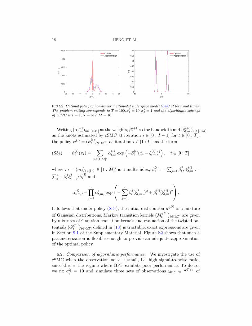
18 HENG ET AL.

-20 -15 -10 -5 0 5 10 15 200

0.005

0.01

0.015

0.02

0.025

Optimal

Approximation

-50 0 500

0.05

0.1

0.15

0.2

0.25

0.3

0.35

0.4

Optimal

Approximation

Fig S2. Optimal policy of non-linear multimodal state space model (S33) at terminal times.The problem setting corresponds to T = 100, σ2

f = 10, σ2g = 1 and the algorithmic settings

of cSMC is I = 1, N = 512,M = 16.

Writing (αi+1t,m )m∈[1:M ] as the weights, βi+1

t as the bandwidth and (ξi+1t,m )m∈[1:M ]

as the knots estimated by cSMC at iteration i ∈ [0 : I − 1] for t ∈ [0 : T ],

the policy ψ(i) = (ψ(i)t )t∈[0:T ] at iteration i ∈ [1 : I] has the form

(S34) ψ(i)t (xt) =

∑m∈[1:M ]i

α(i)t,m exp

(−β(i)

t (xt − ξ(i)t,m)2

), t ∈ [0 : T ],

where m = (mj)j∈[1:i] ∈ [1 : M ]i is a multi-index, β(i)t :=

∑ij=1 β

jt , ξ

(i)t,m :=∑i

j=1 βjt ξjt,mj

/β(i)t and

α(i)t,m :=

i∏j=1

αjt,mj exp

− i∑j=1

βjt (ξjt,mj

)2 + β(i)t (ξ

(i)t,m)2

.

It follows that under policy (S34), the initial distribution µψ(i)

is a mixture

of Gaussian distributions, Markov transition kernels (Mψ(i)

t )t∈[1:T ] are givenby mixtures of Gaussian transition kernels and evaluation of the twisted po-

tentials (Gψ(i)

t )t∈[0:T ] defined in (13) is tractable; exact expressions are givenin Section 9.1 of the Supplementary Material. Figure S2 shows that such aparameterization is flexible enough to provide an adequate approximationof the optimal policy.

6.2. Comparison of algorithmic performance. We investigate the use ofcSMC when the observation noise is small, i.e. high signal-to-noise ratio,since this is the regime where BPF exhibits poor performance. To do so,we fix σ2

f = 10 and simulate three sets of observations y0:T ∈ YT+1 of


Observation noiseσ2g = 0.1 σ2

g = 0.5 σ2g = 1

Algorith

m

BPF

N 2252 4710 6553ESS% 15.07% 30.24% 39.12%logZ −281.6185± 1.0054 −262.9861± 0.6037 −250.6369± 0.2845RVAR 1.27× 10−5 5.27× 10−6 1.29× 10−6

cSMC

I 1 1 1N 512 512 512M 16 16 16τ 0.5 0.4 0.3

ESS% 82.35% 92.51% 94.66%logZ −281.1483± 0.2295 −262.7223± 0.2425 −250.6949± 0.1439RVAR 6.67× 10−7 (19.1) 8.52× 10−7 (6.18) 3.29× 10−7 (3.91)

Table S1Non-linear multimodal state space model (S33): algorithmic settings and performance of

BPF and cSMC for each observation noise considered. Notationally, N refers to thenumber of particles, I is the number of iterations taken by cSMC, M denotes the numberof components and τ the bandwidth factor used in the ADP approximation. Results wereobtained using 100 independent repetitions each of method. The shorthand ESS% denotesthe percentage of effective sample size averaged over time and repetitions, logZ refers tothe estimation of the normalizing constant in logarithmic scale (± a standard deviation),RVAR is the sample relative variance of these estimates over the repetitions. Shown in

bold is the gain that cSMC offers relative to BPF.

length T + 1 = 100 according to (S33) as σ2g takes values in 0.1, 0.5, 1.

We use N = 512 particles in cSMC and I = 1 iteration as preliminary runsindicate that policy refinement under the parameterization (S34) provideslittle improvement, especially when additional computing time is taken intoaccount. The number of particles in BPF is then chosen to match compu-tational time. The number of components M and bandwidth factor τ weretuned using preliminary runs. These algorithmic settings and the resultsobtained in 100 independent repetitions of each method are summarized inTable S1. As expected, although the performance gains over BPF diminishas the observation noise increases, it can be substantial when σ2

g is small.

7. Linear quadratic Gaussian control. This section considers a Gaus-sian static model (Section 2.4) which will allow us to draw connectionsto concepts from the linear quadratic Gaussian (LQG) control literature[1]. Consider µ(dx0) = N (x0;µ0,Σ0)dx0 on (X,X ) = (Rd,B(Rd)) and`(x, y) = exp(−(y − x)TR−1(y − x)/2) for some y ∈ Y = Rd and symmetricpositive definite R ∈ Rd×d. By conjugacy, the models (6) are Gaussian andfor t ∈ [0 : T ] we have ηt(dxt) = N (xt;µt,Σt)dxt with

µt := Σt(Σ−10 µ0 + λtR

−1y), Σt := (Σ−10 + λtR

−1)−1

20 HENG ET AL.

and

Zt = det(Σ0)−1/2 det(Σt)1/2 exp

(−1

2

µT0 Σ−1

0 µ0 + λtyTR−1y − µTt Σ−1

t µt)

.

7.1. Riccati equation. We now show that the backward recursion (19)with ψ initialized as a policy of constant one functions can be performedexactly to obtain analytic expressions of the optimal policy w.r.t. Q. Firstnote that under the choice of forward and backward Markov transition ker-nels specified in Section 7 with pre-conditioner Γ = Id, the potentials (7)have the form

− logGt(xt−1, xt) = xTt Atxt + xTt bt + ct + xTt−1Dtxt−1 + xTt−1et,(S35)

where

At :=1

8hΣ−2

t , bt := −1

4hΣ−2

t µt, ct :=1

2(λt − λt−1)yTR−1y,

(S36)

Dt := −1

8hΣ−2

t +1

2(λt − λt−1)R−1, et := −(λt − λt−1)R−1y +

1

4hΣ−2

t µt,

for t ∈ [1 : T ]. For sufficiently small step size, observe that dropping O(h)terms in (S36) gives logGt(xt−1, xt) ≈ (λt − λt−1) log `(xt−1, y) which, asexpected, recovers the AIS potentials (8). For notational convenience, we set(A0, b0, c0, D0, e0) as the zero matrix or vector of the appropriate size andwrite the mean of the Euler-Maruyama move as xt−1 + h∇ log ηt(xt−1)/2 =Ptxt−1 + qt with Pt := Id − hΣ−1

t /2 and qt := hΣ−1t µt/2.

Proposition 3. The optimal policy ψ∗ = (ψ∗t )t∈[0:T ] w.r.t. Q is givenby

− logψ∗0(x0) = xT0 A∗0x0 + xT0 b

∗0 + c∗0,

(S37)

− logψ∗t (xt−1, xt) = xTt A∗txt + xTt b

∗t + c∗t + xTt−1D

∗t xt−1 + xTt−1e

∗t , t ∈ [1 : T ],

where the coefficients (A∗t , b∗t , c∗t , D

∗t , e∗t )t∈[0:T ] are determined by the back-


ward recursion

A∗t = At +1

2h−1Pt+1(Id −K∗t+1)Pt+1 +D∗t+1,(S38)

b∗t = bt + Pt+1K∗t+1b

∗t+1 + e∗t+1 +

1

2Pt+1(Id −K∗t+1)Σ−1

t+1µt+1,

c∗t = ct + c∗t+1 −1

2log det(K∗t+1) +

1

2h−1qTt+1qt+1

− 1

2h−1(qt+1 − hb∗t+1)TK∗t+1(qt+1 − hb∗t+1),

D∗t = Dt,

e∗t = et,

for t ∈ [T − 1 : 0], with K∗t := (Id + 2hA∗t )−1, t ∈ [1 : T ] and initialization at

(A∗T , b∗T , c∗T , D

∗T , e∗T ) = (AT , bT , cT , DT , eT ).

Proof. We proceed by induction. Clearly, (S37) holds for t = T sinceψ∗T = GT . Assume that (S37) holds for time t + 1. The recursion (19) canbe written as

− logψ∗t (xt−1, xt) = − logGt(xt−1, xt)− logMt+1(ψ∗t+1)(xt).

Some manipulations yield

− logMt+1(ψ∗t+1)(xt) = xTt

(1

2h−1Pt+1(Id −K∗t+1)Pt+1 +D∗t+1

)xt

+ xTt

(Pt+1K

∗t+1b

∗t+1 + e∗t+1 +

1

2Pt+1(Id −K∗t+1)Σ−1

t+1µt+1

)− 1

2log det(K∗t+1)

+ c∗t+1 +1

2h−1

qTt+1qt+1 − (qt+1 − hb∗t+1)TK∗t+1(qt+1 − hb∗t+1)

.

Adding this to (S35) establishes that − logψ∗t has the desired form (S37)and equating coefficients of the polynomial gives (S38).

The backward recursion (S38) for the coefficients is analogous to the Ric-cati equation in the context of LQG control. To illustrate the behaviour ofthese coefficients, we set the prior as µ0 = 0d, Σ0 = Id and the likelihood asy = (ξ, . . . , ξ)T for some ξ ∈ R and Ri,j = δi,j + (1 − δi,j)ρ for i, j ∈ [1 : d]and some ρ ∈ [−1, 1] (here δi,j denotes the Kronecker delta). The time evo-lution of these coefficients is plotted in the top row of Figure S3 for theproblem setting d = 2, ξ = 4, ρ = 0.8. Noting that the optimal value of the

22 HENG ET AL.

Kullback-Leibler control problem (S30) is

v∗ = − logZ = c∗0 +1

2log det(Σ0)− 1

2log det(K∗0 )

− 1

2(Σ−1

0 µ0 − b∗0)TK∗0 (Σ−10 µ0 − b∗0) +

1

2µT0 Σ−1

0 µ0

with K∗0 := (Σ−10 + 2A∗0)−1, the dominant contribution that the constant c∗0

has to v∗ suggests that it is important to estimate the constants in (S37) tolearn good policies. Moving from the bottom left to top left plot, observe thatincreasing the location parameter ξ from 1 to 4 increases the magnitude of(b∗t , e

∗t )t∈[0:T ] but leaves (A∗t , D

∗t )t∈[0:T ] unchanged. This behaviour is evident

from the expressions of (D∗t , e∗t )t∈[0:T ] and is unsuprising for (A∗t )t∈[0:T ] as

the parameter ξ does not alter the ‘structure’ of the problem. The increasein the magnitude of (b∗t )t∈[0:T ] shows that the optimally controlled SMCmethod achieves the desired terminal distribution by initializing

(S39) µψ∗(dx0) = N (x0;K∗0 (Σ−1

0 µ0 − b∗0),K∗0 )dx0

closer to the posterior distribution and taking larger drifts in(S40)

Mψ∗

t (xt−1, dxt) = N (xt;K∗t (Ptxt−1 + qt − hb∗t ), hK∗t ) dxt, t ∈ [1 : T ].

Comparing the plots in the bottom row reveals that the off-diagonal elementsof (A∗t , D

∗t )t∈[0:T ] vanish under independence. Therefore these terms should

be taken into account for posterior distributions that are very correlated.Having obtained the optimal policy w.r.t. Q in a backward sweep, we maythen simulate the optimally controlled SMC method in a forward pass. InFigure S4, we contrast the output of the uncontrolled SMC method withthat of the optimally controlled.

7.2. Approximate dynamic programming. The ability to compute the op-timal policy in this setting allows us to evaluate the effectiveness of ADPalgorithm (31) under correct parameterization, i.e. select the function classes

F0 =ϕ(x0) = xT0 A0x0 + xT0 b0 + c0 : (A0, b0, c0) ∈ Sd × Rd × R

,

Ft =ϕ(xt−1, xt) = xTt Atxt + xTt bt + ct + xTt−1Dtxt−1 + xTt−1et

: (At, bt, ct, Dt, et) ∈ Sd × Rd × R× Sd × Rd, t ∈ [1 : T ].

This choice corresponds to function classes of the form (38), hence we can uselinear least squares to estimate the coefficients at each iteration of cSMC


0 1 2 3 4

-1.4

-1.2

-1

-0.8

-0.6

-0.4

-0.2

0

0.2

0.4

0 1 2 3 4

1

2

3

4

5

6

7

8

0 1 2 3 4

-1.4

-1.2

-1

-0.8

-0.6

-0.4

-0.2

0

0.2

0.4

0 1 2 3 4

-1.4

-1.2

-1

-0.8

-0.6

-0.4

-0.2

0

0.2

0.4

Fig S3. Coefficients of the optimal policy w.r.t. Q in LQG control under various problemsettings. The algorithmic settings of cSMC are T = 10, h = 0.1, λt = t/T . Note that allexcept the top right plot share the same axes.

0 2 4 6 8 100

10

20

30

40

50

60

70

80

90

100

Uncontrolled SMC

Optimally controlled SMC

0 2 4 6 8 100

50

100

150

200

250Optimal value

True

Uncontrolled SMC

Optimally controlled SMC

Fig S4. Comparison of uncontrolled SMC and optimal LQG controlled SMC in terms ofeffective sample size ( left) and normalizing constant estimation ( right). The problem set-ting considered here is d = 32, ξ = 20, ρ = 0.8 and the algorithmic settings of uncontrolledSMC are N = 2048, T = 10, h = 0.1, λt = t/T .

24 HENG ET AL.

– see (S4) and (S5). If (Ai+1t , bi+1

t , ci+1t , Di+1

t , ei+1t ) denote the coefficients

estimated at iteration i ∈ [0 : I − 1] of Algorithm 3 in step 2(b), it followsthat the policy at iteration i ∈ [1 : I] is given by

− logψ(i)0 (x0) = xT0 A

(i)0 x0 + xT0 b

(i)0 + c

(i)0 ,

− logψ(i)t (xt−1, xt) = xTt A

(i)t xt + xTt b

(i)t + c

(i)t + xTt−1D

(i)t xt−1 + xTt−1e

(i)t ,

for t ∈ [1 : T ], whereA(i)t :=

∑ij=1A

jt , b

(i)t :=

∑ij=1 b

jt , c

(i)t :=

∑ij=1 c

jt , D

(i)t :=∑i

j=1Djt , e

(i)t :=

∑ij=1 e

jt . Observe from (S39) and (S40) that we need to im-

pose the following positive definite constraints

Σ−10 + 2A

(i)0 0, Id + 2hA

(i)t 0, t ∈ [1 : T ],

which can be done by projecting onto the set of real symmetric positivedefinite matrices [9]. In our numerical implementation, we find that theseconstraints are already satisfied when the step size h is sufficiently small.Although the computational complexity of this ADP procedure is O(N), itscales quite costly in dimension d as computation of least squares estimatorsrequire inversion of p× p matrices where p = d2 + 3d+ 1. For problems withlarge d, it might be worth considering the use of iterative linear solvers whichoffer reduced complexity. We note that it is possible to avoid learning thext−1 dependency in the policy ψ∗t (xt−1, xt), t ∈ [1 : T ] and hence reducecomputational complexity drastically; we do not exploit this observationhere for simplicity of presentation but will do so for other applications.

Figure S5 displays the coefficients estimated by cSMC with I = 2 itera-tions. It is striking that with N = 2048 particles, we are able to accuratelyestimate, in a single ADP iteration, the true coefficients in dimension d = 32(here p = 1121). That said, we typically need to increase N with d to pre-vent the Gram matrices (S4) from being ill-conditioned. Moreover, we findthat it is unnecessary to perform policy refinement in this example, as theestimated policies converge immediately to an invariant distribution that isvery concentrated around the optimal policy (S37), which is the fixed pointof the idealized algorithm in Theorem 5.2 under correct parameterization.The performance of the resulting controlled SMC method is indistinguish-able from that in Figure S4.

8. Bayesian logistic regression. Consider a binary regression prob-lem: each observation ym ∈ 0, 1,m ∈ [1 : M ] is modelled as an indepen-dent Bernoulli random variable with probability of success κ(xTXm), whereκ(u) := (1 + exp(−u))−1 for u ∈ R is the logistic link function, x ∈ X = Rd


0 2 4 6 8 10

0

0.1

0.2

0.3

0.4

0.5

0.6

0.7

True

Uncontrolled

Iteration 1

Iteration 2

0 2 4 6 8 10

-0.025

-0.02

-0.015

-0.01

-0.005

0

True

Uncontrolled

Iteration 1

Iteration 2

0 2 4 6 8 10

-0.7

-0.6

-0.5

-0.4

-0.3

-0.2

-0.1

0

True

Uncontrolled

Iteration 1

Iteration 2

0 2 4 6 8 10

0

50

100

150

200

250

300

True

Uncontrolled

Iteration 1

Iteration 2

Fig S5. Coefficients of the optimal policy w.r.t. Q in LQG control against estimates ob-tained using ADP algorithm. The problem setting is d = 32, ξ = 20, ρ = 0.8 and thealgorithmic settings of uncontrolled SMC are N = 2048, T = 10, h = 0.1, λt = t/T .

26 HENG ET AL.

denotes the unknown regression coefficients and Xm ∈ Rd the m ∈ [1 : M ]row of a model matrix X ∈ RM×d. Hence the likelihood function and itsgradient is given by

`(x, y) = exp

(yTXx−

M∑m=1

log(1 + exp(xTXm))

)and

∇ log `(x, y) = XT y −M∑m=1

(1 + exp(−xTXm))−1Xm

where y = (ym)m∈[1:M ] ∈ Y = 0, 1M is a given dataset of interest. Follow-ing [8], we specify a Gaussian prior distribution µ(dx0) = N (x0;µ0,Σ0)dx0

on (X,X ) = (Rd,B(Rd)) of the form µ0 = 0d and Σ0 = π2M/(3d)(XTX)−1.

8.1. Approximate dynamic programming. In view of Proposition 1 andthe previous section on LQG control, we consider the function classes in (45).As before, coefficients (Ai+1

t , bi+1t , ci+1

t )t∈[0:T ] at each iteration i ∈ [0 : I − 1]

can be estimated by linear least squares and the policy ψ(i) = (ψ(i)t )t∈[0:T ]

at iteration i ∈ [1 : I] has the form

− logψ(i)0 (x0) = xT0 A

(i)0 x0 + xT0 b

(i)0 + c

(i)0 ,

− logψ(i)t (xt−1, xt) = xTt A

(i)t xt + xTt b

(i)t + c

(i)t − (λt − λt−1) log `(xt−1, y),

for t ∈ [1 : T ], where A(i)t :=

∑ij=1A

jt , b

(i)t :=

∑ij=1 b

jt , c

(i)t :=

∑ij=1 c

jt for

t ∈ [0 : T ]. Assuming that the constraints K(i)0 := (Σ−1

0 + 2A(i)0 )−1 0,

K(i)t := (Γ−1 + 2hA

(i)t )−1 0, t ∈ [1 : T ] are satisfied or imposed, then

sampling from

µψ(i)

(dx0) = N(x0;K

(i)0 (Σ−1

0 µ0 − b(i)0 ),K(i)0

)dx0

and

(S41) Mψ(i)

t (xt−1,dxt) = N(xt;K

(i)t Γ−1qt(xt−1)− hb(i)t , hK

(i)t

)dxt,

with qt(xt−1) := xt−1 + hΓ∇ log ηt(xt−1)/2 for t ∈ [1 : T ] is feasible and

evaluation of the twisted potentials (Gψ(i)

t )t∈[0:T ] defined in (13) is tractablesince

µ(ψ(i)0 ) = det(Σ0)−1/2 det(K

(i)0 )1/2 exp

(1

2(Σ−1

0 µ0 − b(i)0 )TK(i)0 (Σ−1

0 µ0 − b(i)0 )

)× exp

(−1

2µT0 Σ−1

0 µ0 − c(i)0

)


and

Mt(ψ(i)t )(xt−1) = det(Γ)−1/2 det(K

(i)t )1/2

× exp

(1

2h−1(Γ−1qt − hb(i)t )TK

(i)t (Γ−1qt − hb(i)t )(xt−1)

)× exp

(−1

2h−1(qTt Γ−1qt)(xt−1)− c(i)

t + (λt − λt−1) log `(xt−1, y)

)for t ∈ [1 : T ]. We note that imposing At = 0 and letting bt depend on theargument xt−1 in (45) is related to the approach in [11, 14], as (S41) thencorresponds to an Euler-Maruyama discretization of a controlled diffusion

with an additive control xt−1 7→ b(i)t (xt−1). For this application, we set the

pre-conditioner as Γ = Id and we illustrate in Figure S6 that the param-eterization (45) provides a good approximation of the optimal policy on aparticular dataset concerning modeling of heart diseases.

8.2. Comparison of algorithmic performance. We now perform a com-parison of algorithms on the analysis of three real datasets1 with differentcharacteristics, in the same manner as Section 7.2. We use N = 1024 numberof particles in cSMC and select the number of iterations using preliminaryruns – see Figure S6. The number of particles used in AIS is then chosen tomatch computational cost, measured in terms of run time. These algorithmicsettings and the results obtained using 100 independent repetitions each ofmethod are summarized in Table S2. Although AIS provides state-of-the-artresults in complex scenarios for these models [6], the comparison shows thatfor all datasets considered, cSMC outperforms it and particularly so for thetask of marginal likelihood estimation by several orders of magnitude.

9. Model specific expressions.

9.1. Expressions for non-linear multimodal state space model. For no-tational simplicity, we write µ0 = 0, σ2

0 = 5 and µt(xt−1) := xt−1/2 +25xt−1/(1 + x2

t−1) + 8 cos(1.2t) for t ∈ [1 : T ]. Assume that the policy

ψ(i) = (ψ(i)t )t∈[0:T ] at iteration i ∈ [1 : I] has the form (S34). The initial

distribution is given by

µψ(i)

(dx0) =∑

m∈[1:M ]i

A(i)0,mN

(x0;µ

(i)0,m, (σ

(i)0 )2

)dx0

1Datasets were downloaded from the UCI machine learning repository and standardizedbefore analysis.

http://archive.ics.uci.edu/ml/

28 HENG ET AL.

0 5 10 15 20

0

10

20

30

40

50

60

70

80

90

100

Uncontrolled

Iteration 1

Iteration 2

Iteration 3

Iteration 4

Iteration 5

0 5 10 15 20

-140

-120

-100

-80

-60

-40

-20

0

Uncontrolled

Iteration 1

Iteration 2

Iteration 3

Iteration 4

Iteration 5

Fig S6. Comparison of uncontrolled and controlled SMC methods in terms of effectivesample size ( top left), normalizing constant estimation ( top right) and variance of particleweights ( bottom row) when performing Bayesian logistic regression on the Heart diseasedataset. The algorithmic settings of cSMC are I = 5, N = 1024, T = 20, h = 1×10−4, λt =t/T .


DatasetHeart disease Australian credit German credit

(M = 270, d = 14) (M = 690, d = 15) (M = 1000, d = 25)

Algorith

m

AIS

N 1843 1843 2048h 5× 10−2 3× 10−2 1× 10−2

ESS% 82.95% 79.75% 74.95%logZ −118.0198± 0.4383 −252.8699± 1.5128 −527.4392± 3.3088VAR 1.92× 10−1 2.29 10.95

RMSE 4.40× 10−1 2.60 10.06

cSMC

I 3 4 3N 1024 1024 1024h 1× 10−4 1× 10−3 5× 10−4

ESS% 99.99% 99.95% 99.91%logZ −117.9638± 0.0117 −250.7504± 0.0101 −517.9299± 0.0092VAR 1.36× 10−4 (1.41× 103) 1.03× 10−4 (2.23× 104) 8.39× 10−5 (1.31× 105)

RMSE 1.16× 10−2 (37.86) 1.02× 10−2 (2.55× 102) 9.11× 10−3 (1.10× 103)Table S2

Algorithmic settings and performance of AIS and cSMC when performing Bayesianlogistic regression for each dataset. Notationally, N refers to the number of particles, h

the step size used in MALA for AIS and ULA for cSMC, and I is the number ofiterations taken by cSMC. Both algorithms take T = 20 time steps for all datasets.

Results were obtained using 100 independent repetitions each of method. The shorthandESS% denotes the percentage of effective sample size averaged over time and repetitions,

logZ refers to the estimation of the normalizing constant in logarithmic scale (± astandard deviation), VAR is the sample variance of these estimates over the repetitions

and RMSE the corresponding root mean squared error, which we computed by takingreference to an estimate obtained using many repetitions of a SMC method with a large

number of particles. Shown in bold are the gains that cSMC offers relative to AIS.

30 HENG ET AL.

with

µ(i)0,m := (σ

(i)0 )2

(2β

(i)0 ξ

(i)0,m + µ0σ

−20

), (σ

(i)0 )2 :=

(2β

(i)0 + σ−2

0

)−1,

and

A(i)0,m :=

α(i)0,m exp

(−β(i)

0 (ξ(i)0,m)2 + (µ

(i)0,m)2(σ

(i)0 )−2/2

)∑

n∈[1:M ]i α(i)0,n exp

(−β(i)

0 (ξ(i)0,n)2 + (µ

(i)0,n)2(σ

(i)0 )−2/2

) .For each t ∈ [1 : T ], the Markov transition kernel

Mψ(i)

t (xt−1,dxt) =∑

m∈[1:M ]i

A(i)t,m(xt−1)N

(xt;µ

(i)t,m(xt−1), (σ

(i)t )2

)dxt

with

µ(i)t,m(xt−1) := (σ

(i)t )2

(2β

(i)t ξ

(i)t,m + µt(xt−1)σ−2

f

), (σ

(i)t )2 :=

(2β

(i)t + σ−2

f

)−1,

and

A(i)t,m(xt−1) :=

α(i)t,m exp

(−β(i)

t (ξ(i)t,m)2 + µ

(i)t,m(xt−1)2(σ

(i)t )−2/2

)∑

n∈[1:M ]i α(i)t,n exp

(−β(i)

t (ξ(i)t,n)2 + µ

(i)t,n(xt−1)2(σ

(i)t )−2/2

) .Evaluation of the twisted potentials (Gψ

(i)

t )t∈[0:T ] defined in (13) is tractablesince

µ(ψ(i)0 ) =

σ(i)0

σ0exp

(−1

2µ2

0σ−20

) ∑m∈[1:M ]i

α(i)0,m exp

(−β(i)

0 (ξ(i)0,m)2 +

1

2(µ

(i)0,m)2(σ

(i)0 )−2

)

and

Mt(ψ(i)t )(xt−1) =

σ(i)t

σfexp

(−1

2µt(xt−1)2σ−2

f

)×

∑m∈[1:M ]i

α(i)t,m exp

(−β(i)

t (ξ(i)t,m)2 +

1

2µ

(i)t,m(xt−1)2(σ

(i)t )−2

)

for t ∈ [1 : T ].


9.2. Expressions for Lorenz-96 model. Suppose that the current policyis given by (44) and write

A(i)t := A

(0)t +A

(i)t , b

(i)t := b

(0)t + b

(i)t , c

(i)t := c

(0)t + c

(i)t ,

for t ∈ [0 : T ], where (A(0)t , b

(0)t , c

(0)t )t∈[0:T ] are the coefficients correspond-

ing to APF. If the constraints K(i)0 := (σ−2

f Id + 2A(i)0 )−1 0, K

(i)t :=

(σ−2f h−1Id+ 2A

(i)t )−1 0, t ∈ [1 : T ] are satisfied or imposed, then sampling

fromµψ

(i)(dx0) = N

(x0;−K(i)

0 b(i)0 ,K

(i)0

)dx0

and

Mψ(i)

t (xt−1,dxt) = N(K

(i)t σ

−2f h−1q(xt−1)− b(i)t ,K

(i)t

)dxt, t ∈ [1 : T ],

is feasible and evaluation of the twisted potentials (Gψ(i)

t )t∈[0:T ] defined in(13) is tractable since

µ(ψ(i)0 ) = σ−df det(K

(i)0 )1/2 exp

(1

2(b

(i)0 )TK

(i)0 b

(i)0 − c

(i)0

)and

Mt(ψ(i)t )(xt−1) = σ−df h−d/2 det(K

(i)t )1/2 exp

(−1

2σ−2f h−1(qT q)(xt−1)− c(i)

t

)× exp

(1

2(σ−2f h−1q − b(i)t )TK

(i)t (σ−2

f h−1q − b(i)t )(xt−1)

)for t ∈ [1 : T ].

9.3. Expressions for neuroscience model. Assume that the constraints

k(i)0 := (1 + 2a

(i)0 )−1 > 0, k

(i)t := (σ−2 + 2a

(i)t )−1 > 0, t ∈ [1 : T ] are satisfied

or imposed. Then the initial distribution

µψ(i)

(dx0) = N(x0;−k(i)

0 b(i)0 , k

(i)0

)dx0

and the Markov transition kernels

Mψ(i)

t (xt−1,dxt) = N(xt; k

(i)t (ασ−2xt−1 − b(i)t ), k

(i)t

)dxt

for t ∈ [1 : T ]. Moreover, the twisted potentials (Gψ(i)

t )t∈[0:T ] defined in (13)can be evaluated since

µ(ψ(i)0 ) = (k

(i)0 )1/2 exp

(1

2k

(i)0 (b

(i)0 )2 − c(i)

0

)

32 HENG ET AL.

and

Mt(ψ(i)t )(xt−1) = (k

(i)t )1/2σ−1 exp

(1

2k

(i)t (ασ−2xt−1 − b(i)t )2 − 1

2σ−2α2x2

t−1 − c(i)t

)for t ∈ [1 : T ].

References.

[1] B. D. Anderson and J. B. Moore. Optimal Control: Linear Quadratic Methods. DoverPublications, 2007.

[2] D. P. Bertsekas and J. N. Tsitsiklis. Neuro-dynamic Programming. Athena Scientific,1996.

[3] P. Dai Pra, L. Meneghini and W.J. Runggaldier. Connections between stochastic con-trol and dynamic games. Mathematics of Control, Signals and Systems, 9(4):303–326,1996.

[4] P. Del Moral. Feynman-Kac Formulae. Springer, 2004.[5] P. Diaconis and D. Freedman. Iterated random functions. SIAM Review. 41(1):45–76,

1999.[6] N. Chopin and J. Ridgeway. Leave Pima Indians alone: binary regression as a bench-

mark for Bayesian computation. Statistical Science, 32(1):64-87, 2017.[7] N. Gordon, J. Salmond and A. Smith. A novel approach to non-linear/non-

Gaussian Bayesian state estimation. IEE Proceedings on Radar and Signal Processing,140:107–113, 1993.

[8] T. E. Hanson, A. J. Branscum and W. O. Johnson. Informative g-priors for logisticregression. Bayesian Analysis, 9(3):597–612, 2014.

[9] N. J. Higham. Computing a nearest symmetric positive semidefinite matrix. LinearAlgebra and its Applications, 103:103–118, 1988.

[10] H. J. Kappen, V. Gomez and M. Opper. Optimal control as a graphical model infer-ence problem. Machine learning, 87(2):159–182, 2012.

[11] H. J. Kappen and H. C. Ruiz. Adaptive importance sampling for control and infer-ence. Journal of Statistical Physics, 162(5):1244–1266, 2016.

[12] G. Kitagawa. Monte Carlo filter and smoother for non-Gaussian nonlinear state spacemodels. Journal of Computational and Graphical Statistics, 5(1):1–25, 1996.

[13] C. L. Lawson and R. J. Hanson. Solving Least Squares Problems. Prentice-Hall, 1974.[14] H. C. Ruiz and H. J. Kappen. Particle smoothing for hidden diffusion pro-

cesses: adaptive path integral smoother. IEEE Transactions on Signal Processing,65(12):3191–3203, 2017.

[15] E. Todorov. Efficient computation of optimal actions. Proceedings of the NationalAcademy of Sciences, 106(28):11478–11483, 2009.

[16] J. N. Tsitsiklis and B. Van Roy. Regression methods for pricing complex American-style options. IEEE Transactions on Neural Networks, 12(4):694–703, 2001.

5 Nepal ParkSingapore 139408, SingaporeE-mail: [email protected]

15 BroadwaySydney, NSW 2007, AustraliaE-mail: [email protected]

24-29 St Giles’Oxford OX1 3LB, UKE-mail: [email protected]; [email protected]





Controlled Sequential Monte Carlo - Oxford Statistics

Documents

Transcript of Controlled Sequential Monte Carlo - Oxford Statistics