Sequential Adaptation through Prediction of Structured Climate Risk

James Doss-Gollin

Submitted in partial fulfillment of therequirements for the degree of

Doctor of Philosophyunder the Executive Committee

of the Graduate School of Arts and Sciences

COLUMBIA UNIVERSITY

2020

© 2020

James Doss-Gollin

All Rights Reserved

Abstract

Sequential Adaptation through Prediction of Structured Climate Risk

James Doss-Gollin

Infrastructure systems around the world face immediate crises and smoldering long-term

challenges. Consequently, system owners and managers must balance the need to repair and

replace the aging and deteriorating systems already in place against the need for transfor-

mative investments in deep decarbonization, climate adaptation, and transportation that will

enable long-term competitiveness. Complicating these decisions are deep uncertainties, finite

resources, and competing objectives.

These challengesmotivate the integration of “hard” investments in physical infrastructure

with “soft” instruments like insurance, land use policy, and ecosystem restoration that can

improve service, shrink costs, scale up or down as future needs require, and reduce vulnera-

bility to population loss and economic contraction. A critical advantage of soft instruments

is that they enable planners to adjust, expand, or reduce them at regular intervals, unlike

hard instruments which are difficult to modify once in place. As a result, soft instruments

can be precisely tailored to meet near-term needs and conditions, including projections of

the quasi-oscillatory, regime-like climate processes that dominate seasonal to decadal hydro-

climate variability, thereby reducing the need to guess the needs and hazards of the distant

future. The objective of this dissertation is to demonstrate how potentially predictable modes of

structured climate variability can inform the design of soft instruments and the formulation of

adaptive infrastructure system plans.

Using climate information for sequential adaptation requires developing credible projec-

tions of climate variables at relevant time scales. Part I considers the drivers of river floods in

large river basins, which is used throughout this dissertation as an example of a high-impact

hydroclimate extreme. First, chapter 2 opens by exploring the strengths and limitations of

existing methodologies, and by developing a statistical-dynamical causal chain framework

within which to consider flood risk on interannual to secular time scales. Next, chapter 3 de-

scribes the physical mechanisms responsible for heavy rainfall (90th percentile exceedance)

and flooding in the Lower Paraguay River Basin (LPRB), focusing on a November-February

(NDJF) 2015-16 flood event that displaced over 170 000 people. This chapter shows that

1. persistent large-scale conditions over the South American continent during NDJF 2015-

16 strengthened the South American Low-Level Jet (SALLJ), bringing warm air and

moisture to South East South America (SESA), and steered the jet towards the LPRB,

leading to repeated heavy rainfall events and large-scale flooding;

2. while the observed El Niño event contributed to a stronger SALLJ, the Madden-Julien

Oscillation (MJO) and Atlantic ocean steered the jet over the LPRB; and

3. while numerical sub-seasonal to seasonal (S2S) and seasonal models projected an ele-

vated risk of flooding consistent with the observed El Niño event, they had limited skill

at lead times greater than two weeks, suggesting that improved representation of MJO

and Atlantic teleconnections could improve regional forecast skill.

Finally, chapter 4 shows how mechanistic understanding of the physical causal chain that

leads to a particular hazard of interest – in this case heavy rainfall over a large area in the

Ohio River Basin (ORB) – can inform future risks. Taking the GFDL coupled model, version

3 (CM3) as a representative general circulation model (GCM), this chapter shows that

1. the GCM simulates too many regional extreme precipitation (REP) events but under-

simulates the occurrence of back to back REP days;

2. REP days show consistent large-scale climate anomalies leading up to the event;

3. indices describing these large-scale anomalies are well simulated by the GCM; and

4. a statistical model describing this causal chain and exploiting simulated large-scale in-

dices from the GCM can be used to inform the future occurrence of REP days.

Even the best climate projections must confront epistemic uncertainties. Part II of this dis-

sertation explores how intrinsically flawed projections should inform sequential adaptation.

First, chapter 5 reviews approaches for planning under uncertainty, considering the role of

classical decision theory, optimization, probability, and nonprobabilistic approaches. Next,

chapter 6 considers how different physical mechanisms impart predictability at different time

scales and the implications of secular, low-frequency cyclical, and high-frequency cyclical

variability for selection between instruments with long and short planning periods. In par-

ticular, this chapter builds from three assertions regarding the nature of climate risk:

1. different climate risk mitigation instruments have different project lifespans;

2. climate risk varies on many scales; and

3. the processeswhich dominate this risk over the planning period depend on the planning

period itself.

Defining M as the nominal design life of a structural or financial instrument and N as the

length of the observational record (a proxy for total informational uncertainty), chapter 7

presents a series of stylized computational experiments to probe the implications of these

premises. Key findings are that:

1. quasi-periodic and secular climate signals, with different identifiability and predictabil-

ity, control future uncertainty and risk;

2. adaptation strategies need to consider how uncertainties in risk projections influence

the success of decision pathways; and

3. stylized experiments reveal how bias and variance of climate risk projections influence

risk mitigation over a finite planning period.

Chapter 7 elaborates these findings through a didactic case study of levee heightening in

the Netherlands. Integrating a conceptual model of low-frequency variability with credible

projections of sea level rise, chapter 7 uses dynamic programming to co-optimize hard (levee

increase) and soft (insurance) instruments. Key findings are that

1. large but distant and uncertain changes (e.g., sea level rise) do not necessarily motivate

immediate investment in structural risk protection;

2. soft adaptation strategies are robust to different model structures and assumptions

while hard instruments perform poorly under conditions for which they were not de-

signed; and

3. increasing the hypothetical predictability of near-term climate extremes significantly

lowers long-term adaptation costs.

Finally, part III seeks to unpack the conceptual experiments of parts I and II to inform

policy and future research. Chapter 8 describes how constructive narratives about climate

change can discourage climate fatalism. Instead, chapter 8 emphasizes that while climate

change is and will be a critical stressor of infrastructure systems, individuals, communities,

and regions have agency and can mitigate its consequences. Finally, chapter 9 concludes by

discussing the key findings of this dissertation and exploring how future work on decision

under uncertainty, technology, and earth systems science can aid the design and management

of effective infrastructure services.

Table of Contents

List of Tables . . . . . . . . . . . . . . . . . . . . . . . . . . . . . . . . . . . . . . . . iv

List of Figures . . . . . . . . . . . . . . . . . . . . . . . . . . . . . . . . . . . . . . . . v

List of Acronyms . . . . . . . . . . . . . . . . . . . . . . . . . . . . . . . . . . . . . . ix

Acknowledgments . . . . . . . . . . . . . . . . . . . . . . . . . . . . . . . . . . . . . xii

Chapter 1: Introduction . . . . . . . . . . . . . . . . . . . . . . . . . . . . . . . . . . 1

1.1 Conceptual Framework . . . . . . . . . . . . . . . . . . . . . . . . . . . . . . . 3

I Understanding and Predicting Structured Climate Variability 7

Chapter 2: Review of Methods for Projecting Future Flood Hazard . . . . . . . . . . . 8

2.1 Physical Drivers of Large River Floods . . . . . . . . . . . . . . . . . . . . . . 9

2.2 Methods for Constraining Hydroclimate Risks . . . . . . . . . . . . . . . . . . 16

2.3 Integrating Conceptual Understanding through Imperfect Models . . . . . . . 21

Chapter 3: Heavy Rainfall in Paraguay During the 2015-2016 Austral Summer: Causesand Sub-Seasonal-to-Seasonal Predictive Skill . . . . . . . . . . . . . . . . 27

3.1 Introduction . . . . . . . . . . . . . . . . . . . . . . . . . . . . . . . . . . . . . 29

3.2 Data . . . . . . . . . . . . . . . . . . . . . . . . . . . . . . . . . . . . . . . . . . 33

3.3 Methods . . . . . . . . . . . . . . . . . . . . . . . . . . . . . . . . . . . . . . . 36

3.4 Diagnostics . . . . . . . . . . . . . . . . . . . . . . . . . . . . . . . . . . . . . . 41

3.5 Forecasts . . . . . . . . . . . . . . . . . . . . . . . . . . . . . . . . . . . . . . . 47

i

3.6 Discussion . . . . . . . . . . . . . . . . . . . . . . . . . . . . . . . . . . . . . . 52

3.7 Summary . . . . . . . . . . . . . . . . . . . . . . . . . . . . . . . . . . . . . . . 58

Chapter 4: Regional Extreme Precipitation Events: Robust Inference from CrediblySimulated GCM Variables . . . . . . . . . . . . . . . . . . . . . . . . . . . 59

4.1 Introduction . . . . . . . . . . . . . . . . . . . . . . . . . . . . . . . . . . . . . 61

4.2 Methods and Data . . . . . . . . . . . . . . . . . . . . . . . . . . . . . . . . . . 64

4.3 Regional Extreme Precipitation Days and Streamflow . . . . . . . . . . . . . . 68

4.4 Regional Extreme Precipitation in a GCM and Observations . . . . . . . . . . 69

4.5 Circulation Patterns Associated with Regional Extreme Precipitation . . . . . 73

4.6 Atmospheric Indices . . . . . . . . . . . . . . . . . . . . . . . . . . . . . . . . 77

4.7 Conditional Simulation . . . . . . . . . . . . . . . . . . . . . . . . . . . . . . . 80

4.8 Summary and Discussion . . . . . . . . . . . . . . . . . . . . . . . . . . . . . . 87

II Sequential Adaptation 91

Chapter 5: Review of Methods for Infrastructure Planning under Uncertainty . . . . . 92

5.1 Decision Theory . . . . . . . . . . . . . . . . . . . . . . . . . . . . . . . . . . . 93

5.2 Decision Frameworks for Planning under True Uncertainty . . . . . . . . . . . 102

5.3 Instrument Design for Resilient Systems . . . . . . . . . . . . . . . . . . . . . 106

Chapter 6: Robust Adaptation to Multiscale Climate Variability . . . . . . . . . . . . 111

6.1 Introduction . . . . . . . . . . . . . . . . . . . . . . . . . . . . . . . . . . . . . 112

6.2 Methods . . . . . . . . . . . . . . . . . . . . . . . . . . . . . . . . . . . . . . . 119

6.3 Results . . . . . . . . . . . . . . . . . . . . . . . . . . . . . . . . . . . . . . . . 126

6.4 Discussion . . . . . . . . . . . . . . . . . . . . . . . . . . . . . . . . . . . . . . 132

6.5 Summary . . . . . . . . . . . . . . . . . . . . . . . . . . . . . . . . . . . . . . . 134

ii

Chapter 7: Near-Term Predictability Lowers Long-Term Adaptation Costs . . . . . . . 136

7.1 Introduction . . . . . . . . . . . . . . . . . . . . . . . . . . . . . . . . . . . . . 137

7.2 Methods . . . . . . . . . . . . . . . . . . . . . . . . . . . . . . . . . . . . . . . 139

7.3 Results and Discussion . . . . . . . . . . . . . . . . . . . . . . . . . . . . . . . 150

7.4 Summary and Implications . . . . . . . . . . . . . . . . . . . . . . . . . . . . . 159

III Discussion and Conclusions 165

Chapter 8: Policy Implications . . . . . . . . . . . . . . . . . . . . . . . . . . . . . . 166

8.1 Introduction . . . . . . . . . . . . . . . . . . . . . . . . . . . . . . . . . . . . . 167

8.2 How Climate Disasters Emerge . . . . . . . . . . . . . . . . . . . . . . . . . . 167

8.3 Towards Constructive Narratives . . . . . . . . . . . . . . . . . . . . . . . . . 169

8.4 Final Word . . . . . . . . . . . . . . . . . . . . . . . . . . . . . . . . . . . . . . 172

Chapter 9: Summary, Discussion, and Future Work . . . . . . . . . . . . . . . . . . . 173

9.1 Summary . . . . . . . . . . . . . . . . . . . . . . . . . . . . . . . . . . . . . . . 173

9.2 Discussion . . . . . . . . . . . . . . . . . . . . . . . . . . . . . . . . . . . . . . 176

9.3 Future Work . . . . . . . . . . . . . . . . . . . . . . . . . . . . . . . . . . . . . 178

References . . . . . . . . . . . . . . . . . . . . . . . . . . . . . . . . . . . . . . . . . . 180

iii

List of Tables

3.1 List of MOS methods used to correct the sub-seasonal forecasts. . . . . . . . . 40

3.2 Centroids of each weather type in 4-dimensional phase space . . . . . . . . . . 45

3.3 Weather type occurrence fraction during NDJF 2015-16 . . . . . . . . . . . . . 47

4.1 The distributions of atmospheric indices in GCMs and reanalysis are moresimilar than the distributions of REP days per year. . . . . . . . . . . . . . . . 70

4.2 As table 4.1 but for the historical period observed REPs vs. mean of simulationmodel predicted REPs . . . . . . . . . . . . . . . . . . . . . . . . . . . . . . . 83

6.1 Six real-world riskmitigation instruments and the associated project planningperiod (M ). . . . . . . . . . . . . . . . . . . . . . . . . . . . . . . . . . . . . . 114

7.1 Exact value of parameters used . . . . . . . . . . . . . . . . . . . . . . . . . . 148

7.2 List of deep and model structural uncertainties . . . . . . . . . . . . . . . . . . 148

7.3 Cost-minimizing 2020 levee height increases . . . . . . . . . . . . . . . . . . . 161

7.4 As table 7.3 but for initial levee height 375 cm . . . . . . . . . . . . . . . . . . 163

iv

List of Figures

2.1 Conceptual physical causal chain for riverine flooding in the mid-latitudes. . . 9

3.1 Topographical map of the LPRB . . . . . . . . . . . . . . . . . . . . . . . . . . 30

3.2 Gridded estimate of population density . . . . . . . . . . . . . . . . . . . . . . 31

3.3 Monthly composite anomalies observed during NDJF 2015-16 . . . . . . . . . 31

3.4 Classifiability index as a function ofK (the number of weather types created). 38

3.5 River stage time series for four gauges on the Paraguay River . . . . . . . . . . 42

3.6 Composite anomalies associated with heavy rainfall in the LPRB . . . . . . . . 44

3.7 Loadings of the four leading EOFs of daily NDJF 850 hPa streamfunction . . . 44

3.8 Composite anomalies associated with each weather type . . . . . . . . . . . . 45

3.9 Time series of area-averaged rainfall in the LPRB for NDJF 2015-16 . . . . . . 46

3.10 Seasonal model forecast for probability of exceedance of 90th percentile ofDJF rainfall, as issued in November 2015 . . . . . . . . . . . . . . . . . . . . . 48

3.11 Chiclet diagram of ensemble-mean precipitation anomaly forecasts over theLPRB for NDJF 2015-16 . . . . . . . . . . . . . . . . . . . . . . . . . . . . . . . 49

3.12 Raw and MOS-adjusted S2S model forecasts and spatial skill scores . . . . . . 50

3.13 Anomalous probability of occurrence of each weather type concurrent withobservance of each MJO and ENSO phase . . . . . . . . . . . . . . . . . . . . . 53

3.14 Monthly NINO 3.4 time series during the study period . . . . . . . . . . . . . 54

3.15 Monthly SST anomalies during December of three major El Niño events. . . . 55

3.16 Evolution of the MJO during NDJF 2015-16 . . . . . . . . . . . . . . . . . . . . 56

v

3.17 Schematics of low-level jet events (red arrows) during austral summer and ElNiño years . . . . . . . . . . . . . . . . . . . . . . . . . . . . . . . . . . . . . . 57

4.1 Map of the ORB study area . . . . . . . . . . . . . . . . . . . . . . . . . . . . . 65

4.2 Relationship between streamflow and REP days . . . . . . . . . . . . . . . . . 68

4.3 Frequency distribution of REP days in observations and GCM output . . . . . 69

4.4 Frequency distribution of local extreme precipitation days in GCM simula-tions and observations . . . . . . . . . . . . . . . . . . . . . . . . . . . . . . . 71

4.5 The distribution of the regional extreme precipitation days by month for theobserved record and GCM ensemble members . . . . . . . . . . . . . . . . . . 71

4.6 Average precipitation percentiles when at least one of the 15 study area gridcells experienced a local 99th percentile exceedance . . . . . . . . . . . . . . . 72

4.7 Difference between each GCM ensemble member and the observed record ofprecipitation percentiles averaged over all REP days. . . . . . . . . . . . . . . 73

4.8 Daily Z700 and Q700 composite anomalies and Q700 from four days beforeeach MAM REP event to one day following the event . . . . . . . . . . . . . . 73

4.9 Daily Z700 andQ700 composite anomalies on the day of REP events in each ofthe GFDL CM3 GCM ensemble members and the observed-reanalysis record. 75

4.10 Composites of Z700 anomalies and absolute Z700 during REP days for obser-vations and GCM ensemble members. . . . . . . . . . . . . . . . . . . . . . . 76

4.11 The difference in standard deviation of daily MAM geopotential height at700 hPa for between reanalysis and each GCM ensemble member. . . . . . . . 76

4.12 Climatological zonal 200 hPa wind for reanalysis and each GCM ensemblemember. . . . . . . . . . . . . . . . . . . . . . . . . . . . . . . . . . . . . . . . 76

4.13 Regions used to define the atmospheric indices used for statistical modelingand the distribution of these indices before and after REP days. . . . . . . . . 77

4.14 Cumulative distribution functions, serial correlation functions, and serial tailpersistence functions for each of the climate-derived statistical indices. . . . . 79

4.15 Qualitative diagnostics and checks for the Bayesian logistic regression model. 82

4.16 The probability of a REP event given a REP event the day prior, divided bythe marginal probability of a REP event, for the observed record and 1000simulated records from the Bayesian logistic regression model. . . . . . . . . 83

vi

4.17 Wavelet power spectrum for the number of REP events per year in observa-tions and in simulations from the Bayesian logistic regression model. . . . . . 84

4.18 Comparison of REP day representation in observation and GCM simulation. . 85

4.19 Projected number of MAM REP days using raw GCM output, a naive biascorrection, and the Bayesian logistic regression model. . . . . . . . . . . . . . 86

4.20 PDFs for the number of REPs per year over three different time periods basedon simulations from the Bayesian logistic regression model. . . . . . . . . . . 87

6.1 Time series and wavelet global spectra of some representative hydroclimatetime series . . . . . . . . . . . . . . . . . . . . . . . . . . . . . . . . . . . . . . 117

6.2 A stylized illustration of irreducible and estimation uncertainty. . . . . . . . . 118

6.3 Wavelet analysis of the synthetic annual NINO3 time series . . . . . . . . . . . 121

6.4 Consequences of model bias or incorrect model representation of uncertainty. 124

6.5 Flow chart describing experiment design . . . . . . . . . . . . . . . . . . . . . 125

6.6 Illustration of the estimation procedure for a single time series . . . . . . . . 126

6.7 Expected estimation bias and variance for sequences generated with secularchange only (no LFV). . . . . . . . . . . . . . . . . . . . . . . . . . . . . . . . 127

6.8 As fig. 6.7 for sequences generated with the two-state Markov chain model. . 128

6.9 As fig. 6.7 but for sequences generated with zero secular change and stronglow-frequency variability (LFV). . . . . . . . . . . . . . . . . . . . . . . . . . . 129

6.10 LFV only: as fig. 6.9 for sequences generated with the two-state Markov chainmodel. . . . . . . . . . . . . . . . . . . . . . . . . . . . . . . . . . . . . . . . . 130

6.11 As fig. 6.7 but for sequences generated with both LFV and secular change. . . 130

6.12 As fig. 6.11 for sequences generated with the two-state Markov chain model. 131

6.13 The importance of predicting different signals, and the identifiability and pre-dictability of the signals, depends on the degree of informational uncertainty(N ) and the project planning period (M ). . . . . . . . . . . . . . . . . . . . . 133

7.1 Simulations of LSL from the SDP model through 2120 . . . . . . . . . . . . . . 140

vii

7.2 PDFs of simulated LSL at Delfzijl, Netherlands in cm in 2020, 2040, 2060, 2080,2100, and 2120 for each of three RCP scenarios and each of two physical models. 141

7.3 Different models and scenarios agree that local mean sea level at Delfzijl,Netherlands will rise over the next centuries but differ sharply on the magni-tude and timing of this rise. . . . . . . . . . . . . . . . . . . . . . . . . . . . . . 142

7.4 Historical flood data at Delfzijl, Netherlands . . . . . . . . . . . . . . . . . . . 144

7.5 The transition matrices LX that specify P(x′|x, τ) (eq. 7.4) for all value of τ . 145

7.6 Illustration of levee construction cost function . . . . . . . . . . . . . . . . . . 146

7.7 Simulations from the SDP model . . . . . . . . . . . . . . . . . . . . . . . . . . 151

7.8 As fig. 7.7 (using the Deconto and Pollard, 2016 (DP16) model and τ = 0.25)but with a 7% discount rate. . . . . . . . . . . . . . . . . . . . . . . . . . . . . 152

7.9 As fig. 7.7 (using the DP16 model and τ = 0.25) but with a 1% discount rate. . 152

7.10 As fig. 7.7 but for the Kopp et. al, 2014 (K14) model, τ = 1.0, and a 1% discountrate. . . . . . . . . . . . . . . . . . . . . . . . . . . . . . . . . . . . . . . . . . 153

7.11 Regret as a function of levee height increase for different physical models,RCP scenarios, and discount rates . . . . . . . . . . . . . . . . . . . . . . . . . 155

7.12 As fig. 7.11 but for τ = 0.125 and initial LFV state 0. . . . . . . . . . . . . . . 156

7.13 As fig. 7.11 (τ = 1.0) but for initial LFV state 0. . . . . . . . . . . . . . . . . . 156

7.14 As fig. 7.11 (initial LFV state 4) but for τ = 0.125. . . . . . . . . . . . . . . . . 157

7.15 Expected discounted costs over the full adaptation pathway as a function ofinitial LFV state for different RCP scenarios and different values of τ . . . . . 158

7.16 As fig. 7.15 (discount rate 4%) but for DP16 model. . . . . . . . . . . . . . . . 158

7.17 As fig. 7.15 (K14 model) but for 1% discount rate. . . . . . . . . . . . . . . . . 158

7.18 As fig. 7.15 (K14 model) but for 7% discount rate. . . . . . . . . . . . . . . . . 159

viii

List of Acronyms

AA arctic amplification

ACC anthropogenic climate change

AMO Atlantic Meridional Oscillation

AMOC Atlantic Meridional Overturning Circulation

AR atmospheric river

BDT Bayesian decision theory

CBA cost-benefit analysis

CC Clausius-Clapeyron

CCA canonical correlation analysis

CM3 GFDL coupled model, version 3

CMIP climate model intercomparison project

CPC Center for Climate Prediction

DAPP dynamic adaptive policy pathways

DJF December-February

DOD Department of Defense

DP dynamic programming

DP16 Deconto and Pollard, 2016

DPS dynamic policy search

ECMWF European Centre for Medium-Range Weather Forecasts

ENSO the El Niño-Southern Oscillation

EOF empirical orthogonal function

EPA United States Environmental Protection Agency

EPG equator to pole temperature gradient

ix

ESM Earth system model

ETC extratropical cyclone

FEMA the Federal Emergency Management Agency

GCM general circulation model

GEV generalized extreme value

GFDL Geophysical Fluid Dynamics Laboratory

GRFP Graduate Research Fellowship Program

HMM hidden Markov model

HXLR heteroscedastic extended logistic regression

IID independent and identically distributed

IPO Interdecadal Pacific Oscillation

IRI International Research Institute for Climate and Society

JJA June-August

K14 Kopp et. al, 2014

LBDA Living Blended Drought Analysis

LFV low-frequency variability

LPRB Lower Paraguay River Basin

LSL local sea level

MAM March-May

MDP Markov decision process

MJO Madden-Julien Oscillation

MORDM multiobjective robust decision-making

MOS model output statistics

NAO North Atlantic Oscillation

NCAR National Center for Atmospheric Research

NCEP National Center for Environmental Prediction

NDJF November-February

x

NHMM nonhomogeneous hidden Markov model

NPV net present value

NSF National Science Foundation

OLR outgoing longwave radiation

ORB Ohio River Basin

PCR principal components regression

PDF probability density function

PDO Pacific Decadal Oscillation

QBO Quasi-Biennial oscillation

RCP representative concentration pathway

RDM robust decision making

REP regional extreme precipitation

RL reinforcement learning

ROA real options analysis

S2D seasonal to decadal

S2S sub-seasonal to seasonal

SACZ South Atlantic Convergence Zone

SALLJ South American Low-Level Jet

SCAD South Central Atlantic Dipole

SDP stochastic dynamic programming

SERDP Strategic Environmental Research and Development Program

SESA South East South America

SST sea surface temperature

TC tropical cyclone

TME tropical moisture export

US United States

USACE United States Army Corps of Engineers

USGS United States Geological Survey

WT weather type

XLR homoscedastic extended logistic regression

xi

Acknowledgements

This work would not have been possible had I not benefited from privileged access to re-

sources for study and research, including incredible mentors and collaborators. Therefore

as I recognize a need for systemic reforms that promote a more equitable access to these

resources, I would also like to express my profound gratitude to everyone who helped and

guided me along my journey.

First, it has been my great pleasure and honor to work for the past five years with Dr.

Upmanu Lall. Manu treated me like a colleague from the day I arrived on campus, challenging

me dive headfirst into new ideas and expand my understanding of what is possible. I am

grateful not only for his guidance and patience, but also for the inspiring example of academic

research driven by curiosity and empathy. I am also deeply grateful to the other members of

my dissertation committee, Pierre Gentine, Casey Brown, Andrew Robertson, and Ngai Yin

Yip, for their valuable insight, guidance, and mentorship.

I would next like to thank the many collaborators who pushed my thinking forward and

contributed to my work. First, I want to thank the coauthors of the research presented in

this dissertation: David J. Farnham, Michelle Ho, Upmanu Lall, Jonathan Lamontagne, Si-

mon J. Mason, Ángel Muñoz, Max Pastén, and Scott Steinschneider. More generally, I would

like to thank the brilliant, compassionate, and mission-oriented researchers at the Columbia

Water Center and in the Department of Earth and Environmental Engineering, the members

of Jonathan Lamontagne’s research group at Tufts, and the broader water resources commu-

nity for enriching my work, exposing me to new ideas, and helping me to maintain some

semblance of sanity.

xii

I would next like to thank the countless teachers and advisers who, over many years,

helped me uncover my interests. In particular, I would like to thank the teachers at Wilbur

Cross for their dedication to education. As an undergraduate I benefited from the opportunity

to work in the research groups of Jan Schroers, Jaehong Kim, and Francisco de Assis de Souza

Filho, and from the mentorship of Dave Sacco, Emily Byrne, James Saiers, Osny Enéas da

Silva, and Patricia Melton. I would also like to thank my funders, colleagues, and community

partners in Paraguay, Brazil, and Cameroon.

I am also grateful for other forms of support. My research benefited from the support

of the Department of Defense (DOD) Strategic Environmental Research and Development

Program (SERDP) and the National Science Foundation (NSF) Graduate Research Fellowship

Program (GRFP) Climate and Large-Scale Atmospheric Dynamics program. I would also like

to thank the Columbia Presidential Fellowship and the Nickolas and Liliana Themelis Fellow-

ship for their financial support. I will strive to repay these investments by developing open

tools and knowledge to address the deep societal problems that motivate my work, and by

combating the systemic inequalities from which I have benefited. I would also like to thank

the administrative staff who helped to support my research, and in particular Margo Weiss,

Lisa Mucciacito, Thresine Nichols, and Elizabeth Allende. Further, I would like to extend my

sincere thanks to the volunteer developers and maintainers of the software packages I used

to organize data, build models, and compile this document.

In light of the frightening world conditions from which I write, I want to thank the heal-

ers, first responders, truth tellers, food workers, justice seekers, cleaners, organizers, and

countless others who are guiding the world through the outbreaks of COVID-19, racism, and

repression. You are heroes who inspire us all. At the same time, the inevitable stress of thesis

writing has been greatly diminished (and the enjoyable aspects compounded!) by knowing

what will come next. I am grateful to Klaus Keller and his research group at the Pennsyl-

vania State University and to the Rice University Department of Civil and Environmental

Engineering for their confidence. Great adventures lie ahead!

I would finally like to thank my friends and family for their support during this long

process. Mari: you are the love of my life. You have made every frustration more bearable

xiii

and every triumph sweeter. Your resilience, determination, and compassion inspire me every

day. Simon, Mom, and Dad: thank you for being my foundation and my guides. Your love,

advice, support, and friendship have guided me every day of my life. To the rest of my friends

and family: I consider surrounding myself with courageous, resilient, ambitious, and loving

people to be my greatest accomplishment; I am fortunate beyond measure to have you in my

life.

xiv

It was like facing an angry dark ocean. The wind was fierce enough that that dayit tore away roofs, smashed windows, and blew down the smokestack - 130 feethigh and 54 inches in diameter – at the giant A. G. Wineman & Sons lumber mill,destroyed half of the 110-foot-high smokestack of the Chicago Mill and LumberCompany, and drove great chocolate waves against the levee, where the surf broke,splashing waist-high against the men, knocking them off-balance before rollingdown to the street. Out on the river, detritus swept past – whole trees, a roof, fenceposts, upturned boats, the body of a mule.

John M. Barry, Rising Tide

1Introduction

Many of the most powerful, terrifying, and mysterious deities encountered by human civ-

ilization, from Jupiter and Shango to Tupã and Thor, are associated with extreme weather,

climate, and hydrology. Despite profound changes to nearly every aspect of society’s rela-

tionship with nature since these stories developed, extreme hydroclimate events continue to

wreak havoc upon life and property. Between 2010 and 2018, river floods in places such as

Paraguay (Doss-Gollin et al., 2018, and chapter 3), the Balkans (Stadtherr et al., 2016), Central

Europe (Bissolli et al., 2011; Grams et al., 2014), the Ohio River Basin (Schubert et al., 2016;

Kornhuber et al., 2016; Farnham et al., 2018, and chapter 4), and Pakistan (Trenberth and Fa-

sullo, 2012; Petoukhov et al., 2013; Kornhuber et al., 2016) caused over 50 thousand deaths

and displaced at least 55 million people (Brakenridge, 2018). Over the same period, persis-

tent drought challenged the viability of cities such as Cape Town (Muller , 2018), Los Angeles

(Seager et al., 2014), and São Paulo (Escobar , 2015; Seth et al., 2015), stunted global agricul-

1

tural production, and disrupted livelihoods and economies. Further contributions to death

and destruction have manifested in the form of tropical cyclones (Gale and Saunders, 2013),

tornadoes (Lu et al., 2015), hailstorms (Rädler et al., 2019), and landslides (Cheng et al., 2018).

Physical infrastructure will play a pivotal role in managing hydroclimate risks over the

next century, both because damage to built infrastructure and disruption to those who rely

upon it is a critical impact of hydroclimate extremes, and because civil infrastructure is an

expression of local and regional planning, which dramatically influences societal exposure

and vulnerability (section 5.1.2). Of course, protection from hydroclimate hazards is just one

of the many demands that society will make of its infrastructure systems over the 21st cen-

tury. Deep decarbonization and mitigation of anthropogenic climate change (ACC) will re-

quire new infrastructure for energy generation, transmission, and storage at a massive scale

(MacDonald et al., 2016; Jacobson et al., 2017; Davis et al., 2018). Achieving universal access

to water, electricity, telecommunications, and transportation services will require engineer-

ing designs and business models accessible to the world’s poorest (Sadoff et al., 2020). And

remediating widespread environmental contamination, restoring degraded ecosystems, con-

necting the world through telecommunications, monitoring diseases, and facilitating sustain-

able urban growth through public transit and mobility will further demand changes of civil

infrastructure systems.

In light of these many needs, infrastructure system designers and managers need to se-

quence and prioritize different types of investment. Three key factors complicate this task.

First, existing infrastructure in the developed and developing world is aging and deterio-

rating (Ho et al., 2017; Brown and Willis, 2006; Harsha, 2019) and was designed to meet now-

inadequate societal and environmental requirements (Lopez-Cantu and Samaras, 2018;Chester

et al., 2020). This implies that planners need to evaluate new investments against the need to

repair, replace, or abandon the infrastructure already in place. Second, while infrastructure

has traditionally been designed to meet narrowly specified criteria, “deep uncertainty” as to

future climate, technology, economics, and demographics means that these criteria are un-

likely to meet the future needs of the infrastructure system as a whole or society more broadly

(chapter 5). Finally, over-investment in large and static infrastructure projects can make com-

2

munities and utilities – the intended beneficiaries of infrastructure –more fragile (Taleb, 2012)

by imposing debt payments (Ansar et al., 2016, 2014; Papakonstantinou et al., 2016) and main-

tenance obligations (Marohn, 2019). This leaves systems vulnerable to future scenarios in

which funding becomes scarce or demand for services dissipates, leading to infrastructure

decay. Examples of infrastructure decay such as lead poisoning in Flint and Newark or in-

adequate transit and housing in superstar cities highlight that the consequences of financial

stress on infrastructure systems are felt most strongly by disadvantaged communities and

people.

These challenges and opportunities underscore the need for better projections of future

risks, better tools for planning under uncertainty, and better decision levers. These are broad

challenges; this dissertation focuses in particular on integrating scientific understanding of

potentially predictable and spatiotemporally structuredmodes of climate variability into proac-

tive risk management strategies. A central premise is that planning is both sequential and

path-dependent (Wise et al., 2014), and so decisions made today necessarily affect the op-

tions available in the future. The remainder of this chapter elaborates upon the conceptual

framework that motivates an emphasis on structured climate variability.

1.1 Conceptual Framework

This dissertation is divided into three parts. Part I explores the physical causal chains for

significant river floods in large mid-latitude basins as an example of a high-impact hydrocli-

mate extreme. Floods merit study given the high costs in life and property that they generate

(Munich Re, 2017; Swiss Re Institute, 2017; Brakenridge, 2018). Part I builds on the premise that

(i) hydroclimate extremes are driven by an interaction of boundary forcing, weather regimes,

and synoptic weather patterns that organize and modulate large-scale moisture transport

(section 2.1), and (ii) there is strong potential predictability of local climate risk at seasonal to

decadal (S2D) timescales but deep uncertainty on multidecadal to century timescales. More

specific hypotheses are articulated in section 1.1.1 and chapter 2, and novel research is pre-

sented in chapters 3 and 4.

Next, part II examines the implications of structured climate risk for infrastructure plan-

3

ning and management. This starting points for this discussion are that (i) uncertain future

technology, costs, demographics, climate, local environmental conditions, and societal pref-

erences imply that the design specifications of today are unlikely to meet the needs of the

future; (ii) a mix of structural and flexible (e.g., financial and operational) policies may more

effectively meet evolving future needs than a single static policy; and (iii) the role of sci-

ence and decision theory in planning complex problems is to transparently and reproducibly

map assumptions and preferences to outcomes. More specific hypotheses are outlined in

section 1.1.2 and chapter 5 and novel research is presented in chapters 6 and 7.

Finally, Part III discusses the essential findings and implications of this work. Chapter 8

explores broadly applicable policy implications while chapter 9 considers future work that

may better support adaptive, reliable, and cost-effective infrastructure services.

1.1.1 Causal Drivers of River Risks

In order to assess which predictive models may best inform sequential adaptation, it is critical

to understand the causal dynamics that govern hydroclimate systems and, in particular, their

extremes. Section 2.1 provides evidence for four hypotheses:

1. heavy rainfall over large river basins requires both large-scale moisture convergence

and rainfall-generating mechanisms, which occur jointly in only a finite, and poten-

tially identifiable, set of synoptic circulation patterns (“weather types;” section 2.1.1);

2. hemispheric-scale background circulations modulate these synoptic circulations, shift-

ing the probability of basin-scale floods and droughts on sub-seasonal to seasonal (S2S)

timescales (“weather regimes”; section 2.1.2);

3. low-frequency variability and anthropogenic climate change modulate the spatial and

temporal expression of weather regimes on interannual and longer time scales, leading

to nonstationarity of risk (section 2.1.3); and

4. low-order nonlinear dynamical systems provide an interpretable and informative frame-

work for understanding the chaotic dynamics of hydroclimate extremes (section 2.1.4).

While there is intrinsic scientific value in understanding climate dynamics, the motivation

for engineers and decision-makers to understand these phenomena is that better understand-

4

ing can lead to better decisions and outcomes. A range of engineering designs and policy

decisions (see Ayyub, 2018, for examples from engineering practice) rely upon projections

of relevant hydroclimate variables. Section 2.2 outlines two broad classes of widely used

methodologies for estimating future risk:

1. data-driven methods that use predictive modeling to extrapolate future risk from one

or more time series (section 2.2.1); and

2. dynamical models based on the numerical approximations to the laws of physics (sec-

tion 2.2.2).

Though presented separately, there are deep theoretical links and shared challenges because

these numerical models are also statistical models whose parameters must be calibrated or

estimated, even if their functional forms derive from well-understood theories.

Section 2.3 considers how the full causal chain of relevant hydroclimate extremes may re-

spond to ACC and how this understanding may be represented through models that integrate

statistical and dynamical approaches. Key findings are that

1. the thermodynamic changes of weather extremes are moderately well understood, but

dynamic changes remain deeply uncertain (section 2.3.1);

2. changes in the spatial expression, seasonality, persistence, and frequency of weather

regimes are anticipated but often governed by conflicting and uncertain dynamics (sec-

tion 2.3.2); and

3. hybrid statistical-dynamical models can bridge physical reasoning and statistical mod-

eling to credibly quantify uncertainties, though they are dependent on the represen-

tation of underlying dynamics and exogenous conditions like the extent of ACC (sec-

tion 2.3.3).

1.1.2 Sequential Adaptation andTransformation for Infrastructure Systems

Decisions about climate adaptation, systems planning, and infrastructure operation draw

upon theoretical frameworks for decision science developed in other fields, including eco-

nomics, policy, and business. These theories emphasize that

5

1. the axioms of rationality and Bayesian decision theory provide a calculus for value and

choice, conditional upon subjective assessments of preference and belief (section 5.1.1);

2. many uncertainties that govern real-world planning problems cannot be described through

a single, objective probability distribution (section 5.1.2);

3. the design and management of infrastructure is intrinsically “wicked” because objec-

tives cannot be clearly defined and conflict is intrinsic (section 5.1.3); and thus

4. the role of decision theory, and science more broadly, for wicked problems should be

to transparently link assumptions, preferences, and outcomes (section 5.1.4).

Various decision frameworks have been proposed for problems in wicked systems under deep

(or “true”) uncertainty. Despite significant differences, these frameworks generally agree in

their

1. use of system models to explore the response to a wide range of plausible scenarios

(section 5.2.1);

2. formulation of adaptive and sequential plans to exploit new information as it emerges

over time (section 5.2.2); and

3. explicit quantification of competing tradeoffs (section 5.2.3).

In conjunction with developing more transparent and useful tools for decision under uncer-

tainty, science can be used to develop new instruments so that better options are available

to decision-makers. Improving the quality and reducing the cost of the options available to

decision-makers can lead to better outcomes regardless of the formal decision framework

used. In particular,

1. flexibility and optionality allow systems to manage changing conditions and generally

increase robustness (section 5.3.1);

2. limiting exposure to hazards dramatically reduces losses (section 5.3.2); and

3. financial instruments, in coordination with other policy tools, can support proactive

risk management strategies (section 5.3.3)

6

Part I

Understanding and Predicting

Structured Climate Variability

7

First a subterranean sob rocked the cotton fields, curling them like waves of foam.Geologists had set up their seismographs weeks before and knew that the moun-tain had awakened again. For some time they had predicted that the heat ofthe eruption could detach the eternal ice from the slopes of the volcano, but noone heeded their warnings; they sounded like the tales of frightened old women.The towns in the valley went about their daily life, deaf to the moaning of theearth, until that fateful Wednesday night in November when a prolonged roarannounced the end of the world, and walls of snow broke loose, rolling in anavalanche of clay, stones, and water that descended on the villages and buriedthem beneath unfathomable meters of telluric vomit.

Isabel Allende, De Barro Estamos Hechostranslated by Margaret Sayers Peden

2Review of Methods for Projecting Future Flood

Hazard

Although some uncertainties, particularly those depending upon human actions (including

climate in the distant future) are deep (as defined in chapter 5), credible and accurate projec-

tions of hydroclimate variables can inform sequential adaptation decisions on shorter time

scales (see Nissan et al., 2019).

As in chapter 1, the specific methods and examples discussed in this chapter focus on pro-

jecting flood hazard over large river basins in the mid-latitudes, but the theoretical framework

and broadmethodological approaches are applicable to a range of hazards. The premise of this

chapter is that quantifying future risks requires understanding the mechanisms that govern

them. Section 2.1 begins by examining the drivers of persistent, heavy rainfall that can lead

to floods over large river basins. Then, section 2.2 considers data-driven and model-driven

8

approaches for predicting future risk and their strengths and weaknesses. Finally, some op-

portunities for combining conceptual insight and imperfect models to constrain future risks

are discussed in section 2.3.

2.1 Physical Drivers of Large River Floods

In order to assess which predictive models may best inform sequential adaptation, it is critical

to understand the causal dynamics that govern hydroclimate systems and, in particular, their

extremes. This section provides evidence for four hypotheses, shown schematically in fig. 2.1:

1. heavy rainfall over large river basins requires both large-scale moisture convergence

and rainfall-generating mechanisms, which occur jointly in only a finite, and poten-

tially identifiable, set of synoptic circulation patterns (“weather types;” section 2.1.1);

2. hemispheric-scale background circulations modulate these synoptic circulations, shift-

ing the probability of basin-scale floods and droughts on sub-seasonal to seasonal (S2S)

timescales (“weather regimes”; section 2.1.2);

3. low-frequency variability and anthropogenic climate change modulate the spatial and

temporal expression of weather regimes over time, leading to temporal nonstationarity

of risk (section 2.1.3); and

4. low-order nonlinear dynamical systems provide an interpretable and informative frame-

work for understanding the chaotic dynamics of hydroclimate extremes (section 2.1.4)

which motivate the use of specific methods for quantifying future risk (section 2.3).

2.1.1 Basin-Scale Drivers of Heavy Rainfall

The observational record provides substantial evidence that heavy rainfall over large river

basins (the recurrence of which drives basin-scale flooding as discussed in section 2.1.2) re-

quires organized transport and convergence of moisture.

Boundaryforcing Weather regime Synoptic weather Moisture transport

and convergence Flood potential

Figure 2.1: Conceptual physical causal chain for riverine flooding in the mid-latitudes.

9

For example, atmospheric rivers (ARs) have been widely studied and linked to heavy

rainfall and floods in many regions of the world (see Gimeno et al., 2014; Dacre et al., 2015;

Ralph and Dettinger , 2011; Payne et al., 2020, for a review). While a universal definition eludes

the field of ARs, all definitions describe coherent filaments of moisture transported over long

distances in the atmosphere, typically along the boundaries between large areas of divergent

surface airflow. Often this large-scale moisture transport occurs in the warm conveyor belt

of extratropical cyclones (ETCs) (Bao et al., 2006). However, organized large-scale moisture

transport can also occur along fronts (Catto and Pfahl, 2013) and in some cases what appears

to be large-scale moisture transport is local convergence along the track (Payne et al., 2020).

In general, these distinctions are sensitive to place and definition used for ARs.

Cutting across different definitions are observational links between ARs, rainfall, and

floods, particularly in the mid-latitudes. For example, statistical analyses have linked ARs to

winter flooding in Britain (Lavers et al., 2011), across Europe more generally (Lavers and Vil-

larini, 2013a), and in the Midwestern United States (US) (Lavers and Villarini, 2013b; Dirmeyer

and Kinter , 2011, 2010). Case studies of particular storms have demonstrated the relevance of

ARs to meteorologically distinct regions including France (Lu et al., 2013), Iran (Dezfuli, 2019),

and Norway (Stohl et al., 2008; Sodemann and Stohl, 2013). ARs are best known for their in-

fluence on rainfall and flooding in Western North America, particularly California where a

large fraction of total annual rainfall is typically concentrated within a few AR events. This

means that while ARs can cause floods, a lack of ARs can also cause drought (Dettinger et al.,

2011).

A complementary perspective to that of ARs, which often focus on their impact, is to

study the hemispheric or global moisture cycle using a Lagrangian frame. For example, par-

ticle tracking studies have shown that a few small “source regions,” typically oceanic, sup-

ply most of the moisture for continental rainfall (Gimeno et al., 2010). These studies have

also shown that large-scale sea surface temperature (SST) patterns including the El Niño-

Southern Oscillation (ENSO) modulate this moisture budget (van der Ent and Savenije, 2013;

Castillo et al., 2014). Since the source regions that feed the mid-latitude hydrological cycle are

typically tropical, this large-scale transport of water vapor is often called tropical moisture

10

export (TME) (Knippertz and Wernli, 2010; Knippertz et al., 2013).

Although links between heavy rainfall, organized large-scale moisture transport, and

rainfall generating mechanisms are most apparent in mid-latitude basins without adjacent

moisture sources, there is also evidence that a finite set of potentially identifiable circulations

is responsible for large-scale rainfall in other regions. For example, while Houston sits on

the Gulf of Mexico (a dominant moisture source for the entire Great Plains; Gimeno et al.,

2010; Dirmeyer and Kinter , 2010), the severe “tax day floods” of 15 April 2016 were driven

by a large-scale Ω block over the continental US which caused heavy precipitation, much of

it as snowfall, across the entire Great Plains (Fritz, 2016). This emphasizes the importance

of large-scale organization even when there are nearby moisture sources. Similarly, much

of South East South America (SESA), a subtropical region (a subset of which is the subject

of chapter 3), relies upon the South American Low-Level Jet (SALLJ) to inject warm, moist

air from the Amazon, providing both moisture and a rainfall-generating mechanism (Saulo

et al., 2007; Salio et al., 2002). Though anecdotal, this evidence suggests the relevance of this

conceptual framework to adaptation and planning beyond the US and Western Europe.

2.1.2 Weather Regimes and S2S Variability

While individual large-scale rainfall events depend on organized moisture transport and a

rainfall-generating mechanism, requiring specific synoptic circulation patterns, this does not

fully explain floods and droughts over large basins on S2S time scales.

Several case studies illustrate this claim. For example, severe 2015-16 floods in the Lower

Paraguay River Basin (LPRB) were the result of repeated heavy rainfall, rather than being

driven by a single storm (see chapter 3). Similarly, Trenberth and Fasullo (2012) show that

during the austral summer 2010, convection in the tropical Atlantic drove a wavetrain into

Europe, creating anomalous cyclonic conditions over the Mediterranean. These interacted

with an anomalously strongmonsoon circulation, helping to support a persistent atmospheric

anticyclonic regime over Russia and flooding in Pakistan (Lau and Kim, 2012). Similarly,

Nakamura et al. (2013) showed that significant springtime floods in the Ohio River Basin

(ORB) require several storms and positive anomalies of moisture transport over several weeks.

11

Najibi et al. (2019) find that in the adjacentMissouri River basin, a persistent block drives flood

risk regardless of the presence of atmospheric and local moisture.

These persistent flow regimes shift hemispheric moisture cycles, and thus global flood and

drought risk. For example, Rothlisberger et al. (2016) use indices of jet stream sinuosity to con-

clude that more meanders lead to more extremes. Similarly, Screen and Simmonds (2014) show

that at monthly time scales, high amplitudes of particular planetary waves influence temper-

ature and precipitation extremes. Lehmann and Coumou (2015) assess statistical relationships

between the storm tracks (i.e., area of high baroclinicity through which ETCs tend to propa-

gate) and hydroclimate extremes, finding that (i) summer heat extremes are associated with

low storm track activity over large parts of mid-latitude continental regions, (ii) winter cold

spells are related to low storm track activity over parts of eastern North America, Europe,

and central- to eastern Asia, (iii) pronounced storm track activity favors monthly rainfall ex-

tremes throughout the year, and (iv) dry spells are associated with a lack thereof. And Teng

and Branstator (2016) and Seager et al. (2014) show that a continuum of k = 5 circumglobal

teleconnection patterns, originating in adiabatic processes in the midlatitudes independent

of ENSO, cause many droughts in California.

These findings motivate further theoretical development. Reinhold and Pierrehumbert

(1982) define interactions between quasi-stationary large-scale behavior and organized syn-

optic behavior as “weather regimes”. The mechanisms that give rise to this behavior are de-

scribed through a set of related yet distinct theoretical frameworks. For example, Kaspi and

Schneider (2013) analyze the storm tracks through mean-eddy interaction theory. Alterna-

tively, Tyrlis and Hoskins (2008) summarize the known literature on blocking, a special class of

weather regimes whose intrinsic dynamics remain imperfectly understood. Branstator (2002)

develops a “circumglobal global teleconnection” with meridional wavenumber k ≈ 5. And

Woollings et al. (2018, 2014a) explore large-scale variability of the jet, noting multi-modality

of jet latitude and speed that vary on daily to decadal scales. The presence of regime be-

havior and multimodality motivates the use of low-order nonlinear dynamical systems as

a conceptual framework for understanding these dynamics (see Hannachi et al., 2017, and

section 2.1.4).

12

Mechanistic understanding can help interpret past events and inform future possibili-

ties. Petoukhov et al. (2013) derive a quasi-resonant summer mode, when waveguides for

quasi-stationary Rossby waves with 6 ≤ k ≤ 8 can form. Although quasi-resonance itself

relies upon linear dynamics, the formation of these waveguides may depend upon more com-

plex nonlinear phenomena such as Rossby wave breaking (Palmer , 2013; Kornhuber et al.,

2016). Quasi-resonance can also drive midlatitude synchronization of extreme heat and rain-

fall events on monthly (Coumou et al., 2014) and other subseasonal (Kornhuber et al., 2019a;

Coumou et al., 2014) timescales, and to specific flood events (e.g., Stadtherr et al., 2016). This

literature demonstrates the importance of understanding regimes and their effect on spa-

tiotemporally clustered hydroclimate risk.

Although this section argues that large-scale transport of moisture drives hydroclimate

extremes, this does not imply that all water falling as rainfall in a particular basin originates

in a distant source region. For example, Dirmeyer and Kinter (2010) use Lagrangian moisture

tracking to show that relatively little moisture supplying summer floods in the US Midwest

comes directly from distant oceanic sources. However, they also show that the large-scale

transport of moisture is linked to regional water recycling (see Trenberth, 1999, for a discus-

sion of water recycling) and therefore that the variability of the large-scale transport drives in-

terannual flood variability. This also is consistent with Steinschneider and Lall (2016), who find

strong spatiotemporal co-variability between leading empirical orthogonal functions (EOFs)

of TMEs and floods in the northeastern US. At the other end of the hydrological spectrum,

Roy et al. (2018) compare a drought in Texas (2011) and the Upper Midwest (2012), finding

that reduced advection from the tropical and midlatitude Atlantic drove the the drought in

Texas while an absence of precipitation-generating mechanisms (which Hoerling et al., 2014,

link to reduced cyclone and frontal activity) caused the upper Midwest drought. Thus, while

land-atmosphere feedbacks and other local dynamics likely contribute to regime behavior, it

is important to understand local hydroclimate extremes within the context of the regional

and hemispheric water cycles.

13

2.1.3 Interannual to Secular Modulation of Weather Regimes

Time series analyses of paleoclimate and historical records consistently show evidence of

high-amplitude, quasi-periodic interannual to multidecadal modes of variability.

For example, Cook et al. (2010) use tree ring reconstructions to demonstrate that both the

western US and the Mississippi River Valley have experienced multi-decade “megadroughts”

several times in the past millennium. Similarly, Swierczynski et al. (2012) use sediment core

analysis to produce a 1600 year record of flooding from the Austrian alps; this also shows

strongmultidecadal clustering of flood events. To generalize this insightHodgkins et al. (2017)

analyze an observational dataset from the US and Europe, finding that “changes over time

in the occurrence of major floods were dominated by multidecadal variability rather than

by long-term trend.” Low-frequency variability (LFV) has been observed in a wide range

of local, regional, and global processes including Antarctic sea ice extent (which interacts

nonlinearly with mean SSTs; Jenkins et al., 2018), North Atlantic jet latitude (Woollings et al.,

2014b;Hannachi et al., 2011), and lightning activity in western Venezuela (Muñoz et al., 2016a).

The mechanisms governing some modes of LFV are increasingly well understood; the

most studied mode is the El Niño-Southern Oscillation (ENSO) (see Sarachik and Cane, 2009,

for a comprehensive reference). ENSO is the leading mode of global hydroclimate variability

and modulates of flood hazard and other hydroclimate hazards around the world (Ward et al.,

2014; Ropelewski and Halpert, 1987; Cai et al., 2020; Anderson et al., 2018; Grimm, 2003). While

several dynamical frameworks have been proposed for understanding and predicting ENSO

(e.g., Zebiak and Cane, 1987; Timmermann et al., 2018), all note a variety of relevant frequen-

cies whose frequencies are locked by specific nonlinear resonances within the Earth’s annual

cycle (Jin et al., 1994). Such LFV may contribute to the strong potential predictability identi-

fied using numerical models (Gonzalez and Goddard, 2015) and convolutional neural networks

(Ham et al., 2019), though most dynamical models report lower predictability and struggle to

capture the “diversity” of different ENSO events that lead to different impacts (Capotondi

et al., 2015; Williams and Patricola, 2018). Zhang et al. (2018) suggest that a key challenge for

ENSO predictability is that it interacts with other low-frequency modes of Pacific variability

(e.g., the Pacific Decadal Oscillation (PDO) and Interdecadal Pacific Oscillation (IPO)) and that

14

insufficient data is available to characterize these cross-timescale relationships. The modula-

tion of ENSO predictability by these lower-frequency modes may explain why studies using

different time periods for validation report different degrees of ENSO predictability.

The Hurst phenomenon, ENSO, and some examples of time series with high-amplitude

LFV are discussed at length in chapter 6.

2.1.4 Synthesis: Cross-Timescale Chaotic Dynamics

The observational and modeling studies detailed above describe that hydroclimate hazards,

including river floods in large basins, vary on a range of time scales.

A helpful framework through which to consider these dynamics is chaos theory (in-

troduced and popularized by Lorenz, 1963, 1984). As suggested in sections 2.1.2 and 2.1.3,

low-order dynamical representations of the climate consistently exhibit multiple modes and

regime behavior as predicted by these simple models (Hannachi et al., 2017; Ghil, 2020; Ghil

et al., 2011). While the climate is a high-dimensional nonlinear system, this suggests that

low-dimensional nonlinear systems provide a valuable complement to linear wave theory for

understanding persistent extremes.

For example, the response of the Lorenz (1963) model to boundary forcing is (up to a

threshold) to shift the probability associated with the system being in each of the two regimes,

rather than to shift the properties of either regime (Palmer , 1993, 1999; Corti et al., 1999). A

significant obstacle to the real-world application of these theories is that defining the phase

space of a system is an arbitrary and open-ended decision (Kimoto and Ghil, 1993). Despite

limitations as predictive tools, these theories provide a helpful framework for understanding

more detailed theories for how specific climate mechanisms (e.g., changing seasonality and

Hadley expansion; see section 2.3) may change under anthropogenic warming.

While this section has emphasized mid-latitude dynamics (e.g., the jet, storm tracks, and

blocking), other mechanisms (e.g., the Madden-Julien Oscillation (MJO) and ENSO) drive hy-

droclimate variability in the tropics on S2S timescales. Like mid-latitude dynamics, these

phenomena are also modulated by lower-frequency modes of variability as discussed in sec-

tion 2.1.3 (defined in Muñoz et al., 2015, 2016b, as “cross-timescale interactions”). It is there-

15

fore reasonable to argue that this section’s key conclusions – that quantification of future

hydroclimate risk must explicitly take into account regime behavior and LFV – apply to hy-

droclimate risks beyond river floods in large mid-latitude basins, though the specific causal

chains will depend on the hazard and location of interest.

2.2 Methods for Constraining Hydroclimate Risks

While there is intrinsic scientific value in understanding climate dynamics, the motivation for

engineers and decision-makers to understand these phenomena is that better understanding

can lead to better decisions and better outcomes. A broad range of engineering designs and

policy decisions (see Ayyub, 2018, for examples from engineering practice) rely upon projec-

tions of relevant hydroclimate variables. This section outlines two broad classes of widely

used methodologies for estimating future risk:

1. data-driven methods that use predictive modeling to extrapolate future risk from one

or more time series (section 2.2.1); and

2. dynamicalmodels based on the laws of physics, that simulate numerical representations

of key processes (section 2.2.2).

Though presented separately, there are deep theoretical links and shared challenges because

these numerical models are also statistical models whose parameters must be calibrated or

estimated, even if their functional forms derive from well-understood theories. Hybrid meth-

ods that combine statistical parameterization and physical understanding are considered in

section 2.3.3.

2.2.1 Curve-Fitting Methods

An intuitive way to constrain future risk is to use historical records of the quantity of interest,

where available. Given N observations of this variable y = y1, y2, . . . , yN , the parameters θ

of a particular distribution D can be estimated. Future observations y are then assumed to

follow this distribution: y ∼ D(θ) (the statistical notation used throughout approximately

follows the convention of Gelman et al., 2014).

16

The past, however, is unlikely to be a perfect proxy for the future. First, short records

of fat-tailed distributions offer limited information about the tails of the distribution (Lall,

1986). When large floods do eventually arrive, they incur a high degree of surprise (Smith

et al., 2018), emphasizing the difficulty and intrinsic uncertainty of modeling tail probabilities.

Second, “nonstationarity” (Milly et al., 2008) due to global climate change, local environmental

change, and water management practices (Merz et al., 2014) implies that risks are changing

in time. To address nonstationarity, one or more predictors X = x1,x2, . . . ,xN (the most

common of which is time) can be added so that the full model to estimate is

yi|xi ∼ D(θi(xi)), (2.1)

implying that yi continues to follow yi ∼ D(θi) but that θi depends on xi. These are referred

to as “nonstationary” models and, in the special case where x is just time, as trend models.

The future distribution of y, (y), can be estimated analytically or numerically by plugging

estimates for θ into a model for future values of x.

To build a predictive model for y, the analyst must choose the distribution D, the pre-

dictors x (if any), the “nonstationary” parameterization θ(x), and an estimator. Even in the

stationary case, the choice of distribution D and estimator for θ have occupied substantial

attention; seeMatalas and Fiering (1977) and Loucks (2017) for an overview or Stedinger (1997)

for a discussion of which questions different formulations are best suited to answer. In the

case of trend distributions, the most common formulation for θ(x) involves imposing a linear

dependence for one or more of the parameters θ on time (e.g., Obeysekera et al., 2014; Obey-

sekera and Salas, 2016; Salas et al., 2014; Read and Vogel, 2016a) though other formulations are

also used (see Salas et al., 2018, for a comprehensive review). In general these trend models

lack theoretical foundation and may extrapolate poorly (Montanari and Koutsoyiannis, 2014;

Serinaldi and Kilsby, 2015; Matalas, 2012).

One key assumption that these models make is that observations of y are independent and

identically distributed (IID). In practice, hydroclimate time series exhibit strong spatiotempo-

ral dependence, which renders this assumption doubtful. For example, Cohn and Lins (2005)

uses simple simulation models to show that the statistical significance of standard models

17

is inaccurate in the presence of LFV. This matters, as many methods use trend detection for

formal selection (e.g., El Adlouni et al., 2008; Salas et al., 2018); further simulations illustrating

this pitfall are presented in chapter 7. In a similar spirit, Pizarro (2006) shows that in the pres-

ence of LFV, IID assumptions lead to biased estimates of flood risk and under-representation

of true variability. However, Pizarro (2006) also finds that if LFV is explicitly modeled and

accounted for (i.e., by adding sufficient information to eq. (2.1) to model y|x as conditionally

IID), credible risk projections can be developed. This point is revisited in section 2.3 and chap-

ter 4.

A second limitation of this approach is that, when many combinations of model formu-

lation are considered and their cumulative uncertainties considered jointly, uncertainties be-

come very large, particularly as the analyst extrapolates farther into the future (or, more

generally, out of sample). For example, Wong et al. (2018) combine four models, each with

linear relationships between the North Atlantic Oscillation (NAO) and parameters of a gen-

eralized extreme value (GEV) distribution, using Bayesian model averaging and find that the

total uncertainty is larger that of any individual model. Many methods for model selection

in the hydrological literature look for the model that performs the best, by some metric, over

the historical time series or use hypothesis testing (e.g., a trend test) to determine whether

to expand a model (El Adlouni et al., 2008; Read and Vogel, 2016a,b). However, the literature

on Bayesian model selection emphasizes that selecting a single best model without a strong

theoretical rationale is a form of over-fitting that can lead to poor out of sample prediction

and, by neglecting model structure uncertainty, artificially inflate the certainty of projections

produced (Heinze et al., 2018; Greenland, 2008; Heinze and Dunkler , 2017; Van der Weele, 2019;

Gelman and Loken, 2013; Yao et al., 2018; McShane et al., 2017; MacGillivray, 2019).

2.2.2 Numerical Climate Prediction

The increasing skill and ubiquity of general circulationmodels (GCMs) and other Earth system

models (ESMs) (the term GCM is used henceforth) suggest that they should play an important

role quantifying local hydroclimate hazards.

A motivating advantage of GCMs relative to purely statistical models (stationary or oth-

18

erwise) is that their physical basis constrains quantities estimated under extrapolation, such

as hydroclimate hazard in a warmer world. Originally developed as sandboxes within which

to conduct numerical experiments, GCMs are now widely used for numerical weather pre-

diction, S2S and seasonal to decadal (S2D) prediction (Cassou et al., 2018; Meehl et al., 2014;

Merryfield et al., 2020; Kushnir et al., 2019), and to study response to boundary conditions (e.g.,

anthropogenic climate change (ACC)).

Despite advantages, GCMs are also intrinsically limited for informing long-term plan-

ning. One challenge is their representation of rainfall, which Stephens et al. (2010) describe

as “dreary” because GCM precipitation fields tend to “smear” rainfall in space and time, lead-

ing to artificially high counts of rainy days and biased representation of extremes (Dai, 2006;

Kendon et al., 2012). These biases typically decrease as data are aggregated in space in time,

and as model resolution increases (Kendon et al., 2012). However, outputs from GCMs are

commonly used as inputs for other models (e.g., crop yield and hydrological models), which

also contain biases and errors, and as these model “chains” (Merz et al., 2014) grow more

complex, these biases and errors can propagate in counterintuitive ways (e.g., as described in

Dittes et al., 2018).

In light of these deficiencies, “bias correction” ormodel output statistics (MOS) approaches

are commonly used to transform model outputs, thereby improving their performance (by

some metrics) over the observational record. A simple and widely used form is quantile-

quantile mapping, in which the quantile of the model output at each grid cell is mapped to

the corresponding quantile of the observational record (e.g., Block et al., 2009), but more so-

phisticated models are also used. For example, some models explicitly modify the model’s

temporal structure, e.g. by forcing a lagged autocorrelation to match that of observations at

one or more time scales (Johnson and Sharma, 2012; Rocheta et al., 2017). A fundamental as-

sumption that these models make is that the relationship between model output and the true

quantity of interest is stationary. This may be a reasonable assumption for weather predic-

tion and even S2S forecasting, explaining some successes with these methods (Piani et al.,

2010; Glahn and Lowry, 1972; Rajczak et al., 2016, and chapter 3). However, this stationary

assumption is not in general valid, particularly under ACC, and can lead to poor extrapola-

19

tion even when bias correction schemes show good performance on observed data (Lanzante

et al., 2018; Ehret et al., 2012). Not only do first principles (i.e., section 2.1) suggest that climate

change may violate this relationship (for example, if the models do not accurately represent

poleward shifts of the storm tracks) but studies have also shown that the presence of strong

LFV can violate this relationship and lead to poor extrapolation (Bock et al., 2018; Maraun

and Widmann, 2018). Bias correction models also suffer from the model selection challenges

outlined in section 2.2.1.

More fundamentally, GCM projections of hydroclimate variability on S2S and longer time

scales seem to exhibit dynamical shortcomings that bias correction cannot, in general, rem-

edy. Specifically, climate model intercomparison project (CMIP) models under-represent a

wide range of LFV modes that, as discussed in section 2.1.3, drive global hydroclimate haz-

ards such as monsoons, teleconnections, drought, and blocking (Trenberth and Fasullo, 2012;

Moon et al., 2018). For example, Espinoza et al. (2018) show that in general models under-

estimate AR frequency and moisture transport, albeit with substantial inter-model spread.

CMIP models also underestimate the amplitude of many modes of LFV, such as the Atlantic

Meridional Overturning Circulation (AMOC) (Yan et al., 2018). Kim et al. (2020) show that just

half of the CMIP climate models simulate the Quasi-Biennial oscillation (QBO), a dominant

mode of interannual variability in the stratosphere, and that none of them capture the ob-

served relationship between the QBO and the MJO, a dominant mode of subseasonal tropical

variability. Kravtsov et al. (2018) find a discrepancy between simulated and observed multi-

decadal variability, even suggesting that there may be a missing mode of variability. Greene

and Robertson (2017) find that just eight of 31 ensemble members studied reasonably repro-

duce the two leading modes of the seasonal rainfall cycle in the Upper Indus Basin. And Feng

et al. (2019) show that most CMIP models drastically under-represent the true diversity of

ENSO variability, possibly because of large differences in intrinsic ENSO dynamics of these

models (Wengel et al., 2018). This poor representation of LFV likely results from a combina-

tion of factors, including poor simulation of clouds and deep convection (Muller et al., 2011)

and artificial damping of variability to reduce the propagation of numerical errors and better

fit the historical record (hypothesized in Palmer , 1999).

20

While one workaround is to select only the models or ensemble members that have per-

formed the best over the historical record, there is no guarantee that thesemodelswill perform

well in a warming world with different background dynamics. These findings emphasize the

need for careful interpretation of the output of any model, including both GCMs and bias

correction schemes, and for analysts to communicate uncertainties and limitations clearly

(Saltelli, 2019; Stainforth et al., 2007). Although model improvements are likely to reduce

some of these specific limitations, the fundamental limitations of using models to extrapolate

far into the future remain.

Some specific models MOSmodels for S2S prediction are discussed in more detail in chap-

ter 3, and some additional perspectives on bias correction are explored in chapter 4.

2.3 Integrating Conceptual Understanding through Imperfect

Models

While sections 2.2.1 and 2.2.2 argue that “plug and play” models that credibly project hydro-

climate variables far into the future at an arbitrary location do not exist, it may be possible

to create credible projections for specific variables and locations by integrating mechanis-

tic understanding of the physical causal chain with careful statistical modeling. This section

considers how synoptic weather, including ETCs and tropical cyclones (TCs), responds to

ACC, then how weather regimes and LFV may respond, and finally how this understanding

may be represented through models that integrate statistical and dynamical approaches. In

particular, this chapter argues that:

1. thermodynamic changes of weather extremes are relatively well understood, but dy-

namic changes remain deeply uncertain (section 2.3.1);

2. changes in the spatial expression, seasonality, persistence, and frequency of weather

regimes are anticipated but often governed by conflicting and uncertain dynamics (sec-

tion 2.3.2); and

3. hybrid statistical-dynamical models can bridge physical reasoning and statistical mod-

eling to credibly quantify uncertainties, though they are dependent on the representa-

21

tion of underlying dynamics (section 2.3.3).

Taken together, these findings imply that strong potential predictability of hydroclimate haz-

ard in a particular location on S2D timescales but deep uncertainty onmultidecadal to century

timescales.

2.3.1 Response of Extreme Weather Patterns to ACC

The response of extreme-generating synoptic weather patterns, including ETCs and TCs, to

warming has been the subject of extensive study.

In general, thermodynamic responses are better understood than dynamical ones. This lit-

erature builds on the well-known Clausius-Clapeyron (CC) equation, which relates the mois-

ture holding capacity of air to temperature. CC theory predicts a water vapor increase of

approximately 7.5% for every 1 K increase in moisture vapor, and indeed observations indi-

cate that total columnwater scales approximately with the CC relation (Held and Soden, 2006).

While large-scale moisture transport is likely to scale with total column water (and, hence,

CC scaling), rainfall does not obey such simple relationships (Pall et al., 2007). Instead, theory

and simulation suggest that characteristics of rainfall, such as storm size and intensity, are

more likely to respond to warming than bulk averages (Trenberth et al., 2003). These dynami-

cal changes are highly dependent upon specific mechanisms. For example, Rädler et al. (2019)

build a regression model for thunderstorms and instability, finding that rising humidity near

the earth’s surface will likely increase instability, and thus thunderstorm-related hazard, over

Europe. This is consistent with Pendergrass and Knutti (2018), who argue that the skewness of

rainfall distributions is likely to increase under ACC, and with Berg et al. (2013), who combine

radar measurements and rain gauge data over Germany to show that convective precipita-

tion responds much more sensitively to temperature increases than stratiform precipitation.

A general interpretation is that in many locations, and for many mechanisms, storms are

anticipated to get smaller but more intense (Chang et al., 2016). Other extensions of the CC

scaling improve the fidelity of simulated rainfall, e.g. by adding a term for upward veloc-

ity ω (O’Gorman and Schneider , 2009; O’Gorman, 2015; Nie et al., 2020; Pfahl et al., 2017) or

large-scale moisture transport (Byrne and O’Gorman, 2015). However, this approach induces

22

a dependence on the dynamical terms, which are themselves uncertain, emphasizing the role

of dynamics for understanding future rainfall (Palmer , 2013).

One relativelywell understoodmechanism is TC intensity. The thermodynamics of Carnot

processes gives a theoretical upper bound on the intensity of TCs (Emanuel, 1988), providing

a sound basis to anticipate an intensification of TCs, at least for the most intense events, un-

der climate change, Knutson et al. (2010). However, the response of more complex behaviors

linked to high-impact storms in recent years, including rapid intensification and stalling, re-

mains much less certain (Emanuel, 2017a). These uncertainties matter: simulation of a wide

range of plausible, or “grey swan” TCs indicates that small changes in assumed dynamics can

have a very large effect on the return periods of high-impact storms (Lin and Emanuel, 2016).

2.3.2 Response of Weather Regimes and LFV to Warming

While less well understood than the response of long-term averages over large areas or

within-storm behavior, the response of weather regimes and LFV modes are likely to domi-

nate changes in many types of hydroclimate risk, including river floods in large basins.

One motivation for understanding the role of these dynamics comes from the “time of

emergence” literature, which uses GCMs to estimate the point at which the signal of ACC

exceeds that of internal climate variability. Hawkins and Sutton (2012) shows that this time of

emergence can be from 30 to 60 years, that estimates differ between representative concen-

tration pathway (RCP) scenarios by a decade or more, and that time of emergence depends

heavily on location (e.g., arriving sooner in the Arctic). Of course, some variables integrate

past changes; the time of emergence for sea level is very different from that of extreme rainfall

(Lyu et al., 2014). Similarly, Santer et al. (2018) show that a classification model can distin-

guish between historical and current weather patterns at the global scale, signifying that even

if the time of emergence for specific local hazards in a particular place is distant that global

weather already shows measurable ACC impacts. While this literature often treats internal

climate variability as a source of noise that complicates the estimation of ACC signals, these

findings also highlight the importance of S2S and S2D modes of variability to adaptation pol-

icy.

23

There are some dynamical changes for which simple theories and model simulations

agree, providing relative confidence. An example is the response of the Hadley circulation to

warming, which simple theories (see Vallis, 2006, chapter 11), notably including (i) that an-

gular momentum conservation sets the extent of the tropics (Held and Hou, 1980) and (ii) that

the tropics extend to the latitude at which the tropical jet is baroclinically unstable (Lu et al.,

2007) project to expand with ACC. Idealized GCMs also have this effect (Tandon et al., 2012),

more realistic models estimate it at 2° by 2100 (Seidel et al., 2007), and reanalysis also shows

it (after adjusting for lack of mass conservation; see Davis and Davis, 2018). Even if the exact

magnitude and timing are uncertain, the high confidence in Hadley expansion should inform

long-term planning, not only in the subtropical regions directly affected, but also in regions

exposed to phenomena including TCs (Ng and Vecchi, 2020; Sharmila and Walsh, 2018) that

respond to changing background conditions.

The response of other phenomena, such as the storm tracks, mid-latitude jet, and block-

ing (see section 2.1.2) to warming remains more uncertain. Typically, the problem is not a

lack of understanding but rather competition between opposing mechanisms. For example,

Shaw et al. (2016) describe that as mean temperatures increase, short-wave radiative changes

increase the equator to pole temperature gradient (EPG) while long-wave changes act to re-

duce it. Changes to the EPG have also been studied through the lens of arctic amplification

(AA): while the lower tropopause has warmed (and is anticipated to continue to warm) faster

in the Arctic than elsewhere, its impact on the jet stream remains uncertain. Although Fran-

cis and Vavrus (2012) found a statistical relationship between the lower troposphere EPG and

the phase speed of ETCs, consistent with simple scaling relationships suggesting lower EPG

would lead to slower wave speeds and more quasi-stationary behavior, these results proved

sensitive to definitions and methods (Barnes and Screen, 2015). For example, while the EPG in

the lower troposphere has weakened, it has strengthened at higher altitudes, which could in-

stead strengthen the extratropical jet (Cohen et al., 2014). This would agree with experiments

from a dry idealized GCM that show a robust decline in blocked area and meridional wave

amplitude as lower tropospheric EPG declines, despite the decrease in zonal winds and zonal

Z500 gradient (Hassanzadeh et al., 2014), part of a weak consensus that blocking may actually

24

decline with warming (Hoskins and Woollings, 2015). Other studies have found important

second-order effects. For example, a slowing AMOC in response to ACC (Rahmstorf et al.,

2015) can cause cold SSTs over the northern Atlantic and favor blocking over Western Eu-

rope (Duchez et al., 2016; Coumou et al., 2018), which portends an increase in quasi-stationary

behavior for some regions and seasons. Interaction between global mean temperatures and

hemispheric or regional dynamic processes would be consistent with paleo records, e.g. for

drought risk in Europe (Markonis et al., 2018) or floods in the American Southwest (Hoff-

man and Gelman, 2011), though spatial patterns of future warming will differ from historical

patterns and so these proxies are imperfect. Other anticipated changes include changing

seasonality of floods (Mallakpour and Villarini, 2015), longer summers (Pfleiderer et al., 2019),

and increased quasi-resonant (as defined in section 2.1.2) wavetrains (though with large inter-

model spread; Huntingford et al., 2019; Mann et al., 2018).

2.3.3 Hybrid Statistical-Dynamical Methods

A general challenge that complicates estimation of the response of regime behavior to warm-

ing is that GCMs and ESMs struggle to capture these dynamics, as discussed in section 2.2.2.

This suggests a role for physically informed models that use statistical and machine learning

tools to represent processes that GCMs do not adequately capture.

While naive statistical modeling of dynamical systems can be misleading, particularly

for the characterization of extremes (Faranda et al., 2013; Lucarini et al., 2014), integrated

statistical-dynamical models can shed light on a wide range of phenomena (see Ghil et al.,

2011; Ghil, 2020, for discussion and examples). For example, weather typing using clustering

(Lee and Sheridan, 2018; Muñoz et al., 2015; Doss-Gollin et al., 2018; Michelangeli et al., 1995),

self-organizing maps (Agel et al., 2018), and archetypes (Steinschneider and Lall, 2015a; Han-

nachi and Trendafilov, 2017) can diagnose the circulations and regimes that drive phenomena

of interest. Complex networks and event synchronization tools can inform, for example, how

extreme rainfall propagates through a given domain (Boers et al., 2014; Conticello et al., 2017;

Boers et al., 2013; Conticello et al., 2020). Alternatively, metrics of persistence and complexity

derived from dynamical systems theory can inform the potential predictability of different

25

flow regimes at low computational cost (Faranda et al., 2017; Messori et al., 2017).

Statistical-dynamical approaches can also quantify aspects of future hydroclimate of par-

ticular interest. For example, hidden Markov models (HMMs) (Rabiner and Juang, 1986) and

nonhomogeneous hidden Markov models (NHMMs) can provide a quantitative framework

for weather typing analyses, downscale rainfall from a GCM (Robertson et al., 2004; Holsclaw

et al., 2015), reconstruct streamflow at multiple sites (Bracken et al., 2016; Steinschneider and

Brown, 2013), or feed a stochastic weather generator (Steinschneider et al., 2019). Farnham

et al. (2017) use EOFs of the Atlantic and Pacific jet to model winter rainfall over the US,

conditional on large-scale climate indices. Hierarchical spatial models can be used to in-

form rainfall or flood hazard (Lima and Lall, 2010; Lima et al., 2016), possibly conditioned on

large-scale fields such as TMEs (Steinschneider and Lall, 2015b). Delgado et al. (2014) build a

statistical-dynamical model of flood risk based on a mechanistic link between the Western

Pacific monsoon and flood risk in the lower Mekong river (Delgado et al., 2012). More purely

data-driven approaches can also be valid, e.g. using analog prediction with deep learning for

short-term weather prediction (Kalchbrenner and Sønderby, 2020; Chattopadhyay et al., 2020)

or a nonhomogeneous Markov renewal process for hurricane tracks (Nakamura et al., 2015).

Though extrapolation, i.e. out of sample performance, presents a challenge to models that

make an assumption of stationarity between inputs and outputs, when carefully designed

they can credibly inform a wide range of risks.

Chapter 3 illustrates how weather types can be used to help identify sequences of syn-

optic circulations that lead to significant risk of heavy rainfall and flooding in the LPRB, and

chapter 4 exploits a credible mechanistic link for statistical prediction of rainfall hazard in the

ORB.

26

Pero toda esa estampa borró la lluvia del verano. La crecida del río llegó con sucanto de penas y angustias. Mi casita su puerta perdió, la invadieron las aguas.En canoa de pena subí, emigré hacia la altura pero un día a mi hogar volveré;erguiré sus paredes aliado al trabajo, al sol, a la fe.

But the summer rains washed it all away. The river rose with its song of sorrowsand anguish and the invading waters carried away my door. So I climbed into aflimsy canoe and departed for higher ground, but one day I will return home torebuild these walls with my sweat, the sun, and faith.

Maneco Galeano, Soy De La Chacarita

3Heavy Rainfall in Paraguay During the

2015-2016 Austral Summer: Causes and

Sub-Seasonal-to-Seasonal Predictive Skill

This chapter describes the physical mechanisms which are responsible for heavy rainfall and

flooding in the Lower Paraguay River Basin (LPRB), focusing in particular on a November-

February (NDJF) 2015-16 flood event that displaced over 170 000 people. This work addresses

three specific questions; summarized conclusions are shown for each.

1. What physical mechanisms caused the NDJF 2015-16 flooding?

• Persistent and recurrent heavy rainfall events, which were collectively but not

individually exceptional, caused severe flooding due to the flat topography of the

LPRB.

27

• Frequent and intense South American Low-Level Jet (SALLJ) events broughtmois-

ture and latent energy to South East South America (SESA).

• A persistent low-level anticyclonic circulation over central Brazil favored “No-

Chaco” jet events, create vertical shear and favor mesoscale convection over the

LPRB.

2. What climate modes were responsible for the persistence and recurrence of heavy rain-

fall in the LPRB during NDJF 2015-16?

• The strong El Niño event observed favored SALLJ activity but does not itself ex-

plain why No-Chaco jet events were favored.

• Interactions between theMadden-JulienOscillation (MJO) and the El Niño-Southern

Oscillation (ENSO) better explain observed sequences of weather patterns than

ENSO alone.

• During El Niño events, a persistent sea surface temperature (SST) dipole anomaly

in the subtropical Atlantic can block extratropical wave activity from the Pacific,

favoring No-Chaco jet events.

3. Did sub-seasonal to seasonal (S2S) climate models accurately predict flood risk during

this event?

• At lead times greater than two weeks, the ensemble-mean forecast did not show

high probability of the heavy rainfall that was observed.

• At weather timescales (less than one week), the ensemble-mean successfully pre-

dicts the timing and amplitude of area-averaged rainfall.

• Model output statistics (MOS) approaches that explicitly model spatial modes sub-

stantially enhance the accuracy of heavy rainfall forecasts.

This chapter has been published as

Doss-Gollin, J., Á. G. Muñoz, S. J. Mason, and M. Pastén (2018), Heavy rainfall

in Paraguay during the 2015-2016 austral summer: Causes and sub-seasonal-

to-seasonal predictive skill, Journal of Climate, 31(17), 6669–6685, doi: 10.1175/

JCLI-D-17-0805.1

28

and is reproduced with permission of all authors.

3.1 Introduction

During the austral summer of 2015-16, repeated heavy rainfall events led to severe flooding in

the LPRB (figs. 3.1 and 3.3), displacing approximately 170 000 people (Brakenridge, 2018) and

causing tremendous damage to property and infrastructure (MOPC, 2016). Because popula-

tion in South America tends to concentrate along coasts and rivers (fig. 3.2), flooding in the

LPRB directly affects not only much of the population of Paraguay, but also of populations in

Argentina and Uruguay who lie along the Paraná and la Plata rivers, into which the Paraguay

River drains. Heavy rainfall and flooding in the LPRB also has important implications for hy-

dropower generation, for agriculture, and for regional water resource management. The aim

of this paper is to diagnose the drivers of the NDJF 2015-16 rainfall and flooding events, and

to assess the skill of the associated S2S predictions.

The climatology of the LPRB varies strongly by season, with extratropical characteristics

in the winter and monsoonal characteristics in the summer. The most notable circulation fea-

tures during NDJF, which is the focus of this study, are the upper-tropospheric Bolivian High,

the lower-level subtropical highs, the Chaco Low over northern Argentina, the South Atlantic

Convergence Zone (SACZ), and the SALLJ (Grimm and Zilli, 2009;Marengo et al., 2012). Rain-

fall peaks around 5mmd−1 during the warm months (October-May) and reaches a minimum

near 2mmd−1 in July and August. However, the flat topography limits the river’s ability to

carry the summer runoff, causing seasonal inundation of the Pantanal and distributing the

river discharge in time (Bravo et al., 2012; Barros et al., 2004). Thus, upstream of the Pantanal

the streamflowmaxima typically occurs in phase with precipitation, while downstream of the

Pantanal - an area which we define in fig. 3.1 as the Lower Paraguay River Basin - the annual

peak typically occurs between April and July.

During the warm season, a large fraction of rainfall, and nearly all heavy rainfall, in the

LPRB is associated with mesoscale convection (Velasco and Fritsch, 1987). Previous studies

of organized convection and precipitation across subtropical continental South America have

found close correspondencewith the exit region of the low-level jets (Velasco and Fritsch, 1987;

29

Figure 3.1: Topographical map of the study area. Colors indicate log10 of el-evation, in m, from the Global Land One-Km Base Elevation project available athttp://iridl.ldeo.columbia.edu/SOURCES/.NOAA/.NGDC/.GLOBE/.topo/.(a): all of South America. The domains of the Lower Paraguay River Basin and the domainused for weather typing are indicated in red and blue, respectively. (b): The Lower ParaguayRiver Basin (LPRB). As for (a), the LPRB is marked with a red box. Streamflow time seriesshown in fig. 3.5 were taken from the fours stations indicated. The Paraguay River and itstributaries, from the Natural Earth database (www.naturalearthdata.com), are alsoshown. Full station names are: Bahía Negra (Bne); Concepción (Conc); Asunción (Asu); Pilar(Pil).

30

Figure 3.2: Gridded estimate of population density (color; in units of persons per squarekilometer) (image from Center for International Earth Science Information Network, 2016).

50°S

30°S

10°S

10°N(a)

November 2015(b)

December 2015(c)

January 2016(d)

February 2016

80°W 60°W 40°W50°S

30°S

10°S

10°N(e)

80°W 60°W 40°W

(f)

80°W 60°W 40°W

(g)

80°W 60°W 40°W

(h)

6

4

2

0

2

4

6

850 Anomaly [m

2/s]

1e6

8

4

0

4

8

Precip. Anomaly [m

m/d]

Figure 3.3: Monthly composite anomalies observed during NDJF 2015-16. Top row (a-d)shows streamfunction anomalies at 850 hPa, in units of m2 s−1. Bottom row (e-h) shows rain-fall anomalies, in units of mmd−1.

31

Marengo et al., 2004; Saulo et al., 2007; Salio et al., 2007), which is influenced in both summer

and winter by mid-latitude baroclinic wave trains that interact with the Andes topography to

generate orographically bound cyclones and northerly low-level flow (Campetella and Vera,

2002; Seluchi et al., 2006; Boers et al., 2013, 2014). The strength and direction of this moisture

transport varies substantially between events, and SALLJ exit regions range from central Ar-

gentina (“Chaco Jet Events”; Salio et al., 2002) to Paraguay and southeastern Brazil (“No-Chaco

Jet Events”; Vera et al., 2006).

At sub-seasonal timescales, heavy rainfall and convection in the LPRB is modulated by a

variety of drivers, notably including the SACZ and the MJO. During SACZ conditions, strong

low-level convergence is observed over the Amazon basin with low-level divergence over

southwestern Brazil, northern Argentina and Paraguay (Herdies et al., 2002; Carvalho et al.,

2010a); the opposite is true for so-called No-SACZ conditions. SACZ occurrence is related to

westerly wind regimes over South East South America, as well as “active” and “break” periods

of the South American Monsoon System (Marengo et al., 2004). The MJO has been associated

with the South American “seesaw” pattern (Nogués-Paegle and Mo, 1997; Paegle et al., 2000;

Liebmann et al., 2004), and has been identified as a source of rainfall predictability for the

region (e.g. Muñoz et al., 2015).

At seasonal timescales, ENSO is the dominant driver of convection variability in the LPRB.

During El Niño years, a low-level anticyclonic anomaly over central Brazil enhances occur-

rence of the low-level jet, favoring the development of mesoscale convective systems (Velasco

and Fritsch, 1987). The intensity and extent of this anomaly is relevant for the precise impact

of ENSO events. The region also exhibits substantial variability between seasons of rain-

fall during El Niño years, including a reversal of rainfall anomalies between November of

that year and January of the following one, influenced by land-surface interactions (Grimm,

2003; Grimm and Zilli, 2009). Even beyond El Niño years, regional land-surface feedbacks can

cause regions that exhibit wet anomalies in the spring to experience more summer precipi-

tation on average (Grimm et al., 2007). Similarly, mid-latitude dynamics influence low-level

wind anomalies on many time scales, though this relationship is complicated due to coupled

tropical-extratropical interactions (Jones and Carvalho, 2002;Carvalho et al., 2004). To address

32

these potential interactions, a cross-timescale approach based on synoptic circulation types

is employed here to diagnose the causes of the rainfall events. This method has been used in

previous work for southeastern South America (Muñoz et al., 2015, 2016b) and other regions

(Moron et al., 2015).

The paper proceeds as follows. We first describe our data sources in section 3.2 and our

methods in section 3.3. In section 3.4 we start our diagnosis highlighting the observed flood-

ing and contextualizing it within a long river stage time series; we then use composites and a

weather typing analysis to diagnose the circulation patterns associated with the heavy rain-

fall during NDJF 201516. We turn in section 3.5 to the question of whether the observed

rainfall was successfully predicted by available models. To carry out this analysis we study

both forecasts targeting the entire series for a limited area, and also forecasts targeting a large

spatial area for only the first week of December, when the most important flooding events

began. We also explore the impact on forecasts of several bias-correction schemes.

3.2 Data

The analysis presented makes use of both observations and model forecasts.

3.2.1 Observations

The period analyzed for diagnostic purposes is from 1 Nov 1979 through 28 Feb 2016. Fig-

ure 3.1 shows the study area and defines several spatial domains which are discussed through-

out the paper.

Rainfall data are taken from the CPC Unified Gauge-based Analysis of Global Daily Pre-

cipitation dataset (Chen et al., 2008). Spatial resolution is 0.500° and temporal resolution is

daily. We define “heavy” rainfall events to be exceedances of the 90th percentile; while the

value is different for each grid cell, the 90th percentile of area-averaged rainfall over the LPRB

is approximately 15mmd−1.

Atmospheric circulations are diagnosed using daily data from the NCAR-NCEP Reanaly-

sis II dataset (Kanamitsu et al., 2002). Spatial resolution is 2.50°. Because the end-of-day time

for the rainfall data is 12:00 GMT over most of South America (Chen et al., 2008), we use six-

33

hour reanalysis data, and shift by twelve hours before re-sampling to the daily time step. This

ensures that the time steps in the reanalysis and rainfall data sets are the same, but means

that a day is defined as beginning at 12:00 GMT. Since most summer rainfall in this region

occurs overnight (Vera et al., 2006; Salio et al., 2007), this end-of-day time (which translates to

approximately 8:00 AM locally depending on the exact time zone) tends to separate distinct

events. The primary atmospheric variable used was the 850 hPa streamfunction, calculated

directly from thewind field as described in section 3.3. The streamfunction is preferable to, for

example, the geopotential height Φ because Φ has weak gradients near the equator, making

it difficult to visualize circulations that span from the tropics to the extratropics. The 850 hPa

height level was used because it is representative of SALLJ activity and moisture transport in

this region (Marengo et al., 2004; Salio et al., 2007).

Oceanic SST patterns are explored at the monthly time step using the 1° NOAA OI.v2

dataset (Reynolds et al., 2002).

Streamflow data was collected by the Paraguayan Navy and National Administration of

Navigation and Ports of Paraguay and was processed and distributed by the Paraguayan

Directorate of Meteorology and Hydrology. Locations of streamflow gauges are shown in

fig. 3.1. Because no stage-discharge curves are available, we present only the river stage

values; while this is relevant from the perspective of flood damage, flow rates cannot be es-

timated without these curves (which are difficult to reconstruct as river geometry changes

over time).

This study alsomakes use of some climate indices. Data on ENSO, specifically theNINO3.4

index, came from a statistical-dynamical interpolation (Kaplan et al., 1998), which is con-

strained by relatively high-quality observations during the study period. Data on the MJO

came from the Australian Bureau of Meteorology (Wheeler and Hendon, 2004).

3.2.2 Model Forecasts

This study analyzes probabilistic seasonal and sub-seasonal forecasts of heavy rainfall events,

which we define as exceedance of the 90th percentile of NDJF daily precipitation across all

ensemble members and initializations.

34

The seasonal predictions used are known as “flexible format” forecasts, provided by the

International Research Institute for Climate and Society (IRI). These forecasts use a multi-

model ensemble approach, with bias-corrected retrospective probabilistic forecasts produced

using a total of 144 members forced by evolving SSTs and 68 members forced by persisted

sea-surface temperatures; for details see Barnston et al. (2010). Flexible format means that

the user of these forecasts can arbitrarily choose particular thresholds (percentiles) to com-

pute the probability of exceedance (or non-exceedance) from the complete probability density

function (PDF) of the climatological distribution, rather than using the more common tercile

categories. The DJF 2015-2016 forecasts analyzed were produced in November 2015. Due to

the short sample of flexible format forecasts available (only for 2012-2016 at the time of writ-

ing this paper), no verification was performed for these seasonal predictions. These forecasts

are provided at a horizontal resolution of 2.50°. The DJF 2015-2016 forecasts analyzed were

produced in November 2015.

The sub-seasonal forecasts used were issued by the European Centre for Medium-Range

Weather Forecasts (ECMWF) using the IFS cycle 41R1 coupled model. These forecasts are

available via the S2S Prediction Project Database (Vitart et al., 2016) at 1.50° resolution. Fore-

casts consider the period starting in Dec 2015 until Mar 2016, and hindcasts to assess the

real-time predictive skill consider the period Dec 1-7, 1995-2014. There is a total of 51 ensem-

ble members for each forecast, and 11 ensemble members for each of the 20 hindcasts (Dec

1-7, 1995-2014).

Hindcasts were used to define the significant event threshold, and for probabilistic fore-

cast verification; forecasts were used to analyze modeled rainfall during the entire NDJF 2015-

16 season and in particular the week of Dec 1-7, 2015. For probabilistic analysis of the rainfall

during the week 1-7 December 2015, rainfall forecasts and hindcasts considered were initial-

ized on November 12th and 16th, 2015.

Anomalies were calculated relative to the seasonal mean fromNovember 1979 to February

2016, and the anomalies thus contain information on intra-seasonal variability.

35

3.3 Methods

Several types of analyses are used to diagnose the causes of the heavy rainfall events, and to

bias-correct and verify the forecasts. Computation was performed in the python environment

using stable open source packages (Hunter , 2007; McKinney, 2010; van der Walt et al., 2011;

Hoyer and Hamman, 2017). All codes to reproduce or modify this analysis are available at the

permanent link https://doi.org/10.5281/zenodo.1243104.

Given the behavior of the Paraguay River discussed above, we define the Lower Paraguay

River Basin as the region bounded by −59.8 °W to −55.8 °W and 26.8 °S to 22.8 °S, as shown

in fig. 3.1. In this region, given topography and previous studies (Barros et al., 2004; Bravo

et al., 2012), one might hypothesize rainfall inputs to most closely correspond to river levels

at the stream gauges in fig. 3.1.

3.3.1 Weather Typing

A cluster algorithm is used on daily data to diagnose mechanisms associated with the rainfall

events of interest in this research.

The clustering was performed on the daily NDJF 850 hPa streamfunction field (ψ), cal-

culated by integrating the meridional and zonal wind fields using spherical harmonics, as

implemented in the windspharm package (Dawson, 2016), over the domain spanning 15 °S

to 30 °S and 65 °W to 45 °W (fig. 3.1).

To facilitate clustering (which tends to perform poorly in high-dimensional spaces), the

NDJF anomaly field of ψ850 was projected onto its four leading empirical orthogonal func-

tions (EOFs), accounting for > 95% of the total observed variance. No meridional weighting

was applied as the selected domain is relatively small and does not extend into high latitudes.

Once the EOFs were calculated, the principal component time series were computed for each

day and scaled to unit variance. This rescaling is not a necessary step; its effect is to treat all

retained principal components as equally important, which provides relatively greater weight

to EOFs 2, 3, and 4 than carrying out the clustering without re-scaling. Though our approach

of first selecting the number of EOFs to use and then choosing to scale them equally involves

more subjective decisions than an approach without rescaling, in this case the resulting phys-

36

ical patterns described by the EOFsmore closely represent patterns identified in the literature;

this is further discussed in section 3.4.

Next, the K-means algorithm was used to assign a single cluster value to each day on

record using the 4-dimension principal component time series. The K-means technique is a

partitioning method that classifies all days in the study into a predefined number of clusters.

The algorithm proceeds as follows:

1. Randomly chooseK cluster centers µ(0)1 , . . . , µ(0)K (where 0 refers to the 0th iteration)

2. Iterate until convergence, indexing each iteration with j:

(a) Assign each observation (day) xi to the nearest cluster center; we define this us-

ing the Euclidean distance but other measures, such as the Mahalanobis distance,

could also be used:

m(j+1)i := arg min

k∈1,...,K

∣∣∣∣∣∣xi − µ(j)k

∣∣∣∣∣∣ (3.1)

(b) Recompute the cluster centers as the mean of all points assigned to that cluster

µ(j+1)k :=

1∣∣∣i∣∣m(j+1)i = k

∣∣∣∑

i|m(j+1)i =k

xi (3.2)

where |·| denotes vector length.

(c) Stop iteration if the change in centroids µ(j+1) − µ(j) is less than a small but

non-zero tolerance parameter τ .

The cluster centroids µk produced by the K-means algorithm can then be interpreted as a

Voronoi decomposition of the phase space into K regions, and specifically as the Voronoi

diagram which minimizes within-cluster variance.

The K-means algorithm is guaranteed to converge to a local minimum of inter-cluster

variance; to select the best partition, 500 simulations were created using the implementation

in Python’s scikit-learn package (Pedregosa et al., 2011). Next, the classifiability index

ofMichelangeli et al. (1995) was computed between each partition and the 499 others. The par-

tition whose classifiability index, averaged for all 499 pairwise comparisons, was the highest

37

2 3 4 5 6 7 8 9 10Number of Weather Types

0.800

0.825

0.850

0.875

0.900

0.925

0.950

0.975

1.000

Clas

sifia

bilit

y In

dex

Figure 3.4: Classifiability index as a function ofK (the number of weather types created).

was selected. Calculation of the classifiability index for several values ofK (fig. 3.4) suggests

that states with K = 5, 6, . . . , 8 are all reasonable. We chose the solution K = 6 because

the clusters identified are qualitatively similar to those determined over southeastern South

America (Muñoz et al., 2015, 2016b) and have an intuitive physical meaning, which we discuss

further in the following sections. We refer to the resulting clusters as weather types (WTs).

From a physical point of view, theK-means algorithm helps identify typical atmospheric cir-

culation patterns in the EOF-filtered field via clustering of days with similar streamfunction

configurations. These clusters can also be understood as proxies of the available states of the

system, or the most frequently visited trajectories in the phase space of the physical system

(Muñoz et al., 2015, 2016b, 2017).

3.3.2 Forecasts and Model Output Statistics

A wide variety of methods, generically known as MOS (Glahn and Lowry, 1972), have been

proposed to correct for different types of bias in model outputs. In this work, we analyze how

well the rainfall events could have been predicted, both using the raw sub-seasonal forecasts

and MOS-adjusted sub-seasonal forecasts. We use four types of MOS techniques: the ho-

moscedastic extended logistic regression homoscedastic extended logistic regression (XLR);

the heteroscedastic extended logistic regression (HXLR); principal components regression

(PCR); and canonical correlation analysis (CCA).

Logistic regression models the probability of binary events, conditional on one or more

predictors, and has been widely used in MOS. Nonetheless, when using logistic regression to

38

address multiple thresholds via independent fits, the predicted probabilities are, in general,

not mutually consistent (Messner et al., 2014). The XLR was designed to address this short-

coming via the consideration of a transformation of the thresholds of interest as an additional

predictor variable (Wilks, 2009). The HXLR, a generalization of the XLR, was proposed to

appropriately use the ensemble spread as predictor for the dispersion of the predictive distri-

bution (Messner et al., 2014).

CCA is a common statistical method frequently used to forecast rainfall using a purely

empirical approach (Mason and Baddour , 2008; Barnston et al., 2012; Jolliffe and Stephenson,

2012; Barnston and Ropelewski, 1992; Wilks, 2006). CCA identifies modes of co-variability,

called canonical variates or canonical modes, by maximizing the correlation between linear

combinations of the predictor and predictand’s EOFs. Themethod forecasts spatial patterns of

variability spanning across the region of interest rather than making forecasts for individual

locations. In PCR, a special case of CCA, each grid cell in the predictand field is estimated

by regression using a linear combination of the predictor’s EOFs (Mason and Baddour , 2008;

Wilks, 2006) rather than by identifying canonical modes. Unlike the XLR and HXLR models,

which perform bias correction independently for each grid cell, the CCA and PCRmodels can

address biases in both the magnitude and the spatial distribution of the modeled precipitation

patterns.

For the purposes of MOS corrections, the predictand (variable to forecast) is the observed

rainfall for the target period of interest, and the predictor (variable to be corrected) is the

uncorrected S2Smodel forecast rainfall for the same period. Exceedance of the 90th percentile

during the 1995-2014 period is used to define the heavy event cases. We use the same spatial

domain [39 °S to 17 °S; 66 °W to 49 °W] for both the predictor and the predictand, except for the

PCR and CCA cases, in which a larger domain [0 °S to 60 °S; 80 °W to 30 °W] was used to better

capture the spatial patterns in the uncorrected S2S model forecast field. A variety of domains

and ways to combine initialization times were explored; the best results were selected in

terms of the corresponding Kendall’s τ rank correlation coefficient between observations and

hindcasts. A summary of the final candidate predictors found to be most skillful for eachMOS

model is presented in table 3.1.

39

Table 3.1: MOS methods used to correct the ECMWF sub-seasonal forecasts. Spatial domainfor predictand is always the same (39 °S to 17 °S; 66 °W to 49 °W). Two initializations are used:Nov 12th and 16th, 2015.

Model Region (Predictor) Final predictor(s) selected

Raw39 °S to 17 °S;66 °W to 49 °W

Ensemble mean, computed using members from the twoinitializations. No correction performed.

XLR39 °S to 17 °S;66 °W to 49 °W

Ensemble mean, computed using members from the twoinitializations.

HLXR39 °S to 17 °S;66 °W to 49 °W

Ensemble mean and spread, computed using membersfrom the two initializations.

PCR60 °S to 0 °S; 80 °Wto 30 °W

Linear combination of model’s EOFs computed usingboth initializations as independent predictors (10 EOFs).

CCA60 °S to 0 °S; 80 °Wto 30 °W

Canonical modes computed using both initializations asindependent predictors. (10 predictor EOFs, 4 predictandEOFs, 4 canonical modes)

To evaluate model skill, we use a cross-validation approach with a 5-year window. In this

framework, five continuous years are left out of the record, the regression coefficients are

computed with the remaining of the time series, and the resulting model is validated compar-

ing the prediction for the third year left out (middle of the window) against observations. The

5-year-long window is redefined a year at a time, moving from the beginning of the record

to its end.

To visualize the probability of heavy rainfall at each grid cell, we present all predictions

in terms of odds relative to the climatological odds:

oddsr ≡p

(1− p)(1− pc)pc

(3.3)

where p and pc represent the forecast probability for the exceedance of the 90th percentile,

and the related climatological probability, respectively.

As indicated earlier, the IRI’s seasonal forecasts are already provided with spatial MOS

corrections of systematic errors of the individual models in the ensemble via CCA (Barnston

et al., 2012), and thus we did not perform any further MOS on the seasonal rainfall fields.

40

3.3.3 Probabilistic Forecast Verification

In addition to visually comparing predictions and observations to verify how well the heavy

rainfall events could have been predicted, we use the Ignorance Score,

IGN ≡ − log2 p(Y ), (3.4)

where Y is the observed outcome and p(Y ) is the density function of the forecast distribution

(Good, 1952; Roulston and Smith, 2002; Bröcker and Smith, 2007). The Ignorance Score was

introduced as an information theory-based verification measure, decomposable into easily

interpretable components: reliability, resolution and uncertainty (Weijs et al., 2010). Due to

its close relationship to Shannon’s information entropy, it is used to measure forecast utility,

or the amount of information gain expected from a forecast (Roulston and Smith, 2002).

We also compute the Generalized Relative Operating Characteristics score, also known as

the 2AFC score (Mason and Weigel, 2009), to evaluate skill of probabilistic rainfall forecasts.

This score measures the “proportion of all available pairs of observations of differing category

whose probability forecasts are discriminated in the correct direction” (Mason and Weigel,

2009). It has an intuitive interpretation as an indication of how often the forecasts are correct.

These two metrics, measuring reliability, resolution, uncertainty and discrimination, are

deemed here to be sufficient to characterize the forecast skill for our events of interest. To

conduct the verification in a consistent manner, we use the Climate Predictability Tool, de-

veloped and maintained by the IRI (Mason and Tippett, 2017).

3.4 Diagnostics

3.4.1 Observed Flooding

Figure 3.5 shows the streamflow time series at several gauges on the Paraguay River during

NDJF 2015-16 in the context of their seasonality and decadal variability. During November

and December 2015, the river rose rapidly at Concepción, Asunción, and Pilar, though not

at Bahía Negra. As discussed in Barros et al. (2004); Bravo et al. (2012), the location of the

Bahía Negra gauge (see fig. 3.1) in the Pantanal region means that it responds very slowly to

41

Conc Pil

Asu Bne

Oct Jan Oct Jan

0.0

2.5

5.0

7.5

10.0

0.0

2.5

5.0

7.5

10.0

Time

Riv

er S

tage

[m]

2015−16

Seasonality

(a)

Conc Pil

Asu Bne

1940 1960 1980 2000 2020 1940 1960 1980 2000 2020

0.0

2.5

5.0

7.5

10.0

0.0

2.5

5.0

7.5

10.0

0.0

2.5

5.0

7.5

10.0

0.0

2.5

5.0

7.5

10.0

Time

Riv

er S

tage

[m]

Daily

(b)

Figure 3.5: River stage (height; inm) for the Paraguay River at four gauges along the ParaguayRiver. The station names are shortened versions of those shown in fig. 3.1. (a): Seasonality(orange) and time series of 2015-16 observations (black) at each stream gauge. Seasonalitywas fit using local polynomial regression as implemented in the locfit package in the Rstatistical programming environment (Loader , 1999). (b): Time series of daily stage measure-ments from 1929 to 2016 at each station.

rainfall input. The three downstream gauges, because they are located in the LPRB, respond

to the rainfall forcing with a slow but steady rise. Despite several very heavy storms, the

streamflow record at Asunción and Pilar (which are downstream of Concepción) indicates

relatively little response to individual storms. Because the region is so flat (see topographic

data in fig. 3.1), river levels at a particular point may be affected not only by rain in the

catchment corresponding to that point, but also by elevated river levels downstream which

reduce the pressure gradient available to drive flow.

Examination of fig. 3.5b suggests multidecadal oscillation in the streamflow record. This is

in agreementwith previous studies (Collischonn et al., 2001;Carvalho et al., 2010b)which find a

changepoint in the 1970s, possibly associated with low-frequency Pacific variability. Because

only river stage data (and not discharge) are available, it is not possible to discern whether

the observed changes in river stage are driven by sediment loading and local measurement

characteristics or by large-scale climate fluctuations. Further treatment of this question is

beyond the scope of this paper.

42

3.4.2 Heavy Rainfall: Climatological Drivers

To understand how circulation anomalies observed duringNDJF 2015-2016 led to the observed

floods it is helpful to first explore the atmospheric circulations which are typically associated

with heavy rainfall in the lower Paraguay River during the full observed record.

Figure 3.6 shows time-lagged anomalies up to and after heavy rainfall dates (when area-

averaged daily rainfall in the LPRB exceeds its NDJF 90th percentile) and is consistent with

previous analysis of heavy rainfall and intense convection in this region (Liebmann et al., 2004;

Marengo et al., 2004; Salio et al., 2007; Marwan and Kurths, 2015). At t = −2 d a mid-latitude

baroclinic system approaches the South American continent, intensifying and moving to the

East from −1 d to 1 d. This system interacts with the sub-tropical low and the Andes Moun-

tains to produce an anticyclonic anomaly over Brazil. Along the cold front associated with

this system, a low-level northerly jet advects heat and moisture to the region. As the system

progresses, the jet below 20 °S transitions from predominantly meridional flow (“Chaco Jet”;

t = −1 d) to predominantly zonal flow (“No-Chaco Jet”; t = 0 d). The pattern resembles com-

posites identified using one standard deviation exceedances of rainfall at 60 °W, 30 °S (Lieb-

mann et al., 2004) and analysis for the 95th or 99th percentiles of daily rainfall (not shown)

yield similar results, implying that the synoptic mechanism for the most heavy events is not

fundamentally distinct from the mechanism for moderate-intensity events. This mean field,

like all composites, masks between-event variation but exploration of individual events (not

shown) indicates that the core features identified are generally present.

3.4.3 Weather Type Analysis: Daily Circulation Patterns

Wenext use the weather typing algorithm outlined in section 3.33.3.1 to understand particular

circulations and sequences of circulations associated with heavy rainfall in the LPRB.

The first step of the weather typing algorithm is to identify leading EOFs of the 850 hPa

streamfunction ψ. The EOF loadings are shown in fig. 3.7. Of these, EOF 1 explains a sub-

stantial amount of variance (≈ 72%) while EOFs 2, 3, and 4 collectively explain approximately

27% of total variance. The resulting WTs, shown in fig. 3.8, reveal patterns associated with

synoptic- and regional-scale circulation regimes. This is consistent with the hypothesis that

43

(a)t=-2 d

(b)t=-1 d

(c)t=0 d

(d)t=1 d

(e) (f) (g) (h)

21

012 850 Anom

aly [m2/s]

1e6

2 m/s 1284

04812

Precip. Anomaly [m

m/d]

Figure 3.6: Composite anomalies associated with heavy rainfall (90th percentile exceedanceof area-averaged rainfall in the Lower Paraguay River Basin). Lagged composites are shown,by column, for t = −2 d, −1 d, 0 d and 1 d relative to the date of heavy rainfall. Top row(a-d) shows composite streamfunction and wind anomalies at 850 hPa. Strongest 5% of windanomaly vectors between 60 °S and 10 °N (all longitudes) are also shown. Bottom row (e-h)shows composite rainfall anomalies, in units of mmd−1.

64°W 60°W 56°W 52°W 48°W30°S

25°S

20°S

15°S(a)

EOF 1 (72.2%)

64°W 60°W 56°W 52°W 48°W

(b)EOF 2 (15.0%)

64°W 60°W 56°W 52°W 48°W

(c)EOF 3 (10.3%)

64°W 60°W 56°W 52°W 48°W

(d)EOF 4 (2.4%)

0.3

0.2

0.1

0.0

0.1

0.2

0.3

Figure 3.7: Loadings of the four leading EOFs of daily NDJF 850 hPa streamfunction over theweather typing region shown in fig. 3.1. Parentheses in sub-plot titles indicate the percentageof total variance explained by each EOF.

the EOFs over the study area are associated with large-scale patterns.

WT 1 describes a SALLJ event in which the strongest wind penetrates southward of 25 °S,

leading to heavy rainfall over NE Argentina and Uruguay; this has been called a “Chaco Jet”

event (Salio et al., 2002). WT 4 also shows SALLJ activity, but the wind turns to the East

northward of 25 °S, leading to heavy rainfall over Eastern Paraguay and SW Brazil; this has

been called a “No-Chaco” Jet event (Vera et al., 2006). Table 3.2 shows the centroids of each

cluster, in the 4-dimensional phase space of the leading EOFs of 850 hPa streamfunction.

WTs 5 and 3 look loosely inverses of WTs 1 and 4, respectively, and are associated with

dry anomalies over the LPRB. The fact that they are not exact inverses suggest important

nonlinearities in the system. Weather types 1 and 5 resemble the two phases of the South

American “seesaw” dipole, which is related to the SACZ (Nogués-Paegle andMo, 1997). Finally,

WTs 2 and 6 are related to a high-pressure configuration bringing below-average rainfall over

44

50°S

30°S

10°S

10°N(a)WT 1: 21.3% of days

(b)WT 2: 18.4% of days

(c)WT 3: 15.6% of days

(d)WT 4: 15.6% of days

(e)WT 5: 15.0% of days

(f)WT 6: 14.0% of days

80°W 60°W 40°W50°S

30°S

10°S

10°N(g)

80°W 60°W 40°W

(h)

80°W 60°W 40°W

(i)

80°W 60°W 40°W

(j)

80°W 60°W 40°W

(k)

80°W 60°W 40°W

(l)

42

024 850 Anom

aly [m2/s]

1e6

3 m/s642

0246 Precip. Anom

aly [mm

/d]

Figure 3.8: Composite anomalies associated with each weather type. Top row (a-f) showsstreamfunction anomalies at 850 hPa. Strongest 20% of wind anomaly vectors over the plotarea are also shown. Bottom row (g-l) shows rainfall anomalies, in units of mmd−1. Therelative frequency of occurrence of each weather type (in days) is presented on the top ofeach column.

EOF 1 EOF 2 EOF 3 EOF 4WT

1 -0.325 1.035 -1.015 0.1242 -0.887 0.519 0.647 -0.8123 1.312 0.325 0.208 0.0754 0.190 -0.807 -0.120 -0.8445 -0.307 -0.849 -0.741 0.8266 -0.334 0.057 1.093 1.033

Table 3.2: Centroids of each weather type in 4-dimensional phase space, where each dimen-sion is an EOF of 850 hPa streamfunction over the weather typing region. These centroidsare chosen by choosing theK-means partition which maximizes the Classifiability Index; seesection 3.3. The weather type for each day is computed by projecting the 850 hPa onto itsleading four EOFs, re-scaling the EOFs as discussed in Methods, and identifying the nearest(Euclidean distance) centroid.

45

Nov Dec Jan2016

Feb Mar0

10

20

30

40

Are

a-A

vera

ged

Rai

nfal

l [m

m/d

]

664

5

555

221

1

1155

1

14

14

5214

4

1

1

1

552

2114

5

551

4

5

11

4

1

511

4

2

211

2

2

21

1

4

44

4

11

1

1

3

3366

444336333333331

4

4

51

64

44

21

222

12

222112

2

2222

22

22

44

44

5

Figure 3.9: Time series of area-averaged rainfall in the Lower Paraguay River Basin (fig. 3.1)for each day of NDJF 2015-16. Lines indicate the rainfall value, in units of mmd−1. Theweather type corresponding to each day is indicated in an adjacent text label. Dashed bluelines indicate (from bottom to top) the climatological 50th, 90th, and 99th percentiles of NDJFarea-averaged rain over the Lower Paraguay River Basin.

most of Brazil, and a dipole pattern conducive to above-average rainfall over central Brazil,

respectively (fig. 3.8).

3.4.4 NDJF 2015-16: Circulation Sequences

We next use monthly-mean circulation anomalies (spatial patterns) and weather type se-

quences (temporal patterns) to understand the specific events of NDJF 2015-16.

While weather typing requires simplifying the dynamics of daily circulation patterns, its

advantage is that it greatly facilitates the analysis of sequences of precipitation. Figure 3.9

shows a time series of area-averaged rainfall over the LPRB for NDJF 2015-16 and the cor-

responding weather types. This plot shows that heavy rainfall concentrated over a period

spanning from mid-November 2015 through early January 2016, with shorter peaks in late

January and mid-February.

As indicated in fig. 3.9, the most heavy rainfall occurred during WTs 1 and 4. During

NDJF 2015-16, WTs 1 and 4 (Chaco and No-Chaco jet extensions, respectively), occurred more

frequently than their climatology (table 3.3); WT 2 also occurred more frequently than its

climatology, largely due to a long sequence in February 2016. In mid-January 2016, during a

sequence of persistent low rainfall, WT 3 featured persistently, leading to heavy rainfall over

central Brazil (not shown) and negative rainfall anomalies over the LPRB. Thus, while the

intensity and persistence of heavy rainfall was atypical, the causal mechanism of the heavy

rainfall observed during this season was consistent with climatology.

46

WT NDJF 2015-16 Climatology

1 0.273 0.2132 0.231 0.1853 0.107 0.1564 0.207 0.1565 0.132 0.1506 0.050 0.140

Table 3.3: Weather type occurrence fraction during NDJF 2015-16

Inspection of fig. 3.9 also suggests that at time scales of days to weeks, particular se-

quences of weather types tend to recur, and are associated with repeated rainfall storms.

From mid November to late December 2015, nearly all days were weather types 1, 4, and

5, consistent with the anticyclonic anomaly observed over central Brazil during that time

(fig. 3.3). Nearly all of the heavy rainfall occurred during WTs 1 and 4. During mid to late

January 2016, repeated WT 3 days led to persistent low rainfall, and in mid February 2016

frequent occurrence of WT 2 led to frequent, though generally not intense, rainfall.

Transitioning from exploring the time evolution of the reduced-dimension system rep-

resented by the weather types, monthly-scale circulation anomalies (fig. 3.3) show a weak

anticyclonic circulation that set up over central Brazil during November 2015 and strength-

ened into the following month. In January 2016 it weakened before returning in February

2016. The observed rainfall and circulation anomalies are consistent with the aggregation of

the observed weather types shown in fig. 3.9 and discussed above.

3.5 Forecasts

In this section we analyze the extent to which forecasts were able to predict the persistent

rainfall during summer of 2015-16. There are advantages in simultaneously considering useful

climate information at multiple timescales, rather than just focusing on one of them (Hellmuth

et al., 2011; Goddard et al., 2014). In this study we analyze probabilistic seasonal (DJF 2015-

2016) and sub-seasonal (Dec 1-7, 2015) forecasts.

47

65°W 60°W 55°W 50°W

40°S

35°S

30°S

25°S

20°S

0

1

2

3

4

5

6

7

Odds Ratio

Figure 3.10: Seasonal model forecast for probability of exceedance of 90th percentile of DJFrainfall, as issued in November 2015. Color indicates the forecast probability of exceeding the90th percentile of climatological rainfall during DJF 2015-16 – this is presented as the oddsratio as defined in eq. (3.3). A value greater than 1 indicates that the model forecast greater-than-average odds of rainfall exceeding the 90th percentile. Grid cells which observed anexceedance of the 90th percentile of DJF rainfall are outlined in black.

3.5.1 Seasonal Forecast

Heavy rainfall over the regionwas forecast for the DJF 2015-2016 season since at least Novem-

ber 2015 (see fig. 3.10). Relative odds as high as 9:1 are visible over southern Paraguay and

Brazil, and northern Uruguay and Argentina, broadly in agreement with observations. The

model predicted only very weakly increased odds of heavy rainfall in the Pantanal region

(directly north of the LPRB) and in northern Argentina at ≈ 65 °W, and missed the heavy

precipitation along most of the northeastern border of Paraguay. However, the regionally

elevated forecast of heavy rainfall could have been used for disaster preparedness at least one

month in advance.

3.5.2 Sub-Seasonal Forecasts

Sub-seasonal predictions are still too new to be used as operational tools, and their skill is nor-

mally not high enough to be useful for most decision-making (Vigaud et al., 2017). Nonethe-

48

0

10

20

30

40

Lead

Tim

e (D

ays)

2015-11-03

2015-11-17

2015-12-01

2015-12-15

2015-12-29

2016-01-12

2016-01-26

2016-02-09

2016-02-23

Date

0

20

40Rain

fall

[mm

/day

]

climatology

15

10

5

0

5

10

15 Ensemble-M

ean Rainfall Forecast [mm

/day]

Figure 3.11: Chiclet diagram (seeCarbin et al., 2016) of ensemble-mean precipitation anomalyforecasts over the Lower Paraguay River Basin (see fig. 3.1) from uncorrected ECMWF S2Smodel forecast data, as a function of the forecast target date (horizontal axis) and lead time(vertical axis). Time series of CPC daily mean precipitation over the same area is plotted withy-axis inverted; horizontal black line denotes NDJF climatology.

less, the international S2S Prediction Project (Vitart et al., 2016) provides free access to almost-

real-time sub-seasonal forecasts from multiple models, an opportunity to explore how well

the heavy rainfall events of the first week of December 2015 could have been predicted.

Figure 3.11 uses a Chiclet diagram (Carbin et al., 2016) to visualize, as a function of lead

time, the time evolution of the uncorrected, ensemble-mean rainfall anomaly forecast, spa-

tially averaged over the LPRB. At times greater than about two weeks, the ensemble-mean

forecast is for slightly positive rainfall anomalies at nearly all initialization dates and lead

times. At weather timescales (less than one week), the ensemble-mean successfully predicts

the timing and amplitude of the area-averaged rainfall. At timescales of one to three weeks,

the ensemble average successfully forecast the strongest breaks and pauses in the rainfall,

such as the heavy rainfall during December 2015 and the dry period during mid-January

2016.

To examine these forecasts more closely, we turn to the 14-19 day forecast of the Decem-

ber 1-7 2015 period. As seen in fig. 3.12, the raw (uncorrected) sub-seasonal forecast of the

ECMWF model for Dec 1-7 2015 indicated very high relative odds for occurrence of heavy

rainfall but with important biases in the actual location and spatial pattern; for Paraguay, it

confidently suggests occurrence of heavy rainfall to the south-southeast of the country, which

49

35°S

30°S

25°S

20°S

(a)

Raw

(b)

XLR

(c)

HXLR

(d)

PCR

(e)

CCA

35°S

30°S

25°S

20°S

(f) (g) (h) (i) (j)

65°W 60°W 55°W 50°W

35°S

30°S

25°S

20°S

(k)

65°W 60°W 55°W 50°W

(l)

65°W 60°W 55°W 50°W

(m)

65°W 60°W 55°W 50°W

(n)

65°W 60°W 55°W 50°W

(o)

0123456789

Odds Ratio

1.0

1.2

1.4

1.6

1.8

2.0

Ignorance Score

0

20

40

60

80

100

2AFC Skill Score

Figure 3.12: Raw and MOS-adjusted S2S model forecasts and skill scores for the methodsindicated in table 3.1. Top row (a-e) shows the heavy rainfall forecast for 1-7 December 2015as the odds ratio defined in eq. (3.3) over the target domain. A value greater than 1 indicatesthat the model forecast greater-than-average odds of rainfall exceeding the 90th percentile.Second row (f-j) shows the Ignorance Score defined in eq. (3.4), with zero indicating a perfectforecast. Bottom row (k-o) shows the 2AFC skill score for each grid cell; a value greater than50 indicates that themodel outperforms climatology. Columns separate differentMOSmodelsexcept for “Raw” (a,f,k), which indicates the uncorrected S2S model output. For all rows thegrid cells which observed a 90th percentile exceedance for 1-7 December 2015 are outlined inblack.

was mostly not observed. Overall, the 20-year skill of probabilistic forecasts for the first week

of December is highest over southern Brazil, parts of Argentina and the western border of the

domain under study (see fig. 3.12 f,k), but not over Paraguay. These skill scores indicate that

the model is capturing a signal and suggest the use of MOS methods to explore the extent to

which corrections in the magnitudes and spatial patterns may improve the forecast.

In general, the use of extended logistic regressionmodels does not improve the forecast for

the week. For example, with respect to the raw prediction, XLR tends to amplify the relative

odds, and to cluster and shift the forecast location of the heavy rainfall events (fig. 3.12 a,b); the

forecast tends to be better for Uruguay, but suggests heavy rainfall in the Paraguayan Chaco,

50

which was not present in the raw prediction. On the other hand, the use of the ensemble

spread in the HXLR model does not help; this forecast tends to be over-confident on the

events occurring in almost all the region of interest (fig. 3.12 c).

Comparison of long-term skill between the uncorrected S2S model forecast output and

both extended logistic regression models shows similar results. Reliability, resolution and

uncertainty, as measured by the Ignorance Score (fig. 3.12f-h), suggests slight skill improve-

ment in southern Brazil, deterioration in Argentina and Uruguay, and basically the same

as the uncorrected S2S model forecast for Paraguay and southeastern Bolivia. Changes in

forecast discrimination exhibited by the extended logistic models, as measured via the 2AFC

score (fig. 3.12k-m), are null. The extended logistic models operate on a grid-by-grid basis to

recalibrate the probabilities, and so this recalibration happens monotonically. Since the 2AFC

score is insensitive to monotonic transformations of forecasts, the forecast discrimination is

unchanged.

Better forecasts are obtained when both magnitude and spatial corrections are performed,

although with relative odds considerably less confident than the ones in the raw forecast. The

PCR model correctly shows high relative odds in most of the places where heavy rainfall was

observed (fig. 3.12 d), although it also indicates heightened risk in areas where heavy rainfall

did not occur, like zones of western Paraguay and northeastern Argentina. The main problem

with the CCA model is its lack of discrimination between occurrence or non-occurrence of

heavy rainfall in the region: the spatial distribution of odds is too homogeneous (fig. 3.12 e).

The 20-year based skill maps of probabilistic forecasts computed with these two EOF-

based models are very similar to each other, both in terms of the reliability, resolution and

uncertainty measured by the Ignorance Score, and discrimination measured by the 2AFC

score (fig. 3.12 i,j,n,o). In terms of long-term skill for the regions of interest over Paraguay,

outputs from the PCR- and CCA-based MOS tend to outperform the raw forecasts and the ex-

tended logistic regression models, especially regarding discrimination (fig. 3.12 k-o). The en-

hanced skill is achieved through the spatial corrections via the EOF-based regressions, which

- in contrast with the extended logistic models - use information from multiple grid-boxes,

and thus the original forecasts are not in general calibrated monotonically.

51

Despite the particular errors in the Dec 1-7 2015 forecasts, on the long term both PCR

and CCA verify considerably better than the raw, XLR, and HXLR predictions. Yet despite

the generally high skill score for these forecasts, there are still zones along the eastern part

of Paraguay with lower discrimination skill than that of climatology.

3.6 Discussion

Co-occurrence of WTs 1 and 4, particularly in late November through late December 2015,

favored advection of moisture and moist static energy into the LPRBs, and low-level wind

shear favored mesoscale convective activity, consistent with previous analyses in this region

(Velasco and Fritsch, 1987; Marengo et al., 2004; Saulo et al., 2007; Salio et al., 2007). Although

many of the individual rainfall events of NDJF 2015-16 were intense, they were nonetheless

driven by the climatological mechanism for heavy rainfall and intense convection shown

in fig. 3.6 rather than by some other extreme mechanism. Consequently, the most striking

hydrometeorological feature of this season, likely a key driver of the observed flooding, was

the persistence of the heavy rainfall and the manner in which it switched “on” and “of”

over the study region (fig. 3.9). In fact, this apparent “on” and “of” switching was manifest

principally as a spatial shift in the rainfall occurrence (fig. 3.3) consistent with the increased

occurrence of WT 3 during mid-late January 2016 (figs. 3.8 and 3.9); this pattern has been

previously described as the South American “seesaw” pattern (Nogués-Paegle and Mo, 1997).

Although many news reports blamed the flooding on El Niño (British Broadcasting Corpo-

ration, 2015), NDJF 2015-16 featured more intense rainfall than previous major El Niño events,

and this intense rainfall persisted for a longer time. While the link between El Niño and flood-

ing in the LPRB is consistent with previous studies of ENSO and summertime rainfall in this

region (Velasco and Fritsch, 1987; Grimm et al., 2000; Salio et al., 2002; Grimm, 2003; Carvalho

et al., 2004; Grimm and Tedeschi, 2009; Bravo et al., 2012), both the “on”-“of” switching and

the differences from previous major El Niño events suggest that other physical mechanisms,

and their cross-timescale interactions, are relevant for understanding and predicting future

events.

Figure 3.13 shows that WT 1 occurs more frequently during El Niño years for most MJO

52

1 2 3 4 5 6Weather Type

0

1

2

3

4

5

6

7

8

MJO

Pha

se

La Niña

1 2 3 4 5 6Weather Type

Neutral

1 2 3 4 5 6Weather Type

El Niño

0.3

0.2

0.1

0.0

0.1

0.2

0.3

Anomalous Probability of Occurrence

Figure 3.13: Anomalous probability of occurrence of each weather type concurrent withobservance of each MJO phase. When MJO amplitude is less than 1, it is defined as neutralphase (0). Plots are shown separately for El Niño (NINO 3.4 > 1), La Niña (NINO 3.4 < −1),and Neutral ENSO phases. Only values which are significant at α = 0.10, calculated with abootstrap of 5000 samples, are shown.

phases, particularly during phase 2. During El Niño years, WT 3 - associated with dryness

over the LPRB - occurs less frequently during MJO phases 4, 6, and 7, and more often during

MJO phase 8; this is consistent with the lack of WT 3 during December 2015 and the frequent

WT 3 occurrence in mid-January 2016 (fig. 3.9). Detailed consideration of the role of MJO-

ENSO interaction with circulation patterns over the study region is beyond the scope of this

paper, but these two patterns provided background conditions favorable for the weather type

sequences observed during NDJF 2015-16.

By analyzing how the joint behavior physical mechanisms modulate the probability of

occurrence of certain weather types, it may be possible to better understand the drivers of

this and future extreme event(s). As a starting point, we consider the joint role of ENSO,

discussed above, and theMJO. During NDJF 2015-16 the NINO 3.4 indexwas strongly positive,

representing a strong El Niño state (figs. 3.14 and 3.15). The MJO began in November 2015

in a strong phase 3 and transitioned to phase 4 before losing amplitude around 21 November

(fig. 3.16). It stayed neutral until early December where it strengthened from a weak phase

4 to a strong phase 4 ten days later. Maintaining a high amplitude, it transitioned through

phases 4-8 and reached phase 1 in mid January 2016. The MJO then weakened slightly before

emerging as a mid-strength phase 4 event in late January 2016 and moving through phases

53

19801985

19901995

20002005

20102015

Time

2

1

0

1

2

3

NINO

3.4

Inde

x

Figure 3.14: MonthlyNINO 3.4 time series during the study period. Eachmonth fromNovem-ber 2015 through February 2016 is specifically marked with a blue dot. Data from Kaplan et al.(1998).

5-7.

Of course, since a large fraction of the signal in fig. 3.13 seems to come from the ENSO sig-

nal, a logical question is whyNDJF 2015-16 featuredmore persistent and intense rainfall in the

LPRB than during other major El Niño events (fig. 3.15). Previous studies of the SALLJ (e.g.,

Vera et al., 2006) and the modulation of rainfall in southeastern South America by extratrop-

ical transient wave trains during El Niño years emphasize the importance of Pacific-Atlantic

interaction for forecasting climate events in this (and other) region(s) (Barreiro, 2017).

In particular, a persistent dipolar SST anomaly in the central southern Atlantic Oceanmay

favor the occurrence of WT 4 by blocking transient extratropical wave activity from the Pa-

cific, facilitating transitions from “Chaco” jet events (WT 1) to “No-Chaco” jet events (WT 4)

via enhanced low-level wind circulation from southern Brazil towards the Atlantic, and back

to north-east Brazil and the Amazon (see fig. 3.17) due to land-sea temperature contrasts. We

illustrate a schematic of this mechanism in fig. 3.17 and note that it is consistent with the

mechanism found to produce heavy rainfall in the LPRB (fig. 3.6) and with previous studies

(e.g., Salio et al., 2002; Liebmann et al., 2004; Vera et al., 2006). We refer to his mechanism as

the South Central Atlantic Dipole (SCAD) and measure it as the mean meridional SST gradi-

ent over the box shown in fig. 3.17. Examination of the SST anomalies observed during NDJF

2015-16 (fig. 3.15) indicates that the mechanism illustrated in fig. 3.17 was active - particularly

in December 2015 when the most intense rainfall occurred. This suggests that not only did

ENSO-MJO conditions favor SALLJ activity, but Atlantic-Pacific interactions specifically fa-

54

50°S

30°S

10°S

10°N (a)November 1982

(b)November 1997

(c)November 2015

50°S

30°S

10°S

10°N (d)December 1982

(e)December 1997

(f)December 2015

50°S

30°S

10°S

10°N (g)January 1983

(h)January 1998

(i)January 2016

160°W 140°W 120°W 100°W 80°W 60°W 40°W 20°W 0°

50°S

30°S

10°S

10°N (j)February 1983

160°W 140°W 120°W 100°W 80°W 60°W 40°W 20°W 0°

(k)February 1998

160°W 140°W 120°W 100°W 80°W 60°W 40°W 20°W 0°

(l)February 2016

321

0123

321

0123

321

0123

321

0123

321

0123

321

0123

321

0123

321

0123

321

0123

321

0123

321

0123

321

0123

Figure 3.15: Monthly SST anomalies during December of three major El Niño events. Monthsshown are NDJF of (a,d,g,j): 1982-83, (b,e,h,k): 1997-98, and (c,f,i,l): 2015-16. Units are in °C.SST data from Reynolds et al. (2002). Also shown are rainfall anomalies over South America,from Chen et al. (2008). Rainfall contour intervals are 1mmd−1.

vored WT 4 occurrence, helping to explain why the most intense rainfall anomalies occurred

specifically in the LPRB.

This Atlantic-Pacific interaction may also help to explain spatial uncertainty in model-

based estimates of heavy rainfall in the region. In order to adequately forecast rainfall in

certain parts of southeastern South America during El Niño years, models need to reproduce

stationary wave trains originating in the Pacific and the Atlantic and their interactions (Bar-

reiro, 2017). Other mechanisms that have been known to modulate rainfall signals in this

region include the SACZ (Carvalho et al., 2004; Muñoz et al., 2015, 2016b) and land-biosphere-

atmosphere interactions (Grimm et al., 2000, 2007) which also tend to be poorly represented

in models (Koster et al., 2004; Green et al., 2017). The stationary wavetrain interactions, land-

atmosphere interactions, and topography may explain why simulating heavy rainfall in this

region is so difficult (figs. 3.11 and 3.12). Improving understanding of these phenomena is

important opportunity for S2S prediction, and is left for future work.

Finally, it is of interest to consider the link between the observed rainfall events and the

observed flooding. Although we motivated this work by describing the impacts of severe

flooding in the LPRB, the analysis presented has focused on climate drivers of rainfall. As

55

3 2 1 0 1 2 3MJO RMM1

3

2

1

0

1

2

3

MJO

RM

M2

1

2 3

4

5

67

8

0

20

40

60

80

100

120

Days

Sin

ce 2

015-

11-0

1

Figure 3.16: Evolution of the MJO during NDJF 2015-16. Points are plotted on RMM1 (x-axis)and RMM2 (y-axis), derived from leading EOFs of OLR fields (Wheeler and Hendon, 2004).Gray lines divide the plot into the eight phases used in the text. Colors show the time evo-lution of the system from 01 November 2015 (blue) to 29 February 2016 (yellow). Gray circleindicates the area of neutral MJO activity with amplitude < 0.

56

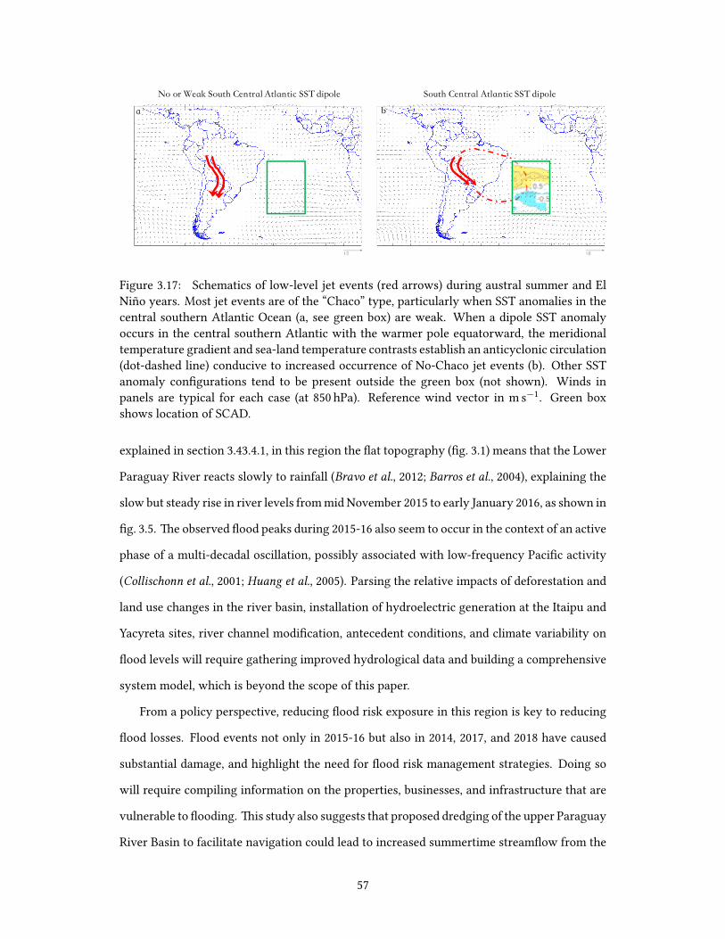
No or Weak South Central Atlantic SST dipole South Central Atlantic SST dipoleba

Figure 3.17: Schematics of low-level jet events (red arrows) during austral summer and ElNiño years. Most jet events are of the “Chaco” type, particularly when SST anomalies in thecentral southern Atlantic Ocean (a, see green box) are weak. When a dipole SST anomalyoccurs in the central southern Atlantic with the warmer pole equatorward, the meridionaltemperature gradient and sea-land temperature contrasts establish an anticyclonic circulation(dot-dashed line) conducive to increased occurrence of No-Chaco jet events (b). Other SSTanomaly configurations tend to be present outside the green box (not shown). Winds inpanels are typical for each case (at 850 hPa). Reference wind vector in m s−1. Green boxshows location of SCAD.

explained in section 3.43.4.1, in this region the flat topography (fig. 3.1) means that the Lower

Paraguay River reacts slowly to rainfall (Bravo et al., 2012; Barros et al., 2004), explaining the

slow but steady rise in river levels frommidNovember 2015 to early January 2016, as shown in

fig. 3.5. The observed flood peaks during 2015-16 also seem to occur in the context of an active

phase of a multi-decadal oscillation, possibly associated with low-frequency Pacific activity

(Collischonn et al., 2001; Huang et al., 2005). Parsing the relative impacts of deforestation and

land use changes in the river basin, installation of hydroelectric generation at the Itaipu and

Yacyreta sites, river channel modification, antecedent conditions, and climate variability on

flood levels will require gathering improved hydrological data and building a comprehensive

system model, which is beyond the scope of this paper.

From a policy perspective, reducing flood risk exposure in this region is key to reducing

flood losses. Flood events not only in 2015-16 but also in 2014, 2017, and 2018 have caused

substantial damage, and highlight the need for flood risk management strategies. Doing so

will require compiling information on the properties, businesses, and infrastructure that are

vulnerable to flooding. This study also suggests that proposed dredging of the upper Paraguay

River Basin to facilitate navigation could lead to increased summertime streamflow from the

57

Upper Paraguay River Basin (Pantanal), effectively coupling the phases of streamflow from

the Upper and Lower Paraguay River Basins which currently have a time-delay (Bravo et al.,

2012).

3.7 Summary

In this study we examined the regional climate drivers of the persistent and heavy NDJF

2015-16 rainfall over the Lower Paraguay River Basin which was associated with severe flood

events.

Both enhanced moisture inflow from the low-level jet and convergence associated with

baroclinic systems drove the observed heavy rainfall. Repeated SALLJ events, particularly

No-Chaco jet events, led to favorable conditions for mesoscale convective activity in this

region. Large-scale climate patterns at both seasonal and sub-seasonal scales favored the

synoptic weather patterns observed. Notably, a strong El Niño and an active MJO in phases

4-5 favored SALLJ occurrence. The presence of a dipolar SST anomaly in the central southern

Atlantic Ocean also favored the occurrence of No-Chaco jet events.

Numerical forecasts skillfully predicted enhanced risk of heavy rainfall at the seasonal

scale, consistent with the observed ENSO signal, but biases in the spatial patterns of forecast

rainfall suggest that models imperfectly capture the physical interactions between the Pacific

and the Atlantic basins. At sub-seasonal time scales, uncorrected model forecasts of rainfall

had limited skill beyond 15 days, though use of model output statistics – particularly the PCR

and CCAmethods that correct both spatial patterns and magnitudes – substantially improved

forecast skill.

58

It all began on March 23, 1913, with a series of nearly a dozen tornadoes. Bodiesfell from the sky, but the real terror was to come. The heavens opened with freezingrains and the flooding began. Some people drowned in their homes, others on theroads when they tried to flee. All the while, fires raged despite the torrent.

Geoffrey Williams, Washed Away: How the Great Flood of 1913, America’sMost Widespread Natural Disaster, Terrorized a Nation and Changed It

Forever

4Regional Extreme Precipitation Events: Robust

Inference from Credibly Simulated GCM

Variables

General circulation models (GCMs) are widely used to estimate future precipitation, with ap-

plication to a variety of engineering, planning, and financial use cases. Yet while theory pre-

dicts substantial sensitivity of the hydrologic cycle to anthropogenic climate change (ACC),

there is generally low confidence in future projections of extreme precipitation frequency

at the river basin scale. As described in chapter 2, some of these uncertainties stem from

fundamental uncertainties as to the response of large-scale climate patterns (e.g., the storm

tracks) to ACC while others stem from intrinsically flawed parameterization of local rainfall

in GCMs. In this paper we focus on the latter limitation and build a statistical-dynamical

59

model using large-scale climate features from a GCM plus a statistical model for local rainfall

extremes, conditional upon these large-scale features. We take the Ohio River Basin (ORB) as

a case study because prior work has illuminated the drivers of large-scale river floods in this

basin, reducing the need for diagnostic exploration. This chapter addresses four particular

questions, with summarized conclusions shown below for each.

1. For the ORB, are the extreme springtime precipitation events that cause floods well

simulated by the GCM?

• Regional extreme precipitation (REP) events (defined in section 4.1) increase the

probability of subsequent streamflow extremes in the ORB, particularly in the

December-February (DJF) and March-May (MAM) seasons.

• The GCM studied simulates too many REP days but under-simulates the occur-

rence of back-to-back REP days.

• North-South movement of storms in the GCM is under-simulated, causing pre-

cipitation (particularly along cold fronts) to exit the study region too quickly.

2. Can atmospheric indices that are associated with the onset of REP events be identified

from re-analysis?

• Most REP days during the MAM season are associated with an extratropical cy-

clone (ETC) to the West of the basin and ridging in the West Atlantic.

• Moisture from the Gulf of Mexico and Caribbean is steered by this zonal dipole.

• An anomalous ridge in the northwestern PacificOcean, likely part of a low-frequency

hemispheric pattern, is a precursor to REP days in the ORB.

3. Are suitably derived atmospheric indices associated with REP events in atmospheric

re-analysis credibly simulated by the GCM?

• The GCM credibly represents a set of five indices (in marginal distribution, auto-

correlation, and tail persistence) that describe the above identified synoptic pat-

tern.

4. If GCMs represent the large-scale atmospheric indices more credibly than they do the

REP events, can we use the GCM derived atmospheric indices to directly simulate ex-

60

treme precipitation events in the current and future climate?

• A regression model for REP occurrence conditional on credibly simulated atmo-

spheric indices mitigates the bias in GCM simulation of REP events.

• An increasing trend in REP day frequency is projected using the regressionmodel,

but the magnitude of this trend is smaller than that identified using only GCM

simulations.

This chapter has been published as

Farnham, D. J., J. Doss-Gollin, and U. Lall (2018), Regional extreme precipitation

events: Robust inference from credibly simulated GCM variables,Water Resources

Research, 54(6), doi: 10.1002/2017wr021318

and is included with permission of all authors.

4.1 Introduction

Floods are responsible for significant loss of life and economic damages both within the

United States (US) and worldwide. Flood impacts in the US are estimated at $USD 8 billion (in

2014 dollars) and 82 fatalities per year from 1984 to 2013, while worldwide flood losses were

estimated to be about $USD 85 billion (in 2012 US dollars) in 1993 alone (Kundzewicz et al.,

2013). Furthermore, trends in population and urbanization are expected to increase expo-

sure to hydroclimate extremes (including floods) into the future (Jongman et al., 2012). Given

that projections of extreme precipitation changes remain highly uncertain (IPCC, 2012), par-

ticularly in the mid-latitudes, improved estimation of future hydroclimate extremes is a key

ingredient for the mitigation of future flood impacts.

The poor representation of precipitation fields (particularly extreme precipitation) inGCM

simulations (Dai, 2006; Stephens et al., 2010; Kendon et al., 2012) complicate the projections

of future hydroclimate extremes. Simulated precipitation fields are often used as inputs to

hydrologic models (e.g. Kundzewicz et al., 2010; Hirabayashi et al., 2013; Lehner et al., 2006;

Winsemius et al., 2016) after some form of bias correction (e.g. quantile-quantile mapping;

Gudmundsson et al., 2012)) or downscaling is applied. However, it is often difficult to justify

61

a bias correction approach, especially for extrapolation into the future, since there is no ac-

companying insight as to the underlying cause for the bias, or whether the bias correction

used would be applicable in the future. In this paper we explore whether some atmospheric

variables that are closely related to the occurrence of glsrep are well simulated by GCMs,

such that their use for conditional prediction of REPs under seasonal forecasts or for climate

change projections can be an effective strategy.

4.1.1 ResearchQuestions

An important question is whether a GCM reproduces REP events well in the historical record.

Since GCMs represent the coupled dynamics of the ocean-atmosphere-land systems, answer-

ing such a question is highly dependent on the physical parameterizations of each individual

GCM. One possibility is that the GCMs credibly simulate large-scale climate circulations but

that grid-scale (and sub grid-scale) precipitation mechanisms are not well represented. In

this case it may be possible to use credibly simulated state variables from GCM simulations

to derive or simulate credible sequences of REP events associated with major floods. We ex-

plore this possibility by focusing on a single GCM and a set of atmospheric circulation indices

relevant to floods in the ORB. The following set of questions provide the framework for our

overall goal of identifying the causal structure associated with REP events and developing an

empirical model that allows the causal structure to be tested and used in a predictive context.

Q1 For theOhio River basin, are the extreme springtime precipitation events that cause floods

well simulated by the GCM?

Q2 Can atmospheric indices that are associated with the onset of REP events be identified

from re-analysis?

Q3 Are suitably derived atmospheric indices associated with REP events in atmospheric re-

analysis credibly simulated by the GCM?

Q4 If GCMs represent the large-scale atmospheric indicesmore credibly than they do the REP

events, can we use the GCM derived atmospheric indices to directly simulate extreme

precipitation events in the current and future climate?

62

4.1.2 Flooding, Extreme Precipitation, and Atmospheric Circulations in the

ORB

We use the ORB, which has a long history of regional flooding, to examine the questions

presented in section 4.1.1. Major events in 1933, 1937, 1945, 1997, and 2011 are among the

numerous floods that have had high financial and human life costs. The springtime flood of

1913 caused over 450 deaths (Perry, 2000), while the springtime flood of 2011 is estimated

to have cost over $3 billion in damages (Smith et al., 2016). Although floods are influenced

by water management strategies, land use, and soil characteristics, the floods in the ORB

are generally associated with heavy and/or persistent precipitation events and/or snowmelt

(Nakamura et al., 2013). The dominance of the precipitation signal is also supported by Mal-

lakpour and Villarini (2015), who primarily attribute changes in flood frequency in the central

US to changes in heavy rainfall frequency and temperatures while noting that land surface

changes play a secondary role.

In the study region, and in the mid-latitudes more generally, intense rainfall over a large

area typically requires large-scale advection ofmoisture from the tropics (Knippertz andWernli,

2010; Lu et al., 2013; Steinschneider and Lall, 2016). Tropical moisture export-related precip-

itation over the central and eastern United States is dominated by the Great Plains activity

center, which sources moisture primarily from the Gulf of Mexico and Caribbean Sea (Gi-

meno et al., 2010; Lavers and Villarini, 2013b; Steinschneider and Lall, 2016). Dirmeyer and

Kinter (2010) showed that large-scale flooding across the US Midwest is often associated with

moisture sources extending through Texas, Eastern Mexico, the western Gulf of Mexico, and

the Caribbean Sea (termed the “Maya Express”). Nakamura et al. (2013) showed that spring-

time extreme streamflow in the ORB is driven by a unique, recurrent, persistent and strong

atmospheric anticyclonic circulation anomaly located to the east of the US Atlantic coast (i.e.

the Bermuda High), which forces anomalous northward moisture transport from the Gulf of

Mexico and tropical Atlantic.

The remainder of the paper is organized as follows: In section 4.2 we describe our meth-

ods and data sources. In section 4.3 we introduce the regional extreme precipitation index

and evaluate its relationship to flood flows in the region. In section 4.4 we compare ob-

63

served precipitation records to historical GCM runs and discuss the origin of the GCM bias.

In section 4.5 and section 4.6 we present the results of a diagnostic composite analysis, define

atmospheric circulation and moisture indices associated with the regional extreme precipita-

tion onset, and compare the indices as derived from reanalysis data vs. the historical GCM

runs. In section 4.7 we present the results of the conditional simulation of the precipitation

events given the GCM fields for the historical (1950-2005) and future (2006-2100) periods. In

section 4.8 we summarize our results and discuss the broader implications of our findings.

4.2 Methods and Data

4.2.1 Methodological Overview

We build on the diagnostic literature discussed in section 4.1.2 in this paper and focus directly

on predicting whether or not a REP process is likely to occur on a given day based on atmo-

spheric conditions as summarized by a set of indices. The REP event is defined here as a day

when at least 4 of the 15 sub-regions in the region of interest experiences a daily rainfall that

exceeds the 99th percentile of daily rainfall at that location. Sub-regions are defined by the

blue grid in fig. 4.1 and are based on the GCM’s spatial grid. Thus, a spatiotemporal extreme

precipitation process is implicitly considered conditional on variables that are derived from

a climate model. Notably, we do not explicitly address issues related to the ability of GCMs

to simulate extreme precipitation as a function of spatial resolution (such as in Wehner et al.,

2010).

We focus on flood-relevant extreme precipitation events and fit and simulate from a

Bayesian model that propagates the parameter estimation uncertainties to the future simula-

tions. This latter point is vital for decision making since understanding the range of possible

future outcomes, via various prediction intervals, is helpful for determining our level of con-

fidence in the projections and thus whether the projections represent actionable information

or not.

Our approach is conceptually similar to a nonhomogeneous hiddenMarkovmodel (NHMM)

(Hughes et al., 1999; Kwon et al., 2009; Holsclaw et al., 2015; Cioffi et al., 2016, 2017) for precip-

itation downscaling. In the NHMM approach, a stochastic model is considered for the daily

64

rainfall process, where rainfall occurrence is modeled conditionally on a latent (unobserved)

state, and the probability of being in a particular hidden state is informed by a set of appropri-

ate atmospheric circulation variables. This approach is useful in the context of flood model-

ing, since it preserves the sequence of rainfall occurrence and hence of antecedent conditions

and event rainfall, both of which are important for determining flood potential. A challenge

with this approach is that rainfall extremes may or may not be well represented, since often

they are not explicitly conditioned on changing climate state. The end result of simulating

a credible precipitation index time-series from dynamical model outputs is common to both

our proposed method and many bias correction and statistical downscaling techniques (e.g.

Wilby et al., 2002; Maraun et al., 2010; Gutmann et al., 2014). Our method, however, places

a central focus on identifying and representing the underlying dynamics of the process. We

discuss bias-correction and downscaling approaches common to the literature in section 4.8.2.

32.5

35.0

37.5

40.0

42.5

45.0

−90 −85 −80 −75

Longitude

Latit

ude

Figure 4.1: Map of study area. Blue grid shows resolution of GFDL CM3 coupled model cells.Red grid shows native resolution of CPC precipitation data cells. The shaded area indicatesthe ORB (∼ 530 000 km2) as defined by the USGS.

Lastly, we focus on the spring (Mar-Apr-May, MAM) season in theORB (fig. 4.1), following

the observation in Nakamura et al. (2013) that this is the dominant season for major regional

65

floods. Our historical study period is from 01 March 1950 through 30 May 2005, and our

future study period is from 01 March 2006 through 30 May 2100. All anomalies are estimated

relative to the historical monthly mean unless otherwise noted.

4.2.2 Regional Extreme Precipitation Days and Extreme Streamflow

We use the Climate Prediction Center (CPC) US unified gauge-based surface precipitation (P )

data at horizontal resolution of 0.250° by 0.250° (Chen et al., 2008). The data is defined as the

precipitation accumulated in the prior 24 hours at 12 UTC and is available online from the

International Research Institute for Climate and Society (IRI)’s Data library at https://

iridl.ldeo.columbia.edu/SOURCES/.NOAA/.NCEP/.CPC/.UNIFIED_PRCP/

.GAUGE_BASED/.GLOBAL/.v1p0/. We upscale the CPC precipitation data by taking

the spatial average of the daily precipitation over the coarser horizontal grid of the dynamical

climate model introduced below (2.50° longitude by 2.00° latitude). We refer to this upscaled

CPC precipitation data as observed precipitation throughout the manuscript.

The 99th percentile precipitation exceedances, used to define the REP days, are defined

from the full-year daily record for each individual grid cell within the region of interest. In

this case, the region refers to all of the area covered by the blue and red grids in fig. 4.1. The

99th percentile thresholds used to derive the REP days are estimated separately for the ob-

served and GCM records from the observational record (1950-2005) unless noted otherwise.

This means that our REP record is insensitive to bias in the 99th percentile precipitation in

the GCM, which in turn means that this work does not address GCM bias in precipitation

intensity (such as in Maraun et al., 2010). Using the available data shown in fig. 4.1, a REP

day means that 4 or more of the region’s 15 grid cells experience a 99th percentile exceedance

of daily rainfall. We use the Hydro-Climatic Data Network streamflow data from the USGS

data downloaded with the dataRetrieval package of the R statistical programming lan-

guage, and retain only sites with drainage areas larger than 15 000 km2 and with fewer than

25 missing days over the historical study period. Six streamflow stations in the ORB meet

these criteria and are shown in fig. 4.2.

Our first goal is to investigate the relationship between the REP days and extreme stream-

66

flow days, the latter of which we define as streamflow greater than the 1 in 365 day stream-

flow (≈ 99.7th percentile), defined from each site’s full record. We use the log odds ratio of

eq. (4.1) to assess the extent to which REP day occurrence in the previous 15 days corresponds

to enhanced probabilities of extreme streamflow at the six long record streamflow gauges.

(LORs|REP) = ln[

P(Sst>Ss

364/365

∣∣∑tt′=(t−15) REPt′≥1

)/P

(Sst≤Ss

364/365

∣∣∑tt′=(t−15) REPt′≥1

)P(Sst>Ss

364/365

∣∣∑tt′=(t−15) REPt′=0

)/P

(Sst≤Ss

364/365

∣∣∑tt′=(t−15) REPt′=0

)]

(4.1)

where Sst is the streamflow at time step t and streamflow station s, Ss

364/365 is the 1 in 365

day streamflow at site s, and t′ is a dummy variable to loop from (t− 15) to t.

4.2.3 Atmospheric Reanalysis for Event Diagnostics

We use atmospheric specific humidity (Q), geopotential height (Z), upward velocity (ω), and

zonal wind (U ) fields from theNational Center for Environmental Prediction (NCEP)/National

Center for Atmospheric Research (NCAR) reanalysis 1 data set (Kalnay et al., 1996). The

NCEP/NCAR reanalysis dataset has a horizontal resolution of 2.50° by 2.50° and 17 pressure

levels. We download six hourly data and define each day as the average value between 12 UTC

and 12 UTC to ensure that the atmospheric reanalysis data is on the same temporal grid as the

CPC precipitation. The NCEP/NCAR Reanalysis 1 data is available from NOAA/OAR/ESRL

PSD, Boulder, Colorado, USA, online at http://www.esrl.noaa.gov/psd/.

4.2.4 General Circulation Model

We use the P ,Q, Z , ω, and U fields from the CM3 (Donner et al., 2011). The surface and atmo-

sphere in CM3 has a resolution of 2.50° longitude by 2.00° latitude (fig. 4.1). CM3 outputs are

available online athttps://www.gfdl.noaa.gov/coupled-physical-model-cm3/.

Based on the atmospheric variables and daily resolution that we required for this work, we

could only acquire two historic ensemble member simulations and one future simulation.

67

KanawhaFalls (K)Louisville (L)MtCarmel (M)

Natrona (N)

Petersburg (P)

WabashLafayette (W)

37

39

41

−88 −84 −80

Longitude

Latit

ude

Drainage Area (x 10000 sq. km)

0

5

10

15

20

25

Streamflow gauges

0.0000

0.0025

0.0050

0.0075

0.0100

DJF MAM JJA SON

season

Pr(S

s>

S36

436

5s

)

site KanawhaFalls

Louisville

MtCarmel

Natrona

Petersburg

WabashLafayette

InfInf

MAM

KanawhaFalls Louisville MtCarmel Natrona PetersburgWabashLafayette

0

2

4

6

1+

(LO

Rs |

RE

P)

Figure 4.2: Relationship between streamflow and REP days. (Left) Locations and drainage ar-eas of the six long record streamflow stations. (Top, right) The seasonality of extreme stream-flow (>≈ 99.7th percentile) for each site in colors as expressed through the probability ofextreme streamflow occurrence during each season. (Bottom, right) The log odds ratio ofeq. (4.1) and confidence interval associated with MAM days when one of more REP days haveoccurred in the previous fifteen days vs. those when no REP days have occurred in the pre-vious 15 days and streamflow being above or below the ≈ 99.7th percentile. The odds ratioconfidence interval was calculated via the unconditional maximum likelihood estimation (orthe Wald method) via the epitools package of the R statistical programming language.

4.3 Regional Extreme Precipitation Days and Streamflow

Figure 4.2 highlights the positive relationship between REP incidence and subsequent extreme

streamflows during MAM in the study basin. DJF and MAM dominate the record of extreme

streamflows (≈ 99.7th percentile) and the station with the largest drainage area (Louisville)

shows a clear maximum in MAM. The estimated log odds ratio defined in eq. (4.1) is positive

for all stations during MAM (fig. 4.2), a clear indication that the occurrence of REP days

is strongly associated with the occurrence of extreme streamflows during MAM in the ORB.

The extreme streamflow seasonality and enhanced odds of occurrence following REP days are

similar when extreme streamflow is defined using the 99th and 99.9th percentiles, indicating

that the relationship between high streamflows and antecedent REP events is not sensitive to

the definition of extreme streamflow.

68

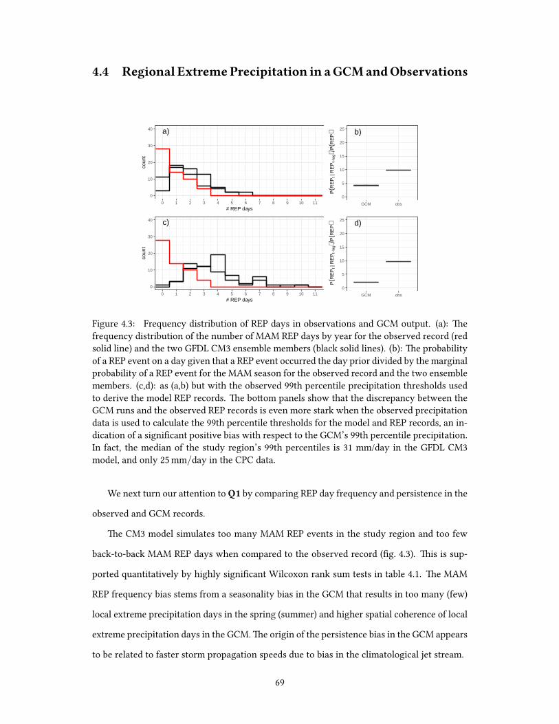
4.4 Regional ExtremePrecipitation in aGCMandObservations

a)

0

10

20

30

40

0 1 2 3 4 5 6 7 8 9 10 11

# REP days

coun

t

c)

0

10

20

30

40

0 1 2 3 4 5 6 7 8 9 10 11

# REP days

coun

t

b)

0

5

10

15

20

25

GCM obs

P(R

EP

t | R

EP

t−la

g)P

(RE

P)

d)

0

5

10

15

20

25

GCM obs

P(R

EP

t | R

EP

t−la

g)P

(RE

P)

Figure 4.3: Frequency distribution of REP days in observations and GCM output. (a): Thefrequency distribution of the number of MAM REP days by year for the observed record (redsolid line) and the two GFDL CM3 ensemble members (black solid lines). (b): The probabilityof a REP event on a day given that a REP event occurred the day prior divided by the marginalprobability of a REP event for the MAM season for the observed record and the two ensemblemembers. (c,d): as (a,b) but with the observed 99th percentile precipitation thresholds usedto derive the model REP records. The bottom panels show that the discrepancy between theGCM runs and the observed REP records is even more stark when the observed precipitationdata is used to calculate the 99th percentile thresholds for the model and REP records, an in-dication of a significant positive bias with respect to the GCM’s 99th percentile precipitation.In fact, the median of the study region’s 99th percentiles is 31 mm/day in the GFDL CM3model, and only 25mm/day in the CPC data.

We next turn our attention toQ1 by comparing REP day frequency and persistence in the

observed and GCM records.

The CM3 model simulates too many MAM REP events in the study region and too few

back-to-back MAM REP days when compared to the observed record (fig. 4.3). This is sup-

ported quantitatively by highly significant Wilcoxon rank sum tests in table 4.1. The MAM

REP frequency bias stems from a seasonality bias in the GCM that results in too many (few)

local extreme precipitation days in the spring (summer) and higher spatial coherence of local

extreme precipitation days in the GCM.The origin of the persistence bias in the GCM appears

to be related to faster storm propagation speeds due to bias in the climatological jet stream.

69

Table 4.1: The distributions of atmospheric indices in GCMs and reanalysis are more similar(per two-sample Wilcoxon rank sum tests) than the distributions of REP days per year basedon the GCM and precipitation and the observed precipitation. The null hypothesis of this testis that it is equally likely that a randomly selected value from sample A (i.e., observations)is greater than or less than a randomly selected value from sample B (i.e., GCM ensemblemember).

Observed/Reanalysis & Observed/Reanalysis &GCM ensemble member 1 GCM ensemble member 2

Variables being compared W -statistic p-value W -statistic p-value

# REPs (yearly) 2.2× 103 1.8× 10−4 2.5× 103 8.1× 10−8

ZL (daily) 1.3× 107 9.1× 10−1 1.3× 107 8.7× 10−1

ZH (daily) 1.3× 107 8.1× 10−1 1.3× 107 6.1× 10−1

ZP (daily) 1.3× 107 3.1× 10−1 1.3× 107 4.6× 10−1

HUM (daily) 1.3× 107 8.2× 10−1 1.3× 107 8.8× 10−1

OMG (daily) 1.4× 107 1.0× 10−1 1.4× 107 9.6× 10−2

While the CM3model exhibits a wet bias in the 99th percentile precipitation, the approach

used to define REP events means that this does not explain the inflated MAM REP counts in

the GCM. Since the total number of local (one cell) extreme precipitation days (i.e. > 99th

percentile) is the same for both the observed and GCM records, the REP frequency bias can

stem from a bias in the seasonal distribution of the local extreme precipitation days or a bias

in the spatial correlation across the study region.

There is clearly a bias in the seasonality of the extreme precipitation days, which con-

tributes to the over-simulation of MAM REP days. The CM3 model ensemble members show

37 and 38 percent of their local (single-grid) extreme precipitation days occurring during

MAM, while the observed record shows only 27 percent (see fig. 4.4). Conversely, the CM3

members simulate between 10 and 11 percent of local extreme precipitation days during June-

August (JJA), less than the observed value of 26 percent. This seasonality bias is manifest in

the REP climatology itself (fig. 4.5) with the GCM simulating relatively few REP days dur-

ing JJA and relatively more during MAM. Deficiencies in simulating extreme precipitation

during boreal mid-latitude summer has been observed and discussed for other models (e.g.

Durman et al., 2001) andmay be attributable to parameterizations of sub-grid-scale convective

processes (Liang et al., 2006).

70

DJF JJA MAM SON

1 3 5 7 9 1 3 5 7 9 1 3 5 7 9 1 3 5 7 9

0

50

100

150

200

# of local intense precipitation events on a given day

OB

S c

ount

− G

CM

cou

nt

no REP

REP

Figure 4.4: The difference of frequency distributions (between the observed and two GCMensemble members) of local (one cell) extreme precipitation days by season (columns) overthe observational record for all days with at least 1 local extreme precipitation event in thestudy region.

GCM ens 1 GCM ens 2 OBS

1 2 3 4 5 6 7 8 9 10 11 12 1 2 3 4 5 6 7 8 9 10 11 12 1 2 3 4 5 6 7 8 9 10 11 120

5

10

15

20

month

% o

f RE

Ps

Figure 4.5: The distribution of the regional extreme precipitation days by month for theobserved record and each of the two GCM ensemble members. Note that the GCM ensemblemembers are very similar and averaging across them does not significantly reduce the biaswith respect to spring (MAM, or months 3, 4, and 5) and summer (JJA, or months 6, 7, and 8)REP frequency.

71

GCM ens 1 GCM ens 2 OBS

−100 −90 −80 −70 −100 −90 −80 −70 −100 −90 −80 −70

25

30

35

40

45

50

Longitude

Latit

ude

0.75

0.80

0.85

0.90P percentile

Figure 4.6: The precipitation percentiles (shading) averaged over all days when at least one ofthe 15 study area cells received rainfall greater than the 99th percentile for the observed andtwo GCM ensemble members. All cells with mean percentile less than the 75th are shadedwhite.

The second reason for the inflated MAM REP counts is a tendency of the CM3 model to

produce too many co-occurring local extreme precipitation days. More precisely, REP days

occur during 22 and 24 percent of all MAM days when there is at least one local extreme pre-

cipitation event in the two CM3 ensemble members, respectively, compared to just 11 percent

in the observed records (see fig. 4.4). This indicates that when the model produces extreme

precipitation in any part of the study region, it has a tendency to simultaneously produce

extreme precipitation in several grid cells. This high regional covariance, or smearing, of the

extreme precipitation can be seen in fig. 4.6. This high spatial covariance is not surprising

given that the effective resolution of numerical models is known to be significantly greater

than the grid spacing (e.g., Grasso, 2000). This point is noteworthy for any regional flood

hazard assessment that uses GCMs.

In addition to the frequency bias, the CM3model under-simulates the occurrence of back-

to-back REP days (fig. 4.3, right panels). The probability of a REP day following the occur-

rence of a REP day is about 4 times more than the marginal probability of REP occurrence

in the GCM, compared to about 10 times in the observed record. This appears to be related

to representation of the storm tracks, which in CM3 propagate primarily from west to east,

under-representing observed south to north movement. This causes the precipitation (partic-

ularly along cold fronts) to exit the study region more quickly (fig. 4.7). We conclude that the

relevant precipitation events are not well simulated by the CM3 model (i.e. no to Q1)

and turn our attention to Q2 by investigating the atmospheric circulations associated with

72

GCM ens 1 − OBS GCM ens 2 − OBS

−100 −90 −80 −70 −100 −90 −80 −70

25

30

35

40

45

50

Longitude

Latit

ude

−0.2

−0.1

0.0

0.1

0.2

PGCM percentile −

POBS percentile

Figure 4.7: The difference between each GCM ensemble member and the observed record ofprecipitation percentiles (shading) averaged over all REP days.

REP days.

4.5 CirculationPatternsAssociatedwithRegional ExtremePre-

cipitation

The atmospheric circulation during the REP days is similar in the reanalysis record and the

CM3 historical runs, aside from a modest southward shift in the composite storm location in

the GCM that appears to be a manifestation of latitudinal bias in the jet.

X

X

XX X

XX

XX

XXX

XX

XX

XXX X

XXX

XX

XXXXXX

XXXXXX

XXXXXXX

XXXXXX

XXXXXX

XXXXXX

XXX X

X

XXXX

XX

X X X X

X

XXX

XX

XX

XXX

XXX

XXXX

XXXXX

XXXXX

XXX

X

X

X

X

XX

XX

X

X

X

X

X

X

XXX

XX

XXXX

XXX

XXX

XXXX

XXXX

X XX

XXXX

XXXX

XXX

X

XXX

XXXXX

XXXXXX

X

XXXXXXXXX

XXXXXXXXXX

XXXXXXXXX

XXXXXXX

X

XXXX

XX

X

X X XXX

XX

XXXX

XXXXX

XXXXXX

XXXXXXXX

XXXXXXXX

XXXXXXXX

XXXXXXX

XXXXXX

XXX

X

XXX

XX X

XXX

X X

X

XX

X

X

X

XX

XXXXX

XXXXX

XXXXX

XXX X

XXX

XXXX

XXXXX

XXXXXXX

XXXXXXX

XXXXX

X

X

X

X X

−1 0 1

−4 −3 −2

−140 −100 −60 −140 −100 −60 −140 −100 −60

20

40

60

20

40

60

Longitude

Latit

ude

−50

0

50

Z700 (m)

Figure 4.8: Daily composites of Z700 anomalies (shades) and Q700 (contours at4× 10−4 kg kg−1) from four days before each MAM REP event to one day following the eventfor the observed-reanalysis record. Solid contours represent positive anomalies and dashedcontours represent negative anomalies. An “X” indicates that at least 80% of composite mem-bers (i.e. at least 37 of the 46 REP events) hadZ700 anomalies of the same sign in that location.

73

Figure 4.8 shows the composite time-lagged geopotential height and specific humidity

anomalies at 700 hPa (Z700 and Q700) preceding and during the MAM REP days for the ob-

served record. The dominant features of the atmospheric development of the REP are similar

to those found in Nakamura et al. (2013) for the top 20 floods in the ORB and include:

1. A zonal dipole pattern in the anomalous Z700 field at latitudes between about 35 °N to

45 °N preceding and accompanying the REP events

2. The dipole pattern migrates eastward beginning approximately three days prior to the

REP events, accompanied by an intensification of the dipole and significant northward

low-level wind anomalies (not shown)

3. A well-organized positive anomaly in the Q700 field over the ORB along the interface

of low and high Z700 anomalies that peaks during the day of the event

4. An anomalous warm surface and low-level temperature anomaly that stretches from

the Gulf of Mexico up to the Northeast US (not shown), indicating that the REP events

are often associated with frontal systems which in turn are often coupled with extrat-

ropical cyclones (not shown)

5. An anomalous high pressure ridge in the northwest Pacific Ocean south of the Gulf of

Alaska that starts to intensify at least 4 days prior to the REP day and persists through

the day after the REP day. This north Pacific ridge appears to be a lower frequency

pattern that together with the pressure dipole (noted above) forms a tripole structure

spanning from the eastern Pacific to the western Atlantic during REP days that is rem-

iniscent of the wavenumber 6 pattern.

The most consistent of the atmospheric features associated with the REP days is a high

pressure system (Western Atlantic ridging) which is for some events related to an intensified

and westward-extended subtropical high. Another consistent feature is the presence of a low

pressure system in the western US that forms about 2-3 days prior to the REP days.

Despite the bias in the rainfall field, the CM3 ensemble member composites of Z700

(figs. 4.9 and 4.10) during MAM REP events show a similar pattern of troughing west of

the basin and ridging east of the basin, compared to the reanalysis record. There are, how-

ever, a few subtle differences. The ridging patterns associated with REP days in the CM3

74

XX

XXXXX

XXXX

XXXX

XX

XXXXXX

XXXXXXXX

XXXXXXXXXXX

XXXXXXXXXX

20

40

60

−140 −100 −60

Longitude

Latit

ude

GCM ens 1

XXX

XXXXX

XXXX

XXX

XXXX

XXXXX

X

XXXXXX

XXXXX

20

40

60

−140 −100 −60

Longitude

Latit

ude

GCM ens 2

XXX

XX

XXXX

XXX

XXX

XXXX

XXXX

X XX

XXXX

XXXX

XXX

X

XXX

XXXXX

XXXXXX

X

XXXXXXXXX

XXXXXXXXXX

XXXXXXXXX

XXXXXXX

X

XXXX

XX

X

20

40

60

−140 −100 −60

Longitude

Latit

ude

OBS & NCEP/NCAR

−40

0

40

Z700 (m)

Figure 4.9: Same as fig. 4.8 but for the day of the REP event (lag = 0) and each of the GFDLCM3 GCM ensemble members and the observed-reanalysis record (panels). As in fig. 4.8, an“X” indicates that at least 80% of composite members had Z700 anomalies of the same signin that location. This 80% criteria translates to at least 83 out of 103 REP events, 92 out of115 REP events, and 37 out of 46 REP events, for the two CM3 ensemble members and theobserved-reanalysis record, respectively.

model have a tendency to extend to the north-east of the study area, while in the reanalysis

record the ridging tends to extend over locations to the south-east of the study area. The CM3

model also shows a southward displacement of the low pressure center relative to the reanal-

ysis record, evident in the extent and location of precipitation during study region REP days

(stronger/weaker southeast/northwest precipitation during GCM REP events can be seen in

the difference between the GCM and observation percentile precipitation during REP events

in fig. 4.6). This is likely related to a southward displacement of the storm tracks in the CM3

model, which can be seen in the enhanced (suppressed) standard deviation of MAM 700 hPa

geopotential height to the south (north) of 30 °N to 35 °N in the GCM ensemble members

compared to reanalysis (fig. 4.11) and the clear southward displacement of the springtime

jet (fig. 4.12). We also note the absence of the REP-associated ridging in the north Pacific

in the GCM, which along with the higher frequency wave train associated with REPs in the

GCM, suggests that the GCM can produce REP days in the ORBwithout the presence of hemi-

spherically organized flow compared to the observed-reanalysis record. Despite the modest

latitudinal bias, and the lack of a clear tripole pattern, we highlight that the Z700 patterns

associated with MAM REP events are largely similar between the GCM and reanalysis.

75

XX

XXXXX

XXXX

XXXX

XX

XXXXXX

XXXXXXXX

XXXXXXXXXXX

XXXXXXXXXX

20

40

60

−140 −100 −60

Longitude

Latit

ude

GCM ens 1

XXX

XXXXX

XXXX

XXX

XXXX

XXXXX

X

XXXXXX

XXXXX

20

40

60

−140 −100 −60

Longitude

Latit

ude

GCM ens 2

XXX

XX

XXXX

XXX

XXX

XXXX

XXXX

X XX

XXXX

XXXX

XXX

X

XXX

XXXXX

XXXXXX

X

XXXXXXXXX

XXXXXXXXXX

XXXXXXXXX

XXXXXXX

X

XXXX

XX

X

20

40

60

−140 −100 −60

Longitude

Latit

ude

OBS & NCEP/NCAR

−50

0

50

Z700 (m)

Figure 4.10: MAM REP day composites of Z700 anomalies (shading) and absolute Z700

(contours in 50m increments with 3000 m marked with a thicker contour) for both the ob-served/reanalysis (i.e. reanalysis Z700 during observed REPs) and each of the two GCM en-semble members. Solid contours represent positive anomalies and dashed contours representnegative anomalies. An “X” indicates that at least 80% of compositemembers hadZ700 anoma-lies of the same sign in that location. This 80% criteria translates to at least 83 out of 103 REPevents, 92 out of 115 REP events, and 37 out of 46 REP events, for the two CM3 ensemblemembers and the observed-reanalysis record, respectively.

GCM ens 1 − NCEP/NCAR GCM ens 2 − NCEP/NCAR

−140 −100 −60 −140 −100 −60

20

30

40

50

60

Longitude

Latit

ude

−20

−10

0

10

20

∆σZ700 (m)

Figure 4.11: The difference in standard deviation of dailyMAMgeopotential height at 700 hPafor the reanalysis and each of the two GCM ensemble members. Note that the pattern associ-ated with each ensemble member looks very similar, i.e. averaging across ensemble membersdoes not meaningfully reduce the bias with respect to the reanalysis record.

GCM ens 1

−160 −120 −80 −40

20

40

60

Longitude

Latit

ude

GCM ens 2

−160 −120 −80 −40

20

40

60

Longitude

Latit

ude

NCEP/NCAR

−160 −120 −80 −40

20

40

60

Longitude

Latit

ude

0

10

20

30

40U200 (m/s)

Figure 4.12: The climatological zonal wind 200 hPa (shading and contours) inm s−1 for the re-analysis and each of the two GCM ensemble members. The contours show 15m s−1, 25m s−1

and 35m s−1. Note that the pattern associated with each ensemble member looks very similar,i.e. averaging across ensemble members does not meaningfully reduce the bias with respectto the reanalysis record.

76

4.6 Atmospheric Indices

In this section we show that the GCM appears to reasonably simulate the distributional and

persistence features of five atmospheric indices that modulate the likelihood of REP events.

This is critical to the conditional simulation strategy proposed in section 4.7.

ZP ZL

HUMOMG

ZH30

40

50

−175 −150 −125 −100 −75 −50

Longitude

Latit

ude

−1

0

1

2

−5 −4 −3 −2 −1 0 1 2 3

Days after REP event

ZP In

dex

−2

−1

0

1

−5 −4 −3 −2 −1 0 1 2 3

Days after REP event

ZL

Inde

x

−1

0

1

2

−5 −4 −3 −2 −1 0 1 2 3

Days after REP event

HU

M In

dex

−2

0

2

−5 −4 −3 −2 −1 0 1 2 3

Days after REP event

OM

G In

dex

−1

0

1

−5 −4 −3 −2 −1 0 1 2 3

Days after REP event

ZH

Inde

x

Figure 4.13: (Top) the regions that define each of the atmospheric indices. The index namesare shown in red. The Ohio River basin, shown in more detail in fig. 4.1 is shaded in dark gray.The ZP index is defined by the average Z700 within the area between 130 °W and 155 °W and30 °N and 55 °N (leftmost dashed box), the ZL index is defined by the average Z700 within thearea between 87.5 °W and 103 °W and 30 °N and 45 °N (middle dashed box), and the ZH indexis defined by the average Z700 within the area between 62.5 °W and 77.5 °W and 30 °N and45 °N (rightmost dashed box). The OMG and HUM indices are defined using the average at-mospheric vertical velocity and specific humidity within the area between 77.5 °W and 90 °Wand 36 °N and 42 °N (solid box). (Middle and bottom) The index values prior to and after theREP events. The black line shows the median index value. The dark shaded area shows therange capturing the middle 50% of days, while the light shaded area shows the range captur-ing the middle 90% of days. All panels use the observed REP record and the correspondingreanalysis-based atmospheric indices.

Given that the CM3 model credibly represents the pressure dipole associated with MAM

REP events, we define two indices by geopotential heights in boxes to the east and west of the

ORB. We call these indices the ZL and ZH (for the low and high pressure systems associated

77

with the REP days) and define them as the mean of Z700 in the western and eastern boxes,

respectively, shown in fig. 4.13. The boxes have a large meridional extent to capture both the

center of the low pressure storms in the GCM REP days and the observed REP days (fig. 4.9).

We also define an index by the mean Z700 in the large box in the northwest Pacific during

the three days prior to the current day. We call this index ZP and include it to represent the

impact of a strong wavetrain with a center of high pressure in the North Pacific on the proba-

bility of REP event (figs. 4.8 and 4.13). We also define two indices to capture the atmospheric

conditions over the ORB. The first of these indices is defined as the mean of Q700 over the

basin and is called HUM; we assume that higher values of moisture over the basin increase

the probability of a REP day. The next of these indices is the mean of ω700 over the basin

and is called OMG. This index is important since it represents the existent or absence of local

convergence and uplift that is important for the occurrence of precipitation.

All five of these indices are defined as their standardized quantities (subtracting their

seasonal mean and dividing by their seasonal standard deviation) following Karl et al. (1990).

Most importantly, all five of these indicesmodulate the probability of REP occurrence (fig. 4.13).

It should be noted, however, that the daily reanalysis-based indices have been defined by the

12 UTC to 12 UTC values to match the temporal grid of the CPC data while the CM3 indices

have been defined on a standard daily grid that begins and ends with 0 UTC to match the

daily temporal grid of the CM3 precipitation. We assume that the relationship between the

indices and REP occurrence is insensitive to this temporal grid difference. Based on (fig. 4.13),

we conclude that indices that are associated with the onset of REP events can be iden-

tified from re-analysis (i.e. yes to Q2) and turn our attention to Q3 by investigating the

atmospheric simulation of the indices in the CM3 GCM.

Figure 4.14 illustrates that the distributional and persistence properties of each of the

indices are reasonably well simulated by the GCM (i.e. yes to Q3). Table 4.1 quantitatively

illustrates (based on Wilcoxon rank sum tests) that the distributions of the atmospheric in-

dices based on the GCM and reanalysis are more similar than the distributions of REP days

per year based on the GCM precipitation and the observed precipitation. There are, however,

a few differences between the GCM and reanalysis indices. These differences include slightly

78

− OMG − ZL HUM ZH ZP

−2 0 2 −2 0 2 −2 0 2 −2 0 2 −2 0 2

0.00

0.25

0.50

0.75

1.00

Index

F(I

ndex

)

− OMG − ZL HUM ZH ZP

1 2 3 4 5 6 7 1 2 3 4 5 6 7 1 2 3 4 5 6 7 1 2 3 4 5 6 7 1 2 3 4 5 6 7

0.00

0.25

0.50

0.75

1.00

lag

Cor

(Inde

x t ,

Inde

x t−l

ag)

− OMG − ZL HUM ZH ZP

1 2 3 4 5 6 7 1 2 3 4 5 6 7 1 2 3 4 5 6 7 1 2 3 4 5 6 7 1 2 3 4 5 6 7

0.0

0.2

0.4

0.6

0.8

lagPr(F

(Inde

x t) >

0.9

| F(In

dex t

−lag

) > 0

.9)

Figure 4.14: (Top) Cumulative distribution function for the MAM indices. (Middle)The serialcorrelation function for the MAM indices. (Bottom) The serial tail persistence of the MAMindices when in high states as shown by the probability of the index being above the 90thpercentile on day t, given that the index was above that percentile on day t-lag, where lagvalues of 1 through 10 are shown along the x-axis. In all panels the solid line is the reanalysis-based indices and the dashed lines are the GCM ensemble member-based indices. NegativeOMG and ZL are shown for easier interpretation since low values of these two indices areassociated with REP days.

lower HUM index autocorrelation, slightly higher ZP autocorrelation, and higher persistence

of extreme low values of ZL for the GCM (fig. 4.14). It seems likely that the persistence bias of

the HUM index partially explains the reduced persistence in the GCM-based REP days com-

pared to the observed. On the other hand, the other notable persistence biases of the ZL and

ZP indices should increase the probability of back-to-back REP days in the GCM compared

to the observed record. Despite these minor differences, we conclude that the atmospheric

indices associated with REP events are credibly simulated by the GCM (i.e. yes toQ3).

We now turn our attention to the problem of directly using these indices to simulate the REP

events (i.e. Q4).

79

4.7 Conditional Simulation

In this section we turn our attention to Q4 and demonstrate that:

1. the conditional simulation of REP days based on a regression on the atmospheric indices

addresses the bias in the observational record;

2. a future upward trend in REP day frequency is projected both when using the raw

GCM precipitation fields and when using the conditional simulation model based on

GCM-derived atmospheric indices;

3. this positive trend appears to be driven both by a trend in the moisture index (which

is in turn at least partially the result of increasing temperatures), and by trends in the

other indices.

To set up the logistic regression-based simulation model, with a binary response vari-

able (REP or no REP), we assume that the ZH, ZL, ZP, OMG, and HUM indices on day t

linearly modulate the probability of REP occurrence on day t. Based on this assumption,

we define a logistic regression model to estimate the probability of a REP day given the five

indices (eq. (4.2)). We estimate α, βZL , βZH , βZP , βHUM, βOMG from the observation-derived

REPs and reanalysis-derived indices (eq. (4.2)). We refer to these parameter estimates as

a, bZL , bZH , bZP , bHUM, bOMG. We use a fully Bayesian model (Jaynes, 2003; Gelman et al., 2014;

McElreath, 2016) implemented in Stan (Carpenter et al., 2017) inR. We use diffuse normal prior

distributions with means of 0 and standard deviations of 25 and 5 for the α and β parameters,

respectively.

P(REPobst = 1) =

exp[α+ βZL

(ZLreanalt+1

)+ βZH

(ZHreanal

t

)+ βZP

(ZPreanalt

)+ βHUM

(HUMreanal

t

)+ βOMG

(OMGreanal

t

)]1 + exp

[α+ βZL

(ZLreanalt+1

)+ βZH

(ZHreanal

t

)+ βZP

(ZPreanalt

)+ βHUM

(HUMreanal

t

)+ βOMG

(OMGreanal

t

)](4.2)

Where t is a time index and REP is the regional extreme precipitation indicator (either 0 or

1).After fitting this model on the observed/reanalysis record, we are able to simulate REP

days from the GCM-derived indices using eq. (4.3). Specifically, we sample from a Bernoullidistribution for each day with probability of a REP as computed from eq. (4.3). We retain 1000

80

samples for each day.

P( REPmodt = 1) =

exp[a+ bZL

(ZLmod

t+1

)+ bZH

(ZHmod

t

)+ bZP

(ZPmod

t

)+ bHUM

(HUMmod

t

)+ bOMG

(OMGmod

t

)]1 + exp

[a+ bZL

(ZLmod

t+1

)+ bZH

(ZHmod

t

)+ bZP

(ZPmod

t

)+ bHUM

(HUMmod

t

)+ bOMG

(OMGmod

t

)] (4.3)

4.7.1 Model Checking

To verify that our model captures a substantial portion of the variance in the record, we first

evaluate the ability of our model to reproduce the observed record by fitting the model on the

first 42 years (1950-1991; about three quarters of the data) and predicting the last 14 years.

We use these time intervals so that the calibration sample contains at least several years of

the relatively data rich period after the introduction of satellite observations systems in the

late 1970s and early 1980s. The model is only able to capture a small portion of the day-

to-day variation with daily hit rates of 12% and 11% for the calibration and testing samples,

respectively, and false alarm rates of 88% for both the calibration and testing samples. If we

allow the simulation to be off by one day in either direction, however, then we have hit rates

of 22% and 14% and false alarm rates of 0%. Figures 4.15 and 4.16 show that the model captures

a portion of the interannual variation, and has a negative bias with respect to representing

the persistence of REP days. Lastly, the proposed model explains 33% of the deviance in the

data and partially reproduces the spectral peaks at 3-4 years and 7-8 years when fit on the

full historical data (fig. 4.17). In summary, the physical variables that we have identified only

explain a portion of the variance in the REP record and can therefore be seen as necessary

but not sufficient to predict day-to-day REP occurrence with high probability. This model

is potentially useful, however, for understanding long-term changes in the REP frequency

associated with changes to these underlying physical variables, as we show below.

4.7.2 Simulation Results

The results of our conditional simulation based on the GCM-derived atmospheric indices and

the reanalysis-observation coefficient estimates for the historical record are shown in fig. 4.18.

When the model is estimated based on the full historic reanalysis-observed record, the regres-

sion coefficient estimates for bZL , bZH , bZP , bHUM, bOMG have means of -0.72, 0.65, 0.41, 0.90,

and -1.11, and standard deviations of 0.18, 0.30, 0.18, 0.25, and 0.21. All coefficients are of their

81

0

1

2

3

1950 1960 1970 1980 1990 2000

year

# R

EP

s

sample Calibration Testing

0.0

0.5

1.0

1.5

2.0

2.5

1950 1960 1970 1980 1990 2000

year

Pfo

reca

st(k

= k

*)P

mar

gina

l(k =

k*)

0.00

0.25

0.50

0.75

1.00

1950 1960 1970 1980 1990 2000

year

P(X

* for

ecas

t≤

x obs

erva

tion)

Calibration Testing

0 1 2 3 0 1 2

0

1

2

3

4

5

6

7

8

# REPs observed in year

# R

EP

s pr

edic

ted

in y

ear

0.1 0.2 0.3 0.4 0.5

Figure 4.15: (Top) Yearly record of the number of REP days per year for the observed record(solid black points and line), themean of the regression predicted record during the calibrationperiod (solid blue points and line) and testing period (solid red points and line). The 50thpercentile prediction intervals are also shown for each year with blue and red vertical linesfor calibration and testing periods, respectively. (Second from top) The probability that themodel simulates the observed number of REPs in a year divided by the calibration sampleprobability of observing that same number of REPs in a year for the calibration and testingsamples (blue and red points and lines, respectively). A ratio greater than one indicates skill.The training and testing sample median ratios are shown with blue and red dashed lines.(Third from top) The probability that the simulated number of REPs in a year were less thanthe observed number of REPs in a year. Random noise with mean zero and standard deviationof 0.001 is added to the simulation derived yearly time-series to avoid the ties that result fromthe discrete nature of the data. (Bottom) The discrete probability distribution of simulatednumber of REP days for years where 0, 1, 2, or 3 REP days were observed. That is, eachcolumn of tiles sums to 1. A 1:1 line is shown via dashed lines.

82

0

5

10

15

20

25

sims obs

set

P(R

EP

t | R

EP

t−1)

P(R

EP

)

Calibration period

0

5

10

15

20

25

sims obs

set

P(R

EP

t | R

EP

t−1)

P(R

EP

)

Testing period

Figure 4.16: The probability of a REP event on a day given that a REP event occurred theday prior divided by the marginal probability of a REP event for the MAM season for theobserved record (obs) and 1000 simulated records from the Bayesian regression model (sims)for the calibration (left) and testing (right) periods. The boxplot whiskers extend to pointswithin 1.5 of the interquartile range, and any observation outside of this range is shown as apoint.

Table 4.2: As table 4.1 but for the historical period observed REPs vs. mean of simulationmodel predicted REPs

Observed & mean of model predictionVariables being compared W -statistic p-value

# REPs (yearly) 1.3× 103 1.2× 10−1

expected sign and the HUM and OMG indices have the strongest effect on the probability of

REP occurrence. The bias in the REP frequency is substantially reduced through the use of

this simulation model (compare fig. 4.18 to the top panel of fig. 4.3), while the persistence bias

is still significant. The bottom row of table 4.1 and table 4.2 quantitatively illustrate (based

on Wilcoxon rank sum tests) that the distributions of GCM-index-based simulated REP days

per year and observed REP days per year are more similar than the distributions of GCM-

precipitation-based REP days per year and observed REP days per year.

We use a future simulation of the CM3 GCM under the RCP 8.5 forcing scenario to sim-

ulate daily REP records via our conditional simulation model for the years 2006 to 2100 and

compare these projections against future daily REP records estimated directly from the GCM’s

precipitation field (fig. 4.19). The standardization of the indices was still based on the histor-

ical mean and standard deviation. We also compare our future simulations against projec-

tions based on a linear bias-corrected version of the GCM REPs where we assume that the

83

0.0

0.0

0.1

0.2

0.3

2.5

Observed spectrum

2

4

8

16

perio

d (y

ears

)

10 20 30 40 50

years past 1950

0.0

0.0

0.1

0.1

0.3

2.2

mean predicted spectrum

2

4

8

16

perio

d (y

ears

)

10 20 30 40 50

years past 1950

Figure 4.17: (Top) Wavelet power spectrum for the observed # of REP events by year. Colorindicates power and regions inside of the white borders are significant at the 90% level asdetermined by shuffling the given time-series (i.e. bootstrapping). (Bottom) Same as (Top)but for the mean model predicted # REP by year.

84

a)

0

1

2

3

1960 1970 1980 1990 2000

year

# R

EP

b)

0

10

20

30

40

0 1 2 3 4 5 6 7 8

# REP

coun

t

c)

0

5

10

15

20

25

ens # 1 ens # 4 obs

P(R

EP

t | R

EP

t−la

g)P

(RE

P)

Figure 4.18: Comparison of REP day representation in observation and GCM simulation. (a)The number of MAM REP days by year based on the two GFDL CM3 ensemble member’sprecipitation fields (black solid lines), the mean of the simulated REP counts obtained via theregression on the indices derived from the two GFDL CM3 ensemble member’s Z700, Q700,and ω700 fields (black dashed lines), and the 50th and 95th percentile prediction intervalsbased on the 1000 simulations (dark and light shaded regions, respectively). All data has beenGaussian kernel smoothed (bandwidth = 10 years) before the mean and prediction intervalsare computed. The first and last 5 years of the smooths have been truncated from the fig-ure to avoid edge effects. (b) The counts for the number of MAM REP days by year for theobserved record (solid red line), the record derived from the GFDL GCM CM3 precipitationfields (solid black lines), and the mean of the simulations for each ensemble member (dashedblack lines). (c) Probability of a MAM REP day on a day given that a REP day occurred theday prior divided by the marginal probability of a REP day for the observed record and theREP simulated records for the two ensemble members and the observed record. The boxplotwhiskers extend to points within 1.5 times the interquartile range above the 75th percentile,and any observation outside of this range is shown as a point.

past frequency bias in the GCM REP record is multiplicative and representative of GCM REP

frequency bias in the future. Our simulation model projects a significant increasing trend

throughout much of the 21st century similar to that projected by the GCMprecipitation fields,

although the index-based projections show lower absolute REP frequency. The rescaled GCM

precipitation field derived projection (blue line in fig. 4.19), i.e. the bias corrected GCM REP

projection, deviates substantially from the mean index simulation projections in the late pe-

riod of the 21st century. However, the rescaled projections do lie within the 95th percentile

prediction interval of the simulation model projections. The observation that a positive, albeit

weaker trend exists even after our conditional simulation provides some evidence that an in-

creasing trend may occur. However, we emphasize restraint in this interpretation, since both

approaches assume the RCP 8.5 forcing scenario and that the large-scale circulation patterns

in the future are well-represented by the CM3 model physics.

85

a)

0

2

4

6

2025 2050 2075

year

# R

EP

b)

0

10

20

30

40

50

0 1 2 3 4 5 6 7 8 9 10 11

# REP

coun

t

Figure 4.19: Projected number of MAMREP days using raw GCM output, a naive bias correc-tion, and the Bayesian logistic regression model. (a) The projected number of MAM REP daysby year based on the GFDL CM3 RCP 8.5 ensemble member precipitation field (black solidline), the mean of the simulated REP counts obtained via the regression on the GCM-basedindices (black dashed lines), and the 50th and 95th percentile prediction intervals based onthe 1000 simulations (dark and light shaded regions, respectively). The blue dashed line is theprojected MAM REP record when we assume that the historical bias between the GCM andobserved REP frequency is multiplicative and stationary and we rescale the projection basedon the GCM precipitation field. In this case, this amounts to dividing the solid black line byabout 2.2. All data has been Gaussian kernel smoothed (bandwidth = 10 years) before themean and prediction intervals are computed. The first and last 5 years of the smooths havebeen truncated from the figure to avoid edge effects. (b) The counts for the number of MAMREP days by year with corresponding line colors and types as in (a).

4.7.3 Moisture Trend Contribution

It is notable that the increase in REP frequency estimated by our conditional sampling model

is driven by a positive shift in the probability distribution of the as well as the other indices.

To explore the relative contribution of the moisture changes (HUM) vs. changes in the other

indices, we performed additional simulations using the last 30 years of GCM output from each

of the twentieth and twentieth first centuries (1970-1999 and 2070-2099). We first compute

the mean change in all GCM-derived indices between these two time periods (using the GCM

ensemble mean for the historic period). We find that the meanMAMHUM increases by about

0.6 (i.e. about half a standard deviation). Then we use the regression estimates from the full

observed historical record, but simulate REPs using three sets of predictors: 1) using the GCM

indices for the 2070-2099 time period; 2) removing the trend in the HUM index by subtracting

0.6 from all HUM index values from 2070-2099 and then simulating the REPs for the 2070-

2099 time period; 3) using the GCM indices for the 1970-1999 time period. We retain 1000

simulations for each of these scenarios and plot the resulting REP incidence in fig. 4.20. The

median increase in the GCM simulations using our procedure from 1970-1999 to 2070-2099 is

86

0.00

0.25

0.50

0.75

1.00

1.25

0 1 2 3 4 5

Mean # of REPs per year

dens

ity

experiment

1970−1999

2070−20992070−2099 (moisture trend removed)

Figure 4.20: Kernel density smoothed PDFs showing the mean number of simulated MAMREP days over the 30 year periods of 1970-1999 (red line) and 2070-2099 (short-dashed greenline) and 2070-2099 after the trend in the HUM index has been removed (long-dashed blueline). Each curve is composed from 1000 points that represent the mean # of REPs per yearin a 30 year simulation.

about 200 percent when all index trends are included. It is only 60 percent when the trends

in the HUM are removed. These results suggest that, given our model, about two-thirds of

the future increase in MAM REPs is due to a humidity increase.

4.8 Summary and Discussion

4.8.1 Summary

Precipitation is the primary climate input into the modeling of extreme riverine floods. Con-

sequently, hydrologists need to consider how to best use future predictions of regional climate

in GCMs, given that many factors contribute to the well-documented biases in GCM based

precipitation simulation. We were interested in an approach that provided a diagnostic of the

physical factors associated with such biases. Next we were interested whether these factors

could be used to achieve a better representation of the causal factors associated with extreme

precipitation, and especially with regional extreme precipitation in a large river basin (the

Ohio as the example), such that future GCM simulations could be used to statistically assess

potential changes.

87

We began by defining a regional extreme precipitation index, illustrating its relationship

to extreme streamflows in the study region, and investigating the dominant atmospheric cir-

culation patterns associatedwith the precipitation events. Next we showed that the frequency

and persistence properties of this regional extreme precipitation index are not well simulated

by a GCM, but that the large scale atmospheric circulation indices (defined by large scale

geopotential height, moisture, and vertical velocity fields) that are strongly associated with

the extreme precipitation are credibly simulated by the same GCM. Then we constructed a

logistic regression model to simulate the regional extreme precipitation index at the daily

scale based on five atmospheric indices. This simulation framework greatly reduced the fre-

quency bias in the observational record of the GCM REP days. Using this model for future

projections we found that future GCM simulations likely overestimate the total number of

regional extreme precipitation events out to the year 2100. However, an increasing trend in

REP occurrence in the 21st century, attributed to trends in both the moisture index and other

circulation indices, is still evident in our simulations. We acknowledge that our approach

still relies on the assumptions that the relationship between the large-scale climate indices

and the REP occurrence is stationary into the future and that our regression is valid over the

ranges of the indices in the future GCM runs.

4.8.2 Relationship to Bias Correction and Downscaling Approaches

Like many bias correction and downscaling techniques, we assume that the GCM is deficient

in its simulation of processes that link the global-synoptic scale circulations and the grid-scale

processes that determine precipitation over a specific river basin which may represent just

a few grid cells of the GCM. We developed our approach with the following common limi-

tations of bias correction and downscaling approaches in mind. Using most bias-correction

techniques (e.g. Gutmann et al., 2014; Piani et al., 2010; Yang et al., 2005; Friederichs and Hense,

2007; Goly et al., 2014; Pierce et al., 2015) for extrapolation into the future projections is un-

certain given that most approaches do not explicitly identify the underlying model deficien-

cies (Ehret et al., 2012; Dittes et al., 2018; Bosshard et al., 2018). Many statistical downscaling

schemes to recover precipitation estimates from large scale circulation features (e.g. (Wilby

88

et al., 2002)) have been proposed, including many tailored for use in future climate projec-

tion (see Maraun et al., 2010, and references therein). However, it is often unclear how to

adapt weather generator (e.g. (Thorndahl et al., 2017)) and weather typing approaches (e.g.

Jacobeit et al., 2003; Muñoz et al., 2015) in a non-stationary climate. Dynamical downscaling

(e.g. Schmidli et al., 2007)) is another option, but is computationally expensive (Wilby et al.,

2002), and is often sensitive to precipitation-related parameterizations and the size of the em-

bedded domain used (Liu et al., 2011; Leduc and Laprise, 2009). Regression downscaling (e.g

Wilby et al., 2002) is computationally cheap and is more able to deal with non-stationary con-

ditions. However, the regressions often do not represent the extremes well and explain only a

relatively small portion of the variance in the data (Wilby et al., 2002). The latter point is par-

ticularly problematic if a goal of the downscaling is to estimate future precipitation conditions

since it may be that the model sensitivity to future regional forcing is below the level of the

noise (i.e. a signal in the precipitationmay simply be an artifact of the model parameterization

and estimation).

4.8.3 Caveats and Further Discussion

A shortcoming of our model is that it does not fully capture the serial correlation in the REP

process, as represented by figs. 4.15 and 4.18. The negative persistence bias in the reconstruc-

tion of the observed-reanalysis record suggests that our model could be improved through the

incorporation of other variables that inform the temporal clustering of the REP days. While

the persistence bias can be partially mitigated by including lagged REP days as predictors, we

chose not to include a lagged REP predictor because the predictor was not significant given

the presence of the other predictors and the absence of a lagged REP predictor greatly reduces

the computational cost of the simulation model.

As previously noted, our simulation method does not avoid a reliance on the assumption

that circulation (and associated moisture) changes are well simulated into the future by the

GCM. The frequency bias in the regional extreme precipitation record appears to be a mani-

festation of inflated spatial correlation of high intensity precipitation. The precipitation event

persistence bias appears to be a manifestation of a strong and southerly displaced springtime

89

jet in the GCM that results in faster moving storms and lower autocorrelation in the humidity

field over our study region. We were able to limit our simulation model’s sensitivity to the

southerly displacement bias by using standardized indices (i.e. a form of bias correction to

translate the mean to be ≈0 and rescale the variance to be ≈1), but we did not fully address

the persistence bias. Other approaches to handling biases in GCM circulation fields have

been proposed when credible precipitation fields are the desired outcome; Eden et al. (2012)

advocate for the approach of nudging GCM fields toward observed fields and then letting the

GCM simulate the precipitation fields. Two deficiencies of this approach, however, are the

reliance on the convective parameterization scheme of the GCM (which can be particularly

problematic during summer), and an inability to project future precipitation events because

there exists no future reanalysis field to nudge towards. Thus, it is difficult to avoid a reliance

on GCM circulation fields when it comes to projecting regional scale precipitation events, and

difficult to estimate the validity of the GCM under warming and other related and relevant

changes such as changing mid-latitude meridional temperature gradients due to Arctic Am-

plification (Barnes and Screen, 2015). Finally, the simulation model presented in this paper

has been shown to better predict the REP event frequency than do the GCM precipitation

fields and is therefore plausibly useful for understanding the future trends in REP frequency.

Having said that, the simulation model does not necessarily provide daily time sequences that

are appropriate for impacts models given figs. 4.16 and 4.18.

90

Part II

Sequential Adaptation

91

Themore you know, the harder it is to take decisive action. Once you are informed,you start seeing complexities and shades of gray. You realize nothing is as clearas it first appears. Ultimately, knowledge is paralyzing. Being a man of action, Icannot afford to take that risk.

Bill Watterson, The Authoritative Calvin and Hobbes

5Review of Methods for Infrastructure Planning

under Uncertainty

Whereas part I outlined a physical-dynamical approach to constraining future hydroclimate

hazards, part II of this dissertation is concerned with using intrinsically uncertain projections

to inform decisions and improve outcomes for local risk management and adaptation.

This chapter reviews approaches to planning and designing infrastructure systems under

uncertainty. This is a field replete not only with competing methods but also deep philo-

sophical disagreements. When should optimization be used when a system’s objectives are

unclear? How should probability be used to reason about uncertainties, including unknown

unknowns? How can models inform decision-making for complex systems? What should

decision-makers do when different models give different results? Who gets to decide the

answers to these questions?

92

Though this chapter does not attempt to provide a definitive answer to these questions,

it does seek to frame these debates and advocate a general perspective. First, section 5.1

reviews decision-theoretic approaches, focusing in particular on the uses and restrictions

of rationality and optimization. Though rationality is found to be limited as a descriptive

model of the world, it gives rise to useful notions of subjective probability and conditional

optimization. Next, section 5.2 outlines approaches to decision-making for wicked problems

under “true” uncertainty. In particular, widely sampling from possible outcomes, identifying

fundamental tradeoffs, and representing path dependence can provide quantitative answers

to qualitative questions. Finally, section 5.3 describes how engineering, policy, and financial

instruments can support better outcomes. Since a decision framework is only as good as the

decisions considered, “soft” instruments that improve the flexibility and performance of the

system, evaluated using option theory and portfolio analysis, can lead to better outcomes.

5.1 DecisionTheory

Decisions about climate adaptation, systems planning, and infrastructure operation draw

upon theoretical frameworks for decision science developed in other fields, including eco-

nomics, grand strategy, computer science, operations research, and business strategy. These

theories emphasize that

1. the axioms of rationality and Bayesian decision theory provide a calculus for value and

choice, conditional upon assessments of preference and belief (section 5.1.1);

2. many uncertainties that govern real-world planning problems cannot be described through

a single objective probability distribution (section 5.1.2);

3. the design and management of infrastructure is intrinsically “wicked” because objec-

tives cannot be clearly defined and conflict is intrinsic (section 5.1.3); and thus

4. the role of decision theory, and science more broadly, for wicked problems should be

to transparently link assumptions, preferences, and outcomes (section 5.1.4).

93

5.1.1 Rationality, DecisionTheory, and Optimization

The theory of rational decision making evolved in the middle of the 20th century in tandem

with mathematical theories of probability and economics. In particular, Von Neumann and

Morgenstern (1953) proposed four axioms for rational choice: (i) completeness of preference;

(ii) transitivity of preference; (iii) continuity of preference, and (iv) independence of prefer-

ence from the existence of irrelevant alternatives. Von Neumann andMorgenstern then proved

that an individual or firm that follows these actions behaves as though maximizing the ex-

pectation of some function, which they called a utility function. Similarly, individuals and

firms that do not follow these axioms can be systematically exploited (see the “Dutch book”

arguments of De Finetti, 1972).

Over the next decades, the descriptive model of rationality used to study firms and individ-

uals (see Savage, 1954; Debreu, 1959) became widely applied as a normative tool for planning.

Efforts such as the Harvard Water Program (see Maass et al., 1962) popularized the use of

top-down rational planning approaches for water management (Howe, 1971) and other so-

cial planning problems. These methods used the vocabulary and mathematical framework of

Bayesian decision theory (BDT) (Gelman et al., 2014; Savage, 1954), bringing a formal math-

ematical treatment of these problems. Four elements define a formal decision problem in

BDT:

• an action space A that describes all possible actions a ∈ A available to the decision-

maker which, depending upon the problem at hand, may be continuous, discrete, mul-

tivariate, etc.;

• a state space S, of potentially many dimensions, which specifies all the information

available to the decision-maker;

• a reward function (alternatively called a utility function or objective and its negative

as loss or cost function) R : S ×A → R that maps information about the state of the

world and a particular action taken to a real number; and

• a representation of uncertainty p(s) that describes the probability that a given state of

the world s ∈ S occurs.

These four elements can be combined to calculate the expected reward of taking a particular

94

action:

E[R | a] =∫S

R(a, s)p(s) ds , (5.1)

allowing the decision maker to select the best action

a∗.= argmax

a∈AE[R | a] . (5.2)

In the case where the reward function is a discounted cash flow, eq. (5.1) is equivalent to

classical cost-benefit analysis (CBA) or net present value (NPV) analysis using discounted

cash flows. A key insight from eq. (5.1) is that

E[R | a] = R(E[s] , a), (5.3)

meaning uncertainties must be fully described (see Gelman et al., 2014, ch. 9, for simple ex-

amples in which these expectations diverge). For example, Oddo et al. (2017) revisit the point

estimates used by van Dantzig (1956) to optimize levee heightening in the Netherlands and

that show that considering uncertainties leads to substantially different decisions (this case

study is revisited in chapter 7).

Many problems in infrastructure planning and management are sequential, meaning that

(i) the goal is to solve for a policy π : S → A that maximizes expected future reward, and

(ii) each action affects the decisions and rewards available in the future. For example, reservoir

management, capacity expansion, and water quality control are all examples of sequential

planning (see section 5.2.2 for further discussion). The extension of BDT to sequential decision

problems is reinforcement learning (RL) (see Sutton and Barto, 2018, for a comprehensive

review), in which the goal is to identify the action a ∈A that maximizes, in expectation, the

quantity

Gt = γRt+1 + γ2Rt+2 + . . . (5.4)

where γ ∈ (0, 1) is a discount factor which is assumed constant (though it could depend on

time or other factors; seeArrow et al., 2013). A popular and widely used class of RL algorithms

is dynamic programming (DP) (Bellman, 1954, 1957) and its extensions (Bertsekas, 1976; Ste-

95

dinger et al., 1984; Faber and Stedinger , 2001; Lamontagne, 2015). Another class of algorithms

approximates the Q-function

qπ(s, a).= Eπ[Gt | St = s,At = a]

= Eπ

[ ∞∑k=0

Rt+k+1

∣∣∣∣∣ St = s,At = a

]∀s ∈ S, a ∈A,

(5.5)

which gives the expected discounted future rewards, conditional on being in state s, tak-

ing action a, and following an optimal strategy thereafter. Q learning, often using neural

networks for function approximation (i.e., “deep Q learning”), has surpassed human perfor-

mance in benchmarks including Atari video games (Mnih et al., 2013, 2015; Wang et al., 2016;

van Hasselt et al., 2015; Schaul et al., 2015; Fortunato et al., 2019; Hessel et al., 2017). However,

application to problems with complex action spaces or sparse rewards remains a challenge

(Doss-Gollin et al., 2019a). An alternative is to instead model the policy π : S → A as a

function of parameters θ ∈ Rd, and to search for approximately optimal θ (Schmidhuber ,

2001). This approach exploits theoretical properties such as the policy gradient theorem (Sut-

ton et al., 2000), and has been used in models like AlphaGo, which famously surpassed human

performance at the game of Go (Silver et al., 2017, 2018). Policy search methods are also used

widely for multiobjective optimization (see section 5.2.3).

5.1.2 Epistemic Uncertainty and Subjective Probability

To implement an optimization procedure or calculate expected reward following eq. (5.1),

one must first specify a probabilistic model for the probability of each state (or, in the case of

sequential problems, for the evolution of states over time).

Projections of the relationship between decision and outcome depend upon complex dy-

namics, including human actions, that are intrinsically unpredictable, particularly in the dis-

tant future. In general, uncertainties can be grouped into four classes, describing those that

are (i) purely stochastic with known parameters; (ii) stochastic with known model structure

but unknown parameters; (iii) imaginable, with unknown model structure but a well char-

acterized event space; and (iv) truly uncertain, in the sense that the events cannot even be

imagined (Walker et al., 2013b, fig. 1 divides these into five categories). The uncertainties

96

from categories (iii) and (iv) have been described as “deep uncertainty” (Walker et al., 2013b,a;

Lempert, 2002), “true uncertainty” (as opposed to categories (i) and (ii), termed “risk”; Langlois

and Cosgel, 1993; Knight, 1921) and “black swans” (to refer specifically to events that cannot

be proven impossible; Taleb, 2007). Uncertainties have also been characterized as epistemic if

the modeler sees a possibility to reduce them by gathering more data or by refining models

and aleatory otherwise.

There are many sources of deep and true uncertainty in projections of flood risk and its

response to intervention. If risk is crudely defined as the product of hazard, meaning the

probability that a particular event occurs (as discussed in chapter 2), and exposure, meaning

the damage that will occur should the hazard arrive, total uncertainty stems from both (note

that this definition of risk is unrelated to that of Knight, 1921).

Many of the physical dynamics discussed in part I lead large and deep uncertainties as to

future hazard. Climate sensitivity, arctic amplification (AA) and the storm track response, and

the response of clouds to warming illustrate the large uncertainties intrinsic to future climate.

Hydroclimate extremes are also sensitive to anthropogenic climate change (ACC), and since

future greenhouse gas emissions depend on political, economic, and technological factors,

future hydroclimate extremes are themselves sensitive to these deep uncertainties. Humans

also modify local environmental conditions in ways that affect hydroclimate hazard but are

not readily quantifiable. For example, channelizing upstream portions of a river can reduce

flood hazard upstream but increase it downstream (Juan et al., 2020); these dynamics are

therefore as much political and social as physical. Similarly, local land use change, including

deforestation (Lawrence and Vandecar , 2015) andmangrove removal (Hochard et al., 2019), can

depend on deeply uncertain human actions, and the effect of these changes on hydroclimate

hazard is often highly nonlinear.

Historical data also highlights the central role of exposure to total risk. For example,

global exposure to river floods has grown exponentially since 1970, far outpacing increases

in hazard (Jongman et al., 2012). Tedesco et al. (2020) find that damage caused by Hurricane

Florence was exacerbated by an increase in exposed property – from 10 to 52 billion dollars

between 2000 and 2018 – and that while construction has slowed over the past decade, it has

97

nearly all occurred in low-lying and otherwise vulnerable areas. More generally, Pielke et al.

(2008) attribute trends in loss to hurricanes over the past century in the United States (US) to

changes in exposure, consistent with global analyses (Peduzzi et al., 2012). This does not only

lead to increased loss of property; Di Baldassarre et al. (2010) argue that increased exposure in

vulnerable areas has increased floodmortality in sub-Saharan Africa. Economic risks can also

cascade in non-intuitive ways through increasingly global supply chains (Helbing, 2013); both

conceptual (Inoue and Todo, 2019) and observational (e.g. of Thailand’s 2011 flood; Haraguchi

and Lall, 2015) evidence suggests that supply chain interruptions can substantially exceed

direct damage. A corollary to this point is that interventions to manage hydroclimate risk

can have unintended consequences. For example, high traffic often motivates communities

to widen and expand highways, but this can have the effect of decreasing the marginal cost

of driving, thereby encouraging people to move their homes and workplaces farther apart

and worsening traffic (Lee et al., 1999). Similarly, the “safe development paradox” (Haer et al.,

2020) and “levee effect” (Tobin, 1995) describe the process by which structural flood protec-

tion can reduce minor floods and perceived risks, induce a sense of safety, motivate increased

exposure, and thereby lead to greater losses when a large flood eventually occurs (Baren-

drecht et al., 2017; Merz et al., 2014; Di Baldassarre et al., 2018a; Aerts et al., 2018; Kousky and

Kunreuther , 2010). Through a similar logic, measures to increase water supply can lead to

higher water demand and thus greater vulnerability to droughts when they eventually occur

(Di Baldassarre et al., 2018b; Srinivasan et al., 2017).

The observation that many of these mechanisms cannot be represented by a single ob-

jective probability density function (PDF) has motivated many criticisms of the application

of BDT to planning problems. For example, Shackle (1972) argued probability to be an inap-

propriate calculus for true uncertainty, chiefly because the event space is model-dependent,

and proposed an alternative calculus of surprise (see also Derbyshire, 2017). Yet while the

lack of objective probabilities may merit alternative decision methodologies in practice, this

theoretical argument is something of a straw man. In fact, BDT was conceived as a calculus

for reasoning rather than for identifying objective truth; De Finetti often said that “probabil-

ity does not exist” (De Finetti, 1972). Savage (1954) and Ramsey (2016), among others, also

98

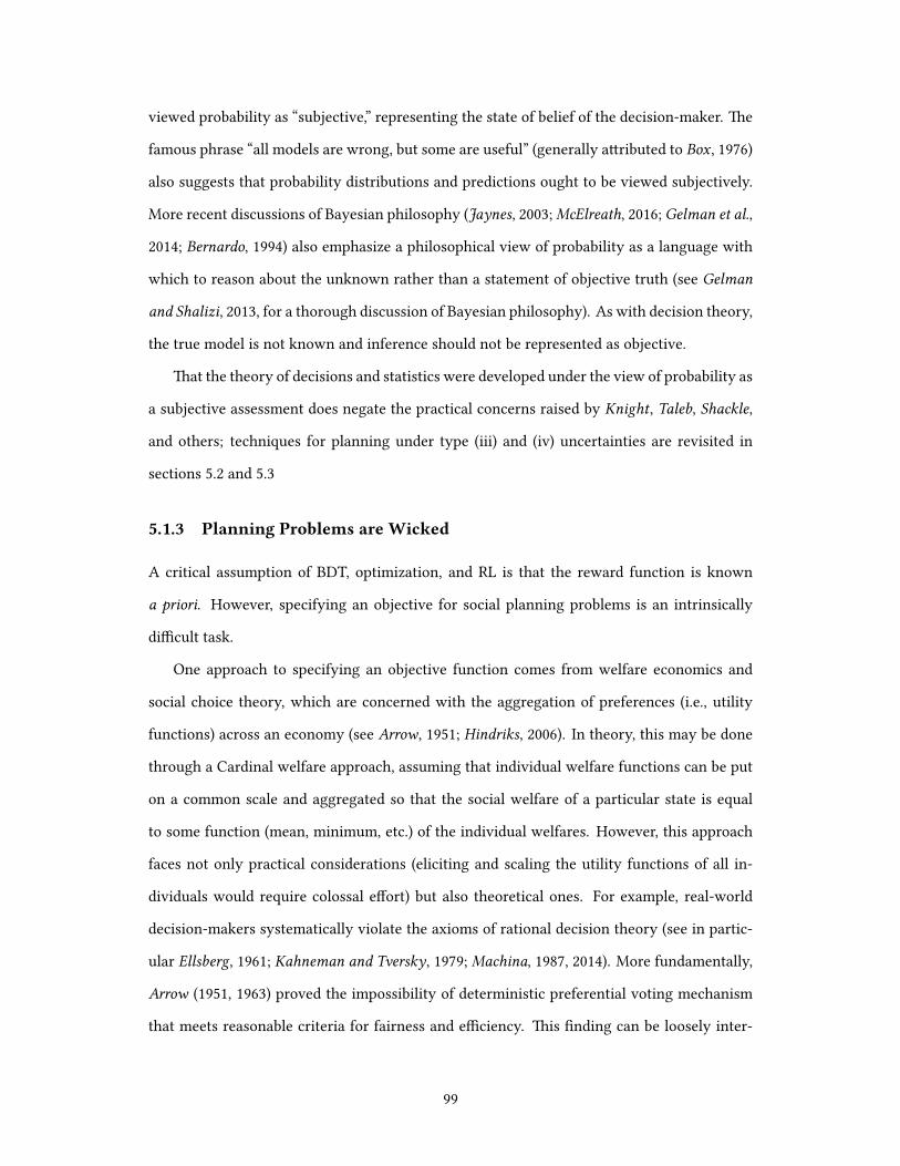
viewed probability as “subjective,” representing the state of belief of the decision-maker. The

famous phrase “all models are wrong, but some are useful” (generally attributed to Box, 1976)

also suggests that probability distributions and predictions ought to be viewed subjectively.

More recent discussions of Bayesian philosophy (Jaynes, 2003; McElreath, 2016; Gelman et al.,

2014; Bernardo, 1994) also emphasize a philosophical view of probability as a language with

which to reason about the unknown rather than a statement of objective truth (see Gelman

and Shalizi, 2013, for a thorough discussion of Bayesian philosophy). As with decision theory,

the true model is not known and inference should not be represented as objective.

That the theory of decisions and statistics were developed under the view of probability as

a subjective assessment does negate the practical concerns raised by Knight, Taleb, Shackle,

and others; techniques for planning under type (iii) and (iv) uncertainties are revisited in

sections 5.2 and 5.3

5.1.3 Planning Problems are Wicked

A critical assumption of BDT, optimization, and RL is that the reward function is known

a priori. However, specifying an objective for social planning problems is an intrinsically

difficult task.

One approach to specifying an objective function comes from welfare economics and

social choice theory, which are concerned with the aggregation of preferences (i.e., utility

functions) across an economy (see Arrow, 1951; Hindriks, 2006). In theory, this may be done

through a Cardinal welfare approach, assuming that individual welfare functions can be put

on a common scale and aggregated so that the social welfare of a particular state is equal

to some function (mean, minimum, etc.) of the individual welfares. However, this approach

faces not only practical considerations (eliciting and scaling the utility functions of all in-

dividuals would require colossal effort) but also theoretical ones. For example, real-world

decision-makers systematically violate the axioms of rational decision theory (see in partic-

ular Ellsberg, 1961; Kahneman and Tversky, 1979; Machina, 1987, 2014). More fundamentally,

Arrow (1951, 1963) proved the impossibility of deterministic preferential voting mechanism

that meets reasonable criteria for fairness and efficiency. This finding can be loosely inter-

99

preted as demonstrating that it is not only practically infeasible but also theoretically impos-

sible to identify an objective social welfare function.

Another challenge to rational decision making in the domain of public planning is intrin-

sic conflict. Barry (1997) describes “levee patrols” of armed vigilantes who during the 1927

Mississippi River flood protected levee sections against saboteurs from the opposite river-

bank. While the field of game theory (Debreu, 1959; Von Neumann and Morgenstern, 1953;

Nash, 1951, 1950) provides a framework for descriptive understanding of the responses of dif-

ferent actors to planning decisions, it does not seek to provide a normative definition of the

“best” policy, except where there is a role for an external facilitator to enforce “win-win” out-

comes (see Madani, 2010, for examples including groundwater management as a prisoner’s

dilemma game).

In light of these challenges, Rittel and Webber (1973) argue that most problems in plan-

ning are “wicked,” meaning that (i) the solution is sensitive to the problem definition and the

problem definition to the solution; (ii) stakeholders have radically different world views and

different frames for understanding the problem; (iii) the constraints to which that the prob-

lem is subject and the resources needed to solve it change over time; and (iv) the problem is

never solved definitively. In particular, Rittel and Webber argue that the appealing notion of

objective technocratic problem-solving is a myth, that there is not and cannot exist a true ob-

jective function, and that the expert is inevitably a player in a political game. This argument

is bolstered by findings that ex ante analyses of infrastructure projects are systematically bi-

ased towards under-estimation of costs and over-estimation of benefits, reflecting that they

are political documents rather than sincere attempts at objective truth (Flyvbjerg et al., 2005;

Flyvbjerg, 2009).

While many of the conflicts described by wicked problems are apparent during the plan-

ning process, intrinsic conflict across time is not. Inter-temporal choice is generally treated

by discounting the future at a constant rate. A conceptual challenge is that discount rates are

used both to represent opportunity cost (which is why they are often higher in developing

nations than developed ones) and to represent the preference between the value of consump-

tion today and consumption in the future (which, if it is assumed to be richer than the present,

100

can be discounted on grounds of decreasing marginal returns to money or other goods) (Es-

pinoza et al., 2019; Arrow et al., 2013). For example, in the US the executive branch budgetary

process assesses United States Army Corps of Engineers (USACE) projects at a discount rate

of 7% on most projects, conceptually reflecting the opportunity cost of capital in the private

sector, though many have argued for different approaches (Carter and Nesbitt, 2016). In gen-

eral, planning decisions are quite sensitive to the choice of discount rate (Weitzman, 2007) and

change when a distribution of discount rates are assumed relative to a single rate (Zarekarizi

et al., 2020). Estimating discount rates from past behavior is complicated because, among

other reasons, many of the costs passed on to the future are opaque to the decision-makers

who choose to pass them on (e.g., infrastructure maintenance costs; Marohn, 2019).

5.1.4 The Role of DecisionTheory

The central message of this section is that while rationality is a helpful construct which gives

rise to powerful optimization tools, there cannot exist an objective assessment of belief or

preference. This is not to say that all beliefs are equally valid – some are more or less con-

sistent with science and evidence than others – but rather that disagreement is inevitable.

Given that planning problems, including flood risk management policies, confront deep un-

certainties and are intrinsically wicked, a philosophical perspective on the role of science and

decision theory is helpful.

Gilboa et al. (2018) suggest that decision theory should form the framework for a conver-

sation between modelers and stakeholders. In this framework, the implications of different

preferences and assumptions should be mapped clearly onto the likelihood of different out-

comes. This approach is consistent with the a posteriori approach proposed by Tsoukiàs (2008),

though it emphasizes an iterative process. One particular pitfall in stakeholder engagement

for planning in wicked problems like flood risk management is that different stakeholders

may have different preferences, and the preferences of the stakeholders “in the room” (often

representing engineers, local government, utilities, and civic organizations) may not reflect

the preferences of those not in the room. Thus, the scientist should provide a reproducible

map from assumptions and preferences to outcomes so that others can explore the effect of

101

different preferences, assumptions, and beliefs.

5.2 Decision Frameworks for PlanningunderTrueUncertainty

A variety of decision frameworks are used for problems in wicked systems under deep or true

uncertainty. Despite important differences, these frameworks generally share

1. the use of system models to explore response to a wide range of plausible scenarios

(section 5.2.1);

2. the formulation of adaptive and sequential plans to exploit new information as it emerges

over time (section 5.2.2); and

3. an explicit quantification of tradeoffs between conflicting goals and outcomes (sec-

tion 5.2.3).

5.2.1 Bottom-Up and Exploratory Modeling

A common approach across frameworks for planning under uncertainty is to invert standard

“predict then plan” approaches in favor of “bottom-up” perspectives that use a system model

to explore its response to a broad range of plausible scenarios before assessing how likely

these scenarios are.

For example, Bankes (1993) distinguishes between consolidative modeling, which seeks to

integrate all information about a particular system into a single model, and exploratory mod-

eling, which is used to understand possible behavior. In particular, exploratory modeling

can demonstrate the existence of particular outcomes, generate hypotheses, build qualitative

insight, and identify scenarios worthy of further study. An explicit recognition that a mod-

eling exercise is exploratory can help to limit the likelihood of over-interpreting mathemati-

cal models and drawing misleading conclusions (Saltelli, 2019). Frameworks for exploratory

modeling (e.g., Kwakkel and Pruyt, 2013) are widely used in a variety of strategic planning

fields.

The philosophical underpinnings of exploratory modeling are also evident in a variety of

widely used frameworks for infrastructure systems planning under uncertainty. For example,

decision scaling explores a system’s “response surface” to forcing such as mean precipitation

102

and temperature (Brown et al., 2012; Steinschneider et al., 2015; Poff et al., 2015). Once a sys-

tem’s essential fragilities have been identified, their likelihood is assessed using projections

from a wide set of models. Derivative approaches, including the World Bank’s decision tree

framework (Ray et al., 2018) and the resilience by design approach (Brown et al., 2020), also

emphasize bottom-upmodeling or vulnerability assessment and consideration of awide range

of plausible scenarios.

Another framework for bottom-up analysis with wide application to infrastructure plan-

ning is robust decision making (RDM) (Lempert et al., 2003). Like decision scaling, RDM uses

an iterative process to identify potential strategies, characterize the vulnerabilities of such

strategies, and evaluate the tradeoffs among them. For example, Lempert et al. (2012) run

hundreds of CBAs for different plausible values of parameters, conduct scenario discovery

through cluster analysis, and finally compare the groups of scenarios that lead to particularly

good or poor outcomes with values from the scientific literature to assess how likely they

are. Like exploratory modeling and decision scaling, RDM emphasizes an iterative process of

engagement with stakeholders rather than a single prescriptive or normative solution; this

process can lead to recognition of opportunities for collaboration rather than competition

between stakeholders (e.g., between adjacent water uitilities; Zeff et al., 2016; Gorelick et al.,

2019; Herman et al., 2014; Trindade et al., 2017, 2019).

5.2.2 Policies and Decision Pathways

Since infrastructure planning is a dynamic process, many decision support tools explicitly

recognize the role of time.

For example, dynamic adaptive policy pathways (DAPP) is a qualitative framework (often

implemented with quantitative modeling) emphasizing (i) that adaptation and investment de-

cisions are sequential by nature, and (ii) that infrastructure and urban systems embody strong

path dependence (Haasnoot et al., 2012, 2013). Like RDM and decision scaling, DAPP empha-

sizes exploratory modeling and iterative stakeholder engagement (Kwakkel et al., 2016, 2015),

but DAPP particularly emphasizes the formulation of (i) candidate development pathways

(Wise et al., 2014) along which the system might develop, (ii) triggers or tipping points that

103

specify when particular actions will be taken, and (iii) signposts that allow proactive moni-

toring of key system variables (Haasnoot et al., 2015; Raso et al., 2019; Lawrence and Haasnoot,

2017). The methodology was originally developed for projects on the Thames Estuary and

Dutch Delta, but has been applied to problems in water resources, regional planning, coastal

planning, and heat risk management (see Bloemen et al., 2018).

Alternatively, an optimization framework can solve sequential decision problems (see sec-

tion 5.1.1). Since optimization models require a probabilistic representation of uncertainty,

these often proceed by specifying a finite set of scenarios of deeper uncertainties, then devel-

oping scenario-dependent optimal policies (Bertoni et al., 2017; Kang and Lansey, 2014). Often

the probabilistic weighting of scenarios is implicitly a uniform distribution over an arbitrary

set of scenarios considered (Herman et al., 2020).

Like DAPP, sequential optimization and RL aim to exploit information as it emerges over

time. For example, Fletcher et al. (2017) formulate the question of water system capacity ex-

pansion in Melbourne, Australia as a multistage decision and solve it using DP. Given an

initial model for the evolution of reservoir inflows and population growth over time, the DP

formulation enables learning. The analysis is repeated for several scenarios of electricity

price, water shortage penalties, and demand per capita which are considered deeply uncer-

tain. Similar approaches can inform reservoir planning (Fletcher et al., 2019a), groundwater

management (Fletcher et al., 2019b), and coastal hurricane protection (Lickley et al., 2014).

Another DP model for coastal adaptation is discussed in chapter 7.

5.2.3 TradeoffQuantification

In wicked problems for which no objective utility function can be formulated (section 5.1.3), it

is common to use tradeoff analysis to compare how different actions or policies might affect a

set of performance metrics chosen by a set of stakeholders. While these analyses do not yield

a single optimal decision, they can narrow the set of decisions considered to a non-dominated,

or Pareto-optimal, subset, meaning the set of decisions for which there is no way to improve

one metric without making another worse. One approach to tradeoff analysis is multiob-

jective optimization, which searches directly for a non-dominated set of decisions. While

104

multiobjective methods have been used since the 1970s (Geoffrion et al., 1972; Benayoun et al.,

1971) they introduce substantial computational cost and require sophisticated algorithms for

non-trivial problems (Reed et al., 2013; Hadka and Reed, 2012).

Multiobjective optimization is widely used for decision making under uncertainty, for ex-

ample through the multiobjective robust decision-making (MORDM) framework which con-

siders multiple objectives and a particular definition of robustness. First, a best estimate sce-

nario is developed and an approximately pareto-optimal set of policies is generated for that

scenario. Second, a large ensemble of alternative scenarios is generated and the performance

of each policy is evaluated across these alternatives to ascertain robustness (Kasprzyk et al.,

2013, 2012; Hadka et al., 2015). Different metrics of robustness are widely used and capture

different metrics about the system’s performance (Herman et al., 2015; McPhail et al., 2019)

though measuring robustness over a set of scenarios requires weighting each scenario (often

implicitly by a uniform distribution; Herman et al., 2020).

In the sequential case, (section 5.2.2), dynamic policy search (DPS) is used to find a policy

π(a|s,θ) (see section 5.1.1) that stochastically or deterministically maps a state s to an ac-

tion a and is solved by identifying the set of θ that lead to non-dominated policies (Giuliani

et al., 2016). RDM, MORDM, and DPS have been widely used in practice, including to inform

long-termwater resources planning in Lima (Kalra et al., 2015), to identify cost-effective path-

ways for water system capacity expansion (Trindade et al., 2019), to manage crop yield (Yoon

et al., 2019), and to identify a set of climate change mitigation strategies that perform well

over a wide range of socioeconomic scenarios (Lamontagne et al., 2019). Many other frame-

works, including decision scaling (Steinschneider et al., 2015), also incorporate multiobjective

optimization or assessment.

Beyond assessing tradeoffs at the aggregate level, many frameworks also seek to quantify

the sensitivity of different performance metrics to assumptions, parameters, and particular

scenarios. For example, global sensitivity analysis (Saltelli et al., 2010; Herman and Usher ,

2017; Sobol, 2001), causality analysis (Kumar and Gupta, 2020; Perdigão et al., 2020; Weijs and

Ruddell, 2020; Goodwell et al., 2020), clustering analysis, and induction rules (Friedman and

Fisher , 1999) are used to identify scenarios or assumptions for which relevant system metrics

105

are particularly high or low.

5.3 Instrument Design for Resilient Systems

In conjunction with developing more transparent and effective tools for decision under un-

certainty, science can help develop new instruments so that better options are available to

decision-makers. Improving the quality and reducing the cost of these options can lead to

better outcomes regardless of the formal decision framework used. In particular,

1. flexibility and optionality allow systems to manage changing conditions and generally

increase robustness (section 5.3.1);

2. limiting exposure to hazards greatly reduces losses (section 5.3.2); and

3. financial instruments, in coordination with other policy tools, can support proactive

risk management strategies (section 5.3.3)

5.3.1 Flexibility and Optionality

Rather than trying to design a static system which performs well over all plausible future

states of the world, it is often preferable to design flexible and adaptive systems that adapt to

new conditions and broaden the set of scenarios over which a system is able to perform well

(Gupta and Rosenhead, 1968).

The value of flexibility is often quantified through real options analysis (ROA), which val-

ues the option, but not requirement, to take a particular action Mun (2006). ROA, sometimes

called engineering options analysis to emphasize options that are incorporated into engi-

neering design rather than financial contracts (de Neufville et al., 2019; de Neufville and Smet,

2019), has been used in water system capacity expansion (Erfani et al., 2018; Fletcher et al.,

2017, 2019b,a), coastal adaptation (Prime et al., 2018; Kim et al., 2018), flood risk management

(Hino and Hall, 2017), and beyond to evaluate under what assumptions an early investment

in flexibility pays off. In a didactic example, de Neufville et al. (2006) show that building a

5-story garage but paying extra to strengthen the foundations so that two additional levels

can be added should the need arise is, under some assumptions about the future, preferable to

building a 5-story (cheaper but no option value) or 7-story (more expensive up front) struc-

106

ture. ROA describes an approach rather than a particular solution methodology and the use

of inappropriate solutionmethods will give poor results (Schachter andMancarella, 2016;Kind

et al., 2018)

New technologies can also facilitate adaptive design. For example, decentralized and dis-

tributed infrastructure, including decentralized treatment and re-use (Shannon et al., 2008;

Massoud et al., 2009; Daigger et al., 2019; Lackey Katy et al., 2020; Biggs et al., 2010), rainwater

harvesting (Doss-Gollin et al., 2015; Ennenbach et al., 2018; Concha Larrauri et al., 2020; World

Bank, 2018), and distributed solar electricity generation (Hagerman et al., 2016; Burger et al.,

2019) can reduce the need for costly infrastructure expansion while improving resilience to

physical hazards (Talebiyan and Dueñas-Osorio, 2020; Paredes et al., 2019;González et al., 2016).

Further, distributed systems may be able to scale up and down to meet changing demand for

infrastructure services (Liu et al., 2020), unlike large static systems which often substitute size

for scale and cannot scale down (Ansar et al., 2017); this can be viewed as an option to scale

down a system and reduce maintenance costs. This point is also discussed in section 9.3.

Although adaptive design is often assessed using multiple metrics, flexibility is a life-cycle

system property of an engineering system that can be useful in achieving performance goals,

not a performance metric itself, and should not be added as an objective to an optimization

formulation (Fletcher , 2018; Weck et al., 2011).

5.3.2 Exposure Reduction

Another broadly effective strategy for managing hydroclimate risks is to relentlessly lower

exposure to extreme events.

As discussed in section 5.1.2, changes in exposure have outpaced changes in hazard for

many risks including coastal and river flooding over the past several decades (see also Jong-

man et al., 2012; Pielke et al., 2008; Tedesco et al., 2020). This effect has been described as an

“expanding bullseye” to emphasize that increasing exposure dramatically expands the set of

hazards that can cause significant damage (Ashley et al., 2013). Limiting the growth of expo-

sure is therefore a first-order lever for controlling future risk, regardless of projected future

hazard, and, at the household and community level, requires new policies around land use,

107

transportation, and insurance. For the specific case of river floods, construction in low-lying

areas and along riverbanks of wetlands and has not only increased exposure, but also al-

tered hydrological dynamics to increase peak floods. This implies that reversing these trends

through “green” infrastructure may lessen or reverse the impacts of land use change (Jacob

et al., 2014; Brody et al., 2014), improve water quality and reliability (Tellman et al., 2018;

Schmadel et al., 2019) and reduce both riverine and coastal flooding (Gutman, 2019; Guannel

et al., 2016; Menéndez et al., 2020), though green and gray infrastructure often work best in

tandem (Du et al., 2020).

Exposure reduction is also a helpful paradigm for institutions with assets and supply

chain spanning many locations. The spatial correlation of risk across locations (e.g., at a

portfolio of assets owned by a mining company) leads to aggregate hazard that is not con-

sistent with independent and identically distributed (IID) Poisson count models but instead

fat-tailed (Bonnafous and Lall, 2020; Bonnafous et al., 2017a,b). Spatially clustered risks can

also arise from compound (Zscheischler et al., 2018) and consecutive (de Ruiter et al., 2020)

events, complicating prediction. Similarly, mechanisms including the El Niño-Southern Os-

cillation (ENSO) (Anderson et al., 2018), the Madden-Julien Oscillation (MJO) (Anderson et al.,

2020), Rossby waves (Kornhuber et al., 2019b,a) and ACC (Tigchelaar et al., 2018) can affect

crop yields around the world and raise a possibility of global breadbasket failure; as Taleb

(2007, 2012); Taleb et al. (2014) emphasize, not having observed this in the past is uninforma-

tive as to future risk. However, spatial correlation doesn’t need to be a vulnerability; instead,

large institutions can exploit negative correlations across space to diversify their exposure to

physical risks (Parhi, 2020).

5.3.3 Financial Instruments

Another way to build adaptive, flexible, and robust infrastructure systems is through financial

instruments. These can fund capital improvements, provide rapid funds for disaster response

and recovery and align public and private incentives for risk-taking. Though they cannot

solve every problem, financial instruments can improve the reliability and level of service of

infrastructure systems while lessening the requirement for permanent and costly structures.

108

One class of instruments used to manage hydroclimate risks is comprised of products,

like index insurance, whose aim is to facilitate rapid disaster response and recovery. An

advantage of index insurance is that funds can be made available as soon as a disaster arrives,

thereby funding immediate operational needs. This stands in contrast to reactive modes of

disaster response in which funds for recovery must be requested from national governments

or international organizations, often incurring significant delays at a critical juncture (Clarke

and Dercon, 2016;Wolfrom, 2016;World Bank, 2015). Index insurance has been used to protect

water utilities (Zeff and Characklis, 2013), hydropower operators (Foster et al., 2015), and the

shipping industry (Meyer et al., 2016) from drought and for managing hydroclimate extremes

in the developing world (Khalil et al., 2007; Barnett and Mahul, 2007; Carriquiry and Osgood,

2012; Greatrex et al., 2015). A central challenge is designing a suitable index, which must be

closely related to the risk at hand, free from moral hazard, and triggered early enough to

support risk management. When suitable indices can be identified (e.g., drought insurance

for water utilities based on season-ahead snowpack measurements;Hamilton et al., 2020) they

can effectively mitigate financial risks and reduce the need for structural risk protection (Zeff

and Characklis, 2013). Other financial instruments that are not based on indices but that also

provide a nonstructural hedge against physical risk include option contracts such as a city

purchasing the right to flood upstream farmers rather than raising urban levees (Spence and

Brown, 2016).

Financial instruments can also reduce exposure to risk and incentivize risk-avoiding be-

havior. In general, flood insurance can be a valuable tool for risk management within a holis-

tic policy framework and with the active involvement of financial institutions, builders, and

government (Kunreuther , 1996; Surminski et al., 2016; Horn and McShane, 2013). One chal-

lenge is that as a market player, the insurance industry has the option to raise rates or exit a

market (Cremades et al., 2018), which is not necessarily consistent with societal goals. Other

challenges are social and political. A a study of flood insurance in St. Louis (Kousky and

Kunreuther , 2010) demonstrated that (i) many property owners do not buy flood insurance;

(ii) people underestimate flood risk (see also Brody et al., 2017); (iii) flood maps are frequently

inaccurate or biased (Highfield and Brody, 2017); (iv) many cities have a “love affair” with

109

levees (Tobin, 1995); (v) flood exposure is increasing over time; and (vi) communities take

deep pride in rebuilding after a disaster, even when they are rebuilding in high-risk areas.

Mechanisms of revenue collection and taxation can also disincentivize risk reduction: Pinter

(2005) find that flood buyouts are often offset by construction in floodplains, which increases

total risk, but this may be rational from the perspective of local leaders who need property

tax revenue to fund critical services (BenDor et al., 2020). On the other hand, there is ev-

idence that where incentives are aligned risk, decreases: communities participating in the

the Federal Emergency Management Agency (FEMA) community ratings program decreased

flood losses by about 40% relative to those that did not (Highfield and Brody, 2017). These

approaches illustrate how local communities can reduce flood losses without taking on costly

debt and maintenance obligations (Kunreuther and Heal, 2012; World Bank, 2018; Papakon-

stantinou et al., 2016).

110

El hombre, mis hijos – nos decía –, es como un río. Tiene barraca y orilla. Nacey desemboca en otros ríos. Alguna utilidad debe prestar. Mal río es el que muereen un estero.

Man, my sons – he told us –, is like a river, which has banks to keep it to its course,which is fed by other rivers, and which in turn feeds them. Men, like rivers, mustserve some purpose. It is a bad river which ends up in a bog.

Augusto Antonio Roa Bastos, Hijo de Hombre

6Robust Adaptation to Multiscale Climate

Variability

This chapter begins with three assertions regarding the nature of climate risk, based on the

findings presented in part I:

1. that different climate risk mitigation instruments have different planned lifespans;

2. that climate risk varies on many scales; and

3. that the processes which dominate this risk over the planning period depend on the

planning period itself.

Defining M as the nominal design life of a structural or financial instrument and N as the

length of the observational record (a proxy for total informational uncertainty), this chapter

presents a series of stylized computational experiments to probe the implications of these

111

premises. Key findings are that:

1. quasi-periodic and secular climate signals, with different identifiability and predictabil-

ity, control future uncertainty and risk;

2. adaptation strategies need to consider how uncertainties in risk projections influence

success of decision pathways; and

3. stylized experiments reveal how bias and variance of climate risk projections influence

risk mitigation over a finite planning period.

This chapter has been published as

Doss-Gollin, J., D. J. Farnham, S. Steinschneider, and U. Lall (2019b), Robust adap-

tation tomultiscale climate variability, Earth’s Future, 7 (7), doi: 10.1029/2019EF001154

and is included with permission of all authors.

6.1 Introduction

Recent climate extremes such as floods, droughts, hurricanes, tornadoes, hailstorms, and heat

waves have caused death and destruction, motivating investments in climate adaptation for

the public and private sectors. Further, rapid and continuing changes to global climate haz-

ard and exposure underscore the need for adaptation strategies. For example, population

growth and urbanization have driven rapid increases in global exposure to events such as

floods (Jongman et al., 2012) and tropical cyclones (Peduzzi et al., 2012). At the same time,

anthropogenic modification of global and local climate processes affects the frequency, in-

tensity, and location of extreme events (IPCC, 2012; Milly et al., 2008; Shaw et al., 2016). Even

if future mitigation efforts are successful, existing levels of atmospheric CO2 and ocean heat

content necessitate the development of novel adaptation strategies.

This need has motivated a multitude of approaches for estimating the probability distri-

bution of future climate risk, and for choosing between different risk mitigation instruments

based on these estimates (see, e.g., Merz et al., 2014). A typical goal is to create systems which

are robust in the sense that they perform well over a wide range of plausible futures (Lempert

and Collins, 2007; Borgomeo et al., 2018) and which fail along non-catastrophic modes (Brown,

112

2010). Although climate risk has traditionally been managed with centrally planned struc-

tural instruments (e.g., a levee), the high price (Papakonstantinou et al., 2016), environmental

costs (Dugan et al., 2010), and vulnerability to biased climate projections (Lempert and Collins,

2007) have recently dampened enthusiasm. Rather, actors such as New York City have turned

to a combination of structural (e.g., stormwater barrier), operational (e.g., improved evacu-

ation routes), and financial (e.g., a catastrophe bond) instruments for reducing vulnerability

and increasing resilience to climate extremes (Bloomberg, 2013). These instruments are not

typically implemented in isolation or statically. Instead, investment decisions made at each

point in time affect the viability, costs, and benefits of future decisions, causing the system to

trace a “pathway” through time (Walker et al., 2013a; Haasnoot et al., 2013, 2015).

Despite recent insights, important questions remain. How should a portfolio of risk mit-

igation instruments be optimized? How should one choose between permanent and tran-

sient instruments? Under what conditions is a permanent, large infrastructure investment

required, and what information is needed to recognize this threshold? In this paper we focus

more narrowly on the temporal structure of climate risk and how the uncertainty associated

with its estimation influences the answers to these questions. We continue this section with

three specific observations about climate risk which, while seemingly obvious, have impor-

tant and subtle implications that we examine in sections 6.2 to 6.4.

6.1.1 Planning Decisions Are Made with Finite Horizons

Public or private sector investments in climate adaptation require not only the design of each

potential instrument, but also selecting between instruments with vastly different operational

planning periods. This project planning period, which we define as beingM years, describes

the nominal economic or physical lifespan of the structure or contract. Typical planning

periods may vary from M = 1 year or less for a financial contract to M = 100 years or

longer for a structural instrument, as illustrated in table 6.1. The planning period can also

be interpreted as the finite period over which cost-benefit analysis (CBA) is conducted when

assessing the project.

Typical climate risk management policies do not use a single risk mitigation instrument,

113

Location Description M Reference

Iowa River

Purchase options for inundation ofdownstream agricultural lands to allowhigher release flows from the floodcontrol reservoir

1 Spence and Brown (2016)

New York CityCatastrophe bond for protectionagainst storm surge caused by namedstorms and earthquakes

3

County of SantaBarbara, California

Emergency improvements to portionsof the Santa Maria Levee to reduce riskof levee failure

5 USACE (2007)

Iowa River Raise levees by 6 feet 30 Spence and Brown (2016)

Dallas, TX Evacuation of Rockefeller Boulevard 50 USACE (2014)

Central California Tulare Lake storage and floodwaterprotection project 100 GEI Consultants, Inc. (2017)

Table 6.1: Six real-world risk mitigation instruments and the associated project planningperiod (M ).

but rather build a portfolio of several instruments. Each has its own operational period, which

may or may not match the planning horizon of the portfolio as a whole. This means that even

if the portfolio has a long planning period, i.e. if long-term plans are a priority, this goal

may be best accomplished through a series of flexible and adaptive instruments with short

individual planning periods. For example, the optimal policy for New York City to manage

uncertain hurricane risk in the 21st century might potentially be to keep areas devastated

by hurricane Sandy zoned for low-impact development for the next 10 years. This would

reduce future risk over all climate scenarios while postponing major investments until large

uncertainties as to the magnitude of future sea level rise are resolved. The costs and benefits

of each individual instrument will be assessed over its individual, finite planning period, but

decisions about the portfolio structure are evaluated over the longer planning horizon.

The availability of precise climate information in the near future may significantly alter

the choice between a large, long-duration instrument and a sequence of smaller, short dura-

tion instruments that can be executed quickly. For example, if above-average climate risk is

projected over the next few years, a more costly project might be justified. However, in the

plausible case of a long construction period for the large, permanent instrument, a financial

risk mitigation instrument might be needed in the immediate term to cover potential losses

before the large project is completed. Conversely, if the near-term risk is projected to be low,

114

then deferral of the large, potentially expensive instrument may be warranted. These cases

highlight how the precision of short- and long-term climate risk projections plays directly

into climate adaptation.

6.1.2 Climate Risk Varies on Many Scales

Climate risk is governed by a variety of physical processes which occur on scales ranging

from local and transient to global and permanent. Of these processes, anthropogenic climate

change (ACC) has received the most attention in the climate adaptation literature and its

influence on some river floods, droughts, hurricanes, urban flooding, and many other climate

hazards has been the subject of substantial investigation (e.g., Coumou and Rahmstorf , 2012;

Milly et al., 2008; O’Gorman and Schneider , 2009; Trenberth et al., 2003). Human activities can

also affect climate risk through modification of local land or river systems (see Merz et al.,

2014), and through changes in exposure to extremes (Di Baldassarre et al., 2018a; Jongman

et al., 2012). In combination, these effects highlight that the past may not be an adequate

representation of future climate risk (termed “nonstationarity” by Milly et al., 2008).

Secular change is not the only mechanism which can cause historical records to pro-

vide a biased view of future risk. The Hurst phenomenon is a well-known mathematical

relationship which describes the long memory of processes found in in geophysics, physics,

biology, medicine, traffic, network dynamics, and finance (O’Connell et al., 2016). The exten-

sive observations of such behavior in hydrologic and climatic time series emphasize the need

to consider such processes as underlying any discussion of climate change or nonstationar-

ity (Koutsoyiannis, 2003; Markonis and Koutsoyiannis, 2013; Palmer , 1993). The Hurst phe-

nomenon has also been connected to low frequency quasi-periodic phenomenon, especially

where fractal scaling is expected. For example, wavelet methods have been used to estimate

the Hurst exponent (Simonsen et al., 1998; Chamoli et al., 2007), and to design simulation al-

gorithms that reproduce self-similarity, long range dependence and quasi-periodic regimes

(Kwon et al., 2007; Bullmore et al., 2001; Geweke and Porter-Hudak, 1983; Feng et al., 2005). The

Hurst phenomenon also provides a link between catchment hydrology and global climate dy-

namics (Blöschl and Montanari, 2010;Montanari, 2003). The Hurst exponent is directly related

115

to the fractal dimension of a process, and there is a rich multi-disciplinary literature as to the

process level and statistical justification of long memory and fractal processes in hydrology

(Mandelbrot, 1985; Mandelbrot and Wallis, 1969; Beran, 1994). These processes have also been

used to describe multi-scale dynamics of the climate (Lovejoy and Schertzer , 2012, 2013; Love-

joy, 2013; Selvam, 2017), including the El Niño-Southern Oscillation (ENSO) (Maruyama, 2018;

Živković and Rypdal, 2013) and the Pacific Decadal Oscillation (PDO) (Mantua et al., 1997).

External forcing from structured climate signals (“teleconnections”; Ångström, 1935) and

catchment dynamics are both useful in explaining the low-frequency variability (LFV) ob-

served in natural hydroclimate time series. We illustrate such LFV in fig. 6.1, which shows

a 500 year drought reconstruction from the Living Blended Drought Analysis (LBDA) (Cook

et al., 2010), a 100 year record of annual maximum streamflow on the American River at Fol-

som, and the global wavelet power spectrum for both (Torrence and Compo, 1998; Roesch and

Schmidbauer , 2016). Peaks for the American River time series are apparent at 2.3 and 15 years

and in the LBDA time series at approximately 8, 20, and 64 years. This is illustrated by the

blue line in fig. 6.1(b), which shows a 20 year moving average of the LBDA time series. A

detailed analysis of these time series is beyond the scope of this paper, but we note that the

high amplitude and long time periods of the quasi-periodic oscillations they exhibit are con-

sistent with analyses of LFV in other hydroclimate systems (Kiem et al., 2002; Swierczynski

et al., 2012; Woollings et al., 2014b; Hodgkins et al., 2017). The key implication is that the ob-

servations, (Jain and Lall, 2001), trends (Bhattacharya et al., 1983), and frequencies (Newman

et al., 2016) observed in the past are often poor predictors of future behavior.

6.1.3 The Dominant Processes Depend on the Planning Period

Evaluating a particular risk mitigation instrument involves projecting climate risk over the

M -year planning period. Consequently, the physical mechanisms which impart predictabil-

ity on the system differ between projects with long and short planning periods. As illustrated

in fig. 6.2 (a), the lifetime risk of a permanent structure with a 100 year planning period de-

pends on the magnitude and extent of future human activities, with very large associated

uncertainty. Even in the idealized and unrealistic case of a perfect climate model, these un-

116

1920 1940 1960 1980 2000

050

100

200

(a) American River at Folsom

Water Year

Ann

−M

ax S

trea

mflo

w [m

m/d

ay]

1500 1600 1700 1800 1900 2000

−6

−2

24

68

(b) Living Blended Drought Analysis

Year

Dro

ught

Sev

erity

[uni

tless

]

Annual20−Year Moving Average

(c) American River at Folsom

0.050.1

0 0.1 0.2 0.3 0.4 0.5 0.6

Average Wavelet Period

2

4

8

16

32

Per

iod

[yea

rs]

(d) Living Blended Drought Analysis

0.050.1

0 0.05 0.1 0.15 0.2 0.25

Average Wavelet Period

2

4

8

16

32

64

128

Per

iod

[yea

rs]

Figure 6.1: Hydroclimate time series vary on many time scales. (a) A 500 year reconstructionof summer rainfall over Arizona from the Living Blended Drought Analysis (LBDA). Lowervalues indicate more severe drought. A 20-year running mean is also shown in blue. (b)A 100 year record of annual-maximum streamflow for the American River at Folsom. Dailystreamflow values were divided by the catchment area to yield a normalized flow in units ofmmd−1. (c) The global wavelet power spectrum of the LBDA time series (a). Blue (red) dotsindicate frequencies which are significant at α = 0.10(0.05) compared to white noise. (d)Global wavelet power spectrum, like (c), for the American River data.

117

2020 2040 2060 2080 2100Cl

imat

e Ha

zard Dominated by

Climate Variability

Catastrophic Climate Change

Successful Mitigation

(a): Irreducible Uncertainty

1960 1980 2000 2020 2040 2060 2080

Clim

ate

Haza

rd

Periodic Climate Signal

Observed

(b): Estimation UncertaintyTrend IIDPerfect Information

Figure 6.2: A stylized illustration of (a) irreducible and (b) estimation uncertainty. (a): Ir-reducible uncertainty cannot be resolved with better models or data and is dominated in theshort term by chaotic behavior of the climate, and in the long term by the uncertainty infuture anthropogenic climate change. (b): Informational uncertainty limits the potential toidentify different climate signals. The blue line shows an idealized climate signal and theblack line shows observations, which are scattered stochastically around the signal line. Thegreen shading shows the true range within which observations will occur 95% of the time,while the gray shading the 95% confidence interval as estimated with a linear trend model.

certainties will be large. By contrast, this perfect climatemodel may usefully inform estimates

of climate hazard over a three-year insurance contract with much less associated uncertainty.

Of course, scientists are not equipped with perfect models. Since different physical pro-

cesses control climate risk at different timescales, successful integration of climate projections

into decision frameworks depends on identifying, and subsequently predicting, these pro-

cesses. A key question is whether the limited information in anN -year observational record

permits the identification and projection of cyclical climate variability and secular change,

and what the resulting bias and uncertainty portend for risk mitigation instruments with a

planning period ranging from a few years to several decades. As shown in fig. 6.2 (b), the

combination of LFV, stochastic variability, and secular change in a limited record can lead

to large uncertainty in estimated future risk. Although fig. 6.2 focuses on physical processes,

similar conclusions would also be valid for the socioeconomic processes which drive exposure

to floods and other hydroclimate hazards.

118

6.2 Methods

We consider a set of stylized experiments to assess how well one can identify and predict risk

associated with cyclical and secular climate signals for the M -year planning period and the

probability of over- or under-design of a climate adaptation strategy based on these projec-

tions. We consider different temporal structures for the underlying risk which encompass

quasi-periodic, regime-like, and secular change, as well as simple statistical models for esti-

mating this risk from an N -year historical record. The relative importance of estimating the

short- or long-term risk associated with these extremes depends on the design lifeM , but the

potential to understand and predict these different types of variability depends on the infor-

mational uncertainty in theN -year historical record. Though we illustrate our findings with

a simple flood risk example, the conclusions drawn apply to other hydroclimate hazards, and

in particular those typically characterized through a time series of annual maxima or minima.

We consider three scenarios for climate risk, which we define by the structure of the

underlying climate signal: (i) secular change only; (ii) LFV only; and (iii) LFV plus secular

change. For each scenario, and for its identification from theN year length historical data, the

bias and variance of the estimated flood risk over theM year design life relative to the “true

model” are computed. We repeat the simulations J = 1000 times for each combination of

experiment parameters to obtain estimates of the expected bias and variance for each scenario

givenM and N (section 6.2.3).

We caution the reader that the models for sampling climate risk (section 6.2.1) and for

statistically projecting future risk (section 6.2.2) were chosen for their intuitive interpretation,

rather than their general validity (see Held, 2005, for a thoughtful discussion of the value of

simple models). We do not, in general, endorse these models for practical use but instead

argue that the conclusions drawn from these simple models may be straightforwardly applied

to more complex and realistic models. This discussion continues in section 6.4.

6.2.1 Sampling Climate Risk

The first step is to sample climate risk by generating synthetic streamflow sequences. To do

this, we model annual-maximum flood peaks with a log-normal distribution, conditional on

119

a location parameter which varies in time:

logQ(t) ∼ N(µ(t), σ(t)). (6.1)

We further assume a constant coefficient of variation of the log streamflow,

σ(t) = ξµ(t) (6.2)

and apply a lower threshold on the standard deviation

σ(t) ≥ σmin > 0. (6.3)

This formulation describes all scenarios for future climate considered in this paper within a

single equation. To add climate variability to the system, the only component which needs

to change is the dependence of µ(t) on time, which we parameterize as

µ(t) = µ0 + βx(t) + γ(t− t0), (6.4)

where x(t) represents a climate time series which itself exhibits LFV but not secular change.

This parameterization is analogous to the “climate-informed” approach described in several

studies for estimating climate risk (Delgado et al., 2014; Merz et al., 2014; Farnham et al., 2018).

Following eq. (6.4), when β = 0 there will be LFV, and when γ = 0 there will be secular

change.

We represent the climate state variable x(t) through an index for ENSO, which has been

shown to impact flood risk around the world (Ropelewski and Halpert, 1987; Ward et al., 2014)

and has characteristic variability on timescales of 3 to 7 years (Sarachik and Cane, 2009) as

well as a “staircase” of lower-frequency scales (Jin et al., 1994). We model ENSO variability by

taking a 20 000 year integration of the Cane-Zebiak model (Zebiak and Cane, 1987) to produce

a monthly NINO3 index (Ramesh et al., 2016). To create an annual time series, we average

the October-December values of the NINO3 index for each year. Figure 6.3 shows a wavelet

spectrum and time series plot of the resulting annual time series.

120

Figure 6.3: Wavelet analysis of the synthetic annual NINO3 time series. (L): wavelet powerspectrum. Note that the color bar uses a quantile scale and is thus nonlinear. (R): global(average) power spectrum. Blue dots indicate frequencies which are significant at α = 0.10and red dots frequencies which are significant at α = 0.05 compared to white noise.

To explore the sensitivity of our results to the assumed model structure, we also develop

an alternative parameterization for µ(t) using a two-state Markov chain model. A Markov

chain explicitly models transition between a fixed number of regimes, mimicking similar phe-

nomena observed in nature. The transition matrix is given by

T =

π1 1− π1

1− π2 π2

. (6.5)

This transition matrix is first used to generate a sequence of states S(t). The value µ(t)

depends only on S(t) and on time itself:

µ(t) =

µ1 + γ1(t− t0) if S(t) = 1

µ2 + γ2(t− t0) if S(t) = 2

(6.6)

For simplicity, we assume that the coefficient of variation is the same for both states and that

π1 = π2. We further impose µ1 > µ2 so that state 1 can be interpreted as the “wet” state and

state 2 as the “dry” state.

121

6.2.2 Projecting Climate Risk over the Future M years

Once a synthetic streamflow sequence has been generated, we evaluate the identifiability and

predictability of the dominant climate modes by fitting the sequence to statistical models and

creating probabilistic projections of the future. We use three well-studied statistical methods

for future flood risk, each of which parameterizes time in a different way. One is purely

stationary, another captures LFV, and the third captures secular change. We choose these

models for their interpretability and simplicity, rather than because of a belief that they are

generally valid. For each synthetic flood sequence to be analyzed, the firstN years are treated

as observations. Once a statistical model is fit to these observations, thenK = 1000 sequences

of future annual-maximum streamflow over the futureM -year record are generated from the

fitted model using Monte Carlo simulation.

In the first case we fit a stationary model to the observed flood record, following classical

assumptions of independent and identically distributed (IID) sequences. In this model annual-

maximum streamflow are taken to follow a log-normal distribution with constant mean and

variance. We refer to this model as “LN2 Stationary.” The parameters of the model are fit in a

Bayesian framework to fully represent the posterior uncertainty, using the stan probabilistic

computing package (Carpenter et al., 2017) with weakly informative priors (Gelman et al.,

2017; Simpson et al., 2017). Equation (6.7) gives the full stationary model:

logQhist ∼ N(µ, σ)

µ ∼ N(7, 1.5)

σ ∼ N+(1, 1)

(6.7)

where N denotes the normal distribution and N+ denotes a half-normal distribution.

Next, we modify this stationary model to incorporate secular change. Many studies have

done this by regressing certain parameters of the model on time (see Salas et al., 2018, for

a comprehensive review). We consider an extension of the stationary log-normal model by

adding a time trend on the scale parameter andmaintaining a constant coefficient of variation,

as given in eq. (6.8). We refer to this model as “LN2 Linear Trend.” This model gives a lower

bound on total informational uncertainty because it correctly represents the trend’s known

122

form, whereas in real-world analyses the form of the trend is unknown (and likely nonlinear).

The full model, including priors, for the trend log-normal model is given by equation (6.8):

µ = µ0 + βµ(t− t0)

logQhist ∼ N(µ, ξµ)

µ0 ∼ N(7, 1.5)

βµ ∼ N(0, 0.1)

log ξ ∼ N(0.1, 0.1)

(6.8)

where ξ is an estimated coefficient of variation. The stan models used are available with other

codes athttps://github.com/jdossgollin/2018-robust-adaptation-cyclical-risk.

Finally, we explicitly model LFV using a hidden Markov model (HMM). An HMM is a la-

tent variable model in which the system beingmodeled is assumed to follow aMarkov process

with unobserved (i.e. hidden) states S(t) (Rabiner and Juang, 1986). The (unobserved) states

evolve following a first-order Markov process, and the observed variable (e.g. streamflow) de-

pends only on the underlying state. HMMs have been widely used for modeling streamflow

sequences (Bracken et al., 2016) and ENSO (Rojo Hernandez et al., 2017). We fit streamflow

sequences using a HMM with two states. The model is fit using the Baum-Welch algorithm,

assuming that the data follow a log-normal distribution that is conditional only on the un-

observed state variables. This algorithm simultaneously estimates the transition matrix of

the Markov process and the conditional parameters of each distribution. For simplicity, we

fit only a two-state HMM to each sequence. Future floods are then estimated by simulating

future states from the estimated transition matrix and then drawing Q(t) conditional on the

simulated state.

6.2.3 Evaluating Fitting Models

Both estimation bias and estimation uncertainty affect the utility of a climate risk projec-

tion. An instrument whose design was based on projections with overestimated variance or

positive bias will be over-designed, either causing the risk manager to avoid the investment,

given its higher cost, or will lead to unnecessary diversion of funds from other instruments.

123

Negative Bias Positive Bias

Uncertainty too Low

Uncertainty too High

Over-Design:Instrument too expensive

Under-Design:Instrument likely to fail

Figure 6.4: Consequences of model bias or incorrect model representation of uncertainty.If an estimate has a positive bias and overestimates uncertainty, the instrument may be tooexpensive. If an estimate has negative bias and underestimates uncertainty, it will be likelyto fail.

Similarly, an instrument designed based on underestimated variance or negative bias may be

under-designed, and thus fail to protect the public. This point is illustrated in fig. 6.4.

We evaluate both the estimation bias and estimation uncertainty. For a given choice of

M , N , and generating model, we compare the synthetic streamflow sequence’s N -year “his-

torical record” and the K = 1000 posterior simulations of future flows. The quantity pT ,

the estimated expected number of floods per year, is taken by calculating, for each of the K

posterior simulations, the number of exceedances of the flood design threshold, then dividing

byM to get exceedances per year. We then compute the variance of these K estimates. We

further calculate the bias of pT by averaging it across the K samples and comparing this to

the number of times the M -year “future period” of the synthetic streamflow sequence ex-

ceeds the flood design threshold. Since the “observed” number of flood exceedances from the

generating model is inherently noisy for an M -year period, we average the bias and vari-

ance across J = 1000 different streamflow sequences to compute expected values of both.

These sequences are generated with the same underlying parameters, but the specific syn-

thetic NINO3 sequence (or set of Markov states) may differ between the J sequences.

124

Scenario

N

M

Synthetic FloodSequence

First N Years

Next M Years

Projected FutureExceedances per Year

ObservedExceedances per Year

Estimating Model

Flood Design Level

Bias of Mean

Variance

Figure 6.5: Flow chart describing experiment design. Parameters are shown in red. Ndenotes the informational uncertainty (length of historical record) andM the amount of ex-trapolation (project design life). Calculated quantities are shown in white. Quantities usedfor analysis are shown in blue.

6.2.4 Experiment design

Figure 6.5 describes the experimental design. We assess estimation bias and variance for

three scenarios of future climate. First, we consider an idealized scenario where only secular

change is present in the system and LFV is fully damped (“secular change only”). Next, we

consider the “pre-industrial” case where there is no secular change but LFVmodulates climate

risk in time (“low-frequency variability only”). Finally, we consider a more realistic (though

still idealized) case with both LFV and secular change (“low-frequency variability plus secular

change”).

Computation was carried out in the python programming language, making particular

use of the matplotlib, numpy, pandas, pomegranate, scipy, and xarray libraries for scientific

computing (Hunter , 2007; van der Walt et al., 2011; McKinney, 2010; Schreiber , 2017; Virtanen

et al., 2020; Hoyer and Hamman, 2017). Wavelet analysis was conducted using the Wavelet-

Comp package (Roesch and Schmidbauer , 2016) in the R programming language. Bayesian

models were written in the stan probabilistic programming language (Carpenter et al., 2017)

using the No U-Turn Sampler (Hoffman and Gelman, 2011; Betancourt, 2017). The codes used

to generate the figures and text of this paper are available at on GitHub.

125

102

103

104An

nual

-Max

imum

Flo

od

Secular Only LFV Only

LN2 Stationary

Secular + LFV

102

103

104

Annu

al-M

axim

um F

lood LN2 Linear Trend

40 20 0 20 40 60 80 100Time

102

103

104

Annu

al-M

axim

um F

lood

40 20 0 20 40 60 80 100Time

40 20 0 20 40 60 80 100Time

Hidden Markov M

odel

Data Generating Process

Estimation M

odel

Figure 6.6: An illustration of the estimation procedure. A single streamflow sequence withN = 50 andM = 100 is shown for each of the three cases (secular only, LFV only, and secularplus LFV) considered. The blue line shows the observed sequence. The gray shading indicatesthe 50% and 95% confidence intervals using each of the three fitting methods discussed (rows).The horizontal black line indicates the flood threshold.

6.3 Results

These three scenarios for future climate considered are illustrated in fig. 6.6, which shows

a single synthetic streamflow sequence generated with N = 50 and M = 100. We also

show projected future climate risk with each of the three estimating models described in

section 6.2.2. This figure highlights that even where projections of average streamflow are

unbiased, if the spread is too large then projection of the threshold exceedance probability

may be too large. In the remainder of this section we present a more systematic analysis of

each of these three cases.

6.3.1 Secular Change Only

In the idealized case where only secular change exists, accurate climate predictions need to

either use a long record to identify andmodel this trend, or to ignore the trend and predict only

a few years ahead. This is shown in fig. 6.7, which depicts the estimation bias and variance

for each of the three estimation models for many combinations ofM and N .

126

100

5030

2010

52

M

Hidden Markov Model LN2 Linear Trend LN2 Stationary

20 25 30 50 75 100 150 250N

100

5030

2010

52

M

20 25 30 50 75 100 150 250N

20 25 30 50 75 100 150 250N

0.08

0.04

0.00

0.04

0.08

Expe

cted

Bia

s

4.8

4.0

3.2

2.4

1.6

0.8

Expe

cted

Log

Std

. Dev

.

Varia

nce

Bias

Figure 6.7: Expected estimation bias and variance for sequences generated with secularchange only (no LFV). Sequences were fit to each of three statistical models (columns) fordifferent N and M (x and y axis, respectively). Top row shows estimation bias and bottomrow shows log standard deviation of estimates. Note the uneven spacing of the x and y axes.

The log-normal trend model tends to over-estimate risk (positive bias), except whenN is

large, because the model gives a non-zero probability to the trend being larger than it actually

is. The variance of these estimates is also large. This again highlights the difficulty of fitting

complex models for estimating risk when informational uncertainty is large. By contrast,

the stationary log-normal model and HMM, which do not account for secular change, show

relatively low variance of their estimates and exhibit low bias for shortM . AsN →∞, these

(mis-specified) models can only represent the trend by setting the scale parameter very large,

leading to high estimation variance and (as M → ∞) also a large bias. This principle has

prompted some to consider only the most recent years of the data, deliberately shorteningN

(i.e. Müller et al., 2014). However, these results also highlight that the increase in variance as

N is reduced may quickly outpace the utility of any bias reductions.

If the analyst could know a priori that secular change is present in a time series, and ifM

is long, then the use of a complex model which represents the processes causing this change

is required. Here the log-normal linear trend model has the advantage of being correctly

specified (both the generating and fitting processes assume a log-normal distribution condi-

tional on a linear time trend), which is generally not the case in the real world (Montanari

and Koutsoyiannis, 2014; Serinaldi and Kilsby, 2015). As a result, in real-world settings longer

127

100

5030

2010

52

M

Hidden Markov Model LN2 Linear Trend LN2 Stationary

20 25 30 50 75 100 150 250N

100

5030

2010

52

M

20 25 30 50 75 100 150 250N

20 25 30 50 75 100 150 250N

0.08

0.04

0.00

0.04

0.08

Expe

cted

Bia

s

4.8

4.0

3.2

2.4

1.6

0.8

Expe

cted

Log

Std

. Dev

.

Varia

nce

Bias

Figure 6.8: As fig. 6.7 for sequences generated with the two-state Markov chain model.

N may be required to identify trends whose exact form is not known. Alternatively, ifM is

small then it may be reasonable to use a stationary estimate, since the bias will be small and

the variance substantially lower.

6.3.2 Low-Frequency Variability Only

We next turn to the idealized case where LFV is present but there is no secular change in the

system. Figure 6.9 highlights that identification of nonexistent trends from limited data may

lead to gross over-estimation of true risk through an increase in the variance of the estimated

risk. As expected, the stationary log-normal model performs well overall, with low bias and

low variance. The HMM actually out-performs the stationary model, with slightly lower

variance than the stationary model, because it better captures the multimodal distribution

that emerges from dependence on the ENSO index, which exhibits several regimes (fig. 6.3).

By contrast, the linear trend model performs poorly for lowN and highM because a positive

probability is assigned to the existence of a positive trend.

Of particular relevance to analysis of real-world data sets is the ratio of the project plan-

ning period M to the characteristic periods of variability of the LFV. If this period is much

larger than M , then a stationary assumption may provide reasonable estimates, and fewer

observations may be required (shorterN ). As shown in fig. 6.3, the ENSO time series is most

128

100

5030

2010

52

M

Hidden Markov Model LN2 Linear Trend LN2 Stationary

20 25 30 50 75 100 150 250N

100

5030

2010

52

M

20 25 30 50 75 100 150 250N

20 25 30 50 75 100 150 250N

0.08

0.04

0.00

0.04

0.08

Expe

cted

Bia

s

4.8

4.0

3.2

2.4

1.6

0.8

Expe

cted

Log

Std

. Dev

.

Varia

nce

Bias

Figure 6.9: As fig. 6.7 but for sequences generated with zero secular change and strong LFV.

active in the 3 year to 6 year band. In the real world, however, many hydroclimate time se-

ries vary at multidecadal and longer frequencies. In this case, as illustrated in fig. 6.2, the

characteristic periods may be as large or larger than M , particularly if multidecadal modes

such as the PDO or Atlantic Meridional Oscillation (AMO) are involved, and the LFV must

therefore be estimated explicitly. This in turn requires a longer observational record N in

order to identify and predict these different signals.

6.3.3 Low-Frequency Variability and Secular Change

In the final and most realistic case, where both LFV and secular change are present, stationary

models perform well for shortM while for longM the trend must be identified from a long

record and modeled explicitly.

Consistent with the conceptual illustration of fig. 6.2, the results of fig. 6.11 highlight that

the relative importance of secular change and LFV depends onM . WhenM is long, climate

risk is dominated by secular change and it becomes essential to model this risk explicitly

with a more complex model (i.e., the linear trend model). Alternatively, when M is short,

LFV dominates and the increased variance associated with estimating a trend is not worth

the modest reduction in bias. As before, when the informational uncertainty is large (small

N ), the identifiability and predictability of the trend are limited.

129

100

5030

2010

52

M

Hidden Markov Model LN2 Linear Trend LN2 Stationary

20 25 30 50 75 100 150 250N

100

5030

2010

52

M

20 25 30 50 75 100 150 250N

20 25 30 50 75 100 150 250N

0.08

0.04

0.00

0.04

0.08

Expe

cted

Bia

s

4.8

4.0

3.2

2.4

1.6

0.8

Expe

cted

Log

Std

. Dev

.

Varia

nce

Bias

Figure 6.10: LFV only: as fig. 6.9 for sequences generated with the two-state Markov chainmodel.

100

5030

2010

52

M

Hidden Markov Model LN2 Linear Trend LN2 Stationary

20 25 30 50 75 100 150 250N

100

5030

2010

52

M

20 25 30 50 75 100 150 250N

20 25 30 50 75 100 150 250N

0.08

0.04

0.00

0.04

0.08

Expe

cted

Bia

s

4.8

4.0

3.2

2.4

1.6

0.8

Expe

cted

Log

Std

. Dev

.

Varia

nce

Bias

Figure 6.11: As fig. 6.7 but for sequences generated with both LFV and secular change.

130

100

5030

2010

52

M

Hidden Markov Model LN2 Linear Trend LN2 Stationary

20 25 30 50 75 100 150 250N

100

5030

2010

52

M

20 25 30 50 75 100 150 250N

20 25 30 50 75 100 150 250N

0.08

0.04

0.00

0.04

0.08

Expe

cted

Bia

s4.8

4.0

3.2

2.4

1.6

0.8

Expe

cted

Log

Std

. Dev

.

Varia

nce

Bias

Figure 6.12: As fig. 6.11 for sequences generated with the two-state Markov chain model.

131

6.4 Discussion

Evaluating and implementing investments for climate riskmitigation involvesmaking projec-

tions of climate risk, which generally exhibits both LFV and secular trends, over theM -year

project life of the instrument. The success of this prediction will depend on the identifiability

of different signals from limited information, the time scales of LFV relative to the project

life of the instrument, and the degree of intrinsic uncertainty in the system. In this paper we

took a synthetic data approach to explore the implications of varying M and N in stylized

scenarios that represent important features of real-world hydroclimate systems.

Figures 6.7 and 6.11 show that for projects where M is sufficiently short, intrinsic un-

certainty is low and cyclical climate variability is dominant over the project planning period

(Jain and Lall, 2001; Hodgkins et al., 2017). However, one’s ability to identify and predict this

variability depends on having a model of sufficient complexity to represent the processes that

cause LFV, and the data to fit the model. In this case, the project may be in the “potential pre-

dictability zone” of fig. 6.13. If sufficient information is not available, however, then simple

models which represent fewer processes may be preferred (the “rough guess zone”).

For projects with longerM , our results highlight the importance of identifying and pre-

dicting secular change. As illustrated schematically in fig. 6.2, large uncertainties (e.g., as

to future CO2 concentrations and local climate impacts) lead to large intrinsic uncertainty

in projections of future climate risk. As the physical mechanisms cascade from global (e.g.,

global mean surface temperature) to regional (e.g., storm track position; Barnes and Screen,

2015) and local (e.g., annual-maximum streamflows) scales, informational uncertainties also

compound and increase (Dittes et al., 2018; Bosshard et al., 2018). With sufficient information

(large N ), this informational uncertainty may be reduced, but this data cannot address in-

trinsic uncertainty and this zone is thus named the “intrinsic uncertainty zone”. Finally, if N

is limited then there will be strong potential for misleading estimates and over-extrapolation

(i.e. a “danger zone” for planning).

These findings were derived conceptually and through idealized computational experi-

ments for simulating and predicting climate risk, but the principles are applicable to more

complex, physically based methods. For example, flood frequency analysis may join observa-

132

N

M

Rough Guess Zone Potential Predictability Zone

Intrinsic Uncertainty ZoneDanger Zone:Over-Extrapolation

Data-Scarce Data-Rich

Adap

tive

Plan

Perm

anen

t Pla

n

Figure 6.13: The importance of predicting different signals, and the identifiability and pre-dictability of the signals, depends on the degree of informational uncertainty (N ) and theproject planning period (M ).

133

tions across time and space (Lima et al., 2016; Merz and Blöschl, 2008) or apply model chains

based on general circulation models and hydrologic models (see Merz et al., 2014) to increase

N . We suggest that the sample size N defined in our experiments may be straightforwardly

interpreted as a measure of the total informational uncertainty in the analysis; asN increases,

informational uncertainty decreases.

Similarly, real-world climate adaptation plans will typically include multiple instruments

which may be placed in different locations and times in a sequential fashion. Even if the

planning period of a portfolio is long, the individual instruments within the portfolio may

have short planning periods. Since section 6.3 shows that the bias and variance of climate risk

projections tend to increase withM , the total bias and variance associated with sequencing

20 consecutive M = 5 year projects will be less than that associated with making a single

M = 100 year project. This effect will be compounded by the fact that if the firstM = 5 year

project is based on estimates with informational uncertainty N , the second will have N + 5,

the third N + 10, and so on.

The climate adaptation decisions which our analysis can inform are typically framed as

economic cost-benefit analyses which discount future cash flows at some annual rate (So-

dastrom et al., 1999; Powers, 2003). The application of a positive discount rate, mandated for

many public sector projects in the United States (Powers, 2003), further emphasizes the im-

portance of predicting near-term risk. Projects with long planning periods must therefore

overcome future discounting, the potential for large bias or variance, and that all estimates

are made with informational uncertainty N . By contrast, the informational uncertainties

for a sequence of short-term instruments are N,N +M,N + 2M, . . ., potentially yielding

improved identifiability and predictability of relevant climate signals.

6.5 Summary

In this paper we considered how the temporal structure of the climate affects the potential

for successful prediction over a finiteM -year future period. We began with three premises,

or observations, about the nature of climate risk: (i) that different climate risk mitigation

instruments have different planned lifespans; (ii) that climate risk varies on many scales;

134

and (iii) that the processes which dominate this risk over the planning period depend on

the planning period itself. Although the simulations presented here are neatly divided into

secular change, LFV only, and LFV plus secular change, real-world hydroclimate time series

exhibit LFV onmany timescales and several sources of (not necessarily linear) secular change,

adding further informational and intrinsic uncertainties.

Depending on the specific climate mechanisms that impact a particular site, and the pre-

dictability thereof, the cost and risk associated with a sequence of short-term adaptation

projects may be lower than with building a single, permanent structure to prepare for a

worst-case scenario far into the future. For most large actors, a portfolio of both large M

and smallM projects will likely be necessary, none of which precludes the need for mitiga-

tion of global and local climate change and the development or the execution of vulnerability

reduction strategies.

135

He who lives by the crystal ball soon learns to eat ground glass.

Edgar R. Fiedler

7Near-Term Predictability Lowers Long-Term

Adaptation Costs

Chapter 6 hypothesizes that a sequence of adaptation strategies with short project planning

periods may more flexibly and robustly meet fast-changing societal needs than a single static

investment. This chapter elaborates upon this hypothesis by identifying “optimal” sequences

of levee heightening for a didactic case study in theNetherlands. Byminimizing the joint costs

of hard (levee construction) and soft (insurance for residual risk) instruments, this chapter

shows that

1. large but distant and uncertain changes (e.g., sea level rise) should not necessarily mo-

tivate immediate investment in structural risk protection;

2. soft adaptation strategies are robust to different model structures and assumptions

while hard instruments perform poorly under conditions for which they were not de-

136

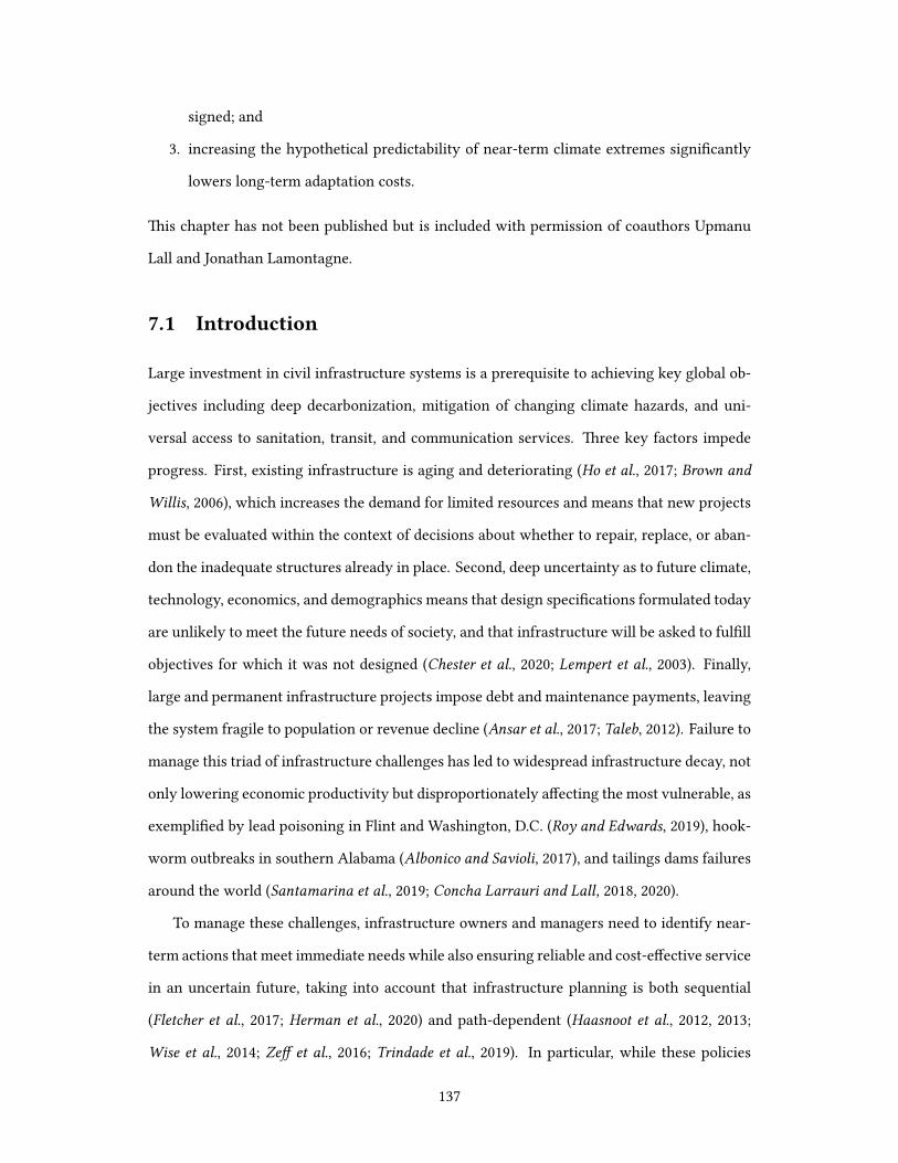
signed; and

3. increasing the hypothetical predictability of near-term climate extremes significantly

lowers long-term adaptation costs.

This chapter has not been published but is included with permission of coauthors Upmanu

Lall and Jonathan Lamontagne.

7.1 Introduction

Large investment in civil infrastructure systems is a prerequisite to achieving key global ob-

jectives including deep decarbonization, mitigation of changing climate hazards, and uni-

versal access to sanitation, transit, and communication services. Three key factors impede

progress. First, existing infrastructure is aging and deteriorating (Ho et al., 2017; Brown and

Willis, 2006), which increases the demand for limited resources and means that new projects

must be evaluated within the context of decisions about whether to repair, replace, or aban-

don the inadequate structures already in place. Second, deep uncertainty as to future climate,

technology, economics, and demographics means that design specifications formulated today

are unlikely to meet the future needs of society, and that infrastructure will be asked to fulfill

objectives for which it was not designed (Chester et al., 2020; Lempert et al., 2003). Finally,

large and permanent infrastructure projects impose debt and maintenance payments, leaving

the system fragile to population or revenue decline (Ansar et al., 2017; Taleb, 2012). Failure to

manage this triad of infrastructure challenges has led to widespread infrastructure decay, not

only lowering economic productivity but disproportionately affecting the most vulnerable, as

exemplified by lead poisoning in Flint and Washington, D.C. (Roy and Edwards, 2019), hook-

worm outbreaks in southern Alabama (Albonico and Savioli, 2017), and tailings dams failures

around the world (Santamarina et al., 2019; Concha Larrauri and Lall, 2018, 2020).

To manage these challenges, infrastructure owners and managers need to identify near-

term actions that meet immediate needs while also ensuring reliable and cost-effective service

in an uncertain future, taking into account that infrastructure planning is both sequential

(Fletcher et al., 2017; Herman et al., 2020) and path-dependent (Haasnoot et al., 2012, 2013;

Wise et al., 2014; Zeff et al., 2016; Trindade et al., 2019). In particular, while these policies

137

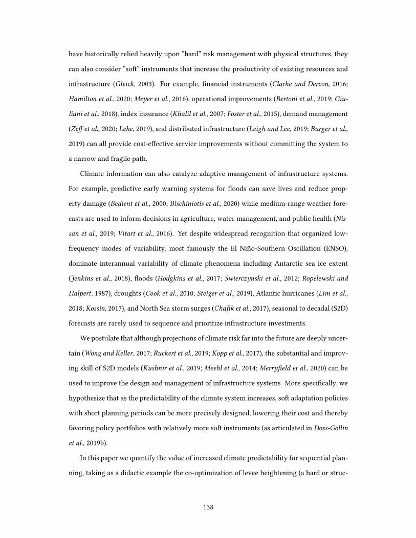
have historically relied heavily upon “hard” risk management with physical structures, they

can also consider “soft” instruments that increase the productivity of existing resources and

infrastructure (Gleick, 2003). For example, financial instruments (Clarke and Dercon, 2016;

Hamilton et al., 2020; Meyer et al., 2016), operational improvements (Bertoni et al., 2019; Giu-

liani et al., 2018), index insurance (Khalil et al., 2007; Foster et al., 2015), demand management

(Zeff et al., 2020; Lehe, 2019), and distributed infrastructure (Leigh and Lee, 2019; Burger et al.,

2019) can all provide cost-effective service improvements without committing the system to

a narrow and fragile path.

Climate information can also catalyze adaptive management of infrastructure systems.

For example, predictive early warning systems for floods can save lives and reduce prop-

erty damage (Bedient et al., 2000; Bischiniotis et al., 2020) while medium-range weather fore-

casts are used to inform decisions in agriculture, water management, and public health (Nis-

san et al., 2019; Vitart et al., 2016). Yet despite widespread recognition that organized low-

frequency modes of variability, most famously the El Niño-Southern Oscillation (ENSO),

dominate interannual variability of climate phenomena including Antarctic sea ice extent

(Jenkins et al., 2018), floods (Hodgkins et al., 2017; Swierczynski et al., 2012; Ropelewski and

Halpert, 1987), droughts (Cook et al., 2010; Steiger et al., 2019), Atlantic hurricanes (Lim et al.,

2018; Kossin, 2017), and North Sea storm surges (Chafik et al., 2017), seasonal to decadal (S2D)

forecasts are rarely used to sequence and prioritize infrastructure investments.

We postulate that although projections of climate risk far into the future are deeply uncer-

tain (Wong and Keller , 2017; Ruckert et al., 2019; Kopp et al., 2017), the substantial and improv-

ing skill of S2D models (Kushnir et al., 2019; Meehl et al., 2014; Merryfield et al., 2020) can be

used to improve the design and management of infrastructure systems. More specifically, we

hypothesize that as the predictability of the climate system increases, soft adaptation policies

with short planning periods can be more precisely designed, lowering their cost and thereby

favoring policy portfolios with relatively more soft instruments (as articulated in Doss-Gollin

et al., 2019b).

In this paper we quantify the value of increased climate predictability for sequential plan-

ning, taking as a didactic example the co-optimization of levee heightening (a hard or struc-

138

tural instrument) and index insurance (a soft or nonstructral approach) in Delfzijl, Nether-

lands (van Dantzig, 1956; Oddo et al., 2017; Garner and Keller , 2018; Eijgenraam et al., 2014).

In particular, we pose the following three questions.

1. What is the sensitivity of the optimal levee heightening to assumptions regarding near-

term (seasonal to decadal) and long-term (century scale) sea level rise?

2. Is investing today in infrastructure designed for worst-case scenarios a robust response

to large but distant and uncertain risks?

3. Can predictability of near-term risks lower the long-term costs of the adaptation path-

way?

This general problem of combining hard and soft instruments to manage deep and dynamic

uncertainties is relevant to a wide range of planning problems in infrastructure systems, and

in particular coastal adaptation in the low-lying communities home to hundreds of millions

of people worldwide (Kulp and Strauss, 2019).

7.2 Methods

We consider a didactic case study first developed by van Dantzig (1956) of levee heightening

for a polder surrounded by a single reach of dike in the Netherlands. We frame this as an

optimal control problem (Herman et al., 2020) and use stochastic dynamic programming (SDP),

which is a well-known exact solution method, to identify the decision for each time step

(1 year) that, conditional on the observed state of the world, minimizes the expected future

costs of constructing levees plus insuring residual risks. SDP can be used to compute exact

and optimal policies given a representation of the environment as a finite Markov decision

process (MDP), meaning that the state set S, reward set R, and action set A are each finite

and that the state’s dynamics are governed by a set of known probabilities P(s′, r | s, a) for

all s ∈ S, a ∈ A(s), and r ∈ R, where s′ indicates the state at the next time step (following

the notation of Sutton and Barto, 2018). SDP works by converting the Bellman equation for

139

0

100

200

300

400 (a)RCP 2.6

(b)RCP 4.5

Model: DP16

(c)RCP 8.5

2025 2050 2075 2100 21250

100

200

300

400

(d)

2025 2050 2075 2100 2125

(e)

2025 2050 2075 2100 2125

Model: K14

(f)

0.0 0.2 0.4 0.6 0.8 1.00.0

0.2

0.4

0.6

0.8

1.0

Delfz

ijl Se

a Le

vel [

cm]

Figure 7.1: Different models and scenarios agree that local mean sea level at Delfzijl, Nether-lands will rise over the next centuries but differ sharply on the magnitude and timing of thisrise. Plot shows mean (blue line) and 50, 90, and 95 percent confidence intervals (gray shad-ing) for lag-1 Markov models (eq. 7.2) fit to simulations of LSL at Delfzijl, Netherlands incm for each of three RCP scenarios (columns) and each of two physical models described inKopp et al. (2017): (i) the K14 model and (ii) the DP16 model (rows). The model described ineq. (7.2) credibly represents the complex dynamics from the K14 and DP16 models; simula-tions directly from these models are shown in figs. 7.2 and 7.3.

state-action value

q∗(s, a) =∑s′, r

P(s′, r | s, a)[r + γmax

a′q∗(s

′, a′)

], (7.1)

where γ is a discount rate and s′ is the state at the next time step, into an optimal policy

a∗ = maxa q(s, a). The state-action value is solved by exhaustive recursive search described

in algorithm 1. The remainder of this section defines the state space, reward function, and

transition probabilities.

7.2.1 State Space and Transitions

Thestate spaceS consists of time t plus three additional variables, eachwith its own transition

probability. At each time step the state space is fully described as a tuple s = (t, ℓ, x, h) giv-

ing the time, local sea level, low-frequency variability (LFV) state variable, and levee height,

140

0

100

200

300

400

Loca

l Sea

Lev

el [c

m]

(a): RCP Scenario 2.6DP16K14

0

100

200

300

400

Loca

l Sea

Lev

el [c

m]

(b): RCP Scenario 4.5

2020 2040 2060 2080 2100 2120Year

0

100

200

300

400

Loca

l Sea

Lev

el [c

m]

(c): RCP Scenario 8.5

Figure 7.2: PDFs of simulated LSL at Delfzijl, Netherlands in cm in 2020, 2040, 2060, 2080,2100, and 2120 (columns) for each of three RCP scenarios (columns) and each of two physicalmodels: DP16 and K14 (colors) as outlined in Kopp et al. (2017). The PDFs are representedusing a letter plot (Hofmann et al., 2017); like boxplots, letter plots show only actual datavalues rather than smoothed values or estimated densities, but a broader set of quantiles canbe presented. Distributions are estimated from 10 000 simulations for each model and eachscenario.

141

0

250

500

750

1000 (a)RCP Scenario 2.6

(b)RCP Scenario 4.5

Model: DP16

(c)RCP Scenario 8.5

2050 2100 2150 22000

250

500

750

1000

(d)

2050 2100 2150 2200

(e)

2050 2100 2150 2200

Model: K14

(f)

0.0 0.2 0.4 0.6 0.8 1.00.0

0.2

0.4

0.6

0.8

1.0

Delfz

ijl Se

a Le

vel [

cm]

Figure 7.3: Different models and scenarios agree that local mean sea level at Delfzijl, Nether-lands will rise over the next centuries but differ sharply on the magnitude and timing of thisrise. Plot shows mean (blue line) and 50, 90, and 95 percent confidence intervals (gray shad-ing) for simulations of LSL at Delfzijl, Netherlands in cm for each of three RCP scenarios(columns) and each of two physical models: DP16 and K14 (rows). Note that in contrast tofigs. 7.1 and 7.2 the x axis on this plot goes to 2220.

respectively.

The annual-maximum flood in a particular year, y, is decomposed into an average value

of LSL for that year ℓ and a superimposed storm surge y′. Figure 7.4 shows historical values

of ℓ and y′.

The evolution of LSL (ℓ) was modeled using a first-order Markov transition model with

nL states (table 7.1). To estimate the corresponding Markov transition matrix L, 10 000 sim-

ulations of LSL at Delfzijl were generated following the methodology of Kopp et al. (2017) for

each of three RCP scenarios, and for each of two parameterizations of ice sheet dynamics: the

more pessimistic assumptions of DP16 and the more optimistic assumptions of K14. These

models produce estimates of LSL in 10 year increments, so the values were linearly interpo-

lated to annual time steps. Transition probabilities were estimated empirically using observed

counts of pairwise transitions for each of the 10 000 simulations. Given an estimate of this

transition matrix, the transition probability for local sea level rise can be calculated (defining

142

an index iL by ℓ = LiL ) as

P(i′L|s, a) = P(i′L|iL) = LiL,i′L, (7.2)

where nL is the number of discrete states created for LSL. In total six separate transition

matrices were created for LSL: the RCP scenarios and physical models used are summarized

in table 7.2. For each transition matrix, LSL was discretized to nL values (table 7.1). Figure 7.1

shows simulations of LSL from each of the six transition matrices; this lag-1 Markov model

credibly represents the full model dynamics shown in figs. 7.2 and 7.3.

In addition to secular LSL rise, coastal floods depend on storm surges (y′). As shown in

fig. 7.4, annual-maximum storm surges at Delfzijl exhibit some autocorrelation. This tempo-

ral structure was also modeled following a first-order Markov process for a LFV state variable

x. Conditional on the state x, the storm surge y′ was modeled following a Normal distribu-

tion with mean µx and standard deviation σx (exact values given in table 7.1). Rather than

estimating an empirical transition matrix, however, a set of hypothetical transition matrices

were generated, depending on a parameter τ ∈ (0, 1] governing the persistence of each LFV

state:

Xij(τ) =τ (j−i+1) mod nX∑nX

i=1 τi

for i, j = 1, . . . , nX (7.3)

where mod indicates the modulo operator. Since eq. (7.3) matrix structure makes X quasi-

periodic and symmetric, the marginal distribution of y is independent of τ . As τ → 0, the

persistence increases and the system evolves slowly and predictably; as τ → 1 the transitions

become completely random. Thus, changing τ can be interpreted as a change in hypothetical

medium-range climate predictability. The transition matrices shown are plotted in fig. 7.5 for

all values of τ used in this study. Because of the assumed structure of the model, the formal

transition probability for the LFV state depends only on x:

P(x′|s, a) = P(x′|x) = Xx,x′ . (7.4)

The values of µ and σ shown in table 7.1 are based on values derived from a hidden Markov

model (HMM) applied to observed storm surges (fig. 7.4b), but the HMM’s transition matrix

143

20

10

0

10

20

cm a

bove

bas

elin

e

(a) Local Sea Level

1880 1900 1920 1940 1960 1980 2000 2020

250

300

350

400

cm a

bove

LSL

(b) Annual Maximum Storm Surge

Figure 7.4: Historical flood data at Delfzijl, Netherlands (data adapted from Oddo et al., 2017).(a): annual average of daily-mean sea level measurements, relative to baseline, in cm. (b):annual maximum of superimposed storm surges (calculated by subtracting the mean sea levelfrom the maximum height recorded), also in cm.

was not used; instead X comes from eq. (7.3).

The last state variable is the levee height h. Possible levee heights are discretized to

0, 25, 50, . . . , 1500 cm. Although h is managed directly by the decision-maker, it is still

stochastic: if a peak flood overtops the levee, the structure is destroyed and h ← 0, trigger-

ing a decision about whether (and how high) to rebuild. Since storm surges y′ are modeled

following a Normal distribution conditional on the LFV state, the probability of flooding is

given by the Gaussian survival function

Pflood(s, a) = Pflood(h, ℓ, x, a) = 1− 1

2

[1 + erf

(h+ a− ℓ− µx

σ√2

)], (7.5)

where erf is the error function, h is the levee height, ℓ is the LSL, µx is the expected storm

surge for LFV state x, and σ is the within-state standard deviation of storm surges. The levee

height therefore evolves in time following

P(h′|s, a) = P(h′|h, ℓ, x, a) =

1− Pflood(h, ℓ, x) h′ = h+ a

Pflood(h, ℓ, x) h′ = 0

0 else.

(7.6)

144

01

23

4Pr

evio

us S

tate

(a) = 0.125 (b) = 0.25

0 1 2 3 4Next State

01

23

4Pr

evio

us S

tate

(c) = 0.5

0 1 2 3 4Next State

(d) = 1.0

0.0

0.2

0.4

0.6

0.8

1.0

Figure 7.5: The transition matrices LX that specify P(x′|x, τ) (eq. 7.4) for all value of τ .

145

0 50 100 150 200 250 300 350 400Height Increase [cm]

0.0

0.2

0.4

0.6

0.8

1.0

1.2

1.4

Cons

truct

ion

Cost

[eur

os]

1e11Initial Levee Height [cm]

250375500625750

Figure 7.6: Construction costs increase quadratically with the initial levee height, in cm,and with the amount by which to raise the levee, and are discontinuous at zero. The exactequation is given by eq. (7.7) with parameters from table 7.1.

7.2.2 Cost Functions

At each time step, the decision-maker must decide whether to raise the levee, and if so by

how much. The cost of raising the levee from h cm to (h+ a) cm is

cc(s, a) = cc(h, a) = α1a2 + α2h+ α3; (7.7)

we use the values of α1, α2, α3 from Eijgenraam et al. (2012) for dike ring 16, as repro-

duced in table 7.1. Figure 7.6 plots this function for several values of h and for all a ∈ A.

Importantly, eq. (7.7) is discontinuous at a = 0; this reflects large fixed costs of construction

such as permitting, equipment procural, engineering design, and covering the levee surface.

Thus, a policy based on incrementally heightening the levee every few years is prohibitively

expensive.

The second lever available to the decision-maker is implicit: the residual flood risk is

covered through an index insurance contract which is renewed every year. Specifically, the

146

contract pays out v dollars:

v(t) = v0(1 + τv)t−t0 (7.8)

if the maximum flood height y overtops the levee. This makes the strong assumption that the

value insured (representing the value of property lost and costs of evacuation) is unaffected

by flood events. Although we assume that decisions are made every year and that insurance

contracts are priced fairly, it is unreasonable to allow the insurance price to reflect concurrent

climate information. The insurance rate is therefore assumed to reflect the distribution of

floods by keeping sea level ℓ constant but looking forward one step in time for low-frequency

variability x. In other words, the pricing of the next year’s contract reflects a prediction of

flood risk for the next year considering the levee height, the current sea level, and the full

distribution for the next year’s LFV index. The cost of insuring residual risk is therefore

ci(s) = ci(h, t, x) = v(t)E[P ′

flood]+ λσ

[P ′

flood], (7.9)

where

E[P ′

flood]=

nX∑x′=1

P(x′|x)Pflood(h, ℓ, x′, a) (7.10)

and

σ[P ′

flood]=

nX∑x′=1

P(x′|x)[Pflood(h, ℓ, x

′, a)− E[P ′

flood]]21/2

. (7.11)

The penalty in eq. (7.9) is equivalent to the Wang transform (Wang, 2002) if Pflood is assumed

to be normally distributed; previous work on weather derivatives has found λ = 0.25 to be a

reasonable value (Hamilton et al., 2020; Foster et al., 2015).

Combining these two costs, the total reward r at each time step is defined as r = −cc−ci.

7.2.3 Experiment Design

The state-value function eq. (7.1) was solved for each combination of structural or deep un-

certainties, listed in table 7.2, using the recursive search approach of algorithm 1. The al-

gorithm was implemented in python using efficient well-documented open-source libraries

(Lam et al., 2015; Köster and Rahmann, 2012; Hunter , 2007; van der Walt et al., 2011; Hoyer

147

Symbol Value Description Unit

α1 0.102 Quadratic construction cost term Million Euros per cm2

α2 3.20 Linear construction cost term Million Euros per cmα3 319 Fixed cost of construction Million Eurosv0 22 700 Initial exposure Million Eurost0 2020 Start year yearτV 0.0100 Real exposure growth rate year−1

nL 100 Number of discrete states for LSL countnH 61 Number of possible levee heights countnX 5 Number of discrete LFV states counth0 425 Initial levee height cmµ1 242 Expected storm surge in state 1 cmµ2 278 Expected storm surge in state 2 cmµ3 287 Expected storm surge in state 3 cmµ4 326 Expected storm surge in state 4 cmµ5 386 Expected storm surge in state 5 cmσ1 12.0 Standard deviation of storm surge for state 1 cmσ1 16.2 Standard deviation of storm surge for state 2 cmσ1 12.6 Standard deviation of storm surge for state 3 cmσ1 21.2 Standard deviation of storm surge for state 4 cmσ1 23.4 Standard deviation of storm surge for state 5 cmλ 0.250 Risk premium for insurance contract

Table 7.1: Exact value of parameters used

and Hamman, 2017); codes are available at https://github.com/jdossgollin/

2020-sequential-adaptation. Rather than assigning a terminal value to the final

state, the model was run to the year 2220 and all results after 2120 were discarded.

Description Values used

Physical model for LSL DP16, K14RCP scenario 2.6, 4.5, 8.6Discount rate 1− γ 1%, 4%, 7%Climate predictability parameter τ 0.125, 0.25, 0.5, 1.0

Table 7.2: Deep uncertainties and model structural uncertainties were treated by calculat-ing the state-value function separately for each combination of parameters (i.e., the outerproduct).

148

Algorithm 1: Exact solution method for discretized state-value function.Input: Vector T of length nT giving time steps in 1 year incrementsInput: Vector H of length nH giving possible levee heightsInput: Vector L of length nL giving possible local mean sea levelsInput: VectorM of length nX giving mean storm surge for each LFV stateInput: Real σ giving state-conditional standard deviation of storm surgeInput: Matrix X of shape nX × nX giving LFV state transition probabilitiesInput: Matrix L of shape nL × nL giving LSL transition probabilitiesInput: Real discount rate 1− γOutput: State-value function V of shape [nT , nH , nL, nX ]Initialize state-value V = 0;for iT = nT − 1, nT − 2, . . . , 1 do

Assign t = TniT;

Calculate v(t) following eq. (7.8);for iH = 1, . . . , nH do

Assign h = HiH ;Define possible levee increases: A = HiH+iA −HiH foriA = 0, . . . , nH − iH ;

for iL = 1, . . . , nL doAssign ℓ = LiL ;for iX = 1, . . . , nX do

Assign x = XiX ;Define s = t, h, ℓ, x;Initialize state-action values Q = 0 ;for iA = 0, . . . , nH − iH : do

Assign a = AiA ;Calculate cc(h, a) from eq. (7.7);Calculate ci(s, a) from eq. (7.9);r ← −cc − ci;for h′ in H do

Calculate P(h′|s, a) from eq. (7.6);for ℓ′ in L do

Calculate P(ℓ′|s, a) from eq. (7.2);for x′ in X do

Calculate P(x′|s, a) from eq. (7.4);P(s′|s, a)← P (h′|s, a)P (ℓ′|s, a)P (x′|s, a);QiA ← r + γP (s′|s, a)Vt+1,h′,ℓ′,x′ ;

Vt,h,ℓ,x ← maxQ;

149

7.3 Results and Discussion

The SDP model identifies the optimal (cost-minimizing) levee heightening each year, as a

function of levee height, sea level, and LFV state.

7.3.1 Optimal Levee Heightening

Thefirst question considered is the sensitivity of the optimal levee heightening to assumptions

regarding long-term sea level rise. One way to answer this question is to extract from the full

solution the optimal amount by which to heighten the levee at the first time step (in 2020),

shown for different assumptions in table 7.3. This table generally indicates that it is optimal to

not increase the levee height, though for the lowest discount rate and the most extreme LFV

state it does advise to heighten the levee by an amount that depends mainly on the scenario

of sea level rise considered. Interestingly, the one scenario for which the model does not

recommend heightening the levee – even in the highest-risk LFV state – is the DP16 RCP

8.5 scenario shown in fig. 7.1c. This reflects that while this is the scenario with the highest

eventual sea level rise, it is also that with the greatest intra-scenario uncertainty. It is therefore

advantageous to defer investment until this uncertainty is partially resolved.

Similarly, fig. 7.7(d-f) shows simulations of levee height as a function of time for different

simulations from the DP16 model with a 4% discount rate. In these simulations all levees are

eventually heightened to a level specific to the RCP scenario and physical model. However,

the timing of these height increases varies widely between different simulations. Results are

qualitatively similar for different values of τ and discount rate and for the other physical

model (see figs. 7.8 to 7.10). These illustrate that deferring an investment in physical infras-

tructure does not preclude its eventual implementation, but merely defers it until a later date,

partially discounting construction costs on the grounds of opportunity cost: resources in-

vested in levees are not improving schools, supporting public health programs, or alleviating

poverty. Once the near-term benefits (here lower insurance premiums) of heightening out-

weigh the costs, the levee is raised. If the levee height were lower (h0 = 375 cm), the model

recommends immediate heightening as shown in table 7.4.

This model’s guidance to not raise levees in 2020 should not be interpreted as implying

150

0.0

0.1

0.2

0.3

prob

abilit

y

(a)RCP 2.6

(b)RCP 4.5

Flood Probability

(c)RCP 8.5

0

500

1000

cent

imet

ers (d) (e) Levee Height

(f)

2020 2040 2060 2080 2100 21200

200

400

cent

imet

ers (g)

2020 2040 2060 2080 2100 2120

(h)

2020 2040 2060 2080 2100 2120

Local Sea Level

(i)

Figure 7.7: Simulations from the SDP model show that the optimal amount by which toheighten the levee is dominated by assumed future LSL conditions, but that levee heighteningshould be delayed. This (i) delays construction costs until the future, which is discounted, and(ii) allows some uncertainties to resolve over time. All simulations shown are exchangeable– two are highlighted (one blue and one orange) at random in order to more easily visualizespecific trajectories. Results shown here for DP16 model with τ = 0.25 and a 4% discountrate.

that communities should do nothing in the face of long-term climate challenges, but reflects

that the only levers available in this model are levees and insurance. Real-world communities

have many other levers available for flood risk management, including land use management

(Blum et al., 2020), buyouts (BenDor et al., 2020), early warning systems (Bedient et al., 2000),

and exposure management (particularly important since structural risk management can in-

crease exposure via the “levee effect”; Barendrecht et al., 2017; Di Baldassarre et al., 2018a;

Tobin, 1995).

7.3.2 Robustness of Over- or Under-Design

Wenext turn to the question ofwhethermaking immediate capital investments in anticipation

of the eventual emergence of worst-case scenarios is a robust response to large but distant

and uncertain risks. In this model sea level rise is large and inevitable, but its timing and

magnitude vary dramatically between the most optimistic (fig. 7.1d) and pessimistic (fig. 7.1c)

scenarios. The possibility of this scenario motivates the consideration of building large levees

151

0.0

0.2

0.4

Prop

ortio

n

(a)RCP 2.6

(b)RCP 4.5

Insurance Rate

(c)RCP 8.5

0

500

1000

cent

imet

ers (d) (e) Levee Height

(f)

2020 2040 2060 2080 2100 21200

200

400

cent

imet

ers (g)

2020 2040 2060 2080 2100 2120

(h)

2020 2040 2060 2080 2100 2120

Local Sea Level

(i)

Figure 7.8: As fig. 7.7 (using the DP16 model and τ = 0.25) but with a 7% discount rate.

0.000

0.025

0.050

0.075

prob

abilit

y

(a)RCP 2.6

(b)RCP 4.5

Flood Probability

(c)RCP 8.5

0

500

1000

cent

imet

ers (d) (e) Levee Height

(f)

2020 2040 2060 2080 2100 21200

200

400

cent

imet

ers (g)

2020 2040 2060 2080 2100 2120

(h)

2020 2040 2060 2080 2100 2120

Local Sea Level

(i)

Figure 7.9: As fig. 7.7 (using the DP16 model and τ = 0.25) but with a 1% discount rate.

152

0.00

0.02

0.04pr

obab

ility

(a)RCP 2.6

(b)RCP 4.5

Flood Probability

(c)RCP 8.5

0

200

400

600

cent

imet

ers (d) (e) Levee Height

(f)

2020 2040 2060 2080 2100 21200

50

100

cent

imet

ers (g)

2020 2040 2060 2080 2100 2120

(h)

2020 2040 2060 2080 2100 2120

Local Sea Level

(i)

Figure 7.10: As fig. 7.7 but for the K14 model, τ = 1.0, and a 1% discount rate.

today in order to be protected against all plausible scenarios.

Yet this approach is in fact highly fragile to the choice of scenario used. Figure 7.11 shows

the expected scenario-conditional regret as a function of levee height increase for each RCP

scenario, discount rate, and physical model, fixing τ and x. The scenario-conditional regret is

defined as the difference in expected discounted costs over the adaptation pathway between

(i) raising the levee by a given amount in 2020, then following the optimal investment strat-

egy for a given strategy thereafter; and (ii) raising the levee in 2020 by the optimal amount.

This value therefore answers the question “what is the expected cost penalty, for a particular

probabilistic model of sea level rise, of raising the levee by a given amount?” It implicitly as-

sumes that the optimal investment policy, for each scenario, is known after the first time step

– in other words, in 2021 the decision-maker knows which RCP scenario and model govern

the system and is able to optimize accordingly. By definition, the optimal action for a given

scenario has an expected scenario-conditional regret of 0.

Like table 7.3, fig. 7.11 shows that the optimal decision, if you know you are in a particular

scenario, is sometimes to raise the levee. However, raising the levee is not a robust strategy

(as defined in Herman et al., 2015): the optimal heightening for a moderate climate scenario

(< 250 cm) has very high regret for a more extreme scenario (c), and vice-versa. This is

because under construction cost function used (eq. (7.7) and fig. 7.6), it is more costly to build

153

incrementally than to build just once. If the levee is raised too high, resources are wasted, but

if the levee is raised too little it will need to be raised again in the future, incurring additional

costs. This illustrates that under deep uncertainty, deferring large static expenditures – when

this preserves the flexibility and adaptive capacity of the system – can be a robust decision.

Results for different values of τ , and for different initial LFV states, are qualitatively similar

(figs. 7.12 and 7.14).

It is also informative to examine when the model does recommend heightening. Fig-

ures 7.9 and 7.10 shows simulations from the K14 model with τ = 1.0 and a 1% discount

rate. In this case near-term risks are high (because the of initial LFV state), there is zero pre-

dictability (τ = 1.0), and uncertainties as to future sea level rise are small (because it uses the

K14 model). Under these conditions, the model recommends early heightening. However,

fig. 7.11 shows that even though heightening is the optimal choice if the RCP scenario and

model are known, deferring heightening is robust to model structure uncertainty.

7.3.3 Reducing Costs Through Near-Term Predictability

We finally consider whether improving the potential predictability of flood risk can reduce

long-term adaptation costs.

The simulations shown in fig. 7.7 indicate that flood risk varies significantly from year

to year (a-c), reflecting the changing LFV state over time. The different distribution of storm

surges in each state leads to very different flood probabilities in each, and this is also reflected

in the insurance premium (not shown). This suggests that being able to predict these varia-

tions could inform timing decisions for levee heightening: if the climate is in a low-risk state

and likely to remain in one for the foreseeable future, there is no need to raise the levee but

if the climate is in a high-risk state the levee should be heightened.

We explore this quantitatively by varing τ , a parameter that describes the intrinsic per-

sistence and predictability of the LFV state: as τ → 0 the climate becomes highly persistent

and predictable and as τ → 1 the state-conditional distribution of storm surges converges

to the marginal distribution (eqs. (7.3) and (7.4)). Figure 7.15 shows the expected costs over

the adaptation pathway of being in a particular state as a function of the initial LFV state

154

0.00

0.25

0.50

0.75

1.00

1.25 1e11(a)

RCP 2.6

Discount Rate0.010.040.07

(b)RCP 4.5

Model: DP16

(c)RCP 8.5

0 500 1000

0.00

0.25

0.50

0.75

1.00

1.25

1e11(d)

0 500 1000

(e)

0 500 1000

Model: K14

(f)

0.0 0.2 0.4 0.6 0.8 1.0Levee Height Increase in 2015 [cm]

0.0

0.2

0.4

0.6

0.8

1.0

Regr

et [E

uros

]

Figure 7.11: Under deep and model structure uncertainty, deferring capital expenses can bea robust solution. The y-axis shows the expected scenario-conditional regret as a functionof levee height increase in 2020 for each physical model, RCP scenario, and discount rate.Although a height increase of 0 (deferring construction) is not the optimal solution for allscenarios, it has low regret for all; conversely heightening the levee by an amount which isoptimal for one scenario may have very high regret in another. Here τ = 1.0 and x0 = 4.

155

0.00

0.25

0.50

0.75

1.00

1.25 1e11(a)

RCP 2.6

Discount Rate0.010.040.07

(b)RCP 4.5

Model: DP16

(c)RCP 8.5

0 500 1000

0.00

0.25

0.50

0.75

1.00

1.25

1e11(d)

0 500 1000

(e)

0 500 1000

Model: K14

(f)

0.0 0.2 0.4 0.6 0.8 1.0Levee Height Increase in 2015 [cm]

0.0

0.2

0.4

0.6

0.8

1.0Re

gret

[Eur

os]

Figure 7.12: As fig. 7.11 but for τ = 0.125 and initial LFV state 0.

0.00

0.25

0.50

0.75

1.00

1.25 1e11(a)

RCP 2.6

Discount Rate0.010.040.07

(b)RCP 4.5

Model: DP16

(c)RCP 8.5

0 500 1000

0.00

0.25

0.50

0.75

1.00

1.25

1e11(d)

0 500 1000

(e)

0 500 1000

Model: K14

(f)

0.0 0.2 0.4 0.6 0.8 1.0Levee Height Increase in 2015 [cm]

0.0

0.2

0.4

0.6

0.8

1.0

Regr

et [E

uros

]

Figure 7.13: As fig. 7.11 (τ = 1.0) but for initial LFV state 0.

156

0.00

0.25

0.50

0.75

1.00

1.25 1e11(a)

RCP 2.6

Discount Rate0.010.040.07

(b)RCP 4.5

Model: DP16

(c)RCP 8.5

0 500 1000

0.00

0.25

0.50

0.75

1.00

1.25

1e11(d)

0 500 1000

(e)

0 500 1000

Model: K14

(f)

0.0 0.2 0.4 0.6 0.8 1.0Levee Height Increase in 2015 [cm]

0.0

0.2

0.4

0.6

0.8

1.0

Regr

et [E

uros

]

Figure 7.14: As fig. 7.11 (initial LFV state 4) but for τ = 0.125.

and of τ for different RCP scenarios. If τ < 1 then the expected costs over the adaptation

pathway are less for low-risk LFV states than for high risk LFV states. Further, for all but

the highest-risk LFV state, the savings resulting from increased predictability (lower τ ) are of

order 5× 109 Euro, which is comparable to the cost difference between RCP 4.5 and RCP 2.6.

Unsurprisingly, more severe climate scenarios lead to higher costs over the adaptation

pathway. This underscores that the value of deferring capital investments in this study, which

considers adaptation under exogenous and dynamic uncertainty, does not imply a high value

deferring investments in climate change mitigation. In particular, increasing the severity of

the sea level rise scenario reduces flexibility and optionality for the decision-maker. Since

climate mitigation reduces the uncertainty in future climate risk (Daniel et al., 2019), our

results emphasize thatmitigation creates value by increasing the options available to decision-

makers.

157

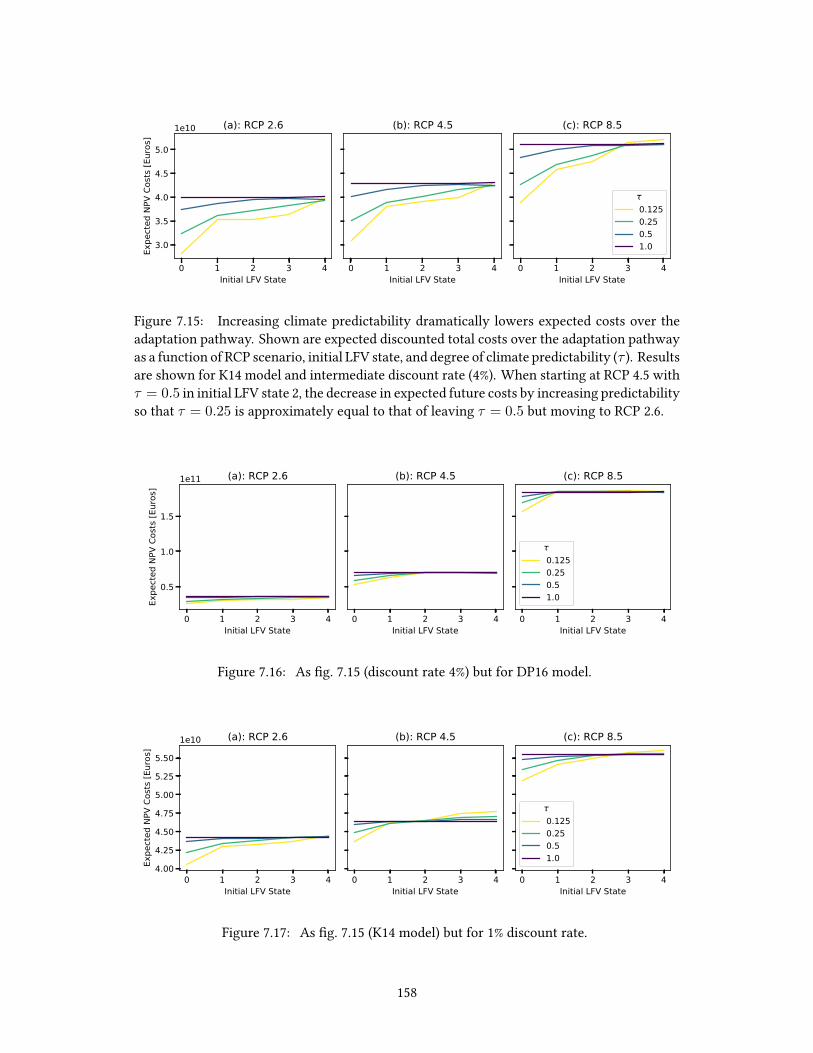
0 1 2 3 4Initial LFV State

3.0

3.5

4.0

4.5

5.0Ex

pect

ed N

PV C

osts

[Eur

os]

1e10 (a): RCP 2.6

0 1 2 3 4Initial LFV State

(b): RCP 4.5

0 1 2 3 4Initial LFV State

(c): RCP 8.5

0.1250.250.51.0

Figure 7.15: Increasing climate predictability dramatically lowers expected costs over theadaptation pathway. Shown are expected discounted total costs over the adaptation pathwayas a function of RCP scenario, initial LFV state, and degree of climate predictability (τ ). Resultsare shown for K14 model and intermediate discount rate (4%). When starting at RCP 4.5 withτ = 0.5 in initial LFV state 2, the decrease in expected future costs by increasing predictabilityso that τ = 0.25 is approximately equal to that of leaving τ = 0.5 but moving to RCP 2.6.

0 1 2 3 4Initial LFV State

0.5

1.0

1.5

Expe

cted

NPV

Cos

ts [E

uros

]

1e11 (a): RCP 2.6

0 1 2 3 4Initial LFV State

(b): RCP 4.5

0 1 2 3 4Initial LFV State

(c): RCP 8.5

0.1250.250.51.0

Figure 7.16: As fig. 7.15 (discount rate 4%) but for DP16 model.

0 1 2 3 4Initial LFV State

4.00

4.25

4.50

4.75

5.00

5.25

5.50

Expe

cted

NPV

Cos

ts [E

uros

]

1e10 (a): RCP 2.6

0 1 2 3 4Initial LFV State

(b): RCP 4.5

0 1 2 3 4Initial LFV State

(c): RCP 8.5

0.1250.250.51.0

Figure 7.17: As fig. 7.15 (K14 model) but for 1% discount rate.

158

0 1 2 3 4Initial LFV State

2.0

2.5

3.0

3.5

4.0

4.5Ex

pect

ed N

PV C

osts

[Eur

os]

1e10 (a): RCP 2.6

0 1 2 3 4Initial LFV State

(b): RCP 4.5

0 1 2 3 4Initial LFV State

(c): RCP 8.5

0.1250.250.51.0

Figure 7.18: As fig. 7.15 (K14 model) but for 7% discount rate.

7.4 Summary and Implications

Coastal communities around the world facing inevitable but uncertain sea level rise face a

challenging decision: build infrastructure today that is robust to worst-case scenarios of sea

level rise over its design life, or instead build cheaper infrastructure that may not perform

acceptably under all scenarios. This is, however, a false dichotomy: adaptation is sequential,

and so decision-makers who choose not to build today can – in an idealized world free of

time-sensitive funding mechanisms – instead build tomorrow. In this paper we consider a

didactic case study in the Netherlands and identify the cost-minimizing levee heightening as

a function of time, levee height, local sea level, and LFV state for each of several RCP scenarios,

discount rates, physical models of sea level rise, and degrees of intrinsic predictability of the

climate system that governs storm surges. We find that

1. even when large sea level rise is anticipated for the future, the decision to invest in

structural risk protection is dominated by near-term risks;

2. soft risk protection instruments preserve options and performance over a wide range

of future scenarios while hard instruments designed for one scenario perform poorly

in another; and

3. as the potential predictability of near-term hydroclimate risk increases, soft adaptation

strategies can be more precisely designed to manage near-term risks, thereby lowering

long-term adaptation costs.

In this paper we considered only uncertainty in sea level rise. Real-world planners must

159

confront deep uncertainties including levee strength and failure probability (physical), the

future rate of growth and vulnerability within the polder and the recovery after a flood event

(socio-economic), future technologies for structural flood risk protection (technological), and

the costs of capital finance, insurance premiums, infrastructure maintenance, and construc-

tion (financial). Our results show that in general, increasing the magnitude of dynamic un-

certainties leads to a greater preference for deferring static investments, and so our results

are likely a lower bound on the preference for not raising the levees today.

Although we find that making large investments today to protect against risks that will

emerge only after several decades does not, in general, justify the opportunity costs associ-

ated, this does not imply that climate change should be neglected in engineering design. First,

we show that as climate change worsens, adaptation costs grow. This emphasizes the value

of early and decisive action for climate change mitigation. Second, we show that when large

investments are eventually made, they need to take climate change into consideration so that

expensive retrofitting is not required.

Our findings are relevant for a broad range of problems in climate adaptation and infras-

tructure transformation where (i) credible probabilistic S2D climate risk forecasts are avail-

able; and (ii) uncertainties are deep and dynamic; (iii) fixed capital costs are high. Of course,

the financial and regulatory processes governing levee heightening in most parts of the world

are slow and deliberative by design, complicating efforts to develop adaptive plans. These

findings underscore a need for adaptive regulatory frameworks, possibly by granting permits

and funds for future structural investments to be made when fixed conditions (i.e., “signposts”

Raso et al., 2019; Haasnoot et al., 2013) are met. These results can also directly inform deci-

sion problems in the private sector, including home elevation and other building-scale flood

resilience problems that are not “wicked” (Rittel and Webber , 1973) and where deliberative

political processes are not required.

160

Table 7.3: Cost-minimizing first-year (2020) height increases for initial levee height 425 cmabove sea level for different combinations of (columns) the physical model for local sea levelrise and RCP scenario and (rows) discount rate, rate parameter describing low-frequencyvariability, and storm surge (mean, standard deviation).

LSL Model DP16 K14RCP Scenario 2.6 4.5 8.5 2.6 4.5 8.5

Discount Rate LFV Rate τ Storm Surge

0.01

0.125

(241.6, 12.0) 0 0 0 0 0 0(278.3, 16.2) 0 0 0 0 0 0(287.1, 12.6) 0 0 0 0 0 0(325.9, 21.2) 0 0 0 0 0 0(386.3, 23.4) 175 425 0 225 250 300

0.250

(241.6, 12.0) 0 0 0 0 0 0(278.3, 16.2) 0 0 0 0 0 0(287.1, 12.6) 0 0 0 0 0 0(325.9, 21.2) 0 0 0 0 0 0(386.3, 23.4) 175 425 0 225 225 300

0.500

(241.6, 12.0) 0 0 0 0 0 0(278.3, 16.2) 0 0 0 0 0 0(287.1, 12.6) 0 0 0 0 0 0(325.9, 21.2) 175 0 0 0 225 300(386.3, 23.4) 175 425 0 225 225 300

1.000

(241.6, 12.0) 175 0 0 0 0 300(278.3, 16.2) 175 0 0 0 0 300(287.1, 12.6) 175 0 0 0 0 300(325.9, 21.2) 175 0 0 0 0 300(386.3, 23.4) 175 0 0 0 225 300

0.04

0.125

(241.6, 12.0) 0 0 0 0 0 0(278.3, 16.2) 0 0 0 0 0 0(287.1, 12.6) 0 0 0 0 0 0(325.9, 21.2) 0 0 0 0 0 0(386.3, 23.4) 0 0 0 0 0 0

0.250

(241.6, 12.0) 0 0 0 0 0 0(278.3, 16.2) 0 0 0 0 0 0(287.1, 12.6) 0 0 0 0 0 0(325.9, 21.2) 0 0 0 0 0 0(386.3, 23.4) 0 0 0 0 0 0

0.500

(241.6, 12.0) 0 0 0 0 0 0(278.3, 16.2) 0 0 0 0 0 0(287.1, 12.6) 0 0 0 0 0 0(325.9, 21.2) 0 0 0 0 0 0(386.3, 23.4) 0 0 0 0 0 0

1.000

(241.6, 12.0) 0 0 0 0 0 0(278.3, 16.2) 0 0 0 0 0 0

Continued on next page

161

LSL Model DP16 K14RCP Scenario 2.6 4.5 8.5 2.6 4.5 8.5

Discount Rate LFV Rate τ Storm Surge

(287.1, 12.6) 0 0 0 0 0 0(325.9, 21.2) 0 0 0 0 0 0(386.3, 23.4) 0 0 0 0 0 0

0.07

0.125

(241.6, 12.0) 0 0 0 0 0 0(278.3, 16.2) 0 0 0 0 0 0(287.1, 12.6) 0 0 0 0 0 0(325.9, 21.2) 0 0 0 0 0 0(386.3, 23.4) 0 0 0 0 0 0

0.250

(241.6, 12.0) 0 0 0 0 0 0(278.3, 16.2) 0 0 0 0 0 0(287.1, 12.6) 0 0 0 0 0 0(325.9, 21.2) 0 0 0 0 0 0(386.3, 23.4) 0 0 0 0 0 0

0.500

(241.6, 12.0) 0 0 0 0 0 0(278.3, 16.2) 0 0 0 0 0 0(287.1, 12.6) 0 0 0 0 0 0(325.9, 21.2) 0 0 0 0 0 0(386.3, 23.4) 0 0 0 0 0 0

1.000

(241.6, 12.0) 0 0 0 0 0 0(278.3, 16.2) 0 0 0 0 0 0(287.1, 12.6) 0 0 0 0 0 0(325.9, 21.2) 0 0 0 0 0 0(386.3, 23.4) 0 0 0 0 0 0

162

Table 7.4: Cost-minimizing first-year (2020) height increases for initial levee height 375 cmabove sea level for different combinations of (columns) the physical model for local sea levelrise and RCP scenario and (rows) discount rate, rate parameter describing low-frequencyvariability, and storm surge (mean, standard deviation).

LSL Model DP16 K14RCP Scenario 2.6 4.5 8.5 2.6 4.5 8.5

Discount Rate LFV Rate τ Storm Surge

0.01

0.125

(241.6, 12.0) 0 0 0 0 0 0(278.3, 16.2) 0 0 0 0 0 0(287.1, 12.6) 225 475 0 275 275 350(325.9, 21.2) 225 475 1000 275 275 350(386.3, 23.4) 225 475 1000 275 300 350

0.250

(241.6, 12.0) 0 0 0 0 0 0(278.3, 16.2) 225 0 0 275 275 350(287.1, 12.6) 225 475 0 275 275 350(325.9, 21.2) 225 475 1000 275 275 350(386.3, 23.4) 225 475 1000 275 275 350

0.500

(241.6, 12.0) 225 475 0 275 275 350(278.3, 16.2) 225 475 1000 275 275 350(287.1, 12.6) 225 475 1000 275 275 350(325.9, 21.2) 225 475 1000 275 275 350(386.3, 23.4) 225 475 1000 275 275 350

1.000

(241.6, 12.0) 225 475 1000 275 275 350(278.3, 16.2) 225 475 1000 275 275 350(287.1, 12.6) 225 475 1000 275 275 350(325.9, 21.2) 225 475 1000 275 275 350(386.3, 23.4) 225 475 1000 275 275 350

0.04

0.125

(241.6, 12.0) 0 0 0 0 0 0(278.3, 16.2) 0 0 0 0 0 0(287.1, 12.6) 0 0 0 0 0 0(325.9, 21.2) 225 450 0 250 275 325(386.3, 23.4) 225 450 975 250 275 325

0.250

(241.6, 12.0) 0 0 0 0 0 0(278.3, 16.2) 0 0 0 0 0 0(287.1, 12.6) 0 0 0 0 0 0(325.9, 21.2) 225 450 0 250 275 325(386.3, 23.4) 225 450 975 250 275 325

0.500

(241.6, 12.0) 0 0 0 0 0 0(278.3, 16.2) 225 0 0 250 275 325(287.1, 12.6) 225 450 0 250 275 325(325.9, 21.2) 225 450 0 250 275 325(386.3, 23.4) 225 450 975 250 275 325

1.000

(241.6, 12.0) 225 450 0 250 275 325(278.3, 16.2) 225 450 0 250 275 325

Continued on next page

163

LSL Model DP16 K14RCP Scenario 2.6 4.5 8.5 2.6 4.5 8.5

Discount Rate LFV Rate τ Storm Surge

(287.1, 12.6) 225 450 0 250 275 325(325.9, 21.2) 225 450 0 250 275 325(386.3, 23.4) 225 450 0 250 275 325

0.07

0.125

(241.6, 12.0) 0 0 0 0 0 0(278.3, 16.2) 0 0 0 0 0 0(287.1, 12.6) 0 0 0 0 0 0(325.9, 21.2) 0 0 0 225 250 300(386.3, 23.4) 200 425 0 225 250 325

0.250

(241.6, 12.0) 0 0 0 0 0 0(278.3, 16.2) 0 0 0 0 0 0(287.1, 12.6) 0 0 0 0 0 0(325.9, 21.2) 200 0 0 225 250 300(386.3, 23.4) 200 425 0 225 250 300

0.500

(241.6, 12.0) 0 0 0 0 0 0(278.3, 16.2) 0 0 0 0 0 0(287.1, 12.6) 200 0 0 225 250 300(325.9, 21.2) 200 425 0 225 250 300(386.3, 23.4) 200 425 0 225 250 300

1.000

(241.6, 12.0) 200 450 0 225 250 325(278.3, 16.2) 200 450 0 225 250 325(287.1, 12.6) 200 450 0 225 250 325(325.9, 21.2) 200 450 0 225 250 325(386.3, 23.4) 200 450 0 225 250 325

164

Part III

Discussion and Conclusions

165

What’s the use of having developed a science well enough to make predictions if,in the end, all we’re willing to do is stand around and wait for them to come true?

F. Sherwood Rowland

8Policy Implications

The preceding chapters have laid out evidence for a set of specific hypotheses describing se-

quential climate adaptation and presented idealized experiments to probe these hypotheses.

The intended audience of those chapters is scholars and researchers developing methodolo-

gies for engineering and planning practice. This chapter seeks to distill insight from the pre-

vious chapters into simple recommendations for professional engineers and policy-makers

involved with infrastructure systems planning. This chapter has been published as

Doss-Gollin, J., D. J. Farnham, M. Ho, and U. Lall (2020), Adaptation over fatal-

ism: Leveraging high-impact climate disasters to boost societal resilience, Jour-

nal of Water Resources Planning andManagement, 146(4), doi: 10.1061/(ASCE)WR.

1943-5452.0001190

and is reproduced with permission of all authors.

166

8.1 Introduction

The property damaged and the lives disrupted by recent hurricanes, floods, droughts, and

water quality violations highlight the inadequacy of water infrastructure in the United States

and around the world. Decisions about managing these infrastructure systems are strongly

informed by societal perceptions of risk, which in turn are shaped through narratives of high-

impact events in academic, governmental, commercial, and popular media.

In recent years, post-hoc analyses of high-impact water and climate disasters have in-

creasingly focused on the role of anthropogenic climate change (ACC). This is a welcome

development which helps to build support for much-needed mitigation of global greenhouse

gas emissions and pushes companies, governments, and aid agencies to prepare for a chang-

ing environment. Yet climate impacts require a confluence of physical hazards and societal

vulnerabilities, and so narratives centered only on the role of ACC can neglect the aging

infrastructure, increasing development with exposure to climate risks, and inadequate main-

tenance that set the stage for meteorological and hydrological events to become humanitar-

ian disasters. The fatalistic narratives that emerge, which often imply that because an event

was exacerbated by climate change its consequences could not have been averted, discourage

adaptive planning.

8.2 How Climate Disasters Emerge

Climate risk is defined as the product of hazard, or the probability that a particular event oc-

curs, and exposure, which encompasses vulnerability and resilience to describe the damage

that will result if the event does occur. ACC causes dynamic and thermodynamic changes

that have already altered the intensity, seasonality, frequency, and location of water-related

climate extremes, thereby shifting climate hazard, and further changes are anticipated. Yet

analysis of recent high-impact water and climate disasters reveals that avoidable planning

decisions including poor land use policy, misaligned incentives for risk taking, and inade-

quate physical infrastructure dramatically amplify the impact of climate hazards. Systematic

analysis of global changes in exposure to floods (Jongman et al., 2012) and hurricanes (Peduzzi

167

et al., 2012) emphasize that changing exposure far outpaces changing hazard in the historical

record.

For example, failure of the primary and auxiliary spillways at the Oroville dam in 2017,

which prompted an evacuation of the Feather River (California) basin, was widely blamed

on ACC in popular and scientific (e.g., Huang et al., 2018) media, despite an absence of such

claims by the state management agency. While ACC may have contributed to this event

both directly, by increasing the moisture-holding capacity of the atmosphere, and indirectly,

by possibly favoring the persistence of the wet regime, the flows over the two spillways at

the time of their failures were only 18% and 3% of the design capacities, respectively (France

et al., 2018). Further, continued development of highly vulnerable downstream communi-

ties increased the number of individuals and the total value of property exposed to potential

flooding even though the structural deficiencies had been known and documented for several

decades. Thus, while the rainy spring may have been exacerbated by ACC, the resulting flood

risk was dominated by inadequate system planning and investment.

Recent hurricanes also illustrate the importance of local decisions in high-impact events.

For example, while ACC made Hurricane Harvey’s precipitation approximately 15% more in-

tense (Emanuel, 2017b), unmanaged sprawl and the destruction of Bayou wetlands increased

peak runoff volume and the total value of property exposed to flooding (Jacob et al., 2014).

Even worse, forensic infrastructure inspection in New Orleans following Hurricane Katrina

revealed that unrealistic design assumptions and inadequate maintenance caused several lev-

ees to fail before design levels were reached (Sills et al., 2008). Even though hurricane intensity

is anticipated to increase under ACC (Knutson et al., 2010), the first lesson of New Orleans

and Houston is that human error, inadequate infrastructure maintenance, and inadequate risk

zoning for regional growth dominate observed changes in many climate risks.

These factors have also turned unexceptional hydrological droughts into severe water

shortages. For example, the 2015-17 “day zero” drought in Cape Town was described as un-

precedented and linked to ACC in the public narrative. While Cape Town’s reservoirs were

designed primarily to supply urban demand, the government approved withdrawals for ir-

rigation following a long wet period. These agricultural releases were maintained through

168

much of the drought, contributing to day zero. Although ACC is projected to increase the

frequency of multi-year droughts (Otto et al., 2018), similar droughts were observed in the

late 1930s and early 1970s, and hydrologists had warned that they could occur again (Muller ,

2018). Recent water crises in Mexico City, São Paulo, and Barcelona also occurred during me-

teorological droughts that had close analogs within the historical record. In all these cases,

predictable water shortages were exacerbated by unmanaged consumption, leakage losses (in

the case of Mexico City as much as 130 liters per person per day, or 40% of total supply; Tor-

tajada, 2006), poor water allocation, and new agricultural water consumption. Although it is

tempting to use ACC as a scapegoat, responsible authorities must better communicate to the

public the ways in which short-sighted planning dramatically increases long-term risk.

8.3 Towards Constructive Narratives

Despite clear risks from ACC, local resource and infrastructure systems management still

drive societal resilience to water and climate risks. Improving these built and social systems

requires developing consensus for large investments and management shifts, which may be

easier if ACC is presented as one of many stress factors challenging our water infrastructure.

In this section we offer some suggestions for ways in which researchers and practitioners

working on water infrastructure systems can discuss ACC in ways that emphasize both the

need for improved local resilience, and also the need for mitigation of global greenhouse

emissions.

DO discuss specific ways in which the local environment has changed over the design life of

existing infrastructure. Even where detailed attribution studies that assess the causal

effect of specific forcings are not available, observational evidence can be connected

to collective memory. For example, changes in snow frequency have already been ob-

served in many parts of New England (Huntington et al., 2004), which has implications

not only for snowmanagement but also for stormwater design and reservoir operation.

Communicating ACC by relating history and local memories to rigorous science can

build credibility and help frame discussion of future changes.

169

DO describe how uncertainties including the extent of future greenhouse emissions, global

climate dynamics, and local environment challenge long-term planning. Making costly

investments for a specific, possibly worst-case, scenario that does not arrive (i.e. “over-

preparation”) leads to significant opportunity costs relative to other activities that may

require a more immediate response. For example, while rising sea levels threaten

coastal communities, it may not be financially or physically prudent to build storm

walls around every continent – particularly for worst-case scenarios of sea level rise.

Instead, it is important to help communities develop flexible and adaptive policies that

make use of climate and demographic forecasts at many timescales.

DO NOT conflate “deep uncertainty” as to the distant future with uncertainty as to the

near future. There has been successful identification and prediction of climate on sub-

seasonal to decadal time scales, and this can be used to inform the development of tools

to alleviate the impact of weather and climate hazards. For example, skillful prediction

of the North Atlantic Oscillation could inform hurricane risk and coastal adaptation de-

cisions along the Susquehanna river (Toomey et al., 2019) or financial preparedness and

disaster allocation for floods in Europe (Zanardo et al., 2019). In order to use these fore-

casts, however, planners must embrace uncertainty and develop decision frameworks

that make use of probabilistic information at many timescales.

DO talk about how local changes in development, land use, and disaster readiness have

changed the consequences of a given storm. For example, better early warnings and

early action plans have dramatically reduced the number of lives lost to land-falling

tropical cyclones even in very poor regions (Kumar et al., 2019). However, as develop-

ment alongwaterfronts has grown, the value of property damaged for a given storm has

risen dramatically. While ideas like risk, exposure, and vulnerability can seem abstract,

contextualizing them within the local environment can bring them to life.

DO talk about the original design considerations relative to current needs. It is natural to

pay water infrastructure little attention until something goes wrong. However, tens of

thousands of dams in the United States that put life and property at risk are well beyond

170

their original design age, and their maintenance status is generally poor or unknown

(Ho et al., 2017). While recent dam failures have not had an impact as significant as the

Johnstown floods of 1889 and 1977, dam failure remains a risk for many communities.

Further, as the case of Cape Town illustrates, past and future changes in demograph-

ics, regulations, funding, technology, and resource management often demand that our

critical infrastructure perform tasks for which was never designed.

DO NOT assume that construction is sufficient to solve infrastructure systems challenges.

Well-recognized paradoxes include the “levee effect” or “safe development paradox,“

which describe the mechanism by which new flood protection infrastructure can lead

to low perceived risk, increased development, and thus amplified impacts when ex-

tremes eventually occur. Analogs to this effect exist in water storage (increased water

availability can lead to increasedwater demand), transportation (building highways can

lower the marginal cost of driving and induce greater traffic), and many other applica-

tions. This does not imply that new structures are never needed, but rather emphasizes

the need to couple themwith strong governance. For example, the construction of flood

protection infrastructure could be accompanied by zoning regulations that limit devel-

opment in the floodplain it protects. This sort of comprehensive planning can impose

order on the complex feedbacks between humans, the environment, and infrastructure

systems that the safe development paradox describes.

DO consider how financial, regulatory, and technological advances can help water systems

“fail safely” (Brown, 2010) and support resilience. Strict zoning policies can limit fu-

ture sprawl and ensure that new construction in high-risk areas like the New York

Citywaterfront canwithstand anticipated storms. Decentralizedwater re-use networks

can provide clean drinking water without requiring costly public investments in water

treatment facilities, conveyance, and source development. Parametric and forecast in-

surance can provide funds for rapid response and recovery (Clarke and Dercon, 2016).

The particular circumstances of each place are unique, but a public discourse that trans-

parently evaluates a wide range of options should be promoted.

171

DO NOT fall back on fatalist narratives in the aftermath of natural disasters. Fatalist cli-

mate narratives divert attention from productive discussions about the use of adaptive

planning andmanagement strategies to decrease damages from similar events in the fu-

ture. Promoting policies that curb excessive exposure and promote responsible upkeep

of critical infrastructure may be particularly constructive.

8.4 Final Word

Deep uncertainty caused by ACC, the unpredictable performance of aging infrastructure,

changing social and economic conditions, and a myriad of other factors have motivated the

integration of structural and non-structural adaptation strategies for managing water infras-

tructure systems. These instruments represent creative and resilient solutions for climate risk

adaptation, transcending traditional infrastructure design and build approaches to more in-

tegrally consider land use and financial instruments as part of a strategy for response and

recovery. By communicating the challenges of climate change adaptation through a systems

lens, the public can more readily assess which strategies make sense in their specific context.

Of course, the execution of thoughtful local climate adaptation plans can by no means

preclude the need for dramatic action to mitigate global greenhouse gas emissions.

172

I changed what I could, and what I couldn’t, I endured.

Dorothy Vaughan

9Summary, Discussion, and Future Work

This chapter summarizes the key findings, discusses strengths and limitations of the ap-

proaches taken, and suggests directions for future research, focusing on real-world appli-

cations of the conceptual framework developed here.

9.1 Summary

Floods are a leading cause of death and destruction, resulting in global losses worth over $USD

60 billion in 2016 alone (Munich Re, 2017) and displacing at least 55 million people between

2010 and 2018 (Brakenridge, 2018). Historical and projected changes to both the physical

mechanisms that generate floods and the socio-techno-demographic processes that control

vulnerability and exposure are expected to worsen future flood losses.

This dissertation began with the premise that mechanistic understanding of the drivers

173

of floods in a particular location could be used to constrain and evaluate projections of future

risk. Chapter 2 reviewed the literature on flood-generating mechanisms, focusing mainly on

riverine floods in large mid-latitude basins. The key argument advanced in chapter 2 was

that the intrinsic limitations of generic black-box modeling approaches, including general

circulation models (GCMs) and local statistical distributions, limit their suitability for pro-

jecting future risks, and that mechanistic understanding is necessary to further evaluate and

constrain projections. Chapter 3 illustrates this framework by exploring the climatological

drivers of heavy rainfall in the Lower Paraguay River Basin (LPRB) and the sub-seasonal to

seasonal (S2S) factors responsible for persistent rainfall and flooding. Rainfall forecasts from

numerical models are shown to exhibit significant deficiencies in simulation of the South

American Low-Level Jet (SALLJ) and its relationship with large-scale flood-generating mech-

anisms. However, multiple sources of predictability, including the El Niño-Southern Oscil-

lation (ENSO), the Madden-Julien Oscillation (MJO), and the South Central Atlantic Dipole

(SCAD) could inform future flood risks. Chapter 4 illustrates how mechanistic understand-

ing might constrain projections of future hydroclimate hazard, taking as a case study regional

extreme rainfall in the Ohio River Basin (ORB). Although a GCM was found not to simulate

regional extreme precipitation (REP) days credibly, the model was found to credibly simulate

five climate indices representing the synoptic circulations that were responsible for them,

and this relationship was used to develop a probabilistic regression model. This approach

can be applied to generic hydroclimate hazards around the world, though it relies on having

process-based understanding of the drivers of the hazard and sufficient observational data to

assess the credibility of GCM simulations.

Part II turns to the question of how one should use projections that are intrinsically un-

certain and imperfect to inform risk management plans in the public and private sectors.

Chapter 5 reviews the literature on planning under uncertainty and describes a philosophy

for using imperfect models to inform choice in “wicked” (Rittel and Webber , 1973) problems

embedded within complex systems. The philosophy advanced draws from the Savage (1954)

notion of subjective probability, the Bankes (1993) framework of exploratory modeling, and

the Weinberg (1972) idea of trans-science to advocate the exploration of the implications and

174

tradeoffs of different possible actions, conditional on modeling choices and assumptions that

are known to be wrong (Gelman and Shalizi, 2013) but potentially useful (Box, 1976). A sec-

ond premise of this chapter is that improving civil infrastructure services does not always

require new physical structures, and that long-term planning needs to account for (i) a port-

folio of different tools and strategies, (ii) evaluated within a sequential planning framework,

and (iii) subject to path dependence. Chapter 6 focuses on a key distinction between “hard”

and “soft” adaptation strategies, which is that the former, in general, commit resources and are

exposed to uncertainty over a longer time horizon than the latter. Since the bias and variance

of risk projections increase with time, as demonstrated through numerical experiments, hard

instruments must contend with larger and deeper uncertainties than soft ones. This implies a

cost penalty for static instruments and that, under some circumstances, a sequence of adaptive

instruments tailored to evolving conditionsmay bemore cost-effective than a single static one

designed to meet performance specifications over all plausible states of the world. Chapter 7

illustrates this concept through a didactic case study of levee heightening under uncertain

sea level rise. Scenario-conditional optimization illustrates (i) that deferring permanent in-

vestments can be a robust response to deep uncertainty, particularly if the near-term benefits

of construction are small, and (ii) that skillful projections of near-term climate variability can

inform the design of soft instruments, thereby reducing long-term adaptation costs.

Parts I and II use observational analyses and numerical experiments to explore concep-

tual advances. Because of the breadth and novelty of the perspectives, the examples advanced

are generally conceptual. Chapter 8 concludes by considering their implications for general

planning problems in the public and private sector. Chapter 8 focuses particularly on ways

to frame constructive narratives around anthropogenic climate change (ACC) with the goal

of clearly communicating uncertainties and tradeoffs instead of relying on the lazy and fatal-

istic narrative that ACC renders losses inevitable. At a moment in which fatalistic narratives

regarding COVID-19 prevail, the generality of this point appears particularly salient.

175

9.2 Discussion

A central assumption of part I is that the mechanistic causal chain for a particular event is

insensitive to ACC and other secular trends. This assumption is most explicit in the statis-

tical model developed in chapter 4, which hypothesizes a stationary relationship between

large-scale climate indices and REP events (see section 4.8.3). This assumption is approxi-

mately valid if sufficient conditioning information is included within the predictive variables.

Since these physical processes are relatively well understood, this is a reasonable assumption;

however, great care must be taken to develop a statistical model that truly represents well-

understood physical processes and to avoid “data mining” which may perform well over the

historical record but extrapolate poorly. Further, limited historical records cannot rule out the

possibility of impactful events driven by other mechanisms. However, running GCM experi-

ments under a wide range of possible boundary forcing and model structures to explore what

could be possible, and subsequently assessing probability in the spirit of bottom-up modeling

approaches discussed in part II, could reduce vulnerability to “black swan” events (i.e., those

that have not been observed but cannot be proven impossible Taleb, 2007).

A secondary, mostly implicit, assumption of part I is that increasing model skill due to

improved resolution (Cook et al., 2020; Wehner et al., 2010; Kendon et al., 2012; Muller et al.,

2011) and parameterization (Rasp et al., 2018; Gentine et al., 2018; Wong et al., 2017; Liu et al.,

2011; Pithan et al., 2016) will not, alone, be adequate to overcome the limitations of GCMs for

simulating hydroclimate variables at spatiotemporal scales relevant to decision makers. As

improved representation of clouds, aerosols, and land feedbacks enable GCMs more credibly

simulate local hydroclimate processes, the set of uses for which GCM rainfall fields can be

used “out of the box” will increase. At the same time, fundamental limitations arise from

the (i) discretization and approximation of the continuous equations of motion, (ii) damping

of low-frequency modes of variability (Palmer , 1999), and (iii) finite set of processes repre-

sented in the model, and these limitations are most noticeable for the extreme events of the

greatest importance to societal decision-making. It is therefore reasonable to assume that hy-

brid models or model output statistics (MOS) of some form will be needed for the foreseeable

future, though the set of variables used to inform these models and the statistical model’s

176

structure should evolve. Of course, neither improved model skill nor statistical-dynamical

models address deep uncertainties in boundary forcing and other human activities.

Chapter 6 bridges the work on understanding and predicting hydroclimate variability

with the work on sequential planning. The forms of uncertainty considered in this chapter

are parametric and structural, but the set of model structures considered is finite (i.e. the M-

closed case defined by Bernardo, 1994). In the real world, uncertainties are far deeper and the

structure is not known (theM-open case). Although experiments were conducted within the

context of this strong assumption, increasing degrees of parametric uncertainty were taken

as a proxy for epistemic or deep uncertainties. Thus, as deep and structural uncertainties

increase, the cost of extrapolation should increase. This might imply, for example, that if

the model of chapter 7 were extended to consider additional sources of uncertainty including

population and land value, construction costs, the cost of capital, and the value of various

alternatives (including managed retreat, hardening properties within the dike ring, etc.) then

the preference for deferring large capital costs might again increase.

The argument that large, static, and centrally planned, designed, managed, and funded

infrastructure tends to be cost-ineffective is not entirely new. For example, China’s large in-

frastructure projects may have traded short-term benefit for excessive debt (Ansar et al., 2016).

This type of investment strategy is fragile (as defined by Taleb, 2012) as these static infrastruc-

ture systems cannot readily scale up or down (Ansar et al., 2017, notes that they trade size for

scalability). Marohn (2019) makes a similar argument, calling development-driven sprawling

development in the United States (US) a Ponzi scheme argues and that the value generated

doesn’t justify the long-term maintenance, repair, and replacement obligations. As discussed

in chapter 5, engineers should, in general, embrace the fact that complex problems are po-

litical. Yet the gap between how prospective investments in infrastructure are described and

their actual performance (Flyvbjerg et al., 2005; Flyvbjerg, 2009; Ansar et al., 2014) emphasizes

a need for science to more transparently inform political decisions.

177

9.3 Future Work

Adaptive plans that evaluate and optimize over different sources of uncertainty on differ-

ent timescales can be used to inform climate adaptation and infrastructure transformation at

the household, community, company, and national scales. Key actors have already commit-

ted substantial resources to climate adaptation, and more is expected. For example, at the

federal scale, the United States Army Corps of Engineers (USACE) has proposed structural

flood protection projects across the US including a possible $USD 100 billion floodwall along

the New York / New Jersey coast (USACE, 2019). At local scales, cities including New York

(Bloomberg, 2013), Houston (City of Houston, 2020), and Chicago (Chicago Climate Task Force,

2008) have developed resilience or climate adaptation plans. And the private sector is in-

creasingly coming to view climate as a financial risk rather than a reputational one (such as

Oliver Wyman, a multinational management consulting company with particular expertise

in finance and technology; Colas et al., 2019). Recognition of the need for improved infras-

tructure to manage climate risks, decarbonize the economy, generate wealth, and improve

quality of life implies a critical role for science-based analysis to inform the sequencing and

prioritization of different projects.

This dissertation focused on water and floods, but there are related problems in many ar-

eas of infrastructure systems planning. For example, deep decarbonization of the electricity

and energy sectors is a critical step towards mitigating global greenhouse gas emissions. A

number of plans have been put forth suggesting different pathways towards this goal (e.g.,

Davis et al., 2018; Jacobson et al., 2017). Yet investments in the energy sector face deep and dy-

namic uncertainties, including (i) the price and efficiency of solar panels, wind turbines, and

batteries (technological uncertainty), (ii) the timing and occurrence of carbon tax or other

regulations (political uncertainty), and (iii) demand for electricity (economic uncertainty).

Planning in the energy sector must also account for the potential emergence of new tech-

nologies such as safe next-generation nuclear power and closed-loop liquid carbon fuels. The

decision problem is therefore quite complex: optimizing for energy system safety, reliability,

cost, and carbon emissions, to prioritize investments in energy storage (Arbabzadeh et al.,

2019), transmission (MacDonald et al., 2016), and different generation technologies across

178

large areas.

The approaches developed in this dissertation can help in two ways. First, decision mod-

els used for long-term planning are generally run on time steps of one or more years. This

requires parameterizing generation and demand at shorter time scales (e.g., Su et al., 2020;

Chowdhury et al., 2019). Parametric space-time models that capture the availability of corre-

lated electricity sources (such as complementary solar andwind availability in Texas; Slusarewicz

and Cohan, 2018) over long time scales can be used to inform the sequencing and location of

transmission and generation projects. Second, it is likely that the learning rate of uncertain-

ties like renewable energy costs will be quite rapid. Like the problem of confronting uncer-

tain sea level rise (chapter 7), sequential planning in the electricity sector needs to account

for learning over time, model structure uncertainty, and stochastic uncertainties.

Another application is in urban planning and land use. Observational data (Pielke et al.,

2008; Jongman et al., 2012; Peduzzi et al., 2012; Tedesco et al., 2020; Ashley et al., 2013) and

modeling efforts (Haer et al., 2020; Srikrishnan and Keller , 2019; Barendrecht et al., 2019) em-

phasize that changing exposure is a dominant driver of total flood risk. At the same time,

the actions that affect exposure – construction and development in floodplains – can also

change flood hazard, particularly in downstream locations. For example, Blum et al. (2020)

find that, on average, a one percentage point increase in impervious basin cover causes a 3.3%

increase in annual flood magnitude. This is in agreement with findings that land use changes

(Sebastian et al., 2019) and river channelization (Juan et al., 2020) significantly increased peak

streamflows in recent Houston floods. Yet while it is easy to advise cities to restrict devel-

opment in areas that generate substantial risk (hazard or exposure), cities are heavily reliant

on near-term tax revenues, and development offers immediate resources even if it increases

long-term risks and obligations. To manage these risks, cities need coherent land use policies

that balance tax revenue, long-term expenses and fragilities, equity, and scalability (BenDor

et al., 2020). Improving policies to allocate resources, across space, between levers like cen-

tralized drainage, managed retreat (Hino et al., 2017), resilience bonds (Ruggeri, 2017), and

green infrastructure (Ochoa-Tocachi et al., 2019) and home elevation (Zarekarizi et al., 2020)

can help cities better navigate tradeoffs between revenue and risk. Tools for spatial policy

179

search, planning under uncertainty, and modeling the local correlation structure of hydrocli-

mate extremes will be particularly helpful.

A third application is in distributed water-energy systems. As briefly mentioned in sec-

tion 5.3.1, distributed resources offer important advantages in scale and reliability. This is

not an entirely novel approach; as the United States Environmental Protection Agency (EPA)

notes, decentralized wastewater treatment systems (e.g., septic tanks) served 25% of the US

population and were used in one-third of all new housing and commercial developments in

1997 (USEPA, 2005). Yet cities and utilities increasingly recognize the cost and scale issues

detailed in chapter 1 (Broaddus, 2019; Jones et al., 2012). Since landscapes and yards are a

major consumer of urban water, findings that rainwater harvesting can supply up to 50% of

the annual demand for traditional landscaping and over 100% of the water-smart landscap-

ing in Colorado (Gilliom et al., 2019) suggest that utilities may be able to manage growth

and increased water usage without costly capital expenditures (see Trindade et al., 2019, for

an example of these costs). Distributed water resources may also manage the flashiness of

pluvial floods (Jamali et al., 2020) and protect fragile ecosystems from stormwater extremes

(Cunningham and Gharipour , 2018), and optimization models suggest that while the optimal

degree of centralization is site-specific, the calculated optimal degree of centralization is sub-

stantially lower than the current level (for a case study in Switzerland Eggimann et al., 2015,

2016). However, studies of distribution in the energy sector have identified challenges as well

as opportunities – particularly around the incentive of thewealthy to contribute to centralized

systems, the need for monitoring and local system control, and local efficiencies (Burger et al.,

2019; MIT Energy Initiative, 2016). A comprehensive research agenda for decentralized water

infrastructure that develops engineering component designs, digital monitoring, and regula-

tory and management frameworks, and that matches different technologies to different use

cases, can drastically improve the set of levers available to decision-makers with significant

potential to improve outcomes.

180

Bibliography

Aerts, J. C. J. H., W. J. W. Botzen, K. C. Clarke, S. L. Cutter, J. W. Hall, B. Merz, E. Michel-Kerjan, J. Mysiak, S. Surminski, and H. Kunreuther (2018), Integrating human behaviourdynamics into flood disaster risk assessment, Nature Climate Change, 8(3), 193–199, doi:10.1038/s41558-018-0085-1.

Agel, L., M. Barlow, S. B. Feldstein, and W. J. J. Gutowski (2018), Identification of large-scalemeteorological patterns associated with extreme precipitation in the US northeast, ClimateDynamics, 50(5-6), 1819–1839, doi: 10.1007/s00382-017-3724-8.

Albonico, M., and L. Savioli (2017), Hookworm: A neglected resurgent infection, BMJ, 359,doi: 10.1136/bmj.j4813.

Anderson, W., R. Seager, W. E. Baethgen, and M. A. Cane (2018), Trans-Pacific ENSO tele-connections pose a correlated risk to agriculture, Agricultural and Forest Meteorology, 262,298–309, doi: 10.1016/j.agrformet.2018.07.023.

Anderson, W. B., Han, Eunjin, Baethgen, Walter, Goddard, Lisa, Muñoz, Ángel G., and Robert-son AndrewW. (2020), The Madden-Julian Oscillation affects crop yields around the world,Earth and Space Science Open Archive, doi: 10.1002/essoar.10501965.1.

Ångström, A. (1935), Teleconnections of Climatic Changes in Present Time, Geografiska An-naler, 17 (3-4), 242–258, doi: 10.1080/20014422.1935.11880600.

Ansar, A., B. Flyvbjerg, A. Budzier, and D. Lunn (2014), Should we build more large dams?The actual costs of hydropower megaproject development, Energy Policy, 69, 43–56, doi:10.1016/j.enpol.2013.10.069.

Ansar, A., B. Flyvbjerg, A. Budzier, andD. Lunn (2016), Does Infrastructure Investment Lead toEconomic Growth or Economic Fragility? Evidence from China, Oxford Review of EconomicPolicy, 32(3), 360–390, doi: 10.1093/oxrep/grw022.

Ansar, A., B. Flyvbjerg, A. Budzier, and D. Lunn (2017), Big is Fragile: An Attempt at Theo-rizing Scale, arXiv:1603.01416 [q-fin].

Arbabzadeh, M., R. Sioshansi, J. X. Johnson, and G. A. Keoleian (2019), The role of energystorage in deep decarbonization of electricity production, Nature Communications, 10(1),3413, doi: 10.1038/s41467-019-11161-5.

Arrow, K., M. Cropper, C. Gollier, B. Groom, G. Heal, R. Newell, W. Nordhaus, R. Pindyck,W. Pizer, P. Portney, T. Sterner, R. S. J. Tol, and M. Weitzman (2013), Determining benefitsand costs for future generations, Science, 341(6144), 349–350, doi: 10.1126/science.1235665.

Arrow, K. J. (1951), Social Choice and Individual Values, Wiley, New York.

181

Arrow, K. J. (1963), Social Choice and Individual Values, Yale Univeristy Press, New Haven, CT.

Ashley, W. S., S. Strader, T. Rosencrants, and A. J. Krmenec (2013), Spatiotemporal changes intornado Hazard exposure: The case of the expanding bull’s-eye effect in Chicago, Illinois,Weather, Climate, and Society, 6(2), 175–193, doi: 10.1175/WCAS-D-13-00047.1.

Ayyub, B. M. (2018), Climate-Resilient Infrastructure: Adaptive Design and Risk Management,American Society of Civil Engineers, Reston, Virginia.

Bankes, S. (1993), Exploratory Modeling for Policy Analysis, Operations Research, 41(3), 435–449, doi: 10.1287/opre.41.3.435.

Bao, J.-W., S. A. Michelson, P. J. Neiman, F. M. Ralph, and J. M. Wilczak (2006), Interpretationof Enhanced Integrated Water Vapor Bands Associated with Extratropical Cyclones: TheirFormation and Connection to Tropical Moisture, Monthly Weather Review, 134(4), 1063–1080, doi: 10.1175/MWR3123.1.

Barendrecht, M. H., A. Viglione, and G. Blöschl (2017), A dynamic framework for flood risk,Water Security, 1, 3–11, doi: 10.1016/j.wasec.2017.02.001.

Barendrecht, M. H., A. Viglione, H. Kreibich, B. Merz, S. Vorogushyn, and G. Blöschl (2019),The Value of Empirical Data for Estimating the Parameters of a Sociohydrological FloodRisk Model, Water Resources Research, 55(2), 1312–1336, doi: 10.1029/2018WR024128.

Barnes, E. A., and J. A. Screen (2015), The impact of Arctic warming on the midlatitude jet-stream: Can it? Has it? Will it?, Wiley Interdisciplinary Reviews-Climate Change, 6(3),277–286, doi: 10.1002/wcc.337.

Barnett, B. J., and O. Mahul (2007), Weather index insurance for agriculture and rural areasin lower-income countries, American Journal of Agricultural Economics, 89(5), 1241–1247,doi: 10.1111/j.1467-8276.2007.01091.x.

Barnston, A. G., and C. F. Ropelewski (1992), Prediction of ENSO Episodes Using CanonicalCorrelation Analysis, Journal of Climate, 5(11), 1316–1345, doi: 10.1175/1520-0442(1992)005<1316:POEEUC>2.0.CO;2.

Barnston, A. G., S. Li, S. J. Mason, D. G. DeWitt, L. Goddard, and X. Gong (2010), Verificationof the First 11 Years of IRIs Seasonal Climate Forecasts, Journal of Applied Meteorology andClimatology, 49(3), 493–520, doi: 10.1175/2009jamc2325.1.

Barnston, A. G., M. K. Tippett, M. L. LHeureux, S. Li, and D. G. DeWitt (2012), Skillof Real-Time Seasonal ENSO Model Predictions During 2002–11: Is Our Capability In-creasing?, Bulletin of the American Meteorological Society, 93(5), ES48–ES50, doi: 10.1175/bams-d-11-00111.2.

Barreiro, M. (2017), Interannual variability of extratropical transient wave activity and itsinfluence on rainfall over Uruguay, International Journal of Climatology, 37 (12), 4261–4274,doi: 10.1002/joc.5082.

Barros, V. R., L. Chamorro, G. Coronel, and J. Baez (2004), The major discharge events in theParaguay River: Magnitudes, source regions, and climate forcings, Journal of Hydrometeo-rology, 5(6), 1161–1170, doi: 10.1175/JHM-378.1.

182

Barry, J. M. (1997), Rising Tide : TheGreatMississippi Flood of 1927 andHow It ChangedAmerica,Simon & Schuster, New York.

Bedient, P. B., B. C. Hoblit, D. C. Gladwell, and B. E. Vieux (2000), NEXRAD radar for flood pre-diction in Houston, Journal of Hydrologic Engineering, 5(3), 269–277, doi: 10.1061/(ASCE)1084-0699(2000)5:3(269).

Bellman, R. (1954), The theory of dynamic programming, Bulletin of the American Mathemat-ical Society, 60(6), 503–515, doi: 10.1090/S0002-9904-1954-09848-8.

Bellman, R. (1957), Dynamic Programming, Princeton University Press, Princeton, New Jersey.

Benayoun, R., J. de Montgolfier, J. Tergny, and O. Laritchev (1971), Linear programming withmultiple objective functions: Step method (stem), Mathematical Programming, 1(1), 366–375, doi: 10.1007/BF01584098.

BenDor, T. K., D. Salvesen, C. Kamrath, and B. Ganser (2020), Floodplain buyouts and munic-ipal finance, Natural Hazards Review, 21(3), 04020,020, doi: 10.1061/(ASCE)NH.1527-6996.0000380.

Beran, J. (1994), Statistics for Long-Memory Processes, Chapman & Hall, New York.

Berg, P., C. Moseley, and J. O. Haerter (2013), Strong increase in convective precipitation inresponse to higher temperatures, Nature Geoscience, 6(3), 181–185, doi: 10.1038/ngeo1731.

Bernardo, J. M. (1994), Bayesian Theory, Wiley, New York.

Bertoni, F., M. Giuliani, and A. Castelletti (2017), Scenario-based fittedQ-iteration for adaptivecontrol of water reservoir systems under uncertainty, IFAC-PapersOnLine, 50(1), 3183–3188,doi: 10.1016/j.ifacol.2017.08.340.

Bertoni, F., A. Castelletti, M. Giuliani, and P. M. Reed (2019), Discovering dependencies, trade-offs, and robustness in joint dam design and operation: An ex-post assessment of the KaribaDam, Earth’s Future, 7 (12), 1367–1390, doi: 10.1029/2019EF001235.

Bertsekas, D. P. (1976), Dynamic Programming and Stochastic Control, no. 125 in Mathematicsin Sciencce and Engineering, Academic Press.

Betancourt, M. (2017), A Conceptual Introduction to Hamiltonian Monte Carlo, Methodology(stat.ME).

Bhattacharya, R. N., V. K. Gupta, and E.Waymire (1983),TheHurst effect under trends, Journalof Applied Probability, 20(3), 649–662, doi: 10.2307/3213900.

Biggs, C., C. Ryan, and J. Wiseman (2010), Distributed Systems: A design model for sustain-able and resilient infrastructure, Tech. Rep. 3, Victorian Eco-Innovation Lab.

Bischiniotis, K., H. de Moel, M. van den Homberg, A. Couasnon, J. Aerts, G. Guimarães Nobre,E. Zsoter, and B. van den Hurk (2020), A framework for comparing permanent and forecast-based flood risk-reduction strategies, Science of The Total Environment, 720, 137,572, doi:10.1016/j.scitotenv.2020.137572.

183

Bissolli, P., K. Friedrich, J. Rapp, and M. Ziese (2011), Flooding in eastern central Europe inMay 2010 – reasons, evolution and climatological assessment, Weather, 66(6), 147–153, doi:10.1002/wea.759.

Block, P. J., F. A. S. Filho, L. Sun, and H.-H. Kwon (2009), A streamflow forecasting frameworkusing multiple climate and hydrological models, JAWRA Journal of the American WaterResources Association, 45(4), 828–843, doi: 10.1111/j.1752-1688.2009.00327.x.

Bloemen, P., T. Reeder, C. Zevenbergen, J. Rijke, and A. Kingsborough (2018), Lessons learnedfrom applying adaptation pathways in flood risk management and challenges for the fur-ther development of this approach, Mitigation and Adaptation Strategies for Global Change,23(7), 1083–1108, doi: 10.1007/s11027-017-9773-9.

Bloomberg, M. (2013), A Stronger, More Resilient New York, Tech. rep., City of New York, NewYork.

Blöschl, G., and A. Montanari (2010), Climate change impacts—throwing the dice?, Hydrolog-ical Processes, 24(3), 374–381, doi: 10.1002/hyp.7574.

Blum, A. G., P. J. Ferraro, S. A. Archfield, and K. R. Ryberg (2020), Causal Effect of ImperviousCover onAnnual FloodMagnitude for the United States,Geophysical Research Letters, 47 (5),doi: 10.1029/2019GL086480.

Bock, A. R., L. E. Hay, G. J. McCabe, S. L. Markstrom, and R. D. Atkinson (2018), Do Down-scaled General CirculationModels Reliably Simulate Historical Climatic Conditions?, EarthInteractions, 22(10), 1–22, doi: 10.1175/EI-D-17-0018.1.

Boers, N., B. Bookhagen, N. Marwan, J. Kurths, and J. Marengo (2013), Complex networksidentify spatial patterns of extreme rainfall events of the South AmericanMonsoon System,Geophysical Research Letters, 40(16), 4386–4392, doi: 10.1002/grl.50681.

Boers, N., B. Bookhagen, H. M. J. Barbosa, N. Marwan, J. Kurths, and J. A. Marengo (2014),Prediction of extreme floods in the eastern Central Andes based on a complex networksapproach, Nature Communications, 5(1), 5199, doi: 10.1038/ncomms6199.

Bonnafous, L., and U. Lall (2020), Space-time clustering of climate extremes amplify globalclimate impacts, leading to fat-tailed risk, Natural Hazards and Earth System Sciences Dis-cussions, pp. 1–19, doi: 10.5194/nhess-2019-405.

Bonnafous, L., U. Lall, and J. Siegel (2017a), A water risk index for portfolio exposure to cli-matic extremes: Conceptualization and an application to the mining industry, Hydrologyand Earth System Sciences, 21(4), 2075–2106, doi: 10.5194/hess-21-2075-2017.

Bonnafous, L., U. Lall, and J. Siegel (2017b), An index for drought induced financial risk in themining industry, Water Resources Research, 53(2), 1509–1524, doi: 10.1002/2016WR019866.

Borgomeo, E., M. Mortazavi-Naeini, J. W. Hall, and B. P. Guillod (2018), Risk, Robustness andWater Resources Planning Under Uncertainty, Earth’s Future, 6(3), 468–487, doi: 10.1002/2017EF000730.

Bosshard, T., M. Carambia, K. Goergen, S. Kotlarski, P. Krahe, M. Zappa, and C. Schär(2018),Quantifying uncertainty sources in an ensemble of hydrological climate-impact pro-jections, Water Resources Research, pp. 1523–1536, doi: 10.1029/2011WR011533@10.1002/(ISSN)1944-7973.IMPACRIVR1.

184

Box, G. E. P. (1976), Science and Statistics, Journal of the American Statistical Association,71(356), 791–799, doi: 10.1080/01621459.1976.10480949.

Bracken, C., B. Rajagopalan, and C. Woodhouse (2016), A Bayesian hierarchical nonhomo-geneous hidden Markov model for multisite streamflow reconstructions, Water ResourcesResearch, 52(10), 7837–7850, doi: 10.1002/2016WR018887.

Brakenridge, G. R. (2018), Global Active Archive of Large Flood Events,http://floodobservatory.colorado.edu/Archives/index.html.

Branstator, G. (2002), Circumglobal Teleconnections, the Jet StreamWaveguide, and the NorthAtlantic Oscillation, Journal of Climate, 15(14), 1893–1910, doi: 10.1175/1520-0442(2002)015<1893:cttjsw>2.0.co;2.

Bravo, J. M., D. Allasia, A. R. Paz, W. Collischonn, and C. E. M. Tucci (2012), CoupledHydrologic-Hydraulic Modeling of the Upper Paraguay River Basin, Journal of HydrologicEngineering, 17 (5), 635–646, doi: 10.1061/(ASCE)HE.1943-5584.0000494.

British Broadcasting Corporation (2015), Flooding ’Worst in 50 Years’, as 150,000 Flee inParaguay, Argentina, Brazil and Uruguay, BBC News.

Broaddus, L. E. (2019), Distributed Infrastructure, Tech. rep., Broadview Collaborative.

Bröcker, J., and L. A. Smith (2007), Scoring Probabilistic Forecasts: The Importance of BeingProper, Weather and Forecasting, 22(2), 382–388, doi: 10.1175/WAF966.1.

Brody, S., R. Blessing, A. Sebastian, and P. Bedient (2014), Examining the impact of landuse/land cover characteristics on flood losses, Journal of Environmental Planning and Man-agement, 57 (8), 1252–1265, doi: 10.1080/09640568.2013.802228.

Brody, S. D., W. E. Highfield, M. Wilson, M. K. Lindell, and R. Blessing (2017), Understandingthemotivations of coastal residents to voluntarily purchase federal flood insurance, Journalof Risk Research, 20(6), 760–775, doi: 10.1080/13669877.2015.1119179.

Brown, C., F. Boltz, S. Freeman, J. Tront, and D. Rodriguez (2020), Resilience by design: A deepuncertainty approach for water systems in a changingworld,Water Security, 9, 100,051, doi:10.1016/j.wasec.2019.100051.

Brown, C. M. (2010), The End of Reliability, Journal of Water Resources Planning and Manage-ment, 136(2), 143–145, doi: 10.1061/(ASCE)WR.1943-5452.65.

Brown, C. M., Y. Ghile, M. Laverty, and K. Li (2012), Decision scaling: Linking bottom-up vul-nerability analysis with climate projections in the water sector, Water Resources Research,48(9), doi: 10.1029/2011WR011212.

Brown, R., and H.Willis (2006), The economics of aging infrastructure, IEEE Power and EnergyMagazine, 4(3), 36–43, doi: 10.1109/MPAE.2006.1632452.

Bullmore, E., C. Long, J. Suckling, J. Fadili, G. Calvert, F. Zelaya, T. A. Carpenter, andM. Bram-mer (2001), Colored noise and computational inference in neurophysiological (fMRI) timeseries analysis: Resampling methods in time and wavelet domains, Human Brain Mapping,12(2), 61–78, doi: 10.1002/1097-0193(200102)12:2<61::AID-HBM1004>3.0.CO;2-W.

185

Burger, S. P., J. D. Jenkins, S. C. Huntington, and I. J. Perez-Arriaga (2019), Why distributed?A critical review of the tradeoffs between centralized and decentralized resources, IEEEPower and Energy Magazine, 17 (2), 16–24, doi: 10.1109/MPE.2018.2885203.

Byrne, M. P., and P. A. O’Gorman (2015), The Response of Precipitation Minus Evapotranspi-ration to Climate Warming: Why the “Wet-Get-Wetter, Dry-Get-Drier” Scaling Does NotHold over Land, Journal of Climate, 28(20), 8078–8092, doi: 10.1175/JCLI-D-15-0369.1.

Cai, W., M. J. McPhaden, A. M. Grimm, R. R. Rodrigues, A. S. Taschetto, R. D. Garreaud,B. Dewitte, G. Poveda, Y.-G. Ham, A. Santoso, B. Ng, W. Anderson, G. Wang, T. Geng, H.-S.Jo, J. A. Marengo, L. M. Alves, M. Osman, S. Li, L. Wu, C. Karamperidou, K. Takahashi, andC. Vera (2020), Climate impacts of the El Niño–Southern Oscillation on South America,Nature Reviews Earth & Environment, 1(4), 215–231, doi: 10.1038/s43017-020-0040-3.

Campetella, C. M., and C. S. Vera (2002), The influence of the Andes mountains on theSouth American low-level flow, Geophysical Research Letters, 29(17), 7–1–7–4, doi: 10.1029/2002GL015451.

Capotondi, A., A. T. Wittenberg, M. Newman, E. Di Lorenzo, J.-Y. Yu, P. Braconnot, J. Cole,B. Dewitte, B. Giese, E. Guilyardi, F.-F. Jin, K. Karnauskas, B. Kirtman, T. Lee, N. Schnei-der, Y. Xue, and S.-W. Yeh (2015), Understanding ENSO Diversity, Bulletin of the AmericanMeteorological Society, 96(6), 921–938, doi: 10.1175/BAMS-D-13-00117.1.

Carbin, G.W., M. K. Tippett, S. P. Lillo, andH. E. Brooks (2016), Visualizing Long-Range SevereThunderstorm Environment Guidance from CFSv2, Bulletin of the American MeteorologicalSociety, 97 (6), 1021–1031, doi: 10.1175/BAMS-D-14-00136.1.

Carpenter, B., A. Gelman, M. D. Hoffman, D. Lee, B. Goodrich, M. Betancourt, M. A. Brubaker,J. Guo, P. Li, and A. Riddell (2017), Stan: A Probabilistic Programming Language, JournalOf Statistical Software, 76(1), 1–29, doi: 10.18637/jss.v076.i01.

Carriquiry, M. A., and D. E. Osgood (2012), Index insurance, probabilistic climate forecasts,and production, Journal of Risk and Insurance, 79(1), 287–300, doi: 10.1111/j.1539-6975.2011.01422.x.

Carter, N. T., and A. C. Nesbitt (2016), Discount rates in the economic evaluation of U.S. ArmyCorps of Engineers projects, CRS Report R44594, Congressional Research Service.

Carvalho, L. M. V., C. Jones, and B. Liebmann (2004),The South Atlantic convergence zone: In-tensity, form, persistence, and relationships with intraseasonal to interannual activity andextreme rainfall, Journal of Climate, 17 (1), 88–108, doi: 10.1175/1520-0442(2004)017<0088:TSACZI>2.0.CO;2.

Carvalho, L. M. V., A. E. Silva, C. Jones, B. Liebmann, P. L. Silva Dias, and H. R. Rocha (2010a),Moisture transport and intraseasonal variability in the South America monsoon system,Climate Dynamics, 36(9-10), 1865–1880, doi: 10.1007/s00382-010-0806-2.

Carvalho, L. M. V., C. Jones, A. E. Silva, B. Liebmann, and P. L. Silva Dias (2010b), The SouthAmerican Monsoon System and the 1970s climate transition, International Journal of Cli-matology, 31(8), 1248–1256, doi: 10.1002/joc.2147.

186

Cassou, C., Y. Kushnir, E. Hawkins, A. Pirani, F. Kucharski, I.-S. Kang, and N. Caltabiano(2018), Decadal Climate Variability and Predictability: Challenges and Opportunities, Bul-letin of the American Meteorological Society, 99(3), 479–490, doi: 10.1175/BAMS-D-16-0286.1.

Castillo, R., R. Nieto, A. Drumond, and L. Gimeno (2014), The role of the ENSO cycle in themodulation of moisture transport from major oceanic moisture sources, Water ResourcesResearch, 50(2), 1046–1058, doi: 10.1002/2013WR013900.

Catto, J. L., and S. Pfahl (2013), The importance of fronts for extreme precipitation, Journal ofGeophysical Research: Atmospheres, 118(19), 10, 791–10, 801, doi: 10.1002/jgrd.50852.

Center for International Earth Science Information Network (2016), Gridded Population ofthe World, Version 4 (GPWv4): Population Density Adjusted to Match 2015 Revision UNWPP Country Totals, Revision 10, Tech. rep., Gridded Population of the World, Version 4(GPWv4): Population Density Adjusted to Match 2015 Revision UN WPP Country Totals,Revision 10.

Chafik, L., J. E. Ø. Nilsen, and S. Dangendorf (2017), Impact of North Atlantic teleconnectionpatterns on northern European sea level, Journal of Marine Science and Engineering, 5(3),43, doi: 10.3390/jmse5030043.

Chamoli, A., A. Ram Bansal, and V. P. Dimri (2007), Wavelet and rescaled range approach forthe Hurst coefficient for short and long time series, Computers & Geosciences, 33(1), 83–93,doi: 10.1016/j.cageo.2006.05.008.

Chang, W., M. L. Stein, J. Wang, V. R. Kotamarthi, and E. J. Moyer (2016), Changes inspatiotemporal precipitation patterns in changing climate conditions, Journal of Climate,29(23), 8355–8376, doi: 10.1175/JCLI-D-15-0844.1.

Chattopadhyay, A., P. Hassanzadeh, and S. Pasha (2020), Predicting clustered weather pat-terns: A test case for applications of convolutional neural netwcorks to spatio-temporalclimate data, Scientific Reports, 10(1), 1–13, doi: 10.1038/s41598-020-57897-9.

Chen, M., W. Shi, P. Xie, V. B. S. Silva, V. E. Kousky, R. Wayne Higgins, and J. E. Janowiak(2008), Assessing objective techniques for gauge-based analyses of global daily precipita-tion, Journal of Geophysical Research, 113(D4), 1147, doi: 10.1029/2007JD009132.

Cheng, D., Y. Cui, F. Su, Y. Jia, and C. E. Choi (2018), The characteristics of the Mocoa com-pound disaster event, Colombia, Landslides, 10(6), 1–1232, doi: 10.1007/s10346-018-0969-1.

Chester, M. V., B. S. Underwood, and C. Samaras (2020), Keeping infrastructure reliable underclimate uncertainty, Nature Climate Change, pp. 1–3, doi: 10.1038/s41558-020-0741-0.

Chicago Climate Task Force (2008), Chicago Climate Action Plan, Tech. rep., Chicago.

Chowdhury, A. K., J. Kern, T. D. Dang, and S. Galelli (2019), PowNet: A power systems analysismodel for large-scale water-energy nexus studies, arXiv:1909.12529 [physics].

Cioffi, F., F. Conticello, and U. Lall (2016), Projecting changes in Tanzania rainfall for the 21stcentury, International Journal of Climatology, 36(13), 4297–4314, doi: 10.1002/joc.4632.

187

Cioffi, F., F. Conticello, U. Lall, L. Marotta, and V. Telesca (2017), Large scale climate andrainfall seasonality in a Mediterranean Area: Insights from a non-homogeneous Markovmodel applied to the Agro-Pontino plain, Hydrological Processes, 31(3), 668–686, doi: 10.1002/hyp.11061.

City of Houston (2020), Resilient Houston, Tech. rep., Houston, TX.

Clarke, D. J., and S. Dercon (2016), Dull Disasters? How Planning AheadWill Make a Difference,Oxford University Press, doi: 10.1093/acprof:oso/9780198785576.001.0001.

Cohen, J., J. A. Screen, J. C. Furtado, M. Barlow, D. Whittleston, D. Coumou, J. Francis,K. Dethloff, D. Entekhabi, J. Overland, and J. Jones (2014), Recent Arctic amplification andextreme mid-latitude weather, Nature Geoscience, 7 (9), 627–637, doi: 10.1038/ngeo2234.

Cohn, T. A., and H. F. Lins (2005), Nature’s style: Naturally trendy, Geophysical ResearchLetters, 32(23), 393, doi: 10.1029/2005GL024476.

Colas, J., I. Khaykin, and A. Pyanet (2019), Climate Change - Managing a New Financial Risk,Tech. rep., Oliver Wyman.

Collischonn, W., C. Tucci, and R. T. Clarke (2001), Further evidence of changes in the hy-drological regime of the River Paraguay: Part of a wider phenomenon of climate change?,Journal of Hydrology, 245(1-4), 218–238, doi: 10.1016/S0022-1694(01)00348-1.

Concha Larrauri, P., and U. Lall (2018), Tailings dams failures: Updated statistical model fordischarge volume and runout, Environments, 5(2), 28, doi: 10.3390/environments5020028.

Concha Larrauri, P., and U. Lall (2020), Assessing the exposure of critical infrastructure andother assets to the climate induced failure of aging dams in the US, Tech. rep., ColumbiaWater Center.

Concha Larrauri, P., J. P. C. Gutierrez, U. Lall, and M. Ennenbach (2020), A City Wide Assess-ment of the Financial Benefits of Rainwater Harvesting in Mexico City, JAWRA Journal ofthe American Water Resources Association, doi: 10.1111/1752-1688.12823.

Conticello, F., F. Cioffi, B. Merz, and U. Lall (2017), An event synchronization method to linkheavy rainfall events and large-scale atmospheric circulation features, International Journalof Climatology, 38(3), 1421–1437, doi: 10.1002/joc.5255.

Conticello, F. R., F. Cioffi, U. Lall, and B. Merz (2020), Synchronization and delay betweencirculation patterns and high streamflow events in Germany, Water Resources Research, p.e2019WR025598, doi: 10.1029/2019WR025598.

Cook, E. R., R. Seager, R. R. Heim Jr, R. S. Vose, C. Herweijer, and C. Woodhouse (2010),Megadroughts in North America: Placing IPCC projections of hydroclimatic change in along-term palaeoclimate context, Journal of Quaternary Science, 25(1), 48–61, doi: 10.1002/jqs.1303.

Cook, L. M., S. McGinnis, and C. Samaras (2020), The effect of modeling choices on updat-ing intensity-duration-frequency curves and stormwater infrastructure designs for climatechange, Climatic Change, 159(2), 289–308, doi: 10.1007/s10584-019-02649-6.

188

Corti, S., F. Molteni, and T. N. Palmer (1999), Signature of recent climate change in frequenciesof natural atmospheric circulation regimes, Nature, 398(6730), 799–802, doi: 10.1038/19745.

Coumou, D., and S. Rahmstorf (2012), A decade of weather extremes, Nature Climate Change,10(7), P100,013–496, doi: 10.1038/nclimate1452.

Coumou, D., V. Petoukhov, S. Rahmstorf, S. Petri, and H. J. Schellnhuber (2014), Quasi-resonant circulation regimes and hemispheric synchronization of extreme weather in bo-real summer, Proceedings of the National Academy of Sciences of the United States of America,111(34), 12,331–12,336, doi: 10.1073/pnas.1412797111.

Coumou, D., G. Di Capua, S. Vavrus, L. Wang, and S. Wang (2018), The influence of Arcticamplification on mid-latitude summer circulation, Nature Communications, 9(1), 501, doi:10.1038/s41467-018-05256-8.

Cremades, R., S. Surminski, M. Máñez Costa, P. Hudson, P. Shrivastava, and J. Gascoigne(2018), Using the adaptive cycle in climate-risk insurance to design resilient futures, NatureClimate Change, 8(1), 4–7, doi: 10.1038/s41558-017-0044-2.

Cunningham, C., and M. Gharipour (2018), Pipe Dreams: Urban Wastewater Treatment forBiodiversity Protection, Urban Science, 2(1), 10, doi: 10.3390/urbansci2010010.

Dacre, H. F., P. A. Clark, O. Martinez-Alvarado, M. A. Stringer, and D. A. Lavers (2015), HowDo Atmospheric Rivers Form?, Bulletin of the American Meteorological Society, 96(8), 1243–1255, doi: 10.1175/BAMS-D-14-00031.1.

Dai, A. (2006), Precipitation characteristics in eighteen coupled climate models, Journal ofClimate, 19(18), 4605–4630, doi: 10.1175/JCLI3884.1.

Daigger, G. T., N. Voutchkov, U. Lall, and W. Sarni (2019), The future of water: A collectionof essays on ”disruptive” technologies that may transform the water sector in the next10 years, Tech. Rep. IDB-DP-657, Interamerican Development Bank Water and SanitationDivision.

Daniel, K. D., R. B. Litterman, and G. Wagner (2019), Declining CO2 price paths, Proceedingsof the National Academy of Sciences, p. 201817444, doi: 10.1073/pnas.1817444116.

Davis, N. A., and S. M. Davis (2018), Reconciling Hadley Cell Expansion Trend Estimates inReanalyses, Geophysical Research Letters, doi: 10.1029/2018GL079593.

Davis, S. J., N. S. Lewis, M. Shaner, S. Aggarwal, D. Arent, I. L. Azevedo, S. M. Benson,T. Bradley, J. Brouwer, Y.-M. Chiang, C. T. M. Clack, A. Cohen, S. Doig, J. Edmonds, P. Fen-nell, C. B. Field, B. Hannegan, B.-M. Hodge, M. I. Hoffert, E. Ingersoll, P. Jaramillo, K. S.Lackner, K. J. Mach, M. Mastrandrea, J. Ogden, P. F. Peterson, D. L. Sanchez, D. Sperling,J. Stagner, J. E. Trancik, C.-J. Yang, and K. Caldeira (2018), Net-zero emissions energy sys-tems, Science, 360(6396), eaas9793, doi: 10.1126/science.aas9793.

Dawson, A. (2016), Windspharm: A High-Level Library for Global Wind Field ComputationsUsing Spherical Harmonics, Journal of Open Research Software, 4(1), 751, doi: 10.5334/jors.129.

De Finetti, B. (1972), Probability, Induction and Statistics; the Art of Guessing, J. Wiley, NewYork.

189

de Neufville, R., and K. Smet (2019), Engineering Options Analysis (EOA), in Decision Makingunder Deep Uncertainty: FromTheory to Practice, edited by V. A.W. J. Marchau,W. E.Walker,P. J. T.M. Bloemen, and S.W. Popper, pp. 117–132, Springer International Publishing, Cham,doi: 10.1007/978-3-030-05252-2_6.

de Neufville, R., S. Scholtes, and T. Wang (2006), Real Options by Spreadsheet: ParkingGarage Case Example, Journal of Infrastructure Systems, 12(2), 107–111, doi: 10.1061/(ASCE)1076-0342(2006)12:2(107).

de Neufville, R., K. Smet, M.-A. Cardin, and M. Ranjbar-Bourani (2019), Engineering OptionsAnalysis (EOA): Applications, in Decision Making under Deep Uncertainty: From Theory toPractice, edited by V. A. W. J. Marchau, W. E. Walker, P. J. T. M. Bloemen, and S. W. Popper,pp. 223–252, Springer International Publishing, Cham, doi: 10.1007/978-3-030-05252-2_11.

de Ruiter, M. C., A. Couasnon, M. J. C. van den Homberg, J. E. Daniell, J. C. Gill, and P. J.Ward (2020), Why we can no longer ignore consecutive disasters, Earth’s Future, 8(3),e2019EF001,425, doi: 10.1029/2019EF001425.

Debreu, G. (1959), Theory of Value; an Axiomatic Analysis of Economic Equilibrium, Yale Uni-veristy Press, New Haven, CT.

Delgado, J. M., B. Merz, and H. Apel (2012), A climate-flood link for the lower Mekong River,Hydrology and Earth System Sciences, 16(5), 1533–1541, doi: 10.5194/hess-16-1533-2012.

Delgado, J. M., B. Merz, and H. Apel (2014), Projecting flood hazard under climate change:An alternative approach to model chains, Natural Hazards and Earth System Science, 14(6),1579–1589, doi: 10.5194/nhess-14-1579-2014.

Derbyshire, J. (2017), Potential surprise theory as a theoretical foundation for scenario plan-ning, Technological Forecasting and Social Change, 124, 77–87, doi: 10.1016/j.techfore.2016.05.008.

Dettinger, M. D., F. M. Ralph, T. Das, P. J. Neiman, and D. R. Cayan (2011), Atmospheric Rivers,Floods and theWater Resources of California, Water, 3(2), 445–478, doi: 10.3390/w3020445.

Dezfuli, A. (2019), Rare atmospheric river caused record floods across theMiddle East, Bulletinof the American Meteorological Society, doi: 10.1175/BAMS-D-19-0247.1.

Di Baldassarre, G., A. Montanari, H. Lins, D. Koutsoyiannis, L. Brandimarte, and G. Blöschl(2010), Flood fatalities in Africa: From diagnosis to mitigation, Geophysical Research Letters,37 (22), doi: 10.1029/2010GL045467.

Di Baldassarre, G., H. Kreibich, S. Vorogushyn, J. Aerts, K. Arnbjerg-Nielsen, M. Barendrecht,P. Bates, M. Borga, W. Botzen, P. Bubeck, B. D. Marchi, C. Llasat, M. Mazzoleni, D. Molinari,E. Mondino, J. Mård, O. Petrucci, A. Scolobig, A. Viglione, and P. J. Ward (2018a), HessOpinions: An interdisciplinary research agenda to explore the unintended consequencesof structural flood protection, Hydrology and Earth System Sciences, 22(11), 5629–5637, doi:10.5194/hess-22-5629-2018.

Di Baldassarre, G., N. Wanders, A. AghaKouchak, L. Kuil, S. Rangecroft, T. I. E. Veldkamp,M. Garcia, P. R. van Oel, K. Breinl, and A. F. Loon (2018b), Water shortages worsened byreservoir effects, Nature Sustainability, 1(11), 617, doi: 10.1038/s41893-018-0159-0.

190

Dirmeyer, P. A., and J. L. Kinter (2010), Floods over the U.S. Midwest: A Regional Water CyclePerspective, Journal of Hydrometeorology, 11(5), 1172–1181, doi: 10.1175/2010JHM1196.1.

Dirmeyer, P. A., and J. L. Kinter (2011), The ”Maya Express”: Floods in the U.S. Midwest, EOS,Transactions American Geophysical Union, 90(12), 101–102, doi: 10.1029/2009EO120001.

Dittes, B., O. Špačková, L. Schoppa, and D. Straub (2018), Managing uncertainty in floodprotection planning with climate projections, Hydrology and Earth System Sciences, 22(4),2511–2526, doi: 10.5194/hess-22-2511-2018.

Donner, L. J., B. L. Wyman, R. S. Hemler, L. W. Horowitz, Y. Ming, M. Zhao, J.-C. Golaz, P. Gi-noux, S.-J. Lin, M. D. Schwarzkopf, J. Austin, G. Alaka, W. F. Cooke, T. L. Delworth, S. M.Freidenreich, C. T. Gordon, S. M. Griffies, I. M. Held, W. J. Hurlin, S. A. Klein, T. R. Knut-son, A. R. Langenhorst, H.-C. Lee, Y. Lin, B. I. Magi, S. L. Malyshev, P. C. D. Milly, V. Naik,M. J. Nath, R. Pincus, J. J. Ploshay, V. Ramaswamy, C. J. Seman, E. Shevliakova, J. J. Sirutis,W. F. Stern, R. J. Stouffer, R. J. Wilson, M. Winton, A. T. Wittenberg, and F. Zeng (2011),The Dynamical Core, Physical Parameterizations, and Basic Simulation Characteristics ofthe Atmospheric Component AM3 of the GFDL Global Coupled Model CM3, Journal ofClimate, 24(13), 3484–3519, doi: 10.1175/2011JCLI3955.1.

Doss-Gollin, J., F. d. A. de Souza Filho, and F. O. E. da Silva (2015), Analytic modeling ofrainwater harvesting in the Brazilian Semiarid Northeast, Journal of the American WaterResources Association, 52(1), 129–137, doi: 10.1111/1752-1688.12376.

Doss-Gollin, J., Á. G. Muñoz, S. J. Mason, and M. Pastén (2018), Heavy rainfall in Paraguayduring the 2015-2016 austral summer: Causes and sub-seasonal-to-seasonal predictive skill,Journal of Climate, 31(17), 6669–6685, doi: 10.1175/JCLI-D-17-0805.1.

Doss-Gollin, J., U. Lall, and J. Lamontagne (2019a), Towards adaptive resilience: Managing un-certainties and exploiting predictability across timescales, in American Geophsyical UnionFall Meeting, San Francisco, CA, doi: 10.6084/m9.figshare.11397936.v1.

Doss-Gollin, J., D. J. Farnham, S. Steinschneider, and U. Lall (2019b), Robust adaptation tomultiscale climate variability, Earth’s Future, 7 (7), doi: 10.1029/2019EF001154.

Doss-Gollin, J., D. J. Farnham, M. Ho, and U. Lall (2020), Adaptation over fatalism: Lever-aging high-impact climate disasters to boost societal resilience, Journal of Water ResourcesPlanning and Management, 146(4), doi: 10.1061/(ASCE)WR.1943-5452.0001190.

Du, S., P. Scussolini, P. J. Ward, M. Zhang, J. Wen, L. Wang, E. Koks, A. Diaz-Loaiza, J. Gao,Q. Ke, and J. C. J. H. Aerts (2020), Hard or soft flood adaptation? Advantages of a hybridstrategy for Shanghai, Global Environmental Change, 61, 102,037, doi: 10.1016/j.gloenvcha.2020.102037.

Duchez, A., E. Frajka-Williams, S. A. Josey, D. G. Evans, J. P. Grist, R. Marsh, G. D. McCarthy,B. Sinha, D. I. Berry, and J. J.-M. Hirschi (2016), Drivers of exceptionally cold North AtlanticOcean temperatures and their link to the 2015 European heat wave, Environmental ResearchLetters, 11(7), 074,004, doi: 10.1088/1748-9326/11/7/074004.

Dugan, P. J., C. Barlow, A. A. Agostinho, E. Baran, G. F. Cada, D. Chen, I. G. Cowx, J. W. Fer-guson, T. Jutagate, M. Mallen-Cooper, G. Marmulla, J. Nestler, M. Petrere, R. L. Welcomme,and K. O. Winemiller (2010), Fish Migration, Dams, and Loss of Ecosystem Services in theMekong Basin, AMBIO, 39(4), 344–348, doi: 10.1007/s13280-010-0036-1.

191

Durman, C. F., J. M. Gregory, D. C. Hassell, R. G. Jones, and J. M. Murphy (2001), A compar-ison of extreme European daily precipitation simulated by a global and a regional climatemodel for present and future climates, Quarterly Journal of the Royal Meteorological Society,127 (573), 1005–1015, doi: 10.1002/qj.49712757316.

Eden, J. M., M. Widmann, D. Grawe, and S. Rast (2012), Skill, Correction, and Downscal-ing of GCM-Simulated Precipitation, Journal of Climate, 25(11), 3970–3984, doi: 10.1175/JCLI-D-11-00254.1.

Eggimann, S., B. Truffer, and M. Maurer (2015), To connect or not to connect? Modelling theoptimal degree of centralisation for wastewater infrastructures, Water Research, 84, 218–231, doi: 10.1016/j.watres.2015.07.004.

Eggimann, S., B. Truffer, and M. Maurer (2016), Economies of density for on-site waste watertreatment, Water Research, 101, 476–489, doi: 10.1016/j.watres.2016.06.011.

Ehret, U., E. Zehe, V. Wulfmeyer, K. Warrach-Sagi, and J. Liebert (2012), Should we apply biascorrection to global and regional climate model data?, Hydrology and Earth System Sciences,16(9), 3391–3404, doi: 10.5194/hess-16-3391-2012.

Eijgenraam, C., R. Brekelmans, D. denHertog, and K. Roos (2012), Flood prevention by optimaldike heightening.

Eijgenraam, C., J. Kind, C. Bak, R. Brekelmans, D. den Hertog, M. Duits, K. Roos, P. Vermeer,andW. Kuijken (2014), Economically Efficient Standards to Protect the Netherlands AgainstFlooding, INFORMS Journal on Applied Analytics, 44(1), 7–21, doi: 10.1287/inte.2013.0721.

El Adlouni, S.-E., B. Bobée, and T. B. M. J. Ouarda (2008), On the tails of extreme event distribu-tions in hydrology, Journal of Hydrology, 355(1-4), 16–33, doi: 10.1016/j.jhydrol.2008.02.011.

Ellsberg, D. (1961), Risk, Ambiguity, and the Savage Axioms, The Quarterly Journal of Eco-nomics, 75(4), 643–669, doi: 10.2307/1884324.

Emanuel, K. (2017a), Will Global Warming Make Hurricane Forecasting More Difficult?, Bul-letin of the American Meteorological Society, 98(3), 495–501, doi: 10.1175/BAMS-D-16-0134.1.

Emanuel, K. (2017b), Assessing the present and future probability of Hurricane Harvey’srainfall, Proceedings of the National Academy of Sciences, 114(48), 12,681–12,684, doi:10.1073/pnas.1716222114.

Emanuel, K. A. (1988), The maximum intensity of hurricanes, Journal of the Atmospheric Sci-ences, 45(7), 1143–1155, doi: 10.1175/1520-0469(1988)045<1143:TMIOH>2.0.CO;2.

Ennenbach, M. W., P. C. Larrauri, and U. Lall (2018), County-Scale Rainwater Harvest-ing Feasibility in the United States: Climate, Collection Area, Density, and Reuse Con-siderations, Journal of the American Water Resources Association, 54(1), 255–274, doi:10.1111/1752-1688.12607.

Erfani, T., K. Pachos, and J. J. Harou (2018), Real-Options Water Supply Planning: Multi-stage Scenario Trees for Adaptive and Flexible Capacity Expansion Under ProbabilisticClimate Change Uncertainty, Water Resources Research, 54(7), 5069–5087, doi: 10.1029/2017WR021803.

192

Escobar, H. (2015), Drought triggers alarms in Brazil’s biggest metropolis, Science, 347 (6224),812–812, doi: 10.1126/science.347.6224.812.

Espinoza, D., J. Morris, H. Baroud, M. Bisogno, A. Cifuentes, A. Gentzoglanis, L. Luccioni,J. Rojo, and F. Vahedifard (2019),The role of traditional discounted cash flows in the tragedyof the horizon: Another inconvenient truth, Mitigation and Adaptation Strategies for GlobalChange, doi: 10.1007/s11027-019-09884-3.

Espinoza, V., D. E. Waliser, B. Guan, D. A. Lavers, and F. M. Ralph (2018), Global Analysisof Climate Change Projection Effects on Atmospheric Rivers, Geophysical Research Letters,47 (3), 514, doi: 10.1029/2017GL076968.

Faber, B. A., and J. R. Stedinger (2001), Reservoir optimization using sampling SDP with en-semble streamflow prediction (ESP) forecasts, Journal of Hydrology, 249(1), 113–133, doi:10.1016/S0022-1694(01)00419-X.

Faranda, D., J. M. Freitas, V. Lucarini, G. Turchetti, and S. Vaienti (2013), Extreme valuestatistics for dynamical systems with noise, Nonlinearity, 26(9), 2597–2622, doi: 10.1088/0951-7715/26/9/2597.

Faranda, D., G. Messori, and P. Yiou (2017), Dynamical proxies of North Atlantic predictabilityand extremes, Scientific reports, 7, 41,278, doi: 10.1038/srep41278.

Farnham, D. J., S. Steinschneider, and U. Lall (2017), Zonal Wind Indices to ReconstructCONUS Winter Precipitation, Geophysical Research Letters, 44(24), 12, 236–12, 243, doi:10.1002/2017GL075959.

Farnham, D. J., J. Doss-Gollin, and U. Lall (2018), Regional extreme precipitation events: Ro-bust inference from credibly simulated GCM variables, Water Resources Research, 54(6), doi:10.1002/2017wr021318.

Feng, H., T. R. Willemain, and N. Shang (2005), Wavelet-Based Bootstrap for Time SeriesAnalysis, Communications in Statistics - Simulation and Computation, 34(2), 393–413, doi:10.1081/SAC-200055722.

Feng, J., T. Lian, J. Ying, J. Li, and G. Li (2019), Do CMIP5 models show El Niño diversity?,Journal of Climate, doi: 10.1175/JCLI-D-18-0854.1.

Fletcher, S., M. Lickley, and K. Strzepek (2019a), Learning about climate change uncertaintyenables flexible water infrastructure planning, Nature Communications, 10(1), 1782, doi:10.1038/s41467-019-09677-x.

Fletcher, S., K. Strzepek, A. Alsaati, and O. de Weck (2019b), Learning and flexibility for wa-ter supply infrastructure planning under groundwater resource uncertainty, EnvironmentalResearch Letters, 14(11), 114,022, doi: 10.1088/1748-9326/ab4664.

Fletcher, S. M. (2018), Learning and flexibility for water supply infrastructure planning underdiverse uncertainties, Ph.D. Thesis, Massachusetts Institute of Technology.

Fletcher, S. M., M. Miotti, S. Jaichander, M. M. Klemun, K. Strzepek, and A. Siddiqi (2017),Water Supply Infrastructure Planning: Decision-Making Framework to Classify MultipleUncertainties and Evaluate Flexible Design, Journal of Water Resources Planning and Man-agement, 143(10), 04017,061, doi: 10.1061/(ASCE)WR.1943-5452.0000823.

193

Flyvbjerg, B. (2009), Survival of the unfittest: Why the worst infrastructure gets built-andwhat we can do about it, Oxford Review of Economic Policy, 25(3), 344–367, doi: 10.1093/oxrep/grp024.

Flyvbjerg, B., M. K. S. Holm, and S. L. Buhl (2005), How (in)accurate are demand forecastsin public works projects?: The case of transportation, Journal of the American PlanningAssociation, 71(2), 131–146, doi: 10.1080/01944360508976688.

Fortunato, M., M. G. Azar, B. Piot, J. Menick, I. Osband, A. Graves, V. Mnih, R. Munos,D. Hassabis, O. Pietquin, C. Blundell, and S. Legg (2019), Noisy Networks for Exploration,arXiv:1706.10295 [cs.LG].

Foster, B. T., J. D. Kern, and G. W. Characklis (2015), Mitigating hydrologic financial riskin hydropower generation using index-based financial instruments, Water Resources andEconomics, 10, 45–67, doi: 10.1016/j.wre.2015.04.001.

France, J. W., I. A. Alvi, P. A. Dickson, H. T. Falvery, S. J. Rigbey, and J. Trojanowski (2018),Independent Forensic Team Report Oroville Dam Spillway Incident, Tech. rep., CaliforniaInstitution of Water Resources.

Francis, J. A., and S. J. Vavrus (2012), Evidence linking Arctic amplification to extremeweatherin mid-latitudes, Geophysical Research Letters, 39(6), doi: 10.1029/2012GL051000.

Friederichs, P., and A. Hense (2007), Statistical Downscaling of Extreme Precipitation EventsUsing Censored Quantile Regression, Monthly Weather Review, 135(6), 2365–2378, doi: 10.1175/MWR3403.1.

Friedman, J. H., and N. I. Fisher (1999), Bump hunting in high-dimensional data, Statistics andComputing, 9(2), 123–143, doi: 10.1023/A:1008894516817.

Fritz, A. (2016), ’Omega block’ will create warmth and sun for some, feet of snow for others,The Washington Post.

Gale, E. L., and M. A. Saunders (2013), The 2011 Thailand flood: Climate causes and returnperiods, Weather, 68(9), 233–237, doi: 10.1002/wea.2133.

Garner, G. G., and K. Keller (2018), Using direct policy search to identify robust strategies inadapting to uncertain sea-level rise and storm surge, Environmental Modelling & Software,107, 96–104, doi: 10.1016/j.envsoft.2018.05.006.

GEI Consultants, Inc. (2017), Tulare Lake Storage and Floodwater Protection Feasibility Re-port, Tech. rep., California Water Comission.

Gelman, A., and E. Loken (2013), The garden of forking paths: Why multiple comparisons canbe a problem, even when there is no “fishing expedition” or “p-hacking” and the researchhypothesis ….

Gelman, A., and C. R. Shalizi (2013), Philosophy and the practice of Bayesian statistics, BritishJournal of Mathematical and Statistical Psychology, 66(1), 8–38, doi: 10.1111/j.2044-8317.2011.02037.x.

Gelman, A., J. B. Carlin, H. S. Stern, and D. B. Rubin (2014), Bayesian Data Analysis, third ed.,Chapman & Hall/CRC Boca Raton, FL, USA.

194

Gelman, A., D. Simpson, and M. Betancourt (2017), The Prior Can Often Only Be Understoodin the Context of the Likelihood, Entropy, 19(10), 555, doi: 10.3390/e19100555.

Gentine, P., M. Pritchard, S. Rasp, G. Reinaudi, and G. Yacalis (2018), Could machine learn-ing break the convection parameterization deadlock?, Geophysical Research Letters, 45(11),5742–5751, doi: 10.1029/2018GL078202.

Geoffrion, A. M., J. S. Dyer, and A. Feinberg (1972), An Interactive Approach for Multi-Criterion Optimization, with an Application to the Operation of an Academic Department,Management Science, 19(4), 357–368, doi: 10.1287/mnsc.19.4.357.

Geweke, J., and S. Porter-Hudak (1983), The Estimation and Application of Long MemoryTime Series Models, Journal of Time Series Analysis, 4(4), 221–238, doi: 10.1111/j.1467-9892.1983.tb00371.x.

Ghil, M. (2020), Hilbert problems for the geosciences in the 21st century &ndash; 20 yearslater, Nonlinear Processes in Geophysics Discussions, pp. 1–30, doi: 10.5194/npg-2020-13.

Ghil, M., P. Yiou, S. Hallegatte, B. D. Malamud, P. Naveau, A. Soloviev, P. Friederichs, V. Keilis-Borok, D. Kondrashov, V. Kossobokov, O. Mestre, C. Nicolis, H. W. Rust, P. Shebalin,M. Vrac, A. Witt, and I. Zaliapin (2011), Extreme events: Dynamics, statistics and pre-diction, Nonlinear Processes in Geophysics, 18(3), 295–350, doi: 10.5194/npg-18-295-2011.

Gilboa, I., M. Rouziou, and O. Sibony (2018), Decision theory made relevant: Between thesoftware and the shrink, Research in Economics, 72(2), 240–250, doi: 10.1016/j.rie.2018.01.001.

Gilliom, R. L., C. D. Bell, T. S. Hogue, and J. E. McCray (2019), A Rainwater Harvest-ing Accounting Tool for Water Supply Availability in Colorado, Water, 11(11), 2205, doi:10.3390/w11112205.

Gimeno, L., A. Drumond, R. Nieto, R. M. Trigo, and A. Stohl (2010), On the origin of conti-nental precipitation, Geophysical Research Letters, 37 (13), doi: 10.1029/2010GL043712.

Gimeno, L., R. Nieto, M. Vázquez, and D. A. Lavers (2014), Atmospheric rivers: A mini-review,Frontiers in Earth Science, 2, 1063, doi: 10.3389/feart.2014.00002.

Giuliani, M., A. Castelletti, F. Pianosi, E. Mason, and P. M. Reed (2016), Curses, Tradeoffs,and Scalable Management: Advancing Evolutionary Multiobjective Direct Policy Search toImproveWater Reservoir Operations, Journal ofWater Resources Planning andManagement,142(2), 04015,050, doi: 10.1061/(ASCE)WR.1943-5452.0000570.

Giuliani, M., J. D. Quinn, J. D. Herman, A. Castelletti, and P. M. Reed (2018), Scalable multiob-jective control for large-scale water resources systems under uncertainty, IEEE Transactionson Control Systems Technology, 26(4), 1492–1499, doi: 10.1109/TCST.2017.2705162.

Glahn, H. R., and D. A. Lowry (1972), The Use of Model Output Statistics (MOS) in Objec-tive Weather Forecasting, Journal of Applied Meteorology, 11(8), 1203–1211, doi: 10.1175/1520-0450(1972)011<1203:tuomos>2.0.co;2.

Gleick, P. H. (2003), Global freshwater resources: Soft-path solutions for the 21st century,Science, 302(5650), 1524–1528, doi: 10.1126/science.1089967.

195

Goddard, L., W. E. Baethgen, H. Bhojwani, and A. W. Robertson (2014), The InternationalResearch Institute for Climate & Society: Why, what and how, Earth Perspectives, 1(1), 10,doi: 10.1186/2194-6434-1-10.

Goly, A., R. S. V. Teegavarapu, and A. Mondal (2014), Development and Evaluation of Statis-tical Downscaling Models for Monthly Precipitation, Earth Interactions, 18(18), 1–28, doi:10.1175/EI-D-14-0024.1.

González, A. D., L. Dueñas-Osorio, M. Sánchez-Silva, and A. L. Medaglia (2016), The interde-pendent network design problem for optimal infrastructure system restoration, Computer-Aided Civil and Infrastructure Engineering, 31(5), 334–350, doi: 10.1111/mice.12171.

Gonzalez, P. L. M., and L. Goddard (2015), Long-lead ENSO predictability from CMIP5 decadalhindcasts, Climate Dynamics, 46(9-10), 3127–3147, doi: 10.1007/s00382-015-2757-0.

Good, I. J. (1952), Rational Decisions, Journal of the Royal Statistical Society. Series B (Method-ological), 14(1), 107–114, doi: 10.1111/j.2517-6161.1952.tb00104.x.

Goodwell, A. E., P. Jiang, B. L. Ruddell, and P. Kumar (2020), Debates: Does informationtheory provide a new paradigm for earth science? Causality, interaction, and feedback,Water Resources Research, 56(2), e2019WR024,940, doi: 10.1029/2019WR024940.

Gorelick, D. E., L. Lin, Zeff, Y. Kim, J. Vose, J. Coulston, D. Wear, L. Band, P. M. Reed,and G. W. Characklis (2019), Accounting for adaptive water supply management whenquantifying climate and landcover change vulnerability, Water Resources Research, doi:10.1029/2019WR025614.

Grams, C. M., H. Binder, S. Pfahl, N. Piaget, and H. Wernli (2014), Atmospheric processestriggering the central European floods in June 2013, Natural Hazards and Earth SystemScience, 14(7), 1691–1702, doi: 10.5194/nhess-14-1691-2014.

Grasso, L. D. (2000), The Differentiation between Grid Spacing and Resolution and Their Ap-plication to Numerical Modeling, Bulletin of the AmericanMeteorological Society, 81(3), 579–586, doi: 10.1175/1520-0477(2000)081<0579:CAA>2.3.CO;2.

Greatrex, H., J. Hansen, S. Garvin, R. Diro, L. G. M, B. S, R. Kolli, and D. E. Osgood (2015),Scaling up index insurance for smallholder farmers: Recent evidence and insights, Report,CGIAR Research Program on Climate Change, Agriculture and Food Security (CCAFS).

Green, J. K., A. G. Konings, S. H. Alemohammad, J. Berry, D. Entekhabi, J. Kolassa, J.-E. Lee,and P. Gentine (2017), Regionally strong feedbacks between the atmosphere and terrestrialbiosphere, Nature Geoscience, 10(6), 410–+, doi: 10.1038/NGEO2957.

Greene, A. M., and A. W. Robertson (2017), Interannual and low-frequency variability of Up-per Indus Basin winter/spring precipitation in observations and CMIP5 models, ClimateDynamics, 49(11-12), 4171–4188, doi: 10.1007/s00382-017-3571-7.

Greenland, S. (2008), Invited Commentary: Variable Selection versus Shrinkage in the Controlof Multiple Confounders, American Journal of Epidemiology, 167 (5), 523–529, doi: 10.1093/aje/kwm355.

196

Grimm, A. M. (2003), The El Niño Impact on the Summer Monsoon in Brazil: RegionalProcesses versus Remote Influences, Journal of Climate, 16(2), 263–280, doi: 10.1175/1520-0442(2003)016<0263:teniot>2.0.co;2.

Grimm, A.M., and R. G. Tedeschi (2009), ENSO and Extreme Rainfall Events in South America,Journal of Climate, 22(7), 1589–1609, doi: 10.1175/2008JCLI2429.1.

Grimm, A. M., and M. T. Zilli (2009), Interannual Variability and Seasonal Evolution ofSummer Monsoon Rainfall in South America, Journal of Climate, 22(9), 2257–2275, doi:10.1175/2008JCLI2345.1.

Grimm, A. M., V. R. Barros, and M. E. Doyle (2000), Climate variability in southern SouthAmerica associated with El Nino and La Nina events, Journal of Climate, 13(1), 35–58, doi:10.1175/1520-0442(2000)013<0035:CVISSA>2.0.CO;2.

Grimm, A. M., J. S. Pal, and F. Giorgi (2007), Connection between Spring Conditions andPeak Summer Monsoon Rainfall in South America: Role of Soil Moisture, Surface Tem-perature, and Topography in Eastern Brazil, Journal of Climate, 20(24), 5929–5945, doi:10.1175/2007JCLI1684.1.

Guannel, G., K. Arkema, P. Ruggiero, and G. Verutes (2016), The Power of Three: Coral Reefs,seagrasses and mangroves protect coastal regions and increase their resilience, PLOS ONE,11(7), e0158,094, doi: 10.1371/journal.pone.0158094.

Gudmundsson, L., J. B. Bremnes, J. E. Haugen, and T. Engen-Skaugen (2012), Technical Note:Downscaling RCM precipitation to the station scale using statistical transformations – acomparison of methods, Hydrology and Earth System Sciences, 16(9), 3383–3390, doi: 10.5194/hess-16-3383-2012.

Gupta, S. K., and J. Rosenhead (1968), Robustness in Sequential Investment Decisions, Man-agement Science, 15(2), B18–B29, doi: 10.1287/mnsc.15.2.B18.

Gutman, J. (2019), Commentary: Urban wetlands restoration as NBS for flood risk mitigation:From positive case to legitimate practice, in the view of evidence-based flood risk policymaking, in Nature-Based Flood Risk Management on Private Land: Disciplinary Perspectiveson a Multidisciplinary Challenge, edited by T. Hartmann, L. Slavíková, and S. McCarthy, pp.127–134, Springer International Publishing, Cham, doi: 10.1007/978-3-030-23842-1_13.

Gutmann, E., T. Pruitt, M. P. Clark, L. Brekke, J. R. Arnold, D. A. Raff, and R. M. Rasmussen(2014), An intercomparison of statistical downscaling methods used for water resourceassessments in the United States, Water Resources Research, 50(9), 7167–7186, doi: 10.1002/2014WR015559.

Haasnoot, M., H. Middelkoop, A. Offermans, E. van Beek, and W. P. A. van Deursen (2012),Exploring pathways for sustainable water management in river deltas in a changing envi-ronment, Climatic Change, 115(3), 795–819, doi: 10.1007/s10584-012-0444-2.

Haasnoot, M., J. H. Kwakkel, W. E. Walker, and J. ter Maat (2013), Dynamic adaptive policypathways: A method for crafting robust decisions for a deeply uncertain world, GlobalEnvironmental Change, 23(2), 485–498, doi: 10.1016/j.gloenvcha.2012.12.006.

197

Haasnoot, M., J. Schellekens, J. J. Beersma, H. Middelkoop, and J. C. J. Kwadijk (2015), Tran-sient scenarios for robust climate change adaptation illustrated for water management inThe Netherlands, Environmental Research Letters, 10(10), 105,008, doi: 10.1088/1748-9326/10/10/105008.

Hadka, D., and P. Reed (2012), Borg: An Auto-Adaptive Many-Objective Evolutionary Com-puting Framework, Evolutionary Computation, 21(2), 231–259, doi: 10.1162/EVCO_a_00075.

Hadka, D., J. Herman, P. Reed, and K. Keller (2015), An open source framework for many-objective robust decision making, Environmental Modelling & Software, 74, 114–129, doi:10.1016/j.envsoft.2015.07.014.

Haer, T., T. G. Husby, W. J. W. Botzen, and J. C. J. H. Aerts (2020), The safe developmentparadox: An agent-based model for flood risk under climate change in the European Union,Global Environmental Change, 60, 102,009, doi: 10.1016/j.gloenvcha.2019.102009.

Hagerman, S., P. Jaramillo, and M. G. Morgan (2016), Is rooftop solar PV at socket paritywithout subsidies?, Energy Policy, 89, 84–94, doi: 10.1016/j.enpol.2015.11.017.

Ham, Y.-G., J.-H. Kim, and J.-J. Luo (2019), Deep learning for multi-year ENSO forecasts, Na-ture, pp. 1–5, doi: 10.1038/s41586-019-1559-7.

Hamilton, A., G. W. Characklis, and P. M. Reed (2020), Managing financial risk tradeoffs forhydropower generation using snowpack-based index contracts, Earth and Space ScienceOpen Archive, doi: 10.1002/essoar.10502068.1.

Hannachi, A., and N. Trendafilov (2017), Archetypal Analysis: Mining Weather and ClimateExtremes, Journal of Climate, 30(17), 6927–6944, doi: 10.1175/JCLI-D-16-0798.1.

Hannachi, A., T. Woollings, and K. Fraedrich (2011), The North Atlantic jet stream: A lookat preferred positions, paths and transitions, Quarterly Journal of the Royal MeteorologicalSociety, 138(665), 862–877, doi: 10.1002/qj.959.

Hannachi, A., D. M. Straus, C. L. E. Franzke, S. Corti, and T. Woollings (2017), Low-frequencynonlinearity and regime behavior in the Northern Hemisphere extratropical atmosphere,Reviews of Geophysics, 55(1), 199–234, doi: 10.1002/2015RG000509.

Haraguchi, M., and U. Lall (2015), Flood risks and impacts: A case study of Thailand’s floodsin 2011 and research questions for supply chain decision making, International Journal ofDisaster Risk Reduction, 14, 256–272, doi: 10.1016/j.ijdrr.2014.09.005.

Harsha, J. (2019), Ageing large dams and future water crisis, Economic and Political Weekly,54(26-27), 7–8.

Hassanzadeh, P., Z. Kuang, and B. F. Farrell (2014), Responses of midlatitude blocks and waveamplitude to changes in the meridional temperature gradient in an idealized dry GCM,Geophysical Research Letters, 41(14), 5223–5232, doi: 10.1002/2014GL060764.

Hawkins, E., and R. Sutton (2012), Time of emergence of climate signals, Geophysical ResearchLetters, 39(1), doi: 10.1029/2011GL050087.

Heinze, G., and D. Dunkler (2017), Five myths about variable selection, Transplant Interna-tional, 30(1), 6–10, doi: 10.1111/tri.12895.

198

Heinze, G., C. Wallisch, and D. Dunkler (2018), Variable selection – A review and rec-ommendations for the practicing statistician, Biometrical Journal, 60(3), 431–449, doi:10.1002/bimj.201700067.

Helbing, D. (2013), Globally networked risks and how to respond, Nature, 497 (7447), 51–59,doi: 10.1038/nature12047.

Held, I. M. (2005), The Gap between Simulation and Understanding in Climate Model-ing, Bulletin of the American Meteorological Society, 86(11), 1609–1614, doi: 10.1175/BAMS-86-11-1609.

Held, I. M., and A. Y. Hou (1980), Nonlinear Axially Symmetric Circulations in a NearlyInviscid Atmosphere, Journal of the Atmospheric Sciences, 37 (3), 515–533, doi: 10.1175/1520-0469(1980)037<0515:nascia>2.0.co;2.

Held, I. M., and B. J. Soden (2006), Robust Responses of the Hydrological Cycle to GlobalWarming, Journal of Climate, 19(21), 5686–5699, doi: 10.1175/JCLI3990.1.

Hellmuth, M. E., S. J. Mason, C. Vaughan, M. van Aalst, and R. Choularton (2011), A Bet-ter Climate for Disaster Risk Management, International Research Institute for Climate andSociety, Palisades.

Herdies, D. L., A. da Silva, M. A. F. Silva Dias, and R. Nieto Ferreira (2002), Moisture budget ofthe bimodal pattern of the summer circulation over South America, Journal of GeophysicalResearch: Atmospheres, pp. LBA 42–1, doi: 10.1029/2001JD000997.

Herman, J., and W. Usher (2017), SALib: An open-source Python library for Sensitivity Anal-ysis, Journal of Open Source Software, 2(9), 97, doi: 10.21105/joss.00097.

Herman, J. D., H. B. Zeff, P. M. Reed, and G. W. Characklis (2014), Beyond optimality: Multi-stakeholder robustness tradeoffs for regional water portfolio planning under deep uncer-tainty, Water Resources Research, 50(10), 7692–7713, doi: 10.1002/2014WR015338.

Herman, J. D., P. M. Reed, H. B. Zeff, and G. W. Characklis (2015), How Should Robustness BeDefined for Water Systems Planning under Change?, Journal of Water Resources Planningand Management, 141(10), 04015,012, doi: 10.1061/(ASCE)WR.1943-5452.0000509.

Herman, J. D., J. D.Quinn, S. Steinschneider, M. Giuliani, and S. Fletcher (2020), Climate adap-tation as a control problem: Review and perspectives on dynamic water resources planningunder uncertainty, Water Resources Research, p. e24389, doi: 10.1029/2019WR025502.

Hessel, M., J. Modayil, H. van Hasselt, T. Schaul, G. Ostrovski, W. Dabney, D. Horgan, B. Piot,M. Azar, and D. Silver (2017), Rainbow: Combining Improvements in Deep ReinforcementLearning, arXiv:1710.02298 [cs.AI].

Highfield, W. E., and S. D. Brody (2017), Determining the effects of the FEMA CommunityRating System program on flood losses in the United States, International Journal of DisasterRisk Reduction, 21, 396–404, doi: 10.1016/j.ijdrr.2017.01.013.

Hindriks, J. (2006), Intermediate Public Economics, MIT Press, Cambridge, Mass.

Hino, M., and J. W. Hall (2017), Real Options Analysis of Adaptation to Changing Flood Risk:Structural and Nonstructural Measures, ASCE-ASME Journal of Risk and Uncertainty in En-gineering Systems, Part A: Civil Engineering, 3(3), 04017,005, doi: 10.1061/AJRUA6.0000905.

199

Hino, M., C. B. Field, and K. J. Mach (2017), Managed retreat as a response to natural hazardrisk, Nature Climate Change, 7 (5), 364–370, doi: 10.1038/nclimate3252.

Hirabayashi, Y., R. Mahendran, S. Koirala, L. Konoshima, D. Yamazaki, S. Watanabe, H. Kim,and S. Kanae (2013), Global flood risk under climate change, Nature Climate Change, 3(9),816–821, doi: 10.1038/nclimate1911.

Ho, M., U. Lall, M. Allaire, N. Devineni, H.-H. Kwon, I. Pal, D. Raff, and D. Wegner (2017),The future role of dams in the United States of America, Water Resources Research, 53(2),982–998, doi: 10.1002/2016WR019905.

Hochard, J. P., S. Hamilton, and E. B. Barbier (2019), Mangroves shelter coastal economicactivity from cyclones, Proceedings of the National Academy of Sciences, 116(25), 12,232–12,237, doi: 10.1073/pnas.1820067116.

Hodgkins, G. A., P. H. Whitfield, D. H. Burn, J. Hannaford, B. Renard, K. Stahl, A. K. Fleig,H. Madsen, L. Mediero, J. Korhonen, C. Murphy, and D. Wilson (2017), Climate-drivenvariability in the occurrence of major floods across North America and Europe, Journal ofHydrology, 552, 704–717, doi: 10.1016/j.jhydrol.2017.07.027.

Hoerling, M., J. Eischeid, A. Kumar, R. Leung, A. Mariotti, K. Mo, S. Schubert, and R. Seager(2014), Causes and predictability of the 2012 Great Plains drought, Bulletin of the AmericanMeteorological Society, 95(2), 269–282, doi: 10.1175/BAMS-D-13-00055.1.

Hoffman, M. D., and A. Gelman (2011), The No-U-Turn Sampler: Adaptively Setting PathLengths in Hamiltonian Monte Carlo, arXiv:1111.4246 [stat.CO].

Hofmann, H., H.Wickham, and K. Kafadar (2017), Letter-Value Plots: Boxplots for Large Data,Journal of Computational and Graphical Statistics, 26(3), 469–477, doi: 10.1080/10618600.2017.1305277.

Holsclaw, T., A. M. Greene, A. W. Robertson, and P. Smyth (2015), A Bayesian Hidden MarkovModel of Daily Precipitation over South and East Asia, Journal of Hydrometeorology, 17 (1),3–25, doi: 10.1175/JHM-D-14-0142.1.

Horn, D., and M. McShane (2013), Flooding the market, Nature Climate Change, 3(11), 945–947, doi: 10.1038/nclimate2025.

Hoskins, B., and T. Woollings (2015), Persistent Extratropical Regimes and Climate Extremes,Current Climate Change Reports, 1(3), 115–124, doi: 10.1007/s40641-015-0020-8.

Howe, C. W. (1971), Benefit-Cost Analysis for Water System Planning, American GeophysicalUnion, Washington.

Hoyer, S., and J. Hamman (2017), Xarray: N-D labeled Arrays and Datasets in Python, Journalof Open Research Software, 5(1), 304, doi: 10.5334/jors.148.

Huang, H.-P., R. Seager, and Y. Kushnir (2005), The 1976/77 transition in precipitation over theAmericas and the influence of tropical sea surface temperature, Climate Dynamics, 24(7),721–740, doi: 10.1007/s00382-005-0015-6.

Huang, X., A. D. Hall, and N. Berg (2018), Anthropogenic Warming Impacts on Today’s SierraNevada Snowpack and Flood Risk, Geophysical Research Letters, 45(12), 6215–6222, doi:10.1029/2018GL077432.

200

Hughes, J. P., P. Guttorp, and S. P. Charles (1999), A non-homogeneous hidden Markov modelfor precipitation occurrence, Journal of the Royal Statistical Society: Series C (Applied Statis-tics), 48(1), 15–30, doi: 10.1111/1467-9876.00136.

Hunter, J. D. (2007), Matplotlib: A 2D graphics environment, Computing in Science & Engi-neering, 9(3), 90–95, doi: 10.1109/MCSE.2007.55.

Huntingford, C., D. Mitchell, K. Kornhuber, D. Coumou, S. Osprey, and M. Allen (2019), As-sessing changes in risk of amplified planetary waves in a warming world, AtmosphericScience Letters, doi: 10.1002/asl.929.

Huntington, T. G., G. A. Hodgkins, B. D. Keim, and R. W. Dudley (2004), Changes in theProportion of Precipitation Occurring as Snow in New England (1949–2000), Journal ofClimate, 17 (13), 2626–2636, doi: 10.1175/1520-0442(2004)017<2626:CITPOP>2.0.CO;2.

Inoue, H., and Y. Todo (2019), Firm-level propagation of shocks through supply-chain net-works, Nature Sustainability, 2(9), 841–847, doi: 10.1038/s41893-019-0351-x.

IPCC (2012), Managing the Risks of Extreme Events and Disasters to Advance Climate ChangeAdaptation, Cambridge University Press, Cambridge, UK.

Jacob, J. S., K. Pandian, R. Lopez, and H. Biggs (2014), Houston-Area FreshwaterWetland Loss,1992-2010, Tech. Rep. TAMU-SG-14-303, The Texas A&M University System.

Jacobeit, J., H. Wanner, J. Luterbacher, C. Beck, A. Philipp, and K. Sturm (2003), Atmosphericcirculation variability in the North-Atlantic-European area since the mid-seventeenth cen-tury, Climate Dynamics, 20(4), 341–352, doi: 10.1007/s00382-002-0278-0.

Jacobson, M. Z., M. A. Delucchi, Z. A. F. Bauer, S. C. Goodman, W. E. Chapman, M. A.Cameron, C. Bozonnat, L. Chobadi, H. A. Clonts, P. Enevoldsen, J. R. Erwin, S. N. Fobi, O. K.Goldstrom, E. M. Hennessy, J. Liu, J. Lo, C. B. Meyer, S. B. Morris, K. R. Moy, P. L. O’Neill,I. Petkov, S. Redfern, R. Schucker, M. A. Sontag, J. Wang, E. Weiner, and A. S. Yachanin(2017), 100% Clean and RenewableWind, Water, and Sunlight All-Sector Energy Roadmapsfor 139 Countries of the World, Joule, 1(1), 108–121, doi: 10.1016/j.joule.2017.07.005.

Jain, S., and U. Lall (2001), Floods in a changing climate: Does the past represent the future?,Water Resources Research, 37 (12), 3193–3205, doi: 10.1029/2001WR000495.

Jamali, B., P. M. Bach, and A. Deletic (2020), Rainwater harvesting for urban flood manage-ment – An integrated modelling framework, Water Research, 171, 115,372, doi: 10.1016/j.watres.2019.115372.

Jaynes, E. T. (2003), Probability Theory: The Logic of Science, Cambridge University Press, NewYork, NY.

Jenkins, A., D. Shoosmith, P. Dutrieux, S. Jacobs, T. W. Kim, S. H. Lee, H. K. Ha, and S. Stam-merjohn (2018), West Antarctic Ice Sheet retreat in the Amundsen Sea driven by decadaloceanic variability, Nature Geoscience, 11(10), 733–738, doi: 10.1038/s41561-018-0207-4.

Jin, F. F., J. D. Neelin, and M. Ghil (1994), El-Nino on the Devils Staircase - Annual Subhar-monic Steps to Chaos, Science, 264(5155), 70–72, doi: 10.1126/science.264.5155.70.

201

Johnson, F., and A. Sharma (2012), A nesting model for bias correction of variability at mul-tiple time scales in general circulation model precipitation simulations, Water ResourcesResearch, 48(1), 1, doi: 10.1029/2011WR010464.

Jolliffe, I. T., and D. B. Stephenson (2012), Forecast Verification: A Practitioner’s Guide in At-mospheric Science, 2nd ed ed., John Wiley & Sons.

Jones, C., and L. M. V. Carvalho (2002), Active and Break Phases in the South American Mon-soon System, Journal of Climate, 15(8), 905–914, doi: 10.1175/1520-0442(2002)015<0905:aabpit>2.0.co;2.

Jones, K. J., A. Ravichandran, and M. J. Rolen (2012), Decentralized wastewater treatment inthe City of Sugar Land and Sugar Land’s extra territorial jurisdictions, Tech. Rep. 1148311259,Texas Water Development Board.

Jongman, B., P. J. Ward, and J. C. J. H. Aerts (2012), Global exposure to river and coastalflooding: Long term trends and changes, Global Environmental Change, 22(4), 823–835,doi: 10.1016/j.gloenvcha.2012.07.004.

Juan, A., A. Gori, and A. Sebastian (2020), Comparing floodplain evolution in channelized andunchannelized urban watersheds in Houston, Texas, Journal of Flood Risk Management, p.e12604, doi: 10.1111/jfr3.12604.

Kahneman, D., and A. Tversky (1979), Prospect Theory: An Analysis of Decision under Risk,Econometrica, 47 (2), 263–291, doi: 10.2307/1914185.

Kalchbrenner, N., and C. Sønderby (2020), A neural weather model for eight-hour precipita-tion forecasting.

Kalnay, E., M. Kanamitsu, R. Kistler, W. Collins, D. Deaven, L. Gandin, M. Iredell, S. Saha,G. White, J. Woollen, Y. Zhu, M. Chelliah, W. Ebisuzaki, W. Higgins, J. Janowiak, K. C.Mo, C. Ropelewski, J. Wang, A. Leetmaa, R. Reynolds, R. Jenne, and D. Joseph (1996), TheNCEP/NCAR 40-year reanalysis project, Bulletin of the American Meteorological Society,77 (3), 437–471, doi: 10.1175/1520-0477(1996)077<0437:TNYRP>2.0.CO;2.

Kalra, N. R., D. G. Groves, L. Bonzanigo, E. Molina Perez, C. Ramos, C. J. Brandon, and I. Ro-driguez Cabanillas (2015), Robust decision-making in the water sector: A strategy for im-plementing Lima’s long-term water resources master plan, Tech. Rep. WPS7439, The WorldBank.

Kanamitsu, M., W. Ebisuzaki, J. Woollen, S.-K. Yang, J. J. Hnilo, M. Fiorino, and G. L. Pot-ter (2002), NCEP–DOE AMIP-II Reanalysis (R-2), Bulletin of the American MeteorologicalSociety, 83(11), 1631–1643, doi: 10.1175/bams-83-11-1631(2002)083<1631:nar>2.3.co;2.

Kang, D., and K. Lansey (2014), Multiperiod Planning of Water Supply Infrastructure Basedon Scenario Analysis, Journal of Water Resources Planning and Management, 140(1), 40–54,doi: 10.1061/(ASCE)WR.1943-5452.0000310.

Kaplan, A., M. A. Cane, Y. Kushnir, A. C. Clement, M. B. Blumenthal, and B. Rajagopalan(1998), Analyses of global sea surface temperature 1856-1991, Journal of Geophysical Re-search: Oceans, 103(C9), 18,567–18,589, doi: 10.1029/97JC01736.

202

Karl, T. R., W.-C. Wang, M. E. Schlesinger, R. W. Knight, and D. Portman (1990), A Method ofRelating General Circulation Model Simulated Climate to the Observed Local Climate. PartI: Seasonal Statistics, Journal of Climate, 3(10), 1053–1079, doi: 10.1175/1520-0442(1990)003<1053:AMORGC>2.0.CO;2.

Kaspi, Y., and T. Schneider (2013), The Role of Stationary Eddies in Shaping Midlatitude StormTracks, Journal of the Atmospheric Sciences, 70(8), 2596–2613, doi: 10.1175/JAS-D-12-082.1.

Kasprzyk, J. R., P. M. Reed, G. W. Characklis, and B. R. Kirsch (2012), Many-objective deNovo water supply portfolio planning under deep uncertainty, Environmental Modelling &Software, 34, 87–104, doi: 10.1016/j.envsoft.2011.04.003.

Kasprzyk, J. R., S. Nataraj, P. M. Reed, and R. J. Lempert (2013), Many objective robust decisionmaking for complex environmental systems undergoing change, Environmental Modelling& Software, 42, 55–71, doi: 10.1016/j.envsoft.2012.12.007.

Kendon, E. J., N. M. Roberts, C. A. Senior, and M. J. Roberts (2012), Realism of Rainfall in aVery High-Resolution Regional Climate Model, Journal of Climate, 25(17), 5791–5806, doi:10.1175/JCLI-D-11-00562.1.

Khalil, A. F., H.-H. Kwon, U. Lall, M. J. Miranda, and J. Skees (2007), El Niño–SouthernOscillation–based index insurance for floods: Statistical risk analyses and application toPeru, Water Resources Research, 43(10), doi: 10.1029/2006WR005281.

Kiem, A. S., S. W. Franks, and G. Kuczera (2002), Multi-decadal variability of flood risk, Geo-physical Research Letters, 30(2), 3, doi: 10.1029/2002GL015992.

Kim, H., J. M. Caron, J. H. Richter, and I. R. Simpson (2020), The lack of QBO-MJO con-nection in CMIP6 models, Geophysical Research Letters, p. e2020GL087295, doi: 10.1029/2020GL087295.

Kim, M.-J., R. J. Nicholls, J. M. Preston, and G. A. M. de Almeida (2018), An assessment of theoptimum timing of coastal flood adaptation given sea-level rise using real options analysis,Journal of Flood Risk Management, 0(0), e12,494, doi: 10.1111/jfr3.12494.

Kimoto, M., and M. Ghil (1993), Multiple Flow Regimes in the Northern Hemisphere Winter.Part I: Methodology and Hemispheric Regimes, Journal of the Atmospheric Sciences, 50(16),2625–2644, doi: 10.1175/1520-0469(1993)050<2625:MFRITN>2.0.CO;2.

Kind, J. M., J. H. Baayen, and W. J. W. Botzen (2018), Benefits and Limitations of Real Op-tions Analysis for the Practice of River Flood Risk Management, Water Resources Research,95(6144), 76, doi: 10.1002/2017WR022402.

Knight, F. H. (1921), Risk, Uncertainty and Profit, Boston ; New York : Hougthon Mifflin Com-pany, Place of publication not identified.

Knippertz, P., and H. Wernli (2010), A Lagrangian Climatology of Tropical Moisture Exportsto the NorthernHemispheric Extratropics, Journal of Climate, 23(4), 987–1003, doi: 10.1175/2009JCLI3333.1.

Knippertz, P., H. Wernli, and G. Gläser (2013), A Global Climatology of Tropical MoistureExports, Journal of Climate, 26(10), 3031–3045, doi: 10.1175/JCLI-D-12-00401.1.

203

Knutson, T. R., J. L. McBride, J. Chan, K. Emanuel, G. Holland, C. Landsea, I. Held, J. P. Kossin,A. K. Srivastava, and M. Sugi (2010), Tropical cyclones and climate change, Nature Geo-science, 3(3), 157–163, doi: 10.1038/ngeo779.

Kopp, R. E., R. M. DeConto, D. A. Bader, C. C. Hay, R. M. Horton, S. Kulp, M. Oppenheimer,D. Pollard, and B. H. Strauss (2017), Evolving Understanding of Antarctic Ice-Sheet Physicsand Ambiguity in Probabilistic Sea-Level Projections, Earth’s Future, 5(12), 1217–1233, doi:10.1002/2017EF000663.

Kornhuber, K., V. Petoukhov, S. Petri, S. Rahmstorf, and D. Coumou (2016), Evidence for waveresonance as a key mechanism for generating high-amplitude quasi-stationary waves inboreal summer, Climate Dynamics, 49(5-6), 1961–1979, doi: 10.1007/s00382-016-3399-6.

Kornhuber, K., S. Osprey, D. Coumou, S. Petri, V. Petoukhov, S. Rahmstorf, and L. Gray (2019a),Extremeweather events in early summer 2018 connected by a recurrent hemispheric wave-7 pattern, Environmental Research Letters, 14(5), 054,002, doi: 10.1088/1748-9326/ab13bf.

Kornhuber, K., D. Coumou, E. Vogel, C. Lesk, J. F. Donges, J. Lehmann, and R. M. Horton(2019b), Amplified Rossby waves enhance risk of concurrent heatwaves in major breadbas-ket regions, Nature Climate Change, pp. 1–6, doi: 10.1038/s41558-019-0637-z.

Kossin, J. P. (2017), Hurricane intensification along United States coast suppressed duringactive hurricane periods, Nature, 541(7637), 390–393, doi: 10.1038/nature20783.

Köster, J., and S. Rahmann (2012), Snakemake: A scalable bioinformatics workflow engine,Bioinformatics, 28(19), 2520–2522, doi: 10.1093/bioinformatics/bts480.

Koster, R. D., P. A. Dirmeyer, Z. Guo, G. Bonan, E. Chan, P. Cox, C. T. Gordon, S. Kanae,E. Kowalczyk, D. Lawrence, P. Liu, C.-H. Lu, S. Malyshev, B. McAvaney, K. Mitchell,D. Mocko, T. Oki, K. Oleson, A. Pitman, Y. C. Sud, C. M. Taylor, D. Verseghy, R. Vasic,Y. Xue, and T. Yamada (2004), Regions of Strong Coupling Between Soil Moisture and Pre-cipitation, Science, 305(5687), 1138–1140, doi: 10.1126/science.1100217.

Kousky, C., and H. Kunreuther (2010), Improving Flood Insurance and Flood-Risk Man-agement: Insights from St. Louis, Missouri, Natural Hazards Review, 11(4), 162–172, doi:10.1061/(ASCE)NH.1527-6996.0000021.

Koutsoyiannis, D. (2003), Climate change, the Hurst phenomenon, and hydrological statistics,Hydrological Sciences Journal, 48(1), 3–24, doi: 10.1623/hysj.48.1.3.43481.

Kravtsov, S., C. Grimm, and S. Gu (2018), Global-scale multidecadal variability missing instate-of-the-art climate models, npj Climate and Atmospheric Science, 1(1), 34, doi: 10.1038/s41612-018-0044-6.

Kulp, S. A., and B. H. Strauss (2019), New elevation data triple estimates of global vulnerabilityto sea-level rise and coastal flooding, Nature Communications, 10(1), 1–12, doi: 10.1038/s41467-019-12808-z.

Kumar, H., J. Gettleman, and S. Yasir (2019), How Do You Save a Million People From a Cy-clone? Ask a Poor State in India, The New York Times.

204

Kumar, P., and H. V. Gupta (2020), Debates: Does information theory provide a newparadigm for earth science?,Water Resources Research, 56(2), e2019WR026,398, doi: 10.1029/2019WR026398.

Kundzewicz, Z. W., N. Lugeri, R. Dankers, Y. Hirabayashi, P. Döll, I. Pińskwar, T. Dysarz,S. Hochrainer, and P. Matczak (2010), Assessing river flood risk and adaptation in Europe—review of projections for the future,Mitigation and Adaptation Strategies for Global Change,15(7), 641–656, doi: 10.1007/s11027-010-9213-6.

Kundzewicz, Z. W., S. Kanae, S. I. Seneviratne, J. Handmer, N. Nicholls, P. Peduzzi, R. Mechler,L. M. Bouwer, N. Arnell, K. Mach, R. Muir-Wood, G. R. Brakenridge, W. Kron, G. Benito,Y. Honda, K. Takahashi, and B. Sherstyukov (2013), Flood risk and climate change: Globaland regional perspectives,Hydrological Sciences Journal, 59(1), 1–28, doi: 10.1080/02626667.2013.857411.

Kunreuther, H. (1996), Mitigating disaster losses through insurance, Journal of Risk and Un-certainty, 12(2-3), 171–187, doi: 10.1007/BF00055792.

Kunreuther, H., and G. Heal (2012), Managing Catastrophic Risk, Working Paper 18136, Na-tional Bureau of Economic Research, doi: 10.3386/w18136.

Kushnir, Y., A. A. Scaife, R. Arritt, G. Balsamo, G. Boer, F. Doblas-Reyes, E. Hawkins, M. Ki-moto, R. K. Kolli, A. Kumar, D. Matei, K. Matthes, W. A. Müller, T. O’Kane, J. Perl-witz, S. Power, M. Raphael, A. Shimpo, D. Smith, M. Tuma, and B. Wu (2019), To-wards operational predictions of the near-term climate, Nature Climate Change, p. 1, doi:10.1038/s41558-018-0359-7.

Kwakkel, J. H., and E. Pruyt (2013), Exploratory modeling and analysis, an approach formodel-based foresight under deep uncertainty, Technological Forecasting and Social Change,80(3), 419–431, doi: 10.1016/j.techfore.2012.10.005.

Kwakkel, J. H., M. Haasnoot, and W. E. Walker (2015), Developing dynamic adaptive policypathways: A computer-assisted approach for developing adaptive strategies for a deeplyuncertain world, Climatic Change, 132(3), 373–386, doi: 10.1007/s10584-014-1210-4.

Kwakkel, J. H., M. Haasnoot, and W. E. Walker (2016), Comparing Robust Decision-Makingand Dynamic Adaptive Policy Pathways for model-based decision support under deep un-certainty, Environmental Modelling & Software, 86, 168–183, doi: 10.1016/j.envsoft.2016.09.017.

Kwon, H.-H., U. Lall, and A. F. Khalil (2007), Stochastic simulation model for nonstationarytime series using an autoregressive wavelet decomposition: Applications to rainfall andtemperature, Water Resources Research, 43(5), 287, doi: 10.1029/2006WR005258.

Kwon, H.-H., U. Lall, and J. Obeysekera (2009), Simulation of daily rainfall scenarios withinterannual and multidecadal climate cycles for South Florida, Stochastic EnvironmentalResearch and Risk Assessment, 23(7), 879–896, doi: 10.1007/s00477-008-0270-2.

Lackey Katy, Sharkey Suzanne, Sharvelle Sybil, Kehoe Paula, and Chang Taylor (2020), De-centralized water reuse: Implementing and regulating onsite nonpotable water wystems,Journal of SustainableWater in the Built Environment, 6(1), 02519,001, doi: 10.1061/JSWBAY.0000891.

205

Lall, U. (1986), Project Risk Considering Samplng Uncertainties and a Finite Project OperationPeriod, in Proceedings of the International Symposium on Flood Frequency and Risk Analyses,pp. 305–318, Baton Rouge, U.S.A.

Lam, S. K., A. Pitrou, and S. Seibert (2015), Numba: A LLVM-based Python JIT compiler, inProceedings of the Second Workshop on the LLVM Compiler Infrastructure in HPC, LLVM’15, pp. 1–6, Association for Computing Machinery, Austin, Texas, doi: 10.1145/2833157.2833162.

Lamontagne, J. (2015), Representation of uncertainty and corridor DP for hydropower opti-mization, Ph.D Thesis, Cornell University.

Lamontagne, J. R., P. M. Reed, G. Marangoni, K. Keller, and G. G. Garner (2019), Robust abate-ment pathways to tolerable climate futures require immediate global action,Nature ClimateChange, 9(4), 290–294, doi: 10.1038/s41558-019-0426-8.

Langlois, R. N., and M. M. Cosgel (1993), Frank Knight on Risk, Uncertainty, and the Firm:A New Interpretation, Economic Inquiry, 31(3), 456–465, doi: 10.1111/j.1465-7295.1993.tb01305.x.

Lanzante, J. R., K. W. Dixon, M. J. Nath, C. E. Whitlock, and D. Adams-Smith (2018), SomePitfalls in Statistical Downscaling of Future Climate, Bulletin of the AmericanMeteorologicalSociety, 99(4), 791–803, doi: 10.1175/BAMS-D-17-0046.1.

Lau, W. K. M., and K.-M. Kim (2012), The 2010 Pakistan Flood and Russian Heat Wave: Tele-connection of Hydrometeorological Extremes, Journal of Hydrometeorology, 13(1), 392–403,doi: 10.1175/JHM-D-11-016.1.

Lavers, D. A., and G. Villarini (2013a), The nexus between atmospheric rivers and extremeprecipitation across Europe, Geophysical Research Letters, 40(12), 3259–3264, doi: 10.1002/grl.50636.

Lavers, D. A., and G. Villarini (2013b), Atmospheric Rivers and Flooding over the CentralUnited States, Journal of Climate, 26(20), 7829–7836, doi: 10.1175/JCLI-D-13-00212.1.

Lavers, D. A., R. P. Allan, E. F.Wood, G. Villarini, D. J. Brayshaw, and A. J. Wade (2011), Winterfloods in Britain are connected to atmospheric rivers, Geophysical Research Letters, 38(23),doi: 10.1029/2011GL049783.

Lawrence, D., and K. Vandecar (2015), Effects of tropical deforestation on climate and agri-culture, Nature Climate Change, 5(1), 27–36, doi: 10.1038/nclimate2430.

Lawrence, J., and M. Haasnoot (2017), What it took to catalyse uptake of dynamic adaptivepathways planning to address climate change uncertainty, Environmental Science & Policy,68, 47–57, doi: 10.1016/j.envsci.2016.12.003.

Leduc, M., and R. Laprise (2009), Regional climate model sensitivity to domain size, ClimateDynamics, 32(6), 833–854, doi: 10.1007/s00382-008-0400-z.

Lee, C. C., and S. C. Sheridan (2018), Trends inweather type frequencies across NorthAmerica,npj Climate and Atmospheric Science, 1(1), 41, doi: 10.1038/s41612-018-0051-7.

206

Lee, D., L. Klein, and G. Camus (1999), Induced Traffic and Induced Demand, TransportationResearch Record: Journal of the Transportation Research Board, 1659, 68–75, doi: 10.3141/1659-09.

Lehe, L. (2019), Downtown congestion pricing in practice, Transportation Research Part C:Emerging Technologies, 100, 200–223, doi: 10.1016/j.trc.2019.01.020.

Lehmann, J., and D. Coumou (2015), The influence of mid-latitude storm tracks on hot, cold,dry and wet extremes, Scientific reports, 5(1), 3220, doi: 10.1038/srep17491.

Lehner, B., P. Döll, J. Alcamo, T. Henrichs, and F. Kaspar (2006), Estimating the Impact ofGlobal Change on Flood and Drought Risks in Europe: A Continental, Integrated Analysis,Climatic Change, 75(3), 273–299, doi: 10.1007/s10584-006-6338-4.

Leigh, N. G., and H. Lee (2019), Sustainable and Resilient Urban Water Systems: The Role ofDecentralization and Planning, Sustainability, 11(3), 918, doi: 10.3390/su11030918.

Lempert, R. J. (2002), A new decision sciences for complex systems, Proceedings of the NationalAcademy of Sciences, 99(suppl 3), 7309–7313, doi: 10.1073/pnas.082081699.

Lempert, R. J., and M. T. Collins (2007), Managing the Risk of UncertainThreshold Responses:Comparison of Robust, Optimum, and Precautionary Approaches, Risk Analysis, 27 (4),1009–1026, doi: 10.1111/j.1539-6924.2007.00940.x.

Lempert, R. J., S. W. Popper, and S. C. Bankes (2003), Shaping the next one hundred years:New methods for quantitative, long-term policy analysis, Tech. Rep. MR-1626-RPC, RANDCorporation, Santa Monica, CA.

Lempert, R. J., R. L. Sriver, and K. Keller (2012), Characterizing Uncertain Sea Level Rise Pro-jections to Support Investment Decisions, Product Page, RAND.

Liang, X.-Z., J. Pan, J. Zhu, K. E. Kunkel, J. X. L. Wang, and A. Dai (2006), Regional climatemodel downscaling of the U.S. summer climate and future change, Journal of GeophysicalResearch: Atmospheres, 111(D10), doi: 10.1029/2005JD006685.

Lickley, M. J., N. Lin, and H. D. Jacoby (2014), Analysis of coastal protection under rising floodrisk, Climate Risk Management, 6, 18–26, doi: 10.1016/j.crm.2015.01.001.

Liebmann, B., G. N. Kiladis, C. S. Vera, A. C. Saulo, and L. M. V. Carvalho (2004), Subseasonalvariations of rainfall in South America in the vicinity of the low-level jet east of the Andesand comparison to those in the South Atlantic convergence zone, Journal of Climate, 17 (19),3829–3842, doi: 10.1175/1520-0442(2004)017<3829:SVORIS>2.0.CO;2.

Lim, Y.-K., S. D. Schubert, R. Kovach, A. M. Molod, and S. Pawson (2018), The roles of climatechange and climate variability in the 2017 Atlantic hurricane season, Scientific Reports, 8(1),1–10, doi: 10.1038/s41598-018-34343-5.

Lima, C. H. R., and U. Lall (2010), Spatial scaling in a changing climate: A hierarchical bayesianmodel for non-stationary multi-site annual maximum and monthly streamflow, Journal ofHydrology, 383(3-4), 307–318, doi: 10.1016/j.jhydrol.2009.12.045.

Lima, C. H. R., U. Lall, T. Troy, and N. Devineni (2016), A hierarchical Bayesian GEVmodel forimproving local and regional flood quantile estimates, Journal of Hydrology, 541, 816–823,doi: 10.1016/j.jhydrol.2016.07.042.

207

Lin, N., and K. Emanuel (2016), Grey swan tropical cyclones, Nature Climate Change, 6(1),106–111, doi: 10.1038/nclimate2777.

Liu, C., K. Ikeda, G. Thompson, R. Rasmussen, and J. Dudhia (2011), High-Resolution Sim-ulations of Wintertime Precipitation in the Colorado Headwaters Region: Sensitivity toPhysics Parameterizations, Monthly Weather Review, 139(11), 3533–3553, doi: 10.1175/MWR-D-11-00009.1.

Liu, L., E. Lopez, L. Dueñas-Osorio, L. Stadler, Y. Xie, P. J. J. Alvarez, and Q. Li (2020), Theimportance of system configuration for distributed direct potable water reuse, Nature Sus-tainability, pp. 1–8, doi: 10.1038/s41893-020-0518-5.

Loader, C. (1999), Local Regression and Likelihood, Springer,, New York :.

Lopez-Cantu, T., and C. Samaras (2018), Temporal and spatial evaluation of stormwater en-gineering standards reveals risks and priorities across the United States, EnvironmentalResearch Letters, 13(7), doi: 10.1088/1748-9326/aac696.

Lorenz, E. N. (1963), Deterministic Nonperiodic Flow, Journal of the Atmospheric Sciences,20(2), 130–141, doi: 10.1175/1520-0469(1963)020<0130:DNF>2.0.CO;2.

Lorenz, E. N. (1984), Irregularity: A fundamental property of the atmosphere, Tellus A, 36A(2),98–110, doi: 10.1111/j.1600-0870.1984.tb00230.x.

Loucks, D. P. (2017), Water Resource Systems Planning and Management: An Introduction toMethods, Models, and Applications, Imprint: Springer, Cham.

Lovejoy, S. (2013), What Is Climate?, EOS, Transactions American Geophysical Union, 94(1),1–2, doi: 10.1002/2013EO010001.

Lovejoy, S., and D. Schertzer (2012), Low-Frequency Weather and the Emergence of the Cli-mate, in Extreme Events and Natural Hazards: The Complexity Perspective, pp. 231–254,American Geophysical Union (AGU), doi: 10.1029/2011GM001087.

Lovejoy, S., and D. Schertzer (Eds.) (2013), The Weather and Climate Emergent Laws and Mul-tifractal Cascades, Cambridge University Press,, Cambridge :.

Lu, J., G. A. Vecchi, and T. Reichler (2007), Expansion of the Hadley cell under global warming,Geophysical Research Letters, 34(6), doi: 10.1029/2006GL028443.

Lu, M., U. Lall, A. Schwartz, and H. Kwon (2013), Precipitation predictability associated withtropical moisture exports and circulation patterns for a major flood in France in 1995,WaterResources Research, 49(10), 6381–6392, doi: 10.1002/wrcr.20512.

Lu, M., M. Tippett, and U. Lall (2015), Changes in the seasonality of tornado and favorablegenesis conditions in the central United States, Geophysical Research Letters, 42(10), 4224–4231, doi: 10.1002/2015GL063968.

Lucarini, V., D. Faranda, J.Wouters, and T. Kuna (2014), Towards a GeneralTheory of Extremesfor Observables of Chaotic Dynamical Systems, Journal of Statistical Physics, 154(3), 723–750, doi: 10.1007/s10955-013-0914-6.

208

Lyu, K., X. Zhang, J. A. Church, A. B. A. Slangen, and J. Hu (2014), Time of emergencefor regional sea-level change, Nature Climate Change, 4(11), 1006–1010, doi: 10.1038/nclimate2397.

Maass, A., M. M. Hufschmidt, R. Dorfman, H. A. Thomas Jr., S. A. Marglin, and G. M. Fair(1962), Design of Water Resource Systems, Harvard University Press, Cambridge, MA.

MacDonald, A. E., C. T. M. Clack, A. Alexander, A. Dunbar, J. Wilczak, and Y. Xie (2016),Future cost-competitive electricity systems and their impact on US CO2 emissions, NatureClimate Change, 6(5), 526–531, doi: 10.1038/nclimate2921.

MacGillivray, B. H. (2019), Null Hypothesis Testing = scientific inference: A critique of theshaky premise at the heart of the science and values debate, and a defense of value-neutralrisk assessment, Risk Analysis, 0(0), doi: 10.1111/risa.13284.

Machina, M. (2014), Handbook of the Economics of Risk and Uncertainty, Elsevier, Oxford.

Machina, M. J. (1987), Choice under Uncertainty: Problems Solved and Unsolved, Journal ofEconomic Perspectives, 1(1), 121–154, doi: 10.1257/jep.1.1.121.

Madani, K. (2010), Game theory and water resources, Journal of Hydrology, 381(3), 225–238,doi: 10.1016/j.jhydrol.2009.11.045.

Mallakpour, I., and G. Villarini (2015), The changing nature of flooding across the cen-tral United States, Nature Climate Change, 5(3), 250–254, doi: 10.1038/nclimate2516.

Mandelbrot, B. B. (1985), Self-Affine Fractals and Fractal Dimension, Physica Scripta, 32(4),257–260, doi: 10.1088/0031-8949/32/4/001.

Mandelbrot, B. B., and J. R. Wallis (1969), Robustness of the rescaled range R/S in the measure-ment of noncyclic long run statistical dependence, Water Resources Research, 5(5), 967–988,doi: 10.1029/WR005i005p00967.

Mann, M. E., S. Rahmstorf, K. Kornhuber, B. A. Steinman, S. K. Miller, S. Petri, and D. Coumou(2018), Projected changes in persistent extreme summer weather events: The role of quasi-resonant amplification, Science Advances, 4(10), eaat3272, doi: 10.1126/sciadv.aat3272.

Mantua, N. J., S. R. Hare, Y. Zhang, J. M. Wallace, and R. C. Francis (1997), A Pacific inter-decadal climate oscillation with impacts on salmon production, Bulletin of the AmericanMeteorological Society, 78(6), 1069–1079, doi: 10.1175/1520-0477(1997)078<1069:APICOW>2.0.CO;2.

Maraun, D., and M. Widmann (2018), Cross-validation of bias-corrected climate simula-tions is misleading, Hydrology and Earth System Sciences, 22(9), 4867–4873, doi: 10.5194/hess-22-4867-2018.

Maraun, D., F. Wetterhall, A. M. Ireson, R. E. Chandler, E. J. Kendon, M. Widmann, S. Brienen,H. W. Rust, T. Sauter, M. Themeßl, V. K. C. Venema, K. P. Chun, C. M. Goodess, R. G.Jones, C. Onof, M. Vrac, and I. Thiele-Eich (2010), Precipitation downscaling under climatechange: Recent developments to bridge the gap between dynamical models and the enduser, Reviews of Geophysics, 48(3), doi: 10.1029/2009RG000314.

209

Marengo, J. A., W. R. Soares, C. Saulo, and M. Nicolini (2004), Climatology of the Low-LevelJet East of the Andes as Derived from the NCEP–NCAR Reanalyses: Characteristics andTemporal Variability, Journal of Climate, 17 (12), 2261–2280, doi: 10.1175/1520-0442(2004)017<2261:cotlje>2.0.co;2.

Marengo, J. A., B. Liebmann, A. M. Grimm, V. Misra, P. L. Silva Dias, I. F. A. Cavalcanti, L. M. V.Carvalho, E. H. Berbery, T. Ambrizzi, C. S. Vera, A. C. Saulo, J. Nogues Paegle, E. Zipser,A. Seth, and L. M. Alves (2012), Recent developments on the South American monsoonsystem, International Journal of Climatology, 32(1), 1–21, doi: 10.1002/joc.2254.

Markonis, Y., and D. Koutsoyiannis (2013), Climatic Variability Over Time Scales SpanningNine Orders of Magnitude: Connecting Milankovitch Cycles with Hurst–Kolmogorov Dy-namics, Surveys in Geophysics, 34(2), 181–207, doi: 10.1007/s10712-012-9208-9.

Markonis, Y., M. Hanel, P. Máca, J. Kyselý, and E. R. Cook (2018), Persistent multi-scale fluc-tuations shift European hydroclimate to its millennial boundaries, Nature Communications,9(1), 17, doi: 10.1038/s41467-018-04207-7.

Marohn, C. (2019), Strong Towns: A Bottom-Up Revolution to Rebuild American Prosperity, 1stedition ed., John Wiley & Sons.

Maruyama, F. (2018), The Relation among the Solar Activity, the Total Ozone, QBO, NAO, andENSO byWavelet-Based Multifractal Analysis, Journal of Applied Mathematics and Physics,06, 1301, doi: 10.4236/jamp.2018.66109.

Marwan, N., and J. Kurths (2015), Complex network based techniques to identify extremeevents and (sudden) transitions in spatio-temporal systems, Chaos: An InterdisciplinaryJournal of Nonlinear Science, 25(9), 097,609, doi: 10.1063/1.4916924.

Mason, S. J., and O. Baddour (2008), Statistical Modelling, in Seasonal Climate: Forecast-ing and Managing Risk, edited by A. Troccoli, M. Harrison, D. L. T. Anderson, andS. J. Mason, NATO Science Series, pp. 163–201, Springer Netherlands, Dordrecht, doi:10.1007/978-1-4020-6992-5_7.

Mason, S. J., and M. K. Tippett (2017), Climate Predictability Tool Version 15.5.10.

Mason, S. J., and A. P. Weigel (2009), A Generic Forecast Verification Framework for Adminis-trative Purposes, Monthly Weather Review, 137 (1), 331–349, doi: 10.1175/2008MWR2553.1.

Massoud, M. A., A. Tarhini, and J. A. Nasr (2009), Decentralized approaches to wastewatertreatment and management: Applicability in developing countries, Journal of Environmen-tal Management, 90(1), 652–659, doi: 10.1016/j.jenvman.2008.07.001.

Matalas, N. C. (2012), Comment on the Announced Death of Stationarity, Journal of WaterResources Planning and Management, 138(4), 311–312, doi: 10.1061/(ASCE)WR.1943-5452.0000215.

Matalas, N. C., and M. B. Fiering (1977), 6. Water-Resource Systems Planning., in Climate, Cli-matic Change, and Water Supply, pp. 99–110, The National Academies Press, Washington,DC.

McElreath, R. (2016), Statistical Rethinking: A Bayesian Course with Examples in R and Stan,RC Press Taylor & Francis Group, Boca Raton.

210

McKinney, W. (2010), Data Structures for Statistical Computing in Python, in Proceedings ofthe 9th Python in Science Ldots.

McPhail, C., H. R. Maier, J. H. Kwakkel, M. Giuliani, A. Castelletti, and S. Westra (2019), Ro-bustnessMetrics: HowAreThey Calculated, When ShouldThey Be Used andWhyDoTheyGive Different Results?, Earth’s Future, pp. 169–191, doi: 10.1002/2017EF000649.

McShane, B. B., D. Gal, A. Gelman, C. Robert, and J. L. Tackett (2017), Abandon StatisticalSignificance, arXiv:1709.07588 [stat.ME].

Meehl, G. A., L. Goddard, G. Boer, R. Burgman, G. Branstator, C. Cassou, S. Corti, G. Danaba-soglu, F. Doblas-Reyes, E. Hawkins, A. Karspeck, M. Kimoto, A. Kumar, D. Matei, J. Mignot,R. Msadek, A. Navarra, H. Pohlmann, M. Rienecker, T. Rosati, E. Schneider, D. M. Smith,R. Sutton, H. Teng, G. J. vanOldenborgh, G. A. Vecchi, and S. Yeager (2014), Decadal ClimatePrediction: An Update from the Trenches, Bulletin of the American Meteorological Society,95(2), 243–267, doi: 10.1175/BAMS-D-12-00241.1.

Menéndez, P., I. J. Losada, S. Torres-Ortega, S. Narayan, and M. W. Beck (2020), Theglobal flood protection benefits of mangroves, Scientific Reports, 10(1), 1–11, doi: 10.1038/s41598-020-61136-6.

Merryfield, W. J., J. Baehr, L. Batté, E. J. Becker, A. H. Butler, C. A. S. Coelho, G. Danabasoglu,P. A. Dirmeyer, F. J. Doblas-Reyes, D. I. V. Domeisen, L. Ferranti, T. Ilynia, A. Kumar,W. A. Müller, M. Rixen, A. W. Robertson, D. M. Smith, Y. Takaya, M. Tuma, F. Vitart, C. J.White, M. S. Alvarez, C. Ardilouze, H. Attard, C. Baggett, M. A. Balmaseda, A. F. Beraki,P. S. Bhattacharjee, R. Bilbao, F. M. de Andrade, M. J. DeFlorio, L. B. Díaz, M. A. Ehsan,G. Fragkoulidis, S. Grainger, B. W. Green, M. C. Hell, J. M. Infanti, K. Isensee, T. Kataoka,B. P. Kirtman, N. P. Klingaman, J.-Y. Lee, K. Mayer, R. McKay, J. V. Mecking, D. E. Miller,N. Neddermann, C. H. Justin Ng, A. Ossó, K. Pankatz, S. Peatman, K. Pegion, J. Perlwitz,G. C. Recalde-Coronel, A. Reintges, C. Renkl, B. Solaraju-Murali, A. Spring, C. Stan, Y. Q.Sun, C. R. Tozer, N. Vigaud, S. Woolnough, and S. Yeager (2020), Current and emergingdevelopments in subseasonal to decadal prediction, Bulletin of the American MeteorologicalSociety, doi: 10.1175/BAMS-D-19-0037.1.

Merz, B., J. C. J. H. Aerts, K. Arnbjerg-Nielsen, M. Baldi, A. Becker, A. Bichet, G. Blöschl,L. M. Bouwer, A. Brauer, F. Cioffi, J. M. Delgado, M. Gocht, F. Guzzetti, S. Harrigan,K. Hirschboeck, C. Kilsby, W. Kron, H. H. Kwon, U. Lall, R. Merz, K. Nissen, P. Sal-vatti, T. Swierczynski, U. Ulbrich, A. Viglione, P. J. Ward, M. Weiler, B. Wilhelm, andM. Nied (2014), Floods and climate: Emerging perspectives for flood risk assessment andmanagement, Natural Hazards and Earth System Science, 14(7), 1921–1942, doi: 10.5194/nhess-14-1921-2014.

Merz, R., and G. Blöschl (2008), Flood frequency hydrology: 1. Temporal, spatial, and causalexpansion of information, Water Resources Research, 44(8), 3, doi: 10.1029/2007WR006744.

Messner, J. W., G. J. Mayr, A. Zeileis, and D. S.Wilks (2014), Heteroscedastic Extended LogisticRegression for Postprocessing of Ensemble Guidance,MonthlyWeather Review, 142(1), 448–456, doi: 10.1175/MWR-D-13-00271.1.

Messori, G., R. Caballero, and D. Faranda (2017), A dynamical systems approach to studyingmidlatitude weather extremes, Geophysical Research Letters, 44(7), 3346–3354, doi: 10.1002/2017GL072879.

211

Meyer, E. S., G. W. Characklis, C. M. Brown, and P. Moody (2016), Hedging the financial riskfromwater scarcity for Great Lakes shipping,Water Resources Research, 52(1), 227–245, doi:10.1002/2015WR017855.

Michelangeli, P. A., R. Vautard, and B. Legras (1995), Weather Regimes - Recurrence andQuasi Stationarity, Journal of the Atmospheric Sciences, 52(8), 1237–1256, doi: 10.1175/1520-0469(1995)052<1237:WRRAQS>2.0.CO;2.

Milly, P. C. D., J. Betancourt, M. Falkenmark, R. M. Hirsch, Z. W. Kundzewicz, D. P. Letten-maier, and R. J. Stouffer (2008), Stationarity Is Dead: Whither Water Management?, Science,319(5863), 573–574, doi: 10.1126/science.1151915.

MIT Energy Initiative (2016), Utility of the future, Tech. rep., Massachusetts Institute of Tech-nology, Cambridge, MA.

Mnih, V., K. Kavukcuoglu, D. Silver, A. Graves, I. Antonoglou, D. Wierstra, and M. Riedmiller(2013), Playing Atari with Deep Reinforcement Learning, arXiv:1312.5602 [cs.LG].

Mnih, V., K. Kavukcuoglu, D. Silver, A. A. Rusu, J. Veness, M. G. Bellemare, A. Graves, M. Ried-miller, A. K. Fidjeland, G. Ostrovski, S. Petersen, C. Beattie, A. Sadik, I. Antonoglou, H. King,D. Kumaran, D. Wierstra, S. Legg, and D. Hassabis (2015), Human-level control throughdeep reinforcement learning, Nature, 518(7540), 529–533, doi: 10.1038/nature14236.

Montanari, A. (2003), Long-range dependence in hydrology, in Theory and Applications ofLong-Range Dependence, edited by P. Doukhan, G. Oppenheim, and M. Taqqu, pp. 461–472,Birkhäuser Basel, Basel, Switzerland.

Montanari, A., and D. Koutsoyiannis (2014), Modeling and mitigating natural hazards:Stationarity is immortal!, Water Resources Research, 50(12), 9748–9756, doi: 10.1002/2014WR016092.

Moon, H., L. Gudmundsson, and S. I. Seneviratne (2018), Drought Persistence Errors in GlobalClimate Models, Journal of Geophysical Research: Atmospheres, 50(20), 7541–3496, doi: 10.1002/2017JD027577.

MOPC (2016), Evaluación Del Impacto de El Niño 2015-2016 En Sector Transporte y Comu-nicación Paraguay, Tech. rep., Ministerio de Obras Públicas y Comunicación.

Moron, V., A.W. Robertson, J.-H. Qian, andM. Ghil (2015), Weather types across the MaritimeContinent: From the diurnal cycle to interannual variations, Frontiers in EnvironmentalScience, 2, 163, doi: 10.3389/fenvs.2014.00065.

Müller, B., M. Wild, A. Driesse, and K. Behrens (2014), Rethinking solar resource assessmentsin the context of global dimming and brightening, Solar Energy, 99, 272–282, doi: 10.1016/j.solener.2013.11.013.

Muller, C. J., P. A. O, and L. E. Back (2011), Intensification of Precipitation Extremes withWarming in a Cloud-Resolving Model, Journal of Climate, 24(11), 2784–2800, doi: 10.1175/2011JCLI3876.1.

Muller, M. (2018), Cape Town’s drought: Don’t blame climate change, Nature, 559(7713), 174–176, doi: 10.1038/d41586-018-05649-1.

212

Mun, J. (2006), Real Options Analysis : Tools and Techniques for Valuing Strategic Investmentsand Decisions, John Wiley & Sons, Hoboken, N.J.

Munich Re (2017), Natural catastrophe losses at their highest for four years, Tech. rep., MunicRE.

Muñoz, Á. G., L. Goddard, A. W. Robertson, Y. Kushnir, andW. E. Baethgen (2015), CrossTimeScale Interactions and Rainfall Extreme Events in Southeastern South America for theAustral Summer. Part I: Potential Predictors, Journal of Climate, 28(19), 7894–7913, doi:10.1175/JCLI-D-14-00693.1.

Muñoz, Á. G., J. Díaz-Lobatón, X. Chourio, and M. J. Stock (2016a), Seasonal Prediction ofLightning Activity in North Western Venezuela: Large-Scale versus Local Drivers, Atmo-spheric Research, 172173, 147–162, doi: 10.1016/j.atmosres.2015.12.018.

Muñoz, Á. G., L. Goddard, S. J. Mason, and A. W. Robertson (2016b), CrossTime Scale Interac-tions and Rainfall Extreme Events in Southeastern South America for the Austral Summer.Part II: Predictive Skill, Journal of Climate, 29(16), 5915–5934, doi: 10.1175/JCLI-D-15-0699.1.

Muñoz, Á. G., X. Yang, G. A. Vecchi, A. W. Robertson, and W. F. Cooke (2017), A Weather-Type-Based Cross-Time-Scale Diagnostic Framework for Coupled Circulation Models,Journal of Climate, 30(22), 8951–8972, doi: 10.1175/jcli-d-17-0115.1.

Najibi, N., N. Devineni, M. Lu, and R. A. P. Perdigão (2019), Coupled flow accumulation andatmospheric blocking govern flood duration, npj Climate and Atmospheric Science, 2(1), 19,doi: 10.1038/s41612-019-0076-6.

Nakamura, J., U. Lall, Y. Kushnir, A. W. Robertson, and R. Seager (2013), Dynamical Structureof Extreme Floods in the U.S. Midwest and the United Kingdom, Journal of Hydrometeorol-ogy, 14(2), 485–504, doi: 10.1175/JHM-D-12-059.1.

Nakamura, J., U. Lall, Y. Kushnir, and B. Rajagopalan (2015), HITS: Hurricane Intensity andTrack Simulator with North Atlantic Ocean Applications for Risk Assessment, Journal ofApplied Meteorology and Climatology, 54(7), 1620–1636, doi: 10.1175/JAMC-D-14-0141.1.

Nash, J. (1951), Non-Cooperative Games, Annals of Mathematics, 54(2), 286–295, doi: 10.2307/1969529.

Nash, J. F. (1950), Equilibrium points in n-person games, Proceedings of the National Academyof Sciences, 36(1), 48–49, doi: 10.1073/pnas.36.1.48.

Newman, M., M. A. Alexander, T. R. Ault, K. M. Cobb, C. Deser, E. Di Lorenzo, N. J. Mantua,A. J. Miller, S. Minobe, H. Nakamura, N. Schneider, D. J. Vimont, A. S. Phillips, J. D. Scott,and C. A. Smith (2016),The Pacific Decadal Oscillation, Revisited, Journal of Climate, 29(12),4399–4427, doi: 10.1175/JCLI-D-15-0508.1.

Ng, C. H. J., and G. A. Vecchi (2020), Large-scale environmental controls on the seasonalstatistics of rapidly intensifying North Atlantic tropical cyclones, Climate Dynamics, doi:10.1007/s00382-020-05207-4.

213

Nie, J., P. Dai, and A. H. Sobel (2020), Dry and moist dynamics shape regional patterns ofextreme precipitation sensitivity, Proceedings of the National Academy of Sciences, doi: 10.1073/pnas.1913584117.

Nissan, H., L. Goddard, E. C. de Perez, J. Furlow, W. Baethgen, M. C.Thomson, and S. J. Mason(2019), On the use and misuse of climate change projections in international development,Wiley Interdisciplinary Reviews: Climate Change, 0(0), 579, doi: 10.1002/wcc.579.

Nogués-Paegle, J., and K. C. Mo (1997), Alternating wet and dry conditions over South Amer-ica during summer, MonthlyWeather Review, 125(2), 279–291, doi: 10.1175/1520-0493(1997)125<0279:AWADCO>2.0.CO;2.

Obeysekera, J., and J. D. Salas (2016), Frequency of Recurrent Extremes under Nonstationar-ity, Journal of Hydrologic Engineering, 21(5), 04016,005, doi: 10.1061/(ASCE)HE.1943-5584.0001339.

Obeysekera, J., J. D. Salas, and J. D. Salas (2014),Quantifying the Uncertainty of Design Floodsunder Nonstationary Conditions, Journal of Hydrologic Engineering, 19(7), 1438–1446, doi:10.1061/(ASCE)HE.1943-5584.0000931.

Ochoa-Tocachi, B. F., J. D. Bardales, J. Antiporta, K. Pérez, L. Acosta, F. Mao, Z. Zulkafli, J. Gil-Ríos, O. Angulo, S. Grainger, G. Gammie, B. D. Bièvre, and W. Buytaert (2019), Potentialcontributions of pre-Inca infiltration infrastructure to Andean water security, Nature Sus-tainability, 2(7), 584–593, doi: 10.1038/s41893-019-0307-1.

O’Connell, P. E., D. Koutsoyiannis, H. F. Lins, Y. Markonis, A. Montanari, and T. Cohn (2016),The scientific legacy of Harold Edwin Hurst (1880–1978), Hydrological Sciences Journal,61(9), 1571–1590, doi: 10.1080/02626667.2015.1125998.

Oddo, P. C., B. S. Lee, G. G. Garner, V. Srikrishnan, P. M. Reed, C. E. Forest, and K. Keller(2017), Deep Uncertainties in Sea-Level Rise and Storm Surge Projections: Implications forCoastal Flood Risk Management, Risk Analysis, 0(0), doi: 10.1111/risa.12888.

O’Gorman, P. A. (2015), Precipitation Extremes Under Climate Change, Current ClimateChange Reports, 1(2), 49–59, doi: 10.1007/s40641-015-0009-3.

O’Gorman, P. A., and T. Schneider (2009), The physical basis for increases in precipi-tation extremes in simulations of 21st-century climate change, Proceedings of the Na-tional Academy of Sciences of the United States of America, 106(35), 14,773–14,777, doi:10.1073/pnas.0907610106.

Otto, F. E. L., P. Wolski, F. Lehner, C. Tebaldi, G. J. van Oldenborgh, S. Hogesteeger, R. Singh,P. Holden, N. S. Fučkar, R. C. Odoulami, and M. New (2018), Anthropogenic influence onthe drivers of theWestern Cape drought 2015–2017, Environmental Research Letters, 13(12),124,010, doi: 10.1088/1748-9326/aae9f9.

Paegle, J. N., L. A. Byerle, and K. C. Mo (2000), Intraseasonal modulation of South Amer-ican summer precipitation, Monthly Weather Review, 128(3), 837–850, doi: 10.1175/1520-0493(2000)128<0837:IMOSAS>2.0.CO;2.

Pall, P., M. R. Allen, and D. A. Stone (2007), Testing the Clausius–Clapeyron constraint onchanges in extreme precipitation under CO2 warming, Climate Dynamics, 28(4), 351–363,doi: 10.1007/s00382-006-0180-2.

214

Palmer, T. N. (1993), A nonlinear dynamical perspective on climate change, Weather, 48(10),314–326, doi: 10.1002/j.1477-8696.1993.tb05802.x.

Palmer, T. N. (1999), A Nonlinear Dynamical Perspective on Climate Prediction, Journal ofClimate, 12(2), 575–591, doi: 10.1175/1520-0442(1999)012<0575:ANDPOC>2.0.CO;2.

Palmer, T. N. (2013), Climate extremes and the role of dynamics, Proceedings of the NationalAcademy of Sciences of the United States of America, 110(14), 5281–5282, doi: 10.1073/pnas.1303295110.

Papakonstantinou, V., T. Maier, R. R. Kaldany, A. Belelieu, and M. Drexler (2016), Risk Miti-gation Instruments in Infrastructure, Tech. rep., World Economic Forum.

Paredes, R., L. Dueñas-Osorio, K. S. Meel, andM. Y. Vardi (2019), Principled network reliabilityapproximation: A counting-based approach, Reliability Engineering & System Safety, 191,106,472, doi: 10.1016/j.ress.2019.04.025.

Parhi, P. (2020), Utility of climate forecast insurance as a pre-hazard risk reduction fundingtool.

Payne, A. E., M.-E. Demory, L. R. Leung, A. M. Ramos, C. A. Shields, J. J. Rutz, N. Siler,G. Villarini, A. Hall, and F. M. Ralph (2020), Responses and impacts of atmospheric riversto climate change, Nature Reviews Earth & Environment, 1(3), 143–157, doi: 10.1038/s43017-020-0030-5.

Pedregosa, F., G. Varoquaux, A. Gramfort, V. Michel, B. Thirion, O. Grisel, M. Blondel, P. Pret-tenhofer, R. Weiss, V. Dubourg, J. Vanderplas, A. Passos, D. Cournapeau, M. Brucher,M. Perrot, and É. Duchesnay (2011), Scikit-learn: Machine Learning in Python, Journalof Machine Learning Research, 12(1), 2825–2830, doi: 10.18637/jss.v033.i01.

Peduzzi, P., B. Chatenoux, H. Dao, A. De Bono, C. Herold, J. Kossin, F. Mouton, and O. Nord-beck (2012), Global trends in tropical cyclone risk, Nature Climate Change, 2(4), 289–294,doi: 10.1038/nclimate1410.

Pendergrass, A. G., and R. Knutti (2018), The uneven nature of daily precipitation and itschange, Geophysical Research Letters, 0(ja), doi: 10.1029/2018GL080298.

Perdigão, R. A. P., U. Ehret, K. H. Knuth, and J. Wang (2020), Debates: Does informationtheory provide a new paradigm for earth science? Emerging concepts and pathwaysof information physics, Water Resources Research, 56(2), e2019WR025,270, doi: 10.1029/2019WR025270.

Perry, C. A. (2000), Significant floods in the United States during the 20th century: USGSmeasures a century of floods, Tech. Rep. USGS Fact Sheet 024–00, United States GeologicalSurvey.

Petoukhov, V., S. Rahmstorf, S. Petri, and H. J. Schellnhuber (2013), Quasiresonant Amplifica-tion of Planetary Waves and Recent Northern Hemisphere Weather Extremes, Proceedingsof the National Academy of Sciences of the United States of America, 110(14), 5336–5341, doi:10.1073/pnas.1222000110.

215

Pfahl, S., P. A. O’Gorman, and E. M. Fischer (2017), Understanding the regional pattern ofprojected future changes in extreme precipitation, Nature Climate Change, 7 (6), 423–427,doi: 10.1038/nclimate3287.

Pfleiderer, P., C.-F. Schleussner, K. Kornhuber, and D. Coumou (2019), Summer weather be-comes more persistent in a 2 C world, Nature Climate Change, pp. 1–6, doi: 10.1038/s41558-019-0555-0.

Piani, C., J. O. Haerter, and E. Coppola (2010), Statistical bias correction for daily precipitationin regional climatemodels over Europe,Theoretical andApplied Climatology, 99(1), 187–192,doi: 10.1007/s00704-009-0134-9.

Pielke, R. A., G. Joel, C. Landsea, C. Douglas, M. A. Saunders, and M. Rade (2008), NormalizedHurricane Damage in the United States: 1900–2005, Natural Hazards Review, 9(1), 29–42,doi: 10.1061/(ASCE)1527-6988(2008)9:1(29).

Pierce, D.W., D. R. Cayan, E. P.Maurer, J. T. Abatzoglou, and K. C. Hegewisch (2015), ImprovedBias Correction Techniques for Hydrological Simulations of Climate Change, Journal ofHydrometeorology, 16(6), 2421–2442, doi: 10.1175/JHM-D-14-0236.1.

Pinter, N. (2005), One Step Forward, Two Steps Back on U.S. Floodplains, Science, 308(5719),207–208, doi: 10.1126/science.1108411.

Pithan, F., T. G. Shepherd, G. Zappa, and I. Sandu (2016), Climate model biases in jet streams,blocking and storm tracks resulting from missing orographic drag, Geophysical ResearchLetters, 43(13), 7231–7240, doi: 10.1002/2016GL069551.

Pizarro, G. (2006), Instruments for Managing Seasonal Flood Risk Using Climate Forecasts,Ph.D. thesis, Columbia University / Columbia University, United States – New York.

Poff, N. L., C. M. Brown, T. E. Grantham, J. H. Matthews, M. A. Palmer, C. M. Spence, R. L.Wilby, M. Haasnoot, G. F. Mendoza, K. C. Dominique, and A. Baeza (2015), Sustainablewater management under future uncertainty with eco-engineering decision scaling, NatureClimate Change, 6(1), 25–34, doi: 10.1038/nclimate2765.

Powers, K. (2003), Benefit-Cost Analysis and the Discount Rate for the Corps of Engineers’Water Resource Projects: Theory and Practice, Tech. Rep. RL31976, Congressional ResearchService, Washington, DC.

Prime, T., K. Morrissey, J. Brown, and A. Plater (2018), Protecting Energy Infrastructureagainst the Uncertainty of Future Climate Change: A Real Options Approach, Journal ofOcean and Coastal Economics, 5(1), doi: 10.15351/2373-8456.1075.

Rabiner, L., and B. Juang (1986), An Introduction to Hidden Markov Models, IEEE ASSP Mag-azine, 3(1), 4–16, doi: 10.1109/MASSP.1986.1165342.

Rädler, A. T., P. H. Groenemeijer, E. Faust, R. Sausen, and T. Púčik (2019), Frequency of se-vere thunderstorms across Europe expected to increase in the 21st century due to risinginstability, npj Climate and Atmospheric Science, 2(1), 1–5, doi: 10.1038/s41612-019-0083-7.

Rahmstorf, S., J. E. Box, G. Feulner, M. E. Mann, A. Robinson, S. Rutherford, and E. J. Schaf-fernicht (2015), Exceptional twentieth-century slowdown in Atlantic Ocean overturningcirculation, Nature Climate Change, 5(5), 475–480, doi: 10.1038/nclimate2554.

216

Rajczak, J., S. Kotlarski, and C. Schär (2016), Does Quantile Mapping of Simulated Precipita-tion Correct for Biases in Transition Probabilities and Spell Lengths?, Journal of Climate,29(5), 1605–1615, doi: 10.1175/JCLI-D-15-0162.1.

Ralph, F. M., and M. D. Dettinger (2011), Storms, floods, and the science of atmospheric rivers,EOS, Transactions American Geophysical Union, 92(32), 265, doi: 10.1029/2011EO320001.

Ramesh, N., M. A. Cane, R. Seager, and D. E. Lee (2016), Predictability and prediction of per-sistent cool states of the Tropical Pacific Ocean, Climate Dynamics, 49(7-8), 2291–2307, doi:10.1007/s00382-016-3446-3.

Ramsey, F. P. (2016), Truth and Probability, in Readings in Formal Epistemology, edited byH. Arló-Costa, V. F. Hendricks, and J. van Benthem, Springer Graduate Texts in Philosophy,pp. 21–45, Springer International Publishing, Cham, doi: 10.1007/978-3-319-20451-2_3.

Raso, L., J. Kwakkel, J. Timmermans, and G. Panthou (2019), How to evaluate a monitoringsystem for adaptive policies: Criteria for signposts selection and their model-based evalu-ation, Climatic Change, doi: 10.1007/s10584-018-2355-3.

Rasp, S., M. S. Pritchard, and P. Gentine (2018), Deep learning to represent subgrid processesin climate models, Proceedings of the National Academy of Sciences, 115(39), 9684–9689, doi:10.1073/pnas.1810286115.

Ray, P. A., M. Ü. Taner, K. E. Schlef, S.Wi, H. F. Khan, S. S. G. Freeman, and C.M. Brown (2018),Growth of the Decision Tree: Advances in Bottom-Up Climate Change Risk Management,Journal of the American Water Resources Association, 0(0), doi: 10.1111/1752-1688.12701.

Read, L. K., and R.M. Vogel (2016a), Hazard function theory for nonstationary natural hazards,Natural Hazards and Earth System Science, 16(4), 915–925, doi: 10.5194/nhess-16-915-2016.

Read, L. K., and R. M. Vogel (2016b), Hazard function analysis for flood planning under non-stationarity, Water Resources Research, 52(5), 4116–4131, doi: 10.1002/2015WR018370.

Reed, P. M., D. Hadka, J. D. Herman, J. R. Kasprzyk, and J. B. Kollat (2013), Evolutionarymultiobjective optimization in water resources: The past, present, and future, Advances inWater Resources, 51, 438–456, doi: 10.1016/j.advwatres.2012.01.005.

Reinhold, B. B., and R. T. Pierrehumbert (1982), Dynamics of Weather Regimes - Quasi-Stationary Waves and Blocking, Monthly Weather Review, 110(9), 1105–1145, doi: 10.1175/1520-0493(1982)110<1105:DOWRQS>2.0.CO;2.

Reynolds, R. W., N. A. Rayner, T. M. Smith, D. C. Stokes, and W. Wang (2002), An ImprovedIn Situ and Satellite SST Analysis for Climate, Journal of Climate, 15(13), 1609–1625, doi:10.1175/1520-0442(2002)015<1609:AIISAS>2.0.CO;2.

Rittel, H. W. J., and M. M. Webber (1973), Dilemmas in a general theory of planning, PolicySciences, 4(2), 155–169, doi: 10.1007/BF01405730.

Roa Bastos, A. A. (1961), Hijo de Hombre, Editorial Losada, Buenos Aires.

Robertson, A. W., S. Kirshner, and P. Smyth (2004), Downscaling of Daily Rainfall Occurrenceover Northeast Brazil Using a HiddenMarkovModel, Journal of Climate, 17 (22), 4407–4424,doi: 10.1175/JCLI-3216.1.

217

Rocheta, E., J. P. Evans, and A. Sharma (2017), Can Bias Correction of Regional Climate ModelLateral Boundary Conditions Improve Low-Frequency Rainfall Variability?, Journal of Cli-mate, 30(24), 9785–9806, doi: 10.1175/JCLI-D-16-0654.1.

Roesch, A., and H. Schmidbauer (2016), WaveletComp: Computational wavelet analysis. Rpackage version 1.1.

Rojo Hernandez, J. D., U. Lall, and O. J. Mesa (2017), ENSODynamics and Trends, an AlternateView, AGU Fall Meeting Abstracts, 41.

Ropelewski, C. F., and M. S. Halpert (1987), Global and Regional Scale Precipitation PatternsAssociated with the El-Nino Southern Oscillation, Monthly Weather Review, 115(8), 1606–1626, doi: 10.1175/1520-0493(1987)115<1606:GARSPP>2.0.CO;2.

Rothlisberger, M., S. Pfahl, and O. Martius (2016), Regional-Scale Jet Waviness Modulatesthe Occurrence of Mid-Latitude Weather Extremes, Geophysical Research Letters, 43(20),2016GL070,944–10, 997, doi: 10.1002/2016GL070944.

Roulston, M. S., and L. A. Smith (2002), Evaluating Probabilistic Forecasts Using Informa-tion Theory, Monthly Weather Review, 130(6), 1653–1660, doi: 10.1175/1520-0493(2002)130<1653:EPFUIT>2.0.CO;2.

Roy, S., and M. A. Edwards (2019), Preventing another lead (Pb) in drinking water crisis:Lessons from the Washington D.C. and Flint MI contamination events, Current Opinion inEnvironmental Science & Health, 7, 34–44, doi: 10.1016/j.coesh.2018.10.002.

Roy, T., J. A. Martinez, J. E. Herrera-Estrada, Y. Zhang, F. Dominguez, A. Berg, M. Ek, and E. F.Wood (2018), Role of moisture transport and recycling in characterizing droughts: Perspec-tives from two recent U.S. droughts and the CFSv2 system, Journal of Hydrometeorology,20(1), 139–154, doi: 10.1175/JHM-D-18-0159.1.

Ruckert, K. L., V. Srikrishnan, and K. Keller (2019), Characterizing the deep uncertainties sur-rounding coastal flood hazard projections: A case study for Norfolk, VA, Scientific Reports,9(1), 1–12, doi: 10.1038/s41598-019-47587-6.

Ruggeri, A. (2017), ’Resilience bonds’: A secret weapon against catastrophe, BBC Future.

Sadoff, C. W., E. Borgomeo, and S. Uhlenbrook (2020), Rethinking water for SDG 6, NatureSustainability, pp. 1–2, doi: 10.1038/s41893-020-0530-9.

Salas, J. D., J. D. Salas, and J. Obeysekera (2014), Revisiting the Concepts of Return Periodand Risk for Nonstationary Hydrologic Extreme Events, Journal of Hydrologic Engineering,19(3), 554–568, doi: 10.1061/(ASCE)HE.1943-5584.0000820.

Salas, J. D., J. Obeysekera, and R. M. Vogel (2018), Techniques for assessing water infras-tructure for nonstationary extreme events: A review, Hydrological Sciences Journal, 63(3),325–352, doi: 10.1080/02626667.2018.1426858.

Salio, P., M. Nicolini, and A. C. Saulo (2002), Chaco low-level jet events characteriza-tion during the austral summer season, Journal of Geophysical Research, 107 (D24), doi:10.1029/2001JD001315.

218

Salio, P., M. Nicolini, and E. J. Zipser (2007), Mesoscale convective systems over southeast-ern South America and their relationship with the South American low-level jet, MonthlyWeather Review, 135(4), 1290–1309, doi: 10.1175/MWR3305.1.

Saltelli, A. (2019), A short comment on statistical versusmathematical modelling,Nature Com-munications, 10(1), 1–3, doi: 10.1038/s41467-019-11865-8.

Saltelli, A., P. Annoni, I. Azzini, F. Campolongo, M. Ratto, and S. Tarantola (2010), Variancebased sensitivity analysis of model output. Design and estimator for the total sensitivityindex, Computer Physics Communications, 181(2), 259–270, doi: 10.1016/j.cpc.2009.09.018.

Santamarina, J. C., L. A. Torres-Cruz, and R. C. Bachus (2019), Why coal ash and tailings damdisasters occur, Science, 364(6440), 526–528, doi: 10.1126/science.aax1927.

Santer, B. D., S. Po-Chedley, M. D. Zelinka, I. Cvijanovic, C. Bonfils, P. J. Durack, Q. Fu, J. Kiehl,C. Mears, J. Painter, G. Pallotta, S. Solomon, F. J. Wentz, and C.-Z. Zou (2018), Humaninfluence on the seasonal cycle of tropospheric temperature, Science, 361(6399), doi: 10.1126/science.aas8806.

Sarachik, E. S., and M. A. Cane (2009), The El Niño–Southern Oscillation Phenomenon, Cam-bridge University Press, Cambridge.

Saulo, C., J. Ruiz, and Y. G. Skabar (2007), Synergism between the low-level jet and organizedconvection at its exit region, Monthly Weather Review, 135(4), 1310–1326, doi: 10.1175/MWR3317.1.

Savage, L. (1954), Foundations of Statistics., Wiley, New York.

Schachter, J. A., and P. Mancarella (2016), A critical review of Real Options thinking for valu-ing investment flexibility in Smart Grids and low carbon energy systems, Renewable andSustainable Energy Reviews, 56, 261–271, doi: 10.1016/j.rser.2015.11.071.

Schaul, T., J. Quan, I. Antonoglou, and D. Silver (2015), Prioritized Experience Replay,arXiv:1511.05952 [cs.LG].

Schmadel, N. M., J. W. Harvey, G. E. Schwarz, R. B. Alexander, J. D. Gomez-Velez, D. Scott,and S. W. Ator (2019), Small ponds in headwater catchments are a dominant influenceon regional nutrient and sediment budgets, Geophysical Research Letters, 0, doi: 10.1029/2019GL083937.

Schmidhuber, J. (2001), Sequential Decision Making Based on Direct Search, in SequenceLearning: Paradigms, Algorithms, and Applications, edited by R. Sun and C. L. Giles, Lec-ture Notes in Computer Science, pp. 213–240, Springer, Berlin, Heidelberg, doi: 10.1007/3-540-44565-X_10.

Schmidli, J., C. M. Goodess, C. Frei, M. R. Haylock, Y. Hundecha, J. Ribalaygua, and T. Schmith(2007), Statistical and dynamical downscaling of precipitation: An evaluation and compar-ison of scenarios for the European Alps, Journal of Geophysical Research: Atmospheres,112(D4), doi: 10.1029/2005JD007026.

Schreiber, J. (2017), Pomegranate: Fast and Flexible Probabilistic Modeling in Python, Journalof Machine Learning Research, 18(1), 5992–5997.

219

Schubert, S. D., Y. Chang, H. Wang, R. Koster, and M. Suarez (2016), A Modeling Study ofthe Causes and Predictability of the Spring 2011 Extreme U.S. Weather Activity, Journal ofClimate, 29(21), 7869–7887, doi: 10.1175/JCLI-D-15-0673.1.

Screen, J. A., and I. Simmonds (2014), Amplified Mid-Latitude Planetary Waves Favour Par-ticular Regional Weather Extremes, Nature Climate Change, 4(8), 704–709, doi: 10.1038/nclimate2271.

Seager, R., M. Hoerling, S. D. Schubert, H. Wang, B. Lyon, A. Kumar, J. Nakamura, and N. H.Henderson (2014), Causes and predictability of the 2011-14 California Drought : Assess-ment report, Tech. rep., NOAA Modeling, Analysis, Predictions, and Projections.

Sebastian, A., A. Gori, R. B. Blessing, K. van der Wiel, and B. Bass (2019), Disentangling theimpacts of human and environmental change on catchment response during HurricaneHarvey, Environmental Research Letters, 14(12), 124,023, doi: 10.1088/1748-9326/ab5234.

Seidel, D. J., Q. Fu, W. J. Randel, and T. J. Reichler (2007), Widening of the tropical belt in achanging climate, Nature Geoscience, 1(1), 21–24, doi: 10.1038/ngeo.2007.38.

Seluchi, M. E., R. Garreaud, F. A. Norte, and A. C. Saulo (2006), Influence of the SubtropicalAndes on Baroclinic Disturbances: A Cold Front Case Study, Monthly Weather Review,134(11), 3317–3335, doi: 10.1175/MWR3247.1.

Selvam, A. M. (2017), Universal Inverse Power-Law Distribution for Fractal Fluctuationsin Dynamical Systems: Applications for Predictability of Inter-Annual Variability of In-dian and USA Region Rainfall, Pure and Applied Geophysics, 174(1), 413–426, doi: 10.1007/s00024-016-1394-9.

Serinaldi, F., and C. G. Kilsby (2015), Stationarity Is Undead: Uncertainty Dominates the Dis-tribution of Extremes, Advances in Water Resources, 77, 17–36, doi: 10.1016/j.advwatres.2014.12.013.

Seth, A., K. Fernandes, and S. J. Camargo (2015), Two Summers of São Paulo Drought: Originsin the Western Tropical Pacific, Geophysical Research Letters, 42(24), 2015GL066,314–10,823, doi: 10.1002/2015GL066314.

Shackle, G. L. S. (1949), Expectation in Economics, University Press, Cambridge, UK.

Shackle, G. L. S. G. L. S. (1972), Epistemics and Economics: A Critique of Economic Doctrines,Cambridge University Press, Cambridge, UK.

Shannon, M. A., P. W. Bohn, M. Elimelech, J. G. Georgiadis, B. J. Mariñas, and A. M. Mayes(2008), Science and technology for water purification in the coming decades, Nature,452(7185), 301–310, doi: 10.1038/nature06599.

Sharmila, S., and K. J. E. Walsh (2018), Recent poleward shift of tropical cyclone forma-tion linked to Hadley cell expansion, Nature Climate Change, 8(8), 730–736, doi: 10.1038/s41558-018-0227-5.

Shaw, T. A., M. Baldwin, E. A. Barnes, R. Caballero, C. I. Garfinkel, Y. T. Hwang, C. Li, P. A.O’Gorman, G. Rivière, I. R. Simpson, and A. Voigt (2016), Storm Track Processes and theOpposing Influences of Climate Change, Nature Geoscience, 9(9), 656–664, doi: 10.1038/ngeo2783.

220

Sills, G. L., N. D. Vroman, R. E. Wahl, and N. T. Schwanz (2008), Overview of New Or-leans Levee Failures: Lessons Learned and Their Impact on National Levee Design andAssessment, Journal of Geotechnical and Geoenvironmental Engineering, 134(5), 556–565,doi: 10.1061/(ASCE)1090-0241(2008)134:5(556).

Silver, D., J. Schrittwieser, K. Simonyan, I. Antonoglou, A. Huang, A. Guez, T. Hubert, L. Baker,M. Lai, A. Bolton, Y. Chen, T. Lillicrap, F. Hui, L. Sifre, G. van den Driessche, T. Graepel, andD.Hassabis (2017), Mastering the game of Gowithout human knowledge,Nature, 550(7676),354–359, doi: 10.1038/nature24270.

Silver, D., T. Hubert, J. Schrittwieser, I. Antonoglou, M. Lai, A. Guez, M. Lanctot, L. Sifre,D. Kumaran, T. Graepel, T. Lillicrap, K. Simonyan, and D. Hassabis (2018), A general rein-forcement learning algorithm that masters chess, shogi, and Go through self-play, Science,362(6419), 1140–1144, doi: 10.1126/science.aar6404.

Simonsen, I., A. Hansen, and O. M. Nes (1998), Determination of the Hurst exponent by useof wavelet transforms, Physical Review E, 58(3), 2779–2787, doi: 10.1103/PhysRevE.58.2779.

Simpson, D., H. Rue, A. Riebler, T. G. Martins, and S. H. Sørbye (2017), Penalising ModelComponent Complexity: A Principled, Practical Approach to Constructing Priors, Statisti-cal Science, 32(1), 1–28, doi: 10.1214/16-STS576.

Slusarewicz, J. H., and D. S. Cohan (2018), Assessing solar andwind complementarity in Texas,Renewables: Wind, Water, and Solar, 5(1), 7, doi: 10.1186/s40807-018-0054-3.

Smith, A., N. Lott, T. Houston, K. Shein, J. Crouch, and J. Enloe (2016), U.S. billion-dollarweather & climate disasters 1980-2016, Tech. rep., NOAA National Centers for Environ-mental Information.

Smith, J. A., A. A. Cox, M. L. Baeck, L. Yang, and P. Bates (2018), Strange floods: The uppertail of flood peaks in the United States, Water Resources Research, 54(9), 6510–6542, doi:10.1029/2018WR022539.

Sobol, I. M. (2001), Global sensitivity indices for nonlinear mathematical models and theirMonte Carlo estimates, Mathematics and Computers in Simulation, 55(1), 271–280, doi: 10.1016/S0378-4754(00)00270-6.

Sodastrom, E., J. Sokolove, and S. K. Fairfax (1999), Federal Reserved Water Rights Appliedto School Trust Lands Land and Water Division: Article, Land and Water Law Review, 34,1–38.

Sodemann, H., and A. Stohl (2013), Moisture Origin andMeridional Transport in AtmosphericRivers and Their Association with Multiple Cyclones, Monthly Weather Review, 141(8),2850–2868, doi: 10.1175/MWR-D-12-00256.1.

Spence, C. M., and C. M. Brown (2016), Nonstationary DecisionModel for Flood Risk DecisionScaling, Water Resources Research, 52(11), 8650–8667, doi: 10.1002/2016WR018981.

Srikrishnan, V., and K. Keller (2019), Small increases in agent-based model complexity canresult in large increases in required calibration data, arXiv:1811.08524 [stat].

Srinivasan, V., M. Konar, and M. Sivapalan (2017), A dynamic framework for water security,Water Security, 1, 12–20, doi: 10.1016/j.wasec.2017.03.001.

221

Stadtherr, L., D. Coumou, V. Petoukhov, S. Petri, and S. Rahmstorf (2016), Record BalkanFloods of 2014 Linked to Planetary Wave Resonance, Science Advances, 2(4), e1501,428–e1501,428, doi: 10.1126/sciadv.1501428.

Stainforth, D. A., T. E. Downing, R. Washington, A. Lopez, and New, Mark (2007), Issues in theinterpretation of climatemodel ensembles to inform decisions, Philosophical Transactions ofthe Royal Society A: Mathematical, Physical and Engineering Sciences, 365(1857), 2163–2177,doi: 10.1098/rsta.2007.2073.

Stedinger, J. R. (1997), Expected probability and annual damage estimators, Journal of WaterResources Planning and Management, 123(2), 125–135, doi: 10.1061/(ASCE)0733-9496(1997)123:2(125).

Stedinger, J. R., B. F. Sule, and D. P. Loucks (1984), Stochastic dynamic programming modelsfor reservoir operation optimization, Water Resources Research, 20(11), 1499–1505, doi: 10.1029/WR020i011p01499.

Steiger, N. J., J. E. Smerdon, B. I. Cook, R. Seager, A. P.Williams, and E. R. Cook (2019), Oceanicand radiative forcing of medieval megadroughts in the American Southwest, Science Ad-vances, 5(7), eaax0087, doi: 10.1126/sciadv.aax0087.

Steinschneider, S., and C. Brown (2013), A semiparametric multivariate, multisite weathergenerator with low-frequency variability for use in climate risk assessments, Water Re-sources Research, 49(11), 7205–7220, doi: 10.1002/wrcr.20528.

Steinschneider, S., and U. Lall (2015a), Daily Precipitation and Tropical Moisture Exportsacross the Eastern United States: An Application of Archetypal Analysis to Identify Spa-tiotemporal Structure, Journal of Climate, 28(21), 8585–8602, doi: 10.1175/JCLI-D-15-0340.1.

Steinschneider, S., and U. Lall (2015b), A hierarchical Bayesian regional model for nonstation-ary precipitation extremes in Northern California conditioned on tropical moisture exports,Water Resources Research, 51(3), 1472–1492, doi: 10.1002/2014WR016664.

Steinschneider, S., and U. Lall (2016), Spatiotemporal Structure of Precipitation Related toTropical Moisture Exports over the Eastern United States and Its Relation to Climate Tele-connections, Journal of Hydrometeorology, 17 (3), 897–913, doi: 10.1175/JHM-D-15-0120.1.

Steinschneider, S., R. McCrary, S. Wi, K. Mulligan, L. O. Mearns, and C. M. Brown (2015),Expanded Decision-Scaling Framework to Select Robust Long-Term Water-System Plansunder Hydroclimatic Uncertainties, Journal of Water Resources Planning and Management,141(11), doi: 10.1061/(ASCE)WR.1943-5452.0000536.

Steinschneider, S., P. Ray, S. H. Rahat, and J. Kucharski (2019), A weather-regime basedstochastic weather generator for climate vulnerability assessments of water systems in theWestern United States, Water Resources Research, 0(ja), doi: 10.1029/2018WR024446.

Stephens, G. L., T. L’Ecuyer, R. Forbes, A. Gettlemen, J.-C. Golaz, A. Bodas-Salcedo, K. Suzuki,P. Gabriel, and J. Haynes (2010), Dreary State of Precipitation in Global Models, Journal ofGeophysical Research: Atmospheres, 115(D24), D24,211, doi: 10.1029/2010JD014532.

222

Stohl, A., C. Forster, and H. Sodemann (2008), Remote Sources of Water Vapor Forming Pre-cipitation on the Norwegian West Coast at 60N: A Tale of Hurricanes and an AtmosphericRiver, Journal of Geophysical Research: Atmospheres, 113(D5), doi: 10.1029/2007JD009006.

Su, Y., J. D. Kern, S. Denaro, J. Hill, P. Reed, Y. Sun, J. Cohen, and G. W. Characklis (2020), Anopen source model for quantifying risks in bulk electric power systems from spatially andtemporally correlated hydrometeorological processes, Environmental Modelling & Software,126, 104,667, doi: 10.1016/j.envsoft.2020.104667.

Surminski, S., L. M. Bouwer, and J. Linnerooth-Bayer (2016), How Insurance Can SupportClimate Resilience, Nature Climate Change, 6(4), 333–334, doi: 10.1038/nclimate2979.

Sutton, R. S., and A. G. Barto (2018), Reinforcement Learning: An Introduction, second editioned., MIT Press.

Sutton, R. S., D. A. McAllester, S. P. Singh, and Y. Mansour (2000), Policy gradient methodsfor reinforcement learning with function approximation, in Neural Information ProcessingSystems 12, pp. 1057–1063.

Swierczynski, T., A. Brauer, S. Lauterbach, C. Martín-Puertas, P. Dulski, U. von Grafenstein,and C. Rohr (2012), A 1600 Yr Seasonally Resolved Record of Decadal-Scale Flood Variabilityfrom the Austrian Pre-Alps, Geology, 40(11), 1047–1050, doi: 10.1130/G33493.1.

Swiss Re Institute (2017), Presliminary Sigma Estimates for 2017: Global Insured Losses ofUSD 136 Billion Are Third Highest on Sigma Records, Tech. rep., Swiss Re Ltd.

Taleb, N. N. (2007), The Black Swan: The Impact of the Highly Improbable, RandomHouse, NewYork.

Taleb, N. N. (2012), Antifragile: Things That Gain from Disorder, Random House, New York.

Taleb, N. N., R. Read, R. Douady, J. Norman, and Y. Bar-Yam (2014), The Precautionary Princi-ple (withApplication to the GeneticModification of Organisms), arXiv:1410.5787 [q-fin.GN].

Talebiyan, H., and L. Dueñas-Osorio (2020), Decentralized decisionmaking for the restorationof interdependent networks, Journal of Risk and Uncertainty in Engineering Systems, 6(2),04020,012, doi: 10.1061/AJRUA6.0001035.

Tandon, N. F., E. P. Gerber, A. H. Sobel, and L. M. Polvani (2012), Understanding Hadley cellexpansion versus contraction: Insights from simplified models and implications for recentobservations, Journal of Climate, 26(12), 4304–4321, doi: 10.1175/JCLI-D-12-00598.1.

Tedesco, M., S. McAlpine, and J. R. Porter (2020), Exposure of real estate properties to the2018 Hurricane Florence flooding, Natural Hazards and Earth System Sciences, 20(3), 907–920, doi: 10.5194/nhess-20-907-2020.

Tellman, B., R. I. McDonald, J. H. Goldstein, A. L. Vogl, M. Flörke, D. Shemie, R. Dudley,R. Dryden, P. Petry, N. Karres, K. Vigerstol, B. Lehner, and F. Veiga (2018), Opportunitiesfor natural infrastructure to improve urban water security in Latin America, PLOS ONE,13(12), e0209,470, doi: 10.1371/journal.pone.0209470.

Teng, H., andG. Branstator (2016), Causes of Extreme RidgesThat Induce California Droughts,Journal of Climate, 30(4), 1477–1492, doi: 10.1175/JCLI-D-16-0524.1.

223

Thorndahl, S., A. K. Andersen, and A. B. Larsen (2017), Event-based stochastic point rain-fall resampling for statistical replication and climate projection of historical rainfall series,Hydrology and Earth System Sciences, 21(9), 4433–4448, doi: 10.5194/hess-21-4433-2017.

Tigchelaar, M., D. S. Battisti, R. L. Naylor, and D. K. Ray (2018), Future warming increasesprobability of globally synchronized maize production shocks, Proceedings of the NationalAcademy of Sciences of the United States of America, 5, 201718,031, doi: 10.1073/pnas.1718031115.

Timmermann, A., S.-I. An, J.-S. Kug, F.-F. Jin, W. Cai, A. Capotondi, K. Cobb, M. Lengaigne,M. J. McPhaden, M. F. Stuecker, K. Stein, A. T. Wittenberg, K.-S. Yun, T. Bayr, H.-C. Chen,Y. Chikamoto, B. Dewitte, D. Dommenget, P. Grothe, E. Guilyardi, Y.-G. Ham, M. Hayashi,S. Ineson, D. Kang, S. Kim, W. Kim, J.-Y. Lee, T. Li, J.-J. Luo, S. McGregor, Y. Planton,S. Power, H. Rashid, H.-L. Ren, A. Santoso, K. Takahashi, A. Todd, G. Wang, G. Wang,R. Xie, W.-H. Yang, S.-W. Yeh, J. Yoon, E. Zeller, and X. Zhang (2018), El Niño–SouthernOscillation complexity, Nature, 559(7715), 535–545, doi: 10.1038/s41586-018-0252-6.

Tobin, G. A. (1995), The Levee Love-Affair - a Stormy Relationship, Water Resources Bulletin,31(3), 359–367, doi: 10.1111/j.1752-1688.1995.tb04025.x.

Toomey, M., M. Cantwell, S. Colman, T. Cronin, J. Donnelly, L. Giosan, C. Heil, R. Korty,M.Marot, andD.Willard (2019),Themighty Susquehanna—extreme floods in EasternNorthAmerica during the past two millennia, Geophysical Research Letters, 46(6), doi: 10.1029/2018GL080890.

Torrence, C., and G. P. Compo (1998), A Practical Guide to Wavelet Analysis, Bulletin ofthe American Meteorological Society, 79(1), 61–78, doi: 10.1175/1520-0477(1998)079<0061:APGTWA>2.0.CO;2.

Tortajada, C. (2006), Water Management in Mexico City Metropolitan Area, InternationalJournal of Water Resources Development, 22(2), 353–376, doi: 10.1080/07900620600671367.

Trenberth, K. E. (1999), Atmospheric moisture recycling: Role of advection and local evap-oration, Journal of Climate, 12(5), 1368–1381, doi: 10.1175/1520-0442(1999)012<1368:AMRROA>2.0.CO;2.

Trenberth, K. E., and J. T. Fasullo (2012), Climate Extremes and Climate Change: The RussianHeat Wave and Other Climate Extremes of 2010, Journal of Geophysical Research: Atmo-spheres, 117 (D17), doi: 10.1029/2012JD018020.

Trenberth, K. E., A. Dai, R. M. Rasmussen, and D. B. Parsons (2003), The Changing Characterof Precipitation, Bulletin of the American Meteorological Society, 84(9), 1205–1217, doi: 10.1175/BAMS-84-9-1205.

Trindade, B. C., P. M. Reed, J. D. Herman, H. B. Zeff, and G. W. Characklis (2017), Reducingregional drought vulnerabilities and multi-city robustness conflicts using many-objectiveoptimization under deep uncertainty, Advances in Water Resources, 104, 195–209, doi: 10.1016/j.advwatres.2017.03.023.

Trindade, B. C., P. M. Reed, and G. W. Characklis (2019), Deeply uncertain pathways: Inte-grated multi-city regional water supply infrastructure investment and portfolio manage-ment, Advances in Water Resources, p. 103442, doi: 10.1016/j.advwatres.2019.103442.

224

Tsoukiàs, A. (2008), From decision theory to decision aiding methodology, European Journalof Operational Research, 187 (1), 138–161, doi: 10.1016/j.ejor.2007.02.039.

Tyrlis, E., and B. J. Hoskins (2008), The Morphology of Northern Hemisphere Blocking, Jour-nal of the Atmospheric Sciences, 65(5), 1653–1665, doi: 10.1175/2007JAS2338.1.

USACE (2007), AdvancedMeasures Report Based on Technical Assistance Investigation, SantaMaria Valley Levees, Santa Barbara County, CA, Tech. rep., United States Army Corps ofEngineers Los Angeles District, Los Angeles, CA.

USACE (2014), Dallas Floodway, Dallas TX, Tech. rep., United States Army Corps of Engineers,Fort Worth District, Fort Worth, TX.

USACE (2019), New York – New Jersey Harbor and Tributaries Coastal Storm Risk Manage-ment Feasibility Study Interim Report, Tech. rep., United States Army Corps of EngineersNew York District, New York, NY.

USEPA (2005), Decentralized wastewater treatment systems: A program strategy, Tech. Rep.832-R-05-002, United States Environmental Protection Agency.

Vallis, G. K. (2006), Atmospheric and Oceanic Fluid Dynamics: Fundamentals and Large-ScaleCirculation, Cambridge University Press.

van Dantzig, D. (1956), Economic Decision Problems for Flood Prevention, Econometrica,24(3), 276–287, doi: 10.2307/1911632.

van der Ent, R. J., and H. H. G. Savenije (2013), Oceanic Sources of Continental Precipitationand the Correlation with Sea Surface Temperature, Water Resources Research, 49(7), 3993–4004, doi: 10.1002/wrcr.20296.

van der Walt, S., S. C. Colbert, and G. Varoquaux (2011), The NumPy Array: A Structure forEfficient Numerical Computation, Computing in Science & Engineering, 13(2), 22–30, doi:10.1109/MCSE.2011.37.

Van der Weele, T. J. (2019), Principles of confounder selection, European Journal of Epidemi-ology, 34(3), 211–219, doi: 10.1007/s10654-019-00494-6.

van Hasselt, H., A. Guez, and D. Silver (2015), Deep Reinforcement Learning with DoubleQ-learning, arXiv:1509.06461 [cs.LG].

Velasco, I., and J. M. Fritsch (1987), Mesoscale convective complexes in the Americas, Journalof Geophysical Research, 92(D8), 9591, doi: 10.1029/JD092iD08p09591.

Vera, C., J. Baez, M. Douglas, C. B. Emmanuel, J. Marengo, J. Meitin, M. Nicolini, J. Nogues Pae-gle, J. Paegle, O. Penalba, P. Salio, A. C. Saulo, M. A. Silva Dias, P. L. S. Dias, and E. Zipser(2006), The South American Low-Level Jet Experiment, Bulletin of the American Meteoro-logical Society, 87 (1), 63–78, doi: 10.1175/BAMS-87-1-63.

Vigaud, N., A.W. Robertson, andM. K. Tippett (2017), Multimodel Ensembling of SubseasonalPrecipitation Forecasts over North America, Monthly Weather Review, 145(10), 3913–3928,doi: 10.1175/MWR-D-17-0092.1.

225

Virtanen, P., R. Gommers, T. E. Oliphant, M. Haberland, T. Reddy, D. Cournapeau, E. Burovski,P. Peterson, W. Weckesser, J. Bright, S. J. van der Walt, M. Brett, J. Wilson, K. J. Millman,N. Mayorov, A. R. J. Nelson, E. Jones, R. Kern, E. Larson, C. J. Carey, İ. Polat, Y. Feng, E. W.Moore, J. VanderPlas, D. Laxalde, J. Perktold, R. Cimrman, I. Henriksen, E. A. Quintero,C. R. Harris, A. M. Archibald, A. H. Ribeiro, F. Pedregosa, and P. van Mulbregt (2020), SciPy1.0: Fundamental algorithms for scientific computing in Python, Nature Methods, 17 (3),261–272, doi: 10.1038/s41592-019-0686-2.

Vitart, F., F. Vitart, C. Ardilouze, A. Bonet, A. Brookshaw, M. Chen, C. Codorean, M. Déqué,M. Déqué, L. Ferranti, L. Ferranti, E. Fucile, E. Fucile, M. Fuentes, M. Fuentes, H. Hen-don, J. Hodgson, J. Hodgson, H. S. Kang, H. s Kang, A. Kumar, A. Kumar, H. Lin, H. Lin,G. Liu, G. Liu, X. Liu, X. Liu, P. Malguzzi, P. Malguzzi, I. Mallas, I. Mallas, M. Manous-sakis, M. Manoussakis, D. Mastrangelo, D. Mastrangelo, C. MacLachlan, C. MacLach-lan, P. McLean, P. McLean, A. Minami, A. Minami, R. Mladek, R. Mladek, T. Nakazawa,T. Nakazawa, S. Najm, S. Najm, Y. Nie, Y. Nie, M. Rixen, M. Rixen, A. W. Robertson, A. W.Robertson, P. Ruti, P. Ruti, C. Sun, C. Sun, Y. Takaya, Y. Takaya, M. Tolstykh, M. Tolstykh,F. Venuti, F. Venuti, D. Waliser, D. Waliser, S. Woolnough, S. Woolnough, T. Wu, T. Wu, D.-J. Won, D. J. Won, H. Xiao, H. Xiao, R. Zaripov, R. Zaripov, L. Zhang, and L. Zhang (2016),The Sub-Seasonal to Seasonal Prediction (S2S) Project Database, Bulletin of the AmericanMeteorological Society, 98(1), 163–173, doi: 10.1175/BAMS-D-16-0017.1.

Von Neumann, J., and O. Morgenstern (1953), Theory of Games and Economic Behavior, 3rdedition ed., Princeton University Press, Princeton.

Walker, W., M. Haasnoot, and J. Kwakkel (2013a), Adapt or Perish: A Review of PlanningApproaches for Adaptation under Deep Uncertainty, Sustainability, 5(3), 955–979, doi: 10.3390/su5030955.

Walker, W. E., R. J. Lempert, and J. H. Kwakkel (2013b), Deep Uncertainty, in Encyclopedia ofOperations Research and Management Science, edited by S. I. Gass andM. C. Fu, pp. 395–402,Springer US, Boston, MA, doi: 10.1007/978-1-4419-1153-7_1140.

Wang, S. S. (2002), A universal framework for pricing financial and insurance risks, ASTINBulletin: The Journal of the IAA, 32(2), 213–234, doi: 10.2143/AST.32.2.1027.

Wang, Z., T. Schaul, M. Hessel, H. van Hasselt, M. Lanctot, and N. de Freitas (2016), DuelingNetwork Architectures for Deep Reinforcement Learning, arXiv:1511.06581 [cs.LG].

Ward, P. J., B. Jongman, M. Kummu, M. D. Dettinger, F. C. Sperna Weiland, and H. C. Win-semius (2014), Strong Influence of El Nino Southern Oscillation on Flood Risk around theWorld, Proceedings of the National Academy of Sciences of the United States of America,111(44), 15,659–15,664, doi: 10.1073/pnas.1409822111.

Watterson, B. (1990), The Authoritative Calvin and Hobbes, Andrews McMeel Publishing.

Weck, O. L. D., D. Roos, and C. L. Magee (2011), Engineering Systems: Meeting Human Needsin a Complex Technological World, MIT Press.

Wehner, M. F., R. L. Smith, G. Bala, and P. Duffy (2010), The effect of horizontal resolution onsimulation of very extreme US precipitation events in a global atmosphere model, ClimateDynamics, 34(2), 241–247, doi: 10.1007/s00382-009-0656-y.

226

Weijs, S. V., and B. L. Ruddell (2020), Debates: Does information theory provide a newparadigm for Earth Science? Sharper predictions using Occam’s Digital Razor, Water Re-sources Research, 56(2), e2019WR026,471, doi: 10.1029/2019WR026471.

Weijs, S. V., R. van Nooijen, and N. van de Giesen (2010), Kullback–Leibler Divergenceas a Forecast Skill Score with Classic Reliability–Resolution–Uncertainty Decomposition,Monthly Weather Review, 138(9), 3387–3399, doi: 10.1175/2010mwr3229.1.

Weinberg, A. M. (1972), Science and trans-science, Minerva, 10(2), 209–222, doi: 10.1007/BF01682418.

Weitzman, M. L. (2007), A Review of the Stern Review on the Economics of Climate Change,Journal of Economic Literature, 45(3), 703–724, doi: 10.1257/jel.45.3.703.

Wengel, C., D. Dommenget, M. Latif, T. Bayr, and A. Vijayeta (2018), What Controls ENSO-Amplitude Diversity in Climate Models?, Geophysical Research Letters, 45(4), 1989–1996,doi: 10.1002/2017GL076849.

Wheeler, M. C., and H. H. Hendon (2004), An all-season real-time multivariate MJO index:Development of an index for monitoring and prediction, Journal of Climate, 132(8), 1917–1932, doi: 10.1175/1520-0493(2004)132<1917:AARMMI>2.0.CO;2.

Wilby, R. L., C. W. Dawson, and E. M. Barrow (2002), Sdsm — a decision support tool for theassessment of regional climate change impacts, Environmental Modelling & Software, 17 (2),145–157, doi: 10.1016/S1364-8152(01)00060-3.

Wilks, D. S. (2006), Comparison of ensemble-MOS methods in the Lorenz ’96 setting, Meteo-rological Applications, 13(3), 243–256, doi: 10.1017/S1350482706002192.

Wilks, D. S. (2009), Extending logistic regression to provide full-probability-distribution MOSforecasts, Meteorological Applications, 16(3), 361–368, doi: 10.1002/met.134.

Williams, G. (2013), Washed Away: How the Great Flood of 1913, America’s Most WidespreadNatural Disaster, Terrorized a Nation and Changed It Forever, Pegasus Books.

Williams, I. N., and C. M. Patricola (2018), Diversity of ENSO Events Unified by ConvectiveThreshold Sea Surface Temperature: ANonlinear ENSO Index,Geophysical Research Letters,45(17), 9236–9244, doi: 10.1029/2018GL079203.

Winsemius, H. C., J. C. J. H. Aerts, L. P. H. van Beek, M. F. P. Bierkens, A. Bouwman,B. Jongman, J. C. J. Kwadijk, W. Ligtvoet, P. L. Lucas, D. P. van Vuuren, and P. J. Ward(2016), Global drivers of future river flood risk, Nature Climate Change, 6(4), 381–385, doi:10.1038/nclimate2893.

Wise, R. M., I. Fazey, M. Stafford Smith, S. E. Park, H. C. Eakin, E. R. M. Archer Van Garderen,and B. Campbell (2014), Reconceptualising adaptation to climate change as part of path-ways of change and response, Global Environmental Change, 28, 325–336, doi: 10.1016/j.gloenvcha.2013.12.002.

Wolfrom, L. (2016), Financial Instruments for Managing Disaster Risks Related to Cli-mate Change, OECD Journal: Financial Market Trends, 2015(1), 25–47, doi: 10.1787/fmt-2015-5jrqdkpxk5d5.

227

Wong, T. E., and K. Keller (2017), Deep Uncertainty Surrounding Coastal Flood Risk Pro-jections: A Case Study for New Orleans, Earth’s Future, 5(10), 1015–1026, doi: 10.1002/2017EF000607.

Wong, T. E., A. M. R. Bakker, and K. Keller (2017), Impacts of Antarctic fast dynamics on sea-level projections and coastal flood defense, Climatic Change, 144(2), 347–364, doi: 10.1007/s10584-017-2039-4.

Wong, T. E., A. Klufas, V. Srikrishnan, and K. Keller (2018), Neglecting model structural un-certainty underestimates upper tails of flood hazard, Environmental Research Letters, 13(7),074,019, doi: 10.1088/1748-9326/aacb3d.

Woollings, T., C. Czuchnicki, and C. Franzke (2014a), Twentieth century North Atlantic jetvariability, Quarterly Journal of the Royal Meteorological Society, 140(680), 783–791, doi:10.1002/qj.2197.

Woollings, T., C. Franzke, D. L. R. Hodson, B. Dong, E. A. Barnes, C. C. Raible, and J. G.Pinto (2014b), Contrasting Interannual and Multidecadal NAO Variability, Climate Dynam-ics, 45(1-2), 539–556, doi: 10.1007/s00382-014-2237-y.

Woollings, T., E. A. Barnes, B. Hoskins, Y.-O. Kwon, R. W. Lee, C. Li, E. Madonna, M. McGraw,T. Parker, R. Rodrigues, C. Spensberger, and K. Williams (2018), Daily to Decadal Modula-tion of Jet Variability, Journal of Climate, 31(4), 1297–1314, doi: 10.1175/JCLI-D-17-0286.1.

World Bank (2015), Financial Protection Against Natural Disasters: An Operational Frame-work for Disaster Risk Financing and Insurance, Tech. rep., World BankGroup,Washington,DC.

World Bank (2018), Water Scarce Cities : Thriving in a Finite World. World Bank, Tech. rep.,World Bank, Washington, DC.

Yan, X., R. Zhang, and T. R. Knutson (2018), Underestimated AMOC Variability and Implica-tions for AMV and Predictability in CMIP Models, Geophysical Research Letters, 43(9-10),2333, doi: 10.1029/2018GL077378.

Yang, D., D. Kane, Z. Zhang, D. Legates, and B. Goodison (2005), Bias corrections of long-term (1973–2004) daily precipitation data over the northern regions, Geophysical ResearchLetters, 32(19), doi: 10.1029/2005GL024057.

Yao, Y., A. Vehtari, D. Simpson, and A. Gelman (2018), Using Stacking to Average BayesianPredictive Distributions, Bayesian Analysis, doi: 10.1214/17-BA1091.

Yoon, E. J., J. H. Thorne, C. Park, D. K. Lee, K. S. Kim, H. Yoon, C. Seo, Chul-Hee Lim,H. Kim, and Y.-I. Song (2019), Modeling spatial climate change landuse adaptation withmulti-objective genetic algorithms to improve resilience for rice yield and species rich-ness and to mitigate disaster risk, Environmental Research Letters, 14(2), 024,001, doi:10.1088/1748-9326/aaf0cf.

Zanardo, S., L. Nicotina, A. G. J. Hilberts, and S. P. Jewson (2019), Modulation of EconomicLosses From European Floods by the North Atlantic Oscillation, Geophysical Research Let-ters, 46(5), 2563–2572, doi: 10.1029/2019GL081956.

228

Zarekarizi, M., V. Srikrishnan, and K. Keller (2020), Neglecting Uncertainties Leads to Subop-timal Decisions About Home-Owners Flood Risk Management, arXiv:2001.06457 [physics,q-fin, stat].

Zebiak, S. E., and M. A. Cane (1987), A Model El Niño-Southern Oscillation, Monthly WeatherReview, 115(10), 2262–2278, doi: 10.1175/1520-0493(1987)115<2262:AMENO>2.0.CO;2.

Zeff, H. B., and G. W. Characklis (2013), Managing water utility financial risks through third-party index insurance contracts, Water Resources Research, 49(8), 4939–4951, doi: 10.1002/wrcr.20364.

Zeff, H. B., J. D. Herman, P. M. Reed, and G. W. Characklis (2016), Cooperative droughtadaptation: Integrating infrastructure development, conservation, and water transfersinto adaptive policy pathways, Water Resources Research, 52(9), 7327–7346, doi: 10.1002/2016WR018771.

Zeff, H. B., G. W. Characklis, and W. Thurman (2020), How do price surcharges impact waterutility financial incentives to pursue alternative supplies during drought?, Journal of WaterResources Planning and Management, 146(6), 04020,042, doi: 10.1061/(ASCE)WR.1943-5452.0001228.

Zhang, L., G. Kuczera, A. S. Kiem, andG.Willgoose (2018), Using paleoclimate reconstructionsto analyse hydrological epochs associatedwith Pacific Decadal Variability,Hydrological andEarth System Science, pp. 1–38, doi: 10.5194/hess-22-6399-2018.

Živković, T., and K. Rypdal (2013), ENSO dynamics: Low-dimensional-chaotic or stochastic?,Journal of Geophysical Research: Atmospheres, 118(5), 2161–2168, doi: 10.1002/jgrd.50190.

Zscheischler, J., S. Westra, B. J. J. M. van den Hurk, S. I. Seneviratne, P. J. Ward, A. Pit-man, A. AghaKouchak, D. N. Bresch, M. Leonard, T. Wahl, and X. Zhang (2018), Fu-ture climate risk from compound events, Nature Climate Change, 332, 220, doi: 10.1038/s41558-018-0156-3.

229