
Simulation and Optimization of Primary Oil and Gas ...
206
ALI ALLAHYARZADEH BIDGOLI Simulation and Optimization of Primary Oil and Gas Processing Plant of FPSO Operating in Pre-Salt Oil Field. São Paulo 2018
-
Upload
khangminh22 -
Category
Documents
-
view
0 -
download
0
Transcript of Simulation and Optimization of Primary Oil and Gas ...
ALI ALLAHYARZADEH BIDGOLI
Simulation and Optimization of Primary Oil and Gas
Processing Plant of FPSO Operating in Pre-Salt Oil Field.
São Paulo2018

ALI ALLAHYARZADEH BIDGOLI
Simulation and Optimization of Primary Oil and GasProcessing Plant of FPSO Operating in Pre-Salt Oil Field.
Thesis presented at the Polytechnic Schoolof the University of São Paulo in support ofthe candidature for the Degree of Doctor inScience of Mechanical Engineering.
São Paulo2018
ALI ALLAHYARZADEH BIDGOLI
Simulation and Optimization of Primary Oil and GasProcessing Plant of FPSO Operating in Pre-Salt Oil Field.
Thesis presented at the Polytechnic Schoolof the University of São Paulo in support ofthe candidature for the Degree of Doctor inScience of Mechanical Engineering.
Field of Study:Mechanical Engineering - Energy and Fluids.
Supervised by:Prof. Dr. Jurandir Itizo Yanagihara
São Paulo2018

Este exemplar foi revisado e alterado em relação à versão original, sobresponsabilidade única do autor e com a anuência de seu orientador.
São Paulo, ....... de ...................de 2018
Assinatura do autor.....................................
Assinatura do orientador.....................................
Catalogação-na-publicação
Allahyarzadeh Bidgoli, Ali Simulation and Optimization of Primary Oil and Gas Processing Plant of FPSO Operating in Pre-Salt Oil Field / A. Allahyarzadeh Bidgoli -- versão corr.
-- São Paulo, 2018. 206 p.
Tese (Doutrado) - Escola Politécnica da Universidade de SãoPaulo. Departamento de Engenharia Mecânica.
1.Plataforma offshore de processamento de óleo e gás 2.Análise termodinâmica 3.Análise de sensibilidade 4.Método híbrido 5. Otimização I.Universidade de São Paulo.Mecânica II.t.
Escola Politécnica. Departamento de Engenharia


م�در و ما� ، م �قد�م � ���ر
To my wife and my parents
Á minha Família


ACKNOWLEDGEMENTS
I would like to thank my great loving Creator as a First and Foremost Teacher who gave
me the thirst for science, the best family, the best teachers and the opportunity to write this
thesis. I can do nothing without believing in Him.
I am very much thankful to my wife, for her love, for staying by my side and following my
moments of difficulties. I could not complete this research work without your support.
I am extremely appreciative to my parents, for their love, prayers, motivating and sacrifices
for educating and preparing me for my future. I would like to extend my thanks to my sisters
and also my father and mother-in-law, Mohammad and Maryam.
I would like to express my sincerest thanks and gratitude to my advisor, Prof. Dr. Jurandir
Itizo Yanagihara for his advices and guidances. Every time I needed him, he was present
and after every discussion, I had a new motivation that helped me to make a significant
progress in my work.
I would also like to thank Prof. Silvio de Oliveira Jr., for providing valuable discussions and
support during the project.
A special thanks to my friends and colleagues from Universidade de São Paulo: Alencar
Migliavacca, Eduardo Suzuki, Felipe Malta, João Gouveia, Prof. Daniel Dezan, Yamid
Sanchez, Felipe D’Aloia, Rafael Nakashima, Daniel Flórez-Orrego, Tomas Mora, Milton
Gallo, Antonio Fernando Maiorquim, Ehsan Heidaryan, Esther Siroky, Paulo Faggioni Filho e
Sidney Carneiro .
I wish to acknowledge the support from PPGEM/POLI/USP, CAPES and BG/Shell Brasil.


"Buscai o conhecimento, do berço à sepultura!"
Profeta Mohammad (S.A.A.S)

RESUMO
As plantas FPSO (Floating, Production, Storage e Offloading) , assim como outras plataformas
de processamento offshore de petróleo e gás, são conhecidas por terem processos com
uso intensivo de energia. Portanto, qualquer aplicação de procedimentos de otimização
para consumo de energia e/ou produção pode ser útil para encontrar as melhores condições
de operação da unidade, reduzindo custos e emissões de CO2 de empresas que atuam
na área de petróleo e gás. Uma planta de processamento primário de uma plataforma
FPSO típica, operando em um campo de petróleo em águas profundas brasileiras e
em áreas do pré-sal, é modelada e simulada usando seus dados operacionais reais:
(i) Teor máximo de óleo / gás (modo 1), (ii) 50 % de teor de BSW no óleo (modo 2)
e (iii) teor elevado de água / CO2 no óleo (modo 3). Além disso, uma turbina a gás
aeroderivativa (RB211G62 DLE 60Hz) para aplicação offshore é considerada para a unidade
de geração da potência eletrica e calor, através dos seus dados reais de desempenho.
O impacto de oito parâmetros termodinâmicos de entrada no consumo de combustível
e na recuperação de hidrocarbonetos líquidos da unidade FPSO são investigados pelo
método SS-ANOVA (Smoothing Spline ANOVA). A partir do SS-ANOVA, os parâmetros de
entrada que apresentaram o maior impacto no consumo de combustível e na recuperação
de hidrocarbonetos líquidos foram selecionados para aplicação em um procedimento de
otimização. Os processos de análise da triagem (usando SS-ANOVA) e de otimização, que
consiste em um Algoritmo Híbrido (método NSGA-II + SQP), utilizaram o software Aspen
HYSYS como simulador de processo. As funções objetivo utilizadas na otimização foram:
minimização do consumo de combustível das plantas de processamento e utilidade e a
maximização da recuperação de hidrocarbonetos líquidos. Ainda utilizando SS-ANOVA,
a análise estatística realizada revelou que os parâmetros mais importantes que afetam o
consumo de combustível da planta são: (1) pressão de saída da primeira válvula de controle
(P1); (2) pressão de saída do segundo estágio do trem de separação (e antes da mistura
com água de diluição) (P2); (3) pressão de entrada do terceiro estágio do trem de separação
(P3); (4) pressão de entrada da água de diluição (P4); (5) pressão de saída do compressor
principal de gás (Pc); temperatura de saída de petróleo no primeiro trocador de calor (T1);
(7) temperatura de saída de petróleo no segundo trocador de calor (T2); e (8) temperatura
da água de diluição. Os parâmetros de entrada de P1, P2, P3 e Pc correspondem a 95% da
contribuição total para a recuperação de hidrocarbonetos líquidos da planta para os modos
1. Analogamente, os três parâmetros de entrada P3, Pc e T2 correspondem a 97% e 98%
do contribuição total para o consumo de combustível para os modos 2 e 3, respectivamente.
Para a recuperação de hidrocarbonetos líquidos da plant, os parâmetros de entrada de P1,
P2, P3 e T2 correspondem a 96% da contribuição total para o consumo de combustível para

o modo 1. Da mesma forma, os três parâmetros de entrada P3, P2 e T2 correspondem a 97%
e 97% da contribuição total para a recuperação de hidrocarbonetos líquidos para os modos
2 e 3, respectivamente. Os resultados do caso otimizado indicaram que a minimização do
consumo de combustível é obtida aumentando a pressão de operação no terceiro estágio
do trem de separação e diminuindo a temperatura de operação no segundo estágio do
trem de separação para todos os modos de operação. Houve uma redução na demanda
de potência de 6,4% para o modo 1, 10% para o modo 2 e 2,9% para o modo 3, em
comparação com o caso base. Consequentemente, o consumo de combustível da planta
foi reduzido em 4,46% para o modo 1, 8,34% para o modo 2 e 2,43% para o modo 3,
quando comparado com o caso base. Além disso, o procedimento de otimização identificou
uma melhora na recuperação dos componentes voláteis, em comparação com os casos
baseline. A condição ótima de operação encontrada pelo procedimento para otimização da
recuperação de hidrocarbonetos líquidos apresentou um aumento de 4,36% para o modo 1,
3,79% para o modo 2 e 1,75% para modo 3, na recuperação líquida de hidrocarbonetos
líquidos (e estabilização), quando comparado com as condições operacionais convencionais
das suas baseline.
Palavras-chave: Plataforma offshore de processamento de óleo e gás, Análise termodinâmica,
Análise de sensibilidade, Método híbrido, Otimização.

ABSTRACT
FPSO (Floating, Production, Storage e Offloading) plants, similarly to other oil and gas
offshore processing plants, are known to be an energy-intensive process. Thus, any energy
consumption and production optimization procedures can be applied to find optimum
operating conditions of the unit, saving money and CO2 emissions from oil and gas
processing companies. A primary processing plant of a typical FPSO operating in a Brazilian
deep-water oil field on pre-salt areas is modeled and simulated using its real operating
data. Three operation conditions of the oil field are presented in this research: (i) Maximum
oil/gas content (mode 1), (ii) 50% BSW oil content (mode 2) and (iii) high water/CO2 in
oil content (mode 3). In addition, an aero-derivative gas turbine (RB211G62 DLE 60Hz)
with offshore application is considered for the heat and generation unit using the real
performance data. The impact of eight thermodynamic input parameters on fuel consumption
and hydrocarbon liquids recovery of the FPSO unit are investigated by the Smoothing Spline
ANOVA (SS-ANOVA) method. From SS-ANOVA, the input parameters that presented the
highest impact on fuel consumption and hydrocarbon liquids recovery were selected for an
optimization procedure. The software Aspen HYSYS is used as the process simulator for the
screening analysis process and for the optimization procedure, that consisted of a Hybrid
Algorithm (NSGA-II +SQP method). The objective functions used in the optimization were the
minimization of fuel consumption of the processing and utility plants and the maximization of
hydrocarbon liquids recovery. From SS-ANOVA, the statistical analysis revealed that the most
important parameters affecting the fuel consumption of the plant are: (1) output pressure of
the first control valve (P1); (2) output pressure of the second stage of the separation train
before mixing with dilution water (P2); (3) input pressure of the third stage of separation train
(P3); (4) input pressure of dilution water (P4); (5) output pressure of the main gas compressor
(Pc); (6) output petroleum temperature in the first heat exchanger (T1); (7) output petroleum
temperature in the second heat exchanger (T2); (8) and dilution water temperature (T3). Four
input parameters (P1, P2, P3 and Pc), three input parameters (P3, Pc and T2) and three
input parameters (P3, Pc and T2) correspond to 96%, 97% and 97% of the total contribution
to fuel consumption for modes 1, 2 and 3, respectively. For hydrocarbon liquids recovery of
the plant: Four input parameters (P1,P2,P3 and T2), three input parameters (P3, P2 and T2)
and three input parameters (P3, P2 and T2) correspond to 95%, 97% and 98% of the total
contribution to hydrocarbon liquids recovery for modes 1, 2 and 3, respectively. The results
from the optimized case indicated that the minimization of fuel consumption is achieved by
increasing the operating pressure in the third stage of the separation train and by decreasing
the operating temperature in the second stage of the separation train for all operation modes.
There were a reduction in power demand of 6.4% for mode 1, 10% for mode 2 and 2.9%

for mode 3, in comparison to the baseline case. Consequently, the fuel consumption of the
plant was decreased by 4.46% for mode 1, 8.34% for mode 2 and 2.43% for mode 3 , when
compared to the baseline case. Moreover, the optimization found an improvement in the
recovery of the volatile components, in comparison with the baseline cases. Furthermore,
the optimum operating condition found by the optimization procedure of hydrocarbon liquids
recovery presented an increase of 4.36% for mode 1, 3.79% for mode 2 and 1.75% for
mode 3 in hydrocarbon liquids recovery (stabilization and saving), when compared to a
conventional operating condition of their baseline.
Keywords: Offshore oil and gas processing platform, Thermodynamic analysis, Sensitivity
analysis, Hybrid method, Optimization.
LIST OF FIGURES
Figure 1.1 – Photo of the typical FPSO on site . . . . . . . . . . . . . . . . . . . . . 34
Figure 1.2 – Gravitational Separator . . . . . . . . . . . . . . . . . . . . . . . . . . . 35
Figure 1.3 – Outline . . . . . . . . . . . . . . . . . . . . . . . . . . . . . . . . . . . . 39
Figure 2.1 – Phase diagram of a typical dry gas reservoir with a line of reduction of
reservoir pressure and surface conditions. . . . . . . . . . . . . . . . . . 42
Figure 2.2 – Phase diagram of a typical wet gas reservoir with a line of reduction of
reservoir pressure and surface conditions. . . . . . . . . . . . . . . . . . 43
Figure 2.3 – Phase diagram of a Condensate gas reservoir with a line of reduction of
reservoir pressure and surface separation conditions. . . . . . . . . . . 44
Figure 2.4 – Phase diagram of a volatile oil reservoir with a line of reduction of reservoir
pressure and surface separation conditions. . . . . . . . . . . . . . . . . 44
Figure 2.5 – Phase diagram of a black oil reservoir with a line of reduction of reservoir
pressure and surface separation conditions. . . . . . . . . . . . . . . . . 45
Figure 2.6 – Offshore Production Process . . . . . . . . . . . . . . . . . . . . . . . . 47
Figure 2.7 – Global offshore crude oil production, 2005-15. . . . . . . . . . . . . . . 48
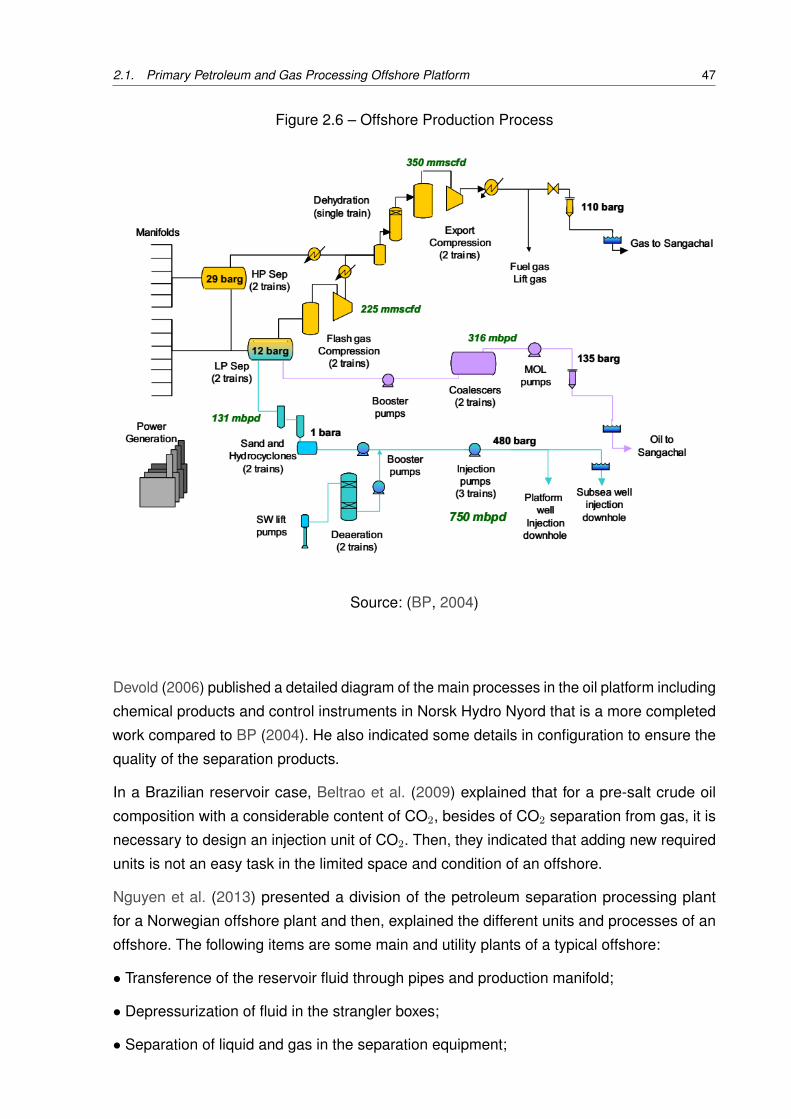
Figure 2.8 – Standardized FPSO processing scheme includes basic production separation
and treating systems. . . . . . . . . . . . . . . . . . . . . . . . . . . . . 50
Figure 2.9 – Overall scheme of a standards FPSOs topside process facilities. . . . . 51
Figure 2.10–Modules of a Replicant FPSO. . . . . . . . . . . . . . . . . . . . . . . . 52
Figure 2.11–Simplified overview of an offshore oil and gas platform . . . . . . . . . . 54
Figure 2.12–Oil, gas, CO2 and water production and exports regarding its power
demand for the platform during its operation years . . . . . . . . . . . . 56
Figure 2.13–The presented methodology framework in Wang et al. (2012) . . . . . . 62
Figure 2.14–Generic superstructure of an oil and gas processing plant. S1−2, S3−6
and S7−14 indicate separation configurations in one, two and three stages,
while the numbers indicated for the other steps, e.g. R1, C1, T1 and P1,
are the number of re-compression, compression, treatment and pumping
stages, respectively. . . . . . . . . . . . . . . . . . . . . . . . . . . . . . 63
Figure 2.15–The framework of the process optimization with GA. . . . . . . . . . . . 66
Figure 3.1 – Relative and global minima. . . . . . . . . . . . . . . . . . . . . . . . . 81
Figure 3.2 – Contours of the objective function in the constraint surfaces in a design
space . . . . . . . . . . . . . . . . . . . . . . . . . . . . . . . . . . . . . 82
Figure 3.3 – Input variable types in optimization. . . . . . . . . . . . . . . . . . . . . 83
Figure 3.4 – Example of the regular grid (left) and Latin square (right) designs for
two-dimensional design with 9 member ensemble. . . . . . . . . . . . . 88
Figure 3.5 – LHS designs with significant differences in terms of uniformity. . . . . . . 89
Figure 3.6 – Incremental Space Filler (ISF). Existing points in the database (previously
generated designs) (a), New points are added to fill the space uniformly (b). 90
Figure 3.7 – The Genes, chromosomes and genetic operations. . . . . . . . . . . . . 93
Figure 4.1 – Top view of a typical FPSO unit and all related processes. . . . . . . . . 99
Figure 4.2 – The general scheme of a FPSO . . . . . . . . . . . . . . . . . . . . . . 100
Figure 4.3 – Simplified scheme of three-stage separation train. . . . . . . . . . . . . 101
Figure 4.4 – Simplified scheme of degasser and electrostatic treatment. . . . . . . . 102
Figure 4.5 – Simplified scheme of Vapor Recovery Unit. . . . . . . . . . . . . . . . . 103
Figure 4.6 – Simplified scheme of Main Gas Compression unit. . . . . . . . . . . . . 103
Figure 4.7 – Simplified scheme of Gas Dehydration System. . . . . . . . . . . . . . . 104
Figure 4.8 – Simplified scheme of Hydrocarbons Dew Point Control System. . . . . . 105
Figure 4.9 – Simplified scheme of Exportation Gas Compression unit. . . . . . . . . . 106
Figure 4.10–Simplified scheme of CO2 Removal Unit. . . . . . . . . . . . . . . . . . 107
Figure 4.11–Simplified scheme of CO2 Compression Unit. . . . . . . . . . . . . . . . 108
Figure 4.12–Simplified scheme of Injection Gas Compression Unit. . . . . . . . . . . 108
Figure 4.13–Simplified scheme of Gas Turbine and WHRU. . . . . . . . . . . . . . . 109
Figure 4.14–The general scheme of oil and gas processing in FPSO - operational
mode 1. . . . . . . . . . . . . . . . . . . . . . . . . . . . . . . . . . . . 111
Figure 4.15–The general scheme of oil and gas processing in FPSO - operational
mode 2. . . . . . . . . . . . . . . . . . . . . . . . . . . . . . . . . . . . 112
Figure 4.16–The general scheme of oil and gas processing in FPSO - operational
mode 3. . . . . . . . . . . . . . . . . . . . . . . . . . . . . . . . . . . . 112
Figure 4.17–Conceptual structure of the general methodology and computational steps
to perform an optimization procedure for proposed FPSO. . . . . . . . . 115
Figure 4.18–How Aspen HYSYS Works . . . . . . . . . . . . . . . . . . . . . . . . . 116
Figure 4.19–Sketch of the proposed FPSO with. . . . . . . . . . . . . . . . . . . . . 120
Figure 4.20–Flowchart indicating the processes for screening analyses . . . . . . . . 121
Figure 4.21–Initial population designs checking by statistical tools. . . . . . . . . . . 122
Figure 4.22–General flowchart of the optimization procedure . . . . . . . . . . . . . . 124
Figure 4.23–The procedure of optimization in ModeFRONTIERTM
. . . . . . . . . . . 125
Figure 5.1 – Power consumption [kW] and percentage for FPSO systems[%] for operational
mode 1. . . . . . . . . . . . . . . . . . . . . . . . . . . . . . . . . . . . 130
Figure 5.2 – Power consumption [kW] and percentage for FPSO systems[%] for operational
mode 2. . . . . . . . . . . . . . . . . . . . . . . . . . . . . . . . . . . . 130
Figure 5.3 – Power consumption [kW] and percentage for FPSO systems[%] for operational
mode 3. . . . . . . . . . . . . . . . . . . . . . . . . . . . . . . . . . . . 131
Figure 5.4 – Scatter matrix chart for screening analysis of the input parameters of
operation mode 1. . . . . . . . . . . . . . . . . . . . . . . . . . . . . . . 133
Figure 5.5 – Contribution of the input parameters to hydrocarbon liquids recovery for
operation mode 1. . . . . . . . . . . . . . . . . . . . . . . . . . . . . . . 134
Figure 5.6 – Total separation efficiency for the conditions shown in Table 5.4. . . . . . 135
Figure 5.7 – C7+ molar fraction in exportation oil for the conditions shown in in Table 5.4.136
Figure 5.8 – Scatter matrix chart for screening analysis of the input parameters of
operation mode 2. . . . . . . . . . . . . . . . . . . . . . . . . . . . . . . 137
Figure 5.9 – Contribution of the input parameters to hydrocarbon liquids recovery for
operation mode 2. . . . . . . . . . . . . . . . . . . . . . . . . . . . . . . 137
Figure 5.10–Total separation efficiency for the conditions shown in Table 5.5. . . . . . 138
Figure 5.11–Scatter matrix chart for screening analysis of the input parameters of
operation mode 2. . . . . . . . . . . . . . . . . . . . . . . . . . . . . . . 139
Figure 5.12–Contribution of the input parameters to hydrocarbon liquids recovery for
operation mode 3. . . . . . . . . . . . . . . . . . . . . . . . . . . . . . . 140
Figure 5.13–Contribution of input parameters to fuel consumption in mode 1. . . . . . 142
Figure 5.14–Contribution of input parameters to fuel consumption in mode 2. . . . . . 143
Figure 5.15–Contribution of input parameters to fuel consumption in mode 3. . . . . . 144
Figure 5.16–Contribution of input parameters on FPSO process and utility units. . . . 146
Figure 5.17–SQP convergence curve for the function of hydrocarbon liquids recovery
maximization. . . . . . . . . . . . . . . . . . . . . . . . . . . . . . . . . 147
Figure 5.18–Simplex convergence curve for the objective function of Fuel consumption
minimization. . . . . . . . . . . . . . . . . . . . . . . . . . . . . . . . . 148
Figure 5.19–NSGA-II method convergence curve for the objective function of Fuel
consumption minimization. . . . . . . . . . . . . . . . . . . . . . . . . . 149
Figure 5.20–Hybrid method convergence curve for the objective function of Fuel
consumption minimization. . . . . . . . . . . . . . . . . . . . . . . . . . 150
Figure 5.21–The separated gas flow composition in the third stage of separation train
for the baseline and optimized cases for operation mode 1. . . . . . . . 152
Figure 5.22–The separated gas flow composition in the third stage of separation train
for the baseline and optimized case for operation mode 2. . . . . . . . . 154
Figure 5.23–The separated gas flow composition in the third stage of separation train
for the baseline and optimized cases for operation mode 3 . . . . . . . . 156
Figure 5.24–Selected point in process steps of separation. . . . . . . . . . . . . . . . 158
Figure 5.25–Stabilization of phase during the separation processes for the baseline
and optimized cases of operation mode 1. . . . . . . . . . . . . . . . . . 161
Figure 5.26–Stabilization of phase during the separation processes for the baseline
and optimized case of operation mode 2. . . . . . . . . . . . . . . . . . 163
Figure 5.27–Stabilization of phase during the separation processes for the baseline
and optimized case of operation mode 3. . . . . . . . . . . . . . . . . . 165
Figure A.1 – Efficiency curves by variation of the load. . . . . . . . . . . . . . . . . . 185
Figure A.2 – Curves of exhausted gas mass flow rate by variation of the load. . . . . 186
Figure A.3 – Curve of the exhausted gas temperature by variation of the load. . . . . 186
Figure A.4 – The used worksheet to calculate RB211 off-designs. . . . . . . . . . . . 187
Figure A.5 – The performance data of RB211 that regarding the variation of input
parameters . . . . . . . . . . . . . . . . . . . . . . . . . . . . . . . . . 187
Figure A.6 – Applied Gas turbine RB211 performance data in Aspen HYSYS. . . . . 188
Figure B.1 – General scheme of proposed FPSO . . . . . . . . . . . . . . . . . . . . 189
Figure B.2 – An overview of simulation of FPSO by Aspen HYSYS . . . . . . . . . . 190
Figure B.3 – Configuration of FPSO plant and utilities plant in this study. . . . . . . . 191
Figure B.4 – Vapor Recovery Unit (VRU) . . . . . . . . . . . . . . . . . . . . . . . . . 191
Figure B.5 – Main Gas Compression Unit (MGC) . . . . . . . . . . . . . . . . . . . . 192
Figure B.6 – Gas Dehydration System and CO2 Removal Unit (GDS&CO2RU) . . . . 192
Figure B.7 – CO2 Compression(CO2C) . . . . . . . . . . . . . . . . . . . . . . . . . 193
Figure B.8 – Exportation Gas Compression(EGC) . . . . . . . . . . . . . . . . . . . . 195
Figure B.9 – Injection Gas Compression(IGC) . . . . . . . . . . . . . . . . . . . . . . 195
Figure B.10–Gas Turbine and Waste Heat Recovery Unit (GT&WHRU) . . . . . . . . 195
Figure C.1 – Couple ModeFrontier with ASPEN HYSYS . . . . . . . . . . . . . . . . 197
Figure C.2 – Work flow of ModeFrontier for an optimization procedure . . . . . . . . . 198
Figure C.3 – Results of SS-ANOVA of hydrocarbon liquids recovery in ModeForntier . 199
Figure D.1 – Hybrid algorithm convergence curve for fuel consumption minimization-
mode 1 . . . . . . . . . . . . . . . . . . . . . . . . . . . . . . . . . . . 201
Figure D.2 – Hybrid algorithm convergence curve for fuel consumption minimization-
mode 2 . . . . . . . . . . . . . . . . . . . . . . . . . . . . . . . . . . . 202
Figure D.3 – Hybrid algorithm convergence curve for fuel consumption minimization-
mode 3 . . . . . . . . . . . . . . . . . . . . . . . . . . . . . . . . . . . 202
Figure D.4 – Hybrid algorithm convergence curve for hydrocarbon liquids recovery
maximization - mode 1 . . . . . . . . . . . . . . . . . . . . . . . . . . . 203
Figure D.5 – Hybrid algorithm convergence curve for hydrocarbon liquids recovery
maximization - mode 2 . . . . . . . . . . . . . . . . . . . . . . . . . . . 203
Figure D.6 – Hybrid algorithm convergence curve for hydrocarbon liquids recovery
maximization - mode 3 . . . . . . . . . . . . . . . . . . . . . . . . . . . 204
LIST OF TABLES
Table 2.1 – Summary of the main works on the thermodynamics analysis of oil and
gas platforms. . . . . . . . . . . . . . . . . . . . . . . . . . . . . . . . . 57
Table 2.2 – Summary of the main works on the performance of oil and gas platforms. 58
Table 2.3 – Summary of the main works on the performance of oil and gas platforms. 59
Table 2.4 – Summary of the main works on the process synthesis, sensitivity analysis
and optimization of processing plants. . . . . . . . . . . . . . . . . . . . 74
Table 2.5 – Summary of the main works on the process synthesis, sensitivity analysis
and optimization of processing plants. . . . . . . . . . . . . . . . . . . . 75
Table 2.6 – Summary of the main works on the process synthesis, sensitivity analysis
and optimization of processing plants. . . . . . . . . . . . . . . . . . . . 76
Table 4.1 – Crude oil composition of the three operational modes (molar fraction). . . 113
Table 4.2 – Input parameter ranges and their respective constraints . . . . . . . . . . 119
Table 5.1 – Mass flow rates of the three operational modes. . . . . . . . . . . . . . . 128
Table 5.2 – Operating pressures and temperatures of streams in the three operational
modes. . . . . . . . . . . . . . . . . . . . . . . . . . . . . . . . . . . . . 129
Table 5.3 – Operating pressures and temperatures of streams in the three operational
modes. . . . . . . . . . . . . . . . . . . . . . . . . . . . . . . . . . . . . 129
Table 5.4 – Hypothetic conditions to perform separation efficiency . . . . . . . . . . . 135
Table 5.5 – Different pressure operating conditions to perform separation efficiency . 138
Table 5.6 – Input parameters and their respective operating ranges to be used in the
maximization of hydrocarbon liquids recovery . . . . . . . . . . . . . . . 141
Table 5.7 – Input parameters and their respective operating ranges to be used in the
optimization procedure of fuel consumption minimization . . . . . . . . . 145
Table 5.8 – Fuel consumption and power demand of the FPSO unit for the baseline
and optimized case of operation mode 1 . . . . . . . . . . . . . . . . . . 151
Table 5.9 – Input parameters for the baseline and optimized configurations of operation
mode 1. . . . . . . . . . . . . . . . . . . . . . . . . . . . . . . . . . . . . 152
Table 5.10–Fuel consumption and power demand of the FPSO unit for the baseline
and optimized case of operation mode 2. . . . . . . . . . . . . . . . . . . 153
Table 5.11–Input parameters for the baseline and optimized configurations of operation
mode 2 . . . . . . . . . . . . . . . . . . . . . . . . . . . . . . . . . . . . 154
Table 5.12–Fuel consumption and power demand of the FPSO unit for the baseline
and optimized case of operation mode 3. . . . . . . . . . . . . . . . . . . 155
Table 5.13–Input parameters for the baseline and optimized configurations of operation
mode 3 . . . . . . . . . . . . . . . . . . . . . . . . . . . . . . . . . . . . 156
Table 5.14–Input parameters for the baseline and optimized configurations of operation
mode 1- Hydrocarbon liquids recovery case. . . . . . . . . . . . . . . . . 159
Table 5.15–Exportation oil rate, separation performance of all separators and propane,
butane and pentane percentage of exportation oil of the FPSO unit for the
baseline and optimized case of operation mode 1. . . . . . . . . . . . . . 162
Table 5.16–Input parameters for the baseline and optimized configurations of operation
mode 2 - hydrocarbon liquids recovery case. . . . . . . . . . . . . . . . . 163
Table 5.17–Exportation oil rate, separation performance of all separators and propane,
butane and pentane percentage of exportation oil of the FPSO unit for the
baseline and optimized case of operation mode 2. . . . . . . . . . . . . . 164
Table 5.18–Input parameters for the baseline and optimized configurations of operation
mode 3-Hydrocarbon liquids recovery case. . . . . . . . . . . . . . . . . 165
Table 5.19–Exportation oil rate, separation performance of all separators and propane,
butane and pentane percentage of exportation oil of the FPSO unit for the
baseline and optimized case of operation mode 3. . . . . . . . . . . . . . 166
Table B.1 – Required injection pressure as a function of CO2 composition and gas flow. 194
ACRONYMS
ABC Air Bottoming Cycle
AfilterSQP Adaptive Filter Sequential Quadratic Programming
ANOVA ANalysis Of VAriance
ANN Anime News Network
API American Petroleum Institute gravity
BSW Basic Sediment and Water
BG British Gas
BORC Basic Organic Rankine Cycle
BP British Petroleum
CAPEX CAPital EXpenditures
CCD Central Composite Design
CCS Carbon Capture and Storage
CMA-ES Covariance Matrix Adaptation Evolution Strategy
CONAMA Conselho Nacional do Meio Ambiente
CO2C CO2 Compression Unit
CO2RU CO2 Removal Unit
C3MR Propane precooled Mixed Refrigerant process
DEA Diethanolamine
DoE Design of Experiment
DOD D-optimal design
DMR Double Mixed Refrigerant
EA Evolutionary Algorithms
EGC Exportation Gas Compression unit
EIA U.S. Energy Information Administration
EOR Enhance Oil Recovery
EOS Equation of State
FLNG Floating Liquefied Natural Gas
FPSO Floating, Production, Storage and Offloading
FWKO Free Water Knockout
GA Genetic Algorithm
GAMS The General Algebraic Modeling System
GDP Gross Domestic Product
GDS Gas Dehydration System
GHG GreenHouse Gas
GOR Gas-to-Oil Ratio
GT Gas Turbine
HE Heat Exchanger
HX Heat Exchanger
HDP Hyrocarbon Dew Point control system
HRVG Heat Recovery Vapor Generator
HVAC Heating, Ventilation and Air Conditioning
IGC Injection Gas Compression unit
IOGP The International Association of Oil & Gas Producers
ISF Incremental Space Filler
KanGAL Kanpur Genetic Algorithms Laboratory
KBO Knowledge-Based Optimization
KSMR Korea Single Mixed Refrigerant
LEC Levelized Energy Cost
LH Latin Hypercube
LHS Latin Hypercube Sampling
LHV Lower Heating Value
LNG Liquefied Natural Gas
MCD Coordinate Descent Methodology
MDEA Methyldiethanolamine
MF ModeFRONTIERTM
MGC Main Gas Compression unit
MILP Mixed-Integer Linear Programming
MINLP Mixed-Integer Non-Linear Programming
MIPSQP Mixed Integer Programming Sequential Quadratic Programming
MOPSO Multi Objective Particle Swarm Optimizer
MRC Mixed Refrigerant Cycle
NCS Norwegian Continental Shelf
NG Natural Gas
NGL Natural Gas Liquid
NLP NonLinear Programming
NNA Nearest Neighbor Algorithm
NMPC Non Linear Model Predictive Control
NSGA Non-dominated Sorting Genetic Algorithm
OAD Orthogonal Array Design
OPEX OPerating EXpenditure
ORC Organic Rankine Cycle
PSO Particle Swarm Optimization
PDF Probability Density Function
RORC Regenerative Organic Rankine cycle
RSM Response Surface Methodology

PR Peng-Robinson
SG Specific Gravity
SQP Sequential Quadratic Programming
SS-ANOVA Smoothing Spline-ANalysis Of VAriance
ST Separation Train
St.Dev. Standard Deviation
TGC Technology Global Center
UD Uniform Design
ULH Uniform Latin Hypercube
VBA Visual Basic for Applications
VBScript Microsoft Visual Basic Scripting Edition
VRU Vapor Recovery Unit
WAG Water Alternating Gas
WHEN Work-Heat Exchanger Networks
WHRU Waste Heat Recovery Unit
WOR Water to Oil Ratio

NOTATIONS
Symbols
C1 Methane
C2 Ethan
C3 Propane
C4 Butane
C5 Pentane
C6 Hexane
C7 Heptane
C8 Octane
h Specific enthalpy
LHV Lower heating value
m Mass flow rate
n Molar flow rate
P Pressure
Q Heat
SG Specific gravity
T Temperature
W Power
Greek symbols
κk Collinearity index
η Efficiency
ν Volume
Subscripts
air Air
cc Combustion chamber
Feed Feed crude oil
GT Gas Turbine
Heavy Heavy Hydrocarbons
in Input
i i-th component
Light Light Hydrocarbons
Medium Medium Hydrocarbons
net Net
out Output
sep Separation

CONTENTS
1 INTRODUCTION . . . . . . . . . . . . . . . . . . . . . . . . . . . . . . 31
1.1 Background . . . . . . . . . . . . . . . . . . . . . . . . . . . . . . . . . 31
1.1.1 Outlook . . . . . . . . . . . . . . . . . . . . . . . . . . . . . . . . . . . . 31
1.2 Primary (Petroleum) Processing Plant of FPSO . . . . . . . . . . . . 33
1.2.1 Primary Separation Train of Petroleum . . . . . . . . . . . . . . . . . . . 34
1.2.2 Gas compression treatment, re-injection and exportation system . . . . . 35
1.2.3 CO2 Removal, Compression and Injection System . . . . . . . . . . . . 36
1.3 FPSO operational modes . . . . . . . . . . . . . . . . . . . . . . . . . 36
1.3.1 Operational mode 1 . . . . . . . . . . . . . . . . . . . . . . . . . . . . . 36
1.3.2 Operational mode 2 . . . . . . . . . . . . . . . . . . . . . . . . . . . . . 36
1.3.3 Operational mode 3 . . . . . . . . . . . . . . . . . . . . . . . . . . . . . 36
1.4 Motivation . . . . . . . . . . . . . . . . . . . . . . . . . . . . . . . . . . 37
1.5 Objectives . . . . . . . . . . . . . . . . . . . . . . . . . . . . . . . . . . 37
1.6 Outline of the Thesis . . . . . . . . . . . . . . . . . . . . . . . . . . . . 38
2 LITERATURE REVIEW . . . . . . . . . . . . . . . . . . . . . . . . . . . 41
2.1 Primary Petroleum and Gas Processing Offshore Platform . . . . . 41
2.1.1 Composition, Crude Oil, Gas and Reservoir Fluid . . . . . . . . . . . . . 41
2.1.2 Offshore Platforms: Processes and Configurations . . . . . . . . . . . . 45
2.1.3 Brazilian Reservoir, Offshore industry and FPSO Configurations . . . . . 48
2.1.4 Thermodynamics analysis of oil and gas processing plant . . . . . . . . 52
2.2 Process Optimization in Processing Plants . . . . . . . . . . . . . . 60
2.2.1 Process Synthesis and Modeling . . . . . . . . . . . . . . . . . . . . . . 60
2.2.2 Sensitivity analysis and Optimization of Industrial Processing Plant . . . 64
2.2.3 Sensitivity analysis and Optimization of Oil and Gas Processing Plants . 69
2.3 Overview . . . . . . . . . . . . . . . . . . . . . . . . . . . . . . . . . . 77
3 THEORETICAL FOUNDATION . . . . . . . . . . . . . . . . . . . . . . . 79
3.1 Thermodynamic Analysis . . . . . . . . . . . . . . . . . . . . . . . . . 79
3.1.1 Separation Performance . . . . . . . . . . . . . . . . . . . . . . . . . . . 80
3.2 Optimization . . . . . . . . . . . . . . . . . . . . . . . . . . . . . . . . 80
3.2.1 Algorithmic methods . . . . . . . . . . . . . . . . . . . . . . . . . . . . . 83
3.2.2 Classification of algorithmic optimization methods . . . . . . . . . . . . . 84
3.2.3 Screening Analysis . . . . . . . . . . . . . . . . . . . . . . . . . . . . . 86
3.2.4 Design of Experiments (DoE) . . . . . . . . . . . . . . . . . . . . . . . . 86
3.2.4.1 Latin hypercube sampling (LHS), Uniform Latin Hypercube (ULH) and Incremental Space
Filler (ISF) . . . . . . . . . . . . . . . . . . . . . . . . . . . . . . . . . . . 88
3.2.4.2 Smoothing spline ANOVA method (SS-ANOVA) . . . . . . . . . . . . . . . . . . 90
3.2.5 Genetic Algorithms – Fundamentals . . . . . . . . . . . . . . . . . . . . 93
3.2.5.1 Non-dominated sorting genetic algorithm II (NSGA-II) . . . . . . . . . . . . . . . . 94
3.2.5.2 Hybrid optimization method (GA+SQP) . . . . . . . . . . . . . . . . . . . . . . 95
3.2.6 Sensitivity of the optimum . . . . . . . . . . . . . . . . . . . . . . . . . . 96
3.2.7 Conclusion . . . . . . . . . . . . . . . . . . . . . . . . . . . . . . . . . . 96
4 METHODOLOGY IMPLEMENTATION . . . . . . . . . . . . . . . . . . . 99
4.1 System description and simulation . . . . . . . . . . . . . . . . . . . 99
4.1.1 Separation Train . . . . . . . . . . . . . . . . . . . . . . . . . . . . . . . 100
4.1.2 Gas Treatment Units . . . . . . . . . . . . . . . . . . . . . . . . . . . . . 102
4.1.2.1 Vapor Recovery Unit (VRU) . . . . . . . . . . . . . . . . . . . . . . . . . . . 102
4.1.2.2 Main Gas Compression (MGC) . . . . . . . . . . . . . . . . . . . . . . . . . . 103
4.1.2.3 Gas dehydration System (GDS) . . . . . . . . . . . . . . . . . . . . . . . . . 104
4.1.2.4 Hydrocarbons Dew Point Control System (HDP) . . . . . . . . . . . . . . . . . . 104
4.1.2.5 Exportation Gas Compression System (EGC) . . . . . . . . . . . . . . . . . . . 105
4.1.3 CO2 Treatment Units . . . . . . . . . . . . . . . . . . . . . . . . . . . . . 106
4.1.3.1 CO2 Removal Unit (CO2RU) . . . . . . . . . . . . . . . . . . . . . . . . . . . 106
4.1.3.2 CO2 Compression system (CO2C) . . . . . . . . . . . . . . . . . . . . . . . . 107
4.1.3.3 Injection Gas Compression unit(IGC) . . . . . . . . . . . . . . . . . . . . . . . 108
4.1.4 Utility plants . . . . . . . . . . . . . . . . . . . . . . . . . . . . . . . . . 109
4.1.4.1 Power and heat generation unit . . . . . . . . . . . . . . . . . . . . . . . . . . 109
4.1.4.2 Hot Water system . . . . . . . . . . . . . . . . . . . . . . . . . . . . . . . . 110
4.1.4.3 Cooling Water system . . . . . . . . . . . . . . . . . . . . . . . . . . . . . . 110
4.1.4.4 Water Injection System . . . . . . . . . . . . . . . . . . . . . . . . . . . . . 110
4.1.5 Operation Scenarios . . . . . . . . . . . . . . . . . . . . . . . . . . . . . 111
4.2 Assumptions for modeling and simulation . . . . . . . . . . . . . . . 113
4.3 Modeling, Simulation and optimization description . . . . . . . . . . 114
4.3.1 Strategy . . . . . . . . . . . . . . . . . . . . . . . . . . . . . . . . . . . 114
4.3.2 Simulation of FPSO in HYSYS . . . . . . . . . . . . . . . . . . . . . . . 115
4.3.3 Sensitivity analysis description . . . . . . . . . . . . . . . . . . . . . . . 118
4.3.4 Optimization description . . . . . . . . . . . . . . . . . . . . . . . . . . . 123
4.3.4.1 Optimization in ModeFRONTIERTM . . . . . . . . . . . . . . . . . . . . . . . . 124
5 RESULTS AND DISCUSSIONS . . . . . . . . . . . . . . . . . . . . . . 127
5.1 Thermodynamic analysis results . . . . . . . . . . . . . . . . . . . . . 127
5.2 Sensitivity analysis results . . . . . . . . . . . . . . . . . . . . . . . . 131
5.2.1 Contribution of Input Parameters on Hydrocarbon Liquids Recovery . . . 131
5.2.1.1 Operation mode 1 . . . . . . . . . . . . . . . . . . . . . . . . . . . . . . . . 132
5.2.1.2 Operation mode 2 . . . . . . . . . . . . . . . . . . . . . . . . . . . . . . . . 136
5.2.1.3 Operation mode 3 . . . . . . . . . . . . . . . . . . . . . . . . . . . . . . . . 139
5.2.2 The contribution of Input Parameters To Fuel Consumption . . . . . . . . 141
5.2.2.1 Operation mode 1 . . . . . . . . . . . . . . . . . . . . . . . . . . . . . . . . 141
5.2.2.2 Operation mode 2 . . . . . . . . . . . . . . . . . . . . . . . . . . . . . . . . 143
5.2.2.3 Operation mode 3 . . . . . . . . . . . . . . . . . . . . . . . . . . . . . . . . 144
5.3 Optimization Results . . . . . . . . . . . . . . . . . . . . . . . . . . . . 146
5.3.1 Assessment of applied optimization methods . . . . . . . . . . . . . . . 146
5.3.2 Fuel consumption . . . . . . . . . . . . . . . . . . . . . . . . . . . . . . 150
5.3.2.1 Operation Mode 1 . . . . . . . . . . . . . . . . . . . . . . . . . . . . . . . . 150
5.3.2.2 Operation mode 2 . . . . . . . . . . . . . . . . . . . . . . . . . . . . . . . . 153
5.3.2.3 Operation mode 3 . . . . . . . . . . . . . . . . . . . . . . . . . . . . . . . . 155
5.3.3 Hydrocarbon liquids recovery . . . . . . . . . . . . . . . . . . . . . . . . 157
5.3.3.1 Operation mode 1 . . . . . . . . . . . . . . . . . . . . . . . . . . . . . . . . 158
5.3.3.2 Operation mode 2 . . . . . . . . . . . . . . . . . . . . . . . . . . . . . . . . 162
5.3.3.3 Operation mode 3 . . . . . . . . . . . . . . . . . . . . . . . . . . . . . . . . 164
6 CONCLUSION AND FUTURE WORK . . . . . . . . . . . . . . . . . . . 167
6.1 Conclusion . . . . . . . . . . . . . . . . . . . . . . . . . . . . . . . . . 167
6.2 Future work . . . . . . . . . . . . . . . . . . . . . . . . . . . . . . . . . 169
REFERENCES . . . . . . . . . . . . . . . . . . . . . . . . . . . . . . . 171
APPENDIX A – MODELING AND SIMULATION OF RB211G62 DLE
60HZ TURBINE IN GATECYCLE AND USING THIS
DATA IN ASPEN HYSYS . . . . . . . . . . . . . . . . 185
APPENDIX B – MODELING AND SIMULATION SIMULATOR ILLUSTRATION
OF FPSO BY ASPEN HYSYS . . . . . . . . . . . . . 189
APPENDIX C – COUPLING MODEFRONTIER WITH ASPEN HYSYS . 197
APPENDIX D – CONVERGED OBJECTIVE FUNCTIONS . . . . . . . 201

31
1 INTRODUCTION
1.1 Background
1.1.1 Outlook
Petroleum has been used since ancient times. About 4000 years ago, it was utilized in
Babylon as a material for building walls and towers. Ancient Persian tablets also indicate
medicinal and lighting applications of petroleum at the higher levels of society (Chisholm,
Hugh, 1911). However, oil is important in the Energy Matrix, but it currently has an inevitable
role across society, concerning environmental pollution, economy, geopolitics, and technology.
After many decades, petroleum is still one of the most important fossil fuels. New resources,
such as shale gas besides shale oil, tar sand, pre-salt oil and condensate and heavy oil are
also of interest for exploitation. The increase in the world energy use is planned to reach
56% in the next three decades, which is considered mainly a result of population growth and
rising prosperity in developing countries (U.S. ENERGY INFORMATION ADMINISTRATION,
2013). In the last annual report of EIA in 2018 (U.S. Energy Information Administration (EIA),
2018), the projected gross domestic product (GDP) of the world from 2017 is dependent
on hydrocarbons fuel and natural gas accounts for the largest share of the total energy
production.
According to the statistical report published in 2015 by British Petroleum, Brazil is the eighth
largest energy consumer in the world and, behind the United States and Canada, it is the third
largest in the Americas. Most of this energy consumption involves oil and other liquid fuels,
followed by hydropower and natural gas. Due to the discovery of new Brazilian pre-Salt fields,
the reservoirs have expanded from 15 billion barrels of oil in 2004 to more than 30 billion in
2009, making Brazil a top 10 liquid fuel producer in the world. In 2014, Brazil produced a
large amount of oil, about 2.95 million barrels per day (b/d), representing a 9.5% increase as
compared to 2013. Fossil fuels such as oil, natural gas and condensate production represent
about 60% of the Brazilian energy matrix and increasing domestic oil and gas production
has been a long-term objective of the Brazilian government. In turn, Brazil is identified as
the world’s 7th-largest emitter of greenhouse gases and as the third largest emitter after
China and India among the developing countries. The oil and gas exploration and production
industries emit a considerable percentage of greenhouse gases and are energy intensive.
Some countries were therefore compelled to promote the mitigation of contamination and
the common proposal is to lower the CO2 rate. The reduction in CO2 emissions is hence an
important factor in industrial development (LOUREIRO et al., 2013)(PB, 2015)(Ministério de
Minas e Energia, 2015).
32 Chapter 1. Introduction
Hence, there are the following important challenges that need addressing for the energy
strategy of any oil and gas industrial:
• Efficiency challenge (developing and improving the applied thermal systems in the oil and
gas industry regarding crude oil compositions and operating conditions).
• Environmental impact and sustainability challenges (reduction in energy consumption
and/or reduction in the environmental effect of oil and processing plants).
The first issue may be addressed by carrying out a precise system analysis to improve and
to optimize the thermal efficiency and performance of diverse energy- consuming processes
(power and heating).
The second one can be solved by first, mitigating CO2 emission in oil and gas processing,
including CO2 content of oil and gas compositions. Second, reducing the required power
demand leads to less total fuel consumption of an oil and gas processing plant.
This environmental purpose is a sustainability requirement of technological planning comprising
both processing and utility plants. Note that sustainable proposals should also be developed
for offshore processes, including security demands, reliability, besides the demands of size
and weight increment, especially comparing offshore-type processes to onshore processes
(REAY et al., 2013). Moreover, along with the two challenges considered, the profitability
of the system, including increasing oil and gas production can play an effective role to
encourage companies to mitigate the environmental impacts.
Oil and gas production and processing in offshore platforms are an important sector of the
global oil industry. These platforms have been configured in two plants, which comprise
processing plants and utility units. The main plant is responsible for separating oil from
associated gas, water, salt, and for processing the desired production. The utility plants are
where air, fuel gas, cooling and heating water are used.
A typical oil and gas offshore installation, may contain the following systems (NGUYEN et
al., 2013):
• Production manifolds;
• Oil separation;
• Oil pumping and exportation;
• Re-compression and gas purification;
• Gas compression and exportation;
•Wastewater treatment;
• Sea water injection;

1.2. Primary (Petroleum) Processing Plant of FPSO 33
• Power and heat generation unit;
• HVAC and other utilities.
The power generation unit is responsible for the consumption of the plant itself and a number
of important considerations could involve diagrams and a power generation planning scheme
in conjunction with the process scheme as follows: conditions and standards of the production
process, available technologies, energy analysis methods, dynamic manufacturing process.
Furthermore, utilities must seek the best options in terms of the arrangement, capacity, type
and number of machines, to ensure an adequate economic/financial return and reasonable
operation to meet efficient operation and the project requirements (BALESTIERI, 2002).
In addition to the indicated technological options available, many studies can be implemented
in the production process of offshore platforms for sustainability. In some oil offshore platform
processes, water is required and this process permits, for example, capturing the water
contained in the gas combustion of a gas turbine. This is a potential water source for this
type of applications (NGUYEN et al., 2013). Furthermore, in crude oil with considerable CO2
content, the separated CO2 should be stored (because of environmental issues) or injected
into the well as EOR (enhance oil recovery) and for an offshore plant, the separated gas
cannot be sent to the flare (ARAÚJO et al., 2017).
1.2 Primary (Petroleum) Processing Plant of FPSO
A wide variety of offshore installations have been used throughout the world, and the most
suitable offshore plants for deep-water are floating platforms. The FPSO (Floating Production,
Storage and Offloading) units have a technical advantage for the short-lived well exploration
and the remote marginal field, whereby fixed offshore installations are impractical and
whereby building a pipeline is cost-prohibitive (GEHLING et al., 1994) (KINNEY P.E., 2012).
FPSOs are useful in oil regions, which do not have a pipeline infrastructure in that place and
a storage tank does not need to be idle while a processing facility produces enough oil to fill
it. In addition, the advantage of those FPSOs over the pipelines is that once an oil field has
been exhausted, the vessel can be moved to another location. There are currently about
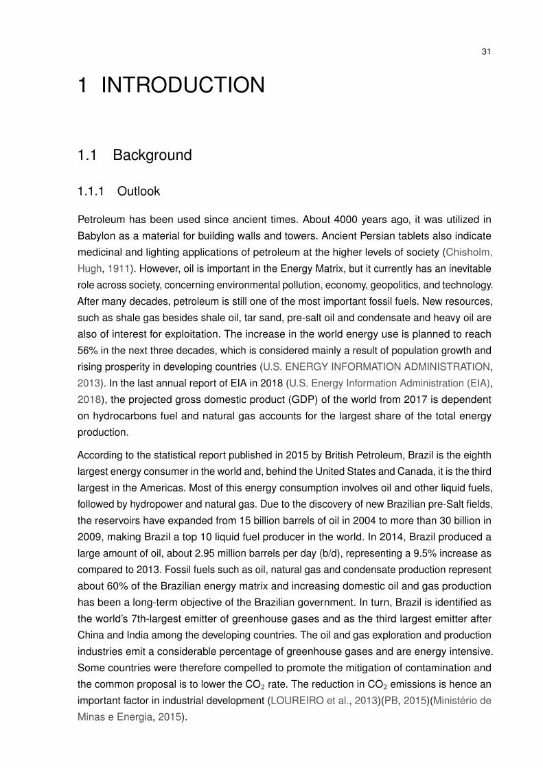
200 of such vessels operating worldwide. Figure 1.1 shows a typical FPSO on site.
In Brazil, petroleum is one of the main industries. The offshore exploration in Brazil is
located in the Santos Basin in the south and the Espirito Santo Basin in the north, where
the salt layer has a thickness ranging from 200 to 2000 m. Because Brazilian reserves are
characterized by their location in relation to the salt deposits, reserves placed above the salt
layer are called Post-salt, and those below the salt layer are called Pre-salt. For this reason,
Petrobras is the second operator with the largest number of FPSO units (about 12 owned
and 14 operating), utilizing over 15% FPSOs of all those existing worldwide (SHIMAMURA,
34 Chapter 1. Introduction
Figure 1.1 – Photo of the typical FPSO on site
Source: (FONTAINE et al., 2013)
2002)(HALLIBURTON, 2014)(BARRERA et al., 2015).
The concept of FPSO is for working as a floating unit, which can be used for the primary
production of petroleum and gas. This allows storing the explored petroleum in a repository
tank, besides being able to offload to another storage unit. A typical FPSO is described
briefly in the next subsection.
1.2.1 Primary Separation Train of Petroleum
In a primary processing installation, the role of the processing plant is to separate the well
fluid into three components. Thus, the crude oil comes into the separation train, which
consists of several stages and separator types. For example, in a three-phase separator
known as gravitational separator (Figure 1.2), Gas as a less dense fluid, is initially separated
from liquids by the action of gravity and water with more density separates under oil.
The separated gas in the separator train is forwarded to the compression units of the platform,
and water is sent to the produced water treatment system. Next, the processed oil goes
through two sequences of heat exchangers, to raise its temperature to levels that facilitate
separation in the subsequent part. The hot fluid of the first sequence of heat exchangers is
the oil stream (as exportation oil) leaving the processing plant to the Cargo Tank and the
hot fluid of the second heat exchanger is provided by the hot water from the Waste Heat
Recovery Unit of gas turbines (MORAIS, 2013).
In the next steps of separation, there are two similar pairs of heat exchangers, called
Degassers and Electrostatic treaters. Degassers are responsible for separating of the light

1.2. Primary (Petroleum) Processing Plant of FPSO 35
Figure 1.2 – Gravitational Separator
Source: (PROCESSONLINE.COM.AU, 2014)
hydrocarbon fractions in operating pressure of about eight bars. The output oil of that
separator is forwarded to the Electrostatic treater. In that, water drops remain separate
from the oil by electric polarized plates with the alternative current. The second pair of heat
exchangers operates in the same way, but the pressure level is lower, in order to have an
increment separation before transmitting oil to the cargo tanks (PETROBRAS, 2007).
1.2.2 Gas compression treatment, re-injection and exportation system
The phase of each treatment process is designed to achieve the necessary criteria to enable
its appropriate destination. For gas, the targets are forwarding, exporting via pipeline and
sometimes re-injecting them in a reservoir. Therefore, reducing the number of contaminants
to acceptable levels, and achieving the proper initial pressure are important points.
After separation processes, there are three gas streams with different pressures; high,
medium and low-pressure levels. High-pressure gas that comes from the main separator
(gravitational separator) is forwarded directly to the main gas compression unit. Medium
and low-pressure gases must go through an additional system, called Vapor Recovery Unit
(VRU) to recover and to complete its pressure to the suction level of the main compressors.
In the main compression unit, after the input gas goes through a scrubber vessel, there are
three compressors and three gas-water coolers to remove the thermal load absorbed by the
gas during compression.
The received gas with a low content of CO2, after CO2 removal, is sent to the compression
system of exportation. There, the pressure of the gas stream is elevated up to about 250 bar,
which is required from the pressure level for the pipeline to transport the gas (MORAIS, 2013).
36 Chapter 1. Introduction
1.2.3 CO2 Removal, Compression and Injection System
The gas without water and heavy components enters the CO2 Removal system composed
of membranes. The input gas has CO2 content ranging from 8-40% and after going through
the membranes, one output that has CO2 content in its composition varies between 2-5%
and another output varies between 30-50%. This gas stream with greater CO2 content is
routed to the CO2 compression unit, where its pressure is raised to a level of 250 bar (the
initial feed pressure of re-injection compressors) and then it is re-injected with the pressure
of 500 bar (MORAIS, 2013).
1.3 FPSO operational modes
Operating conditions are often determined by the features of the fluid reservoir, based on
the composition of the hydrocarbons and on the amount of impurities in the oil content.
According to the crude oil composition of pre-salt wells, the operating life of a reservoir fluid
and consequently, the operational modes of FPSO are divided into three general modes:
Mode 1, 2 and 3.
1.3.1 Operational mode 1
Operational mode 1 represents the typical early life condition and is applied when the crude
oil has a high GOR (gas-oil ratio ) and all of the processed gas is assumed to be exported
and the removed CO2 is injected into the wells. In this operational mode, the fuel gas is
obtained from the treated gas after the CO2 membrane unit.
1.3.2 Operational mode 2
This operational mode is used when the crude oil contains 50% BSW. In operational mode 2,
50% of the separated gas from the separation processes is injected in the CO2 removal unit
in order to be exported and 50% of the bypassed gas is injected into the production wells at
a pressure of 494 bar, approximately.
1.3.3 Operational mode 3
Operation Mode 3 is the end of life condition of an oil field and in that, all the gas separated
from the crude oil with the maximum quantity of water/CO2, is injected into production wells
through a bypass located in the CO2 removal system.
1.4. Motivation 37
1.4 Motivation
A Floating Production Storage and Offloading (FPSO) plant is a high energy consumer
(from a few to several hundreds of megawatts). The fuel consumption, power demand, and
production of a typical FPSO change regarding the operating conditions and lifetime of a field.
The possibility of improving for a FPSO plant configuration (in current operation) from early
life to the end of life of reservoir by changing thermodynamic operating parameters through a
formal optimization procedure has motivated the development of the current thesis. Moreover,
applying a systematic and automation optimization procedure to increase the sustainability
and profitability of a FPSO simultaneously, without adding any new technology and imposed
costs, is necessary to address existing gaps. Finally, suggesting a new standardized design
from the optimization configuration, for a Brazilian FPSO that meets the technical challenges
related to pre-salt oil field and operating in offshore conditions, is considered in the objectives
framework of the current research.
1.5 Objectives
The main objective of this thesis is the development and application of an optimization
methodology, based on the thermodynamics analysis and sensitivity analysis, for proposing
optimum and sustainable configurations of Primary Petroleum Platform of typical FPSO. Or
rather:
• Implementation of thermodynamics analysis to find important operating parameters on
energy consumption sources for the existing configuration of main and utility plants in a
FPSO Primary Petroleum Processing using the real performance data of applied gas turbine;
• Application of a screening analysis to identify the main and interaction effects of thermodynamic
parameters on fuel consumption, hydrocarbon liquids recovery and performance of separation
(as one of the possible improvements) for specific scenarios related to a Brazilian FPSO
operating on a pre-salt oil field;
• Application of an appropriate optimization procedure for fuel consumption minimization and
maximization of hydrocarbon liquids stabilization and recovery as a step in the improvement
of separation performance purposes, subject to several constraints, of a Brazilian FPSO for
early life, mid-life and end of life of a pre-salt oil field.
• Integrating of Aspen Hysys as a robust simulator of chemical processes and ModeForntier
as an automation process of screen analyzing and optimization procedure to achieve the
presented item above.
38 Chapter 1. Introduction
1.6 Outline of the Thesis
The thesis is divided into six chapters.
Chapter 1 introduces a brief outlook on the importance of the oil and gas industry in the
global Energy Matrix, indicating the current and ahead energy and environmental challenges
of this industry, along with the motivation, objectives, and outline of this thesis.
Chapter 2 sets the literature review of the offshore industry, including the role of crude
oil type on processing and utility plants, Brazilian offshore and FPSO oil and gas industry,
and thermodynamics analysis of these plants. Furthermore, this capture contains a brief
revision of the system modelling methods, screening analysis, optimization procedures, and
application of process optimization into oil and gas processing plants;
Chapter 3 describes the theoretical foundations and methodologies for determining major
energy consumers, indicators of separation performance. Moreover, algorithmic optimization
methods, statistical analysis methods, and focusing on Genetic algorithm techniques are
presented in this chapter;
Chapter 4 shows the description and implementation of the modeling and simulation of
the FPSO plants considering three operational modes and well-fluid compositions in its
useful life. Additionally, the strategy of an integration of simulation and optimizer to perform
automated sensitivity analysis and optimization is explained;
Chapter 5 demonstrates the obtained results from modeling, sensitivity analysis, and
optimization procedures that meet the desired objectives of the current thesis.
Chapter 6 concludes the present thesis, summarize the main findings of this work and
pinpoints the possibilities for future ones.
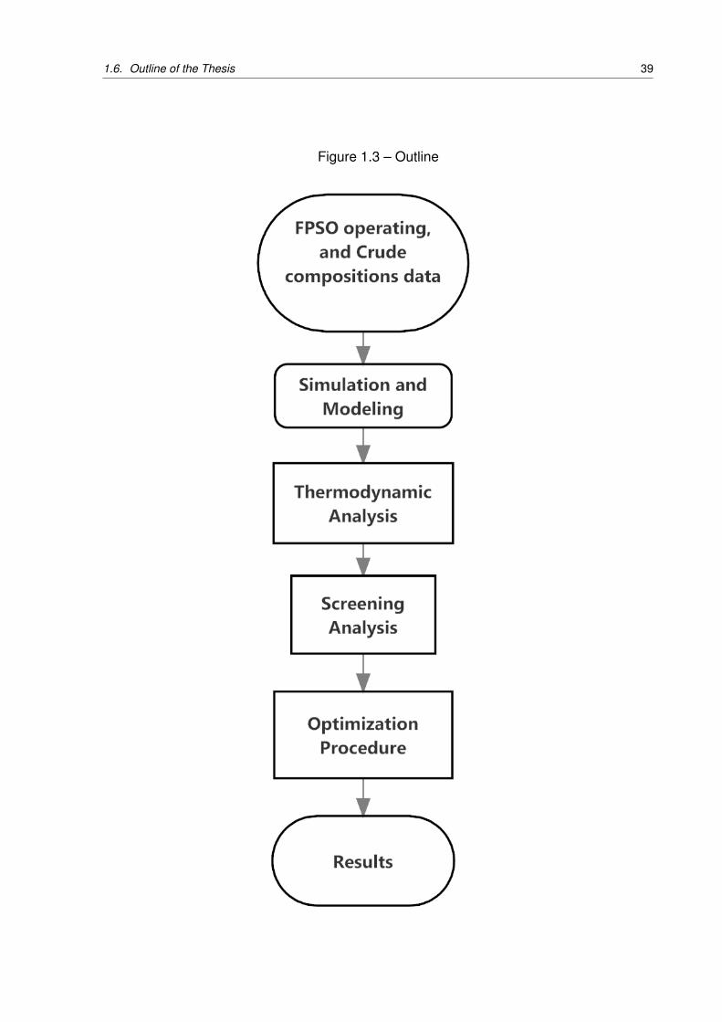
Figure 1.3 shows the generic steps to achieve the results of the current thesis.
1.6. Outline of the Thesis 39
Figure 1.3 – Outline

41
2 LITERATURE REVIEW
The last decades have witnessed the development and application of energy efficiency
tools to various thermal systems and industrial applications. Several authors have studied
thermodynamics, economic and environmental analysis of the oil and gas production base
platforms in diverse operating condition ranges, reservoir fluids, processes and technologies.
However, the oil and gas processing platforms are energy-intensive systems and many
fulfilled works using thermodynamics analysis confirmed that, but, there are very few
researches, which discussing the possibility of improving of a plant configuration (in current
operation) through an optimization procedure in an offshore.
This chapter provides an overview of the most relevant research works, to discuss the state
of art in the literature. The studies are divided into two main subjects, which are considered
for this chapter content.
2.1 Primary Petroleum and Gas Processing Offshore Platform
To analyze a typical offshore, understanding relation among components and structure
is essential. Thus, this section presents the generalized information of reservoir fluid and
processing platforms in two first sub-section and eventually, a Brazilian standardized FPSO
as the studied case is described.
2.1.1 Composition, Crude Oil, Gas and Reservoir Fluid
The main function of an offshore platform is to separate oil from reservoir fluid and associated
gas. Reservoir fluid is a complex mixture contained within the hydrocarbons and a wide
variety of other solution and chemical components.It is in liquid form at condition of underground
reservoirs and remains a liquid when brought to the surface. The composition and properties
of each well differ significantly from one reservoir to another. Petroleum derivations of the
wells are produced from processing crude oil and other liquids, such as high-content heavy
hydrocarbons, intermediate and volatile hydrocarbons, methane, light hydrocarbons and
water at petroleum processing platforms.
The hydrocarbon in crude oil compounds belongs to one of the following subclasses (IUPAC,
1993)(ABDEL-AAL et al., 2015):
• Alkanes or paraffins which are saturated hydrocarbons with the general formula (CnH2n+2).
They may be straight-chain or components in branched form, because of the production of
high-octane gasoline, the latter are more valuable than the former;
42 Chapter 2. Literature Review
•Cycloalkanes or cycloparaffins (naphthenes) which are unsaturated hydrocarbons (examples
are cyclopentane (C5H10) and cyclohexane (C6H12)). The presence of large amounts of
these cyclic compounds in the naphtha range is significant in the production of aromatic
compounds;
• Aromatic hydrocarbons that only monomolecular component in the range of C6−C8 have
gained commercial importance.
According to McCain et al. (2011), a reservoir fluid regarding some thermodynamic properties,
such as pressure and temperature, and composition can be categorized into following main
classifications:
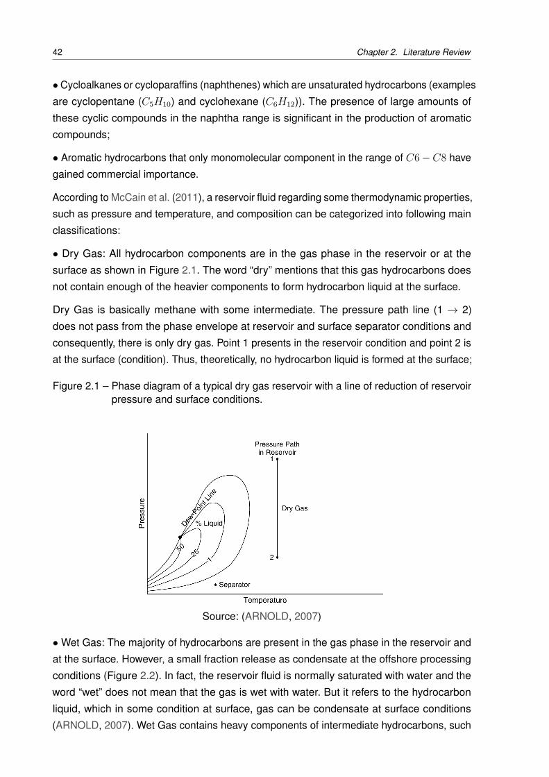
• Dry Gas: All hydrocarbon components are in the gas phase in the reservoir or at the
surface as shown in Figure 2.1. The word “dry” mentions that this gas hydrocarbons does
not contain enough of the heavier components to form hydrocarbon liquid at the surface.
Dry Gas is basically methane with some intermediate. The pressure path line (1 → 2)
does not pass from the phase envelope at reservoir and surface separator conditions and
consequently, there is only dry gas. Point 1 presents in the reservoir condition and point 2 is
at the surface (condition). Thus, theoretically, no hydrocarbon liquid is formed at the surface;
Figure 2.1 – Phase diagram of a typical dry gas reservoir with a line of reduction of reservoirpressure and surface conditions.
Source: (ARNOLD, 2007)
•Wet Gas: The majority of hydrocarbons are present in the gas phase in the reservoir and
at the surface. However, a small fraction release as condensate at the offshore processing
conditions (Figure 2.2). In fact, the reservoir fluid is normally saturated with water and the
word “wet” does not mean that the gas is wet with water. But it refers to the hydrocarbon
liquid, which in some condition at surface, gas can be condensate at surface conditions
(ARNOLD, 2007). Wet Gas contains heavy components of intermediate hydrocarbons, such
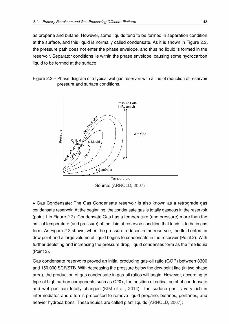
2.1. Primary Petroleum and Gas Processing Offshore Platform 43
as propane and butane. However, some liquids tend to be formed in separation condition
at the surface, and this liquid is normally called condensate. As it is shown in Figure 2.2,
the pressure path does not enter the phase envelope, and thus no liquid is formed in the
reservoir. Separator conditions lie within the phase envelope, causing some hydrocarbon
liquid to be formed at the surface;
Figure 2.2 – Phase diagram of a typical wet gas reservoir with a line of reduction of reservoirpressure and surface conditions.
Source: (ARNOLD, 2007)
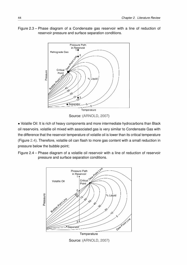
• Gas Condensate: The Gas Condensate reservoir is also known as a retrograde gas
condensate reservoir. At the beginning, the condensate gas is totally gaseous in the reservoir
(point 1 in Figure 2.3). Condensate Gas has a temperature (and pressure) more than the
critical temperature (and pressure) of the fluid at reservoir condition that leads it to be in gas
form. As Figure 2.3 shows, when the pressure reduces in the reservoir, the fluid enters in
dew point and a large volume of liquid begins to condensate in the reservoir (Point 2). With
further depleting and increasing the pressure drop, liquid condenses form as the free liquid
(Point 3).
Gas condensate reservoirs proved an initial producing gas-oil ratio (GOR) between 3300
and 150,000 SCF/STB. With decreasing the pressure below the dew-point line (in two phase
area), the production of gas condensate in gas-oil ratios will begin. However, according to
type of high carbon components such as C20+, the position of critical point of condensate
and wet gas can totally changes (KIM et al., 2014). The surface gas is very rich in
intermediates and often is processed to remove liquid propane, butanes, pentanes, and
heavier hydrocarbons. These liquids are called plant liquids (ARNOLD, 2007);
44 Chapter 2. Literature Review
Figure 2.3 – Phase diagram of a Condensate gas reservoir with a line of reduction ofreservoir pressure and surface separation conditions.
Source: (ARNOLD, 2007)
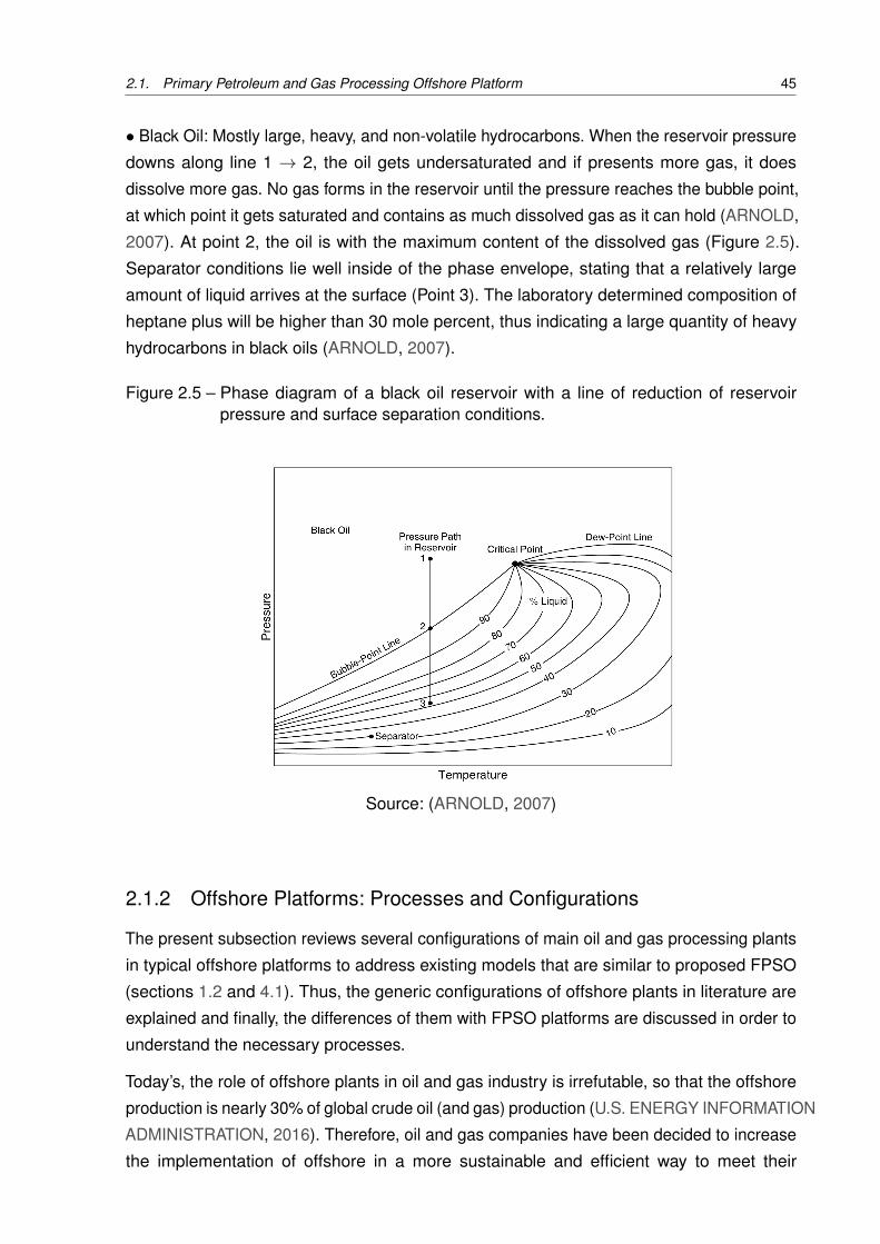
• Volatile Oil: It is rich of heavy components and more intermediate hydrocarbons than Black
oil reservoirs. volatile oil mixed with associated gas is very similar to Condensate Gas with
the difference that the reservoir temperature of volatile oil is lower than its critical temperature
(Figure 2.4). Therefore, volatile oil can flash to more gas content with a small reduction in
pressure below the bubble point;
Figure 2.4 – Phase diagram of a volatile oil reservoir with a line of reduction of reservoirpressure and surface separation conditions.
Source: (ARNOLD, 2007)
2.1. Primary Petroleum and Gas Processing Offshore Platform 45
• Black Oil: Mostly large, heavy, and non-volatile hydrocarbons. When the reservoir pressure
downs along line 1 → 2, the oil gets undersaturated and if presents more gas, it does
dissolve more gas. No gas forms in the reservoir until the pressure reaches the bubble point,
at which point it gets saturated and contains as much dissolved gas as it can hold (ARNOLD,
2007). At point 2, the oil is with the maximum content of the dissolved gas (Figure 2.5).
Separator conditions lie well inside of the phase envelope, stating that a relatively large
amount of liquid arrives at the surface (Point 3). The laboratory determined composition of
heptane plus will be higher than 30 mole percent, thus indicating a large quantity of heavy
hydrocarbons in black oils (ARNOLD, 2007).
Figure 2.5 – Phase diagram of a black oil reservoir with a line of reduction of reservoirpressure and surface separation conditions.
Source: (ARNOLD, 2007)
2.1.2 Offshore Platforms: Processes and Configurations
The present subsection reviews several configurations of main oil and gas processing plants
in typical offshore platforms to address existing models that are similar to proposed FPSO
(sections 1.2 and 4.1). Thus, the generic configurations of offshore plants in literature are
explained and finally, the differences of them with FPSO platforms are discussed in order to
understand the necessary processes.
Today’s, the role of offshore plants in oil and gas industry is irrefutable, so that the offshore
production is nearly 30% of global crude oil (and gas) production (U.S. ENERGY INFORMATION
ADMINISTRATION, 2016). Therefore, oil and gas companies have been decided to increase
the implementation of offshore in a more sustainable and efficient way to meet their
46 Chapter 2. Literature Review
operations and desired productions in short-term and long-term plans.
The primary design of an offshore is based on: first, the oceanic conditions such as site
temperature and second, well conditions such as well composition, useful years of operation,
distance from cost and depth from sea level. Note that the crude oil composition has
a decisive role in the configuration of the main and utility systems of an offshore plant
(ETA-OFFSHORE-SEMINARS, 1976).
Arnold & Stewart (1998) in their book with title ofdesign of oil-handling systems and facilities
explained that a typical offshore platform consists of several main plants where separation,
compression, treatment and pumping processes are carried out, and utility plants are
considered to provide the required power and heating for the main plants. Arnold & Stewart
(1998) also indicated that the performance of processing plant may be impacted by many
key parameters, such as well-fluid flow rates, operating pressures and temperatures, well
fluid properties, the final treatment of productions, among others.
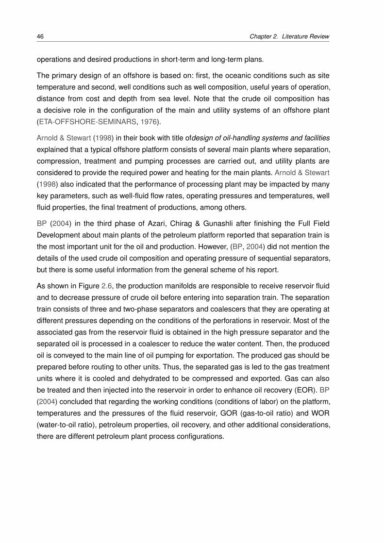
BP (2004) in the third phase of Azari, Chirag & Gunashli after finishing the Full Field
Development about main plants of the petroleum platform reported that separation train is
the most important unit for the oil and production. However, (BP, 2004) did not mention the
details of the used crude oil composition and operating pressure of sequential separators,
but there is some useful information from the general scheme of his report.
As shown in Figure 2.6, the production manifolds are responsible to receive reservoir fluid
and to decrease pressure of crude oil before entering into separation train. The separation
train consists of three and two-phase separators and coalescers that they are operating at
different pressures depending on the conditions of the perforations in reservoir. Most of the
associated gas from the reservoir fluid is obtained in the high pressure separator and the
separated oil is processed in a coalescer to reduce the water content. Then, the produced
oil is conveyed to the main line of oil pumping for exportation. The produced gas should be
prepared before routing to other units. Thus, the separated gas is led to the gas treatment
units where it is cooled and dehydrated to be compressed and exported. Gas can also
be treated and then injected into the reservoir in order to enhance oil recovery (EOR). BP
(2004) concluded that regarding the working conditions (conditions of labor) on the platform,
temperatures and the pressures of the fluid reservoir, GOR (gas-to-oil ratio) and WOR
(water-to-oil ratio), petroleum properties, oil recovery, and other additional considerations,
there are different petroleum plant process configurations.
2.1. Primary Petroleum and Gas Processing Offshore Platform 47
Figure 2.6 – Offshore Production Process
Source: (BP, 2004)
Devold (2006) published a detailed diagram of the main processes in the oil platform including
chemical products and control instruments in Norsk Hydro Nyord that is a more completed
work compared to BP (2004). He also indicated some details in configuration to ensure the
quality of the separation products.
In a Brazilian reservoir case, Beltrao et al. (2009) explained that for a pre-salt crude oil
composition with a considerable content of CO2, besides of CO2 separation from gas, it is
necessary to design an injection unit of CO2. Then, they indicated that adding new required
units is not an easy task in the limited space and condition of an offshore.
Nguyen et al. (2013) presented a division of the petroleum separation processing plant
for a Norwegian offshore plant and then, explained the different units and processes of an
offshore. The following items are some main and utility plants of a typical offshore:
• Transference of the reservoir fluid through pipes and production manifold;
• Depressurization of fluid in the strangler boxes;
• Separation of liquid and gas in the separation equipment;

48 Chapter 2. Literature Review
• Pumping systems to export oil, storage and final treatment to pump onshore;
• Treatment of produced gas in separation to remove water from it;
• Compression of produced gas to export it, to use in gas-lift or electricity generation unit(s);
• Treatment of the produced water in the separation to be returned to the sea or other
purposes in the plant.
2.1.3 Brazilian Reservoir, Offshore industry and FPSO Configurations
Exploration of the discovered reservoir in 2007, confirmed a significant potential to develop
petroleum resources in Brazil, especially the pre-salt areas. The pre-salt area is characterized
by deepwater and ultra-deepwater oil field with water depth around 2200 m and a layer of salt
that reaches about 2000 m in thickness (FORMIGLI, 2007). As shown in Figure 2.7, Brazil
was the second-largest offshore producer in 2015 and by supporting small production, this
increment continues in 2016 and 2017 (U.S. ENERGY INFORMATION ADMINISTRATION,
2016). Likewise, the recently published report of Ministério de Minas e Energia in 2017
confirmed the prevision of EIA and showed an increase of 3.2% compared to 2015 that it
means an additional produced oil of 81 thousand barrels per day (Ministério de Minas e
Energia, 2017). However, there is an increase of 7.9% (+7.6 million cubic meters per day) in
natural gas production that should be considered as important as in oil production strategies.
Figure 2.7 – Global offshore crude oil production, 2005-15.
Source: (U.S. ENERGY INFORMATION ADMINISTRATION, 2016)
2.1. Primary Petroleum and Gas Processing Offshore Platform 49
The pre-salt areas are located in water depth ranging from 2,000 to 2,500m, spread over very
large areas, around 300 km from the coast. Given these points, FPSOs can be the first option
for pre-salt areas, mainly due to crude oil and natural gas storage capabilities. Thus, does not
require the construction of long-length oil pipelines, and also because of other characteristics
that allow a short-term completion with economic advantages. On the other word, FPSO
plant is relocatable to other fields, its value retains and upfront investment and abandonment
costs are less than fixed platforms. Therefore, FPSO structure and its development were
chosen by Petrobras and partners for extraction, processing and exportation of oil and
gas (Minerals Management Service Gulf of Mexico OCS Region, 2000) (BELTRAO et al.,
2009)(ANDRADE et al., 2015).
Hence, Brazil is turned to use the FPSO facilities extensively as from 2009 to present. Only
until 2013, US$174.4 billion were investigated for pre-salt area in order to increase Brazilian
oil production that allowed Brazil to have more than 63 new vessels and offshore platform.
However, those investments have been affected in 2014, because of economic crises.
Nevertheless, the production of liquid fuels in Brazil has increased due to the operation of five
new FPSOs: P-62, P-58, P-57, Cidade de Ilhabela and Cidade de Mangaritiba (OFFSHORE
CENTER DENMARK, 2009)(U.S. ENERGY INFORMATION ADMINISTRATION, 2015b).
A typical FPSO has almost the same main and utility plants of a fixed offshore. In that there
are oil and gas processing and treatment, and the oil and water require for specific treatment
operations to achieve the expected specifications of the productions. Gas is scrubbed,
dehydrated and compressed in order to be used as fuel, to be injected as GOR and/or to
be exported. Moreover, produced oil is separated from water, gas, etc., by the separation
processes, and then the treated oil may be stored, transferred or exported. Separated
water is prepared to remove the emulsified oil before disposal at sea. Hence, all oil and
gas production operations are projected in a very complex and well-structured processing
plant to attend different operating and demands of the production process (MUELLER;
ROOBAERT, 2008). Therefore, due to increasing the benefit of a large machine such
as FPSO, standardization is necessary. Because it can reduce risks of delay and poor
performance in the equipment design and supply (PINTO et al., 2014).
Figure 2.8 shows a scheme of the basic production separation and treatment unit of a
standardized FPSO unit. In that, subsea crude oil from the production manifold enters in the
basic separation train, which has two separation stages: high and low pressure. Separated
gas is routed to treatment processes (compression, dehydration and dew point control) in
order to be injected or exported. Produced oil is sent to a set of more treatments such as
oil stabilization that ensuring the final specifications. Separated water from separators is
prepared to be discharged into seawater. Additionally, seawater can be injected into the wells.
The optional units are shown as necessary for project-specific production requirements.
50 Chapter 2. Literature Review
Figure 2.8 – Standardized FPSO processing scheme includes basic production separationand treating systems.
Source: adapted from (MUELLER; ROOBAERT, 2008)&(SÁNCHEZ, 2017)
The FPSO plant size and design, required processing plants and consequently, the oil
capacity, depend on the following parameters (PINTO et al., 2014):
• Amount of gas solubilized in the oil or GOR;
• CO2 content in produced gas;
• Need for CO2 removal;
• Water injection flow rate in order to pressure maintenance;
• Oil treatment difficulty.
For instance, the standard FPSOs are supposed to be used in Santos Basin pre-salt area,
regarding crude oil composition, the presence of fluid contamination such as CO2 and H2S,
GOR and area of well positions, besides what was discussed above, must have a nominal
capacity of processing 150,000 bpd of oil, 100,000 bpd of produced water and 6,000,000
Sm3/d of gas. In addition, concerning the gas plant, the main concept of FPSO consists in
the following steps (ANDRADE et al., 2015):
• A molecular sieve for gas dehydration unit;
• A hydrocarbon dew point control unit;
• A single stage of CO2 removal membrane with maximum 3% of CO2 content in exported
gas.
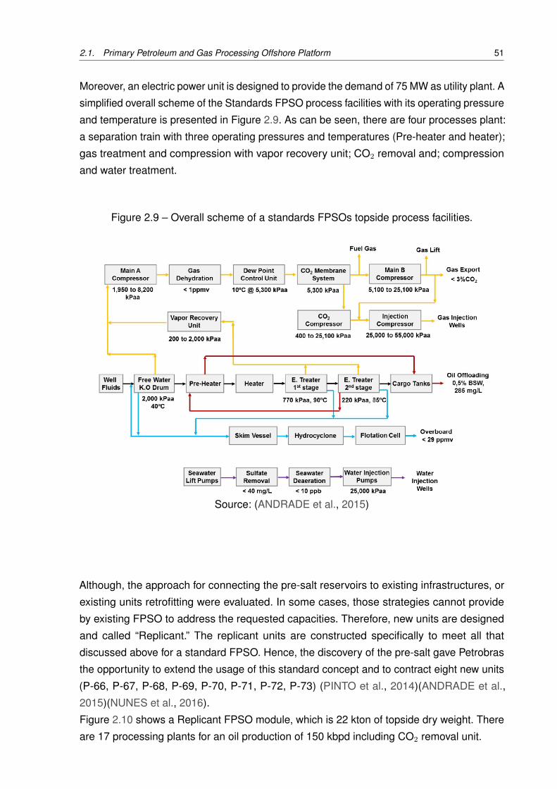
2.1. Primary Petroleum and Gas Processing Offshore Platform 51
Moreover, an electric power unit is designed to provide the demand of 75 MW as utility plant. A
simplified overall scheme of the Standards FPSO process facilities with its operating pressure
and temperature is presented in Figure 2.9. As can be seen, there are four processes plant:
a separation train with three operating pressures and temperatures (Pre-heater and heater);
gas treatment and compression with vapor recovery unit; CO2 removal and; compression
and water treatment.
Figure 2.9 – Overall scheme of a standards FPSOs topside process facilities.
Source: (ANDRADE et al., 2015)
Although, the approach for connecting the pre-salt reservoirs to existing infrastructures, or
existing units retrofitting were evaluated. In some cases, those strategies cannot provide
by existing FPSO to address the requested capacities. Therefore, new units are designed
and called “Replicant.” The replicant units are constructed specifically to meet all that
discussed above for a standard FPSO. Hence, the discovery of the pre-salt gave Petrobras
the opportunity to extend the usage of this standard concept and to contract eight new units
(P-66, P-67, P-68, P-69, P-70, P-71, P-72, P-73) (PINTO et al., 2014)(ANDRADE et al.,
2015)(NUNES et al., 2016).
Figure 2.10 shows a Replicant FPSO module, which is 22 kton of topside dry weight. There
are 17 processing plants for an oil production of 150 kbpd including CO2 removal unit.

52 Chapter 2. Literature Review
Figure 2.10 – Modules of a Replicant FPSO.
Source: (NUNES et al., 2016)
2.1.4 Thermodynamics analysis of oil and gas processing plant
In the last decades, several tools based on the First and Second Laws of thermodynamics
have been developed for defining indicators to assess the performance of chemical and
industrial processes including oil and gas processing plant. This subsection lists several
evaluation of performance articles in oil and gas processing platforms. Energy is the first
indicator approached in most of the papers on performance evaluation of various industrial
processes. Although, other concepts, such as environmental impact and exergy are also
presented.
Manning & Thompson (1995) as one of the primary researches, performed an energy
analysis to indicate the major users and consumers in an oil field processing with three-stage
separation train.
The first work on the thermodynamic performance of oil and gas offshore processing was the
exergy analysis by Oliveira-Jr. & Hombeeck (1997). They analyzed a Brazilian case facility,
where petroleum is extracted at low temperature and exported to ashore, along with gas.
The plant was modeled and simulated in HYSIM (HYPROTECH-LTD, 1991). The process
plants were composed of a separation process as the most inefficient process, comprising
an oil heater and three-phase separators, a gas compression process for exporting, which
2.1. Primary Petroleum and Gas Processing Offshore Platform 53
has four stages with cooling and liquid separation, an oil pumping process with two pumps,
and the crude oil heating that is the most exergy-destruction one.
Svalheim & King (2003) presented an energy performance study based on the survey of
field data from the Norwegian Continental Shelf (NCS). They pointed the compression,
exportation and injection (gas or seawater) are the reasons of the large energy demand
of processes and discussed the advantages that resulted from applying energy efficiency
measures (e.g. operating gas turbines at high load and reducing flaring practices). However,
they did not evaluate the effect of utility system, but it was emphasized that the interest of
this indicator is limited, because as each oil field has different natural characteristics. The
study by (SVALHEIM; KING, 2003) also analyzed other indicators based on environmental
impact studies and conventional energy assessments. In order to have a more complete
assessment of energy consumption concentrating on utility units, Bothamley et al. (2004)
examined the offshore processing options for oil platforms and compared the processing
schemes of the platforms in the Gulf of Mexico with offshore in the North Sea regions. The
results showed the heating demand was mainly related to the crude oil stabilization, the
cooling demand for the oil and gas handling processes, and the power demand for the gas
compression.
In addition, Vanner (2005) concentrated on the energy usage over the lifetime of an offshore
facility and illustrated that changes in main field, have an impact on the energy intensity
of the oil product. The general trend is a higher energy intensity with time, because of the
variations in the gas-and water-to-oil ratios, as well as the use of operating scenarios, such
as gas lift and water injection, which are employed to enhance the production.
Voldsund et al. (2010) performed an exergy analysis in an oil and gas processing platform
in the North Sea. The plant analysis included the power plant and the process plants.
The studied separation train is composed of three separators and the separated gas is
compressed in three stages with a cooling and liquid separation for each stage which is
similar to the most used offshore todays. Their simulations were performed by using Aspen
HYSYS and the Peng-Robinson EoS to estimate the properties of mass and energy flows.
Figure 2.11 shows a simplified overview of delimiting inputs, outputs and boundaries of a
typical offshore in North Sea that was used in (VOLDSUND et al., 2010). The results of
this study showed the compression process for injection besides being the highest power
consumption, has the highest irreversibility of the plant (66%), followed by the separation
process (20%) and the re-compression process (11%) and, finally, the oil pumping process
(3.1%).

54 Chapter 2. Literature Review
Figure 2.11 – Simplified overview of an offshore oil and gas platform
Source: (VOLDSUND et al., 2010)
The International Association of Oil and Gas Producers (IOGP) collected environmental data
from its member companies as an annual review in the last 13 years of activity before 2012.
They indicated that in the activities of oil and gas industry, energy planning includes a review
of the energy consumption inventory and the variables which affect energy consumption and
the selected performance indicators. The report of (IOGP, 2012) proposed several energy
indicators accepted by IOGP member companies in order to improve the environmental
effects, inducing gaseous emission, energy consumption and flaring as principal issues. In
addition, the report showed that the average energy consumption in 2012 was 1.4 GJ (Giga
Joules) of energy for each tonne of hydrocarbon produced and Green-House-Gas /GHG
emission rates were 160 tonnes of GHG per 1000 tonnes of hydrocarbon production in 2011.
The studies above and others, such as (VOLDSUND et al., 2012),(VOLDSUND et al., 2013b)
and (NGUYEN et al., 2013) are the major works in the field of thermodynamics analysis and
its application to offshore platforms. It can be noted that the number of studies has increased
in the last five years and that environmental law and carbon dioxide emissions are aspects
that have promoted a greater amount of research on this topic.
Voldsund et al. (2012), in another work, used three cases to perform thermodynamics
analysis. First and second cases with and without anti-surge system, the third case using
an increased efficiencies compressor. Additionally, the work included the fuel gas treatment
process and the anti-surge control of the compressors. Their result are achieved using
Aspen HYSYS and it was shown that the processes with more destroying of exergy are
compression and cooling of gas for injection. Voldsund et al. (2013b) detailed the exergy
assessment of Voldsund et al. (2010) by adding exergy rate and physical exergy parameters.
Next, Nguyen et al. (2013) described a generic model of an offshore in six cases to
simulate the processes and utilities plant, operating conditions and different reservoir fluid
2.1. Primary Petroleum and Gas Processing Offshore Platform 55
compositions using Aspen Plus R©. Their work showed that the highest destroyed exergy
occurs in the combustion chamber reaction such as in gas turbine. They compared their
results with results obtained by Oliveira-Jr. & Hombeeck (1997) and concluded that offshore
platforms located in different regions may considerably differ due to their process and
characteristics.
Nguyen et al. (2014a) and Nguyen et al. (2014b) analyzed the life efficiency of an offshore
platform to study the pinch and exergy-based methods to find the destroyed exergy of the
system and component. Their results indicated that according to the changes in the flow rate
of production and treated fluids, the power and energy demands of systems and subsystems
(both main and utilities) also alter for the plateau, mid-decline and end-life cases. Moreover,
Voldsund et al. (2014) applied exergy destruction to sub-systems of four different platforms.
Their results established that gas treatment and manifold production processes have a major
contribution to exergy destruction.
For a Brazilian FPSO, Carranza-Sánchez et al. (2015) performed a thermodynamics analysis
of three operation modes in a FPSO. They reported that the highest power consumption of
the main compressor was observed for the crude oil composition with high GOR, including
condensate components. The authors also concluded that 4.3% of the gas produced is used
for both power and heat generation unit. Next, Nguyen & Oliveira-Jr (2017) investigated a
process synthesis of an oil and gas platforms over different production profiles and feed
compositions for a Brazilian pre-salt oil field. In that, the effects of operating parameters
assessed on oil and gas production. Their results highlighted that however, oil production and
stabilization slightly change the power and heat demands, but they are strongly correlated to
gas production.
In a gas condensate processing plant, Mehrpooya et al. (2016) simulated an ethane
recovery process in South Pars of Persian Gulf by Aspen HYSYS to find the large sources
of irreversibility using exergy analysis. They showed that the operating temperature of
compressors can increase irreversibility, and pressure drop as a key parameter can affect
the cycle efficiency.
In addition, Gallo et al. (2017) investigated another thermodynamic analysis of a Brazilian
FPSO to analyze the performance of a compression system, by considering the operating of
components under off-design conditions. They performed the simulation for three conditions
of the well fluid composition and mass flow during 25 years (Figure 2.12a). The researchers
identified that the major sources of irreversibility and power load variation in each operating
year, which can offer opportunities for energy saving. Figures 2.12b shows the highest
production rate and power demand is between 5th and 10th year of operation.
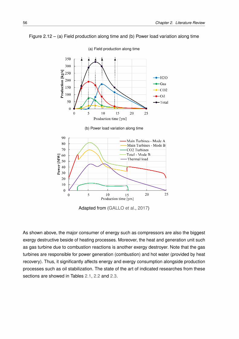
56 Chapter 2. Literature Review
Figure 2.12 – (a) Field production along time and (b) Power load variation along time
(a) Field production along time
(b) Power load variation along time
Adapted from (GALLO et al., 2017)
As shown above, the major consumer of energy such as compressors are also the biggest
exergy destructive beside of heating processes. Moreover, the heat and generation unit such
as gas turbine due to combustion reactions is another exergy destroyer. Note that the gas
turbines are responsible for power generation (combustion) and hot water (provided by heat
recovery). Thus, it significantly affects energy and exergy consumption alongside production
processes such as oil stabilization. The state of the art of indicated researches from these
sections are showed in Tables 2.1, 2.2 and 2.3.
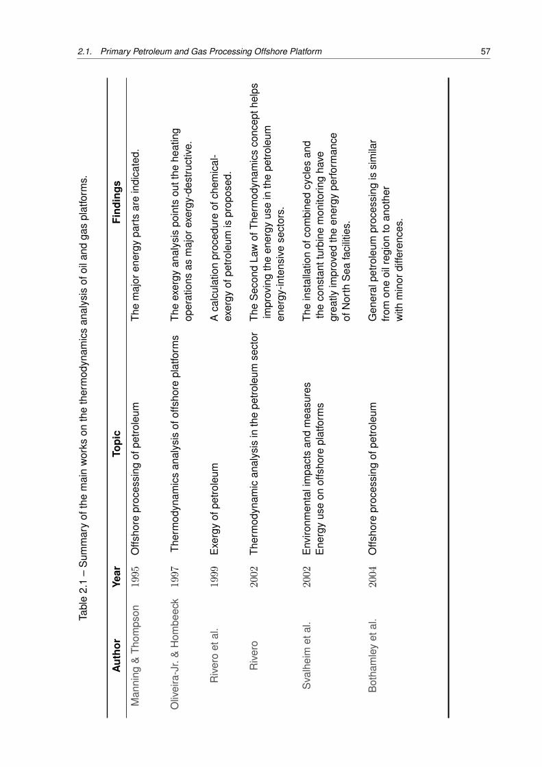
2.1. Primary Petroleum and Gas Processing Offshore Platform 57
Tabl
e2.
1–
Sum
mar
yof
the
mai
nw
orks
onth
eth
erm
odyn
amic
san
alys
isof
oila
ndga
spl
atfo
rms.
Aut
hor
Year
Topi
cFi
ndin
gs
Man
ning
&Th
omps
on19
95O
ffsho
repr
oces
sing
ofpe
trole
umTh
em
ajor
ener
gypa
rts
are
indi
cate
d.
Oliv
eira
-Jr.
&H
ombe
eck
1997
Ther
mod
ynam
ics
anal
ysis
ofof
fsho
repl
atfo
rms
The
exer
gyan
alys
ispo
ints
outt
hehe
atin
gop
erat
ions
asm
ajor
exer
gy-d
estr
uctiv
e.
Riv
ero
etal
.19
99E
xerg
yof
petro
leum
Aca
lcul
atio
npr
oced
ure
ofch
emic
al-
exer
gyof
petro
leum
ispr
opos
ed.
Riv
ero
2002
Ther
mod
ynam
ican
alys
isin
the
petro
leum
sect
orTh
eS
econ
dLa
wof
Ther
mod
ynam
ics
conc
epth
elps
impr
ovin
gth
een
ergy
use
inth
epe
trole
umen
ergy
-inte
nsiv
ese
ctor
s.
Sva
lhei
met
al.
2002
Env
ironm
enta
lim
pact
san
dm
easu
res
The
inst
alla
tion
ofco
mbi
ned
cycl
esan
dE
nerg
yus
eon
offs
hore
plat
form
sth
eco
nsta
nttu
rbin
em
onito
ring
have
grea
tlyim
prov
edth
een
ergy
perfo
rman
ceof
Nor
thS
eafa
cilit
ies.
Bot
ham
ley
etal
.20
04O
ffsho
repr
oces
sing
ofpe
trole
umG
ener
alpe
trole
umpr
oces
sing
issi
mila
rfro
mon
eoi
lreg
ion
toan
othe
rw
ithm
inor
diffe
renc
es.
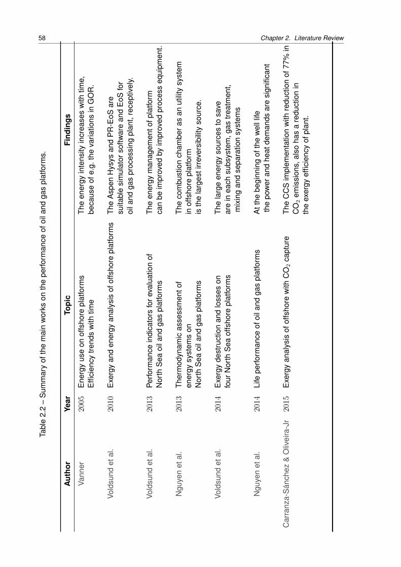
58 Chapter 2. Literature ReviewTa
ble
2.2
–S
umm
ary
ofth
em
ain
wor
kson
the
perfo
rman
ceof
oila
ndga
spl
atfo
rms.
Aut
hor
Year
Topi
cFi
ndin
gs
Vann
er20
05E
nerg
yus
eon
offs
hore
plat
form
sTh
een
ergy
inte
nsity
incr
ease
sw
ithtim
e,E
ffici
ency
trend
sw
ithtim
ebe
caus
eof
e.g.
the
varia
tions
inG
OR
.
Vold
sund
etal
.20
10E
xerg
yan
den
ergy
anal
ysis
ofof
fsho
repl
atfo
rms
The
Asp
enH
ysys
and
PR
-EoS
are
suita
ble
sim
ulat
orso
ftwar
ean
dE
oSfo
roi
land
gas
proc
essi
ngpl
ant,
rece
ptiv
ely.
Vold
sund
etal
.20
13Pe
rform
ance
indi
cato
rsfo
reva
luat
ion
ofTh
een
ergy
man
agem
ento
fpla
tform
Nor
thS
eaoi
land
gas
plat
form
sca
nbe
impr
oved
byim
prov
edpr
oces
seq
uipm
ent.
Ngu
yen
etal
.20
13Th
erm
odyn
amic
asse
ssm
ento
fTh
eco
mbu
stio
nch
ambe
ras
anut
ility
syst
emen
ergy
syst
ems
onin
offs
hore
plat
form
Nor
thS
eaoi
land
gas
plat
form
sis
the
larg
esti
rrev
ersi
bilit
yso
urce
.
Vold
sund
etal
.20
14E
xerg
yde
stru
ctio
nan
dlo
sses
onTh
ela
rge
ener
gyso
urce
sto
save
four
Nor
thS
eaof
fsho
repl
atfo
rms
are
inea
chsu
bsys
tem
,gas
treat
men
t,m
ixin
gan
dse
para
tion
syst
ems
Ngu
yen
etal
.20
14Li
fepe
rform
ance
ofoi
land
gas
plat
form
sA
tthe
begi
nnin
gof
the
wel
llife
the
pow
eran
dhe
atde
man
dsar
esi
gnifi
cant
Car
ranz
a-S
ánch
ez&
Oliv
eira
-Jr
2015
Exe
rgy
anal
ysis
ofof
fsho
rew
ithC
O2
capt
ure
The
CC
Sim
plem
enta
tion
with
redu
ctio
nof
77%
inC
O2
emis
sion
s,al
soha
sa
redu
ctio
nin
the
exer
gyef
ficie
ncy
ofpl
ant.

2.1. Primary Petroleum and Gas Processing Offshore Platform 59
Tabl
e2.
3–
Sum
mar
yof
the
mai
nw
orks
onth
epe
rform
ance
ofoi
land
gas
plat
form
s.
Aut
hor
Year
Topi
cFi
ndin
gs
Car
ranz
a-S
ánch
ezet
al.
2015
Ene
rgy
and
Exe
rgy
Perfo
rman
ceTh
ehi
gher
oilc
onte
ntin
the
crud
eoi
linc
reas
esof
thre
eFP
SO
Ope
ratio
nalM
odes
the
pow
eran
dex
ergy
requ
irem
ents
ofth
epr
oces
sing
plan
t
Meh
rpoo
yaet
al.
2016
Ther
mod
ynam
ican
alys
isof
The
oper
atin
gpr
essu
rean
dte
mpe
ratu
reof
hydr
ocar
bons
reco
very
proc
ess
can
alte
rthe
com
pres
sore
ffici
ency
and
the
tota
leffi
cien
cyof
cycl
e
Ngu
yen
&O
livei
ra-J
r20
17Th
erm
odyn
amic
anal
ysis
ofoi
land
gas
plat
form
sTh
eoi
lpro
duct
ion
and
stab
iliza
tion
slig
htly
chan
geov
erdi
ffere
ntpr
oduc
tion
profi
les
and
feed
com
posi
tions
chan
geth
epo
wer
and
heat
dem
ands
and
they
are
stro
ngly
corr
elat
edto
gas
prod
uctio
n
Gal
loet
al.
2017
Ape
rform
ance
anal
ysis
ofFP
SO
faci
litie
sTh
em
ajor
sour
ces
ofirr
ever
sibi
lity
and
itspr
ime
mov
ers
fora
FPS
Oun
itar
eth
eco
mpr
esso
rsan
dga
stu
rbin
eis
anut
ility
syst
emw
itha
poss
ibili
tyto
impr
ove

60 Chapter 2. Literature Review
2.2 Process Optimization in Processing Plants
Process optimization means adjusting or modulating a process so as to optimize some
specific set of variables without violating some constraints. The minimization of cost and
energy consumption, and maximization of throughput and/or efficiency are the main purposes.
By the same token, process optimization is the final and most important task, and is essential
for improving the performance of the process. Hence, it has attracted the attentions of
engineers and researchers.
In this section of the literature review, a large number of researches and techniques of
process synthesis, modeling and optimization of the various industrial processes, including
liquefied natural gas and oil and gas processing plants are investigated. However, there are
very few optimization studies concentrating on a thermal system of an offshore, particularly
on FPSO operation range, scale and its limitations.
Accordingly, in general, Process Optimization is divided into two main parts: 1- Process
synthesis and modeling, and 2- Optimization challenges related to optimal scheduling of the
different unit tasks to perform the overall process objective (or objectives).
2.2.1 Process Synthesis and Modeling
Process Synthesis is a research area which interest of it has grown over the last decades
for chemical processes. However, very few works deal with the systematic synthesis of an
entire oil and gas platform. In this subsection, a review of the existing literature of process
synthesis and its importance for modeling chemical processes is detailed.
A few decades ago, Rudd et al. (1973) explained that processing systems are characterized
by two distinct features. The first one is chemical and physical properties of process
components and interconnections between components, and the second one is the capacities
and operating conditions of these process components. Nonetheless, to synthesize of a
process due to finding an optimal configuration, a directed search over the feasible alternative
configurations as well as over the design variables is necessary.
In the importance of process synthesis in system design, Bradley et al. (1977) also stated
that the engineer must formulate the problem and the constraints imposed, and then highlight
the results of the model in the light of gained experiences and intuitions, recognizing the
model restrictions. After reviewing of 190 papers of process synthesis, Nishida et al. (1981)
explained that Process Synthesis is the first step in process plant design by the systematic
generation of alternative process flow sheets and the selection of one or few configurations
and parameters to optimize a given objective(s) function.
In the design of chemical processes by process synthesis, Colmenares & Seider (1989)
showed that the performance of the utility system directly influences the operating cost and
2.2. Process Optimization in Processing Plants 61
efficiency of a process.
Additionally, Smith (2005) mentioned that the overall purpose of process synthesis is to
design the processes with the suitable physical and/or chemical transformations (in main
or/and utility systems), which are necessary to achieve the desired outputs and productions.
It can either be performed by designing new facilities or modifying existing ones (retrofit).
After all, recently, the process synthesis has been the inseparable part of optimization
procedures in chemical processes of the most researches and works. Then, the mathematical
modeling is used to set the complexes structure and chemical process to calculate the
objective functions based on real variables and constraint in a nonlinear programming formats
(ADJIMAN et al., 1998). In the following, the implemented process synthesis methods in
various studied cases of industrial cycle focusing on oil and gas processing plants are raised.
Next, Lee et al. (2002) proposed a novel method to select the refrigerant compositions
based on the combination of nonlinear programming (NLP) and thermodynamic analysis.
They developed a systematic synthesis method as a tool for completing the design of a
mixed-refrigerant cycle. Their case studies demonstrated up to 25% saving in the shaft works
power demand compared to the commercial process. Although, the complex procedures
were time-consuming.
To develop a nonlinear model to connect the superstructure and process components, the
process synthesis should be detailed in a methodology framework. Wang et al. (2012)
presented a new methodology for process synthesis of LNG liquefaction to minimize energy
consumption. A procedure using MINLP (mixed-integer non-linear programming) model is
developed for a C3MR LNG plant and it is solved in GAMS by a solver called LINDOGlobal.
The synthesis model comprise of mass and energy balances employed in the optimization
model. They claimed that their methodology reduced energy consumption by approximately
13% and as shown in Figure 2.13, the validation thermodynamics properties and numerical
solution results were examined by Aspen Plus R©.
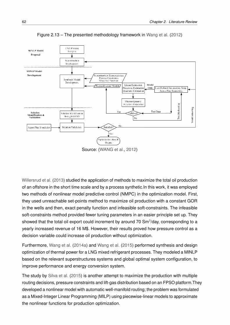
62 Chapter 2. Literature Review
Figure 2.13 – The presented methodology framework in Wang et al. (2012)
Source: (WANG et al., 2012)
Willersrud et al. (2013) studied the application of methods to maximize the total oil production
of an offshore in the short time scale and by a process synthetic.In this work, it was employed
two methods of nonlinear model predictive control (NMPC) in the optimization model. First,
they used unreachable set-points method to maximize oil production with a constant GOR
in the wells and then, exact penalty function and infeasible soft-constraints. The infeasible
soft-constraints method provided fewer tuning parameters in an easier principle set up. They
showed that the total oil export could increment by around 70 Sm3/day, corresponding to a
yearly increased revenue of 16 M$. However, their results proved how pressure control as a
decision variable could increase oil production without optimization.
Furthermore, Wang et al. (2014a) and Wang et al. (2015) performed synthesis and design
optimization of thermal power for a LNG mixed refrigerant processes. They modeled a MINLP
based on the relevant superstructures systems and global optimal system configuration, to
improve performance and energy conversion system.
The study by Silva et al. (2015) is another attempt to maximize the production with multiple
routing decisions, pressure constraints and lift-gas distribution based on an FPSO platform.They
developed a nonlinear model with automatic well-manifold routing; the problem was formulated
as a Mixed-Integer Linear Programming (MILP) using piecewise-linear models to approximate
the nonlinear functions for production optimization.
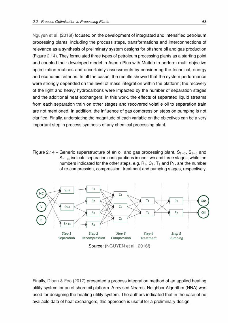
2.2. Process Optimization in Processing Plants 63
Nguyen et al. (2016f) focused on the development of integrated and intensified petroleum
processing plants, including the process steps, transformations and interconnections of
relevance as a synthesis of preliminary system designs for offshore oil and gas production
(Figure 2.14). They formulated three types of petroleum processing plants as a starting point
and coupled their developed model in Aspen Plus with Matlab to perform multi-objective
optimization routines and uncertainty assessments by considering the technical, energy
and economic criterias. In all the cases, the results showed that the system performance
were strongly depended on the level of mass integration within the platform; the recovery
of the light and heavy hydrocarbons were impacted by the number of separation stages
and the additional heat exchangers. In this work, the effects of separated liquid streams
from each separation train on other stages and recovered volatile oil to separation train
are not mentioned. In addition, the influence of gas compression steps on pumping is not
clarified. Finally, understating the magnitude of each variable on the objectives can be a very
important step in process synthesis of any chemical processing plant.
Figure 2.14 – Generic superstructure of an oil and gas processing plant. S1−2, S3−6 andS7−14 indicate separation configurations in one, two and three stages, while thenumbers indicated for the other steps, e.g. R1, C1, T1 and P1, are the numberof re-compression, compression, treatment and pumping stages, respectively.
Source: (NGUYEN et al., 2016f)
Finally, Diban & Foo (2017) presented a process integration method of an applied heating
utility system for an offshore oil platform. A revised Nearest Neighbor Algorithm (NNA) was
used for designing the heating utility system. The authors indicated that in the case of no
available data of heat exchangers, this approach is useful for a preliminary design.
64 Chapter 2. Literature Review
2.2.2 Sensitivity analysis and Optimization of Industrial Processing Plant
To join the nature of the industrial process system and oil and gas process, this subsection is
a review of existing papers about sensitivity analysis and optimization in an industrial process.
The origin of any industrial optimization study stands in a presumption that the feasible
improvements can be produced in a controllable system. The first point for solving a problem,
is to assess all the facts about a problem considering their interactions and restrictions. Aute
(2014) defined that the optimization of thermal systems is usually performed with a mixture
of technology decisions and the optimization of specific properties of selected components.
Screening or sensitivity analysis is often a preliminary step in any optimization procedure
that uses a large number of input parameters as decision variables. The main objective of
the screening analysis is to identify the most important contributors to increase/decrease an
output value. Hence, to have an intelligent optimization process, using sensitivity analysis is
unavoidable. In this subsection, sensitivity analysis and some of the optimization methods in
industrial processing plant are indicated.
Sensitivity analysis is a generalized methodology to identify and localize influential variables
for a conceptual process design or optimization process under uncertainty. Similarly, it
is divided to a methodology into three steps: process design and sensitivity analysis to
identify the effective variables, elimination of non-influential input variables, determination
and regionalization of critical variables or/and performing optimization procedure with these
given steps (LUCAY et al., 2015).
Global sensitivity analysis has been applied to different chemical processes in order to
provide a quantitative ranking of critical parameters (VERMA et al., 2017). There are
also many studies which applied sensitivity analysis as a tool to evaluate the process
structures and operational behaviors of chemical and industrial cycles (HATCHER et al.,
2012; JIANG et al., 2012; CHU; HAHN, 2013; SEPÚLVEDA et al., 2014). Additionally,
Sensitivity analysis provides the important parameters that should be considered in input
variables of an optimization process and a responses surface of output values ( indirect
optimization). For example, Gao et al. (2010) proposed nitrogen expansion liquefaction
process with propane pre-cooling. The authors performed the sensitivity analysis of several
parameters on the liquefaction process to find the space solution, without performing a
systematic optimization of the process.
Optimization of LNG plants and their related subsystems is one of the objectives that there
are several works related to it are published. AS the LNG is an energy-intensive process,
the most of works used screening analysis for operating parameters to minimize the power
and energy consumption of an LNG plant.
For a mixed-refrigerant LNG process, Hatcher et al. (2012) proposed a systematic analysis
of optimization formulation of the cycle. They used refrigerant flow rate, outlet pressures
2.2. Process Optimization in Processing Plants 65
of expansion and compression, and outlet temperatures of heat exchangers for natural
gas stream as input variables. Moreover, they implemented sensitivity analysis to show
which parameter is most effective on energy minimization. Chu & Hahn (2013) also used
existing global sensitivity analysis techniques to illustrate the influence of selected variables
on the optimal experimental design of process systems. In addition, Jiang et al. (2012)
studied the sensitivity of the methane gas production rate during depressurization from
hydrate reservoirs by the operation parameters using a numerical model of of reservoir
fluid, thermodynamic and chemical relations. However, varying of output by changing the
input parameters is simply considered as a sensitivity method that, it could not be a robust
strategy.
In another optimization research of LNG processes, Hwang et al. (2013) used the hybrid
optimization method (GA+ SQP) to find the optimal operating condition of a DMR cycle at
LNG FPSO. The implementation of SQP method increased the convergence of GA. The
required power at the obtained minimum condition decreased by 34.5% compared with the
patent, and by 1.2% compared with the conditions obtained from the relevant baseline.
Moreover, in an optimization of capital cost and energy consumption, Wang et al. (2014b)
used a sensitivity analysis in C3MR and DMR processes. Their objectives were to identify the
effect of the variation of the operating and cost parameters on reducing energy consumption
and total capital expenditure (CAPEX) including operating expenditure (OPEX) using
PR-EOS. Then, they performed an optimization procedure using box methodology and
controlled elitist GA to improve the exploration of the design space.
There are two researches of using sensitivity analysis in the different applications of industrial
processing. Xia et al. (2014) examined the effect of some key parameters on the system
performance of a solar-powered transcritical CO2 cycle with LNG as a heat sink based on the
recovery of cryogenic energy of LNG. Parametric sensitive analysis is carried out to identify
the contributors of key parameters on the performance. Then, the parametric optimization is
carried out to find the optimal performance using GA. Sepúlveda et al. (2014) also analyzed
the impact of statistical distributions of input variables data on the resultant distribution by
global sensitivity analysis in mineral processing circuits.
In a N2–CO2 expander LNG process, Khan et al. (2014a) minimized the total compression
energy requirement for NG liquefaction. The operating pressures (suction and discharge)
of N2 cycle, CO2 degree of super-heating and N2 flow rate were selected as variables to
analyze compression shaft work of N2 compressor, CO2 compressor and N2 expander. A
mono-objective optimization algorithm made by in-depth process analysis integrated with
a simulation to fulfill N2–CO2 expander process. The optimization results revealed energy
savings of 15% compared to the base case and 7% increase in the refrigerator exergy
efficiency. However, the operating and capital cost is not considered in the optimization
algorithm.

66 Chapter 2. Literature Review
Moreover, Khan et al. (2014b) developed a novel liquefaction of NG cycle. Then, the
separation of NG liquids was performed using energy efficient thermally coupled distillation
schemes. They optimized the energy consumption of compressors by altering the refrigerant
composition and operating pressures using knowledge-based optimization (KBO) methodology.
Their results demonstrated an improvement of 9% in plant energy requirement of as
compared to the baseline. However, it would be more interesting, if the implemented method
was compared with some convenient method such as GA to explain the advantage and
disadvantage of KBO method.
Figure 2.15 shows, a systematic optimization procedure using commercial simulator (Aspen
HYSYS) and GA (by Matlab) that was presented by (HE; JU, 2014).
Figure 2.15 – The framework of the process optimization with GA.
Source: (HE; JU, 2014)
They modelled a novel mixed refrigerant cycle with NGL recovery unit. In their paper, the
calculated energy consumption was considered as the objective function and optimization
process performed just after the convergence of numerical simulation (Figure 2.15). In
addition, He & Ju (2015) proposed four configuration strategies of expansion liquefaction
cycle for distributed-scale LNG plant to evaluate the liquefaction cycles and exergy analysis
for distributed scale LNG plant. They configured sixteen feasible liquefaction cycles to
maximize FOM (figure of merit) as an objective function for optimal synthesis. To solve the
optimization problem, GA is selected. They coupled again Aspen HYSYS as a simulator with
MATLAB as an optimizer. Their results showed a case with two cycles, namely R410A. The
2.2. Process Optimization in Processing Plants 67
pre-cooling cycle and the parallel nitrogen expansion cycle formed the optimized liquefaction
cycle.
The effective variables on objective function, such as the pressures and the molar flow rate
of the mixed refrigerant, the inlet temperature of the demethanizer, the inlet temperature
of the demethanizer, and the inlet pressure of the deethanizer were considered. Their
results were established by a 9.64% reduction in energy consumption as compared with
the baseline, and 11.68% in molar flow rate of mixed-type refrigerants. Likewise, Soffiato et
al. (2015) used Matlab to run optimization method and to couple with simulator. In that, the
problem formulation was performed by EES and SQP was carried out as the gradient-based
optimization method in a two-stage ORC. They defined the system efficiency as objective
function subject to technical constraints. Moreover, Mosaffa et al. (2017) investigated
four configurations: three single-stage ORC (simple, recuperative and regenerative) with
n-pentane as the working fluid and one two-stage ORC with n-pentane/n-butane as the fluid
combination. However, the fluid optimization was performed with a parametric optimization
of six effective parameters. They used the DIRECT algorithm in the EES software for
optimization.
Feng et al. (2015) performed a thermo-economic analysis for RORC and BORC using
multi-objective optimization by using the Non-dominated Sorting Genetic Algorithm (NSGA-II).
Next, they applied the Pareto Frontier solution with bi-objective to compare the corresponding
solutions of a single-objective. The thermodynamic performance, exergy efficiency, and
levelized energy cost (LEC) for BORS and PORC are assumed objective. The constraints
were defined based on pinch-point temperature difference and energy balance. In this study,
the key parameters, such as evaporator outlet temperature, condenser temperature, degree
of superheat, pinch point temperature difference, and degree of supercooling are selected
as the decision variables. In accordance with the results presented; RORC had 8.1% higher
exergy efficiency and LEC was about 21.1% more than in other cycles.
To find the optimum refrigerant composition and operating pressures for compression
energy requirement, and application to LNG plant, Park et al. (2015a) used the modified
Coordinate Descent Methodology (MCD) (a derivative-free optimization algorithm). They
expressed that in Korean Single Mixed Refrigerant (KSMR) process, energy requirement of
the compression is strongly a function of refrigerant composition and its operating pressures.
Thus, optimization of these parameters can reduce the power consumption significantly.
Their results of optimization showed 40% and 11% in energy savings, compared with the
representative base cases. In addition, they compared the suitability, calculation time and
ease of implementation of the MCD algorithm with PSO (Particle Swarm Optimization) and
NSGA-II that are the advantage of their methodology. Furthermore, in a process synthesis
to make a new design Park et al. (2015) evaluated a novel natural gas liquid (NGL) recovery
process with lower equipment numbers that are suitable for floating applications such as
68 Chapter 2. Literature Review
offshore by comparing several representative patented NGL recovery processes. They
carried out the techno-economic analysis to evaluate a variety of processes for comparison
with the proposed novel one. Their steady-state simulations were used to screen the
alternatives and to develop a process with better heat integration and better separation
efficiency.
A configuration design to satisfy the profitability and reliability of chemical processes was the
subject of few researches in the last decade. Getu et al. (2015) made an optimal decision
to investigate the risk of natural gas liquid (NGL) recovery processes. They analyzed
the performance with respect to the uncertainty from the plant inlet of six representative
NGL recovery processes. They simulated cases by ASPEN HYSYS and formulated the
optimization models for each process scheme using General Algebraic Modeling System
(GAMS). They considered the important topic of uncertainty and its incorporation in the
optimization of natural gas liquid (NGL) recovery plant designs. Their optimal decision was
made based on the profitability and reliability of holding the process constraints. Mehrpooya
et al. (2016) also performed a sensitivity analysis in a gas processing plant and showed
that pressure drop is a significant permanent parameter with a great effect on energy
consumption and performance of the process. I addition, the exergy analysis was used to
increase the reliability of system.
Next, Fergani et al. (2016) performed an evolutionary multi-objective optimization by the
MOPSO (Multi Objective Particle Swarm Optimizer) algorithm that uses multi-criteria exergy
to optimize an Organic Rankine Cycle in cement industries. The Pareto front of a multi-objective
optimization is used for the range of optimal point and Particle swarm optimization method.
They considered three working fluids for ORC, the turbine inlet pressure, the pinch point
temperature difference in the evaporator, the pinch point temperature difference in the
condenser, and the inlet temperature of the heat transfer fluid as decision variables. Cyclohexane
had the best exergoeconomic results and benzene was the best from the exergo- environmental
point of view for cycle turbine.
With the increase of capability in computing power of computers, simulators and optimizers,
the number of selected operating parameters as input variables in studies have also
increased. Moreover, the systems with more complexity have been investigated ((HE; JU,
2014), (KHAN et al., 2014a), (KHAN et al., 2014b), (HE; JU, 2015), (FENG et al., 2015),
(PHAM et al., 2016), (YAO et al., 2016) and (KWAK et al., 2018)). Among them, some of
works have conducted the novelty in applied simulation or optimization which are detailed
and discussed in down.
Pham et al. (2016) examined the effects of the flow rates of the each refrigerant components
and the working pressures on the liquefaction efficiency. It was also investigated the
interpreting the geometric pattern of the temperature difference (in a plot) between the
hot and cold composite curves for a heat exchanger of cryogenic cycles. The minimization of
2.2. Process Optimization in Processing Plants 69
energy compression consumption on modified single mixed refrigerant cycle of natural gas
liquefaction targeted for offshore applications is elected as objective function. They carried
out a process to choose the impossible “perfect” beginning point and a search sequence
of variables for the coordinate descent algorithm using a multivariate Coggin’s algorithm.
The results presented a 21.9% and 18% reduction in compression energy compared to two
selected base cases.However, the authors in abstract indicated that "knowledge-inspired
hybrid optimization approach with a robust convergence" has been use, but There is no any
information or graph about them in the paper.
Yao et al. (2016) also applied NSGA-II to obtain maximum thermodynamic efficiency by a
novel integration cooling, heating, and power system from a small-scale compressed air
energy. They also studied the effect of key parameters on system performance by sensitivity
analysis. They concluded that the incremental of inlet temperature, the pressure of the
turbine and effectiveness of the heat exchangers enhance the thermodynamic performance
and 52.51% of exergy efficiency can be achieved.
An optimization process for a boil-off gas (BOG) re-liquefaction cycle applied by (KWAK et
al., 2018) in LNG fuelled ship. They used Unisim to simulate and GA to find optimal operating
conditions of proposed process. BOG compressors of baselines were reported as one of
the key design issues, and optimization procedure found 11.4% and 20.8% reduction in
total power consumption of proposed compressors. Sensitivity analysis is also fulfilled to
understand the contributions of BOG operating pressures, composition, and re-liquefaction
rate on BOG re-liquefaction processes. However,the implemented sensitivity analysis is
performed after optimization procedure and it is a screening of the effect of input parameters
on optimal results.
As it was observed, the sensitivity analysis can show more effective parameters in order to
remove not influential parameters. Moreover, due to complexity of industrial processes and
supporting all type of variables in GA, it is a more commonly used method in optimization
in these processes. In conclusion, there are many works that because of using the same
process, method and illustrated system are not indicated here.
2.2.3 Sensitivity analysis and Optimization of Oil and Gas Processing Plants
The growing demand of gas-petroleum and the maturing of existing oil fields have compelled
its operators to invest in new researches and technologies to optimize their production
processes. Thus, the oil and gas industries have spent a lot of time and effort in optimizing
of processing plant in order to improve the efficiency of applied thermal systems and desired
productions. Similarly, the optimization techniques have been applied to almost all aspects
of the oil and gas industry. The selection of appropriate objective functions, key decision
variables, optimization method and constraints are the principal structure of any optimization
70 Chapter 2. Literature Review
work.
In this subsection, the applications of optimization techniques in various objectives, such as
power and energy consumption with environmental effect and production system design and
operations are reviewed. Consequently, the decision to perform appropriate steps for the
present thesis is made in 2.3 overview section.
Production optimization has been a topic of interest in academic and industry for many years.
The main endeavor was to model the mathematical tools which can help decision-makers
to select the best production plan. the maximization of liquid hydrocarbons production by
stabilization of volatile components is under attention recently.
For those reasons, an accurate methodology for optimizing the separator pressure in a
crude oil production unit was suggested by (BAHADORI et al., 2008). They explained that
due to different temperatures in winter and summer seasons, the dissolved gases at high
pressure tend to come out from liquid phase at low pressures. To address this issue, they
used flash calculations to determine optimum pressures of separators at different stages
of separation and consequently to optimize the operating conditions without installing any
additional equipment. They performed a hierarchical optimization method to minimize GOR
sequentially with the stage order of the separators using Aspen HYSYS. However, they
did not explain clearly the procedure of finding the optimum pressures. Willersrud et al.
(2013) also reported that pressure control can be used to increase oil production without
any optimization procedure using the active constraint of the pressure at inlet separator. The
authors reported an increase in oil production of 143 Sm3/day compared to no control.
Next, Ghaedi et al. (2014) implemented an optimization procedure for operating pressures
of separators in multistage production units. They used Genetic Algorithm to optimize the
separator pressure for a crude oil production unit with four separation stages and gas
condensate production unit with three separation stages. Compared to a baseline condition,
their results showed the improvement of 2.4% and 8.6% for crude oil and gas condensate
productions, respectively.
In a Korean case of offshore plant, Kim et al. (2014) used Aspen HYSYS and CMA-ES
(Covariance Matrix Adaptation Evolution Strategy) as a stochastic optimization in the
production for an oil offshore platform. The Peng-Robinson EoS model was used in this work
as a suitable one for predicting the phase equilibrium and thermodynamic properties for
a High GOR ceude oil. They determined the design variables for the crude oil separation
process simultaneously, to achieve the maximized profits. They concluded condensate
recycling increases the profits more than increasing the number of separation stages. Kylling
(2009), also optimized the profits in terms of oil sales and compression cost based on
equation-based modeling and brute force optimization with a simpler method.
In the modeling of an oil and gas processing offshore, one Norwegian filed with volatile oil,
2.2. Process Optimization in Processing Plants 71
and two Brazilian fields, Nguyen & Oliveira-Jr (2016g) studied three petroleum feeds by
different content of gas and carbon dioxide contents. Then, they carried out an optimization
process using GA by coupling Matlab and Aspen Plus. The operating temperatures and
pressures beside the number of separation stages are considered as variables. Their results
indicated the integration of a three stage separation train and the heaters are very beneficial
for separation performance of hydrocarbons. However, the authors did not explain the
function and sequences of the separation stages.
Allahyarzadeh-Bidgoli et al. (2017b) optimized the fuel consumption of a Brazilian FPSO for
petroleum composition with maximum oil and gas content by using NSGA-II. The optimal
operational parameters found by the optimization procedure presented a reduction of 4.6 %
in fuel consumption and indirectly increased the hydrocarbon liquids by 1.95% as compared
to the baseline operational condition of a Brazilian FPSO plant.
As it was shown in the literature review of optimization in desire production, the new power
demand and energy in optimization model are not investigated. While, optimized operating
pressure and temperature in order to increase production, regarding operating condition of
compressors, pumps, and heat exchangers could lead to more energy consumption.
In optimization of an equipment and the effect of improvement on all of cycle, Pierobon et al.
(2013) investigated a multi-objective optimization to improve design and working fluid in an
organic Rankine cycle offshore. Thermal efficiency, compactness, and net present value are
studied by employing Genetic Algorithm. They calculated the waste heat recovery of gas
turbine. Their results showed almost 4% increase in thermal efficiency by using acetone as
the working fluid and the net present reached from 17.7 to 19.8 M$ and for Cyclopentane
27-28.1% thermal efficiency and 19.7-20.1 M$ for net present value. Next, Pierobon &
Haglind (2014a) presented two new design to recover exhaust heat from offshore platforms.
Then, it were considered maximizing the economic revenue, the power production, and the
compactness of air-bottoming cycle for waste as multi-objective. They used the Genetic
Algorithm and the theory of power maximization to obtain the optimal point. More than 15
variables such as turbine inlet pressure, Pinch point recuperator, the Inner diameter of the
tubes in HEs, etc were applied in optimization process. They found about 16% more boosting
for the power of gas turbine (SGT-500) and an increase of 5.2% in thermal efficiency. In
another research, Pierobon et al. (2014b) performed a study to assess three waste heat
recovery (WHR) units for a gas and oil offshore platform. They compared Air bottoming cycle
power, Rankine cycle and organic Rankine cycle as WHR. The objective functions are net
present value, weight and annual carbon dioxide emissions. They assumed the combined
cycle to have a turbine gas and a bottoming cycle unit. The multi-objective optimization used
a controlled elitist GA for 16 variables to analyze such as inlet pressure of gas turbine, Pinch
point recuperator, Inner diameter of the tubes in HEs, etc to select simultaneous optimization
solutions. This work showed that combined cycle design-point and part-load present better
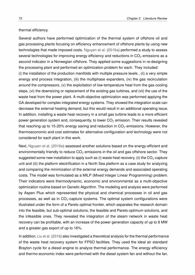
72 Chapter 2. Literature Review
thermal efficiency.
Several authors have performed optimization of the thermal system of offshore oil and
gas processing plants focusing on efficiency enhancement of offshore plants by using new
technologies that made imposed costs. Nguyen et al. (2016a) performed a study to assess
several technologies for improving energy efficiency and reductions in CO2-emissions as a
second indicator in a Norwegian offshore. They applied some suggestions in re-designing
the processing plant and performed an optimization problem for each. They included:
(i) the installation of the production manifolds with multiple pressure levels , (ii) a very simple
energy and process integration, (iii) the multiphase expanders, (iv) the gas recirculation
around the compressors, (v) the exploitation of low-temperature heat from the gas cooling
steps, (vi) the downsizing or replacement of the existing gas turbines, and (vii) the use of the
waste heat from the power plant. A multi-objective optimization was performed applying the
GA developed for complex integrated energy systems. They showed the integration scale can
decrease the external heating demand, but this would result in an additional operating issue.
In addition, installing a waste heat recovery in a small gas turbine leads to a more efficient
power generation system and, consequently, to lower CO2 emission. Their results revealed
that reaching up to 15-20% energy saving and reduction in CO2-emissions. However, the
thermoeconomic and cost estimates for alternative configuration and technology were not
considered for each plant in this work.
Next, Nguyen et al. (2016e) assessed another solutions based on the energy-efficient and
environmentally friendly to reduce CO2-emissions in the oil and gas offshore sector. They
suggested some new installation to apply such as (i) waste heat recovery, (ii) the CO2-capture
unit and (iii) the platform electrification in a North Sea platform as a case study for analyzing
and comparing the minimization of the external energy demands and associated operating
costs. The model was formulated as a MILP (Mixed Integer Linear Programming) problem.
Their indicators were thermodynamic, economic and environmental as a multi-objective
optimization routine based on Genetic Algorithm. The modeling and analysis were performed
by Aspen Plus which represented the physical and chemical processes in oil and gas
processes, as well as in CO2-capture systems. The optimal system configurations were
illustrated under the form of a Pareto optimal frontier, which separates the research domain
into the feasible, but sub-optimal solutions, the feasible and Pareto-optimum solutions, and
the infeasible ones. They revealed the integration of the steam network in waste heat
recovery can be profitable, with an increase of the power generation capacity of up to 8 MW
and a greater gas export of up to 16%.
In addition, Liu et al. (2016) also investigated a theoretical analysis for the thermal performance
of the waste heat recovery system for FPSO facilities. They used the ideal air standard
Brayton cycle for a diesel engine to analyze thermal performance. The energy efficiency
and thermo-economic index were performed with the diesel system fan and without the fan.

2.2. Process Optimization in Processing Plants 73
They showed the fan can increase efficiency and energy saving; however, with regards to
the limited space in FPSO, it can be removed.
Finally, Reis & Gallo (2018) explored some alternatives for waste heat recovery in an
FPSO platform using an organic Rankine cycle (ORC) to meet a required heat demand
for two different cycle configurations. The authors used the Genetic Algorithm for electric
power demand minimization. They reported a significant average reduction of 22.5% in fuel
consumption during the lifetime of the FPSO.
The state of the art of indicated researches from these sections are showed in Tables 2.4,
2.5 and 2.6.
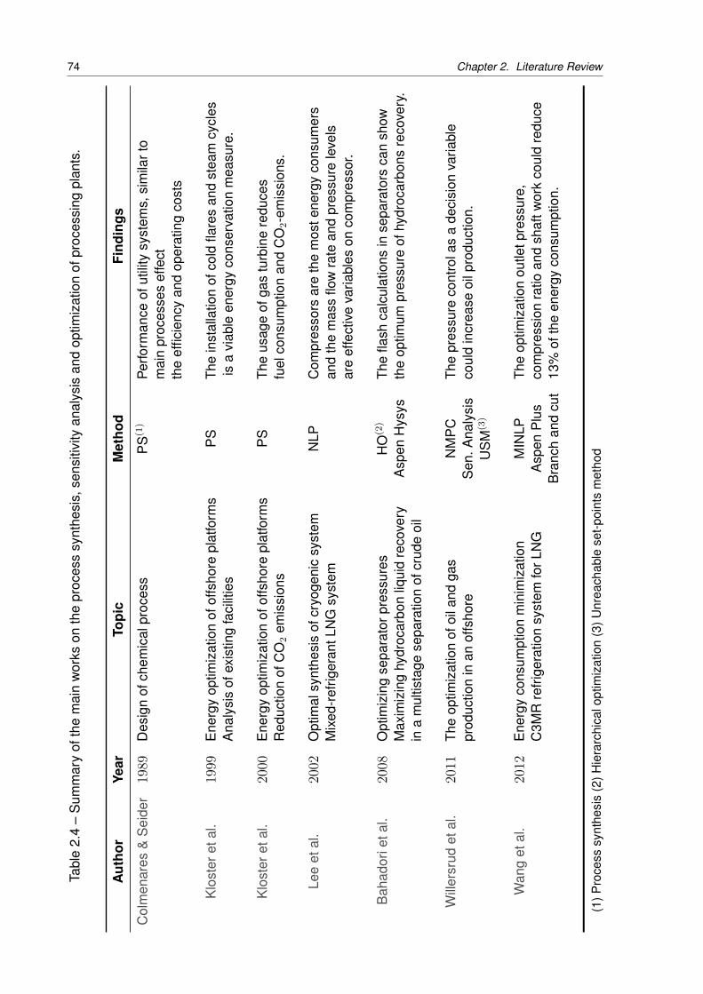
74 Chapter 2. Literature ReviewTa
ble
2.4
–S
umm
ary
ofth
em
ain
wor
kson
the
proc
ess
synt
hesi
s,se
nsiti
vity
anal
ysis
and
optim
izat
ion
ofpr
oces
sing
plan
ts.
Aut
hor
Year
Topi
cM
etho
dFi
ndin
gs
Col
men
ares
&S
eide
r19
89D
esig
nof
chem
ical
proc
ess
PS
(1)
Perfo
rman
ceof
utili
tysy
stem
s,si
mila
rto
mai
npr
oces
ses
effe
ctth
eef
ficie
ncy
and
oper
atin
gco
sts
Klo
ster
etal
.19
99E
nerg
yop
timiz
atio
nof
offs
hore
plat
form
sP
STh
ein
stal
latio
nof
cold
flare
san
dst
eam
cycl
esA
naly
sis
ofex
istin
gfa
cilit
ies
isa
viab
leen
ergy
cons
erva
tion
mea
sure
.
Klo
ster
etal
.20
00E
nerg
yop
timiz
atio
nof
offs
hore
plat
form
sP
STh
eus
age
ofga
stu
rbin
ere
duce
sR
educ
tion
ofC
O2
emis
sion
sfu
elco
nsum
ptio
nan
dC
O2-
emis
sion
s.
Lee
etal
.20
02O
ptim
alsy
nthe
sis
ofcr
yoge
nic
syst
emN
LPC
ompr
esso
rsar
eth
em
oste
nerg
yco
nsum
ers
Mix
ed-r
efrig
eran
tLN
Gsy
stem
and
the
mas
sflo
wra
tean
dpr
essu
rele
vels
are
effe
ctiv
eva
riabl
eson
com
pres
sor.
Bah
ador
ieta
l.20
08O
ptim
izin
gse
para
torp
ress
ures
HO
(2)
The
flash
calc
ulat
ions
inse
para
tors
can
show
Max
imiz
ing
hydr
ocar
bon
liqui
dre
cove
ryA
spen
Hys
ysth
eop
timum
pres
sure
ofhy
droc
arbo
nsre
cove
ry.
ina
mul
tista
gese
para
tion
ofcr
ude
oil
Will
ersr
udet
al.
2011
The
optim
izat
ion
ofoi
land
gas
NM
PC
The
pres
sure
cont
rola
sa
deci
sion
varia
ble
prod
uctio
nin
anof
fsho
reS
en.A
naly
sis
coul
din
crea
seoi
lpro
duct
ion.
US
M(3
)
Wan
get
al.
2012
Ene
rgy
cons
umpt
ion
min
imiz
atio
nM
INLP
The
optim
izat
ion
outle
tpre
ssur
e,C
3MR
refr
iger
atio
nsy
stem
forL
NG
Asp
enP
lus
com
pres
sion
ratio
and
shaf
twor
kco
uld
redu
ceB
ranc
han
dcu
t13
%of
the
ener
gyco
nsum
ptio
n.
(1)P
roce
sssy
nthe
sis
(2)H
iera
rchi
calo
ptim
izat
ion
(3)U
nrea
chab
lese
t-poi
nts
met
hod
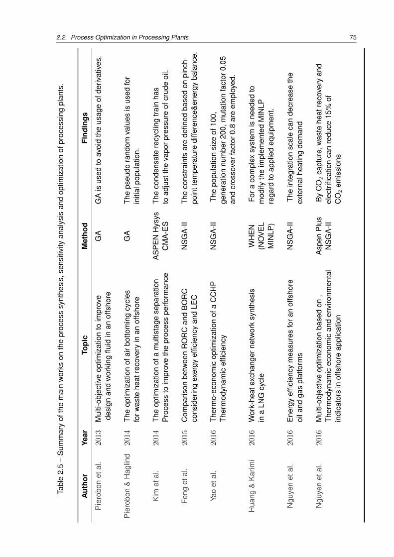
2.2. Process Optimization in Processing Plants 75
Tabl
e2.
5–
Sum
mar
yof
the
mai
nw
orks
onth
epr
oces
ssy
nthe
sis,
sens
itivi
tyan
alys
isan
dop
timiz
atio
nof
proc
essi
ngpl
ants
.
Aut
hor
Year
Topi
cM
etho
dFi
ndin
gs
Pie
robo
net
al.
2013
Mul
ti-ob
ject
ive
optim
izat
ion
toim
prov
eG
AG
Ais
used
toav
oid
the
usag
eof
deriv
ativ
es.
desi
gnan
dw
orki
ngflu
idin
anof
fsho
re
Pie
robo
n&
Hag
lind
2014
The
optim
izat
ion
ofai
rbot
tom
ing
cycl
esG
ATh
eps
eudo
rand
omva
lues
isus
edfo
rfo
rwas
tehe
atre
cove
ryin
anof
fsho
rein
itial
popu
latio
n.
Kim
etal
.20
14Th
eop
timiz
atio
nof
am
ultis
tage
sepa
ratio
nA
SP
EN
Hys
ysTh
eco
nden
sate
recy
clin
gtra
inha
sP
roce
ssto
impr
ove
the
proc
ess
perfo
rman
ceC
MA
-ES
toad
just
the
vapo
rpre
ssur
eof
crud
eoi
l.
Feng
etal
.20
15C
ompa
rison
betw
een
RO
RC
and
BO
RC
NS
GA
-IITh
eco
nstra
ints
are
defin
edba
sed
onpi
nch-
cons
ider
ing
exer
gyef
ficie
ncy
and
LEC
poin
ttem
pera
ture
diffe
renc
e&en
ergy
bala
nce.
Yao
etal
.20
16Th
erm
o-ec
onom
icop
timiz
atio
nof
aC
CH
PN
SG
A-II
The
popu
latio
nsi
zeof
100,
Ther
mod
ynam
icef
ficie
ncy
gene
ratio
nnu
mbe
r200
,mut
atio
nfa
ctor
0.05
and
cros
sove
rfac
tor0
.8ar
eem
ploy
ed.
Hua
ng&
Kar
imi
2016
Wor
k-he
atex
chan
gern
etw
ork
synt
hesi
sW
HE
NFo
raco
mpl
exsy
stem
isne
eded
toin
aLN
Gcy
cle
(NO
VE
Lm
odify
the
impl
emen
ted
MIN
LPM
INLP
)re
gard
toap
plie
deq
uipm
ent.
Ngu
yen
etal
.20
16E
nerg
yef
ficie
ncy
mea
sure
sfo
ran
offs
hore
NS
GA
-IITh
ein
tegr
atio
nsc
ale
can
decr
ease
the
oila
ndga
spl
atfo
rms
exte
rnal
heat
ing
dem
and
Ngu
yen
etal
.20
16M
ulti-
obje
ctiv
eop
timiz
atio
nba
sed
on,
Asp
enP
lus
By
CO
2ca
ptur
e,w
aste
heat
reco
very
and
Ther
mod
ynam
icec
onom
ican
den
viro
nmen
tal
NS
GA
-IIel
ectr
ifica
tion
can
redu
ce15
%of
indi
cato
rsin
offs
hore
appl
icat
ion
CO
2em
issi
ons
76 Chapter 2. Literature ReviewTa
ble
2.6
–S
umm
ary
ofth
em
ain
wor
kson
the
proc
ess
synt
hesi
s,se
nsiti
vity
anal
ysis
and
optim
izat
ion
ofpr
oces
sing
plan
ts.
Aut
hor
Year
Topi
cM
etho
dFi
ndin
gs
Ngu
yen
&O
livei
ra-J
r20
16O
ptim
izat
ion
ofa
prel
imin
ary
oil
As.
Plu
sTh
ree
sepa
ratio
nst
age
and
and
gas
proc
essi
ngpl
atfo
rmE
NN
Ahe
ater
sar
eve
ryim
port
antt
oac
hiev
ebe
tterv
olat
ileco
mpo
nent
sre
cove
ry
Dib
an&
Foo
2017
Des
ign
ofhe
atin
gut
ility
syst
emO
ptim
umco
nfigu
ratio
nof
WH
RU
2fo
rFP
SO
plat
form
NN
Are
duce
d17
%of
tota
lann
ualis
edco
stas
com
pare
dto
the
conv
entio
nald
esig
n
Alla
hyar
zade
h-B
idgo
liet
al.
2017
Perfo
rman
ceop
timiz
atio
nof
apr
e-co
olin
gH
YS
YS
Inte
grat
ion
ofus
eful
sim
ulat
oran
dop
ti-LN
Gcy
cle
byim
prov
emen
tofa
pplie
dN
SG
A-II
miz
erso
ftwar
eal
low
sto
appl
yal
leffe
ctiv
eH
eate
xcha
nger
varia
ble
inop
timiz
atio
npr
oced
ure
Alla
hyar
zade
h-B
idgo
liet
al.
2017
Min
imiz
atio
nof
FPS
Ofu
elco
nsum
ptio
nw
ithH
YS
YS
Ope
ratin
gpr
essu
rean
dte
mpe
ratu
reof
ahi
ghG
OR
and
CO
2co
nten
tN
SG
A-II
sepa
ratio
ntra
inca
nef
fect
fuel
cons
umpt
ion
ofcr
ude
oilc
ompo
sitio
nan
dal
sooi
lsta
biliz
atio
n
Rei
s&
Gal
lo20
18O
ptim
izat
ion
ofth
epo
wer
prod
uctio
nE
ES
+so
me
alte
rnat
ives
forw
aste
heat
reco
very
byan
orga
nic
Ran
kine
cycl
ein
anFP
SO
unit
Ther
mofl
exin
anFP
SO
plat
form
was
pres
ente
d,by
GA
usin
gan
orga
nic
Ran
kine
cycl
e(O
RC
)
2.3. Overview 77
2.3 Overview
The literature review showed that for various reservoir fluids and operating conditions, there
are different types of offshore installations operation. In addition, Aspen Hysys and Aspen
Plus are the most used simulators for chemical processing, including oil and gas processing
plants. These softwares are normally integrated with optimization softwares such as Matlab
and Excel. However, ModeFrontier is the most comprehensive optimization software, but,
from the literature review, there is not any coupling of Aspen Hysys or Aspen Plus with
ModeFrontier.
On the other side, GA is the most chosen optimization method for the researches on oil
and gas processing plants. This is because of the complexity of oil and gas processes,
variety of applied equipment, number and types of existing design variables, and avoiding
the calculation of derivatives in optimization.
Moreover, key operating parameters for performance of thermal systems and desired
productions are operating pressures and temperatures of the separation process, heaters,
compressors, and pumps. As shown in the literature review, these operation parameters are
many, thus, to understand their effects on objectives and to reduce less effective parameters,
a sensitivity analysis is necessary. However, in all works with a sensitivity analysis section,
it is just a sensitivity of optimum solution that shows how the input parameters change the
optimum results.
Finally, the literature review did not present any research discussing the possibilities for the
improvement of a Brazilian FPSO plant configuration (in current operation) by changing
thermodynamic parameters. Furthermore, none of the published researches addressed the
potentiality of the optimization procedure to reduce fuel consumption and to improve the
separation performance to enhance oil production and yield products with higher value.
In the next chapter, the theoretical foundations of thermodynamic analysis and optimization
methods and their advantages/disadvantages will be discussed.


79
3 THEORETICAL FOUNDATION
This chapter is structured in terms of theoretical and conceptual frameworks. It consists of
concepts and, together with their definitions and references to relevant scholarly literature,
the existing theories used for thermodynamic assessment, Optimization methods, such as
statistical analysis (screening analysis) methods, optimization algorithms, and sensitivity of
optimum.
3.1 Thermodynamic Analysis
The First Law of Thermodynamics states that energy can be neither created nor destroyed,
but it only can be transformed from one form to another. Therefore, it gives indications on
the processes in which energy is converted, lost and dissipated. For a control volume, in
steady-state conditions and steady-flow processes, the energy balance is written as:
Q− W =∑
mouthout −∑
minhin (3.1)
where Q and Ware heat rate and power, respectively, m is the mass flow rate of the material
stream and h is the specific enthalpy.
The mass balance and thermal efficiency of the applied gas turbine are calculated as follows:
mout_GT = mair + mF uel (3.2)
η = Wnet
mF uel × LHV(3.3)
where mout_GT is the output mass flow of the gas turbine, mair is the input mass flow rate
of the air in the combustion chamber, and mF uel is the consumed fuel mass flow in the
combustion chamber. η , Wnet and LHV are thermal efficiency, shaft power from the gas
turbine and lower heating value, respectively.
The calculations of the physical (e.g. density) and thermodynamic properties of each
substance require information, such as the pressure, volume and temperature (P, ν& T).
These properties are predicted using chemical thermodynamic models, which are based
on either equations of state (EoS). Peng & Robinson (1976) Equation of State (PR-EoS) is
most commonly used EoS in offshore simulation works (GALLO et al., 2017; REIS; GALLO,
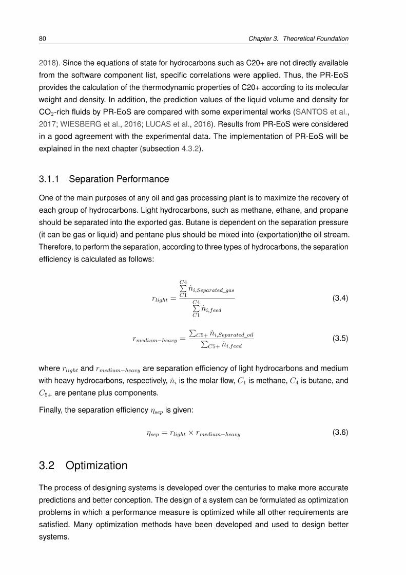
80 Chapter 3. Theoretical Foundation
2018). Since the equations of state for hydrocarbons such as C20+ are not directly available
from the software component list, specific correlations were applied. Thus, the PR-EoS
provides the calculation of the thermodynamic properties of C20+ according to its molecular
weight and density. In addition, the prediction values of the liquid volume and density for
CO2-rich fluids by PR-EoS are compared with some experimental works (SANTOS et al.,
2017; WIESBERG et al., 2016; LUCAS et al., 2016). Results from PR-EoS were considered
in a good agreement with the experimental data. The implementation of PR-EoS will be
explained in the next chapter (subsection 4.3.2).
3.1.1 Separation Performance
One of the main purposes of any oil and gas processing plant is to maximize the recovery of
each group of hydrocarbons. Light hydrocarbons, such as methane, ethane, and propane
should be separated into the exported gas. Butane is dependent on the separation pressure
(it can be gas or liquid) and pentane plus should be mixed into (exportation)the oil stream.
Therefore, to perform the separation, according to three types of hydrocarbons, the separation
efficiency is calculated as follows:
rlight =
C4∑C1ni,Separated_gas
C4∑C1ni,feed
(3.4)
rmedium−heavy =∑
C5+ ni,Separated_oil∑C5+ ni,feed
(3.5)
where rlight and rmedium−heavy are separation efficiency of light hydrocarbons and medium
with heavy hydrocarbons, respectively, ni is the molar flow, C1 is methane, C4 is butane, and
C5+ are pentane plus components.
Finally, the separation efficiency ηsep is given:
ηsep = rlight × rmedium−heavy (3.6)
3.2 Optimization
The process of designing systems is developed over the centuries to make more accurate
predictions and better conception. The design of a system can be formulated as optimization
problems in which a performance measure is optimized while all other requirements are
satisfied. Many optimization methods have been developed and used to design better
systems.
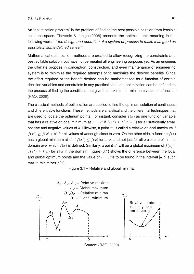
3.2. Optimization 81
An “optimization problem” is the problem of finding the best possible solution from feasible
solutions space. Thevenin & Janiga (2008) presents the optimization’s meaning in the
following words: “ the design and operation of a system or process to make it as good as
possible in some defined sense. ”
Mathematical optimization methods are created to allow recognizing the constraints and
best suitable solution, but have not permeated all engineering purposes yet. As an engineer,
the ultimate propose in conception, construction, and even maintenance of engineering
system is to minimize the required attempts or to maximize the desired benefits. Since
the effort required or the benefit desired can be mathematized as a function of certain
decision variables and constraints in any practical situation, optimization can be defined as
the process of finding the conditions that give the maximum or minimum value of a function
(RAO, 2009).
The classical methods of optimization are applied to find the optimum solution of continuous
and differentiable functions. These methods are analytical and the differential techniques that
are used to locate the optimum points. For instant, consider f(x) as one function variable
that has a relative or local minimum at x = x∗ if f(x∗) ≤ f(x∗ + h) for all sufficiently small
positive and negative values of h. Likewise, a point x∗ is called a relative or local maximum if
f(x∗) ≥ f(x∗ + h) for all values of henough close to zero. On the other side, a function f(x)has a global minimum at x∗ if f(x∗) ≤ f(x) for all x, and not just for all x close to x∗, in the
domain over which f(x) is defined. Similarly, a point x∗ will be a global maximum of f(x) if
f(x∗) ≥ f(x) for all x in the domain. Figure (3.1) shows the difference between the local
and global optimum points and the value of x = x∗is to be found in the interval [a, b] such
that x∗ minimizes f(x).Figure 3.1 – Relative and global minima.
Source: (RAO, 2009)
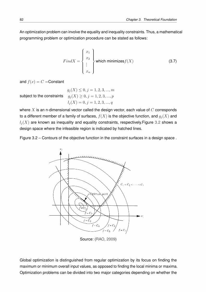
82 Chapter 3. Theoretical Foundation
An optimization problem can involve the equality and inequality constraints. Thus, a mathematical
programming problem or optimization procedure can be stated as follows:
FindX =
x1
x2...
xn
which minimizesf(X) (3.7)
and f(x) = C =Constant
subject to the constraintsgj(X) ≤ 0, j = 1, 2, 3, ...,mgj(X) ≥ 0, j = 1, 2, 3, ..., plj(X) = 0, j = 1, 2, 3, ..., q
where X is an n-dimensional vector called the design vector, each value of C corresponds
to a different member of a family of surfaces, f(X) is the objective function, and gj(X) and
lj(X) are known as inequality and equality constraints, respectively.Figure 3.2 shows a
design space where the infeasible region is indicated by hatched lines.
Figure 3.2 – Contours of the objective function in the constraint surfaces in a design space .
Source: (RAO, 2009)
Global optimization is distinguished from regular optimization by its focus on finding the
maximum or minimum overall input values, as opposed to finding the local minima or maxima.
Optimization problems can be divided into two major categories depending on whether the
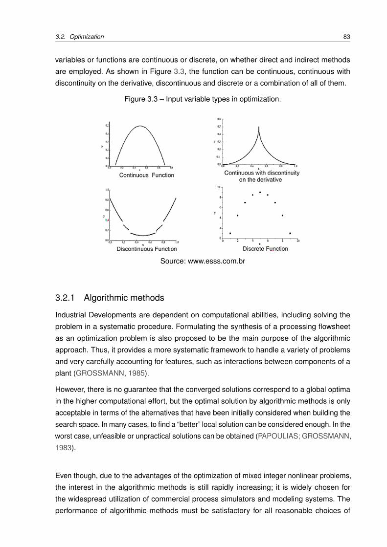
3.2. Optimization 83
variables or functions are continuous or discrete, on whether direct and indirect methods
are employed. As shown in Figure 3.3, the function can be continuous, continuous with
discontinuity on the derivative, discontinuous and discrete or a combination of all of them.
Figure 3.3 – Input variable types in optimization.
Source: www.esss.com.br
3.2.1 Algorithmic methods
Industrial Developments are dependent on computational abilities, including solving the
problem in a systematic procedure. Formulating the synthesis of a processing flowsheet
as an optimization problem is also proposed to be the main purpose of the algorithmic
approach. Thus, it provides a more systematic framework to handle a variety of problems
and very carefully accounting for features, such as interactions between components of a
plant (GROSSMANN, 1985).
However, there is no guarantee that the converged solutions correspond to a global optima
in the higher computational effort, but the optimal solution by algorithmic methods is only
acceptable in terms of the alternatives that have been initially considered when building the
search space. In many cases, to find a “better” local solution can be considered enough. In the
worst case, unfeasible or unpractical solutions can be obtained (PAPOULIAS; GROSSMANN,
1983).
Even though, due to the advantages of the optimization of mixed integer nonlinear problems,
the interest in the algorithmic methods is still rapidly increasing; it is widely chosen for
the widespread utilization of commercial process simulators and modeling systems. The
performance of algorithmic methods must be satisfactory for all reasonable choices of
84 Chapter 3. Theoretical Foundation
the initial variables. Therefore, reliable algorithmic methods could be robust and accurate,
although the desired state uses less computer time and storage. On the other hand, it should
be able to identify a solution without being overly sensitive to truncation or to round off errors
(GROSSMANN, 2013; GONG, 2004).
3.2.2 Classification of algorithmic optimization methods
Since specific methods are available for the efficient solution of a particular class of
problems, from a computational and methodological point of view, the classification of
the optimization problems is important. At the first level, the numerical algorithms can be
classified into mathematical programming (deterministic) and stochastic methods (SMITH,
2005). Mathematical programming requires the assessment of mathematical properties
of the objective function and constraints, including objective function evaluations and
calculation of gradients or even the second order of derivation, without involving any
random steps. Deterministic methods can be further classified according to the type of
problems that must deal with, e.g. linear or nonlinear (including sequential approaches, i.e.,
a successive solution of approximate sub problems), constrained or unconstrained, single
or multi-variable problems, and discrete or continuous (or mixed) variable problems. The
most traditional deterministic methods based on derivatives of the objective and constraint
functions are the calculation methods, e.g. the Lagrange multipliers method. Elimination
methods (dichotomous search) and pattern search methods (Nealder Mead simplex method,
univariate search) are iterative techniques used to proceed from an initial guess towards the
optimum without requiring the calculation of derivatives or making any assumption in the
form of the objective function (HAFTKA; GÜRDAL, 2012).
Search methods are used for solving unconstrained non-linear problems and they can be
divided into the zeroth (e.g. Powell conjugated directions), first (gradient-based) and second
(Hessian-based) order methods. First and second order methods are based on calculating
the first and second derivative of the function from a chosen starting point and then moving
this point to the location.It causes the largest reduction in the objective function (if it is a
minimization problem) following a step length criterion required by each method (HAFTKA;
GÜRDAL, 2012).
For example, in the steepest descent first order method, the search direction is along
the direction of the gradient of the objective function which is calculated from the current
point. Gradient and Hessian matrices can be obtained numerically rather than analytically;
therefore, multimodel functions could make the method unstable (JALURIA, 2007).
Among the methods are used for solving constrained optimization problems, more specifically
those in which the objective function, as well as the constraints, are linear functions of the
independent variables (linear programming), the simplex method is a widely used efficient
3.2. Optimization 85
scheme. This method searches along the boundary of the feasible domain from one vertex,
given by the constraints, to the next until the optimum is obtained (JALURIA, 2007).
In the case of nonlinear constrained optimization problems, generalized reduced gradients
and projected gradient methods, as well as the feasible direction methods, can be used. In
these methods, the initial guess or starting point is in the feasible domain. Then, the search
is moved to the constraint and obtains a point in the constraint. From this point, the search is
moved tangentially to the constraint. Since by doing this, the trial point violates the constraint,
the next step is used to bring the point back to the feasible region (JALURIA, 2007).
However, for the common, complex problems encountered in industrial and chemical plant
flowsheets, those techniques are usually ineffective. Other approaches take advantage of
the robust optimization tools, such as the mixed integer linear and non-linear programming,
Mixed-integer linear programming (MILP), and Mixed integer nonlinear programming (MINLP)
with Branch and Bound or Outer Approximation approaches that avoid the exhaustive
evaluation of the integer variables by using relaxation models and a decision tree. Moreover,
MIPSQP (Mixed Integer Programming Sequential Quadratic Programming) is a single-objective
gradient-based optimization algorithm for solving non-linear mixed discrete-continuous
problems. MIPSQP splits variables into relaxable (discrete ordered), non relaxable (discrete
unordered) and continuous, and applies different strategies to each type. Therefore, the
decision tree produces the partial and potential solutions through connection nodes. Nevertheless,
these types of approaches still face two major challenges when are applied to process
design: (a) existing non-convex models that conduct to local optima and (b) combinatorial
explosion leading a difficulty to solve industrial processes (GROSSMANN, 1985; SMITH,
2005; INUTECH-GMBH, 2007; ANANTHARAMAN, 2011; XUE et al., 2012).
Thus, there has been considerable development in the use of optimization methods in
process synthesis that include stochastic techniques and evolutionary algorithms, such as
GA, which uses the random points from an initial population to orient the search direction
or can take the search in a deterioration side of the objective function. This method can be
useful and handle the problems when the calculation of the derivatives would be complex and
make deterministic methods to fail (such as the objective functions of this research) (SMITH,
2005). The GA is detailed in the next subsection (subsection 3.2.5). Even though both mixed
integer non-linear programming and genetic algorithms operate in a specified superstructure,
genetic algorithms have the advantage of revealing more than one near-optimal configuration,
so the designer may apply additional criteria to select the preferable one (FAZLOLLAHI
et al., 2015). Another stochastic method one that is called global search metaheuristic
method, uses the simulated annealing method, with an ability to find the global optimum
from created the random search procedures. These random search processes evaluate the
objective function at different points of the sample space that the points are chosen by a set
of heuristics combined with the generation of random numbers (ANTONIN et al., 2005a).
86 Chapter 3. Theoretical Foundation
However, heuristics and genetic algorithm do not guarantee that the found optimum point
is actuality a global optimum solution, since the optimum configuration may be one that is
currently unknown.They also do not provide a common framework for synthesizing a variety
of different types of major system components or even operating conditions, but there are
several genetic algorithmic approaches that have been widely applied in process synthesis
and optimization works. Hence, the genetic algorithm is selected for complex systems using
the crossover and mutation operators very close to 1.0 which allow a broad capability of
exploration and exploitation of the solution space.
For optimization problems, simulations can be approximated by optimizing metamodels as
surrogates for the costly simulation response functions. Local metamodels can be used
within an iterative optimization strategy, developed or updated as the optimization progresses.
Its run times is generally shorter than the original simulation design and its response is
deterministic (BARTON; MECKESHEIMER, 2006). On the other words, the metamodeling
process includes basically four steps: (1) choosing a Design of Experience (3.2.4) or the
manner to consistently conduct the (numerical) experiments and generate data; (2) selecting
a model (of the simulation model) to represent the data; (3) fitting the model and; (4)
validating the model from the observed data that are obtained in the first step. There
are many selections for each of these steps and combination among them also can be
considered to develop many metamodeling techniques. The most frequently used methods
include response surface methodology (RSM), inductive learning, artificial neural network,
and Kriging models.
3.2.3 Screening Analysis
Screening Analysis (sensitivity analysis) is a tool to evaluate the process structures and
operational behaviors of chemical and industrial cycles. Thus, an analysis of sensitivity is
to determine the rate at which the objective function changes while one of the decision
variables is changed. Therefore, cost, power and energy consumption minimizations, and
the performance, profits maximizations are important objectives in all design efforts. Despite
several progress made in the last few decades, many challenging problems relating to oil
and gas processing are still not addressed. In the current context, the sensitivity analysis
methods are described and discussed.
3.2.4 Design of Experiments (DoE)
Design of Experiments (DoE) is a methodology that maximizes the knowledge gained from
experimental data. It is originated in 1920 by a British scientist, Sir R. A. Fisher, (FISHER et
al., 1937) to provide a strong tool to design and to analyze experiments.
The assumption of a random error exists in a laboratory experiment; it is fundamental and
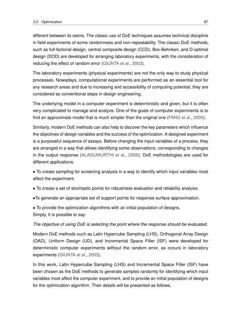
3.2. Optimization 87
different between its stems. The classic use of DoE techniques assumes technical discipline
in field experiments of some randomness and non-repeatability. The classic DoE methods,
such as full-factorial design, central composite design (CCD), Box-Behnken, and D-optimal
design (DOD) are developed for arranging laboratory experiments, with the consideration of
reducing the effect of random error (GIUNTA et al., 2003).
The laboratory experiments (physical experiments) are not the only way to study physical
processes. Nowadays, computational experiments are performed as an essential tool for
any research areas and due to increasing and accessibility of computing potential, they are
considered as conventional steps in design engineering.
The underlying model in a computer experiment is deterministic and given, but it is often
very complicated to manage and analyze. One of the goals of computer experiments is to
find an approximate model that is much simpler than the original one (FANG et al., 2005).
Similarly, modern DoE methods can also help to discover the key parameters which influence
the objectives of design variables and the success of the optimization. A designed experiment
is a purposeful sequence of assays. Before changing the input variables of a process, they
are arranged in a way that allows identifying some observations, corresponding to changes
in the output response (ALAGUMURTHI et al., 2006). DoE methodologies are used for
different applications:
• To create sampling for screening analysis in a way to identify which input variables most
affect the experiment.
• To create a set of stochastic points for robustness evaluation and reliability analysis.
•To generate an appropriate set of support points for response surface approximation.
• To provide the optimization algorithms with an initial population of designs.
Simply, It is possible to say:
The objective of using DoE is selecting the point where the response should be evaluated.
Modern DoE methods such as Latin Hypercube Sampling (LHS), Orthogonal Array Design
(OAD), Uniform Design (UD), and Incremental Space Filler (ISF) were developed for
deterministic computer experiments without the random error, as occurs in laboratory
experiments (GIUNTA et al., 2003).
In this work, Latin Hypercube Sampling (LHS) and Incremental Space Filler (ISF) have
been chosen as the DoE methods to generate samples randomly for identifying which input
variables most affect the computer experiment, and to provide an initial population of designs
for the optimization algorithm. Their details will be presented as follows.
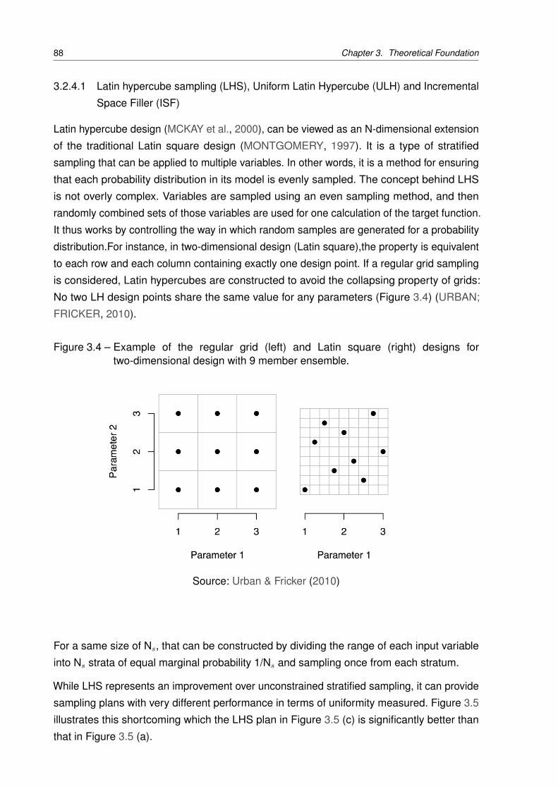
88 Chapter 3. Theoretical Foundation
3.2.4.1 Latin hypercube sampling (LHS), Uniform Latin Hypercube (ULH) and Incremental
Space Filler (ISF)
Latin hypercube design (MCKAY et al., 2000), can be viewed as an N-dimensional extension
of the traditional Latin square design (MONTGOMERY, 1997). It is a type of stratified
sampling that can be applied to multiple variables. In other words, it is a method for ensuring
that each probability distribution in its model is evenly sampled. The concept behind LHS
is not overly complex. Variables are sampled using an even sampling method, and then
randomly combined sets of those variables are used for one calculation of the target function.
It thus works by controlling the way in which random samples are generated for a probability
distribution.For instance, in two-dimensional design (Latin square),the property is equivalent
to each row and each column containing exactly one design point. If a regular grid sampling
is considered, Latin hypercubes are constructed to avoid the collapsing property of grids:
No two LH design points share the same value for any parameters (Figure 3.4) (URBAN;
FRICKER, 2010).
Figure 3.4 – Example of the regular grid (left) and Latin square (right) designs fortwo-dimensional design with 9 member ensemble.
Source: Urban & Fricker (2010)
For a same size of Ns, that can be constructed by dividing the range of each input variable
into Ns strata of equal marginal probability 1/Ns and sampling once from each stratum.
While LHS represents an improvement over unconstrained stratified sampling, it can provide
sampling plans with very different performance in terms of uniformity measured. Figure 3.5
illustrates this shortcoming which the LHS plan in Figure 3.5 (c) is significantly better than
that in Figure 3.5 (a).
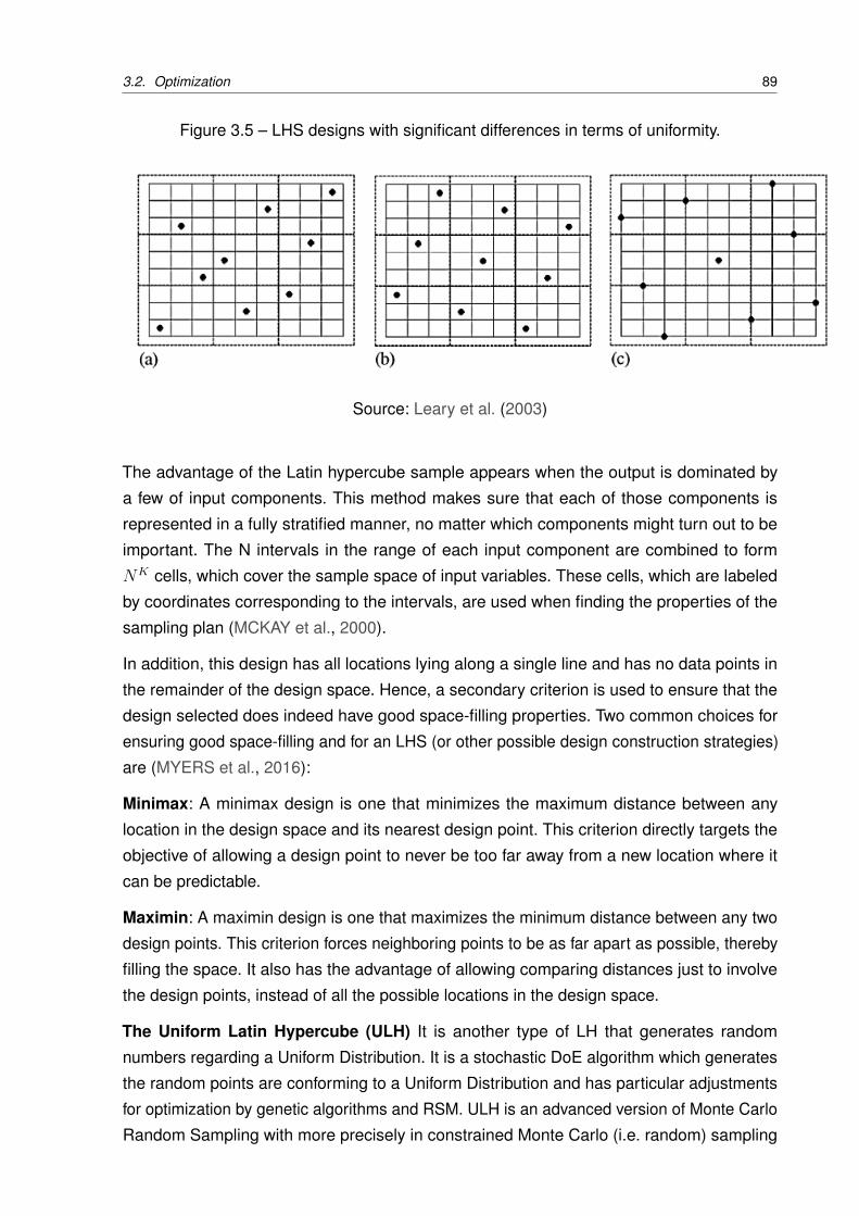
3.2. Optimization 89
Figure 3.5 – LHS designs with significant differences in terms of uniformity.
Source: Leary et al. (2003)
The advantage of the Latin hypercube sample appears when the output is dominated by
a few of input components. This method makes sure that each of those components is
represented in a fully stratified manner, no matter which components might turn out to be
important. The N intervals in the range of each input component are combined to form
NK cells, which cover the sample space of input variables. These cells, which are labeled
by coordinates corresponding to the intervals, are used when finding the properties of the
sampling plan (MCKAY et al., 2000).
In addition, this design has all locations lying along a single line and has no data points in
the remainder of the design space. Hence, a secondary criterion is used to ensure that the
design selected does indeed have good space-filling properties. Two common choices for
ensuring good space-filling and for an LHS (or other possible design construction strategies)
are (MYERS et al., 2016):
Minimax: A minimax design is one that minimizes the maximum distance between any
location in the design space and its nearest design point. This criterion directly targets the
objective of allowing a design point to never be too far away from a new location where it
can be predictable.
Maximin: A maximin design is one that maximizes the minimum distance between any two
design points. This criterion forces neighboring points to be as far apart as possible, thereby
filling the space. It also has the advantage of allowing comparing distances just to involve
the design points, instead of all the possible locations in the design space.
The Uniform Latin Hypercube (ULH) It is another type of LH that generates random
numbers regarding a Uniform Distribution. It is a stochastic DoE algorithm which generates
the random points are conforming to a Uniform Distribution and has particular adjustments
for optimization by genetic algorithms and RSM. ULH is an advanced version of Monte Carlo
Random Sampling with more precisely in constrained Monte Carlo (i.e. random) sampling
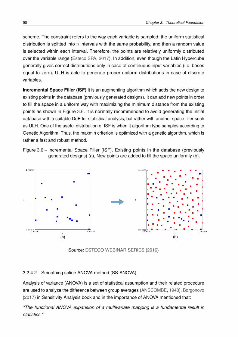
90 Chapter 3. Theoretical Foundation
scheme. The constraint refers to the way each variable is sampled: the uniform statistical
distribution is splitted into n intervals with the same probability, and then a random value
is selected within each interval. Therefore, the points are relatively uniformly distributed
over the variable range (Esteco SPA, 2017). In addition, even though the Latin Hypercube
generally gives correct distributions only in case of continuous input variables (i.e. bases
equal to zero), ULH is able to generate proper uniform distributions in case of discrete
variables.
Incremental Space Filler (ISF) It is an augmenting algorithm which adds the new design to
existing points in the database (previously generated designs). It can add new points in order
to fill the space in a uniform way with maximizing the minimum distance from the existing
points as shown in Figure 3.6. It is normally recommended to avoid generating the initial
database with a suitable DoE for statistical analysis, but rather with another space filler such
as ULH. One of the useful distribution of ISF is when it algorithm type samples according to
Genetic Algorithm. Thus, the maxmin criterion is optimized with a genetic algorithm, which is
rather a fast and robust method.
Figure 3.6 – Incremental Space Filler (ISF). Existing points in the database (previouslygenerated designs) (a), New points are added to fill the space uniformly (b).
Source: ESTECO WEBINAR SERIES (2016)
3.2.4.2 Smoothing spline ANOVA method (SS-ANOVA)
Analysis of variance (ANOVA) is a set of statistical assumption and their related procedure
are used to analyze the difference between group averages (ANSCOMBE, 1948). Borgonovo
(2017) in Sensitivity Analysis book and in the importance of ANOVA mentioned that:
"The functional ANOVA expansion of a multivariate mapping is a fundamental result in
statistics."
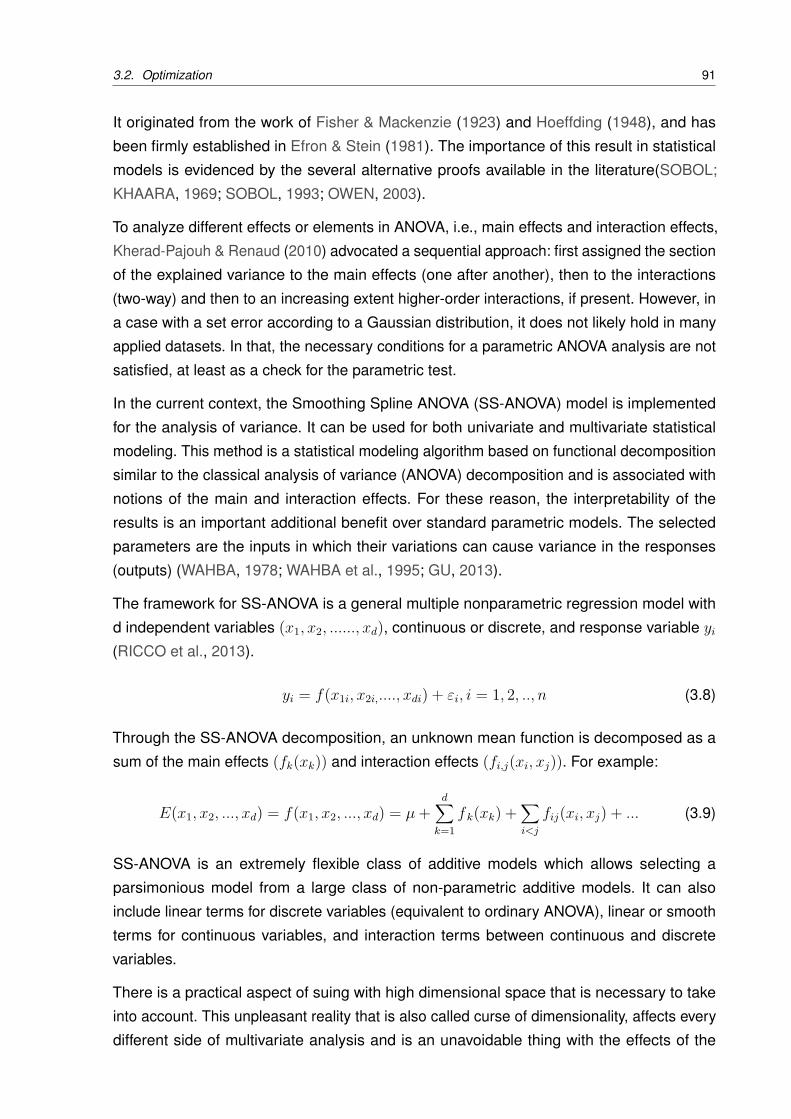
3.2. Optimization 91
It originated from the work of Fisher & Mackenzie (1923) and Hoeffding (1948), and has
been firmly established in Efron & Stein (1981). The importance of this result in statistical
models is evidenced by the several alternative proofs available in the literature(SOBOL;
KHAARA, 1969; SOBOL, 1993; OWEN, 2003).
To analyze different effects or elements in ANOVA, i.e., main effects and interaction effects,
Kherad-Pajouh & Renaud (2010) advocated a sequential approach: first assigned the section
of the explained variance to the main effects (one after another), then to the interactions
(two-way) and then to an increasing extent higher-order interactions, if present. However, in
a case with a set error according to a Gaussian distribution, it does not likely hold in many
applied datasets. In that, the necessary conditions for a parametric ANOVA analysis are not
satisfied, at least as a check for the parametric test.
In the current context, the Smoothing Spline ANOVA (SS-ANOVA) model is implemented
for the analysis of variance. It can be used for both univariate and multivariate statistical
modeling. This method is a statistical modeling algorithm based on functional decomposition
similar to the classical analysis of variance (ANOVA) decomposition and is associated with
notions of the main and interaction effects. For these reason, the interpretability of the
results is an important additional benefit over standard parametric models. The selected
parameters are the inputs in which their variations can cause variance in the responses
(outputs) (WAHBA, 1978; WAHBA et al., 1995; GU, 2013).
The framework for SS-ANOVA is a general multiple nonparametric regression model with
d independent variables (x1, x2, ......, xd), continuous or discrete, and response variable yi
(RICCO et al., 2013).
yi = f(x1i, x2i,...., xdi) + εi, i = 1, 2, .., n (3.8)
Through the SS-ANOVA decomposition, an unknown mean function is decomposed as a
sum of the main effects (fk(xk)) and interaction effects (fi,j(xi, xj)). For example:
E(x1, x2, ..., xd) = f(x1, x2, ..., xd) = µ+d∑
k=1fk(xk) +
∑i<j
fij(xi, xj) + ... (3.9)
SS-ANOVA is an extremely flexible class of additive models which allows selecting a
parsimonious model from a large class of non-parametric additive models. It can also
include linear terms for discrete variables (equivalent to ordinary ANOVA), linear or smooth
terms for continuous variables, and interaction terms between continuous and discrete
variables.
There is a practical aspect of suing with high dimensional space that is necessary to take
into account. This unpleasant reality that is also called curse of dimensionality, affects every
different side of multivariate analysis and is an unavoidable thing with the effects of the
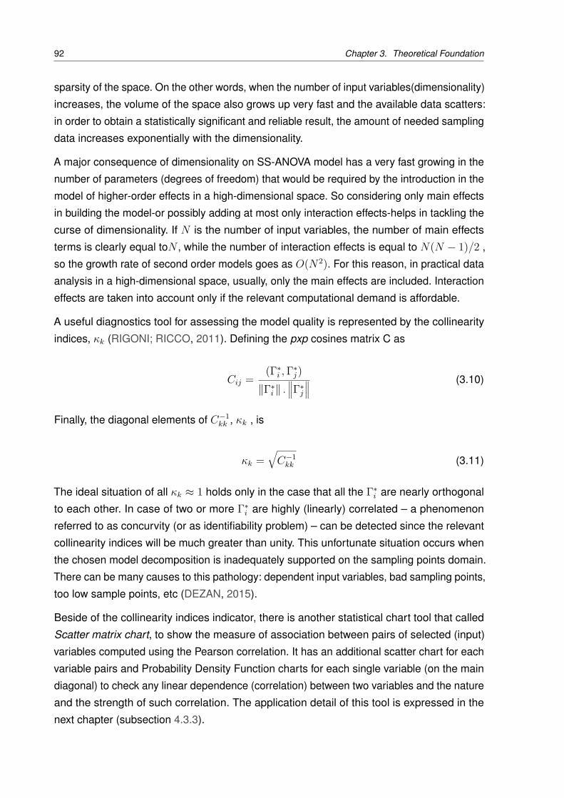
92 Chapter 3. Theoretical Foundation
sparsity of the space. On the other words, when the number of input variables(dimensionality)
increases, the volume of the space also grows up very fast and the available data scatters:
in order to obtain a statistically significant and reliable result, the amount of needed sampling
data increases exponentially with the dimensionality.
A major consequence of dimensionality on SS-ANOVA model has a very fast growing in the
number of parameters (degrees of freedom) that would be required by the introduction in the
model of higher-order effects in a high-dimensional space. So considering only main effects
in building the model-or possibly adding at most only interaction effects-helps in tackling the
curse of dimensionality. If N is the number of input variables, the number of main effects
terms is clearly equal toN , while the number of interaction effects is equal to N(N − 1)/2 ,
so the growth rate of second order models goes as O(N2). For this reason, in practical data
analysis in a high-dimensional space, usually, only the main effects are included. Interaction
effects are taken into account only if the relevant computational demand is affordable.
A useful diagnostics tool for assessing the model quality is represented by the collinearity
indices, κk (RIGONI; RICCO, 2011). Defining the pxp cosines matrix C as
Cij =(Γ∗
i ,Γ∗j)
‖Γ∗i ‖ .
∥∥∥Γ∗j
∥∥∥ (3.10)
Finally, the diagonal elements of C−1kk , κk , is
κk =√C−1
kk (3.11)
The ideal situation of all κk ≈ 1 holds only in the case that all the Γ∗i are nearly orthogonal
to each other. In case of two or more Γ∗i are highly (linearly) correlated – a phenomenon
referred to as concurvity (or as identifiability problem) – can be detected since the relevant
collinearity indices will be much greater than unity. This unfortunate situation occurs when
the chosen model decomposition is inadequately supported on the sampling points domain.
There can be many causes to this pathology: dependent input variables, bad sampling points,
too low sample points, etc (DEZAN, 2015).
Beside of the collinearity indices indicator, there is another statistical chart tool that called
Scatter matrix chart, to show the measure of association between pairs of selected (input)
variables computed using the Pearson correlation. It has an additional scatter chart for each
variable pairs and Probability Density Function charts for each single variable (on the main
diagonal) to check any linear dependence (correlation) between two variables and the nature
and the strength of such correlation. The application detail of this tool is expressed in the
next chapter (subsection 4.3.3).

3.2. Optimization 93
3.2.5 Genetic Algorithms – Fundamentals
Genetic Algorithm (GA) is a direct, parallel, stochastic method of optimization, which is based
on Darwin’s theory of natural selection. GA belong to the class of Evolutionary Algorithms
(EA). Evolutionary algorithms use the three main principles of natural evolution: reproduction,
natural selection (crossover) and diversity of the species (mutation), accomplished by the
differences of each generation from the previous one. Genetic Algorithms generate a set of
individuals, representing possible solutions of the design (population) as initial population.
The crossover is implemented by using a criterion, giving an evaluation for the individual
regarding the desired solution. The best-suited individuals create the next generation. The
large variety of problems in the engineering, as well as in other fields, needs the use of
algorithms from different types, characteristics and settings such GAs(ARORA, 2016).
The main ingredients of GA are divided into major parts:
• Chromosomes:
For the genetic algorithms, the chromosomes act as a set of genes, which code the
independent variables. Every chromosome represents a solution of the given problem.
Individual and vector of variables will be used as other words for chromosomes. A set
of different chromosomes (individuals) forms a generation (Figure 3.7). By means of
evolutionary operators, such as selection, recombination and mutation an offspring population
is created (POPOV, 2005).
Figure 3.7 – The Genes, chromosomes and genetic operations.
Source: https://protosity.wordpress.com/
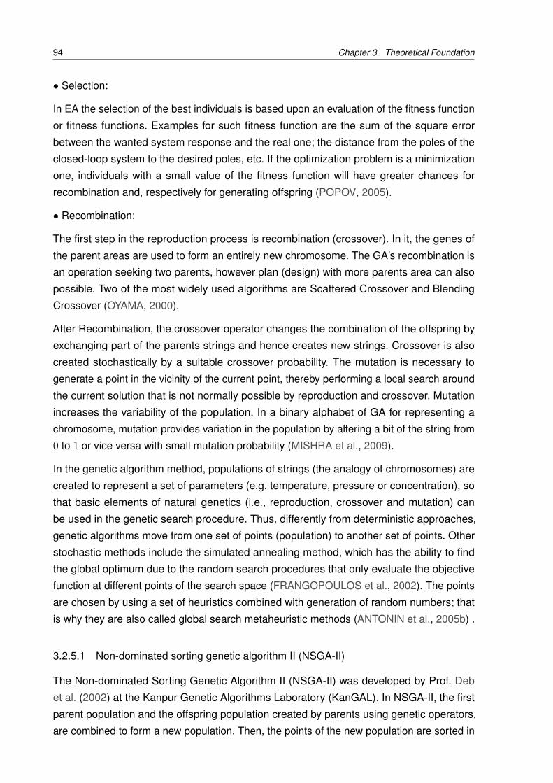
94 Chapter 3. Theoretical Foundation
• Selection:
In EA the selection of the best individuals is based upon an evaluation of the fitness function
or fitness functions. Examples for such fitness function are the sum of the square error
between the wanted system response and the real one; the distance from the poles of the
closed-loop system to the desired poles, etc. If the optimization problem is a minimization
one, individuals with a small value of the fitness function will have greater chances for
recombination and, respectively for generating offspring (POPOV, 2005).
• Recombination:
The first step in the reproduction process is recombination (crossover). In it, the genes of
the parent areas are used to form an entirely new chromosome. The GA’s recombination is
an operation seeking two parents, however plan (design) with more parents area can also
possible. Two of the most widely used algorithms are Scattered Crossover and Blending
Crossover (OYAMA, 2000).
After Recombination, the crossover operator changes the combination of the offspring by
exchanging part of the parents strings and hence creates new strings. Crossover is also
created stochastically by a suitable crossover probability. The mutation is necessary to
generate a point in the vicinity of the current point, thereby performing a local search around
the current solution that is not normally possible by reproduction and crossover. Mutation
increases the variability of the population. In a binary alphabet of GA for representing a
chromosome, mutation provides variation in the population by altering a bit of the string from
0 to 1 or vice versa with small mutation probability (MISHRA et al., 2009).
In the genetic algorithm method, populations of strings (the analogy of chromosomes) are
created to represent a set of parameters (e.g. temperature, pressure or concentration), so
that basic elements of natural genetics (i.e., reproduction, crossover and mutation) can
be used in the genetic search procedure. Thus, differently from deterministic approaches,
genetic algorithms move from one set of points (population) to another set of points. Other
stochastic methods include the simulated annealing method, which has the ability to find
the global optimum due to the random search procedures that only evaluate the objective
function at different points of the search space (FRANGOPOULOS et al., 2002). The points
are chosen by using a set of heuristics combined with generation of random numbers; that
is why they are also called global search metaheuristic methods (ANTONIN et al., 2005b) .
3.2.5.1 Non-dominated sorting genetic algorithm II (NSGA-II)
The Non-dominated Sorting Genetic Algorithm II (NSGA-II) was developed by Prof. Deb
et al. (2002) at the Kanpur Genetic Algorithms Laboratory (KanGAL). In NSGA-II, the first
parent population and the offspring population created by parents using genetic operators,
are combined to form a new population. Then, the points of the new population are sorted in
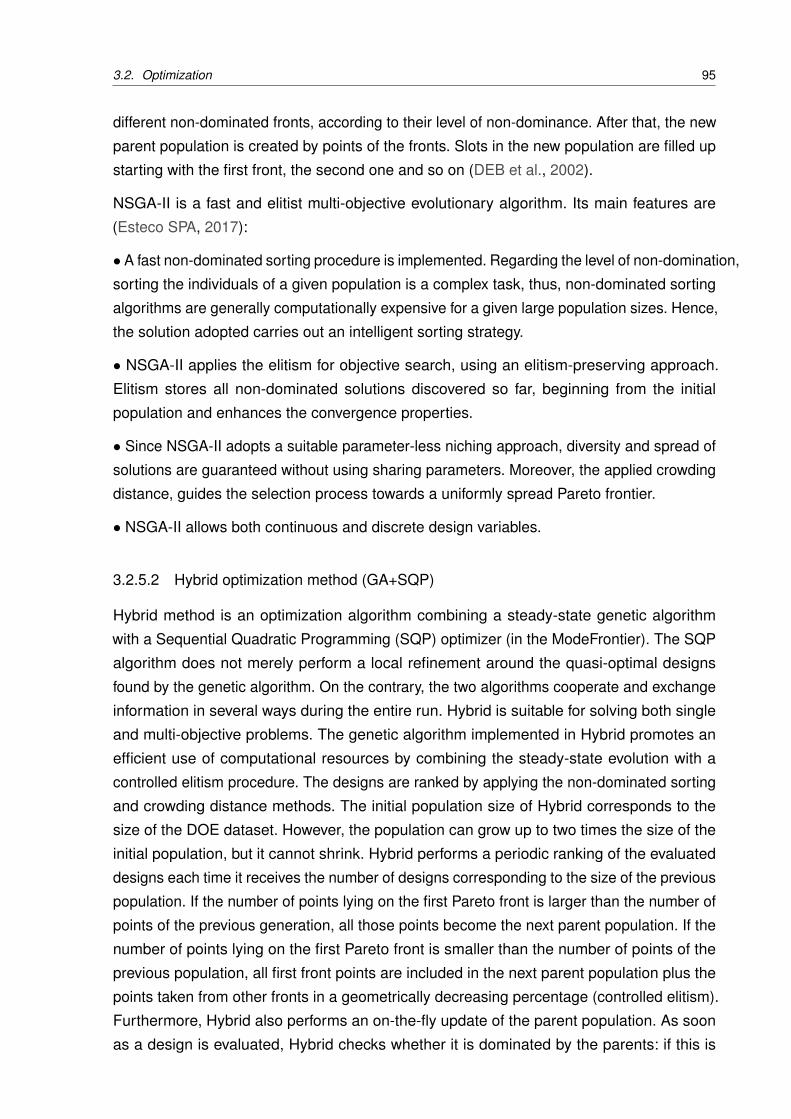
3.2. Optimization 95
different non-dominated fronts, according to their level of non-dominance. After that, the new
parent population is created by points of the fronts. Slots in the new population are filled up
starting with the first front, the second one and so on (DEB et al., 2002).
NSGA-II is a fast and elitist multi-objective evolutionary algorithm. Its main features are
(Esteco SPA, 2017):
• A fast non-dominated sorting procedure is implemented. Regarding the level of non-domination,
sorting the individuals of a given population is a complex task, thus, non-dominated sorting
algorithms are generally computationally expensive for a given large population sizes. Hence,
the solution adopted carries out an intelligent sorting strategy.
• NSGA-II applies the elitism for objective search, using an elitism-preserving approach.
Elitism stores all non-dominated solutions discovered so far, beginning from the initial
population and enhances the convergence properties.
• Since NSGA-II adopts a suitable parameter-less niching approach, diversity and spread of
solutions are guaranteed without using sharing parameters. Moreover, the applied crowding
distance, guides the selection process towards a uniformly spread Pareto frontier.
• NSGA-II allows both continuous and discrete design variables.
3.2.5.2 Hybrid optimization method (GA+SQP)
Hybrid method is an optimization algorithm combining a steady-state genetic algorithm
with a Sequential Quadratic Programming (SQP) optimizer (in the ModeFrontier). The SQP
algorithm does not merely perform a local refinement around the quasi-optimal designs
found by the genetic algorithm. On the contrary, the two algorithms cooperate and exchange
information in several ways during the entire run. Hybrid is suitable for solving both single
and multi-objective problems. The genetic algorithm implemented in Hybrid promotes an
efficient use of computational resources by combining the steady-state evolution with a
controlled elitism procedure. The designs are ranked by applying the non-dominated sorting
and crowding distance methods. The initial population size of Hybrid corresponds to the
size of the DOE dataset. However, the population can grow up to two times the size of the
initial population, but it cannot shrink. Hybrid performs a periodic ranking of the evaluated
designs each time it receives the number of designs corresponding to the size of the previous
population. If the number of points lying on the first Pareto front is larger than the number of
points of the previous generation, all those points become the next parent population. If the
number of points lying on the first Pareto front is smaller than the number of points of the
previous population, all first front points are included in the next parent population plus the
points taken from other fronts in a geometrically decreasing percentage (controlled elitism).
Furthermore, Hybrid also performs an on-the-fly update of the parent population. As soon
as a design is evaluated, Hybrid checks whether it is dominated by the parents: if this is
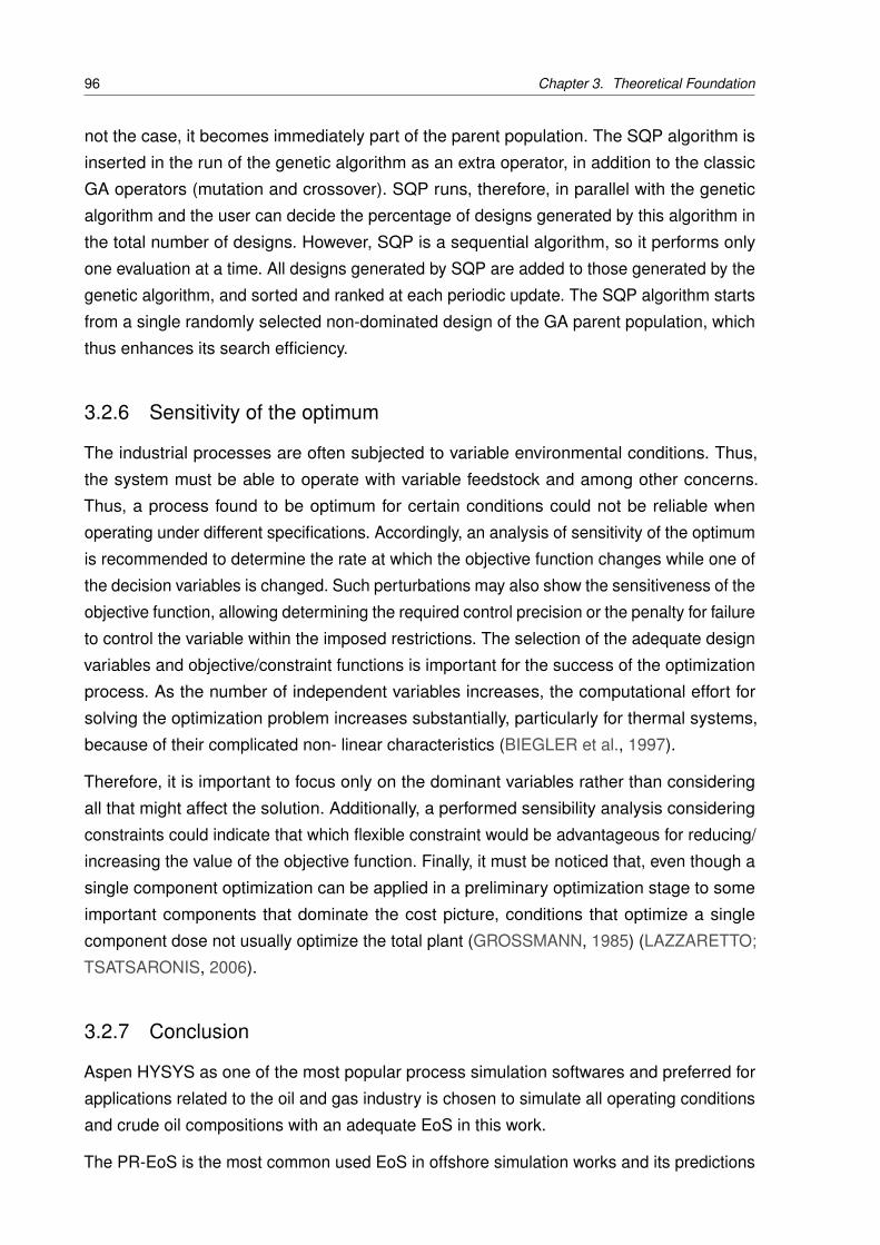
96 Chapter 3. Theoretical Foundation
not the case, it becomes immediately part of the parent population. The SQP algorithm is
inserted in the run of the genetic algorithm as an extra operator, in addition to the classic
GA operators (mutation and crossover). SQP runs, therefore, in parallel with the genetic
algorithm and the user can decide the percentage of designs generated by this algorithm in
the total number of designs. However, SQP is a sequential algorithm, so it performs only
one evaluation at a time. All designs generated by SQP are added to those generated by the
genetic algorithm, and sorted and ranked at each periodic update. The SQP algorithm starts
from a single randomly selected non-dominated design of the GA parent population, which
thus enhances its search efficiency.
3.2.6 Sensitivity of the optimum
The industrial processes are often subjected to variable environmental conditions. Thus,
the system must be able to operate with variable feedstock and among other concerns.
Thus, a process found to be optimum for certain conditions could not be reliable when
operating under different specifications. Accordingly, an analysis of sensitivity of the optimum
is recommended to determine the rate at which the objective function changes while one of
the decision variables is changed. Such perturbations may also show the sensitiveness of the
objective function, allowing determining the required control precision or the penalty for failure
to control the variable within the imposed restrictions. The selection of the adequate design
variables and objective/constraint functions is important for the success of the optimization
process. As the number of independent variables increases, the computational effort for
solving the optimization problem increases substantially, particularly for thermal systems,
because of their complicated non- linear characteristics (BIEGLER et al., 1997).
Therefore, it is important to focus only on the dominant variables rather than considering
all that might affect the solution. Additionally, a performed sensibility analysis considering
constraints could indicate that which flexible constraint would be advantageous for reducing/
increasing the value of the objective function. Finally, it must be noticed that, even though a
single component optimization can be applied in a preliminary optimization stage to some
important components that dominate the cost picture, conditions that optimize a single
component dose not usually optimize the total plant (GROSSMANN, 1985) (LAZZARETTO;
TSATSARONIS, 2006).
3.2.7 Conclusion
Aspen HYSYS as one of the most popular process simulation softwares and preferred for
applications related to the oil and gas industry is chosen to simulate all operating conditions
and crude oil compositions with an adequate EoS in this work.
The PR-EoS is the most common used EoS in offshore simulation works and its predictions
3.2. Optimization 97
of the liquid volume and density for CO2-rich fluids are compared to some experimental
works. According to the existing literature, the results from PR-EoS are in a good agreement
with the experimental data. Hence, it is chosen as EoS of the current research.
Moreover, in order to obtain more precise results, using the real data of offshore is essential.
Therefore, beside utilizing operating scenarios of a Brazilian FPSO that works on a pre-salt
field (from early life to end of life of the reservoir), a real performance data of an aero-derivative
gas turbine (RB211G62 DLE 60Hz turbine) with offshore application (as principal utility
system of plant) from GATECYCLETM commercial software (General Electric , 2013) is
applied here.
Furthermore, regarding the quantity of existing operating parameters as variables to evaluate
the objectives, it is necessary to create an automated process (integration) to couple a
simulator-modeler software with a statistical analyzer-optimizer tool to cut the development
time between simulation models and outputs. ESTECO ModeFRONTIERTM
is a powerful
integration platform for a multi-objective and multi-disciplinary optimization that enables the
automation of the design simulation process and facilitates analytic decision making. In the
current thesis, for the first time, Aspen HYSYS is coupled with ModeFRONTIER to make an
automated optimization process.
On the other hand, the complexity of the calculating derivatives of objective functions for
this research can cause deterministic methods to fail. Therefore, the chosen method should
be well suited for practical optimization problems, even difficult black-box problems possibly
with discrete decision variables. Non-dominated Sorting Genetic Algorithm II (NSGA-II) with
Controlled Elitism as a stochastic method and one of the most used evolutionary method is
selected to be implemented here. Moreover, GA is a robust optimization algorithm that has the
advantage of avoiding stalling problem, since it is able to find the global maximum/minimum in
a problem with multiple local optima. Although, the existing hybrid methods based on NSGA-II
will be verified in terms of convergence. The process synthesis based on evolutionary method
needs stochastic techniques using random choice to guide the search. Therefore, the entire
DOE table is used as a sequence of initial points for different local optimization problems and
screening analysis that will be provided by the Uniform Latin Hypercube (ULH) DoE algorithm
and Incremental Space Filler (ISF) (according to collinearity induces and Probability Density
Pearson (PDF)) by the ESTECO ModeFRONTIERTM
software.
The details and algorithm of the problem formulation for Aspen Hysys 9.0 and ESTECO
ModeFRONTIERTM
2017 and their coupling in the optimization process will be shown in the
next chapter.

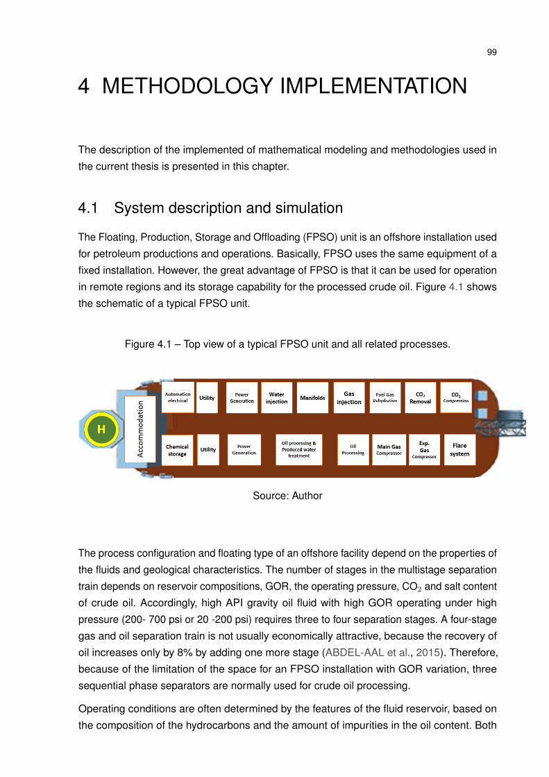
99
4 METHODOLOGY IMPLEMENTATION
The description of the implemented of mathematical modeling and methodologies used in
the current thesis is presented in this chapter.
4.1 System description and simulation
The Floating, Production, Storage and Offloading (FPSO) unit is an offshore installation used
for petroleum productions and operations. Basically, FPSO uses the same equipment of a
fixed installation. However, the great advantage of FPSO is that it can be used for operation
in remote regions and its storage capability for the processed crude oil. Figure 4.1 shows
the schematic of a typical FPSO unit.
Figure 4.1 – Top view of a typical FPSO unit and all related processes.
Source: Author
The process configuration and floating type of an offshore facility depend on the properties of
the fluids and geological characteristics. The number of stages in the multistage separation
train depends on reservoir compositions, GOR, the operating pressure, CO2 and salt content
of crude oil. Accordingly, high API gravity oil fluid with high GOR operating under high
pressure (200- 700 psi or 20 -200 psi) requires three to four separation stages. A four-stage
gas and oil separation train is not usually economically attractive, because the recovery of
oil increases only by 8% by adding one more stage (ABDEL-AAL et al., 2015). Therefore,
because of the limitation of the space for an FPSO installation with GOR variation, three
sequential phase separators are normally used for crude oil processing.
Operating conditions are often determined by the features of the fluid reservoir, based on
the composition of the hydrocarbons and the amount of impurities in the oil content. Both
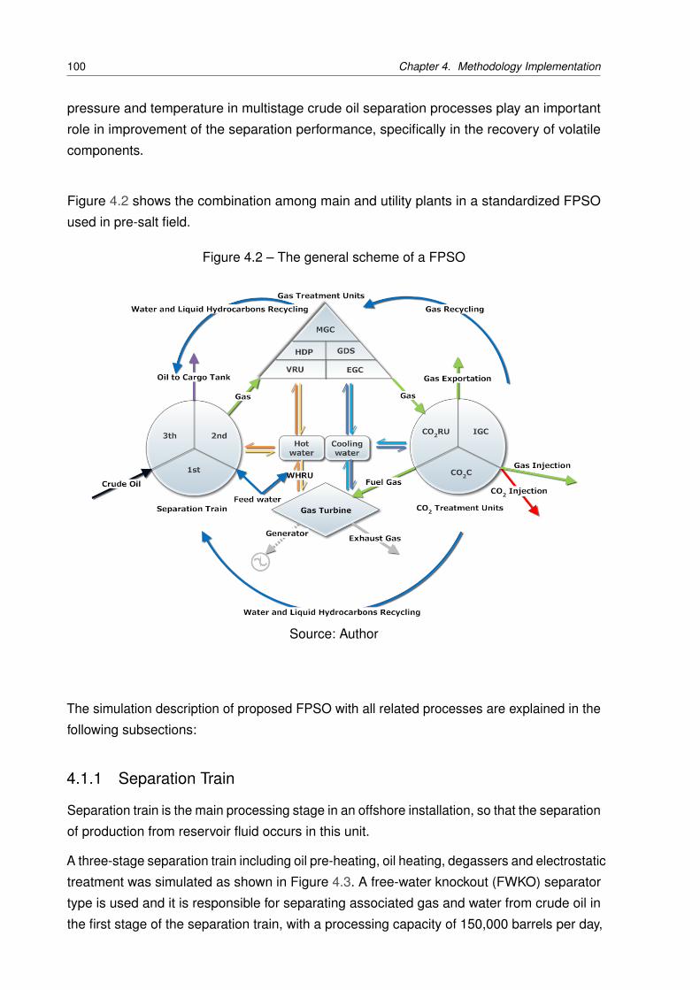
100 Chapter 4. Methodology Implementation
pressure and temperature in multistage crude oil separation processes play an important
role in improvement of the separation performance, specifically in the recovery of volatile
components.
Figure 4.2 shows the combination among main and utility plants in a standardized FPSO
used in pre-salt field.
Figure 4.2 – The general scheme of a FPSO
Source: Author
The simulation description of proposed FPSO with all related processes are explained in the
following subsections:
4.1.1 Separation Train
Separation train is the main processing stage in an offshore installation, so that the separation
of production from reservoir fluid occurs in this unit.
A three-stage separation train including oil pre-heating, oil heating, degassers and electrostatic
treatment was simulated as shown in Figure 4.3. A free-water knockout (FWKO) separator
type is used and it is responsible for separating associated gas and water from crude oil in
the first stage of the separation train, with a processing capacity of 150,000 barrels per day,
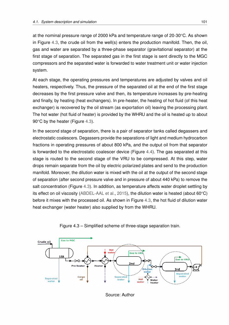
4.1. System description and simulation 101
at the nominal pressure range of 2000 kPa and temperature range of 20-30oC. As shown
in Figure 4.3, the crude oil from the well(s) enters the production manifold. Then, the oil,
gas and water are separated by a three-phase separator (gravitational separator) at the
first stage of separation. The separated gas in the first stage is sent directly to the MGC
compressors and the separated water is forwarded to water treatment unit or water injection
system.
At each stage, the operating pressures and temperatures are adjusted by valves and oil
heaters, respectively. Thus, the pressure of the separated oil at the end of the first stage
decreases by the first pressure valve and then, its temperature increases by pre-heating
and finally, by heating (heat exchangers). In pre-heater, the heating of hot fluid (of this heat
exchanger) is recovered by the oil stream (as exportation oil) leaving the processing plant.
The hot water (hot fluid of heater) is provided by the WHRU and the oil is heated up to about
90oC by the heater (Figure 4.3).
In the second stage of separation, there is a pair of separator tanks called degassers and
electrostatic coalescers. Degassers provide the separations of light and medium hydrocarbon
fractions in operating pressures of about 800 kPa, and the output oil from that separator
is forwarded to the electrostatic coalescer device (Figure 4.4). The gas separated at this
stage is routed to the second stage of the VRU to be compressed. At this step, water
drops remain separate from the oil by electric polarized plates and send to the production
manifold. Moreover, the dilution water is mixed with the oil at the output of the second stage
of separation (after second pressure valve and in pressure of about 440 kPa) to remove the
salt concentration (Figure 4.3). In addition, as temperature affects water droplet settling by
its effect on oil viscosity (ABDEL-AAL et al., 2015), the dilution water is heated (about 60oC)
before it mixes with the processed oil. As shown in Figure 4.3, the hot fluid of dilution water
heat exchanger (water heater) also supplied by from the WHRU.
Figure 4.3 – Simplified scheme of three-stage separation train.
Source: Author
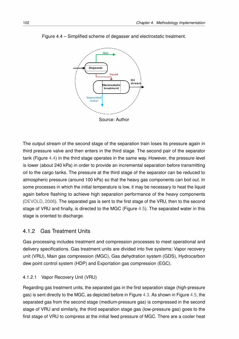
102 Chapter 4. Methodology Implementation
Figure 4.4 – Simplified scheme of degasser and electrostatic treatment.
Source: Author
The output stream of the second stage of the separation train loses its pressure again in
third pressure valve and then enters in the third stage. The second pair of the separator
tank (Figure 4.4) in the third stage operates in the same way. However, the pressure level
is lower (about 240 kPa) in order to provide an incremental separation before transmitting
oil to the cargo tanks. The pressure at the third stage of the separator can be reduced to
atmospheric pressure (around 100 kPa) so that the heavy gas components can boil out. In
some processes in which the initial temperature is low, it may be necessary to heat the liquid
again before flashing to achieve high separation performance of the heavy components
(DEVOLD, 2006). The separated gas is sent to the first stage of the VRU, then to the second
stage of VRU and finally, is directed to the MGC (Figure 4.5). The separated water in this
stage is oriented to discharge.
4.1.2 Gas Treatment Units
Gas processing includes treatment and compression processes to meet operational and
delivery specifications. Gas treatment units are divided into five systems: Vapor recovery
unit (VRU), Main gas compression (MGC), Gas dehydration system (GDS), Hydrocarbon
dew point control system (HDP) and Exportation gas compression (EGC).
4.1.2.1 Vapor Recovery Unit (VRU)
Regarding gas treatment units, the separated gas in the first separation stage (high-pressure
gas) is sent directly to the MGC, as depicted before in Figure 4.3. As shown in Figure 4.5, the
separated gas from the second stage (medium-pressure gas) is compressed in the second
stage of VRU and similarly, the third separation stage gas (low-pressure gas) goes to the
first stage of VRU to compress at the initial feed pressure of MGC. There are a cooler heat
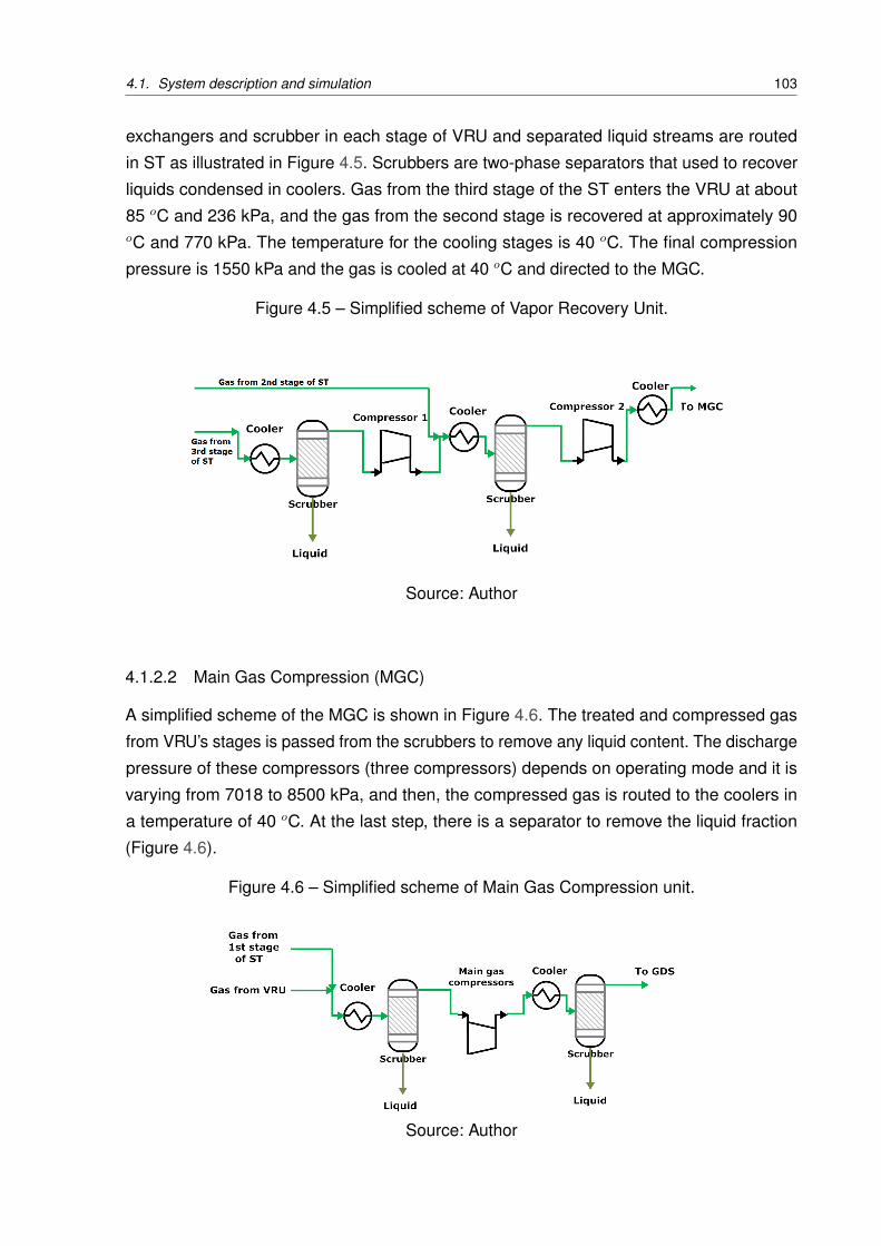
4.1. System description and simulation 103
exchangers and scrubber in each stage of VRU and separated liquid streams are routed
in ST as illustrated in Figure 4.5. Scrubbers are two-phase separators that used to recover
liquids condensed in coolers. Gas from the third stage of the ST enters the VRU at about
85 oC and 236 kPa, and the gas from the second stage is recovered at approximately 90oC and 770 kPa. The temperature for the cooling stages is 40 oC. The final compression
pressure is 1550 kPa and the gas is cooled at 40 oC and directed to the MGC.
Figure 4.5 – Simplified scheme of Vapor Recovery Unit.
Source: Author
4.1.2.2 Main Gas Compression (MGC)
A simplified scheme of the MGC is shown in Figure 4.6. The treated and compressed gas
from VRU’s stages is passed from the scrubbers to remove any liquid content. The discharge
pressure of these compressors (three compressors) depends on operating mode and it is
varying from 7018 to 8500 kPa, and then, the compressed gas is routed to the coolers in
a temperature of 40 oC. At the last step, there is a separator to remove the liquid fraction
(Figure 4.6).
Figure 4.6 – Simplified scheme of Main Gas Compression unit.
Source: Author

104 Chapter 4. Methodology Implementation
4.1.2.3 Gas dehydration System (GDS)
The Gas Dehydration system is part of the Gas Treatment units required to meet the
specifications in the produced natural gas from the production wells prior to be used as fuel
gas, gas-lift, exportation gas and injection gas. The gas stream from MGC at 40oC, is cooled
down in the gas cooler until 26oC, resulting in a mixed phase flow at about 26 o. This mixed
phase stream is the feed of the GDS. The pressure of this mixed phase stream may vary
from 6500 up to 8100 kPa. As Figure 4.7 shows, the dehydrated gas stream from GDS shall
comply with water content less than 1 ppmv and will be routed to HDP. The GDS consists of
3 (three) vessels containing the desiccant bed for water (molecular sieves). Upstream the
vessels, there is a gas coalescer filter in order to remove condensate. However, in present
simulation, this dehydration processes by desiccant bed for water were not modeled in detail
and a splitter unit was used instead. A simplified scheme of the GDS is presented in Figure
4.7.
The modeling of molecular sieves was simulated and simplified regarding technical reports
and its efficiency. Thus, a splitter unit was used to perform the adapted output compositions
and conditions.
Figure 4.7 – Simplified scheme of Gas Dehydration System.
Source: Author
4.1.2.4 Hydrocarbons Dew Point Control System (HDP)
The Hydrocarbon Dew Point Control System is required to achieve a dew point of 10oC and
5350 kPa and consists of the following equipment as shown in Figure 4.8:
• Gas/Liquid exchanger;
• Cold separator and;
• Coalescer filter.
The gas stream from GDS is directed to Gas/Liquid exchanger, where it is cooled down to
21o C. This stream is directed to the Cold separator passing through the Joule-Thomson
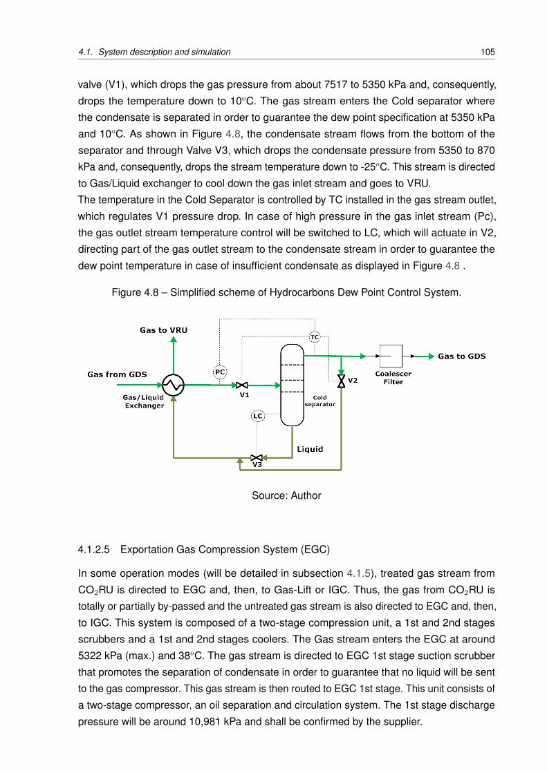
4.1. System description and simulation 105
valve (V1), which drops the gas pressure from about 7517 to 5350 kPa and, consequently,
drops the temperature down to 10oC. The gas stream enters the Cold separator where
the condensate is separated in order to guarantee the dew point specification at 5350 kPa
and 10oC. As shown in Figure 4.8, the condensate stream flows from the bottom of the
separator and through Valve V3, which drops the condensate pressure from 5350 to 870
kPa and, consequently, drops the stream temperature down to -25oC. This stream is directed
to Gas/Liquid exchanger to cool down the gas inlet stream and goes to VRU.
The temperature in the Cold Separator is controlled by TC installed in the gas stream outlet,
which regulates V1 pressure drop. In case of high pressure in the gas inlet stream (Pc),
the gas outlet stream temperature control will be switched to LC, which will actuate in V2,
directing part of the gas outlet stream to the condensate stream in order to guarantee the
dew point temperature in case of insufficient condensate as displayed in Figure 4.8 .
Figure 4.8 – Simplified scheme of Hydrocarbons Dew Point Control System.
Source: Author
4.1.2.5 Exportation Gas Compression System (EGC)
In some operation modes (will be detailed in subsection 4.1.5), treated gas stream from
CO2RU is directed to EGC and, then, to Gas-Lift or IGC. Thus, the gas from CO2RU is
totally or partially by-passed and the untreated gas stream is also directed to EGC and, then,
to IGC. This system is composed of a two-stage compression unit, a 1st and 2nd stages
scrubbers and a 1st and 2nd stages coolers. The Gas stream enters the EGC at around
5322 kPa (max.) and 38oC. The gas stream is directed to EGC 1st stage suction scrubber
that promotes the separation of condensate in order to guarantee that no liquid will be sent
to the gas compressor. This gas stream is then routed to EGC 1st stage. This unit consists of
a two-stage compressor, an oil separation and circulation system. The 1st stage discharge
pressure will be around 10,981 kPa and shall be confirmed by the supplier.
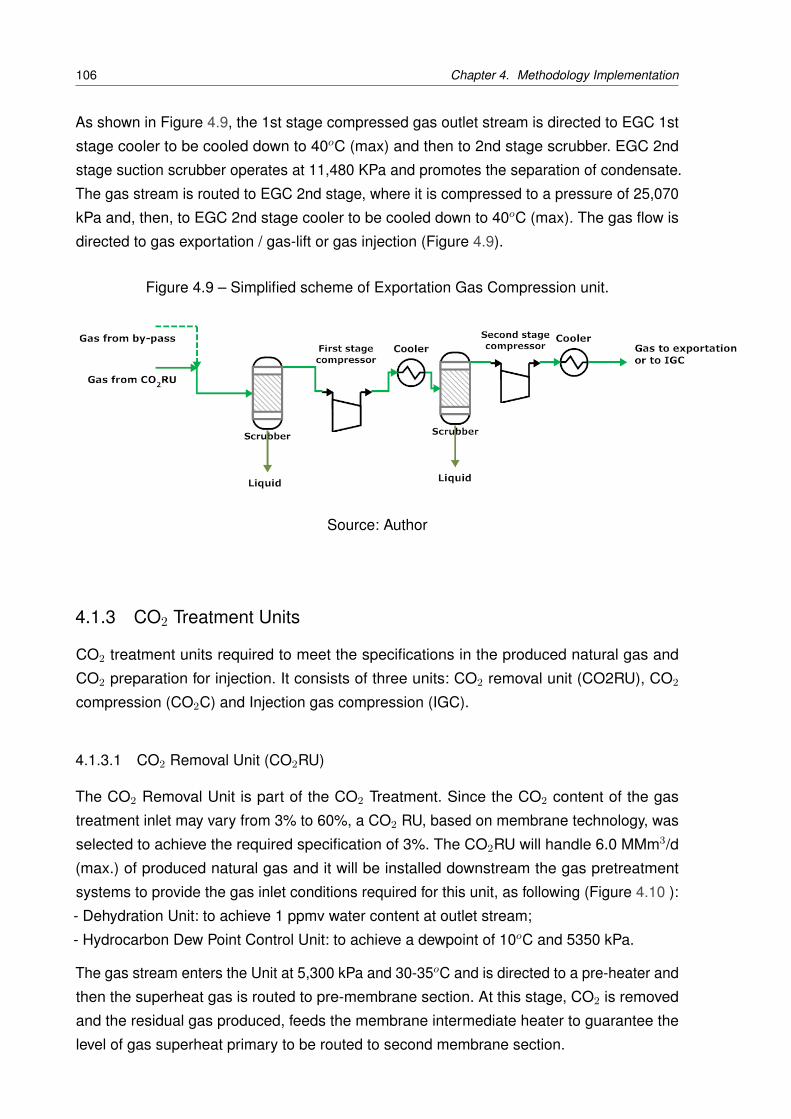
106 Chapter 4. Methodology Implementation
As shown in Figure 4.9, the 1st stage compressed gas outlet stream is directed to EGC 1st
stage cooler to be cooled down to 40oC (max) and then to 2nd stage scrubber. EGC 2nd
stage suction scrubber operates at 11,480 KPa and promotes the separation of condensate.
The gas stream is routed to EGC 2nd stage, where it is compressed to a pressure of 25,070
kPa and, then, to EGC 2nd stage cooler to be cooled down to 40oC (max). The gas flow is
directed to gas exportation / gas-lift or gas injection (Figure 4.9).
Figure 4.9 – Simplified scheme of Exportation Gas Compression unit.
Source: Author
4.1.3 CO2 Treatment Units
CO2 treatment units required to meet the specifications in the produced natural gas and
CO2 preparation for injection. It consists of three units: CO2 removal unit (CO2RU), CO2
compression (CO2C) and Injection gas compression (IGC).
4.1.3.1 CO2 Removal Unit (CO2RU)
The CO2 Removal Unit is part of the CO2 Treatment. Since the CO2 content of the gas
treatment inlet may vary from 3% to 60%, a CO2 RU, based on membrane technology, was
selected to achieve the required specification of 3%. The CO2RU will handle 6.0 MMm3/d
(max.) of produced natural gas and it will be installed downstream the gas pretreatment
systems to provide the gas inlet conditions required for this unit, as following (Figure 4.10 ):
- Dehydration Unit: to achieve 1 ppmv water content at outlet stream;
- Hydrocarbon Dew Point Control Unit: to achieve a dewpoint of 10oC and 5350 kPa.
The gas stream enters the Unit at 5,300 kPa and 30-35oC and is directed to a pre-heater and
then the superheat gas is routed to pre-membrane section. At this stage, CO2 is removed
and the residual gas produced, feeds the membrane intermediate heater to guarantee the
level of gas superheat primary to be routed to second membrane section.
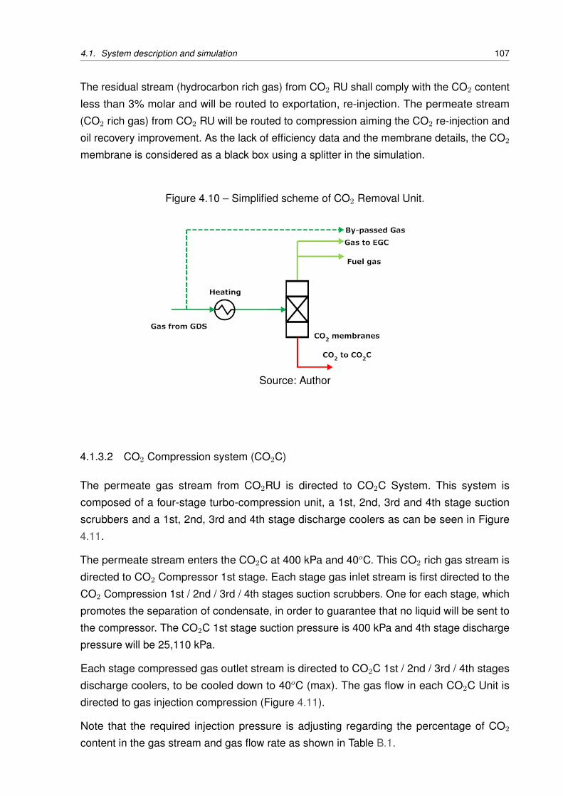
4.1. System description and simulation 107
The residual stream (hydrocarbon rich gas) from CO2 RU shall comply with the CO2 content
less than 3% molar and will be routed to exportation, re-injection. The permeate stream
(CO2 rich gas) from CO2 RU will be routed to compression aiming the CO2 re-injection and
oil recovery improvement. As the lack of efficiency data and the membrane details, the CO2
membrane is considered as a black box using a splitter in the simulation.
Figure 4.10 – Simplified scheme of CO2 Removal Unit.
Source: Author
4.1.3.2 CO2 Compression system (CO2C)
The permeate gas stream from CO2RU is directed to CO2C System. This system is
composed of a four-stage turbo-compression unit, a 1st, 2nd, 3rd and 4th stage suction
scrubbers and a 1st, 2nd, 3rd and 4th stage discharge coolers as can be seen in Figure
4.11.
The permeate stream enters the CO2C at 400 kPa and 40oC. This CO2 rich gas stream is
directed to CO2 Compressor 1st stage. Each stage gas inlet stream is first directed to the
CO2 Compression 1st / 2nd / 3rd / 4th stages suction scrubbers. One for each stage, which
promotes the separation of condensate, in order to guarantee that no liquid will be sent to
the compressor. The CO2C 1st stage suction pressure is 400 kPa and 4th stage discharge
pressure will be 25,110 kPa.
Each stage compressed gas outlet stream is directed to CO2C 1st / 2nd / 3rd / 4th stages
discharge coolers, to be cooled down to 40oC (max). The gas flow in each CO2C Unit is
directed to gas injection compression (Figure 4.11).
Note that the required injection pressure is adjusting regarding the percentage of CO2
content in the gas stream and gas flow rate as shown in Table B.1.
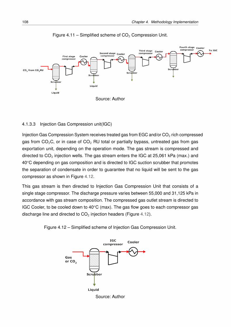
108 Chapter 4. Methodology Implementation
Figure 4.11 – Simplified scheme of CO2 Compression Unit.
Source: Author
4.1.3.3 Injection Gas Compression unit(IGC)
Injection Gas Compression System receives treated gas from EGC and/or CO2 rich compressed
gas from CO2C, or in case of CO2 RU total or partially bypass, untreated gas from gas
exportation unit, depending on the operation mode. The gas stream is compressed and
directed to CO2 injection wells. The gas stream enters the IGC at 25,061 kPa (max.) and
40oC depending on gas composition and is directed to IGC suction scrubber that promotes
the separation of condensate in order to guarantee that no liquid will be sent to the gas
compressor as shown in Figure 4.12.
This gas stream is then directed to Injection Gas Compression Unit that consists of a
single stage compressor. The discharge pressure varies between 55,000 and 31,125 kPa in
accordance with gas stream composition. The compressed gas outlet stream is directed to
IGC Cooler, to be cooled down to 40oC (max). The gas flow goes to each compressor gas
discharge line and directed to CO2 injection headers (Figure 4.12).
Figure 4.12 – Simplified scheme of Injection Gas Compression Unit.
Source: Author
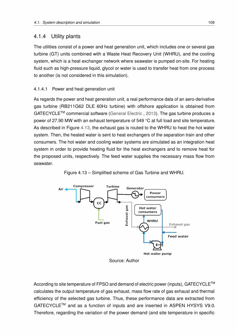
4.1. System description and simulation 109
4.1.4 Utility plants
The utilities consist of a power and heat generation unit, which includes one or several gas
turbine (GT) units combined with a Waste Heat Recovery Unit (WHRU), and the cooling
system, which is a heat exchanger network where seawater is pumped on-site. For heating
fluid such as high-pressure liquid, glycol or water is used to transfer heat from one process
to another (is not considered in this simulation).
4.1.4.1 Power and heat generation unit
As regards the power and heat generation unit, a real performance data of an aero-derivative
gas turbine (RB211G62 DLE 60Hz turbine) with offshore application is obtained from
GATECYCLETM commercial software (General Electric , 2013). The gas turbine produces a
power of 27.90 MW with an exhaust temperature of 549 oC at full load and site temperature.
As described in Figure 4.13, the exhaust gas is routed to the WHRU to heat the hot water
system. Then, the heated water is sent to heat exchangers of the separation train and other
consumers. The hot water and cooling water systems are simulated as an integration heat
system in order to provide heating fluid for the heat exchangers and to remove heat for
the proposed units, respectively. The feed water supplies the necessary mass flow from
seawater.
Figure 4.13 – Simplified scheme of Gas Turbine and WHRU.
Source: Author
According to site temperature of FPSO and demand of electric power (inputs), GATECYCLETM
calculates the output temperature of gas exhaust, mass flow rate of gas exhaust and thermal
efficiency of the selected gas turbine. Thus, these performance data are extracted from
GATECYCLETM and as a function of inputs and are inserted in ASPEN HYSYS V9.0.
Therefore, regarding the variation of the power demand (and site temperature in specific

110 Chapter 4. Methodology Implementation
condition), ASPEN HYSYS provides required information of heat water temperature, water
mass flow and efficiency of gas turbine. The simulation of aero-derivative gas turbine
(RB211G62 DLE 60Hz turbine) in GATECYCLETM and using this performance data is
explained in Appendix A .
4.1.4.2 Hot Water system
The Hot Water System is a closed system that uses pressurized fresh water. Heat is
recovered from the gas exhausted from each gas turbine (WHRU- Waste Heat Recovery
Unit). Hot Water at 100oC, is pumped by the hot water circulation pump, through the Turbo
generator Waste Heat Recovery Unit, where it is heated up to 130oC. Hot Water leaves
the consumers at 100oC (min.). Make up water is fed to the system by Hot Water Make up
pumps from seawater (Figure 4.13).
4.1.4.3 Cooling Water system
The cooling water system consists of a closed fresh water system, indirectly (heat exchanger)
cooled by sea water. The seawater at 25oC is pumped into the heat exchanger, where cooling
water is cooled down from 55 to 35oC, to the consumers and, then, back to pump suction.
The seawater at around 45oC is rejected to the sea. In fact, the last destination of free
water will be the sea, according to the CONAMA 303/07 legal standard; the maximum
concentration of oils and grease that can be disposed in water is 29 mg/L.
In the first stage of the water treatment system, a series of small vessels, called hydrocyclones,
is included. The stream accelerated by the continuous decrease in the vessel diameter makes
a centrifugal force separate heavier components such as water and solids from the wall and
oil rejects on the opposite side of the water output, in the central portion.
Finally, the floater vessel removes the remaining oil parcels agglomerated in water, with the
aid of an upward air stream. If the analyzer finds a value above that allowed by law, the flow
is redirected from the sea output to specific tanks or it will be injected into a reservoir through
injection wells.
4.1.4.4 Water Injection System
Treated sea water is pumped by booster injection water pumps through injection water heat
exchanger to main injection water pump and, then, to be injected in WAG (water alternating
gas) injection wells for EOR at a pressure of 25000 kPa and 44oC.
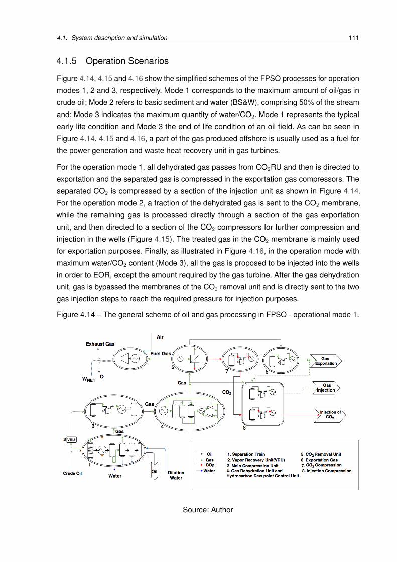
4.1. System description and simulation 111
4.1.5 Operation Scenarios
Figure 4.14, 4.15 and 4.16 show the simplified schemes of the FPSO processes for operation
modes 1, 2 and 3, respectively. Mode 1 corresponds to the maximum amount of oil/gas in
crude oil; Mode 2 refers to basic sediment and water (BS&W), comprising 50% of the stream
and; Mode 3 indicates the maximum quantity of water/CO2. Mode 1 represents the typical
early life condition and Mode 3 the end of life condition of an oil field. As can be seen in
Figure 4.14, 4.15 and 4.16, a part of the gas produced offshore is usually used as a fuel for
the power generation and waste heat recovery unit in gas turbines.
For the operation mode 1, all dehydrated gas passes from CO2RU and then is directed to
exportation and the separated gas is compressed in the exportation gas compressors. The
separated CO2 is compressed by a section of the injection unit as shown in Figure 4.14.
For the operation mode 2, a fraction of the dehydrated gas is sent to the CO2 membrane,
while the remaining gas is processed directly through a section of the gas exportation
unit, and then directed to a section of the CO2 compressors for further compression and
injection in the wells (Figure 4.15). The treated gas in the CO2 membrane is mainly used
for exportation purposes. Finally, as illustrated in Figure 4.16, in the operation mode with
maximum water/CO2 content (Mode 3), all the gas is proposed to be injected into the wells
in order to EOR, except the amount required by the gas turbine. After the gas dehydration
unit, gas is bypassed the membranes of the CO2 removal unit and is directly sent to the two
gas injection steps to reach the required pressure for injection purposes.
Figure 4.14 – The general scheme of oil and gas processing in FPSO - operational mode 1.
Source: Author
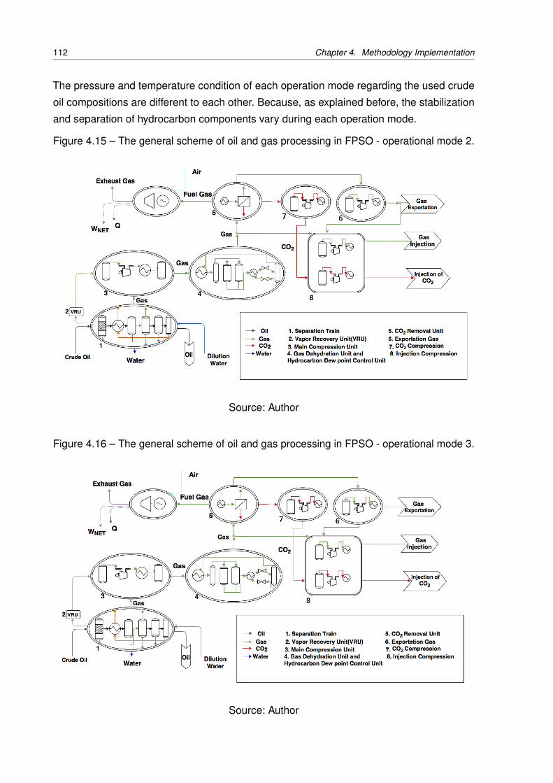
112 Chapter 4. Methodology Implementation
The pressure and temperature condition of each operation mode regarding the used crude
oil compositions are different to each other. Because, as explained before, the stabilization
and separation of hydrocarbon components vary during each operation mode.
Figure 4.15 – The general scheme of oil and gas processing in FPSO - operational mode 2.
Source: Author
Figure 4.16 – The general scheme of oil and gas processing in FPSO - operational mode 3.
Source: Author
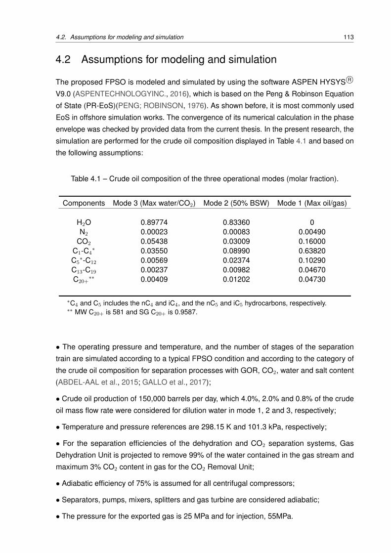
4.2. Assumptions for modeling and simulation 113
4.2 Assumptions for modeling and simulation
The proposed FPSO is modeled and simulated by using the software ASPEN HYSYS R©
V9.0 (ASPENTECHNOLOGYINC., 2016), which is based on the Peng & Robinson Equation
of State (PR-EoS)(PENG; ROBINSON, 1976). As shown before, it is most commonly used
EoS in offshore simulation works. The convergence of its numerical calculation in the phase
envelope was checked by provided data from the current thesis. In the present research, the
simulation are performed for the crude oil composition displayed in Table 4.1 and based on
the following assumptions:
Table 4.1 – Crude oil composition of the three operational modes (molar fraction).
Components Mode 3 (Max water/CO2) Mode 2 (50% BSW) Mode 1 (Max oil/gas)
H2O 0.89774 0.83360 0N2 0.00023 0.00083 0.00490
CO2 0.05438 0.03009 0.16000C1-C4
∗ 0.03550 0.08990 0.63820C5
∗-C12 0.00569 0.02374 0.10290C13-C19 0.00237 0.00982 0.04670C20+
∗∗ 0.00409 0.01202 0.04730
∗C4 and C5 includes the nC4 and iC4, and the nC5 and iC5 hydrocarbons, respectively.∗∗ MW C20+ is 581 and SG C20+ is 0.9587.
• The operating pressure and temperature, and the number of stages of the separation
train are simulated according to a typical FPSO condition and according to the category of
the crude oil composition for separation processes with GOR, CO2, water and salt content
(ABDEL-AAL et al., 2015; GALLO et al., 2017);
• Crude oil production of 150,000 barrels per day, which 4.0%, 2.0% and 0.8% of the crude
oil mass flow rate were considered for dilution water in mode 1, 2 and 3, respectively;
• Temperature and pressure references are 298.15 K and 101.3 kPa, respectively;
• For the separation efficiencies of the dehydration and CO2 separation systems, Gas
Dehydration Unit is projected to remove 99% of the water contained in the gas stream and
maximum 3% CO2 content in gas for the CO2 Removal Unit;
• Adiabatic efficiency of 75% is assumed for all centrifugal compressors;
• Separators, pumps, mixers, splitters and gas turbine are considered adiabatic;
• The pressure for the exported gas is 25 MPa and for injection, 55MPa.
114 Chapter 4. Methodology Implementation
4.3 Modeling, Simulation and optimization description
In this section, the procedure of modeling, simulation and optimization with their details are
explained and discussed as Strategy title:
4.3.1 Strategy
The structure of this methodology for optimization consists of:
• System modeling using flow sheeting tools as much as possible using real operating and
performance data;
• Applying evaluation methods for system analysis;
• Applying a robust statistical method of screening analysis (SS-ANOVA) to identify the most
important contributors to values of outputs and;
• System optimization based on powerful evolutionary algorithms and heuristics search such
as GA (and/or a hybrid method of GA in order to improve the accuracy).
The fundamental programming base on VBscript is provided during simulation and modeling
to couple the integration softwares such as GATECYCLE in order to use real performance
data of power and heat generation unit and ESTECO modeFRONTIER as a statistical
analyzer and multidisciplinary optimizer of design process software.
Thus, as an initial step, after simulating the proposed system via Aspen HYSYSr and Aspen
Simulation Workbook (Aspen Technology, Inc, 2014) (step1), the major energy and power
consumers, and details of the desired production are analyzed (step 2) as shown in Figure
4.17.
Then, the important operating parameters from the literature and evaluation methods are
extracted from modeling and the data of model simulation are categorized and transferred
through VBScript to be used by a preliminary screening analyzer software (via the Smoothing
Splice ANOVA method) to reduce the number of input variables for the optimization procedure
(step 3).
As described in Figure 4.17, after that, only the most relevant input parameters are delivered
to the optimization procedure and Hybrid GA method (via ModeFRONTIERTM
(Esteco SPA,
2017)) was performed by modifying the value assigned to the input variables as decision
variables and analyzing the outputs as defined objectives. Finally, data such as temperatures,
pressures, oil production and etc, are extracted from the process models (post-processing)
and sent to the next computing step to justify the obtained results (step 4).
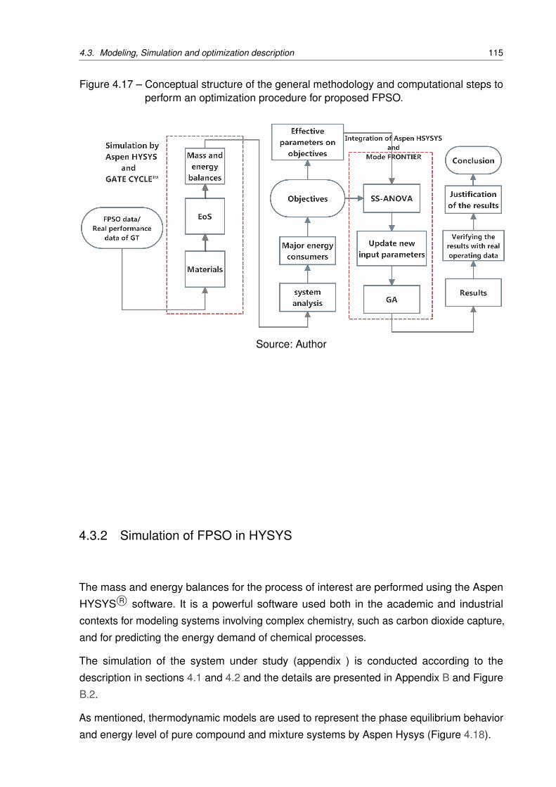
4.3. Modeling, Simulation and optimization description 115
Figure 4.17 – Conceptual structure of the general methodology and computational steps toperform an optimization procedure for proposed FPSO.
Source: Author
4.3.2 Simulation of FPSO in HYSYS
The mass and energy balances for the process of interest are performed using the Aspen
HYSYS R© software. It is a powerful software used both in the academic and industrial
contexts for modeling systems involving complex chemistry, such as carbon dioxide capture,
and for predicting the energy demand of chemical processes.
The simulation of the system under study (appendix ) is conducted according to the
description in sections 4.1 and 4.2 and the details are presented in Appendix B and Figure
B.2.
As mentioned, thermodynamic models are used to represent the phase equilibrium behavior
and energy level of pure compound and mixture systems by Aspen Hysys (Figure 4.18).
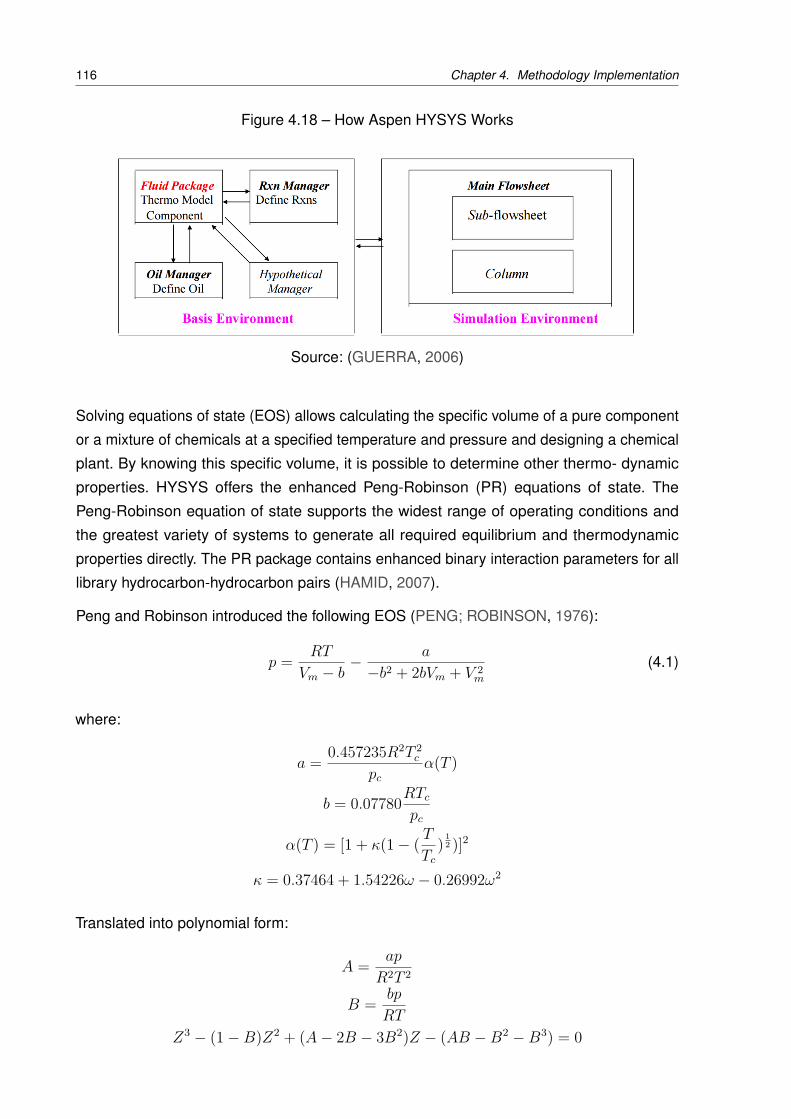
116 Chapter 4. Methodology Implementation
Figure 4.18 – How Aspen HYSYS Works
Source: (GUERRA, 2006)
Solving equations of state (EOS) allows calculating the specific volume of a pure component
or a mixture of chemicals at a specified temperature and pressure and designing a chemical
plant. By knowing this specific volume, it is possible to determine other thermo- dynamic
properties. HYSYS offers the enhanced Peng-Robinson (PR) equations of state. The
Peng-Robinson equation of state supports the widest range of operating conditions and
the greatest variety of systems to generate all required equilibrium and thermodynamic
properties directly. The PR package contains enhanced binary interaction parameters for all
library hydrocarbon-hydrocarbon pairs (HAMID, 2007).
Peng and Robinson introduced the following EOS (PENG; ROBINSON, 1976):
p = RT
Vm − b− a
−b2 + 2bVm + V 2m
(4.1)
where:
a = 0.457235R2T 2c
pc
α(T )
b = 0.07780RTc
pc
α(T ) = [1 + κ(1− ( TTc
) 12 )]2
κ = 0.37464 + 1.54226ω − 0.26992ω2
Translated into polynomial form:
A = ap
R2T 2
B = bp
RT
Z3 − (1−B)Z2 + (A− 2B − 3B2)Z − (AB −B2 −B3) = 0
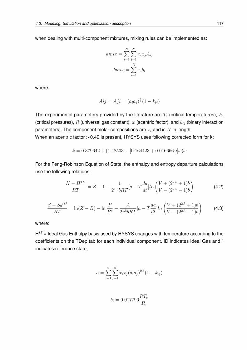
4.3. Modeling, Simulation and optimization description 117
when dealing with multi-component mixtures, mixing rules can be implemented as:
amix =N∑
i=1
N∑j=1
xixjAij
bmix =N∑
i=1xibi
where:
Aij = Aji = (aiaj)12 (1− kij)
The experimental parameters provided by the literature are Tc (critical temperatures), Pc
(critical pressures), R (universal gas constant), ω (acentric factor), and kij (binary interaction
parameters). The component molar compositions are xi and is N in length.
When an acentric factor > 0.49 is present, HYSYS uses following corrected form for k:
k = 0.379642 + (1.48503− [0.164423 + 0.016666ω]ω)ω
For the Peng-Robinson Equation of State, the enthalpy and entropy departure calculations
use the following relations:
H −HID
RT= Z − 1− 1
21.5bRT[a− T da
dt]ln
(V + (22.5 + 1)bV − (22.5 − 1)b
)(4.2)
S − S0ID
RT= ln(Z −B)− ln P
P o− A
21.5bRT[a− T da
dt]ln
(V + (22.5 + 1)bV − (22.5 − 1)b
)(4.3)
where:
HID= Ideal Gas Enthalpy basis used by HYSYS changes with temperature according to the
coefficients on the TDep tab for each individual component. ID indicates Ideal Gas and o
indicates reference state,
a =n∑
i=1
n∑j=1
xixj(aiaj)0.5(1− kij)
bi = 0.077796RTc
Pc
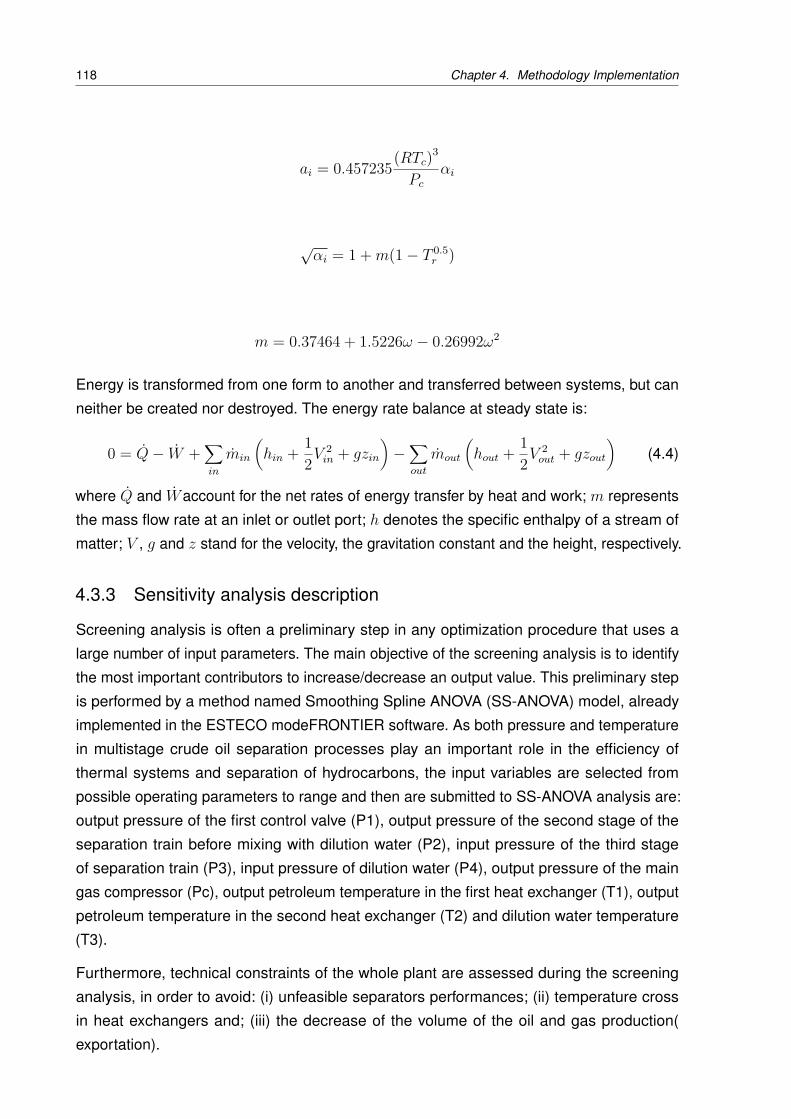
118 Chapter 4. Methodology Implementation
ai = 0.457235(RTc)3
Pc
αi
√αi = 1 +m(1− T 0.5
r )
m = 0.37464 + 1.5226ω − 0.26992ω2
Energy is transformed from one form to another and transferred between systems, but can
neither be created nor destroyed. The energy rate balance at steady state is:
0 = Q− W +∑in
min
(hin + 1
2V2
in + gzin
)−∑out
mout
(hout + 1
2V2
out + gzout
)(4.4)
where Q and Waccount for the net rates of energy transfer by heat and work; m represents
the mass flow rate at an inlet or outlet port; h denotes the specific enthalpy of a stream of
matter; V , g and z stand for the velocity, the gravitation constant and the height, respectively.
4.3.3 Sensitivity analysis description
Screening analysis is often a preliminary step in any optimization procedure that uses a
large number of input parameters. The main objective of the screening analysis is to identify
the most important contributors to increase/decrease an output value. This preliminary step
is performed by a method named Smoothing Spline ANOVA (SS-ANOVA) model, already
implemented in the ESTECO modeFRONTIER software. As both pressure and temperature
in multistage crude oil separation processes play an important role in the efficiency of
thermal systems and separation of hydrocarbons, the input variables are selected from
possible operating parameters to range and then are submitted to SS-ANOVA analysis are:
output pressure of the first control valve (P1), output pressure of the second stage of the
separation train before mixing with dilution water (P2), input pressure of the third stage
of separation train (P3), input pressure of dilution water (P4), output pressure of the main
gas compressor (Pc), output petroleum temperature in the first heat exchanger (T1), output
petroleum temperature in the second heat exchanger (T2) and dilution water temperature
(T3).
Furthermore, technical constraints of the whole plant are assessed during the screening
analysis, in order to avoid: (i) unfeasible separators performances; (ii) temperature cross
in heat exchangers and; (iii) the decrease of the volume of the oil and gas production(
exportation).
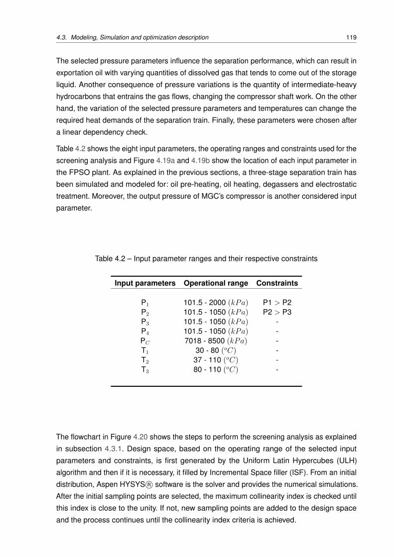
4.3. Modeling, Simulation and optimization description 119
The selected pressure parameters influence the separation performance, which can result in
exportation oil with varying quantities of dissolved gas that tends to come out of the storage
liquid. Another consequence of pressure variations is the quantity of intermediate-heavy
hydrocarbons that entrains the gas flows, changing the compressor shaft work. On the other
hand, the variation of the selected pressure parameters and temperatures can change the
required heat demands of the separation train. Finally, these parameters were chosen after
a linear dependency check.
Table 4.2 shows the eight input parameters, the operating ranges and constraints used for the
screening analysis and Figure 4.19a and 4.19b show the location of each input parameter in
the FPSO plant. As explained in the previous sections, a three-stage separation train has
been simulated and modeled for: oil pre-heating, oil heating, degassers and electrostatic
treatment. Moreover, the output pressure of MGC’s compressor is another considered input
parameter.
Table 4.2 – Input parameter ranges and their respective constraints
Input parameters Operational range Constraints
P1 101.5 - 2000 (kPa) P1 > P2P2 101.5 - 1050 (kPa) P2 > P3P3 101.5 - 1050 (kPa) -P4 101.5 - 1050 (kPa) -PC 7018 - 8500 (kPa) -T1 30 - 80 (oC) -T2 37 - 110 (oC) -T3 80 - 110 (oC) -
The flowchart in Figure 4.20 shows the steps to perform the screening analysis as explained
in subsection 4.3.1. Design space, based on the operating range of the selected input
parameters and constraints, is first generated by the Uniform Latin Hypercubes (ULH)
algorithm and then if it is necessary, it filled by Incremental Space filler (ISF). From an initial
distribution, Aspen HYSYS R© software is the solver and provides the numerical simulations.
After the initial sampling points are selected, the maximum collinearity index is checked until
this index is close to the unity. If not, new sampling points are added to the design space
and the process continues until the collinearity index criteria is achieved.
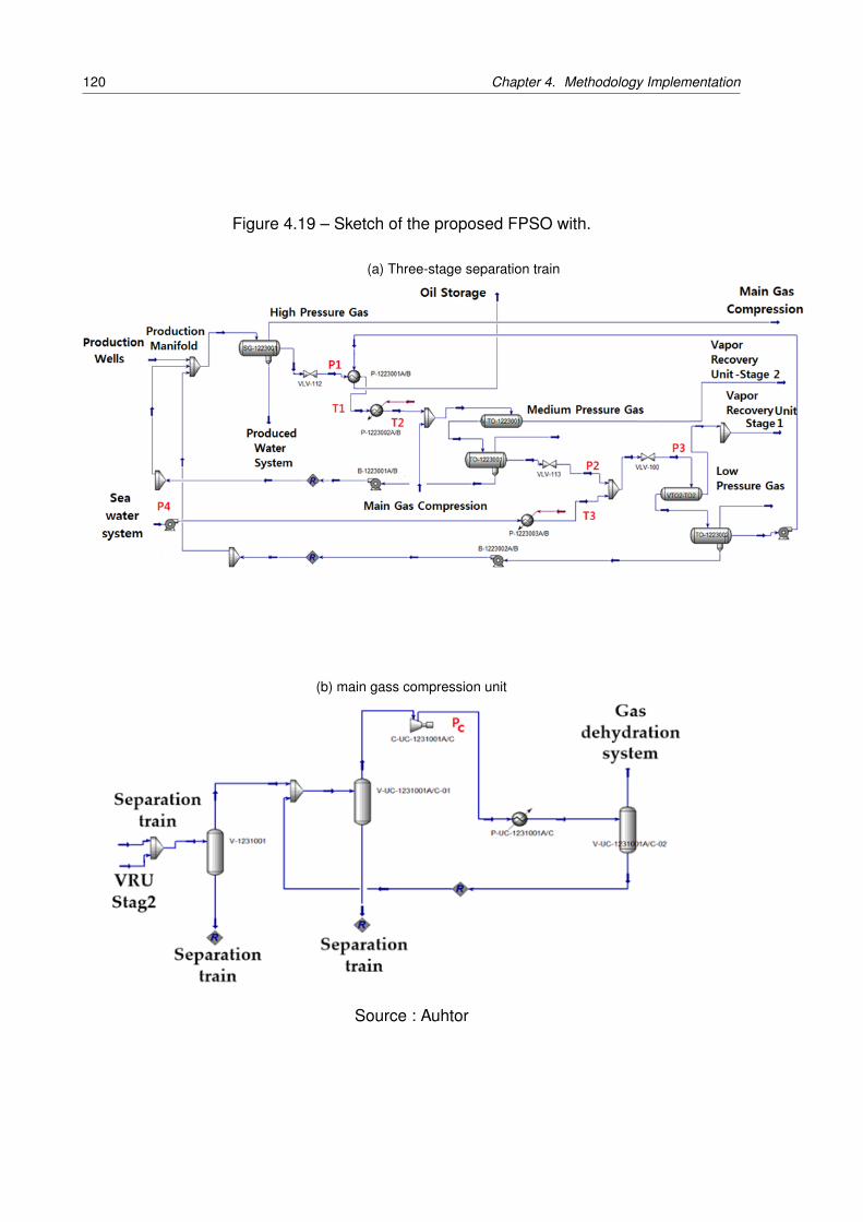
120 Chapter 4. Methodology Implementation
Figure 4.19 – Sketch of the proposed FPSO with.
(a) Three-stage separation train
(b) main gass compression unit
Source : Auhtor

4.3. Modeling, Simulation and optimization description 121
Figure 4.20 – Flowchart indicating the processes for screening analyses
Source: Author
There is a tool to verify if the sample distribution of the selected input variables in design
space was good sufficient. Scatter matrix chart is to see all the pairwise scatter plots of
the input variables, linear dependence (correlation) between all the input variables and
the Probability Density Function chart for each input variable. For example, Figure 4.21a
shows the scatter matrix chart of the selected input parameter’s distribution on the total
fuel consumption of proposed FPSO. In that, each column and row represent a parameter.
Squares with the number show the correlation of each variable and the other displays
distribution points.
The Probability Density Function is practically uniform for all input variables and no correlation
between the eight input variables is observed. Therefore, the design space can be considered
satisfactory to perform the screening analysis of those eight input parameters.
Figure 4.21b shows an example distribution design point between P2 and P4. The green
line represents the regression line that it is not observed any correlation between two input
parameter P2 and P4. After ensuring from the initial distribution, Aspen HYSYS R© software is
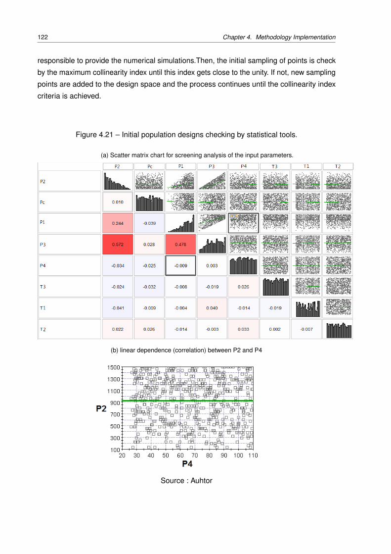
122 Chapter 4. Methodology Implementation
responsible to provide the numerical simulations.Then, the initial sampling of points is check
by the maximum collinearity index until this index gets close to the unity. If not, new sampling
points are added to the design space and the process continues until the collinearity index
criteria is achieved.
Figure 4.21 – Initial population designs checking by statistical tools.
(a) Scatter matrix chart for screening analysis of the input parameters.
(b) linear dependence (correlation) between P2 and P4
Source : Auhtor
4.3. Modeling, Simulation and optimization description 123
4.3.4 Optimization description
Optimization aims at defining the system configurations that, for example, simultaneously
minimize the energy consumption or environmental impacts, while maximizing the thermodynamic
performance (MARÉCHAL; KALITVENTZEFF, 1999).
The optimization problem is based on the decision variables, which can be changed in
practice (for example, the output pressure of separator or the design temperature at the
outlet of a heat exchanger), and on separation performance (subsection 3.1.1).
The objective function and design variables are firstly defined for the optimization procedure.
The design space is then built by using Latin Hypercube Sampling and ISF (if necessary).
In the next step, the Integrator software (modeFRONTIER) calls the thermodynamic solver
(ASPEN HYSYS), which solves energy and mass balances for each component of the FPSO
unit. After the thermodynamic convergence is achieved for the whole plant, the technical
constraints are assessed. If the technical constraints are satisfied, values of Obj are picked
up by integrator software. The optimization procedure is sought out by using NSGA-II. At the
end of the optimization process, the Min or Max value of Obj calculates, if the convergence
criteria fail, new points are generated and the procedure is restarted. The overall optimization
procedure using the two programs (HYSYS and ModeFRONTIERTM
- details in Appendix C)
is shown in Figure 4.22.
The objective function defined for the optimization procedure is a function of input parameters,
their operating ranges and constraints:
Obj = Function(Input parameters) (4.5)
For example:
Fuel Consumption = f(Input parameters) (4.6)
Hydrocarbon liquids recovery = f(Input parameters) (4.7)
According to Rao (2009), defining a design vector I , the optimization problem can be stated
as follows:
I = {Inputs} (4.8)
Find I = {...} which minimizes/maximizes Obj subject under constraints
Pi > Pi+1 i = 1, 2 (4.9)
It is important to note that all indicated technical constraints in the sensitivity analysis are
also considered in the optimization procedure.The design of experiment of initial population

124 Chapter 4. Methodology Implementation
of optimization procedure is also is verified by scatter matrix chart and collinearity induces.
Figure 4.22 – General flowchart of the optimization procedure
Source: Author
4.3.4.1 Optimization in ModeFRONTIERTM
The ModeFRONTIERTM
is a multi-objective and multi-disciplinary optimization platform
and design environment. Its workflow environment allows formalizing and managing all the
logical steps composing an engineering process. The ModeFRONTIERTM
can be coupled
with the popular engineering solvers or style tools available for building a bridge between
ModeFRONTIERTM
and any commercial or in-house codes. Figure 4.23 illustrates the
procedure of optimization in ModeFRONTIERTM
.
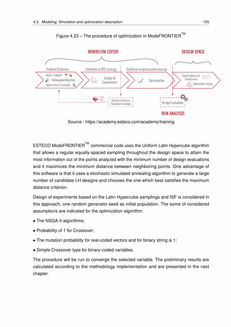
4.3. Modeling, Simulation and optimization description 125
Figure 4.23 – The procedure of optimization in ModeFRONTIERTM
Source : https://academy.esteco.com/academy/training
ESTECO ModeFRONTIERTM
commercial code uses the Uniform Latin Hypercube algorithm
that allows a regular equally-spaced sampling throughout the design space to attain the
most information out of the points analyzed with the minimum number of design evaluations
and it maximizes the minimum distance between neighboring points. One advantage of
this software is that it uses a stochastic simulated annealing algorithm to generate a large
number of candidate LH designs and chooses the one which best satisfies the maximum
distance criterion.
Design of experiments based on the Latin Hypercube samplings and ISF is considered in
this approach, one random generator seed as initial population. The some of considered
assumptions are indicated for the optimization algorithm:
• The NSGA-II algorithms;
• Probability of 1 for Crossover;
• The mutation probability for real-coded vectors and for binary string is 1;
• Simple Crossover type for binary-coded variables.
The procedure will be run to converge the selected variable. The preliminary results are
calculated according to the methodology implementation and are presented in the next
chapter.

127
5 RESULTS AND DISCUSSIONS
In this chapter, the obtained optimization results for a primary oil and gas processing
plant in FPSO are presented and discussed. So that, a synthesis plant of typical Brazilian
FPSO with three scenarios of operation is modeled and simulated by Aspen Hysys to
calculate thermodynamic properties. The under investigation operation modes in the present
research are: Mode 1, Maximum oil/gas content; Mode 2, 50% BS&W oil content and; Mode
3, Maximum water/CO2 oil content. The thermodynamic modeling and simulation of the
proposed FPSO plant are performed using the real performance data of a commercial gas
turbine (RB211G62 DLE 60Hz).
In addition, several thermodynamic parameters are submitted to a screening analysis via the
Smoothing Splice ANOVA method to reduce the number of input variables for the optimization
procedure. Finally, the main results from the optimization procedure via hybrid method for
proposed objective functions are discussed and compared with a baseline configuration.
5.1 Thermodynamic analysis results
The FPSO plant model was used to investigate three operational modes shown in the Figures
4.14, 4.15 and 4.16, in order to obtain the required values of parameters, such as net oil,
gas, water and CO2 production flows (mass balance) and energy balance. Table 5.1 shows
the mass flow rates of the three studied operation modes. In that, as it was expected, the
operation mode with more gas and oil (mode 1) has more (mass flow) production resulting in
more required fuel for heat and power generation unit. Next, the operation mode 3 with more
amounts of gas for injection than Mode 2, is in second place of the calculated electric power
demand. Although, these two values are very close. Note that mode 1 has the highest gas
mass flow rate and mode 2 has the lowest one, regarding the gas content of each crude oil
and operating condition of separation train.
Moreover, as Mode 3 is maximum water/CO2 oil content, the input mass flow rate of dilution
water is the lowest and as Mode 1 is almost without water content, it has the highest of the
necessary input mass flow rate of dilution water (Table 5.1).
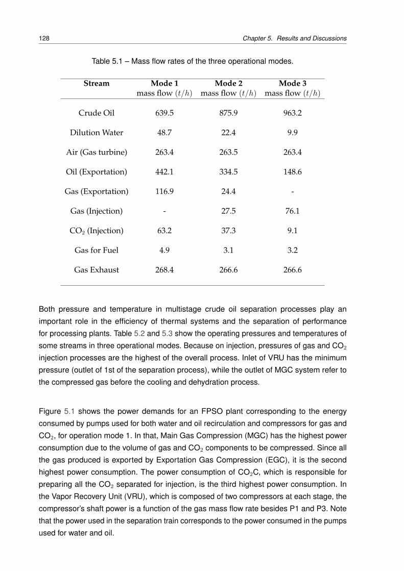
128 Chapter 5. Results and Discussions
Table 5.1 – Mass flow rates of the three operational modes.
Stream Mode 1 Mode 2 Mode 3mass flow (t/h) mass flow (t/h) mass flow (t/h)
Crude Oil 639.5 875.9 963.2
Dilution Water 48.7 22.4 9.9
Air (Gas turbine) 263.4 263.5 263.4
Oil (Exportation) 442.1 334.5 148.6
Gas (Exportation) 116.9 24.4 -
Gas (Injection) - 27.5 76.1
CO2 (Injection) 63.2 37.3 9.1
Gas for Fuel 4.9 3.1 3.2
Gas Exhaust 268.4 266.6 266.6
Both pressure and temperature in multistage crude oil separation processes play an
important role in the efficiency of thermal systems and the separation of performance
for processing plants. Table 5.2 and 5.3 show the operating pressures and temperatures of
some streams in three operational modes. Because on injection, pressures of gas and CO2
injection processes are the highest of the overall process. Inlet of VRU has the minimum
pressure (outlet of 1st of the separation process), while the outlet of MGC system refer to
the compressed gas before the cooling and dehydration process.
Figure 5.1 shows the power demands for an FPSO plant corresponding to the energy
consumed by pumps used for both water and oil recirculation and compressors for gas and
CO2, for operation mode 1. In that, Main Gas Compression (MGC) has the highest power
consumption due to the volume of gas and CO2 components to be compressed. Since all
the gas produced is exported by Exportation Gas Compression (EGC), it is the second
highest power consumption. The power consumption of CO2C, which is responsible for
preparing all the CO2 separated for injection, is the third highest power consumption. In
the Vapor Recovery Unit (VRU), which is composed of two compressors at each stage, the
compressor’s shaft power is a function of the gas mass flow rate besides P1 and P3. Note
that the power used in the separation train corresponds to the power consumed in the pumps
used for water and oil.
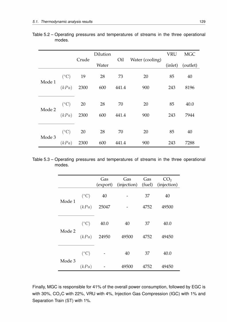
5.1. Thermodynamic analysis results 129
Table 5.2 – Operating pressures and temperatures of streams in the three operationalmodes.
Dilution VRU MGCCrude Oil Water (cooling)
Water (inlet) (outlet)
(◦C) 19 28 73 20 85 40Mode 1
(kPa) 2300 600 441.4 900 243 8196
(◦C) 20 28 70 20 85 40.0Mode 2
(kPa) 2300 600 441.4 900 243 7944
(◦C) 20 28 70 20 85 40Mode 3
(kPa) 2300 600 441.4 900 243 7288
Table 5.3 – Operating pressures and temperatures of streams in the three operationalmodes.
Gas Gas Gas CO2(export) (injection) (fuel) (injection)
(◦C) 40 - 37 40Mode 1
(kPa) 25047 - 4752 49500
(◦C) 40.0 40 37 40.0
Mode 2(kPa) 24950 49500 4752 49450
(◦C) - 40 37 40.0
Mode 3(kPa) - 49500 4752 49450
Finally, MGC is responsible for 41% of the overall power consumption, followed by EGC is
with 30%, CO2C with 22%, VRU with 4%, Injection Gas Compression (IGC) with 1% and
Separation Train (ST) with 1%.
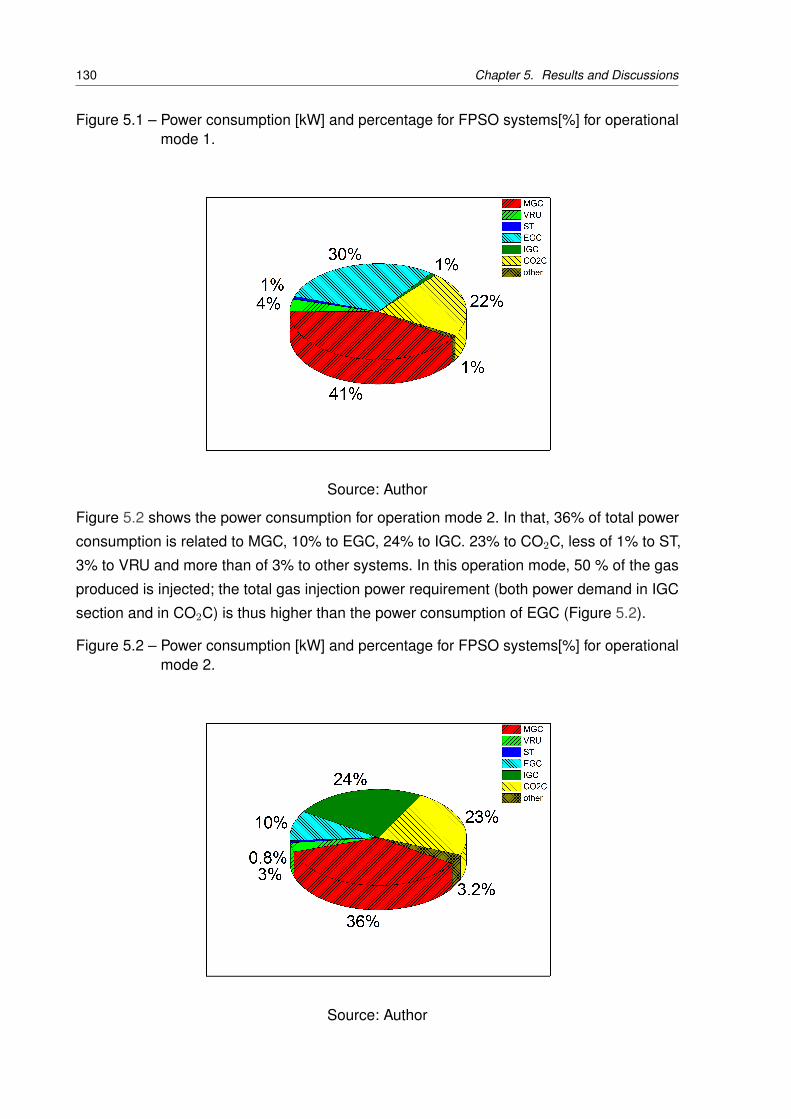
130 Chapter 5. Results and Discussions
Figure 5.1 – Power consumption [kW] and percentage for FPSO systems[%] for operationalmode 1.
Source: Author
Figure 5.2 shows the power consumption for operation mode 2. In that, 36% of total power
consumption is related to MGC, 10% to EGC, 24% to IGC. 23% to CO2C, less of 1% to ST,
3% to VRU and more than of 3% to other systems. In this operation mode, 50 % of the gas
produced is injected; the total gas injection power requirement (both power demand in IGC
section and in CO2C) is thus higher than the power consumption of EGC (Figure 5.2).
Figure 5.2 – Power consumption [kW] and percentage for FPSO systems[%] for operationalmode 2.
Source: Author
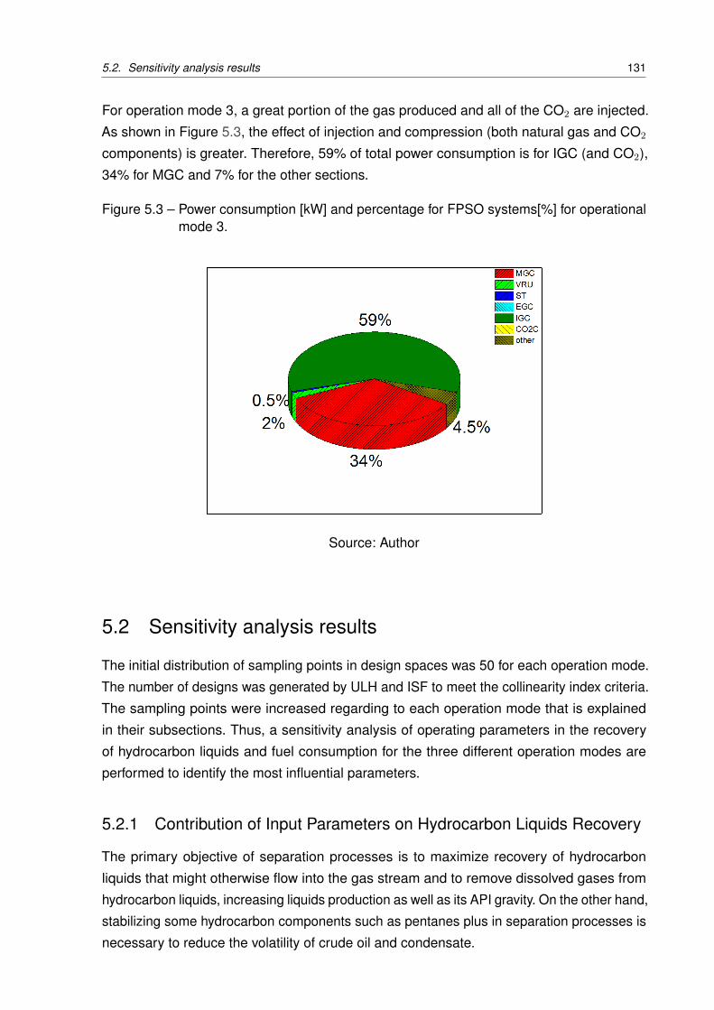
5.2. Sensitivity analysis results 131
For operation mode 3, a great portion of the gas produced and all of the CO2 are injected.
As shown in Figure 5.3, the effect of injection and compression (both natural gas and CO2
components) is greater. Therefore, 59% of total power consumption is for IGC (and CO2),
34% for MGC and 7% for the other sections.
Figure 5.3 – Power consumption [kW] and percentage for FPSO systems[%] for operationalmode 3.
Source: Author
5.2 Sensitivity analysis results
The initial distribution of sampling points in design spaces was 50 for each operation mode.
The number of designs was generated by ULH and ISF to meet the collinearity index criteria.
The sampling points were increased regarding to each operation mode that is explained
in their subsections. Thus, a sensitivity analysis of operating parameters in the recovery
of hydrocarbon liquids and fuel consumption for the three different operation modes are
performed to identify the most influential parameters.
5.2.1 Contribution of Input Parameters on Hydrocarbon Liquids Recovery
The primary objective of separation processes is to maximize recovery of hydrocarbon
liquids that might otherwise flow into the gas stream and to remove dissolved gases from
hydrocarbon liquids, increasing liquids production as well as its API gravity. On the other hand,
stabilizing some hydrocarbon components such as pentanes plus in separation processes is
necessary to reduce the volatility of crude oil and condensate.
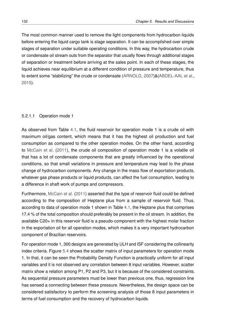
132 Chapter 5. Results and Discussions
The most common manner used to remove the light components from hydrocarbon liquids
before entering the liquid cargo tank is stage separation. It can be accomplished over simple
stages of separation under suitable operating conditions. In this way, the hydrocarbon crude
or condensate oil stream outs from the separator that usually flows through additional stages
of separation or treatment before arriving at the sales point. In each of these stages, the
liquid achieves near equilibrium at a different condition of pressure and temperature, thus
to extent some “stabilizing” the crude or condensate (ARNOLD, 2007)&(ABDEL-AAL et al.,
2015).
5.2.1.1 Operation mode 1
As observed from Table 4.1, the fluid reservoir for operation mode 1 is a crude oil with
maximum oil/gas content, which means that it has the highest oil production and fuel
consumption as compared to the other operation modes. On the other hand, according
to McCain et al. (2011), the crude oil composition of operation mode 1 is a volatile oil
that has a lot of condensate components that are greatly influenced by the operational
conditions, so that small variations in pressure and temperature may lead to the phase
change of hydrocarbon components. Any change in the mass flow of exportation products,
whatever gas phase products or liquid products, can affect the fuel consumption, leading to
a difference in shaft work of pumps and compressors.
Furthermore, McCain et al. (2011) asserted that the type of reservoir fluid could be defined
according to the composition of Heptane plus from a sample of reservoir fluid. Thus,
according to data of operation mode 1 shown in Table 4.1, the Heptane plus that comprises
17.4 % of the total composition should preferably be present in the oil stream. In addition, the
available C20+ in this reservoir fluid is a pseudo-component with the highest molar fraction
in the exportation oil for all operation modes, which makes it a very important hydrocarbon
component of Brazilian reservoirs.
For operation mode 1, 300 designs are generated by ULH and ISF considering the collinearity
index criteria. Figure 5.4 shows the scatter matrix of input parameters for operation mode
1. In that, it can be seen the Probability Density Function is practically uniform for all input
variables and it is not observed any correlation between 8 input variables. However, scatter
matrix show a relation among P1, P2 and P3, but it is because of the considered constraints.
As sequential pressure parameters must be lower than previous one, thus, regression line
has sensed a connecting between these pressure. Nevertheless, the design space can be
considered satisfactory to perform the screening analysis of those 8 input parameters in
terms of fuel consumption and the recovery of hydrocarbon liquids.
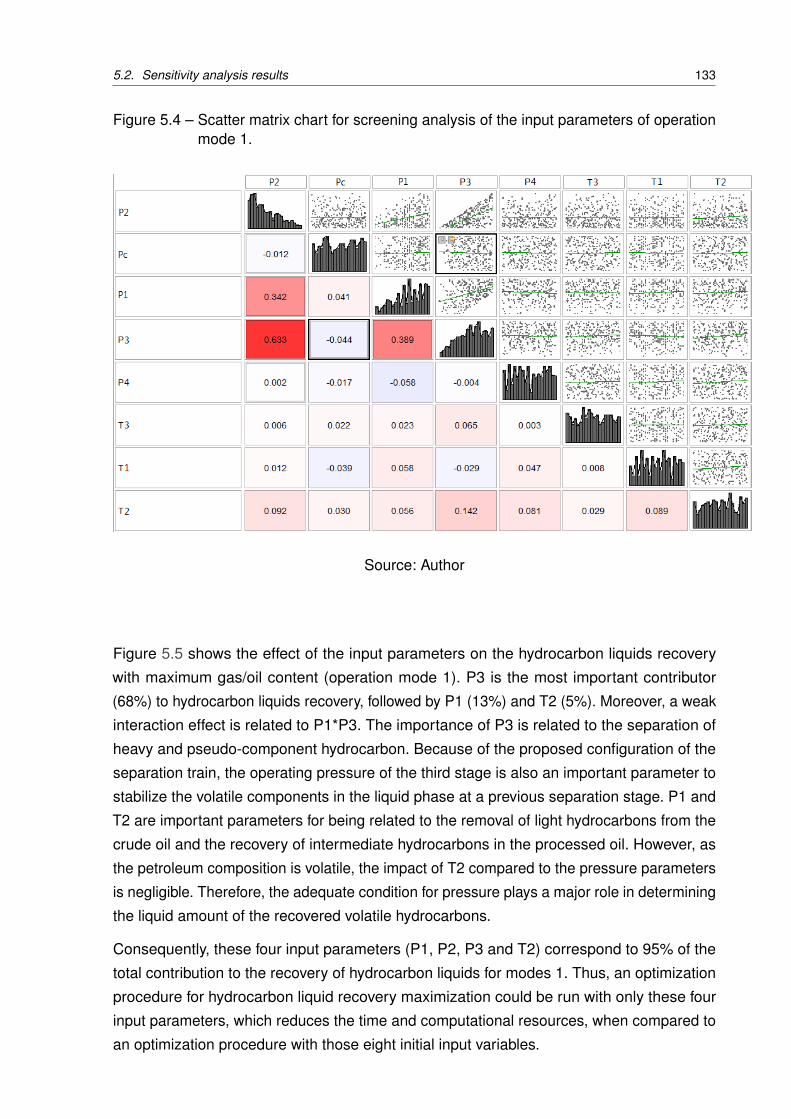
5.2. Sensitivity analysis results 133
Figure 5.4 – Scatter matrix chart for screening analysis of the input parameters of operationmode 1.
Source: Author
Figure 5.5 shows the effect of the input parameters on the hydrocarbon liquids recovery
with maximum gas/oil content (operation mode 1). P3 is the most important contributor
(68%) to hydrocarbon liquids recovery, followed by P1 (13%) and T2 (5%). Moreover, a weak
interaction effect is related to P1*P3. The importance of P3 is related to the separation of
heavy and pseudo-component hydrocarbon. Because of the proposed configuration of the
separation train, the operating pressure of the third stage is also an important parameter to
stabilize the volatile components in the liquid phase at a previous separation stage. P1 and
T2 are important parameters for being related to the removal of light hydrocarbons from the
crude oil and the recovery of intermediate hydrocarbons in the processed oil. However, as
the petroleum composition is volatile, the impact of T2 compared to the pressure parameters
is negligible. Therefore, the adequate condition for pressure plays a major role in determining
the liquid amount of the recovered volatile hydrocarbons.
Consequently, these four input parameters (P1, P2, P3 and T2) correspond to 95% of the
total contribution to the recovery of hydrocarbon liquids for modes 1. Thus, an optimization
procedure for hydrocarbon liquid recovery maximization could be run with only these four
input parameters, which reduces the time and computational resources, when compared to
an optimization procedure with those eight initial input variables.
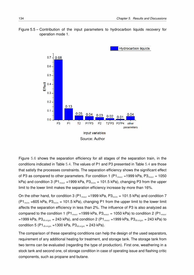
134 Chapter 5. Results and Discussions
Figure 5.5 – Contribution of the input parameters to hydrocarbon liquids recovery foroperation mode 1.
Source: Author
Figure 5.6 shows the separation efficiency for all stages of the separation train, in the
conditions indicated in Table 5.4. The values of P1 and P3 presented in Table 5.4 are those
that satisfy the processes constraints. The separation efficiency shows the significant effect
of P3 as compared to other parameters. For condition 1 (P1max =1999 kPa, P3max = 1050
kPa) and condition 3 (P1max =1999 kPa, P3min = 101.5 kPa), changing P3 from the upper
limit to the lower limit makes the separation efficiency increase by more than 16%.
On the other hand, for condition 3 (P1max =1999 kPa, P3min = 101.5 kPa) and condition 7
(P1min =605 kPa, P3min = 101.5 kPa), changing P1 from the upper limit to the lower limit
affects the separation efficiency in less than 2%. The influence of P3 is also analyzed as
compared to the condition 1 (P1max =1999 kPa, P3max = 1050 kPa) to condition 2 (P1max
=1999 kPa, P3design = 243 kPa), and condition 2 (P1max =1999 kPa, P3design = 243 kPa) to
condition 5 (P1design =1300 kPa, P3design = 243 kPa).
The comparison of these operating conditions can help the design of the used separators,
requirement of any additional heating for treatment, and storage tank. The storage tank from
two terms can be evaluated (regarding the type of production). First one, weathering in a
stock tank and second one, oil storage condition in case of operating issue and flashing critic
components, such as propane and butane.

5.2. Sensitivity analysis results 135
Figure 5.6 – Total separation efficiency for the conditions shown in Table 5.4.
Source: Author
Table 5.4 – Hypothetic conditions to perform separation efficiency
Conditions P1(kPa) P3(kPa)1 1999 10502 1999 2433 1999 101.54 1300 7905 1300 2436 1300 101.57 605 101.5
Figure 5.7 shows the molar fraction of C7+ in the exportation oil for the conditions shown in
Table 5.4. Similarly to Figure 5.6, the effect of P3 on C7+ is evident, yet the best condition
for separation efficiency is not necessarily the best condition (condition 6) for the maximum
stabilization of C7+. Considering the effect of the operating conditions on the intermediate
hydrocarbon separation that occurs at the second stage of separation, it is possible to state
that P1 =1300 kPa is a better operating pressure for all phase of products rather than 605
kPa.
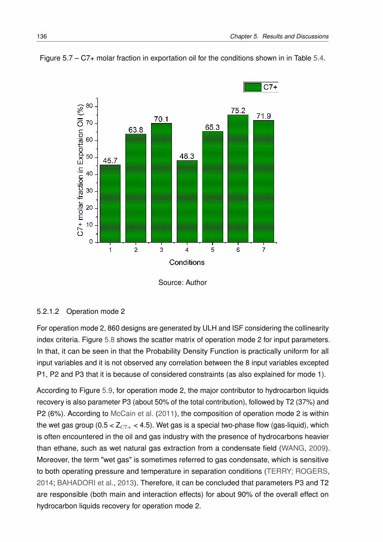
136 Chapter 5. Results and Discussions
Figure 5.7 – C7+ molar fraction in exportation oil for the conditions shown in in Table 5.4.
Source: Author
5.2.1.2 Operation mode 2
For operation mode 2, 860 designs are generated by ULH and ISF considering the collinearity
index criteria. Figure 5.8 shows the scatter matrix of operation mode 2 for input parameters.
In that, it can be seen in that the Probability Density Function is practically uniform for all
input variables and it is not observed any correlation between the 8 input variables excepted
P1, P2 and P3 that it is because of considered constraints (as also explained for mode 1).
According to Figure 5.9, for operation mode 2, the major contributor to hydrocarbon liquids
recovery is also parameter P3 (about 50% of the total contribution), followed by T2 (37%) and
P2 (6%). According to McCain et al. (2011), the composition of operation mode 2 is within
the wet gas group (0.5 < ZC7+ < 4.5). Wet gas is a special two-phase flow (gas-liquid), which
is often encountered in the oil and gas industry with the presence of hydrocarbons heavier
than ethane, such as wet natural gas extraction from a condensate field (WANG, 2009).
Moreover, the term "wet gas" is sometimes referred to gas condensate, which is sensitive
to both operating pressure and temperature in separation conditions (TERRY; ROGERS,
2014; BAHADORI et al., 2013). Therefore, it can be concluded that parameters P3 and T2
are responsible (both main and interaction effects) for about 90% of the overall effect on
hydrocarbon liquids recovery for operation mode 2.
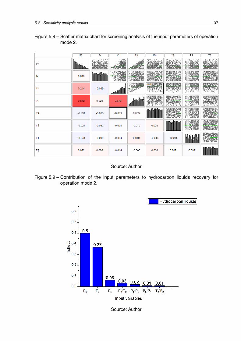
5.2. Sensitivity analysis results 137
Figure 5.8 – Scatter matrix chart for screening analysis of the input parameters of operationmode 2.
Source: Author
Figure 5.9 – Contribution of the input parameters to hydrocarbon liquids recovery foroperation mode 2.
Source: Author
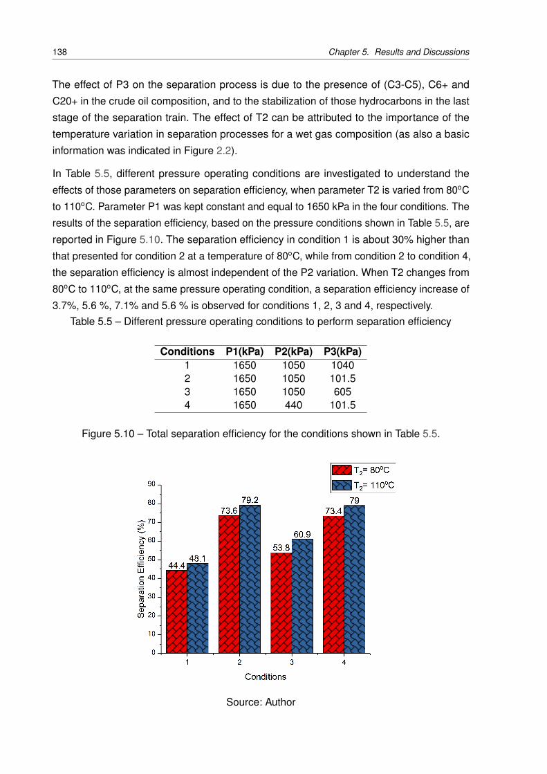
138 Chapter 5. Results and Discussions
The effect of P3 on the separation process is due to the presence of (C3-C5), C6+ and
C20+ in the crude oil composition, and to the stabilization of those hydrocarbons in the last
stage of the separation train. The effect of T2 can be attributed to the importance of the
temperature variation in separation processes for a wet gas composition (as also a basic
information was indicated in Figure 2.2).
In Table 5.5, different pressure operating conditions are investigated to understand the
effects of those parameters on separation efficiency, when parameter T2 is varied from 80oC
to 110oC. Parameter P1 was kept constant and equal to 1650 kPa in the four conditions. The
results of the separation efficiency, based on the pressure conditions shown in Table 5.5, are
reported in Figure 5.10. The separation efficiency in condition 1 is about 30% higher than
that presented for condition 2 at a temperature of 80oC, while from condition 2 to condition 4,
the separation efficiency is almost independent of the P2 variation. When T2 changes from
80oC to 110oC, at the same pressure operating condition, a separation efficiency increase of
3.7%, 5.6 %, 7.1% and 5.6 % is observed for conditions 1, 2, 3 and 4, respectively.Table 5.5 – Different pressure operating conditions to perform separation efficiency
Conditions P1(kPa) P2(kPa) P3(kPa)1 1650 1050 10402 1650 1050 101.53 1650 1050 6054 1650 440 101.5
Figure 5.10 – Total separation efficiency for the conditions shown in Table 5.5.
Source: Author
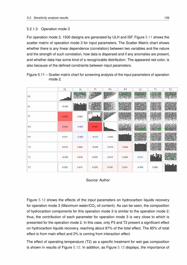
5.2. Sensitivity analysis results 139
5.2.1.3 Operation mode 3
For operation mode 3, 1500 designs are generated by ULH and ISF. Figure 5.11 shows the
scatter matrix of operation mode 3 for input parameters. The Scatter Matrix chart shows
whether there is any linear dependence (correlation) between two variables and the nature
and the strength of such correlation, how data is dispersed and if any anomalies are present,
and whether data has some kind of a recognizable distribution. The appeared red color, is
also because of the defined constraints between input parameters.
Figure 5.11 – Scatter matrix chart for screening analysis of the input parameters of operationmode 2.
Source: Author
Figure 5.12 shows the effects of the input parameters on hydrocarbon liquids recovery
for operation mode 3 (Maximum water/CO2 oil content). As can be seen, the composition
of hydrocarbon components for this operation mode 3 is similar to the operation mode 2;
thus, the contribution of each parameter for operation mode 3 is very close to which is
presented for the operation mode 2. In this case, only P3 and T2 present a significant effect
on hydrocarbon liquids recovery, reaching about 87% of the total effect. The 85% of total
effect is from main effect and 2% is coming from interaction effect.
The effect of operating temperature (T2) as a specific treatment for wet gas composition
is shown in results of Figure 5.12. In addition, as Figure 5.12 displays, the importance of
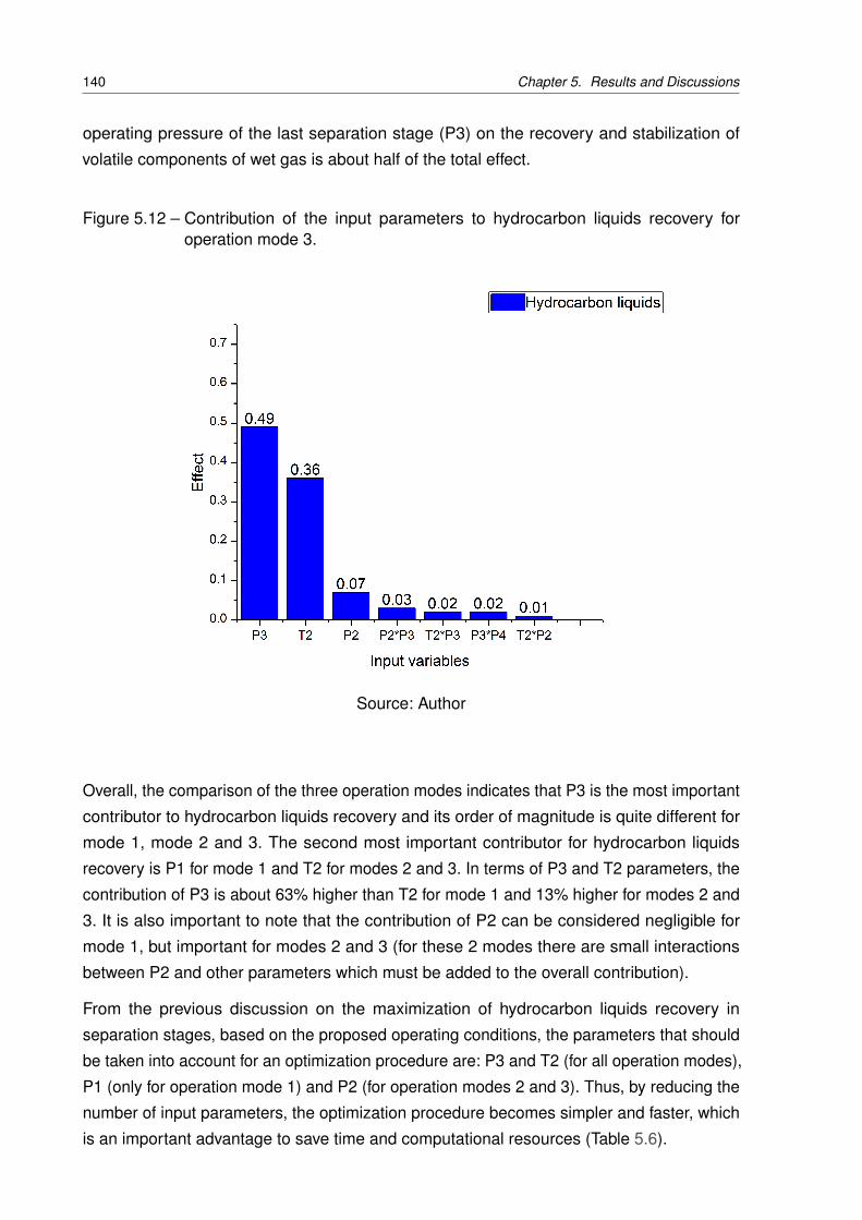
140 Chapter 5. Results and Discussions
operating pressure of the last separation stage (P3) on the recovery and stabilization of
volatile components of wet gas is about half of the total effect.
Figure 5.12 – Contribution of the input parameters to hydrocarbon liquids recovery foroperation mode 3.
Source: Author
Overall, the comparison of the three operation modes indicates that P3 is the most important
contributor to hydrocarbon liquids recovery and its order of magnitude is quite different for
mode 1, mode 2 and 3. The second most important contributor for hydrocarbon liquids
recovery is P1 for mode 1 and T2 for modes 2 and 3. In terms of P3 and T2 parameters, the
contribution of P3 is about 63% higher than T2 for mode 1 and 13% higher for modes 2 and
3. It is also important to note that the contribution of P2 can be considered negligible for
mode 1, but important for modes 2 and 3 (for these 2 modes there are small interactions
between P2 and other parameters which must be added to the overall contribution).
From the previous discussion on the maximization of hydrocarbon liquids recovery in
separation stages, based on the proposed operating conditions, the parameters that should
be taken into account for an optimization procedure are: P3 and T2 (for all operation modes),
P1 (only for operation mode 1) and P2 (for operation modes 2 and 3). Thus, by reducing the
number of input parameters, the optimization procedure becomes simpler and faster, which
is an important advantage to save time and computational resources (Table 5.6).
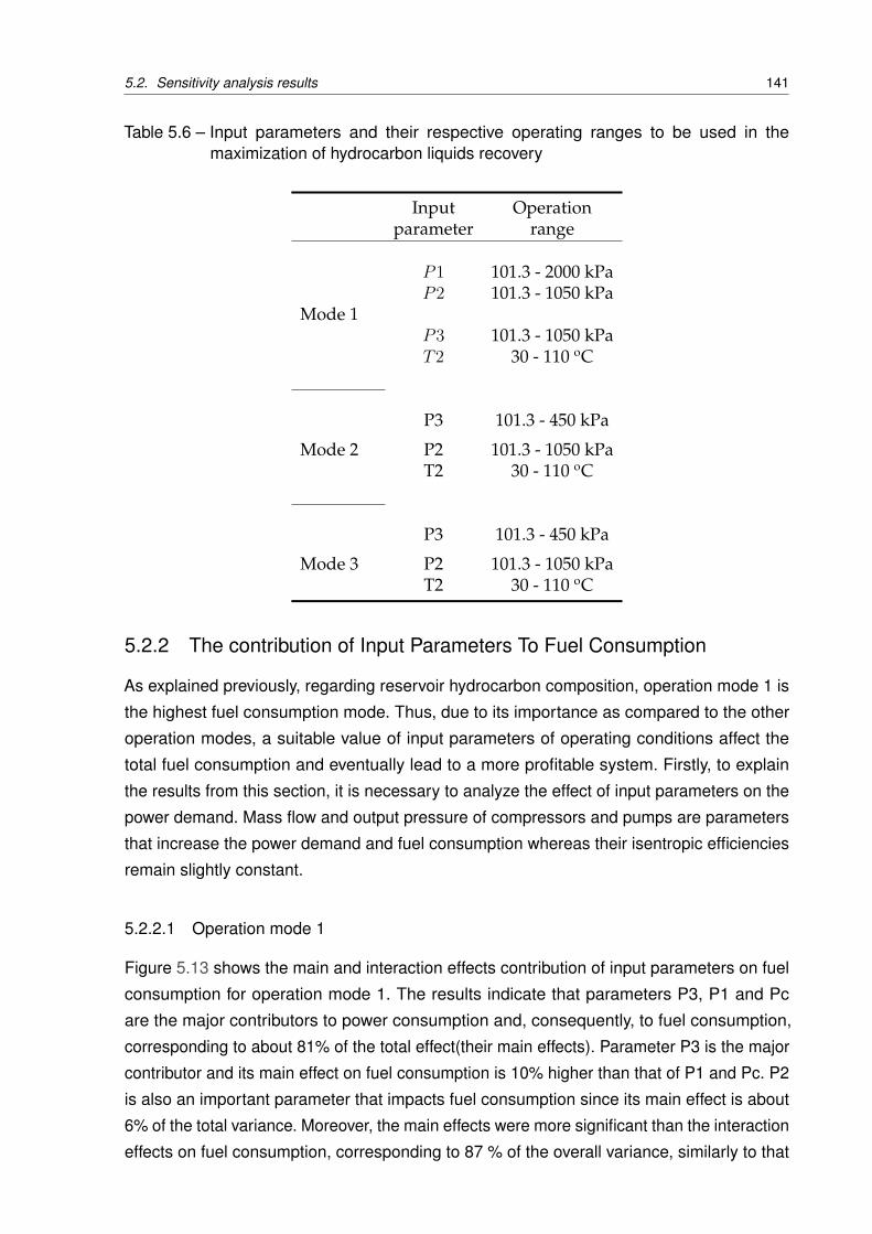
5.2. Sensitivity analysis results 141
Table 5.6 – Input parameters and their respective operating ranges to be used in themaximization of hydrocarbon liquids recovery
Input Operationparameter range
P1 101.3 - 2000 kPaP2 101.3 - 1050 kPa
Mode 1P3 101.3 - 1050 kPaT2 30 - 110 oC
P3 101.3 - 450 kPa
Mode 2 P2 101.3 - 1050 kPaT2 30 - 110 oC
P3 101.3 - 450 kPa
Mode 3 P2 101.3 - 1050 kPaT2 30 - 110 oC
5.2.2 The contribution of Input Parameters To Fuel Consumption
As explained previously, regarding reservoir hydrocarbon composition, operation mode 1 is
the highest fuel consumption mode. Thus, due to its importance as compared to the other
operation modes, a suitable value of input parameters of operating conditions affect the
total fuel consumption and eventually lead to a more profitable system. Firstly, to explain
the results from this section, it is necessary to analyze the effect of input parameters on the
power demand. Mass flow and output pressure of compressors and pumps are parameters
that increase the power demand and fuel consumption whereas their isentropic efficiencies
remain slightly constant.
5.2.2.1 Operation mode 1
Figure 5.13 shows the main and interaction effects contribution of input parameters on fuel
consumption for operation mode 1. The results indicate that parameters P3, P1 and Pc
are the major contributors to power consumption and, consequently, to fuel consumption,
corresponding to about 81% of the total effect(their main effects). Parameter P3 is the major
contributor and its main effect on fuel consumption is 10% higher than that of P1 and Pc. P2
is also an important parameter that impacts fuel consumption since its main effect is about
6% of the total variance. Moreover, the main effects were more significant than the interaction
effects on fuel consumption, corresponding to 87 % of the overall variance, similarly to that
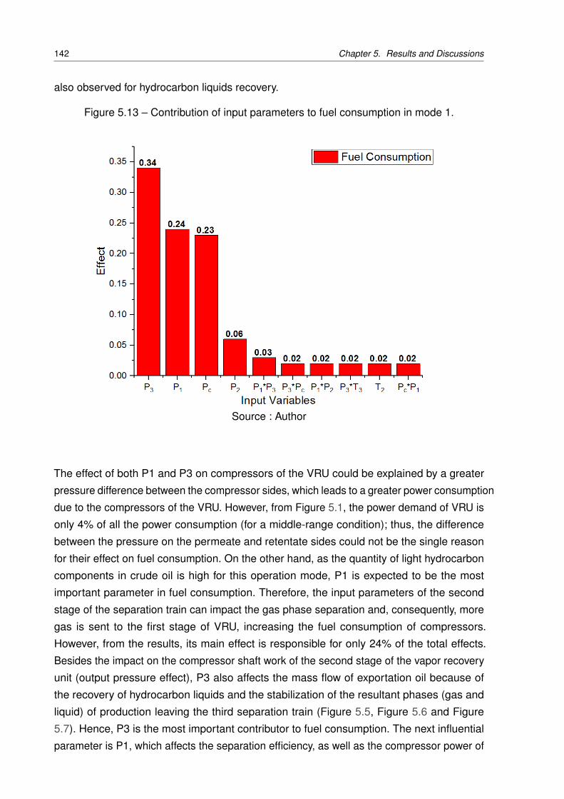
142 Chapter 5. Results and Discussions
also observed for hydrocarbon liquids recovery.
Figure 5.13 – Contribution of input parameters to fuel consumption in mode 1.
Source : Author
The effect of both P1 and P3 on compressors of the VRU could be explained by a greater
pressure difference between the compressor sides, which leads to a greater power consumption
due to the compressors of the VRU. However, from Figure 5.1, the power demand of VRU is
only 4% of all the power consumption (for a middle-range condition); thus, the difference
between the pressure on the permeate and retentate sides could not be the single reason
for their effect on fuel consumption. On the other hand, as the quantity of light hydrocarbon
components in crude oil is high for this operation mode, P1 is expected to be the most
important parameter in fuel consumption. Therefore, the input parameters of the second
stage of the separation train can impact the gas phase separation and, consequently, more
gas is sent to the first stage of VRU, increasing the fuel consumption of compressors.
However, from the results, its main effect is responsible for only 24% of the total effects.
Besides the impact on the compressor shaft work of the second stage of the vapor recovery
unit (output pressure effect), P3 also affects the mass flow of exportation oil because of
the recovery of hydrocarbon liquids and the stabilization of the resultant phases (gas and
liquid) of production leaving the third separation train (Figure 5.5, Figure 5.6 and Figure
5.7). Hence, P3 is the most important contributor to fuel consumption. The next influential
parameter is P1, which affects the separation efficiency, as well as the compressor power of
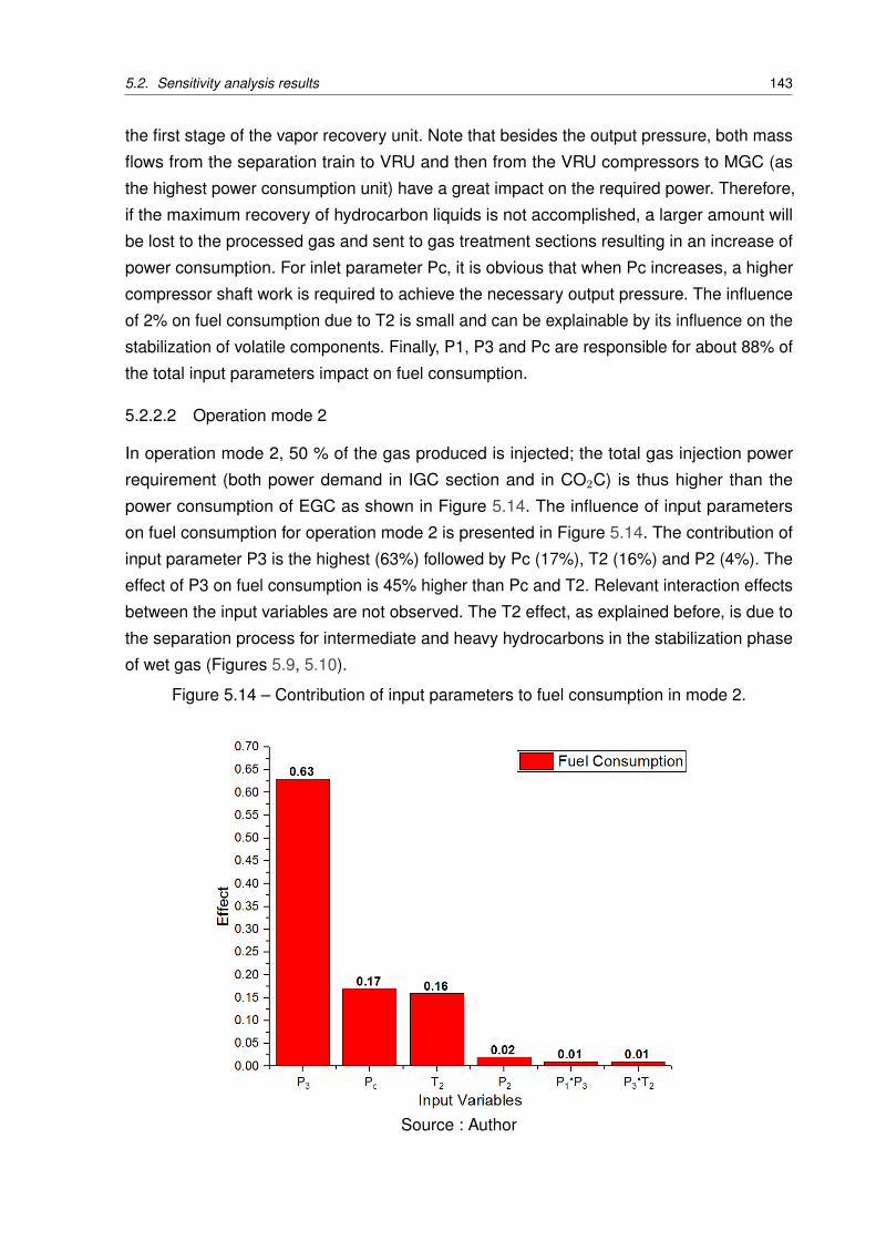
5.2. Sensitivity analysis results 143
the first stage of the vapor recovery unit. Note that besides the output pressure, both mass
flows from the separation train to VRU and then from the VRU compressors to MGC (as
the highest power consumption unit) have a great impact on the required power. Therefore,
if the maximum recovery of hydrocarbon liquids is not accomplished, a larger amount will
be lost to the processed gas and sent to gas treatment sections resulting in an increase of
power consumption. For inlet parameter Pc, it is obvious that when Pc increases, a higher
compressor shaft work is required to achieve the necessary output pressure. The influence
of 2% on fuel consumption due to T2 is small and can be explainable by its influence on the
stabilization of volatile components. Finally, P1, P3 and Pc are responsible for about 88% of
the total input parameters impact on fuel consumption.
5.2.2.2 Operation mode 2
In operation mode 2, 50 % of the gas produced is injected; the total gas injection power
requirement (both power demand in IGC section and in CO2C) is thus higher than the
power consumption of EGC as shown in Figure 5.14. The influence of input parameters
on fuel consumption for operation mode 2 is presented in Figure 5.14. The contribution of
input parameter P3 is the highest (63%) followed by Pc (17%), T2 (16%) and P2 (4%). The
effect of P3 on fuel consumption is 45% higher than Pc and T2. Relevant interaction effects
between the input variables are not observed. The T2 effect, as explained before, is due to
the separation process for intermediate and heavy hydrocarbons in the stabilization phase
of wet gas (Figures 5.9, 5.10).
Figure 5.14 – Contribution of input parameters to fuel consumption in mode 2.
Source : Author
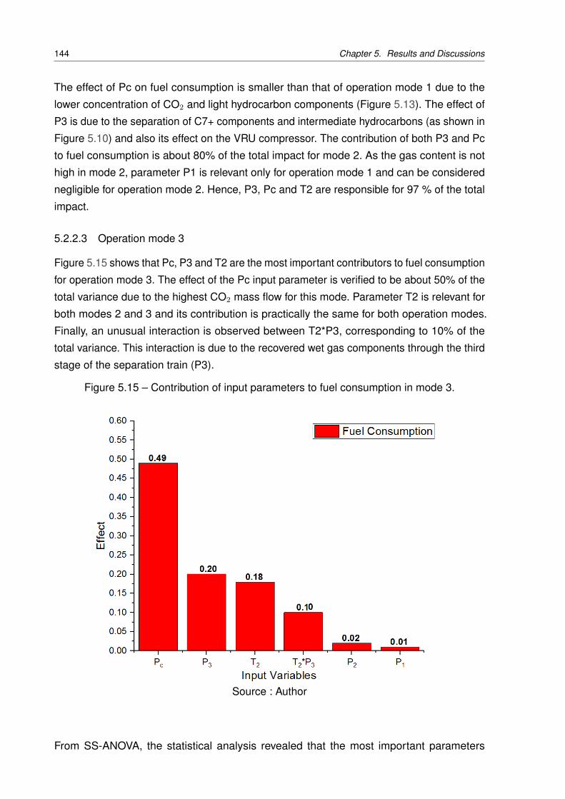
144 Chapter 5. Results and Discussions
The effect of Pc on fuel consumption is smaller than that of operation mode 1 due to the
lower concentration of CO2 and light hydrocarbon components (Figure 5.13). The effect of
P3 is due to the separation of C7+ components and intermediate hydrocarbons (as shown in
Figure 5.10) and also its effect on the VRU compressor. The contribution of both P3 and Pc
to fuel consumption is about 80% of the total impact for mode 2. As the gas content is not
high in mode 2, parameter P1 is relevant only for operation mode 1 and can be considered
negligible for operation mode 2. Hence, P3, Pc and T2 are responsible for 97 % of the total
impact.
5.2.2.3 Operation mode 3
Figure 5.15 shows that Pc, P3 and T2 are the most important contributors to fuel consumption
for operation mode 3. The effect of the Pc input parameter is verified to be about 50% of the
total variance due to the highest CO2 mass flow for this mode. Parameter T2 is relevant for
both modes 2 and 3 and its contribution is practically the same for both operation modes.
Finally, an unusual interaction is observed between T2*P3, corresponding to 10% of the
total variance. This interaction is due to the recovered wet gas components through the third
stage of the separation train (P3).
Figure 5.15 – Contribution of input parameters to fuel consumption in mode 3.
Source : Author
From SS-ANOVA, the statistical analysis revealed that the most important parameters
5.2. Sensitivity analysis results 145
affecting the fuel consumption of the plant for three operation mode are shown in Table
5.7, these most effective of input parameters correspond to 96%, 97% and 97% of the total
contribution to fuel consumption for modes 1, 2 and 3, respectively. Thus, an optimization
procedure for fuel consumption minimization could be run with only these input parameters,
which reduces the time and computational resources, when compared to an optimization
procedure with those eight initial input variables.
Table 5.7 – Input parameters and their respective operating ranges to be used in theoptimization procedure of fuel consumption minimization
Input Operationparameter range
P1 101.3 - 2000 kPaP2 101.3 - 1050 kPa
Mode 1P3 101.3 - 1050 kPaPc 7018 - 8500 kPa
P3 101.3 - 450 kPa = P2
Mode 2 Pc 7018 - 8500 kPaT2 30 - 110 oC
P3 101.3 - 450 kPa = P2
Mode 3 Pc 7018 - 8500 kPaT2 30 - 110 oC
Figure 5.16 shows the contribution of input pressure and temperature parameters on FPSO
process and utility units. Ps and Ts represent the operating pressures and temperatures, and
1,2 and 3 are the numbers of each stage. The green, orange, red and black lines are liquid
flow, gas flow, temperature, and pressure effects, respectively. The gray line presents the
power demand. In that, the input parameters directly influence the separation train stages.
The separated gas flow and liquid flow affect the separation train stages, VRU stages and
MGC.The discharge pressure of MGC from operating pressures changes the power demand
of MGC. Next, the separated volatile components as gas flow from separation stages form
liquid in Hydrocarbon dew point control system (HDP) and the liquid flow is forwarded to the
second stage of VRU. Then, after passing through heat exchanger and separator’s VRU,
the separated gas components are routed to MGC. In following, the remaining hydrocarbon
liquids go to separation train.
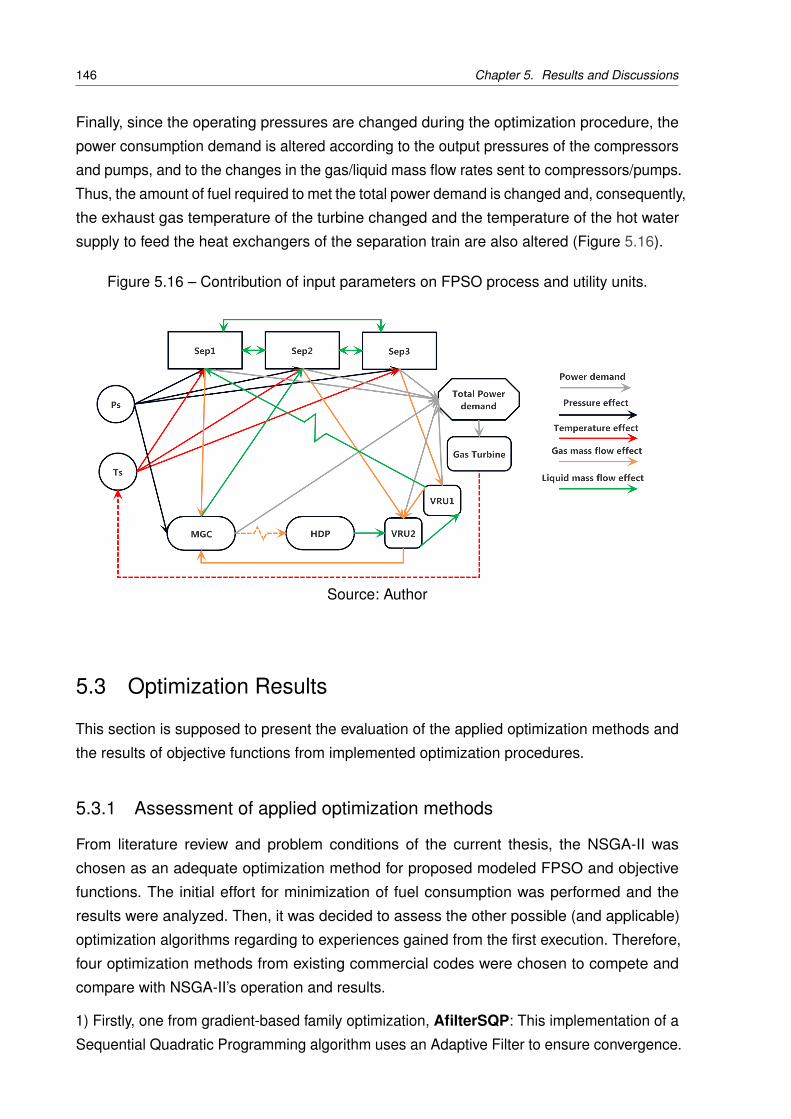
146 Chapter 5. Results and Discussions
Finally, since the operating pressures are changed during the optimization procedure, the
power consumption demand is altered according to the output pressures of the compressors
and pumps, and to the changes in the gas/liquid mass flow rates sent to compressors/pumps.
Thus, the amount of fuel required to met the total power demand is changed and, consequently,
the exhaust gas temperature of the turbine changed and the temperature of the hot water
supply to feed the heat exchangers of the separation train are also altered (Figure 5.16).
Figure 5.16 – Contribution of input parameters on FPSO process and utility units.
Source: Author
5.3 Optimization Results
This section is supposed to present the evaluation of the applied optimization methods and
the results of objective functions from implemented optimization procedures.
5.3.1 Assessment of applied optimization methods
From literature review and problem conditions of the current thesis, the NSGA-II was
chosen as an adequate optimization method for proposed modeled FPSO and objective
functions. The initial effort for minimization of fuel consumption was performed and the
results were analyzed. Then, it was decided to assess the other possible (and applicable)
optimization algorithms regarding to experiences gained from the first execution. Therefore,
four optimization methods from existing commercial codes were chosen to compete and
compare with NSGA-II’s operation and results.
1) Firstly, one from gradient-based family optimization, AfilterSQP: This implementation of a
Sequential Quadratic Programming algorithm uses an Adaptive Filter to ensure convergence.

5.3. Optimization Results 147
The adaptive filter helps achieve convergence starting from a random point in the search
space. AfilterSQP formulates a quadratic programming (QP) problem, a line search is
performed along the computed direction and the adaptive filter checks whether the point
can be accepted. The adaptive filter helps achieve convergence starting from a random
point in the search space. It considers the entire history of the current optimization run
and accepts a new point only if it is not dominated by a previously computed point (Esteco
SPA, 2017). Furthermore, because of the several numbers of accomplished works using
the SQP methods in optimization of chemical and processing cycles, SQP was chosen. On
the other hand, the current developed SQP can be implemented for both objective function
and constraint satisfaction and it handles constraints by applying the Lagrange Multipliers
methods. The maximization of hydrocarbon liquids of operating mode 1 as the objective
function was defined and 8000 space designs were appointed as the maximum number of
design evaluation.
As Figure 5.17 displays, after approximately 500 designs (with 200 designs of initial DoE),
the optimization procedure is not converged and stopped. Therefore, it was found that SQP
(or any modified one) is individually not suitable for this problem.
Figure 5.17 – SQP convergence curve for the function of hydrocarbon liquids recoverymaximization.
Source : Author
2) Simplex: The considered Simplex optimization algorithm implemented here is the
Nelder-Mead or downhill simplex method. It does not compute derivatives, which makes it
more robust than gradient-based methods and suitable for problems with noisy functions.
This heuristic algorithm uses the concept of a simplex, which is a polyhedron with N+1
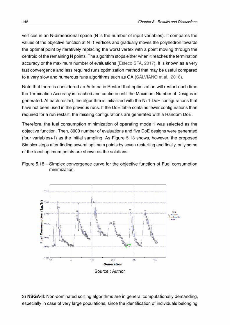
148 Chapter 5. Results and Discussions
vertices in an N-dimensional space (N is the number of input variables). It compares the
values of the objective function at N+1 vertices and gradually moves the polyhedron towards
the optimal point by iteratively replacing the worst vertex with a point moving through the
centroid of the remaining N points. The algorithm stops either when it reaches the termination
accuracy or the maximum number of evaluations (Esteco SPA, 2017). It is known as a very
fast convergence and less required runs optimization method that may be useful compared
to a very slow and numerous runs algorithms such as GA (SALVIANO et al., 2016).
Note that there is considered an Automatic Restart that optimization will restart each time
the Termination Accuracy is reached and continue until the Maximum Number of Designs is
generated. At each restart, the algorithm is initialized with the N+1 DoE configurations that
have not been used in the previous runs. If the DoE table contains fewer configurations than
required for a run restart, the missing configurations are generated with a Random DoE.
Therefore, the fuel consumption minimization of operating mode 1 was selected as the
objective function. Then, 8000 number of evaluations and five DoE designs were generated
(four variables+1) as the initial sampling. As Figure 5.18 shows, however, the proposed
Simplex stops after finding several optimum points by seven restarting and finally, only some
of the local optimum points are shown as the solutions.
Figure 5.18 – Simplex convergence curve for the objective function of Fuel consumptionminimization.
Source : Author
3) NSGA-II: Non-dominated sorting algorithms are in general computationally demanding,
especially in case of very large populations, since the identification of individuals belonging
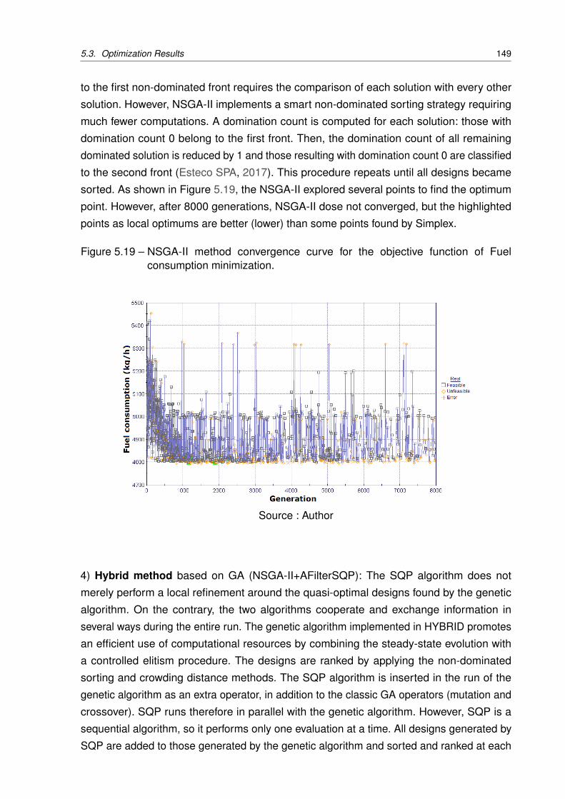
5.3. Optimization Results 149
to the first non-dominated front requires the comparison of each solution with every other
solution. However, NSGA-II implements a smart non-dominated sorting strategy requiring
much fewer computations. A domination count is computed for each solution: those with
domination count 0 belong to the first front. Then, the domination count of all remaining
dominated solution is reduced by 1 and those resulting with domination count 0 are classified
to the second front (Esteco SPA, 2017). This procedure repeats until all designs became
sorted. As shown in Figure 5.19, the NSGA-II explored several points to find the optimum
point. However, after 8000 generations, NSGA-II dose not converged, but the highlighted
points as local optimums are better (lower) than some points found by Simplex.
Figure 5.19 – NSGA-II method convergence curve for the objective function of Fuelconsumption minimization.
Source : Author
4) Hybrid method based on GA (NSGA-II+AFilterSQP): The SQP algorithm does not
merely perform a local refinement around the quasi-optimal designs found by the genetic
algorithm. On the contrary, the two algorithms cooperate and exchange information in
several ways during the entire run. The genetic algorithm implemented in HYBRID promotes
an efficient use of computational resources by combining the steady-state evolution with
a controlled elitism procedure. The designs are ranked by applying the non-dominated
sorting and crowding distance methods. The SQP algorithm is inserted in the run of the
genetic algorithm as an extra operator, in addition to the classic GA operators (mutation and
crossover). SQP runs therefore in parallel with the genetic algorithm. However, SQP is a
sequential algorithm, so it performs only one evaluation at a time. All designs generated by
SQP are added to those generated by the genetic algorithm and sorted and ranked at each
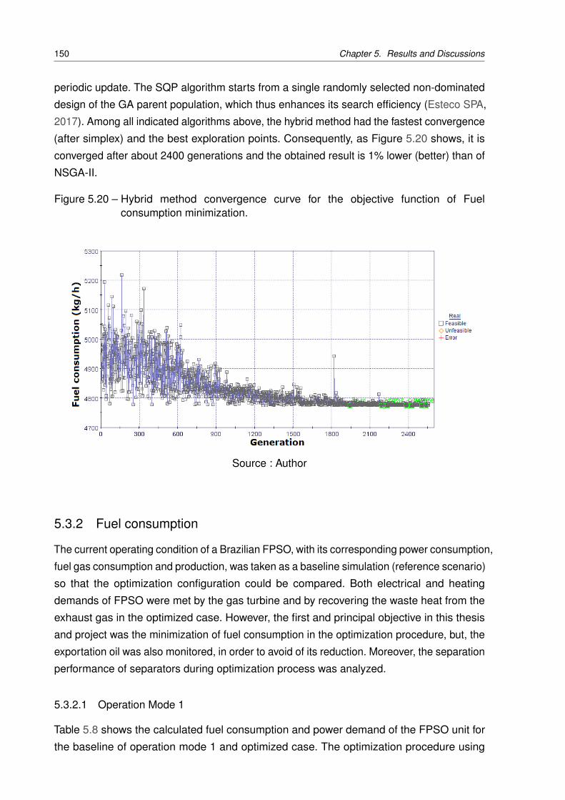
150 Chapter 5. Results and Discussions
periodic update. The SQP algorithm starts from a single randomly selected non-dominated
design of the GA parent population, which thus enhances its search efficiency (Esteco SPA,
2017). Among all indicated algorithms above, the hybrid method had the fastest convergence
(after simplex) and the best exploration points. Consequently, as Figure 5.20 shows, it is
converged after about 2400 generations and the obtained result is 1% lower (better) than of
NSGA-II.
Figure 5.20 – Hybrid method convergence curve for the objective function of Fuelconsumption minimization.
Source : Author
5.3.2 Fuel consumption
The current operating condition of a Brazilian FPSO, with its corresponding power consumption,
fuel gas consumption and production, was taken as a baseline simulation (reference scenario)
so that the optimization configuration could be compared. Both electrical and heating
demands of FPSO were met by the gas turbine and by recovering the waste heat from the
exhaust gas in the optimized case. However, the first and principal objective in this thesis
and project was the minimization of fuel consumption in the optimization procedure, but, the
exportation oil was also monitored, in order to avoid of its reduction. Moreover, the separation
performance of separators during optimization process was analyzed.
5.3.2.1 Operation Mode 1
Table 5.8 shows the calculated fuel consumption and power demand of the FPSO unit for
the baseline of operation mode 1 and optimized case. The optimization procedure using
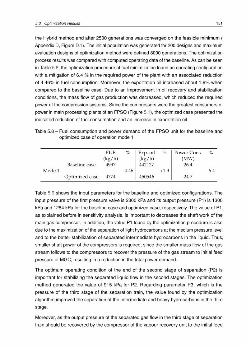
5.3. Optimization Results 151
the Hybrid method and after 2500 generations was converged on the feasible minimum (
Appendix D, Figure D.1). The initial population was generated for 200 designs and maximum
evaluation designs of optimization method were defined 8000 generations. The optimization
process results was compared with computed operating data of the baseline. As can be seen
in Table 5.8, the optimization procedure of fuel minimization found an operating configuration
with a mitigation of 6.4 % in the required power of the plant with an associated reduction
of 4.46% in fuel consumption. Moreover, the exportation oil increased about 1.9% when
compared to the baseline case. Due to an improvement in oil recovery and stabilization
conditions, the mass flow of gas production was decreased, which reduced the required
power of the compression systems. Since the compressors were the greatest consumers of
power in main processing plants of an FPSO (Figure 5.1), the optimized case presented the
indicated reduction of fuel consumption and an increase in exportation oil.
Table 5.8 – Fuel consumption and power demand of the FPSO unit for the baseline andoptimized case of operation mode 1
FUE % Exp. oil % Power Cons. %(kg/h) (kg/h) (MW)
Baseline case 4997 442127 26.4Mode 1 -4.46 +1.9 -6.4
Optimized case 4774 450546 24.7
Table 5.9 shows the input parameters for the baseline and optimized configurations. The
input pressure of the first pressure valve is 2300 kPa and its output pressure (P1) is 1300
kPa and 1284 kPa for the baseline case and optimized case, respectively. The value of P1,
as explained before in sensitivity analysis, is important to decreases the shaft work of the
main gas compressor. In addition, the value P1 found by the optimization procedure is also
due to the maximization of the separation of light hydrocarbons at the medium pressure level
and to the better stabilization of separated intermediate hydrocarbons in the liquid. Thus,
smaller shaft power of the compressors is required, since the smaller mass flow of the gas
stream follows to the compressors to recover the pressure of the gas stream to initial feed
pressure of MGC, resulting in a reduction in the total power demand.
The optimum operating condition of the end of the second stage of separation (P2) is
important for stabilizing the separated liquid flow in the second stages. The optimization
method generated the value of 915 kPa for P2. Regarding parameter P3, which is the
pressure of the third stage of the separation train, the value found by the optimization
algorithm improved the separation of the intermediate and heavy hydrocarbons in the third
stage.
Moreover, as the output pressure of the separated gas flow in the third stage of separation
train should be recovered by the compressor of the vapour recovery unit to the initial feed
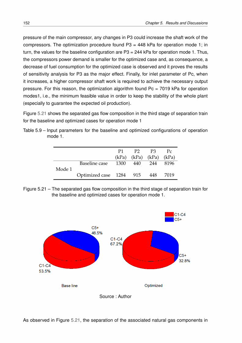
152 Chapter 5. Results and Discussions
pressure of the main compressor, any changes in P3 could increase the shaft work of the
compressors. The optimization procedure found P3 = 448 kPa for operation mode 1; in
turn, the values for the baseline configuration are P3 = 244 kPa for operation mode 1. Thus,
the compressors power demand is smaller for the optimized case and, as consequence, a
decrease of fuel consumption for the optimized case is observed and it proves the results
of sensitivity analysis for P3 as the major effect. Finally, for inlet parameter of Pc, when
it increases, a higher compressor shaft work is required to achieve the necessary output
pressure. For this reason, the optimization algorithm found Pc = 7019 kPa for operation
modes1, i.e., the minimum feasible value in order to keep the stability of the whole plant
(especially to guarantee the expected oil production).
Figure 5.21 shows the separated gas flow composition in the third stage of separation train
for the baseline and optimized cases for operation mode 1
Table 5.9 – Input parameters for the baseline and optimized configurations of operationmode 1.
P1 P2 P3 Pc(kPa) (kPa) (kPa) (kPa)
Baseline case 1300 440 244 8196Mode 1
Optimized case 1284 915 448 7019
Figure 5.21 – The separated gas flow composition in the third stage of separation train forthe baseline and optimized cases for operation mode 1.
Source : Author
As observed in Figure 5.21, the separation of the associated natural gas components in
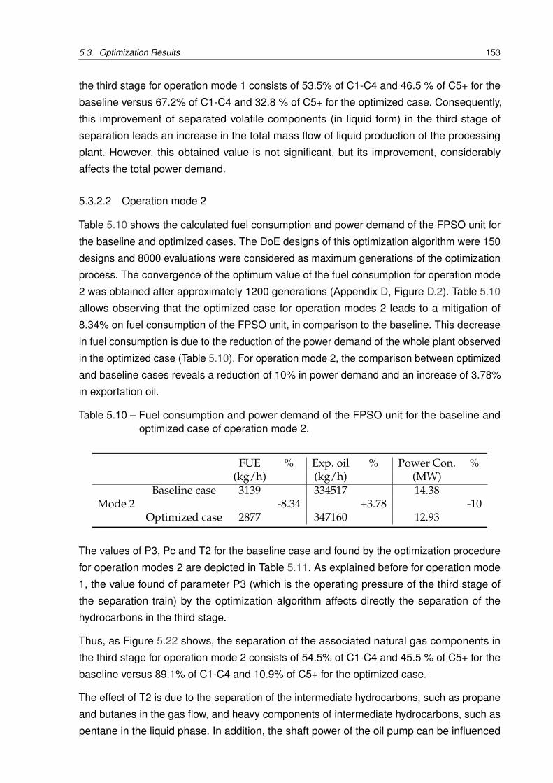
5.3. Optimization Results 153
the third stage for operation mode 1 consists of 53.5% of C1-C4 and 46.5 % of C5+ for the
baseline versus 67.2% of C1-C4 and 32.8 % of C5+ for the optimized case. Consequently,
this improvement of separated volatile components (in liquid form) in the third stage of
separation leads an increase in the total mass flow of liquid production of the processing
plant. However, this obtained value is not significant, but its improvement, considerably
affects the total power demand.
5.3.2.2 Operation mode 2
Table 5.10 shows the calculated fuel consumption and power demand of the FPSO unit for
the baseline and optimized cases. The DoE designs of this optimization algorithm were 150
designs and 8000 evaluations were considered as maximum generations of the optimization
process. The convergence of the optimum value of the fuel consumption for operation mode
2 was obtained after approximately 1200 generations (Appendix D, Figure D.2). Table 5.10
allows observing that the optimized case for operation modes 2 leads to a mitigation of
8.34% on fuel consumption of the FPSO unit, in comparison to the baseline. This decrease
in fuel consumption is due to the reduction of the power demand of the whole plant observed
in the optimized case (Table 5.10). For operation mode 2, the comparison between optimized
and baseline cases reveals a reduction of 10% in power demand and an increase of 3.78%
in exportation oil.
Table 5.10 – Fuel consumption and power demand of the FPSO unit for the baseline andoptimized case of operation mode 2.
FUE % Exp. oil % Power Con. %(kg/h) (kg/h) (MW)
Baseline case 3139 334517 14.38Mode 2 -8.34 +3.78 -10
Optimized case 2877 347160 12.93
The values of P3, Pc and T2 for the baseline case and found by the optimization procedure
for operation modes 2 are depicted in Table 5.11. As explained before for operation mode
1, the value found of parameter P3 (which is the operating pressure of the third stage of
the separation train) by the optimization algorithm affects directly the separation of the
hydrocarbons in the third stage.
Thus, as Figure 5.22 shows, the separation of the associated natural gas components in
the third stage for operation mode 2 consists of 54.5% of C1-C4 and 45.5 % of C5+ for the
baseline versus 89.1% of C1-C4 and 10.9% of C5+ for the optimized case.
The effect of T2 is due to the separation of the intermediate hydrocarbons, such as propane
and butanes in the gas flow, and heavy components of intermediate hydrocarbons, such as
pentane in the liquid phase. In addition, the shaft power of the oil pump can be influenced
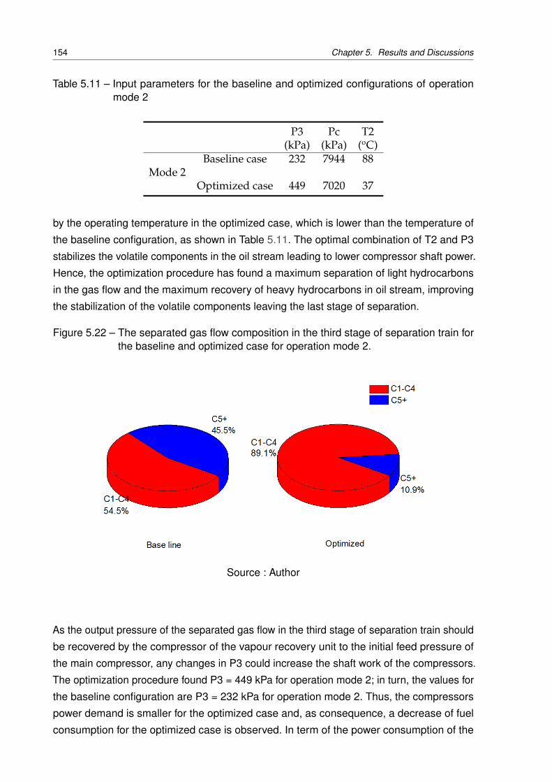
154 Chapter 5. Results and Discussions
Table 5.11 – Input parameters for the baseline and optimized configurations of operationmode 2
P3 Pc T2(kPa) (kPa) (oC)
Baseline case 232 7944 88Mode 2
Optimized case 449 7020 37
by the operating temperature in the optimized case, which is lower than the temperature of
the baseline configuration, as shown in Table 5.11. The optimal combination of T2 and P3
stabilizes the volatile components in the oil stream leading to lower compressor shaft power.
Hence, the optimization procedure has found a maximum separation of light hydrocarbons
in the gas flow and the maximum recovery of heavy hydrocarbons in oil stream, improving
the stabilization of the volatile components leaving the last stage of separation.
Figure 5.22 – The separated gas flow composition in the third stage of separation train forthe baseline and optimized case for operation mode 2.
Source : Author
As the output pressure of the separated gas flow in the third stage of separation train should
be recovered by the compressor of the vapour recovery unit to the initial feed pressure of
the main compressor, any changes in P3 could increase the shaft work of the compressors.
The optimization procedure found P3 = 449 kPa for operation mode 2; in turn, the values for
the baseline configuration are P3 = 232 kPa for operation mode 2. Thus, the compressors
power demand is smaller for the optimized case and, as consequence, a decrease of fuel
consumption for the optimized case is observed. In term of the power consumption of the

5.3. Optimization Results 155
main compressors and inlet parameter Pc, when it increases, a higher compressor shaft
work is required to achieve the necessary output pressure. For this reason, the optimization
algorithm found Pc = 7020 kPa, considering the minimum feasible value in order to keep the
stability of the all processing plant that is check by the process simulator.
5.3.2.3 Operation mode 3
Table 5.12 shows the calculated fuel consumption and also power demand of the FPSO
unit for the baseline and optimized cases of operation mode 3. In that, there is a mitigation
of 2.43 % on the FPSO units fuel consumption, in comparison to the baseline. It is also
observed in Table 5.12 that the comparison between optimized and baseline cases reveals a
reduction of 2.9% in power demand for operation mode 3. In addition, an increase of 1.7% in
exportation oil mass flow of optimized case is reported compared to the baseline case. The
DoE designs of this optimization algorithm were 150 designs and 8000 evaluations were
considered as maximum generations of the optimization process. The convergence of the
optimum value of fuel consumption for operation mode 3 was obtained after approximately
3000 generations (Appendix D, Figure D.3).
Table 5.12 – Fuel consumption and power demand of the FPSO unit for the baseline andoptimized case of operation mode 3.
FUE % Exp. oil % Power Con. %(kg/h) (kg/h) (MW)
Baseline case 3201 148610 14.72Mode 3 -2.43 +1.7 -2.9
Optimized case 3123 151138 14.29
The values of input parameters for the baseline and optimized configurations of operation
mode 3 is shown in Table 5.13. There, except the operating temperature of the second stage
of separation train (T2), the value of optimization procedure for other parameters are almost
the same with operation mode 2. It is because of very close hydrocarbons composition
among operation mode 2 and operation mode 3.
According to McCain et al. (2011) and the explanations in previous chapters, the compositions
of operation modes 2 and 3 are included in the wet gas group. Wet gas is a special two-phase
flow (gas-liquid) with volatile components which is often encountered in condensate compositions.
Thus, the optimal combination of T2 and P3 stabilizes the volatile components in the oil
stream leading to lower compressor shaft power. Hence, the optimization procedure has
found a maximum separation of light hydrocarbons in the gas flow and the maximum recovery
of heavy hydrocarbons in oil stream, improving the stabilization of the volatile components
leaving the last stage of separation. However, the volatile components of wet gas compared to
156 Chapter 5. Results and Discussions
condensate oil is fewer and this behavior is used in hydrocarbon liquids recovery subsection
to maximize the exportation oil.
Table 5.13 – Input parameters for the baseline and optimized configurations of operationmode 3
P3 Pc T2(kPa) (kPa) (oC)
Baseline case 229 7287 88Mode 3
Optimized case 447 7020 48
In operation mode 3, the separation of the associated natural gas in the third stage is 64.2%
of C1-C4 and 35.8 % of C5+ for the baseline versus 87.5% of C1-C4 and 12.5% of C5+ of
the optimized case (Figure 5.23).
Figure 5.23 – The separated gas flow composition in the third stage of separation train forthe baseline and optimized cases for operation mode 3 .
Source : Author
After all, the oil production rate as hydrocarbon liquids recovery is not considered as a
direct objective function for the optimization process. However, the operating pressures
and the operating temperatures, of the FPSO unit are changed to search the minimum
fuel consumption, the recovery of hydrocarbon liquid components in separation processes
changes as well. Note that the crude oil composition evaluated in this research has volatile
components with condensate molecules. Thus, since the crude oil stabilization is also
influenced by pressure and temperature operating conditions, a smaller value of gas mass
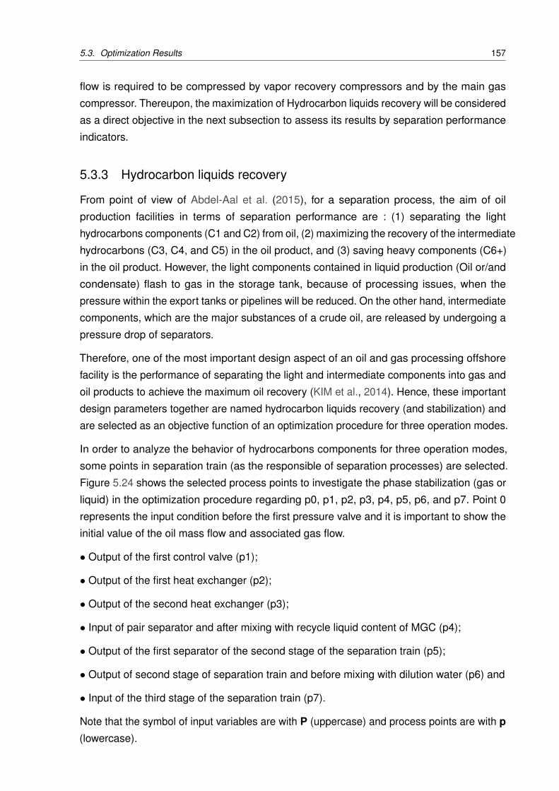
5.3. Optimization Results 157
flow is required to be compressed by vapor recovery compressors and by the main gas
compressor. Thereupon, the maximization of Hydrocarbon liquids recovery will be considered
as a direct objective in the next subsection to assess its results by separation performance
indicators.
5.3.3 Hydrocarbon liquids recovery
From point of view of Abdel-Aal et al. (2015), for a separation process, the aim of oil
production facilities in terms of separation performance are : (1) separating the light
hydrocarbons components (C1 and C2) from oil, (2) maximizing the recovery of the intermediate
hydrocarbons (C3, C4, and C5) in the oil product, and (3) saving heavy components (C6+)
in the oil product. However, the light components contained in liquid production (Oil or/and
condensate) flash to gas in the storage tank, because of processing issues, when the
pressure within the export tanks or pipelines will be reduced. On the other hand, intermediate
components, which are the major substances of a crude oil, are released by undergoing a
pressure drop of separators.
Therefore, one of the most important design aspect of an oil and gas processing offshore
facility is the performance of separating the light and intermediate components into gas and
oil products to achieve the maximum oil recovery (KIM et al., 2014). Hence, these important
design parameters together are named hydrocarbon liquids recovery (and stabilization) and
are selected as an objective function of an optimization procedure for three operation modes.
In order to analyze the behavior of hydrocarbons components for three operation modes,
some points in separation train (as the responsible of separation processes) are selected.
Figure 5.24 shows the selected process points to investigate the phase stabilization (gas or
liquid) in the optimization procedure regarding p0, p1, p2, p3, p4, p5, p6, and p7. Point 0
represents the input condition before the first pressure valve and it is important to show the
initial value of the oil mass flow and associated gas flow.
• Output of the first control valve (p1);
• Output of the first heat exchanger (p2);
• Output of the second heat exchanger (p3);
• Input of pair separator and after mixing with recycle liquid content of MGC (p4);
• Output of the first separator of the second stage of the separation train (p5);
• Output of second stage of separation train and before mixing with dilution water (p6) and
• Input of the third stage of the separation train (p7).
Note that the symbol of input variables are with P (uppercase) and process points are with p
(lowercase).
158 Chapter 5. Results and Discussions
Figure 5.24 – Selected point in process steps of separation.
Source : Author
5.3.3.1 Operation mode 1
In this subsection, the optimized configurations of operation mode 1 to achieve the maximum
hydrocarbon liquids recovery was discussed and compared with the baseline configuration.
As the crude oil composition of this operation mode was condensate oil, the recovery
of volatile components and stabilization and saving oil components have attracted more
attention. The finding optimum procedure was performed using 150 DoE designs (ULH and
ISF) and a maximum number of evaluation was settled for 8000 designs. The optimization
convergence was achieved after 3000 generations (Appendix D, Figure D.4) in the value of
462300 (kg/h) for exportation oil.
Table 5.14 shows the input parameters for the baseline and optimized configurations. The
input pressure of the first pressure valve is 2300 kPa and its output pressure (P1) is 1300 kPa
and 1302 kPa for the baseline case and optimized case, respectively. Next, the optimization
procedure found P2 = 560 kPa and P3 = 449 kPa for optimization case while the values
for the baseline configuration are P2 = 440 kPa and P3 = 244 kPa for operation mode 1.
The significant difference among baseline case and optimization is reported for T2 that the
temperature of petroleum at the heater for the baseline case is 90 oC, while for the optimized
case, it is 37.3 oC (Table 5.14). The justification of this results is expressed in Figures 5.25a
& 5.25b.
Figures 5.25a & 5.25b show the stabilization of phase during the separation processes
for the baseline and optimized case of operation mode 1 regarding presented points in
5.3. Optimization Results 159
Table 5.14 – Input parameters for the baseline and optimized configurations of operationmode 1- Hydrocarbon liquids recovery case.
P1 P2 P3 T2(kPa) (kPa) (kPa) (oC)
Baseline case 1300 440 244 90Mode 1
Optimized case 1302 560 449 37.3
Figure 5.24. The black line shows the gas phase components flow rate while the blue line
represents the liquid phase components flow rate. Up to point 3, the total gas mass flow
rate is separated by the first stage of the separator( including pre-heater and heater units).
The effect of T2 is due to the separation of the intermediate hydrocarbons, such as propane
and butanes in the gas flow, and heavy components of intermediate hydrocarbons, such as
pentane in the liquid phase. The change of mass flow (both gas and liquid) for baseline case
and optimization between p2 and p3 is because of T2. Therefore, this argument proves the
results of sensitivity analysis of T2 for hydrocarbons liquid recovery in operation mode 1.
Next, due to the very small rate of recycling pipe from MGC, the conditions of p3 and p4 are
the same for oil (Figures 5.25a & 5.25b). Then, all of the gas is separated after point 4 as a
medium pressure gas and, consequently, the gas mass flow rate is zero at point 5. At p6
and p7(after pressure valves VLV-113 and VLV-100), the gas flow content is separated from
liquid content.
Moreover, as shown in Figures 5.25a & 5.25b, from the same composition of the crude
oil, an increase of the oil recovery and stabilization for the optimized case are verified
when compared to the baseline. The optimum operating condition led to an improvement
of the separation performance of the gas and liquid hydrocarbons. As the crude oil stream
is involved by dissolved gas components, the heavy components of the intermediate
hydrocarbons, condensate components and pseudo-component of petroleum, the variation
in pressure and temperature influences the phase stabilization of these components.
For example, as shown in Figures 5.25a & 5.25b, at point 3, the optimum configuration
provides a condition to maximize the stabilization of intermediate hydrocarbons in the liquid
phase, especially propane and butane (466400 kg/h). In turn, for the baseline, a large
amount of heavy components of intermediate hydrocarbons is separated in the gas phase
(17000 kg/h). Moreover, at point 7, the exportation of oil increased about 20173 kg/h by the
improvement in the recovery of oil components at the optimum configuration (Figures 5.25a
& 5.25b).
Table 5.15 shows the exportation oil rate, separation performance of all separators and
propane, butane and pentane percentage in exportation oil of the FPSO unit for the
baseline and optimized case of operation mode 1. The optimization process found an
160 Chapter 5. Results and Discussions
operating configuration with an increase of 4.36 % of exportation oil as compared with
baseline configuration. Consequently, The results from the optimized case indicated that
the maximization of hydrocarbons liquid recovery is achieved by increasing the operating
pressure in the second and the third stages of the separation train and by decreasing the
operating temperature in oil heater of the separation train for operation mode1.
In the optimization process, exportation oil rate is considered as the objective function
and two indicators are monitored. Thus, the separation performance of separators (all
three stages) from equation 3.6 is calculated and the content of intermediate hydrocarbon
components (C3, C4 and C5) in exportation oil is used to analyze the quality of exportation
oil. Next, two indicators (one from (KIM et al., 2014) and the other one from (NGUYEN;
OLIVEIRA-JR, 2016g)) are selected to analyze the optimization of hydrocarbon liquids
recovery. For example, in equation 3.6, C1-C4 should be separated in gas flow while in (KIM
et al., 2014) cited from (ABDEL-AAL et al., 2015) is indicated that C3 and C4 also should be
separated in oil product.
Table 5.15 shows that the separation performance of the optimization case is increased from
65% of baseline to 68% and the C3-C5 content of optimization case has an increase of 10%
as compared with baseline case. Moreover, as observed in Table 5.15, the power demand of
optimization case is decreased by 4.9% when compared to the baseline case due to less
compressed of gas mass flow by compressors (MGC and EGC) .
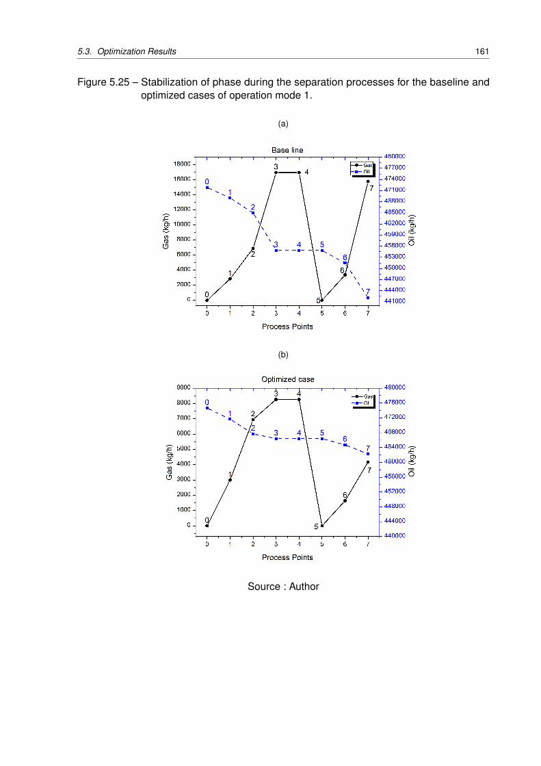
5.3. Optimization Results 161
Figure 5.25 – Stabilization of phase during the separation processes for the baseline andoptimized cases of operation mode 1.
(a)
(b)
Source : Author
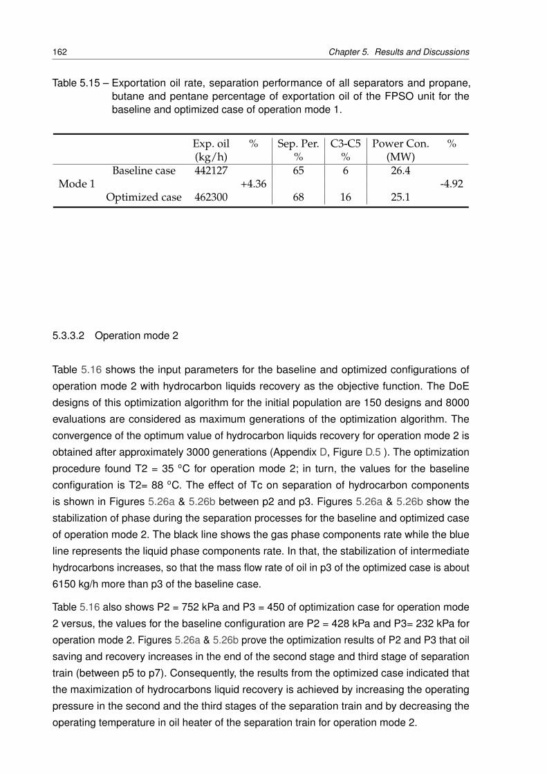
162 Chapter 5. Results and Discussions
Table 5.15 – Exportation oil rate, separation performance of all separators and propane,butane and pentane percentage of exportation oil of the FPSO unit for thebaseline and optimized case of operation mode 1.
Exp. oil % Sep. Per. C3-C5 Power Con. %(kg/h) % % (MW)
Baseline case 442127 65 6 26.4Mode 1 +4.36 -4.92
Optimized case 462300 68 16 25.1
5.3.3.2 Operation mode 2
Table 5.16 shows the input parameters for the baseline and optimized configurations of
operation mode 2 with hydrocarbon liquids recovery as the objective function. The DoE
designs of this optimization algorithm for the initial population are 150 designs and 8000
evaluations are considered as maximum generations of the optimization algorithm. The
convergence of the optimum value of hydrocarbon liquids recovery for operation mode 2 is
obtained after approximately 3000 generations (Appendix D, Figure D.5 ). The optimization
procedure found T2 = 35 oC for operation mode 2; in turn, the values for the baseline
configuration is T2= 88 oC. The effect of Tc on separation of hydrocarbon components
is shown in Figures 5.26a & 5.26b between p2 and p3. Figures 5.26a & 5.26b show the
stabilization of phase during the separation processes for the baseline and optimized case
of operation mode 2. The black line shows the gas phase components rate while the blue
line represents the liquid phase components rate. In that, the stabilization of intermediate
hydrocarbons increases, so that the mass flow rate of oil in p3 of the optimized case is about
6150 kg/h more than p3 of the baseline case.
Table 5.16 also shows P2 = 752 kPa and P3 = 450 of optimization case for operation mode
2 versus, the values for the baseline configuration are P2 = 428 kPa and P3= 232 kPa for
operation mode 2. Figures 5.26a & 5.26b prove the optimization results of P2 and P3 that oil
saving and recovery increases in the end of the second stage and third stage of separation
train (between p5 to p7). Consequently, the results from the optimized case indicated that
the maximization of hydrocarbons liquid recovery is achieved by increasing the operating
pressure in the second and the third stages of the separation train and by decreasing the
operating temperature in oil heater of the separation train for operation mode 2.
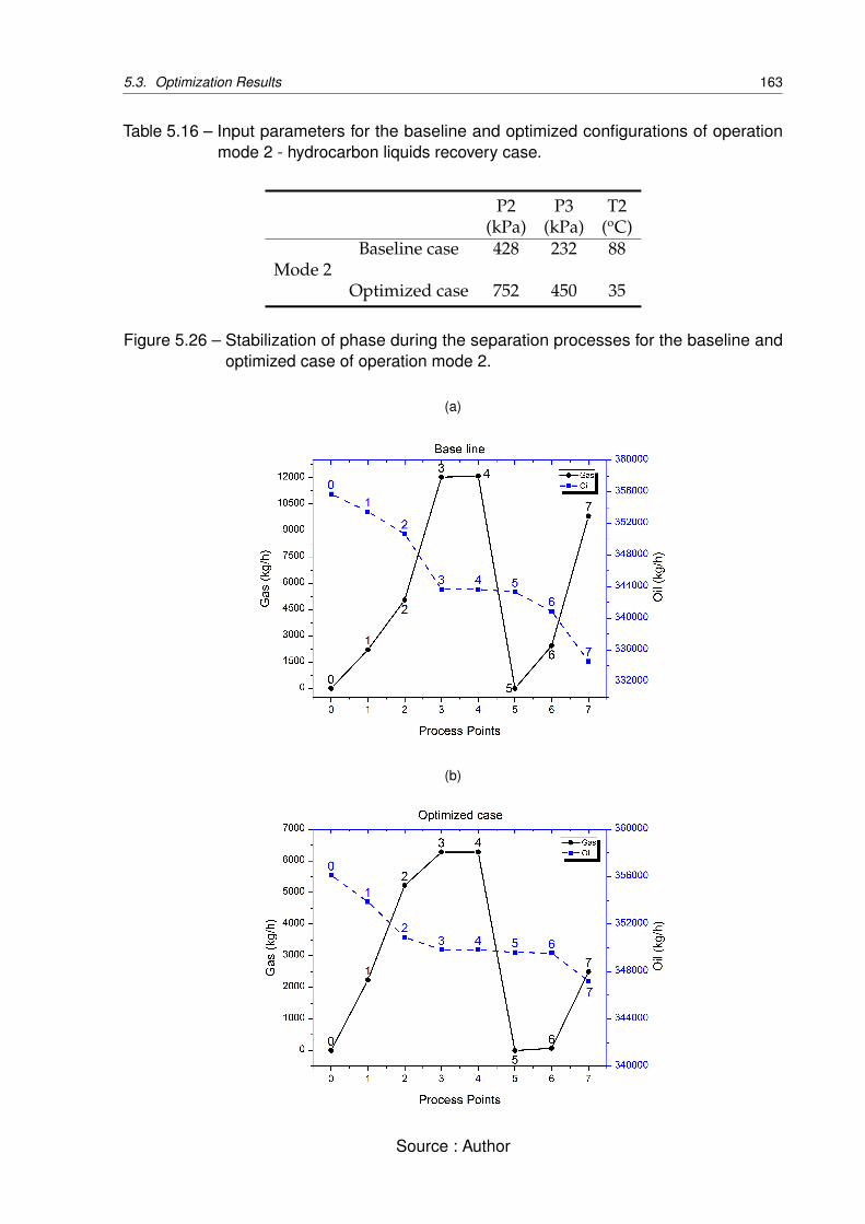
5.3. Optimization Results 163
Table 5.16 – Input parameters for the baseline and optimized configurations of operationmode 2 - hydrocarbon liquids recovery case.
P2 P3 T2(kPa) (kPa) (oC)
Baseline case 428 232 88Mode 2
Optimized case 752 450 35
Figure 5.26 – Stabilization of phase during the separation processes for the baseline andoptimized case of operation mode 2.
(a)
(b)
Source : Author
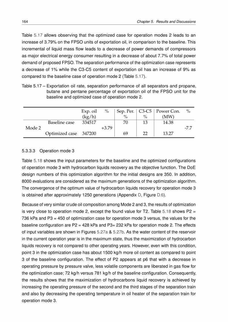
164 Chapter 5. Results and Discussions
Table 5.17 allows observing that the optimized case for operation modes 2 leads to an
increase of 3.79% on the FPSO units of exportation oil, in comparison to the baseline. This
incremental of liquid mass flow leads to a decrease of power demands of compressors
as major electrical energy consumer resulting in a decrease of about 7.7% of total power
demand of proposed FPSO. The separation performance of the optimization case represents
a decrease of 1% while the C3-C5 content of exportation oil has an increase of 9% as
compared to the baseline case of operation mode 2 (Table 5.17).
Table 5.17 – Exportation oil rate, separation performance of all separators and propane,butane and pentane percentage of exportation oil of the FPSO unit for thebaseline and optimized case of operation mode 2.
Exp. oil % Sep. Per. C3-C5 Power Con. %(kg/h) % % (MW)
Baseline case 334517 70 13 14.38Mode 2 +3.79 -7.7
Optimized case 347200 69 22 13.27
5.3.3.3 Operation mode 3
Table 5.18 shows the input parameters for the baseline and the optimized configurations
of operation mode 3 with hydrocarbon liquids recovery as the objective function. The DoE
design numbers of this optimization algorithm for the initial designs are 350. In addition,
8000 evaluations are considered as the maximum generations of the optimization algorithm.
The convergence of the optimum value of hydrocarbon liquids recovery for operation mode 3
is obtained after approximately 1250 generations (Appendix D, Figure D.6).
Because of very similar crude oil composition among Mode 2 and 3, the results of optimization
is very close to operation mode 2, except the found value for T2. Table 5.18 shows P2 =
736 kPa and P3 = 450 of optimization case for operation mode 3 versus, the values for the
baseline configuration are P2 = 428 kPa and P3= 232 kPa for operation mode 2. The effects
of input variables are shown in Figures 5.27a & 5.27b. As the water content of the reservoir
in the current operation year is in the maximum state, thus the maximization of hydrocarbon
liquids recovery is not compared to other operating years. However, even with this condition,
point 3 in the optimization case has about 1500 kg/h more oil content as compared to point
3 of the baseline configuration. The effect of P2 appears at p6 that with a decrease in
operating pressure by pressure valve, less volatile components are liberated in gas flow for
the optimization case; 72 kg/h versus 781 kg/h of the baseline configuration. Consequently,
the results shows that the maximization of hydrocarbons liquid recovery is achieved by
increasing the operating pressure of the second and the third stages of the separation train
and also by decreasing the operating temperature in oil heater of the separation train for
operation mode 3.
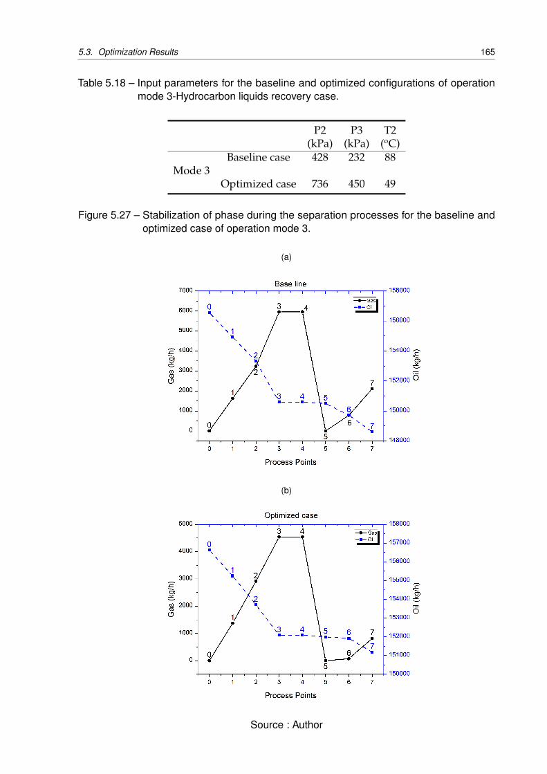
5.3. Optimization Results 165
Table 5.18 – Input parameters for the baseline and optimized configurations of operationmode 3-Hydrocarbon liquids recovery case.
P2 P3 T2(kPa) (kPa) (oC)
Baseline case 428 232 88Mode 3
Optimized case 736 450 49
Figure 5.27 – Stabilization of phase during the separation processes for the baseline andoptimized case of operation mode 3.
(a)
(b)
Source : Author
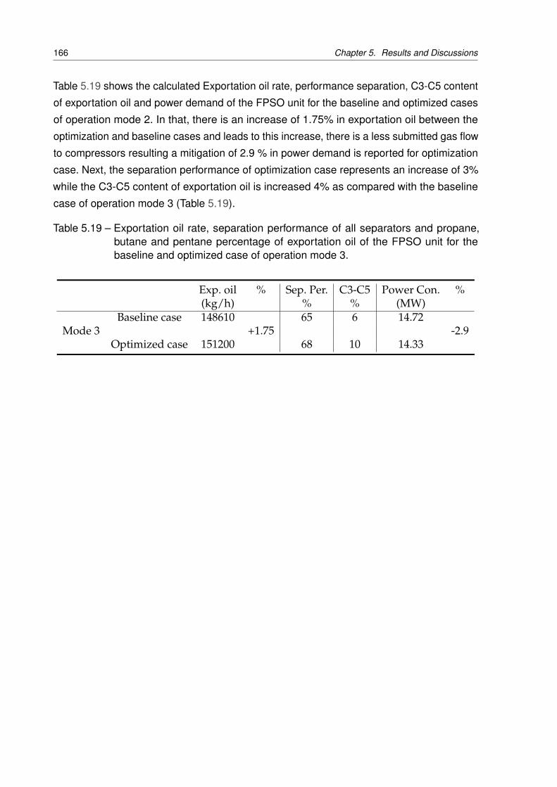
166 Chapter 5. Results and Discussions
Table 5.19 shows the calculated Exportation oil rate, performance separation, C3-C5 content
of exportation oil and power demand of the FPSO unit for the baseline and optimized cases
of operation mode 2. In that, there is an increase of 1.75% in exportation oil between the
optimization and baseline cases and leads to this increase, there is a less submitted gas flow
to compressors resulting a mitigation of 2.9 % in power demand is reported for optimization
case. Next, the separation performance of optimization case represents an increase of 3%
while the C3-C5 content of exportation oil is increased 4% as compared with the baseline
case of operation mode 3 (Table 5.19).
Table 5.19 – Exportation oil rate, separation performance of all separators and propane,butane and pentane percentage of exportation oil of the FPSO unit for thebaseline and optimized case of operation mode 3.
Exp. oil % Sep. Per. C3-C5 Power Con. %(kg/h) % % (MW)
Baseline case 148610 65 6 14.72Mode 3 +1.75 -2.9
Optimized case 151200 68 10 14.33
167
6 CONCLUSION AND FUTURE WORK
This chapter presents the conclusion of the current research and the suggestion research
activities in the future of this work.
6.1 Conclusion
A primary processing plant of a typical FPSO operating in a Brazilian deep-water oil field on
pre-salt areas is modeled and simulated using its real operating data. Three operation
conditions of the oil field are presented in this research: (i) Maximum oil/gas content
(mode 1), (ii) 50% BSW oil content (mode 2) and (iii) high water/CO2 in oil content (mode
3). Then, the impact of eight thermodynamic input parameters on fuel consumption and
hydrocarbon liquids recovery of the FPSO unit are investigated by the Smoothing Spline
ANOVA (SS-ANOVA) method. From SS-ANOVA, the input parameters that presented the
highest impact on fuel consumption and hydrocarbons liquids recovery were selected for an
optimization procedure.
The optimization procedure consists of a hybrid Genetic Algorithm (NSGA-II+SQP method),
which is coupled with the Aspen HYSYS R© software as the simulator. The objective functions
used in the optimization were the minimization of fuel consumption of the processing
plant and the maximization of hydrocarbon liquids recovery. The following items are the
contributions and novelty of the current thesis:
• Applying the real performance data of a commercial-offshore gas turbine (RB211G62 DLE)
with adequate efficiency interacting with simulation of Aspen Hysys (for the first time ever);
• Integrating of Aspen Hysys and ModeForntier as an automation process of screen
analyzing and optimization procedure (for the first time ever);
• Implementation of SS-ANOVA (considering the analysis of the main and interaction effects)
in an oil and gas processing simulation of proposed FPSO to identify the major effects and
to decrease the input variable of optimization procedure;
• Assessment of the available and recommended optimization methods from literature in
order to select the suitable one for current problem;
• Applying an optimization procedure to increase the sustainability and profitability of a
typical FPSO simultaneously, without adding any new technology and imposed costs;
• Applying a formal optimization procedure for fuel consumption minimization that consequently
168 Chapter 6. Conclusion and Future Work
reduces the produced CO2 in the processes and for hydrocarbons liquid recovery , subject
to several constraints, of a Brazilian FPSO in three operation scenarios.
From SS-ANOVA, the statistical analysis revealed that the most important parameters
affecting the fuel consumption of the plant are: (1)output pressure of the first control valve
(P1); (2)output pressure of the second stage of the separation train before mixing with
dilution water (P2); (3) input pressure of the third stage of the separation train (P3); (4) output
pressure of the main gas compressor (Pc) and; (5) output petroleum temperature in the
second heat exchanger (T2). These four input parameters (P1, P2, P3 and Pc), three input
parameters (P3, Pc and T2) and three input parameters (P3, Pc and T2) correspond to 96%,
97% and 97% of the total contribution to fuel consumption for modes 1, 2 and 3, respectively.
For hydrocarbon liquids recovery of the plant: These four input parameters (P1, P2, P3 and
T2), three input parameters (P3, P2 and T2) and three input parameters (P3, P2 and T2)
correspond to 95%, 97% and 98% of the total contribution to hydrocarbon liquid recovery
for modes 1, 2 and 3, respectively. The results showed that P3 is very important to fuel
consumption and hydrocarbon liquids recovery due to its impact on separation efficiency
and stabilization of the resultant phases of production at the third stage of the separators.
Moreover, parameter T2 is more relevant for modes 2 and 3 and its contribution is practically
the same for both operation modes. It has an important role in the separation efficiency of wet
gas composition at the second stage of the separation train, indicating that it is necessary
to provide a heat source to enhance hydrocarbons recovery at the second stage of the
separation train.
The implementation of Sensitivity Analysis showed what are the most important parameters
that affect the objective function and resulted in a great reduction in the computation time for
optimization. For example, the convergence time for the optimization procedure, for some
cases, was reduced from 2 weeks to 3 days.
The results from the optimized case indicated that the minimization of fuel consumption is
achieved by increasing the operating pressure in the third stage of the separation train and
by decreasing the operating temperature in the second stage of the separation train for all
operation modes. There was a reduction in power demand of 6.4 % for mode 1, 10 % for
mode 2 and 2.9% for mode 3, in comparison to the baseline case. Consequently, the fuel
consumption of the plant was decreased by 4.46% for mode 1 (223 kg/h less consumed
gas), 8.34% for mode 2 (262 kg/h less consumed gas) and 2.43% for mode 3 (87 kg/h less
consumed gas), when compared to the baseline case. Moreover, the optimization producer
found an improvement in the recovery of the volatile components, in comparison with the
baseline cases.
Furthermore, the optimum operating condition found by the optimization procedure of
hydrocarbon liquids recovery presented an increase of 4.36 % for mode 1 (10% improvement
6.2. Future work 169
of C3-C5 content in exportation oil), 3.79% for mode 2 (an improvement of 9% for C3-C5
content in exportation oil) and 1.75% for mode 3 (an increase of 4% for C3-C5 content in
exportation oil), in hydrocarbons liquid recovery (stabilization and saving), when compared
to the conventional operating conditions of their baseline.
6.2 Future work
Overall, the optimization process showed to be a robust and promising tool to find optimal
operational configurations of an FPSO plant, since the integration between optimization
methods and thermodynamic modeling speeds up the evaluation of several configurations
automatically.
The operation mode working with high GOR and oil reservoirs have a great potential to be
optimized in both objective functions of fuel consumption minimization and hydrocarbon
liquid recovery. There are four more real crude oil compositions that can be simulated and
used in an optimization procedure.
Moreover, in this research, the separation performance is considered as an indicator to
explain the effect of temperatures and pressures on hydrocarbons recovery and stabilization
of oil components and the assessment of the optimization results. In future studies, it can be
used as an objective function aiming to improve the recovery of hydrocarbons components
for each operation mode considering API gravity number.

171
REFERENCES
ABDEL-AAL, H. K.; AGGOUR, M. A.; FAHIM, M. A. Petroleum and Gas Field Processing,Second Edition. 2nd. ed.: CRC Press, 2015. ISBN 9781482255928. Cited 7 times in pages41, 99, 101, 113, 132, 157, and 160.
ADJIMAN, C. S.; SCHWEIGER, C. A.; FLOUDAS, C. A. Mixed-integer nonlinear optimizationin process synthesis. In: Handbook of Combinatorial Optimization: Springer US, 1998. p.1–76. Cited in page 61.
ALAGUMURTHI, N.; PALANIRADJA, K.; SOUNDARARAJAN, V. Optimization of grindingprocess through design of experiment (doe) - a comparative study. Materials andManufacturing Processes, Taylor & Francis, v. 21, n. 1, p. 19–21, 2006. Cited in page 87.
ALLAHYARZADEH-BIDGOLI, A.; DEZAN, D. J.; YANAGIHARA, J. I. PERFORMANCEOPTIMIZATION OF PLATE-FIN HEAT EXCHANGERS USED IN a THREE STAGEPROPANE PRE-COOLING CYCLE OF THE CASCADE LNG PLANT. In: Proceedings ofCHT-17 ICHMT International Symposium on Advances in Computational Heat Transfer May28-June 1, 2017, Napoli, Italy : Begellhouse, 2017. Cited in page 76.
ALLAHYARZADEH-BIDGOLI, A. et al. Optimization of a brazilian fpso fuel consumption forpetroleum composition with maximum oil and gas content using genetic algorithm method.In: Proceedings of ECOS 2017-the 30th International Conference on Efficiency, Cost,Optimization, Simulation and Environmental Impact of Energy Systems, 2017. Cited 2times in pages 71 and 76.
ANANTHARAMAN, R. Energy Efficiency in Process Plants with emphasis on HeatExchanger Networks Optimization, Thermodynamics and Insight. Thesis (PhD) —Department of Energy and Process Engineering Norwegian University of Science andTechnology, 2011. Available from Internet: <http://www.ivt.ntnu.no/ept/fag/tep4215/innhold/Rahul%20-%20thesis%20-%20final%20version%20-%2030%20May%202011.pdf>. Citedin page 85.
ANDRADE, A. M. T. de et al. Offshore production units for pre-salt projects. In: OFFSHORETECHNOLOGY CONFERENCE. Offshore Technology Conference, 2015. Cited 3 times inpages 49, 50, and 51.
ANSCOMBE, F. J. The validity of comparative experiments. Journal of the Royal StatisticalSociety. Series A (General), JSTOR, v. 111, n. 3, p. 181, 1948. Cited in page 90.
ANTONIN, P. et al. About the relevance of mathematical programming and stochasticoptimisation methods: Application to optimal batch plant design problems. In: ComputerAided Chemical Engineering: Elsevier, 2005. p. 49–54. Cited in page 85.
ANTONIN, P. et al. About the relevance of mathematical programming and stochasticoptimisation methods: application to optimal batch plant design problems. Computer AidedChemical Engineering, Elsevier, v. 20, p. 49–54, 2005. Cited in page 94.

172 References
ARAÚJO, O. de Q. F. et al. Comparative analysis of separation technologies for processingcarbon dioxide rich natural gas in ultra-deepwater oil fields. Journal of Cleaner Production,Elsevier BV, v. 155, p. 12–22, jul 2017. Cited in page 33.
ARNOLD, K.; STEWART, M. Design of oil-handling systems and facilities: Gulf ProfessionalPublishing, 1998. Cited in page 46.
ARNOLD, M. S. K. Surface Production Operations, Volume 1: Elsevier Science & Technology,2007. ISBN 0750678534. Cited 5 times in pages 42, 43, 44, 45, and 132.
ARORA, J. Introduction to optimum design. 4th edition. ed.: Academic Press, 2016. Cited inpage 93.
Aspen Technology, Inc. Aspen Simulation Workbook datasheet, 2014. Cited in page 114.
ASPENTECHNOLOGYINC. Aspen HYSYS V9.0, 2016. Cited in page 113.
AUTE, V. C. Thermal Systems Optimization: Wiley Online Library, 2014. Cited in page 64.
AYRES, R. U.; AYRES, L. W.; MARTINÁS, K. Exergy, waste accounting, and life-cycleanalysis. Energy, Elsevier, v. 23, n. 5, p. 355–363, 1998. No citation in text.
BAHADORI, A.; NWAOHA, C.; CLARK, M. W. Dictionary of Oil, Gas, and PetrochemicalProcessing: CRC PR INC, 2013. ISBN 9781466588257. Cited in page 136.
BAHADORI, A.; VUTHALURU, H. B.; MOKHATAB, S. Optimizing separator pressures inthe multistage crude oil production unit. Asia-Pacific Journal of Chemical Engineering,Wiley-Blackwell, v. 3, n. 4, p. 380–386, jul 2008. Cited 2 times in pages 70 and 74.
BALESTIERI, J. A. P. Cogeraçao: Geraçao combinada de electricidade e calor : Editora daUFSC, 2002. Cited in page 33.
BARRERA, J. E.; BAZZO, E.; KAMI, E. Exergy analysis and energy improvement of abrazilian floating oil platform using organic rankine cycles. Energy, Elsevier, v. 88, p. 67–79,2015. Cited in page 34.
BARTON, R. R.; MECKESHEIMER, M. Chapter 18 metamodel-based simulationoptimization. In: Simulation: Elsevier, 2006. p. 535–574. Cited in page 86.
BELTRAO, R. L. C. et al. Ss: Pre-salt santos basin-challenges and new technologies for thedevelopment of the pre-salt cluster, santos basin, brazil. In: OFFSHORE TECHNOLOGYCONFERENCE. Offshore Technology Conference, 2009. Cited 2 times in pages 47 and 49.
BIEGLER, L. T.; GROSSMANN, I. E.; WESTERBERG, A. W. Systematic methodsfor chemical process design. Prentice Hall, Old Tappan, NJ (United States),1997. ISSN 978-0134924229. ISBN 978-0134924229. Available from Internet:<https://www.ebook.de/de/product/3714872/lorenz_t_biegler_ignacio_e_grossmann_arthur_w_westerberg_systematic_methods_of_chemical_process_design.html>. Cited inpage 96.
BORGONOVO, E. Sensitivity Analysis: Springer International Publishing, 2017. Cited inpage 90.
References 173
BOTHAMLEY, M. et al. Offshore processing options for oil platforms. In: SOCIETY OFPETROLEUM ENGINEERS. SPE Annual Technical Conference and Exhibition, 2004. p.1–17. Cited 2 times in pages 53 and 57.
BP, B.-P. Azari, Chirag & Gunashli Full Field Development Phase 3. Environmental& Socio-economic impact assessment,. 2004. Report. Available from Internet: <http://disciplinas.stoa.usp.br/pluginfile.php/161720/mod_folder/content/0/05%20Chapt%205%20PD%20Section%205.5%20Process_ENG_FINAL_Oct%2004.pdf?forcedownload=1>.Visited on: 05/05/2016. Cited 2 times in pages 46 and 47.
BRADLEY, S.; HAX, A.; MAGNANTI, T. Applied mathematical programming.Addison Wesley, 1977. ISBN 978-0201004649. Available from Internet: <https://www.amazon.com/Applied-Mathematical-Programming-Stephen-Bradley/dp/020100464X?SubscriptionId=0JYN1NVW651KCA56C102&tag=techkie-20&linkCode=xm2&camp=2025&creative=165953&creativeASIN=020100464X>. Cited in page 60.
CARRANZA-SÁNCHEZ, Y. A.; OLIVEIRA-JR, S. de. Exergy analysis of offshore primarypetroleum processing plant with co 2 capture. Energy, Elsevier, v. 88, p. 46–56, 2015. Citedin page 58.
CARRANZA-SÁNCHEZ, Y. A. et al. Energy and exergy performance of three fpsooperational modes. In: Proceedings of the 23rd Abcm International Congress of MechanicalEngineering, 2015. Cited 2 times in pages 55 and 59.
Chisholm, Hugh. ’Petroleum’. 1911 Encyclopedia Britanica. 1911. Available fromInternet: <http://www.studylight.org/encyclopedias/bri/view.cgi?number=25685>. Visited on:01/12/2015. Cited in page 31.
CHU, Y.; HAHN, J. Necessary condition for applying experimental design criteria to globalsensitivity analysis results. Computers & Chemical Engineering, Elsevier, v. 48, p. 280–292,jan 2013. Cited 2 times in pages 64 and 65.
COLMENARES, T. R.; SEIDER, W. D. Synthesis of utility systems integrated with chemicalprocesses. Industrial & engineering chemistry research, ACS Publications, v. 28, n. 1, p.84–93, 1989. Cited 2 times in pages 60 and 74.
DEB, K. et al. A fast and elitist multiobjective genetic algorithm: Nsga-ii. IEEE transactionson evolutionary computation, IEEE, v. 6, n. 2, p. 182–197, 2002. Cited 2 times in pages 94and 95.
DEVOLD, H. Oil and gas production handbook: an introduction to oil and gas production:AAB, 2006. Cited 2 times in pages 47 and 102.
DEZAN, D. J. HEAT TRANSFER ENHANCEMENT AND OPTIMIZATION OF FLAT-TUBEMULTILOUVERED FIN COMPACT HEAT EXCHANGERS WITH DELTAWINGLET VORTEXGENERATORS. Thesis (PhD) — Universidade de Sao Paulo, 2015. Cited in page 92.
DIBAN, P.; FOO, D. C. Targeting and design of heating utility system for offshore platform.Energy, Elsevier, v. 146, p. 98–111, mar 2017. Cited 2 times in pages 63 and 76.
EFRON, B.; STEIN, C. The jackknife estimate of variance. The Annals of Statistics, JSTOR,p. 586–596, 1981. Cited in page 91.

174 References
Esteco SPA. ModeFRONTIER - User’s Guide Version 5.6.0.1 2017, 2017. Cited 7 times inpages 90, 95, 114, 147, 148, 149, and 150.
ESTECO WEBINAR SERIES. LEVERAGING SMART DESIGN EXPLORATION FORRESOURCE-INTENSIVE CFD ANALYSIS. 2016. Cited in page 90.
ETA-OFFSHORE-SEMINARS, i. The technology of offshore drilling, completion andproduction: Pennwell Corp, 1976. Cited in page 46.
FANG, K.-T.; LI, R.; SUDJIANTO, A. Design and modeling for computer experiments: CRCPress, 2005. Cited in page 87.
FAZLOLLAHI, S. et al. Multi-objective, multi-period optimization of district energy systems:Iv–a case study. Energy, Elsevier, v. 84, p. 365–381, 2015. Cited in page 85.
FENG, Y. et al. Comparison between regenerative organic rankine cycle (rorc) and basicorganic rankine cycle (borc) based on thermoeconomic multi-objective optimizationconsidering exergy efficiency and levelized energy cost (lec). Energy Conversion andManagement, Elsevier, v. 96, p. 58–71, 2015. Cited 3 times in pages 67, 68, and 75.
FERGANI, Z.; TOUIL, D.; MOROSUK, T. Multi-criteria exergy based optimization of anorganic rankine cycle for waste heat recovery in the cement industry. Energy Conversionand Management, Elsevier, v. 112, p. 81–90, 2016. Cited in page 68.
FISHER, R. A.; MACKENZIE, W. A. Studies in crop variation. ii. the manurial response ofdifferent potato varieties. The Journal of Agricultural Science, Cambridge University Press,v. 13, n. 3, p. 311–320, 1923. Cited in page 91.
FISHER, S. R. A. et al. The design of experiments: Oliver and Boyd Edinburgh, 1937. v. 1.Cited in page 86.
FONTAINE, E. et al. Reliability analysis and response based design of a moored fpso inwest africa. Structural Safety, Elsevier, v. 41, p. 82–96, 2013. Cited in page 34.
FORMIGLI, J. Pre-salt reservoirs offshore brazil: perspectives and challenges. In: EnergyConference. Miami, 2007. p. 12–23. Cited in page 48.
FRANGOPOULOS, C. A.; SPAKOVSKY, M. R. V.; SCIUBBA, E. A brief review of methodsfor the design and synthesis optimization of energy systems. International Journal ofThermodynamics, v. 5, n. 4, p. 151–160, 2002. Cited in page 94.
GALLO, W. L. et al. Exergy analysis of the compression systems and its prime movers for aFPSO unit. Journal of Natural Gas Science and Engineering, Elsevier BV, v. 44, p. 287–298,Aug 2017. Cited 6 times in pages 55, 56, 59, 79, 80, and 113.
GAO, T. et al. Coalbed methane liquefaction adopting a nitrogen expansion process withpropane pre-cooling. Applied Energy, Elsevier BV, v. 87, n. 7, p. 2142–2147, jul 2010. Citedin page 64.
GEHLING, R. C.; LANE, M. P.; THORNTON, R. M. Floating production, storage andoffloading (fpso) facilities-impact of the new oil tanker construction rules. APEA JOURNAL,Australian Petroleum Exploration Association, v. 34, p. 178–178, 1994. Cited in page 33.
References 175
General Electric . Gate Cycle V6.1.2. New York, USA, 2013. Cited 2 times in pages 97and 109.
GETU, M. et al. Risk-based optimization for representative natural gas liquid (ngl) recoveryprocesses by considering uncertainty from the plant inlet. Journal of Natural Gas Scienceand Engineering, Elsevier, v. 27, p. 42–54, 2015. Cited in page 68.
GHAEDI, M.; EBRAHIMI, A. N.; PISHVAIE, M. R. APPLICATION OF GENETIC ALGORITHMFOR OPTIMIZATION OF SEPARATOR PRESSURES IN MULTISTAGE PRODUCTIONUNITS. Chemical Engineering Communications, Informa UK Limited, v. 201, n. 7, p.926–938, mar 2014. Cited in page 70.
GIUNTA, A. A. et al. Overview of modern design of experiments methods for computationalsimulations. In: Proceedings of the 41st AIAA aerospace sciences meeting and exhibit,AIAA-2003-0649, 2003. Cited in page 87.
GONG, M. Using exergy and optimization models to improve industrial energy systemstowards sustainability. Linköpings universitet, 2004. Cited in page 84.
GROSSMANN, I. E. Mixed-integer programming approach for the synthesis of integratedprocess flowsheets. Computers & chemical engineering, Elsevier, v. 9, n. 5, p. 463–482,1985. Cited 3 times in pages 83, 85, and 96.
GROSSMANN, I. E. Global Optimization in engineering design: Springer Science &Business Media, 2013. v. 9. Cited in page 84.
GU, C. Smoothing Spline ANOVA Models: Springer New York, 2013. Cited in page 91.
GUERRA, M. J. Aspen HYSYS Property Packages-Overview and Best Practices forOptimum Simulations. 2006. Pdf. Available from Internet: <http://sites.poli.usp.br/d/pqi2408/BestPracticesOptimumSimulationsHYSYSPropertyPackages.pdf>. Cited in page 116.
HAFTKA, R. T.; GÜRDAL, Z. Elements of structural optimization: Springer Science &Business Media, 2012. v. 11. Cited in page 84.
HALLIBURTON. Água profundas - Brasil. 2014. Available from Internet: <http://www.halliburton.com/public/solutions/contents/Deep_Water/related_docs/Brazil%20Deepwater%20Map%20Final%20-%20Portuguese.pdf>. Visited on: 07/05/2016. Cited inpage 34.
HAMID, M. K. A. Hysys R©: An introduction to chemical engineering simulation. Apostila deHamid, 2007. Cited in page 116.
HATCHER, P.; KHALILPOUR, R.; ABBAS, A. Optimisation of lng mixed-refrigerantprocesses considering operation and design objectives. Computers & Chemical Engineering,Elsevier, v. 41, p. 123–133, jun 2012. Cited in page 64.
HE, T.; JU, Y. Design and optimization of a novel mixed refrigerant cycle integrated with nglrecovery process for small-scale lng plant. Industrial & Engineering Chemistry Research,ACS Publications, v. 53, n. 13, p. 5545–5553, 2014. Cited 2 times in pages 66 and 68.
HE, T.; JU, Y. Optimal synthesis of expansion liquefaction cycle for distributed-scale lng(liquefied natural gas) plant. Energy, Elsevier, v. 88, p. 268–280, 2015. Cited 2 times inpages 66 and 68.
176 References
HOEFFDING, W. A class of statistics with asymptotically normal distribution. The annals ofmathematical statistics, JSTOR, p. 293–325, 1948. Cited in page 91.
HUANG, K.; KARIMI, I. Work-heat exchanger network synthesis (whens). Energy, Elsevier,v. 113, p. 1006–1017, oct 2016. Cited in page 75.
HWANG, J.-H.; ROH, M.-I.; LEE, K.-Y. Determination of the optimal operating conditions ofthe dual mixed refrigerant cycle for the LNG FPSO topside liquefaction process. Computers& Chemical Engineering, Elsevier BV, v. 49, p. 25–36, feb 2013. Cited in page 65.
HYPROTECH-LTD. HYSIM User’s Guide - Version C1.50, 1991. Cited in page 52.
INUTECH-GMBH. Mipsqp - a new approach to solve mixed integer optimization problems.dez. 2007. Cited in page 85.
IOGP, I. A. O. O. . G. P. Environmental performance indicators 2011 data - InternationalAssociation of Oil & Gas Producers, London, October 2012. 2012. Available from Internet:<www.ogp.org.uk>. Visited on: 14/05/2016. Cited in page 54.
IUPAC. International union of pure and applied chemistry organic chemistry division.a guideto iupac nomenclature of organic compounds (recommendations 1993). Blackwell ScientificPublications, 1993. Cited in page 41.
JALURIA, Y. Design and optimization of thermal systems: CRC press, 2007. Cited 2 timesin pages 84 and 85.
JIANG, X.; LI, S.; ZHANG, L. Sensitivity analysis of gas production from class i hydratereservoir by depressurization. Energy, Elsevier, v. 39, n. 1, p. 281–285, mar 2012. Cited 2times in pages 64 and 65.
KHAN, M. S. et al. Energy saving opportunities in integrated ngl/lng schemes exploiting:Thermal-coupling common-utilities and process knowledge. Chemical Engineering andProcessing: Process Intensification, Elsevier, v. 82, p. 54–64, 2014b. Cited 2 times in pages66 and 68.
KHAN, M. S. et al. Process knowledge based opportunistic optimization of the n 2–co 2expander cycle for the economic development of stranded offshore fields. Journal of NaturalGas Science and Engineering, Elsevier, v. 18, p. 263–273, 2014a. Cited 2 times in pages65 and 68.
KHERAD-PAJOUH, S.; RENAUD, O. An exact permutation method for testing any effect inbalanced and unbalanced fixed effect ANOVA. Computational Statistics & Data Analysis,Elsevier BV, v. 54, n. 7, p. 1881–1893, jul 2010. Cited in page 91.
KIM, I. H. et al. Simulation-based optimization of multistage separation process in offshoreoil and gas production facilities. Industrial & Engineering Chemistry Research, AmericanChemical Society (ACS), v. 53, n. 21, p. 8810–8820, may 2014. Cited 5 times in pages 43,70, 75, 157, and 160.
KINNEY P.E., D. B. PF and C: Expanding Facilities Knowledge Workshop Session1 - Field Development Options / Selection Strategy. 2012. Available from Internet:<http://www.spegcs.org/events/1984/>. Visited on: 05/04/2016. Cited in page 33.
References 177
KLOSTER, P. et al. Energy optimization on offshore installations with emphasis on offshorecombined cycle plants. In: SOCIETY OF PETROLEUM ENGINEERS. Offshore Europe Oiland Gas Exhibition and Conference, 1999. Cited in page 74.
KLOSTER, P. et al. Reduction of emissions to air through energy optimisation on offshoreinstallations. In: SOCIETY OF PETROLEUM ENGINEERS. SPE International Conferenceon Health, Safety and Environment in Oil and Gas Exploration and Production, 2000. Citedin page 74.
KWAK, D.-H. et al. Energy-efficient design and optimization of boil-off gas (BOG)re-liquefaction process for liquefied natural gas (LNG)-fuelled ship. Energy, Elsevier BV,v. 148, p. 915–929, apr 2018. Cited 2 times in pages 68 and 69.
KYLLING, Ø. W. Optimizing separator pressure in a multistage crude oil production plant.Dissertação (Mestrado) — Norwegian University of Science and Technology-Department ofEngineering Cybernetics, 2009. Cited in page 70.
LAZZARETTO, A.; TSATSARONIS, G. Speco: a systematic and general methodologyfor calculating efficiencies and costs in thermal systems. Energy, Elsevier, v. 31, n. 8, p.1257–1289, 2006. Cited in page 96.
LEARY, S.; BHASKAR, A.; KEANE, A. Optimal orthogonal-array-based latin hypercubes.Journal of Applied Statistics, Taylor & Francis, v. 30, n. 5, p. 585–598, 2003. Cited in page89.
LEE, G.; SMITH, R.; ZHU, X. Optimal synthesis of mixed-refrigerant systems forlow-temperature processes. Industrial & engineering chemistry research, ACS Publications,v. 41, n. 20, p. 5016–5028, 2002. Cited 2 times in pages 61 and 74.
LIU, X. et al. Thermal performance analysis of brayton cycle with waste heat recovery boilerfor diesel engines of offshore oil production facilities. Applied Thermal Engineering, Elsevier,2016. Cited in page 72.
LOUREIRO, S.; ROVERE, E.; MAHLER, C. Analysis of potential for reducing emissions ofgreenhouse gases in municipal solid waste in brazil, in the state and city of rio de janeiro.Waste management, Elsevier, v. 33, n. 5, p. 1302–1312, 2013. Cited in page 31.
LUCAS, M. A. et al. Use of real crude oil fractions to describe the high pressure phasebehavior of crude oil in carbon dioxide. The Journal of Supercritical Fluids, Elsevier BV,v. 118, p. 140–147, dec 2016. Cited in page 80.
LUCAY, F.; CISTERNAS, L.; GÁLVEZ, E. Global sensitivity analysis for identifying criticalprocess design decisions. Chemical Engineering Research and Design, Elsevier, v. 103, p.74–83, nov 2015. Cited in page 64.
MANNING, F. S.; THOMPSON, R. E. Oilfield processing of petroleum: Crude oil : Pennwellbooks, 1995. v. 2. Cited 2 times in pages 52 and 57.
MARÉCHAL, F.; KALITVENTZEFF, B. Targeting the optimal integration of steam networks:Mathematical tools and methodology. Computers & Chemical Engineering, Elsevier, v. 23, p.S133–S136, 1999. Cited in page 123.
MCCAIN, W. D.; SPIVEY, J. P.; LENN, C. P. Petroleum reservoir fluid property correlations:PennWell Books, 2011. Cited 4 times in pages 42, 132, 136, and 155.
178 References
MCKAY, M. D.; BECKMAN, R. J.; CONOVER, W. J. A comparison of three methodsfor selecting values of input variables in the analysis of output from a computer code.Technometrics, Taylor & Francis Group, v. 42, n. 1, p. 55–61, 2000. Cited 2 times in pages88 and 89.
MEHRPOOYA, M. et al. Energy and advanced exergy analysis of an existing hydrocarbonrecovery process. Energy Conversion and Management, Elsevier, v. 123, p. 523–534, 2016.Cited 3 times in pages 55, 59, and 68.
Minerals Management Service Gulf of Mexico OCS Region. Proposed Use of FloatingProduction, Storage, and Offloading Systems On the Gulf of Mexico Outer Continental Shelf :U.S. Department of the Interior, Minerals Management Service Gulf of Mexico OCS Region,2000. Cited in page 49.
Ministério de Minas e Energia. Resenha Energética Brasileira Ministério de Minas eEnergia Exercício de 2014 - Edição de junho de 2015. 2015. Available from Internet:<http://www.mme.gov.br/documents/1138787/1732840/Resenha+Energ%C3%A9tica+-+Brasil+2015.pdf/4e6b9a34-6b2e-48fa-9ef8-dc7008470bf2>. Visited on: 05/05/2016. Citedin page 31.
Ministério de Minas e Energia. Resenha Energética Brasileira Ministério de Minas e EnergiaExercício de 2016 - Edição de junho de 2017. 2017. Available from Internet: <http://www.mme.gov.br/documents/10584/3580498/02+-+Resenha+Energ%C3%A9tica+Brasileira+2017+-+ano+ref.+2016+%28PDF%29/13d8d958-de50-4691-96e3-3ccf53f8e1e4?version=1.0>. Visited on: 05/01/2018. Cited in page 48.
MISHRA, M.; DAS, P.; SARANGI, S. Second law based optimisation of crossflow plate-finheat exchanger design using genetic algorithm. Applied Thermal Engineering, Elsevier,v. 29, n. 14, p. 2983–2989, 2009. Cited in page 94.
MONTGOMERY, D. C. Design and analysis of experiments. 4th. ed.: John Wiley & Sons,1997. Cited in page 88.
MORAIS, J. M. d. Petróleo em águas profundas: uma história tecnológica da petrobras naexploração e produção offshore. Instituto de Pesquisa Econômica Aplicada (Ipea), 2013.Cited 3 times in pages 34, 35, and 36.
MOSAFFA, A.; MOKARRAM, N. H.; FARSHI, L. G. Thermo-economic analysis of combineddifferent ORCs geothermal power plants and LNG cold energy. Geothermics, Elsevier BV,v. 65, p. 113–125, jan 2017. Cited in page 67.
MUELLER, W.; ROOBAERT, N. Standardization adds value to fpso topsides. Offshore,Pennwell, v. 68, n. 3, 2008. Cited 2 times in pages 49 and 50.
MYERS, R. H.; MONTGOMERY, D. C.; ANDERSON-COOK, C. M. Response surfacemethodology: process and product optimization using designed experiments: John Wiley &Sons, 2016. Cited in page 89.
NGUYEN, T.-V. et al. Life performance of oil and gas platforms: Site integration andthermodynamic evaluation. Energy, Elsevier, v. 73, p. 282–301, 2014b. Cited 2 times inpages 55 and 58.
References 179
NGUYEN, T.-V.; OLIVEIRA-JR, S. de. Optimisation of preliminary systems designs foroffshore oil and gas production. In: 4th International Conference on Contemporary Problemsof Thermal Engineering CPOTE 2016, 14-16 September 2016, Katowice, Poland Institute ofThermal Technology, 2016g. Cited 3 times in pages 71, 76, and 160.
NGUYEN, T.-V.; OLIVEIRA-JR, S. de. Thermodynamic analysis of oil and gas platformsover various production profiles and feed compositions. In: 30th International Conferenceon Efficiency, Cost, Optimization, Simulation and Environmental Impact of EnergySystemsInternational Conference on Efficiency, Cost, Optimization, Simulation andEnvironmental Impact of Energy Systems, 2017. Cited 2 times in pages 55 and 59.
NGUYEN, T.-V. et al. Exergetic assessment of energy systems on north sea oil and gasplatforms. Energy, Elsevier, v. 62, p. 23–36, 2013. Cited 5 times in pages 32, 33, 47, 54,and 58.
NGUYEN, T.-V.; SIN, G.; ELMEGAARD, B. Synthesis of preliminary system designsfor offshore oil and gas production. In: ELSEVIER SCIENCE. Proceedings of the 26thEuropean Symposium on Computer Aided Process Engineering, 2016f. Cited in page 63.
NGUYEN, T.-V. et al. Co 2-mitigation options for the offshore oil and gas sector. AppliedEnergy, Elsevier, v. 161, p. 673–694, 2016e. Cited 2 times in pages 72 and 75.
NGUYEN, T.-V. et al. Energy efficiency measures for offshore oil and gas platforms. Energy,Elsevier, 2016a. Cited 2 times in pages 72 and 75.
NGUYEN, T.-V. et al. On the definition of exergy efficiencies for petroleum systems:Application to offshore oil and gas processing. Energy, Elsevier, v. 73, p. 264–281, 2014a.Cited in page 55.
NISHIDA, N.; STEPHANOPOULOS, G.; WESTERBERG, A. W. A review of processsynthesis. AIChE Journal, Wiley Online Library, v. 27, n. 3, p. 321–351, 1981. Cited in page60.
NUNES, G. C. et al. Petrobras approach to fpso cost reduction. In: OFFSHORETECHNOLOGY CONFERENCE. Offshore Technology Conference, 2016. Cited 2 times inpages 51 and 52.
OFFSHORE CENTER DENMARK. Overview of the Brazilian oil and gas industry.2009. Internet. Available from Internet: <http://www.offshorecenter.dk/filer/files/Project/Internationalisering/OCD%20report%20Brazil.pdf>. Visited on: 15/05/2017. Cited in page49.
OLIVEIRA-JR., S. D.; HOMBEECK, M. V. Exergy analysis of petroleum separationprocesses in offshore platforms. Energy Conversion and Management, Elsevier, v. 38, n. 15,p. 1577–1584, 1997. Cited 3 times in pages 52, 55, and 57.
OWEN, A. B. The dimension distribution and quadrature test functions. Statistica Sinica,JSTOR, p. 1–17, 2003. Cited in page 91.
OYAMA, A. Wing design using evolutionary algorithms. Thesis (PhD) — Tohoku University,2000. Cited in page 94.
180 References
PAPOULIAS, S. A.; GROSSMANN, I. E. A structural optimization approach in processsynthesis - iii: Total processing systems. Computers & chemical engineering, Elsevier, v. 7,n. 6, p. 723–734, 1983. Cited in page 83.
PARETO, V. Manuale di economia politica: Societa Editrice, 1906. v. 13. No citation in text.
PARK, J. H. et al. Techno-economic evaluation of a novel ngl recovery scheme withnine patented schemes for offshore applications. Journal of Natural Gas Science andEngineering, Elsevier, v. 27, p. 2–17, 2015. Cited in page 67.
PARK, J. H.; KHAN, M. S.; LEE, M. Modified coordinate descent methodology for solvingprocess design optimization problems: application to natural gas plant. Journal of NaturalGas Science and Engineering, Elsevier, v. 27, p. 32–41, 2015a. Cited in page 67.
PB, P. B. Statistical review of world energy 2015. BP, London, 2015. Cited in page 31.
PENG, D.-Y.; ROBINSON, D. B. A new two-constant equation of state. Industrial &Engineering Chemistry Fundamentals, American Chemical Society (ACS), v. 15, n. 1, p.59–64, feb 1976. Cited 3 times in pages 79, 113, and 116.
PETROBRAS, U. P. E. d. C. e. T. E. e. P. PROCESSAMENTO Primeiro de Petróleo.2007. Available from Internet: <https://engenhariaquimica.files.wordpress.com/2010/04/apostila-ppp.pdf>. Visited on: 25/05/2016. Cited in page 35.
PHAM, T. N. et al. Optimization of modified single mixed refrigerant process of natural gasliquefaction using multivariate coggin’s algorithm combined with process knowledge. Journalof Natural Gas Science and Engineering, Elsevier, 2016. Cited in page 68.
PIEROBON, L. et al. Waste heat recovery technologies for offshore platforms. AppliedEnergy, Elsevier, v. 136, p. 228–241, 2014b. Cited in page 71.
PIEROBON, L.; HAGLIND, F. Design and optimization of air bottoming cycles for waste heatrecovery in off-shore platforms. Applied Energy, Elsevier, v. 118, p. 156–165, 2014a. Cited2 times in pages 71 and 75.
PIEROBON, L. et al. Multi-objective optimization of organic rankine cycles for waste heatrecovery: Application in an offshore platform. Energy, Elsevier, v. 58, p. 538–549, 2013.Cited 2 times in pages 71 and 75.
PINTO, C. et al. An evaluation of large capacity processing units for ultra deep water andhigh gor oil fields. In: OFFSHORE TECHNOLOGY CONFERENCE. Offshore TechnologyConference, 2014. Cited 3 times in pages 49, 50, and 51.
POPOV, A. Genetic algorithms for optimization. User Manual, Hamburg, v. 2013, 2005.Cited 2 times in pages 93 and 94.
PROCESSONLINE.COM.AU. Using electrical control valve actuatorson oil and gas separators. 2014. Report. Available from Internet:<http://www.processonline.com.au/content/process-control-systems/article/using-electrical-control-valve-actuators-on-oil-and-gas-separators-75422284>.Visited on: 30/05/2016. Cited in page 35.
RAO, S. S. Engineering optimization: theory and practice: John Wiley & Sons, 2009. Cited3 times in pages 81, 82, and 123.
References 181
REAY, D.; RAMSHAW, C.; HARVEY, A. Process Intensification: Engineering for efficiency,sustainability and flexibility : Butterworth-Heinemann, 2013. Cited in page 32.
REIS, M. M. L.; GALLO, W. L. Study of waste heat recovery potential and optimization of thepower production by an organic rankine cycle in an FPSO unit. Energy Conversion andManagement, Elsevier BV, v. 157, p. 409–422, Feb 2018. Cited 4 times in pages 73, 76, 79,and 80.
RICCO, L.; RIGONI, E.; TURCO, A. Smoothing spline anova for variable screening.Dolomites Research Notes on Approximation, v. 6, n. Special_Issue, 2013. Cited in page91.
RIGONI, E.; RICCO, L. Smoothing spline ANOVA for variable screening, 2011. Cited inpage 92.
RIVERO, R. Application of the exergy concept in the petroleum refining and petrochemicalindustry. Energy conversion and Management, Elsevier, v. 43, n. 9, p. 1199–1220, 2002.Cited in page 57.
RIVERO, R.; RENDON, C.; MONROY, L. The exergy of crude oil mixtures and petroleumfractions: calculation and application. International Journal of Thermodynamics, v. 2, n. 3, p.115–123, 1999. Cited in page 57.
RUDD, D. F.; POWERS, G. J.; SIIROLA, J. J. Process synthesis: Prentice-Hall, 1973. Citedin page 60.
SALVIANO, L. O.; DEZAN, D. J.; YANAGIHARA, J. I. Thermal-hydraulic performanceoptimization of inline and staggered fin-tube compact heat exchangers applying longitudinalvortex generators. Applied Thermal Engineering, Elsevier BV, v. 95, p. 311–329, feb 2016.Cited in page 148.
SÁNCHEZ, Y. A. C. Exergy and environmental assessment of FPSO offshore platforms withCO2 capture and storage. Thesis (PhD) — Universidade de São Paulo, 2017. Cited in page50.
SANTOS, M. G. et al. Natural gas dehydration by molecular sieve in offshore plants: Impactof increasing carbon dioxide content. Energy Conversion and Management, Elsevier BV,v. 149, p. 760–773, oct 2017. Cited in page 80.
SEPÚLVEDA, F. D.; CISTERNAS, L. A.; GÁLVEZ, E. D. The use of global sensitivity analysisfor improving processes: Applications to mineral processing. Computers & ChemicalEngineering, Elsevier BV, v. 66, p. 221–232, jul 2014. Cited 2 times in pages 64 and 65.
SHIMAMURA, Y. Fpso/fso: State of the art. Journal of marine science and technology,Springer, v. 7, n. 2, p. 59–70, 2002. Cited in page 34.
SILVA, T. L. et al. Modeling of flow splitting for production optimization in offshore gas-liftedoil fields: Simulation validation and applications. Journal of Petroleum Science andEngineering, Elsevier, v. 128, p. 86–97, 2015. Cited in page 62.
SMITH, R. Chemical process design: Wiley Online Library, 2005. Cited 3 times in pages 61,84, and 85.
182 References
SOBOL, I.; KHAARA, M. kvadraturnye formuly i funktsii. Multidimensional quadratureformulas and functions Haar : Nauka, Moscow, USSR, 1969. Cited in page 91.
SOBOL, I. M. Sensitivity estimates for nonlinear mathematical models. Mathematicalmodelling and computational experiments, v. 1, n. 4, p. 407–414, 1993. Cited in page 91.
SOFFIATO, M. et al. Design optimization of ORC systems for waste heat recovery on boarda LNG carrier. Energy Conversion and Management, Elsevier BV, v. 92, p. 523–534, mar2015. Cited in page 67.
SUMAN, B. Study of simulated annealing based algorithms for multiobjective optimizationof a constrained problem. Computers & chemical engineering, Elsevier, v. 28, n. 9, p.1849–1871, 2004. No citation in text.
SVALHEIM, S.; KING, D. C. Life of field energy performance. In: SOCIETY OF PETROLEUMENGINEERS. Offshore Europe, 2003. Cited in page 53.
SVALHEIM, S. M. et al. Environmental regulations and measures on the norwegiancontinental shelf. In: SOCIETY OF PETROLEUM ENGINEERS. SPE InternationalConference on Health, Safety and Environment in Oil and Gas Exploration and Production,2002. Cited in page 57.
TERRY, R. E.; ROGERS, J. B. Applied Petroleum Reservoir Engineering (3rd Edition):Prentice Hall, 2014. ISBN 978-0133155587. Cited in page 136.
THEVENIN, D.; JANIGA, G. Optimization and computational fluid dynamics. Springer-VerlagBerlin Heidelberg, 2008. Available from Internet: <http://www.springer.com/us/book/9783540721529#aboutBook>. Cited in page 81.
URBAN, N. M.; FRICKER, T. E. A comparison of latin hypercube and grid ensembledesigns for the multivariate emulation of an earth system model. Computers & Geosciences,Elsevier, v. 36, n. 6, p. 746–755, 2010. Cited in page 88.
U.S. ENERGY INFORMATION ADMINISTRATION. Annual energy outlook 2013. US EnergyInformation Administration, Washington, DC, 2013. Cited in page 31.
U.S. ENERGY INFORMATION ADMINISTRATION. International energy statistics. 2015b.Internet. Available from Internet: <http://www.eia.gov/countries/cab.cfm?fips=br>. Visited on:07/05/2016. Cited in page 49.
U.S. ENERGY INFORMATION ADMINISTRATION. Offshore production nearly30of global crude oil output in 2015. 2016. Report. Available from Internet:<https://www.eia.gov/todayinenergy/detail.php?id=28492>. Cited 2 times in pages 45and 48.
U.S. Energy Information Administration (EIA). Annual Energy Outlook 2018 with projectionsto 2050. 2018. Available from Internet: <https://www.eia.gov/outlooks/aeo/pdf/AEO2018.pdf>.Cited in page 31.
VANNER, R. Energy use in offshore oil and gas production: trends and drivers for efficiencyfrom 1975 to 2025. Policy Studies Institute (PSI) Working Paper, September, 2005. Cited 2times in pages 53 and 58.

References 183
VERMA, S. K.; FENILA, F.; SHASTRI, Y. Sensitivity analysis and stochastic modelling oflignocellulosic feedstock pretreatment and hydrolysis. Computers & Chemical Engineering,Elsevier BV, v. 106, p. 23–39, nov 2017. Cited in page 64.
VOLDSUND, M. et al. Exergy analysis of the oil and gas separation processes on anorth sea oil platform. Proceedings of 23th International conference on efficiency, cost,optimization, simulation and environmental impact of energy systems - ECOS 2010, p.303–310, 2010. Cited 3 times in pages 53, 54, and 58.
VOLDSUND, M. et al. Evaluation of the oil and gas processing at a real production day on anorth sea oil platform using exergy analysis. Proceedings of 25th International conferenceon efficiency, cost, optimization, simulation and environmental impact of energy systems -ECOS 2012, p. 153–166, 2012. Cited in page 54.
VOLDSUND, M. et al. Comparative study of the sources of exergy destruction on four northsea oil and gas platforms. In: CHINESE SOCIETY OF ENGINEERING THERMOPHYSICS.Proceedings of Ecos 2013-the 26th International Conference on Efficiency, Cost,Optimization, Simulation and Environmental Impact of Energy Systems, 2013, 2013b. Citedin page 54.
VOLDSUND, M. et al. Performance indicators for evaluation of north sea oil and gasplatforms. In: CHINESE SOCIETY OF ENGINEERING THERMOPHYSICS. Proceedings ofEcos 2013-the 26th International Conference on Efficiency, Cost, Optimization, Simulationand Environmental Impact of Energy Systems, 2013, 2013c. Cited in page 58.
VOLDSUND, M. et al. Exergy destruction and losses on four north sea offshore platforms: Acomparative study of the oil and gas processing plants. Energy, Elsevier, v. 74, p. 45–58,2014. Cited 2 times in pages 55 and 58.
WAHBA, G. Improper priors, spline smoothing and the problem of guarding against modelerrors in regression. Journal of the Royal Statistical Society. Series B (Methodological),JSTOR, p. 364–372, 1978. Cited in page 91.
WAHBA, G. et al. Smoothing spline anova for exponential families, with application to thewisconsin epidemiological study of diabetic retinopathy: the 1994 neyman memorial lecture.The Annals of Statistics, Institute of Mathematical Statistics, v. 23, n. 6, p. 1865–1895, 1995.Cited in page 91.
WANG, L. et al. Superstructure-free synthesis and optimization of thermal power plants.Energy, Elsevier, v. 91, p. 700–711, nov 2015. Cited in page 62.
WANG, L. et al. Systematic optimization of the design of steam cycles using minlp anddifferential evolution. Journal of Energy Resources Technology, American Society ofMechanical Engineers, v. 136, n. 3, p. 031601, mar 2014. Cited in page 62.
WANG, M.; KHALILPOUR, R.; ABBAS, A. Thermodynamic and economic optimization ofLNG mixed refrigerant processes. Energy Conversion and Management, Elsevier BV, v. 88,p. 947–961, dec 2014. Cited in page 65.
WANG, M.; ZHANG, J.; XU, Q. Optimal design and operation of a c3mr refrigeration systemfor natural gas liquefaction. Computers & Chemical Engineering, Elsevier, v. 39, p. 84–95,apr 2012. Cited 4 times in pages 15, 61, 62, and 74.
184 References
WANG, M. E. X. Advanced Natural Gas Engineering: GULF PUB CO, 2009. ISBN9781933762388. Cited in page 136.
WIESBERG, I. L. et al. Carbon dioxide management by chemical conversion to methanol:HYDROGENATION and BI-REFORMING. Energy Conversion and Management, ElsevierBV, v. 125, p. 320–335, oct 2016. Cited in page 80.
WILLERSRUD, A. et al. Short-term production optimization of offshore oil and gasproduction using nonlinear model predictive control. Journal of Process Control, Elsevier BV,v. 23, n. 2, p. 215–223, feb 2013. Cited 3 times in pages 62, 70, and 74.
XIA, G. et al. Thermodynamic analysis and optimization of a solar-powered transcritical CO2(carbon dioxide) power cycle for reverse osmosis desalination based on the recovery ofcryogenic energy of LNG (liquefied natural gas). Energy, Elsevier BV, v. 66, p. 643–653, mar2014. Cited in page 65.
XUE, Z. et al. Optimization strategies to explore multiple optimal solutions and its applicationto restraint system design. SAE International Journal of Passenger Cars - MechanicalSystems, SAE International, v. 5, n. 1, p. 540–551, apr 2012. Cited in page 85.
YAO, E. et al. Thermo-economic optimization of a combined cooling, heating and powersystem based on small-scale compressed air energy storage. Energy Conversion andManagement, Elsevier, v. 118, p. 377–386, jun 2016. Cited 3 times in pages 68, 69, and 75.
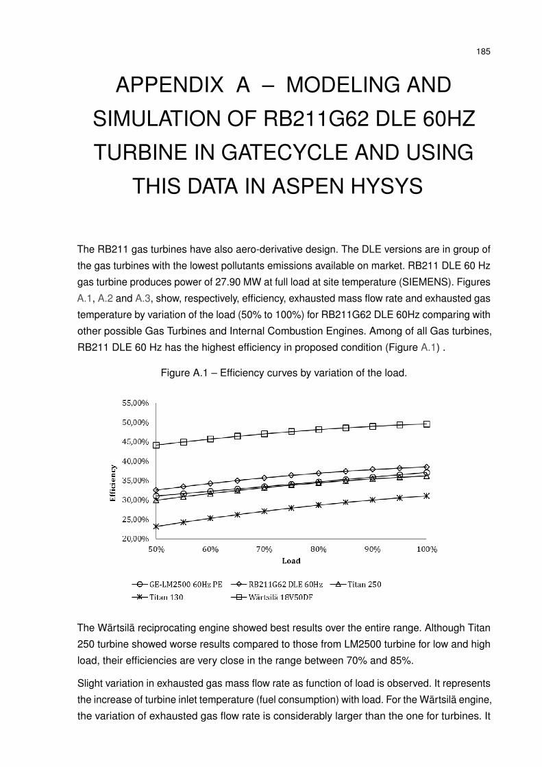
185
APPENDIX A – MODELING AND
SIMULATION OF RB211G62 DLE 60HZ
TURBINE IN GATECYCLE AND USING
THIS DATA IN ASPEN HYSYS
The RB211 gas turbines have also aero-derivative design. The DLE versions are in group of
the gas turbines with the lowest pollutants emissions available on market. RB211 DLE 60 Hz
gas turbine produces power of 27.90 MW at full load at site temperature (SIEMENS). Figures
A.1, A.2 and A.3, show, respectively, efficiency, exhausted mass flow rate and exhausted gas
temperature by variation of the load (50% to 100%) for RB211G62 DLE 60Hz comparing with
other possible Gas Turbines and Internal Combustion Engines. Among of all Gas turbines,
RB211 DLE 60 Hz has the highest efficiency in proposed condition (Figure A.1) .
Figure A.1 – Efficiency curves by variation of the load.
The Wärtsilä reciprocating engine showed best results over the entire range. Although Titan
250 turbine showed worse results compared to those from LM2500 turbine for low and high
load, their efficiencies are very close in the range between 70% and 85%.
Slight variation in exhausted gas mass flow rate as function of load is observed. It represents
the increase of turbine inlet temperature (fuel consumption) with load. For the Wärtsilä engine,
the variation of exhausted gas flow rate is considerably larger than the one for turbines. It

186APPENDIX A. Modeling and simulation of RB211G62 DLE 60Hz turbine in GATECYCLE and using this data
in Aspen Hysys
Figure A.2 – Curves of exhausted gas mass flow rate by variation of the load.
indicates that for this engine both, fuel and air consumption, increase. The exhausted gas
temperature curves as function of load for the turbines showed similar patterns. See Figure
A.3: The Titan 130 presented temperatures considerably lower than the other models of
turbines (since this turbine has lower efficiency, it indicates lower temperature at expander
inlet). In turn, RB211 DLE 60 Hz presents the adequate exhausted gas temperature for
WHRU even in condition of 80% of total load.
Figure A.3 – Curve of the exhausted gas temperature by variation of the load.
Figure A.4 shows the worksheet of various off-design calculation of RB211. In that, the input
parameters are changing to find the converged condition of RB211.
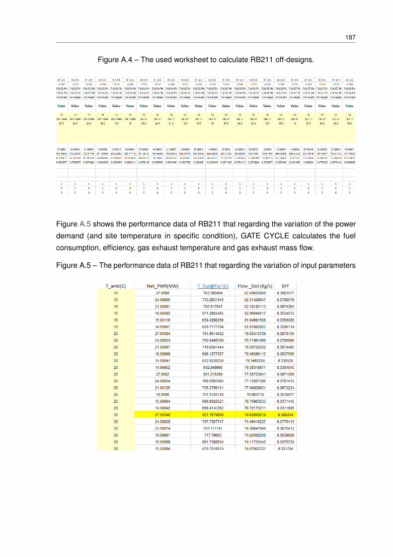
187
Figure A.4 – The used worksheet to calculate RB211 off-designs.
Figure A.5 shows the performance data of RB211 that regarding the variation of the power
demand (and site temperature in specific condition), GATE CYCLE calculates the fuel
consumption, efficiency, gas exhaust temperature and gas exhaust mass flow.
Figure A.5 – The performance data of RB211 that regarding the variation of input parameters
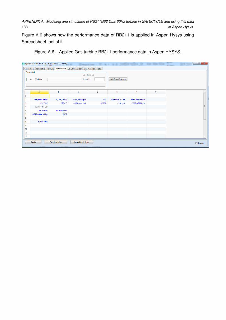
188APPENDIX A. Modeling and simulation of RB211G62 DLE 60Hz turbine in GATECYCLE and using this data
in Aspen Hysys
Figure A.6 shows how the performance data of RB211 is applied in Aspen Hysys using
Spreadsheet tool of it.
Figure A.6 – Applied Gas turbine RB211 performance data in Aspen HYSYS.
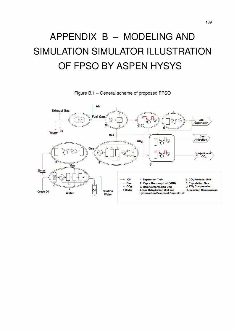
189
APPENDIX B – MODELING AND
SIMULATION SIMULATOR ILLUSTRATION
OF FPSO BY ASPEN HYSYS
Figure B.1 – General scheme of proposed FPSO
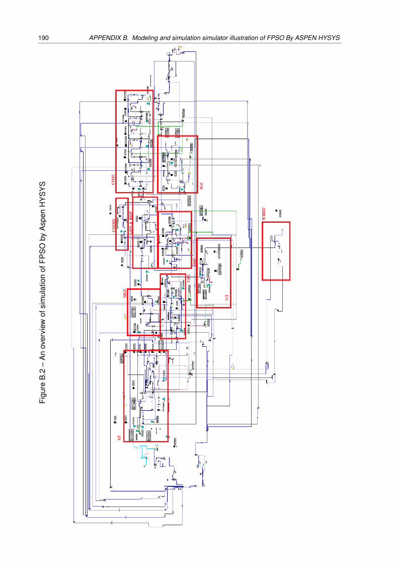
190 APPENDIX B. Modeling and simulation simulator illustration of FPSO By ASPEN HYSYSFi
gure
B.2
–A
nov
ervi
ewof
sim
ulat
ion
ofFP
SO
byA
spen
HY
SY
S
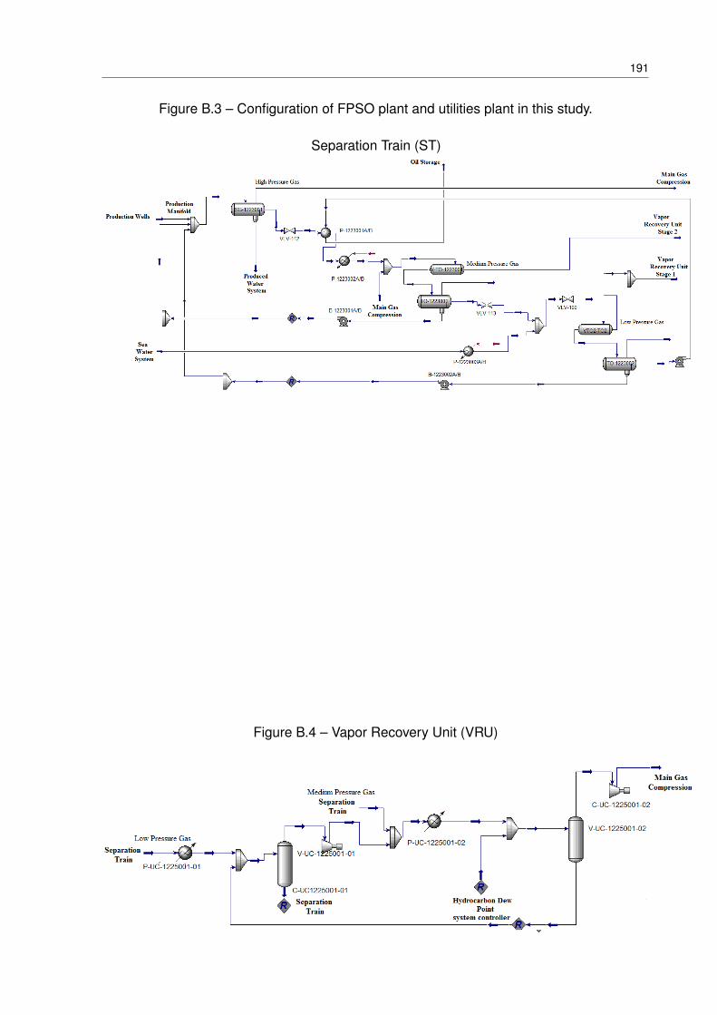
191
Figure B.3 – Configuration of FPSO plant and utilities plant in this study.
Separation Train (ST)
Figure B.4 – Vapor Recovery Unit (VRU)

192 APPENDIX B. Modeling and simulation simulator illustration of FPSO By ASPEN HYSYS
Figure B.5 – Main Gas Compression Unit (MGC)
Figure B.6 – Gas Dehydration System and CO2 Removal Unit (GDS&CO2RU)

193
Figure B.7 – CO2 Compression(CO2C)

194 APPENDIX B. Modeling and simulation simulator illustration of FPSO By ASPEN HYSYSTa
ble
B.1
–R
equi
red
inje
ctio
npr
essu
reas
afu
nctio
nof
CO
2co
mpo
sitio
nan
dga
sflo
w.

195
Figure B.8 – Exportation Gas Compression(EGC)
Figure B.9 – Injection Gas Compression(IGC)
Figure B.10 – Gas Turbine and Waste Heat Recovery Unit (GT&WHRU)

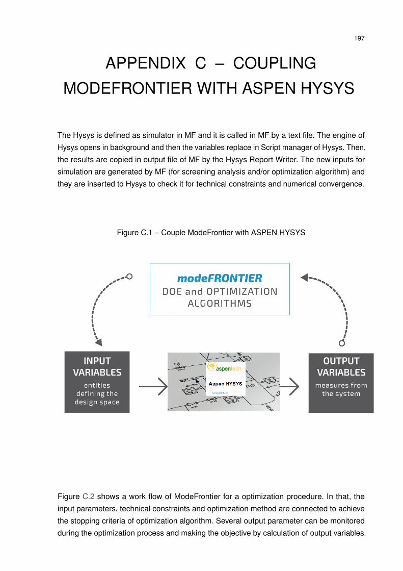
197
APPENDIX C – COUPLING
MODEFRONTIER WITH ASPEN HYSYS
The Hysys is defined as simulator in MF and it is called in MF by a text file. The engine of
Hysys opens in background and then the variables replace in Script manager of Hysys. Then,
the results are copied in output file of MF by the Hysys Report Writer. The new inputs for
simulation are generated by MF (for screening analysis and/or optimization algorithm) and
they are inserted to Hysys to check it for technical constraints and numerical convergence.
Figure C.1 – Couple ModeFrontier with ASPEN HYSYS
Figure C.2 shows a work flow of ModeFrontier for a optimization procedure. In that, the
input parameters, technical constraints and optimization method are connected to achieve
the stopping criteria of optimization algorithm. Several output parameter can be monitored
during the optimization process and making the objective by calculation of output variables.

198 APPENDIX C. Coupling ModeFrontier with ASPEN HYSYS
Figure C.2 – Work flow of ModeFrontier for an optimization procedure
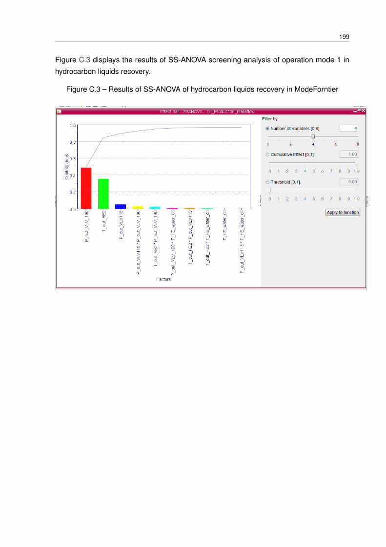
199
Figure C.3 displays the results of SS-ANOVA screening analysis of operation mode 1 in
hydrocarbon liquids recovery.
Figure C.3 – Results of SS-ANOVA of hydrocarbon liquids recovery in ModeForntier

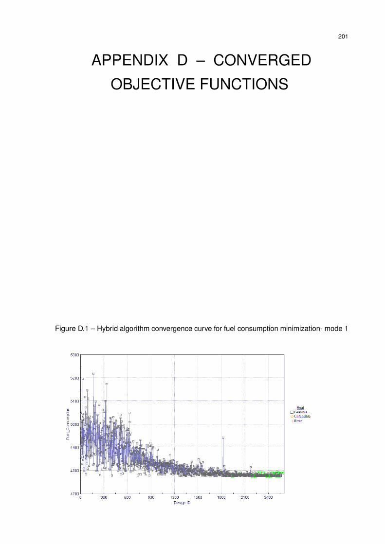
201
APPENDIX D – CONVERGED
OBJECTIVE FUNCTIONS
Figure D.1 – Hybrid algorithm convergence curve for fuel consumption minimization- mode 1
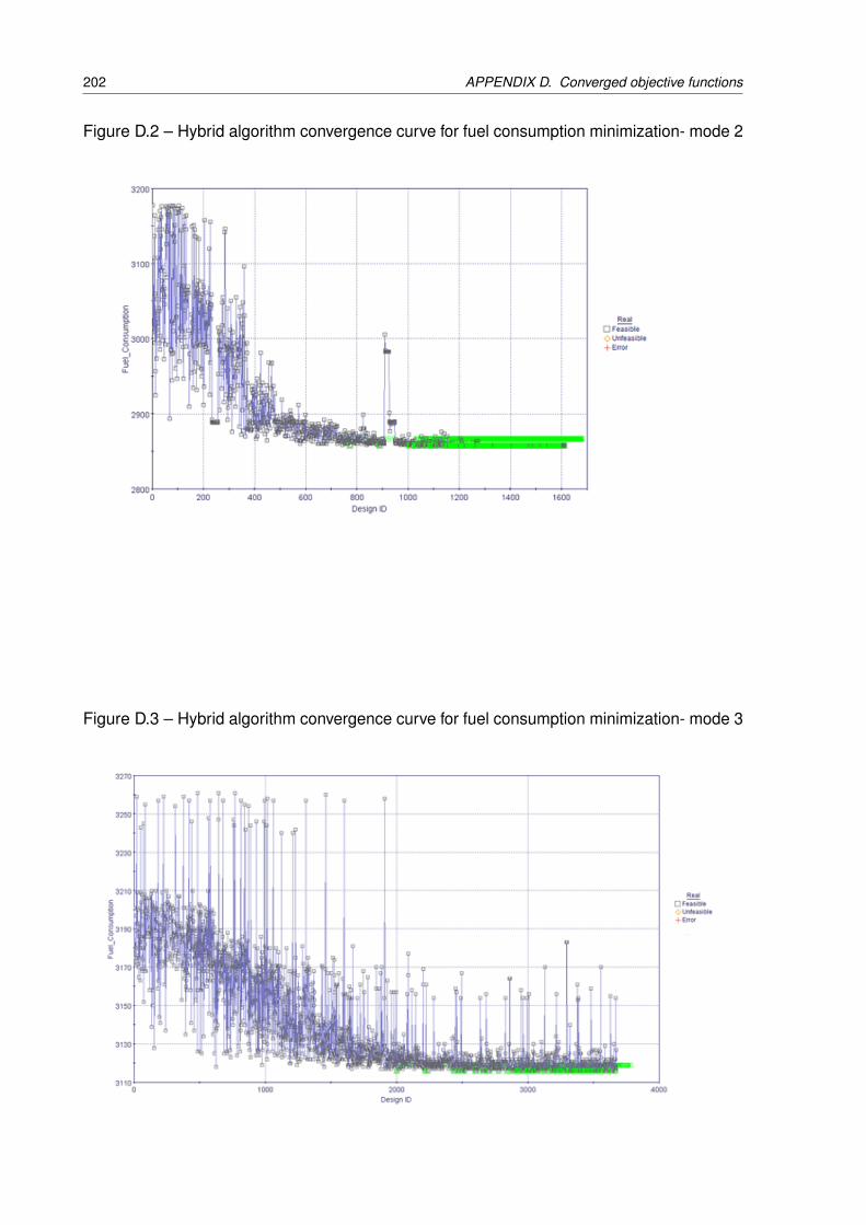
202 APPENDIX D. Converged objective functions
Figure D.2 – Hybrid algorithm convergence curve for fuel consumption minimization- mode 2
Figure D.3 – Hybrid algorithm convergence curve for fuel consumption minimization- mode 3
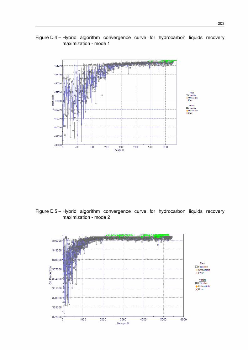
203
Figure D.4 – Hybrid algorithm convergence curve for hydrocarbon liquids recoverymaximization - mode 1
Figure D.5 – Hybrid algorithm convergence curve for hydrocarbon liquids recoverymaximization - mode 2
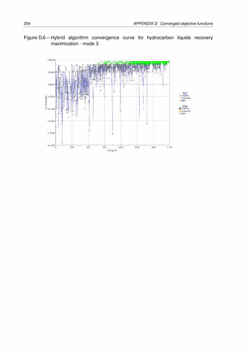
204 APPENDIX D. Converged objective functions
Figure D.6 – Hybrid algorithm convergence curve for hydrocarbon liquids recoverymaximization - mode 3