SOLIDWORKS Flow Simulation 2020 - SDC Publications

An Introduction to SOLIDW

ORKS Flow

Simulation 2020

SOLIDWORKS Flow Simulation 2020

An Introduction to®

John E. Matsson, Ph.D., P.E.

SDCP U B L I C AT I O N S www.SDCpublications.com

Better Textbooks. Lower Prices.

NewFeatures a New Chapter

on Free Surface Flow

https://www.sdcpublications.com

Visit the following websites to learn more about this book:

Powered by TCPDF (www.tcpdf.org)

https://www.sdcpublications.com/Textbooks/Introduction-SOLIDWORKS-Flow-Simulation-2020/ISBN/978-1-63057-327-0/

https://www.amazon.com/gp/product/1630573272?ie=UTF8&tag=sdcpublications&linkCode=as2&camp=211189&creative=374929&creativeASIN=1630573272

http://books.google.com/books?vid=ISBN1630573272&printsec=frontcover

http://www.barnesandnoble.com/s/1630573272?dref=1&keyword=1630573272

http://www.tcpdf.org

CHAPTER 2. FLAT PLATE BOUNDARY LAYER

21


A. Objectives

• Creating the SOLIDWORKS part needed for the Flow Simulation • Setting up Flow Simulation projects for internal flow • Setting up a two-dimensional flow condition • Initializing the mesh • Selecting boundary conditions • Inserting global goals, point goals and equation goals for the calculations • Running the calculations • Using Cut Plots to visualize the resulting flow field • Use of XY Plots for velocity profiles, boundary layer thickness, displacement thickness, momentum thickness and friction coefficients • Use of Excel templates for XY Plots • Comparison of Flow Simulation results with theories and empirical data • Cloning of the project

B. Problem Description In this chapter, we will use SOLIDWORKS Flow Simulation to study the two-dimensional laminar

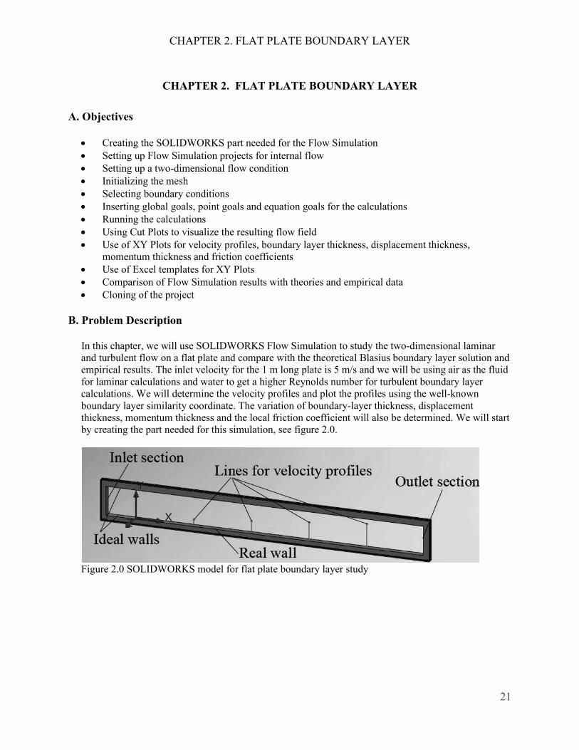
and turbulent flow on a flat plate and compare with the theoretical Blasius boundary layer solution and empirical results. The inlet velocity for the 1 m long plate is 5 m/s and we will be using air as the fluid for laminar calculations and water to get a higher Reynolds number for turbulent boundary layer calculations. We will determine the velocity profiles and plot the profiles using the well-known boundary layer similarity coordinate. The variation of boundary-layer thickness, displacement thickness, momentum thickness and the local friction coefficient will also be determined. We will start by creating the part needed for this simulation, see figure 2.0.

Figure 2.0 SOLIDWORKS model for flat plate boundary layer study


22

C. Creating the SOLIDWORKS Part

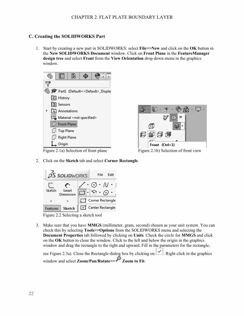
1. Start by creating a new part in SOLIDWORKS: select File>>New and click on the OK button in the New SOLIDWORKS Document window. Click on Front Plane in the FeatureManager design tree and select Front from the View Orientation drop down menu in the graphics window.

Figure 2.1a) Selection of front plane Figure 2.1b) Selection of front view

2. Click on the Sketch tab and select Corner Rectangle.

Figure 2.2 Selecting a sketch tool

3. Make sure that you have MMGS (millimeter, gram, second) chosen as your unit system. You can check this by selecting Tools>>Options from the SOLIDWORKS menu and selecting the Document Properties tab followed by clicking on Units. Check the circle for MMGS and click on the OK button to close the window. Click to the left and below the origin in the graphics window and drag the rectangle to the right and upward. Fill in the parameters for the rectangle,

see Figure 2.3a). Close the Rectangle dialog box by clicking on . Right click in the graphics

window and select Zoom/Pan/Rotate>> Zoom to Fit.


23

Figure 2.3a) Parameter settings for the rectangle

Figure 2.3b) Zooming in the graphics window

4. Repeat steps 2 and 3 but create a larger rectangle outside of the first rectangle. Dimensions are

shown in figure 2.4.

Figure 2.4 Dimensions of second larger rectangle


24

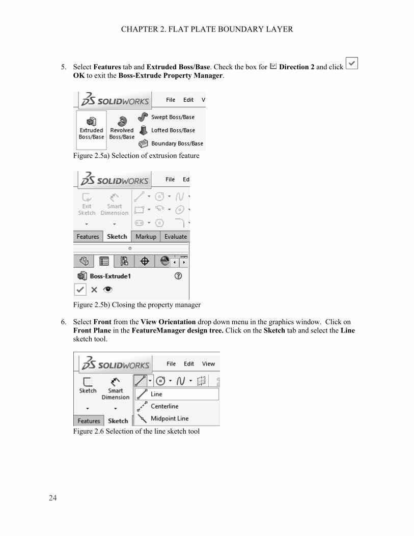
5. Select Features tab and Extruded Boss/Base. Check the box for Direction 2 and click OK to exit the Boss-Extrude Property Manager.

Figure 2.5a) Selection of extrusion feature

Figure 2.5b) Closing the property manager

6. Select Front from the View Orientation drop down menu in the graphics window. Click on

Front Plane in the FeatureManager design tree. Click on the Sketch tab and select the Line sketch tool.

Figure 2.6 Selection of the line sketch tool


25

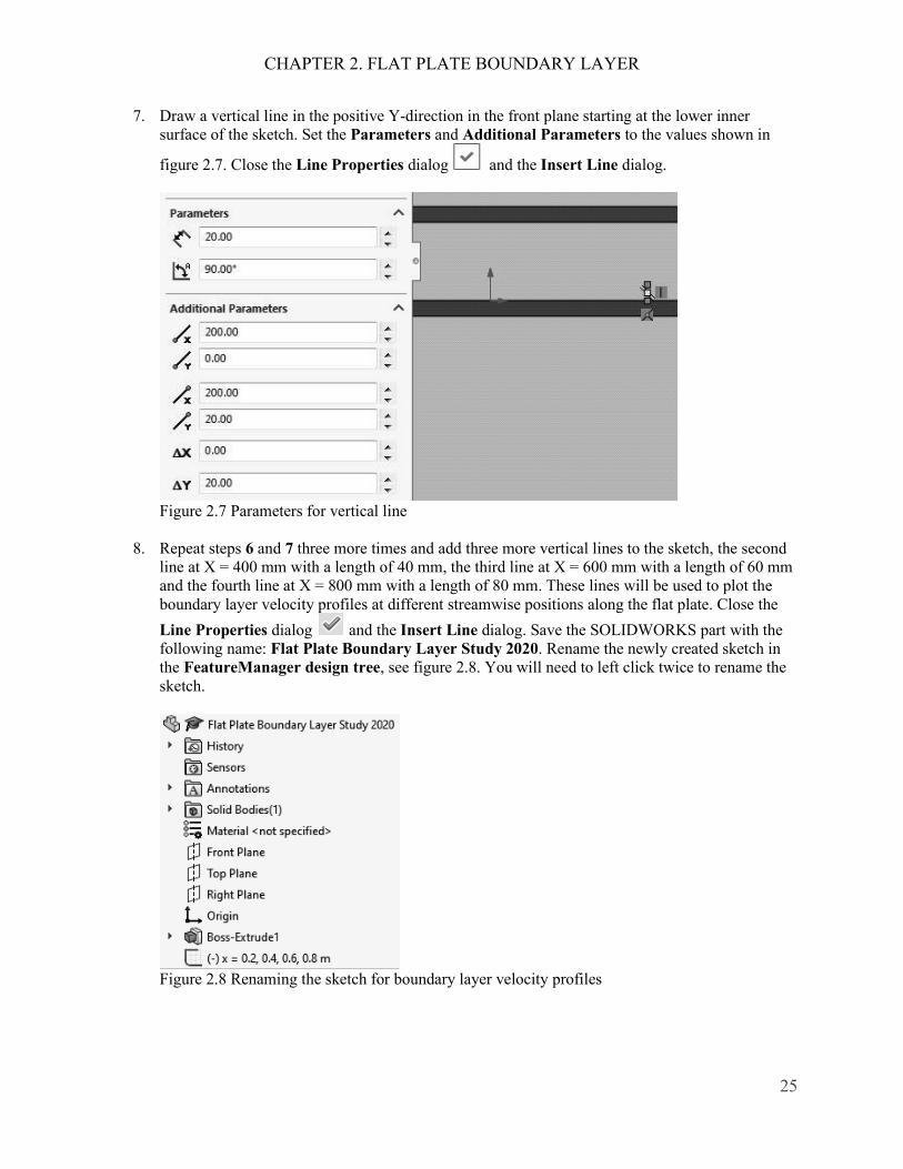
7. Draw a vertical line in the positive Y-direction in the front plane starting at the lower inner surface of the sketch. Set the Parameters and Additional Parameters to the values shown in

figure 2.7. Close the Line Properties dialog and the Insert Line dialog.

Figure 2.7 Parameters for vertical line

8. Repeat steps 6 and 7 three more times and add three more vertical lines to the sketch, the second

line at X = 400 mm with a length of 40 mm, the third line at X = 600 mm with a length of 60 mm and the fourth line at X = 800 mm with a length of 80 mm. These lines will be used to plot the boundary layer velocity profiles at different streamwise positions along the flat plate. Close the Line Properties dialog and the Insert Line dialog. Save the SOLIDWORKS part with the following name: Flat Plate Boundary Layer Study 2020. Rename the newly created sketch in the FeatureManager design tree, see figure 2.8. You will need to left click twice to rename the sketch.

Figure 2.8 Renaming the sketch for boundary layer velocity profiles


26

9. Click on the Rebuild symbol in the SOLIDWORKS menu. Repeat step 6 and draw a horizontal line in the X-direction starting at the origin of the lower inner surface of the sketch. Set the Parameters and Additional Parameters to the values shown in figure 2.9 and close the Line Properties dialog and the Insert Line dialog. Click on the Rebuild symbol. Rename the sketch in the FeatureManager design tree and call it x = 0 – 0.9 m.

Figure 2.9 Sketch of a line in the X-direction

10. Next, we will create a split line. Repeat step 6 once again but this time select the Top Plane and draw a line in the Z-direction through the origin of the lower inner surface of the sketch. It will help to zoom in and rotate the view to complete this step. Set the Parameters and Additional Parameters to the values shown in figure 2.10 and close the dialog. Click on the Rebuild symbol.

Figure 2.10 Drawing of a line in the Z-direction


27

11. Rename the new sketch in the FeatureManager design tree and call it Split Line. Select

Insert>>Curve>>Split Line… from the SOLIDWORKS menu. Select Projection under Type to Split. Select Split Line for Sketch to Project under Selections. For Faces to Split, select the

surface where you have drawn your split line, see figure 2.11b). Close the dialog . You have now finished the part for the flat plate boundary layer. Select File>>Save from the SOLIDWORKS menu.

Figure 2.11a) Creating a split line

Figure 2.11b) Selection of surface for the split line


28

D. Setting Up the Flow Simulation Project

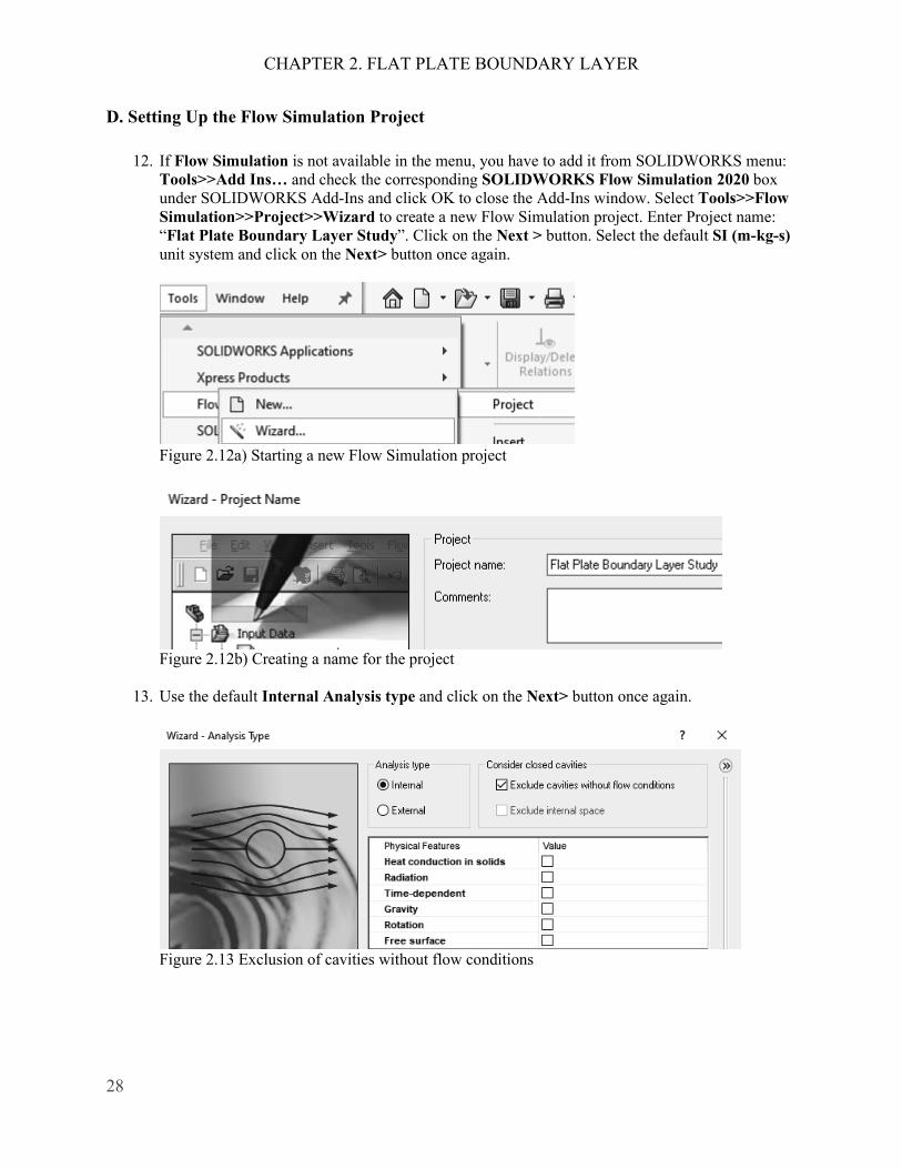
12. If Flow Simulation is not available in the menu, you have to add it from SOLIDWORKS menu: Tools>>Add Ins… and check the corresponding SOLIDWORKS Flow Simulation 2020 box under SOLIDWORKS Add-Ins and click OK to close the Add-Ins window. Select Tools>>Flow Simulation>>Project>>Wizard to create a new Flow Simulation project. Enter Project name: “Flat Plate Boundary Layer Study”. Click on the Next > button. Select the default SI (m-kg-s) unit system and click on the Next> button once again.

Figure 2.12a) Starting a new Flow Simulation project

Figure 2.12b) Creating a name for the project

13. Use the default Internal Analysis type and click on the Next> button once again.

Figure 2.13 Exclusion of cavities without flow conditions


29

14. Select Air from the Gases and add it as Project Fluid. Select Laminar Only from the Flow

Type drop down menu. Click on the Next > button. Use the default Wall Conditions and click on the Next > button. Insert 5 m/s for Velocity in X direction as Initial Conditions and click on the Finish button. You will get a fluid volume recognition failure message. Answer Yes to this question and create a lid on each side of the model. Answer Yes to the questions when you create the lids.

Figure 2.14 Selection of fluid for the project and flow type

15. Select Tools>>Flow Simulation>>Computational Domain…. Click on the 2D simulation

button under Type and select XY plane. Close the Computational Domain dialog .

Figure 2.15a) Modifying the computational domain

Figure 2.15b) Selecting 2D simulation in the XY plane


30

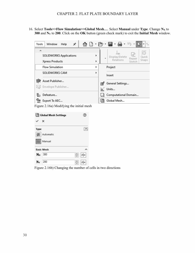
16. Select Tools>>Flow Simulation>>Global Mesh…. Select Manual under Type. Change NX to

300 and NY to 200. Click on the OK button (green check mark) to exit the Initial Mesh window.

Figure 2.16a) Modifying the initial mesh

Figure 2.16b) Changing the number of cells in two directions


31

E. Selecting Boundary Conditions

17. Select the Flow Simulation analysis tree tab, open the Input Data folder by clicking on the plus sign next to it and right click on Boundary Conditions. Select Insert Boundary Condition…. Select Wireframe as the Display Style. Right click in the graphics window and select Zoom/Pan/Rotate>>Zoom to Fit. Once again, right click in the graphics window and select Zoom/Pan/Rotate>>Rotate View. Click and drag the mouse so that the inner surface of the left boundary is visible. Right click again and unselect Zoom/Pan/Rotate>>Rotate View. Right click on the left inflow boundary surface and select Select Other. Select the Face corresponding to the inflow boundary. Select Inlet Velocity in the Type portion of the Boundary Condition window and set the velocity to 5 m/s in the Flow Parameters window. Click OK to exit the window. Right click in the graphics window and select Zoom to Area and select an area around the left boundary.

Figure 2.17a) Inserting boundary condition Figure 2.17b) Modifying the view

Figure 2.17c) Velocity boundary condition on the inflow


32

Figure 2.17d) Inlet velocity boundary condition indicated by arrows

18. Red arrows pointing in the flow direction appears indicating the inlet velocity boundary condition, see figure 2.17d). Right click in the graphics window and select Zoom to Fit. Right click again in the graphics window and select Rotate View once again to rotate the part so that the inner right surface is visible in the graphics window. Right click and click on Select. Right click on Boundary Conditions in the Flow Simulation analysis tree and select Insert Boundary Condition…. Right click on the outflow boundary surface and select Select Other. Select the Face corresponding to the outflow boundary. Click on the Pressure Openings button in the Type portion of the Boundary Condition window and select Static Pressure. Click OK to exit the window. If you zoom in on the outlet boundary, you will see blue arrows indicating the static pressure boundary condition, see figure 2.18b).

Figure 2.18a) Selection of static pressure as boundary condition at the outlet of the flow region


33

Figure 2.18b) Outlet static pressure boundary condition

19. Enter the following boundary conditions: Ideal Wall for the lower and upper walls at the inflow region, see figures 2.19. These will be adiabatic and frictionless walls.

Figure 2.19 Ideal wall boundary condition for two wall sections


34

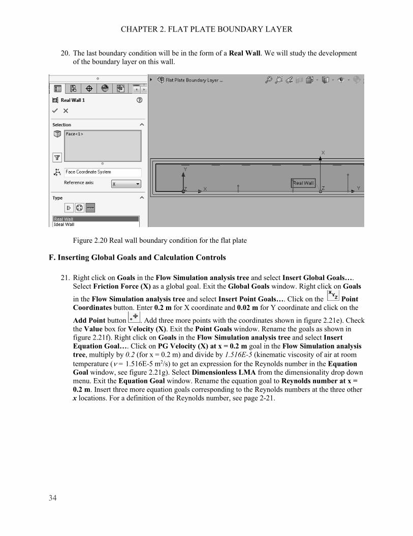
20. The last boundary condition will be in the form of a Real Wall. We will study the development of the boundary layer on this wall.

Figure 2.20 Real wall boundary condition for the flat plate

F. Inserting Global Goals and Calculation Controls

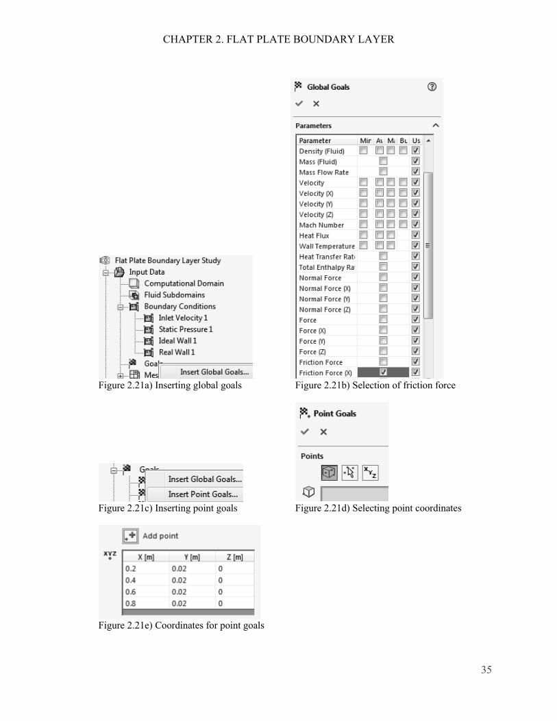
21. Right click on Goals in the Flow Simulation analysis tree and select Insert Global Goals…. Select Friction Force (X) as a global goal. Exit the Global Goals window. Right click on Goals

in the Flow Simulation analysis tree and select Insert Point Goals…. Click on the Point Coordinates button. Enter 0.2 m for X coordinate and 0.02 m for Y coordinate and click on the

Add Point button . Add three more points with the coordinates shown in figure 2.21e). Check the Value box for Velocity (X). Exit the Point Goals window. Rename the goals as shown in figure 2.21f). Right click on Goals in the Flow Simulation analysis tree and select Insert Equation Goal…. Click on PG Velocity (X) at x = 0.2 m goal in the Flow Simulation analysis tree, multiply by 0.2 (for x = 0.2 m) and divide by 1.516E-5 (kinematic viscosity of air at room temperature (ν = 1.516E-5 m2/s) to get an expression for the Reynolds number in the Equation Goal window, see figure 2.21g). Select Dimensionless LMA from the dimensionality drop down menu. Exit the Equation Goal window. Rename the equation goal to Reynolds number at x = 0.2 m. Insert three more equation goals corresponding to the Reynolds numbers at the three other x locations. For a definition of the Reynolds number, see page 2-21.


35

Figure 2.21a) Inserting global goals Figure 2.21b) Selection of friction force

Figure 2.21c) Inserting point goals Figure 2.21d) Selecting point coordinates

Figure 2.21e) Coordinates for point goals


36

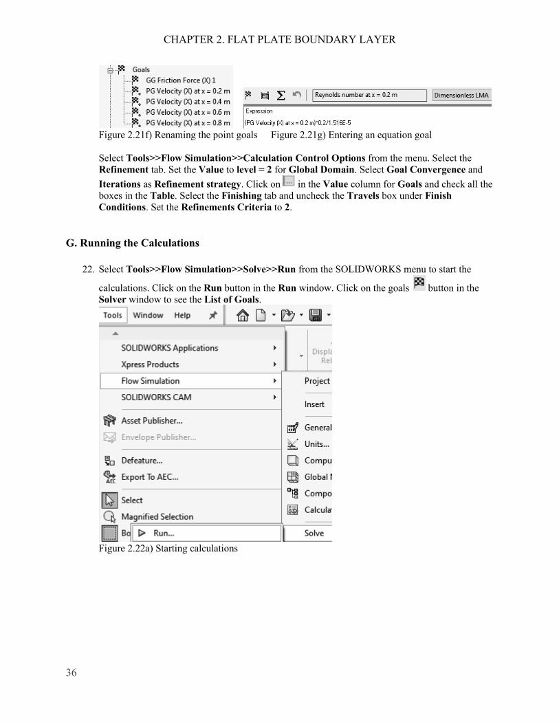
Figure 2.21f) Renaming the point goals Figure 2.21g) Entering an equation goal Select Tools>>Flow Simulation>>Calculation Control Options from the menu. Select the Refinement tab. Set the Value to level = 2 for Global Domain. Select Goal Convergence and Iterations as Refinement strategy. Click on in the Value column for Goals and check all the boxes in the Table. Select the Finishing tab and uncheck the Travels box under Finish Conditions. Set the Refinements Criteria to 2.

G. Running the Calculations

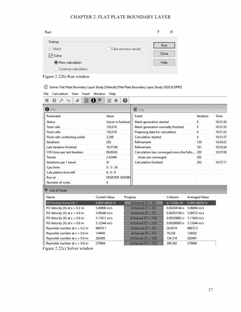
22. Select Tools>>Flow Simulation>>Solve>>Run from the SOLIDWORKS menu to start the

calculations. Click on the Run button in the Run window. Click on the goals button in the Solver window to see the List of Goals.

Figure 2.22a) Starting calculations


37

Figure 2.22b) Run window

Figure 2.22c) Solver window


38

H. Using Cut Plots to Visualize the Flow Field

Open the Results folder, right click on Cut Plots in the Flow Simulation analysis tree under Results and select Insert…. Select the Front Plane from the FeatureManager design tree. Slide the Number of Levels slide bar to 255. Select Pressure from the Parameter drop down menu. Click OK to exit the Cut Plot window. Figure 2.23a) shows the high pressure region close to the leading edge of the flat plate. Rename the cut plot to Pressure. You can get more lighting on the cut plot by selecting Tools>>Flow Simulation>>Results>>Display>>Lighting from the SOLIDWORKS menu. Right click on the Pressure Cut Plot in the Flow Simulation analysis tree and select Hide. Repeat this step but instead choose Velocity (X) from the Parameter drop down menu. Rename the second cut plot to Velocity (X). Figures 2.23b) and 2.23c) show the velocity boundary layer close to the wall.

Figure 2.23a) Pressure distribution along the flat plate

Figure 2.23b) X – Component of Velocity distribution on the flat plate

Figure 2.23c) Close up view of the velocity boundary layer


39

I. Using XY Plots with Templates

23. Place the file “graph 2.24c).xlsm” on the desktop. This file and the other exercise files are available for download at the SDC Publications website. Click on the FeatureManager design

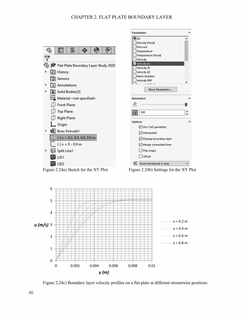
tree. Click on the sketch x = 0.2, 0.4, 0.6, 0.8 m. Click on the Flow Simulation analysis tree tab. Right click XY Plot and select Insert…. Check the Velocity (X) box. Open the Resolution portion of the XY Plot window and slide the Geometry Resolution as far as it goes to the right. Click on the Evenly Distribute Output Points button and increase the number of points to 500. Open the Options portion and check the Display boundary layer box. Select the “Excel Workbook (*.xlsx)” from the drop-down menu. Click Export to Excel to create the XY Plot window. An Excel file will open with a graph of the velocity in the boundary layer at different streamwise positions. Double click on the graph 2.24c) file to open the file. Click on Enable Content if you get a Security Warning that Macros have been disabled. If Developer is not available in the menu of the Excel file, you will need to do the following: Select File>>Options from the menu and click on the Customize Ribbon on the left hand side. Check the Developer box on the right hand side under Main Tabs. Click OK to exit the Excel Options window. Click on the Developer tab in the Excel menu for the graph 2.24c) file and select Visual Basic on the left hand side to open the editor. Click on the plus sign next to VBAProject (XY Plot 1.xlsx) and click on the plus sign next to Microsoft Excel Objects. Right click on Sheet2 (Plot Data) and select View Object. Select Module1 in the Modules folder under VBAProject (graph 2.24c).xlsm). Select Run>>Run Macro from the menu of the MVB for Applications window. Click on the Run button in the Macros window. Figure 2.24c) will become available in Excel showing the streamwise velocity component u (m/s) versus wall normal coordinate y (m). Close the XY Plot window and the graph 2.24c) window in Excel. Exit the XY Plot window in SOLIDWORKS Flow Simulation and rename the inserted xy-plot in the Flow Simulation analysis tree to Laminar Velocity Boundary Layer.


40

Figure 2.24a) Sketch for the XY Plot Figure 2.24b) Settings for the XY Plot

Figure 2.24c) Boundary layer velocity profiles on a flat plate at different streamwise positions

0

1

2

3

4

5

6

0 0.002 0.004 0.006 0.008 0.01

u (m/s)

y (m)

x = 0.2 m

x = 0.4 m

x = 0.6 m

x = 0.8 m


41

J. Comparison of Flow Simulation Results with Theory and Empirical Data

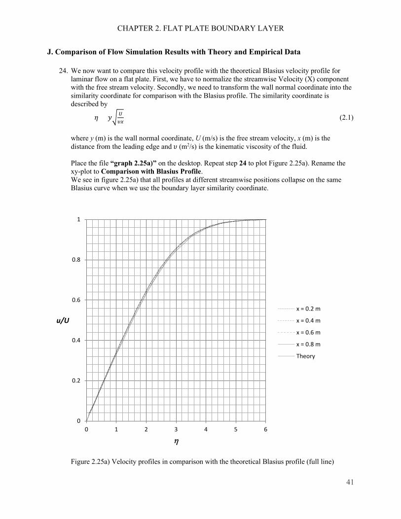
24. We now want to compare this velocity profile with the theoretical Blasius velocity profile for laminar flow on a flat plate. First, we have to normalize the streamwise Velocity (X) component with the free stream velocity. Secondly, we need to transform the wall normal coordinate into the similarity coordinate for comparison with the Blasius profile. The similarity coordinate is described by

𝜂𝜂 = 𝑦𝑦�𝑈𝑈𝜐𝜐𝜐𝜐

(2.1)

where y (m) is the wall normal coordinate, U (m/s) is the free stream velocity, x (m) is the distance from the leading edge and 𝜐𝜐 (m2/s) is the kinematic viscosity of the fluid. Place the file “graph 2.25a)” on the desktop. Repeat step 24 to plot Figure 2.25a). Rename the xy-plot to Comparison with Blasius Profile. We see in figure 2.25a) that all profiles at different streamwise positions collapse on the same Blasius curve when we use the boundary layer similarity coordinate.

Figure 2.25a) Velocity profiles in comparison with the theoretical Blasius profile (full line)

0

0.2

0.4

0.6

0.8

1

0 1 2 3 4 5 6

u/U

η

x = 0.2 m

x = 0.4 m

x = 0.6 m

x = 0.8 m

Theory


42

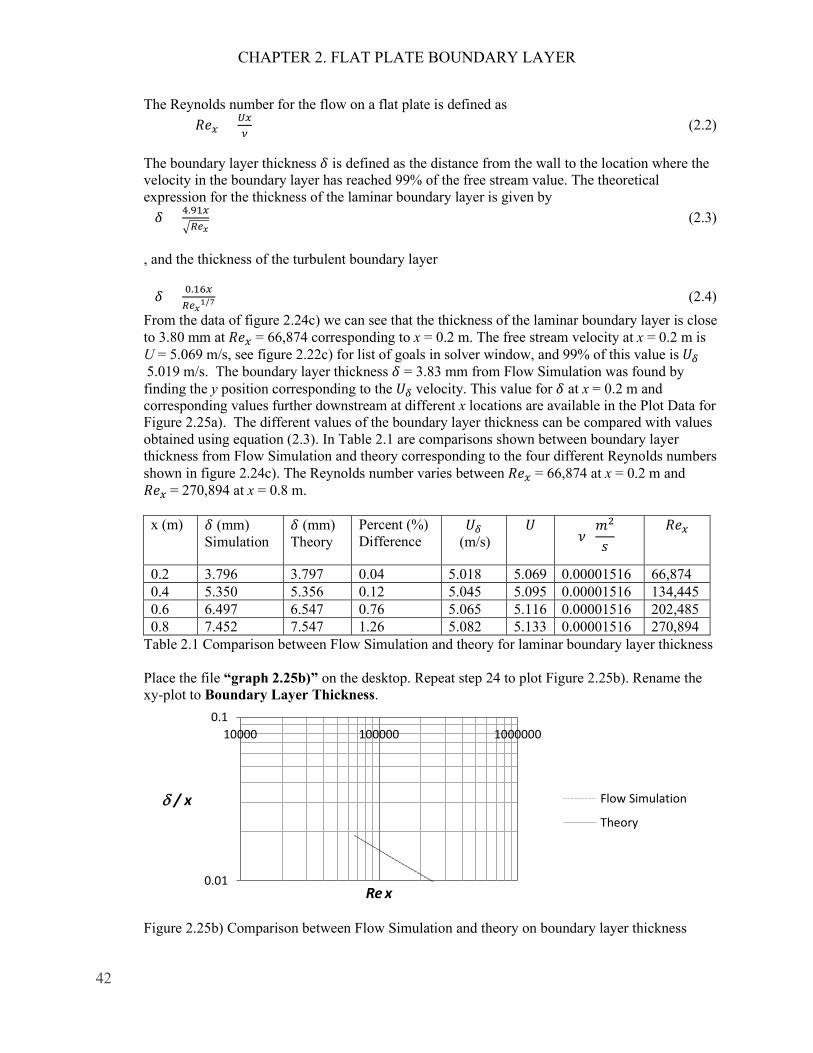
The Reynolds number for the flow on a flat plate is defined as 𝑅𝑅𝑅𝑅𝜐𝜐 = 𝑈𝑈𝜐𝜐

𝜈𝜈 (2.2)

The boundary layer thickness 𝛿𝛿 is defined as the distance from the wall to the location where the velocity in the boundary layer has reached 99% of the free stream value. The theoretical expression for the thickness of the laminar boundary layer is given by 𝛿𝛿 = 4.91𝜐𝜐

�𝑅𝑅𝑅𝑅𝑥𝑥 (2.3)

, and the thickness of the turbulent boundary layer 𝛿𝛿 = 0.16𝜐𝜐

𝑅𝑅𝑅𝑅𝑥𝑥1/7 (2.4) From the data of figure 2.24c) we can see that the thickness of the laminar boundary layer is close to 3.80 mm at 𝑅𝑅𝑅𝑅𝜐𝜐 = 66,874 corresponding to x = 0.2 m. The free stream velocity at x = 0.2 m is U = 5.069 m/s, see figure 2.22c) for list of goals in solver window, and 99% of this value is 𝑈𝑈𝛿𝛿 = 5.019 m/s. The boundary layer thickness 𝛿𝛿 = 3.83 mm from Flow Simulation was found by finding the y position corresponding to the 𝑈𝑈𝛿𝛿 velocity. This value for 𝛿𝛿 at x = 0.2 m and corresponding values further downstream at different x locations are available in the Plot Data for Figure 2.25a). The different values of the boundary layer thickness can be compared with values obtained using equation (2.3). In Table 2.1 are comparisons shown between boundary layer thickness from Flow Simulation and theory corresponding to the four different Reynolds numbers shown in figure 2.24c). The Reynolds number varies between 𝑅𝑅𝑅𝑅𝜐𝜐 = 66,874 at x = 0.2 m and 𝑅𝑅𝑅𝑅𝜐𝜐 = 270,894 at x = 0.8 m. x (m) 𝛿𝛿 (mm)

Simulation 𝛿𝛿 (mm) Theory

Percent (%) Difference

𝑈𝑈𝛿𝛿 (m/s)

𝑈𝑈 𝜈𝜈 (𝑚𝑚2

𝑠𝑠)

𝑅𝑅𝑅𝑅𝜐𝜐

0.2 3.796 3.797 0.04 5.018 5.069 0.00001516 66,874 0.4 5.350 5.356 0.12 5.045 5.095 0.00001516 134,445 0.6 6.497 6.547 0.76 5.065 5.116 0.00001516 202,485 0.8 7.452 7.547 1.26 5.082 5.133 0.00001516 270,894

Table 2.1 Comparison between Flow Simulation and theory for laminar boundary layer thickness Place the file “graph 2.25b)” on the desktop. Repeat step 24 to plot Figure 2.25b). Rename the xy-plot to Boundary Layer Thickness.

Figure 2.25b) Comparison between Flow Simulation and theory on boundary layer thickness

0.01

0.110000 100000 1000000

δ / x

Re x

Flow Simulation

Theory


43

25. We now want to study how the local friction coefficient varies along the plate. It is defined as the local wall shear stress divided by the dynamic pressure: 𝐶𝐶𝑓𝑓,𝜐𝜐 = 𝜏𝜏𝑤𝑤

12𝜌𝜌𝑈𝑈

2 (2.5)

The theoretical local friction coefficient for laminar flow is given by 𝐶𝐶𝑓𝑓,𝜐𝜐 = 0.664

�𝑅𝑅𝑅𝑅𝑥𝑥 𝑅𝑅𝑅𝑅𝜐𝜐 < 5 ∙ 105 (2.6)

and for turbulent flow 𝐶𝐶𝑓𝑓,𝜐𝜐 = 0.027

𝑅𝑅𝑅𝑅𝑥𝑥1/7 5 ∙ 105 ≤ 𝑅𝑅𝑅𝑅𝜐𝜐 ≤ 107 (2.7) Place the file “graph 2.26” on the desktop. Repeat step 24 but this time choose the sketch x = 0 – 0.9 m, uncheck the box for Velocity (X) and check the box for Shear Stress. Use the file “graph 2.26” to create Figure 2.26. Rename the xy-plot to Local Friction Coefficient. Figure 2.26 shows the local friction coefficient versus the Reynolds number compared with theoretical values for laminar boundary layer flow.

Figure 2.26 Local friction coefficient as a function of the Reynolds number The average friction coefficient over the whole plate Cf is not a function of the surface roughness for the laminar boundary layer but a function of the Reynolds number based on the length of the plate ReL, see figure E3 in Exercise 8 at the end of this chapter. This friction coefficient can be determined in Flow Simulation by using the final value of the global goal, the X-component of the Shear Force Ff , see figure 2.22c), and dividing it by the dynamic pressure times the area A in the X-Z plane of the computational domain related to the flat plate. 𝐶𝐶𝑓𝑓 = 𝐹𝐹𝑓𝑓

12𝜌𝜌𝑈𝑈

2𝐴𝐴= 0.0001475𝑁𝑁

12∙1.204𝑘𝑘𝑘𝑘/𝑚𝑚3∙52𝑚𝑚2/𝑠𝑠2∙1𝑚𝑚∙0.004𝑚𝑚

=0.00245 (2.8)

𝑅𝑅𝑅𝑅𝐿𝐿 = 𝑈𝑈𝐿𝐿

𝜈𝜈= 5𝑚𝑚/𝑠𝑠∙1𝑚𝑚

1.516∙10−5𝑚𝑚2/𝑠𝑠= 3.3 ∙ 105 (2.9)

0.001

0.01

0.1100 1000 10000 100000 1000000

Cf,x

Rex

Flow Simulation

Theory


44

The average friction coefficient from Flow Simulation can be compared with the theoretical value for laminar boundary layers 𝐶𝐶𝑓𝑓 = 1.328

�𝑅𝑅𝑅𝑅𝐿𝐿= 0.002312 𝑅𝑅𝑅𝑅𝐿𝐿 < 5 ∙ 105 (2.10)

This is a difference of 6 %. For turbulent boundary layers the corresponding expression is 𝐶𝐶𝑓𝑓 = 0.0315

𝑅𝑅𝑅𝑅𝐿𝐿1/7 5 ∙ 105 ≤ 𝑅𝑅𝑅𝑅𝐿𝐿 ≤ 107 (2.11) If the boundary layer is laminar on one part of the plate and turbulent on the remaining part, the average friction coefficient is determined by 𝐶𝐶𝑓𝑓 = 0.0315

𝑅𝑅𝑅𝑅𝐿𝐿1/7 −1𝑅𝑅𝑅𝑅𝐿𝐿

(0.0315𝑅𝑅𝑅𝑅𝑐𝑐𝑐𝑐67 − 1.328�𝑅𝑅𝑅𝑅𝑐𝑐𝑐𝑐) (2.12)

where 𝑹𝑹𝑹𝑹𝒄𝒄𝒄𝒄 is the critical Reynolds number for laminar to turbulent transition.

K. Cloning of the Project

26. In the next step, we will clone the project. Select Tools>>Flow Simulation>>Project>>Clone Project…. Enter the Project Name “Flat Plate Boundary Layer Study Using Water”. Select Create New Configuration and exit the Clone Project window. Next, change the fluid to water in order to get higher Reynolds numbers. Start by selecting Tools>>Flow Simulation>>General Settings… from the SOLIDWORKS menu. Click on Fluids in the Navigator portion, select Air and click on the Remove button. Select Water from the Liquids and Add it as the Project Fluid. Change the Flow type to Laminar and Turbulent, see figure 2.27d). Click on the OK button to close the General Settings window.

Figure 2.27a) Cloning the project


45

Figure 2.27b) Creating a new project Figure 2.27c) Selection of general settings

Figure 2.27d) Selection of fluid and flow type


46

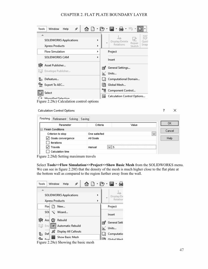
27. Select Tools>>Flow Simulation>>Computational Domain… Set the size of the computational domain to the values shown in figure 2.28a). Click on the OK button to exit. Select Tools>>Flow Simulation>>Global Mesh… from the SOLIDWORKS menu, select Manual Type and change the Number of cells per X: to 400 and the Number of Cells per Y: to 200. Also, click on Control Planes. Change the Ratio for X to -5 and the Ratio for Y to -100. Click on the green check mark above Ratio, see Figure 2.28b). This will increase the number of cells close to the wall where the velocity gradient is high. Select Tools>>Flow Simulation>>Calculation Control Options… from the SOLIDWORKS menu. Change the Maximum travels value to 5 by first changing to Manual from the drop-down menu. Travel is a unit characterizing the duration of the calculation. Click on the OK button to exit.

Figure 2.28a) Setting the size of the computational domain

Figure 2.28b) Increasing the number of cells and changing the distribution of cells


47

Figure 2.28c) Calculation control options

Figure 2.28d) Setting maximum travels

Select Tools>>Flow Simulation>>Project>>Show Basic Mesh from the SOLIDWORKS menu. We can see in figure 2.28f) that the density of the mesh is much higher close to the flat plate at the bottom wall as compared to the region further away from the wall.

Figure 2.28e) Showing the basic mesh


48

Figure 2.28f) Mesh distribution in the X-Y plane

28. Right click the Inlet Velocity Boundary Condition in the Flow Simulation analysis tree and select Edit Definition…. Open the Boundary Layer section and select Laminar Boundary Layer. Click OK to exit the Boundary Condition window. Right click the Reynolds number at x = 0.2 m goal and select Edit Definition…. Change the viscosity value in the Expression to 1.004E-6. Click on the OK button to exit. Change the other three equation goals in the same way.

Select Tools>>Flow Simulation>>Calculation Control Options from the menu. Select the Refinement tab. Set the Value to level = 2 for Global Domain. Select Goal Convergence and Iterations as Refinement strategy. Click on in the Value column for Goals and check all the boxes in the Table. Select the Finishing tab and uncheck the Travels box under Finish Conditions. Set the Refinements Criteria to 2.

Select Tools>>Flow Simulation>>Solve>>Run to start calculations. Click on the Run button in the Run window.

Figure 2.29a) Selecting a laminar boundary layer

Figure 2.29b) Modifying the equation goals


49

Figure 2.29c) Creation of mesh and starting a new calculation

Figure 2.29d) Solver window and goals table for calculations of turbulent boundary layer


50

29. Place the file “graph 2.30a)” on the desktop. Repeat step 24 and choose the sketch x = 0.2, 0.4,

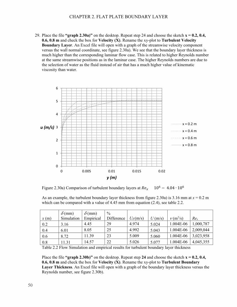
0.6, 0.8 m and check the box for Velocity (X). Rename the xy-plot to Turbulent Velocity Boundary Layer. An Excel file will open with a graph of the streamwise velocity component versus the wall normal coordinate, see figure 2.30a). We see that the boundary layer thickness is much higher than the corresponding laminar flow case. This is related to higher Reynolds number at the same streamwise positions as in the laminar case. The higher Reynolds numbers are due to the selection of water as the fluid instead of air that has a much higher value of kinematic viscosity than water.

Figure 2.30a) Comparison of turbulent boundary layers at 𝑅𝑅𝑅𝑅𝜐𝜐 = 106 − 4.04 ∙ 106 As an example, the turbulent boundary layer thickness from figure 2.30a) is 3.16 mm at x = 0.2 m which can be compared with a value of 4.45 mm from equation (2.4), see table 2.2.

x (m) δ (mm) Simulation

δ (mm) Empirical

% Difference Uδ (m/s) U (m/s) ν (m2/s) Rex

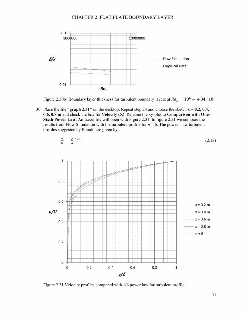
0.2 3.16 4.45 29 4.974 5.024 1.004E-06 1,000,787 0.4 6.01 8.05 25 4.992 5.043 1.004E-06 2,009,044 0.6 8.72 11.39 23 5.009 5.060 1.004E-06 3,023,958 0.8 11.31 14.57 22 5.026 5.077 1.004E-06 4,045,355 Table 2.2 Flow Simulation and empirical results for turbulent boundary layer thickness Place the file “graph 2.30b)” on the desktop. Repeat step 24 and choose the sketch x = 0.2, 0.4, 0.6, 0.8 m and check the box for Velocity (X). Rename the xy-plot to Turbulent Boundary Layer Thickness. An Excel file will open with a graph of the boundary layer thickness versus the Reynolds number, see figure 2.30b).

0

1

2

3

4

5

6

0 0.005 0.01 0.015 0.02

u (m/s)

y (m)

x = 0.2 m

x = 0.4 m

x = 0.6 m

x = 0.8 m


51

Figure 2.30b) Boundary layer thickness for turbulent boundary layers at 𝑅𝑅𝑅𝑅𝜐𝜐 = 106 − 4.04 ∙ 106

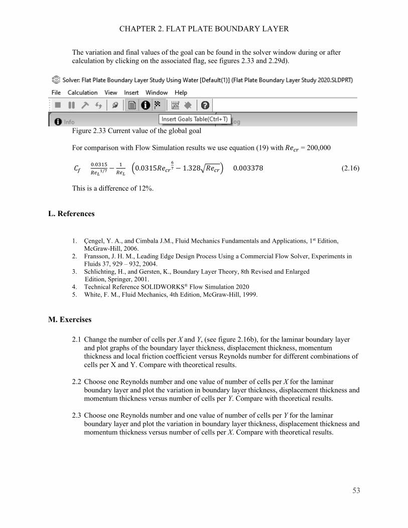
30. Place the file “graph 2.31” on the desktop. Repeat step 24 and choose the sketch x = 0.2, 0.4, 0.6, 0.8 m and check the box for Velocity (X). Rename the xy-plot to Comparison with One-Sixth Power Law. An Excel file will open with Figure 2.31. In figure 2.31 we compare the results from Flow Simulation with the turbulent profile for n = 6. The power –law turbulent profiles suggested by Prandtl are given by

𝑢𝑢𝑈𝑈

= (𝑦𝑦𝛿𝛿

)1/𝑛𝑛 (2.13)

Figure 2.31 Velocity profiles compared with 1/6 power law for turbulent profile

0.01

0.11000000 10000000

δ/x

Rex

Flow Simulation

Empirical Data

0

0.2

0.4

0.6

0.8

1

0 0.2 0.4 0.6 0.8 1

u/U

y/δ

x = 0.2 m

x = 0.4 m

x = 0.6 m

x = 0.8 m

n = 6


52

31. Place the file “graph 2.32” on the desktop. Repeat step 24 and choose the sketch x = 0 – 0.9 m, uncheck the box for Velocity (X) and check the box for Shear Stress. Rename the xy-plot to Local Friction Coefficient for Laminar and Turbulent Boundary Layer. An Excel file will open with figure 2.32. Figure 2.32 is showing the Flow Simulation is able to capture the local friction coefficient in the laminar region in the Reynolds number range 10,000 – 200,000. At Re = 200,000 there is an abrupt increase in the friction coefficient caused by laminar to turbulent transition. In the turbulent region the friction coefficient is decreasing again but the local friction coefficient from Flow Simulation is significantly lower than empirical data.

Figure 2.32 Flow Simulation (dashed line) and theoretical turbulent friction coefficients

The average friction coefficient over the whole plate Cf is a function of the surface roughness for the turbulent boundary layer and also a function of the Reynolds number based on the length of the plate ReL, see figure E3 in Exercise 8. This friction coefficient can be determined in Flow Simulation by using the final value of the global goal, the X-component of the Shear Force Ff and dividing it by the dynamic pressure times the area A in the X-Z plane of the computational domain related to the flat plate, see figure 2.28a) for the size of the computational domain.

𝐶𝐶𝑓𝑓 = 𝐹𝐹𝑓𝑓12𝜌𝜌𝑈𝑈

2𝐴𝐴= 0.148166𝑁𝑁

12∙998𝑘𝑘𝑘𝑘/𝑚𝑚3∙52𝑚𝑚2/𝑠𝑠2∙1𝑚𝑚∙0.004𝑚𝑚

=0.002969 (2.14)

𝑅𝑅𝑅𝑅𝐿𝐿 = 𝑈𝑈𝐿𝐿

𝜈𝜈= 5𝑚𝑚/𝑠𝑠∙1𝑚𝑚

1.004∙10−6𝑚𝑚2/𝑠𝑠= 4.98 ∙ 106 (2.15)

0.0001

0.001

0.01

0.11000 10000 100000 1000000 10000000

Cf,x

Rex

Flow Simulation

Theory


53

The variation and final values of the goal can be found in the solver window during or after calculation by clicking on the associated flag, see figures 2.33 and 2.29d).

Figure 2.33 Current value of the global goal For comparison with Flow Simulation results we use equation (19) with 𝑅𝑅𝑅𝑅𝑐𝑐𝑐𝑐 = 200,000 𝐶𝐶𝑓𝑓 = 0.0315

𝑅𝑅𝑅𝑅𝐿𝐿1/7 −1𝑅𝑅𝑅𝑅𝐿𝐿

�0.0315𝑅𝑅𝑅𝑅𝑐𝑐𝑐𝑐67 − 1.328�𝑅𝑅𝑅𝑅𝑐𝑐𝑐𝑐� = 0.003378 (2.16)

This is a difference of 12%.

L. References

1. Çengel, Y. A., and Cimbala J.M., Fluid Mechanics Fundamentals and Applications, 1st Edition, McGraw-Hill, 2006.

2. Fransson, J. H. M., Leading Edge Design Process Using a Commercial Flow Solver, Experiments in Fluids 37, 929 – 932, 2004.

3. Schlichting, H., and Gersten, K., Boundary Layer Theory, 8th Revised and Enlarged Edition, Springer, 2001.

4. Technical Reference SOLIDWORKS® Flow Simulation 2020 5. White, F. M., Fluid Mechanics, 4th Edition, McGraw-Hill, 1999.

M. Exercises

2.1 Change the number of cells per X and Y, (see figure 2.16b), for the laminar boundary layer and plot graphs of the boundary layer thickness, displacement thickness, momentum thickness and local friction coefficient versus Reynolds number for different combinations of cells per X and Y. Compare with theoretical results.

2.2 Choose one Reynolds number and one value of number of cells per X for the laminar boundary layer and plot the variation in boundary layer thickness, displacement thickness and momentum thickness versus number of cells per Y. Compare with theoretical results.

2.3 Choose one Reynolds number and one value of number of cells per Y for the laminar boundary layer and plot the variation in boundary layer thickness, displacement thickness and momentum thickness versus number of cells per X. Compare with theoretical results.


54

2.4 Import the file “Leading Edge of Flat Plate”. Study the air flow around the leading edge at 5

m/s free stream velocity and determine the laminar velocity boundary layer at different locations on the upper side of the leading edge and compare with the Blasius solution. Also, compare the local friction coefficient with figure 2.26. Use different values of the initial mesh to see how it affects the results.

Figure E1. Leading edge of asymmetric flat plate, see Fransson (2004) 2.5 Modify the geometry of the flow region used in this chapter by changing the slope of the

upper ideal wall so that it is not parallel with the lower flat plate. By doing this you get a streamwise pressure gradient in the flow. Use air at 5 m/s and compare your laminar boundary layer velocity profiles for both accelerating and decelerating free stream flow with profiles without a streamwise pressure gradient.

Figure E2. Example of geometry for a decelerating outer free stream flow. 2.6 Determine the displacement thickness, momentum thickness and shape factor for the

turbulent boundary layers in figure 2.30a) and determine the percent differences as compared with empirical data.

2.7 Change the distribution of cells using different values of the ratios in the X and Y directions,

see figure 2.28b), for the turbulent boundary layer and plot graphs of the boundary layer thickness, displacement thickness, momentum thickness and local friction coefficient versus Reynolds number for different combinations of ratios. Compare with theoretical results.


55

2.8 Use different fluids, surface roughness, free stream velocities and length of the computational domain to compare the average friction coefficient over the entire flat plate with figure E3.

Figure E3. Average friction coefficient for flow over smooth and rough flat plates, White (1999)


56

Notes:

SOLIDWORKS Flow Simulation 2020 - SDC Publications

Documents

Transcript of SOLIDWORKS Flow Simulation 2020 - SDC Publications