Structural Design Optimization of Transformer Tanks using optiSLang and ANSYS
Upload
khangminh22Category
view
0download
0
ACCESS CODEUNIQUE CODE INSIDE
Finite Element Sim
ulations with AN
SYS Workbench 19
Theory, Applications, Case Studies
Finite Element Simulationswith ANSYS Workbench 19Theory, Applications, Case Studies
Huei-Huang Lee
®
SDCP U B L I C AT I O N S www.SDCpublications.com
Better Textbooks. Lower Prices.
Printed
in Full Color

Visit the following websites to learn more about this book:
Powered by TCPDF (www.tcpdf.org)
SketchingChapter 2
A 3D geometry can be viewed as a series of adding/removing material of simple solid bodies. Each solid body is often created by first drawing a 2D sketch, called a profile, and then extruding/revolving/sweeping the profile to generate the 3D solid body.
Purpose of This ChapterThis chapter provides exercises for the students so that they know how to draw 2D sketches using an ANSYS Workbench's geometry editor, DesignModeler. The profiles of several mechanical parts will be sketched in this chapter, and each sketch is then used to generate a mechanical part using a 3D modeling tool such as Extrude or Revolve. The use of these 3D modeling tools is trivial so that we may focus on 2D sketching techniques. More sophisticated use of 3D modeling tools will be introduced in Chapter 4.
About Each SectionEach mechanical part will be completed in a section. Section 2.1 sketches a cross section of W16x50; the cross section is then extruded to become a 3D beam. Section 2.2 sketches a triangular plate; the sketch is then extruded to become a 3D plate. Section 2.3 does not provide a hands-on case; rather, it overviews the sketching tools in a systematic way, attempting to complement what was missed in the first two sections. Sections 2.4, 2.5, and 2.6 provide three additional exercises, in which we purposely leave out some steps for the students to figure out the details themselves.
� Chapter 2 Sketching� 5656� Chapter 2 Sketching
16.2
5"
.628 "
.380"
7.07 "
R.375"
W16x50 Beam
� Section 2.1 W16x50 Beam� 57
Section 2.1
[1] In this section, we will create a W16x50 steel beam (see [2-5]). The beam has a length of 10 ft. ↙
2.1.1 About the W16x50 Beam
W16x50
[2] Wide-flange I-shape section. →
[3] Nominal depth 16 in. → [4] Weight 50 lb/ft. → [5] W16x50
cross section. #
[3] Expand Component Systems by clicking the button with a plus sign; the plus sign becomes a
minus sign (-). →
[6] Right-click the Geometry cell and select New DesignModeler
Geometry... to start up DesignModeler (see 1.1.4[1], page 13),
a geometry modeler. [1] Launch Workbench. ↗
2.1.2 Start Up DesignModeler
[5] If Geometry is not visible, scroll down
to reveal it.
[2] Workbench GUI appears. ↙
[4] Double-click Geometry to create a Geometry system in the Project Schematic window. If Geometry
is not visible, see [5].

� Section 2.1 W16x50 Beam� 58
About Textboxes[12] In this book, a round-cornered textbox (e.g., [1, 3-6, 9]) is used to indicate that mouse or keyboard ACTIONS are needed in that step. A sharp-cornered textbox (e.g., [2, 7-8, 10-11]) is used for commentary only; no mouse or keyboard actions are needed in that step. #
[9] Pull-down-select Units/Inch as the length unit and also
make sure that Degree is selected as the angle unit.
[8] DesignModeler GUI appears.
[10] Units are displayed here. ←
[11] There are two modes in DesignModeler: the Modeling mode and
the Sketching mode. In this chapter, we'll mostly work in the Sketching mode.
DesignModeler vs. SpaceClaim[7] As mentioned in 1.1.4[2], page 13, Workbench provides two geometric modelers: DesignModeler and SpaceClaim. Until ANSYS 15, DesignModeler was the only modeler provided by Workbench. For simple and small models, DesignModeler serves well enough; but for complicated and large models, the engineers often create a geometric model using a CAD software such as SOLIDWORKS, PTC Creo, Autodesk Inventor, etc., and then import the model to Workbench. In ANSYS 16 and 17, SpaceClaim was included in Workbench as an alternative modeler, and DesignModeler remained as the default modeler. Starting from ANSYS 18, SpaceClaim becomes the default modeler, and DesignModeler serves as an alternative modeler.� In this book, since all the geometric models are simple and small, we will use DesignModeler to create the geometric models. Remember, the focus of this book is the finite element simulations, not the geometric modeling. ↙
58� Chapter 2 Sketching
2.1.3 Draw a Rectangle on XYPlane
[1] Current sketching plane is displayed here. By
default, XYPlane is the current sketching plane.
[2] Click the Sketching tab. →
[5] Click the Rectangle tool.
[4] Click Look At so that you look at the sketching
plane, XYPlane. ←
� Section 2.1 W16x50 Beam� 59
[3] This is the global coordinates system. Workbench
uses red, green, and blue (RGB) arrows to indicate the X, Y, and Z
directions, respectively.
[7] As soon as you begin to draw, a sketch with the default name Sketch1
is created on the sketching plane.
[6] Draw a rectangle roughly like this by clicking a corner
and then dragging to the diagonally opposite corner. ↖

� Section 2.1 W16x50 Beam� 60
[8] Click the Constraints toolbox. We want to impose
symmetry constraints.
[10] Click the Symmetry tool. ↘
[11] Click the vertical axis and then the two vertical lines; this makes the two lines symmetric
about the vertical axis.
[12] Right-click anywhere on the graphic area to open a context
menu, and choose Select new symmetry axis.
[13] Click the horizontal axis and then the
two horizontal lines to make the two lines
symmetric about the horizontal
axis. ↙
[9] If the Symmetry tool is not visible, click to scroll down
until you see the tool.
[14] Click the Dimensions toolbox.
[15] General is the default tool, providing smart dimensioning
capabilities. ↗
[19] In Details View, type 7.07 (in) for H1 and
16.25 (in) for V2.
[16] Click this line, move the mouse upward, and click again
to create H1.
[17] Click this line, move the mouse rightward, and click
again to create V2.
[20] Click Zoom to Fit. #
[18] All the lines turn to blue color. Colors are used to
indicate constraint status. The blue color means the
geometric entities are well-defined (fixed in the space). ←
60� Chapter 2 Sketching
� Section 2.1 W16x50 Beam� 61
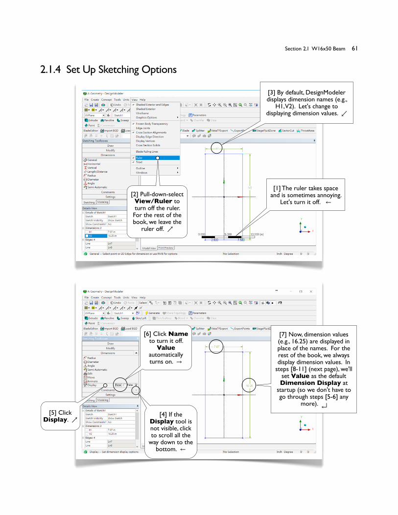
2.1.4 Set Up Sketching Options
[1] The ruler takes space and is sometimes annoying.
Let's turn it off. ← [2] Pull-down-select View/Ruler to turn off the ruler.
For the rest of the book, we leave the
ruler off. ↗
[4] If the Display tool is not visible, click to scroll all the
way down to the bottom. ←
[5] Click Display. ↗
[6] Click Name to turn it off.
Value automatically turns on. →
[7] Now, dimension values (e.g., 16.25) are displayed in place of the names. For the rest of the book, we always display dimension values. In
steps [8-11] (next page), we'll set Value as the default Dimension Display at
startup (so we don't have to go through steps [5-6] any
more).
[3] By default, DesignModeler displays dimension names (e.g.,
H1, V2). Let's change to displaying dimension values. ↙

� Section 2.1 W16x50 Beam� 62
[8] Pull-down-select Tools/Options...
[9] Select Sketching. →
[10] Select Value as the default Dimension
Display.
[11] Click OK to dismiss the Options window. Click Yes to
confirm the changes.
Background Color of the Graphic Area[12] In this book, for better readability, the background color of the graphic area is always shown in white. To set up the background color, pull-down-select Tools/Options in Workbench GUI (2.1.2[2], page 57; not DesignModeler GUI, 2.1.2[8], page 58) and select Appearance. #
62� Chapter 2 Sketching
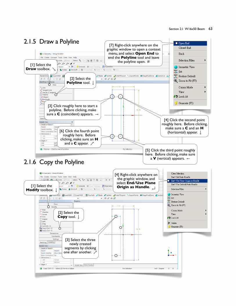
2.1.6 Copy the Polyline
� Section 2.1 W16x50 Beam� 63
2.1.5 Draw a Polyline
[1] Select the Draw toolbox. ↘
[2] Select the Polyline tool.
[3] Click roughly here to start a polyline. Before clicking, make
sure a C (coincident) appears. →[4] Click the second point
roughly here. Before clicking, make sure a C and an H (horizontal) appear.
[5] Click the third point roughly here. Before clicking, make sure
a V (vertical) appears. ←
[6] Click the fourth point roughly here. Before
clicking, make sure an H and a C appear. ↗
[7] Right-click anywhere on the graphic window to open a context menu, and select Open End to end the Polyline tool and leave
the polyline open. #
[1] Select the Modify toolbox.
[2] Select the Copy tool.
[3] Select the three newly created
segments by clicking one after another. ↗
[4] Right-click anywhere on the graphic window, and select End/Use Plane Origin as Handle.

� Section 2.1 W16x50 Beam� 64
[1] Now, try these basic mouse operations in the sketching mode [2-7]. Press ESC to deselect all entities. After trying any of [5-7], click Zoom to Fit (2.1.3[20], page 60) or Look At (2.1.3[4], page 59) to display a fitting view. ↙
[8] Right-click-select End to end the Paste tool. An alternative way
(which is also a more convenient way) is to press ESC to end a tool. #
[6] Right-click-select Flip Horizontal.
[5] The Paste tool is automatically activated. → [7] Right-click-select Paste
at Plane Origin. ↙
[2] Click: add a sketching entity to the selection set. Click a selected entity to remove it
from the selection set.
[3] Click-Sweep: continuous selection. →
[4] Right-click: open a context menu.
[5] Right-click-drag: box zoom.
[6] Scroll-wheel: zoom in/out. ←
[7] Middle-click-drag: rotate.Shift-middle-click-drag: zoom.
Control-middle-click-drag: pan. #
2.1.7 Basic Mouse Operations in Sketching Mode
64� Chapter 2 Sketching

� Section 2.1 W16x50 Beam� 65
2.1.8 Trim Away Unwanted Segments
[3] Click to trim this segment. →
[4] And click to trim this
segment. #
[1] Select the Trim tool in the Modify
toolbox.
[2] Turn on Ignore Axis. Without turning it on, the
axes would act as trimming tools.
2.1.9 Impose Symmetry Constraints
[2] Select Symmetry.
[3] Click the horizontal axis and then two horizontal segments on both sides as shown to make the two segments symmetric about
the horizontal axis. ↗
[1] Select the Constraints
toolbox.
[4] Right-click-select Select new symmetry axis.
[5] Click the vertical axis and then two vertical segments on both sides as shown to
make the two segments symmetric about the vertical axis. Although they seem
already symmetric before we impose this constraint, the symmetry is "weak;" i.e., they
may be overridden by other constraints. Now, the symmetry is "strong" and cannot
be overridden. #
� Section 2.1 W16x50 Beam� 66
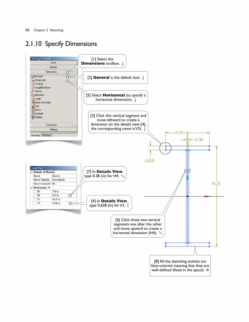
2.1.10 Specify Dimensions
[2] General is the default tool.
[1] Select the Dimensions toolbox.
[5] Select Horizontal (to specify a horizontal dimension).
[3] Click this vertical segment and move leftward to create a
dimension (in the details view [4], the corresponding name is V3).
[6] Click these two vertical segments one after the other and move upward to create a horizontal dimension (H4). ↖
[7] In Details View, type 0.38 (in) for H4. ↘
[8] All the sketching entities are blue-colored, meaning that they are well-defined (fixed in the space). #
[4] In Details View, type 0.628 (in) for V3.
66� Chapter 2 Sketching
� Section 2.1 W16x50 Beam� 67
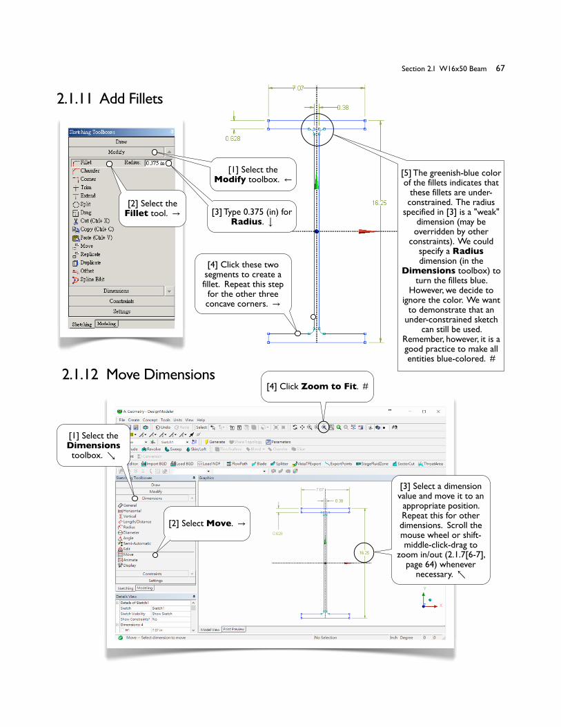
2.1.11 Add Fillets
2.1.12 Move Dimensions
[1] Select the Modify toolbox. ←
[2] Select the Fillet tool. → [3] Type 0.375 (in) for
Radius.
[4] Click these two segments to create a fillet. Repeat this step
for the other three concave corners. →
[2] Select Move. →
[3] Select a dimension value and move it to an appropriate position. Repeat this for other dimensions. Scroll the mouse wheel or shift-middle-click-drag to
zoom in/out (2.1.7[6-7], page 64) whenever
necessary. ↖
[1] Select the Dimensions toolbox. ↘
[5] The greenish-blue color of the fillets indicates that
these fillets are under-constrained. The radius
specified in [3] is a "weak" dimension (may be
overridden by other constraints). We could
specify a Radius dimension (in the
Dimensions toolbox) to turn the fillets blue.
However, we decide to ignore the color. We want
to demonstrate that an under-constrained sketch
can still be used. Remember, however, it is a good practice to make all entities blue-colored. #
[4] Click Zoom to Fit. #

� Section 2.1 W16x50 Beam� 68
2.1.13 Generate a 3D Solid Body
[10] Click Zoom to Fit. Feel free to use this tool any time.
[9] Click Display Plane to turn off the display of the
sketching plane. ←
[11] Click all the plus signs (+) to expand the model tree and browse its structure. #
[3] Remember that the active sketch is shown here (2.1.3[7], page 59). ↙
[6] Click Apply. By default, the active
sketch [3] is selected as Geometry.
[2] The view rotates to an isometric view. ↖
[5] The Modeling mode is automatically activated.
[7] Type 120 (in) for Depth.
[1] Click the little cyan sphere to rotate the view
to an isometric view, which is a convenient 3D view. ↙[4] Click
Extrude. →
[8] Click Generate. ↘
68� Chapter 2 Sketching
� Section 2.1 W16x50 Beam� 69
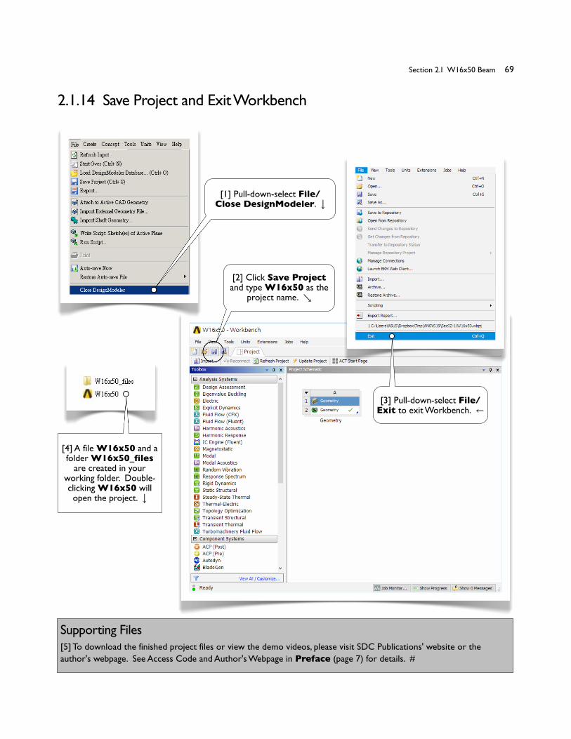
2.1.14 Save Project and Exit Workbench
[1] Pull-down-select File/Close DesignModeler.
[2] Click Save Project and type W16x50 as the
project name. ↘
Supporting Files[5] To download the finished project files or view the demo videos, please visit SDC Publications' website or the author's webpage. See Access Code and Author's Webpage in Preface (page 7) for details. #
[4] A file W16x50 and a folder W16x50_files
are created in your working folder. Double-clicking W16x50 will open the project.
[3] Pull-down-select File/Exit to exit Workbench. ←
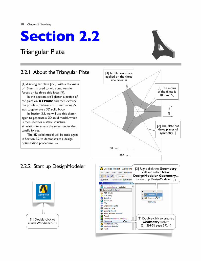
Triangular Plate
� Section 2.2 Triangular Plate� 70
Section 2.2
[1] A triangular plate [2-3], with a thickness of 10 mm, is used to withstand tensile forces on its three side faces [4].� In this section, we'll sketch a profile of the plate on XYPlane and then extrude the profile a thickness of 10 mm along Z-axis to generate a 3D solid body.� In Section 3.1, we will use this sketch again to generate a 2D solid model, which is then used for a static structural simulation to assess the stress under the tensile forces.� The 2D solid model will be used again in Section 8.2 to demonstrate a design optimization procedure. →
2.2.1 About the Triangular Plate
40
mm
30 mm
300 mm
[2] The plate has three planes of symmetry.
[3] The radius of the fillets is
10 mm. ↖
[4] Tensile forces are applied on the three
side faces. #
2.2.2 Start up DesignModeler
[1] Double-click to launch Workbench. →
[2] Double-click to create a Geometry system
(2.1.2[4-5], page 57).
[3] Right-click the Geometry cell and select New
DesignModeler Geometry... to start up DesignModeler.
70� Chapter 2 Sketching
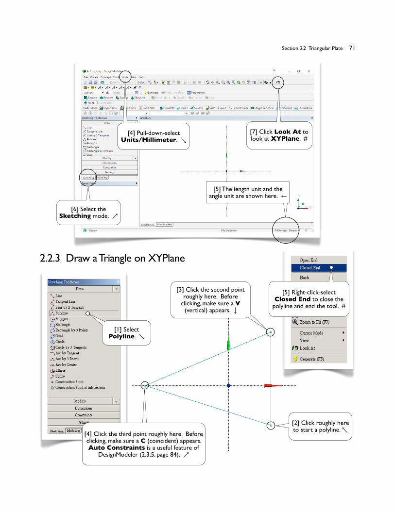
� Section 2.2 Triangular Plate� 71
[6] Select the Sketching mode. ↗
[7] Click Look At to look at XYPlane. #
[4] Pull-down-select Units/Millimeter. ↘
[2] Click roughly here to start a polyline. ↖
[3] Click the second point roughly here. Before
clicking, make sure a V (vertical) appears.
[4] Click the third point roughly here. Before clicking, make sure a C (coincident) appears. Auto Constraints is a useful feature of
DesignModeler (2.3.5, page 84). ↗
[5] Right-click-select Closed End to close the
polyline and end the tool. #
[1] Select Polyline. ↘
2.2.3 Draw a Triangle on XYPlane
[5] The length unit and the angle unit are shown here. ←

� Section 2.2 Triangular Plate� 72
[1] Tools for 2D graphics controls are available in the Display Toolbar [2-10]. Click the tools in [4-6] to toggle them on/off. Feel free to use these tools any time. Try to click each tool now; they don't modify the model. Note that other ways to Pan, Zoom, and Box Zoom are given in 2.1.7[5-7] (page 64) and 2.3.4[1] (page 83).
2.2.4 Make the Triangle Regular
[1] From the Constraints toolbox, select the Equal
Length tool. ↗
[2] Click this and the vertical segments to make their lengths
equal.
[3] Click this and the vertical segments to make their lengths
equal. #
[9] Click Undo to undo what you've just done. Multiple undo is
allowed. This tool is available only in Sketching mode. →
[10] Click Redo to redo what you've just undone. This tool is available only
in Sketching mode. #
[3] Zoom to Fit fits the entire sketch in the graphic area. ←
[5] When on, Box Zoom allows you to click-and-drag a box on the graphic area to enlarge that portion of
the sketch. ←
[6] When on, Zoom allows you to click-and-drag on the
graphic area to zoom in/out. →
[2] Look At rotates the view so that you look at the active sketching plane. ←
[7] Click Previous View to go to the previous view.
[8] Click Next View to go to
the next view. ↙
[4] When on, Pan allows you to click-and-drag on the graphic area to move the sketch. ↘
2.2.5 2D Graphics Controls
72� Chapter 2 Sketching

� Section 2.2 Triangular Plate� 73
2.2.7 Draw an Arc
[1] From the Dimension toolbox, select Horizontal. ↘
[5] Select Move and move the dimensions to appropriate positions
(2.1.12[2-3], page 67). #
[2] Click the left vertex (before clicking, make sure the cursor turns to a point)
and the vertical line, and then move the mouse downward
to create this dimension. (The value 300 is typed in
step [4].) ←
[3] Click the left vertex and the vertical axis, and then move the mouse
downward to create this dimension. All the segments turn blue, indicating they are well defined now. (The value 200 is
typed in step [4].) Remember, if you make any mistake, you always can click
UNDO (2.2.5[9], last page.
[4] In Details View, type 300 (mm) and 200 (mm) for the dimensions just created.
Click Zoom to Fit (2.2.5[3], last page). ↙
[2] Click this vertex as the arc center.
Before clicking, make sure a P (point)
constraint appears. ←
[3] Click the second point roughly here. Before clicking, make sure a C (coincident)
constraint appears. ↘
[4] Click the third point here. Before
clicking, make sure a C (coincident)
constraint appears. #
[1] From the Draw toolbox, select Arc by Center. →
2.2.6 Specify Dimensions

� Section 2.2 Triangular Plate� 74
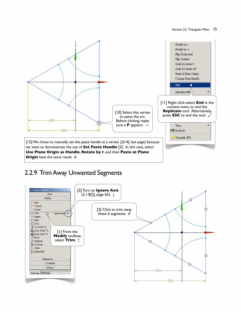
2.2.8 Replicate the Arc
[2] Select the arc. →
[4] Select this vertex as paste handle. Before clicking, make sure a P (point) appears. ↙
[1] From the Modify toolbox, select Replicate. Type 120 (degrees) for r (rotate). Replicate is
equivalent to Copy+Paste (2.1.6[2, 5], pages 63-64). ↘
[7] Whenever you have difficulty making P appear, click Selection Filter: Points in the toolbar.
Selection Filter is also available in the context
menu (see [8]).
[3] Right-click-select End/Set Paste
Handle. ↖
[8] Selection Filter is also available in the context menu. ↙
[6] Click this vertex to paste the arc. Before clicking, make sure a P appears. If you have
difficulty making P appear, see [7-8]. →
[5, 9] Right-click-select Rotate by r from the
context menu.
74� Chapter 2 Sketching
� Section 2.2 Triangular Plate� 75
[12] We chose to manually set the paste handle at a vertex ([3-4], last page) because we want to demonstrate the use of Set Paste Handle [3]. In this case, select Use Plane Origin as Handle, Rotate by r, and then Paste at Plane Origin have the same result. #
2.2.9 Trim Away Unwanted Segments
[10] Select this vertex to paste the arc.
Before clicking, make sure a P appears. →
[11] Right-click-select End in the context menu to end the
Replicate tool. Alternatively, press ESC to end the tool. ↙
[3] Click to trim away these 6 segments. #
[1] From the Modify toolbox, select Trim.
[2] Turn on Ignore Axis (2.1.8[2], page 65).

� Section 2.2 Triangular Plate� 76
Constraint Status[7] The three straight segments turn blue, indicating they are well-defined, while the three arcs remain greenish-blue, indicating they are not well-defined yet (under-constrained). Other color codes are black for fixed, red for over-constrained, and gray for inconsistency. #
[1] From the Constraints toolbox, select Equal
Length.
[5] Select the horizontal axis as
the line of symmetry.
[4] Select Symmetry. →
[2] Select this segment and the vertical segment to make
their lengths equal.
[6] And select the lower and upper
arcs to make them symmetric.
[2] Click the vertical segment and move the mouse rightward to create this
dimension. All the entities turn to blue now. (The value 40 is typed in [3].)
2.2.10 Impose Constraints
2.2.11 Specify Dimension for Side Edges
[1] Select the Dimension toolbox and leave General
as the active tool. ↘[3] Type 40 (mm)
for the new dimension. #
[3] Select this segment and the vertical segment to make
their lengths equal. ←
76� Chapter 2 Sketching
� Section 2.2 Triangular Plate� 77
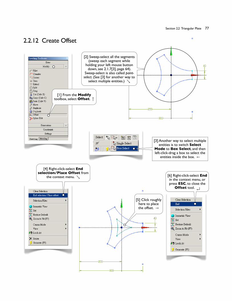
2.2.12 Create Offset
[1] From the Modify toolbox, select Offset.
[2] Sweep-select all the segments (sweep each segment while
holding your left mouse button down, see 2.1.7[3], page 64).
Sweep-select is also called paint-select. (See [3] for another way to
select multiple entities.) ↘
[4] Right-click-select End selection/Place Offset from
the context menu. ↘ [6] Right-click-select End in the context menu, or press ESC, to close the
Offset tool.
[5] Click roughly here to place the offset. →
[3] Another way to select multiple entities is to switch Select
Mode to Box Select, and then left-click-drag a box to select the
entities inside the box. ←
� Section 2.2 Triangular Plate� 78
2.2.13 Create Fillets
[1] In the Modify toolbox, select Fillet. Type 10 (mm)
for Radius. →
[7] From the Dimension toolbox, select Horizontal.
[8] Create this dimension by clicking the left two arcs and move
downward. Note that all the entities turn to blue now. ↗
[9] Type 30 (mm) for the new dimension.
[2] Click these two segments to create a fillet. Repeat this step to create the other two fillets. The fillets are in greenish-blue color,
indicating they are weakly defined (see [3]). ↙
[3] Dimensions specified in a toolbox are "weak," meaning
they may be overridden by other constraints or
dimensions (also see 2.1.11[5], page 67).
[10] If you see something like this, never mind; there is
nothing wrong with it. #
78� Chapter 2 Sketching
� Section 2.2 Triangular Plate� 79
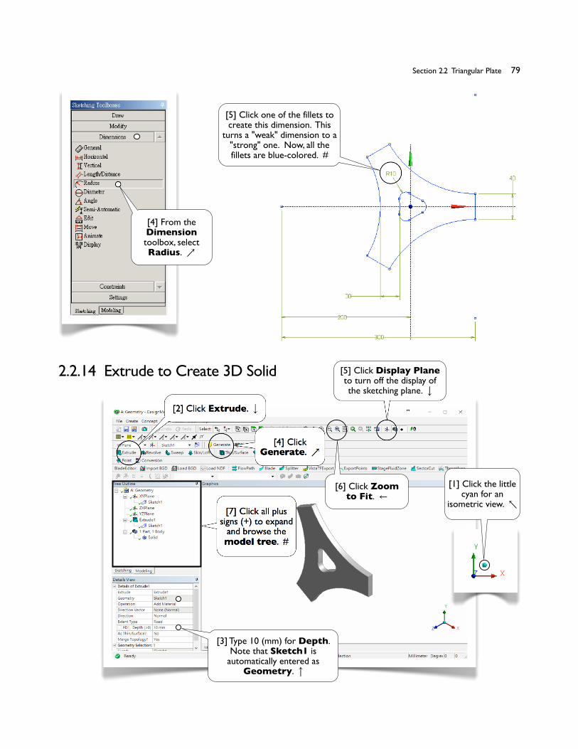
2.2.14 Extrude to Create 3D Solid
[2] Click Extrude.
[4] Click Generate. ↗
[5] Click Display Plane to turn off the display of the sketching plane.
[7] Click all plus signs (+) to expand
and browse the model tree. #
[1] Click the little cyan for an
isometric view. ↖
[4] From the Dimension toolbox, select Radius. ↗
[5] Click one of the fillets to create this dimension. This
turns a "weak" dimension to a "strong" one. Now, all the fillets are blue-colored. #
[6] Click Zoom to Fit. ←
[3] Type 10 (mm) for Depth. Note that Sketch1 is
automatically entered as Geometry.

� Section 2.2 Triangular Plate� 80
2.2.15 Save the Project and Exit Workbench
[1] Click Save Project. Type Triplate as the
project name.
[2] In Workbench GUI, pull-down-select File/Exit to
exit Workbench. #
80� Chapter 2 Sketching
More Details
� Section 2.3 More Details� 81
Section 2.3
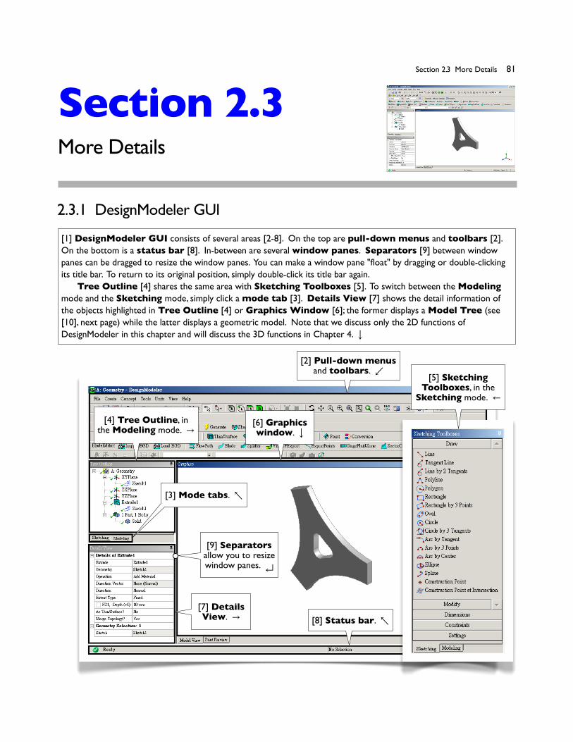
2.3.1 DesignModeler GUI
[1] DesignModeler GUI consists of several areas [2-8]. On the top are pull-down menus and toolbars [2]. On the bottom is a status bar [8]. In-between are several window panes. Separators [9] between window panes can be dragged to resize the window panes. You can make a window pane "float" by dragging or double-clicking its title bar. To return to its original position, simply double-click its title bar again.� Tree Outline [4] shares the same area with Sketching Toolboxes [5]. To switch between the Modeling mode and the Sketching mode, simply click a mode tab [3]. Details View [7] shows the detail information of the objects highlighted in Tree Outline [4] or Graphics Window [6]; the former displays a Model Tree (see [10], next page) while the latter displays a geometric model. Note that we discuss only the 2D functions of DesignModeler in this chapter and will discuss the 3D functions in Chapter 4.
[2] Pull-down menus and toolbars. ↙
[4] Tree Outline, in the Modeling mode. →
[7] Details View. →
[6] Graphics window.
[8] Status bar. ↖
[5] Sketching Toolboxes, in the
Sketching mode. ←
[3] Mode tabs. ↖
[9] Separators allow you to resize window panes.
� Section 2.3 More Details� 82
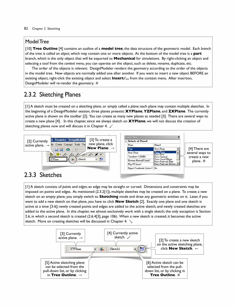
Model Tree[10] Tree Outline [4] contains an outline of a model tree, the data structure of the geometric model. Each branch of the tree is called an object, which may contain one or more objects. At the bottom of the model tree is a part branch, which is the only object that will be exported to Mechanical for simulations. By right-clicking an object and selecting a tool from the context menu, you can operate on the object, such as delete, rename, duplicate, etc.� The order of the objects is relevant. DesignModeler renders the geometry according to the order of the objects in the model tree. New objects are normally added one after another. If you want to insert a new object BEFORE an existing object, right-click the existing object and select Insert/... from the context menu. After insertion, DesignModeler will re-render the geometry. #
[1] A sketch consists of points and edges; an edge may be straight or curved. Dimensions and constraints may be imposed on points and edges. As mentioned (2.3.2[1]), multiple sketches may be created on a plane. To create a new sketch on an empty plane, you simply switch to Sketching mode and draw any geometric entities on it. Later, if you want to add a new sketch on that plane, you have to click New Sketch [2]. Exactly one plane and one sketch is active at a time [3-6]; newly created points and edges are added to the active sketch, and newly created sketches are added to the active plane. In this chapter, we almost exclusively work with a single sketch; the only exception is Section 2.6, in which a second sketch is created (2.6.4[3], page 106). When a new sketch is created, it becomes the active sketch. More on creating sketches will be discussed in Chapter 4. ↘
[1] A sketch must be created on a sketching plane, or simply called a plane; each plane may contain multiple sketches. In the beginning of a DesignModeler session, three planes preexist: XYPlane, YZPlane, and ZXPlane. The currently active plane is shown on the toolbar [2]. You can create as many new planes as needed [3]. There are several ways to create a new plane [4]. In this chapter, since we always sketch on XYPlane, we will not discuss the creation of sketching planes now and will discuss it in Chapter 4. ↙
2.3.2 Sketching Planes
2.3.3 Sketches
[4] There are several ways to create a new
plane. #
[2] To create a new sketch on the active sketching plane,
click New Sketch. ←
[3] Currently active plane. →
[4] Currently active sketch. ↙
[5] Active sketching plane can be selected from the
pull-down list, or by clicking in Tree Outline. →
[6] Active sketch can be selected from the pull-
down list, or by clicking in Tree Outline. #
[2] Currently active plane. →
[3] To create a new plane, click
New Plane. →
82� Chapter 2 Sketching
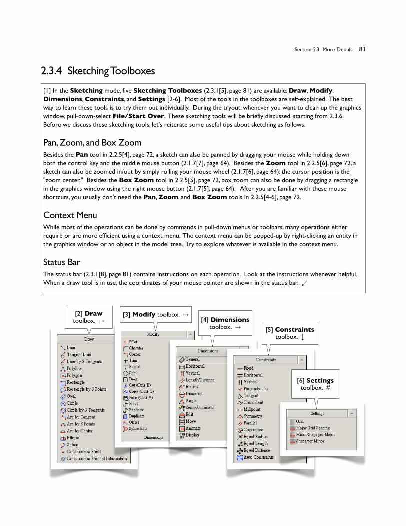
[1] In the Sketching mode, five Sketching Toolboxes (2.3.1[5], page 81) are available: Draw, Modify, Dimensions, Constraints, and Settings [2-6]. Most of the tools in the toolboxes are self-explained. The best way to learn these tools is to try them out individually. During the tryout, whenever you want to clean up the graphics window, pull-down-select File/Start Over. These sketching tools will be briefly discussed, starting from 2.3.6. Before we discuss these sketching tools, let's reiterate some useful tips about sketching as follows.
Pan, Zoom, and Box ZoomBesides the Pan tool in 2.2.5[4], page 72, a sketch can also be panned by dragging your mouse while holding down both the control key and the middle mouse button (2.1.7[7], page 64). Besides the Zoom tool in 2.2.5[6], page 72, a sketch can also be zoomed in/out by simply rolling your mouse wheel (2.1.7[6], page 64); the cursor position is the "zoom center." Besides the Box Zoom tool in 2.2.5[5], page 72, box zoom can also be done by dragging a rectangle in the graphics window using the right mouse button (2.1.7[5], page 64). After you are familiar with these mouse shortcuts, you usually don't need the Pan, Zoom, and Box Zoom tools in 2.2.5[4-6], page 72.
Context MenuWhile most of the operations can be done by commands in pull-down menus or toolbars, many operations either require or are more efficient using a context menu. The context menu can be popped-up by right-clicking an entity in the graphics window or an object in the model tree. Try to explore whatever is available in the context menu.
Status BarThe status bar (2.3.1[8], page 81) contains instructions on each operation. Look at the instructions whenever helpful. When a draw tool is in use, the coordinates of your mouse pointer are shown in the status bar. ↙
� Section 2.3 More Details� 83
2.3.4 Sketching Toolboxes
[2] Draw toolbox. →
[3] Modify toolbox. →[4] Dimensions
toolbox. → [5] Constraints toolbox.
[6] Settings toolbox. #

� Section 2.3 More Details� 84
2.3.5 Auto Constraints[Refs 1, 2]
[1] By default, DesignModeler is in the Auto Constraints mode, both globally and locally. DesignModeler attempts to detect the user's intentions and tries to automatically impose constraints on sketching entities. The following cursor symbols indicate the kind of constraints that are applied:
� C� - The cursor is coincident with a line.� P� - The cursor is coincident with a point.� T� - The cursor is a tangent point.� ⊥� - The cursor is a perpendicular foot.� H� - The line is horizontal.� V� - The line is vertical.� //� - The line is parallel to another line.� R� - The radius is equal to another radius.
Both Global and Cursor modes are based on all entities of the active plane (not just the active sketch). The difference is that Cursor mode only examines the entities nearby the cursor, while Global mode examines all the entities in the active plane. →
2.3.6 Draw Tools[Ref 3]
Line[2] Draws a line by two clicks.
Tangent LineClick a point on a curve (e.g., circle, arc, ellipse, or spline) to create a line tangent to the curve at that point.
Line by 2 TangentsClick two curves to create a line tangent to these two curves. Click a curve and a point to create a line tangent to the curve and connecting to the point.
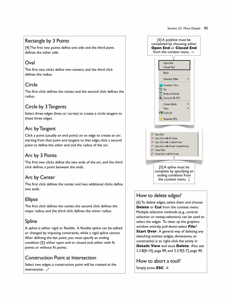
PolylineA polyline consists of multiple straight lines. A polyline must be completed by choosing either Open End or Closed End from the context menu ([3], next page).
PolygonDraws a regular polygon. The first click defines the center and the second click defines the radius of the circumscribing circle.
[2] By default, DesignModeler is in the Auto Constraints
mode, both globally and locally. #
[1] The Draw toolbox. ←
84� Chapter 2 Sketching
� Section 2.3 More Details� 85
Rectangle by 3 Points[4] The first two points define one side and the third point defines the other side.
OvalThe first two clicks define two centers, and the third click defines the radius.
CircleThe first click defines the center, and the second click defines the radius.
Circle by 3 TangentsSelect three edges (lines or curves) to create a circle tangent to these three edges.
Arc by TangentClick a point (usually an end point) on an edge to create an arc starting from that point and tangent to that edge; click a second point to define the other end and the radius of the arc.
Arc by 3 PointsThe first two clicks define the two ends of the arc, and the third click defines a point between the ends.
Arc by CenterThe first click defines the center, and two additional clicks define two ends.
EllipseThe first click defines the center, the second click defines the major radius, and the third click defines the minor radius.
SplineA spline is either rigid or flexible. A flexible spline can be edited or changed by imposing constraints, while a rigid spline cannot. After defining the last point, you must specify an ending condition [5]: either open end or closed end; either with fit points or without fit points.
Construction Point at IntersectionSelect two edges; a construction point will be created at the intersection. ↗
[3] A polyline must be completed by choosing either Open End or Closed End from the context menu. ←
How to delete edges?[6] To delete edges, select them and choose Delete or Cut from the context menu. Multiple selection methods (e.g., control-selection or sweep-selection) can be used to select the edges. To clean up the graphics window entirely, pull-down-select File/Start Over. A general way of deleting any sketching entities (edges, dimensions, or constraints) is to right-click the entity in Details View and issue Delete. Also see 2.3.8[8-10], page 89, and 2.3.9[5-7], page 90.
How to abort a tool?Simply press ESC. #
[5] A spline must be complete by specifying an
ending condition from the context menu.
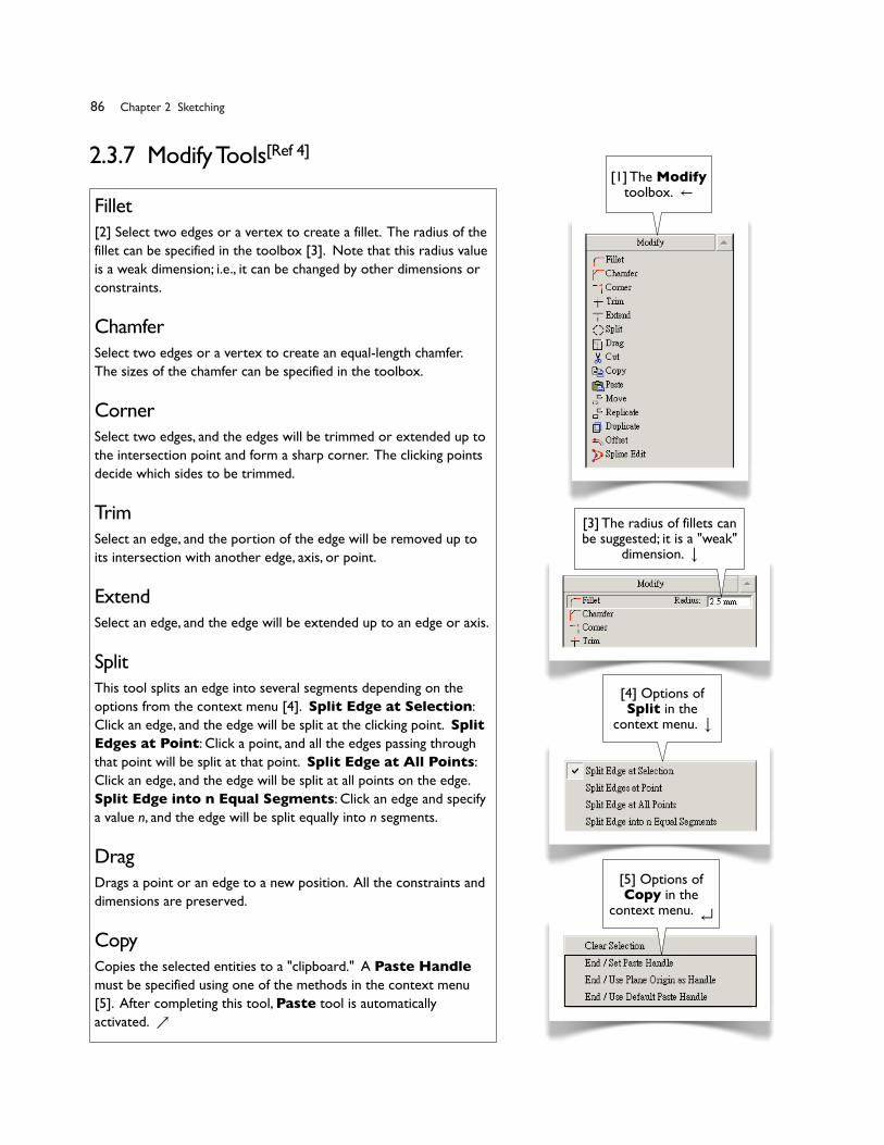
Fillet[2] Select two edges or a vertex to create a fillet. The radius of the fillet can be specified in the toolbox [3]. Note that this radius value is a weak dimension; i.e., it can be changed by other dimensions or constraints.
ChamferSelect two edges or a vertex to create an equal-length chamfer. The sizes of the chamfer can be specified in the toolbox.
CornerSelect two edges, and the edges will be trimmed or extended up to the intersection point and form a sharp corner. The clicking points decide which sides to be trimmed.
TrimSelect an edge, and the portion of the edge will be removed up to its intersection with another edge, axis, or point.
ExtendSelect an edge, and the edge will be extended up to an edge or axis.
SplitThis tool splits an edge into several segments depending on the options from the context menu [4]. Split Edge at Selection: Click an edge, and the edge will be split at the clicking point. Split Edges at Point: Click a point, and all the edges passing through that point will be split at that point. Split Edge at All Points: Click an edge, and the edge will be split at all points on the edge. Split Edge into n Equal Segments: Click an edge and specify a value n, and the edge will be split equally into n segments.
DragDrags a point or an edge to a new position. All the constraints and dimensions are preserved.
CopyCopies the selected entities to a "clipboard." A Paste Handle must be specified using one of the methods in the context menu [5]. After completing this tool, Paste tool is automatically activated. ↗
� Section 2.3 More Details� 86
2.3.7 Modify Tools[Ref 4]
[1] The Modify toolbox. ←
[3] The radius of fillets can be suggested; it is a "weak"
dimension.
[5] Options of Copy in the
context menu.
[4] Options of Split in the
context menu.
86� Chapter 2 Sketching

� Section 2.3 More Details� 87
Cut[6] Similar to Copy, except that the copied entities are removed.
PastePastes the entities in the "clipboard" to the graphics window. The click defines the point at which the Paste Handle positions. Many options can be chosen from the context menu [7], where the rotating angle r and the scaling factor f can be specified in the toolbox.
MoveEquivalent to a Cut followed by a Paste. (The original is removed.)
ReplicateEquivalent to a Copy followed by a Paste. (The original is preserved.)
DuplicateSimilar to Replicate. However, Duplicate copies entities to the same position in the active plane. Duplicate can be used to copy features of a solid body or plane boundaries.
OffsetCreates a set of edges that are offset by a distance from an existing set of edges.
Spline EditUsed to modify flexible splines. You can insert, delete, drag the fit points, etc [8]. For details, see the reference[Ref 4]. ↗
[7] Options of Paste in the
context menu.
[8] Options of Spline Edit in the
context menu. #
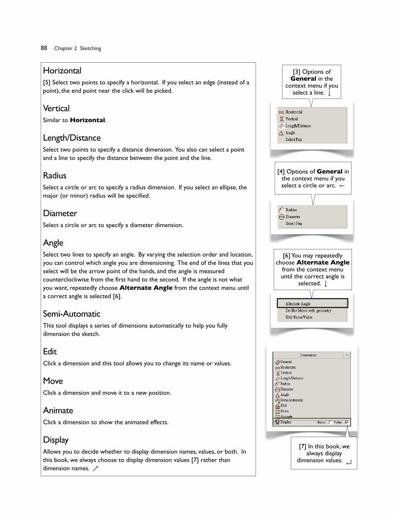
2.3.8 Dimensions Tools[Ref 5] [1]
General[2] Allows creation of any of the dimension types, depending on what edge and context-menu options are selected. If the selected edge is a straight line, the default dimension is its length ([3], next page.) If the selected edge is a circle or arc, the default dimension is its radius ([4], next page).
[1] The Dimension toolbox. ↙
� Section 2.3 More Details� 88
Horizontal[5] Select two points to specify a horizontal. If you select an edge (instead of a point), the end point near the click will be picked.
VerticalSimilar to Horizontal.
Length/DistanceSelect two points to specify a distance dimension. You also can select a point and a line to specify the distance between the point and the line.
RadiusSelect a circle or arc to specify a radius dimension. If you select an ellipse, the major (or minor) radius will be specified.
DiameterSelect a circle or arc to specify a diameter dimension.
AngleSelect two lines to specify an angle. By varying the selection order and location, you can control which angle you are dimensioning. The end of the lines that you select will be the arrow point of the hands, and the angle is measured counterclockwise from the first hand to the second. If the angle is not what you want, repeatedly choose Alternate Angle from the context menu until a correct angle is selected [6].
Semi-AutomaticThis tool displays a series of dimensions automatically to help you fully dimension the sketch.
EditClick a dimension and this tool allows you to change its name or values.
MoveClick a dimension and move it to a new position.
AnimateClick a dimension to show the animated effects.
DisplayAllows you to decide whether to display dimension names, values, or both. In this book, we always choose to display dimension values [7] rather than dimension names. ↗
[3] Options of General in the
context menu if you select a line.
[4] Options of General in the context menu if you select a circle or arc. ←
[6] You may repeatedly choose Alternate Angle
from the context menu until the correct angle is
selected.
[7] In this book, we always display
dimension values.
88� Chapter 2 Sketching
� Section 2.3 More Details� 89
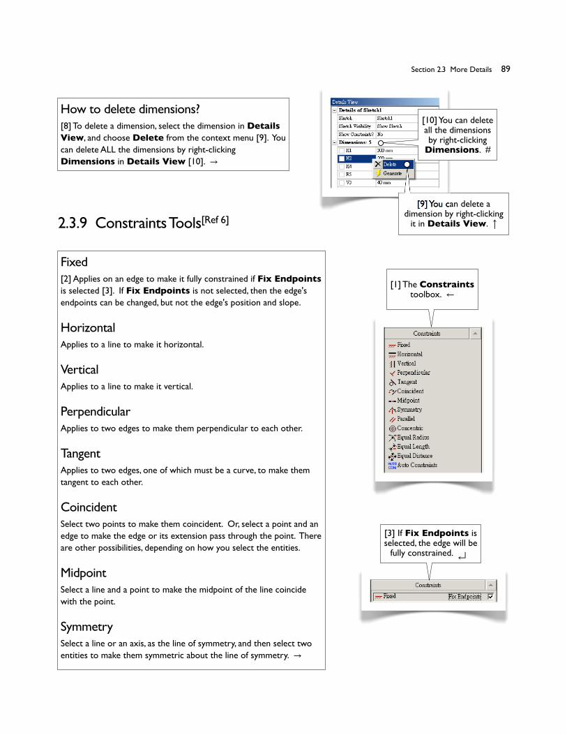
How to delete dimensions?[8] To delete a dimension, select the dimension in Details View, and choose Delete from the context menu [9]. You can delete ALL the dimensions by right-clicking Dimensions in Details View [10]. →
[9] You can delete a dimension by right-clicking
it in Details View. 2.3.9 Constraints Tools[Ref 6]
Fixed[2] Applies on an edge to make it fully constrained if Fix Endpoints is selected [3]. If Fix Endpoints is not selected, then the edge's endpoints can be changed, but not the edge's position and slope.
HorizontalApplies to a line to make it horizontal.
VerticalApplies to a line to make it vertical.
PerpendicularApplies to two edges to make them perpendicular to each other.
TangentApplies to two edges, one of which must be a curve, to make them tangent to each other.
CoincidentSelect two points to make them coincident. Or, select a point and an edge to make the edge or its extension pass through the point. There are other possibilities, depending on how you select the entities.
MidpointSelect a line and a point to make the midpoint of the line coincide with the point.
SymmetrySelect a line or an axis, as the line of symmetry, and then select two entities to make them symmetric about the line of symmetry. →
[1] The Constraints toolbox. ←
[3] If Fix Endpoints is selected, the edge will be
fully constrained.
[10] You can delete all the dimensions by right-clicking
Dimensions. #

Parallel[4] Applies to two lines to make them parallel to each other.
ConcentricApplies to two curves, which may be circle, arc, or ellipse, to make their centers coincident.
Equal RadiusApplies to two curves, which must be circle or arc, to make their radii equal.
Equal LengthApplies to two lines to make their lengths equal.
Equal DistanceApplies to two distances to make them equal. A distance can be defined by selecting two points, two parallel lines, or one point and one line.
Auto ConstraintsAllows you to turn on/off Auto Constraints (2.3.5, page 84).
How to delete constraints?[5] By default, constraints are not displayed in Details View. To display constraints, select Yes for Show Constraints? in Details View [6]. To delete a constraint, right-click the constraint and issue Delete [7].
[6] Select Yes for Show Constraints? in Details View.
[7] Right-click a constraint and issue Delete. #
� Section 2.3 More Details� 9090� Chapter 2 Sketching

40 mm
� Section 2.3 More Details� 91
2.3.10 Settings Tools[Ref 7]
Grid[2] Allows you to turn on/off grid visibility and snap capability [3-4]. The grid is not required to enable snapping.
Major Grid SpacingAllows you to specify Major Grip Spacing [5-6] if Show in 2D is turned on.
Minor-Steps per MajorAllows you to specify Minor-Steps per Major [7-8] if Show in 2D is turned on.
Snaps per MinorAllows you to specify Snaps per Minor [9] if Snap is turned on. ↗
[6] Major Grid Spacing = 10 mm. →
[8] Minor-Steps per Major = 2. →
[3] Check here to turn on Show in 2D. →
[1] The Settings
toolbox. ←
[4] Check here to turn on Snap.
[5] If Show in 2D is turned on, specify Major Grid
Spacing here. ↙
[9] If Snap is turned on, specify Snaps per
Minor here. #
[7] If Show in 2D is turned on, specify Minor-Steps
per Major here. ↙
References1.� ANSYS Help//DesignModeler//ANSYS DesignModeler User's Guide//2D Sketching//Auto Constraints2.� ANSYS Help//DesignModeler//ANSYS DesignModeler User's Guide//2D Sketching//Constraints Toolbox//Auto
Constraints3.� ANSYS Help//DesignModeler//ANSYS DesignModeler User's Guide//2D Sketching//Draw Toolbox4.� ANSYS Help//DesignModeler//ANSYS DesignModeler User's Guide//2D Sketching//Modify Toolbox5.� ANSYS Help//DesignModeler//ANSYS DesignModeler User's Guide//2D Sketching//Dimensions Toolbox6.� ANSYS Help//DesignModeler//ANSYS DesignModeler User's Guide//2D Sketching//Constraints Toolbox7.� ANSYS Help//DesignModeler//ANSYS DesignModeler User's Guide//2D Sketching//Settings Toolbox
M20x2.5 Threaded Bolt
� Section 2.4 M20x2.5 Threaded Bolt� 92
Section 2.4
[1] In this section, we'll create a sketch and revolve the sketch 360� to generate a 3D solid body, a body representing a portion of an M20x2.5 threaded bolt as shown in [2-7]. We will use this sketch in Section 3.2 again to generate a 2D solid body, which is then used for a static structural simulation.
2.4.1 About the M20x2.5 Threaded Bolt[Refs 1, 2]
M20x2.5
H = ( 3 2)p = 2.165 mm
d1= d − (5 8)H × 2 =17.294 mm
32
11×
p=27.5
d
1
d
p
Externalthreads(bolt)
Internalthreads(nut)
H4
H8
p
Minor diameter of internal thread d
1
Major diameter d
60�
H
[3] Metric system. →
[4] Major diameter
d = 20 mm. →[5] Pitch
p = 2.5 mm.
[2] The threaded bolt created in this
exercise.
[6] Thread standards in the
metric system. →
[7] Calculations of some details. #
92� Chapter 2 Sketching

2.4.2 Draw a Horizontal Line
� Section 2.4 M20x2.5 Threaded Bolt� 93
2.4.3 Draw a Polyline
[2] Draw a horizontal line
with dimensions like this. #
[3] Draw a polyline of 3 segments. #
[2] This is the line drawn in 2.4.2[2]. ↘
[1] Launch Workbench and create a Geometry system. Save the project as Threads. Start up DesignModeler. Select Millimeter as the length unit.� On XYPlane, draw a horizontal line and specify the dimensions (8.647 mm and 27.5 mm) as shown in [2]. →
[1] Draw a polyline of 3 segments [2-3] and specify the dimensions (30o, 60o, 60o, 0.541 mm, and 2.165 mm) as shown. To specify angle dimensions, please see Angle, 2.3.8[5], page 88.

� Section 2.4 M20x2.5 Threaded Bolt� 94
2.4.4 Draw a Line and a Fillet
[2] Draw a vertical line and specify its position
(0.271 mm). ←
[3] Create a fillet (also see [4]) and specify its
position (0.541 mm). →[4] Before creating fillets, specify an approximate
radius value, say 0.5 mm. #
2.4.5 Trim Away Unwanted Segments
[2] The sketch after trimming. #[1] Trim away these
three segments. →
[1] Draw a vertical line and specify its position [2]. Create a fillet and specify its position [3-4]. ↘
94� Chapter 2 Sketching
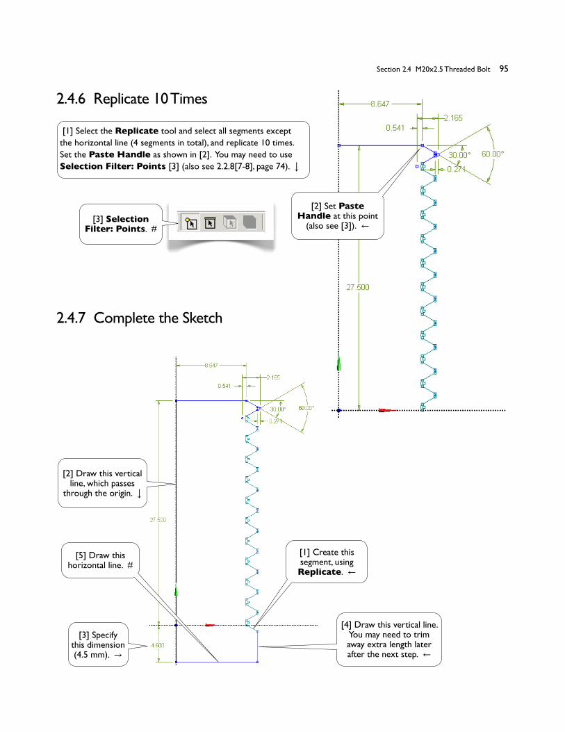
� Section 2.4 M20x2.5 Threaded Bolt� 95
2.4.7 Complete the Sketch
[1] Create this segment, using Replicate. ←
[5] Draw this horizontal line. #
[2] Draw this vertical line, which passes
through the origin.
[4] Draw this vertical line. You may need to trim away extra length later after the next step. ←
[3] Specify this dimension (4.5 mm). →
2.4.6 Replicate 10 Times
[3] Selection Filter: Points. #
[2] Set Paste Handle at this point
(also see [3]). ←
[1] Select the Replicate tool and select all segments except the horizontal line (4 segments in total), and replicate 10 times. Set the Paste Handle as shown in [2]. You may need to use Selection Filter: Points [3] (also see 2.2.8[7-8], page 74).

� Book Title. M20x2.5 Threaded Bolt� 96
2.4.8 Revolve to Create 3D Solid
References1.� Zahavi, E., The Finite Element Method in Machine Design, Prentice-Hall, 1992; Chapter 7. Threaded Fasteners.2.� Deutschman, A. D., Michels, W. J., and Wilson, C. E., Machine Design: Theory and Practice, Macmillan Publishing Co., Inc.,
1975; Section 16-6. Standard Screw Threads.
[2] Select the Y-axis as the Axis of revolution. (Make sure you correctly select the Y-axis.) #
[1] Click Revolve to generate a solid of revolution. Select the Y-axis as the axis of revolution [2]. Remember to click Generate. Save the project and exit Workbench. We will resume this project in Section 3.2.
96� Chapter 2 Sketching
Spur Gears
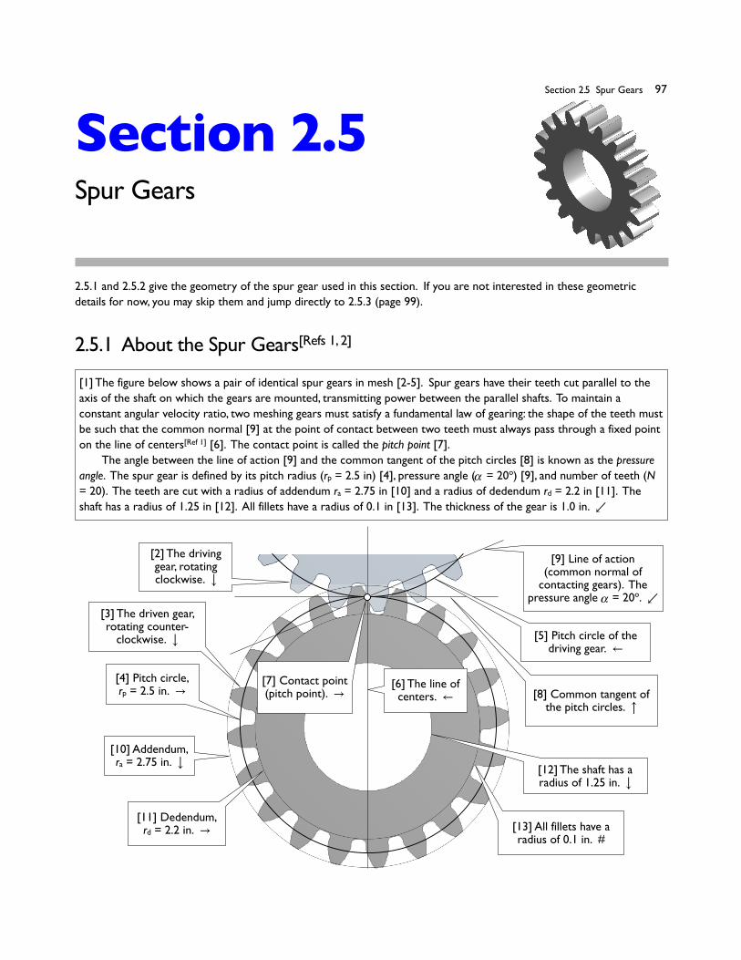
� Section 2.5 Spur Gears� 97
Section 2.5
[8] Common tangent of the pitch circles.
[7] Contact point (pitch point). →
[9] Line of action (common normal of
contacting gears). The pressure angle α = 20o. ↙
[4] Pitch circle,rp = 2.5 in. →
[10] Addendum,ra = 2.75 in.
[11] Dedendum,rd = 2.2 in. →
[2] The driving gear, rotating clockwise.
[3] The driven gear, rotating counter-
clockwise. [5] Pitch circle of the driving gear. ←
[6] The line of centers. ←
[13] All fillets have a radius of 0.1 in. #
[12] The shaft has a radius of 1.25 in.
[1] The figure below shows a pair of identical spur gears in mesh [2-5]. Spur gears have their teeth cut parallel to the axis of the shaft on which the gears are mounted, transmitting power between the parallel shafts. To maintain a constant angular velocity ratio, two meshing gears must satisfy a fundamental law of gearing: the shape of the teeth must be such that the common normal [9] at the point of contact between two teeth must always pass through a fixed point on the line of centers[Ref 1] [6]. The contact point is called the pitch point [7].� The angle between the line of action [9] and the common tangent of the pitch circles [8] is known as the pressure angle. The spur gear is defined by its pitch radius (rp = 2.5 in) [4], pressure angle (α = 20o) [9], and number of teeth (N = 20). The teeth are cut with a radius of addendum ra = 2.75 in [10] and a radius of dedendum rd = 2.2 in [11]. The shaft has a radius of 1.25 in [12]. All fillets have a radius of 0.1 in [13]. The thickness of the gear is 1.0 in. ↙
2.5.1 About the Spur Gears[Refs 1, 2]
2.5.1 and 2.5.2 give the geometry of the spur gear used in this section. If you are not interested in these geometric details for now, you may skip them and jump directly to 2.5.3 (page 99).
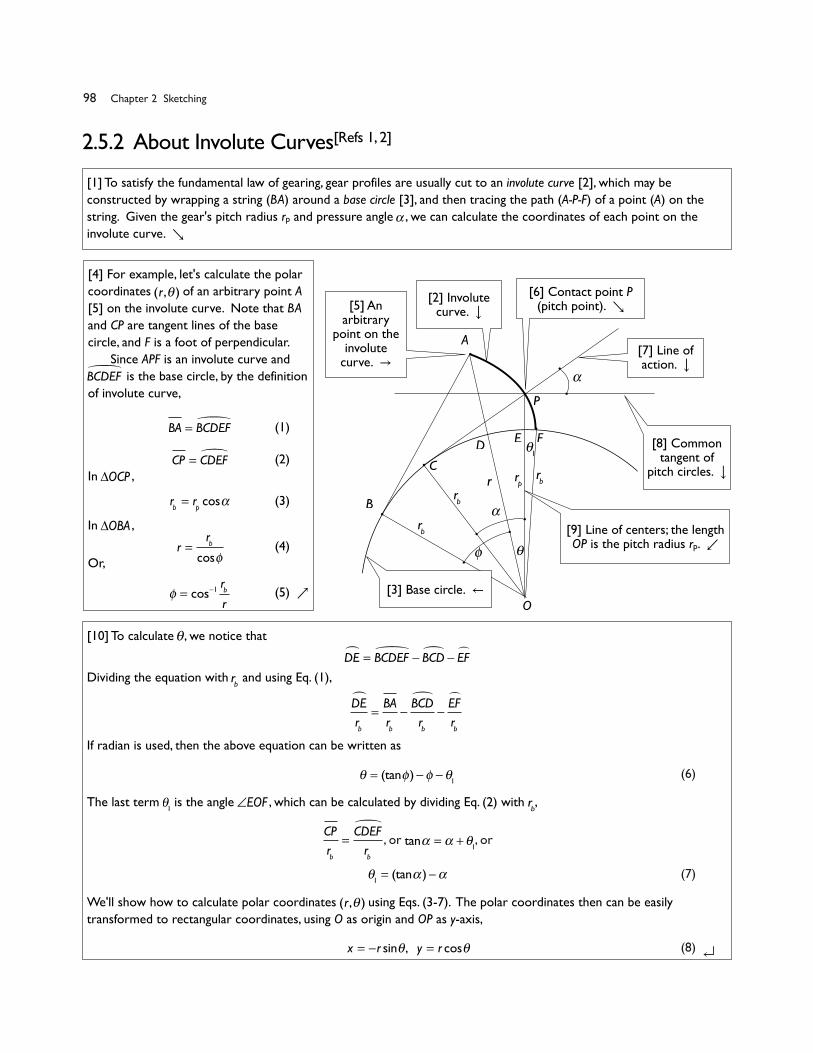
α
θ
A
C
P
B
rb
rp r
α
D
rb
rb
E F
φ
θ
1
� Section 2.5 Spur Gears� 98
[1] To satisfy the fundamental law of gearing, gear profiles are usually cut to an involute curve [2], which may be constructed by wrapping a string (BA) around a base circle [3], and then tracing the path (A-P-F) of a point (A) on the string. Given the gear's pitch radius rp and pressure angle α , we can calculate the coordinates of each point on the involute curve. ↘
2.5.2 About Involute Curves[Refs 1, 2]
[4] For example, let's calculate the polar coordinates (r,θ ) of an arbitrary point A [5] on the involute curve. Note that BA and CP are tangent lines of the base circle, and F is a foot of perpendicular.� Since APF is an involute curve and
BCDEF� is the base circle, by the definition of involute curve,
� BA = BCDEF�� (1)
� CP = CDEF�� (2)In ∆OCP ,
� rb= r
pcosα � (3)
In ∆OBA ,
� r =
rb
cosφ� (4)
Or,
� φ = cos−1 r
b
r� (5)�↗
O
[10] To calculate θ , we notice that
� DE� = BCDEF� − BCD� − EF�
Dividing the equation with rb and using Eq. (1),
�
DE�
rb
=BA
rb
−BCD�
rb
−EF�
rb
If radian is used, then the above equation can be written as
� θ = (tanφ )−φ −θ
1� (6)
The last term θ1 is the angle ∠EOF , which can be calculated by dividing Eq. (2) with rb,
�
CP
rb
=CDEF�
rb
, or tanα = α +θ1, or
� θ1= (tanα )−α � (7)
We'll show how to calculate polar coordinates (r,θ ) using Eqs. (3-7). The polar coordinates then can be easily transformed to rectangular coordinates, using O as origin and OP as y-axis,
� x = −r sinθ , y = r cosθ� (8)�
[3] Base circle. ←
[7] Line of action.
[8] Common tangent of
pitch circles.
[9] Line of centers; the length OP is the pitch radius rp. ↙
[6] Contact point P (pitch point). ↘[2] Involute
curve. [5] An arbitrary
point on the involute
curve. →
98� Chapter 2 Sketching

� Section 2.5 Spur Gears� 99
Numerical Calculations of Coordinates[11] In our case, the pitch radius
rp= 2.5 in, and pressure angle α = 20o; from Eqs. (3) and (7) respectively,
rb = 2.5cos20o = 2.349232 in
θ
1= tan20o −
20o
180oπ = 0.01490438 (rad)
The table below lists the calculated coordinates. The values in the first column (r) are chosen such that, except the pitch point (r = 2.5 in), the intermediate points are at the quarter points between
rb (r = 2.349232 in) and
ra (r = 2.75 in).
Also note that, when using Eqs. (6) and (7), radians are used as the unit of angles; in the table below, however, degrees are used. #
2.5.3 Draw an Involute Curve
[2] The pitch point is on the Y-axis. ↙
[4] Re-fit spline. #
[3] It is equally good that you draw the spline by using the Spline tool directly without first creating construction points. To do so, at the end of the Spline tool, select Open End with Fit Points from the context menu. After dimensioning each point, use the Spline Edit tool to edit the spline and select Re-fit Spline [4] from the context menu to smooth out the spline. ↗
rin. Eq. (5), degrees Eq. (6), degrees in. in.
2.349232 0.000000 -0.853958 -0.03501 2.3490
2.449424 16.444249 -0.387049 -0.01655 2.4494
2.500000 20.000000 0.000000 0.00000 2.5000
2.549616 22.867481 0.442933 0.01971 2.5495
2.649808 27.555054 1.487291 0.06878 2.6489
2.750000 31.321258 2.690287 0.12908 2.7470
x = −r sinθ y = r cosθφ θ
[1] Launch Workbench. Create a Geometry system. Save the project as Gear. Start up DesignModeler. Select Inch as the length unit.� From the Draw toolbox, select the Construction Point tool, draw 6 points and specify dimensions as shown, where the vertical dimensions are measured from the X-axis and the horizontal dimensions are measured from the Y-axis. The pitch point [2] is coincident with the Y-axis.� Connect these six points using the Spline tool in the Draw toolbox, leaving Flexible option on, finishing the spline with Open End. →
[6] Sometimes, turning off Display Plane may be helpful when working on the graphics window [7]. In this case, all the dimensions referring to the plane axes disappear.
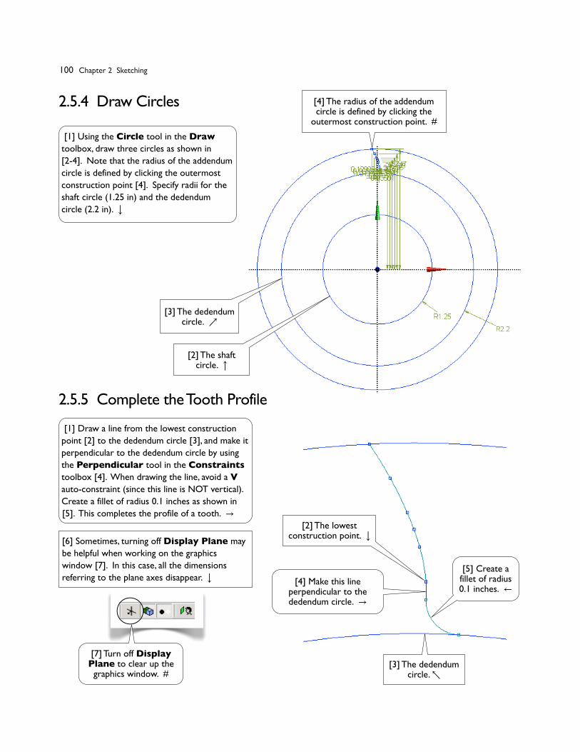
� Section 2.5 Spur Gears� 100
2.5.4 Draw Circles
2.5.5 Complete the Tooth Profile
[4] The radius of the addendum circle is defined by clicking the
outermost construction point. #
[2] The shaft circle.
[3] The dedendum circle. ↗
[4] Make this line perpendicular to the dedendum circle. →
[5] Create a fillet of radius 0.1 inches. ←
[3] The dedendum circle. ↖
[7] Turn off Display Plane to clear up the
graphics window. #
[2] The lowest construction point.
[1] Using the Circle tool in the Draw toolbox, draw three circles as shown in [2-4]. Note that the radius of the addendum circle is defined by clicking the outermost construction point [4]. Specify radii for the shaft circle (1.25 in) and the dedendum circle (2.2 in).
[1] Draw a line from the lowest construction point [2] to the dedendum circle [3], and make it perpendicular to the dedendum circle by using the Perpendicular tool in the Constraints toolbox [4]. When drawing the line, avoid a V auto-constraint (since this line is NOT vertical). Create a fillet of radius 0.1 inches as shown in [5]. This completes the profile of a tooth. →
100� Chapter 2 Sketching
� Section 2.5 Spur Gears� 101
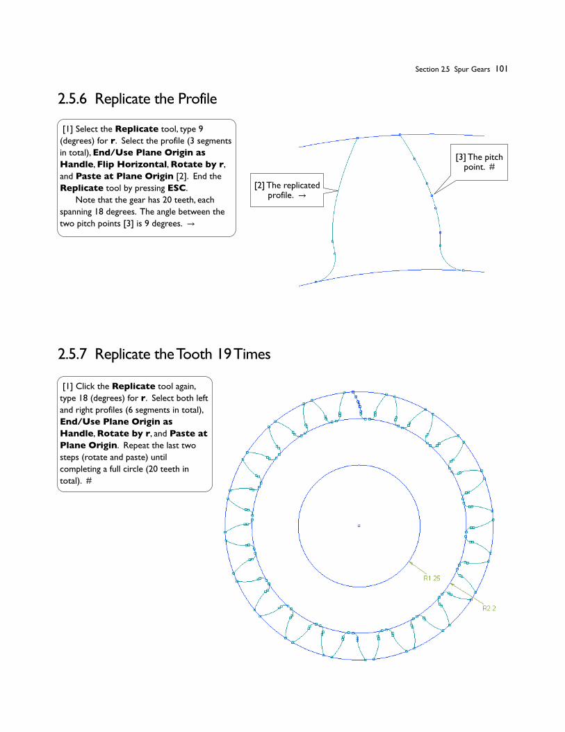
2.5.6 Replicate the Profile
2.5.7 Replicate the Tooth 19 Times
[2] The replicated profile. →
[3] The pitch point. #
[1] Select the Replicate tool, type 9 (degrees) for r. Select the profile (3 segments in total), End/Use Plane Origin as Handle, Flip Horizontal, Rotate by r, and Paste at Plane Origin [2]. End the Replicate tool by pressing ESC.� Note that the gear has 20 teeth, each spanning 18 degrees. The angle between the two pitch points [3] is 9 degrees. →
[1] Click the Replicate tool again, type 18 (degrees) for r. Select both left and right profiles (6 segments in total), End/Use Plane Origin as Handle, Rotate by r, and Paste at Plane Origin. Repeat the last two steps (rotate and paste) until completing a full circle (20 teeth in total). #

� Section 2.5 Spur Gears� 102
References1.� Deutschman, A. D., Michels, W. J., and Wilson, C. E., Machine Design: Theory and Practice, Macmillan Publishing Co., Inc.,
1975; Chapter 10. Spur Gears.2.� Zahavi, E., The Finite Element Method in Machine Design, Prentice-Hall, 1992; Chapter 9. Spur Gears.
2.5.8 Trim Away Unwanted Segments
2.5.9 Extrude to Create 3D Solid
[2] It is equally good that you create a single tooth (a 3D solid body) and then duplicate it by using Create/Pattern in the Modeling mode. In this exercise, however, we use Replicate in Sketching mode because our focus in this chapter is to practice sketching techniques. #
[1] Trim away unwanted segments in the addendum circle and the dedendum circle, as shown. #
[1] Extrude the sketch 1.0 inch to create a 3D solid. Save the project and exit from Workbench. We will resume this project again in Section 3.4.
102� Chapter 2 Sketching

Microgripper
� Section 2.6 Microgripper� 103
Section 2.6
480
144
176
280
400
140
212
77
47
87
20
R25 R45
32
92
D30
Unit: µm
Thickness: 300 µm
[1] The microgripper is made of a rubber-like polymer material and actuated by a shape memory alloy (SMA) actuator [2-4]. The motion of the SMA is caused by temperature change, which is controlled by electric current. In the lab, the microgripper is tested by gripping a steel bead of a diameter of 30 micrometers [5].� In this section, we will create a solid model for the microgripper. The model will be used for simulation in Section 13.3 to assess the gripping forces on the bead with an actuation force of the SMA actuator.
2.6.1 About the Microgripper[Refs 1, 2]
[3] Actuation direction.
[2] Gripping direction. →
[4] SMA actuator.
[5] Steel bead. #

� Section 2.6 Microgripper� 104
2.6.2 Create Half of the Gripper
[2] Before trimming. ←
[3] After trimming.
[4] Extrude the sketch both sides symmetrically. →
[5] A half of the gripper. #
[1] Launch Workbench. Create a Geometry system. Save the project as Microgripper. Start up DesignModeler. Select Micrometer as the length unit.� Draw a sketch on XYPlane as shown in [2]. Trim away unwanted segments [3]. Note that we drew only half of the model because of the symmetry. Extrude the sketch 150 µm both sides symmetrically (the total depth is 300 µm) [4]. We now have a half of the gripper [5].
104� Chapter 2 Sketching

� Section 2.6 Microgripper� 105
2.6.3 Mirror Copy the Solid Body
[2] In the graphics window, select the solid
body and click Apply.
[5] Click Generate. #
[4] In Tree Outline, select YZPlane and click
Apply. ↙
[3] Click this yellow area to bring up the Apply/
Cancel buttons.
[1] Pull-down-select Create/Body Transformation/
Mirror. ↗

� Section 2.6 Microgripper� 106
2.6.4 Create the Bead
[7] Impose a Tangent constraint between the
semicircle and the sloping line. ↙
[4] The semicircle can be created by creating a full
circle and then trimming it using the axis.
[6] Specify the radius (15 µm).
References1.� Chang, R. J., Lin , Y. C., Shiu, C. C., and Hsieh, Y. T., �“Development of SMA-Actuated Microgripper in Micro Assembly
Applications,” IECON, IEEE,Taiwan, 2007.2.� Shih, P. W., Applications of SMA on Driving Micro-gripper, MS Thesis, NCKU, ME, Taiwan, 2005.
[2] Select XYPlane. →
[3] Click New Sketch. ↙
[10] Right-click to rename each body like this. ↙
[9] The two bodies are treated as two parts (see [10]). ↗
[5] Close the sketch by drawing a vertical line. ↘
[8] Revolve the sketch about the Y-axis to create
a sphere.
[1] Create a new sketch on XYPlane as shown in [2-3] and draw a semicircle as shown in [4-7]. Revolve the sketch
360� about the Y-axis to create the bead [8]. Note that the two bodies are treated as two parts [9]. Rename the two bodies as Gripper and Bead respectively [10]. →
Wrap Up[11] Close DesignModeler, save the project and exit Workbench. We will resume this project in Section 13.3. #
106� Chapter 2 Sketching
Review
� Section 2.7 Review� 107
Section 2.7
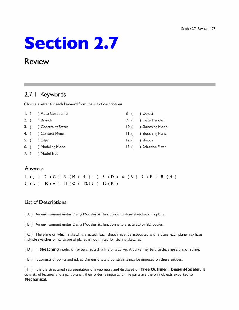
1.� (� )�Auto Constraints
2.� (� )�Branch
3.� (� )�Constraint Status
4.� (� )�Context Menu
5.� (� )�Edge
6.� (� )�Modeling Mode
7.� (� )�Model Tree
2.7.1 Keywords
Answers:1.� (� J� )� 2.� (�G� )� 3.� (�M� )� 4.� (� I� )� 5.� (�D� )� 6.� (�B� )� 7.� (�F� )� 8.� (�H� )�
9.� (� L� )� 10.�(�A� )� 11.�(�C� )� 12.�(�E� )� 13.�(�K� )
Choose a letter for each keyword from the list of descriptions
8.� (� )�Object
9.� (� )�Paste Handle
10.�( � )�Sketching Mode
11.�(� )�Sketching Plane
12.�(� )�Sketch
13.�(� )�Selection Filter
List of Descriptions
(�A� )� An environment under DesignModeler; its function is to draw sketches on a plane.
(�B� )� An environment under DesignModeler; its function is to create 3D or 2D bodies.
(�C�)� The plane on which a sketch is created. Each sketch must be associated with a plane; each plane may have multiple sketches on it. Usage of planes is not limited for storing sketches.
(�D�)� In Sketching mode, it may be a (straight) line or a curve. A curve may be a circle, ellipse, arc, or spline.
(�E� )� It consists of points and edges. Dimensions and constraints may be imposed on these entities.
(�F� )� It is the structured representation of a geometry and displayed on Tree Outline in DesignModeler. It consists of features and a part branch; their order is important. The parts are the only objects exported to Mechanical.

� Section 2.7 Review� 108
(�G�)� An object of a model tree and consists of one or more objects under itself.
(�H�)� A leaf or branch of a model tree.
(� I� )� The menu that pops up when you right-click your mouse. The contents of the menu depend on what you click.
(� J� )� While drawing in Sketching mode, by default, DesignModeler attempts to detect the user's intentions and tries to automatically impose constraints on points or edges. Detection is performed over entities on the active plane, not just active sketch. It can be switched on/off in the Constraints toolbox.
(�K� )� It filters one type of geometric entity. When it is turned on/off, the corresponding type of entity becomes selectable/unselectable. In Sketching mode, there are two selection filters, namely points and edges filters. Along with these two filters, face and body selection filters are available in Modeling mode.
(�L� )� A reference point used in a copy/paste operation. The point is defined during copying and will coincide with a specified location when pasting.
(�M�)� In Sketching mode, entities are color coded to indicate their constraint status: greenish-blue for under-constrained; blue and black for well constrained (i.e., fixed in the space); red for over-constrained; gray for inconsistent.
2.7.2 Additional Workbench Exercises
Create Geometric Models with Your Own WayAfter so many exercises, you should be able to figure out many alternative ways of creating the geometric models in this chapter. Try to re-create the models in this chapter using your own way.
108� Chapter 2 Sketching
Copyright © 2022 FDOKUMEN