Simulation Of Notch Driven Hydraulic Fracture In Open Hole ...
152
University of North Dakota University of North Dakota UND Scholarly Commons UND Scholarly Commons Theses and Dissertations Theses, Dissertations, and Senior Projects January 2020 Simulation Of Notch Driven Hydraulic Fracture In Open Hole Simulation Of Notch Driven Hydraulic Fracture In Open Hole Completion Completion Nejma Djabelkhir Follow this and additional works at: https://commons.und.edu/theses Recommended Citation Recommended Citation Djabelkhir, Nejma, "Simulation Of Notch Driven Hydraulic Fracture In Open Hole Completion" (2020). Theses and Dissertations. 3265. https://commons.und.edu/theses/3265 This Dissertation is brought to you for free and open access by the Theses, Dissertations, and Senior Projects at UND Scholarly Commons. It has been accepted for inclusion in Theses and Dissertations by an authorized administrator of UND Scholarly Commons. For more information, please contact [email protected].
-
Upload
khangminh22 -
Category
Documents
-
view
3 -
download
0
Transcript of Simulation Of Notch Driven Hydraulic Fracture In Open Hole ...

University of North Dakota University of North Dakota
UND Scholarly Commons UND Scholarly Commons
Theses and Dissertations Theses, Dissertations, and Senior Projects
January 2020
Simulation Of Notch Driven Hydraulic Fracture In Open Hole Simulation Of Notch Driven Hydraulic Fracture In Open Hole
Completion Completion
Nejma Djabelkhir
Follow this and additional works at: https://commons.und.edu/theses
Recommended Citation Recommended Citation Djabelkhir, Nejma, "Simulation Of Notch Driven Hydraulic Fracture In Open Hole Completion" (2020). Theses and Dissertations. 3265. https://commons.und.edu/theses/3265
This Dissertation is brought to you for free and open access by the Theses, Dissertations, and Senior Projects at UND Scholarly Commons. It has been accepted for inclusion in Theses and Dissertations by an authorized administrator of UND Scholarly Commons. For more information, please contact [email protected].

i
SIMULATION OF NOTCH DRIVEN HYDRAULIC FRACTURE IN OPEN
HOLE COMPLETION
by
Nejma Djabelkhir Tavakolian
Bachelor of Science and Technology, University of Science and Technology Houari Boumediene,
Algiers, Algeria, 2000
Geological Engineer, University of Science and Technology Houari Boumediene,
Algiers, Algeria, 2003
A Dissertation
Submitted to the Graduate Faculty
of the
University of North Dakota
In fulfillment of the requirements
for the degree of
Doctor of Philosophy
Grand Forks, North Dakota
August 2020

ii
This thesis, submitted by Nejma Djabelkhir in partial fulfillment of the requirements for the
Degree of PhD from the University of North Dakota, has been read by the Faculty Advisory
Committee under whom the work has been done and is hereby approved.
_______________________________________
Dr. Vamegh Rasouli
__________________________________________
Dr. Branko Damjanac
__________________________________________
Dr. Iraj Mamaghani
__________________________________________
Dr. Minou Rabiei
__________________________________________
Dr. Kegang Ling
__________________________________________
Dr. Hui Pu
This dissertation is being submitted by the appointed advisory committee as having met all of the
requirements of the School of Graduate Studies at the University of North Dakota and is hereby
approved.
_______________________________________________
Christopher Nelson
Associate Dean of the Graduate School
_______________________________________________
Date

iii

iv
PERMISSION
Title Simulation of Notch Driven Hydraulic Fracture in Open Hole Completion
Department Petroleum Engineering
Degree Doctor of Philosophy
In presenting this thesis in partial fulfillment of the requirements for a graduate degree from
the University of North Dakota, I agree that the library of this University shall make it freely
available for inspection. I further agree that permission for extensive copying for scholarly
purposes may be granted by the professor who supervised my thesis work or, in his absence, by
the chairperson of the department or the dean of the Graduate School. It is understood that any
copying or publication or other use of this thesis or part thereof for financial gain shall not be
allowed without my written permission. It is also understood that due recognition shall be given
to me and to the University of North Dakota in any scholarly use which may be made of any
material in my thesis.
Nejma Djabelkhir
August 4, 2020

v
Table of Contents
LIST OF FIGURES ........................................................................................................................................vii
LIST OF TABLES ......................................................................................................................…………………...x
ACKNOWLEDGMENTS ................................................................................................................................ xi
ABSTRACT ..................................................................................................................................………………xii
Chapter 1 ....................................................................................................................................................... 1
1.1 Introduction .................................................................................................................................. 1
1.2 OH versus CH Fracking Completion .............................................................................................. 3
1.2.1 Open Hole (OH) Fracking Completion ................................................................................... 5
1.2.2 Cased Hole(CH) Fracking Completion ................................................................................... 8
1.3 Objectives...................................................................................................................................... 8
1.4 Methodology ............................................................................................................................... 10
1.5 Significance ................................................................................................................................. 11
1.6 Thesis Structure .......................................................................................................................... 11
1.7 Summary ..................................................................................................................................... 12
Chapter 2 ..................................................................................................................................................... 14
2.1 Introduction ................................................................................................................................ 14
2.2 Analytical Models ........................................................................................................................ 15
2.3 Experimental Studies .................................................................................................................. 20
2.4 Numerical Simulations ................................................................................................................ 27
2.5 Field Practices ............................................................................................................................. 31
2.6 Summary ..................................................................................................................................... 35
Chapter 3 ..................................................................................................................................................... 37
3.1 Introduction ................................................................................................................................ 37
3.2 Lattice Formulation ..................................................................................................................... 37
3.2.1 Mechanical Model............................................................................................................... 38
3.2.2 Fluid Flow Model ................................................................................................................. 41
3.2.3 Hydro-Mechanical Coupling ................................................................................................ 43
3.3 Building a HF Model in XSite ....................................................................................................... 44
3.3.1 Rock and Fluid Properties, and In-Situ Stresses .................................................................. 44
3.3.2 Borehole Construction and Fluid Injection ......................................................................... 47
3.3.3 Resolution ........................................................................................................................... 51
vi
3.3.4 Solution ............................................................................................................................... 55
3.4 Simulation Examples ................................................................................................................... 56
3.4.1 Injection Rate Effect on Fracture Pressures ........................................................................ 56
3.4.2 Fluid viscosity Effect on Fracture Pressures ........................................................................ 59
To investigate the effect of fluid viscosity on fracture pressure, we run three models with the same
flow rate as before but viscosities of 0.002pas.sec, 0.02pas.sec and 0.2pas.sec, respectively. The
plot of pressure and crack numbers versus time are shown in Figure 3.16. it is seen that as viscosity
increases the fracture initiation pressure increases and also the time to reach the FIP becomes
larger. This conclusion is in agreement with what we expect as higher viscosities require more
energy for the fluid to be pumped and it increases the fracture pressure. ....................................... 59
3.5 Summary ..................................................................................................................................... 60
Chapter 4 ..................................................................................................................................................... 61
4.1 Introduction ................................................................................................................................ 61
4.2 Stress Perturbation around a Wellbore ...................................................................................... 62
4.3 Axial Crack Edging from a Horizontal Wellbore .......................................................................... 71
4.4 Wellbore Pressurization Rate ..................................................................................................... 79
4.5 Longitudinal versus Transverse Fractures ................................................................................... 83
4.5.1 Bi-Wing Crack ...................................................................................................................... 84
4.5.2 Multiple (Star) Crack ........................................................................................................... 91
4.6 Fracture Propagation Regimes and Scaling Law ......................................................................... 93
4.7 Summary ..................................................................................................................................... 95
Chapter 5 ..................................................................................................................................................... 98
5.1 Introduction ................................................................................................................................ 98
5.2 Borehole Without Notch ............................................................................................................. 98
5.2.1 Model Geometry ................................................................................................................. 99
5.3 Transverse versus Axial Fracture .............................................................................................. 101
5.4 Axial Fractures with Different Orientations .............................................................................. 114
5.5 Multiple Fractures ..................................................................................................................... 119
5.5.1 Axial Star Fractures ........................................................................................................... 119
5.5.2 Multiple Transverse Fractures .......................................................................................... 121
5.5.3 Random Fractures ............................................................................................................. 124
5.6 Summary ................................................................................................................................... 128
Chapter 6 ................................................................................................................................................... 129

vii
6.1 Conclusions ............................................................................................................................... 129
6.2 Recommendations .................................................................................................................... 133
Table of Figures
FIGURE 1.1: (A) LONGITUDINAL FRACTURE (B) TRANSVERSE FRACTURE. HORIZONTAL WELLS IN UNCONVENTIONAL RESERVOIR ARE OFTEN
DRILLED IN THE DIRECTION OF MINIMUM STRESS. .............................................................................................................. 3 FIGURE 1.2: RESERVOIR COMPLETION METHODS. THE FIGURE SHOWS DIFFERENT TYPE OF COMPLETIONS (FROM LEFT TO RIGHT) WITH A
MINIMUM OF DOWNHOLE EQUIPMENT TO THE MOST COMPLETED ONE (BELLARBY 2009). ....................................................... 4 FIGURE 1.3: PLUG AND PERF COMPLETION SYSTEM (BAGCI ET AL 2017). ..................................................................................... 6 FIGURE 1.4: THE HYDRAULIC NOTCHING TOOL CUTS A NOTCH AS IT IS ROTATED WHILE A HIGH PRESSURE STREAM OF ABRASIVE-CONTAINING
LIQUID IS JETTED THROUGH SMALL ORIFICES (HUITT 1960). ............................................................................................... 7 FIGURE 2.1: GEOMETRY OF THE CORNER USED TO DETERMINE THE FRACTURE INITIATION PRESSURE (LEFT) AND THE
GEOMETRY OF NOTCHED THREE-POINT FLEXURE SPECIMEN USED TO EXTRACT THE CRITICAL STRESS INTENSITY
(AFTER DUNN AND SUWITO 1997). ..................................................................................................................... 16 FIGURE 2.2: SUPERPOSITION OF FOUR LOADING SOURCES TO DETERMINE TOTAL SYSTEM INTENSITY FACTOR (AFTER RUMMEL, 1987) .... 18 FIGURE 2.3: FRACTURE INITIATION PRESSURE AS A FUNCTION OF THE INITIAL DEFECT SIZE FOR BOTH AXIAL AND TRANSVERSE NOTCH FOR
THE CASE OF SLOW PRESSURIZATION (LECAMPION ET AL 2013). ........................................................................................ 20 FIGURE 2.4: DEVELOPMENT OF DIFFERENT FRACTURE GEOMETRIES IN A WELLBORE DRILLED PARALLEL (LEFT) AND AT 45° WITH RESPECT TO
THE PREFERRED FRACTURE PLANE (WEIJERS ET AL 1994). ................................................................................................ 21 FIGURE 2.5: DIFFERENT TYPE OF FRACTURE GEOMETRIES ARE OBSERVED DEPENDING ON THE PRODUCT OF THE FLOW RATE AND VISCOSITY
AND THE MAXIMUM PRESSURE (WEIJERS ET AL 1994). ................................................................................................... 21 FIGURE 2.6: PRESSURE-VOLUME PLOT IN HF EXPERIMENTS AT SLOW AND FAST INJECTION RATES (NAKAGAWA ET AL 2016). ............... 23 FIGURE 2.7: HF VISUALIZATION ENHANCED BY FLUORESCENCE INDUCED BY LONG-WAVELENGTH UV LIGHT (NAKAGAWA ET AL 2016). .. 24 FIGURE 2.8: HF IF WEAK BLOCKS WITH SLOW (LEFT) AND FAST (RIGHT) INJECTION RATE (NAKAGAWA ET AL 2016)............................. 24 FIGURE 2.9: FRACTURING BY SLOW (LEFT) VERSUS FAST (RIGHT) INJECTION (NAKAGAWA ET AL 2016). ............................................ 24 FIGURE 2.10: PROTOTYPE MOULD OF THE 75° PRE-EXISTING CIRCULAR NOTCH (LEFT) AND PROTOTYPE SPECIMEN CUT IN HALF ALONG THE
AXIS OF THE BOREHOLE, THE 75° PRE-EXISTING CIRCULAR NOTCH APPEARS AT THE BOTTOM OF THE BOREHOLE SECTION
(SCHWARTZKOPFF 2017). ......................................................................................................................................... 25 FIGURE 2.11: MODEL SET UP USED BY CHEN ET AL (2018) TO RUN HF EXPERIMENTS TO STUDY THE EFFECT OF THE NOTCH GEOMETRY ON
INITIATION PRESSURE . .............................................................................................................................................. 26 FIGURE 2.12: EXPERIMENTAL RESULTS OF NOTCHED HF TESTS BY CHEN ET AL (2018). NOTCHES WITH DIFFERENT LENGTH AND ANGLE
WERE USED AND THE EFFECT OF THE INJECTION RATE WAS ALSO CONSIDERED. ...................................................................... 26 FIGURE 2.13: MODEL GEOMETRY OF AN OPEN HOLE WITH A TRANSVERSE CIRCULAR NOTCH (LEFT) AND THE SCHEMATIC OF THE LAB
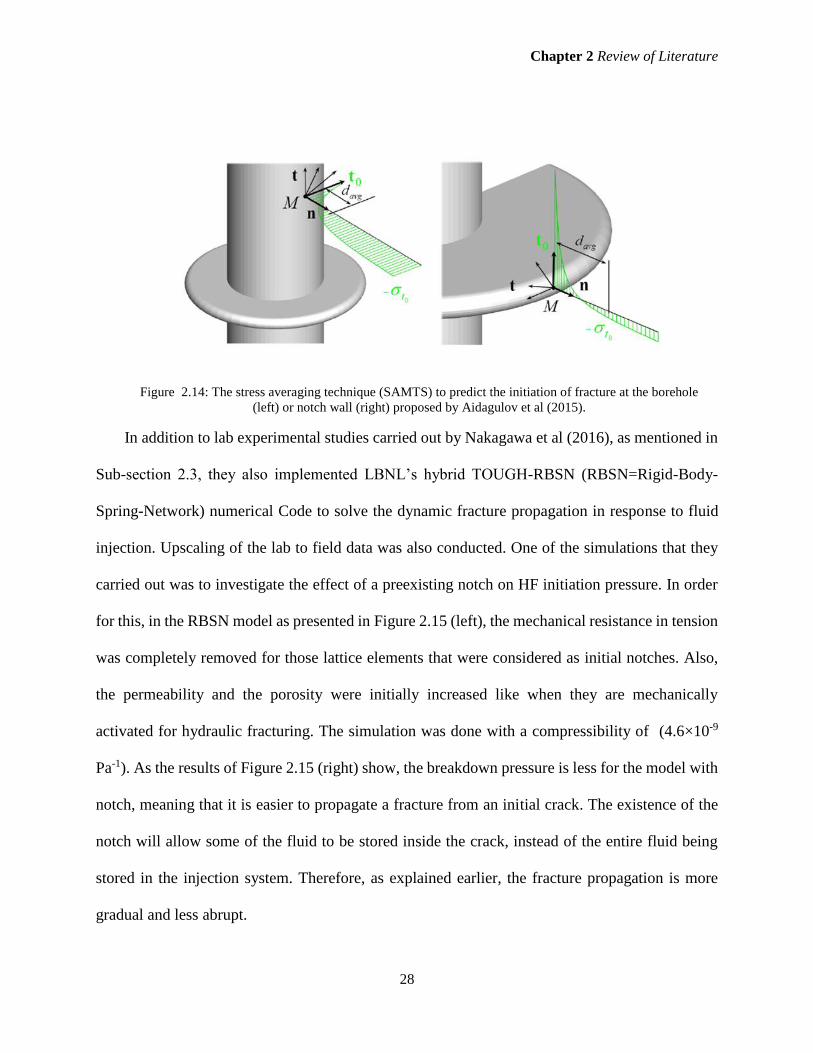
TESTING BLOCK USED FOR NUMERICAL SIMULATIONS BY AIDAGULOV ET AL (2015). .............................................................. 27 FIGURE 2.14: THE STRESS AVERAGING TECHNIQUE (SAMTS) TO PREDICT THE INITIATION OF FRACTURE AT THE BOREHOLE (LEFT) OR
NOTCH WALL (RIGHT) PROPOSED BY AIDAGULOV ET AL (2015). ........................................................................................ 28 FIGURE 2.15: RBSN MODEL FOR A HF WITH NOTCH (LEFT) AND THE PRESSURE EVOLUTION FOR MODELS WITH AND WITHOUT NOTCHES
(NAKAGAWA ET AL 2016). ........................................................................................................................................ 29 FIGURE 2.16: THE MODEL GEOMETRY USED TO SIMULATE THE EFFECT OF NOTCH ANGLE ON HF PRESSURES (MARTINEZ ET AL 2019). .... 30 FIGURE 2.17: HF BREAKDOWN PRESSURE AS A FUNCTION OF THE NOTCH ANGLES (MARTINEZ ET AL 2019). ..................................... 31 FIGURE 2.18: THE DESIGNED INDENTER TO CREATE FRACTURE IN A DESIRED DIRECTION: IN TRANSPORTATION MODE (LEFT) AND IN
OPERATION (RIGHT) (PATUTIN AND SERDYUKOV 2017)................................................................................................... 32
viii
FIGURE 2.19: THE INTERACTION FORCES BETWEEN THE INDENTER AND THE OPENING CRACK (PATUTIN AND SERDYUKOV, 2017) .......... 32 FIGURE 2.20: FRACTURE INITIATION PRESSURE AS A FUNCTION OF WELLBORE DEVIATION AND DIRECTION WITH RESPECT TO THE DIRECTION
OF H (ABBAS ET AL 2009). .................................................................................................................................... 34 FIGURE 2.21: THE JETTING TOOL PROPOSED BY ABBAS ET AL (2009) TO CREATE A VERTICAL HOLE TO FACILITATE FRACTURE INITIATION. . 35 FIGURE 3.1: SCHEMATIC MODEL OF A LATTICE ARRAY. NODES AND SPRINGS (CUNDALL 2011)....................................................... 38 FIGURE 3.2: CORRELATION BETWEEN THE 3D PARTICLE MODEL AND CORRESPONDING PIPE NETWORK (DAMJANAC, DETOURNAY, AND
CUNDALL 2016) ...................................................................................................................................................... 42 FIGURE 3.3: LOCATION OF VARIABLES IN THE MATRIX FLOW SCHEME AS DESCRIBED IN XSITE DESCRIPTION OF
FORMULATION (DAMJANAC ET ALL 2011) ........................................................................................................... 43 FIGURE 3.4: AN EXAMPLE OF XSITE MATERIAL PROPERTIES WINDOW. INPUT DATA CORRESPONDS TO BAKKEN FORMATION. ................ 46 FIGURE 3.5: AN EXAMPLE OF XSITE FLUID PROPERTIES WINDOW. INPUT DATA CORRESPONDS TO BAKKEN FORMATION. ...................... 46 FIGURE 3.6: AN EXAMPLE OF XSITE IN-SITU STRESS WINDOW. INPUT DATA CORRESPONDS TO BAKKEN FORMATION. ........................... 46 FIGURE 3.7: AN EXAMPLE OF ROCK GEOMETRY WITH SOFT BOUNDARY IN XSITE........................................................................... 47 FIGURE 3.8: BOREHOLE PANEL IN XSITE (TOP) TO ENTER FLUID PUMPING (LOW LEFT) ANDBOREHOLE TRAJECTORY AND GEOMETRY AND
RADIUS (BOTTOM RIGHT). THE OH COMPLETION IS CHOSEN IN THIS EXAMPLE WITH CLUSTER SECTION BEING INACTIVATED ........... 48 FIGURE 3.9: DIFFERENT OPTIONS FOR FLUID INJECTION IN XSITE, VIA A BOREHOLE AND CLUSTER (LEFT), PERFORATIONS (MIDDLE) AND OH
COMPLETION (RIGHT)................................................................................................................................................ 50 FIGURE 3.10: JOINT SET PANEL IN XSITE TO ENTER THE PARAMETERS OF NATURAL FRACTURES ....................................................... 50 FIGURE 3.11: RESOLUTION DOMAINS FOR A TRANSVERSE FRACTURE MODEL .............................................................. 53 FIGURE 3.12: MODEL GEOMETRY OF AN AXIAL NOTCH AND FRACTURE (LEFT) AND THE RESOLUTION DOMAINS......... 55 FIGURE 3.13: BATCH SIMULATION PANEL IN XSITE TO SET UP THE THREE MAIN STAGES AND EXECUTE THE MODEL .............................. 56 FIGURE 3.14: FRACTURE APERTURES CORRESPONDING TO INJECTION RATE OF Q=0.06M3/SEC (TOP) AND
Q=0.08M3/SEC (BOTTOM) OVER SIMULATION TIME OF T=0.SEC .......................................................................... 57 FIGURE 3.15: FRACTURE PRESSURE AND CRACK NUMBERS VERSUS TIME FOR DIFFERENT INJECTION RATES ......................................... 58 FIGURE 3.16: FRACTURE PRESSURE AND CRACK NUMBERS VERSUS TIME FOR DIFFERENT FLUID VISCOSITIES ........................................ 60 FIGURE 4.1: PLAN VIEW OF A VERTICAL WELLBORE WITH IN-SITU AND DRILLING INDUCED STRESSES. ................................................. 63 FIGURE 4.2: PLAN VIEW OF A HORIZONTAL WELLBORE DRILLED PARALLEL TO H DIRECTION WITH IN-SITU AND DRILLING INDUCED STRESSES.
............................................................................................................................................................................ 65 FIGURE 4.3: AXIAL (LEFT) AND TRANSVERSE FRACTURES (RIGHT) AROUND A HORIZONTAL WELLBORE. .............................................. 65 FIGURE 4.4: DISTRIBUTION OF DRILLING INDUCED STRESSES AROUND A HORIZONTAL WELLBORE DRILLED ALONG 𝝈𝒉 DIRECTION BASED ON
KIRSCH’S EQUATIONS. ............................................................................................................................................... 67 FIGURE 4.5: VARIATION OF TANGENTIAL STRESSES AROUND THE WELLBORE WALL AS A FUNCTION OF STRESS ANISOTROPY.................... 70 FIGURE 4.6: FRACTURE MECHANICS MODEL FOR CRACK GROWTH IN A PRESSURIZED CIRCULAR BOREHOLE. ........................................ 72 FIGURE 4.7: FUNCTIONS F(B), G(B), HB, HC (FOR CONSTANT PRESSURE CASE) VERSUS B. ................................................................. 73 FIGURE 4.8: INTENSITY FACTORS (TOP) AND BOREHOLE PRESSURES (MIDDLE) AT UNSTABLE CRACK EXTENSION
VALUES FOR DIFFERENT LOADING SOURCES AS A FUNCTION OF CRACK LENGTH AT THE WELLBORE WALL. THE
BOTTOM FIGURE SHOWS THE TOTAL PRESSURE, PC. ............................................................................................. 77 FIGURE 4.9: FRACTURE COEFFICIENTS CORRESPONDING TO DIFFERENT LOADING SOURCES. ............................................................. 78 FIGURE 4.10: HYDRAULIC FRACTURING TENSILE STRENGTH AS A FUNCTION OF WELLBORE SIZE. ....................................................... 78 FIGURE 4.11: DIMENSIONLESS FUNCTIONS FOR THE CASE OF RAPID (LEFT) AND SLOW (RIGHT) PRESSURIZATION RATES (AFTER CHARLEZ
1997). .................................................................................................................................................................. 80 FIGURE 4.12: CRITICAL BOREHOLE PRESSURES CALCULATED FOR THE FAST AND SLOW PRESSURIZATION IN CASE OF ISOTROPIC AND
ANISOTROPIC HORIZONTAL STRESSES. ........................................................................................................................... 83 FIGURE 4.13: CHANGE OF THE WEIGHT FUNCTION F WITH RESPECT TO 𝒙𝑳 FOR AXIAL AND TRANSVERSE CRACKS. ................................ 87 FIGURE 4.14: FRACTURE INITIATION PRESSURES FOR TRANSVERSE AND AXIAL FRACTURES IN PRESENCE OF DIFFERENT STRESS REGIMES.... 90 FIGURE 4.14 (CONTINUED): FRACTURE INITIATION PRESSURES FOR TRANSVERSE AND AXIAL FRACTURES IN PRESENCE OF DIFFERENT STRESS
REGIMES. ............................................................................................................................................................... 90

ix
FIGURE 4.15: CHANGE OF THE WEIGHT FUNCTION F FOR MULTIPLE FRACTURES WITH RESPECT TO THE NUMBER OF FRACTURES AND THE
RATIO OF CRACK LENGTH TO CIRCUMFERENTIAL DISTANCE BETWEEN FRACTURES. .................................................................. 92 FIGURE 4.16: FRACTURE INITIATION PRESSURES MULTIPLE AXIAL FRACTURES. .............................................................................. 92 FIGURE 4.17: DIMENSION TOUGHNESS PARAMETER CHANGES AS A FUNCTION OF PRESSURIZATION RATE FOR TYPICAL FIELD AND LAB SCALE
HF OPERATIONS. ..................................................................................................................................................... 96
List of Tables
TABLE 4.1: BAKKEN SHALE FORMATION MECHANICAL PROPERTIES AND IN-SITU STRESSES ............................................................... 66

x
ACKNOWLEDGMENTS
I wish to express my sincere appreciation to my senior supervisor Dr. Vamegh Rasouli for all his
helps and attentions during my PhD tenure as PhD student at the University of North Dakota. In
particular, I would like to thank him for his support to my thesis topic and defense, providing me
an exclusive opportunity to learn from his depth of knowledge in this field.
Provision of the XSite academic license through the Itasca IEP program was fundamental to
conduct this research and highly appreciated. I would like to also thank Dr. Branko Damjanac for
his continuous support and feedback on simulation models. I would also want to thank other
members of my advisory committee members Dr. Minou Rabiei, Dr. Hui Pu, Kegang Ling and
Dr. Iraj Mamaghani for their support. I would also like to thank my fellow classmates Nourelhouda
Benouadah, Xueling Song for their helps. The financial support of the North Dakota Industrial
Commission (NDIC) is highly appreciated.
Last but not the least, I would like to thank my husband Dr. Kouhyar Tavakolian and my
parents-in-law for all their support at home and when I was busy with the final stage of drafting
the thesis. I would also like to thank my parents and my brothers and sisters for their
encouragements. I thank my friend Nassima Djelal and all my dear friends.

xi
Dedicated to people who are missing in my life.
xii
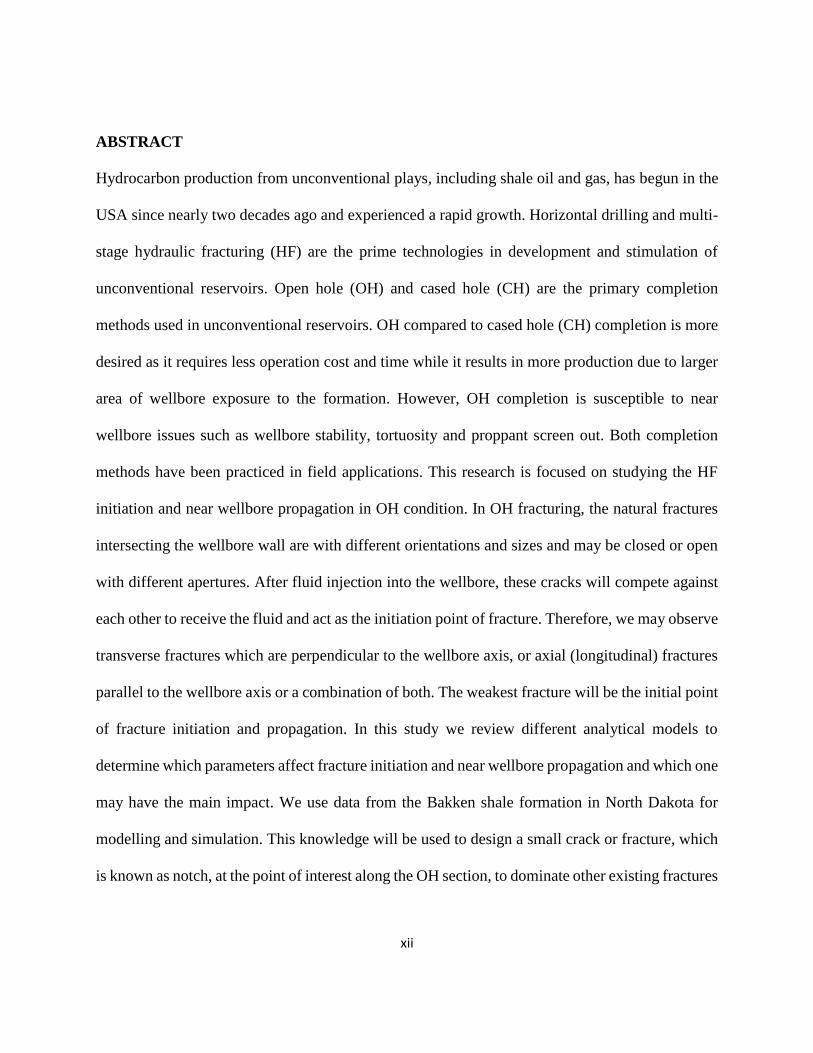
ABSTRACT
Hydrocarbon production from unconventional plays, including shale oil and gas, has begun in the
USA since nearly two decades ago and experienced a rapid growth. Horizontal drilling and multi-
stage hydraulic fracturing (HF) are the prime technologies in development and stimulation of
unconventional reservoirs. Open hole (OH) and cased hole (CH) are the primary completion
methods used in unconventional reservoirs. OH compared to cased hole (CH) completion is more
desired as it requires less operation cost and time while it results in more production due to larger
area of wellbore exposure to the formation. However, OH completion is susceptible to near
wellbore issues such as wellbore stability, tortuosity and proppant screen out. Both completion
methods have been practiced in field applications. This research is focused on studying the HF
initiation and near wellbore propagation in OH condition. In OH fracturing, the natural fractures
intersecting the wellbore wall are with different orientations and sizes and may be closed or open
with different apertures. After fluid injection into the wellbore, these cracks will compete against
each other to receive the fluid and act as the initiation point of fracture. Therefore, we may observe
transverse fractures which are perpendicular to the wellbore axis, or axial (longitudinal) fractures
parallel to the wellbore axis or a combination of both. The weakest fracture will be the initial point
of fracture initiation and propagation. In this study we review different analytical models to
determine which parameters affect fracture initiation and near wellbore propagation and which one
may have the main impact. We use data from the Bakken shale formation in North Dakota for
modelling and simulation. This knowledge will be used to design a small crack or fracture, which
is known as notch, at the point of interest along the OH section, to dominate other existing fractures

xiii
and be the point of fracture initiation. We also use lattice numerical simulations, which is a particle
based model to simulate a number of cases and compare the results with analytical solutions.
The results of this study indicated that stress anisotropy and notch orientation and dimension
are the most important parameters that dominate the fracture initiation point and type of fractures
propagating (i.e. transverse or axial). The next parameters include formation properties as well as
fluid injection rate and viscosity. When the notch size is small, usually axial fractures are dominant,
however, beyond a certain notch size, transverse notch will initiate and propagate. The notch size
at the cross over point is a strong function of stress anisotropy and moves to the larger notch sizes
when stress anisotropy reduces; to the extent that in isotropic stress condition regardless of the size
of the notch, no transverse fracture will initiate. The simulation results showed how, in case of
axial notch, the base length of the notch along the wellbore axis, plays an important role in fracture
initiation pressure. The results indicated that the larger the notch size the lower the initiation
pressure and easier for fracture to propagate. If the notch is not along the preferred plane of
propagation, after moving away from near wellbore drilling induced zone, the fracture tends to
reorient itself to align to the preferred direction. Simulation of multiple axial and transverse
fractures and random fractures, similar to real field cases, showed that the initiation pressure
increases as the number of fractures increases and that following the knowledge obtained from this
study we can determine the most likely fractures that will serve as the fracture initiation point. This
conclusion suggest that the near wellbore fractures should be picked up accurately using the image
logs and other tools in order to analyze them using the workflow presented in this research to
design the geometry of the notch that will dominate existing fractures for multi-stage HF operation.
Chapter 1 Openhole Fracturing Completion
1
CHAPTER 1
Open hole Fracturing Completion
1.1 Introduction
Hydrocarbon production from unconventional reservoirs requires stimulation techniques. In shale
oil and gas plays, hydraulic fracturing (HF), or fracking operation, is the dominated stimulation
technique that is currently practiced in the industry. In this method, a high pressure fluid with
designed viscosity is injected into a horizontal wellbore to open a long bi-wing fracture of a few
thousand feet. This fracture serves as the main path to direct the hydrocarbon to the wellbore, while
the shattered zone around the fracture plane creates the drained zone or stimulated reservoir
volume (SRV). Several parameters should be considered in the design of HF including in-situ
stresses of the field, formation mechanical properties and fracturing fluid properties (Gandossi,
2013; Ling, Zeng 2013). Theoretically, HF initiates and propagates perpendicular to the direction
of minimum in-situ stress, it is more straight plane in presence of large stress anisotropy and the
stimulated reservoir volume (SRV) depends on elastic properties of the formation and the fluid
injection rate and viscosity can change the initiation pressure significantly (Fallahzadeh et al, 2015;
2017; Serajian and Ghassemi, 2011; Jeffrey et al, 2010)
Broadly speaking, there are two main well completion techniques that commonly used in oil
and gas industry: open hole (OH) and cased hole (CH) (Gottschling and Co, 2005). The benefits

Chapter 1 Openhole Fracturing Completion
2
of OH completion are its much larger area of exposure of the fluid to the formation, and that it is
more cost effective. In CH completion, the fluid path is through small perforation tunnels drilled
around the wellbore, so more pressure drops are expected so the operation is more expensive and
difficult than OH completion, however, in many cases, to keep the wellbore integrity CH
completion is the only applicable option.
In real field situation, there are several defects including natural fractures around the wellbore
which play as the seed points to initiate the HF, in most cases they are oriented in directions
different than ideal direction for fracture initiation and propagation. Similarly, in CH completion,
drilling perforation tunnels in incorrect directions with respect to the in-situ stresses will results in
complex fracture geometry, multiple fractures, and tortuosity near wellbore which creates severe
operational and technical problems.
This study is focused on understanding the HF initiation and propagation in OH completion.
The previous literature shows that in an OH wellbore both longitudinal (axial) and transverse
fractures are observed. As depicted in Figure 1.1, the axial fracture propagates along the wellbore
direction, whereas transverse fracture propagates perpendicular to the wellbore axis. Practically,
transverse fracture is the desired type of fracture that is expected to create during HF operation. In
this research, we discuss in details the conditions where axial and transverse fracture may create.
We also, introduce the concept of creating a notch (small crack) around the wellbore to dominate
transverse over axial fracture. The conditions where the notch will be effective are discussed and
the analysis and discussions are supported by analytical models and numerical simulations.
Ultimately, the goal is to propose creating notches with certain geometry and in defined directions
in an OH section of the wellbore that dominates all existing natural fractures and defects and play
as the main point of induced fracture initiation and propagation.

Chapter 1 Openhole Fracturing Completion
3
In this study, XSite, a newly developed software by Itasca group will be employed. This
software is explicitly designed for simulation of hydraulic fractures. The simulator works based
on the physics of the granular material.
In the following sections, a brief discussion regarding OH and CH completions will be
presented with some highlights about each method. Then the objectives, research methodology
and significance of this research study will be presented with an overview of the content of each
Chapter of the thesis.
Figure 1.1: (a) longitudinal fracture (b) Transverse fracture. Horizontal wells in unconventional reservoir are
often drilled in the direction of minimum stress.
1.2 OH versus CH Fracking Completion
Well-completion is a fundamental part of any hydrocarbon field development project. Well-
completion represents a connection of hydrocarbon reservoir and surface facilities, which refers to
the process of completing a well, so it is ready to produce hydrocarbons. For a comprehensive
discussion on different types of reservoir completion one may refer to Bellarby (2009). Figure 1.2
presents the most commonly completion methods from simple to complex one based on the
equipment used in the wellbore. The main objective of the design stage is to maximize the recovery
from the well. Furthermore, a completion design is a combination of multiple disciplines, from

Chapter 1 Openhole Fracturing Completion
4
chemistry, mathematics, geology, hydraulics to material science, and practical hands-on wellsite
experience Bellarby (2009). Well completion engineering plays a vital role in the process; it
involves ensuring regular and safe production that should last for many years of the production
life of oil and gas wells Economids (2000). For efficient production flow, it is essential to prepare
the well for production by setting up the necessary equipment into the well to permit the safe and
controlled flow hydrocarbons at the surface.
Figure 1.2: Reservoir completion methods. The figure shows different type of completions (from left to right)
with a minimum of downhole equipment to the most completed one (Bellarby 2009).
One of the most crucial differences between OH versus CH completion is the cost of the
personnel involved and the supplies needed in each procedure. Depending on the characteristics
of the reservoir to be produced, one might be more favorable than the other. The analysis of
physical properties and pore configuration are crucial for drilling and completion fluid design, as
well as the selected treatment Renpu (2011). In OH completions, the casing is only required to run
through the well to the top of the reservoir. Special fluids are utilized to prevent the well from
collapsing, but this is a less costly procedure.
Chapter 1 Openhole Fracturing Completion
5
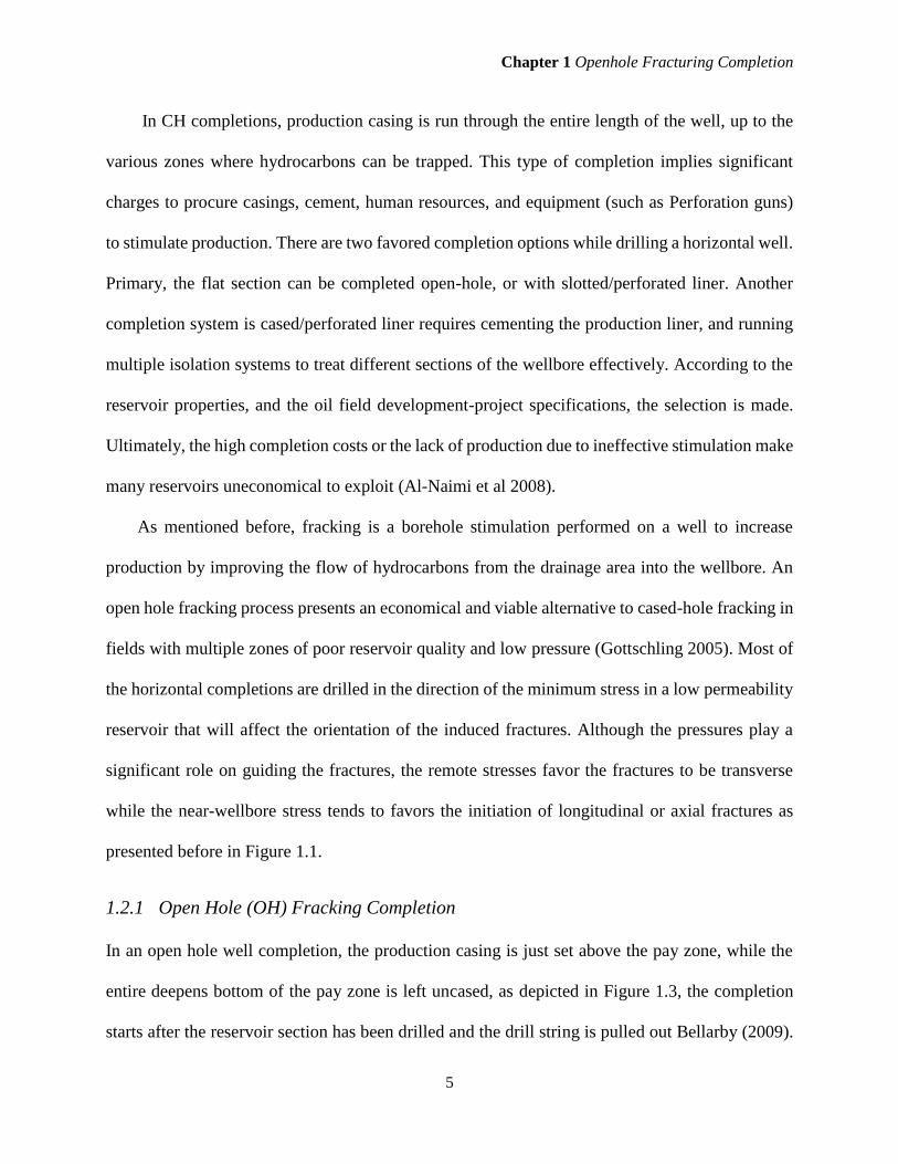
In CH completions, production casing is run through the entire length of the well, up to the
various zones where hydrocarbons can be trapped. This type of completion implies significant
charges to procure casings, cement, human resources, and equipment (such as Perforation guns)
to stimulate production. There are two favored completion options while drilling a horizontal well.
Primary, the flat section can be completed open-hole, or with slotted/perforated liner. Another
completion system is cased/perforated liner requires cementing the production liner, and running
multiple isolation systems to treat different sections of the wellbore effectively. According to the
reservoir properties, and the oil field development-project specifications, the selection is made.
Ultimately, the high completion costs or the lack of production due to ineffective stimulation make
many reservoirs uneconomical to exploit (Al-Naimi et al 2008).
As mentioned before, fracking is a borehole stimulation performed on a well to increase
production by improving the flow of hydrocarbons from the drainage area into the wellbore. An
open hole fracking process presents an economical and viable alternative to cased-hole fracking in
fields with multiple zones of poor reservoir quality and low pressure (Gottschling 2005). Most of
the horizontal completions are drilled in the direction of the minimum stress in a low permeability
reservoir that will affect the orientation of the induced fractures. Although the pressures play a
significant role on guiding the fractures, the remote stresses favor the fractures to be transverse
while the near-wellbore stress tends to favors the initiation of longitudinal or axial fractures as
presented before in Figure 1.1.
1.2.1 Open Hole (OH) Fracking Completion
In an open hole well completion, the production casing is just set above the pay zone, while the
entire deepens bottom of the pay zone is left uncased, as depicted in Figure 1.3, the completion
starts after the reservoir section has been drilled and the drill string is pulled out Bellarby (2009).
Chapter 1 Openhole Fracturing Completion
6
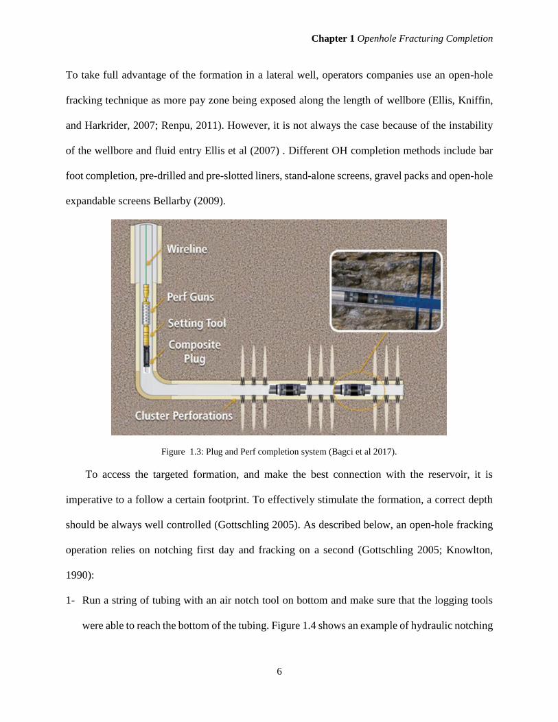
To take full advantage of the formation in a lateral well, operators companies use an open-hole
fracking technique as more pay zone being exposed along the length of wellbore (Ellis, Kniffin,
and Harkrider, 2007; Renpu, 2011). However, it is not always the case because of the instability
of the wellbore and fluid entry Ellis et al (2007) . Different OH completion methods include bar
foot completion, pre-drilled and pre-slotted liners, stand-alone screens, gravel packs and open-hole
expandable screens Bellarby (2009).
Figure 1.3: Plug and Perf completion system (Bagci et al 2017).
To access the targeted formation, and make the best connection with the reservoir, it is
imperative to a follow a certain footprint. To effectively stimulate the formation, a correct depth
should be always well controlled (Gottschling 2005). As described below, an open-hole fracking
operation relies on notching first day and fracking on a second (Gottschling 2005; Knowlton,
1990):
1- Run a string of tubing with an air notch tool on bottom and make sure that the logging tools
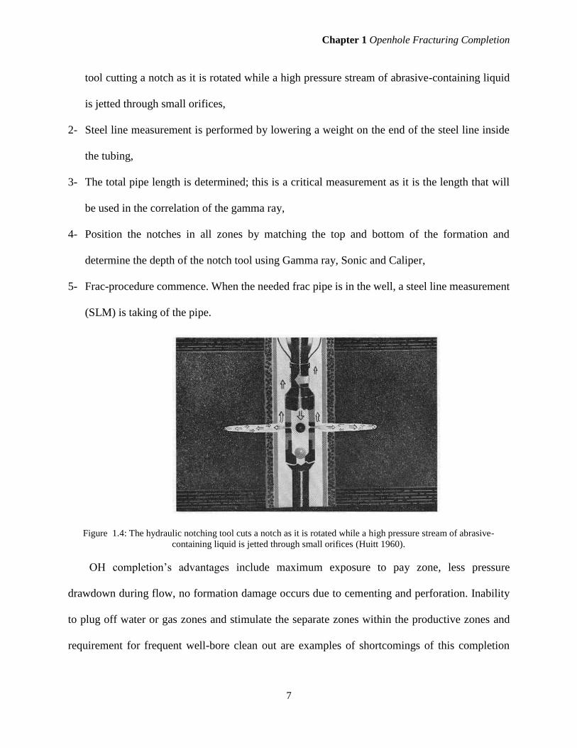
were able to reach the bottom of the tubing. Figure 1.4 shows an example of hydraulic notching
Chapter 1 Openhole Fracturing Completion
7
tool cutting a notch as it is rotated while a high pressure stream of abrasive-containing liquid
is jetted through small orifices,
2- Steel line measurement is performed by lowering a weight on the end of the steel line inside
the tubing,
3- The total pipe length is determined; this is a critical measurement as it is the length that will
be used in the correlation of the gamma ray,
4- Position the notches in all zones by matching the top and bottom of the formation and
determine the depth of the notch tool using Gamma ray, Sonic and Caliper,
5- Frac-procedure commence. When the needed frac pipe is in the well, a steel line measurement
(SLM) is taking of the pipe.
Figure 1.4: The hydraulic notching tool cuts a notch as it is rotated while a high pressure stream of abrasive-
containing liquid is jetted through small orifices (Huitt 1960).
OH completion’s advantages include maximum exposure to pay zone, less pressure
drawdown during flow, no formation damage occurs due to cementing and perforation. Inability
to plug off water or gas zones and stimulate the separate zones within the productive zones and
requirement for frequent well-bore clean out are examples of shortcomings of this completion

Chapter 1 Openhole Fracturing Completion
8
method. A brief overview of different OH completion methods will be presented in the next
Chapter.
1.2.2 Cased Hole(CH) Fracking Completion
Cased hole completion consists of casing and cementing and perforation subsequently. The first
step is that the casing/liner has to be cemented, then comes the mud displacement and wellbore
clean-out Bellarby (2009). The hole is drilled through the target formation(s), and production
casing is run cemented in the hole. Hydraulic fracturing is conducted in short sections called stages
along the lateral section of the wellbore and starts at the end of the wellbore (toe) and progresses
towards the beginning (hill). The operation includes the following typical steps:
1- A perforating gun is lowered into a targeted position within the horizontal portion of the well.
2- An electrical current is sent down the well to set off a small explosive charge. This shoots tiny
holes through the well casing and out a short, controlled distance into the shale formation.
3- The holes created by the “perf” gun serve two purposes. They provide path for the fracturing
fluid to enter the formation and subsequently allows natural gas to enter the wellbore.
Advantages of CH completion include: excessive gas and water production can be controlled
more easily, adaptable to multiple completion techniques, can be easily deepened and control most
sand. Some of the shortcomings of this method include cost of casing cement and perforating for
long zones, well productivity is less that productivity of open hole completion, and no adaptable
to special drilling techniques to minimize formation damage.
1.3 Objectives
As explained above, creating a proper notch is of significant importance in OH completion to
ensure that the fracture initiation and propagation is performed optimally. Therefore, the overall

Chapter 1 Openhole Fracturing Completion
9
goal of this study is to investigate how to enhance the openhole fracturing technique by cutting a
notch in the wellbore wall to serve as a weak point where the hydraulic fracture initiates. The
detailed objectives of this work can be summarized as followings:
1. Comprehensive review of existing literature on the impact of the notch geometry on fracture
initiation and propagation. This includes analytical models, lab experimental studies,
numerical simulations and field observations.
2. Under what conditions axial and transverse fractures will be created and how the notch can
dominate transverse fractures. Also, what is the impact of fluid viscosity and injection rate as
well as pressurization rate on initiation pressure.
3. Determine the impact of in-situ field stresses on the type of fractures (axial vs transverse)
around the wellbore in a notched OH wellbore.
4. The applications and limitations of analytical models in estimation of fracture initiation
pressure in presence of a notch emanating from a cylindrical borehole will be discussed. This
will be extended to star fractures, where more than one bi-wing notch it edging from the
wellbore.
5. Capabilities and unique features of lattice simulations for HF simulations and studying the
effect of notch on fracture initiation and propagation. XSite software, which is a particle based
numerical simulator and works on the basis of distinct element method (DEM), will be
implemented in this study.
6. Conduct numerical simulations using published lab data as well as field scales and compare
the results with analytical models to identify the impact of the notch on fracture pressures. This
will be extended to presence of multi cracks emanating from the borehole.

Chapter 1 Openhole Fracturing Completion
10
7. Recommend notch geometry and orientation in an OH lateral wellbore with existing natural
fractures to dominate fracture initiation in desired spot and direction.
1.4 Methodology
The methodology that will be used to achieve the above objectives comprises of data inventory,
analytical solutions and numerical simulations. These are briefly explained below.
1. In order to perform calibrated numerical simulations, we collect sets of lab data from the
literature. Similarly, field scale data will be gathered for the same purpose. While the
simulations will be based on Bakken formation, we use data from other fields for comparison
purposes.
2. Numerical simulations will be run using XSite software to estimation fracture initiation
pressure in OH completion and in presence of notches with different length and orientations.
The impact in-situ stresses and formation properties will be studied. Sensitivity analysis of
various parameters will be done to determine the competition between axial versus transverse
fractures and the impact of the notch size and orientation on this.
3. Different analytical models will be introduced to predict the fracture initiation in a borehole
with a crack emanating from its edge. The impact of notch size and orientation on generation
of axial and transverse fracture will be discussed and the effect of fluid viscosity and injection
rate and pressurization rate will be studied. The limitations and range of applications of each
model will be discussed.
4. The results of analytical models and numerical simulations will be compared to draw some
practical applications in terms of determining the best notch geometry and orientation in an
OH completion for desired HF results.

Chapter 1 Openhole Fracturing Completion
11
1.5 Significance
The results of this research study will present multifold novelties including the followings:
1. This research project helps to address the gaps between analytical solutions and numerical
simulations and elaborate potential solutions.
2. Unique features of the XSite software, and lattice numerical simulations, as will be presented
in this study, is one of the first attempt to study the impact of notches on OH completion HF.
3. The outcome of this project will help to drill notches at specific points along the lateral section
of an OH within each fracking stage in order to optimize HF initiation and propagation.
4. The results of this study can also be applied partially in CH completion where the fracturing
fluid injection through a perforation may penetrate into natural fractures behind the cement
sheet. Also, the length of the perforation may also be designed in the same approach that is
discussed for the notch in this study.
5. Practical recommendations and suggestions that are proposed in this study can improve the
operation of OH HF which in turn can be of significant financial benefits for the companies.
1.6 Thesis Structure
This thesis consists of five chapters.
Chapter 1 provides the background to the project and a very brief explanation of the basics of
hydraulic fracturing in open-hole versus cased-hole, emphasizing on the techniques used in open-
hole fracking. It also contains the objectives of this study, the methodology used and the
significance of this research.
In Chapter 2 a brief review of the literature regarding the OH completion methods will be
presented. Also, a summary of past studies related to the lab work, numerical simulations and

Chapter 1 Openhole Fracturing Completion
12
analytical models to estimate initiation pressure of HF from an OH with a notch and multi notches
will be given.
Chapter 3 presents a brief overview of the background and theory of lattice simulation used
in this study and the features and modelling using the XSite software. Constitutive lattice
formulation and simulation features are also summarized.
Chapter 4 comprises of different analytical models that study the impact of the notch size and
orientations on HF initiation pressure and stress intensity factor. These models integrate the impact
of different parameters including net pressure on the notch surface, rock elastic properties and
pressurization rate. The range of applications and limitations of these models will be discussed.
Chapter 5 presents the results of the numerical simulations. The simulations consider the
effects of notch orientation and dimension and the impact of different parameters in initiation
pressure from an OH. Also, in this Chapter the results are compared with analytical models
presented in the preceding Chapter and conclusions are made.
In Chapter 6 a summary of the findings from this study will be presented along with some
recommendations and future studies that can be carried out.
1.7 Summary
This Chapter introduced the OH and CH completion and the advantages and shortcomings of each
method. It was highlighted that in OH completion, creating a notch with proper size and orientation
is necessary to ensure that the HF initiates and propagate in desirable direction. Also, it was
explained that field in-situ stresses as well as injecting fluid properties and formation
characteristics will impact the effectiveness of the notch. The notch also can dominate the
generation of axial versus transverse fractures in OH. Also, in this Chapter, a summary of the

Chapter 1 Openhole Fracturing Completion
13
main objectives of this research, the methodology which will be implemented, distinguished
aspects of this study and the structure of this thesis were presented.
In the next Chapter, a review of the literature will be presented to give a background to the
OH completion methods and the models that are used for estimation of HF pressure in notched
wellbores.

Chapter 2 Review of Literature
14
CHAPTER 2
Review of Literature: Near Wellbore Fracturing in
Open Hole Completion
2.1 Introduction
In the previous Chapter the advantages of the OH completion over CH completion were briefly
mentioned. While CH completion is perhaps a more frequently used technique due to the additional
wellbore stability and flexibility in production, whenever possible, the operators prefer to complete
the well OH to benefit from the extra exposure to the formation and more production.
As one may expect, in OH completion, the type of near wellbore issues is different than CH
completion and with respect to the HF operation may include the dominance of fracture initiation
point along the horizontal section and change of fracture initiation and breakdown pressure due to
the existence of the natural fractures around the wellbore, fracture tortuosity and screen outs
(Belyadi, H et al, 2019). In multi-stage HF in OH as well as CH completion, the stress shadow effect
is another design parameter that needs to be considered to properly estimate fracture dimensions.
The use of a notch in OH completion will assist in better design of the HF treatment. This
was briefly explained in the preceding Chapter and will be discussed in further details in this and
next Chapters. The design of the notch (e.g. dimension and orientation) with respect to the wellbore

Chapter 2 Review of Literature
15
direction and the orientation of principal stresses has a significant impact on the effectiveness of
the notch.
In this Chapter, we present a brief overview of the past research and studies on the impact of
the notch on HF initiation and propagation. We classify these studies into analytical models,
experimental studies, numerical simulations and field practices.
2.2 Analytical Models
The impact of an existing crack or notch on fracture initiation and propagation in medium with
different geometry has been the subject of studies in different science and engineering disciplines.
These methods, in general, include the effect of the notch by modifying the critical stress intensity
factor based on the shape of the notch and its position with respect to the structure.
The concept of weight function initially introduced by Bueckner (1970) has been extensively
used in future work. According to this theory, as quoted by Rice (1972) “the stress intensity factor
is expressed as a sum of work-like products between applied forces and values of the weight
function at their points of application”. Rice (1972) used this theory to determine the intensity
factor for a crack in a remotely uniform stress field subject to an arbitrary traction distribution on
the faces of a crack.
Glinka (1996) presented the weight functions to calculate the stress intensity factors around
cracks with different shapes in a thick cylinder subjected to complex stress fields. He provided the
approximation of the weight functions with different orders.
Dunn and Suwito (1997) studied the fracture initiation at sharp notches. The geometry of the
corner that they considered in their studies is shown in Figure 2.1 (left). They determined the
magnitude of the stress intensity 𝐾𝑙𝑛 for notched mode I three-point flexure specimens (see Figure
2.1, right) using a combination of Williams (1952) asymptotic method, dimensional

Chapter 2 Review of Literature
16
considerations, and detailed finite element analysis. They showed that 𝐾𝑙𝑛 is a function of the
geometry of the structure and the loading.
Figure 2.1: Geometry of the corner used to determine the fracture initiation pressure (left) and the geometry of
notched three-point flexure specimen used to extract the critical stress intensity (After Dunn and Suwito (1997).
The critical stress intensity factor (𝐾𝑙𝑛) was calculated as:
𝐾𝑙𝑛 = 𝜎0ℎ1−𝜆𝑓 (
𝑎
ℎ) = (
3𝑃𝐿
2𝑏ℎ2) ℎ1−𝜆𝑓 (
𝑎
ℎ) (2.1)
where, based on the parameters shown in Figure 2.1, and that -1 is the elastic singularity, they
proposed the following polynomial fit for f(a/h) when 0.5 ≤ 𝑓(𝑎 ℎ⁄ ) ≤ 0.7:
𝑓 (𝑎
ℎ) = 𝑐1 (
𝑎
ℎ) + 𝑐2 (
𝑎
ℎ)2
+ 𝑐3 (𝑎
ℎ)3
+ 𝑐4 (𝑎
ℎ)4
+ 𝑐5 (𝑎
ℎ)5
(2.2)
The results of their experiments on notched polymethyl methacrylate (PMMA) three-point
flexure specimens with notch angles of 60°, 90°, and 120° demonstrated the feasibility of using a
critical value of 𝐾𝑙𝑛 to correlate fracture initiation.
In a similar attempt, Leguillon and Yosibash (2003), presented a criterion to predict crack
onset at a sharp notch in homogeneous brittle materials. Their experiments on a stiffer material
(Alumina/Zirconia) showed that it is less sensitive to small notch tip radii than that of PMMA.
With specific application in Hydraulic fracturing, Rummel (1987) used the weighting function
approach to estimate the critical borehole pressure at unstable crack extension. The intensity of the

Chapter 2 Review of Literature
17
stress field in the vicinity of the crack tips can be formulated based on the principle of superposition
of stress intensity factors (KI) from each loading source. In his 2D modelling, he considered the
magnitude of the two horizontal stresses, borehole pressure and the pressure inside the crack to
estimate the total intensity factor of the system. This method allows evaluating the impact of each
parameter on fracture initiation. Figure 22 depicts the concept of the superposition of loading
sources. A detailed discussion about this model will be presented in Chapter 4 using the data from
Bakken formation in North Dakota.
Charlez (1997) used the weighting function to calculate the HF initiation pressure in presence
of a crack from the edge of a circular opening as a function of average magnitude of the stresses,
differential stresses, fluid pressure and pore pressure. In particular, he considered the
pressurization rate in his equations. In fast pressurization, he stated that the crack pressure will be
equal to the pore pressure, whereas, in slow pressurization, it becomes the same as the wellbore
pressure. Similar results reported by Detournay and Carbonell (1997). Further discussion of this
model will be presented in Chapter 4.

Chapter 2 Review of Literature
18
Figure 2.2: Superposition of four loading sources to determine total system intensity factor (after Rummel, 1987)
A very applicable analytical model to the applications within the context of this research was
proposed by Nilson and Proffer (1984). They investigated the fracture initiation from a pre-existing
crack emanating from a wall of a cylindrical excavation. Using the weight functions, they
calculated the stress intensity and opening displacements for planar (transverse) or axisymmetric
(axial or longitudinal) fractures emanating from a cylindrical or spherical hole in an elastic
medium. They showed how their solutions reduce to known exact solutions when the notch size
becomes very short and to the penny-shaped or Griffith fracture in case of very long fracture. They
Chapter 2 Review of Literature
19
proposed the solutions for both wedge-shaped and disc-shaped fractures and also for more than
one axial fracture emanating from a circular borehole. Their proposed generalized integral
formulas present a fast, simple, and reasonably accurate method for solving a wide range of
engineering problems, and specific to this study, hydraulic fracturing applications, where borehole
pressurization, stress magnitude and anisotropy and fracture length is important parameters.
Lecampion et al (2013) further investigated the model proposed by Nilson and Proffer (1984)
and calculated the fracture initiation from a horizontal borehole along the direction of min
horizontal stress in a normal stress regime with different notch sizes for both axial and transverse
fractures. They used the data corresponding to four different fields (Barnett, Marcellus,
Haynseville, and Undisclosed). The results of scaled fracture initiation pressures as a function of
the normalized initial notch size (divided by wellbore radius) for both axial and transverse fractures
are presented in Figure 23. The state of stresses is also presented in these Figures for each field.
The results are presented for the case of slow pressurization rate where transverse fractures can be
created. From the results of this Figure, it is seen that in case of isotropic stresses (i.e. Barnett)
regardless of the notch size, the axial fracture is always dominating and requires less pressure than
transverse fracture to create. Otherwise, transverse fracture can be created if the notch size is larger
than a critical value (𝛾0∗). The lower the stress anisotropy, the larger the 𝛾0
∗, i.e. the cross over from
axial to transverse fracture. It is also seen that the Hubbert-Willis (H-W) initiation pressure for the
case of fast pressurization and Haimson-Fairhurst (H-F) initiation pressure corresponding to slow
pressurization are the upper and lower limits of the pressures in the proposed model by Lecampion
et al (2013). In Chapter 4 we present the details of this model and the results for the case of Bakken
formation. The results will be further compared with the corresponding numerical simulation
models in Chapter 5.

Chapter 2 Review of Literature
20
Figure 2.3: Fracture initiation pressure as a function of the initial defect size for both axial and transverse notch
for the case of slow pressurization (Lecampion et al, 2013).
2.3 Experimental Studies
In a different attempt by Weijers et al (1994) they conducted series of experimental tests to
investigate the possible reasons for high fracture initiation pressure in the wellbore drilled with
high azimuth with respect to the preferred fracture plane in the Dan Field. In their scale lab
experiments they observed changes in the initiation pressure as a function of fracture geometry.
Figure 2.4 presents the images of a two rock block tested in the lab where wellbore was drilled
perpendicular to the preferred fracture plane (left) and at 45° with respect to the preferred fracture
plane. In the first case both axial and transverse fractures are observed, whereas in the latter case
multiple fractures in addition to fracture reorientation are visible. This suggested that the change
of breakdown pressure in the field cannot be only related to the stresses.

Chapter 2 Review of Literature
21
Figure 2.4: Development of different fracture geometries in a wellbore drilled parallel (left) and at 45° with
respect to the preferred fracture plane (right) Weijers et al (1994).
The results of the studies by Weijers et al (1994) also showed that transverse fractures
initiate at low flow rate and viscosity in presence of high horizontal stress contrast, whereas
the axial fractures initiate at high flow rate and viscosity while the fracture reorient gradually
and multiple fractures form. The multiple fractures are more created when the wellbore is at
an oblique orientation with respect to the preferred fracture plane. Figure 2.5 shows
schematically the formation of different type of fractures as a function of the maximum
pressure versus the product of the flow rate and viscosity (or pressurization rate). As
mentioned, at high values of pressurization rate multiple fractures are more likely to be
observed.
Figure 2.5: Different type of fracture geometries are observed depending on the product of the flow rate and
viscosity and the maximum pressure (Weijers et al 1994).

Chapter 2 Review of Literature
22
In an extensive series of lab testing to simulate the in-situ hydraulic fracturing experiments
conducted at the Mont Terri underground research laboratory in Switzerland, Nakagawa et al
(2016) conducted polyaxial HF tests on 3”×3”×6” to 2.5”×2.5”×6” rectangular samples natural
(shale) and analogue rock samples (soda-lime glass) with preexisting cracks and layers.
As an important finding of their studies with respect to this work was that the use of a pre-
notch will reduce the breakdown pressure. This will avoid the abrupt fracture growth due to the
sudden release of strain energy in both fluids in the system and the solid around the borehole. The
stabilized fracture growth is important when it is intended to capture the growth of the fracture and
visualize its interaction with existing natural fractures.
Nakagawa et al (2016) also conducted HF/visualization experiments, using 100% glycerol
containing 1%wt sulfur-rhodamine B as the fracturing fluid at slow injection rate of 0.425 μL/min
and fast injection rate of 8.50 μL/min, (20 times than slow rate). The tests were done on intact rock
(i.e. no fractures) as well as weak and strong rocks. Figure 2.6 represents the pressure versus fluid
volume plots. The results show that, in general, the breakdown pressure (i.e. the peak of the curves)
is higher in the fast injection rate than that of slow injection rate. In slow injection rate, the strong
block (prepared at 650°C) behaves similarly to the intact rock. Figure 2.7 is the post HF
visualization enhanced by fluorescence. From this Figure it is also observed that the strong block
at slow injection rate results in similar well defined planar fracture geometry to that of the intact
rock. Interestingly, this is the same fracture geometry that is produced for the weak block at slow
injection rate, whereas, at fast injection rate, dendritic fracture network are produced in the weak
block. This observation is further confirmed by looking at Figure 2.8 where the hydraulic
fracturing responses of glass samples containing fracture networks with similar fracture properties,
subjected to either slow or fast injection of fracturing fluid are presented. In fast injection, the

Chapter 2 Review of Literature
23
fracture front is free of fluid and creates a well-defined, flat hydraulic fractures. In contrast, in slow
injection the preexisting cracks are filled with the injecting fluid and there is no clear sign of HF.
The reason for these observations, as also reported by other researchers is that in fast injection, the
fluid does not have adequate time to fill in the preexisting cracks, so the fluid will not load the
fractures as opposed to slow injection rate.
The difference in slow versus fast injection is schematically shown in Figure 2.9. The rapid
pressure drop along the fracture in case of fast injection results in a wedge effect, which creates a
vacuum or vapor filled zone behind the leading edge of the fracture. The low fluid pressure in this
zone cannot activate the potentially preexisting cracks, hence, the induced fracture will continue
its preferred propagation direction and has more chance to cross the interfaces, as compared to the
low injection case (Nakagawa et al, 2016).
The results of the analytical models and numerical simulation that will be presented in Chapters
4 and 5, respectively, are in agreement with the above findings.
Figure 2.6: Pressure-Volume plot in HF experiments at slow and fast injection rates (Nakagawa et al, 2016).

Chapter 2 Review of Literature
24
Figure 2.7: HF visualization enhanced by fluorescence induced by long-wavelength UV light (Nakagawa et al,
2016).
Figure 2.8: HF if weak blocks with slow (left) and fast (right) injection rate (Nakagawa et al, 2016).
Figure 2.9: Fracturing by slow (left) versus fast (right) injection (Nakagawa et al, 2016).
Schwartzkopff (2017) conducted experiments to investigate the breakdown pressures and
fracture propagation surfaces of a pressurized circular thin notch emanating from a circular

Chapter 2 Review of Literature
25
borehole, subjected to external confining stresses. Figure 2.10 shows the prototype mould of the
75° pre-existing circular notch before and after it is placed inside the sample.
Figure 2.10: Prototype mould of the 75° pre-existing circular notch (left) and prototype specimen cut in half
along the axis of the borehole, the 75° pre-existing circular notch appears at the bottom of the borehole section
(Schwartzkopff, 2017).
Under the shear stress conditions that they studied, their results showed that the breakdown
pressures can be estimated using only the resultant normal stress on the plane of the notch. They
also mapped the propagation surfaces from the experiments and compared to numerical predictions
based on the maximum tangential stress criterion and observed a close agreement. Their results
also confirmed that the propagation of arbitrarily orientated notches will eventually realign to be
perpendicular to the minor principal stress direction.
Figure 2.11 represents the experimental model set up that Chen et al (2018) used to investigate
the effect of the notch geometry of fracture initiation pressure. They performed true triaxial HF
tests on 30 cm cubical mortar samples. From the test results presented in Figure 2.12, they observed
that fracture initiation pressure decreased as the notch length and injection rate increased.
However, the initiation pressure decreased as the notch angle decreases. The fracture showed to
propagate perpendicular to the direction of minimum stress.

Chapter 2 Review of Literature
26
Figure 2.11: Model set up used by Chen et al (2018) to run HF experiments to study the effect of the notch
geometry on initiation pressure.
Figure 2.12: Experimental results of notched HF tests by Chen et al (2018). Notches with different length
and angle were used and the effect of the injection rate was also considered.

Chapter 2 Review of Literature
27
2.4 Numerical Simulations
Aidagulov et al (2015) developed a 3D model to predict the position, orientation and pressure at
which a fracture initiates from a notched open hole (see Figure 2.13, left). The right image of The
lab test data from Chang et al (2014) was used in this study to validate the model results. This lab
set up is shown in Figure 2.13 (right). Stresses are analyzed using the brittle fracture criteria and
resolved with boundary element method (BEM). Their studies showed that the conventional
maximum tensile stress (MTS) criterion cannot reproduce the observed trend in initiation pressure
and fracture orientation. Therefore, they proposed the nonlocal modification of the MTS criterion
based on the stress averaging technique (SAMTS) to predict the initiation of fracture at the
borehole or notch wall. The concept is presented schematically in Figure 2.14. The proposed model
predicted well the initiation pressure in a uniaxially stressed dry boreholes tested in the lab and
could capture the borehole size effect. In further analysis of simulating experimental data, their
model was able to predict the position and orientation of the initiated fracture. As a limitation of
the method, Aidagulov et al (2015) mentioned that it overestimates the absolute pressure.
Figure 2.13: Model geometry of an open hole with a transverse circular notch (left) and the schematic of the lab
testing block used for numerical simulations by Aidagulov et al (2015).
Chapter 2 Review of Literature
28
Figure 2.14: The stress averaging technique (SAMTS) to predict the initiation of fracture at the borehole
(left) or notch wall (right) proposed by Aidagulov et al (2015).
In addition to lab experimental studies carried out by Nakagawa et al (2016), as mentioned in
Sub-section 2.3, they also implemented LBNL’s hybrid TOUGH-RBSN (RBSN=Rigid-Body-
Spring-Network) numerical Code to solve the dynamic fracture propagation in response to fluid
injection. Upscaling of the lab to field data was also conducted. One of the simulations that they
carried out was to investigate the effect of a preexisting notch on HF initiation pressure. In order
for this, in the RBSN model as presented in Figure 2.15 (left), the mechanical resistance in tension
was completely removed for those lattice elements that were considered as initial notches. Also,
the permeability and the porosity were initially increased like when they are mechanically
activated for hydraulic fracturing. The simulation was done with a compressibility of (4.6×10⁻⁹
Pa-1). As the results of Figure 2.15 (right) show, the breakdown pressure is less for the model with
notch, meaning that it is easier to propagate a fracture from an initial crack. The existence of the
notch will allow some of the fluid to be stored inside the crack, instead of the entire fluid being
stored in the injection system. Therefore, as explained earlier, the fracture propagation is more
gradual and less abrupt.

Chapter 2 Review of Literature
29
Figure 2.15: RBSN model for a HF with notch (left) and the pressure evolution for models with and without
notches (Nakagawa et al, 2016).
Song and Rahman (2018) used the 3D J-integral (as opposed to the stress intensity factor,
crack tip opening displacement or energy release rate) to evaluate crack geometry, stress field and
stability state of fracture tip for fluid driven fractures. As stated by Song and Rahman (2018) “J-
integral is a path integral along the contour starting from any point on bottom surface of the crack
and ending in top surface”. The value of J-integral is equal to the energy release rate during crack
extension, which is independent on its integration path. The path-independence characteristics of
the J-integral has become a powerful tool for studying different types of loading, material laws
and field problems, in both linear elastic and elastoplastic conditions.
Lhomme (2005) investigate the fracture initiation of HF in a permeable sandstone with the
objective of understanding the possibility of forcing the location of the fracture initiation to occur
from the open hole section. He developed his model based on a transverse fracture by extracting a
set of scalings for a radial fracture driven by a viscos fluid in a permeable elastic-brittle material
assuming the compressibility effect induced by the compliance of the injection system. He also
conducted laboratory experiments to validate the results. Some of the lab observations could not
be justified with the developed model which shows the complexity of rock properties.

Chapter 2 Review of Literature
30
Hussain and Murthy (2019) presented solutions to mixed mode (I/II) notch stress intensity
factors of sharp V-notches using point substitution displacement technique
Martinez et al. (2019) used the extended finite element method (XFEM) to simulate the effect
of the notch angle on HF initiation in both 2D and 3D. Figure 2.16 depicts the model geometry
they used. The notch angle is considered from the x, which is the minimum confining stress. As
the results of Figure 2.17 demonstrates, the larger the notch angle, the less the breakdown pressure.
They also reported that the fracture propagation starts from the notch tip and then deviates to
become perpendicular to the minimum confining stress direction, a conclusion which is expected.
In addition, Martinez et al. (2019) stated that the horizontal stress anisotropy is the dominant factor
affecting the HF propagation path.
Figure 2.16: The model geometry used to simulate the effect of notch angle on HF pressures (Martinez et al,
2019).

Chapter 2 Review of Literature
31
Figure 2.17: HF Breakdown pressure as a function of the notch angles (Martinez et al, 2019).
Most of the numerical simulations, for the sake of simplicity and processing time, consider a
predefined fracture plane perpendicular to the direction of minimum stress. However, it is evident
that, depending on state of stresses and rock inhomogeneity, the fracture may follow an irregular
and non -planar path. In addition, to more realistically simulate the formations that we encounter
in oil and gas industry, the use of continuum models where the rock is considered as one medium
is not appropriate. In this study, as we will discuss in the next Chapter, a particle based numerical
model based on lattice simulation will be used to simulate the near wellbore hydraulic fracturing
initiation and propagation pressure. We will present the results in Chapter 5 and compare the
results with analytical models of Chapter 4. The advantages of the lattice numerical simulations
will be discussed and presented in Chapter 5.
2.5 Field Practices
Not many field scale observations are reported to show the impact of the notch on HF treatment.
In in-mine hydraulic fracturing it is intended to create parallel cracks oriented across the axis of

Chapter 2 Review of Literature
32
the wellbore. In-seam boreholes with this type of fracture system can be used for different
applications including coal bed methane production, sealing of degassing boreholes and controlled
collapse of the roof (Patutin & Serdyukov, 2017). In order to create a fracture in a preferred
direction from the wellbore wall, Patutin and Serdyukov (2017) used an indenter impression
located between two inflatable packers. During indentation fracturing, the crack is propagated due
to the injection of high pressure fluid. Figure 2.18 shows the view of the designed indenter to create
a transverse fracture.
Figure 2.18: The designed indenter to create fracture in a desired direction: in transportation mode (left) and in
operation (right) (Patutin and Serdyukov 2017).
Figure 2.19: The interaction forces between the indenter and the opening crack (Patutin and Serdyukov, 2017)
Assuming a wedge shape indenter pushing the wellbore wall with force Fi to open the edges of an
existing crack with depth a, the stress intensity factor is calculated as (see Figure 2.19):
Chapter 2 Review of Literature
33
𝐾𝐼 = 0.8256𝐹𝑠
𝑙√𝜋
𝑎 (2.3)
𝐾 = −1.1215𝜎√𝜋𝑎 (2.4)
𝐹𝑠 =𝐹𝑖
2tan(𝛼) (2.5)
In above equations the stress intensity factor from the compression stress on the infinity is l is the
length of the wedge-shaped indenter’s cutting edge, is the wedge-shaped indenter angle.
If KI + K = 0 the length of the crack that is opened by the indenter can be estimated as:
𝑎 =0.3681𝐹𝑖
𝜎𝑙tan(𝛼) (2.6)
The above equation shows that the use of an indenter with a smaller wedge angle increases the
crack length. Patutin and Serdyukov (2017) also noted that when the crack is extended due to the
implementation of an indenter: KI + K = KIC. For the sandstone this value is 0.59·106 N/m3/2 based
on averaged test results, and:
𝑎 =0.4128𝐹𝑖
𝑙tan(𝛼)√
𝜋
𝑎′− 1.1215𝜎√𝜋𝑎′ = 𝐾𝐼𝐶 (2.7)
Here, 𝑎′ is the length of the crack that is formed in the rock mass by indenter impression. In
practice, several indenters need to be used on the fracture plane to increase the effectiveness of the
oriented HF (Patutin and Serdyukov, 2017).
Figure 2.20 shows the fracture initiation pressure in a normal stress regime, as a function of
wellbore deviation and orientation with respect to the maximum horizontal stress (H) as presented
by Abbas et al (2009). From this Figure it is seen that minimum breakdown pressure occurs for a
vertical wellbore, hence they proposed that regardless of the direction of the wellbore, drilling
small vertical hole along an open hole section, a fracture will initiate from the vertical hole, and
therefore, there is no need to employ mechanical isolation for the fracture initiation. The

Chapter 2 Review of Literature
34
application of the notch is indeed along with the same idea, however, the notch will create a
fracture all around the wellbore wall, whereas, the vertical borehole is directing the fluid in one
direction, so its application requires an adequate knowledge of the in-situ stresses.
Figure 2.20: Fracture initiation pressure as a function of wellbore deviation and direction with respect to the
direction of H (Abbas et al, 2009).
Abbas et al (2009) proposed a jetting tool (see Figure 2.21) to create the single vertical hole
for oriented fracturing. The tool was designed to provide diameter, length and a required
orientation to bypass the stress induced zone around the wellbore as well as being aligned in the
direction which requires the least pressure to initiate the HF. They demonstrated the application of
the jetting tool in two field scale case studies and observed promising results. As shown in Figure
2.21, the tool enters the wellbore with the jetting side faced down (top Figure), and as it leaves the
well, the jetting side is indicated by the white line on top (bottom Figure).
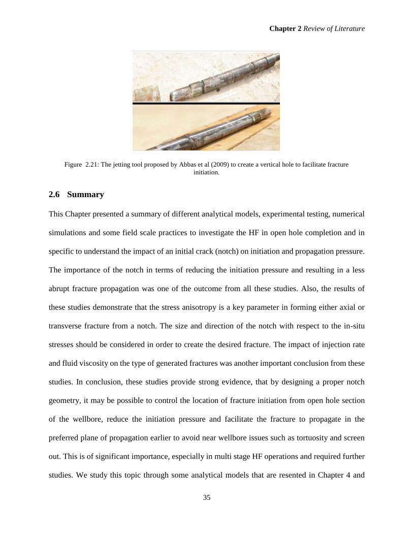
Chapter 2 Review of Literature
35
Figure 2.21: The jetting tool proposed by Abbas et al (2009) to create a vertical hole to facilitate fracture
initiation.
2.6 Summary
This Chapter presented a summary of different analytical models, experimental testing, numerical
simulations and some field scale practices to investigate the HF in open hole completion and in
specific to understand the impact of an initial crack (notch) on initiation and propagation pressure.
The importance of the notch in terms of reducing the initiation pressure and resulting in a less
abrupt fracture propagation was one of the outcome from all these studies. Also, the results of
these studies demonstrate that the stress anisotropy is a key parameter in forming either axial or
transverse fracture from a notch. The size and direction of the notch with respect to the in-situ
stresses should be considered in order to create the desired fracture. The impact of injection rate
and fluid viscosity on the type of generated fractures was another important conclusion from these
studies. In conclusion, these studies provide strong evidence, that by designing a proper notch
geometry, it may be possible to control the location of fracture initiation from open hole section
of the wellbore, reduce the initiation pressure and facilitate the fracture to propagate in the
preferred plane of propagation earlier to avoid near wellbore issues such as tortuosity and screen
out. This is of significant importance, especially in multi stage HF operations and required further
studies. We study this topic through some analytical models that are resented in Chapter 4 and

Chapter 2 Review of Literature
36
numerical simulations in Chapter 5. In the next Chapter, a brief overview of the lattice numerical
simulation, which is the method we use in this study using the XSite software will be presented.

Chapter 3 Lattice Formulation & XSite Software
37
CHAPTER 3
Lattice Formulation and XSite Software
3.1 Introduction
In this Chapter, first a brief overview of the lattice simulation, which is a type of discrete element
method (DEM) is presented. XSite software, developed by Itasca group works based on lattice for
hydraulic fracturing (HF) simulations. An overview of the XSite software and its feature will be
presented in the second part of this Chapter with some examples to of open-hole (OH) completion
HF simulations, which will be developed in further details in Chapter 5 as the main topic of this
research study. For detailed review of lattice formulation and XSite software features, the readers
can refer to the XSite description of formulation (2011), and HF Simulator User Guide (2013). A
brief summary from these references are presented in this Chapter.
3.2 Lattice Formulation
The numerical simulation program of XSite is based on the Synthetic Rock Mass (SRM) and
Lattice methods. The SRM is a simulation technique that was developed based on the distinct
element method (DEM), the SRM is accounted to be more efficient than DEM, it is used to
describe the mechanical behavior of a rock mass in three dimensions, this approach is used to
represent the rock mass characteristic by using the bonded-particle model (BPM), which include

Chapter 3 Lattice Formulation & XSite Software
38
an assembly of circular or spherical particles bonded to each other. Therefore, the BPM offers a
great solution for the simulation of hydraulic fracturing (Damjanac and Cundall, 2016) and gives
a good approximation of mechanical behavior of a brittle rock (Potyondy and Cundall, 2004).
Lattice simulation, which is grain-based numerical model, is a simplification of the BPM in
which the finite-sized particles and contacts are replaced by nodes and springs as shown in Figure
3.1. The lattice is a modified version of the smooth joint model (SJM) which is a group of
circular/spherical particles. The lattice simulation model is computationally more efficient than
SJM, the simulated three dimensional model is represented by a random number of discrete mass
(nodes) connected by springs.
Figure 3.1: Schematic model of a lattice array. Nodes and springs (Cundall, 2011)
3.2.1 Mechanical Model
The lattice is a group of nodes connected by a non-linear spring, it applies random distribution of
lattices and springs with microscale mechanical properties. The lattice uses the same concept of
PFC (Particle Flow Code) PFC3D, a simplification of the DEM (Discrete Element Model) which
is considered as a discontinuum method. The XSite software, which uses the lattice formulation,
is based on a time step algorithm, and treat rock as an assembly of bonded particles that follow a
combination of a force displacement law and law of motion during the calculation. The numerical

Chapter 3 Lattice Formulation & XSite Software
39
formulation of the code is provided by Damjanac et al (2011). The computational model is an
explicit numerical method, and the formulations are based on dependent variable. The codes follow
a non-linear behavior, efficient to model some features such as fracture, slip and joints. The
injected fluid can follow either a Newtonian law or a power law and can contain proppant
(characterized as grand particles with specific size and dimension) and the code allows a single
fluid and single phase.
a) Lattice Model
The law of lattice motion uses the central difference equations 3.1 and (3.2 below during the
simulation, to calculate the translational degrees of freedom. The Angular Velocity of nodes are
calculated using equation 3.3:
�̇�𝑖(𝑡+∆𝑡/2)
= �̇�𝑖(𝑡−∆𝑡/2)
+ Σ𝐹𝑖(𝑡)Δ𝑡/𝑚 (3.1)
�̇�𝑖(𝑡+Δ𝑡) = �̇�𝑖
(𝑡) + �̇�𝑖(𝑡+∆𝑡/2)
Δ𝑡 (3.2)
𝜔𝑖(𝑡+Δ𝑡/2)
= 𝜔𝑖(𝑡−Δ𝑡/2)
+ Σ𝑀𝑖
(𝑡)
𝐼Δ𝑡 (3.3)
In the above equations, �̇�𝑖(𝑡)
and 𝑢𝑖(𝑡)
are the velocity and position (respectively) of component i
(i =1,3) at time t, ∑𝐹𝑖 is the sum of all force-components i acting on the node of mass m, with time
step ∆𝑡.The angular velocities are represented by 𝜔𝑖 , of component i (i =1,3) at time t.
Then, the forces (normal and Shear) acting on springs are updated and calculated using
equations 3.4 and 3.5 where N and S are the normal Shear forces, respectively, taking into account
spring normal 𝑘𝑁 and shear stiffness 𝑘𝑠, the conditioning is set automatically if a force is larger
than the spring strength, then a micro crack is created (Damjanac et al, 2016)
𝐹𝑁 ⟵𝐹𝑁 +�̇�𝑖𝑁 𝑘𝑁Δ𝑡 (3.4)
𝐹𝑖𝑠 ⟵𝐹𝑖
𝑠 +�̇�𝑖𝑠 𝑘𝑠Δ𝑡 (3.5)
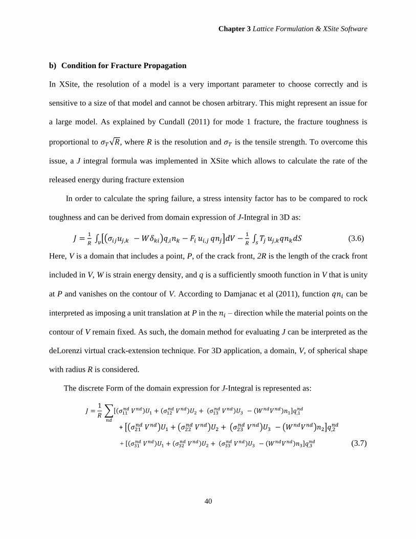
Chapter 3 Lattice Formulation & XSite Software
40
b) Condition for Fracture Propagation
In XSite, the resolution of a model is a very important parameter to choose correctly and is
sensitive to a size of that model and cannot be chosen arbitrary. This might represent an issue for
a large model. As explained by Cundall (2011) for mode 1 fracture, the fracture toughness is
proportional to 𝜎𝑇√𝑅, where R is the resolution and 𝜎𝑇 is the tensile strength. To overcome this
issue, a J integral formula was implemented in XSite which allows to calculate the rate of the
released energy during fracture extension
In order to calculate the spring failure, a stress intensity factor has to be compared to rock
toughness and can be derived from domain expression of J-Integral in 3D as:
𝐽 =1
𝑅∫ [(𝜎𝑖𝑗𝑢𝑗,𝑘 −𝑊𝛿𝑘𝑖)𝑞,𝑖𝑛𝑘 − 𝐹𝑖𝑢𝑖,𝑗𝑞𝑛𝑗]𝑑𝑉 −
1
𝑅∫ 𝑇𝑗𝑢𝑗,𝑘𝑞𝑛𝑘𝑑𝑆𝑠𝑣
(3.6)
Here, V is a domain that includes a point, P, of the crack front, 2R is the length of the crack front
included in V, W is strain energy density, and q is a sufficiently smooth function in V that is unity
at P and vanishes on the contour of V. According to Damjanac et al (2011), function 𝑞𝑛𝑖 can be
interpreted as imposing a unit translation at P in the 𝑛𝑖 – direction while the material points on the
contour of V remain fixed. As such, the domain method for evaluating J can be interpreted as the
deLorenzi virtual crack-extension technique. For 3D application, a domain, V, of spherical shape
with radius R is considered.
The discrete Form of the domain expression for J-Integral is represented as:
𝐽 =1
𝑅∑[(𝜎11
𝑛𝑑𝑉𝑛𝑑)𝑈1 + (𝜎12𝑛𝑑𝑉𝑛𝑑)𝑈2 +(𝜎13
𝑛𝑑𝑉𝑛𝑑)𝑈3 − (𝑊𝑛𝑑𝑉𝑛𝑑)𝑛1]𝑞,1𝑛𝑑
𝑛𝑑
+ [(𝜎21𝑛𝑑 𝑉𝑛𝑑)𝑈1 + (𝜎22
𝑛𝑑 𝑉𝑛𝑑)𝑈2 +(𝜎23𝑛𝑑 𝑉𝑛𝑑)𝑈3 − (𝑊𝑛𝑑𝑉𝑛𝑑)𝑛2]𝑞,2
𝑛𝑑
+ [(𝜎31𝑛𝑑𝑉𝑛𝑑)𝑈1 + (𝜎32
𝑛𝑑𝑉𝑛𝑑)𝑈2 +(𝜎33𝑛𝑑𝑉𝑛𝑑)𝑈3 − (𝑊𝑛𝑑𝑉𝑛𝑑)𝑛3]𝑞,3
𝑛𝑑 (3.7)

Chapter 3 Lattice Formulation & XSite Software
41
where the summation is taken on lattice nodes with the centre included in the (spherical) domain
of integration, 𝑈𝑖𝑛𝑑 is the gradient of displacement component i in direction n, and 𝑉𝑛𝑑 is nominal
node volume.
The stress intensity factor is defined as:
𝐾𝑖 =√𝐽𝐸 (3.8)
In this equation, J is the J integral and E is the rock’s Young’s modulus. The following conditions
has to be taking into consideration when calculating the stress intensity factor (Damjanac & et al
2016), where 𝐾𝐼 is the local stress intensity factor and 𝐾𝐼𝐶 is the local fracture toughness.
• If 𝐾𝐼 ≪ 𝐾𝐼𝐶, Spring tensile strength is the criterion for fracture propagation.
• If 𝐾𝐼 is close to 𝐾𝐼𝐶, use 𝐾𝐼 ≥ 𝐾𝐼𝐶, the local fracture toughness will be the criteria.
3.2.2 Fluid Flow Model
The fluid flow motions in XSite are treated in different way. First, when the simulation starts in
the model input, the fluid is created in the joints, this is called “flow Joints.” Second, new fluid
nodes are generated, after the microcracks are created due to the springs breakage, known as
“Matrix Fluid.” It is important to note that the fluid circulates between the fractures (joints) and
the matrix.
a) Flow in Joints
The fluid flow in joints is simulated using the fluid elements (fluid nodes) as shown in Figure 3.2,
that are connected by pipes, those pipes can be located either in the centre of a broken spring or
pre-existing joints, representing a conduit to the fluid flow. The pressure of the fluid is found
within the fluid element. The flow rate between nodes through the pipe is calculated using the
blurbification theory below (Qiu et al. 2019):

Chapter 3 Lattice Formulation & XSite Software
42
𝑞 = 𝛽𝑘𝑟𝑎3
12𝜇[𝑝𝐴 −𝑝𝐵 +𝜌𝑤𝑔(𝑧
𝐴 −𝑧𝐵] (3.9)
In this equation, a is the hydraulic aperture, 𝜇is viscosity of the fluid, and 𝑝𝐴 and 𝑝𝐵 fluid pressures
at nodes “A” and “B”, respectively. 𝑧𝐴 and 𝑧𝐴 are elevations of nodes “A” and “B”, 𝜌𝑤 is fluid
density, and 𝑔 is the acceleration due to gravity. 𝑘𝑟 is the relative permeability, which is a function
of saturation, and becomes 1 when the pipe is saturated. β is a dimensionless calibrated parameter.
Figure 3.2: Correlation between the 3D particle model and corresponding pipe network (Damjanac, Detournay,
and Cundall 2016)
The pressure increment delta P increases and it is solved as below:
Δ𝑃 =𝑄
𝑉𝐾𝑓Δ𝑡𝑓 (3.10)
Here, Q is the sum of flow rate from the pipes connected to the fluid element, V is the volume of
the fluid element, 𝐾𝑓 is the apparent fluid element bulk modulus, and ∆𝑡𝑓 is the flow time step
(Damjanac et al, 2016).
b) Matrix Flow
The matrix flow which is the permeability in the model is in fact the leak-off into the intact rock.
There are different variables to be considered in the matrix flow. The locations of these variables
are shown in Figure 3.4. The blue circles represent lattice nodes, the red dots which represent the
pressures are located in the centre of the springs.

Chapter 3 Lattice Formulation & XSite Software
43
Figure 3.3: Location of variables in the matrix flow scheme (Damjanac et all 2011)
Scanning effect takes place for quality check of the calculated pressure taking into
consideration the flow rate, conductivity and node pressures using the lattice data structure. �̅�
represents the pressure at each node is calculated as (𝜂𝑖 is the conductivity):
�̅�= ∑ 𝜂𝑃(𝑖)𝑖=1,𝑁
/ ∑ 𝜂𝑖𝑖=1,𝑁 (3.11)
3.2.3 Hydro-Mechanical Coupling
The mechanical process and fluid flow are essential in HF. The coupling fluid mechanical for
fracture propagation is implemented in XSite using the codes that were suggested by Peter Cundall.
It is more efficient than the one actually run in the software as it allows faster computational time.
Two aspects are now contributing in the simulation, the rock compressibility and a stable time
step. In fact, the longer fluid time steps is now permitted as the apparent fluid bulk modulus is very
small comparing to fluid bulk modulus considered as “relaxation parameter’ of the model. The
fluid bulk modulus property is related to the compressibility of the Hydraulic fluid and the stiffness
of the lattice model. Another parameter that is crucial in the simulation process is the permeability
of the fracture. In XSite this parameter is based upon the initial fracture aperture and deformation
of the model (computed from the fluid pressure). The fluid pressure impacts the strength of the

Chapter 3 Lattice Formulation & XSite Software
44
model and the deformation of the model that impact the fluid pressures that can be determined
even with undrained state.
3.3 Building a HF Model in XSite
In this section the steps to build and run a HF model in XSite software are presented. For the details
of XSite software the reader should refer to the HF Simulator User Guide (2013), as here the main
features of the software related to the simulations of this research are reviewed.
3.3.1 Rock and Fluid Properties, and In-Situ Stresses
XSite allows constructing a rectangular prism as the initial model of the rock. The length, height
and width can be determined by the user, and these can be all equal. A reference point is defined,
from which all future measurements are done. Detailed rock and fluid properties can be entered
manually by the user. Figures 3.5 and 3.6 show an example of the rock and fluid properties menu,
respectively. The data in these two Tables correspond to the Bakken formation in North Dakota,
Williston Basin. Both metric and imperial units can be selected. As it is seen from the right panel
of Figure 3.5, the software considers anisotropic rock properties, in particular for shale formations.
Rock anisotropy has not been considered in this study. Fracture toughness and fluid viscosity are
the two important rock and fluid properties with respect to the HF simulations. In Bakken these
values considered as 2 MPa.m0.5 and 0.002 pa.s (2cp), respectively.
The in-situ stresses are applied as three principal stress components of vertical, minimum and
maximum horizontal stresses (𝜎𝑣,𝜎ℎ ,𝜎𝐻). The orientation of these stresses can be defined in such
a way to mimic normal (𝜎𝑣>𝜎𝐻>𝜎ℎ), strike-slip (𝜎𝐻>𝜎𝑣>𝜎ℎ) and reverse/thrust fault (𝜎𝐻>𝜎ℎ>𝜎𝑣)
stress regimes. Figure 3.7 shows the panel where the magnitude and directions of the three
principal in-situ stresses can be entered. As it is seen at the bottom of Figure 3.7, the only boundary

Chapter 3 Lattice Formulation & XSite Software
45
condition that is considered in XSite is fixed or roller boundaries. For smaller models where large
deformation reaches the boundaries, it can cause a significant change in in-situ stresses at the
boundaries and a stress based boundary condition may be more appropriate. This is not
automatically observed and applied in the XSite. A numerical trick that has been proposed and
also used in this study is the implementation of the Soft boundaries. The Soft boundaries are soft
material (e.g. 10 to 100 times lower stiffness than the rock Young’s modulus) that are built all
around the model to simulate stress based boundary. This material absorbs the deformation while
maintaining relatively constant stress.
Figure 3.8 shows an example of sketch model in XSite representing a 1.5m×2.5m×2.5m rock
block including 0.125m soft boundary (100 times less Young’s modulus than that of the formation)
placed around all 6 faces.
Figure 3.4: An example of XSite Material Properties window. Input data corresponds to Bakken formation.

Chapter 3 Lattice Formulation & XSite Software
46
Figure 3.5: An example of XSite Fluid Properties window. Input data corresponds to Bakken formation.
Figure 3.6: An example of XSite in-situ stress window. Input data corresponds to Bakken formation.
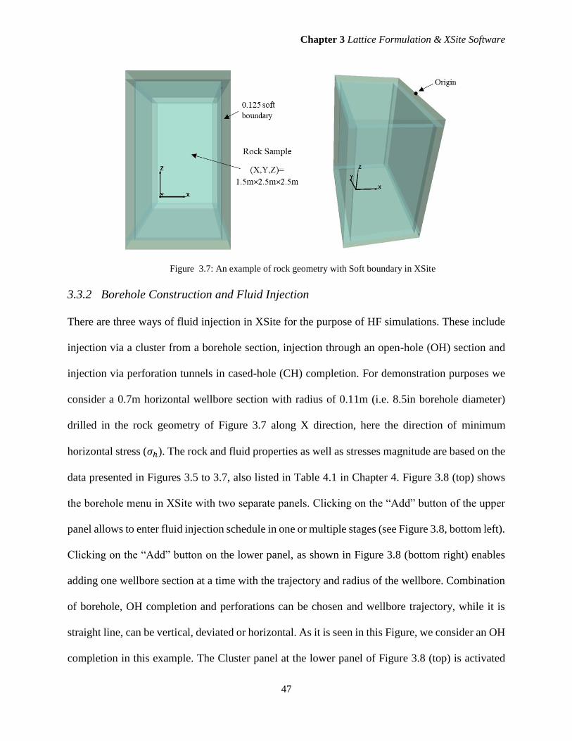
Chapter 3 Lattice Formulation & XSite Software
47
Figure 3.7: An example of rock geometry with Soft boundary in XSite
3.3.2 Borehole Construction and Fluid Injection
There are three ways of fluid injection in XSite for the purpose of HF simulations. These include
injection via a cluster from a borehole section, injection through an open-hole (OH) section and
injection via perforation tunnels in cased-hole (CH) completion. For demonstration purposes we
consider a 0.7m horizontal wellbore section with radius of 0.11m (i.e. 8.5in borehole diameter)
drilled in the rock geometry of Figure 3.7 along X direction, here the direction of minimum
horizontal stress (𝜎ℎ). The rock and fluid properties as well as stresses magnitude are based on the
data presented in Figures 3.5 to 3.7, also listed in Table 4.1 in Chapter 4. Figure 3.8 (top) shows
the borehole menu in XSite with two separate panels. Clicking on the “Add” button of the upper
panel allows to enter fluid injection schedule in one or multiple stages (see Figure 3.8, bottom left).
Clicking on the “Add” button on the lower panel, as shown in Figure 3.8 (bottom right) enables
adding one wellbore section at a time with the trajectory and radius of the wellbore. Combination
of borehole, OH completion and perforations can be chosen and wellbore trajectory, while it is
straight line, can be vertical, deviated or horizontal. As it is seen in this Figure, we consider an OH
completion in this example. The Cluster panel at the lower panel of Figure 3.8 (top) is activated

Chapter 3 Lattice Formulation & XSite Software
48
when borehole type is selected. It is important that that each stage of fluid injection is correctly
assigned to the corresponding segment so the software recognizes where the fluid injection should
start from.
Figure 3.8: Borehole panel in XSite (top) to enter fluid pumping (low left) andborehole trajectory and geometry
and radius (bottom right). The OH completion is chosen in this example with cluster section being inactivated

Chapter 3 Lattice Formulation & XSite Software
49
Figure 3.9: Different options for fluid injection in XSite, via a borehole and cluster (left), perforations (middle)
and OH completion (right).
Figure 3.9 shows schematically the three options for the fluid injection in XSite. In case of
injection through the cluster, a spherical (more common) or cylindrical shape cluster is placed at
the point where the injection is intended to begin from the borehole (see Figure 3.9, left). The
size of the cluster is slightly larger than the wellbore radius (here, cluster radius was chosen as
0.15m). The cluster is the point of the fluid injection. In order to facilitate the fracture to initiate,
a very weak starter crack (either rectangular or circular shape) is placed in the middle of the
cluster oriented along the preferred plane of propagation, i.e. perpendicular to 𝜎ℎ. The size of the
starter crack is slightly larger than the cluster diameter (here we used a circular fracture with
radius of 0.3m) with a very small opening (aperture) of in the order of 1×10⁻⁵m. Figure 3.10
shows the joint set panel in XSite where several parameters associated with the starter crack can
be defined by the user. The same panel is used to introduce any natural fracture planes in the
model with various orientation, stiffness, spacing, aperture mechanical properties (i.e. Tensile
strength, friction angle, cohesion and dilation angle). The use of the cluster injection is more
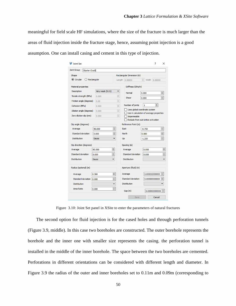
Chapter 3 Lattice Formulation & XSite Software
50
meaningful for field scale HF simulations, where the size of the fracture is much larger than the
areas of fluid injection inside the fracture stage, hence, assuming point injection is a good
assumption. One can install casing and cement in this type of injection.
Figure 3.10: Joint Set panel in XSite to enter the parameters of natural fractures
The second option for fluid injection is for the cased holes and through perforation tunnels
(Figure 3.9, middle). In this case two boreholes are constructed. The outer borehole represents the
borehole and the inner one with smaller size represents the casing. the perforation tunnel is
installed in the middle of the inner borehole. The space between the two boreholes are cemented.
Perforations in different orientations can be considered with different length and diameter. In
Figure 3.9 the radius of the outer and inner boreholes set to 0.11m and 0.09m (corresponding to

Chapter 3 Lattice Formulation & XSite Software
51
an 8.5” wellbore with 7” casing). Two perforations are installed in the middle of the model in this
example with in the upper and lower side of the wellbore with diameter of 0.0254m (1 in) and a
length of 0.3m.
The third option for fluid injection in XSite is through the OH completion (see Figure 3.9,
right). In this case, instead of borehole, we choose the OH completion feature to install a wellbore
section. In this case, the fluid is injected through the entire OH section area once the fluid mode is
activated. Here, in order to facilitate the fracture initiation, we install an initial crack oriented along
the preferred fracture propagation direction, i.e. in this example, perpendicular to the direction of
𝜎ℎ. The size of this initial crack, also known as notch, will have a great impact on fracture initiation.
This is the main topic of this research which will be discussed in details in the next two Chapters.
Also, similar to the first case, we assume an aperture of 1×10⁻⁵m for this initial crack. The OH
completion is suitable for the cases where the near wellbore HF is simulated and the objective is
to study the fracture initiation and short propagation around the wellbore.
3.3.3 Resolution
The resolution of the model is perhaps the most important parameter in simulation. It is defined as
the average lattice node spacing. The smaller the lattice resolution, the more accurate the modelling
will be but at the expense of a larger processing time. The number of nodes across a given model
dimension should be considered before setting the resolution. For example, if approximately 50
nodes across a 500-m block are required, then the resolution should be set to 1000 cm. The model
run time is very sensitive function of the resolution, particularly if the uniform resolution is used
throughout the model. Roughly, the simulation time is inversely proportional to the resolution
power of five. This sensitivity can be reduced if variable resolution

Chapter 3 Lattice Formulation & XSite Software
52
As stated in the HF Simulator User Guide (2013) “The apparent fracture toughness of the
lattice will be a function of the spring tensile strength (calibrated to the macroscopic strength of
the material) and the current resolution. Thus, if the spring tensile strength is calibrated to
macroscopic tensile strength of the material, the fracture toughness can be matched by adjusting
the resolution. For relatively small resolutions (of the order of 1 cm or smaller), the lattice
toughness will be of the order of 1 MPa×m0.5, which is typical or rocks. However, if the resolutions
are greater (e.g., of the order of 1 m or greater, as usually necessary for simulation of the problems
on the time and length scales of interest for field operations), the default lattice setup will
overestimate the realistic rock toughness and will not match the specified fracture toughness. The
fracture toughness will be matched if Store Spring Forces is checked (in Reset Lattice menu) after
initialization of stresses (forces) in the model.”
In general, the resolution for the domain next to an OH section should be 10 times less than
the borehole diameter. For cluster injection, as the near wellbore fracture analysis is not the main
focus and fracture propagation at large scale is taken into consideration, the resolution is compared
with respect to the model size. As a rule of thumb, for a 1m model size we need to consider at least
50 nodes, i.e. 2cm resolution. For more accurate results, the resolution of 1cm may be considered,
while it increases the running time exponentially larger.
a) Domain Resolution
In order to optimize the discretization, one may use different resolutions at different locations of
the model. Usually, finer resolutions are used closer to the injection point or important features in
the model and coarser resolutions towards the boundaries. Rectangular, cylindrical and triangular
resolution domain geometries are available in XSite. We will use domain resolution in Chapter 5
for OH HF simulations.

Chapter 3 Lattice Formulation & XSite Software
53
In this study, for the case of transverse fracture we consider three resolution domains as shown
in Figure 3.11. The cylindrical domain around the axis of the wellbore has length of L=2m and
diameter of D=0.20m with a resolution of 2.2cm. This will ensure that growth of any axial fracture,
if it occurs due to the small notch size, will be propagated in a high resolution zone. The second
cylindrical domain with length of L=0.85m and diameter of D=0.25m is in perpendicular to the
wellbore axis, along the direction that the fracture is expected to propagate. This domain has a
high resolution of 2.2cm. The third cylindrical domain with length of L=0.88m and diameter of
D=2.15m has a resolution of 4.4cm and the remaining of the model was assigned a resolution of
8.8cm using the resolution feature under the “Solution” Tab. The transition from one to the second
domain has a ratio of 2 for resolution to ensure the stability of the model and accuracy of the
results.
For conveniences, throughout this research study, we refer to the scaled length of the notch
as = Ln /a. Here Ln is the length of the notch, that for a circular transverse fracture is equivalent
to its radius and a is the wellbore radius (see Figure 3.11).
Figure 3.11: Resolution domains for a transverse fracture model
1st domain,
Resolution of
2.2cm
2nd domain,
Resolution of
2.2cm
3rd domain,
Resolution of
4.4cm
The resolution for
rest of the model
is 8.8cm
Transverse Notch
scaled Length: =Ln/a
Ln 2a
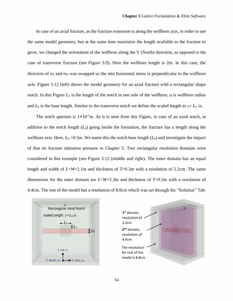
Chapter 3 Lattice Formulation & XSite Software
54
In case of an axial fracture, as the fracture extension is along the wellbore axis, in order to use
the same model geometry, but at the same time maximize the length available to the fracture to
grow, we changed the orientation of the wellbore along the Y (North) direction, as opposed to the
case of transverse fracture (see Figure 3.9). Here the wellbore length is 2m. In this case, the
direction of h and H was swapped so the min horizontal stress is perpendicular to the wellbore
axis. Figure 3.12 (left) shows the model geometry for an axial fracture with a rectangular shape
notch. In this Figure Ln is the length of the notch in one side of the wellbore, a is wellbore radius
and Lb is the base length. Similar to the transverse notch we define the scaled length as = Ln /a.
The notch aperture is 1×10⁻⁵m. As it is seen from this Figure, in case of an axial notch, in
addition to the notch length (Ln) going inside the formation, the fracture has a length along the
wellbore axis. Here, Lb =0.5m. We name this the notch base length (Lb) and investigate the impact
of that on fracture initiation pressure in Chapter 5. Two rectangular resolution domains were
considered in this example (see Figure 3.12 (middle and right). The inner domain has an equal
length and width of L=W=2.1m and thickness of T=0.3m with a resolution of 2.2cm. The same
dimensions for the outer domain are L=W=2.3m and thickness of T=0.5m with a resolution of
4.4cm. The rest of the model has a resolution of 8.8cm which was set through the “Solution” Tab.
1st domain,
resolution of
2.2cm
2nd domain,
resolution of
4.4cm
The resolution
for rest of the
model is 8.8cm
Rectangular Axial Notch
Lb Ln
Z, Up, v
X, East, H Y, North, h
2a
scaled Length: =Ln/a
Chapter 3 Lattice Formulation & XSite Software
55
Figure 3.12: Model geometry of an axial notch and fracture (left) and the resolution domains
b) Nested Resolution
This feature can be used to optimize model discretization by building a graded resolution transition
from the finest resolution (typically in a domain that includes the injection points in the center of
the model) to the coarser resolutions towards the model boundaries. User should avoid sudden
jumps in resolution (e.g., the ratio of resolutions between the adjacent domains greater than two)
Nesting resolution can be applied only to rectangular closed-volume domains.
3.3.4 Solution
In order to run a HF model in XSite, usually, three main steps are to be taken. Firstly, the borehole
is excavated. During this step, the model is not subjected to either mechanical (i.e. effect of in-situ
stresses) or fluid flow (injection of fracturing fluid). This is followed by the equilibrium step,
where the in-situ stresses are applied to the model. This step needs to continue until the entire
model reaches the equilibrium. This may be checked by looking at the contours of the velocity:
the model usually reaches equilibrium when the velocity vectors go below 1×10⁻⁶m/s. the final
stage is the hydromechanical phase, where, under the effect of in-situ stresses the fluid pumping
starts. The Batch simulation panel (see an example of it in Figure 3.13) is used to set up the three
solution steps and then execute the model. The panel shows the time corresponding to each step
and the bottom section of the panel in Figure 3.13 reports a summary of the model status and any
possible errors.

Chapter 3 Lattice Formulation & XSite Software
56
Figure 3.13: Batch Simulation panel in XSite to set up the three main stages and execute the model
3.4 Simulation Examples
To demonstrate some applications of the XSite for HF simulations, here a few examples are
presented.
3.4.1 Injection Rate Effect on Fracture Pressures
For demonstration purposes, using the data corresponding to the Bakken formation (see Table 4.1,
Chapter 4) and model geometry of Figure 3.11, we performed HF simulations in OH completion.
To investigate the effect of injection rate change of fracture pressures, a transverse notch
model with length of Ln=0.066m, or scaled length of =0.066/0.11= 0.6 considered for simulation
purposes. Detailed simulations will be presented in Chapter 5. Figure 3.14 shows the fracture
apertures corresponding to injection rates of Q=0.06m3/sec (top) and 0.08m3/sec. Figure 3.15
presents the plot of fracture pressure and crack numbers versus time.
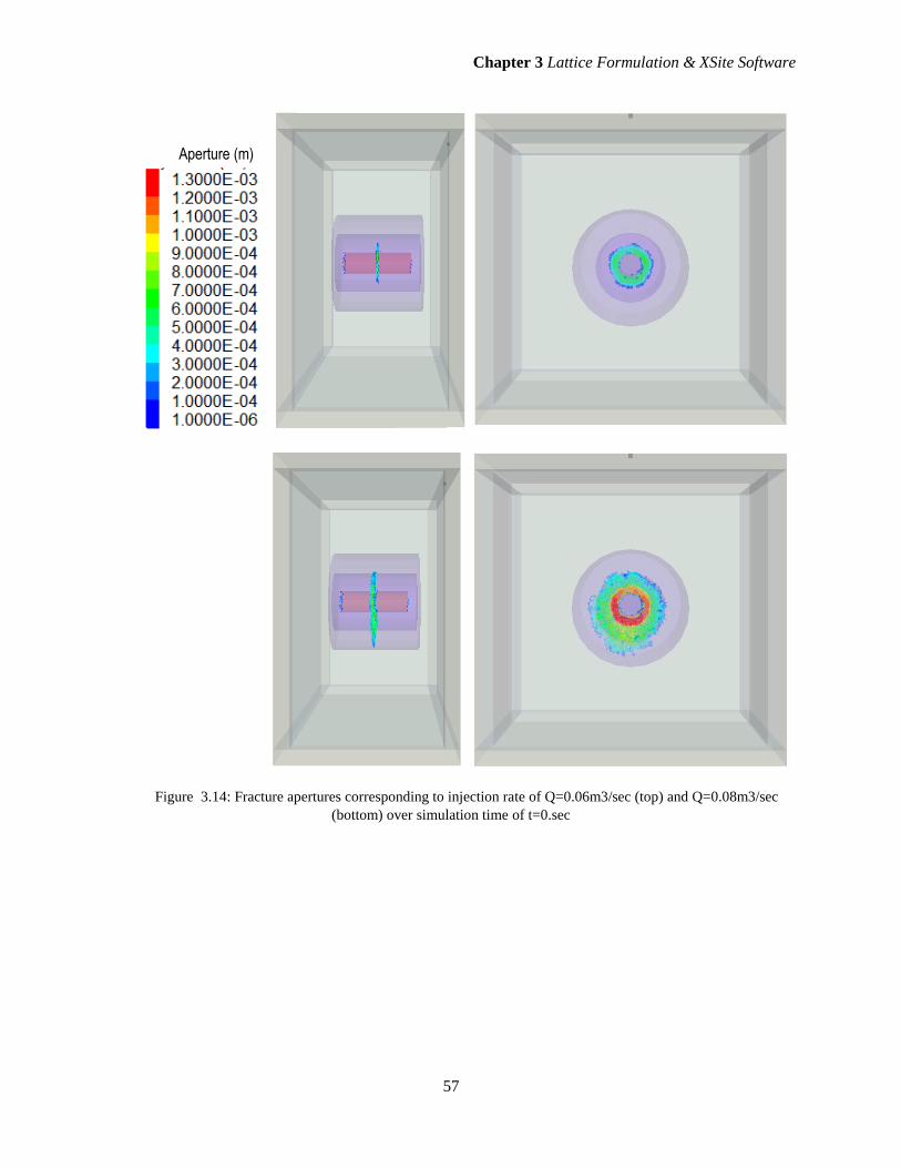
Chapter 3 Lattice Formulation & XSite Software
57
Figure 3.14: Fracture apertures corresponding to injection rate of Q=0.06m3/sec (top) and Q=0.08m3/sec
(bottom) over simulation time of t=0.sec
Aperture (m)
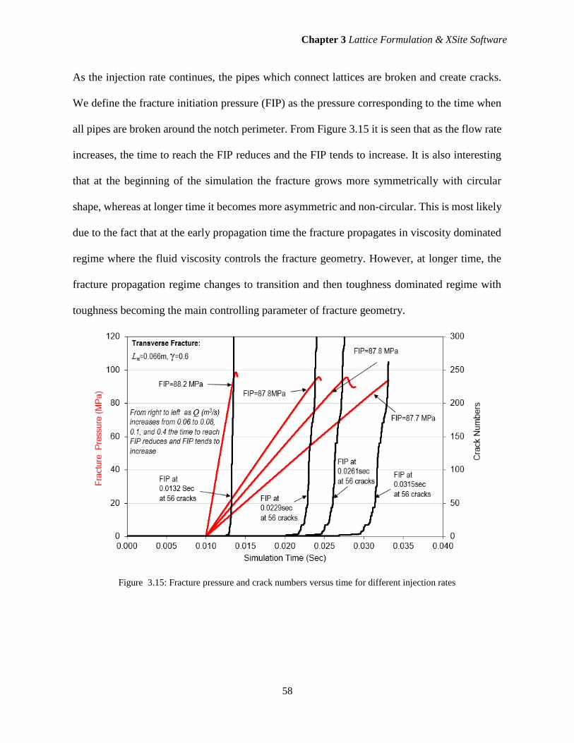
Chapter 3 Lattice Formulation & XSite Software
58
As the injection rate continues, the pipes which connect lattices are broken and create cracks.
We define the fracture initiation pressure (FIP) as the pressure corresponding to the time when
all pipes are broken around the notch perimeter. From Figure 3.15 it is seen that as the flow rate
increases, the time to reach the FIP reduces and the FIP tends to increase. It is also interesting
that at the beginning of the simulation the fracture grows more symmetrically with circular
shape, whereas at longer time it becomes more asymmetric and non-circular. This is most likely
due to the fact that at the early propagation time the fracture propagates in viscosity dominated
regime where the fluid viscosity controls the fracture geometry. However, at longer time, the
fracture propagation regime changes to transition and then toughness dominated regime with
toughness becoming the main controlling parameter of fracture geometry.
Figure 3.15: Fracture pressure and crack numbers versus time for different injection rates
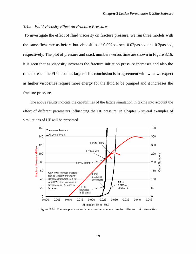
Chapter 3 Lattice Formulation & XSite Software
59
3.4.2 Fluid viscosity Effect on Fracture Pressures
To investigate the effect of fluid viscosity on fracture pressure, we run three models with
the same flow rate as before but viscosities of 0.002pas.sec, 0.02pas.sec and 0.2pas.sec,
respectively. The plot of pressure and crack numbers versus time are shown in Figure 3.16.
it is seen that as viscosity increases the fracture initiation pressure increases and also the
time to reach the FIP becomes larger. This conclusion is in agreement with what we expect
as higher viscosities require more energy for the fluid to be pumped and it increases the
fracture pressure.
The above results indicate the capabilities of the lattice simulation in taking into account the
effect of different parameters influencing the HF pressure. In Chapter 5 several examples of
simulations of HF will be presented.
Figure 3.16: Fracture pressure and crack numbers versus time for different fluid viscosities
Chapter 3 Lattice Formulation & XSite Software
60
3.5 Summary
A summary of formulations used in lattice numerical simulation were presented in this Chapter.
Also, the features of the XSite software which uses this particle based simulation were introduced.
The capabilities of lattice simulation in coupling the fluid and stress in hydraulic fracturing
modelling makes it unique for applications if this study and this is presented in detail in Chapter
5.

Chapter 4 Analytical Models
61
CHAPTER 4
Analytical Models
4.1 Introduction
As mentioned in the previous Chapters, OH hydraulic fracturing offers several advantages over
CH completion. The challenge, however, is that the fracture initiation and propagation in long OH
sections are dominantly controlled by the existing natural fractures around the wellbore. Therefore,
in real applications, the mechanics of hydraulic fracturing is considered as propagation of an
existing crack with a given geometry and direction from the wellbore wall.
In this Chapter, firstly a brief review of the classical Kirsch models to estimate the fracture
pressure around a circular borehole will be given. This is based on the assumption of isotropic
elastic rock. Then, the theory of critical borehole pressure at unstable crack extension proposed by
Rummel (1987) will be presented which calculates the initiation pressure based on superposition
of the stress intensity functions associated with the stresses, wellbore pressure and the pressure
inside the crack. The analytical model presented by Charlez (1997) which integrates the effect of
pressurization rate on fracture initiation from a borehole with a bi-wing notch will be discussed.
This will be followed by the analytical model of Nilson and Proffer (1984) which includes the
competition between axial and transverse fracture initiation due to the notch geometry and the
shape of the cavity.

Chapter 4 Analytical Models
62
4.2 Stress Perturbation around a Wellbore
In Petroleum geomechanics, it is common to consider the vertical or overburden stress (v),
minimum horizontal stress (h) and maximum horizontal stress (H) as the three principal stresses,
which are also known as far field or in-situ stresses. The common industry approach to determine
the magnitude of these stresses is based on construction of the Mechanical Earth Model (MEM).
The vertical stress is simply an integration of the density times the thickness of different layers.
The density log is the main input to estimate the vertical stress profile. Knowing that the horizontal
stresses are functions of the vertical stress and the rock elastic properties (in simple isotropic
medium these are the Young’s modulus and Poisson’s ratio), the MEM workflow builds the
continuous logs of rock elastic and strength properties along the wellbore trajectory based on their
relationship with the physical properties of the formations which are obtained from petrophysical
logs. These input are used to build the profile of the horizontal stresses through the well know
poro-elastic equations. The details of the MEM workflow can be found from several literatures
(e.g. Rasouli et al 2011)
Due to drilling operation, the in-situ stresses around the wellbore are altered. Figure 4.1 shows
the drilling induced stresses in a cylindrical coordinate system at a point with distance r from the
wellbore center and angle 𝜑 with respect to the maximum far field horizontal stress (H). The
induced stresses are the vertical stresses (zz), radial stresses (rr), tangential or hoop stresses ()
and the shear stresses (r). Figure 4.1 shows cross section of a vertical wellbore with vertical
stress being perpendicular to the plane.
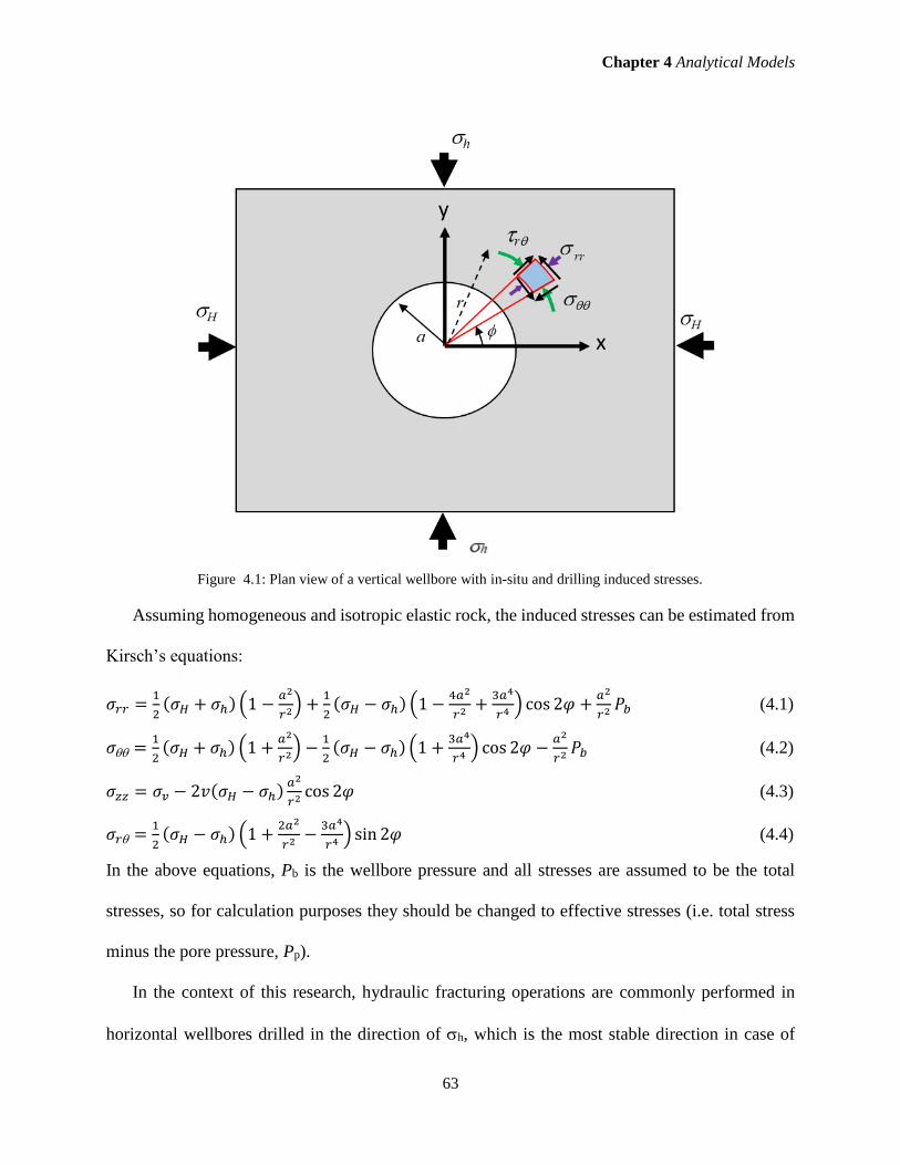
Chapter 4 Analytical Models
63
Figure 4.1: Plan view of a vertical wellbore with in-situ and drilling induced stresses.
Assuming homogeneous and isotropic elastic rock, the induced stresses can be estimated from
Kirsch’s equations:
𝜎𝑟𝑟 =1
2(𝜎𝐻 + 𝜎ℎ) (1 −
𝑎2
𝑟2) +
1
2(𝜎𝐻 − 𝜎ℎ) (1 −
4𝑎2
𝑟2+
3𝑎4
𝑟4) cos 2𝜑 +
𝑎2
𝑟2𝑃𝑏 (4.1)
𝜎 =1
2(𝜎𝐻 + 𝜎ℎ) (1 +
𝑎2
𝑟2) −
1
2(𝜎𝐻 − 𝜎ℎ) (1 +
3𝑎4
𝑟4) cos 2𝜑 −
𝑎2
𝑟2𝑃𝑏 (4.2)
𝜎𝑧𝑧 = 𝜎𝑣 − 2𝑣(𝜎𝐻 − 𝜎ℎ)𝑎2
𝑟2cos 2𝜑 (4.3)
𝜎𝑟 =1
2(𝜎𝐻 − 𝜎ℎ) (1 +
2𝑎2
𝑟2−
3𝑎4
𝑟4) sin 2𝜑 (4.4)
In the above equations, Pb is the wellbore pressure and all stresses are assumed to be the total
stresses, so for calculation purposes they should be changed to effective stresses (i.e. total stress
minus the pore pressure, Pp).
In the context of this research, hydraulic fracturing operations are commonly performed in
horizontal wellbores drilled in the direction of h, which is the most stable direction in case of

Chapter 4 Analytical Models
64
normal (v>H>h) or strike-slip stress regime (H>v>h). In this case, as shown in Figure 4.2,
the two far field stresses acting on the wellbore wall are v and H. In case of normal stress regime,
if axial (longitudinal) fractures develop around the wellbore, it will be along v direction
(perpendicular to the least tangential stress, , i.e. on the top and bottom of the wellbore, along
z direction), as depicted in Figure 4.3. In this Figure, �̅� is the average pressure inside the crack. In
this case, the drilling induced stresses around the wellbore are obtained from the Kirsch’s equations
by replacing vh,H = v and h=H in equations 4.1 to 4.4, for the case of normal stress regime
which results in:
𝜎𝑟𝑟 =1
2(𝜎𝑣 + 𝜎𝐻) (1 −
𝑎2
𝑟2) +
1
2(𝜎𝑣 − 𝜎𝐻) (1 −
4𝑎2
𝑟2+
3𝑎4
𝑟4) cos 2𝜑 +
𝑎2
𝑟2𝑃𝑏 (4.5)
𝜎 =1
2(𝜎𝑣 + 𝜎𝐻) (1 +
𝑎2
𝑟2) −
1
2(𝜎𝑣 − 𝜎𝐻) (1 +
3𝑎4
𝑟4) cos 2𝜑 −
𝑎2
𝑟2𝑃𝑏 (4.6)
𝜎𝑦𝑦 = 𝜎ℎ − 2𝑣(𝜎𝑣 − 𝜎𝐻)𝑎2
𝑟2cos 2𝜑 (4.7)
𝜎𝑟 =1
2(𝜎𝑣 − 𝜎𝐻) (1 +
2𝑎2
𝑟2−
3𝑎4
𝑟4) sin 2𝜑 (4.8)
Similarly, in case of strike-slip stress regime, if axial (longitudinal) fractures develop around
the wellbore, it will be along H direction (perpendicular to the least tangential stress, 𝜎, i.e. on
the sides of the wellbore along x direction), as shown in Figure 4.3.
In both cases of normal and strike-slip stress regimes, the transverse fractures develop
orthogonal to the wellbore axis, perpendicular to the y direction or against yy. The conditions
where either transverse or axial fractures are more favorable to initiate and propagate from the
wellbore wall will be discussed later in this Chapter.

Chapter 4 Analytical Models
65
Figure 4.2: Plan view of a horizontal wellbore drilled parallel to h direction with in-situ and drilling induced
stresses.
Figure 4.3: Axial (left) and transverse fractures (right) around a horizontal wellbore.
Figure 4.4 shows the plot of the vertical, radial and tangential stresses as a function of the
distance from the wellbore wall. The input data are taken from Table 4.1 which corresponds to
typical parameters of Bakken Shale formation in North Dakota, USA. We use this data throughout

Chapter 4 Analytical Models
66
this thesis for consistency purposes. From Table 4.1, it is seen that the magnitude of the stress
anisotropy (i.e. H-h) is not significant, so in some examples in this Chapter we also use larger
stress anisotropy to demonstrate the initiation pressure changes due to a large stress anisotropy.
Table 4.1: Bakken Shale Formation mechanical properties and in-situ stresses
Property Unit Value
Density Kg/m^3 2650
Young’s Modulus E GPa 30
Mpsi 4.3511
Uniaxial Compressive Strength UCS MPa 50
psi 7,251
Tensile Strength To MPa 5
psi 725
Toughness KIC
Mpa.m^0.5 2.0
psi.in^0.5 1820.1
Friction Angle degree 30
Poisson’s ratio v - 0.25
Porosity ∅ % 2
Permeability K Darcy 0.1
Minimum Horizontal Stress h MPa 54.8
psi 7950
Maximum Horizontal Stress H MPa 61.6
psi 8,930
Vertical Stress v MPa 68.4
psi 9,920
Pore Pressure Pp MPa 30
psi 4,350
Wellbore Pressure PbMPa 30
psi 4,350
Fluid Viscosity Pa.s 0.002
Flow Rate Q m3/s 0.08
bbl/m 30
Borehole Radius a inch 4.375
m 0.11

Chapter 4 Analytical Models
67
Figure 4.4 (left) shows the stresses corresponding to 𝜑=0° or along the direction of v
(remember that 𝜑 is the angle from maximum stress direction, which in this case is v), whereas
Figure 4.4 (right) represents the stresses corresponding to 𝜑 =90°, or along H direction.
From Figure 4.4, it is seen that the radial stress is minimum at the wellbore wall and is
equivalent in all different directions around the wellbore but increases as moving away from the
wellbore wall. It ultimately reaches the value of v along 𝜑=0° and H along 𝜑=90° at far distance
from the wellbore, i.e. getting back to the far field stresses. This distance, appears to be
approximately 4 times the radius of the wellbore. On the other hand, the tangential stresses (𝜎𝜑𝜑)
are maximum at the wellbore wall but they are different in different directions. It is the largest at
𝜑=90° (parallel to v direction) and the least along 𝜑=0° (parallel to H
direction). The tangential
stresses reduce as moving further away from the wellbore wall and at far distance they reach H
and v along 𝜑=0° and 𝜑=90°, respectively.
It is interesting to note that based on this simplified model, the induced stresses are independent
of the wellbore radius, while, in real field cases, as the size of the wellbore is increased, due to the
higher potential for existence of the micro cracks and different type of defects around the wellbore
the rock becomes less strong and the induced stresses around the wellbore will be different.
Figure 4.4: Distribution of drilling induced stresses around a horizontal wellbore drilled along 𝝈𝒉 direction
based on Kirsch’s equations.
Chapter 4 Analytical Models
68
One interesting case to consider is the distribution of stresses around the wellbore, i.e. replacing
r=a in equations 4.5 to 4.8. In this case, the induced stresses around the wellbore wall will simplify
to the followings:
𝜎𝑟𝑟 = 𝑃𝑏 (4.9)
𝜎𝜃𝜃 = (𝜎𝑣 + 𝜎𝐻) − 2(𝜎𝑣 − 𝜎𝐻) cos 2𝜑 − 𝑃𝑏 (4.10)
𝜎𝑦𝑦 = 𝜎ℎ − 2𝑣(𝜎𝑣 − 𝜎𝐻) cos 2𝜑 (4.11)
𝜎𝑟𝜃 = 0 (4.12)
The above equations indicate that around the wellbore the radial stress is the wellbore pressure (or
mud pressure) and it is applying the same pressure in different directions. The shear stress is zero
but the tangential stress is direction dependent. For the two directions along v (i.e. 𝜑 = 0°) and
H (i.e. 𝜑 = 90° ), equation 4.10 will be simplified as:
𝜑 = 0° => 𝜎 = 3𝜎𝐻 − 𝜎𝑣 − 𝑃𝑏 (4.13)
𝜑 = 90° => 𝜎 = 3𝜎𝑣 − 𝜎𝐻 − 𝑃𝑏 (4.14)
Equations 4.13 and 4.14 imply that the maximum tangential compression stress around the
wellbore will occur along H direction whereas along the v direction, or in general, perpendicular
to the least stress direction, the wellbore wall is under the minimum amount of compressional
stress. From the point of view of this work, this means that the axial hydraulic fracture will initiate
perpendicular to the H direction, assuming adequate wellbore pressure is pumped.
Assuming 𝐾 =𝜎𝐻
𝜎𝑣, equation 4.10 can be rewritten as:
𝜎
𝜎𝑣= (1 + 𝐾) − 2(1 − 𝐾)cos 2𝜑 −
𝑃𝑏
𝜎𝑣 (4.15)
where,
𝜑 = 0° => 𝜎𝜃𝜃
𝜎𝑣= 3𝐾 − 1 −
𝑃𝑏
𝜎𝑣 (4.16)
𝜑 = 90° => 𝜎𝜃𝜃
𝜎𝑣= 3 − 𝐾 −
𝑃𝑏
𝜎𝑣 (4.17)

Chapter 4 Analytical Models
69
Figure 4.5 presents the plot of 𝜎𝜃𝜃
𝜎𝑣 versus K for two different directions of 𝜑 = 0° and 𝜑 =
90°, respectively. It is seen that when stresses are isotropic around the wellbore (K=1.0) tangential
stresses are as twice as v, in all directions. For K=0, corresponding to the maximum stress
anisotropy, the tangential stress is compressional and as big as three times the v at 𝜑 = 90°,
whereas it is tensional and equal to -v at 𝜑 = 0°. This Figure also shows that for K<0.33, the
tangential stresses become tensional along 𝜑 = 0°.
Figure 4.5: Variation of tangential stresses around the wellbore wall as a function of stress anisotropy.
To initiate hydraulic fracture, the fluid pressure inside the wellbore should overcome the
tangential stress along 𝜑 = 0° plus the tensile strength (T0) of the formation. The tensile strength
of the rocks is commonly considered as 10% of the Uniaxial Compressive Strength (UCS). The
fracture breakdown pressure, or critical borehole pressure is expressed as (Detournay and
Carbonell, 1997):
𝑃𝑐 = 3𝜎𝐻 − 𝜎𝑣 + 𝑇0 − 𝑃𝑝 (4.18)
The above equation is known as Hubbert-Willis (H-W) expression, which is applicable to
impermeable rocks. Later on, it will be discussed that this equation corresponds to the fast
pressurization into a wellbore with an infinitely small length crack edging from the wellbore wall.

Chapter 4 Analytical Models
70
In this situation the wellbore fluid cannot penetrate into the crack, hence its pressure will be
equivalent to the pore pressure.
Considering permeable rock, the above equation is modified as the Haimson-Fairhurst (H-F)
expression (Detournay and Carbonell, 1997):
𝑃𝑐 =3𝜎𝐻−𝜎𝑣+𝑇0−2𝜂𝑃𝑝
2(1−𝜂) (4.19)
In the above equation, 𝜂 is a poro-elastic constant varying between 0 and 0.5 and this constant
controls the stress induced by the pore fluids.
One paradox coming from equations 4.18 and 4.19 is that if we replace 𝜂 = 0 (i.e. ignoring
the fluid pressure effect in the pores, or considering a dry rock) in equation 4.19, it leads to:
𝑃𝑐 =1
2(3𝜎𝐻 − 𝜎𝑣 + 𝑇0), (4.20)
instead of converging to equation 4.18 for an impermeable rock. This means that the breakdown
pressure based on H-F criterion could be as low as half the H-W value. It will be discussed later
that this equation corresponds to slow pressurization into a wellbore with infinitely small crack
edging from the wellbore wall. In this case, the crack pressure is equal to wellbore pressure, hence
pore pressure does not have any contribution to the total critical pressure Pc.
Another discrepancy related to the above breakdown pressures is the fact that these pressures
correspond to the peak of pressure-time curve, however, based on the non-linearity that is observed
before the peak point, it appears that the fracture initiates before reaching to this peak point. So, it
is important to distinguish between fracture initiation and breakdown pressures (Detournay and
Carbonell, 1997).
In the next section, it will be discussed that in real field cases, there are always defects such
as natural fractures around the wellbore which act as the initiation point for hydraulic fracture, so

Chapter 4 Analytical Models
71
the initiation and propagation of an induced fracture should be considered based on the fracture
mechanics, which is different that the classic mechanics explained above for the hydraulic fracture.
The above information provides some insight into how the stresses are distributed around the
wellbore after drilling, however, in practice, cares should be taken when using these equations as
they are based on the assumption of isotropic and elastic rocks, which are not observed in real field
applications.
4.3 Axial Crack Edging from a Horizontal Wellbore
In this section the theoretical model proposed by Rummel (1987) based on the superposition of
the stress intensity factors of different parameters affecting the initiation pressure of a borehole
with a bi-wing axial crack is presented.
Figure 4.6 depicts the same circular borehole shown in Figure 4.2 with an addition of a crack
with half-length c on each side of the wellbore. The borehole is assumed to be in an infinite plate.
Normal stress regime is assumed. To simplify the problem, we assume that the crack is
perpendicular to H direction, i.e. along 𝜑 = 0°. This is perpendicular to the least resistant stress
direction and most favorable direction for the fracture to open comparing to all other directions.
The borehole is pressurized and the fluid can penetrate into the crack. In this section, we adopt the
approach presented by Rummel (1987) to estimate the critical borehole pressure at unstable crack
extension.

Chapter 4 Analytical Models
72
Figure 4.6: Fracture mechanics model for crack growth in a pressurized circular borehole.
The intensity of the stress field in the vicinity of the crack tips can be formulated based on the
principle of superposition of stress intensity factors (KI) from each loading source:
𝐾𝐼(𝜎𝑣, 𝜎𝐻, 𝑃𝑏 , �̅�) = 𝐾𝐼(𝜎𝑣) + 𝐾𝐼(𝜎𝐻) + 𝐾𝐼(𝑃𝑏) + 𝐾𝐼(�̅�) (4.21)
Rummel (1987) formulated the values of each of the above intensity factors as:
𝐾𝐼(𝜎𝑣) =-𝜎𝑣√𝑎𝑓(𝑏) (4.22)
𝐾𝐼(𝜎𝐻) =-𝜎𝐻√𝑎𝑔(𝑏) (4.23)
𝐾𝐼(𝑃𝑏) = 𝑃𝑏√𝑎ℎ𝑏(𝑏) (4.24)
𝐾𝐼(�̅�) = �̅�√𝑎ℎ𝑐(𝑏) (4.25)
where,
𝑏 = 1 +𝑐
𝑎 (4.26)
𝑓(𝑏) = −2√(𝑏2−1)
𝜋𝑏7 (4.27)

Chapter 4 Analytical Models
73
𝑔(𝑏) = √𝜋𝑏(1 −2
𝜋sin−1
1
𝑏) + 2(𝑏2 + 1)√
(𝑏2−1)
𝜋𝑏7 (4.28)
ℎ𝑏(𝑏) = 1.3𝑏−1
1+𝑏3 2⁄+ 7.8
[sin(𝑏−1) 2⁄ ]
2𝑏5 2⁄ −1.7 (4.29)
hc is defined based on the assumption of pressure distribution in the crack. For example, for
constant pressure inside the crack:
�̅�(𝑥) = �̅� (4.30)
ℎ𝑐1 = √𝜋𝑏(1 −2
𝜋sin−1
1
𝑏) (4.31)
Figure 4.7 shows the plot of functions f(b), g(b), hb, hc (for constant pressure case) versus b
(crack size normalized by borehole radius).
Figure 4.7: Functions f(b), g(b), hb, hc (for constant pressure case) versus b.
The critical borehole pressure at unstable crack extension is defined according to the
superposition of the stress intensity functions. This, considering the three intensity factors
associated with 𝜎𝑣, 𝜎𝐻and𝑃𝑏 will be expressed as:

Chapter 4 Analytical Models
74
𝑃𝑐 =1
ℎ𝑏+ℎ𝑐(𝐾𝐼𝐶
√𝑎+ 𝜎𝑣𝑓 + 𝜎𝐻𝑔) (4.32)
In the above equation, KIC is the rock’s fracture toughness for model I crack growth (opening
mode).
Comparing the first term in the above equation:
𝑃∞ =1
ℎ𝑏+ℎ𝑐(𝐾𝐼𝐶
√𝑎) (4.33)
with classical fracture mechanics equation 4.18, it suggests that 𝑃∞ represents the hydraulic
fracturing tensile strength of the rock measured under zero far field stresses. It is also known as
cohesive stress. It is evident that 𝑃∞ is a function of the wellbore size (a), i.e. it is scale dependent,
a property that is not captured in classical fracture mechanics.
In case of crack length becoming very short, b=1, f=0, g=0, hb=0, hc=0, hence to open the
crack at the borehole wall, the wellbore pressure must exceed the value of 𝑃∞, which in this case
tends to infinity (see equation 4.32). This indicates why opening a fracture in lab experimental set
up where the drilled borehole is free of any noticeable defects may not be possible without creating
a notch. Similarly, this also justifies the reason for development of axial (longitudinal) fractures in
horizontal wellbores when there are no effective natural fractures around the wellbore. This is the
core idea of this project, where cutting cracks (notches) around the open hole section of the
horizontal wellbores are proposed to act as the fracture initiation points. Design of the size and
geometry of these notches and the impact of injecting fluid characteristics on the effectiveness of
the notch will be discussed in details through numerical simulations with reference to the lab
experimental data in the next Chapter.
From equation 4.32 the fracture coefficients associated with 𝜎𝑣, 𝜎𝐻 and 𝑃𝑏=𝑃∞can be defined
as:

Chapter 4 Analytical Models
75
𝑘𝜎𝑣 =𝑓
ℎ𝑏+ℎ𝑐 𝑘𝜎𝐻 =
𝑔
ℎ𝑏+ℎ𝑐 𝑘∞ =
1
ℎ𝑏+ℎ𝑐 (4.34)
And the pressures corresponding to each of these loading source can be calculated as:
𝑃𝑐(𝜎𝑣) = 𝑘𝜎𝑣𝜎𝑣 𝑃𝑐(𝜎𝐻) = 𝑘𝜎𝐻𝜎𝐻 𝑃𝑐(∞) = 𝑘∞𝐾𝐼𝐶
√𝑎 (4.35)
Here, 𝐾𝐼𝐶 is the toughness of the formation.
The above coefficients determine the contribution of each of the far field stresses as well as the
cohesive force on hydraulic fracture breakdown pressure.
Using Bakken data from Table 4.1, the intensity factors and critical pressures corresponding
to different loading sources were calculated and the results are presented in Figure 4.8. It is to be
noted that these results correspond to 𝜑 = 0°, i.e. along v direction, which is the most favorable
direction for fracture initiation and propagation. From this Figure, it is observed that as the crack
size is increased the impact of the KI(v) is reduced while KI(H) is increased to some extent and
then reduces. In terms of critical pressures, it is seen that at very small crack size (i.e. b tends to
unity) v has the largest contribution, which is due to the fact that the crack is primarily under the
compression by this induced stress component. However, as the crack size becomes larger, the
effect of H becomes greater while v
presents less contribution to the total borehole pressure at
crack extension. It is also interesting to see that the borehole pressure Pb or 𝑃∞ presents a large
increase when the crack size reduces and tends to zero. This, in fact, indicates the large borehole
pressure required to open the wellbore wall in absence of any crack and indeed, the necessity for
cutting a notch in order to assist the fracture propagation in lab experiments. Therefore, as Figure
4.8 (bottom) shows, the total borehole pressure at unstable crack extension is extremely large in
absence of crack, however, it experiences a sharp drop as soon as the crack is introduced to the
wellbore wall and then increased to some extent before it plateaus. From Figure 4.8, unstable crack

Chapter 4 Analytical Models
76
growth (i.e. critical pressure reduces as crack length increases) is observed for crack lengths of
less than 10% of wellbore radius (i.e. c=0.1a or b=1.1). The critical pressure then increases but
reaches a plateau for crack lengths of larger than wellbore diameter (i.e. c=2a or b=3). While lower
critical pressures associate with smaller crack sizes than wellbore diameter, in practice, the small
crack length may not be sufficiently long to bypass the disturbed stress zone around the wellbore
due to the drilling operation, hence, they do not present an effective entry to propagate the fracture.
This is a key point in the design of the notch geometry for OH hydraulic fracturing design that will
be considered in the next Chapter.
It is also to be noted that in the current discussion, the impact of pressurization rate (i.e. the
product of viscosity of the injecting fluid and flow rate) is not taken into consideration on fracture
breakdown pressure. This effect will be discussed in detail in the next Section.
Figure 4.9 presents the fracture coefficients corresponding to maximum and minimum horizontal
stresses. Similar to the conclusions obtained from Figure 4.8, it is seen that the impact of v reduces
and H increases, respectively as the crack size increases and these coefficients plateau for crack
sizes larger than wellbore diameter (i.e. b>3). The interesting point is that these coefficients
converge to the values of 3 and -1, respectively, in absence of crack (i.e. stress concentration
around a borehole without a crack), which is presented by classical fracture mechanics (see
equation 4.13). Also, from Figure 4.9 it is seen that as crack size becomes very small, hydraulic
fracturing tensile strength tends to a very large number needing high pressure to open the rock
around the wellbore.

Chapter 4 Analytical Models
77
Figure 4.8: Intensity factors (top) and borehole pressures (middle) at unstable crack extension values for different
loading sources as a function of crack length at the wellbore wall. The bottom figure shows the total pressure, Pc.

Chapter 4 Analytical Models
78
Figure 4.9: Fracture coefficients corresponding to different loading sources.
Figure 4.10 shows the results of hydraulic fracturing tensile strength (see equation 4.33) as a
function of wellbore radius (a) and the crack size. As mentioned before, 𝑃∞ is scale dependent and
as the results of Figure 4.10 shows, it reduces as wellbore size becomes larger. Again, it appears
that this impact is less pronounced for crack sizes larger than wellbore diameter. However, in
absence of crack, theoretically, a very large amount of pressure is needed to open the wellbore
wall in tension, similar to the conclusions made from Figure 4.9. This result is in good agreement
with hydraulic fracturing lab experiments where the drilled borehole is free of any defects and
without cutting a notch it is not possible to initiate hydraulic fracture.
Figure 4.10: Hydraulic fracturing tensile strength as a function of wellbore size.

Chapter 4 Analytical Models
79
4.4 Wellbore Pressurization Rate
The discussion presented in the previous sections did not consider the effect of the pressurization
rate on breakdown pressure. Pressurization rate is the product of injecting fluid viscosity and flow
rate (Q). It is important to understand the impact of this parameter on hydraulic fracturing
breakdown pressure, as in field applications, the viscosity and the flow rate are the only
controllable design parameters. Also, in the lab experiments, in order to run hydraulic fracturing
tests comparable to field scales, as will be discussed in Section 4.5, much smaller fluid viscosity
should be injected at very low pumping rate. As it is evident, the pressurization rate is an important
parameter in operation of hydraulic fracturing tests.
As the objective of this study is to investigate the impact of pre-existing crack or notch on
fracture initiation and propagation, we consider the wellbore geometry shown in Figure 4.6 with
an axial crack length of c edging at a wellbore with radius a. Here, in addition to the wellbore
pressure (Pb) and the average pressure in the crack (�̅�), we include the pore pressure (Pp) effect,
due to the fluid pressure inside the pores, or also known as the reservoir pressure.
Before increasing pressure inside the wellbore, it can be assumed that the average crack
pressure is the same as pore pressure. If pressure increases in the wellbore slowly (i.e. pseudo-
static injection rate), the pressure drop in the crack can be ignored and the crack pressure
continuously remains equal to the wellbore pressure. This is known as slow pressurization rate.
On the other hand, if the pressurization rate is infinitely high, the pressure drop in the crack
becomes infinite, and during the initiation process, the crack pressure is equal to the reservoir
pressure (Charlez, 1997).
Pressurization rate can be formulated as dimensionless parameter (f):
𝑓 =�̅�−𝑃𝑝
𝑃𝑏−𝑃𝑝 (4.36)

Chapter 4 Analytical Models
80
For high pressurization rates, f=0 whereas f=1 for low pressurization rates. At equilibrium (i.e.
when KI=KIc), the pressure required to propagate an existing crack at the wellbore wall will be:
𝑃𝑐 [𝑐
𝑎, 𝑓] = 𝛼1 (
𝑐
𝑎, 𝑓)
𝐾𝐼𝐶
√𝑎+ 𝛼2 (
𝑐
𝑎, 𝑓)
𝜎𝑣+𝜎𝐻
2− 𝛼3 (
𝑐
𝑎, 𝑓)
𝜎𝑣−𝜎𝐻
2− 𝛼4 (
𝑐
𝑎, 𝑓) 𝑃𝑝 (4.37)
In the above equation, coefficients 𝛼1, 𝛼2, 𝛼3 and 𝛼4 are functions of both crack length (c/a) and
the pressurization rate (f). These functions define the contribution of four independent terms on
fracture breakdown pressure: the material toughness (𝛼1), the average and deviatoric parts of the
geostatic stress tensor (𝛼2 and 𝛼3, respectively), and the pore pressure (𝛼4). This equation shows
that the rock toughness and average of stresses increase the critical pressure to propagate a crack,
whereas, the deviatoric stress and pore pressure have a negative impact. Detournay & Carbonell
(1997) provided solutions for these functions. Figure 4.11 shows the change of these dimensionless
functions with respect to the crack length for the two cases of fast (f=0) and slow (f=1)
pressurization rates, respectively.
Figure 4.11: Dimensionless functions for the case of rapid (left) and slow (right) pressurization rates (after
Charlez, 1997).
For the case of very small crack length (i.e. 𝑐 → 0), Detournay & Carbonell (1997) showed
that the critical pressure will tends to the following asymptotic expression:
𝑃𝑐 [𝑐
𝑎, 𝑓] =
1
1+𝑓
𝐾𝐼𝐶
2√𝑎+
2
1+𝑓
𝜎𝑣+𝜎𝐻
2−
4
1+𝑓
𝜎𝑣−𝜎𝐻
2−
1−𝑓
1+𝑓𝑃𝑝 (4.38)
Replacing f=0 in the above equation, it reduces to:

Chapter 4 Analytical Models
81
𝑃𝑐 [𝑐
𝑎, 0] =
𝐾𝐼𝐶
2√𝑎+ 3𝜎𝐻 − 𝜎𝑣 − 𝑃𝑝 (4.39)
Comparing this equation with equation 4.14 it is seen that in case of rapid pressurization rate, it
recovers the H-W expression.
In case of slow pressurization (f=1), equation 4.38 will reduce to:
𝑃𝑐 [𝑐
𝑎, 1] =
1
2[𝐾𝐼𝐶
2√𝑎+ 3𝜎𝐻 − 𝜎𝑣] (4.40)
which recovers equation 4.15, i.e. Haimson-Fairhurst (H-F) expression, assuming a dry rock.
Comparing the above equations with equations 4.32 and 4.33 for the case of negligible crack
length, it appears that in this model, the critical pressure approaches the value of 𝐾𝐼𝐶
2√𝑎 whereas in
the previous model, it approaches an infinite number (cohesive stress or hydraulic fracture tensile
strength of the rock). This may be more representative of field and lab situation as in case of very
small crack length, opening the wellbore requires a very high amount of pressure.
Figure 4.12 presents the critical wellbore pressure calculated using equation 4.37. The results
are presented for two cases of slow and fast pressurization and assuming isotropic and anisotropic
horizontal stresses. Here, for consistency purposes, we use the same input parameters of Table 4.1,
however, as the horizontal stress anisotropy is relatively small for Bakken data, in addition to the
original values we consider another case where we use the values of H=61.6 MPa and h=30.0
MPa for demonstration purposes. For isotropic case we consider H=h=60MPa.
The results of Figure 4.12 (top) shows that for slow pressurization (f=1), and anisotropic
stress case, the crack is unstable for very small crack sizes of less than about 10% of the wellbore
radius and then becomes stable until it starts to become unstable again when propagates several
radius of the wellbore. In contrary, in isotropic case, the crack is unstable for all crack lengths, i.e.
the pressure to propagate crack is reducing as crack length becomes larger. This result was
Chapter 4 Analytical Models
82
expected from Figure 4.11 (right) for the case of slow pressurization, where for the isotropic case,
in addition to 4=0, we have 3=0. As 2=1 for different crack lengths but 1 shows a rapid
reduction when crack length increases, the combined effect of 1 and 2 is expected to always
show a declining trend. This means that in this case the rock toughness is the main factor
controlling the propagation pressure of the crack and the larger the crack length, the lower the
required pressure will be. Also, as expected, the critical borehole pressure to propagate the crack
is much larger for isotropic than anisotropic stresses. In this Figure, the two dashed horizontal lines
represent the Haimson-Fairhurst (H-F) expressions for the case of very small crack length in
presence of isotropic and anisotropic stresses.
Figure 4.12 (bottom) represents the same results for fast pressurization (f=0). It is seen that
in this case, for both isotropic and anisotropic stresses, the crack is unstable when its length is less
than about 10% of the wellbore radius, and then becomes stable. It is also noted that he critical
borehole pressure to open the crack is much larger in case of fast pressurization than that of slow
pressurization. Also, the change of pore pressure has no impact on critical pressure in case of fast
pressurization.
The above results provide a great knowledge regarding the effect of pressurization rate on
fracture propagation pressure and how the flow rate and viscosity in hydraulic fracturing
operations may be adjusted to optimize the design parameters. It is important to understand the
assumptions integrated in deriving these analytical solutions and therefore their limits of use and
shortcomings. In Chapter 5 we present the simulation results and compare with these analytical
solutions.
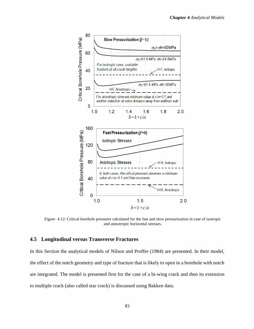
Chapter 4 Analytical Models
83
Figure 4.12: Critical borehole pressures calculated for the fast and slow pressurization in case of isotropic
and anisotropic horizontal stresses.
4.5 Longitudinal versus Transverse Fractures
In this Section the analytical models of Nilson and Proffer (1984) are presented. In their model,
the effect of the notch geometry and type of fracture that is likely to open in a borehole with notch
are integrated. The model is presented first for the case of a bi-wing crack and then its extension
to multiple crack (also called star crack) is discussed using Bakken data.

Chapter 4 Analytical Models
84
4.5.1 Bi-Wing Crack
According to Nilson and Proffer (1984), the strength of the tensile stress singularity at the tip of a
fracture emanating from a hole in an infinite elastic medium can be calculated from:
𝐾 =2
√𝜋√𝐿 ∫ (𝑃 − 𝜎)𝑓 (
𝑥
𝐿,𝐿
𝑎)
𝑑𝑥
√𝐿2−𝑥2
𝐿
0 (4.41)
Also, the width of the fracture (twice the opening displacement) can be estimated as:
𝑤(𝑥) =4
𝜋
(1−𝑣)
𝐺∫ (∫ (𝑃 − 𝜎)𝑓 (
𝜉
𝑎,𝑎
𝑅)
𝑑𝜉
√𝑎2−𝜉2
𝑎
0)
𝐿
𝑥𝑓 (
𝑥
𝑎,𝑎
𝑅) (
𝑎+𝑅
𝑥+𝑅)𝑛 𝑎𝑑𝑎
√𝑎2−𝑥2 (4.42)
In the above equation, K is the mode 1 stress intensity factor, L is the length of the fracture, a is
the radius of the hole, x is the position variable along the fracture, P(x) is the internal
pressure within the fracture, and (x) is external confining stress acting normal to the fracture
plane, therefore, P-(x) is the net pressure.
It is to be noted that the proposed models here, and also in the previous Sections, are 2D
models where, in case of an axial fracture, the base of the fracture (fracture depth), i.e. its length
along the wellbore axis (La) is consider unit. This represents a plane strain solution. Incorporating
the impact of the fracture depth, into these calculations requires development of 3D models, which
is not the intention in this work. However, we discuss this in the next Chapter when presenting the
numerical simulation results.
The internal pressure P(x) depends on the pressurization type. In case of slow pressurization,
where there is enough time for the fluid to penetrate into the crack, the internal crack pressure is
equal to the wellbore pressure. However, in case of fast pressurization, as it was mentioned before,
the fluid cannot enter the crack, hence the internal pressure is equal to the pore pressure. The
discussions presented in this section is with regards to the slow pressurization rate. In case of fast

Chapter 4 Analytical Models
85
pressurization limit, the fracture initiation pressure is infinite for the case of transverse fracture
and it is higher than slow pressurization limit (up to a factor of two) for axial fracture as noted by
Detournay and Carbonell (1997) We present in the next Chapter some simulation results
corresponding to these cases for comparison purposes.
The configuration or weight function f is dependent on geometry and can be expressed as a
combined effect of radial divergence (frad) and stress free (uniformly pressurized) notch surface
(fnotch):
𝑓 = 𝑓𝑟𝑎𝑑 𝑓𝑛𝑜𝑡𝑐ℎ = (𝑥 𝐿⁄ +𝑎 𝐿⁄
1+𝑎 𝐿⁄)𝑛
[1 + 0.3 (1 −𝑥
𝐿) (
1
1+𝐿 𝑎⁄)2𝑚
] (4.43)
In the above equation, m=2 for a cylindrical cavity, which is the geometry of the borehole in this
study, and m=3 for spherical cavity. In planar problem, corresponding to an axial fracture in the
case of a horizontal wellbore that we analysed earlier (see Figure 4.3), n=0, whereas n=1 in case
of axisymmetric problems, corresponding to transverse fracture shown in Figure 4.3.
For transverse fractures (n=1), 𝑓𝑟𝑎𝑑 can be rewritten as a linear function in form of:
𝑓𝑟𝑎𝑑 = (1
1+𝑎 𝐿⁄)
𝑥
𝐿+ (
𝑎 𝐿⁄
1+𝑎 𝐿⁄) (4.44)
where 1
1+𝑎 𝐿⁄ is the slope and
𝑎 𝐿⁄
1+𝑎 𝐿⁄ is the intercept of the linear function, respectively. It is seen
that the slope and the intercept of 𝑓𝑟𝑎𝑑 are positive.
Similarly, 𝑓𝑛𝑜𝑡𝑐ℎ can be written as a linear function in form of:
𝑓𝑛𝑜𝑡𝑐ℎ = −0.3 (1
1+𝐿 𝑎⁄)4
𝑥
𝐿+ 1 + 0.3 (
1
1+𝐿 𝑎⁄)4
(4.45)
where −0.3 (1
1+𝐿 𝑎⁄)4
and 1 + 0.3 (1
1+𝐿 𝑎⁄)4
are the slope and intercept of the linear function,
respectively. The slope and intercept of this function are positive.
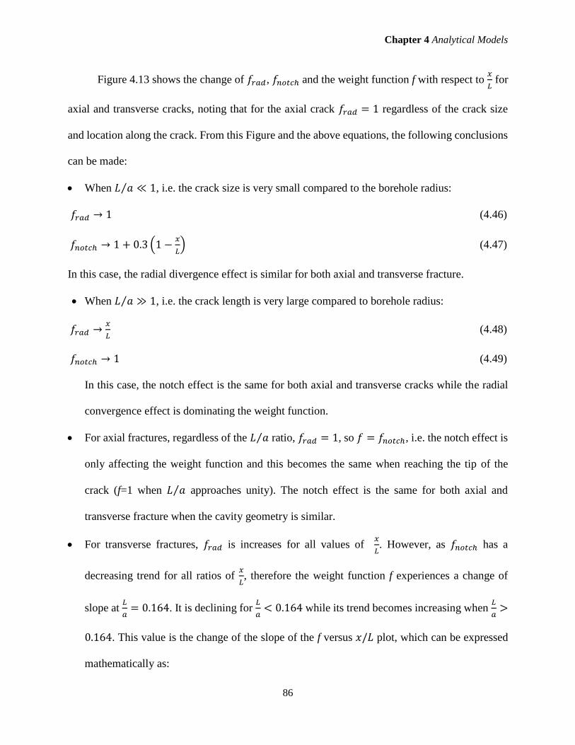
Chapter 4 Analytical Models
86
Figure 4.13 shows the change of 𝑓𝑟𝑎𝑑, 𝑓𝑛𝑜𝑡𝑐ℎand the weight function f with respect to 𝑥
𝐿 for
axial and transverse cracks, noting that for the axial crack 𝑓𝑟𝑎𝑑 = 1 regardless of the crack size
and location along the crack. From this Figure and the above equations, the following conclusions
can be made:
When 𝐿 𝑎⁄ ≪ 1, i.e. the crack size is very small compared to the borehole radius:
𝑓𝑟𝑎𝑑 → 1 (4.46)
𝑓𝑛𝑜𝑡𝑐ℎ → 1 + 0.3 (1 −𝑥
𝐿) (4.47)
In this case, the radial divergence effect is similar for both axial and transverse fracture.
When 𝐿 𝑎⁄ ≫ 1, i.e. the crack length is very large compared to borehole radius:
𝑓𝑟𝑎𝑑 →𝑥
𝐿 (4.48)
𝑓𝑛𝑜𝑡𝑐ℎ → 1 (4.49)
In this case, the notch effect is the same for both axial and transverse cracks while the radial
convergence effect is dominating the weight function.
For axial fractures, regardless of the 𝐿 𝑎⁄ ratio, 𝑓𝑟𝑎𝑑 = 1, so 𝑓 = 𝑓𝑛𝑜𝑡𝑐ℎ, i.e. the notch effect is
only affecting the weight function and this becomes the same when reaching the tip of the
crack (f=1 when 𝐿 𝑎⁄ approaches unity). The notch effect is the same for both axial and
transverse fracture when the cavity geometry is similar.
For transverse fractures, 𝑓𝑟𝑎𝑑 is increases for all values of 𝑥
𝐿. However, as 𝑓𝑛𝑜𝑡𝑐ℎ has a
decreasing trend for all ratios of 𝑥
𝐿, therefore the weight function f experiences a change of
slope at 𝐿
𝑎= 0.164. It is declining for
𝐿
𝑎< 0.164 while its trend becomes increasing when
𝐿
𝑎>
0.164. This value is the change of the slope of the f versus 𝑥/𝐿 plot, which can be expressed
mathematically as:

Chapter 4 Analytical Models
87
Figure 4.13: Change of the weight function f with respect to 𝒙
𝑳 for axial and transverse cracks.

Chapter 4 Analytical Models
88
𝜕
𝜕(𝐿 𝑎⁄ )[
𝜕𝑓
𝜕(𝑥 𝐿⁄ )= 0] = 0 (4.50)
The result of the above function is 𝐿
𝑎= 0.164.
We used data from Bakken formation shown in Table 4.1 and calculated the scaled initiation
pressure (𝑃𝑓
𝑃∗) for bi-wing notch with different sizes for both axial and transverse fractures along
the most favourable directions. The characteristic pressure is defined as (Lecampion et al., 2013):
𝑃∗=√32𝜋𝐾𝐼𝐶
√𝑎 (4.51)
where 𝐾𝐼𝐶 is the mode I of rock fracture toughness. Figure 4.14 shows the results for 4 different
cases below:
Case 1: V=68.48 MPa >H=61.58 MPa > h=54.82 MPa
This is the stress values of Bakken formation, a normal stress regime with low horizontal stress
anisotropy. The curves corresponding to the transverse and axial fractures cross over at
approximately L/a=0.2. This means that for cracks or notches larger than this ratio transverse
fracture will be dominated and more likely to occur.
Case 2: V=H =60.0MPa > h=54.82 MPa
This is a case at the threshold of normal/strike slip stress regime with isotropic stresses
perpendicular to the wellbore direction. The results are the same as Case 1, however, the cross
over point has moved to the left indicating that with a notch length of at least 0.1a (i.e. 10% of
wellbore radius) the transverse fracture will dominate.
Case 3: V=68.48MPa > H=h=58.21 MPa
This case represents isotropic horizontal stresses with average horizontal stresses considered as
the isotropic stress in this case. No cross over is observed in this case meaning that the axial

Chapter 4 Analytical Models
89
fracture is always dominant regardless of the crack length. This is a critical situation in practice as
transverse fracture is unlikely to initiate.
Case 4: V=68.48 MPa >H=61.58 MPa > h=54.82 MPa
Here, using Bakken data, similar to Case 1, the initiation pressure for axial fractures in three
different directions (i.e. perpendicular to H, perpendicular to V, and at 45° with respect to V)
are compared with transverse fractures. The results show that the cross over point moves to the
right as the axial fracture is further oriented towards its most favourable direction. This means that
larger notches are needed to dominate transverse fractures. It is seen that in general, as the stress
anisotropy reduces, the cross over points moves to the right, i.e. larger notch length is needed in
order to dominate transverse fracture.
Figure 4.14: Fracture initiation pressures for transverse and axial fractures in presence of different stress regimes.
2
4
6
8
10
0.001 0.01 0.1 1 10
Sca
led
Initi
atio
n P
ress
ure
Fracture length to wellbore radius (L/a)
Axial Fracture
Transverse Fracture
Cross over at L/a=0.2, this means if the notch length is
greater than 10% of the wellbore radius transverse
fracture will be more favorable to occur
Case 1: V=68.48 MPa > H=61.58 MPa > h=54.82 MPa
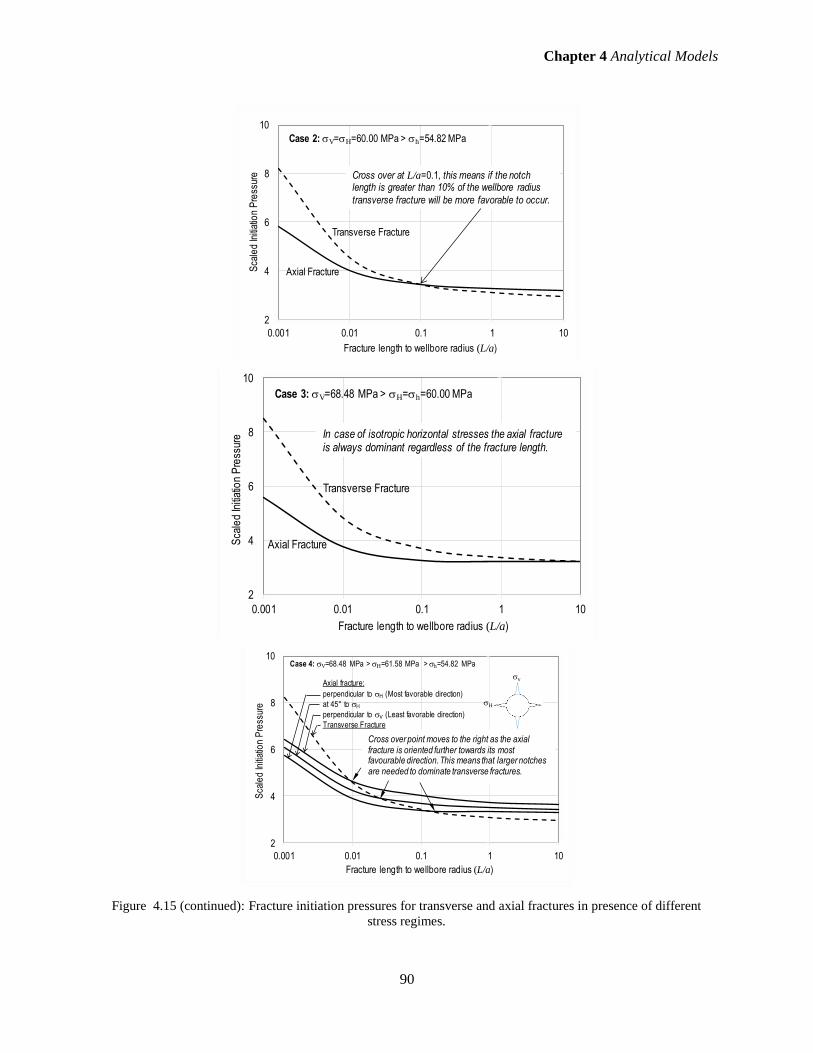
Chapter 4 Analytical Models
90
Figure 4.15 (continued): Fracture initiation pressures for transverse and axial fractures in presence of different
stress regimes.
2
4
6
8
10
0.001 0.01 0.1 1 10
Sca
led
Initi
atio
n P
ress
ure
Fracture length to wellbore radius (L/a)
Axial Fracture
Transverse Fracture
Cross over at L/a=0.1, this means if the notch length is greater than 10% of the wellbore radius
transverse fracture will be more favorable to occur.
Case 2: V=H=60.00 MPa > h=54.82 MPa
2
4
6
8
10
0.001 0.01 0.1 1 10
Sca
led
Initi
atio
n P
ress
ure
Fracture length to wellbore radius (L/a)
Axial Fracture
Transverse Fracture
In case of isotropic horizontal stresses the axial fracture is always dominant regardless of the fracture length.
Case 3: V=68.48 MPa > H=h=60.00 MPa
2
4
6
8
10
0.001 0.01 0.1 1 10
Sca
led
Initi
atio
n P
ress
ure
Fracture length to wellbore radius (L/a)
Cross over point moves to the right as the axial fracture is oriented further towards its most favourable direction. This means that larger notches are needed to dominate transverse fractures.
Axial fracture:
perpendicular to H (Most favorable direction)
at 45° to H
perpendicular to V (Least favorable direction)
Transverse Fracture
Case 4: V=68.48 MPa > H=61.58 MPa > h=54.82 MPa
v
H

Chapter 4 Analytical Models
91
4.5.2 Multiple (Star) Crack
Multiple fractures are expected to occur when pressurization rate is fast (i.e. the rise time of the
driving pressure pulse is relatively short compared with the time required for stress waves to circle
the cavity). This situation is happening more likely in case of axial fracture. For axial multifracture
configurations, Nilson and Proffer (1984) extended the geometry function f for two wing fracture
(see Equation 4.41) by including in the overall weighting function, f, an additional multiplier, fN,
in form of (i.e. the f function of equation 4.43 is multiplied by fN for case of more than 2 cracks):
𝑓𝑁 =(𝑓∞+𝑓∞
𝐿
𝜋𝑎 𝑁⁄)
(𝑓∞+𝐿
𝜋𝑎 𝑁⁄)
(4.52)
𝑓∞ = 2√𝑁−1
𝑁 (4.53)
Here, N is the number of fractures and 𝜋𝑎 𝑁⁄ is the circumferential distance between fractures. It
assumes that cracks have similar distances from each other and the first crack is along the most
favourable direction. Figure 4.15 shows the plot of 𝑓∞ versus N and 𝑓∞ as a function of 𝐿
𝜋𝑎 𝑁⁄. The
results show that the multiplier 𝑓∞reduces from 1 (for case of bi-wing crack) as the number of
cracks increases, corresponding to increase of the crack length to circumferential distance between
cracks. This Figure also shows that the multiplier factor becomes flatten as the crack length to
circumferential distance increases over 4 to 8 cracks for low to higher number of cracks,
respectively.
Figure 4.16 presents the initiation pressures for the case of 6, 15 and 25 axial fractures,
respectively. The differences, as seen from this Figure, are minor. In this Figure also the initiation
pressure curve corresponding to the transverse fracture is shown. It is seen that as the number of
fractures increases, cross over point moves to the left, i.e. less notch length can result in transverse
fracture to dominate the axial fracture.

Chapter 4 Analytical Models
92
Figure 4.16: Change of the weight function f for multiple fractures with respect to the number of fractures and
the ratio of crack length to circumferential distance between fractures.
Figure 4.17: Fracture initiation pressures multiple axial fractures.
Chapter 4 Analytical Models
93
4.6 Fracture Propagation Regimes and Scaling Law
Fracture propagation is a complex process which is governed by a series of physical mechanisms
such as elasticity, fluid flow and leak-off and fracture mechanics (Lecampion et al. 2017).
Propagation of a radial hydraulic fracture in the field is expected to be governed at early time,
when fracture radius is small, by the dissipation of the viscous flow. This is known as viscosity
dominated regime. However, at large time, as the fracture perimeter is increases, the fracture
energy, or toughness, to create an increment of fracture surface becomes larger. The fracture
propagation in this case is known to be toughness dominated. Here, we ignored the effect of the
injection system compliance, which is mostly governed by fluid compressibility and then
wellbore deformation. In a small scale laboratory test considering the case of a penny shaped
fracture, it is most likely that toughness controls the fracture propagation regime at the final stage
of propagation after a period of specific time.
In field scale hydraulic fracturing operations for the purpose of enhanced oil recovery (EOR),
the range of injecting fluid viscosity is 0.001-0.1 pa.s (1-100 cp) with the flow rate of 20-30 barrel
per minute (0.05-0.08 m3/s). However, when a lab experiments is performed on very small sample
size to represent field scale operations, the fluid viscosity should be increased to as high as on
average 100 pa.s with very small flow rate of as low as 1×10⁻⁹ m3/s (Sarmadivaleh & Rasouli,
2013). This will ensure that the fracture propagates very slowly within a few centimeters of rock
sample size to allow monitoring and recording the pressure versus time data.
In order to propagate the fracture in the same regime (i.e. toughness or viscosity dominated)
as occurred in the field, the viscosity and flow rates, as well as the wellbore diameter should be
designed accordingly. This is done through the scaling law, which is well known and used for
design of a hydraulic fracturing lab experiments (De Pater et al. 1994). For this purpose, a set of

Chapter 4 Analytical Models
94
dimensionless groups of physical parameters that describe a specific fracturing process are defined
in the way that they become identical using laboratory and field parameters. These dimensionless
variables are driven from the fluid flow (mass and momentum conservation laws) and rock
behaviour (rock deformation, crack opening and extension) partial differential equations.
The scaling period is valid for the time from initiation until stopping the injection of fluid.
To have viscose dominated fracture propagation; following condition should be met during
fracture propagation (De Pater et al. 1994):
f
nIC
rPK 2 (4.54)
where rf is fracture radius and Pn is fracture net pressure.
For viscous dominated propagation regime, the dimensionless toughness parameter of a
Penny-Shaped fracture can be calculated as (Detournay 2004):
18/1
1335
2
'''
EQ
tK
o (4.55)
where Qo is flow rate and t is the experiment time. Other material properties are defined as:
ICKK
2/132
'
,
21'
v
EE
, 12' (4.56)
Here, μ is fracturing fluid viscosity, E is the rock Young’s modulus, and v is Poisson’s ratio.
In equation 4.55, the fracture propagation will be viscose dominated if is below one whereas it
is toughness dominated when dimensionless toughness number exceeds 3.5. In contrast with
Equation 4.55, the dimensionless toughness parameter is time dependent: this means that fracture
regime may change from one type to another as time evolves. Also the propagation regime was

Chapter 4 Analytical Models
95
checked against another criterion proposed by (Bunger et al 2005). In this method the evaluation
criterion is based on three characteristic times of leak-off, toughness, and viscosity.
Figure 4.17 (top) plots the changes of dimensionless toughness as a function of pressurization
rate for data corresponding to typical lab and field scale HF operations. Average propagation time
of 3000s and 100s has een considered as examples, corresponding to field and lab scale testing. In
the top Figure, the viscosity is set to a certain value (0.001 pa.s at field scale operation and 100
pa.s for lab experiments) and the pressurization rate is varied by changing the flow rate. As one
may expect, larger pressurization rate is expected at field scale HF operation compared with lab
experiments. Therefore, in overall, lab experiments HF are more likely to be in viscosity dominated
regime. While field scale HF operations starts usually at viscosity dominated regime, it will change
into transition and then toughness dominated regimes after long time propagation.
In Figure 4.17 (bottom) the flow rate is set to a constant value (0.08 m3/s at field scale and
1×10⁻⁹ m3/s at lab scale) and the pressurization rate is calculated and plotted against the
dimensionless toughness parameter. From this Figure, it is seen that the propagation regime is
more sensitive to the changes of viscosity than flow rate, a result which is evident from Equation
(4.55).
4.7 Summary
In this Chapter an overview of different analytical models to estimate the fracture initiation
pressure through an existing crack emanating from wellbore wall were presented. It was seen that
these models are based on some simplified assumptions, so when one using these models, should
carefully consider their limits and application ranges. In general, most of these models are based
on the concept of superposition law in order to determine the impact of different parameters on
fracture initiation pressure. We presented models which consider the effect of in-situ stresses and

Chapter 4 Analytical Models
96
wellbore pressure, those which also integrate the impact of pressurization rate and finally models
which consider the axial and transverse fracture initiation and propagation.
Figure 4.18: Dimension toughness parameter changes as a function of pressurization rate for typical field and lab
scale HF operations.
While these models provide great knowledge about the effect of different parameters on crack
initiation from an existing notch, they cannot be conveniently used for simulation of real cases
where fractures with different geometry and properties are distributed around an OH borehole.
Therefore, we introduce the lattice numerical modelling in the next Chapter, which will be used to
conduct numerical simulations of some of the cases presented in this Chapter to compare the results

Chapter 4 Analytical Models
97
with analytical solutions. We also expand this to more complex cases where analytical solutions
do not exist and interpret the results. The results of numerical simulations will be presented in
Chapter 5. In the next Chapter we also simulate fracture propagation pressure and discuss the
impact of different parameters on competition between axial and transverse fracture propagation.

Chapter 5 Numerical Simulations
98
CHAPTER 5
Numerical Simulations
5.1 Introduction
In this Chapter, the results of lattice numerical simulations of hydraulic fracturing are presented.
The effect of both axial and transverse notch geometry on fracture initiation and breakdown as
well as propagation pressures will be studied and compared with the analytical models presented
in the preceding Chapter. The impact of the flow rate and fluid viscosity together with the
pressurization rate on fracture pressure and geometry will be modelled. In addition, the models are
presented for different stress regimes and stress anisotropy, as the most important parameter
changing the axial to transverse fracture limits. The results will be compared with the analytical
models presented in the previous Chapters and conclusions are made.
5.2 Borehole Without Notch
We start the simulations by looking at a horizontal wellbore drilled along the minimum horizontal
stress direction in a normal stress regime. It is assumed that no natural fractures or notches present
around the wellbore wall. For consistency, we build the model geometry corresponding to the
Bakken data presented in Table 4.1, in the previous Chapter.

Chapter 5 Numerical Simulations
99
5.2.1 Model Geometry
As this study focuses initially at the fracture initiation pressure and also fracture propagation near
wellbore (i.e. a few times than the wellbore radius), model dimension is considered to be
1.5m×2.5m×2.5m. The model geometry is shown in Figure 5.1, where the stress magnitudes are
applied in different directions in such a way that the fracture is expected in the plane of larger
model dimension. The horizontal wellbore has a diameter of 0.11m and a length of 8m and is
placed in the center of the model. In XSite, there is no direct feature available to keep the external
stresses applied to the model constant during the fluid injection and fracture propagation, to mimic
real field stresses. Hence, in order to implement the so called servo control stress condition, an
outer soft layer with thickness of 0.125m has been placed all around the model. The Young’s
modulus of this layer is assumed to be much lower than that of the formation Young’s modulus
(here we assumed 100 times less, to be 0.3 GPa – see Table 4.1) with a large Poisson’s ratio (here
we considered o.45). This soft boundary will dampen the stresses during the fluid injection time
step and keeps the stresses to remain constant on the model.
The model configurations presented in Chapter 3 was used in the simulations of this
Chapter. Figure 5.1 shows the model geometry without notch. Because in absence of the notch we
expect an axial notch to be initiated and developed, we use the model geometry corresponding to
this fracture geometry (see Figure 3.12 in Chapter 3). As discussed in Chapter 3 (see Figure 3.12)
two rectangular resolution domains are considered here, the inner domain has an equal length and
width of L=W=2.1m and thickness of T=0.3m with a resolution of 2.2m and the outer domain has
dimension of L=W=2.3m and thickness of T=0.5m with a resolution of 4.4m. The rest of the model
has a resolution of 8.8cm.

Chapter 5 Numerical Simulations
100
Figure 5.1. Model geometry for a horizontal wellbore along H.
As explained in details in Chapter 3, model construction in XSite includes three steps.
Initially, the borehole is excavated. Then, the mechanical step is run, which includes applying the
in-situ stresses until the model reaches stability stage. It is to be noted that mechanical stability is
achieved when the velocity field data becomes negligible in the entire model. The final step is the
fluid step, where the injecting fracturing fluid is applied. This step continues until the fracture
initiation and breakdown points are reached and then it propagates to the desired extent. We can
monitor several data, including the pressure-time curve, number of initiated fractures before
fracture breakdown pressure and after that and fracture aperture contours during model evolution.
The model was run for 0.01s simulation time during mechanical step, and continued for
0.02s during fluid injection step. Figure 5.2 shows the fracture apertures as well as the
corresponding pressure-time curve and the number of cracks developed around the wellbore as
time evolved for model geometry of Figure 5.1 and the data corresponding to the Bakken formation
presented in Table 4.1 in Chapter 4. The results show that in absence of any notch (i.e. natural
fractures or any defect at the wellbore wall), several cracks are developed around the wellbore,
mostly along the wellbore axis (corresponding to axial fracture). The fracture initiation pressure is
approximated at 117MPa which is higher compared to cases where notches exist around the
wellbore. This observation is in agreement with the results of the analytical models presented in
Horizontal Wellbore
Z, Up, v
X, East, H Y, North, h
Resolution domains

Chapter 5 Numerical Simulations
101
Chapter 4 (see Section 4.2). We will see in the next Section, how the presence of a notch facilitated
the initiation and propagation of the fracture.
Presence of the peak pressure or breakdown pressure depends on the rock properties and
may not be necessarily observed in a HF test. As discussed in Chapter 3, Both initiation and
breakdown pressures are functions of the flow rate and viscosity. Therefore, changing these input
parameters the pressure values will change.
Figure 5.2. Fracture apertures evolution per simulation time from 0.312sec to 0.314sec and 0.316sec, left to right
(top), and pressure-time and crack numbers plots (bottom) for an open hole completion with no notch
5.3 Transverse versus Axial Fracture
In this section, the simulation models are presented with both transverse and axial notches to
compare the competition between these two types of fracture geometry as a function of the notch
dimension, stress anisotropy and stress regimes. The results and discussions are outlined in the
0
500
1,000
1,500
2,000
2,500
0
20
40
60
80
100
120
0.000 0.010 0.020 0.030 0.040
Cra
ck N
um
be
rs
Fra
ctu
re I
nitia
tio
n P
ressure
(M
Pa
)
Simulation Time (Sec)
Fracture initiation pressure (FIP) defined at the time when
axial cracks generated along one direction of the wellbore, here at around 250 cracks
Open Hole Completion with no Notch
0.031 Sec corresponding
time to the FIP
FIP=117 MPa
t=0.312sec t=0.314sec t=0.316sec

Chapter 5 Numerical Simulations
102
following subsections and include the cases for which analytical analysis was done in Chapter 4
(subsection 4.5.1).
Case 1: V=68.48 MPa >H=61.58 MPa > h=54.82 MPa
This is the case of normal stress regime, corresponding to the Bakken data in Table 4.1 (Chapter
4). Numerical simulations were carried out for transverse fractures with different notch lengths.
The initiation pressure for each case was determined corresponding to the time when cracks around
the notch perimeter are all open. Similarly, axial fractures were simulated with different notch
lengths (Ln) and base length of Lb=1m. Figure 5.3 shows, as examples, the aperture values of the
fracture propagated near wellbore for transverse fracture with notch length of Ln =0.011m
(=L/a=0.1) at 0.025sec simulation time. In this Figure also the corresponding pressure-time curve
and crack numbers are shown. Similar results are shown in Figure 5.4 for the transverse fracture
with a notch length of Ln=0.22m (=2) at the same simulation time of 0.025sec for the case of
transverse fracture with =0.1. From Figures 5.3 and 5.4 is it seen that as the notch length increases,
the initiation pressure reduces, a conclusion that we expected and discussed based on analytical
models in Chapter 4. For small notch size of =0.1, it is seen that due to the fact that the notch is
not enough long, it is not as effective as it should be and this resulted in the development of some
sparse fractures along the wellbore. In this case, the fracture also propagated in one direction more
than other directions with an asymmetric geometry.
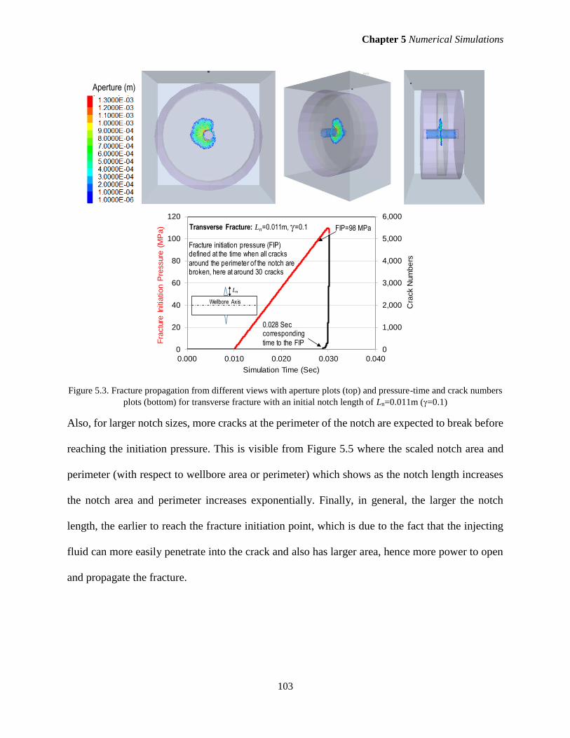
Chapter 5 Numerical Simulations
103
Figure 5.3. Fracture propagation from different views with aperture plots (top) and pressure-time and crack numbers
plots (bottom) for transverse fracture with an initial notch length of Ln=0.011m (=0.1)
Also, for larger notch sizes, more cracks at the perimeter of the notch are expected to break before
reaching the initiation pressure. This is visible from Figure 5.5 where the scaled notch area and
perimeter (with respect to wellbore area or perimeter) which shows as the notch length increases
the notch area and perimeter increases exponentially. Finally, in general, the larger the notch
length, the earlier to reach the fracture initiation point, which is due to the fact that the injecting
fluid can more easily penetrate into the crack and also has larger area, hence more power to open
and propagate the fracture.
0
1,000
2,000
3,000
4,000
5,000
6,000
0
20
40
60
80
100
120
0.000 0.010 0.020 0.030 0.040
Cra
ck N
um
be
rs
Fra
ctu
re I
nitia
tio
n P
ressure
(M
Pa
)
Simulation Time (Sec)
Fracture initiation pressure (FIP) defined at the time when all cracks
around the perimeter of the notch are broken, here at around 30 cracks
FIP=98 MPaTransverse Fracture: Ln=0.011m, =0.1
0.028 Sec corresponding
time to the FIP
Wellbore Axis
Ln
Aperture (m)
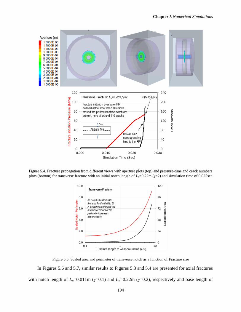
Chapter 5 Numerical Simulations
104
Figure 5.4. Fracture propagation from different views with aperture plots (top) and pressure-time and crack numbers
plots (bottom) for transverse fracture with an initial notch length of Ln=0.22m (=2) and simulation time of 0.025sec
Figure 5.5. Scaled area and perimeter of transverse notch as a function of Fracture size
In Figures 5.6 and 5.7, similar results to Figures 5.3 and 5.4 are presented for axial fractures
with notch length of Ln=0.011m (=0.1) and Ln=0.22m (=0.2), respectively and base length of
0
40
80
120
160
200
240
0
20
40
60
80
100
120
0.000 0.010 0.020 0.030
Cra
ck N
um
be
rs
Fra
ctu
re I
nitia
tio
n P
ressure
(M
Pa
)
Simulation Time (Sec)
Fracture initiation pressure (FIP) defined at the time when all cracks
around the perimeter of the notch are broken, here at around 110 cracks
FIP=73 MPaTransverse Fracture: Ln=0.22m, =2
0.0247 Sec corresponding
time to the FIP
Wellbore Axis
Ln
0
24
48
72
96
120
0.0
2.0
4.0
6.0
8.0
10.0
0.1 1 10
Scale
d N
otc
h A
rea
Scale
d N
otc
h P
erim
ete
r
Fracture length to wellbore radius (L/a)
Transverse Fracture
As notch size incresses the area for the fluid to fill in becomes larger and the number of cracks at the perimeter increases exponentially
Aperture (m)

Chapter 5 Numerical Simulations
105
Lb=1m for a simulation time of 0.045sec. Similar conclusions drawn for the case of transverse
fracture are observed here. It is seen that the fracture has opened larger in case of larger notch
length of =2 (higher aperture values) comparing to =0.1. Also, comparing the same notch
lengths, axial fractures result in higher apertures than transverse fractures (see Figures 5.3 and 4.5)
which is due to their larger area open to the fluid flow.
Figure 5.6. Fracture propagation with aperture plots from different views (top) and pressure-time and crack numbers
plots (bottom) for axial fracture with an initial notch length of Ln=0.011m (=0.1) and based length of Lb=1m and
simulation time of 0.045sec
0
1,000
2,000
3,000
4,000
5,000
6,000
0
20
40
60
80
100
120
0.000 0.010 0.020 0.030 0.040 0.050
Cra
ck N
um
be
rs
Fra
ctu
re I
nitia
tio
n P
ressure
(M
Pa
)
Simulation Time (Sec)
Fracture initiation pressure (FIP) defined at the time when all cracks
around the perimeter of the notch are broken, here at around 43 cracks
FIP=87 MPaAxial Fracture: Ln=0.011m, =0.1, Lb=1m
0.036 Sec corresponding time to
Wellbore Axis
Lb
Ln
Aperture (m)

Chapter 5 Numerical Simulations
106
Figure 5.7. Fracture propagation with aperture plots from different views (top) and pressure-time plot (bottom) and
crack numbers for axial fracture with an initial notch length of Ln=0.22m (=2) and base length of Lb=1m and
simulation time of 0.045sec
Correct comparison of the results of axial notch with the transverse notch requires careful
consideration of the base length Lb. To explain this, in Figure 5.8 the results of scaled notch area
and perimeter of the transverse fracture (Figure 5.5) are compared with two axial notches with
base lengths of Lb=1m and Lb=0.5m. from this Figure it is seen that in case of Lb=1m (top plot in
Figure 5.8) the area and perimeter of axial notch are larger than transverse fracture but this does
change after a certain notch length. However, for base length of Lb=0.5m or smaller, the axial
notch has always larger area and perimeter than that of transverse notch. This indicates that
depending on the notch base length the time to reach the FIP and the number of corresponding
cracks at the perimeter of the notch may how different trends.
0
300
600
900
1,200
1,500
1,800
0
20
40
60
80
100
120
0.000 0.010 0.020 0.030 0.040 0.050
Cra
ck N
um
be
rs
Fra
ctu
re I
nitia
tio
n P
ressure
(M
Pa
)
Simulation Time (Sec)
Fracture initiation pressure (FIP) defined at the time when all
cracks around the perimeter of the notch are broken, here at around 100 cracks
FIP=70 MPa
Axial Fracture: Ln=0.22m, =2, Lb=1m
Wellbore Axis
Lb
Ln
0.04 Sec corresponding time to the FIP
Aperture (m)

Chapter 5 Numerical Simulations
107
Figure 5.8. Scaled area and perimeter of axial notch with base length Lb=1m (top) and Lb=0.5m (bottom) as a
function of Fracture size compared with transverse notch
However, from practical point of view, as the base length of the axial fracture reduces, the
chance for the fluid to enter the crack becomes less, resulting the notch to be ineffective to act as
the starting point for fracture initiation regardless of its length. This is visible from Figure 5.9
0
24
48
72
96
120
0.0
2.0
4.0
6.0
8.0
10.0
0.1 1 10
Scale
d N
otc
h A
rea
Scale
d N
otc
h P
erim
ete
r
Fracture length to wellbore radius (L/a)
Solid lines for Transverse Fracture,Dashed lines for Axial Fracture with Lb=1m
Depending on the base length of axial fracture, there maybe a change over in the notch perimeter and area of the transverse and axial fracture
0
24
48
72
96
120
0.0
2.0
4.0
6.0
8.0
10.0
0.1 1 10
Scale
d N
otc
h A
rea
Scale
d N
otc
h P
erim
ete
r
Fracture length to wellbore radius (L/a)
Solid lines for Transverse Fracture,Dashed lines for Axial Fracture with Lb=0.5m
It appears that for axial notch with base lines of less than 0.5m, transverse fracture has always larger area and perimeter than axial fracture

Chapter 5 Numerical Simulations
108
where the fracture geometries are shown for three axial notches with base length of Lb=0.5m,
=0.1m (top), Lb=0.2m, =0.1m (middle) and Lb=0.2m, =8 (bottom) and the same simulation time
of 0.045sec for the case of Lb=1m. From this Figure (top and middle), it is seen that the fracture
initiated from the axial notch appears to be irregular and also a number of other fractures starting
to grow along the axis of the wellbore. Also it is seen that the fracture did not propagate as much
as it did in the case of axial fracture with a base length of Lb=1m, which shows that the notch base
length is not adequate to present a good path for the fluid to flow easily and open the fracture. It is
to be noted that the fractures developed at both ends of the wellbore are due to the boundary effect
and should not be considered for interpretation purposes in the context of this study. From Figure
5.9 (bottom) it is observed that even that the notch length is very long, as the base length is small,
the fracture starts to propagate to the sides and not from the end of the notch lengths. If the
simulation time continues further propagation of axial notches are expected in this case. One
should also note that these conclusions are valid for the geometry of the notches used in these
simulations and if the notch geometry is change, for example, a rectangular geometry for transverse
notch or radial geometry for axial notch are considered the analysis should be repeated. The last
point to add is that the XSite simulations do not consider the effect of compressibility of the system
including the wellbore or drillstring, while this effect cannot be neglected (Lecampion, 2013). This
effect should be considered in the future simulations.

Chapter 5 Numerical Simulations
109
Figure 5.9. Fracture propagation and aperture plots from different views for axial fracture with base length Lb=0.5m,
Ln=0.011m (=0.1) (top); Lb=0.2m, Ln=0.011m (=0.1) (middle) and Lb=0.2m, Ln=1.98m (=8) (bottom) and
simulation time of 0.045sec
Aperture (m)
Aperture (m)
Aperture (m)

Chapter 5 Numerical Simulations
110
The initiation pressures for transverse and axial fractures with different notch sizes are
presented in Figure 5.10. Also, in this Figure the results of analytical models presented in Chapter
4 are shown in this Figure. A number of observations are made from results of Figure 5.4. Firstly,
it is seen that regardless of fracture geometry, the simulation results show higher initiation pressure
than analytical models. This is a reasonable observation as the analytical models do not consider
several parameters such as the fracture tortuosity and frictional pressure drop resulting in
underestimation of the initiation pressure. Secondly, the cross over from axial to transverse fracture
is found to be at L/a=4 compared to L/a=0.2 which resulted from analytical solution. This suggests
that in real cases larger notch lengths are needed to dominate transverse fracture over the axial
fracture. Finally, it is to be noted that simulations with notch lengths of L/a < 0.1 resulted in no
transverse fracture but unstable fracture growth mostly in form of axial fracture and similar to the
case of no notch case, presented in the previous Section. Therefore, no data are reported for this
part of the plot in Figure 5.10.
Figure 5.10. Scaled initiation pressures for transverse and axial fractures with different notch lengths. The axial
notch has a base length of Lb=1m
2
4
6
8
10
0.001 0.01 0.1 1 10
Sca
led
Initia
tio
n P
ressure
Fracture length to wellbore radius (L/a)
Analytical Transverse
Analytical Axial
Simulation Transverse
Simulation Axial (Lb=1m)
Cross over from axial to transverse fracture at L/a=0.2 from analytical
model versus L/a=4 from numerical
simulations. Analytical models also
underestimate the initiation pressure
At large notch size, the initiation pressure tends to min stress (h/P*)
Case 1: V=68.48 MPa > H=61.58 MPa > h=54.82 MPa
For L/a <0.1 the notch appeared ineffective and
the results were similar to a without notch model
Transverse vs Axial Notch
Wellbore Axis
Lb
Ln
Wellbore Axis
Ln

Chapter 5 Numerical Simulations
111
The above results are based on the assumption of a base length of Lb=1m for the axial fracture.
In order to investigate the impact of the base length on the cross over point, simulations of axial
fracture were repeated with a smaller base length of Lb=0.5m. Figure 5.11 shows the result as
addition of the new data to Figure 5.10. From this Figure, it is seen that with reducing the base
length, as expected, the fracture initiation pressure increases, but more importantly, the cross over
point moved to the left at L/a=0.6 and becomes closer to the analytical model of L/a=0.2. Also, at
this base length, the results of axial fracture initiation are very close to the transverse fractures.
This result shows the importance of the base length on determining initiation pressure for the case
of axial fractures. From practical point of view, when detecting the natural fractures around the
wellbore from the image logs, it is important to also note their mark length on the wellbore wall,
in specific, when it is aligned in the wellbore axis. This will assist to make a more reasonable
estimation of impact of these natural fractures as potentials for the starting point of fracture
initiation.
Figure 5.11. Scaled initiation pressures for transverse and axial fractures in a normal stress regime
2
4
6
8
10
0.001 0.01 0.1 1 10
Sca
led
Initia
tio
n P
ressure
Fracture length to wellbore radius (L/a)
Analytical Transverse
Analytical Axial
Simulation Transverse
Simulation Axial (Lb=1m)
Simulation Axial (Lb=0.5m)
When axial notch size reduces from 1m to 0.5m, the cross over from axial
to transverse fracture moves to the left where L/a=0.6 and becomes closer to
analytical solutions
(h/P*)
Case 1: V=68.48 MPa > H=61.58 MPa > h=54.82 MPa

Chapter 5 Numerical Simulations
112
Case 2: V=H =60.0MPa > h=54.82 MPa
In this case, the stress regime is in transition between normal to the strike slip. With the results
observed from Case 1, here and for the rest of simulations in this Chapter, for the axial fracture,
we only present the simulations for a notch base length of Lb=0.5m. Figure 5.12 presents the results
of scaled initiation pressure versus scaled notch length for this stress regime. The results of
analytical models for both transverse and axial fractures are shown in this Figure. The simulation
results for the case of transverse fracture is similar to Case 1 (see Figure 5.11). This is due to the
fact that the transverse fracture opens against h, which is identical in both cases. The simulation
results for the case of axial notch with base length of Lb=0.5m is also presented in Figure 5.12.
The cross over point, in this case, is L/a=0.02 from analytical model and is 0.1< L/a <0.2 from
simulations. It is seen that, for both analytical and simulation results, the cross over point has
shifted to the left, compared to Case 1, as expected. This indicates the dominant effect of stress
regime on the initiation pressure and the design of proper notch size if transverse fracture is
preferred to be created.

Chapter 5 Numerical Simulations
113
Figure 5.12. Scaled initiation pressures for transverse and axial fractures in a transition from normal to strike slip
stress regime
Case 3: V=68.48MPa > H=h=58.21MPa
This case represents isotropic stresses, where the horizontal stresses considered as the average of
H and h in Bakken. The analytical solution indicates that regardless of the notch size, always
axial fracture is dominant. This result was discussed in Chapter 4. The simulation results presented
in Figure 5.13, show the same conclusion, while higher initiation pressures observed comparing
to analytical models as explained earlier on. The results shown in this Figure correspond to an
axial notch with a base length of Lb=0.5m. Shortening the base length will increase the initiation
pressure as the chance for the fluid to penetrate into the notch will be less. This could potentially
result in cross over of the transverse and axial notch curves, however, as explained in detail in
Case 1, from practical point of view the fracture does not tend to propagate symmetrically and
penetrate into the formation effectively. Therefore, in case of isotropic field stresses, creation of
transverse fractures will be challenging.
2
4
6
8
10
0.001 0.01 0.1 1 10
Sca
led
Initia
tio
n P
ressure
Fracture length to wellbore radius (L/a)
Analytical Transverse
Analytical Axial
Simulation Transverse
Simulation Axial (Lb=0.5m)
h/P*
Case 2: H=V=65 MPa > h=54.8 MPa
Compared to Case 1 (normal stress regime) the cross over point has shifted to the left for both
analytical and simulations). The L/a=0.02 from analytical model and 0.1<L/a<0.2 from simulation

Chapter 5 Numerical Simulations
114
Figure 5.13. Scaled initiation pressures for transverse and axial fractures with different notch lengths for
isotropic stresses
5.4 Axial Fractures with Different Orientations
In the previous Section, the results of HF simulations for axial fractures were presented for the
cases where the axial notch was created perpendicular to the minimum stress. In case of normal
stress regime, this is perpendicular to the maximum horizontal stress, H. This is the most
favourable orientation for an axial fracture to initiate and propagate near wellbore. The results
presented for notches with different lengths and two base lengths of 0.5m and 1.0m. in this Section,
for comparison purposes, axial notches with similar base length of 1m are simulated in the same
normal stress regime as in the previous Section, but in two different orientations of =45° and
=90° with respect to the most favourable orientation. The simulations will be done for three notch
lengths corresponding to =0.1, 0.3 and 0.6.
Figures 5.14 to 5.16 show, correspondingly, the evolution of fracture propagation for an axial
notch at 90° with respect to the preferred direction ( =90°) with three notch lengths of =0.1,
2
4
6
8
10
0.001 0.01 0.1 1 10
Sca
led
Initia
tio
n P
ressure
Fracture length to wellbore radius (L/a)
Analytical Transverse
Analytical Axial
Simulation Transverse
Simulation Axial (Lb=0.5) In case of isotropic stresses axial fracture appears to be dominant regardless of the notch size. This
holds true always for analytical model where the base length of the axial fracture (Lb) is ignored. However, this result corresponds to Lb= 0.5 in
numerical simulation and change of base length may change the results
h/P*
Case 3: V=68.48 MPa > H=h=58.21 MPa

Chapter 5 Numerical Simulations
115
=0.3 and =0.6 with base length of Lb=1m at two different time steps of t=0.051sec (top) and
t=0.055sec (bottom). From Figure 5.14 it is seen that, as the notch size is small, the fracture did
not propagate from the notch, but instead cracks started to initiate along the axis of the wellbore at
=0°, i.e. the preferred propagation plane. This means that when the notch length is not adequate,
it is not effective and the fracture initiation is similar to a wellbore without notch (see Figure 5.2).
From this Figure it is also observed that as the time evolves, the fracture starts to propagate from
the ends of the wellbore, here, mostly from the left end, instead of along the preferred propagation
plane. This is due to the model geometry and the short length of the wellbore simulated here and
should not misinterpreted incorrectly.
Figure 5.14. Fracture propagation for an axial notch at 90° with respect to the preferred direction. Lb=1m,
Ln=0.011m (=0.1) at simulation time of t=0.051sec (top) and t=0.055sec (bottom)
Aperture (m)

Chapter 5 Numerical Simulations
116
In Figure 5.15 similar results to Figure 5.14 are shown but the notch length has increased to
=0.3. It is seen that in this case, the fracture initiation begins from the notch, yet some dispersed
cracks start to grow along the wellbore axis, perpendicular to the notch plane, but less than the
case of =0.1. This observation becomes more manifest when the notch size increases to =0.6
(see Figure 5.16): the fracture initiates more favourably from the notch comparing to smaller notch
sizes, with less cracks growing outside the notch plane. In all cases, if the fracture propagates
further away from the wellbore wall, it is expected that it will reorient itself to become
perpendicular to the preferred propagation direction, i.e. orthogonal to H plane (i.e. when =0°).
While this is not clearly visible from Figure 5.16, due to the very long running time of the high
resolution model, we observed this behaviour in models with lower resolutions.
Figure 5.15. Fracture propagation for an axial notch at 90° with respect to the preferred direction. Lb=1m,
Ln=0.033m (=0.3) at simulation time of t=0.051sec (top) and t=0.055sec (bottom)
Aperture (m)

Chapter 5 Numerical Simulations
117
Figure 5.16. Fracture propagation for an axial notch at 90° with respect to the preferred direction. Lb=1m,
Ln=0.066m (=0.6) at simulation time of t=0.051sec (top) and t=0.055sec (bottom)
For the case of the axial fracture at =45° the simulation results for =0.1 showed that the
fracture did not initiate from the notch plane, instead cracks started to grow along the preferred
propagation plane, similar to the previous case. For =0.3 the crack initiated from the notch but
did not propagate much. Figure 5.17 shows the results for the case of =0.6. from this Figure, it is
seen that the fracture has initiated and propagated from the notch. It is interesting to see that in this
case, the fracture intends to propagate to the downside of the wellbore rather than upper side,
resulting in an asymmetric geometry. As we did not activate the gravitational effect in the
simulation, this observation is due to the slippage effect that is maximized at 45° degree inclined
fracture surface. At this orientation, the shear component of the fluid injection pressure is higher
than that of the normal component. This also, as can be seen from Figure 5.17 compared to Figure
5.16, resulted in less fracture aperture. Finally, while it is not very much visible from Figure 5.17,
Aperture (m)
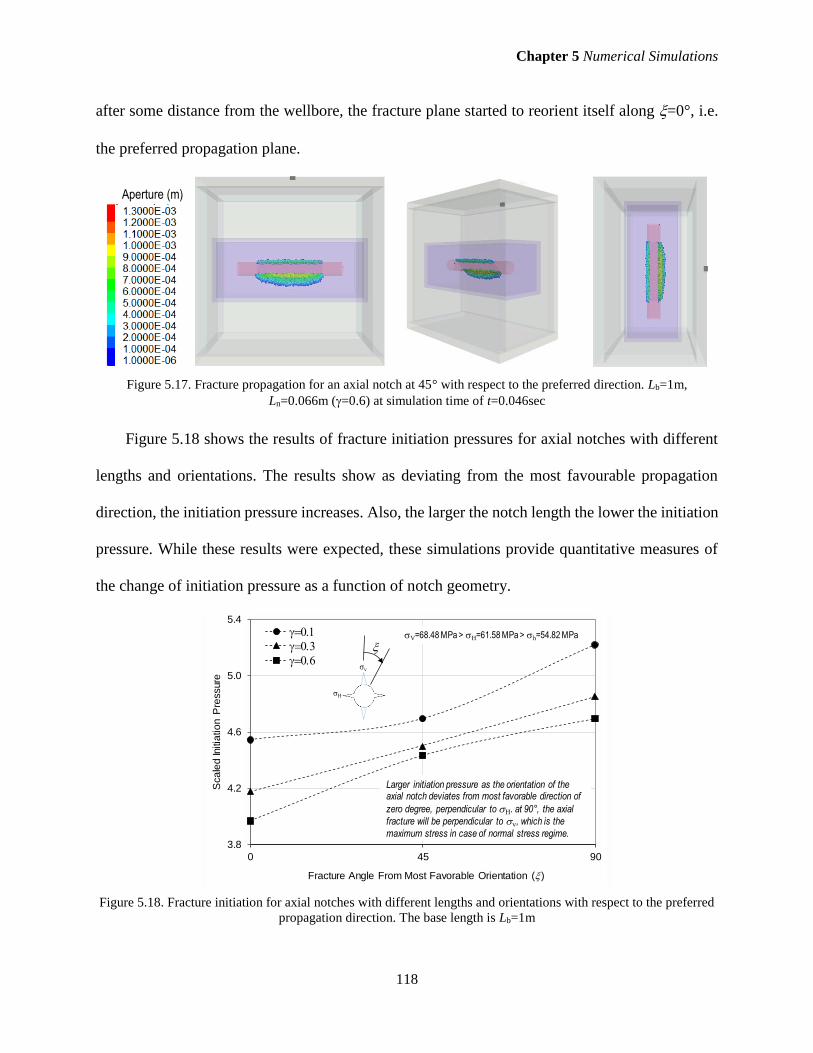
Chapter 5 Numerical Simulations
118
after some distance from the wellbore, the fracture plane started to reorient itself along =0°, i.e.
the preferred propagation plane.
Figure 5.17. Fracture propagation for an axial notch at 45° with respect to the preferred direction. Lb=1m,
Ln=0.066m (=0.6) at simulation time of t=0.046sec
Figure 5.18 shows the results of fracture initiation pressures for axial notches with different
lengths and orientations. The results show as deviating from the most favourable propagation
direction, the initiation pressure increases. Also, the larger the notch length the lower the initiation
pressure. While these results were expected, these simulations provide quantitative measures of
the change of initiation pressure as a function of notch geometry.
Figure 5.18. Fracture initiation for axial notches with different lengths and orientations with respect to the preferred
propagation direction. The base length is Lb=1m
3.8
4.2
4.6
5.0
5.4
0 45 90
Sca
led
Initia
tio
n P
ressure
Fracture Angle From Most Favorable Orientation ()
0.1
0.3
0.6
Larger initiation pressure as the orientation of the axial notch deviates from most favorable direction of
zero degree, perpendicular to H. at 90°, the axial
fracture will be perpendicular to v, which is the
maximum stress in case of normal stress regime.
V=68.48 MPa > H=61.58 MPa > h=54.82 MPa
v
H
Aperture (m)

Chapter 5 Numerical Simulations
119
5.5 Multiple Fractures
In real field OH cases, there are multiple natural fractures intersecting the wellbore at different
orientations with different lengths and geometry. The induced fracture tends to initiate initially
from the weakest notch, based on the detailed discussions presented in the previous sections and
also in the previous Chapter. Understanding the location of the weakest notches along the OH
section is of paramount importance in terms of design of the multistage fracturing and determining
if there will be need to create a weaker notch that existing natural fractures along a given OH
section to dominate the existing cracks and act as the initiation point for induced fracture.
5.5.1 Axial Star Fractures
The case of multiple axial (star cracks) is perhaps one of the simplest type of multiple fractures
that one can consider for simulations. This is similar to the geometry for which the analytical
models were presented in Subsection 4.5.2, in the preceding Chapter. Figure 5.19 presents the
geometry of the model with 8 cracks of equal distance around the wellbore. Notch length of
Ln=0.066m (=0.6) with a base length of Lb=1m was used for simulation purposes. All fractures
have similar initial aperture of 1×10⁻⁵m. Figure 5.20 shows the aperture plots around the wellbore
and fracture pressure and crack numbers versus time as well as the after 0.05sec simulation time.
From this Figure it is seen that the initiation started initially from the notch oriented at =0°, i.e.
the direction perpendicular to H (least stress in this geometry) with larger aperture comparing to
other cracks.
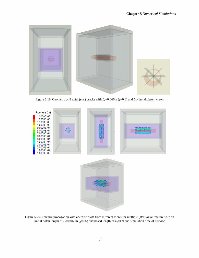
Chapter 5 Numerical Simulations
120
Figure 5.19. Geometry of 8 axial (star) cracks with Ln=0.066m (=0.6) and Lb=1m, different views
Figure 5.20. Fracture propagation with aperture plots from different views for multiple (star) axial fracture with an
initial notch length of Ln=0.066m (=0.6) and based length of Lb=1m and simulation time of 0.05sec
Aperture (m)

Chapter 5 Numerical Simulations
121
Figure 5.21 shows the pressure and crack numbers versus time plot for the 8 cracks model. The
fracture initiation pressure is approximately 78MPa, which is slightly larger than its corresponding
bi-wing case of 74MPa (see Figure 5.11). From analytical models presented in subsection 4.5.2 of
Chapter 4, it is found that the shape coefficient (Fn) for the case of 8 cracks with Ln=0.066 is
Fn=0.765 (Equation 4.52). Multiplying this coefficient by the weight factor f of equation 4.43, and
doing the calculations using equation 4.41, the initiation pressure is estimated to be 64.3MPa,
which is less than what was seen from the numerical simulations. This underestimation could be
due to the ignorance of pressure drop due to the friction and flow convergence effect around the
wellbore that is ignored in the analytical models.
Figure 5.21. Fracture pressure and crack numbers versus time plot for 8 axial fracture model geometry
5.5.2 Multiple Transverse Fractures
The first example in this Section represents simulation of three vertical transverse fractures as
shown in Figure 5.22. From right to left, the fractures are perpendicular, parallel and at 45° with
respect to h, or wellbore axis. The fracture parallel to the wellbore axis is indeed an axial fracture
with a circular geometry. The model contains two resolution domains and used the same data as
previous models for comparison purposes. The fracture apertures are illustrated in Figure 5.23. As
0
140
280
420
560
700
0
20
40
60
80
100
0.000 0.010 0.020 0.030 0.040
Cra
ck N
um
be
rs
Fra
ctu
re I
nitia
tio
n P
ressure
(M
Pa
)
Simulation Time (Sec)
Initiation pressure for multiple cracks (here 78MPa) is expected
to be larger than equivalent bi-wing crack (74MPa). The analytical model suggests this to
be app. 64.3MPa)
FIP=78 MPa
Star Fracture (8 Axial Cracks): Ln=0.066m, =0.6, Lb=1m

Chapter 5 Numerical Simulations
122
one expects, the fracture perpendicular to h (the rightest fracture in this Figure) is the fracture
which took the fluid first and has the largest opening and propagation. As the notch size is
adequately large, we expect to be on the right side of the cross over point, hence the axial transverse
fracture dominates over the axial one.
Figure 5.22. Model geometry of three transverse fractures perpendicular, parallel and at 45° with respect to wellbore
axis. View from the top (left) and front (right)
Figure 5.23. Fracture apertures (different views) for the model with three transverse fracture with different
orientations
As a second example, similar to the axial star fractures transverse fractures with different
orientations were modelled to examine how they compete in receiving the fluid and acting as the
main fracture initiation point. Figure 5.24 shows the geometry of 8 wings transverse fractures
Aperture (m)

Chapter 5 Numerical Simulations
123
equivalent to =0.6. two cylindrical resolution domains of 2.2cm and 4.4cm have been considered
around the wellbore with the remaining part of the model having resolution of 8.8cm. The wellbore
ais long h, so the fracture perpendicular to the wellbore axis is the most favourable one to open.
Figure 5.25 confirms this as it shows that the apertures of this fracture after a simulation time of
0.028sec are larger than other fractures. It is interesting to see that the fracture parallel to the
wellbore axis, which in fact is an axial fracture, has initiated slightly and the other two fracture
sets with orientation of 45° and 135° with respect to the most favourable propagation plane have
relatively similar openings, as expected. The results of this simulation also show the effect of
fracture geometry and orientation and field stresses on the effectiveness of notches to act as the
initiation point.
Figure 5.24. Geometry of 8 wings transverse fractures used for HF simulations. Perspective view (left) and plan
view (right). All cracks have similar scaled length of =0.6

Chapter 5 Numerical Simulations
124
Figure 5.25. Fracture apertures after simulation time of t=0.028sec. Perspective view (left) and from above
(right)
5.5.3 Random Fractures
In real cases, the distribution of natural fractures is random and based on the analysis of image
logs it may follow a Gaussian distribution. Here, the objective is not to simulate complex real
examples of natural fractures around the wellbore, however, to explain the application of the
knowledge gained from this study to determine which of the natural fractures may act as the seed
point to initiate the hydraulic fracture, as an example, 6 natural fractures with different orientations
and lengths were considered for simulation purposes. Figure 5.26 shows the geometry of the
fractures from above (top) and front (bottom) views. The most left and right fractures (#1 and 6)
represent transverse notches with radius of 0.2m and 0.14m, respectively. The second and third
fractures from left (#2 and 3) represent two axial notches, first one oriented horizontally along the
least favorable direction (i.e. =90°) with Ln=0.18m and Lb=0.5m, the second one vertically
oriented along the most favorable direction (i.e. =0°) with Ln=0.28m and Lb=0.4m (note that Ln
is the length of one side of the notch from the wellbore wall). Two fractures are also considered
with dip and dip directions of 45°/30° and 135°/60°, respectively (#4 and 5) with the length and
width along the fracture plane of 0.4m and 0.5m for the first and 0.7m and 0.286m for the second
notch. All fractures have similar initial aperture of 1×10⁻⁵m.
Aperture (m)

Chapter 5 Numerical Simulations
125
Figure 5.26. Six notches with random orientations and sizes used to simulate fracture initiation. Views from the top
(top) and front (bottom)
Figure 5.27 and 5.28 show the fracture apertures after simulation time of t=0.0475sec and
t=0.488sec, respectively. from these Figures, it is seen that the apertures in vertical axial fracture
(#3) started to open before other fractures and continued to propagate longer with higher apertures
than other fractures. Comparing to axial fracture #2, this notch is weaker and more prone to open
as it is oriented along the most favourable orientation and its length (Ln=0.28m) is larger than
fracture #2, even though its base length is slightly smaller. Comparing to transverse fractures,
while the length of this fracture is slightly less than fracture #1 (Ln=0.2m), it appears that it is still
less than the minimum length of the cross over point, so the axial fracture is dominant. The two
#1 D/DD=90°/0°
Ln = r = 0.20m
#6 D/DD=90°/0°
Ln = r = 0.14m
#2 D/DD=0°/90°
Ln = 0.18m
Lb = 0.50m
#3 D/DD=90°/90°
Ln = 0.28m
Lb = 0.40m
#4 D/DD=45°/30°
#5 D/DD=135°/60°
Lb = 0.50m
Lb = 0.18m

Chapter 5 Numerical Simulations
126
oriented notches #4 and #5 compete in taking the fluid to this time of simulation but look to be
more competent than both transverse fractures.
Figure 5.27. Fracture apertures after t=0.0475sec simulation time. Views from the top (top) and front (bottom)
Figure 5.28. Fracture apertures after t=0.488sec simulation time. Views from the top (top) and front (bottom)
Aperture (m)
Aperture (m)

Chapter 5 Numerical Simulations
127
In real field cases, in order to design the notch geometry in order to confine the location of
the fracture initiation, the FMI and other image logs may be utilized to extract the geometry of
natural fractures around the wellbore. With currently available advanced commercial software
packages this is straightforward to do. Figure 5.29 shows an example of natural fractures dip events
picked, categorized, and displayed by using the Schlumberger’s Techlog wellbore software
platform with data from the FMI-HD microimager. Natural fractures 3D geometry is presented in
the second track and the last track shows the dip and dip direction analysis. Extracting the geometry
of natural fractures in each HF stage and conducting similar analysis presented in this study using
simulations and analytical models will help to identify the most likelihood fractures which will be
the initiation point of an induced fracture and if necessary notches can be designed and created to
control the location of the fracture initiation. While from the image logs the type of fractures (e.g.
open, close, semi-close, conductive), orientation and aperture can be defined, estimation of the
fracture length (i.e. the penetration into the formation) may not be easily calculated. This is a topic
that needs further studies to establish a specific algorithm to extract the fracture data with their use
in this type of study from the image logs and other tools, including sonic scanner.
Figure 5.29. Natural fractures dip event extracted from the FMI-HD microimager using the Techlog platform (image
is courtesy of Schlumberger)

Chapter 5 Numerical Simulations
128
5.6 Summary
In this Chapter the results of XSite numerical simulations of hydraulic fracturing with pre-existing
transverse and axial notches were presented. The effect of notch size on fracture initiation pressure
and geometry of the propagated fracture near wellbore were discussed. It was seen that the stress
anisotropy is the dominant parameter in competition between transverse and axial notch creation.
The larger the stress anisotropy the easier for transverse fracture to initiate at smaller notch length.
For isotropic stress fields, it was seen that creation of transverse fracture, even with a very large
notch size is challenging. For the case of axial fracture, it was observed that the base length plays
an important role in initiation of fracture. The smaller the notch base length the less opportunity
for the fluid to flow into the fracture and even with large fracture length, the fracture cannot
propagate symmetrically and penetrate into the formation. The results of simulations presented
were compared with analytical models of the previous Chapter and it was seen that the analytical
models, due to their simplified assumptions, underestimate initiation pressure and also may not
consider realistically the geometry of the fractures, especially in case of axial fracture. Extension
of the simulations to the multiple fractures including star cracks showed the competition between
different notches in initiating the fracture, depending on their size, geometry and orientation. These
findings will help to analyze the natural fractures along an OH section of the wellbore from the
image logs before HF operation to predict the likelihood location of the fracture initiation and
creating notches as required to dictate the location of fracture initiation.
Chapter 6 Conclusions and Recommendations
129
CHAPTER 6
Conclusions and Recommendations
The effect of transverse and axial pre-existing cracks (notch) on fracture initiation pressure was
studies in details as part of this research project. The first Section of this Chapter lists the main
conclusions made from this work and the second Section presents some of the future work that is
recommended as continuation of this study.
6.1 Conclusions
From this study the following conclusions are drawn:
OH completion is more favorable over CH completion due to larger production and less costs
and operational complexity. Creating properly designed pre-existing cracks (notches) along
the OH section of each stage of a multi-stage HF can dictate the point of fracture opening and
avoid unfavorable single or multiple fracture growth around the wellbore which is one of the
issues in OH HF operation.
The design of proper notch geometry in an OH section of a horizontal wellbore can dominate
the fracture initiation to start from this point instead of existing natural fractures and defects
along the lateral at unfavorable locations. It also reduces the fracture initiation pressure and
mitigates the near wellbore damage and tortuosity.
Chapter 6 Conclusions and Recommendations
130
The only controllable parameters during fracturing operation are the injection rate and fluid
viscosity. These parameters individually and their combined effect, i.e. pressurization rate,
have great influences on the type of fractures initiating in an OH HF operation.
Analytical models are of great use to obtain preliminary information about the impact of the
notch on fracture initiation pressure and how different parameters influence it. However, each
of them have simplified assumptions which result in deviating from the real cases. Therefore,
conducting numerical simulations, before field trial is of great importance.
The superposition law is an effective analytical method to estimate the influence of different
parameters on fracture initiation pressure.
The results of analytical models indicated that for slow pressurization, and anisotropic stress
case, the crack is unstable for very small crack sizes of less than about 10% of the wellbore
radius and then becomes stable until it starts to become unstable again when propagates several
radius of the wellbore. In contrary, in isotropic case, the crack is unstable for all crack lengths,
i.e. the pressure to propagate crack is reducing as crack length becomes larger.
The results of analytical models showed that for fast pressurization, for both isotropic and
anisotropic stresses, the crack is unstable when its length is less than about 10% of the wellbore
radius, and then becomes stable. It is also noted that he critical borehole pressure to open the
crack is much larger in case of fast pressurization than that of slow pressurization. Also, the
change of pore pressure has no impact on critical pressure in case of fast pressurization.
From practical point of view, generation of transverse fractures are more favorable than axial
(longitudinal) fractures. Among other parameters, design of proper notch geometry can
facilitate generation of the transverse over axial fractures in some cases.

Chapter 6 Conclusions and Recommendations
131
Among other parameters, it is evident that stress anisotropy has a dominant effect on whether
transverse or axial fracture will initiate from an OH lateral.
Theoretically, in absence of any pre-existing notch, or ineffective notches (e.g. inadequate
length) axial fractures dominate and initiate from multiple section of the wellbore. In this case,
the fracture initiation pressure becomes very large.
Analytical models showed that minimum initiation pressure to open a fracture reduces as the
notch size increases. However, for notches less than a certain length the axial notch is
dominant, whereas, exceeding this limit, the transverse fracture is more favorable to open. The
notch length at which this change of behavior is observed is mostly affected by the stress
anisotropy. As the stress anisotropy increased this cross over point shifts to the left, i.e.
transverse fractures can open with smaller notch size. For fully isotropic stresses it was
observed that the axial fracture is always dominant.
Assuming a horizontal wellbores drilled along minimum stress direction, in case of axial
fractures, in different directions it was seen that the cross over point moves to the right as the
axial fracture is further oriented towards its most favorable direction. This means that larger
notches are needed to dominate transverse fractures.
Multiple fractures are expected to occur when pressurization rate is fast (i.e. the rise time of
the driving pressure pulse is relatively short compared with the time required for stress waves
to circle the cavity). This situation is happening more likely in case of axial fracture. The results
of analytical models showed that in this case, as the number of fractures increases, cross over
point moves to the left, i.e. less notch length can result in transverse fracture to dominate the
axial fracture.

Chapter 6 Conclusions and Recommendations
132
XSite software, which is a lattice based DEM numerical simulator, and works based on the
analysis of particles forces and displacement, showed great capabilities to simulate near
wellbore hydraulic fracturing and takes into consideration the effect of notch in OH
completion.
The coupled mechanical and fluid model implemented in XSite can simulate real geometry of
the fracture depending on stress regime and rock inhomogeneity. It was seen that using correct
resolution in modelling is perhaps the most important key factor to generate realistic results.
The use of resolution domains helps to reduces the running time.
In 3D numerical simulations, as opposed to the 2D analytical models, for the case of axial
fracture, in addition to the notch length, the length of the notch along the wellbore axis is a
secondary parameter to be considered in model geometry. It was seen that this base length has
a great impact on the initiation and propagation of fractures.
The results of numerical simulations when compared with analytical models, showed that, in
general, analytical models underestimate the initiation pressure, which is due to several
simplified assumptions that are used to develop them.
The fracture geometry looks more symmetric and circular during the viscosity dominated
propagation regime, which is usually during the early time, and asymmetric and non-circular
in late time, when the propagation becomes toughness dominated.
It was observed that the initiation pressure is a function of the injection rate and fluid viscosity
and as these two parameters are increasing the initiation pressure becomes larger.
The initiation point in XSite models can be determined at the time when the entire cracks
around the notch perimeter are broken.

Chapter 6 Conclusions and Recommendations
133
The simulation results for both axial and transverse fractures showed that the cross over point
is at larger notch length compared to the analytical models. This means that in real cases, larger
notch sizes should be made to dominate initiation of transverse fracture. However, as the axial
fracture base length is reduced, the cross over point shifts to the left.
As the base length of the axial fracture becomes less, the fluid cannot flow easily into the crack,
which results in higher initiation pressures, less effectiveness of the notch and more axial
fractures being developed around the wellbore axis.
As the notch length increases the notch area and perimeter increases exponentially. This results
in more cracks to be broken to reach the fracture initiation point. Also, the larger the notch
length, the earlier to reach the fracture initiation point, which is due to the fact that the injecting
fluid can more easily penetrate into the crack and also has larger area, hence more power to
open and propagate the fracture.
In general, comparing the same notch lengths, axial fractures result in higher apertures than
transverse fractures due to their larger area open to the fluid flow.
Depending on the geometry of the notch, the initiation pressure and the effectiveness of the
notch may be different.
6.2 Recommendations
Several ideas and potential applications of notched driven OH HF were mentioned throughout this
study, which require further investigations. Here, some of these ideas are recommended as
continuation of this study:
Expanding the analytical models in 3D will be a great expansion of this work to compare their
results with the simulations.

Chapter 6 Conclusions and Recommendations
134
Developing the 2D and 3D analytical models to determine the stress intensity factor and notch
geometry effects on HF initiation pressure in transverse isotropic (TI) formations representing
shales will carry great applications as shale plays require HF treatment for enhanced
production.
XSite simulations do not consider the effect of compressibility of the system including the
wellbore or drillstring, while this effect cannot be neglected. This effect should be considered
in the future simulations and the possibility of adding this feature to XSite will be beneficial
for future research.
Using the anisotropic rock properties features in XSite to simulate notch driven HF in OH
completion is an application to further study. The existing feature in XSite allows to consider
two Young’s Modulus and permeabilities for the rock in two orthogonal directions replicating
shales.
While in this study we considered a radial notch in case of transverse fracture and a rectangular
notch geometry for axial fracture, due to their closeness to real fracture geometry that are
expected to be propagated, one may simulate the impact of other type of notch geometry (e.g.
pyramid) to see the extend of the changes in the result. If any specific geometry will favor the
initiation of transverse fracture, that may be considered for possible field implications.
While the FMI and other image logs can be used to determine the type of natural fractures (e.g.
open, close, conductive) and their aperture and length marked on the wellbore wall,
determining the length of these fractures penetrating into the formation (i.e. depth) is not
straight forward. Investigation of the use of the image logs in combination with sonic scanner
or the use of any other methods to estimate the depth of natural fractures will be important in
order to design proper notch geometry in a section of OH.

Chapter 6 Conclusions and Recommendations
135
A few field scale notch makers have been proposed in OH HF. The operation of these tools are
mechanical or hydraulic. There is a big demand of studies in this area to propose a deployable
tool in order to make the required notch geometry and in specific orientation as fast as possible
with less inconvenience.

136
REFERENCE
Abass, H. H., Soliman, M.Y., Tahini, A.M., Surjaatmadja. J.B., Meadows. D.L., and Sierra.L., 2009.
Oriented Fracturing: A New Technique to Hydraulically Fracture Openhole Horizontal Well.
Proceedings - SPE Annual Technical Conference and Exhibition:124483.
Aidagulov, G., Alekseenko, O., Chang, F.F., Bartko, K., Cherny, S., Esipov, D., Kuranakov, D., and Lapin,
V., 2015. Model of hydraulic fracture initiation from the notched open hole. SPE178027-MS.
Al-Naimi, K.M,. Lee, B.O., Bartko, K.M., Kelkar, S.K., Shaheen, M and Johnston, B., 2008. Application
of a Novel Open Hole Horizontal Well Completion in Saudi Arabia. SPE Indian Oil and Gas
Technical Conference and Exhibition:113553.
Bagci, S., Castro, L., and Flores, J., 2017. Optimization of Hydraulic Fracturing and Production
Enhancement: Case Studies for US Shale Plays and Tight Sand Reservoirs. Society of
Petroleum Engineers - SPE Europec Featured at 79th EAGE Conference and Exhibition
(June):1057–81.
Bellarby, J., 2009. Well Completion Design.Developments in Petroleum Science.
Belyadi, H., Fathi, E., and Belyadi, F., 2019. Hydraulic Fracturing in Unconventional Reservoirs, Theories,
Operations, and Economic Analysis. 2nd edition. p 632
Bueckner, H.F., 1970. A novel principle for the computation of stress intensity factors. Z. angew. Math.
Mech. 50, 529-546.
Bunger, Andrew P., Emmanuel Detournay, and Dmitry I. Garagash. 2005. Toughness-Dominated
Hydraulic Fracture with Leak-Off. International Journal of Fracture 134(2):175–90.
Chang, F. F., Bartko, K., Dyer, S., Aidagulov, G., Suarez-Rivera, R., & Lund. J., 2014. Multiple fracture
initiation in openhole without mechanical isolation: First step to fulfill an ambition. SPE
Hydraulic Fracturing Technology Conference
Charlez, Ph.A. 1997, Rock Mechanics: Vol. 2 – Petroleum Applications, Editions Technip, Paris, 661 pp
Chen, Y., Meng, Q., and Zhang, J., 2018. Effects of the Notch Angle, Notch Length and Injection Rate on
Hydraulic Fracturing under True Triaxial Stress: An Experimental Study. Water 2018, Vol. 10,
801.
Cundall, P. A. 2011. Lattice method for modeling brittle , jointed rock. C Continuum and Distinct Element
Numerical Modeling in Geomechanics
Damjanac. B., Detournay. C., Cundall. P., Puvance. M., Hazzard. J. 2011. XSite Description of Formulation
Revision I
Damjanac, Branko., Detournay. C and Cundall. P.A. 2016. Application of Particle and Lattice Codes to
Simulation of Hydraulic Fracturing. Computational Particle Mechanics 3(2):249–61
De Pater, C.J., Cleary, M.P., Quinn, T.S., Barr, D.T., Johnson, D.E., and Weijers, L., 1994. Experimental
verification of dimensional analysis for hydraulic fracturing. SPE Prod Facil Vol 9(4), p.p 230–
238.
Detournay, E. 2004. Propagation Regimes of Fluid-Driven Fractures in Impermeable Rocks. International
Journal of Geomechanics 4(1):35–45.
Detournay, E., and Carbonell, R., 1997. Fracture-mechanics analysis of the breakdown process in
minifracture or leakoff test. SPE production and facilities. p.p 195-199.
Dunn, M.L., and Suwito, W., 1997. Fracture initiation at sharp notches: correlation using critical stress
Intensities. Int. J. Solids Structures Vol. 34, No. 29, p.p. 3873~3883.
Economides, M.J., Nolte, K.G., 2000. Reservoir stimulation, 3rd edition. Wiley, New York
Ellis, P. D., Kniffin, G. M and Harkrider, J. D., 2007. Application of Hydraulic Fractures in Openhole
Horizontal Wells. SPE/Petroleum Society of CIM 65464
Fallahzadeh, S. H., James Cornwell, A., Rasouli, V and Hossain, M .,2015. The Impacts of Fracturing

137
Fluid Viscosity and Injection Rate on the near Wellbore Hydraulic Fracture Propagation in Cased
Perforated Wellbores. 49th US Rock Mechanics / Geomechanics Symposium 2015. 2:984–1001.
Fallahzadeh, S.H., Hossain,M., Cornwell, AJ and Rasouli,V., 2017. Near Wellbore Hydraulic Fracture
Propagation from Perforations in Tight Rocks: The Roles of Fracturing Fluid Viscosity and
Injection Rate. Energies V10. Issue(3).
Gandossi, L., 2013. An Overview of Hydraulic Fracturing and Other Formation Stimulation Technologies
for Shale Gas Production.
Glinka, G., 1996. Development of weight functions and computer integration procedures for calculating
stress intensity factors around cracks subjected to complex stress fields. A report prepared for
Analytical Services& Materials, Inc.
Gottschling, J. C., 2005. Openhole vs Cased-Hole Hydraulic Fracturing. SPE 97172.
Haimson.. B and C. Fairhurst. Initiation and extension of hydraulic fractures in rocks. SPEJ, Dec., 310-
318, 1967
Huitt, J. L., 1960. Hydraulic Fracturing with the Single-Point Entry Technique. Journal of Petroleum
Technology 12(03):11–13.
Hussain, M.K and Murthy, K.S.R.K., 2019. Evaluation of mixed mode (I/II) notch stress intensity factors
of sharp V-notches using point substitution displacement technique. Vol. 48 pp. 599-610.
Jeffrey, RG., Zhang, X., 2010. Mechanics of Hydraulic Fracture Growth from a Borehole. CSUG/SPE
137393. Pages 1112-1121
Kirsch, G., 1898, Die Theorie der Elastizitat und die Bediirfnisse der Festigkeitslehre: Zeitschr. Ver.
Deutsch. Ingenieure, v. 42, p. 797
Lecampion, B., Abbas, S., Prioul, R., 2013. Competition between transverse and axial hydraulic fractures
in horizontal wells. SPE163848.
Lecampion, B., Desroches, J., Jeffrey, R.G., and Bunger, A.P., 2017. Experiments versus theory for the
initiation and propagation of radial hydraulic fractures in low‐permeability materials. J. Geophys.
Res. Solid Earth, 122, p.p 1239–1263
Lhomme, T.P.Y, 2005. Initiation of hydraulic fractures in natural sandstones. Master Thesis in
Geomechanics, University of Minnesota
Leguillon, D., and Yosibash, Z., 2003. Crack onset at a v-notch. Influence of the notch tip radius.
International Journal of Fracture 122: 1–21.
Martinez, E.R., Farias, M.M., and Junior, F.E., 2019. Investigation of the notch angle in hydraulic fracturing
using XFEM. Journal of the Brazilian Society of Mechanical Sciences and Engineering.
Nakagawa, S., Rutqvist, J., Kneafsey, T., Kim, K., Birkholzer, J., and Prieto, H., 2016. Laboratory and
Numerical Investigation of Hydraulic Fracture Propagation and Permeability Evolution in
Heterogeneous and Anisotropic Shale. Lawrence Berkeley National Laboratory.
Nilson, R.H., and Proffer, W.J., 1984. Engineering formulas for fractures emanating from cylindrical and
spherical holes. J. Appl. Mech. 51:929-933
Patutin, A., and Serdyukov, S., 2017. Transverse Hydraulic Fracture Initiation by Indentation in an Uncased
Borehole. Procedia Engineering 191, pp. 287 – 290
Potyondy, D.O.., Cundall, P.A., 2004. Abbonded particle model for rock. International Journal of Rock
Mechanics and Mining Sciences.p.p 1329-1364
Qiu. D., Rasouli .V., Damjanac.B., and Wan.X., 2019. Narrow versus Wide Fairway Fracture
Geometry.53rd U.S. Rock Mechanics/Geomechanics Symposium.
Rasouli, V., Zacharia, J., and Elike, M., 2011. The influence of perturbed stresses near faults on drilling
strategy: A case study in Blacktip field, North Australia. Journal of Petroleum Science &
Engineering. 76: 37-50.
Renpu, W., 2011. Advanced Well Completion Engineering.Third edition. p.p 256-293
Rice, J.R., 1972. Some remarks on elastic crack-tip stress fields. Int. J. Solids Structures. Vol. 8, pp. 751-
758.

138
Rummel, F. (1987). Fracture Mechanics Approach to Hydraulic Fracturing Stress Measurements. In:
Fracture mechanics of rock. Ed. by Atkinson, B. K. Academic Press geology series. London:
Academic Press, pp. 217–239.
Schwartzkopff, A.K. 2017. Breakdown pressure and propagation surface of a hydraulically pressurized
circular notch within a rock material. Ph.D. Dissertation, University of Adelaide.
Song, H., and Rahman, S., 2018. An extended J-integral for evaluating fluid-driven cracks in hydraulic
Fracturing. Journal of Rock Mechanics and Geotechnical Engineering Vol. 10, pp. 832-843.
Vahid , S. and Ghassemi, A. 2011. Hydraulic Fracture Initiation from a Wellbore in Transversely
Isotropic Rock. 45th US Rock Mechanics / Geomechanics Symposium.
Weijers, L., De Pater, C.J., Owens, K.A., and Kogsboll, H.H., 1994. Geometry of hydraulic fractures
induced from horizontal wellbores. SPE production and facilities.
Williams, M. L. (1952) Stress singularities resuIting from various boundary conditions in angular corners
of plates in extension. Journal 0/ Applied Mechanics 74, 526-528.