Simulation of an SEIR infectious disease model on the

dynamic contact network of conference attendees

Juliette Stehlé1, Nicolas Voirin2,3§, Alain Barrat1,4, Ciro Cattuto4, Vittoria Colizza5,6,7,

Lorenzo Isella4, Corinne Régis3, Jean-François Pinton8, Nagham Khanafer2,3, Wouter

Van den Broeck4 and Philippe Vanhems2,3

1Centre de Physique Théorique de Marseille, CNRS UMR 6207, Marseille, France2Hospices Civils de Lyon, Hôpital Edouard Herriot, Service d’Hygiène, Epidémiologie et

Prévention, Lyon, France3Université de Lyon; université Lyon 1; CNRS UMR 5558, laboratoire de Biométrie et de

Biologie Evolutive, Equipe Epidémiologie et Santé Publique, Lyon, France4Complex Networks and Systems Group, Institute for Scientific Interchange (ISI) Foundation,

Torino, Italy5 INSERM, U707, Paris F-75012, France6 UPMC Université Paris 06, Faculté de Médecine Pierre et Marie Curie, UMR S 707, Paris

F75012, France

7Computational Epidemiology Laboratory, Institute for Scientific Interchange (ISI)

Foundation, Torino, Italy8Laboratoire de Physique de l’Ecole Normale Supérieure de Lyon, CNRS UMR 5672, Lyon,

France§Corresponding author

Email addresses:

JS: juliette.stehle@gmail.com

NV: nicolas.voirin@chu-lyon.fr

AB: alain.barrat@cpt.univ-mrs.fr

CC: ciro.cattuto@isi.it

VC: vcolizza@inserm.fr

LI: lorenzo.isella@isi.it

CR: corinneregis@yahoo.fr

JFP: jfpinton@gmail.com

NK : nagham.khanafer@chu-lyon.fr

WVdB : wouter.vandenbroeck@isi.it

PV : philippe.vanhems@chu-lyon.fr

- 1 -

Abstract

Background

The spread of infectious diseases crucially depends on the pattern of contacts among

individuals. Knowledge of these patterns is thus essential to inform models and

computational efforts. Few empirical studies are however available that provide

estimates of the number and duration of contacts among social groups. Moreover,

their space and time resolution are limited, so that data is not explicit at the person-to-

person level, and the dynamical aspect of the contacts is disregarded. Here, we want

to assess the role of data-driven dynamic contact patterns among individuals, and in

particular of their temporal aspects, in shaping the spread of a simulated epidemic in

the population.

Methods

We consider high resolution data of face-to-face interactions between the attendees of

a conference, obtained from the deployment of an infrastructure based on Radio

Frequency Identification (RFID) devices that assess mutual face-to-face proximity.

The spread of epidemics along these interactions is simulated through an SEIR model,

using both the dynamical network of contacts defined by the collected data, and two

aggregated versions of such network, in order to assess the role of the data temporal

aspects.

Results

We show that, on the timescales considered, an aggregated network taking into

account the daily duration of contacts is a good approximation to the full resolution

network, whereas a homogeneous representation which retains only the topology of

the contact network fails in reproducing the size of the epidemic.

Conclusions

These results have important implications in understanding the level of detail needed

to correctly inform computational models for the study and management of real

epidemics.

- 2 -

Background

The pattern of contacts among individuals is a crucial determinant for the spread of

infectious diseases in a population (1). The topological structure, the presence of

individuals with a much larger number of contacts than the average value (2-5), the

clustering and presence of well-identified communities of individuals (6-10), the

frequency and duration of contacts (11-13) have important implications for the spread

and control of epidemics. Knowledge of contact patterns is critical for building and

informing computational models of infectious diseases transmission (14-23). Though

some of the properties of contact patterns are found to dramatically affect the model

predictions (3-5), little is known on their empirical characteristics, and few

experiments have been conducted to collect data on how individuals mix and interact.

The starting point of most modeling approaches consists in the homogeneous mixing

assumption for which every individual has an equal probability of contacting other

individuals in the population (1). No heterogeneity in the mixing pattern or in the

duration or frequency of the contact is considered, and the dynamical nature of the

contacts is disregarded. Going beyond this approximation, various approaches have

proposed to estimate mixing properties among classes of individuals (e.g. social or

age classes) using indirect (1) and, more recently, direct (11, 24-27) methods. Indirect

methods are based on estimating the elements of a “Who Acquires Infection From

Whom” (WAIFW) matrix using observed seroprevalence data. In direct methods,

each element of a contact matrix is estimated independently of the epidemiologic

data. Direct methods rely on data collection about at-risk events via diaries (11, 12) or

time-use data (2, 27). To date, research on human social interaction has been mainly

based on self-reported data. Despite a real improvement of the description of potential

contacts with respect to a homogeneous mixing approach, self-reported methods

involve a limited number of people who provide information on a limited number of

snapshots in time (usually one day). The obtained data may suffer from uncontrolled

bias and a lack of representativeness since it is not based on objective reports, and the

data collection is performed on a random day and generally lacks the longitudinal

aspect. These limitations become particularly relevant in the case of contact patterns

and infectious diseases transmitted by the respiratory or close-contact route. Here all

- 3 -

types of social encounters, even random contacts of very short duration e.g. on public

transport, may be important for the transmission, but are rather difficult to report

objectively and exhaustively through a diary method.

New technologies are now available that allow the tracking of proximity and

interactions of individuals (28-37), deeply transforming our ability to understand and

characterize social behavior (38). Detection of contact patterns can rely on objective

and unsupervised measures of proximity behavior, that can be extended to a large

number of individuals, with a high temporal and spatial resolution (28, 30), thus

overcoming the limitations of self-reported data. Departing from the typical static

representation of a network of contacts among individuals (39), it is now possible to

describe the dynamic nature of the interactions. The analysis of the dynamics of a

contact network needs to incorporate two essential features: (i) the variations in the

duration and frequency of the contacts between individuals, and (ii) the existence of

causality constraints in the possible chains of transmission.

Finally, little is known on the level of detail that should be incorporated in the

modeling effort to perform in practice realistic simulations of epidemics spreading in

a population. Very coarse descriptions of human behavior, such as the homogeneous

mixing hypothesis, leave out crucial elements. Conversely, extremely detailed

information may yield a lack of transparency in the models, making it difficult to

discriminate the impact of any particular modeling assumption or component.

The aim of this paper is to assess the role of the temporal aspects, and of the

heterogeneities and constraints of dynamical contact patterns in shaping the dynamics

of an infectious disease in a population using data collected during a two-day medical

conference. To this aim, we capitalize on the recent development of a data collection

infrastructure that allows the tracking of face-to-face proximity of individuals at a

high temporal resolution (28, 30). We use the data collected during a scientific

conference providing the temporal information on individual contact events. This can

be mapped into a dynamic network of contacts, where all information on interactions

between pairs of individuals, time of occurrence and duration are explicit in the

network representation. Along with the explicit dynamic network of contacts, we

consider two different projections of the data, defining two types of daily networks

that aggregate the empirical data in different ways, reflecting different amounts of

available knowledge about the contacts between individuals. We then simulate the

- 4 -

spread of an infectious disease over these networks, and highlight the role that

different features of contacts patterns and their dynamical aspects play during the

course of the simulated outbreak. The results have important implications to identify

the level of detail needed in the contact data in order to adequately and realistically

inform modeling approaches applied to public health problems.

Methods

Data collection platform & Deployment

Contact network measurements are based on the SocioPatterns RFID platform

(28,30). Individuals are asked to wear a badge equipped with an active Radio

Frequency IDentification (RFID) device (“tags”). RFID devices engage in bi-

directional radio communication at multiple power levels, exchanging packets that

contain a device-specific identificator. At low power level, packets can only be

exchanged between tags within a 1-2 meters radius (28, 30). This threshold has been

set in order to detect a close-contact situation during which a communicable disease

infection can be transmitted either following, for example, cough or sneeze, or

directly by physical contact. Individuals were asked to wear the RFID badges on their

chest, so that contacts are recorded only when participants face each other, as the

body acts as a shield for the proximity-sensing RF signals. In addition to sensing for

nearby devices, RFID tags send the locally collected contact information to a number

of receivers installed in the environment, which relay this information over a local

area network to a computer system used for monitoring and data storage. Proximity

scans are performed at random times and each tag dispatches information to the

receivers every few seconds. Time is then coarse-grained over 20 second intervals,

over which face-to-face proximity can be assessed with a confidence in excess of 99%

(28, 30). This time scale also is also adequate to follow the dynamics of social

interaction.

All communication is encrypted: from tag to tag, from tags to receivers, and from

receivers to the data storage system. Contact data are stored in encrypted form, and all

data management is completely anonymous. Other details on the data collection

infrastructure can be found elsewhere (28,30).

- 5 -

Participants attending the 2009 Annual French Conference on Nosocomial Infections

(www.sfhh.org) were asked to wear RFID tags. Face-to-face interactions between 405

voluntary individuals among the 1,200 attendees were collected during two days of

the conference (June 3rd and 4th, 2009). The data was collected from 9am to 9pm on

the first day and from 8.30am to 4.30pm on the second day (periods defined as “day”

in the following). Contacts were not recorded outside of these time periods (periods

defined as “nights”). Attendees to the conference signed a written informed consent.

The data have been collected anonymously. The ethics committee of Lyon university

hospital gave the agreement for this study.

Empirical contact networks

In order to assess the role of the dynamical nature of the network of contacts in the

spreading dynamics, we consider the network built on the explicit representation of

the dynamical interactions among individuals (referred to as DYN), at the shortest

available temporal resolution (20 seconds) against two benchmark networks that are

built on progressively lower amounts of information available on the interactions.

These are referred to as HET, and HOM.

Taking advantage of the full spatial and temporal resolution, DYN considers the

empirical sequence of successive contact events collected during the congress. Each

contact is identified by the RFID identification numbers of the two individuals it

involves, and by its starting and ending times. The resulting network is a dynamical

object that encodes the actual chronology and duration of contacts, therefore

preserving the heterogeneity in the duration of contacts, as well as the causality

constraints between events. The latter is particularly important for spreading

processes, as it may prevent the propagation along certain sequences of interactions

that would be otherwise allowed in an aggregated static representation of the contact

patterns. For example, if a susceptible individual A interacts first with an infectious

individual B and then with a susceptible C, a disease transmission can occur from B to

A and then from A to C. If instead A meets first C and later B, A can get infected

from B, but the propagation from B to A and then to C is not possible anymore.

The benchmark networks correspond to a coarse-graining of the data on a daily scale.

The first one, HET, is produced for each conference day by connecting individuals

who have been in contact during this conference day, thus aggregating all daily

dynamical information in a single snapshot, and weighting each link by the total time

- 6 -

the two individuals spent in face-to-face presence during the considered day.

Therefore, HET includes information on the actual contacts between individuals (who

has met whom) and on the total duration of these contacts (how long A has been in

contact with B during the whole day), but disregards information about the temporal

order of contacts. In the previous example, the transmission from A to C could take

place in both situations representing the different sequences of the events. It is a daily

aggregated network in which contacts are aggregated over a day but keeping the

whole neighborhood structure between individuals. As the conference lasted two

days, the aggregation procedure produces two such networks, one each day.

Finally, a homogeneous network (HOM) is constructed for each day by connecting

individuals who were in face-to-face contact during the conference day, again

aggregating all daily dynamical information in a single snapshot, but weighting each

link with equal weight, corresponding to the average duration of contacts between two

person that have met each other the same day in the HET network. The HOM

construction may correspond to networks constructed by asking each participant to

report with whom he or she has been in contact during the conference day and then

estimating for how long this lasted on average. For each conference day, HET and

HOM have exactly the same structure of interactions from a topological point of view,

and they differ by the assignments of weights on the links.

Generation of contact networks on longer timescales

Since we simulate the spreading of a realistic infectious disease characterized by

longer timescales than the data collection period, we introduce three different

procedures to longitudinally extend the data-driven network, by preserving some of its

features. The simplest procedure consists in repeating the two-day recordings. This

repetition procedure, denoted by “REP” in the following, is performed for the

dynamical sequence of contacts, and consistently for the set of daily HET and HOM

networks. In this simple procedure, each attendee repeated again and again the same

contacts for each simulated sequence of two days, i.e., always meets the same set of

other attendees, in the same order and during the same duration. While this procedure

yields a realistic contact pattern for each single day, as it uses only empirical data,

such a “deterministic” repetition is rather unrealistic as time goes on. We therefore

consider two additional procedures that improve this limitation.

- 7 -

The first one, “RAND-SH”, consisted in producing two-day sequences by randomly

reshuffling the participant's identities, as given by their tags IDs. The overall sequence

of contacts was preserved, but each contact occurs between different attendees from

one two-day sequence to the next. DYN networks were then constructed as before by

taking into account the 20 seconds temporal resolution, while HET and HOM

networks were obtained by aggregating the data for each day, as previously explained.

More realistic contact patterns are thus obtained, in a way that avoids the unrealistic

repetition of interactions between individuals. However, the RAND-SH procedure

completely erases correlations between the contact patterns of an attendee in

successive two-day sequences, which is also unrealistic. The analysis of the empirical

contact networks shows indeed that a correlation exists between the number of

contacts of an attendee in the first and second conference days and also that a fraction

of contacts are repeated from one day to the next. We therefore design a third

procedure for the generation of synthetic contact patterns starting from the two-day

sequence (“CONSTR-SH”) that constrains the reshuffling to preserve the correlations

between the attendees’ social activity as well as the same fraction of repeated contacts

between successive days. The description of the data extension procedure 'CONSTR-

SH’ is shown in the Additional Material.

It is important to note that in all cases we preserve the time frame during which data

was collected, since no collection occurred outside the conference premises. For this

reason, each individual was considered as isolated during the “nights” periods in the

DYN network. We therefore introduce such “nights” in the HET and HOM networks

by “switching off” the links (i.e., considering individuals as isolated) during these

periods, thus resembling the circadian pattern encoded in the empirical data.

Epidemiological model

We consider a simple SEIR epidemic model for the simulation of the infectious

disease spread in the population under study, in which no births, deaths or

introduction of individuals occurred. Individuals are each assigned to one of the

following disease states: susceptible (S), exposed (E), infectious (I), recovered (R).

The model is individual-based and stochastic. Susceptible individuals may contract

the disease with a given rate when in contact with an infectious individual, and enter

the exposed disease state where individuals are infected but not yet infectious.

- 8 -

Exposed individuals enter the I class at a rate σ with σ−1 representing the average

latent period of the disease. Infectious individuals can transmit the disease during

their infectious period whose average duration is equal to ν--1. After this period, they

enter the recovered compartment, acquiring permanent immunity to the disease.

In order to compare simulation results obtained from the three different networks, we

need to adequately define the rate of infection on a given infectious-susceptible pair,

depending on the definition of the networks themselves. Let us define β as the

constant rate of infection from an infected individual to one of his/her susceptible

contacts on the unitary time step dt of the process. Given then two individuals, an

infectious A and a susceptible B who are in contact during the unitary time step, the

probability of B becoming infected during this period is given by βdt. In order to

obtain the same average infection probability in the HET and HOM networks over an

entire day (day + night), the weights on such networks need to be rescaled by WAB/ΔT,

defined as the ratio between the total sum of the duration of all contacts between A

and B in a day and the effective duration of the day (i.e. total time during which the

links in the daily networks are considered active, discarding the “nights”). Therefore

the infection probability between A and B during the time step dt is βWAB dt/ΔT for

the HET network, and β<W> dt/ΔT for the HOM network (with <W> being the

average weight of the links in the HET network).

We consider two different disease scenarios for the spreading simulations on all

networks under study. In particular, the duration of the average latency period,

average infectious period and transmission rates assume the following values: (i) σ-

1=1 days, ν--1=2 days and β=3.10-4 s-1 (very short incubation and infectious periods);

(ii) σ-1=2 days, ν--1=4 days and β=15.10-5 s-1 (short incubation and infectious periods).

These sets of parameter values are chosen in order to maintain the same value of β/ν,

which is the biological factor responsible for the rate of increase of cases during the

epidemic outbreak, while changing the global timescales of incubation and infectious

periods, and assessing the role played by the social factors embedded in the contact

patterns. These values correspond to short incubation and infectious periods, in order

to minimize the consequences of the arbitrariness in the construction procedures of

long data sets as described previously. Each simulation started with a single randomly

chosen infectious individual, with the rest of the population in the susceptible state.

- 9 -

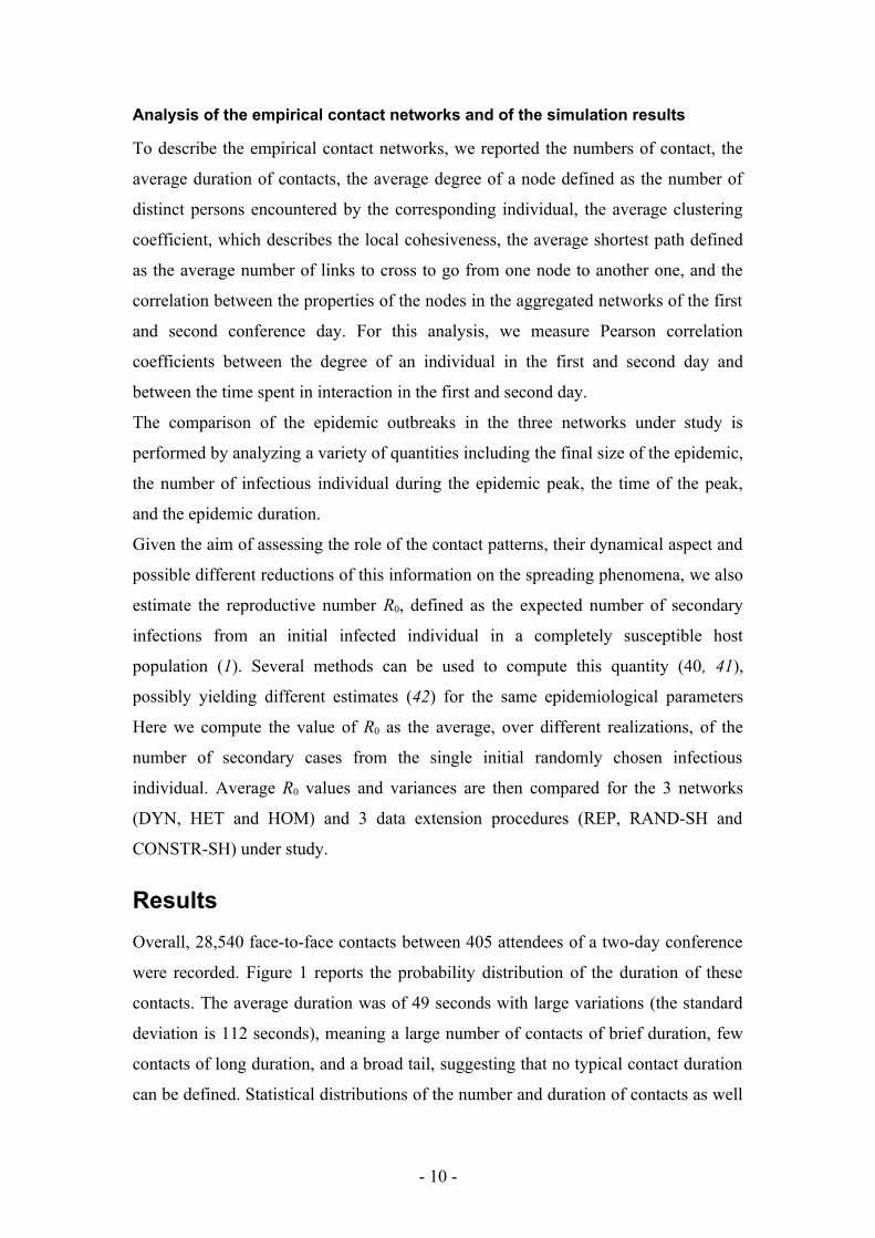
Analysis of the empirical contact networks and of the simulation results

To describe the empirical contact networks, we reported the numbers of contact, the

average duration of contacts, the average degree of a node defined as the number of

distinct persons encountered by the corresponding individual, the average clustering

coefficient, which describes the local cohesiveness, the average shortest path defined

as the average number of links to cross to go from one node to another one, and the

correlation between the properties of the nodes in the aggregated networks of the first

and second conference day. For this analysis, we measure Pearson correlation

coefficients between the degree of an individual in the first and second day and

between the time spent in interaction in the first and second day.

The comparison of the epidemic outbreaks in the three networks under study is

performed by analyzing a variety of quantities including the final size of the epidemic,

the number of infectious individual during the epidemic peak, the time of the peak,

and the epidemic duration.

Given the aim of assessing the role of the contact patterns, their dynamical aspect and

possible different reductions of this information on the spreading phenomena, we also

estimate the reproductive number R0, defined as the expected number of secondary

infections from an initial infected individual in a completely susceptible host

population (1). Several methods can be used to compute this quantity (40, 41),

possibly yielding different estimates (42) for the same epidemiological parameters

Here we compute the value of R0 as the average, over different realizations, of the

number of secondary cases from the single initial randomly chosen infectious

individual. Average R0 values and variances are then compared for the 3 networks

(DYN, HET and HOM) and 3 data extension procedures (REP, RAND-SH and

CONSTR-SH) under study.

Results

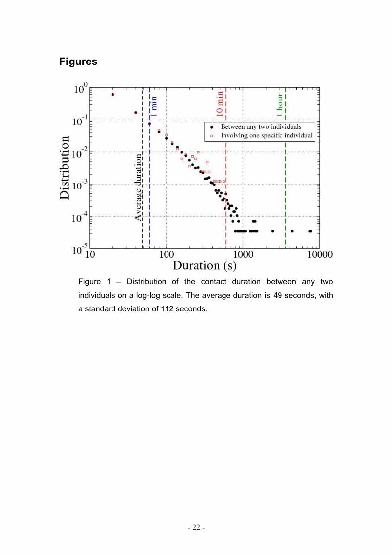
Overall, 28,540 face-to-face contacts between 405 attendees of a two-day conference

were recorded. Figure 1 reports the probability distribution of the duration of these

contacts. The average duration was of 49 seconds with large variations (the standard

deviation is 112 seconds), meaning a large number of contacts of brief duration, few

contacts of long duration, and a broad tail, suggesting that no typical contact duration

can be defined. Statistical distributions of the number and duration of contacts as well

- 10 -

as of the link weights were similar from one day to the next, although the two daily

contact networks are obviously not identical.

In the daily contact networks, the average degree of a node was close to 30, with a

distribution decaying exponentially for large numbers. The average clustering

coefficient was 0.28, much larger than the average value of 0.07 obtained for a

random network with the same size and average degree. The network was also a

small-world, with an average shortest path of 2.2.

The links weights were on the other hand broadly distributed, with an average

cumulated duration of the interaction between two attendees of 2 minutes. The total

duration spent in contact by any attendee was also broadly distributed, with an

average of 1h15mn. The Pearson correlation coefficient was 0.37 between the degree

of an individual in the first and second day, and 0.52 between the total time spent in

interaction in the first and second day. The fraction of repeated contacts in the second

day with respect to the first was of 12%, and was independent from the degree.

Figure 2 reports the distributions of R0 for the three networks, for the REP procedure.

In all cases, the number of secondary cases from the initial seed of the single

infectious individual ranges from 0, corresponding to the most probable event of no

outbreak, to around 20-25 individuals. Figure 3 and supplementary table 1 give the

average values and the variances obtained for the estimation of R0 depending on the

scenarios and the network type. In all scenarios, higher values of R0, together with

larger variances, are observed in the HOM network compared to the HET and DYN

networks.

Figure 4 shows the distribution of the final number of cases for the three networks and

the REP data extension procedure. A high probability of rapid extinction of the

pathogens spread is observed, corresponding to a small number of individuals who

become infected. This is slightly smaller in the HOM case compared to the HET and

DYN networks. On the contrary, when the epidemic starts, the final number of cases

is high, and it is larger in the HOM case as compared to the HET and DYN networks.

Intermediate cases with limited propagation are rare.

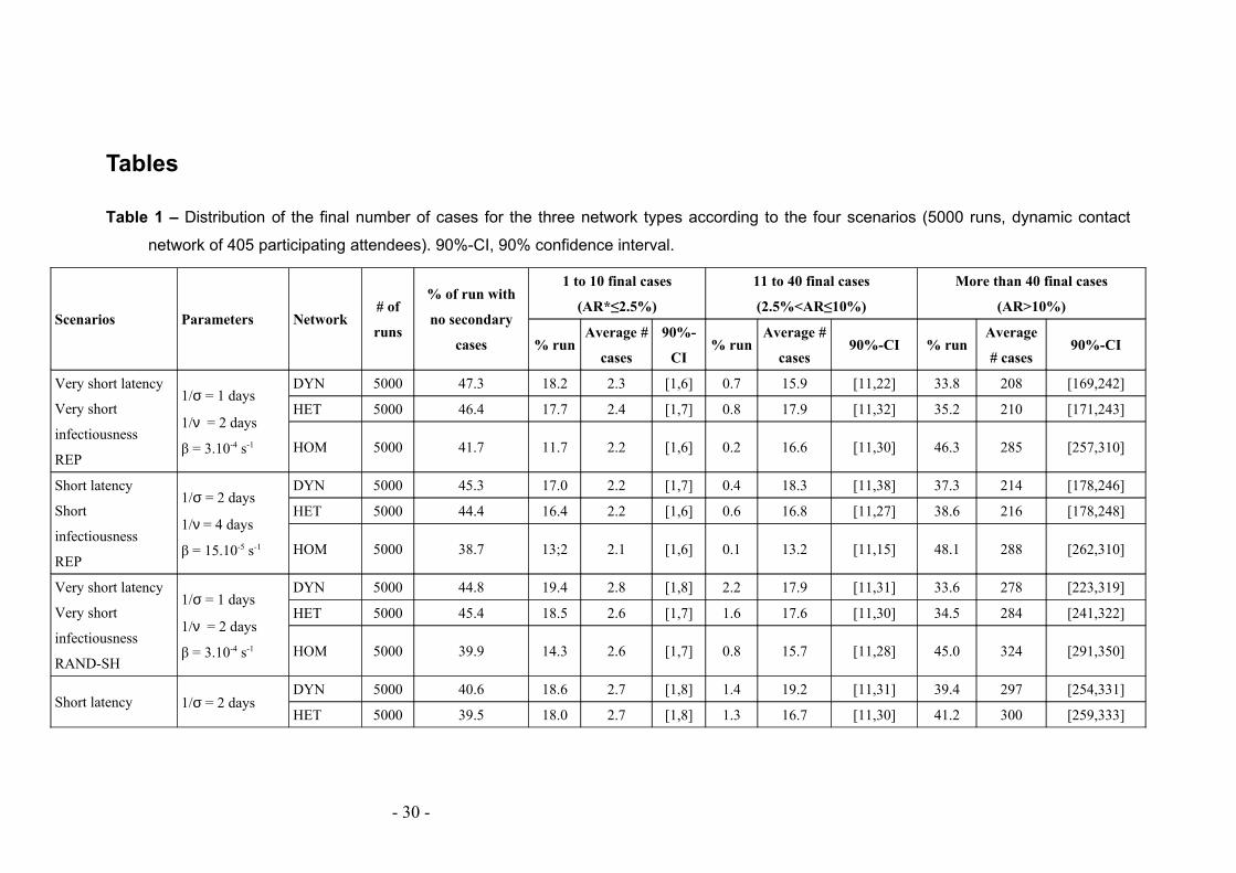
Table 1 and supplementary figure 4 summarize the distribution of the final number of

cases for the three networks for the various parameters of the SEIR model and in the

various data extension scenarios. For all cases, and independently from the procedure

adopted for extending the two-day data set, the probability of extinction is lower for

the HOM cases compared to the HET and DYN networks. In case of propagation, the

- 11 -

final size is higher in the HOM network compared to the HET and DYN networks.

Propagation over HET and DYN networks leads to similar extinction probability and

final number of cases. The final numbers of cases are also rather close in the two

disease scenarios.

Figure 5 and supplementary table 2 display the peak times of the spreading in the

various cases. In most cases, the epidemic peak is reached on average first for the

spreading on the HOM network. The differences between the peak times are however

small: even the simulations on the network with the least information give a good

estimate of the peak time obtained when including the full information on the contact

patterns.

Figures 6 and 7 display the temporal behavior of the spreading, through the evolution

in time of the number of infectious and recovered individuals, for the different data

extension procedures and for the two sets of SEIR parameters. Symbols represent the

median values and lines represent the 5th and 95th percentiles of the number of

infectious and recovered individuals. In all cases, the spreading on the HOM network

evolves slightly faster, and reaches a significantly larger number of individuals, while

spread on HET and DYN present very similar characteristics.

Figures 5 to 7 also highlight interesting differences in the results of simulations on

data sets extended with different procedures: the spread is slightly slower in the

RAND-SH case, but lasts longer, and as a result the final number of cases R∞ is

larger. In fact, we have systematically R∞(REP) < R∞(CONSTR-SH) < R∞(RAND-

SH): the more the identities of the tags are shuffled, the more efficient the spreading.

Discussion

Using a recently developed data collection technique deployed in a two-day

conference involving 405 volunteers, we have provided measurements of the

dynamics of contact (close face-to-face) interactions between individuals during such

a social event. We have used the data to compare the simulated spreading of

communicable diseases on this dynamic network and on two heterogeneous and

homogeneous networks obtained by aggregating the dynamic network at two distinct

levels of precision. To compensate for the relatively short duration of the data set (two

days), we have put forward different procedures to provide contact networks for an

- 12 -

extended time period during which the spread of an infectious disease can be

simulated.

The broad distributions of the various characteristics of the network analyzed in this

study have been, as expected, also observed in other contexts (30, 36, 37). In the

present case, we obtained results which are statistically similar to other conference

interaction networks, as reported in (30, 36). As also described in (30, 36), the

resulting picture is not characterized by the presence of “superspreaders” if defined in

terms of the number of different persons contacted, although it was less clear if the

cumulated interaction time was taken into account.

In the three networks, disease extinction occurs as frequently (between 36% and 47%)

as large outbreaks (between 34% and 49%) and outbreaks are rather explosive (attack

rate between 51% and 80%) which is consistent with previous work (4). A strong

difference in the spreading process is observed between the HOM network that does

not include any information on the heterogeneity of contact durations nor on the

dynamical aspect and the two other networks, with a systematically larger number of

infected individuals for the HOM network. This result implies that heterogeneity in

the contact durations between individuals is associated with a lower spread of

transmission. That suggests that one individual who does not spend her/his time

equally between her/his contacts effectively reduces the spreading routes (12,15).

Disregarding the heterogeneity of contact durations can lead to strong differences in

the estimation of the number of cases, suggesting that information on the daily

cumulated contact time between individuals gives crucial information for correctly

modeling disease spreading. Interestingly however, the peak time is only slightly

changed in the HOM network, showing that even rather limited information can yield

good estimates of the epidemic timescales.

The comparison between the spreading on the HET and DYN networks provides us

with insights on whether temporal constraints due to the precise sequence of the

contacts may impact the propagation of diseases. Given two individuals, the overall

expected probability of a transmission occurring during the interval ΔT is indeed the

same in both cases (i.e., βWAB) so the only difference is that the contact is not

continuously present in the DYN network, but it may be intermittent and repeated

only during the actual recorded contacts. This introduces time constraints on the paths

that the infectious agent can follow between individuals in the DYN network, which

may slow down the spreading on the DYN network, compared to the HET network.

- 13 -

This slowing down and the differences in the final number of cases between the HET

and DYN are however too small to be relevant for the simulations investigated here.

The similarity between the spreading behaviors on HET and DYN was observed

independently from the different procedures used to extend the initial two-day data

set. These procedures create successive artificial “days” which differ from each other

by various amounts, i.e., with a different amount of repetition of contacts from one

day to the next. The robustness of the comparison between HET and DYN indicates

therefore that it is due to the strong difference between the timescales considered for

propagation, which are of the order of days, and the temporal resolution and the

contact durations, respectively of 20 seconds and of the order of minutes, up to a few

hours. The information contained in the total time spent in contact by each pair of

individuals is in this context sufficient to describe precisely the propagation pattern,

as described by the peak time and the final number of cases. Therefore, for the

simulation of diseases such as those in this study, contact information at a daily

resolution may be enough to characterize the spreading, and the precise order of the

sequence of contacts could not be needed. This would however not be the case for

extremely fast spreading processes, as shown in (36); this implies that there is a

crossover between the two regimes, which will be the subject of future investigations.

The difference between the results obtained for the different procedures REP, RAND-

SH and CONSTR-SH finally shows the importance of the knowledge of the

respective fractions of repeated and new contacts between successive days (8, 12, 43).

Repeated encounters favor propagation, so that the REP procedure leads to faster

spread at short times, but contacts between different individuals from one day to the

next favor propagation across the network, so that the RAND-SH procedure leads in

the end to a larger attack rate.

Compared to other approaches (11, 26, 27), the data collection method used in this

study makes it possible to gather information on actual face-to-face contacts, with

high temporal and spatial resolutions (28,30,36). This gives access to the precise

durations as well as the time and order of the successive contacts between individuals,

fully representing the corresponding heterogeneity and the causality constraints in the

chain of transmission.

Unsupervised data collection systems based on RFID infrastructures, such as the one

presented here (28, 30, 37), present some caveats that need to be discussed. First,

individuals are not followed outside of the zone covered by RFID readers, so that

- 14 -

contacts between participants that occur during the day outside of the area covered by

the RFID readers are not monitored. This leads to an underestimation of the number

of contacts, and therefore of the spreading possibilities. Moreover, periods of “nights”

represent a proportion of 56% of time during which individuals are assumed to be

isolated. This may artificially increase the probability of extinction if the

contagiousness period of an infected individual ends during these periods, precluding

further transmission. This issue may be solved by upcoming technological

improvements that will allow operating the RFID sensing layer in a fully distributed

fashion with on-board storage on the devices, i.e., such RFID tags will register and

store contacts even if they are not close to RFID readers.

Another issue, well known in the field of social networks, is due to the partial

sampling of the population. Among the 1,200 attendees to the conference, 405 (34%)

have participated in the data collection. Only these attendees are taken into account in

the spreading model, while they were in fact also in contact with the remaining

attendees. Previous investigation (30) has shown that for a broad variety of real-world

deployments of the RFID proximity-sensing platform as used in this study, the

behavior of the statistical distributions of quantities such as contact durations is not

altered by unbiased sampling of individuals. However, spreading paths between

sampled attendees involving unsampled attendees may have existed, but are not taken

into account. This effect may lead to an underestimation of the spreading, and future

work will focus on a quantification of such possible biases, for instance through

bootstrapping procedures. In addition, it is possible that volunteering participants may

introduce a systematic bias in the sampled population concerning their interaction

behavior, as they self-select to participate to the experiment. The assessment of this

effect would however require independent data sources for monitoring unsampled

individuals, inevitably limiting the size of populations and settings because of

logistics constraints. Though interesting for the understanding of social behavior, such

a study would need to be specifically designed and tailored to the research question,

thus going beyond the aim of the present study. Another interesting perspective would

be to compare and integrate the results of unsupervised contact measurements with

the results of simultaneously performed surveys- or diaries-based inquiries.

Finally, the limited period of time (two days) of data collection made it necessary to

generate artificially longer data sets by different procedures, in order to model the

spreading of pathogens on realistic timescales. Deployment of the measuring

- 15 -

infrastructure on much longer timescales is planned, in order to validate such

generation procedures and to measure their effect.

Conclusions

In spite of these limitations, the present study emphasizes the effects of contacts

heterogeneities on the dynamics of communicable diseases. On the one hand, the

small differences between simulated spreading on HET and DYN networks shows

that taking into account the very detailed actual time ordering of the contacts between

individuals, at a time resolution of minutes, does not seem essential to describe the

spreading on the timescale of several days or weeks. On the other hand, the strong

differences observed with the spreading on the HOM network underline the need to

include detailed information about the contact duration heterogeneity (compared to an

assumption of homogeneity) to model disease spread, as also found in (12, 13) for

simulations of spreading dynamics based on diary-based survey data. Results for the

different procedures for the extension of data show also how the rate of new contacts

is a very important parameter (8, 12, 43). Overall, the combined comparison of the

spreading processes simulated on the HET, DYN and HOM networks, and using the

different data extension procedures, give an important assessment of the level of

details concerning the contact patterns of individuals needed to inform modeling

frameworks of epidemics spreading.

In this context, a data collection infrastructure such as the one used in this study

appears to be very effective, as it gives access to the level of information needed, and

also allows the simulation of very fast spreading processes characterized by

timescales comparable to the ones intrinsic to the social dynamics, where even the

precise ordering of contacts events becomes crucial. These measurements should be

also extended to other contexts were individuals are closely interacting in different

ways, such as workplaces, school or hospitals (44). More experimental works is

needed to collect data over longer time periods, in particular to understand better how

data sets limited in time can be artificially extended to yield realistic data sets, on

various samples of individuals and in various locations. The results of these

approaches could be helpful to anticipate the impact of preventive measures and

contribute to decisions about the best strategies to control the spreading of known or

emerging infections.

- 16 -

Competing interests

The authors declared no competing interests.

Authors' contributions

JS, NV, AB, CC, VC, LI, CR, JFP, WVdB and PV conceived and designed the

experiments. NV, AB, CC, CR, JFP, NK, WVdB and PV performed the data

collection. JS, NV, AB, CC, VC, LI and JFP analyzed the data. JS, NV, AB, CC, VC,

LI, JFP and PV wrote the paper. All authors read and approved the final manuscript.

Acknowledgements

We acknowledge the contribution of all partners of the SocioPatterns project. We are

grateful to the organizers of the conference of “Société Française d’Hygiène

Hospitalière (SFHH)” .VC is partially supported by the ERC Ideas contract ERC-

2007-Stg204863 (EPIFOR) and by the FET projects Epiwork and Dynanets. LI is

partially supported by the FET project Dynanets. This project was partly supported by

“La Société Française d’Hygiène Hospitalière” and GOJO France. This study was

partly supported by a grant of the “Programme de Recherche, A(H1N1)” co-ordinated

by the “Institut de Microbiologie et Maladies Infectieuses”. We thank all the attendees

of the conferences who volunteered to participate in the data collection.

References

1. Anderson RM, May RM: Infectious Diseases of Humans: dynamics and

control. Oxford University Press 1991

2. Liljeros F, Edling CR, Amaral LA, Stanley HE, Aberg Y: The web of human

sexual contacts. Nature 2001,;411:907-8

3. Lloyd AL, May RM: Epidemiology. How viruses spread among computers

and people. Science 2001, 292:1316-7.

- 17 -

4. Lloyd-Smith JO, Schreiber SJ, Kopp PE, Getz WM: Superspreading and the

effect of individual variation on disease emergence. Nature 2005, 438:355-

9

5. Pastor-Satorras R, Vespignani A: Epidemic spreading in scale-free

networks. Phys Rev Lett 2001, 86:3200-3

6. Eames KT: Modelling disease spread through random and regular

contacts in clustered populations. Theor Popul Biol 2008, 73:104-11

7. Keeling MJ: The effects of local spatial structure on epidemiological

invasions. Proc Biol Sci 1999, 266:859-67

8. Smieszek T, Fiebig L, Scholz RW: Models of epidemics: when contact

repetition and clustering should be included. Theor Biol Med Model 2009,

6:11.

9. Szendroi B, Csanyi G: Polynomial epidemics and clustering in contact

networks. Proc Biol Sci 2004, 271(Suppl 5):S364-6

10. Zaric GS: Random vs. nonrandom mixing in network epidemic models.

Health Care Manag Sci 2002, 5:147-55

11. Mossong J, Hens N, Jit M, Beutels P, Auranen K, Mikolajczyk R, Massari M,

Salmaso S, Tomba GS, Wallinga J, Heijne J, Sadkowska-Todys M, Rosinska

M, Edmunds WJ: Social contacts and mixing patterns relevant to the

spread of infectious diseases. PLoS Med 2008, 5:e74

12. Read JM, Eames KT, Edmunds WJ: Dynamic social networks and the

implications for the spread of infectious disease. J R Soc Interface 2008,

5:1001-7

13. Smieszek T: A mechanistic model of infection: why duration and intensity

of contacts should be included in models of disease spread. Theor Biol Med

Model 2009, 6:25

14. Balcan D, Colizza V, Gonçalves B, Hu H, Ramasco JJ, Vespignani A:

Multiscale mobility networks and the spatial spreading of infectious

diseases. Proc Natl Acad Sci U S A 2009,106:21484-9

15. Colizza V, Barrat A, Barthélemy M, Vespignani A: The role of the airline

transportation network in the prediction and predictability of global

epidemics. Proc Natl Acad Sci U S A 2006, 103:2015-20

- 18 -

16. Eubank S, Guclu H, Kumar VS, Marathe MV, Srinivasan A, Toroczkai Z,

Wang N: Modelling disease outbreaks in realistic urban social networks.

Nature 2004, 429:180-4

17. Ferguson NM, Cummings DA, Fraser C, Cajka JC, Cooley PC, Burke DS:

Strategies for mitigating an influenza pandemic. Nature 2006, 442:448-52

18. Germann TC, Kadau K, Longini IM Jr, Macken CA: Mitigation strategies

for pandemic influenza in the United Statpluriel scénario anglaises. Proc

Natl Acad Sci U S A 2006, 103:5935-40

19. Hufnagel L, Brockmann D, Geisel T: Forecast and control of epidemics in a

globalized world. Proc Natl Acad Sci U S A 2004, 101:15124-9

20. Longini IM Jr, Nizam A, Xu S, Ungchusak K, Hanshaoworakul W, Cummings

DA, Halloran ME: Containing pandemic influenza at the source. Science

2005, 309:1083-7

21. Merler S, Ajelli M: The role of population heterogeneity and human

mobility in the spread of pandemic influenza. Proc Biol Sci 2009, 277:557-

65

22. Riley S: Large-scale spatial-transmission models of infectious disease.

Science 2007, 316:1298-301

23. Rvachev LA, Longini IM, Jr: A mathematical model for the global spread

of influenza. Math Biosciences 1985,75:3-22

24. Beutels P, Shkedy Z, Aerts M, Van Damme P: Social mixing patterns for

transmission models of close contact infections: exploring self-evaluation

and diary-based data collection through a web-based interface. Epidemiol

Infect 2006, 134:1158-66

25. Edmunds WJ, O'Callaghan CJ, Nokes DJ: Who mixes with whom? A

method to determine the contact patterns of adults that may lead to the

spread of airborne infections. Proc Biol Sci 1997, 264:949-57

26. Wallinga J, Teunis P, Kretzschmar M: Using data on social contacts to

estimate age-specific transmission parameters for respiratory-spread

infectious agents. Am J Epidemiol 2006, 164:936-44

27. Zagheni E, Billari FC, Manfredi P, Melegaro A, Mossong J, Edmunds WJ:

Using time-use data to parameterize models for the spread of close-

contact infectious diseases. Am J Epidemiol 2008, 168:1082-90

28. The SocioPatterns project [http://www.sociopatterns.org/]

- 19 -

29. Brockmann D, Hufnagel L, Geisel T: The scaling laws of human travel.

Nature 2006, 439:462-5

30. Cattuto C, Van den Broeck W, Barrat A, Colizza V, Pinton JF, Vespignani A:

Dynamics of Person-to-Person Interactions from Distributed RFID

Sensor Networks. PloS One 2010, 5:e11596

31. Kossinets G, Watts DJ: Empirical analysis of an evolving social network.

Science 2006, 311:88-90

32. O'Neill E, Kostakos V, Kindberg T, Fatah gen. Schiek A, Penn A:

Instrumenting the city: developing methods for observing and

understanding the digital cityscape. Lecture Notes in Computer Science

2006, 4206:315-22

33. Onnela JP, Saramäki J, Hyvönen J, Szabó G, Lazer D, Kaski K, Kertész J,

Barabási AL: Structure and tie strengths in mobile communication

networks. Proc Natl Acad Sci U S A 2007, 104:7332-6

34. Pentland A: The Global Information Technology Report 2008-2009. 2009

35. Watts DJ: A twenty-first century science. Nature 2007, 445:489

36. Isella L, Stehlé J, Barrat A, Cattuto C, Pinton J-F, Van den Broeck W: What's

in a crowd? Analysis of face-to-face behavioral networks. J. Theor. Biol.

2010, 271:166-180..

37. Salathé M, Kazandjieva M, Lee JW, Levis P, Feldman MW, Jones JH: A

high-resolution human contact network for infectious disease

transmission. Proc. Natl. Acad. Sci. (USA) 2010, 107:22020-22025.

38. Lazer D, Pentland A, Adamic L, Aral S, Barabasi AL, Brewer D, Christakis N,

Contractor N, Fowler J, Gutmann M, Jebara T, King G, Macy M, Roy D, Van

Alstyne M: Social science. Computational social science. Science 2009,

323:721-3

39. Barrat A, Barthélemy M, Vespignani A: Dynamical processes on complex

networks. Cambridge University Press 2008

40. Diekmann O, Heersterbeek J, Metz J: On the definition and the

computation of the basic reproduction number ratio R0 in models for

infectious diseases in heterogeneous populations. J Math Biol 1990, 28:365-

82

41. Heffernan JM, Smith RJ, Wahl LM: Perspectives on the basic reproductive

ratio. J R Soc Interface 2005, 2:281-93

- 20 -

42. Breban R, Vardavas R, Blower S: Theory versus data: how to calculate R0?

PloS One 2007, 2:e282

43. Smieszek T, Flebig L, Scholz RW: Models of epidemics: when contact

repetition and clustering should be included. Theoretical Biology and

Medical Modelling 2009, 6:11.

44. Polgreen PM, Tassier TL, Pemmaraju SV, Segre AM. Prioritizing healthcare

worker vaccinations on the basis of social network analysis. Infect Control

Hosp Epidemiol. 2010, 31:893-900.

- 21 -

Figures

Figure 1 – Distribution of the contact duration between any two

individuals on a log-log scale. The average duration is 49 seconds, with

a standard deviation of 112 seconds.

- 22 -

Figure 2 – Distribution of R0 for the HOM, HET and DYN networks with

the parameters s-1 =2 days, n-1 = 4 days and β = 15.10-5 s-1 (short

latency, short infectiousness), in the REP procedure.

- 23 -

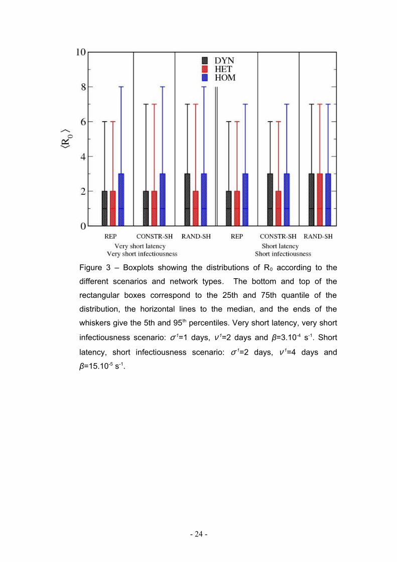
Figure 3 – Boxplots showing the distributions of R0 according to the

different scenarios and network types. The bottom and top of the

rectangular boxes correspond to the 25th and 75th quantile of the

distribution, the horizontal lines to the median, and the ends of the

whiskers give the 5th and 95th percentiles. Very short latency, very short

infectiousness scenario: σ-1=1 days, ν-1=2 days and β=3.10-4 s-1. Short

latency, short infectiousness scenario: σ-1=2 days, ν-1=4 days and

β=15.10-5 s-1.

- 24 -

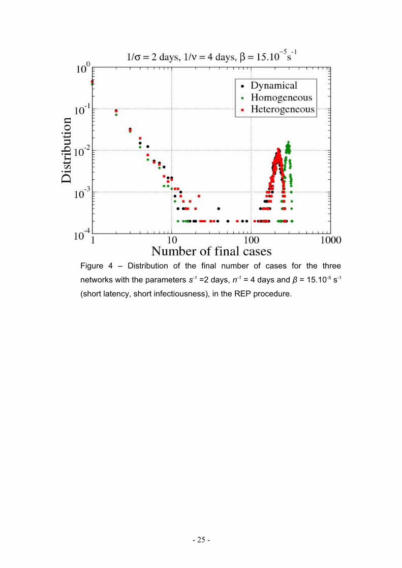
Figure 4 – Distribution of the final number of cases for the three

networks with the parameters s-1 =2 days, n-1 = 4 days and β = 15.10-5 s-1

(short latency, short infectiousness), in the REP procedure.

- 25 -

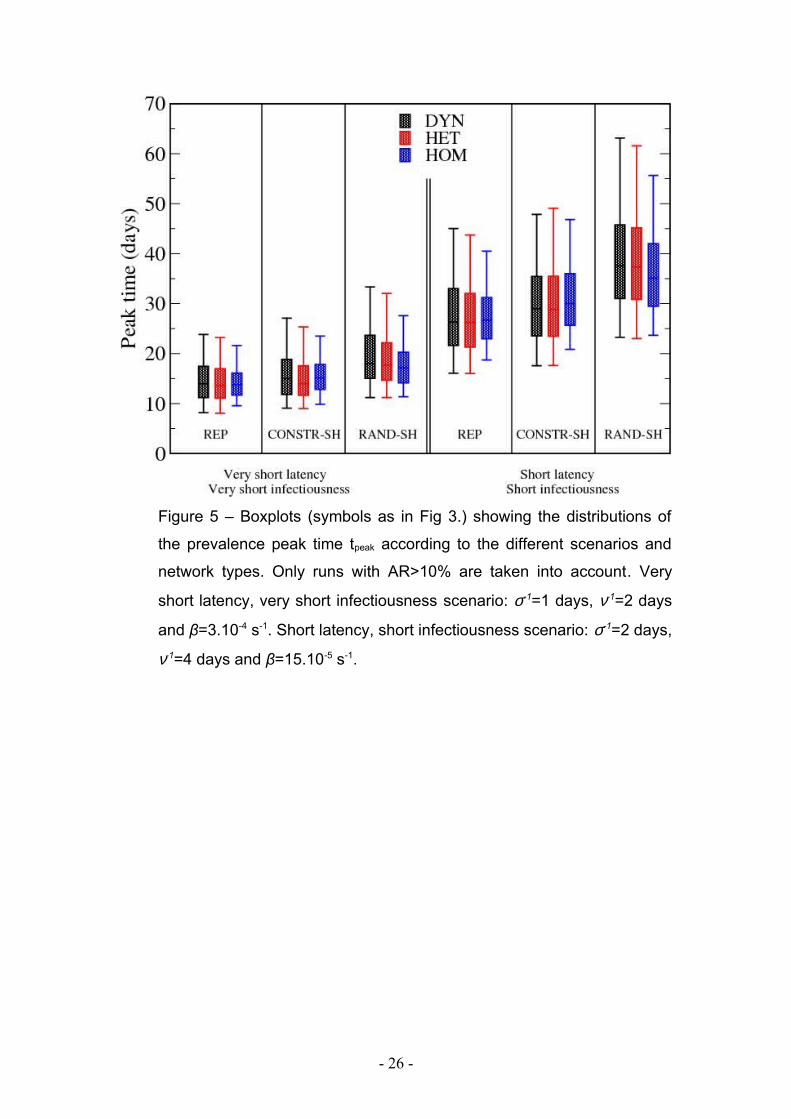
Figure 5 – Boxplots (symbols as in Fig 3.) showing the distributions of

the prevalence peak time tpeak according to the different scenarios and

network types. Only runs with AR>10% are taken into account. Very

short latency, very short infectiousness scenario: σ-1=1 days, ν-1=2 days

and β=3.10-4 s-1. Short latency, short infectiousness scenario: σ-1=2 days,

ν-1=4 days and β=15.10-5 s-1.

- 26 -

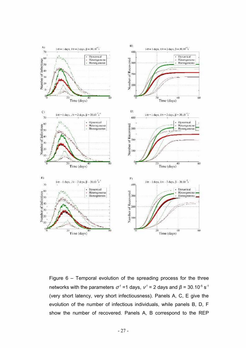
Figure 6 – Temporal evolution of the spreading process for the three

networks with the parameters σ-1 =1 days, ν-1 = 2 days and β = 30.10-5 s-1

(very short latency, very short infectiousness). Panels A, C, E give the

evolution of the number of infectious individuals, while panels B, D, F

show the number of recovered. Panels A, B correspond to the REP

- 27 -

procedure, panels C, D to the CONSTR-SH procedure, and panels E, F

to the RAND-SH one. Only runs with AR>10% are taken into account.

Symbols represent the median values and lines represent the 5th and

95th percentiles of the number of infectious and recovered individuals.

- 28 -

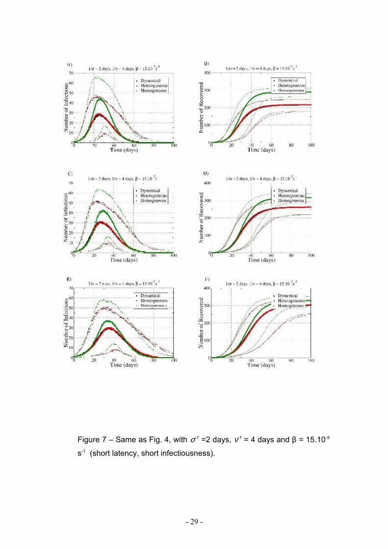
Figure 7 – Same as Fig. 4, with σ-1 =2 days, ν-1 = 4 days and β = 15.10-5

s-1 (short latency, short infectiousness).

- 29 -

Tables

Table 1 – Distribution of the final number of cases for the three network types according to the four scenarios (5000 runs, dynamic contact

network of 405 participating attendees). 90%-CI, 90% confidence interval.

Scenarios Parameters Network# of

runs

% of run with

no secondary

cases

1 to 10 final cases

(AR*≤2.5%)

11 to 40 final cases

(2.5%<AR≤10%)

More than 40 final cases

(AR>10%)

% runAverage #

cases

90%-

CI% run

Average #

cases90%-CI % run

Average

# cases90%-CI

Very short latency

Very short

infectiousness

REP

1/σ = 1 days

1/ν = 2 days

β = 3.10-4 s-1

DYN 5000 47.3 18.2 2.3 [1,6] 0.7 15.9 [11,22] 33.8 208 [169,242]

HET 5000 46.4 17.7 2.4 [1,7] 0.8 17.9 [11,32] 35.2 210 [171,243]

HOM 5000 41.7 11.7 2.2 [1,6] 0.2 16.6 [11,30] 46.3 285 [257,310]

Short latency

Short

infectiousness

REP

1/σ = 2 days

1/ν = 4 days

β = 15.10-5 s-1

DYN 5000 45.3 17.0 2.2 [1,7] 0.4 18.3 [11,38] 37.3 214 [178,246]

HET 5000 44.4 16.4 2.2 [1,6] 0.6 16.8 [11,27] 38.6 216 [178,248]

HOM 5000 38.7 13;2 2.1 [1,6] 0.1 13.2 [11,15] 48.1 288 [262,310]

Very short latency

Very short

infectiousness

RAND-SH

1/σ = 1 days

1/ν = 2 days

β = 3.10-4 s-1

DYN 5000 44.8 19.4 2.8 [1,8] 2.2 17.9 [11,31] 33.6 278 [223,319]

HET 5000 45.4 18.5 2.6 [1,7] 1.6 17.6 [11,30] 34.5 284 [241,322]

HOM 5000 39.9 14.3 2.6 [1,7] 0.8 15.7 [11,28] 45.0 324 [291,350]

Short latency 1/σ = 2 daysDYN 5000 40.6 18.6 2.7 [1,8] 1.4 19.2 [11,31] 39.4 297 [254,331]

HET 5000 39.5 18.0 2.7 [1,8] 1.3 16.7 [11,30] 41.2 300 [259,333]

- 30 -

Scenarios Parameters Network# of

runs

% of run with

no secondary

cases

1 to 10 final cases

(AR*≤2.5%)

11 to 40 final cases

(2.5%<AR≤10%)

More than 40 final cases

(AR>10%)

% runAverage #

cases

90%-

CI% run

Average #

cases90%-CI % run

Average

# cases90%-CI

Short

infectiousness

RAND-SH

1/ν = 4 days

β = 15.10-5 s-1

HOM 5000 35.9 15.7 2.5 [1,7] 0.9 17.0 [11,31] 47.5 325 [293,352]

Very short latency

Very short

infectiousness

CONSTR-SH

1/σ = 1 days

1/ν = 2 days

β = 3.10-4 s-1

DYN 5000 45.4 17.7 2.4 [1,7] 1.0 17.0 [11,28] 35.8 240 [194,278]

HET 5000 46.8 16.5 2.4 [1,7] 0.8 19.0 [11,33] 35.9 245 [202,282]

HOM 5000 39.8 13.3 2.3 [1,6] 0.7 15.4 [11,21] 46.2 308 [278,334]

Short latency

Short

infectiousness

CONSTR-SH

1/σ = 2 days

1/ν = 4 days

β = 15.10-5 s-1

DYN 5000 40.9 18.2 2.3 [1,6] 0.8 16.8 [11,34] 40.2 258 [215,292]

HET 5000 41.3 16.8 2.3 [1,7] 0.5 14.0 [11,25] 41.4 257 [213,292]

HOM 5000 35.7 14.8 2.4 [1,7] 0.4 15.2 [11,21] 49.2 314 [284,339]

- 31 -

Additional Material

- 32 -

Description of the data extension procedure 'CONSTR-SH'.

The data describes a list of contact events between pairs of individuals. Upon reshuffling of

two tag identities, for instance of tags i and j, an artificial data set is generated such that each

time the tag i was in contact with another tag, say with k, from time t0 to time t1, in the real

data, the contact was replaced by a contact between j and k between times t0 and t1.

As explained in the main text, the empirical data set allows constructing daily aggregated

contact networks. Let us denote by femp the observed average fraction of repeated contacts

from one day to the next: for each individual i, one considers the set V(i,1)={j1,j2,...} of

individuals with whom i has had a contact on day 1, and V(i,2)={k1,k2,...} with whom he or

she has had a contact on day 1. The fraction femp is then the average over all individuals of the

ratio between the size of the intersection of V(i,1) and V(i,2), and the size of V(i,1). If femp = 0,

it means that i has encountered only new individuals during the second day and if femp = 1, it

means that i has encountered exactly the same set of participants in both days.

For each reshuffling of the tags, we can aggregate the reshuffled contact data on a daily scale

and create the reshuffled daily contact networks. We then computed the average fraction f of

repeated contacts between the empirical and the reshuffled daily aggregated networks. By

constraining f to be close to femp, we constructed reshuffled contact sequences that conserve a

realistic amount of correlations between the sets of individuals encountered from one day to

the next in the artificial data set.

We proceeded by the following steps:

1. Choose two tag Ids at random

2. Exchange their identities, as described above

3. Compute f and (f – femp)2

4. Accept the exchange with a probability decreasing with b (f – femp)2, where b is a

parameter

5. Go back to step 1.

By tuning and increasing slowly the parameter b, it is then possible to produce reshufflings

which have very low values of (f – femp)2, and thus reproduce the empirical correlations

between the successive daily networks.

- 33 -

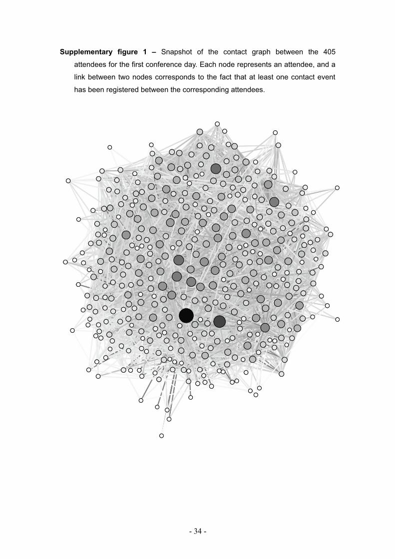
Supplementary figure 1 – Snapshot of the contact graph between the 405

attendees for the first conference day. Each node represents an attendee, and a

link between two nodes corresponds to the fact that at least one contact event

has been registered between the corresponding attendees.

- 34 -

Supplementary figure 2 – Same as supplementary figure 1, in which only links

corresponding to a cumulated time spent in proximity of at least 1mn have been

kept.

- 35 -

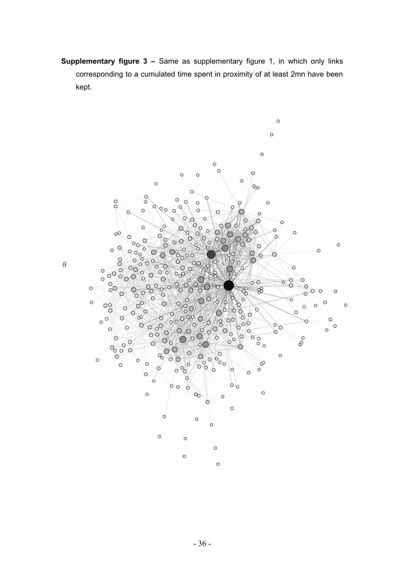
Supplementary figure 3 – Same as supplementary figure 1, in which only links

corresponding to a cumulated time spent in proximity of at least 2mn have been

kept.

- 36 -

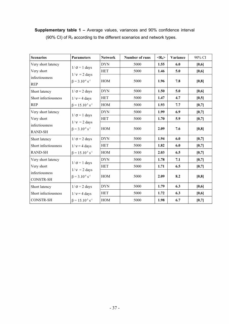
Supplementary table 1 – Average values, variances and 90% confidence interval

(90% CI) of R0 according to the different scenarios and network types.

Scenarios Parameters Network Number of runs <R0> Variance 90% CI

Very short latency

Very short

infectiousness

REP

1/ σ = 1 days

1/ ν = 2 days

β = 3.10-4 s-1

DYN 5000 1.55 6.0 [0,6]

HET 5000 1.46 5.0 [0,6]

HOM 5000 1.96 7.8 [0,8]

Short latency

Short infectiousness

REP

1/ σ = 2 days

1/ ν = 4 days

β = 15.10-5 s-1

DYN 5000 1.50 5.0 [0,6]

HET 5000 1.47 4.7 [0,5]

HOM 5000 1.93 7.7 [0,7]

Very short latency

Very short

infectiousness

RAND-SH

1/ σ = 1 days

1/ ν = 2 days

β = 3.10-4 s-1

DYN 5000 1.99 6.9 [0,7]

HET 5000 1.70 5.9 [0,7]

HOM 5000 2.09 7.6 [0,8]

Short latency

Short infectiousness

RAND-SH

1/ σ = 2 days

1/ ν = 4 days

β = 15.10-5 s-1

DYN 5000 1.94 6.0 [0,7]

HET 5000 1.82 6.0 [0,7]

HOM 5000 2.03 6.5 [0,7]

Very short latency

Very short

infectiousness

CONSTR-SH

1/ σ = 1 days

1/ ν = 2 days

β = 3.10-4 s-1

DYN 5000 1.78 7.1 [0,7]

HET 5000 1.71 6.5 [0,7]

HOM 5000 2.09 8.2 [0,8]

Short latency

Short infectiousness

CONSTR-SH

1/ σ = 2 days

1/ ν = 4 days

β = 15.10-5 s-1

DYN 5000 1.79 6.3 [0,6]

HET 5000 1.72 6.3 [0,6]

HOM 5000 1.98 6.7 [0,7]

- 37 -

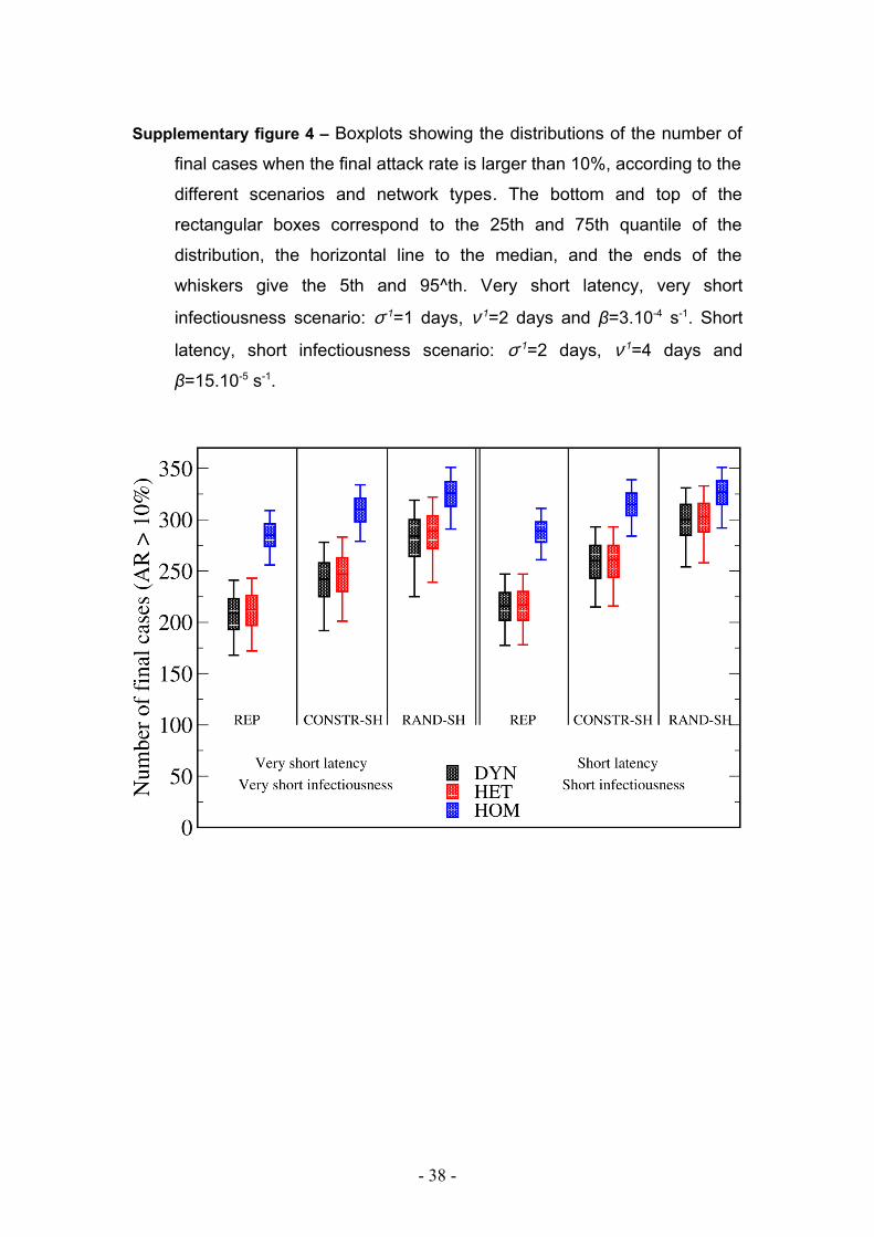
Supplementary figure 4 – Boxplots showing the distributions of the number of

final cases when the final attack rate is larger than 10%, according to the

different scenarios and network types. The bottom and top of the

rectangular boxes correspond to the 25th and 75th quantile of the

distribution, the horizontal line to the median, and the ends of the

whiskers give the 5th and 95^th. Very short latency, very short

infectiousness scenario: σ-1=1 days, ν-1=2 days and β=3.10-4 s-1. Short

latency, short infectiousness scenario: σ-1=2 days, ν-1=4 days and

β=15.10-5 s-1.

- 38 -

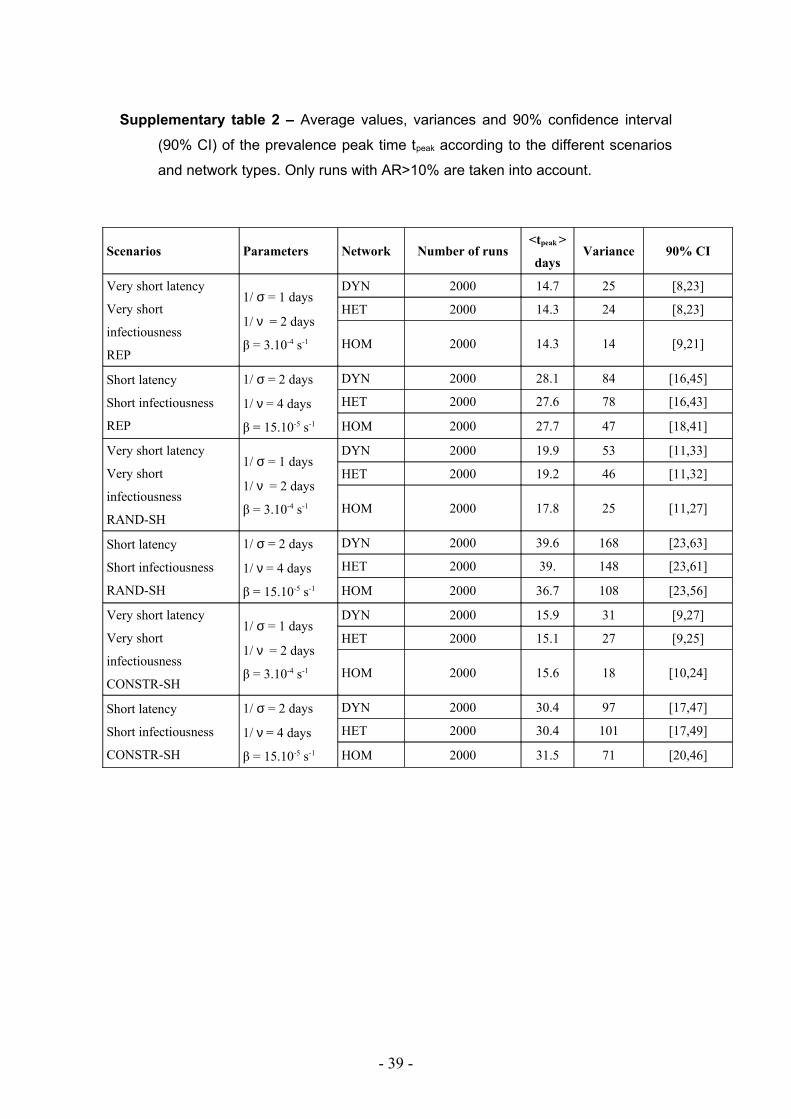
Supplementary table 2 – Average values, variances and 90% confidence interval

(90% CI) of the prevalence peak time tpeak according to the different scenarios

and network types. Only runs with AR>10% are taken into account.

Scenarios Parameters Network Number of runs<tpeak >

daysVariance 90% CI

Very short latency

Very short

infectiousness

REP

1/ σ = 1 days

1/ ν = 2 days

β = 3.10-4 s-1

DYN 2000 14.7 25 [8,23]

HET 2000 14.3 24 [8,23]

HOM 2000 14.3 14 [9,21]

Short latency

Short infectiousness

REP

1/ σ = 2 days

1/ ν = 4 days

β = 15.10-5 s-1

DYN 2000 28.1 84 [16,45]

HET 2000 27.6 78 [16,43]

HOM 2000 27.7 47 [18,41]

Very short latency

Very short

infectiousness

RAND-SH

1/ σ = 1 days

1/ ν = 2 days

β = 3.10-4 s-1

DYN 2000 19.9 53 [11,33]

HET 2000 19.2 46 [11,32]

HOM 2000 17.8 25 [11,27]

Short latency

Short infectiousness

RAND-SH

1/ σ = 2 days

1/ ν = 4 days

β = 15.10-5 s-1

DYN 2000 39.6 168 [23,63]

HET 2000 39. 148 [23,61]

HOM 2000 36.7 108 [23,56]

Very short latency

Very short

infectiousness

CONSTR-SH

1/ σ = 1 days

1/ ν = 2 days

β = 3.10-4 s-1

DYN 2000 15.9 31 [9,27]

HET 2000 15.1 27 [9,25]

HOM 2000 15.6 18 [10,24]

Short latency

Short infectiousness

CONSTR-SH

1/ σ = 2 days

1/ ν = 4 days

β = 15.10-5 s-1

DYN 2000 30.4 97 [17,47]

HET 2000 30.4 101 [17,49]

HOM 2000 31.5 71 [20,46]

- 39 -