arX

iv:2

203.

1700

6v1

[qu

ant-

ph]

31

Mar

202

2

Quantum Simulation of Real-Space Dynamics

Andrew M. Childs1,2 Jiaqi Leng1,3 Tongyang Li4,5,6 Jin-Peng Liu1,3 Chenyi Zhang7

1Joint Center for Quantum Information and Computer Science, University of Maryland2Department of Computer Science, University of Maryland

3Department of Mathematics, University of Maryland4Center on Frontiers of Computing Studies, Peking University

5School of Computer Science, Peking University6Center for Theoretical Physics, Massachusetts Institute of Technology

7Institute for Interdisciplinary Information Sciences, Tsinghua University

Abstract

Quantum simulation is a prominent application of quantum computers. While there is ex-tensive previous work on simulating finite-dimensional systems, less is known about quantumalgorithms for real-space dynamics. We conduct a systematic study of such algorithms. In par-ticular, we show that the dynamics of a d-dimensional Schrödinger equation with η particles canbe simulated with gate complexity1 O

(ηdF poly(log(g′/ǫ))

), where ǫ is the discretization error,

g′ controls the higher-order derivatives of the wave function, and F measures the time-integratedstrength of the potential. Compared to the best previous results, this exponentially improvesthe dependence on ǫ and g′ from poly(g′/ǫ) to poly(log(g′/ǫ)) and polynomially improves thedependence on T and d, while maintaining best known performance with respect to η. For thecase of Coulomb interactions, we give an algorithm using η3(d + η)T poly(log(ηdTg′/(∆ǫ)))/∆one- and two-qubit gates, and another using η3(4d)d/2T poly(log(ηdTg′/(∆ǫ)))/∆ one- and two-qubit gates and QRAM operations, where T is the evolution time and the parameter ∆ regulatesthe unbounded Coulomb interaction. We give applications to several computational problems,including faster real-space simulation of quantum chemistry, rigorous analysis of discretizationerror for simulation of a uniform electron gas, and a quadratic improvement to a quantumalgorithm for escaping saddle points in nonconvex optimization.

1 Introduction

Simulating quantum physics is one of the primary applications of quantum computers [29]. Thefirst explicit quantum simulation algorithm was proposed by Lloyd [44] using product formulas,and numerous quantum algorithms for quantum simulations have been extensively developed sincethen [1, 3–7, 15, 19, 26, 35, 38, 41–43, 49–51, 53, 55, 58, 59, 62–65], with various applicationsranging from quantum field theory [40, 52] to quantum chemistry [7, 10, 20] and condensed matterphysics [8, 25].

The Schrödinger equation that determines the evolution of a quantum wave function in d-dimensional real space has the form

i∂

∂tΦ(x, t) =

[− 1

2∇2 + f(x)

]Φ(x, t) (1)

1The O notation omits poly-logarithmic terms. Specifically, O(g) = O(g poly(log g)).

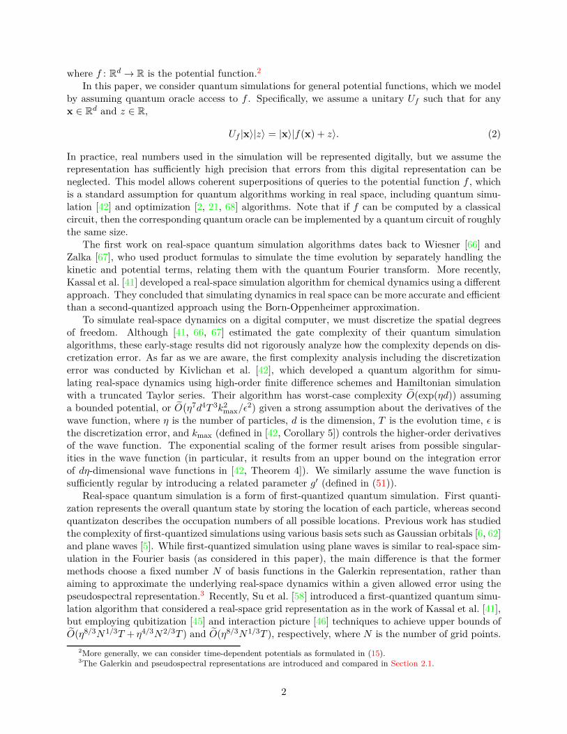
where f : Rd → R is the potential function.2

In this paper, we consider quantum simulations for general potential functions, which we modelby assuming quantum oracle access to f . Specifically, we assume a unitary Uf such that for anyx ∈ R

d and z ∈ R,

Uf |x〉|z〉 = |x〉|f(x) + z〉. (2)

In practice, real numbers used in the simulation will be represented digitally, but we assume therepresentation has sufficiently high precision that errors from this digital representation can beneglected. This model allows coherent superpositions of queries to the potential function f , whichis a standard assumption for quantum algorithms working in real space, including quantum simu-lation [42] and optimization [2, 21, 68] algorithms. Note that if f can be computed by a classicalcircuit, then the corresponding quantum oracle can be implemented by a quantum circuit of roughlythe same size.

The first work on real-space quantum simulation algorithms dates back to Wiesner [66] andZalka [67], who used product formulas to simulate the time evolution by separately handling thekinetic and potential terms, relating them with the quantum Fourier transform. More recently,Kassal et al. [41] developed a real-space simulation algorithm for chemical dynamics using a differentapproach. They concluded that simulating dynamics in real space can be more accurate and efficientthan a second-quantized approach using the Born-Oppenheimer approximation.

To simulate real-space dynamics on a digital computer, we must discretize the spatial degreesof freedom. Although [41, 66, 67] estimated the gate complexity of their quantum simulationalgorithms, these early-stage results did not rigorously analyze how the complexity depends on dis-cretization error. As far as we are aware, the first complexity analysis including the discretizationerror was conducted by Kivlichan et al. [42], which developed a quantum algorithm for simu-lating real-space dynamics using high-order finite difference schemes and Hamiltonian simulationwith a truncated Taylor series. Their algorithm has worst-case complexity O(exp(ηd)) assuminga bounded potential, or O

(η7d4T 3k2

max/ǫ2) given a strong assumption about the derivatives of the

wave function, where η is the number of particles, d is the dimension, T is the evolution time, ǫ isthe discretization error, and kmax (defined in [42, Corollary 5]) controls the higher-order derivativesof the wave function. The exponential scaling of the former result arises from possible singular-ities in the wave function (in particular, it results from an upper bound on the integration errorof dη-dimensional wave functions in [42, Theorem 4]). We similarly assume the wave function issufficiently regular by introducing a related parameter g′ (defined in (51)).

Real-space quantum simulation is a form of first-quantized quantum simulation. First quanti-zation represents the overall quantum state by storing the location of each particle, whereas secondquantizaton describes the occupation numbers of all possible locations. Previous work has studiedthe complexity of first-quantized simulations using various basis sets such as Gaussian orbitals [6, 62]and plane waves [5]. While first-quantized simulation using plane waves is similar to real-space sim-ulation in the Fourier basis (as considered in this paper), the main difference is that the formermethods choose a fixed number N of basis functions in the Galerkin representation, rather thanaiming to approximate the underlying real-space dynamics within a given allowed error using thepseudospectral representation.3 Recently, Su et al. [58] introduced a first-quantized quantum simu-lation algorithm that considered a real-space grid representation as in the work of Kassal et al. [41],but employing qubitization [45] and interaction picture [46] techniques to achieve upper bounds ofO(η8/3N1/3T + η4/3N2/3T ) and O(η8/3N1/3T ), respectively, where N is the number of grid points.

2More generally, we can consider time-dependent potentials as formulated in (15).3The Galerkin and pseudospectral representations are introduced and compared in Section 2.1.

2

The latter complexity matches the best known scaling of first-quantized methods [5]. Comparedto the real-space quantum simulation result of Kivlichan et al. [42], Su et al. focused more on theN -dependence of the complexity than on other parameters. Appendix K of [58] indicates that thefactor of N1/3 results from an upper bound on the potential term in Eq. (K7), but further work isneeded to better understand the required dependence of N on T , ǫ, and g′.

Many quantum algorithms for simulating quantum chemistry rely on second quantization. Inparticular, algorithms for the electronic structure problem using a second-quantized representationare widely studied as a near-term application of quantum computers [3]. Work on this topic hasadopted different representations including Gaussian orbitals [3, 4, 7, 35, 49, 51, 53, 55, 64, 65] andplane waves [8, 15, 26, 46, 59] in search of algorithms with lower resource requirements.

Although second-quantized approaches to quantum simulation are perhaps more widely studied,there is growing interest in first quantization. In particular, the aforementioned work of Su et al.[58] recently gave a systematic study of the practical performance of first-quantized simulationmethods. While the worst-case complexity of simulating first-quantized real-space dynamics with abounded potential scales as O(exp(ηd)) [42], first-quantized simulation enjoys asymptotically lowerspace and gate complexity in terms of η and N when considering algorithms that work with afixed number of basis functions N , as mentioned above. For simulating arbitrary-basis electronicstructure Hamiltonians, the space complexities of these general-purpose first- and second-quantizedalgorithms are O(η logN) and O(N), respectively, and the best gate complexities we are aware of

are O(η83N

13 ) [5, 58] and O(N5) [4], respectively.4 Since N = Ω(η) due to the Pauli exclusion

principle, the space and gate complexities of second-quantization algorithms are no better thanthose of first-quantization algorithms. Furthermore, first-quantized simulation can simulate the fulldynamics of molecular Schrödinger equations, while second-quantized simulation usually operatesin the Born-Oppenheimer approximation with electronic orbitals chosen for fixed nuclear positions.In addition, the choice of basis functions for second-quantized simulation algorithms can dependheavily on prior knowledge. The complexity of simulating Hamiltonian systems using heuristicbasis sets has been well analyzed, but the discretization error from the original continuum systemhas only been discussed asymptotically, and in many studies is simply neglected. As pointed outby Kassal et al. [41], this source of error could lead in general to the same O(exp(ηd)) scalingencountered with real-space simulation methods, although this issue might be mitigated in practiceby choosing appropriate basis functions. Assumptions about properties of a basis could also beunreliable for more general applications such as optimization.

Contributions. In this paper, we propose efficient quantum simulation algorithms in first quan-tization for multi-particle real-space Schrödinger equations.

Our primary consideration is to control the error in a discrete approximation of the continuumsolution of a Schrödinger equation. We perform spatial discretization using the Fourier spectralmethod. Since the error of this method decreases exponentially with the number of basis func-tions [17], it provides a high-precision approximation, as characterized in Lemma 1. The Fourierspectral method yields a discretized Hamiltonian of the form H = A+B, where A is the (truncated)kinetic term and B is the (discretized) potential term. We explore three different techniques tosimulate this discretized Hamiltonian.

First, we develop and analyze a kth-order product formula method for simulating the Hamil-tonian H = A + B. This method uses the fact that the evolution operators e−iAt and e−iBt canbe efficiently implemented, since the potential operator B is diagonal in the computational basis,

4Some studies suggest that the gate complexity of second-quantized algorithms could grow more slowly with Nfor certain models and representations [15, 43, 59].

3

while the quantum Fourier transform diagonalizes the kinetic operator A. Such an approach wasconsidered in early work of Wiesner [66] and Zalka [67], although they did not rigorously bound thecomplexity. The kth-order product formula method uses O(52k(‖H‖T )1+1/2k/ǫ1/2k) exponentialsto simulate H for time T with error at most ǫ [12]. Furthermore, its empirical performance can bebetter in practice than other Hamiltonian simulation methods for modestly sized classically hardinstances of particular models such as spin systems [25]. Combining the error analysis of the Fourierspectral method and the kth-order product formula method, we obtain the following result.

Theorem 1 (Informal version of Theorem 6). Consider an instance of the Schrödinger equation(1) for η particles in d dimensions, with a time-independent potential f(x) satisfying ‖f(x)‖L∞ ≤‖f‖max. Hamiltonian simulation with the kth-order product formula method can produce an ap-proximated wave function at time T on a set of grid nodes, with ℓ2 error at most ǫ, with asymptoticgate complexity

O(52kηd(ηd + ‖f‖max)1+1/2kT 1+1/2k/ǫ1/2k · poly

(log

(ηdTg′/ǫ

))), (3)

where g′ defined in (51) upper bounds the high-order derivatives of the wave function.

Second, we combine the Fourier spectral method with the truncated Taylor series approach toHamiltonian simulation [13] to develop high-precision real-space simulations. We provide a concretecomplexity analysis of truncating the Fourier series and performing Hamiltonian simulation inposition space, and achieve the following result for any bounded potential.

Theorem 2 (Informal version of Theorem 7). Consider an instance of the Schrödinger equation(1) for η particles in d dimensions, with a time-independent potential f(x) satisfying ‖f(x)‖L∞ ≤‖f‖max. Hamiltonian simulation with a truncated Taylor series can produce an approximated wavefunction at time T on a set of grid nodes, with ℓ2 error at most ǫ, with asymptotic gate complexity

ηd(ηd + ‖f‖max)T poly(log

(ηdTg′/ǫ

)), (4)

where g′ defined in (51) upper bounds the high-order derivatives of the wave function.

This result resolves the exponential scaling problem of Kivlichan et al. [42], exponentially improvesthe dependence on ǫ, and polynomially improves the dependence on η, d, and T .

Third, we also consider the case in which the potential function f(x, t) has an explicit timedependence. We assume f(x, t) is bounded for any t ≥ 0 and Lipschitz continuous in terms of t.We apply the Fourier spectral method to the time-dependent Hamiltonian to obtain a discretizedHamiltonian of the form H = A + B(t), where A represents the kinetic operator −1

2∇2 and B(t)captures the potential function f(x, t). The matrix A is an approximation of an unbounded op-erator, so its spectral norm is usually much larger than that of B(t). Since A is diagonalized inFourier basis, we can give an efficient implementation of e−iAt for any t. Under such conditions, itis natural to apply interaction picture simulation [46]. Combining that approach with the rescaledDyson-series algorithm [14], we obtain the following result.

Theorem 3 (Informal version of Theorem 8). Consider an instance of the Schrödinger equation(1) for η particles in d dimensions, with a time-dependent potential f(x, t) that is bounded for anyfixed t ≥ 0 and is L-Lipschitz continuous in t. Hamiltonian simulation with a rescaled Dyson seriesand interaction picture can produce an approximated wave function at time T on a set of grid nodes,with ℓ2 error at most ǫ, with asymptotic gate complexity

ηd‖f‖max,1 poly(log

(L‖f‖max,1g

′/ǫ)), (5)

4

where ‖f‖max,1 :=∫ T

0 ‖f(t)‖max dt measures the integrated strength of the potential f , and g′ definedin (51) upper bounds the high-order derivatives of the wave function.

We can compare these results as follows. Theorem 1, based on product formulas, gives a real-space quantum simulation algorithm with significant improvements in η, d, T, 1/ǫ compared to theprevious state-of-the-art result [42]. This method may be advantageous since product formulas areconceptually simple and often perform well in practice. Theorem 2, based on a truncated Taylorseries, achieves high-precision real-space quantum simulation with poly-logarithmic scaling in 1/ǫ.Given sufficient information about the Hamiltonian, Theorem 3 uses the interaction picture methodto address high-precision real-space quantum simulation with time-dependent potentials, and fur-ther improves the dependence on d to give our best asymptotic bound. Moreover, by exploiting thetechniques from the rescaled Dyson-series algorithm [14], we achieve an L1-norm scaling in terms off , which is advantageous when the maximum value of f changes significantly during the simulationtime. We emphasize that the results of our last two methods scale as poly(log(1/ǫ)), while previousfirst-quantized simulations scale as poly(1/ǫ).

For a black-box time-independent potential f with an upper bound M on each pairwise inter-action, we have ‖f(t)‖max ≤ M

(η2

)= Mη(η − 1)/2 and ‖f‖max,1 ≤ Mη(η − 1)T/2. Therefore, by

Theorem 3, the quantum gate complexity of simulating the Schrödinger equation is

Mη3dT poly(log

(MLηTg′/ǫ

)). (6)

However, in concrete applications, we need to implement the black box for the potential. Weexplore this by considering the real-space dynamics of η charged particles in d dimensions undera generalized Coulomb potential. This scenario raises two issues. First, the Coulomb potential isunbounded for arbitrarily close particles. This can be addressed by considering a modified potentialwith an approximation parameter ∆ such that M ≤ O(1/∆), as defined formally in Eq. (81).Second, we must consider the computational cost of evaluating the pairwise interactions. Thegeneralized Coulomb potential can be computed either by directly summing pairwise interactions,with cost O(η2); or by more advanced numerical techniques for η-body problems such as themultipole-based Barnes-Hut simulation algorithm [9], with cost linear in η when the dimension dis a constant. Taking these issues into account, we obtain the following result.

Corollary 1 (Informal version of Corollary 5). Consider an instance of Theorem 3 where f(x) isthe modified Coulomb potential (81) with qi = q for all 1 ≤ i ≤ η. Then the η-particle Hamiltoniancan be simulated for time T with accuracy ǫ, with either of the following costs:

1. η3(d+ η)T poly(log(ηdTg′/(∆ǫ)))/∆ one- and two-qubit gates, or

2. η3(4d)d/2T poly(log(ηdTg′/(∆ǫ)))/∆ one- and two-qubit gates and QRAM operations, if ∆is chosen small enough that the intrinsic simulation error due to the difference between theactual Coulomb potential and the modified Coulomb potential is O(ǫ).

While the details of how to choose ∆ for a given application are outside the scope of this paper,we expect the modified Coulomb potential to give a good approximation of the actual Coulombpotential provided ∆ is small compared to the minimum distances between particles, as discussedfurther in Section 2.5. Since this intrinsic simulation error must be small for the modified Coulombpotential to be relevant, the extra condition in the second simulation of Corollary 1 should besatisfied in practice.

In Table 1, we compare the gate complexities of our methods with previous first-quantizedmethods for simulating the real-space dynamics of d-dimensional η-electron Schrödinger equations

5

Reference Representation Algorithm Complexity

Kivlichan et al. [42] Finite Difference Taylor ηd(η6d2T 2(g′)2/ǫ2 + ‖f‖max)T poly(log(ηdT g′/ǫ)

)

Theorem 2 Spectral Method Taylor ηd(ηd + ‖f‖max)T poly(log(ηdT g′/ǫ)

)

Theorem 3 Spectral Method Interaction Picture ηd‖f‖maxT poly(log(ηdT g′/ǫ)

)

Table 1: Gate complexity comparison of for simulating the real-space dynamics of a d-dimensional η-particleSchrödinger equation with the potential f(x) satisfying ‖f(x, t)‖L∞ ≤ ‖f‖max. Here T is the evolution time,ǫ is the ℓ2 real-space error, and g′ denoted in (51) upper bounds the high-order derivatives of the wavefunction.

with the potential f(x) satisfying ‖f(x, t)‖L∞ ≤ ‖f‖max. We let ǫ denote the real-space error inℓ2 norm, including contributions from both the spatial discretization and the time discretization.The quantity g′ defined in (51) upper bounds the high-order derivatives of the wave function. Theevolution time is denoted by T .

Previous work gave the complexities of discretized Hamiltonian simulations as a function ofthe grid spacing h or the number of grid points N [42, 58]. However, such dependence cancontribute additional polynomial factors of η, T, ǫ, g′ to the complexity. For instance, Ref. [42]considers a d-dimensional real-space simulation discretized on a grid by the central finite differ-ence method. The complexity of this simulation is O((ηd/h2 + ‖f‖max)T ) [42, Theorem 3]. Sinceh = O(ǫ/ηd(g′ +η2T )) [42, Theorem 4 and Corollary 5], the complexity of the real-space simulationis O

(η7d3T 3(g′)2/ǫ2), as shown in Table 1.

Compared to Kivlichan et al. [42], we exponentially improve the dependence on ǫ and g′ frompoly(g′/ǫ) to poly(log(g′/ǫ)). In addition, we polynomially improve the dependence on η, d, T tobe linear, avoiding an additional polynomial dependence of these parameters when discretizing thespace as in [42].

Most previous work does not explicitly consider the quantum gate complexity as a functionof d for simulations of general d-dimensional η-particle Schrödinger equations. An exception is[42], whose cost scales as O(d4). In contrast, our Corollary 5 (based on the interaction picturealgorithm) can achieve quantum gate complexity (η3d + η4)T poly

(log(ηdT/(∆δǫ))

)/∆ when d is

large, polynomially improving the dependence on d to O(d).

Applications. First, we consider the application of our algorithms to quantum chemistry. Assuggested by Kassal et al. [41], direct simulation of the full quantum chemical dynamics may bemore accurate and efficient than using the Born-Oppenheimer approximation, making this a poten-tially promising application of real-space simulation. We consider the exact molecular Schrödingerequation under the interaction of time-independent electron-electron, electron-nucleus, and nucleus-nucleus Coulomb potentials. We then apply the Fourier spectral method and interaction picturesimulation to develop an efficient real-space simulation. Using Theorem 3, we derive the followinggate complexity.

Corollary 2 (Informal version of Corollary 6). Consider an instance of the Schrödinger equationfor ηe electrons and ηn nuclei in three spatial dimensions under the Coulomb interaction (81), wherethe nucleus has mass number M and atomic number Z. These molecular dynamics can be simulatedon a quantum computer within error ǫ with

(ηe +Mηn)3TZ2/(M∆) · poly(log((ηe +Mηn)Tg′/(∆ǫ)

)) (7)

one- and two-qubit gates, along with the same number (up to poly-logarithmic factors) of QRAMoperations.

6

Compared to the best previous result for real-space quantum simulation of chemical dynamics [41],the above result matches the dependence of the query and gate complexity on the particle numbersηe and ηn, gives explicit dependence of T , and achieves poly(log(1/ǫ)) dependence on ǫ.

Second, we apply our interaction picture algorithm with L1-norm scaling, developed in Section 3,to the uniform electron gas model (also known as jellium), which is a simple yet powerful model insolid-state physics. Several authors have considered quantum algorithms for simulating jellium [8,48]. However, to the best of our knowledge, these works have not established an asymptotic boundon the simulation complexity that takes discretization error into account. Using Theorem 3, webound the simulation cost as follows.

Corollary 3 (Informal version of Corollary 7). The 3-dimensional uniform electron gas model withη electrons can be simulated for time T on a quantum computer within error ǫ with

η3T poly(log(ηTg′/(∆ǫ)

))/∆, (8)

one- and two-qubit gates, along with the same number (up to poly-logarithmic factors) of QRAMoperations.

Third, we consider possible applications of our real-space dynamics simulation algorithms in thecontext of optimization. Recent work [68] demonstrated that for a saddle point of a high dimen-sional nonconvex function, one can detect its nearby negative curvature structure by simulatingthe Schödinger dynamics of a Gaussian wavepacket centered at this point. Since saddle points areubiquitous in the landscape of nonconvex functions (see e.g. [28, 30]), escaping from saddle pointsis one of the major difficulties in nonconvex optimization. By exploiting our interaction picturealgorithm with L1-norm scaling (Proposition 1), we show that we can escape from saddle pointsand further find a local minimum of the objective function with the following cost.

Corollary 4 (Informal version of Corollary 8). For a d-dimensional twice-differentiable functionf that is ℓ-smooth and ρ-Hessian Lipschitz, and for any ǫ > 0, there exists a quantum algorithmthat outputs an ǫ-approximate local minimum with probability at least 2/3 using O

(f(x0)−f∗

ǫ1.75 log d)

queries to the evaluation oracle Uf , where x0 is an initial point and f∗ is the global minimum of f .

Compared to [68], which uses O(log2 d/ǫ1.75) queries to find a local minimum, our algorithm achievesa quadratic speedup in terms of log d.

Organization. The rest of the paper is organized as follows. Section 2 introduces the Fourierspectral method and develops simulations of time-independent multi-particle Schrödinger equationsbased on product formulas and the truncated Taylor series method. Section 3 generalizes high-precision real-space simulation to time-dependent multi-particle Schrödinger equations by utilizingthe interaction picture technique. Section 4 discusses several applications of our results, includingquantum chemistry, the uniform electron gas, and optimization. We conclude and discuss openquestions in Section 5. Appendix A introduces some notation used throughout the paper, andAppendix B establishes an error bound for the Fourier spectral method.

2 Simulating Schrödinger equations in real space

2.1 Fourier spectral method

In this section, we develop an approach to simulating the Schrödinger equation in real space thatcombines the Fourier spectral method with Hamiltonian simulation. The Fourier spectral method

7

(also known as the Fourier pseudospectral method) provides a global approximation to the exactsolution of a partial differential equation with periodic boundary conditions. This approch can becontrasted with local approximations—such as the finite difference method—that approximate thesolution on a set of grid points. In general, the Fourier spectral method approximates the solutionby a linear combination of Fourier basis functions with undetermined time-dependent coefficients.By interpolating the partial differential equations at uniformly spaced nodes, we obtain a systemof ordinary differential equations that can be solved numerically [17, 56]. Applying this approachto the Schrödinger equation, we obtain a discretized Hamiltonian system that can be handled bystandard Hamiltonian simulation algorithms.

At first glance, the Fourier spectral method looks similar to plane-wave methods widely usedin first-quantized quantum simulations. Although these two approaches both employ Fourier basisfunctions, their primary difference is that they approximate the infinite-dimensional functionalspace in different finite-dimensional subspaces, and in particular, result in different discretizedHamiltonian systems. To illustrate this difference, let Φ(x, t) and Φ(x, t) denote the exact andapproximated solutions, respectively, of a one-dimensional Schrödinger equation, and let

Rn(x, t) =[i∂

∂t+

1

2∇2 − f(x)

]Φ(x, t) (9)

denote the residue, where n + 1 is the number of the basis functions. The residue quantifies theextent to which the approximated solution fails to satisfy the Schrödinger equation (1). In general,Rn cannot be zero as a function of t unless the exact solution Φ is a finite combination of basisfunctions. Instead, we seek a reasonable choice of Φ such that the projection of Rn onto somefinite-dimensional subspace vanishes. As we describe below in more detail, the Fourier spectralapproach requires the residue to vanish at the set of interpolation nodes, while Galerkin plane wavemethods instead guarantee that its integrations with Fourier test functions are zero.

In the Galerkin approach [18, 61], the residue is orthogonal to a subspace of n+ 1 chosen testfunctions, denoted φjnj=0. In other words, we require that

〈φj |Rn〉 = 〈φj |H|Φ〉 = 0, j ∈ [n + 1]0 = 0, 1, . . . , n, (10)

where angle brackets denote the inner product over the spatial domain, and H is the Galerkindiscretized Hamiltonian. For the Schrödinger equation (1), we have H = T + V where the matrixelements of the discretized kinetic and potential terms are given by [58]

Tpq =

∫dr φ∗

p(x)

(−∇

2

2

)φq(x), (11)

Vpq =

∫dr φ∗

p(x)f(x)φq(x). (12)

(See Appendix B of [58] for Galerkin representations of molecular Hamiltonians.)Equation (10) is a system of n + 1 ordinary differential equations with time-dependent coef-

ficients. For first-quantized plane-wave methods, the basis functions used in constructing Φ aswell as the test functions φj are all chosen as Fourier basis functions. While this discretizationis commonly used in first-quantized quantum simulations [5, 6, 58, 62], previous studies neglectthe discretization error. If the Schrödinger operator includes an unbounded potential or is highlyoscillatory, such a Galerkin representation may not provide a reasonable approximation.

On the other hand, in the spectral approach [17, 56], we choose the test functions φj in (10)to be delta functions on the uniform interpolation nodes χjnj=0. Then we have

〈δj |Rn〉 = Rn(χj , t) = 0, k ∈ [n + 1]0, (13)

8

which is equivalent to

[i∂

∂t+

1

2∇2 − f(x)

]Φ(χj , t) = 0, k ∈ [n+ 1]0. (14)

This choice again defines a system of n + 1 ordinary differential equations with time-dependentcoefficients. The spectral approach can provide a straightforward approximation of real-spacequantum dynamics by determining the number of interpolation points n+1 explicitly as a functionof the allowed discretization error, the particle number, and the norms of high-order derivatives ofthe wave function. In contrast, previous simulations based on the Galerkin approach [5, 6, 58, 62] didnot explicitly take the real-space discretization error into account, and instead merely determinedthe complexity in terms of the number of basis functions used.

We now introduce our Fourier spectral approach for time-dependent Schrödinger equations ofthe general form

i∂

∂tΦ(x, t) =

[− 1

2∇2 + f(x, t)

]Φ(x, t) (15)

where x ∈ Rd represents the position of the quantum particle, t ∈ R represents time, ∇ =

( ∂∂xi

)∣∣di=1

is the gradient, and f : Rd × R → R is the potential function. This generalizes (1) to the case oftime-dependent potentials. We assume access to the potential through a unitary oracle Uf suchthat for any x ∈ R

d, t ∈ R, and z ∈ R,

Uf |x〉|t〉|z〉 = |x〉|t〉|f(x) + z〉. (16)

For concreteness, we consider x ∈ Ω := [0, 1]d and assume periodic boundary conditions forΦ(x, 0), i.e.,

∂(p)

∂x(p)j

Φ(x1, . . . , xj−1, 0, xj+1, . . . , xd, 0) =∂(p)

∂x(p)j

Φ(x1, . . . , xj−1, 1, xj+1, . . . , xd, 0) (17)

holds for all p ∈ N, j ∈ [d], where ∂(p)

∂x(p)j

is the pth-order partial derivative with respect to the jth

coordinate of x = [x1, . . . , xd]T .

We first apply the Fourier spectral method for the spatial discretization. We approximate thesolution Φ(x, t) by a Fourier series of the form

Φ(x, t) =∑

‖k‖∞≤nck(t)φk(x) (18)

for some even number n ∈ N, where k = (k1, . . . , kd) with kj ∈ [n+ 1]0, ck(t) ∈ C, and

φk(x) =d∏

j=1

φkj(xj) (19)

with

φk(x) := e2πi(k−n/2)x (20)

for k ∈ [n + 1]0 and x ∈ [0, 1].

9

Plugging (18) into (15), we obtain an approximated PDE system

i∂

∂tΦ(x, t) =

[− 1

2∇2 + f(x, t)

]Φ(x, t) (21)

with the initial condition

Φ(x, 0) = Φ(x, 0). (22)

In terms of the basis functions, this gives

i∑

‖k‖∞≤n

d

dtck(t)φk(x) =

∑

‖k‖∞≤nck(t)

[− 1

2

∑

‖r‖∞≤n[Ln,d]krφr(x) + f(x, t)φk(x)

](23)

where Ln,d is the multi-dimensional Laplacian matrix

Ln,d :=d⊕

j=1

D2n = D2

n ⊗ I⊗d−1 + I ⊗D2n ⊗ I⊗d−2 + · · ·+ I⊗d−1 ⊗D2

n (24)

and Dn is a differential matrix for the Fourier basis functions (20), the (n+1)-dimensional diagonalmatrix with entries

[Dn]kk = 2πi(k − n/2) (25)

for k ∈ [n + 1]0.To produce a system of ordinary differential equations, we introduce the uniform interpolation

nodes χl = (χl1 , . . . , χld)‖l‖∞≤n with lj ∈ [n+ 1]0, where

χlj =lj

n+ 1. (26)

Considering (23) at the uniform interpolation nodes (26), we obtain an (n + 1)d-dimensional ap-proximated ODE system

i∑

‖k‖∞≤n

d

dtck(t)φk(χl)|l1〉 . . . |ld〉

=∑

‖k‖∞≤nck(t)

[− 1

2

∑

‖r‖∞≤n[Ln]krφr(χl) + f(χl, t)φk(χl)

]|l1〉 . . . |ld〉, (27)

where lj ∈ [n+ 1]0, j ∈ [d].The well-known quantum Fourier transform (QFT) maps the (n+1)-dimensional quantum state

v = (v0, v1, . . . , vn) ∈ Cn+1 to the state v = (v0, v1, . . . , vn) ∈ C

n+1 with

vl =1√n+ 1

n∑

k=0

exp(2πikl

n+ 1

)vk, l ∈ [n+ 1]0. (28)

In other words, the QFT is the unitary transform

Fn :=1√n+ 1

n∑

k,l=0

exp(2πikl

n+ 1

)|l〉〈k|. (29)

10

The closely related quantum shifted Fourier transform (QSFT) maps the (n+1)-dimensional quan-tum state v ∈ C

n+1 to the state v ∈ Cn+1 with

vl =1√n+ 1

n∑

k=0

exp(2πi(k − n/2)l

n+ 1

)vk, l ∈ [n + 1]0. (30)

In other words, the QSFT is the unitary transform

F sn :=1√n+ 1

n∑

k,l=0

exp(2πi(k − n/2)l

n+ 1

)|l〉〈k|. (31)

Notice that the QSFT can be written as the product

F sn = SnFn, (32)

of the QFT defined above and the diagonal matrix

Sn =n∑

l=0

exp(− πinl

n+ 1

)|l〉〈l|. (33)

The QSFT can be performed with gate complexity O(log n log log n) [24, Lemma 5]. Using (18) inthe one-dimensional case with vk = ck(t), the QSFT maps the state v to v = F snv satisfying

vl =1√n+ 1

n∑

k=0

ck(t)φk(χl) =1√n+ 1

Φ(χl, t), l ∈ [n + 1]0. (34)

In other words, the QSFT maps the coefficient vector v =∑nk=0 ck(t)|k〉 to approximate interpolated

solution v = 1√n+1

∑nl=0 Φ(χl, t)|l〉. We use the QSFT (instead of the ordinary QFT) to align with

the phase convention specified in (18).We also define the multi-dimensional QSFT as

Fsn,d :=

d⊗

j=1

F sn. (35)

Letting

c(t) :=∑

‖k‖∞≤nck(t)|k1〉 . . . |kd〉, |c(t)〉 :=

c(t)

‖c(t)‖ , (36)

and

Vn,d(t) :=∑

‖l‖∞≤nf(χl, t)|l1〉 . . . |ld〉〈l1| . . . 〈ld|, (37)

the ODE system (27) can be rewritten as

iFsn,d

d

dt|c(t)〉 = Fs

n,dLn,d|c(t)〉 + Vn,d(t)Fsn,d|c(t)〉. (38)

Equivalently,

id

dt|c(t)〉 = Hn,d(t)|c(t)〉 = [Ln,d + (Fs

n,d)−1Vn,d(t)F

sn,d]|c(t)〉 (39)

11

which is a Hamiltonian system in the momentum space, with the Hamiltonian

Hn,d(t) := Ln,d + (Fsn,d)

−1Vn,d(t)Fsn,d. (40)

Alternatively, (39) can be expressed as

id

dt[Fsn,d|c(t)〉] = [Fs

n,dLn,d(Fsn,d)

−1 + Vn,d(t)][Fsn,d|c(t)〉]. (41)

Using (18), we write

Φ(t) =∑

‖l‖∞≤nΦ(χl, t)|l1〉 . . . |ld〉 =

∑

‖l‖∞≤nck(t)φk(χl)|l1〉 . . . |ld〉, |Φ(t)〉 :=

Φ(t)

‖Φ(t)‖, (42)

such that

Φ(t) = Fsn,dc(t), |Φ(t)〉 = Fs

n,d|c(t)〉 (43)

provide approximations of the exact solution and its ℓ2 normalized state

Φ(t) =∑

l

Φ(χl, t)|l1〉 . . . |ld〉, |Φ(t)〉 :=Φ(t)

‖Φ(t)‖ , (44)

respectively. Thus we see that Eq. (39) is a Hamiltonian system in position space

id

dt|Φ(t)〉 = Hn,d(t)|Φ(t)〉 = [Fs

n,dLn,d(Fsn,d)

−1 + Vn,d(t)]|Φ(t)〉, (45)

with the Hamiltonian

Hn,d(t) := Fsn,dLn,d(F

sn,d)

−1 + Vn,d(t) (46)

= Fsn,dHn,d(t)(F

sn,d)

−1. (47)

Furthermore, we assume the ℓ2 norm of the exact (n + 1)d-dimensional initial condition Φ(0)satisfies

‖Φ(0)‖2 =∑

‖l‖∞≤n|Φ(χl, 0)|2 = (n+ 1)d. (48)

This is a discrete analog of the condition∫

x∈Ω |Φ(x, 0)|2 dx = 1 on the (n+1)d uniform interpolationnodes χl. In more detail, consider the trapezoidal rule for numerical integration [36]. On eachd-dimensional grid cell, we replace the integration of Φ(x, 0) by the average value of 2d nearbyinterpolation points Φ(χl, 0) times the volume 1

(n+1)d of the d-dimensional grid cell. In this setting,

‖Φ(0)‖2/(n+1)d approximates∫

x∈Ω |Φ(x, 0)|2 dx. For convenience, we normalize the state accordingto (48).5 Because the Schrödinger equation is unitary, this ensures that

‖Φ(t)‖2 =∑

‖l‖∞≤n|Φ(χl, t)|2 = (n+ 1)d (49)

for all t ∈ R.

5Given an arbitrary initial condition Φ(x, 0) and its corresponding discretized state Φ(0), we can rescale the initial

condition as Φ(x, 0) → (n+1)d/2

cΦ(x, 0) and Φ(0) → (n+1)d/2

cΦ(0) where c := ‖Φ(0)‖, such that the rescaled state

satisfies ‖Φ(0)‖ = (n + 1)d.

12

2.2 Truncation number of the Fourier spectral method

The overall simulation error includes two contributions: the error introduced by discretizing theproblem with the Fourier spectral method and the error introduced by the Hamiltonian simulationalgorithm. To ensure overall error at most ǫ, we choose the parameters of the Fourier spectralmethod to upper bound the spatial discretization error between the exact and approximated nor-malized states (|Φ(t)〉 and |Φ(t)〉, respectively) by ǫ/2, and choose the parameters of the Hamiltoniansimulation algorithm to also upper bound its error by ǫ/2. The latter calculation uses standardanalysis to bound the error accumulated over the course of the simulation. In the following, weanalyze the error of the Fourier spectral method.

Spectral methods typically exhibit exponential convergence if the solution is smooth [17]. Inparticular, we establish exponential convergence for approximating Φ(x, t) by Φ(x, t).

Lemma 1. Let Φ(x, t) and Φ(x, t) denote the exact and approximated solutions of (1) by the Fourierspectral method, respectively, where Φ(x, t) is analytic in t and x. Then for any even integer n ≥ 6,the error from the Fourier spectral method satisfies

maxx,t|Φ(x, t)− Φ(x, t)| ≤ 2

π

maxt ‖Φ(n/2)(·, t)‖L1

(n/2)n/2. (50)

Lemma 1 gives an estimate of the maximal error of approximating Φ(x, t) by Φ(x, t) in spaceand time. We prove Lemma 1 in Appendix B.

Using this error estimate, we can determine a sufficient truncation number n that ensures theapproximated solution Φ(x, t) is within the allowed error tolerance. For simplicity, we denote

g′ := maxt‖Φ(n/2)(·, t)‖L1 . (51)

The parameter g′ describes the higher-order regularity of the wave function Φ(x, t). Usually, whenΦ(x, t) is not strongly localized, it is common to assume g′ is bounded from above [38, 42]. Infact, Bourgain [16] shows that the derivatives of the wave function Φ(x, t) are bounded when thepotential function f(x, t) is sufficiently smooth. However, to our best knowledge, the exact scalingof g′ in terms of d and n remains unknown. Therefore, in the present analysis, we parametrize theoverall complexity by g′.

Using (50), for any t ∈ R+ and x = χl defined in (26), we have

∣∣∣Φ(χl, t)− Φ(χl, t)∣∣∣ ≤ 2

π

g′

(n/2)n/2. (52)

Recall that the sets of all entries of Φ(t) and Φ(t) as presented in (44) and (42) are Φ(χl, t) andΦ(χl, t) for all χl, respectively. Each entry of Φ(t) − Φ(t) is bounded by the right-hand side of(52), giving

∥∥∥Φ(t)− Φ(t)∥∥∥

∞≤ 2

π

g′

(n/2)n/2(53)

for any t ∈ R+. With respect to the ℓ2 norm, using ‖v‖2 ≤

√(n+ 1)d‖v‖∞ for the (n + 1)d-

dimensional vector v = Φ(t)− Φ(t), we have

∥∥∥Φ(t)− Φ(t)∥∥∥ ≤ 2

π

g′

(n/2)n/2(n+ 1)d/2 (54)

13

for any t ∈ R+.

This bound implies that the error of the normalized states |Φ(t)〉 and |Φ(t)〉 satisfies

∥∥∥|Φ(t)〉 − |Φ(t)〉∥∥∥ ≤

∥∥Φ(t)− Φ(t)∥∥

min‖Φ(t)‖, ‖Φ(t)‖≤ δ

‖Φ(t)‖ − δ , (55)

where δ := maxt∥∥Φ(t)− Φ(t)

∥∥. Recall that ‖Φ(t)‖ = (n+ 1)d/2 by (49). To satisfy the inequality

δ

‖Φ(t)‖ − δ =δ

(n + 1)d/2 − δ ≤ ǫ/2 ⇐⇒ δ ≤ ǫ/2

1 + ǫ/2(n+ 1)d/2, (56)

based on (54), we choose n so that

2

π

g′

(n/2)n/2(n+ 1)d/2 ≤ ǫ/2

1 + ǫ/2(n + 1)d/2, (57)

which is equivalent to

(n/2)n/2 ≥ 4g′(1 + ǫ/2)

πǫ. (58)

Since ǫ/2 ≤ 1, and noticing the condition n ≥ 6 in Lemma 1, it suffices to select

n = max

2⌈ log(ω)

log(log(ω))

⌉, 6

, (59)

where

ω =4g′

πǫ. (60)

2.3 Hamiltonian simulation with product formulas

Early work of Wiesner [66] and Zalka [67] used the so-called split-operator method to simulatereal-space quantum dynamics on quantum computers. This method uses the truncated Fourierseries to discretize the Schrödinger equation in space and construct a discrete Hamiltonian system,with the Hamiltonian as a sum of the potential and kinetic operators. The diagonal potentialoperator is encoded in the position space, and the kinetic operator is diagonalized by quantumFourier transform in the momentum space. The kinetic and potential operators are propagatedindependently, and these time evolutions are combined using product formulas. Subsequently,Kassal et al. [41] applied this method to chemical dynamics. However, these previous works do notprovide rigorous error analysis. In particular, they all replace the continuous kinetic operator bythe discretized one without accounting for the discretization error, as discussed in [42, Theorem 4].

Having derived the Fourier spectral method with concrete real-space error analysis to obtain thediscrete Hamiltonian system (45), we now describe the simulation using product formulas. Given aHamiltonian H = A+B, the standard 2kth-order Suzuki product formula [60] is defined recursivelyas

ST2 (t) := e−i t

2A · e−itB · e−i t

2A, (61)

ST2k(t) := S2k−2(ukt)

2S2k−2((1 − 4uk)t)S2k−2(ukt)

2 (62)

14

where uk := 1/(1 − 41/(2k−1)). In our problem, the Hamiltonian Hn,d(t) in (46) is the sum of

A = Fsn,dLn,d(F

sn,d)

−1, (63)

B = Vn,d(t). (64)

Instead of directly simulating A, we observe that e−itFsn,d

Ln,d(Fsn,d

)−1

= Fsn,de

−itLn,d(Fsn,d)

−1, i.e.,

the evolution in the position space coincides with the Fourier transform of the evolution of e−itLn,d

in the momentum space. In other words,

id

dt|Φ(t)〉 = Fs

n,dLn,d(Fsn,d)

−1|Φ(t)〉 ⇐⇒ id

dt|c(t)〉 = Ln,d|c(t)〉, (65)

where |c(t)〉 = (Fsn,d)

−1|Φ(t)〉 by (43). Therefore, the split-operator method with the kth-orderSuzuki product formula for simulating (45) can be presented recursively as

SB2 (t) = (Fs

n,d)−1e−i t

2Vn,d ·Fs

n,de−itLn,d · (Fs

n,d)−1e−i t

2Vn,d , (66)

SB2k(t) = S2k−2(ukt)

2S2k−2((1 − 4uk)t)S2k−2(ukt)

2. (67)

We now give concrete upper bounds on the gate complexities of the kth-order split-operatormethod for simulating the discretized Schrödinger equation.

Lemma 2. Consider an instance of time-independent Hamiltonian simulation as defined in (46),with a time-independent potential f(x) satisfying ‖f(x)‖L∞ ≤ ‖f‖max, for time T > 0. Let g′ =maxt ‖Φ(n/2)(·, t)‖L1 as in (51). There exists a quantum algorithm producing a normalized statethat approximates |Φ(T )〉 with ℓ2 error at most ǫ/2, with gate complexity

O(52kd(d+ ‖f‖max)1+1/2kT 1+1/2k/ǫ1/2k

). (68)

Proof. We apply standard error bounds for product formulas [12]. For the complexity analysiswe simply need to include the additional cost of performing the quantum Fourier transform Fs

n,d

and its inverse (Fsn,d)

−1. The number of QFTs equals the number of exponentials, which is upperbounded by [12, Theorem 1] with m = 2, which shows that

NQFT = Nexp ≤ 4 · 52k(2‖H‖T )1+1/2k/(ǫ/2)1/2k . (69)

exponentials suffice to ensure that we approximate |Φ(T )〉 with ℓ2 error at most ǫ/2. Using ‖Ln,d‖ ≤dn2

4 and ‖Vn,d‖ ≤ ‖f‖max, we have

NQFT = Nexp ≤ 4 · 52k21+1/k[T

(dn2

4+ ‖f‖max

)]1+1/2k/ǫ1/2k. (70)

Since Lsn,d, Vsn,d, Fs

n,d, and (Fsn,d)

−1 can all be performed with gate complexity dpoly(log n), the costof implementing either an exponential or an inverse quantum Fourier transform is O(dpoly(log n));the claim follows by including this factor.

Combining this with an upper bound on the discretization error gives our main result onproduct-formula simulation.

15

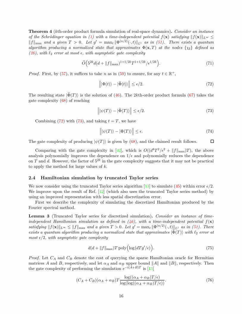
Theorem 4 (kth-order product formula simulation of real-space dynamics). Consider an instanceof the Schrödinger equation in (1) with a time-independent potential f(x) satisfying ‖f(x)‖L∞ ≤‖f‖max and a given T > 0. Let g′ = maxt ‖Φ(n/2)(·, t)‖L1 as in (51). There exists a quantumalgorithm producing a normalized state that approximates Φ(x, T ) at the nodes χl defined as(26), with ℓ2 error at most ǫ, with asymptotic gate complexity

O(52kd(d+ ‖f‖max)1+1/2kT 1+1/2k/ǫ1/2k

). (71)

Proof. First, by (57), it suffices to take n as in (59) to ensure, for any t ∈ R+,

∥∥∥|Φ(t)〉 − |Φ(t)〉∥∥∥ ≤ ǫ/2. (72)

The resulting state |Φ(T )〉 is the solution of (46). The 2kth-order product formula (67) takes thegate complexity (68) of reaching

∥∥∥|ψ(T )〉 − |Φ(T )〉∥∥∥ ≤ ǫ/2. (73)

Combining (72) with (73), and taking t = T , we have

∥∥∥|ψ(T )〉 − |Φ(T )〉∥∥∥ ≤ ǫ. (74)

The gate complexity of producing |ψ(T )〉 is given by (68), and the claimed result follows.

Comparing with the gate complexity in [42], which is O((d4T 2/ǫ2 + ‖f‖max)T ), the aboveanalysis polynomially improves the dependence on 1/ǫ and polynomially reduces the dependenceon T and d. However, the factor of 52k in the gate complexity suggests that it may not be practicalto apply the method for large values of k.

2.4 Hamiltonian simulation by truncated Taylor series

We now consider using the truncated Taylor series algorithm [13] to simulate (45) within error ǫ/2.We improve upon the result of Ref. [42] (which also uses the truncated Taylor series method) byusing an improved representation with less spatial discretization error.

First we describe the complexity of simulating the discretized Hamiltonian produced by theFourier spectral method.

Lemma 3 (Truncated Taylor series for discretized simulation). Consider an instance of time-independent Hamiltonian simulation as defined in (46), with a time-independent potential f(x)satisfying ‖f(x)‖L∞ ≤ ‖f‖max and a given T > 0. Let g′ = maxt ‖Φ(n/2)(·, t)‖L1 as in (51). Thereexists a quantum algorithm producing a normalized state that approximates |Φ(T )〉 with ℓ2 error atmost ǫ/2, with asymptotic gate complexity

d(d+ ‖f‖max)T poly(log

(dTg′/ǫ

)). (75)

Proof. Let CA and CB denote the cost of querying the sparse Hamiltonian oracle for Hermitianmatrices A and B, respectively, and let αA and αB upper bound ‖A‖ and ‖B‖, respectively. Thenthe gate complexity of performing the simulation e−i(A+B)T is [13]

(CA + CB)(αA + αB)Tlog((αA + αB)T/ǫ)

log(log((αA + αB)T/ǫ)). (76)

16

To simulate (46), we take A = Fsn,dLn,d(F

sn,d)

−1 and B = Vn,d. Using ‖Ln,d‖ ≤ dn2

4 , ‖Vn,d‖ ≤‖f‖max, and the fact that the gate complexity of performing each of Lsn,d, Vs

n,d, Fsn,d, or (Fs

n,d)−1

is dpoly(log n), we obtain the gate complexity

dpoly(log n)(dn2 + ‖f‖max)Tlog

((dn2 + ‖f‖max)T/ǫ

)

log(log((dn2 + ‖f‖max)T/ǫ)). (77)

Using the value of n from (59), we see that the complexity is

d(d + ‖f‖max)T poly(log

(dTg′/ǫ

))(78)

as claimed.

Theorem 5 (Truncated Taylor series for real-space simulation). Consider an instance of the Schrö-dinger equation (1), with a time-independent potential f(x) satisfying ‖f(x)‖L∞ ≤ ‖f‖max and agiven T > 0. Let g′ = maxt ‖Φ(n/2)(·, t)‖L1 as in (51). There exists a quantum algorithm producinga normalized state that approximates Φ(x, T ) at the nodes χl defined as (26), with ℓ2 error atmost ǫ, with the gate complexity

d(d+ ‖f‖max)T poly(log

(dTg′/ǫ

)). (79)

Proof. The result follows immediately from the same logic as in the proof of Theorem 4.

Whereas the gate complexity in [42] is O((d4T 2/ǫ2 + ‖f‖max)T ), our approach achieves com-plexity O(d(d + ‖f‖max)T log(1/ǫ)) in terms of ℓ2 error, exponentially improving the dependenceon 1/ǫ, reducing the cubic dependence on T to linear, and reducing the quartic dependence on dto quadratic.

2.5 Interacting multi-particle systems

Now we consider simulating a multi-particle Schrödinger equation

i∂

∂tΦ(x, t) =

[− 1

2∇2 + f(x, t)

]Φ(x, t) (80)

with a fixed number of particles η in d dimensions, interacting through a potential function f(x).Here x ∈ R

ηd represents the positions of the particles, where entries x(j−1)d+1, . . . , xjd indicate

the position of particle j ∈ [η], t ∈ R represents time, ∇ =(∂∂xi

) ∣∣∣ηd

i=1, and f : Rηd × R → R

is the potential function of the Schrödinger equation. As above, we consider the case where fis independent of time in this section. Also, we assume for simplicity that all particles have thesame mass; this is easily generalized to the case of particles with different masses, as discussed inSection 4.1.

To make simulation tractable, we consider an ηd-dimensional hypercubic domain Ω = [0, 1]ηd

and assume the wave function can be treated as periodic on this domain [8, 42, 47, 58]. The periodicboundary condition is natural for crystalline solids. As for a non-periodic system subject to a long-range potential such as the Coulomb potential, we can embed the system into a sufficiently largeperiodic box Ω such that the particles remain far from the boundary. Then, we can implementquantum simulations within the periodic box Ω because the tail of the wave function outside of Ωis negligible. In this case, one can imagine the full space R

ηd is covered by repeated copies of thepotential function restricted to Ω, but the periodic images of the potential outside of the box Ω do

17

not significantly interact with the wave functions supported on Ω [8, 47, 58]. In practice, it is notnecessary to simulate the periodic images of the potential function outside of Ω.

We also want the potential function f(x) to be bounded, i.e., ‖f(x)‖L∞ ≤ ‖f‖max. However,typical potentials arising in physics include singularities, such as the divergence of the Coulombpotential for two particles at the same location. We can handle this by modifying the potentialin a way that does not significantly affect the solution at relevant length scales. For example, ad-dimensional generalization of the Coulomb potential can be modified as [42]

fCoulomb(x) =∑

1≤i<j≤η

qiqj√∑dk=1

(x(i−1)d+k − x(j−1)d+k

)2+ ∆2

, (81)

where qi is the charge of the ith particle and ∆ > 0 serves to keep the potential bounded [42].Letting q := maxi |qi|, we have

‖f(x)‖L∞ ≤ η(η − 1)q2

2∆= ‖f‖max. (82)

The parameter ∆ captures how closely the modified Coulomb potential (81) approximates theunbounded potential. To accurately reproduce the behavior of the unbounded Coulomb potential,we would like to simulate the model for small ∆ > 0, and we expect the complexity of the simulationto grow with 1/∆ as a consequence of the upper bound (82). In practice, the modified Coulombpotential (81) should give a good approximation of the original Coulomb potential provided particlesremain separated by distances large compared with ∆.

As considered in [13, 42, 46], we analyze the gate complexity of implementing the sparse Hamil-tonian oracle, where we count a query to the modified Coulomb potential in the implementation asone gate.

Theorem 4 and Theorem 5 directly imply quantum algorithms for simulating (80) using productformulas and the truncated Taylor series method, respectively.

Theorem 6 (kth-order product formula simulation of interacting particles). Consider an instanceof the multi-particle Schrödinger equation (80) with a time-independent potential f(x) satisfying‖f(x)‖L∞ ≤ ‖f‖max, and a given T > 0. Let g′ = maxt ‖Φ(n/2)(·, t)‖L1 as in (51). There existsa quantum algorithm producing a normalized state that approximates Φ(x, T ) at the nodes χldefined in (26), with ℓ2 error at most ǫ, with asymptotic gate complexity

O(52kηd(ηd + ‖f‖max)1+1/2kT 1+1/2k/ǫ1/2k

). (83)

Proof. It suffices to replace d by ηd in the proof of Theorem 4.

Theorem 7 (Truncated Taylor series simulation of interacting particles). Consider an instanceof the multi-particle Schrödinger equation (80), with a time-independent potential f(x) satisfying‖f(x)‖L∞ ≤ ‖f‖max, and a given T > 0. Let g′ = maxt ‖Φ(n/2)(·, t)‖L1 as in (51). There existsa quantum algorithm producing a normalized state that approximates Φ(x, T ) at the nodes χldefined in (26), with ℓ2 error at most ǫ, with asymptotic gate complexity

ηd(ηd + ‖f‖max)T poly(log

(ηdTg′/ǫ

)). (84)

Proof. As in the previous result, it suffices to replace d by ηd in the proof of Theorem 5.

18

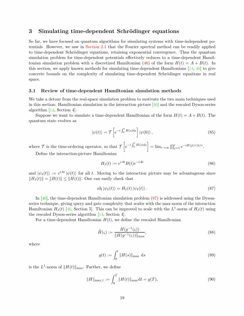
3 Simulating time-dependent Schrödinger equations

So far, we have focused on quantum algorithms for simulating systems with time-independent po-tentials. However, we saw in Section 2.1 that the Fourier spectral method can be readily appliedto time-dependent Schrödinger equations, retaining exponential convergence. Thus the quantumsimulation problem for time-dependent potentials effectively reduces to a time-dependent Hamil-tonian simulation problem with a discretized Hamiltonian (46) of the form H(t) = A + B(t). Inthis section, we apply known methods for simulating time-dependent Hamiltonians [14, 46] to giveconcrete bounds on the complexity of simulating time-dependent Schrödinger equations in realspace.

3.1 Review of time-dependent Hamiltonian simulation methods

We take a detour from the real-space simulation problem to motivate the two main techniques usedin this section: Hamiltonian simulation in the interaction picture [46] and the rescaled Dyson-seriesalgorithm [14, Section 4].

Suppose we want to simulate a time-dependent Hamiltonian of the form H(t) = A+B(t). Thequantum state evolves as

|ψ(t)〉 = T[e−i

∫ t

0H(s)ds

]|ψ(0)〉 , (85)

where T is the time-ordering operator, so that T[e−i

∫ t

0H(s)ds

]= limr→∞

∏rj=1 e

−iH(jt/r)t/r .

Define the interaction-picture Hamiltonian

HI(t) := eiAtB(t)e−iAt (86)

and |ψI(t)〉 := eiAt |ψ(t)〉 for all t. Moving to the interaction picture may be advantageous since‖HI(t)‖ = ‖B(t)‖ ≤ ‖H(t)‖. One can easily check that

i∂t |ψI(t)〉 = HI(t) |ψI(t)〉 . (87)

In [46], the time-dependent Hamiltonian simulation problem (87) is addressed using the Dyson-series technique, giving query and gate complexity that scales with the max-norm of the interactionHamiltonian HI(t) [46, Section 5]. This can be improved to scale with the L1-norm of HI(t) usingthe rescaled Dyson-series algorithm [14, Section 4].

For a time-dependent Hamiltonian H(t), we define the rescaled Hamiltonian

H(ς) :=H(g−1(ς))

‖H(g−1(ς))‖max, (88)

where

g(t) :=

∫ t

0‖H(s)‖max ds (89)

is the L1-norm of ‖H(t)‖max. Further, we define

‖H‖max,1 :=

∫ T

0‖H(t)‖maxdt = g(T ), (90)

19

where T denotes the total simulation time. A key observation is that the rescaling of the Hamilto-nian does not affect the target state:

|ψ(t)〉 = T[e−i

∫ t

0H(s) ds

]|ψ(0)〉 = T

[e−i

∫ g(t)

0H(ς) dς

]|ψ(0)〉 . (91)

Given this rescaling procedure, if we have

1. an algorithm that simulates the rescaled Hamiltonian H(ς) for 0 ≤ ς ≤ T with L∞-normcost, i.e., with complexity O(T‖H(ς)‖max,∞) where

‖H(ς)‖max,∞ = supς∈[0,T ]

‖H(ς)‖max, (92)

and

2. the ability to compute g−1(ς) for any ς ∈ [0, T ] and the max-norm ‖H(s)‖max for any s ∈ [0, T ](so that we have access to the rescaled Hamiltonian H(ς) for any ς),

then we are able to simulate the original Hamiltonian H(T ) for 0 ≤ t ≤ T with L1-norm cost, i.e.,with complexity O(

∫ T0 ‖H(t)‖max dt). To see this, note that ‖H(ς)‖max = 1 for all ς ∈ [0, g(T )].

Therefore, if we apply the simulation algorithm with L∞-norm cost to H(ς) for 0 ≤ ς ≤ g(T ), thecost is bounded by g(T ), which is the the L1-norm of ‖H(s)‖max:

g(T )‖H(ς)‖max,∞ = g(T ), (93)

which is the L1 norm.Now, we apply the above rescaling procedure to the interaction-picture Hamiltonian HI(t) (86).

The rescaled interaction-picture Hamiltonian HI(ς) satisfies

HI(ς) = eiAg−1(ς)B(ς)e−iAg−1(ς), (94)

where

B(ς) := B(g−1(ς))/‖B(g−1(ς))‖max (95)

stands for the rescaled operator for B.

Lemma 4. The max-norm of the rescaled interaction-picture Hamiltonian HI(ς) as defined in (94)is bounded by 1 for any 0 ≤ ς ≤ g(t):

‖HI(ς)‖max ≤ 1. (96)

Proof. First, note that the max-norm of any matrix is upper bounded by its ℓ2-norm, we have

‖HI(ς)‖max ≤ ‖HI(ς)‖ ≤ ‖eiAg−1(ς)‖‖B(ς)‖‖e−iAg−1(ς)‖ ≤ ‖B(ς)‖. (97)

The last two steps hold because the matrix ℓ2-norm is sub-multiplicative: ‖AB‖ ≤ ‖A‖‖B‖, whilethe unitary operators eiAg

−1(ς) and e−iAg−1(ς) have unit ℓ2-norm. Since the rescaled operator B(ς) isdiagonal, its max-norm and ℓ2-norm are equally 1. This proves our claim that ‖HI(ς)‖max ≤ 1.

Similarly, if we have an L∞-norm algorithm (e.g., the standard Dyson-series simulation) thatsimulates the rescaled interaction-picture Hamiltonian HI(ς) for 0 ≤ ς ≤ g(t) as well as the accessto rescaled Hamiltonian HI(ς), we can simulate the original Hamiltonian H(s) with the total costO(g(t)) = O(

∫ t0 ‖B(s)‖max ds). Note that although the Hamiltonian is a sum of two operators,

H(t) = A+B(t), the simulation cost only depends on the L1-norm of ‖B(s)‖max and not A. Thisis the advantage of using the interaction picture simulation method.

20

3.2 Block-encoding of the rescaled interaction-picture Hamiltonian

The input model of the truncated Dyson series method is a unitary oracle for a so-called block-encoding (defined in Appendix A). In the present context, the values of the potential f(x, t) canbe produced by an evaluation oracle (16). Therefore, we provide an explicit construction of therelevant block-encoding oracle using queries to the potential.

Efficient simulations of eiAt. Interaction picture simulation is adventageous when it is easy toimplement eiAt, even for large t. When simulating the time-dependent Schrödinger equation (15)with the Fourier spectral method, the A term in the Hamiltonian (46) is

A = Fsn,dLn,d(F

sn,d)

−1, (98)

where Ln,d is an explicit diagonal matrix and Fsn,d is the multi-dimensional quantum shifted Fourier

transform (QSFT). The transformation Fsn,d and its inverse can be performed with gate complexity

O(d log n log log n) [24, Lemma 5]. Therefore, eiAt can be simulated as Fsn,de

iLn,dt(Fsn,d)

−1. By

standard techniques (see for example Rule 1.6 in [22, Section 1.2]), eiLn,dt can be simulated withgate complexity O(d log n).

Lemma 5. Let B ∈ C2w×2w

be a diagonal matrix. Suppose we have access to the evaluation oracleUf that returns the values of diagonal entries of B in binary as

Uf |j〉 |t〉 |0z〉 = |j〉 |t〉 |fj(t)〉 = |j〉 |t〉 |Bjj(t)〉 , ∀j ∈ [2w]− 1, (99)

where Bjj = fj(t) is a z-bit binary description of the jth diagonal entry of B(t). Additionally, sup-pose we have the following two oracles6 that implement the inverse change-of-variable and computethe max-norm:

Oinv |ς, z〉 =∣∣∣ς, z ⊕ g−1(ς)

⟩, (100)

Onorm |τ, z〉 = |τ, z ⊕ ‖B(τ)‖max〉 . (101)

Then we can implement the following evaluation oracle UB

for the rescaled operator B(ς) definedin (95), acting as

UB|j〉 |ς〉 |0〉z = |j〉 |ς〉

∣∣∣Bjj(ς)⟩

∀j ∈ [2w]− 1, (102)

using O(1) queries to the oracles Uf , Oinv, Onorm and additionally using O(z2) one- and two-qubitgates.

Proof. The main idea follows the proof of [14, Theorem 10]. Let the function g(t) be defined as in(89).

We use oracles Oinv and Onorm to implement the transformation

|ς, 0, 0〉 7→∣∣∣ς, g−1(ς), ‖B(g−1(ς))‖max

⟩. (103)

We then query Uf and normalize the result with ‖B(g−1(ς))‖max to compute Bjj(ς):

∣∣∣g−1(ς), ‖B(g−1(ς))‖max, j, 0⟩7→

∣∣∣g−1(ς), ‖B(g−1(ς))‖max, j, Bjj(ς)⟩. (104)

6This is a standard assumption; see for example [14, Section 4.2].

21

Then we uncompute the ancilla registers and obtain an evaluation oracle for the rescaled operator,namely

UB|j〉 |ς〉 |0〉z = |j〉 |ς〉

∣∣∣Bjj(ς)⟩

∀j ∈ [2w]− 1. (105)

This process uses O(1) queries to the oracles Uf , Oinv, and Onorm.We now analyze the gate complexity. Each entry of B is given using z qubits. The above

implementation process only involves arithmetic operations on these qubits, which can be imple-mented with complexity O(z2). Such operation is called only if an oracle query happens, so we canimplement all the arithmetic operations with O(z2) additional gates.

Next, we evaluate the cost of implementing the unitary oracle HAM-THI

of the rescaled

interaction-picture Hamiltonian HI(ς). The definition of the HAM-T oracle, originally from [46],can be found in Appendix A.

Lemma 6. Let HI be the rescaled interaction-picture Hamiltonian in (94). Then the oracleHAM-T

HIcan be approximated with error at most δ at the following cost:

1. Queries to the oracles Uf , Oinv and Onorm: O(1),

2. One- and two-qubit gates: O(z2 + log2.5(1/δ) + d log n

).

Proof. Observe that HAM-THI

can be approximated by eiAg−1(ς)O

Be−iAg−1(ς) to any desired accu-

racy. Since we require the error of HAM-THI

be bounded by δ, the error of the above three terms

should be O(δ).By Lemma 5 and Lemma 15, an (1, ω+ 3, ǫ)-block-encoding of B, denoted O

B, can be approxi-

mated. with O(1) queries to oracles Uf , Oinv, Onorm, and O(z2 +w+log2.5(1/δ)) one- and two-qubitgates.

To implement eiAg−1(ς) and e−iAg−1(ς), the diagonal elements and g−1(ς) should be known to

O(log(1/δ)) bits of precision. Then they can be simulated using O(d log n + log(1/δ)) one- andtwo-qubit gates. Note that w is at most O(d log n), then in total O

(z2 + log2.5(1/δ) + d log n

)one-

and two-qubit gates suffice.

3.3 Rescaled Dyson-series algorithm with L1-norm scaling

The rescaled Dyson-series algorithm uses a block-encoding oracle to achieve the following simulation[46].

Lemma 7 ([46, Lemma 6]). Let A ∈ C2ns ×2ns

, B ∈ C2ns×2ns

, and let αA, αB be known constantssuch that ‖A‖ ≤ αA and ‖B‖ ≤ αB. Assume the existence of a unitary oracle HAM-T

HIthat block-

encodes the Hamiltonian within the interaction picture, which implicitly depends on the time-stepsize τ = O(α−1

B ) and number of time-steps M = O(t(αA + αB)/ǫ). Then for all t ≥ 2αBτ , thetime-evolution operator e−i(A+B)t may be approximated to error ǫ with the following cost.

1. Simulations of e−iAτ : O(αBt),

2. Queries to HAM-THI

: O(αBt

log(αBt/ǫ)log log(αBt/ǫ)

),

3. Primitive gates: O(αBt

(na + log(t(αA + αB)/ǫ)

)αBt

log(αBt/ǫ)log log(αBt/ǫ)

).

22

When simulating a time-dependent Schrödinger equation, it is natural to let B be the termcorresponding to the potential energy f(x, t). Then B is a diagonal matrix and we have accessto its diagonal components through the evaluation oracle (16). This can be used to efficientlyimplement the evaluation oracle for its rescaling B, which can in turn be used to implement theHamiltonian HAM-T

HIspecified in Definition 6.

Proposition 1. For τ ∈ [0, T ], let H(τ) = −∇2+B(τ) be a discretized real-space Hamiltonian withB(τ) a diagonal matrix whose diagonal elements are specified by the potential function f(x, τ) : Rd×R→ R. Suppose that f is a positive and continuously differentiable function, L-Lipschitz in termsof τ , and can be computed with z bits of precision. Then H can be simulated for time T withaccuracy ǫ with the following costs.

1. Queries to Uf , Oinv, Onorm: O(‖f‖max,1

log(‖f‖max,1/ǫ)log log(‖f‖max,1/ǫ)

)where ‖ · ‖max,1 is defined in (90)

and the oracles are defined in Lemma 5;

2. One- and two-qubit gates:

O

(‖f‖max,1

(poly(z) + log2.5(L‖f‖max,1/ǫ) + d log

(log(g′/ǫ)

log log(g′/ǫ)

))log(‖f‖max,1/ǫ)

log log(‖f‖max,1/ǫ)

);

where g′ = maxt ‖Φ(n/2)(·, t)‖L1 as defined in (51).

The following lemma from [46] is useful for proving this theorem:

Lemma 8 ([46, Corollary 4]). Let H(ς) : [0, t]→ C2w×2w

, and suppose ‖H‖max is bounded by some

constant CH

, and⟨‖ d

dς H‖⟩

= 1t

∫ t0 ‖ d

dς H(ς)‖dς. Set M = O(‖H‖max,1

ǫ

( ⟨‖ d

dς H‖⟩

+ ‖H‖2max

))to be

the number of time intervals in the HAM-TH

oracle. Then for all ǫ > 0, an operation W can beimplemented with failure probability at most O(ǫ), such that

‖W − T[e∫ g−1(t)

ς=0H(ς)dς ]‖ ≤ ǫ (106)

with the following costs.

1. Queries to HAM-TH

: O(‖H‖max,1

log(

‖H‖max,1/ǫ)

log log(

‖H‖max,1/ǫ)

),

2. Primitive gates: O(‖H‖max,1

(na + log

(‖H‖max,1

ǫ

( ⟨‖ d

dς H‖⟩

+ ‖H‖2max

))) log(

‖H‖max,1/ǫ)

log log(

‖H‖max,1/ǫ)

).

Here na denotes the number of ancillary qubits needed to implement HAM-TH

.

Now we present the proof of Proposition 1.

Proof. We follow the simulation method of [46]. Whenever HAM-THI

is called to obtain the

block-encoding of HI(ς), since in the interaction picture the simulation time equals ‖f‖max,1, werequire an O(ǫ/‖fmax,1‖)-approximate HAM-T

HIto guarantee that the overall error is bounded by

ǫ. By Lemma 6, this can be achieved using O(1) queries to oracles Uf , Oinv, Onorm and O(z2 +

log2.5(‖f‖max,1/ǫ) + d log n)

one- and two-qubit gates.Also note that

‖HI(ς)‖max ≤ ‖HI(ς)‖ = ‖B(ς)‖ = ‖B(ς)‖max ∀ς, (107)

23

so

‖HI‖max,1 ≤ ‖B‖max,1 = ‖f‖max,1. (108)

Then by Lemma 8, the query complexity to oracles Uf , Oinv and Onorm is

O(‖f‖max,1

log(‖f‖max,1/ǫ)

log log(‖f‖max,1/ǫ)

). (109)

We have

dHI

dς= eiAg

−1(ς) dB

dςe−iAg−1(ς) + i · dg−1

dς(AeiAg

−1(ς)Be−iAg−1(ς) + eiAg−1(ς)BAe−iAg−1(ς)), (110)

and since A = −∇2 is a Hermitian operator, we can further deduce that

dH

dς= eiAg

−1(ς) dB

dςe−iAg−1(ς), (111)

where

∥∥∥dHI

dς

∥∥∥ =∥∥∥

dB

dς

∥∥∥ = O(∥∥∥

dB

dt

∥∥∥)

= O(L). (112)

Hence, the number of one- and two-qubit gates needed in this procedure is

O(‖f‖max,1

(na + log(L‖f‖max,1/ǫ)

) log(‖f‖max,1/ǫ)

log log(‖f‖max,1/ǫ)

)

+O(‖f‖max,1(z2 + log2.5(‖f‖max,1/ǫ) + d log n) · log(‖f‖max,1/ǫ)

log log(‖f‖max,1/ǫ)

). (113)

This expression uses the fact that each primitive gate can be implemented using O(1) one- andtwo-qubit gates. By the proof of [46, Lemma 8], na can be upper bounded by poly(z). Furthermore,

by (59), the truncation parameter is n = 2

⌈log(ω)

log(log(ω))

⌉for ω = 8g′

πǫ . Therefore, the gate complexity

can be expressed as

O

(‖f‖max,1

(poly(z) + log2.5

(L‖f‖max,1

ǫ

)+ d log

( log(g′/ǫ)log log(g′/ǫ)

)) log(‖f‖max,1/ǫ)

log log(‖f‖max,1/ǫ)

)(114)

as claimed.

3.4 Generalization to multi-particle systems

We now generalize Proposition 1 to the case of a fixed number of particles η in d dimensionsinteracting through a potential function f(x). As in Section 2.5, here x ∈ R

ηd represents thepositions of the particles and the evolution of the wave function Φ(x, t) follows the time-dependentmulti-particle Schrödinger equation (80). In this subsection, we suppose the oracles Uf , Oinv,Onorm defined in Lemma 5 are still available in this multi-particle scenario. Using Proposition 1,the complexity of simulating (80) in the interaction picture is as follows.

Theorem 8. For τ ∈ [0, T ], let H(τ) = −∇2 + B(τ) be a discretized multi-particle real-spaceHamiltonian with B(τ) a diagonal matrix whose diagonal elements are specified by the potentialfunction f(x, τ). Suppose that f : Rηd × R → R is a positive, continuously differentiable function,L-Lipschitz in terms of τ , and can be computed with z bits of precision. Then H can be simulatedfor time T with accuracy ǫ with the following cost:

24

1. Queries to Uf , Oinv, Onorm: O(‖f‖max,1

log(‖f‖max,1/ǫ)log log(‖f‖max,1/ǫ)

)where ‖ · ‖max,1 is defined in (90)

and the oracles are defined in Lemma 5;

2. One- and two-qubit gates:

O

(‖f‖max,1

(poly(z) + log2.5(L‖f‖max,1/ǫ) + ηd log

(log(g′/ǫ)

log log(g′/ǫ)

))log(‖f‖max,1/ǫ)

log log(‖f‖max,1/ǫ)

);

where g′ = maxt ‖Φ(n/2)(·, t)‖L1 as defined in (51).

Proof. It suffices to replace d by ηd in the proof of Proposition 1 and choose the value of thetruncation parameter n as in (59) to obtain the complexity for general case.

We now discuss the cost of simulating an η-electron system under the modified Coulomb poten-tial f(x) defined in (81) using the approach of Theorem 8. To give a complete algorithm, we mustimplement the evaluation oracle Uf for the modified Coulomb potential. The most straightforwardimplementation directly computes the sum of η(η−1)/2 pairwise Coulomb interactions, giving gatecomplexity O(η2). However, more advanced numerical techniques for η-body problems such as theBarnes-Hut algorithm [9] and the fast multipole method [33] can evaluate the η-particle Coulombpotential faster, reducing the cost to linear in η when the dimension d is a constant.

In particular, for d = 3 the Barnes-Hut algorithm [9] proceeds as follows. We divide the unitcube into cubic cells in an octree structure of height h until each cell contains at most one particle.We then compute the pairwise Coulomb interactions between particles in nearby cells. Finally,we approximate the remaining Coulomb interactions between particles in distant cells by treatingnearby particles as a single large particle located at their geometric center. The cost of this approachis as follows.

Lemma 9 ([54]). For a system of η particles in a three-dimensional unit cube, the Barnes-Hutalgorithm [9] of height h approximates the total Coulomb potential to a constant accuracy in timeO(ηh). Adopting the fast multipole method [33] as a subroutine to estimate the Coulomb interac-tion between well-separated clusters of particles, the reulting multipole-based Barnes-Hut algorithmapproximates the total Coulomb potential to accuracy ǫ in time O(ηh log2(1/ǫ)).

In particular, the error introduced by the fast multipole subroutine is bounded as follows.

Lemma 10 ([33]). Suppose that k particles of charge qj for j ∈ 1, . . . , k are located within a spherecentered at 0 with radius rs. Then after a reusable preprocessing step with time complexity O(k), forany point P at a distance r > rs from the origin, the pth-order fast multipole method approximatesthe Coulomb potential φ(P ) to accuracy Q

r−rs

( rs

r

)p+1in time O(p2), where Q :=

∑kj=1 |qj|.

This method can be generalized to approximate the d-dimensional modified Coulomb potentialdefined in Lemma 5. We analyze the complexity of this method in a random-access memory (RAM)model, which allows for fast retrieval of the information stored in the tree data structure. Inparticular, to use this algorithm on a quantum computer, we work in the quantum RAM (QRAM)model, in which we can perform a memory access gate

|j〉 |y〉 |x1, . . . , xm〉 7→ |j〉 |y ⊕ xj〉 |x1, . . . , xm〉 (115)

at unit cost. Note that implementing this operation with elementary two-qubit gates requires Ω(m)overhead [11, Theorem 4], so the cost of the algorithm described below would be larger by a factorof η in the standard quantum circuit model, as its tree data structure occupies m = Θ(η) qubits.We leave it as an open question whether similar performance can be achieved without QRAM.

25

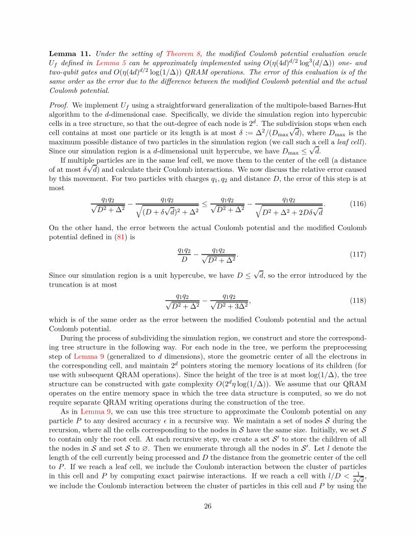
Lemma 11. Under the setting of Theorem 8, the modified Coulomb potential evaluation oracleUf defined in Lemma 5 can be approximately implemented using O(η(4d)d/2 log3(d/∆)) one- andtwo-qubit gates and O(η(4d)d/2 log(1/∆)) QRAM operations. The error of this evaluation is of thesame order as the error due to the difference between the modified Coulomb potential and the actualCoulomb potential.

Proof. We implement Uf using a straightforward generalization of the multipole-based Barnes-Hutalgorithm to the d-dimensional case. Specifically, we divide the simulation region into hypercubiccells in a tree structure, so that the out-degree of each node is 2d. The subdivision stops when eachcell contains at most one particle or its length is at most δ := ∆2/(Dmax

√d), where Dmax is the

maximum possible distance of two particles in the simulation region (we call such a cell a leaf cell).Since our simulation region is a d-dimensional unit hypercube, we have Dmax ≤

√d.

If multiple particles are in the same leaf cell, we move them to the center of the cell (a distanceof at most δ

√d) and calculate their Coulomb interactions. We now discuss the relative error caused

by this movement. For two particles with charges q1, q2 and distance D, the error of this step is atmost

q1q2√D2 + ∆2

− q1q2√(D + δ

√d)2 + ∆2

≤ q1q2√D2 + ∆2

− q1q2√D2 + ∆2 + 2Dδ

√d. (116)

On the other hand, the error between the actual Coulomb potential and the modified Coulombpotential defined in (81) is

q1q2

D− q1q2√

D2 + ∆2. (117)

Since our simulation region is a unit hypercube, we have D ≤√d, so the error introduced by the

truncation is at most

q1q2√D2 + ∆2

− q1q2√D2 + 3∆2

, (118)

which is of the same order as the error between the modified Coulomb potential and the actualCoulomb potential.

During the process of subdividing the simulation region, we construct and store the correspond-ing tree structure in the following way. For each node in the tree, we perform the preprocessingstep of Lemma 9 (generalized to d dimensions), store the geometric center of all the electrons inthe corresponding cell, and maintain 2d pointers storing the memory locations of its children (foruse with subsequent QRAM operations). Since the height of the tree is at most log(1/∆), the treestructure can be constructed with gate complexity O(2dη log(1/∆)). We assume that our QRAMoperates on the entire memory space in which the tree data structure is computed, so we do notrequire separate QRAM writing operations during the construction of the tree.

As in Lemma 9, we can use this tree structure to approximate the Coulomb potential on anyparticle P to any desired accuracy ǫ in a recursive way. We maintain a set of nodes S during therecursion, where all the cells corresponding to the nodes in S have the same size. Initially, we set Sto contain only the root cell. At each recursive step, we create a set S ′ to store the children of allthe nodes in S and set S to ∅. Then we enumerate through all the nodes in S ′. Let l denote thelength of the cell currently being processed and D the distance from the geometric center of the cellto P . If we reach a leaf cell, we include the Coulomb interaction between the cluster of particlesin this cell and P by computing exact pairwise interactions. If we reach a cell with l/D < 1

2√d,

we include the Coulomb interaction between the cluster of particles in this cell and P by using the

26

pth-order fast multipole approximation. Since in the latter case all the particles of this cell arewithin a hyperball with radius l

√d/2, the error of the pth-order fast multipole method is at most

Q

D − l√d/2

( l√d

2D

)p+1, (119)

where Q denotes the absolute sum of all the charges in this cell. Choosing p = log(d/∆2

)=

O(log(d/∆)), the cumulative error of the fast-multipole approximations is O(Q∆2/Dd). This is ofthe same order as the error of the modified Coulomb potential, which is at least of order

Ω(QD− Q√

D2 + ∆2

)= Ω

(Q∆2

Dd

)(120)

(since D ≤√d for a d-dimensional hypercubic simulation region). If we did not reach a leaf cell

and l/D ≥ 12√d, we add the corresponding node into the set S. The recursive process stops when

both S and S ′ are empty.Observe that in any recursive step, the set S essentially stores all the cells of some specific

size l that are either not leaf cells or that have distances D to P that are not far enough (inparticular, those with D ≤ 1

2l√d). Hence, during the recursive process, the size of S can be upper

bounded by O(dd/2), whereas the size of S ′ can be upper bounded by O((4d)d/2). Thus, there arein total O((4d)d/2) lookup operations to the tree structure, or equivalently, O((4d)d/2) queries tothe QRAM.

Moreover, since the height of the tree is at most O(log(1/∆)), the number of recursive stepsis at most O(log(1/∆)). Thus the gate complexity for evaluating the Coulomb potential for oneparticle is

O((4d)d/2p2 log(1/∆)) = O((4d)d/2 log3(d/∆)). (121)

Therefore, the overall complexity is O(η(4d)d/2 log3(d/∆)), and the overall number of QRAMqueries is O(η(4d)d/2 log(1/∆)), as claimed.

As discussed above, the evaluation oracle Uf for the modified Coulomb potential can be im-plemented via two different approaches. First, by directly evaluating all η(η − 1)/2 pairwise in-teractions, Uf can be implemented with O(η2) one- and two- qubit gates. Alternatively, usingLemma 11, the cost of implementing Uf by the fast multipole method is O(η(4d)d/2 log3(d/∆))one- and two- qubit gates along with O(η(4d)d/2 log(1/∆)) QRAM operations. Consequently, wehave the following.7

Corollary 5. Consider the setting of Theorem 8 where f(x) is the modified Coulomb potentialdefined in (81) for particles of fixed charge (i.e., qi is independent of i). Then the η-particleHamiltonian can be simulated for time T with accuracy ǫ with either of the following costs:

1. (Direct evaluation) η3(d+ η)T poly(log(ηdTg′/(∆ǫ)))/∆ one- and two-qubit gates, or

2. (Fast multipole method) η3(4d)d/2T poly(log(ηdTg′/(∆ǫ)))/∆ one- and two-qubit gates andQRAM operations, if ∆ is chosen small enough that the intrinsic simulation error due to thedifference between the actual Coulomb potential and the modified Coulomb potential is O(ǫ),

7Appendix K of [58] develops an approximate block-encoding of the modified Coulomb potential that avoidsdirectly evaluating the potential function. That method also provides a simulation with cubic dependence on η byusing LCU techniques [27]. Here we focus on an approach that evaluates the modified Coulomb potential explicitly.

27

where g′ := maxt ‖Φ(n/2)(·, t)‖L1 as defined in (51).

Proof. By Theorem 8, the Hamiltonian can be simulated with

O

(Tη2q2

∆

(poly(z) + log2.5(Tη2q2/(∆ǫ)) + ηd log

( log(g′/ǫ)log log(g′/ǫ)

)) log(Tη2q2/(∆ǫ)

)

log log(Tη2q2/(∆ǫ))

)(122)

one- and two- qubit gates and

O(Tη2q2

∆· log

(Tη2q2/(∆ǫ)

)

log log(Tη2q2/(∆ǫ))

)(123)

queries to the evaluation oracle Uf . The oracle can be implemented via the direct pairwise inter-action with gate complexity O(η2), or the fast multipole method as described in Lemma 11 whileintroducing an error at most O(ǫ). Then the gate complexity and number of QRAM queries are asclaimed.

4 Applications

In this section, we study the applications of quantum simulation in real space. Our targets are sev-eral computational problems of fundamental importance in quantum chemistry, solid-state physics,and optimization.

4.1 Quantum chemistry

One of the most well-studied applications of quantum simulation is the electronic structure problemin quantum chemistry, which aims to determine ground states or low-lying excited states of theelectronic Hamiltonian of molecules [10, 20]. To prepare eigenstates, quantum simulation caneither be used as a subroutine in quantum phase estimation, or directly used in an adiabatic statepreparation procedure. Thus our improved simulations could potentially be used to give fasteralgorithms for these eigenstate determination problems.

However, we focus here on quantum simulation of chemical dynamics, which go beyond staticproperties to consider dynamical effects in chemical recation processes. To describe chemical dy-namics, we start from the exact molecular Schrödinger equation

i∂

∂tΦ(x, t) = HmΦ(x, t) =

[Tn + He

]Φ(x, t), (124)

where the molecular Hamiltonian Hm = Tn + He is a sum of the nuclear kinetic energy

Tn = −ηn∑

A=1

1

2MA∇2A (125)

and the electronic Hamiltonian

He = −1

2

ηe∑

i=1

∇2i +

1

2

∑

i6=j

1

|ri − rj|− 1

2

∑

i,A

ZA

|ri − RA|+

1

2

∑

A 6=B

ZAZB

|RA − RB |, (126)

where ri and RA are the positions of the ith electron and the Ath nucleus, and M and Z are the massand the atomic number of the nucleus, respectively. This problem can be simplified using the well-known Born-Oppenheimer approximation. In this approximation, the nuclear kinetic energy Tn is

28

neglected, the positions of the nuclei R are fixed, and the time-independent electronic Schrödingerequation

Heχ(r, R) = Ee(R)χ(r, R) (127)

is solved to obtain the electronic wave function χ(r, R) and the electronic energy eigenvalue Ee(R).Varying R and repeatedly solving (127), one can obtain the potential energy surface Ee(R) as afunction of the nuclear positions. Then, the time-dependent Schrödinger equation of the nucleidynamics

i∂

∂tΨ(R, t) =

[Tn + Ee(R)

]Ψ(R, t). (128)

can be solved separately. Since the nuclei move much more slowly than the electrons, this approachoften provides a good approximation and leads to a more practical method.

In classical computational chemistry, the Born-Oppenheimer approximation is often used tosimplify calculations for chemical reactions, because the overall cost of calculating Ee(R) from(127) with varying R and then calculating Ψ(R, t) from (128) is less than the cost of simulatingthe full dynamics (124). Such an approximation can be trusted if the potential energy surfaces ofthe electronic states are well separated. However, Kassal et al. [41] pointed out that simulatingthe full dynamics on a quantum computer will not only yield more accurate results, but can alsobe faster than the Born-Oppenheimer approximation. In particular, Fig. 3 of [41] shows that thecomputational resources for fitting a potential energy surface Ee(R) from interpolation increasesexponentially with the atomic number ZA, while the cost of simulating the full dynamics onlyincreases polynomially. For chemical reactions with more than 4 atoms, it is more efficient fora quantum computer to evolve all the nuclei and electrons than to use the Born-Oppenheimerapproximation [41].

As an application of multi-particle Schrödinger equation, we apply Theorem 7 on the full dynam-ics (124). Similar to (81), generalizations of electron-electron, electron-nucleus, and nucleus-nucleusCoulomb potentials are modified as

fe-e =∑

A 6=B

1√∑3k=1

(x3(i−1)+k − x3(j−1)+k

)2+ ∆2

, (129)

fn-e =∑

i,A

Z√∑3k=1

(x3(i−1)+k − x3(A−1)+k

)2+ ∆2

, (130)

fn-n =∑

A 6=B

Z2

√∑3k=1

(x3(A−1)+k − x3(B−1)+k

)2+ ∆2

. (131)

The total Coulomb potential f(x) of the multi-particle Schrödinger equation (80) is bounded by

‖f(x)‖L∞ ≤ (ηe + ηn)(ηe + ηn − 1)Z2

2∆. (132)

Therefore, we find the following result.

Corollary 6. Consider an instance of the molecular Schrödinger equation (124), with the Coulombpotentials (129), (130), and (131), and a given T > 0. Let g′ = maxt ‖Φ(n/2)(·, t)‖L1 as in (51).There exists a quantum algorithm producing a state that approximates Φ(x, T ) at the nodes χldefined in (26), with ℓ2 error at most ǫ+O(ǫ0), with

(ηe +Mηn)3TZ2/(M∆) · poly(log((ηe +Mηn)Tg′/(∆ǫ)

)) (133)

29

one- and two-qubit gates, along with the same number (up to poly-logarithmic factors) of QRAMoperations

Proof. We first rescale (124) with t := t/MA and T := T/MA. Now the molecular dynamicsbecomes

i∂

∂tΦ(x, t) = MAHmΦ(x, t) = MA

[Tn + He

]Φ(x, t). (134)

This means we “accelerate the time” to capture the movement of nuclei, whose nuclear kinetic energyis rescaled as MTn = −∑ηn

A=112∇2

A. Then we treat the rescaled electronic Hamiltonian MHe as a

Hamiltonian of Mηe of electrons, with a rescaled potential bounded by M (ηe+ηn)(ηe+ηn−1)Z2

2∆ . Wethen find the gate complexity (133) by straightforwardly applying Corollary 5 with d = 3.

Compared to the previous work for simulating the full dynamics of electrons and nuclei ona quantum computer, Kassal et al. [41] represent real-space quantum dynamics using a discretesystem of qubits and apply product formulas to propagate the system. The query complexity ofthis approach scales quadratically with the particle number, and the gate complexity should belarger by an additional factor of the particle number, due to the analysis of Theorem 8. The queryand gate complexity of our approach matches the dependence of the particle number ηe and ηn.Furthermore, our analysis explicitly bounds the complexity as a function of T and d, and achievespoly(log(1/ǫ)) dependence on the error ǫ.

4.2 Uniform electron gas

The uniform electron gas, also known as jellium, is a simple theoretical model of delocalized electronsin a metal. It considers a large system of interacting electrons with a homogeneous jelly-likecontinuum of positive background charge, so that the entire system is charge-neutral [32]. Jelliumis considered a good approximation of electrons confined in semiconductor wells, or valence electrondistributions of alkali metals such as sodium. Despite its simplicity, the jellium model can beclassically hard to simulate in some regimes, and it is widely used as a benchmark problem for newclassical quantum simulation methods [8].

For concreteness, we consider η electrons in a 3-dimensional cubic box Ω = [0, 1]3η and assumethe wave function can be treated as periodic on this domain. As in the discussion in Section 2.5,we can realize this assumption by embedding the system into a sufficiently large periodic box. Letm denote the electron mass and let e denote the unit charge. Then the jellium Hamiltonian reads

H =η∑

i=1

p2i

2m+

1

2

∑

i6=j

e2

|ri − rj|+ He−b + Hb−b, (135)

where pi, ri are the momentum and position operators for the ith electron, and He−b and Hb−b arethe electron-background and background-background interactions, respectively. These backgroundterms take the form

He−b = −e2ηη∑

i=1

∫

Ω

1

|ri −R|dR, (136)

Hb−b = e2η2∫

Ω2

1

|R−R′|dRdR′. (137)

The background-background interaction operator Hb−b is constant. Because of the homogeneityof jellium, the electron-background operator He−b is also constant in the periodic cubic box Ω [8].

30

For simplicity, we assume Hb−b = He−b = 0 as constant operators merely add a global phase to thewave function in the quantum evolution.

Similarly to Eq. (81), we handle the singularity in the electron-electron interaction by introduc-ing a modified Coulomb potential

fe−e =1

2

∑

i6=j

e2

√∑3k=1

(x3(i−1)+k − x3(j−1)+k

)2+ ∆2

. (138)

This potential satisfies

‖fe−e(x)‖L∞ ≤ η(η + 1)e2

2∆. (139)

Therefore, we obtain the following result.

Corollary 7. Consider an instance of the Schrödinger equation (135) describing a uniform gasof η electrons in 3-dimensional space, with the modified Coulomb potential between the electronsdefined in (138). Then the dynamics for time T can be simulated with accuracy ǫ+O(ǫ0) using

η3T poly(log(ηTg′/(∆ǫ)

))/∆ (140)

one- and two-qubit gates and QRAM operations, where g′ = maxt ‖Φ(n/2)(·, t)‖L1 as defined in(51), and ǫ0 denotes the intrinsic simulation error due to the difference between the actual Coulombpotential and the modified Coulomb potential.

Proof. It suffices to replace q by e in the proof of Corollary 5 and set d = 3 to obtain the claimedquery and gate complexities.

4.3 Optimization

In recent work on quantum algorithms for nonconvex optimization [68], Schrödinger equation sim-ulation was used as a technique for escaping from saddle points, a key challenge in optimizationtheory. Ref. [68] demonstrated that for a d-dimensional nonconvex function f , a quantum speedupcan be achieved for the problem of escaping from saddle point if we replace the uniform perturba-tion step in the classical state-of-the-art algorithm [37, Algorithm 2] by a perturbation obtained bysimulating the Schrödinger equation

i∂

∂tΦ =

[− r2

0

2∇2 +

1

r20

f(x)]Φ (141)

in a hyperball region with a small radius r0. The resulting quantum algorithm [68, Algorithm 2] ispresented as Algorithm 1, with the QuantumSimulation subroutine [68, Algorithm 1] in Algorithm 1shown in Algorithm 2.

Using Proposition 1, we demonstrate that our real-space simulation algorithm can be used toperform Algorithm 2 and thereby obtain a better complexity for Algorithm 1.

Lemma 12. Suppose f(x) : Rd → R is continuously differentiable and have a saddle point atx = 0 with f(0) = 0. Suppose f(x) = 1

2xTHx in a hypercubic domain Ω = x ∈ Rd : ‖x‖ ≤ M

for some universal upper bound M > 0. Consider the Schrödinger equation (141) defined on

31

Algorithm 1: Perturbed Gradient Descent with Quantum Simulation.

1 for t = 0, 1, ..., T do

2 if ‖∇f(xt)‖ ≤ ǫ then

3 ξ ∼QuantumSimulation(xt,r0,T ′,f(x)− 〈∇f(xt),x − xt〉);4 ∆t ← 2ξ

3‖ξ‖

√ρǫ ;

5 xt ← arg minζ∈xt+∆t,xt−∆t f(ζ);

6 xt+1 ← xt − η∇f(xt);

Algorithm 2: QuantumSimulation(x, r0, t, f(·)).1 Put a Gaussian wave packet into the potential field f , with the initial state

Φ0(x) =( 1

2π

)d/4 1

rd/20

exp(−(x− x)2/4r2

0

); (142)

Simulate its evolution in potential field f with the Schrödinger equation for time t;2 Measure the position of the wave packet and output the measurement outcome.

the compact domain Ω with Dirichlet boundary conditions.8 Given the quantum evaluation oracleUf |x〉|0〉 = |x〉|f(x)〉 encoding the potential function f and an arbitrary initial state at time 0, theevolution of (141) for time t > 0 can be simulated with precision ǫ using

O

(M2‖H‖t

r20

· log(M2‖H‖t/(r2

0ǫ))

log log(M2‖H‖t/(r2

0ǫ))

)= O(t log(t/ǫ)) (143)

queries to Uf , with

O

(M2‖H‖t

r20

(poly(z) + log2.5

(M2‖H‖tr2

0ǫ

)+ d log

( log(g′/ǫ)log log(g′/ǫ)

)) log(M2‖H‖t/(r2

0ǫ))

log log(M2‖H‖t/ǫ)

)(144)

additional one- and two-qubit gates. Here g′ = maxt ‖Φ(n/2)(·, t)‖L1 as defined in (51).

Proof. We rescale (141) as

i∂

∂tΨ =

[− 1

2∇2 +

1

r20

f(r0 · x)]Ψ (145)

on the compact domain Ω′ = x ∈ Rd : ‖x‖ ≤M/r0 with Dirichlet boundary conditions. Observe

that the wave function Ψ in (145) and the original wave function Φ in (141) are related as

Φ(x, t) = Ψ(x/r0, t), (146)

8As in simulations of multi-particle quantum dynamics, we consider a wave function defined on an underlyingperiodic d-dimensional hypercubic domain. However, as before, this technique is capable of handling the non-periodicproblem at hand. Specifically, we slightly “mollify” f near the boundary of the domain to respect periodicity. Thismollification does not have a significant impact for optimization because our simulation time is short and the wavefunction has little chance to hit the boundary.

32

so it suffices to simulate (145) instead of (141), where the potential function is f ′(x) = f(r0 · x)/r20

satisfying

|f ′(x)| ≤M2‖H‖/r20 , ∀x ∈ Ω′. (147)

Furthermore, note that the value of f ′ is time-independent, indicating the oracles Onorm and Oinv

act trivially. Thus we can determine the query complexity to Uf from Proposition 1, giving

O

(M2‖H‖t

r20

· log(M2‖H‖t/(r2

0ǫ))

log log(M2‖H‖t/(r2

0ǫ))

). (148)

Absorbing all absolute constants in the big-O notation, the query complexity is O(t log(t/ǫ)).Finally, the gate complexity can also be derived using Proposition 1, giving

O

(M2‖H‖t

r20

(poly(z) + log2.5

(M2‖H‖tr2

0ǫ

)+ d log

( log(g′/ǫ)log log(g′/ǫ)

)) log(M2‖H‖t/(r2

0ǫ))

log log(M2‖H‖t/(r2

0ǫ))

)(149)

as claimed.

Note that under the parameter choice of [68], there exists a small enough constant Cr satisfying

r0 = Cr ·M. (150)

The following lemma characterizes the number of calls to the quantum simulation procedure inthe entire quantum optimization algorithm.

Lemma 13 ([68, Theorem 3]). Let f : Rd → R be a twice-differentiable function satisfying

‖∇f(x1)−∇f(x2)‖ ≤ ℓ‖x1 − x2‖ ∀x1,x2 ∈ Rd (151)

and

‖H(x1)−H(x2)‖ ≤ ρ‖x1 − x2‖ ∀x1,x2 ∈ Rd (152)

where H is the Hessian matrix of f and ρ, ℓ are constants. Then for any ǫ > 0, Algorithm 1 findsan ǫ-approximate local minimum with success probability at least 2/3 using O

(f(x0)−f∗

ǫ1.5

)calls to the

quantum simulation of Eq. (141), where in each call Eq. (141) is simulated for time

T′ :=

8

(ρǫ)1/4log

(ℓ(f(x0)− f∗)

ǫ2√ρ

(d+ 2 log

(3(f(x0)− f∗)/ǫ1.5

))), (153)

where x0 is the initial point of the algorithm and f∗ is the global minimum of f .

We can analyze the overall cost of Algorithm 1 by combining Lemma 13 with a bound on thecost of quantum simulation.

Corollary 8. Let f : Rd → R be a twice-differentiable function satisfying

‖∇f(x1)−∇f(x2)‖ ≤ ℓ‖x1 − x2‖ ∀x1,x2 ∈ Rd, (154)

and

‖H(x1)−H(x2)‖ ≤ ρ‖x1 − x2‖ ∀x1,x2 ∈ Rd, (155)

where H is the Hessian matrix of f and ρ, ℓ are constants,. Then for any ǫ > 0, Algorithm 1 outputsan ǫ-approximate local minimum with success probability at least 2/3 using O

(f(x0)−f∗

ǫ1.75 log d)

queriesto the evaluation oracle Uf , where x0 is the initial point of the algorithm, f∗ is the global minimumof f , and the O notation omits poly-logarithmic factors as in Footnote 1.

33

Proof. In Algorithm 1, queries to Uf are only performed in the quantum simulation step in Line 3of Algorithm 1. By Lemma 12 and Lemma 13, each quantum simulation call uses

O(‖H‖T ′ log(‖H‖T ′/ǫ)

log log(‖H‖T ′/ǫ)

)(156)

queries to Uf . By the ℓ-smoothness of f , we have ‖H‖ ≤ ℓ. Therefore

O(‖H‖T ′ log(‖H‖T ′/ǫ)

log log(‖H‖T ′/ǫ)

)= O

( log d

ǫ1/4

). (157)

Since there are in total O(f(x0)−f∗

ǫ1.5

)quantum simulation calls, the overall query complexity is

O(f(x0)− f∗

ǫ1.5

)O

( log d

ǫ1/4

)= O

(f(x0)− f∗

ǫ1.75log d

)(158)

as claimed.

For comparison, the previous result [68] uses O(f(x0)−f∗

ǫ1.75 log2 d)

quantum evaluation queries,so our simulation approach achieves a quadratic speedup in terms of log d. Compared to classicalalgorithms for escaping from saddle points, we achieve polynomial speedup over the seminal workof Jin et al. [37] which makes O

(f(x0)−f∗

ǫ1.75 log6 d)

gradient queries, and match the iteration number

of the state-of-the-art result [69] which makes O(f(x0)−f∗

ǫ1.75 log d)

classical gradient queries.The fact that this simulation-based quantum algorithm uses only evaluation queries instead of

gradient queries enables a larger range of applications than classical approaches [37, 69], especiallyfor problems where the gradient values are not directly available. Although in principle one canuse Jordan’s algorithm [39] to replace the classical gradient queries in [69] by quantum evaluationqueries with logarithmic overhead in query complexity, Jordan’s algorithm must be implementedwith high precision to detect feasible directions for escaping from saddle points since the gradientsnear saddles have small norms. Therefore, the number of qubits required in an approach based onJordan’s algorithm may be large.

5 Conclusions

In this paper, we conducted a systematic study of quantum algorithms for simulating real-spacedynamics. We also gave applications to several computational problems in quantum chemistry,solid-state physics, and optimization.

Our work also leaves several other natural open questions for future investigation:

• Can we achieve better bounds using additional assumptions about the potential? For instance,in Hamiltonian simulation, faster quantum algorithms can be achieved using commutatorbounds for various classes of Hamiltonians [26] and Lieb-Robinson bounds for geometricallylocal Hamiltonians [34]. It is natural to investigate whether such ideas can be incorporatedinto simulation of real-space dynamics.

• Can we prove lower bounds on the number of queries to the quantum evaluation oracle?There is an Ω(T ) quantum lower bound for simulating finite-dimensional systems known asthe “no-fast-forwarding theorem” [12], and we believe that the same bound holds for real-space simulation. Can we prove lower bounds in terms of other parameters such as the spatialdimension and the simulation error?

34

• Since the Fourier spectral method is widely used to solve PDEs, it might be possible togeneralize our results to other kinds of PDEs with various boundary conditions. Due to thediverse conditions and properties related to the existence, uniqueness, and well-posedness ofthe solutions, it may be difficult to merge solvers of different types of PDEs into a unifiedalgorithmic framework. Future work might begin by focusing on PDEs with a similar structureto the Schrödinger equation.

• One approach to simulating quantum field theories is to relate them to multi-particle Schrö-dinger equations [67]. Related ideas have been discussed in the literature [40, 52], but to thebest of our knowledge, a systematic and rigorous treatment of the simulation cost is lacking.

• The recent paper [57] proved that the probability density function ψs of a continuous version ofthe stochastic gradient descent algorithm satisfies the Fokker–Planck–Smoluchowski equation

∂ψs∂t

=1

2∇2ψs +

(∇2f

2− ‖∇f‖

22

2

)ψs, (159)

which is similar to the Schrödinger equation except for the absence of the imaginary unit i.It might be worth exploring whether the dynamics of stochastic gradient descent could beaccelerated using real-space quantum simulation.

• We generalize the Barnes-Hut algorithm to construct a quantum evaluation oracle for Coulombinteractions with O(η(4d)d/2 log3(d/∆)) gates and O(η(4d)d/2 log(1/∆)) additional QRAMoperations, achieving a quadratic gate complexity advantage in η compared to the straight-forward method of evaluating all η2 pairwise interactions (for constant dimension d). Cansimilar simulation performance can be achieved without QRAM?

Acknowledgments

We thank Ryan Babbush, Lin Lin, and Yuan Su for feedback on a preliminary version of this paper.AMC received support from the National Science Foundation (grant CCF-1813814 and QLCI

grant OMA-2120757) and the Department of Energy, Office of Science, Office of Advanced ScientificComputing Research, Quantum Algorithms Teams and Accelerated Research in Quantum Com-puting programs. JL was supported by the National Science Foundation (grant CCF-1816695). TLwas supported by the the National Science Foundation (grant PHY-1818914), a Samsung AdvancedInstitute of Technology Global Research Partnership, a startup fund from Peking University, andthe Advanced Institute of Information Technology, Peking University. JPL was supported by theNational Science Foundation (grant CCF-1813814) and the National Science Foundation QuantumInformation Science and Engineering Network (QISE-NET) triplet award (DMR-1747426).

References

[1] Dong An, Di Fang, and Lin Lin, Time-dependent Hamiltonian simulation of highly oscillatorydynamics, 2021, arXiv:2111.03103.

[2] Joran van Apeldoorn, András Gilyén, Sander Gribling, and Ronald de Wolf, Convex optimiza-tion using quantum oracles, Quantum 4 (2020), 220, arXiv:1809.00643.

[3] Alán Aspuru-Guzik, Anthony D. Dutoi, Peter J. Love, and Martin Head-Gordon, Simu-lated quantum computation of molecular energies, Science 309 (2005), no. 5741, 1704–1707,arXiv:quant-ph/0604193.

35

[4] Ryan Babbush, Dominic W. Berry, Ian D. Kivlichan, Annie Y. Wei, Peter J. Love, and AlánAspuru-Guzik, Exponentially more precise quantum simulation of fermions in second quanti-zation, New Journal of Physics 18 (2016), no. 3, 033032, arXiv:1506.01020.

[5] Ryan Babbush, Dominic W. Berry, Jarrod R. McClean, and Hartmut Neven, Quantum sim-ulation of chemistry with sublinear scaling in basis size, Npj Quantum Information 5 (2019),no. 1, 1–7, arXiv:1807.09802.

[6] Ryan Babbush, Dominic W. Berry, Yuval R. Sanders, Ian D. Kivlichan, Artur Scherer, Annie Y.Wei, Peter J. Love, and Alán Aspuru-Guzik, Exponentially more precise quantum simulationof fermions in the configuration interaction representation, Quantum Science and Technology3 (2017), no. 1, 015006, arXiv:1506.01029.

[7] Ryan Babbush, Jarrod McClean, Dave Wecker, Alán Aspuru-Guzik, and Nathan Wiebe, Chem-ical basis of Trotter-Suzuki errors in quantum chemistry simulation, Physical Review A 91

(2015), no. 2, 022311, arXiv:1410.8159.

[8] Ryan Babbush, Nathan Wiebe, Jarrod McClean, James McClain, Hartmut Neven, and GarnetKin-Lic Chan, Low-depth quantum simulation of materials, Physical Review X 8 (2018), no. 1,011044, arXiv:1706.00023.

[9] Josh Barnes and Piet Hut, A hierarchical O(n log n) force-calculation algorithm, nature 324

(1986), no. 6096, 446–449.

[10] Bela Bauer, Sergey Bravyi, Mario Motta, and Garnet Kin-Lic Chan, Quantum algorithms forquantum chemistry and quantum materials science, Chemical Reviews 120 (2020), no. 22,12685–12717, arXiv:2001.03685.

[11] Robert Beals, Stephen Brierley, Oliver Gray, Aram W. Harrow, Samuel Kutin, Noah Linden,Dan Shepherd, and Mark Stather, Efficient distributed quantum computing, Proceedings of theRoyal Society A 469 (2013), no. 2153, 20120686, arXiv:1207.2307.

[12] Dominic W. Berry, Graeme Ahokas, Richard Cleve, and Barry C. Sanders, Efficient quantumalgorithms for simulating sparse Hamiltonians, Communications in Mathematical Physics 270

(2007), 359–371, arXiv:quant-ph/0508139.

[13] Dominic W. Berry, Andrew M. Childs, Richard Cleve, Robin Kothari, and Rolando D Somma,Simulating Hamiltonian dynamics with a truncated Taylor series, Physical Review Letters 114

(2015), no. 9, 090502, arXiv:1412.4687.

[14] Dominic W. Berry, Andrew M. Childs, Yuan Su, Xin Wang, and Nathan Wiebe,Time-dependent Hamiltonian simulation with L1-norm scaling, Quantum 4 (2020), 254,arXiv:1906.07115.

[15] Dominic W. Berry, Craig Gidney, Mario Motta, Jarrod R. McClean, and Ryan Babbush,Qubitization of arbitrary basis quantum chemistry leveraging sparsity and low rank factoriza-tion, Quantum 3 (2019), 208, arXiv:1902.02134.

[16] Jean Bourgain, On growth of Sobolev norms in linear Schrödinger equations with smooth timedependent potential, Journal d’Analyse Mathématique 77 (1999), no. 1, 315–348.

[17] John P. Boyd, Chebyshev and Fourier spectral methods, Courier Corporation, 2001.

36

[18] Susanne C. Brenner and L. Ridgway Scott, The mathematical theory of finite element methods,vol. 3, Springer, 2008.

[19] Earl Campbell, Random compiler for fast Hamiltonian simulation, Physical Review Letters123 (2019), no. 7, 070503, arXiv:1811.08017.

[20] Yudong Cao, Jonathan Romero, Jonathan P. Olson, Matthias Degroote, Peter D. Johnson,Mária Kieferová, Ian D. Kivlichan, Tim Menke, Borja Peropadre, Nicolas P. D. Sawaya, et al.,Quantum chemistry in the age of quantum computing, Chemical Reviews 119 (2019), no. 19,10856–10915, arXiv:1812.09976.

[21] Shouvanik Chakrabarti, Andrew M. Childs, Tongyang Li, and Xiaodi Wu, Quantum algorithmsand lower bounds for convex optimization, Quantum 4 (2020), 221, arXiv:1809.01731.

[22] Andrew M. Childs, Quantum information processing in continuous time, Ph.D. thesis, Mas-sachusetts Institute of Technology, 2004.

[23] Andrew M. Childs and Robin Kothari, Limitations on the simulation of non-sparse Hamilto-nians, Quantum Information & Computation 10 (2010), no. 7, 669–684, arXiv:0908.4398.

[24] Andrew M. Childs, Jin-Peng Liu, and Aaron Ostrander, High-precision quantum algorithmsfor partial differential equations, Quantum 5 (2021), 574, arXiv:2002.07868.

[25] Andrew M. Childs, Dmitri Maslov, Yunseong Nam, Neil J. Ross, and Yuan Su, Toward the firstquantum simulation with quantum speedup, Proceedings of the National Academy of Sciences115 (2018), no. 38, 9456–9461, arXiv:1711.10980.

[26] Andrew M. Childs, Yuan Su, Minh C. Tran, Nathan Wiebe, and Shuchen Zhu, Theoryof Trotter error with commutator scaling, Physical Review X 11 (2021), no. 1, 011020,arXiv:1912.08854.

[27] Andrew M. Childs and Nathan Wiebe, Hamiltonian simulation using linear combinationsof unitary operations, Quantum Information & Computation 12 (2012), no. 11-12, 901–924,arXiv:1202.5822.

[28] Yann N. Dauphin, Razvan Pascanu, Caglar Gulcehre, Kyunghyun Cho, Surya Ganguli, andYoshua Bengio, Identifying and attacking the saddle point problem in high-dimensional non-convex optimization, Advances in Neural Information Processing Systems, pp. 2933–2941, 2014,arXiv:1406.2572.

[29] Richard P. Feynman, Simulating physics with computers, International Journal of TheoreticalPhysics 21 (1982), no. 6, 467–488.

[30] Yan V. Fyodorov and Ian Williams, Replica symmetry breaking condition exposed by randommatrix calculation of landscape complexity, Journal of Statistical Physics 129 (2007), no. 5-6,1081–1116, arXiv:cond-mat/0702601.

[31] András Gilyén, Yuan Su, Guang Hao Low, and Nathan Wiebe, Quantum singular value trans-formation and beyond: exponential improvements for quantum matrix arithmetics, Proceedingsof the 51st Annual ACM SIGACT Symposium on Theory of Computing, pp. 193–204, 2019,arXiv:1806.01838.

37

[32] Gabriele Giuliani and Giovanni Vignale, Quantum theory of the electron liquid, CambridgeUniversity Press, 2005.

[33] Leslie Greengard and Vladimir Rokhlin, A fast algorithm for particle simulations, Journal ofComputational Physics 73 (1987), no. 2, 325–348.

[34] Jeongwan Haah, Matthew Hastings, Robin Kothari, and Guang Hao Low, Quantum algorithmfor simulating real time evolution of lattice Hamiltonians, Proceedings of the 59th AnnualSymposium on Foundations of Computer Science, pp. 350–360, IEEE, 2018, arXiv:1801.03922.

[35] Matthew B. Hastings, Dave Wecker, Bela Bauer, and Matthias Troyer, Improving quantumalgorithms for quantum chemistry, Quantum Information & Computation 15 (2015), no. 1-2,1–21, arXiv:1403.1539.

[36] Francis Begnaud Hildebrand, Introduction to numerical analysis, Courier Corporation, 1987.

[37] Chi Jin, Praneeth Netrapalli, and Michael I. Jordan, Accelerated gradient descent escapessaddle points faster than gradient descent, Conference on Learning Theory, pp. 1042–1085,2018, arXiv:1711.10456.

[38] Shi Jin, Xiantao Li, and Nana Liu, On quantum algorithms for the Schrödinger equation inthe semi-classical regime, 2021, arXiv:2112.13279.

[39] Stephen P. Jordan, Fast quantum algorithm for numerical gradient estimation, Physical ReviewLetters 95 (2005), no. 5, 050501, arXiv:quant-ph/0405146.

[40] Stephen P. Jordan, Keith S.M. Lee, and John Preskill, Quantum algorithms for quantum fieldtheories, Science 336 (2012), no. 6085, 1130–1133, arXiv:1111.3633.

[41] Ivan Kassal, Stephen P. Jordan, Peter J. Love, Masoud Mohseni, and Alán Aspuru-Guzik,Polynomial-time quantum algorithm for the simulation of chemical dynamics, Proceedings ofthe National Academy of Sciences 105 (2008), no. 48, 18681–18686, arXiv:0801.2986.

[42] Ian D. Kivlichan, Nathan Wiebe, Ryan Babbush, and Alán Aspuru-Guzik, Bounding the costsof quantum simulation of many-body physics in real space, Journal of Physics A: Mathematicaland Theoretical 50 (2017), no. 30, 305301, arXiv:1608.05696.

[43] Joonho Lee, Dominic Berry, Craig Gidney, William J. Huggins, Jarrod R. McClean, NathanWiebe, and Ryan Babbush, Even more efficient quantum computations of chemistry throughtensor hypercontraction, PRX Quantum 2 (2021), no. 3, 030305, arXiv:2011.03494.

[44] Seth Lloyd, Universal quantum simulators, Science (1996), 1073–1078.

[45] Guang Hao Low and Isaac L. Chuang, Hamiltonian simulation by qubitization, Quantum 3

(2019), 163, arXiv:1610.06546.

[46] Guang Hao Low and Nathan Wiebe, Hamiltonian simulation in the interaction picture, 2018,arXiv:1805.00675.

[47] Richard M. Martin, Electronic structure, Cambridge University Press, 2004.

[48] Sam McArdle, Earl Campbell, and Yuan Su, Exploiting fermion number in factorized decompo-sitions of the electronic structure Hamiltonian, Physical Review A 105 (2022), no. 1, 012403,arXiv:2107.07238.

38

[49] Jarrod R. McClean, Ryan Babbush, Peter J. Love, and Alán Aspuru-Guzik, Exploiting localityin quantum computation for quantum chemistry, The Journal of Physical Chemistry Letters 5

(2014), no. 24, 4368–4380.

[50] Mario Motta, Erika Ye, Jarrod R. McClean, Zhendong Li, Austin J. Minnich, Ryan Babbush,and Garnet Kin-Lic Chan, Low rank representations for quantum simulation of electronicstructure, npj Quantum Information 7 (2021), no. 1, 1–7, arXiv:1808.02625.

[51] David Poulin, Matthew B. Hastings, David Wecker, Nathan Wiebe, Andrew C. Doberty,and Matthias Troyer, The Trotter step size required for accurate quantum simulation ofquantum chemistry, Quantum Information & Computation 15 (2015), no. 5-6, 361–384,arXiv:1406.4920.

[52] John Preskill, Simulating quantum field theory with a quantum computer, The 36th AnnualInternational Symposium on Lattice Field Theory, vol. 334, p. 024, SISSA Medialab, 2019,arXiv:1811.10085.

[53] Markus Reiher, Nathan Wiebe, Krysta M. Svore, Dave Wecker, and Matthias Troyer, Eluci-dating reaction mechanisms on quantum computers, Proceedings of the National Academy ofSciences 114 (2017), no. 29, 7555–7560, arXiv:1605.03590.

[54] Vivek Sarin, Ananth Grama, and Ahmed Sameh, Analyzing the error bounds of multipole-based treecodes, SC’98: Proceedings of the 1998 ACM/IEEE Conference on Supercomputing,pp. 19–19, IEEE, 1998.

[55] Jacob T. Seeley, Martin J. Richard, and Peter J. Love, The Bravyi-Kitaev transformation forquantum computation of electronic structure, The Journal of Chemical Physics 137 (2012),no. 22, 224109, arXiv:1208.5986.

[56] Jie Shen and Tao Tang, Spectral and high-order methods with applications, Science Press Bei-jing, 2006, https://www.math.purdue.edu/ shen7/sp_intro12/book.pdf.

[57] Bin Shi, Weijie J. Su, and Michael I. Jordan, On learning rates and Schrödinger operators,2020, arXiv:2004.06977.

[58] Yuan Su, Dominic W Berry, Nathan Wiebe, Nicholas Rubin, and Ryan Babbush, Fault-tolerantquantum simulations of chemistry in first quantization, PRX Quantum 2 (2021), no. 4, 040332,arXiv:2105.12767.

[59] Yuan Su, Hsin-Yuan Huang, and Earl T. Campbell, Nearly tight Trotterization of interactingelectrons, Quantum 5 (2021), 495, arXiv:2012.09194.

[60] Masuo Suzuki, General theory of fractal path integrals with applications to many-body theoriesand statistical physics, Journal of Mathematical Physics 32 (1991), no. 2, 400–407.

[61] Barna Szabó and Ivo Babuška, Finite element analysis, John Wiley & Sons, 1991.

[62] Borzu Toloui and Peter J. Love, Quantum algorithms for quantum chemistry based on thesparsity of the CI-matrix, 2013, arXiv:1312.2579.

[63] Vera von Burg, Guang Hao Low, Thomas Häner, Damian S. Steiger, Markus Reiher, Mar-tin Roetteler, and Matthias Troyer, Quantum computing enhanced computational catalysis,Physical Review Research 3 (2021), no. 3, 033055, arXiv:2007.14460.

39

[64] Dave Wecker, Bela Bauer, Bryan K. Clark, Matthew B. Hastings, and Matthias Troyer, Gate-count estimates for performing quantum chemistry on small quantum computers, PhysicalReview A 90 (2014), no. 2, 022305, arXiv:1312.1695.

[65] James D. Whitfield, Jacob Biamonte, and Alán Aspuru-Guzik, Simulation of electronic struc-ture Hamiltonians using quantum computers, Molecular Physics 109 (2011), no. 5, 735–750,arXiv:1001.3855.

[66] Stephen Wiesner, Simulations of many-body quantum systems by a quantum computer, 1996,arXiv:quant-ph/9603028.

[67] Christof Zalka, Efficient simulation of quantum systems by quantum computers, Fortschritteder Physik: Progress of Physics 46 (1998), no. 6-8, 877–879, arXiv:quant-ph/9603026.

[68] Chenyi Zhang, Jiaqi Leng, and Tongyang Li, Quantum algorithms for escaping from saddlepoints, Quantum 5 (2021), 529, arXiv:2007.10253v3.

[69] Chenyi Zhang and Tongyang Li, Escape saddle points by a simple gradient-descent based algo-rithm, Advances in Neural Information Processing Systems, vol. 34, 2021, arXiv:2111.14069.

A Notation

Throughout the paper, N denotes the set of all positive integers, and N0 := N ∪ 0. We also let[n] := 1, . . . , n and [n + 1]0 := 0, 1, . . . , n. We introduce a variety of norms that are used inour analysis.

Definition 1 (Vector norms). For a vector v = (v1, ..., vd)T ∈ C

d, and 1 ≤ p ≤ ∞, the vector lpnorm of v is

‖v‖p :=

(∑dj=1 |vj |p

)1/p1 ≤ p <∞

maxj=1,2,...,d |vj| p =∞.(160)

Definition 2 (Matrix norms). For a matrix A ∈Md×d(C), the Schatten p-norm of A is

‖A‖p :=

Tr(√

A†A)

p = 1√Tr(A†A) p = 2

max‖|ψ〉‖2=1 ‖A |ψ〉 ‖2 p =∞.(161)

The Schatten ∞-norm is also referred to as the spectral norm, as it equals the largest singularvalue of A. In this paper, we usually let ‖A‖ denote the spectral norm of A when the context isunambiguous.

Definition 3 (Function norms). If f : Ω → C is a continuous function defined on a set Ω ⊂ Rd,

the Lp-norm of the function f is

‖f‖p :=

(∫

Ω |f(x)|p dx)1/p 1 ≤ p <∞supx∈Ω |f(x)| p =∞.

(162)

40

We combine these notations to define norms for vector-valued (or operator-valued) functions.If v : [0, t]→ C

d is a continuous vector-valued function, where the jth coordinate at time s is vj(s),then the notation ‖v‖p,q indicates that we take the lp norm ‖v(s)‖p for every s ∈ [0, t] and computethe Lq-norm of the resulting scalar function. For instance,

‖v‖1,∞ := sups∈[0,t]

d∑

j=1

|vj(s)|. (163)

Definition 4. The largest matrix element of A in absolute value is denoted

‖A‖max := maxj,k|Aj,k|. (164)

Note that ‖A‖max is a vector norm of A but does not satisfy the sub-multiplicative property of amatrix norm.

Lemma 14 ([23, Lemma 1]). For any Hermitian matrix A ∈ CN × C

N , we have

‖A‖max ≤ ‖A‖ ≤ N‖A‖max. (165)

Finally, we introduce the notion of block encoding and some related concepts.

Definition 5 (Block encoding). Suppose that A is an s-qubit operator, α, ǫ ∈ R+, and a ∈ N. Then

we say the (s+ a)-qubit unitary U is an (α, a, ǫ)-block-encoding of A if

‖A− α(〈0|⊗a ⊗ 1s)U(|0〉⊗a ⊗ 1s)

)‖ ≤ ǫ. (166)

The following result shows that sparse matrices can be efficiently block-encoded.

Lemma 15 ([31, Lemma 48]). Let Γ ∈ C2ω×2ω

be a matrix that is sr-row-sparse and sc-column-sparse, and each element of Γ has absolute value at most 1. Suppose that we have access to thefollowing sparse-access oracles acting on two ω + 1 qubit registers:

Or : |i〉 |k〉 → |i〉 |rik〉 , ] ∀i ∈ [2ω]− 1, k ∈ [sr], (167)

and

Oc : |ℓ〉 |j〉 → |cℓj〉 |j〉 ∀ℓ ∈ [sc], j ∈ [2ω ]− 1, (168)

where rij is the index of the jth non-zero entry in the ith row of Γ, or j + 2ω if there are fewerthan i non-zero entries; and similarly, cij is the index of the ith non-zero entry in the jth columnof Γ, or i+ 2ω if there are fewer than j non-zero entries. Additionally, assume that we have accessto an oracle OΓ for the entries of A:

OΓ : |i〉 |j〉 |0〉⊗z → |i〉 |j〉 |Γij〉 , ∀i, j ∈ [2ω ]− 1, (169)

where Γij is a z-bit binary encoding of the ij-matrix element of Γ. Then we can implement a(√srsc, ω + 3, ǫ)-block-encoding of Γ with a single use of Or, Oc, two uses of OΓ, and O

(ω +

log2.5 (srsc

ǫ

))additional one- and two-qubit gates.

We also define a block encoding of a time-dependent Hamiltonian.

41

Definition 6 (HAM-T). Let HI(t) : [0, ς]→ C2w×2w

be the rescaled interaction-picture Hamiltonianin (94). We define a block-encoding unitary oracle HAM-T ∈ C

M2na+w×M2na+w

satisfying

HAM-T =

H ·· ·

(170)

in which

H = diag[HI(t)(0), HI(ς/M), · · · , HI ((M − 1)ς/M)

]. (171)

A direct calculation shows that

(〈0|a ⊗ 1) HAM-T(|0〉a ⊗ 1) =M−1∑

m=0

|m〉 〈m| ⊗ HI(mς/M). (172)

B Exponential convergence of the Fourier spectral method

Here we establish a concrete error estimate for the Fourier spectral method.

Lemma 16 ([17, Theorem 20]). Let f(x) have the exact, infinite trigonometric polynomial repre-sentation

f(x) =α0

2+

∞∑

k=0

αk cos(kx) +∞∑

k=0

βk sin(kx). (173)

Let Sn+1(x) denote the trigonometric polynomial that interpolates to a function f(x) on (26),

Sn+1(x) =a0

2+

n/2∑

k=0

ak cos(kx) +

n/2∑

k=0

bk sin(kx). (174)

Then the error from the Fourier spectral method satisfies

|f(x)− Sn+1(x)| ≤ 2∞∑

k=n/2+1

(|αk|+ |βk|). (175)

Lemma 16 tells us that the error from the Fourier spectral method is bounded by an infinitesum of the Fourier coefficients of f(x). It is well-known that the Fourier coefficients decay rapidlyin terms of n, which is formally established as follows.

Lemma 17. Let f(x) have the exact, infinite Fourier series representation

f(x) =∞∑

k=−∞f(k)eikx. (176)

Assume f(x) ∈ Cp. Then the Fourier coefficient f(k) satisfies

|f(k)| ≤ ‖f(p)‖L1

kp. (177)

42

Proof. The Fourier coefficient f(k) on [−π, π] is

f(k) =1

2π

∫ π

−πf(x)e−ikxdx. (178)

Using f(x) ∈ Cp and f (k)(−π) = f (k)(π) for arbitrary k ∈ N, integrating by parts p times, we

obtain

f(k) =(−i)k2πkp

∫ π

−πf (p)(x)e−ikxdx. (179)

Thus, the magnitude of the Fourier coefficient has the gbound

|f(k)| ≤ 1

2πkp

∫ π

−π|f (p)(x)|dx =

‖f (p)‖L1

2πkp(180)

as claimed.

Note that the coefficients of the trigonometric polynomial and Fourier series of f(x) are relatedas

f(k) =

12 (αk + iβk), k ∈ Z

+;12α0, k = 0;12 (αk − iβk), k ∈ Z

−.

(181)

Combining Lemma 16 with Lemma 17 gives an error bound for the Fourier spectral method.

Lemma 18. Under the same assumptions as Lemma 16, the error from the Fourier spectral methodsatisfies

|f(x)− Sn+1(x)| ≤ 2‖f (p)‖L1

π(p− 1)(n/2 + 1)p−1. (182)

Proof. Using (175) and (181), we upper bound the error by

|f(x)− Sn+1(x)| ≤ 2∞∑

k=n/2+1

(|αk|+ |βk|) ≤ 4∞∑

k=n/2+1

|f(k)|. (183)

Plugging in (177) gives

∞∑

k=n/2+1

|f(k)| ≤∞∑

k=n/2+1

‖f (p)‖L1

2πkp. (184)

Such an infinite sum can be bounded by an infinite integral, using

∞∑

k=n/2+1

1

kp≤

∞∑

k=n/2+1

∫ k

k−1

1

ypdy =

∫ ∞

n/2

1

ypdy =

1

(p− 1)(n/2 + 1)p−1. (185)

Therefore

|f(x)− Sn+1(x)| ≤ 2‖f (p)‖L1

π(p − 1)(n/2 + 1)p−1(186)

as claimed.

43

Since we are concerned with analytic f(x), it suffices to choose p = n/2 (for n ≥ 6) to obtainthe following result.

Lemma 19. If f(x) is analytic, according to Lemma 16, the error from the Fourier spectral methodsatisfies

|f(x)− Sn+1(x)| ≤ 2

π

‖f (n/2)‖L1

(n/2)n/2(187)

for any even integer n ≥ 6.

This result implies an exponential convergence rate in terms of n.

44