arX

iv:0

811.

2196

v1 [

gr-q

c] 1

3 N

ov 2

008

Space-Time Structure of Loop Quantum Black Hole

Leonardo ModestoPerimeter Institute for Theoretical Physics, 31 Caroline St., Waterloo, ON N2L 2Y5, Canada

(Dated: November 13, 2008)

In this paper we have improved the semiclassical analysis of loop quantum black hole (LQBH) in theconservative approach of constant polymeric parameter. In particular we have focused our attentionon the space-time structure. We have introduced a very simple modification of the sphericallysymmetric Hamiltonian constraint in its holonomic version. The new quantum constraint reducesto the classical constraint when the polymeric parameter δ goes to zero. Using this modification wehave obtained a large class of semiclassical solutions parametrized by a generic function σ(δ). Wehave found that only a particular choice of this function reproduces the black hole solution withthe correct asymptotic flat limit. In r = 0 the semiclassical metric is regular and the Kretschmanninvariant has a maximum peaked in rmax ∼ lP . The radial position of the pick does not depend onthe black hole mass and the polymeric parameter δ. The semiclassical solution is very similar tothe Reissner-Nordstrom metric. We have constructed the Carter-Penrose diagrams explicitly, givinga causal description of the space-time and its maximal extension. The LQBH metric interpolatesbetween two asymptotically flat regions, the r → ∞ region and the r → 0 region. We have studiedthe thermodynamics of the semiclassical solution. The temperature, entropy and the evaporationprocess are regular and could be defined independently from the polymeric parameter δ. We havestudied the particular metric when the polymeric parameter goes towards to zero. This metric isregular in r = 0 and has only one event horizon in r = 2m. The Kretschmann invariant maximumdepends only on lP . The polymeric parameter δ does not play any role in the black hole singularityresolution. The thermodynamics is the same.

INTRODUCTION

Quantum gravity is the theory attempting to reconcilegeneral relativity and quantum mechanics. In general rel-ativity the space-time is dynamical, then it is not possi-ble to study other interactions on a fixed background be-cause the background itself is a dynamical field. The the-ory called “loop quantum gravity” (LQG) [1] is the mostwidespread nowadays. This is one of the non perturba-tive and background independent approaches to quan-tum gravity. LQG is a quantum geometric fundamen-tal theory that reconciles general relativity and quantummechanics at the Planck scale and we expect that thistheory could resolve the classical singularity problems ofGeneral Relativity. Much progress has been done in thisdirection in the last years. In particular, the applicationof LQG technology to early universe in the context ofminisuperspace models have solved the initial singularityproblem [2], [3].

Black holes are another interesting place for testing thevalidity of LQG. In the past years applications of LQGideas to the Kantowski-Sachs space-time [4] lead to someinteresting results in this field. In particular, it has beenshowed [5] [6] that it is possible to solve the black holesingularity problem by using tools and ideas developed infull LQG. Other remarkable results have been obtainedin the non homogeneous case [7].

There are also works of semiclassical nature which tryto solve the black hole singularity problem [8],[9], [9]. Inthese papers the authors use an effective Hamiltonianconstraint obtained replacing the Ashtekar connectionA with the holonomy h(A) and they solve the classicalHamilton equations of motion exactly or numerically. In

this paper we try to improve the semiclassical analysisintroducing a very simple modification to the holonomicversion of the Hamiltonian constraint. The main resultis that the minimum area [11] of full LQG is the fun-damental ingredient to solve the black hole space-timesingularity problem in r = 0. The S2 sphere bounces onthe minimum area a0 of LQG and the singularity disap-pears. We show the Kretschmann invariant is regular inall space-time and the position of the maximum is inde-pendent on mass and on polymeric parameter introducedto define the holonomic version of the scalar constraint.The radial position of the curvature maximum dependsonly on GN and ~.

This paper is organized as follows. In the first sec-tion we recall the classical Schwarzschild solution inAshtekar’s variables and we introduce a class of Hamil-tonian constraints expressed in terms of holonomies thatreduce to the classical one in the limit where the poly-mer parameter δ → 0. We solve the Hamilton equa-tions of motion obtaining the semiclassical black holesolution for a particular choice of the quantum con-straint. In the third section we show the regularity ofthe solution by studying the Kretschmann operator andwe write the solution in a very simple form similar tothe Reissner-Nordstrom solution for a black hole withmass and charge. In section four we study the space-time structure and we construct the Carter-Penrose dia-grams. In section five section we show the solution has aSchwarzschild core in r ∼ 0. In section six we analyze theblack hole thermodynamic calculating temperature, en-tropy and evaporation. In section seven we calculate thelimit δ → 0 of the metric and we obtain a regular semi-classical solution with the same thermodynamic proper-ties but with only one event horizon at the Schwarzschild

2

radius. We analyze the causal space-time structure andconstruct the Carter-Penrose diagrams.

I. SCHWARZSCHILD SOLUTION IN

ASHTEKAR VARIABLES

In this section we recall the classical Schwarzschild so-lution inside the event horizon [5] [6]. For the homoge-neous but non isotropic Kantowski-Sachs space-time theAshtekar’s variables [12] are

A = cτ3dx+ bτ2dθ − bτ1 sin θdφ+ τ3 cos θdφ,

E = pcτ3 sin θ∂

∂x+ pbτ2 sin θ

∂

∂θ− pbτ1

∂

∂φ. (1)

The components variables in the phase space have lengthdimension [c] = L−1, [pc] = L2, [b] = L0, [pb] = L. TheHamiltonian constraint is

CH = −∫Ndx sin θdθdφ

8πGNγ2

[

(b2 + γ2)pb sgn(pc)√

|pc|+ 2bc

√

|pc|]

.(2)

Using the general relation Eai E

bj δ

ij = det(q)qab (qab

is the metric on the spatial section) we obtain qab =(p2

b/|pc|, |pc|, |pc| sin2 θ).We restrict integration over x to a finite interval L0

and the Hamiltonian takes the form [6]

CH = − N

2GNγ2

[

(b2 + γ2)pb sgn(pc)√

|pc|+ 2bc

√

|pc|]

. (3)

The rescaled variables are: b = b, c = L0c, pb = L0pb,pc = pc. The length dimensions of the new phasespace variables are: [c] = L0, [pc] = L2, [b] = L0,[pb] = L2. From the symmetric reduced connection anddensity triad we can read the components variables inthe phase space: (b, pb), (c, pc), with Poisson algebrac, pc = 2γGN , b, pb = γGN . We choose the gauge

N = γ√

|pc| sgn(pc)/b and the Hamiltonian constraintreduce to

CH = − 1

2GNγ

[(b2 + γ2)pb/b+ 2cpc

]. (4)

The Hamilton equations of motion are

b = b, CH = −b2 + γ2

2b,

pb = pb, CH =1

2

[

pb −γ2pb

b2

]

,

c = c, CH = −2c,

pc = pc, CH = 2pc. (5)

The solutions of equations (5) using the time parametert ≡ eT and redefining the integration constant ≡ eT0 =

2m (see the papers in [5] [6]) are

b(t) = ±γ√

2m/t− 1,

pb(t) = p0b

√

t(2m− t)

c(t) = ∓γmp0bt

−2,

pc(t) = ±t2. (6)

This is exactly the Schwarzschild solution insideand also outside the event horizon as we can ver-ify passing to the metric form defined by hab =diag(p2

b/|pc|L20, |pc|, |pc| sin2 θ) (m contains the gravita-

tional constant parameter GN ). The line element is

ds2 = −N2dt2

t2+

p2b

|pc|L20

dx2 + |pc|(sin2 θdφ2 + dθ2). (7)

Introducing the solution (6) in (7) we obtain theSchwarzschild solution in all space-time except in t = 0where the classical curvature singularity is localized andexcept in r = 2m where there is a coordinate singularity

ds2 = − dt2

2mt − 1

+(p0

b)2

L20

(2m

t− 1

)

dx2 + t2dΩ(2), (8)

where dΩ(2) = sin2 θdφ2 + dθ2. To obtain theSchwarzschild metric we choose L0 = p0

b . In this waywe fix the radial cell to have length L0 and p0

b disap-pears from the metric. In the semiclassical LQBH metricp0

b does not disappears fixing L0. At this level we havenot fixed p0

b but only the dimension of the radial cell.This is the correct choice to reproduce the Schwarzschildsolution. We have defined the dimension of the cell inthe x direction to be L0 = p0

b obtaining the correctSchwarzschild metric in all space time, we will do thesame choice for the semiclassical metric. With this choicep0

b will not disappears from the semiclassical metric andin particular from the pc(t) solution. We will use theminimum area of the full theory to fix p0

b . For the semi-classical solution at the end of section (V) we will givealso a possible physical interpretation of p0

b .

II. A GENERAL CLASS OF HAMILTONIAN

CONSTRAINS

The correct dynamics of loop quantum gravity is themain problem of the theory. LQG is well defined at kine-matical level but it is not clear what is the correct ver-sion of the Hamiltonian constraint, or more generically,in the covariant approach, what is the correct spin-foammodel [13]. An empirical principle to construct the cor-rect Hamiltonian constraint is to recall the correct semi-classical limit [14]. When we impose spherical symmetryand homogeneity, the connection and density triad as-sume the particular form given in (1). We can choose alarge class of Hamiltonian constraints, expressed in termsof holonomies h(δ)(A), which reduce to the same classicalone (4) when the polymeric parameter δ goes towards to

3

zero. We introduce a parametric function σ(δ) that la-bels the elements in the class of Hamiltonian constraintscompatible with spherical symmetry and homogeneity.We call CLQG the constrain for the full theory and Cσ(δ)

the constraint for the homogeneous spherical minisuper-space model. The reduction from the full theory to theminisuperspace model is

CLQG → Cσ(δ), (9)

where the arrow represents the spherical symmetric re-duction of the full loop quantum gravity hamiltonian con-straint. To obtain the classical Hamiltonian constraint(4) in the limit δ → 0 we recall that the function σ(δ)satisfies the following condition

limδ→0

σ(δ) = 1 → limδ→0

Cσ(δ) = CH . (10)

We are going to show that just one particular choiceof σ(δ) gives the correct asymptotic flat limit forthe Schwarzschild black hole. In fact the asymptoticboundary condition selects the particular form of thefunction σ(δ).

The classical Hamiltonian constraint can be written inthe following form

CH =1

γ2

∫

d3xǫijke−1EaiEbj

[γ2Ωk

ab −0 F kab

], (11)

where Ω = − sin θτ3dθ ∧ dφ and 0F = dK + [K,K] (K isthe extrinsic curvature, A = Γ + γK and Γ = cos θ τ3 dφ). The holonomies in the directions x, θ, φ for a genericpath ℓ are defined by

h(ℓ)1 = cos

ℓc

2+ 2τ3 sin

ℓc

2,

h(ℓ)2 = cos

ℓb

2− 2τ1 sin

ℓb

2,

h(ℓ)3 = cos

ℓb

2+ 2τ2 sin

ℓb

2. (12)

We define the field straight 0F iab in terms of holonomies

in the following way

0F iabτi =0 F i

ij0ωi

a0ωj

b

(

h(δi)i h

(δj)j h

(δi)−1i h

(δj)−1j

δ2

)

,

δi = (δc, σ(δ)δb, σ(δ)δb), (13)

it’s a simple exercise to verify that when δ → 0 (13)we obtain the classical field straight. The Hamiltonian

constraint in terms of holonomies is

Cσ(δ) =−N

(8πGN )2γ3δ3×

×Tr[∑

ijk

ǫijkh(δi)i h

(δj)j h

(δi)−1i h

(δj)−1j h

(δ)k

h(δ)−1k , V

+2γ2δ2τ3h(δ)1

h(δ)−11 , V

]

= − N

2GNγ2

2sin δc

δ

sin(σ(δ)δb)

δ

√

|pc|

+

(sin2(σ(δ)δb)

δ2+ γ2

)pb sgn(pc)√

|pc|

. (14)

V = 4π√

|pc|pb is the spatial section volume. We haveintroduced modifications depending on the function σ(δ)only in the field straight but this is sufficient to have alarge class of semiclassical hamiltonian constraints com-patible with spherical simmetry. The Hamiltonian con-straint Cδ in (14) can be substantially simplified in the

gauge N = (γ√

|pc|sgn(pc)δ)/(sin σ(δ)δb)

Cσ(δ) = − 1

2γGN

2sin δc

δpc +

(sinσ(δ)δb

δ+

γ2δ

sinσ(δ)δb

)

pb

. (15)

From (15) we obtain two independent sets of equationsof motion on the phase space

c = −2sin δc

δ,

pc = 2pc cos δc,

b = −1

2

(sinσ(δ)δb

δ+

γ2δ

sinσ(δ)δb

)

,

pb =σ(δ)

2cosσ(δ)δb

(

1 − γ2δ2

sin2 σ(δ)δb

)

pb. (16)

Solving the first three equations and using the Hamilto-nian constraint Cδ = 0, with the time parametrizationeT = t and imposing to have the Schwarzschild eventhorizon in t = 2m, we obtain

c(t) =2

δarctan

(

∓ γδmp0b

2t2

)

,

pc(t) = ± 1

t2

[(γδmp0b

2

)2

+ t4]

,

cosσ(δ)δb =

= ρ(δ)

1 −(

2mt

)σ(δ)ρ(δ)

P(δ)

1 +(

2mt

)σ(δ)ρ(δ)

P(δ)

,

pb(t) = −2 sin δc sinσ(δ)δb pc

sin2 σ(δ)δb + γ2δ2, (17)

4

where we have defined the quantities

ρ(δ) =√

1 + γ2δ2,

P(δ) =

√

1 + γ2δ2 − 1√

1 + γ2δ2 + 1. (18)

Now we focus our attention on the term (2m/t)σ(δ)ρ(δ).The choice of this term and in particular the choice of theexponent will be crucial to have the correct flat asymp-totic limit. The exponent is in the form (2m/t)1+ǫ andexpanding in powers of the small parameter ǫ ∼ δ2 weobtain (2m/t)1+ǫ ∼ −(2m/t) log(t/2m) at large distance(t ≫ 2m) (we remember that outside the event horizonthe coordinate t plays the rule of spatial radial coordi-nate). It is straightforward to see that exists only onepossible way to obtain the correct asymptotic limit andit is given by the choice σ(δ) = 1/

√

1 + γ2δ2. In otherwords we can say that any function xǫ ∼ ǫ log(x) divergeslogarithmically for small ǫ and large distance (x≫ 1).

Let as take σ(δ) = 1/√

1 + γ2δ2. In force of the correctlarge distance limit and in force also of the regularity ofthe curvature invariant in all space time, we will extendthe solution outside the event horizons with the redefini-tion t↔ r. I will come back to this extension in the nextsection.

A crucial difference with the classical Schwarzschild so-lution is that pc has a minimum in tmin = (γδmp0

b/2)1/2,and pc(tmin) = γδmp0

b . The solution has a spacetimestructure very similar to the Reissner-Nordstrom metricand presents an inner horizon in

r− = 2mP(δ)2 = 2m

(

2 + γ2δ2 − 2√

1 + γ2δ2

2 + γ2δ2 + 2√

1 + γ2δ2

)

. (19)

For δ → 0, r− ∼ mγ4δ4/8. We observe that the in-side horizon position r− 6= 2m ∀γ ∈ R (we recall γ isthe Barbero-Immirzi parameter). Now we study the tra-jectory in the plane (pb/p

0b, log(pc)) and we compare the

result with the Schwarzschild solution. In Fig.1 we have aparametric plot of (|pb|, log(pc)); we can follow the trajec-tory from t > 2m where the classical (dashed trajectory)and the semiclassical (continuum trajectory) solution arevery close. For t = 2m, pc → (2m)2 and pb → 0 (thispoint corresponds to the Schwarzschild radius). Fromthis point decreasing t we reach a minimum value forpc,m ≡ pc(tmin) > 0. From t = tmin, pc starts to growagain until pb = 0, this point corresponds to a new hori-zon in t = r− localized. In the time interval t < tmin, pc

grows together with |pb| and as it is very clear from thepicture the solution approach the second specular blackhole for t → 0. In particular we have a second flatasymptotic region for t ∼ 0.

Metric form of the solution.

In this section we write the solution in the metric formand we extend that to the all space-time. We recall the

-5 0 5 10

5

10

15

20

logHPcL

Pb

FIG. 1: Semiclassical dynamical trajectory on the plane(p

|p2

b |/p0

b , log(pc)) for positive values of pc. The dashed tra-jectory corresponds to the classical Schwarzschild solutionand the continuum trajectory corresponds to the semiclas-sical solution. The plot refers to m = 10, pb = 1/10 andγδ = log(4)/π.

Kantowski-Sachs metric is ds2 = −N2(t)dt2+X2(t)dx2+Y 2(t)(dθ2+sin θdφ2). The metric components are relatedto the connection variables by

N2(t) =γ2δ2|pc(t)|t2 sin2 σ(δ)δb

, X2(t) =p2

b(t)

L20|pc(t)|

Ω(δ),

Y 2(t) = |pc(t)|. (20)

We have introduced Ω(δ) by a coordinate transformation

x→√

Ω(δ) x,

Ω(δ) = 16(1 + γ2δ2)2/(1 +√

1 + γ2δ2)4 (21)

This coordinate transformation is useful to obtain theMinkowski metric in the limit t → ∞. The explicit formof the lapse function N(t)2 in terms of the coordinate tis

N2(t) =γ2δ2

[(γδmp0

b

2t2

)2

+ 1]

1 − ρ2(δ)

[1−( 2m

t )P(δ)

1+( 2mt )P(δ)

]2 . (22)

Using the second relation in (20) we can obtain the X2(t)metric component,

X2(t) =

(2γδm)2Ω(δ)

(

1 − ρ2(δ)[

1− 2mt

P(δ)

1+ 2mt

P(δ)

]2)

t2

ρ4(δ)

(

1 −[

1− 2mt

P(δ)

1+ 2mt

P(δ)

]2)2 [(

γδmp0b

2

)2

+ t4].

(23)

The function Y 2(t) corresponds to |pc(t)| given in (17).The metric obtained has the correct asymptotic limit for

5

0.0 0.5 1.0 1.5 2.0 2.5 3.00

1000

2000

3000

4000

5000

t

K

FIG. 2: Plot of the Kretschmann scalar invariant RµνρσRµνρσ

for m = 10, p0

b = 1/10 and γδ ∼ 1, ∀t > 0; the large tbehaviour is 1/t6.

t→ +∞ and in fact N2(t→ 0) → −1, X2(t→ 0) → −1,Y 2(t → 0) → t2. The semiclassical metric goes to a flatlimit also for t → 0. We can say that LQBH interpo-lates between two asymptotic flat region of the space-time. The metric obtained in this paper has the cor-rect flat asymptotic limit for t → +∞ and reproducethe Minkowski metric for m → 0. Both those limit arenot satisfied in the work [8]. The small modification in-troduced in the holonomy form of the Hamiltonian isnecessary for those two fundamental consistency limit.

III. LQBH IN ALL SPACE-TIME

In this section we extend the (metric) semiclassical so-lution obtained obtained in the previous section to allspace-time. As explained in the previous subsection themetric solution has the correct flat limit for t → 0 andgoes to Minkowski for m → 0. Now we shaw thatthe Kretschmann scalar K = RµνρσRµνρσ is regular inall space-time. In terms of N(t), X(t) and Y (t) theKretschmann scalar is

RµνρσRµνρσ =

=4

[(1

XN

d

dt

(1

N

dX

dt

))2

+ 2

(1

Y N

d

dt

(1

N

dY

dt

))2

+2

(1

XN

dX

dt

1

Y N

dY

dt

)2

+1

Y 4N4

(

N2 +(dY

dt

)2)2]

.

(24)

In Fig.2 is plotted a graph of K, it is regular in all space-time and the large t behavior is the classical singularscalar RµνρσRµνρσ = 48m2/t6.

What about p0b? Now we fix the parameter p0

b usingthe full theory (LQG). In particular we choose p0

b in such

way the position rMax of the Kretschmann invariant max-imum is independent of the black hole mass. This meansthe S2 sphere bounces on a minimum radius that is in-dependent from the mass of the black hole and from p0

band depends only on lP . We consider the solution pc(t)and we impose the minimum area AMin = 4πγδmp0

b ofthe S2 sphere to be equal to the minimum gap area ofloop quantum gravity a0 = 2

√3πγl2P . With the choice

γδmp0b = a0/4π we obtain a significative physical result.

We have not impose pc(t) to have a minimum in a0 butwe have just impose that the minimum of pc(t) is theminimum area of the full theory. The minimum area ofthe two sphere is a result and not a request. We observethat this choice of p0

b fixes the absolute maximum andrelative minimum of pb(t) to be independent of the massm as this is manifest from the plot in Fig.3.

We want to provide an argument to support the choicep0

b ∼ a0/m. In the paper [15] it is shown the phasespace is parametrized by m and the conjugated mo-mentum pm and it is shown that are both constantsof motion (in our notation pm = p0

b). As usual inelementary quantum mechanics to derive the Heisen-berg uncertainty relation, we can introduce the state|φ〉 = (m + iλpm)|ψ〉, where m and pm are the massand momentum operators and λ ∈ R. From the pos-itive norm 〈φ|φ〉 = 〈m2〉 + iλ〈[m, pm]〉 + λ2〈p2

m〉 > 0we have the discriminant, of second order in λ, is neg-ative or zero. The condition on the discriminant gives〈m2〉〈p2

m〉 > −〈[m, pm]〉2/4. Introducing the commuta-tor [m, pm] = il2P we obtain 〈m2〉〈p2

m〉 > l4P . We cancalculate 〈m2〉 on semiclassical gaussian states,

Ψ(m)m0,p0 =e−

(m−m0)2

4∆2 eip0m

l2P

(2π∆2)1/4, (25)

and the result is 〈m2〉 = 4m20 (for ∆ =

√3m0). Using

the Heisenberg uncertainty relation we determine 〈p2m〉 =

l4P /16m20. If we identify 〈p2

m〉 = (p0b)

2 we obtain m0p0b =

l2P /4, which is exactly mp0b = a0/4πγδ for δ = 2

√3, a0 =

2√

3πγl2P and m0 ≡ m. We have introduced explicitlyall the coefficients but the main result is p0

b ∼ a0/m.However the presented here is just an argument and nota proof.

At the end of section (V) we will give a physical inter-pretation of p0

b .We now want underline the similarity between the

equation of motion for pc(t) and the Friedmann equationof loop quantum cosmology. We can write the differentialequation for pc(t) in the following form

(pc

pc

)2

= 4

(

1 − a20

16π2p2c

)

. (26)

From this equation is manifest that pc bounces on thevalue a0/4π. This is quite similar to the loop quantumcosmology bounce [16].

As it is evident from Fig.4 the maximum of theKretschmann invariant is independent of the mass and

6

0 10 20 30 400.0

0.2

0.4

0.6

0.8

1.0

1.2

r

pb2

FIG. 3: Plot of p2

b(t) for different values of the mass (m =10, 15, 20). Max (absolute) and Min (relative) of p2

b(t) areindependent of the mass m.

it is in rMax ∼ √a0 (a0 ∼ l2P ) localized. At this point we

redefine the variables t↔ x (with the subsequent identi-fication x ≡ r) and the metric components to bring thesolution in the standard Schwarzschild form

−N2(t) → grr(r),

X2(t) → gtt(r),

Y 2(t) → gθθ(r) = gφφ/ sin2 θ. (27)

Schematically the properties of the metric are the follow-ing,

• limr→+∞

gµν(r) = ηµν ,

• limr→0

gµν(r) = ηµν ,

• limm,a0→0

gµν(r) = ηµν ,

• K(g) <∞ ∀r,• rMax(K(g)) ∼ √

a0. (28)

We consider the property (28) sufficient to extend thesolution in all space-time. The solution is summarizedin the following table (in the table we have not fixed theparameter p0

b).

gµν LQBH Classical

gtt(r)

(2γδm)2Ω(δ)

ρ4(δ)

„

1−ρ2(δ)

„

1− 2mr

P(δ)

1+ 2mr

P(δ)

«2«

„

1−

„

1− 2mr

P(δ)

1+ 2mr

P(δ)

«2«2"(

γδmp0b

2r

)2

+r2

# −(1 − 2mr )

grr(r) −γ2δ2

"(γδmp0

b2r2

)2

+1

#

1−ρ2(δ)

„

1− 2mr

P(δ)

1+ 2mr

P(δ)

«21

1− 2mr

gθθ(r)(

γδmp0b

2r

)2

+ r2 r2

We have said in the previous section the metric solutionhas two event horizons. An event horizon is defined by a

FIG. 4: Plot of the Kretschmann invariant RµνρσRµνρσ(m, r)for m ∈ [0, 106], t ∈ [0, 2] γδ ∼ 1.

null surface Σ(r, θ) = const.. The surface Σ(r, θ) = const.is a null surface if the normal ni = ∂Σ/∂xi is a null vectoror satisfied the condition nin

i = 0. The last identity saysthat the vector ni is on the surface Σ(r, θ) itself, in factdΣ = dxi∂Σ/∂xi and dxi‖ni. The norm of the vector ni

is given by

nini = gij ∂Σ

∂xi

∂Σ

∂xi= 0. (29)

In our case (29) reduces to

grr ∂Σ

∂r

∂Σ

∂r+ gθθ ∂Σ

∂θ

∂Σ

∂θ= 0. (30)

and this equation is satisfied where grr(r) = 0 and if thesurface is independent from θ, Σ(r, θ) = Σ(r). The pointswhere grr = 0 are r− and r+ = 2m.

We can write the metric in another form which is moresimilar to the Reissner-Nordstrom space-time. The met-ric can be written in the following form

ds2 = −64π2(r − r+)(r − r−)(r + r+P(δ))2

64π2r4 + a20

dt2

+dr2

64π2(r−r+)(r−r−)r4

(r+r+P(δ))2(64π2r4+a20)

+( a2

0

64π2r2+ r2

)

dΩ(2),

(31)

If we develop the metric (31) by the parameter δ andthe minimum area a0 at the zero order we obtain the

7

0.00 0.01 0.02 0.03 0.04 0.05

-0.0001

0.0000

0.0001

0.0002

0.0003

t

-

1 g11

0 10 20 30 40-2

0

2

4

6

t-

1 g11

FIG. 5: Plot of −1/g11 for r ∈ [0,∼ r−

] (in the first picture)and −1/g11 for r ∈ [∼ r

−,∞[ (in the second picture) .

0 1 2 3 4-1000

-500

0

500

1000

1500

2000

t

g00

0.030 0.035 0.040 0.045 0.050

-100

-50

0

50

100

t

g00

FIG. 6: Plot of g00 for r ∈ [0,∼ r−

] (in the first picture) andg00 for r ∈ [∼ r

−,∞[ (in the second picture). For r → 0 (and

small δ), g00 → −4m4π2γ8δ8/a2

0.

Schwarzschild solution: gtt(r) = −(1 − 2m/r) +O(δ2) +O(a2

0), grr(r) = 1/(1 − 2m/r) + O(δ2) + O(a20) and

gθθ(r) = gφφ(r)/ sin2 θ = r2 + O(a20). We have correc-

tion to the metric from the polymer parameter δ andalso from the minimum area a0.

To check the semiclassical limit we calculate the per-turbative expansion of the curvature invariant for small δand a0 and we obtain a divergent quantity in r = 0 at anyorder of the development. The regularity of K is a nonperturbative result, in fact for small values of the radialcoordinate r, K ∼ 3145728π4r6/a4

0γ8δ8m2 diverges for

a0 → 0. (For the semiclassical solution the trace of theRicci tensor (R = Rµ

µ) is not identically zero as for theSchwarzschild solution. We have calculated also this op-erator and we have obtained a regular quantity in r = 0).We conclude this section showing the independence of

the pick position of Kretschmann invariant from the poly-meric parameter δ. We have plotted the invariantK(δ, r)and we have obtained the result in Fig.(7). From the pic-ture is evident the position of the Kretschmann invariantmaximum is independent from δ.

Corrections to the Newtonian potential. In this paperwe are interested to to singularity problem in black holephysics and not to the Post-Newtonian approximation,however we want give the fist correction to the gravita-tional potential. The gravitational potential is related tothe metric by Φ(r) = −(gtt(r) + 1)/2. Developing thegtt component of the metric in power of 1/r to the or-der O(r−7), for fixed values of the parameter δ and the

FIG. 7: Plot of the Kretschmann invariant as function oft ∈ [0, 0.5] and the polymeric parameter δ ∈ [0, 1].

minimal gap area a0, we obtain the potential

Φ(r) = −mr

(P − 1)2 − 4m2

r2P(P2 − P + 1)

−4m3

r3(P − 1)2P2 +

(

8m4P4 − a20

128π2

)

1

r4

+ma2

0(P − 1)2

64π2r5+m2a2

0P(1 − P + P2)

16π2r6+O(r−7),

(32)

where P ≡ P(δ) is defined in (18).

IV. CAUSAL STRUCTURE AND

CARTER-PENROSE DIAGRAM

In this section we construct the Carter-Penrose dia-grams [17] for the semiclassical metric (31). To obtainthe diagrams we will do many coordinate changing andwe enumerate them from one to eight.

1) We can put the metric (31) in the form ds2 =g00(r(r

∗))(dt2−dr∗2) introducing the tortoise coordinater∗ defined by :

r∗ =

∫ √

−g11g00

dr =1

512π2

[

− 2a20

P(δ)2m2r+ 512π2r

+a20(P(δ)2 + 1)

P(δ)4m3log(r) − a2

0 + 1024π2m4

(P(δ)2 − 1)m3log |r − r+|

+a20 + 1024π2P(δ)4m4

(P(δ)2 − 1)P(δ)4m3log |r − r−|

]

, (33)

2) The second coordinate set to use is (u, v, θ, φ), whereu = t − r∗ and v = t + r∗. The metric becomes ds2 =g00(u, v)du dv.

3) The singularity on the event horizon r+ disappear-ances using the coordinates (U+, V +, θ, φ) defined by

8

U+ = − exp(−k+u)/k+, V + = exp(−k+v)/k+, where

k+ =256π2(1 − P(δ)2)m3

(a20 + 1024π2m4)

. (34)

We introduce also the parametric function

k− =256π2(P(δ)2 − 1)P(δ)4m3

(a20 + 1024π2P(δ)4m4)

. (35)

Note that k+ > 0 and k− < 0. In those coordinates themetric is

ds2 = −64π2(r + r+P(δ))2

64π2r4 + a20

(r − r−)1−

k+k−

e−

k+

256π2

[

−2a2

0P(δ)2m2r

+512π2r+a20(P(δ)2+1)

P(δ)4 m3 log(r)

]

dU+dV +

= −F (r)2dU+dV +, (36)

where we have introduced the function F (r)2 =−g00(r)(∂u/∂U+)(∂v/∂V +) which is defined implicitlyin terms of U+ and V +.

4) Using coordinate (t′, x′, θ, φ) defined by x′ = (U+ −V +)/2, t′ = (U+ + V +)/2, the metric (36) assumes theconformally flat form ds2 = F (r)2(−dt′2+dx′2). In thosecoordinates the trajectories of constant r-coordinate are

U+V + = t′2 − x′2 = −e2k+r∗

k2+

= − 1

k2+

(r − r+)(r − r−)k+k−

ek+

256π2

[

−2a2

0P(δ)2m2r

+512π2r+a20(P(δ)2+1)

P(δ)4 m3 log(r)

]

(37)

The event horizons r+ and r− are localized in

U+V + = t′2 − x′2 = 0 , r = r+,

U+V + = t′2 − x′2 = +∞ , r = r−. (38)

5) A first Carter-Penrose diagram for the region r > r−can be construct using coordinates (ψ, ξ, θ, φ) defined byU+ ∼ tan[(ψ−ξ)/2], V + ∼ tan[(ψ+ξ)/2] and −π 6 ψ 6π, −π 6 ξ 6 π . The event horizon r = r+ is localizedin U+V + = 0 or ψ = ±ξ. The event horizon r = r− islocalized in U+V + = +∞ or: ψ = ±ξ±π for −π/2 6 ξ 60, ψ = ∓ξ ± π for 0 6 ξ 6 π/2. The other asymptoticregions are: I+, I− (ψ = ∓ξ ± π), i0 (ψ = 0, ξ = π),i+ (ψ = π/2, ξ = π/2), i0 (ψ = −π/2, ξ = π/2). TheCarter-Penrose diagram for this region is given in thepicture on the left in Fig.(8).

6) In the coordinates introduced above, the metric (31)is not regular in r−. To remove the singularity in r−we introduce the coordinates (U−, V −, θ, φ) defined byU− = − exp(−k−u)/k−, V − = exp(−k−v)/k−. In thosecoordinates the metric is

ds2 = −64π2(r + r+P(δ))2

64π2r4 + a20

(r+ − r)1−

k−

k+

e−

k+

256π2

[

−2a2

0P(δ)2m2r

+512π2r+a20(P(δ)2+1)

P(δ)4 m3 log(r)

]

dU+dV +

= −F ′(r)2dU−dV −. (39)

r

=

r

+

r

=

r +r

=

r

+

r

=

r−

r

=

r−

r

=

r

−

r

=

r

−

r

=

r +

I+

LI

+

R

I−

RI−

L

r

=

r

+

r

=

r−

r

=

r−

r

=

r

−

r

=

r

−

r

=

r +

r

=

r +r

=

r

+

r=

0

r=

0r=

0

r=

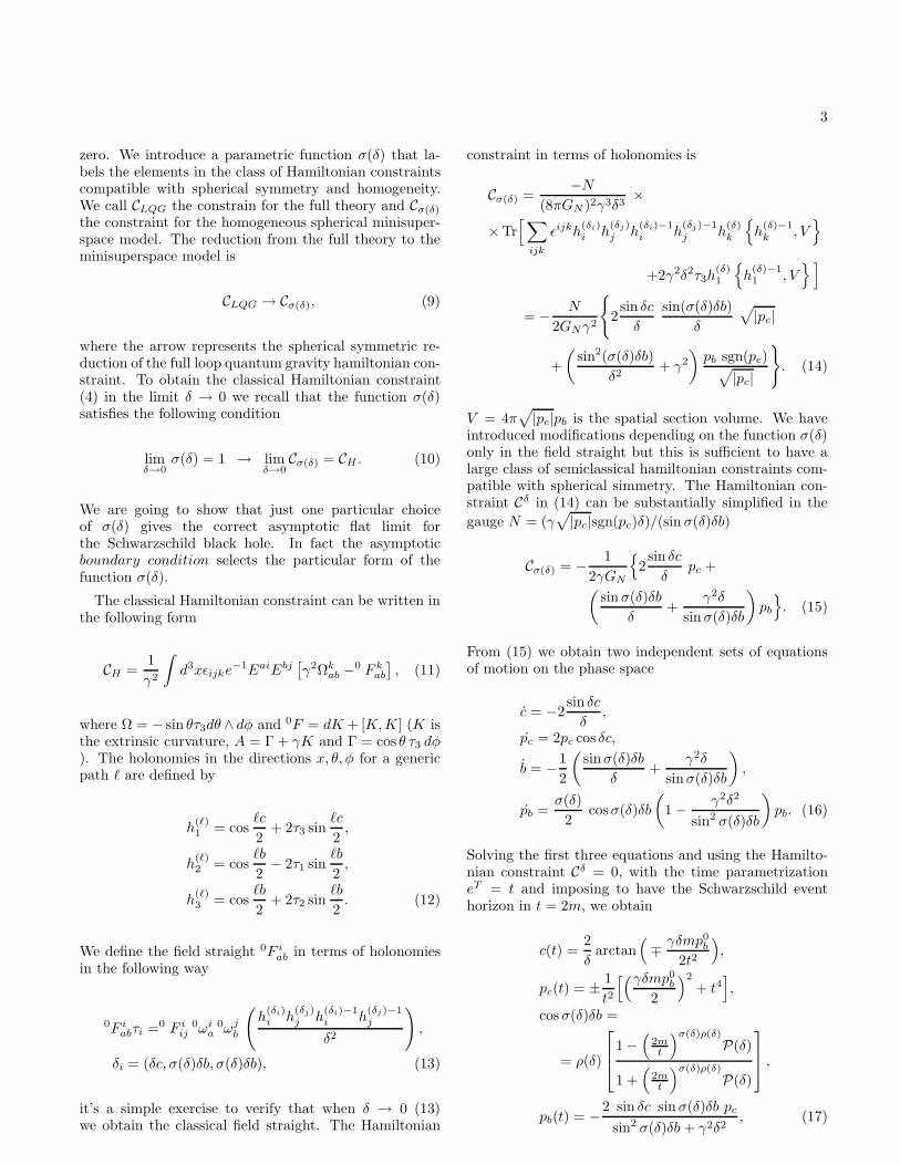
0

FIG. 8: The picture on the left represents the Carter-Penrosediagram in the region outside r

−and the picture on the right

the diagram for r−

6 r 6 0.

where F ′(r)2 = −g00(r)(∂u/∂U−)(∂v/∂V −). Now themetric is regular in r = r− but singular in r = r+.

7) As in the region r > r− we introduce coordinates(t′′, x′′, θ, φ) in terms of which ds2 = F ′ 2(r)(−dt′′2 +dx′′ 2). The r-constant trajectories are defined by thecurves

U−V − = t′′ 2 − x′′ 2 =

= − 1

k2−

(r− − r)(r+ − r)k+k−

e2

k+

256π2

[

−2a2

0P(δ)2m2r

+512π2r+a20(P(δ)2+1)

P(δ)4 m3 log(r)

]

. (40)

In particular the horizons r+, r− and the point r = 0 aredefined by the curves

U−V − = t′′ 2 − x′′ 2 = +∞ , r = r+,

U−V − = t′′ 2 − x′′ 2 = 0 , r = r−,

U−V − = t′′ 2 − x′′ 2 = −∞ , r = 0. (41)

8) In coordinate (ψ′, φ′, θ, φ) defined by U− ∼ tan[(ψ′−ξ′)/2], V + ∼ tan[(ψ′ + ξ′)/2]. The event horizon r = r−is localized in U−V − = 0 or ψ′ = ±ξ′, The event horizonr = r+ is localized in U−V − = +∞ or: ψ′ = ∓ξ′ ± π for0 6 ξ′ 6 π/2, ψ′ = ±ξ′ ± π for 0 6 ξ′ 6 π/2. The otherasymptotic regions are defined by r = 0 : ψ′ = ±ξ′ ∓ πfor π/2 6 ξ 6 π and ψ′ = ±ξ′ ± π for −π 6 ξ′ 6 −π/2.The Carter-Penrose diagram for this region is the pictureon the right in Fig.(8).

Now we are going to show that any massive particlecould not fall in r = 0 in a finite proper time. We considerthe radial geodesic equation for a massive point particle

(−gtt grr)r2 = E2

n + gtt, (42)

where “ ˙ ” is the proper time derivative and En is thepoint particle energy. If the particle falls from the infinitywith zero initial radial velocity the energy is En = 1. Wecan write (42) in a more familiar form

(−gtt grr)︸ ︷︷ ︸

>0 ∀r

r2 + Veff︸︷︷︸

−gtt

(r) = E︸︷︷︸

E2n

, (43)

9

0.00 0.01 0.02 0.03 0.04 0.05

-0.0001

0.0000

0.0001

0.0002

0.0003

0.0004

r

Vef

f

0 20 40 60 80 100-2

-1

0

1

2

rV

eff

FIG. 9: Plot of Veff (r). On the left there is a zoom of Veff

for r ∼ 0.

I+

RI+

L

I−

LI−

R

I+

RI+

L

I−

L

I−

R

2m

2m

2m

2m

r−

r−

r−

r−

r−

r−

r−

r−

r−

r−

r−

r−

r−

r−

r−

r−

r+

r+ r+

r+

r=

0r=

0

r=

0r=

0

r=

0r=

0

r=

0r=

0

r=

0r

=0

r=

0r

=0

FIG. 10: Maximal space-time extension of the LQBH on theright and the analog extension for the Reissner-Nordstromblack hole.

A plot of Veff is in Fig.(9). For r = 0, Veff (r = 0) =4m4π2γ8δ8/a2

0 then any particle with En < Veff (0) couldnot arrive in r = 0. If the particle energy is En > Veff (0),the geodesic equation for r ∼ 0 is r2 ∼ r4 and integratingτ ∼ 1/r − 1/r0 or ∆τ ≡ τ(r0) − τ(0) → +∞. We cancompose the diagrams in Fig.(8) to obtain a maximal ex-tension similar to the Reissner-Nordstrom one, the resultis represented in Fig.(10).

V. ASYMPTOTIC SCHWARZSCHILD CORE

NEAR r ∼ 0

In this section we study the r ∼ 0 limit of the metric(31). If we develop the metric very closed to the pointr ∼ 0 we obtain :

ds2 = −(a− b r)dt2 +dr2

c r4 − d r5+dΩ

c r2

(2)

. (44)

The parametric functions a, b, c, d are

a =64Ω(δ)m4π2γ4δ4P(δ)2

a20(1 + γ2δ2)2

,

b =128Ω(δ)m3π2γ2δ2P(δ)

a20(1 + γ2δ2)

,

c =64π2

a20

,

d =128π2(1 + γ2δ2)P(δ)

a20mγ

2δ2. (45)

We consider the coordinate changing R = 1/r√c. The

point r = 0 is mapped in the point R = +∞. The metricin the new coordinates is

ds2 = −(1 − m1

R

)dt2 +

dR2

1 − m2

R

+R2dΩ(2), (46)

where m1 and m2 are functions of m, a0, δ, γ,

m1 =b

a√c

=a0

4πmγ2δ2P(δ),

m2 =d

c3/2=

a0(1 + γ2δ2)

4πmγ2δ2P(δ). (47)

For small δ we obtain m1 ∼ m2 and (46) converges to theSchwarzschild metric of mass M ∼ a0/2mπγ

4δ4. We canconclude the space-time near the point r ∼ 0 is describedby an effective Schwarzschild metric of mass M ∼ a0/min the large distance limit R ≫ M . An observer in theasymptotic region r = 0 experiments a Schwarzschildmetric of mass M ∼ a0/m.

We now want give a possible physical interpretation ofp0

b . If we reintroduce p0b ∼ a0/m in the core mass M

defined above we obtain M ∼ p0b , then we can interpret

p0b as the mass of the black hole as it is seen from an

observer in r ∼ 0. In [9] the authors interpret p0b as the

mass of a second black hole, in our analysis instead p0b

seems to be the mass of the black hole but from the pointof view of an observer in the asymptotic region r ∼ 0.

VI. LQBH TERMODYNAMICS

In this section we study the termodynamics of theLQBH [19]. The form of the metric calculated in theprevious section has the general form

ds2 = −g(r)dt2 +dr2

f(r)+ h2(r)(dθ2 + sin2 θdφ2), (48)

where the functions f(r), g(r) and h(r) depend on themass parameter m and are the components of the met-ric (31). We can introduce the null coordinate v to ex-press the metric (48) in the Bardeen form. The nullcoordinate v is defined by the relation v = t + r∗,

10

where r∗ =∫ rdr/√

f(r)g(r) and the differential is dv =

dt+ dr/√

f(r)g(r). In the new coordinate the metric is

ds2 = −g(r)dv2 + 2

√

g(r)

f(r)drdv + h2(r)dΩ(2). (49)

We can interpret our black hole solution has been gener-ated by an effective matter fluid that simulates the loopquantum gravity corrections (in analogy with the paper[19]). The effective gravity-matter system satisfies bydefinition of the Einstein equation G = 8πT , where T isthe effective energy tensor. The stress energy tensor for aperfect fluid compatible with the space-time symmetriesis T µ

ν = (−ρ, Pr, Pθ, Pθ) and in terms of the Einstein ten-sor the components are ρ = −Gt

t/8πGN , Pr = Grr/8πGN

and Pθ = Gθθ/8πGN . The semiclassical metric to zero

order in δ and a0 is the classical Schwarzschild solution(gC

µν) that satisfies Gµν (gC) ≡ 0.

A. Temperature

In this paragraph we calculate the temperature for thequantum black hole solution and analyze the evaporationprocess. The Bekenstein-Hawking temperature is givenin terms of the surface gravity κ by T = κ/2π, the sur-face gravity is defined by κ2 = −gµνgρσ∇µχ

ρ∇νχσ/2 =

−gµνgρσΓρµ0Γ

σν0/2, where χµ = (1, 0, 0, 0) is a timelike

Killing vector and Γµνρ is the connection compatibles with

the metric gµν of (48). Using the semiclassical metric wecan calculate the surface gravity in r = 2m obtaining andthen the temperature,

T (m) =128πσ(δ)

√

Ω(δ)m3

1024π2m4 + a20

. (50)

The temperature (50) coincides with the Hawking tem-perature in the large mass limit. In Fig.11 we have a plotof the temperature as a function of the black hole massm. The dashed trajectory corresponds to the Hawkingtemperature and the continuum trajectory correspondsto the semiclassical one. There is a substantial differencefor small values of the mass, in fact the semiclassical tem-perature tends to zero and does not diverge for m → 0.The temperature is maximum for m∗ = 31/4√a0/

√32π

and T ∗ = 33/4σ(δ)√

Ω(δ)/√

32πa0. Also this result, asfor the curvature invariant, is a quantum gravity effect,in fact m∗ depends only on the Planck area a0. If wecalculate the limit δ → 0 in T (m) and T ∗ we obtain twophysical quantities which are independent of δ,

limδ→0

T (m) =128πm3

1024π2m4 + a20

,

limδ→0

T ∗ =33/4

4√

2πa0. (51)

0.0 0.5 1.0 1.5 2.00.0

0.1

0.2

0.3

0.4

0.5

m

THmL

FIG. 11: Plot of the temperature T (m). The continuum plotrepresent the LQBH temperature and the dashed line repre-sent the Hawking temperature T = 1/8πm.

B. Entropy

In this section we calculate the entropy for the LQBHmetric. By definition the entropy as function of the ADMenergy is SBH =

∫dm/T (m). Calculating this integral

for the LQBH we find

S =1024π2m4 − a2

0

256πm2σ(δ)√

Ω(δ)+ const.. (52)

We can express the entropy in terms of the event horizonarea. The event horizon area (in r = 2m) is

A =

∫

dφdθ sin θ pc(r)∣∣∣r=2m

= 16πm2 +a20

64πm2. (53)

Inverting (53) for m = m(A) and introducing the resultin (52) we obtain

S =

√

A2 − a20

4σ(δ)√

Ω(δ). (54)

A plot of the entropy is in Fig.12. The first plot rep-resents entropy as a function of the event horizon areaA. The second plot in Fig.12 represents the event hori-zon area as function of m. The semiclassical area hasa minimum value in A = a0 for m =

√

a0/32π. As forthe temperature also for the entropy we can calculate thelimit δ → 0 and we obtain a regular quantity which de-pends on the event horizon area, on the Planck area butit is independent from δ,

limδ→0

S =

√

A2 − a20

4. (55)

In the limit a0 → 0, S → A/4.We want underline the parameter δ does not play any

regularization rule in the observable quantities T (m), T ∗,

11

0.0 0.1 0.2 0.3 0.4 0.50

2

4

6

8

10

m

Ent

ropy

0.0 0.1 0.2 0.3 0.4 0.50

2

4

6

8

10

m

Are

a

FIG. 12: In the first plot we have the entropy for the LQBH asfunction of the event horizon area (dashed line represents theclassical area low Scl = A/4). In the second plot we representthe event horizon area as function and the mass (dashed linerepresents the classical area Acl = 16πm2).

m∗ and in the evaporation process that we will study inthe following section. We obtain finite quantities takingthe limit δ → 0. This is an important prediction of themodel.

C. The evaporation process.

In this section we focus our attention on the evapora-tion process of the black hole mass and in particular inthe energy flux from the hole. First of all the luminos-ity can be estimated using the Stefan law and it is givenby L(m) = αA(m)T 4

BH(m), where (for a single mass-less field with two degree of freedom) α = π2/60, A(m)is the event horizon area and T (m) is the temperaturecalculated in the previous section. At the first order inthe luminosity the metric (49) which incorporates the de-creasing mass as function of the null coordinate v is alsoa solution but with a new effective stress energy tensor asunderlined previously. Introducing the results (50) and(53) of the previous paragraphs in the luminosity L(m)we obtain

L(m) =4194304m10π3ασ4Ω2

(a20 + 1024m4π2)3

. (56)

Using (56) we can solve the fist order differential equation

− dm(v)

dv= L[m(v)] (57)

to obtain the mass function m(v). The result of integra-tion with initial condition m(v = 0) = m0 is

−n1a60 + n2a

40m

4π2 + n3a20m

8π4 − n4m12π6

n5m9π3ασ(δ)4Ω(δ)2+

+n1a

60 + n2a

40m

40 + π2 + n3a

20m

80π

4 − n4m120 π

6

n5m90π

3ασ(δ)4Ω(δ)2= −v

(58)

where n1 = 5, n2 = 27648, n3 = 141557760, n4 =16106127360, n5 = 188743680. From the solution (58)we see the mass evaporate in an infinite time. Also in(58) we can take the limit δ → 0 obtaining a regularquantity independent from δ. In the limit m → 0 equa-tion (58) becomes

n1a60

n5π3ασ(δ)4Ω(δ)2m9= v. (59)

We can take the limit δ → 0 obtaining n1a60/n5π

3αm9 ∼v. Inverting this equation for small m we obtain: m ∼(a6

0/α v)1/9.

VII. THE METRIC FOR δ → 0

We have shown in the previous section that same phys-ical observable can be defined independently from thepolymeric parameter δ. This result suggest to calculatethe limit of the semiclassical metric (31) for δ → 0. Wewill obtain a regular metric and we will study its space-time structure. In the quantum theory we can not takethe limit δ → 0 because we haven’t weakly continuity inthe polymeric parameter δ. However the LQBH’metric(31) is very close to the Reissner-Nordstrom metric whichis not stable and this suggest that also (31) could be notstable when we consider non homogeneities [20]. If it isthe case then the horizon r− disappearances or in otherwords by (19), P(δ) → 0. Another motivation to cal-culate and to study this extreme limit of the metric isto show that the polymeric parameter does not play anyrule in the singularity problem reslution. For δ → 0 the(√

|p2b |/p0

b/p0b, log(pc)) plot is given in Fig.13.

We redefine the metric of section (31) introducing anexplicit dependence from δ (the redefinition is: gµν(r) →gµν(r; δ)). The new metric is mathematically defined by

limδ→0

gµν(r; δ) ≡ gµν(r). (60)

The result of this limit gives the following very simplemetric which is independent from the polymeric param-eter δ,

ds2 = −64π2r3(r − 2m)

64π2r4 + a20

dt2 +dr2

64π2r3(r−2m)64π2r4+a2

0

+( a2

0

64π2r2+ r2

)

dΩ(2). (61)

12

-20 -10 0 10 200

2

4

6

8

10

12

logHpcL

pb

FIG. 13: Plot (p

|p2

b |/p0

b , log(pc)) for δ → 0. The dashed linerepresents the classical solution.

This metric has an event horizon in r+ = 2m and this isin accord with the solution for general values of δ, in factlimδ→0 r− = 0. The question now is to see if the solutionis regular in all space-time and in particular in r = 0. Wecan calculate the Kretschmann invariant and we obtain

K(r) =65536π4r2

(a20 + 64π2r4)6

(−6291456a20π

6m(2m− r)r12

+50331648m2π8r16 + a80(15m2 − 24mr + 11r2)

−128a60π

2r4(36m2 − 56mr + 17r2)

+4096a40π

4r8(294m2 − 272mr + 63r2)). (62)

The invariant (62) is regular in all space-time and inparticular in r = 0. For a0 ∼ 0 we find K(r) =48m2/r6 + O(a2

0) and for r ∼ 0 we have K(r) =(983040m2π4r2)/a4

0 + O(r3) that shows the non pertur-bative character of the singularity resolution. From thesecond picture in Fig.(16) is evident the r-coordinate ofthe pick of the curvature invariantK is independent fromthe black hole mass.

What about temperature, entropy and the evaporationprocess? We calculate the surface gravity for the metric(61) and we obtain

κ =65536m6π4

(a20 + 1024m4π2)2

. (63)

This result is exactly the same quantity obtained in sec-tion (VI) but with δ → 0. From this point the analysisis the same of section (VI): temperature, entropy andevaporation are the same of (51), (55), (58).

Causal structure and Carter-Penrose diagrams

In this section we construct the Carter-Penrose dia-grams for the metric obtained taking the limit δ → 0. Toobtain the diagrams we must do many coordinate chang-ing and we enumerate them from one to five.

0.0 0.2 0.4 0.6 0.8 1.00

2.´107

4.´107

6.´107

8.´107

r

K

FIG. 14: Plot of the Kretschmann invariant for the metric(61). The first picture represent K(r) and the second oneK(r,m) for m ∈ [0, 1010] and r ∈ [0, 0.6]. It is manifest theposition of the maximum of K(m, r) is independent of themass m.

1) First of all we calculate the tortoise coordinate r∗

for the metric (61) defined by dr∗2 = −g11(r)dr2/g00(r),

r∗ =1

64π2

(

a20

4mr2+

a20

4m2r+ 64π2r − a2

0 log |r|8m3

+(a2

0 + 1024m4π2) log |r − 2m|8m3

)

. (64)

The coordinate (64) reduces to the Schwarzschild tortoisecoordinate r∗ = r + 2m log |r − 2m| for a0 → 0. On theother side for r → 0, r∗ ∼ a0/4mr

2. Using coordinate(t, r∗, θ, φ) the metric is

ds2 = g00(r(r∗))(dt2 − dr∗2) + gθθ(r(r

∗))dΩ(2), (65)

where g00(r(r∗)) is implicitly define by (64) (from now

on we will not write the S2 sphere part of the metric).2) Now we write the metric in coordinate (v, w, θ, φ)

defined by v = t+r∗ and w = t−r∗. The metric becomes

ds2 = g00(r(r∗))dvdw = −64π2r3(r − 2m)

64π2r4 + a20

dvdw, (66)

where r is defined implicitly in terms of v, w.

13

3) We can do another coordinate changing which leavesthe two space conformally invariant. The news coordi-nate (v′, w′, θ, φ) are defined by v′ = v′(v) and w′ =w′(w). The metric is

ds2 = −64π2r3(r − 2m)

64π2r4 + a20

dv

dv′dw

dw′dv′dw′, (67)

4) We introduce the new coordinates (t′, x′, θ, φ) de-fined by t′ = (v′ + w′)/2 and x′ = (v′ − w′)/2. Themetric is

ds2 =64π2r3(r − 2m)

64π2r4 + a20

dv

dv′dw

dw′(−dt′2 + dx′2). (68)

All the coordinates in the conformal factor are implicitlydefined in terms of t′, x′.

At this point we choose explicitly the functions v′(v)and w′(w) to eliminate the singularity in r = 2m. Fol-lowing the analysis of the Schwarzschild case we takev′(v) = exp(v/λ) and w′(w) = − exp(−w/λ), where2/λ = 512π2m3/(a2

0 + 1024π2m4). This is the correctcoordinate changing also in our case to eliminate the co-ordinate singularity on the event horizon. We define thefunction F 2(r) = −g00(∂v/∂v′)(∂w/∂w′) that in termsof the radial coordinate r becomes

F 2(r) = −λ2g00(r)e−

(v−w)λ = −λ2g00(r)e

−2r∗

λ

= 4

(

a20 + 1024π2m4

512π2m3

)2(

64π2r3

64π2r4 + a20

)

×

× e−

2λ

[a20

256π2mr

(

1r+ 1

m

)

+r−a20

512π2m3 log(r)

]

. (69)

The metric ds2 = F 2(r)(−dt′2 + dx′2) is regular on theevent horizon. In the coordinates (t′, x′) the event hori-zon and the point r = 0 are localized respectively in

t′2 − x′2 = 0,

t′2 − x′2 → 2m exp( 2a2

0

256π2mλr2

)

→ +∞.

(70)

5) We conclude writing the metric in the coordinates(ψ, ξ, θ, φ) defined by v′ ∼ tan[(ψ + ξ)/2] and w′ ∼tan[(ψ − ξ)/2]. The event horizon r = 2m is definedby the curve t′2 − x′2 = v′w′ = 0 and then by theψ = ±ξ. From (70) the point r = 0 is defined by thecurve t′2 − x′2 = v′w′ = +∞ and or by the segments(ψ = ∓ξ ± π, 0 6 ξ 6 π/2), (ψ = ±ξ ± π, 0 6 ξ 6 π/2).The other sectors are: I+, I− (ψ = −∓ ξ ± π, −π 6 ξ 6π), i0 (ψ = 0, ξ = π), i+, i− (ψ = ±π/2, ξ = π/2). TheCarter-Penrose diagram of the regular space-time is rep-resented in Fig.(16). The maximal space-time extensionis represented in Fig.(17), the diagram can be infinitelyextended in the four directions.

We now show that a massive particle arrives in r =0 in a finite proper time. The radial geodesic equa-tion is (dr/dτ)2 = E2

n − 1/grr (τ is the proper time,

-4 -2 0 2 4

-60

-40

-20

0

20

40

60

r

g00H

rL

FIG. 15: Plot of gtt(r) for −∞ < r < +∞. In the picture isnot visible the horizon in r = 2m.

2m 2m

2m2m I+

LI+

R

I−

RI−

L

r = 0

r = 0

FIG. 16: Carter-Penrose diagram for the regular space-timedescribed by the metric (61) in coordinate (ψ, ξ), the verticaland horizontal axes are respectively ψ and ξ.

En the particle energy) and for r ∼ 0 reduces tor(1 − 64π2mr3/a2

0E2n) ∼ −En. The τ(r) solution is

r − r0 − 16π2m(r4 − r40)/E2na

20 = −Enτ and the proper

time to fall in r = 0 starting from r0 & 0 is: ∆τ =τ(0) − τ(r0) = (1 − 16π2mr30/E

2na

20)r0/En. Any massive

particle falls in r = 0 in a finite proper-time interval.To conclude the analysis we extend the radial coordi-

nate to negative values. The surface Σ(r, θ) = r = 0is a null surface as can be shown following the analysisin (III) (in particular grr|r=0 = 0). We can extend theradial coordinate r to negative values because the space-time is singularity free. The metric is asymptotically flatfor r → −∞ and at the order O(r−2) takes the form

ds2 = −(

1 − 2m

r

)

dt2 +dr2

1 − 2mr

+ r2dΩ(2) , r 6 0.

(71)

Because r 6 0 we have not event horizons in the negativeregion. The metric (61) is regular in all space-time −∞ <r < +∞. The Carter-Penrose diagrams are in Fig.(18).

14

r = 0

r = 0

r = 0

r = 0

r = 0

r = 0

r = 0

r=

0r

=0

r = 0

r=

0

r=

0

r=

0

r=

0

r=

0

r=

0

I+

RI

+

L

I−

LI−

R

2m

2m

2m

2m

FIG. 17: A possible maximal space-time extension of theCarter-Penrose diagram in Fig.(16).

2m 2m

2m2m I+

LI+

R

I−

RI−

L

r = 0

r = 0

2m

2m

2m

2m

r

=

−∞

r

=

−∞

r=

0

r=

0r=

0

r=

0

r

=

−∞

r

=

−∞

r=

0

r=

0

r=

0

r=

0r=

0

r=

0

r=

0

r=

0

I+

RI

+

L

I−

L

I−

R

2m

2m

2m

2m

r

=

−

∞

r

=

−

∞

r

=

−

∞

r

=

−

∞

r

=

−

∞

r

=

−

∞

r

=

−

∞

r

=

−

∞

FIG. 18: Carter-Penrose diagrams for r > 0 on the left andr 6 0 on the right. The lower picture represents a maximalextension for −∞ 6 r 6 +∞ .

We can obtain the same results of this section in an-other equivalent way. Essentially what we have done inthis section is to show that to solve the black hole singu-larity problem at semiclassical level it is sufficient to re-place the component c(t) with the holonomy h = exp(δc)without to replace the component b(t) with the relativeholonomy. In fact the solution (61) can be obtained di-rectly from the semi-quantum Hamiltonian constraint

Csq = − 1

2γGN

2(sin δc/δ) pc︸ ︷︷ ︸

Quantum Sector

+ (b2 + γ2)pb/b︸ ︷︷ ︸

Classical Sector

. (72)

The scalar constraint (72) is classic in the b, pb sector but

quantum in the c, pc sector (N = γ√

|pc|sgn(pc)/b andσ(δ) = 1). The constraint introduced in (14) is not themore general. We can introduce two different polymericparameter δb and δc respectively in the directions θ, φand r obtaining the constraint

Cδb,δc= − N

2GNγ2

2sin δcc

δc

sin(σ(δb)δbb)

δb

√

|pc|

+

(sin2(σ(δb)δbb)

δ2b+ γ2

)pb sgn(pc)√

|pc|

, (73)

and N = N = γ√

|pc|sgn(pc)δb/ sin(σ(δb)δbb). Thescalar constraint (72) is obtained taking the limit

limδb→0

C(δb,δc)|δc=δ = Csq. (74)

The main result is that the singularity problem issolved by a bounce of the two sphere on a minimal areaa0. The parameter δ does not play any role in the sin-gularity problem resolution. This is evident from theKretschmann invariant (62) which is independent fromδ. The parameter δ is related to the position of the innerhorizon and for δ → 0 the horizon r− disappearances.

CONCLUSIONS & DISCUSSION

In this paper we have introduced a simple modificationof the holonomic Hamiltonian constraint which gives themetric with the correct semiclassical asymptotic flat limitwhen the Hamilton equations of motion are solved. Werecall here the LQBH’s metric

ds2 = −64π2(r − r+)(r − r−)(r + r+P(δ))2

64π2r4 + a20

dt2 +dr2

64π2(r−r+)(r−r−)r4

(r+r+P(δ))2(64π2r4+a20)

+( a2

0

64π2r2+ r2

)

(sin2 θdφ2 + dθ2), (75)

15

We have shown the LQBH’s metric (75) has the followingproperties

1. limr→+∞ gµν(r) = ηµν ,

2. limr→0 gµν(r) = ηµν ,

3. limm,a0→0 gµν(r) = ηµν ,

4. K(g) <∞ ∀r,

5. rMax(K(g)) ∼ √a0.

In particular (see point 5.) the position (rMax) where

the Kretschmann invariant operator is maximum is in-

dependent from the black hole mass and from the poly-

meric parameter δ. The metric has two event horizonsthat we have defined r+ and r−; r+ is the Schwarzschildevent horizon and r− is an inside horizon. The solutionhas many similarities with the Reissner-Nordstrom met-ric but without curvature singularities. In particular theregion r = 0 corresponds to another asymptotically flatregion. Any massive particle can not arrive in this regionin a finite proper time. A careful analysis shows the met-ric has a Schwarzschild core in r ∼ 0 of mass M ∼ a0/m.

We have calculated the limit gµν(δ → 0; r) of theLQBH metric obtaining another metric regular in r = 0.This solution can be also obtained from (75) taking thelimit δ → 0 or more simple P(δ) = 0 and r− = 0. Theresult is

ds2 = −64π2r3(r − 2m)

64π2r4 + a20

dt2 +dr2

64π2r3(r−2m)64π2r4+a2

0

+( a2

0

64π2r2+ r2

)

(sin2 θdφ2 + dθ2). (76)

This metric could be see as a solution of the Hamil-ton equation of motion for the semi-quantum scalar con-straint (72).

Our analysis shows that the singularity problem issolved by a bounce of the S2 sphere on a minimum areaa0 > 0. This happens for both the metrics obtainedin this paper, the first one of Reissner-Nordstrom type(75) and the second one of Schwarzschild type (76). The

parameter δ does not play any rule in the singularity res-

olution problem. The solution (76) has all the good prop-erties of (75) and in particular it is singularity free. Thismetric has an event horizon in r = 2m and the thermo-dynamics is exactly the same of (75). When we considerthe maximal extension to r < 0 we find a second internalevent horizon in r = 0.

We have studied the black hole thermodynamics : tem-perature, entropy and the evaporation process. The mainresults are:

1. The temperature T (m) is regular for m ∼ 0 andreduces to the Bekenstein-Hawking temperature forlarge values of the mass Bekenstein-Hawking

T (m) =128πm3

1024π2m4 + a20

. (77)

2. The black hole entropy in terms of the event horizonarea and the LQG minimum area eigenvalue is

S =

√

A2 − a20

4(78)

3. The evaporation process needs an infinite time inour semiclassical analysis but the difference withthe classical result is evident only at the Planck

scale. In this extreme energy conditions it is neces-sary a complete quantum gravity analysis that canimplies a complete evaporation [18].

We have shown it is possible to take the limit δ → 0in T (m), S(A) and the evaporation process equationF(m;m0, a0) = v obtaining regular quantities indepen-dent of the polymeric parameter δ. The result of the limitare physical quantities that depend only on the Planckarea and not on the polymeric parameter.

We want to conclude the discussion with a stimulat-ing observation. In this paper we have calculated thetemperature (77) that in general we can see as a rela-tion between temperature, mass and the minimum areaa0. If we solve (77) for the minimum area we obtain theuniversal critical behavior a0 ∼ (Tc − T )1/2. The criti-cal exponent ζ = 1/2 is independent from the mass andfrom the particular choice of the Hamiltonian constraintmodification. The critical temperature is the classicalHawking temperature Tc = 1/8πm [21].

Some open problems. In this paper we have fixed thep0

b parameter (which comes from the integration of theHamilton equations of motion) introducing the minimumarea a0 (of the full theory) in the metric solution. Inthis way we have obtained a bounce of the S2 sphere onthe minimum area a0. A priori it is not obvious how toobtain the same bounce at the quantum level. Howeversolving the quantum constraint we think we will obtaina bounce on a minimum area a0 ∼ GN~. The QEEcontains only dimensionless quantities, the eigenvaluesτ, µ of the operators pc, pb and the polymeric parameterδ. When we reintroduce the length dimensions in theQEE we have µ ≡ 2pb/γl

2P , τ ≡ pc/γl

2P , then in the

quantum evolution l2P will play the rule played by a0 inthe semiclassical analysis and we will have a quantum

16

bounce of the wave function on l2P ∼ a0. This is manifestin the effective Wheeler-DeWitt equation obtained fromthe QEE in the limit µ ≫ δ, τ ≫ δ [6] where a2

0 ∼ l4Pappears explicitly,

l4P

(

√pc

∂2Ψ

∂pb∂pc+

pb

4√pc

∂2Ψ

∂2pb+

1

2√pc

∂Ψ

∂pb

)

+

− pb

4√pc

Ψ = 0. (79)

However the quantum evolution of a coherentSchwarzschild state is an open problem.

A problem related to the previous one is that we havefixed the integration in the x direction to a cell of fi-nite volume Lx and this can imply a non scale invariantresolution of the singularity problem under a rescalingLx → L′

x [23].Another problem can be related to the entropy calcu-

lation. In fact we obtain a regular entropy but we do notobtain the usual logarithmic correction. We think it ispossible to solve this problem with a simple modification

of the holonomic version of the Hamiltonian constraintor taking into account the possibility that quantum prop-erties of the background space-time alter geometry nearthe horizon [24].

Other problems could be related to the maximal ex-tension of the space-time. If we observe carefully thediagram in Fig.17 we can see that close time-like curve

(CTC) are possible. This is manifest in the Fig.19 wherea null CTC is represented by a close black curve. In thesecond diagram of Fig.19 we have represented the lightcones along a CTC curve. We can have CTCs also withjust one diagram if we identify the upper and lower ex-tremes of the diagram (18).

Acknowledgements

We are grateful also to Parampreet Singh, MicheleArzano and Eugenio Bianchi for many important andclarifying discussions.

[1] Carlo Rovelli, Quantum Gravity, (Cambridge UniversityPress, Cambridge, 2004); A. Ashtekar, Background inde-

pendent quantum gravity: A Status report, Class. Quant.Grav. 21, R53 (2004), gr-qc/0404018; T. Thiemann, Loop

quantum gravity: an inside view, hep-th/0608210; T.Thiemann, Introduction to Modern Canonical Quantum

General Relativity, gr -qc/0110034; Lectures on Loop

Quantum Gravity, Lect. Notes Phys. 631, 41-135 (2003),gr-qc/0210094

[2] Martin Bojowald, Loop quantum cosmology, Living Rev.Rel. 8:11, 2005, gr-qc/0601085; Martin Bojowald, Ab-sence of singularity in loop quantum cosmology Phys.Rev. Lett. 86:5227-5230, 2001. e-Print: gr-qc/0102069

[3] A. Ashtekar, M. Bojowald and J. Lewandowski, Mathe-

matica structure of loop quantum cosmology, Adv. Theor.Math. Phys. 7 (2003) 233-268, gr-qc/0304074 AbhayAshtekar , Tomasz Pawlowski, Parampreet Singh, KevinVandersloot, Loop quantum cosmology of k=1 FRW mod-

els, Phys. Rev. D75 (2007) 024035, gr-qc/0612104; Ab-hay Ashtekar, Tomasz Pawlowski, Parampreet Singh,Quantum Nature of the Big Bang: Improved dynamics,Phys. Rev. D74 (2006) 084003, gr-qc/0607039; AbhayAshtekar, Tomasz Pawlowski, Parampreet Singh, Quan-

tum Nature of the Big Bang: An Analytical and Nu-

merical Investigation. I, Phys.Rev.D73 (2006) 124038,gr-qc/0604013

[4] R. Kantowski and R. K. Sachs, J. Math. Phys. 7 (3)(1966); Luca Bombelli & R. J. Torrence Perfect fluids

and Ashtekar variables, with application to Kantowski-

Sachs models, Class. Quant. Grav. 7 (1990) 1747-1745[5] Leonardo Modesto, Disappearance of the black hole sin-

gularity in loop quantum gravity, Phys. Rev. D 70(2004) 124009, gr-qc/0407097; Leonardo Modesto, The

kantowski-Sachs space-time in loop quantum gravity, In-ternational Int. J. Theor. Phys. 45 (2006) 2235-2246,gr-qc/0411032; Leonardo Modesto, Loop quantum gravity

and black hole singularity, proceedings of 17th SIGRAVConference, Turin, Italy, 4-7 Sep 2006, hep-th/0701239;Leonardo Modesto, Gravitational collapse in loop quan-

tum gravity, Int. J. Theor. Phys.47 (2008) 357-373,gr-qc/0610074; Leonardo Modesto, Quantum gravita-

tional collapse, gr-qc/0504043[6] A. Ashtekar and M. Bojowald, Quantum geometry and

Schwarzschild singularity Class. Quant. Grav. 23 (2006)391-411, gr-qc/0509075; Leonardo Modesto, Loop quan-

tum black hole, Class. Quant. Grav. 23 (2006) 5587-5602,gr-qc/0509078

[7] Rodolfo Gambini, Jorge Pullin, Black holes in loopquantum gravity: The Complete space-time, Phys.Rev. Lett.101:161301, 2008, arXiv:0805.1187; MiguelCampiglia, Rodolfo Gambini, Jorge Pullin, Loop quan-

tization of spherically symmetric midi-superspaces : the

interior problem, AIP Conf. Proc. 977:52-63, 2008,arXiv:0712.0817; Miguel Campiglia, Rodolfo Gambini,Jorge Pullin, Loop quantization of spherically symmet-ric midi-superspaces Class. Quant. Grav. 24:3649-3672,2007, gr-qc/0703135

[8] Leonardo Modesto, Black hole interior from loop quan-

tum gravity, gr-qc/06011043; Leonardo Modesto, Evapo-

rating loop quantum black hole, gr-qc/0612084[9] ChristianG. Bohmer, KevinVandersloot, Loop quantum

dynamics of the Schwarzschild Interior, arXiv:0709.2129[10] Dah-Wei Chiou, Phenomenological Loop Quantum Ge-

ometry of the Schwarzschild Black Hole, arXiv:0807.0665[11] C. Rovelli and L. Smolin, Loop Space Representation Of

Quantum General Relativity, Nucl. Phys. B 331 (1990)80; C. Rovelli and L. Smolin, Discreteness of area and

volume in quantum gravity, Nucl. Phys. B 442 (1995)593; Eugenio Bianchi, The Length operator in Loop

Quantum Gravity, Nucl. Phys. B 807 (2009) 591-624,arXiv:0806.4710

[12] Abhay Ashtekar, New Hamiltonian formulation of gen-

17

r = 0

r = 0

r = 0

r = 0

r = 0

r = 0

r = 0

r=

0r

=0

r = 0

r=

0

r=

0

r=

0

r=

0

r=

0

r=

0

I+

RI

+

L

I−

LI−

R

2m

2m

2m

2m

2m

2m

2m

2m

r=

0

r=

0

r=

0

r=

02m

2m

2m

2m

2m

2m

r=

0

r=

0

r=

0r=

0

2m

2m

r=

0

r=

0

r=

0

2m

2m

2m

2m

r=

0

FIG. 19: Carter-Penrose diagram of Fig.17 with evidenced alight CTC curve in the first diagram and the light cones alonga CTC curve in the second diagram.

eral relativity, Phys. Rev. D 36 1587-1602[13] Florian Conrady, Laurent Freidel, Path integral represen-

tation of spin foam models of 4d gravity, arXiv:0806.4640;Jonathan Engle, Etera Livine, Roberto Pereira, CarloRovelli, LQG vertex with finite Immirzi parameter, Nucl.Phys. B799 (2008) 136-149, arXiv:0711.0146; JonathanEngle, Roberto Pereira, Carlo Rovelli, Flipped spinfoam

vertex and loop gravity Nucl. Phys. B798 (2008) 251-290,arXiv:0708.1236; Jonathan Engle, Roberto Pereira, CarloRovelli, The Loop-quantum-gravity vertex-amplitude,Phys. Rev. Lett. 99 (2007) 161301, arXiv:0705.2388

[14] Florian Conrady, Laurent Freidel, On the semiclassical

limit of 4d spin foam models, arXiv:0809.2280; EmanueleAlesci, Carlo Rovelli, The Complete LQG propagator I.

Difficulties with the Barrett-Crane vertex, Phys. Rev.D76 (2007) 104012, arXiv:0708.0883; Simone Speziale,Background-free propagation in loop quantum gravity

arXiv:0810.1978; Eugenio Bianchi, Leonardo Modesto,Carlo Rovelli, Simone Speziale Graviton propagator in

loop quantum gravity, Class. Quant. Grav. 23 (2006)6989-7028, gr-qc/0604044; Leonardo Modesto, CarloRovelli Particle scattering in loop quantum gravity in

Phys. Rev. Lett. 95 (2005) 191301, gr-qc/0502036; Euge-nio Bianchi, Leonardo Modesto, The Perturbative Regge-

calculus regime of loop quantum gravity, Nucl. Phys. B796 (2008) 581-621, arXiv:0709.2051; Eugenio Bianchi,Alejandro Satz, Semiclassical regime of Regge calculus

and spin foams, arXiv:0808.1107[15] Karel V. Kuchar, Geometrodynamics of Schwarzschild

Black Hole, Phys. Rev. D50 (19994) 3961-3981,gr-qc/9403003; T. Thiemann, Reduced models for quan-

tum gravity, Lect. Notes Phys. 434 (1994) 289-318,gr-qc/9910010; H.A. Kastrup, T. Thiemann, Spheri-

cally symmetric gravity as a completely integrable sys-

tem, Nucl. Phys. B 425 (1994) 665-686, e-Print:gr-qc/9401032; T. Thiemann, H.A. Kastrup, Canon-

ical quantization of spherically symmetric gravity in

Ashtekar’s selfdual representation Nucl. Phys. B 399(1993) 211-258, gr-qc/9310012

[16] Abhay Ashtekar, Tomasz Pawlowski, Parampreet Singh,Quantum Nature of the Big Bang: An Analytical and

Numerical Investigation. I, Phys.Rev.D73 (2006) 124038,gr-qc/0604013

[17] Alessandro Fabbri and Jose Navarro-Salas, Modeling

Black Hole Evaporation, Imperial College Press (2005)[18] Abhay Ashtekar & Martin Bojowald, Black hole evapo-

ration : A paradigm Class. Quant. Grav. 22 (2005) 3349-3362, gr-qc/0504029

[19] Alfio Bonanno, Martin Reuter, Renormalization group

improved black hole space-times, Phys. Rev. D 62(2000) 043008, hep-th/0002196; Alfio Bonanno, Mar-tin Reuter Spacetime structure of an evaporating black

hole in quantum gravity, Phys. Rev. D 73 (2006)083005, hep-th/0602159; Yun Soo Myung, Yong-WanKim, Young-Jai Park, Thermodynamics of regular black

hole, arXiv:0708.3145; Yun Soo Myung, Yong-Wan Kim,Young-Jai Park, Quantum Cooling Evaporation Process

in Regular Black Holes Phys. Lett. B (2007) 656:221-225,gr-qc/0702145; Piero Nicolini, Noncommutative Black

Holes, The Final Appeal To Quantum Gravity: A Re-

view, arXiv:0807.1939[20] Michael Simpson and Roger Penrose, Internal instability

in Reissner-Nordstrom black hole, Int. J. Theor. Phys. 7(1973) 183-197

[21] Danile Oriti, Group field theory as the microscopic

description of the quantum spacetime fluid: A New

perspective on the continuum in quantum gravity

arXiv:0710.3276[22] Luca Bombelli & R. J. Torrence Perfect fluids and

Ashtekar variables, with application to Kantowski-Sachs

models Class. Quant. Grav. 7 (1990) 1747-1745[23] Alejandro Corichi and Parampreet Singh, Is loop quan-

tization in cosmology unique?, Phys. Rev. D78 (2008)024034, e-Print: arXiv:0805.0136

[24] Michele Arzano, Black hole entropy, log corrections

and quantum ergosphere Phys.Lett.B634 (2006) 536-540,gr-qc/0512071; Michele Arzano, A.J.M. Medved, EliasC. Vagenas, Hawking radiation as tunneling through the

quantum horizon JHEP 0509 (2005) 037, hep-th/0505266