Dynamics of an Acoustic Black Hole as an Open Quantum System

Fernando C. Lombardo and Gustavo J. TuriaciDepartamento de Fısica Juan Jose Giambiagi, FCEyN UBA,

Facultad de Ciencias Exactas y Naturales, Ciudad Universitaria,Pabellon I, 1428 Buenos Aires, Argentina - IFIBA

(August 1, 2012)

We studied the process of decoherence induced by the presence of an environment in acoustic blackholes, using the open quantum system approach, thus extending previous work. We focused on theion trap model but the formalism is general to any experimental implementation. We computed thedecoherence time for that setup. We found that a quantum to classical transition occurs during themeasurement and we proposed improved parameters to avoid such a feature. We provide analyticestimations for both zero and finite temperature. We also studied the entanglement between theHawking-pair phonons for an acoustic black hole while in contact with a reservoir, through thequantum correlations, showing that they remain strongly correlated for small enough times andtemperatures. We used the stochastic formalism and the method of characteristic to solve the fieldwave equation.

PACS numbers: 04.70.Dy, 03.70.+k, 03.75.-b, 04.62.+v, 37.10.Ty

I. INTRODUCTION

Hawking effect, i.e. the particle creation process thatgives rise to a thermal spectrum of radiation outgoingfrom a black hole [1], is a prediction of quantum field the-ory in curved space-time. This effect together with its en-tropy complete the interpretation of black holes as ther-mal objects. On one hand, it is believed that the heart ofa theory that unifies quantum mechanics and gravity liesin understanding the nature of this thermality. On theother hand, it is also important to collect experimentalevidence in order to gain insight into this phenomenon,but this is practically impossible since black holes’ tem-peratures are less than nK. Since the phenomenon hasnot been observed experimentally, it is of crucial impor-tance that all the assumptions underlying the Hawkingeffect be carefully studied so as to try to understand theprocess.

W. G. Unruh proposed an analogue gravity hydrody-namical model where phonons propagate in a fluid witha subsonic and supersonic regime [2]. This model obeysthe dynamics of a massless scalar field near a black holeand provides a possible experimental implementation tostudy the Hawking effect. Subsequently, there have beenseveral more realistic proposals that involved BEC [3],moving dielectrics [4], waveguides [5], slow light systems[6], among others.

On general grounds, an acoustic black hole is a systemin which phonons are unable to escape from a fluid thatis flowing more quickly than the local speed of sound.Therefore, trapped phonons are analogous to light in realgravitational black holes. The phonons propagating inperfect fluids exhibit the same properties of motion asfields, such as gravity, in space and time.

The current proposals do not provide conclusive evi-dence of the Hawking effect (see for example [7]). Nev-ertheless, we believe that a particular one by Horstmannet al., [8], provides a promising setup. This system con-

sists of a circular ring of trapped ions moving with aninhomogeneous velocity profile emulating a black hole,as explained above. The signature of this quantum radi-ation is the correlation between entangled phonons nearthe horizon, [9], which can be measured by coupling theions’ motional degrees of freedom to their internal state,[10].

Given that we are interested in the quantum nature ofthe effect, in this paper we make a study of the interac-tions of the acoustic black hole with an environment andhow this induces decoherence in the system.

The presence of an environment can destroy all thetraces of the quantumness of a system. All real worldquantum systems interact with their surrounding envi-ronment to a greater or lesser extent. As the quantumsystem is in interaction with an environment defined asany degrees of freedom coupled to the system which canentangle its states, a degradation of pure states into mix-tures takes place. No matter how weak the couplingthat prevents the system from being isolated, the evo-lution of an open quantum system is eventually plaguedby nonunitary features like decoherence and dissipation.Decoherence, in particular, is a quantum effect wherebythe system loses its ability to exhibit coherent behavior.Nowadays, decoherence stands as a serious obstacle inquantum information processing. All in all, it should becrucial to control decoherence in order to plan a concretesetup for measuring the Hawking radiation as a quantumfeature of analogue gravity models.

In this paper, we show a more detailed and deepertreatment of the problem given in [11], and we presentnew results concerning the evaluation of the decoher-ence time and analytical expressions for correlation func-tions of the quantum fields. We continue using the field-theoretical description in order to present a derivationapplicable to any implementation of an acoustic blackhole. Nevertheless, given our interest in the ion trap weprovide numerical results corresponding to that particu-

arX

iv:1

208.

0198

v1 [

quan

t-ph

] 1

Aug

201

2

2

lar setup.The article is organized as follows: in Sec. II we show

the specific model we are using. In Sec. III we presentthe model of environment and show the non-equilibriumdynamics of the system. Sec. IV contains the estimationof the decoherence time and we show, in Sec. V thedynamics of the entanglement through the analysis ofcorrelations. Finally, we summarize our results in Sec.VI.

II. A PARTICULAR ACOUSTIC BLACK HOLE:THE ION RING

As stated above, we will work in the context of the fieldtheoretical description. Given that we are interested inthe ion ring model, and with the purpose of introducingthe subject of analogue gravity with a specific example,we will explain in detail this set up from first principles.We will begin with the discrete description of N ions ofmass m in a circular trap of radius R to end with thedescription of a massless scalar field in a curved back-ground.

Following the study done in Ref. [8], the Hamiltoniandescribing the ions of the circular trap is given by

H = −N∑i=1

~2

2mR2

∂2

∂θ2i

+

N∑i=1

V e(θi, t)+Vc(θ1, ..., θN ), (1)

where V e(θi, t) is an external field potential correspond-ing to an electric field that induces the classical trajec-tories θ0

i (t) and V c(θ1, ..., θN ) is the Coulomb potentialbetween the ions. Those are such that the velocity profileis

v(θ, t) =

vmin 0 ≤ θ ≤ θH − γ1

β + α(θ−θHγ1

)−γ1 ≤ (θ − θH) ≤ γ1

vmax θH + γ1 ≤ θ ≤ 2π − θH − γ2

β − α(θ−2π+θH

γ2

)−γ2 ≤ (θ − 2π + θH) ≤ γ2

vmin 2π − θH + γ2 ≤ θ ≤ 2π,

where β = (vmax +vmin)/2 and α = (vmax−vmin)/2. Theminimum and maximum velocity are constrained by thecondition that each ion has to make one revolution dur-ing a period T . It is important to notice that we use anapproximate velocity profile, as introduced in Ref. [11].The real, as explained in Ref. [8], must be C3 but oursis a good approximation appropriate to our calculations.Taking this into account, the parameters γi and θH donot exactly match those of Horstmann et al. The systemmay be prepared in an initial thermal state with temper-ature T0. An illustration of the setup and the velocityprofile can be found in Figs. 1 and 2 of Ref. [8].

Initially, the velocity profile is constant with vmin(t =0) = vmax(t = 0) = 2π/T but during a time τ the profilechange such that vmin(t τ) < 2π/T and vmax(t τ) > 2π/T in the following way

vmin(t) = vmin +

(2π

T− vmin

)e−t

2/τ2

, (2)

where we call τ = 0.05 · T the collapse time, which ismuch smaller than T , and after that time the asymptoticprofile is given by the parameter vmin(t τ) = vmin. Itis important to notice that the measurement can only beperformed during one period T , since after that time thesystem’s classical configuration loses its stability, see Ref.[8]. Therefore, we assume that any possible measurementought to end after one revolution, but must last longerthan τ in order for the acoustic black hole to form, as wewill see below.

The problem can be linearized for small perturbationsof the trajectories θi = θ0

i + δθi as

H ≈ −N∑i=1

~2

2mR2

∂2

∂δθ2i

+m

2

∑i6=j

Fij(t)δθiδθj . (3)

We are interested in the continuous description of thissystem, described by the field Φ(θ = θ0

i (t), t) = δθi(t).After diagonalizing the previous hamiltonian and goingto the continuous limit we end up with the Lagrangian

L[Φ] =

∫ 2π

0

dθρ(θ)

2

(∂tΦ+v(θ)∂θΦ)2

−(D(−i∂θ)Φ(θ, t))2

, (4)

where D(θ, k) = c(θ)k+O(k3) is the dispersion relation.The speed of sound is given by

c(θ) =

√2n(θ)Q2

mR3, (5)

where n is the local density of the ions and Q their elec-tric charge. The conformal factor is ρ(θ) = mR2n(θ) =mR2(N/(v(θ)T )).

In Ref. [12], Unruh has shown that the Hawking ra-diation is robust against small deviations from a lineardispersion relation, so we take simply D(θ, k) = c(θ)k.Moreover, the conformal factor can be included to firstorder in the definition of the field, redefined as φ =

√ρΦ.

Taking this into account, we can describe the field bymeans of an action written in the suggestive form (thisdescription is the starting point also in Ref. [11])

S[φ] =1

2

∫d2x√−ggµν∂µφ∂νφ, (6)

where xµ = (t, x = θ) and the effective metric is

ds2 = (c2 − v2)dt2 + 2vdxdt− dx2. (7)

Of course this system is non-relativistic and it must bethought of as an effective sigma-like model describing thephonons in the ion trap. Nevertheless, this is indeed ananalogue black hole, since it presents an event horizon inthe points where v2 = c2. This analogy can be clarifiedif we change the variables

t→ τ = t+

∫v

c2 − v2dx,

3

then the metric is

ds2 = (c2 − v2)dτ2 − dx2

1− v2/c2, (8)

and expanding linearly around the angle θH of the eventhorizon where v(θH) = c(θH), we recover the Schwarchildmetric. This field φ(x) describing the phononic exitationof the continuous array of ions can now be quantized. Re-peating the Hawking radiation derivation, the Hawkingtemperature can be obtained

TH =~

4πvkB

d

dθ(v2 − c2)

∣∣∣∣H

. (9)

As suggested by Balbinot et al. [9] and studied bySchutzhold and Unruh [13], the signature of the quantumradiation, in contradistinction with a stimulated emis-sion, and what would be measured in the proposal, isthe peak present in the correlation 〈δpL(θ)δpL(θ′)〉, be-tween two points inside and outside the acoustic blackhole. The magnitude δpL is the left moving componentof the canonical momentum conjugate to δθ.

This feature reflects the entanglement between theHawking pair of phonons emitted near the event hori-zon. Following the discussion in Ref. [9], this can beseen writing the “in” vacuum in terms of the “out” vac-uum as a squeezed state

|in〉 ∝ exp

(∑ω

e−~ω/2kBTHa(esc)†ω a(tr)†

ω

)|out〉 (10)

where a(esc),(tr)† are creation operators for, respectively,the outgoing escaping and trapped modes.

This magnitude was calculated numerically and the re-sults are shown in Fig. 9 of Ref. [8]. When one increasesthe initial temperature T0 of the system, the entangle-ment is lost due to a quantum to classical transition in-duced by thermal effects. In [8] they computed, as a mea-sure of the entanglement, the logarithmic negativity, seeFig. 14 of Ref. [8]. On one hand, for fixed temperature,the system needs a certain amount of time to generatethe entanglement through the creation of the Hawkingpairs. As the temperature increase above a threshold,∼ 100·TH , the entanglement is lost and the system startsbehaving classically. This is also reflected in the corre-lation at the same temperature scale. In this paper wewill be interested in the quantum to classical transitioninduced by the non-equilibrium dynamics with an envi-ronment instead.

Another feature that can affect the measurement isthe presence of a noise in the force used to producethe trajectories. This stochastic component of the forcecan be described by the parameter γ defined such that(noise) = γ × (mean force). The requirement that thepeak in the correlation is distinguishable imposes the fol-lowing bound

γ . 5 · 10−6. (11)

Although the problem can be treated in a discrete fash-ion, we choose to stick to the field description since theaction given in Eq. (6) is common to every realization ofacoustic black holes, not restricted to ion traps. For ex-ample, in the case of a BEC acoustic black hole it emergesfrom the Gross-Pitaevski equation or in the waveguidesetup from Maxwell’s equations, etc, but the point is thatthe system must always be described with an action asEq. (6) in some regime. Therefore, it is important tonotice that the analysis carried in the following sectionscan be applied to any set-up.

III. CHARACTERIZATION OF BOSONICENVIRONMENTS AND THE

NON-EQUILIBRIUM DYNAMICS

A. Interaction Model

Our aim in this paper is to study the behavior out ofequilibrium of this system while interacting with a quan-tum environment, since this coupling acts as a mecha-nism that induces decoherence and the system starts be-having classically after the decoherence time. As usualfor this kind of tasks we use the Schwinger-Keldysh or“in-in” formalism.

As explained in the previous section, our system is de-scribed with the action of a massless scalar field in adynamical background,

S0[φ] =1

2

∫d2x√−ggµν∂µφ∂νφ. (12)

Following the quantum Brownian motion (QBM)paradigm, the environment is described by a continu-ous array of bosonic quantum harmonic oscillators dis-tributed in each position of the circular trap, followingRef. [11]. The bath is at rest with respect to the labora-tory and it will be represented by the following degreesof freedom qν(θ, t) with the action

SE [qν ] =1

2

∫ ∞0

dνI(ν)

∫d2x[q2ν(x, t)−ν2q2

ν(x, t)]. (13)

The function I(ν) corresponds to the mass of each os-cillator that compose the environment. The interactionbetween the system and the environment is given by thefollowing term in the action

Sint[φ, qν ] = −∫ ∞

0

dν

∫ζ(ν)d2x φ(x)qν(x), (14)

in such a way that the total action is

S[φ, qν ] = S0[φ] + SE [qν ] + Sint[φ, qν ]. (15)

The nature of the environment depends strongly onthe specific model of black hole considered. For example,in the ion ring proposal the velocity profile is generated

4

by the action of an electric field, which in turn is pro-duced by plane-parallel electrodes. The irregularities ofits surface produce fluctuations in the force they induce.The noiseless component of this force is included in theeffective action of the system in Eq. (12), such that theanalogue gravity model is achieved. The pure noise com-ponent due to the fluctuations can be introduced as anenvironment and the oscillators represent the correspond-ing modes of the stochastic electric field. The details ofthe possible natures of an environment was extensivelydiscussed in Ref. [14]. The fact that we are thinking ofan electric field coupled to the ions’ coordinates justifiesthe bilinear coupling used here. Nevertheless, in otheranalogue gravity models as long as the environment isbosonic, this model is fairly general. For example, if thefield is coupled to the ions’ velocity instead of their posi-tion, then this amounts only to a change I(ν) 7→ I(ν)ν2,as can be seen below. Therefore, the information of eachparticular case is encoded in the spectral density.

To simplify the analysis we take an ohmic environment,although more general environments do not change sub-stantially the results as can be seen in Ref. [15] in thecontext of quantum Brownian motion.

In Ref. [16] it was shown that the presence of an en-vironment with scales bigger than the Planck scale cangenerate instabilities such as Miles-type instabilities thatjeopardize the detection of the Hawking radiation as aquantum induced effect. The environment is at rest withrespect to de laboratory and within the approximationused, both the environment as the ions are in the lineardispersion relation regime, far from being in the Planck-ian regime, where the correct description is the Coulombchain expression. Therefore, the model used here doesnot present any instability whatsoever induced by theenvironment.

In the following we will present the formalism usedto study the non-equilibrium dynamics of this composedsystem.

B. Reduced Density Matrix

The dynamics of any system out of equilibrium is de-scribed by its density matrix together with its evolutionin time. The matrix elements of this operator are givenby

ρ(φ, q;φ′, q′|t) = 〈φ, q|ρ(t)|φ′, q′〉. (16)

We use an uncorrelated initial state between the systemand environment, in such a way that

ρ(ti) = ρS(ti)⊗ ρE(ti). (17)

These initial density matrices correspond to a thermalstate with temperature T0 = (kBβ)−1, i.e. ρ ∼ e−βH . Inprinciple the initial temperature of the system and theenvironment can be different and the result we obtainbelow for the decoherence depends only on the initial en-vironmental temperature. Nevertheless, it is more appro-priate in the experiment to think of an initial equilibriumstate between the system and the bath.

More general states do not change substantially theprocess of decoherence, as can be seen in Ref. [17].

The reduced density matrix, which represents the con-cept of coarse graining the environmental degrees of free-dom, which are of no interest to us, is defined in the usualway as the partial trace over their degrees of freedom

ρr(φ, φ′|t) = TrEρ. (18)

The generalization of the non-equilibrium dynamics of a quantum harmonic oscillator to the study on fields isstraightforward and can be found in Ref. [18]. The evolution in time of the reduced density matrix is given by thefollowing expression

ρr(φ, φ′; t) =

∫DφiDφ′iJr(φ, φ′; t|φi, φ′i; ti)ρS(φi, φ

′i; ti), (19)

where we defined the evolution operator associated with the reduced density matrix

Jr(φ, φ′; t|φi, φ′i; ti) ≡∫ φ

φi

Dφ∫ φ′

φ′i

Dφ′ei(S0[φ]−S0[φ′])/~F [φ, φ′]. (20)

In this expression the influence functional is defined following the Feynman-Vernon treatment

F [φ, φ′] ≡ eiSIF[φ,φ′,t]/~ =

∫CTP

Dqν ρE(qi, q′i) exp

i(SE [qν ]− SE [q′ν ] + Sint[φ, q]− Sint[φ

′, q])/~, (21)

where the prime and unprimed represent both branches of the closed time path curve over which we integrate, seeRef. [18, 19].

Therefore, the evolution of the system is dictated by the coarse grained effective action

Seff [φ, φ′] = S0[φ]− S0[φ′] + SIF[φ, φ′]. (22)

5

The computation of the Feynman-Vernon influence action is identical to the QBM case and the result can be castinto the form

SIF [φ, φ′] =

∫d2xd2x′φ−(x)

(D(x, x′)φ+(x′) +

i

2N(x, x′)φ−(x′)

), (23)

with the usual definitions φ− = φ−φ′ y φ+ = (φ+φ′)/2. The kernels D(x, x′) and N(x, x′) have the same expressionthat the QBM case regarding the temporal behavior, and they are local in space.

D(x, x′) =

∫ ∞0

dνJ(ν) sin ν(t− t′)Θ(t− t′)δ(x− x′), (24)

N(x, x′) =1

2

∫ ∞0

dνJ(ν) cothβν

2cos ν(t− t′)δ(x− x′), (25)

where the effective spectral density J(ν) is defined as

J(ν) =ζ2(ν)

I(ν)ν. (26)

As we stated previously, we consider an ohmic environ-ment and this translate into the following form of thespectral density

J(ν) = γ2νf(ν) (27)

where γ plays the role of an effective coupling constantand f(ν) is a generic cut-off function whose effect is toregularize the expression, and to this aim it must satisfythe following requirements

f(ν = 0) = 1 and f(ν Λ)→ 0. (28)

Starting with the effective action Seff , we can writethe semiclassical equation of motion, analogous to thestochastic Langevin equation for the field, i.e.

1√g

∂

∂xµ

(√ggµν

∂φ

∂xν

)+

∫dsD(t, s)φ(s, x) = ξ(x, t).

The field ξ is a stochastic force with a gaussian proba-bility distribution with zero mean 〈ξ〉 = 0 and two-pointfunction given by

〈ξ(x)ξ(x′)〉 = ~N(x, x′). (29)

This stochastic force can be identified as the noise pre-sented in the previous section, quantified with the pa-rameter γ.

C. Estimation of the Effective Coupling Constant

To make contact with the parameters used in Ref. [8]we will calculate the relationship between the effectivecoupling constant γ coming from the environmental spec-tral density and the parameter that characterizes thenoise, the fluctuations in the force applied to the ions,introduced above as noise = γF .

Making a comparison between the equation that de-fines γ with the Eq. (29) it is possible to identify thestochastic force with the fluctuations γF . Using theequation 2φ + . . . = ξ one can obtain m2(Rδθ) + . . . =mRξ/

√ρ and therefore

mR√ρξrms = γF , (30)

where ξrms =√〈ξξ〉 is the root mean square of the

stochastic force.The mean force can be estimated as F ∼ mR(vmax −

vmin)/τ . Therefore, coming back to the previous expres-sion

1√ρ

√〈ξξ〉 = γ

1

τ(vmax − vmin). (31)

The noise kernel is given by 〈ξξ〉 = ~N(0) and if oneuses a cut-off function of the form f(ν) = e−ν/Λ we ob-tain

N =1

2γ2

∫ ∞0

dννe−ν/Λ =1

2γ2Λ2. (32)

Therefore ξrms =√

~/2γΛ, and

γ = γ

√ρ√

~/2Λτ(vmax − vmin). (33)

If we assume that τ is the minimum amount of timeduring which the distribution changes appreciably (as wedid to compute the mean value of the force) and it isof the same order that the magnitude of the time scaleassociated to the environment, then the Lorentzian cut-off frequency satisfy the relation Λτ ≈ 1 and we finallyarrive to the desired expression

γ = γ

√2ρ√~

(vmax − vmin). (34)

6

In accordance to the results presented in the Ref. [8]the bound of the coupling constant proposed originally isγ(γ) ≤ 5·10−6. As explained in the previous section, thisbound comes from the requirement that the fluctuationsin the trajectories due to the noise in the force do notwash out the characteristic peak in the correlation.

In the following section we will learn that this boundis not appropriate since in this range decoherence occurseven before the acoustic black hole is formed, at a time ofthe order of τ . To increase the decoherence time to valuesbigger than the measurement time, of order T , the mag-nitude of the noise present in the system, characterizedby γ, must be appropriately reduced.

IV. DECOHERENCE TIME

A. Master equation for the reduced densitymatrix.

To obtain the decoherence time first one has to obtainthe relevant coefficients included in the master equation.In particular, those corresponding to diffusive effects. Inorder to obtain this equation, the procedure consists ofderiving the evolution operator with respect to time togenerate the derivative of the reduced density matrix.The next step is to multiply Jrρr(ti) and finally integratethe initial conditions thus generating ρr(t) instead of itsinitial value [18, 19].

The derivative of Jr is

i~∂

∂tJr[φf , φ′f , t|φi, φ′i, 0] = Jr[φf , φ′f , t|φi, φ′i, 0]

− ∂

∂tSeff[φcl, φ

′cl, t]

, (35)

and using the following identity that comes from the causality of the dissipation kernel

SIF[φ, φ′, t+ dt] = SIF[φ, φ′, t] + dt

∫dxφ−(x, t)

∫ t

0

dsD(t, s)φ+(x, s) + iN(t, s)φ−(x, s), (36)

one can obtain, after performing the functional integrals

∂

∂tρr(φ, φ

′; t) = − i~〈φ|[HS , ρr(t)]|φ′〉 −

1

~

∫dx(φ(x)− φ′(x))

∫ t

0

dt′

×N(t, t′)[Φ− Φ′](φ, φ′; t′)− i

2D(t, t′)[Φ + Φ′](φ, φ′, t)

. (37)

The first term that comes from deriving the free part of the effective action generates the usual Liouville-von Neumannterm. The second contribution was defined as

Φ(φ, φ′; t′) ≡∫φ(t,x)=φ(x),φ′(t,x)=φ′(x)

DxDx′ eiSeff/~ρr(φ0, φ′0; 0)φ(x, t′), (38)

and a similar expression for Φ′[φ, φ′; t′] with φ(t′) 7→ φ′(t′). In the case of weakly coupled environments, γ ∼ 10−6

and since this terms are already beyond linear order with respect to the coupling constant because of the presenceof the kernels, the expression above can be approximated by Seff [φ, φ′] ' S0[φ] − S0[φ′] in the functional integral.

This way, we can see that this functions are the matrix elements of the operators Φ(x, t′) = φ(x, t′ − t)ρr(t) y

Φ′(x, t′) = ρr(t)φ(x, t′ − t). Using this expression we can finally obtain the master equation from

~∂

∂tρr(t) = −i[Hs, ρr(t)]−

∫ t

0

dτdx

N(t, t−τ)[φS(x), [φ(x,−τ), ρr(t)]]−

i

2D(t, t−τ)[φS(x), φ(x,−τ), ρr(t)]

, (39)

where φS(x) is the field operator in the Schrodinger picture and φ(x,−τ) corresponds to the Heisenberg one. Tostudy the decoherence, we are only interested in the term proportional to the noise kernel since those are the onesthat generates the necessary diffusion terms in the master equations. To achieve this, we need to replace the solutionof the Heisenberg equations of motion (EOM).

To continue we will obtain the solutions of the Heisen-berg EOM, which coincide with the classical EOM of thefield. Since we are in 1 + 1 dimensions, the solution can

be cast in the following form

φ = f(u) + g(v), (40)

7

where we define the null coordinates associated with theeffective metric

u = t−∫

dx

c(x) + v(x)= t− xu

v = t+

∫dx

c(x)− v(x)= t− xv.

Therefore, we can study the decoherence for each modeu and each mode v separately

φ(x, t) = φu/v cosω(t− xu/v). (41)

The allowed frequencies ω can be found requiring the fol-lowing condition since the spatial dimension is compact,x ≡ x + 2nπ, and one has to impose periodic bound-ary conditions over the ring cosω(t− xu/v(x+ 2nπ)) =cosω(t− xu/v(x)). We take as the maximum allowed fre-quency to be ωmax ∼ N/T . The solution is continuousin the subsonic-supersonic transition regions. The con-tribution proportional to the canonically conjugate mo-mentum ΠS can be discarded since it does not generatea diffusive term.

We will study separately the decoherence present ineach mode of frequency ω and both u and v modes. In-serting this solution of the EOM in Eq. (39) the relevantterm is given by∫ t

0

dτdxN(t, t− τ)[φu/v cosωxu/v,

[φu/v cosω(τ + xu/v), ρr(t)]]. (42)

Taking the appropriate expectation value one obtains

(φu/v − φ′u/v)2

∫ t

0

dτdxN(t, t− τ) cosωxu/v

× cosω(xu/v + τ)ρr(φ, φ′)

= (φu/v − φ′u/v)2

∫ t

0

dτdxN(t, t− τ) cosωxu/v(cosωxu/v cosωτ − sinωxu/v sinωτ

)ρr(φ, φ

′).

To estimate the decoherence time we study trajectorieswith (φu/v − φ′u/v)

2 ∼ ρδ2, where δ = 2π/N , the mean

separation of the ions since it is the smallest length scaleof the system. We use the usual definition of the normaland anomalous diffusion coefficients respectively

D(t) =

∫ t

0

dτN(t, t− τ) cosωτ

f(t) =

∫ t

0

dτN(t, t− τ) sinωτ, (43)

and we also define the following coefficients

V1u/v =

∫ 2π

0

dx(cosωxu/v)2

V2u/v =

∫ 2π

0

dx cosωxu/v sinωxu/v. (44)

Therefore, the diffusion term we obtain is given by

~ρr ∼ −ρδ2D(t)V1u/v + f(t)V2u/vρr. (45)

This term contributes in the following way to the solutionof the master equation

ρr ∼ ρUr exp

− 1

~ρ

∫ t

0

dt′(D(t′)V1u/v + f(t′)V2u/v)δ2

,

(46)where ρU represents the unitary evolution of the reduceddensity matrix. The decoherence time is defined basedon the following relation

ρ

~

∫ tD

0

dt′(D(t′)V1u/v + f(t′)V2u/v)δ2 ≈ 1. (47)

This corresponds to the fact that for times t > tD the nondiagonal elements of the density matrix that encompassthe quantum coherence effects are suppressed. In orderto compute it, we will need explicit expressions for D(t)y f(t).

Lets start with the normal diffusion coefficients at zerotemperature T0 = 0

D(t) =γ2

2

∫ ∞0

dν

∫ t

0

dsν

1 +(νΛ

)2 cos νs cosωs, (48)

where the expression was written with a Lorentzian cut-off to attenuate high frequencies. According to Ref. [20],the explicit calculation of this integral gives the followingresult

D(t) =γ2

2

ω

1 +(ωΛ

)2 [Shi(Λt)

(Λ

ωcosωt cosh Λt

+ sinωt sinh Λt

)− Chi(Λt)

(Λ

ωcosωt sinh Λt

+ sinωt cosh Λt

)+ Si(ωt)

],

where Shi(x) and Chi(x) are the hyperbolic sine and co-sine integral respectively and Si(x) is the sine integral.

On one hand, for times much larger than the frequencycut-off scale, i.e. t Λ−1, this expression can be approx-imated as

D(t) ≈ γ2

2

ω

1 +(ωΛ

)2 Si(ωt). (49)

On the other hand, for times much larger than the scaleimposed by the field frequency, t ω−1, the sine integralcan be approximated as Si(ωt) ≈ π/2 and for frequencies

much lower than the cut-off ω Λ, 1/1 +(ωΛ

)2 ≈ 1.Finally, one obtains the expression

D(t) ≈ γ2ωπ

4. (50)

Therefore, the integral of the coefficient is given by∫ tD

0

dsD(s) ≈ γ2π

4ωtD. (51)

8

The same analysis can be done for the anomalous dif-fusion coefficient and can be found in [20]. The result fort ω−1,Λ−1 is

f(t) ≈ γ2

2πω log

Λ

ω. (52)

As in the previous section, we can estimate the charac-teristic time of the environment as Λ−1 ∼ τ , then afterperforming the integral, the anomalous diffusion coeffi-cient can be estimated as

∫ tD

0

dsf(s) ≈ γ2

2π log

1

ωτωtD. (53)

Putting the previous results together, for an initial state

0 20 40 60 80 100-0.006

-0.004

-0.002

0.000

0.002

0.004

0.006

Ω

Ωmin

LogAHΩΤL-

2EV

2

V1

(a)

0 20 40 60 80 100

0.90

0.95

1.00

1.05

Ω

Ωmin

V1

u

V1

v

(b)

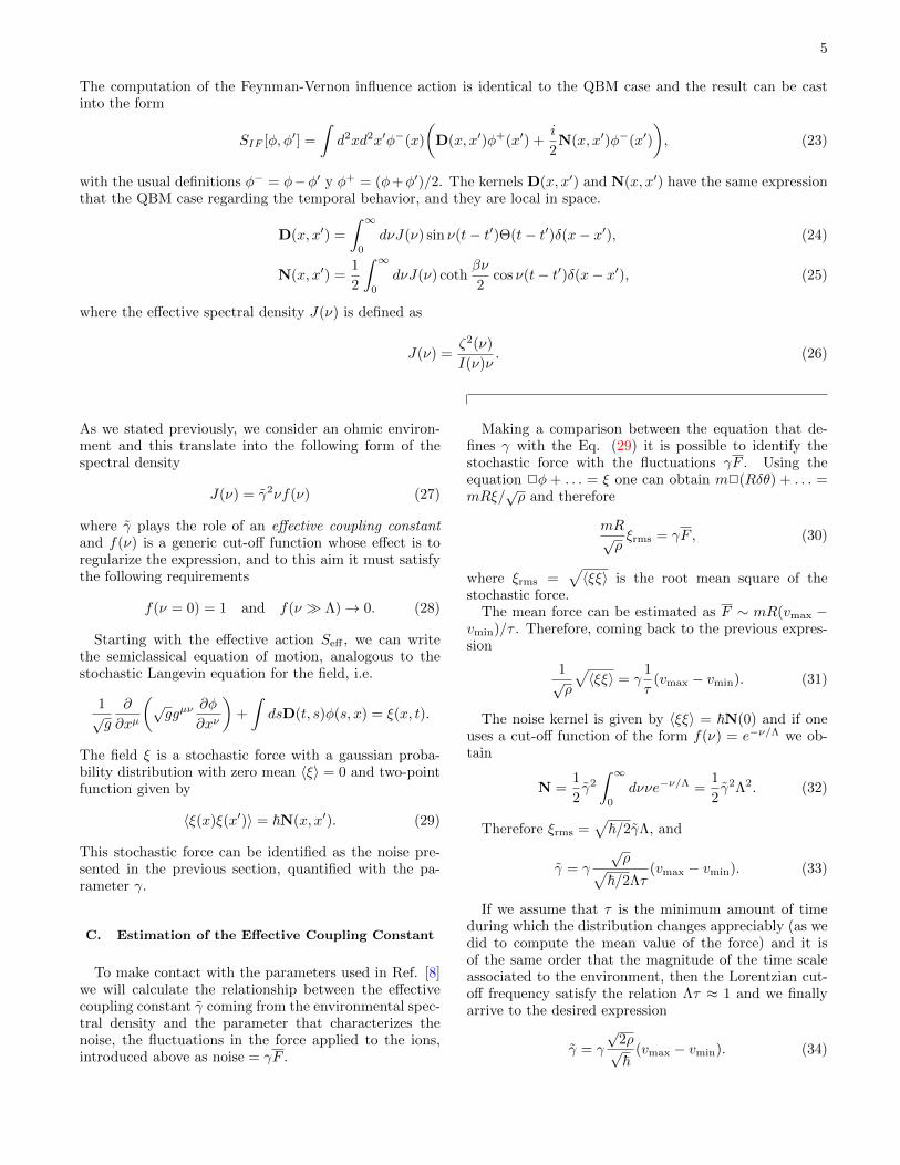
FIG. 1. Plot of the functions (a) log (ωτ)−2V2u/v V1u/v,showing that the anomalous component is negligible; and (b)V1u/V2v with respect to the mode frequency ω, showing thatthe decoherence time is the same for both u and v modes.

with zero temperature T0 = 0, the decoherence time is

given by the following expression

tD(T0 = 0) ≈ 4~ρδ2γ2πω(V1u/v + 2 log 1

ωτ V2u/v)

=2~2

γ2∆vδ2ωπρ2

× (V1u/v + 2 log1

ωτV2u/v)

−1, (54)

where ∆v ≡ vmax−vmin. If we focus in the ions’ ring andthe experimental parameters proposed for the system,then the expression can be simplified even more, sincewe are in a possition to approximate

2 log

(1

ωτ

)V2u/v V1u/v and V1u ' V2v ≡ V, (55)

as can be verified in the plots shown in Fig. 1. Finally,we obtain the following result for the decoherence time

tD(T0 = 0) =2~2

γ2∆vδ2ωπρ2V. (56)

In Fig. 2 the result for the decoherence time as a function

tD

T

Ω = Ωmin

Ω = Ωmax

Γ

0 1.´ 10-6

2.´ 10-6

3.´ 10-6

4.´ 10-6

5.´ 10-

0.001

0.01

0.1

1

10

100

1000

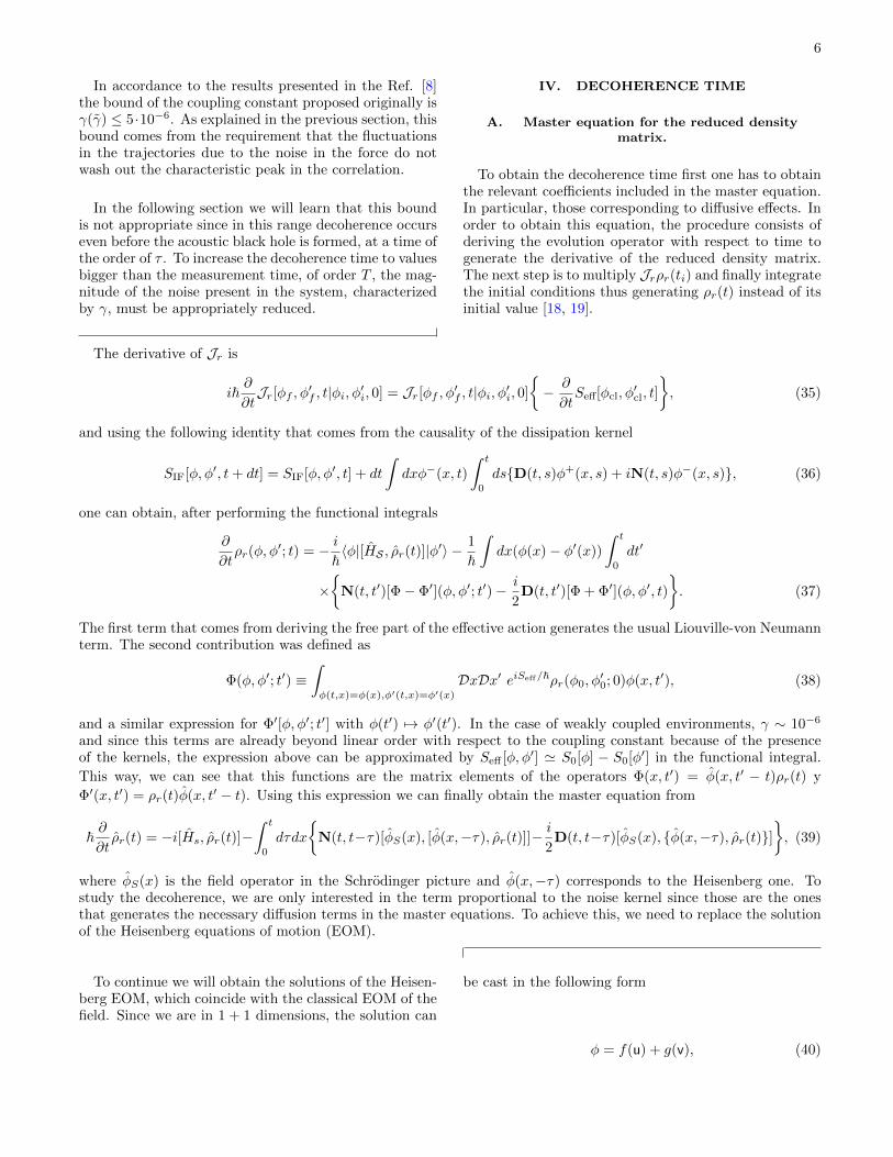
FIG. 2. [Color Online] Dependence of the decoherence timeas a function of the relative noise in the force γ. The coloredband includes all the allowed frequency range of the solutions.

of the force relative noise γ is shown. The decoherencetime is much shorter that T for the bound presented inthe Ref. [8], γ ∼ 5 · 10−6. As explained in section II,the period T is also of the same order of magnitude asthe time needed to perform the measurement. For timeslarger, the system becomes classically unstable and fortimes smaller the black hole would have no time to de-velop. The system, for the experimental parameters pro-posed in Ref. [8], shows decoherence in a time-scale tooshort and this would make impossible the measurementof the aspects of the Hawking effect, which is purely ofa quantum nature. Moreover, decoherence happens ina time of the same order of magnitude as the collapsetD ∼ τ , therefore there is no time for the acoustic blackhole to form.

9

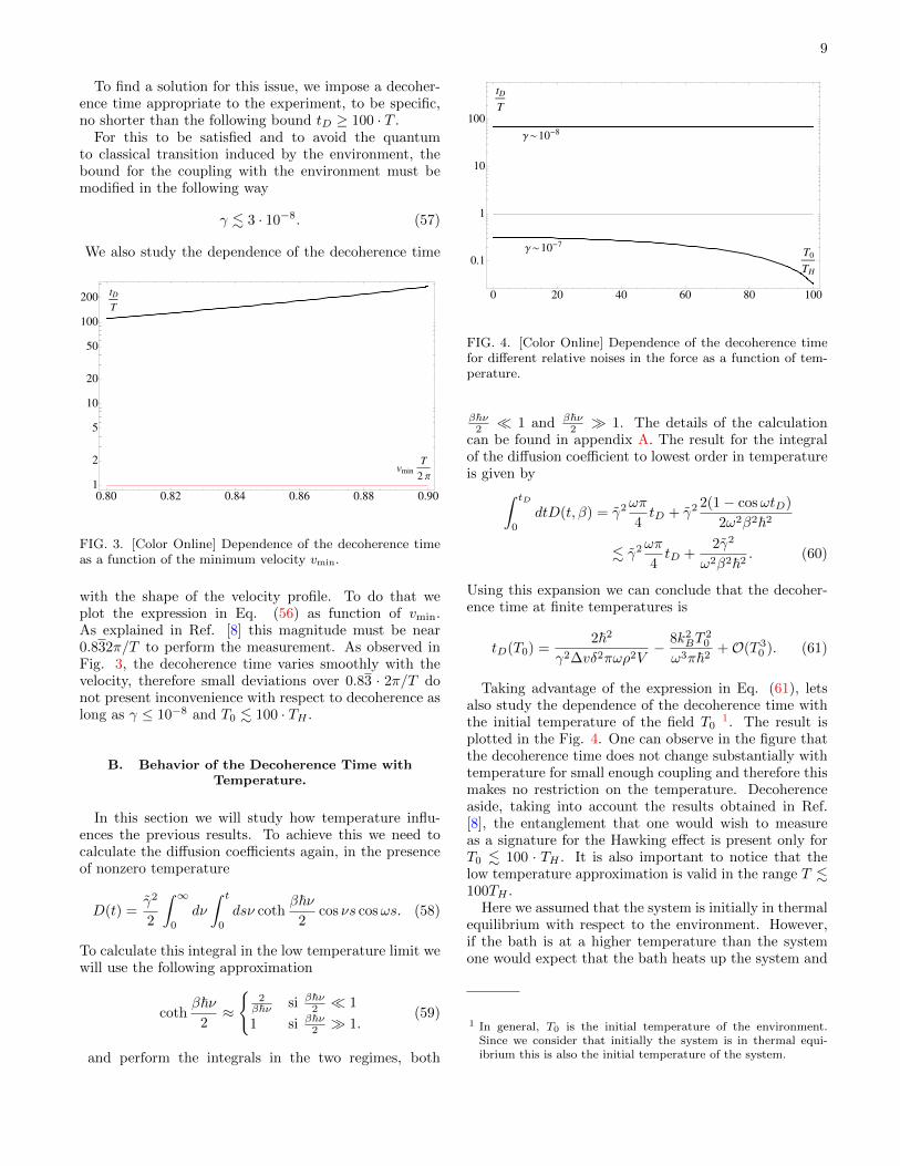
To find a solution for this issue, we impose a decoher-ence time appropriate to the experiment, to be specific,no shorter than the following bound tD ≥ 100 · T .

For this to be satisfied and to avoid the quantumto classical transition induced by the environment, thebound for the coupling with the environment must bemodified in the following way

γ . 3 · 10−8. (57)

We also study the dependence of the decoherence time

vmin

T

2 Π

tD

T

0.80 0.82 0.84 0.86 0.88 0.90

1

2

5

10

20

50

100

200

FIG. 3. [Color Online] Dependence of the decoherence timeas a function of the minimum velocity vmin.

with the shape of the velocity profile. To do that weplot the expression in Eq. (56) as function of vmin.As explained in Ref. [8] this magnitude must be near0.832π/T to perform the measurement. As observed inFig. 3, the decoherence time varies smoothly with thevelocity, therefore small deviations over 0.83 · 2π/T donot present inconvenience with respect to decoherence aslong as γ ≤ 10−8 and T0 . 100 · TH .

B. Behavior of the Decoherence Time withTemperature.

In this section we will study how temperature influ-ences the previous results. To achieve this we need tocalculate the diffusion coefficients again, in the presenceof nonzero temperature

D(t) =γ2

2

∫ ∞0

dν

∫ t

0

dsν cothβ~ν

2cos νs cosωs. (58)

To calculate this integral in the low temperature limit wewill use the following approximation

cothβ~ν

2≈

2β~ν si β~ν

2 1

1 si β~ν2 1.

(59)

and perform the integrals in the two regimes, both

tD

T

Γ~10-8

T0

TH

Γ~10-7

0 20 40 60 80 100

0.1

1

10

100

FIG. 4. [Color Online] Dependence of the decoherence timefor different relative noises in the force as a function of tem-perature.

β~ν2 1 and β~ν

2 1. The details of the calculationcan be found in appendix A. The result for the integralof the diffusion coefficient to lowest order in temperatureis given by∫ tD

0

dtD(t, β) = γ2ωπ

4tD + γ2 2(1− cosωtD)

2ω2β2~2

. γ2ωπ

4tD +

2γ2

ω2β2~2. (60)

Using this expansion we can conclude that the decoher-ence time at finite temperatures is

tD(T0) =2~2

γ2∆vδ2πωρ2V− 8k2

BT20

ω3π~2+O(T 3

0 ). (61)

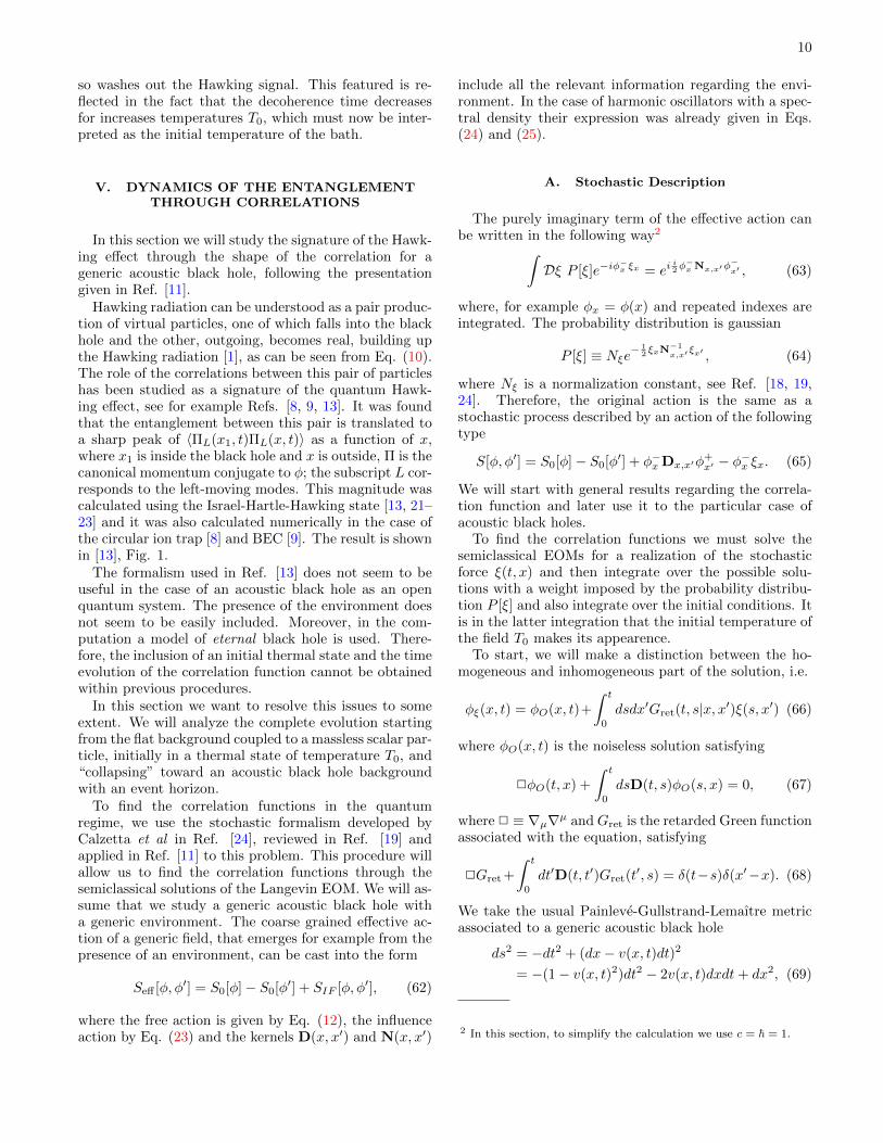
Taking advantage of the expression in Eq. (61), letsalso study the dependence of the decoherence time withthe initial temperature of the field T0

1. The result isplotted in the Fig. 4. One can observe in the figure thatthe decoherence time does not change substantially withtemperature for small enough coupling and therefore thismakes no restriction on the temperature. Decoherenceaside, taking into account the results obtained in Ref.[8], the entanglement that one would wish to measureas a signature for the Hawking effect is present only forT0 . 100 · TH . It is also important to notice that thelow temperature approximation is valid in the range T .100TH .

Here we assumed that the system is initially in thermalequilibrium with respect to the environment. However,if the bath is at a higher temperature than the systemone would expect that the bath heats up the system and

1 In general, T0 is the initial temperature of the environment.Since we consider that initially the system is in thermal equi-ibrium this is also the initial temperature of the system.

10

so washes out the Hawking signal. This featured is re-flected in the fact that the decoherence time decreasesfor increases temperatures T0, which must now be inter-preted as the initial temperature of the bath.

V. DYNAMICS OF THE ENTANGLEMENTTHROUGH CORRELATIONS

In this section we will study the signature of the Hawk-ing effect through the shape of the correlation for ageneric acoustic black hole, following the presentationgiven in Ref. [11].

Hawking radiation can be understood as a pair produc-tion of virtual particles, one of which falls into the blackhole and the other, outgoing, becomes real, building upthe Hawking radiation [1], as can be seen from Eq. (10).The role of the correlations between this pair of particleshas been studied as a signature of the quantum Hawk-ing effect, see for example Refs. [8, 9, 13]. It was foundthat the entanglement between this pair is translated toa sharp peak of 〈ΠL(x1, t)ΠL(x, t)〉 as a function of x,where x1 is inside the black hole and x is outside, Π is thecanonical momentum conjugate to φ; the subscript L cor-responds to the left-moving modes. This magnitude wascalculated using the Israel-Hartle-Hawking state [13, 21–23] and it was also calculated numerically in the case ofthe circular ion trap [8] and BEC [9]. The result is shownin [13], Fig. 1.

The formalism used in Ref. [13] does not seem to beuseful in the case of an acoustic black hole as an openquantum system. The presence of the environment doesnot seem to be easily included. Moreover, in the com-putation a model of eternal black hole is used. There-fore, the inclusion of an initial thermal state and the timeevolution of the correlation function cannot be obtainedwithin previous procedures.

In this section we want to resolve this issues to someextent. We will analyze the complete evolution startingfrom the flat background coupled to a massless scalar par-ticle, initially in a thermal state of temperature T0, and“collapsing” toward an acoustic black hole backgroundwith an event horizon.

To find the correlation functions in the quantumregime, we use the stochastic formalism developed byCalzetta et al in Ref. [24], reviewed in Ref. [19] andapplied in Ref. [11] to this problem. This procedure willallow us to find the correlation functions through thesemiclassical solutions of the Langevin EOM. We will as-sume that we study a generic acoustic black hole witha generic environment. The coarse grained effective ac-tion of a generic field, that emerges for example from thepresence of an environment, can be cast into the form

Seff [φ, φ′] = S0[φ]− S0[φ′] + SIF [φ, φ′], (62)

where the free action is given by Eq. (12), the influenceaction by Eq. (23) and the kernels D(x, x′) and N(x, x′)

include all the relevant information regarding the envi-ronment. In the case of harmonic oscillators with a spec-tral density their expression was already given in Eqs.(24) and (25).

A. Stochastic Description

The purely imaginary term of the effective action canbe written in the following way2∫

Dξ P [ξ]e−iφ−x ξx = ei

i2φ−xNx,x′φ

−x′ , (63)

where, for example φx = φ(x) and repeated indexes areintegrated. The probability distribution is gaussian

P [ξ] ≡ Nξe−12 ξxN

−1

x,x′ξx′ , (64)

where Nξ is a normalization constant, see Ref. [18, 19,24]. Therefore, the original action is the same as astochastic process described by an action of the followingtype

S[φ, φ′] = S0[φ]− S0[φ′] + φ−xDx,x′φ+x′ − φ

−x ξx. (65)

We will start with general results regarding the correla-tion function and later use it to the particular case ofacoustic black holes.

To find the correlation functions we must solve thesemiclassical EOMs for a realization of the stochasticforce ξ(t, x) and then integrate over the possible solu-tions with a weight imposed by the probability distribu-tion P [ξ] and also integrate over the initial conditions. Itis in the latter integration that the initial temperature ofthe field T0 makes its appearence.

To start, we will make a distinction between the ho-mogeneous and inhomogeneous part of the solution, i.e.

φξ(x, t) = φO(x, t)+

∫ t

0

dsdx′Gret(t, s|x, x′)ξ(s, x′) (66)

where φO(x, t) is the noiseless solution satisfying

2φO(t, x) +

∫ t

0

dsD(t, s)φO(s, x) = 0, (67)

where 2 ≡ ∇µ∇µ andGret is the retarded Green functionassociated with the equation, satisfying

2Gret +

∫ t

0

dt′D(t, t′)Gret(t′, s) = δ(t−s)δ(x′−x). (68)

We take the usual Painleve-Gullstrand-Lemaıtre metricassociated to a generic acoustic black hole

ds2 = −dt2 + (dx− v(x, t)dt)2

= −(1− v(x, t)2)dt2 − 2v(x, t)dxdt+ dx2, (69)

2 In this section, to simplify the calculation we use c = ~ = 1.

11

where v(x, t) is the velocity profile, in principle arbitraryas long as it has a supersonic subsonic transition, i.e. anevent horizon. In this section we now consider its timedependence instead.

In this paper we work under the weak coupling approx-imation, in such a way that we can estimate φO beginningwith the zeroth order limit of the EOM 2φO ' 0 whichexplicitly, replacing the metric of Eq. (69), is given by

[(∂t + ∂xv(x, t))(∂t + v(x, t)∂x)− ∂2x]φO(x, t) = 0, (70)

and moreover, we can approximate Gret from

2Gret(t, s|x, x′) ' δ(t− s)δ(x′ − x). (71)

Therefore to first order in the coupling with the environ-ment we can consider the dissipation term in Eq. (67) asan inhomogeneity, replacing the complete solution φO bythe solution of the Eq. (70),

2φ ' ξ(x, t)−∫ t

0

dt′D(t, t′)φO(x, t′), (72)

which in turn has the solution

φξ(x, t) ' φO(x, t) +

∫ t

0

dsdx′Gret(t, s|x, x′)ξf (s, x′),

(73)where we define ξf as

ξf (t, x) = ξ(t, x)−∫ t

0

dsD(t, s)φO(x, s). (74)

Assuming that we have this solutions, the correlationfunction relevant to the study of the entanglement be-tween the Hawking pair phonons can be obtained from

〈φ1φ2〉 ≡ 〈〈φ(x1, t1)φ(x2, t2)〉ξ〉in, (75)

where 〈 . . . 〉in represents the mean value integrated overthe initial conditions weighted with the thermal distribu-tion with T0. To obtain the correlation function betweenthe conjugate momentums one simply has to derive theequation above following the definition below

Π(x, t) =∂φ

∂t+ v(x, t)

∂φ

∂x. (76)

Therefore, following the formalism presented in [24],

〈φ1φ2〉 = 〈(φO1 +G1xξfx)(φO2 +G2xξ

fx)〉ξ,in

= 〈φO1φO2〉in −G2x′Dx′x〈φOxφO2〉in−G2x′Dx′x〈φOxφO1〉in+G1x′〈ξx′ξx〉ξ,inG2x. (77)

Using the properties of the stochastic force probabilitydistribution we get

〈φ1φ2〉= 〈φO1φO2〉in −G2x′Dx′x〈φOxφO2〉in−G2x′Dx′x〈φOxφO1〉in +G1x′Nx′xG2x. (78)

In the case without environment, where the field φ rep-resents particles in an acoustic black hole background,the previous formalism can be used but only the firstterm contributes. Therefore, in the general case one canwrite

〈φ1φ2〉O = 〈φ1φ2〉C +O(λ), (79)

where λ is the coupling constant with the environment.The subindices C and O means that it corresponds to theclosed and open system, respectively. This simple casedropping the O(λ) terms already presents the main diffi-culties inherent with the calculation and we will developa technique to deal with the equations in the followingsections.

B. Modes for the Wave Equation.

To solve the EOM for the field we will use the methodof characteristics, well known from mechanics of com-pressible fluids, see Ref. [25]. If one has a general differ-ential equation of the form

a(x, t)∂u

∂x+ b(x, t)

∂u

∂t+ c(x, t)u = 0, (80)

with initial condition u(x, 0) = f(x) then it can be solvedin the following way. First find the characteristic curves,defined as

dx

ds= a(x, t) and

dt

ds= b(x, t). (81)

Then find the evolution of u(x, t) along the characteris-tic curves finding the solution for the following ordinarydifferential equation

du

ds(x(s), t(s)) + c(x(s), t(s))u(x(s), t(s)) = 0. (82)

Finally, having the congruence of characteristic curves, toknow u(x, t) invert (x, t) 7→ (x0, s) where x0 is the initialcondition and s the parameter along the characteristicthat goes through (x, t). Then, u(x, t) = f(x0).

In the rest of this section we will use this method tofind the solution of the EOM for the field.

Before attempting to solve for the modes we have togive a specific velocity profile,

v(x, t) = σ(t)×

vmin para −∞ < x < −a1 + κx para − a < x < a

vmax para a < x <∞,(83)

where σ(t) is a function that must satisfy σ(0) = 0, toguaranty that at t = 0 the metric is flat and σ(t τ) = 1, in order for the background to “collapse” in anstable acoustic black hole after the time interval τ . Aparticular function that satisfies this requirement and iseasy to manipulate is

σ(t) = tanht

τ. (84)

12

We will solve the equations first for the region −a <x < a without taking into account the rest of the space.These solutions are the same in the other regions uponthe following changes κ = 0 and σ 7→ vmax/minσ. Afterthis, we will see how to introduce them properly and thusobtain the full solution.

Nevertheless, the problem that the presence of differ-ent regions introduce are the interfaces. For example, acharacteristic curve that starts in −a < x0 < a eventu-ally reach the point x(si) = a and for s > si the char-acteristic to use is the one corresponding to the regiona < x <∞. In this section we will see that the solutionsthat do not go through this boundaries do not present thecharacteristic peak associated with the entanglement ofthe Hawking pair. In the following section we will studythe full solution and we will learn how the entanglementis developed and its relationship to this issues.

The equation we have to solve is Eq. (70) which canbe cast into the following form

(∂t+∂xv(x, t)+∂x)(∂t+v(x, t)∂x−∂x)φO(x, t) = 0. (85)

Defining the operators

∂L =∂

∂t+ v(x, t)

∂

∂x− ∂

∂x(86)

∂R =∂

∂t+

∂

∂xv(x, t) +

∂

∂x. (87)

the equation can be written as ∂R∂Lφ = 0. One can firstsolve ∂LφL = 0. Then one has to solve ∂RφR = 0 andfinally ∂LφR = φR in order to obtain φR. This way, themore general solution is φO = φL + φR. Both left andright moving components can not be solved separatelysince [∂L, ∂R] 6= 0.

The procedure to find the solution with the character-istic curves is developed in appendix B. For example, thecharacteristic curves for the left moving modes are givenby

x(t) =exp

(κ

∫ t

0

σ(s)ds

)×(x0 −

∫ t

0

(1− σ(t))e−κ∫ s0σ(s′)ds′ds

). (88)

To make contact with the usual expansion in flat fieldtheory we cast the solution into the following form

φ(x) =

∫dk(uk(x)ak + H.c.), (89)

where H.c. means taking the hermitian conjugate of theexpression and the modes are given by

uk(x) =1√2|k|

eikxe−κ

∫ t0 σ(s)ds+ik

∫ t0

(1−σ(s))e−κ∫ s0 σ(s′)ds′ds

×

1−Θ(k)2i|k|∫ t

0

ds

×e−2ik∫ s0e−κ

∫ s′0 σ(s′′)ds′′ds′−κ

∫ s0σ(s′)ds′

. (90)

The coefficients ak and a†k corresponds at early timesto the creation and annihilation operators upon quanti-zation and they would carry the subindex “in”.

To compute the correlation function when an environ-ment is added we need the retarded Green function thatwe compute as Gret(t, t

′|x, x′) = [φ(x, t), φ(x′, t′)]Θ(t −t′).

C. Entanglement: Closed System.

In this section we study the behavior of the two-pointfunction of the left moving part of the momentum, ΠL.Using the expansion given in Eq. (89) and the definitionof the left moving part of the momentum, Eq. (76), wecan obtain the correlation function after integrating overthe initial conditions

〈ΠL(x1, t)ΠL(x2, t)〉 =

∫ ∞0

dk√2kk2

×e−ik(x1−x2)e−κ∫ t0 σ(s)ds−κ

∫ t0σ(s)ds coth

βk

2, (91)

with the usual definition β = (kBT0)−1.Either for the region −a < x < a where the velocity

changes with position, or the regions where the velocityis homogeneous (as stated, upon the replacements κ 7→0 and σ 7→ vσ), the expression below depends only on(x1 − x2). Therefore, this expression cannot present thecharacteristic peak discussed. Accordingly, the regionswhere this solution is valid do not present the signatureof the quantum Hawking effect, as explained in previoussections.

a x

t

x0FIG. 5. Schematic illustration of a characteristic curve thatintersects the interface in x = a and starts at x0.

The correct way of getting the solutions of differentregions is matching the characteristic curves as shownin Fig. 5. For example, if x > a and different regionsshare the characteristic then x0 is obtained matching thecharacteristic for v(x, t) constant with the characteristicfor x < a and finally finding the x0 corresponding tothe latter. The signature of the entanglement between

13

the Hawking pair was shown to be present in the leftcomponent of the correlation so we are only interested inthe curves associated with this modes.

To carry on this procedure, we approximate for longtimes (t τ) the characteristic for |x| < a as x(t) 'x0e

κt. In the region x > a, the characteristic is

x(t) = A− t+ f(t)vmax, (92)

where A is a constant of integration, f(t) ≡∫ t

0dsσ(s)

and vmax ≈ 1 + κa. The relationship between A and x0

can be found recalling that

x(ta) = a ⇒ ta = κ−1 log a/x0, (93)

because the |x| < a characteristic reach x = a at ta and

A− ta + f(ta)vmax = a, (94)

because the x > a characteristic must match the previousone at x(ta) = a.

From this two equations, for times t τ , we can ob-tain A as a function of x0 and then use x0 as a functionof x, t and put it in the eikx0 factor, finding

x0 = ae(x+t−f(t)vmax−a)/a, for x > a and (95)

x0 = −ae−(x+t−f(t)vmin−a)/a, for x < −a. (96)

Therefore the left moving modes are given by

uLk(x) =1√2|k|

eikae(x+t−f(t)vmax−a)/a

, for x > a

uLk(x) =1√2|k|

e−ikae(−x−t+f(t)vmin+a)/a

, for x < −a.

Finally, we calculate 〈φL(x1, t)φL(x2, t)〉 for an initial

XPLH-yL PLHxL\

Black Hole

x

a

y = 4 y = 6

0 2 4 6 80.00

0.05

0.10

0.15

0.20

0.25

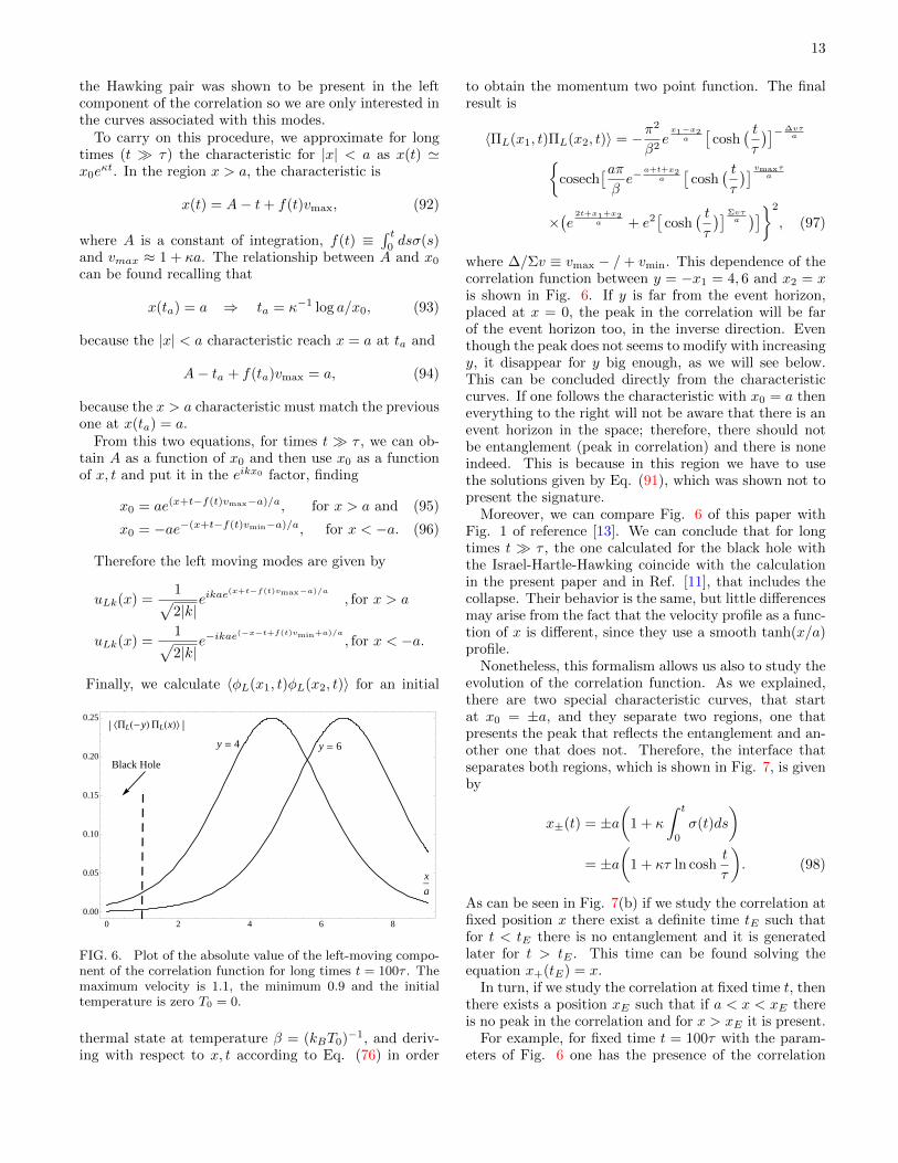
FIG. 6. Plot of the absolute value of the left-moving compo-nent of the correlation function for long times t = 100τ . Themaximum velocity is 1.1, the minimum 0.9 and the initialtemperature is zero T0 = 0.

thermal state at temperature β = (kBT0)−1, and deriv-ing with respect to x, t according to Eq. (76) in order

to obtain the momentum two point function. The finalresult is

〈ΠL(x1, t)ΠL(x2, t)〉 = −π2

β2ex1−x2a

[cosh

( tτ

)]−∆vτa

cosech[aπβe−

a+t+x2a

[cosh

( tτ

)] vmaxτa

×(e

2t+x1+x2a + e2

[cosh

( tτ

)]Σvτa)]2

, (97)

where ∆/Σv ≡ vmax − /+ vmin. This dependence of thecorrelation function between y = −x1 = 4, 6 and x2 = xis shown in Fig. 6. If y is far from the event horizon,placed at x = 0, the peak in the correlation will be farof the event horizon too, in the inverse direction. Eventhough the peak does not seems to modify with increasingy, it disappear for y big enough, as we will see below.This can be concluded directly from the characteristiccurves. If one follows the characteristic with x0 = a theneverything to the right will not be aware that there is anevent horizon in the space; therefore, there should notbe entanglement (peak in correlation) and there is noneindeed. This is because in this region we have to usethe solutions given by Eq. (91), which was shown not topresent the signature.

Moreover, we can compare Fig. 6 of this paper withFig. 1 of reference [13]. We can conclude that for longtimes t τ , the one calculated for the black hole withthe Israel-Hartle-Hawking coincide with the calculationin the present paper and in Ref. [11], that includes thecollapse. Their behavior is the same, but little differencesmay arise from the fact that the velocity profile as a func-tion of x is different, since they use a smooth tanh(x/a)profile.

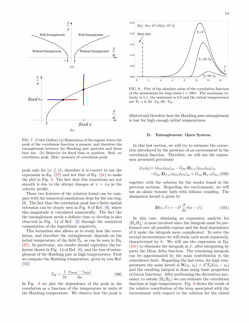
Nonetheless, this formalism allows us also to study theevolution of the correlation function. As we explained,there are two special characteristic curves, that startat x0 = ±a, and they separate two regions, one thatpresents the peak that reflects the entanglement and an-other one that does not. Therefore, the interface thatseparates both regions, which is shown in Fig. 7, is givenby

x±(t) = ±a(

1 + κ

∫ t

0

σ(t)ds

)= ±a

(1 + κτ ln cosh

t

τ

). (98)

As can be seen in Fig. 7(b) if we study the correlation atfixed position x there exist a definite time tE such thatfor t < tE there is no entanglement and it is generatedlater for t > tE . This time can be found solving theequation x+(tE) = x.

In turn, if we study the correlation at fixed time t, thenthere exists a position xE such that if a < x < xE thereis no peak in the correlation and for x > xE it is present.

For example, for fixed time t = 100τ with the param-eters of Fig. 6 one has the presence of the correlation

14

1-1

xa

Without EntanglementWithout Entanglement

With EntanglementWith Entanglement

tt

(a)

1

xa

tt

fixed x

fixed t

(b)

FIG. 7. [Color Online] (a) Illustration of the regions where thepeak of the correlation function is present, and therefore theentanglement between the Hawking pair particles and thosethat not. (b) Behavior for fixed time or position. Red: nocorrelation peak. Blue: presence of correlation peak.

peak only for |x| . 11, therefore it is correct to use theexpression in Eq. (97) and not that of Eq. (91) to makethe plot in Fig. 6. The fact that this transitions are notsmooth is due to the abrupt changes at x = ±a in thevelocity profile.

These two features of the solution found can be com-pare with the numerical simulations done for the ion ring,[8]. The fact that the correlation peak has a finite spatialextension can be clearly seen in Fig. 9 of Ref. [8], wherethis magnitude is calculated numerically. The fact thethe entanglement needs a definite time to develop is alsoobserved in Fig. 14 of Ref. [8] through the numericalcomputation of the logarithmic negativity.

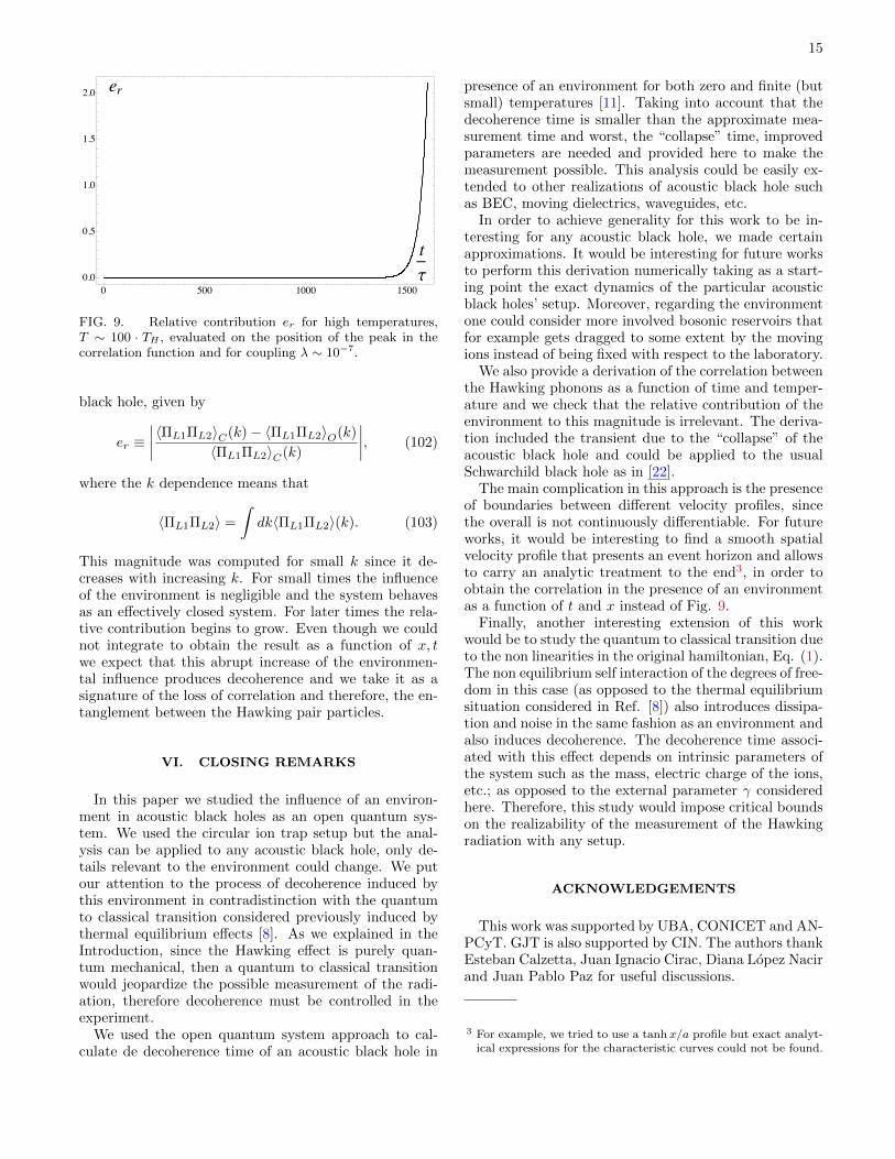
This formalism also allows us to study how the corre-lation, and therefore the entanglement, depends on theinitial temperature of the field T0, as can be seen in Eq.(97). In particular, our results should reproduce the be-havior shown in Fig. 14 of Ref. [8], and the loss of entan-glement of the Hawking pair at high temperatures. Firstwe compute the Hawking temperature, given by (see Ref.[12])

TH =1

2π

|vmax − vmin|2a

. (99)

In Fig. 8 we plot the dependence of the peak in thecorrelation as a function of the temperature in units ofthe Hawking temperature. We observe how the peak is

YPLI-10 a, 102 ΤM PLIx, 102 ΤM]

Black HoleT0 =0

T0 =20 × TH

T0 =60 × TH

x

a

0 2 4 6 8 10 12 140.00

0.05

0.10

0.15

0.20

0.25

FIG. 8. Plot of the absolute value of the correlation functionof the momentum for long times t = 100τ . The maximum ve-locity is 1.1, the minimum is 0.9 and the initial temperaturesare T0 = 0, 20 · TH , 60 · TH .

diluted and therefore how the Hawking pair entanglementis lost for high enough initial temperatures.

D. Entanglement: Open System.

In this last section, we will try to estimate the correc-tion introduced by the presence of an environment in thecorrelation function. Therefore, we will use the expres-sion presented previously

〈φ1φ2〉= 〈φO1φO2〉in −G2x′Dx′x〈φOxφO2〉in−G2x′Dx′x〈φOxφO1〉in +G1x′Nx′xG2x,(100)

together with the solution for the modes found in theprevious sections. Regarding the environment, we willuse an ohmic bosonic bath with bilinear coupling. Thedissipation kernel is given by

D(s, s′) = −λ2 ∂

∂sδ(s− s′). (101)

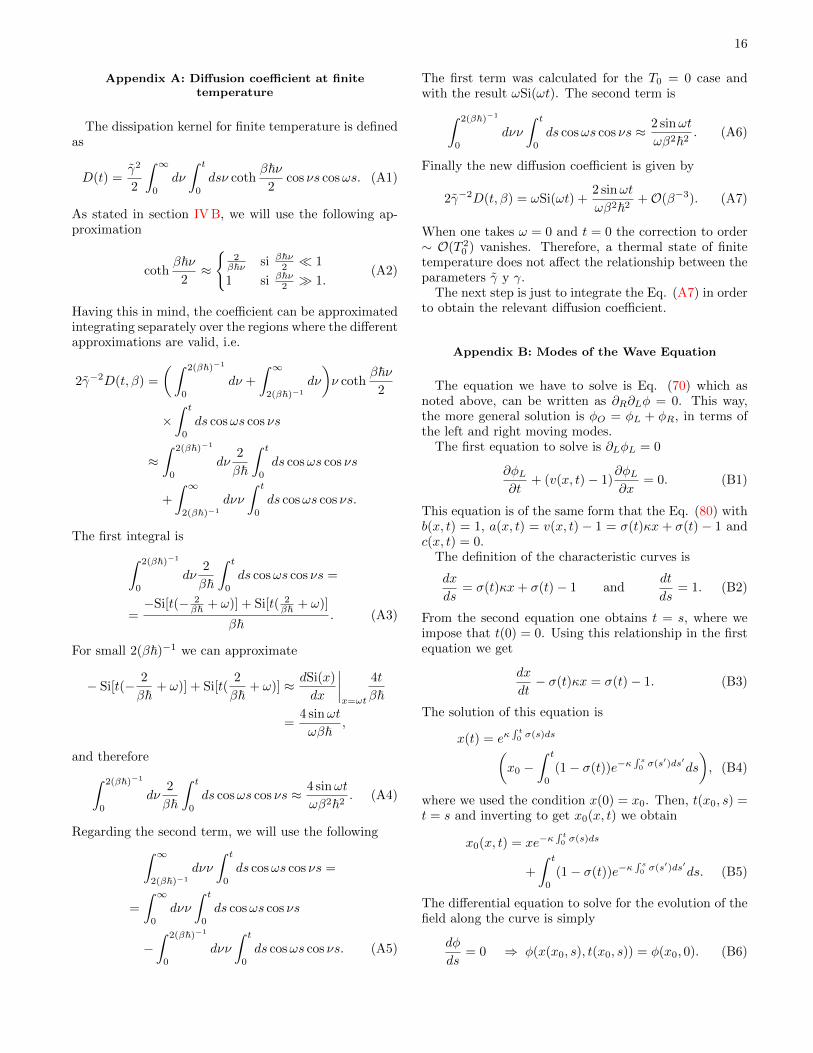
In this case, obtaining an expression analytic for〈ΠLΠL〉 is more involved since the integrals must be per-formed over all possible regions and the final dependenceof k make the integrals more complicated. To solve thesecond inconvenience we will study each mode separately,characterized by k. We will use the expression in Eq.(101) to eliminate the integrals in s′, after integrating byparts the Dirac delta function. The remaining integralscan be approximated by the main contribution in thecoincidence limit. Regarding the last term, for high tem-peratures the noise kernel is N(s1, s2) = λ2T0δ(s1 − s2)and the resulting integral is done using basic propertiesof Green functions. After performing the derivatives nec-essary to obtain 〈ΠLΠL〉 we can estimate the correlationfunction at high temperatures. Fig. 9 shows the result ofthe relative contribution of the term associated with theenvironment with respect to the solution for the closed

15

er

t!

0 500 1000 15000.0

0.5

1.0

1.5

2.0

FIG. 9. Relative contribution er for high temperatures,T ∼ 100 · TH , evaluated on the position of the peak in thecorrelation function and for coupling λ ∼ 10−7.

black hole, given by

er ≡∣∣∣∣ 〈ΠL1ΠL2〉C(k)− 〈ΠL1ΠL2〉O(k)

〈ΠL1ΠL2〉C(k)

∣∣∣∣, (102)

where the k dependence means that

〈ΠL1ΠL2〉 =

∫dk〈ΠL1ΠL2〉(k). (103)

This magnitude was computed for small k since it de-creases with increasing k. For small times the influenceof the environment is negligible and the system behavesas an effectively closed system. For later times the rela-tive contribution begins to grow. Even though we couldnot integrate to obtain the result as a function of x, twe expect that this abrupt increase of the environmen-tal influence produces decoherence and we take it as asignature of the loss of correlation and therefore, the en-tanglement between the Hawking pair particles.

VI. CLOSING REMARKS

In this paper we studied the influence of an environ-ment in acoustic black holes as an open quantum sys-tem. We used the circular ion trap setup but the anal-ysis can be applied to any acoustic black hole, only de-tails relevant to the environment could change. We putour attention to the process of decoherence induced bythis environment in contradistinction with the quantumto classical transition considered previously induced bythermal equilibrium effects [8]. As we explained in theIntroduction, since the Hawking effect is purely quan-tum mechanical, then a quantum to classical transitionwould jeopardize the possible measurement of the radi-ation, therefore decoherence must be controlled in theexperiment.

We used the open quantum system approach to cal-culate de decoherence time of an acoustic black hole in

presence of an environment for both zero and finite (butsmall) temperatures [11]. Taking into account that thedecoherence time is smaller than the approximate mea-surement time and worst, the “collapse” time, improvedparameters are needed and provided here to make themeasurement possible. This analysis could be easily ex-tended to other realizations of acoustic black hole suchas BEC, moving dielectrics, waveguides, etc.

In order to achieve generality for this work to be in-teresting for any acoustic black hole, we made certainapproximations. It would be interesting for future worksto perform this derivation numerically taking as a start-ing point the exact dynamics of the particular acousticblack holes’ setup. Moreover, regarding the environmentone could consider more involved bosonic reservoirs thatfor example gets dragged to some extent by the movingions instead of being fixed with respect to the laboratory.

We also provide a derivation of the correlation betweenthe Hawking phonons as a function of time and temper-ature and we check that the relative contribution of theenvironment to this magnitude is irrelevant. The deriva-tion included the transient due to the “collapse” of theacoustic black hole and could be applied to the usualSchwarchild black hole as in [22].

The main complication in this approach is the presenceof boundaries between different velocity profiles, sincethe overall is not continuously differentiable. For futureworks, it would be interesting to find a smooth spatialvelocity profile that presents an event horizon and allowsto carry an analytic treatment to the end3, in order toobtain the correlation in the presence of an environmentas a function of t and x instead of Fig. 9.

Finally, another interesting extension of this workwould be to study the quantum to classical transition dueto the non linearities in the original hamiltonian, Eq. (1).The non equilibrium self interaction of the degrees of free-dom in this case (as opposed to the thermal equilibriumsituation considered in Ref. [8]) also introduces dissipa-tion and noise in the same fashion as an environment andalso induces decoherence. The decoherence time associ-ated with this effect depends on intrinsic parameters ofthe system such as the mass, electric charge of the ions,etc.; as opposed to the external parameter γ consideredhere. Therefore, this study would impose critical boundson the realizability of the measurement of the Hawkingradiation with any setup.

ACKNOWLEDGEMENTS

This work was supported by UBA, CONICET and AN-PCyT. GJT is also supported by CIN. The authors thankEsteban Calzetta, Juan Ignacio Cirac, Diana Lopez Nacirand Juan Pablo Paz for useful discussions.

3 For example, we tried to use a tanhx/a profile but exact analyt-ical expressions for the characteristic curves could not be found.

16

Appendix A: Diffusion coefficient at finitetemperature

The dissipation kernel for finite temperature is definedas

D(t) =γ2

2

∫ ∞0

dν

∫ t

0

dsν cothβ~ν

2cos νs cosωs. (A1)

As stated in section IV B, we will use the following ap-proximation

cothβ~ν

2≈

2β~ν si β~ν

2 1

1 si β~ν2 1.

(A2)

Having this in mind, the coefficient can be approximatedintegrating separately over the regions where the differentapproximations are valid, i.e.

2γ−2D(t, β) =

(∫ 2(β~)−1

0

dν +

∫ ∞2(β~)−1

dν

)ν coth

β~ν2

×∫ t

0

ds cosωs cos νs

≈∫ 2(β~)−1

0

dν2

β~

∫ t

0

ds cosωs cos νs

+

∫ ∞2(β~)−1

dνν

∫ t

0

ds cosωs cos νs.

The first integral is∫ 2(β~)−1

0

dν2

β~

∫ t

0

ds cosωs cos νs =

=−Si[t(− 2

β~ + ω)] + Si[t( 2β~ + ω)]

β~. (A3)

For small 2(β~)−1 we can approximate

− Si[t(− 2

β~+ ω)] + Si[t(

2

β~+ ω)] ≈ dSi(x)

dx

∣∣∣∣x=ωt

4t

β~

=4 sinωt

ωβ~,

and therefore∫ 2(β~)−1

0

dν2

β~

∫ t

0

ds cosωs cos νs ≈ 4 sinωt

ωβ2~2. (A4)

Regarding the second term, we will use the following∫ ∞2(β~)−1

dνν

∫ t

0

ds cosωs cos νs =

=

∫ ∞0

dνν

∫ t

0

ds cosωs cos νs

−∫ 2(β~)−1

0

dνν

∫ t

0

ds cosωs cos νs. (A5)

The first term was calculated for the T0 = 0 case andwith the result ωSi(ωt). The second term is∫ 2(β~)−1

0

dνν

∫ t

0

ds cosωs cos νs ≈ 2 sinωt

ωβ2~2. (A6)

Finally the new diffusion coefficient is given by

2γ−2D(t, β) = ωSi(ωt) +2 sinωt

ωβ2~2+O(β−3). (A7)

When one takes ω = 0 and t = 0 the correction to order∼ O(T 2

0 ) vanishes. Therefore, a thermal state of finitetemperature does not affect the relationship between theparameters γ y γ.

The next step is just to integrate the Eq. (A7) in orderto obtain the relevant diffusion coefficient.

Appendix B: Modes of the Wave Equation

The equation we have to solve is Eq. (70) which asnoted above, can be written as ∂R∂Lφ = 0. This way,the more general solution is φO = φL + φR, in terms ofthe left and right moving modes.

The first equation to solve is ∂LφL = 0

∂φL∂t

+ (v(x, t)− 1)∂φL∂x

= 0. (B1)

This equation is of the same form that the Eq. (80) withb(x, t) = 1, a(x, t) = v(x, t) − 1 = σ(t)κx + σ(t) − 1 andc(x, t) = 0.

The definition of the characteristic curves is

dx

ds= σ(t)κx+ σ(t)− 1 and

dt

ds= 1. (B2)

From the second equation one obtains t = s, where weimpose that t(0) = 0. Using this relationship in the firstequation we get

dx

dt− σ(t)κx = σ(t)− 1. (B3)

The solution of this equation is

x(t) = eκ∫ t0σ(s)ds(

x0 −∫ t

0

(1− σ(t))e−κ∫ s0σ(s′)ds′ds

), (B4)

where we used the condition x(0) = x0. Then, t(x0, s) =t = s and inverting to get x0(x, t) we obtain

x0(x, t) = xe−κ∫ t0σ(s)ds

+

∫ t

0

(1− σ(t))e−κ∫ s0σ(s′)ds′ds. (B5)

The differential equation to solve for the evolution of thefield along the curve is simply

dφ

ds= 0 ⇒ φ(x(x0, s), t(x0, s)) = φ(x0, 0). (B6)

17

Finally the solution is

φL(x, t) = φ

(xe−κ

∫ t0σ(s)ds

+

∫ t

0

(1− σ(t))e−κ∫ s0σ(s′)ds′ds, 0

). (B7)

To rewrite it in a useful way, taking into account thatwe will have to eventually integrate over the initial con-ditions, we expand in modes φ(x, 0) =

∫dk/2πeikxφk,

then the solution for the field is

φL(x, t) =

∫dk

2πφkexp

ik

(xe−κ

∫ t0σ(s)ds

+

∫ t

0

(1− σ(t))e−κ∫ s0σ(s′)ds′ds

). (B8)

Having an expression for the left moving modes, wenow have to solve the equation for the right modes,∂RφR = 0, (

∂

∂t+

∂

∂xv(x, t) +

∂

∂x

)φR = 0(

∂

∂t+ σ(t)κ+ σ(t)(1 + κx)

∂

∂x+

∂

∂x

)φR = 0(

∂

∂t+ σ(t)κ+ (σ(t) + σ(t)κx+ 1)

∂

∂x

)φR = 0.(B9)

Again, t = s, but the spatial part of the characteristicis

x(t) = eκ∫ t0σ(s)ds(

x0 +

∫ t

0

(σ(s) + 1)e−κ∫ s0σ(s′)ds′ds

), (B10)

and after taking the inverse x0

x0(x, t) = xe−κ∫ t0σ(s)ds

−∫ t

0

(1 + σ(s))e−κ∫ s0σ(s′)ds′ds. (B11)

Now the equation for the value φR along the character-istics is

dφ

dt= −σ(t)κφ, (B12)

then

φ(x(x0, s), t(x0, s)) = φ(x0, 0)e−κ∫ s0σ(s′)ds′ . (B13)

Therefore, expanding again in modes

φR(x, t) =

∫dk

2πφkexp

ik

(xe−κ

∫ t0σ(s)ds

−∫ t

0

(1 + σ(t))e−κ∫ s0σ(s′)ds′ds

)−κ∫ t

0

σ(s)ds

. (B14)

Taking advantage of this result for φR, the right movingmode can be found from (∂t + v(x, t)∂x − ∂x)φR = φR.To solve this equation we propose a solution of the form

φR(x, t)=

∫dk

2πφk(x, t)exp

ik

(xe−κ

∫ t0σ(s)ds

+

∫ t

0

(1− σ(s))e−κ∫ s0σ(s′)ds′ds

). (B15)

If we use this result in the equation and use that theexponential is a solution of the homogeneous equation ofthe left moving modes, we obtain

∂LφR =

∫dk

2π∂Lφk(x, t)exp

[ik(xe−κ

∫ t0σ(s)ds

+

∫ t

0

(1− σ(s))e−κ∫ s0σ(s′)ds′ds

)]. (B16)

On the other hand, the solution φR can be rewritten as

φR(x, t)=

∫dk

2πφkexp[−2ik

∫ t

0

e−κ∫ s0σ(s′)ds′ds− κ

∫ t

0

σ(s)ds]

×eik(xe−κ

∫ t0 σ(s)ds+

∫ t0

(1−σ(s))e−κ∫ s0 σ(s′)ds′ds

). (B17)

Equating both sides of this equation gives

∂Lφk(x, t) = φke−2ik

∫ t0e−κ

∫ s0 σ(s′)ds′ds−κ

∫ t0σ(s)ds. (B18)

To find the particular solution we can use a φk such thatφk(x, t) = Ψk(t) and therefore

∂tφk(t) = φke−2ik

∫ t0e−κ

∫ s0 σ(s′)ds′ds−κ

∫ t0σ(s)ds (B19)

Integrating in time, the solution is

φR(x, t)=

∫dk

2πΦke

ik(xe−κ

∫ t0 σ(s)ds+

∫ t0

(1−σ(s))e−κ∫ s0 σ(s′)ds′ds

)∫ t

0

dse−2ik∫ s0e−κ

∫ s′0 σ(s′′)ds′′ds′−κ

∫ s0σ(s′)ds′ . (B20)

The remaining steps are just to write down the full so-lution and cast it into the usual mode expansion form.To do this one has to write φkL and φkR in terms of theFourier transform of the initial condition of the field andthe conjugate momentum φk(t = 0) and Πk(t = 0).

18

[1] S. Hawking, Nature (London) 248, 30 (1974); Commun.Math. Phys. 43, 199 (1975); J. Hartle & S. Hawking,Phys. Rev. D 13, 2188 (1976).

[2] W.G. Unruh, Phys. Rev. Lett. 46, 1351 (1981).[3] L. J. Garay, J. R. Anglin, J. I. Cirac, and P. Zoller, Phys.

Rev. Lett. 85, 4643 (2000); Phys. Rev. A 63, 023611(2001); L.J. Garay, Int. J. Theor. Phys. 41, 2073 (2002);C. Barcelo, S. Liberati, and M. Visser, Classical Quan-tum Gravity 18, 1137 (2001).

[4] R. Schutzhold, G. Plunien, and G. Soff, Phys. Rev. Lett.88, 061101 (2002); I. Brevik and G. Halnes, Phys. Rev.D 65, 024005 (2001).

[5] R. Schutzhold and W. G. Unruh, Phys. Rev. Lett. 95,031301 (2005).

[6] W. G. Unruh and R. Schutzhold, Phys. Rev. D 68,024008 (2003).

[7] F. Belgiorno, S.L. Cacciatori, M. Clerici, V. Gorini, G.Ortenzi, L. Rizzi, E. Rubino, V. G. Sala, and D. Faccio,Phys. Rev. Lett. 105, 203901(2010); R. Schutzhold andW. G. Unruh, ibid. 107, 149401 (2011); F. Belgiorno, S.L. Cacciatori, M. Clerici, V. Gorini, G. Ortenzi, L. Rizzi,E. Rubino, V. G. Sala, and D. Faccio, ibid. 107, 149402(2011).

[8] B. Horstmann, B. Reznik, S. Fagnocchi, and J.I. Cirac,Phys. Rev. Lett. 104, 250403 (2010); New J. Phys. 13,045008 (2011).

[9] R. Balbinot, A. Fabbri, S. Fagnocchi, A. Recati andI. Carusotto, Phys. Rev. A 78, 021603 (2008); I. Caru-sotto, S. Fagnocchi, A. Recati, R. Balbinot and A. Fab-bri, New J. Phys. 10, 103001 (2008); J. Macher andR. Parentani, Phys. Rev. A 80, 043601 (2009).

[10] C. Monroe, D. M. Meekhof, B. E. King, S. R. Jefferts,W.M. Itano, and D.J. Wineland, Phys. Rev. Lett. 75,4011 (1995); D.J. Wineland et al. J. Res. Natl. Inst.Stand. Technol. 103, 259 (1998); R. Schutzhold, Phys.Rev. Lett. 97, 190405 (2006).

[11] F. C. Lombardo and G. J. Turiaci, Phys. Rev. Lett. 108,

261301 (2012).[12] W. G. Unruh, Phys. Rev. D 51, 2827 (1995).[13] R. Schutzhold and W.G. Unruh, Phys. Rev. D 81, 124033

(2010).[14] S. Schneider and G. J. Milburn, Phys. Rev. A 59, 3766

(1999); C. J. Wyatt, B. E. King, Q. A. Turchette, C. A.Sackett, D. Kielpinski, W.M. Itano, C. Monroe, and D.J.Wineland, Nature (London) 403, 269 (2000); Seidelin etal., Phys. Rev. Lett. 96, 253003 (2006);

[15] B. L. Hu, J. P. Paz, and Y. Zhang, Phys. Rev. D 47, 1576(1993); J. P. Paz, S. Habib, and W. H. Zurek, ibid. 47,488 (1993); F.C. Lombardo and P.I. Villar, Phys. Lett.A 371, 190 (2007).

[16] W.G. Unruh and R. Schutzhold, Phys. Rev. D 71, 024028(2005).

[17] L.D. Romero and J.P. Paz, Phys. Rev. A 55, 4070 (1997)[18] F.C. Lombardo and F.D. Mazzitelli, Phys. Rev. D 53,

2001(1996); F. C. Lombardo, F. D. Mazzitelli, and R. J.Rivers, Nucl. Phys. B672, 462 (2003); F.C. Lombardoand D.Lopez Nacir, Phys.Rev.D 72, 063506 (2005).

[19] E.A. Calzetta and B.L. Hu, Nonequilibrium QuantumField Theory, (Cambridge University Press, Cambridge,England, 2008).

[20] F.C. Lombardo and P.I. Villar, Phys. Lett. A 336, 16(2005).

[21] D. G. Boulware, Phys. Rev. D 11, 1404 (1975).[22] N.D. Birrell and P.C.W. Davies, Quantum Field Theory

in Curved Space Cambridge Monographs, England, 1984.[23] W. Israel, Phys. Lett. A 57, 107 (1976);[24] E.A. Calzetta, A. Roura, and E. Verdaguer, Physica

(Amsterdam) 319A, 188-212 (2003).[25] L.D Landau and E.M. Lifshitz, Fluid Mechanics, Perga-

mon, 1959; A.H. Shapiro, The Dynamics and Thermody-namics of Compressible Fluid Flow. (Ronald, New York(1953).