arX

iv:g

r-qc

/061

1112

v1 2

1 N

ov 2

006

IGPG–06/11–4, AEI–2006–086gr–qc/0611112

Effective constraints of loop quantum gravity

Martin Bojowald1∗, Hector H. Hernandez2†, Mikhail Kagan1‡ and Aureliano Skirzewski2§

1Institute for Gravitational Physics and Geometry, The Pennsylvania State University,104 Davey Lab, University Park, PA 16802, USA

2Max-Planck-Institut fur Gravitationsphysik, Albert-Einstein-Institut,Am Muhlenberg 1, D-14476 Potsdam, Germany

Abstract

Within a perturbative cosmological regime of loop quantum gravity corrections toeffective constraints are computed. This takes into account all inhomogeneous degreesof freedom relevant for scalar metric modes around flat space and results in explicitexpressions for modified coefficients and of higher order terms. It also illustrates therole of different scales determining the relative magnitude of corrections. Our resultsdemonstrate that loop quantum gravity has the correct classical limit, at least in itssector of cosmological perturbations around flat space, in the sense of perturbativeeffective theory.

1 Introduction

Interacting quantum theories in low energy or semiclassical regimes can be described by ef-fective equations which amend the classical ones by correction terms. Compared to the fullquantum description an analysis of such effective equations is much easier once they havebeen derived. In addition to the simpler mathematical structure, difficult conceptual andinterpretational problems of wave functions can be evaded, still allowing one to computepotentially observable effects. Technical and conceptual problems are even more severe inquantum gravity, in particular in background independent formulations. Yet, especially inthis case observational guidance would be of invaluable help. Since the high energy regimesof cosmology are commonly considered as the best access to such guidance, an effectivedescription for fields relevant for early universe cosmology is needed. In this paper weuse an effective framework of perturbative loop quantum gravity around a spatially flatisotropic background space-time to derive correction terms to the classical constraints.

∗e-mail address: bojowald@gravity.psu.edu†e-mail address: hehe@aei.mpg.de‡e-mail address: mak411@psu.edu§e-mail address: skirz@aei.mpg.de

1

Our analysis will be done for scalar metric modes in longitudinal gauge as this can beused to simplify the perturbative basic variables. They can then be chosen to be of diagonalform, although now fully inhomogeneous, which is the main reason for simplifications asthey have been used extensively in symmetric models [1, 2, 3, 4]. The main constructionsof these models can thus be extended, in a similarly explicit form, to inhomogeneoussituations without assuming any symmetry. This allows us to compute explicit correctionsto effective constraints which, in combination with the Hamiltonian analysis of cosmologicalperturbation theory in [5], leads to corrected perturbation equations and new effects [6].

A physical regime is selected by introducing a background geometry in the backgroundindependent quantization through a specific class of states [7]. This keeps the characteristicbackground independent features of the quantum theory, such as its spatial discreteness,intact while bringing the theory to a form suitable for perturbative expansions and appli-cations. In the perturbative regime, we will make use of special structures provided bythe geometrical background which can usually be chosen to allow symmetries, e.g. isotropyfor cosmological perturbations around a Friedmann–Robertson–Walker model. In particu-lar, we use this to introduce regular lattice states with a spacing (in geometrical variablesrather than embedding coordinates) whose size determines at which scales quantum effectsbecome important. The geometrical spacing thus specifies on which scales physical fieldsare being probed by a given class of states. On such a lattice, explicit calculations can bedone.

We demonstrate this by providing higher curvature terms as well as corrections toinverse powers of metric components. Several issues that arose in isotropic models will beclarified. Finally, we discuss general aspects of effective equations and the semiclassicallimit of loop quantum gravity. The article thus consists of two parts, an explicit scheme toderive correction terms presented in Sec. 3 and 4, and a more general discussion of effectiveequations and the classical limit in Sec. 5.

2 Basic variables and operators

The basic variables of interest for a canonical formulation of gravity [8] are the spatialmetric qab occurring in the space-time metric

ds2 = −N2dt2 + qab(dxa +Nadt)(dxb +N bdt) . (1)

(or equivalent quantities such as a triad eia with ei

aeib = qab or its inverse ea

i ), extrinsiccurvature Kab = (2N)−1(qab − DaNb − DbNa) (or related objects such as the Ashtekarconnection) and matter fields with their momenta. The components N (lapse function)and Na (shift vector) of the space-time metric are not dynamical, and thus do not havemomenta, but are important for selecting the space-time slicing or the gauge.

Because of their role in loop quantum gravity, we will use Ashtekar variables [9, 10]which are a densitized triad Ea

i = | det ejb|ea

i and the connection Aia = Γi

a − γKia with the

spin connectionΓi

a = −ǫijkebj(∂[ae

kb] +

12ec

kela∂[ce

lb]) . (2)

2

compatible with the triad, Kia = Kabe

bi and the positive Barbero–Immirzi parameter γ [10,

11]. We use them here in perturbative form on a flat isotropic metric background, focusingon scalar modes. This means, as explained in more detail in [5], that the unperturbedmetric as well as its perturbations can be assumed to be diagonal, Ea

i = p(i)(x)δai , which

simplifies calculations. For scalar modes, all diagonal components of the metric qab =a2(1 − 2ψ(x)2)δab are in fact equal, but we will see that this restriction is not generalenough for formulating a loop quantization. Moreover, we can choose a vanishing shiftvector Na = 0, implying that extrinsic curvature Ki

a = k(i)(x)δia is diagonal, too. (The

Ashtekar connection, on the other hand, will not be diagonal because it has non-diagonalcontributions from the spin connection. It is of the form Ai

a = k(i)(x)δia + ψI(x)ǫ

iIa where

the non-diagonal part ψI arising from the spin connection computed in Sec. 3.1.4 can bedealt with perturbatively.) Our calculations will thus be done in a given gauge, and wouldbe more complicated in others. Nevertheless, we are including the general perturbationsof metric and matter variables relevant for scalar modes without too strong restrictions asthey could arise in other gauges.

2.1 Gauge choices and their implications for a quantization

In general, the space-time gauge is determined by prescribing the behavior of lapse functionN and shift vector Na occurring in a metric (1). The lapse function, as we will see, canbe chosen arbitrarily in our calculations, but the shift vector is restricted for a diagonalperturbation to be realized. We are thus using a particular class of gauges in setting up ourcalculations, although we do not explicitly make use of the form of gauge transformations.This is important because the canonical constraints, most importantly the Hamiltonianconstraint H in addition to the diffeomorphism constraint Da, and thus also the gaugetransformations δξf = {f, ξ0H + ξaDa} they generate will be corrected by quantum ef-fects. Classical properties of the gauge transformations should thus not be used before onecomputes quantum corrections. It is then a priori unclear which particular gauge choices,other than fixing lapse and shift directly, are allowed. Some gauges implicitly refer togauge transformation equations to relate metric to matter perturbations, or to select thespace-time slicing such as for the flat gauge. In this example, one would make use of gaugetransformations to set the spatial metric perturbation equal to zero which allows one tofocus calculations on the simpler matter part. In this process, one solves gauge transfor-mation equations of the metric perturbation, depending on lapse and shift, such that thetransformed perturbation vanishes. This determines a gauge to be chosen, but makes useof explicit gauge transformation equations which are not guaranteed to remain unchangedwith quantum corrections. Our choice of vanishing shift, on the other hand, is harmlessbecause it does not refer to explicit gauge transformation equations. We are thus workingat a more general level keeping metric and matter perturbations independent. A combinedgauge invariant combination of the two perturbations can be determined once the quantumcorrected gauge transformations have been computed.

When constraints are modified, manifest covariance of the resulting equation becomesan issue as it is discussed in more detail in [5]. Such quantum corrections are derived from

3

effective constraints of gravity which are defined as expectation values of quantum gravityoperators in general states [12]. We motivate the procedure here briefly, and will providesome further information in Sec. 5; for details we refer to [12, 13, 14]. If constraint operatorssatisfy the classical constraint algebra, covariance would be manifest for the expectationvalues. But there is an additional step involved in deriving effective equations: the expec-tation values depend on infinitely many quantum variables such as the spreads of stateswhich do not have classical analogs. Effective equations are obtained by truncating this tofinitely many fields (similarly to the derivative expansion in low energy effective actions),resulting in equations of motion of the classical form corrected by quantum terms. Indeed,any quantum theory is based on states which are not just determined by expectation valuesof the basic variables such as Ai

a and Eai in loop quantum gravity. Expectation values of

the basic variables would correspond to the classical values in constraint expressions, butthere are infinitely many further parameters such as the spread and deformations of thestate from a Gaussian. These additional, quantum variables can suitably be parameterizedin the form

Ga,nq = 〈(q − 〈q〉)n−a(pq − 〈pq〉)a〉Weyl (3)

for any degree of freedom (q, pq) present in the classical theory. Here, 1 < n ∈ N, 0 ≤ a ≤ n,and the subscript “Weyl” denotes totally symmetric ordering. Every classical degree offreedom thus does not only give rise to expectation values 〈q〉 and 〈pq〉 but to infinitelymany additional quantum variables. All of these variables are dynamical, and are in generalcoupled to each other.

Moreover, expectation values of most operators, including Hamiltonians, in generalstates depend on all these infinitely many variables. This is to be reduced to a finite setfor an effective description which introduces quantum correction terms into the classicalequations. In particular, spread and deformation parameters are usually assumed to besubdominant compared to expectation values. Without explicitly constructing semiclassi-cal states satisfying such conditions, one can make semiclassicality assumptions for thoseparameters to be negligible. This is what we will do in this paper as a shortcut to derivingeffective expressions from a full quantum theory. Since special quantization steps are in-volved in the construction of operators which reformulate classical expressions, correctionsin effective equations will result which are not sensitive to the precise form of semiclassicalstates.

2.2 Lattice states and basic operators

We are thus able to implement all degrees of freedom needed for inhomogeneities in away which is accessible to explicit calculations. While the general kinematical arena ofloop quantum gravity is based on discrete spatial structures built on arbitrary graphs withpossibly high-valent vertices, we will use regular lattices with 6-valent vertices. Regularityof the lattice is implemented by making use of symmetries of the background we areperturbing around: The three independent generators of translational symmetry definelattice directions. In explicit constructions of lattice states, a scale ℓ0 will appear which

4

is the coordinate length of lattice links measured in a given, fixed embedding.1 But thisparameter is independent of the quantum variables assigned to each link we will be using,which means that the quantum theory will be defined on “freely floating” lattices as in thefull theory, respecting diffeomorphism invariance. The scale ℓ0 will only become importantin the continuum limit, when making contact between the quantum variables and classicalcontinuous fields. This obviously breaks manifest diffeomorphism covariance, just as theclassical perturbation theory in basic fields rather than gauge-invariant combinations, sincethe classical perturbations are written with respect to a background space-time.

Compared to the full theory, we are restricting states by assuming regularity and thusallowing, e.g., only unknotted links and vertices of valence at most six. This turns outto be sufficient to include all relevant perturbative degrees of freedom. While the generalgraphs of loop quantum gravity allow more freedom, its meaning is not known and appearsredundant in our application.

2.2.1 Holonomies and fluxes

The canonical fields are given by (Aia, E

bj ) which are to be turned into operators on a suitable

Hilbert space. To set this up, we need to choose a functional representation of state, whichis conveniently done in the connection representation where states are functionals of Ai

a.According to loop quantum gravity, lattice graphs then label states and determine theirexpressions as functions of connections: a state associated with a given graph depends onthe connection only through holonomies

he(A) = P exp(∫e

dtAiae

aτi)

along its edges. Here τj = − i2σj are the SU(2)-generators in terms of Pauli matrices σj

and P denotes path ordering. That those are the basic objects represented on a Hilbertspace together with fluxes

FS(E) =

∫

S

d2yEai τ

ina (4)

for surfaces S with co-normal na is the basic assumption of loop quantum gravity [15]. Ourcorrections to cosmological perturbation equations will be implications of this fact and thustest the theory directly. Using the perturbative form of Ai

a, we can split off perturbativelythe non-diagonal part (composed of spin connection components) in an expansion andexploit the diagonality of the remaining part to obtain hv,I = exp(γτI

∫

ev,IdtkI(ev,I(t)).

Similarly, fluxes will be of the form Fv,I =∫

Sv,Id2ypI(y). A lattice link starting at a vertex

v in direction I in a fixed orientation is denoted ev,I , and a lattice plaquette transversal tothis edge and centered at its midpoint as Sv,I . (Here and in the following set-up we closelyfollow [7] to which we refer the reader for more details; note, however, that γ has beenabsorbed there in kI .)

1The coordinate length need not be the same for all links, but can be chosen this way without loss ofgenerality.

5

Matrix elements of the variables hv,I together with Fv,I form the basic objects of loopquantum gravity in this setting. They are thus elementary degrees of freedom, comparableto atoms in condensed matter. Classical fields will, as we display in detail later, emergefrom these objects in suitable regimes and limits only. Even in such regimes where one canrecover the usual metric perturbations there will in general be correction terms examplesof which we aim to compute below. Correction functions will then also depend on thebasic objects hv,I and Fv,I directly, which can be expressed through the classical metricperturbations in a secondary step.2

To recover the correct semiclassical behavior one has to make sure that effective equa-tions of motion can indeed be written in a form close to the classical ones. Since classicalHamiltonians are local functionals of extrinsic curvature and densitized triad components,it must then be possible to approximate the non-local, integrated objects hv,I and Fv,I bylocal values of kI and pI evaluated in single points This is indeed possible if we assume thatkI is approximately constant along any edge, whose coordinate lengths are ℓ0 =

∫

ev,Idt.

We can then write

hv,I = exp( ∫ev,I

dtγkIτI) ≈ cos(ℓ0γkI(v + I/2)/2) + 2τI sin(ℓ0γkI(v + I/2)/2) (5)

where v + I/2 denotes, in a slight abuse of notation, the midpoint of the edge which weuse as the most symmetric relation between holonomies and continuous fields, and

Fv,I =

∫

Sv,I

pI(y)d2y ≈ ℓ20pI(v + I/2) (6)

(note that the surface Sv,I is defined to be centered at the midpoint of the edge ev,I).This requires the lattice to be fine enough, which will be true in regimes where fieldsare not strongly varying. For more general regimes this assumption has to be droppedand non-local objects appear even in effective approximations since a function kI willbe underdetermined in terms of the hv,I . Since the recovered classical fields must becontinuous, this means that they can arise only if quantizations of hv,I and Fv,I , respectively,for nearby lattice links do not have too much differing expectation values in a semiclassicalstate. If this is not satisfied, continuous classical fields can only be recovered after a processof coarse graining as we will briefly discuss in Sec. 5.2.1.

In addition to the assumption of slowly varying fields on the lattice scale, we have alsomade use of the diagonality of extrinsic curvature which allows us to evaluate the holonomyin a simple way without taking care of the factor ordering of su(2)-values along the path.We can thus re-formulate the theory in terms of U(1)-holonomies

ηv,I = exp(i ∫ev,I

dtγkI/2) ≈ exp(iℓ0γkI(v + I/2)/2) (7)

2This already indicates that difficulties which were sometimes perceived in isotropic models, wherecorrections seemed to depend on the scale factor whose total scale is undetermined, do not occur in thisinhomogeneous setup.

6

along all lattice links ev,I . On the lattice, a basis of all possible states is then given byspecifying an integer label µv,I for each edge starting at vertex v in direction I and defining

〈k(x)| . . . , µv,I , . . .〉 :=∏

v,I

exp(iµv,I ∫ev,I

dtγkI/2) (8)

as the functional form of the state | . . . , µv,I , . . .〉 in the k-representation. The form of thestates is a consequence of the representation of holonomies. States are functions of U(1)-holonomies, and any such function can be expanded in terms of irreducible representationswhich for U(1) are just integer powers. This would be more complicated if we allowedall possible, also non-diagonal, curvature components as one is doing in the full theory.In such a case, one would not be able to reduce the original SU(2)-holonomies to simplephase factors and more complicated multiplication rules would have to be considered. Inparticular, one would have to make sure that matrix elements of holonomies are multipliedwith each other in such a way that functions invariant under SU(2)-gauge rotations result[16]. This requires additional vertex labels which we do not need in the perturbativesituation.

For the same reason we have simple multiplication operators given by holonomies as-sociated with lattice links,

ηv,I | . . . , µv′,J , . . .〉 = | . . . , µv,I + 1, . . .〉 . (9)

There are also derivative operators with respect to kI , quantizing the conjugate triadcomponents. Just as holonomies are obtained by integrating the connection or extrinsiccurvature, densitized triad components are integrated on surfaces, then called fluxes (4),before they can be quantized. For a surface S of lattice plaquette size intersecting a singleedge ev,I outside a vertex, we have

Fv,I | . . . , µv′,J , . . .〉 = 4πγℓ2Pµv,I | . . . , µv′,J , . . .〉 (10)

orFv,I | . . . , µv′,J , . . .〉 = 2πγℓ2P(µv−I,I + µv,I)| . . . , µv′,J , . . .〉 . (11)

if the intersection happens to be at the vertex. The Planck length ℓP =√G~ arises

through a combination of G from the basic Poisson brackets and ~ from a quantizationof momenta as derivative operators. Here, in a similar notation as above, v − I denotesthe vertex preceding v along direction I in the given orientation. We will later call suchlabels simply µv−I,I = µv,−I as illustrated in Fig. 1. These operators quantize integratedtriad components (6). This shows that all basic degrees of freedom relevant for us can beimplemented without having to use the more involved SU(2)-formulation.

Note, that even for scalar perturbations which classically have triads proportional tothe identity, distinct pI(v)-components have to be treated differently at the quantum level.One cannot assume all edge labels around any given vertex to be identical while stillallowing inhomogeneity. Moreover, operators require local edge holonomies which changeone edge label µv,I independently of the others. Similarly, corresponding operators Fv,I

7

=µv+Ie =e v e

v−I,I

v−I,I v,−I

v,−I v,I

v,I

µ µ

−1v−I

Figure 1: Edges adjacent to a vertex v in a given direction I. For the edge orientedoppositely to the chosen one for direction I, the labels “v − I, I” and “v,−I” can bechosen interchangeably, defining in this way negative values for the label I.

and Fv,J (I 6= J) act on different links coming out of a vertex v and have thus independenteigenvalues in general. To pick a regime of scalar modes, one will choose a state whoseedge fluxes are peaked close to the same triad value in all directions and whose holonomiesare peaked close to the same exponentiated extrinsic curvature values, thus giving effectiveequations for a single scalar mode function. But this to equal values in different directionscannot be done at the level of operators.

These basic operators hv,I and Fv,I will appear in more complicated ones and in partic-ular in the constraints. As we can see, they depend not directly on the classical fields pI(x)and kI(x) but, in local approximations, on quantities pI(x) := ℓ20p

I(x) and kI(x) := ℓ0kI(x)rescaled by factors of the lattice link size ℓ0. This re-scaling occurring automatically in ourbasic variables has two advantages: It makes the basic variables independent of coordinatesand provides them unambiguously with dimensions of length squared for p while k becomesdimensionless. (Otherwise, one could choose to put dimensions in coordinates or in metriccomponents which would make arguments for the expected relevance of quantum correc-tions more complicated.) This also happens in homogeneous models [17], but in that case,especially in spatially flat models, there was sometimes confusion about the meaning ofeven the re-scaled variables. This is because the scale factor, for instance, as the isotropicanalog of pI could be multiplied by an arbitrary constant and thus the total scale wouldhave no meaning even when multiplied by the analog of ℓ20. Thus, correction functionsdepending on this quantity in an isotropic model require an additional assumption on howthe total scale is fixed.

This is not necessary in inhomogeneous situations. Here, the quantities pI will appear inquantum corrections and their values determine unambiguously when corrections becomeimportant. The corresponding fluxes are the relevant quantum excitations, and whenthey are close to the Planck scale quantum corrections will unambiguously become large.On the other hand, if the pI become too large, approaching the Hubble length squaredor a typical wave length squared, discreteness effects become noticeable even in usualphysics. As we will see in more detail in Sec. 5.2.2, this allows one to estimate orders ofmagnitudes of corrections to be expected even without detailed calculations [6]. Althoughthe size of the pI is coordinate independent, unlike the value of the scale factor, say, itsrelation to the classical field depends on ℓ0 and thus on the lattice size. It may thusappear that pI is coordinate dependent, but this is clearly not the case because it derivesdirectly from a coordinate independent flux. The lattice values are defined independentlyof coordinates, just by attaching labels µv,I to lattice links. Once they have been specifiedand the lattice has been embedded in a spatial manifold, their relation to classical metric

8

fields can be determined. It is, of course, the classical fields such as metric componentswhich depend on the coordinate choice when they are tensorial. The relation between pI

and the classical metric depends on the lattice spacing measured in coordinates becausethe representation of the classical metric itself depends on which coordinates have beenchosen. Thus, our basic quantities are coordinate independent and coordinates enter onlywhen classical descriptions are recovered in a semiclassical limit.

2.2.2 Volume

An important ingredient to construct constraints is the volume operator. Using the classical

expression V =∫

d3x√

|p1p2p3| we introduce the volume operator V =∑

v

∏3I=1

√

|Fv,I |which, using (11), has eigenvalues

V ({µv,I}) =(

2πγℓ2P)3/2

∑

v

3∏

I=1

√

|µv,I + µv−I,I | . (12)

While densitized triad components are directly implemented through basic fluxes, theprocess of quantizing triad or co-triad components is more indirect. While they are uniquelydetermined from the densitized triad classically, one needs to take inverse components.With flux operators having discrete spectra containing zero, this is not possible in a directmanner at the quantum level. Nevertheless [18], one can construct operators for co-triadcomponents based on the classical identity

{

Aia,

∫

√

| detE|d3x

}

= 2πγGǫijkǫabc

EbjE

ck

√

| detE|= 4πγGei

a . (13)

On the left hand side, no inverse appears and we just need to express connection compo-nents in terms of holonomies, use the volume operator and replace the Poisson bracket bya commutator. Resulting operators are then of the form he[h

−1e , V ] for SU(2)-holonomies

along suitable edges e, e.g.

tr(τ ihv,I [h−1v,I , Vv]) ∼ −1

2i~ℓ0 {Ai

a, Vv} (14)

for hv,I as in (5). This shows that factors of the link size ℓ0 are needed in reformulatingPoisson brackets through commutators with holonomies, which, as will become clear below,are provided by the discretized integration measure in spatial integrations such as theyoccur in the Hamiltonian constraint.

3 Hamiltonian constraint

Holonomies, the volume operator and commutators between them are finally used to defineHamiltonian constraint operators. We will briefly describe the general procedure and thenderive resulting correction terms in effective equations for both gravitational and mattercontributions to the constraint.

9

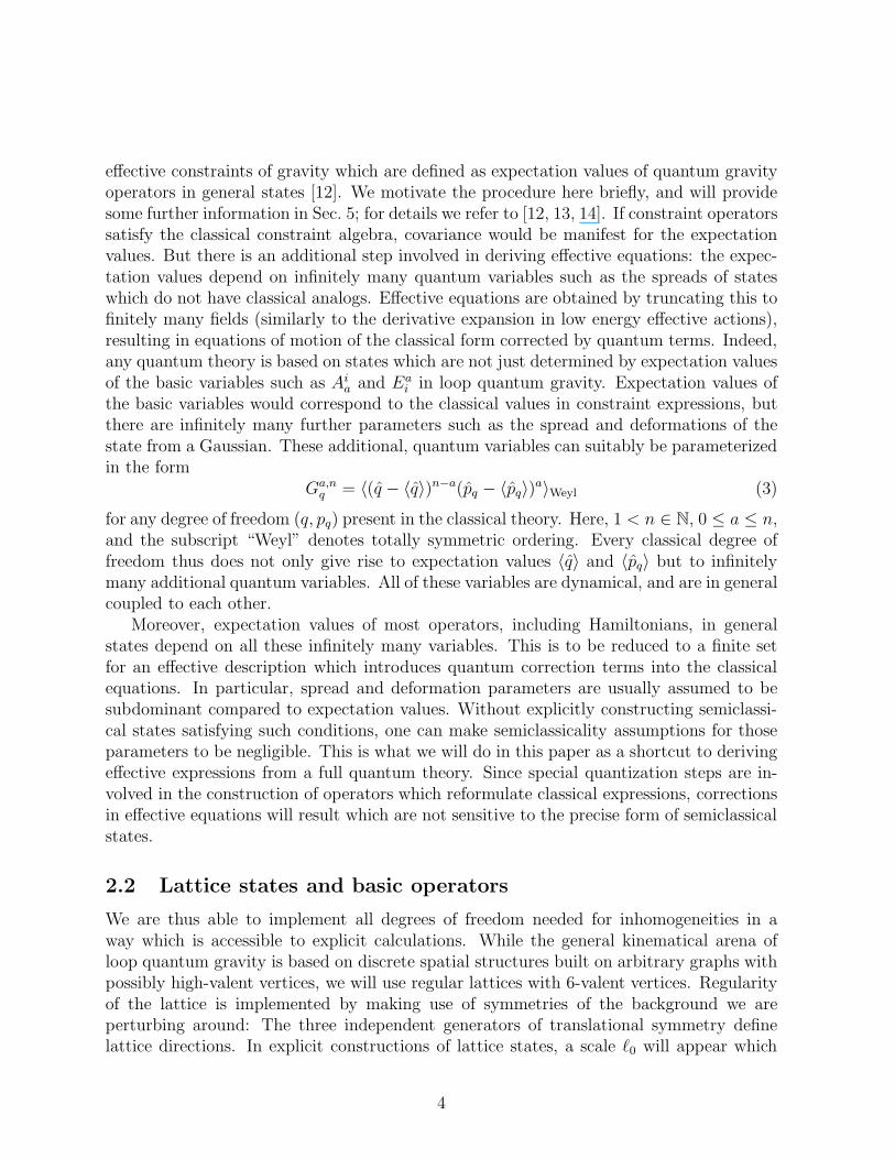
3.1 Gravitational part

The gravitational contribution to the Hamiltonian constraint is given by

H [N ] =1

16πG

∫

Σ

d3xN |detE|−1/2 (ǫijkFiabE

ajE

bk (15)

− 2(1 + γ−2)(Aia − Γi

a)(Ajb − Γj

b)E[ai E

b]j

)

in terms of Ashtekar variables with the curvature F iab = 2∂[aA

ib] + ǫijkAj

aAkb . The second

term, quadratic in extrinsic curvature components Kia = γ−1(Γi

a − Aia), is in general more

complicated to deal with due to the appearance of spin connection components as func-tionals of Ea

i through (2). One usually starts with quantizing the first term and then usesthe identity [18]

Kia = γ−1(Ai

a − Γia) ∝

{

Aia,

{

∫

d3xF iab

ǫijkEajE

bk

√

| detE|,

∫

√

| detE|d3x

}}

(16)

which allows one to express the second contribution in terms of the first. In the first term,then, the densitized triad components including the inverse determinant can be quantizedusing (13), and the curvature components F i

ab can be obtained through holonomies aroundappropriately chosen small loops [19]. On our regular lattices, natural loops based at a givenvertex are provided by the adjacent lattice plaquettes. After replacing the Poisson bracketsby commutators, the resulting first part of the Hamiltonian operator, H(1) =

∑

v H(1)v has

non-zero action only in vertices of a lattice state, each contribution being of the form

H(1)v =

1

16πG

2i

8πγG~

N(v)

8

∑

IJK

∑

σI∈{±1}

σ1σ2σ3ǫIJK (17)

× tr(hv,σII(A)hv+σII,σJJ(A)hv+σJJ,σII(A)−1hv,σJ J(A)−1hv,σKK(A)[hv,σKK(A)−1, V ])

summed over all non-planar triples of edges in all possible orientations. (There are 48 termsin the sum, but we need to divide only by 8 since a factor of six arises in the contractionof basic fields occurring in the constraint.) The combination

hv,σII(A)hv+σII,σJJ(A)hv+σJ J,σII(A)−1hv,σJ J(A)−1

gives a single plaquette holonomy with tangent vectors ev,σI I and ev,σJJ as illustrated inFig. 2.

When expanded in ℓ0 assuming sufficiently small edges, the leading term is of the orderℓ30 which automatically results in a Riemann sum representation of the first term in (15).This justifies H(1) as a quantization of the classical expression. As seen from the argument,one needs to assume that the lattice is sufficiently fine for classical values of the fieldsAi

a. Thus, there are states corresponding to coarser lattices on which stronger quantumcorrections can result. As usually, semiclassical behavior is not realized on all states butonly for a select class. For any low-curvature classical configuration, one can make surethat a chosen lattice leads only to small quantum corrections such that sufficiently manysemiclassical states exist.

10

2

v

1

h v+1

h

h

h

v+2

v,1

v+1,2v,2−1

v+2,1−1

Figure 2: Elementary lattice plaquette with holonomies around a closed loop.

3.1.1 Quantization

The required calculations for SU(2) holonomies and their products usually do not allowexplicit diagonalizations of operators. But some physical regimes allow one to decouple thematrix components at least approximately. This is realized for several symmetric modelsand also for perturbations at least of some metric modes around them. In particular,after splitting off the non-diagonal part of the connection in the perturbative expansionconsidered here, we can take the trace explicitly and reduce the expression to U(1). Sincethe diagonal part of the Ashtekar connection for our perturbations is contributed entirely byextrinsic curvature, we are effectively using “holonomies” computed for extrinsic curvaturerather than the Ashtekar connection. Although extrinsic curvature is a tensor rather thana connection, it is meaningful to use it in expressions resembling holonomies, denoted heresimply as hv,I , on a given metric background. This has the additional advantage of easilycombining the remaining quadratic terms in Ki

a with the first term of the constraint (15)without using squares of multiple commutators from quantizing (16). Writing

F iab = 2∂[aΓ

ib] + 2γ∂[aK

ib] + ǫijk

(

Γja + γKj

a

) (

Γkb + γKk

b

)

= 2∂[aΓib] + 2γ∂[aK

ib] + γǫijk

(

ΓjaK

kb + Γk

bKja

)

+ ǫijk(

ΓjaΓ

kb + γ2Kj

aKkb

)

(18)

we obtain a term 2γ∂[aKib] + γ2Kj

aKkb resembling “curvature” F i

ab(K) as computed fromextrinsic curvature alone, a curvature term of the spin connection as well as cross-termsǫijk(

ΓjaK

kb + Γk

bKja

)

. In our context due to the diagonality conditions the cross-termsdisappear [5] and we only have theK-curvature term and spin connection terms to quantize.The first term can then be combined with the term quadratic in Ki

a in (15), removing theneed to use double commutators. We denote this contribution to the constraint as

HK [N ] :=1

8πG

∫

Σ

d3xN |detE|−1/2 (ǫijkγ∂aKib −Kj

aKkb

)

E[aj E

b]k (19)

11

(since also ∂aKib drops out as used later, the constraint is γ-independent) and the remaining

term as

HΓ[N ] :=1

8πG

∫

Σ

d3xN |detE|−1/2 (ǫijk∂aΓib + Γj

aΓkb

)

E[aj E

b]k . (20)

Then, H [N ] = HK [N ] + HΓ[N ] is the constraint for scalar modes in longitudinal gauge.Both terms can rather easily be dealt with, using holonomies around a loop for the firstterm (this subsection) and direct quantizations of Γi

a for the second (Sec. 3.1.4). Thesplit-off spin connection components are thus quantized separately, which is possible in theperturbative treatment on a background, and then added on to the operator.

Note also that as a further simplification the derivative term of extrinsic curvaturedisappears from the constraint for diagonal variables as assumed here. This will automat-ically happen also from holonomies around loops. We emphasize that the quantizationprocedure followed is special to the given context of scalar perturbations on a flat isotropicbackground. Nevertheless, it mimics essential steps of the full constructions as discussedin more detail in Sec. 4.2.1. Its main advantage is that it allows explicit derivations of allnecessary terms and thus explicit effective equations to be confronted with observations.Moreover, it is far from clear that the constructions currently done in the full setting willremain unchanged with further developments. We thus evaluate the key features of thescheme without paying too close attention to current details.

Following the general procedure, we thus obtain vertex contributions

HK,v = − 1

16πG

2i

8πγ3G~

N(v)

8

∑

IJK

∑

σI∈{±1}

σ1σ2σ3ǫIJK (21)

× tr(

hv,σIIhv+σI I,σJJh−1v+σJ J,σIIh

−1v,σJ Jhv,σKK

[

h−1v,σKK , Vv

])

.

As before, hv,I denotes a K-holonomy along the edge oriented in the positive I-directionand starting at vertex v, but we also include the opposite direction hv,−I in the sum toensure rotational invariance. Note that following our convention, such holonomies areidentified with h−1

v−I,I . In some of the holonomies, v + I is again the vertex adjacent to vin the positive I-direction. The {IJK}-summation is taken over all possible orientationsof the IJ-loop and a transversal K-direction. Also, for notational brevity, we introduce

cv,I :=1

2tr(hv,I) , sv,I := − tr(τ(I)hv,I) (22)

such that (5) becomes hv,I = cv,I + 2τIsv,I . In a continuum approximation, we have

cv,I = cos(γkI(v + I/2)/2) , sv,I = sin(γkI(v + I/2)/2) (23)

where kI(v) = ℓ0kI(v). After substituting this expression into (21) and making use of theidentity3 (for some fixed I, J,K and numbers xi and yi)

ǫIJK tr [(x11I + 2y1τI)(x21I + 2y2τJ)(x31I + 2y3τK)] = ǫIJK tr(x1x2x31I) + 8ǫIJK tr(y1y2y3τIτJτK)

= 2(x1x2x3 − y1y2y3ǫIJK)ǫIJK ,

3Here the fundamental representation of τI has been used: tr(1I) = 2, tr(τIτJ ) = − 1

2δIJ

12

any one term of the sum in (21) becomes

i

8πγG~tr(hv,Ihv+I,Jh

−1v+J,Ih

−1v,Jhv,K [h−1

v,K , Vv]) (24)

= −ǫIJK

{

[(cv,Icv+J,I + sv,Isv+J,I)cv,Jcv+I,J + (cv,Icv+J,I − sv,Isv+J,I)sv,Jsv+I,J ] Av,K

}

+ǫ2IJK

{

[(cv,Isv+J,I − sv,Icv+J,I)sv,Jcv+I,J + (sv,Icv+J,I + cv,Isv+J,I)cv,Jsv+I,J ] Bv,K

}

,

where

Av,K :=1

4πiγG~

(

Vv − cv,K Vvcv,K − sv,KVvsv,K

)

,

Bv,K :=1

4πiγG~

(

sv,K Vvcv,K − cv,K Vvsv,K

)

. (25)

In the first line of (24), the expression inside the curly braces is symmetric in the in-dices I and J , hence vanishes when contracted with ǫIJK . Therefore only the second linecontributes, and the extrinsic curvature part of the gravitational constraint is

HK,v =−N(v)

64πγ2G

∑

IJK

∑

σI∈{±1}

{[(cv,σIIsv+σJ J,σII − sv,σIIcv+σJ J,σII)sv,σJJcv+σII,σJJ

+(sv,σIIcv+σJ J,σII + cv,σIIsv+σJ J,σII)cv,σJJsv+σI I,σJJ ]Bv,σKK} (26)

=−N(v)

64πγ2G

∑

IJK

∑

σI∈{±1}

{[s−v,σII,σJJsv,σJJcv+σI I,σJJ + s+v,σII,σJJcv,σJJsv+σII,σJJ ]Bv,σKK} ,

where in the last line trigonometric identities have been used to express products of sinesand cosines through

s±v,σII,σJJ := sin(γ

2(kσII(v + σII/2) ± kσII(v + σJJ + σII/2)

)

.

As in this expression, all functions kI are, as before, evaluated at the midpoint of the edgeev,I . We see that in the homogeneous case the first term in the sum vanishes and theleading contribution is

4 sin(γkI/2) cos(γkI/2) sin(γkJ/2) cos(γkJ/2)Bv,K , (27)

in agreement with [2].

3.1.2 Higher curvature corrections

There are two types of corrections visible from this expression: Using commutators toquantize inverse densitized triad components implies eigenvalues of Bv,I which differ fromthe classical expectation at small labels µv,I . Moreover, using holonomies contributes higherorder terms in extrinsic curvature together with higher spatial derivatives when sines and

13

cosines are expanded in small curvature regimes. We will now compute the next-leadingterms of higher powers and spatial derivatives of kI(v) before dealing with inverse powercorrections in the following subsection.

First, recall the usual expectation that quantum gravity gives rise to low energy effectiveactions with higher curvature terms such as

∫

d4x√

| det g|ℓ2PR2 or∫

d4x√

| det g|ℓ2PRµνρσRµνρσ

added to the Einstein–Hilbert action∫

d4x√

| det g|R. Irrespective of details of numerical

coefficients, there are two key aspects: The Planck length ℓP =√G~ must be involved for

dimensional reasons in the absence of any other length scale, and higher spatial as wellas time derivatives arise with higher powers of Rµνρσ. In canonical variables, one expectshigher powers and higher spatial derivatives of extrinsic curvature and the triad, togetherwith components of the inverse metric necessary to define scalar quantities from highercurvature powers (which forces one to raise indices on the Riemann tensor, for instance).Higher time derivatives, on the other hand, are more difficult to see in a canonical treat-ment and correspond to the presence of independent quantum variables without classicalanalog [13].

Any quantization such as that followed here starts from the purely classical action where~ and thus ℓP vanishes. In effective equations of the resulting quantum theory, quantumcorrections depending on ~ will nevertheless emerge. As a first step in deriving such effectiveequations, we have non-local holonomy terms in a Hamiltonian operator which through itsexpectation values in semiclassical states will give rise to similar contributions of the samefunctional form of kI(v). At first sight, however, the expressions above do not agree withexpectations from higher curvature actions: One can easily see that in (26) there are higherpowers of extrinsic curvature by expanding the trigonometric functions, and higher spatialderivatives of extrinsic curvature by Taylor expanding the discrete displacement involved,e.g., in kI(v + I/2). Moreover, higher spatial derivatives of the triad arise from similarnon-local terms in the spin connection contribution HΓ discussed later. But there are nofactors of the Planck length in such higher powers (all factors of G and ~ are written outexplicitly and not “set equal to one”). In fact, by definition kI(v) is dimensionless sinceit is obtained by multiplying the curvature component kI(v) with ℓ0 in which all possibledimensions cancel. Higher power terms here thus do not need any dimensionful prefactor.Moreover, there are no components of the inverse metric (which would be 1/pI(v) for ourdiagonal triads) in contrast to what is required in higher curvature terms.

Curvature expansion. To see how this is reconciled, we expand the Hamiltonian explic-itly in ℓ0 after writing kI = ℓ0kI . This corresponds to a slowly varying field approximationwith respect to the lattice size. For the (+I,+J)-plaquette, a single term in the sum (21)becomes

2s−v,I,Jsv,Jcv+I,J + 2s+v,I,Jcv,Jsv+I,J = γ2ℓ20kI kJ +

1

2γ2ℓ30

(

kI kJ,J + kJ kI,I + 2kJ kI,I

)

+1

8γ2ℓ40

(

kI kJ,JJ + kJ kI,II + 4(kI kJ,II + kI kJ,IJ + kI,I kJ,I + kI,J kJ,I)

14

x

t

t

t t

t t

t

t

vv−I v+I

v − J

v + J v+I+J

v+I−J

v−I+J

v−I−J

12

3 4

-�

6

?

6

?

-

-

6

?

�

�

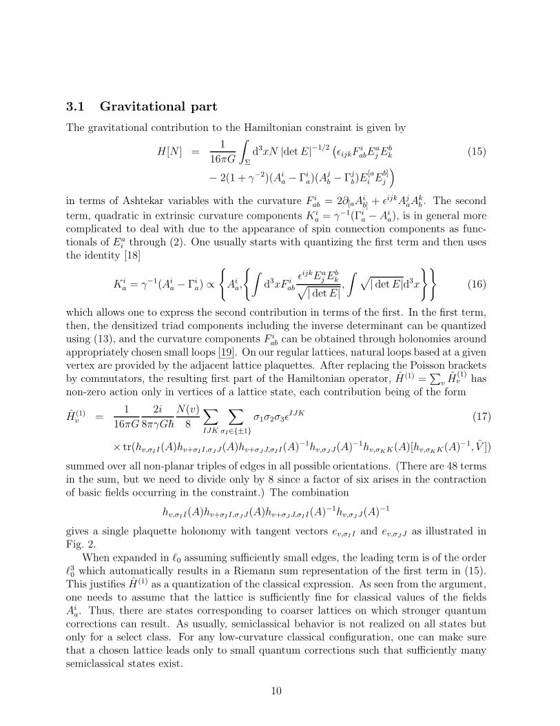
Figure 3: Four plaquettes adjacent to vertex v in the (I, J)-plane. The arrows indicate thedirections in which the relevant holonomies are traversed.

+2kI,I kJ,J − 4

3γ2kI kJ(k2

I + k2J)

)

+O(ℓ50) . (28)

(Commas on the classical field kI indicate partial derivatives along a direction given bythe following index.) For a fixed direction K there are in total eight terms to be includedin the sum (21). They are obtained from (28) by taking into account the four plaquettesin the (I, J)-plane meeting at vertex v (Fig. 3) and considering both orientations in whicheach plaquette can be traversed. While the latter merely boils down to symmetrizationover I and J , the former requires some care, noting that in the Hamiltonian constraint(21) hv,−I means h−1

v−I,I . The contribution (28) corresponds to plaquette 1 of Fig. 3 andhas σI = σJ = σK = 1. Accounting for the overall sign dictated by the σ-factors, one canobtain the expressions for the three remaining plaquettes 2, 3 and 4 following the recipebelow.

plaquette extrinsic curvature components sign(1) kI(v + I/2) kJ(v + I + J/2) −kI(v + I/2 + J) −kJ(v + J/2)(2) −kI(v − I/2) kJ(v − I + J/2) kI(v − I/2 + J) −kJ(v + J/2) (−1)(3) −kI(v − I/2) −kJ (v − I − J/2) kI(v − I/2 − J) kJ(v − J/2) (−1)2

(4) kI(v + I/2) −kJ(v + I − J/2) −kI(v + I/2 − J) kJ(v − J/2) (−1)

The first column designates a plaquette number, whereas the last one indicates the overallsign factor. The other four columns show the correspondence between the relevant linklabels.

After the symmetrization over all four plaquettes (traversed in both directions), thecubic terms drop out

γ2ℓ20kI kJ − γ4ℓ406kI kJ(k2

I + k2J) (29)

+γ2ℓ408

(

kI kJ,JJ + kJ kI,II + 2(kI kJ,II + kJ kI,JJ + kI,I kJ,I + kI,J kJ,J))

+O(ℓ50) .

Note that the link labels k were introduced as values of the extrinsic curvature componentsevaluated at midpoints of edges in the continuum approximation (23) of our basic non-local

15

variables. The expression above is written in terms of just two components kI(v) and kJ(v)(and their partial spatial derivatives) Taylor expanded around the vertex v. The first term,when combined with Bv,K and summed over all triples IJK, reproduces the correct classicallimit of the constraint HK . This limit is obtained in two steps: we first performed thecontinuum approximation by replacing holonomies with mid-point evaluations of extrinsiccurvature components. This would still give us a non-local Hamiltonian since each vertexcontribution now refers to evaluations of the classical field at different points. In a secondstep we then Taylor expanded these evaluations around the central vertex v, which givesa local result and corresponds to a further, slowly-varying field approximation.

Comparison with higher curvature terms. Here, the factor ℓ20 in the leading termtogether with a factor ℓ0 from Bv,K through (14) combines to give the Riemann measureof the classical integral. Higher order terms, however, come with additional factors of ℓ0 in(29) which are not absorbed in this way. The result is certainly independent of coordinatessince the whole construction (26) in terms of kI is coordinate independent. But for acomparison with higher curvature terms we have to formulate corrections in terms of kI

and pI as these are the components of classical extrinsic curvature and densitized triadtensors. Higher order terms in the expansion are already formulated with kI in coordinateindependent combinations with ℓ0-factors. It remains to interpret the additional ℓ0 factorsappropriately for a comparison with low energy effective actions.

This can be done quite simply in a way which removes the above potential discrepanciesbetween our expansions and higher curvature terms in low energy effective actions. Wesimply use (6) to write ℓ20 = pI/pI which is the only well-defined possibility to express ℓ0in terms of the fields. Thus, inverse metric components 1/pI directly occur in combinationwith kJ factors as required for higher curvature terms. The fact that the cubic term inℓ0 in (29) drops out is also in agreement with higher curvature corrections since in thatcase only even powers of the length scale ℓP occur. Moreover, there are now factors of pI

multiplying the corrections. These are basic variables of the quantum theory determiningthe fundamental discreteness. Thus, factors of the Planck length occurring in low energyeffective actions are replaced by the state specific quantities pI . While the Planck lengthℓP =

√G~ is expected to appear for dimensional reasons without bringing in information

about quantum gravity (it can just be computed using classical gravity for G and quantummechanics for ~), the pI are determined by a state of quantum gravity. If expressed throughlabels µv,I , the Planck length also appears, but it can be enlarged when µv,I > 1. Moreover,the lattice labels are dynamical (and in general inhomogeneous) and can thus change intime in contrast to ℓP. Although the form of corrections is analogous to those for low energyeffective actions, the conceptual as well as dynamical appearance of correction terms is thusquite different.

The terms considered so far could not give rise to higher time derivatives of the spatialmetric. In general, higher time derivatives describe the effect of quantum variables (3) ofthe field theory, which appear in the expectation value of the Hamiltonian constraint ina generic state. Quantum variables are thus, in a certain sense, analogous to higher time

16

derivatives in effective actions [13], which indicates that the correction terms they implyshould combine with those in (29) obtained by expanding sines and cosines to higherpowers of space-time curvature components. All corrections of these types should thusbe considered together since they will eventually be mixed up despite of their differentderivations. A computation of terms containing quantum variables requires more detailedinformation about the expectation value of the constraint operator in an arbitrary state.These terms are thus more difficult to compute, which also makes an interpretation of theremaining higher curvature terms alone, especially concerning their possible covariance,more difficult.4 We will thus focus from now on on corrections coming from commutatorsBv,K to quantize inverse powers which are independent of the higher order corrections andeven give rise to non-perturbative terms. Moreover, in Sec. 5.2.2 below we will demonstratethat those corrections are expected to be dominant in cosmological perturbation theory.

3.1.3 Inverse triad corrections

A direct calculation using (8) and (12) shows that Bv,K commutes with all flux operatorsand thus has flux eigenstates as eigenbasis, as it happens also in homogeneous models [4].The action

Bv,K | . . . , µv,K , . . .〉 :=(

2πγℓ2P)1/2

√

|µv,I + µv,−I ||µv,I + µv,−J | (30)

×(

√

|µv,K + µv,−K + 1| −√

|µv,K + µv,−K − 1|)

| . . . , µv,K , . . .〉

directly shows the eigenvalues which do not agree exactly with the classical expectationeK(v) =

√

|pI(v)pJ(v)/pK(v)| ∼√

|µv,Iµv,J/µv,K | (indices such that ǫIJK = 1) for theco-triad (13) which appears as a factor in the Hamiltonian constraint. But for large valuesµv,I ≫ 1 the classical expectation is approached as an expansion of the eigenvalues shows.

Inverse triad corrections are obtained by extracting the corrections which Bv,K receiveson smaller scales. We introduce the correction function as a factor αv,K , depending onthe lattice labels µv,I , such that Bv,K = αv,Kev,K and αv,K → 1 classically, i.e. for µv,K ≫1. Comparing the eigenvalues of Bv,K with those of flux operators in the combination√

|Fv,IFv,J/Fv,K |, we find

αv,K =√

|µv,K + µv,−K |(

√

|µv,K + µv,−K + 1| −√

|µv,K + µv,−K − 1|)

(31)

4It is sometimes tempting to “sum the whole perturbations series” of higher order terms simply byusing the left hand side of (28) directly in effective equations without an expansion. However, this is ingeneral not a consistent approximation since arbitrarily small higher order terms are included but othertypes of corrections such as higher time derivatives or quantum variables are completely ignored. Thereis currently only one known model where the procedure is correct since all quantum variables have beenshown to decouple from the expectation values [20]. But this model, a free isotropic scalar in a certainfactor ordering of the constraint operator, is very special. Under modifications such as a scalar potentialquantum variables do not decouple and their motion implies further correction terms in effective equationsnot captured in the trigonometric functions arising from holonomies.

17

After having computed the operators and their eigenvalues, we can specialize the cor-rection function to perturbations of the scalar mode. We reduce the number of independentlabels by imposing µv,I + µv,−I = µv,J + µv,−J for arbitrary I and J . This corresponds toa metric proportional to the identity δab for a scalar perturbation. We then assign a newvariable p(v) = 2πγℓ2P(µv,I + µv,−I) to each vertex v, which is independent of the directionof the edge I and describes the diagonal part of the triad. Quantum numbers in eigenvaluesof the lattice operators can then be replaced by p(v), and the resulting functions comparedwith the classical ones. The remaining subscript v indicates that the physical quantities arevertex-dependent, i.e. inhomogeneous. Then the averaging over the plaquette orientationsin the constraint becomes trivial and the total correction reads

αv = 2√

|µv|(

√

|µv + 1/2| −√

|µv − 1/2|)

(32)

i.e.

α[p(v)] =

√

|p(v)|2πγℓ2P

(

√

|p(v) + 2πγℓ2P| −√

|p(v) − 2πγℓ2P|)

. (33)

We will continue analyzing these correction functions in Sec. 3.3 after having discussedhow such functions also enter the spin connection and matter terms.

3.1.4 Spin connection

So far, the holonomies we used only contributed the extrinsic curvature terms to theHamiltonian but no spin connection terms at all. In the procedure followed here, we thushave to quantize Γi

a[E] directly which is possible in the perturbative regime where lineintegrals of the spin connection have covariant meaning. This gives rise to one furthercorrection function in the effective expression of the spin connection

ΓiI = −ǫijkeb

j

(

∂[Iekb] +

1

2ec

kela∂[ce

lb]

)

, (34)

as it also contains a co-triad (13). Since the triad and its inverse have a diagonal form

eIi ≡ EI

i√

| detE|= e(I)δI

i , eI = e(I)δiI (35)

with the components given by

eI =pI

√

| detE|= (eI)

−1 , detE = pIpJpK , (36)

the spin-connection simplifies to

ΓiI = ǫicI e

(c)∂ce(I). (37)

18

In terms of components of a densitized triad it reads

ΓiI =

1

2ǫijIp(j)

p(I)

(

∑

J

∂jpJ

pJ− 2

∂jpI

pI

)

. (38)

Since there are many alternative choices in performing the quantization of such an ob-ject, but not much guidance from a potential operator in the full theory, we first discussgeneral aspects one can expect for the quantization of the spin connection in a simple ver-sion. It includes corrections of inverse densitized triad components by correction functionsin each term of (38). We thus mimic a quantization to the extent that expectation valuesof classical expressions containing inverse powers of p acquire a correction factor

1

pI(v)→ βI(v)

pI(v), (39)

where the correction functions βI are kept different from the function α used before becausethe object to be quantized is different. There will also be corrections from the discretization∆I of partial derivatives ℓ0∂I , but we ignore them in what follows for the same reason whichallowed us to ignore such effects from the loop holonomy quantizing F i

ab. The effectiveanalog of (38) is then of the form

(ΓiI)eff =

1

2ǫijI β

I pj

pI

(

∑

J

βJ ∂jpJ

pJ− 2βI ∂jp

I

pI

)

. (40)

At this stage the triad components, corresponding to different orientations, can be putequal to each other in effective equations, pI = pJ = pK = p. This implies an analogousrelation between the correction functions βI = βJ = βK = β0. Comparing (40) with

the ansatz ΓiI = 1

2ǫijI β

∂jp

p, we conclude that also the spin connection receives a correction

function β = β20 .

For a precise quantization we observe that we need terms of the form ℓ20ΓiaΓ

jb and

ℓ20∂aΓib in the constraint since one factor ℓ0 of the Riemann measure will be absorbed in

the commutator Bv,I . To quantize ℓ0Γia, we combine ℓ0 with the partial derivative ∂I in

(37) to approximate a lattice difference operator ∆I defined by (∆If)v = fv+I − fv forany lattice function f . A well-defined lattice operator thus results once a prescription forquantizing the inverse triad has been chosen. One can again make use of Poisson identitiesfor the classical inverse which, however, allows more freedom than for the combination oftriad components we saw in the Hamiltonian constraint. Such a freedom, corresponding toquantization ambiguities, will also be encountered when we consider matter Hamiltonians.For any choice we obtain a well-defined operator which would not be available without theperturbative treatment since the full spin connection is not a tensorial object.

An explicit example can most easily be derived by writing the spin connection integratedalong a link ev,I as it might appear in a holonomy,

∫

ev,I

eaIΓ

ia ≈ ℓ0Γ

iI = ǫicI e

(c)ℓ0∂ce(I) ≈ ǫiKIp(K)

√

| detE|∆Ke(I)

19

using the lattice difference operator ∆I ≈ ℓ0∂I . We then have to deal with the inversepowers explicit in the fraction and implicit in the co-triad eI . The latter is standard,replacing eI by ℓ−1

0 hI{h−1I , Vv} based on (13). The inverse determinant in the fraction

cannot be absorbed in the resulting Poisson bracket because (i) it does not commutewith the derivative and (ii) absorbing a single inverse in a single co-triad would lead to alogarithm of Vv in the Poisson bracket which would not be well-defined. It can, however, beabsorbed in the flux ℓ20p

K if we do not use the basic flux operator Fv,K but the classicallyequivalent expression

Fv,K ≈ ℓ20pK =

1

2ℓ20δ

k(K)ǫkijǫ

KIJeiIe

jJ

= −1

4(4πγG)−2

∑

IJ

∑

σI∈{±1}

σIσJǫIJK tr(τ(K)hI{h−1

I , Vv}hJ{h−1J , Vv}) (41)

which is analogous to expressions used in [21]. Since there are two Poisson brackets, we cansplit the inverse Vv evenly among them, giving rise to square roots of Vv in the brackets:

pK

√

| detE|≈ ℓ0

Fv,K

Vv

= − ℓ016π2γ2G2

∑

IJ

∑

σI∈{±1}

σIσJǫIJK tr(τ(K)hI{h−1

I ,√

Vv}hJ{h−1J ,√

Vv}) .(42)

The remaining factor of ℓ0 is absorbed in eI inside the derivative which is quantized follow-ing the standard procedure. A well-defined quantization of spin connection componentsthus follows, which is not local in a vertex since the difference operator connects to thenext vertex. Similarly, the derivative of the spin connection needed in the Hamiltonianconstraint leads to further connections to next-to-next neighbors.

Explicitly, one can thus write an integrated spin connection operator quantizing Γiv,I :=

∫

ev,Idtea

IΓia as

Γiv,I = ǫI

iK

(

1

16π2γ2ℓ2P

∑

J,L,σJ ,σL

σJσLǫJLK tr

(

τ(K)hJ [h−1J , V 1/2

v ]hL[h−1L , V 1/2

v ])

× ∆K

(

i

2πγℓ2Ptr(τ (I)hI [h

−1I , Vv])

))

. (43)

Replacing the commutators by classical expressions times correction functions α definedas before and α1/2 defined similarly for a commutator containing the square root of thevolume operator leads to an expression

(ΓiI)eff = α1/2(p

i)α1/2(pI)ǫI

ice(c)∂c(α(pI)eI)

= α1/2(pi)α1/2(p

I)α(pI)ΓiI + α1/2(p

i)α1/2(pI)α′(pI)eIǫI

ice(c)∂cp(I)

20

where the prime denotes a derivative by pI . Using the relation pJ = eIeK wheneverǫJIK = 1 between densitized triad and co-triad components allows us to write

(ΓiI)eff = α1/2(p

i)α1/2(pI)α(pI)Γi

I + α1/2(pi)α1/2(p

I)α′(pI)eIǫIice(c)∂c(eJeK)|ǫIJK=1

= α1/2(pi)α1/2(p

I)

(

α(pI)ΓiI +

∑

K 6=I

α′(pI)pKΓiK

)

(44)

for the effective spin connection components. For scalar modes, using that all pI at a givenpoint are equal, this can be written with a single correction function

β[p(v)] = α1/2[p(v)]2(α[p(v)] + 2pα′[p(v)]) (45)

for ΓiI , where α′ = dα/dp.

3.2 Matter Hamiltonian

Matter fields are quantized by similar means in a loop quantization, using lattice states, andthen coupled dynamically to geometry by adding the matter Hamiltonian to the constraint.For a scalar field φ, the momentum π =

√

| detE|φ/N is a density of weight one. In theφ-representation, states will simply be of the form already used for the gravitational field,except that each vertex now also carries a label νv ∈ R describing the dependence on thescalar field φ(v) through exp(iνvφ(v)) [22]. Well-defined lattice operators are then given

by exp(iν0φv), for any ν0 ∈ R, which shifts the label νv by ν0. The momentum, with itsdensity weight, has to be integrated before it can meaningfully be quantized. We introduce

Pv :=

∫

Rv

d3xπ ≈ ℓ30π(v)

where Rv is a cubic region around the vertex v of the size of a single lattice site. Since wehave {φ(v), Pw} = χRw

(v) in terms of the characteristic function χR(v) = 1 if v ∈ R andzero otherwise, a momentum operator Pv must have eigenvalue ~νv in a state introducedabove.

3.2.1 Inverse triad corrections

For the matter Hamiltonian of a scalar field φ with momentum π and potential U(φ) wehave the classical expression

Hφ[N ] =

∫

d3xN(x)

[

1

2√

det(q)π(x)2 +

Eai E

bi

2√

det q∂aφ(x)∂bφ(x) +

√

det qU(φ)

]

containing inverse powers of the metric, too. It can be quantized by loop techniques [23, 24]making use of identities similar to (13). One first generalizes the identity to arbitrarypositive powers of the volume in a Poisson bracket,

{Aia, V

rv } = 4πγG rV r−1

v eia (46)

21

and then combines such factors with suitable exponents r to produce a given product oftriad and co-triad components. Since such identities would be used only when inversecomponents of densitized triads are involved and a positive power of volume must resultin the Poisson bracket, the allowed range for r is 0 < r < 2. Any such Poisson bracket willbe quantized to

eaK{Ai

a, Vrv } 7→ −2

i~ℓ0tr(τ ihv,K [h−1

v,K , Vrv ])

using holonomies hv,I in direction I with tangent vector eaK . Since holonomies in our lattice

states have internal directions τK for direction K, we can compute the trace and obtain

V r−1v ei

K =−2

8πirγℓ2Pℓ0

∑

σ∈{±1}

σ tr(τ ihv,σK [h−1v,σK , Vv

r]) =

1

2ℓ0(B

(r)v,K − B

(r)v,−K)δi

(K) (47)

where, for symmetry, we use both edges touching the vertex v along direction K and B(r)v,K

is the generalized version of (25):

B(r)v,K :=

1

4πiγG~r

(

sv,KVrv cv,K − cv,K V

rv sv,K

)

(48)

The exponent used for the gravitational part was r = 1, and r = 1/2 already occurred inthe spin connection, while the scalar Hamiltonians introduced in [23, 24], which we closelyfollow in the construction of the matter Hamiltonian here, use r = 1/2 for the kinetic termand r = 3/4 for the gradient term. With

ǫabcǫijk{Aia, V

1/2v }{Aj

b, V1/2v }{Ak

c , V1/2v } = (2πγG)3ǫabcǫijk

eiae

jbe

kc

V3/2v

=6(2πγG)3

ℓ30V1/2v

for a lattice site volume Vv ≈ ℓ30| det(eia)| and

ǫabcǫijk{Ajb, V

3/4v }{Ak

c , V3/4v } = (3πγG)2ǫabcǫijk

ejbe

kc

V1/2v

= 6(3πγG)2 Eai

V1/2v

one can replace the inverse powers in the scalar Hamiltonian as follows: For the kineticterm, we discretize

∫

d3xπ2

√det q

≈∑

v

ℓ30π(v)2

√

det q(v)≈∑

v

Pv2

Vv.

Then, the classically singular

1

Vv=

(

ℓ306ǫabcǫijk

eiae

jbe

kc

V3/2v

)2

=

(

ℓ306(2πγG)3

ǫabcǫijk{Aia, V

1/2v }{Aj

b, V1/2v }{Ak

c , V1/2v }

)2

(49)

will be quantized to(

1

48ǫIJKǫijk(B

(1/2)v,I − B

(1/2)v,−I )δi

(I)(B(1/2)v,J − B

(1/2)v,−J )δj

(J)(B(1/2)v,K − B

(1/2)v,−K)δk

(K)

)2

.

22

Similarly, we discretize the gradient term by

∫

d3xEa

i Ebi√

det q∂aφ∂bφ ≈

∑

v

ℓ30Ea

i (v)Ebi (v)

√

det q(v)(∂aφ)(v)(∂bφ)(v) ≈

∑

v

pI(v)pJ(v)

Vv∆Iφv∆Jφv

where we replace spatial derivatives ∂a by lattice differences ∆I . Now, using

δi(I)

pI(v)

V1/2v

= ℓ20EI

i (v)

V1/2v

=ℓ206

ǫIbcǫijkejbe

kc

V1/2v

=ℓ20

6(3πγG)2ǫIbcǫijk{Aj

b, V3/4v }{Ak

c , V3/4v }

we can quantize the metric contributions to the gradient term by

1

242ǫIKLǫijk(B

(3/4)v,K − B

(3/4)v,−K)δj

(K)(B(3/4)v,L − B

(3/4)v,−L)δk

(L) (50)

×ǫJMN ǫimn(B(3/4)v,M − B

(3/4)v,−M)δm

(M)(B(3/4)v,N − B

(3/4)v,−N)δn

(N) .

In addition to the fact that we are using different values for r in each term in the grav-itational and matter parts, giving rise to different correction functions, the matter termsare less unique than the gravitational term and can be written with different parametersr. This corresponds to quantization ambiguities which will appear also in effective equa-tions and which could have phenomenological implications. Some choices are preferredsince they give rise to simpler expressions, but this does not suffice to determine a uniquequantization. Instead of using r = 1/2 in the kinetic term, for instance, we can use theclass of relations

1√

| detE|=

(det e)k

(detE)(k+1)/2=

(

1

6ǫabcǫijk(4πGγ)

3

×{Aia, V

(2k−1)/3k}{Ajb, V

(2k−1)/3k}{Ajc, V

(2k−1)/3k})k

for any positive integer k to write the inverse determinant through Poisson brackets notinvolving the inverse volume (see also the appendix of [25]). This determines an integerfamily of quantizations with rk = (2k − 1)/3k > 1

3. For k = 2 we obtain the previous

expression, but other choices are possible. Moreover, using the same r in all terms arisingin gravitational and matter Hamiltonians can only be done in highly contrived ways, ifat all. There is thus no clearly distinguished value. From now on we will work with thechoices specified above.

On regular lattice states, all ingredients are composed to a Hamiltonian operator

Hφ[N ] =∑

v∈γ

Nv

1

2P 2

v

1

48

∑

IJK,σI∈{±1}

σ1σ2σ3ǫIJKB

(1/2)v,σ1IB

(1/2)v,σ2JB

(1/2)v,σ3K

2

(51)

+1

2

1

48

∑

IJK,σI∈{±1}

σ1σ2σ3ǫIJK(σ1∆σ1Iφ)vB

(3/4)v,σ2JB

(3/4)v,σ3K

2

+ VvU(φv)

,

23

0

0.5

1

1.5

2

2.5

0 0.5 1 1.5 2

(r)α

µ

r=1/2r=3/4

r=1r=3/2

r=2

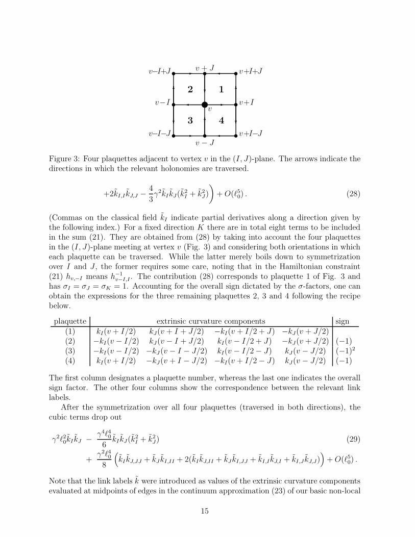
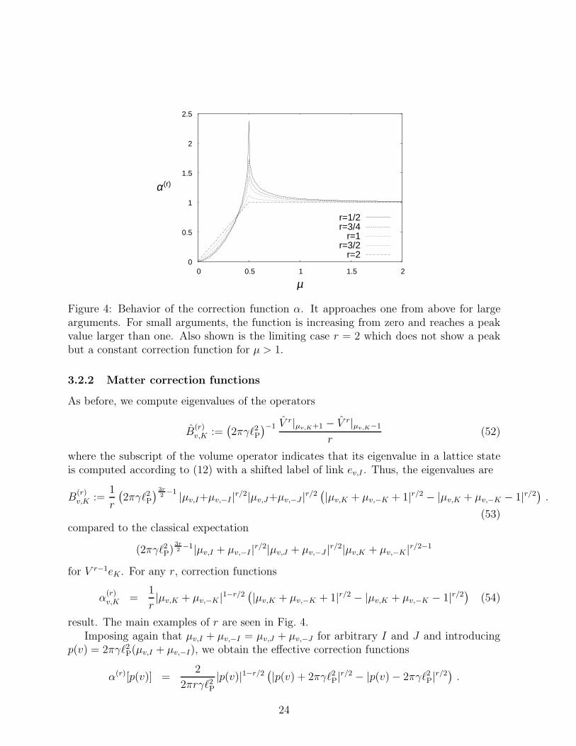
Figure 4: Behavior of the correction function α. It approaches one from above for largearguments. For small arguments, the function is increasing from zero and reaches a peakvalue larger than one. Also shown is the limiting case r = 2 which does not show a peakbut a constant correction function for µ > 1.

3.2.2 Matter correction functions

As before, we compute eigenvalues of the operators

B(r)v,K :=

(

2πγℓ2P)−1 V

r|µv,K+1 − V r|µv,K−1

r(52)

where the subscript of the volume operator indicates that its eigenvalue in a lattice stateis computed according to (12) with a shifted label of link ev,I . Thus, the eigenvalues are

B(r)v,K :=

1

r

(

2πγℓ2P) 3r

2−1 |µv,I+µv,−I |r/2|µv,J+µv,−J |r/2

(

|µv,K + µv,−K + 1|r/2 − |µv,K + µv,−K − 1|r/2)

.

(53)compared to the classical expectation

(2πγℓ2P)3r2−1|µv,I + µv,−I |r/2|µv,J + µv,−J |r/2|µv,K + µv,−K |r/2−1

for V r−1eK . For any r, correction functions

α(r)v,K =

1

r|µv,K + µv,−K |1−r/2

(

|µv,K + µv,−K + 1|r/2 − |µv,K + µv,−K − 1|r/2)

(54)

result. The main examples of r are seen in Fig. 4.Imposing again that µv,I + µv,−I = µv,J + µv,−J for arbitrary I and J and introducing

p(v) = 2πγℓ2P(µv,I + µv,−I), we obtain the effective correction functions

α(r)[p(v)] =2

2πrγℓ2P|p(v)|1−r/2

(

|p(v) + 2πγℓ2P|r/2 − |p(v) − 2πγℓ2P|r/2)

.

24

This can be used to write the effective matter Hamiltonian on a conformally flat spaceqab = |p(x)|δab as

Hφ =

∫

Σ

d3xN(x)

(

D[p(x)]

2|p(x)|3/2π(x)2 +

σ[p(x)])|p(x)| 12 δab

2∂aφ∂bφ+ |p(x)| 32U(φ)

)

,

where comparison with (51) shows that

D[p(v)] = α(1/2)[p(v)]6 and σ[p(v)] = α(3/4)[p(v)]4 . (55)

3.3 Properties of correction functions from inverse powers

We have derived several different correction functions, making use of different parametersr. In most cases one could make different choices of such parameters and still write theclassically intended expression in an equivalent way. This gives rise to quantization ambi-guities since the eigenvalues of B

(r)v,K depend on the value r, and so will correction functions.

In addition to the ambiguities in the exponents r, one could use different representationsfor holonomies before taking the trace rather than only the fundamental representationunderstood above [26, 27]. In this case, we have more generally

B(r,j)v,K =

3

irj(j + 1)(2j + 1)

(

2πγℓ2P)−1

trj

(

τKhv,K Vrv h

−1v,K

)

.

Eigenvalues of such operators can be expressed as

B(r,j)v,K =

3

rj(j + 1)(2j + 1)

(

2πγℓ2P)

3r2−1 |µv,I+µv,−I |r/2|µv,J+µv,−J |r/2

j∑

m=−j

m|µv,K+µv,−K+2m|r/2

(56)which leads to the general class of correction functions

α(r,j)v,K =

3

rj(j + 1)(2j + 1)|µv,K + µv,−K |1− r

2

j∑

m=−j

m |µv,K + µv,−K + 2m|r/2 . (57)

After imposing isotropy the last expression becomes

α(r,j) =6

rj(j + 1)(2j + 1)|µ|1− r

2

j∑

m=−j

m |µ+m|r/2 (58)

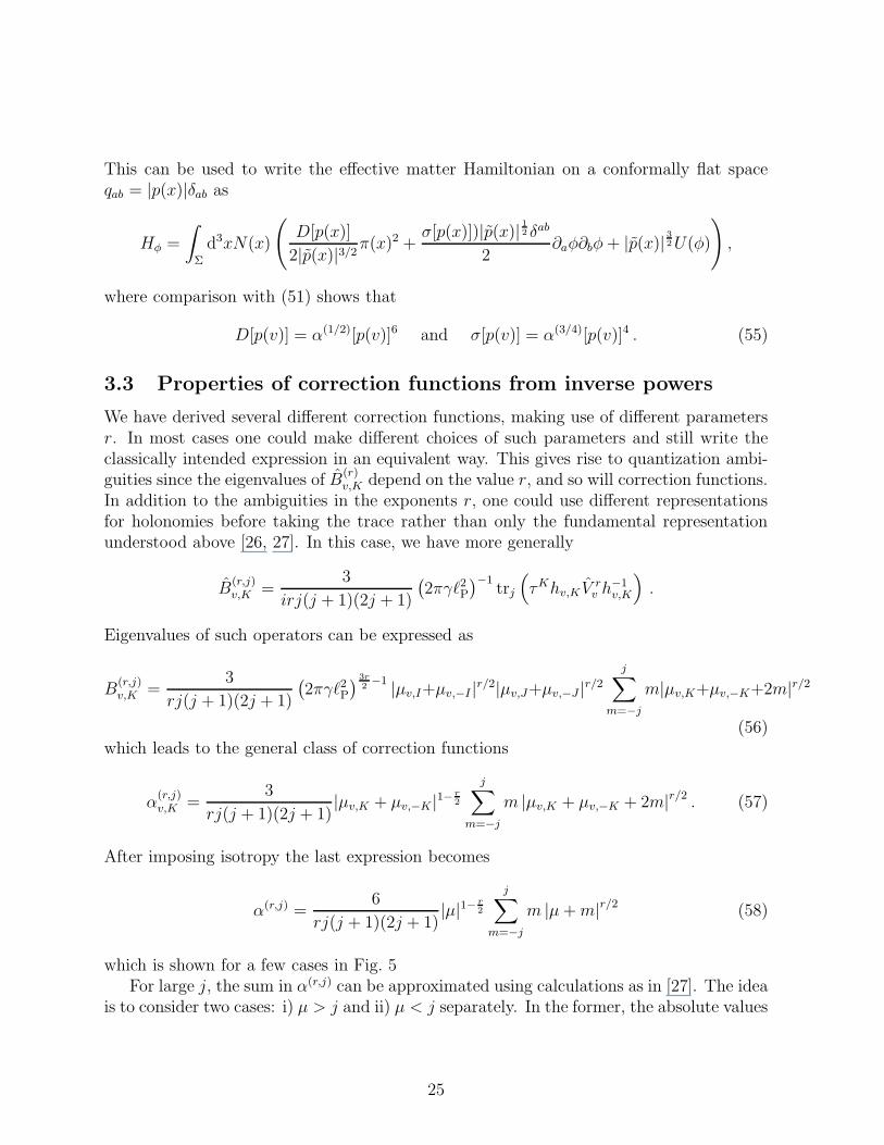
which is shown for a few cases in Fig. 5For large j, the sum in α(r,j) can be approximated using calculations as in [27]. The idea

is to consider two cases: i) µ > j and ii) µ < j separately. In the former, the absolute values

25

0

0.2

0.4

0.6

0.8

1

1.2

1.4

1.6

0 0.5 1 1.5 2

(r,j)α

µ~

j=10

r=1/2r=1

r=3/2

Figure 5: Behavior of the correction function α for larger j. The general trend is similarto the case for j = 1/2, but there are [j] + 1 spikes at µ = 1, . . . , j for integer j andµ = 1/2, . . . , j otherwise. Above the peak, the function is smooth.

can be omitted as all the expressions under the sum are positive. Then the summation isto be replaced by integration to yield

α(r,j) =12j3µ1− r

2

rj(j + 1)(2j + 1)

[

1

r + 4

(

(µ+ 1)r2+2 − (µ− 1)

r2+2)

− µ

r + 2

(

(µ+ 1)r2+1 − (µ− 1)

r2+1)

]

, µ > 1

where µ := µ/j. In the second case, the terms in the sum corresponding to m < µ andm > µ should again be considered separately. The end result, however, is very similar tothe previous one

α(r,j) =12j3µ1− r

2

rj(j + 1)(2j + 1)

[

1

r + 4

(

(µ+ 1)r2+2 − (1 − µ)

r2+2)

− µ

r + 2

(

(µ+ 1)r2+1 + (1 − µ)

r2+1)

]

, µ < 1

After some rearrangements and using that j ≫ 1 these two expressions can be combinedinto a single one as

α(r,j) =6µ1− r

2

r(r + 2)(r + 4)

[

(µ+ 1)r2+1(r + 2 − 2µ) + sgn(µ− 1)|µ− 1| r

2+1(r + 2 + 2µ)

]

.(59)

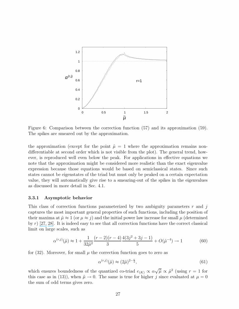
The approximation is compared to the exact expression of the correction function ob-tained through eigenvalues in Fig. 6. As one can see, the spikes are smeared out by

26

0

0.2

0.4

0.6

0.8

1

1.2

0 0.5 1 1.5 2

(r,j)α

µ~

r=1

Figure 6: Comparison between the correction function (57) and its approximation (59).The spikes are smeared out by the approximation.

the approximation (except for the point µ = 1 where the approximation remains non-differentiable at second order which is not visible from the plot). The general trend, how-ever, is reproduced well even below the peak. For applications in effective equations wenote that the approximation might be considered more realistic than the exact eigenvalueexpression because those equations would be based on semiclassical states. Since suchstates cannot be eigenstates of the triad but must only be peaked on a certain expectationvalue, they will automatically give rise to a smearing-out of the spikes in the eigenvaluesas discussed in more detail in Sec. 4.1.

3.3.1 Asymptotic behavior

This class of correction functions parameterized by two ambiguity parameters r and jcaptures the most important general properties of such functions, including the position oftheir maxima at µ ≈ 1 (or µ ≈ j) and the initial power law increase for small µ (determinedby r) [27, 28]. It is indeed easy to see that all correction functions have the correct classicallimit on large scales, such as

α(r,j)(µ) ≈ 1 +1

32µ2

(r − 2)(r − 4)

3

4(3j2 + 3j − 1)

5+ O(µ−4) → 1 (60)

for (32). Moreover, for small µ the correction function goes to zero as

α(r,j)(µ) ≈ (2µ)2− r2 , (61)

which ensures boundedness of the quantized co-triad e(K) ∝ α√µ ∝ µ2 (using r = 1 for

this case as in (13)), when µ → 0. The same is true for higher j since evaluated at µ = 0the sum of odd terms gives zero.

27

This function is not smooth but has a cusp at its maximum at µ = 1/2, or moregenerally a cusp at integer or half-integer values between 0 and j. The second derivativeα′′ is always positive while α′ changes sign between any two cusps. To the right of the cuspat the largest µ, the derivatives satisfy

α′ < 0, α′′ > 0 . (62)

Note that the approximation used for larger j smears out the cusps and does not everywherehave positive second derivative. The behavior above the peak and the general increasebelow is, however, reproduced well by the approximation. The definite sign of α′′ has far-reaching implications in the quantum corrected equations of motion [6]. Small correctionsthen add up during long cosmic evolution times which would not be realized if, e.g., αwould oscillate around the classical value which is also conceivable a priori.

3.3.2 Small-scale behavior and ambiguities

We will mostly use here and in cosmological applications of the corrected perturbationequations of [5] the behavior for larger values of µ above the peak. On very small scales, theapproach to zero at µ = 0 is special to operators with U(1)-holonomies as they appear in theperturbative treatment here. In particular, as we have seen explicitly the volume operatorV and gauge covariant combinations of commutators such as tr(τ ih[h−1, V ]) commute. It isthus meaningful to speak of the (eigen-)value of inverse volume on zero volume eigenstates.For non-Abelian holonomies such as those for SU(2) in the full theory, the operators becomenon-commuting [29]. The inverse volume at zero volume eigenstates thus becomes unsharpand one can at most make statements about expectation values rather than eigenvalueswhich again requires more information on semiclassical states. Then, the expectation valuesare not expected to become sharply zero at zero volume, as calculations indeed show [30].In addition, also here quantization ambiguities matter: We can write volume itself, andnot just inverse volume, through Poisson brackets such as [29]

V =

∫

d3x

(

ǫabcǫijk6(10πγG/3)3

∫

d3y1{Aia(x), | det e(y1)|5/6}

×∫

d3y2{Ajb(x), | det e(y2)|5/6}

∫

d3y3{Ajc(x), | det e(y3)|5/6}

)2

.

After a lattice regularization as before, using Vv ≈ ℓ30| det(eia)|, we obtain

Vv = ℓ60

( | det e|√Vv

)2

= ℓ60

(

ǫabcǫijkei

a

V1/6v

ejb

V1/6v

ekc

V1/6v

)2

=

(

ǫabcǫijk6(10πγG/3)3

ℓ30{Aia, V

5/6v }{Aj

b, V5/6v }{Aj

c, V5/6v }

)2

whose quantization, making use of commutators, differs from the original volume operator(12). If non-Abelian holonomies are used, it would not commute with the full volume

28

operator of [31] or [32]. This clearly shows that the usual quantization ambiguity alsoapplies to what is considered the relevant geometrical volume. (Related ambiguities forflux operators have been discussed in [21].) It is not necessarily the original volume op-erator constructed directly from fluxes, but could be any operator having volume as theclassical limit. For finding zero volume states to be related to classical singularities, for in-stance, dynamics indicates that volume constructed in the more complicated way throughcommutators with the original volume operator is more relevant than the volume operatorconstructed directly from fluxes [29]. Thus, specific volume eigenstates have to be usedwith great care in applications with non-Abelian holonomies. Also, the behavior of correc-tion functions below the peak value, especially whether or not they approach zero at zerovolume, is thus less clear in a general context. In any case, below the peak positions scalesare usually so small, unless one uses larger j, that perturbation theory breaks down. Thebehavior above the peak, by contrast, is robust and gives characteristic modifications tothe cosmological evolution of structure.

4 Effective Hamiltonian

Calculations of distinct terms in the constraint presented in the preceding section can nowbe used to derive effective Hamiltonian constraints.

4.1 Expectation values in semiclassical states and quantum vari-

ables

The derivation of an effective Hamiltonian constraint proceeds by computing expectationvalues of the constraint operator in semiclassical states which are superpositions of our lat-tice states peaked on perturbative metric and extrinsic curvature components. Such statesare easily constructible although, for the order we are working at here, we do not need to doso explicitly. The peak values of perturbative fields are thus in particular diagonal whichmeans that expectation values can easily be computed via Abelian calculations.5 The onlycomplication arises from the fact that we are necessarily dealing with operators as productsof holonomies and fluxes which are not simultaneously diagonalizable. It is most conve-nient to use the triad eigenbasis | . . . , µv,I , . . .〉 for triad or inverse triad operators, and aholonomy eigenbasis for products of holonomies. This was implicitly assumed previously inthe curvature expansion and when using inverse triad eigenvalues for correction functions.However, for expectation values of the complete constraint operator as a product of holon-omy and co-triad terms we need to transform between the two eigenbases, which as usually

5Although initially SU(2)-holonomies appear in the constraint, they only refer to lattice directions suchthat those holonomies are of the form exp(AτI). While these matrices do not commute among themselvesfor different I, one can easily re-arrange the order; see, e.g., [33, 3] for a discussion of the analogous effectin symmetric models. The special form of SU(2)-matrices occurring in our context is also the reason whywe can take the trace in the Hamiltonian constraint explicitly and reduce it to a product of sines andcosines of curvature components.

29

is possible by inserting sums over complete sets of states: 〈ψ|H|ψ〉 =∑

I〈|ψH1|I〉〈I|H2|ψ〉if {|I〉} is the complete set of states and H = H1H2 is factorized into the two parts men-tioned above. For a complete treatment we thus need to compute matrix elements of H1

and H2, not just eigenvalues.Nevertheless, the calculations presented before already provide the main terms under

the following approximation: We assume, without loss of generality, that the complete setof states {|I〉} contains a state |ψ〉 we are interested in. More crucially, we assume thatthe spread σ of ψ in basic variables is small. Under this assumption, 〈I|Hi|ψ〉, i = 1, 2,are dominated by 〈ψ|Hi|ψ〉 since (i) there is not much overlap with most other states inthe complete set and (ii) the states |ψ〉, having small spreads, are as close as possibleto eigenstates of H1 and H2, respectively. With H1 being a product of holonomies andH2 depending on fluxes, the spreads required in this construction cannot be arbitrarilysmall because they are restricted by uncertainty relations. This implies that additionalcorrections not computed before arise due to the unavoidable spread of semiclassical states.As a direct consequence of spreading, such terms depend on parameters such as σ whichare nothing but the quantum variables (3) mentioned before. These variables necessarilyfeature in a complete effective Hamiltonian, describing how spreading and deformations ofthe state back-react on the peak position [13].

Apart from these quantum variable terms, the main effective Hamiltonian then is ofthe form 〈ψ|H1|ψ〉〈ψ|H2|ψ〉 where |ψ〉 is a semiclassical state peaked on a given classicalgeometry. Each of the two factors is of the form

∑

µ

Oµ|ψ(µ0)µ |2 ∼

∑

µ

Oµf(µ− µ0) ∼∫

dµO(µ)f(µ− µ0) = (O ⋆ f)(µ0) (63)

where Oµ are eigenvalues of an operator O and µ0 is the peak value of the state |ψ〉 in thebasic variable µ whose eigenbasis is used. On the right hand side, we see that the effect ofcomputing an expectation value in a semiclassical state is mainly, to the given order, thateigenvalues appear in a form convoluted with the shape of the semiclassical state.

In such a convolution, sharp features in eigenvalue functions such as the spikes in Fig. 5will be smeared out. But otherwise the general behavior is already displayed well byexplicit eigenvalues, and, similarly, higher order curvature corrections are close to what wecomputed before. For general features we can thus avoid dealing with details of states andtheir convolution with eigenvalues. The form of effective Hamiltonians we arrive at is thus

Heff [N ] =1

8πG

∫

Σ

d3xN(x)α[p](

−3k2 + ∆K (64)

+β[p](−p−1∂I∂I p+1

2p−2(∂I p)(∂I p)) + ∆

(1)∂

)

√

|p|

+

∫

Σ

d3xN(x)

(

D[p]

2|p|3/2π2 +

σ[p]|p| 122

(∂Iφ)(∂Iφ) + ∆(2)∂ + |p| 32U(φ)

)

+

∫

Σ

d3xN(x)∆Q

30

for metrics including scalar perturbations in longitudinal gauge. Note that the correc-tion functions depend functionally on the field p(x), not p, which shows that their scaleis uniquely determined by the state irrespective of choices of coordinates. Unspecifiedcorrection terms are higher order curvature corrections ∆K (see Eq. (29)), discretization

corrections ∆(1/2)∂ from different spatial derivative terms in the constraint, and terms con-

taining quantum variables ∆Q which arise from metric as well as matter fields.This form of effective constraints also demonstrates potential effects of using SU(2)

representations different from the fundamental one. Notice that we did not compute this forthe higher curvature expansion since the required traces of different Pauli matrices are moreinvolved. But it is clear that this can only change the coefficients in the expansion ∆K sinceit always remains at a perturbative level. Generally, larger values of j mean that curvaturecorrections will become important at smaller curvatures compared to j = 1/2, and thuscoefficients in an expansion will increase with j. The effect in inverse triad corrections α[p],which we did compute explicitly here, is more pronounced since j determines the scale atwhich one enters the non-perturbative regime of such inverse triad corrections. The maindifference between larger values of j and the minimal one is that in the former case peakedstates exist whose spread is smaller than the peak position of eigenvalues of an inversetriad operator. When this is realized, the non-perturbative branch of increasing behaviorbetween µ = 0 and µ = j is not completely washed out in the convolution but remainsvisible in an effective Hamiltonian.

In an effective Hamiltonian this consequence is obvious, but it was not always clearfrom the underlying difference equation in isotropic models. There, the discrete stepsize,determined by the SU(2)-representation of holonomies in the constraint, equals the peakposition of inverse triad eigenvalues (see, e.g., [34]). Thus, the discrete step in the differenceequation always jumps from zero directly to the peak when the same representation is usedfor all holonomies occurring in the gravitational as well as matter parts of the constraint.One could thus argue that dynamics will be insensitive to the value of the representation.Effective equations, if they are applicable in this small-scale regime, show that this is notnecessarily so. The representation enters higher curvature terms differently from inversetriad corrections, thus allowing effects of the non-perturbative part to remain.

4.2 Technical issues

We now illustrate some of the more important choices we made in constructing the con-straint operators used here.

4.2.1 Quantization procedures

Our construction is suitable for a treatment of cosmological perturbations within loopquantum gravity, but it does circumvent some of its general aspects. First, we do not takeinto account full non-abelian features; they can be included perturbatively but are notrequired for our selection of mode and gauge. Secondly, we do not allow irregular latticesor valence higher than six. Also this can be included by summing operator contributions

31

over triples of edges (as they are constructed in the full setting). Detailed coefficients ineffective expressions may then change, but not qualitative effects. Moreover, as alreadymentioned the labels coming with additional edges or higher valent vertices are redundantfor cosmological perturbations.

We have presented higher power corrections using “holonomies” based on extrinsiccurvature rather than connection components since this simplifies the calculations con-siderably. Using the background, it is mathematically possible to define such objects,although in a full background independent setting only holonomies of a connection wouldbe well-defined. We use this mainly as a first possibility to demonstrate which types ofcorrections one expects and will discuss now how general the resulting expressions can beconsidered to be. This refers to corrections to terms of the Lorentzian constraint which,schematically, can be written as

F +K2 = dA + A2 + (A− Γ)2 = d(Γ +K) + (Γ +K)2 +K2 (65)

to be multiplied by triad components dealt with by Poisson brackets.Using extrinsic curvature as basic object, one obtains trigonometric functions of its

components which when expanded give higher power corrections to dK + K2. But sincethe spin connection has been split off from the basic object, one has to quantize it indi-vidually and add suitable combinations for dΓ + Γ2 to the constraint. Here, we assumethat the cross-term ΓK does not contribute which is indeed the case for diagonal triads(implying anti-symmetric spin connection components) and extrinsic curvature. This isnot much of a restriction: K is required to be diagonal for K-holonomies to simplify thecalculations. Moreover, the perturbative non-diagonal part of Γ must be antisymmetricbecause it perturbs an SO(3)-matrix. If there is a diagonal contribution, e.g. from a spa-tially curved background, it can be combined with K. As for corrections, we have higherpower corrections in the quantization of dK +K2 and inverse triad corrections in dΓ + Γ2

since the spin connection contains inverse triad components.Using A-holonomies gives, at first sight, a different picture. Now, F = dA+A2 receives

higher power corrections, but the spin connection is not quantized directly, not givingimmediate inverse triad corrections. One rather has to proceed as in the full theory [18]where the term (A−Γ)2 = K2 in the constraint is re-written using (16). The double-Poissonbracket (16) used to quantize extrinsic curvature now leads to additional corrections. Inparticular, since inverse triad quantizations have been used in H(1) in (17), correspondingcorrections do arise which are qualitatively similar to those in a direct quantization of thespin connection. One thus expects similar types of corrections, as with K-holonomies andΓ-quantizations, although in different combinations.

In our construction, K-holonomies arose from A-holonomies through a perturbativeexpansion in non-diagonal components. When using A-holonomies on a spatially curvedbackground such as a closed Friedmann–Robertson–Walker model, it is furthermore neces-sary to take lattice effect of an inhomogeneous model [7] or related effects [35] into account.A fine enough lattice (N ≫ 1) is required for a semiclassical expansion of holonomies since

exp(iA) ∼ exp(i(Γ +K)) ∼ exp(i(K + N−1/3Γ + δΓ))

32

with the background spin connection possibly of the order Γ = V1/30

˜Γ = O(1) can beexpanded in all terms only if N is large. (For a closed isotropic model, for instance,

Γ = 1/2 [36].) The number of vertices N enters through ℓ0˜Γ = N−1/3Γ in holonomies.

The spin connection perturbation δΓ will be small in perturbative regimes such that wecan always write

exp(i(K + N−1/3Γ + δΓ)) = exp(i(K + N−1/3Γ))(1 + iδΓ + · · ·) .

But the remaining exponential also has to reduce to the leading terms of an expansion insemiclassical regimes. While K is then automatically small, this may not be the case for Γ.Without the reduction by N−1/3 for a fine lattice, one could not expand the exponentialsto reproduce the polynomials in K and Γ classically occurring in the constraints.

We have focused here on the first type of quantization which is simpler to compute ex-plicitly but may not be as close to the full theory. Using A-holonomies, no diagonality canbe used, but perturbative treatments of non-diagonal components are possible. It is thuspossible, though more involved, to compute correction terms obtained through differentquantization schemes and to compare their consequences, in particular those at the phe-nomenological level. A first result in this direction follows from the perturbation equationsderived in [5] which show that effects of inverse triad corrections in Γ are less significantthan those in the commutator [6]. Thus, one can hope that the precise quantization pro-cedure of curvature is not very important for physical aspects accessible so far. A detailedinvestigation of all consequences can nevertheless provide important guidance as to whichprocedure should be pursued in the full theory.

4.2.2 Different types of correction functions

In fact, we have included in the computation of perturbative effects four different correctionfunctions α, β,D and σ. All of them come from inverse triad corrections. With all functionscoming from the same type of modification, one may wonder why they should not all beidentical.

It is clear from the procedure that these functions arise from different classical func-tionals of densitized triad components. For instance, α comes from the antisymmetricpart of Ea

i Ebi /√

| detE| while σ comes from the symmetric part. They could be related tothe same correction, but the quantization requires quite different rewritings (25) and (50)of the corresponding terms in Hamiltonians such that correction functions will differ. Inparticular, they come with different parameters such as r. On top of that, each correctionfunction is subject to quantization ambiguities. As we have seen, however, the typicalbehavior is robust under changes of the parameters. In particular, all correction functionshave the same qualitative properties and differ only quantitatively in a way parameterizedby a few parameters.

33

4.2.3 Implications for gauge issues

The assumptions on states used to derive effective constraints have a bearing on the gaugeissue. By specifying the peak value of a spatial geometry and its extrinsic curvature in asemiclassical state we are fixing the spatial diffeomorphism constraint rather than solvingit by averaging as done in the full theory [37]. Choosing the form of peak values partiallyimplements a chosen gauge, but still allows some freedom. We also note that even thoughspatial diffeomorphisms are fixed, one still has to impose the constraint. This will give riseto one of the cosmological perturbation equations as is clear from [5].

Fixing the diffeomorphism constraint also implies a different viewpoint for the Hamilto-nian constraint operator of the loop quantization. In the full construction [18], one makesuse of diffeomorphisms in order to make the operator more independent of the choice ofedges used to quantize curvature. When diffeomorphisms are fixed, this is no longer pos-sible and effective constraints would depend on precisely how such edges are chosen. Wehave fixed this freedom here by laying the edges entirely on the lattice resulting in a graphpreserving operator. Thus, holonomy corrections in the constraint depend on the latticespacing provided through a state implementing the background geometry. While this sim-plifies the calculations without leading to significant quantitative changes in coefficients,we are as a consequence disregarding the creation of new vertices by the constraint opera-tor. Thus, N is constant for the construction, but may effectively be assumed to be slowlydependent on, e.g., the total volume (see [7] for more details).

5 General implications for effective theory

Our calculations, following the scheme to derive effective equations sketched before, haveled to corrections (64) which arise as leading order terms in an effective theory of pertur-bative loop quantum gravity. No complete expression has been derived, but characteristicterms are clear and lead to interesting phenomena [6]. Rather than studying one modelin detail we have provided here an illustration of the general scheme: The characteristicfeature of loop quantizations is the use of holonomies, which give rise to typical correctionterms. They can be split into higher power corrections, which are always perturbative,and corrections to inverse powers of triad components which become non-perturbative atsmall scales. All these corrections are in addition to discretization and genuine quantumeffects such as higher time derivatives. In this section we highlight conceptual conclusionsthat can be drawn from such a scheme.

5.1 Basic variables in quantum gravity corrections

Holonomy corrections arise through expectation values and thus depend on the basic vari-ables used in the quantization. Using commutators to quantize triad components, forinstance, modifies the classical expressions in a way which can be computed through theexplicitly available eigenvalues such as (56) of these operators. The occurrence of trigono-metric functions instead of direct curvature or connection components leads to higher power

34

terms when expanded in an effective constraint. Such corrections depend, by construction,on p(x)/ℓ2P = ℓ20p(x)/ℓ

2P and k(x) = ℓ0k(x), respectively, both of which are independent

under rescaling the coordinates. They do depend, however, on the lattice size which de-termines the scales on which a state probes the field.

If we split the fields into background parts

˜p :=1

V0

∫

d3xp(x) and ˜k :=1

V0

∫

d3xk(x) (66)

by integrating over a cube (sufficiently large to contain, say, the Hubble volume) of coor-dinate volume V0 =

∫

d3x and perturbations

δp(x) = p(x) − ˜p and δk(x) = k(x) − ˜k (67)

to set up cosmological perturbation theory [5],6 we can see from preceding constructionsthat it is not these fields directly which occur in correction functions. In isotropic loopquantum cosmology, the quantization is based on variables

p = V2/30

˜p ≈ 1

V1/30

∑

v

ℓ30p(v) =1

N 1/3

∑

v

p(v) (68)

and

k = V1/30

˜k ≈ 1

V2/30

∑

v

ℓ30k(v) =1

N 2/3

∑

v

k(v) (69)

which now appear as lattice averages in an inhomogeneous setting and provide the back-ground for cosmological perturbation theory. As such, they do not depend on the auxiliarycoordinate volume V0 as they would in homogeneous models [17] but on the number N oflattice vertices. These two quantities are related by V0 = N ℓ30 through the lattice size ℓ0,but N has significance as a parameter specifying the states rather than just being auxiliaryas V0. Similarly, basic variables of the inhomogeneous theory are functions7

p(x) = ℓ20p(x) =ℓ20

V2/30

p + δp(x) =1

N∑

v

p(v) + δp(x) (70)

which directly occur in correction functions through fluxes, and

k(x) = ℓ0k(x) =ℓ0

V1/30

k + δk(x) =1

N∑

v

k(v) + δk(x) (71)

occurring in higher power corrections through holonomies.

6In [5], only written here with a tilde have been used, but the tilde was dropped for notational conve-nience.

7Note that ℓ0 is used to rescale the inhomogeneous p(x) while V0 is used to rescale ˜p as it is done inisotropic models [17].

35

This shows that the resulting equations are rescaling invariant when p, k and ℓ0 changesimultaneously, a fact which was not always obvious in isotropic models based on thescale factor. As expected, the equations are also dependent on specifics (mainly N ) ofthe state whose dynamics is described effectively. This shows which states are suitable forperturbation theory and when perturbations break down. A perturbation scheme worksonly if δp ≪ ˜p which from (70) implies that differences between local edge labels of thestate (corresponding to δp(x) = ℓ20δp(x)) must be small compared to the average latticelabel N−1

∑

v p(v) (corresponding to the perturbative background value of p(x)). Since thelabels are discrete, differences between them have a positive lower bound unless they areequal. Thus, the average label must be large compared to the discrete gap in the spectrumof labels. In our U(1)-theory, labels are integer valued which means that the average labelmust be larger than one, and local edge labels must not stray too much from the average.There is no such restriction from the curvature perturbations because curvature does nothave a discrete spectrum.

5.2 Quantum variables and classical limit

Starting from the Hamiltonian (constraint) operator in any quantum theory, the quantumHamiltonian is defined as a function on the projective Hilbert space determined by takingexpectation values. This can be seen as the Hamiltonian function of a dynamical systemwhose phase space is obtained from the Hilbert space [38, 39, 40]. The system thus appearsof classical form at least as far as dynamics is concerned, but each of its classical degrees offreedom is accompanied by infinitely many quantum variables (3). An effective descriptionrequires a further step, truncating the infinitely many quantum variables to a finite set[12]. If this is done consistently, one obtains effective equations which amend the classicalones by quantum corrections. One often performs such a truncation by using a certainclass of semiclassical states to compute expectation values of the Hamiltonian operator.The regime under consideration determines what a suitable set of semiclassical states is.

Based on the assumed semiclassicality of states peaked at values pI and kJ , the expres-sions we derived give the main part of the effective Hamiltonian constraint computed as anexpectation value in such states. Note that we did not explicitly compute expectation val-ues in states but read off corrections from operators by expanding trigonometric functionsarising from holonomies or eigenvalues of inverse triad operators. Each of these correc-tions requires, strictly speaking, eigenstates of holonomies for higher order corrections ink or flux eigenstates for corrections as functions of p. But even if we were to computeexpectation values in peaked states, the main corrections would be of the form read offfrom different eigenstates as seen by analogous calculations in the isotropic case [17, 41].In general, one has to use semiclassical states which are neither eigenstates of holonomiesnor of flux operators. This gives rise to additional contributions depending, e.g., on thespread of the state. From the spread and other detailed properties of states one obtainscontributions depending on additional independent quantum variables corresponding tofluctuations and correlations. For non-quadratic Hamiltonians or constraints, these quan-tum variables couple to classical variables and influence their motion. To some degree,

36

the appearance of additional independent quantum variables corresponds to higher deriva-tive terms in effective actions [13]. Thus, we obtain modified coefficients (from correctionfunctions such as α), higher powers in momenta (from sin kI and cos kI) and higher deriva-tive terms from quantum variables (interpreted as higher time derivatives) and from thediscretization (higher spatial derivatives), which comprise all effects known and expectedfrom effective actions. The first two arise as typical corrections by using holonomies.

5.2.1 Basic variables vs. coarse graining

In our treatment here we assumed that lattice scales are small compared to other scalesof the relevant physical fields such as matter or classical metric modes to be obtained in asemiclassical limit. In such a context, it is sufficient to use the basic variables as they comeas labels of a quantum state directly in effective correction functions. This is not possiblein regimes where basic variables of the states are themselves strongly inhomogeneous as itnecessarily happens when the discrete flux labels µv,I approach the lowest non-zero valueone. Then, the perturbative condition δµv,I ≪ µv,I where δµv,I refers to the difference innearby labels cannot be satisfied unless δµv,I = 0, i.e. the labels are exactly homogeneous.Most likely, this happens in strong curvature regimes where perturbation theory would beexpected to break down even classically. But since the discreteness of the labels µv,I plays arole in this simple argument, there can be regimes where classical perturbation theory wouldbe applicable but the underlying lattice formulation would not seem to be in a perturbativeregime. In such cases, one would have to coarse grain the basic variable, i.e. replace thebasic lattice site variables by averages over larger patches of an intermediate scale. Then,the averaged labels would increase, relieving the contradiction between δµv,I ≪ µv,I andquantum discreteness.

5.2.2 Orders of magnitude of corrections

With several different correction terms, it is helpful to know whether in certain regimessome of them can be ignored. This can be difficult to determine in homogeneous modelsunless one makes special choices of ambiguity parameters such as large values of j [42]. Ininhomogeneous situations it is often simpler to determine which corrections are expected tobe dominant because they depend differently on the basic scale contained in pv,I [7]. Thesevariables are parameters determining the state and thus the physical regime being probed.When pv,I is small, i.e. close to its minimum ℓ2P, inverse triad corrections are large. Theydecrease when pv,I becomes larger, but this also implies larger and fewer lattice sites suchthat discretization effects become important. Moreover, in nearly isotropic configurationsextrinsic curvature is given by

kv,I =√

8πGpv,Iρ/3 (72)

as it follows from the Friedmann equation. The energy density scale ρ thus determineswhen curvature corrections are relevant. Since there is also a factor of pv,I , curvaturecorrections increase with larger pv,I just as discretization corrections.

37

For a semiclassical regime we must have pv,I > ℓ2P in order to reproduce closely thecorrect inverse powers of triad components. We must also have a discreteness scale pv,I

which is sufficiently small in order to avoid discretization effects already in, say, particlephysics. This requires pv,I to be much smaller than the typical physical scale squared, suchas a wave length λ of field modes or even the Hubble length a/a. We thus have a rangeℓ2P < pv,I ≪ λ2 or ℓ2P < pv,I ≪ (8πGρ)−1 if we express the Hubble length in terms of energydensity. At the upper bound we ensure that discretization effects do not disrupt otherphysics used essentially in a given scenario. As a consequence of (72), this implies thathigher order corrections in curvature are small, too. The dominant contributions are thengiven by inverse triad corrections which we have focused on in the preceding derivations.Note that the semiclassical range for pv,I is large in late time cosmology, implying thatcorrections can be arbitarily small, for instance to the propagation of signals from gammaray bursts. In the early universe, however, and in particular during inflation the energyscale is much higher, restricting the range more narrowly [6]. The best tests of quantumgravity effects are thus expected from early universe cosmology.

5.2.3 Classical limit

We have ignored in our calculations so far any detailed specifics of states and terms contain-ing quantum variables. Implicitly, we are thus assuming that such terms are subdominant,just as one assumes analogous terms to be subdominant in a derivative expansion of lowenergy effective actions. Under this assumption we reproduce classical expressions in thesuitable limit, which proves that loop quantum gravity has the correct classical limit inthis perturbative regime in the same sense as in usual effective theories. This statementcertainly includes inhomogeneities in the perturbative sector considered here. For instance,the Newton potential and corrections on smaller scales can be obtained from perturbationequations derived from the effective constraints [6].

In effective theory, verifying the correct classical limit does not require one to constructexplicit dynamical coherent states, not even approximately. This would certainly be ofinterest, but would be highly complicated and is rarely done in interacting field theorieswhere one can nevertheless be certain about the correct classical limit. We emphasizethat, in any case, a discussion of the semiclassical limit based on coherent states doesrequire such states to be dynamical coherent states, or at least must involve statementson dynamical changes of state parameters to specify suitable regimes. This means thatstates must stay approximately coherent under evolution or, in a fully constrained theorysuch as gravity, solve the Hamiltonian constraint. If this is not realized, quantum variablesand the back-reaction of spread and deformations on the classical variables are not undersufficient control to ensure the correct classical limit.

There are two viable procedures to verify the correct classical limit of a quantumtheory, be it a constrained or unconstrained system. First, one may use kinematical co-herent states to compute expectation values of the dynamical operators (a Hamiltonian orconstraint operators) and then analyze the dependence of quantum variables in resultingequations of motion; if their effect on expectation values is small in suitable regimes, the

38

correct classical limit results. Secondly, dynamical coherent states can be used if they canbe constructed at least approximately, which directly illustrates whether the dynamics ofexpectation values is close to the classical one. The second procedure is much more com-plicated for interacting theories since the full quantum dynamics would have to be solvedat least approximately at the quantum level. The first procedure, by contrast, allows oneto derive effective dynamical equations first and then approximate solutions to understandthe behavior of expectation values. Thus, usually kinematical semiclassical states are usedin explicit effective descriptions, followed by an analysis such as one in a derivative expan-sion in quantum field theory. Such a further analysis is always required when kinematicalsemiclassical states are used, and it can only be done in a regime dependent way to bringin conditions for when semiclassicality should be satisfied. We have done this implicitly inour discussion by assuming slowly varying fields as in usual derivative expansions, both inspace by doing a continuum limit of the lattice states and in time by assuming quantumvariables to be negligible.

We emphasize again that even if one can demonstrate an “instant” classical limit byusing kinematical coherent states, a dynamical statement would still require one to assume(or to show) that such back-reaction effects of quantum variables on expectation values arenot strong. This picks the correct regime of states in which one has semiclassical behavior.Without such an additional analysis, kinematical coherent states would neglect the back-reaction of spreading and deformations of states on expectation values which are essentialfor dynamical effective equations [12]. An additional aspect arises for generally covariantsituations where not all variables can be peaked in a semiclassical state as it would be thecase in a common kinematical coherent state. Some of the phase space variables will haveto play the role of internal “clocks” in which evolution of expectation values as well asquantum variables is measured. Thus, when constructing kinematical coherent states tocheck the classical limit, they must not be peaked on all phase space variables; a choice ofclock has to be made before the calculation. Then, quantum variables also back-react onthe change of the clock.

Often, investigations of classical limits based on kinematical coherent states are moti-vated by well-known constructions of the harmonic oscillator or free quantum field theories.The behavior of quantum variables or of dynamical coherent states in general can, how-ever, be very different from the well-studied aspects of the free systems. Such systems orsmall deviations from them with anharmonicity can well be studied by coherent state tech-niques. But gravity is very different and not expanded around a set of harmonic oscillators.In fact, gravity with its unbounded Hamiltonian even lacks a ground state or vacuum toexpand around. The bounce model solved in [20], for instance, shows that the spreadschange exponentially rather than being constant or at least periodic as it happens for theharmonic oscillator. The resulting semiclassical picture is very different from that providedby harmonic oscillator coherent states. This must be taken into account in semiclassicalanalyses; effective theory provides suitable means to study such situations in sufficientlygeneral terms as initiated in this paper.

39

5.3 Collective graviton

The constructions indicate a picture of the classical limit of quantum gravity where linearmetric modes appearing in the evolution equations are not basic excitations of a quantumfield. They arise, rather, as collective excitations out of the underlying discrete quantumtheory. At a basic level, degrees of freedom are encoded in quantum numbers µv,I whilethe scalar mode, for instance, is obtained through the difference between such a local labeland the average value on the whole lattice. The classical modes thus arise as non-local,effective excitations out of the underlying quantum state [7]. This shows in a well-definedsense how classical degrees of freedom are obtained as collective excitations, analogously tophonons in a crystal. That the correct classical dynamics results for these collective modesis demonstrated, for instance, by the derivation of Newton’s potential for perturbations ona flat isotropic background in [6].

6 Summary

Together with [12, 7, 5] we have shown in this paper that techniques are now availableto derive effective equations of cosmological perturbation theory. The geometrical back-ground on which cosmological perturbations are defined is introduced through a class ofstates, rather than being used to set up the quantization. Background independent quan-tum properties thus remain, but one can make use of perturbation expansions for explicitcalculations. The role of quantum labels and basic variables is clear from this procedure,which determines the type as well as order of magnitudes of correction terms which re-mained obscure previously. The inhomogeneous treatment including all relevant modesallows us to see all possible correction terms. Note, for instance, that since the isotropicexpression for the co-triad is finite on small scales even classically, it would not contributea correction function to the gravitational part of the Hamiltonian constraint in a purelyisotropic setting. When isotropic expressions are quantized directly, a cancellation of theinverse isotropic triad component hides possible quantum effects of the full constraint. Thisdoes not arise in our context starting from an inhomogeneous lattice quantization. Thus,complete corrections are obtained in reliable form.

Many different regimes are still to be explored to obtain a full overview of all effects.Moreover, gauge issues have to be investigated which is of relevance for the full quantumtheory, too. While general effective equations including the relevant inhomogeneities arenow available and orders of correction terms can be estimated, one still has to use them withcare since they are not yet formulated for gauge invariant perturbations. In this contextone should notice that not only evolution equations but also gauge transformations aredetermined by the constraints and thus modified by quantum corrections. It is thus notpossible to use classical expressions for gauge invariant quantities since they will receiveadditional corrections. These issues are currently being studied to complete the derivationof equations with quantum corrections. The strategy for computing those corrections fromquantum operators has been provided in this paper.

40

When speaking of quantum corrections to classical equations it is clear that to zerothorder the correct classical limit has to be satisfied. In fact, what we have shown here impliesthat loop quantum gravity has the correct classical limit for scalar modes in longitudinalgauge propagating on a spatially flat background. In the process, we have demonstratedwhich steps must be involved in such a detailed calculation, most importantly a continuumlimit but also a slowly varying field approximation. Extensions to other modes and gauges,and different backgrounds, can be done by the same techniques but are technically moreinvolved to do explicitly. Nevertheless, it is clear from the construction that the correctclassical limits will also be reproduced in those cases. More precisely, we have shownin Sec. 5.2.2 that there are always ranges of the basic lattice variables such that quantumcorrections are small in nearly classical situations of low energy density and small curvature.In more energetic cosmological situations, those ranges can shrink to narrow intervals suchthat significant quantum corrections can be expected [6].

This demonstration of the correct classical limit crucially rests on a new understandingof effective theory [12]. Although it has not yet been formulated fully for field theories (butsee [14]), this scheme is applicable here due to the ultraviolet cut-off of quantum gravity.On any lattice state we have only finitely many degrees of freedom in any compact spatialvolume to which the quantum mechanical techniques of [12] directly apply. While loopquantum gravity does not possess a sharp cut-off but is rather based on arbitrary graphsin space any of which can occur in a general superposition [37], effective equations arealways defined with respect to a single class of states. The physical state thus determinesthe cut-off dynamically. We have certainly not used explicit physical solutions of theHamiltonian constraint but rather computed effective equations from general states. If aphysical solution were available, the labels pv would be determined explicitly and fix theorder of correction terms completely. Moreover, a full solution would determine how thelattice itself changes by the creation of new vertices in terms of an internal clock such as thetotal volume. This graph-changing nature seems to be one of the most important effectsto be understood especially for late-time evolution in cosmology, or any dynamical issuerelevant for large spatial slices. Although such a full solution seems currently out of reach,models and effective analyses already provide quite detailed information on the dynamicsof background independent quantum gravity in cosmologically relevant regimes.

Acknowledgements

MB was supported by NSF grant PHY-0554771, HH by the fellowship A/04/21572 ofDeutscher Akademischer Austauschdienst (DAAD) and MK by the Center for Gravita-tional Wave Physics under NSF grant PHY-01-14375. We thank Parampreet Singh forjoining us in initial calculations of this project.

41

References

[1] M. Bojowald, Isotropic Loop Quantum Cosmology, Class. Quantum Grav. 19 (2002)2717–2741, [gr-qc/0202077]

[2] M. Bojowald, Homogeneous loop quantum cosmology, Class. Quantum Grav. 20(2003) 2595–2615, [gr-qc/0303073]

[3] M. Bojowald, Spherically Symmetric Quantum Geometry: States and Basic Opera-tors, Class. Quantum Grav. 21 (2004) 3733–3753, [gr-qc/0407017]

[4] M. Bojowald, Loop Quantum Cosmology, Liv-ing Rev. Relativity 8 (2005) 11, [gr-qc/0601085],http://relativity.livingreviews.org/Articles/lrr-2005-11/

[5] M. Bojowald, H. Hernandez, M. Kagan, P. Singh, and A. Skirzewski, Hamiltonian cos-mological perturbation theory with loop quantum gravity corrections, [gr-qc/0609057]

[6] M. Bojowald, H. Hernandez, M. Kagan, P. Singh, and A. Skirzewski, Formation andevolution of structure in loop cosmology, [astro-ph/0611685]

[7] M. Bojowald, Loop quantum cosmology and inhomogeneities, Gen. Rel. Grav., toappear, [gr-qc/0609034]

[8] R. Arnowitt, S. Deser, and C. W. Misner, The Dynamics of General Relativity, Wiley,New York, 1962

[9] A. Ashtekar, New Hamiltonian Formulation of General Relativity, Phys. Rev. D 36(1987) 1587–1602

[10] J. F. Barbero G., Real Ashtekar Variables for Lorentzian Signature Space-Times,Phys. Rev. D 51 (1995) 5507–5510, [gr-qc/9410014]

[11] G. Immirzi, Real and Complex Connections for Canonical Gravity, Class. QuantumGrav. 14 (1997) L177–L181

[12] M. Bojowald and A. Skirzewski, Effective Equations of Motion for Quantum Systems,Rev. Math. Phys. 18 (2006) 713–745, [math-ph/0511043]

[13] M. Bojowald and A. Skirzewski, Quantum Gravity and Higher Curvature Actions, InCurrent Mathematical Topics in Gravitation and Cosmology (42nd Karpacz WinterSchool of Theoretical Physics), [hep-th/0606232]

[14] A. Skirzewski, Effective Equations of Motion for Quantum Systems, PhD thesis,Humboldt-Universitat Berlin, 2006

[15] C. Rovelli and L. Smolin, Loop Space Representation of Quantum General Relativity,Nucl. Phys. B 331 (1990) 80–152

42

[16] C. Rovelli and L. Smolin, Spin Networks and Quantum Gravity, Phys. Rev. D 52(1995) 5743–5759

[17] A. Ashtekar, M. Bojowald, and J. Lewandowski, Mathematical structure of loopquantum cosmology, Adv. Theor. Math. Phys. 7 (2003) 233–268, [gr-qc/0304074]

[18] T. Thiemann, Quantum Spin Dynamics (QSD), Class. Quantum Grav. 15 (1998)839–873, [gr-qc/9606089]

[19] C. Rovelli and L. Smolin, The physical Hamiltonian in nonperturbative quantumgravity, Phys. Rev. Lett. 72 (1994) 446–449, [gr-qc/9308002]

[20] M. Bojowald, Large scale effective theory for cosmological bounces, [gr-qc/0608100]

[21] K. Giesel and T. Thiemann, Consistency Check on Volume and Triad Operator Quan-tisation in Loop Quantum Gravity I, Class. Quantum Grav. 23 (2006) 5667–5691,[gr-qc/0507036]

[22] A. Ashtekar, J. Lewandowski, and H. Sahlmann, Polymer and Fock representationsfor a Scalar field, Class. Quantum Grav. 20 (2003) L11–L21, [gr-qc/0211012]

[23] T. Thiemann, QSD V: Quantum Gravity as the Natural Regulator of Matter QuantumField Theories, Class. Quantum Grav. 15 (1998) 1281–1314, [gr-qc/9705019]

[24] H. Sahlmann and T. Thiemann, Towards the QFT on Curved Spacetime Limit ofQGR. I: A General Scheme, Class. Quantum Grav. 23 (2006) 867–908, [gr-qc/0207030]

[25] M. Bojowald, J. E. Lidsey, D. J. Mulryne, P. Singh, and R. Tavakol, InflationaryCosmology and Quantization Ambiguities in Semi-Classical Loop Quantum Gravity,Phys. Rev. D 70 (2004) 043530, [gr-qc/0403106]

[26] M. Gaul and C. Rovelli, A generalized Hamiltonian Constraint Operator in LoopQuantum Gravity and its simplest Euclidean Matrix Elements, Class. Quantum Grav.18 (2001) 1593–1624, [gr-qc/0011106]

[27] M. Bojowald, Quantization ambiguities in isotropic quantum geometry, Class. Quan-tum Grav. 19 (2002) 5113–5130, [gr-qc/0206053]

[28] M. Bojowald, Loop Quantum Cosmology: Recent Progress, In Proceedings of theInternational Conference on Gravitation and Cosmology (ICGC 2004), Cochin, India,Pramana 63 (2004) 765–776, [gr-qc/0402053]

[29] M. Bojowald, Degenerate Configurations, Singularities and the Non-Abelian Nature ofLoop Quantum Gravity, Class. Quantum Grav. 23 (2006) 987–1008, [gr-qc/0508118]

[30] J. Brunnemann and T. Thiemann, Unboundedness of Triad-Like Operators in LoopQuantum Gravity, Class. Quantum Grav. 23 (2006) 1429–1483, [gr-qc/0505033]

43

[31] C. Rovelli and L. Smolin, Discreteness of Area and Volume in Quantum Gravity, Nucl.Phys. B 442 (1995) 593–619, [gr-qc/9411005], Erratum: Nucl. Phys. B 456 (1995) 753

[32] A. Ashtekar and J. Lewandowski, Quantum Theory of Geometry II: Volume Opera-tors, Adv. Theor. Math. Phys. 1 (1997) 388–429, [gr-qc/9711031]

[33] M. Bojowald, Loop Quantum Cosmology: I. Kinematics, Class. Quantum Grav. 17(2000) 1489–1508, [gr-qc/9910103]

[34] K. Vandersloot, On the Hamiltonian Constraint of Loop Quantum Cosmology, Phys.Rev. D 71 (2005) 103506, [gr-qc/0502082]

[35] A. Ashtekar, T. Pawlowski, and P. Singh, Quantum Nature of the Big Bang: An An-alytical and Numerical Investigation, Phys. Rev. D 73 (2006) 124038, [gr-qc/0604013]

[36] M. Bojowald and K. Vandersloot, Loop quantum cosmology, boundary proposals, andinflation, Phys. Rev. D 67 (2003) 124023, [gr-qc/0303072]

[37] A. Ashtekar, J. Lewandowski, D. Marolf, J. Mourao, and T. Thiemann, Quantizationof Diffeomorphism Invariant Theories of Connections with Local Degrees of Freedom,J. Math. Phys. 36 (1995) 6456–6493, [gr-qc/9504018]

[38] T. W. B. Kibble, Geometrization of quantum mechanics, Commun. Math. Phys. 65(1979) 189–201

[39] A. Heslot, Quantum mechanics as a classical theory, Phys. Rev. D 31 (1985) 1341–1348

[40] A. Ashtekar and T. A. Schilling, Geometrical Formulation of Quantum Mechanics, InOn Einstein’s Path: Essays in Honor of Engelbert Schucking, Ed A. Harvey, p. 23–65,Springer, New York, 1999, [gr-qc/9706069]

[41] J. Willis, On the Low-Energy Ramifications and a Mathematical Extension of LoopQuantum Gravity, PhD thesis, The Pennsylvania State University, 2004

[42] M. Bojowald, Inflation from quantum geometry, Phys. Rev. Lett. 89 (2002) 261301,[gr-qc/0206054]

44