Linköping University

Division of Fluid and Mechatronics System

Master’s Thesis 2017 | LIU-IEI-TEK-A--17/02753—SE

Simulation Model Development of a Subscale Fighter Demonstrator: Aerodynamic Database Generation and Propulsion

Modeling

Carry Prameswari

Linköping University

SE-581 83 Linköping, Sweden

+46 013 28 10 00, www.liu.se

Linköping University

Department of Management and Engineering

Division of Fluid and Mechatronics System

Master’s Thesis 2017| LIU-IEI-TEK-A--17/02753—SE

Simulation Model Development of a Subscale Fighter Demonstrator: Aerodynamic Database Generation and Propulsion

Modeling

Carry Prameswari

Supervisor: Alejandro Sobron

Examiner: Ph.D. David Lundström

i

Abstract

The main objective of this thesis was to improve the simulation model of a subscale fighter

demonstrator that had been developed previously. In order to give a reliable result, the

simulation model should be modeled correctly and employ accurate input. To fulfill this

objective two approaches was performed, the first was by providing the aerodynamic

derivatives database in order to be implemented in the simulation model, and the second

process is to improve the propulsion module of the simulation model. The aerodynamic

database was generated by several VLM and panel method software, namely Tornado,

VSPAero and XFLR5, which uses subscale fighter demonstrator called Generic Future

Fighter (GFF) as the aircraft model. The results from different methods and software were

then compared first before it was implemented to the simulation model. The second process

includes enhancing the propulsion model and implementation of the aerodynamic database.

The propulsion model enhancement covers the improvement of thrust modeling and

development of fuel consumption model. Additionally, the aerodynamic database

implementation was executed by connecting the external sets of the database into the

simulation model automatically. The verification process was performed by comparing the

result of the simulation model against recorded flight data, also by comparing the improved

and the previous simulation model result to see the effect of improvement that was carried

out. Using the improved model of engine thrust and fuel consumption model, the propulsion

module can produce a reliable outcome of forces and moments computation. Moreover, the

implementation of the aerodynamic database also gives a significant improvement in the

simulation model result.

Keywords: panel methods, vortex lattice method, simulation model, flight characteristics, subscale demonstrator

ii

Acknowledgments

This work was carried out at the Division of Fluid and Mechatronic Systems at Linköping

University. I would first like to thank my supervisor Alejandro Sobrón who has given me the

opportunity to carry out this thesis and for his encouragement, guidance and suggestions that

enabled me to develop my research skills and understanding of the subject. I gratefully

acknowledge my examiner David Lundström for his expert advice and guidance during the

process of the thesis work. I also owe my deepest gratitude to my family and friends, here in

Sweden and in Indonesia, for their unstoppable love and support.

It is an honor for me to extend my thanks to Indonesian Endowment Fund for Education that

has provided me the full scholarship to pursue my master study in Sweden. I hope this thesis

could be beneficial for those who want to carry on similar research in the future.

Linköping, June 2017

Carry Prameswari

iii

Nomenclature Acronyms

AC Aircraft AoA Angle of attack BC Boundary Condition CG Center of gravity CM Center of moment DoF Degrees of freedom FluMeS Fluid and Mechatronic Systems GUI Graphical user interface IMU Inertial measurement unit LiU Linköping University MAC Mean aerodynamic chord MSDEMO Methods for Scaled Demonstrator NED North, east, down NP Neutral point RMSE Residual Mean Square Error SAAB AB Svenska Aeroplanaktiebolaget SFT Subscale flight testing VLM Vortex Lattice Method VSP Vehicle Sketch Pad

Symbols Greek Letters α Angle of attack β Sideslip angle θ Pitch angle φ Roll angle ψ Yaw angle

Small Letters b Wing span g Gravitational acceleration m Mass 𝑚𝑓̇ Fuel mass rate p Pressure p Roll rate q Pitch rate r Yaw rate u Axial velocity v Lateral velocity w Normal velocity �̅� Dynamic pressure 𝑐̅ Mean aerodynamic chord

iv

Capital Letters I Moment of inertia tensor Tf Finished time Ti Initial time �̅� Velocity vector in polar form

𝑉𝑏̅̅ ̅ Velocity vector, body reference frame

𝑉�̅� Velocity vector, inertial reference frame

𝑉𝑤̅̅ ̅ Velocity vector, wind reference frame

𝑋𝑒̅̅ ̅ Position vector, inertial reference frame

Aerodynamic Coefficients & Derivatives

CD0 Reference drag coefficient

CDα Aircraft drag coefficient w.r.t. AoA

CDβ Aircraft drag coefficient w.r.t. sideslip angle

CDP Aircraft drag coefficient w.r.t. roll rate

CDQ Aircraft drag coefficient w.r.t. pitch rate

CDR Aircraft drag coefficient w.r.t. yaw rate

CDMach Aircraft drag coefficient w.r.t. Mach number

CDU Aircraft drag coefficient w.r.t. axial velocity

CFX0 Reference aircraft force coefficient in x-body coordinate

CFXα Aircraft force coefficient in x-body coordinate w.r.t. AoA

CFXβ Aircraft force coefficient in x-body coordinate w.r.t. sideslip angle

CFXP Aircraft force coefficient in x-body coordinate w.r.t. roll rate

CFXQ Aircraft force coefficient in x-body coordinate w.r.t. pitch rate

CFXR Aircraft force coefficient in x-body coordinate w.r.t. yaw rate

CFXMach Aircraft force coefficient in x-body coordinate w.r.t. Mach number

CFXU Aircraft force coefficient in x-body coordinate w.r.t. axial velocity

CFY0 Reference sideslip angle

CFYα Aircraft side force coefficient w.r.t. AoA

CFYβ Aircraft side force coefficient w.r.t. sideslip angle

CFYP Aircraft side force coefficient w.r.t. roll rate

CFYQ Aircraft side force coefficient w.r.t. pitch rate

CFYR Aircraft side force coefficient w.r.t. yaw rate

CFYMach Aircraft side force coefficient w.r.t. Mach number

CFYU Aircraft side force coefficient w.r.t. axial velocity

CFZ0 Reference aircraft force coefficient in z-body coordinate

CFZα Aircraft force coefficient in z-body coordinate w.r.t. AoA

CFZβ Aircraft force coefficient in z-body coordinate w.r.t. sideslip angle

CFZP Aircraft force coefficient in z-body coordinate w.r.t. roll rate

CFZQ Aircraft force coefficient in z-body coordinate w.r.t. pitch rate

CFZR Aircraft force coefficient in z-body coordinate w.r.t. yaw rate

CFZMach Aircraft force coefficient in z-body coordinate w.r.t. Mach number

CFZU Aircraft force coefficient in z-body coordinate w.r.t. axial velocity

CL0 Reference lift coefficient

CLα Aircraft lift coefficient w.r.t. AoA

CLβ Aircraft lift coefficient w.r.t. sideslip angle

CLP Aircraft lift coefficient w.r.t. roll rate

v

CLQ Aircraft lift coefficient w.r.t. pitch rate

CLR Aircraft lift coefficient w.r.t. yaw rate

CLMach Aircraft lift coefficient w.r.t. Mach number

CLU Aircraft lift coefficient w.r.t. axial velocity

CLδcanard Aircraft lift coefficient w.r.t. canard deflection

Clδcanard Aircraft roll rate coefficient w.r.t. canard deflection

Clδe Aircraft roll rate coefficient w.r.t. elevator deflection

CMl0 Reference aircraft roll moment coefficient

CMlα Aircraft roll moment coefficient w.r.t. AoA

CMlβ Aircraft roll moment coefficient w.r.t. sideslip angle

CMlP Aircraft roll moment coefficient w.r.t. roll rate

CMlQ Aircraft roll moment coefficient w.r.t. pitch rate

CMlR Aircraft roll moment coefficient w.r.t. yaw rate

CMlMach Aircraft roll moment coefficient w.r.t. Mach number

CMlU Aircraft roll moment coefficient w.r.t. axial velocity

CMm0 Reference aircraft pitch moment coefficient

CMmα Aircraft pitch moment coefficient w.r.t. AoA

CMmβ Aircraft pitch moment coefficient w.r.t. sideslip angle

CMmP Aircraft pitch moment coefficient w.r.t. roll rate

CMmQ Aircraft pitch moment coefficient w.r.t. pitch rate

CMmR Aircraft pitch moment coefficient w.r.t. yaw rate

CMmMach Aircraft pitch moment coefficient w.r.t. Mach number

CMmU Aircraft pitch moment coefficient w.r.t. axial velocity

CMn0 Reference aircraft yaw moment coefficient

CMnα Aircraft yaw moment coefficient w.r.t. AoA

CMnβ Aircraft yaw moment coefficient w.r.t. sideslip angle

CMnP Aircraft yaw moment coefficient w.r.t. roll rate

CMnQ Aircraft yaw moment coefficient w.r.t. pitch rate

CMnR Aircraft yaw moment coefficient w.r.t. yaw rate

CMnMach Aircraft yaw moment coefficient w.r.t. Mach number

CMnU Aircraft yaw moment coefficient w.r.t. axial velocity

CMX0 Reference aircraft moment coefficient in x-body coordinate

CMXα Aircraft moment coefficient in x-body coordinate w.r.t. AoA

CMXβ Aircraft moment coefficient in x-body coordinate w.r.t. sideslip angle

CMXP Aircraft moment coefficient in x-body coordinate w.r.t. roll rate

CMXQ Aircraft moment coefficient in x-body coordinate w.r.t. pitch rate

CMXR Aircraft moment coefficient in x-body coordinate w.r.t. yaw rate

CMXMach Aircraft moment coefficient in x-body coordinate w.r.t. Mach number

CMXU Aircraft moment coefficient in x-body coordinate w.r.t. axial velocity

CMY0 Reference aircraft moment coefficient in y-body coordinate

CMYα Aircraft moment coefficient in y-body coordinate w.r.t. AoA

CMYβ Aircraft moment coefficient in y-body coordinate w.r.t. sideslip angle

CMYP Aircraft moment coefficient in y-body coordinate w.r.t. roll rate

CMYQ Aircraft moment coefficient in y-body coordinate w.r.t. pitch rate

CMYR Aircraft moment coefficient in y-body coordinate w.r.t. yaw rate

CMYMach Aircraft moment coefficient in y-body coordinate w.r.t. Mach number

CMYU Aircraft moment coefficient in y-body coordinate w.r.t. axial velocity

CMZ0 Reference aircraft moment coefficient in z-body coordinate

CMZα Aircraft moment coefficient in z-body coordinate w.r.t. AoA

CMZβ Aircraft moment coefficient in z-body coordinate w.r.t. sideslip angle

vi

CMZP Aircraft moment coefficient in z-body coordinate w.r.t. roll rate

CMZQ Aircraft moment coefficient in z-body coordinate w.r.t. pitch rate

CMZR Aircraft moment coefficient in z-body coordinate w.r.t. yaw rate

CMZMach Aircraft moment coefficient in z-body coordinate w.r.t. Mach number

CMZU Aircraft moment coefficient in z-body coordinate w.r.t. axial velocity

CMδcanard Aircraft moment coefficient w.r.t. canard deflection

CDδcanard Aircraft drag coefficient w.r.t. canard deflection

CDδe Aircraft drag coefficient w.r.t. elevator deflection

CMδe Aircraft moment coefficient w.r.t. elevator deflection

CNδcanard Aircraft yaw moment coefficient w.r.t. canard deflection

CNδe Aircraft yaw moment coefficient w.r.t. elevator deflection

CXδcanard Aircraft force coefficient in x-direction w.r.t. canard deflection

CXδe Aircraft force coefficient in x-direction w.r.t. elevator deflection

CYδcanard Aircraft force coefficient in y-direction w.r.t. canard deflection

CYδe Aircraft force coefficient in y-direction w.r.t. elevator deflection

CZδcanard Aircraft force coefficient in z-direction w.r.t. canard deflection

CZδe Aircraft force coefficient in z-direction w.r.t. elevator deflection

Control Inputs δa Aileron deflection δC Canard deflection δe Elevator deflection δE Elevon deflection δElp Elevon Port deflection δEls Elevon Starboard deflection δF Flap deflection δN Nozzle deflection δNp Nozzle pitch deflection δNy Nozzle yaw deflection δR Rudder deflection δT Throttle command

vii

Contents

Abstract ........................................................................................................... i

Acknowledgments .......................................................................................... ii

Nomenclature................................................................................................ iii

Contents ....................................................................................................... vii

List of Figures ................................................................................................ ix

List of Tables .................................................................................................. x

Chapter 1 Introduction .................................................................................... 1

1.1 Objectives ................................................................................................................. 3

1.2 Delimitations ........................................................................................................... 3

1.3 Methodology ............................................................................................................ 4

1.4 Thesis Outline .......................................................................................................... 5

Chapter 2 Method ........................................................................................... 6

2.1 Vortex-Lattice and Panel Method ....................................................................... 6

2.2 Aerodynamic Database Generation Tools ........................................................ 9

2.2.1 Vehicle Sketch Pad ......................................................................................................... 9

2.2.2 Tornado ........................................................................................................................ 10

2.2.3 XFLR5 ........................................................................................................................... 11

2.3 Geometry Model and Flight Condition Setting ..............................................12

2.3.1 Open VSP ..................................................................................................................... 12

2.3.2 Tornado ........................................................................................................................ 14

2.3.3 XFLR5 .......................................................................................................................... 15

2.3.4 Flight Condition Setting .............................................................................................. 16

2.4 Panel Independency Study ..................................................................................16

2.5 Neutral Point Position ......................................................................................... 18

2.5.1 Analytical Computation ............................................................................................... 18

2.5.2 Neutral Point Estimation Built-in Function .............................................................. 19

2.6 Flight Mechanics Model (Matlab/Simulink)...................................................19

2.6.1 Review of the previous work .......................................................................................20

2.6.2 Improvement of Simulator Modules ..........................................................................20

Verification process .................................................................................................................... 26

Chapter 3 Results ......................................................................................... 28

3.1 Neutral Point Position ......................................................................... 28

3.2 Aero-database comparison .................................................................. 30

3.3 Longitudinal and lateral stability and control derivatives .................... 32

3.4 Simulation with aero-database implementation .................................. 35

3.4.1 Verification of the Results .................................................................................. 35

viii

Derivatives Implementation ....................................................................................................... 35

Engine model modification ........................................................................................................ 36

Fuel consumption modeling ....................................................................................................... 37

Simulation Model Results .......................................................................................................... 38

Chapter 4 Discussion .................................................................................... 39

4.1 Neutral Point Estimation .................................................................................... 39

4.2 Aerodynamic Database Comparison ............................................................... 40

4.3 Aerodynamic Characteristics .............................................................................41

4.4 Simulation Model Implementation.................................................................. 43

Chapter 5 Conclusions .................................................................................. 44

Chapter 6 Future Work ................................................................................ 45

References .................................................................................................... 46

APPENDIX A ................................................................................................ 48

APPENDIX B ................................................................................................ 54

ix

List of Figures

Figure 1: Generic Future Fighter Subscale Demonstrator [5] ................................................... 2

Figure 2: Thesis Workflow ......................................................................................................... 4

Figure 3: Vortex Lattice Method Modeling ................................................................................ 7

Figure 4: Representation of an Aircraft flow field by panel (or singularity) methods [10] ....... 8

Figure 5: Stability/wind Axis Reference [17] ........................................................................... 10

Figure 6: VSPAero Stability/wind Axis Reference [16] ............................................................ 10

Figure 7: Tornado Stability/wind Axis Reference [18] ............................................................. 11

Figure 8: XFLR5 Stability/wind Axis Reference [20] ...............................................................12

Figure 9: Open VSP Geometry for Panel Method Analysis ....................................................... 13

Figure 10: OpenVSP Geometry for VLM Analysis .................................................................... 13

Figure 11: Geometry of GFF Subscale in Tornado ....................................................................14

Figure 12: Geometry Editor in XFLR5 ...................................................................................... 15

Figure 13: Geometry of GFF Subscale in XFLR5 ...................................................................... 15

Figure 14: Configuration with least number of panels, .............................................................16

Figure 15: Configuration with most number of panels ............................................................. 17

Figure 16: Result of Panel Independency Study ....................................................................... 17

Figure 17: The influence of center of gravity position of longitudinal static stability ...............19

Figure 18: Top level of the simulation model version 2.0 in the Simulink GUI ...................... 20

Figure 19: JetCat P160 Static Thrust [24] .................................................................................21

Figure 20: Engine Model Subsystem v2.0 ................................................................................21

Figure 21: Fuel Consumption and Mass Model Subsystem ..................................................... 22

Figure 22: Top View of Aerodynamics Module version 2.0 ..................................................... 23

Figure 23: Aerodynamic Forces and Moments Subsystem version 2.0 ................................... 24

Figure 24: Lateral Qualities Subsystem Details version 2.0 .................................................... 25

Figure 25: Different CG Location to Define Neutral Point in XFLR5 ...................................... 28

Figure 26: Different CG Location to Define Neutral Point in VSPAero VLM .......................... 29

Figure 27: Focused CMy values from AoA -4 to 4 degree ........................................................ 29

Figure 28: Neutral Point Positions Estimation from Different Methods ................................ 30

Figure 29: Lift Coefficient Comparison of GFF Subscale Aircraft ............................................ 31

Figure 30: Induced Drag Coefficient Comparison of GFF Subscale Aircraft............................ 31

Figure 31: Pitching Moment Coefficient Comparison of GFF Subscale Aircraft ..................... 32

Figure 32: Longitudinal and lateral forces and moment coefficient w.r.t. the angle of attack 33

Figure 33: Yawing and rolling moment coefficients w.r.t side slip angle, roll and yaw rate ... 34

Figure 34: Simulation result after implementation of aerodynamic database ........................ 35

Figure 35: Engine thrust observation after engine model modified ........................................ 36

Figure 36: Fuel consumption model result during flight ......................................................... 37

Figure 37: Simulated results for position and body angles using test case 1 ........................... 38

Figure 38: Simulated results for position and body angles using test case 10 ........................ 38

x

List of Tables

Table 1: List of Aerodynamic Derivatives Obtained from VSP .................................................. 9

Table 2: List of Aerodynamic Derivatives Obtained from Tornado .......................................... 11

Table 3: List of Main Aerodynamic Derivatives Obtained from XFLR5 ...................................12

Table 4: Main Geometric Reference of GFF ..............................................................................12

Table 5: Flight Condition Reference .........................................................................................16

Table 6: Result of Panel Independency Study .......................................................................... 17

Table 7: Main Aerodynamic Coefficient Sign ........................................................................... 26

Table 8: Control Surface Coefficients Sign .............................................................................. 26

Table 9: Summary of Neutral Point Position Estimation ........................................................ 30

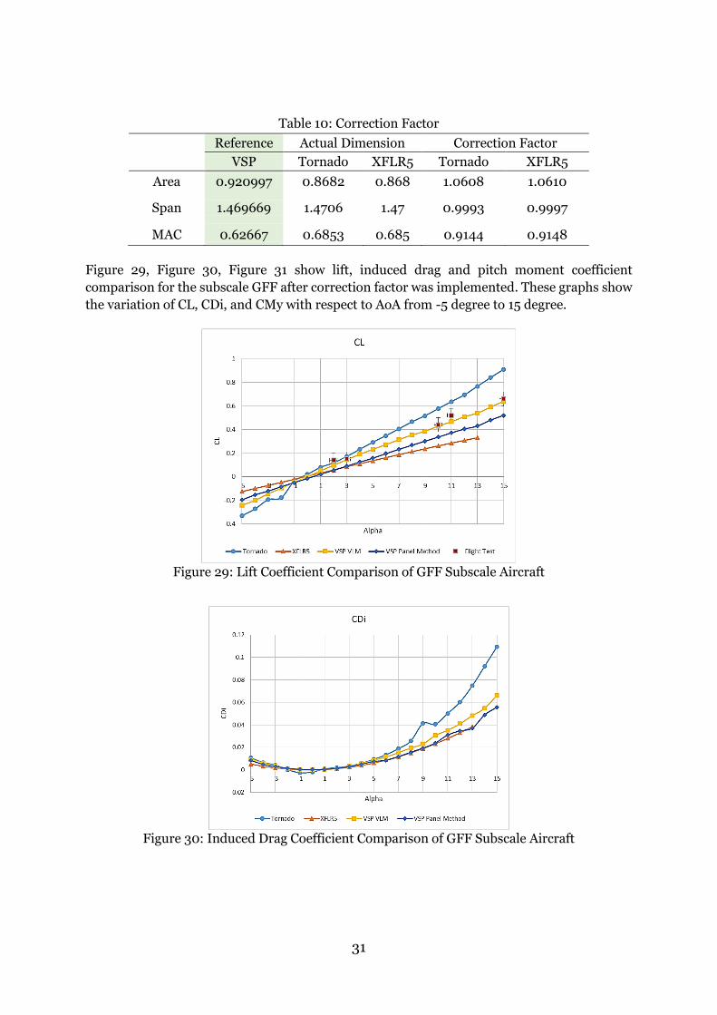
Table 10: Correction Factor ....................................................................................................... 31

Table 11: Control surface coefficients ....................................................................................... 34

Table 12: List of Implemented Derivatives .............................................................................. 35

Table 13: Comparison of RMS between version 1.0 and version 2.0 ....................................... 36

1

Chapter 1

Introduction

Aircraft design can be divided into three major phases: conceptual, preliminary and detail

design [1]. This thesis belongs to the first phase, the conceptual design when the basic

questions of configuration arrangement, size and weight, and performance are answered. It

is possible that each time the latest design is analyzed, there will be a change in the weight,

size and configuration. This leads to a crucial evaluation of the systems before and after they

are physically tested. Therefore, the simulation models are used to obtain idea and knowledge

so that decision can be made in at all development stages, and early detection and correction

of design fault can be performed.

According to Fritzson [2], the main advantages of developing simulation model rather than

setting up a real world experiment are the cost and hazard risk that can be greatly reduced

and it can simulate the system that may not yet exist. In addition, the other benefits of the

simulation model are, it can provide observation of some variables that are not accessible in

the real system, and the ease to use and modify models also to change parameters and time

scale of the system. For a more comprehensive explanation about aircraft vehicle systems

modeling and simulation, the reader can refer to [3].

This thesis is a continuation work from the previous work by Öhman [4] which was the

development of modular simulation model for a subscale fighter demonstrator. The same

aircraft model is used in this thesis, the Generic Future Fighter (GFF) Figure 1, which has

been part of the MSDEMO (Methods for Scaled Demonstrator Development) project by the

FLUMES (Fluid and Mechatronic System) division at Linköping University. Aiming to add

detail feature in some modules of the previous simulation model, the final result is expected

to give more realistic behavior of the aircraft. The work performed in this thesis involved

analyzing the aerodynamic characteristic of the aircraft also test the general aircraft

performance using simulation. Furthermore, the simulation model will also further develop

by doing some improvement on aerodynamics and engine/propulsions system module.

2

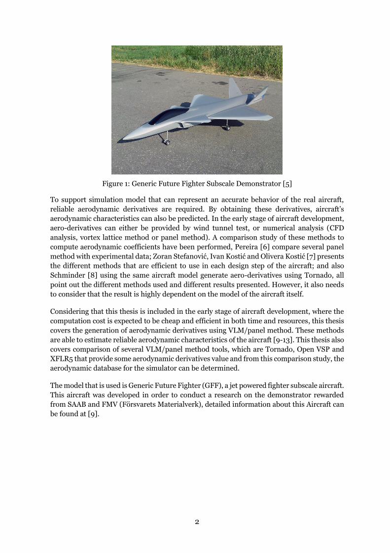
Figure 1: Generic Future Fighter Subscale Demonstrator [5]

To support simulation model that can represent an accurate behavior of the real aircraft,

reliable aerodynamic derivatives are required. By obtaining these derivatives, aircraft’s

aerodynamic characteristics can also be predicted. In the early stage of aircraft development,

aero-derivatives can either be provided by wind tunnel test, or numerical analysis (CFD

analysis, vortex lattice method or panel method). A comparison study of these methods to

compute aerodynamic coefficients have been performed, Pereira [6] compare several panel

method with experimental data; Zoran Stefanović, Ivan Kostić and Olivera Kostić [7] presents

the different methods that are efficient to use in each design step of the aircraft; and also

Schminder [8] using the same aircraft model generate aero-derivatives using Tornado, all

point out the different methods used and different results presented. However, it also needs

to consider that the result is highly dependent on the model of the aircraft itself.

Considering that this thesis is included in the early stage of aircraft development, where the

computation cost is expected to be cheap and efficient in both time and resources, this thesis

covers the generation of aerodynamic derivatives using VLM/panel method. These methods

are able to estimate reliable aerodynamic characteristics of the aircraft [9-13]. This thesis also

covers comparison of several VLM/panel method tools, which are Tornado, Open VSP and

XFLR5 that provide some aerodynamic derivatives value and from this comparison study, the

aerodynamic database for the simulator can be determined.

The model that is used is Generic Future Fighter (GFF), a jet powered fighter subscale aircraft.

This aircraft was developed in order to conduct a research on the demonstrator rewarded

from SAAB and FMV (Försvarets Materialverk), detailed information about this Aircraft can

be found at [9].

3

1.1 Objectives

The main purpose of this thesis is to refine and complete the flight mechanical model of the

subscale fighter simulator that can be approached with two steps, modeling the aerodynamics

behavior and modeling the other subsystem in the simulator. The focus in the aerodynamic

behavior analysis is to obtain numerical aerodynamic data of a subscale fighter demonstrator

using different VLM and/or panel method. The results of this study are then compared and

implemented into the flight mechanical system in the simulation model. After completing the

comparative study, the next objective is to improve flight mechanical model of the subscale

fighter demonstrator. In this case, the usability of the model will be expanded and the

complexity of the model is increased by adding some subsystems of the aircraft.

To complement the primary objectives, the following specific objectives are pursued:

a) Generate a complete aerodynamic database of the subscale demonstrator using different

panel-based tools, which are Tornado VLM, VSPAero VLM and Panel Method, XFLR5,

and present performance and stability figures.

b) Adapt the existing simulation model to make use of the external aero-database.

c) Develop an appropriate model for the propulsion system including fuel consumption and

thrust modeling.

d) Use given experimental data (system identification is not part of the task), verify

functionality against real flight data and tune the model accordingly.

1.2 Delimitations

The essential aspect of both aerodynamic database generation and flight mechanics

simulation is the flying condition of the aircraft. Due to the real flight conditions, the flight

condition in the simulator is limited in a near sea level altitude with a subsonic and

incompressible setting of the aircraft. When developing the aerodynamic database, the

geometry construction of the subscale fighter refers to CAD model [5]. Furthermore, to make

sure that the generated database is in the correct range, some experimental data are also

presented as a comparison. This experimental data was obtained from a flight test performed

in June 2016.

The simulation model also assumes that the flying condition of the aircraft is in a subsonic

setting below the stratosphere. Subsystems that are developed and improved in this thesis are

the Aerodynamic module, where the connection between aerodynamic database is applied

and the engine module with improvement in thrust and fuel consumption modeling. Some

other subsystems had also been prepared before but were not developed during the work of

this thesis, one of them is the FCS subsystems.

Since this report does not include the explanation of methodology of aircraft modeling, it is

recommended to read Öhman report [4] in order to obtain comprehensive knowledge of the

overall simulation model.

4

1.3 Methodology

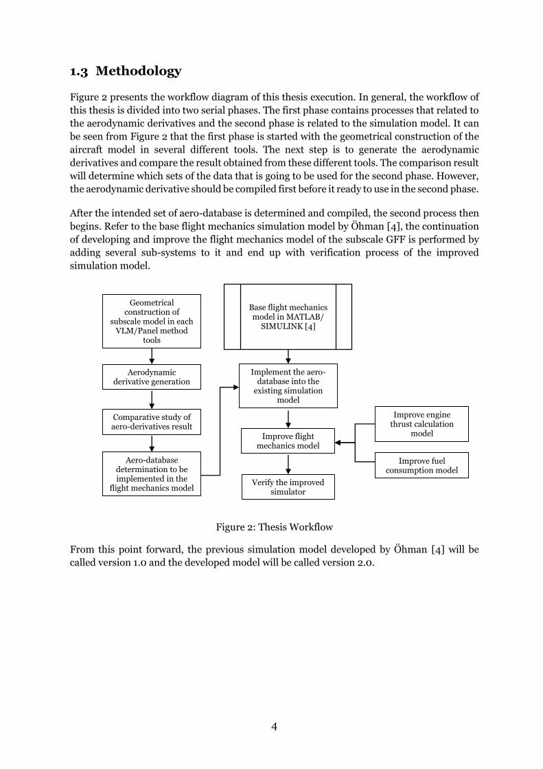
Figure 2 presents the workflow diagram of this thesis execution. In general, the workflow of

this thesis is divided into two serial phases. The first phase contains processes that related to

the aerodynamic derivatives and the second phase is related to the simulation model. It can

be seen from Figure 2 that the first phase is started with the geometrical construction of the

aircraft model in several different tools. The next step is to generate the aerodynamic

derivatives and compare the result obtained from these different tools. The comparison result

will determine which sets of the data that is going to be used for the second phase. However,

the aerodynamic derivative should be compiled first before it ready to use in the second phase.

After the intended set of aero-database is determined and compiled, the second process then

begins. Refer to the base flight mechanics simulation model by Öhman [4], the continuation

of developing and improve the flight mechanics model of the subscale GFF is performed by

adding several sub-systems to it and end up with verification process of the improved

simulation model.

Figure 2: Thesis Workflow

From this point forward, the previous simulation model developed by Öhman [4] will be

called version 1.0 and the developed model will be called version 2.0.

Geometrical construction of

subscale model in each VLM/Panel method

tools

Aerodynamic derivative generation

Comparative study of aero-derivatives result

Aero-database determination to be implemented in the

flight mechanics model

Improve flight mechanics model

Implement the aero-database into the

existing simulation model

Improve fuel consumption model

Improve engine thrust calculation

model

Verify the improved simulator

Base flight mechanics model in MATLAB/

SIMULINK [4]

5

1.4 Thesis Outline

In order to give an understanding of how the work is presented in this report, this subchapter

will explain brief explanation about how the report is constructed. This report consists of an

introduction, three main chapters and followed with the conclusions and future works

chapters. The introduction chapter contains a short explanation of the research background,

objectives, scope and methodology. The second chapter contains the explanation about the

methods that are used to solve and answer the objectives stated in the introduction chapter.

This chapter also covers the explanation of each tool/software that is used to generate

aerodynamic derivatives, include the short description of geometrical and flight setting.

Furthermore, this chapter also discusses the development of the flight mechanics model, also

the verification method used. The third chapter contains a comprehensive result of all the

work done in this thesis; neutral point position estimation, the aerodynamic database

comparison, the aircraft aerodynamic characteristics and the implementation of aero-

database into the simulation model. The fourth chapter contains a general discussion and

evaluation about the result. Finally, conclusion, recommendation and future work are

presented in the fifth and sixth chapter.

6

Chapter 2

Method

This chapter contains the explanation of the methods that is underlying the generation of the

aerodynamic database also the overview of the basic simulation model version 1.0. It begins

with a brief description about the vortex-lattice and panel method; the history, application and

advantages and drawback of these methods. Then proceed with the explanation of each tool

that is used to generate the aerodynamic derivatives, how the geometry is constructed and

flight condition setting. Panel independency study and neutral point estimation method are

also discussed here. Then the aircraft modeling methodology based on version 1.0 is discussed

at the end of this chapter, including the system development and verification process

performed in this thesis.

2.1 Vortex-Lattice and Panel Method

Both vortex-lattice and panel modeling are a numerical method used in computational fluid

dynamics which suited for aerodynamic configurations that consist mainly of thin lifting

surfaces and small angle of attack and sideslip angle. With its efficient computational cost,

these methods are suitable as computational tools in the early stage of aircraft design.

Vortex lattice methods were first formulated in the late ‘30s but only until 1943 when Falkner

published his first paper on this subject, “Vortex Lattice Method” was formalized the as the

name of this method. The basic principle of this method is to solve incompressible flows around

lifting surfaces of finite span. Each lifting surface is superimposed by the grid of horseshoe

vortices, and the velocities induced by each horseshoe vortex at a specified control point are

calculated using the Biot-Savart law. To compute the horseshoe vortex strength of the surface,

a summation is performed for all control points on the surface and this leads to a set of linear

algebraic equations which should satisfy the boundary condition of no flow through the

surface. The surface circulation and pressure difference between upper and lower surface also

related to the vortex strength. The pressure differentials are then integrated in order to obtain

the total forces and moment [10].

7

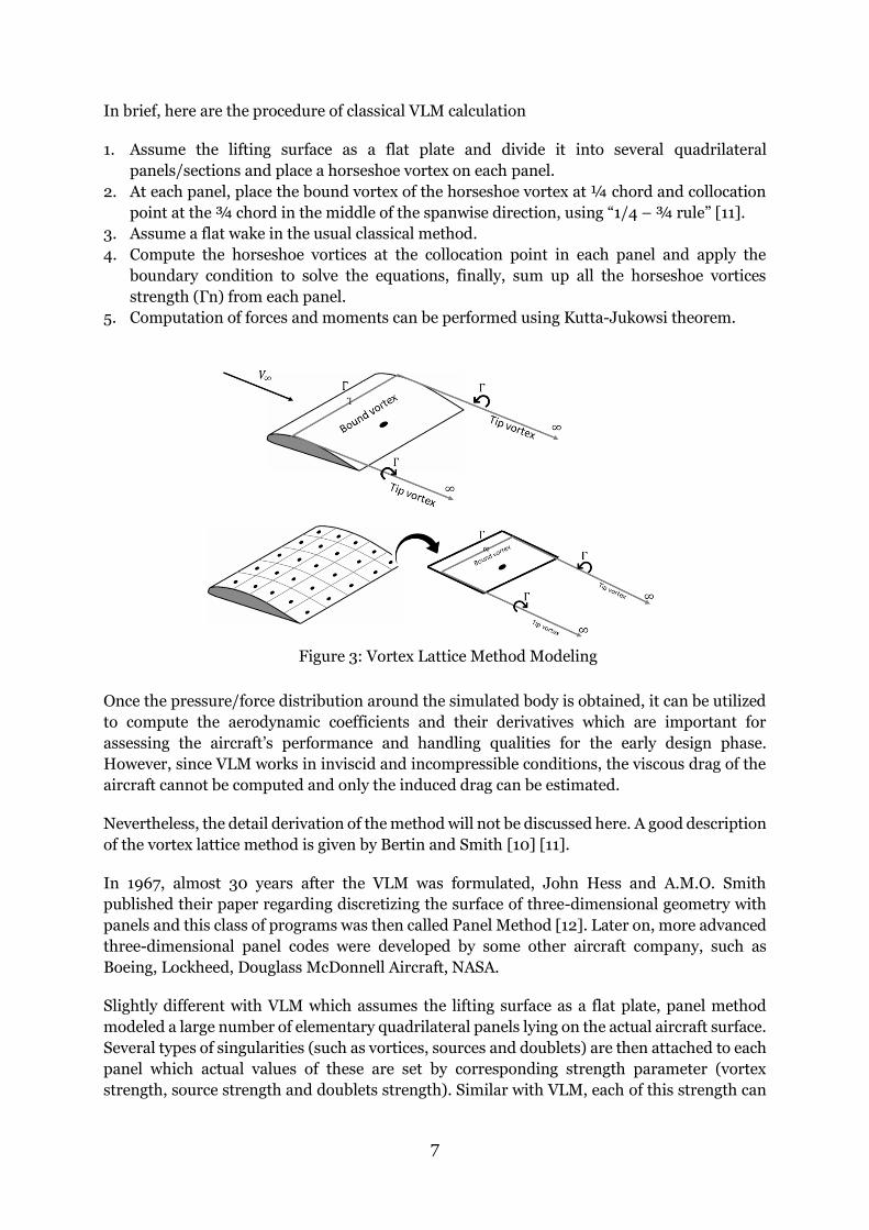
In brief, here are the procedure of classical VLM calculation

1. Assume the lifting surface as a flat plate and divide it into several quadrilateral

panels/sections and place a horseshoe vortex on each panel.

2. At each panel, place the bound vortex of the horseshoe vortex at ¼ chord and collocation

point at the ¾ chord in the middle of the spanwise direction, using “1/4 – ¾ rule” [11].

3. Assume a flat wake in the usual classical method.

4. Compute the horseshoe vortices at the collocation point in each panel and apply the

boundary condition to solve the equations, finally, sum up all the horseshoe vortices

strength (Γn) from each panel.

5. Computation of forces and moments can be performed using Kutta-Jukowsi theorem.

Figure 3: Vortex Lattice Method Modeling

Once the pressure/force distribution around the simulated body is obtained, it can be utilized

to compute the aerodynamic coefficients and their derivatives which are important for

assessing the aircraft’s performance and handling qualities for the early design phase.

However, since VLM works in inviscid and incompressible conditions, the viscous drag of the

aircraft cannot be computed and only the induced drag can be estimated.

Nevertheless, the detail derivation of the method will not be discussed here. A good description

of the vortex lattice method is given by Bertin and Smith [10] [11].

In 1967, almost 30 years after the VLM was formulated, John Hess and A.M.O. Smith

published their paper regarding discretizing the surface of three-dimensional geometry with

panels and this class of programs was then called Panel Method [12]. Later on, more advanced

three-dimensional panel codes were developed by some other aircraft company, such as

Boeing, Lockheed, Douglass McDonnell Aircraft, NASA.

Slightly different with VLM which assumes the lifting surface as a flat plate, panel method

modeled a large number of elementary quadrilateral panels lying on the actual aircraft surface.

Several types of singularities (such as vortices, sources and doublets) are then attached to each

panel which actual values of these are set by corresponding strength parameter (vortex

strength, source strength and doublets strength). Similar with VLM, each of this strength can

8

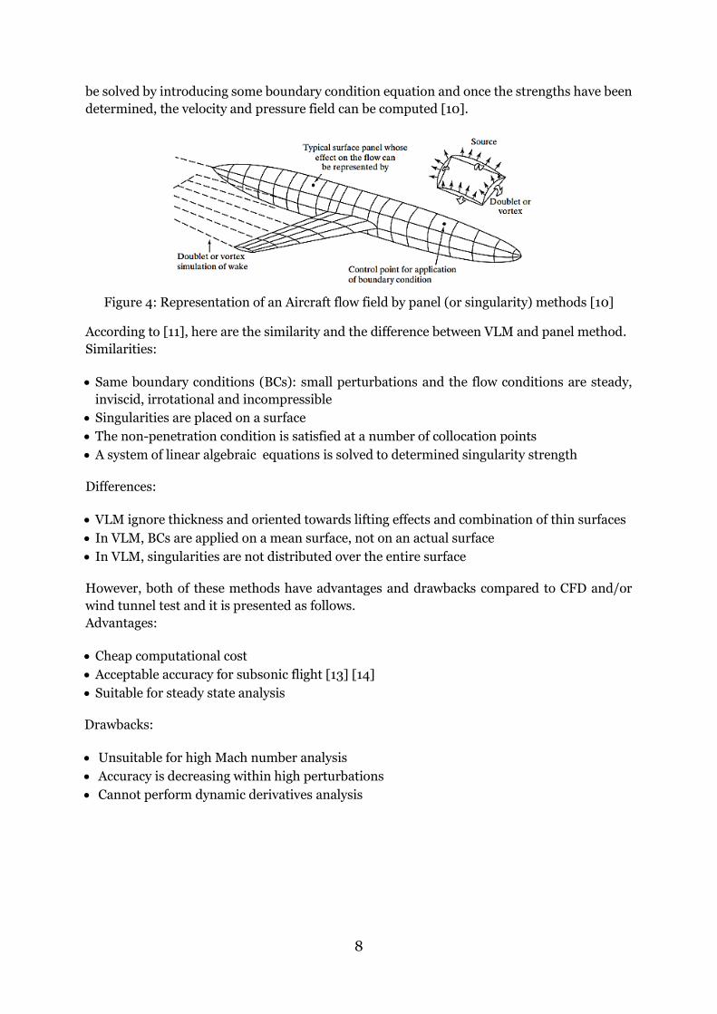
be solved by introducing some boundary condition equation and once the strengths have been

determined, the velocity and pressure field can be computed [10].

Figure 4: Representation of an Aircraft flow field by panel (or singularity) methods [10]

According to [11], here are the similarity and the difference between VLM and panel method.

Similarities:

Same boundary conditions (BCs): small perturbations and the flow conditions are steady,

inviscid, irrotational and incompressible

Singularities are placed on a surface

The non-penetration condition is satisfied at a number of collocation points

A system of linear algebraic equations is solved to determined singularity strength

Differences:

VLM ignore thickness and oriented towards lifting effects and combination of thin surfaces

In VLM, BCs are applied on a mean surface, not on an actual surface

In VLM, singularities are not distributed over the entire surface

However, both of these methods have advantages and drawbacks compared to CFD and/or

wind tunnel test and it is presented as follows.

Advantages:

Cheap computational cost

Acceptable accuracy for subsonic flight [13] [14]

Suitable for steady state analysis

Drawbacks:

Unsuitable for high Mach number analysis

Accuracy is decreasing within high perturbations

Cannot perform dynamic derivatives analysis

9

2.2 Aerodynamic Database Generation Tools

2.2.1 Vehicle Sketch Pad

Vehicle Sketch Pad (VSP) is a parametric aircraft geometry modeling tool for conceptual

aircraft design. VSP and its predecessors have been developed since the early 1990’s by J.R.

Gloudemans and others for NASA until 2012 it was released as an open source project under

NASA Open Source Agreement (NOSA) [15].

This tool has several modules to support aircraft analysis in the preliminary design phase.

Among other modules, the highlighted ones in this thesis work are OpenVSP for geometric

generation and VSPAero for aerodynamic analysis. To determine and construct the aircraft

geometry OpenVSP provides some default shape of the wing, fuselage and propeller which can

be modified following the aircraft model used. Furthermore, after the geometry is ready to

analyze, the user can use VSPAero module to mesh the aircraft model so that the analysis and

generate aerodynamic derivatives can be executed. The VSPAero module also provides two

different approaches of analysis, VLM and Panel Method, hence when one analysis types are

determined, the tools will automatically generate the aircraft mesh as can be seen in Figure 9

for Panel Method analysis and Figure 10 for VLM analysis. After the setup parameters are set,

the analysis method is determined and the aircraft mesh is generated, the numerical analysis

can be executed. Table 1 presents the list of aerodynamic derivatives that can be obtained from

VSPAero. Detail explanation of how to use VSP can be found in [16]).

Table 1: List of Aerodynamic Derivatives Obtained from VSP

CL0 CLα CLβ CLP CLQ CLR CLMach CLU

CD0 CDα CDβ CDP CDQ CDR CDMach CDU

CMl0 CMlα CMlβ CMlP CMlQ CMlR CMlMach CMlU

CMm0 CMmα CMmβ CMmP CMmQ CMmR CMmMach CMmU

CMn0 CMnα CMnβ CMnP CMnQ CMnR CMnMach CMnU

CFX0 CFXα CFXβ CFXP CFXQ CFXR CFXMach CFXU

CFY0 CFYα CFYβ CFYP CFYQ CFYR CFYMach CFYU

CFZ0 CFZα CFZβ CFZP CFZQ CFZR CFZMach CFZU

CMX0 CMXα CMXβ CMXP CMXQ CMXR CMXMach CMXU

CMY0 CMYα CMYβ CMYP CMYQ CMYR CMYMach CMYU

CMZ0 CMZα CMZβ CMZP CMZQ CMZR CMZMach CMZU

CLδcanard CDδcanard CCδcanard Clδcanard Cmδcanard Cnδcanard CXδcanard CYδcanard

CXδe CYδe CZδe Clδe Cdδe Ccδe Clδe Cmδe

CZδcanard Cnδe

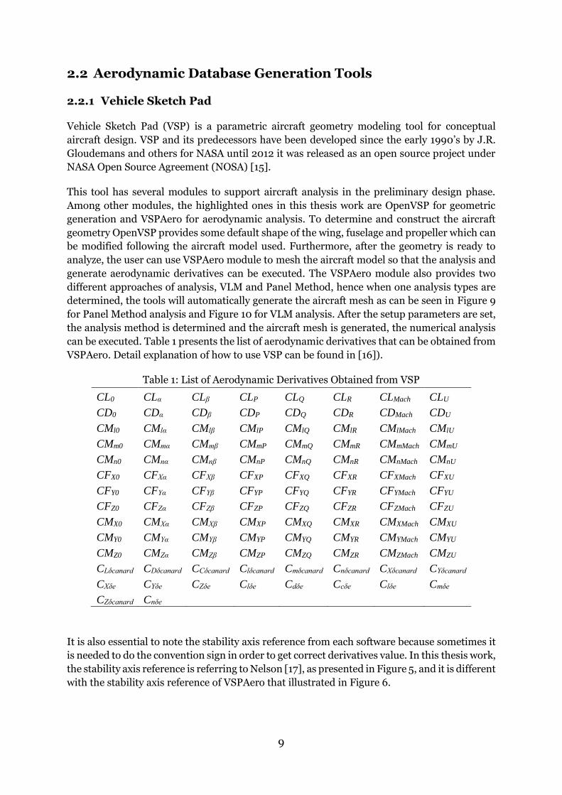
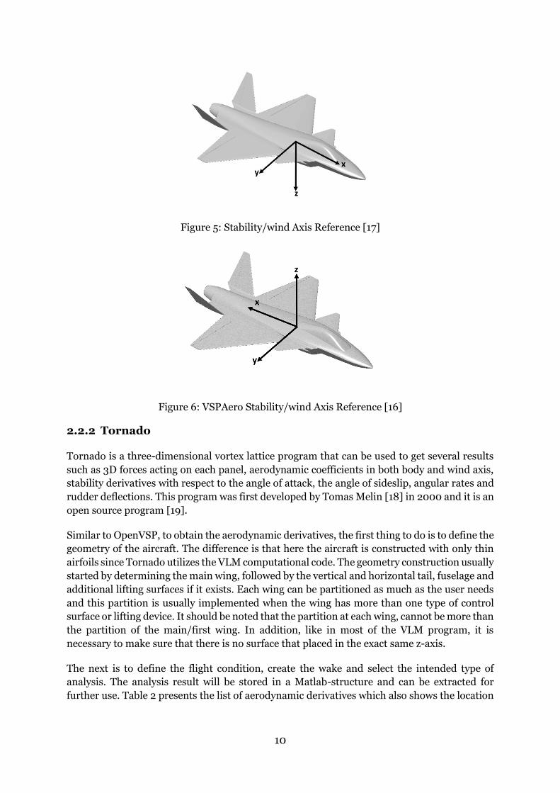
It is also essential to note the stability axis reference from each software because sometimes it

is needed to do the convention sign in order to get correct derivatives value. In this thesis work,

the stability axis reference is referring to Nelson [17], as presented in Figure 5, and it is different

with the stability axis reference of VSPAero that illustrated in Figure 6.

10

Figure 5: Stability/wind Axis Reference [17]

Figure 6: VSPAero Stability/wind Axis Reference [16]

2.2.2 Tornado

Tornado is a three-dimensional vortex lattice program that can be used to get several results

such as 3D forces acting on each panel, aerodynamic coefficients in both body and wind axis,

stability derivatives with respect to the angle of attack, the angle of sideslip, angular rates and

rudder deflections. This program was first developed by Tomas Melin [18] in 2000 and it is an

open source program [19].

Similar to OpenVSP, to obtain the aerodynamic derivatives, the first thing to do is to define the

geometry of the aircraft. The difference is that here the aircraft is constructed with only thin

airfoils since Tornado utilizes the VLM computational code. The geometry construction usually

started by determining the main wing, followed by the vertical and horizontal tail, fuselage and

additional lifting surfaces if it exists. Each wing can be partitioned as much as the user needs

and this partition is usually implemented when the wing has more than one type of control

surface or lifting device. It should be noted that the partition at each wing, cannot be more than

the partition of the main/first wing. In addition, like in most of the VLM program, it is

necessary to make sure that there is no surface that placed in the exact same z-axis.

The next is to define the flight condition, create the wake and select the intended type of

analysis. The analysis result will be stored in a Matlab-structure and can be extracted for

further use. Table 2 presents the list of aerodynamic derivatives which also shows the location

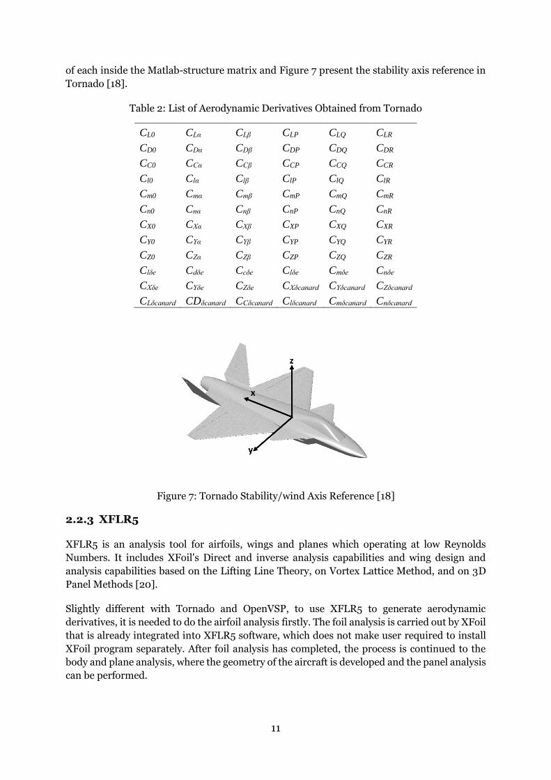
11

of each inside the Matlab-structure matrix and Figure 7 present the stability axis reference in

Tornado [18].

Table 2: List of Aerodynamic Derivatives Obtained from Tornado

CL0 CLα CLβ CLP CLQ CLR

CD0 CDα CDβ CDP CDQ CDR

CC0 CCα CCβ CCP CCQ CCR

Cl0 Clα Clβ ClP ClQ ClR

Cm0 Cmα Cmβ CmP CmQ CmR

Cn0 Cnα Cnβ CnP CnQ CnR

CX0 CXα CXβ CXP CXQ CXR

CY0 CYα CYβ CYP CYQ CYR

CZ0 CZα CZβ CZP CZQ CZR

Clδe Cdδe Ccδe Clδe Cmδe Cnδe

CXδe CYδe CZδe CXδcanard CYδcanard CZδcanard

CLδcanard CDδcanard CCδcanard Clδcanard Cmδcanard Cnδcanard

Figure 7: Tornado Stability/wind Axis Reference [18]

2.2.3 XFLR5

XFLR5 is an analysis tool for airfoils, wings and planes which operating at low Reynolds

Numbers. It includes XFoil's Direct and inverse analysis capabilities and wing design and

analysis capabilities based on the Lifting Line Theory, on Vortex Lattice Method, and on 3D

Panel Methods [20].

Slightly different with Tornado and OpenVSP, to use XFLR5 to generate aerodynamic

derivatives, it is needed to do the airfoil analysis firstly. The foil analysis is carried out by XFoil

that is already integrated into XFLR5 software, which does not make user required to install

XFoil program separately. After foil analysis has completed, the process is continued to the

body and plane analysis, where the geometry of the aircraft is developed and the panel analysis

can be performed.

12

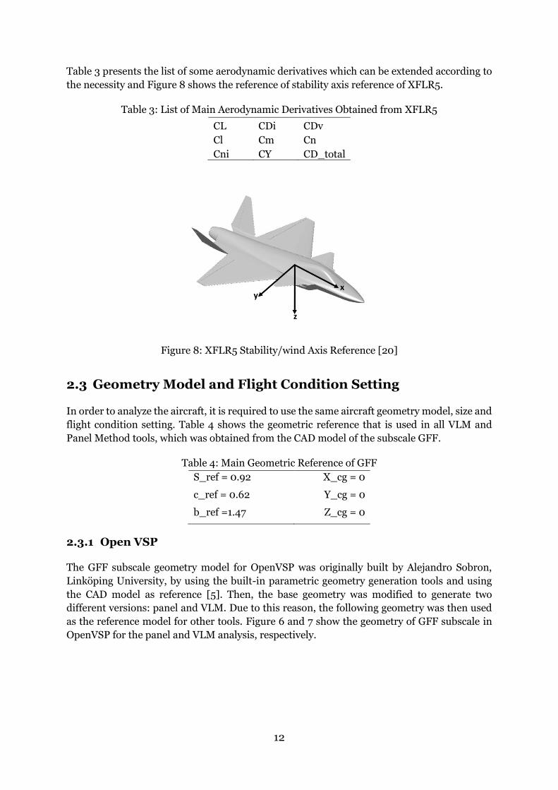
Table 3 presents the list of some aerodynamic derivatives which can be extended according to

the necessity and Figure 8 shows the reference of stability axis reference of XFLR5.

Table 3: List of Main Aerodynamic Derivatives Obtained from XFLR5

CL CDi CDv

Cl Cm Cn

Cni CY CD_total

Figure 8: XFLR5 Stability/wind Axis Reference [20]

2.3 Geometry Model and Flight Condition Setting

In order to analyze the aircraft, it is required to use the same aircraft geometry model, size and

flight condition setting. Table 4 shows the geometric reference that is used in all VLM and

Panel Method tools, which was obtained from the CAD model of the subscale GFF.

Table 4: Main Geometric Reference of GFF

S_ref = 0.92 X_cg = 0

c_ref = 0.62 Y_cg = 0

b_ref =1.47 Z_cg = 0

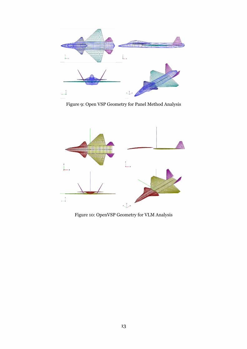
2.3.1 Open VSP

The GFF subscale geometry model for OpenVSP was originally built by Alejandro Sobron,

Linköping University, by using the built-in parametric geometry generation tools and using

the CAD model as reference [5]. Then, the base geometry was modified to generate two

different versions: panel and VLM. Due to this reason, the following geometry was then used

as the reference model for other tools. Figure 6 and 7 show the geometry of GFF subscale in

OpenVSP for the panel and VLM analysis, respectively.

13

Figure 9: Open VSP Geometry for Panel Method Analysis

Figure 10: OpenVSP Geometry for VLM Analysis

14

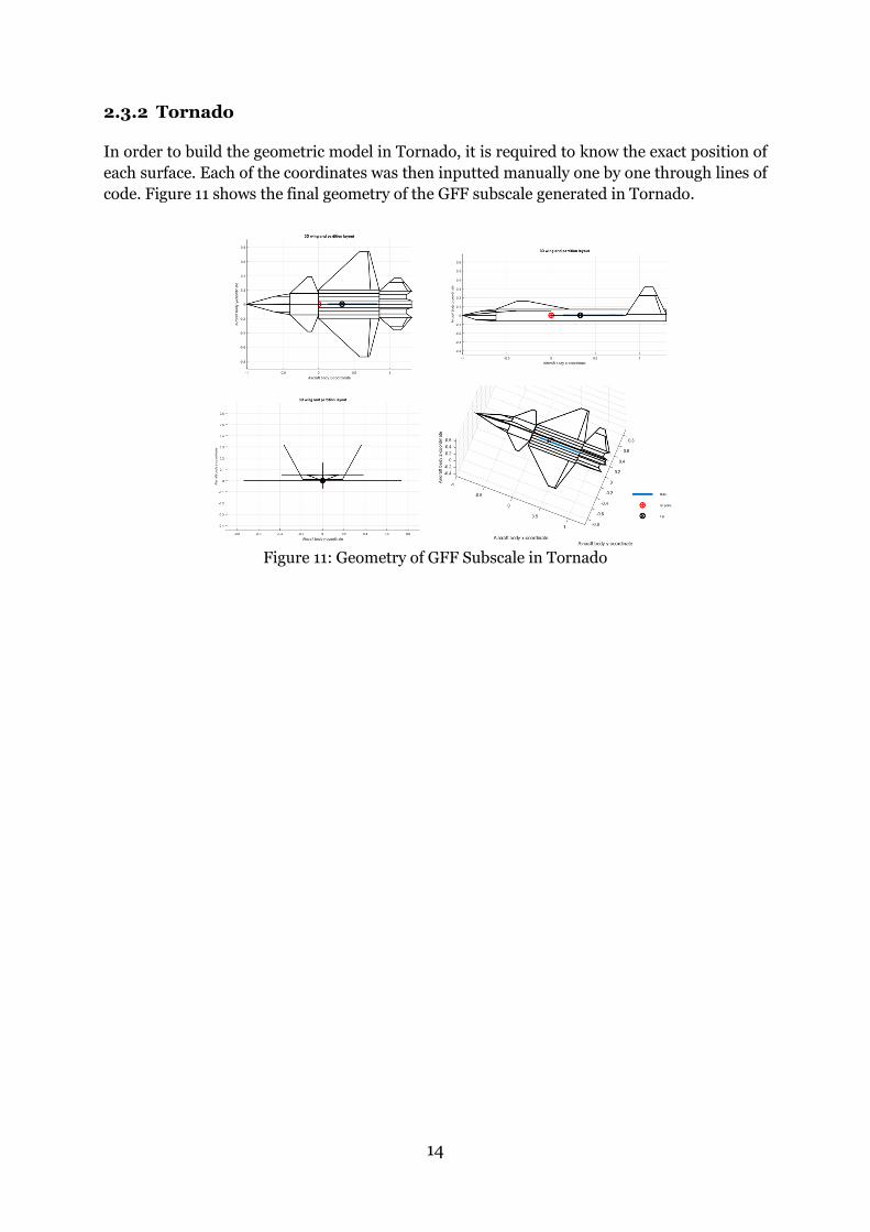
2.3.2 Tornado

In order to build the geometric model in Tornado, it is required to know the exact position of

each surface. Each of the coordinates was then inputted manually one by one through lines of

code. Figure 11 shows the final geometry of the GFF subscale generated in Tornado.

Figure 11: Geometry of GFF Subscale in Tornado

15

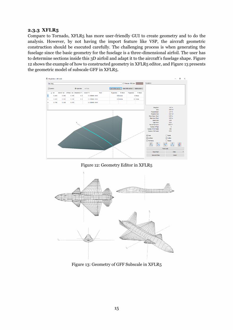
2.3.3 XFLR5 Compare to Tornado, XFLR5 has more user-friendly GUI to create geometry and to do the

analysis. However, by not having the import feature like VSP, the aircraft geometric

construction should be executed carefully. The challenging process is when generating the

fuselage since the basic geometry for the fuselage is a three-dimensional airfoil. The user has

to determine sections inside this 3D airfoil and adapt it to the aircraft’s fuselage shape. Figure

12 shows the example of how to constructed geometry in XFLR5 editor, and Figure 13 presents

the geometric model of subscale GFF in XFLR5.

Figure 12: Geometry Editor in XFLR5

Figure 13: Geometry of GFF Subscale in XFLR5

16

2.3.4 Flight Condition Setting

Similar to the geometry, the flight condition setting should be the same for all software. The

following Table 5 presents the reference of flight condition setting implemented in all VLM and

Panel method tools used.

Table 5: Flight Condition Reference

Velocity [m/s] = 40 Mach range = 0.04 – 0.2

Air density [kg/m3] = 1.2250 AoA range = -5 – 15

Reynolds number = 1.800.000 Sideslip range = 0 – 5

This flight conditions are based on the real operating flight condition of the subscale aircraft

and since—on the later subchapter—one of the validations processed is to compare the

numerical with experimental result, it is necessary to have the same flying condition between

numerical and experimental, which is a sea level, subsonic and incompressible flying

condition.

Furthermore, the limitation of AoA and sideslip angle is due to keeping the result as reliable as

possible. Another research about VLM software comparison had also been performed by

Pereira [21], he compares different software for the calculation of the aerodynamic coefficient

of several types of an aircraft wing. His result shows that within the increment of perturbation,

the accuracy of the result obtained is decreased, as can be observed from the RMS. Further

discussion about the relation between high perturbation and result’s accuracy can be found in

subchapter 4.2.

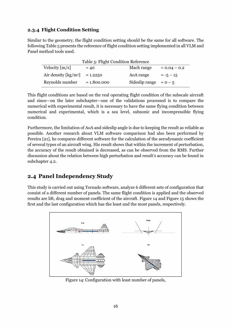
2.4 Panel Independency Study

This study is carried out using Tornado software, analyze 6 different sets of configuration that

consist of a different number of panels. The same flight condition is applied and the observed

results are lift, drag and moment coefficient of the aircraft. Figure 14 and Figure 15 shows the

first and the last configuration which has the least and the most panels, respectively.

Figure 14: Configuration with least number of panels,

17

Figure 15: Configuration with most number of panels

Table 6, Figure 15 and Figure 16 present the result of the panel independency study. It can be

seen that the standard deviation of the observed coefficients are below 0.5% making each

configuration panel independent. However, the computational time was in accordance with

the number of panels, where more number of panel making computational time more

expensive. Considering this reason, configuration number 3 was chosen as the reference

regarding a number of panels.

Table 6: Result of Panel Independency Study

Config. Number of panels

CL CD CM Computational

time [s]

#1 212 0.1634 0.003632 -0.04382 5

#2 340 0.16878 0.003732 -0.05208 18

#3 518 0.16841 0.003572 -0.05113 18

#4 1036 0.16833 0.003447 -0.05019 54

#5 1122 0.16979 0.003495 -0.04999 124

#6 1518 0.16838 0.003404 -0.0498 409 Standard Deviation

0.002247 0.000123 0.002912

Figure 16: Result of Panel Independency Study

18

2.5 Neutral Point Position

Neutral point (NP) is a reference point for which the pitching moment does not depend on the

angle of attack but only depend on the Aircraft’s external geometry. It is important to know the

position of the neutral point in order to predict the longitudinal stability behavior of the

aircraft. A longitudinally stable aircraft will have neutral point position behind the CG position

and by this means that at a high angle of attack, the aircraft will tend to decrease its AoA further

rather than increasing it. On the other hand, if the neutral point is located in front of the CG it

denotes that the aircraft is unstable in longitudinal dimension and tend to increase AoA when

the aircraft is having a high AoA.

There are several ways to estimate the neutral point position or static margin (distance between

CG and NP). One of the direct analytical equation can be found in [22], while in some software

it is provided in their analysis function. Nevertheless, even though there is no direct function

to compute NP in a software, an estimation of its location can be performed by changing the

CG position until a position where there is no change in CMy with respect to AoA.

In this thesis, all third of the method was performed; analytical calculation, static margin (SM)

computation by software function (in Tornado) and by changing CG until the “constant” CMyα

is obtained.

2.5.1 Analytical Computation

Since GFF is not conventional aircraft (with canard and V-tail), the equation for calculating NP

position was different with the aircraft that only has 2 lifting surfaces. Refer to [22], the

following formula was used to estimate the neutral point position of the subscale GFF. The area

of the tail in this computation was using the projected area of the V-tail in the horizontal

position.

�̅�𝑎𝑐𝐴=

�̅�𝑎𝑐𝑤𝑓−

𝐶𝐿𝛼𝑐

𝐶𝐿𝛼𝑤𝑓

𝜂𝑐𝑆𝑐𝑆

�̅�𝑎𝑐𝑐(1 +

𝑑𝜀𝑐𝑑𝛼

) +𝐶𝐿𝛼ℎ

𝐶𝐿𝛼𝑤𝑓

𝜂ℎ𝑆ℎ𝑆

�̅�𝑎𝑐ℎ(1 −

𝑑𝜀𝑑𝛼

)

1 +𝐶𝐿𝛼𝑐

𝐶𝐿𝛼𝑤𝑓

𝜂𝑐𝑆𝑐𝑆 (1 +

𝑑𝜀𝑐𝑑𝛼

) +𝐶𝐿𝛼ℎ

𝐶𝐿𝛼𝑤𝑓

𝜂ℎ𝑆ℎ𝑆 (1 −

𝑑𝜀𝑑𝛼

)

(1)

�̅�𝑎𝑐𝐴

: Neutral point position

�̅�𝑎𝑐 : Aerodynamic center position 𝐶𝐿𝛼 : Lift coefficient w.r.t AoA

𝜂 : Efficiency factor 𝑑𝜀/𝑑𝛼 : Downwash effect from the upstream wing

𝑆 : Wing area

Gudmundsson [23] also provide a comprehensive derivation of NP calculation for

conventional and canard aircraft. However, there is no straightforward equation that can be

used to compute NP for aircraft with three lifting surfaces. The book [23] provide the NP

analytical equations for conventional aircraft (aircraft with wing and horizontal tail

configuration) and for canard aircraft (aircraft with canard and wing lifting surfaces).

Therefore, in order to obtain the NP equation for three lifting surfaces (canard, wing and

19

horizontal tail) the following equation was derived to compute NP for subscale GFF, referring

to his book.

ℎ𝑛

𝐶𝑀𝐺𝐶=

ℎ𝐴𝐶

𝐶𝑀𝐺𝐶+

𝜂𝐻𝑇𝑆𝐻𝑇𝑙𝐻𝑇𝑆𝐶𝑀𝐺𝐶

𝐶𝑙𝛼𝐻𝑇 (1 −2𝐶𝑙𝛼𝜋𝐴𝑅

) −𝑆𝐶𝑁 𝑙𝑐𝑎𝑛𝑆𝐶𝑀𝐺𝐶

𝐶𝑙𝛼𝐶𝑎𝑛 − 𝐶𝑀𝛼𝐴𝐶

𝐶𝑙𝛼

(2)

ℎ𝑛 : Neutral point position ℎ𝐴𝐶 : Aerodynamic center position

𝐶𝑀𝐺𝐶 : Mean geometrical chord 𝑙 : Arm distance

𝐴𝑅 : Aspect ratio

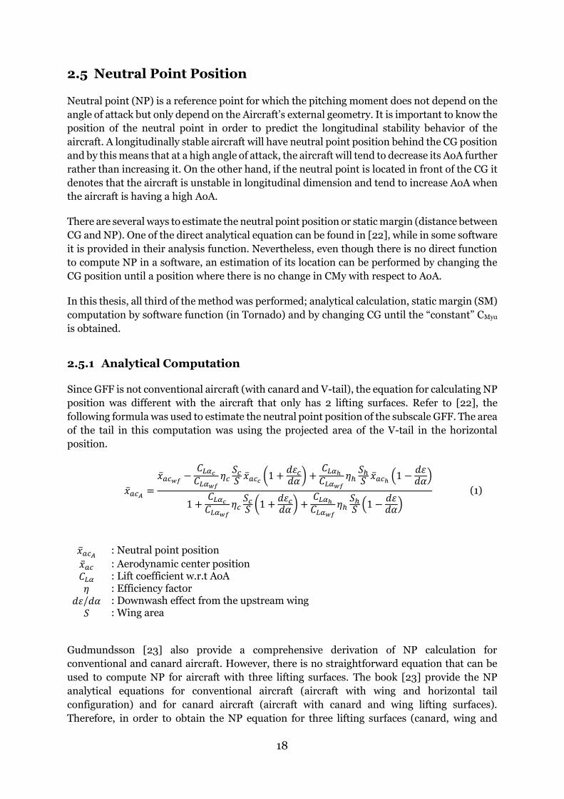
2.5.2 Neutral Point Estimation Built-in Function

Tornado software provides a built-in function of static margin computation that can be used

directly after the geometry and flight condition of the aircraft is set. Meanwhile, in VSPAero

and XFLR5, there is no direct function to calculate either static margin or neutral point

position. However, the user can still utilize this tools in order to compute the neutral point

semi-automatically by using the sweep function in these tools. By changing the c.g position of

the aircraft and monitor the moment coefficient along the Y-axis of the aircraft, the user can

define the neutral point as the position of c.g where there is no change in moment coefficient

with respect to AoA.

Figure 17: The influence of center of gravity position of longitudinal static stability

2.6 Flight Mechanics Model (Matlab/Simulink)

The work regarding the development of a simulation model performed in this thesis is a

continuation of the previous thesis by Öhman [4]. This subchapter contains discussion about

a short review of the previous simulation model, continued with its subsystem development

and ended with verification process for the simulation model.

20

2.6.1 Review of the previous work

Simulation model version 1.0 was designed to study the implemented flight control system in

order to fly a subscale demonstrator aircraft in an unstable configuration [4]. The simulation

model, created in Simulink, is able to be executed without Aerospace Blockset licensed by

Mathworks, which gives great advantages for later development. The model is general, flexible

and contains basic 6-DoF equations, it also prepared for more advanced system

implementation. However, since the model is still in early stage of development, many

subsystems still have limitations and applied some simplifications.

The subsystems that are highlighted in this thesis to be developed are the propulsion and

aerodynamics modules. In the simulation model version 1.0, the propulsion module does not

include the fuel consumption model. The fuel consumption model is controlled by applying the

power usage of the engine, a constant fuel mass flow and the recorded fuel pump data, while

the thrust model does not implement the real engine relation between the throttle and RPM

setting of the engine used (JetCat P160). Additionally, in the aerodynamic module version 1.0,

there is no connection between the external aerodynamic derivatives database with the

simulation model. All the derivatives are written in the Matlab file and only the main

aerodynamic derivatives (CFx, CFz and CMy) that are varied with AoA and velocity.

In this thesis work, the simulation model development includes the application of more

realistic computation of thrust and fuel consumption, also implementation of the external

aerodynamic derivatives database of the subscale GFF aircraft to the simulation model.

2.6.2 Improvement of Simulator Modules

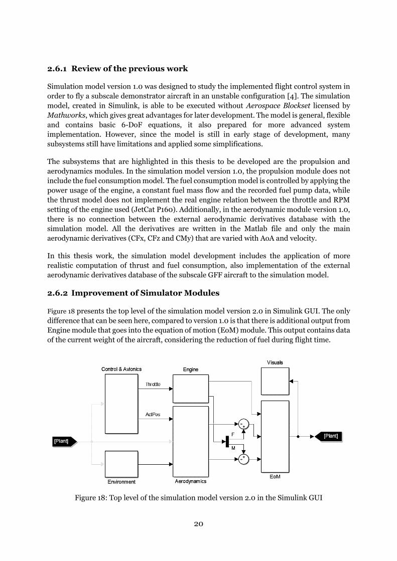
Figure 18 presents the top level of the simulation model version 2.0 in Simulink GUI. The only

difference that can be seen here, compared to version 1.0 is that there is additional output from

Engine module that goes into the equation of motion (EoM) module. This output contains data

of the current weight of the aircraft, considering the reduction of fuel during flight time.

Figure 18: Top level of the simulation model version 2.0 in the Simulink GUI

21

Engine Module

Development of the engine module includes the addition of throttle function so that the thrust

produced is more like the real engine. The equation in the function is obtained from [24] that

provide the information about engine Jetcat P160 which is the engine that is used in the

subscale GFF. The relation between thrust and RPM can be seen in Figure 19. However, the

value in the graph is obtained at standard temperature and pressure and assuming that RPM

is proportional to throttle.

Using this approach, equation (3) was obtained and the relation between engine RPM and

throttle can be simplified using equation (4). The equations were then implemented to the

thrust system as can be seen in Figure 20.

Figure 19: JetCat P160 Static Thrust [24]

𝑇ℎ𝑟𝑢𝑠𝑡 [𝑁] = (2𝐸 − 08)(𝑅𝑃𝑀)2 − 0.0012(𝑅𝑃𝑀) + 23.92 (3)

𝑅𝑃𝑀 = 𝑚𝑎𝑥 𝑅𝑃𝑀 × 𝑡ℎ𝑟𝑜𝑡𝑡𝑙𝑒 𝑜𝑝𝑝𝑒𝑛𝑖𝑛𝑔 (4)

Figure 20: Engine Model Subsystem v2.0

22

Nevertheless, this engine model subsystem is still a simplification from the reality that does

not take into account the variation of thrust with airspeed. In the reality, the turbine thrust is

coupled with airspeed which is challenging to be modeled as it also depends on the aircraft’s

inlet and duct design. Hence, in this thesis, the engine model is simplified as can be seen in

Figure 20.

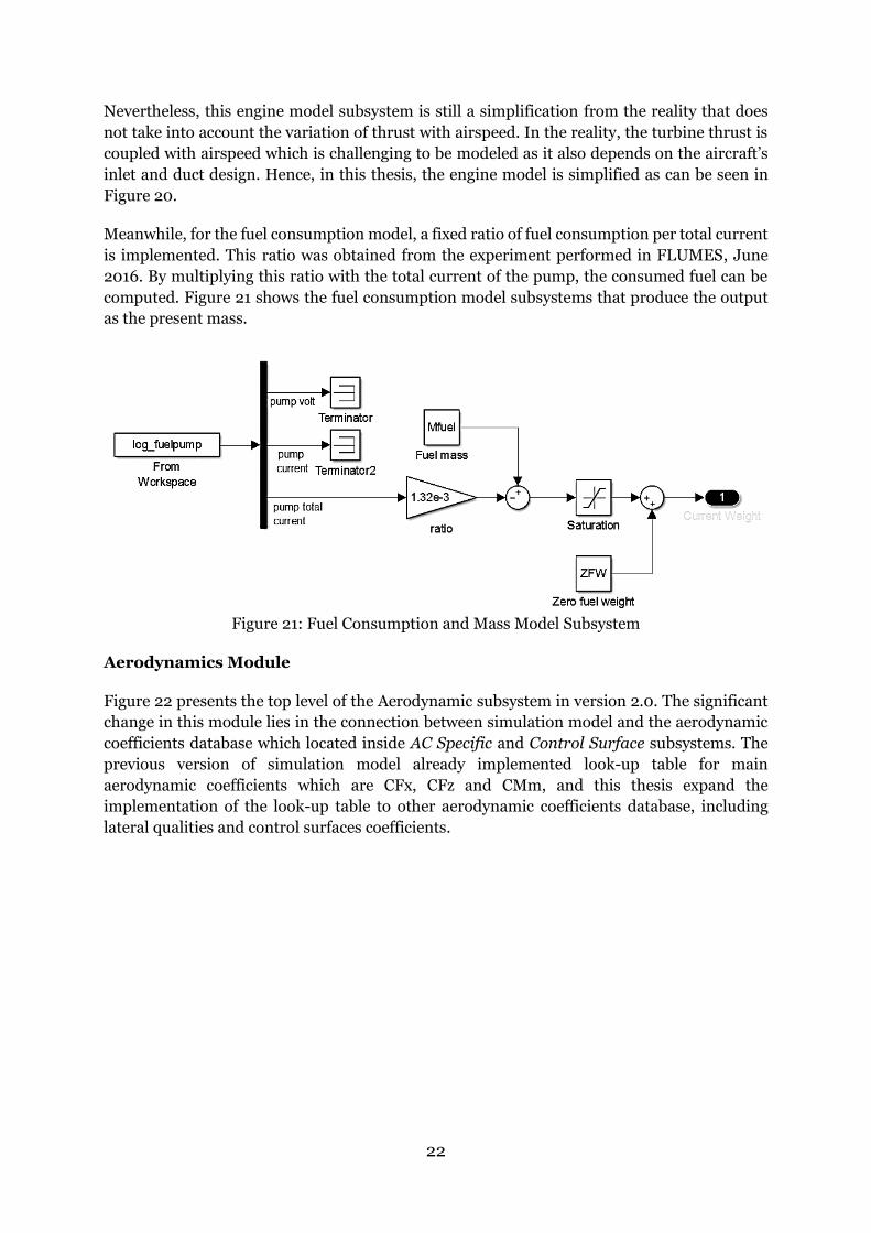
Meanwhile, for the fuel consumption model, a fixed ratio of fuel consumption per total current

is implemented. This ratio was obtained from the experiment performed in FLUMES, June

2016. By multiplying this ratio with the total current of the pump, the consumed fuel can be

computed. Figure 21 shows the fuel consumption model subsystems that produce the output

as the present mass.

Figure 21: Fuel Consumption and Mass Model Subsystem

Aerodynamics Module

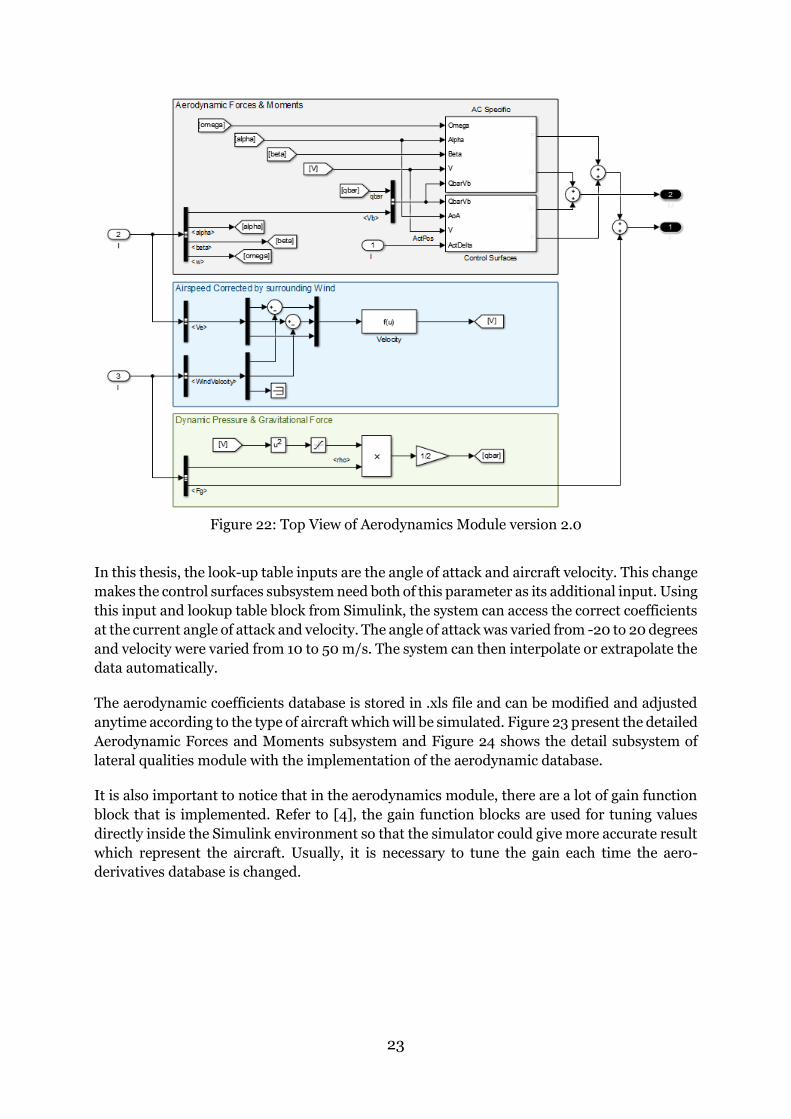
Figure 22 presents the top level of the Aerodynamic subsystem in version 2.0. The significant

change in this module lies in the connection between simulation model and the aerodynamic

coefficients database which located inside AC Specific and Control Surface subsystems. The

previous version of simulation model already implemented look-up table for main

aerodynamic coefficients which are CFx, CFz and CMm, and this thesis expand the

implementation of the look-up table to other aerodynamic coefficients database, including

lateral qualities and control surfaces coefficients.

23

Figure 22: Top View of Aerodynamics Module version 2.0

In this thesis, the look-up table inputs are the angle of attack and aircraft velocity. This change

makes the control surfaces subsystem need both of this parameter as its additional input. Using

this input and lookup table block from Simulink, the system can access the correct coefficients

at the current angle of attack and velocity. The angle of attack was varied from -20 to 20 degrees

and velocity were varied from 10 to 50 m/s. The system can then interpolate or extrapolate the

data automatically.

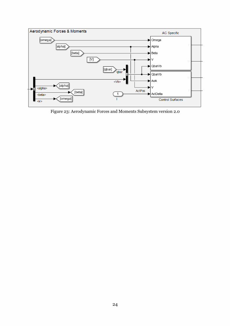
The aerodynamic coefficients database is stored in .xls file and can be modified and adjusted

anytime according to the type of aircraft which will be simulated. Figure 23 present the detailed

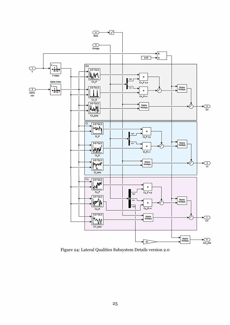
Aerodynamic Forces and Moments subsystem and Figure 24 shows the detail subsystem of

lateral qualities module with the implementation of the aerodynamic database.

It is also important to notice that in the aerodynamics module, there are a lot of gain function

block that is implemented. Refer to [4], the gain function blocks are used for tuning values

directly inside the Simulink environment so that the simulator could give more accurate result

which represent the aircraft. Usually, it is necessary to tune the gain each time the aero-

derivatives database is changed.

24

Figure 23: Aerodynamic Forces and Moments Subsystem version 2.0

25

Figure 24: Lateral Qualities Subsystem Details version 2.0

26

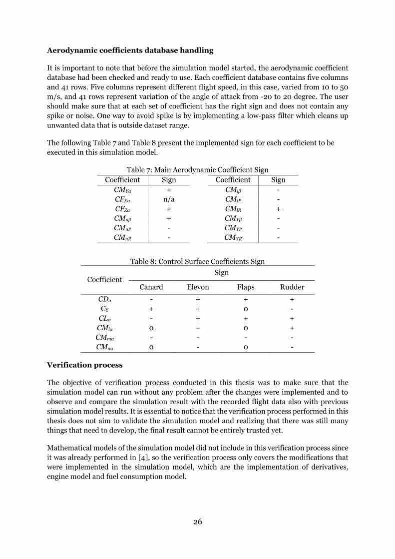
Aerodynamic coefficients database handling

It is important to note that before the simulation model started, the aerodynamic coefficient

database had been checked and ready to use. Each coefficient database contains five columns

and 41 rows. Five columns represent different flight speed, in this case, varied from 10 to 50

m/s, and 41 rows represent variation of the angle of attack from -20 to 20 degree. The user

should make sure that at each set of coefficient has the right sign and does not contain any

spike or noise. One way to avoid spike is by implementing a low-pass filter which cleans up

unwanted data that is outside dataset range.

The following Table 7 and Table 8 present the implemented sign for each coefficient to be

executed in this simulation model.

Table 7: Main Aerodynamic Coefficient Sign

Coefficient Sign Coefficient Sign

CMYα + CMlβ -

CFXα n/a CMlP -

CFZα + CMlR +

CMnβ + CMYβ -

CMnP - CMYP -

CMnR - CMYR -

Table 8: Control Surface Coefficients Sign

Coefficient Sign

Canard Elevon Flaps Rudder

CDα - + + +

CY + + 0 -

CLα - + + +

CMlα 0 + 0 +

CMmα - - - -

CMnα 0 - 0 -

Verification process

The objective of verification process conducted in this thesis was to make sure that the

simulation model can run without any problem after the changes were implemented and to

observe and compare the simulation result with the recorded flight data also with previous

simulation model results. It is essential to notice that the verification process performed in this

thesis does not aim to validate the simulation model and realizing that there was still many

things that need to develop, the final result cannot be entirely trusted yet.

Mathematical models of the simulation model did not include in this verification process since

it was already performed in [4], so the verification process only covers the modifications that

were implemented in the simulation model, which are the implementation of derivatives,

engine model and fuel consumption model.

27

In order to verify the implementation of the aerodynamic database, a comparison between the

recorded data, version 1.0 and version 2.0 simulation model result was performed by observing

the RMS between the experimental data and the simulation data for each version. The RMS

value obtained here can be used to see how much the simulation model result deviate from the

recorded results. The less the RMS value represents the better the simulation model result. The

next is to compare the RMS value between version 1.0 and version 2.0 to see which of these

version represents the better version of the simulation model. The results of verification

process can be found in subchapter 3.4.

28

Chapter 3

Results

This chapter contains result of neutral point estimation, aerodynamic derivatives generation

and comparison and the simulation model implementation. Further discussion about the

following result will be explained more in Chapter 4.

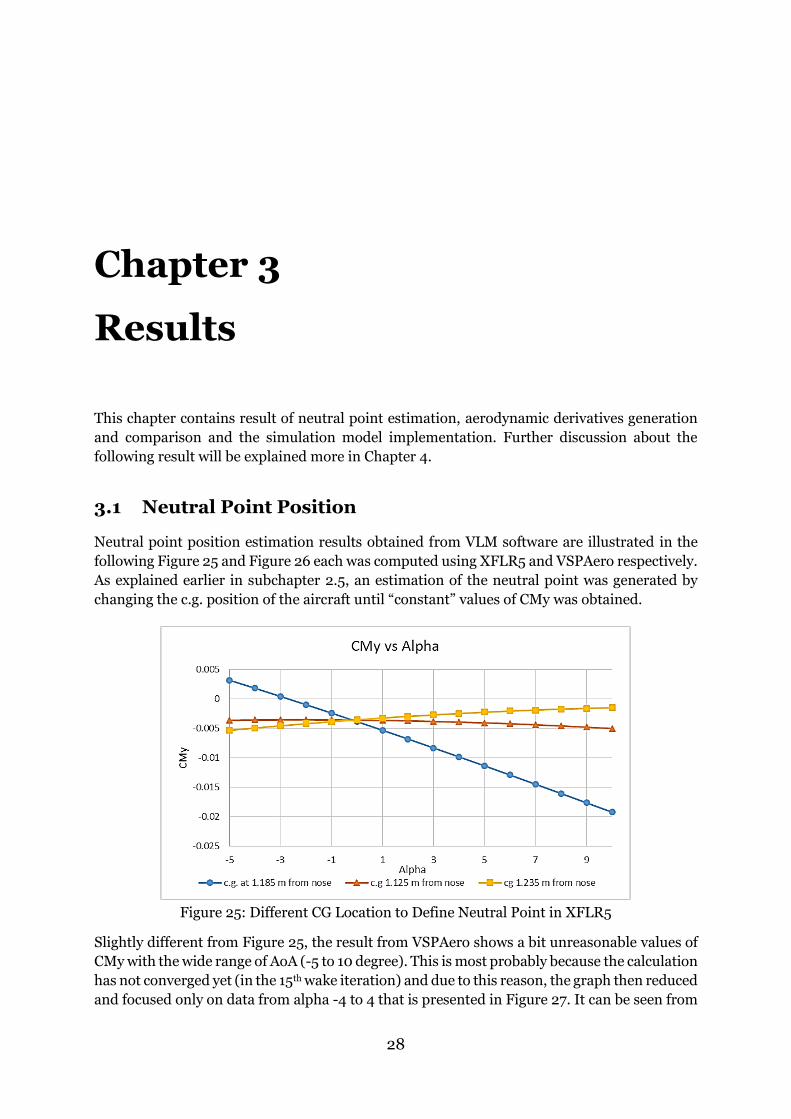
3.1 Neutral Point Position

Neutral point position estimation results obtained from VLM software are illustrated in the

following Figure 25 and Figure 26 each was computed using XFLR5 and VSPAero respectively.

As explained earlier in subchapter 2.5, an estimation of the neutral point was generated by

changing the c.g. position of the aircraft until “constant” values of CMy was obtained.

Figure 25: Different CG Location to Define Neutral Point in XFLR5

Slightly different from Figure 25, the result from VSPAero shows a bit unreasonable values of

CMy with the wide range of AoA (-5 to 10 degree). This is most probably because the calculation

has not converged yet (in the 15th wake iteration) and due to this reason, the graph then reduced

and focused only on data from alpha -4 to 4 that is presented in Figure 27. It can be seen from

29

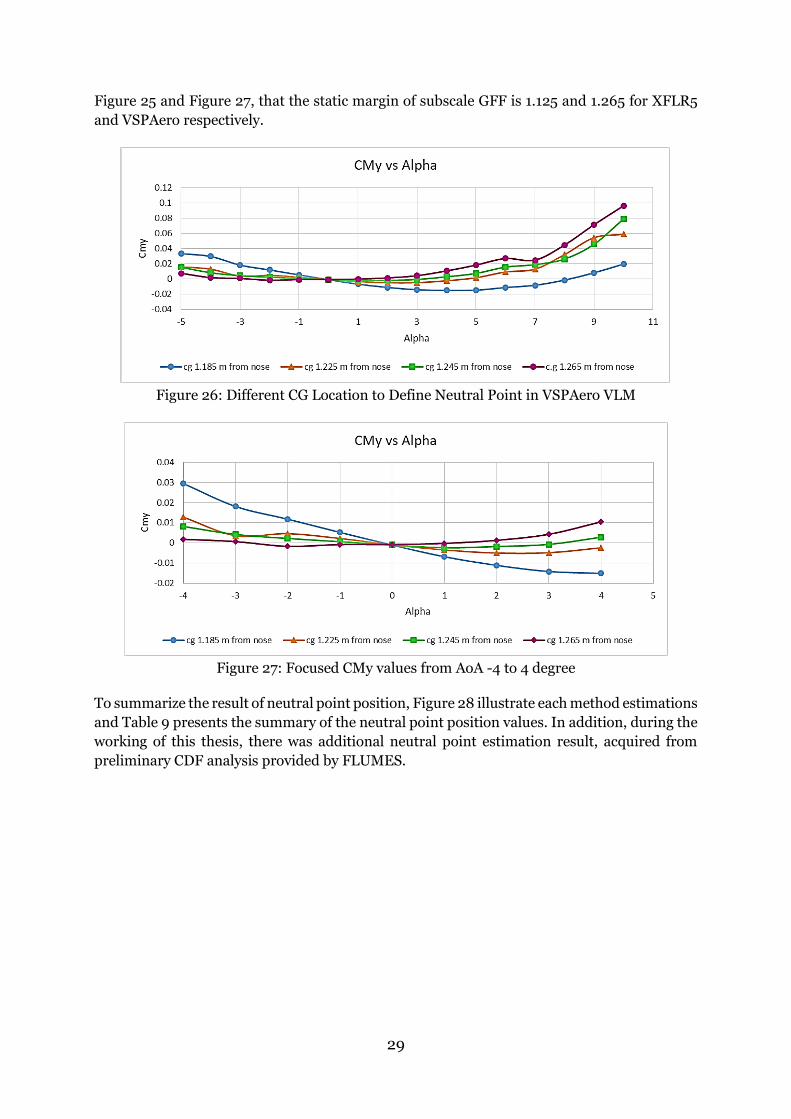
Figure 25 and Figure 27, that the static margin of subscale GFF is 1.125 and 1.265 for XFLR5

and VSPAero respectively.

Figure 26: Different CG Location to Define Neutral Point in VSPAero VLM

Figure 27: Focused CMy values from AoA -4 to 4 degree

To summarize the result of neutral point position, Figure 28 illustrate each method estimations

and Table 9 presents the summary of the neutral point position values. In addition, during the

working of this thesis, there was additional neutral point estimation result, acquired from

preliminary CDF analysis provided by FLUMES.

30

Figure 28: Neutral Point Positions Estimation from Different Methods

Table 9: Summary of Neutral Point Position Estimation

Analytic

(eq.1) Analytic

(eq.2) XFLR5 VSPAero Tornado

Preliminary CFD

NP position [m] (from nose, x-axis)

1.42 1.36 1.12 1.26 1.22 1.25

Static Margin (% of MAC)

34.2 26.2 5.8 11.6 5.3 9.9

3.2 Aero-database comparison

Before performing the result comparison between the different software, it is important to

make sure that each of the software uses the exact same geometry so that the result is valid to

compare. In fact, the exact geometry was hard to be accomplished due to the different approach

of geometry construction in each software. This leads to the needs of correction factors. These

correction factors were computed based on the reference surface and the reference length so

that the coefficients which will be compared are non-dimensional.

31

Table 10: Correction Factor

Reference Actual Dimension Correction Factor

VSP Tornado XFLR5 Tornado XFLR5

Area 0.920997 0.8682 0.868 1.0608 1.0610

Span 1.469669 1.4706 1.47 0.9993 0.9997

MAC 0.62667 0.6853 0.685 0.9144 0.9148

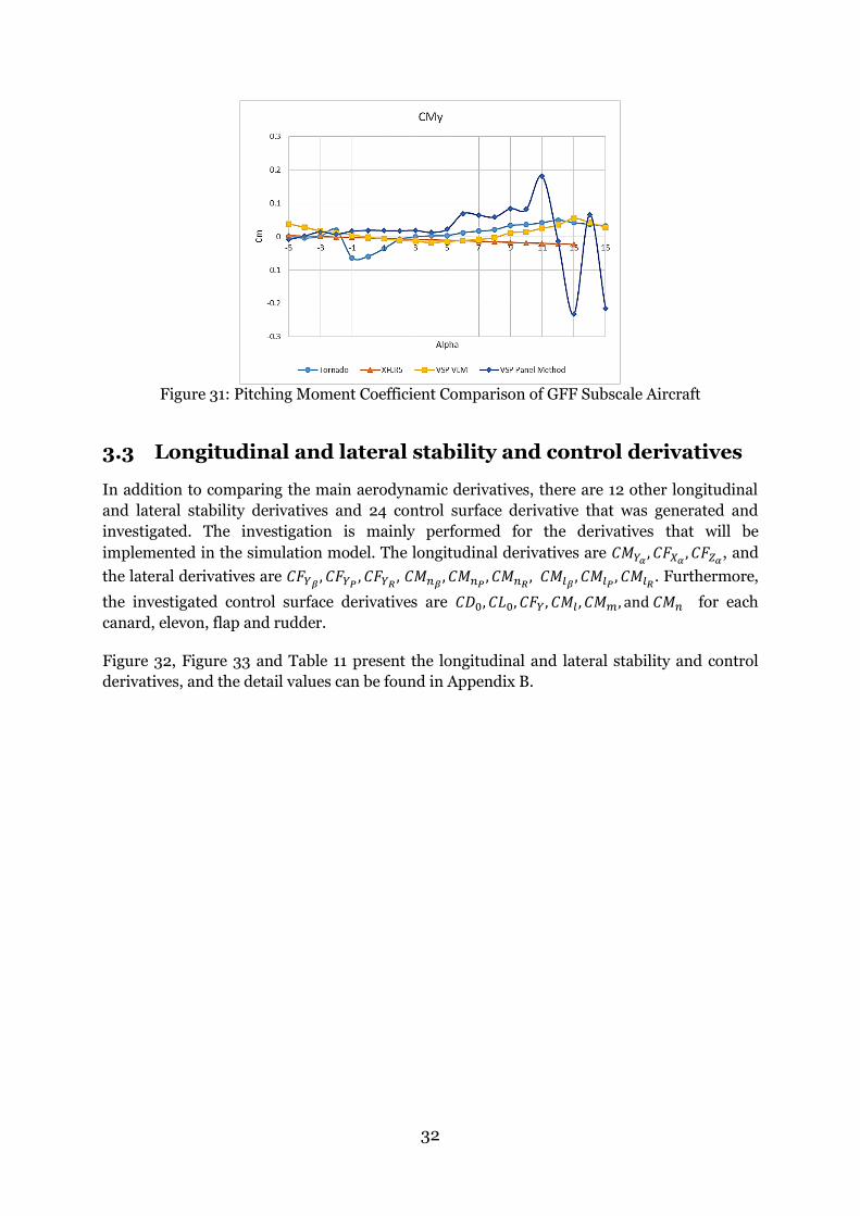
Figure 29, Figure 30, Figure 31 show lift, induced drag and pitch moment coefficient

comparison for the subscale GFF after correction factor was implemented. These graphs show

the variation of CL, CDi, and CMy with respect to AoA from -5 degree to 15 degree.

Figure 29: Lift Coefficient Comparison of GFF Subscale Aircraft

Figure 30: Induced Drag Coefficient Comparison of GFF Subscale Aircraft

32

Figure 31: Pitching Moment Coefficient Comparison of GFF Subscale Aircraft

3.3 Longitudinal and lateral stability and control derivatives

In addition to comparing the main aerodynamic derivatives, there are 12 other longitudinal

and lateral stability derivatives and 24 control surface derivative that was generated and

investigated. The investigation is mainly performed for the derivatives that will be

implemented in the simulation model. The longitudinal derivatives are 𝐶𝑀𝑌𝛼, 𝐶𝐹𝑋𝛼

, 𝐶𝐹𝑍𝛼, and

the lateral derivatives are 𝐶𝐹𝑌𝛽, 𝐶𝐹𝑌𝑃

, 𝐶𝐹𝑌𝑅, 𝐶𝑀𝑛𝛽

, 𝐶𝑀𝑛𝑃, 𝐶𝑀𝑛𝑅

, 𝐶𝑀𝑙𝛽, 𝐶𝑀𝑙𝑃

, 𝐶𝑀𝑙𝑅. Furthermore,

the investigated control surface derivatives are 𝐶𝐷0, 𝐶𝐿0, 𝐶𝐹𝑌, 𝐶𝑀𝑙 , 𝐶𝑀𝑚, and 𝐶𝑀𝑛 for each

canard, elevon, flap and rudder.

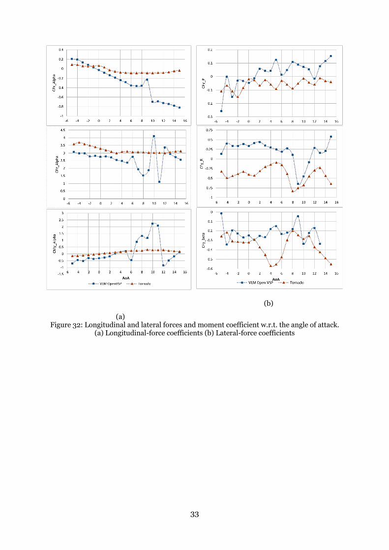
Figure 32, Figure 33 and Table 11 present the longitudinal and lateral stability and control

derivatives, and the detail values can be found in Appendix B.

33

(a)

(b)

Figure 32: Longitudinal and lateral forces and moment coefficient w.r.t. the angle of attack. (a) Longitudinal-force coefficients (b) Lateral-force coefficients

34

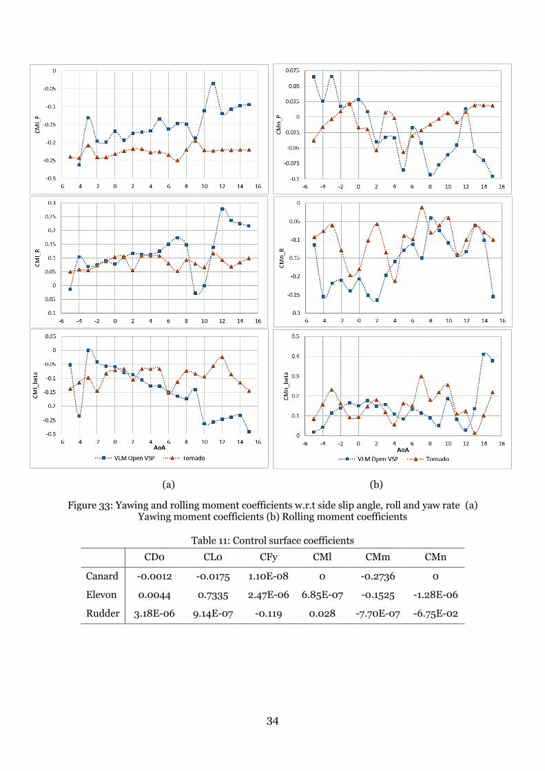
(a) (b)

Figure 33: Yawing and rolling moment coefficients w.r.t side slip angle, roll and yaw rate (a) Yawing moment coefficients (b) Rolling moment coefficients

Table 11: Control surface coefficients

CD0 CL0 CFy CMl CMm CMn

Canard -0.0012 -0.0175 1.10E-08 0 -0.2736 0

Elevon 0.0044 0.7335 2.47E-06 6.85E-07 -0.1525 -1.28E-06

Rudder 3.18E-06 9.14E-07 -0.119 0.028 -7.70E-07 -6.75E-02

35

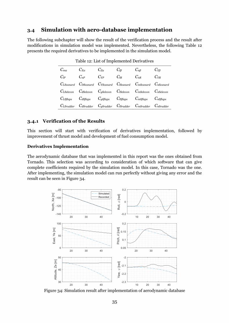
3.4 Simulation with aero-database implementation

The following subchapter will show the result of the verification process and the result after

modifications in simulation model was implemented. Nevertheless, the following Table 12

presents the required derivatives to be implemented in the simulation model.

Table 12: List of Implemented Derivatives

Cmα CXα CZα Clβ Cnβ CYβ

ClP CnP CYP ClR CnR CYR

CLδcanard CDδcanard CYδcanard Clδcanard Cmδcanard Cnδcanard

CLδelevon Cdδelevon Cyδelevon Clδelevon Cmδelevon Cnδelevon

CLδflaps Cdδflaps Cyδflaps Clδflaps Cmδflaps Cnδflaps

CLδrudder Cdδrudder Cyδrudder Clδrudder Cmδrudder Cnδrudder

3.4.1 Verification of the Results

This section will start with verification of derivatives implementation, followed by

improvement of thrust model and development of fuel consumption model.

Derivatives Implementation

The aerodynamic database that was implemented in this report was the ones obtained from

Tornado. This selection was according to consideration of which software that can give

complete coefficients required by the simulation model. In this case, Tornado was the one.

After implementing, the simulation model can run perfectly without giving any error and the

result can be seen in Figure 34.

Figure 34: Simulation result after implementation of aerodynamic database

36

Furthermore, as already mentioned in subchapter 2.6.2 regarding verification process, the

verification of derivatives implementation is carried out by comparing the RMS. Table 13

shows the result of RMS for each version that uses three study cases.

Table 13: Comparison of RMS between version 1.0 and version 2.0

Observed Parameter

Test Case 1 Test Case 2 Test Case 3

v1.0 v2.0 v1.0 v2.0 v1.0 v2.0

Roll 0.0735 0.0337 0.2048 0.1990 0.1063 0.1728

Pitch 0.3338 0.1108 0.1770 0.1605 0.2484 0.2253

Yaw 0.0415 0.0673 0.0664 0.1370 0.0863 0.2483

North 5.3898 0.7116 17.6518 29.8498 96.9239 110.4085

East 17.7499 28.4478 20.2699 47.9915 87.0371 103.7820

Altitude 4.4699 5.9239 2.6147 18.5151 5.3937 8.7306 It can be seen from Table 13 that the result of simulation model highly depends on the test case

used. By observing test case 1 result, the RMSE value of version 2.0 is better in the roll, pitch

and north coordinate position parameters. Meanwhile in the second case, only roll and pitch

parameters that are better that v1.0 and for the third case only pitch parameter that is better

from version 1.0 respectively.

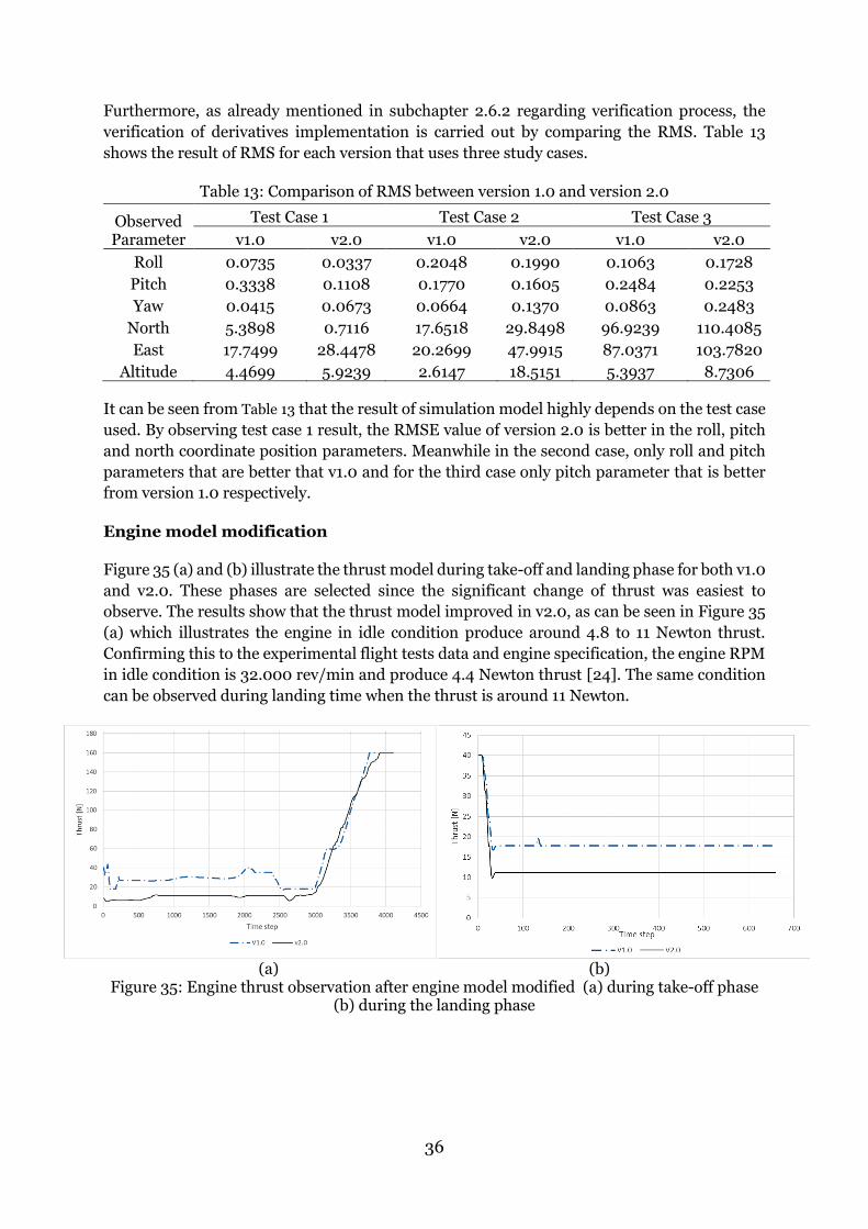
Engine model modification

Figure 35 (a) and (b) illustrate the thrust model during take-off and landing phase for both v1.0

and v2.0. These phases are selected since the significant change of thrust was easiest to

observe. The results show that the thrust model improved in v2.0, as can be seen in Figure 35

(a) which illustrates the engine in idle condition produce around 4.8 to 11 Newton thrust.

Confirming this to the experimental flight tests data and engine specification, the engine RPM

in idle condition is 32.000 rev/min and produce 4.4 Newton thrust [24]. The same condition

can be observed during landing time when the thrust is around 11 Newton.

(a) (b)

Figure 35: Engine thrust observation after engine model modified (a) during take-off phase (b) during the landing phase

37

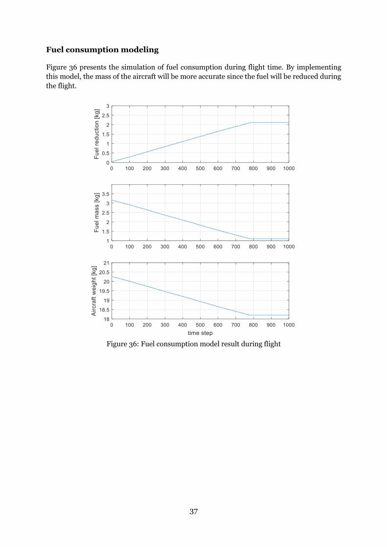
Fuel consumption modeling

Figure 36 presents the simulation of fuel consumption during flight time. By implementing

this model, the mass of the aircraft will be more accurate since the fuel will be reduced during

the flight.

Figure 36: Fuel consumption model result during flight

38

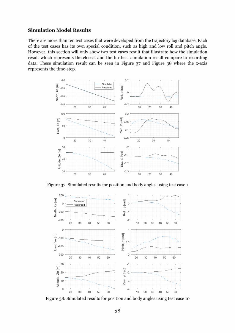
Simulation Model Results

There are more than ten test cases that were developed from the trajectory log database. Each

of the test cases has its own special condition, such as high and low roll and pitch angle.

However, this section will only show two test cases result that illustrate how the simulation

result which represents the closest and the furthest simulation result compare to recording

data. These simulation result can be seen in Figure 37 and Figure 38 where the x-axis

represents the time-step.

Figure 37: Simulated results for position and body angles using test case 1

Figure 38: Simulated results for position and body angles using test case 10

39

Chapter 4

Discussion

The first part of this chapter will deliberate the neutral point estimation, followed by

aerodynamic database comparison that is obtained from different codes. The third section

highlighted the aerodynamic characteristic of subscale GFF according to its derivatives and the

last section contains discussion about simulation model results after modifications performed.

4.1 Neutral Point Estimation

Neutral point position of the subscale GFF subscale model was approached by six methods and

all of the methods giving positive static margin. Positive static margin indicates the neutral

point position of the aircraft is behind the c.g. position, which signifies the subscale GFF

aircraft is statically stable in the longitudinal dimension.

The computation revealed that the furthest neutral point estimation was the one obtained from

the analytical computation (Eq. 1 and Eq. 2), which has 26.23% and 34.27% SM of MAC. The

main reason for this difference is because it was computed by manually and assume some

parameters value at the AoA 0. These parameters value which was assumed in the calculation

could give a great error of the computation, such as the downwash effect from the upstream

wing, the projected area of the tail, or the efficiency factor of canard horizontal tail.

Meanwhile, the nearest one was from Tornado analysis result, 1.22 m from the nose (static

margin of 5.34%), which also positioned behind of c.g. The preliminary CFD analysis outcome

was expected to give positive value since another five methods also give positive static margins.

However, since the preliminary analysis of CFD was beyond the scope of this study, the result

mentioned here was used only as a reference and comparison. The preliminary CFD result of

NP position can also be utilized as a reference of the computational accuracy of the neutral

point estimation by other methods.

As can be seen in Figure 28, the computation result from VSPAero, XFLR5 and Tornado are

the closest to the preliminary CFD result. This proximity of the preliminary CFD analysis and

the software computation of NP give confidence that the neutral point computation as

explained in subchapter 2.5.2 are satisfactory.

40

Furthermore, it is also interesting to discuss the difference in the shape of CMy that presented

in Figure 25 and Figure 26. These figures show that using different tools, the shape of the CMy

produced was also different. The most probable cause of this discrepancies is because the

different method that is used in each software. In VSPAero NP analysis was conducted using

VLM that has some shortcomings—which will be explained in the next subchapter—which

could cause the non-linear result in the computation of CMy. Meanwhile, in the XFLR5, the

computation of NP was performed using Panel Method that gives more linear computational

result of CMy than VSPAero.

To summarize, these outcomes can give estimation range of subscale GFF static margin, which

is between 5.34% and 34.2% of the mean aerodynamic chord. This large variation of NP

position is quite unpredictable since NP position estimation are basically depended only on the

geometry of the aircraft. For the preliminary CFD analysis and Tornado, it can be said that

these methods are the easiest ones to be used since all of the computations were carried out

automatically by the software. However, for VSPAero and XFLR5 the chance of having an error

or inaccurate result is higher because the NP estimation was performed semi-automatically.

Based on the explanation in the subchapter 2.5.2, the NP position can be estimated by changing

the c.g. position until the “constant” CMy w.r.t. AoA is obtained, while when the estimation

was performed semi-automatically, the variation of the c.g. position might not be carried out

thoroughly as the change of c.g. could be too large or the variations are too few. So it could be

said that the amount of human error in the estimation of NP position is the biggest weakness

for the semi-automatic and analytical methods.

4.2 Aerodynamic Database Comparison

Prior discussion about the comparison of aerodynamic derivatives obtained from several

methods, it is necessary to highlight some consequences of using VLM and panel method

rather than CFD. Refer to Subchapter 2.1, where the advantages and drawbacks of VLM and

panel method are discussed, the most significant consequence that needs to be noticed is that

the aerodynamic derivatives at high perturbation are not reliable. In addition, because

unsteady aerodynamic effects were neglected, no partial derivatives with respect to �̇� were

calculated thus the analysis should be carried out separately, either using manual computation

or using CFD analysis, since nor VLM and panel method unable to predict it.

Nevertheless, comparing the advantages and drawbacks, VLM and panel method have more

advantages and more suitable for analyzing the characteristics of subscale GFF in this phase of

aircraft development. The main consideration is the computational cost that is greatly cheaper

than CFD, aerodynamic derivatives can be generated in minutes by VLM and in hours by panel

method. Furthermore, the results obtained are acceptable since the analyzed aircraft is flying

in the subsonic region and near sea level where the flow conditions are assumed to be inviscid,

irrotational and incompressible.

The comparison of the aerodynamic database only uses three main aerodynamic coefficients

(CL, CDi and CMy) as presented in Figure 29, Figure 30 and Figure 31. The reason behind the

selection of these coefficients is because these three coefficients are the most frequently used

in another area in aircraft design process and they can give a general idea of the aircraft’s

aerodynamic characteristics. While the other stability derivatives are usually utilized

specifically for the flight dynamics and performance area.

41

Figure 29 indicate lift coefficients from four different methods plus one additional data from

flight test result. It can be observed that Tornado give overestimated result, which is in contrast

with the result from XFLR5 that gives the lowest lift coefficient value. This figure also shows

the anticipated resemblance between the same types of analysis, as can be seen, that the result

from VLM method is closer to result from Tornado, while the Panel method result from XFLR5

is closer to Panel method of VSPAero. In addition, when comparing these results with the flight

experimental data, the graph shows that the result from VLM VSPAero is the closest one to it.

Having almost the same tendency with lift coefficient, the induced drag coefficient illustrated

in Figure 30 shows that the result from four method is in a good agreement from -5 to 5 degree

of AoA. When the AoA is higher than 5 degrees, the results become branch off following the lift

coefficient trend, where Tornado give the highest drag coefficient along the increment of AoA,

XFLR5 gives the lowest result and both VLM and Panel method from VSPAero in between

these two.

Contrary to lift and drag coefficient, the moment coefficient of subscale GFF is more

unpredictable as shown in Figure 31. Panel method of VSPAero gives a high fluctuation at AoA

higher than 5 degree, which is below expectation. This phenomenon is most probably caused

by the computation that was hard to converge at high AoA for CMy in VSPAero panel method.

According to the user guide of VSPAero [15], there are some factors that might be the reason

of why this phenomenon could happen, namely the basic geometry of the model and how the

geometry is constructed in the OpenVSP. It is stated in [15] that only simplified VSP model

that will work perfectly in VSPAero. In this case, the basic geometry of subscale GFF is already

complex, with three lifting surfaces, delta wing, and Pelikan-tail, this can be one of the reasons

that the computation of CMy did not converge. The other thing is that VSPAero is very sensitive

in terms of intersection between components, a slight improperly intersected components can

lead to a major computational error, and thus the geometry construction in the OpenVSP

should be performed very carefully in order to avoid the computational error. However, this is

already anticipated before as explained in subchapter 2.1 about advantages and drawback of

panel methods.

Moreover, Tornado also gives an anomalous result, where the gradient of the moment

coefficient is positive while it was expected to be negative. On the other hand, the result from

XFLR5 is the most reasonable result, followed by VLM VSPAero’s result.

When it comes to determining which method is the best, the answer will depend on what kind

of outcome that the user want: if they want a complete aerodynamic and stability derivatives

Tornado and VLM VSPAero are the better choices, but if they want high accuracy then XFLR5

or Panel method VSPAero probably the best choice. In addition, it is worthwhile to always

consider the advantages and drawback of these methods compare to CFD or other physical

experiments.

4.3 Aerodynamic Characteristics

The characteristics of an aircraft can be observed from its aerodynamic derivatives with respect

to change in AoA, velocity and environment conditions. The first thing to be highlighted here

is the main aerodynamic characteristic which can be observed through lift and drag coefficient

or force coefficient in z and x aircraft body axis. It is crucial to understand that the coefficients

42

generated through VLM based only on the geometry of the model. For example, the GFF

aircraft has delta wing configuration, which is advantageous in a high AoA since there will be

additional lift coefficient due to the vortex effect. This effect is not considered either in VLM or

Panel method. However, for different aircraft with different wing shape and configuration,

these methods might give a more appropriate result.

The analysis results of these methods cannot be separated from the Reynolds number effect. It

is a fundamental quantity for the aerodynamics field also as a scaling factor for all aerodynamic

calculations. Since the main object of this study is a subscale aircraft, the small size leads to a

low Reynolds number. Even though the process for analyzing and estimating the aerodynamic

characteristics in low Reynolds number aircraft is similar to that on a large scale aircraft, the

results are significantly different [25]. Study about the characteristic of the flow over an airfoil

at low Reynolds number, carried out by Derksen, Agelinchaab and Tachie [26], reveal that at

low Reynolds numbers, the airfoil’s characteristics will be unsteady, with fluctuation in the lift,

drag and pitching moment. This study confirmed that the low Reynolds number is also one of

the factors that make the aerodynamic derivatives of subscale GFF fluctuates and hard to

estimate.

Another significant thing to notice is that the result of the aerodynamic derivatives generated

by all utilized software gives exactly the same outcome for variation of velocity. This occurrence

is undoubtedly due to the difference of 10 m/s in velocity variation does not give significant

effect to the final computation of derivatives.

Drag coefficient, in addition, also only consider the induced drag of the aircraft, without taking

into account the viscous since one of the assumptions of VLM and Panel method is having

inviscid flow. While for moment coefficient, other than issues discussed in the previous sub-

chapter, VLM and Panel method can predict it well enough as long as the correct inertia and

mass distribution of the aircraft are well arranged.

Lead to the subsequent analysis of lateral stability coefficient that is presented in Figure 32 and

Figure 33. These figures illustrate lateral force coefficients, yawing and moment coefficient

w.r.t. to change in sideslip angle, roll rate and yaw rate acquired from VLM OpenVSP and

Tornado software. The analysis was carried out by varying AoA from -5 to 15 degree.

Figure 33 (a) illustrates yaw moment with respect to changing in sideslip angle, roll rate and

yaw rate. It can be seen that the values of 𝐶𝑀𝑛𝛽 are positive, which indicate good stability sign

since the aircraft will yaw toward the direction of sideslip to align the longitudinal, x-axis with

the relative wind. Additionally, 𝐶𝑀𝑛𝑝 should have a negative sign to show that the induced

change in AoA on a rolling wing will produce yawing moment opposite direction of the roll.

However, from the analysis results, it shows that the 𝐶𝑀𝑛𝑝 fluctuates from positive to negative

values. Next is coefficient of yaw moment w.r.t yaw rate, or also known as yaw damping 𝐶𝑀𝑛𝑟,

negative values of this derivatives will indicate that the opposing aerodynamic damping force

will build up ahead and behind the c.g when the aircraft has a yaw rate. The study result shows

that GFF has negative values of 𝐶𝑀𝑛𝑟.

Furthermore, Figure 33 (b) presents the rolling moment coefficients w.r.t changing in sideslip

angle, roll rate and yaw rate. 𝐶𝑀𝑙𝛽 is lateral stability produced by dihedral angle, within the

negative value of this derivative denotes that the aircraft that will roll away from the direction

of sideslip. For the rolling moment due to roll rate 𝐶𝑀𝑙𝑝 (roll damping), the negative value of

43

this derivative indicate that when the aircraft rolls in response of disturbance, the resulting

change in the lift in left and right wing will produce an opposing rolling moment, hence the

aircraft will stop rolling. The last lateral derivatives that will discuss here is the rolling moment

due to yaw rate 𝐶𝑀𝑙𝑟. This derivative should have a positive value in order to give minimize the

effect of the rolling moment when the aircraft is introduced to yaw rate.

In general, it can be said that refer to this study result, the GFF subscale aircraft is statically

stable in longitudinal and lateral dimension.

Although the results of aerodynamic derivatives are not in a perfect agreement between the

VLM and Panel method software utilized here, this sets of data can give preliminary range

prediction of the required derivative values. Moreover, since this study results are intended to

utilize in the preliminary phase of aircraft design, the further analysis of the aerodynamic

should be followed by another method that can give more accurate results.

4.4 Simulation Model Implementation

The improvement that was implemented in the simulation model is proven to produce better

simulation result compare to the version one. The most fundamental thing that gives the

results more accuracy is by implementing the suitable aerodynamic derivatives. Despite the

limitation in the control surface derivatives, which was not varied with respect to AoA yet, the

simulation model still can work perfectly without any error.

Nevertheless, some of the simulation model features still need to handle with caution in order

to yield an accurate outcome. For example, it is needed to tune the gain in the aerodynamic

module if the aerodynamic derivative is altered in order to adjust simulations so that it can

represent more of the real conditions. It is also important to notice that the accuracy of the

simulation model can differ from one case to another. The primary cause of the accuracy

discrepancy is the reliability of the aerodynamic database. As explained earlier, for high AoA,

the generated derivatives are no longer reliable. Thus for some cases which include high

maneuverability, the simulation result is less reliable.

The simplification in the tail configuration also gives a significant effect on the accuracy of the

simulation model result. In this simulation model, the tail is simplified as one conventional

vertical tail with one rudder, while the GFF subscale has a Pelikan-tail configuration with two

rudders attached on each tail. However, the aerodynamic derivatives generation process was

taking into account the real configuration of the GFF subscale. It makes it clear that this

simplification contributes to the discrepancies between the simulation model results and the

recorded flight test data on the lateral-directional dimension. Although the simulation model

provides some gain blocks so that the user can tune the derivative, it takes some times to find

the correct gain values and these values should be adjusted each time new sets of derivatives

are implemented, which leads to inefficient pre-processing phase.

The implementation of new thrust modeling, on the other hand, gives more confidence to the

simulation model to produce more realistic thrust, which also leads to giving more realistic

forces and moments. Together with the development of fuel consumption system, which was

not implemented in version 1.0, the equation of motion of the aircraft will become more

realistic since the mass of the aircraft will change accordingly.

44

Chapter 5

Conclusions

The complete aerodynamic database of the subscale demonstrator has been generated using

four different software, which are Tornado VLM, VSPAERO VLM, VSPAERO panel method

and XFLR5 panel method. The aerodynamic derivatives include main aerodynamic coefficients

(CL, CD and CMy) also longitudinal and lateral stability and control derivatives.

The comparison of the VLM and panel method software utilized in this study indicates that

Tornado gives an overestimated result, but also one of the software that provides a

comprehensive list of derivative that can be generated. VSPAero, on the other hand, could give

the user an option to do the analysis either by using VLM or Panel method according to the

user’s needs. Panel method of VSPAero gives a more realistic result for small perturbation, but

it takes the longest time to do the analysis among the others. The VLM of VSPAero can produce

a slightly more optimistic result compare to its panel method with a decent computational

time. Finally the XFLR5, which generated derivative that more likely similar to panel method

of VSPAERO, but with more tolerable computational time.

Moreover, these derivatives are not only useful for the simulation result but also can give a

preliminary prediction of the aerodynamic characteristic of the subscale demonstrator. The

evidence from this study implies that the subscale demonstrator is statically stable in

longitudinal and lateral dimension.

The next objective as to implement the database to the simulation model has also been carried

out. The engine thrust model as the part of propulsion module has also been improved by

implementing the new thrust function of the real engine and new fuel consumption model has

also been developed.

The verification process for the improvement of the simulation model has confirmed that the

new model can run perfectly at different time intervals and different case configuration.

Additionally, the verification process also provides comparison result between version 1.0 and

version 2.0 presented in RMS value. The comparison indicates the version 2.0 has better RMS

values in some parameters and in some cases.

45

Chapter 6

Future Work

Regarding the delimitations of the work carried out in this thesis, the following are some suggestions in order to improve the simulation model and the study about the comparison of VLM and Panel Method for the aerodynamic database generation.

• Both panel method and VLM results from VSPAero software show some heavy fluctuation

in CMy for AoA higher than 5 degree. This results can be improved by review and enhance

the geometric model of the aircraft also the software’s setting.

• In order to give a confidence overview of the accuracy level of the VLM and Panel method

software analysis results, a comparison between these results with CFD analysis or even

experimental flight data would be very useful.

• The simulation result of the lateral stability of the aircraft was still undesirable, thus it is

suggested to perform further comprehensive analysis in lateral stability derivatives with

respect to the variation of sideslip angle also analysis for the control surface derivative with

respect to the variation of AoA and sideslip angle.

• To support aerodynamic and stability characteristics of the aircraft, investigation and

implementation of the dynamic derivative to simulation model could also be beneficial.

• Since the simulation model itself still has some limitations, additional development of

simulation model as suggested in future work of previous study [4] can also be executed,

such as development in flight control system, environment system, actuator servo

parameters and so on.

46

References

[1] D. P. Raymer, Aircraft Design: A Conceptual Approach, California: AIAA, 1992.

[2] P. Fritzson, Principles of Object-Oriented Modeling and Simulation with Modelica 2.1, New York, USA: Wiley-IEEE Press, 2004.

[3] S. Steinkellner, "Aircraft Vehicle Systems Modeling and Simulation under Uncertainty," Master Thesis Report,Department IEI Linköping University, Linköping, 2011.

[4] V. Öhman, "Development and Verification of a Modular Simulation Model for a Subscale Fighter Demonstrator," Linköping University, 2016.

[5] FLUMES, GFF CAD Geometry, Linköping: Linköping University.

[6] R. Pereira, "Validation of Software for The Calculation of Aerodynamic Coefficients with A Focus on The Software Package Tornado," Linköping University, 2010.

[7] Z. Stefanovic, I. Kostic and O. Kostic, "Efficient Evaluation of Preliminary Aerodynamic Characteristics of Light Trainer Aircraft," Croatian Scientific Journal: Engineering Review Vol. 32, Issue 1, pp. 49-56, 2012.

[8] J. Schminder, "Feasibility Study of Different Methods for The Use in Aircraft Conceptual Design," Linköping University, Linköping , 2012.

[9] K. Amadori, C. Jouannet and P. Berry, "Development of a subscale flight testing platform for a generic future fighter," 27th Congress of International Council of the Aeronautical Sciences, 2010.

[10] J. Bertin and M. L. Smith, Aerodynamics for Engineers, Prentice-Hall, Inc., 2014.

[11] R. M. Cummings, W. H. M. Scott A. Morton and D. R. McDaniel, Applied Computational Aerodynamic, Cambridge University Press, 2015.

[12] J. Smith and L. Hess, "Calculation of Potential Flow about Arbitrary Three Dimensional Lifting Bodies," Douglas Aircraft Company, Long Beach California, 1972.

[13] P. Cosyn and J. Vierendeels, "Numerical Investigation of Low-Aspect-Ratio Wings," Journal of Aircraft, vol. 43 No. 3, no. May-June 2006, pp. 713-722, 2006.

[14] J. E. Lamar, "Extension of Leading-Edge-Suction Analogy to Wings with Separated," NASA TR R-428, L-9460, 1974.

[15] V. NASA, "https://software.nasa.gov/featuredsoftware/openvsp," [Online]. [Accessed 22 March 2017].

[16] V. Wiki, "http://www.openvsp.org/wiki/doku.php?id=start," [Online]. [Accessed 22 March 2017].

47

[17] R. C. Nelson, Flight Stability and Automatic Control, McGraw-Hill Book Company.

[18] T. Melin, User’s Guide Tornado 1.0, 2001.

[19] T. Melin, "A Vortex Lattice MATLAB Implementation for Linear Aerodynamic Wing Applications," Royal Institute of Technology (KTH), Stockholm, 2000.

[20] M. Drela, XFOIL User’s Guide, version 6.94, MIT Aero and Astro Department.

[21] R. L. Pereira, "Validation of Software for the Calculation of Aerodynamic Coefficients with a focus on the software Tornado," Bachelor Thesis, Linköping University, Linköping, 2010.

[22] J. Roskam, Airplane Flight Dyamics and Flight Automatic Controls Part I, DAR Coorporation, 2001.

[23] S. Gudmundsson, General aviation aircraft design: applied methods and procedures, Oxford, UK : Butterworth-Heinemann, 2014.

[24] "Ultimate Jets Kits," [Online]. Available: http://yellowaircraft.webs.com/jetcatp160sx.htm. [Accessed 17 May 2017].

[25] D. L. Shaffer and M. S. Turner, "Aerodynamic Prediction for Low Reynolds Numbers," Department of Aerospace and Mechanical Engineering, University of Notre Dame, 2010.

[26] R. W. Derksen, M. Agelinchaab and M. Tachie, "Characteristics of the flow over a NACA 0012 airfoil at low Reynolds numbers," WIT Transactions on Engineering Sciences, vol. 59, 2008.

[27] G. Picture, "http://www.cozy.simpex.com/Ch13_06.html," [Online]. [Accessed 21 March 2017].

[28] B. L. Stevens, F. L. Lewis and E. N. Johnson, Aircraft Control and Simulation, Third Edition, New Jersey: John Wiley & Sons Inc., 2016.

[29] D. Lundstöm, "Aircraft Design Automation and Subscale Testing," PhD Thesis, Linköping University, Linköping , 2012.

[30] A. Sobron, "Design and Testing of a Flight Control System for Unstable Subscale Aircraft," Master’s thesis, Linköping University, Linköping, 2015.

[31] "XFLR5," [Online]. Available: http://www.xflr5.com/xflr5.htm. [Accessed 22 03 2017].

[32] B. Litherland and K. Rieth, "VSP Aircraft Analysis User Manual," National Aeronautics and Space Administration, 2014.

[33] S. Lupo, H. Nyberg, A. Karlsson and K. and Mohseni, "Xwing – A 3D Viscous," 46th AIAA Aerospace sciences Meeting and Exhibit, no. Reno, NV, USA, 2008.

[34] K. Cunningham, J. Foster, E. A. Morelli and A. M. Murch, "Practical Application of a Subscale transport Aircraft for Flight Research in Control Upset and Failure Conditions," American Institute of Aeronautics and Astronautics, 2008.