NORTH ATLANTIC TREATY ORGANIZATION

SCIENCE AND TECHNOLOGY ORGANIZATION

AC/323(AVT-296)TP/1015 www.sto.nato.int

STO TECHNICAL REPORT TR-AVT-296-UU

Rotorcraft Flight Simulation Model Fidelity Improvement and Assessment

(Amélioration et évaluation de la fidélité des modèles de simulation du vol à voilure tournante)

Final report of NATO STO AVT-296 Research Task Group.

Published May 2021

Distribution and Availability on Back Cover

NORTH ATLANTIC TREATY ORGANIZATION

SCIENCE AND TECHNOLOGY ORGANIZATION

AC/323(AVT-296)TP/1015 www.sto.nato.int

STO TECHNICAL REPORT TR-AVT-296-UU

Rotorcraft Flight Simulation Model Fidelity Improvement and Assessment

(Amélioration et évaluation de la fidélité des modèles de simulation du vol à voilure tournante)

Final report of NATO STO AVT-296 Research Task Group.

ii STO-TR-AVT-296-UU

The NATO Science and Technology Organization

Science & Technology (S&T) in the NATO context is defined as the selective and rigorous generation and application of state-of-the-art, validated knowledge for defence and security purposes. S&T activities embrace scientific research, technology development, transition, application and field-testing, experimentation and a range of related scientific activities that include systems engineering, operational research and analysis, synthesis, integration and validation of knowledge derived through the scientific method.

In NATO, S&T is addressed using different business models, namely a collaborative business model where NATO provides a forum where NATO Nations and partner Nations elect to use their national resources to define, conduct and promote cooperative research and information exchange, and secondly an in-house delivery business model where S&T activities are conducted in a NATO dedicated executive body, having its own personnel, capabilities and infrastructure.

The mission of the NATO Science & Technology Organization (STO) is to help position the Nations’ and NATO’s S&T investments as a strategic enabler of the knowledge and technology advantage for the defence and security posture of NATO Nations and partner Nations, by conducting and promoting S&T activities that augment and leverage the capabilities and programmes of the Alliance, of the NATO Nations and the partner Nations, in support of NATO’s objectives, and contributing to NATO’s ability to enable and influence security and defence related capability development and threat mitigation in NATO Nations and partner Nations, in accordance with NATO policies.

The total spectrum of this collaborative effort is addressed by six Technical Panels who manage a wide range of scientific research activities, a Group specialising in modelling and simulation, plus a Committee dedicated to supporting the information management needs of the organization.

• AVT Applied Vehicle Technology Panel

• HFM Human Factors and Medicine Panel

• IST Information Systems Technology Panel

• NMSG NATO Modelling and Simulation Group

• SAS System Analysis and Studies Panel

• SCI Systems Concepts and Integration Panel

• SET Sensors and Electronics Technology Panel

These Panels and Group are the power-house of the collaborative model and are made up of national representatives as well as recognised world-class scientists, engineers and information specialists. In addition to providing critical technical oversight, they also provide a communication link to military users and other NATO bodies.

The scientific and technological work is carried out by Technical Teams, created under one or more of these eight bodies, for specific research activities which have a defined duration. These research activities can take a variety of forms, including Task Groups, Workshops, Symposia, Specialists’ Meetings, Lecture Series and Technical Courses.

The content of this publication has been reproduced directly from material supplied by STO or the authors.

Published May 2021

Copyright © STO/NATO 2021 All Rights Reserved

ISBN 978-92-837-2334-9

Single copies of this publication or of a part of it may be made for individual use only by those organisations or individuals in NATO Nations defined by the limitation notice printed on the front cover. The approval of the STO Information Management Systems Branch is required for more than one copy to be made or an extract included in another publication. Requests to do so should be sent to the address on the back cover.

STO-TR-AVT-296-UU iii

Table of Contents

Page

List of Figures xii

List of Tables xxii

Foreword xxv

AVT-296 Membership List xxvi

Executive Summary and Synthèse ES-1

Chapter 1 – Introduction 1-1 1.1 Objectives 1-1 1.2 Report Overview and Organisation 1-2 1.3 References 1-3

Chapter 2 – Group Overview 2-1 2.1 Partners 2-1 2.2 Summary of Activities 2-1

2.2.1 Meeting 1: University of Liverpool, Liverpool, UK 2-6 2.2.2 Meeting 2: Georgia Institute of Technology, Atlanta, USA 2-6 2.2.3 Meeting 3: DLR, Braunschweig, Germany 2-7 2.2.4 Meeting 4: National Research Council, Ottawa, Canada 2-8 2.2.5 Meeting 5: Online 2-9 2.2.6 Meeting 6: Online 2-10

Chapter 3 – Review of Recent Fidelity Assessment and Model 3-1 Update Activities 3.1 Recent Research Activities by Participating Organisations 3-1

3.1.1 US Technology Development Directorate – Ames (TDD-A) 3-1 3.1.2 University of Liverpool 3-1 3.1.3 Office National d’Études et de Recherches Aérospatiales 3-1

(ONERA) 3.1.4 German Aerospace Centre (DLR) 3-2 3.1.5 National Research Council of Canada (NRC) 3-2 3.1.6 Defence Science and Technology Group (DST Group) 3-2 3.1.7 Delft University of Technology (TUD) 3-3 3.1.8 Pennsylvania State University 3-4 3.1.9 University of Applied Science Osnabrück (UASOS) 3-4 3.1.10 United States Naval Academy (USNA) 3-4 3.1.11 Georgia Institute of Technology 3-4 3.1.12 Boeing 3-5 3.1.13 Thales Group 3-5

iv STO-TR-AVT-296-UU

3.1.14 CAE 3-6 3.1.15 Advanced Rotorcraft Technology, Inc. (ART) 3-6 3.1.16 Sikorsky 3-6 3.1.17 Leonardo Helicopters 3-7 3.1.18 Aerotim/Middle East Technical University (METU) 3-7

3.2 Industry Best Practices 3-7 3.2.1 Modelling Methods 3-7 3.2.2 Application of System Identification Methods 3-8 3.2.3 Simulation Model Fidelity Calibration 3-8 3.2.4 Simulation Model Fidelity Metrics 3-8

3.3 Other Working Groups: GARTEUR, AGARD 3-8 3.3.1 Review of AGARD Activities on Simulation Fidelity 3-8

Enhancement and Associated Criteria 3.3.1.1 Introduction 3-8 3.3.1.2 AGARD Helicopter Aeromechanics – 3-9

Lecture Series N° 139 [Padfield (1985)] 3.3.1.3 AGARD Symposium on Flight Simulation 3-9

[AGARD (1986)] 3.3.2 Review of GARTEUR Action Groups on Simulation Fidelity 3-10

Enhancement and Associated Criteria 3.3.2.1 Introduction 3-10 3.3.2.2 AG-06 3-10 3.3.2.3 AG-09 3-11 3.3.2.4 AG-12 3-12 3.3.2.5 AG-21 3-13

3.4 References 3-14

Chapter 4 – Model Fidelity Assessment Methods and Metrics 4-1 4.1 Bounds of Maximum Unnoticeable Added Dynamics (MUAD) and 4-1

Allowable Error Envelopes (AEE) 4.1.1 Bounds of Maximum Unnoticeable Added Dynamics (MUAD) 4-1 4.1.2 Allowable Error Envelopes (AEE) 4-2

4.2 Model/Flight Data Mismatch, Integrated Cost Functions 4-4 4.2.1 Frequency-Domain Integrated Cost Function, 4-4 4.2.2 Time-Domain Integrated Cost Function, 4-6

4.3 ValCrit-T and ValCrit-F Validation Criteria for Assessing the 4-7 Simulation Model Fidelity 4.3.1 Review of ValCrit-T Parameter in the Time Domain 4-7 4.3.2 Review of ValCrit-F Parameter in the Frequency Domain 4-11

4.4 Phase/Gain Errors in Motion Cues 4-12 4.4.1 Motion Cueing for Different Simulator Applications 4-13 4.4.2 Motion Cueing Fidelity Assessment Techniques 4-14 4.4.3 Motion Cueing and Model Gain and Phase Errors 4-18 4.4.4 Conclusion 4-18

4.5 Simulation Fidelity Rating Scale – Background 4-19 4.5.1 Structure of the SFR Scale 4-20 4.5.2 SFR Scale Terminology 4-21 4.5.3 Use of the SFR Scale 4-24

STO-TR-AVT-296-UU v

4.6 Qualification Test Guide Performance Standards (QTG) 4-25 4.7 Engineering Fidelity Metrics 4-32

4.7.1 A New Approach to Simulation Fidelity 4-33 4.7.2 Methodology for Simulation Fidelity Based on Handling 4-33

Qualities Engineering 4.7.3 Handling Qualities Predictive Fidelity Metrics 4-35 4.7.4 Perceptual Fidelity Metrics 4-37

4.8 References 4-39

Chapter 5 – Model Fidelity Improvement Methods 5-1 5.1 Gain/Time-Delay Corrections for Key Responses 5-1

5.1.1 Organisations 5-1 5.1.2 Purpose and Objectives 5-1 5.1.3 Methodology 5-2 5.1.4 Limitations 5-2

5.2 ‘Black-Box’ Input and Output Filters 5-2 5.2.1 Organisations 5-2 5.2.2 Purpose and Objectives 5-2 5.2.3 Methodology 5-3

5.2.3.1 Single-Input Single-Output (SISO) Systems 5-3 5.2.3.2 Multiple-Input Multiple-Output (MIMO) Systems 5-3 5.2.3.3 Technical Implementation 5-5

5.2.4 Limitations 5-7 5.3 Force and Moment Increments Based on Stability Derivatives 5-7

5.3.1 Organisations 5-7 5.3.2 Purpose and Applications 5-7 5.3.3 Methodology 5-7 5.3.4 Additive System Identification (ASID) 5-9 5.3.5 Linear Parameter Identification Using Adaptive Learning 5-11 5.3.6 Limitations 5-12

5.4 Reduced Order Models and Physics-Based Corrections 5-13 5.4.1 Organisations 5-13 5.4.2 Purpose and Applications 5-13 5.4.3 Methodology 5-13

5.4.3.1 Rotor Induced Inflow Dynamics 5-13 5.4.3.2 Aerodynamic Interference 5-19 5.4.3.3 Fuselage Aerodynamics 5-19 5.4.3.4 Engine and Drivetrain Dynamics 5-20 5.4.3.5 Sensor and Actuator Dynamics 5-21

5.4.4 Limitations 5-21 5.5 Model Parameter Adjustment for Physics-Based Simulations 5-22

5.5.1 Organisations 5-22 5.5.2 Purpose and Applications 5-22 5.5.3 Methodology 5-22

vi STO-TR-AVT-296-UU

5.5.3.1 Parameter Adjustments for Level D Pilot 5-23 Training Simulator

5.5.3.2 Parameter Adjustments for Engineering Research 5-23 Simulations

5.5.4 Limitations 5-24 5.6 Parameter Identification of Key Simulation Constants 5-24

5.6.1 Organisations 5-24 5.6.2 Purpose and Objectives 5-24 5.6.3 Methodology 5-24 5.6.4 Limitations 5-25

5.7 Stitched Simulation from Point ID Models and Trim Data 5-26 5.7.1 Organisation 5-26 5.7.2 Purpose and Applications 5-26 5.7.3 Methodology 5-26

5.7.3.1 Introduction 5-26 5.7.3.2 Model Stitching Simulation Architecture 5-27 5.7.3.3 Extrapolation to Off-Nominal Loading 5-28

Configurations 5.7.3.4 Implementation Details 5-29 5.7.3.5 Combination with Other Update Methods 5-30

5.7.4 Limitations 5-30 5.8 Summary 5-31 5.9 References 5-31

Chapter 6A – Aircraft Databases with System Identification 6A-1 Results and Simulation Models 6.1 NRC Bell 412 ASRA 6A-1

6.1.1 Basic Data Overview 6A-1 6.1.2 Summary of Available Modelling Data 6A-4 6.1.3 Modelling Activities and Baseline Models 6A-6

6.1.3.1 Identified Models in Forward Flight 6A-6 6.1.3.2 Identified Models in Hover 6A-8 6.1.3.3 University of Liverpool Physics-Based Model 6A-11

6.2 US Army TDD UH-60 RASCAL 6A-11 6.2.1 Basic Data Overview 6A-11 6.2.2 Summary of Available Modelling Data 6A-14 6.2.3 Modelling Activities and Baseline Models 6A-15

6.2.3.1 GenHel Based Model 6A-15 6.2.3.2 FLIGHTLAB Based Model 6A-16

6.3 EC 135 6A-17 6.3.1 Basic Data Overview 6A-17 6.3.2 Summary of Available Modelling Data 6A-19 6.3.3 Modelling Activities and Baseline Models 6A-20

6.3.3.1 DLR Physics-Based Simulator Model 6A-20 6.3.3.2 DLR SysID Models 6A-21

STO-TR-AVT-296-UU vii

6.3.3.3 Thales 6A-22 6.3.3.4 Aerotim/METU 6A-22

6.4 CH-47F Chinook Digital Automatic Flight Control System (DAFCS) 6A-23 Test Aircraft 6.4.1 Basic Data Overview 6A-23 6.4.2 Summary of Available Modelling Data 6A-27 6.4.3 Modelling Activities and Baseline Models 6A-28

6.4.3.1 Baseline System Identification Models: 6A-28

Chapter 6B – Aircraft Databases with System Identification 6B-1 Results and Simulation Models 6.5 AW139 Long Nose 6B-1

6.5.1 Basic Data Overview 6B-1 6.5.2 Summary of Available Modelling Data 6B-3 6.5.3 Modelling Activities and Baseline Models 6B-4

6.5.3.1 Baseline Model 6B-4 6.6 AW109 Trekker 6B-5

6.6.1 Basic Data Overview 6B-5 6.6.2 Summary of Available Modelling Data 6B-7 6.6.3 Modelling Activities and Baseline Models 6B-8

6.6.3.1 Baseline Model 6B-8 6.7 Sikorsky X2 TechnologyTM Demonstrator 6B-9

6.7.1 Basic Data Overview 6B-9 6.7.2 Summary of Available Modelling Data 6B-10 6.7.3 Modelling Activities and Baseline Models 6B-12

6.7.3.1 X2TD GenHel Simulation Model 6B-12 6.7.3.2 X2TD HeliUM Simulation Model 6B-12

6.8 3DR IRIS+ Quadcopter 6B-13 6.8.1 Basic Data Overview 6B-13 6.8.2 Summary of Available Modelling Data 6B-14 6.8.3 Modelling Activities and Baseline Models 6B-15

6.8.3.1 Hover 6B-15 6.8.3.2 Forward Flight 6B-16

6.9 References 6B-18

Chapter 7 – Assessment and Update Case Studies 7-1

Chapter 7.1 – Gain/Time Delay Corrections 7.1-1 7.1.1 CH-47F 7.1-1 7.1.2 UH-60 7.1-3 7.1.3 CH-53E 7.1-4 7.1.4 BO-105 7.1-5 7.1.5 Summary 7.1-8 7.1.6 References 7.1-8

viii STO-TR-AVT-296-UU

Chapter 7.2 – ‘Black Box’ Input and Output Filters 7.2-1 7.2.1 Bell 412 7.2-1

7.2.1.1 Time-Domain Approach 7.2-1 7.2.1.2 Algebraic Approach 7.2-3 7.2.1.3 Comparison 7.2-4

7.2.2 EC135 7.2-6 7.2.2.1 Frequency-Domain Approach 7.2-6 7.2.2.2 Algebraic Approach 7.2-10

7.2.3 CH-47 7.2-12 7.2.4 Summary 7.2-15 7.2.5 References 7.2-15

Chapter 7.3 – Force and Moment Increments Based on Stability 7.3-1 Derivatives

7.3.1 Bell 412: The Prediction of Rotorcraft Lateral-Directional 7.3-1 Oscillation Characteristics at 90 kn 7.3.1.1 SID Renovation in the Frequency Domain 7.3-2 7.3.1.2 Application of ASID to a 3-DOF Model of the 7.3-8

F-B412 at 90 kn 7.3.1.3 Concluding Remarks 7.3-13

7.3.2 Bell 412: Simulation Model Improvements in Hover 7.3-14 7.3.2.1 OO-BERM Model Validation 7.3-17 7.3.2.2 Concluding Remarks 7.3-20

7.3.3 EC135: Improving the Off-Axis Response Characteristics 7.3-20 in Hover 7.3.3.1 Introduction 7.3-20 7.3.3.2 Linear Model Parameter Identification 7.3-21 7.3.3.3 EC135: Helicopter Off-Axis Correction Using 7.3-24

‘Delta’ Moment Derivatives 7.3.3.4 Concluding Remarks 7.3-26

7.3.4 AW139: Lateral-Directional Fidelity Improvement at 75 kn 7.3-27 7.3.4.1 Introduction 7.3-27 7.3.4.2 Partial Derivatives SID 7.3-28 7.3.4.3 Corrective Force and Moment Terms 7.3-31 7.3.4.4 Discussion 7.3-35

7.3.5 Concluding Remarks 7.3-35 7.3.6 References 7.3-36

Chapter 7.4A – Case Studies of Reduced Order Models and 7.4A-1 Physics-Based Correction Method

7.4.1 UH-60 Case Study 7.4A-1 7.4.1.1 Baseline Model 7.4A-1 7.4.1.2 Model Improvement with Rotor Ground Effect 7.4A-3

Correction 7.4.1.3 Model Improvement with Rotor Inflow Correction 7.4A-4 7.4.1.4 Model Improvement with Rotor Interference 7.4A-5

Correction

STO-TR-AVT-296-UU ix

7.4.1.5 Model Improvement with Fuselage Interference 7.4A-6 Correction

7.4.1.6 Model Improvement with Fuselage Aerodynamic 7.4A-8 Drag Correction

7.4.1.7 Off-Axis Response Due to Rotor Wake Distortion in 7.4A-9 Manoeuvring Flight

7.4.2 CH-47 Case Study 7.4A-12 7.4.2.1 CH-47 Simulation Handling Qualities Fidelity 7.4A-12

Improvement by Physics-Inspired Modelling of Rotor-on-Rotor Dynamic Inflow Interactions

7.4.2.2 Rotor Mutual Interference Models 7.4A-20 7.4.2.3 Elastic Drivetrain Dynamics 7.4A-25

7.4.3 AW109 Trekker Case Study 7.4A-26 7.4.3.1 Aerodynamic Interference 7.4A-27 7.4.3.2 Engine and Drivetrain Dynamics 7.4A-27 7.4.3.3 Sensor and Actuator Dynamics 7.4A-35

Chapter 7.4B – Case Studies of Reduced Order Models and 7.4B-1 Physics-Based Correction Method

7.4.4 X2TD Case Study 7.4B-1 7.4.4.1 Baseline Model Responses 7.4B-1 7.4.4.2 Model Improvement with Inflow Model Identification 7.4B-1

7.4.5 Summary of Case Studies of Reduced Order Models and 7.4B-6 Physics-Based Correction Method

7.4.6 References 7.4B-7

Chapter 7.5 – Simulation Model Parameter Adjustment 7.5-1 7.5.1 Bell 412 ASRA 7.5-1 7.5.2 UH-60A 7.5-5 7.5.3 EC 135 7.5-12 7.5.4 CAE Updates to CH-147F Model 7.5-17

7.5.4.1 Description of the CH-147F Data Used 7.5-17 7.5.4.2 CAE BERM Model Description 7.5-17 7.5.4.3 Initial Model Results 7.5-18 7.5.4.4 Tuning of BERM with Components of the 7.5-20

BHSIM Inflow Model 7.5.4.5 Force and Moment Tuning Based on Physical 7.5-21

Parameters for Hover Pitch and Yaw Response 7.5.5 Australian DSTG Updates to CH-47F Model 7.5-24

7.5.5.1 Inertia Correction 7.5-24 7.5.5.2 Lag Damper Correction 7.5-26

7.5.6 Summary 7.5-28 7.5.7 References 7.5-30

x STO-TR-AVT-296-UU

Chapter 7.6 – Case Study of Parameter Identification of Key 7.6-1 Simulation Constants

7.6.1 X2TD Case Study 7.6-1 7.6.2 Summary 7.6-5 7.6.3 References 7.6-5

Chapter 7.7 – Stitched Simulation from Point ID Models and 7.7-1 Trim Data

7.7.1 Bell 412 7.7-1 7.7.1.1 Model Stitching Process 7.7-1 7.7.1.2 Flight-Identified Point Models of the Bell 412 7.7-1 7.7.1.3 Stitched Simulation Model of the Bell 412 7.7-2 7.7.1.4 Conclusions 7.7-4

7.7.2 UH-60A 7.7-4 7.7.2.1 Anchor Point Models and Trim Data 7.7-4 7.7.2.2 Stitched Model Verification 7.7-5 7.7.2.3 Extrapolation for Weight 7.7-9 7.7.2.4 Accurate Simulation for Low-Speed and Quartering 7.7-10

Flight Conditions 7.7.2.5 Conclusions 7.7-11

7.7.3 EC135 7.7-12 7.7.3.1 Models and Data 7.7-12 7.7.3.2 Application of the Stitching Architecture 7.7-13 7.7.3.3 Manoeuvring Flight 7.7-14 7.7.3.4 Combination with Update Method 2 ‘Black Box’ 7.7-14 7.7.3.5 Fidelity Metrics 7.7-14 7.7.3.6 Conclusions 7.7-16

7.7.4 IRIS+ Quadcopter 7.7-16 7.7.4.1 STITCH Software 7.7-16 7.7.4.2 Flight-Identified Point Models and Trim Data

of the IRIS+ Quadcopter 7.7-16 7.7.4.3 Quadcopter Stitched Simulation Model Using STITCH 7.7-18 7.7.4.4 Flight-Test Implications for Development of 7.7-21

Small-Scale Multi-Rotor Stitched Models 7.7.4.5 Conclusions 7.7-21

7.7.5 Summary and Overall Conclusions 7.7-22 7.7.6 References 7.7-22

Chapter 7.8 – Perceptual Fidelity Assessment Based on the 7.8-1 SFR Scale: BELL 412

7.8.1 References 7.8-5

STO-TR-AVT-296-UU xi

Chapter 7.9 – Summary of Update Methods: Principle, 7.9-1 Applications, Effort, Advantages, Limitations

Chapter 8 – Simulation Application Oriented Discussion on 8-1Model Development / Update Methods 8.1 Engineering Simulation for Supporting Design and Test 8-1

8.1.1 Model Development and Validation 8-18.1.1.1 Model Update During a New Design 8-28.1.1.2 Model Verification and Validation 8-2

8.1.2 Correlation with Flight-Test Data and Model Improvement 8-38.1.2.1 Test Data Collection 8-38.1.2.2 Model Update Methods for Improving Correlation 8-3

with Test Data 8.2 Handling Qualities and Flight Control 8-6

8.2.1 Simplified Flight Control Development Roadmap and the Role 8-6of Validated Models

8.2.2 Explicit Model-Following Control System Architecture 8-8Example (Inner-Loop)

8.2.3 Integrated Simulation Validation and Key Metrics 8-98.2.4 Outer-Loop Control System Architecture and Validation 8-168.2.5 Discussion 8-17

8.3 Training Simulation 8-188.3.1 Level D Data Package Requirement 8-188.3.2 Blade-Element Rotor Models 8-198.3.3 Flight Simulator Model Development 8-198.3.4 Simulator Qualification Requirements 8-20

8.4 Fidelity Metrics Revisited 8-228.4.1 Time-Domain Metrics 8-228.4.2 Frequency-Domain Metrics 8-27

8.5 Perspective on Model Fidelity and Improvement Methods 8-308.6 References 8-32

Chapter 9 – Discussion, Conclusions, and Recommendations 9-19.1 Discussion 9-19.2 Conclusions and Recommendations 9-29.3 Final Concluding Remarks 9-59.4 References 9-5

xii STO-TR-AVT-296-UU

List of Figures

Figure Page

Figure 1-1 AVT-296 Flight Simulation Model Update Methods and 1-3 Flight-Test Databases

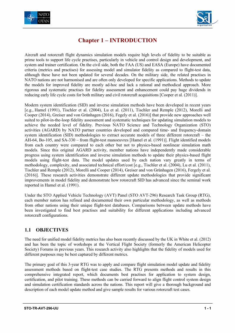
Figure 2.2.1-1 Meeting 1 Group Photo at the University of Liverpool’s 2-6 Flight Simulator Figure 2.2.2-1 Meeting 2 Group Photo at the Georgia Tech Flight 2-7 Simulator Figure 2.2.3-1 Meeting 3 Group Photo in the DLR Hangar 2-8 Figure 2.2.4-1 Meeting 4 Group Photo in the NRC’s Hangar 2-9 Figure 2.2.5-1 Meeting 5 Online Meeting Group Photo 2-10 Figure 2.2.6-1 Meeting 6 Online Meeting Group Photo 2-11

Figure 4.1-1 XV-15 Cruise Error Functions and MUAD Bounds 4-2 [Hodgkinson (1998)] Figure 4.1-2 Simulator-Specific AEE in Roll [Penn (2013)] 4-3 Figure 4.1-3 AEE Envelope by Mitchell (2006a), MUAD Envelope by 4-4 Wood and Hodkinson (1980), VESA MUAD Envelope by Carpenter and Hodkinson (1980) and AEE Envelope by Penn (2013) Figure 4.3-1 Test for Statistical Significance of ValCrit-T Metric and 4-8 Their P-Value for Levels of Simulation Error as Proposed in GARTEUR HC/AG-09 [Haverdings et al. (2000)] Figure 4.3-2 Helicopter Pitch Motion After a Longitudinal Cyclic 4-9 Pitch θ1s Step Input, Semi Rigid Rotor Configuration Figure 4.3-3 ValCrit-T Parameter for the Helicopter Pitch Response 4-10 Figure 4.4-1 Sinacori/Schroeder Motion Fidelity Criteria 4-15 [Schroeder (1999)] Figure 4.4-2 Example of OMCT Fidelity Boundaries, Roll Motion Gain 4-16 and Phase [Jones (2018)] Figure 4.4-3 Objective Motion Cueing Test OMCT [Li (2016)] 4-16 Figure 4.4-4 Comparison of Current Boundaries for OMCT and Schroeder 4-17 Metrics [Jones et al. (2017)] Figure 4.4-5 Motion Fidelity Rating Scale 4-18 Figure 4.5-1 SFR Fidelity Matrix [Perfect et al. (2014)] 4-20 Figure 4.5-2 Simulation Fidelity Rating Scale [Perfect et al. (2014)] 4-21 Figure 4.5-3 Simulation Fidelity Questionnaire [Perfect et al. (2014)] 4-23 Figure 4.6-1 Distribution of QTG Throughout the Flight Envelope 4-26 Figure 4.7-1 Methodology for Integrated Predicted and Perceptual 4-35 Simulator Fidelity Assessment [Perfect et al. (2013)]

STO-TR-AVT-296-UU xiii

Figure 4.7-2 Dynamo Construct for Dynamic Response Criteria 4-36 [Padfield (2018)] Figure 4.7-3 Comparison of Pitch and Roll Bandwidth-Phase Delay 4-37 in Hover [Padfield (2018)] Figure 4.7-4 Comparison of Pitch and Roll Attitude Quickness in 4-37 Hover [Padfield (2018)] Figure 4.7-5 Attack Point Parameters [Perfect et al. (1993)] 4-39

Figure 5.2-1 Possible ‘Black-Box’ Update Models 5-3 Figure 5.2-2 Overview of Methodologies to Derive ‘Black-Box’ 5-4 Input Model Updates Figure 5.2-3 Inverse Simulation Framework to Compute the 5-5 Residual Frequency Response Figure 5.2-4 Schematic Representation of the Algebraic Approach 5-6 Figure 5.3.3-1 Force and Moment Increment Method Flow Chart 5-8 Figure 5.3.4-1 General Approach to Additive System Identification 5-10 Figure 5.3.5-1 Linear Parameter Identification Using Adaptive Learning 5-12 Figure 5.4.3.1-1 Rotor Wake Distortion Due to TPP Rotation 5-14 Figure 5.4.3.4-1 Engine Model 5-20 Figure 5.7.3.2-1 Model Stitching Simulation Architecture – Top Level 5-27 Schematic

Figure 6.4-1 CH-47 Control Mixer Reconstruction from Upstream Control 6A-31 Positions, Correction to k5 Bell Crank Mechanical Gain

Figure 7-1 AVT-296 – Flight Simulation Model Update Methods and 7-1 Flight-Test Databases, Repeated from Figure 1-1 Figure 7.1.1-1 Gain/Time Delay Corrections for Lateral and Longitudinal 7.1-2 Axes in Hover (Flight Data Redacted) Figure 7.1.1-2 Time-Domain Comparison for Lateral and Longitudinal 7.1-3 Axes in Hover (Flight Data Redacted) Figure 7.1.2-1 UH-60 Hover Response Model Comparisons and 7.1-4 Improvements when Compared to Flight Test Figure 7.1.3-1 Comparison of Model and Flight-Test Responses 7.1-5 Figure 7.1.4-1 DLR’s BO-105 Helicopter 7.1-5 Figure 7.1.4-2 Comparison of Baseline and Updated 6-DOF Model 7.1-6 Figure 7.1.4-3 Comparison of 6-DOF (Rigid-Body) and High-Order 7.1-7 Model Figure 7.1.4-4 Time- and Frequency-Domain Comparison of Baseline 7.1-7 and Updated High Order Model Figure 7.2.1-1 Results of Inverse Simulation and Modelling Step 7.2-2 Figure 7.2.1-2 Comparison of Baseline and Updated Model – 7.2-2 Time-Domain Derived Filter Figure 7.2.1-3 Frequency-Domain Comparison of Baseline and Updated 7.2-3 Model – Time-Domain Derived Filter

xiv STO-TR-AVT-296-UU

Figure 7.2.1-4 Comparison of Baseline and Updated Model – Algebraic 7.2-4 Approach Figure 7.2.1-5 Frequency-Domain Comparison of Baseline and 7.2-4 Updated Model – Algebraic Approach Figure 7.2.1-6 Comparison of RMS Cost Function for Baseline and 7.2-5 Updated Models Figure 7.2.2-1 Steps to Update the Baseline 11-DOF Model 7.2-6 Figure 7.2.2-2 Inverse Simulation of EC135 ACT/FHS Collective 7.2-7 Sweep Data at 60 kn Forward Flight Figure 7.2.2-3 Frequency Response of the Yaw Rate Due to 7.2-8 Collective r/δcol at 60 kn Figure 7.2.2-4 Frequency Responses and Resulting Input Filter for Inverse 7.2-8 Pedal Control Due to Measured Collective Figure 7.2.2-5 Collective Multistep Input at 60 kn Forward Flight 7.2-8 Figure 7.2.2-6 Longitudinal Multistep Input at 60 kn Forward Flight 7.2-8 Figure 7.2.2-7 RMS Cost in the Time Domain 7.2-9 Figure 7.2.2-8 Frequency Costs for Collective Input at 60 kn Forward Flight 7.2-9 Figure 7.2.2-9 Physical Effects Regarded by the Baseline Model and 7.2-9 Additional Effects Respected by the Input Filter Figure 7.2.2-10 Results of the Input Filter for 60 kn 3211 Longitudinal 7.2-11 and Lateral Inputs Figure 7.2.2-11 Inverse Control Inputs Created by the Input Filter for the 7.2-11 Lateral Manoeuvre of Figure 7.2.2-10 Figure 7.2.2-12 RMS Cost Function Values for Baseline and Updated 7.2-11 Model: 3211 Inputs at 60 kn Figure 7.2.2-13 Frequency Responses of the Pitch Rate Due to Lateral 7.2-12 Input at 60 kn Figure 7.2.2-14 Off-Axis Response Error and Input Filter of the Modified 7.2-12 Longitudinal Control Due to Lateral Stick Input Figure 7.2.3-1 Boeing Flight-Test Data and CAE Simulation Pitch 7.2-13 Responses Figure 7.2.3-2 Boeing Flight-Test Data and CAE Simulation Yaw 7.2-13 Responses Figure 7.2.3-3 Filter Implementation in Simulation 7.2-13 Figure 7.2.3-4 Pitch Response Error of the Baseline Model and its 7.2-14 Model Fit Figure 7.2.3-5 Yaw Response Error of the Baseline Model and its 7.2-14 Model Fit Figure 7.2.3-6 MUAD Boundaries of the Pitch Axis for the Baseline and 7.2-15 Updated Simulation Figure 7.2.3-7 MUAD Boundaries of the Yaw Axis for the Baseline and 7.2-15 Updated Simulation

Figure 7.3.1-1 Comparison of SID Estimates from Flight, and Simulation 7.3-2 predictions of the Lateral-Directional Oscillatory Mode Characteristics [Padfield and DuVal (1991)]

STO-TR-AVT-296-UU xv

Figure 7.3.1-2 Comparison of Responses of FT with F-B412 Before 7.3-4 (Baseline) and After Renovation (RF-B412); Lateral CyclicPedal Inputs at 90 kn Figure 7.3.1-3 Error Functions for the Yaw Rate from Pedal Frequency 7.3-5 Response Figure 7.3.1-4 Error Functions for the Roll Rate from Pedal Frequency 7.3-5 Response Figure 7.3.1-5 LDO Characteristics of F-B412 Before and After Renovation 7.3-7 Compared with Flight Figure 7.3.1-6 Contributions of Various F-B412 Components to the 7.3-7 Weathercock Stability from Hover to 90 kn Figure 7.3.1-7 Responses of B-412 with Pedal Input at 90 kn 7.3-9 Figure 7.3.1-8 Estimating NXp Using the ASID Approach 7.3-9 Figure 7.3.1-9 Estimating Nr Using the ASID Approach 7.3-10 Figure 7.3.1-10 Estimating Np Using the ASID Approach 7.3-10 Figure 7.3.1-11 Estimating Nv Using the ASID Approach 7.3-11 Figure 7.3.1-12 Reconstructing the Dynamics Using the Identified 7.3-11 Derivatives (v Response) Figure 7.3.1-13 Reconstructing the Dynamics Using the Identified 7.3-12 Derivatives (p Response) Figure 7.3.1-14 Reconstructing the Dynamics Using the Identified 7.3-12 Derivatives (r Response) Figure 7.3.1-15 Validation Study: Comparison of Responses of FT with 7.3-13 ASID; Lateral Cyclic Pedal Inputs at 90 kn Figure 7.3.2-1 Frequency-Domain Comparison of the Flight Data with 7.3-16 Identified CIFER® Hover Model and Baseline/Updated OO-BERM Model Figure 7.3.2-2 Time-Domain Validation of the Hover Model OO-BERM 7.3-19 Against Flight Data Figure 7.3.3-1 Evolution of Adaptive Weights 3211 Manoeuvres Around 7.3-21 Hover Figure 7.3.3-2 Comparison of Accelerations of Identified Linear Model 7.3-22 and Nonlinear Baseline Model Figure 7.3.3-3 Comparison of States of Identified Linear and Nonlinear 7.3-22 Baseline Model Figure 7.3.3-4 Comparison of Identified Linear Model and Flight-Test 7.3-23 Data Figure 7.3.3-5 Comparison of Identified Linear Model and Flight-Test 7.3-23 Data Figure 7.3.3-6 Comparison of Uncoupled Eigenvalues of the Identified 7.3-24 Models Figure 7.3.3-7 Baseline Model Update Using Identified Delta Forces and 7.3-25 Moments Figure 7.3.3-8 Response to right Lateral Cyclic Step Input in Hover 7.3-25

xvi STO-TR-AVT-296-UU

Figure 7.3.3-9 Response to Aft Longitudinal Step Input in Hover 7.3-26

Figure 7.3.4-1 Transfers from δlat to Roll Rate (p) and Lateral 7.3-28 Acceleration (ay)

Figure 7.3.4-2 Transfers from δped to Roll Rate (p) and Yaw Rate (r) 7.3-29

Figure 7.3.4-3 Transfers from δped to Lateral Acceleration (ay) and 7.3-29 Lateral Speed (v) Figure 7.3.4-4 Time-Domain Verification Tests: Lateral Double Doublet 7.3-30 Input; Pedal Doublet Figure 7.3.4-5 Flight Case 1 – Comparison with FT, Before and After 7.3-33 Force and Moment Corrections Figure 7.3.4-6 Flight Case 2 – Comparison with FT, Before and After 7.3-33 Force and Moment Corrections Figure 7.3.4-7 Flight Case 3 – Comparison with FT, Before and After 7.3-34 Force and Moment Corrections Figure 7.3.4-8 Flight Case 4 – Comparison with FT, Before and After 7.3-34 Force and Moment Corrections

Figure 7.4.1-1 Baseline Model Correlation with Hover Test Data 7.4A-2 Figure 7.4.1-2 Baseline Model Correlation with Level Flight Trim 7.4A-2 Test Data Figure 7.4.1-3 Baseline Model On-Axis Response to Roll, Pitch, and 7.4A-2 Yaw Controls in Hover Figure 7.4.1-4 Baseline Model On-Axis Response to Roll, Pitch, and 7.4A-3 Yaw Controls at Cruise Speed Figure 7.4.1-5 Main Rotor Power and Collective Stick Position in 7.4A-4 Low Speed Longitudinal Flight Figure 7.4.1-6 Main Rotor Power and Collective Stick Position in 7.4A-4 Low Speed Lateral Flight Figure 7.4.1-7 Pitch Response to 10% Lateral Doublet Input in Hover 7.4A-5 Figure 7.4.1-8 Pitch Attitude and Longitudinal Stick Position in 7.4A-6 Low Speed Longitudinal Flight Figure 7.4.1-9 Pedal Position in Forward Climb/Descent and 7.4A-7 Autorotation Figure 7.4.1-10 Pitch Attitude in Forward Climb/Descent and 7.4A-7 Autorotation Figure 7.4.1-11 Collective Stick Position and Main Rotor Power in 7.4A-8 Forward Climb/Descent Figure 7.4.1-12 Autorotation Rate of Descent 7.4A-9 Figure 7.4.1-13 On-Axis Roll Rate Response and Off-Axis Pitch Rate 7.4A-10 Response to a Lateral Doublet Input in Hover for a UH-60Helicopter [Zhao et al. (2004)] Figure 7.4.1-14 UH-60 Frequency Response to Longitudinal Control 7.4A-11 in Hover Figure 7.4.1-15 UH-60 Frequency Response to Lateral Control in Hover 7.4A-11 Figure 7.4.2-1 Boeing Helicopters Simulation (BHSIM) Math Model 7.4A-12

STO-TR-AVT-296-UU xvii

Figure 7.4.2-2 Roll Attitude to Lateral Control Position Frequency 7.4A-14 Response, CH-47D, 41,850 lb Gross Weight, Hover, AFCS-OFF Figure 7.4.2-3 Maximum Unnoticeable Additional Dynamics Error 7.4A-15 Bound Envelopes for Roll Attitude to Lateral Control Position Frequency Response, CH-47D, 41,850 lb Gross Weight, Hover, AFCS-OFF Figure 7.4.2-4 ADS-33E Lateral Axis Bandwidth and Phase Delay 7.4A-16 Parameters, Usable Cue Environment > 1 and or Divided Attention Operations, CH-47D, 41,850 lb Gross Weight, Hover, AFCS-OFF Figure 7.4.2-5 Tandem Rotor Pitching Moment and Physics-Inspired 7.4A-17 Notional Downwash Pattern During Steady Left Roll Rate Perturbation Figure 7.4.2-6 Tandem Rotor Helicopter Lateral Flapping and Aircraft 7.4A-17 Rolling Moment During Steady Left Roll Rate Perturbation Figure 7.4.2-7 Effect of Varying Howlett GenHel Inflow Model Pitch 7.4A-18 Aerodynamic Hub Moment Influence Factor on Roll and Pitch Rate Damping Derivatives, CH-47D/F, 46,000 lb Gross Weight, Hover Figure 7.4.2-8 Effect of Varying Howlett GenHel Inflow Model Roll 7.4A-18 Aerodynamic Hub Moment Influence Factor on Roll and Pitch Rate Damping Derivatives, CH-47D/F, 46,000 lb Gross Weight, Hover Figure 7.4.2-9 Hover Longitudinal Baseline Model Comparison 7.4A-21 Figure 7.4.2-10 Longitudinal Trim for Various Uniform Velocity Decay 7.4A-22 Values (Flight Data Redacted) Figure 7.4.2-11 Effective Wake Skew Modification 7.4A-23 Figure 7.4.2-12 Longitudinal Trim of Baseline Comparison for Interference 7.4A-23 Model Update (Flight Data Redacted) Figure 7.4.2-13 Hover Frequency Response Comparison for Interference 7.4A-24

Model Update of Longitudinal Axis and Lateral Axis (Flight Data Redacted)

Figure 7.4.2-14 Time-Domain Comparison of Pitch Response to Doublet 7.4A-24 in Hover (Flight Data Redacted) Figure 7.4.2-15 Effect of Lag Stiffness on Rotor-on-Rotor Mode Dipole 7.4A-25 Frequency Figure 7.4.2-16 Hover Longitudinal Frequency Response Comparison 7.4A-26 for Lag Stiffness Update (Flight Data Redacted) Figure 7.4.3-1 Longitudinal Cyclic Position and Pitch Attitude as 7.4A-27 Function of Speed Figure 7.4.3-2 Fuel Flow to Engine Torque Transfer Function Model 7.4A-27 Figure 7.4.3-3 Fuel Flow to Engine Torque Frequency Response for 7.4A-28 Collective Input in Hover Figure 7.4.3-4 NR Error to Fuel Flow and Collective to Fuel Flow 7.4A-28 Transfer Function Models

xviii STO-TR-AVT-296-UU

Figure 7.4.3-5 NR Error to Fuel Flow Frequency Response for Pedal 7.4A-29 Input in Hover Figure 7.4.3-6 Collective to Fuel Flow Frequency Response for 7.4A-30 Collective Input in Hover Figure 7.4.3-7 Engine Fuel Flow and Torque Response to Collective 7.4A-31 3-2-1-1 Input in Hover Figure 7.4.3-8 Engine Fuel Flow and Torque Response to Pedal 3-2-1-1 7.4A-31 Input in Hover Figure 7.4.3-9 Yaw Rate (r) and Rotor Speed (NR) Frequency Response 7.4A-32 to Collective (DCOL) in Hover Figure 7.4.3-10 Engine Torque (Tq) and Normal Load Factor (Nz) 7.4A-33 Frequency Response to Collective (DCOL) in Hover Figure 7.4.3-11 Yaw Rate (r) and Rotor Speed (NR) Frequency 7.4A-34 Responses to Pedal (DPED) in Hover Figure 7.4.3-12 Engine Torque (Tq) Frequency Response to 7.4A-35 Pedal (DPED) in Hover Figure 7.4.3-13 Normal Load Factor (Nz) and Engine Torque (Tq) 7.4A-36 Frequency Response to Collective (DCOL) in Hover Figure 7.4.3-14 Roll Rate (p) to Lateral (DLAT) and Pitch Rate (q) to 7.4A-37 Longitudinal (DLON) Frequency Responses in Hover Figure 7.4.3-15 Longitudinal Load Factor (Nx) to Longitudinal (DLON) 7.4A-38 and Lateral Load Factor (Ny) to Lateral (DLAT) Frequency Responses in Hover

Figure 7.4.4-1 Roll and Pitch Bare-Airframe Aircraft Responses to 7.4B-1 Total Commands Figure 7.4.4-2 Hover Roll and Pitch Responses with GenHel Model 7.4B-2 Improvement Figure 7.4.4-3 Hover Roll Doublet Response with GenHel Model 7.4B-3 Improvement Figure 7.4.4-4 Frequency-Response Comparisons of the Upper and 7.4B-4 Lower Rotor Inflow Responses to Aerodynamic Inputs for the Identified Inflow Model and MFW Figure 7.4.4-5 Improvements to Roll and Pitch Rate Responses to 7.4B-5 On-Axis Inputs by Using Inflow Model Obtained from System Identification of MFW versus the Baseline Model in a Flight Dynamics Simulation

Figure 7.5.1-1 Frequency-Comparison of the Flight Data Roll Rate 7.5-4 Response with Identified CIFER Hover Model and Baseline/Updated OO-BERM Model Figure 7.5.1-2 Frequency-Domain Comparison of the Flight-Data Pitch 7.5-5 Rate Response with Identified CIFER Hover Model and Baseline/Updated OO-BERM Model Figure 7.5.2-1 UH-60A On-Axis Angular Rate Response in Hover 7.5-6 Figure 7.5.2-2 UH-60A On-Axis Flapping Response in Hover 7.5-7

STO-TR-AVT-296-UU xix

Figure 7.5.2-3 Close-Up of UH-60A Regressive Lag Mode in Roll Rate 7.5-8 Frequency Response Figure 7.5.2-4 Roll Rate Frequency-Domain Cost vs Lateral Stick Linkage Gain 7.5-9 Figure 7.5.2-5 Contours of Frequency-Domain Cost vs Lag Damper Factor 7.5-10 and Lag Stiffness Figure 7.5.2-6 Time-Domain Verification, UH-60A Lateral Doublet in 7.5-11 Hover, Roll Rate RMS Cost is Reduced from JRMS = 10.3 in Baseline Model to JRMS = 7.39 in Updated Model, Pitch Rate RMS Cost is Reduced from JRMS = 6.13 in Baseline Model to JRMS = 4.37 in Updated Model Figure 7.5.2-7 Time-Domain Verification, UH-60A Longitudinal Doublet 7.5-11 in Hover, Roll Rate RMS Cost is Reduced from JRMS = 3.41 in Baseline Model to JRMS = 2.53 in Updated Model, Pitch Rate RMS Cost is Reduced from JRMS = 3.27 in Baseline Model to JRMS = 2.04 in Updated Model Figure 7.5.3-1 Time-Domain EC135 Longitudinal 3-2-1-1 60 kn 7.5-13 Figure 7.5.3-2 Time-Domain EC135 Longitudinal Sweep 60 kn 7.5-15 Figure 7.5.3-3 Time-Domain EC135 Lateral Sweep 60 kn 7.5-16 Figure 7.5.4-1 Keller Lateral Axis Test Data, SAS ON 7.5-17 Figure 7.5.4-2 Keller Longitudinal Axis Test Data, SAS ON 7.5-17 Figure 7.5.4-3 Initial CAE Simulation Roll Response 7.5-18 Figure 7.5.4-4 Initial CAE Simulation Roll MUAD 7.5-18 Figure 7.5.4-5 Initial CAE Simulation Pitch Response 7.5-19 Figure 7.5.4-6 Initial CAE Simulation Pitch MUAD 7.5-19 Figure 7.5.4-7 Initial CAE Simulation Yaw Response 7.5-19 Figure 7.5.4-8 Initial CAE Simulation Yaw MUAD 7.5-19 Figure 7.5.4-9 Improved CAE Simulation Roll Response 7.5-21 Figure 7.5.4-10 Improved CAE Simulation Roll MUAD 7.5-21 Figure 7.5.4-11 Description of Yaw Phase and Magnitude Adjustment 7.5-22 Figure 7.5.4-12 Improved CAE Simulation Pitch Response 7.5-23 Figure 7.5.4-13 Improved CAE Simulation Pitch MUAD 7.5-23 Figure 7.5.4-14 Improved CAE Simulation Yaw Response 7.5-23 Figure 7.5.4-15 Improved CAE Simulation Yaw MUAD 7.5-23 Figure 7.5.5-1 Effect of Pitch Inertia on Model Mismatch Cost 7.5-24 Figure 7.5.5-2 Inertia Correction Results for Longitudinal Axis and Lateral 7.5-25 Axis (Flight Data Redacted) Figure 7.5.5-3 Effect of Lag Damping on Longitudinal Response 7.5-26 Figure 7.5.5-4 Baseline and Updated Frequency Response Comparisons for 7.5-27

Longitudinal Axis and Directional Axes (Flight Data Redacted)

Figure 7.5.5-5 Lateral Axis Frequency Response Comparison for Baseline 7.5-28 and Updated Model (Flight Data Redacted)

xx STO-TR-AVT-296-UU

Figure 7.6.1-1 Baseline Roll and Pitch Bare-Airframe Aircraft Responses 7.6-2 to Total Commands Figure 7.6.1-2 Comparison of Roll and Pitch Bare-Airframe Aircraft 7.6-4 Responses to Total Commands for the CIFER State-Space Identified Model, the Baseline Model, and Flight Data Figure 7.6.1-3 Comparisons of Roll and Pitch Bare-Airframe Aircraft 7.6-4 Responses to Total Commands for Updated HeliUM Model, the Baseline HeliUM Model, and Flight Data

Figure 7.7.1-1 Regression of Zδcol vs Advance Ratio 7.7-3 Figure 7.7.1-2 Regression of Longitudinal Force Naught Term 7.7-3 Figure 7.7.1-3 Proof of Match (POM) of Stitched Model 7.7-4 Figure 7.7.2-1 Check of Xu and Mu from Stitched Model vs Simulation 7.7-5 Figure 7.7.2-2 Pitch Rate Response from Stitched Model and Nonlinear 7.7-6 Simulation Figure 7.7.2-3 Average Predictive Accuracy for Doublet Inputs of the 7.7-7 Stitched Model as Compared to the Point Models for Hover and 80 kn Figure 7.7.2-4 Time Response Comparison of Stitched Model and Nonlinear 7.7-8 Simulation for a Realistic Manoeuvring Scenario Figure 7.7.2-5 Verification of Off-Nominal Weight Extrapolation of Stitched 7.7-9 Model Figure 7.7.2-6 U,V Airspeed Points for Anchor Trim Data And Point Models 7.7-10 Included in the Stitched Model Figure 7.7.2-7 Stitched Model Trim Results of Position-Held/Heading-Held 7.7-11 Hovering Flight in the Presence of a Rotating 10-kn Wind Through 360 Degrees Figure 7.7.3-1 Trim Data of the ACT/FHS and Approximated Trim Curves 7.7-12 Figure 7.7.3-2 Comparison of Linear Point Model and Stitched Model at 7.7-13 60 kn for Lateral Inputs Figure 7.7.3-3 Eigenvalues of the ACT/FHS Models and their Transition 7.7-14 Figure 7.7.3-4 Comparison of Linear Point Model (60 kn) and Stitched 7.7-15 Model for a Deceleration-Acceleration Manoeuvre Figure 7.7.3-5 Comparison of the Stitched Model and Flight-Test Data 7.7-15 Figure 7.7.3-6 MUAD Plot for the Longitudinal On-Axis (q/δlon) at 60 kn 7.7-16 Forward Flight Figure 7.7.3-7 MUAD Plot for the Directional On-Axis (r/δped) in Hover 7.7-16 Figure 7.7.4-1 3D Robotics IRIS+, Shown in Heavy Loading Configuration 7.7-17 with 200-Gram Payload Figure 7.7.4-2 Anchor Points Included in the Stitched Model 7.7-19 Figure 7.7.4-3 Variation in Trim States and Controls Over the Full Airspeed 7.7-19 Range Figure 7.7.4-4 Dynamic Response Verification, Hover (J = 3.75) 7.7-19 Figure 7.7.4-5 Dynamic Response Verification, 17 kn (J = 51.7) 7.7-19

STO-TR-AVT-296-UU xxi

Figure 7.7.4-6 Interpolation for Airspeed Compared to Truth 10-kn Pitch-Rate 7.7-20 Response from Flight Figure 7.7.4-7 Extrapolation for Heavy Loading Compared to Truth Heavy 7.7-20 Trim Data from Flight

Figure 7.8-1 Precision Hover MTE [ADS-33 (2000)] 7.8-1 Figure 7.8-2 Precision Hover MTE Task Performance 7.8-2 Figure 7.8-3 Precision Hover MTE Control Activity 7.8-2 Figure 7.8-4 Precision Hover MTE Attack Analysis 7.8-3 Figure 7.8-5 Collective to Yaw Predicted Cross-Couplings 7.8-4

Figure 8.2-1 Flight Control System Development Roadmap, Reproduced 8-7 from Tischler et al. Figure 8.2-2 Model-Following Architecture (Pitch) 8-8 Figure 8.2-3 Perturbation and Sweep Method for Determining the Feedback 8-10 Response from a SIMLINK Block Diagram Figure 8.2-4 Perturbation Linearization of the SIMULINK Feedback 8-11 Response, Frequency Sweep Determination of the SIMULINK Control Laws, and Ground Sweep Validation of the Real-Time Control Laws Figure 8.2-5 Definition of Broken-Loop Response Metrics and SAE AS94000 8-12 Stability Margin Specification Figure 8.2-6 Analysis Model Validation for Broken-Loop Pitch Response 8-12 Figure 8.2-7 Definition of the ADS-33 Bandwidth and Phase Delay Metrics and ADS-33F Criteria for Pitch Axis 8-13 Figure 8.2-8 Analysis Model Validation for Closed-Loop Pitch Response 8-14 Figure 8.2-9 Definition of ADS-33 Disturbance Rejection Specification Metrics 8-15 Figure 8.2-10 ADS-33 Disturbance Rejection Specifications for Pitch: DRB; DRP 8-15 Figure 8.2-11 Analysis Model Validation for Disturbance Rejection Yaw Response 8-16 Figure 8.2-12 Typical Outer-Loop Schematic for Explicit Model-Following System 8-17 Figure 8.4.1-1 Typical Time-Domain Metrics Required in a QTG Package 8-23 Figure 8.4.1-2 Bell 412 Hover Proof of Match 8-26 Figure 8.4.2-1 Transport Delay for Training Simulator 8-28 Figure 8.4.2-2 Frequency-Domain Validation of the Hover Model OO-BERM 8-29 Against Flight Data

xxii STO-TR-AVT-296-UU

List of Tables

Table Page

Table 2.1-1 AVT-296 Participants 2-2

Table 2.2-1 AVT-296 Meeting Activities 2-4

Table 4.4-1 Modified Simulator Motion Fidelity Scale Used in Industry 4-18 [Miller et al. (2009)]

Table 4.6-1 Performance, Takeoff 4-27

Table 4.6-2 Performance, Trimmed Flight Control Positions 4-28

Table 4.6-3 Performance, Landing and Autorotation 4-29

Table 4.6-4 Low Airspeed Handling Qualities 4-30

Table 4.6-5 Longitudinal Handling Qualities 4-30

Table 4.6-6 Lateral and Directional Handling Qualities 4-31

Table 6.4-1 CH-47F System Identified Longitudinal/Vertical Axis 6A-29 Model Stability Derivatives for Heavy Gross Weight at Hover

Table 6.4-2 CH-47F System Identified Longitudinal/Vertical Axis 6A-29 Model Control Sensitivity Derivatives and Effective Time Delays for Heavy Gross Weight at Hover

Table 6.4-3 CH-47F System Identified Lateral/Directional Axis Model 6A-30 Stability Derivatives for Light, Medium, and Heavy Gross Weight at Hover

Table 6.4-4 CH-47F System Identified Lateral/Directional Axis Model 6A-30 Control Sensitivity Derivatives and Effective Time Delays for Light, Medium, and Heavy Gross Weight at Hover

Table 6.5-1 Partial Stability and Control Derivatives from AW139 SID 6B-5 on FT at Vy

Table 6.5-2 Eigenvalues (rad/sec) from AW139 SID on FT at Vy 6B-5

Table 6.8-1 Identified Stability and Control Derivatives, Hover 6B-15

Table 6.8-2 Identified Model Costs, Hover 6B-16

Table 6.8-3 Identified Stability and Control Derivatives, 17 kn 6B-17

Table 6.8-4 Identified Model Costs, 17 kn 6B-18

Table 7.1.1-1 Cost Function Comparison for Baseline and Updated Model 7.1-2

Table 7.1.1-2 Time-Domain Cost for Baseline and Updated Model 7.1-3

Table 7.1.2-1 Cost Function Comparison for Baseline and Updated Model 7.1-4

Table 7.1.4-1 Time- and Frequency-Domain Cost Functions for Baseline 7.1-7 and Updated Models

STO-TR-AVT-296-UU xxiii

Table 7.2.1-1 Frequency-Domain Cost Functions of Baseline and Updated 7.2-5 Models for Selected Frequency Responses Table 7.2.2-1 Integrated Frequency Cost at 60 kn Forward Flight 7.2-8 Table 7.2.3-1 Filter Coefficients 7.2-13 Table 7.2.3-2 Integrated Frequency Cost Function Values J 7.2-15

Table 7.3.1-1 Stability and Control Derivatives from Linearized F-B412 7.3-3 and SID (FT) (90 kn)

Table 7.3.1-2 LDO Damping (ζ) and Frequency (ω) from FT, 3-DOF, 7.3-4 and 6-DOF Models Table 7.3.1-3 Renovation of F-B412 7.3-6

Table 7.3.1-4 LDO Damping (ζ) and Frequency (ω) for RF-B412 Model 7.3-6 Table 7.3.1-5 FT EE ASID Stability and Control Derivatives 7.3-8

Table 7.3.1-6 Comparison of LDO Damping (ζ) and Frequency (ω) from 7.3-13 Different Approaches Table 7.3.2-1 CIFER Identified Rolling and Pitching Static/Dynamic 7.3-14 Derivatives Compared with Baseline and Updated OO-BERM Calculated Derivatives for the Hover Model Table 7.3.2-2 Trim Control Gradients with Respect to Airspeed in Hover 7.3-15 Table 7.3.2-3 Frequency-Domain Integrated Cost J 7.3-18 Table 7.3.2-4 Root Mean Square Cost Jrms 7.3-18 Table 7.3.3-1 Reduced Order ‘Delta’ Derivatives 7.3-24 Table 7.3.3-2 Jrms Comparison for Baseline and Corrected Models 7.3-26 Table 7.3.4-1 Partial Stability and Control Derivatives from AW139 Model 7.3-31 Linearization and SID on FT (Vy) Table 7.3.4-2 Eigenvalues (rad/sec) from AW139 SID on FT (Vy) 7.3-31

Table 7.4.2-1 Model/Flight Data Mismatch Frequency-Domain Integrated 7.4A-14 Cost Function Metric Values for Roll Attitude to Lateral Control Position Frequency Response, CH-47D, 41,850 lb Gross Weight, Hover, AFCS-OFF Table 7.4.2-2 Frequency-Domain Cost Metrics for Baseline and Updated 7.4A-24 Model Table 7.4.4-1 Mismatch Cost Function Comparisons Between Baseline 7.4B-5 and Updated Models Table 7.4.4-2 Comparisons of Wake Distortion, KR, Constants for Coaxial 7.4B-6 Rotors from Various Identified Models

Table 7.5.1-1 CIFER Identified Rolling and Pitching Control Derivatives 7.5-2 Compared with Baseline and Updated OO-BERM Calculated Derivatives for Hover Model Table 7.5.1-2 Measured Aeromechanical Parameters Optimal Solution 7.5-3 Table 7.5.1-3 Frequency-Domain Integrated Cost J 7.5-5

Table 7.5.2-1 List of Model Parameters Investigated in UH-60A 7.5-8 Simulation Update

xxiv STO-TR-AVT-296-UU

Table 7.5.2-2 Final Frequency-Domain Cost Improvements in for UH-60A 7.5-10 in Hover Table 7.5.3-1 Time-Domain RMS Cost EC135 Longitudinal 3-2-1-1 60 kn 7.5-13 Table 7.5.3-2 Time-Domain RMS Cost EC135 Longitudinal Sweep 60 kn 7.5-15 Table 7.5.3-3 Time-Domain RMS Cost EC135 Lateral Sweep 60 kn 7.5-16 Table 7.5.4-1 Model Frequency-Domain Cost Functions 7.5-24 Table 7.5.5-1 Baseline and Updated Inertia and Cost Values 7.5-25 Table 7.5.5-2 Cost Comparison for Lag Damper Update 7.5-28

Table 7.6.1-1 Frequency Response Costs Between Flight Data and Math 7.6-4 Models

Table 7.7.3-1 RMS Cost for Stitched Model and Augmented Model 7.7-15 Compared to Flight-Test Data Table 7.7.4-1 Stability and Control Derivatives Comparison 7.7-17 Table 7.7.4-2 Modes Comparison 7.7-18

Table 7.8-1 Precision Hover Perceptual Metrics 7.8-3

Table 8.1.2-1 Examples of Model Corrections/Adjustments 8-5 Table 8.2-1 Comparison of Fidelity Metrics for Analysis vs Flight 8-17 Table 8.3.5-1 Summary of the Reduction in QTG Test Cases Using 8-21 Frequency Sweeps Table 8.5-1 Summary of Model Development and improvement Methods 8-31 with Respect to Different Applications

STO-TR-AVT-296-UU xxv

Foreword

In March of 2016, Subject Matter Experts (SMEs) from the US Army, University of Liverpool (UK), and DLR (Germany) in the fields of rotorcraft flight simulation and control, met to discuss the potential for collaboration focused on flight simulation model update methods and fidelity assessment metrics. A key new aspect was the ability to leverage the extensive progress made in rotorcraft system identification, especially under the landmark effort of NATO AGARD Working Group 18 (1991), and in the continued advancement in the 30 years since. System identification provides a ‘truth model’ and important physical insight into the flight dynamics from flight-test data that can be used for updating physics-based models and assessing the model’s fidelity. In the course of follow-on discussions with SMEs from other nations, and in light of the advances in both rotorcraft physics-based flight simulation methods and system identification, it became clear that there was a need for a new look at the topic and SME recommendations as determined from comprehensive applications to multiple flight-test case studies. Discussions with SMEs from other nations indicated a broad interest in this topic and a research working group was proposed under the NATO RTO umbrella that became AVT-296: Rotorcraft Flight Simulation Model Fidelity Improvement and Assessment. The NATO umbrella allowed for very broad participation, sharing of flight data and simulation results, regular discussions held at biannual meetings at the member nation facilities, and finally resulting in this comprehensive report and a forth coming short course (June 2021). In total, there were 31 members in the research team from 9 nations, representing training simulator developers, rotorcraft manufacturers, government research laboratories, and academia, who worked together for three years during the period 2018 ‒ 2021. We hope that the comprehensive research effort and this resulting in-depth final report and forthcoming short course will help to advance and standardize the state-of-the-art in rotorcraft flight simulation.

Dr. Mark B. TISCHLER Army Technology Development Directorate

UNITED STATES AVT-296 Co-Chair

Prof. Mark D. WHITE University of Liverpool UNITED KINGDOM AVT-296 Co-Chair

xxvi STO-TR-AVT-296-UU

AVT-296 Membership List

CO-CHAIRS

Prof. Mark D. WHITE University of Liverpool UNITED KINGDOM

Email: mdw@liverpool.ac.uk

MEMBERS

Mr. Stefano D’AGOSTO Leonardo Company ITALY Email: stefano.dagosto@leonardocompany.com

Dr. Neil CAMERON The University of Liverpool UNITED KINGDOM Email: ncameron@liverpool.ac.uk

Prof. Steffen GREISER1 University of Applied Sciences Osnabrück GERMANY Email: s.greiser@hs-osnabrueck.de

Mr. Arthur GUBBELS National Research Council of Canada CANADA Email: Bill.Gubbels@nrc.ca

Mr. Feyyaz GUNER Georgia Institute of Technology UNITED STATES Email: feyyazguner@gatech.edu

Dr. Chengjian HE Advanced Rotorcraft Technology UNITED STATES Email: he@flightlab.com

Prof. Joseph HORN Pennsylvania State University UNITED STATES Email: joehorn@psu.edu

1 Former affiliation was DLR, Germany.

Mr. Ken HUI National Research Council of Canada CANADA Email: Kenneth.Hui@nrc-cnrc.gc.ca

Dr. Michael JONES DLR Braunschweig GERMANY Email: Michael.Jones@dlr.de

Dr. Ondrej JUHASZ United States Naval Academy UNITED STATES Email: juhasz@usna.edu

Ms. Olivia LEE San Jose State University UNITED STATES Email: olivia.h.lee@sjsu.edu

Mr. Rhys LEHMANN Defence Science and Technology Group AUSTRALIA Email: Rhys.Lehmann@dst.defence.gov.au

Mr. David MILLER The Boeing Company UNITED STATES Email: david.g.miller@boeing.com

Mr. Vincent MYRAND-LAPIERRE CAE CANADA Email: vincent.myrandlapierre@cae.com

Dr. Mark B. TISCHLER Army Technology Development Directorate

UNITED STATES Email: usarmy.redstone.devcom-

avmc.mbx.pao@mail.mil

STO-TR-AVT-296-UU xxvii

Mr. Michel NADEAU-BEAULIEU CAE CANADA Email: michel.nadeaubeaulieu@cae.com Mr. Samuel NADELL2 Universities Space Research Association UNITED STATES Email: snadell@usra.edu Prof. Gareth PADFIELD The University of Liverpool UNITED KINGDOM Email: padfield@liverpool.ac.uk Dr. Marilena PAVEL Delft University of Technology NETHERLANDS Email: M.D.Pavel@tudelft.nl Prof. Jonnalagadda PRASAD Georgia Institute of Technology UNITED STATES Email: jvr.prasad@aerospace.gatech.edu Mr. Andrea RAGAZZI Leonardo Company ITALY Email: andrea.ragazzi@leonardocompany.com Mr. Sylvain RICHARD Thales Group FRANCE Email: sylvain.richard@thalesgroup.com Mr. Pavle SCEPANOVIC DLR Braunschweig GERMANY Email: Pavle.Scepanovic@dlr.de Ms. Susanne SEHER-WEIß DLR Braunschweig GERMANY Email: Susanne.Seher-Weiss@dlr.de

2 This work was also supported by the National Aeronautics and Space Administration (NASA) under award number

NNA16BD14C for NASA Academic Mission Services (NAMS).

Mr. Jonathan SOONG Contractor, Army Technology Development Directorate UNITED STATES Email: usarmy.redstone.devcom-

avmc.mbx.pao@mail.mil Mr. Olaf STROOSMA Delft University of Technology NETHERLANDS Email: O.Stroosma@tudelft.nl Dr. Armin TAGHIZAD ONERA FRANCE Email: armin.taghizad@onera.fr Mr. Eric TOBIAS Army Technology Development Directorate UNITED STATES Email: usarmy.redstone.devcom-

avmc.mbx.pao@mail.mil Dr. Hong XIN Sikorsky Aircraft, a Lockheed Martin Company UNITED STATES Email: hong.xin@lmco.com Dr. Ilkay YAVRUCUK Middle East Technical University TURKEY Email: yavrucuk@metu.edu.tr

2 This work was also supported by the National Aeronautics and Space Administration (NASA) under award number NNA16BD14C for NASA Academic Mission Services (NAMS).

xxviii STO-TR-AVT-296-UU

PANEL/GROUP MENTOR

Prof. Cord ROSSOW DLR

GERMANY Email: cord.rossow@dlr.de

STO-TR-AVT-296-UU ES - 1

Rotorcraft Flight Simulation Model Fidelity Improvement and Assessment

(STO-TR-AVT-296-UU)

Executive Summary Rotorcraft flight dynamics simulation models require high levels of fidelity to be suitable as prime items in support of life cycle practices, particularly vehicle and control design and development, and system and trainer certification. On the civil side, both the FAA (US) and EASA (Europe) have documented criteria (metrics and practices) for assessing model and simulator fidelity as compared to flight-test data, although these have not been updated for several decades. On the military side, the related practices in NATO nations are not harmonised and often only developed for specific applications. Methods to update the models for improved fidelity are mostly ad hoc and lack a rational and methodical approach. Modern rotorcraft System Identification (SID) and inverse simulation methods have been developed in recent years that provide new approaches well suited to pilot-in-the-loop fidelity assessment and systematic techniques for updating simulation models to achieve the needed level of fidelity. To coordinate efforts and improve the knowledge in this area, STO Applied Vehicle Technology Panel Research Task Group (STO AVT-296 RTG) was constituted to evaluate update methods used by member nations to find best practices and suitability for different applications including advanced rotorcraft configurations.

This report presents the findings of the AVT-296 RTG. An overview of previous rotorcraft simulation fidelity Working Groups is presented, followed by a review of the metrics that have been used in previous studies to quantify the fidelity of a flight model or the overall perceptual fidelity of a simulator. The theoretical foundations of the seven different update methods and a description of the eight flight databases (Bell 412, UH-60, IRIS+, EC135, CH-47, AW139, AW109, and X2, provided by the National Research Council of Canada, US Army, Airbus Helicopters, Boeing, Leonardo Helicopter Division, and Sikorsky) used by the RTG is presented. Both time- and frequency-domain fidelity assessment methods are considered, including those in current use by simulator qualification authorities and those used in the research community. Case studies are used to show the application, utility, and limitations of the update and assessment methods to the flight-test data.

The work of the RTG has shown that time- and frequency-domain SID based metrics are suitable for use for assessing the model fidelity across a wide range of rotorcraft configurations. Gain and time delay update methods work well for well-developed flight dynamics models and can be used for flight control system design, but do not provide physical insights into the sources of errors in a model. Deriving stability and control derivatives from flight-test data using SID and nonlinear simulation models using perturbation extraction methods provides insight into the missing dynamics of the simulation model, which can subsequently be updated using additional forces and moments to significantly improve the fidelity of the model and can be used to update models for flight simulation training application methods. Reduced order model and physics-based correction methods provide large benefits when extrapolating to other flight conditions but does require detailed flight-test data. SID can quickly provide accurate point models, if detailed flight-test data are available, which can be ‘stitched’ together to produce models suitable for real-time piloted simulation and control design applications. However, the dependency on flight-test data means that this method is not suitable for early aircraft development activities.

ES - 2 STO-TR-AVT-296-UU

This documentation of rotorcraft simulation fidelity assessment and model update strategies will benefit NATO nations by allowing for common, agreed-upon best practices and recommendations, ensuring each country’s flight dynamics and simulation models are of the highest calibre possible. The collaboration between industry, academia, and government laboratories has been key to the success of this RTG; this cooperation model should be adopted in future research activities. As industries strive to achieve greater efficiency and safety in their products, the fidelity of simulation should match commercial aspirations to ensure that the ‘right first time’ ethos is fully embedded into industrial best practices. Militaries will be able to use the methods and metrics presented to set criteria that will underpin the use of modelling and simulation in certification to accelerate development and acquisition and reduce the cost of new aircraft systems, e.g., advanced high-speed rotorcraft and legacy system upgrades. The criteria may also set standards for training devices used to support the expansion of synthetic environments for training to offset the high costs of flight hours. This RTG has identified that current flight training simulator standards could be updated to use the flight model and perceptual fidelity metrics presented in this report to ensure that models are not ‘over-tuned’ and a more rigorous method of subjective simulator assessment is adopted.

STO-TR-AVT-296-UU ES - 3

Amélioration et évaluation de la fidélité des modèles de simulation du vol à voilure tournante

(STO-TR-AVT-296-UU)

Synthèse Les modèles de simulation de la dynamique du vol à voilure tournante doivent avoir un niveau de fidélité élevé pour servir d’éléments principaux étayant les pratiques du cycle de vie, en particulier la conception et la mise au point des véhicules et des commandes et la certification du système et du simulateur. Dans le domaine civil, tant la FAA (États-Unis) que l’AESA (Europe) ont documenté des critères (indicateurs et pratiques) d’évaluation de la fidélité des modèles et simulateurs par rapport aux données d’essai en vol, même si ces critères n’ont pas été mis à jour depuis des décennies. Dans le domaine militaire, les pratiques correspondantes dans les pays de l’OTAN ne sont pas harmonisées et ne sont souvent élaborées que pour des applications bien précises. Les méthodes de mise à jour des modèles pour en améliorer la fidélité sont principalement ad hoc et manquent d’une approche rationnelle et méthodique. Des méthodes modernes d’identification des systèmes (SID) d’aéronefs à voilure tournante et de simulation inverse ont été mises au point ces dernières années. Elles constituent de nouvelles approches bien adaptées à l’évaluation de la fidélité avec pilote dans la boucle et aux techniques systématiques de mise à jour des modèles de simulation pour atteindre le niveau de fidélité nécessaire. Dans le but de coordonner les travaux et améliorer les connaissances dans ce domaine, le groupe de recherche de la Commission sur la technologie appliquée aux véhicules de la STO (RTG STO AVT-296) a été constitué afin d’évaluer les méthodes de mise à jour qu’emploient les pays membres, de trouver les meilleures pratiques et d’évaluer leur adéquation aux différentes applications, notamment les configurations perfectionnées d’aéronef à voilure tournante.

Ce rapport présente les conclusions du RTG AVT-296. Il donne une vue d’ensemble des groupes de travail précédents portant sur la fidélité de la simulation des aéronefs à voilure tournante, puis passe en revue les indicateurs qui ont été utilisés dans les précédentes études pour quantifier la fidélité d’un modèle de vol ou la fidélité perceptive générale d’un simulateur. Le rapport présente les fondements théoriques des sept méthodes de mise à jour et décrit les huit bases de données de vol (Bell 412, UH-60, IRIS+, EC135, CH-47, AW139, AW109 et X2, fournies par le Conseil national de recherches Canada, l’Armée de terre des États-Unis, Airbus Helicopters, Boeing, Leonardo Helicopter Division et Sikorsky) utilisées par le RTG. Des méthodes d’évaluation de la fidélité du domaine temporel et fréquentiel sont étudiées, y compris celles actuellement utilisées par les autorités de qualification des simulateurs et celles utilisées dans la communauté de la recherche. Des études de cas montrent l’application, l’utilité et les limites de la mise à jour et des méthodes d’évaluation des données d’essai en vol.

Le travail du RTG montre que les indicateurs basés sur le SID du domaine temporel et fréquentiel sont adaptés à l’évaluation de la fidélité du modèle dans une large gamme de configurations d’aéronefs à voilure tournante. Les méthodes de mise à jour du gain et de la temporisation fonctionnent bien pour les modèles de dynamique de vol bien développés et peuvent servir à concevoir des systèmes de commande de vol, mais elles ne fournissent pas d’informations physiques sur les sources d’erreur d’un modèle. La déduction des dérivées de stabilité et de commande à partir de données d’essai en vol utilisant le SID et de modèles de simulation non linéaires utilisant des méthodes d’extraction des perturbations fournit un aperçu de la dynamique manquante du modèle de simulation, lequel peut ensuite être mis à jour avec des forces et moments supplémentaires pour améliorer sensiblement la fidélité du modèle et peut servir à actualiser les modèles des méthodes applicatives de formation par simulation de vol. Les méthodes de correction

ES - 4 STO-TR-AVT-296-UU

basées sur la physique et les modèles réduits offrent de grands avantages lors de l’extrapolation à d’autres conditions de vol, mais nécessitent des données détaillées d’essai en vol. Le SID peut fournir rapidement des modèles de point exacts, si des données détaillées d’essai en vol sont disponibles, lesquels peuvent être « assemblés » pour produire des modèles adaptés à la simulation pilotée en temps réel et aux applications de conception des commandes. Cependant, la dépendance aux données d’essai en vol signifie que cette méthode n’est pas adaptée aux activités précoces de mise au point des aéronefs.

Cette documentation de l’évaluation de la fidélité de simulation des aéronefs à voilure tournante et des stratégies de mise à jour des modèles bénéficiera aux pays de l’OTAN en leur permettant de convenir des meilleures pratiques et des recommandations communes, qui garantiront le niveau le plus élevé possible des modèles de simulation et de dynamique de vol de chaque pays. La collaboration entre l’industrie, le monde universitaire et les laboratoires publics a été la clé de la réussite de ce RTG. Ce modèle de coopération devrait être adopté dans les futures activités de recherche. Alors que les industries s’efforcent d’atteindre une plus grande efficacité et une meilleure sécurité de leurs produits, la fidélité de la simulation devrait correspondre aux aspirations commerciales, afin que la philosophie de « réussite du premier coup » soit pleinement intégrée dans les meilleures pratiques industrielles. Les militaires pourront utiliser les méthodes et indicateurs présentés pour établir des critères qui étaieront l’utilisation de la modélisation et simulation dans la certification, afin d’accélérer la mise au point et l’acquisition et de réduire le coût des nouveaux systèmes d’aéronefs, par exemple les aéronefs à voilure tournante à grande vitesse et les systèmes hérités modernisés. Ces critères peuvent également établir des normes pour les appareils de formation servant à soutenir le développement des environnements synthétiques dans l’entraînement, afin de contrebalancer le coût élevé des heures de vol. Le présent RTG a déterminé que les normes actuelles des simulateurs d’entraînement au vol pourraient être mises à jour pour utiliser le modèle de vol et les indicateurs de fidélité perceptive présentés dans ce rapport, afin de s’assurer que les modèles ne sont pas adaptés de manière excessive et qu’une méthode plus rigoureuse d’évaluation subjective des simulateurs est adoptée.

STO-TR-AVT-296-UU 1 - 1

Chapter 1 – INTRODUCTION

Aircraft and rotorcraft flight dynamics simulation models require high levels of fidelity to be suitable as prime tools to support life cycle practises, particularly in vehicle and control design and development, and system and trainer certification. On the civil side, both the FAA (US) and EASA (Europe) have documented criteria (metrics and practises) for assessing model and simulator fidelity as compared to flight-test data, although these have not been updated for several decades. On the military side, the related practises in NATO nations are not harmonised and are often only developed for specific applications. Methods to update the models for improved fidelity are mostly ad-hoc and lack a rational and methodical approach. More rigorous and systematic practises for fidelity assessment and enhancement could pay huge dividends in reducing early life cycle costs for both military and civil rotorcraft acquisitions [Cooper et al. (2011)].

Modern system identification (SID) and inverse simulation methods have been developed in recent years [e.g., Hamel (1991), Tischler et al. (2004), Lu et al. (2011), Tischler and Remple (2012), Morelli and Cooper (2014), Greiser and von Grünhagen (2016), Fegely et al. (2016)] that provide new approaches well suited to pilot-in-the-loop fidelity assessment and systematic techniques for updating simulation models to achieve the needed level of fidelity. Previous NATO Science and Technology Organization (STO) activities (AGARD) by NATO partner countries developed and compared time- and frequency-domain system identification (SID) methodologies to extract accurate models of three different rotorcraft – the AH-64, Bo-105, and SA-330 – from flight-test manoeuvres [Hamel et al. (1991)]. Flight identified models from each country were compared to each other but not to physics-based nonlinear simulation math models. Since this original AGARD activity, member nations have independently made considerable progress using system identification and inverse simulation methods to update their physics-based flight models using flight-test data. The model updates used by each nation vary greatly in terms of methodology, complexity, and associated technical effort/cost [e.g., Tischler et al. (2004), Lu et al. (2011), Tischler and Remple (2012), Morelli and Cooper (2014), Greiser and von Grünhagen (2016), Fergely et al. (2016)]. These research activities demonstrate different update methodologies that provide significant improvements in model fidelity and demonstrate how rotorcraft SID has advanced since the seminal work reported in Hamel et al. (1991).

Under the STO Applied Vehicle Technology (AVT) Panel (STO AVT-296) Research Task Group (RTG), each member nation has refined and documented their own particular methodology, as well as methods from other nations using their unique flight-test databases. Comparisons between update methods have been investigated to find best practises and suitability for different applications including advanced rotorcraft configurations.

1.1 OBJECTIVES

The need for unified model fidelity metrics has also been recently discussed by the UK in White et al. (2012) and has been the topic of workshops at the Vertical Flight Society (formerly the American Helicopter Society) Forums in previous years. This research activity also highlights that the fidelity of models used for different purposes may be best captured by different metrics.

The primary goal of this 3-year RTG was to apply and compare flight simulation model update and fidelity assessment methods based on flight-test case studies. The RTG presents methods and results in this comprehensive integrated report, which documents best practises for application to system design, certification, and pilot training. These methods can be carried forward to align flight control system design and simulation certification standards across the nations. This report will give a thorough background and description of each model update method and give sample results for various rotorcraft test cases.

INTRODUCTION

1 - 2 STO-TR-AVT-296-UU

Making such update methods, metrics, and practises more accessible and standardized for industrial and government use was a strong motivation for the RTG. Especially important was the involvement of flight simulation companies as RTG members, to capture their current methods, needs, perspective, and concerns. This documentation of simulation fidelity assessment and model update strategies will benefit NATO nations by allowing for common, agreed-upon best practises and recommendations, ensuring each country’s flight dynamics and simulation models are of the highest calibre possible. Militaries will be able to use the methods and metrics presented to set criteria that will underpin the use of modelling and simulation in certification to accelerate development and acquisition and reduce the cost of new aircraft systems and legacy system upgrades. The criteria may also set standards for training devices used to support the expansion of synthetic environments for training to offset the high costs of flight hours.

1.2 REPORT OVERVIEW AND ORGANISATION

This report aims to give an overview of the past several decades of technical work in simulation fidelity and model assessment from the perspectives of researchers, Original Equipment Manufacturer (OEM) engineers, academics, and simulator developers. As the complexity of future rotorcraft designs continues to increase, this report serves as a launching point for model validation efforts and is a snapshot of the current state-of-the-art methods used to improve model fidelity. From an organisational standpoint, references are given at the end of each section or chapter to assist the reader in quickly finding additional technical content.

Chapters 1 and 2 give an overview of the task group members, task group timeline, and technical meetings held. Chapter 3 covers each organisation’s motivation for participating in this RTG, brief summaries of the methods each organisation are currently employing for math model update, and the end application of the models they develop (simulation, engineering design, control law development, etc.). This chapter highlights current areas of research in model fidelity improvement and summarizes past work in system identification and modelling.

Chapter 4 discusses various quantitative and qualitative simulation model fidelity metrics. Rotorcraft flight dynamics simulation models serve a variety of purposes and are evaluated by different metrics based on the end application. The metrics and their backgrounds are discussed to give the reader an impression of how models can be evaluated. Many metrics are introduced, and several are down-selected and used to evaluate an update method’s efficacy in later chapters.

Chapter 5 ‒ 7 review the model update methods, flight-test databases, and present detailed case studies with each update method illustrated with 1 or more flight-test databases. A concise summary of the update methods and case studies is presented in Figure 1.1.

Chapter 5 broadly categorises and gives a detailed description of model update methodologies in terms of complexity and level of technical effort required. Methods range from gross empirical corrections to more complicated methods that require detailed knowledge of rotorcraft dynamics and aerodynamics.

Chapter 6 gives an overview and presents databases for the 8 rotorcraft to which simulation update methods are applied in this study. Information provided includes aircraft configuration, flight-test data available, flight simulation modelling tools, system identification methods and results for model fidelity assessment and update. Effort was taken to include a large variety of rotorcraft configurations: legacy to advanced high-speed configurations, partial-authority to full-authority flight control system considerations, and piloted vs UAVs. This large range of rotorcraft configurations provides insight into the modelling nuances of each and to give an impression of deficiencies that may be encountered in new designs.

Chapter 7 presents an extensive set of update case studies organised in the same order as Chapter 5, by update method. The same method is generally applied to multiple aircraft by researchers from different

INTRODUCTION

STO-TR-AVT-296-UU 1 - 3

organisations to give a variety of perspectives on each method. Conciseness of each case study is emphasized to allow the reader to grasp the concepts of each method. Additional technical details are left to cited technical papers available in the literature.

Figure 1-1: AVT-296 Flight Simulation Model Update Methods and Flight-Test Databases.

Chapter 8 gives viewpoints from simulation companies, OEMs, and flight controls researchers on the applicability of each update method to their industry and how and when to use each method. Recommendations are made regarding the current simulator certification process and how it may be improved based on the results in this report.

Finally, Chapter 9 summarises the report’s key findings and makes recommendations for future work.

1.3 REFERENCES

[1] Cooper, J., Padfield, G.D., Abdelal, G., Cameron, N. Fisher, M., Forrest, J. Georgiou, G., Hon, K.K.B., Jump, M., Robotham, A.J., Shao, F., Webster, M., and White, M.D. (2011), Virtual Engineering Centre – Examples of Virtual Prototyping and Multidisciplinary Design Optimization, NATO RTO-MP-AVT-173, Paper NBR1-29, October 2011.

[2] Fegely, C., Xin, H., Juhasz, O., and Tischler, M.B. (2016), “Flight Dynamics and Control Modeling with System Identification Validation of the Sikorsky X2 Technology Demonstrator”, Presented at the 72nd Annual Forum of the American Helicopter Society, West Palm Beach, FL, May 2016.

[3] Greiser, S., and von Grünhagen, W. (2016), “Improving System Identification Results: Combining a Physics-Based Stitched Model with Transfer Function Models Obtained Through Inverse Simulation”, Presented at the 72nd Annual Forum of the American Helicopter Society, West Palm Beach, FL, May 2016.

[4] Hamel, P.G. (1991), “Rotorcraft System Identification”, AGARD AR-280, Sept. 1991.

INTRODUCTION

1 - 4 STO-TR-AVT-296-UU

[5] Lu, L., Padfield, G.D., White, M.D., and Perfect P. (2011), “Fidelity Enhancement of a Rotorcraft Simulation Model Through System Identification”, The Aeronautical Journal, Vol. 115, No. 1170, August 2011.

[6] Morelli, E.A., and Cooper, J. (2014), “Frequency-Domain Method for Automated Simulation Updates based on Flight Data”, Presented at AIAA SciTech Modeling and Simulation Technologies Conference, National Harbor, MD, January 2014.

[7] Tischler, M.B., Blanken, C.L., Cheung, K.K., Swei, S.S.M., Sahasrabudhe, V., and Faynberg, A. (2004), “Optimization and Flight Test Results of Modern Control Laws for the UH-60 Black Hawk”, Presented at the AHS 4th Decennial Specialists’ Conference on Aeromechanics, San Francisco, CA, January 2004.

[8] Tischler, M.B., and Remple, R.K. (2012), Aircraft and Rotorcraft System Identification: Engineering Methods with Flight Test Examples, AIAA, Second Edition, Reston, VA, 2012.

[9] White, M.D., Perfect, P., Padfield, G.D., Gubbels, A.W., and Berryman, A.C. (2012), “Acceptance Testing and Commissioning of a Flight Simulator for Rotorcraft Simulation Fidelity Research”, Proceedings of the Institution of Mechanical Engineers Part G: Journal of Aerospace Engineering, 227(4), March 2012.

STO-TR-AVT-296-UU 2 - 1

Chapter 2 – GROUP OVERVIEW

2.1 PARTNERS

To address the objectives detailed in Chapter 1, partners were drawn from industry (6), government research laboratories (5), and academia (9) with 31 people contributing. Table 2.1-1 provides the list of the partners’ affiliations and contact details.

2.2 SUMMARY OF ACTIVITIES

The plan was to hold two formal main technical meetings per year at partner locations during the RTG rather than the usual method of operation, which is for partners to meet during the NATO Panel Board Meetings. The rationale for this approach was that it provided partners with longer face-to-face contact time to share and discuss technical work, and it also allowed the partners to see the facilities used to gather the results in this RTG. Unfortunately, due to restrictions imposed by the COVID-19 pandemic, it was not possible to complete all the onsite meetings, and teleconferences were arranged in their place. Additional meetings were held during conferences when partners were in attendance, e.g., the Vertical Flight Society Annual Fora and mid-term teleconferences. Table 2.2-1 lists the meetings that were conducted during the RTG with dates, locations, and the list of attendees.

The estimated level of effort for this AVT is 169 person-months with approximately 70 hours of flight-testing contributing to the project.

GROUP OVERVIEW

2 - 2 STO-TR-AVT-296-UU

Table 2.1-1: AVT-296 Participants.

Organisation Type Organisation Name Email

Industry

CAE, Canada Vincent Myrand-Lapierre (VML)

Michel Nadeau-Beaulieu (MNB)

vincent.myrandlapierre@cae.com

michel.nadeaubeaulieu@cae.com

Thales, France Sylvain Richard (SR) sylvain.richard@thalesgroup.com

Leonardo Helicopters, Italy Andrea Ragazzi (AR)

Stefano D’Agosto (SDA)

andrea.ragazzi@leonardocompany.com

stefano.dagosto@leonardocompany.com

Advanced Rotorcraft Technology, USA Chengjian He (CH) he@flightlab.com

Boeing, USA David Miller (DM) david.g.miller@boeing.com

Sikorsky, a Lockheed Martin Company, USA Hong Xin (HX) hong.xin@lmco.com

Government Laboratories

Australian Department of Defence, Defence Science and Technology Group (DSTG) Rhys Lehmann (RL) Rhys.Lehmann@dst.defence.gov.au

National Research Council, Canada Bill Gubbels (BG)

Ken Hui (KH)

Bill.Gubbels@nrc.ca

Kenneth.Hui@nrc-cnrc.gc.ca

ONERA, France Armin Taghizad (AT) armin.taghizad@onera.fr

DLR, Institute of Flight Systems, Germany

Michael Jones (MJ)

Pavle Scepanovic (PS)

Susanne Seher-Weiss (SSW)

Michael.Jones@dlr.de

Pavle.Scepanovic@dlr.de

Susanne.Seher-Weiss@dlr.de

Army Technology Development Directorate, USA

Mark Tischler (MT)

Eric Tobias (ET)

usarmy.redstone.devcom-avmc.mbx.pao@mail.mil (for both participants)

Contractor, Army Technology Development Directorate, USA Jonathan Soong (JS) usarmy.redstone.devcom-avmc.mbx.pao@mail.mil

GROUP OVERVIEW

STO-TR-AVT-296-UU 2 - 3

Organisation Type Organisation Name Email

Academia

Osnabrück University of Applied Sciences, Germany Steffen Greiser (SG)1 s.greiser@hs-osnabrueck.de

Delft University of Technology, Netherlands Marilena Pavel (MP)

Olaf Stroosma (OS)

M.D.Pavel@tudelft.nl

O.Stroosma@tudelft.nl

Middle East Technical University, Turkey Ilkay Yavrucuk (IY) yavrucuk@metu.edu.tr

University of Liverpool, UK

Mark D White (MDW)

Gareth D Padfield (GDP)

Neil Cameron (NC)

mdw@liverpool.ac.uk

padfield@liverpool.ac.uk

ncameron@liverpool.ac.uk

Georgia Institute of Technology, USA JVR Prasad (JVR)

Feyyaz Guner (FG)

jvr.prasad@aerospace.gatech.edu

feyyazguner@gatech.edu

Naval Academy, USA Ondrej Juhasz (OJ) juhasz@usna.edu

Pennsylvania State University, USA Joseph Horn (JH) joehorn@psu.edu

Universities Space Research Association, USA Samuel Nadell (SN)2 snadell@usra.edu

San Jose State University, USA Olivia Lee (OL) olivia.h.lee@sjsu.edu

1 Former affiliation was DLR, Germany. 2 This work was also supported by the National Aeronautics and Space Administration (NASA) under award number

NNA16BD14C for NASA Academic Mission Services (NAMS).

GROUP OVERVIEW

2 - 4 STO-TR-AVT-296-UU

Table 2.2-1: AVT-296 Meeting Activities.

Date Location Activity Attendees

9 ‒ 13 October 2017 Utrecht, The Netherlands, AVT 40th Panel Business Meeting Week MDW

13 ‒ 15 March 2018 Flight Science and Technology Research Group, The University of Liverpool, Liverpool, UK

Meeting 1 MT, OJ, JS, CH, DM, VML, MP, SG, PS, JVR, AR, BG, KH, FC, HX, SR, MDW, GDP, NC

16 ‒ 20 April 2018 Torino, Italy 41st Panel Business Week Presentation MDW, NC

14 May 2018 American Helicopter Society Forum, Phoenix, USA Update meeting BG, MDW, MJ, CH, MT

18 July 2018 Teleconference Mid-term meeting DM, BG, MDW, PS, SG, NC, JVR, MT, HX

16 ‒ 18 October 2018 Georgia Institute of Technology, Department of Aerospace Engineering, Atlanta, USA

Meeting 2

RL, BG, KH, AT, SG, OJ, VML, SR, CH, DM, HX, OS, NC, MDW, JVR, JH, MT, JS Guest: Maj. Shaun Brown, Australian Army Aviation Test and Evaluation Section

16 January 2019 Teleconference Mid-term meeting DM, OJ, BG, MDW, NC, PS, MJ, FG, JVR, CH, MT, HX

26 ‒ 28 March 2019 DLR Braunschweig, Germany Meeting 3

BG, KH, SG, MH, MJ, PS, SSW, OJ, MT, JS, MDW, GDP, NC, AR, IY, CH, DM, HX, OS, JVR, JH, SR, VML, MNB Guests: Dr. Marc Höfinger and Dr. Wolfgang von Grünhagen DLR

15 May 2019 Vertical Flight Society Annual Forum, Philadelphia, USA

Update meeting and Specialist Sessions in the Modelling and Simulation technical program for 6 AVT-296 papers

DM, BG, MDW, NC, MJ, SSW, FG, CH, MT, Guest: Dr. Marc Höfinger DLR

GROUP OVERVIEW

STO-TR-AVT-296-UU 2 - 5

Date Location Activity Attendees

21 August 2019 Teleconference Mid-term meeting call OS, MP, SSW, NC, ET, MT JS, VML, HX, BG, MNB, OJ, CH, MJ

22 ‒ 24 October 2019 Flight Research Laboratory, National Research Council of Canada, Ottawa, Canada

Meeting 4 MT, MP, AT, AR, CH, HX, IY, KH, MDW, MJ, NC, OJ, RL, JS, SSW, VML, BG, DM, ET, SR, MNB, JS, JVR, JH

29 January 2020 Teleconference Mid-term meeting call DM, BG, MDW, NC, SSW, PS, FG, JVR, CH, MT, HX

17 March 2020 Teleconference Mid-term meeting call DM, BG. MDW, NC, SG, MJ, SSW, PS, FG, JVR, CH, MT, HX

22 ‒ 26 June 2020 Online meeting Replacement for planned meeting 5 at ONERA

MT, MP, AT, AR, CH, HX, IY, KH, MDW, MJ, NC, OJ, PS, RL, SG, SSW, VML, BG, DM, ET, FG, MNB, JS, JVR, JH, SR, SDA, FG

19 August 2020 Teleconference Mid-term meeting NC, DM, SSW, PS, MJ, FG, JVR, MT, HX

7 October 2020 Teleconference Presentation of RLS proposal to NATO Panel MDW

12 ‒ 16 October 2020 Online Meeting Meeting 6 NC, SG, BG, FG, CH, JH, KH, MJ, OJ, OL, RL, DM, VML, MNB, SN, GDP, MP, JVR, AR, SR, PS, SSW, OS, AT, MT, ET, MW, XH, IY

2 December 2020 Teleconference Mid-term meeting NC, SG, BG, FG, CH, JH, KH, MJ, OJ, OL, DM, VML, MNB, SN, MP, JVR, PS, SSW, OS, AT, MT, ET, MDW, HX, IY

GROUP OVERVIEW

2 - 6 STO-TR-AVT-296-UU

2.2.1 Meeting 1: University of Liverpool, Liverpool, UK The kick-off meeting was hosted by the Flight Science and Technology research group at the University of Liverpool, 13-15 March 2018. At this first meeting, there were 20 participants, representing 14 organisations from 7 NATO countries. Meetings during the first day (13 March) covered introductions by the RTG members, with each presenting a 30-min overview of their activities relevant to this RTG. During the second day, the RTG self-organised around 9 flight-test databases and 7 methods for model updates. The Point Of Contact (POC) for each database summarised the key aspects of their database (e.g., flight condition, etc.) and activities by RTG team members that would use their databases. A structure of the final report was proposed with team members offering suggestions for refinements and lead authorship of the various sections. Also, a table was developed that showed what databases would be used to illustrate each of the 7 model update methods. During the development of this table, several additional opportunities for collaborations were found, e.g., application of update methods to different databases. Also, the participants toured the University of Liverpool flight simulator facilities (Figure 2.2.1-1). On the third day, the POC for each database reported final plans for use of their database and the various collaboration opportunities that were identified.

Figure 2.2.1-1: Meeting 1 Group Photo at the University of Liverpool’s Flight Simulator.

2.2.2 Meeting 2: Georgia Institute of Technology, Atlanta, USA At this meeting, 16 ‒ 18 October 2018, there were 19 participants, representing 16 organisations from 8 countries. Meetings during the first day (16 March) started with a status update of the specific action items as consolidated since the previous meeting in Liverpool. Next, reports were presented concerning the

GROUP OVERVIEW

STO-TR-AVT-296-UU 2 - 7

‘Overarching Methods’ that span the AVT-296 activity: 1) Common flight-test database template; 2) Quantitative fidelity metrics and associated automated scripts; and 3) Perceptual fidelity methods. The following 1.5 days of the meeting were organised by flight-test database (e.g., 412, UH-60, etc.). There is a total of 9 databases and 7 distinct simulation ‘update methods.’ Each database was organised, and efforts coordinated by a ‘database coordinators.’ Methodology coordinators and initial summaries of the update methods were drafted. During these 1.5 days, database organisation details and availability on the NATO Science Connect website were summarised, and work by each of the participants using the databases was presented. In-depth discussions were held among the database teams to coordinate future efforts. During these in-depth discussions, several additional opportunities for new collaborations were found. During the second day, the participants toured the Georgia Tech flight simulator facilities (Figure 2.2.2-1). On the third day, the final report structure was reviewed, and the organisation was approved by the AVT membership. The core of the report will be organised by ‘update method,’ with 2 or more databases illustrating each method. The overall time schedule for AVT-286 was reviewed and the urgency to complete all technical results by Fall 2019 was emphasised. All materials developed during the meeting were reviewed in detail.

Figure 2.2.2-1: Meeting 2 Group Photo at the Georgia Tech Flight Simulator.

2.2.3 Meeting 3: DLR, Braunschweig, Germany The third meeting was held 26 ‒ 28 March 2019. At this meeting, there were 27 participants, representing 17 organisations from 9 countries. The RTG welcomed a new member nation, Turkey, with participation from Dr. Ilkay Yavrucuk. Additionally, a visiting guest from Airbus Helicopters, Dr. Tobias Ries, was invited by the DLR to give an overview of his organisation’s simulation activities.

Meetings started with a discussion on the overarching methods, including quantitative and perceptual model fidelity evaluation methods and 7 methods of model updates based on flight-test system identification. The next section covered a review of the 8 flight-test databases (reduced from 9 from the previous meeting), ranging from conventional single-rotor helicopter to tandem and a UAV. Each participant briefed their progress using their chosen update methods on their organisation’s models. A tour was given of the DLR research aircraft hangar (Figure 2.2.3-1) and flight simulator. The next period of the meeting was dedicated to individual group discussions organised by aircraft databases to coordinate activities among contributors. Key databases (e.g., Bell 412 and UH-60) chose a common flight condition (hover) across methods to assess the relative effectiveness of each model update method. The final section of the meeting was dedicated to reviewing and updating the proposed report structure outline.

GROUP OVERVIEW

2 - 8 STO-TR-AVT-296-UU

Figure 2.2.3-1: Meeting 3 Group Photo in the DLR Hangar.

2.2.4 Meeting 4: National Research Council, Ottawa, Canada The 4th meeting was held 22 ‒ 24 October 2019. At this meeting, there were 22 participants, representing 17 organisations from 9 countries. The RTG welcomed a new member with participation from Mr. Eric Tobias from the U.S. Army Technology Development Directorate.

Meetings started with a review of the draft material on the overarching methods, including quantitative and perceptual model fidelity evaluation methods. The next section covered a review of the 8 flight-test databases with each organisation providing their technical progress and near-completion of various update methods. A single point of contact was established for each chapter and update methods, with members working in small groups to organise their writing sections. The leads presented a summary report with their current draft status and future plans. A consensus was reached on a common set of frequency and time-domain simulation assessment and update criteria, as well as a common report formatting and style.

The follow-on Research Lecture Series was reviewed, with the concept of 4 locations within 2 weeks in March 2021. The locations would be 2 in Europe (Northern and Southern Europe) and 2 in North America (East and West Coast). Location POCs have been established to explore the details and arrangement of the lecture series. A first draft of the speakers was proposed, with a recognition that speakers may vary due to travel availability.

A tour was given of the NRC aircraft hangar (Figure 2.2.4-1), with Mr. Bill Gubbels showing their fleet and latest research activities. The meeting concluded with an informal deadline to complete report drafts by the mid-term teleconference meeting in January 2020.

GROUP OVERVIEW

STO-TR-AVT-296-UU 2 - 9

Figure 2.2.4-1: Meeting 4 Group Photo in the NRC’s Hangar.

2.2.5 Meeting 5: Online Due to restrictions caused by the COVID-19 pandemic, the in-person meeting that was originally planned to be held in March 2020 at ONERA’s research laboratories in Salon-en-Provence were postponed until June to try and facilitate a face-to-face meeting. However, this was not possible, and an online meeting was held instead 22 ‒ 26 June. The meeting spanned 7 time zones, and 27 members of the group, from 18 organisations participated (Figure 2.2.5-1).

The meeting commenced with a review of the report outline and updates were provided for each chapter to produce a final version of the methods and databases matrices. On each day, there was an initial full-group meeting held prior to the team splitting into sub-group meetings to discuss and write material for each chapter.

Internal reviewers were identified for each chapter together with an external reviewer who was not directly involved in the production of the chapter material. It was agreed to try and provide chapter reviews by 15 September to allow sufficient time for chapter leads to incorporate changes by the next formal meeting which was planned for 12-16 October hosted by the United States Naval Academy in Annapolis.

A virtual mid-term meeting was planned for the 19 August to review progress prior to the sixth meeting.

GROUP OVERVIEW

2 - 10 STO-TR-AVT-296-UU

Figure 2.2.5-1: Meeting 5 Online Meeting Group Photo.

2.2.6 Meeting 6: Online The sixth biannual meeting of the NATO AVT-296 Research Task Group on Rotorcraft Flight Simulation Model Fidelity Improvement and Assessment was held virtually from 12 ‒ 16 October 2020. It was attended by 29 participants from 20 organisations and 9 countries (Figure 2.2.6-1).

Each day, a team meeting was held starting at 7 am Pacific Time for 1 ‒ 3 hours and side meetings were organised as needed by the lead authors of each chapter. After each team meeting, action items and a chart package with updated status and meeting schedule were sent to focus the efforts of the group.

The first 3 days focused on producing a final rough draft ready for formatting and final review in NATO report form, which will be submitted to NATO at the end of 2020. On Monday, 12 October, the team meeting covered welcome, introduction, meeting agenda, round table discussion of the status of each chapter, and path forward. On Tuesday, 13 October, a brief team meeting was held to check in on the status of each chapter of the report, and most of the day was allocated for finalizing chapter drafts. On Wednesday, 14 October, the team meeting was held to assess the status of the NATO report and determine final actions for its completion. The last 2 days focused on developing charts and discussing plans for the Research Lecture Series, which will be held virtually from 2 ‒ 4 March 2021 in Europe and 9 ‒ 11 March 2021 in North America. On Thursday, 15 October, work was begun to outline and determine presenters/aircraft databases for each chapter of the lecture series and a

GROUP OVERVIEW

STO-TR-AVT-296-UU 2 - 11

group photo was taken. Friday, 16 October, involved round table discussion of the lecture series status for each chapter, path forward, and meeting wrap up and conclusions.

After the meeting all publication-ready chapters will be submitted to the Research Task Group leadership. The group’s technical writer will compile and format the report to comply with NATO guidelines. A final technical review will be performed by the group’s leadership and publication authorisation will be obtained for each organisation, as necessary. A 1-day mid-term meeting is being scheduled for the first week of December and will cover final review/discussion of the report by the group. The final report will be submitted to NATO for publication at the end of 2020.

Figure 2.2.6-1: Meeting 6 Online Meeting Group Photo.

GROUP OVERVIEW

2 - 12 STO-TR-AVT-296-UU

STO-TR-AVT-296-UU 3 - 1

Chapter 3 – REVIEW OF RECENT FIDELITY ASSESSMENT AND MODEL UPDATE ACTIVITIES

3.1 RECENT RESEARCH ACTIVITIES BY PARTICIPATING ORGANISATIONS

3.1.1 US Technology Development Directorate – Ames (TDD-A) The US Army CCDC AvMC Technology Development Directorate – Ames (TDD-A) conducts flight dynamics modelling, handling qualities, and control system design research to support Army Aviation needs. This research requires an understanding and development of flight dynamics models for present and future army rotorcrafts (piloted and UAVs). This understanding of flight dynamics comes from two sources, physics-based models derived from the HeliUM flight dynamics modelling tool [Juhasz et al. (2012)] and flight-identified models developed using the CIFER® tool [Tischler (2012)]. When both math model and flight data are available, comparisons can be made between the two to assess model fidelity and make modelling improvements as needed, as demonstrated for the X2TM Technology Demonstrator [Fegely et al. (2016)] for example in the report (Section 7.4.4 and Section 7.6.). This research helps TDD-A understand what the sources of modelling errors are, and modelling improvement needs to correctly capture the aircraft dynamic response, enabling support of aircraft Acquisition, Testing and Evaluation. The TDD-A conducts ground-based handling qualities and flight control experiments using the NASA Vertical Motion Simulator (VMS) [Aponso et al. (2009)], the RASCAL in-flight simulator [Fletcher et al. (2008)], and several UAVs [e.g., Gong et al. (2019)]. Key research products are ADS-33 handling qualities guidelines [ADS-33 (2000) and Blanken et al. (2019)] and advanced flight control concepts for piloted aircraft [e.g., Berger et al. (2020)] and UAVs [e.g., Berrios et al. (2017)].

3.1.2 University of Liverpool The Flight Science and Technology (FS&T) research group at the University of Liverpool, conducts flight modelling and simulation research to address questions related to pilot-vehicle technologies, flight handling qualities, simulation fidelity for pilot training and rotorcraft certification and operations in harsh environments, including the aircraft-ship interface [Owen et al. (2017)]. The primary flight modelling environment used is FLIGHTLAB®. Collaboration with the NRC Ottawa (FRL, 2004 ‒ present) has enabled FS&T to conduct validation studies with data from the ASRA Bell-412. Two full motion flight simulators are operated [White et al. (2013) and Padfield and White (2003)] to conduct real-time piloted simulation research. FS&T contributed to GARTEUR Helicopter Action Group-12 [Pavel et al. (2013)], conducting a critical review of the helicopter simulator qualification document JAR-FSTD (H). Subsequent research has developed new methods for improving the predictive fidelity of flight simulation models using System Identification [Lu et al. (2011) and Perfect et al. (2013)], and for the subjective assessment of perceptual fidelity, using a Simulation Fidelity Rating Scale [Perfect et al. (2014)].

3.1.3 Office National d’Études et de Recherches Aérospatiales (ONERA) The French Aerospace Centre in Provence (ONERA-CSP) conducts research in rotorcraft flight dynamics modelling, flight control systems, and new concepts of vehicles to support the French DGA (General Delegation for Armament) and Industrial partners. This research requires both an understanding of the flight physics to develop/improve physics-based models [Padfield et al. (1997), Haverdings et al. (1999), and Padfield et al. (2004)] and the development of techniques to integrate complex phenomena in the flight dynamics tools [Taghizad et al. (1998)]. Because of its strong cooperation, several industrial partners share with the CSP helicopter team (RFDS – Rotorcraft Flight Dynamics and Systems) both their flight dynamics modelling tools and their helicopter data package. As such, ONERA hosts the Airbus Helicopters’ Overall

REVIEW OF RECENT FIDELITY ASSESSMENT AND MODEL UPDATE ACTIVITIES

3 - 2 STO-TR-AVT-296-UU

Simulation Tool [Benoit et al. (2000)] and the Thales Training Simulator Model software. For its own basic research, ONERA uses different homemade tools (with different model granularity). For international cooperation, ONERA uses FLIGHTLAB. Model improvements are assessed, and deficiencies are identified through comparisons with flight data when available [Taghizad et al. (2002)]. Since recently, ONERA is focusing on the use of rotorcraft identification techniques to support model calibration for enhanced simulation fidelity.

3.1.4 German Aerospace Centre (DLR) In the last decade, rotorcraft system identification activities at DLR Institute of Flight Systems have focused on developing and improving models for the Active Control Technology/Flying Helicopter Simulator (ACT/FHS) that is based on an EC 135. First identification results were presented in Seher-Weiß and von Grünhagen (2007). The physics-based models were improved by accounting for rotor and engine dynamics as documented in Seher-Weiß and von Grünhagen (2014), Seher-Weiß (2015), and Seher-Weiß (2019). In Seher-Weiß (2017), the models were further augmented by accounting for flexible modes. Parallel to these identification efforts using classical methods, the predictor-based subspace identification method was also applied to ACT/FHS data [Wartmann and Seher-Weiß (2013), Wartmann and Greiser (2015), Wartmann (2017), and Wartmann et al. (2018)]. In Seher-Weiß and Wartmann (2018), possible combinations of both identification approaches were investigated. Using model stitching to derive a wide envelope, Greiser and Seher-Weiß (2014) documents quasi-nonlinear simulation developed from point models that were identified at different reference speeds. Greiser and von Grünhagen (2013), Greiser and von Grünhagen (2016), and Greiser (2019) analyse deficits of identified models by inverse simulation and improve the model fidelity by adding transfer function models.

3.1.5 National Research Council of Canada (NRC) The National Research Council of Canada’s Flight Research Laboratory (FRL) has conducted fixed-wing aircraft and helicopter modelling using flight-test data since the 1980s. To support these efforts, FRL has conducted research into novel flight-test instrumentation [Hui and Collins (2000)], new flight-test techniques [Hui et al. (1996)], and improved modelling methods [Hui et al. (2005)]. The FRL uses the maximum likelihood time-domain technique to identify the stability and control derivatives from flight-test data and then, incorporates stitching methods to create a global model of the aircraft. FRL clients, such as Bell Helicopter and CAE, have used the results of the FRL modelling efforts to greatly improve their in-house physics-based models. Many of the simulation models developed by FRL have resulted in simulators certified to Level D standards, the highest fidelity designation recognized by the Transport Canada and the FAA [Hui et al. (2006)].

Since 2004, the NRC has been involved in an extensive collaboration with the University of Liverpool in the area of rotorcraft modelling and simulation fidelity. This effort has produced multiple Bell 412 data sets to support model development and has resulted in improved aircraft models for control law design [Manimala et al. (2007)] and the development of the Simulation Fidelity Rating (SFR) scale [Perfect et al. (2014) and Lu et al. (2011)].

3.1.6 Defence Science and Technology Group (DST Group)

Non-Linear Models

DST Group develops non-linear models in the FLIGHTLAB environment for use with human-in-the-loop (HIL) simulation activities, accident investigation, helicopter-ship interface studies, and slung-load modelling. Flight models are developed to represent the fleet of rotary wing aircraft operated by the Australian Defence Force (ADF).

REVIEW OF RECENT FIDELITY ASSESSMENT AND MODEL UPDATE ACTIVITIES

STO-TR-AVT-296-UU 3 - 3

HIL studies are conducted in the DST Group Air Operations Simulation Centre, which consists of numerous fixed base vehicle representative cockpits which are placed within 200° field of view dome projection setup. HIL studies are generally focused on Human Machine Interface (HMI), tactics development, or evaluation of different crew strategies [Blanchonette et al. (2002)]. These simulators have also been used as a basis for the application of the SFR scale to HIL research activities in collaboration with the University of Liverpool [Manso et al. (2014) and White et al. (2016)].

Accident investigation is conducted on a case by case basis, but generally involves either simulation to reproduce the conditions of the accident, or simulation to establish likely effects of various failure modes or hypothesis. Examples include the effects of rotor droop during fast approaches to a ship deck, evaluation of the effects of in-flight control system discontinuities, and simulation of edge-of-the-envelope scenarios including flight control system saturation [Lehmann (2015)].

Helicopter-ship interface studies are performed to assist in the conduct of First of Class Flight Trials (FOCFT), which typically occur prior to the introduction of a new helicopter/ship combination into service. FOCFTs are used to establish Ship Helicopter Operating Limits (SHOLs), which define wind speed/direction envelopes for safe operation of a helicopter from a particular ship. DST Group non-linear flight models are used to assist in the estimation of control margins and startup/shutdown envelopes prior to conduct of the flight test, establishing a ‘virtual’ SHOL. This assists in the development of flight-test plans, highlighting likely problem areas and improving the efficiency of the test activities [Jarrett (2017)].

Slung-load modelling involves incorporating the non-linear helicopter model with a slung load aerodynamic/dynamic model to assist in the planning of load clearance testing. Various helicopter load rigging combinations can be assessed, which allows preliminary safe operating envelopes to be developed prior to test, improving flight-test efficiency and safety [Stuckey (2001) and Reddy et al. (2008)].

Linear Models

DST Group utilises linear flight dynamic models for a range of rotorcraft related activities, including operational analysis and survivability/vulnerability studies. Linear models are also developed for small scale UAS vehicles using system identification techniques for use with control law development and optimization.

Flight Performance Models

DST Group also develops rotorcraft flight performance models, which typically don’t include representative vehicle dynamics but provide a good indication of vehicle performance characteristics across a range of mission representative manoeuvres.

3.1.7 Delft University of Technology (TUD)

Validation Criteria for Simulation Model

Maximum Unnoticeable Added Dynamics (MUADs) and Allowable Error Envelops (AEE) boundaries have been identified for a helicopter model identical to the one used by Mitchell et al. (2006) representing a first-order eight state-space system (velocity in three axes, angular velocity, and angular rate) and flying a roll control manoeuvre in a hovering helicopter.

ValCrit-T and ValCrit-F GARTEUR HC/AG-06 [Padfield et al. (1997)], GARTEUR HC/AG-09 [Haverdings et al. (1999)] and GARTEUR HC/ AG-12 [Padfield et al. (2004)] investigated the use of a proposed ValCrit-T and ValCrit-F validation criteria for evaluation of flight-test data and model discrepancy. Up to the present, a simple helicopter model was used to investigate the ValCrit-T criteria for a pitch manoeuvre.

REVIEW OF RECENT FIDELITY ASSESSMENT AND MODEL UPDATE ACTIVITIES

3 - 4 STO-TR-AVT-296-UU

3.1.8 Pennsylvania State University The rotorcraft flight mechanics group at Pennsylvania State University conducts research on physics-based modelling, advanced flight control design, and handling qualities for rotorcraft. Penn State has developed the PSUHeloSim code to support this research. This code is based on the GenHel model but implemented in state-space form within the MATLAB/Simulink environment in order to support advanced flight control design (as described in Horn (2019)). Penn State uses frequency domain identification tools (e.g., CIFER) to support model fidelity assessment and improvement. System identification methods are used to identify differences in basic stability and control parameters (e.g., S&C derivatives) between simulation and flight-test data. This knowledge is then used to guide adjustments in uncertain physical parameters in the model input data in order to better match the flight data. Some examples of this approach include the development of an SH-2 simulation model [O’Neill (2011)], development of a validated external slung-load model for the UH-60 [Krishnamurthi et al. (2015)], and development of the simulation model of the X-49A experimental compound rotorcraft [Geiger et al. (2010)].

3.1.9 University of Applied Science Osnabrück (UASOS) The research strength of the University of Applied Science Osnabrück (UASOS) is based on the commitment of a number of scientists and scholars in many disciplines. The various research activities address energy systems, agricultural system technology, health services research, and more. Drone technologies are applied in the various UASOS activities and will be further investigated by the modelling and simulation methods reported herein.

Math model updating for helicopters has not been a research topic at UASOS. Due to a knowledge-transfer from the DLR, the current situation allows to cooperate with the DLR on math model updating for the EC-135. Specifically, Method 2 (black box filters) and Method 7 (model stitching) as published recently by Greiser (2019) are being jointly investigated.

3.1.10 United States Naval Academy (USNA) The United States Naval Academy (USNA) conducts flight dynamics modelling research to help better understand the physics that are required to correctly develop flight dynamics models of existing rotorcraft [Juhasz et al. (2012), Juhasz et al. (2020)] and what modelling requirements are needed for future rotorcraft configurations [Berger et al. (2019)]. HeliUM [Juhasz et al. (2012)] is the software tool used for model development while system identification methods are used for extracting linear flight dynamics models from flight-test data for making comparisons [Tischler and Remple (2012)]. Configurations that have been analysed include traditional single main rotor helicopters, tiltrotors, and lift-offset compound rotorcraft. Future configurations will include unmanned transitioning VTOL UAS.

3.1.11 Georgia Institute of Technology Georgia Institute of Technology has a long history of conducting state-of-the-art basic research in the rotorcraft flight mechanics, control, and flight simulation areas. In the early 1990s, Georgia Tech established the Flight Simulation Laboratory (FLIGHT SIM) to support this basic research and to serve as an integration facility for other disciplinary research conducted under the rotorcraft centre. Some of the research conducted for the Army, Navy, and FAA in the FLIGHT SIM during the 1990s include the following: Rotating Frame Turbulence (RFT) modelling for Army Nap-Of-the-Earth (NOE) flight and Navy Ship Dynamic Interface problems; Apache helicopter flight simulation via model stitching for the General Electric engine integration study; enhanced fidelity for rotary wing real-time man-in-the-loop flight simulation using parallel processing including blade element modelling and dynamic inflow; enhanced fidelity modelling and simulation for addressing rotary wing flight safety problems for the FAA and NTSB (such as mast-bumping on the Robinson R-22 helicopter); and evaluation of manned and unmanned aerial vehicle (UAV) interfaces and

REVIEW OF RECENT FIDELITY ASSESSMENT AND MODEL UPDATE ACTIVITIES

STO-TR-AVT-296-UU 3 - 5

control. In the 2000s, the support provided by FLIGHT SIM included research for the Army and NASA on carefree manoeuvring and for DARPA on the Software Enabled Control (SEC) for Intelligent UAVs Program and the Heliplane Demonstrator Aircraft Program. A recent addition to FLIGHT SIM is a reconfigurable rotorcraft flight simulator, which is an FAA Level 7 style fixed base simulator. It includes Level D quality MOOG control loaders, a 270° horizontal and 60° vertical field of view, and a state-of-the-art Image Generation (IG) system. The simulator can run any flight dynamics code that is compatible with the Common Image Generation Interface (CIGI) version 3.3 protocols. The simulator can also run COTS programs, such as X-plane 11. Some of the on-going research in the FLIGHT SIM includes development of adaptive cueing for rotorcraft shipboard and autorotational landings and piloted evaluations of reduced order multi-rotor inflow models and rotorcraft load alleviation/limiting control laws. Over the years, several software simulation tools have been used in FLIGHT SIM that include ART’s FLIGHTLAB, AFDD’s Real-Time Interactive Prototype Technology Integration/Development Environment (RIPTIDE) software, the NASA GenHel helicopter simulation model, and the Georgia Tech Unmanned Aerial Vehicle Simulation Tool (GUST).

3.1.12 Boeing The Boeing Company is an Original Equipment Manufacturer (OEM) that relies on physics-based simulation models to design and support its diverse rotorcraft product line. Boeing Flight Simulation Laboratory (FSL) handling qualities and full mission simulator facilities in Philadelphia, Pennsylvania, and Mesa, Arizona, comprise approximately 30,000 square feet of computer areas, operator consoles, cab buildup areas, and fixed base and moving base domed simulators for high fidelity pilot design assessment and training. Harding et al. (1990), Miller et al. (2009), and Parham et al. (1991) exemplify Boeing research capabilities and experience in improving quantitative and perceptual simulation fidelity in physics-based simulation models of its signature AH-64 Apache single rotor helicopter, H-47 Chinook tandem rotor helicopter, and V-22 Osprey tiltrotor rotorcraft products.

3.1.13 Thales Group Thales group delivers extraordinary high technology solutions in defence and security, digital identity and security, aerospace, space, and transport markets. The training and simulation division delivers training equipment or complex turnkey training services, spanning from security and transportation to power plants and naval platforms.

For its helicopter Flight Simulator Training Devices (FSTD), Thales either integrates flight models from helicopter Original Equipment Manufacturer (OEM) or uses its own flight model. Thales flight model is a high fidelity, real-time Blade Element Theory (BET) model that complies with European Aviation Safety Agency (EASA) and Federal Aviation Administration (FAA) requirements up to the highest Full Flight Simulator (FFS) Level D.

The flight model has to match both pilot subjective assessment and actual helicopter data collected on the ground and in flight, within the prescribed tolerances. It needs to have a continuous and consistent behaviour through the whole flight envelope and to have a plausible behaviour out of the flight envelope (including vortex ring, full autorotational landing, flight above VNE, and may also include acrobatic flight). The flight model has also to accurately simulate the necessary parameters required for pilot cueing (e.g., rotor disc attitudes, blade in flapping limits, vortex vibrations level, etc.).

Depending on the fidelity level sought – ranging from Flight and Navigation Procedure Trainers (FNPT) and Tactical Trainers to FFS as well as on the available flight data – the model will be tuned either in the frequency domain by identification of the key physical constants or in the time domain by adjusting simulation parameters. Validation is performed in the time domain, according to EASA and FAA standards. Non-regression testing is performed in the time and/or the frequency domain.

REVIEW OF RECENT FIDELITY ASSESSMENT AND MODEL UPDATE ACTIVITIES

3 - 6 STO-TR-AVT-296-UU

3.1.14 CAE CAE is a high technology company and has been developing rotorcraft model for training simulators from flight-test data for more than 20 years [Van Esbroeck and Giannias (2000), Spira and Davidson (2001), Spira et al. (2006), Spira and Martelli-Garon (2008a), Spira and Martelli-Garon (2008b), Theophanides and Spira (2009), Spira et al. (2012), and Myrand-Lapierre et al. (2020)]. Currently, CAE uses a real-time nonlinear simulation platform called “Object Oriented Blade Element Rotor Model” (OO-BERM) [Theophanides and Spira (2009)]. The OO-BERM is a flight mechanics simulation framework that allows users to compose multibody vehicle models of scalable fidelity at simulation load time using C++ compiled libraries. In the last years [Spira et al. (2012) and Seher-Weiß et al. (2019)], CAE has developed a systematic method to develop a high fidelity model for “FFS Level D” pilot training simulation. Engineers also are involved in the planning and execution of flight-test programs for simulator data collection. CAE uses Computational Fluid Dynamics (CFD) in many of its processes, from aerodynamic modelling (initial baseline for airfoil and fuselage forces and moments) to the creation of immersive environments for training. CFD solutions are developed for high accuracy wind profiles around the ships’ superstructures to capture effects of blockage, vortices, and turbulence. It improves training scenario realism when performing ship deck takeoffs and landings.

CAE holds patents over methods for modelling aircraft behaviour and frequency response methods for monitoring, troubleshooting, and repairing simulators. Some of these methods are mentioned in Sections 8.3.4 and 8.4.2 of the report. These methods were conceived by CAE independently from its involvement with the STO Applied Vehicle Technology Panel Research Task Group.

3.1.15 Advanced Rotorcraft Technology, Inc. (ART) Advanced Rotorcraft Technology, Inc. (ART) is an aerospace engineering and consulting firm, located in Sunnyvale, California, USA. ART developed FLIGHTLAB, a comprehensive modelling and analysis program that is widely used for high fidelity rotorcraft fight simulation. FLIGHTLAB simulation models are extensively used in rotorcraft design and engineering analysis as well as in real-time full flight simulation (up to FAA Level D fidelity). FLIGHTLAB has been extensively validated and continuously enhanced with state-of-the-art rotorcraft modelling technology. In recent years, ART has dedicated research efforts in the development of first-principle-based Viscous Vortex Particle Method (VVPM) for providing an accurate and efficient solution to address aerodynamic interaction [He and Zhao (2009) and He and Rajmohan (2016)]. VVPM has been integrated with FLIGHTLAB to resolve the complicated mutual interference between rotor-rotor, rotor-wing/empennage, and rotor-fuselage subsystems for improved performance, control and stability, and flight simulation. To support control design and real-time simulation using high fidelity VVPM, ART conducts research to extract state-space inflow and interference models from VVPM for multi-rotor air vehicle modelling [He et al. (2019)]. ART’s recent research efforts also include modelling of elastic fuselage effects, multi-rotor eVTOL air vehicle modelling and analysis, etc.

3.1.16 Sikorsky GenHel (General Helicopter Flight Dynamics Simulation) is a Sikorsky proprietary simulation environment that allows for complete free flight analysis and real-time simulation of any rotorcraft for which sufficient model data is available. GenHel is capable of modelling the complete air vehicle including engine/fuel control dynamics, flight control systems, elastic airframe deformation, and external load dynamics. Its algorithmic foundation is total force, nonlinear, and does not use small angle assumptions. A full aircraft GenHel model includes nonlinear aerodynamics for the fuselage and empennage of which the data maps were derived from the wind tunnel test. The rotor interference on fuselage and empennage is modelled using data maps generated from a higher-order aerodynamic model such as a free wake model.

REVIEW OF RECENT FIDELITY ASSESSMENT AND MODEL UPDATE ACTIVITIES

STO-TR-AVT-296-UU 3 - 7

GenHel has been developed over four decades at Sikorsky and has been used for the flight dynamic modelling of all current production and development aircraft and various non-Sikorsky aircraft. It has been extensively correlated against a wide variety of flight-test data and updated as appropriate. Recent research activities have been emphasized on GenHel improvement to support the design and flight testing of advanced compound rotorcraft configurations, including the development of a robust state-space solution algorithm and physics-based math models for elastic blades, elastic rotor shaft, flexible drivetrain, nonlinear unsteady airloads, and rotor dynamic inflow with mutual interference. A finite-state rotor interference model has been collaboratively developed with Georgia Tech and applied for coaxial rotor modelling [Prasad et al. (2012), Nowak et al. (2013), and Xin et al. (2014)]. The model computes the induced velocity in state-space form at a circular disk off the rotor. The influence coefficient matrix (L matrix) and time constants (M matrix) of the model can be pre-computed using either a pressure potential model [Prasad et al. (2012) and Nowak et al. (2013)] or a free vortex wake model [Xin et al. (2014)]. A coaxial compound rotorcraft model developed in State-Space GenHel showed good correlation with flight-test data [Xin et al. (2014) and Fegely et al. (2016)].

3.1.17 Leonardo Helicopters Leonardo Helicopters is one of the top companies in the rotorcraft industry. Leonardo Helicopters heavily relies on physics-based model simulation to support design, development, certification, and training of all its products [Bianco Mengotti et al. (2016) and Bianco Mengotti (2016)]. Its mathematical models, continuously improved by comparison against flight-test-data both in the time and frequency domain, are used for off-line and pilot-in-the-loop simulations.

3.1.18 Aerotim/Middle East Technical University (METU) Aerotim Engineering is a spin-off company of the Middle East Technical University (METU), dedicated to developing flight dynamics software for rotary wing flight simulators. This includes the development of the aerodynamic models, flight control systems (AFCS), engine dynamics, related malfunctions, etc. The company developed such models for EASA Level D certified full flight simulators mostly located in Europe. A specialty is that such development is based on flight-test data and open literature information only. Aerotim and METU are located in Ankara, Turkey.

Aerotim Engineering holds close relations to METU and makes use of up-to-date developments in the area of dynamic model development and system identification tools.

3.2 INDUSTRY BEST PRACTICES

Flight Simulation Training Devices (FSTD) and rotorcraft flight simulators, in general, can be categorized into two primary groups. One group of flight simulators is used for pilot flying skills training, such as those specified by FAA 14 Part 60 (2016) and EASA CS-FSTD (H) (2012) in various levels of fidelity including Levels 5, 6, and 7 (see Sections 4.5, 4.6 and 8.3 for more details). The other group of flight simulators is more diverse and mainly used in engineering applications in support of aircraft design, development, and certification, as well as research. A survey was conducted on simulation modelling and calibration practices, and the survey responses were received from rotorcraft and FSTD manufacturers and research and engineering organisations. The survey covers flight simulation modelling practices for single main rotor helicopters, tiltrotors, and compound rotorcraft. This section summarises the survey results on modelling practices and model fidelity calibration methods and metrics used.

3.2.1 Modelling Methods Main rotor: Although there may be some differenced in implementation details, blade element methods are used for main rotors in all organisations surveyed. The blade segment airfoil tables are derived from wind

REVIEW OF RECENT FIDELITY ASSESSMENT AND MODEL UPDATE ACTIVITIES

3 - 8 STO-TR-AVT-296-UU

tunnel tests or Computational Fluid Dynamics (CFD). Rotor CFD solver analysis is also adopted in some applications to supply additional information as needed. Rotor induced inflow is resolved using a 3-state dynamic inflow model of either Pitt-Peters or Peters-He. Most consider rigid blade dynamics with hub retention degrees of freedom, such as flap and lead-lag dynamics. Elastic blade models are adopted in some applications as well.

Tail Rotor: The analytical Bailey rotor model is used in most organisations surveyed. More advanced blade element modelling is also used in some simulations. Specific modelling methods are used for Fenestrons, including modelling of the fan, duct, diffusor, etc.

Fuselage Airloads: All organisations surveyed adopt table lookups or equations describing aerodynamic forces and moments with respect to fuselage angle of attack (AoA) and angle of sideslip. The tables or equations are extracted from wind tunnel tests or CFD solutions. In the calculation of flow variables (e.g., AoA), most also consider the effect of rotor induced interference using an empirical approach.

Aerodynamic Surfaces: Table lookups or equations describing aerodynamic forces and moments are used for horizontal surfaces and vertical fins. The table data are derived from wind tunnel tests or CFD simulation.

Aerodynamic Interference: Parametric models or empirical table lookups are used in modelling rotor or fuselage interference. The data are mostly generated from wind tunnel measurements, comprehensive analysis (vortex wake, viscous vortex particle method, etc.) or CFD.

3.2.2 Application of System Identification Methods System identification methods are used in: 1) Physical modelling parameter extraction; 2) Control law development; and 3) Simulation model validation and calibration.

3.2.3 Simulation Model Fidelity Calibration The simulation model calibration methods include: 1) Modelling parameter adjustment; 2) System identified dynamic/control derivative based adjustment; and 3) Subject matter expert/pilot based model adjustment.

3.2.4 Simulation Model Fidelity Metrics FSTD manufacturers use FAA 14 Part 60 (2016) or EASA CS-FSTD (H) (2012) Qualification Test Guide (QTG) specifications in time domain with quantitative criteria for simulation model acceptance. Frequency domain is also used for training simulator model development validation. On the other hand, research and engineering simulators mostly adopt self-specified criteria which emphasize match of the variation trend.

3.3 OTHER WORKING GROUPS: GARTEUR, AGARD

3.3.1 Review of AGARD Activities on Simulation Fidelity Enhancement and Associated Criteria

3.3.1.1 Introduction

During several decades, the mission of AGARD (Advisory Group for Aerospace Research and Development) was to bring together the leading personalities of the NATO nations in the field of science and technology relating to aerospace for the following purposes:

REVIEW OF RECENT FIDELITY ASSESSMENT AND MODEL UPDATE ACTIVITIES

STO-TR-AVT-296-UU 3 - 9

• Exchanging of scientific and technical information.

• Continuously stimulating advances in the aerospace science.

• Improving the cooperation among member nations.

• Providing scientific and technical assistance to the Military Committee.

• Recommending effective ways for the member nations to use their research and development capabilities for the common benefit of the NATO community.

Among the topics supported by AGARD, simulation fidelity has been the subject of several symposiums (lecture series) with the objective of providing an up-to-date description of the progress in this field and of the state-of-the-art achieved. Reporting the progress in helicopters aeromechanics modelling or the simulators fidelity enhancement were among the topics addressed by AGARD activities.

3.3.1.2 AGARD Helicopter Aeromechanics – Lecture Series N° 139 [Padfield (1985)]

This lecture provided a review of flight-test techniques and test data interpretation methods for helicopter performance and flying qualities analysis. The distinction was drawn between quasi-steady and dynamic testing.

Performance topics covered steady state performance in hover and forward flight, flight envelope boundaries, and take-off and landing performance. Flying qualities mainly addressed the treatment of static stability tests and progress to dynamic stability, control response, system identification and mission-related evaluation techniques. The specificity of tests for certification, development phases, and research was also addressed. The lecture also discusses the forms in which flight data can be presented and draws a review of data reduction and analysis methods.

3.3.1.3 AGARD Symposium on Flight Simulation [AGARD (1986)]

The symposium addressed both fixed-wing and rotary wing aircraft simulations. Its objective was first to provide an up-to-date description of state-of-the-art technology and engineering for both ground-based and in-flight simulators, together with an indication of future possibilities. The second objective of the conference was to place the role of ground-based and in-flight simulators into context with one another and within the aerospace scope.

The symposium addressed three technical topics:

1) Engineering, technology, and techniques for simulators.

2) Applications.

3) Validation, correlation, and in-flight simulation added-values.

This latter topic highlighted 2 significant factors contributing to improve simulations fidelity:

1) The use of valuable airborne trials and data as key elements for model validation.

2) The growth of in-flight simulation as a valuable tool in aeronautical research and development.

In the field of fixed-wing aircraft, Nieuwpoort et al. (1986) stressed the importance of high fidelity aerodynamic models in achieving a right level of simulation fidelity through correlation with experimental data. He emphasized the growing importance of this issue due to the integration of flight controls with the design process and the need for accurate aerodynamic information in flight management computers. The paper provided a complete description of the correlation issues between flight simulation and flight test.

REVIEW OF RECENT FIDELITY ASSESSMENT AND MODEL UPDATE ACTIVITIES

3 - 10 STO-TR-AVT-296-UU

In the field of helicopters, Ashkenas (1986) introduced the distinction between two main types of fidelity criteria: objective and perceptual. Objective fidelity (also called engineering fidelity) was defined as the degree of which the simulator reproduces measurable aircraft states and conditions. In contrast, perceptual fidelity was the degree to which pilots perceive the simulator to duplicate aircraft states or conditions. This type of fidelity is pilot-centred and includes both psychological and physiological effects. Furthermore, the author presented a set of diagnostic methods and tools useful for investigating quantitative and qualitative differences between simulations and flight tests. A review of success and shortcomings on both fixed based and moving based simulation was done through several examples.

3.3.2 Review of GARTEUR Action Groups on Simulation Fidelity Enhancement and Associated Criteria

3.3.2.1 Introduction

The Group for Aeronautical Research and Technology in Europe (GARTEUR) has initiated a number of collaborative activities aimed at improving the predictive capability of rotorcraft modelling since early 1980s. In early 1990s, the advent of ADS-33C standards and their set of discerning flying qualities criteria raised between the European partners a common interest to focus on the modelling of rotorcraft flying qualities. This has been the topic of a series of GARTEUR Action Groups (AG) between 1990 and 2005. The AG-03 team introduced the common baseline model concept for a Bo105 helicopter, that allowed participants (from industry and research labs in the UK, The Netherlands, France, and Germany) to create their own simulation models and identify shortcomings based on test data provided by the DFVLR (now DLR) Braunschweig. Although the work of AG-03 was not published in the open literature, it provided a basis for the work of AG-06 [Padfield et al. (1997)], where the prediction of Handling Qualities (HQs) was the focus. AG-09 [Haverdings et al. (1999)] extended this work with the exploration of different forms of validation criteria. As a follow-up activity, AG-12 [Padfield et al. (2004)] undertook a review of the criteria contained in the JAR-STD 1H (2001) for helicopter flight simulators and identified various areas where improvements to the standards would be beneficial to safety. Recommendations to develop new metrics for fidelity assessments were also proposed within this action group. Finally, AG-21 [White and Pavel (2020)] was established to bring together researchers engaged with the theme of rotorcraft simulation fidelity to examine some of the outstanding issues in this area. The research was conducted through several desktop analyses and real-time piloted simulation. The goal was to determine where gaps exist in simulation fidelity research and to identify areas for new research.

As the first three groups were mainly focusing on modelling support to design and development, the emphasis was to enhance the physics-based models. Only AG-12 addressed the simulation fidelity for the purposes of training but mainly from the perspective of validation criteria and not for model enhancement.

Regarding the validation criteria, the approach was mainly in time domain. However, AG-09 also proposed a criterion in the frequency domain using the classical time domain pilot inputs (pulses, steps, doublets, and 3-2-1-1) to generate the input-output frequency responses.

3.3.2.2 AG-06

GARTEUR Action Group AG-06 aimed at examining the simulation modelling requirements for the prediction of rotorcraft flying qualities with two principal objectives:

• To raise the standard of flying qualities modelling in Europe to encourage a more effective use of simulation in design, development, and airworthiness qualification programs.

• To derive new criteria and validation methods that better quantify modelling fidelity.

REVIEW OF RECENT FIDELITY ASSESSMENT AND MODEL UPDATE ACTIVITIES

STO-TR-AVT-296-UU 3 - 11

Using a Common Baseline Model (CBM), AG-06 examined the flying qualities within the classical framework of trim, stability, and dynamic response to calibrated pilot inputs. Model performance was assessed through comparisons with the Bo105 test data provided by DLR. ADS-33 flight tests were also available and were used to cover a large range of forward flight, in open loop, for the dynamic response characteristics.

Several model upgrades were identified and tested in order to lead to a better understanding of basic aeromechanics for simulation. As an outcome of this AG, rotor inflow effects, interactional aerodynamics, and rotor dynamics (torque, RPM, etc.) were identified as main contributors to deficiencies and hence, the required improvements of simulation models.

Another significant activity in AG-06 was the effort to explore validation criteria, including those newly proposed within JAR-STD 1H (2001) standards for helicopter simulators. Nevertheless, the main approach in the modelling assessment was the time-domain validation with a direct comparison with flight-test data.

3.3.2.3 AG-09

As a continuation of AG-06, Action Group 09 aimed at further improving modelling fidelity for the purpose of predicting helicopter flying qualities. The flight mechanics enhancements investigated were the inclusion of dynamic induced velocities [Pitt and Peters (1981)], the wake distortion effect due to hub motion, and an improved engine torque transmission system. If the inclusion of these effects demonstrated a significant enhancement of the physics-based model, they also introduced a new set of parameters which needed to be adjusted to the helicopter type but also, in some cases, to the flight condition. One example is the wake distortion model. Its effect is captured by adding a second term to the inflow model equation. This term is linearly linked to the rotor disc angular rates (𝑝𝑝 − 𝛽𝛽𝑠 and 𝑞𝑞 − 𝛽𝛽𝑐). Two new parameters, Kp and Kq are introduced by this modelling.

(3.3.2.3-1)

The use of this model will obviously need an adjustment of these 2 gains to the helicopter type and to the flight speed.

Another contribution of AG-09 was the extension of the validation criteria developed in AG-06. A major improvement was obtained by normalizing the criteria, in order to get an unbiased contribution of each parameter in the cost (global error) function.

(3.3.2.3-2)

where

(3.3.2.3-3)

REVIEW OF RECENT FIDELITY ASSESSMENT AND MODEL UPDATE ACTIVITIES

3 - 12 STO-TR-AVT-296-UU

The parameter 𝑥 is the p-dimensional state vector, obtained from measurements; xbias is a bias correction that may be applied; and x model is the output state from the model prediction. The matrix X allows for (time varying) weighting of the difference between the model outputs and the measurements.

The scalar 𝐽𝐽𝑇𝑇 can be regarded as the ratio of the model error variance and the allowed inaccuracy of the data when X equals the measurement inaccuracy. 𝑍𝑍𝑇𝑇 can be assimilated to a normal variate with zero mean and unit variance. It can be interpreted as a closeness-of-fit criterion.

The Action Group also investigated an approach to use the frequency content of the model prediction error. A frequency domain criterion was developed and partially assessed. The criterion uses the gain and phase errors between the model and the test data, as presented below:

(3.3.2.3-4)

where

(3.3.2.3-5)

The parameters g and ϕ are respectively gain and phase p-dimensional vectors of the frequency response; p is the number of measured parameters. They are calculated for both the model and the real aircraft based on the available flight tests. Again, matrices 𝑋𝑋𝑔𝑔 and 𝑋𝑋𝜙𝜙 allow for weighting the parameters effects between each other.

In order to define statistical boundaries, the probability of 𝜒𝜒2 law (Chi-squared) variates are used. The parameters 𝐽𝐽𝐹𝐹 and 𝐽𝐽𝑇𝑇 are related to 𝜒𝜒2 through the relation 𝐽𝐽𝐹𝐹,𝑇𝑇 = 1

𝑁𝑁𝑁𝑁𝜒𝜒2(𝑁𝑁𝑝𝑝), where N is the number of

samples and p the number of parameters measured. For defined values of probabilities of exceedance (𝛼𝛼), the corresponding values for 𝐽𝐽𝐹𝐹 and 𝐽𝐽𝑇𝑇 can be derived.

For 𝑍𝑍𝑇𝑇 and 𝑍𝑍𝐹𝐹 the values are based on two-tailed probabilities. Based on these probabilities, quality-of-fit indicators are defined using the probability of exceedance values of 𝛼𝛼.

This approach was applied to some test cases during AG-09 activities. One important conclusion of this work was that all the criteria (both in the time and frequency domains) were sensitive to the control input types (doublets, steps, pulses, and 3-2-1-1). This sensitivity comes from the frequency content of each input and the AG concludes that the fidelity should be assessed using the full frequency range of the inputs.

3.3.2.4 AG-12

As presented above, the first Action Groups (03, 06 and 09), were mainly focusing on modelling support to design and development, and the groups addressed the approaches used to enhance the fidelity of rotorcraft simulations and the criteria to validate the model upgrades. GARTEUR Action Group HC-AG12 was re-focused on real-time simulation models for flight training simulators. One main question addressed was whether the tolerances set in the JAR-STD 1H (2001) standard were fine enough that they lead to only minor changes in ADS-33 (1989) handling qualities.

REVIEW OF RECENT FIDELITY ASSESSMENT AND MODEL UPDATE ACTIVITIES

STO-TR-AVT-296-UU 3 - 13

A review of the JAR tolerances and criteria used revealed that the source is largely that developed for fixed-wing applications. The appropriateness to civil or military helicopter missions was therefore questionable. Initial industry experience with JAR-STD 1H has been generally positive but has required the development of a comprehensive model (physical) tuning and (non-physical) adjustment process. The physical tuning can achieve a fit (i.e., agreement or fidelity), in a general sense, within 80% of the JAR tolerances. The adjustment process is more challenging and can lead to distortions in the model behaviour in areas not checked by the JAR criteria.

In CS-FSTD(H), the revised version of JAR-STD 1H, the fidelity of the flight model is assessed, in part, by proof of match time-histories comparing flight and simulation data; the model is deemed ‘acceptable’ if the model response ‘matches’ FT within certain tolerances, e.g., a match of angular attitudes and velocities within ±10% following a step control input. The work conducted by HC/AG-12 recommended that the response metrics in the standards should be re-assessed as there is no historical validation evidence indicating how they were derived or how they were demonstrating relationships between fidelity and the tolerances. HC/AG-12 showed that the relationship is a complex one and sensitive to the nature of the manoeuvre flown. New metrics derived from the Dynamic Response Criteria (DRC) contained with ADS-33E-PRF were proposed to address some of the shortcomings in the CS fidelity metrics.

As a conclusion on the tolerances prescribed by JAR-STD 1H, the Action Group highlighted that:

1) The relationship between the fidelity and the tolerances is sensitive to the nature of the manoeuvre performed and the errors in the simulation model. When validating complex and long running manoeuvres (e.g., the landing manoeuvre in JAR-STD), the errors introduced by modelling, or the value of discretization used in the control inputs from flight tests, can be very high, making the task of meeting the Level D requirements difficult.

2) While there is a general equivalence between the JAR tolerances and handling qualities, in some cases, an aircraft response that ranges across the tolerances can result in quite different ADS-33 handling qualities.

The Action Group also recommended the use of models of the pilot or aircraft-pilot combination as a useful source of metrics for measuring simulation fidelity. In one example, the pilot model parameters reflected the errors between flight and simulator. In another, the parameters reflected components of guidance and stabilization control strategy for which equivalence between flight and simulation is important for high fidelity.

The use of the ADS-33 handling metrics and manoeuvres as a supplement to JAR-STD 1H was also suggested as more substantiated framework for model response fidelity.

The sensitivity analyses conducted by the GARTEUR AG have highlighted the need for more substantiation of the criteria and qualification procedures.

3.3.2.5 AG-21

AG-21, ‘Rotorcraft Simulation Fidelity Assessment Predicted and Perceived Measures of Fidelity’, was established to bring together researchers engaged with the theme of rotorcraft simulation fidelity to examine some of the outstanding issues in this area. The research was conducted through several desktop analyses and real-time piloted simulation. The goal was to determine where gaps exist in simulation fidelity research and to identify areas for new research.

Quantifying ‘How good is good enough?’ is key to the assessment of predictive fidelity. AG-12 demonstrated that the current simulator standards would benefit from a review of the tolerances used in defining the acceptable match [Haverdings et al. (1999)] between flight and simulation. Using an approach

REVIEW OF RECENT FIDELITY ASSESSMENT AND MODEL UPDATE ACTIVITIES

3 - 14 STO-TR-AVT-296-UU

developed in AG-09, AG-12 re-examined the suitability of the ValCrit-T metrics as a possible metric for model fidelity. ValCrit-T was found to be a useful metric for quantifying and comparing the relative statistical significance of errors between two models. However, it is not an absolute metric of model quality but could be used to place bounds on acceptable data noise amplitude. The topic of fidelity metrics is ongoing should feature in future research efforts.

The topic of immersion and presence, and their effect on human operations in virtual environments, is a complicated one and extends into different training domains [Meyer et al. (2012)]. While there has been significant fundamental research in this area, the findings from this work have not been adopted into defining fidelity requirements in flight simulation environments. For example, the rotorcraft simulation standard, CS-FSTD(H), states, ‘When evaluating Functions and Subjective Tests, the fidelity of simulation required for the highest Level of Qualification should be very close to the aircraft. However, for the lower Levels of Qualification the degree of fidelity may be reduced in accordance with the criteria contained (within the document).’ This requirement is poorly defined and open to interpretation by the operator and qualifying body. It is suggested that this existing requirement for the subjective aspect of simulator qualification is unsatisfactory and should be improved and that further research is conducted to develop a new methodology to include measures of immersion in the overall fidelity assessment of flight simulators.

Motion cueing research remains an area for debate, new research, and development of fidelity metrics. In this AG, it was shown that high fidelity motion cueing, judged subjectively by pilots, is achievable with a short stroke motion platform with careful selection of motion algorithm parameters [Hodge et al. (2015a), Hodge et al. (2015b), and Jones et al. (2017)]. Steps have been made to rationalise the subjective evaluation process and ratings scales used to provide consistency across experiments. However, there are still challenges to be overcome regarding the design of experiments to show the benefit of motion cueing. While pilots in one study seemed able to recognize a large degradation in both rotorcraft dynamics and motion, degrading either one of these characteristics yielded less conclusive results. Pilot comments in support of the awarded ratings suggest that pilots are able to perceive and identify crucial characteristics of deficiencies in the simulated environment. However, the awarded pilot ratings and supporting comments were not always found to be in agreement with one another. This suggests further work is required to ensure that the test protocols deliver coherent results and where there are differences, examination of all available data (e.g., pilot control activity and task performance) is conducted.

3.4 REFERENCES

[1] ADS-33 (1989), “Aeronautical Design Standard (ADS) 33C – Handling Qualities for Military Helicopters, US Army AVSCOM.

[2] ADS-33 (2000), “Aeronautical Design Standard, Handling Qualities Requirements for Military Rotorcraft”, USAAMCOM ADS-33E-PRF, US Army Aviation and Missile Command, Huntsville, AL, March.

[3] AGARD (1986), “Flight Simulation”, AGARD Conference Proceedings No. 408. Nov.

[4] CS-FSTD(H). (2012), “Certification Specifications for Helicopter Flight Simulation Training Devices”, European Aviation Safety Agency EASA, CS-FSTD(H), June, https://www.easa.europa.eu/ certification-specifications/cs-fstdh-helicopter-flight-simulation-training-devices, Retrieved on June 4th, 2020.

[5] Aponso, B.L., Beard, S.D., and Schroeder, J.A. (2009), “The NASA Ames Vertical Motion Simulator – A Facility Engineered for Realism”, Royal Aeronautical Society Flight Simulation Conference, London, UK, 3 ‒ 4 June.

REVIEW OF RECENT FIDELITY ASSESSMENT AND MODEL UPDATE ACTIVITIES

STO-TR-AVT-296-UU 3 - 15

[6] Ashkenas, I.L. (1986), “Collected Flight and Simulation Comparisons and Considerations”, AGARD Conference Proceedings No. 408. (Flight Simulation), Nov.

[7] Berger, T., Juhasz, O., Lopez, M.J.S., Tischler, M.B., and Horn, J. (2019), “Modeling and Control of Lift Offset Coaxial and Tiltrotor Rotorcraft”, CEAS Aeronautical Journal. 11. 10.1007/s13272-019-00414-0.

[8] Berger, T., Tischler, M.B., and Horn, J.F. (2020), “Outer-Loop Control Design and Simulation Handling Qualities Assessment for a Coaxial-Compound Helicopter and Tiltrotor”, proceedings of the 76th Annual Forum & Technology Display, Virginia Beach, Virginia, October 6 – 8.

[9] Blanchonette, P., MacPherson, B., Robbie, A., Lewis, C., Tartaggia, S., Yildiz, J., Manso, S., and Hughes, P. (2002), “Night Vision Goggle Symbology for Maritime Helicopter Operations”.

[10] Benoit, B., Dequin, A.M., Basset, P.M., Gimonet, B., von Grünhagen, W., and Kampa, K. (2000), “HOST, A General Helicopter Simulation Tool for Germany and France”, 56th American Helicopter Society Annual Forum Proceedings.

[11] Berrios, M., Berger, T., Tischler, M.B., Juhasz, O., and Sanders, F.C. (2017), “Hover Flight Control Design for UAS Using Performance-Based Disturbance Rejection Requirements”, 73rd Annual AHS International Forum & Technology Display Fort Worth, Texas, May 9 ‒ 11.

[12] Bianco Mengotti, R. (2016), “The Advantages of Virtual Engineering in the Rotorcraft Flight Mechanics Design Process”, Rotorcraft Virtual Engineering Conference, Liverpool, UK.

[13] Bianco Mengotti, R., Ragazzi, A., Del Grande, F., Cito, G., and Zappellini, A.B. (2016), “AW189 Engine-Off-Landing Certification by Simulation”, AHS 72nd Annual Forum, West Palm Beach, Florida, USA.

[14] Blanken, C.L., Tischler, M.B., Lusardi, J.A., Berger, T., Ivler, C.M., and Lehmann, R. (2019), “Proposed Revisions to Aeronautical Design Standard-33E (ADS-33E-PRF) Toward ADS-33F-PRF”, US Army CCDC AvMC Special Report FCDD-AMV-19-01, Sept.

[15] FAA 14 Part 60 (2016), “Flight Simulation Training Device Initial and Continuing Qualification and Use”, Appendix C to Part 60-Qualification Performance Standards for Helicopter Full Flight Simulators.

[16] Fegely, C., Xin, H., Juhasz, O., and Tischler, M.B. (2016), “Flight Dynamics and Control Modeling with System Identification Validation of the Sikorsky X2 Technology Demonstrator”, American Helicopter Society 72nd Annual Forum Proceedings, May, West Palm Beach, FL.

[17] Fletcher, J.W., Lusardi, J., Mansur, M.H., Moralez, E., Robinson, D.E., Cherepinsky, I., Driscoll, J., Morse, C.S., Arterburn, D.R., and Kalinowski, K.F. (2008), “UH-60M Upgrade Fly-by-Wire Flight Control Risk Reduction using the RASCAL JUH-60A In-Flight Simulator”, American Helicopter Society 64th Annual Forum, Montreal, Canada, April – May.

[18] Geiger, B.R., Piasecki, F.W., Horn, J.F., Schifferle, P., and Lotterio, M. (2010), “Challenges of Flight Control in a Compound Helicopter”, Proceedings of the International Powered Lift Conference, Philadelphia, PA, October 5 – 7.

[19] Gong, A., Sanders, F.C., Hess, R.A., and Tischler, M.B. (2019), “System Identification and Full Flight-Envelope Model Stitching of a Package-Delivery Octocopter”, AIAA Science and Technology Forum and Exposition, San Diego, California, Jan 7 – 11.

REVIEW OF RECENT FIDELITY ASSESSMENT AND MODEL UPDATE ACTIVITIES

3 - 16 STO-TR-AVT-296-UU

[20] Greiser, S. (2019), “High-Fidelity Rotorcraft Simulation Model: Analyzing and Improving Linear Operating Point Models”, CEAS Aeronautical Journal, 10 (3), pp. 687-702, DOI 10.1007/s13272-018-0345-9.

[21] Greiser, S., and von Grünhagen W. (2013), “Analysis of Model Uncertainties Using Inverse Simulation”, AHS 69th Annual Forum, May 21 ‒ 23, Phoenix, AZ.

[22] Greiser, S., and von Grünhagen, W. (2016), “Improving System Identification Results: Combining a Physics-Based Stitched Model with Transfer Function Models Obtained through Inverse Simulation”, AHS 72nd Annual Forum, May 17 ‒ 19, Palm Beach, Florida.

[23] Greiser, S., and Seher-Weiß, S. (2014), “A Contribution to the Development of a Full Flight Envelope Quasi-Nonlinear Helicopter Simulation”, CEAS Aeronautical Journal, 5(1), March, pp. 53-66, DOI: 10.1007/s13272-013-0090-z.

[24] Haverdings. H., Dequin, A. M., Basset, P.M., von Grünhagen, W., Kampa, K., Massey, C., McCallum, A.T., and Meerwijk, E.L. (1999), “Final Report of GARTEUR Helicopters Action Group HC (AG09) on: Mathematical Modelling for the Prediction of Helicopter Flying Qualities Phase 3”, NLR TR-99185/GARTEUR TP-116, November.

[25] Harding, J.W., and Bass, S.M. (1990), “Validation of a Flight Simulation Model of the AH-64 Apache Attack Helicopter Against Flight Test Data”, Proceedings of the 46th Annual Forum of the American Helicopter Society, Washington, D.C., May 21 ‒ 23.

[26] He, C., Gladfelter, M., Chang, C., Tischler, M.B., and Juhasz, O., (2019), “VPM-Derived State Space Inflow Model for Multi-Rotor Air Vehicle Modelling and Simulation”, Vertical Flight Society (VFS) 75th Annual Forum, Philadelphia, PA, May.

[27] He, C., and Rajmohan, N. (2016), “Modelling the Aerodynamic Interaction of Multiple Rotor Vehicles and Compound Rotorcraft with Viscous Vortex Particle Method”, AHS 72nd Annual Forum, West Palm Beach, May.

[28] He, C., and Zhao, J. (2009), “Modelling Rotor Wake Dynamics with Viscous Vortex Particle Method”, AIAA Journal, Vol. 47, N0. 4, April.

[29] Hodge, S.J., Perfect, P., Padfield, G.D., and White, M.D. (2015a), “Optimising the Yaw Motion Cues Available from a Short Stroke Hexapod Motion Platform”, The Aeronautical Journal, January 2015, Vol. 119, No. 1211, pp. 1-21. https://doi.org/10.1017/S0001924000010228.

[30] Hodge, S. J., Perfect, P., Padfield, G. D., and White, M. D. (2015b), “Optimising the Roll-Sway Motion Cues Available from a Short Stroke Hexapod Motion Platform”, The Aeronautical Journal, January, Vol. 119, No. 1211, pp. 23-44.

[31] Horn, J.F. (2019), “Non-Linear Dynamic Inversion Control Design for Rotorcraft”, Aerospace, Special issue on Rotorcraft, Vol. 6 (3), 38, https://doi.org/10.3390/aerospace6030038, March.

[32] Hui, K., Auriti, L., and Ricciardi, J. (2005), “Advances in Real-Time Aerodynamic Model Identification Technique”, Journal of Aircraft, volume 42, issue 1, pp. 73-79, JA-FRL-2003-0044.

[33] Hui, K., and Collins, D. (2000), “In-Flight Calibration of Air Data Systems Using an Innovative Nose-Mask Sensor”, Proceedings of the 39th AIAA Aerospace Sciences Meeting and Exhibit in Reno, Nevada ‒ publication #AIAA-2001-0410.

REVIEW OF RECENT FIDELITY ASSESSMENT AND MODEL UPDATE ACTIVITIES

STO-TR-AVT-296-UU 3 - 17

[34] Hui, K., Lambert, E., and Seto, J. (2006), “Bell M427 Flight Test Data Gathering and Level-D Simulator Model Development”, ICAS 2006 International Congress of the Aeronautical Sciences, Sept. 3 ‒ 8, Hamburg, Germany.

[35] Hui, K., Srinivasan, R., Baillie, S.W. (1996), “Simultaneous Calibration of Aircraft Position Error and Airflow Angles Using Differential GPS”, CASI Journal, volume 42, issue 4, JA-FRL-1996-0042.

[36] JAR-STD 1H (2001), “Helicopter Flight Simulators”, Joint Aviation Requirements Standard JAR STD.

[37] Jarrett, D., and Manso, S. (2017), “Validation of Simulated Ship Air Wake Effects on Helicopter Recoveries”, Proceedings to 73rd AHS Annual Forum, Fort Worth, TX.

[38] Jones, M., White, M.D., Fell, T., and Barnett, M. (2017), “Analysis of Motion Parameter Variations for Rotorcraft Flight Simulators”, Presented at AHS 73rd Annual Forum, May 9 ‒ 11, Fort Worth, Texas, USA.

[39] Juhasz, O., Celi, R, Ivler, C.M., Tischler, M.B., and Berger, T., (2012), “Flight Dynamics Simulation Modelling of a Large Flexible Tiltrotor Aircraft”, Proceedings of the 68th Annual AHS Forum, Fort Worth, TX, May 1 ‒ 3.

[40] Juhasz, O., Xin, H., and Tischler, M.B. (2020), “Inflow Based Flight Dynamics Modeling Improvements for the Sikorsky X2 Technology ‒ TM Demonstrator”, Proceedings of the 76th Annual VFS Forum, Virginia Beach, VA, October 6 ‒ 8.

[41] Krishnamurthi, J., and Horn, J.F. (2015), “Helicopter Slung Load Control Using Lagged Cable Angle Feedback”, Journal of the American Helicopter Society, Vol. 60 (2), April.

[42] Lehmann, R. (2015), “Analysis of Chinook AFCS Induced Divergent Pitch Oscillations with Reference to an Australian Army Accident”, Proceedings to 71st AHS Annual Forum, Virginia Beach, VA.

[43] Lu, L., Padfield, G.D., White, M.D., and Perfect, P. (2011), “Fidelity Enhancement of a Rotorcraft Simulation Model Through System Identification”, The Aeronautical Journal, Volume 115, No. 1170, pp. 453-470, August.

[44] Manimala, B.J., Walker, D.J., Padfield, G.D., Voskuijl, M., and Gubbels, A.W. (2007), “Rotorcraft Simulation Modelling and Validation for Control Law Design”, The Aeronautical Journal of the RAeS, Vol 111, No. 1116, Feb, pp. 77-88.

[45] Manso, S., and Bourne, K. (2014) “Assessing the Fidelity of a Human-in-the-Loop Helicopter Flight Research Simulator”, Proceedings to 70th AHS Annual Forum, May 22 ‒ 24, Montreal, Canada.

[46] Manso, S., White, M.D., and Hodge, S., (2015), “An Investigation of Task Specific Motion Cues for Rotorcraft Simulators”, AIAA Modeling and Simulation Technologies Conference (Scitech), Orlando, FL, January.

[47] Meyer, G.F., Wong, L., Timson, E., Perfect, P., and White, M.D. (2012), “Objective Fidelity Evaluation in Multisensory Environments: Auditory Cue Fidelity in Flight Simulation”, PLoS ONE, Vol. 7 No. 9.

[48] Miller, D.G., Kocher, E., Hughes, D.F., Grugan, R.A., Taylor, J.E., and Bender, J.S. (2009), “Complementary Moving Base and Dynamic Motion Seat Cueing for Rotorcraft Simulation”, American Institute of Aeronautics and Astronautics Modeling and Simulation Technologies Conference, AIAA 2009-6249, Chicago, Illinois, August 10 ‒ 13.

REVIEW OF RECENT FIDELITY ASSESSMENT AND MODEL UPDATE ACTIVITIES

3 - 18 STO-TR-AVT-296-UU

[49] Mitchell, D.G., Hoh, R.H., He, C., and Strop, K. (2006), “Determination of Maximum Unnoticeable Added Dynamics”, AIAA Atmospheric Flight Mechanics Conference and Exhibit, 21 ‒ 24 August, Keystone, Colorado.

[50] Myrand-Lapierre, V. “Repairing a Model Associated to a Simulated Interactive Object”, inter alia, Canadian Patent No. 2,963,253.

[51] Nieuwpoort, A.M.H., Breeman, J.H., Erkelens, L.J.J., van der Geest, P.J.J. (1986), “Correlation Between Flight Simulation and Processing of Flight Tests Based on Inertial Measurements”, AGARD Conference Proceedings No. 408. (Flight Simulation), Nov.

[52] Nowak, M., Prasad, J.V.R., Xin, H., and Peters, D.A., (2013), “A Potential Flow Model for Coaxial Rotors in Forward Flight”, 39th European Rotorcraft Forum, September, Moscow, Russia.

[53] O’Neill, E., (2011), “Modeling and Control of Trailing Edge Flaps for Gust Alleviation and Handling Qualities”, M.S. Thesis, The Pennsylvania State University, May.

[54] Owen, I., White, M.D., Padfield, G.D., and Hodge, S. (2017), “A Virtual Engineering Approach to the Ship-Helicopter Dynamic Interface; a Decade of Modelling and Simulation Research at The University of Liverpool”, The Aeronautical Journal, Volume 121, Issue 1246 December 2017, pp. 1833-1857.

[55] Padfield, G.D. (1985), “Helicopter Aeromechanics”, AGARD, Paper printed from Lecture Series No. 139.

[56] Padfield, G.D., Casolaro, D., Hamers, M., Pavel, M., Roth, G., and Taghizad, A. (2004), “Validation Criteria for Helicopter Real-time Simulation Models – Sketches from the Work of Garteur HC-AG12”, 30th European Rotorcraft Forum, Marseille, France, September.

[57] Padfield, G.D., Dequin, A.M., von Grünhagen, W., Haddon, D., Haverdings. H., Kampa, K., McCallum, A.T., and Weinstock, S. (1997), “Final Report of Action Group HC AG06: Mathematical Modelling for the Prediction of Helicopter Flying Qualities”, GARTEUR TP-075, April.

[58] Padfield, G.D., and White, M.D. (2003), “Flight Simulation in Academia: HELIFLIGHT in its First Year of Operation”, The Aeronautical Journal, Royal Aeronautical Society, Vol. 107, No. 1075, pp. 529-538, September.

[59] Parham, T. Jr., Popelka, D., Miller, D.G., and Froebe, A.T. (1991), “V-22 Pilot-in-the-Loop Aeroelastic Stability Analysis”, Proceedings of the 47th Annual Forum of the American Helicopter Society, Phoenix, Arizona, May 6 ‒ 8.

[60] Pavel, M.D., White, M.D., Padfield, M.D., Roth, G., Hamers, M., and Taghizad, A. (2013), “Validation of Mathematical Models for Helicopter Flight Simulators Current and Future Challenges “, The Aeronautical Journal, Royal Aeronautical Society, Volume 117, Number 1190, pp. 343-388, April.

[61] Perfect, P., Timson, E., White, M.D., Padfield, G.D., Erdos, R., and Gubbels, A.W. (2014), “A Rating Scale for the Subjective Assessment of Simulation Fidelity”, The Aeronautical Journal, August, Volume 11, No 1206, pp. 953-974.

[62] Perfect, P., White, M.D., Padfield, G.D., and Gubbels, A.W. (2013) “Rotorcraft Simulation Fidelity: New Methods for Quantification and Assessment”, The Aeronautical Journal of the RAeS, Vol 117, No. 1189, March.

REVIEW OF RECENT FIDELITY ASSESSMENT AND MODEL UPDATE ACTIVITIES

STO-TR-AVT-296-UU 3 - 19

[63] Pitt, D.M., and Peters, D.A. (1981) “Theoretical Prediction of Dynamic-Inflow Derivatives”, Vertica, Vol 5, No 1.

[64] Prasad, J.V.R., Nowak, M., and Xin, H. (2012), “Finite State Inflow Models for a Coaxial Rotor in Hover”, 38th European Rotorcraft Forum, September, Amsterdam, Netherlands.

[65] Reddy, K.R., Truong, T.T., Bourne, K.J., Stuckey, R.A., and Blacker, N. (2008), “Chinook Helicopter and Slung Load Coupled Body Dynamic Simulation’, 34th European Rotorcraft Forum, ERF34.

[66] Seher-Weiß, S. (2015), “Comparing Different Approaches for Modeling the Vertical Motion of the EC 135”, CEAS Aeronautical Journal, 6 (3), pp. 395-406, DOI: 10.1007/s13272-015-0150-7.

[67] Seher-Weiß, S. (2017), “First Attempts to Account for Flexible Modes in ACT/FHS System Identification”, 43rd European Rotorcraft Forum, Sep. 12 ‒ 15, Milano, Italy.

[68] Seher-Weiß, S. (2019), “ACT/FHS System Identification Including Rotor and Engine Dynamics”, AHS Journal, 64(2), April, DOI: 10.4050/JAHS.64.022003.

[69] Seher-Weiß, S. Greiser, S., Wartmann, J., Myrand-Lapierre, V., Gubbels, A., Ricciardi, J., and Hui, K. (2019), “Bell 412 System Identification: Comparing Methods and Tools”, Vertical Flight Society ‒ Forum 75, Philadelphia, PA, May 13 ‒ 16.

[70] Seher-Weiß, S., and von Grünhagen, W. (2007), “EC135 System Identification for Model Following Control and Turbulence Modeling”, in Proceedings of the 1st CEAS European Air and Space Conference, Berlin, Germany, pp. 2439-2447.

[71] Seher-Weiß, S., and von Grünhagen, W. (2014), “Comparing Explicit and Implicit Modeling of Rotor Flapping Dynamics for the EC 135”, CEAS Aeronautical Journal, 5 (3), pp. 319-332, DOI: 10.1007/s13272-014-0109-0.

[72] Seher-Weiß, S., and Wartmann, J. (2018), “Complementary Use of Black-Box and Physics-Based Techniques in Rotorcraft System Identification”, 44th European Rotorcraft Forum, Sep. 18 ‒ 21, Delft, Netherlands.

[73] Spira, D., Agnerian, A., and Boulianne, M.A. (2006), “Validation of High Fidelity Helicopter Simulation Models: An A/MH-6M Case Study”, American Helicopter Society 62th Annual Forum, Phoenix, AZ, May.

[74] Spira, D., and Davidson, I. (2001), “Development and Use of an Advanced Tandem-Rotor Helicopter Simulator for Pilot Training”, Proceedings of the RAeS Conference on The Challenge of Realistic Rotorcraft Simulation, London, UK, November.

[75] Spira, D., and Martelli-Garon, P. (2008a), “Combined Linear-Nonlinear Modeling Strategy for Level-D Helicopter Simulation”, International Conference on Aerospace Science and Technology, 26 ‒ 28 June, Bangalore, India.

[76] Spira, D., and Martelli-Garon, P. (2008b), “Physics-Based Modelling of Asymmetric Control Response for Level-D Helicopter Simulation”, AHS 64th Annual Forum, April 29 ‒ May 2, Montreal, Canada.

[77] Spira, D., Myrand-Lapierre, V., and Soucy, O. (2012), “Reducing Blade Element Model Configuration Data Requirements Using System Identification and Optimization”, American Helicopter Society 68th Annual Forum, Fort Worth Texas, May.

REVIEW OF RECENT FIDELITY ASSESSMENT AND MODEL UPDATE ACTIVITIES

3 - 20 STO-TR-AVT-296-UU

[78] Stuckey, R.A. (2001), “Mathematical Modeling of Helicopter Slung-Load Systems”, DSTO TR-1257.

[79] Taghizad, A., Verbeke, C.H., Desopper, A. (1998), “Aerodynamic Perturbations Encountered by a Helicopter Landing on a Ship ‒ Effects on the Helicopter Flight Dynamics”, RTO AVT Symposium Proceedings 15. AGARD Fluid Dynamics Panel, Amsterdam, The Netherlands, 5 ‒ 8 October.

[80] Taghizad, A., Binet, L., Jimenez, J., and Heuzé, D. (2002), “Experimental and Theoretical Investigations to Develop a Model of Rotor Aerodynamics Adapted to Steep Descents”, American Helicopter Society 58th Annual Forum, Montréal, Canada, June 11 ‒ 13.

[81] Tischler, M.B., Remple, R.K., (2012), “Aircraft and Rotorcraft System Identification: Engineering Methods with Flight Test Examples”, American Institute of Aeronautics and Astronautics, Inc., Reston, VA, 2nd ed.

[82] Theophanides, M., and Spira, D. (2009), “An Object-Oriented Framework for Blade Element Rotor Modelling and ScalableFlightMechanicsSimulation”, Proceedings of the 35th European Rotorcraft Forum, Hamburg, Germany, September 22 ‒ 25.

[83] Van Esbroeck, P., and Giannias, N. (2000), “Model Development of a Level D Black Hawk Flight Simulator”, Paper No. AIAA-2000-4582, AIAA Modeling and Simulation Technologies Conference. Denver, CO, August.

[84] Wartmann, J. (2015), “ACT/FHS System Identification including Engine Torque and Main Rotor Speed using the PBSIDopt Method”, 41st European Rotorcraft Forum, September 1 ‒ 4, Munich, Germany.

[85] Wartmann, J. (2017), “Closed-Loop Rotorcraft System Identification Using Generalized Binary Noise”, AHS International 73rd Annual Forum & Technology Display, May 9 ‒ 11, Fort Worth, Texas.

[86] Wartmann, J., and Greiser, S. (2018), “Identification and Selection of Rotorcraft Candidate Models to Predict Handling Qualities and Dynamic Stability”, 44th European Rotorcraft Forum, September 18 ‒ 21, Delft, Netherlands.

[87] Wartmann, J., and Seher-Weiß, S. (2013), “Application of the Predictor-Based Subspace Identification Method to Rotorcraft System Identification”, 39th European Rotorcraft Forum, Sep. 3 ‒ 6, Moscow, Russia.

[88] White, M.D., Manso S., and Hodge, S. (2016), “An Investigation of Task Specific Motion Cues for Rotorcraft Simulators”, Paper AIAA-2016-2138, AIAA Science and Technology Forum and Exposition (SciTech) San Diego, USA, 4 ‒ 8 January.

[89] White, M.D., and Pavel, M.D. (2020) “Garteur HC/AG-21 Rotorcraft Simulation Fidelity Assessment. Predicted and Perceived Measures of Fidelity”, Garteur TP–189.

[90] White, M.D., Perfect, P., Padfield, G.D., Gubbels, A.W., and Berryman, A.C. (2013), “Acceptance Testing and Commissioning of a Flight Simulator for Rotorcraft Simulation Fidelity Research”, Proceedings of the Institution of Mechanical Engineers, Part G: Journal of Aerospace Engineering, Volume 227 Issue 4, pp. 663-686, April.

[91] Xin, H., Goss, J.D., and Parkes, C. (2014), “Development of a Three-State Rotor Interference Model and Application to Coaxial Rotor Inflow Modeling”, American Helicopter Society Aeromechanics Specialists Conference, January, San Francisco, CA.

STO-TR-AVT-296-UU 4 - 1

Chapter 4 – MODEL FIDELITY ASSESSMENT METHODS AND METRICS

A primary question to be answered when applying system identification for improving a simulation model is ‘Which validation criteria should be used to evaluate model quality?’ This chapter concerns the methods and metrics used for model quality evaluation. Section 4.1 introduces the concept of Maximum Unnoticeable Added Dynamics (MUAD; pronounced ‘moo-ad’) and Allowable Error Envelopes (AEE) for determining: 1) Whether the math model is adequate; or 2) If a simulation facility is adequate to accomplish proposed evaluations. Section 4.2 discusses the integrated cost functions as metrics in the frequency and time domains for assessing the fidelity of a simulation model. Section 4.3 presents the ValCrit-T and ValCrit-F validation criteria for assessing the simulation model fidelity. Section 4.4 moves towards the problem of motion cueing fidelity as part of simulator device acceptance. Motion cueing metrics are reviewed herein such as Sinacori/Schroeder boundaries and the Objective Motion Cueing Test (OMCT). Section 4.5 presents the concept of Simulation Fidelity Rating (SFR) scale for evaluating the fidelity of a simulation device for flight training. Finally, Section 4.6 reviews the Qualification Test Guide Performance Standards (QTG) for simulator qualification as a training device.

4.1 BOUNDS OF MAXIMUM UNNOTICEABLE ADDED DYNAMICS (MUAD) AND ALLOWABLE ERROR ENVELOPES (AEE)

4.1.1 Bounds of Maximum Unnoticeable Added Dynamics (MUAD) The overlay of flight-test and simulation frequency responses is a direct and efficient means to validate model fidelity and assess model improvements. After making modifications to the simulation model, the comparison is repeated to determine whether the validity of the model has been improved. The simulation model accuracy for each frequency response pair can also be characterised in terms of the error response function 𝜀𝜀model(𝑓𝑓) defined as

𝜀𝜀model(𝑓𝑓) ≡ 𝑇𝑇(𝑓𝑓) 𝑇𝑇c(𝑓𝑓)⁄ (4.1-1)

where the frequency response for simulation denoted as 𝑇𝑇, and the associated flight-test data frequency response is denoted as 𝑇𝑇c [Tischler and Remple (2012)]. In terms of the magnitude (dB) and phase (deg) responses,

Magerr(𝑓𝑓) = (|𝑇𝑇| − 𝑇𝑇c) (4.1-2)

Phaseerr(𝑓𝑓) = (∠𝑇𝑇 − ∠𝑇𝑇c) (4.1-3)

where an error function with 0-dB magnitude and 0-deg phase indicates perfect tracking of the flight and simulation results. The magnitude and phase of the error response functions for the XV-15 GTR simulation model in cruise are shown as the dashed curves in Figure 4.1-1 from Tischler and Remple (2012). Also shown in the figure as the solid curves are boundaries that correspond to limits on MUAD, beyond which a pilot will detect a deviation in the aircraft model compared to flight [Hodgkinson (1998) and Smith et al. (1981)]. These boundaries are used in the fixed-wing handling qualities criteria of the USAF MIL-STD-1797B (2006) to evaluate the mismatch between an actual aircraft response and a Lower-Order Equivalent System (LOES) model. The equations for the MUAD boundaries [Hodgkinson (1998)] are shown in the figure. If the error functions fall within these boundaries, then the simulation model response would be judged by a pilot as being indistinguishable from the actual flight response, thereby providing a good basis for simulation model fidelity assessment. Tischler (1995) first proposed the use of the MUAD boundaries for simulation model fidelity assessment and FAA Level D simulation fidelity criteria. The same

MODEL FIDELITY ASSESSMENT METHODS AND METRICS

4 - 2 STO-TR-AVT-296-UU

approach of mismatch boundaries in the frequency domain was also independently proposed and applied by DLR researchers to detect the effects of unnoticeable dynamics in the case of helicopters [Hamel and Jategaonkar (1996)] and for evaluating the fidelity of in-flight simulation [Buchholz et al. (1996)]. A good overview on low-order equivalent systems was presented by Hodgkinson (2005). More recent research by Mitchell et al. (2009) supports these boundaries as useful for evaluating rotorcraft simulation fidelity as well.

Figure 4.1-1: XV-15 Cruise Error Functions and MUAD Bounds [Hodgkinson (1998)].

4.1.2 Allowable Error Envelopes (AEE) Mitchell et al. (2006b) verified the application of MUAD to military simulators certification. The MUAD envelopes, as described previously, were developed to define limits on unnoticeable added dynamics from a fixed-wing airplane database. Given that the envelopes have been proposed for simulation validation, Mitchell et al. (2006b) applied MUAD for validation of military helicopter simulators. It was concluded that the concept of MUAD and added dynamics should be carefully implemented in the case of helicopter simulator validation. The envelopes describing Maximum Unnoticeable Added Dynamics although still generally ubiquitous when applied to simulation validation, in the case of helicopter roll tasks, added dynamics were still unnoticeable to the pilot. Therefore, it was concluded that the MUAD boundaries violated the equivalent mismatch criterion as defined by Wood and Hodkinson (1980) and were not directly applicable to helicopters as the boundaries were overly stringent. The new goal of Mitchell et al. (2006b) was to identify a set of frequency-domain envelopes defining the boundary between unnoticeable and noticeable dynamics. These envelopes are referred to as ‘Allowable Error Envelopes’ (AEE), to distinguish them from the MUAD envelopes, and to more accurately reflect their ultimate purpose, i.e., to define the allowable errors in simulation validation.

Based on MUAD envelopes for simulation validation, Mitchell et al. (2006b) developed the so-called Allowable Error Envelopes (AEEs) defined as ‘boundaries between unnoticeable and noticeable dynamics.’ The idea was that, as pilots cannot evaluate what they cannot see, variations of parameters that caused change in frequency response within the envelope could not be meaningfully evaluated. The AEE envelopes

MODEL FIDELITY ASSESSMENT METHODS AND METRICS

STO-TR-AVT-296-UU 4 - 3

could be used to determine whether the mathematical simulation model is adequate or to determine whether a simulation facility is adequate to accomplish proposed evaluations. It was foreseen that the AEE envelopes would probably be larger for fixed-base simulators than for moving-base simulators, and the smallest envelopes were to be expected for in-flight simulator. Therefore, AEE should be developed separately for fixed-base piloted simulations, moving-base piloted simulations and for in-flight piloted simulations.

The experiment of Mitchell et al. (2006b) involved a helicopter hovering task, as described in the ADS-33E (2000), performed with a simple helicopter model, i.e., the helicopter translated along a 45-degree angle ground track at low altitude and decelerated to stop at a predefined hover position. This task was appropriate for AEE design as it effectively captured high bandwidth closed loop pilot activity. This experiment was extended by Penn (2013) using more pilots and more simulators. Figure 4.1-2 shows some typical differences in AEE boundaries for different simulators (SRS = SIMONA research simulator at Delft University of Technology TUD, http://cs.lr.tudelft.nl/simona, HPS = Helicopter Pilot Station at Netherlands Aerospace Centre NLR, https://www.nlr.nl) and pilots (Subject 1, Subject 2, Subject 3).

Figure 4.1-2: Simulator-Specific AEE in Roll [Penn (2013)].

Finally, combining all the results of the experiments, Delft University and Netherlands Aerospace Centre proposed AEE boundaries as shown in Figure 4.1-3 as the most stringent condition per subject and per simulator. The new proposed AEE boundaries are represented with continuous line in Figure 4.1-3.

10 0 10 1

Frequency [rad/sec]

-15

-10

-5

0

5

10

15

Mag

nitu

de [d

B]

Proposed critical boundaries of HPS experiment

HPS Subject 1

HPS Subject 2

HPS Subject 3

10 0 10 1

Frequency [rad/sec]

-150

-100

-50

0

50

100

150

Phas

e [d

eg]

Proposed critical boundaries of HPS experiment

HPS Subject 1

HPS Subject 2

HPS Subject 3

10 0 10 1

Frequency [rad/sec]

-15

-10

-5

0

5

10

15

Mag

nitu

de [d

B]

Proposed critical boundaries of SRS experiment

SRS Subject 1

SRS Subject 2

SRS Subject 3

10 0 10 1

Frequency [rad/sec]

-150

-100

-50

0

50

100

150

Phas

e [d

eg]

Proposed critical boundaries of SRS experiment

SRS Subject 1

SRS Subject 2

SRS Subject 3

MODEL FIDELITY ASSESSMENT METHODS AND METRICS

4 - 4 STO-TR-AVT-296-UU

Figure 4.1-3: AEE Envelope by Mitchell (2006a), MUAD Envelope by Wood and Hodkinson (1980), VESA MUAD Envelope by Carpenter and Hodkinson (1980) and AEE Envelope by Penn (2013).

4.2 MODEL/FLIGHT DATA MISMATCH, INTEGRATED COST FUNCTIONS

Single integrated metrics are useful measures of the overall precision of the simulation model. The frequency-domain metric 𝐽𝐽ave indicates the overall integrated cost function based on the comparison of the simulation model and flight-test frequency responses. The time-domain metric 𝐽𝐽rms indicates the overall integrated cost function for responses to a control input.

4.2.1 Frequency-Domain Integrated Cost Function, 𝑱𝑱𝐚𝐚𝐚𝐚𝐚𝐚 A frequency-domain metric useful for assessing the fidelity of a simulation model frequency response as compared to flight data for a Single Input / Single-Output (SISO) frequency-response pair (e.g., 𝑝𝑝/𝛿𝛿a, 𝑞𝑞/𝛿𝛿e, etc.) at a particular flight condition was originally proposed by Hodgkinson and fully covered in Hodgkinson (1998) based on the weighted sum of magnitude and phase squared errors:

𝐽𝐽 =20𝑛𝑛ω

𝑊𝑊γ[𝑊𝑊g

ω𝑛𝑛ω

ω1

(𝑇𝑇c − |𝑇𝑇|)2 + 𝑊𝑊p(∠𝑇𝑇c − ∠𝑇𝑇)2] (4.2-1)

MODEL FIDELITY ASSESSMENT METHODS AND METRICS

STO-TR-AVT-296-UU 4 - 5

where:

| | = magnitude (dB) at each frequency ω.

∠ = phase (deg) at each frequency ω.

𝑛𝑛ω = number of frequency points (typically selected as 𝑛𝑛ω = 20).

ω1 and ω𝑛𝑛ω = starting and ending frequencies of fidelity assessment (typically covering 1 – 2 decades).

By selecting the 𝑛𝑛ω frequency points ω1, ω2, …, ω𝑛𝑛ω with a uniform spacing on a log-frequency scale (rad/s), the fidelity metric or cost (𝐽𝐽) well reflects the error as displayed on the Bode plot.

𝑊𝑊g and 𝑊𝑊p are the relative weights for magnitude and phase squared errors. The normal convention from USAF MIL-STD-1797B (2006) is to use the values 𝑊𝑊g = 1.0 and 𝑊𝑊p = 0.01745. This choice of weighting means that a 1-dB magnitude error is comparable with a 7.57-deg phase error. However, the fidelity metric is largely insensitive to the exact choice of these weighting values.

Tischler and Remple (2012) also included function 𝑊𝑊γ to weight the fidelity metric more heavily when the flight data is more reliable as determined from the coherence function at each frequency ω:

𝑊𝑊γ(ω) = [1.58(1 − 𝑒𝑒−γ𝑥𝑥𝑥𝑥2 )]2 (4.2-2)

For a coherence of 𝛾𝛾𝑥𝑥𝑥𝑥2 = 0.6, this function reduces the weight on the squared errors by 50%. As a guideline for simulation fidelity and based on extensive experience, Tischler and Remple (2012) proposes that a cost function of

Guideline:𝐽𝐽 ≤ 100 (4.2-3)

generally reflects an acceptable level of accuracy for flight-dynamics modelling and reflects a good simulation model response for rotorcraft. A cost function of 𝐽𝐽 ≤ 50 can be expected to produce a model that is nearly indistinguishable from the flight data in the frequency domain and time domain.

Tischler with Remple (2012) generalized the SISO cost function for a Multi-Input / Multi-Output (MIMO) matrix of output/input frequency-response pairs for the simulation model 𝑻𝑻(𝑠𝑠) and flight data 𝑻𝑻c. The associated overall fidelity metric at the same flight condition is a direct extension of the SISO formulation of Equation 4.2-1 and is now simply the summed cost for the 𝑛𝑛TF transfer functions:

𝐽𝐽 = 20𝑛𝑛ω

𝑊𝑊γ[𝑊𝑊g

ω𝑛𝑛ω

ω1

(𝑇𝑇c − |𝑇𝑇|)2 + 𝑊𝑊p(∠𝑇𝑇c − ∠𝑇𝑇)2]

𝑙𝑙

𝑛𝑛TF

𝑙𝑙=1

(4.2-4)

In most cases, the matrix of flight-test responses will not have good data for several of the theoretically possible input-to-output combinations, as indicated by poor coherence for the entire frequency range of interest. Such responses are dropped entirely from the cost function. So only a subset 𝑛𝑛TF of the frequency-response pairs will be included in the cost function. The frequency-response pairs retained in the identification are denoted by 𝑇𝑇𝑙𝑙, l = 1, 2, 3, …, 𝑛𝑛TF. The choice of frequency range (ω1, ω𝑛𝑛ω) is made separately for each response pair 𝑇𝑇𝑙𝑙, corresponding that pair’s range of acceptable coherence.

The accuracy of the identified model is best characterised by the average overall cost function or integrated cost function:

MODEL FIDELITY ASSESSMENT METHODS AND METRICS

4 - 6 STO-TR-AVT-296-UU

𝐽𝐽ave =𝐽𝐽𝑛𝑛TF

(4.2-5)

The weighting functions 𝑊𝑊γ, 𝑊𝑊g, and 𝑊𝑊p all retain the same definitions as in the SISO formulation and are evaluated at each frequency point (ω1, ω2, …, ω𝑛𝑛ω) for each frequency-response pair 𝑇𝑇𝑙𝑙.

The interpretation of the MIMO fidelity metric extends directly from the SISO case, where an overall average cost function that achieves

Guideline:𝐽𝐽ave ≤ 100 (4.2-6)

generally reflects an acceptable level of accuracy for flight-dynamics modelling and is typical of rotorcraft. Some of the individual cost functions, especially for the off-axis responses, can reach the guideline of

Guideline:𝐽𝐽𝑙𝑙 ≤ 150 to 200 (4.2-7)

without resulting in a noticeable loss of overall predictive accuracy.

4.2.2 Time-Domain Integrated Cost Function, 𝑱𝑱𝐫𝐫𝐫𝐫𝐫𝐫 The time-domain integrated cost function 𝐽𝐽rms is useful for assessing the predictive accuracy for a short-term doublet input, typically about 5 sec. The simulation response is determined from direct numerical integration of the equations of motion of the simulation model using measured control inputs from the flight data. The simulation model outputs are compared with the flight-data measurements and should not include reconstructed signals. The integrated time-domain cost function is determined from Tischler and Remple (2012):

𝐽𝐽rms = (1

𝑛𝑛t ∙ 𝑛𝑛o)[(𝑦𝑦data − 𝑦𝑦)𝑇𝑇(𝑦𝑦data − 𝑦𝑦)]𝑛𝑛t

𝑖𝑖=1

(4.2-8)

where 𝒚𝒚data = time-history measurement vector from the flight data. 𝒚𝒚 = simulation model time-history response vector. 𝑛𝑛t = number of time-history points in the time history data record. 𝑛𝑛o = number of outputs (measurement signals) in the time history vector, 𝒚𝒚.

A good rule of thumb is to select the units of the measurement vector for SI units as:

deg, deg/sec, m/sec, m/sec2 (4.2-9)

and for English units as:

deg, deg/sec, ft/sec, ft/s2 (4.2-10)

Experience shows that a 𝐽𝐽rms value in the range of [Tischler and Remple (2012)]

𝐽𝐽rms ≤ 1.0 to 2.0 (4.2-11)

which generally reflects an acceptable level of accuracy for flight-dynamics modelling when the error function is calculated based on the units of Equation 4.2-9 or Equation 4.2-10.

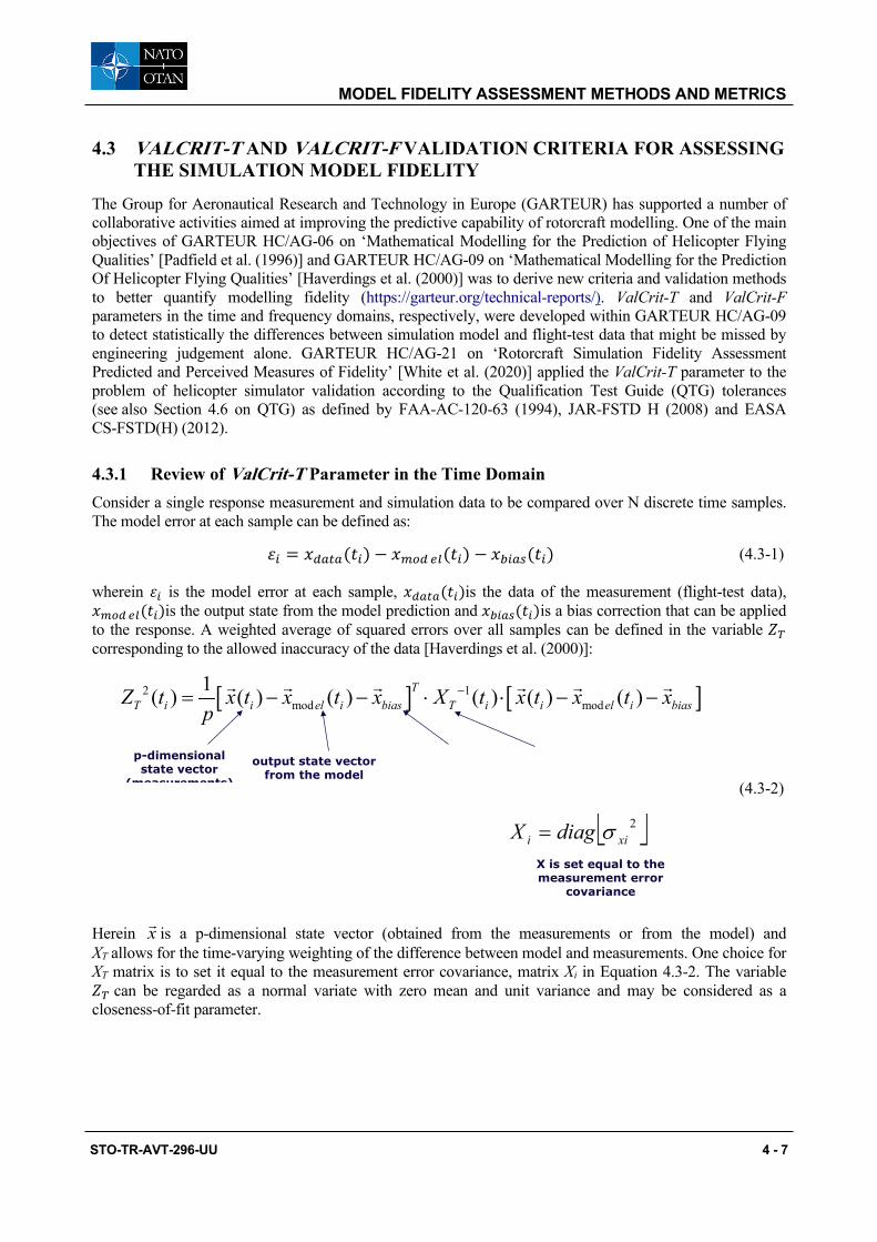
MODEL FIDELITY ASSESSMENT METHODS AND METRICS

STO-TR-AVT-296-UU 4 - 7

4.3 VALCRIT-T AND VALCRIT-F VALIDATION CRITERIA FOR ASSESSING THE SIMULATION MODEL FIDELITY

The Group for Aeronautical Research and Technology in Europe (GARTEUR) has supported a number of collaborative activities aimed at improving the predictive capability of rotorcraft modelling. One of the main objectives of GARTEUR HC/AG-06 on ‘Mathematical Modelling for the Prediction of Helicopter Flying Qualities’ [Padfield et al. (1996)] and GARTEUR HC/AG-09 on ‘Mathematical Modelling for the Prediction Of Helicopter Flying Qualities’ [Haverdings et al. (2000)] was to derive new criteria and validation methods to better quantify modelling fidelity (https://garteur.org/technical-reports/). ValCrit-T and ValCrit-F parameters in the time and frequency domains, respectively, were developed within GARTEUR HC/AG-09 to detect statistically the differences between simulation model and flight-test data that might be missed by engineering judgement alone. GARTEUR HC/AG-21 on ‘Rotorcraft Simulation Fidelity Assessment Predicted and Perceived Measures of Fidelity’ [White et al. (2020)] applied the ValCrit-T parameter to the problem of helicopter simulator validation according to the Qualification Test Guide (QTG) tolerances (see also Section 4.6 on QTG) as defined by FAA-AC-120-63 (1994), JAR-FSTD H (2008) and EASA CS-FSTD(H) (2012).

4.3.1 Review of ValCrit-T Parameter in the Time Domain Consider a single response measurement and simulation data to be compared over N discrete time samples. The model error at each sample can be defined as:

𝜀𝜀𝑖𝑖 = 𝑥𝑥𝑑𝑑𝑑𝑑𝑑𝑑𝑑𝑑(𝑡𝑡𝑖𝑖) − 𝑥𝑥𝑚𝑚𝑚𝑚𝑑𝑑 𝑒𝑒𝑙𝑙(𝑡𝑡𝑖𝑖) − 𝑥𝑥𝑏𝑏𝑖𝑖𝑑𝑑𝑠𝑠(𝑡𝑡𝑖𝑖) (4.3-1)

wherein 𝜀𝜀𝑖𝑖 is the model error at each sample, 𝑥𝑥𝑑𝑑𝑑𝑑𝑑𝑑𝑑𝑑(𝑡𝑡𝑖𝑖)is the data of the measurement (flight-test data), 𝑥𝑥𝑚𝑚𝑚𝑚𝑑𝑑𝑒𝑒𝑙𝑙(𝑡𝑡𝑖𝑖)is the output state from the model prediction and 𝑥𝑥𝑏𝑏𝑖𝑖𝑑𝑑𝑠𝑠(𝑡𝑡𝑖𝑖)is a bias correction that can be applied to the response. A weighted average of squared errors over all samples can be defined in the variable 𝑍𝑍𝑇𝑇 corresponding to the allowed inaccuracy of the data [Haverdings et al. (2000)]:

(4.3-2)

Herein is a p-dimensional state vector (obtained from the measurements or from the model) and XT allows for the time-varying weighting of the difference between model and measurements. One choice for XT matrix is to set it equal to the measurement error covariance, matrix Xi in Equation 4.3-2. The variable 𝑍𝑍𝑇𝑇 can be regarded as a normal variate with zero mean and unit variance and may be considered as a closeness-of-fit parameter.

[ ] [ ]2 1mod mod

1( ) ( ) ( ) ( ) ( ) ( )TT i i el i bias T i i el i biasZ t x t x t x X t x t x t x

p−= − − ⋅ ⋅ − −

p-dimensional state vector

(measurements)

output state vector from the model

2xii diagX σ=

X is set equal to the measurement error

covariance

x

MODEL FIDELITY ASSESSMENT METHODS AND METRICS

4 - 8 STO-TR-AVT-296-UU

A validation criterion in the time domain can be defined which consists in fact of a ‘performance’ scalar 𝐽𝐽𝑇𝑇, the so-called ValCrit-T parameter, with the following function,

𝑉𝑉𝑉𝑉𝑉𝑉𝑉𝑉𝑉𝑉𝑉𝑉𝑡𝑡 − 𝑇𝑇 = 𝐽𝐽𝑇𝑇 =1𝑁𝑁𝑍𝑍𝑇𝑇2(𝑡𝑡𝑖𝑖)𝑁𝑁

𝑖𝑖=1

(4.3-3)

where N is the number of time samples considered. For the response of a k parameter of a simulation model, ValCrit-T value corresponds to:

𝐽𝐽𝑘𝑘 =1𝑁𝑁𝜀𝜀𝑖𝑖𝑋𝑋𝑖𝑖

𝑁𝑁

𝑖𝑖=1

𝜀𝜀𝑖𝑖 (4.3-4)

where 𝑋𝑋𝑖𝑖 matrix becomes the identity matrix in the simpler case when unity weight is given to each sample. The single ValCrit-T value of Equation 4.3.-4 reduces to the average square error:

𝐽𝐽𝑘𝑘 =1𝑁𝑁𝜀𝜀𝑖𝑖2𝑁𝑁

𝑖𝑖=1

(4.3-5)

When p responses of the simulation model are considered, the ValCrit-T value becomes the aggregate value over all these responses:

𝑉𝑉𝑉𝑉𝑉𝑉𝑉𝑉𝑉𝑉𝑉𝑉𝑡𝑡 − 𝑇𝑇 = 𝐽𝐽𝑇𝑇 =1𝑝𝑝𝐽𝐽𝑘𝑘

𝑃𝑃

𝑘𝑘=1

=1𝑝𝑝𝑁𝑁

𝜀𝜀𝑖𝑖𝑘𝑘𝑋𝑋𝑖𝑖𝑘𝑘

𝑁𝑁

𝑖𝑖=1

𝜀𝜀𝑖𝑖𝑘𝑘

𝑃𝑃

𝑘𝑘=1

(4.3-6)

Consider next the set error samples as a set of N normal random variables. It follows that the term 𝐽𝐽𝑇𝑇𝑝𝑝𝑁𝑁 can be interpreted as a simulation error statistic that can be tested against a chi-squared distribution with pN degrees of freedom, denoted as 𝜒𝜒𝑁𝑁𝑁𝑁2 . The statistical significance of that error can be assessed by comparing it with a 𝜒𝜒𝑁𝑁𝑁𝑁2 function’s corresponding p-value (Figure 4.3-1). If we hypothesize that the test statistic 𝐽𝐽𝑇𝑇𝑝𝑝𝑁𝑁represents an insignificant simulation error, then this hypothesis is falsified if 𝐽𝐽𝑇𝑇𝑝𝑝𝑁𝑁 exceeds the value of z corresponding to a given threshold of the 𝜒𝜒𝑁𝑁𝑁𝑁2 cumulative distribution function. The values of 𝑝𝑝 for four qualitative levels of simulation error as recommended in GARTEUR HC/AG-09 [Haverdings et al. (2000)] are listed in Figure 4.3-1.

Figure 4.3-1: Test for Statistical Significance of ValCrit-T Metric and Their P-Value for Levels of Simulation Error as Proposed in GARTEUR HC/AG-09 [Haverdings et al. (2000)].

iε

1 p−

MODEL FIDELITY ASSESSMENT METHODS AND METRICS

STO-TR-AVT-296-UU 4 - 9

GARTEUR HC/AG-09 [Haverdings et al. (2000)] proposed boundaries for the J (cumulative) and Z (instantaneous) functions based on statistical tables for chi-square distribution. In this sense, ValCrit-T can be seen as a generalization of the integrated cost function described in Section 4.2.

For a simple application of ValCrit-T parameter, consider the assessment of a simulation model fidelity for a very simple manoeuvre, i.e., the first few instants during the helicopter transition from hover to forward flight after a step input of longitudinal cyclic pitch. One may assume that only a pitching motion of the helicopter occurs at the very beginning of this manoeuvre before forward speed builds up and begins to have an influence. The equation describing the pitching of the helicopter body (Figure 4.3-2) can be written as:

𝑞 = −𝑇𝑇𝐼𝐼𝑥𝑥

ℎ 𝑠𝑠𝑉𝑉𝑛𝑛(𝜃𝜃1𝑠𝑠 − 𝛽𝛽1𝑐𝑐) −𝑁𝑁

2𝐼𝐼𝑥𝑥𝐾𝐾𝛽𝛽(𝜃𝜃1𝑠𝑠 − 𝛽𝛽1𝑐𝑐) (4.3-7)

where q is pitch rate of the helicopter body, T is the rotor thrust force, 𝐼𝐼𝑥𝑥 is the mass moment of inertia around lateral axis, h is the vertical distance between the helicopter centre of gravity and rotor, N is the number of rotor blades, 𝜃𝜃1𝑠𝑠 is the longitudinal tilt of swashplate (cyclic stick displacement), and 𝛽𝛽1𝑐𝑐 is the longitudinal disc tilt w.r.t. plane of no-feathering. Regarding the rotor flap dynamics, if we assume that this can be represented through a time constant for flapping dynamics 𝜏𝜏𝑓𝑓, then this results in the following equation for the flapping dynamics w.r.t. no-feathering plane:

𝜏𝜏𝑓𝑓𝛽1𝑐𝑐 + 𝛽𝛽1𝑐𝑐 = −16𝛾𝛾𝑞𝑞𝛺𝛺

(4.3-8)

where γ is the Lock-number, and Ω is the angular speed of the rotor. Setting 𝜏𝜏𝑓𝑓 = 0 is equivalent with neglecting the transient flapping motion, assuming that the rotor flapping responds instantaneously to control inputs as well as to pitching motion and helicopter velocity.

Figure 4.3-2: Helicopter Pitch Motion After a Longitudinal Cyclic Pitch θ1s Step Input, Semi-Rigid Rotor Configuration.

MODEL FIDELITY ASSESSMENT METHODS AND METRICS

4 - 10 STO-TR-AVT-296-UU

Consider the numerical example of a helicopter with the following characteristics: mass m = 2,200 kg, rotor radius R = 7.32 m, rotor tip speed 𝛺𝛺𝛺𝛺 = 200 m/sec, Lock-number 𝛾𝛾 = 6, moment of inertia 𝐼𝐼𝑥𝑥 = 10,625 kg m2, distance h = 1 meter, semi-rigid rotor with Kβ = 460,000 Nm. Figure 4.3-2 presents the helicopter body pitch response as given by Equation 4.3-7 to a 1-degree step input in longitudinal cyclic pitch without and with rotor flapping dynamics as given by Equation 4.3-8. The right-hand side of Figure 4.3-2 presents the helicopter pitch rate response plotted within the Qualification Test Guide (QTG) tolerances of ±3-deg pitch rate as given in the simulator qualification standards FAA-AC-120-63 (1994), JAR-FSTD H (2008) and EASA CS-FSTD(H) (2012). The QTG tolerances represent acceptable differences between the simulation model results and the flight-test data. These are typically within ±10% for flight model. Two simulation models have been considered for understanding the ValCrit-T concept: 1) a 1-DOF “Baseline model” which is the simulation model containing only pitch Degree of Freedom (DOF) in Equation 4.3-7 with no flapping dynamics added to the model; and 2) a 2-DOF “Enhanced model” containing the helicopter body pitch motion in Equation 4.3-7 and the first order flapping dynamics in Equation 4.3-8 with 𝜏𝜏𝑓𝑓 = 0.14 𝑠𝑠𝑒𝑒𝑠𝑠−1 this value of 𝜏𝜏𝑓𝑓 sets the simulation model to the upper boundary of allowed QTG tolerance). Looking at Figure 4.3-2, one can see that the addition of first order rotor flapping dynamics as given by the time constant 𝜏𝜏𝑓𝑓 does influence the helicopter response rather profoundly. The enhanced model is now at the limit of the allowed QTG boundary, and this probably will be noticed by the pilot in the simulator.

The ValCrit-T parameter can be next calculated for the Baseline model and Enhanced model of the helicopter pitch response (see Equation 4.3-6), assuming that the QTG boundaries are the flight-test data. This will be performed in two ways: 1) Including the model error of helicopter pitch angle response 𝜀𝜀𝑖𝑖𝑖𝑖; and 2) Including the model error of both pitch angle 𝜀𝜀𝑖𝑖𝑖𝑖 and pitch rate 𝜀𝜀𝑖𝑖𝑖𝑖 responses. Figure 4.3-3 presents the variance of the model pitch error w.r.t. the boundaries of Moderate J (p-value = 0.05) according to the Figure 4.3-1, i.e., when 𝐽𝐽𝑇𝑇 tends to unity (the variance of the model error becomes close to the allowable error). From this figure, it is apparent that 𝐽𝐽𝑇𝑇 is sensitive to the number of time samples considered in the 𝐽𝐽𝑇𝑇 calculation: the larger the number of degrees of freedom included in the model, the more the values of 𝐽𝐽𝑇𝑇 tend to unity (the variance of the model error gets close to the allowable error). When too large, the quality of the model fit becomes poor. Thus, only when considering both the pitch angle and pitch rate in the helicopter responses, can one capture the fact that the pitch rate is approaching the simulator tolerances (around second 0.3 sec). It can be concluded that the ValCrit-T can be used to quantify and compare the relative statistical significance of errors between two models, but it cannot be interpreted as an absolute metric of model quality. This might suggest a correlation between the ValCrit-T metric and tolerances used in the flight simulator standards for validation of simulator mathematical models. Also, it might suggest correlation with the integrated cost function described in Section 4.2.

Figure 4.3-3: ValCrit-T Parameter for the Helicopter Pitch Response.

0 0.1 0.2 0.3 0.4 0.5 0.6 0.7 0.8 0.9 10

0.2

0.4

0.6

0.8

1

time(sec)

JTpa

rt pitc

h

0 6

0.8

1

t

Moderate J

MODEL FIDELITY ASSESSMENT METHODS AND METRICS

STO-TR-AVT-296-UU 4 - 11

Concerning the effect of data noise on ValCrit-T parameter, according to Haverdings et al. (2000), ValCrit analysis places bounds on acceptable levels of combined model error and data noise. The effect of data noise on ValCrit-T analysis was studied by GARTEUR HC/AG-21 [White et al. (2020)] by introducing Gaussian white noise of different levels to the flight-test data in the QTG tests. It was concluded that sometimes the data noise cancelled instantaneous model errors randomly over a large number of time samples, and therefore, ValCrit-T could not draw sufficient conclusions about the model fidelity response. This confirmed that ValCrit-T is a metric for the combination of model fidelity and data quality as suggested by Haverdings et al. (2000). The variance of the ValCrit-T distribution increased with noise amplitude. In the lowest noise amplitude cases studied, there remained a 10% probability that the noisy data ValCrit-T value fell below the clean-data value.

In conclusion, the following statements can be drawn about the ValCrit-T parameter:

1) ValCrit-T is a useful metric for quantifying and comparing the relative statistical significance of errors between two models.

2) ValCrit-T is not an absolute metric of model quality.

3) Both the mean and variance of the distribution of ValCrit-T results increases with data noise amplitude.

4) To obtain reliable results of a comparative study of model variants, the truth data used as a basis for ValCrit-T should be as free of noise as possible.

5) ValCrit-T could be used to place bounds on acceptable data noise amplitude.

4.3.2 Review of ValCrit-F Parameter in the Frequency Domain Same as ValCrit-T in the time domain and in the frequency domain, GARTEUR HC/AG-09 introduced a very similar validation criterion, the so-called ValCrit-F parameter:

𝑉𝑉𝑉𝑉𝑉𝑉𝑉𝑉𝑉𝑉𝑉𝑉𝑡𝑡 − 𝐹𝐹 = 𝐽𝐽𝐹𝐹 =1𝑁𝑁𝑍𝑍𝐹𝐹2(𝜔𝜔𝑖𝑖)𝑁𝑁

𝑖𝑖=1

(4.3-9)

where the variable to be summed in the frequency domain is:

(4.3-10)

MODEL FIDELITY ASSESSMENT METHODS AND METRICS

4 - 12 STO-TR-AVT-296-UU

As such, one may specify statistical boundaries for 𝐽𝐽𝐹𝐹 to exceed a certain value and hence, have a certain model quality because 𝐽𝐽𝐹𝐹 exactly as 𝐽𝐽𝑇𝑇 relates to the chi-squared statistic as follows:

𝑉𝑉𝑉𝑉𝑉𝑉𝑉𝑉𝑉𝑉𝑉𝑉𝑡𝑡 − 𝐹𝐹 = 𝐽𝐽𝐹𝐹 =1𝜈𝜈𝜒𝜒𝐹𝐹2(𝜔𝜔𝑖𝑖)𝑁𝑁

𝑖𝑖=1

(4.3-11)

where 𝜈𝜈 = 𝑝𝑝𝑁𝑁 is the number of degrees of freedom. Exactly as for the 𝐽𝐽𝑇𝑇, the corresponding values for 𝐽𝐽𝐹𝐹can be derived for defined values of probabilities of exceedance. Quality-of-fit indicators related to exceedance values of α are excellent (α = 0.5), good (α = 0.1), moderate (α = 0.5), or poor (α = 0.01) (see Figure 4.3-1). The values for 𝑍𝑍𝐹𝐹 are based on a two-tailed probability as 𝑍𝑍𝐹𝐹 may be both positive and negative, i.e., the null-hypothesis tested is:

𝐻𝐻0𝑍𝑍𝐹𝐹 > 𝑔𝑔 𝑜𝑜𝑉𝑉 𝑍𝑍𝐹𝐹 < −𝑔𝑔 = 𝐻𝐻0|𝑍𝑍𝐹𝐹| > 𝑔𝑔 𝐻𝐻0𝑍𝑍𝐹𝐹 > 𝜙𝜙 𝑜𝑜𝑉𝑉 𝑍𝑍𝐹𝐹 < −𝜙𝜙 = 𝐻𝐻0|𝑍𝑍𝐹𝐹| > 𝜙𝜙

(4.3-12)

For the frequency domain, GARTEUR HC/AG-09 used for each frequency a maximum allowable error of 10 percent (95th percentile) of the gain and 20 degrees error (also 95th percentile) in phase angle, i.e.,

𝑋𝑋𝑔𝑔𝑖𝑖(𝜔𝜔) = (0.1 × 1.645)𝑑𝑑𝑉𝑉𝑉𝑉𝑔𝑔⌊𝑔𝑚𝑚𝑚𝑚𝑑𝑑 𝑒𝑒𝑙𝑙(𝜔𝜔𝑖𝑖)𝑔𝑚𝑚𝑚𝑚𝑑𝑑 𝑒𝑒𝑙𝑙𝑇𝑇 (𝜔𝜔𝑖𝑖)⌋ 𝑋𝑋𝜙𝜙(𝜔𝜔) = 3.183

(4.3-13)

The factor of 1.645 in Equation 4.3-13 stems from conversion of the 95th percentile value to standard deviation.

In conclusion, in combination with the ValCrit-T parameter, which was defined to quantify and compare the relative statistical significance of errors between models and flight-test data, ValCrit-F could be included in the analysis for a complete understanding of the model fidelity.

4.4 PHASE/GAIN ERRORS IN MOTION CUES

If a helicopter simulation model is not only used for analysis but also in a pilot-in-the-loop simulator, any model fidelity deficiencies might be masked or exacerbated by the simulator’s cueing systems. While outside, visual instrument and force feel cueing systems usually distort the helicopter’s dynamics with little more than a time delay; a simulator’s motion system can introduce more elaborate distortions of the perceived helicopter dynamics. This is caused by the inherently limited motion space of a ground-based simulator and the motion cueing algorithms that are necessarily deployed to transform the model’s motion cues into physical motions of the simulator. This section of the report explores how the phase and gain errors of a simulator’s motion system can influence the overall perceived fidelity of the simulation.

In general, a human pilot’s vestibular system is sensitive to the specific forces, rotational rates, and accelerations of the helicopter. Similar to an accelerometer, a human directly perceives the aerodynamic, engine, and landing gear forces acting on the helicopter. These cues play a number of roles in a piloted simulation:

• They provide the pilot with additional signals to stabilise and control their aircraft. Especially for unstable vehicles such as (un-augmented) helicopters, the phase lead present in the motion cues with respect to the visual position and attitude cues helps to increase the phase margin of the closed-loop system.

• They signal to the pilot that certain important events or state changes are occurring in the vehicle. An example is the vibrations associated with Effective Translational Lift (ETL), providing timing signals to help when performing the landing flare [Miller et al. (2009)].

MODEL FIDELITY ASSESSMENT METHODS AND METRICS

STO-TR-AVT-296-UU 4 - 13

• Motion cues help create an immersive virtual environment that elicit realistic pilot behaviour. High levels of behavioural fidelity improve training effectiveness and engineering and scientific simulator validity.

• Apart from providing cues that help the pilot perform their task, physical motion can also be detrimental to task performance, e.g., vibrations impacting touchscreen effectiveness. Such effects must in some cases be replicated in the simulator.

Multiple techniques exist to provide physical motion cues to the simulator pilot. The most common type of motion system moves the simulator cab as a whole in one or more degrees of freedom. In helicopter simulators, sometimes a dedicated in-cabin motion platform moves part of the cabin, such as the seat. Additionally, dynamic seats can move parts of the pilot seat independently to give an illusion of motion, e.g., moving the lumbar support to signal sustained specific force cues through independent actuation of seat backpad surge and sway and seat pan cushion and seat bucket heave degrees of freedom. A common whole-cabin motion system is based on the Gough-Stewart 6-degree-of-freedom mechanism [Stewart (1965)].

The motion base’s cueing algorithm, which converts the simulated vehicle’s cues to simulator motions, must achieve two competing goals: provide realistic cues to the pilot and keep the simulator in the available motion space. Many motion cueing algorithms exist (most of them proprietary), but the underlying mechanisms are usually similar to the UTIAS Classical Washout Algorithm described by Reid and Nahon (1985). In this algorithm, the translational specific forces and rotational accelerations go through their own high-pass filter channels, and a special cross-coupling is made (“tilt coordination”) by which sustained, low-frequency surge and sway cues can be simulated by tilting the simulator and using gravity to cue the specific force.

In both the rotational and translational channels, it is important to note that in essence, the algorithm employs high-pass filters. This means for frequencies that the filter (starts to) attenuates the motion, a phase lead is present. At higher frequencies (e.g., greater than 10 rad/s), phase lag will mostly be present due to the motion base’s inertia and control system.

The parameters used in the motion cueing algorithm (which essentially define the phase and gain cueing), can significantly affect the simulator’s motion fidelity. As such the simulator engineer has some freedom to shape or tune the motion response to the requirements for a certain application. The freedom is, of course, limited by the available motion envelope of the platform (governed by design and size) and the detrimental effects of false cues inherent to the algorithm.

4.4.1 Motion Cueing for Different Simulator Applications Flight simulators are used for pilot training and currency checking and as engineering tools within industry. In general, a simulator used to train pilots in ab-initio or type conversion situations must support the acquisition of flying skills that transfer successfully to real flight. In an engineering application, the simulator is used to gather relevant data on the real-world behaviour of the aircraft-pilot combination. The validity of this engineering data is highly dependent on both the simulator (model) fidelity and the adaptation of the pilot’s behaviour and control strategy. The four roles of motion cueing identified earlier impact these applications in different ways.

For the closed loop use of motion cues, if a certain aircraft requires the use of motion cues to control it in real flight, the training simulator should present these cues in a way that provides positive transfer of training. This usually involves accurately cueing the vehicle’s motion states in terms of amplitude and phase. If the training simulator is used to check a pilot’s proficiency, their capabilities to safely operate the real aircraft should be accurately reflected in their performance in the simulator. In both cases, if the pilot has to adapt their control behaviour (control gain, phase lead generation, etc.), the usefulness of the simulator will diminish.

MODEL FIDELITY ASSESSMENT METHODS AND METRICS

4 - 14 STO-TR-AVT-296-UU

A similar argument can be made for the motion system’s role as a signalling device. The simulator should replicate the relevant signalling cues to provide good training and fair proficiency assessment but not necessarily through accurate reproduction of cues from the vehicle model. The use of “special effects” in the form of appropriately scaled and timed vibrations, or other signals implemented directly to the motion base, can increase the training simulator’s usefulness without having to fully model the relevant phenomena or pass them through the cueing algorithm without distortion.

The immersive contribution of motion cues can increase the believability of the training simulator and induce a ‘suspension of disbelief’ in the trainee pilot, leading to a learning situation that is close to real flight operations. For this purpose, the occurrence of immersion breaking false cues should be minimized, including distracting magnitude and phase errors, noticeable washout effects, and objectionable motion base deficiencies (noise, latency, cross-talk, etc.).

In the case where motion impedes the pilot’s performance, the training simulator can increase their workload to real-world levels by replicating those cues. In helicopter applications, the major type of motion in this category would be vibratory loads from the rotor to the flight deck. As with the signalling cues, these cues might not be fully physically modelled but representatively “hard-coded” into either the general motion base or possibly a dedicated high frequency vibration platform.

Engineering simulators are used to design and develop systems and equipment for new aircraft designs. The purpose of engineering simulators is to gather data from experienced test pilots immersed in the most realistic representation of the design alternatives under consideration. Hence, physical correspondence between motion cues in engineering simulators and actual aircraft is clearly valuable when it improves simulator handling qualities fidelity.

4.4.2 Motion Cueing Fidelity Assessment Techniques In any tuning environment, it is important to specify the metric used to evaluate the tuning process’ outcome. In many simulator applications, this metric will be related to the simulator’s fidelity or ability to mimic a vehicle’s flight. A combination of objective and subjective techniques is used to assess the fidelity of simulator’s motion system as a whole. The application of assessment techniques varies based on the application, predominantly regulatory or research purposes. In both Europe (EASA) and the USA (FAA), specific requirements are given to assess the suitability of simulation devices for pilot training aspects [EASA CS-FSTD(H) (2012) and FAA-AC-120-63 (1994)]. Taking the example of the EASA guidance, for helicopters, these cover three broad areas: hardware and software capablilities (through robotic tests), repeatability, and vibrations. However, it is acknowledged that the current test pracitices do not explicitly show the capability of the system to adequately cue the pilot. It is stated, ‘until there is an objective procedure for determination of the motion cues necessary to support pilot tasks and stimulate the pilot response that occurs in an aircraft for the same tasks, motion systems should continue to be “tuned” subjectively’ [EASA CS-FSTD(H) (2012)]. As such, no attempt is currently made to regulate the motion cueing algorithms, or their tuning based upon objective methods. Here, there is a large emphasis on the subjective opinion of the assessing pilot, which is always a combination of the complete system (perceptual fidelity). If we consider the high quality of modern motion base hardware, the largest phase and gain errors in the perceived motion cues are now caused by these unregulated algorithms, which leaves the motion cueing errors largely outside of regulatory control.

Despite the lack of use for training simulation devices, over the years, a number of techniques to objectively quantify motion cueing quality have been proposed and validated to some extent. Here, an overview of some of the methods often used is given, supplemented with some recent work to illustrate directions of research currently being explored. A more elaborate overview is provided by Jones (2017), who focuses specifically on helicopter simulation and also proposes an optimization approach for motion tuning.

MODEL FIDELITY ASSESSMENT METHODS AND METRICS

STO-TR-AVT-296-UU 4 - 15

The first objective motion cueing criteria was developed by Sinacori (1977), who identified a metric of the cueing response that specifies a level of fidelity of the resulting cues. This well-established metric examines the phase and magnitude of the cueing algorithm at 1 rad/sec and categorizes it in one of three fidelity levels (low, medium, and high). Schroeder (1999) later refined the limits based on helicopter tests in the NASA Ames Vertical Motion Simulator (VMS) (see Figure 4.4-1). The VMS’s large vertical and horizontal travel allowed Schroeder to develop baseline tasks incorporating one-to-one motion without encountering motion envelope limits. Schroeder then developed the Modified Sinacori Criteria [Schroeder (1999)] for rotational and translational motion. To date, this method is the most commonly applied to rotorcraft simulation devices. Reardon et al. (2014), for example, developed an indirect motion fidelity criterion varying the motion filter parameters from Schroeder’s experiment and using the subjective Simulation Fidelity Rating (SFR) scale (for more details on SFR scale the reader should consult Section 4.5).

Figure 4.4-1: Sinacori/Schroeder Motion Fidelity Criteria [Schroeder (1999)].

It is acknowledged that there exist limitations of the assessment method as developed by Sinacori/Schroeder. To increase the (frequency) range over which the motion cueing is evaluated and thereby creating a more comprehensive evaluation than the Sinacori/Schroeder criteria, the International Civil Aviation Organization (ICAO) has proposed the Objective Motion Cueing Test (OMCT) [Advani and Hosman (2006), Advani et al. (2007), Hosman and Advani (2012)]. This test works by independently exciting each degree of freedom of the motion base at frequencies varying from 0.1 to almost 16 rad/s and examining the corresponding motion outputs (main effect) as well as some unwanted cross-couplings (false cues). It examines these responses in the frequency domain to effectively generate a frequency response function of the combination of the motion cueing algorithm’s software and the motion base’s hardware. As such, it fits well with the common practice of investigating the helicopter’s model as a transfer function in the frequency domain. Dalmeijer et al. (2017) extended the OMCT to measure rotorcraft motion characteristics. An example of fidelity envelopes derived from a study involving 10 simulators used for fixed-wing aircraft (both training and research) is shown in Figure 4.4-2. The fidelity envelope was defined by taking the highest and lowest settings from the group of simulators (following extraction of outliers).

As an example of the OMCT, some typical results (in blue) are shown in Figure 4.4-3. The recommended boundaries are shown in red [Li (2016)]. The surge due to surge test (Figure 4.4-3, left-hand side) shows how the high-pass filter at high frequencies, and the tilt coordination at low frequencies work together to provide reasonably scaled and phase-distorted longitudinal specific force cues. The rotation needed to provide the tilt coordination generates a false cue that is assessed in the pitch due to surge test (Figure 4.4-3, middle). For the heave (vertical) specific force test, the cueing algorithm’s 3rd order high-pass characteristics are clearly visible as low-frequency attenuation and phase lead up to 270 degrees.

MODEL FIDELITY ASSESSMENT METHODS AND METRICS

4 - 16 STO-TR-AVT-296-UU

Figure 4.4-2: Example of OMCT Fidelity Boundaries, Roll Motion Gain and Phase [Jones (2018)].

Figure 4.4-3: Objective Motion Cueing Test OMCT [Li (2016)].

To validate and refine the boundaries in the OMCT plots, Zaal et al. (2018) has recently performed a number of fixed-wing simulator experiments on NASA’s Vertical Motion Simulator. For a number of flying tasks, objective and subjective performance as well as cueing quality metrics were gathered for different motion cueing configurations, both within and outside of the previously defined boundaries. The resulting refined boundaries could form the basis for FAA fixed-wing regulations in the future. Similar rotorcraft efforts would be helpful to define standards for both engineering and pilot training.

Studies reported in Hodge et al. (2015a), Hodge et al. (2015b), and Jones et al. (2017) suggested large differences between perceived motion fidelity and objective fidelity using Sinacori/Schroeder boundaries. Both studies found beneficial and representative motion was attained when performing typical mission task elements performed by rotorcraft. The tests were conducted in two simulation facilities with independent pilots and simulation settings. The reservations are confirmed when one compares the acceptable required fidelity for current OMCT and Schroeder metrics. Figure 4.4-4 shows the difference between rotational requirements, plotted on the gain-phase plot. Using the Schroeder approach, the same boundaries are used to assess pitch, roll, and yaw dynamics. For the OMCT boundaries, a range of boundaries are presented. Both acceptable roll and yaw requirements do not reflect Schroeder boundaries. Meanwhile, pitch boundaries are more stringent. As a result of these discrepancies, further research is required in this area prior to the adoption of OMCT as an objective method to assess rotorcraft training simulators. For example, Miletović et al. (2018) proposed novel motion cueing fidelity criteria for rotorcraft flight simulation.

In additional research investigations conducted by Jones et al. (2017), further motion cases were tested to determine initial OMCT fidelity boundaries specifically for rotorcraft simulation. During these investigations, the differences between current OMCT boundaries and perceived fidelity was again confirmed. Like results

10-1

100

101

102

10-2

10-1

100

101 OMCT surge test 6

frequency [rad/s]

mag

nitu

de [-

]

10-1

100

101

102

-200

-100

0

100

200

frequency [rad/s]

phas

e [d

eg]

10-1

100

101

102

10-4

10-2

100

102 OMCT surge cross test 7

frequency [rad/s]

mag

nitu

de [m

s2 /de

g]

10-1

100

101

102

-400

-200

0

200

frequency [rad/s]

phas

e [d

eg]

10-1

100

101

102

10-4

10-2

100 OMCT heave test 10

frequency [rad/s]

mag

nitu

de [-

]

10-1

100

101

102

-100

0

100

200

300

frequency [rad/s]

phas

e [d

eg]

OMCT heave due to heave

MODEL FIDELITY ASSESSMENT METHODS AND METRICS

STO-TR-AVT-296-UU 4 - 17

from previous studies, the investigation showed a clear preference for low phase errors in the motion system. This was even for cases with very low motion gain. Three pilots participated in the study and stated that motion cueing with high phase errors led to significant false cues, sickness, and adversely affected performance. Pilots were clearly able to consistently recognise motion configurations. Adverse motion cues led to a reduction in task aggression (thereby, suppressing false cues). During completion of typical ADS-33 manoeuvres, this led to an increase in task completion time.

Figure 4.4-4: Comparison of Current Boundaries for OMCT and Schroeder Metrics [Jones et al. (2017)].

As stated above, particularly for training simulators and from the view of the regulator, there is a reliance upon subjective opinion. To ensure acceptability of a flight simulator for either engineering or training purposes, the end user’s subjective assessment of its fidelity cannot be ignored. In addition, many of the objective motion cueing quality metrics have been validated by expert pilot opinion with varying levels of success. Pilot opinion still remains the standard against which motion cueing quality is measured.

To standardize and streamline subjective assessments a number of techniques have been used, which will be introduced in this section. Some have already found use outside their academic origins while others are still being developed. The most common technique takes the form of a rating scale, similar to the Cooper-Harper Rating Scale [Cooper and Harper (1969)] for handling qualities assessments in combination with one or more standardized manoeuvres, e.g., from ADS-33E (2000).

The University of Liverpool and the German Aerospace Centre (DLR) have worked on defining both a Motion Fidelity Rating scale and a more general Simulator Fidelity Rating scale (Figure 4.4-5). These scales were validated with experienced test pilots in respective simulators.

In industry, Miller et al. (2009) added numerical ratings to the Simulator Motion Fidelity scale developed by Schroeder to allow finer grading of motion fidelity within the high, medium, and low fidelity rating levels as shown in Table 4.4-1 during motion system tuning.

MODEL FIDELITY ASSESSMENT METHODS AND METRICS

4 - 18 STO-TR-AVT-296-UU

Figure 4.4-5: Motion Fidelity Rating Scale (Right-Hand Side Figure from Hodge et al. (2015a) and Hodge et al. (2015b); Left-Hand Side Figure from Jones et al. (2017).

Table 4.4-1: Modified Simulator Motion Fidelity Scale Used in Industry [Miller et al. (2009)].

4.4.3 Motion Cueing and Model Gain and Phase Errors Helicopter modelling errors can be characterised by gain and phase errors, as evident from this report. The Sinacori/Schroeder and OMCT motion cueing metrics show that the motion cueing algorithms of a simulator by themselves also introduce gain and phase errors. These additional cueing errors might alleviate or bring forward any errors in the model part of the simulator.

One way to look at the severity of model gain and phase errors is the concept of MUAD/AEE (see Section 4.1). The noticeability of model errors by a pilot might change depending on the characteristics of the simulator used, the flying task, pilot strategy, or some feature of the baseline model. As discussed in Section 4.1.2, Mitchell et al. (2006b) proposed AEE boundaries for the roll axis based on an experiment on a fixed-base simulator and a single experienced pilot. Penn (2013) later replicated this experiment at Delft University with three pilots on two different simulators: a fixed-base helicopter simulator (Helicopter Pilot Station, HPS at the National Aerospace Centre NLR in The Netherlands), and a generic motion simulator (SIMONA Research Simulator (SRS) at the Delft University TU Delft). It is highly likely that at least some of the differences he found in the MUAD boundaries between the simulators can be attributed to the influence of the presence of motion cueing on the SRS.

4.4.4 Conclusion Simulator motion cueing introduces phase and gain errors that have an impact on the perceived helicopter response that is comparable to the model errors described in earlier chapters. By tuning the motion cueing parameters, these errors can, to an extent, be reduced. Some metrics to help in this process are available but should be used with care.

Motion sensations like those of flight.

Motion Sensations are noticeably different from flight, but not objectionable.

Motion sensations are noticeably different from flight and objectionable.

High (7-9)

Medium (4-6)

Low (1-3)

Fidelity Rating Definition

MODEL FIDELITY ASSESSMENT METHODS AND METRICS

STO-TR-AVT-296-UU 4 - 19

While established and easy to apply, Sinacori/Schroeder boundaries do not fully predict the motion fidelity of modern simulation devices. They were developed using hardware and software not representative of current state-of-the-art simulation devices. Cueing environment of current simulators is much more realistic. Particularly the visual cueing offers ‘motion cues’ far surpassing those used to define the criteria. The original tests did not account for the complex high-pass adaptive filtering of modern systems.

The OMCT method provides a more modern and comprehensive picture, but it has no defined boundaries for tuning rotorcraft flight simulators. Boundaries developed from fixed-wing simulators were found to result in poor motion fidelity when performing rotorcraft mission tasks. This reflects the difference in roles and utilization of the vehicles.

In general, it is good to keep in mind that cueing, and especially motion cueing, in the simulator can have a significant impact on (part of) the helicopter dynamics as perceived by the pilot. Before putting in large efforts to reduce the last small modelling errors, it is advisable to assure that these improvements are not overshadowed by remaining motion cueing errors in the final simulator.

4.5 SIMULATION FIDELITY RATING SCALE – BACKGROUND

The evaluation of the fidelity of a simulation device for flight training typically includes a series of quantitative requirements contained within simulator qualification documents such as EASA CS-FSTD(H) (2012) or FAA 14 Part 60 (2016). These quantitative requirements examine the response or behaviour of the individual elements of a simulation device – the visual system, the motion platform (if so equipped), the flight dynamics model, etc. – to a set of predetermined inputs. The results of these tests are typically termed ‘engineering fidelity’ and only partially serve to characterise the utility of a simulator. The implicit assumption in tests of engineering fidelity is that a strong quantitative match of simulator component systems with the flight vehicle will assure a high degree of simulator utility. Experience has shown that this assumption is not always valid, and that tests of engineering fidelity are insufficient to guarantee a sufficiently accurate simulation. Hence, the qualification standards require a piloted, subjective assessment of the simulation in addition to the quantitative elements. These subjective tests ‘[arise] from the need to confirm that the simulation has produced a totally integrated and acceptable replication of the helicopter’ [EASA CS-FSTD(H) (2012)]. However, the guidance provided in the qualification documents regarding the approach taken to subjective evaluations is very limited. Section AMC1 FSTD(H).300, paragraph ( C ) Functions and Subjective tests (2) Test requirements (iv) of Book e EASA CS-FSTD (2012) states:

When evaluating functions and subjective tests, the fidelity of simulation required for the highest level of qualification should be very close to the helicopter. However, for the lower levels of qualification the degree of fidelity may be reduced in accordance with the criteria (within the document).

This requirement is poorly defined, and potentially open to interpretation by the operator and qualifying body. The work undertaken in GARTEUR HC/AG12 [Pavel et al. (2013)] suggests that the existing requirement for the subjective aspect of simulator qualification is unsatisfactory and should be improved. Hence, the Simulation Fidelity Rating (SFR) [Perfect et al. (2014)] was developed at the University of Liverpool in collaboration with the National Research Council of Canada to provide a repeatable, prescriptive method for the subjective assessment of fidelity into the overall qualification process.

The SFR scale should be used to complement and augment the existing simulator evaluation processes of CS-FSTD(H) and other applicable simulator qualification processes. It is proposed that the SFR scale may be used as part of a fidelity evaluation methodology based on the use of engineering metrics for both the prediction of the fidelity of the individual simulator components (flight model, motion platform, visual system, etc.) [Perfect (2014)] and the assessment of the perceptual fidelity of the integrated simulation system as experienced by the pilot.

MODEL FIDELITY ASSESSMENT METHODS AND METRICS

4 - 20 STO-TR-AVT-296-UU

4.5.1 Structure of the SFR Scale The SFR scale employs several key concepts that are considered fundamental to the utility of a simulation device. They are as follows:

• Transfer of Training (ToT) – the degree to which behaviours learned in a simulator are appropriateto flight.

• Comparative Task Performance (CTP) – comparison of the precision with which a task is completedin flight and simulator.

• Task Strategy Adaptation (TSA) – the degree to which the pilot is required to modify theirbehaviours when transferring from simulator to flight and vice versa.

The relationship between task performance and strategy adaptation is similar to that between performance and compensation in a handling qualities evaluation. In the Handling Qualities Rating (HQR) scale [Perfect (2014)], the expectation is that the pilot’s perception of deteriorating performance will stimulate higher levels of compensation, indicative of worsening Handling Qualities (HQ). While this correlation can be expected in measuring HQ, in the context of fidelity assessment, task performance and adaptation will not necessarily change in correlation with each other but will instead depend on the nature of the fidelity deficiencies present in a simulator.

A matrix presenting all possible combinations of comparative performance and task strategy adaptation was constructed (Figure 4.5-1); this was used to form the basic structure of the SFR scale (Figure 4.5-2).

Comparative Performance

Equivalent Similar Not Similar

Stra

tegy

Ada

ptat

ion

Negligible LEVEL 1

Full Transfer of Training

(SFR 1-2)

Minimal

Moderate LEVEL 2

Limited Transfer of Training

(SFR 3-6)

Considerable

Excessive

LEVEL 3

Negative Transfer of Training

(SFR 7-9)

Figure 4.5-1: SFR Fidelity Matrix [Perfect et al. (2014)].

Each of the ratings SFR = 1 to SFR = 9 corresponds to a region in the fidelity matrix. An SFR = 10 rating indicates a simulation that is entirely inappropriate for the purpose, so comparisons with flight cannot be made. As with the HQR scale, boundaries have been defined between the potential combinations of comparative performance and adaptation, reflecting value judgements on levels of fidelity. As the SFR worsens through each level, it can be seen from Figure 4.5-1 that the individual comparative performance and adaptation measures may not degrade in a progressive manner. However, the intention is that the overall ‘experience’ of the simulation fidelity degrades progressively as the SFR worsens.

MODEL FIDELITY ASSESSMENT METHODS AND METRICS

STO-TR-AVT-296-UU 4 - 21

Figure 4.5-2: Simulation Fidelity Rating Scale [Perfect et al. (2014)].

4.5.2 SFR Scale Terminology The SFR scale has been designed to evaluate a simulator on a task-by-task basis. Consequently, where fidelity defines fitness for purpose, a collection of ratings for various Mission Task Elements (MTE) would define the boundaries of positive training transfer for a given simulator. This is similar to the approach adopted by an International Working Group led by the Royal Aeronautical Society that has been revising and updating the existing training simulator certification standards; in the new framework of ICAO 9625 (2015), the required complexity for each of the simulation components is based on the tasks that will be trained.

The first definition that must be made prior to the commencement of fidelity assessment with the SFR scale is that of the purpose of the simulator. The purpose describes the range of tasks to be flown using the simulator and hence, the scope of the SFR evaluations. Each task identified in this step would be assessed on an individual basis; the results for each task would then be used to create a ‘usage envelope,’ within which the simulator may be effectively (and safely) employed.

In the context of a training simulator, the definition of the levels of fidelity has been made relative to the Transfer of Training (ToT) that occurs when a pilot transitions between the simulator and the aircraft. It should be noted that in assigning the level of fidelity, the evaluating pilot is being asked to make a subjective judgement on the degree of ToT that is likely to take place. For the SFR scale, the definition of the four levels of fidelity depends on the objective of the training. Three types of simulation training have been defined – skills acquisition, skills development, and skills assessment, where acquisition and development would correspond to the processes of initial training and recurrent training, respectively. For skills acquisition, the levels have been defined as follows:

• Level 1 fidelity: Simulation training is sufficient to allow operational performance to be attained with minimal pilot adaptation. There is complete ToT from the simulator to the aircraft in this task.

• Level 2 fidelity: Additional training in the aircraft would be required in order to achieve an operational level of performance. There is limited positive ToT from the simulator to the aircraft in this task but no negative ToT.

MODEL FIDELITY ASSESSMENT METHODS AND METRICS

4 - 22 STO-TR-AVT-296-UU

• Level 3 fidelity: Negative ToT occurs (i.e., the pilot learns an inappropriate technique), and the simulator is not suitable for training to fly the aircraft in this task.

Similarly, the levels for skills development have been defined as:

• Level 1 fidelity: Simulation training is sufficient to restore previous performance capabilities.

• Level 2 fidelity: Simulation training provides limited improved performance capability. Additional training is required.

• Level 3 fidelity: No positive ToT occurs. The simulator is unsuitable for training.

And the levels for skills assessment are defined as:

• Level 1 fidelity: Simulation is sufficient to comprehensively demonstrate skills associated with qualified performance.

• Level 2 fidelity: Performance in the simulator demonstrates limited elements of the required skills.

• Level 3 fidelity: Performance in the simulator does not serve to demonstrate the required skills.

Please note that in each of these cases, a Level 4 fidelity rating indicates that it is not even possible to complete the task using the simulator.

The task may be defined as the training manoeuvre/procedure, accompanied by a set of performance requirements and environmental conditions. In an HQR evaluation, an MTE specification consists of the target manoeuvre profile alongside a set of ‘desired’, and ‘adequate’ performance tolerances for each element of the manoeuvre profile (height, airspeed, heading, etc.), where the achievement of a certain category of performance assists the pilot with determining the level of handling qualities of the aircraft. The same style of task definition is adopted for an SFR evaluation. The comparison of the achieved level of performance between flight and simulator assists the evaluating pilot with the judgement of comparative performance. The three levels of comparative performance have been defined as follows:

• Equivalent performance: The same level of task performance (desired, adequate, etc.) is achieved for all defined parameters in simulator and flight. Any variations in performance are small.

• Similar performance: There are no large single variations in task performance, or there are no combinations of multiple moderate variations across the defined parameters.

• Not similar performance: Any large single variation in task performance or multiple moderate variations will put the comparison of performance into this category.

Definition of ‘moderate’ and ‘large’ variations has proven to be a complex process. Initially, the test pilots were instructed to consider these as being a deviation from desired to adequate or adequate to beyond adequate for a moderate variation and from desired to beyond adequate and vice versa for a large variation. However, this proved to be too restrictive: the pilots commented that with certain test configurations, desired performance may be just achievable on one side of the flight simulator comparison but marginally unachievable on the other, forcing the pilot to degrade the fidelity rating to Level 2 despite a very small change in the actual task experience. In the final implementation of the SFR scale, the pilots have been allowed a greater degree of flexibility in making decisions regarding whether a deviation is small, moderate, or large. This approach allows the pilots to ensure that they rate the simulation in the level that they consider to be appropriate rather than being driven by the task performance. The use of a fidelity rating questionnaire (Figure 4.5-3) would help to ensure a group of evaluating pilots applies consistent interpretations to these judgements.

MODEL FIDELITY ASSESSMENT METHODS AND METRICS

STO-TR-AVT-296-UU 4 - 23

Figure 4.5-3: Simulation Fidelity Questionnaire [Perfect et al. (2014)].

A second area where the pilots are asked to make a qualitative distinction is for strategy adaptation. This is intended to capture all aspects of a pilot’s behaviour, and would include:

• Control strategy – differences in the size, shape, and frequency of the applied control inputs. • Cueing – differences in the way in which task cues are presented to the pilot. • Workload – including differences in the physical effort of moving the controls; scanning of the

available task cues; and the mental work associated with interpreting cues and determining the required control inputs.

• Vehicle response – differences in the perceived response of the vehicle.

Any other aspects of the task, other than the achieved level of performance that are perceived to be different between the simulation and flight test, should also be included within the level of adaptation required. Five levels of strategy adaptation are defined – negligible, minimal, moderate, considerable, and excessive. These

Task Performance/ Aggressiveness (only rate the states featured in task definition)

Far worse performance achieved in simulation

(unrep.)

Worse performance achieved in simulation

(representative)

Achieved Performance Comparable

Better performance achieved in simulation

(representative)

Far better performance achieved in simulation

(unrep.) Roll N/A

Pitch N/A Yaw N/A

Lateral Pos. N/A Longitudinal Pos. N/A

Heave/Vertical Pos. N/A Speed N/A

Overall N/A Aggressiveness

Comments highlight worst case

Task Strategy (Flight model)

Flight model characteristics

give representative

strategy

Minimal strategy

adaptation required

Moderate strategy

adaptation required

Considerable strategy

adaptation required

Extensive adaptation

required

Completely dissimilar strategy required

Lat.Cyclic Long. Cyclic

Collective Pedals

Comments highlight worst case

Task Strategy (Cueing Environment)

Cueing characteristics

give representative

strategy

Minimal strategy

adaptation required

Moderate strategy

adaptation required

Considerable strategy

adaptation required

Extensive adaptation

required

Completely dissimilar strategy required

Visual Cues Motion Cues

Aural Cues Inceptors Vibration

Cockpit Comments: worst case

HQR 1 2 3 4 5 6 7 8 9 10

Simulation Truth

Comments main factor(s)

SFR 1 2 3 4 5 6 7 8 9 10 Comments main factor(s)

Additional Comments

MODEL FIDELITY ASSESSMENT METHODS AND METRICS

4 - 24 STO-TR-AVT-296-UU

terms have deliberately been selected to be familiar in name and meaning to pilots who have used the HQR scale and have, thus, rated compensation/workload during a task. There are, however, differences in the interpretation of some of the terms when used in the SFR scale:

• The shift from minimal to moderate adaptation signifies the Level 1/Level 2 boundary, as is the case with minimal to moderate compensation in the HQR scale. However, minimal adaptation additionally features as a Level 2 fidelity rating when found in combination with ‘similar’ performance.

• The boundary between Level 2 and Level 3 HQR occurs between compensation levels ‘extensive’ and ‘maximum tolerable’. Both terms were considered representative of insufficient simulation fidelity and have been replaced by a single adaptation level – ‘excessive’, which exists only in the Level 3 fidelity region.

Due to these inherent complexities in assessing the level of adaptation and comparative performance (analogous to the use of the HQR scale), satisfactory performance during simulation fidelity assessment may be limited to trained practitioners only. In order to ensure reliable SFR, it is necessary for the evaluating pilot to possess a strong awareness of training effectiveness, training requirements, and the processes of skills acquisition and development.

A final aspect of SFR terminology is the term ‘fidelity’ itself. In the common vernacular, a full-flight simulator may be referred to as a ‘high fidelity’ device, a part-task trainer as a ‘medium fidelity’ device, and a procedures trainer as a ‘low fidelity’ device. In the context of the SFR, however, these labels are inappropriate. Instead, the intention is for ‘fidelity’ to be reflective of the suitability of the simulation device for the role it is performing. In this sense, all the above devices can be ‘high fidelity’ as long as they provide the appropriate degree of transfer of training for the tasks for which they are employed. Using these concepts, the definition of ‘fidelity’ according to Heffley is used: ‘the simulator’s ability to induce the pilot trainee to output those behaviours known to be essential to control and operation of the actual aircraft in performance of a specific task’ [Heffley et al. (1981)].

4.5.3 Use of the SFR Scale In the context of a training simulator evaluation as part of a certification process, the missions and scenarios for which the simulator is expected to be used need to be broken down into a series of small sections that are representative of individual training tasks – for example, these could be engine start, takeoff, hover, etc. For each of these tasks, the expected profile, and the allowable deviation away from the profile must be specified; these will form the basis of the comparative task performance section of the fidelity evaluation.

The evaluating pilots would be expected to be proficient and current at flying each of the tasks on the aircraft and thus, to be able to carry that experience to the simulator during the evaluation process. While this evaluation method is consistent with that used currently in training simulator evaluations, it is not always the same as that in which the trainees experience the simulator – where the simulator may be used to provide initial training prior to the first experience on the aircraft. Thus, an alternative evaluation method would be for the evaluating pilot to fly the tasks in the simulator and then, to repeat the tasks in the aircraft and award the SFR following this flight. An essential aspect of either evaluation method, however, must be that the time period between the flight and simulator experiences be short and uncontaminated with other aircraft or simulator types; thus, the memory of the first system remains reasonably fresh when the second system is flown.

A further consideration here is the duration of the simulator evaluation process. One of the outcomes of the trials at University of Liverpool was that the pilots became acclimatised to the fidelity deficiencies of the simulator after a period of exposure (a process distinct from the initial adaptation used in the fidelity assessment) and thus, became less sensitive to those deficiencies as further tasks were evaluated. The ideal assessment process may therefore be for short periods of simulator evaluation, followed by periods of re-familiarisation in the aircraft.

MODEL FIDELITY ASSESSMENT METHODS AND METRICS

STO-TR-AVT-296-UU 4 - 25

During an evaluation, the pilot would fly the training tasks individually and provide an SFR based upon each one. It is recommended that the evaluating pilot performs several repeats of each task. While the initial experience of a new system is important in quantifying the magnitude of fidelity deficiencies and forming an impression of the differences that exist, continued exposure allows the pilot to determine the nature of the deficiency. During the simulation trials in which the SFR scale was developed, the test pilots were asked to award an SFR on the first run with a new configuration, and then, they were asked to perform three additional repeats of the task. At the end of this repeat phase, the pilot could revise their SFR if necessary. Continued repetition of tasks should, however, be avoided, as the evaluator may begin to lose memory of the original reference – the flight test.

For any fidelity evaluation, but especially in the case of ratings in Levels 2 or 3, the justifications for the ratings are critical. This is particularly the case given that the SFR scale, as with the HQR scale, is ordinal so that the interval between individual ratings is not uniform across the scale. Hence, the pilot’s narrative supporting the rating explains the specific deficiencies that exist and the reasons why an SFR = 3 was given rather than SFR = 2, for example. This assists the simulator engineer in determining the areas of the system that must be upgraded if fidelity is to be improved. During the trials at University of Liverpool, each pilot was asked to complete a questionnaire following each fidelity evaluation; the questionnaire documenting the areas where task performance changed, and adaptation was considered to have taken place.

Following the evaluations with each of the individual training tasks, the fidelity of the simulator in its overall role can be considered. In the event that different levels of fidelity are determined for different tasks, a breakdown of the utility of the simulator may be made – for those tasks for which Level 1 fidelity ratings were awarded, the simulator can be used with no additional training; while for those tasks awarded Level 2 SFR, the simulator may still be used but in the knowledge that the trainee will require additional training on the aircraft prior to reaching operational proficiency. The narrative substantiating the SFR should help determine the specific aircraft training requirements. Finally, for any tasks for which a Level 3 SFR has been awarded, the simulator should not be used as it will impart incorrect behaviours to trainees.

In addition to the utility of the SFR scale in the direct assessment of the fidelity of an overall simulation, the scale may be used to support the development of new metrics for the quantification of fidelity. A series of ‘predictive’ metrics for flight model fidelity based upon ADS-33E-PRF handling qualities criteria and ‘perceptual’ metrics for the assessment of overall simulation fidelity have been proposed, and their sensitivity to variations in fidelity are demonstrated [Perfect et al. (2013) and Timson et al. (2012)]. The SFR scale has also been used to examine fidelity boundaries [Timson et al. (2011)] where existing criteria are not well defined, e.g., the correct trend and magnitude of off-axis responses in CS-FSTD(H). Through correlation of the degradation in SFR across level boundaries with the values of the various predictive metrics, the change in the metrics at the boundary crossing points can be determined. With sufficient data, accurate mapping of the fidelity boundaries may be achieved.

4.6 QUALIFICATION TEST GUIDE PERFORMANCE STANDARDS (QTG)

Helicopter training simulators need to provide high fidelity immersive environment for pilots in order to obtain a Level D qualification, which is the highest level of simulator qualification defined by the Federal Aviation Administration (FAA), FAA 14 Part 60 (2016), and the European Aviation Safety Agency (EASA) [EASA CS-FSTD(H) (2012)]. They are the regulatory authorities responsible for the acceptance of Full-Flight Simulators (FFS). The FAA 14 Part 60 (2016) standard in United States and EASA CS-FSTD(H) (2012) standard in Europe formalize the qualifying criteria and procedures needed for approval for each of the major components of a Level D helicopter simulator. A Level D qualification process allows the replacement of most of the flight hours required for a pilot’s type rating or recurrent training by simulator hours. A Level D training simulator is made of many sub-system models related to the vehicle dynamics (flight dynamics, engines autopilot, and flight controls), vehicles systems (avionics, ancillaries, etc.) and

MODEL FIDELITY ASSESSMENT METHODS AND METRICS

4 - 26 STO-TR-AVT-296-UU

simulator immersive cueing environment (motion sound, visual, weather, airport environment, etc.). Each of these sub-systems must meet qualitative and quantitative validation criteria for the specific aircraft type to meet Level D simulator requirements. This section will concentrate on the flight dynamics model sub-system which is currently validated by simulated aircraft response time history to the flight-test data for a set of required manoeuvres within the Level D requirement imposed tolerances.

Both the FAA and EASA are using a functional performance standard called Qualification Test Guide (QTG). The QTG is a document designed to assess and validate that the performance and handling qualities of a simulator are within prescribed limits of those of the aircraft and that all applicable regulatory requirements have been met. The QTG includes both the helicopter flight-test data and simulator data used to support the validation. A flight-test data package must contain more than one hundred individual events to meet the minimum Level D validation requirements. The qualifying criteria of the mathematical model are formulated by using ‘tolerances’ and it includes an evaluation based on the comparison between reference flight-test data and results of identical tests computed on a simulator. Also, subjective validation requirements comprise a series of training tasks and abnormal conditions that are normally spot checked during the final assessment to ensure that there are no discontinuities between simulated fight regimes. The combination of objective and subjective testing is meant to guarantee that the fully integrated simulator is sufficiently representative of the aircraft. A complete background and history on the qualification of helicopter training simulators over the years can be found in Pavel et al. (2013).

QTG manoeuvres (Table 4.6-1 to Table 4.6-6 and Figure 4.6-1) can be separated in 3 test categories: snapshot test, dynamics tests, and trajectories tests. Snapshot test are used when a steady state condition exists in the flight-test data at the instant of time captured [Myrand-Lapierre et al. (2020)]. Dynamics tests involve a pre-defined control input perturbation at a trim condition. Trajectories tests are highly non-linear manoeuvre that will go through multiple flight regimes.

Table 4.6-1 to Table 4.6-6 show examples of tolerances of the objective test cases required for qualification related to performance and handling qualities. It should be noted that Table 4.6-1 to Table 4.6-6 are a summary of the different regulatory authorities’ tolerances for each QTG and should not be only used as an official document. For example, from Table 4.6-4, it can be found that in hover, FAA [Table C2A in FAA 14 Part 60 (2016) and SUBPART C in EASA CS-FSTD(H)] require for longitudinal cyclic input cases a tolerance of ±10% or 2 deg/sec (whichever is the highest) on the pitch rate response and of ±1.5 degrees on the pitch attitude change following a control input. For lateral cyclic input cases, a tolerance of ±10% or 3 deg/sec (whichever is the highest) on the roll rate response and of ±3 degrees on the roll attitude change following a control input are required. Also, for all cases, the off-axis response must show correct trend for un-augmented cases. Figure 4.6-1 shows the distribution of each of the test cases in Table 4.6-1 to Table 4.6-6 throughout the flight envelope.

Figure 4.6-1: Distribution of QTG Throughout the Flight Envelope.

𝑢

w

v 2b1b

1e

hover2b3a2b3b2b3c2b3d

1d(IGE,OGE)

2b1a

2b2 𝑢

w

v 2d2

1g

1h

vy2c1

2c3a2c3b2d1a2d1b2d3a2d3b2d3c

2c2

𝑢

w

v1h

vh

2c2

2c12c3a2c3b2d1a2d1b2d3a2d3b2d3c

2d2

1f 1f

2c4 2c4

1f

1i,1j1

1j2a 1j2b1j3

1c11c21c3

MODEL FIDELITY ASSESSMENT METHODS AND METRICS

STO-TR-AVT-296-UU 4 - 27

Table 4.6-1: Performance, Takeoff.

Test Entry

Number

Test Title Tolerances Speed Regime

Flight Condition

Type

1.c.1 Takeoff, All Engines control positions ±10%; attitudes ±( )𝑑𝑑 ( )𝑒𝑒( )𝑓𝑓; torque ±3%; rotor speed ±1.5%; airspeed ±3 kt; vertical velocity ±100 fpm or ±10%; altitude ±20 ft

Multiple Ground/ Takeoff; and Initial Segment of Climb

Trajectories

1.c.2 Takeoff, One Engine Inoperative Continued

control positions ±10%; attitudes ±( )𝑑𝑑 ( )𝑒𝑒( )𝑓𝑓; torque ±3%; rotor speed ±1.5%; airspeed ±3 kt; vertical velocity ±100 fpm or ±10%; altitude ±20 ft

Multiple Ground/ Takeoff; and Initial Segment of Climb

Trajectories

1.c.3 Takeoff, One Engine Inoperative Rejected

control positions ±10%; attitudes ±( )𝑑𝑑 ( )𝑒𝑒( )𝑓𝑓; torque ±3%; rotor speed ±1.5%; airspeed ±3 kt; vertical velocity ±100 fpm or ±10%; altitude ±20 ft; distance: ±7.5% or ±30 m (100 ft)

Multiple Ground, Takeoff

Trajectories

1.c.1 Takeoff, All Engines control positions ±10%; attitudes ±2/1.5/2 deg (roll/pitch/heading)/; torque ±3%; rotor speed ±1.5%; airspeed ±3 kt; vertical velocity ±100 fpm or ±10%; altitude ±20 ft

Multiple Ground/ Takeoff; and Initial Segment of Climb

Trajectories

1.c.2 Takeoff, One Engine Inoperative Continued

control positions ±10%; attitudes ±2/1.5/2 deg (roll/pitch/heading)/; torque ±3%; rotor speed ±1.5%; airspeed ±3 kt; vertical velocity ±100 fpm or ±10%; altitude ±20 ft

Multiple Ground/Takeoff; and Initial Segment of Climb

Trajectories

1.c.3 Takeoff, One Engine Inoperative Rejected

control positions ±10%; attitudes ±2/1.5/2 deg (roll/pitch/heading); torque ±3%; rotor speed ±1.5%; airspeed ±3kt; vertical velocity ±100 fpm or ±10%; altitude ±20 ft; distance: ±7.5% or ±30 m (100 ft)

Multiple Ground, Takeoff

Trajectories

( )𝑑𝑑roll attitude ±2 deg, ( )𝑒𝑒pitch attitude ±1.5 deg, ( )𝑓𝑓heading ±2 deg

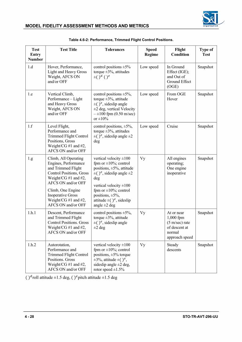
MODEL FIDELITY ASSESSMENT METHODS AND METRICS

4 - 28 STO-TR-AVT-296-UU

Table 4.6-2: Performance, Trimmed Flight Control Positions.

Test Entry

Number

Test Title Tolerances Speed Regime

Flight Condition

Type of Test

1.d Hover, Performance, Light and Heavy Gross Weight, AFCS ON and/or OFF

control positions ±5% torque ±3%, attitudes ±( )𝑑𝑑 ( )𝑒𝑒

Low speed In Ground Effect (IGE); and Out of Ground Effect (OGE)

Snapshot

1.e Vertical Climb, Performance ‒ Light and Heavy Gross Weight, AFCS ON and/or OFF

control positions ±5%, torque ±3%, attitude ±( )𝑒𝑒, sideslip angle ±2 deg, vertical Velocity ‒ ±100 fpm (0.50 m/sec) or ±10%

Low speed From OGE Hover

Snapshot

1.f Level Flight, Performance and Trimmed Flight Control Positions, Gross Weight/CG #1 and #2, AFCS ON and/or OFF

control positions, ±5%, torque ±3%, attitudes ±( )𝑒𝑒, sideslip angle ±2 deg

Low speed Cruise Snapshot

1.g Climb, All Operating Engines, Performance and Trimmed Flight Control Positions, Gross Weight/CG #1 and #2, AFCS ON and/or OFF

Climb, One Engine Inoperative Gross Weight/CG #1 and #2, AFCS ON and/or OFF

vertical velocity ±100 fpm or ±10%; control positions, ±5%, attitude ±( )𝑒𝑒, sideslip angle ±2 deg

vertical velocity ±100 fpm or ±10%; control positions, ±5%, attitude ±( )𝑒𝑒, sideslip angle ±2 deg

Vy All engines operating; One engine inoperative

Snapshot

1.h.1 Descent, Performance and Trimmed Flight Control Positions. Gross Weight/CG #1 and #2, AFCS ON and/or OFF

control positions ±5%, torque ±3%, attitude ±( )𝑒𝑒, sideslip angle ±2 deg

Vy At or near 1,000 fpm (5 m/sec) rate of descent at normal approach speed

Snapshot

1.h.2 Autorotation, Performance and Trimmed Flight Control Positions. Gross Weight/CG #1 and #2, AFCS ON and/or OFF

vertical velocity ±100 fpm or ±10%; control positions, ±5% torque ±3%, attitude ±( )𝑒𝑒, sideslip angle ±2 deg, rotor speed ±1.5%

Vy Steady descents

Snapshot

( )𝑑𝑑roll attitude ±1.5 deg, ( )𝑒𝑒pitch attitude ±1.5 deg

MODEL FIDELITY ASSESSMENT METHODS AND METRICS

STO-TR-AVT-296-UU 4 - 29

Table 4.6-3: Performance, Landing and Autorotation.

Test Entry

Number

Test Title Tolerances Speed Regime

Flight Condition

Type

1.i. Autorotation, Entry control positions ±10%; roll attitude ±3 deg, pitch attitude ±2 deg, heading ±5 deg, torque ±3%; rotor speed ±3%; airspeed ±5kt; vertical velocity ±200 fpm (1.00 m/sec) or 10%; altitude ±20 ft

Multiple Cruise or Climb

Trajectory

1.j.1 Landing, All Engines control positions ±10%; attitudes ±( )𝑑𝑑 ( )𝑒𝑒( )𝑓𝑓; torque ±3%; rotor speed ±1.5%; airspeed ±3kt; vertical velocity ±100 fpm or ±10%; altitude ±20 ft

Multiple Approach Trajectory

1.j.2a Landing, One Engine Inoperative CAT “A” Completed Landing

control positions ±10%; attitudes ±( )𝑑𝑑 ( )𝑒𝑒( )𝑓𝑓; torque ±3%; rotor speed ±1.5%; airspeed ±3kt; vertical velocity ±100 fpm or ±10%; altitude ±20 ft

Multiple Approach Trajectory

1.j.2b Landing, One Engine Inoperative CAT “B” Completed

control positions ±10%; attitudes ±( )𝑑𝑑 ( )𝑒𝑒( )𝑓𝑓; torque ±3%; rotor speed ±1.5%; airspeed ±3kt; vertical velocity ±100 fpm or ±10%; altitude ±20 ft

Multiple Approach Trajectory

1.j.3 Landing, One Engine Inoperative Balked

control positions ±10%; attitudes ±( )𝑑𝑑 ( )𝑒𝑒( )𝑓𝑓; torque ±3%; rotor speed ±1.5%; airspeed ±3kt; vertical velocity ±100 fpm or ±10%; altitude ±20 ft

Multiple Approach Trajectory

1.j.4 Landing, Autorotational Landing

control positions ±10%; pitch attitude ±2 deg, roll attitude ±2 deg, heading ±5 deg torque ±3%; rotor speed ±3%p; vertical velocity ±100 fpm or ±10%; altitude ±20 ft

Multiple Landing Trajectory

( )𝑑𝑑roll attitude ±1.5 deg, ( )𝑒𝑒pitch attitude ±1.5 deg, ( )𝑓𝑓heading ±2 deg

MODEL FIDELITY ASSESSMENT METHODS AND METRICS

4 - 30 STO-TR-AVT-296-UU

Table 4.6-4: Low Airspeed Handling Qualities.

Test Entry

Number

Test Title Tolerances Speed Regime

Flight Condition

Type

2.b.1 Low Airspeed Handling Qualities, Trimmed Flight Control Positions. AFCS ON and/or OFF

Control positions, ±5%, torque ±3%, attitudes ( )𝑑𝑑( )𝑒𝑒%

Low Airspeed

Flight IGE – Sideward (Left, Right), Rearward, and Forward Flight

Snapshot

2.b.2 Low Airspeed Handling Qualities, Critical Azimuth, AFCS ON and/or OFF

Control positions, ±5% torque ±3%, attitudes ( )𝑑𝑑( )𝑒𝑒%

Low Airspeed

Stationary Hover, Critical quadrant

Snapshot

2.b.3 Low Airspeed Handling Qualities, Control Response (Longitudinal, Lateral, Directional, Vertical). AFCS ON and OFF

Angular velocities ±10% or ± 𝑑𝑑 ( )𝑏𝑏( )𝑐𝑐, attitudes change ±10% or ±( )𝑔𝑔 ( )ℎ( )𝑖𝑖, normal acceleration ±( )𝑗𝑗

Low Airspeed

Hover Dynamic

( )𝑑𝑑roll rate ±3 deg/s, ( )𝑏𝑏pitch rate ±2 deg/s, ( )𝑐𝑐yaw rate ±2 deg/s, ( )𝑑𝑑roll attitude ±2 deg, ( )𝑒𝑒pitch attitude ±1.5 deg, ( )𝑓𝑓heading ±2 deg, ( )𝑔𝑔roll attitude change ±3deg, ( )ℎpitch attitude change ±1.5 deg, ( )𝑖𝑖heading change ±2 deg, ( )𝑗𝑗normal acceleration ±0.1 g.

Table 4.6-5: Longitudinal Handling Qualities.

Test Entry Number

Test Title Tolerances Speed Regime

Flight Condition

Type

2.c.1 Longitudinal Handling Qualities, Control Response, AFCS ON and OFF

Angular velocities ±( )𝑏𝑏 or Attitude ±( )𝑒𝑒

Vy, Vh Cruise Dynamic

2.c.2 Longitudinal Handling Qualities, Static Stability, AFCS ON and/or OFF

Longitudinal Control Position: ±10% of change from trim or ±0.25 in. (6.3 mm) or Longitudinal Control Force: ±0.5 lb. (0.223 daN) or ±10%. torque ±3%, attitudes ±2%

Vy, Vh Cruise or Climb. Autorotation

Snapshot

MODEL FIDELITY ASSESSMENT METHODS AND METRICS

STO-TR-AVT-296-UU 4 - 31

Test Entry Number

Test Title Tolerances Speed Regime

Flight Condition

Type

2.c.3.a Longitudinal Handling Qualities, Dynamic Stability, Long Term Response, AFCS ON and OFF

±10% of calculated period, ±10% of time to ½ or double amplitude, or ±0.02 of damping ratio For non-periodic responses, the time history must be matched within ±3º pitch; and ±5 kts airspeed over a 20 sec period following release of the controls

Vy or Vh Cruise Dynamic

2.c.3.b Longitudinal Handling Qualities, Dynamic Stability, Short Term Response, AFCS ON and OFF

( )𝑏𝑏 or ( )𝑒𝑒 , ( )𝑗𝑗 Vy, Vh Cruise or Climb Dynamic

2.c.4 Longitudinal Handling Qualities, Manoeuvring Stability, Augmentation On and Off

Longitudinal Control Position: ±10% of change from trim or ±0.25 in. (6.3 mm) or Longitudinal Control Force: ±0.5 lb. (0.223 daN) or ±10%. torque ±3%, attitudes ±2%

Vy, Vh Cruise or Climb Snapshot

( )𝑏𝑏pitch rate ±2 deg/s, ( )𝑒𝑒pitch attitude ±1.5 deg, ( )𝑗𝑗normal acceleration ±0.1 g.

Table 4.6-6: Lateral and Directional Handling Qualities.

Test Entry

Number

Test Title Tolerances Speed Regime

Flight Conditions

Type

2.d.1 Lateral and Directional Handling Qualities, Control Response (Lateral, Directional), AFCS ON and OFF

Lateral: ( )𝑑𝑑, ( )𝑔𝑔 Directional: ( )𝑐𝑐, ( )𝑖𝑖

Vy, Vh Cruise Dynamic

2.d.2 Lateral and Directional Handling Qualities, Directional Static Stability, Augmentation On and Off

Control Positions ±10% ( )𝑑𝑑, Vertical Velocity ‒ ±100 fpm (0.50 m/sec) or 10%

Vy, Vh Cruise or Climb (may use Descent instead of Climb if desired)

Snapshot

MODEL FIDELITY ASSESSMENT METHODS AND METRICS

4 - 32 STO-TR-AVT-296-UU

Test Entry

Number

Test Title Tolerances Speed Regime

Flight Conditions

Type

2.d.3.a Lateral and Directional Handling Qualities, Dynamic Lateral and Directional Stability. Lateral Directional Oscillations, AFCS ON and OFF

±0.5 sec. or ±10% of period, ±10% of time to ½ or double amplitude or ±0.02 of damping ratio, ±20% or ±1 sec of time difference between peaks of bank and sideslip. For non-periodic responses, the time history must be matched within ±10 knots Airspeed; ±5º/s Roll Rate or ±5º Roll Attitude; ±4º/s Yaw Rate or ±4º Yaw Angle over a 20 sec period roll angle following release of the controls

Vy, Vh Cruise or Climb

Dynamic

2.d.3.b Lateral and Directional Handling Qualities Lateral and Directional Handling Qualities. Spiral Stability, AFCS ON and OFF

±2º or ±10% roll angle

Left and Right turn, Vy or Vh

Cruise or Climb

Dynamic

2.d.3.c Lateral and Directional Handling Qualities, Lateral and Directional Handling Qualities, Adverse/Proverse Yaw, AFCS ON and OFF

Correct Trend, ±2º transient sideslip angle

Left and Right Turn, Vy or Vh

Cruise or Climb

Dynamic

( )𝑑𝑑roll rate ±3 deg/s, ( )𝑐𝑐yaw rate ±2 deg/s, ( )𝑑𝑑roll attitude ±1.5 deg, ( )𝑔𝑔roll attitude change ±3 deg, ( )𝑖𝑖heading change ±2 deg.

4.7 ENGINEERING FIDELITY METRICS

For flight training devices, EASA CS-FSTD(H) (2012) and FAA 14 Part 60 (2016) describe the criteria, tolerances, and procedures for the qualification of rotorcraft flight training simulators and also detail the component or predictive fidelity required to achieve a ‘fit for purpose’ approval. Currently, however, there are no quantitative methods used to assess the fidelity of the overall system. The quantification of fidelity using an engineering metrics approach must underpin the confidence required to employ flight simulators for research and development. These substantial challenges have not, as yet, been fully addressed in the rotorcraft world.

MODEL FIDELITY ASSESSMENT METHODS AND METRICS

STO-TR-AVT-296-UU 4 - 33

In support of establishing an engineering basis for civil simulator qualification standards, GARTEUR Action Group (AG) HC/AG-12 [Padfield et al. (2004), Padfield et al. (2005), and Pavel et al. (2013)] was formed to conduct a critical examination of the existing simulator standard, JAR-STD 1H (2001). This standard was consolidated along with JAR-STD 2H (2003) and JAR-STD 3H (2002) into JAR-FSTD H (2008), and subsequently adopted as EASA CS-FSTD(H) (2012), including correlation of handling qualities and fidelity metrics. The work revealed a range of shortcomings. For example, GARTEUR HC/AG-12 showed that the relationship between fidelity and the JAR-STD 1H tolerances is sensitive to the nature of the manoeuvre being flown, and, more significantly, it showed that matching tolerances does not always lead to matching handling qualities.

Simulators are extensively used in research and development especially in the assessment of Handling Qualities (HQ) and the development of crew-station systems. The use of HQ engineering as a framework to quantify overall simulation fidelity has developed in several forms. Hess and colleagues [Hess and Malsbury (1991), Hess and Siwakosit (2001), and Schroeder et al. (2000)] introduced the handling qualities sensitivity function as a quality metric. Padfield et al. (1996) and McCallum and Charlton (2001) first proposed the handling qualities standard, ADS-33E (2000) ‘Handling Qualities Requirements for Military Rotorcraft’, as the basis for deriving metrics; since the HQ parameters define the flying characteristics, they should also be suitable to judge the fidelity.

Within the JSHIP project, Advani and Wilkinson (2001) and Roscoe and Thompson (2003) used comparative performance and control activity and handling qualities ratings given for the same tasks flown in simulation and flight. In each of these approaches, the adopted philosophy has been to develop a rational and systematic approach to the identification of differences between simulation and flight and hence, the areas where the simulator is deficient. These methods have met with partial success, but this only highlights the need for new fidelity criteria for use in design, development, and product qualification. Development of new criteria was the focus of the Lifting Standards research project at the University of Liverpool [Perfect et al. (2013)], and the new approach is presented in the following sections.

4.7.1 A New Approach to Simulation Fidelity It is this need to have objective measures of predictive fidelity, complemented by subjective measures of perceptual fidelity, that was the main focus of the University of Liverpool ‘Lifting Standards: A Novel Approach to the Development of Fidelity Criteria for Rotorcraft Flight Simulators’ [Perfect et al. (2010), White et al. (2010), and White et al. (2013)]. A two-stage approach for defining fidelity criteria for simulator qualification was developed in Lifting Standards. The first stage involved the development of a quantitative basis for prediction of fidelity using metrics derived, in part, from HQ engineering. The second stage consists of perceptual fidelity metrics supplemented by a Simulator Fidelity Rating scale [Perfect et al. (2014)] (see Section 4.5), used to assign the perceptual fidelity of the simulator.

4.7.2 Methodology for Simulation Fidelity Based on Handling Qualities Engineering In the area of HQ engineering, two assessment processes, prediction, and assignment, are integrated and combined to give the overall HQ of an aircraft. The practises adopted in the Lifting Standards project draw on this integrative process and the HQ performance specification, [ADS-33E (2000)]. For both processes, the test aircraft is assessed to be in one of three handling qualities ‘levels.’ Level 1 HQ (HQ ratings of 1, 2, and 3) indicate that there is no requirement for improvement to the aircraft, and all operational tasks can be accomplished with low workload. In Level 2 (with HQR of 4, 5, and 6), the workload will be higher, and the level of precision reduced; the safety of the aircraft, however, is not significantly at risk. If Level 3 HQ are found (HQR > 6), then the level of workload has increased to the extent that task performance is no longer achievable. At the higher end of Level 3 (HQR 9 and 10, which are sometimes defined as Level 4), flight safety is compromised as the risk of loss of control increases.

MODEL FIDELITY ASSESSMENT METHODS AND METRICS

4 - 34 STO-TR-AVT-296-UU

Much of this methodology can be directly applied to the fidelity assessment of a flight simulator – both handling qualities and fidelity are intimately related to pilot control strategy and task performance. If a pilot makes the same control inputs in the simulator as they are required to in flight, then correct behavioural patterns have been learned, and the simulator training will have been effective. This means that the pilot will have benefitted from their time in the simulator. The goal in fidelity assessment is to establish the ‘quality’ of the simulator in replicating the behaviour of the real aircraft and its pilot, rather than purely to assess the handling qualities of the simulated aircraft. In the case of the prediction metrics, the fidelity assessment is focused on the simulator components (e.g., the flight model, the image generation system, etc.) with the fidelity predictions for each component contributing towards a prediction for the overall simulation. For the assignments, the pilot’s impression of the behavioural accuracy of the model is closely linked with the experienced cues. The primary generators of task cues within the simulator are the visual, motion, audio, and inceptor force feel systems. In fidelity, we describe the pilot’s experience as the perceptual fidelity.

As in the HQ assessment process, a comparison of results from predictive and perceptual assessments forms a key component of the overall fidelity assessment process. This is required to establish that the predicted and perceptual results are consistent. For the same reason, predictive and perceptual assessments are required in the simulator in order to understand better any differences. A flow diagram representing the process for the assessment of predicted and perceptual simulator fidelity is shown in Figure 4.7-1. The process begins with a definition of the required purpose of the flight simulator and hence, the tasks that will be trained (Blocks 1-3 in Figure 4.7-1) which will set the required level of fidelity. Once the purpose of the simulator has been defined, testing on the simulator and the simulated aircraft can be conducted (Block 4). This leads to the computation of the predicted fidelity (Block 5), using a set of metrics described later. The results for each simulator component in the predicted fidelity stage can then be analysed to arrive at an overall level of predicted fidelity for a particular task. The results from these tests feed into the first decision point. The question is do the individual predictive fidelity metrics show a sufficiently good match between flight and simulation. (Block 6). This stage highlights the quality of individual components of the simulation. Subject to a satisfactory result at this stage, further flight and simulator testing can be conducted to examine the perceptual fidelity of the simulation (Block 7). As with the predictive fidelity, metrics are computed for each test point (Block 8) and a decision made as to the suitability of the resultant Level of perceptual fidelity for the intended purpose (Block 9).

A third decision point addresses the acceptability of the comparison between predictive and perceptual fidelity (Block 10). This stage is analogous to the comparison between predictive and assigned HQ as an assessment of the validity of the testing. If the test results are valid, it would be expected that the predictive level of fidelity for the simulator would agree with that from the perceptual assessment processes. In addition, the analysis at this point provides a further indicator as to the source of discrepancies between flight and simulation. For example, if the predictive metrics for the flight model show a good match while the perceptual metrics do not, then the indication is that the fidelity issues lie within the generation of the task cues and not the flight model. If all questions (Blocks 6, 9 and 10) can be answered positively, then a decision can be made that the simulator is fit for its designed purpose and can be accepted for service (Blocks 11 and 12). If, however, one of the fidelity requirements is not met, this would be an indicator that the simulator is not fit for purpose, and an upgrade, either to the cueing or the flight model or both, is required (Block 13). It should be recognised that a simulator may be fit for some purposes but not others – thus, it may have limited fidelity.

MODEL FIDELITY ASSESSMENT METHODS AND METRICS

STO-TR-AVT-296-UU 4 - 35

Figure 4.7-1: Methodology for Integrated Predicted and Perceptual Simulator Fidelity Assessment [Perfect et al. (2013)].

4.7.3 Handling Qualities Predictive Fidelity Metrics The first part of the fidelity assessment process involves analysis of the individual simulator components. For the flight model, the predicted HQ of the test aircraft and flight model are computed with dynamic response criteria drawn from the response to clinical tests, such as pulse, step, doublet, and frequency sweep control inputs. HQ metrics define the level of performance/compensation achievable/required to fly the defined missions. Metrics have been developed in both the time and frequency domains to assess the full range of aircraft response (from low to high frequency and from small to large amplitude) and are presented as the dynamo construct shown in Figure 4.7-2 from Padfield (2018).

MODEL FIDELITY ASSESSMENT METHODS AND METRICS

4 - 36 STO-TR-AVT-296-UU

Figure 4.7-2: Dynamo Construct for Dynamic Response Criteria [Padfield (2018)].

Dynamic response criteria are often displayed in two-parameter charts, for example damping and frequency or bandwidth and phase delay, with boundary lines demarking regions of Level 1, 2 and 3 performance. As measures of dynamic performance, these metrics provide a sound basis for quantifying predictive simulation fidelity since they are referenced to missions and pilot control strategies in operational tasks. The fidelity of the simulated flight model is defined as the goodness of the match between flight and simulation for each of the predicted HQ metrics.

Moving through the dynamo construct, the stability and agility criteria adopted in the predicted HQ section of ADS-33E-PRF to assess each region are:

1) Small amplitude, high frequency – bandwidth and phase delay.

2) Small amplitude, low to medium frequency – open-loop stability.

3) Moderate amplitudes – quickness.

4) Large amplitudes – maximum response.

A further set of HQ metrics is required that specify the required level of handling for the cross-coupled, off-axis responses, e.g., pitch response to roll control inputs (and vice versa) and the yaw response to collective control inputs. Additionally, for forward flight, the magnitude of the pitch response to a collective input is assessed.

Comparisons of these HQ metrics, flight vs simulation, provides an indication of the fidelity of the model as shown in Perfect et al. (2013) and Padfield (2018). Figure 4.7-3 and Figure 4.7-4 show a comparison of the pitch and roll attitude bandwidth, phase delay, and quickness in hover for a FLIGHTLAB® Bell 412 and the NRC’s Bell 412 aircraft. Fidelity boundaries of 10% and 20% are shown in Figure 4.7-3, indicating that the pitch bandwidth is on the 10 ‒ 20 % boundary and the roll simulation bandwidth is outside the 20% boundary. Similarly, in Figure 4.7-4, differences between flight and simulation quickness values can be illustrated using this HQ metric.

In addition to quantification of the flight model fidelity, prediction of the fidelity of the other simulator components would also be performed at this stage. Techniques such as those described by Hodge et al. (2015a) and Hodge et al. (2015b) for motion platform response would be used.

MODEL FIDELITY ASSESSMENT METHODS AND METRICS

STO-TR-AVT-296-UU 4 - 37

Figure 4.7-3: Comparison of Pitch and Roll Bandwidth-Phase Delay in Hover [Padfield (2018)].

Figure 4.7-4: Comparison of Pitch and Roll Attitude Quickness in Hover [Padfield (2018)].

4.7.4 Perceptual Fidelity Metrics Once the predicted fidelity levels have been computed, the assessment can proceed to perceptual fidelity, computed through the process of assigning Handling Qualities Ratings (HQR) and Simulator Fidelity Ratings (SFR) (see Section 4.5 and Perfect et al. (2014)). In this stage, the test aircraft is flown in a range of manoeuvres that are representative of those that would be expected in the aircraft’s operational role, the Mission Task Elements (MTE).

Prior to the initiation of the MTE flying, expected results based on the predicted HQ can be developed. For example, a precision hover MTE predominantly requires small amplitude corrective inputs, so the bandwidth and open-loop stability of the aircraft will be of primary importance. The acceleration-deceleration MTE, in contrast, requires moderate to large pitch attitude changes, increasing the importance of the quickness and maximum response amplitude.

Test pilots fly each of the MTE and rate the performance of the aircraft using the Cooper-Harper HQR scale [Cooper and Harper (1969)]. This scale requires the test pilot to award a rating based on both the level of compensation needed to fly the task and the achievable level of precision and aggressiveness. Precision is judged relative to a set of ‘adequate’ tolerances, which represent safe flight in the Level 2 region, and more stringent ‘desired’ tolerances, which represent low workload flight in the Level 1 region.

MODEL FIDELITY ASSESSMENT METHODS AND METRICS

4 - 38 STO-TR-AVT-296-UU

The HQR is an important element in the perceptual fidelity process. If a match is not achieved here, then a flaw must exist in the simulation. However, the HQR by itself is insufficient to quantify differences between flight and simulation fully; the same HQR can be given for very different aircrafts. To complement the HQR, the test pilot is asked to rate the effect of the visual cues on vehicle control through the visual cue rating (VCR) [ADS-33E (2000)] from which a Usable Cue Environment (UCE) can be derived. As with the HQR, it is desirable for a match between flight and simulation VCRs and UCEs to be demonstrated. The VCR, as a measure of the precision achievable and aggressiveness of control inputs that can be applied by the pilot, provides a subjective assessment of not just the differences in visual cues, but also any differences in the control strategies adopted in flight and simulation. The UCE concept was developed within ADS-33 for specific purposes, and this extension to simulation fidelity will need further refinement.

As a new addition to the subjective rating process, the SFR scale provides a method for an evaluating pilot to directly rate the suitability of the overall simulation for a specified task [Perfect et al. (2014)]. The pilot is asked to compare the level of performance attained in flight and simulator and to judge the level of adaptation of task strategy that must be made to convert from one environment to the other. The use of the SFR scale in the assessment of simulator fidelity is described in detail in Section 4.5 and Perfect et al. (2014).

As with HQ assessments, task performance and compensation metrics are fundamental for quantifying differences between flight and simulator. For task performance, these are

1) Task time. The time taken to move from the start point to the end point of the manoeuvre. This is less than the total time spent performing the task, which additionally includes stabilisation time prior to and after the manoeuvre.

2) Time spent within desired performance. Percentage of the total manoeuvre time spent within the desired performance tolerance.

3) Time spent within adequate performance. Percentage of the total manoeuvre time within the adequate performance tolerance (including the desired performance region).

4) Time spent beyond adequate performance. Percentage of the total manoeuvre time spent beyond the adequate performance tolerance.

Quickness can be applied to assess closed loop in addition to open-loop and agility. The closed loop quickness, QCL, can be summarised using the following parameters:

1) Number of quickness points (the total number of discrete attitude changes of greater than 0.5° occurring during an MTE).

2) Quickness points per second. This is the number of quickness points expressed in terms of the average number of attitude changes per second.

3) Mean quickness. This is the mean quickness measured for each of the individual attitude changes. 4) Mean attitude change. This is the mean attitude change measured for each of the individual

quickness points.

For the pilot’s control compensation, the following metrics are used:

1) Control attack [Padfield et al. (1994)] which measures the size and rapidity of a pilot’s control inputs, defined as:

where η is the pilot’s control deflection (Figure 4.7-5). The control attack is summarised using the following parameters, which are analogous to those described above for closed loop attitude quickness.

MODEL FIDELITY ASSESSMENT METHODS AND METRICS

STO-TR-AVT-296-UU 4 - 39

2) Attack number. This is the total number of times that the pilot moves a particular control by more than 0.5% of full travel.

3) Attack number per second. This is the attack number expressed in terms of the average number of control movements per second.

4) Mean attack rate. This is the mean rate at which the pilot is moving his control and is expressed in terms of the % control travel per second.

5) Mean control displacement. This is the mean of the control displacements measured for each of the attack points.

Figure 4.7-5: Attack Point Parameters [Perfect et al. (1993)].

In the frequency domain, one can assess [Blanken and Pausder (1994) and Tischler and Remple (2012)]:

1) Root-Mean-Square (RMS) of the Power Spectral Density (PSD) in each control axis.

2) Cut-off frequency, where 70% of the control displacement signal has accumulated. The RMS value and cut-off frequency are calculated over the interval 0.2 Hz > f > 2Hz, with the lower limit largely removing the lower frequency guidance element of the control activity from the analysis and the upper limit removing artefacts introduced in the time frequency-domain transformation.

4.8 REFERENCES

[1] ADS-33E (2000), “Aeronautical Design Standard, Performance Specification, Handling Qualities Requirements for Military Rotorcraft”, US Army, ADS-33E-PRF.

[2] Advani, S.K., and Hosman, R.J.A.W. (2006), “Revising Civil Simulator Standards – An Opportunity for Technological Pull”, AIAA Modeling and Simulation Technologies Conference and Exhibit, Paper No. AIAA-2006-6248.

[3] Advani, S.K., Hosman, R.J.A.W., and Potter, M. (2007), “Objective Motion Fidelity Qualification in Flight Training Simulators”, AIAA Modeling and Simulation Technologies Conference and Exhibit, Paper No. AIAA-2007-6802.

[4] Advani, S.K. and Wilkinson, C.H. (2001), “Dynamic Interface Modelling and Simulation – A Unique Challenge”, Royal Aeronautical Society Conference on Helicopter Flight Simulation, London, UK.

MODEL FIDELITY ASSESSMENT METHODS AND METRICS

4 - 40 STO-TR-AVT-296-UU

[5] Blanken, C.L., and Pausder, H.J. (1994), “Investigation of the Effects of Bandwidth and Time Delay on Helicopter Roll-Axis Handling Qualities”, Journal of the American Helicopter Society, 39, (3), pp 24-33, July.

[6] Buchholz, J.J., Bauschat, J.M., Hahn, K.U., and Pausder, H.J. (1996), “ATTAS & ATTHeS In-Flight Simulators: Recent Application Experiences and Future Programs”, AGARD-CP577, Paper no. 31, April.

[7] Carpenter, C.G., and Hodgkinson, J. (1980), “V/STOL Equivalent Systems Analysis”, Technical Report NADC-79141-60, McDonnell Aircraft Co.

[8] Cooper, G.E., and Harper, R.P. Jr. (1969), “The Use of Pilot Rating in the Evaluation of Aircraft Handling Qualities”, NASA TN D-5133.

[9] Dalmeijer, W., Miletović, I., Stroosma, O., and Pavel, M.D. (2017), “Extending the Objective Motion Cueing Test to Measure Rotorcraft Simulator Motion Characteristics”, 73rd American Helicopter Society Forum, pp. 1876-1891.

[10] EASA CS-FSTD(H) (2012), “Certification Specifications for Helicopter Flight Simulation Training Devices”, European Aviation Safety Agency EASA CS-FSTD(H), June, https://www.easa.europa.eu/ certification-specifications/cs-fstdh-helicopter-flight-simulation-training-devices, Retrieved on June 4th, 2020.

[11] FAA-AC-120-63 (1994), “Advisory Circular on Helicopter Simulator Qualification”, Federal Aviation Administration, FAA-AC-120-63, https://www.faa.gov/regulations_policies/advisory_circulars/index. cfm/go/document.information/documentID/23203, Retrieved on June 4th, 2020.

[12] FAA 14 Part 60 (2016), “Flight Simulation Training Device Initial and Continuing Qualification and Use”, FAA 14 Part 60 Appendix C to Part 60-Qualification Performance Standards for Helicopter Full Flight Simulators.

[13] Hamel, P.G., and Jategaonkar, R.V. (1996), “The Evolution of Flight Vehicle System Identification”, Journal of Aircraft, 33(1), pp. 10-28, Jan.

[14] Haverdings, H., Dequin, A.M, Basset, P.M., von Grünhagen, W., Kampa, K, Massey, C., McCallum, A., Meerwijk, E.L. (2000), “Mathematical Modeling for the Prediction of Helicopter Flying Qualities within GARTEUR ‒ Phase 3”, European Rotorcraft Forum, The Hague, Netherlands, Sept. 26 – 29.

[15] Heffley, R.K., Clement, W.F., Ringland, R.F., Jewell, W.F. (1981), “Determination of Motion and Visual System Requirements for Flight Training Simulators”, Systems Technology Inc., Technical Report No. 546, August.

[16] Hess, R.A. and Malsbury, T. (1991), “Closed Loop Assessment of Flight Simulator Fidelity”, Journal of Guidance, Control and Dynamics, 14(1), pp 191-197.

[17] Hess, R. A., and Siwakosit, W. (2001), “Assessment of Flight Simulator Fidelity in Multi-Axis Tasks Including Visual Cue Quality”, Journal of Aircraft, 38(4), pp 607-614.

[18] Hodge, S.J., Perfect, P., Padfield, G.D. and White, M.D. (2015a), “Optimising the Yaw Motion Cues Available from a Short Stroke Hexapod Motion Platform”, The Aeronautical Journal, January, 119(1211), pp. 1-21.

MODEL FIDELITY ASSESSMENT METHODS AND METRICS

STO-TR-AVT-296-UU 4 - 41

[19] Hodge, S.J., Perfect, P., Padfield, G.D. and White, M.D. (2015b), “Optimising the Roll-Sway Motion Cues Available from a Short Stroke Hexapod Motion Platform”, The Aeronautical Journal, January, 119(1211), pp. 23-44.

[20] Hodgkinson, J. (1998), Aircraft Handling Qualities, AIAA Educational Series, AIAA, Reston, VA.

[21] Hodgkinson, J. (2005), “History of Low-Order Equivalent Systems for Aircraft Flying Qualities”, Journal of Guidance, Control, and Dynamics, July-August, 28(4), pp. 577-583.

[22] Hosman, R.J.A.W., and Advani, S.K. (2012), “Status of the ICAO Objective Motion Cueing Test”, Flight Simulation Research, New Frontiers Conference Proceedings, Royal Aeronautical Society, London.

[23] ICAO 9625 (2015), “Manual of Criteria for the Qualification of Flight Simulation Training Devices”, ICAO Document 9625, Vol. II ‒ Helicopters, 4th edition.

[24] JAR-STD 1H (2001), “Helicopter flight simulators”, April 2001, Joint Aviation Authorities.

[25] JAR-STD 2H (2003), “Helicopter flight training devices”, September 2003, Joint Aviation Authorities.

[26] JAR-STD 3H (2002), “Helicopter flight simulators”, May 2002, Joint Aviation Authorities.

[27] JAR-FSTD H (2008), “JAR-FSTD H Helicopter Flight Simulation Training Devices, Joint Aviation Authorities”, Joint Aviation Authorities, https://www.caa.md/files/2014_01/569.pdf, Retrieved on June 4th, 2020.

[28] Jones, M. (2017), “Motion Cueing Optimisation Applied to Rotorcraft Flight Simulation”, CEAS Aeronautical Journal, 8(523), pp. 523-539, https://doi.org/10.1007/s13272-017-0256-1.

[29] Jones, M., White, M., Fell, T., and Barnett, M. (2017), “Analysis of Motion Parameter Variations for Rotorcraft Flight Simulators”, Proceedings of the 73rd AHS Annual Forum & Technology Display, Fort Worth, Texas, USA, May 9 ‒ 11.

[30] Jones, M. (2018), “Enhancing Motion Cueing Using an Optimisation Technique”, The Aeronautical Journal, 122(1249), pp. 487-518, doi:10.1017/aer.2017.14.

[31] Li, M. (2016), “Effect of Helicopter Degree of Freedom and Motion Cues on Allowable Error Envelopes”, Unpublished MSc. thesis, Delft University of Technology.

[32] McCallum, A.T., and Charlton, M.T. (2001), “Structured Approach to Helicopter Simulator Acceptance, The Challenge of Realistic Rotorcraft Simulation”, November Royal Aeronautical Society Conference, London, UK.

[33] Miletović, I., Pavel, M.D., Stroosma, O., Van Paassen, M.M., Wentink, M., and Mulder, M. (2018), “Eigenmode Distortion as a Novel Criterion for Motion Cueing Fidelity in Rotorcraft Flight Simulation”, 44th European Rotorcraft Forum, Delft, Netherlands, Paper No. 45.

[34] Miller, D., Kocher, E., Hughes, D.F., Grugan, R.A., and Taylor, J.E. (2009), “Complementary Moving Base and Dynamic Motion Seat Cueing for Rotorcraft Simulation”, AIAA Modeling and Simulation Technologies Conference, Chicago.

[35] MIL-STD-1797B (2006), “Flying Qualities of Piloted Aircraft”, Department of Defense Interface Standard.

MODEL FIDELITY ASSESSMENT METHODS AND METRICS

4 - 42 STO-TR-AVT-296-UU

[36] Mitchell D.G., He C., and Strope K. (2006a), “Determination of Maximum Unnoticeable Added Dynamics”, AIAA Atmospheric Flight Mechanics Conference and Exhibit Keystone, Colorado, AIAA 2006-6492.

[37] Mitchell, D.G., Hoh, R.H., He, C., and Strope, K. (2006b), “Development of an Aeronautical Design Standard for Validation of Military Helicopter Simulators”, 62nd Annual Forum of the American Helicopter Society, Phoenix, AZ.

[38] Mitchell, D.G., Nicoll, T.K., Klyde, D.H., and Schulze, C. (2009), “Effects of Time Varying Rotorcraft Dynamics on Pilot Control”, AIAA Atmospheric Flight Mechanics Conference, AIAA 2009-6055, Aug.

[39] Myrand-Lapierre V., Tischler M.B., Pavel M.D., Nadeau-Beaulieu M., Stroosma O., and Gubbels B. (2020), “Bell 412 Modeling and Model Fidelity Assessment for Level-D Training Simulators”, Vertical Flight Society Forum 76th, Oct. 6-8, Virginia Beach.

[40] Padfield, G.D. (2018), Helicopter Flight Dynamics: Including a Treatment of Tiltrotor Aircraft, Third Ed. John Wiley & Sons.

[41] Padfield, G.D., Charlton, M.T., and McCallum, A.T. (1996), “The Fidelity of Hi-Fi Lynx on the DERA Advanced Flight Simulator using ADS-33 Handling Qualities Metrics”, DRA/AS/FDS/TR96103/1, pp 1-152, December.

[42] Padfield G.D., Jones J.P., Charlton M.T., Howell S., and Bradley R. (1994), “Where Does the Workload Go When Pilots Attack Manoeuvres? – An Analysis of Results from Flying Qualities Theory and Experiment”, 20th European Rotorcraft Forum, Amsterdam, The Netherlands, October.

[43] Padfield, G.D., McCallum, A.T., Dequin Haddon, D., Kampa, K. Basset, P.M., and von Grünhagen, W., (2006), “Predicting Rotorcraft Flying Qualities through Simulation Modelling. A Review of Key Results from GARTEUR HC/AG-06”, 22th European Rotorcraft Forum, Brighton, United Kingdom, 16 ‒ 19 September.

[44] Padfield, G.D., Pavel, M.D., Casolaro, D., Roth, G., Hamers, M., and Taghizad, A. (2004), “Validation Criteria for Helicopter Real-Time Simulation Models, Sketches from the work of GARTEUR HC/AG-12”, 30th European Rotorcraft Forum, Marseilles, France.

[45] Padfield, G.D., Pavel, M.D., Casolaro, D., Roth, G., Hamers, M., and Taghizad, A. (2005), “Fidelity of Helicopter Real-Time Models”, 61st Annual Forum of the American Helicopter Society, Grapevine, TX, June.

[46] Pavel, M.D., White, M.D., Padfield, M.D., Roth, G., Hamers, M., and Taghizad, A. (2013), “Validation of Mathematical Models for Helicopter Flight Simulators Current and Future Challenges”, The Aeronautical Journal, 117(1190), pp. 343-388, April.

[47] Penn, H. (2013), “Investigating the Feasibility of applying MUAD to Helicopter Simulator Model Validation: An Analysis of the Effect of Multiple Simulators on Allowable Error Envelopes Using Multiple Pilots”, Unpublished M.Sc. thesis, Delft University of Technology, July.

[48] Perfect, P., Timson E., White, M.D., Padfield, G.D., Erdos, R., and Gubbels, A.W. (2014), “A Rating Scale for the Subjective Assessment of Simulation Fidelity”, The Aeronautical Journal, August, 118(1206), pp. 953-974.

MODEL FIDELITY ASSESSMENT METHODS AND METRICS

STO-TR-AVT-296-UU 4 - 43

[49] Perfect, P., White, M.D., Padfield, G.D., Gubbels, A.W., and Berryman, A.C. (2010), “Integrating Predicted and Perceived Fidelity for Flight Simulators”, 36th European Rotorcraft Forum, Paris, France, September.

[50] Perfect, P., White, M.D., Padfield, G., and Gubbels, A.W. (2013), “Rotorcraft Simulation Fidelity: New Methods for Quantification and Assessment”, The Aeronautical Journal, March, 117(1189), pp. 235-282.

[51] Reardon, S.E., Beard, S.D., and Aponso, B.L. (2014), “Effects of Motion Filter Parameters on Simulation Fidelity Ratings”, 70th Annual Forum of the American Helicopter Society, Montreal, Canada May 20 – 22.

[52] Reid, L.D., and Nahon, M.A. (1985), “Flight Simulation Motion-Base Drive Algorithms: Part 1 – Development and Testing of the Equations”, University of Toronto, Institute of Aerospace Studies, UTIAS Report No. 296.

[53] Roscoe, M.F., and Thompson, J.H. (2003), “JSHIP’s Dynamic Interface Modelling and Simulation Systems: A Simulation of the UH-60A Helicopter/LHA Shipboard Environment Task”, 59th Annual Forum of the American Helicopter Society, Phoenix, AZ, May.

[54] Schroeder, J.A. (1999), “Helicopter Flight Simulation Motion Platform Requirements”, NASA-TP-1999-208766.

[55] Schroeder, J.A., Chung, W.W.Y., and Hess, R.A. (2000), “Evaluation of Motion Fidelity Criterion with Visual Scene Changes”, Journal of Aircraft, 37(4), pp 580-587.

[56] Sinacori, J. B., (1977), “The Determination of Some Requirements for a Helicopter Research Simulation Facility”, NASA-CR-152066.

[57] Smith, R.E., Hodgkinson, J., and Snyder, R.C. (1981), “Equivalent System Verification and Evaluation of Augmentation Effects on Fighter Approach and Landing Flying Qualities”, U.S. Air Force, Wright Aeronautical Lab., AFWAL-TR-81-3116, Vol. 2, Wright-Patterson Air Force Base, OH.

[58] Stewart, D. (1965), “A Platform with Six Degrees of Freedom”, Proceedings of the Institution of Mechanical Engineers, 180(1), 371-386, https://doi.org/10.1243/PIME_PROC_1965_180_029_02.

[59] Timson, E., Perfect, P., White, M.D., Padfield, G.D., Erdos, R., and Gubbels, A.W. (2011), “Pilot Sensitivity to Flight Model Dynamics in Rotorcraft Simulation”, 37th European Rotorcraft Forum, Vergiate and Gallarate, Italy, Paper no. 172.

[60] Timson, E., White, M.D., Perfect, P. and Padfield, G.D. (2012), “Subjective Methods for Fidelity Assessment of Rotorcraft Training Simulators”, 68th Annual Forum of the American Helicopter Society, Texas USA, 1 ‒ 3 May.

[61] Tischler, M.B. (1995), “System Identification Methods for Aircraft Flight Control Development and Validation”, NASA Technical Memorandum 110369.

[62] Tischler, M.B., and Remple, R.K. (2012), Aircraft and Rotorcraft System Identification: Engineering Methods with Flight-Test Examples, 2nd Edition, AIAA Educational Series, November.

[63] White, M D., Pavel, M.D., Jones, M., Spira, D., Cuzieux, F., and van den Vorst, J. (2020), “Rotorcraft Simulation Fidelity Assessment Predicted and Perceived Measures of Fidelity”, Report for GARTEUR HC/AG-21, GARTEUR TP–189, March.

MODEL FIDELITY ASSESSMENT METHODS AND METRICS

4 - 44 STO-TR-AVT-296-UU

[64] White, M.D., Perfect, P., Padfield, G.D., Gubbels, A.W, and Berryman, A.C. (2010), “Progress in the Development of Unified Fidelity Metrics for Rotorcraft Flight Simulators”, 66th Annual Forum of the American Helicopter Society, Phoenix, AZ, May.

[65] White, M.D., Perfect, P., Padfield, G.D., Gubbels, A.W. and Berryman, A.C. (2013), “Acceptance Testing and Commissioning of a Flight Simulator for Rotorcraft Simulation Fidelity Research”, Proceedings of the Institution of Mechanical Engineers, Part G: Journal of Aerospace Engineering, April, 227(4), pp. 663-686.

[66] Wood, J.R., and Hodgkinson, J. (1980), “Definition of Acceptable Levels of Mismatch for Equivalent Systems of Augmented CTOL Aircraft”, Technical Report Number, 1600, A6792, McDonnell Douglas Corp., 1980.

[67] Zaal, P.M.T., Schroeder, J.A., and Chung, W.W. (2018), “Objective Motion Cueing Criteria for Commercial Transport Simulators”, AIAA Modeling and Simulation Technologies Conference, Paper No. AIAA 2018-2935.

STO-TR-AVT-296-UU 5 - 1

Chapter 5 – MODEL FIDELITY IMPROVEMENT METHODS

Seven different methods for improving a baseline simulation method are presented in this chapter. They are ordered by complexity, starting from the simplest methods, and ending with the most complex.

The first two methods, namely Method 1, ‘Gain/Time-Delay Corrections for Key Responses,’ and Method 2, ‘Black-Box’ Input and Output Filter Corrections,’ do not modify the baseline model. Instead, corrections are applied to the external structure of the model, either as SISO (Single-Input / Single-Output) gain/time-delay corrections or MIMO (Multi-Input / Multi-Output) corrections filters.

On the contrary, the next four methods modify the baseline model. Method 3, ‘Force and Moment Increments Based on Stability Derivatives,’ uses a comparison of stability and control derivatives as identified from flight-test data with those from the baseline model to derive force and moment increments/decrements that have to be added to the baseline model. Method 4, ‘Reduced Order Models and Physics-Based Corrections,’ improves the baseline model by adding physics-based model structures for higher-order effects such as inflow dynamics, rotor wake interference, engine/drivetrain dynamics, and actuator dynamics. Method 5, ‘Simulation Model Parameter Adjustment,’ aims at adjusting aeromechanical parameters (e.g., moments of inertia or hinge offsets) through matching stability and control derivatives or minimizing frequency-domain errors. Method 6, ‘Parameter Identification of Key Simulation Constants,’ uses system identification to directly determine rotorcraft physical parameters such as the fuselage/blade inertias or flapping/lagging hinge offsets from flight-test data.

Finally, Method 7, ‘Stitched Simulation from Point ID Models and Trim Data,’ replaces the baseline model by stitching together linear models at different anchor points. These linear models can either be identified from flight-test data or derived through numerical linearization of a nonlinear simulation. The latter allows to derive a real-time simulation from computationally intensive nonlinear simulations.

5.1 GAIN/TIME-DELAY CORRECTIONS FOR KEY RESPONSES

5.1.1 Organisations Defence Science and Technology Group (Australia), US Army Technology Development Directorate – Ames (AvMC), DLR Institute of Flight Systems.

5.1.2 Purpose and Objectives This section describes the general method for improving the fidelity of flight simulation models for use in design through to certification and training purposes.

This method provides a simple, easily implemented, method for applying corrections to a flight simulation model using ‘truth’ responses from flight-test data. The gain/time-delay method is particularly well-suited to:

1) Applications requiring a simple, easily implemented correction with limited fidelity requirements.

2) Applying small adjustments to high-fidelity models to correct for unknown elements in the simulation model (e.g., vehicle inertia, control system rigging, and unattributed time delays). This is frequently used to correct broken-loop responses for control system optimization as discussed in Section 8.2, Tischler et al. (2012), Tischler et al. (1989), Tischler et al. (2017), and Tischler et al. (2004).

MODEL FIDELITY IMPROVEMENT METHODS

5 - 2 STO-TR-AVT-296-UU

3) Applying corrections to lower-order models to account for higher-order dynamics (actuators, rotor dynamics, processing delays, etc.) [Fu and Kaletka (1990)].

4) Accounting for additional delays introduced by the simulation environment [Takahashi et al. (1995)].

5.1.3 Methodology In this method, the truth data in the form of frequency responses collected from flight-test data via system identification are used to evaluate and correct the quantitative response of the simulation model for key on-axis responses. Bare-airframe frequency responses from flight test and the corresponding frequency responses of the simulation model (e.g., from linearization or frequency-sweep testing) for the key motions are required.

The truth bare-airframe frequency responses are ‘divided’ by the model responses (in the frequency domain) to obtain the error responses [𝜖𝜖(s), as in Equation 4.1-1]. A gain (𝑘𝑘) and time-delay (𝜏𝜏) model structure 𝑦𝑦(𝑠𝑠):

𝑦𝑦(𝑠𝑠) = 𝑘𝑘𝑒𝑒−𝜏𝜏𝑠𝑠 (5.1-1)

is identified from the error response over the frequency range of interest. If the model and truth responses are identical, the identified correction will be a unity gain and zero time-delay, 𝑦𝑦(𝑠𝑠) = 1. The gain and time-delay corrections are identified and tabulated for each key output/input response.

The gain and time-delay corrections are then applied to the simulation model. The gain corrections are implemented as a gain on each of the control inputs of the simulation model. Time-delay corrections are implemented as transport delays. These transport delays may be applied to the inputs of the simulation model, or alternatively may be placed in the feedback path of the control system if the total closed-loop time delay is excessive (e.g., when accounting for other simulation processing/visual delays).

Case studies for the gain/time-delay method are presented in Section 7.1. These cover updates to the DST Group CH-47F FLIGHTLAB® model (as described in Section 6.4) along with updates to the US Army UH-60 FORECAST model (as described in Section 6.2). Also presented in Section 7.1 are a range of case studies of the gain/time-delay method extracted from published literature.

5.1.4 Limitations The primary limitation of the gain/time-delay method is that it is not necessarily physically representative. For cases where the underlying physics of the system being modelled are not captured within the model structure, it is unlikely that the gain/time-delay method will improve the model response. Similarly, where the physics are represented in the model but occur at different frequencies, this method will likely not lead to improvement. The notable exception is the case of an equivalent time delay used to represent higher-order dynamics, where an improvement will be attained if the frequency range of interest is much lower than the frequency of the unmodelled higher-order dynamics.

5.2 ‘BLACK-BOX’ INPUT AND OUTPUT FILTERS

5.2.1 Organisations DLR Institute of Flight Systems, CAE.

5.2.2 Purpose and Objectives This method aims at improving the fidelity of an existing helicopter baseline model by adding low-order correction models. As these correction models are not physics-based, these are called ‘black-box’ corrections.

MODEL FIDELITY IMPROVEMENT METHODS

STO-TR-AVT-296-UU 5 - 3

In principle, such correction models can be added at the input side (input filter) in parallel to the baseline model and at the output side (output filter) as shown in Figure 5.2-1. If the correction model is in parallel or on the output side, care has to be taken to retain physical relationships, e.g., if the yaw rate has to be improved, the Euler angles have to be recalculated consistently. To avoid this problem, the use of a correction model at the input side is usually preferred. Input and output filters can be combined in such a way that an input filter is first designed to correct the main deficiencies of the baseline model and any remaining deficiencies are then corrected by output filters.

Figure 5.2-1: Possible ‘Black-Box’ Update Models.

All case studies in Chapter 7.2 deal only with input filters.

5.2.3 Methodology

5.2.3.1 Single-Input Single-Output (SISO) Systems

SISO systems are driven by one input and provide one output signal. If the Bode magnitude and phase show differences between the measurement 𝐺𝐺𝑚𝑚(𝑗𝑗𝜔𝜔) and baseline model 𝐺𝐺(𝑗𝑗𝜔𝜔), a black-box filter is added to improve the baseline model. In case of SISO systems, the input filter equals the output filter so that the black-box filter becomes 𝐺𝐺(𝑗𝑗𝜔𝜔)−1 ∙ 𝐺𝐺𝑚𝑚(𝑗𝑗𝜔𝜔) = 𝑢(𝑗𝑗𝜔𝜔)/𝑢(𝑗𝑗𝜔𝜔) = 𝑦𝑦(𝑗𝑗𝜔𝜔)/𝑦𝑦(𝑗𝑗𝜔𝜔). In other words, errors of Bode magnitude (dB) and Bode phase (deg) can be directly extracted1 and modelled using system identification in the frequency domain as implemented in tools such as CIFER® [Tischler and Remple (2012)] or FitlabGui [Seher-Weiß (2016)].

Several examples exist to extract black-box filters from SISO transfer functions. One of the most prominent examples is the modelling of regressive lead-lag dynamics [Seher-Weiss and von Grünhagen (2012), Tischler and Remple (2012)]. An application example is shown in Section 7.2.3 for the CH-47 database [Myrand-Lapierre et al. (2020)].

5.2.3.2 Multiple-Input Multiple-Output (MIMO) Systems

Possible modelling procedures to design the input filter for MIMO systems are shown in Figure 5.2-2. The first two procedures (columns) focus in a first step on the derivation of the modified inputs 𝑢 using inverse simulation. These are the inputs that are required so that the baseline model yields the correct (i.e., measured) outputs 𝑦𝑦. In a second step, the input correction model is determined based on measured inputs 𝑢 and modified inverse simulated inputs 𝑢. The third procedure (column) focuses on the derivation of the input filter directly using system identification to produce a high-fidelity state-space model 𝑢(𝑡𝑡) → 𝑦𝑦(𝑡𝑡).

1 Inversion of frequency responses 𝐺𝐺(𝑗𝑗𝜔𝜔)−1 is considered only for SISO systems. For MIMO systems, the inversion of the frequency responses is more difficult (and not considered in this section) especially if the coherence is low as is usually observed for off-axis responses.

MODEL FIDELITY IMPROVEMENT METHODS

5 - 4 STO-TR-AVT-296-UU

Figure 5.2-2: Overview of Methodologies to Derive ‘Black-Box’ Input Model Updates.

For the first two procedures (columns) in Figure 5.2-2, several methods can be used to extract the modified or inverse simulated control inputs 𝑢 in the first step:

• Nonlinear Inversion A completely nonlinear model can be inverted in the time-domain using a numerical optimization process as derived by Murray-Smith (2008). This technique provides an optimal match between selected measured and simulated output data but needs high computational resources.

• Linear Dynamic Inversion in the Time Domain If the baseline model is linear or can be linearized, a linear inverse in the time domain can be calculated by dynamic inversion, as described in Rynaski (1980) or Falb and Wolovich (1967). Alternatively, a (weighted) pseudoinverse can be used as described in Mönnich (1999). Dynamic inversion provides an exact match when the number of outputs is the same as the number of control inputs. The pseudo-inverse allows to match more outputs but achieves only an optimal match and not an exact one.

• Approximate Inversion Especially in simulation environments, a high-gain or high-bandwidth controller can be used as shown in Seher-Weiss and von Grünhagen (2012), Gray and von Grünhagen (1998). In this case, the controller is tracking the measured response 𝑦𝑦(𝑡𝑡), and the controller outputs are the delta controls 𝑢(𝑡𝑡) − 𝑢(𝑡𝑡). Current state of the art does not provide guidelines on the requirements of the control system (bandwidth, damping, etc.).

Once the inverse simulated inputs 𝑢(𝑡𝑡) have been generated, several options exist for deriving the input filter model in a second step for the first two procedures in the Figure 5.2-2:

• A black-box time-domain identification method, such as the optimized predictor-based subspace identification (PBSIDopt) method [Wartmann (2017)], can be used to derive the input filter directly from the time histories for 𝑢(𝑡𝑡) and 𝑢(𝑡𝑡). This approach is applied to Bell 412 data in Section 7.2.1.1.

• If frequency responses for 𝑢(𝑗𝑗𝜔𝜔) 𝑢(𝑗𝑗𝜔𝜔)⁄ can be generated, they can be approximated by transfer functions 𝑢(𝑠𝑠) 𝑢(𝑠𝑠)⁄ in the same way as for the SISO case. The guideline for which elements of 𝑢(𝑗𝑗𝜔𝜔) 𝑢(𝑗𝑗𝜔𝜔)⁄ need to be accounted for is provided in Section 5.2.3.3.3. The generated input filter consists of a 4x4 matrix of transfer functions which can optionally be transferred into a state-space model. Section 7.2.2 shows an application to the EC135.

MODEL FIDELITY IMPROVEMENT METHODS

STO-TR-AVT-296-UU 5 - 5

The third procedure in Figure 5.2-2 features the algebraic inversion which involves system identification in a first step to produce a high-fidelity model of the measured responses. In a second step, the existing linear baseline model (numerically linearized, identified or extracted from literature) is inverted and multiplied by the high-fidelity model. This procedure, thus, directly produces the linear input model and is presented in more detail by von Grünhagen et al. (1994) and Seher-Weiß et al. (2019). Examples of its application are shown for the Bell-412 in Section 7.2.1.2 and the EC135 in Section 7.2.2.2.

5.2.3.3 Technical Implementation

5.2.3.3.1 Inverse Simulation Based on Dynamic Inversion

In the following, an overview of linear inversion is given. In such a case, the baseline linear state-space model is

𝑥 = A𝑥𝑥 + B𝑢, y = C𝑥𝑥 + D𝑢 (5.2-1)

with x – states, u – control inputs, and y – outputs. Corresponding measurements have the index m.

The process of linear dynamic inversion is shown in Figure 5.2-3. A key element is the inverse simulation block which induces several additional requirements on data preparation and analysis. Inverse simulation, as proposed by Rynaski (1980), requires the definition of outputs 𝑦𝑦1 that match the respective measurements (i.e., y1 = ym,1). Note that the remaining outputs y2 do not necessarily match the measured ones ym,2. Based on the defined outputs 𝑦𝑦m,1, the state-space model used for inverse simulation is calculated algebraically and has the form:

𝑥2 = A∗𝑥𝑥2 + B∗ 𝑦m,1𝑦𝑦m,1

, 𝑢𝑦𝑦 = C∗𝑥𝑥2 + D∗ 𝑦m,1𝑦𝑦𝑚𝑚,1

(5.2-2)

Figure 5.2-3: Inverse Simulation Framework to Compute the Residual Frequency Response.

Measured outputs 𝑦𝑦m,1 and their derivatives 𝑦m,1 drive this state-space model. As derivatives are needed, these must either be available through measurements or reconstructed by flight path reconstruction. It has to be ensured that the integrated 𝑦𝑟𝑟 values perfectly match 𝑦𝑦𝑟𝑟 values – otherwise the inverse simulation will

MODEL FIDELITY IMPROVEMENT METHODS

5 - 6 STO-TR-AVT-296-UU

produce obscure results. In addition, the reference values must equal the measured ones 𝑦𝑦𝑟𝑟 = 𝑦𝑦m,1. The result of the inverse simulation are inverse simulated controls 𝑢 together with inverse simulated outputs 𝑦𝑦 – it is highly recommended to calculate both by one state-space model. For a head start on the calculation of the ‘*-matrices’, Greiser (2019) may be used. Detailed information is documented in Greiser and von Grünhagen (2013).

The second step as shown in Figure 5.2-3 features the analysis of the inverse controls 𝑢 and inverse outputs as these reveal modelling errors of the baseline model. It should be focused on the frequency responses 𝑢/𝑢 and 𝑦𝑦2/𝑦𝑦𝑚𝑚,2. Frequency responses are useful to relate modelling deficits to the frequency content while the separate analysis of the control and output signals simplifies the derivation of black-box input and output filters, respectively. These black-box filters may be generated using any system identification technique (time or frequency domain) and should follow the best practices presented in Section 5.2.3.3.3.

5.2.3.3.2 Algebraic Inversion

If a high-fidelity system identification model (defined by matrices 𝐴𝐴𝐼𝐼𝐼𝐼 ,𝐵𝐵𝐼𝐼𝐼𝐼 ,𝑉𝑉𝐼𝐼𝐼𝐼 ,𝐷𝐷𝐼𝐼𝐼𝐼) has been derived from flight-test data and a linear model of the baseline simulation (represented by matrices A, B, C, and D) exists, the input filter can be generated algebraically without the need for inverse simulation. First, both of the models have to be reduced to a 4x4 system (size of C and D model matrices) by selecting the same output variables as a quadratic system is a prerequisite for an algebraic inversion. The input filter is then derived by multiplying the inverted baseline model with the identified model of the helicopter. The input filter Δ in the Laplace domain is, thus, simply given by

input filter = (Baseline Linear Model)-1 x (Helicopter SysID Model) Δ = (C(𝑠𝑠𝐼𝐼 − 𝐴𝐴)−1B + 𝐷𝐷)−1 × (CID(𝑠𝑠𝐼𝐼 − 𝐴𝐴𝐼𝐼𝐼𝐼)−1BID + 𝐷𝐷𝐼𝐼𝐼𝐼) (5.2-3)

When the linear baseline model is inverted, care has to be taken of the stability – a guideline on the stability of Δ is provided in Section 5.2.3.3.3. Depending on the models used, the algebraic equation may yield improper models, i.e., the transfer function Δ of the system has a higher-order numerator than the denominator. In order to implement these improper transfer functions, they can be either reduced by designated model reduction techniques or by adding poles to the respective transfer functions. The result is a 4x4 black-box transfer function matrix Δ that can be implemented as a correction to the baseline model. A schematic description of the algebraic approach is given in the Figure 5.2-4.

Figure 5.2-4: Schematic Representation of the Algebraic Approach.

5.2.3.3.3 Best Practices for the Implementation of ‘Black-Box’ Filters

The input filter is either derived by system identification or by the algebraic equation as presented in Figure 5.2-2. In either case, the input filter should meet specific requirements on stability (eigenvalues):

• Guideline for piloted simulation: unstable modes’ time-to-double should not exceed 1.5 sec.

MODEL FIDELITY IMPROVEMENT METHODS

STO-TR-AVT-296-UU 5 - 7

The input filter and its individual transfer function are especially useful when magnitudes meet the guideline:

• Guideline for the magnitude of the input filter (Bode diagram): off-axis dynamics above -20 dB and on-axis dynamics exciting +/-1 dB should be considered.

Once the input filter is determined, it should be checked if additional output filters are required for any outputs of the model that have not been accounted for in the determination of the input filter. Typical examples are forward and lateral speed. The guideline is that the integrated frequency cost function 𝐽𝐽𝑑𝑑𝑎𝑎𝑒𝑒 (see Section 4.2.1) for the updated model should be less than 100.

5.2.4 Limitations Requirements for the model-based inverse simulation are:

• Particular care has to be taken for the baseline model’s right half-plane invariant zeros. Any right half-plane zero becomes an unstable eigenvalue in the input filter. For (piloted) simulation, the time-to-double of unstable eigenvalues of the input filter should not exceed 1.5 sec.

• Modelling data (such as frequency sweeps) and validation data (such as multistep and doublet excitations) of the vehicle must be available as usually needed for SID methods.

5.3 FORCE AND MOMENT INCREMENTS BASED ON STABILITY DERIVATIVES

5.3.1 Organisations University of Liverpool, CAE, ONERA, METU.

5.3.2 Purpose and Applications State-space models are widely used to analyse rotorcraft Handling Qualities (HQs) and dynamic responses. To complement shortfalls in responses predicted by simulation models, e.g., for the qualification test guide (QTG), state-space models can be used as a reference basis for nonlinear model updates to achieve an improved model fidelity.

In this section, methods that use increments in forces and moments are described. These methods are used to improve model responses and HQs to meet, e.g., CS-FSTD(H) (2012) or ADS-33E-PRF (2000) requirements, by adding force and moment increments as delta derivatives to the nonlinear simulation, generating the additional accelerations needed to capture the dynamics lacking in the simulation model.

These delta derivatives are obtained by quantifying differences between stability and control derivatives obtained using System Identification (SID), through Flight Test (FT) and Simulation (FS) responses, in both the time and frequency domains. When the derivative mismatches are identified, the physical source of the low fidelity can be more directly investigated.

5.3.3 Methodology Deficiencies in the fidelity of the nonlinear model can be corrected with incremental forces and moments as ‘delta’ derivatives as summarised in Figure 5.3.3-1.

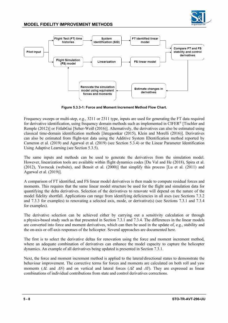
MODEL FIDELITY IMPROVEMENT METHODS

5 - 8 STO-TR-AVT-296-UU

Figure 5.3.3-1: Force and Moment Increment Method Flow Chart.

Frequency sweeps or multi-step, e.g., 3211 or 2311 type, inputs are used for generating the FT data required for derivative identification, using frequency domain methods such as implemented in CIFER® [Tischler and Remple (2012)] or FitlabGui [Seher-Weiß (2016)]. Alternatively, the derivatives can also be estimated using classical time-domain identification methods [Jategaonkar (2015), Klein and Morelli (2016)]. Derivatives can also be estimated from flight-test data using the Additive System IDentification method reported by Cameron et al. (2019) and Agarwal et al. (2019) (see Section 5.3.4) or the Linear Parameter Identification Using Adaptive Learning (see Section 5.3.5).

The same inputs and methods can be used to generate the derivatives from the simulation model. However, linearization tools are available within flight dynamics codes [Du Val and He (2018), Spira et al. (2012), Yavrucuk (website), and Benoit et al. (2000)] that simplify this process [Lu et al. (2011) and Agarwal et al. (2019)].

A comparison of FT identified, and FS linear model derivatives is then made to compute residual forces and moments. This requires that the same linear model structure be used for the flight and simulation data for quantifying the delta derivatives. Selection of the derivatives to renovate will depend on the nature of the model fidelity shortfall. Applications can range from identifying deficiencies in all axes (see Sections 7.3.2 and 7.3.3 for examples) to renovating a selected axis, mode, or derivative(s) (see Sections 7.3.1 and 7.3.4 for examples).

The derivative selection can be achieved either by carrying out a sensitivity calculation or through a physics-based study such as that presented in Section 7.3.1 and 7.3.4. The differences in the linear models are converted into force and moment derivatives, which can then be used in the update of, e.g., stability and the on-axis or off-axis responses of the helicopter. Several approaches are documented here.

The first is to select the derivative deltas for renovation using the force and moment increment method, where an adequate combination of derivatives can enhance the model capacity to capture the helicopter dynamics. An example of all derivatives being updated is presented in Section 7.3.1.

Next, the force and moment increment method is applied to the lateral/directional states to demonstrate the behaviour improvement. The corrective terms for forces and moments are calculated on both roll and yaw moments (∆L and ∆N) and on vertical and lateral forces (∆Z and ∆Y). They are expressed as linear combinations of individual contributions from state and control derivatives corrections.

MODEL FIDELITY IMPROVEMENT METHODS

STO-TR-AVT-296-UU 5 - 9

∆𝐿𝐿 = 𝐼𝐼𝑥𝑥𝑥𝑥𝐿𝐿𝑁𝑁_𝐼𝐼𝐼𝐼 − 𝐿𝐿𝑁𝑁_𝑙𝑙𝑖𝑖𝑛𝑛𝑝𝑝 + 𝐿𝐿𝑎𝑎_𝐼𝐼𝐼𝐼 − 𝐿𝐿𝑎𝑎_𝑙𝑙𝑖𝑖𝑛𝑛𝑣𝑣 + 𝐿𝐿𝑟𝑟_𝐼𝐼𝐼𝐼 − 𝐿𝐿𝑟𝑟_𝑙𝑙𝑖𝑖𝑛𝑛𝑉𝑉 +𝐿𝐿𝑙𝑙𝑑𝑑𝑑𝑑_𝐼𝐼𝐼𝐼 − 𝐿𝐿𝑙𝑙𝑑𝑑𝑑𝑑_𝑙𝑙𝑖𝑖𝑛𝑛𝛿𝛿𝑙𝑙𝑑𝑑𝑑𝑑 + 𝐿𝐿𝑁𝑁𝑒𝑒𝑑𝑑_𝐼𝐼𝐼𝐼 − 𝐿𝐿𝑁𝑁𝑒𝑒𝑑𝑑_𝑙𝑙𝑖𝑖𝑛𝑛𝛿𝛿𝑁𝑁𝑒𝑒𝑑𝑑

∆𝑁𝑁 = 𝐼𝐼𝑧𝑧𝑧𝑧𝑁𝑁𝑎𝑎_𝐼𝐼𝐼𝐼 − 𝑁𝑁𝑎𝑎_𝑙𝑙𝑖𝑖𝑛𝑛𝑣𝑣 + 𝑁𝑁𝑟𝑟_𝐼𝐼𝐼𝐼 − 𝑁𝑁𝑟𝑟_𝑙𝑙𝑖𝑖𝑛𝑛𝑉𝑉 + 𝑁𝑁𝑁𝑁𝑒𝑒𝑑𝑑_𝐼𝐼𝐼𝐼 −𝑁𝑁𝑁𝑁𝑒𝑒𝑑𝑑_𝑙𝑙𝑖𝑖𝑛𝑛𝛿𝛿𝑁𝑁𝑒𝑒𝑑𝑑

∆𝑌𝑌 = 𝑚𝑚𝑌𝑌𝑎𝑎_𝐼𝐼𝐼𝐼 − 𝑌𝑌𝑎𝑎_𝑙𝑙𝑖𝑖𝑛𝑛𝑣𝑣 + 𝑌𝑌𝑟𝑟_𝐼𝐼𝐼𝐼 − 𝑌𝑌𝑟𝑟_𝑙𝑙𝑖𝑖𝑛𝑛𝑉𝑉 + 𝑌𝑌𝑙𝑙𝑑𝑑𝑑𝑑_𝐼𝐼𝐼𝐼 − 𝑌𝑌𝑙𝑙𝑑𝑑𝑑𝑑_𝑙𝑙𝑖𝑖𝑛𝑛𝛿𝛿𝑙𝑙𝑑𝑑𝑑𝑑

∆𝑍𝑍 = 𝑚𝑚𝑍𝑍𝑤𝑤_𝐼𝐼𝐼𝐼 − 𝑍𝑍𝑤𝑤_𝑙𝑙𝑖𝑖𝑛𝑛𝑤𝑤

(5.3.3-1)

where 𝐼𝐼𝑥𝑥𝑥𝑥, 𝐼𝐼𝑧𝑧𝑧𝑧 are the helicopter moments of inertia about the roll and the yaw axes, m is the helicopter mass, extension “_ID” designates derivatives from system identification whereas “_lin” designates those calculated from the nonlinear model linearization.

Finally, the corrected rolling moment 𝐿𝐿𝑁𝑁𝑁𝑁−𝑐𝑐𝑚𝑚𝑟𝑟𝑟𝑟𝑒𝑒𝑐𝑐𝑑𝑑𝑒𝑒𝑑𝑑 for the nonlinear simulation is given as:

𝐿𝐿𝑁𝑁𝐿𝐿−𝑠𝑠𝑜𝑜𝑉𝑉𝑉𝑉𝑒𝑒𝑠𝑠𝑡𝑡𝑒𝑒𝑑𝑑 = 𝐿𝐿𝑁𝑁𝐿𝐿−𝑜𝑜𝑉𝑉𝑉𝑉𝑔𝑔𝑉𝑉𝑛𝑛𝑉𝑉𝑉𝑉 + 𝛥𝛥𝐿𝐿 (5.3.3-2)

and analogously for the other axes. Results for this analysis are presented in Section 7.3.2. Results for this analysis are presented in Section 7.3.2.

Another approach for selecting the derivative deltas for renovation is to identify those that have a quantified impact on a user-defined cost function [Lu et al. (2011)]. An example application of renovating the lateral-directional oscillations for a forward flight case is given in Section 7.3.1.

5.3.4 Additive System Identification (ASID) The identification approach presented in this section is described as ‘Additive System Identification’ (ASID), based on Equation-Error (EE) analysis in the time domain. The method has been developed principally to aid investigations of nonlinear aerodynamic complexities [Agarwal et al. (2019)]. The ASID method can then be augmented by the force and moment increment method (described earlier in this section) to complete the model update process with delta derivatives or nonlinear force and moment contributions.

The ASID approach is illustrated schematically in Figure 5.3.4-1 and is based on the equation-error model structure shown in Equation (5.3.4-1):

𝑓𝑓 = 𝑌𝑌𝑥𝑥𝑖𝑖𝑥𝑥𝑖𝑖

𝑁𝑁

𝑖𝑖=1

(5.3.4-1)

where f is the specific force, N (= 7 for this case) is the number of identified derivatives, 𝑌𝑌𝑥𝑥𝑖𝑖 are coefficients, and xi are the state/control variables. The ordering of variables xi is determined by the sequence in which different physical dynamics are activated (an example is provided in Section 7.3.1). The coefficient value Yxi of a variable xi is identified corresponding to the minimum fit error at the timing point Tj, as defined in Equation

𝐹𝐹𝑉𝑉𝑡𝑡𝐹𝐹𝑉𝑉𝑉𝑉𝑜𝑜𝑉𝑉 =1𝑇𝑇𝑗𝑗

∫ (𝑓𝑓 − ∑ 𝑌𝑌𝑥𝑥𝑖𝑖𝑥𝑥𝑖𝑖𝑁𝑁𝑖𝑖=1 )2𝑑𝑑𝑡𝑡𝑇𝑇𝑗𝑗

0

∫ 𝑓𝑓2𝑑𝑑𝑡𝑡𝑇𝑇𝑗𝑗0

(5.3.4-2)

in which Tj is the local period for the jth identification step, starting from the beginning of the ASID process.

MODEL FIDELITY IMPROVEMENT METHODS

5 - 10 STO-TR-AVT-296-UU

The left-hand edge of the analysis window in Figure 5.3.4-1 remains at the initial time point and the right-hand edge opens to increase the window size for determination of the current state or control variable. The local least-squares fit error for the specific force (𝑓𝑓, force/moment normalised by the rotorcraft mass or moment of inertia), is integrated over the window size Tj in Equation 5.3.4-2. The window size increases as xi variables are added, until the complete manoeuvre is modelled, or no further improvement can be achieved. Once identified in a specific time window, the derivatives stay fixed for the remainder of the manoeuvre and the subsequent application of the ASID process.

Figure 5.3.4-1: General Approach to Additive System Identification.

This feature of the ASID approach clearly differentiates it from the classical SID methods in both time and frequency domains, in terms of either EE or Output-Error (OE) analyses [Klein and Morelli (2016), Tischler and Remple (2012)].

The primary differences are summarised here. Firstly, the ASID approach identifies flight model parameters sequentially based on their contribution to the local dynamic response of the system. Conventional SID approaches process the complete time history, so the identified derivatives are a form of average for the whole manoeuvre; or, put in another way, the identified system shows average system behaviour [Jategaonkar (2015)]. The rationale behind the development of ASID is that a large part of the physics in the force or moment contributions to a rotorcraft’s motion should be ‘identifiable’ at the times when they are most significant. For example, in Figure 5.3.4-1, the variable x2 is identified at time T4 and so on. Having clearly identified a force contribution, it will be fixed and not distorted later – perhaps to compensate for a mismatch occurring from an incorrect model structure. This assumes that linear, instantaneous approximations to the motion are valid. Secondly, the ASID approach is similar to recursive estimation methods [Haykin (1986), Ljung (1983)] that are widely used for real-time SID in that the latter conduct the SID based on the data point by point when they become available. However, these recursive estimation methods have no mechanism applied to judge the sequence of derivatives to be identified based on the physical information in the way that ASID does. Moreover, the number of derivatives is typically fixed during the recursive SID process, but in the ASID method, it is variable.

0 1 2 3 4 5-1

0

1

0 1 2 3 4 5

T1

Yx1

T2 T3 T4 T5

Yx3

Yx6Yx2 Yx7

MODEL FIDELITY IMPROVEMENT METHODS

STO-TR-AVT-296-UU 5 - 11

5.3.5 Linear Parameter Identification Using Adaptive Learning Another SID approach used is a time-domain based identification method based on recent proofs and results in the area of Model Reference Adaptive Control, where it is shown that the uncertainty arising from the unmodelled dynamics could be linearly parameterized, and the convergence of the adaptive weights around the optimal locations is possible. Moreover, a unique optimal solution exists if the basis of the adaptive element is composed of a minimal representation of the dynamic system [Chowdhary (2010), Chowdhary et al. (2013)].

In Yavrucuk and Prasad (2012) and Gursoy and Yavrucuk (2016), algorithms are proposed that aim to represent model uncertainty using sensor measurement during flight in real time. Here, those algorithms are used off line for the purpose of system identification. Combined with results of Chowdhary (2010) and Chowdhary et al. (2013), a linear model is obtained using measured flight-test data in time domain that is optimal and unique.

Representing the helicopter dynamics as the summation of an approximate linear model and a model uncertainty 𝜉𝜉, where 𝑥𝑥 ∈ 𝛺𝛺𝑛𝑛 is the state vector and 𝑢 ∈ 𝛺𝛺𝑁𝑁 is a known control input vector:

𝑥 = 𝐴𝐴𝑥𝑥 + 𝐵𝐵𝑢 + 𝜉𝜉(𝑥𝑥, 𝑢) (5.3.5-1)

Assuming that the uncertainty 𝜉𝜉 can be linearly parameterized, there exists a set of unique optimal weights 𝑊𝑊∗ ∈ 𝛺𝛺(𝑛𝑛+𝑁𝑁)×𝑛𝑛 with a reconstruction error 𝜀𝜀 such that

𝜉𝜉(𝑥𝑥,𝑢) = W∗T 𝑥 + 𝜀𝜀 (5.3.5-2)

where 𝑥 = [𝑥𝑥 𝑢]𝑇𝑇 ∈ 𝛺𝛺𝑛𝑛+𝑁𝑁 is the basis vector, an optimal reconstruction of 𝑊𝑊 would lead to a linear model representation of the aircraft. Such a re-construction is shown to be possible when the following update law is used:

𝑊(t) = ΓxeTP + 𝑥𝑗𝑗

𝑙𝑙

𝑗𝑗=1

𝜉𝜉𝑗𝑗 −𝑊𝑊𝑇𝑇𝑥𝑗𝑗 (5.3.5-3)

In order to achieve guaranteed boundedness around optimal weights, recorded linearly independent elements 𝑥𝑗𝑗 are reused during convergence. Therefore, the adaptation uses a set of recorded data at each update:

𝑍𝑍 = [𝑥1, 𝑥2, 𝑥3, … , 𝑥𝑙𝑙] (5.3.5-4)

Here, 𝑥𝑗𝑗 ∈ 𝛺𝛺𝑚𝑚, 𝑗𝑗 = 1,2, … , 𝑉𝑉 are the basis vectors recorded at different times, and 𝑍𝑍 is an 𝑛𝑛 × 𝑉𝑉 history stack matrix. Any basis vector that increases the minimum singular value of the 𝑍𝑍 matrix is reused to update weights. Once the 𝑍𝑍 matrix is full, new data will replace the old only if the minimum singular value of 𝑍𝑍 is increased. This is used in Chowdhary (2010) and Chowdhary et al. (2013) and later in Gursoy and Yavrucuk (2016).

If the rigid body states and control inputs of the helicopter are used to form the basis vector 𝑥 , a unique representation of the matrix W is found as this basis vector can be thought of a minimal representation of the helicopter rigid-body dynamics. A representation of the overall setup is given in Figure 5.3.5-1. An application is shown in Section 7.3.3.

MODEL FIDELITY IMPROVEMENT METHODS

5 - 12 STO-TR-AVT-296-UU

Figure 5.3.5-1: Linear Parameter Identification Using Adaptive Learning.

5.3.6 Limitations Limitations and conditions for successful SID (for both the frequency-domain and time-domain methods described above) concern four aspects. First, the quality of the flight-test data should be high. Measurement and process noise, including sensor bias and scale factor errors, should be minimized to ensure quality measurements of motions and controls. Second, the control inputs should excite the vehicle dynamics sufficiently well that the force and moment contributions from the states and controls are ‘strong’ enough to be identifiable. Third, the assumed model structure should capture the vehicle dynamics sufficiently well that reduced order approximations remain valid. Finally, because of the complexities of rotorcraft flight dynamics, any SID method arguably requires a user, or user-team, to have an advanced level of abilities in the mathematical processes and physical interpretations.

At the end of the process, it is expected that the time responses will generally match the flight-test data well and could be used, for example, in training simulators. Minor differences from the 6-DOF state-space responses are expected since the non-linear models contain higher-order dynamics such as flap and lead-lag. Nonlinearities, e.g., from the main rotor wake/tail rotor interactions, are also approximately represented within the 6-DOF linear models. Moreover, the success criteria for some of the above methods are defined to match QTG requirements. Therefore, the training data used for adaptation can involve more time history data, other than the 3211 identification results. The time history data could include manoeuvres present in the QTG requirements in addition to 3211 related data.

More generally, the force and moment increment method associated with both frequency- and time-domain methods provides insight into model deficiencies through the ‘delta’ derivatives and points to the potential areas of improvement, but it does not directly identify the root causes of the model’s deficiency. The search for the missing physics is the next stage in the renovation process.

MODEL FIDELITY IMPROVEMENT METHODS

STO-TR-AVT-296-UU 5 - 13

5.4 REDUCED ORDER MODELS AND PHYSICS-BASED CORRECTIONS

5.4.1 Organisations Advanced Rotorcraft Technology, Inc., Sikorsky, a Lockheed Martin Company, The Boeing Company, Georgia Institute of Technology, United States Naval Academy, Defence Science and Technology Group (Australia), Leonardo Helicopters (Italy).

5.4.2 Purpose and Applications Reduced order modelling and physics-based corrections are considered for improved rotorcraft flight simulation fidelity. With its physics-based solution, the method is applicable to both engineering simulation for supporting design and analysis and real-time flight simulation for training simulator applications.

5.4.3 Methodology Although remarkable progress has been made in developing high-fidelity methods for improved prediction of rotorcraft aerodynamics, such as CFD, direct use of such methods in flight simulation is limited by the high computational speed required for real-time flight simulation. Reduced order models can be extracted from high-fidelity models while providing efficient computation. Properly derived reduced order models with physics-based correction of the modelling parameters can retain the simulation accuracy needed for both engineering and real-time flight simulation; therefore, this provides a practical and effective means of meeting the requirements for both prediction accuracy and computational efficiency. Reduced order modelling and physics-based correction methods were investigated and demonstrated through simulation fidelity assessment with case studies as detailed in Chapter 7.4. This section covers multiple modelling aspects, including rotor induced inflow dynamics, aerodynamic interference, fuselage aerodynamics, engine/drivetrain dynamics with rotor lead-lag dynamics, and sensor and swashplate actuator dynamics. The following subsections describe each of the investigated physics-based reduced order modelling methods.

5.4.3.1 Rotor Induced Inflow Dynamics

The rotor induced inflow model is a vital part of accurate rotor aerodynamics and dynamics modelling that impacts flight simulation in various ways, including performance, stability, and control response. Pitt-Peters [Pitt et al. (1987)] and Peters-He inflow models [Peters et al. (1991)] are widely used in most current flight simulations. Both inflow models only address rotor self-induced induced inflow over the rotor plane and therefore lack the capability for predicting rotor interference on other rotors and aerodynamic surfaces. Both inflow models also assume rigid rotor wake geometry, and hence, are limited for modelling the effect of rotor wake distortion that occurs in manoeuvring flight.

Rotor wake distortion resulting from rotor Tip-Path-Plane (TPP) rotation in manoeuvring flight was found to be a cause of erroneous prediction of off-axis response of single main rotor helicopter in hover and low-speed flight [Rosen et al. (1994)]. As shown in Figure 5.4.3.1-1, the rotor wake experiences noticeable distortion of curvature along with compression on one side while expansion on the other during rotor TPP pitch or roll rotation. The distorted manoeuvring wake leads to significant change of rotor induced inflow. The inflow models formulated in the following sections include additional modelling terms that addresses the effect.

MODEL FIDELITY IMPROVEMENT METHODS

5 - 14 STO-TR-AVT-296-UU

Figure 5.4.3.1-1: Rotor Wake Distortion Due to TPP Rotation.

5.4.3.1.1 Augmented Dynamic Inflow Model for Manoeuvring Flight

It was found that the effect of rotor wake distortion involves two dynamic modes. One is the fast mode with rotor induced inflow dynamics that can be addressed by introducing a correction term (so-called Kr parameter [Keller and Curtiss (1998)]) directly into the baseline inflow model. The other is the slower mode that is related to the dynamic change of the curved wake geometry during rotor Tip-Path Plane (TPP) rotation. There are multiple ways to derive the wake distortion model. In Krothapalli et al. (2001) and Zhao et al. (2004), the authors adapted a manoeuvring vortex tube model and derived the wake curvature terms as augmentation to the inflow gain matrix 𝐿𝐿 of the baseline dynamic inflow model. Also, it is important to allow for a dynamic change of the wake geometry while incorporating the wake curvature, as it was found that a quasi-steady wake curvature model could lead to simulation divergence. The augmented three-state dynamic inflow model that includes the wake curvature terms for manoeuvres from hover can be written as [Zhao et al. (2004)].

[𝑀𝑀]𝜆𝑚𝑚𝜆𝑠𝑠𝜆𝑐𝑐

+ [𝑉𝑉][𝐿𝐿 + 𝐾𝐾𝑅𝑅𝑒𝑒∆𝐿𝐿]−1 𝜆𝜆𝑚𝑚𝜆𝜆𝑠𝑠𝜆𝜆𝑐𝑐 =

𝑉𝑉𝑇𝑇−𝑉𝑉𝑁𝑁−𝑉𝑉𝑀𝑀

(5.4.3.1.1-1)

where 𝐾𝐾𝑅𝑅𝑒𝑒 is the modelling parameter used for scaling the effect of wake curvature and ∆𝐿𝐿 is the augmentation to the inflow gain matrix that models the wake curvature effect, and it is derived using vortex tube theory as

Δ𝐿𝐿 =

⎣⎢⎢⎢⎢⎡ 0

𝜅𝜅𝑠𝑠2

𝜅𝜅𝑐𝑐2

𝜅𝜅𝑠𝑠2

0 0𝜅𝜅𝑐𝑐2

0 0 ⎦⎥⎥⎥⎥⎤

(5.4.3.1.1-2)

In order to realize the dynamic change of wake geometry during a pitch or roll manoeuvre, the longitudinal and lateral wake curvatures (𝜅𝜅𝑐𝑐 , 𝜅𝜅𝑠𝑠) in the above equation are related to the rotor tip-path-plane pitch and roll rates through a first-order lag with a time constant, 𝜏𝜏 = 16

15𝜋𝜋𝑎𝑎ℎ, [Zhao et al. (2004)].

𝜏𝜏𝜅𝑐𝑐 + 𝜅𝜅𝑐𝑐 =𝑞𝑞 − 𝛽𝑐𝑐𝑣𝑣ℎ

(5.4.3.1.1-3)

MODEL FIDELITY IMPROVEMENT METHODS

STO-TR-AVT-296-UU 5 - 15

𝜏𝜏𝜅𝑠𝑠 + 𝜅𝜅𝑠𝑠 =𝑝 − 𝛽𝑠𝑠𝑣𝑣ℎ

(5.4.3.1.1-4)

where 𝑣𝑣ℎ is the non-dimensional mean induced velocity in hover. The application of the augmented dynamic inflow model is illustrated in Section 7.4.1, where the UH-60 case study results are shown.

5.4.3.1.2 Reduced Order Inflow Model Derived from Viscous Vortex Particle Method

Another approach for the development of a reduced order induced inflow model is to derive it from the first principle-based rotor wake solution, e.g., viscous Vortex Particle Method (VPM) [He et al. (2008, 2009)]. By truncating Peters-He’s finite state induced inflow model to a dynamic inflow equation of 3 states (i.e., uniform and cosine and sine harmonics), it reduces to an equivalent Pitt-Peters inflow model. Both inflow models incur the limitations resulting from their rigid (no distortion) wake geometry and potential flow (non-viscid) assumption. Physics-based inflow model parameter corrections are considered for improved model fidelity through calibration of inflow influence coefficients and interference parameters against high-fidelity models, such as the viscous vortex particle method [He et al. (2019)].

[𝑀𝑀] ∝10

∝21𝑐𝑐

∝21𝑠𝑠 + [𝐿𝐿]−1[𝑉𝑉]

∝10

∝21𝑐𝑐

∝21𝑠𝑠 =

12𝜏𝜏10

𝜏𝜏21𝑐𝑐

𝜏𝜏21𝑠𝑠 +

𝐾𝐾𝑟𝑟𝑚𝑚𝑑𝑑𝜏𝜏𝑠𝑠𝑆𝑆 + 1

0

𝑞𝑞 − 𝛽1𝑐𝑐𝑝𝑝 − 𝛽1𝑠𝑠

(5.4.3.1.2-1)

where ∝10, ∝21𝑐𝑐, and ∝21𝑠𝑠 are the uniform, first harmonic (cosine and sine) cyclic induced inflow states, respectively, 𝜏𝜏10, 𝜏𝜏21𝑐𝑐 , and 𝜏𝜏21𝑠𝑠 are the corresponding inflow forcing functions, and 𝑉𝑉 is the mass flow parameter [Peters and He (1991)]. The above inflow dynamics equation is based on Peters-He’s formulation but with the modelling parameters, i.e., [M] (apparent mass matrix) and [L] (inflow influence coefficient matrix), identified from first principle-based viscous vortex simulations using the CIFER® system identification technique [He et al. (2019)]. In addition, the effect of rotor wake distortion in manoeuvring flight is added as an inflow forcing function with the rotor tip-path-plane pitch and roll rate, as shown in the above equation (i.e., the Krot term, [He et al. (2019)]). The application of the reduced order inflow dynamic model derived from the VPM is illustrated in Section 7.4.1, where the UH-60 case study results are shown. Physical corrections to the L-matrix elements are also discussed in the UH-60 case study [Zhang et al. (2017)]. The model fidelity improvement using the VPM is further shown in Section 7.4.3 where AW109 case study results are discussed.

5.4.3.1.3 PPSIM Induced Inflow Model

Pressure Potential Superposition Inflow Model (PPSIM) assumes that flow around the rotor disk is incompressible and inviscid. In PPSIM, rotors’ individual pressure fields are superimposed. Then, the governing inflow equation for a tandem rotor configuration can be obtained as [Guner et al. (2018)]

𝑀𝑀𝐹𝐹𝐹𝐹 𝑀𝑀𝑅𝑅𝐹𝐹𝑀𝑀𝐹𝐹𝑅𝑅 𝑀𝑀𝑅𝑅𝑅𝑅

𝛼𝛼𝐹𝛼𝑅𝑅 + 𝑉𝑉𝑚𝑚𝐹𝐹 0

0 𝑉𝑉𝑚𝑚𝑅𝑅 𝐿𝐿𝐹𝐹𝐹𝐹 𝐿𝐿𝑅𝑅𝐹𝐹𝐿𝐿𝐹𝐹𝑅𝑅 𝐿𝐿𝑅𝑅𝑅𝑅

−1𝛼𝛼𝐹𝐹𝛼𝛼𝑅𝑅 =

12𝜏𝜏𝐹𝐹𝜏𝜏𝑅𝑅

(5.4.3.1.3-1)

where [𝑀𝑀] and [𝐿𝐿] are the apparent mass and inflow influence coefficient matrices, respectively, and 𝜏𝜏′𝑠𝑠 are the inflow forcing functions. In PPSIM, while diagonal blocks in [𝑀𝑀] and [𝐿𝐿] matrices are related to self-induced inflow, off-diagonal element blocks capture aerodynamic interference effects caused by the other rotor [Prasad et al. (2012) and Guner et al. (2018)]. Simulation modelling fidelity improvement through application of PPSIM model is demonstrated in Section 7.4.2 where the CH-47 case study results are discussed.

MODEL FIDELITY IMPROVEMENT METHODS

5 - 16 STO-TR-AVT-296-UU

5.4.3.1.4 Howlett GenHel Rotor Induced Inflow Model

Howlett (1981a) defines the equations used to model rotor air mass dynamics in the nonlinear mathematical model of the UH-60A Black Hawk helicopter based on the Sikorsky General Helicopter (GenHel) flight dynamics simulation. Howlett (1981b) documents the derivation of the inflow model equations and provides background and descriptive information which supports understanding of GenHel rotor airmass degree of freedom modelling. The methodology used in GenHel to represent rotor induced inflow dynamics is widely known and applied in the rotorcraft flight simulation community and provides a succinct formulation of the inflow model defining equations that combines established theory with a capacity for empirical extrapolation based on flight-test data or information provided by more advanced rotor wake modelling methods.

The GenHel rotor induced inflow dynamic model is based primarily on a downwash distribution prescribed as a function of rotor aerodynamic loading. GenHel calculates total downwash at any point on the rotor as a combination of the three elements below:

1) A basic uniform component which results from generating aerodynamic rotor thrust.

2) First harmonic component derived by cyclic aerodynamic hub moment on the rotor disk.

3) A cosine harmonic component due to rotor wake skew with increasing rotor advance ratio.

The first basic component of rotor downwash in the Howlett GenHel model, which is derived by application of simple momentum theory, is a uniform distribution of induced inflow over the rotor disk, which is calculated as a function of the total rotor aerodynamic thrust. The second component is a first harmonic, or cyclic, inflow distribution, a reaction of the airflow to aerodynamic hub moments. Howlett (1981b) notes that the first harmonic induced inflow component due to rotor aerodynamic hub moments ‘would not exist for a centrally hinged rotor in a steady state condition but would exist in the steady state for hingeless rotors or rotors with hinge offset (which can produce aerodynamic hub moments)’. Howlett (1981b) observes that experimental data justifying the analytical modelling of the influence of aerodynamic hub moments on first harmonic inflow is based largely on hingeless rotor experimental data. Therefore, while provisioning GenHel to account for the effect of rotor aerodynamic hub moments on rotor first harmonic inflow was considered important, the GenHel Black Hawk simulation model was configured with respect to zero hub moment induced inflow terms because Howlett (1981b) concluded that it was not possible to justify quantitative model input parameters. The third component of rotor downwash is the element of wind axis first harmonic longitudinal inflow skew due to wake blowback as modelled by classical Glauert downwash factors in the GenHel model. This third component of rotor downwash is due to the tendency of the rotor wake to blowback or skew as wind axis advance ratio increases, resulting in a redistribution of rotor induced downwash along the wind axis across the rotor. This redistribution of downwash over the rotor tends to reduce downwash on the upwind side of the rotor and increase downwash on the downwind side of the rotor.

Inflow model description: The defining equations for the Howlett GenHel rotor induced inflow model follow from the discussion above and are shown in Equations 5.4.3.1.4-1 – 5.4.3.1.4-4 below:

𝜆𝜆𝑖𝑖 = 𝜆𝜆𝑖𝑖0 + 𝜆𝜆𝑖𝑖1𝐶𝐶 cos𝜓𝜓 + 𝜆𝜆𝑖𝑖1𝑆𝑆 sin𝜓𝜓 (5.4.3.1.4-1)

𝜆𝜆𝑖𝑖0 = 𝐾𝐾𝐶𝐶𝑇𝑇𝑉𝑉𝑇𝑇

2𝑉𝑉𝑇𝑇

1

𝜏𝜏0𝑉𝑉𝑇𝑇 𝑠𝑠 + 1

(5.4.3.1.4-2)

MODEL FIDELITY IMPROVEMENT METHODS

STO-TR-AVT-296-UU 5 - 17

𝜆𝜆𝑖𝑖1𝐶𝐶 =𝜇𝜇𝑉𝑉𝑇𝑇𝜇𝜇𝑥𝑥𝜆𝜆𝑖𝑖0 −

𝐾𝐾𝐶𝐶𝑀𝑀𝑉𝑉𝑀𝑀𝑉𝑉𝑇𝑇

1

𝜏𝜏𝑐𝑐𝑉𝑉𝑇𝑇 𝑠𝑠 + 1

(5.4.3.1.4-3)

𝜆𝜆𝑖𝑖1𝑆𝑆 =𝜇𝜇𝑉𝑉𝑇𝑇𝜇𝜇𝑥𝑥𝜆𝜆𝑖𝑖0 −

𝐾𝐾𝐶𝐶𝑁𝑁𝑉𝑉𝑁𝑁𝑉𝑉𝑇𝑇

1

𝜏𝜏𝑠𝑠𝑉𝑉𝑇𝑇 𝑠𝑠 + 1

(5.4.3.1.4-4)

where 𝑉𝑉𝑇𝑇 is the total flow velocity passing through the rotor nondimensionalized with respect to rotor tip speed and formulated as 𝑉𝑉𝑇𝑇 = 𝜇𝜇2 + 𝜆𝜆2. Note that the Howlett GenHel rotor induced inflow model structure is used in the CH-47 case study in Section 7.4.2.

5.4.3.1.5 Boeing Helicopters Simulation Inflow Modelling Method (BHSimIMM)

BHSimIMM is an industry standard inflow model used in the CH-47 simulation, and it is empirically tuned to match with flight-test data [Hackett et al. (1983)]. BHSimIMM has a three-state inflow representation similar to the Pitt-Peters inflow model [Peters and HaQuang (1988)] as shown in Equation 5.4.3.1.5-1.

𝜆𝜆(𝑉,𝜓𝜓) = 𝜆𝜆𝑖𝑖0 + 𝜆𝜆𝑖𝑖1𝐶𝐶𝑉 cos𝜓𝜓 + 𝜆𝜆𝑖𝑖1𝑆𝑆𝑉 sin𝜓𝜓 (5.4.3.1.5-1)

In BHSimIMM, there is only uniform inflow coupling between the rotors and this coupling comes purely from empirical relations. For example, the uniform inflow component of the front rotor is calculated using Equations 5.4.3.1.5-2 – 5.4.3.1.5-4. Here, subscripts ‘𝑆𝑆𝐹𝐹𝐿𝐿𝐹𝐹’ and ‘𝐼𝐼𝑁𝑁𝑇𝑇𝐹𝐹’ represent inflow due to the respective rotor’s loading and interference inflow due to the other rotor’s loading, respectively. The symbol ‘𝐹𝐹’ stands for front rotor, the symbol ‘𝛺𝛺’ stands for rear rotor, and 𝑑𝑑𝑅𝑅𝐹𝐹 represents the empirical correction to incorporate the effect of rear rotor on front rotor’s uniform inflow component.

𝜆𝜆𝑖𝑖0𝐹𝐹 = 𝜆𝜆𝑖𝑖0𝐹𝐹 𝑆𝑆𝑆𝑆𝑆𝑆𝐹𝐹+ 𝜆𝜆𝑖𝑖0𝐹𝐹 𝐼𝐼𝐼𝐼𝐼𝐼𝐹𝐹

(5.4.3.1.5-2)

𝜆𝜆𝑖𝑖0𝐹𝐹 𝑆𝑆𝑆𝑆𝑆𝑆𝐹𝐹=

𝑉𝑉𝑇𝑇𝐹𝐹2𝑉𝑉𝑇𝑇𝐹𝐹

1

𝜏𝜏11𝑠𝑠 + 1 (5.4.3.1.5-3)

𝜆𝜆𝑖𝑖0𝐹𝐹 𝐼𝐼𝐼𝐼𝐼𝐼𝐹𝐹= 𝑑𝑑𝑅𝑅𝐹𝐹𝜆𝜆𝑖𝑖0𝑅𝑅 𝑆𝑆𝑆𝑆𝑆𝑆𝐹𝐹

1

𝜏𝜏𝐼𝐼𝑁𝑁𝑇𝑇𝐹𝐹𝑠𝑠 + 1 (5.4.3.1.5-4)

where 𝑉𝑉𝑇𝑇𝐹𝐹 is the total flow velocity passing through the front rotor nondimensionalized with respect to rotor tip speed and formulated as 𝑉𝑉𝑇𝑇𝐹𝐹 = 𝜇𝜇𝐹𝐹2 + 𝜆𝜆𝐹𝐹2 .

In BHSimIMM, the first harmonic induced inflow distributions are free from the mutual interference effects of the rotors [Hackett et al. (1983)]. BHSimIMM models the first harmonic rotor induced inflow distributions using equations of the form of the Howlett GenHel Rotor Induced Inflow Model [Howlett (1981a)] discussed in Section 5.4.3.1.4 above.

𝜆𝜆𝑖𝑖1𝐶𝐶 =𝜇𝜇𝑉𝑉𝑇𝑇√2𝜇𝜇𝑥𝑥𝜆𝜆𝑖𝑖0 −

𝐾𝐾𝐶𝐶𝑀𝑀𝑉𝑉𝑀𝑀𝑉𝑉𝑇𝑇

1

𝜏𝜏𝑐𝑐𝑉𝑉𝑇𝑇 𝑠𝑠 + 1

(5.4.3.1.5-5)

MODEL FIDELITY IMPROVEMENT METHODS

5 - 18 STO-TR-AVT-296-UU

𝜆𝜆𝑖𝑖1𝑆𝑆 =𝜇𝜇𝑉𝑉𝑇𝑇√2𝜇𝜇𝑥𝑥𝜆𝜆𝑖𝑖0 −

𝐾𝐾𝐶𝐶𝑁𝑁𝑉𝑉𝑁𝑁𝑉𝑉𝑇𝑇

1

𝜏𝜏𝑠𝑠𝑉𝑉𝑇𝑇 𝑠𝑠 + 1

(5.4.3.1.5-6)

The first term in Equations 5.4.3.1.5-5 and 5.4.3.1.5-6 is usually referred to as the trim first harmonic induced inflow distribution (wake skew effect) and ‘√2’ comes from the White and Blake Inflow Model [White and Blake (1979)]. The second term refers to the first harmonic induced inflow distribution due to rotor aerodynamic hub moment. The hub moment influence factors, KCM and KCL, and normalised time constants (𝜏𝜏𝑐𝑐, 𝜏𝜏𝑠𝑠) are introduced as tuning parameters to match flight-test data. It is important to note that subscripts ‘𝐹𝐹’ and ‘𝛺𝛺’ are dropped in Equations 5.4.3.1.5-5 and 5.4.3.1.5-6 because there is no interference in the first harmonic induced inflow distributions. For example, 𝜆𝜆𝑖𝑖1𝐶𝐶𝐹𝐹and 𝜆𝜆𝑖𝑖1𝑆𝑆𝐹𝐹 are only calculated using front rotor variables. The case study of the BHSimMM inflow model is illustrated in Section 7.4.2, where the CH-47 case study results are shown.

5.4.3.1.6 Higher-Order Inflow Model Identification from Free-Vortex Wake

This method uses system identification to develop a low-order model of the inflow for a coaxial rotor from a free-vortex wake. The method is similar in nature to Section 5.4.3.1.2 but uses a different identified inflow model structure. The inflow dynamics model structure given in Equation 5.4.3.1.6-1 is identical to the Pitt-Peters formulation with the addition of wake distortion and slowly varying “far” wake dynamics [Keller et al. (2019)]. The far wake coupling gives the resulting inflow response a higher-order behaviour that has been observed in free-vortex wake results [Rand et al. (2015), Hersey et al. (2018), Keller et al. (2019), and Juhasz et al. (2020)]. Time delays on thrust to aerodynamic loading and flapping equations account for computational delays in the stepping between the Maryland Free Wake (MFW) [Leishman et al. (2002)] and flight dynamics code for additional dynamics in the MFW that are not accounted for by the model.

[𝜏𝜏] 𝜆𝑈𝑈𝜆𝑁𝑁 + 𝜆𝑈𝑈

𝜆𝑁𝑁 = [𝐿𝐿] 𝑉𝑉𝑈𝑈𝑉𝑉𝑁𝑁

𝑒𝑒−𝜏𝜏𝑑𝑑,𝐶𝐶 + 𝛽1𝑠𝑠𝛽1𝑐𝑐

𝑒𝑒−𝜏𝜏𝑑𝑑,𝛽𝛽 + [𝐾𝐾𝐶𝐶]𝜆𝜆𝐹𝐹 (5.4.3.1.6-1)

𝜆𝑈𝑈 and 𝜆𝑁𝑁 are the upper and lower rotor self-induced velocities at the rotor plane and include uniform and first harmonic sine and cosine components:

𝜆 = 𝜆0𝜆𝑐𝑐𝜆𝑠𝑠 (5.4.3.1.6-2)

The forcing for each rotor’s inflow comes from each rotor’s aerodynamic thrust as well as pitching and rolling moments:

𝑉𝑉 = 𝑉𝑉𝑇𝑇𝑉𝑉𝑀𝑀𝑉𝑉𝑁𝑁 (5.4.3.1.6-3)

The far wake velocities, 𝜆𝜆𝐹𝐹, represent a slowly evolving dynamic wake downstream of the rotor planes and are thus combined into a single set of equations which contain only sine and cosine components [Keller et al. (2019)].

MODEL FIDELITY IMPROVEMENT METHODS

STO-TR-AVT-296-UU 5 - 19

𝜆𝜆𝐹𝐹 = 𝜆𝜆𝐹𝐹𝑐𝑐𝜆𝜆𝐹𝐹𝑠𝑠 (5.4.3.1.6-4)

The far wake dynamics couple with the near wake cosine and sine harmonics in Equation. 5.4.3.1.6-1 and are:

[𝜏𝜏𝐹𝐹]𝜆𝐹𝐹 + 𝜆𝜆𝐹𝐹 = −[𝐾𝐾𝑀𝑀] 𝜆𝑈𝑈𝜆𝑁𝑁 + [𝐾𝐾𝐹𝐹] 𝛽𝑐𝑐

𝛽𝑠𝑠 𝑒𝑒−𝜏𝜏𝑑𝑑,𝛽𝛽 (5.4.3.1.6-5)

Finally, the total inflow at each rotor disk is the sum of the self-induced velocity at that rotor and a contribution from the other rotor:

𝜆𝜆𝑈𝑈𝜆𝜆𝑁𝑁 = 1 𝐻𝐻𝑈𝑈𝑁𝑁

𝐻𝐻𝑁𝑁𝑈𝑈 1 𝜆𝑈𝑈𝜆𝑁𝑁 (5.4.3.1.6-6)

where [𝐻𝐻𝑈𝑈𝑁𝑁] and [𝐻𝐻𝑁𝑁𝑈𝑈] are identified influence coefficient matrices that capture each rotor’s influence on the total velocity at the plane of each rotor. Section 7.4.4 demonstrates the use of this technique for the identification of a coaxial rotor inflow model of the Sikorsky X2 Technology Demonstrator from the MFW.

5.4.3.2 Aerodynamic Interference

A rotorcraft involves complicated aerodynamic interference between its rotors, aerodynamic surfaces, and fuselage. Rotorcraft aerodynamic interference modelling remains a very challenging aspect for an accurate flight simulation. Most of existing flight simulation models rely on potential flow-based methods, such as real-time finite state rotor interference models [He et al. (2004)] or engineering vortex wake simulation to generate data for table look-up. These potential flow-based methods rely on empirical parameters in order to model the effects of wake distortion and wake vorticity dissipation. The empirical interference model parameters can be derived from first principle-based rotor wake simulation, such as VPM [He and Zhao (2009)] or calibrated against measured data [He et al. (2004)]. The aerodynamic interference method applies the rotor interference on aero-surfaces, fuselage, and other rotors. The aerodynamic interference method also addresses the ground effect in hover and low flight speed.

Section 7.4.1 UH-60 case study illustrates the application of the aerodynamic interference method and physics-based correction of rotor interference effect showing improved correlation with flight-test data [Zhang et al. (2017)]. Section 7.4.2 CH-47 case study shows the simulation model fidelity improvement using PPSIM rotor-to-rotor interference method and VPM based calibration of Peters-He finite state inflow interference [Kong et al. (2020) and He et al. (2004)]. Section 7.4.3 AW109 Trekker case study applies the VPM to the AW109 Trekker helicopter in trimmed level flight.

5.4.3.3 Fuselage Aerodynamics

Fuselage aerodynamics covers both fuselage airloads and fuselage interference on aerodynamic surfaces (e.g., horizontal stabilator and vertical fin). Most current simulations use empirical table look-up for estimating fuselage airloads. The empirical data are typically derived from wind tunnel tests or CFD solutions where only an isolated fuselage is considered without the effect of rotor interference. The interference effect is recovered later in the simulation through simple superposition which often uses only single interference sampling points. The empirical fuselage airloads approach can lack sufficient data to cover the full flight envelope. The fuselage interference effect is not usually as strong as rotors, but sometimes plays a role in both trim and transient response [Xin et al. (2019)]. Section 7.4.1 UH-60 case study shows the example simulation prediction improvement through physics-based correction of fuselage airloads and interference modelling.

MODEL FIDELITY IMPROVEMENT METHODS

5 - 20 STO-TR-AVT-296-UU

5.4.3.4 Engine and Drivetrain Dynamics

Engine and drivetrain dynamics modelling is important to correctly simulate those flight manoeuvres where rotor speed (NR) is not constant in time due to its effect on forces and moments transmitted from the rotor to the fuselage. Manoeuvres of this kind are, for example, those involving the use of collective and pedals. The axes which are most involved are typically those of heave and yaw.

The engine modelling consists of the representation of the drivetrain, of the engine thermodynamics, and of the fuel flow control logics. For flight mechanics purposes the drivetrain can be modelled as a simple inertia-spring-damping model with equivalent inertia set to guarantee same kinetic energy content and effective spring parameter tuned to capture the dynamics of the lower torsional mode. Engine dynamics can be represented as look-up tables to represent the engine static thermodynamics characteristics and a series of transfer functions to represent engine dynamics and fuel flow control logics.

This section discusses a physics-based modelling approach of engine and drivetrain to improve rotorcraft modelling fidelity. The method presented here provides a way to create a simplified model of a turboshaft engine by estimating thermodynamics static performance and engine dynamics and control laws transfer functions from data measured in flight. These kinds of models are called “Time-Constant Models”, and they are used with great success for flight dynamics modelling and simulation purposes.

Time-Constant Models: Time-Constants Models for the engine are presented in different papers and textbooks. In particular, a helpful reference is Dreier (2007), where different levels of accuracy of Engine Time-Constants Models are presented.

The engine model structure and interface with the rotorcraft drivetrain used in this report are represented in Figure 5.4.3.4-1.

Figure 5.4.3.4-1: Engine Model.

𝐾𝐾𝐼𝐼 +𝐾𝐾𝑃𝑃𝑠𝑠 + 𝑠𝑠𝐾𝐾𝐷𝐷 𝜇𝜇

1 + 𝜏𝜏𝑠𝑠

NR governor

𝜏𝜏1𝑠𝑠 + 𝑘𝑘𝑐𝑐𝜏𝜏2𝑠𝑠 + 1

Combustor and Torque model

Rotorcraft

Collective feed-forward

MODEL FIDELITY IMPROVEMENT METHODS

STO-TR-AVT-296-UU 5 - 21

Combustor and Torque Model: Given a step input in available fuel, the fireball in the combustion chamber instantly increases pressure. The pressure difference across the power turbine increases the available power (PWR). In the following, torque (TQ) will be used instead of power because directly available from flight data and proportional to power. In fact, according to the relation ∆𝑃𝑃𝑊𝑊𝛺𝛺 = ∆𝑇𝑇𝑇𝑇 ∙ 𝑁𝑁𝛺𝛺 + 𝑇𝑇𝑇𝑇 ∙ ∆𝑁𝑁𝛺𝛺, the ∆𝑁𝑁𝛺𝛺 contribution can be discarded when significantly lower than the ∆𝑇𝑇𝑇𝑇 contribution like in typical FADEC controlled propulsive systems.

This dynamic can be represented via a first-order equation. The equivalent transfer function can be represented by the following formula:

𝑇𝑇𝑇𝑇𝐹𝐹𝐹𝐹

= 𝜇𝜇

1 + 𝜏𝜏𝑠𝑠 (5.4.3.4-1)

where TQ is the engine torque, and FF is the commanded fuel flow. Parameter 𝜇𝜇 corresponds to the static gain between torque and fuel flow, and it can be derived from static performance results. Parameter 𝜏𝜏 is a time-delay constant related to the engine dynamics. The fuel flow is a function of both collective position and NR control:

𝐹𝐹𝐹𝐹 = 𝐹𝐹𝐹𝐹𝑃𝑃𝐼𝐼𝐼𝐼 + 𝐹𝐹𝐹𝐹𝐶𝐶 (5.4.3.4-2)

The fuel flow amount due to NR governor can be modelled with a generic Proportional, Integral and Derivative (PID) control:

𝐹𝐹𝐹𝐹𝑃𝑃𝐼𝐼𝐼𝐼 = 𝐾𝐾𝐼𝐼 +𝐾𝐾𝑃𝑃𝑠𝑠

+ 𝑠𝑠𝐾𝐾𝐼𝐼 ∙ 𝑁𝑁𝛺𝛺 − 𝑁𝑁𝛺𝛺𝑅𝑅𝑒𝑒𝑓𝑓 (5.4.3.4-3)

The feed-forward contribution from collective is added to the NR governor fuel flow contribution. This amount can be modelled with a simple lead-lag filter:

𝐹𝐹𝐹𝐹𝐶𝐶 = 𝜏𝜏1𝑠𝑠 + 𝑘𝑘𝑐𝑐𝜏𝜏2𝑠𝑠 + 1

∙ 𝛿𝛿𝑐𝑐𝑚𝑚𝑙𝑙𝑙𝑙 (5.4.3.4-4)

Tuning of Engine Parameters: All the unknown parameters (gain of transfer functions, time delay and constants) presented in the previous sections can be tuned in order to match the real behaviour of the engine to be modelled. An application example is described in Section 7.4.3. AW109 Trekker Case Study. However, the approach is general, and it can be applied to any helicopter equipped with turboshaft engines.

5.4.3.5 Sensor and Actuator Dynamics

Methods of sensor and actuator dynamics involve consideration of the effect of sensor dynamics (low-pass frequency) and actuator dynamics on aircraft control response prediction. A sensor is usually described in terms of the type of filter (e.g., Butterworth filter), bandwidth, and computational delay. These pieces of information can be found in the sensor or actuator’s data sheet. Actuator’s dynamics properties can be derived from the input-output frequency responses function of input displacement that are part of the actuator’s qualification test report. An application example is described in Section 7.4.3 AW109 Trekker Case Study.

5.4.4 Limitations Physics-based methods are based on physical laws and their approximate model formulations; therefore, they can be used for both design/engineering analysis and flight training simulators. The applications of physics-based approaches require good understanding of rotorcraft aerodynamics, dynamics, propulsion, and flight controls for identifying the root cause of the modelling discrepancies and applying the corrections accordingly.

MODEL FIDELITY IMPROVEMENT METHODS

5 - 22 STO-TR-AVT-296-UU

5.5 MODEL PARAMETER ADJUSTMENT FOR PHYSICS-BASED SIMULATIONS

5.5.1 Organisations CAE, Penn State University, Thales, ONERA, Defence Science and Technology Group (Australia).

5.5.2 Purpose and Applications Physics-based models have some advantages compared to their strictly parametric counterparts. Unfortunately, they also can have a rather large number of physical parameters that must be set to the appropriate value for the model to accurately predict the behaviour of a particular helicopter. Updates of physics-based models require either tuning of the physical parameters to achieve the best overall match with the measured response or the addition of artificial correction factors (e.g., added force and moment terms as discussed in Section 5.3).

Blade-element models of helicopter dynamics are usually employed to meet the fidelity requirements for Level D simulator classification. These physics-based models are also used in engineering simulations applied towards aircraft and flight control system development. Simulator manufacturers and simulation model developers do not often have a complete set of physical modelling data. The aircraft manufactures and operators do not always publish or even know all of the relevant parameters. The specific configuration used in a given flight test (e.g., weight and balance) are not always known and documented, and there are always some parameters that are difficult to measure accurately. Furthermore, the model is invariably incomplete with practical limits on overall simulation fidelity. All of these factors lead to various degrees of uncertainty on each parameter required for a physics-based blade-element model, which in turn lead to mismatch between the model and flight-test data.

Model parameter adjustment is justified by the following set of conditions:

1) There is significant uncertainty associated with certain key parameters that affect observed discrepancies.

2) The model developer can draw a direct physical relationship between the uncertain parameter and the discrepancy in the flight-test data, for example through system identification of linear model terms (e.g., stability and control derivatives) than can then be directly related to the uncertain parameter through well-established theoretical relationships [Tischler and Remple (2012)].

3) Non-linear physics-based models are required for the specific application, such that direct use of identified linear models is not a suitable substitute for the particular application.

5.5.3 Methodology Methodologies for physical parameter adjustment vary widely, ranging from comprehensive numerical optimizations using a large number of input parameters to parametric studies involving only one or two parameters. The appropriate method depends largely on the application. Thus, descriptions of update methods below are organised by application. Section 5.5.3.1 discusses parameter adjustments for pilot training simulators, where the key objective is to match test data within the bounds defined by certification requirements. Section 5.5.3.2 discusses parameter adjustments for engineering research simulators, where gaining physical insight to the rotorcraft dynamics is more critical.

MODEL FIDELITY IMPROVEMENT METHODS

STO-TR-AVT-296-UU 5 - 23

5.5.3.1 Parameter Adjustments for Level D Pilot Training Simulator

Systematic methods to overcome a data gap for full flight simulator Level D pilot training simulations are discussed in Spira et al. (2012). A modelling/optimization framework is used to determine unknown aeromechanical parameters in a blade-element rotor model to best match the dynamic response of a helicopter following a manoeuvre. It is advisable to initialize unknown aeromechanical parameters starting from the available data of another helicopter type of the same class. Aeromechanical parameters can include moments of inertia, pitch-flap coupling, aerodynamic phase angle. or rotor blades hinge offsets. An optimization objective is used to minimise the residuals between flight-test identified stability and control derivatives obtained by linearization of the blade-element model using numerical approximation at a given trim condition. While manual tuning of these parameters is possible, it is more time-consuming and may not lead to the best overall set of parameters. An alternative method is to adjust parameters to minimize the error in frequency-domain response of the helicopter in terms of magnitude and phase; this requires reference flight data with good sensor correlation and rich frequency content. Non-aeromechanical parameters can also be used, such as main rotor inflow (steady and harmonic components), helicopter inflow skew angles, skew angle rates rotor-to-rotor interference corrections for dual rotor helicopters and duct interference for Fenestron tail rotors [Basset and Brocard (2004)]. They may also include direct correction of aerodynamic corrections of forces and moments coefficients based on some physical parameters such as the ones described above. Addressing handling qualities during acrobatic manoeuvres, such as those described in Anon. (2000), may require additional tuning, depending on the training needs. Sections 7.5.1, 7.5.3, and 7.5.4 provide case studies of parameter updates for Level D pilot training simulators with application to the Bell 412, EC 135, and CH-147F, respectively.

5.5.3.2 Parameter Adjustments for Engineering Research Simulations

Physics-based simulations are used for engineering research on rotorcraft handling qualities requirements, vehicle design, and advanced flight control design. Model validation and updates are an important aspect of these efforts, and as discussed above, this is best achieved via a combination of frequency-domain and time-domain identification techniques. Rotorcraft simulation models need to cover a broad range of dynamics, where lower frequency dynamics are most critical for handling qualities and pilot perception. Higher frequency dynamics associated with rotor blade and inflow modes can also be important for high-bandwidth control design and structural load predictions. Geiger et al. (2010), O’Neill (2011), and Krishnamurthi and Horn (2015) discuss some approaches to systematic tuning of engineering simulation models via parameter adjustment to match flight data. This includes matching of identified frequency response of the SH-2, matching frequency response of external slung load dynamics on the UH-60 and matching time- and frequency-domain flight data of the X-49A experimental compound rotorcraft. All of these approaches used frequency-domain system identification to derive low-order models of the dynamics of interest. The discrepancies between identified stability and control derivatives were then used to guide direct parameter adjustment in the non-linear simulation model. Adjustments were made on a small number of uncertain parameters that were known to have direct effect on the observed discrepancies, and parameter sweeps were conducted to optimize these parameters to minimize frequency response mismatch. Time responses are generally checked as well to verify the parameter optimization.

For research simulators, optimization on a large set of parameters is generally avoided since there is often strong correlation between certain physical parameters in terms of their effect on the rotorcraft response (this is illustrated in some of the case studies in Section 7.5). Step-by-step parametric studies on one or two parameters is preferred so that the model developer can gain physical insight as to the input parameters that most likely cause the discrepancy with test data. Sections 7.5.2 and 7.5.5 provide case studies of parameter updates for research simulators with application to the UH-60A and CH-47F, respectively.

MODEL FIDELITY IMPROVEMENT METHODS

5 - 24 STO-TR-AVT-296-UU

5.5.4 Limitations Model parameter adjustment can be problematic in some cases, notably due to the following issues:

1) Certain parameters might be highly correlated in terms of their effect on overall aircraft response making it difficult to isolate which parameter should be updated.

2) The sheer number of uncertain model parameters can be overwhelming and result in a time-consuming process.

These limitations have different impacts depending on the application of the simulation. For Level D simulations, where the main goal is to match the flight-test data, the first limitation is of less importance. The optimization techniques discussed in Section 5.5.3.1 can be used when dealing with a large number of model parameters. For engineering research, it is more important to gain physical understanding of the observed discrepancies. In this case, parameter updates should make use of system identification methods to identify the key linear model terms to adjust and, if possible, isolate model parameters with uncorrelated relationships to the discrepancies.

5.6 PARAMETER IDENTIFICATION OF KEY SIMULATION CONSTANTS

5.6.1 Organisations US Army Technology Development Directorate – Ames (CCDC AvMC), US Naval Academy.

5.6.2 Purpose and Objectives One purpose of these methods is the identification of physical rotorcraft flight dynamics parameters which improves model correlation to test data. This model update strategy is best utilized when there is uncertainty in the input data for a helicopter model. This may stem from a lack of physical input data or low confidence in input data quality.

A second purpose is to improve model fidelity for control design and flight dynamics analysis. Flight-identified linear models are compared to a linearized math model. Once updated, the math model will have the correct rigid-body and rotor modes, enabling analysis of the flight dynamics and control system design and analysis.

5.6.3 Methodology The equations of motion needed to properly capture a rotorcraft flight dynamics response are well understood. These basic equations include rigid-body, rotor, and inflow degrees of freedom. Higher fidelity simulations may also model engine and drivetrain dynamics, airframe or control system flexibility, and interactional aerodynamics, amongst the dynamic components. Even though the basic modelling requirements are well understood, assumptions may aggregate into an overall mismatch between the model predicted aircraft response and the actual response.

Potential sources of errors in the model, along with examples of each, may include:

• Model input errors: Difficulty in measuring modelling parameters exactly.

• Aircraft CG and displacements from CG to various aircraft components.

• Simplification effects: Simplification of aircraft components to keep the model tractable in size.

• Finite state inflow models.

MODEL FIDELITY IMPROVEMENT METHODS

STO-TR-AVT-296-UU 5 - 25

• Single aerodynamic coefficients for fuselage lift and drag.

• Simplified look-up tables for interactional aerodynamics.

• Discretization effects: Discretization of components in order to be used in simulation.

• Blade spanwise properties and aerodynamic look-up tables.

• Loading effects: Variation of certain parameters in flight.

• Weight and inertias are continuously varying.

• Installation effects: Variation in dynamics characteristics of components when integrated onto aircraft.

• Aircraft control system pushrods/linkages and small differences between these components when installed.

• Offsets due to static and dynamic structural flexibility.

This update method acknowledges that simulation input parameter values may not be known exactly and uses system identification methods, such as Tischler and Remple (2012), to directly identify key flight dynamics parameter values to help align the simulation response to flight data. Key rotorcraft flight dynamics constants can be obtained from analytical flight dynamics equations. Coupled non-linear rigid-body/rotor-flap dynamics are given in state-space form by Chen (1980), and engine and main rotor lead/lag dynamics are shown in Tischler and Remple (2012). A comprehensive reference on rotorcraft flight simulation is Padfield (2018). To apply this method to a non-linear flight simulation, a linear state-space response is first extracted at a certain flight condition. Various terms of the linear state-space model are replaced by their analytical equivalent and system identification is used to adjust model parameters to improve model match to flight data. If desired, the identified terms can then be used to update the non-linear flight simulation input data.

Application of this methodology is demonstrated for the Sikorsky X2TM Technology Demonstrator [Fegely et al. (2016)]. The coupled rigid-body/flapping equations of motion are written out analytically, and aircraft properties, such as inertia and flap frequency, are identified directly from flight data. Model input data are changed to align the model flap frequency and inertia to the identified values, greatly improving model fit when compared to flight data. Additional details of the X2TM Technology Demonstrator model update are given as an example in the Chapter 7.6.

This method allows only parameters for which there is low confidence to be identified. For example, blade properties may be held fixed, and only inertias can be identified. Furthermore, proper use of this method can shed light into areas where further model refinement is needed.

5.6.4 Limitations This update methodology identifies changes in modelling parameters that are required to improve a model fit to flight data. The choice of parameters to be identified is left to the user to determine. If poor choices of parameters to be identified are made or multiple parameters are correlated with each other, then the identification procedure can produce incorrect results. Moreover, if the model is missing key dynamics that show up in the flight data, this method will lump the net impact of those dynamics into the identified parameters.

MODEL FIDELITY IMPROVEMENT METHODS

5 - 26 STO-TR-AVT-296-UU

5.7 STITCHED SIMULATION FROM POINT ID MODELS AND TRIM DATA

5.7.1 Organisation U.S. Army CCDC AvMC Technology Development Directorate – Ames (TDD), German Aerospace Centre (DLR), and National Research Council of Canada (NRC).

5.7.2 Purpose and Applications Linear state-space perturbation models, which represent the dynamic response of an aircraft for a discrete reference flight condition and configuration, are accurate within some limited range of the reference condition. These discrete point linear models are suitable for point control system design and point handling qualities analyses; however, continuous, full-envelope simulation is desirable for full-mission simulation.

Model stitching combines linear models and trim data for discrete flight conditions with nonlinear elements to produce a continuous, quasi-nonlinear simulation model that can replace a physics-based model for full-envelope simulation. Applications of model stitching include the development of Level D flight simulators, hardware-in-the-loop simulation, high-accuracy simulation of off-nominal loading configurations (CG, mass, and inertia), alternate conditions (e.g., air density), and wide-envelope simulation models of unconventional aircraft.

Strictly, the stitched simulation approach is not a model update process, but rather a means to obtain an accurate real-time full flight-envelope model based on look-up tables of perturbation (LTI point) models and trim from a non-real-time nonlinear simulation or system identification (LTI point) models and trim from flight-test data. This approach has been demonstrated by application to be an effective approach to create a quasi-nonlinear simulation model for a defined flight envelope as the basis for updating using any of the six previous update methods.

5.7.3 Methodology

5.7.3.1 Introduction

Model stitching is the technique of combining or ‘stitching’ together individual linear models and trim data for discrete flight conditions to produce a continuous, full flight-envelope simulation model. In this technique, the stability and control derivatives and trim data for each discrete point model are stored as a function of key parameters, such as airspeed and altitude. The look-up of trim and derivatives is combined with nonlinear components to produce a continuous, quasi-nonlinear, stitched simulation model. Additional nonlinear dynamics may be included to cover complex or edge-of-the-flight-envelope manoeuvres, e.g., autorotation.

The theoretical concept of the model stitching technique was first proposed and demonstrated in the 1980s. Aiken (1980) documents a model of a helicopter for use in piloted simulation and describes the basic technique of model stitching in x-body airspeed. Tischler (1982) outlines the model stitching approach for a piloted V/STOL simulation and covers key theoretical model stitching concepts including the implicit representation of speed perturbation derivatives, the balancing of gravity forces by the trim aerodynamic forces, and the inclusion of nonlinear equations of motion. Müller (1987) demonstrates the stitching of numerically linearized models derived from a nonlinear model of the Bo105 to estimate helicopter airspeed in the low-speed regime.

Application of the model stitching technique using rotorcraft flight-test data was pioneered by NRC, TDD, and DLR. Hui et al. (2006) built a Level D simulator model from flight-identified point models of the Bell 427. Zivan and Tischler (2010) refined the stitching technique and produced a stitched model of the

MODEL FIDELITY IMPROVEMENT METHODS

STO-TR-AVT-296-UU 5 - 27

Bell 206 helicopter from seven flight-identified point models. Greiser and Seher-Weiß (2014) developed a stitched model of the EC135 from five flight-identified higher-order models, which included rotor flapping, inflow, and lead-lag effects (Section 7.7.3).

Tischler and Remple (2012) elaborate on the theoretical approach of the model stitching technique for applications to fixed-wing and rotary-wing aircraft. Tobias and Tischler (2016) applies the theoretical concept of the model stitching technique to develop a model stitching simulation architecture, which incorporates extrapolation methods for the simulation of off-nominal aircraft weight, inertia, and CG. Flight-test implications for the development of stitched models from flight-identified point models are also presented in this reference.

In addition to the applications mentioned above, model stitching has been successfully used in the development of other simulation models for numerous applications including Bell 412 (Section 7.7.1), UH-60 (Section 7.7.2), CH-53 [Greiser (2016)], NASA Large Civil Tiltrotor [Lawrence et al. (2010)], King Air [Hui et al. (2002)], Citation CJ1 [Hui et al. (2008) and Tobias and Tischler (2016)], and F-16 [Knapp et al. (2018)]. Stitched models of unmanned aircraft have been developed as well, including the Aphid ultralight helicopter [Trentini et al. (2015)] and IRIS+ quadcopter (Section 7.7.4).

5.7.3.2 Model Stitching Simulation Architecture

The key requirement for model stitching is a series of state-space point models and associated trim data of the states and controls for point flight conditions or “anchor” points. Additional, more finely-spaced ‘trim shot’ data, which capture the variation in trim states and controls over the full airspeed range, are recommended. The dimensional stability and control derivatives are extracted from the anchor point models and stored in lookup tables. The trim data of the states and controls are typically first fitted with splines before being stored in lookup tables. The lookup tables are combined with the nonlinear equations of motion and other simulation elements to yield the model stitching simulation architecture as shown in Figure 5.7.3.2-1. The key elements of this figure are briefly discussed below. For a more detailed discussion see Tobias and Tischler (2016).

Figure 5.7.3.2-1: Model Stitching Simulation Architecture – Top Level Schematic.

MODEL FIDELITY IMPROVEMENT METHODS

5 - 28 STO-TR-AVT-296-UU

State and Control Perturbations and : Given the current x-body airspeed 𝑈𝑈, lookups are performed to find the vectors of trim aircraft states and controls, 𝑋𝑋0|𝑈𝑈 and 𝑈𝑈0|𝑈𝑈. With the current aircraft state vector 𝑋𝑋 and current control vector 𝑈𝑈, the state perturbation vector ∆x and control perturbation vector ∆u are calculated.

Aerodynamic Perturbation Forces and Moments : Aerodynamic perturbation forces and moments are calculated based on the dimensional stability and control derivative matrices 𝐴𝐴aero and 𝐵𝐵aero at the current airspeed, as stored in the corresponding lookup tables and the state and control perturbation vectors ∆x and ∆u. The dimensional mass matrix M, which is comprised of the flight-test values of aircraft mass and inertia tensor, is multiplied into the matrix of stability derivatives 𝐴𝐴aero and the state perturbation vector ∆x to yield a vector of aerodynamic dimensional perturbation forces and moments. Likewise, the mass matrix is multiplied into 𝐵𝐵aero and control perturbation vector ∆u to produce a vector of dimensional perturbation control forces and moments.

Aerodynamic Trim Forces : The specific aerodynamic trim forces are computed based on lookups of the trim aircraft pitch and roll attitude at the current airspeed, Θ0|𝑈𝑈 and Φ0|𝑈𝑈, and acceleration due to gravity. The specific aerodynamic trim forces are multiplied by aircraft mass m to obtain the dimensional aerodynamic trim forces.

Total Aerodynamic Forces and Moments : The aerodynamic dimensional perturbation forces and moments are summed with the dimensional aerodynamic trim forces to yield the total aerodynamic forces and moments.

Nonlinear Gravitational Forces : The stitching architecture incorporates nonlinear kinematics, i.e., small angle approximations are not made. The specific gravity forces acting at the aircraft CG are nonlinear with respect to the current, instantaneous values of the aircraft pitch attitude Θ and roll attitude Φ [McRuer et al. (1973)]; no look-up of trim data is performed. The specific gravity forces are then multiplied by the current simulation value of aircraft mass msim to obtain the dimensional gravity forces.

Total Forces and Moments : The aerodynamic forces and moments are summed with the gravity forces to yield the total external, dimensional forces and moments acting at the CG. These may be augmented with user-specified forces and moments for the simulation of additional modelling components (e.g., landing gear).

Nonlinear Equations of Motion : Given the total forces and moments about the aircraft CG and the simulation values of mass and inertia, msim and Isim, the 6-DOF body-axes nonlinear representation of Newton’s equations of motion are used to obtain the state-dot vector 𝑋. The equations of motion contain the nonlinear Euler equations, which include the cross-coupling inertial and Coriolis terms in full nonlinear form.

Integration : The state-dot vector is integrated to obtain the updated aircraft state vector 𝑋𝑋. For a 6-DOF model, the state vector consists of [𝑈𝑈 𝑉𝑉 𝑊𝑊 𝑃𝑃 𝑇𝑇 𝛺𝛺 Φ Θ Ψ]T. Higher-order states may also be included.

Airspeed Filter : A first-order low-pass filtered airspeed 𝑈𝑈f is used for look-up of the stability and control derivatives. Applying the filter ensures that the derivative values remain constant for short-term motion; thereby, accurate dynamic responses are retained at the anchor points.

5.7.3.3 Extrapolation to Off-Nominal Loading Configurations

A powerful feature of the model stitching architecture is the ability to accurately simulate off-nominal aircraft loading configurations without the need for additional data, as presented by Tobias and Tischler (2016). Simulation of off-nominal values of aircraft mass, inertia, and/or Centre of Gravity (CG) that differ from the identified/baseline values is accomplished using extrapolation methods within the stitching

MODEL FIDELITY IMPROVEMENT METHODS

STO-TR-AVT-296-UU 5 - 29

architecture. This extrapolation capability can be used to simulate an alternate gross weight, as well as continuous, real-time simulation of fuel burn and changes in inertia/CG location due to jettisoning of external stores, for example. These extrapolation capabilities allow a stitched model to be constructed using only a small number of point models and dramatically reduce the required number of flight-test points for identified models. Flight-test data collection of an off-nominal configuration is useful for validation.

For simulation of off-nominal weight and inertia, the mass used in the calculation of the nonlinear gravitational forces and the mass and inertia tensor used in the nonlinear equations of motion are replaced with those values of the current simulation loading configuration. The simulation mass and inertia tensor, denoted by msim and Isim, are incorporated as shown in Figure 5.7.3.2-1. Off-nominal centre of gravity locations may be simulated in the stitched model, following Tobias and Tischler (2016). See Section 7.7.2 for extrapolation results for the UH-60. The extrapolated effects on trim and dynamic response of the IRIS+ quadcopter configured with a payload and verified against truth flight-test data are presented in Section 7.7.4. Another example is deterministic reconfiguration of control laws for UAV package delivery as demonstrated by Gong et al. (2019) for octocopter flight-test results.

5.7.3.4 Implementation Details

When preparing to collect a set of anchor point models and trim data, as identified from flight testing, or derived from a non-real-time model, for example, important best practices are as follows.

• Identification point models are typically valid over ±20 kn from the ID airspeed, so a 40 kn spacing is recommended for the identification of anchor point models. Anchor point derivatives should change reasonably and may be linearly or piecewise cubic interpolated.

• More finely-spaced trim data are recommended. Trim data should be collected in straight and level flight at a fine increment around hover and low-speed forward flight (a 3 – 5 kn speed increment is recommended up to 20 – 30 kn), and thereafter, a 10 kn increment up to cruise airspeed is recommended to ensure the capture of key trim trends. The collected data should be fit to a fine grid to extract trim gradients correctly; anchor point derivatives may be kept in a coarser grid.

• Additional validation data are helpful for proof-of-match of static stability, extrapolated loading configuration, and manoeuvring flight time-history data.

Strategies to build the model stitching architecture are based on the general stitching state equation:

𝑋 = 𝐴𝐴aero|𝑈𝑈f𝑋𝑋 − 𝑋𝑋0|𝑈𝑈𝑋𝑋 + 𝐵𝐵aero|𝑈𝑈f𝑈𝑈 − 𝑈𝑈0|𝑈𝑈𝑈𝑈 + 𝑓𝑓(𝑋𝑋,𝑈𝑈) + 𝐹𝐹aero0 (5.7.3.4-1)

The dimensional stability and control derivatives are stored in matrices 𝐴𝐴aero and 𝐵𝐵aero and are looked-up as a function of filtered airspeed 𝑈𝑈f. Nonlinear terms, including the equations of motion and other nonlinear elements, are incorporated as a function of the states and controls, 𝑓𝑓(𝑋𝑋,𝑈𝑈), and the aerodynamic trim forces are accounted for by the vector 𝐹𝐹aero0. The instantaneous states and controls are shown by vectors 𝑋𝑋 and 𝑈𝑈. There are three strategies for the lookup of trim data vectors 𝑋𝑋0 and 𝑈𝑈0:

1) Instantaneous trim data (𝑋𝑋0|𝑈𝑈 and 𝑈𝑈0|𝑈𝑈): Instantaneous airspeed 𝑈𝑈 is used for the lookup of trim states and controls; 𝑈𝑈𝑋𝑋 = 𝑈𝑈𝑈𝑈 = 𝑈𝑈. Speed derivatives (e.g., 𝑋𝑋𝑢𝑢, 𝑍𝑍𝑢𝑢, 𝑀𝑀𝑢𝑢) are nulled-out but retained implicitly by speed variation of the trim states and controls, as shown in Tobias and Tischler (2016). The overall stitched model captures well the anchor point model dynamics and preserves the instantaneous trim data, which is important for moderately aggressive manoeuvring through the flight envelope. This strategy is employed by TDD.

MODEL FIDELITY IMPROVEMENT METHODS

5 - 30 STO-TR-AVT-296-UU

2) Filtered trim states and instantaneous trim controls (𝑋𝑋0|𝑈𝑈f and 𝑈𝑈0|𝑈𝑈): Filtered airspeed is used for the lookup of trim states (𝑈𝑈𝑋𝑋 = 𝑈𝑈f) while instantaneous airspeed is used for the look-up of trim controls (𝑈𝑈𝑈𝑈 = 𝑈𝑈). Speed derivatives are retained implicitly by speed variation of the trim controls and by residual derivatives in the matrix 𝐴𝐴aero as shown in Greiser and Seher-Weiß (2014) and Section 7.7.2. The overall stitched model matches anchor point dynamics while still using instantaneous trim controls. This strategy is employed by DLR.

3) Filtered trim data (𝑋𝑋0|𝑈𝑈f and 𝑈𝑈0|𝑈𝑈f): Filtered airspeed is used for both the lookup of states and controls; 𝑈𝑈𝑋𝑋 = 𝑈𝑈𝑈𝑈 = 𝑈𝑈f. Speed derivatives are therefore retained explicitly; thus, the stitched model matches anchor point dynamics exactly at the anchor points. An example is shown in Seher-Weiß et al. (2019) and Section 7.7.1. The filter break frequency must be carefully selected to allow for accurate manoeuvring flight, especially for applications involving small aircraft, in which the flight envelope can be flown through rapidly. This strategy is employed by NRC.

Each strategy provides a simulation with manoeuvre capability from anchor point models; the choice is dictated by application and implementation level of effort. Additionally, so-called naught terms [Maine and Iliff (1986)] may be used to balance the force and moment equations to account for flight-test data measurement bias.

5.7.3.5 Combination with Other Update Methods Stitched models can be extended by one or more of the other update methods to further improve the simulation results. In Section 7.2.2 for instance, the stitched model built from identified 11-DOF models of the EC135 is improved by a black-box input filter (Method 2). This input filter accounts for unmodelled engine/drivetrain dynamics and structural dynamics of the anchor point models. Model stitching interpolation can be used to tune blade-element rotor models between the identified trim points, as mentioned in Section 8.3.

In Hui et al. (2006) NRC uses higher-order dynamics optimization to identify cross-axis and nonlinear dynamics. This optimization method is either based on simplified physics models (corresponding to Method 4, ‘Reduced Order Models and Physics-based Correction’) or equation-error methods that minimize the differences in force and moment components between the stitched model and flight-test data (as in Method 3, ‘Force and Moment Increments’). These updates enable the simulation of edge-of-the-envelope manoeuvres such as takeoff, autorotation, and landing.

5.7.4 Limitations There are some key limitations of the model stitching technique:

• A collection of point-wise linear models, as identified from flight-test data or obtained by linearizing a nonlinear or non-real-time simulation model, are required. The model structure and included states must be consistent among the point models.

• The quantity and spacing of the anchor points must sufficiently capture the dynamics and trim data trends over the flight envelope of interest. The data should vary smoothly or first be processed with piecewise cubic interpolation.

• For higher-order point models, trim data of the higher-order states must be included. If these higher-order state trim data are not collected in flight, the data must be calculated and tabulated in processing.

• The stitched model is a quasi-nonlinear flight dynamics simulation model with linear, time-varying aerodynamics. The stitched model is accurate over the nominal flight envelope but does not, by default, include certain nonlinearities or edge-of-the-envelope dynamics, such as stall or autorotation. Nonlinear components can be incorporated into the stitched model but require additional flight-test data and modelling efforts.

MODEL FIDELITY IMPROVEMENT METHODS

STO-TR-AVT-296-UU 5 - 31

5.8 SUMMARY Seven model update methods of different complexity have been presented in this chapter. Within the working group, these methods have been applied to the different databases that are described in Chapter 6 of this report. The case studies in Chapter 7 present a selection of these applications and show the improvement that can be achieved by applying the various methods.

5.9 REFERENCES [1] ADS-33 (2000) “ADS-33, Handling Qualities Requirements for Military Rotorcraft”, U.S. Army

AMCOM, Redstone, AL, (A version 1987, B version 1988, C version 1989, D version, 1994, D-PRF version 1996, E-PRF version 2000).

[2] ADS-33E-PRF (2000), “Aeronautical Design Standard Performance Specification Handling Qualities Requirements for Military Rotorcraft”, United States Army Aviation and Missile Command, Aviation Engineering Directorate, March 21.

[3] Aiken, E.W. (1980), “A Mathematical Representation of an Advanced Helicopter for Piloted Simulator Investigations of Control System and Display Variations”, NASA TM 81203, July.

[4] Agarwal, D., Lu, L., Padfield, G.D., Cameron, N., White, M.D., and Gubbels, A.W. (2019), “Rotorcraft Simulation Fidelity for Low Speed Manoeuvring Using ‘Additive’ System Identification”, 45th European Rotorcraft Forum, 17-20 September, Warsaw, Poland.

[5] Basset, P.M., and Brocard, M. (2004), “Fenestron Model for Improving the Helicopter Yaw Dynamics Flight Simulation”, 30th European Rotorcraft Forum, Marseille, France.

[6] Benoit, B., Dequin, A.D., Kampa, K., von Grünhagen, W., Basset, P.M., and Gimonet, B. (2000), “HOST, a General Helicopter Simulation Tool for Germany and France”, American Helicopter Society, 56th Annual Forum and Technology Display, Virginia Beach, VA, May 2-4, 2000

[7] Cameron, N., White, M.D., Padfield, G.D., Lu, L., Agarwal, D., and Gubbels, A.W. (2019), “Rotorcraft Modelling Renovation for Improved Fidelity”, 75th Vertical Flight Society Annual Forum & Technology Display, Philadelphia, PA, May 13-16.

[8] Chen, R.T.N. (1980), “Effects of Primary Rotor Parameters of Flapping Dynamics”, NASA TP-1431, January.

[9] Chowdhary, G. (2010), “Concurrent Learning for Convergence in Adaptive Control Without Persistency of Excitation”, PhD. Thesis, Georgia Institute of Technology.

[10] Chowdhary, G., Yucelen, T., Muhlegg, M., and Johnson, E.N. (2013), “Concurrent Learning Adaptive Control of Linear Systems with Exponentially Convergent Bounds”, International Journal of Adaptive Control and Signal Processing, Vol. 27, No. 4, April, pp. 280-301. doi: 10.1002/acs.2297

[11] CS-FSTD(H) (2012), “Certification Specifications for Helicopter Flight Simulation Training Devices”, CS-FSTD(H), EASA, Initial issue, 26 June 2012.

[12] Du Val, R., and He, C. (2018), “Validation of the FLIGHTLAB Virtual Engineering Toolset”. The Aeronautical Journal, 122(1250), 519-555. doi:10.1017/aer.2018.12

[13] Dreier, M.E. (2007), “Introduction to Helicopter and Tiltrotor Flight Simulation”, AIAA Education Series, Mar 15, 2007

MODEL FIDELITY IMPROVEMENT METHODS

5 - 32 STO-TR-AVT-296-UU

[14] Falb, P.L., and Wolowich, W.A. (1967), “Decoupling in the Design and Synthesis of Multivariable Control Systems”, IEEE Transactions on Automatic Control, Vol. AC-12, No. 6, Dec.

[15] Fegely, C., Juhasz, O., Xin, H., and Tischler, M.B. (2016), “Flight Dynamics and Control Modeling with System Identification Validation of the Sikorsky X2TM Technology Demonstrator,” Proceedings of the 72nd Annual AHS Forum, West Palm Beach, FL, May 17-19.

[16] Fu, K.H., and Kaletka, J. (1990), Frequency-Domain Identification of Bo 105 Derivative Models with Rotor Degrees of Freedom, Proceedings of the 16th European Rotorcraft Forum, Glasgow, UK, 1990.

[17] Gong, A., Sanders, F.C., Hess, R.A., and Tischler, M.B. (2019), “System Identification and Full Flight-Envelope Model Stitching of a Package-Delivery Octocopter”, AIAA Science and Technology Forum and Exposition, San Diego, California, 7-11 Jan.

[18] Gray, G.J., and von Grünhagen, W. (1998), “An Investigation of Open-Loop and Inverse Simulation as Nonlinear Model Validation Tools for Helicopter Flight Mechanics”, Mathematical and Computer Modeling of Dynamical Systems 4(1), pp. 32-57.

[19] Geiger, B.R., Piasecki, F.W., Horn, J.F., Schifferle, P., and Lotterio, M. (2010), “Challenges of Flight Control in a Compound Helicopter”, Proceedings of the International Powered Lift Conference, Philadelphia, PA, October 5-7.

[20] Greiser, S. (2016), “Erhöhung der Simulationsgüte linearer Arbeitspunktmodelle für den Entwurf von Hubschrauberregelungen”, PhD, DLR Braunschweig, FB2016-72.

[21] Greiser, S. (2019), “High-Fidelity Rotorcraft Simulation Model: Analyzing and Improving Linear Operating Point Models”, CEAS Aeronautical Journal, 10 (3), pp. 687-702, DOI 10.1007/s13272-018-0345-9.

[22] Greiser, S., and Seher-Weiß, S. (2014), “A Contribution to the Development of a Full Flight Envelope Quasi-Nonlinear Helicopter Simulation”, CEAS Aeronautical Journal, Vol. 5, (1), pp. 53-66.

[23] Greiser, S., and von Grünhagen, W. (2013), “Analysis of Model Uncertainties Using Inverse Simulation”, American Helicopter Society 69th Annual Forum, Phoenix, AZ, May 21 – 23.

[24] Guner, F., Kong, Y.B, Prasad, J.V.R., Peters, D.A., and He, C. (2018), “Development of Finite State Inflow Models for Multi-Rotor Configurations using Analytical Approach”, Proceedings of the AHS 74th Annual Forum, Phoenix, AZ, May.

[25] Gursoy, G., and Yavrucuk, I. (2016), “Direct Adaptive Limit and Control Margin Estimation with Concurrent Learning”, Journal of Guidance, Control, and Dynamics, Vol. 39, No. 6, 2016, pp. 1356-1373. doi: 10.2514/1.G001515

[26] Haykin, S.S. (1986), Adaptive Filter Theory, Prentice-Hall, Inc.

[27] Hackett, W.E., Garnett, T.S., and Borek, B.V. (1983), “Mathematical Model of the CH-47B Helicopter Capable of Real-Time Simulation of the Full Flight Envelope”, Vol.1, NASA CR-166458, July.

[28] He, C., Xin, H., and Bhagwat, M. (2004), “Advanced Rotor Wake Interference Modeling for Multiple Aircraft Shipboard Landing Simulation”, AHS 59th Annual Forum, Baltimore, MD.

MODEL FIDELITY IMPROVEMENT METHODS

STO-TR-AVT-296-UU 5 - 33

[29] He, C., and Zhao, J. (2008), “A Real Time Finite State Induced Flow Model Augmented with High Fidelity Viscous Vortex Particle Simulation”, AHS 64th Annual Forum, Montreal, Quebec, Canada, April – May.

[30] He, C., and Zhao, J. (2009), “Modeling Rotor Wake Dynamics with Viscous Vortex Particle Method”, AIAA Journal, Vol. 47, No. 4, April.

[31] He, C., Gladfelter, M., Chang, C., Tischler, M.B., and Juhasz, O. (2019), “VPM-Derived State Space Inflow Model for Multi-Rotor Air Vehicle Modeling and Simulation”, VFS 75th.Annual Forum, Philadelphia, PA, May.

[32] Hersey, S., Celi, R., Juhasz, O., and Tischler, M. (2018), “Accurate State Space Inflow Modeling for Flight Dynamics and Control of a Coaxial-Pusher Rotorcraft”, AHS 74th Annual Forum, Phoenix, AZ, May.

[33] Howlett, J. (1981a), “UH-60A Black Hawk Engineering Simulation Program: Volume I – Mathematical Model”, NASA CR- 166309, December.

[34] Howlett, J. (1981b), “UH-60A Black Hawk Engineering Simulation Program: Volume II – Background Report”, NASA CR-166310, December.

[35] Hui, K., Auriti, L., and Ricciardi, J. (2008), “Cessna Citation CJ1 Flight-Test Data Gathering and Level-C Simulator Aerodynamic Model Development”, ICAS 26th Congress, Anchorage, Alaska, September.

[36] Hui, K., Lambert, E., and Seto, J. (2006), “Bell M427 Flight Test Data Gathering and Level-D Simulator Model Development”, ICAS 25th Congress, Hamburg, Germany, September.

[37] Hui, K., Srinivasan, R., Auriti, L., Ricciardi, J., Blair, K., and Pokhariyal, D. (2002), “King Air Flight-Test Data Gathering and Level-D Simulator Model Development”, ICAS 23rd Congress, Toronto, Ontario, September.

[38] Jategaonkar, R.V. (2015), Flight Vehicle System Identification: A Time-Domain Methodology, American Institute of Aeronautics and Astronautics, Inc.

[39] Juhasz, O., Xin, H., and Tischler, M.B. (2020), “Inflow Based Flight Dynamics Modeling Improvements for the Sikorsky X2 Technology™ Demonstrator,” VFS 76th Annual Forum, Virtual, Oct 5-8.

[40] Keller, J.D., and Curtiss, H.C. (1998), “A Critical Examination of the Methods to Improve the Off-Axis Response Prediction of Helicopters,” AHS 54th Annual Forum, Washington D.C., May.

[41] Keller, J., McKillip, R., Wachspress, D., Tischler, M.B., and Juhasz, O, (2019), “Linear Inflow and Interference Models from High Fidelity Free Wake Analysis for Modern Rotorcraft Configurations”, AHS 75th Annual Forum, Philadelphia, PA, May.

[42] Klein, V., and Morelli, E.A. (2016), Aircraft System Identification: Theory and Practice, 2nd Ed. Sunflyte Enterprises Williamsburg, VA.

[43] Knapp, M.E., Berger, T., Tischler, M.B., Cotting, M.C., and Marcus, A. (2018), “Development of a Full Envelope Flight Identified F-16 Simulation Model”, AIAA Atmospheric Flight Mechanics Conference, AIAA SciTech Forum, Kissimmee, FL, January.

MODEL FIDELITY IMPROVEMENT METHODS

5 - 34 STO-TR-AVT-296-UU

[44] Kong, Y.B., Prasad, J.V.R., and He, C. (2020), “Model Enhancements of a Finite State Coaxial Rotor Inflow Model Using VVPM-Extracted Influence Coefficients”, Journal of the American Helicopter Society, Vol. 65.

[45] Krishnamurthi, J., and Horn, J.F. (2015), “Helicopter Slung Load Control Using Lagged Cable Angle Feedback,” Journal of the American Helicopter Society, Vol. 60 (2), April.

[46] Krothapalli, K.R., Prasad, J.V.R., and Peters, D.A. (2001), “Helicopter Rotor Dynamic Inflow Modeling For Maneuvering Flight”, Journal of the American Helicopter Society, Vol. 46, No. 2.

[47] Lawrence, B., Malpica, C.A., and Theodore, C.R. (2010), “The Development of a Large Civil Tiltrotor Simulation for Hover and Low-Speed Handling Qualities Investigations”, 36th European Rotorcraft Forum, Paris, France, September.

[48] Leishman, J.G., Bhagwat, M.J., and Bagai, A. (2002), “Free Vortex Filament Methods for the Analysis of Helicopter Rotor Wake”, Journal of Aircraft, Vol.39(5), Sept ‒ Oct., pp.759-775.

[49] Ljung, L., and Söderström, T. (1983), Theory and Practice of Recursive Identification, MIT Press.

[50] Lu, L., Padfield, G.D., White, M.D., and Perfect, P. (2011), “Fidelity Enhancement of a Rotorcraft Simulation Model Through System Identification”, The Aeronautical Journal, Volume 115, No. 1170, pp. 453-470 August.

[51] Maine, R.E., and Iliff, K.W. (1986), “Application of Parameter Estimation to Aircraft Stability and Control: The Output-Error Approach”, NASA RP 1168, June.

[52] McRuer, D.T., Ashkenas, I., and Graham, D. (1973), Aircraft Dynamics and Automatic Control, Princeton University Press, Princeton, NJ.

[53] Mönnich, W. (Ed.) (1999), “Vorsteuerungsansätze für Modellfolgesysteme”, DLR IB 1999/20, Institut für Flugmechanik, Braunschweig.

[54] Murray-Smith, D.J (2008), “Inverse Simulation Methods and Applications”, Grand Challenges in Modeling and Simulation Conference, Edinburgh, Scotland, UK, June 16 – 19, 2008, p. 143-150.

[55] Müller, B. (1987), “Ein Beitrag zur Bestimmung der Fluggeschwindigkeit von Hubschraubern mit Zustandsbeobachtern”, DFVLR Braunschweig, Institute of Flight Guidance, May.

[56] Myrand-Lapierre, V., Tischler, M.B., Pavel, M.D., Nadeau Beaulieu, M., Stroosma, O., Gubbels, B., and White, M. (2020), “Bell 412 Modeling and Model Fidelity Assessment for Level-D Training Simulators”, Vertical Flight Society Forum 76, Virtual, Oct 5 ‒ 8.

[57] O’Neill, E. (2011), “Modeling And Control of Trailing Edge Flaps for Gust Alleviation and Handling Qualities”, M.S. Thesis, The Pennsylvania State University, May.

[58] Peters, D., and HaQuang, N. (1988), “Dynamic Inflow for Practical Applications”, Journal of the American Helicopter Society, Vol 33, No. 4, October.

[59] Peters, D.A., and He, C. (1991), “Correlation of Measured Induced Velocities with a Finite State Wake Model,” Journal of American Helicopter Society, Vol. 37, No. 3, Jul.

[60] Pitt, D., and Peters, D.A. (1981), “Dynamic Inflow for Practical Applications,” Vertica, Vol. 5, No. 1.

MODEL FIDELITY IMPROVEMENT METHODS

STO-TR-AVT-296-UU 5 - 35

[61] Prasad, J.V.R., Nowak, M., and Xin, H. (2012), “Finite State Inflow Models for a Co-Axial Rotor in Hover”, Proceedings of 38th European Rotorcraft Forum, Amsterdam, Netherlands, Sept, 3 ‒ 6.

[62] Rand, O., Khromov, V., Hersey, S, Celi, R., Juhasz, O., and Tischler, M.B. (2015), “Linear Inflow Model Extraction from High-Fidelity Aerodynamic Models for Flight Dynamics Applications”, AHS 71st Annual Forum, Virginia Beach, VA, May.

[63] Rosen, A., and Isser, M. (1994), “A New Model of Rotor Dynamics During Pitch and Roll of a Hovering Helicopter”, AHS 49th Annual Forum, Washington, D.C. May.

[64] Rynaski, E.G. (1980), “Adaptive Multivariable Model Following”, Joint Automatic Control Conference, San Francisco, CA, August 13 ‒ 15.

[65] Seher-Weiß, S. (2016), “FitlabGui – A Versatile Tool for Data Analysis, System Identification and Helicopter Handling Qualities Analysis”, 42nd European Rotorcraft Forum, Sep. 5 ‒ 8, Lille, France.

[66] Seher-Weiß, S., Greiser, S., Wartmann, J., Myrand-Lapierre, V., Gubbels, A., Ricciardi, J., and Hui, K. (2019), “Bell 412 System Identification: Comparing Methods and Tools”, VFS 75th Annual Forum & Technology Display, Philadelphia, PA, USA, May.

[67] Seher-Weiß, S., Tischler, M.B., Scepanovic, P., and Gubbels, A. (2019), “Bell 412 System Identification and Model Fidelity Assessment for Hover and Forward Flight”, 8th Asian/Australian Rotorcraft Forum, Ankara, Turkey, Oct. 30 ‒ Nov. 2.

[68] Seher-Weiss, S., von Gruenhagen, W. (2012), “Development of EC 135 Turbulence Models via System Identification”, Aerospace Science and Technology, Vol. 23, p. 43-52.

[69] Spira, D., Myrand-Lapierre, V., and Soucy, O. (2012), “Reducing Blade Element Model Configuration Data Requirements Using System Identification and Optimization”, American Helicopter Society 68th Annual Forum, Fort Worth TX, May.

[70] Takahashi, M.D., Fletcher, J.W., and Tischler, M.B. (1995), Development of a Model Following Control Law for Flight Simulation Using Analytical and Identified Models, USAATCOM Technical Report 95-A-007, 1995.

[71] Tischler, M. B. (1982), “Aerodynamic Model for Piloted V/STOL Simulation”, Systems Technology, Inc., WP 1171-2, Hawthorne, CA, May.

[72] Tischler, M.B., Berger, T., Ivler, C.M., Mansur, M.H., Cheung, K.K., and Soong, J.Y. (2017), Practical Methods for Aircraft and Rotorcraft Flight Control Design – An Optimization-Based Approach, American Institute of Aeronautics and Astronautics, Inc., Reston, VA, 2017.

[73] Tischler, M.B. Blanken, C.L., Cheung, K.K., Swei, S.M., Sahasrabudhe, V., and Faynberg, A. (2004), Optimization and Flight Test Results of Modern Control Laws for the UH-60 Black Hawk, Proceedings to AHS 4th Decennial Specialists’ Conference on Aeromechanics, San Francisco, CA, 21 ‒ 23 January, 2004.

[74] Tischler, M.B., Fletcher, J.W., Morris, P.M., and Tucker, G.T. (1989), Applications of Flight Control System Methods to an Advanced Combat Rotorcraft, NASA Technical Memorandum 101054, 1989.

[75] Tischler, M.B., and Remple, R.K. (2012), Aircraft and Rotorcraft System Identification: Engineering Methods with Flight Test Examples, American Institute of Aeronautics and Astronautics, Inc., Reston, VA, 2nd ed., 2012.

MODEL FIDELITY IMPROVEMENT METHODS

5 - 36 STO-TR-AVT-296-UU

[76] Tobias, E.L., and Tischler, M.B. (2016), “A Model Stitching Architecture for Continuous Full Flight-Envelope Simulation of Fixed-Wing Aircraft and Rotorcraft from Discrete-Point Linear Models”, U.S. Army AMRDEC Special Report RDMR-AF-16-01, April.

[77] Trentini, M., Hui, K., Godbolt, B., Fenrick, D., Desgagnes, R., Anderson, D., Funk, J., Gillis, G., Sabados, D., and Crain, A. (2015), “Flight Testing & High-Fidelity Modelling of the Aphid Unmanned Helicopter”, NATO STO-MP-SCI-269-08, April.

[78] von Grünhagen, W., Bouwer, G., Pausder, H. J., Henschel, F., and Kaletka, J. (1994), “A High Bandwidth Control System for the Helicopter In-Flight Simulator ATTHeS ‒ Modelling, Performance and Applications”, International Journal of Control, 59 (1).

[79] Wartmann, J. (2017), “Closed-Loop Rotorcraft System Identification Using Generalized Binary Noise”, American Helicopter Society 73rd Annual Forum, Fort Worth, TX, May 9 ‒ 11.

[80] White, F., and Blake, B.B. (1979), “Improved Method of Predicting Helicopter Control Response and Gust Sensitivity”, in Proceedings of the AHS 34th Annual Forum, Washington D. C., May.

[81] Xin, H., Zhang, C., and Driscoll, J. (2019), “Enhancement of an Engineering Simulation Model to Improve the Correlation with Flight Test Data in Climb/Descent and Autorotations”, AHS 75th Annual Forum, Philadelphia, PA, May.

[82] Yavrucuk, I., www.aerotim.com.tr.

[83] Yavrucuk, I., and Prasad, J.V.R. (2012), “Online Dynamic Trim and Control Limit Estimation”, Journal of Guidance, Control, and Dynamics, Vol. 35, No. 5, 2012, pp. 1647-1656. doi: 10.2514/1.53116

[84] Zhang, C.; Xin, H., Driscoll, J. (2017), “Development and Validation of an Engineering Simulation Model in FLIGHTLAB with Customized Modeling Enhancements,” AHS 73rd Annual Forum, Fort Worth, Texas, May.

[85] Zhao, J., Prasad, J.V.R., and Peters, D.A. (2004), “Rotor Dynamic Wake Distortion Model for Helicopter Manoeuvring Flight,” Journal of the American Helicopter Society, Vol. 49, No. 4, October, pp. 414-424.

[86] Zivan, L., and Tischler, M.B. (2010), “Development of a Full Flight Envelope Helicopter Simulation Using System Identification”, Journal of the American Helicopter Society, Vol. 55, (022003), pp. 1-15.

STO-TR-AVT-296-UU 6A - 1

Chapter 6A – AIRCRAFT DATABASES WITH SYSTEM IDENTIFICATION RESULTS

AND SIMULATION MODELS

To support the case studies described in this report, comprehensive sets of flight-test data were required from a variety of different aircraft. Ideally, multiple aircraft configurations would be represented so that the various model update methods could be applied to more than just single main rotor helicopters. For this reason, the eight aircraft databases described in this chapter include not only conventional configurations, but also a tandem rotor helicopter, a Fenestron equipped helicopter, a co-axial rotor helicopter, and a quadcopter. Each aircraft is presented along with its basic weight and balance information, rotor characteristics, a list of instrumented parameters from the flight test, and a summary of the configuration and flight-test data available for modelling purposes. Each section also describes the modelling activities and baseline aircraft models to which the update methods were applied.

6.1 NRC Bell 412 ASRA

6.1.1 Basic Data Overview

Basic Information:

Type: Manufacturer: Class:

Bell 412 HP Bell (formerly Bell Helicopter) Conventional single main rotor

Role: Accommodation: Registration

Medium Utility 15, including one or two pilots Canadian C-FPGV sn 36034

Weights:

Empty: Maximum Takeoff: Useful Load:

6,838 lb 11,900 lb 5,111 lb

Cargo Hook Limit: Internal Volume: Max Fuel Load:

4,500 lb 358 cubic ft 2,150 lb

AIRCRAFT DATABASES WITH SYSTEM IDENTIFICATION RESULTS AND SIMULATION MODELS

6A - 2 STO-TR-AVT-296-UU

Performance:

Cruise Speed: VNE: Range:

125 kn 140 kn 330 nm

Endurance: Max Sideward Velocity: Max Rearward Velocity:

3.7 hrs 35 kn 30 kn

Engines:

Type: Manufacturer: Number:

PT6T-3BE Twin Pac Pratt and Whitney Canada 2

Max Power: De-rated Takeoff Power:

1800 shp 1300 shp

Dimensions (sourced from the Bell Maintenance Manual):

AIRCRAFT DATABASES WITH SYSTEM IDENTIFICATION RESULTS AND SIMULATION MODELS

STO-TR-AVT-296-UU 6A - 3

Centre of Gravity Envelope:

Longitudinal Centre of Gravity (CG) is referenced to station 0 located in the nose of the aircraft. The very tip of the nose is at station -20.

Main Rotor Data:

Hub: Number of Blades: Blade Material:

Soft-in-plane flex beam 4 Stainless spar with fibreglass skin

Radius: Chord: Solidity:

23 ft 1.167 ft 0.065

Tip Speed: Rotational Speed: Hinge Offset Ratio:

780 ft/s 324 rpm ~0.08

Airfoil: Twist: Blade Mass:

Various ‒ Bell Proprietary Bell Proprietary 117 lbs

Tail Rotor Data:

Hub: Number of Blades: Blade Material:

Semi-rigid 2 All metal

Radius: Chord: Solidity:

4.25 ft 0.958 ft 0.142

Tip Speed: Rotational Speed: Hinge Offset Ratio:

739 ft/s 1,660 rpm 0

Airfoil: Twist:

NACA 0012 0

AIRCRAFT DATABASES WITH SYSTEM IDENTIFICATION RESULTS AND SIMULATION MODELS

6A - 4 STO-TR-AVT-296-UU

Empty Weight Moments of Inertia:

Ixx: Iyy: Izz:

2,516 slug-ft^2 11,789 slug-ft^2 10,097 slug-ft^2

Ixz: Ixy: Iyz:

1,396 slug-ft^2 11 slug-ft^2 12 slug-ft^2

6.1.2 Summary of Available Modelling Data

Approximately 40 hours of flight testings were performed to acquire the following data.

Configuration Data

Main rotor cyclic blade angle ranges

Main rotor collective blade angle ranges

Tail rotor collective blade angle ranges

Tail rotor delta-3

Main rotor mass and stiffness data

Horizontal stabiliser dimensions and airfoil

Horizontal stabiliser spring properties (stab is spring-loaded)

Vertical stabiliser dimensions and airfoil

Main rotor 3D scanned model (step file)

Fuselage 3D scanned model (step file)

Flight-Test Data

Trim points 30, 60, 90, 120 kn

Climbs and descents at 60, 75, 90, 105 kn and 500, 1000, 1500, 2000 ft/min

RUDR at 5, 10, 15, 20, 25, 30 kn at 30 degree azimuths

Beta sweeps at 60 and 90 kn

Autorotation at 60, 90, 120 kn

Frequency sweep at hover, 30, 60, 90, Vh kn

2311 at hover, 30, 60, 90, 120 kn

2311 in climbs and descents at 60 and 90 kn, 1000 ft/min

ADS33 Acel/decel, sidestep and bob-up

Hover at 5, 10, 20, 30, 40, 50 ft in turbulence behind a hangar

AIRCRAFT DATABASES WITH SYSTEM IDENTIFICATION RESULTS AND SIMULATION MODELS

STO-TR-AVT-296-UU 6A - 5

Instrumented Parameter List:

Control Positions Pilot stick positions (pre SAS) Control positions (post SAS)

Inertial

Body axis rates Body axis accelerations Attitude WGS-84 position and height Velocity (3 components) Radar altitude Laser altitude

Air Data

Static and Dynamic pressure (raw and PEC) Airspeed Altitude Angle of attack Sideslip Total temperature Wind direction Wind speed Fuselage pressure measurements at 200+ locations

Drivetrain

Mast torque Engine 1 and 2 torque Rotor speed Power turbine 1 and 2 speed Gas generator 1 and 2 speed

Rotor States

Individual blade flap Individual blade lag Coning Lateral tilt Longitudinal tilt Lateral lag Longitudinal lag Blue blade beam bending at station 36 Blue blade chord bending at station 36 Blue blade beam bending at station 132 Blue blade chord bending at station 132

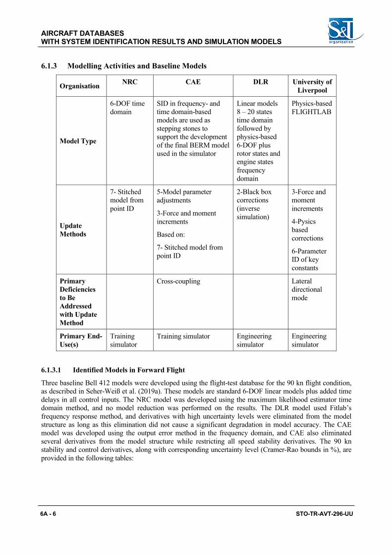
AIRCRAFT DATABASES WITH SYSTEM IDENTIFICATION RESULTS AND SIMULATION MODELS

6A - 6 STO-TR-AVT-296-UU

6.1.3 Modelling Activities and Baseline Models

Organisation NRC CAE DLR University of Liverpool

Model Type

6-DOF time domain

SID in frequency- and time domain-based models are used as stepping stones to support the development of the final BERM model used in the simulator

Linear models 8 – 20 states time domain followed by physics-based 6-DOF plus rotor states and engine states frequency domain

Physics-based FLIGHTLAB

Update Methods

7- Stitched model from point ID

5-Model parameter adjustments

3-Force and moment increments

Based on:

7- Stitched model from point ID

2-Black box corrections (inverse simulation)

3-Force and moment increments

4-Pysics based corrections

6-Parameter ID of key constants

Primary Deficiencies to Be Addressed with Update Method

Cross-coupling Lateral directional mode

Primary End-Use(s)

Training simulator

Training simulator Engineering simulator

Engineering simulator

6.1.3.1 Identified Models in Forward Flight

Three baseline Bell 412 models were developed using the flight-test database for the 90 kn flight condition, as described in Seher-Weiß et al. (2019a). These models are standard 6-DOF linear models plus added time delays in all control inputs. The NRC model was developed using the maximum likelihood estimator time domain method, and no model reduction was performed on the results. The DLR model used Fitlab’s frequency response method, and derivatives with high uncertainty levels were eliminated from the model structure as long as this elimination did not cause a significant degradation in model accuracy. The CAE model was developed using the output error method in the frequency domain, and CAE also eliminated several derivatives from the model structure while restricting all speed stability derivatives. The 90 kn stability and control derivatives, along with corresponding uncertainty level (Cramer-Rao bounds in %), are provided in the following tables:

AIRCRAFT DATABASES WITH SYSTEM IDENTIFICATION RESULTS AND SIMULATION MODELS

STO-TR-AVT-296-UU 6A - 7

NRC CR DLR FR CR CAE CR 𝑋𝑋𝑢𝑢 -.03772 (6) -.04661 (7) -.0074 - c 𝑋𝑋𝑎𝑎 -.01057 (12) 0 - a 0 - a 𝑋𝑋𝑤𝑤 .0864 (4) .08626 (3) .0716 - c 𝑋𝑋𝑁𝑁 -.2152 (20) 0 - a 0 - a

𝑋𝑋𝑖𝑖 .6029 (12) -.1580 (50) 0 - a

𝑋𝑋𝑟𝑟 .0099 (111) .6909 (9) 0 - a 𝑌𝑌𝑢𝑢 -.01396 (23) -.0567 (10) 0 - a 𝑌𝑌𝑎𝑎 -.1407 (2) -.1558 (2) -.1330 - c 𝑌𝑌𝑤𝑤 -.06555 (9) .0636 (7) 0 - a 𝑌𝑌𝑁𝑁 -1.4822 (3) -1.268 (3) -.5299 (35)

𝑌𝑌𝑖𝑖 1.4603 (9) -2.281 (8) 0 - a

𝑌𝑌𝑟𝑟 .05900 (19) 0 - a 0 - a 𝑍𝑍𝑢𝑢 .1436 (9) .3336 (10) -.0395 - c 𝑍𝑍𝑎𝑎 -.01097 (22) 0 - a 0 - a 𝑍𝑍𝑤𝑤 -.8449 (2) -.9386 (2) -.7737 - c 𝑍𝑍𝑁𝑁 1.741 (9) 4.370 (4) 0 - a

𝑍𝑍𝑖𝑖 2.0099 (8) 1.413 (28) 0 - a

𝑍𝑍𝑟𝑟 .3356 (25) 0 - a 0 - a 𝐿𝐿𝑢𝑢 -.0373 (5) -.0512 (5) .0055 - c 𝐿𝐿𝑎𝑎 -.0701 (2) -.0703 (3) -.0822 - c 𝐿𝐿𝑤𝑤 .0112 (17) .0588 (3) .0354 - c 𝐿𝐿𝑁𝑁 -2.008 (2) -2.136 (2) -1.9934 (6)

𝐿𝐿𝑖𝑖 .7462 (10) -.6554 (10) .2068 (78)

𝐿𝐿𝑟𝑟 -.04492 (9) -.2379 (22) 1.0172 (68) 𝑀𝑀𝑢𝑢 .0022 (16) -.0087 (14) .0079 - c 𝑀𝑀𝑎𝑎 .0102 (3) .0184 (3) .0162 - c 𝑀𝑀𝑤𝑤 -.0158 (4) .0188 (6) .0061 - c 𝑀𝑀𝑁𝑁 -.1657 (6) -.1460 (6) -.1131 (40)

𝑀𝑀𝑖𝑖 -.8769 (2) -1.438 (3) -1.0868 (8)

𝑀𝑀𝑟𝑟 .09451 (8) .1343 (14) 0 - a 𝑁𝑁𝑢𝑢 -.0125 (18) .0428 (5) 0 - a 𝑁𝑁𝑎𝑎 .0123 (96) .0289 (3) .0176 - c 𝑁𝑁𝑤𝑤 -.1031 (31) -.0578 (3) .0005 - c 𝑁𝑁𝑁𝑁 -.5048 (7) -.1563 (9) -.6595 (15)

𝑁𝑁𝑖𝑖 2.377 (6) 1.589 (3) 1.1200 (123)

𝑁𝑁𝑟𝑟 -1.306 (6) -1.121 (2) -1.1487 (10)

AIRCRAFT DATABASES WITH SYSTEM IDENTIFICATION RESULTS AND SIMULATION MODELS

6A - 8 STO-TR-AVT-296-UU

NRC CR DLR FR CR CAE CR 𝑋𝑋𝛿𝛿𝑙𝑙𝑙𝑙𝑛𝑛 -.0421 (4) -.0318 (3) -.0330 (11)

𝑋𝑋𝛿𝛿𝑙𝑙𝑙𝑙𝑙𝑙 0 (435) 0 - a 0 - a

𝑋𝑋𝛿𝛿𝑐𝑐𝑙𝑙𝑙𝑙 .0095 (16) .0188 (4) .0227 (12)

𝑋𝑋𝛿𝛿𝑝𝑝𝑝𝑝𝑑𝑑 -.0057 (21) 0 - a 0 - a

𝑌𝑌𝛿𝛿𝑙𝑙𝑙𝑙𝑛𝑛 -.106 (18) .0116 (32) 0 - a

𝑌𝑌𝛿𝛿𝑙𝑙𝑙𝑙𝑙𝑙 .0879 (2) .0497 (2) .0733 (10)

𝑌𝑌𝛿𝛿𝑐𝑐𝑙𝑙𝑙𝑙 -.0164 (14) 0 - a 0 - a

𝑌𝑌𝛿𝛿𝑝𝑝𝑝𝑝𝑑𝑑 -.003 (426) -.0196 (6) 0 - a

𝑍𝑍𝛿𝛿𝑙𝑙𝑙𝑙𝑛𝑛 -.235 (2) -.2166 (2) -.1762 (5)

𝑍𝑍𝛿𝛿𝑙𝑙𝑙𝑙𝑙𝑙 .0199 (21) .0185 (18) 0 - a

𝑍𝑍𝛿𝛿𝑐𝑐𝑙𝑙𝑙𝑙 -.347 (1) -.3930 (1) -.3238 (2)

𝑍𝑍𝛿𝛿𝑝𝑝𝑝𝑝𝑑𝑑 -.0094 (71) 0 - a 0 - a

𝐿𝐿𝛿𝛿𝑙𝑙𝑙𝑙𝑛𝑛 .0157 (13) .0323 (3) .0246 (8)

𝐿𝐿𝛿𝛿𝑙𝑙𝑙𝑙𝑙𝑙 .1064 (1) .1045 (2) .1122 (4)

𝐿𝐿𝛿𝛿𝑐𝑐𝑙𝑙𝑙𝑙 .0124 (11) .0243 (4) .0225 (45)

𝐿𝐿𝛿𝛿𝑝𝑝𝑝𝑝𝑑𝑑 -.0184 (7) -.0154 (4) -.0205 (24)

𝑀𝑀𝛿𝛿𝑙𝑙𝑙𝑙𝑛𝑛 .0322 (1) .0396 (2) .0352 (3)

𝑀𝑀𝛿𝛿𝑙𝑙𝑙𝑙𝑙𝑙 -.002 (13) -.0028 (6) -.0022 (102)

𝑀𝑀𝛿𝛿𝑐𝑐𝑙𝑙𝑙𝑙 .0117 (2) .0237 (2) .0141 (37)

𝑀𝑀𝛿𝛿𝑝𝑝𝑝𝑝𝑑𝑑 -.0013 (10) 0 - a 0 - a

𝑁𝑁𝛿𝛿𝑙𝑙𝑙𝑙𝑛𝑛 -.0195 (14) -.0312 (3) 0 - a

𝑁𝑁𝛿𝛿𝑙𝑙𝑙𝑙𝑙𝑙 .0204 (9) .0180 (2) .0333 (14)

𝑁𝑁𝛿𝛿𝑐𝑐𝑙𝑙𝑙𝑙 -.0063 (14) 0 - a .0181 (16)

𝑁𝑁𝛿𝛿𝑝𝑝𝑝𝑝𝑑𝑑 .0362 (5) .0409 (2) .0363 (8)

𝜏𝜏𝑙𝑙𝑚𝑚𝑛𝑛 .117 – b .080 (2) .073 (17) 𝜏𝜏𝑙𝑙𝑑𝑑𝑑𝑑 .117 – b .085 (2) .073 - c 𝜏𝜏𝑐𝑐𝑚𝑚𝑙𝑙 .078 – b .067 (3) .046 (45) 𝜏𝜏𝑁𝑁𝑒𝑒𝑑𝑑 .078 – b .082 (3) .103 (55)

(𝑢, 𝑣𝑣,𝑤𝑤 in m/s, 𝑝𝑝, 𝑞𝑞, 𝑉𝑉 in rad/s, controls in %, delays in s a: eliminated, b: fixed, c: constrained parameter)

Time domain and frequency domain comparisons between the above 90 kn models and flight-test data are provided in [Seher-Weiß et al. (2019a)].

6.1.3.2 Identified Models in Hover Two baseline Bell 412 models were developed using the flight-test database for the hover flight condition. The TDD model was developed using the CIFER® tool in the frequency domain. This state-space model was comprised of the standard 6-DOF equations-of-motion augmented with inflow and coning equations and

AIRCRAFT DATABASES WITH SYSTEM IDENTIFICATION RESULTS AND SIMULATION MODELS

STO-TR-AVT-296-UU 6A - 9

a simple Padé engine model as described in [Seher-Weiß et al. (2019b)]. The TDD hover model stability and control derivatives, along with corresponding uncertainty level (Cramer-Rao bounds and insensitivity), are provided in the following table.

Param. Value CR % Insens. % Param. Value CR % Insens. % 𝑋𝑋𝑢𝑢 -.064 12.2 1.2 𝑁𝑁𝑁𝑁 -.539 6.3 2.3 𝑋𝑋𝑎𝑎 -.073 10.2 1.5 𝑁𝑁𝑖𝑖 0 a - - 𝑋𝑋𝑤𝑤 0 a - - 𝑁𝑁𝑟𝑟 -.234 11.1 3.7 𝑋𝑋𝑁𝑁 .290 34.3 5.5 𝑋𝑋𝛿𝛿𝑙𝑙𝑙𝑙𝑛𝑛 -.069 2.2 0.7 𝑋𝑋𝑖𝑖 .454 23.2 3.5 𝑋𝑋𝛿𝛿𝑙𝑙𝑙𝑙𝑙𝑙 -.018 23.8 4.5 𝑋𝑋𝑟𝑟 0 a - - 𝑋𝑋𝛿𝛿𝑐𝑐𝑙𝑙𝑙𝑙 0 a - - 𝑌𝑌𝑢𝑢 0 a - - 𝑋𝑋𝛿𝛿𝑝𝑝𝑝𝑝𝑑𝑑 0 a - -

𝑌𝑌𝑎𝑎 -.295 6.1 1.4 𝑌𝑌𝛿𝛿𝑙𝑙𝑙𝑙𝑛𝑛 0 a - - 𝑌𝑌𝑤𝑤 0 a - - 𝑌𝑌𝛿𝛿𝑙𝑙𝑙𝑙𝑙𝑙 .102 3.0 0.9 𝑌𝑌𝑁𝑁 -1.144 9.9 2.9 𝑌𝑌𝛿𝛿𝑐𝑐𝑙𝑙𝑙𝑙 0 a - - 𝑌𝑌𝑖𝑖 0 a - - 𝑌𝑌𝛿𝛿𝑝𝑝𝑝𝑝𝑑𝑑 0 a - -

𝑌𝑌𝑟𝑟 0 a - - 𝑍𝑍𝛿𝛿𝑙𝑙𝑙𝑙𝑛𝑛 -.037 4.2 1.8 𝑍𝑍𝑢𝑢 -.061 31.4 10.2 𝑍𝑍𝛿𝛿𝑙𝑙𝑙𝑙𝑙𝑙 0 a - - 𝑍𝑍𝑎𝑎 0 a - - 𝑍𝑍𝛿𝛿𝑝𝑝𝑝𝑝𝑑𝑑 0 a - -

𝑍𝑍𝑤𝑤 -.354 5.2 1.9 𝐿𝐿𝛿𝛿𝑙𝑙𝑙𝑙𝑛𝑛 .023 3.8 1.5 𝑍𝑍𝑁𝑁 .261 16.2 6.8 𝐿𝐿𝛿𝛿𝑙𝑙𝑙𝑙𝑙𝑙 .131 2.7 0.6 𝑍𝑍𝑖𝑖 .701 22.0 7.2 𝐿𝐿𝛿𝛿𝑐𝑐𝑙𝑙𝑙𝑙 0 a - - 𝑍𝑍𝑟𝑟 0 a - - 𝐿𝐿𝛿𝛿𝑝𝑝𝑝𝑝𝑑𝑑 -.017 4.0 1.8

𝐿𝐿𝑢𝑢 .102 6.3 1.2 𝑀𝑀𝛿𝛿𝑙𝑙𝑙𝑙𝑛𝑛 .032 2.5 0.8 𝐿𝐿𝑎𝑎 -.071 10.8 2.1 𝑀𝑀𝛿𝛿𝑙𝑙𝑙𝑙𝑙𝑙 .006 17.6 4.8 𝐿𝐿𝑤𝑤 0 a - - 𝑀𝑀𝛿𝛿𝑐𝑐𝑙𝑙𝑙𝑙 0 a - - 𝐿𝐿𝑁𝑁 -2.362 4.0 0.7 𝑀𝑀𝛿𝛿𝑝𝑝𝑝𝑝𝑑𝑑 0 a - -

𝐿𝐿𝑖𝑖 -.274 27.0 7.0 𝑁𝑁𝛿𝛿𝑙𝑙𝑙𝑙𝑛𝑛 0 a - - 𝐿𝐿𝑟𝑟 0 a - - 𝑁𝑁𝛿𝛿𝑙𝑙𝑙𝑙𝑙𝑙 .021 5.4 2.1 𝑀𝑀𝑢𝑢 .056 8.7 1.0 𝑁𝑁𝛿𝛿𝑐𝑐𝑙𝑙𝑙𝑙 .047 5.8 1.5 𝑀𝑀𝑎𝑎 .058 8.0 1.3 𝑁𝑁𝛿𝛿𝑝𝑝𝑝𝑝𝑑𝑑 .025 4.2 2.0

𝑀𝑀𝑤𝑤 0 a - - 𝜏𝜏𝑒𝑒 .315 19.8 7.5 𝑀𝑀𝑁𝑁 -.446 6.3 1.5 𝜏𝜏𝛿𝛿𝑙𝑙𝑙𝑙𝑛𝑛 .054 8.4 3.7 𝑀𝑀𝑖𝑖 -.528 11.0 2.2 𝜏𝜏𝛿𝛿𝑙𝑙𝑙𝑙𝑙𝑙 .068 6.0 2.5 𝑀𝑀𝑟𝑟 0 a - - 𝜏𝜏𝛿𝛿𝑐𝑐𝑙𝑙𝑙𝑙 .021 14.9 7.4 𝑁𝑁𝑢𝑢 0 a - - 𝜏𝜏𝛿𝛿𝑝𝑝𝑝𝑝𝑑𝑑 .084 8.7 4.2

𝑁𝑁𝑎𝑎 0 a - - 𝑁𝑁𝑤𝑤 .058 11.7 2.7

a eliminated during model structure reduction, 𝑢, 𝑣𝑣,𝑤𝑤 in m/s, 𝑝𝑝, 𝑞𝑞, 𝑉𝑉 in rad/s, controls in %, delays in s.

Time domain and frequency domain matches with flight-test data for the TDD hover model are provided in [Seher-Weiß et al. (2019b)].

AIRCRAFT DATABASES WITH SYSTEM IDENTIFICATION RESULTS AND SIMULATION MODELS

6A - 10 STO-TR-AVT-296-UU

The NRC model was developed using the MLE tool in the time domain. This state-space model was comprised of the standard 6-DOF equations-of-motion. The NRC hover model stability and control derivatives are provided in the following table.

Identified Parameters of the NRC Hover Model:

Param. Value CR % Param. Value CR % 𝑋𝑋𝑢𝑢 -0.04548 9.3 𝑋𝑋𝛿𝛿𝑙𝑙𝑙𝑙𝑛𝑛 1.462 1.7 𝑋𝑋𝑎𝑎 -0.03968 35.0 𝑋𝑋𝛿𝛿𝑙𝑙𝑙𝑙𝑙𝑙 -0.3424 33.3 𝑋𝑋𝑤𝑤 0.1908 47.8 𝑋𝑋𝛿𝛿𝑐𝑐𝑙𝑙𝑙𝑙 0.7044 13.0 𝑋𝑋𝑁𝑁 0.8882 21.8 𝑋𝑋𝛿𝛿𝑝𝑝𝑝𝑝𝑑𝑑 0.3602 26.0

𝑋𝑋𝑖𝑖 4.281 10.5 𝑌𝑌𝛿𝛿𝑙𝑙𝑙𝑙𝑛𝑛 -0.2542 18.4 𝑋𝑋𝑟𝑟 -0.3539 7.9 𝑌𝑌𝛿𝛿𝑙𝑙𝑙𝑙𝑙𝑙 2.564 3.3 𝑌𝑌𝑢𝑢 0.03058 7.3 𝑌𝑌𝛿𝛿𝑐𝑐𝑙𝑙𝑙𝑙 -0.9706 13.6 𝑌𝑌𝑎𝑎 -0.072 8.1 𝑌𝑌𝛿𝛿𝑝𝑝𝑝𝑝𝑑𝑑 -0.7854 29.0

𝑌𝑌𝑤𝑤 -0.4324 6.9 𝑍𝑍𝛿𝛿𝑙𝑙𝑙𝑙𝑛𝑛 1.994 2.9 𝑌𝑌𝑁𝑁 -4.66 5.9 𝑍𝑍𝛿𝛿𝑙𝑙𝑙𝑙𝑙𝑙 1.404 33.5 𝑌𝑌𝑖𝑖 -0.1214 18.6 𝑍𝑍𝛿𝛿𝑐𝑐𝑙𝑙𝑙𝑙 -10.87 1.4 𝑌𝑌𝑟𝑟 -0.4364 9.7 𝑍𝑍𝛿𝛿𝑝𝑝𝑝𝑝𝑑𝑑 -1.246 7.4

𝑍𝑍𝑢𝑢 0.07937 26.7 𝐿𝐿𝛿𝛿𝑙𝑙𝑙𝑙𝑛𝑛 -0.1493 6.9 𝑍𝑍𝑎𝑎 -0.02386 13.7 𝐿𝐿𝛿𝛿𝑙𝑙𝑙𝑙𝑙𝑙 0.9711 2.0 𝑍𝑍𝑤𝑤 -2.07 7.2 𝐿𝐿𝛿𝛿𝑐𝑐𝑙𝑙𝑙𝑙 -0.2541 7.1 𝑍𝑍𝑁𝑁 2.879 21.0 𝐿𝐿𝛿𝛿𝑝𝑝𝑝𝑝𝑑𝑑 0.1597 12.2

𝑍𝑍𝑖𝑖 -3.589 17.7 𝑀𝑀𝛿𝛿𝑙𝑙𝑙𝑙𝑛𝑛 -0.2475 0.1 𝑍𝑍𝑟𝑟 -9.126 10.4 𝑀𝑀𝛿𝛿𝑙𝑙𝑙𝑙𝑙𝑙 0.05274 8.7 𝐿𝐿𝑢𝑢 0.01992 5.6 𝑀𝑀𝛿𝛿𝑐𝑐𝑙𝑙𝑙𝑙 0.033 14.5 𝐿𝐿𝑎𝑎 -0.01804 5.5 𝑀𝑀𝛿𝛿𝑝𝑝𝑝𝑝𝑑𝑑 0.02513 244.7 𝐿𝐿𝑤𝑤 -0.04578 25.3 𝑁𝑁𝛿𝛿𝑙𝑙𝑙𝑙𝑛𝑛 0.02462 139.5 𝐿𝐿𝑁𝑁 -2.461 2.4 𝑁𝑁𝛿𝛿𝑙𝑙𝑙𝑙𝑙𝑙 0.2791 11.5 𝐿𝐿𝑖𝑖 -0.3338 29.3 𝑁𝑁𝛿𝛿𝑐𝑐𝑙𝑙𝑙𝑙 -0.172 5.9 𝐿𝐿𝑟𝑟 0.2709 19.9 𝑁𝑁𝛿𝛿𝑝𝑝𝑝𝑝𝑑𝑑 -0.5079 4.7

𝑀𝑀𝑢𝑢 0.009202 2.7 𝜏𝜏𝛿𝛿𝑙𝑙𝑙𝑙𝑛𝑛 0.117 𝑀𝑀𝑎𝑎 0.009302 5.0 𝜏𝜏𝛿𝛿𝑙𝑙𝑙𝑙𝑙𝑙 0.117 𝑀𝑀𝑤𝑤 -0.00081 6.5 𝜏𝜏𝛿𝛿𝑐𝑐𝑙𝑙𝑙𝑙 0.078 𝑀𝑀𝑁𝑁 -0.5252 3.7 𝜏𝜏𝛿𝛿𝑝𝑝𝑝𝑝𝑑𝑑 0.078

𝑀𝑀𝑖𝑖 -0.7337 3.1 𝑀𝑀𝑟𝑟 0.138 6.5 𝑁𝑁𝑢𝑢 0.0107 15.2 𝑁𝑁𝑎𝑎 0.03444 665.5 𝑁𝑁𝑤𝑤 -0.1888 53.8 𝑁𝑁𝑁𝑁 -0.7157 8.0 𝑁𝑁𝑖𝑖 -0.5704 27.8 𝑁𝑁𝑟𝑟 -1.007 15.8

𝑢, 𝑣𝑣,𝑤𝑤 in ft/s, 𝑝𝑝, 𝑞𝑞, 𝑉𝑉 in rad/s, controls in inch, delays in s

AIRCRAFT DATABASES WITH SYSTEM IDENTIFICATION RESULTS AND SIMULATION MODELS

STO-TR-AVT-296-UU 6A - 11

6.1.3.3 University of Liverpool Physics-Based Model The description of the FLIGHTLAB® Bell 412 (F-B412) begins with the main rotor. A centre-spring rigid-blade model has been developed which has the added benefit of simplifying greatly the modelling [Padfield (2018)]. The spring strengths and locations were chosen to match the first flap and lag frequency estimated from measurements on the NRC ASRA. A blade element model is used where the blade aerodynamic segments are defined based on the equal annuli area approach. The quasi-steady aerodynamic loads are calculated by treating the blade sections as two-dimensional panels. The 2D aerofoil table includes lift, drag and pitch moment coefficients as functions of angle of attack and Mach number. The inflow model used is the enhanced Peters-He finite three state dynamic inflow model which is augmented with dynamic wake distortion to correct the often poorly predicted off-axis roll/pitch response in low speed transient manoeuvres.

The tail rotor is modelled using FLIGHTLAB’s Bailey rotor component. Fuselage aerodynamics are included as a table look-up where the lift, drag and pitching moment coefficients are supplied as functions of angle of attack and sideslip angle and inertias provided by NRC. Each horizontal stabiliser is represented as one aerofoil section with an inverted Clark-Y aerofoil with a Gurney flap fitted on the trailing edge. The stabilisers and fin are represented as 2D aerodynamic lookup tables with one and 3 sections, respectively. In addition, the spring-loaded stabiliser angle is determined by the aerodynamic pitching moment. The geometry and location of these components was obtained from [Anon. (2002)].

6.2 US ARMY TDD UH-60 RASCAL

6.2.1 Basic Data Overview

Basic Information:

Type: Manufacturer: Class: JUH-60A Sikorsky Conventional single main rotor Role: Accommodation: Registration Medium Utility 15, including two pilots Army S/N 78-23012

Weights:

Empty: Maximum Takeoff: Useful Load: 10,260 lb 20,250 lb Cargo Hook Limit: Internal Volume: Max Fuel Load: 8,000 lb 362 gallons

AIRCRAFT DATABASES WITH SYSTEM IDENTIFICATION RESULTS AND SIMULATION MODELS

6A - 12 STO-TR-AVT-296-UU

Performance:

Cruise Speed: VNE: Range: 150 kts 193 kts 1,380 nm (with external tanks) Endurance: Max Sideward Velocity: Max Rearward Velocity: 45 kts 45 kts

Engines:

Type: Manufacturer: Number: GE T-700 General Electric 2 Max Power: Transmission Limited Power: 1553 hp 2828 shp

Dimensions (sourced from the UH-60 Operator’s Manual):

AIRCRAFT DATABASES WITH SYSTEM IDENTIFICATION RESULTS AND SIMULATION MODELS

STO-TR-AVT-296-UU 6A - 13

Centre of Gravity Envelope (Sourced from NASA CR-166309):

Main Rotor Data:

Hub: Number of Blades: Blade Material:

Articulated w/elastomeric bearings 4 Titanium/fibreglass

Radius: Chord: Solidity:

26.8 ft 1.75 ft 0.0826

Tip Speed: Rotational Speed: Hinge Offset Ratio:

724 ft/s 258 rpm ~0.08

Airfoil: Twist:

SC 1095 -18 deg

Tail Rotor Data:

Hub: Number of Blades: Blade Material:

Bearingless cross-beam 4 Composite

Radius: Chord: Solidity:

5.5 ft 0.81 ft 0.1875

Tip Speed: Rotational Speed: Hinge Offset Ratio:

739 ft/s 1,188 rpm N/A

Airfoil: Twist:

SC 1095 -18

AIRCRAFT DATABASES WITH SYSTEM IDENTIFICATION RESULTS AND SIMULATION MODELS

6A - 14 STO-TR-AVT-296-UU

Empty Weight Moments of Inertia:

Ixx: Iyy: Izz:

4,900 slug-ft^2 41,323 slug-ft^2 29,436 slug-ft^2

Ixz: Ixy: Iyz:

1,882 slug-ft^2 - slug-ft^2 - slug-ft^2

6.2.2 Summary of Available Modelling Data

Configuration Data

Available in Howlett Report (NASA CR-166309)

Mixer identified from US Army RASCAL

Nominal US Army RASCAL Inertias

Flight-Test Data

Frequency sweeps at hover and 80 kts. Time histories as well as frequency response [Tischler and Remple (2012)]

Doubles at hover

2311 at 80 kn

Base Instrumented Parameter List (Hover has many more parameters)

Control Positions

Pilot stick positions (SAS off, so these are control positions)

Swashplate and tail rotor servo positions

Stabilator position

Inertial

Body axis angular rates and accelerations

Body axis linear accelerations

Attitudes

Air Data

Static pressure

Differential pressure

Speed

Angle of attack

Angle of sideslip

Drivetrain Rotor speed

Rotor States

Individual blade flap

Individual blade lag

Individual blade pitch

Rotor azimuth

Fixed-frame flapping

AIRCRAFT DATABASES WITH SYSTEM IDENTIFICATION RESULTS AND SIMULATION MODELS

STO-TR-AVT-296-UU 6A - 15

6.2.3 Modelling Activities and Baseline Models

Organisation USNA ART GT

Model Type GenHel Based linearised blade element model

FLIGHTLAB® based blade element model

FLIGHTLAB based blade element model

Update Methods

1-Gain and Time Delay Corrections

4- Reduced Order Models and Physics-Based Corrections

4- Reduced Order Models and Physics-Based Corrections

Primary Deficiencies to Be Addressed with Update Method

Mismatch for key on-axis responses

Off-Axis responses mismatch

Off-axis response mismatch

Primary End-Use(s) Handling Qualities and Flight Control Design

Training simulator Engineering Simulator

Organisation SAC PSU TDD

Model Type FLIGHTLAB based blade element model

GenHel based linearised blade element model

GenHel based linearised blade element model

Update Methods 4- Reduced Order Models and Physics-Based Corrections

5- Simulation model parameter adjustment

7- Stitched Simulation from Point ID Models and Trim Data

Primary Deficiencies to Be Addressed with Update Method

Overall match with flight-test data in trim and dynamic response in variety of flight conditions

General mismatch in frequency responses

Original model is not real-time

Primary End-Use(s) Engineering simulator Training simulator Training Simulator

The UH-60 simulation models used in this report are broadly categorised to originate from two commonly used simulation environments, ones based on GenHel and other using FLIGHTLAB.

6.2.3.1 GenHel Based Model

The first and still widely used UH-60 model is the GenHel nonlinear blade element simulation originated at Sikorsky Aircraft [Howlett (1981)], which had rigid blades, Glauert harmonic inflow distribution, 2D airfoil tables, and wind-tunnel based lookup tables for the fuselage. The Ames GenHel model variant [Ballin and Dalang-Secretan (1991)], used by TDD, USNA, and PSU, incorporated a 3-state Pitt-Peters inflow model and a sophisticated engine/drivetrain model for the 701C engine. Using the simulation equations from GenHel, the University of Maryland and TDD developed the companion tool FORECAST [Kim et al. (1993)] to determine an accurate trim solution (based on periodic balance) and to extract high-order linearised models of varying complexity (up to 54 states) using numerical perturbation methods. Wake curvature effects due to tip-path-plane rate have a first-order effect on the off-axis angular responses in conventional flapping rotors and the on-axis response of stiff hingeless rotors.

AIRCRAFT DATABASES WITH SYSTEM IDENTIFICATION RESULTS AND SIMULATION MODELS

6A - 16 STO-TR-AVT-296-UU

Wake curvature corrections included in Ames GenHel and FORECAST use a defined lookup table of the aerodynamic phase lag as obtained from system identification results of UH-60 flight data [Schulein et al (2002)] and are used in this study. The user can also select the Keller correction to the Pitt-Peters model, which has been shown to provide an equivalent correction effect [Schulein et al (2002)]. FORECAST linear models have been used extensively for handling qualities and flight dynamics and control applications [e.g., Fletcher et al. (2008)]. The PSU version of the GenHel model (PSU-HeloSim) was derived from the AMES variant of GenHel, but it was re-hosted in the MATLAB/Simulink environment and implemented in state-space form such that high-order linear models can be extracted (41 states). In addition, the Pitt-Peters inflow model was modified to include the wake curvature effects of [Zhao (2005)].

6.2.3.2 FLIGHTLAB Based Model

The second UH-60 model is obtained from the FLIGHTLAB simulation environment. FLIGHTLAB is a multibody dynamics-based comprehensive rotorcraft modelling and simulation tool used in UH-60 simulation model fidelity improvement method study. The baseline UH-60 simulation model from FLIGHTLAB was built using blade element modelling option [He et al. (2005)]. The blade element model covers rotor structural dynamics, unsteady airloads, and Peters-He’s finite state (truncated to 3-states) induced inflow dynamics. The rotor dynamics model considers geometrically the exact hub articulated retention, both flap and lag hinge dynamics, and rigid blades. The unsteady airloads modelling includes quasi-steady nonlinear airfoil table lookup with respect to blade segment local angle of attack and Mach number plus the effects of yawed flow, unsteady pitch rate, stall delay, and dynamic rotor wake. The fuselage is modelled with nonlinear 6-DOFs and the table lookup of airloads with respect to angle of attack and angle of sideslip of fuselage. Airloads of empennage, both horizontal stabilator and vertical fin, are computed with respect to local angle of attack of aerodynamic segments with the effect of rotor and fuselage interference. The Viscous Vortex Particle Method (VPM) was adopted for improved rotor wake and interference modelling. VPM is a high fidelity first principle-based rotor wake dynamics solver but is computationally very efficient. In the current research, a reduced order rotor inflow dynamics model extracted from VPM simulation [He et al. (2017)] is used and integrated with FLIGHTLAB’s full flight simulation model for the methodology study.

Sikorsky also developed an engineering simulation model in FLIGHTLAB for the S-70i International Black Hawk helicopter [Zhang et al. (2017) and Xin et al. (2019)]. A blade element model was applied for both main and tail rotors. The main rotor three-hinge articulation was modelled, including a nonlinear damper with accurate kinematics and validated damping characteristics. The hingeless tail rotor was modelled with an effective hinge offset and a flapping hinge spring to match the measured flatwise bending frequency. The main and tail rotor were modelled with nonlinear quasi-unsteady airloads with stall delay. A 45-state Peters-He inflow model for the main rotor and a 6-state model for the tail rotor provided sufficient inflow fidelity. The inflow L-matrix correction was applied to modelling the effects of the wake distortion in manoeuvre and the ground vortex in ground effect. Various aerodynamic interference effects were modelled, including the main rotor interference on the fuselage, empennage, tail rotor, the tail rotor interference on the vertical fin, and the fuselage interference on the empennage. The flight control system model consisted of the control laws, sensors, SAS servos, mixer, and primary servos. The propulsion system consisted of a turboshaft engine model with unsteady thermodynamics, engine fuel control system model, a rigid shaft drivetrain modelled with clutch characteristics, and power losses due to the transmission and engine/drivetrain accessories.

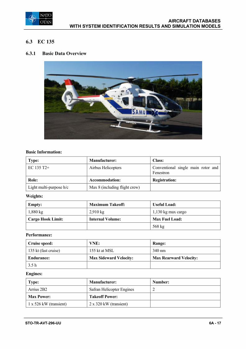
AIRCRAFT DATABASES WITH SYSTEM IDENTIFICATION RESULTS AND SIMULATION MODELS

STO-TR-AVT-296-UU 6A - 17

6.3 EC 135

6.3.1 Basic Data Overview

Basic Information:

Type: Manufacturer: Class:

EC 135 T2+ Airbus Helicopters Conventional single main rotor and Fenestron

Role: Accommodation: Registration:

Light multi-purpose h/c Max 8 (including flight crew)

Weights:

Empty: Maximum Takeoff: Useful Load:

1,880 kg 2,910 kg 1,130 kg max cargo

Cargo Hook Limit: Internal Volume: Max Fuel Load:

568 kg

Performance:

Cruise speed: VNE: Range:

135 kt (fast cruise) 155 kt at MSL 340 nm

Endurance: Max Sideward Velocity: Max Rearward Velocity:

3.5 h

Engines:

Type: Manufacturer: Number:

Arrius 2B2 Safran Helicopter Engines 2

Max Power: Takeoff Power:

1 x 526 kW (transient) 2 x 320 kW (transient)

AIRCRAFT DATABASES WITH SYSTEM IDENTIFICATION RESULTS AND SIMULATION MODELS

6A - 18 STO-TR-AVT-296-UU

Dimensions:

Centre of Gravity Envelope:

The datum plane is located at 2 – 160 mm forward of the levelling point in the front door frame. The datum plane is the fuselage median plane. Lateral CG limit is 100 mm left and right.

AIRCRAFT DATABASES WITH SYSTEM IDENTIFICATION RESULTS AND SIMULATION MODELS

STO-TR-AVT-296-UU 6A - 19

Main Rotor Data:

Hub: Number of Blades: Blade Material:

Bearing-less hinge-less 4 Fibre composite

Radius: Chord: Solidity:

5.1 m 0.288m

Tip Speed: Rotational Speed: Hinge Offset Ratio:

210 m/s 395 rpm / 41.36 rad/s 8.7%

Airfoil: Twist:

DM-H3 and DM-H4 -2°/m

Tail Rotor Data:

Hub: Number of Blades: Blade Material:

Fenestron 10 (unequally spaced)

Radius: Chord: Solidity:

0.5 m

Tip Speed: Rotational Speed: Hinge Offset Ratio:

188 m/s 3 590 rpm / 376 rad/s

Airfoil: Twist:

Empty Weight Moments of Inertia are restricted and cannot be provided. Sources of data are the EASA documents [EASA (2012) and EASA (2019)] and the publication of [Kampa (1997)].

6.3.2 Summary of Available Modelling Data The DLR conducted flight tests with the EC135 ACT/FHS and gathered data at five operating points from hover to 120 kn. About 1 flight hour per trim speed was required for the basic SysID manoeuvres (frequency sweeps and 2311 multistep manoeuvres) of the EC135 database. One flight hour was needed for the trim points at different airspeeds (necessary for model stitching) and approximately one additional flight hour was needed to repeat certain test points. Thus, the overall effort is about 7 flight hours. From this database, the hover and 60 kn flight-test data are shared as presented below in the tables:

Flight-Test Data

2311 multistep data at hover and 60 kn (ACT/FHS EC135)

Sweep data at hover and 60 kn (ACT/FHS EC135)

Steps at hover and 60 kn (Thales EC135 T2+)

All SAS off

AIRCRAFT DATABASES WITH SYSTEM IDENTIFICATION RESULTS AND SIMULATION MODELS

6A - 20 STO-TR-AVT-296-UU

Instrumented Parameter List:

Control Positions cyclic (longitudinal and lateral), directional, collective

Inertial

load factor (longitudinal, lateral, and vertical)

angular rates (pitch, roll, and yaw)

attitude (pitch, roll, and heading)

ground speed (horizontal, longitudinal, lateral, and vertical)

Altitude

Air Data ACT/FHS: side slip, angle of attack, and true airspeed from noseboom

Thales: estimated sideslip, and airspeed

6.3.3 Modelling Activities and Baseline Models

Organisation DLR Thales Aerotim/METU

Model Type

Physics-based and

11-DOF identified

Physics-based

Blade Element Theory (BET) for the main rotor

Physics-based flight model with

Blade element rotor model for main rotor

Update Methods 2: Black box corrections

7: Stitched model from point ID

5: Model parameter adjustments

3: Force and moment increments

Primary Deficiencies to Be Addressed with Update Method

2: include missing high-order dynamics

7: better match with flight-test data

Lateral damping at high frequency

Off-axis response

Primary End-Use(s) Engineering simulator Training simulator Training simulator

6.3.3.1 DLR Physics-Based Simulator Model

DLR’s Air Vehicle Simulator (AVES) Centre operates a flight simulator for the Active Control Technology/Flying Helicopter Simulator (ACT/ FHS) rotorcraft. The bare-airframe ACT/FHS helicopter is represented in AVES by a real-time nonlinear flight simulation model in a program system called HeliWorX. The original model, based on previous SIMH code, was developed by Hamers and von Grünhagen [Hamers and von Grünhagen (1997) and Hamers and von Grünhagen (1998)], and it was validated using the Bölkow BO 105 database. It has a classical modular structure dividing the helicopter model into its components (fuselage, horizontal stabiliser, vertical stabiliser, main rotor, tail rotor, etc.), which allows both component-wise validation and simple reconfiguration of single elements. The EC135 configuration data were provided by Eurocopter Deutschland during the ACT/FHS project realization phase. The main rotor is modelled as fully articulated with an equivalent hinge offset and spring restraint in order to represent flapping and lagging natural frequencies. Each main rotor blade is modelled as a rigid blade, and blade element theory is used to calculate the aerodynamic forces and moments. Overall, 10 blade sections are used to model each blade of the main rotor, and the dynamic inflow model of Pitt and Peters is used for the piloted simulation.

AIRCRAFT DATABASES WITH SYSTEM IDENTIFICATION RESULTS AND SIMULATION MODELS

STO-TR-AVT-296-UU 6A - 21

6.3.3.2 DLR SysID Models

The system identification database for the EC135 consists of sweeps and 3211-multistep manoeuvres at five operating points (hover, 30, 60, 90, 120 kn). For each operating point, a high-order 11-DOF model was identified that considers the body-fixed velocities (u, v, w – m/s), angular rates (p, q, r – rad/sec), flapping (a, b – rad), regressive lead-lag (𝑥𝑥𝑙𝑙𝑙𝑙 ,𝑦𝑦𝑙𝑙𝑙𝑙 – rad), and mean inflow (ν – m/s). The identification was performed using the maximum likelihood method in the frequency domain over a frequency range of 1 – 20 rad/s. Details of the model structure and exemplary results are documented in Seher-Weiss and von Grünhagen (2007). A stitched version of these 11-DOF models (Section 7.7.3) is available in the AVES. The state equation of the high-order model is:

𝑥 = 𝐴𝐴𝑥𝑥 + 𝐵𝐵𝑢

The control vector u consists of longitudinal 𝛿𝛿𝑥𝑥, lateral 𝛿𝛿𝑥𝑥, pedal 𝛿𝛿𝑁𝑁, and collective 𝛿𝛿0 inputs which are given in (%) ranging from 0 to 100% (trim may be assumed as 50%). Compared to Seher-Weiss and von Grünhagen (2007), the model structure shown below uses the collective control input instead of its derivative. Therefore, an additional, artificial state 𝑤𝑤ℎ is introduced.

Identified coefficients of the A- matrix at 60 kn forward flight (including trim):

𝑨𝑨 𝑢 𝑣𝑣 𝑤𝑤 𝑝𝑝 𝑞𝑞 𝑉𝑉 𝑤𝑤ℎ 𝑝 𝑞 𝑥𝑥𝑙𝑙𝑙𝑙 𝑥𝑙𝑙𝑙𝑙 𝑦𝑦𝑙𝑙𝑙𝑙 𝑦𝑙𝑙𝑙𝑙 𝜙𝜙 𝜃𝜃

-0.0167 0.0102 0.0371 -0.1431 -1.637 0 0 0 -0.42 0 0 0 0 0 -9.8005

𝑣 0 -0.1454 0 1.346 0 -30.84 0 0.1568 0 0 0 0 0 9.8005 0

𝑤 0 0 -16.63 0 0 0 1 0 0 0 0 0 0 0 0

𝑝 0 0 0 0 0 0 0 1 0 0 0 0 0 0 0

𝑞 0 0 0 0 0 0 0 0 1 0 0 0 0 0 0

𝑉 -0.0016 0.0698 -0.0452 0 0.2187 -0.7366 0 0.2447 0 0 0 0 0 0 0

𝑤ℎ 0 -1.6 -10.12 0 513.41 0 0 -5.874 50.12 0 0 0 0 0 0

𝑝 0 -1.556 1.386 -62.53 0 0 0 -11.31 -14.66 -13.29 -0.6466 8.463 0.3937 0 0

𝑞 0 0.7029 0.0709 0 -23.35 0 0 1.819 -11.31 2.277 -0.5271 0.1743 0.1301 0 0

𝑥𝑙𝑙𝑙𝑙 0 0 0 0 0 0 0 0 0 0 1 0 0 0 0

𝑥𝑙𝑙𝑙𝑙 0 0 0 0 0 0 0 0 0 -138.77 -1.282 0 0 0 0

𝑦𝑦𝑙𝑙𝑙𝑙 0 0 0 0 0 0 0 0 0 0 0 0 1 0 0

𝑦𝑙𝑙𝑙𝑙 0 0 0 0 0 0 0 0 0 0 0 -138.77 -1.282 0 0

𝜙 0 0 0 1 0 0.044 0 0 0 0 0 0 0 0 0

𝜃 0 0 0 0 1 0 0 0 0 0 0 0 0 0 0

AIRCRAFT DATABASES WITH SYSTEM IDENTIFICATION RESULTS AND SIMULATION MODELS

6A - 22 STO-TR-AVT-296-UU

Coefficients of the B-matrix:

𝑩𝑩 𝛿𝛿𝑥𝑥 𝛿𝛿𝑥𝑥 𝛿𝛿𝑁𝑁 𝛿𝛿0

-0.0119 -0.0022 0.0039 0.013

𝑣 -0.0141 0 -0.0156 -0.0117

𝑤 0 0 0 -0.3456

𝑝 0 0 0 0

𝑞 0 0 0 0

𝑉 -0.01 -0.0139 0.0222 0.002

𝑤ℎ -2.564 0.6416 0 -3.773

𝑝 0.6066 2.041 -0.0783 0.618

𝑞 0.75 -0.1241 0.0402 0.2762

𝑥𝑙𝑙𝑙𝑙 0 0 0 0

𝑥𝑙𝑙𝑙𝑙 1 0 0 0

𝑦𝑦𝑙𝑙𝑙𝑙 0 0 0 0

𝑦𝑙𝑙𝑙𝑙 0 1 0 0

𝜙 0 0 0 0

𝜃 0 0 0 0

Trim data: 𝑢0 = 30.8 𝑚𝑚/𝑠𝑠, 𝑣𝑣0 = 0,𝑤𝑤0 = 1.3 𝑚𝑚/𝑠𝑠

𝜙𝜙0 = 0,𝜃𝜃0 = 0.044 𝑉𝑉𝑉𝑉𝑑𝑑

The following coefficients are affected by trim data:

A15 𝑋𝑋𝑖𝑖 − 𝑤𝑤0

A16 𝑋𝑋𝑟𝑟 ∓ 𝑣𝑣0 A24 𝑌𝑌𝑁𝑁 + 𝑤𝑤0

A26 𝑌𝑌𝑟𝑟 − 𝑢0 A74 𝑍𝑍𝑁𝑁 − 𝑔𝑔𝑠𝑠𝑉𝑉𝑛𝑛𝜙𝜙0 ∙ 𝑠𝑠𝑜𝑜𝑠𝑠𝜃𝜃0

A75 𝑍𝑍𝑖𝑖 − 𝑔𝑔𝑠𝑠𝑉𝑉𝑛𝑛𝜃𝜃0

A78 𝑍𝑍𝑁 − 𝑣𝑣0

A79 𝑍𝑍𝑖 + 𝑢0

6.3.3.3 Thales Thales EC135 flight model is a real-time, non-linear, physics-based model, intended to be used in a Flight Simulator Training Device (FSTD) that complies with EASA and FAA FFS Level D requirements. The model has a classical structure, divided into components (including main rotor, tail rotor, fuselage, landing gear, and external loads) and includes the interaction between theses components and with the ground.

The model was developped in the time domain using an extended set of data collected on actual aircraft on ground and in flight, mainly based on validation requirements set out in EASA and FAA standards, which includes static performances, controls inputs (pulses, steps, doublets, etc.), proper modes (phugoid, dutch roll, etc.), trajectories (take-off, landing, autorotation, acceleration and deceleration, etc.), ground handling, and engine operations. Data were gathered at various altitudes and airspeeds and with various weight and CG configurations within the flight envelope.

6.3.3.4 Aerotim/METU The EC135 baseline model is a nonlinear, physics-based flight model using Aerotim’s core model components, intended for the development of flight models for EASA Level D certified full flight simulators. The model employs a Blade Element Rotor Model (BERM) with virtual blades, 2nd order flapping, Pitt-Peters inflow, aerodynamic derivatives for fuselage, vertical tail and horizontal tail, and Fenestron model. Those model components have been used in Level D certified simulators for helicopters of similar class and have been verified with flight tests. All corrections employed are removed, leaving the models with their basic representation as reported in literature. For demonstration purposed for this work, the main rotor wake curvature off-axis corrections are removed.

A time domain adaptation-based linear model identification is employed to identify the linear system of the helicopter in hover. The 3211 manoeuvre data provided by DLR is used in the process.

AIRCRAFT DATABASES WITH SYSTEM IDENTIFICATION RESULTS AND SIMULATION MODELS

STO-TR-AVT-296-UU 6A - 23

6.4 CH-47F CHINOOK DIGITAL AUTOMATIC FLIGHT CONTROL SYSTEM (DAFCS) TEST AIRCRAFT

6.4.1 Basic Data Overview

Basic Information:

Type: Manufacturer: Class:

CH-47F Chinook Multi-Year 1 Boeing Tandem Rotor Helicopter

Role: Accommodation: Registration:

Cargo/Transport Helicopter 3 Crew and 33 ‒ 55 troops U.S. Army M8003

Weights:

Empty: Maximum Takeoff: Useful Load:

24,578 lb 50,000 lb 24,000 lb

Cargo Hook Limit: Internal Volume: Max Fuel Load:

26,000 lb 1,474 cubic ft 1,030 U.S. Gallons (6,695 lb)

Performance:

Cruise speed: VNE: Range:

160 KTAS 170 KTAS 400 nm

Endurance: Max Sideward Velocity: Max Rearward Velocity:

3.0 hrs 45 KTAS 40 KCAS

Engines:

Type: Manufacturer: Number:

T55-GA-714A Turboshaft Honeywell 2

Max Power: De-rated Takeoff Power:

4777 shp 3750 shp

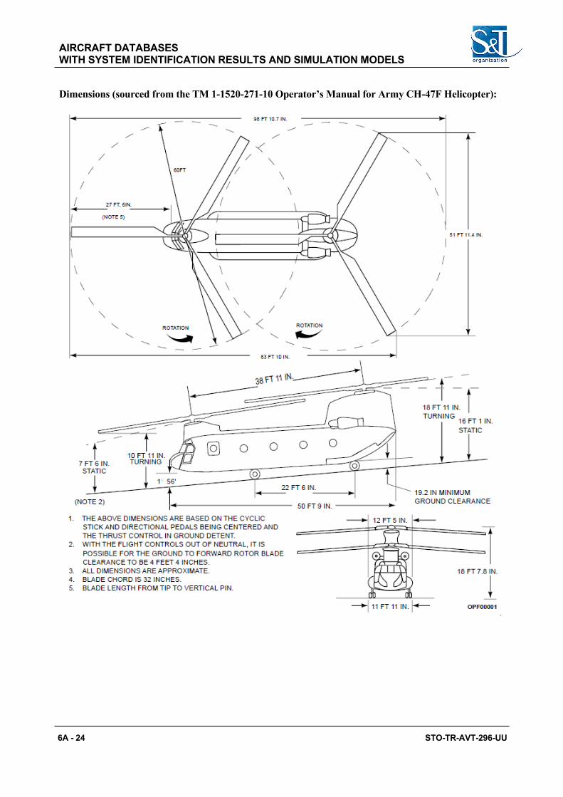
AIRCRAFT DATABASES WITH SYSTEM IDENTIFICATION RESULTS AND SIMULATION MODELS

6A - 24 STO-TR-AVT-296-UU

Dimensions (sourced from the TM 1-1520-271-10 Operator’s Manual for Army CH-47F Helicopter):

AIRCRAFT DATABASES WITH SYSTEM IDENTIFICATION RESULTS AND SIMULATION MODELS

STO-TR-AVT-296-UU 6A - 25

Centre of Gravity Envelope:

* Note that the centre cargo hook is located at Fuselage Station 331 inches.

AIRCRAFT DATABASES WITH SYSTEM IDENTIFICATION RESULTS AND SIMULATION MODELS

6A - 26 STO-TR-AVT-296-UU

Forward Rotor Data:

Hub: Number of Blades: Blade Material:

Fully Articulated 3 Fibreglass

Radius: Chord: Solidity:

30 ft 32.0 inch 0.0849

Tip Speed: Rotational Speed: Hinge Offset Ratio:

707 ft/s 225 rpm 0.022 (Flap Hinge)

Airfoil: Twist: Blade Mass:

VR7 inboard to 85% radius, VR8 tip

12.0 degrees 348 lbs

Shaft Cant:

9.0 degrees forward

Aft Rotor Data:

Hub: Number of Blades: Blade Material:

Fully Articulated 3 Fibreglass

Radius: Chord: Solidity:

30 ft 32.0 inch 0.0849

Tip Speed: Rotational Speed: Hinge Offset Ratio:

707 ft/s 225 rpm 0.022 (Flap Hinge)

Airfoil: Twist: Blade Mass:

VR7 inboard to 85% radius, VR8 tip

12.0 degrees 348 lbs

Shaft Cant:

4.0 degrees forward

Empty Weight Moments of Inertia:

Ixx: Iyy: Izz:

25,500 slug-ft^2 185,000 slug-ft^2 170,000 slug-ft^2

Ixz: Ixy: Iyz:

13,000 slug-ft^2 0.0 slug-ft^2 0.0 slug-ft^2

46,000 lb Mission Gross Weight Moments of Inertia:

Ixx: Iyy: Izz:

40,388 slug-ft^2 220,000 slug-ft^2 207,000 slug-ft^2

Ixz: Ixy: Iyz:

17,500 slug-ft^2 0.0 slug-ft^2 0.0 slug-ft^2

AIRCRAFT DATABASES WITH SYSTEM IDENTIFICATION RESULTS AND SIMULATION MODELS

STO-TR-AVT-296-UU 6A - 27

6.4.2 Summary of Available Modelling Data

Configuration Data

Forward rotor cyclic blade angle ranges

Forward rotor collective blade angle ranges

Aft rotor cyclic blade angle ranges

Aft rotor collective blade angle ranges

Forward rotor inertia and mass moment

Aft rotor inertia and mass moment

Flight-Test Data Trim points at hover, and 60 KCAS

Frequency sweeps at hover, and 60 KCAS

Instrumented Parameter List:

Control Positions

Pilot stick positions

Integrated Lower Controls Actuator (ILCA) positions

Differential Airspeed Hold (DASH) Actuator position

Rotor Longitudinal Cyclic Trim Actuator (LCTA) positions

Longitudinal, Lateral, and Directional Mixer Commands

Rotor Upper Boost Actuator (UBA) positions

Inertial

Body axis rates

Body axis accelerations

Aircraft Attitudes

Velocity (3 components)

Radar altitude

Air Data

Airspeed

Pressure altitude

Outside Air Temperature (OAT)

Differential Pressure (Sideslip)

Drivetrain

Engine 1 and 2 torque

Rotor speed

Power turbine 1 and 2 speed

Gas generator 1 and 2 speed

Rotor States None

AIRCRAFT DATABASES WITH SYSTEM IDENTIFICATION RESULTS AND SIMULATION MODELS

6A - 28 STO-TR-AVT-296-UU

6.4.3 Modelling Activities and Baseline Models

Organisation DSTG CAE Georgia Tech Boeing

Model Type

FLIGHTLAB® – Physics-based flight simulation and analysis model.

CAE Generic Blade Element Rotor Model (BERM) – Physics-based flight simulation model.

FLIGHTLAB – Physics-based flight simulation and analysis model.

Boeing Helicopters Simulation (BHSIM) – Physics-based flight simulation model.

Update Methods

1 – Gain/Time Delay Corrections for Key Responses

4 – Reduced Order Models and Physics-Based Corrections

5 – Simulation Model Parameter Adjustment

2 – ‘Black Box’ Input and Output Filters

4 – Reduced Order Models and Physics-Based Corrections

5 – Simulation Model Parameter Adjustment

4 – Reduced Order Models and Physics-Based Corrections

4 – Reduced Order Models and Physics-Based Corrections

5 – Simulation Model Parameter Adjustment

Primary Deficiencies to Be Addressed with Update Method

Correlation with Australian CH-47F frequency sweep data.

Correlation with frequency sweep data and state-space models identified by Keller et al. (1995) and Lawler et al. (2006)

Correlation with frequency sweep data and state-space models identified by Keller (1995) and Christy Ivler. Lack of finite state inflow models for tandem rotor helicopters.

Correlation with lateral axis frequency sweep data and state-space models identified by Keller, (1995) and Christy Ivler. Underprediction of roll rate damping.

Primary End Use(s)

Engineering simulator

Training simulator Engineering simulator

Engineering simulator

6.4.3.1 Baseline System Identification Models:

CH-47D frequency response data identified from flight-test data generated during Aeronautical Design Standard 33 (ADS-33) compliance testing conducted at Edwards Air Force Base (EAFB) are published in Keller (1995). The published CH-47D system identification data were collected with the Automatic Flight Control System (AFCS) engaged (AFCS-ON); thus, AFCS-OFF frequency response data for the CH-47D are estimated from the system identified AFCS-ON data and the known frequency response characteristics of the CH-47D AFCS. Note that the CH-47D and CH-47F airframe and actuator characteristics are virtually identical although there are significant differences between the Automatic Flight Control Systems implemented on CH-47D and CH-47F Chinooks.

State-space models for the longitudinal/heave dynamics of the CH-47F Chinook in hover from flight-test data generated during the CH-47F Digital Automatic Flight Control System (DAFCS) program are published in Lawler et al. (2006). The baseline quasi-steady system identified longitudinal/vertical axis stability derivatives documented in Lawler et al. (2006) are provided in Table 6.4-1. The corresponding system identified longitudinal/vertical axis model control sensitivity derivatives and effective time delays are provided in Table 6.4-2. In Lawler et al. (2006), Heavy Gross Weight (HGW) is defined as approximately 48,000 lb, Medium Gross Weight (MGW) is defined as approximately 41,000 lb, and Light Gross Weight (LGW) is defined as approximately 33,000 lb.

AIRCRAFT DATABASES WITH SYSTEM IDENTIFICATION RESULTS AND SIMULATION MODELS

STO-TR-AVT-296-UU 6A - 29

State-space models for the lateral/directional dynamics of the CH-47F Chinook in hover were identified by Ivler and Tischler from flight-test data generated during the CH-47F DAFCS program. The lateral/directional stability derivatives identified by Ivler are provided in Table 6.4-3, and the corresponding system identified lateral/directional control sensitivity derivatives and effective time delays are provided in Table 6.4-4. In Ivler’s work, Heavy Gross Weight (HGW) is defined as approximately 48,000 lb, Medium Gross Weight (MGW) is defined as approximately 40,000 lb, and Light Gross Weight (LGW) is defined as approximately 32,000 lb.

Table 6.4-1: CH-47F System Identified Longitudinal/Vertical Axis Model Stability Derivatives for Heavy Gross Weight (Roughly 48,000 lb) at Hover.

Parameter Value Cramer-Rao (%) Insensitivity (%) Xu (1/sec) -0.01890* N/A N/A Xw (1/sec) 7.741e-3 27.02 13.26 Xq (ft/sec) 0.0** N/A N/A Zu (1/sec) 0.0** N/A N/A Zw (1/sec) -0.09929 17.48 8.364 Zq (ft/sec) 0.0** N/A N/A

Mu (1/(sec-ft)) 0.01672 6.518 1.690 Mw (1/(sec-ft)) 0.0** N/A N/A

Mq (1/sec) -1.306 7.213 1.751

*fixed derivative

**eliminated during model structure determination

Table 6.4-2: CH-47F System Identified Longitudinal/Vertical Axis Model Control Sensitivity Derivatives and Effective Time Delays for Heavy Gross Weight (roughly 48,000 lb) at Hover.

Parameter Value Cramer-Rao (%) Insensitivity (%)

XδLON (ft/sec2)/eq-in 0.5807**** 11.22 2.944

XδCOL (ft/sec2)/eq-in 0.5686 3.121 1.530

ZδLON (ft/sec2)/eq-in 0.0** N/A N/A

ZδCOL (ft/sec2)/eq-in -7.233 3.924 1.868

MδLON (1/sec2)/eq-in 0.3384**** 3.228 1.207

MδCOL (1/sec2)/eq-in 0.0** N/A N/A

τLON (sec) 0.07595 13.19 5.433

τCOL (sec) 0.0** N/A N/A

**Eliminated during model structure determination.

****Corrected from value published in Lawler et al. (2006) to correct for erroneous usage of longitudinal bell crank gain of 0.656 in conversion from actuator-inches to equivalent-inches.

AIRCRAFT DATABASES WITH SYSTEM IDENTIFICATION RESULTS AND SIMULATION MODELS

6A - 30 STO-TR-AVT-296-UU

Table 6.4-3: CH-47F System Identified Lateral/Directional Axis Model Stability Derivatives for Light, Medium, and Heavy Gross Weight at Hover.

Parameter Light Gross Weight (LGW)

Medium Gross Weight (MGW)

Heavy Gross Weight (HGW)

Yv (1/sec) -0.04600* -0.08721* -0.04800*

Yp (ft/sec) 0.000** 0.000** 0.000**

Yr (ft/sec) 0.000*** 0.000*** 0.000***

Lv (1/(sec-ft)) 0.000** 0.000** -0.02344

Lp (1/sec) -1.453 -1.753 -2.907

Lr (1/sec) 0.000*** 0.000*** 0.000***

Nv (1/(sec-ft)) 0.000** 0.000** 0.000**

Np (1/sec) 0.000** -0.1121 -0.2431

Nr (1/sec) -0.05000 -0.2221 -0.03109

*Yv restricted by equation [ 𝑣 = 𝑌𝑌𝑎𝑎𝑣𝑣 + 𝑔𝑔𝜙𝜙 ] at low frequency (0.2 – 2.0 rad/sec), such that the low frequency dynamics are preserved.

**Removed in analysis/optimization due to insensitivity or high Cramer-Rao bound in the frequency response fit.

***Set to zero because there was no coherence for p/δPED or v/δPED, which indicates that there is zero response for these transfer functions.

Table 6.4-4: CH-47F System Identified Lateral/Directional Axis Model Control Sensitivity Derivatives and Effective Time Delays for Light, Medium, and Heavy Gross Weight at Hover.

Parameter Light Gross Weight (LGW)

Medium Gross Weight (MGW)

Heavy Gross Weight (HGW)

YδLAT (ft/sec2)/eq-in 0.000** 0.000** 0.000**

YδPED (ft/sec2)/eq-in 0.000*** 0.000*** 0.000***

LδLAT (1/sec2)/eq-in 0.5076**** 0.6203**** 0.8897****

LδPED (1/sec2)/eq-in 0.000*** 0.000*** 0.000***

NδLAT (1/sec2)/eq-in 0.03474**** 0.03743**** 0.06669****

NδPED (1/sec2)/eq-in 0.1501**** 0.2217**** 0.2591****

τLAT (sec) 0.07253 0.08354 0.1077

τPED (sec) 0.07345 0.000** 0.000**

**Removed in analysis/optimization due to insensitivity or high Cramer-Rao bound in the frequency response fit.

***Set to zero because there was no coherence for p/δPED or v/δPED, which indicates that there is zero response for these transfer functions.

****Corrected from value in Ivler’s original work to correct for erroneous usage of lateral bell crank gain of 0.721 or directional bell crank gain of 0.847 in conversion from actuator-inches to equivalent-inches.

AIRCRAFT DATABASES WITH SYSTEM IDENTIFICATION RESULTS AND SIMULATION MODELS

STO-TR-AVT-296-UU 6A - 31

The inputs to the CH-47F system identified state-space dynamic models are the outputs of the mechanical control mixers that combine pilot mechanical path inputs and AFCS inputs. Control mixer positions were not instrumented during the CH-47F DAFCS flight-test program; therefore, the control mixer positions were reconstructed using the upstream pilot lower boost servo mechanical path and AFCS Stability Augmentation System (SAS) Integrated Lower Controls Actuator (ILCA) measurements as shown in the Figure 6.4-1 block diagram.

Figure 6.4-1: CH-47 Control Mixer Reconstruction from Upstream Control Positions, Correction to k5 Bell Crank Mechanical Gain.

The control mixer positions are expressed in equivalent-inches (eq-in) of cockpit stick displacement. Both Lawler and Ivler assumed erroneously that the bell crank mechanical gain k5 in Figure 6.4-1 needed to be applied to the summation of the lower boost servo and ILCA SAS inputs, in addition to the conversion factor from actuator-inches (actr-in) to equivalent-inches of cockpit stick displacement (eq-in). In fact, only the conversion factor from actr-in to eq-in should have been applied because this conversion factor already accounts for all bell cranks and other kinematics in the control runs. Therefore, the longitudinal, lateral, and directional control sensitivity derivatives in Lawler’s and Ivler’s original work, which are expressed in terms of equivalent-inches, were scaled up incorrectly by the ‘Incorrect k5 Gains’ shown in the block diagram. The longitudinal control derivatives shown in Table 6.4-2 and the lateral and directional control derivatives shown in Table 6.4-4 have been modified from their original values in Lawler et al. (2006) American Institute of Aeronautics and Astronautics (AIAA) paper and in Ivler’s original work by scaling them down by the ‘Incorrect k5 Gains’ shown in the block diagram.

Keller et al. (1995) states that ten flight-test hours were required to conduct the frequency sweeps and collect the quantitative CH-47D data described in the database. Miller et al. (2006) states that 12.6 flight-test hours were required to conduct the frequency sweeps from which the CH-47F DAFCS flight-test database information were identified.

[time_rod_position]

[time_SAS1_act_position]

[time_SAS2_act_position]

++

++

k5k1 k2

k3

k3

k4

k6 δMIXERILCA Boost Servo

rod position(actr-in)

SAS1 actuator position(actr-in)

SAS2 actuator position(actr-in)

Transducer calibration gain

SAS1 summing link mechanical gain

SAS2 summing link mechanical gain

ILCA output arm mechanical gain

ILCA output arm mechanical SAS gain

bell crank mechanical gain

Convert actr-in to eq-in

Control Mixer Input (eq-in)

AIRCRAFT DATABASES WITH SYSTEM IDENTIFICATION RESULTS AND SIMULATION MODELS

6A - 32 STO-TR-AVT-296-UU

STO-TR-AVT-296-UU 6B - 1

Chapter 6B – AIRCRAFT DATABASES WITH SYSTEM IDENTIFICATION RESULTS AND SIMULATION MODELS

6.5 AW139 LONG NOSE

6.5.1 Basic Data Overview

Basic Information:

Type: Manufacturer: Class:

AW139 Leonardo Helicopters Conventional single main rotor

Role: Accommodation: Registration:

Medium multi-purpose h/c Max 15 passenger + 2 crew

Weights:

Empty: Maximum Takeoff: Useful Load:

4,250 kg 6,400 kg

Cargo Hook Limit: Internal Volume: Max Fuel Load:

Performance:

Cruise speed: VNE: Range:

150 kt 167 kt at MSL

Endurance: Max Sideward Velocity: Max Rearward Velocity:

5 h 15 See RFM See RFM

Engines:

Type: Manufacturer: Number:

PW PT6C-67C Pratt & Whitney Canada 2

Max Power: Takeoff Power:

2 x 746 kW 2 x 720 kW

AIRCRAFT DATABASES WITH SYSTEM IDENTIFICATION RESULTS AND SIMULATION MODELS

6B - 2 STO-TR-AVT-296-UU

Dimensions:

Main Rotor Data:

Hub: Number of Blades: Blade Material:

Fully articulated 5 Metal and composite

Radius: Chord: Solidity:

6.9 m

Tip Speed: Rotational Speed: Hinge Offset Ratio:

215 m/s 295 rpm

Airfoil: Twist: Blade Mass:

Tail Rotor Data:

Hub: Number of Blades: Blade Material:

Fully articulated 4

Radius: Chord: Solidity:

1.35 m

Tip Speed: Rotational Speed: Hinge Offset Ratio:

250 m/s 1,775 rpm

Airfoil: Twist:

Empty Weight Moments of Inertia are restricted and cannot be provided.

AIRCRAFT DATABASES WITH SYSTEM IDENTIFICATION RESULTS AND SIMULATION MODELS

STO-TR-AVT-296-UU 6B - 3

Source of Data: EASA Type Certificate Data Sheet (TCDS) for AB139 / AW139 No. EASA.R.006 Issue 22, EASA Operational Evaluation Board (OEB) Report AB / AW 139 Revision 4.

6.5.2 Summary of Available Modelling Data

Flight-Test Data

Collective step at Vy Lateral oscillations at Vy Lateral step at Vy Longitudinal doublet at Vy Longitudinal oscillations at Vy

Longitudinal pulse at Vy Longitudinal step at Vy Pedals doublet at Vy

Instrumented Parameter List:

Configuration Gross weight Longitudinal CG position Lateral CG position

Control Positions

Cyclic longitudinal control position Cyclic lateral control position Directional control position Collective control position

Inertial

Longitudinal load factor Lateral load factor Vertical load factor Roll angular rate Pitch angular rate Yaw angular rate Bank angle Pitch attitude Heading Horizontal ground speed Longitudinal ground speed Lateral ground speed Vertical speed Height

AIRCRAFT DATABASES WITH SYSTEM IDENTIFICATION RESULTS AND SIMULATION MODELS

6B - 4 STO-TR-AVT-296-UU

Instrumented Parameter List (cont’d):

Air Data

Estimated side-slip Calibrated airspeed True airspeed Static temperature Estimated wind direction Estimated wind speed Pressure altitude

Drivetrain Main rotor speed Mean engine torque

6.5.3 Modelling Activities and Baseline Models

Organisation ONERA

Model Type Use of Thales Training Simulator model: Nonlinear Flight Mechanics + Blade Element Main Rotor + Aerodynamic interactions

Update Methods 3 – Forces and Moments correction terms Primary Deficiencies to Be Addressed with Update Method

Short term response – lateral damping – lateral directional coupling

Primary End-Use(s) Training Simulator

6.5.3.1 Baseline Model For this application, ONERA used the Thales Training simulation model of the AW139. It is a real-time, nonlinear, physics-based model, developed for Flight Simulator Training Devices (FSTD). It has a classical structure, divided into components (including main rotor, tail rotor, fuselage, landing gear, and external loads) and includes the interactions between these components and with the ground. Blade elements are used to model the main rotor aerodynamics whereas the tail rotor has an analytical aerodynamic model.

In its certified version, the model is assessed and adjusted in time domain using an extended set of data collected on actual aircraft on ground and in flight, mainly based on validation requirements set out in EASA and FAA standards. Therefore, the FSTD integrated version of the model complies with EASA [CS-FSTD(H), (2012)] and FAA [14 Part 60, FAA, (2016)] FFS Level D requirements.

Within AVT-296, the model was used in a degraded version in order to provide a playground for evaluating model improvement Method 3 (“Force and Moment increments”). This version is a step beyond the very initial version of the model (physics-based model configured with the helicopter data package) where some physical parameters are adjusted to comply with the static test points (trim points).

For system identification, a state-space model of lateral axis was used with 4 state variables (𝑝𝑝, 𝑉𝑉,𝜑𝜑, 𝑣𝑣) and 2 inputs (𝛿𝛿𝑙𝑙𝑑𝑑𝑑𝑑 ,𝛿𝛿𝑁𝑁𝑒𝑒𝑑𝑑). TDD provided a support with CIFER® software in order to identify the following partial derivatives [Tischler and Remple (2012)]:

𝑌𝑌𝑎𝑎,𝑌𝑌𝑟𝑟 , 𝐿𝐿𝑎𝑎, 𝐿𝐿𝑁𝑁, 𝐿𝐿𝑟𝑟 ,𝑁𝑁𝑎𝑎,𝑁𝑁𝑟𝑟 ,𝑌𝑌𝑙𝑙𝑑𝑑𝑑𝑑 , 𝐿𝐿𝑙𝑙𝑑𝑑𝑑𝑑, 𝐿𝐿𝑁𝑁𝑒𝑒𝑑𝑑,𝑁𝑁𝑁𝑁𝑒𝑒𝑑𝑑

AIRCRAFT DATABASES WITH SYSTEM IDENTIFICATION RESULTS AND SIMULATION MODELS

STO-TR-AVT-296-UU 6B - 5

The following tables show the AW139 partial SID results including the lateral modes at Vy. One can note that the classical lateral/directional modes are stable whereas the spiral has low frequency instability.

Table 6.5-1: Partial Stability and Control Derivatives from AW139 SID on FT at Vy.

Stability Derivative FT CR (%) Control Derivative FT CR (%)

Zw - 0.606 – Ylat 0.06835 3.953 Yv 0.02552 7.311 Yped 0∗ – Yp 0∗ – Llat 0.1023 4.471 Yr 0.9209 16.17 Lped −0.03617 12.68 Lv −0.01449 22.11 Nlat 0∗ – Lp −1.214 13.59 Nped 0.03582 4.938 Lr 1.563 17.21 τlat 0.06674 6.775 Nv 0.01144 7.763 τped (=1.0*τlat) 0.06674 – Np 0∗ – Nr −0.9458 8.794

∗ : Eliminated during model structure determination

Table 6.5-2: Eigenvalues (rad/sec) from AW139 SID on FT at Vy.

N° Eigenvalues (rad/sec) Mode

1 0.0235 Spiral 2 -1.1537 Roll

3 [ 𝜉𝜉= 0.3594, 𝜔𝜔 = 1.3972] Dutch Roll

4 [ 𝜉𝜉= 0.3594, 𝜔𝜔 = 1.3972]

6.6 AW109 TREKKER

6.6.1 Basic Data Overview

AIRCRAFT DATABASES WITH SYSTEM IDENTIFICATION RESULTS AND SIMULATION MODELS

6B - 6 STO-TR-AVT-296-UU

Basic Information:

Type: Manufacturer: Class:

AW109 Trekker Leonardo Conventional single main rotor

Role: Accommodation: Registration

Light utility 1 or 2 pilots with 7 or 6 passengers

Weights:

Empty: Maximum Takeoff: Useful Load:

MTOW: 3,175 kg (7,000 lb)

Cargo Hook Limit: Internal Volume: Max Fuel Load:

1,250 kg 805 litres (213 US gal)

Performance:

Cruise speed: VNE: Range:

281 km/h 152 kn 281 km/h 152 kn 833 km 450 nm

Endurance: Max Sideward Velocity: Max Rearward Velocity:

4 h 20 min

Engines:

Type: Manufacturer: Number:

PW207C Pratt & Whitney Canada 2

Max Power: De-Rated Takeoff Power:

2 x 735 shp

Dimensions:

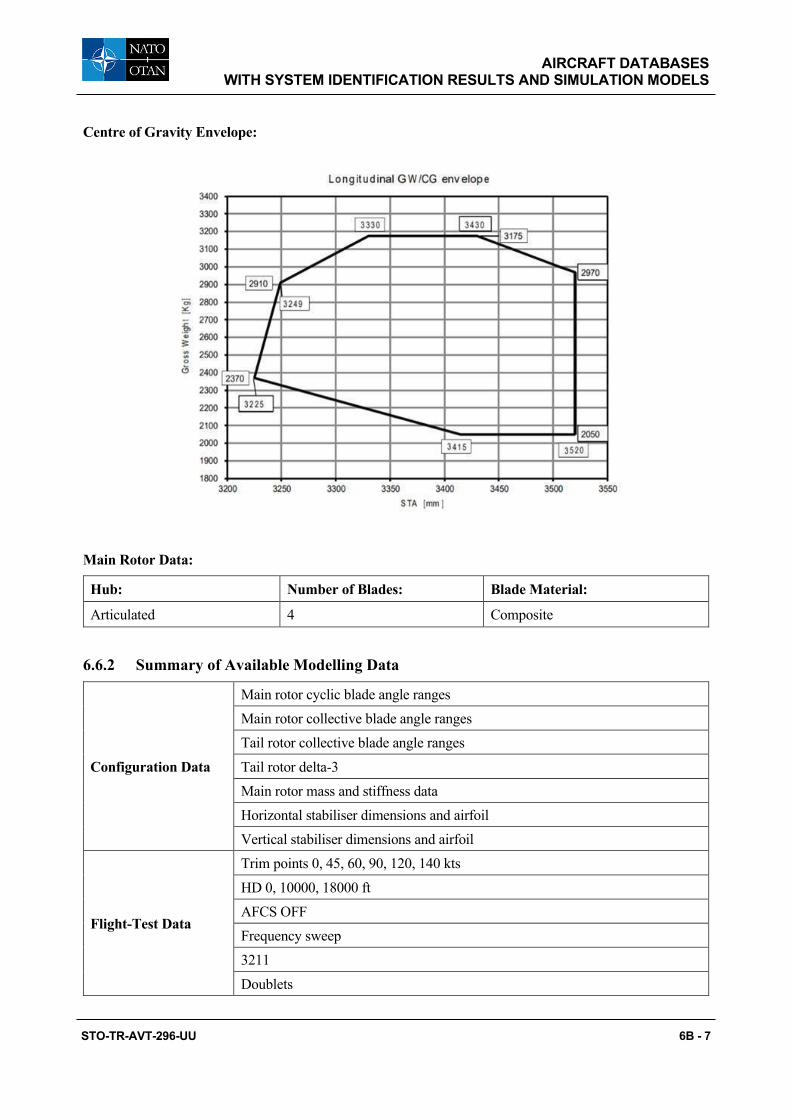
AIRCRAFT DATABASES WITH SYSTEM IDENTIFICATION RESULTS AND SIMULATION MODELS

STO-TR-AVT-296-UU 6B - 7

Centre of Gravity Envelope:

Main Rotor Data:

Hub: Number of Blades: Blade Material:

Articulated 4 Composite

6.6.2 Summary of Available Modelling Data

Configuration Data

Main rotor cyclic blade angle ranges Main rotor collective blade angle ranges Tail rotor collective blade angle ranges Tail rotor delta-3 Main rotor mass and stiffness data Horizontal stabiliser dimensions and airfoil Vertical stabiliser dimensions and airfoil

Flight-Test Data

Trim points 0, 45, 60, 90, 120, 140 kts HD 0, 10000, 18000 ft AFCS OFF Frequency sweep 3211 Doublets

AIRCRAFT DATABASES WITH SYSTEM IDENTIFICATION RESULTS AND SIMULATION MODELS

6B - 8 STO-TR-AVT-296-UU

Instrumented Parameter List:

Control Positions Pilot stick positions

Inertial

Body axis rates Accelerometer measurements Attitude Rate of climb Airspeed Altitude Angle of attack Sideslip Total temperature

Drivetrain

Fuel flow Engine 1 and 2 torque Rotor speed Power turbine 1 and 2 speed Gas generator 1 and 2 speed

6.6.3 Modelling Activities and Baseline Models

Organisation Leonardo Helicopters Model Type Real-time, full non-linear, physic based model developed in FLIGHTLAB®. Update Methods 4 – Reduced Order Models and Physics-Based Corrections

Primary Deficiencies to Be Addressed with Update Method

Main rotor to tail planes interference. Yaw axis response to collective inputs. Roll-off of frequency responses from mid to high frequency.

Primary End-Use(s) Engineering simulator.

6.6.3.1 Baseline Model The base line model is a real-time, full non-linear, physics-based model developed in FLIGHTLAB featuring:

• Blade element main rotor with rigid blades and quasi-unsteady aerodynamics (alpha at ¾ chord point, yawed flow, dynamic stall due to rotation)

• Peters-He finite state wake (3 states)

• Disk tail rotor

• Main rotor interference on tail planes (3 states)

• Wind tunnel data for fuselage and tail planes aerodynamics

• Ideal engine

• AFCS off

AIRCRAFT DATABASES WITH SYSTEM IDENTIFICATION RESULTS AND SIMULATION MODELS

STO-TR-AVT-296-UU 6B - 9

6.7 SIKORSKY X2 TECHNOLOGYTM DEMONSTRATOR

6.7.1 Basic Data Overview

Basic Information:

Type: Manufacturer: Class:

Sikorsky X2 TechnologyTM

Demonstrator Sikorsky, a Lockheed Martin (LM) Company

Coaxial rotor compound with pusher propeller

Role: Accommodation: Registration

Technology demonstrator Two pilots N525SA

Weights:

Empty: Maximum Takeoff: Useful Load:

5,300 lb – –

Cargo Hook Limit: Internal Volume: Max Fuel Load:

N/A – –

Performance:

Cruise speed: VNE: Range:

250 kn – –

Endurance: Max Sideward Velocity: Max Rearward Velocity:

– – –

Engines:

Type: Manufacturer: Number:

LHTEC T800-LHT-801 LHTEC 1

Max Power: De-Rated Takeoff Power:

1563 shp N/A

AIRCRAFT DATABASES WITH SYSTEM IDENTIFICATION RESULTS AND SIMULATION MODELS

6B - 10 STO-TR-AVT-296-UU

Upper and Lower Rotor Data:

Hub: Number of Blades: Blade Material:

Hingeless 4 per rotor –

Radius: Chord: Solidity:

26 ft 5 in – –

Tip Speed: Rotational Speed: Hinge Offset Ratio:

– – –

Airfoil: Twist: Blade Mass:

Various – –

Pusher Propeller Data:

Hub: Number of Blades: Blade Material:

Rigid 6 –

Radius: Chord: Solidity:

– –

Tip Speed: Rotational Speed: Hinge Offset Ratio:

– – –

Airfoil: Twist:

– –

6.7.2 Summary of Available Modelling Data

Configuration Data

Upper and lower rotor mass/inertia and stiffness distribution

Upper and lower rotor chord length, twist, and airfoil distribution

Airfoil characteristics

Propeller inertia and aerodynamic properties

Fuselage inertia and aerodynamic properties

Empennage geometry and aerodynamic properties

Fuselage on empennage interference

Flight control system model

Drivetrain inertia and stiffness

Turboshaft engine model

AIRCRAFT DATABASES WITH SYSTEM IDENTIFICATION RESULTS AND SIMULATION MODELS

STO-TR-AVT-296-UU 6B - 11

Flight-Test Data

Trim controls, hover through 250 kts

Hub moments at trim points, hover through 250 kn

Pitch axis open-loop frequency responses, hover and 200 kn

Roll axis open-loop frequency responses, hover and 180 kn

Pitch axis closed-loop frequency responses, hover

Roll axis closed-loop frequency responses, hover

Time-domain body response to pitch doublet, 200 kn

Time-domain body response to roll doublet, 200 kn

Blade flatwise bending moment at 12.5%R during roll doublet, 200 kn

Upper/lower rotor blade proximity during roll doublet, 200 kn

Instrumented Parameter List:

Control Positions Pilot stick positions

Rotor and propeller Control positions

Inertial

Body axis rates

Body axis accelerations

Attitude

Velocity (3 components)

Radar altitude

Air Data

Static and Dynamic pressure

Airspeed

Altitude

Angle of attack

Sideslip

Total temperature

Drivetrain Engine torque

Rotor speed

Rotor States

Blade flatwise bending at various stations

Blade chordwise bending at various stations

Blade torsion at various stations

Blade proximity

AIRCRAFT DATABASES WITH SYSTEM IDENTIFICATION RESULTS AND SIMULATION MODELS

6B - 12 STO-TR-AVT-296-UU

6.7.3 Modelling Activities and Baseline Models

Modelling Activities:

Organisation Sikorsky US Army TDD

Model Type

State-Space GenHel model

Modal elastic blades, nonlinear unsteady airloads, and 3-state dynamic inflow and mutual interference.

HeliUM model

Modal elastic blades, nonlinear airloads, and 3-state dynamic inflow. Effective interference modelled in hover.

Update Methods

4 – Reduced order models and physics-based corrections

4 – Reduced order models and physics-based corrections

6 – Parameter Identification of Key Simulation Constants

Primary Deficiencies to Be Addressed with Update Method

Roll frequency response

See Sections 7.4.5 for details

Roll frequency response

See Sections 7.4.5 and 7.6.2 for details

Primary End-Use(s) Engineering simulation Engineering simulation

6.7.3.1 X2TD GenHel Simulation Model

GenHel (Generic Helicopter Flight Dynamics Simulation) is a Sikorsky proprietary simulation environment that allows for complete free flight analysis and real-time simulation of any rotorcraft for which sufficient model data is available [Howlett (1981)]. GenHel is capable of modelling the complete air vehicle including engine/fuel control dynamics, flight control systems, elastic airframe deformation, and external load dynamics. GenHel has been developed over many decades at Sikorsky and has been used for the flight dynamic modelling of all current production and development aircraft and various non-Sikorsky aircraft. It has been extensively correlated against a wide variety of flight-test data and updated as appropriate. The State-Space GenHel (SSGH) X2TD model is an engineering simulation model where the coaxial rotors are modelled with elastic blades, nonlinear unsteady airloads, and dynamic inflow with mutual interference [Fegely et al. (2016) and Juhasz, et al. (2020)]. A finite-state rotor interference model has been developed and applied for coaxial rotor modelling [Prasad et al. (2012), Nowak et al. (2013), and Xin et al. (2014)]. The model uses a finite-state form to model the rotor induced velocity at a circular disk off the rotor. The influence coefficient matrix (L-matrix) and time constants (M-matrix) of the model can be pre-calculated using either a pressure potential model [Prasad et al. (2012) and Nowak et al. (2013)] or a free wake model [Xin et al. (2014)]. The full aircraft model includes nonlinear aerodynamics for the fuselage and empennage of which the data maps were derived from the 2012 UTRC Pilot Tunnel Test. The rotor interference on fuselage and empennage is modelled using data maps generated from a CHARM [Quackenbush et al. (1999)] model. The aircraft mass properties are set to be the test aircraft configuration. The flight control system is modelled with SAS gains aligned with the flight test. Estimated control system stiffness is also modelled.

6.7.3.2 X2TD HeliUM Simulation Model

HeliUM is a comprehensive rotorcraft simulation code used primarily for flight dynamics modelling with many flight-test-based validation efforts [Celi (2015) and Juhasz et al. (2012)]. HeliUM derives from a high-order single main rotor helicopter model with a dynamic inflow wake model and flexible blades with coupled non-linear flap/lag/torsion dynamics. Blade, wing, and fuselage aerodynamics come from non-linear

AIRCRAFT DATABASES WITH SYSTEM IDENTIFICATION RESULTS AND SIMULATION MODELS

STO-TR-AVT-296-UU 6B - 13

look up tables. It has a multibody form to allow for structural flexibility and an arbitrary aircraft configuration with multiple rotors [Juhasz et al. (2012)]. In the baseline model, the inflow model for each rotor is a 3-state Peters-He [Peters and He (1991)] dynamic inflow model with inflow coupling between the two rotors. Inflow coupling assumes each rotor is immersed in the uniform component of inflow from the other rotor. Coupling constants are based on analytical velocities above and below an individual rotor’s flow fields [Juhasz et al. (2014)]. The updated HeliUM model is coupled to the Maryland Free Wake (MFW) free-vortex wake method [Leishman et al. (2002)]. Tight coupling between HeliUM and MFW allows for time-marching free-flight manoeuvres, such as frequency sweeps, to be simulated within the model. However, the MFW is not in ordinary differential equation (ODE) form; therefore, direct linearization of the inflow is not possible. To obtain a linear inflow response, a method for extracting linear inflow models using system identification of the MFW response has been extensively documented [Rand et al. (2015), Hersey et al. (2017), and Hersey et al. (2018)]. The ODE inflow model extracted from the high-fidelity MFW is coupled back into the HeliUM flight dynamics model, and the resulting flight dynamics response are compared with flight data and the baseline coupled dynamic inflow [Juhasz, et al. (2020)].

6.8 3DR IRIS+ Quadcopter

6.8.1 Basic Data Overview

Basic Information:

Type: Manufacturer: Class:

IRIS+ 3D Robotics UAV

Size: Accommodation: Registration

19.75 in diagonally motor-to-motor

N/A None

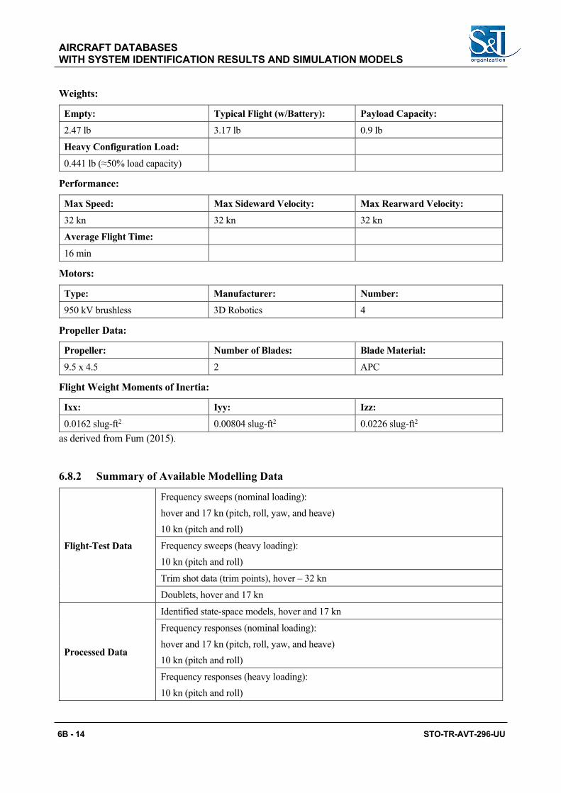
AIRCRAFT DATABASES WITH SYSTEM IDENTIFICATION RESULTS AND SIMULATION MODELS

6B - 14 STO-TR-AVT-296-UU

Weights:

Empty: Typical Flight (w/Battery): Payload Capacity:

2.47 lb 3.17 lb 0.9 lb

Heavy Configuration Load:

0.441 lb (≈50% load capacity)

Performance:

Max Speed: Max Sideward Velocity: Max Rearward Velocity:

32 kn 32 kn 32 kn

Average Flight Time:

16 min

Motors:

Type: Manufacturer: Number:

950 kV brushless 3D Robotics 4

Propeller Data:

Propeller: Number of Blades: Blade Material:

9.5 x 4.5 2 APC

Flight Weight Moments of Inertia:

Ixx: Iyy: Izz:

0.0162 slug-ft2 0.00804 slug-ft2 0.0226 slug-ft2 as derived from Fum (2015).

6.8.2 Summary of Available Modelling Data

Flight-Test Data

Frequency sweeps (nominal loading): hover and 17 kn (pitch, roll, yaw, and heave) 10 kn (pitch and roll)

Frequency sweeps (heavy loading): 10 kn (pitch and roll)

Trim shot data (trim points), hover – 32 kn

Doublets, hover and 17 kn

Processed Data

Identified state-space models, hover and 17 kn

Frequency responses (nominal loading): hover and 17 kn (pitch, roll, yaw, and heave) 10 kn (pitch and roll)

Frequency responses (heavy loading): 10 kn (pitch and roll)

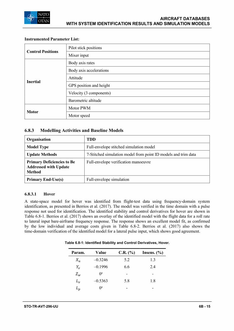
AIRCRAFT DATABASES WITH SYSTEM IDENTIFICATION RESULTS AND SIMULATION MODELS

STO-TR-AVT-296-UU 6B - 15

Instrumented Parameter List:

Control Positions Pilot stick positions

Mixer input

Inertial

Body axis rates

Body axis accelerations

Attitude

GPS position and height

Velocity (3 components)

Barometric altitude

Motor Motor PWM

Motor speed

6.8.3 Modelling Activities and Baseline Models

Organisation TDD

Model Type Full-envelope stitched simulation model

Update Methods 7-Stitched simulation model from point ID models and trim data

Primary Deficiencies to Be Addressed with Update Method

Full-envelope verification manoeuvre

Primary End-Use(s) Full-envelope simulation

6.8.3.1 Hover

A state-space model for hover was identified from flight-test data using frequency-domain system identification, as presented in Berrios et al. (2017). The model was verified in the time domain with a pulse response not used for identification. The identified stability and control derivatives for hover are shown in Table 6.8-1. Berrios et al. (2017) shows an overlay of the identified model with the flight data for a roll rate to lateral input bare-airframe frequency response. The response shows an excellent model fit, as confirmed by the low individual and average costs given in Table 6.8-2. Berrios et al. (2017) also shows the time-domain verification of the identified model for a lateral pulse input, which shows good agreement.

Table 6.8-1: Identified Stability and Control Derivatives, Hover.

Param. Value C.R. (%) Insens. (%)

𝑋𝑋𝑢𝑢 –0.3246 5.2 1.3 𝑌𝑌𝑎𝑎 –0.1996 6.6 2.4 𝑍𝑍𝑤𝑤 0a - - 𝐿𝐿𝑎𝑎 –0.5363 5.8 1.8 𝐿𝐿𝑁𝑁 0a - -

AIRCRAFT DATABASES WITH SYSTEM IDENTIFICATION RESULTS AND SIMULATION MODELS

6B - 16 STO-TR-AVT-296-UU

Param. Value C.R. (%) Insens. (%)

𝑀𝑀𝑢𝑢 1.7355 5.4 1.1

𝑀𝑀𝑖𝑖 0a - -

𝑋𝑋𝛿𝛿lon –7.5513 7.3 2.5

𝑌𝑌𝛿𝛿lat 6.4016 6.6 3.1

𝐿𝐿𝛿𝛿lat 80.0269 3.5 1.2

𝑀𝑀𝛿𝛿lon 92.1241 4.2 0.9

𝑁𝑁𝛿𝛿ped 5.6427 3.9 1.9

𝑍𝑍𝛿𝛿col –60.7660 2.6 1.3

1/𝜏𝜏lag 19.18b - -

𝜏𝜏 0.0122 13.8 8.1 a Eliminated parameter; b Fixed value u,v,w in ft/sec, p,q,r in rad/sec, controls in %, time delay in sec

Table 6.8-2: Identified Model Costs, Hover.

Response Cost (J)

𝑣/𝛿𝛿lat 71.0 𝑝𝑝/𝛿𝛿lat 63.4 𝑉𝑉𝑥𝑥/𝛿𝛿lat 24.5

/𝛿𝛿lon 52.3 𝑞𝑞/𝛿𝛿lon 56.0 𝑉𝑉𝑥𝑥/𝛿𝛿lon 33.3 𝑉𝑉/𝛿𝛿ped 185.9

𝑤/𝛿𝛿col 52.2 𝑉𝑉𝑧𝑧/𝛿𝛿col 52.2

𝐽𝐽ave 65.6 a Eliminated parameter; b Fixed value u,v,w in ft/sec, p,q,r in rad/sec, controls in %, time delay in sec

6.8.3.2 Forward Flight

System identification flights in forward flight were conducted using automated frequency sweep inputs. The frequency sweeps were injected just upstream of the mixer to excite the bare airframe directly. With the control system engaged, logging of the total mixer inputs enables identification of the bare-airframe dynamics (e.g., 𝑝𝑝/𝛿𝛿lat). To ensure a consistent forward-flight velocity, the aircraft pitch attitude was commanded via the transmitter’s longitudinal trim. A racetrack pattern was flown to keep the aircraft within line-of-site while in forward flight.

AIRCRAFT DATABASES WITH SYSTEM IDENTIFICATION RESULTS AND SIMULATION MODELS

STO-TR-AVT-296-UU 6B - 17

The frequency responses obtained from the flight data collection described above were used to generate a state-space model with the CIFER® DERIVID tool. The identified aerodynamic stability derivatives, control derivatives, and time delays for the 17-kn forward-flight model, as given in Tobias et al. (2018), are shown in Table 6.8-3. The paper shows excellent agreement of the identified model overlaid with the flight data in the frequency domain, and Table 6.8-4 supports the fidelity of the model with excellent individual and average costs. The time-domain verification of the identified 17-kn model, using dissimilar data not used in the identification, is also presented in Tobias et al. (2018) and shows the excellent agreement of the model and flight data.

Table 6.8-3: Identified Stability and Control Derivatives, 17 kn.

Param. Value C.R. (%) Insens. (%)

𝑋𝑋𝑢𝑢 –0.2956a - -

𝑌𝑌𝑎𝑎 –0.2346a - -

𝑍𝑍𝑤𝑤 –0.8271 5.6 2.1

𝑍𝑍𝑖𝑖 –1.1668 20.9 9.3

𝐿𝐿𝑁𝑁 –1.2161 24.8 11.4

𝑀𝑀𝑢𝑢 0.3172 21.6 9.2

𝑀𝑀𝑤𝑤 1.6648 7.6 1.7

𝑀𝑀𝑖𝑖 –1.0854 51.4 19.4

𝑁𝑁𝑟𝑟 –1.7768 18.8 6.1

𝑋𝑋𝛿𝛿lon –9.9573 4.5 1.8

𝑌𝑌𝛿𝛿lat 6.2517 5.1 2.0

𝐿𝐿𝛿𝛿lat 85.5219 3.5 1.4

𝑀𝑀𝛿𝛿lon 121.0780 4.4 0.9

𝑁𝑁𝛿𝛿ped 5.6798 4.9 1.7

𝑍𝑍𝛿𝛿col –35.2408 3.9 1.4

𝜏𝜏lat 0.0175 6.2 2.5

𝜏𝜏lon 0.0183 5.8 2.3

𝜏𝜏col 0.0158 8.0 3.4 a Fixed value in ID model from TF fits (e.g., /𝑞𝑞)

u,v,w in ft/sec, p,q,r in rad/sec, controls in %, time delays in sec

AIRCRAFT DATABASES WITH SYSTEM IDENTIFICATION RESULTS AND SIMULATION MODELS

6B - 18 STO-TR-AVT-296-UU

Table 6.8-4: Identified Model Costs, 17 kn.

Response Cost (J)

𝑣/𝛿𝛿lat 39.4

𝑝𝑝/𝛿𝛿lat 27.8

𝑉𝑉𝑥𝑥/𝛿𝛿lat 40.6

/𝛿𝛿lon 41.8

𝑤/𝛿𝛿lon 29.7

𝑞𝑞/𝛿𝛿lon 50.9

𝑉𝑉𝑥𝑥/𝛿𝛿lon 45.4

𝑉𝑉𝑧𝑧/𝛿𝛿lon 85.9

𝑣/𝛿𝛿ped 47.3

𝑉𝑉/𝛿𝛿ped 57.6

𝑤/𝛿𝛿col 64.9

𝑉𝑉𝑧𝑧/𝛿𝛿col 54.9

𝐽𝐽ave 48.9 a Fixed value in ID model from TF fits (e.g., /𝑞𝑞)

u,v,w in ft/sec, p,q,r in rad/sec, controls in %, time delays in sec

6.9 References

[1] 14 Part 60, FAA, (2016), “Flight Simulation Training Device Initial and Continuing Qualification and Use, Appendix C to Part 60-Qualification Performance Standards for Helicopter Full Flight Simulators”.

[2] Anon (2002), “Bell412 EP Product Data”, October.

[3] Ballin, M.G., and Dalang-Secretan, M.A. (1991), “Validation of the Dynamic Response of a Blade-Element UH-60A Simulation Model in Hovering Flight”, Journal of the American Helicopter Society, Vol. 36, No. 4, pp. 77-88.

[4] Berrios, M.G., Berger, T., Tischler, M B., Juhasz, O., and Sanders, F.C. (2017), “Hover Flight Control Design for UAS Using Performance-based Disturbance Rejection Requirements”, American Helicopter Society 73rd Annual Forum, Fort Worth, TX, May.

[5] Celi, R. (2015), “HeliUM 2 Flight Dynamic Simulation Model: Developments, Technical Concepts, and Applications”, American Helicopter Society 71st Annual Forum, May 2015, Virginia Beach, VA.

[6] CS-FSTD(H), (2012), “Certification Specifications for Helicopter Flight Simulation Training Devices”, CS-FSTD(H), EASA, Initial issue, 26 June.

AIRCRAFT DATABASES WITH SYSTEM IDENTIFICATION RESULTS AND SIMULATION MODELS

STO-TR-AVT-296-UU 6B - 19

[7] EASA (2012), “Operational Evaluation Board (OEB) Report EC 135 Family”, July 23rd.

[8] EASA (2019), “Type Certificate Data Sheet (TCDS) for EC135”, No. EASA.R.009, Issue 16.

[9] Fegely, C., Xin, H., Juhasz, O., and Tischler, M.B. (2016), “Flight Dynamics and Control Modeling with System Identification Validation of the Sikorsky X2 Technology Demonstrator”, American Helicopter Society 72nd Annual Forum Proceedings, May 2016, West Palm Beach, FL.

[10] Fletcher, J.W., Lusardi, J.A., Moralez, E., Robinson, D.E., Arterburn, D.R., Cherepinsky, I., Driscoll, J., Morse, C.S., and Kalinowski, K.F. (2008), “UH-60M Upgrade Fly-By-Wire Flight Control Risk Reduction Using the RASCAL JUH-60A In-Flight Simulator”, American Helicopter Society Annual Forum, April – May.

[11] Fum, W.Z. (2015), “Implementation of Simulink Controller Design on IRIS+ Quadrotor”, Master’s thesis, Naval Postgraduate School, Monterey, CA, September.

[12] Hamers M., and von Grünhagen, W. (1997), “Nonlinear Helicopter Model Validation Applied to Realtime Simulations”, 53rd Annual Forum of the American Helicopter Society, Virginia Beach, VA, April 29 – May 1.

[13] Hamers M., and von Grünhagen, W. (1998), “Dynamic Engine Model Integrated in Helicopter Simulation”, 54th Annual Forum of the American Helicopter Society, Washington D.C., May 20 ‒ 22.

[14] He, C., Goericke, J., and Kang, H. (2005), “Modeling Enhancement for Physics-Based Simulation Validation”, AHS 61st Annual Forum, Grapevine, TX, June 2005.

[15] He, C., Syal, M., Tischler, M., and Juhasz, O. (2017), “State-Space Inflow Model Identification from Viscous Vortex Particle Method”, AHS 73rd Annual Forum, Fort Worth, TX, May 2017.

[16] Hersey, S., Celi, R., Juhasz, O., and Tischler, M.B. (2018), “Accurate State-Space Inflow Modeling for Flight Dynamics and Control of a Coaxial-Pusher Rotorcraft”, AHS International 74th Annual Forum Proceedings, May 2018, Phoenix, AZ.

[17] Hersey, S., Celi, R., Juhasz, O., Tischler, M.B., Rand, O., and Khromov, V. (2017), “State-Space Inflow Model Identification and Flight Dynamics Coupling for an Advanced Rotorcraft Configuration”, AHS International 73rd Annual Forum Proceedings, May 2017, Fort Worth, TX.

[18] Howlett, J.J. (1981), “UH-60A Black Hawk Engineering Simulation Program: Volume I ‒ Mathematical Model”, NASA CR-166309, Dec.

[19] Hui, K., (1999), “Advanced Modelling of the Engine Torque Characteristics of a Bell 412 HP Helicopter”, AIAA Atmospheric Flight Mechanics Conference, AIAA-99-4110, Portland, Oregon.

[20] Hui, K., Auriti, L., and Ricciardi, J. (2003), “Advances in Real-Time Aerodynamic Model Identification Techniques”, AIAA Journal of Aircraft Sys ID Special Edition.

[21] Hui, K., and Baillie, S.W. (1994), “Improving Prediction: The Incorporation of Simplified Rotor Dynamics in a Mathematical Model of the Bell 412HP”, CASI Journal, volume 40, issue 4, JA-FRL-1994-0039

[22] Hui, K., and Lambert, E. (2006), “Bell M427 Flight Test Data Gathering and Level-D Simulator Model Development”, ICAS 2006 International Congress of the Aeronautical Sciences, Sept. 3 ‒ 8, Hamburg, Germany.

AIRCRAFT DATABASES WITH SYSTEM IDENTIFICATION RESULTS AND SIMULATION MODELS

6B - 20 STO-TR-AVT-296-UU

[23] Hui, K., Ricciardi J, Srinivasan R, Lambert E and Sarafian A., (2003), “Assessment of Dynamic Stability Characteristics of the Bell Model M427 Helicopter Using Parameter Estimation Technology”, SAE 2002 Transactions ‒ Journal of Aerospace.

[24] Hui, K., and Srinivasan, R., (1998), “The Inclusion of Higher-Order Rotor Dynamics to Improve the Dynamic Model of a Single-Rotor Helicopter in Hover”, NATO Symposium on Systems Identification for Integrated Aircraft Development & Flight Testing, Madrid, Spain.

[25] Juhasz, O., Celi, R., Ivler, C.M., Tischler, M. B., and Berger, T. (2012), “Flight Dynamic Simulation Modeling of Large Flexible Tiltrotor Aircraft”, American Helicopter Society 68th Annual Forum Proceedings, May 2012, Fort Worth, TX.

[26] Juhasz, O., Syal, M., Celi, R., Khromov, V., Rand, O., Ruzicka, G.C., and Strawn, R.C. (2014), “Comparison of Three Coaxial Aerodynamic Prediction Methods Including Validation with Model Test Data”, Journal of the American Helicopter Society, Vol. 59, (3), July 2014.

[27] Juhasz, O., Xin, H., and Tischler, M.B. (2020), “Inflow Based Flight Dynamics Modeling Improvements for the Sikorsky X2 Technology Demonstrator”, American Helicopter Society 76th Annual Forum Proceedings, May 2020, Virginia Beach, VA.

[28] Kampa, K., Enenki, B., Polz, G., and Roth, G. (1997), “Aeromechanic Aspects in the Design of the EC135”, 23rd European Rotorcraft Forum, Dresden, Germany, September 16 ‒ 18.

[29] Keller, J.F., Hart, D.C., Shubert, M.W., and Feingold, A. (1995), “Handling Qualities Specification Development for Cargo Helicopters”, Proceedings of the 51st Annual Forum of the American Helicopter Society, Fort Worth, TX, May 9 ‒ 11.

[30] Kim, F.D., Celi, R.C., and Tischler, M.B. (1993), “Higher-Order State-Space Simulation Models of Helicopter Flight Mechanics”, Journal of the American Helicopter Society, Vol. 38, No. 4, pp. 16 ‒ 27.

[31] Lawler, M.A., Ivler, C.M., Tischler, M.B., and Shtessel, Y.B. (2006), “System Identification of the Longitudinal/Heave Dynamics for a Tandem-Rotor Helicopter Including Higher-Order Dynamics”, Proceedings of the AIAA Atmospheric Flight Mechanics Conference and Exhibit, Keystone, Colorado, Paper No. AIAA-2006-6147.

[32] Leishman, J.G., Bhagwat, M.J., and Bagai, A. (2002), “Free-Vortex Filament Methods for the Analysis of Helicopter Rotor Wakes”, Journal of Aircraft, Vol. 39 (5), September ‒ October 2002.

[33] Miller, R.H., Irwin, J.G., Nieuweboer, H.P., Best, P.R., Gilligan, J.J., Romanoski, M.D., Kocher, J.E., Nester, E.K., Hill, T.H., Eck, D.R., Eland, K.G., Isbel, R.P., and Bednarz, L.J. “Ground and Flight Test Report U.S. Army CH-47F Helicopter with Digital AFCS and CAAS CDRL A077”, Boeing Technical Report D724-10215-2, April 4, 2006.

[34] Nowak, M., Prasad, J.V.R., Xin, H., and Peters, D.A. (2013), “A Potential Flow Model for Coaxial Rotors in Forward Flight”, 39th European Rotorcraft Forum Proceedings, September 2013, Moscow, Russia.

[35] Padfield, G.D., (2018), Helicopter Flight Dynamics: Including a Treatment of Tiltrotor Aircraft, Wiley.

[36] Peters, D.A., and He, C.J. (1991), “Correlation of Measured Induced Velocities with a Finite-State Wake Model”, Journal of the American Helicopter Society, Vol. 36 (30), July 1991, pp. 59-70.

AIRCRAFT DATABASES WITH SYSTEM IDENTIFICATION RESULTS AND SIMULATION MODELS

STO-TR-AVT-296-UU 6B - 21

[37] Prasad, J.V.R., Nowak, M., and Xin, H. (2012), “Finite State Inflow Models for a Coaxial Rotor in Hover”, 38th European Rotorcraft Forum Proceedings, September 2012, Amsterdam, Netherlands.

[38] Quackenbush, T.R., Wachspress, D.A., Boschtisch, A.H., and Curbishley, T.B. (1999), “A Comprehensive Hierarchical Aeromechanics Rotorcraft Model (CHARM) for General Rotor/Surface Interaction”, Continuum Dynamics Inc., CDI Report No. 99-03, January 1999.

[39] Rand, O., Khromov, V., Hersey, S., Celi, R., Juhasz, O., and Tischler, M.B. (2015), “Linear Inflow Model Extraction from High-Fidelity Aerodynamic Models for Flight Dynamics Applications”, American Helicopter Society 71st Annual Forum Proceedings, May 2015, Virginia Beach, VA.

[40] Seher-Weiss, S., Greiser, S., Wartmann, J., Gubbels, A., Ricciardi, J., Hui, K., (2019a), “Bell 412 System Identification: Comparing Methods and Tools”, Vertical Flight Society’s 75th Annual Forum & Technology Display, Philadelphia, PA, USA, May 13 ‒ 16.

[41] Schulein, G.J., Tischler, M.B., Mansur, M.H., and Rosen, A. (2002), “Validation of Cross-Coupling Modeling Improvements for UH-60 Flight Mechanics Simulations”, Journal of the American Helicopter Society, Vol. 47, No 3, pp. 209-213, July.

[42] Seher-Weiß, S., Tischler, M., Scepanovic, P., and Gubbels, A., (2019b), “Bell 412 System Identification and Model Fidelity Assessment for Hover and Forward Flight”, accepted for Journal of the American Helicopter Society, https://doi.org/10.4050/JAHS.66.012004.

[43] Seher-Weiss, S., and von Grünhagen, W. (2007), “EC135 System Identification for Model Following Control and Turbulence Modeling”, in Proceedings of the 1st CEAS European Air and Space Conference, Berlin, pp. 2439-2447.

[44] Tischler, M.B., and Remple, R.K. (2012), “Aircraft and Rotorcraft System Identification: Engineering Methods with Flight Test Examples”, AIAA, 2nd ed., Reston, VA.

[45] Tobias, E.L., Sanders, F.C., and Tischler, M.B. (2018), “Full-Envelope Stitched Simulation Model of a Quadcopter Using STITCH”, American Helicopter Society 74th Annual Forum, Phoenix, AZ, May.

[46] Zhang, C., Xin, H., and Driscoll, J. (2017), “Development and Validation of an Engineering Simulation Model in FLIGHTLAB with Customized Modeling Enhancements”, AHS International 73rd Annual Forum, Fort Worth, TX, USA, May 9 ‒ 11.

[47] Zhao, J. (2005), “Dynamic Wake Distortion Model for Helicopter Maneuvering Flight”, Ph.D. Thesis, Georgia Institute of Technology, Atlanta GA, March.

[48] Xin, H., Goss, J.D., and Parkes, C. (2014), “Development of a Three-State Rotor Interference Model and Application to Coaxial Rotor Inflow Modeling”, American Helicopter Society Aeromechanics Specialists Conference Proceedings, January 2014, San Francisco, CA.

[49] Xin, H., Zhang, C., and Driscoll, J. (2019), “Enhancement of an Engineering Simulation Model to Improve the Correlation with Flight Test Data in Climb/Descent and Autorotation”, AHS International 75th Annual Forum, Philadelphia, PA, USA, May 13 ‒ 16.

AIRCRAFT DATABASES WITH SYSTEM IDENTIFICATION RESULTS AND SIMULATION MODELS

6B - 22 STO-TR-AVT-296-UU

STO-TR-AVT-296-UU 7 - 1

Chapter 7 – ASSESSMENT AND UPDATE CASE STUDIES

This Chapter presents comprehensive case studies of each update method using one or more of the flight test data bases. The full matrix of case studies is given in Figure 7-1 (repeated from Figure 1-1).

Figure 7-1: AVT-296 – Flight Simulation Model Update Methods and Flight-Test Databases, Repeated from Figure 1-1.

ASSESSMENT AND UPDATE CASE STUDIES

7 - 2 STO-TR-AVT-296-UU

STO-TR-AVT-296-UU 7.1 - 1

Chapter 7.1 – GAIN/TIME DELAY CORRECTIONS

The gain/time delay method provides a simple method for adjusting a model response, which can be quite effective in some cases. Depending on the application of the model, this approach affords an easily implemented correction associated with discrepancies relative to test data without delving into the underlying physical mechanisms within the model. It should be noted that because this correction method may not be underpinned by a physical process, the resulting corrected model responses may not be physically representative. For example, if a gain is applied to a response in hover to account for an inflow or interference effect, this gain might not be appropriate at a different airspeed or flight condition. In essence, this method is best suited when the key underlying physics within the frequency range of interest are already well captured in the model. The following case studies detail a number of applications of the gain/time delay correction method, highlighting the primary advantages and limitations of this approach.

7.1.1 CH-47F When compared with frequency responses extracted from flight-test data, a significant gain offset was evident in the model results, particularly in the lateral and longitudinal results. For the lateral axis, the general shape of the model response very closely reflected the flight-test results; however, the model response was offset upwards by approximately 2.5 dB (see Figure 7.1.1-1(a)). In the figure, the red (dashed) curve denotes the uncorrected model response. A model correction factor was computed by identifying a gain and time delay for the error response (of the model relative to flight-test data) using the NAVFIT function in CIFER [Tischler et al. (2012)]. The resulting correction factors are indicated in Figure 7.1.1-1(a) (Gain: 0.68, Delay: 0.025 s), and the model response was then corrected using these values as indicated by the blue (solid) curve in the figure. The corrected model response matches the flight-test data considerably better than the initial model (model mismatch cost was reduced from 𝐽𝐽 = 285 for the initial model down to 𝐽𝐽 = 78 after the correction), indicating that the gain/time delay approach was quite effective in this case. Note that there is a small frequency mismatch in the rigid-body mode at 0.4 rad/sec which does not change with the gain/time delay correction approach.

The limitations of the gain/time delay method are more evident when considering the longitudinal hover response, as shown in Figure 7.1.1-1(b). Here, a similar gain offset to the lateral case is evident; however, a considerable variation in the low frequency rigid-body mode at 0.6 rad/sec is also present. A gain/time delay correction factor was computed as detailed in the figure, along with the corrected model response. The corrected response matches the flight data very well above 2 rad/sec, but poorly below 2 rad/sec due to the influence of the rigid-body mode. This is reflected in the mismatch cost, which reduced from J = 354 to J = 260, representing an improvement, but still a significant difference relative to the flight-test data.

These case studies demonstrate that when the underlying physics of the vehicle are well described in the model for the frequency range of interest, then a gain/time delay correction method can be highly effective at improving the fidelity of the response with minimal effort. When there are differences in the primary dynamics involved within the desired frequency range, then this method is not likely to be particularly effective. It should also be noted that this is a “non-physical” correction method. It is important to crosscheck with other flight conditions (e.g., different airspeeds, gross weights, etc.) to ensure that correcting the response in one regime does not degrade the performance in another. The baseline and updated cost function values are presented in Table 7.1.1-1 for hover, showing cost function improvements between 25 % and 73 %.

GAIN/TIME DELAY CORRECTIONS

7.1 - 2 STO-TR-AVT-296-UU

Figure 7.1.1-1(a): Lateral Axis. Figure 7.1.1-1 (b): Longitudinal Axis.

Figure 7.1.1-1: Gain/Time Delay Corrections for Lateral and Longitudinal Axes in Hover (Flight Data Redacted).

Table 7.1.1-1: Cost Function Comparison for Baseline and Updated Model.

Response Baseline Corrected Improvement (%)

Longitudinal (Hover) 354 259 26.8

Lateral (Hover) 285 78 72.6

The improvements realised in the frequency domain are also realised in the time domain, as demonstrated in Figure 7.1.1-2(a) and (b) for the lateral and longitudinal axes, respectively. Both plots compare the response to on-axis doublet inputs. As was demonstrated in the frequency domain, the gain correction is the primary driver of model improvement, with the reduced gains resulting in significantly better matches for both axes. For both the lateral and longitudinal axes the baseline model peak angular rates in response to the doublet inputs were approximately 35% higher than the flight-test results. For the updated model, the peak rates were quite close to the flight-test data. The resulting time-domain cost metrics are demonstrated in Table 7.1.1-2 for the baseline and updated models. The time-domain cost reduced by approximately 50% in both the lateral and longitudinal axis.

It should be noted that for the frequency-domain comparison the longitudinal axis correction was less effective than the lateral axis because the rigid-body falling leaf mode occurred at a different frequency in the model to the flight-test data. This does not appear to be reflected in the time-domain comparison, likely because the length of record for the time-domain comparison was relatively short (corresponding to a frequency of about 1 rad/sec). In other words, a time-domain comparison of this record length tends to suppress model discrepancies in the very low frequency range and highlight differences in the mid-frequencies.

GAIN/TIME DELAY CORRECTIONS

STO-TR-AVT-296-UU 7.1 - 3

Figure 7.1.1-2(a): Lateral Axis. Figure 7.1.1-2(b): Longitudinal Axis.

Figure 7.1.1-2: Time-Domain Comparison for Lateral and Longitudinal Axes in Hover (Flight Data Redacted).

Table 7.1.1-2: Time-Domain Cost for Baseline and Updated Model.

Axis Baseline Updated Improvement (%)

Longitudinal 1.579 0.798 49.5

Lateral 1.861 1.012 45.6

7.1.2 UH-60 The US Army Technology Development Directorate (TDD-Ames) conducts flight dynamics modelling, control law design, and handling qualities evaluation research to support current and future Army rotorcraft needs. Much of this work has been conducted using the variable stability UH-60A RASCAL helicopter. To support the control law design aspects of its work, an accurate, flight-validated model of the UH-60 is required.

FORECAST has been used to develop flight dynamics models of the UH-60 throughout its flight envelope. Herein, the modelled hover response will be compared with flight data and updated using the gain and time delay method. Modelling capabilities of FORECAST are discussed in detail in Section 6.2.

The linearised baseline FORECAST model is compared with frequency responses obtained from flight data for the roll and pitch axes in Figure 7.1.2-1, with the same line type conventions as in Figure 7.1.1-1(a), (b). For both axes, the baseline predicted FORECAST response is greater in magnitude than flight data. For the roll axis, the baseline response is at or below the MUAD upper bound (see Section 4.1) for a large portion of the response, between 0.2 and 15 rad/sec. For the pitch axis, the baseline response is just above the MUAD boundary between 0.2 and 15 rad/sec. Both baseline responses predict the correct shape of the dynamic response but are offset by constant magnitudes. This magnitude shift was next determined using the gain and time delay method.

As with the CH-47F example above, a gain and time delay transfer function was identified for the error between the frequency responses obtained from the baseline model and flight data. The frequency range used for the identification was 1.4 ≤ ω ≤ 12 rad/sec for the lateral axis and 1.4 ≤ ω ≤ 11 rad/sec for the longitudinal axes. This is the key frequency range for the piloted response and flight control design. Furthermore, this is the range where the predicted response has a magnitude offset over the flight data. Since this method cannot be used to correct for deficiencies in predicted frequencies of rigid-body or rotor modes, its range should only cover where there is a magnitude or phase offset.

GAIN/TIME DELAY CORRECTIONS

7.1 - 4 STO-TR-AVT-296-UU

For the lateral axis, the model fidelity cost (Chapter 4.2) was reduced from 𝐽𝐽𝑏𝑏𝑑𝑑𝑠𝑠𝑒𝑒𝑙𝑙𝑖𝑖𝑛𝑛𝑒𝑒 = 67.3 to 𝐽𝐽𝑢𝑢𝑁𝑁𝑑𝑑𝑑𝑑𝑑𝑑𝑒𝑒𝑑𝑑 = 21.5. The identified gain is 𝐾𝐾𝑙𝑙𝑑𝑑𝑑𝑑 = 0.837, and no time delay was identified. For the longitudinal axis, the cost reduced from 𝐽𝐽𝑏𝑏𝑑𝑑𝑠𝑠𝑒𝑒𝑙𝑙𝑖𝑖𝑛𝑛𝑒𝑒 = 108.9 to 𝐽𝐽𝑢𝑢𝑁𝑁𝑑𝑑𝑑𝑑𝑑𝑑𝑒𝑒𝑑𝑑 = 6.14. The identified gain is 𝐾𝐾𝑙𝑙𝑚𝑚𝑛𝑛 = 0.766, and again no time delay was required. For both axes, there is a substantial reduction in model fit costs and a much improved response that fit well within the MUAD bounds was produced. The baseline and updated cost function values are summarised in Table 7.1.2-1.

Figure 7.1.2-1(a): Roll Axis Model Update. Figure 7.1.2-1(b): Pitch Axis Model Update.

Figure 7.1.2-1: UH-60 Hover Response Model Comparisons and Improvements when Compared to Flight Test.

Table 7.1.2-1: Cost Function Comparison for Baseline and Updated Model.

Response Baseline Corrected Improvement (%)

Longitudinal 67.3 21.5 68.1

Lateral 108.9 6.14 94.4

7.1.3 CH-53E Kaplita et al. (1989) provides a comparison between frequency responses obtained from a Sikorsky GenHel CH-53E model and flight-test data. The GenHel model included a fully-articulated blade element model, flexible fuselage, and rotor speed and engine dynamics. Flight-test frequency response data was derived from frequency sweep tests.

During comparison with flight-test data, the model response produced a constant-gain offset in the low frequency range (0.5 – 4 rad/sec), as indicated in Figure 7.1.3-1. This was corrected by applying empirical gain corrections to the rigid-body modes, providing an improved agreement of the low frequency responses.

GAIN/TIME DELAY CORRECTIONS

STO-TR-AVT-296-UU 7.1 - 5

Figure 7.1.3-1: Comparison of Model and Flight-Test Responses (Lateral Axis, 70 kn, Adapted from Kaplita et al. (1989)).

7.1.4 BO-105 Two applications of the gain/time delay method to the on-axis roll response of the BO-105 helicopter (see Figure 7.1.4-1) in forward flight at 80 knots are presented in this section. The baseline model for both examples are linear models that were extracted from the nonlinear physics-based BO-105 simulation implemented in the Helicopter Overall Simulation Tool (HOST, Benoit et al. (2000)). The HOST helicopter simulation platform is the common simulation tool used by Eurocopter, ONERA, and DLR. Some main functions of HOST are trim calculations, time-domain simulation, and equivalent linear system determination. It is also used for handling qualities investigations, rotor stability in forward flight, loads calculations, and inverse simulation. Another powerful application is the inbuilt parameter identification tool, allowing to apply various methods described in other chapters of this report.

Figure 7.1.4-1: DLR’s BO-105 Helicopter.

GAIN/TIME DELAY CORRECTIONS

7.1 - 6 STO-TR-AVT-296-UU

For the first example, a 6-DOF (8-state) rigid-body model was extracted from the HOST simulation. This baseline 6-DOF model demonstrates a poor match with the flight-test data because the higher-order flapping/lead-lag and actuator dynamics are not captured in the model. The time domain roll acceleration responses of baseline model and flight-test data are shown in Figure 7.1.4-2(a). The model response precedes the flight-test data, indicating that the delays associated with the higher-order dynamics have not been replicated. The same effect can be seen in the corresponding Bode plot in Figure 7.1.4-2(b).

An update using the gain/time delay method was performed resulting in a gain of 0.95 and a time delay of 63 msec. This value for the equivalent time delay corresponds well to the 60 msec delay the had been determined by Kaletka and von Grünhagen (1989) from correlation analysis. This update significantly improved the model performance with respect to flight data as can be seen from Figure 7.1.4-2(a). The addition of the gain/time delay correction to the 6-DOF model resulted in a 29% reduction in RMS error 𝐽𝐽𝑟𝑟𝑚𝑚𝑠𝑠 (see Section 4.2), as shown in Table 7.1.4-1.

Figure 7.1.4-2(a): Time Domain. Figure 7.1.4-2(b): Frequency Domain.

Figure 7.1.4-2: Comparison of Baseline and Updated 6-DOF Model.

A similar improvement can be seen in the frequency domain, as demonstrated in Figure 7.1.4-2(b). The addition of the equivalent time delay can be seen to significantly improve the phase response, resulting in an 78% reduction in frequency-domain cost function 𝐽𝐽 (see Section 4.2) as shown in Table 7.1.4-1.

The residual oscillation in the time and frequency domain flight-test data at about 15 rad/sec is associated with the regressive lead-lag mode (see Kaletka et al. (1991)). The simple gain/time delay correction cannot improve the fidelity of the 6-DOF (quasi-steady) model at these higher frequencies. This is consistent with the time- and frequency-domain cost functions for the updated 6-DOF simulation model (Table 7.1.4-1), that are well in excess of the guidelines of Equations 4.2-3 and 4.2-12, respectively. Therefore, this 6-DOF (lower-order) model does not have adequate fidelity for handling qualities and flight control applications. Instead, method 2 “Black-Box” ‘Input and Output Filter Corrections’ could be used to include these lead-lag dynamics.

For the second example, a high-order (16-state) model was extracted from the HOST simulation that includes rigid-body (8 states), regressive longitudinal and lateral second-order flapping (4 states), and regressive lead-lag dynamics (4 states). A Bode plot comparison for the two models is shown in Figure 7.1.4-3(a). The markers indicate the contribution of the poles and zeros, the pole-zero plot in Figure 7.1.4-3(b) shows their location. The estimated phase shift between the two models of 50 deg at 20 rad/sec corresponds to an equivalent time delay of 42 msec and is caused by the rotor dynamics. (For a rotor speed of 7 Hz, one revolution i.e., 360 deg corresponds to 140 msec).

GAIN/TIME DELAY CORRECTIONS

STO-TR-AVT-296-UU 7.1 - 7

Figure 7.1.4-3(a): Bode Plot. Figure 7.1.4-3(b): Pole-Zero Map.

Figure 7.1.4-3: Comparison of 6-DOF (Rigid-Body) and High-Order Model.

The match of this high-order model with the flight-test data is much better than for the 6-DOF model, as can be seen from Figure 7.1.4-4(a) and Figure 7.1.4-4(b) and the corresponding cost function values in Table 7.1.4-1. However, the Bode plot in Figure 7.1.4-4(b) indicates that the lead-lag frequency of the high-order model is lower than the one observed in flight test.

Figure 7.1.4-4(a): Time Domain. Figure 7.1.4-4(b): Frequency Domain.

Figure 7.1.4-4: Time- and Frequency-Domain Comparison of Baseline and Updated High-Order Model.

Table 7.1.4-1: Time- and Frequency-Domain Cost Functions for Baseline and Updated Models.

6-DOF Model High-Order Model

Baseline Updated Improvement Baseline Updated Improvement

𝐽𝐽 640 144 77.6% 80.2 63.1 21.3%

𝐽𝐽𝑟𝑟𝑚𝑚𝑠𝑠 8.70 6.19 28.8% 5.94 5.78 2.61%

GAIN/TIME DELAY CORRECTIONS

7.1 - 8 STO-TR-AVT-296-UU

The gain/time delay correction method was also applied to this model resulting in a gain of 0.88 and a time delay of 29 msec. The corresponding improvement in model performance with respect to flight data can be seen from Figure 7.1.4-4(a) and Figure 7.1.4-4(b), and the cost function values in Table 7.1.4-1. As mentioned above, the inclusion of rotor dynamics in the high-order baseline model reduces the equivalent time delay by approximately 35 msec, resulting in the smaller identified time delay value of the gain/time delay correction compared to that for the correction of the 6-DOF model. The remaining time delay of 29 msec corresponds well to the estimated value of 22 msec from the transfer function identification in Kaletka et al. (1991) and is mainly attributed to actuator dynamics.

As the gain/time delay update method cannot correct the slight mismatch in lead-lag frequency, this oscillation, which is uncorrelated to the input doublet, is not matched perfectly (see Figure 7.1.4-4(a)). The time-domain cost function herein was based on roll angular acceleration (rather than roll rate) and therefore, exaggerates the mismatch at high frequency. The frequency-domain cost function for the updated higher-order model is within the guideline (𝐽𝐽 ≤ 100), showing that this model is adequate for handling qualities and flight control applications.

7.1.5 Summary

The preceding case studies demonstrate that the gain/time delay method can be highly effective when used for appropriate applications. More specifically, when the underlying physics are well captured in the model for the frequency range of interest, this method can be expected to produce a good correction result. When additional unmodelled dynamics are present or the dynamics are modelled at incorrect frequencies, it is not generally expected that this method will be suitable. The notable exception is when a time delay correction is used to approximate higher-order dynamics, which is effective as long as the frequency range of interest is much lower than the relevant frequency of the dynamics being approximated.

Application of this method requires minimal technical effort, and hence may be considered as a first approach in many circumstances. When correction results are acceptable for a given application, this method can prove to be highly effective due to its simplicity. Care should be exercised when a physically representative system is required since it is difficult to gain insight into the underlying cause of a discrepancy using this method.

7.1.6 References [1] Benoit, B., Dequin, A.-M., Kampa, K., von Grünhagen, W., Basset, P.-M., and Gimonet, B. (2000),

“HOST, a General Helicopter Simulation Tool for Germany and France”, American Helicopter Society 56th Annual Forum, Virginia Beach, Virginia, May 2 ‒ 4.

[2] Kaplita, T.T., Driscoll, J.T., Diftler, M.A., and Hong, S.W. (1989), “Helicopter Simulation Development by Correlation with Frequency Sweep Flight Test Data”, Proceedings to 45th AHS Annual Forum, Boston, MA. May 1989.

[3] Kaletka, J., and von Grünhagen, W. (1989), “Identification of Mathematical Derivative Models for the Design of a Model Following Control System”, Proceedings to 45th AHS Annual Forum, Boston, MA. May 1989.

[4] Kaletka, J., von Grünhagen, W. (1989), “Identification of Mathematical Derivative Models for the Design of a Model Following Control System”, Vertica, Vol. 13 No. 4, pp. 213-218.

[5] Kaletka, J., von Grünhagen, W., Tischler, M.B., and Fletcher J.W. (1991), “Time and Frequency-Domain Identification and Verification of BO 105 Dynamic Models”, AHS Journal, Vol. 36, pp. 25-38, DOI: 10.4050/JAHS.36.25.

GAIN/TIME DELAY CORRECTIONS

STO-TR-AVT-296-UU 7.1 - 9

[6] Tischler, M.B., and Remple, R.K. (2012), Aircraft and Rotorcraft System Identification: Engineering Methods with Flight Test Examples, American Institute of Aeronautics and Astronautics, Inc., Reston, VA, 2nd ed., 2012.

GAIN/TIME DELAY CORRECTIONS

7.1 - 10 STO-TR-AVT-296-UU

STO-TR-AVT-296-UU 7.2 - 1

Chapter 7.2 – ‘BLACK BOX’ INPUT AND OUTPUT FILTERS

With this method, a baseline model is improved by a ‘black box’ (i.e., non-physical) low-order input filter. The framework of the method is presented in Section 5.2 where the different options for inverting the baseline model and for calculating the input filter are described. These options are illustrated with examples from the Bell 412, EC135, and CH-47 databases.

7.2.1 Bell 412 The baseline model to be improved was a linear 6-DOF model for hover provided by the University of Liverpool. The model had been derived by numerical linearization of their nonlinear FLIGHTLAB® simulation without manoeuvre wake distortion. More information about the nonlinear FLIGHTLAB model can be found in Du Val and He (2018) and Section 6.1.3.3. Most on-axis responses are modelled quite well by the baseline model, but deficits are found in the on-axis response in lateral direction (𝑣𝑣 𝛿𝛿𝑥𝑥⁄ ,𝑉𝑉𝑥𝑥 𝛿𝛿𝑥𝑥⁄ ), the cross-axis responses in pitch and roll (𝑞𝑞 𝛿𝛿𝑥𝑥⁄ ,𝑝𝑝 𝛿𝛿𝑥𝑥⁄ ), and the yaw rate responses.

For the Bell 412, two update methods are presented. First, the linear dynamic inversion is applied to the baseline model which yields inverse simulated control signals. These controls are identified by a time-domain identification to provide the input filter. Second, the baseline model is augmented by an input filter that is derived algebraically using the identified Bell 412 hover model from Section 6.1.3.2.

7.2.1.1 Time-Domain Approach

For the time-domain approach, the baseline (linearised FLIGHTLAB) model was reduced to the angular rates 𝑝𝑝, 𝑞𝑞, 𝑉𝑉 and the vertical velocity 𝑤𝑤 as the four outputs to be matched exactly. The inverse of this reduced baseline model was then calculated by dynamic inversion. Based on the inverted model, inverse simulated controls 𝑢 using were generated for all available flight-test manoeuvres.

Taking the measured pilot controls 𝑢 as inputs and the inverse simulated controls 𝑢 as outputs, we then generated an input filter in the time domain using the optimized predictor-based subspace identification (PBSIDopt) method, see Wartmann and Seher-Weiss (2013). PBSIDopt produces a set of linear state-space models from which a stable model with high fidelity and low model order is selected. Figure 7.2.1-1 shows the measured control inputs in the top diagram, the inverse simulated controls, and the model outputs in the four diagrams below for one set of 2311 manoeuvres.

It can be seen that the inverse simulated controls are quite similar to the measured ones for the on-axis controls (e.g., inverse longitudinal cyclic due to measured longitudinal 2311 input) but not for the other ones. The identified model tracks the inverse simulated controls quite well even though some deficits in pedal and collective still exist.

The identified 14th-order input filter was then combined with the baseline model to form the updated model. Figure 7.2.1-2 shows the baseline and the improved model in comparison to the flight-test data for the same set of manoeuvres as in the previous figure. It can be seen that the match of the updated model compared to the baseline model is much improved. Especially the cross-axis responses in roll and pitch and the yaw rate responses are improved. The RMS cost for the three sets of 2311-manoeuvres (lon, lat, ped, col) at hover reduced from 𝐽𝐽𝑟𝑟𝑚𝑚𝑠𝑠 = 3.41 for the baseline model to 𝐽𝐽𝑟𝑟𝑚𝑚𝑠𝑠 = 1.58 which is well within the guideline of 𝐽𝐽𝑟𝑟𝑚𝑚𝑠𝑠 < 2 for helicopter models.

‘BLACK BOX’ INPUT AND OUTPUT FILTERS

7.2 - 2 STO-TR-AVT-296-UU

Figure 7.2.1-1: Results of Inverse Simulation and Modelling Step.

Figure 7.2.1-2: Comparison of Baseline and Updated Model – Time-Domain Derived Filter.

The clear improvement in the pitch and roll responses to cyclic inputs can also be seen from Figure 7.2.1-3 where the match of the baseline and the updated model is shown in the frequency domain. The cross-axis response 𝑞𝑞/𝛿𝛿𝑙𝑙𝑑𝑑𝑑𝑑 is improved most – the response of the baseline model has even the opposite sign compared to the flight-test data, due to the missing manoeuvre wake distortion effect in the baseline model (see Section 7.4.1.7 for this physical phenomenon).

‘BLACK BOX’ INPUT AND OUTPUT FILTERS

STO-TR-AVT-296-UU 7.2 - 3

Figure 7.2.1-3: Frequency-Domain Comparison of Baseline and Updated Model – Time-Domain Derived Filter.

7.2.1.2 Algebraic Approach

As described in Chapter 5.2, an algebraic approach to determine an input filter can be used if a good SysID (also referred to as SID in other sections/chapters) model for the flight-test data exists and if the baseline model is linear or can be linearised. A high-fidelity model for the Bell 412 in hover has been identified in Seher-Weiß (2019) and can thus be used to update the linearised FLIGHTLAB model with the approach depicted in Figure 5.2-4.

First, four outputs (corresponding to the four control inputs) to be matched exactly have to be chosen. For this example, these were the angular rates 𝑝𝑝, 𝑞𝑞, 𝑉𝑉 and the vertical acceleration 𝑉𝑉𝑧𝑧. If both the identified model and the baseline model are reduced to these outputs, the input filter can be determined algebraically via

Filter = (Baseline)−1 × SysID (7.2.1-1)

In the current case, the input filter is a 4x4 model in state-space form. The updated model is then determined by multiplying the baseline model with the input filter. The updated model is thus identical to the SysID model for the four outputs that were chosen in Equation 7.2.1-1. The filter’s unstable modes have a maximum time-to-double of 1.8 sec, which is well above the guideline value of 1.5 sec (see Section 5.2.3.3.3), so that this updated model can still be piloted in a simulator.

The improvement of the updated model in the time domain compared to the baseline model is shown in Figure 7.2.1-4. The match in angular rates is much improved with the remaining deficits in yaw rate due to unmodelled engine effects in the identified model, see Seher-Weiß (2019). The RMS cost for the three sets of 2311-manoeuvres at hover reduced from 𝐽𝐽𝑉𝑉𝑚𝑚𝑠𝑠 = 3.41 for the baseline model to 𝐽𝐽𝑉𝑉𝑚𝑚𝑠𝑠 = 1.63 which is slightly worse than for the time-domain approach, though still well within the guideline of 𝐽𝐽𝑉𝑉𝑚𝑚𝑠𝑠 < 2 for helicopter models.

Figure 7.2.1-5 shows the match in the frequency domain for the on-axis responses of the linear accelerations. No improvement is achieved in the longitudinal and lateral accelerations as these variables were not accounted for in the determination of the input filter correction. The match in vertical acceleration is improved because the SysID model that was used for the update accounts for inflow and coning dynamics, and thus, the updated model matches 𝑉𝑉𝑧𝑧/𝛿𝛿𝑐𝑐𝑚𝑚𝑙𝑙 better at the higher frequencies.

-20

-10

0

10

20

Mag

nitu

de (d

B)

p/lon

-180

-90

0

90

Phas

e (d

eg)

10 0 10 1Frequency (rad/sec)0

0.5

1

Coh

eren

ce

-20

-10

0

10

20q/

lon

-180

-90

0

90

10 0 10 1Frequency (rad/sec)0

0.5

1

-20

-10

0

10

20

p/lat

-180

-90

0

90

10 0 10 1Frequency (rad/sec)

0

0.5

1

-20

-10

0

10

20q/

lat

-180

-90

0

90

measuredbaselineupdated

10 0 10 1Frequency (rad/sec)

0

0.5

1

‘BLACK BOX’ INPUT AND OUTPUT FILTERS

7.2 - 4 STO-TR-AVT-296-UU

Figure 7.2.1-4: Comparison of Baseline and Updated Model – Algebraic Approach.

Figure 7.2.1-5: Frequency-Domain Comparison of Baseline and Updated Model – Algebraic Approach.

7.2.1.3 Comparison

Figure 7.2.1-6 shows the RMS values of the baseline model and the two updates models for all 2311-manoeuvre. It can be seen that the baseline model’s RMS exceeds the 𝐽𝐽𝑉𝑉𝑚𝑚𝑠𝑠 < 2 guideline for all cases. The updated models both show mostly RMS values below 𝐽𝐽𝑟𝑟𝑚𝑚𝑠𝑠 = 2 with the time-domain approach performing slightly better for this time-domain criterion.

-60

-40

-20

0

Mag

nitu

de (d

B)

ax

/lon

-270

-180

-90

Phas

e (d

eg)

10 0 10 1Frequency (rad/sec)

0

0.5

1

Coh

eren

ce

-60

-40

-20

0

ay

/lat

-360

-180measuredbaselineupdated

10 0 10 1Frequency (rad/s)

0

0.5

1

a /

-20

-15

-10

-5

0

az

/col

-225

-180

-135

10 0 10 1Frequency (rad/sec)

0

0.5

1

‘BLACK BOX’ INPUT AND OUTPUT FILTERS

STO-TR-AVT-296-UU 7.2 - 5

Table 7.2.1-1 lists the frequency-domain cost 𝐽𝐽 for those frequency responses associated with the model deficits. It can be seen that the improvement in the cross-axis responses 𝑝𝑝/𝛿𝛿𝑙𝑙𝑚𝑚𝑛𝑛 and 𝑞𝑞/𝛿𝛿𝑙𝑙𝑑𝑑𝑑𝑑 as shown in Figure 7.2.1-3 is reflected by much lower cost function values compared to the baseline model. The yaw rate responses are mostly improved by both approaches. Due to the fact that the algebraic approach forces the yaw rate responses to be identical to those of the identified model, the improvement is greater for the algebraic approach. As the lateral acceleration was not one of the four output variables to be matched for either method, there is no clear improvement in 𝑉𝑉𝑥𝑥 respectively 𝑣, and there is even some degradation. The overall cost function 𝐽𝐽𝑑𝑑𝑎𝑎𝑒𝑒 reduces from 1378 for the baseline model to 847 for the time domain approach and 593 for the algebraic approach.

Overall, both approaches allow to improve the baseline model. The time-domain approach performs slightly better with respect to the (time domain) RMS criterion. The algebraic approach achieves better results in the frequency domain because the underlying SysID model was determined by matching frequency responses. Regarding the effort necessary to generate an improved model, the time-domain approach using a black box identification procedure that needs no physical model structure is quite straight-forward. The algebraic approach, however, needs a higher level of expertise to arrive at a high-fidelity SysID model, especially for the hover case where inflow/coning dynamics usually have to be accounted for.

Figure 7.2.1-6: Comparison of RMS Cost Function for Baseline and Updated Models.

Table 7.2.1-1: Frequency-Domain Cost Functions of Baseline and Updated Models for Selected Frequency Responses.

Freq. Resp. Freq. Range (rad/sec)

Cost Baseline

Cost TD Filter

Cost Algebraic

𝑝𝑝/𝛿𝛿𝑙𝑙𝑚𝑚𝑛𝑛 .9 – 9 968 136 103

𝑞𝑞/𝛿𝛿𝑙𝑙𝑑𝑑𝑑𝑑 1 – 5 5383 71 45

𝑉𝑉/𝛿𝛿𝑙𝑙𝑑𝑑𝑑𝑑 1.5 – 10 205 171 57

𝑉𝑉/𝛿𝛿𝑐𝑐𝑚𝑚𝑙𝑙 .21 – 1.5 319 1315 24

𝑉𝑉/𝛿𝛿𝑁𝑁𝑒𝑒𝑑𝑑 .21 – 12 655 562 119

𝑉𝑉𝑥𝑥/𝛿𝛿𝑙𝑙𝑑𝑑𝑑𝑑 .21 – 12 3644 2885 4202

𝑣𝑣/𝛿𝛿𝑙𝑙𝑚𝑚𝑛𝑛 .3 – 3 2036 2736 295

𝑣𝑣/𝛿𝛿𝑙𝑙𝑑𝑑𝑑𝑑 .95 – 11 2693 3347 3456

𝑣𝑣/𝛿𝛿𝑁𝑁𝑒𝑒𝑑𝑑 1 – 4.8 400 199 47

‘BLACK BOX’ INPUT AND OUTPUT FILTERS

7.2 - 6 STO-TR-AVT-296-UU

7.2.2 EC135 For the EC135, inverse simulation is applied to flight-test data at 60 knots forward flight as provided within the NATO group. Two baseline models are updated to better match the flight-test data:

• 11-DOF system identification model

The baseline model is the ACT/FHS 11-DOF model at 60 kn derived by system identification as presented in Section 6.3.3.2. This model accounts for the rigid-body states and the higher-order modes of flapping, regressive lead-lag and dynamic inflow and was identified over a frequency range of 0.5 ‒ 30 rad/s [Seher Weiß and von Grünhagen (2007)]. Although this model already shows high fidelity, some remaining deficits had to be corrected to be able to use the updated model for control system development. These deficits appear mainly in the yaw response in the mid-frequency range (3 ‒ 37 rad/sec, probably due to missing engine dynamics) and at frequencies above 30 rad/sec.

• DLR’s EC135 engineering simulator model

The baseline model is a nonlinear blade element helicopter model and is presented in Section 6.3.3.1. This model is updated by the algebraic approach using identified models of DLR’s simulator and the ACT/FHS EC135. A black box input filter is derived that updates DLR’s simulator and improves simulation fidelity for all axes and especially for off-axis responses.

7.2.2.1 Frequency-Domain Approach

The EC135’s baseline 11-DOF model at 60 kn is updated by the frequency-domain approach. First, linear dynamic inversion is applied to compute inverse control signals. Then, frequency responses between measured and inverse control signals are computed to identify transfer functions that are used as input filter for the update of the baseline model. Finally, the updated responses are simulated using the input filter. These three steps are summarised in Figure 7.2.2-1.

Figure 7.2.2-1: Steps to Update the Baseline 11-DOF Model.

In the first step, the inverse controls 𝑢 (see Figure 5.2-3 or Figure 7.2.2-1) have to be determined using Rynaski’s approach (Section 5.2.3.3.1). The linear baseline state-space model as presented in Section 6.3.3.2 is partitioned into the states to be matched 𝑥𝑥1 = (𝑝, 𝑞, 𝑉𝑉,𝑤𝑤)𝑇𝑇 and remaining states 𝑥𝑥2 = (𝑢, 𝑣𝑣,𝑝𝑝, 𝑞𝑞,𝑤𝑤ℎ,𝜙𝜙,𝜃𝜃, 𝑥𝑥𝑙𝑙𝑙𝑙, 𝑥𝑙𝑙𝑙𝑙 ,𝑦𝑦𝑙𝑙𝑙𝑙 , 𝑦𝑙𝑙𝑙𝑙). The inverse simulation model is implemented as a state-space model with ‘*-matrices’ as presented in Section 5.2.3.3.1. Inputs to this states-space model are the measured states (𝑝, 𝑞, 𝑉𝑉,𝑤𝑤)𝑇𝑇 and their derivatives (𝑝, 𝑞, 𝑉, 𝑤)𝑇𝑇. Both are generated by flight path reconstruction so that

inverse simulation, Fig. 5.2-3 (matrices A*, B*, C*, D*)

u,v,w,p,q,r,Φ,θ

Step

1

δlon, δlat, δped, δcol

frequency responsesSt

ep 2

Step

3

FitlabGui Black Box input filter, 4x4 transfer function matrix

updated response

cost functionsJrms & Jave

cost functionsJrms & Jave

inverse simulated outputs

inverse simulated controls

δlon, δlat, δped, δcol

inverse controlsδlon, δlat, δped, δcol

measured controls

p, q, r, wp, q, r, w

baseline 11-DoF model

input filterδlon, δlat, δped, δcol

measured controlsu,v,w,p,q,r,Φ,θ

‘BLACK BOX’ INPUT AND OUTPUT FILTERS

STO-TR-AVT-296-UU 7.2 - 7

the integrated 𝑦m,1 perfectly match 𝑦𝑦m,1 which is required to obtain reasonable results. It is important to simulate all outputs, such as forward and lateral speed together with the inverse controls by one state-space model, so that unstable modes such as the phugoid are numerically stabilized. This is especially mandatory if sweep data are analysed which usually have a long duration. All remaining model outputs such as longitudinal and lateral speed do not necessarily match exactly. Due to trim offsets of flight-test data, roll, and pitch angles may have a slight drift offset when compared to the measurements. To overcome this, the drift error is minimized by optimizing the trim values of the inverse state-space model (roll angle trim, pitch angle trim, etc.) [Greiser and von Grünhagen (2013)].

Figure 7.2.2-2 shows the inverse simulation result of a collective sweep input from flight test. The climb and yaw rates (𝑤𝑤, 𝑉𝑉) are part of the states to be matched so that measured and inverse simulated signals match exactly (except for measuring noise). The longitudinal speed is a remaining state which does not match exactly but achieves high fidelity – the RMS error is Jrms = 0.40 at 60 knots forward flight. The RMS cost of the x1-states is zero, and only the remaining states, such as roll and pitch angle, forward and lateral speed, and longitudinal and lateral acceleration, increase the RMS cost. Integrated frequency costs as shown in Table 7.2.2-1 are averaged costs for all the rigid-body states (𝑢, 𝑣𝑣,𝑤𝑤,𝑝𝑝, 𝑞𝑞, 𝑉𝑉,𝜙𝜙,𝜃𝜃) in the frequency range between 1 and 20 rad/sec. Note that for lateral, longitudinal, and pedal axes, the baseline model has already a high fidelity which is indicated by costs of these axes being well within with guideline of 𝐽𝐽 ≤ 100. The cost is reduced most for the collective axis so that any black box filters will most notably improve fidelity for this axis. Figure 7.2.2-3 shows a detailed frequency response from the inverse simulation and ACT/FHS – frequencies above 40 rad/sec are not matched due to a low-pass filter that reduces measuring noise. As a result, inverse simulated outputs have integrated cost values below 𝐽𝐽𝑉𝑉𝑣𝑣𝑒𝑒 ≤ 100 so that an additional output filter is not needed (see guideline in Section 5.2).

In the second step of Table 7.2.2-1 frequency responses between the measured and inverse simulated controls are generated as exemplarily, shown in Figure 7.2.2-4. The frequency responses are plotted for all reference speeds from hover to 120 knots into one diagram – it can be seen that these are very similar, and that all responses are above the guideline of -20 dB so that this axis should be modelled. As all frequency responses 𝑢/𝑢 were mostly independent of reference speed, only one common input filter with stable eigenvalues for the control inputs was extracted by using the tool FitlabGui [Seher-Weiß (2016)]. It was found that this single input model is sufficient for most operating points.

Figure 7.2.2-2: Inverse Simulation of EC135 ACT/FHS Collective Sweep Data at 60 kn Forward Flight.

‘BLACK BOX’ INPUT AND OUTPUT FILTERS

7.2 - 8 STO-TR-AVT-296-UU

Figure 7.2.2-3: Frequency Response of the Yaw Rate Due to Collective r/δcol at 60 kn.

Figure 7.2.2-4: Frequency Responses and Resulting Input Filter for Inverse Pedal Control Due to Measured Collective.

Table 7.2.2-1: Integrated Frequency Cost at 60 kn Forward Flight.

Longitudinal Lateral Pedal Collective

Baseline Model 45.3 66.4 54.8 282.1

Inverse Simulation 44.4 93.2 40.4 50.9

Finally, the updated model is evaluated by RMS and frequency cost functions as indicated by Figure 7.2.2-1. Figure 7.2.2-5 shows a step response to collective at 60 knots forward flight – instead of the body rates, the angular accelerations are displayed to better show the updates achieved. The responses in the accelerations are improved with the updated model – especially the off-axis response in yaw achieves a higher fidelity as frequencies at 3 ‒ 35 rad/sec are matched better. Another example is shown in Figure 7.2.2-6 with a longitudinal multistep input. Here, the off-axis response in roll is improved by the updated model. In both cases, oscillations with a frequency of approximately 35 rad/sec are introduced/added by the black box update.

Figure 7.2.2-5: Collective Multistep Input at 60 kn Forward Flight.

Figure 7.2.2-6: Longitudinal Multistep Input at 60 kn Forward Flight.

‘BLACK BOX’ INPUT AND OUTPUT FILTERS

STO-TR-AVT-296-UU 7.2 - 9

All multistep data are simulated and assessed using the RMS cost function in the time domain with a guideline of 𝐽𝐽𝑉𝑉𝑚𝑚𝑠𝑠 < 2 for an adequate match. The baseline model is already quite good as shown by the red circles in Figure 7.2.2-7. The updated model using one input filter for the whole flight envelope achieves a slightly better match in the time domain (blue markers). If separate input models had been determined for each of the five reference speeds, similar cost function values as indicated by the inverse simulation could have been achieved.

Most notably, the input filter addresses the yaw response due to collective. Figure 7.2.2-8 shows all individual responses of the collective axis to the respective rigid-body states. Frequency costs (calculated for 1 to 10 rad/sec) show that the input model greatly reduces the cost for the yaw rate response 𝑉𝑉. But not all of the states of the updated model achieve a better match with the flight-test data. Note that the input filter is averaged over airspeed so that the black box filter may not capture all effects at each operating point.

Figure 7.2.2-7: RMS Cost in the Time Domain.

Figure 7.2.2-8: Frequency Costs for Collective Input at 60 kn Forward Flight.

From a modelling perspective, the additional input model is ‘black box’ with no physical model structure. This may be regarded as a drawback as it is not known which physical effects are missing in the baseline model. However, by comparing the eigenvalues of the baseline and the augmented model, missing physical effects may be interpreted by flight mechanics experts (see Figure 7.2.2-9). It is believed that the update filter corrects deficits of the baseline model originating from missing engine dynamics (3-5 rad/sec), tailboom flexible modes (approximately 35 rad/sec), and coning mode (approximately 40 rad/sec). Recently, the physical model structure of the system identification models of the ACT/FHS was extended by engine states [Seher-Weiß (2019)] and flexible fuselage states [Seher-Weiß (2017)]. Current work concentrates on the inclusion of all physical effects into one physical model structure. It is believed that such a complete, physics-based modelling structure for system identification may outperform the updated model. Until then, input filters will augment the baseline 11-DOF models and help feedback control design.

Figure 7.2.2-9: Physical Effects Regarded by the Baseline Model (Black) and Additional Effects Respected by the Input Filter (Blue).

flapping

regressive lead-lag

dynamic inflow

coning

‘BLACK BOX’ INPUT AND OUTPUT FILTERS

7.2 - 10 STO-TR-AVT-296-UU

7.2.2.2 Algebraic Approach

Motivated by the successful application of this approach for the linearised FLIGHTLAB® model of the Bell 412 (Section 7.2.1), the algebraic approach is applied also to DLR’s nonlinear flight simulator model. To arrive at a linearised version of the nonlinear simulator model, system identification was used instead of numerical linearization. Thus, sweeps were flown on the simulator and models of different complexity (6-DOF, 11-DOF, and 17th-order) were identified from that data.

The goal is to impose to the simulator the response of the identified models of the EC135 ACT/FHS (see Section 6.3.3.2). The flight-identified models already achieve a high fidelity as presented exemplarily in Section 7.2.2.1 for the 11-DOF model – only the collective axis has an integrated frequency cost above the guideline of 100 while the responses of the remaining axes (longitudinal, lateral, and pedal) are almost indistinguishable from flight-test data. Therefore, in the case of the 11-DOF model, the algebraic approach will thus produce a black box filter that improves the cyclic and pedal axes while the collective axis will still contain deficits.

In order to calculate the input filter, four outputs have to be chosen for both models, i.e., the matrices C and D have to have four rows. The outputs chosen are pitch attitude 𝜃𝜃, roll attitude 𝜙𝜙, yaw rate 𝑉𝑉, and vertical velocity 𝑤𝑤. For these outputs, the baseline simulator model has a stable Rosenbrock matrix – in other words, invariant zeros are in the left half-plane – so that the inverse of each baseline model is stable. The product of the inverted baseline model with the flight-identified ACT/FHS model is characterized by the unstable eigenvalues of the flight-identified model. Only the phugoid mode of the identified model is unstable and has a time-to-double of approximately 7 sec so that this input filter can still be piloted in the simulator (see guideline in Section 5.2). The final result is a 4x4 transfer function matrix that is implemented as a filter to the control inputs, just before the mixer inputs in the simulator model.

Figure 7.2.2-10 shows the time-domain results of the baseline and updated simulator responses at 60 kn. The updated simulator responses are obtained for input filters based on the 17th-order model (blue line). For the lateral input, almost all quantities are significantly improved – especially the on-axis roll attitude angle and off-axis pitch rate. For the longitudinal input, yaw rate is improved the most while the amplitudes of all rates are predicted more correctly. In both cases, the simulator model was improved by the input filter. More details and results for different input filters and for the hover flight condition are published by [Scepanovic and Döring (2020)].

Inverse simulated control inputs together with the original ones are shown in Figure 7.2.2-11. It can be seen that the high-order (17th-order) filter impose more energy into the system than the low-order (6-DOF) filter. Both black box filters exhibit a strong input in pedal (of the same order of magnitude as the main lateral input), indicating missing coupling effects in the baseline model between lateral input and yaw response.

Figure 7.2.2-12 shows the RMS values of the baseline simulation and the updated one (using the 17th-order input filter) for all 3211-manoeuvres at 60 kn. It can be seen that the baseline model is above Jrms = 2 for almost all cases. Both updated models show mostly RMS values below Jrms = 3 with the greatest improvement in the longitudinal axis. It can be observed that all the axes are improved, and the collective axis was the least successful while lateral was the most successful.

Finally, Figure 7.2.2-13 and Figure 7.2.2-14 show the frequency-domain results of the input filter. The overall off-axis response of the pitch rate due to lateral stick input at 60 kn forward flight is shown in Figure 7.2.2-13. Most notably, the lower frequency domain (between 1 and 3 rad/sec) is updated and matches the flight-test data of the ACT/FHS. Details on the input filter are highlighted in Figure 7.2.2-14. Here, the frequency response (grey ‘FR’ line) is generated by the product of the inverted baseline response and the helicopter response. In addition, the different input filter variants for the off-axis signal from longitudinal to lateral are overlaid. It can be seen that the high-order model (blue) matches best the calculated

‘BLACK BOX’ INPUT AND OUTPUT FILTERS

STO-TR-AVT-296-UU 7.2 - 11

frequency response (grey). Both filters show a similar behaviour at lower frequencies (dip in magnitude at 0.7 rad/sec) and a similar trend at mid-frequencies (between 1.5 and 7 rad/sec); however, they differ at higher frequencies.

Figure 7.2.2-10: Results of the Input Filter for 60 kn 3211 Longitudinal (Left) and Lateral (Right) Inputs.

Figure 7.2.2-11: Inverse Control Inputs Created by the Input Filter for the Lateral Manoeuvre of Figure 7.2.2-10.

Figure 7.2.2-12: RMS Cost Function Values for Baseline and Updated Model: 3211 Inputs at 60 kn.

‘BLACK BOX’ INPUT AND OUTPUT FILTERS

7.2 - 12 STO-TR-AVT-296-UU

Figure 7.2.2-13: Frequency Responses of the Pitch Rate Due to Lateral Input at 60 kn.

Figure 7.2.2-14: Off-Axis Response Error and Input Filter of the Modified Longitudinal Control Due to Lateral Stick Input.

7.2.3 CH-47 The CH-47 database is documented in Section 6.4. It contains hover frequency-domain flight-test data for longitudinal, lateral, and directional control inputs. The flight-test data originate from Keller et al. (1995) with SAS ON and are described with more details in Section 7.5.4.1. These data were converted to SAS-OFF data using an autopilot system description document provided by Boeing. CAE uses a generic Blade Element Rotor Model (BERM) to simulate twin rotor helicopters. This blade element rotor model simulates the complete helicopter where the blades are divided into 5 segments, and the forces applied on each segment are fully integrated to generate the complete rotors and helicopter response (including flapping, lead-lag, etc.).

This section will concentrate on the pitch and yaw frequency responses in hover. Figure 7.2.3-1 and Figure 7.2.3-2 show the deficits of the initial CAE model. Changes in various physical parameters in the initial model (inertia, aerodynamic damping, etc.) as described in Section 7.5.4 of this report on parameters adjustments allowed the modeller to improve the gain and phase at low frequencies, but did not allow to model the magnitude dip and sudden change in phase that occurs at 7 rad/sec.

This dip likely originates from a rotor-on-rotor mode specific to a twin rotor helicopter. Lawler et al. (2006) as well as Miller and White (1987) attributed this mode to drive system flexibility in the tandem rotor Chinook, causing a lagging and leading difference between the rotors during high frequency control inputs. These missing dynamics could have been modelled by improving the physical model of the driveshaft between each rotor, but it would have come at a great modelling cost and would not have guaranteed results.

Lawler et al. (2006) modelled the high frequency rotor-on-rotor mode with a filter applied to the state-space model of the Chinook flight dynamics. Therefore, this type of filter modelling was also applied to the CAE model.

The filter has to be applied to inputs to the bare airframe because it models a rotor-on-rotor mode, which is inherent to the airframe itself and not a behaviour of the control gearing. Figure 7.2.3-3 shows where in the simulation the filter is applied.

‘BLACK BOX’ INPUT AND OUTPUT FILTERS

STO-TR-AVT-296-UU 7.2 - 13

Figure 7.2.3-1: Boeing Flight-Test Data and CAE Simulation Pitch Responses.

Figure 7.2.3-2: Boeing Flight-Test Data and CAE Simulation Yaw Responses.

Figure 7.2.3-3: Filter Implementation in Simulation.

In the pitch axis, the filter was applied directly to the differential collective swashplate blade position. The pitch response of the aircraft is determined by the differential collective between the front and aft rotor, hence placing the filter on the collective swashplate is a direct application to the bare airframe, which is confirmed by the frequency-domain response change. The filter was implemented in the time domain using a Z-transform but is given here in the same form as originally published by Lawler et al. (2006):

∆= 𝛺𝛺(𝑠𝑠) =𝑛𝑛2𝑠𝑠2 + 𝑛𝑛1𝑠𝑠 + 𝑛𝑛0𝑑𝑑2𝑠𝑠2 + 𝑑𝑑1𝑠𝑠 + 𝑑𝑑0

(7.2.3-1)

The original filter coefficients are given in Table 7.2.3-1. Note that the input filter is denoted by Δ in Section 5.2 and is referenced to 𝛺𝛺(𝑠𝑠) in the original publication of Lawler et al. (2006). However, as 𝑛𝑛0/𝑑𝑑0 = 5.97/4.554 = 1.31, the original filter increases the steady state response of the system by 31% which shifts the whole magnitude plot in the frequency domain (which is equivalent to an undesired change in flight control gearing). To arrive at a filter which models the rotor-on-rotor dip observed at higher frequency but does not affect the lower frequencies, a new filter was determined by setting n0 = d0 and retuning the remaining filter coefficients. Similar to this, the yaw input filter is derived and applied to the simulator environment.

Table 7.2.3-1: Filter Coefficients.

Coefficient Original Coefficients

Retuned (Pitch) Retuned (Yaw)

n2 0.10450 0.10840 0.10450 n1 0.19110 0.18870 0.19110 n0 5.97000 7.23740 4.55400 d2 0.08205 0.10090 0.08205 d1 0.29150 0.26655 0.29150 d0 4.55400 7.23740 4.55400

‘BLACK BOX’ INPUT AND OUTPUT FILTERS

7.2 - 14 STO-TR-AVT-296-UU

In order to tune the coefficients, the BERM model first was excited in order to extract its initial frequency response Bode magnitude and frequency, which was plotted and compared to the flight-test data. The coefficients n0 and d0 were then set to equal values and the rest of the transfer function coefficients was optimized to minimize the frequency-domain error between the new constrained transfer function and the original transfer function from Lawler et al. (2006). The resulting transfer function Bode magnitude and frequency plots were then added graphically to the original model Bode plots. This process was repeated several times where the values of the coefficients n0 and d0 were iterated for pitch and yaw separately to minimize the frequency-domain error in each axis.

The updated filter coefficients for each axis are presented in Table 7.2.3-1. These are plotted in Figure 7.2.3-4 and Figure 7.2.3-5 in the frequency domain (blue) together with the respective SISO inverse (black). Further background information on the derivation of the SISO inverse is provided in Section 5.2.3.1 – essentially it is formed by the differences of magnitude and phase between the baseline model and the Boeing flight-test data (i.e., red-dashed and black curves in Figure 7.2.3-1 and Figure 7.2.3-2).

Figure 7.2.3-4: Pitch Response Error of the Baseline Model and its Model Fit.

Figure 7.2.3-5: Yaw Response Error of the Baseline Model and its Model Fit.

Finally, once the coefficients were determined offline, they were implemented in the BERM simulation and a frequency sweep of the integrated simulation was conducted to generate the actual frequency-domain results shown in Figure 7.2.3-4 and Figure 7.2.3-5. It can be seen that the applied filter improved the simulation model to better match the high frequency dip seen in yaw and pitch.

The Figure 7.2.3-6 and Figure 7.2.3-7 show the model error before and after the SISO transfer function correction on the gearing in comparison to the MUAD bounds. It can be seen in these figures that the model error was significantly reduced in the high frequency range. The original model (dashed red lines) showed a significant increase of the error at about 7 rad/sec for both pitch and yaw. As can be seen from the figures, the SISO transfer function correction on the BERM model allows to reduce the model error at high frequencies within the MUAD boundary, and hence, adds a dynamic aspect that was not previously present in the model.

Table 7.2.3-2 shows initial and improved frequency-domain cost function values following the dipole model changes in combination with parameters adjustments described in Section 7.5.6. It can be seen that the cost function for the yaw axis is greatly improved.

So overall, this black box method, while not physical, required minimal implementation efforts to reproduce well the relationship between the pilot’s inputs and the response of the helicopter.

‘BLACK BOX’ INPUT AND OUTPUT FILTERS

STO-TR-AVT-296-UU 7.2 - 15

Figure 7.2.3-6: MUAD Boundaries of the Pitch Axis for the Baseline and Updated Simulation.

Figure 7.2.3-7: MUAD Boundaries of the Yaw Axis for the Baseline and Updated Simulation.

Table 7.2.3-2: Integrated Frequency Cost Function Values J (Frequency Range 2-20 rad/s).

Axis Baseline Model Updated Model

q/δlon 78.0 41.5

r/δped 297.9 71.0

7.2.4 Summary

1) The black box filter update method can be used to update a baseline simulation model whenphysics-based modelling of the deficits is impossible or too costly. The range of applicability isfrom linear to nonlinear models and examples are shown for tandem and single rotor helicopterrotorcraft configurations.

2) Nonlinear helicopter simulation models for the CH-47 training simulator and EC135 engineeringsimulator have been updated and fidelity metrics are halved – in the case of the CH-47 for selectedon-axis focusing on a specific phenomenon and in the case of the EC135 for on- and off-axis.

3) Linear baseline models are available for the Bell 412 (derived by numerical linearization) and EC135(extracted by system identification). Updated models use input filters added to the baseline models andimprove the averaged fidelity by a factor of 2.

4) Black box filters are linear models and may not necessarily predict a wider flight envelope. However,these filters are quickly produced and balance well effort and achievable fidelity improvement for flightcontrol, handling qualities, and modelling tasks dominated by linear effects.

7.2.5 References [1] Du Val, R.W., and He C. (2018), “Validation of the FLIGHTLAB Virtual Engineering Toolset”,

The Aeronautical Journal, Vol. 122 (1250), April, pp. 519-555.

‘BLACK BOX’ INPUT AND OUTPUT FILTERS

7.2 - 16 STO-TR-AVT-296-UU

[2] Greiser, S. (2019), “High-Fidelity Rotorcraft Simulation Model: Analyzing and Improving Linear Operating Point Models”, CEAS Aeronautical Journal 10(3), pp. 687-702.

[3] Greiser, S., and von Grünhagen, W. (2013), “Analysis of Model Uncertainties Using Inverse Simulation”, American Helicopter Society 69th Annual Forum, Phoenix, AZ, May 21 ‒ 23.

[4] Lawler, M.A., Ivler, C.M., Tischler, M.B., Shtessel, Y.B. (2006), “System Identification of the Longitudinal/Heave Dynamics for a Tandem-Rotor Helicopter Including Higher-Order Dynamics”, Proceedings of the AIAA Atmospheric Flight Mechanics Conference and Exhibit, Keystone, Colorado, Paper No. AIAA-2006-6147, August 21 ‒ 24.

[5] Keller, D.C., Hart, M.W., and Shubert; Feingold A. (1995), “Handling Qualities Specification Development for Cargo Helicopters”, American Helicopter Society 51st Annual Forum, Fort Worth, TX, May 9 – 11.

[6] Miller, D.G., and White F. (1987), “A Treatment of the Impact of Rotor-Fuselage Coupling on Helicopter Handling Qualities”, American Helicopter Society 43rd Annual Forum, St. Louis, MO, May 18 – 20.

[7] Scepanovic, P., and Döring, F.A. (2020), “Improving a Real-Time Helicopter Simulator Model with Linear Input Filters”, Deutscher Luft- und Raumfahrtkongress, Online, Germany, Sep. 1 ‒ 3.

[8] Seher-Weiß, S., and von Grünhagen, W. (2007), “EC135 System Identification for Model Following Control and Turbulence Modeling”, 1st CEAS European Air and Space Conference, Berlin, pp. 2439-2447.

[9] Seher-Weiß (2016), “FitlabGui – A Versatile Tool for Data Analysis, System Identification and Helicopter Handling Qualities Analysis”, 42nd European Rotorcraft Forum, Lille, France, Sep. 5 ‒ 8.

[10] Seher-Weiß (2017), “First Attempts to Account for Flexible Modes in ACT/FHS System Identification”, 43rd European Rotorcraft Forum, Milan, Italy, Sep. 12 ‒ 15.

[11] Seher-Weiß (2019), “ACT/FHS System Identification Including Rotor and Engine Dynamics”, AHS Journal 64(2), pp. 1-12.

[12] Wartmann, J., and Seher-Weiss, S. (2013), “Application of the Predictor-Based Subspace Identification Method to Rotorcraft System Identification”, 39th European Rotorcraft Forum, Moscow, Russia, September.

STO-TR-AVT-296-UU 7.3 - 1

Chapter 7.3 – FORCE AND MOMENT INCREMENTS BASED ON STABILITY DERIVATIVES

This section presents the model fidelity assessment and update case studies that apply the force and moment increment based on stability derivatives method. With this method, stability and control derivatives are identified from flight-test data and a baseline model simulation model, and the differences, or deltas, are computed. Force and moment increments are added as ‘delta’ derivatives to the non-linear simulation generating the additional linear and angular accelerations needed to capture the dynamics lacking in the simulation model to improve the match between flight and simulation. The detailed method is presented in Section 5.3 where the different system identification and model updating approaches are described. The method is illustrated in this section with examples from the Bell 412 (90 kn and hover), EC135, and AW139 databases.

7.3.1 Bell 412: The Prediction of Rotorcraft Lateral-Directional Oscillation Characteristics at 90 kn

Predicting the damping of the rotorcraft Lateral-Directional Oscillatory (LDO, aka Dutch roll) mode through modelling and simulation has proved notoriously difficult. Padfield and DuVal (1991) and Padfield (2018) describe analyses carried out on three helicopters by the AGARD System Identification (SID) working group WG-18 (in the early 1990s) that showed damping predictions were typically double those measured in flight using SID methods. Figure 7.3.1-1 shows these results and includes the values for the NRC’s Bell 412 research aircraft and the non-linear FLIGHTLAB® (F-B412) simulation model described in Cameron et al. (2019). The LDO frequency (vertical axis) and damping (horizontal axis) are shown in terms of the modal natural frequency (ωn) and relative damping (ζ).

The qualification/certification requirements for the damping of LDO are set out in the military standard [ADS-33 (2000)] and the European civil standard [CS-29 (2019)] for flight in Instrument Meteorological Conditions (IMC) (Figure 7.3.1-1). CS-29 states that the aircraft must (only) be stable for flight in Visual Meteorological Conditions (VMC); this is effectively the vertical, zero damping, line on Figure 7.3.1-1. The charts define minimum acceptable levels considered appropriate for military and civil operations, respectively. The European Certification Standards replicate the FAA standards [CFR 29 (2011)], which themselves appear to be derived from the early MIL-SPEC 8501 from the 1950s [MIL-H8501 (1952)].

Understanding the sources of modelling deficiencies requires a systematic approach to the comparison of flight and simulation responses and the analysis of any differences and their physical sources. SID provides this, and recent developments have enabled the differences to be transformed into model updates or renovations that reflect the missing physics. This contribution to the AVT-296 Report addresses this topic, discussing how SID can be used to reveal modelling deficiencies and to improve fidelity of the LDO mode. The approach is applied to Liverpool’s FLIGHTLAB simulation model of the NRC’s ASRA Bell 412, designated the F-B412. Two methods are presented, one in the frequency domain and the other in the time domain.

FORCE AND MOMENT INCREMENTS BASED ON STABILITY DERIVATIVES

7.3 - 2 STO-TR-AVT-296-UU

Figure 7.3.1-1: Comparison of SID Estimates from Flight, and Simulation predictions of the Lateral-Directional Oscillatory Mode Characteristics [Padfield and DuVal (1991)].

7.3.1.1 SID Renovation in the Frequency Domain

The model updating, or renovation, approach for Method 3 adopted by Liverpool is summarised in Section 5.3.1.1 of this report and described in more detail in Lu et al. (2011). Essentially, deficiencies in the fidelity of the non-linear F-B412 model, or the mismatch between flight and simulation, are corrected with incremental forces and moments as ‘delta’ derivatives. These deltas are derived from comparisons of the parameters in the SID and linearized F-B412 derivative models. Derivative deltas that have a sufficiently large quantified impact on the user-defined cost function are selected for use in renovation.

Table 7.3.1-1 lists the stability (including Coriolis effects) and control derivatives derived from 90 kn frequency sweep Flight-Test (FT) data using the CIFER Frequency Domain (FD) method [Tischler and Remple (2012)] and perturbation analysis of the F-B412. Also estimated are time delays in each of the control axes representing higher-order dynamics not captured by the 6-DOF model. The integrated cost function or value of J function for the identified SID model is J = 52. With a guideline for acceptable fidelity of 𝐽𝐽 ≤ 100 (Equation 4.2-3), the SID model extracted from the flight-test data well meets this fidelity guideline as expected. The LDO mode eigenvalues derived from the (stability) derivative matrices are shown in Table 7.3.1-2. Here, the eigenvalues for the 3 DOF model structure are compared with those for the 6-DOF model structure. Significantly, the LDO eigenvalues from Flight-Test (FT) SID obtained using 3-DOFs are within 2% of the 6-DOF SID models. This suggests that the couplings from surge, heave, and pitch have little impact on the key LDO dynamic characteristics of the Bell 412. As expected, the real aircraft is less stable than predicted by the F-B412. The LDO frequency, dominated by the contribution from Nv, are reasonably well predicted by the approximation, but the damping is consistently under-predicted by the F-B412.

Figure 7.3.1-2 compares the responses from FT lateral cyclic and pedal inputs with the linear SID model and non-linear F-B412 model; these are the responses of primary interest for examining the lateral-directional motion. The figure shows responses to 2311 control inputs with very little free response after the inputs are returned to trim. With the short time period, the LDO mode is not particularly evident in these responses, but they should contain sufficient information to provide insights into the baseline F-B412 fidelity. First, the linear 3-DOF SID model captures the FT

FORCE AND MOMENT INCREMENTS BASED ON STABILITY DERIVATIVES

STO-TR-AVT-296-UU 7.3 - 3

responses reasonably well. Following the lateral cyclic input, the fidelity of the ‘baseline’ yaw rate is poor F-B412. Following the pedal input, both yaw and roll responses show poor fidelity, exposing a need for on-axis renovation.

Table 7.3.1-1: Stability and Control Derivatives from Linearized F-B412 and SID (FT) (90 kn).

Stability Derivative FT F-B412 Control Derivative FT F-B412 Xu -0.027 -0.038 Nq 0.292 -0.070 Xw 0.052 0.074 Nv 0.006 0.024 Xq

ǂ -6.571 -4.666 Np -0.513 -0.452 Xv 0.0¥ 0.004 Nr -0.819 -1.029 Xp

ǂ 0.0¥ -1.445 Xlat -0.234 0.070 Xr

ǂ 0.0¥ -0.561 Xlon 1.229 0.717 Zu -0.422 0.045 Xped 0.0¥ -0.006 Zw -0.684 -0.949 Xcol 0.0¥ 0.781 Zq

ǂ 181.1 159.8 Zlat 0.0¥ 0.687 Zv 0.0¥ -0.025 Zlon 5.376 4.711 Zp

ǂ 0.0¥ 4.702 Zped 0.0¥ -0.029 Zr 0.0¥ 2.566 Zcol -10.86 -11.24 Mu 0.002 0.003 Mlat -0.013 -0.031 Mw 0.001 -0.006 Mlon -0.277 -0.240 Mq -0.996 -0.973 Mped 0.0¥ 0.002 Mv 0.005 0.0005 Mcol 0.164 0.070 Mp -0.107 0.193 Ylat 2.795 0.769 Mr -0.186 0.028 Ylon 0.0¥ -0.199 Yu 0.0¥ 0.003 Yped 0.0¥ 1.187 Yw 0.0¥ -0.006 Ycol 0.0¥ -0.086 Yq 10.2 -0.946 Llat 0.829 0.927 Yv -0.123 -0.111 Llon -0.249 -0.363 Yp

ǂ 5.035 4.867 Lped 0.288 0.366 Yr

ǂ -166.6 -158.5 Lcol 0.0¥ 0.142 Lu 0.0¥ -0.0007 Nlat 0.203 0.167 Lw 0.012 0.003 Nlon 0.0¥ -0.033 Lq -0.567 -1.215 Nped -0.567 -0.671 Lv -0.021 -0.037 Ncol 0.0¥ 0.198 Lp -1.920 -2.516 τlat 0.086 n/a Lr 0.0¥ 0.034 τlon 0.081 n/a Nu 0.0¥ -0.002 τped 0.104 n/a Nw -0.005 -0.005 τcol 0.082 n/a

¥Deleted in the model structure ǂ includes non-zero trim Coriolis values

FORCE AND MOMENT INCREMENTS BASED ON STABILITY DERIVATIVES

7.3 - 4 STO-TR-AVT-296-UU

Table 7.3.1-2: LDO Damping (ζ) and Frequency (ω) from FT, 3-DOF, and 6-DOF Models.

Derivatives Eigenvalues

F-B412 3 DOF [0.166, 2.1418]1

FT 3 DOF -0.207 ± 1.466i

F-B412 6 DOF -0.354 ± 2.107i

FT 6 DOF -0.211 ± 1.450i .1 [ζ, 𝜔𝜔𝑛𝑛], 𝜔𝜔𝑛𝑛 in rad/sec

Figure 7.3.1-2: Comparison of Responses of FT with F-B412 Before (Baseline) and After Renovation (RF-B412); Lateral Cyclic (Left) Pedal (Right) Inputs at 90 kn.

The fidelity of the model can be observed in the magnitude and phase error frequency response functions (FT/model) in Figure 7.3.1-3 and Figure 7.3.1-4. These boundaries relate to limits on Maximum Unnoticeable Added Dynamics (MUAD) of Section 4.1.1 and verified by Mitchell (2009) for rotorcraft simulation fidelity. The integrated cost function or value of J function for the F-B412 model is J = 127 and 215 for p/δped and r/δped, respectively. The fidelity of the baseline physics-based model exceeds this guideline, thus requiring renovation.

FORCE AND MOMENT INCREMENTS BASED ON STABILITY DERIVATIVES

STO-TR-AVT-296-UU 7.3 - 5

Figure 7.3.1-3: Error Functions for the Yaw Rate from Pedal Frequency Response.

Figure 7.3.1-4: Error Functions for the Roll Rate from Pedal Frequency Response.

FORCE AND MOMENT INCREMENTS BASED ON STABILITY DERIVATIVES

7.3 - 6 STO-TR-AVT-296-UU

The renovation method selects the derivatives which are effective in improving the match between the FT and the F-B412 response. The required changes in these derivatives (Δs) are estimated by comparing the values in Table 7.3.1-1. In view of the dominance of the lateral-directional derivatives in the LDO, the renovation of the F-B412 (RF-B412) has been restricted to the 3-DOF sub-set and is shown in Table 7.3.1-3. Figure 7.3.1-2 shows the responses of the RF-B412 to the multi-step control inputs compared with FT, the baseline F-B412, and the 3-DOF SID model. The comparisons confirm the good quality match of the linear SID 3-DOF model with FT, as assessed by the FSTD(H) tolerances, have been preserved in the RF-B412.

Table 7.3.1-3: Renovation of F-B412.

Derivative 𝚫𝚫 Value Change % 𝚫𝚫 Change

Lv 0.0120 -32.5%

Nv -0.0164 -69.5%

Nr 0.2227 -21.6%

Nped 0.1178 -17.5%

The LDO mode eigenvalues from renovation using an increasing number of stability derivatives are shown in Table 7.3.1-4. As before, the F-B412 is more stable than the ‘real’ aircraft, with a higher mode frequency. The renovated 3-DOF lateral-directional model features a modal damping and frequency mismatch of only 2% relative to the 6-DOF results. The integrated cost function or value of J function for the RF-B412 model is J = 58 and 84 for p/δped and r/δped, respectively. The points for the RF-B412 are shown on the eigenvalue chart in Figure 7.3.1-5, with the 10% box centred on the FT indicating the limits for fidelity from the flight training standards [FAA 14 Part 60 (2016) and CS-FSTD(H) (2012)].

Table 7.3.1-4: LDO Damping (ζ) and Frequency (ω) for RF-B412 Model.

Derivatives ζ ω

F-B412 -0.3540 2.107

F-B412 ren. 𝑁𝑁𝑎𝑎 -0.1176 1.487

F-B412 ren. 𝐿𝐿𝑎𝑎 -0.4804 2.114

F-B412 ren. 𝑁𝑁𝑟𝑟 -0.2601 2.145

F-B412 ren. 𝑁𝑁𝑎𝑎 , 𝐿𝐿𝑎𝑎 -0.2828 1.429

F-B412 ren. 𝑁𝑁𝑎𝑎 , 𝐿𝐿𝑎𝑎 ,𝑁𝑁𝑟𝑟 -0.2078 1.476

FT 3 DOF -0.2071 1.466

FT 6 DOF -0.2113 1.450

FORCE AND MOMENT INCREMENTS BASED ON STABILITY DERIVATIVES

STO-TR-AVT-296-UU 7.3 - 7

Figure 7.3.1-5: LDO Characteristics of F-B412 Before and After Renovation Compared with Flight.

7.3.1.1.1 Discussion The close match shown in Table 7.3.1-4 between the updated simulation and flight for the LDO frequency and damping has been achieved through the renovation of three derivatives. The large change required to Nv is undoubtedly the most concerning from a fidelity standpoint. Figure 7.3.1-6 shows a breakdown of the contributions from the various modelling components in the F-B412 to Nv. The vertical stabilizer (Fin) and tail rotor provide positive contributions to stability, so it is perhaps to these components that attention could be drawn for physical fidelity enhancement. The renovation method does not, of course, identify the source of the modelling errors, but the absence of interference between the main rotor wake, fuselage, and rotor hub, the tail, and tail rotor are candidate explanations.

Figure 7.3.1-6: Contributions of Various F-B412 Components to the Weathercock Stability from Hover to 90 kn (10 kn Increments).

FORCE AND MOMENT INCREMENTS BASED ON STABILITY DERIVATIVES

7.3 - 8 STO-TR-AVT-296-UU

7.3.1.2 Application of ASID to a 3-DOF Model of the F-B412 at 90 kn

In this section, the ASID approach introduced in Section 5.3.1.2 from Agarwal et al. (2019) is applied to the B-412 FT data at 90 kn with the 3-DOF state-space model (Y, L, N), using the model structure given in Equation 7.3.1-1.

𝑣 ≈ 𝑌𝑌𝑢𝑢𝑢 + 𝑌𝑌𝑤𝑤𝑤𝑤 + 𝑌𝑌𝑖𝑖𝑞𝑞 + 𝑌𝑌𝑎𝑎𝑣𝑣 + (𝑌𝑌𝑁𝑁 + 𝑊𝑊𝑒𝑒)𝑝𝑝 + (𝑌𝑌𝑟𝑟 − 𝑈𝑈𝑒𝑒)𝑉𝑉 + 𝑔𝑔𝜙𝜙 + 𝑌𝑌𝑋𝑋𝑙𝑙𝑋𝑋𝑑𝑑(𝑡𝑡 − 𝜏𝜏𝑋𝑋𝑙𝑙𝑎) 𝑝 ≈ 𝐿𝐿𝑢𝑢𝑢 + 𝐿𝐿𝑤𝑤𝑤𝑤 + 𝐿𝐿𝑖𝑖𝑞𝑞 + 𝐿𝐿𝑎𝑎𝑣𝑣 + 𝐿𝐿𝑁𝑁𝑝𝑝 + 𝐿𝐿𝑟𝑟𝑉𝑉 + 𝐿𝐿𝑋𝑋𝑙𝑙𝑋𝑋𝑑𝑑(𝑡𝑡 − 𝜏𝜏𝑋𝑋𝑙𝑙𝑁) 𝑉 ≈ 𝑁𝑁𝑢𝑢𝑢 +𝑁𝑁𝑤𝑤𝑤𝑤 + 𝑁𝑁𝑖𝑖𝑞𝑞 + 𝑁𝑁𝑎𝑎𝑣𝑣 + 𝑁𝑁𝑁𝑁𝑝𝑝 +𝑁𝑁𝑟𝑟𝑉𝑉 + 𝑁𝑁𝑋𝑋𝑝𝑝𝑋𝑋𝑁𝑁(𝑡𝑡 − 𝜏𝜏𝑋𝑋𝑝𝑝𝑟) 𝜙 ≈ 𝑝𝑝

(7.3.1-1)

As in the previous analysis, angular accelerations are derived from the rate measurements through first-order differentiation. Translational accelerations have been derived from the corresponding translational accelerometer measurements. A low-pass filter with 3 Hz cut-off frequency has been implemented to smooth the FT data for both input and output responses.

The stability and control derivatives derived using the ASID approach are shown in Table 7.3.1-5. The time point values show the moments when the contribution from the derivatives are chosen. We use the pedal responses shown in Figure 7.3.1-7 to illustrate how to derive these values. In addition, the cross-control derivatives are also estimated for generating the results of the lateral-directional 3-DOF model.

Table 7.3.1-5: FT EE ASID Stability and Control Derivatives.

FT Time Point (sec)

Std FT Time Point (sec)

Std

Yu – – – Nq – – – Yw 0.012 5.48 0.0038 Nv 0.010 4.88 0.0002 Yq 1.620 4.02 1.1659 Np -0.393 1.78 0.0528 Yv -0.157 5.48 0.0066 Nr -0.807 1.73 0.0182 Yp 11.210 3.92 0.1803 𝑌𝑌𝑋𝑋𝑙𝑙 2.868 0.39 0.0872 Yr -165.400 1.41 1.9711 𝐿𝐿𝑋𝑋𝑙𝑙 0.883 1.29 0.0114 Lu -0.036 6.40 0.0042 𝑁𝑁𝑋𝑋𝑝𝑝 -0.569 1.35 0.0062 Lw -0.002 4.17 0.0003 𝑌𝑌𝑋𝑋𝑝𝑝 1.658 1.25 0.1971 Lq -0.326 4.03 0.0720 𝐿𝐿𝑋𝑋𝑝𝑝 0.204 1.47 0.0095 Lv -0.025 4.03 0.0004 𝑁𝑁𝑋𝑋𝑙𝑙 0.193 0.91 0.0101 Lp -1.921 2.85 0.0299 τ𝑋𝑋𝑙𝑙𝑣 0.062 – – Lr -0.053 4.03 0.0101 τ𝑋𝑋𝑙𝑙𝑁 0.086 – – Nu -0.016 6.37 0.0004 τ𝑋𝑋𝑝𝑝𝑟 0.086 – – Nw -0.003 6.19 0.0002

ǂ includes non-zero trim Coriolis values

FORCE AND MOMENT INCREMENTS BASED ON STABILITY DERIVATIVES

STO-TR-AVT-296-UU 7.3 - 9

Figure 7.3.1-7: Responses of B-412 with Pedal Input at 90 kn.

The ASID method estimates the derivatives in sequence. The time delay τ𝑋𝑋𝑝𝑝𝑟 is estimated to be 0.086 sec by comparing the difference between the pedal input and the yaw acceleration. Following this, the control derivative 𝑁𝑁𝑁𝑁 is the first derivative chosen for identification since, following the control input, the rotor disk re-orientates rapidly. 𝑁𝑁𝑋𝑋𝑝𝑝 is chosen as illustrated in Figure 7.3.1-8.

Figure 7.3.1-8: Estimating 𝑵𝑵𝑿𝑿𝒑𝒑 Using the ASID Approach.

Nr is selected as the second derivative, as yaw is the dominant response within the first two seconds. After fixing 𝑁𝑁𝑋𝑋𝑙𝑙, Nr is determined as shown in Figure 7.3.1-9. Np is selected immediately after Nr (Figure 7.3.1-10) arising from the strong yaw/roll inertia coupling (due largely to the non-zero product of inertia, Ixz) and the incremental roll moment resulting from tail rotor thrust variation (above CG). Pitch rate, q, has a strongly aerodynamic coupling with roll, but as discussed earlier in the CIFER analysis, the physical origin of coupling with yaw is perplexing. Although Nq can be selected to contribute to the fit, it does not converge

0 1 2 3 4 5 6-1

0

1X

p (I

nch)

0 1 2 3 4 5 6

-505

1015

(deg

)

0 1 2 3 4 5 6

-100

1020

p (d

eg/s

)

0 1 2 3 4 5 6

-6-4-202

q (d

eg/s

)

0 1 2 3 4 5 6

-10

0

10

r (de

g/s)

0 1 2 3 4 5 6

-20

0

20

u (ft

/s)

0 1 2 3 4 5 6

Time (s)

-40

-20

0

20

v (ft

/s)

0 1 2 3 4 5 6

Time (s)

-20

0

20

w (f

t/s)

1 1.1 1.2 1.3 1.4 1.5 1.6 1.7 1.8 1.9 20

0.2

0.4

0.6

Xp

(inc

h)

1 1.1 1.2 1.3 1.4 1.5 1.6 1.7 1.8 1.9 2

-0.2

0

0.2

1 1.1 1.2 1.3 1.4 1.5 1.6 1.7 1.8 1.9 20

1

2

Erro

r of F

it

1 1.1 1.2 1.3 1.4 1.5 1.6 1.7 1.8 1.9 2

Time (s)

-1

-0.5

0

NX

p

(1/(s

2

In)

X 1.349Y -0.5691

FORCE AND MOMENT INCREMENTS BASED ON STABILITY DERIVATIVES

7.3 - 10 STO-TR-AVT-296-UU

with the ASID process, and its contribution is very small. Therefore, Nq is deleted from the selection, and Nv is selected as the fourth candidate, from the rapidly building up sway velocity (Figure 7.3.1-11). Nu and Nw are the fifth and sixth candidates due to the translational velocities that are dominated at the later stage of the manoeuvre.

Figure 7.3.1-9: Estimating 𝑵𝑵𝒓𝒓 Using the ASID Approach.

Figure 7.3.1-10: Estimating 𝑵𝑵𝒑𝒑 Using the ASID Approach.

1 1.2 1.4 1.6 1.8 2 2.2 2.4-0.8-0.6-0.4-0.2

00.2

Xp

(inc

h)

1 1.2 1.4 1.6 1.8 2 2.2 2.4-15-10

-505

r (de

g/s)

1 1.2 1.4 1.6 1.8 2 2.2 2.40

0.05

Erro

r of F

it

1 1.2 1.4 1.6 1.8 2 2.2 2.4

Time (s)

-1

-0.5

0

Nr (

1/s) X 1.732

Y -0.8074

1 1.5 2 2.5-0.8-0.6-0.4-0.2

00.2

Xp

(inc

h)

1 1.5 2 2.5-15-10

-505

p (d

eg/s

)

1 1.5 2 2.50

0.05

Erro

r of F

it

1 1.5 2 2.5

Time (s)

-1

-0.5

0

0.5

Np

(1/s

)

X 1.771Y -0.3929

FORCE AND MOMENT INCREMENTS BASED ON STABILITY DERIVATIVES

STO-TR-AVT-296-UU 7.3 - 11

Figure 7.3.1-11: Estimating 𝑵𝑵𝒗𝒗 Using the ASID Approach.

The Motion Signatures (MoSis) are used to reveal contributions from the various aircraft motions to the total acceleration, illustrated in Figure 7.3.1-12 to Figure 7.3.1-14 for 𝑣, 𝑝, and 𝑉, respectively. These three figures indicate that along with the control derivative of each degree of freedom, the major contributions are from derivatives associated with v, p, and r. The reduced order 3-DOF LDO model structure provides a good match against FT for both the MoSis and the validation responses shown in Figure 7.3.1-15. Finally, the LDO eigenvalue of the 3-DOF LDO model structure from ASID are compared with those using CIFER (FD) and the F-B412 perturbation values in Table 7.3.1-6. The F-B412 renovation follows a similar process to that previously discussed using the frequency domain results.

Figure 7.3.1-12: Reconstructing the Dynamics Using the Identified Derivatives (𝒗 Response).

1 1.5 2 2.5 3 3.5 4 4.5 5 5.5-1

0

1

Xp

(inc

h)

1 1.5 2 2.5 3 3.5 4 4.5 5 5.5

-40-20

020

v (ft

/s)

1 1.5 2 2.5 3 3.5 4 4.5 5 5.50

0.05

Erro

r of F

it

1 1.5 2 2.5 3 3.5 4 4.5 5 5.5

Time (s)

0

0.01

0.02

Nv

(rad

/(s

ft))

X 4.875Y 0.01095

0 1 2 3 4 5 6 7 8 9-30

-20

-10

0

10

20

30

FORCE AND MOMENT INCREMENTS BASED ON STABILITY DERIVATIVES

7.3 - 12 STO-TR-AVT-296-UU

Figure 7.3.1-13: Reconstructing the Dynamics Using the Identified Derivatives (𝒑 Response).

Figure 7.3.1-14: Reconstructing the Dynamics Using the Identified Derivatives (𝒓 Response).

0 1 2 3 4 5 6 7 8 9-80

-60

-40

-20

0

20

40

0 1 2 3 4 5 6 7 8 9-50

0

50

FORCE AND MOMENT INCREMENTS BASED ON STABILITY DERIVATIVES

STO-TR-AVT-296-UU 7.3 - 13

Figure 7.3.1-15: Validation Study: Comparison of Responses of FT with ASID; Lateral Cyclic (Left) Pedal (Right) Inputs at 90 kn.

Table 7.3.1-6: Comparison of LDO Damping (ζ) and Frequency (ω) from Different Approaches.

Derivatives ζ ω (rad/s)

F-B412 6 DOF -0.353 2.106

FT ASID 3 DOF (TD) -0.243 1.555

FT 3 DOF (FD) -0.207 1.466

FT 6 DOF (FD) -0.211 1.450

7.3.1.3 Concluding Remarks

This section has presented results from the application of Method 5.3, in both frequency and time domains, showing how force and moment increments applied to a nonlinear simulation model in the form of ‘delta’ stability and control derivatives can improve the fidelity. The examples presented considered the Lateral-Directional Oscillation (LDO) stability of the Bell 412 aircraft at a 90 kn flight condition. For the frequency-domain analysis, renovation required the updating of stability derivatives to bring the mode frequency and damping close to the flight estimates, derived from SID. Most of this improvement was achieved by renovating the weathercock, dihedral effects, and yaw damping, pointing to missing

FORCE AND MOMENT INCREMENTS BASED ON STABILITY DERIVATIVES

7.3 - 14 STO-TR-AVT-296-UU

aerodynamic interference from the fuselage and main rotor wake on the tail surfaces. Initial results from the inclusion of interference from flow over the rotor hub and upper fuselage have illustrated a potential source of the renovation mechanics. Results from the TD ASID analysis show a similar story although the resulting 3-DOF SID model has slightly higher damping and frequency. We cannot conclude which model version is more correct, of course, but explaining differences in identified derivatives, such as Np and Lr, could shed more light on this. From the ASID approach, the motion signatures have provided additional insight into the contributions of aircraft motions to the angular accelerations.

7.3.2 Bell 412: Simulation Model Improvements in Hover The case study in this section will present the different steps leading to a Level D model in hover based on the Bell 412 ASRA airborne research simulator referenced in Gubbels et al. (2006). Details and results of the identified model in hover can be found in Seher-Weiß et al. (2019a). The hover model was identified using the CIFER® frequency response method detailed in Tischler and Remple (2012). A Baseline OO-BERM is set-up to simulate a medium twin-engine helicopter configured using the Bell 412 database (details can be found in Section 7.5.1).

Using small perturbation finite differences, we calculated stability and control derivatives for the Baseline OO-BERM configuration in hover. As seen in Table 7.3.2-1, static and dynamic derivatives relative errors are > 88%. It should be noted that the dynamic derivatives 𝐿𝐿𝑁𝑁 and 𝑀𝑀𝑖𝑖 have a higher magnitude than the CIFER identified values. This results in a baseline simulation exhibiting an overdamped response to any pilot control or atmospheric perturbation.

Table 7.3.2-1: CIFER Identified Rolling and Pitching Static/Dynamic Derivatives Compared with Baseline and Updated OO-BERM Calculated Derivatives for the Hover Model.

Par. CIFER Value Baseline OO-BERM

Rel. Error [%]

Updated OO-BERM

Rel. Error [%]

𝐿𝐿𝑢𝑢 .0311 .0028 91.00 .021 32.48

𝐿𝐿𝑎𝑎 -.0216 -.1 362.96 -.032 48.15

𝐿𝐿𝑤𝑤 0𝑑𝑑 -.002 - -.0035 -

𝐿𝐿𝑁𝑁 -2.362 -5.28 123.54 -2.35 0.51

𝐿𝐿𝑖𝑖 -.274 .05 118.25 -.28 2.19

𝐿𝐿𝑟𝑟 0𝑑𝑑 .23 - .05 -

𝑀𝑀𝑢𝑢 .017 .002 88.24 .019 11.76

𝑀𝑀𝑎𝑎 .0178 .0005 97.19 .0126 29.21

𝑀𝑀𝑤𝑤 0𝑑𝑑 -.0011 - -.001 -

𝑀𝑀𝑁𝑁 -.446 -1.6 258.74 -.43 3.59

𝑀𝑀𝑖𝑖 -.528 -1.97 273.11 -.53 0.38

𝑀𝑀𝑟𝑟 0𝑑𝑑 -.037 - .05 -

(𝑢, 𝑣𝑣, 𝑤𝑤 in ft/s, 𝑝𝑝, 𝑞𝑞, 𝑉𝑉 in rad/s, 𝑑𝑑eliminated during model structure reduction)

FORCE AND MOMENT INCREMENTS BASED ON STABILITY DERIVATIVES

STO-TR-AVT-296-UU 7.3 - 15

Once the control derivatives have been updated using Method 5 (see Section 7.5.1 for more details), the dynamic derivatives are implemented in the OO-BERM using body aerodynamic coefficients and interactional aero parameters. Increments of forces and moments are calculated to match the dynamics derivatives (𝐿𝐿𝑁𝑁,𝐿𝐿𝑖𝑖 , etc.). Also, in order to match the Level D requirements for the low speed trimmed attitude and control positions conditions [Table D2A in 14 Part 60 (2016) and SUBPART C in CS-FSTD(H) (2012)], trims and changes of control and attitude each side of the trim condition (Δ𝑢,Δ𝑣𝑣) are calculated to match the trim flight-test data points. By solving 6-DOF quasi-steady model equations for the speed derivatives by imposing accelerations to be zero for all changes of trim condition, it is possible to compute [Seher-Weiß et al. (2019a), Tischler and Remple (2012), and Tobias and Tischler (2016)]:

𝐿𝐿𝑢𝑢 = −𝐿𝐿𝛿𝛿𝑙𝑙𝑙𝑙𝑛𝑛𝛥𝛥𝛿𝛿𝑙𝑙𝑚𝑚𝑛𝑛𝛥𝛥𝑢 ; 𝑀𝑀𝑢𝑢 = −𝑀𝑀𝛿𝛿𝑙𝑙𝑙𝑙𝑛𝑛

𝛥𝛥𝛿𝛿𝑙𝑙𝑚𝑚𝑛𝑛𝛥𝛥𝑢

𝐿𝐿𝑎𝑎 = −𝐿𝐿𝛿𝛿𝑙𝑙𝑙𝑙𝑙𝑙𝛥𝛥𝛿𝛿𝑙𝑙𝑑𝑑𝑑𝑑𝛥𝛥𝑣𝑣

+ 𝐿𝐿𝛿𝛿𝑙𝑙𝑙𝑙𝑛𝑛𝛥𝛥𝛿𝛿𝑙𝑙𝑚𝑚𝑛𝑛𝛥𝛥𝑣𝑣

+ 𝐿𝐿𝛿𝛿𝑝𝑝𝑝𝑝𝑑𝑑𝛥𝛥𝛿𝛿𝑁𝑁𝑒𝑒𝑑𝑑𝛥𝛥𝑣𝑣

𝑀𝑀𝑎𝑎 = −𝑀𝑀𝛿𝛿𝑙𝑙𝑙𝑙𝑙𝑙𝛥𝛥𝛿𝛿𝑙𝑙𝑑𝑑𝑑𝑑𝛥𝛥𝑣𝑣

+ 𝑀𝑀𝛿𝛿𝑙𝑙𝑙𝑙𝑛𝑛𝛥𝛥𝛿𝛿𝑙𝑙𝑚𝑚𝑛𝑛𝛥𝛥𝑣𝑣

+ 𝑀𝑀𝛿𝛿𝑝𝑝𝑝𝑝𝑑𝑑𝛥𝛥𝛿𝛿𝑁𝑁𝑒𝑒𝑑𝑑𝛥𝛥𝑣𝑣

(7.3.2-1)

where only the control gradient contributions are retained. Linear regressions on the control and attitude gradients are performed using low speed trim manoeuvres included in the Bell 412 ASRA database. Table 7.3.2-2 show linear regression value results. Results of the calculated Updated OO-BERM speed derivatives (𝐿𝐿𝑢𝑢, 𝑀𝑀𝑢𝑢, etc.) are shown in Figure 7.3.2-1.

Table 7.3.2-2: Trim Control Gradients with Respect to Airspeed in Hover.

Par Value Value Value

Δ𝛿𝛿𝑙𝑙𝑚𝑚𝑛𝑛Δ𝑢

−0.44 Δ𝛿𝛿𝑙𝑙𝑚𝑚𝑛𝑛Δv

−0.369 Δ𝛿𝛿𝑙𝑙𝑚𝑚𝑛𝑛Δw

0𝑏𝑏

Δ𝛿𝛿𝑙𝑙𝑑𝑑𝑑𝑑Δu

0𝑑𝑑 Δ𝛿𝛿𝑙𝑙𝑑𝑑𝑑𝑑Δv

0.294 Δ𝛿𝛿𝑙𝑙𝑑𝑑𝑑𝑑Δw

0𝑏𝑏

Δ𝛿𝛿𝑑𝑑𝑖𝑖𝑟𝑟Δu

0𝑑𝑑 Δ𝛿𝛿𝑑𝑑𝑖𝑖𝑟𝑟Δv

−0.344 Δ𝛿𝛿𝑑𝑑𝑖𝑖𝑟𝑟Δw

0𝑏𝑏

Δ𝛿𝛿𝑐𝑐𝑚𝑚𝑙𝑙Δu

0𝑑𝑑 Δ𝛿𝛿𝑐𝑐𝑚𝑚𝑙𝑙Δv

0𝑑𝑑 Δ𝛿𝛿𝑐𝑐𝑚𝑚𝑙𝑙Δ𝑤𝑤

−0.5𝑏𝑏

Δ𝜙𝜙Δu

0𝑑𝑑 Δ𝜙𝜙Δv

0.1829 Δ𝜙𝜙Δw

0𝑏𝑏

ΔθΔu

0.102𝑑𝑑 ΔθΔv

0𝑑𝑑 ΔθΔw

0𝑏𝑏

(𝑢, 𝑣𝑣,𝑤𝑤 in ft/s, controls in %, a: eliminated, b: imposed in Baseline configuration)

FORCE AND MOMENT INCREMENTS BASED ON STABILITY DERIVATIVES

7.3 - 16 STO-TR-AVT-296-UU

Figure 7.3.2-1: Frequency-Domain Comparison of the Flight Data with Identified CIFER® Hover Model and Baseline/Updated OO-BERM Model (Top: Roll Rate, Bottom: Pitch Rate).

FORCE AND MOMENT INCREMENTS BASED ON STABILITY DERIVATIVES

STO-TR-AVT-296-UU 7.3 - 17

7.3.2.1 OO-BERM Model Validation

Validation is conducted first in the frequency domain to compare on- and off-axis responses. Figure 7.3.2-1 shows frequency-domain comparison of the Baseline/Updated OO-BERM models with the flight-test data and the identified hover model using CIFER. As expected from the Baseline OO-BERM calculated derivatives in Table 7.3.2-1, Baseline OO-BERM frequency responses show poor results compared to the flight-test data. The significant control derivatives are too low (𝐿𝐿𝛿𝛿𝑙𝑙𝑙𝑙𝑛𝑛 ,𝐿𝐿𝛿𝛿𝑙𝑙𝑙𝑙𝑙𝑙 and 𝑀𝑀𝛿𝛿𝑙𝑙𝑙𝑙𝑛𝑛; see Section 7.5.1 for more details); the on-axis damping terms (𝐿𝐿𝑁𝑁,𝑀𝑀𝑖𝑖) are too high and almost all the other static and dynamic terms have large errors.

Figure 7.3.2-1 shows good results for the Updated OO-BERM model compared to the measurements and the identified linear model from CIFER. Indeed, for on- and off- axis pitch and roll frequency-domain responses were the coherence is acceptable (> 0.6), 𝑝𝑝/𝛿𝛿𝑙𝑙𝑑𝑑𝑑𝑑, 𝑝𝑝/𝛿𝛿𝑙𝑙𝑚𝑚𝑛𝑛 and 𝑞𝑞/𝛿𝛿𝑙𝑙𝑚𝑚𝑛𝑛 responses show good match for both magnitude and phase with the Updated OO-BERM model frequency responses having a difference of phase of 20 degrees at 10 rad/s compared to the Model CIFER frequency responses. Off-axis response 𝑞𝑞/𝛿𝛿𝑙𝑙𝑑𝑑𝑑𝑑 show an average maximum offset of 3.3 dB and a drift in the phase.

In hover, the time-domain criteria in both 14 Part 60 (2016) Table D2A and CS-FSTD(H) (2012) SUBPART C requires for a tolerance of ±10% or 2 deg/sec (whichever is the highest) longitudinal cyclic input cases on the pitch rate response (𝑞𝑞) and of ±1.5 degrees on the pitch attitude change (𝛥𝛥𝜃𝜃) following a control input. For lateral cyclic input cases, a tolerance of ±10% or 3 deg/sec (whichever is the highest) on the roll rate response (𝑝𝑝) and of ±3 degrees on the roll attitude change (𝛥𝛥𝜙𝜙) following a control input are required. Also, all off-axis parameters need to follow the correct trend and have the correct magnitude. Initial condition adjustment is required because the flight-test data is never perfectly trimmed, and small initial linear and angular accelerations are usually required when starting the simulation run on a manoeuvre to ensure that the simulation result is in a steady state before the control inputs. It should be noted that the same initial conditions were applied for each case for the Baseline and Updated OO-BERM.

Figure 7.3.2-2 shows time-domain validation for longitudinal and lateral cyclic input cases of the Baseline and Updated OO-BERM. The grey bands represent the allowable tolerance band. By looking at both frequency responses (Figure 7.3.2-1) and time responses (Figure 7.3.2-2), the Baseline OO-BERM responses are overly damped for the rolling and pitching moments following a pitch input. Roll response due to lateral input is overdamped and pitch response does not follow the trend well. Finally, from Figure 7.3.2-2, one can conclude that the Updated OO-BERM simulation time-domain responses are within the FAA and EASA tolerance bands for the on-axis control input and has a correct trend and magnitude for off-axis responses within 2x the tolerance bands.

Finally, two other metrics that are widely used in the piloted simulator community [Tischler and Remple (2012) and Seher-Weiß et al. (2019b)] are calculated for comparison purpose, namely the frequency-domain integrated cost metric 𝐽𝐽 and the mismatch mean square cost function 𝐽𝐽𝑟𝑟𝑚𝑚𝑠𝑠.

From Tischler and Remple (2012), it is found that the acceptable standard value for frequency-domain integrated cost metric model fidelity is 𝐽𝐽𝑑𝑑𝑎𝑎𝑒𝑒 < 100. It should be noted that 𝐽𝐽𝑑𝑑𝑎𝑎𝑒𝑒 is the average cost of all frequency responses. Table 7.3.2-3 shows the frequency-domain integrated cost of 𝑝𝑝/𝛿𝛿𝑙𝑙𝑑𝑑𝑑𝑑 , 𝑝𝑝/𝛿𝛿𝑙𝑙𝑚𝑚𝑛𝑛, 𝑞𝑞/𝛿𝛿𝑙𝑙𝑑𝑑𝑑𝑑 and 𝑞𝑞/𝛿𝛿𝑙𝑙𝑚𝑚𝑛𝑛. As expected from previous results, Baseline OO-BERM results for on- (𝐽𝐽 > 250) and off-axis (𝐽𝐽 > 400) show poor frequency-domain integrated cost compared to the Updated OO-BERM, where the on-axis frequency responses 𝑝𝑝/𝛿𝛿𝑙𝑙𝑑𝑑𝑑𝑑 and 𝑞𝑞/𝛿𝛿𝑙𝑙𝑚𝑚𝑛𝑛 are below the acceptable standard (𝐽𝐽 < 65). Off-axis response cost 𝑝𝑝/𝛿𝛿𝑙𝑙𝑚𝑚𝑛𝑛 is reasonably low (𝐽𝐽 = 118.9), whereas 𝑞𝑞/𝛿𝛿𝑙𝑙𝑑𝑑𝑑𝑑 still has a very high cost (𝐽𝐽 = 518.7).

FORCE AND MOMENT INCREMENTS BASED ON STABILITY DERIVATIVES

7.3 - 18 STO-TR-AVT-296-UU

From Figure 7.3.2-2, the Updated OO-BERM simulation time-domain responses for the on-axis control input agree with results from Table 7.3.2-3. Also, off-axis roll time response to longitudinal cyclic input seems to show reasonable behaviour as expected. With a very high cost (𝐽𝐽 = 518.7), off-axis pitch time response to lateral cyclic input 𝑞𝑞/𝛿𝛿𝑙𝑙𝑑𝑑𝑑𝑑, one would expect poor results, but the response is within 2x the tolerance bands. This ‘apparent’ inconsistency is due to the small absolute value of the 𝑞𝑞/𝛿𝛿𝑙𝑙𝑑𝑑𝑑𝑑 response in Figure 7.3.2-2, due to the much higher pitch inertia as compared to roll inertia, while the large of J reflects a large relative error in dB (i.e., %) and phase (deg).

Root mean square cost function 𝐽𝐽𝑟𝑟𝑚𝑚𝑠𝑠 values were calculated for each model using time-domain validation OO-BERM against flight-data input manoeuvres in hover. Values of 𝐽𝐽𝑟𝑟𝑚𝑚𝑠𝑠 below 1.0 - 2.0 for rotorcraft models generally reflect acceptable levels of accuracy for flight-dynamics modelling [Seher-Weiß et al. (2019b)]. The results are shown in Table 7.3.2-4. As expected from the results shown in Figure 7.3.2-2, Baseline OO-BERM results for both validation cases show a higher 𝐽𝐽𝑟𝑟𝑚𝑚𝑠𝑠 cost compared to the Updated OO-BERM.

Table 7.3.2-3: Frequency-Domain Integrated Cost 𝑱𝑱.

Frequency Response

𝑱𝑱

Baseline OO-BERM

𝑱𝑱

Updated OO-BERM

𝑝𝑝/𝛿𝛿𝑙𝑙𝑑𝑑𝑑𝑑 400.9 64.2

𝑝𝑝/𝛿𝛿𝑙𝑙𝑚𝑚𝑛𝑛 842.6 118.9

𝑞𝑞/𝛿𝛿𝑙𝑙𝑑𝑑𝑑𝑑 1111.9 518.7

𝑞𝑞/𝛿𝛿𝑙𝑙𝑚𝑚𝑛𝑛 258.6 34.5

Table 7.3.2-4: Root Mean Square Cost 𝑱𝑱𝒓𝒓𝒓𝒓𝒓𝒓.

Time-Domain Validation

𝑱𝑱𝒓𝒓𝒓𝒓𝒓𝒓 Baseline OO-BERM

𝑱𝑱𝒓𝒓𝒓𝒓𝒓𝒓 Updated OO-BERM

lateral input 2.5770 0.5845

long. input 1.4944 0.4026

FORCE AND MOMENT INCREMENTS BASED ON STABILITY DERIVATIVES

STO-TR-AVT-296-UU 7.3 - 19

Figure 7.3.2-2: Time-Domain Validation of the Hover Model OO-BERM Against Flight Data (Top: Lateral Cyclic Input, Bottom: Longitudinal Cyclic Input).

FORCE AND MOMENT INCREMENTS BASED ON STABILITY DERIVATIVES

7.3 - 20 STO-TR-AVT-296-UU

7.3.2.2 Concluding Remarks Increments of forces and moments calculated to match static and dynamic derivatives can be artificial, but they have the advantage of retaining the most direct link with the identified state-space model: it is the simplest form to obtain the required stability and control behaviour. For training simulators, it is more important to achieve good handling qualities through accurate stability and control characteristics rather than through complex aerodynamic models.

7.3.3 EC135: Improving the Off-Axis Response Characteristics in Hover In this section, the off-axis model response of an EC135 helicopter nonlinear baseline model in a hovering flight condition is enhanced by adding moment increments using delta derivatives. These derivatives are obtained by comparing linear models obtained through parameter System Identification (SID) using DLR’s flight-test data (see Chapter 6.3) and the baseline EC135 nonlinear helicopter model response in hover. The purpose of this enhancement is to improve the fidelity of the baseline helicopter model, which is to be used in flight simulator training devices.

7.3.3.1 Introduction A typical single main rotor helicopter is usually coupled in all axes. Classic blade element rotor models with dynamic inflow and flapping dynamics do not capture this response accurately. Particularly, modelling the roll response to pitch rate and the pitch response to roll rate is a challenge. In fact, the direction of the predicted angular rates in the off-axis are often reversed [Ballin (1991), Chaimovich et al. (1992), Tischler et al. (1994), Harding and Bass (1990), Zhao (2005) and Eshow et al. (1988)]. Among others, the rotor wake curvature, which is not captured in the classic rotor inflow models, is believed to modify the pressure distribution around the rotor, such that the off-axis response would change direction.

To capture the deficiencies in the off-axis response when dynamic inflows are used, various corrections have been suggested. For instance, Rosen and Isser (1995) show rotor wake geometric distortion in a pitch/roll motion in hover using a dynamic rotor model. This wake distortion changes the inflow distribution over the disk causing the off-axis response to change sign. Using a free vortex method, Bagai et al. (1999) and Bhagwat and Leishman (2003) also show wake distortion in the pitching/rolling motion. Mansur and Tischler (1998) and Tischler (1999) propose an empirical aerodynamic lag to represent the unsteady nature of the rotor blade section lift and drag forces. In Tischler (1999), the off-axis discrepancy is resolved by changing the effective swashplate phasing angle. Theodore and Celi (2002) use blade elasticity and rotor wake dynamics to overcome the off-axis discrepancy. In more recent studies, Zhao (2005) and Zhao et al. (2004), developed the dynamic wake distortion model with four states (wake spacing, wake skew, and wake curvature in lateral and longitudinal axes) and augmented it with the Pitt-Peters dynamic inflow model.

In this section, the off-axis model response of an EC135 helicopter nonlinear model is enhanced by adding moment increments using delta derivatives. These derivatives are obtained by comparing linear models obtained through parameter system identification (SID) using DLR’s flight-test data and a baseline EC135 nonlinear helicopter model obtained using Aerotim Engineering’s [Aerotim (2020)] core model libraries. The purpose of this enhancement is to improve the model responses that are to be used in flight simulator training devices.

The goal in this section is to improve the off-axis characteristics of a baseline nonlinear helicopter model response with moment increments obtained through SID. First, the baseline nonlinear model is run using 3211 type manoeuvres around hover and SID is performed on the data obtained from the baseline simulation. DLR’s 3211-type flight-test time history data around hover is used for SID to obtain the aerodynamic stability and control derivatives for the EC135 helicopter (see Chapter 6.3). The difference in the relevant aerodynamic derivatives is then added to the baseline nonlinear model as ‘delta derivatives’ to capture the off-axis response seen in the flight data.

FORCE AND MOMENT INCREMENTS BASED ON STABILITY DERIVATIVES

STO-TR-AVT-296-UU 7.3 - 21

7.3.3.2 Linear Model Parameter Identification

A physics-based nonlinear model of the EC135 twin-engine helicopter is built using Aerotim Engineering’s [Aerotim (2020)] core model libraries core model components intended for the development of flight models for EASA Level D certifiable full flight simulators. The model used here has no flight-test data-based corrections and is, therefore, referred to as a ‘baseline flight model.’ Most components are used as reported in literature: A Blade Element Rotor Model (BERM), 2nd order flapping, Pitt-Peters inflow model, aerodynamic derivatives for fuselage, vertical tail, horizontal tail, Fenestron model, and, etc. All stability and control augmentation are turned off.

First, the method described in Chapter 5.3.5 is used to identify a 6-DOF model of the baseline helicopter model around hover. To be consistent in the comparison with the other case studies, a SID approach is preferred instead of model perturbation. 3211 type manoeuvres are given in each channel to the model and the input-output responses are recorded. To simulate a comparable test scenario, the same test input data as DLR’s flight test is used. Adaptation is run in sequence for all channels and is repeated until convergence is achieved. At the beginning of each sequence, the adaptive weights, W, and the recorded data stack, Z, are initialized to the values obtained at the end of the previous sequence. Therefore, a continuous update on the adaptive parameters is obtained. All 8 rigid body states and 4 control channels are used in the linear model.

Results of the adaptive weights convergences with respect to the number of sequences are given in Figure 7.3.3-1, where one run is one set of 3211 manoeuvres in each channel. In Figure 7.3.3-1, the adaptive weights converge approximately after 25 time-windows as the minimum singular values of the recorded data are maximized, an indication that the weights are converged to their optimal values. Here, each weight represents an element of the linear system.

Figure 7.3.3-1: Evolution of Adaptive Weights 3211 Manoeuvres Around Hover.

Acceleration and state comparison of the resulting linear model with the nonlinear baseline model are presented in Figure 7.3.3-2 and Figure 7.3.3-3 for the lateral and longitudinal channels.

FORCE AND MOMENT INCREMENTS BASED ON STABILITY DERIVATIVES

7.3 - 22 STO-TR-AVT-296-UU

Next, the time history data of DLR’s 3211 type manoeuvres around hover are used for parameter identification of a linear model. The method described in Chapter 5.3.5 is used. The adaptation is run in sequence for all channels and is repeated until convergence is achieved. Figure 7.3.3-4 and Figure 7.3.3-5 show a comparison of the response of the angular rates of the identified linear models compared with DLR’s flight-test data.

(a) Hover-Longitudinal cyclic 3211 Input (b) Hover-Lateral cyclic 3211 Input

Figure 7.3.3-2: Comparison of Accelerations of Identified Linear Model and Nonlinear Baseline Model.

(a) Hover-Longitudinal cyclic 3211 Input (b) Hover-Lateral cyclic 3211 Input

Figure 7.3.3-3: Comparison of States of Identified Linear and Nonlinear Baseline Model.

FORCE AND MOMENT INCREMENTS BASED ON STABILITY DERIVATIVES

STO-TR-AVT-296-UU 7.3 - 23

Figure 7.3.3-4: Comparison of Identified Linear Model and Flight-Test Data (Lateral Cyclic Input, Hover).

Figure 7.3.3-5: Comparison of Identified Linear Model and Flight-Test Data (Longitudinal Cyclic Input, Hover).

A comparison of eigenvalues of the linear models, obtained using flight-test data and the identified baseline model are shown in Figure 7.3.3-6 for the uncoupled lateral and longitudinal dynamics.

FORCE AND MOMENT INCREMENTS BASED ON STABILITY DERIVATIVES

7.3 - 24 STO-TR-AVT-296-UU

Figure 7.3.3-6: Comparison of Uncoupled Eigenvalues of the Identified Models.

7.3.3.3 EC135: Helicopter Off-Axis Correction Using ‘Delta’ Moment Derivatives

To obtain ‘delta’ derivatives, the linear models obtained from the identification of the baseline model and the flight-test data are compared numerically. A reduced order (pitch-roll) linear model is used to update the off-axis response. The identified reduced order linear model of the nonlinear baseline model is found to be

𝑝𝑞𝑉 =

−4.49 −4.06 −0.091.10 −1.01 0.01−0.20 −0.12 −0.08

𝑝𝑝𝑞𝑞𝑉𝑉 +

−0.023 0.129 0.0050.047 0.0037 0.001−0.006 0.004 0.021

𝛿𝛿𝑒𝑒𝛿𝛿𝑑𝑑𝛿𝛿𝑁𝑁 (7.3.3-1)

while the identification using DLR’s flight-test data resulted in

𝑝𝑞𝑉 =

−3.09 1.13 −0.01−0.69 −0.92 −0.02−0.51 0.053 −0.36

𝑝𝑝𝑞𝑞𝑉𝑉 +

−0.033 0.12 0.010.037 0.0003 −0.01−0.013 0.018 0.034

𝛿𝛿𝑒𝑒𝛿𝛿𝑑𝑑𝛿𝛿𝑁𝑁 (7.3.3-2)

Although the on-axis parameters in the system matrices in Equation 7.3.3-1 and 7.3.3-2 are close, the sign reversal in the pitch-to-roll and roll-to-pitch off-axis is apparent.

To correct the response of the baseline model, the difference in the identified reduced order models is used. For that, the angular rate equations (p, q, r) along with the longitudinal, lateral, and pedal control input related derivatives are compared. The reduced order linear pairs of the Flight Test (FT) identified model [𝐴𝐴𝐹𝐹𝑇𝑇 ,𝐵𝐵𝐹𝐹𝑇𝑇] and the nonlinear baseline model (m) [𝐴𝐴𝑚𝑚,𝐵𝐵𝑚𝑚] are subtracted from each other to obtain the differences that can be used as corrections. The delta differences between the matrix elements of the reduced order models are shown in Table 7.3.3-1.

Table 7.3.3-1: Reduced Order ‘Delta’ Derivatives.

FORCE AND MOMENT INCREMENTS BASED ON STABILITY DERIVATIVES

STO-TR-AVT-296-UU 7.3 - 25

The nonlinear model is corrected using the differences in the stability and control derivatives by adding moments increments to the 6-DOF equations of motion (Figure 7.3.3-7) of the nonlinear model. Therefore, the moment increments used here are due to the following stability and control derivatives: ∆Lp, ∆Lq, ∆Lr ,∆Mp, ∆Mq ∆Mr, ∆Np, ∆Nq ∆Lδe , ∆Lδa , ∆Lδr , ∆Mδe , ∆Mδa , ∆Mδr , ∆Nδe, ∆Nδa , ∆Nδr . ∆Nr is not used in the update for off-line corrections; hence it appears as zero in Figure 7.3.3-7.

Figure 7.3.3-7: Baseline Model Update Using Identified Delta Forces and Moments.

In Figure 7.3.3-8 and Figure 7.3.3-9, step input flight-test response is compared with the non-corrected baseline model, and the corrected model along with the QTG limits [CS-FSTD(H) (2012)]. As can be observed, both the on-axis responses as well as the off-axis response are improved from the baseline model.

Figure 7.3.3-8: Response to right Lateral Cyclic Step Input in Hover.

FORCE AND MOMENT INCREMENTS BASED ON STABILITY DERIVATIVES

7.3 - 26 STO-TR-AVT-296-UU

Figure 7.3.3-9: Response to Aft Longitudinal Step Input in Hover.

𝐽𝐽𝑟𝑟𝑚𝑚𝑠𝑠 is a metric to identify accuracy in the time domain (see Section 4.2.2). Table 7.3.3-2 shows the calculated 𝐽𝐽𝑟𝑟𝑚𝑚𝑠𝑠 values both for the baseline model response and the corrected model response, when compared with the flight-test data for the manoeuvres shown in Figure 7.3.3-8 and Figure 7.3.3-9.

The model is improved for step inputs in both the lateral and longitudinal channels.

Table 7.3.3-2: 𝑱𝑱𝒓𝒓𝒓𝒓𝒓𝒓 Comparison for Baseline and Corrected Models.

𝑱𝑱𝒓𝒓𝒓𝒓𝒓𝒓 Lateral

Cyclic Step Longitudinal Cyclic Step

Baseline 2.68 2.92

Corrected 1.11 2.71

A major part of the improvement using delta corrections is the fact that the trend of the off-axis responses now matches the flight-test data. This is of major importance in the handling performance of the model when used in a flight simulator. In fact, for FFS Level D simulator certification, the off-axis response “must show correct trend” [CS-FSTD(H) (2012)]. In the case above, this condition is satisfied for the off-axis. A rule of thumb is to use double the tolerance in the off-axis when compared with the tolerance in the on-axis for a particular manoeuvre.

7.3.3.4 Concluding Remarks

Adding force and moment increments to flight models of training devices is a common technique to improve model response such that it stays within QTG tolerances of the flight-test data it is compared against. While managing such improvement, obtaining aerodynamic derivatives through SID techniques, and improving model response using aerodynamic ‘delta’ derivatives result in a systematic, verifiable, procedure. It can improve the flight model over a larger portion of the flight envelope, saving time and cost. Although this procedure does not necessarily identify the physical source of the mismatch of the model and the flight-test data, it can improve the model input-output response relation necessary for flight training devices.

FORCE AND MOMENT INCREMENTS BASED ON STABILITY DERIVATIVES

STO-TR-AVT-296-UU 7.3 - 27

When building flight models for training devices, particularly for Level D fidelity, one type of correction may not always be enough to improve the model. In the example above, the delta moment updates improve the response of the nonlinear model, and the overall response is much closer to that of the flight-test data. Moreover, some aspects of the model response have improved significantly, including a corrected sign reversal of the pitch-roll off-axis angular response. This would be a major improvement in terms of the handling of the flight model in a training device.

7.3.4 AW139: Lateral-Directional Fidelity Improvement at 75 kn

7.3.4.1 Introduction Most of the renovation methods studied in this report makes an extensive use of system identification techniques to generate high fidelity state-space models. Thereafter, these models are used as reference basis for nonlinear model improvements. The quality of the identification result is strongly dependent on the quality of the data gathered for this process. In principle, having recourse to system identification would need to realize a set of calibrated flight tests well representing the system dynamics in the adequate range of frequencies. Formerly, steps, doublets, or 3211 pilot inputs were used for time-domain but also for frequency-domain identification of state-space models. Extensive handling qualities criteria, as introduced by ADS-33 (2000), brought a new perspective in HQ analysis and their experimental assessment. Calibrated frequency sweep tests were used to measure the helicopter response bandwidth and phase delay on each control axis. These tests were also particularly well adapted to SID in the frequency domain, to the extent that they became standard tests for identification, complemented by time-domain tests only when needed.

Despite their interest in using innovative techniques for model renovation, many industrial partners remain quite conservative in this area. The reason comes from the impact of the changes needed on their processes, when introducing such new methods. Including SID system identification criteria requirement in Level D certification of simulators [CS-FSTD(H) (2012)] would require a set of additional identification flight tests, beyond the conventional QTG tests. Whereas QTG tests are, in most cases, performed by the customer pilot on their own aircraft, the identification flight tests would need a qualified test pilot and an enhanced level of instrumentation on the helicopter, not forgetting the costumer approval for conducting frequency sweep tests on their aircraft. This kind of evolution needs, beforehand, reasonable preparation (investment and training) and consequently, more time to be operational at manufacturers. In the meantime, one interesting question would be to know at what extent can these renovation methods be applied to the existing industrial environment before being fully deployed over their internal process. This is the aim of this section.

As a case study, ONERA applied the renovation method based on corrective force and moment terms to the THALES flight mechanics model of the AW139 helicopter. The application focused on the lateral/directional behaviour improvement at Vy (optimal climb speed) which is approximately 75 kn for this aircraft. Flight tests were those from the regular QTG tests used for Level D certification of the simulator. These flights did not include frequency sweep tests; therefore, the data were not ideal for frequency-domain system identification of a 6 DOF state-space model. Using the CIFER software suite [Tischler and Remple (2012)], a reduced order (3-DOF) lateral-directional model could be identified for this application. The SID partial derivatives could be used to complement lateral-directional forces and moments by linear corrective terms. The results of this case study are presented hereafter.

QTG flight tests include lateral and pedal doublet inputs and additional low frequency sweeps in the lateral axis. Due to the low frequency sweeping tests, the identified model was able to better capture the dynamics in response to lateral low frequency inputs. Hence, it was decided to investigate model renovation for pilot lateral inputs.

The SID partial derivatives could be used to complement lateral-directional forces and moments by linear corrective terms. The results of this case study are presented in the following sections.

FORCE AND MOMENT INCREMENTS BASED ON STABILITY DERIVATIVES

7.3 - 28 STO-TR-AVT-296-UU

7.3.4.2 Partial Derivatives SID As stated before, only QTG tests were available for this application. A selection of tests in nil wind conditions was used. System identification was realized with the CIFER software suite. The data inventory and the quality analysis were, beforehand, performed and used to split the 6-DOF state-space model into 2 decoupled models:

• Longitudinal – Collective • Lateral – Directional

The longitudinal – collective model was finally abandoned because of the lack of sufficient flight-test data quality at Vy for longitudinal motion. Only the heave axis could be investigated, and its time constant identified.

The identified lateral – directional model is a 4x4 state-space model defined as below: State vector:

• 𝑝𝑝: roll rate • 𝑉𝑉: yaw rate • 𝑉𝑉𝑥𝑥: lateral body acceleration

• 𝑣𝑣: lateral speed Inputs:

• 𝛿𝛿𝑙𝑙𝑑𝑑𝑑𝑑: lateral stick position • 𝛿𝛿𝑁𝑁𝑒𝑒𝑑𝑑: pedal position

SID achieved good parameter reliability for the decoupled lateral model. The following Figure 7.3.4-1 to Figure 7.3.4-3 show the identification results as transfer functions for Vy nil wind conditions.

Figure 7.3.4-1: Transfers from δlat to Roll Rate (p) and Lateral Acceleration (ay).

FORCE AND MOMENT INCREMENTS BASED ON STABILITY DERIVATIVES

STO-TR-AVT-296-UU 7.3 - 29

Figure 7.3.4-2: Transfers from δped to Roll Rate (p) and Yaw Rate (r).

Figure 7.3.4-3: Transfers from δped to Lateral Acceleration (ay) and Lateral Speed (v).

For verification purposes, the ID model response was compared to flight cases not used during identification. Figure 7.3.4-4 shows the results for a lateral ‘double’ doublet i.e., with two input cycles (a) and a single pedal doublet (b). For the roll rate p, the ID model demonstrates a good predictability in the time domain for both inputs. For the yaw rate, the matching is less accurate; however, the dynamic response character is correctly captured.

Table 7.3.4-1 shows partial stability and control derivatives obtained from SID in comparison with those from nonlinear model linearization. Table 7.3.4-2 shows the resulting eigenvalues extracted from SID.

FORCE AND MOMENT INCREMENTS BASED ON STABILITY DERIVATIVES

7.3 - 30 STO-TR-AVT-296-UU

(a)

(b)

Figure 7.3.4-4: Time-Domain Verification Tests: Lateral Double Doublet Input (a); Pedal Doublet (b).

FORCE AND MOMENT INCREMENTS BASED ON STABILITY DERIVATIVES

STO-TR-AVT-296-UU 7.3 - 31

Table 7.3.4-1: Partial Stability and Control Derivatives from AW139 Model Linearization and SID on FT (Vy).

Stability derivative FT Model Control derivative FT Model

Zw - 0.606 -1.0471 Ylat 0.06835 0.0752

Yv 0.02552 -0.135 Yped 0∗ 0.0746

Yp 0∗ -0.198 Llat 0.1023 0.7405

Yr 0.9209 0.4355 Lped −0.03617 -0.0335

Lv −0.01449 -0.0748 Nlat 0∗ -0.083

Lp −1.214 -2.2763 Nped 0.03582 0.105

Lr 1.563 -0.1483 τlat 0.06674

Nv 0.01144 0.0319 τped (=1.0*τlat) 0.06674 –

Np 0∗ -0.3114

Nr −0.9458 -0.7175 ∗ : Eliminated during model structure determination

Table 7.3.4-2: Eigenvalues (rad/sec) from AW139 SID on FT (Vy).

N° Eigenvalues (rad/sec) Mode

1 0.0235 Spiral

2 -1.1537 Roll

3,4 [ 𝜁𝜁= 0.3594, 𝜔𝜔 = 1.3972] Dutch Roll

7.3.4.3 Corrective Force and Moment Terms

Corrective terms were calculated on roll and yaw moments (∆L and ∆N) and on lateral and vertical forces (∆Y and ∆Z) (Equation 7.3.4-1). They are expressed as linear combinations of individual contributions from state and control derivatives corrections (see below) and directly added to nonlinear force and moment equations.

∆𝐿𝐿 = 𝐼𝐼𝑥𝑥𝑥𝑥𝐿𝐿𝑁𝑁_𝐼𝐼𝐼𝐼 − 𝐿𝐿𝑁𝑁_𝑙𝑙𝑖𝑖𝑛𝑛𝑝𝑝 + 𝐿𝐿𝑎𝑎_𝐼𝐼𝐼𝐼 − 𝐿𝐿𝑎𝑎_𝑙𝑙𝑖𝑖𝑛𝑛𝑣𝑣 + 𝐿𝐿𝑟𝑟_𝐼𝐼𝐼𝐼 − 𝐿𝐿𝑟𝑟_𝑙𝑙𝑖𝑖𝑛𝑛𝑉𝑉 + 𝐿𝐿𝑙𝑙𝑑𝑑𝑑𝑑_𝐼𝐼𝐼𝐼 − 𝐿𝐿𝑙𝑙𝑑𝑑𝑑𝑑_𝑙𝑙𝑖𝑖𝑛𝑛𝛿𝛿𝑙𝑙𝑑𝑑𝑑𝑑 + 𝐿𝐿𝑁𝑁𝑒𝑒𝑑𝑑_𝐼𝐼𝐼𝐼 − 𝐿𝐿𝑁𝑁𝑒𝑒𝑑𝑑_𝑙𝑙𝑖𝑖𝑛𝑛𝛿𝛿𝑁𝑁𝑒𝑒𝑑𝑑 ∆𝑁𝑁 = 𝐼𝐼𝑧𝑧𝑧𝑧 × 𝑁𝑁𝑎𝑎_𝐼𝐼𝐼𝐼 − 𝑁𝑁𝑎𝑎_𝑙𝑙𝑖𝑖𝑛𝑛𝑣𝑣 + 𝑁𝑁𝑟𝑟_𝐼𝐼𝐼𝐼 − 𝑁𝑁𝑟𝑟_𝑙𝑙𝑖𝑖𝑛𝑛𝑉𝑉 + 𝑁𝑁𝑁𝑁𝑒𝑒𝑑𝑑_𝐼𝐼𝐼𝐼 − 𝑁𝑁𝑁𝑁𝑒𝑒𝑑𝑑_𝑙𝑙𝑖𝑖𝑛𝑛𝛿𝛿𝑁𝑁𝑒𝑒𝑑𝑑 ∆𝑌𝑌 = 𝑀𝑀𝑉𝑉𝑠𝑠𝑠𝑠 × 𝑌𝑌𝑎𝑎_𝐼𝐼𝐼𝐼 − 𝑌𝑌𝑎𝑎_𝑙𝑙𝑖𝑖𝑛𝑛𝑣𝑣 + 𝑌𝑌𝑟𝑟_𝐼𝐼𝐼𝐼 − 𝑌𝑌𝑟𝑟_𝑙𝑙𝑖𝑖𝑛𝑛𝑉𝑉 + 𝑌𝑌𝑙𝑙𝑑𝑑𝑑𝑑_𝐼𝐼𝐼𝐼 − 𝑌𝑌𝑙𝑙𝑑𝑑𝑑𝑑_𝑙𝑙𝑖𝑖𝑛𝑛𝛿𝛿𝑙𝑙𝑑𝑑𝑑𝑑 ∆𝑍𝑍 = 𝑀𝑀𝑉𝑉𝑠𝑠𝑠𝑠 × 𝑍𝑍𝑤𝑤_𝐼𝐼𝐼𝐼 − 𝑌𝑌𝑤𝑤_𝑙𝑙𝑖𝑖𝑛𝑛𝑤𝑤

(7.3.4-1)

𝐼𝐼𝑥𝑥𝑥𝑥, 𝐼𝐼𝑧𝑧𝑧𝑧 are the helicopter moments of inertia about roll and yaw axes, and Mass is the helicopter mass. Extension ‘_ID’ designates derivatives from system identification whereas “_lin” designates those calculated from nonlinear model linearization.

These increments are then added to nonlinear forces and moments as illustrated in Equation 7.3.4-2 for the lateral moment.

FORCE AND MOMENT INCREMENTS BASED ON STABILITY DERIVATIVES

7.3 - 32 STO-TR-AVT-296-UU

𝐿𝐿𝑁𝑁𝑁𝑁 = 𝐿𝐿𝑁𝑁𝑁𝑁−𝑏𝑏𝑑𝑑𝑠𝑠𝑒𝑒𝑙𝑙𝑖𝑖𝑛𝑛𝑒𝑒 + ∆𝐿𝐿 + ⋯ (7.3.4-2)

Not all the derivatives are actively involved in lateral-directional dynamics mechanism. Therefore, the NL model sensitivity to derivatives corrections will not be the same from one derivative to another. Consequently, it is recommended to select a coherent set of derivatives for lateral-directional fidelity enhancement. This work is generally supported by a sensitivity analysis.

In the current application, since the number of parameters is limited, the sensitivity study was performed manually and produced the following outcome:

• Lp, Lr and Nr bring a real improvement.

• Ylat and Zw bring minor improvements.

• The other derivatives have no impact or, in some cases, negative effects.

It should be noted that of the yaw axis derivatives only Nr was used for contributing to the lateral-directional dynamics simulation renovation. Tests revealed that the nonlinear model output was almost insensitive to other derivatives for this motion. This observation suggests 2 hypotheses: either the physical model does not need any improvement on yaw axis, or the yaw axis exhibits less contribution during this motion.

Table 7.3.4-1 shows that yaw axis derivatives obtained from SID are quite far from those extracted from the physical model. Therefore, the physical model needs also to be improved on this axis.

The most plausible explanation of the low effect of yaw derivatives in this study is that the lateral-directional dynamics could principally be driven by a dominant roll motion. This suggestion is corroborated with Table 7.3.4-2’s results where roll and yaw transfer functions ‘gains’ are presented. In response to pedals, roll rate gain is several dBs higher than yaw rate gain, proving that the helicopter reaction to pedals has higher amplitudes in roll than in yaw.

Figure 7.3.4-4 also supports this conclusion. The figure shows successively the helicopter response to lateral stick and pedals doublets. For the lateral double doublet (Figure 7.3.4-4(a)), the response amplitude in the yaw axis is very small. For the pedal doublet (Figure 7.3.4-4(b)) the off-axis response on roll rate reaches peaks of -18 and +40 deg/s, whereas the on-axis response oscillates only between -12 and +20 deg/s on yaw rate. These observations confirm that this helicopter should have a roll-dominant Dutch-roll.

In conclusion, the derivatives selected for linear force and moment corrections were: Lp, Lr, Nr, Ylat.

Figure 7.3.4-5 to Figure 7.3.4-8 present, for a set of 4 flight tests, the corrective terms effect on the nonlinear model response.

• uy is the lateral speed in body axes.

• p and r are the roll and yaw angular rates.

• phi and psi are the bank angle and heading.

For all cases tested, a real improvement is brought on the lateral axes responses, namely roll rate and bank angle. For 2 cases (Figure 7.3.4-6 and Figure 7.3.4-8), yaw axes dynamics are also notably improved.

FORCE AND MOMENT INCREMENTS BASED ON STABILITY DERIVATIVES

STO-TR-AVT-296-UU 7.3 - 33

Figure 7.3.4-5: Flight Case 1 – Comparison with FT, Before and After Force and Moment Corrections.

Figure 7.3.4-6: Flight Case 2 – Comparison with FT, Before and After Force and Moment Corrections.

FORCE AND MOMENT INCREMENTS BASED ON STABILITY DERIVATIVES

7.3 - 34 STO-TR-AVT-296-UU

Figure 7.3.4-7: Flight Case 3 – Comparison with FT, Before and After Force and Moment Corrections.

Figure 7.3.4-8: Flight Case 4 – Comparison with FT, Before and After Force and Moment Corrections.

FORCE AND MOMENT INCREMENTS BASED ON STABILITY DERIVATIVES

STO-TR-AVT-296-UU 7.3 - 35

7.3.4.4 Discussion

The results presented above show an improvement of the lateral axis dynamics and marginally for the yaw axis in response to lateral stick inputs. These conclusions are even more interesting as the derivatives are identified from conventional QTG tests.

It appears that corrective force and moment linear terms can likely capture some physical effects potentially missing in the nonlinear model. Furthermore, regarding the benefit brought by mainly 4 derivatives corrections (Lp, Lr, Nr and Ylat), one might expect to get similar results on pitch axis if sufficient flight data were made available for SID.

Furthermore, the conclusions of this study can be compared with those presented in Section 7.3.1, where a similar work has been accomplished by the University of Liverpool on a Bell-412 helicopter. The objective was to enhance the model fidelity for lateral-directional oscillatory damping. In this exercise, the most relevant derivatives producing efficient force and moment terms for renovation were principally related to the helicopter yaw axis dynamics (Lv, Nv, Nr and Nped). Understandably, the authors conclude a lack of sufficient fidelity of the physical model in the yaw axis. Even if the renovation method does not identify the source of the modelling errors, however, it could show where the attention could be drawn for physical fidelity enhancement. In this case, the absence of interference between the main rotor wake, fuselage, rotor hub, the tail, and tail rotor are cited as candidate improvement axes.

For the AW139, the relevant derivatives are mainly lateral axis, highlighting a lack of sufficient modelling on lateral force and roll moment prediction. The potential deficiencies of the physics-based model could come from the blade root flap hinge characteristics (suggested by Lp), blade aerodynamic coefficients (Lp), fuselage inertia (Lp), interactions between the main rotor wake, fuselage (Lp), and the tail (Nr) and the fuselage aerodynamic coefficients (Ylat, Lr).

7.3.5 Concluding Remarks This section has applied update Method 3 in four case studies and three different aircraft. The principal findings are as follows:

1) Case studies for the Lateral-Directional Oscillation (LDO) of the B412 and AW139 aircraft demonstrate that the poor prediction of the baseline model frequency and damping can be corrected by a selection of lateral-directional subset stability derivatives. For the B412 at 90 kn, a poor prediction of natural frequency was corrected by reduced weathercock stability; this may be caused by the absence of the dynamic pressure reduction at the tail in the baseline model.

2) On the AW139, the LDO was revealed to be a roll-dominant motion. This behaviour potentially explains the different derivative candidates for updating identified between the B412 and AW139 studies. For the B412, the relevant stability derivatives were Lv, Nv, Nr and Nped, for AW139 they were mainly associated to lateral axis Lp, Lr, Nr and Ylat. This observation is particularly true for the weathercock stability derivative Nv which played an important role in the B412 LDO damping prediction whereas it was identified as not sufficiently relevant for the AW139. This suggests that different derivative sets should be considered based on the nature the LDO response i.e., p/r ratio.

3) A case study conducted on the EC135 suggests that moment updates on three axes using aerodynamic and control derivatives improve the model off-axis response when compared with the flight tests in the pitch and roll channels. In particular, delta derivatives related to the angular velocities are used. By doing so, a corrected sign reversal in the off-axis response was also achieved. Overall, the baseline model is improved significantly, achieving better performance in the QTG tests. The sign reversal in the off-axis response would also significantly improve the handling of the model in a training device.

FORCE AND MOMENT INCREMENTS BASED ON STABILITY DERIVATIVES

7.3 - 36 STO-TR-AVT-296-UU

4) Increments of forces and moments calculated to match static and dynamic derivatives can be artificial, but for training simulators, it is more important to achieve a good handling qualities match with flight test through accurate stability and control characteristics rather than through complex aerodynamic models; this approach is permitted in current training simulator standards.

7.3.6 References [1] www.aerotim.com.tr (Accessed October 2020).

[2] 14 Part 60, (2016), “Flight Simulation Training Device Initial and Continuing Qualification and Use, Appendix C to Part 60-Qualification Performance Standards for Helicopter Full Flight Simulators”, FAA.

[3] ADS-33, (2000), “ADS-33, Handling Qualities Requirements for Military Rotorcraft”, U.S. Army AMCOM, Redstone, AL, (A version 1987, B version 1988, C version 1989, D version, 1994, D-PRF version 1996, E-PRF version).

[4] Agarwal D., Lu L., Padfield G. D., Cameron N., White M. D., and Gubbels A. W. (2019), “Rotorcraft Simulation Fidelity for Low Speed Manoeuvring Using ‘Additive’ System Identification”, 45th European Rotorcraft Forum, 17 ‒ 20 September, Warsaw, Poland.

[5] Bagai, A. J., Leishman, G., and Park, J. (1999), “Aerodynamic Analysis of a Helicopter in Steady Maneuvering Flight Using a Free-Vortex Rotor Wake Model”, Journal of the American Helicopter Society, Vol. 44, No.2, pp. 109-120.

[6] Ballin, M. G., and Dalang-Secre’tan, M. A. (1991), “Validation of the Dynamic Response of a Blade-Element UH-60 Simulation Model in Hovering flight”, Journal of the American Helicopter Society, Vol. 36, No. 4, pp. 77-88.

[7] Bhagwat, M.J., and Leishman, G.J. (2003), “Rotor Aerodynamics During Maneuvering Flight Using a Time-Accurate Free-Vortex Wake”, Journal of the American Helicopter Society, Vol. 48, No. 3 pp. 143-158.

[8] Cameron, N., White, M.D., Padfield, G.D., Lu, L., Agarwal, D., and Gubbels, A.W. (2019), “Rotorcraft Modelling Renovation for Improved Fidelity”, Vertical Flight Society 75th Annual Forum & Technology Display, Philadelphia, USA, May 13 ‒ 16.

[9] CFR 29 (2011), “Airworthiness Standards: Transport Category Rotorcraft”, 14 CFR 29, Federal Aviation Administration, Department of Transportation January 1.

[10] Chaimovich, M., Rosen A., Rand, O. Mansur, M.H. and Tischler, M.B. (1992), “Investigation of the Flight Mechanics Simulation of a Hovering Helicopter”, AHS, Annual Forum, 48th, Washington, June 3 ‒ 5.

[11] CS-FSTD(H) (2012), “Certification Specifications for Helicopter Flight Simulation Training Devices”, CS-FSTD(H), EASA, Initial issue, 26 June.

[12] CS-29 (2019), “Certification Specifications and Acceptable Means of Compliance for Large Rotorcraft CS-29”, Amendment 7, EASA 15 July.

[13] Eshow, M.M., Orlandi, D., Bonaita, G., and Barbieri, S. (1988), “Results of an A109 Simulation Validation and Handling Qualities Study”, 14th European Rotorcraft Forum, Milan, 20 ‒ 23 September.

FORCE AND MOMENT INCREMENTS BASED ON STABILITY DERIVATIVES

STO-TR-AVT-296-UU 7.3 - 37

[14] Gubbels, A.W., Carignan, S., Ellis, K., Dillon, J., Bastian, M., Swail, C., and Wilkinson, C. (2006), “NRC Bell 412 Aircraft Fuselage Pressure and Rotor State Data Collection Flight Test”, 32nd European Rotorcraft Forum, Maastricht, Netherlands, September 12 ‒ 14.

[15] Harding, J.W., and Bass, S.M. (1990), “Validation of a Flight Simulation Model of the AH-64 Apache Attack Helicopter Against Flight Test Data”, AHS, Annual Forum, 46th, Washington May 21 ‒ 23.

[16] Lu L., Padfield G.D., White M.D., and Perfect P. (2011), “Fidelity Enhancement of a Rotorcraft Simulation Model through System Identification”, The Aeronautical Journal, Vol. 115, no. 1170, pp 453-470.

[17] Mansur, M.H., and Tischler, M.B. (1998), “An Empirical Correction for Improving Off-Axes Response in Flight Mechanics Helicopter Models”, Journal of the American Helicopter Society, Vol. 43, No. 2 pp. 94-102.

[18] MIL-H-8501 (1952), “Military Specification ‒ General Requirements for Helicopter Flying and Ground Handling Qualities”, MIL-H-8501A (superseded by MIL-H-8501A, 1961).

[19] Mitchell D.G., Hoh R., He C., and Strope, K. (2006), “Determination of Maximum Unnoticeable Added Dynamics”, AIAA Atmospheric Flight Mechanics Conference and Exhibit, 21 ‒ 26 August Keystone Colorado.

[20] Padfield G.D. (2018), Helicopter Flight Dynamics: Including a Treatment of Tiltrotor Aircraft, Third Ed. John Wiley & Sons.

[21] Padfield G.D., and DuVal R. (1991), “Application Areas for Rotorcraft System Identification: Simulation Model Validation”, AGARD LS-178, pp 12.1-12.39.

[22] Rosen, A., and Isser, A. (1995), “A New Model of Rotor Dynamics During Pitch and Roll of a Hovering Helicopter”, Journal of the American Helicopter Society, Vol. 40, No. 3, pp. 17-28.

[23] Seher-Weiß., S., Tischler, M.B., Scepanovic, J., and Gubbels, A.W. (2019a), “Bell 412 System Identification and Model Fidelity Assessment for Hover and Forward Flight”, 8th Asian/Australian Rotorcraft Forum, Ankara, Turkey, October 30 ‒ November 2.

[24] Seher-Weiß. S., Greiser, S. Wartmann, J., Myrand-Lapierre, V., Gubbels, A. W., Ricciardi, J., and Hui, K. (2019b), “Bell 412 System Identification: Comparing Methods and Tools”, Vertical Flight Society 75th Annual Forum and Display, Philadelphia, PA, May 13 ‒ 16.

[25] Theodore, C., and Celi, R. (2002), “Helicopter Flight Dynamic Simulation with Refined Aerodynamics and Flexible Blade Modeling”, Journal of Aircraft, Vol. 39, No. 4, pp. 577-586.

[26] Tischler M.B., and Remple, R.K. (2006), Aircraft and Rotorcraft System Identification: Engineering Methods with Flight-test Examples, American Institute of Aeronautics and Astronautics.

[27] Tischler, M.B., and Remple, R.K. (2012), Aircraft and Rotorcraft System Identification: Engineering Methods with Flight Test Examples, 2nd edition, Reston, VA: American Institute of Aeronautics and Astronautics.

[28] Tischler, M.B., Driscoll, J.T., Cauffman, M.G., and Freedman, C.J. (1994), “Study of Bearingless Main Rotor Dynamics from Frequency-Response Wind Tunnel Test Data”, Aeromechanics Specialists Conference on Aerodynamics, Acoustics and Dynamics, San Francisco, CA.

FORCE AND MOMENT INCREMENTS BASED ON STABILITY DERIVATIVES

7.3 - 38 STO-TR-AVT-296-UU

[29] Tischler, M.B. (1999), “Identification of Bearingless Main Rotor Dynamic Characteristics from Frequency-Response Wind-Tunnel Test Data”, Journal of the American Helicopter Society, Vol. 44, No. 1, pp. 63-76.

[30] Tobias, E.L., and Tischler, M.B. (2016), “A Model Stitching Architecture for Continuous Full Flight-Envelope Simulation of Fixed-Wing Aircraft and Rotorcraft from Discrete-Point Linear Models”, U.S. Army AMRDEC Special Report RDMR-AF-16-01, April.

[31] Zhao, J. (2005), “Dynamic Wake Distortion Model for Helicopter Maneuvering Flight”, PhD Thesis, Georgia Institute of Technology.

[32] Zhao, J., Prasad, J.V.R., and Peters, D.A. (2004), “Validation of a Rotor Dynamic Wake Distortion Model for Helicopter Maneuvering Flight Simulation”, American Helicopter Society 60th Annual Forum Proceedings, Baltimore, Maryland.

STO-TR-AVT-296-UU 7.4A - 1

Chapter 7.4A – CASE STUDIES OF REDUCED ORDER MODELS AND PHYSICS-BASED

CORRECTION METHOD

This section presents the model fidelity improvement and assessment case studies that apply the Reduced Order Models (ROM) and physics-based correction methods. A detailed method description can be found in Chapter 5.4. This section presents the case study results and discussion. The aircraft selected for the case studies include the UH-60, CH-47, AW109, and X2TD.

7.4.1 UH-60 Case Study An engineering simulation model developed by Sikorsky [Zhang et al. (2017), Xin et al. (2019)] is used for the UH-60 helicopter case study. FLIGHTLAB® well satisfies all the technical requirements for rotorcraft modelling and was therefore selected for model development. To investigate the rotor wake distortion effect for the off-axis response in manoeuvring flight, two variant simulation models are utilised. One adopts the augmented dynamic inflow model [Zhao et al. (2004)] as integrated with the NASA version of GenHel [Howlett (1981a)] and the other uses a VPM-derived finite state wake model [He et al. (2019)] as integrated with a FLIGHTLAB UH-60 blade element simulation model.

7.4.1.1 Baseline Model

The simulation model developed consists of several major subsystems: main rotor, tail rotor, fuselage, empennage, landing gear, flight control system, and propulsion system. Both the main and tail rotors were modelled using a blade element formulation in FLIGHTLAB. In a blade element approach, each blade is divided into multiple segments, and local segment airflow details are used to compute unsteady airloads using airfoil table lookups plus unsteady, stall delay, and yawed flow enhanced modelling. The 3D unsteady rotor induced inflow is considered using the Peters-He finite state dynamic wake model [Peters and He (1991)] and the rotor interference modelling uses the extended Peters-He finite state model [He et al. (2004)]. Engineering data available from the aircraft manufacturer were used for generating the baseline UH-60 simulation [Zhang et al. (2017), Xin et al. (2019)].

The simulation results were correlated with a broad range of flight-test data from both trim and control response tests. The trim tests included hover (both in- and out-of-ground effect), lateral and longitudinal low-speed flight, level flight, vertical climb, forward climb and descent, and autorotation. The dynamic response tests included longitudinal, lateral, collective, and pedal step and doublet control response tests in both hover and cruise. Detailed descriptions of the flight-test data can be found in Zhang et al. (2017) and Xin et al. (2019). With an accurate and complete data set and appropriate selection of modelling parameters, the baseline model correlates well with the flight-test data in most of the test cases, including the trim sweeps in hover (Figure 7.4.1-1) and level flight (Figure 7.4.1-2), as well as the on-axis control responses in hover (Figure 7.4.1-3) and cruise speed (Figure 7.4.1-4).

CASE STUDIES OF REDUCED ORDER MODELS AND PHYSICS-BASED CORRECTION METHOD

7.4A - 2 STO-TR-AVT-296-UU

Figure 7.4.1-1: Baseline Model Correlation with Hover Test Data.

Figure 7.4.1-2: Baseline Model Correlation with Level Flight Trim Test Data.

Figure 7.4.1-3: Baseline Model On-Axis Response to Roll, Pitch, and Yaw Controls in Hover.

CASE STUDIES OF REDUCED ORDER MODELS AND PHYSICS-BASED CORRECTION METHOD

STO-TR-AVT-296-UU 7.4A - 3

Figure 7.4.1-4: Baseline Model On-Axis Response to Roll, Pitch, and Yaw Controls at Cruise Speed.

7.4.1.2 Model Improvement with Rotor Ground Effect Correction

Discrepancies

Previous research indicates that at small heights above ground, the main rotor power and collective position can increase rather than decrease when entering low speed flight from hover [Zhang et al. (2017), Xin et al. (2019)]. For the UH-60 helicopter, this occurs in both rearward flight (Figure 7.4.1-5) and sideward flight to the left (Figure 7.4.1-6). With the default ground effect model and constant coefficients, the baseline model is unable to capture the asymmetric increase in collective and power at specific speeds, as shown in Figure 7.4.1-5 and Figure 7.4.1-6.

Physical Phenomenon

When the helicopter enters low speed flight from hover at a low height above ground, the rotor is entering the ground vortex at certain speeds, which increases the inflow experienced by the rotor, which in turn increases the power and collective required. This effect is not symmetrical depending on the Tip Path Plane (TPP) angle relative to the ground plane. For the UH-60 helicopter, the tip path plane tilts more flying rearward than flying forward. In sideward flight, the tip path plane tilts more flying to the left than flying to the right. The asymmetric tilt of TPP results in different rotor wake skew, which, in turn, impacts the ground effect on rotor performance and control.

Corrections

Most flight dynamics simulation models use a semi-empirical ground effect model to reduce the mean induced velocity as a function of the height above the ground and airspeed. The equation below is an example for calculating the mean inflow factor, 𝑘𝑘𝑔𝑔𝑒𝑒, due to ground effect:

𝑘𝑘𝑔𝑔𝑒𝑒 = 1 + 𝑘𝑘𝑔𝑔𝑒𝑒1𝛺𝛺ℎ𝑑𝑑𝑔𝑔𝑙𝑙

𝜆𝜆

𝜇𝜇𝑥𝑥2+𝜇𝜇𝑥𝑥2 + 𝜆𝜆2𝑘𝑘𝑔𝑔𝑝𝑝2

(7.4.1.2-1)

where R is rotor radius, ℎ𝑑𝑑𝑔𝑔𝑙𝑙 is height above ground, 𝜆𝜆 is inflow ratio, 𝜇𝜇𝑥𝑥 is advanced ratio in the x-direction, and 𝜇𝜇y is advanced ratio in the y direction. By varying the ground effect coefficients, 𝑘𝑘𝑔𝑔𝑒𝑒1 and 𝑘𝑘𝑔𝑔𝑒𝑒2, as a function of normalized airspeed in the low speed range, the asymmetric increase in main rotor power and collective control can be predicted accurately. Details can be found in Zhang et al. (2017).

CASE STUDIES OF REDUCED ORDER MODELS AND PHYSICS-BASED CORRECTION METHOD

7.4A - 4 STO-TR-AVT-296-UU

Improvement The model improvements are shown in Figure 7.4.1-5 and Figure 7.4.1-6. With the varying coefficient ground effect model, the predicted rotor power shows the initial increase in the rearward flight and in the flight to the left as seen in the test data. The correlation of the collective stick position compared with test data is also improved to satisfactory level in both longitudinal and lateral flights. The improvement is also reflected in J cost function as listed in the figure caption where the first J value in the brackets is for the left plot (main rotor power), while the 2nd number in the brackets is for the right plot (collective stick position). The large difference between the J values of the left and right plots are due to the difference in units.

Figure 7.4.1-5: Main Rotor Power and Collective Stick Position in Low Speed Longitudinal Flight. Baseline Model JRMS = [238.3, 4.3]; Enhanced Model JRMS = [98.2 1.0].

Figure 7.4.1-6: Main Rotor Power and Collective Stick Position in Low Speed Lateral Flight. Baseline Model JRMS = [204.6, 2.0]; Enhanced Model JRMS = [65.7,1.1].

7.4.1.3 Model Improvement with Rotor Inflow Correction

Discrepancies

For control response tests, especially in hover, the baseline model is not able to correctly capture the off-axis responses. Figure 7.4.1-7 shows an example of the pitch responses to a 10% lateral doublet input in hover.

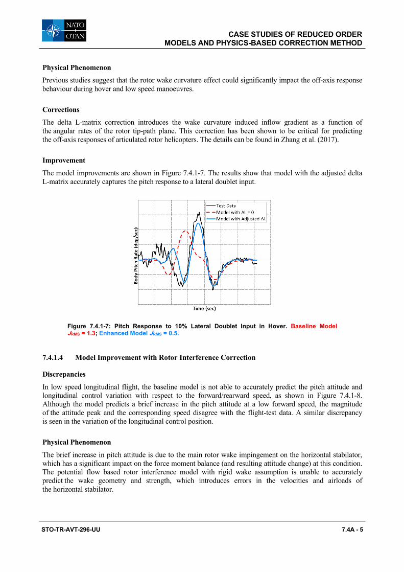
CASE STUDIES OF REDUCED ORDER MODELS AND PHYSICS-BASED CORRECTION METHOD

STO-TR-AVT-296-UU 7.4A - 5

Physical Phenomenon

Previous studies suggest that the rotor wake curvature effect could significantly impact the off-axis response behaviour during hover and low speed manoeuvres.

Corrections

The delta L-matrix correction introduces the wake curvature induced inflow gradient as a function of the angular rates of the rotor tip-path plane. This correction has been shown to be critical for predicting the off-axis responses of articulated rotor helicopters. The details can be found in Zhang et al. (2017).

Improvement

The model improvements are shown in Figure 7.4.1-7. The results show that model with the adjusted delta L-matrix accurately captures the pitch response to a lateral doublet input.

Figure 7.4.1-7: Pitch Response to 10% Lateral Doublet Input in Hover. Baseline Model JRMS = 1.3; Enhanced Model JRMS = 0.5.

7.4.1.4 Model Improvement with Rotor Interference Correction

Discrepancies

In low speed longitudinal flight, the baseline model is not able to accurately predict the pitch attitude and longitudinal control variation with respect to the forward/rearward speed, as shown in Figure 7.4.1-8. Although the model predicts a brief increase in the pitch attitude at a low forward speed, the magnitude of the attitude peak and the corresponding speed disagree with the flight-test data. A similar discrepancy is seen in the variation of the longitudinal control position.

Physical Phenomenon

The brief increase in pitch attitude is due to the main rotor wake impingement on the horizontal stabilator, which has a significant impact on the force moment balance (and resulting attitude change) at this condition. The potential flow based rotor interference model with rigid wake assumption is unable to accurately predict the wake geometry and strength, which introduces errors in the velocities and airloads of the horizontal stabilator.

CASE STUDIES OF REDUCED ORDER MODELS AND PHYSICS-BASED CORRECTION METHOD

7.4A - 6 STO-TR-AVT-296-UU

Corrections For typical rotorcraft, the rotor wake experiences a roll-up as the airspeed increases. An effective wake skew angle, 𝜒𝜒𝑒𝑒, can be used to capture the roll-up effect on the wake geometry. A viscous decay factor can be used to reduce the off-rotor induced velocity magnitude due to the air viscosity. The effective wake skew angle has a large impact on the rotor interference especially during low speed flight. The adjustment of the effective wake skew angle and the viscous decay factor improves the prediction of the rotor wake interference on the horizontal stabilator. A customized effective wake skew angle map was developed to accurately capture the speed condition and the magnitude of the wake impingement on the stabilator. Details can be found in Zhang et al. (2017).

Improvement As shown in Figure 7.4.1-8, the effective wake skew angle adjustment significantly improves both the pitch attitude and longitudinal control variation compared with the flight-test data.

Figure 7.4.1-8: Pitch Attitude and Longitudinal Stick Position in Low Speed Longitudinal Flight. Baseline Model JRMS = [2.0, 6.5]; Enhanced Model JRMS = [1.2, 3.2].

7.4.1.5 Model Improvement with Fuselage Interference Correction

Discrepancies Compared to the flight-test data, the baseline model predicted more right pedal position in forward descent (Figure 7.4.1-9(a)) and autorotation (Figure 7.4.1-9(b)). The baseline model also predicted a more nose-down pitch attitude than the test data in forward descent (Figure 7.4.1-10(a)) and autorotation (Figure 7.4.1-10(b)).

Physical Phenomenon When the helicopter is operating at a high angle of attack condition such as in a high-rate forward descent or an autorotation, the flow separates behind the fuselage and the shed vortices interact with the empennage. When the vertical fin is impacted by the strong unsteady vortices shed from the fuselage, its effectiveness is significantly reduced [Nelson (1989)]. This phenomenon of reduced tail surface effectiveness at high AoA has been observed in fixed-wing aircraft flight test [Napolitano and Spagnuolo (1993)]. Also, when the flow separates behind the fuselage at high angles of attack, the fuselage wake could induce a strong downwash at the horizontal stabilator, which tends to increase the pitch attitude angle.

CASE STUDIES OF REDUCED ORDER MODELS AND PHYSICS-BASED CORRECTION METHOD

STO-TR-AVT-296-UU 7.4A - 7

Corrections Although the fuselage vortex is not explicitly modelled, a similar impact on the vertical fin can be approximately modelled as a reduction in dynamic pressure. The dynamic pressure reduction factor at the vertical fin due to the fuselage was increased around the fuselage AoA of 25 degrees. It is smoothly transitioned to the baseline value at low and high AoA to localise the impact. The dynamic pressure reduction effect is smoothly phased out as the sideslip angle increases and the vertical fin is eventually cleared of the fuselage wake.

The fuselage downwash velocities at the left and right sides of the stabilator were also increased around 25 degrees fuselage AoA. It is transitioned to the baseline value at low and high AoA to localise the impact.

Improvement As shown in Figure 7.4.1-9, the adjustment of the fuselage interference on the vertical fin improves the model-data correlation of the pedal position in both forward descent and autorotation.

(a) Forward Climb/Descent. (b) Autorotation.

Figure 7.4.1-9: Pedal Position in Forward Climb/Descent and Autorotation. Baseline Model JRMS = [8.6, 12.9]; Enhanced Model JRMS = [4.7, 2.8].

As shown in Figure 7.4.1-10, the adjustment of the fuselage interference on horizontal stabilator improves the pitch attitude correlation in both forward descent and autorotation.

(a) Forward Climb/Descent. (b) Autorotation.

Figure 7.4.1-10: Pitch Attitude in Forward Climb/Descent and Autorotation. Baseline Model JRMS =[1.8, 2.3]; Enhanced Model JRMS = [0.8, 1.6].

CASE STUDIES OF REDUCED ORDER MODELS AND PHYSICS-BASED CORRECTION METHOD

7.4A - 8 STO-TR-AVT-296-UU

7.4.1.6 Model Improvement with Fuselage Aerodynamic Drag Correction

Discrepancies

In high-rate forward descent, the baseline model predicted higher collective position and higher rotor power compared with the test data, as shown in Figure 7.4.1-11. In autorotation, the baseline model underpredicts the rate of descent in the low airspeed range and overpredicts the rate of descent in the high airspeed range, as seen in Figure 7.4.1-12.

Physical Phenomenon

At high rates of descent and in autorotation, the fuselage is operating at a high Angle Of Attack (AoA). In these conditions, flow separation occurs at the fuselage, causing the fuselage drag to become unsteady and vary nonlinearly. The fuselage drag data was based on wind-tunnel test results that were obtained in a low AoA range and at 90-deg AoA. A curve fitting was applied in between low and high AoA, causing uncertainties in the fuselage drag data in the mid to high AoA range.

Corrections

Based on the analysis of the model-data discrepancy in high-rate descent and autorotation, the fuselage drag coefficient was slightly reduced in the mid to high AoA range where the wind-tunnel data was unavailable. To localize the impact, the drag coefficient is smoothly transitioned to the baseline value at both low AoA and 90-deg AoA. Further details can be found in Xin et al. (2019).

Improvement

As shown in Figure 7.4.1-11, the enhanced model correlates better with the test data than the baseline, especially at high descent rates. These improvements are due to the adjustment in fuselage drag at high AoA.

Figure 7.4.1-11: Collective Stick Position and Main Rotor Power in Forward Climb/Descent. Baseline Model JRMS = [4.7, 157.1]; Enhanced Model JRMS = [3.4, 107.6].

Figure 7.4.1-12 shows the autorotation rate of descent with respect to varying airspeed. The enhanced model correlates better with the test data than the baseline model over the entire airspeed range. The improvement at high speed is related to the pitch attitude improvement as shown in Figure 7.4.1-10(b). The improvement at low speed is attributed to the adjustment in fuselage drag at high angle of attack.

CASE STUDIES OF REDUCED ORDER MODELS AND PHYSICS-BASED CORRECTION METHOD

STO-TR-AVT-296-UU 7.4A - 9

Figure 7.4.1-12: Autorotation Rate of Descent. Baseline Model JRMS = 422.1; Enhanced Model JRMS = 219.0

7.4.1.7 Off-Axis Response Due to Rotor Wake Distortion in Manoeuvring Flight

Discrepancies

It was not well understood for a while why the baseline simulation predicted the opposite off-axis response compared to flight-test data for a single main rotor helicopter. The erroneous off-axis response prediction was seen in the roll response due to pitch control and pitch response due to roll control, mainly seen in hover or at low speed flight.

Physical Phenomenon

Rotor wake variation in manoeuvring flight exhibits a dynamic wake distortion due to rotor tip-path-plane rotation, which results in a remarkable wake curvature, and in turn, rotor inflow variation that conventional rotor inflow models do not capture.

Corrections

Correction methods address the problem by enhancing the baseline dynamic inflow [Pitt and Peters (1981), Peters and He (1991)] models with additional terms as shown in Equations 5.4.3.1.1-1 and 5.4.3.1.2-1 (Chapter 5.4) to account for the effect of curved wake on the rotor induced flow distribution during a rotor pitch/roll manoeuvre [Zhao et al. (2004), He et al. (2019)].

The dynamic distortion of rotor wake during the manoeuvre was confirmed using a physics-based viscous Vortex Particle Method (VPM) simulation [He et al. (2019)], and an alternate approach was pursued to extract a reduced order inflow dynamics model from the physics-based VPM simulation using CIFER®, a model parameter identification tool, [Tischler et al. (2012)]. In this approach, both L- and M-matrix elements used in the Peters-He inflow model [Peters and He (1991)] are replaced with the VPM-extracted parameters. In addition, the rotor wake distortion effect is also extracted from the VPM rotor wake simulation and used to augment the Peters-He baseline equation with an added inflow forcing term as shown in Equation 5.4.3.1.2-1 (Chapter 5.4).

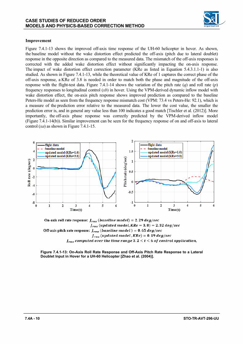
CASE STUDIES OF REDUCED ORDER MODELS AND PHYSICS-BASED CORRECTION METHOD

7.4A - 10 STO-TR-AVT-296-UU

Improvement

Figure 7.4.1-13 shows the improved off-axis time response of the UH-60 helicopter in hover. As shown, the baseline model without the wake distortion effect predicted the off-axis (pitch due to lateral doublet) response in the opposite direction as compared to the measured data. The mismatch of the off-axis responses is corrected with the added wake distortion effect without significantly impacting the on-axis response. The impact of wake distortion effect correction parameter (KRe as listed in Equation 5.4.3.1.1-1) is also studied. As shown in Figure 7.4.1-13, while the theoretical value of KRe of 1 captures the correct phase of the off-axis response, a KRe of 3.8 is needed in order to match both the phase and magnitude of the off-axis response with the flight-test data. Figure 7.4.1-14 shows the variation of the pitch rate (q) and roll rate (p) frequency responses to longitudinal control (xb) in hover. Using the VPM-derived dynamic inflow model with wake distortion effect, the on-axis pitch response shows improved prediction as compared to the baseline Peters-He model as seen from the frequency response mismatch cost (VPM: 73.4 vs Peters-He: 92.1), which is a measure of the prediction error relative to the measured data. The lower the cost value, the smaller the prediction error is, and in general any value less than 100 indicates a good match [Tischler et al. (2012)]. More importantly, the off-axis phase response was correctly predicted by the VPM-derived inflow model (Figure 7.4.1-14(b)). Similar improvement can be seen for the frequency response of on and off-axis to lateral control (xa) as shown in Figure 7.4.1-15.

Figure 7.4.1-13: On-Axis Roll Rate Response and Off-Axis Pitch Rate Response to a Lateral Doublet Input in Hover for a UH-60 Helicopter [Zhao et al. (2004)].

CASE STUDIES OF REDUCED ORDER MODELS AND PHYSICS-BASED CORRECTION METHOD

STO-TR-AVT-296-UU 7.4A - 11

(a) q/xb. (b) p/xb.

Figure 7.4.1-14: UH-60 Frequency Response to Longitudinal Control in Hover. (p/xa response: VPM-ID’s cost = 91.6 vs Peters-He’s cost = 98.3).

(a) p/xa. (b) q/xa.

Figure 7.4.1-15: UH-60 Frequency Response to Lateral Control in Hover. (p/xa response: VPM-ID’s cost = 91.6 vs Peters-He’s cost = 98.3).

CASE STUDIES OF REDUCED ORDER MODELS AND PHYSICS-BASED CORRECTION METHOD

7.4A - 12 STO-TR-AVT-296-UU

7.4.2 CH-47 Case Study

7.4.2.1 CH-47 Simulation Handling Qualities Fidelity Improvement by Physics-Inspired Modelling of Rotor-on-Rotor Dynamic Inflow Interactions

This case study applies the simulation model fidelity improvement method of implementing reduced order models and physics-based corrections. It also identifies rotor dynamic inflow model parameter adjustments encompassed by the simulation model fidelity improvement method of simulation model parameter adjustment illustrated in the Section 7.5.4 ‘CAE Updates to CH-147F Model’ case study.

Baseline Model: Boeing Helicopters Simulation (BHSIM) Math Model

As depicted in Figure 7.4.2-1, BHSIM is a physics-based, nonlinear, full flight envelope, 6-DOF simulation math model [Hackett et al. (1983)]. BHSIM is a generic model capable of simulating all types of tandem rotor helicopters. Blade element rotor models are implemented on both rotor heads that represent the nonlinear and coupled flap and lag motion of each individual rotor blade using the algorithm for computer generation of comprehensive coupled rotor/fuselage equations of motion published in Miller et al. (1987). Rotor dynamic inflow, rotor-on-rotor interference between zeroth harmonic rotor dynamic inflow states, and drive system dynamic coupling are also represented in the BHSIM math model. High fidelity representations of the Chinook’s mechanical and hydraulic flight control systems and Automatic Flight Control System (AFCS) are included in the baseline simulation model.

Figure 7.4.2-1: Boeing Helicopters Simulation (BHSIM) Math Model.

Discrepancies

In this case study, the primary simulation fidelity issue addressed is that test pilots found the hover and low speed lateral axis handling qualities of the Boeing CH-47D Chinook simulator to be degraded with respect to the actual aircraft. Test pilots observed that lateral axis handling qualities were particularly unrealistic in the simulator when the Automatic Flight Control System (AFCS) was selected OFF (AFCS-OFF). Test pilots also noted that lateral axis workload and control response phase loss were exaggerated unrealistically in the simulator when performing ADS-33E Mission Task Elements (MTEs) in the Chinook simulator with the AFCS selected ON (AFCS-ON). Test pilots were particularly critical of simulator fidelity in replicating

CASE STUDIES OF REDUCED ORDER MODELS AND PHYSICS-BASED CORRECTION METHOD

STO-TR-AVT-296-UU 7.4A - 13

workload and performance when re-trimming the lateral stick using the Centering Device Release (CDR) force trim release switch to achieve a roughly zero lateral stick force ‘hands-off’ hover trim state. Test pilots commented that aircraft roll attitude and roll rate responses in the simulator seemed significantly more out of phase with lateral stick inputs than in the actual Chinook helicopter.

Physical Phenomenon

The influence of cyclic inflow dynamics on total vehicle and control characteristics, and in particular aircraft pitch and roll rate damping stability derivatives, has been well understood since the 1970s when Professor Howard C. “Pat” Curtiss documented analytical and experimental investigations of the handling qualities of hingeless and bearingless rotor configurations and developed a quasi-static approximation of the effects of rotor first harmonic induced inflow on helicopter control response and angular rate damping known as the “reduced Lock number” approximation [Quackenbush et al. (2013), Curtiss et al. (1990)]. The reduced Lock number approximation made it clear that first harmonic induced inflow dynamics have a strong effect on helicopter handling qualities in low speed flight and that neglecting or underestimating the sensitivity of cyclic inflow skew to rotor aerodynamic hub moments can result in overly pessimistic predictions of lateral and longitudinal axis control response bandwidth and rate damping.

In light of Curtiss’s well known results and the many subsequent research efforts that built on his initial insights, inadequate or neglected rotor first harmonic induced inflow modelling is an obvious detail that should be investigated whenever a simulation math model exhibits worse lateral and longitudinal axis handling qualities than the actual helicopter in low speed flight. Review of the Boeing Helicopters Simulation (BHSIM) math model code and input data sets revealed that, in similar fashion to the Black Hawk simulation model documented in Howlett (1981b), the BHSIM Chinook simulation was configured to neglect the first harmonic induced inflow distribution which derives from rotor aerodynamic hub pitch and roll moments. BHSIM includes options to implement the Howlett GenHel Rotor Induced Inflow Model features described in Section 5.4.3.1.4 that represent the first harmonic induced inflow distribution component, which derives from cyclic aerodynamic hub moment over the rotor disk. However, quantitative input settings for the Howlett GenHel inflow model equations describing the influence of rotor aerodynamic hub moment on first harmonic inflow were not defined for the Chinook tandem rotor helicopter configuration in the original BHSIM simulation math model.

Figure 7.4.2-2 shows the frequency response of aircraft roll attitude to lateral stick input for the CH-47D in hover with the Automatic Flight Control System (AFCS) selected OFF (AFCS-OFF), which was identified from flight-test data published in Keller et al. (1998). The corresponding frequency response generated by the original BHSIM simulation configuration, for which the influence of rotor hub moments on first harmonic induced inflow is neglected, is also plotted in Figure 7.4.2-2 for comparison. The original BHSIM simulation configuration exhibits significantly higher gain and more control response phase loss than observed during flight test, particularly at frequencies in the vicinity of 1.0 to 4.0 rad/sec where pilots typically control the air vehicle.

Table 7.4.2-1 tabulates values of the “Frequency-Domain Integrated Cost Function” corresponding to the mismatch between the flight test and simulation model frequency responses plotted in Figure 7.4.2-2. A model/flight data mismatch cost function of J = 1211.2 is calculated for the original BHSIM simulation configuration with no modelling of the influence of rotor aerodynamic hub moment on first harmonic rotor induced inflow. This value is an order of magnitude larger than the guideline that the integrated cost function should have a value of 𝐽𝐽 ≤ 100 to reflect good simulation model agreement with flight-test data for rotorcraft [Tischler et al. (2012)].

CASE STUDIES OF REDUCED ORDER MODELS AND PHYSICS-BASED CORRECTION METHOD

7.4A - 14 STO-TR-AVT-296-UU

Figure 7.4.2-2: Roll Attitude to Lateral Control Position Frequency Response, CH-47D, 41,850 lb Gross Weight, Hover, AFCS-OFF.

Table 7.4.2-1: Model/Flight Data Mismatch Frequency-Domain Integrated Cost Function Metric Values for Roll Attitude to Lateral Control Position Frequency Response, CH-47D, 41,850 lb Gross Weight, Hover, AFCS-OFF.

# Simulation Inflow Model Configuration

Model/Flight Data Mismatch Frequency-Domain Integrated

Cost Function Metric

Reduction (Improvement) in Cost Function Metric Relative to

Original Simulation (%)

1 BHSIM, Original 1211.2 0.0

2 BHSIM, Improved 234.5 80.6

3 BHSIM, Pitt-Peters 850.0 29.8

4 BHSIM, PPSIM 237.7 80.4

CASE STUDIES OF REDUCED ORDER MODELS AND PHYSICS-BASED CORRECTION METHOD

STO-TR-AVT-296-UU 7.4A - 15

Figure 7.4.2-3 plots magnitude and phase error functions for the BHSIM simulation with various induced inflow models versus Maximum Unnoticeable Additional Dynamics (MUAD) error bound envelopes for CH-47D AFCS-OFF roll attitude to lateral control position frequency responses in hover. The original BHSIM simulation configuration with no modelling of the influence of rotor aerodynamic hub moment on first harmonic rotor induced inflow results in simulation to flight gain and phase errors that are well outside the MUAD boundaries.

Figure 7.4.2-4 shows lateral axis ADS-33E phase delay and bandwidth for the CH-47D in hover with the AFCS-OFF. The flight-test identified lateral axis ADS-33E bandwidth and phase delay parameters predict that the actual CH-47D helicopter has borderline Level 1 to 2 lateral axis handling qualities for hover and low speed conditions with the AFCS-OFF. In contrast, the original BHSIM simulation configuration that neglects the influence of hub moment on cyclic inflow is predicted to have borderline Level 2 to Level 3 handling qualities for AFCS-OFF operations. Note that the phase for the original BHSIM simulation configuration is always more negative than -135°, hence the bandwidth for this configuration is plotted as the frequency at which phase gets closest to -135°. Comparison of flight test and model lateral axis frequency response plots, integrated model error cost function value, MUAD error bound envelope exceedances, and comparison of flight test and model ADS-33E bandwidth and phase delay parameters all correlate with test pilot comments that the hover and low speed handling qualities of the original BHSIM simulation configuration, wherein the influence of rotor aerodynamic hub moment on first harmonic inflow is unmodelled, are unrealistically degraded with respect to the actual CH-47D helicopter for AFCS-OFF operations.

Figure 7.4.2-3: Maximum Unnoticeable Additional Dynamics (MUAD) Error Bound Envelopes for Roll Attitude to Lateral Control Position Frequency Response, CH-47D, 41,850 lb Gross Weight, Hover, AFCS-OFF.

CASE STUDIES OF REDUCED ORDER MODELS AND PHYSICS-BASED CORRECTION METHOD

7.4A - 16 STO-TR-AVT-296-UU

Figure 7.4.2-4: ADS-33E Lateral Axis Bandwidth and Phase Delay Parameters, Usable Cue Environment (UCE) > 1 and or Divided Attention Operations, CH-47D, 41,850 lb Gross Weight, Hover, AFCS-OFF.

Corrections

The first step towards improving fidelity of the BHSIM simulation by representing the influence of rotor aerodynamic hub moment on first harmonic inflow was to define input settings for the Howlett GenHel inflow model equations, hub moment influence factors, 𝐾𝐾𝐶𝐶𝑀𝑀 and 𝐾𝐾𝐶𝐶𝑁𝑁, and normalized time constants, 𝜏𝜏𝑐𝑐 and 𝜏𝜏𝑠𝑠, based on the Pitt and Peters finite state inflow theory described in Peters and HaQuang (1988). Figure 7.4.2-2, Table 7.4.2-1, Figure 7.4.2-3, and Figure 7.4.2-4 all indicate that implementation of the Pitt-Peters inflow model provides a distinct improvement in simulation fidelity. However, comparison of flight test and model lateral axis frequency response plots, integrated model error cost function value, MUAD error bound envelope exceedances, and comparison of flight test and model ADS-33E bandwidth and phase delay parameters all indicate that the BHSIM Pitt-Peters inflow model simulation configuration continues to result in unrealistically degraded hover and low speed handling qualities with respect to the actual CH-47D helicopter for AFCS-OFF operations.

The Pitt-Peters inflow theory is developed for an individual rotor operating in isolation and neglects tandem rotor helicopter specific rotor-on-rotor induced inflow interference effects. Hence, it is logical to look to the unique physics of tandem rotor helicopters for inspiration on how to improve rotor induced inflow modelling fidelity beyond that provided by Pitt-Peters theory. Figure 7.4.2-5 and Figure 7.4.2-6 illustrate the unique physics and aerodynamics of the tandem rotor configuration that occur when the aircraft undergoes a roll rate perturbation. It is likely that rotor-on-rotor interference effects in tandem rotor helicopters will tend to increase the influence factors and time constants that should be used in tandem rotor helicopter first harmonic inflow models well beyond theoretical isolated rotor values.

The aircraft normalized dimensional roll rate damping derivative (𝐿𝐿𝑝𝑝) plays a significant role in lateral axis frequency response characteristics, particularly for AFCS-OFF conditions. Hence, understanding the effect of inflow model parameters on simulation predicted roll rate damping is a natural step toward physics-based or physics-inspired math model improvements. Figure 7.4.2-7 plots normalized dimensional roll rate damping (𝐿𝐿𝑝𝑝) and pitch rate damping (𝑀𝑀𝑞𝑞) derivatives predicted by the BHSIM flight simulation model verse the hub aerodynamic pitch moment influence factor (𝐾𝐾𝐶𝐶𝑀𝑀) used in the Howlett GenHel inflow model. Note that the BHSIM predictions shown in Figure 7.4.2-7 are generated with the hub aerodynamic roll moment influence factor (𝐾𝐾𝐶𝐶𝑁𝑁) set to zero. Figure 7.4.2-8 plots normalized dimensional roll rate damping (𝐿𝐿𝑝𝑝) and pitch rate damping (𝑀𝑀𝑞𝑞) derivatives predicted by the BHSIM flight simulation model versus the hub aerodynamic roll moment influence factor (𝐾𝐾𝐶𝐶𝑁𝑁) used in the Howlett GenHel inflow model. Note that the BHSIM predictions shown in Figure 7.4.2-8 are generated with the hub aerodynamic roll moment influence factor (𝐾𝐾𝐶𝐶𝑀𝑀) set to zero. Figure 7.4.2-7 also shows the flight-test identified value of 𝐿𝐿𝑝𝑝 identified by Dr. Christina Ivler (US Army), and Figure 7.4.2-8

CASE STUDIES OF REDUCED ORDER MODELS AND PHYSICS-BASED CORRECTION METHOD

STO-TR-AVT-296-UU 7.4A - 17

also shows the flight-test identified value of 𝑀𝑀𝑞𝑞 identified by Mr. Michael Lawler during the CH-47F Chinook Digital Automatic Flight Control System (DAFCS) program documented in Lawler et al. (2006). Note that stable values of 𝐿𝐿𝑝𝑝 and 𝑀𝑀𝑞𝑞 are plotted and referred to subsequently as positive numbers for ease of interpretation and to avoid repeated usage of negative signs. These figures show that the 𝐾𝐾𝐶𝐶𝑀𝑀 parameter affects only the roll rate damping derivative whereas the 𝐾𝐾𝐶𝐶𝑁𝑁 parameter affects only the pitch rate damping derivative.

Figure 7.4.2-5: Tandem Rotor Pitching Moment and Physics-Inspired Notional Downwash Pattern During Steady Left Roll Rate Perturbation.

Figure 7.4.2-6: Tandem Rotor Helicopter Lateral Flapping and Aircraft Rolling Moment During Steady Left Roll Rate Perturbation.

∆Thrust

∆Thrust∆Thrust

∆Thrust

Fwd & aft rotor downwash perturbations add in partially overlapped tandem rotor layout

First harmonic rotor wake skew perturbations amplified as a result of rotor-on-rotor interference

Rotor thrust changes in same direction on both rotors in overlap region to precess rotors

∆(Induced-Velocity)∆(Induced-Velocity)

Forward and aft rotor disks tilt right as a result of lateral flapping

Rightward rolling moments about aircraft center of gravity generated by combination of thrust vector tilt and hub moment

Lateral flapping required to increase blade angle-of-attack on rear part of forward rotor and on forward part of aft rotor to create aerodynamic pitching moments required to precess the rotors

Lateral flapping must create blade angle-of-attack sufficient to overcome first harmonic fore/aft induced inflow response and generate rotor aerodynamic pitching moment required to provide rotor precessional moment necessary to sustain rotor roll rate Increased first harmonic inflow

skew results in increased lateral flapping and increased roll rate damping moment

Left Roll Rate

Perturbation

CASE STUDIES OF REDUCED ORDER MODELS AND PHYSICS-BASED CORRECTION METHOD

7.4A - 18 STO-TR-AVT-296-UU

Figure 7.4.2-7: Effect of Varying Howlett GenHel Inflow Model Pitch Aerodynamic Hub Moment Influence Factor on Roll and Pitch Rate Damping Derivatives, CH-47D/F, 46,000 lb Gross Weight (GW), Hover.

Figure 7.4.2-8: Effect of Varying Howlett GenHel Inflow Model Roll Aerodynamic Hub Moment Influence Factor on Roll and Pitch Rate Damping Derivatives, CH-47D/F, 46,000 lb Gross Weight (GW), Hover.

0

0.5

1

1.5

2

2.5

3

0 1 2 3 4

Normalized DimensionalAngular Rate

Damping Derivative (rad/sec)

Hub Aerodynamic Pitch Moment Influence Factor Parameter (KCM)

Lp BHSIM

Mq BHSIMKCL = 0

KCMparameter affects only roll damping derivative (Lp).

Flight Test Identified Lp ValuePitt & Peters

Value of KCM

00.20.40.60.8

11.21.41.6

0 1 2 3 4

Normalized Dimensional Angular Rate

Damping Derivative (rad/sec)

Hub Aerodynamic Roll Moment Influence Factor Parameter (KCL)

Lp BHSIM

Mq BHSIMKCM= 0

Flight Test Identified Mq Value

Pitt & Peters Value of KCL

KCLparameter affects only pitch damping derivative (Mq).

CASE STUDIES OF REDUCED ORDER MODELS AND PHYSICS-BASED CORRECTION METHOD

STO-TR-AVT-296-UU 7.4A - 19

Increasing the hub aerodynamic pitch moment influence factor (𝐾𝐾𝐶𝐶𝑀𝑀) increases aircraft roll rate damping significantly. The Pitt and Peters theoretical 𝐾𝐾𝐶𝐶𝑀𝑀 value of 1.2 increases 𝐿𝐿𝑝𝑝 to a value of 1.2531 rad/sec from the value of 0.7558 rad/sec predicted by the original BHSIM simulation configuration, wherein 𝐾𝐾𝐶𝐶𝑀𝑀 is set to zero. The flight-test identified value of 𝐿𝐿𝑝𝑝 is 2.9 rad/sec, strongly suggesting that an aerodynamic hub pitch moment influence factor much larger than the Pitt-Peters value should be used to represent the CH-47D as expected based on the physics of rotor-on-rotor aerodynamic interference in tandem rotor helicopters.

Given this physical interpretation, the following values of hub pitch moment influence factor and normalized dimensional cyclic inflow time constant are proposed for use in the improved CH-47 BHSIM simulation math model configuration as a compromise between optimizing correlation with flight-test data and maintaining a reasonable connection with theory.

𝐾𝐾𝐶𝐶𝑀𝑀 = 3.6 and 𝜏𝜏𝑐𝑐 = 0.024 sec

Note that a value of 0.024 sec for the normalized dimensional cyclic inflow model time constant, 𝜏𝜏𝑐𝑐, corresponds to a dimensional value of 0.4 second for the fore/aft cyclic inflow response to hub aerodynamic pitch moment in hover. While this is a significantly larger time constant than predicted by Pitt-Peters isolated rotor theory, a hover cyclic inflow time constant of 0.4 second seems possible in tandem rotor helicopters given the additional transport delays inherent in rotor-on-rotor interactions and a history of achieving better correlation with flight-test data by using longer zeroth harmonic inflow time constants in BHSIM than predicted by theory. For example, the zeroth harmonic tandem rotor-on-rotor interference model in BHSIM uses time constants of 0.35 sec for uniform (zeroth harmonic) rotor-on-rotor interference dynamics.

Improvement

Figure 7.4.2-2 shows that the improved BHSIM simulation configuration improves correlation with flight-test roll attitude to lateral stick frequency response data, particularly for predictions of control response phase. As shown in Table 7.4.2-1, a model/flight data mismatch integrated cost function of 234.5 is calculated for the improved BHSIM simulation configuration for AFCS-OFF operations, representing an 80.6% improvement over the original BHSIM simulation configuration with no rotor hub moment induced cyclic inflow effects. Conforming within the MUAD error bound envelopes (as shown in Figure 7.4.2-3), comparison of flight test and model ADS-33E bandwidth and phase delay parameters (as shown in Figure 7.4.2-4), and comparison of flight-test system identified and simulation model roll rate damping derivatives all indicate that the improved BHSIM simulation configuration results in a realistic representation of the AFCS-OFF handling qualities of the actual CH-47D helicopter. In contrast, the original BHSIM configuration results in unrealistically degraded hover and low speed handling qualities with respect to the actual CH-47D helicopter for AFCS-OFF operations.

The improved BHSIM simulation configuration that models the influence of rotor aerodynamic hub moments on tandem rotor helicopter first harmonic inflow is inspired by physics. However, it also derives from observations of the specific behaviour of the Chinook helicopter and is thus semi-empirical in nature. A more rigorous theoretical basis for tandem rotor first harmonic inflow modelling is beneficial in understanding the limitations of the semi-empirical improved BHSIM reduced order inflow model for Chinook applications and for simulation modelling of future tandem rotor helicopter configurations.

The Pressure Potential Superposition Inflow Model (PPSIM) described in Section 5.4.3.1.3 extends the finite state inflow methodology that is the basis for Pitt-Peters theory to account for rotor-on-rotor interference effects in tandem rotor helicopters and other multi-rotor rotorcraft configurations. It has been shown in Guner et al. (2019) that PPSIM predicts longitudinal inflow components even in hover because PPSIM captures some of the uniform inflow to longitudinal inflow and longitudinal inflow to longitudinal inflow rotor-on-rotor interference couplings effects. In contrast, the longitudinal inflow component (𝜆𝜆1𝑐𝑐) in BHSIM does not include interference effects; therefore, the aerodynamic pitch moment is multiplied by an empirical

CASE STUDIES OF REDUCED ORDER MODELS AND PHYSICS-BASED CORRECTION METHOD

7.4A - 20 STO-TR-AVT-296-UU

correction factor to improve roll damping correlation between the simulation result and flight-test data. By increasing the pitch aerodynamic hub moment influence factor (𝐾𝐾𝐶𝐶𝑀𝑀), a larger longitudinal inflow gradient is created for an applied aerodynamic pitch moment, which results in more roll damping. In BHSIM, a need for the correction factor arises due to the missing longitudinal to longitudinal inflow interference because longitudinal to longitudinal interference effectively increases 𝜆𝜆1𝑐𝑐 for both rotors.

Implementation of PPSIM into BHSIM requires extensive modification to a well-established simulation model. Therefore, an alternate path is used to identify PPSIM pitch aerodynamic hub moment influence factors and time constants. Details of the PPSIM for the CH-47D helicopter and PPSIM pitch aerodynamic hub moment influence factor and time constant identification process are provided in Guner et al. (2020). The following 𝐾𝐾𝐶𝐶𝑀𝑀 and 𝜏𝜏𝑐𝑐 values are identified for the front and rear rotors.

Front Rotor: 𝐾𝐾𝐶𝐶𝑀𝑀𝐹𝐹 = 3.54 𝜏𝜏𝑐𝑐𝐹𝐹 = 0.012 sec Rear Rotor: 𝐾𝐾𝐶𝐶𝑀𝑀𝑅𝑅 = 2.88 𝜏𝜏𝑐𝑐𝑅𝑅 = 0.011 sec

Note that only PPSIM has different values for the front and rear rotors while other inflow models use the same 𝐾𝐾𝐶𝐶𝑀𝑀 and 𝜏𝜏𝑐𝑐 for both rotors.

Model fidelity metrics for BHSIM configured to use the Pressure Potential Superposition Inflow Model (PPSIM) option enabled are presented in Figure 7.4.2-2, Table 7.4.2-1, Figure 7.4.2-3, and Figure 7.4.2-4 for AFCS-OFF conditions. Comparison of flight test and model lateral axis frequency response plots, integrated model error cost function value, MUAD error bound envelope conformity, and comparison of flight test and model ADS-33E bandwidth and phase delay parameters all indicate that the BHSIM PPSIM simulation configuration offers a realistic representation of the AFCS-OFF handling qualities of the actual CH-47D helicopter that is similar to that provided by the semi-empirical physics-inspired improved BHSIM simulation configuration.

Frequency response data and model fidelity metrics for the CH-47D in hover with the Automatic Flight Control System (AFCS) selected ON (AFCS-ON) are presented in Guner et al. (2020) for the inflow model configurations considered in the preceding AFCS-OFF data discussion. Comparison of flight test and model lateral axis frequency response plots, integrated model error cost function value, MUAD error bound envelope exceedances, and comparison of flight test and model ADS-33E bandwidth and phase delay parameters all correlate with test pilot comments that the hover and low speed lateral axis handling qualities of the original BHSIM simulation configuration, wherein the influence of rotor aerodynamic hub moment on first harmonic inflow is unmodelled, are unrealistically degraded with respect to the actual CH-47D helicopter for AFCS-ON operations. In contrast, all of these quantitative metrics indicate that the low speed lateral axis handling qualities represented by the semi-empirical improved BHSIM simulation configuration, which accounts for the influence of rotor aerodynamic hub moments on first harmonic induced inflow in tandem rotor helicopters, and the BHSIM PPSIM simulation configuration are not degraded with respect to the actual CH-47D helicopter for AFCS-ON operations. Test pilot evaluation of ADS-33E Mission Task Elements (MTEs) with AFCS-ON confirm that lateral axis handling qualities in the simulator are better with the semi-empirical improved BHSIM math model and correlate more closely with those of the actual aircraft than the lateral axis handling qualities of the original BHSIM simulation.

7.4.2.2 Rotor Mutual Interference Models

For the tandem rotorcraft configuration, rotor interference effects play a significant role in the dynamics due to overlapping rotors and changes in wake strength and geometry at different airspeeds. The most pronounced effect is on the longitudinal static stability, which undergoes a sign reversal between the hover/low speed regime and forward flight (typically at about 40 kn) [Bramwell (1961)]. As speed increases below the sign reversal speed, induced flow from the front rotor reduces the effectiveness of the aft rotor,

CASE STUDIES OF REDUCED ORDER MODELS AND PHYSICS-BASED CORRECTION METHOD

STO-TR-AVT-296-UU 7.4A - 21

resulting in a stable longitudinal gradient. Above the sign reversal, the induced velocity of both rotors reduces along with the resultant interference effect on the aft rotor. Consequently, above the sign reversal speed, tandem rotor aircraft exhibit a longitudinal static instability.

The DTSG CH-47F FLIGHTLAB® model incorporates a finite state interference model, which utilises empirical correction factors for effective wake skew and wake velocity decay, which must be established for a given rotor configuration. Wake skew and velocity decay influence the geometry and strength, respectively. These strongly affect the speed stability (𝑀𝑀𝑢), as indicated in the trim gradient and low frequency hovering cubic mode. The baseline FLIGHTLAB model exhibited a significantly higher longitudinal trim gradient at low speed as demonstrated in Figure 7.4.2-9(a).

Redacted Redacted

(a) Trim Comparison. (b) Frequency Response Comparison.

Figure 7.4.2-9: Hover Longitudinal Baseline Model Comparison.

A consistent discrepancy was also present in the low frequency longitudinal dynamic response in hover, as demonstrated in Figure 7.4.2-9(b). The break frequency associated with the speed stability mode was approximately 50% higher in the FLIGHTLAB model than in the flight-test data. Both the trim gradient and dynamic response mismatch are consistent with a higher value of speed stability (Mu), resulting from the influence of the front rotor interference on the aft rotor being over-predicted.

The uniform induced velocity decay (η0) parameter was varied to adjust the wake strength, which influenced the longitudinal trim gradient throughout the entire speed range, effectively determining the magnitude of overall control variation. The forward flight regime is relatively insensitive to wake geometry (wake structure is fully rolled up with a skew angle close to 90°), meaning that the interference effects in this region are predominantly a function of wake strength. Consequently, the uniform induced velocity decay parameter was established by calibrating against the longitudinal trim data in forward flight. Figure 7.4.2-10 demonstrates the effect of the wake velocity decay on the trim data. Smaller values of η0 resulted in lower trim gradients throughout the speed range. A value of η0 = 0.1 was found to match the high speed forward flight trim

CASE STUDIES OF REDUCED ORDER MODELS AND PHYSICS-BASED CORRECTION METHOD

7.4A - 22 STO-TR-AVT-296-UU

data very well. Also evident from the figure is the poor agreement of the trim data in low speed flight, indicating that the wake strength alone is unable to account for the entire speed range in this case.

Figure 7.4.2-10: Longitudinal Trim for Various Uniform Velocity Decay Values (Flight Data Redacted).

The wake geometry of the finite state interference model as implemented in FLIGHTLAB is achieved using an effective wake skew (χe), which accounts for the curvature of the wake far from the rotor plane. The standard effective wake skew is implemented using a correction factor, fx, as follows [He et al. (2004)]:

tan𝜒𝜒𝑒𝑒 = 𝑓𝑓𝑥𝑥 tan𝜒𝜒 where 𝑓𝑓𝑥𝑥 = 𝜋𝜋2

4

In order to reduce the amplitude of the model trim gradient in the low speed range, the effect of the wake curvature must be delayed to increase the speed at which the front rotor interference on the aft rotor reaches a maximum. This corresponds to a more linear conversion from wake skew at the rotor plane to effective wake skew, as demonstrated in Figure 7.4.2-11. The effective wake skew in the modified wake skew curve is considerably lower than the standard wake skew in the 0 – 60° range, delaying the point at which the wake begins to roll up. The right-hand portion of the figure presents the effective wake skew as a function of airspeed, which shows the delay of 10 – 15 kn in the modified wake skew relative to the standard values. The modified wake skew approach presented here is similar to results presented in previous studies [Zhang et al. (2017)].

The resultant trim data is presented in Figure 7.4.2-12 and longitudinal frequency response comparisons are presented in Figure 7.4.2-13(a) with the velocity decay and wake skew updates included. A significant improvement in model response is evident in both the trim and dynamic response data. The frequency of the hovering cubic mode reduced from 1 rad/sec to approximately 0.7 rad/sec. As a result of the wake skew update, the cost function reduced from 293 to 141.

The wake skew update also influences the lateral axis response due to the changing structure in the rotor overlap region. Shown in Figure 7.4.2-13(b) is the lateral axis frequency response comparison in hover, before and after the model update. The direction of the phase change at the low frequency hovering cubic mode is reversed after the model update, resulting from a small shift of the speed stability poles into the right half plane. Following the model update, the lateral axis frequency response is essentially an exact match (J = 11). The baseline and updated frequency-domain cost metrics are presented in Table 7.4.2-2 for the longitudinal and lateral axes.

CASE STUDIES OF REDUCED ORDER MODELS AND PHYSICS-BASED CORRECTION METHOD

STO-TR-AVT-296-UU 7.4A - 23

The improvement observed in the longitudinal frequency response metric is evident in the time domain, as shown in Figure 7.4.2-14 for a comparison of the pitch rate response to a longitudinal doublet, before and after the model update. A 74% time-domain cost reduction was achieved as a result of the model update, which occurred due to a reduced long term drift in the response (the cost reduced from 𝐽𝐽rms= 2.97 to 𝐽𝐽rms = 0.76).

Figure 7.4.2-11: Effective Wake Skew Modification.

Figure 7.4.2-12: Longitudinal Trim of Baseline Comparison for Interference Model Update (Flight Data Redacted).

CASE STUDIES OF REDUCED ORDER MODELS AND PHYSICS-BASED CORRECTION METHOD

7.4A - 24 STO-TR-AVT-296-UU

(a) Longitudinal Axis. (b) Lateral Axis.

Figure 7.4.2-13: Hover Frequency Response Comparison for Interference Model Update of Longitudinal Axis and Lateral Axis (Flight Data Redacted).

Table 7.4.2-2: Frequency-Domain Cost Metrics for Baseline and Updated Model.

Axis Baseline Updated Improvement (%)

Longitudinal 293 141 51.9

Lateral 26 11 57.7

Figure 7.4.2-14: Time-Domain Comparison of Pitch Response to Doublet in Hover (Flight Data Redacted).

CASE STUDIES OF REDUCED ORDER MODELS AND PHYSICS-BASED CORRECTION METHOD

STO-TR-AVT-296-UU 7.4A - 25

7.4.2.3 Elastic Drivetrain Dynamics

The CH-47 features a long driveshaft between the two rotors, providing torque and mechanically synchronising the rotors. This couples the lead-lag motion of the rotors, generating rotor-on-rotor dynamic modes. The most dominant mode results from axisymmetric lead-lag, producing pitch and yaw motion located approximately at the blade lag mode. In the DSTG CH-47F FLIGHTLAB model, the frequency of the dipole associated with this mode was higher than the flight-test data. The rotor-on-rotor mode is coupled with the elastic characteristics of the driveshaft. It has been demonstrated that the frequency of the dipole occurs at the blade lag mode for an infinitely stiff driveshaft and progressively reduces as the shaft elasticity increases [Miller et al. (1987)].

The standard FLIGHTLAB drivetrain models do not include provisions for a flexible driveshaft between rotors, and hence, in the baseline model, the rotor-on-rotor mode was located at the blade lag frequency. In order to approximate the effect of the elastic shaft, a negative lag stiffness was applied at each of the lag hinges, which progressively reduced the mode frequency with increasing stiffness magnitude. Shown in Figure 7.4.2-15 is the longitudinal frequency response for the model for a range of lag stiffness values. It can be seen that increasing the magnitude of the lag stiffness term reduces the frequency of the RoR mode, corresponding to increased shaft elasticity. At zero lag stiffness, the RoR frequency occurs at 9.5 rad/sec, which reduced to 7.3 rad/sec for a lag stiffness of -80,000 ft-lb. Also shown in the figure is a cost function comparison of the longitudinal axis response for a range of stiffness values.

Figure 7.4.2-15: Effect of Lag Stiffness on Rotor-on-Rotor Mode Dipole Frequency.

The lowest mismatch cost occurred for a stiffness of -50,000 ft-lb, which also corresponds with the best match in mode frequency with the flight-test data. A comparison of the longitudinal frequency response of the flight-test data with the FLIGHTLAB model is presented in Figure 7.4.2-16 before and after the stiffness update. While a noticeable improvement in the mode performance is evident (the mode frequency is very

CASE STUDIES OF REDUCED ORDER MODELS AND PHYSICS-BASED CORRECTION METHOD

7.4A - 26 STO-TR-AVT-296-UU

close to the flight-test data in the updated model), the resulting mismatch cost is essentially the same for both models owing to the fact that the rotor-on-rotor mode only contributes to a small portion of the overall frequency range. When evaluated over the reduced frequency range of 2 – 20 rad/s, where the rotor-on-rotor mode effect is greatest, the mismatch cost reduced from J = 39 to J = 9, indicating a perfect agreement of the model with the flight data in this frequency range.

Figure 7.4.2-16: Hover Longitudinal Frequency Response Comparison for Lag Stiffness Update (Flight Data Redacted).

7.4.3 AW109 Trekker Case Study This section presents some examples of physics-based model improvement applied to the AW109 Trekker helicopter. The first section focuses on aerodynamic interference modelling on tail planes, the second on turboshaft engine modelling, and the third on sensor and actuator modelling. The figures show the baseline model (red dashed line), updated model (blue line), and reference flight-test data (black markers). Trim data in level flight have been used for the aerodynamic interference case study and frequency sweeps for the turboshaft engine, sensor, and actuator modelling.

CASE STUDIES OF REDUCED ORDER MODELS AND PHYSICS-BASED CORRECTION METHOD

STO-TR-AVT-296-UU 7.4A - 27

7.4.3.1 Aerodynamic Interference

The following two figures show the beneficial effect of using the VPM approach [He and Zhao (2009)] over a non-empirically tuned Peters-He model to improve prediction of the longitudinal cyclic position and pitch attitude for the AW109 Trekker helicopter in trimmed straight and level flight. It can be seen how the VPM model improves the correlation with flight-test data at all speeds but for the highest (possibly due to shortcomings for other components of the model) for both longitudinal stick position and aircraft pitch attitude (Figure 7.4.3-1).

Figure 7.4.3-1: Longitudinal Cyclic Position and Pitch Attitude as Function of Speed.

7.4.3.2 Engine and Drivetrain Dynamics

This section presents an example application of the engine tuning process presented in Section 5.4.3.4. All the unknown parameters (transfer function gains, time delays, and constants) presented in that section will be tuned in order to match the behaviour of the PW207C engine installed on the AW109 Trekker helicopter. Each of the three transfer functions are tuned separately by the using the proper frequency responses. Then, both the individual transfer functions and the whole system are validated in the time domain. To accomplish this, reference flight-test data are needed for both dynamics and static performance:

• Trim sweeps at different ambient conditions and/or fuel consumption vs power vector.

• Flight data from the identification campaign. In particular, pedal and collective sweeps and 3-2-1-1s, with the acquisition at least of the following parameters: 1) Collective and pedal position, 2) Fuel flow, 3) Engine torque, and 4) Rotor speed (NR).

Tuning of Engine Parameters: Combustor and Torque Model

The engine torque response to fuel flow is represented with a transfer function as illustrated in Figure 7.4.3-2 which graphically reflects Equation 5.4.3.4-1. Both the gain and time constant as shown in the block diagram can be tuned by comparing the frequency response of the describing transfer function with that of “fuel flow to torque” computed with CIFER from flight data, via either collective or pedal sweeps (with preference for those with higher coherence).

Figure 7.4.3-2: Fuel Flow to Engine Torque Transfer Function Model.

CASE STUDIES OF REDUCED ORDER MODELS AND PHYSICS-BASED CORRECTION METHOD

7.4A - 28 STO-TR-AVT-296-UU

In the figure, μ corresponds to the static gain between torque and fuel flow and can be derived from static performance data (power vs fuel consumption). This can be checked against the frequency sweeps. Additionally, 𝜏𝜏 is the time constant of the fuel flow to engine torque dynamics, which can be tuned to match fuel flow to torque frequency responses computed with CIFER® from flight data.

Figure 7.4.3-3 shows an example of comparison between the Fuel Flow (FF, in lb/hr) to torque (TQ, in %) model frequency response and that computed with CIFER from flight-test data for collective input in hover at Low weight and Low altitude (LL).

Figure 7.4.3-3: Fuel Flow to Engine Torque Frequency Response for Collective Input in Hover.

Tuning of Engine Parameters: Rotor Speed Governor

The Fuel Flow (FF) is the sum of the contribution due to the collective feed-forward and that of the rotor speed governor (Equations 5.4.3.4-2, -3, and -4 in Chapter 5.4).

Figure 7.4.3-4: NR Error to Fuel Flow and Collective to Fuel Flow Transfer Function Models.

CASE STUDIES OF REDUCED ORDER MODELS AND PHYSICS-BASED CORRECTION METHOD

STO-TR-AVT-296-UU 7.4A - 29

The NR governor parameters (𝐾𝐾𝐼𝐼 , 𝐾𝐾𝑃𝑃 , 𝐾𝐾𝐼𝐼) can be tuned by comparing the frequency response of the model transfer function (PID) with NR to fuel flow frequency responses computed with CIFER using flight data from pedal sweeps. In fact, pedal sweeps are able to induce variations of NR and torque with the collective fixed. In this way, the contribution of the collective feed-forward is a constant, and the variations in Fuel Flow (FF) are affected only by variations of NR.

Figure 7.4.3-5 shows an example of comparison between the PID frequency response and the frequency response computed with CIFER in hover at Low weight and Low altitude (LL).

Figure 7.4.3-5: NR Error to Fuel Flow Frequency Response for Pedal Input in Hover.

Tuning of Engine Parameters: Collective Feed-Forward

In order to tune the collective feed-forward block, the signal FFC (fuel flow contribution due to the collective) is computed as (FF – FFPID) where FF is the fuel flow measured during collective sweep performed in flight, and FFPID is computed by simulation, using (NR – NRRef) measured in flight during the same collective sweep as the input to the PID block transfer function (previously validated).

The collective feed-forward parameters (τ1, τ2, kc) can be tuned by comparing the frequency response of the describing transfer function with that of FFC computed following the process described above. A first guess of kc can be found by looking at flight data in trim conditions.

Figure 7.4.3-6 shows an example comparison between the collective feed-forward describing function and frequency response computed with CIFER.

Notice that the decrease of the phase at high frequency is caused by a 0.2 seconds of transport delay, due to engine data acquisition system synchronization with the helicopter data set (see Section 7.4.3.2).

CASE STUDIES OF REDUCED ORDER MODELS AND PHYSICS-BASED CORRECTION METHOD

7.4A - 30 STO-TR-AVT-296-UU

Figure 7.4.3-6: Collective to Fuel Flow Frequency Response for Collective Input in Hover.

Drivetrain Modelling

Drivetrain is represented as a spring and inertia model calculated from the elastic and inertial properties of the helicopter drivetrain. Further discussion of the model can be found in Chapter 5.4.

Validation in the Time Domain (Open-Loop)

The validation (open-loop) in the time domain of the ‘NR error to fuel flow’ and ‘collective to fuel flow models’ involves comparing the main outputs of the engine model (TQ and FF) with flight-test data following inputs of NR and collective measured in flight. The simulated dynamic responses have been initialized with their values at the trim condition.

Figure 7.4.3-7 shows the comparison between the fuel flow and torque predicted by the model and the flight-test data following NR and collective 3-2-1-1 inputs measured in a collective 3-2-1-1 manoeuvre.

Figure 7.4.3-8 presents the comparison between the fuel flow and torque predicted by the model and the flight-test data following NR and collective inputs measured in a pedal 3211 manoeuvre.

Figure 7.4.3-8 presents the comparison between the fuel flow and torque predicted by the model and the flight-test data for pedal 3211 inputs.

CASE STUDIES OF REDUCED ORDER MODELS AND PHYSICS-BASED CORRECTION METHOD

STO-TR-AVT-296-UU 7.4A - 31

Figure 7.4.3-7: Engine Fuel Flow and Torque Response to Collective 3-2-1-1 Input in Hover.

Figure 7.4.3-8: Engine Fuel Flow and Torque Response to Pedal 3-2-1-1 Input in Hover.

Impact of the Engine Model on Closed-Loop Dynamics (FLIGHTLAB® Model)

To show the improvements produced by this turboshaft model with respect to an ideal engine (perfectly constant NR and infinite available power), Figure 7.4.3-9 and Figure 7.4.3-10 present the frequency responses for yaw rate, rotor speed, engine torque, and body normal loads factor to collective control inputs, which illustrate the significant improvement of simulation using the turboshaft engine model rather than the ideal engine model. The improvement is also reflected in the reduction of the cost function J values as listed. Figure 7.4.3-11 and Figure 7.4.3-12 show the frequency responses for rotor speed (NR), yaw rate, and engine torque, to pedal inputs. Again, the significant improvement in frequency-response agreement of the model and flight data is reflected in the large reduction of the integrated cost function J.

CASE STUDIES OF REDUCED ORDER MODELS AND PHYSICS-BASED CORRECTION METHOD

7.4A - 32 STO-TR-AVT-296-UU

Figure 7.4.3-9: Yaw Rate (r) and Rotor Speed (NR) Frequency Response to Collective (DCOL) in Hover.

CASE STUDIES OF REDUCED ORDER MODELS AND PHYSICS-BASED CORRECTION METHOD

STO-TR-AVT-296-UU 7.4A - 33

Figure 7.4.3-10: Engine Torque (Tq) and Normal Load Factor (Nz) Frequency Response to Collective (DCOL) in Hover.

CASE STUDIES OF REDUCED ORDER MODELS AND PHYSICS-BASED CORRECTION METHOD

7.4A - 34 STO-TR-AVT-296-UU

Figure 7.4.3-11: Yaw Rate (r) and Rotor Speed (NR) Frequency Responses to Pedal (DPED) in Hover.

CASE STUDIES OF REDUCED ORDER MODELS AND PHYSICS-BASED CORRECTION METHOD

STO-TR-AVT-296-UU 7.4A - 35

Figure 7.4.3-12: Engine Torque (Tq) Frequency Response to Pedal (DPED) in Hover.

7.4.3.3 Sensor and Actuator Dynamics

For the AW109 Trekker helicopter test case, the following assumptions were used for sensor and actuator modelling:

• Sensors were modelled as a second order Butterworth filter with 3 Hz bandwidth for accelerations and 8 Hz bandwidth for rates according to the nominal performance taken from the sensor specifications.

• 0.2 s transport delay, due to the engine data acquisition system delay with respect to the helicopter for all engine-related measurements. The estimation was accomplished by measuring the time shift for collective data available in the engine and helicopter data sets.

• Main and tail rotor actuators were modelled as first order filters with 12 Hz bandwidth to match the qualification test data report of the components.

Figure 7.4.3-13 shows the effect of the models listed above on the frequency response of collective to normal load factor (Nz) and engine torque. Figure 7.4.3-14 shows the effect of sensor modelling on roll rate to lateral and pitch rate to longitudinal frequency responses. Figure 7.4.3-15 presents the accelerometer x- and y-component responses to longitudinal and lateral controls, respectively. It can be seen that the improvement, quantified by the cost function J is mostly due to accelerometer sensor and engine data acquisition system modelling that affects frequency ranges lower than those influenced by actuator and rate sensors. The cost function J has slightly worsened the lateral to roll rate response relative to the baseline model, probably due to minimum use of actuator and sensor performance per component specifications.

CASE STUDIES OF REDUCED ORDER MODELS AND PHYSICS-BASED CORRECTION METHOD

7.4A - 36 STO-TR-AVT-296-UU

Figure 7.4.3-13: Normal Load Factor (Nz) and Engine Torque (Tq) Frequency Response to Collective (DCOL) in Hover.

CASE STUDIES OF REDUCED ORDER MODELS AND PHYSICS-BASED CORRECTION METHOD

STO-TR-AVT-296-UU 7.4A - 37

Figure 7.4.3-14: Roll Rate (p) to Lateral (DLAT) and Pitch Rate (q) to Longitudinal (DLON) Frequency Responses in Hover.

CASE STUDIES OF REDUCED ORDER MODELS AND PHYSICS-BASED CORRECTION METHOD

7.4A - 38 STO-TR-AVT-296-UU

Figure 7.4.3-15: Longitudinal Load Factor (Nx) to Longitudinal (DLON) and Lateral Load Factor (Ny) to Lateral (DLAT) Frequency Responses in Hover.

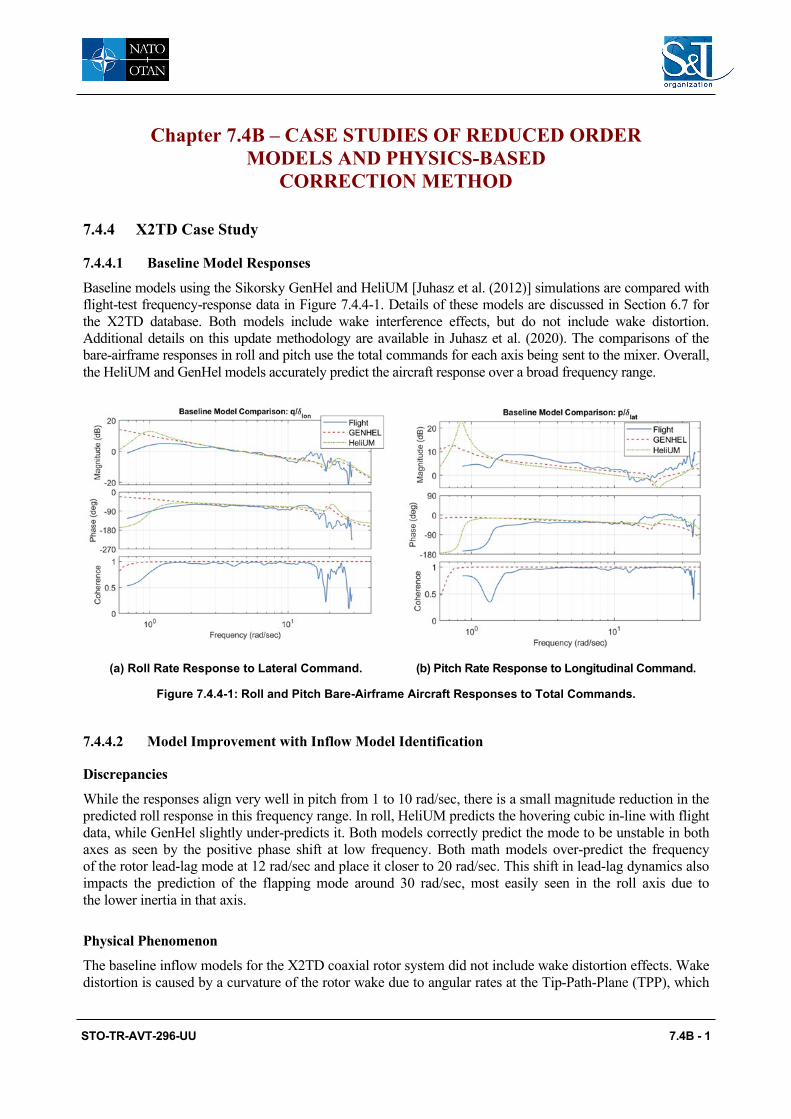
STO-TR-AVT-296-UU 7.4B - 1

Chapter 7.4B – CASE STUDIES OF REDUCED ORDER MODELS AND PHYSICS-BASED

CORRECTION METHOD

7.4.4 X2TD Case Study

7.4.4.1 Baseline Model Responses

Baseline models using the Sikorsky GenHel and HeliUM [Juhasz et al. (2012)] simulations are compared with flight-test frequency-response data in Figure 7.4.4-1. Details of these models are discussed in Section 6.7 for the X2TD database. Both models include wake interference effects, but do not include wake distortion. Additional details on this update methodology are available in Juhasz et al. (2020). The comparisons of the bare-airframe responses in roll and pitch use the total commands for each axis being sent to the mixer. Overall, the HeliUM and GenHel models accurately predict the aircraft response over a broad frequency range.

(a) Roll Rate Response to Lateral Command. (b) Pitch Rate Response to Longitudinal Command.

Figure 7.4.4-1: Roll and Pitch Bare-Airframe Aircraft Responses to Total Commands.

7.4.4.2 Model Improvement with Inflow Model Identification

Discrepancies

While the responses align very well in pitch from 1 to 10 rad/sec, there is a small magnitude reduction in the predicted roll response in this frequency range. In roll, HeliUM predicts the hovering cubic in-line with flight data, while GenHel slightly under-predicts it. Both models correctly predict the mode to be unstable in both axes as seen by the positive phase shift at low frequency. Both math models over-predict the frequency of the rotor lead-lag mode at 12 rad/sec and place it closer to 20 rad/sec. This shift in lead-lag dynamics also impacts the prediction of the flapping mode around 30 rad/sec, most easily seen in the roll axis due to the lower inertia in that axis.

Physical Phenomenon

The baseline inflow models for the X2TD coaxial rotor system did not include wake distortion effects. Wake distortion is caused by a curvature of the rotor wake due to angular rates at the Tip-Path-Plane (TPP), which

CASE STUDIES OF REDUCED ORDER MODELS AND PHYSICS-BASED CORRECTION METHOD

7.4B - 2 STO-TR-AVT-296-UU

affects the airflow around the rotor disk. For an articulated rotor, wake distortion has the largest impact on the off-axis response [Rosen and Isser (1995), Keller et al. (1998), Zhao et al (2004)]. For a hingeless rotor system, such as the X2TD, there is an impact in the on-axis response as well. These effects are modelled by adding analytically derived wake distortion factors, as was done in the GenHel case, or by using system identification to extract an inflow model including wake distortion, as was done for the HeliUM case. The next two sections discuss these two methods in more details.

GenHel Corrections and Improvements

As part of the State-Space GenHel development under the Sikorsky internal funding, the coaxial rotor mutual interference model has been improved by implementing a reduced order model for the wake distortion effect based on the formulation published in Zhao et al. (2004). A set of delta terms are introduced in the L-matrices for the rotor mutual interference. This results in an additional first harmonic rotor interference in response to the TPP angular rate. The model parameters are set to the values recommended in Zhao et al. (2004). As shown in Figure 7.4.4-2(a), modelling of the wake distortion effect improves the GenHel correlation of the roll response with test data in the frequency range of anticipated improvement, between 1 and 10 rad/sec. Due to the relatively large pitch inertia of the aircraft, the wake distortion impact on the pitch response is minimal, as shown in Figure 7.4.4-2(b). In addition, with the wake distortion effect modelled, the phase variations of both roll and pitch responses at low frequency (< 1 rad/sec) now trend correctly when compared to the test data.

(a) Roll Rate Response to Lateral Command. (b) Pitch Rate Response to Longitudinal Command.

Figure 7.4.4-2: Hover Roll and Pitch Responses with GenHel Model Improvement.

The wake distortion mainly affects the responses in hover and at low speed, and the impact reduces with increasing airspeed. At high speed, the wake distortion only shows a small impact on the roll response. Figure 7.4.4-3 shows that the time-domain response to a roll doublet at 200 knots is slightly improved when the wake distortion effect is modelled.

CASE STUDIES OF REDUCED ORDER MODELS AND PHYSICS-BASED CORRECTION METHOD

STO-TR-AVT-296-UU 7.4B - 3

Figure 7.4.4-3: Hover Roll Doublet Response with GenHel Model Improvement.

HeliUM Corrections

The inflow model of Maryland Free Wake (MFW) was coupled with HeliUM to improve model correlation of the linear aircraft response when compared with frequency responses from flight-test data, as shown in Figure 7.4.4-1. A reduced order state-space model of the X2TD inflow dynamics in hover was first extracted from MFW using system identification techniques [Tischler et al. (2012)]. The form of the inflow model is based on the work by Keller (2019) and is presented in Chapter 5.4.3.1 in Equations 5.4.3.1.6-1 to 5.4.3.1.6-6. Additional details about the identification methodology and results can be found in Juhasz et al. (2020).

Inflow Model Identification

The inflow model parameters were identified from MFW [Juhasz et al. (2020)] using the CIFER® system identification tool [Tischler et al. (2012)]. Figure 7.4.4-4(a) compares the identified linear model and the MFW frequency responses of the upper (λ_(0,U)) and lower (λ_(0,L)) rotor uniform inflow to upper rotor thrust inputs (C_(T,U)). The model aligns very well with the data over the entire frequency range used for identification, up to 20 rad/sec. Further, the model and response show the characteristic first order nature of classical dynamic inflow models. The identified output coupling parameters were identified as H_(UL,0) = 0.56 and H_(LU,0) = 1.07. These are similar in magnitude to the simple momentum theory derived values of 0.86 and 1.13, respectively [Juhasz et al. (2014)], that were used in the original coaxial HeliUM inflow model.

Figure 7.4.4-4(b) shows the lateral cyclic inflow response of the lower (𝜆𝜆𝑠𝑠,𝑁𝑁) and upper (𝜆𝜆𝑠𝑠,𝑈𝑈) rotor to lower rotor rolling moment inputs (𝑉𝑉𝑁𝑁,𝑁𝑁). The identified model again very well captures the characteristics of the MFW response as shown by the low overall costs for the curves, as given in Juhasz et al. (2020). The curves show the higher-order behaviour of the wake is well captured by the inflow model structure over a very broad frequency range. The identification results show that there is substantial coupling between the upper and lower rotor inflow through the output coupling matrix. The identified output coupling values for cyclic responses had averages of 𝐻𝐻𝑈𝑈𝑁𝑁 = 0.17 and 𝐻𝐻𝑁𝑁𝑈𝑈 = 0.73. The baseline HeliUM implementation of inflow coupling only included uniform inflow output coupling, so these influences were not captured and are likely a key source of the misalignment of the baseline model relative to flight data.

CASE STUDIES OF REDUCED ORDER MODELS AND PHYSICS-BASED CORRECTION METHOD

7.4B - 4 STO-TR-AVT-296-UU

(a) Upper and Lower Uniform Inflow Response to Upper Rotor Thrust Inputs.

(b) Upper and Lower Rotor First Harmonic Sine Inflow Response to Lower Rotor Rolling Moment Inputs.

Figure 7.4.4-4: Frequency-Response Comparisons of the Upper and Lower Rotor Inflow Responses to Aerodynamic Inputs for the Identified Inflow Model and MFW.

HeliUM Improvements

The identified X2TD dynamic inflow model was coupled into the HeliUM flight dynamics simulation code. Since the identified model is a perturbation model, the X2TD flight dynamics model was first trimmed with the MFW inflow with the trim values from MFW serving as the baseline inflow values for perturbation used in linearization.

𝜆𝜆 = 𝜆𝜆𝑑𝑑𝑟𝑟𝑖𝑖𝑚𝑚𝑀𝑀𝐹𝐹𝑀𝑀

+ 𝜆𝜆𝑁𝑁𝑒𝑒𝑟𝑟𝑑𝑑 𝑆𝑆𝑥𝑥𝑠𝑠 𝐼𝐼𝐼𝐼 𝑀𝑀𝑚𝑚𝑑𝑑𝑒𝑒𝑙𝑙

(7.4.4-9)

Figure 7.4.4-5 shows the resulting roll and pitch rate frequency responses to on-axis commanded inputs. Comparisons are given for the updated model against the baseline model, flight data, and bounds of maximum unnoticeable added dynamics (MUAD). The updated model roll response (Figure 7.4.4-5(a)) shows a dramatic improvement in the mid-frequency range, between 1 rad/sec and 10 rad/sec, the most critical region for flight control design and piloted simulation. There is a shift in response magnitude by using the identified inflow model, which brings it into alignment with flight data. The updated model is within the MUAD bounds, meaning that pilots would not notice a difference in the modelled aircraft response compared with flight. The improvement is also shown by the substantially reduced frequency-response mismatch cost, J, shown in Table 7.4.4-1, where the error is reduced from 𝐽𝐽𝑏𝑏𝑑𝑑𝑠𝑠𝑒𝑒𝑙𝑙𝑖𝑖𝑛𝑛𝑒𝑒 = 248 to 𝐽𝐽𝑢𝑢𝑁𝑁𝑑𝑑𝑑𝑑𝑑𝑑𝑒𝑒 = 85. The low frequency phugoid mode in the updated model is predicted to occur at lower frequency than for the baseline model.

The updated inflow model produces only a small effect on the pitch response, as shown in Figure 7.4.4-5(b). Both models track the flight data well and are generally within the MUAD bounds. Impact on the pitch axis is expected to be smaller than the roll axis primarily due to the much larger inertia in the pitch axis as compared to roll. As with the roll response, the longitudinal phugoid mode shifts to lower frequency in the updated model. This reduction in frequency leads to an increase in the mismatch between the model and flight data, which is captured in the cost increase shown in Table 7.4.4-1 but is still within the guideline (𝐽𝐽 ≤ 100).

CASE STUDIES OF REDUCED ORDER MODELS AND PHYSICS-BASED CORRECTION METHOD

STO-TR-AVT-296-UU 7.4B - 5

Table 7.4.4-1: Mismatch Cost Function Comparisons Between Baseline and Updated Models. Costs calculated between 1 rad/sec and 12 rad/sec.

Response Baseline Model Cost,

J

Updated Model Cost,

J

Cost Change, 𝜟𝜟J

𝑝𝑝/𝛿𝛿𝑙𝑙𝑑𝑑𝑑𝑑 248 85 -163

𝑞𝑞/𝛿𝛿𝑙𝑙𝑚𝑚𝑛𝑛 47 91 +44

(a) Roll Rate Response to Lateral Command. (b) Pitch Rate Response to Longitudinal Command.

Figure 7.4.4-5: Improvements to Roll and Pitch Rate Responses to On-Axis Inputs by Using Inflow Model Obtained from System Identification of MFW versus the Baseline Model in a Flight Dynamics Simulation.

Wake Distortion Comparisons

Wake distortion in traditional SMR helicopters has been extensively studied and applied to first order Pitt-Peters type inflow models; see for example Tischler (1999), Keller et al. (1998), and Zhao et al. (2004). Inclusion of manoeuvring wake distortion on an articulated rotor helicopter is required to correctly model the off-axis response. For the hingeless rotor system of the X2TD, there is also an impact in the on-axis response, as was shown in both the GenHel model update in Figure 7.4.4-2 and the HeliUM update in Figure 7.4.4-5. Table 7.4.4-2 compares the wake distortion analytical value for traditional SMR helicopters in hover [Keller (1998)] with two values obtained from system identification for coaxial rotors (the work herein using MFW and CHARM from Keller et al. (2019)) and from the GenHel update presented in this section. Both coaxial identification methods used the same higher-order model structure, from equivalent 𝐾𝐾𝑅𝑅 is obtained by assuming the far wake dynamics are quasi-static and simplifying.

𝐾𝐾𝑅𝑅 =Ω(𝐾𝐾𝑁𝑁𝑙𝑙𝑣𝑣𝑔𝑔 + 𝐾𝐾𝐹𝐹𝑙𝑙𝑣𝑣𝑔𝑔)

1 + 2𝐾𝐾𝑀𝑀𝑙𝑙𝑣𝑣𝑔𝑔

(7.4.4-10)

CASE STUDIES OF REDUCED ORDER MODELS AND PHYSICS-BASED CORRECTION METHOD

7.4B - 6 STO-TR-AVT-296-UU

The CHARM and MFW free wake models give similar wake distortion values that are less than the analytically derived SMR value. All three coaxial values (CHARM, MFW, GenHel) are similar in magnitude.

Table 7.4.4-2: Comparisons of Wake Distortion, 𝑲𝑲𝑹𝑹, Constants for Coaxial Rotors from Various Identified Models.

Parameter Source Parameter Value

Analytical SMR Value [Keller et al. (1998)] 1.5

CHARM Coax Sys ID [Keller et al. (2019)] 0.86

Present MFW Coaxial Sys ID [Juhasz et al. (2020)] 1.0

GenHel Coaxial Wake Distortion [Juhasz et al. (2020)] 0.95

7.4.5 Summary of Case Studies of Reduced Order Models and Physics-Based Correction Method

Case studies were conducted on four rotorcraft, representing conventional single main rotor (UH-60 and AW109), tandem (CH-47), and modern coaxial rotor (X2TD) configurations. The investigation of the reduced order models derived from high fidelity methods covers VPM- and MFW-extracted rotor inflow models, PPSIM, and enhanced BHSIM. The physics-based modelling corrections address the ground effect phenomenon, the effect of wake distortion due to rotor tip-path-plane rotation, rotor and fuselage aerodynamic interference, fuselage drag, elastic driveshaft dynamics, engine dynamics and fuel control, and sensor and actuator dynamics. The case studies have shown the following:

1) The rotor wake distortion (or wake curvature) effect in manoeuvring flight modelled by VPM or vortex wake extracted inflow dynamics models remarkably improved the off-axis response for a single main rotor helicopter (UH-60) as well as the on-axis response for a modern coaxial rotorcraft (X2TD).

2) Rotor wake interference modelling via effective wake skew, wake decay, and VPM interference significantly improved trim, the static speed derivative, and the control response as shown in the UH-60, CH-47, and AW109 studies.

3) The CH-47 case study showed that with improved BHSIM, using a reduced order cyclic inflow model driven by rotor hub moment and a potential flow pressure based PPSIM inflow model, various remarkable simulation fidelity improvements were obtained in the lateral-axis response, including response prediction with over 80% reduction (improvement) in the cost function value, elimination of nonconformity to the MUAD boundaries, and significantly more accurate representation of ADS-33 bandwidth and phase delay handling qualities metrics.

4) Adding the effects of fuselage interference on the vertical fin and horizontal stabilator remarkably improved the prediction of trim and performance of the UH-60 helicopter in descent and climb.

5) With corrected fuselage drag modelling at high angle of attack, the simulation was improved for descent rate prediction during autorotation, as shown in the UH-60 case study.

6) By considering the effect of elastic driveshaft dynamics, the CH-47 case study demonstrated noticeable improvement in the longitudinal response prediction.

7) The AW109 case study demonstrated the effect of engine dynamics and fuel control modelling. Remarkable improvement in the simulation prediction was shown for the engine torque, rotor speed, and yaw rate response to collective and pedal controls.

CASE STUDIES OF REDUCED ORDER MODELS AND PHYSICS-BASED CORRECTION METHOD

STO-TR-AVT-296-UU 7.4B - 7

8) Considering the effect of sensor and actuator dynamics noticeably improved the prediction of torqueand all three accelerometer component measured responses as shown in the AW109 case study.

9) With a baseline dynamic inflow representation, the flight dynamics models are not able to capturethe proper response in the lateral axis of the X2TD. Coupling of the upper and lower rotors inflowand wake distortion (wake curvature) effects are required for the X2TD rotor system. Coupling mustbe present in the uniform and cyclic inflow components. Similar model improvements maybe obtained by either determining wake influence coefficients analytically (as in the GenHel case) orby using system identification (as in the HeliUM/MFW case).

7.4.6 References [1] Bramwell, A.R.S. (1961), ‘The Longitudinal Stability and Control of the Tandem-Rotor Helicopter”,

Ministry of Aviation, R & M No. 3223.

[2] Curtiss, H., Jr. and McKillip, R.M., Jr. (1990), “Coupled Rotor-Body Equations of Motion in HoverFlight”, NASA-CR-186710.

[3] Guner, F., Prasad, J.V.R., He, C., and Miller, D.G. (2019), “Tandem Rotor Inflow Modeling and itsEffect on Vehicle Dynamics”, VFS 75th Annual Forum, Philadelphia, PA, May.

[4] Guner, F., Miller, D.G., and Prasad, J.V.R. (2020), “Understanding the Effect of Rotor-to-RotorInterference on CH-47D Helicopter Lateral Axis Dynamics in Hover”, VFS 76th Annual Forum,Virginia Beach, VA, Oct.

[5] Hackett, W.E., Garnett, T.S., and Borek, B.V. (1983), “Mathematical Model of the CH-47B HelicopterCapable of Real-Time Simulation of the Full Flight Envelope”, Vol.1, NASA CR-166458, July.

[6] He, C. and Zhao, J. (2009), “Modeling Rotor Wake Dynamics with Viscous Vortex Particle Method”,AIAA Journal, Vol. 47, (4), April.

[7] He, C., Gladfelter, M., Chang, C., Tischler, M.B., and Juhasz, O. (2019), “VPM-Derived State SpaceInflow Model for Multi-Rotor Air Vehicle Modeling and Simulation”, VFS 75th.Annual Forum,Philadelphia, PA, May.

[8] He, C., Xin, H., and Bhagwat, M. (2004), “Advanced Rotor Wake Interference Modeling for MultipleAircraft Shipboard Landing Simulation”, AHS 60th Annual Forum, Baltimore, MD, June.

[9] Hersey, S., Celi, R., Juhasz, O., and Tischler, M. (2018), “Accurate State Space Inflow Modeling forFlight Dynamics and Control of a Coaxial-Pusher Rotorcraft”, AHS 74th Annual Forum, Pheonix, AZ,May.

[10] Howlett, J.J. (1981a), “UH-60A Black Hawk Engineering Simulation Program: Volume I –Mathematical Model”, NASA CR- 166309, December.

[11] Howlett, J.J. (1981b), “UH-60A Black Hawk Engineering Simulation Program: Volume II –Background Report”, NASA CR-166310, December.

[12] Juhasz, O., Celi, R., Ivler, C.M., Tischler, M.B., and Berger, T. (2012), “Flight Dynamic SimulationModeling of Large Flexible Tiltrotor Aircraft”, AHS 68th Annual Forum, FortWorth, TX, May.

CASE STUDIES OF REDUCED ORDER MODELS AND PHYSICS-BASED CORRECTION METHOD

7.4B - 8 STO-TR-AVT-296-UU

[13] Juhasz,O., Syal, M., Celi, R., Khromov, V, Rand, O., Ruzicka, G.C., and Strawn, R.C. (2014), “Comparison of Three Coaxial Aerodynamic Prediction Methods Including Validation with Model Test Data”, Journal of the American Helicopter Society, Vol.59, (3), July.

[14] Juhasz, O., Xin, H., and Tischler, M.B. (2020), “Inflow Based Flight Dynamics Modeling Improvements for the Sikorsky X2 Technology™ Demonstrator”, VFS 76th Annual Forum, Virginia Beach, VA, Oct.

[15] Keller, J.D., and Curtiss, H.C. (1998), “A Critical Examination of the Methods to Improve the Off-Axis Response Prediction of Helicopters”, AHS 54th Annual Forum, Washington D.C., May.

[16] Keller, J.F., Hart, D.C., Shubert, M.W., and Feingold, A. (1995), “Handling Qualities Specification Development for Cargo Helicopters”, Proceedings of the 51st Annual Forum of the American Helicopter Society, Fort Worth, TX, May 9 ‒ 11.

[17] Keller, J., McKillip, R., Wachspress, D., Tischler, M.B., and Juhasz, O. (2019), “Linear Inflow and Interference Models from High Fidelity Free Wake Analysis for Modern Rotorcraft Configurations”, AHS 75th Annual Forum, Philadelphia, PA, May.

[18] Lawler, M.A., Ivler, C.M., Tischler, M.B., and Shtessel, Y.B. (2006), “System Identification of the Longitudinal/Heave Dynamics for a Tandem-Rotor Helicopter Including Higher-Order Dynamics”, AIAA Atmospheric Flight Mechanics Conference and Exhibit, Keystone, Colorado, Paper No. AIAA-2006-6147.

[19] Miller, D.G. and White, F. (1987), “A Treatment of the Impact of Rotor-Fuselage Coupling on Helicopter Handling Qualities”, AHS 43rd AHS Annual Forum, St. Louis, MO.

[20] Nelson, R. (1989), Flight Stability and Automatic Control, McGraw-Hill.

[21] Napolitano, M.R., and Spagnuolo, J.M. (1993), “Determination of the stability and control derivatives of the NASA F/A-18 HARV Using Flight Data”, Technical Report NASA CR-194838, NASA Dryden Flight Research Facility.

[22] Quackenbush, T.R., and McKillip, R.M., Jr. (2013), “The Technical Legacy of Prof. Howard C. “Pat” Curtiss, Jr.”, AHS 69th Annual Forum, Phoenix, Arizona, May.

[23] Peters, D. and HaQuang, N. (1988), “Dynamic Inflow for Practical Applications”, Journal of the American Helicopter Society, Vol.33, (4), October.

[24] Peters, D.A. and He, C. (1991), “Correlation of Measured Induced Velocities with a Finite State Wake Model”, Journal of American Helicopter Society, Vol. 37, (3), Jul.

[25] Pitt, D. and Peters, D.A. (1981), “Dynamic Inflow for Practical Applications”, Vertica, Vol. 5, (1), 1981

[26] Rand, O., Khromov, V., Hersey, S., Celi, R., Juhasz, O., and Tischler, M.B. (2015), “Linear Inflow Model Extraction from High-Fidelity Aerodynamic Models for Flight Dynamics Applications”, AHS 71st Annual Forum, Virginia Beach, VA, May.

[27] Rosen, A., and Isser, A. (1995), “A New Model of Rotor Dynamics during Pitch and Roll of a Helicopter”, Journal of the American Helicopter Society, Vol. 40, (3), July.

CASE STUDIES OF REDUCED ORDER MODELS AND PHYSICS-BASED CORRECTION METHOD

STO-TR-AVT-296-UU 7.4B - 9

[28] Tischler, M.B. and Remple, R.K. (2012), Aircraft and Rotorcraft System Identification, 2nd Edition, AIAA, Education Series.

[29] Tischler, M.B. (1999), “Identification of Bearlingless Main Rotor Dynamic Characteristics from Frequency Response Wind-Tunnel Test Data”, Journal of the American Helicopter Society, Vol. 44, (1), Jan.

[30] Xin, H.; Zhang, C., and Driscoll, J. (2019), “Enhancement of an Engineering Simulation Model to Improve the Correlation with Flight Test Data in Climb/Descent and Autorotations”, AHS 75th Annual Forum, Philadelphia, PA, May.

[31] Zhang, C.; Xin, H. and Driscoll, J. (2017), “Development and Validation of an Engineering Simulation Model in FLIGHTLAB with Customized Modeling Enhancements”, AHS 73rd Annual Forum, Fort Worth, Texas, May.

[32] Zhao, J., Prasad, J.V.R., and Peters, D.A. (2004), “Rotor Dynamic Wake Distortion Model for Helicopter Maneuvering Flight”, Journal of the American Helicopter Society, Vol. 49, (4), Oct.

CASE STUDIES OF REDUCED ORDER MODELS AND PHYSICS-BASED CORRECTION METHOD

7.4B - 10 STO-TR-AVT-296-UU

STO-TR-AVT-296-UU 7.5 - 1

Chapter 7.5 – SIMULATION MODEL PARAMETER ADJUSTMENT

This section describes five case studies investigating model fidelity updates via direct updates to the input parameters of physics-based simulation models. The investigations focus on input parameters that are uncertain and that have known correlation with the observed discrepancies between the models and flight-test data.

7.5.1 Bell 412 ASRA The case study in this section is based on the Bell 412 ASRA airborne research simulator [Gubbels et al. (2006)]. The goal is to demonstrate the steps leading to a Level D physics-based model in hover using flight-test data and configuration data.

Details and results of the identified model in hover can be found in Seher-Weiß et al. (2019). The hover model was identified using the CIFER® frequency response method [Tischler and Remple (2012)]. Currently, CAE uses a real-time nonlinear simulation platform called ‘Object Oriented Blade Element Rotor Model’ (OO-BERM) [Theophanides and Spira (2009)]. The OO-BERM is a flight mechanics simulation framework that allows users to compose multibody vehicle models of scalable fidelity at simulation load time using C++ compiled libraries.

For this study, a baseline OO-BERM is set up to simulate a medium twin-engine helicopter. Four rigid blades with flap and lag degrees of freedom are simulated. The anti-torque tail rotor is modelled as an actuator disc based on Bailey’s equations [Bailey (1941)]. Generic blade, fuselage, horizontal stabiliser, vertical fin, and blade coefficients are used. Using the data and measurement provided in the Bell 412 ASRA data package [Gubbels et al. (2006)], several parameters are fixed in the simulation: main rotor configuration (diameter, mass of blade, and rotation speed) and flight control gearing (blade angles [deg] vs control inputs [%]). All aerodynamics surfaces and position are approximated using the provided drawings. Simplified flight control gearing model is used, and there is no delay between control input and blade deflection. Finally, the OO-BERM is set up to use a quasi-steady inflow model which includes three inflow states representing the average and the first harmonic induced velocities over the rotor plane in the hub-wind frame.

Using small perturbation finite differences, we calculated the stability and control derivatives for the Baseline OO-BERM configuration. As can be seen in Table 7.5.1-1, control derivatives show relative errors > 10%. It should be noted that control derivatives 𝐿𝐿𝛿𝛿𝑙𝑙𝑙𝑙𝑙𝑙, 𝐿𝐿𝛿𝛿𝑙𝑙𝑙𝑙𝑛𝑛, and 𝑀𝑀𝛿𝛿𝑙𝑙𝑙𝑙𝑛𝑛 have a lower magnitude value than the CIFER identified derivatives. This results in a baseline simulation being under-responsive to cyclic control inputs.

The first step of the OO-BERM model optimization process is to adjust well-established theoretical physical relationships of uncertain parameters of the main rotor to obtain correct control derivatives. Using the algorithm presented in Spira et al. (2012), we treated the following rotor design parameters Φ as unknown in the optimization problem: swashplate phase angle offset Δ𝜃𝜃1 [deg], rotor blade pitch-flap coupling angle δ3 [deg] and flap hinge offset e𝛽𝛽[%]. The objective function 𝐽𝐽 (Equation 1) to minimise is defined as a weighted sum of the squared normalised errors of on- and off-axis pitch and roll control derivatives as:

SIMULATION MODEL PARAMETER ADJUSTMENT

7.5 - 2 STO-TR-AVT-296-UU

Φ ≡ Δ𝜃𝜃1,δ3, e𝛽𝛽

minΦ

𝐽𝐽(Φ) , 𝐽𝐽(Φ) =𝑤𝑤𝑖𝑖

4

𝑖𝑖=1

1 − 𝑔𝑔𝑖𝑖𝑀𝑀(Φ)𝑔𝑔𝑖𝑖𝑆𝑆

2

(7.5.1-1)

subject to the physical constraints:

0o ≤ Δ𝜃𝜃1 ≤ 30o

−30o ≤ δ3 ≤ 0o

0% < e𝛽𝛽 ≤ 20o

(7.5.1-2)

where 𝑔𝑔𝑖𝑖𝑆𝑆 are the identified control derivatives (𝑔𝑔1𝑠𝑠 = 𝐿𝐿𝛿𝛿𝑙𝑙𝑙𝑙𝑛𝑛, 𝑔𝑔2𝑠𝑠 = 𝐿𝐿𝛿𝛿𝑙𝑙𝑙𝑙𝑙𝑙, 𝑔𝑔3𝑠𝑠 = 𝑀𝑀𝛿𝛿𝑙𝑙𝑙𝑙𝑛𝑛, and 𝑔𝑔4𝑠𝑠 = 𝑀𝑀𝛿𝛿𝑙𝑙𝑙𝑙𝑙𝑙) and

𝑤𝑤𝑖𝑖 are weighting factors. The OO-BERM control derivatives 𝑔𝑔𝑖𝑖𝑀𝑀(Φ) are calculated using small control perturbation finite differences for pre-defined constrained combination of design variables Φ. The measured aeromechanical parameters and the updated (optimal) solution are presented in Table 7.5.1-2. The updated solution show relatively close aeromechanical parameters compared to its associated measured value. Final calculated control derivatives results (controls in %) are presented in Table 7.5.1-1.

Table 7.5.1-1: CIFER Identified Rolling and Pitching Control Derivatives Compared with Baseline and Updated OO-BERM Calculated Derivatives for Hover Model.

Par CIFER Value

Baseline OO-BERM

Rel. Error [%]

Updated OO-BERM

Rel. Error [%]

𝑳𝑳𝜹𝜹𝒍𝒍𝒍𝒍𝒍𝒍 .023 .0144 37.39 .021 8.70

𝑳𝑳𝜹𝜹𝒍𝒍𝒍𝒍𝒍𝒍 .131 .1144 12.67 .129 1.53

𝐿𝐿𝛿𝛿𝑐𝑐𝑙𝑙𝑙𝑙 0𝑑𝑑 -.01 - -.007 -

𝐿𝐿𝛿𝛿𝑝𝑝𝑝𝑝𝑑𝑑 -.017 -.01 41.18 -.01 41.18

𝑴𝑴𝜹𝜹𝒍𝒍𝒍𝒍𝒍𝒍 .032 .02856 10.75 .0323 0.94

𝑴𝑴𝜹𝜹𝒍𝒍𝒍𝒍𝒍𝒍 .006 -.00208 134.67 -.0024 140

𝑀𝑀𝛿𝛿𝑐𝑐𝑙𝑙𝑙𝑙 0𝑑𝑑 -.0032 - -.003 -

𝑀𝑀𝛿𝛿𝑝𝑝𝑝𝑝𝑑𝑑 0𝑑𝑑 .0003 - .0003 -

𝜏𝜏𝑙𝑙𝑚𝑚𝑛𝑛 .054 0 100 0 100

𝜏𝜏𝑙𝑙𝑑𝑑𝑑𝑑 .068 0 100 0 100

𝜏𝜏𝑙𝑙𝑚𝑚𝑛𝑛 .021 0 100 0 100

𝜏𝜏𝑙𝑙𝑚𝑚𝑛𝑛 .084 0 100 0 100 Controls in %, bold used in objective function for aeromechanical parameters optimization.

SIMULATION MODEL PARAMETER ADJUSTMENT

STO-TR-AVT-296-UU 7.5 - 3

The updated aeromechanical parameters values found by optimization are consistent with what could be expected based on CAE empirical experience, namely:

• Increasing the flap hinge offset e𝛽𝛽 has the effect of increasing the on-axis control derivatives (𝐿𝐿𝛿𝛿𝑙𝑙𝑙𝑙𝑙𝑙 and 𝑀𝑀𝛿𝛿𝑙𝑙𝑙𝑙𝑛𝑛) of the helicopter. Since the Baseline model had lower on-axis derivatives than what was identified by CIFER, it is to be expected that the optimal value of e𝛽𝛽 has increased.

• Increasing the swashplate phase angle offset Δ𝜃𝜃1 has the effect of increasing the off-axis control derivatives of the helicopter (𝑀𝑀𝛿𝛿𝑙𝑙𝑙𝑙𝑙𝑙 and L𝛿𝛿𝑙𝑙𝑙𝑙𝑛𝑛). Since the baseline model had lower on-axis derivatives than what was identified by CIFER, it is to be expected that the optimal value of Δ𝜃𝜃1 has increased.

The pitch-flap coupling δ3 of the baseline model was assumed with an initial value of zero (Table 7.5.1-2), this parameter has some influence on all the control derivatives. Optimizing the pitch-flap coupling allowed the solution for the hinge offset and the phase angle offset to converge closer to their physical values. Any vehicle simulation model is an approximation based on a limited number of parameters; it is, therefore, normal that the solution for these parameters is not equal to their measured value.

Table 7.5.1-2: Measured Aeromechanical Parameters Optimal Solution.

𝚫𝚫𝜽𝜽𝟏𝟏[deg] 𝛅𝛅𝟑𝟑 [deg] 𝐚𝐚𝜷𝜷[%]

Measured/Baseline 13 unknown/0 8

Optimal/Updated Solution 15.4 -7.3 10.3

Rel. error [%] 18.4 N/A 28.8

During early experiments of the optimization, all weighting factor 𝑤𝑤𝑖𝑖 were set to 𝑤𝑤𝑖𝑖=1, but a lower weight (𝑤𝑤4=0.2) was required to be assigned to 𝑔𝑔4𝑠𝑠(𝑀𝑀𝛿𝛿𝑙𝑙𝑙𝑙𝑙𝑙) to prevent it from driving the other derivatives away from their optimal values. Table 7.5.1-1 show that the relative errors are less than 9% for 𝐿𝐿𝛿𝛿𝑙𝑙𝑙𝑙𝑛𝑛, 𝐿𝐿𝛿𝛿𝑙𝑙𝑙𝑙𝑙𝑙, and 𝑀𝑀𝛿𝛿𝑙𝑙𝑙𝑙𝑛𝑛, except for 𝑀𝑀𝛿𝛿𝑙𝑙𝑙𝑙𝑙𝑙 (140%), which had been purposely de-weighted. From CIFER, it can be found that 𝑀𝑀𝛿𝛿𝑙𝑙𝑙𝑙𝑙𝑙 has a higher CR (17.6%) and Insensitivity (4.8%) than the other control derivative. It seems that the final weighting factors 𝑤𝑤𝑖𝑖 values are a close approximation of 1/CR, since the Cramer-Rao bound of Mδlat (CR = 17.6) is about 5 times higher than the other control derivatives (Lδlat (CR = 2.7), Lδlon (CR = 3.8), and Mδlon (CR = 2.5) ). A good practice would be to use 1/CR as initial weighting factors 𝑤𝑤𝑖𝑖. Finally, magnitude of 𝑀𝑀𝛿𝛿𝑙𝑙𝑙𝑙𝑙𝑙 is much lower than the other control derivatives (4 times lower than the corresponding coupling derivative 𝐿𝐿𝛿𝛿𝑙𝑙𝑙𝑙𝑛𝑛), which means that it has much less impact on the dynamics of the B412 ASRA.

Validation is done in the frequency domain to compare on- and off-axis responses. Figure 7.5.1-1 and Figure 7.5.1-2 show frequency-domain comparisons of the Baseline/Updated OO-BERM models with the flight-test data and the identified hover model using CIFER. It should be noted that the stability derivatives are implemented in the OO-BERM for both the baseline and the updated model using body aerodynamic coefficients and interactional aero parameters. Increments of forces and moments are calculated to match the identified dynamic and static derivatives model in hover found in Seher-Weiß et al. (2019) using Method 3 (results are presented in Section 7.3.2).

As expected from the baseline OO-BERM calculated derivatives in Table 7.5.1-1, the frequency responses show different results compared to the flight-test data. This is expected as the significant control derivatives are lower (𝐿𝐿𝛿𝛿𝑙𝑙𝑙𝑙𝑛𝑛 ,𝐿𝐿𝛿𝛿𝑙𝑙𝑙𝑙𝑙𝑙 and 𝑀𝑀𝛿𝛿𝑙𝑙𝑙𝑙𝑛𝑛). There is a difference between the baseline OO-BERM and the updated OO-BERM of approximatively -1 dB for 𝑝𝑝/𝛿𝛿𝑙𝑙𝑑𝑑𝑑𝑑, 𝑞𝑞/𝛿𝛿𝑙𝑙𝑚𝑚𝑛𝑛 frequency responses, which is expected from

SIMULATION MODEL PARAMETER ADJUSTMENT

7.5 - 4 STO-TR-AVT-296-UU

Table 7.5.1-1 using average relative error of 12% (20 log10 1

1.12 ≈ −1). Also, there is difference between

the baseline OO-BERM and the updated OO-BERM of approximatively -3 dB for 𝑝𝑝/𝛿𝛿𝑙𝑙𝑚𝑚𝑛𝑛 , which is what is expected from Table 7.5.1-1 using relative error of 37% (20 log10

11.37

≈ −3). 𝑞𝑞/𝛿𝛿𝑙𝑙𝑑𝑑𝑑𝑑 has a better match for the baseline OO-BERM, and this is consistent with the error still present for 𝑀𝑀𝛿𝛿𝑙𝑙𝑙𝑙𝑙𝑙 in the updated model (Table 7.5.1-1).

Finally, the frequency-domain integrated cost metric 𝐽𝐽 [Seher-Weiß et al. (2019) and Tischler and Remple (2012)] is also calculated for comparison purposes. The acceptable standard value for frequency-domain integrated cost metric model fidelity is 𝐽𝐽𝑑𝑑𝑎𝑎𝑒𝑒 < 100 [Tischler and Remple (2012)]. It should be noted that 𝐽𝐽𝑑𝑑𝑎𝑎𝑒𝑒 is the average cost of all frequency responses. Table 7.5.1-3 shows the unique frequency-domain integrated cost of 𝑝𝑝/𝛿𝛿𝑙𝑙𝑑𝑑𝑑𝑑, 𝑝𝑝/𝛿𝛿𝑙𝑙𝑚𝑚𝑛𝑛, 𝑞𝑞/𝛿𝛿𝑙𝑙𝑑𝑑𝑑𝑑 and 𝑞𝑞/𝛿𝛿𝑙𝑙𝑚𝑚𝑛𝑛. As expected from previous results, baseline OO-BERM results for on- (𝐽𝐽 > 85) and off-axis (𝐽𝐽 > 320) have higher frequency-domain integrated costs compared to the updated OO-BERM with the exception for 𝑞𝑞/𝛿𝛿𝑙𝑙𝑑𝑑𝑑𝑑, which has a lower cost in the baseline OO-BERM (𝐽𝐽 = 324.4 vs 𝐽𝐽 = 518.7). The relatively high cost (𝐽𝐽 = 518.7)of the updated model’s off-axis pitch response would appear to indicate a poor match between the model and the flight data. However, as mentioned previously, an error in 𝑀𝑀𝛿𝛿𝑙𝑙𝑙𝑙𝑙𝑙 may not have a significant impact on the overall dynamics of the helicopter. This means that the parameters Δ𝜃𝜃1,δ3 and e𝛽𝛽 were not sufficient to match all the control derivatives, and adjustment of another design variable affecting 𝑀𝑀𝛿𝛿𝑙𝑙𝑙𝑙𝑙𝑙would be required. Time-domain validation results presented in Section 7.3.2 show this behaviour.

Figure 7.5.1-1: Frequency-Comparison of the Flight Data Roll Rate Response with Identified CIFER Hover Model and Baseline/Updated OO-BERM Model.

10 0 10 1-45

-40

-35

-30

-25

-20

Mag

nitu

de [d

B]

P/LAT

Data Measured

Model CIFER®

Baseline OO-BERM

Updated OO-BERM

10 0 10 1

-60

-55

-50

-45

-40

-35

-30

P/LON

10 0 10 1-150

-100

-50

0

50

100

Phas

e [d

eg]

10 0 10 1

Frequency [rad/s]

0.4

0.6

0.8

1

Coh

eren

ce

10 0 10 1-120

-100

-80

-60

-40

-20

0

10 0 10 1

Frequency [rad/s]

0.5

0.6

0.7

0.8

0.9

1

SIMULATION MODEL PARAMETER ADJUSTMENT

STO-TR-AVT-296-UU 7.5 - 5

Figure 7.5.1-2: Frequency-Domain Comparison of the Flight-Data Pitch Rate Response with Identified CIFER Hover Model and Baseline/Updated OO-BERM Model.

Table 7.5.1-3: Frequency-Domain Integrated Cost 𝑱𝑱.

Freq. Resp 𝑱𝑱

Baseline OO-BERM 𝑱𝑱

Updated OO-BERM

𝑝𝑝/𝛿𝛿𝑙𝑙𝑑𝑑𝑑𝑑 146.9 64.2

𝑝𝑝/𝛿𝛿𝑙𝑙𝑚𝑚𝑛𝑛 526.5 118.9

𝑞𝑞/𝛿𝛿𝑙𝑙𝑑𝑑𝑑𝑑 324.4 518.7

𝑞𝑞/𝛿𝛿𝑙𝑙𝑚𝑚𝑛𝑛 86.2 34.5

7.5.2 UH-60A Fidelity improvements were performed on the PSUHeloSim model of the UH-60A using model parameter adjustments. PSUHeloSim is a variant of the U.S. Army GenHel Model [Howlett (1981)] that is implemented in state-space form within the MATLAB/Simulink framework. Model updates are based on the U.S. Army UH-60A flight-test data as described in Chapter 6.2. For the purposes of comparing the frequency responses, a 41-state linear model is extracted from the nonlinear simulation using small perturbation finite differences, and the frequency responses of the linear model are compared directly to the responses identified from flight-test frequency sweeps which are extracted via CIFER® [Tischler and Remple (2012)].

10 0 10 1-70

-60

-50

-40

-30

-20

-10

Mag

nitu

de [d

B]

Q/ LAT

Data Measured

Model CIFER®

Baseline OO-BERM

Updated OO-BERM

10 0 10 1-55

-50

-45

-40

-35

-30

Q/ LON

10 0 10 1-100

-50

0

50

100

150

200

Phas

e [d

eg]

10 0 10 1

Frequency [rad/s]

0.5

0.6

0.7

0.8

0.9

1

Coh

eren

ce

10 0 10 1-150

-100

-50

0

50

10 0 10 1

Frequency [rad/s]

0.4

0.6

0.8

1

SIMULATION MODEL PARAMETER ADJUSTMENT

7.5 - 6 STO-TR-AVT-296-UU

The model improvements were primarily based on frequency responses, and the parameters were adjusted through one or two variable parametric studies. The frequency-domain cost function was used as the primary objective function in optimizing the adjusted parameters, and it was the primary metric used to evaluate improvements. However, other secondary factors were also considered, such as response bandwidth (as defined in ADS-33E). Time-domain comparisons and the time-domain RMS cost function were also used to verify fidelity improvements.

The focus of the model improvement study was to improve the on-axis roll and pitch responses in hover using frequency-domain evaluations. The model improvement process consists of the following steps:

1) Extract linear models from the simulation, generate frequency response plots, compare to those from flight test, and observe discrepancies in the frequency responses.

2) Identify model parameters that are both uncertain and expected to have an impact on the observed discrepancies.

3) Conduct parametric studies, i.e., vary one or two model parameters and evaluate their impact on frequency-domain costs. At the same time, consider other metrics of performance to assess model fidelity and the validity of the parameter updates.

4) Eliminate model parameters that either have little impact on reducing cost or produce contradictory trends in performance in terms of frequency-domain cost and other metrics.

5) Perform final optimization of the selected parameters.

6) Verify results with time-domain comparisons and evaluation of time-domain RMS costs.

Comparisons of the on-axis roll and pitch responses are shown in Figure 7.5.2-1. This includes the roll rate frequency response to the lateral stick input and the pitch rate response to the longitudinal stick input. On-axis flapping resposes are shown in Figure 7.5.2-2. The figures show the flight data, results for the baseline simulation model, and results for the final improved simulation model.

Figure 7.5.2-1: UH-60A On-Axis Angular Rate Response in Hover.

SIMULATION MODEL PARAMETER ADJUSTMENT

STO-TR-AVT-296-UU 7.5 - 7

Figure 7.5.2-2: UH-60A On-Axis Flapping Response in Hover.

The on-axis phase predicted by the baseline simulation in the 1-10 rad/sec frequency range matches the flight-test data very closely. An important handling qualities metric is the ADS-33E response bandwidth. This is defined by where the on-axis rate response passes through -45°. The simulation predicts the roll axis bandwidth as 3.69 rad/sec, within 1% of the 3.72 rad/sec bandwidth observed in the flight-test data. The simulation pitch axis bandwidth is 0.79 rad/sec, about 10% above the flight-test pitch axis bandwidth of 0.72 rad/sec. The trends in the magnitude also look very good in the 1 ‒ 10 rad/sec range. However, the simulation overpredicts the magnitude by about 1 ‒ 3 dB. While this appears small on the log scale, this constitutes a 10 ‒ 40 % overprediction of the control sensitivity. This discrepancy warranted parameter adjustments to improve matching of the response magnitude.

At higher frequencies, there were some significant differences between the baseline simulation and the flight data around the regressive lag mode frequency (occurs somewhere in the range 10 to 25 rad/sec). Excitation of lead-lag dynamics cause oscillations of the rotor centre of mass, which then couples into the angular rate response of the helicopter. Thus, the discrepancy is most clear in the roll and pitch rate response (while the flapping responses are quite good in this frequency range). Figure 7.5.2-3 shows a close-up of the roll rate frequency response in the 10 to 25 rad/sec frequency range. While the dynamics in this frequency range may not be readily observed by the pilot in flight simulation, accurate modelling of the lag mode is important for stability analysis and rotorcraft flight control design. Thus, the discrepancy warranted parameter adjustments to improve modelling of the lag mode dynamics.

Candidate model parameters that are known to be uncertain and known to influence the observed discrepancies with flight data were then identified. These parameters are summarised in Table 7.5.2-1.

The first six parameters listed were all investigated to address the control sensitivity discrepancy. This analysis was performed first. Then, the last two parameters were investigated to improve the discrepancy in regressive lag mode dynamics.

SIMULATION MODEL PARAMETER ADJUSTMENT

7.5 - 8 STO-TR-AVT-296-UU

The moments of inertia affect control sensitivity, as they inversely impact the control derivatives. However, moments of inertia also strongly effect the rate damping, impacting the ADS-33 bandwidth. As shown above, the bandwidth is already well predicted by the simulation for the roll axis and reasonably well predicted for the pitch axis. When factoring in the error of the response bandwidth, the nominal roll axis inertia was found to be nearly optimal and not modified. Conversely, increases in pitch inertia could improve the pitch bandwidth prediction, but tended to increase frequency-domain cost. Thus, pitch axis inertia was not modified.

Variations in the rotor blade mass properties affect the control sensitivity. Notably, the 1st mass moment is directly related to the hub moment constant, i.e., the ratio of rotor flapping to the moment transferred into the fixed frame is proportional to the 1st mass moment. In fact, both the 1st and 2nd mass moments affect a number of important response characteristics, and they also affect the lead-lag dynamics. However, during parametric studies of these parameters, the trends in flapping response and angular rate response were found to be contradictory. For example, increasing the first mass moment increased the angular rate magnitude but decreased the flapping response magnitude. Thus, these parameters were eliminated from consideration.

Figure 7.5.2-3: Close-Up of UH-60A Regressive Lag Mode in Roll Rate Frequency Response.

Table 7.5.2-1: List of Model Parameters Investigated in UH-60A Simulation Update.

Parameter Definition Nominal Value

Ix Roll axis moment of inertia 4659 sl-ft2

Iy Pitch axis moment of inertia 38512 sl-ft2

𝑴𝑴𝜷𝜷 1st mass moment of rotor blade about its flapping hinge

86.7 sl-ft

𝑰𝑰𝜷𝜷 2nd mass moment of rotor blade about its flapping hinge

1512.6 sl-ft2

Klat Lateral stick linkage gain 0.2062 in/in

Klong Longitudinal linkage gain 0.2172 in/in

Klag Lag stiffness 15,060 ft-lbs/rad

Clag Factor amplifying lag damper force

1.0 (use nominal table of lag damper force vs rate)

SIMULATION MODEL PARAMETER ADJUSTMENT

STO-TR-AVT-296-UU 7.5 - 9

Reductions in control sensitivity via the control linkage gains, Klat and Klong, were found to provide the best fidelity improvement of both the angular rate and flapping responses. The linkage gains convert the pilot stick displacement (in inches) to the UH-60 mixer input (in inches), directly changing the effective control sensitivity without affecting stability characteristics of the aircraft or the response bandwidth. Values of 0.17 in/in were found to be optimal in both the roll and pitch axes. An example of the frequency-domain cost vs parameter variation is shown in Figure 7.5.2-4.

Figure 7.5.2-4: Roll Rate Frequency-Domain Cost vs Lateral Stick Linkage Gain.

As illustrated in Figure 7.5.2-3, there are significant discrepancies in the phase and magnitude around the regressive lag mode frequency. In the roll and pitch response, the lag mode appears as a distortion in the frequency response, resulting in local minima in both magnitude and phase. As discussed below, the mode can be readily represented by a “dipole”, a pair of nearby complex zeros and complex poles. The simulation predicts the mode to occur at a higher frequency and with lower local minima compared to the flight data. The two simulation parameters selected to improve the fidelity are related to mechanical lag stiffness and damping (these are the last two parameters listed in Table 7.5.2-1, Klag and Clag). On helicopters with articulated rotors, the lag damping comes largely from a mechanical lag damper. In PSUHeloSim, the lag damper is modelled with a lookup table that provides the lag damper force as a function of stroke rate. During parameter adjustments, the force is amplified or decreased by the parameter Clag. It should be noted that the lag stiffness, Klag, was not included in the original GenHel simulation model published by Howlett. Much of the stiffness in the lead-lag degree of freedom comes from centrifugal forces, and thus, stiffness in the lag hinge was most likely considered insignificant. The mechanical stiffness term was added in an updated version of the GenHel software to account for stiffness in the elastomeric lag hinge. The nominal value used in the GenHel model (and the same value used in PSUHeloSim) was based on measurements of a non-rotating rotor on single UH-60A. Thus, lag stiffness was considered an uncertain parameter that is likely to impact the behaviour of the regressive lag mode dynamics.

A parametric study was conducted to evaluate the change in roll rate and pitch rate frequency response cost function between the frequencies of 10 and 23 rad/sec with variations in the lag damper damping factor and the lag stiffness. The 10 ‒ 23 rad/sec frequency range was selected as this frequency range had good coherence and is considered to be within the possible frequency range for the lag regressive mode. Figure 7.5.2-5 shows the result of the parametric study in the form of cost function contours.

The optimal solution was found to require a 30% reduction in damping (Clag = 0.7), which agrees closely with the needed lag damper reduction as determined by Tischler and Remple (2012). The PSUHeloSim results also a very large increase in the lag stiffness. The optimal value was Klag = 115,000 ft-lbs/rad as opposed to the nominal value of 15,060 ft-lbs/rad. The resulting modifications in these parameters cuts the cost function by more than 50%. As shown in the frequency responses, the modifications tend to lower the

SIMULATION MODEL PARAMETER ADJUSTMENT

7.5 - 10 STO-TR-AVT-296-UU

frequency of the lag mode. It is not intuitive that an increase in stiffness would result in a lower frequency of the mode. The lag stiffness effect resides in the rotating frame, and the behaviour observed in the angular rate responses represent the mode dynamics transmitted to the fixed frame. As is well known in rotorcraft theory, when transforming rotating frame dynamics into the fixed frame, the dynamics split into collective, regressive, and progressive modes. The regressive mode frequency is approximated by ω = Ω (1−νζ) where Ω is the rotor speed and νζ is the frequency ratio of the lag dynamics in the rotating frame. Thus, larger stiffness in the lag degree of freedom does, in fact, result in a lower regressive mode frequency.

Figure 7.5.2-5: Contours of Frequency-Domain Cost vs Lag Damper Factor and Lag Stiffness (Cost Evaluated for On-Axis Roll and Pitch Rate Responses between 10 and 25 rad/sec).

The final frequency-domain costs were evaluated for the baseline simulation and the improved simulation, and these are summarised in Table 7.5.2-2. Cost functions were evaluated for both the on-axis angular rate responses and the on-axis flapping responses. The table shows significant reduction in costs with most of the costs falling within the acceptable range of J < 100.

Table 7.5.2-2: Final Frequency-Domain Cost Improvements in for UH-60A in Hover.

Frequency-Domain Cost, J between 0.8 and 23 rad/s

Frequency Response Baseline Simulation Updated Simulation

p/δlat 152 67.3

q/δlong 291 53.2

β1s/δlat 166 150

β1c/δlong 226 53.6

As final verification of the fidelity improvements, time-domain analysis was also performed. Simulations replicated flight-test doublets performed in the roll and pitch axes on the UH-60A in hover. Figure 7.5.2-6 and Figure 7.5.2-7 show the time responses of the control inputs and the angular rate responses of flight test, baseline simulation, and updated simulation. Note that there are doublet-like inputs in the primary axis as well as corrective inputs in the other axes (only lateral and longitudinal stick inputs are shown, but inputs were made in the collective and pedals as well). Both the simulation and the flight-test data were passed through a second order 5 Hz filter. A zero-phase non-causal filter was used to avoid adding any lags to the flight data or the simulation data. No attempt was made to match the trim stick positions in the model updates, so there are biases in the stick inputs between the simulation and flight test. The figures show that the updated simulation shows qualitative improvement in the matching of both the roll and pitch rate

SIMULATION MODEL PARAMETER ADJUSTMENT

STO-TR-AVT-296-UU 7.5 - 11

responses. These improvements were quantified by evaluating the time-domain RMS cost which are summarised in the figure captions. The results show that the updated simulation exhibited improvements in time-domain cost for all responses, lending an important final verification step in the model update process.

Figure 7.5.2-6: Time-Domain Verification, UH-60A Lateral Doublet in Hover, Roll Rate RMS Cost is Reduced from JRMS = 10.3 in Baseline Model to JRMS = 7.39 in Updated Model, Pitch Rate RMS Cost is Reduced from JRMS = 6.13 in Baseline Model to JRMS = 4.37 in Updated Model.

Figure 7.5.2-7: Time-Domain Verification, UH-60A Longitudinal Doublet in Hover, Roll Rate RMS Cost is Reduced from JRMS = 3.41 in Baseline Model to JRMS = 2.53 in Updated Model, Pitch Rate RMS Cost is Reduced from JRMS = 3.27 in Baseline Model to JRMS = 2.04 in Updated Model.

SIMULATION MODEL PARAMETER ADJUSTMENT

7.5 - 12 STO-TR-AVT-296-UU

7.5.3 EC 135

The case studied in this section is the Airbus Helicopters type EC135, model T2+.

The flight simulation model that was used for this case study is based on a non-linear modified Pitt and Peters Blade Element Theory (BET) model [Pitt and Peters (1983)] developed by Thales. The simulation model was developed according to the FFS Level D requirements set out in the European Aviation Safety Agency (EASA) CS-FSTD(H) [Anon. (2012a)], the Federal Aviation Administration (FAA) Part 60 [Anon (2019)], and the International Civil Aviation Organisation (ICAO) doc. 9625 [Anon. (2012b)].

The purpose of this study was to compare the behaviour of a model developed in time domain and in compliance with Flight Simulator Training Device (FSTD) regulatory requirements, with a set of new data gathered with 3-2-1-1 multistep and frequency sweeps. The comparisons are done first without any prior model adjustment to address these manoeuvres; then, they are done again with a set of parameter adjustments to reduce the deviation that may be observed.

The 3-2-1-1 multistep and frequency sweeps manoeuvres were provided by DLR Air Vehicle Simulator (AVES) Centre on their Active Control Technology/Flying Helicopter Simulator (ACT/FHS) EC135 [Seher-Weiss and von Grünhagen (2007)]. The ACT/FHS rotorcraft is a EC135 T2+ with modified flight controls compared to the series rotorcraft: the traditional mechanical links of the flight controls are replaced by Fly-By-Light (FBL) technology. This modification has no impact on the kinematics of the rotors or on the aerodynamics of the fuselage. It increases the gross weight of the rotorcraft and is expected to have some influence on the inertia. In absence of detailed information on the weight, balance, and inertia of the ACT/FHS rotorcraft, Thales model was set up at a weight close to EC135 T2+ maximum take-off weight with average centre of gravity position for that weight and unchanged inertia. Also, some deviations were expected since two different rotorcraft of the same type and variant never have exactly the same performances and handling qualities.

The parameters available in the flight data were attitude and heading, sideslip, angular rates, flight controls positions, airspeed, inertial speeds, accelerations, position, and pressure-altitude. Other initial conditions needed to be reconstructed or estimated from the available data.

The first manoeuvre to be replayed with the Thales model is a 3-2-1-1 multistep in the longitudinal axis at 60 kn. The manoeuvre was replayed as it was recorded in the flight data. It is standard practice [RAeS (2009)] to slightly adjust initial conditions and flight controls position in QTG tests, in order to compensate for uncertainties in flight data (sensor accuracy, atmospheric disturbance, partially known initial conditions, etc.). However, this was not done in the analysis presented below.

Comparison between Thales simulation model and flight data are shown in Figure 7.5.3-1 (black and red plots). The time-domain RMS costs for this manoeuvre are shown in Table 7.5.3-1. Increasing deviations on the pitch axis long term response were expected due to uncertainties that build up when not compensated, and off-axis is generally very sensitive to initial conditions, especially on the EC135 that is noticeably unstable with augmentation systems off. The baseline Thales flight model was built using flight data that was significantly different from the DLR data set that it is compared to in the Figure 7.5.3-1. Nonetheless, the results indicate the model is reasonable, and these results can serve as a baseline to evaluate further changes in the model.

SIMULATION MODEL PARAMETER ADJUSTMENT

STO-TR-AVT-296-UU 7.5 - 13

Figure 7.5.3-1: Time-Domain EC135 Longitudinal 3-2-1-1 60 kn.

Table 7.5.3-1: Time-Domain RMS Cost EC135 Longitudinal 3-2-1-1 60 kn.

Response Baseline Simulation JRMS Updated Simulation JRMS

Roll rate 20.39 10.44

Pitch rate 2.61 1.83

Yaw rate 4.08 3.73

-15-10

-505

101520

0 1 2 3 4 5 6 7 8 9 10 11 12

Bank

ang

le (d

eg)

Time (s)

-15

-10

-5

0

5

10

15

0 1 2 3 4 5 6 7 8 9 10 11 12

Roll

rate

(deg

/s)

Time (s)

-15-10

-505

101520

0 1 2 3 4 5 6 7 8 9 10 11 12

Pitc

h at

titud

e (d

eg)

Time (s)

-15

-10

-5

0

5

10

15

0 1 2 3 4 5 6 7 8 9 10 11 12

Pitc

h ra

te (d

eg/s

)

Time (s)

9095

100105110115120125

0 1 2 3 4 5 6 7 8 9 10 11 12

Head

ing

(deg

)

Time (s)

-15

-10

-5

0

5

10

15

0 1 2 3 4 5 6 7 8 9 10 11 12

Yaw

rate

(deg

/s)

Time (s)

SIMULATION MODEL PARAMETER ADJUSTMENT

7.5 - 14 STO-TR-AVT-296-UU

The next step was to compare Thales model with DLR sweeps. Since these are long duration tests (close to 2 min), off-axis needs to be held to prevent divergent behaviour in the same way that the pilot on the ACT/HFS has done. This was done by applying a PID compensation on the off-axis error measured in the aircraft attitude, and the increments were added to the flight controls position after saturation at ± 1% of the total range and filtering through a first order low-pass filter at 15 Hz. The characteristics of the PID gains were chosen such that they maintain stability in the long term off-axis response, but do not have significant effect on the flight dynamics response to the pilot control inputs. The effect of the PID was checked in the frequency-domain to ensure that this goal was achieved. As with the 3-2-1-1 multistep, no other modification in the pilot inputs or in the flight initial conditions was performed.

Longitudinal sweep results are shown on Figure 7.5.3-2, demonstrating a very good correlation between the model and the flight data (see Table 7.5.3-2). Analysis for this axis was therefore not carried out further.

More interestingly, the lateral sweep (see Figure 7.5.3-3, black and red plots) shows good correlation at low frequency, but the model is much too dampened at higher frequency.

An analysis was carried out to determine why the model tends to dampen the high frequency on the lateral/roll axis. Due to aerodynamics load, the actual main rotor blade bends. The model considers this behaviour by modelling an equivalent hinge at an offset from the main rotor axis. This is a classical approach, even for rigid rotors such as on the EC135. However, the characteristics of the equivalent hinge should vary according to flight conditions, which was not the case in the initial model.

The model was updated to better estimate the blade phase depending on the flight conditions. Off-axis response of updated model is mostly unchanged compared to initial model as expected. On-axis high frequency updated model response shows a better match at high frequencies.

Subjective testing of the updated model installed on a FSTD with EASA FFS Level B motion system and EASA FTD Level 3 visual system showed that the updated model was felt too much responsive for small compensations in hover AFCS OFF compared to expected actual aircraft behaviour.

This behaviour was not noticeable on objective tests but was noticed only when tested subjectively with a pilot in the loop. So, low frequency response was slightly dampened to compensate for this unwanted effect, which may also be due to the limited pilot acceleration cues of an FFS Level B motion base. This compromise results in an overall increased RMS cost for the roll axis; pitch and yaw axes, however, are improved (see Table 7.5.3-1 and Table 7.5.3-3, blue curve on Figure 7.5.3-3 and Figure 7.5.3-1). Further subjective evaluation is required to refine the compromise between objective and subjective evaluations.

SIMULATION MODEL PARAMETER ADJUSTMENT

STO-TR-AVT-296-UU 7.5 - 15

Figure 7.5.3-2: Time-Domain EC135 Longitudinal Sweep 60 kn.

Table 7.5.3-2: Time-Domain RMS Cost EC135 Longitudinal Sweep 60 kn.

Response Baseline Simulation JRMS

Roll rate 0.32

Pitch rate 0.33

Yaw rate 0.78

-20-15-10

-505

101520

0 10 20 30 40 50 60 70 80 90 100110

Bank

ang

le (d

eg)

Time (s)

-10

-5

0

5

10

0 10 20 30 40 50 60 70 80 90 100110

Roll

rate

(deg

/s)

Time (s)

-20-15-10

-505

101520

0 10 20 30 40 50 60 70 80 90 100110

Pitc

h at

titud

e (d

eg)

Time (s)

-10

-5

0

5

10

0 10 20 30 40 50 60 70 80 90 100110

Pitc

h ra

te (d

eg/s

)

Time (s)

505560657075808590

0 10 20 30 40 50 60 70 80 90 100110

Head

ing

(deg

)

Time (s)

-10

-5

0

5

10

0 10 20 30 40 50 60 70 80 90 100110

Yaw

rate

(deg

/s)

Time (s)

SIMULATION MODEL PARAMETER ADJUSTMENT

7.5 - 16 STO-TR-AVT-296-UU

Figure 7.5.3-3: Time-Domain EC135 Lateral Sweep 60 kn.

Table 7.5.3-3: Time-Domain RMS Cost EC135 Lateral Sweep 60 kn.

Response Baseline Simulation JRMS Updated Simulation JRMS

Roll rate

Low frequency 2.46 4.21

High frequency 8.25 5.17

Overall 3.90 4.45

Pitch rate 2.99 2.25

Yaw rate 3.82 3.49

-30

-20

-10

0

10

20

30

0 10 20 30 40 50 60 70 80

Bank

ang

le (d

eg)

Time (s)

-30

-20

-10

0

10

20

30

0 10 20 30 40 50 60 70 80

Roll

rate

(deg

/s)

Time (s)

-30

-20

-10

0

10

20

30

0 10 20 30 40 50 60 70 80

Pitc

h at

titud

e (d

eg)

Time (s)

-30

-20

-10

0

10

20

30

0 10 20 30 40 50 60 70 80

Pitc

h ra

te (d

eg/s

)

Time (s)

40

50

60

70

80

90

100

0 10 20 30 40 50 60 70 80

Head

ing

(deg

)

Time (s)

-30

-20

-10

0

10

20

30

0 10 20 30 40 50 60 70 80

Yaw

rate

(deg

/s)

Time (s)

SIMULATION MODEL PARAMETER ADJUSTMENT

STO-TR-AVT-296-UU 7.5 - 17

7.5.4 CAE Updates to CH-147F Model This section is a case study of a CH-147F model (the Canadian version of the CH-47F). Improvements are based on hover frequency-domain flight-test data. This section will first describe the CH-147F data used and a description of the CAE’s BERM framework. It will then show how the parameters adjustment method can be used to significantly improve the frequency-domain simulation results of a Chinook. This case study also leverages the reduced order rotor dynamic inflow models encompassed by the simulation model fidelity improvement method of implementing reduced order models and physics-based corrections illustrated in the Section 7.4.2 CH-47 case study.

7.5.4.1 Description of the CH-147F Data Used

In the CH-147 model improvement effort, the frequency-domain results of the model were compared against frequency-domain results from flight-test data. The flight-test data used is from Keller’s 1995 Chinook flight tests [Keller et al. (1995)] SAS ON data. This data was converted to SAS OFF data using an autopilot system description document provided by Boeing. A transfer function representation of the autopilot system was derived using this document. This transfer function model was then used to transform the closed-loop (SAS ON) frequency responses to open loop (SAS OFF) frequency responses. When using these data, frequencies were restricted with a high coherence (above 0.6) as shown in Figure 7.5.4-1 and Figure 7.5.4-2. In this case, this frequency range is from 0.6 to 12 rad/sec. Likewise, the frequency-domain data were extracted from the model in the same frequency range to facilitate comparison. All subsequent frequency responses are shown with SAS OFF.

Figure 7.5.4-1: Keller Lateral Axis Test Data, SAS ON.

Figure 7.5.4-2: Keller Longitudinal Axis Test Data, SAS ON.

7.5.4.2 CAE BERM Model Description

CAE uses a generic Blade Element Rotor Model (BERM) to simulate twin rotor helicopters. This model divides each blade of the helicopter into 5 segments, and calculates aerodynamic properties such as lift, drag, induced velocity, forces, and moments for each segment. To find the properties of the rotor, individual segment properties are integrated for every element on each blade. This process is repeated on each iteration. This blade element model architecture is used on many rotary wing aircraft flight simulator applications. This blade element rotor model takes as inputs the pilot control positions, atmospheric state, and ground reaction, and outputs the resulting helicopter accelerations, attitudes, and rates in time domain.

SIMULATION MODEL PARAMETER ADJUSTMENT

7.5 - 18 STO-TR-AVT-296-UU

Frequency responses of each input-output relationship are calculated. The choice of technique to sufficiently excite each input-output relationship is left to the model developer as this depends on the simulation framework and tools available. Frequency response matrix calculation is performed by solving a simple system of linear equations over a wide range of frequencies. The frequency response matrix of the system is the frequency-domain response of the helicopter, which is compared against the experimental flight-test data in the frequency range that flight-test data quality allows.

7.5.4.3 Initial Model Results

Figure 7.5.4-3 to Figure 7.5.4-8 show the initial CAE twin rotor simulation model customised using parameters provided by the Boeing on the CH-147F database described in Section 7.5.4.1, with no modifications or improvements, compared against Keller’s experimental data. In these results, the flight-test data have been converted to SAS OFF frequency responses, and the simulation model is also SAS OFF.

Figure 7.5.4-3: Initial CAE Simulation Roll Response.

Figure 7.5.4-4: Initial CAE Simulation Roll MUAD.

SIMULATION MODEL PARAMETER ADJUSTMENT

STO-TR-AVT-296-UU 7.5 - 19

Figure 7.5.4-5: Initial CAE Simulation Pitch Response.

Figure 7.5.4-6: Initial CAE Simulation Pitch MUAD.

Figure 7.5.4-7: Initial CAE Simulation Yaw Response.

Figure 7.5.4-8: Initial CAE Simulation Yaw MUAD.

SIMULATION MODEL PARAMETER ADJUSTMENT

7.5 - 20 STO-TR-AVT-296-UU

The initial simulation results show a significant need for improvement in yaw and roll. In yaw, the magnitude is outside the MUAD below 4 rad/sec. In roll, phase and magnitude are both away from experimental results below 3 and 2 rad/sec, respectively. Pitch is the closest, with results only slightly exceeding the MUAD for magnitude but within the MUAD for phase. Also, the simulation fails to model the dip seen at approximately 7 rad/sec in pitch and yaw. According to Ivler et al. (2006), this dip represents a rotor-on-rotor mode caused by the power transmission from the aft rotor to the front rotor through the main driveshaft. Based on the results, improvement efforts will focus on roll and yaw, which are the furthest from experimental results.

Several methods were used to improve the model performance. In this section a summary of each of these methods is provided. The improved results when applying all methods are shown in Figure 7.5.4-10 to Figure 7.5.4-15 at the end of this document.

7.5.4.4 Tuning of BERM with Components of the BHSIM Inflow Model

To improve low frequency roll response, components from Boeing’s BHSIM model as described by Gunner et. al. (2019) were implemented. BHSIM is an empirically tuned inflow model for CH147F, tuned to match earlier NASA flight-test data [Hackett et al. (1983)]. A detailed description of BHSIM is provided by Gunner et al. (2019). The components added are:

𝜆𝜆(𝑉,𝜓𝜓) = 𝜆𝜆0 + 𝜆𝜆1𝑐𝑐 ∗ 𝑉 cos(𝜓𝜓) + 𝜆𝜆1𝑠𝑠 ∗ 𝑉𝑠𝑠𝑉𝑉𝑛𝑛(𝜓𝜓)

where 𝜆𝜆0 is the steady state inflow, 𝑉 is the rotor radial coordinate where the inflow is calculated and 𝜓𝜓 is the rotor azimuthal coordinate. 𝜆𝜆1𝑐𝑐 and 𝜆𝜆1𝑠𝑠 capture first harmonic inflow distribution contributions to the total inflow calculated as:

𝜆𝜆𝚤𝚤𝑐𝑐 = 𝜇𝜇𝑇𝑇𝑇𝑇𝑇𝑇𝜉𝜉 √2𝜇𝜇𝑥𝑥 𝜆𝜆𝚤𝚤𝑚𝑚 +

𝜇𝜇𝑇𝑇𝑇𝑇𝑇𝑇𝜏𝜏𝑐𝑐𝜉𝜉

√2𝜇𝜇𝑥𝑥 𝜆𝜆𝑖𝑖𝑚𝑚 −𝐾𝐾𝑐𝑐𝑀𝑀𝑉𝑉𝑀𝑀,𝑑𝑑𝑒𝑒𝑟𝑟𝑚𝑚

𝜏𝜏𝑐𝑐−𝜉𝜉𝜏𝜏𝑐𝑐𝜆𝜆𝑖𝑖𝑐𝑐

𝜆𝜆𝚤𝚤𝑠𝑠 = −𝜇𝜇𝑇𝑇𝑇𝑇𝑇𝑇𝜉𝜉 √2𝜇𝜇𝑥𝑥 𝜆𝜆𝚤𝚤𝑚𝑚 −

𝜇𝜇𝑇𝑇𝑇𝑇𝑇𝑇𝜏𝜏𝑠𝑠𝜉𝜉

√2𝜇𝜇𝑥𝑥 𝜆𝜆𝑖𝑖𝑚𝑚 −𝐾𝐾𝑐𝑐𝑁𝑁𝑉𝑉𝑁𝑁,𝑑𝑑𝑒𝑒𝑟𝑟𝑚𝑚

𝜏𝜏𝑠𝑠−𝜉𝜉𝜏𝜏𝑠𝑠𝜆𝜆𝑖𝑖𝑠𝑠

The implemented model from the GenHel model [Howlett (1981)] and provided to CAE by the Boeing company is similar to the Pitt-Peters model, described theoretically by Pitt and Peters [Pitt and Peters (1983)] and described for a practical application by Peters and HaQuang (1988). In these equations [𝜆𝜆0,𝜆𝜆1𝑐𝑐 ,𝜆𝜆1𝑠𝑠 ] are the steady state inflow, 𝜇𝜇𝑇𝑇𝑇𝑇𝑇𝑇 is the total advance ratio of the rotor disk as shown in the following equation:

𝜇𝜇𝑇𝑇𝑇𝑇𝑇𝑇 = 𝜇𝜇𝑥𝑥2 + 𝜇𝜇𝑥𝑥2

And 𝜉𝜉 is the magnitude of the advance ratio and the main rotor inflow:

𝜉𝜉 = 𝜇𝜇𝑥𝑥2 + 𝜇𝜇𝑥𝑥2 + 𝜆𝜆𝑇𝑇𝑇𝑇𝑇𝑇2

The parameters, KcM and KcL are tuning handles, which can be used to change the performance of the model. 𝜏𝜏𝑠𝑠 and 𝜏𝜏𝑐𝑐 are time constants as defined by BHSIM. The combination of the additional contribution to induced flow and the tuning provided by KcM and KcL improved the roll response of the model at low frequencies. This is shown in Figure 7.5.4-10.

The frequency-domain equations were solved numerically as differential equations with forward Euler time marching, which was stable given the explicitly defined derivatives. This enables implementation of

SIMULATION MODEL PARAMETER ADJUSTMENT

STO-TR-AVT-296-UU 7.5 - 21

the model in time domain. The simulation was initialised with stable, defined values for all the terms involved in the BHSIM model, which were subsequently updated on each iteration using the derivatives calculated with the numerical method. The contribution of BHSIM to induced inflow was calculated for each element in the BERM with shared variables calculated outside BERM to prevent redundant calculations. The improvement in the results coming from the BHSIM method is mainly in the low frequency ranges for the roll rate magnitude and phase plots and is shown in Figure 7.5.4-10 and Figure 7.5.4-11 We can see from these figures that it is possible to correct the simulation response to be within the MUAD (Maximum Unnoticeable Added Dynamics) band.

Figure 7.5.4-9: Improved CAE Simulation Roll Response.

Figure 7.5.4-10: Improved CAE Simulation Roll MUAD.

7.5.4.5 Force and Moment Tuning Based on Physical Parameters for Hover Pitch and Yaw Response

Several gains were used as tuning variables on various force and moment calculations to adjust the frequency-domain response of the CH147 model to better match flight-test data. These variables and their effect are described here.

Yaw moment due to differential lateral swashplate angle between rotors was used to adjust yaw response phase. Changes to the moment shifted the response equally across all frequencies, which is particularly useful when there is a consistent error across all frequencies in the model. An inadvertent effect of tuning

SIMULATION MODEL PARAMETER ADJUSTMENT

7.5 - 22 STO-TR-AVT-296-UU

this variable is that increasing the phase lowers the magnitude. As such, a compromise must be made with this method to reduce total error to a minimum in both phase and magnitude; adjusting yaw moment due to differential lateral swashplate angle cannot be used solely to correct either phase or magnitude as it would increase the error in the other variable.

This method was used to correct the phase of the yaw response while it had a limited regression on the yaw magnitude. It is summarised along with the corresponding equation in Figure 7.5.4-11. Yaw magnitude can be individually improved by increasing gain on an aerodynamic moment correction term defined as 𝑉𝑉𝑛𝑛,𝑑𝑑𝑒𝑒𝑟𝑟𝑚𝑚 = 𝑓𝑓(𝛼𝛼,𝛽𝛽) in the yaw axis. This change increased the yaw magnitude response of the aircraft without affecting the yaw phase.

Figure 7.5.4-11: Description of Yaw Phase and Magnitude Adjustment.

As Figure 7.5.4-14 and Figure 7.5.4-15 show, the yaw response was noticeably improved by this quick method, especially at the low frequency ranges. It is worth noting that the development cost of this method is very low as this coefficient can be used as a tuning knob to tune the yaw control derivative of the helicopter.

Pitch response magnitude was corrected with a combination of inertia changes and flight control gearing corrections. Gearing was changed to increase the magnitude of differential collective change due to longitudinal stick inputs. For the tandem rotor CH-147F, longitudinal stick inputs do not control the longitudinal swashplate position on each rotor as in a single rotor helicopter. Instead, longitudinal control inputs change the collective swashplate position of each rotor, and the difference causes a pitch change. Changing the gearing on this difference increased the magnitude of the pitch response across all frequencies. Reducing the pitch and yaw inertias (Iyy and Izz; both were reduced together since they are physically related) by 10% further increased the magnitude of the pitch response, correcting the frequency-domain response to better match the experimental data. We limited the inertia decrease to 10% because in a flight simulator application, we sometimes must demonstrate through a statement of compliance that we match moments of inertias from a manufacturer source within a reasonable tolerance.

The Chinook CH147 frequency response has a high frequency rotor-on-rotor torque mode which adds a dip to the pitch and yaw response at frequencies above approximately 7 rad/sec. Ivler et al. (2006) as well as Miller and White (1987) attributed this mode to drive system flexibility in the tandem rotor Chinook, causing a lagging and leading difference between the rotors during high frequency control input. In the pitch and yaw response results below, a transfer dipole function was used to capture the response at these higher frequencies. The Dipole transfer function is explained in detail in Section 7.2.3 on the ‘Black Box’ input and output filters.

SIMULATION MODEL PARAMETER ADJUSTMENT

STO-TR-AVT-296-UU 7.5 - 23

Figure 7.5.4-12: Improved CAE Simulation Pitch Response.

Figure 7.5.4-13: Improved CAE Simulation Pitch MUAD.

Figure 7.5.4-14: Improved CAE Simulation Yaw Response.

Figure 7.5.4-15: Improved CAE Simulation Yaw MUAD.

SIMULATION MODEL PARAMETER ADJUSTMENT

7.5 - 24 STO-TR-AVT-296-UU

Table 7.5.4-1 below illustrates the cost function improvement resulting from using each of these methods in addition with the dipole transfer function described in Section 7.2.3. Note that depending on the application, it is debatable to use a cost function only to evaluate whether a model is ‘good enough’. In this case, the frequency domain and MUAD plots show a better picture of the strength and limitations of the new model. The suitability of the model becomes dependent on the application.

Table 7.5.4-1: Model Frequency-Domain Cost Functions.

Axis Initial Cost New Cost P/LAT 281.6 237.6 Q/LON 184.3 198.0 R/DIR 410.7 86.2

7.5.5 Australian DSTG Updates to CH-47F Model This section discusses simulation model updates performed by the Australian Defence Science and Technology Group to improve fidelity of a FLIGHLAB simulation model of the CH-47F. Note that this aircraft is essentially the same as the CH-147F addressed in the previous section. However, this represents a separate effort using a different set of flight data and a different simulation model.

7.5.5.1 Inertia Correction In the baseline CH-47F FLIGHTLAB® model, a magnitude discrepancy of approximately 2.5dB was present in the longitudinal-to-pitch and lateral-to-roll frequency responses with respect to flight-test data. This difference was relatively constant with frequency, behaving primarily as a gain offset. The mechanical control system linkage gains were confirmed to be correct, and consequently, a unit conversion issue was discounted as the source of the discrepancy. Vehicle inertia characteristics are typically difficult to estimate [Padfield (2007)]; thus, in order to improve the model response, the moment of inertia values was adjusted. Increasing the model inertia effectively reduces the magnitude of the control derivatives, acting primarily as a gain adjustment [Grauer and Morelli (2013)]. The model inertia was adjusted in each axis separately, and the mismatch cost function of the respective on-axis response was evaluated for each point. Shown in Figure 7.5.5-1 are the cost function results for the longitudinal frequency response (with respect to flight-test data) over a range of longitudinal inertia (IYY) values. The baseline model IYY value is indicated in the figure.

Figure 7.5.5-1: Effect of Pitch Inertia on Model Mismatch Cost.

1 1.5 2 2.5 3 3.5 4

IYY (slug-ft2

) 10 5

100

200

300

400

500

600

700

Cos

t J

Baseline IYY

SIMULATION MODEL PARAMETER ADJUSTMENT

STO-TR-AVT-296-UU 7.5 - 25

The cost function can be seen to reduce in an approximately quadratic manner with increasing inertia, indicating that the model response is approaching the flight-test data response. The inertia value for the updated model was selected as the point of minimum cost function, representing the best match with the flight-test data. The baseline and updated inertia values for pitch and roll are shown in Table 7.5.5-1. The updated inertias are within 30% of the initial data, satisfying the guidelines of Padfield (2007). The cost function values for the baseline and updated models in hover are also given in the table.

Table 7.5.5-1: Baseline and Updated Inertia and Cost Values.

Inertia Baseline (slug-ft2)

Updated (slug-ft2)

Baseline Cost

Updated Cost

Improvement (%)

IXX 37162 50169 261 11 95

IYY 224206 302678 313 142 55

Hover frequency response comparisons in the longitudinal and lateral axes are shown in Figure 7.5.5-2(a) and (b), respectively, before and after the model update. The inertia update can be seen to reduce the magnitude of the model frequency responses as desired, significantly improving the match with the flight-test responses.

(a) Longitudinal Axis. (b) Lateral Axis.

Figure 7.5.5-2: Inertia Correction Results for (a) Longitudinal Axis and (b) Lateral Axis (Flight Data Redacted).

The secondary effect of the inertia increase is a reduction the phase at low frequency, which was particularly prominent in the lateral axis. The lateral axis phase is reduced by approximately 15°,

SIMULATION MODEL PARAMETER ADJUSTMENT

7.5 - 26 STO-TR-AVT-296-UU

improving the match with the flight-test data. It should be noted that while the secondary effect of the correction method was favourable in this case, this is not always true. Following the application of the parameter correction method, the model responses should be checked to ensure that additional undesirable elements have not been introduced.

7.5.5.2 Lag Damper Correction

In the baseline FLIGHTLAB CH-47F model, the magnitude of the dipole associated with the Rotor-On-Rotor (RoR) mode (as detailed in Section 7.4.3) was lower than the flight-test data. This manifested as a reduced coupling between the longitudinal dynamics and the rotor lag modes, primarily around the 8 rad/sec range. The RoR mode produces differential thrust and torque between the forward and aft rotors, which results in a moderately damped coupled pitch-yaw mode.

In order to increase the magnitude of the RoR mode dipole, the blade lag damping was reduced in the model, which directly reduced the damping of the lag modes. Shown in Figure 7.5.5-3(a) is longitudinal frequency response comparison for a range of lag damper values. Note the reduced frequency range of 3-15 rad/sec, utilised to enhance the effect of the RoR dipole on the overall response. As can be seen, the height of the dipole increases in both the magnitude and phase with lower lag damping. Shown in Figure 7.5.5-3(b) is the integrated cost function calculation for the range of lag damper values, evaluated over the reduced frequency range of 3-15 rad/sec. As would be expected, the cost function reduces in a quadratic fashion as the lag damping reduces with a minimum at 4500 ft-lbf-sec/rad.

(a) Frequency Response Comparison. (b) Cost Function Comparison.

Figure 7.5.5-3: Effect of Lag Damping on Longitudinal Response.

2000 3000 4000 5000 6000 7000 8000 9000 10000

Lag Damping (ft-lbf-sec/rad)

24

26

28

30

32

34

36

38

40

42

Cos

t J

SIMULATION MODEL PARAMETER ADJUSTMENT

STO-TR-AVT-296-UU 7.5 - 27

The baseline damping value was 12,506 ft-lbf-sec/rad, which was reduced to 5,000 ft-lbf-sec/rad in the updated configuration. Shown in Figure 7.5.5-4(a) and (b) are the longitudinal and directional frequency responses for the baseline and updated configurations. As can be seen, the lag damping reduction improved the characteristics of the RoR dipole in the longitudinal axis; however, this also resulted in a slightly higher cost in the yaw axis resulting from the yaw magnitude being over-predicted slightly. Hence, when using the lag damping parameter in isolation there appears to be a trade-off between the longitudinal and directional axes. It is expected that this trade-off is a function of the non-linear nature of the actual lag damper. The FLIGHTLAB model incorporated a linear lag damper; hence, these nonlinearities were not captured.

(a) Longitudinal Axis. (b) Directional Axis.

Figure 7.5.5-4: Baseline and Updated Frequency Response Comparisons for (a) Longitudinal Axis (b) and Directional Axes (Flight Data Redacted).

The lag damping characteristics also play a significant role in the lateral axis response because of their influence on the air resonance mode. The air resonance mode manifests in the lateral axis at approximately 15 rad/sec and results in a 180° phase roll-off in the frequency response. Shown in Figure 7.5.5-5 is a comparison of the baseline and updated model responses in the lateral axis. As can be seen, reducing the lag damping appears to have increased the damping of the air resonance mode, as demonstrated by the reduced slope of the phase roll-off. The updated model exhibits a phase roll-off which is closer to the flight-test response than the baseline model.

The model cost function comparisons are demonstrated in Table 7.5.5-2 for the baseline and updated models, in the longitudinal, directional and lateral axes. As can be seen, the lag damper update led to a reduction in the longitudinal and lateral axis cost functions but an increase in the directional axis.

SIMULATION MODEL PARAMETER ADJUSTMENT

7.5 - 28 STO-TR-AVT-296-UU

Table 7.5.5-2: Cost Comparison for Lag Damper Update.

Longitudinal Lateral Directional

Baseline 151 14 44

Updated 140 11 82

Improvement (%) 7.3 21.4 -86.4

Figure 7.5.5-5: Lateral Axis Frequency Response Comparison for Baseline and Updated Model (Flight Data Redacted).

7.5.6 Summary Each of the case studies above sought to improve model fidelity via tuning of model input parameters in physics-based simulation models. Each case study focused on model parameters for which there is significant uncertainty: e.g., pitch-flap coupling effects, equivalent hinge offset on hingeless rotor blades, fuselage moments of inertia, control gearing, lag damper properties, and inflow coefficients. While some of these parameters can be measured, they often vary significantly between aircraft of the same type, and some of these properties can change during flight due to unmodelled physical effects (e.g., linkage flexibility and slop in control gearing, heating and wear effects in lag dampers). Thus, there is justification for tailoring these input parameters if they are known to have direct correlation with observed discrepancies between the model and flight-test data. One advantage of direct tuning of model parameters is that the simulations retain physics-based structure without relying on non-physical corrections. Furthermore, the results of parametric studies can be informative to developing better physics-based models while also providing improvements to the model in the near term while the model physics are investigated further.

SIMULATION MODEL PARAMETER ADJUSTMENT

STO-TR-AVT-296-UU 7.5 - 29

The studies presented above focused on optimizations or parametric studies involving one to three input parameters, and generally similar levels of improvement were achieved in frequency- and time-domain cost functions for each of the cases:

1) The CAE improvements to the Bell 412 model reduced frequency-domain costs for the on-axis roll and pitch responses by 50 ‒ 60 %. This was achieved by optimizing helicopter control derivatives by varying main rotor aeromechanical parameters, such as the swashplate phase angle offset, rotor blade pitch-flap coupling angle, and flap hinge offset. The off-axis roll response to longitudinal input was also significantly improved while the off-axis pitch response was degraded slightly.

2) The PSU improvements to the UH-60A model reduced frequency-domain costs for the on-axis roll and pitch responses by 55 and 80 % respectively. This was achieved by parametric variations on the roll and pitch control linkage gains as well as the lag damper damping and stiffness parameters. Improvements were also seen in the time-domain costs for both on- and off-axis roll and pitch response.

3) Thales improved the EC-135 simulation model reducing time-domain costs 10 ‒ 50 % for 3-2-1-1 inputs. Improvements were achieved via rotor hinge offset adjustments. Results were also verified in the time domain using frequency sweep flight data.

4) CAE efforts to enhance the CH-147 model focused on the roll and yaw axis. The frequency-domain cost in the roll axis was reduced by 16% while the yaw axis cost was reduced by 79%. The pitch axis frequency-domain cost increased slightly.

5) Australian DST Group performed updates to their FLIGHTLAB® model of the CH-47F. Updates to the roll and pitch inertias improved frequency-domain costs by 95% and 55%, respectively. Updates to the lag damper properties resulted in 7% and 21% reductions in the roll and pitch axis frequency-domain costs but increased directional axis cost by 86%.

While these studies illustrate the efficacy of improving model fidelity via parameter adjustments, the studies also illustrate some of the potential pitfalls of the approach:

1) Overall, model discrepancies can be due to multiple different discrepancies physical properties. Therefore, adjustment to parameters may be non-physical. For example, fidelity improvements achieved by adjustments to model parameter A might be overcoming for the true discrepancies that exist in model parameter B, or the adjustment might be covering for some unmodelled physics.

2) Parameter adjustments may have unintended secondary effects. For example, as was shown in two of the studies, increasing inertia to reduce control sensitivity will also lead to phase reduction via equivalent reductions in damping.

3) Corrections applied to improve one axis may degrade the performance in the other axes (e.g., the CH-47 lag damping reduction improved the longitudinal response but degraded the directional axis response).

Thus, model developers need to be cautious in applying modifications to physical input parameters, especially if the intended use of the simulation model is engineering development. These concerns may be of less importance for the development of training simulators where meeting the fidelity requirement for a specific aircraft is the foremost concern.

Some suggested guidelines in safely and successfully applying physical model corrections are summarised below:

1) Model developers should consider as many metrics of fidelity as is practical when tuning their models. For example, optimizing parameters via minimization of frequency-domain costs and then, verifying the improvements via time-domain costs (or vice versa) lend confidence that the parameter adjustments are physical. For models applied on full flight simulators, these changes also need to be

SIMULATION MODEL PARAMETER ADJUSTMENT

7.5 - 30 STO-TR-AVT-296-UU

subjectively validated by a SME pilot with experience on the simulated helicopter type. Checking key handling qualities metrics can also be informative. For example, if parameter adjustment decreases frequency-domain cost but degrades the prediction of the ADS-33E bandwidth, then the parameter adjustment should be re-considered.

2) For conciseness, the cases presented here mainly focus on a single set of flight conditions. However, it would be good practice to optimise (or at least verify) model parameter adjustments across multiple flight conditions to increase confidence.

3) In cases where a parameter adjustment results in undesirable secondary effects, the fidelity improvement can be better suited to enhanced physics modelling as described in Section 7.4. (e.g., one may incorporate a more rigorous non-linear lag damper model rather than correcting the linear damping terms).

4) Therefore, proper documentation of parameter updates is critical, and at least for engineering simulation models, the updates should be followed up by further investigations into the vehicle properties and/or the underlying physics.

7.5.7 References [1] Anon. (2012a), European Aviation Safety Agency, CS-FSTD(H), Certification Specifications for

Helicopter Flight Simulation Training Devices, Initial Issue, June 2012.

[2] Anon. (2012b), International Civil Aviation Organisation, Manual of Criteria for the Qualification of Flight Simulation Training Devices, doc. 9625 Volume II, First Edition.

[3] Anon. (2019), Federal Aviation Administration, National Simulator Program, 14 CFR Part 60, 2019.

[4] Bailey, F.J. (1941), “A Simplified Theoretical Method of Determining the Characteristics of a Lifting Rotor in Forward Flight”, NACA Report No. 716.

[5] Fletcher, J. (1995), A Model Structure for Identification of Linear Models of the UH-60 Helicopter in Hover and Forward Flight, NASA TM 110362, August.

[6] Grauer, J.A., and Morelli, E.A. (2013), “Dynamic Modeling Accuracy Dependence on Errors in Sensor Measurements, Mass Properties, and Aircraft Geometry”, Proceedings to 51st AIAA Aerospace Sciences Meeting, Grapevine TX, January 2013.

[7] Gubbels, A.W., Carignan, S., Ellis, K., Dillon, J., Bastian, M., Swail, C. and Wilkinson, C. (2006), “NRC Bell 412 Aircraft Fuselage Pressure and Rotor State Data Collection Flight Test”, 32nd European Rotorcraft Forum, Maastricht, Netherlands, September 12 ‒ 14.

[8] Gunner, F., Prasad, J.V.R., He, C., and Miller, D.G. (2019), “Tandem Rotor Inflow Modelling and its Effect on Vehicle Dynamics”, Vertical Flight Society 75th Annual Forum & Technology Display, May.

[9] Hackett, W.E., Garnett, T., and Borek, B.V. (1983), “Mathematical Model of the CH-47B Helicopter Capable of Real-Time Simulation of the Full Flight Envelope”, Vol.1, NASA CR-166458, July.

[10] Howlett, J. (1981), UH60A BLACK HAWK Engineering Simulation Program: Volume I Mathematical Model, NASA CR166309.

SIMULATION MODEL PARAMETER ADJUSTMENT

STO-TR-AVT-296-UU 7.5 - 31

[11] Ivler, C.M., Tischler, M.B., and Shtessel, Y. (2006), “System Identification of the Longitudinal/Heave Dynamics for a Tandem-Rotor Helicopter Including Higher-Order Dynamics”, AIAA Atmospheric Flight Mechanics Conference and Exhibit, August.

[12] Keller, J.F., Hart, D.C., Shubert, M.W., and Feingold A. (1995), “Handling Qualities Specification Development for Cargo Helicopters”, American Helicopter Society 51st Annual Forum.

[13] Miller, D.G., and White, F. (1987), “A Treatment of the Impact of Rotor-Fuselage Coupling on Helicopter Handling Qualities”, American Helicopter Society 43rd Annual Forum, May.

[14] Padfield, G.D. (2007), Helicopter Flight Dynamics: The Theory and Application of Flying Qualities and Simulation Modelling, AIAA Education Series, Blackwell Publishing Ltd, Oxford, UK.

[15] Peters, D.A., and HaQuang, N. (1988), “Technical Note: Dynamic Inflow for Practical Applications”, Journal of the American Helicopter Society, October.

[16] Pitt, D.M. and Peters, D.A. (1983), “Rotor Dynamic Inflow Derivatives and Time Constants from Various Inflow Models”, Associazione Italiana di Aeronautica ed Astronautica, September.

[17] RAeS. (2009), Royal Aeronautical Society, Aeroplane Flight Simulation Training Device Evaluation Handbook, Volume I, Fourth Edition.

[18] Seher-Weiß. S., Greiser, S. Wartmann, J., Myrand-Lapierre, V., Gubbels, A. Ricciardi, J., and Hui, K. (2019), “Bell 412 System Identification: Comparing Methods and Tools”, Vertical Flight Society ‒ Forum 75, Philadelphia, PA, May 13 ‒ 16.

[19] Seher-Weiss, S., and von Grünhagen, W. (2007), “EC135 System Identification for Model Following Control and Turbulence Modelling”, Proceedings of the 1st CEAS European Air and Space Conference, Berlin (2007).

[20] Seher-Weiß., S., Tischler, M.B., Scepanovic, J., and Gubbels, B. (2019), “Bell 412 System Identification and Model Fidelity Assessment for Hover and Forward Flight”, 8th Asian/Australian Rotorcraft Forum, Ankara, Turkey, Oct. 30 ‒ Nov. 2.

[21] Spira, D., Myrand-Lapierre, V., and Soucy, O. (2012), “Reducing Blade Element Model Configuration Data Requirements Using System Identification and Optimization”, American Helicopter Society 68th Annual Forum, Fort Worth Texas, May.

[22] Theophanides, M., and Spira, D. (2009), “An Object-Oriented Framework for Blade Element Rotor Modelling and Scalable Flight Mechanics Simulation”. Proceedings of the 35th European Rotorcraft Forum, Hamburg, Germany, September 22 ‒ 25.

[23] Tischler, M.B., and Remple, R.K. (2012), Aircraft and Rotorcraft System Identification: Engineering Methods with Flight Test Examples, 2nd edition, Reston, VA: American Institute of Aeronautics and Astronautics.

SIMULATION MODEL PARAMETER ADJUSTMENT

7.5 - 32 STO-TR-AVT-296-UU

STO-TR-AVT-296-UU 7.6 - 1

Chapter 7.6 – CASE STUDY OF PARAMETER IDENTIFICATION OF KEY SIMULATION CONSTANTS

This section presents a model fidelity update and assessment case study that uses system identification to directly determine rotorcraft physical parameters (e.g., hinge-offset, inertias, spring constants, etc.) from flight-test data. The identified physical parameters are used to update the input parameters of a physics-based model to improve model fidelity. A detailed method description can be found in Section 5.6 and additional detail for this method can be found in Fegely, et al. (2016). The X2TD is the aircraft used for this case study.

7.6.1 X2TD Case Study

Baseline Hover Model Identification and Comparisons

The overall bare-airframe validation based on X2TD flight-test data used the total commands (pilot + flight control) sent to the mixer for each axis. For the validation, first-order actuator dynamics, IMU filtering, and an empirical time delay to account for sensor delay were removed from the flight data.

Frequency sweeps were performed on the aircraft in hover for the lateral and longitudinal axes to capture the dynamic response of the aircraft. Roll and pitch frequency responses to on-axis commands were extracted from flight data and GenHel time histories using CIFER® [Tischler and Remple (2012)] and numerical linearization of the HeliUM model was conducted [Juhasz et al. (2012)]. CIFER converts the frequency sweep time histories into the frequency domain using overlapping windows of varying time lengths and a chirp-Z transform. Multi-input conditioning is then performed to remove effects of off-axis inputs from the pilots. The coaxial rotor system of the X2TD naturally gives a decoupled aircraft response, so off-axis inputs did not have large effects in the on-axis response as they do for single main rotor helicopters.

In addition to frequency response generation, the state-space model identification utility within CIFER was used to provide physical updates to HeliUM model parameters. The state-space model structure was formulated based on first principles equations of motion and constraint equations were used to identify key parameters within the equations. Initial guesses for each parameter came from the baseline HeliUM model.

Figure 7.6.1-1 depicts the bare-airframe frequency response in hover for pitch and roll, respectively. There is a broad frequency range of high-quality flight data, about 1-20 rad/sec for pitch and 1 ‒ 30 rad/sec in roll, as seen from the high coherence. GenHel and HeliUM accurately predict the pitch response from 1.0 to 12 rad/sec. For the roll response, both models under-predict the absolute gain from 2 to 12 rad/sec. GenHel and HeliUM both correctly predict the rotor regressive flap mode at approximately 30 rad/sec as seen in the roll response.

Both models predict the frequency of the lead-lag dipole to be 20 rad/sec, which is closer to 12 rad/sec in the flight data. The models predict different frequencies for the hovering cubic, but all are at low frequency (< 1 rad/sec).

Comprehensive simulation models rely on a large quantity of input parameters for blade and aircraft properties. Many of these parameters are difficult to measure in lab tests, let alone during actual flight test. Furthermore, the analytical formulation of the model simplifies the vehicle geometry, introducing uncertainty into the definition of the input parameters. This is especially true for new/novel configurations like the X2TD that differ significantly from single main rotor helicopters. System identification is used herein to improve the correlation of the math model to flight data.

CASE STUDY OF PARAMETER IDENTIFICATION OF KEY SIMULATION CONSTANTS

7.6 - 2 STO-TR-AVT-296-UU

(a) Pitch Rate Response to Longitudinal Command.

(b) Roll Rate Response to Lateral Command.

Figure 7.6.1-1: Baseline Roll and Pitch Bare-Airframe Aircraft Responses to Total Commands.

Identification of Hover Regressive-Flap/Fuselage Dynamics Analytically derived coupled fuselage and blade flap equations of motion for the Sikorsky X2TD based on the work by Chen (1980) were used to derive flight-test data-based updates to the math model. These analytical equations use a hinge-offset/flap spring to approximate the dynamics of the hingeless Sikorsky X2TD rotor. The coupled rotor-body equations of motion (for a single rotor) are:

⎩⎪⎪⎨

⎪⎪⎧𝑝𝑞𝛽𝛽1𝑐𝑐𝛽𝛽1𝑠𝑠

𝛽𝛽1𝑐𝑐𝛽𝛽1𝑠𝑠 ⎭

⎪⎪⎬

⎪⎪⎫

= Ω

⎣⎢⎢⎢⎢⎢⎢⎢⎢⎢⎢⎢⎢⎡ 0 0 0 0 0

𝐿𝐿β1sΩ

0 0 0 0𝑀𝑀β1cΩ

0

21 +𝑒𝑒𝑀𝑀𝛽𝛽

𝐼𝐼𝛽𝛽

𝛾𝛾2

14−𝑒𝑒3 −𝛾𝛾

18−𝑒𝑒3

+𝑒𝑒2

4 −2 −Ω𝜈𝜈𝛽𝛽

2 − 1 −𝛾𝛾Ω 18−𝑒𝑒3

+𝑒𝑒2

4

𝛾𝛾2

14−𝑒𝑒3 −21 +

𝑒𝑒𝑀𝑀𝛽𝛽

𝐼𝐼𝛽𝛽 2 −𝛾𝛾

18−𝑒𝑒3

+𝑒𝑒2

4 𝛾𝛾Ω

18−𝑒𝑒3

+𝑒𝑒2

4 −Ω𝜈𝜈𝛽𝛽

2 − 1

0 01Ω

0 0 0

0 0 01Ω

0 0 ⎦⎥⎥⎥⎥⎥⎥⎥⎥⎥⎥⎥⎥⎤

⎩⎪⎨

⎪⎧𝑝𝑝𝑞𝑞𝛽𝛽1𝑐𝑐𝛽𝛽1𝑠𝑠𝛽𝛽1𝑐𝑐𝛽𝛽1𝑠𝑠⎭

⎪⎬

⎪⎫

−Ω2𝛾𝛾

2

14−𝑒𝑒3

⎣⎢⎢⎢⎢⎡

0 00 0

𝜃𝜃𝛿𝛿𝑙𝑙𝑙𝑙𝑛𝑛 cos(Γ) 𝜃𝜃𝛿𝛿𝑙𝑙𝑙𝑙𝑙𝑙 sin(Γ)−𝜃𝜃𝛿𝛿𝑙𝑙𝑙𝑙𝑛𝑛 sin(Γ) 𝜃𝜃𝛿𝛿𝑙𝑙𝑙𝑙𝑙𝑙 cos(Γ)

0 00 0 ⎦

⎥⎥⎥⎥⎤

𝛿𝛿𝑙𝑙𝑚𝑚𝑛𝑛𝛿𝛿𝑙𝑙𝑑𝑑𝑑𝑑

(7.6.1-1)

where Tischler and Remple (2012) and Heffley et al. (1986) give:

−𝐿𝐿𝛽𝛽1𝑠𝑠 =𝑊𝑊ℎℎ𝑟𝑟𝐼𝐼𝑥𝑥𝑥𝑥∗ +

𝑛𝑛𝑏𝑏𝑀𝑀𝛽𝛽∗Ω2𝑒𝑒∗

2𝐼𝐼𝑥𝑥𝑥𝑥∗+𝑛𝑛𝑏𝑏𝐾𝐾𝛽𝛽∗

2𝐼𝐼𝑥𝑥𝑥𝑥∗ (7.6.1-2)

𝑀𝑀𝛽𝛽1𝑐𝑐 =𝑊𝑊ℎℎ𝑟𝑟𝐼𝐼𝑥𝑥𝑥𝑥∗

+𝑛𝑛𝑏𝑏𝑀𝑀𝛽𝛽

∗Ω2𝑒𝑒∗

2𝐼𝐼𝑥𝑥𝑥𝑥∗+𝑛𝑛𝑏𝑏𝐾𝐾𝛽𝛽∗

2𝐼𝐼𝑥𝑥𝑥𝑥∗ (7.6.1-3)

𝜈𝜈𝛽𝛽2 = 1 +𝑒𝑒∗𝑀𝑀𝛽𝛽

∗

𝐼𝐼𝛽𝛽∗+

𝐾𝐾𝛽𝛽∗

𝐼𝐼𝛽𝛽∗Ω2 (7.6.1-4)

𝛾𝛾 =𝜌𝜌𝑉𝑉𝑠𝑠𝛺𝛺4

𝐼𝐼𝛽𝛽∗ (7.6.1-5)

* Indicates a parameter that will be identified.

CASE STUDY OF PARAMETER IDENTIFICATION OF KEY SIMULATION CONSTANTS

STO-TR-AVT-296-UU 7.6 - 3

An equivalent set of equations exists for the second rotor. The key drivers of dynamics in the frequency range of the regressive flap mode are the coupling between the fuselage and rotor dynamics through 𝐿𝐿𝛽𝛽1𝑠𝑠 and 𝑀𝑀𝛽𝛽1𝑐𝑐, and the blade flap frequency, 𝑣𝑣𝛽𝛽. The 𝐿𝐿𝛽𝛽1𝑠𝑠 term in Equation 7.6.1-2 is highly dependent on roll inertia, 𝐼𝐼𝑥𝑥𝑥𝑥, and the flap frequency, 𝑣𝑣𝛽𝛽 , which is based on the effective hinge-offset (𝑒𝑒) and flap spring constant, 𝐾𝐾𝛽𝛽, as in Equation 7.6.1-4. The X2TD has a very small fuselage roll inertia of 𝐼𝐼𝑥𝑥𝑥𝑥 = 340 slug-ft2. Small errors in this value have a profound impact on the equations of motion and could lead to over-prediction of the coupled rotor-body flap modes. Flight test derived values of roll inertia and flap frequency were sought to improve the model correlation to flight data.

The HeliUM model in hover was used to initialize the values above. A quasi-static reduction of the lag modes was used to remove lag dynamics from the solution, greatly simplifying the identification procedure. Inflow dynamics were held fixed at the baseline HeliUM values, and no inflow related parameters were identified. Small changes in the rotor and fuselage parameters in the equations above do not affect the dynamic inflow portion of the model.

The entire system of equations above reduces to a few unknowns, namely 𝐼𝐼𝛽𝛽, 𝐼𝐼𝑥𝑥𝑥𝑥, 𝐼𝐼𝑥𝑥𝑥𝑥, 𝐾𝐾𝛽𝛽, and 𝑒𝑒. These unknowns were updated using system identification. The blade first flapping moment of inertia, 𝑀𝑀𝛽𝛽, was constrained to be a factor of 𝐼𝐼𝛽𝛽, the second mass moment of inertia, which is consistent for constant mass scaling along the blade span. The lateral axis control sensitivity, 𝜃𝜃𝛿𝛿𝑙𝑙𝑙𝑙𝑙𝑙, was also identified. The rest of the parameters, such as weight, number of blades, radius, etc. were held as constants. Equations 7.6.1-1 to 7.6.1-5 were implemented within CIFER®’s state-space identification utility DERIVID [Tischler and Remple (2012)]. The equations are constrained to be functions of the unknown parameters, which are initialized using the baseline values from the HeliUM model. The parameters were then optimized to minimize a coherence weighted cost function of the flight data responses over a broad frequency range (3 ‒ 60 rad/sec).

The identification results give a flap frequency estimate (using a hinge-offset/flap spring approximation) of 𝜈𝜈𝛽𝛽 = 1.38 /rev and fuselage roll inertia of 𝐼𝐼𝑥𝑥𝑥𝑥 = 490 slug-ft2. Both values are identified with Cramer-Rao bounds (CR% < 10) and Insensitivities (I% < 2) well within the guidelines given in Tischler and Remple (2012). The 8% reduction in identified flap stiffness as compared to the finite-element approximation encompasses all components in the roll degree of freedom of the aircraft, including shaft and fuselage flexibility as well as any unmodeled flexibility in the hub (from linkages, hub/blade connections, etc.).

The state-space model identification results in an average cost function of 𝐽𝐽𝑑𝑑𝑎𝑎𝑒𝑒 = 100, indicating very good agreement with the test data [Tischler and Remple (2012)].

The identification aligns the response to flight data around the rotor modes. The regressive flap mode was clearly over-predicted by HeliUM and is brought to lower frequencies in the CIFER ID result.

Physical Parameter Update The flap frequency and roll inertia were then reinserted back into the HeliUM math model as necessary reductions in flap stiffness and an increase in roll inertia to match flight data. The stiffness of the innermost portion of the finite-element beam, corresponding to the hub, was reduced to align the flap frequency closer to flight data and the ID result. The fuselage roll inertia was assumed to be well estimated to within ±10% and was only increased within these allowances to 𝐼𝐼𝑥𝑥𝑥𝑥 = 378 slug-ft2.

Blade stiffness in lag was also reduced to match flight data. Shaft torsional flexibility was not modelled and is the key factor in lowering lag frequency below the predicted value. The final updated HeliUM model is compared with flight in Figure 7.6.1-3.

The baseline models (GenHel and HeliUM) have similar and high mismatch costs (𝐽𝐽 > 300) relative to the flight data as shown in Table 7.6.1-1, indicating degraded fidelity for the baseline models [Tischler and Remple

CASE STUDY OF PARAMETER IDENTIFICATION OF KEY SIMULATION CONSTANTS

7.6 - 4 STO-TR-AVT-296-UU

(2012)]. With the corrections included, the updated HeliUM models have an average cost of about 𝐽𝐽𝑑𝑑𝑎𝑎𝑒𝑒 =120, very close to recommended cost of 𝐽𝐽𝑑𝑑𝑎𝑎𝑒𝑒 = 100. The updated HeliUM model in Figure 7.6.1-3 now aligns well with flight data over a broad frequency range including the low-frequency rigid-body and high-frequency rotor dynamics. Relatively small changes in a few key physical parameters greatly improved the overall ability of the model to track flight data.

Table 7.6.1-1: Frequency Response Costs Between Flight Data and Math Models.

Axis GenHel HeliUM: Baseline HeliUM: Updated

Roll 304 404 123 Pitch 303 324 120

(a) Pitch Rate Response to Longitudinal Command. (b) Roll Rate Response to Lateral Command.

Figure 7.6.1-2: Comparison of Roll and Pitch Bare-Airframe Aircraft Responses to Total Commands for the CIFER State-Space Identified Model, the Baseline Model, and Flight Data.

(a) Updated Pitch Rate Response to Longitudinal Command.

(b) Updated Roll Rate Response to Lateral Command.

Figure 7.6.1-3: Comparisons of Roll and Pitch Bare-Airframe Aircraft Responses to Total Commands for Updated HeliUM Model, the Baseline HeliUM Model, and Flight Data.

CASE STUDY OF PARAMETER IDENTIFICATION OF KEY SIMULATION CONSTANTS

STO-TR-AVT-296-UU 7.6 - 5

7.6.2 Summary This case study demonstrated how updating simulation parameters can provide direct insight into sources of modelling error. To be effective, this methodology requires extensive knowledge of the underlying aircraft physics as well as system identification. Further, the identification process gives parameters that minimise the error between the model and flight data. Any physics that is not captured by the math model and identification parameters will skew the identified parameter accuracy.

The results showed that both original GenHel and HeliUM math models similarly over-predicted the frequency range of the coupled fuselage-rotor modes. The update strategy greatly improved the model fidelity within the desired frequency range and resulted in viable values of flap frequency, inertia, and control power.

7.6.3 References [1] Chen, R.T.N. (1980), “Effects of Primary Rotor Parameters on Flapping Dynamics”, NASA TP-1431,

January 1980.

[2] Fegely, C., Xin, H., Juhasz, O., and Tischler, M.B. (2016), “Flight Dynamics and Control Modeling withSystem Identification Validation of the Sikorsky X2 Technology Demonstrator”, Presented at the 72nd

Annual Forum of the American Helicopter Society, West Palm Beach, FL, May 2016.

[3] Heffley, R.K., Bourne, S.M., Curtiss, H.C., Hindson, W.S., and Hess, R.A. (1986), “Study of HelicopterRoll Control Effectiveness Criteria”, NASA CR-177404, April 1986.

[4] Juhasz, O., Celi, R., Ivler, C.M., Tischler, M.B., and Berger, T. (2012), “Flight Dynamic SimulationModeling of Large Flexible Tiltrotor Aircraft”, American Helicopter Society 68th Annual Forum,FortWorth, TX, May 2012.

[5] Tischler, M.B., and Remple, R.K. (2012), Aircraft and Rotorcraft System Identification: EngineeringMethods with Flight Test Examples, AIAA, Second Edition, Reston, VA, 2012.

CASE STUDY OF PARAMETER IDENTIFICATION OF KEY SIMULATION CONSTANTS

7.6 - 6 STO-TR-AVT-296-UU

STO-TR-AVT-296-UU 7.7 - 1

Chapter 7.7 – STITCHED SIMULATION FROM POINT ID MODELS AND TRIM DATA

Model stitching is the technique of combining or “stitching” together individual linear models and trim data for discrete flight conditions to produce a continuous, full flight-envelope stitched simulation model (Section 5.7). Four applications of the model stitching technique are presented below. In each case, a collection of discrete linear models and trim data was used to generate a stitched simulation model and was shown to adequately and accurately cover the nominal flight envelope. Additional flight-test data and extrapolation methods are shown to expand the simulation to cover edge-of-the-envelope manoeuvres and off-nominal loading configurations.

7.7.1 Bell 412 This section presents the development and verification of a continuous, full-envelope stitched simulation model of a helicopter using discrete flight-identified models of the Bell 412 helicopter and the NRC Aerospace’s process of regressing and stitching the point model stability and control derivatives from different flight conditions. Thirty-two flight-identified point models (spanning from hover to 120 kn forward flight with various climbs and descents) were used to develop the bare-airframe dynamics of the Bell 412 nominal flight envelope. The final stitched simulation model is verified against the FAA Part 60 [FAA (2016)] Level D standard for helicopters.

7.7.1.1 Model Stitching Process

For the development of a Level D flight simulator and simulation model, a continuous full-envelope stitched model of a helicopter is needed. The stitched model allows a smooth interpolation between available point models, so the behaviour of the helicopter can be simulated even if a point model near a particular configuration or trim point is not readily available.

The helicopter’s small-perturbation stability and control derivatives were determined at different helicopter configurations and trim conditions. A continuous full-envelope model was developed by regressing and stitching the point model stability and control derivatives from different configurations and trim points against the corresponding averaged trim states and flight conditions. These trim states and flight conditions were determined by averaging two to five seconds of trim data prior to the start of each 2-3-1-1 manoeuvre. An automatic linear interpolation software was used to combine the derivatives into a smooth function across the operating points.

7.7.1.2 Flight-Identified Point Models of the Bell 412

NRC’s Advanced Systems Research Aircraft (ASRA) Bell 412 HP was used for this project, as shown in Section 6.1. The database of collected flight-test data consists of test points flown in a wide variety of steady-state conditions throughout the aircraft’s flight envelope, as well as dynamic manoeuvres in the low-speed regime. Test points included hover, forward flight to VNE, climbs, descents, autorotative descents, coordinated turns up to 45 degrees of bank, steady sideslips, and a selection of ADS-33 manoeuvres. Additionally, a set of aircraft modelling data suitable for use in system identification was collected. This included frequency sweeps and 2-3-1-1s in hover and at 30, 60, 90, and 120 kn, and 2-3-1-1s in climbs and descents.

The measured data for the linear accelerometers and air data sensors were first transformed to the position of the CG. The air data was further corrected for time delays in angle of attack, sideslip angle, and airspeed.

STITCHED SIMULATION FROM POINT ID MODELS AND TRIM DATA

7.7 - 2 STO-TR-AVT-296-UU

These time delays are caused by the pitot-static system used for air data measurement. The numerical values for the delays were determined by correlation analysis. Inertial data were measured using a Honeywell IMU HG1700, which is integrated with Kalman filtering [Leach and Hui (2000)]. After this combination, the unit results in a high-quality inertial Attitude and Heading Reference System (AHRS). A compatibility check performed on the inertial data showed that the rates and attitudes were fully compatible without any corrections. The time delays for the responses to the fly-by-wire control were determined beforehand using correlation analysis, resulting in delays of 117 msec for the cyclic control inputs and 78 msec for pedal and collective control inputs. These delays were kept fixed during the identification.

For the identification, a 6-DOF model structure was implemented with the following input, state, and output variables [Seher-Weiß et al. (2019)]:

𝒖𝒖T = 𝛿𝛿lon, 𝛿𝛿lat, 𝛿𝛿ped, 𝛿𝛿col,𝜙𝜙,𝜃𝜃 𝒙𝒙T = [𝑢, 𝑣𝑣,𝑤𝑤,𝑝𝑝, 𝑞𝑞, 𝑉𝑉] 𝒚𝒚T = 𝑢, 𝑣𝑣,𝑤𝑤,𝑝𝑝, 𝑞𝑞, 𝑉𝑉,𝑉𝑉𝑥𝑥,𝑉𝑉𝑥𝑥,𝑉𝑉𝑧𝑧

(7.7.1-1)

The method uses roll angle, 𝜙𝜙, and pitch angle, 𝜃𝜃, as pseudo-controls. The NRC Aerospace’s Modified Maximum Likelihood Estimation (MMLE) technique [de Leeuw and Hui (1989)] was performed for quick point model identification. With this approach, 60 stability and control derivatives were computed, and the corresponding point models were identified. The point models describe the small-perturbation dynamics of the helicopter around each specific trim flight condition and configuration.

7.7.1.3 Stitched Simulation Model of the Bell 412

The stitched model was developed to satisfy Level D requirements. The process begins with the identified point models for the various flight conditions, which are then stitched together to arrive at a full-envelope model.

7.7.1.3.1 Interpolation of the Derivatives

For the Bell 412, a linear relationship between the stability and control derivatives and advance ratio was found. Figure 7.7.1-1 shows the corresponding regression of one of the 60 derivatives as an example, namely the 𝑍𝑍𝛿𝛿𝑐𝑐𝑙𝑙𝑙𝑙 derivative, versus advance ratio.

With additional flight data, machine learning can be used to identify patterns in the plots and generate additional equations. This allows for enhanced modelling accuracy during simulation and can produce better matches with respect to flight data. See Section 5.7 and Hui et al. (2006) for an example of enhanced modelling as a function of advance ratio, weight, and centre of gravity location as applied to a stitched model of the Bell 427.

7.7.1.3.2 Naught Terms Interpolation

Using trim data of the states and controls, a naught (zero) term model is developed by determining the difference between the measured and calculated values for each of the six forces and moments (𝑋𝑋0,𝑌𝑌0,𝑍𝑍0, 𝐿𝐿0,𝑀𝑀0,𝑁𝑁0). Naught terms allow the model to account for trim data measurement errors and capture any missing aircraft responses. For example, the longitudinal force naught term is determined as follows:

𝑋𝑋calculated = 𝑋𝑋𝑢𝑢𝑢 + 𝑋𝑋𝑎𝑎𝑣𝑣 + 𝑋𝑋𝑤𝑤𝑤𝑤 + 𝑋𝑋𝑁𝑁𝑝𝑝 + 𝑋𝑋𝑖𝑖𝑞𝑞 + 𝑋𝑋𝑟𝑟𝑉𝑉 + 𝑋𝑋𝛿𝛿lon𝛿𝛿lon + 𝑋𝑋𝛿𝛿lat𝛿𝛿lat+ 𝑋𝑋𝛿𝛿col𝛿𝛿col + 𝑋𝑋𝛿𝛿ped𝛿𝛿ped

𝑋𝑋0 = 𝑋𝑋measured − 𝑋𝑋calculated (7.7.1-2)

STITCHED SIMULATION FROM POINT ID MODELS AND TRIM DATA

STO-TR-AVT-296-UU 7.7 - 3

The measured values for the forces are determined from the linear accelerations whereas the measured values for the moments are calculated from the angular accelerations. The naught terms were determined for each flight condition to produce a continuous naught term model. For the Bell 412, the naught terms were regressed against advanced ratio only [Seher-Weiß et al. (2019)]; see Figure 7.7.1-2 for an example.

Figure 7.7.1-1: Regression of 𝒁𝒁𝜹𝜹𝒄𝒄𝒍𝒍𝒍𝒍 vs Advance Ratio.

Figure 7.7.1-2: Regression of Longitudinal Force Naught Term.

7.7.1.3.3 Higher-Order Dynamics Optimization

Higher-order dynamics optimization can be used to identify cross-axis and higher-order dynamics data. This process was shown to minimize the residual between the stitched model’s calculated and measured force and moment components for unique manoeuvre time histories in Hui, et al. (2006). Additionally, nonlinear dynamics, including edge-of-the-flight-envelope manoeuvres (e.g., run up and down the runway, autorotation, and many other large amplitude manoeuvres), ground effect, etc. can be modelled and included in the stitched model, as discussed in Section 5.7. Lastly, known helicopter configuration parameters (CG, weight, longitudinal/lateral flap, altitude, etc.) can be used to identify patterns in the small-perturbation stability and control derivatives and appended to the standard flight envelope to produce a full flight model; this allows the modelling of helicopter responses outside of the small-perturbation domain.

7.7.1.3.4 Full Flight-Envelope Model Verification

The stitched model underwent a two-step verification process. For the first verification step, the preliminary stitched model was used to compute all the state and control derivatives that were fixed in MMLE to obtain the model response compared with the raw data as a quick and straightforward process. Additionally, a simulation was used to verify the stitched model by computing the state and control derivatives and the naught terms at each time step.

As the final verification step, Proof of Match (POM) of the aerodynamic models was conducted to verify the accuracy of the stitched simulation model. This process ensures that the aerodynamic model is verified to the FAA’s Part 60 Helicopter Simulator Qualification Guidelines [FAA (2016)]. Initial conditions for the simulation were obtained from the first trim point. A trim function is also applied, which could result in a small change to the initial conditions. Figure 7.7.1-3 shows an example for such a POM plot. The simulation model response (blue dashed lines) is plotted against the flight data (yellow solid lines) with FAA tolerances (red dash-dot bounds) included; if the model stays within the FAA tolerances, the model is considered verified. An optimization algorithm was developed for an automatic POM process, otherwise POM is time consuming.

STITCHED SIMULATION FROM POINT ID MODELS AND TRIM DATA

7.7 - 4 STO-TR-AVT-296-UU

Figure 7.7.1-3: Proof of Match (POM) of Stitched Model.

7.7.1.4 Conclusions Application of the helicopter aerodynamic stitched modelling technique to develop a full-envelope mathematical model of the Bell 412 helicopter demonstrated the following:

1) The MMLE method provides quick and effective point model identification. With this approach, 60 stability and control derivatives describing the Bell 412’s dynamics were determined automatically.

2) The helicopter stitched model development process is practical. A continuous aerodynamic model spanning the full flight envelope of the Bell 412 was developed.

3) The POM process ensures that the aerodynamic stitched model is verified to the FAA’s Part 60 Helicopter Simulator Qualification Guidelines to satisfy Level D requirements.

7.7.2 UH-60A A stitched model of the UH-60A was developed using the higher-order linear point models and trim data from FORECAST (Section 6.2.3.1). This allows a clear demonstration of the accuracy and trends in the stitching approach for known vehicle dynamics. We recall that FORECAST extracts linear models from the nonlinear simulation GenHel equations. So, the “truth model” in this case is the nonlinear UH-60A GenHel simulation. The stitched model was first configured for ‘stitching in U’, which means the point model derivatives and trim data are stored and subsequently looked-up as a function of x-body airspeed U only. Results for a more accurate simulation for low-speed and quartering flight around hover are obtained by ‘stitching in U and V’, in which all trim data are tabulated as a two-dimensional lookup table and interpolated in x-body airspeed U and y-body airspeed V, as demonstrated in Section 7.7.2.4.

7.7.2.1 Anchor Point Models and Trim Data The UH-60A stitched model was implemented in Simulink® according to the schematic of Figure 5.7-1. The speed range covered from slow rearward flight (–10 kn) to high-speed cruise (160 kn). Trim data for longitudinal speed variations were included at 10-kn increments over the entire speed range. Four state-space models were included corresponding to speeds of hover (1 kn), 40 kn, 80 kn, and 120 kn. This speed resolution of the trim and linearised model data was selected based on the flight-test guidance for rotorcraft implementation [Tobias and Tischler (2016)]. The FORECAST 25-state models incorporate dynamics of the rigid body (8 states), full rotor flap/lag/coning (12 states), dynamic inflow (3 states), and engine (2 states).

STITCHED SIMULATION FROM POINT ID MODELS AND TRIM DATA

STO-TR-AVT-296-UU 7.7 - 5

These higher-order point models are representative of the complete helicopter response as obtained from flight data and are used herein for the stitched simulation to ensure good linear model accuracy for comparison with the nonlinear GenHel simulation.

7.7.2.2 Stitched Model Verification

As a key test of the model stitching process, the speed derivatives obtained from numerical perturbation of the stitched model were compared with the FORECAST perturbation linearised models. For this test, both models were reduced to a 6-DOF (quasi-steady) form. The speed-damping derivative, 𝑋𝑋𝑢𝑢, and speed-stability derivative, 𝑀𝑀𝑢𝑢, are compared with the FORECAST values in Figure 7.7.2-1. Recall that the stitched model is based on trim data at every 10 kn, but only four FORECAST state-space models. For comparison purposes, however, tabulated FORECAST models were obtained every 10 kn to provide the truth data corresponding to each trim point.

Figure 7.7.2-1: Check of 𝑿𝑿𝒖𝒖 and 𝑴𝑴𝒖𝒖 from Stitched Model vs Simulation (UH-60A, Simulation).

The stitched model tracks the FORECAST model well for the speed-damping derivative, 𝑋𝑋𝑢𝑢. In the case of the speed-stability derivative, 𝑀𝑀𝑢𝑢, the absolute values of the derivatives are very small for both models, and there is some fluctuation in sign agreement. But it is important to note that the FORECAST linearised model is also prone to anomalies in the speed derivatives due to considerable sensitivity to increment size during linearization. An additional source of discrepancy is due to the different increments used for generating the trim data tables (stitched model implementation) versus the numerical linearization gradients (in FORECAST). However, the results verify overall that the rotorcraft speed derivatives are adequately captured via the implicit variation in trim states and controls. This was also demonstrated for a tiltrotor simulation by Lawrence et al. (2010), which also exhibited some numerical discrepancies.

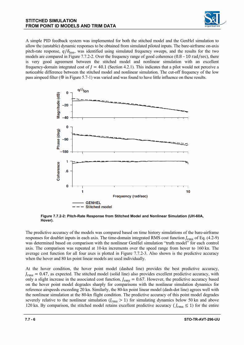
STITCHED SIMULATION FROM POINT ID MODELS AND TRIM DATA

7.7 - 6 STO-TR-AVT-296-UU

A simple PID feedback system was implemented for both the stitched model and the GenHel simulation to allow the (unstable) dynamic responses to be obtained from simulated piloted inputs. The bare-airframe on-axis pitch-rate response, 𝑞𝑞/𝛿𝛿lon, was identified using simulated frequency sweeps, and the results for the two models are compared in Figure 7.7.2-2. Over the frequency range of good coherence (0.8 – 10 rad/sec), there is very good agreement between the stitched model and nonlinear simulation with an excellent frequency-domain integrated cost of 𝐽𝐽 = 40.1 (Section 4.2.1). This indicates that a pilot would not perceive a noticeable difference between the stitched model and nonlinear simulation. The cut-off frequency of the low pass airspeed filter ( in Figure 5.7-1) was varied and was found to have little influence on these results.

Figure 7.7.2-2: Pitch-Rate Response from Stitched Model and Nonlinear Simulation (UH-60A, Hover).

The predictive accuracy of the models was compared based on time history simulations of the bare-airframe responses for doublet inputs in each axis. The time-domain integrated RMS cost function 𝐽𝐽rms of Eq. (4.2-9) was determined based on comparison with the nonlinear GenHel simulation “truth model” for each control axis. The comparison was repeated at 10-kn increments over the speed range from hover to 160 kn. The average cost function for all four axes is plotted in Figure 7.7.2-3. Also shown is the predictive accuracy when the hover and 80 kn point linear models are used individually.

At the hover condition, the hover point model (dashed line) provides the best predictive accuracy, 𝐽𝐽rms = 0.47, as expected. The stitched model (solid line) also provides excellent predictive accuracy, with only a slight increase in the associated cost function, 𝐽𝐽rms = 0.67. However, the predictive accuracy based on the hover point model degrades sharply for comparisons with the nonlinear simulation dynamics for reference airspeeds exceeding 20 kn. Similarly, the 80-kn point linear model (dash-dot line) agrees well with the nonlinear simulation at the 80-kn flight condition. The predictive accuracy of this point model degrades severely relative to the nonlinear simulation (𝐽𝐽rms > 1) for simulating dynamics below 50 kn and above 120 kn. By comparison, the stitched model retains excellent predictive accuracy ( 𝐽𝐽rms ≤ 1) for the entire

STITCHED SIMULATION FROM POINT ID MODELS AND TRIM DATA

STO-TR-AVT-296-UU 7.7 - 7

low-speed range and extending to 120 kn (the last anchor point). At speeds exceeding 120 kn, the predictive capability of the stitched model also degrades at the same rate as the 80-kn point model. Improved predictive accuracy of the stitched model at high speed could be achieved by extracting the linearised state-space models using system identification based on simulated frequency sweeps, rather than numerical perturbation, as demonstrated in Tischler and Remple (2012), Figure 13.13.

Figure 7.7.2-3: Average Predictive Accuracy for Doublet Inputs of the Stitched Model as Compared to the Point Models for Hover and 80 kn (UH-60A, Simulation).

A final simulation test was conducted to explore the predictive accuracy of the stitched model for a realistic manoeuvring scenario, as shown in Figure 7.7.2-4. Herein, a PID controller is used to follow a prescribed speed profile. The simulation starts at hover, accelerates to 60 kn, then executes a 180-deg heading change, and finally returns to hover. The stitched model responses (dashed line) track the nonlinear simulation (solid line) very accurately, as also confirmed by an excellent overall cost function of 𝐽𝐽rms = 0.64. There is also excellent agreement in the transients of the required control inputs, although some small long-term control biases are accumulated as seen in the lateral stick, 𝛿𝛿lat. These results show that the model is well suited for full mission simulation applications.

The influence of the speed filter on the predictive accuracy of the stitched model was evaluated for the manoeuvring scenario. The filter cut-off frequency was increased from the baseline value (𝜔𝜔f = 0.2 rad/sec) to a much higher value (𝜔𝜔f = 20 rad/sec), which essentially eliminates its effect in the simulation. The overall difference in the results for the two filters was found to be small, with the low-frequency filter having a slightly improved predictive accuracy (2% reduction in 𝐽𝐽rms) when compared with the nonlinear simulation. The advantage of the low-frequency cut-off filter was more evident at the manoeuvre transition points in the profile, so this value is recommended to be retained for the stitched model implementation. Experience with the stitched model of the Bell 206 helicopter, determined from system identification of flight-test data [Zivan and Tischler (2010)], also supports this recommendation.

STITCHED SIMULATION FROM POINT ID MODELS AND TRIM DATA

7.7 - 8 STO-TR-AVT-296-UU

Figure 7.7.2-4: Time Response Comparison of Stitched Model and Nonlinear Simulation for a Realistic Manoeuvring Scenario (UH-60A).

STITCHED SIMULATION FROM POINT ID MODELS AND TRIM DATA

STO-TR-AVT-296-UU 7.7 - 9

7.7.2.3 Extrapolation for Weight

The method for off-nominal weight extrapolation incorporated in the model stitching simulation architecture, as presented in Section 5.7.3.3, was utilised on the UH-60A stitched model. The results are verified against a database of off-nominal truth data points from FORECAST. The key results of simulating off-nominal gross weights are shown in Figure 7.7.2-5. The stitched model, configured only with anchor point models and trim data for the nominal 16,000-lb configuration (solid symbols), was re-trimmed and re-linearised for three simulation values of gross weight over the full range of airspeeds (dashed lines) and compared with FORECAST truth data (solid lines). Overall, there is excellent agreement between the extrapolated values from the stitched model and the truth data.

Figure 7.7.2-5: Verification of Off-Nominal Weight Extrapolation of Stitched Model (UH-60A).

A change in gross weight primarily affects the trim collective, 𝛿𝛿col, around hover and low speed and has a noticeable effect on trim pitch attitude in the mid- to high-speed range, which are both captured nearly perfectly by the stitched model. The corresponding longitudinal stick position, 𝛿𝛿lon (positive aft), is primarily affected by trim pitch attitude and is predicted very well by the stitched model. Significant shifts in the primary heave axis control derivative, 𝑍𝑍𝛿𝛿col, values are seen with a change in weight, where a heavier weight results in a smaller vertical net force for a given collective input, and thus a derivative value of smaller magnitude (z-axis positive down). This effect is represented very well by the stitched model and the values from extrapolating the stitched model for the off-nominal weights are in good agreement over the airspeed range. These results verify the capability to extrapolate to off-nominal values of weight using only anchor point data of a nominal weight.

STITCHED SIMULATION FROM POINT ID MODELS AND TRIM DATA

7.7 - 10 STO-TR-AVT-296-UU

7.7.2.4 Accurate Simulation for Low-Speed and Quartering Flight Conditions

A more accurate rotorcraft model for low-speed and quartering flight is obtained from ‘stitching in U and V’ in which trim data are tabulated as a two-dimensional lookup table and subsequently interpolated in x-body airspeed U and y-body airspeed V. In this case the stability and control derivatives are still stored as a function of forward airspeed U only. Fine-increment trim points around hover accurately capture the migration of controls and rotorcraft attitude for low-speed forward, rearward, sideward, and quartering flight, and permit accurate simulation of hovering flight in the presence of winds.

The low-speed forward, rearward, sideward, and quartering trim data points included in this demonstration of ‘stitching in U and V’ are illustrated in Figure 7.7.2-6 on a U,V airspeed grid. The hover/low-speed (stitching in U and V) and forward-flight (stitching in U only) regimes are denoted.

Figure 7.7.2-6: U,V Airspeed Points for Anchor Trim Data And Point Models Included in the Stitched Model (UH-60A).

Figure 7.7.2-7 presents the results of trimming the stitched model in hover with the presence of a steady 10-kn wind of varying direction. The wind vector was rotated in the clockwise direction through 360 degrees as the stitched simulation held the aircraft’s position and Northerly (0-deg) heading. The mapping of the trim cyclic stick position for all wind directions is shown in lateral (𝛿𝛿lat) and longitudinal (𝛿𝛿lon) components, with winds from the cardinal directions of 0, 90, 180, and 270 deg indicated. The trim values of the remaining two controls, collective stick 𝛿𝛿col and pedals 𝛿𝛿ped, as well as the trim aircraft bank angle Φ and pitch angle Θ for the stitched model are plotted at the bottom of Figure 7.7.2-7 against wind direction in degrees. Note that indicated wind direction is from a specified heading and is analogous to flight toward that heading.

The stitched model configured with quartering trim data tracks very well with the FORECAST (nonlinear simulation) truth data throughout the entire wind rotation. Therefore, quartering trim data and ‘stitching in U and V’ should be employed for accurate rotorcraft simulation in quartering flight, which is a key consideration for training simulators.

STITCHED SIMULATION FROM POINT ID MODELS AND TRIM DATA

STO-TR-AVT-296-UU 7.7 - 11

Figure 7.7.2-7: Stitched Model Trim Results of Position-Held / Heading-Held Hovering Flight in the Presence of a Rotating 10-kn Wind Through 360 Degrees (UH-60A).

7.7.2.5 Conclusions

A stitched model of the UH-60A was developed using higher-order linear point models and trim data. The following conclusions were determined:

1) The speed derivatives, as obtained from numerical perturbation of the stitched model, are adequately captured via the implicit variation in the trim states and controls.

STITCHED SIMULATION FROM POINT ID MODELS AND TRIM DATA

7.7 - 12 STO-TR-AVT-296-UU

2) The predictive accuracy of the stitched model for a realistic manoeuvring scenario is very accurate compared to the truth nonlinear simulation, as confirmed by the excellent overall cost function.

3) Accurate simulation of off-nominal weight is accomplished by extrapolation methods within the model stitching simulation architecture. The off-nominal extrapolation necessitates only point models and trim data of the baseline aircraft loading configuration to be included in the stitched model.

4) Collecting low-speed forward, rearward, sideward, and quartering flight trim data and employing “stitching in U and V” was demonstrated to yield good accuracy of the stitched model in the simulation of hovering flight in the presence of steady winds. This is a key consideration for training simulators.

7.7.3 EC135 The EC135 stitched model is based on linear operating point models derived from system identification. Stitching allows a continuous wide-envelope simulation of the EC135 based on just five anchor point models. Extrapolation of mass- and CG-variations of the ACT/FHS (Section 6.3) was not applied due to payload restrictions when flying with the experimental computer system. The stitched model is used for flight control design and for engineering simulators at the DLR.

7.7.3.1 Models and Data

System identification has been applied to flight-test data of the EC135 at five operating points, i.e., hover up to 120 kn in increments of 30 kn. The resulting high-order 11-DOF models have 15 states including rigid body states, regressive blade flapping, regressive lead-lag, and mean inflow as described in Section 6.3. Trim curves for the roll and pitch attitudes and stick inputs, were extracted from trim flights that were conducted in addition to the system identification flights. The trim points were extracted on a fine grid to better approximate the trim gradients, as shown in Figure 7.7.3-1. For the EC135, trim flights are challenging for airspeeds between 20 kn and 35 kn, so the approximated trim gradients in this region are smoothed out.

Figure 7.7.3-1: Trim Data of the ACT/FHS and Approximated Trim Curves.

STITCHED SIMULATION FROM POINT ID MODELS AND TRIM DATA

STO-TR-AVT-296-UU 7.7 - 13

7.7.3.2 Application of the Stitching Architecture

The model stitching architecture presented in Section 5.7 is applied to EC135 ACT/FHS trim data and anchor point models. The identified models for the different operating points have limited validity. If airspeed changes significantly, another operating point model is needed. As presented in Greiser and Seher-Weiß (2014), stitching smoothly combines all given anchor point models. Known kinematic relationships such as the transformation of the gravity force into the body-fixed coordinate system, Euler attitudes, inertia, and helicopter mass are included in their nonlinear form. The vectors of trim controls and states, as well as the stability and control matrices, are interpolated smoothly with respect to the simulated forward speed.

At each of the five operating points, the linearised stitched model is identical to the original anchor point model, as shown in Figure 7.7.3-2. The red dashed curve shows the anchor point model, and the blue curve represents the linearised transfer function of the stitched model. Both curves are identical as the speed derivatives are preserved explicitly, and the trim state vector is low-pass filtered (compare Section 5.7.3.4). Forward speed drives the table lookup for stability and control derivatives of the stitched model so that flight dynamics are interpolated between the anchor points. Small deviations of the forward speed such as those that occur during lateral stick inputs do not result in significant change in flight dynamics. The multi-step input shows that the stitched and linear operating point models are almost identical. The mean RMS between anchor point and stitched model responses for all multi-step inputs in all axes at 60 kn is 0.52 and in hover is 0.47; the integrated frequency cost is zero at the anchor points. The stitched model dynamics are indistinguishable from system identification results in the frequency domain. The verification of the multi-steps in the time domain shows good agreement and differ most if forward speed variations are present (e.g., for longitudinal inputs).

𝑝𝑝/𝛿𝛿lat

Figure 7.7.3-2: Comparison of Linear Point Model and Stitched Model at 60 kn for Lateral Inputs.

Another desired property of the stitched model is smooth eigenvalue transition between the operating points. It has been observed that smooth eigenvalue transition is achieved by piecewise cubic spline interpolation of the anchor point models. This means that first the derivatives of the anchor point models are interpolated, and then the linearised effect of nonlinear kinematic terms ( in Figure 5.7-1) and trim gradients are subtracted from the interpolated matrices. The resulting matrices form the control and stability lookup to calculate the matrix-vector products ( in Figure 5.7-1). The respective eigenvalues and their transition are shown in Figure 7.7.3-3. The path of the eigenvalues looks consistent and supports the application of the stitched model for manoeuvring flight.

STITCHED SIMULATION FROM POINT ID MODELS AND TRIM DATA

7.7 - 14 STO-TR-AVT-296-UU

Figure 7.7.3-3: Eigenvalues of the ACT/FHS Models and their Transition.

7.7.3.3 Manoeuvring Flight One benefit of the stitching architecture is its ability to simulate manoeuvring flight. To match the manoeuvre flight data as well as possible, the filter time constant ( in Figure 5.7-1) should be adjusted based on the flight data. For the EC135 ACT/FHS, the filter time constant was set to Tf = 15 sec.

Figure 7.7.3-4 shows the results obtained for a deceleration-acceleration manoeuvre that covers a wide airspeed range. As this type of manoeuvre has a duration of 2 minutes, unstable modes such as the phugoid mode need to be stabilized. A flight controller minimizing attitude and speed errors is used to stabilize the simulation. The simulated control input is the sum of the measured control and the feedback signal and therefore deviates from the measured control input. The blue curve is the simulated response using the 60 kn anchor point model. For this manoeuvre, the stick input of the linear point model has to be adjusted significantly to obtain a good match for the attitude and forward speed. The two stick input signals deviate mainly between 50 and 80 sec where the 60 kn linear point model is used for small forward-speeds near hover. The red curves represent the responses for the stitched model. Compared to the linear model, the stitched model shows a better match of the longitudinal stick position and the pitch attitude, which originates primarily from the interpolation of the trim vectors. As expected, the stitched model achieves a good approximation of manoeuvring flight data.

7.7.3.4 Combination with Update Method 2 ‘Black Box’ For the ACT/FHS, further improvements were achieved by augmenting the stitched model with an input filter [Greiser (2019)], i.e., by combining the methods of Sections 5.2 and 5.7. As only one input filter correction for all airspeeds was determined, it is an averaged filter that corrects/mitigates major deficiencies observed at all anchor points. Using one filter for all airspeeds enables the black box input filter to be added just to the stitched model simulation. The stitched model’s dynamics are identical to those of the anchor points which further streamlines the direct application of black box transfer functions (Method 2) to stitched model results (Method 7). Figure 7.7.3-5 shows the result of manoeuvring flight with the updated stitched model. The qualitative signal trend of the stick input is slightly improved compared to Figure 7.7.3-4 while the high fidelity of the states is maintained.

7.7.3.5 Fidelity Metrics Fidelity is assessed using the RMS in the time domain and by showing MUAD boundary plots for selected on-axis frequency responses. Table 7.7.3-1 lists the RMS values of the hover and 60 kn forward flight case. As expected, the mean RMS value of the anchor point model and stitched model is almost the same. In the case of manoeuvring flight as shown in Figure 7.7.3-4, the stitched model achieves a much better agreement for the accel/decel manoeuvre; the RMS reduces from 1.08 to 0.89. In addition, the feedback controller inputs (needed for stabilization) are smaller in the case of the stitched model; the mean RMS of all four control inputs is 4.74.

STITCHED SIMULATION FROM POINT ID MODELS AND TRIM DATA

STO-TR-AVT-296-UU 7.7 - 15

Figure 7.7.3-4: Comparison of Linear Point Model (60 kn) and Stitched Model for a Deceleration-Acceleration Manoeuvre.

Figure 7.7.3-5: Comparison of the Stitched Model (with and Without Input Filter Augmentation) and Flight-Test Data.

Additionally, the fidelity is assessed for the augmented stitched model. In the time domain, the input filter only achieves slightly better results. As this filter was designed to respect model deficiencies at higher frequencies between 5 to 40 rad/sec (covering the effect of engine dynamics and flexible modes), the effect of the filter on time-domain responses can hardly be revealed using the RMS. Clearly, the frequency domain is better suited to show the effect of the black box input filter. Figure 7.7.3-6 and Figure 7.7.3-7 show two Maximum Unnoticeable Added Dynamics (MUAD) boundary plots for the longitudinal and pedal on-axis in forward flight and hover, respectively. In both cases, the augmented simulation better fits the MUAD boundary. These results can be even further improved if the black box input filter is extracted for each anchor point individually.

Table 7.7.3-1: RMS Cost for Stitched Model and Augmented Model Compared to Flight-Test Data (Stitched Model Matches Almost Perfectly the Baseline Anchor Point Model).

RMS of the Output

Signals

RMS of the Control

Signals

hover anchor point model 1.47 -

stitched model 1.46 -

augmented stitched model 1.29 -

60 kn anchor point model 1.78 -

stitched model 1.70 -

augmented stitched model 1.71 -

manoeuvre anchor point model 1.08 10.99

stitched model 0.89 4.74

augmented stitched model 0.75 5.20

STITCHED SIMULATION FROM POINT ID MODELS AND TRIM DATA

7.7 - 16 STO-TR-AVT-296-UU

Figure 7.7.3-6: MUAD Plot for the Longitudinal On-Axis (𝒒𝒒/𝜹𝜹𝐥𝐥𝐥𝐥𝐥𝐥) at 60 kn Forward Flight.

Figure 7.7.3-7: MUAD Plot for the Directional On-Axis (𝒓𝒓/𝜹𝜹𝐩𝐩𝐚𝐚𝐩𝐩) in Hover.

7.7.3.6 Conclusions A wide-envelope EC135 simulation model was developed based on five anchor point models and trim data. The following conclusions were determined:

1) Cubic spline interpolation of the derivatives leads to the best and smoothest eigenvalue transitions. 2) Dynamics of the anchor point models are exactly retained by the stitched model. 3) The EC135 stitched model was updated by Method 2 (Black Box) to improve its fidelity.

7.7.4 IRIS+ Quadcopter This section presents the development and verification of a continuous, full-envelope stitched simulation model of the 3D Robotics IRIS+ quadcopter using flight-identified models and the TDD-developed model stitching simulation software, STITCH. Two flight-identified point models (one at hover and one at forward flight), plus some additional trim data, are shown to adequately and accurately capture the bare-airframe dynamics of the IRIS+ over its nominal flight envelope. Additionally, the off-nominal mass-, CG-, and inertia-extrapolation capabilities of STITCH are investigated, and the results are verified for a heavy loading configuration. The overall findings are considered to provide flight-test guidance for the development of stitched simulation models of small-scale multi-rotor vehicles. See Tobias, Sanders, and Tischler (2018) for more details.

7.7.4.1 STITCH Software A comprehensive model stitching simulation architecture is presented in Tobias and Tischler (2016) and Section 5.7, which allows continuous, full flight-envelope simulation from discrete linear models and trim data. Extrapolation methods in the stitching architecture permit accurate simulation of off-nominal aircraft loading configurations, which minimize the required number of point models for full-envelope simulation. STITCH is a software capability developed by TDD that provides a user interface front end to the model stitching simulation architecture and features anticipatory design elements to guide the user through the entire process of generating a stitched model [Tobias et al. (2018)]. STITCH is applicable to any flight vehicle for which point-wise linear models and trim data can be obtained and was employed herein to develop a stitched simulation model of the IRIS+ quadcopter.

7.7.4.2 Flight-Identified Point Models and Trim Data of the IRIS+ Quadcopter Accurate bare-airframe state-space models of the vehicle, which consist of the IRIS+ airframe, mixer, and motors, in hover and forward flight were identified from flight data using CIFER®, as presented in Section 6.8. Steady-state trim data were also collected from hover to 32 kn; six anchor trim points at a spacing of about 6 kn were collected. The flight-test process was repeated in a heavy loading configuration for verification of the extrapolation process.

STITCHED SIMULATION FROM POINT ID MODELS AND TRIM DATA

STO-TR-AVT-296-UU 7.7 - 17

7.7.4.2.1 Aircraft Loading Configurations

The 3D Robotics IRIS+ is a quadcopter that measures 19.75 inches diagonally motor-to-motor, has a total flying weight of 3.2 lb, and a payload capacity of 0.9 lb (see Section 6.8). To verify the extrapolation capabilities of the stitched model, the aircraft was flown in two loading configurations: nominal and heavy. The heavy configuration featured a 200-gram (0.441-lb) cylinder attached to the aircraft, as shown in Figure 7.7.4-1.

Figure 7.7.4-1: 3D Robotics IRIS+, Shown in Heavy Loading Configuration with 200-Gram Payload.

7.7.4.2.2 Identified Models Comparison Table 7.7.4-1 shows a comparison of the identified stability and control derivatives of the IRIS+ in hover and forward flight. The dynamics in hover are driven solely by the translational velocity terms, while in forward flight the angular rate damping terms become active. Table 7.7.4-2 shows a comparison of the hover and forward-flight eigenvalues and respective modes. In hover, the unstable phugoid and real pole, that comprise the hovering cubics, are present in both the pitch and roll axes. In the roll axis in forward flight, the lateral hovering cubic breaks into two stable, real poles. In the pitch axis in forward flight, the longitudinal hovering cubic breaks into four real poles; two of these poles are unstable.

Table 7.7.4-1: Stability and Control Derivatives Comparison.

Derivative Hover 17 kn Derivative Hover 17 kn

𝑋𝑋𝑢𝑢 –0.3246 –0.2956 𝑋𝑋δlon –7.5513 –9.9573

𝑌𝑌𝑎𝑎 –0.1996 –0.2346 𝑌𝑌δlat 6.4016 6.2517

𝑍𝑍𝑤𝑤 0 –0.8271 𝐿𝐿δlat 80.0269 85.5219

𝑍𝑍𝑖𝑖 0 –1.1668 𝑀𝑀δlon 92.1241 121.0780

𝐿𝐿𝑎𝑎 –0.5363 0 𝑁𝑁δped 5.6427 5.6798

𝐿𝐿𝑁𝑁 0 –1.2161 𝑍𝑍δcol –60.7660 –35.2408

𝑀𝑀𝑢𝑢 1.7355 0.3172

𝑀𝑀𝑤𝑤 0 1.6648

𝑀𝑀𝑖𝑖 0 –1.0854

𝑁𝑁𝑟𝑟 0 –1.7768

STITCHED SIMULATION FROM POINT ID MODELS AND TRIM DATA

7.7 - 18 STO-TR-AVT-296-UU

Table 7.7.4-2: Modes Comparison.

Hover Mode 17 kn Mode

[–0.48, 2.55] Roll (0.235) Spiral

(2.65) Roll (1.22) Roll

(0) Roll

(0) Yaw (1.78) Yaw

[–0.48, 3.77] Phugoid (–0.163) Phugoid

(3.93) Short Per. (0.554) Phugoid

(0) Heave (–6.02) Short Per.

(7.84) Short Per.

[𝜁𝜁,𝜔𝜔] = 𝑠𝑠2 + 2𝜁𝜁𝜔𝜔𝑠𝑠 + 𝜔𝜔2, (𝑉𝑉) = (𝑠𝑠 + 𝑉𝑉)

7.7.4.3 Quadcopter Stitched Simulation Model Using STITCH

STITCH was used to develop a full-envelope stitched simulation model of the IRIS+ using the two flight-identified point models and finely-spaced trim data of the nominal configuration. The model was configured for ‘stitching in U’, which means the point model derivatives and trim data are stored and subsequently looked-up as a function of x-body airspeed U only.

7.7.4.3.1 Anchor Point Data

Anchor points are the specific flight conditions for which a linear model or trim data is included in the stitched model. For the IRIS+ stitched model, the two flight-identified point models (hover and 17 kn) were included as the anchor point models. As such, the stability and control derivatives (Table 7.7.4-1) are linearly interpolated in the stitched model between hover and 17 kn (and linearly extrapolated beyond) as a function of x-body airspeed U. The finely-spaced trim data, which capture the variation in trim states and controls for straight-and-level flight over the full airspeed range, were included as the anchor trim data. See Figure 7.7.4-2 for an overview of the anchor points; the two point models and trim data of the nominal configuration are the only data included in the stitched model. The values of the pertinent longitudinal trim states and controls (i.e., trim z-body airspeed, 𝑊𝑊, trim pitch attitude, Θ, trim longitudinal stick, 𝛿𝛿lon, and trim collective, 𝛿𝛿col), as captured by the trim data from flight, are shown by the markers in Figure 7.7.4-3. Shape-preserving piecewise cubic interpolation was performed on the anchor trim data to produce smooth, finely-spaced data for the stitched model, as shown by the dashed curves.

7.7.4.3.2 Stitched Model Verification

Verification of the stitched model is performed by linearizing the stitched model at the anchor point flight conditions, in this case, hover and 17 kn. This is important because it verifies the accuracy of the implicit speed derivatives (see Section 5.7) and their effect on the dynamic response of the stitched model. Figure 7.7.4-4 and Figure 7.7.4-5 show the error responses of the primary on-axis pitch frequency responses between the linearised stitched model and the anchor point models at hover and 17 kn, respectively. There is near-perfect agreement for the hover anchor point condition (J = 3.75). There is very good agreement at 17 kn (J = 51.7); the slight disparity at low frequency is due to small differences in the values of the speed derivatives. However, the response is well within the MUAD bounds, and perfect agreement is realized around crossover frequency ωc ≥ 18 rad/sec.

STITCHED SIMULATION FROM POINT ID MODELS AND TRIM DATA

STO-TR-AVT-296-UU 7.7 - 19

Figure 7.7.4-2: Anchor Points Included in the Stitched Model.

Figure 7.7.4-3: Variation in Trim States and Controls Over the Full Airspeed Range.

Figure 7.7.4-4: Dynamic Response Verification, Hover (J = 3.75).

Figure 7.7.4-5: Dynamic Response Verification, 17 kn (J = 51.7).

7.7.4.3.3 Interpolation for Airspeed The dynamic response of the stitched model at a mid-airspeed point of 10 kn was verified. As truth data, frequency sweeps were performed in flight at 10 kn to generate truth frequency responses. The stitched model, configured only with the two anchor point models at hover and 17 kn, was re-trimmed and re-linearised for the 10-kn flight condition in simulation; this requires interpolation of the stability and control derivatives. Figure 7.7.4-6 shows the pitch-rate response to longitudinal stick comparison of the stitched model for the interpolated airspeed of 10 kn (blue dashed line) against the truth 10-kn response from flight (black solid line). The responses of the anchor point models at hover and 17 kn are included in the figure for context.

Two key conclusions are obtained from these comparisons: 1) The quadcopter’s dynamic responses at hover, 10 kn, and 17 kn are appreciably different; and 2) The stitched model, configured only with the anchor point models at hover and 17 kn, when linearised at 10 kn has a response that agrees with the truth 10-kn response from flight. This confirms that the IRIS+ bare-airframe dynamics are well characterized by two point models, and that the stitched model accurately predicts the dynamics by interpolation at a mid-airspeed condition. The stitched model interpolates continuously in real-time simulation, so accurate dynamics are realized over the full airspeed range.

0 5 10 15 20 25 30 35

Airspeed (kn)

Anchor Trim Points

and Point Models

Trim shot data

Point models + trim data

-30

-20

-10

0

W (f

t/sec

)

-30

-20

-10

0

(deg

)

0 5 10 15 20 25 30 35

Airspeed (kn)

-40

-20

0

lon

(%)

0 5 10 15 20 25 30 35

Airspeed (kn)

40

60

80

col

(%)

Anchor trim points

Stitched model data

-20

-10

0

10

20

Mag

nitu

de (d

B)

q/lon

10 -1 10 0 10 1 10 2

Frequency (rad/sec)

-90

-45

0

45

90

135

Phas

e (d

eg)

Stitched model error

MUAD Bound

-20

-10

0

10

20

Mag

nitu

de (d

B)

q/lon

10 -1 10 0 10 1 10 2

Frequency (rad/sec)

-90

-45

0

45

90

135

Phas

e (d

eg)

Stitched model error

MUAD Bound

STITCHED SIMULATION FROM POINT ID MODELS AND TRIM DATA

7.7 - 20 STO-TR-AVT-296-UU

7.7.4.3.4 Extrapolation for Loading Configuration

The effects of the quadcopter carrying an external payload on trim and dynamic response were investigated. A heavy loading configuration was arranged by attaching a 200-gram (0.441-lb) mass to the underside of the IRIS+ fuselage (see Figure 7.7.4-1), which increased the total weight from 3.168 to 3.609 lbs. The mass was attached 2 inches below, 1 inch left, and 0.5 inches forward of the vehicle’s CG, which shifted the overall CG 0.275 inches down and slightly forward/left, based on a simple calculation of the mass centre. Inertia values for a nominally configured IRIS+ (see Section 6.8) were used as simulation values for the nominal configuration. For the heavy configuration, the added 200-gram mass increased roll inertia Ixx and pitch inertia Iyy by 3% and 6%, respectively.

To verify the stitched model’s ability to simulate for the off-nominal loading configuration, the simulation values of weight, inertia, and CG offset were set to those of the heavy loading. The stitched model, containing only the nominal anchor point data, was then re-trimmed in simulation for the heavy loading over the full airspeed range from hover to 32 kn. Flight-test data of the heavy configuration were collected for use as truth data only. The nominal and heavy trim data comparison results are shown in Figure 7.7.4-7. The anchor trim points (black solid markers) and the corresponding stitched model data for the nominal loading (blue dashed lines) are repeated from those shown previously in Figure 7.7.4-3 for reference. The trim results of the stitched model as re-trimmed (i.e., extrapolated) to the heavy loading are shown by the magenta dashed lines. Lastly, the truth trim points for the heavy loading configuration, as obtained from flight, are shown by the red triangle markers.

Figure 7.7.4-6: Interpolation for Airspeed Compared to Truth 10-kn Pitch-Rate Response from Flight.

Figure 7.7.4-7: Extrapolation for Heavy Loading Compared to Truth Heavy Trim Data from Flight.

-20

-10

0

10

20

30

Mag

nitu

de (d

B)

q/lon

-270

-225

-180

-135

-90

Phas

e (d

eg)

10 -1 10 0 10 1 10 2

Frequency (rad/sec)

0

0.5

1

Coh

eren

ce

Anchor point model, hover (for reference)

Anchor point model, 17 kn (for reference)

Flight data, 10 kn

Linearized stitched model, 10 kn

-30

-20

-10

0

W (f

t/sec

)

-30

-20

-10

0

(deg

)

-40

-20

0

lon

(%)

0 5 10 15 20 25 30 35

Airspeed (kn)

40

60

80

col

(%)

Anchor trim points (nominal)

Stitched model (nominal)

Stitched model (extrap to heavy)

Flight data (heavy)

STITCHED SIMULATION FROM POINT ID MODELS AND TRIM DATA

STO-TR-AVT-296-UU 7.7 - 21

There is excellent agreement between the extrapolated stitched model results and truth heavy trim data. The increased trim angle of attack (analogous to 𝑊𝑊) and trim pitch attitude, Θ, in forward flight for the heavy loading are well predicted by the stitched model. Trim longitudinal stick, 𝛿𝛿lon, is also well predicted. The increased trim collective, 𝛿𝛿col, necessary for hover and level forward flight of the heavy configuration is well extrapolated. See Tobias et al. (2018) for more discussion and results, including the dynamic response of the stitched model configured for the heavy loading as verified against the truth response of the heavy loading configuration from flight.

7.7.4.4 Flight-Test Implications for Development of Small-Scale Multi-Rotor Stitched Models

Flight-test recommendations for future development of stitched models involving small-scale multi-rotor vehicles are presented below, based on the IRIS+ results covered in this section.

Trim Data: Finely-spaced level trim data covering the entire airspeed envelope should be collected for use as anchor trim data in the stitched model. These trim data must include the trim values of the states and controls as a function of x-body airspeed U for ‘stitching in U’. Due to the smooth trends in trim data over the airspeed range for the IRIS+, six trim points, spaced approximately every 6 kn, adequately covered the full airspeed range from hover to about 32 kn. A spacing of approximately 5 – 7 kn is therefore recommended for the collection of trim data.

Point Models: Frequency sweeps should be performed at hover and forward flight for the identification of state-space anchor point models. Airspeed will naturally tend to vary about the trim condition during the frequency sweep; a variation of approximately ±5 kn was observed during the frequency sweep data collection on the IRIS+. Furthermore, the identified linear point models will be accurate over some minimum range of airspeed (approximately ±10-kn accuracy was realized for the IRIS+ point models, as presented in this section). Therefore, it is recommended that the identification of anchor point models be performed at a spacing of 15 – 20 kn for small-scale multi-rotor vehicles.

In summary, two flight-identified point models were found to adequately and accurately capture the bare-airframe dynamics of the IRIS+ over its full airspeed envelope: one point model at hover, valid up to about 10 kn, and one point model at 17 kn, valid from about 10 – 30 kn (30 kn is the approximate maximum airspeed of the IRIS+). However, the spacing of the anchor point models depends on the size of the vehicle (according to the Froude scaling relationship for velocity [Tobias et al. (2018), and Ivler et al. (2019)]) and the complexity of the rotor configuration.

7.7.4.5 Conclusions

A full-envelope stitched simulation model of a quadcopter was developed using two flight-identified models of the IRIS+ and finely-spaced trim data. The following conclusions were determined:

1) Forward-flight dynamics are appreciably different than the dynamics in hover for the IRIS+.

2) Two flight-identified point models (at hover and 17 kn), plus some finely-spaced trim data, are shown to adequately and accurately capture the IRIS+ bare-airframe dynamics over its nominal flight envelope.

3) The stitched model accurately predicts the dynamics at a mid-airspeed condition of 10 kn by interpolation of the stability and control derivatives, as verified by a truth response from flight.

4) The stitched model’s extrapolation for off-nominal loading configuration is very accurate. Therefore, flight testing may be conducted with a nominally loaded UAS only.

STITCHED SIMULATION FROM POINT ID MODELS AND TRIM DATA

7.7 - 22 STO-TR-AVT-296-UU

7.7.5 Summary and Overall Conclusions Four applications of the model stitching technique were presented. In each case, a collection of discrete linear models and trim data were used to generate a stitched simulation model and were shown to adequately and accurately cover the nominal flight envelope. Additionally, extrapolation methods were shown to accurately simulate off-nominal loading configurations. The following overall conclusions were determined:

1) The model stitching method provides a quasi-nonlinear, time-varying simulation model from individual linear models and trim data for discrete flight conditions that is accurate for flight dynamics and control applications over the operational envelope, with good accuracy maintained in the frequency and time domains.

2) Interpolation of the anchor trim data and point model derivatives is important to capture the trends over the flight envelope of interest. Shape-preserving piecewise cubic interpolation performed on the anchor trim data produces smooth, finely-spaced data over the full flight envelope for use in the stitched model. Linear interpolation and piecewise cubic interpolation were both found to adequately capture the stability and control derivatives.

3) Accurate simulation of off-nominal loading configuration (e.g., variations in weight and CG) is accomplished by extrapolation methods in the model stitching simulation architecture. The off-nominal extrapolation necessitates only point models and trim data of the baseline aircraft loading configuration to be included in the stitched model, which significantly reduces required flight-test points and associated flight costs.

7.7.6 References

[1] FAA (2016), “Federal Aviation Administration”, National Simulator Program, 14 CFR Part 60, 2016.

[2] Greiser, S., and Seher-Weiß, S. (2014), “A Contribution to the Development of a Full Flight Envelope Quasi-Nonlinear Helicopter Simulation”, CEAS Aeronautical Journal 5 (1), pp. 53-66.

[3] Greiser, S. (2019), “High-Fidelity Rotorcraft Simulation Model: Analyzing and Improving Linear Operating Point Models”, CEAS Aeronautical Journal 10 (3), pp. 687-702.

[4] Hui, K., Lambert, E., and Seto, J. (2006), “Bell M427 Flight Test Data Gathering and Level-D Simulator Model Development”, ICAS 25th Congress, Hamburg, Germany, September.

[5] Ivler, C.M., Rowe, E.S., Martin, J., Lopez, M.J., and Tischler, M.B. (2019), “System Identification Guidance for Multirotor Aircraft: Dynamic Scaling and Test Techniques”, Vertical Flight Society 75th Annual Forum, Philadelphia, PA, USA, May.

[6] Lawrence, B., Malpica, C.A., and Theodore, C.R. (2010), “The Development of a Large Civil Tiltrotor Simulation for Hover and Low-Speed Handling Qualities Investigations”, 36th European Rotorcraft Forum, Paris, France, September.

[7] Leach, B., and Hui, K. (2000), “Flight Test Applications of Kalman Filter-Based Integrated Navigation Systems Using Differential GPS”, Proceedings of the 7th St. Petersburg International Conference on Integrated Navigation Systems, St. Petersburg, Russia, May.

[8] Leeuw, J. H. de, and Hui, K. (1989), “The Application of Linear Maximum Likelihood Estimation of Aerodynamic Derivatives for the Bell-205 and Bell-206”, Vertica, Vol. 13, Issue 3, pp. 403-412, January.

STITCHED SIMULATION FROM POINT ID MODELS AND TRIM DATA

STO-TR-AVT-296-UU 7.7 - 23

[9] Seher-Weiß, S., Greiser, S., Wartmann, J., Myrand-Lapierre, V., Gubbels, A., Ricciardi, J., and Hui, K. (2019), “Bell 412 System Identification: Comparing Methods and Tools”, VFS 75th Annual Forum & Technology Display, Philadelphia, PA, USA, May.

[10] Tischler, M.B., and Remple, R.K. (2012), Aircraft and Rotorcraft System Identification: Engineering Methods with Flight Test Examples, 2nd ed., AIAA Education Series, August.

[11] Tobias, E.L., and Tischler, M.B. (2016), “A Model Stitching Architecture for Continuous Full Flight-Envelope Simulation of Fixed-Wing Aircraft and Rotorcraft from Discrete-Point Linear Models”, U.S. Army AMRDEC Special Report RDMR-AF-16-01, April.

[12] Tobias, E.L., Sanders, F.C., and Tischler, M.B. (2018), “Full-Envelope Stitched Simulation Model of a Quadcopter Using STITCH”, American Helicopter Society 74th Annual Forum, Phoenix, AZ, USA, May.

[13] Zivan, L., and Tischler, M.B. (2010), “Development of a Full Flight Envelope Helicopter Simulation Using System Identification”, Journal of the American Helicopter Society, Vol. 55, (022003), pp. 1-15.

STITCHED SIMULATION FROM POINT ID MODELS AND TRIM DATA

7.7 - 24 STO-TR-AVT-296-UU

STO-TR-AVT-296-UU 7.8 - 1

Chapter 7.8 – PERCEPTUAL FIDELITY ASSESSMENT BASED ON THE SFR SCALE: BELL 412

The metrics presented in Sections 4.5 and 4.7 were underpinned by a series of simulation trials undertaken using the HELIFLIGHT-R simulator at the University of Liverpool (UoL) [White et al. (2013)] and flight trials using the National Research Council’s (NRC) Bell 412 Advanced Systems Research Aircraft (ASRA) [Perfect et al. (2010), Perfect et al. (2014), Timson et al. (2012), White et al. (2010)]. UoL’s consultant test pilot and NRC’s test pilot, who were familiar with the ADS-33E-PRF test course layouts [ADS-33 (2000)], conducted the flight and simulation trials; for brevity, only the UoL test pilot results are presented here. Flight testing was conducted using two aircraft configurations – ‘bare airframe’ with no control augmentation, and a configuration with an attitude command/attitude hold (ACAH) system, implemented using the ASRA Fly-by-Wire system architecture. Results from the ACAH configuration will form the focus of this section; the reader is directed to Perfect et al. (2013) for the full results.

The Mission Task Elements (MTEs) chosen for the fidelity assessment focused on the hover and low speed flight regime with the precision hover, pirouette, acceleration-deceleration, and lateral reposition ADS-33E-PRF MTEs being performed. The approach is presented in detail in Perfect et al. (2013) and an example of the precision hover MTE (Figure 7.8-1) is presented here for illustration.

Figure 7.8-1: Precision Hover MTE [ADS-33 (2000)].

The task performance and pilot control activity in the precision hover MTE are shown in Figure 7.8-2 and Figure 7.8-3 with the attack, η, analysis (see Section 4.7.4) shown in Figure 7.8-4 for lateral (xa), longitudinal (xb), collective (xc), and pedal (xp) channels. The longitudinal fidelity metrics are presented in Table 7.8-1; full metrics are given in Perfect et al. (2013).

PERCEPTUAL FIDELITY ASSESSMENT BASED ON THE SFR SCALE: BELL 412

7.8 - 2 STO-TR-AVT-296-UU

Figure 7.8-2: Precision Hover MTE Task Performance.

Figure 7.8-3: Precision Hover MTE Control Activity.

PERCEPTUAL FIDELITY ASSESSMENT BASED ON THE SFR SCALE: BELL 412

STO-TR-AVT-296-UU 7.8 - 3

Figure 7.8-4: Precision Hover MTE Attack Analysis.

Table 7.8-1: Precision Hover Perceptual Metrics.

Fidelity Parameter Flight Simulator ∆% HQR 5 4 SFR 3 UCE 1 2 VCR(TR) 3.0 3.0 0 VCR(A) 1.5 2.0 Total task time 30 30 0

Longitudinal Position % time Inside desired 79.2 76.2 -3 Inside adequate 88.5 100 12 Outside adequate 11.5 0 -12 Attack number 172 72 -58 Attack number per sec (/s) 3.21 1.36 -58

PERCEPTUAL FIDELITY ASSESSMENT BASED ON THE SFR SCALE: BELL 412

7.8 - 4 STO-TR-AVT-296-UU

Fidelity Parameter Flight Simulator ∆% Longitudinal

Mean attack rate (%/s) 25 10 -60 Mean control displ (%) 7.8 4.7 -40 No. of quickness points 32 18 -44 Quickness points per sec (/s) 0.59 0.34 -42 Mean quickness (/s) 2.45 0.81 -67 PSD RMS 0.050 0.022 -56 Cut-off frequency (Hz) 0.705 0.340 -52

The HQR 5 to 4 comparison (flight vs simulator) is contrasted by the UCE 1 to 2 comparison. In flight, the excursion into the adequate region and beyond (12% of time) for longitudinal position during the initial capture of the hover, led the pilot to award an HQR of 5. Apart from this excursion, the pilot maintained position within the desired region for nearly 80% of the time and held the desired vertical and lateral position, and heading (ψ), for more than 90% of the time (see [Perfect et al. (2014)] for full results). In simulation, task performance was improved, which resulted in the pilot awarding an HQR of 4. By examining the attack parameters, the control attack, η, shows the pilot using an increased number of cyclic inputs in flight compared with the simulator. The combination of changes in task performance and adaptation of control strategy led to an SFR of 3, indicating ‘fidelity warrants improvement’ and that ‘additional training is required’ on the aircraft.

The control attack shows the pilot using more than double the number of cyclic inputs in flight compared with the simulator, at an average rate of 1.60/1.25 Hz (pitch/roll) compared with 0⋅7/0⋅8 Hz. By comparison, the cut-off frequencies are only about 20% greater in flight.

The pilot commented on a noticeably more unsteady (‘gravelly’) ride during flight, in comparison with the simulation, resulting in attitude disturbances that required ‘extensive compensation’ to achieve an adequate standard. In addition, the pilot noted a need for larger collective inputs during flight to maintain height, leading to heading and torque fluctuations (Level 3 collective to yaw predicted HQs in flight, Level 1 in the simulator) as shown in Figure 7.8-5. Results are shown for collective up and collective down: r(1) and r(3) are the yaw rates (°/s) at 1 and 3 sec, and w(3) is the vertical rate in ft/s after 3 seconds.

Figure 7.8-5: Collective to Yaw Predicted Cross-Couplings.

PERCEPTUAL FIDELITY ASSESSMENT BASED ON THE SFR SCALE: BELL 412

STO-TR-AVT-296-UU 7.8 - 5

The metrics discussed have been shown to provide effective methods to quantify the difference between a pilot’s control strategy in flight and that adopted in the simulator. However, the exact tolerances required to match flight behaviour and enable qualification of a flight simulator have not yet been determined. This process has begun at UoL [Perfect et al. (2014)], in conjunction with the development and validation of the new Simulator Fidelity Rating scale and will be used to identify pilot sensitivity to fidelity tolerances [Timson et al. (2011) and Timson et al. (2012)]. A process of implementing changes to a baseline simulation environment, followed by assignment of fidelity levels using the new scale, is being adopted. The change in the pilot’s control strategy following a change in the simulation will be correlated with the assigned fidelity and conclusions will be drawn on the degree to which the pilot can adapt a control strategy (as measured through the percentage change in each of the metrics) relative to the assigned fidelity level. It is anticipated that this approach can inform the development of future task-specific subjective and objective metrics in new simulator standards.

7.8.1 References [1] ADS-33 (2000), “Handling Qualities Requirements for Military Rotorcraft”, ADS-33E-PRF,

US Army, March.

[2] Perfect P., White M.D., Padfield G.D., Gubbels A.W., and Berryman A.C. (2010), “Integrating Predicted and Perceived Fidelity for Flight Simulators”, 36th European Rotorcraft Forum, September, Paris, France.

[3] Perfect P., White M.D., Padfield G.D., and Gubbels A.W (2013), “Rotorcraft Simulation Fidelity: New Methods for Quantification and Assessment”, The Aeronautical Journal, Vol. 117, Issue 1189 pp. 235-282 March.

[4] Perfect P., Timson E., White M.D., Padfield G.D., Erdos R., and Gubbels A.W. (2014), “A Rating Scale for the Subjective Assessment of Simulation Fidelity”, The Aeronautical Journal, August, Volume 11, No 1206, pp. 953-974.

[5] Timson, E., Perfect, P., White, M.D., Padfield, G.D., and Erdos, R. (2011), “Pilot Sensitivity to Flight Model Dynamics in Flight Simulation, 2011, 37th European Rotorcraft Forum, September, Gallarate, Italy.

[6] Timson E., White M.D., Perfect P., and Padfield G.D. (2012), “Subjective Methods for Fidelity Assessment of Rotorcraft Training Simulators”, Presented at the 68th Annual Forum of the American Helicopter Society, Texas USA, 1 ‒ 3 May.

[7] White M.D., Perfect P., Padfield G.D., Gubbels A.W., and Berryman A.C. (2010), “Progress in the Development of Unified Fidelity Metrics for Rotorcraft Flight Simulators”, 66th Annual Forum of the American Helicopter Society, 2010, Phoenix, AZ, USA.

[8] White M.D., Perfect P., Padfield G.D., Gubbels A.W., and Berryman A.C. (2013), “Acceptance Testing and Commissioning of a Flight Simulator for Rotorcraft Simulation Fidelity Research”, Proceedings of the Institution of Mechanical Engineers, Part G: Journal of Aerospace Engineering, Volume 227 Issue 4, pp. 663-686, April.

PERCEPTUAL FIDELITY ASSESSMENT BASED ON THE SFR SCALE: BELL 412

7.8 - 6 STO-TR-AVT-296-UU

STO-TR-AVT-296-UU 7.9 - 1

Chapter 7.9 – SUMMARY OF UPDATE METHODS: PRINCIPLE, APPLICATIONS, EFFORT, ADVANTAGES, LIMITATIONS

Seven different identification methods for improving a baseline rotorcraft simulation model have been presented and multiple case studies related to the Bell 412, UH-60, EC135, CH-47, AW139, AW109, and X2 helicopters assessed. This documented experience has been invaluable for gaining a better understanding of the advantages and limitations of each method and for comparing and coordinating analysis of a common rotorcraft database. It has been shown that different methods have many distinct and important advantages, such as improving model accuracy, providing particular types of physical insight, applicability to control system design methods, and handling qualities design and assessment, including useful viewpoints for both the data analysis and the modelling. The following table summarises the key aspects of the methods, highlighting their main applications, assumptions, and ease/difficulty in application.

SUMMARY OF UPDATE METHODS: PRINCIPLE, APPLICATIONS, EFFORT, ADVANTAGES, LIMITATIONS

7.9 - 2 STO-TR-AVT-296-UU

Identification Method

Method 1

Gain/Time Delay

Corrections for Rotorcraft Key

Responses

Method 2

‘Black Box’ Input and Output

Filters

Method 3

Force and Moment Increments Based

on Stability Derivatives

Method 4

Reduced Order Models and

Physics-Based Corrections

Method 5

Model Parameter Adjustment for Physics-Based Simulations

Method 6

Parameter Identification of Key Simulation

Constants

Method 7

Stitched Simulation from Point ID Models and Trim Data

Method Principle

The method applies gain/time delay corrections to a flight simulation model based on frequency responses collected from flight-test data. The method does not modify the physical structure of a baseline model.

The method aims at improving the fidelity of an existing baseline model by appending low-order correction models in transfer function or state-space form. The method does not modify the physical structure of the baseline model.

The method modifies the baseline nonlinear simulation model. It uses a comparison of stability and control derivatives from flight-test data and from the baseline model to derive force and moment increments that are then added to the baseline nonlinear model to improve it.

The method modifies the baseline simulation model. It improves the baseline model by adding physics-based reduced order models and corrections for complicated phenomenon such as stall, inflow dynamics, aerodynamic interference, engine/drivetrain dynamics and sensor/actuator dynamics.

The method modifies the baseline simulation model by adjusting aeromechanical parameters (e.g., moments of inertia or hinge offsets) through matching stability and control derivatives or minimizing frequency response errors.

The method modifies the baseline simulation model using system identification to directly determine rotorcraft parameters, e.g., inertias or flapping frequency from flight-test data.

The method replaces the baseline simulation model by stitching together linear point models and trim data at different flight conditions into a real-time, full flight-envelope model. Nonlinear components are included to re-establish and enhance the physical reliability of the linear models, which produces a quasi-nonlinear stitched simulation model.

SUMMARY OF UPDATE METHODS: PRINCIPLE, APPLICATIONS, EFFORT, ADVANTAGES, LIMITATIONS

STO-TR-AVT-296-UU 7.9 - 3

Identification Method

Method 1

Gain/Time Delay

Corrections for Rotorcraft Key

Responses

Method 2

‘Black Box’ Input and Output

Filters

Method 3

Force and Moment Increments Based

on Stability Derivatives

Method 4

Reduced Order Models and

Physics-Based Corrections

Method 5

Model Parameter Adjustment for Physics-Based Simulations

Method 6

Parameter Identification of Key Simulation

Constants

Method 7

Stitched Simulation from Point ID Models and Trim Data

Main Technical Applications

Applying small adjustments to high fidelity models to correct for unknown elements in the simulation model.

Applying corrections to lower order models to account for unmodelled higher-order dynamics.

Accounting for additional delays introduced by the simulation environment.

Provides a reduction of the model dynamic errors across a broad frequency range.

For enhancing the model capacity to capture the rotorcraft dynamics and improving the flight simulator model fidelity. Particular application to training simulators where detailed physical enhancements are not required.

The method can be used for both engineering and training simulators. The cases focus on ground effect, rotor and fuselage aerodynamic interference, fuselage drag, elastic driveshaft dynamics, engine dynamics and fuel control, and sensor and actuator dynamics.

The cases focus on input parameters that were uncertain and that had known correlation with the observed discrepancies between the simulation model and flight-test data.

Improvement of engineering simulation model fidelity for control design and flight dynamics analysis.

Creation of a real-time, quasi-nonlinear model for full-mission and hardware-in-the-loop simulation, control design, and flight dynamics analysis.

SUMMARY OF UPDATE METHODS: PRINCIPLE, APPLICATIONS, EFFORT, ADVANTAGES, LIMITATIONS

7.9 - 4 STO-TR-AVT-296-UU

Identification Method

Method 1

Gain/Time Delay

Corrections for Rotorcraft Key

Responses

Method 2

‘Black Box’ Input and Output

Filters

Method 3

Force and Moment Increments Based

on Stability Derivatives

Method 4

Reduced Order Models and

Physics-Based Corrections

Method 5

Model Parameter Adjustment for Physics-Based Simulations

Method 6

Parameter Identification of Key Simulation

Constants

Method 7

Stitched Simulation from Point ID Models and Trim Data

Main Assumptions

The underlying physics of the system being modelled needs to be well captured by the baseline model structure for the frequency range of interest.

The correction models are not physics-based. Corrections can be added at the input side (input filter) in parallel to the baseline simulation model and/or at the output side.

The assumed model structure should capture the vehicle dynamics sufficiently well that reduced order approximations remain valid. This method provides insight into model deficiencies through the ‘delta’ derivatives but may not directly identify the root causes of the model’s deficiency.

Physics-based methods are based on physical laws. The applications of physics-based approaches require good understanding of rotorcraft aerodynamics, dynamics, propulsion, and flight controls for identifying the root cause of the modelling discrepancies and applying the corrections accordingly.

Depending on the application considered, the simulation model needs to cover the proper range of dynamics, e.g., low-medium frequency dynamics for handling qualities and pilot perception applications, and higher frequency dynamics associated with rotor blade and inflow modes for high bandwidth control design and structural load predictions.

This model update strategy is best utilised when there is uncertainty in the input design data for a rotorcraft.

The stitched model is a quasi-nonlinear simulation model with linear, time-varying aerodynamics. The-process is applicable to any flight vehicle for which point-wise linear models and trim data can be obtained. Trim data trends over the flight envelope should vary smoothly or first be processed with piecewise cubic interpolation.

SUMMARY OF UPDATE METHODS: PRINCIPLE, APPLICATIONS, EFFORT, ADVANTAGES, LIMITATIONS

STO-TR-AVT-296-UU 7.9 - 5

Identification Method

Method 1

Gain/Time Delay

Corrections for Rotorcraft Key

Responses

Method 2

‘Black Box’ Input and Output

Filters

Method 3

Force and Moment Increments Based

on Stability Derivatives

Method 4

Reduced Order Models and

Physics-Based Corrections

Method 5

Model Parameter Adjustment for Physics-Based Simulations

Method 6

Parameter Identification of Key Simulation

Constants

Method 7

Stitched Simulation from Point ID Models and Trim Data

Ease / Difficulty in Application

Rapid and easy to apply, allowing easily implemented corrections without delving into the underlying model physics. However, the method is not physics-based and therefore does not allow for extrapolation to other flight conditions.

Relatively fast and easy to apply, allowing easily implemented corrections. However, the method is not physics-based and therefore does not allow for extrapolation to other flight conditions.

Moderately difficult. The force and moment increments can correct nonlinear model shortfalls very effectively. However, this method requires the selection of an adequate set of derivatives. This depends on the nature of the model shortfall.

The selection of derivatives can be guided by sensitivity analysis or a physics-based study.

Difficult. Good understandings of simulation model assumptions and input parameters are required.

The method is a physics-based correction, so it allows general improvement that may allow for extrapolation to other flight conditions and even other configurations.

Moderately difficult to Difficult. The level of difficulty depends on the specific problem to solve and the parameters that are used. The method requires conducting parametric studies on the simulation model and performing optimization of the selected parameters.

Difficult. Flight identified linear models are compared to a linearised math model. Once updated, the math model will have e.g., the correct rigid-body and rotor modes, enabling analysis of the flight dynamics and control system design and analysis.

Moderately difficult. The key requirement for model stitching is a series of state-space point models and associated trim data of the states and controls for discrete flight conditions. A model stitching simulation architecture, including lookups of the stability and control derivatives and trim data, gravity forces, and nonlinear equations of motion, is required for continuous, full envelope simulation.

SUMMARY OF UPDATE METHODS: PRINCIPLE, APPLICATIONS, EFFORT, ADVANTAGES, LIMITATIONS

7.9 - 6 STO-TR-AVT-296-UU

Identification Method

Method 1

Gain/Time Delay

Corrections for Rotorcraft Key

Responses

Method 2

‘Black Box’ Input and Output

Filters

Method 3

Force and Moment Increments Based

on Stability Derivatives

Method 4

Reduced Order Models and

Physics-Based Corrections

Method 5

Model Parameter Adjustment for Physics-Based Simulations

Method 6

Parameter Identification of Key Simulation

Constants

Method 7

Stitched Simulation from Point ID Models and Trim Data

Level of Specialized Knowledge Needed

Low. The corrections introduced are not necessarily physically representative, so little specialized knowledge is required for application.

Moderate level required for SISO case. MIMO case requires extensive knowledge of inverse simulation and update filter realization. The filters can be combined in such a way that an input filter is first designed to correct the main deficits of the baseline model, and any remaining deficits are then corrected by output filters.

Moderately high. The system identification processes require specialist knowledge. Concerning the simulation model, the assumed model should capture the vehicle dynamics sufficiently well that the reduced order approximations remain valid.

High to very high. Good understanding of baseline simulation model and flight dynamics are required. In addition, a good understanding of the fine details of the system is required (detailed aerodynamic inflow model, very detailed aeromechanical characteristics, etc.).

High. Good understanding of the baseline simulation model and flight-test dynamics are required. While this method requires an understanding of how changing a parameter will change the model behaviour, Method 4 requires an in depth physical calculation of the actual physical parameter.

High. E.g., the physical equations of motion such as of the rotor/inflow dynamics are needed to properly capture the rotorcraft flight dynamics response.

Moderately high to ensure the correct selection of the set of anchor point models and trim data, as identified from flight testing or derived from a non-real-time model. Trim data may require processing to ensure smooth data trends over the flight envelope of interest.

SUMMARY OF UPDATE METHODS: PRINCIPLE, APPLICATIONS, EFFORT, ADVANTAGES, LIMITATIONS

STO-TR-AVT-296-UU 7.9 - 7

Identification Method

Method 1

Gain/Time Delay

Corrections for Rotorcraft Key

Responses

Method 2

‘Black Box’ Input and Output

Filters

Method 3

Force and Moment Increments Based

on Stability Derivatives

Method 4

Reduced Order Models and

Physics-Based Corrections

Method 5

Model Parameter Adjustment for Physics-Based Simulations

Method 6

Parameter Identification of Key Simulation

Constants

Method 7

Stitched Simulation from Point ID Models and Trim Data

Primary Inputs and Measurements for Simulation

Flight test and baseline model bare-airframe frequency responses.

Two steps need to be followed: 1) modified inputs must be determined so that the baseline simulation model yields the correct (measured) outputs and 2) the input correction model is determined from the measured input data and the modified inputs from Step 1.

The stability and control derivatives derived from frequency-sweep or multi-step control inputs from flight test data and the baseline simulation model are needed.

Properly derived reduced order models and physics-based corrections of the modelling parameters can retain the simulation accuracy needed for both engineering and real-time flight simulation.

Examples of simulation model parameters uncertain to the model developer: • Rotorcraft

moments of inertia as these affect control sensitivity.

• Variations in the rotor blade mass properties as they affect the control sensitivity.

• Longitudinal and lateral control linkage gains.

• Swashplate phase angle, rotor blade pitch flap coupling angle, and flap hinge offset.

Assuming measurements are available, this method allows any parameters for which there is uncertainly to be identified while other more reliable parameters may be fixed. For example, blade properties may be held fixed and only inertias identified. Caution must be taken not to over-parameterize the identification. Furthermore, proper use of this method can shed light on areas where further model refinement is needed.

A collection of pointwise linear models and associated values of the trim states and controls for discrete flight conditions are required.

SUMMARY OF UPDATE METHODS: PRINCIPLE, APPLICATIONS, EFFORT, ADVANTAGES, LIMITATIONS

7.9 - 8 STO-TR-AVT-296-UU

Identification Method

Method 1

Gain/Time Delay

Corrections for Rotorcraft Key

Responses

Method 2

‘Black Box’ Input and Output

Filters

Method 3

Force and Moment Increments Based

on Stability Derivatives

Method 4

Reduced Order Models and

Physics-Based Corrections

Method 5

Model Parameter Adjustment for Physics-Based Simulations

Method 6

Parameter Identification of Key Simulation

Constants

Method 7

Stitched Simulation from Point ID Models and Trim Data

Contributions of the Method; Advantages and Limitations

Relatively fast and easy to apply to improve fidelity of model control sensitivities and high frequency response phase. However, it is not physical and therefore does not allow for extrapolation to other flight conditions.

Relatively fast and easy to apply for SISO systems. Black box updates for MIMO systems mostly require an extensive evaluation compared to SISO systems. The corrections do not by default allow for extrapolation to other flight conditions.

The method is applicable for both engineering simulation for supporting design and development and real-time flight-models for training simulator applications. Care must be taken when extrapolating results to flight conditions outside the range considered.

The method is applicable for both engineering simulation in supporting design and analysis and for real-time flight simulation in training simulator applications. A limitation can stem from the reduced order model not being effective at capturing the physics; this emphasizes the skill and knowledge required in applications.

The method is applicable for both engineering simulation in supporting design and analysis and for real-time flight simulation in training simulator applications. It allows moderate extrapolation beyond the flight envelope.

As a limitation, this update methodology identifies changes in physical design parameters that are required to improve a model fit with flight data.

A powerful feature of the model stitching architecture is the ability to accurately simulate off-nominal aircraft loading configurations without the need for additional data. Simulation of off-nominal values of aircraft mass, inertia and/or center of gravity that differ from the identified/baseline values is accomplished using extrapolation methods within the stitching architecture.

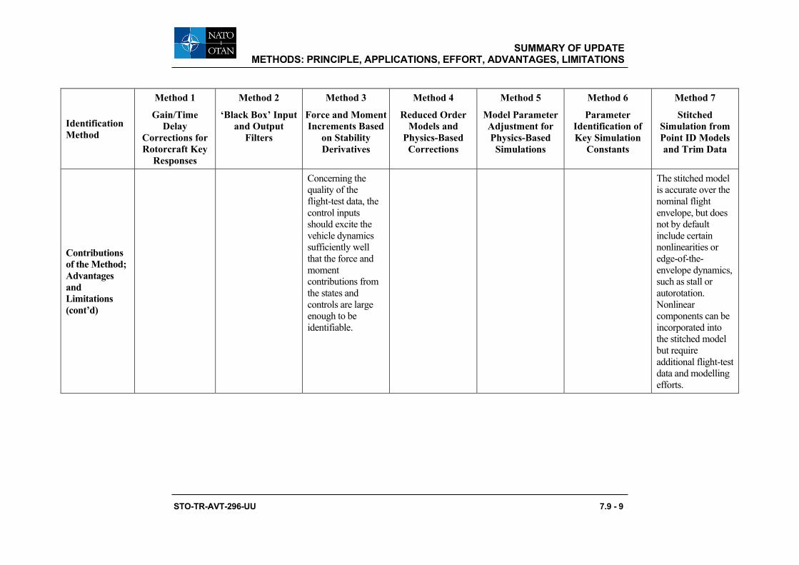
SUMMARY OF UPDATE METHODS: PRINCIPLE, APPLICATIONS, EFFORT, ADVANTAGES, LIMITATIONS

STO-TR-AVT-296-UU 7.9 - 9

Identification Method

Method 1

Gain/Time Delay

Corrections for Rotorcraft Key

Responses

Method 2

‘Black Box’ Input and Output

Filters

Method 3

Force and Moment Increments Based

on Stability Derivatives

Method 4

Reduced Order Models and

Physics-Based Corrections

Method 5

Model Parameter Adjustment for Physics-Based Simulations

Method 6

Parameter Identification of Key Simulation

Constants

Method 7

Stitched Simulation from Point ID Models and Trim Data

Contributions of the Method; Advantages and Limitations (cont’d)

Concerning the quality of the flight-test data, the control inputs should excite the vehicle dynamics sufficiently well that the force and moment contributions from the states and controls are large enough to be identifiable.

The stitched model is accurate over the nominal flight envelope, but does not by default include certain nonlinearities or edge-of-the-envelope dynamics, such as stall or autorotation. Nonlinear components can be incorporated into the stitched model but require additional flight-test data and modelling efforts.

SUMMARY OF UPDATE METHODS: PRINCIPLE, APPLICATIONS, EFFORT, ADVANTAGES, LIMITATIONS

7.9 - 10 STO-TR-AVT-296-UU

Identification Method

Method 1

Gain/Time Delay

Corrections for Rotorcraft Key

Responses

Method 2

‘Black Box’ Input and Output

Filters

Method 3

Force and Moment Increments Based

on Stability Derivatives

Method 4

Reduced Order Models and

Physics-Based Corrections

Method 5

Model Parameter Adjustment for Physics-Based Simulations

Method 6

Parameter Identification of Key Simulation

Constants

Method 7

Stitched Simulation from Point ID Models and Trim Data

Key Lessons Learned from Case Studies

Method is highly effective when used for the right application. More precisely, where the underlying physics is well captured in the baseline model, this method produces good corrections. However, this method will be not suitable when the dynamics are poorly modelled across a range of frequencies.

Care must be taken if the filters have unstable modes – the time-to-double should not exceed 1.5 sec so that a pilot can still stabilize the simulation.

If the correction model is in parallel or on the output side, care must be taken to retain consistency between the outputs. To avoid this problem, the use of a correction model at the input side is usually preferred.

The force and moment increments applied to a nonlinear simulation model in the form of ‘delta’ stability and control derivatives can improve the simulation model fidelity.

For example, model improvements were achieved by renovating the weathercock and dihedral effects and yaw damping, pointing to missing aerodynamic interference from the fuselage and main rotor wake on the tail surfaces.

The method requires good understanding of rotorcraft aerodynamics, dynamics, propulsion, and flight controls for identifying the root cause of the modelling discrepancies and applying the corrections accordingly.

The suitability of the method is dependent on the application. Simulation model developers need to be cautious in applying modifications to physical input parameters, especially if the intended use of the simulation model is engineering development.

If poor choices of parameters to be identified are made, the identification procedure is likely to produce physically implausible results. Also, if the model is missing key dynamics that show up in the flight data; this method will combine the net impact of those dynamics into the identified parameters.

Smooth eigenvalue transition between the operating points is best achieved by piecewise cubic spline interpolation of the original anchor point models. For higher order point models, trim data of the higher-order states must be included. The predictive accuracy of the stitched model for a realistic manoeuvring scenario is very accurate compared to a truth nonlinear simulation.

SUMMARY OF UPDATE METHODS: PRINCIPLE, APPLICATIONS, EFFORT, ADVANTAGES, LIMITATIONS

STO-TR-AVT-296-UU 7.9 - 11

Identification Method

Method 1

Gain/Time Delay

Corrections for Rotorcraft Key

Responses

Method 2

‘Black Box’ Input and Output

Filters

Method 3

Force and Moment Increments Based

on Stability Derivatives

Method 4

Reduced Order Models and

Physics-Based Corrections

Method 5

Model Parameter Adjustment for Physics-Based Simulations

Method 6

Parameter Identification of Key Simulation

Constants

Method 7

Stitched Simulation from Point ID Models and Trim Data

Key Lessons Learned from Case Studies (cont’d)

Physics-based modelling of rotor-on-rotor interference interactions between both cyclic and collective rotor inflow distributions improves simulation fidelity significantly for multi-rotor vehicle configurations.

These concerns may be of less importance for the development of training simulators where meeting the fidelity requirement for a specific aircraft is the foremost concern, not necessarily with physics-based corrections.

The stitched model’s extrapolation for off-nominal loading configurations is very accurate, which necessitates only the point models and trim data of the baseline aircraft loading configuration to be included in the stitched model.

SUMMARY OF UPDATE METHODS: PRINCIPLE, APPLICATIONS, EFFORT, ADVANTAGES, LIMITATIONS

7.9 - 12 STO-TR-AVT-296-UU

Identification Method

Method 1

Gain/Time Delay

Corrections for Rotorcraft Key

Responses

Method 2

‘Black Box’ Input and Output

Filters

Method 3

Force and Moment Increments Based

on Stability Derivatives

Method 4

Reduced Order Models and

Physics-Based Corrections

Method 5

Model Parameter Adjustment for Physics-Based Simulations

Method 6

Parameter Identification of Key Simulation

Constants

Method 7

Stitched Simulation from Point ID Models and Trim Data

Estimated Time to Use Method and Improvement Accuracy

Minimal. The method requires minimal work effort, and hence, it may be considered as a first approach in many circumstances. Care should be exercised when applying this method to cases where a physically representative system is required.

Moderate. As with Method 1, this method may be considered as a first approach leading to good model improvements. Balancing the input-output filters can be a time-consuming activity.

Considerable. Data preparation and conducting the system identification can be time-consuming. The method is an efficient approach to correcting some shortfalls in the baseline nonlinear model.

Considerable, but the payoff is that the corrections implemented for ground effect, rotor and fuselage aerodynamic interference, fuselage drag, elastic driveshaft dynamics, engine dynamics and fuel control, sensor and actuator dynamics showed remarkable improvements in the model.

Considerable. Improvements of system responses were demonstrated. However, in some cases, this method can be a time-consuming process as the sheer number of uncertain model parameters can be high.

Considerable. The method demonstrated that relatively small changes in a few model key physical parameters can greatly improve the overall ability of the updated simulation model to track flight-test data.

Considerable. Stitched models can adequately and accurately cover the nominal helicopter flight envelope. Extrapolation can be performed to simulate off-nominal loading configurations. This proves to significantly reduce required flight-test points and associated flight costs.

STO-TR-AVT-296-UU 8 - 1

Chapter 8 – SIMULATION APPLICATION ORIENTED DISCUSSION ON MODEL

DEVELOPMENT / UPDATE METHODS

This chapter discusses the challenges faced in rotorcraft flight simulation model development, fidelity assessment, and update for various simulation applications. The different end-uses of flight simulation drive the necessary model update strategies. Engineering simulations are usually developed with the primary purpose to support design and development of aircraft systems and equipment. Engineering simulation model development and updates are discussed in Section 8.1. Another major application of an engineering simulation is to support design of flight control system and evaluation of Handling Qualities (HQ). This application and the model development and update methods suitable for this application are discussed in Section 8.2. Model development and update methods for training simulations are discussed in Section 8.3. Section 8.4 revisits the current (FAA and EASA) time-domain simulator fidelity assessment metrics and considers how these could be augmented with new time and frequency-domain assessment methods/metrics demonstrated throughout this report. Taken together the existing and proposed approaches can give a more complete impression of rotorcraft simulator fidelity and can also reduce the overall cost of fidelity assessment flight testing. Finally, Section 8.5 considers the impact of the intended goals and end-uses of the simulation model on the appropriate selection of update methods and fidelity assessment metrics.

8.1 ENGINEERING SIMULATION FOR SUPPORTING DESIGN AND TEST

An engineering simulation can be used to support aircraft conceptual, preliminary, and detailed design, design modification, control laws design and analysis, handling qualities evaluation, flight loads development and analysis, flight testing, test pilot training, accident investigation, etc. The predictive capability of an engineering model is critical for design trade studies and flight envelop expansion tests. On the other hand, a version of the model needs to be capable of operating in real-time for pilot-in-the-loop simulation. These requirements dictate that an engineering simulation must be developed using a physics-based math model and applying proper simplifications/approximations to maintain the computational efficiency. The development and validation of an engineering model to support design and flight test are discussed in this section as well as the proper methods for improving the model correlation with test data.

8.1.1 Model Development and Validation An engineering simulation should faithfully reflect the flight characteristics of the aircraft modelled. Although an engineering simulation does not need to meet FAA Level D trainer criteria, the model must demonstrate good correlation with test data; the trend for the trim states, dynamic responses in both the time and frequency domain, and flight loads must be correct compared to the test data. Therefore, rotorcraft Original Equipment Manufacturers (OEM) have placed significant emphasis and effort to develop high-fidelity flight dynamics models.

In general, a rotorcraft OEM has the advantage of being able to provide a complete and accurate set of model data for an existing aircraft. For a new design, however, the simulation model development is a long and iterative process in parallel with the design of the aircraft. The initial model is usually scaled from an existing aircraft similar to the new design in terms of configuration and/or geometry. It is important that the existing aircraft model has been thoroughly validated with a comprehensive set of flight-test data as discussed in Section 8.1.2.

SIMULATION APPLICATION ORIENTED DISCUSSION ON MODEL DEVELOPMENT / UPDATE METHODS

8 - 2 STO-TR-AVT-296-UU

8.1.1.1 Model Update During a New Design

As the new design becomes progressively mature, the simulation model data are continuously updated from various sources, mainly including but not limited to:

1) Design change: aerodynamic configuration, geometry, structural properties, mass/inertia and CG, flight controls, etc.

2) Analysis using higher-fidelity models: free-wake, vortex-lattice, CFD, finite-element structure, etc.

3) Component test: wind-tunnel tests for airfoil, airframe, and rotor(s), blade rap test, etc.

4) Lessons learned from existing aircraft simulation model validation efforts.

In recent years, high-fidelity analytical tools have become more mature and practical, and thus more routinely applied to supporting the rotorcraft design. Although they are still computationally expensive and usually specialized at certain component levels, these tools can be very useful in generating flight simulation model input data. As examples, using high-fidelity rotor wake models (VPM, CHARM, MFW) to generate rotor inflow model inputs for engineering simulation are presented in He et al. (2019), Xin et al. (2014), Keller et al. (2019), and Juhasz et al. (2020). More detailed discussion and case studies can be found in Sections 5.4 and 7.4.

It is a continuous and progressive process to update the simulation model during the design. It requires the model developer to keep a close interaction with various disciplines of design and analysis. The frequency of simulation model updates is a trade-off between keeping the model consistent with the current design and keeping the model invariant for multi-discipline analysis.

Preparation of model inputs from various data sources/design disciplines can involve data conversion between different units and sign conventions as well as transformation between different coordinate systems. It is highly recommended to develop software tools (in MATLAB or Excel, for example) to automate the data conversion process. Such tools will enable an efficient model data preparation and, more importantly, limit the chance of making errors.

8.1.1.2 Model Verification and Validation

Model verification and validation are critical to ensure the quality of the baseline model. The simulation model should be verified every time any input data are updated. Before test data become available, some of the model input data are generated from different analytical tools, which are usually specialized for certain components. The verification process during this phase mainly involves comparison between the simulation model and other analytical tools. For example, the rotor modal frequencies can be compared with a finite-element model to ensure the geometry (e.g., hinge offset), stiffness of the hinge (and blade, if elastic), and blade inertia data are correct and accurate. This model ‘leveling’ process is to ensure the same model data are correctly interpreted among different models.

When the aircraft design becomes mature and component test data becomes available, the simulation model input data can be updated and validated in a timely manner. The validation process usually requires a carefully designed comparison between the updated simulation model and the source of the input data, either component test data or higher-fidelity model results. Two examples are discussed below.

Example 1: Airframe airloads measured from Wind-Tunnel (WT) tests are important input data for a rotorcraft flight model. Preferably, WT data will be available for the isolated fuselage and combined fuselage/empennage/lifting surfaces. The fuselage data will be converted to airload coefficients for the model inputs. While the empennage airload data can be obtained from high-fidelity aero models, the fuselage-on-empennage interference model is usually semi-empirical. When these data are updated, the simulation model should be run in a wind-tunnel mode to compare the total airframe airloads with

SIMULATION APPLICATION ORIENTED

DISCUSSION ON MODEL DEVELOPMENT / UPDATE METHODS

STO-TR-AVT-296-UU 8 - 3

the WT data for the combined airframe. If discrepancies are observed, the data processing for fuselage and empennage loads needs to be examined. If the data processing is confirmed to be correct, the fuselage-on-empennage interference model data need to be adjusted. The fuselage-on-empennage interference is usually modelled as tangential and normal velocity increments at the tail surfaces. These fuselages induced velocity components can be either derived from CFD or empirically adjusted to match the tail surface lift vs angle of attack curve measured from a wind-tunnel test where the fuselage and empennage are coupled.

Example 2: In order to maintain real-time capability, flight dynamics models usually use modal representation for elastic rotor blades and elastic fuselage to provide a reasonable trade-off between fidelity and computational expense. The mode shapes, which are the inputs to the flight model, are usually generated from high-fidelity Finite-Element (FE) models. When the mode shape data are updated, the simulation model should be linearised to compare the modal frequencies with the FE model results. If discrepancies are observed, the mode shape generation process and data post-processing need to be examined.

8.1.2 Correlation with Flight-Test Data and Model Improvement When flight-test data become available, the simulation model needs to be thoroughly validated against a comprehensive set of flight-test data from both steady trim and dynamic response tests that cover a broad range of vehicle configurations and flight conditions.

8.1.2.1 Test Data Collection

The quality of the flight-test data is very important for supporting the simulation model validation. The test data for model correlation need to be selected through various consistency checks. In general, the following should be considered when preparing the test data for model correlation:

a) Carefully setting up flight conditions is very important to achieve quality data. Flight performance and handling data are preferred to data from load survey tests due to tighter trim tolerances and better monitored wind conditions.

b) Frequency-domain data collection and processing requires special procedures for the difficult flight dynamics of the bare-airframe rotorcraft. Obtaining frequency-domain data of adequate quality involves requires properly designed frequency sweep maneuvers and specialized data processing methods/tools for rotorcraft (e.g., CIFER, FITLAB), which are especially challenging due to the flight test environment (reduced signal to noise) and complex flight dynamics (highly-coupled, high-order, etc.). For validation of aggressive manoeuvres, time-domain data remains a requirement.

8.1.2.2 Model Update Methods for Improving Correlation with Test Data

During model correlation with test data, discrepancies are usually observed in rotor performance, trim control positions and attitude angles, control power and control phase, stability and control derivatives, and dynamic responses in the time- and frequency-domains. To improve the model-test data correlation for an engineering simulation, efforts should first be made on improving the model data accuracy using high-fidelity tools and component test data. After the model data accuracy is examined/improved, the model-data discrepancy analysis should be started with a revisit of the simulation model assumptions and limitations. Once a model-data discrepancy can be related with some missing physics or assumptions/approximations made in the model, a physics-based or physics-inspired correction method can be developed to improve the model-data correlation. It is important to keep in mind that non-physical corrections could compromise the model’s predictive capability.

In some well-developed engineering simulation tools such as GenHel [Howlett (1981)] and FLIGHTLAB®, a series of physics-based, semi-empirical or empirical corrections have been developed based on extensive

SIMULATION APPLICATION ORIENTED DISCUSSION ON MODEL DEVELOPMENT / UPDATE METHODS

8 - 4 STO-TR-AVT-296-UU

model validation/correlation efforts over several decades. Many of these corrections belong to Method 4, which covers ‘reduced order models and physics-based corrections’ as described in Section 5.4 and demonstrated in Section 7.4. Some can be categorized as Method 5, which covers ‘model parameter adjustment’ with examples in Section 7.5. These physics-based corrections are clearly preferred methods to improve the predictive capability of engineering simulation models for supporting new aircraft design and flight tests.

The parameters in many of these corrections can be derived from higher-fidelity analytical tools. Details can be found in Method 4 with discussion in Section 5.4. Most of these corrections can also be empirically derived by matching certain test data. Various examples from the model update case studies can be found in Sections 7.4, 7.5, and 7.6.

As examples, some commonly applied correction methods are listed in Table 8.1.2-1, although some can appear in different forms in different simulation tools. In the table, the 1st column lists the model-data discrepancies often observed from the correlation. The 2nd column lists the possible causes of the discrepancies, most of which are complicated physical phenomenon that are not modelled rigorously in an engineering simulation. Some of the discrepancies could also be caused by model data uncertainty. The 3rd column lists the potential corrections/adjustments, mainly including reduced-order models and semi-empirical and empirical corrections. The 4th column lists the higher-fidelity analytical tools that could be used to derive the parameter values for these corrections. The 5th column lists the test data that could be used to derive the correction parameters empirically.

As shown in the table, some the discrepancies seen, for example, in rotor performance and collective control position could be caused by modelling simplifications in rotor airloads, inflow, ground effect, and rotor-fuselage aerodynamics interaction. Application examples for ground effect model adjustment can be found in Section 7.4.1.2 [Zhang et al. (2017)].

Some discrepancies seen in handling qualities characteristics, such as quickness, bandwidth, and phase delay, and cross coupling, are often related to modelling simplifications in rotor inflow dynamics and wake interference. Wake curvature effect corrections and reduced-order rotor interference models are frequently used to improve the model-data correlation [He et al. (2004)]. These corrections can be derived from higher-fidelity wake models such as free vortex wake or viscous Vortex Particle Method (VPM); see Section 5.4 for details. Several application examples can be found in Section 7.4.1.3 [Zhang et al. (2017)] and Section 7.4.1.7 [Zhao et al. (2004)] for rotor wake distortion corrections, in Section 7.4.2 for tandem rotor mutual interference models [Guner et al. (2020)], and in Section 7.4.4 for coaxial rotor mutual interference models [Fegely et al. (2016), Juhasz et al. (2020)].

The model-data discrepancies in trim attitude angles and control positions are often related to rotor and/or fuselage interference on the empennage, especially in the low-to-mid speed range. This relationship can be confirmed if the empennage loads are measured in the flight test. Various reduced-order interference models have been developed and implemented in flight dynamics simulation tools such GenHel and FLIGHTLAB. These models can be augmented by using high-fidelity tools such as free-wake model or VPM. There are also semi-empirical corrections, such effective wake skew and viscous decay, that can be used to compensate the simplification in the interference models. An example of model improvement with the rotor-on-empennage interference correction is presented in Section 7.4.1.4 [Zhang et al. (2017)]. At high angles of attack and/or high sideslip angle conditions, the fuselage-on-empennage interference becomes important and could significantly impact the model correlation with test data. An example in Section 7.4.1.5 demonstrates the model improvement with the fuselage on vertical fin interference corrections [Xin et al. (2019)].

As shown in Table 8.1.2-1, simplifications in the rotor blade structural model could cause discrepancies in the control power and phase, especially for hingeless rotors. The simplifications in the lead-lag damper

SIMULATION APPLICATION ORIENTED

DISCUSSION ON MODEL DEVELOPMENT / UPDATE METHODS

STO-TR-AVT-296-UU 8 - 5

and drivetrain models could cause discrepancies in the frequency response near the rotor regressive lag mode frequency. With a rigid fuselage assumption, the model will not be able to capture the related structural modes in the frequency response. The corrections listed in the table use reduced-order models to introduce structure flexibility-related dynamics and coupling, which could improve the model correlation with flight-test data in various frequency ranges. The parameters in these reduced-order models and corrections can usually be derived from Finite-Element Models (FEM) such as ANSYS. An example can be found in Section 7.4.3, where the yaw response and rotor speed correlation were improved by including drivetrain dynamics. Another example can be found in Xin et al. (2011), where a semi-empirical approach was developed to modelling the blade torsional dynamics using data derived from beam-element aeroelastic tool RCAS. The enhanced GenHel model was validated again whirl-stand test data.

Table 8.1.2-1: Examples of Model Corrections/Adjustments.

Model-Data Discrepancy Possible Causes Possible Corrections

and Adjustments High-Fidelity

Tools Test Data

Rotor performance and collective control position

3D effect near the blade tip Tip loss factor

Free-wake model

VPM

CFD

Whirl-stand test, wind-tunnel test, flight-test hover, level flight, climb and descent

Additional skin-friction drag on blade Delta drag coef. Correction

Nonuniform inflow distribution

Wake contraction factor; radial variation

Ground effect Ground effect coef.

Rotor downwash on fuselage

Empirical fuselage interference on rotor

Handling qualities (e.g., bandwidth, cross coupling)

Wake distortion effect on inflow

Wake curvature correction factor/map

Free-wake model

VPM

Frequency sweeps; pulse/doublet responses Rotor mutual

interference Rotor interference coef. and time delay

Trim attitude and control position and empennage loads

Rotor-on-empennage interference

Effective wake skew

Wind-tunnel test, low speed flight, level flight trim; climb and descent

Viscous decay

Wake contraction and expansion

Wake geometry change and time delay

Fuselage interference Blockage effect

CFD

Penal methods

3D effect on empennage airloads

Sideslip correction

Lift deficiency correction

Empennage stall Stall characteristics

Control power and control phase

Bending flexibility of hub and/or blade

Effective hinge offset/spring stiffness

Finite-element models such as RCAS, ANSYS,

Rap test; whirl-stand test; wind-tunnel test; trim flight test

Flap-pitch elastic/ geometry coupling Effective δ3 angle

SIMULATION APPLICATION ORIENTED DISCUSSION ON MODEL DEVELOPMENT / UPDATE METHODS

8 - 6 STO-TR-AVT-296-UU

Model-Data Discrepancy Possible Causes Possible Corrections

and Adjustments High-Fidelity

Tools Test Data

Control system flexibility Root torsional spring NASTRAN

Frequency response near rotor lag mode

Damper nonlinearity Effective damping

Frequency sweep (chirp) flight test

Drivetrain dynamics Drivetrain flexibility

Frequency response in high frequency range

Rotor Shaft bending flexibility

Simplified shaft bending model

Fuselage flexibility and structure damping Modal elastic fuselage

In summary, when engineering simulation models are used to support the design and testing for an aircraft under development or modification, model development, validation, and improvement is a progressive process used throughout the entire design and testing cycle. The models need to be continuously updated/enhanced to improve the correlation with test data in order to gain a high level of confidence in the model fidelity. Physics-based methods must be used to preserve the model’s predictive capability, which is critical for design trade studies and flight envelop expansion tests.

8.2 HANDLING QUALITIES AND FLIGHT CONTROL

Model-based design for flight control development holds the “promise” of achieving good Handling Qualities (HQ) and flight control performance with much reduced time/cost in flight testing. This is only possible when the key frequency/time responses and associated metrics of the integrated bare-airframe/flight control system simulation are validated through each step in the development process. Tischler et al. (2017) gives additional background on the validation methods/metrics presented in this section.

8.2.1 Simplified Flight Control Development Roadmap and the Role of Validated Models A simplified roadmap of the flight control development process and the associated central roles of a validated math model are shown in Figure 8.2-1. While this report has focused primarily on update/assessment of the bare-airframe model, this section considers the update and assessment of an integrated airframe/actuators/control system as depicted in Figure 8.2-2 to support the flight control development process. An accurate integrated simulation model ensures that predicted handling qualities and closed-loop flight dynamics translate from desktop design to real-time simulation and eventually to flight with a minimum of costly retuning. The five steps in the roadmap are referred to in the following discussion with bold font and are briefly reviewed.

The flight control development process starts with the definition of the quantitative requirements or Specifications that are appropriate for the intended missions of the aircraft. These specifications are selected largely from among the standard requirements for rotorcraft handling qualities (ADS-33E-PRF) [ADS-33E (2000), Blanken et al. (2019)] and flight control stability/robustness (SAE AS94900) [SAE (2007)] for predicted Level 1 (“satisfactory”) closed-loop aircraft behaviour.

In the flight control system Design phase, overall control system architecture is selected to meet the mission’s needs and is often based on company experience (e.g., explicit model-following or a simple PID nested-loop system), as discussed by Tischler et al. (2017). Control system synthesis is based on a linear

SIMULATION APPLICATION ORIENTED

DISCUSSION ON MODEL DEVELOPMENT / UPDATE METHODS

STO-TR-AVT-296-UU 8 - 7

(state-space) representation of the bare-airframe extracted from nonlinear physics-based simulation model or system identification from flight-test data when a prototype flight vehicle is available. Typically, a continuous (s-plane) block diagram presentation of the control laws is developed (e.g., using SIMULINK®), comprised of numerous linear blocks that represent the control laws and models of key hardware elements, such as actuators, sensors, and filters. In the design phase, math model validation ensures good agreement of key frequency responses and associated quantitative metrics (e.g., closed-loop bandwidth and stability margins) as obtained from linear (perturbation) analysis of the block diagram model (e.g., using the “linearise” function in MATLAB®) with those obtained from frequency sweeps of a more complete simulation. The latter simulation is typically comprised of the nonlinear bare-airframe model and a detailed control system representation, including the nonlinear elements and digital implementation of the control system.

Figure 8.2-1: Flight Control System Development Roadmap, Reproduced from Tischler et al. (2017, Figure 1.4).

The next step is real-time Simulation, where initial piloted HQ and autonomous evaluations are conducted for typical manoeuvres and missions. This uses a real-time nonlinear full flight envelope model capable of running in real-time in a ground-based and/or in-flight simulation facility. Frequency responses are obtained from frequency sweep testing of the complete simulation environment, including visual and motion system dynamics, and checked against the linear (numerical perturbation) results of the design model. Quantitative metrics are rechecked against the linear analysis to ensure that the Level 1 handling qualities and flight control characteristics are preserved in the real-time implementation. The qualitative simulator fidelity rating scale (SFR, Section 4.5) is used to ensure satisfactory perceptual fidelity of the overall simulation environment. Initial “assigned” handling qualities ratings are obtained using the Cooper-Harper Handling Qualities Rating scale and crosschecked with the “predicted” ratings as obtained from the quantitative (specification) metrics. Once validated, the real-time simulation is an invaluable tool for detailed control system development to meet the program objectives across the flight envelope – including a wide range of flight control changes, the degraded visual environment (e.g., “brown out”), and varying atmospheric conditions.

SIMULATION APPLICATION ORIENTED DISCUSSION ON MODEL DEVELOPMENT / UPDATE METHODS

8 - 8 STO-TR-AVT-296-UU

The next step is hardware/software in the loop Development and evaluation in a System Integration Lab (SIL). The SIL includes the complete digital implementation and associated logic of the control laws in the actual flight control processor, actuator hardware, and sensor suite (e.g., an Embedded GPS Inertial Navigation System (EGI)), and it may include testing in a complete Propulsion System Test Bed (PSTB) as illustrated by Tuzzo et al. (2017). A key aspect of the analysis is to validate that the frequency responses of the control laws alone as implemented in software (e.g., using compiled C code) in the actual control system processor match the continuous (s-plane) synthesis model. The frequency responses and associated key metrics of the integrated bare-airframe model and control system hardware are rechecked in the SIL to ensure that the design characteristics are preserved in the final system validation prior to flight. The completed SIL is invaluable for validating the hardware, the overall system performance in typical operational scenarios prior to flight, and the rehearsal of planned flight tests.

Flight testing is the final (and most expensive) step of the flight control development process. Frequency sweep testing is conducted very early in the flight-test program to assess and update the simulation model to accurately track the flight responses. The validated simulation model guides any needed flight control improvements and ensures that the number of cycles and associated costs of the development process to achieve satisfactory flight control behaviour are minimized.

8.2.2 Explicit Model-Following Control System Architecture Example (Inner-Loop) An explicit model-following (EMF) architecture is used as an example of control system validation methods in the discussion that follows, although the methods and metrics would be the same for other architectures. A typical top-level schematic for attitude (inner-loop) control in the longitudinal axis is shown in Figure 8.2-2. The EMF control system architecture has become a widely used standard for rotorcraft, both on many partial-authority upgrade systems and on new-build fly-by-wire rotorcraft systems. This “two degree-of-freedom” architecture allows independent design of the feedback (gust rejection and stability) from pilot response characteristics. Also, the Single Input / Single Output (SISO) architecture allows for transparent design and flight validation/development for each channel. The key elements of the architecture are highlighted in italics and described briefly with a more detailed treatment given by Tischler et al. (2017).

Figure 8.2-2: Model-Following Architecture (Pitch).

The command model is a lower-order (first- or second-order) transfer function, providing a simple pilot-selectable or automatic implementation of various required response types (e.g., attitude-command /

SIMULATION APPLICATION ORIENTED

DISCUSSION ON MODEL DEVELOPMENT / UPDATE METHODS

STO-TR-AVT-296-UU 8 - 9

attitude-hold, rate-command / attitude-hold) as required in ADS-33. A lower-order (first-order) inverse plant ensures that the aircraft short-term response will closely follow the command model, but will not overdrive the actuators and rotor. Placing the inverse in the forward path and outside of the feedback loop ensures that errors in the lower-order inverse will not compromise stability. The equivalent delay synchronizes the commanded and feedback signals to avoid overdriving the higher-order dynamics (i.e., rotor system) or causing actuator saturation. The equivalent delay also improves the model-following performance without introducing additional delay to pilot input. The feedback compensation is typically a classical PID system and may include some lead-lag shaping. Finally, the mixer distributes the channel commands to the control effectors (i.e., rotor push rods, aerodynamic surfaces, etc.). In the full multi-channel system, the mixer contains a crossfeed matrix, derived from the bare-airframe model to decouple the MIMO system into effectively distinct SISO loops. Therefore, achieving a high-fidelity bare-airframe model (using the methods presented in this report) will improve the decoupling. This will improve the accuracy with which the closed-loop system will track the command model for good handling qualities and improve gust rejection.

8.2.3 Integrated Simulation Validation and Key Metrics This section presents the methods and metrics for quantitative validation of the integrated model for each step of the flight control development process, using system identification techniques. The frequency responses and associated metrics used for validation are the same at each step of the development cycle. As more flight hardware and modelling detail is introduced, fidelity and confidence in the integrated simulation improves. A good practice followed by industry is to keep and update a “smart book” that contains the frequency responses and metrics (presented in this section) and a log of model changes throughout the development process. Then, if there is a significant change in flight control system behaviour from one step to the next, sources of possible errors/corrections are more easily traced. Validation examples in this section are based on flight-test data for hover from the RASCAL fly-by-wire UH-60 helicopter, as presented in detail in Mansur and Tischler (2013) and summarised in Tischler et al. (2017).

Prior to flight testing, validation at each step of the development process is based on a comparison of the frequency responses of the linear (analysis) model with those obtained from frequency sweep testing of the nonlinear simulation and comparison with the responses from the previous development step. Then, in the flight-test program, frequency sweep flight testing is typically conducted early to validate and update the integrated bare-airframe / flight control system model as needed to bring the simulation model results into agreement with the flight-test data for the initial gain set and efficiently guide needed system changes based on flight-test performance and pilot qualitative comments. There are three key integrated bare-airframe/flight control frequency responses and associated quantitative metrics (for each inner-loop channel) that must be validated at each step in the development process. Referring to Figure 8.2-2 for the pitch axis, these are the 1) Broken-loop response, 𝛿𝛿𝑙𝑙𝑚𝑚𝑛𝑛𝑓𝑓𝑓𝑓 𝛿𝛿𝑙𝑙𝑚𝑚𝑛𝑛𝑚𝑚𝑥𝑥

⁄ ; 2) Closed-loop response, 𝜃𝜃 𝛿𝛿𝑙𝑙𝑚𝑚𝑛𝑛𝑠𝑠⁄ ; and 3) Disturbance rejection response, 𝜃𝜃′ 𝜃𝜃𝑑𝑑⁄ . Each response has its own frequency range of interest for model validation and associated key metrics to be tracked throughout the development roadmap and finally checked against the design specifications using flight-test data.

Broken-loop response validation. The broken-loop response, 𝛿𝛿𝑙𝑙𝑚𝑚𝑛𝑛𝑓𝑓𝑓𝑓 𝛿𝛿𝑙𝑙𝑚𝑚𝑛𝑛𝑚𝑚𝑥𝑥⁄ , is central to the performance of

the control system, dictating the speed of the feedback response (crossover frequency, 𝜔𝜔𝑐𝑐), stability margins for robustness to modelling uncertainty, command response tracking precision, and closed-loop response damping. Close agreement of the broken-loop response and associated metrics with flight-test data is essential in model-based control system development for effectively guiding needed flight control system improvements. The nature of feedback itself is to supress the effects of errors/uncertainties in the constituent bare-airframe and control system models that make up the overall closed-loop response [Tischler et al. (2017)]. Therefore, considerable errors in the key broken-loop metrics will not be very apparent in the closed-loop response validation. This makes the validation and update of the simulation response for precise broken-loop response fidelity the key step for model-based control system development.

SIMULATION APPLICATION ORIENTED DISCUSSION ON MODEL DEVELOPMENT / UPDATE METHODS

8 - 10 STO-TR-AVT-296-UU

The broken-loop response is obtained experimentally (in desktop/SIL simulation and flight test) by injecting an automated sweep 𝛿𝛿𝑙𝑙𝑚𝑚𝑛𝑛𝐵𝐵𝑆𝑆 in the “channel input” just ahead of the mixer (Figure 8.2-2). Then, the signals 𝛿𝛿𝑙𝑙𝑚𝑚𝑛𝑛𝑚𝑚𝑥𝑥 and 𝛿𝛿𝑙𝑙𝑚𝑚𝑛𝑛𝑓𝑓𝑓𝑓 are recorded, and system identification provides an accurate broken-loop response, 𝛿𝛿𝑙𝑙𝑚𝑚𝑛𝑛𝑓𝑓𝑓𝑓 𝛿𝛿𝑙𝑙𝑚𝑚𝑛𝑛𝑚𝑚𝑥𝑥

⁄ , which is the ‘truth data’. For control system analysis and synthesis, an accurate broken-loop response must be obtained from perturbation linearization (“linearise” function in MATLAB®) of the block diagram (e.g., Figure 8.2-2). This linearization process is subject to errors due to analogue vs digital elements, nonlinear vs linearised simulation model elements, and logic blocks, so the perturbation broken-loop response must be verified to agree closely with the system identification results initially from the nonlinear and real-time simulations and then from flight tests.

The broken-loop response is comprised of the product of the bare-airframe response, 𝑞𝑞′ 𝛿𝛿𝑙𝑙𝑚𝑚𝑛𝑛𝑚𝑚𝑥𝑥⁄ , and the

feedback compensation response, 𝛿𝛿𝑙𝑙𝑚𝑚𝑛𝑛𝑓𝑓𝑓𝑓 𝑞𝑞′⁄ . These responses can be independently determined and verified using the same broken-loop frequency sweep data for the 𝛿𝛿𝑙𝑙𝑚𝑚𝑛𝑛𝐵𝐵𝑆𝑆 input as well as by linearization perturbation. The methods for bare-airframe model update and fidelity assessment to ensure good agreement have been addressed at length in this report, thus at this point we assume that the 𝑞𝑞′ 𝛿𝛿𝑙𝑙𝑚𝑚𝑛𝑛𝑚𝑚𝑥𝑥

⁄ frequency responses from frequency sweeps of the nonlinear simulation and linearization perturbation meet the fidelity criteria of Sections 7.1 and 7.2. The 𝑞𝑞′ and 𝛿𝛿𝑙𝑙𝑚𝑚𝑛𝑛𝑓𝑓𝑓𝑓 signals as recorded in the broken-loop frequency sweep tests, provide an accurate feedback system frequency response, 𝛿𝛿𝑙𝑙𝑚𝑚𝑛𝑛𝑓𝑓𝑓𝑓 𝑞𝑞′⁄ . This system identification result will include both the 𝑞𝑞′ and 𝜃𝜃′ feedback shown in Figure 8.2-2. The perturbation linearization result for the feedback response in the SIMULINK analysis model is determined as shown in Figure 8.2-3 for the pitch axis and must agree very closely with the frequency sweep results.

Figure 8.2-3: Perturbation and Sweep Method for Determining the Feedback Response from a SIMLINK Block Diagram.

A test example in Figure 8.2-4 shows close agreement of 𝛿𝛿𝑙𝑙𝑚𝑚𝑛𝑛𝑓𝑓𝑓𝑓 𝑞𝑞′⁄ using the method Figure 8.2-3 for the 1) Perturbation linearised SIMLINK simulation model vs 2) Sweeps of the SIL; and 3) Test results obtained from manual angular oscillation of the vehicle on the ground. These results validate the analysis model and the pictures-to-code implementation of the control laws in the flight processor.

Small errors in the feedback response simulation model may be due to digitalization and nonlinear effects and can be corrected with a simple gain (magnitude errors) and time delay (phase errors) applied to the output of the feedback signal 𝛿𝛿𝑙𝑙𝑚𝑚𝑛𝑛𝑓𝑓𝑓𝑓 (Figure 8.2-2). Larger errors (e.g., due to logic path problems during the perturbation linearization process) require a more in-depth analysis of the flight control model and linearization. At this point, both the bare-airframe and feedback responses have been individually validated/corrected, and the overall broken-loop response, 𝛿𝛿𝑙𝑙𝑚𝑚𝑛𝑛𝑓𝑓𝑓𝑓 𝛿𝛿𝑙𝑙𝑚𝑚𝑛𝑛𝑚𝑚𝑥𝑥

⁄ , should be compared as obtained from system identification and perturbation linearization and corrected if necessary. Good fidelity of the overall broken-loop simulation response, 𝛿𝛿𝑙𝑙𝑚𝑚𝑛𝑛𝑓𝑓𝑓𝑓 𝛿𝛿𝑙𝑙𝑚𝑚𝑛𝑛𝑚𝑚𝑥𝑥

⁄ , should be achieved for frequencies, 𝜔𝜔 (rad/sec), in the range of

0.3𝜔𝜔𝑐𝑐 ≤ 𝜔𝜔 ≤ 3.0𝜔𝜔𝑐𝑐 (8.2-1)

where, 𝜔𝜔𝑐𝑐 is the “crossover frequency” (rad/sec) at which the response crosses the 0dB line.

SIMULATION APPLICATION ORIENTED

DISCUSSION ON MODEL DEVELOPMENT / UPDATE METHODS

STO-TR-AVT-296-UU 8 - 11

Figure 8.2-4: Perturbation Linearization of the SIMULINK Feedback Response, Frequency Sweep Determination of the SIMULINK Control Laws, and Ground Sweep Validation (By Hand) of the Real-Time Control Laws (in the Flight Processor).

Errors in the broken-loop response are associated with residual discrepancies in the corrected bare-airframe model and uncertainties in sensor and actuator dynamic modelling. The comparison of flight and simulation broken-loop responses provides final gain and time delay corrections that are inserted just ahead of the mixer. The key metrics of interest for this response are the crossover frequency (𝜔𝜔𝑐𝑐), Phase Margin (PM), and Gain Margin (GM) as defined in Figure 8.2-5(a). The simulation and flight values of these metrics should all agree closely, and the Gain/Phase Margin Point (PM, GM) must be in the same region of the SAE AS949000 specification of Figure 8.2-5(b) (e.g., both in the unshaded Level 1 region). An example of the pitch response validation for the UH-60 RASCAL aircraft is given in Figure 8.2-6, which shows very close agreement of the linear simulation (CONDUIT®) and flight responses. The broken-loop metrics for the simulation and flight-test results (𝜔𝜔𝑐𝑐, PM, GM) all agree closely, as is shown for the UH-60 in Table 8.1.2-1, and both are in the Level 1 region of Figure 8.2-5(b).

Closed-loop response validation. The closed-loop response, 𝜃𝜃 𝛿𝛿𝑙𝑙𝑚𝑚𝑛𝑛𝑠𝑠⁄ is determined from a piloted (or automated) sweep injected at the stick input, 𝛿𝛿𝑙𝑙𝑚𝑚𝑛𝑛𝑠𝑠, with the inner (attitude) loops closed. Key closed-loop HQ metrics are the bandwidth frequency and phase delay (𝜔𝜔𝐵𝐵𝑀𝑀, 𝜏𝜏𝑁𝑁), as defined in Figure 8.2-7(a). For attitude response types, the bandwidth, 𝜔𝜔𝐵𝐵𝑀𝑀, is defined as the frequency (rad/sec) at which the phase response is 𝜑𝜑 = −135 deg. For angular-rate response types, the bandwidth is defined as the lesser of the gain margin and phase margin bandwidth frequencies (Figure 8.2-7(a)). The phase delay, 𝜏𝜏𝑁𝑁, is defined by ADS-33E (2000) and discussed by Tischler et al. (2017):

𝜏𝜏𝑁𝑁 = ∆𝜑𝜑2𝜔𝜔180

57.3 (2𝜔𝜔180) (8.2-2)

SIMULATION APPLICATION ORIENTED DISCUSSION ON MODEL DEVELOPMENT / UPDATE METHODS

8 - 12 STO-TR-AVT-296-UU

Figure 8.2-5: (a) Definition of Broken-Loop Response Metrics (b) SAE AS94000 Stability Margin Specification.

Figure 8.2-6: Analysis Model Validation for Broken-Loop Pitch Response (UH-60 RASCAL, Hover).

SIMULATION APPLICATION ORIENTED

DISCUSSION ON MODEL DEVELOPMENT / UPDATE METHODS

STO-TR-AVT-296-UU 8 - 13

Figure 8.2-7: (a) Definition of the ADS-33 Bandwidth and Phase Delay Metrics (b) ADS-33F Criteria for Pitch Axis (All other MTE and/or divided attention).

The parameters in Equation 8.2-2 are defined in Figure 8.2-7(a). The phase delay, 𝜏𝜏𝑁𝑁, is a measure of the phase roll-off beyond the frequency for 𝜑𝜑 = −180 deg (defined as 𝜔𝜔180) and is an approximation of the equivalent system time delay as obtained from system identification of a low-order model 𝜏𝜏𝑒𝑒. Large phase delays (i.e., 𝜏𝜏𝑁𝑁 ≥ 0.120 𝑠𝑠𝑒𝑒𝑠𝑠) can result in degraded handling qualities especially for high-precision piloting tasks (also referred to as “high pilot gain tasks”). These metrics and their importance to pilot handling qualities is discussed further in Tischler et al. (2017). In order to accurately determine these metrics, good fidelity of the simulation response should be achieved for frequencies, 𝜔𝜔 (rad/sec), in the range of

0.5𝜔𝜔𝐵𝐵𝑀𝑀 ≤ 𝜔𝜔 ≤ 2.5𝜔𝜔180 (8.2-3)

And 𝜔𝜔180 is the frequency where the phase response is 𝜑𝜑 = −180 deg. The closed-loop simulation model is validated by ensuring that the error function between the simulation and flight responses is within the “MUAD mismatch boundaries” (Section 7.1) and that the integrated cost function (Section 7.2) meets the criteria of 𝐽𝐽 ≤ 100, for the closed-loop pitch response 𝜃𝜃 𝛿𝛿𝑙𝑙𝑚𝑚𝑛𝑛𝑠𝑠⁄ .

The simulation point (𝜔𝜔𝐵𝐵𝑀𝑀, 𝜏𝜏𝑁𝑁) must be in the same region of the ADS-33 specification as the flight response. For example, both should be in the same region of the HQ specification of Figure 8.2-7(b) (e.g., Level 1 is the unshaded region). Time-domain validation criteria for the closed-loop forced response are given via the QTG criteria (Section 4.6). Another important time-domain criteria is the closed-loop damping ratio 𝜁𝜁, that can be obtained from a log decrement analysis for stick pulse response. An example of the closed-loop pitch response validation for the UH-60 RASCAL is given in Figure 8.2-8, showing very good agreement of the linear simulation (CONDUIT) and flight responses. The closed-loop metrics for the simulation and flight-test results (𝜔𝜔𝐵𝐵𝑀𝑀, 𝜏𝜏𝑁𝑁) agree closely as is shown for the UH-60 in Table 8.2-1, and both are in the Level 1 region of Figure 8.2-7(b).

SIMULATION APPLICATION ORIENTED DISCUSSION ON MODEL DEVELOPMENT / UPDATE METHODS

8 - 14 STO-TR-AVT-296-UU

Figure 8.2-8: Analysis Model Validation for Closed-Loop Pitch Response (UH-60 RASCAL, Hover).

Disturbance rejection response validation. Finally, the disturbance rejection response 𝜃𝜃′ 𝜃𝜃𝑑𝑑⁄ is obtained by injecting an automated frequency sweep 𝜃𝜃𝑑𝑑 as shown in Figure 8.2-2, with the inner (attitude) loops closed. Good fidelity of the simulation response should be achieved for frequencies 𝜔𝜔 (rad/sec) in the range of

0.3𝜔𝜔𝐼𝐼𝑅𝑅𝐵𝐵 ≤ 𝜔𝜔 ≤ 2.0𝜔𝜔𝐼𝐼𝑅𝑅𝑃𝑃 (8.2-4)

where 𝜔𝜔𝐼𝐼𝑅𝑅𝐵𝐵 (also denoted DRB) is the disturbance rejection bandwidth frequency (rad/sec) and 𝜔𝜔𝐼𝐼𝑅𝑅𝑃𝑃 (also denoted DRP) is the disturbance rejection response peak as defined in Figure 8.2-9. The ADS-33 pitch response specifications are given in Figure 8.2-10.

The simulation values of these disturbance response metrics must be in the same region of the ADS-33 specification as the flight response (e.g., Level 1 is the unshaded region in the specifications of Figure 8.2-10). An example of the yaw disturbance rejection response validation for the UH-60 RASCAL is given in Figure 8.2-11. The disturbance response metrics all agree closely as is shown for the UH-60 in Table 8.2-1, and both are within the Level 1 region for the yaw DRB ADS-33F requirement [Blanken et al. (2019)].

SIMULATION APPLICATION ORIENTED

DISCUSSION ON MODEL DEVELOPMENT / UPDATE METHODS

STO-TR-AVT-296-UU 8 - 15

Figure 8.2-9: Definition of ADS-33 Disturbance Rejection Specification Metrics.

Figure 8.2-10: ADS-33 Disturbance Rejection Specifications for Pitch: (a) DRB; (b) DRP.

SIMULATION APPLICATION ORIENTED DISCUSSION ON MODEL DEVELOPMENT / UPDATE METHODS

8 - 16 STO-TR-AVT-296-UU

Figure 8.2-11: Analysis Model Validation for Disturbance Rejection Yaw Response (UH-60 RASCAL, Hover).

8.2.4 Outer-Loop Control System Architecture and Validation The discussion so far in this section has concentrated on the inner (attitude) loop control system. Typically, a nested-loop architecture closes velocity and position “outer loops” around this inner-loop system as required by ADS-33 for the Degraded Visibility Environment (DVE) and shown schematically in Figure 8.2-12. The same three frequency responses and associated metrics, as discussed in the previous sections, are validated for both the velocity and position loops. The outer loop broken-loop response break points are denoted as ‘Point 1’, ‘Point 2’, and ‘Point 3’. More detail on the outer-loop architecture and associated responses and metrics are given by Tischler et al. (2017).

SIMULATION APPLICATION ORIENTED

DISCUSSION ON MODEL DEVELOPMENT / UPDATE METHODS

STO-TR-AVT-296-UU 8 - 17

Figure 8.2-12: Typical Outer-Loop Schematic for Explicit Model-Following System.

8.2.5 Discussion Once the control system architecture is fixed, the integrated bare-airframe / flight control model needs only to be validated against the flight data for any single gain set, and then the model will be valid for all future gain adjustments.

In the Armed Reconnaissance Helicopter (ARH) flight control development program, Bell Helicopter engineers used a flight identified bare-airframe model of the prototype and direct design optimization (CONDUIT) to tune AFCS gains on the Armed Reconnaissance Helicopter (ARH-70A) program to meet ADS-33 Level 1 requirements prior to initial flight testing. Then, the various response metrics were validated for the initial gain set, providing an accurate basis for final flight control tuning. They credit this process with enabling them to ‘clear the ARH-70A in less than one third of the flight-test time that had been originally planned for AFCS development’ [Christensen et al. (2007)].

Other examples of efficient flight control system development using validated simulation models include the CH-47F DAFCS [Irvin et al. (2007)], MH-47G [Link et al. (2011)], and the unmanned FireScout [Downs et al. (2007)]. As shown in Table 8.2-1, the response metrics for the RASCAL UH-60 simulation model all agree closely with the flight data. The excellent validation allowed for a very efficient flight-test that examined several control system gain sets and was instrumental in setting ADS-33 specification boundaries for the disturbance rejection response metrics [Blanken et al. (2019)].

Table 8.2-1: Comparison of Fidelity Metrics for Analysis vs Flight (UH-60 RASCAL, Hover).

Engineering Name Engineering Symbol

Analysis Value

Flight-Test Value

Crossover Frequency, Pitch 𝜔𝜔𝑐𝑐 2.87 rad/sec 2.94 rad/sec

Phase Margin, Pitch PM 49.8 deg 49.3 deg

Gain Margin, Pitch GM 12.3 dB 11.1 dB

Bandwidth, Pitch 𝜔𝜔𝐵𝐵𝑀𝑀 2.72 rad/sec 3.10 rad/sec

Phase Delay, Pitch 𝜏𝜏𝑁𝑁 0.06 sec 0.12 sec

Disturbance Rejection Bandwidth, Yaw 𝜔𝜔DRB 0.96 rad/sec 0.96 rad/sec

Disturbance Rejection Peak, Yaw DRP 2.61 dB 2.42 dB

SIMULATION APPLICATION ORIENTED DISCUSSION ON MODEL DEVELOPMENT / UPDATE METHODS

8 - 18 STO-TR-AVT-296-UU

The summary of this section is as follows:

1) Model-based flight control design requires an accurate model that is validated at each step of the development process, based on three key frequency responses (broken-loop, closed-loop, and disturbance rejection) and associated metrics.

2) With a validated/corrected bare-airframe model, the feedback and broken-loop responses are then corrected with a gain and time delay to provide excellent fidelity.

3) Once the control system architecture is fixed, the integrated bare-airframe/flight control model needs only to be validated against the flight data for a single (any) gain set. Then, the model will be valid for all future gain adjustments as needed to guide flight control and handling qualities improvements.

4) Experience from many flight control development programs demonstrates that using a flight-validated model-based approach can achieve good Handling Qualities (HQ) and flight control performance with much reduced time/cost in flight testing.

8.3 TRAINING SIMULATION

Helicopter training simulators need to provide high-fidelity immersive environments for pilots in order to obtain a Level D qualification, which is the highest level of simulator qualification defined by the Federal Aviation Administration (FAA) [FAA (2016)], the European Union Aviation Safety Agency (EASA) [EASA (2012)], and the International Civil Aviation Organization (ICAO) [ICAO (2012)]. A Level D qualification allows the replacement of most of the flight hours required for a pilot’s type rating or recurrent training with simulator hours. A Level D simulator is made of many subsystem models related to the vehicle dynamics (flight dynamics, flight controls, engines, and autopilot), vehicles systems (avionics, ancillaries, etc.) and simulator immersive cueing environments (motion, sound, visual, weather, airport environment, etc.). Each of these subsystems must meet qualitative and quantitative validation criteria for the specific aircraft type to meet Level D simulator requirements.

8.3.1 Level D Data Package Requirement A flight-test data package must contain measured data for more than one hundred flight-test manoeuvres to meet Level D validation requirements [SAE (2019)]. Typically, a flight-test campaign is required to collect the data for flight model development and simulator certification.

A flight-test instrumentation system consists of distributed data acquisition and recording systems, where several nodes are distributed throughout the aircraft and connected to groups of sensors. Each node receives either analog or digital data (ARINC 429), performs filtering if required, and transfers data to a master node. The analog signals are typically collected at a nominal sampling rate of 5000 Hz. These signals are filtered and outputted to a network. Unfiltered parameters include digital, discrete, air data, and time data parameters. Engine data is collected to the same network consisting of over 100 data channels and recorded typically around 100 Hz. The measurements include sound and vibration at higher frequencies, such as 1000 Hz.

In all, over 1000 test points and Qualification Test Guide (QTG) manoeuvres are typically collected for simulator model generation and validation. The manoeuvres range from those near the ground (hover and low speed, takeoff and landing) to cruise flight performance, static stability, dynamic manoeuvres, and autorotation. The flight-test time can be over 100 hours collected over a period of months. The total number of sorties is about 40.

SIMULATION APPLICATION ORIENTED

DISCUSSION ON MODEL DEVELOPMENT / UPDATE METHODS

STO-TR-AVT-296-UU 8 - 19

8.3.2 Blade-Element Rotor Models While no model structure can give a complete representation of the physics related to helicopter simulation, blade-element rotor models for rotorcraft dynamics are typically used to meet the fidelity requirements for the Level D training simulator classification. Physics-based models such as the blade-element rotor models have some advantages compared to their strictly parametric counterparts, because of their predictability and their capability to extend the flight envelope. Capturing the full flight envelope requires including multiple configurations of gross weight and Centre of Gravity (CG), maximum rearward/sideward speeds up to VNE, low speed azimuths, In-Ground Effect (IGE), climb/descent/autorotation, and high bank turn (manoeuvring stability and coordinated turns). In addition to providing a full continuous envelope and accurate performance and handling qualities, pilots can observe and train for various special flight conditions in training simulators: vortex ring state, retreating blade stall, loss of tail rotor effectiveness, engine malfunctions, autorotation entry, icing, etc. Subject Matter Expert (SME) pilots can also request subjective corrections, which are usually stated in ‘pilot’s language’, for aircraft stability, workload, unexpected behaviours, etc. These comments often offer valuable clues to the engineer about deficiencies in the model.

Blade-element rotor models can easily integrate main rotor inflow models that are determined from reduced-order models and physics-based corrections (Method 4). More precisely, they may come from basic momentum theory or possibly more complete inflow models (e.g., Pitt Peters, harmonic inflow components). If the inflow model from theory is insufficient for agreement between simulation model and flight-test data, it can be augmented by various simulator model parameters adjustments (Method 5). Force and moment increments can also be calculated to complete the updated blade-element rotor model (Method 3). Corrections by adding filters (Method 2) can be used when the blade-element rotor model has reached its limitation or special effects are required. While physics-based models are still most commonly used for engineering and real-time trainer simulations, when flight data exists or can be collected for an existing rotorcraft (manned or UAV), some organisations are using stitched models obtained through system identification are being used entirely for trainer applications in some organisations or as a means to update physics-based models (Method 7).

8.3.3 Flight Simulator Model Development A major challenge of flight simulator model development is the requirement that helicopter training simulations are executed in real-time. This requires high levels of computational efficiency, which effectively limit increases in model complexity associated with improving physical accuracy.

Another major challenge for flight simulator model development is data availability. Simulator manufacturers often do not have full access to the complete set of aircraft data required to generate accurate physics-based models. To meet the Level D simulator requirements despite the model’s limitations or lack of data, the discrepancies between the trainer models and flight-test data can be compensated for using the model update techniques discussed in Chapters 5 and 7.

The flight dynamics modelling effort is treated in various ways by different simulator companies. The majority use dynamics models well established in literature and try to adjust the model to match discrepancies relative to the flight-test data. Common practice is to tune a model based on one set of data and validate the model with an independent set of data.

System identification methods can help to systematically compensate for the missing dynamics. Therefore, often a separate system identification effort is put into place to help identify the dynamics missing from the physics-based models. Many companies make use of the techniques reported in Chapter 5.

SIMULATION APPLICATION ORIENTED DISCUSSION ON MODEL DEVELOPMENT / UPDATE METHODS

8 - 20 STO-TR-AVT-296-UU

8.3.4 Simulator Qualification Requirements The level of effort to obtain the required data package and model fidelity can be adapted depending on the qualification level sought. Level D is the highest standard sought for full flight simulators and requires the highest level of fidelity. Levels A, B, and C require relatively lower levels of fidelity. A thorough definition of these standards is given in FAA Part 60 [FAA (2016)] and CS-FTD (H) [EASA (2012)].

The flight dynamics model is an important part of the qualification of a Level D full flight simulator. The standard requires comparison of the model with flight-test data using metrics such as flight parameters in trimmed flight conditions (e.g., control positions, Euler angles, torque readings, etc.) and responses to pilot inputs. Nearly 50% of the flight tests are simple hands-off control input tests where the pilot performs a step input or doublet in one axis and keeps his hands off of the controls to evaluate the helicopter short-term response. The majority of handling qualities tests include those associated with the longitudinal long-term response (phugoid), lateral-directional oscillations (Dutch roll), spiral stability, and adverse-proverse yaw. In addition, long flight manoeuvres, such as take-off and landing, are compared with the response of the flight model in the simulator. Altogether, more than 100 flight manoeuvres are compared. This is the so-called “objective” part of the qualification procedure related to flight dynamics and is presented to the authorities via documentation. The tolerances required for these comparisons are quite small such that very small violations not even noticeable by a pilot could result in failing certification for the whole simulator. For flight model developers, this results in a very tedious tuning effort, which sometimes results in over-tuned models, i.e., flight model tuning for behaviour not noticeable by pilots. The “subjective” part of certification includes assessment of the general “feel” of the simulator by a subject matter expert pilot, including in flight regimes that were not included in the objective assessment.

The “subjective” part of certification includes assessment of the general “feel” of the simulator by a subject matter expert pilot and flight regimes that were not included in the objective assessment. A common issue arises when a pilot’s subjective opinion does not agree with the objective assessment of the handling qualities.

Reasons for such conflicts can be various and some may be credited to the lack of accurate data. For example, some of the flight-test manoeuvres may be sensitive to initial conditions or environmental conditions. It is also not always possible to accurately measure the magnitude and direction of the wind at the time and location that the flight-test data is recorded. Moreover, it is not entirely clear that the set of validation tests as described in FAA Part 60 [FAA (2016)] and CS-FTD (H) [EASA (2012)] cover the entire frequency range in which the vehicle will operate. The models used may be only be valid in parts of the flight envelope for which data is available and less accurate in parts of the flight envelope for which data was not available. As a result, a compromise is often reached between a model that satisfies the objective part of the validation and the opinion of the subject matter expert pilot.

QTG runs provide full documentation of comparisons of the simulator responses with flight-test data (more details in Chapter 4.5). QTG runs are executed in the simulator during every cycle of its life: flight model development, initial qualification, and every recurrent qualification. QTG runs will be performed by a simulator technician periodically, typically every 6 months. This testing involves running the complete QTG test package, which contains typically about 100 time history and static cases, in real time. The goal of these recurring tests is to determine if any of the results have degraded since the initial simulator qualification for results that were accepted by the civil regulatory authorities. Degradation of the QTG results when the simulator is in operation can occur for the following reasons:

1) A model change required to resolve a valid subjective concern raised by a pilot after the official qualification. This may lead to slight degradation where the results are still in tolerance but lean more towards the pilot needs.

2) Unexpected degradation resulting from a change that was not supposed to affect simulator handling or hardware issue that has gone undetected.

SIMULATION APPLICATION ORIENTED

DISCUSSION ON MODEL DEVELOPMENT / UPDATE METHODS

STO-TR-AVT-296-UU 8 - 21

Whether before or after qualification, once the QTG batch is run, the results have to be printed and analysed. Running a QTG batch itself involves using around 6 hours of simulator time (for which the simulator cannot generate revenue) and involves at least 4 hours of manual review and overlay plots to ensure that the match of the time histories is exactly the same as before. These tests are very sensitive to minor setup or hardware issues (friction, flight control hysteresis, etc.), which may result in a case being falsely out of tolerance. When this happens, simply re-running the case usually solves the problem; however, this uses more of the simulator’s and technician’s time.

Reducing the number of QTG test cases related to flight dynamics would result in a smaller number of flight tests, reduced cost, and faster evaluation of the simulators. Moreover, the recurrent evaluation runs would provide a more exhaustive analysis and recurrent cost would be reduced. This could be achieved by carefully selecting manoeuvres that could replace a number of the current QTGs. By doing so, the new manoeuvres should still preserve data content that was covered by the existing QTGs and that are deemed to be important to the pilot. In the case of military projects, QTG runs are usually a requirement to be met, but it is possible that the models will diverge from the flight-test data. This sometimes happens because a required training task to be performed is in contradiction with the flight-test data. In this case, a rational would be provided by the military regulatory authority.

One way to reduce the number of QTG runs could be the inclusion of frequency-domain based tests. This could help the developer evaluate the model at the frequency bands the pilots primarily operate at. In fact, a pilot rarely flies with “step-type” inputs used in the QTG validation. Validation of training simulator fidelity for pilot-in-the-loop tasks (e.g., tracking tasks, high bandwidth slope and run-on landing), is best accomplished from the simulator vs. flight frequency responses and associated metrics of key input-output pairs.

To validate a model using frequency-domain analysis, the Maximum Unnoticeable Added Dynamics (MUAD) criteria could be applied to the resulting frequency plots in order to evaluate whether or not the change would be noticeable by a pilot. Frequency-domain runs, however, would not replace all QTG runs in time-domain validation, especially tests related to performance and manoeuvres related to actual aircraft operation (takeoff, landings, autorotation entry, etc.). Section 8.4.2 will show the QTG tolerance bands in the frequency domain. A suggested replacement to reduce the number of QTG tests using frequency sweep tests is given in Table 8.3.5-1. Frequency response tests are usually easier to generate inside a simulator, as they do not rely on initial condition adjustments. The table suggests a possible reduction by a factor of 6 in the simulation and flight tests with the inclusion of frequency sweep tests in the overall text matrix.

Table 8.3.5-1: Summary of the Reduction in QTG Test Cases Using Frequency Sweeps.

Flight Regime Current QTG Cases Recommended Frequency Sweep Tests that could Replace

the Current QTG Tests

Hover Longitudinal Control Response, SAS OFF and SAS ON Lateral Control Response, SAS OFF and SAS ON Directional Control Response, SAS OFF and SAS ON Vertical Control Response, SAS OFF and SAS ON Total: 8 cases

Frequency responses, SAS OFF and SAS ON Total: 2 tests

SIMULATION APPLICATION ORIENTED DISCUSSION ON MODEL DEVELOPMENT / UPDATE METHODS

8 - 22 STO-TR-AVT-296-UU

Flight Regime Current QTG Cases Recommended Frequency Sweep Tests that could Replace

the Current QTG Tests Mid Speed Cruise

Longitudinal Long-Term Response, SAS OFF or SAS ON Longitudinal Short-Term Response, SAS OFF and SAS ON Lateral Control Response, SAS OFF and SAS ON Directional Control Response, SAS OFF and SAS ON Lateral-Directional Oscillations, SAS OFF and SAS ON Spiral Stability, Left and Right, SAS OFF or SAS ON Adverse/Proverse Yaw, SAS OFF and SAS ON Total: 18 cases

Frequency responses, SAS OFF and SAS ON Total: 2 tests

High Speed Cruise

Longitudinal Short-Term Response, SAS OFF and SAS ON Lateral Control Response, SAS OFF and SAS ON Directional Control Response, SAS OFF and SAS ON Lateral-Directional Oscillations, SAS OFF and SAS ON Spiral Stability, Left and Right, SAS OFF or SAS ON Adverse/Proverse Yaw, SAS OFF and SAS ON Total: 12 cases

Frequency responses, SAS OFF and SAS ON Total: 2 tests

Total Number of Handing-Related Dynamics Cases

Total: 38 cases Total: 6 tests

8.4 FIDELITY METRICS REVISITED

Section 8.4.1 will describe the fidelity metrics applicable to a flight simulator in the time domain and Section 8.4.2 will demonstrate how frequency-domain metrics may be beneficial in replacing some of the time-domain metrics.

8.4.1 Time-Domain Metrics The timed-domain metrics currently used in flight simulators are described in detail in the various advisory circulars such as FAA Part 60 [FAA (2016)] and EASA (2012). The tolerance bands are expressed in terms of percentage of allowable error. An example of the tolerance requirements in the FAA Part 60 circular is found in Figure 8.4.1-1 below for longitudinal handling qualities, which shows a representative sample of the typical time history tolerances that are found in a circular. For military handling qualities, ADS-33 requirements are used. It has been argued by Perfect (2013) that both the time- (either from the authorities circular or ADS-33 requirements) and frequency-domain metrics are needed to completely cover the range of frequencies and amplitudes of the control inputs and disturbances.

SIMULATION APPLICATION ORIENTED DISCUSSION ON MODEL DEVELOPMENT / UPDATE METHODS

STO-TR-AVT-296-UU 8 - 23

Figure 8.4.1-1: Typical Time-Domain Metrics Required in a QTG Package.

SIMULATION APPLICATION ORIENTED DISCUSSION ON MODEL DEVELOPMENT / UPDATE METHODS

8 - 24 STO-TR-AVT-296-UU

Figure 8.4.1-1 (cont’d): Typical Time-Domain Metrics Required in a QTG Package.

SIMULATION APPLICATION ORIENTED

DISCUSSION ON MODEL DEVELOPMENT / UPDATE METHODS

STO-TR-AVT-296-UU 8 - 25

Figure 8.4.1-1 above shows that the tolerance requirements are customized to put emphasis on what is required in a given manoeuvres. For example, a longitudinal step input case will have a tolerance on the on-axis pitch attitude and pitch rate, while the off-axis responses are only required to have the correct trend (which is very subjective to evaluate). There is no objective measure for quantifying when the pilot would notice a difference from the actual aircraft for the off-axis term. In the longitudinal static stability case, the only requirement is to show the trend of the aircraft in terms of speed stability and the QTG case will plot how much stick displacement and force (for reversible controls) is required to obtain a given airspeed. There is no requirement to show the resulting pitch attitude, rate of descent, or main rotor torque change resulting from a change in airspeed using only the longitudinal stick. CAE experience in simulator qualification and customer acceptance has shown that meeting the certification authorities’ advisory circular requirements in FAA (2016) and EASA (2012) is a necessary, but not necessarily a sufficient condition to ensure the fidelity of a flight dynamics model as it may be perceived by a pilot. The following paragraph describes a program led by NRC to build a full Level D flight model by matching time-domain metrics over the full flight envelope [Hui et al. (2006)].

NRC Aerospace has been successful in fixed-wing aircraft simulator model development. A joint research program between Bell Helicopter Textron Canada (BHTC), NRC Aerospace, and several universities in Montreal (École de technologie Supérieure and École Polytechnique de Montréal) was initiated and addressed various challenges associated with modelling high-fidelity helicopter aerodynamics from a flight-test-generated database.

A parameter estimation technique is routinely used to determine the helicopter’s small-perturbation stability and control derivatives at numerous trim conditions, which are associated with the helicopter’s motion for specific speeds and manoeuvres. For a continuous simulation, the discrete derivatives are equated using the helicopter states and configuration to produce a preliminary global model that covered the majority flight envelope of the helicopter; flight data based on the FAA Helicopter Simulator Qualification Test Guide (Level D) manoeuvres are used to validate the aerodynamic model.

Model stitching is used to combine the three components: a) Preliminary global model; b) Trim curves that are generated from the trim model and equations; and c) Nonlinear gravitational force equations to produce a continuous, quasi-nonlinear, stitched global model. The process ultimately results in a global model able to accurately capture the higher-order dynamics of the helicopter. Details concerning use of the stitched global model for Level D application are described below.

Higher-order dynamics optimization is used to identify cross-axis and non-linear dynamics. This process is used to minimize the difference between the global model’s calculated force and moment components and measured force and moment components for manoeuvres time histories such as translational flight. This optimization method is either based on simplified physics models or equation error methods.

The simplified physics model method was used for heavy/forward critical azimuth low airspeed handling qualities and takeoff and landing, among other manoeuvres. Furthermore, this modelling method allows the non-linear dynamics associated with helicopter responses outside the small-perturbation domain to be identified. The equation error method was used for light/aft critical azimuth low airspeed handling qualities, ground effect, and One Engine Inoperative (OEI) flight. It requires finding trim periods in the flight data and reducing the forces and moments to zero using the averaged trim flight data.

During edge-of-the-flight envelope manoeuvres (for example, run up and down the runway, autorotation, and many other large amplitude manoeuvres) non-linear dynamics are modelled using manoeuvre-specific empirical equations. These dynamics equations are then appended or “stitched” to the global model. When the aircraft response produces ground effects, additional hover ladder flight data (hover trim points at different heights above ground, approximately 5 feet to 55 feet in 10 feet intervals) are required to develop a ground effect model to append to the global model.

SIMULATION APPLICATION ORIENTED DISCUSSION ON MODEL DEVELOPMENT / UPDATE METHODS

8 - 26 STO-TR-AVT-296-UU

Proof of Match (POM) of the Aerodynamic Models is conducted to verify the accuracy of the simulation model. This process ensures that the aerodynamic model is validated to the FAA’s Part 60 Helicopter Simulator Qualification Guidelines [FAA (2016)]. Initial conditions for the simulation are obtained from the flight data and are set to run for a desired duration. The simulation model response is plotted against the flight data with FAA tolerances included, and if the model stays within the FAA tolerances, the model is considered verified.

Mast torque was integrated into the modelling process as a fifth control input. Figure 8.4.1-2(c) shows yaw rate improvements because of the mast torque integration compared to Figure 8.4.1-2(a).

(a) Original. (b) Adjust Weighting. (c) Mast Torque Integrated.

(d) Enlarged Yaw Rate from Original Data.

(e) Enlarged Yaw Rate from Adjust Weighting Data.

(f) Enlarged Yaw Rate from Mast Torque Integrated Data.

Figure 8.4.1-2: Bell 412 Hover Proof of Match [Hui, et al. (2006)] (Delta_P is the Pedal, Delta_Y is the Lateral, Delta_O is the Collective, Delta_x is the Longitudinal).

SIMULATION APPLICATION ORIENTED

DISCUSSION ON MODEL DEVELOPMENT / UPDATE METHODS

STO-TR-AVT-296-UU 8 - 27

The stitching technique has been successfully applied in the development of many aircraft simulations in the last two decades. For fixed-wing aircraft, the technique has been used during the development of flight simulators for the Cessna Citation CJ1 aircraft [Hui et al. (2007)], Beechjet [Hui et al. (2002)] and King Air [Hui et al. (2006)]. Due to this NATO group’s interest in high-fidelity helicopter modelling work, the Bell 427 [Hui et al. (2008)] Level D simulator mathematical model development utilised the stitching technique. Furthermore, higher-order dynamics were used to model main rotor speed and torque during autorotation. Notably, autorotation manoeuvres involve complex non-linear dynamics and are described below. Three different models were produced for each phase of autorotational flight: autorotation entry, landing, and steady autorotation. Autorotation landing refers to the period of an autorotation landing just prior to the flare and includes the decay of main rotor torque and speed after touchdown. Also, an aerodynamic model was developed using flight data to support use of a Commercial Off-The-Shelf (COTS) autopilot for the TRex helicopter [Hui et al. (2015a)] and Aphid UAV [Hui et al. (2015b)]. These models were used in hardware-in-the-loop (also referred to as “HIL”) facility development and gain tuning.

In summary, time-domain metrics are in widespread use in the flight simulator industry primarily because the advisory circulars that qualify flight simulators use them. Since these time-domain metrics are using error tolerance bands instead of a more quantitative approach (such as an RMS cost function), the evaluation of whether a simulation result is “good enough’’ is subject to a wide range of interpretations. Meeting these time-domain criteria also does not guarantee that the simulation response will have a high fidelity across all frequencies that may be of interest to a pilot. The next section will cover the frequency-domain metrics.

8.4.2 Frequency-Domain Metrics In the frequency domain, the boundaries for the allowable mismatch are called Maximum Unnoticeable Added Dynamics (MUAD) envelopes. They were first proposed by Hodgkinson (1998) to assess lower-order model accuracy for fixed-wing handling qualities applications. Being within the MUADs boundaries means that the model mismatch error will remain unnoticed to a SME pilot, and therefore, the added dynamics should be acceptable. The same analysis approach was first proposed by Tischler (1995, 1996) for the assessment of flight simulation model fidelity, and independently proposed by DLR researchers for evaluating the fidelity of unnoticeable dynamics for helicopter simulators by Hamel and Jategaonkar (1995) and for fidelity assessment of in-flight simulators [Buchholz et al. (1996)].

As shown in Figure 8.4.2-2 (more details in Chapter 4), the shape of MUAD envelopes is like an hourglass. Pilots are more sensitive to added dynamics at mid-frequencies (around 1-3 rad/sec), which are characteristic of pilot operating frequencies. As a result, the MUAD allowable mismatch boundaries are most narrow in this range. At either end of the envelope, its shape widens. This means that pilots are less sensitive to added dynamics above and below these frequencies.

The most important characteristic of MUADs envelopes is that the boundaries are defined by a perceived change in the handling qualities. Mitchell et al. (2004) proposed an experiment to study pilot sensitivity to variations in the helicopter dynamics. Instead of determining the critical added dynamics related to degradation of handling qualities, boundaries were determined by SME pilots rating the noticeability of the added dynamics in the so-called Allowable Error Envelops (AEE). Penn (2013) replicated Mitchell’s experiment and further extend the AEE for a roll control of a hovering helicopter. The MUAD boundaries show the envelopes based on handling qualities, and the AEE boundaries show the envelopes based on pilot’s opinion on the task performance. The comparison of the MUAD and AEE boundaries shows that the MUAD boundaries are more restrictive. Figure 8.4.2-2 shows the MUAD and AEE bounds for CAE’s OO-BERM compared to flight-test data. QTG tolerance bands in the frequency domain were also added for responses in each axis:

SIMULATION APPLICATION ORIENTED DISCUSSION ON MODEL DEVELOPMENT / UPDATE METHODS

8 - 28 STO-TR-AVT-296-UU

|𝑇𝑇𝑇𝑇𝐺𝐺𝑏𝑏𝑑𝑑𝑛𝑛𝑑𝑑(𝑗𝑗𝜔𝜔)|𝑑𝑑𝐵𝐵 = ±20 log10(max(𝑉𝑉𝑎𝑎𝑠𝑠, 𝑉𝑉𝑒𝑒𝑉𝑉)))

∠𝑇𝑇𝑇𝑇𝐺𝐺𝑏𝑏𝑑𝑑𝑛𝑛𝑑𝑑(𝑗𝑗𝜔𝜔) = ±Δ𝑡𝑡ω2π

∗ 360 deg (8.4.2-1)

where |…|_dB is the QTG magnitude tolerance band, ∠(…) is the QTG phase tolerance band, abs is the absolute QTG tolerance band, rel is the QTG relative tolerance band, and Δt is the delay introduced by the simulation. It should be noted that the magnitude (gain) tolerance is constant for every frequency whereas the phase tolerance will increase with the frequency.

Both FAA [FAA (2016) Paragraph 15] and EASA [EASA (2012) Appendix 5] define the maximum permissible delay to be 100 ms. This delay can be measured through the “transport delay” test. Transport delay defines the total training simulator system processing time between a pilot primary flight control input and motion system, visual system, or instrument response. It is the overall time delay incurred from signal input until output response perceptible by the pilots. In the case where only the vehicle dynamics loop is analysed (flight dynamics, flight controls, engines, and autopilot), it is reasonable to reduce this maximum permissible delay to 50 ms.

In Figure 8.4.2-1, the sequence to measure the transport delay from control inputs through the interface is shown. In a typical training simulator configuration, there will be up to one iteration between flight controls input and the simulator flight control interface, which calculates the main rotor blade angles from the flight control measured position. This is because a flight controls input can occur at any time in the iteration but will not be processed before the start of the next iteration. There is at least one iteration between the simulator flight control interface and the Host where helicopter aerodynamics is calculated and integrated. This adds up to up to 2 iteration delays that are completely independent from the model itself. If a training simulator is running at 60 Hz, 3 iterations will result in a reasonable delay of 50 ms, while allowing for a very small model error in terms of delay.

Figure 8.4.2-1: Transport Delay for Training Simulator.

Finally, in Figure 8.4.2-2, the Model Error is determined from the following equation:

Model Error = OO-BERM response / flight-test response (8.4.2-2)

As can be seen in Figure 8.4.2-2, time-domain validation of the hover model OO-BERM against flight data (top: lateral cyclic input, bottom: longitudinal cyclic input), the MUAD boundaries are consistent with the QTG boundaries, especially at mid-frequencies, allowing both fidelity assessment methods to be used with a common implied level of fidelity. When comparing the QTG tolerance band to the MUAD, in Figure 8.4.2-2, it can be seen that the magnitude QTG tolerance band is more restrictive at lower and higher frequency. The phase tolerance of the QTG band is very restrictive at lower frequency when compared to the MUAD boundaries. If we assume that the MUAD boundaries are correct, it may indicate that the QTG criteria are sometimes more restrictive than what a pilot would notice at very low and high frequencies. From Figure 8.4.2-2, the Updated OO-BERM frequency-domain errors are within the FAA and EASA tolerance bands for the on-axis responses, and reasonably within 2x the tolerance bands for the off-axis responses.

SIMULATION APPLICATION ORIENTED

DISCUSSION ON MODEL DEVELOPMENT / UPDATE METHODS

STO-TR-AVT-296-UU 8 - 29

As expected, the Baseline OO-BERM frequency-domain errors show poor results. From the Bell 412 case study in Section 7.3 (Method 3), off-axis roll time response to longitudinal cyclic input seems to show reasonable behaviour, but when we look at the 𝑝𝑝 𝛿𝛿lon⁄ Baseline OO-BERM model error from Figure 8.4.2-2, the match is not within the MUAD and QTG boundaries throughout the whole range of frequencies. A similar observation can be made for the off-axis pitch time response to lateral cyclic input, 𝑞𝑞 𝛿𝛿lat⁄ .

Figure 8.4.2-2: Frequency-Domain Validation of the Hover Model OO-BERM Against Flight Data (Top: Lateral Cyclic Input, Bottom: Longitudinal Cyclic Input).

SIMULATION APPLICATION ORIENTED DISCUSSION ON MODEL DEVELOPMENT / UPDATE METHODS

8 - 30 STO-TR-AVT-296-UU

The QTG time-domain metrics are not based on what the pilot might or might not notice. Tests usually represent a fairly broad measure of the accuracy/fidelity of a model to step inputs over the short term. The short-term character means that low frequency behaviour (lower end of MUAD chart) are not captured. However, as shown in the MUAD plots in Figure 8.4.2-2, using the frequency-domain criteria gives a quantifiable measure of how much a pilot would notice a discrepancy between the simulator and flight-test data for both the on- and off-axis response. This criteria is, therefore, more restrictive than the off-axis criteria in the FAA Part 60 circular in Figure 8.4.1-1, which only mentions that the off-axis contribution should have a correct trend. Furthermore, it gives a quantitative measure of the model quality across the complete range of frequencies covered by a frequency sweep test. In fixed-wing applications, the MUAD boundaries are used to assess simulation model fidelity for the primary on-axis responses and are not used for the secondary (and off-axis) responses. The consideration of the MUAD bounds for rotorcraft on-axis responses only is likely also appropriate for handling qualities applications, consideration of the MUAD boundaries for the coupled (off-axis) responses will be appropriate for flight control applications such as design of flight control mixers.

8.5 PERSPECTIVE ON MODEL FIDELITY AND IMPROVEMENT METHODS

NATO AVT-296 has brought together perspectives on model update from a wide variety of industry, academic, and government organisations. These perspectives have generally aligned based on the final application of the simulation model.

Chapter 8 highlights the challenges faced in model simulation fidelity updates based on the model applications, which have been described in detail in the previous sections. The different applications for aircraft design and flight-test support, control laws design and handling qualities evaluation, and pilot training drive the necessary model update strategies. The results focus on these three simulation applications, though the authors acknowledge that there are many other applications of rotorcraft simulation.

Table 8.5-1 summarises the requirements for each simulation and end-uses. The trends show that as the physics become more accurate, the time and cost required to develop the model increases. These costs are well justified for engineering simulations, where investments to develop and improve the predictive capability in their models can pay dividends in future design projects. These investments may not be justified for simulator companies or control design engineers. For simulator companies, the focus is on matching a variety of test data to a model, where some of the requirements may only require trends or signs of responses to be accurate. For control system design, an accurate model is required to improve the accuracy of control system design, which is the ultimate goal.

Table 8.5-1 also highlights that model update methods can change based on the availability of aircraft data. Complex CFD-based corrections may not be justifiable if the basic aerodynamic properties of the rotor system, empennage and fuselage are not known. Ultimately, the engineer must decide on the level of engineering expertise, time, and financial support from that available for a given update task.

SIMULATION APPLICATION ORIENTED

DISCUSSION ON MODEL DEVELOPMENT / UPDATE METHODS

STO-TR-AVT-296-UU 8 - 31

Table 8.5-1: Summary of Model Development and improvement Methods with Respect to Different Applications.

Model Type Engineering Simulation Training Simulation

Application Support aircraft design, modification, and flight testing

Support control laws design and handling qualities evaluation

Pilot training for existing aircraft

Development Goal Predictive capability for design trades and envelope expansion.

Match flight response at key points and distinct manoeuvres.

Duplicate over established envelope and simulate failure scenarios.

Model End-Use

Conceptual / preliminary / detailed design support, design modification, flight loads development and analysis, flight-test support, test pilot training, accident investigation, etc.

Control system design and analysis over a broad frequency range.

Real-time full envelope and failure mode flight simulation.

Primary Model Fidelity Metrics

Reasonably good correlation with test data; correct trending for trim states, dynamic responses in both time and frequency domain, and loads.

Frequency response mismatch cost, MUAD, ADS-33 AS94900.

Regulatory authorities Level A-D Qualification Test Guide.

Data Availability

(Model and Flight-Test Data)

Rotorcraft OEMs have access to complete set of model data. Flight-test data availability gradually increases for a development program, while component level measurements usually available.

Various levels of data availability depending on the performing organisation. Potentially limited availability of model data.

Potentially limited availability of model data. Flight-test data usually covers the entire envelop, but the available measurements could be limited.

Update Methods Documented in Case Studies (Chapter 7)

Rotorcraft OEMs:

Methods: 4, 5

Gov’t and Academic Research Labs:

Methods: 1, 6

Rotorcraft OEMs:

Methods: 4, 5

Gov’t and Academic Research Labs:

Methods:1, 2, 3, 4, 5, 6, 7

Simulator OEMs:

Methods: 2, 3, 4, 5

Gov’t and Academic Research Labs:

Method: 7

Considerations When Choosing Update Method

Emphasis on improving model data accuracy using high-fidelity tools and component test data; understand model assumptions and limitations; relate model-data discrepancy with missing physics in the model; minimize non-physical corrections which could damage the predictive capability.

Accuracy while reducing model improvement effort. End-goal is accurate control system design, not necessarily model. Use simplifications and correction factors to improve response at given flight conditions.

Requires broad, accurate match to aircraft response. Non-physical adjustments of parameters are allowed.

SIMULATION APPLICATION ORIENTED DISCUSSION ON MODEL DEVELOPMENT / UPDATE METHODS

8 - 32 STO-TR-AVT-296-UU

8.6 REFERENCES

[1] ADS-33E, “Aeronautical Design Standard, Handling Qualities Requirements for Military Rotorcraft”, USAAMCOM ADS-33E-PRF, US Army Aviation and Missile Command, Huntsville, AL, March 2000.

[2] Blanken, C.L., Tischler, M.B., Lusardi, J.A. Berger, T., Ivler, C., and Lehmann, R. (2019), “Proposed Revisions to Aeronautical Design Standard – ADS-33E-PRF Toward ADS-33F-PRF”, Special Report FCDD-AMV-19-01, Sept.

[3] Buchholz, J.J., Bauschat, J.M., Hahn, K U., and Pausder, H.J. (1996), “ATTAS & ATTHeS In-Flight Simulators: Recent Application Experiences and Future Programs”, AGARD-CP577, Paper no. 31, April.

[4] Christensen, K.T., Campbell, K.G., Griffith, C.D., Ivler, C.M., Tischler, M.B., and Harding, J.W. (2007), “Flight Control Development for the ARH-70 Armed Reconnaissance Helicopter Program”, American Helicopter Society 63rd Annual Forum, Virginia Beach, VA, May.

[5] Downs, J., Prentice, R., Dalzell, S., Besachio, A., Ivler, C.M., Tischler, M.B., and Mansur, M.H. (2007),), “Control System Development and Flight Test Experience with the MQ-8B Fire Scout Vertical Take-Off Unmanned Aerial Vehicle (VTUAV)”, American Helicopter Society 63rd Annual Forum, Virginia Beach, VA, May.

[6] EASA (2012), European Union Aviation Safety Agency, CS-FSTD(H), Certification Specifications for Helicopter Flight Simulation Training Devices, Initial Issue, June 2012.

[7] FAA (2016), “Federal Aviation Administration”, National Simulator Program, 14 CFR Part 60, 2016.

[8] Fegely, C., Xin, H., Juhasz, O., and Tischler, M.B. (2016), “Flight Dynamics and Control Modeling with System Identification Validation of the Sikorsky X2 Technology Demonstrator”, American Helicopter Society 72nd Annual Forum Proceedings, May, West Palm Beach, FL.

[9] Guner, F., Miller, D.G., and Prasad, J.V.R. (2020), “Understanding the Effect of Rotor-to-Rotor Interference on CH-47D Helicopter Lateral Axis Dynamics in Hover”, VFS 76th Annual Forum, October.

[10] He, C., Gladfelter, M., Chang, C., Tischler, M.B., and Juhasz, O. (2019), “VPM-Derived State Space Inflow Model for Multi-Rotor Air Vehicle Modeling and Simulation”, VFS 75th Annual Forum, Philadelphia, PA, May.

[11] He, C., Xin, H., and Bhagwat, M. (2004), “Advanced Rotor Wake Interference Modeling for Multiple Aircraft Shipboard Landing Simulation”, AHS 59th Annual Forum, Baltimore, MD.

[12] Hodgkinson, J. (1998), Aircraft Handling Qualities, AIAA Education Series, American Institute of Aeronautics and Astronautics, Reston, VA, 1998.

[13] Howlett, J.J. (1981), “UH-60A Black Hawk Engineering Simulation Program: Volume I ‒ Mathematical Model”, NASA CR-166309, Dec.

[14] Hui, K., Ricciardi, J., Ellis, K., and Tuomey, D. (2001), “Beechjet Flight Data Gathering and Level D Simulator Aerodynamic Mathematical Model Development”, AIAA ADM conference in August 2001, Montreal, Quebec.

SIMULATION APPLICATION ORIENTED

DISCUSSION ON MODEL DEVELOPMENT / UPDATE METHODS

STO-TR-AVT-296-UU 8 - 33

[15] Hui, K., Srinivasan, R., Auriti, L., Ricciardi, J., Blair, K., and Pokhariyal, D. (2002), “King Air Flight-Test Data Gathering and Level-D Simulator Model Development”, ICAS 2002 Conference from September 8 ‒ 13, 2002, Toronto, Ontario.

[16] Hui, K., Lambert, E., and Seto, J. (2006), “Bell M427 Flight Test Data Gathering and Level-D Simulator Model Development”, ICAS 2006 International Congress of the Aeronautical Sciences, Sept. 3 ‒ 8, 2006, Hamburg, Germany.

[17] Hui, K., Shives, M., Morbi A., Swartz, M., Robinson, J., and McTavish S. (2007), “Bell 427 Helicopter Level D Full Flight Simulator Mathematical Model Development Technique”, National Research Council of Canada, February 2007, Ottawa, Canada.

[18] Hui, K., Auriti, L., and Ricciardi, J., (2008), “Cessna Citation CJ1 Flight-Test Data Gathering and Level-C Simulator Aerodynamic Model Development”, International Council of the Aeronautical Sciences (ICAS), Sept. 14 ‒ 19, 2008, Anchorage, Alaska USA.

[19] Hui, K., Crain, A., Gorman, J., Ellis, K., Cheung, S., and Giardino, F. (2015a), “Design and Development of a TRex 700E UAV Helicopter for Flight Test Data Gathering and Hover Model Development”, LTR-FRL-2015-0033, 11/6/2015.

[20] Hui, K., Crain, A., and Grymonpre, D. (2015b), “Instrumentation, Flight Testing and Aerodynamic Hover Modeling of the Aphid Unmanned Ultralight Helicopter”, LTR-FRL-2015-0037, 8/5/2015.

[21] ICAO (2012), ICAO 9625 Manual of Criteria for the Qualification of Flight Simulation Training Devices, Volume II ‒ Helicopters, 1st edition, 2012.

[22] Irwin, J.G., Einthoven, P.G., Miller, D.G., and Blanken, C.L. (2007), “ADS-33E Predicted and Assigned Low-Speed Handling Qualities of the CH-47F with Digital AFCS”, American Helicopter Society 63rd Annual Forum, Virginia Beach, VA, May.

[23] Juhasz, O., Xin, H., and Tischler, M.B. (2020), “Inflow Based Flight Dynamics Modeling Improvements for the Sikorsky X2 Technology™ Demonstrator”, VFS 76th Annual Forum, October.

[24] Keller, J., McKillip, R., Wachspress, D., Tischler, M.B., and Juhasz, O. (2019), “Linear Inflow and Interference Models from High Fidelity Free Wake Analysis for Modern Rotorcraft Configurations”, AHS 75th Annual Forum, Philadelphia, PA, May.

[25] Link, D.W., Kashawlic, B.E., Fujizawa, B.T., and Tischler, M.B. (2011), “Influence of Frequency Response Analysis on MH-47G DAFCS Development and Flight Test”, American Helicopter Society 67th Annual Forum, Virginia Beach, VA, May.

[26] Mansur, M.H., and Tischler, M.B. (2013), “Flight Test Comparison of Alternate Strategies for Multi-Loop Control Law Optimization”, American Helicopter Society 69th Annual Forum, Phoenix, Arizona, May 21 ‒ 23.

[27] Mitchell, D.G., Doman D.B., Key D.L., Klyde D.H., Leggett D.B., Moorhouse D.J., Mason D.H., Raney D.L., and Schmidt D.K. (2004), “Evolution, Revolution, and Challenges of Handling Qualities”, Journal of Guidance, Control, And Dynamics, Vol. 27, No. 1, January – February 2004, pp. 12-28.

[28] Perfect, P., White, M.D., Padfield, G.D., Gubbels, A.W., and Berryman, A.C. (2013). Rotorcraft simulation fidelity: new methods for quantification and assessment. The Aeronautical Journal, 117(1189), 235-282.

SIMULATION APPLICATION ORIENTED DISCUSSION ON MODEL DEVELOPMENT / UPDATE METHODS

8 - 34 STO-TR-AVT-296-UU

[29] SAE (2007), “Aerospace ‒ Flight Control Systems ‒ Design, Installation and Test of Piloted Military Aircraft, General Specification for”, SAE-AS94900, July.

[30] SAE (2019), ARINC 450-1 Flight Simulator Design and Performance Data Requirements, 2019.

[31] Tischler, M.B., (1996), Advances in Aircraft Flight Control, Edited, Taylor & Francis Ltd, London, U.K., 1996, pp. 52-54.

[32] Tischler, M.B., Berger, T., Ivler, C.M., Mansur, M.H., Cheung, K.K., and Soong, J.Y. (2017), Practical Methods for Aircraft and Rotorcraft Flight Control Design: An Optimization-Based Approach, AIAA, April.

[33] Tuozzo N., Fox E., Eller E., Mayrides B., Zientek T.A., Lorber P., Narducci R.P., and Sproul T. (2017), “Analytic Tool Correlation Status for the Joint Multi-Role Technology Demonstrator Program”, VFS Annual Forum, Ft Worth, Texas, 9 ‒ 11 May.

[34] Xin, H., Salinas, M., and Geiger, D. (2011), “Development and Validation of a Semi-Empirical Approach to Modeling of the Blade Torsional Dynamics for Active Rotors”, Presented at the American Helicopter Society 67th Annual Forum, Virginia Beach, VA, May 3 ‒ 5.

[35] Xin, H., Goss, J.D., and Parkes, C. (2014), “Development of a Three-State Rotor Interference Model and Application to Coaxial Rotor Inflow Modeling”, American Helicopter Society Aeromechanics Specialists Conference Proceedings, January 2014, San Francisco, CA.

[36] Xin, H., Zhang, C., and Driscoll, J. (2019), “Enhancement of an Engineering Simulation Model to Improve the Correlation with Flight Test Data in Climb/Descent and Autorotation”, AHS 75th Annual Forum, Philadelphia, PA, May.

[37] Zhang, C., Xin, H., and Driscoll, J. (2017), “Development and Validation of an Engineering Simulation Model in FLIGHTLAB with Customized Modeling Enhancements”, AHS 73rd Annual Forum, Fort Worth, Texas, May.

[38] Zhao, J., Prasad, J.V.R., and Peters, D.A. (2004), “Rotor Dynamic Wake Distortion Model for Helicopter Maneuvering Flight”, Journal of the American Helicopter Society, Vol. 49, No. 4, October, pp. 414-424.

STO-TR-AVT-296-UU 9 - 1

Chapter 9 – DISCUSSION, CONCLUSIONS, AND RECOMMENDATIONS

9.1 DISCUSSION

NATO Working Group AVT-296 has engaged in the task to ‘apply and compare rotorcraft flight simulation model update and fidelity assessment methods based on flight-test case studies’ and to ‘document best practices for application to rotorcraft design, certification, and pilot training.’ An ambition of the group was ‘to align control design and simulation certification standards between the nations.’ Industry and government laboratories in NATO nations can derive considerable benefit from a coherent exposition of best practices as planned by the group. The use of System IDentification (SID) methods in flight model updating has been advancing over the decades since AGARD Working Group 18 and associate Lecture Series [AR-280, Hamel (1991)] and now form a rational and systematic approach to the exploration of model fidelity improvements (see Chapter 4). AVT-296 took on the task of reviewing and reporting these advancements as part of their work. Before summarising the findings and recommended practices from AVT-296, it is useful to remind the reader of the different contexts of flight model developments.

Flight simulation modelling and fidelity assessment is an activity within the larger Virtual Engineering discipline, which spans the life-cycle of a rotorcraft [Padfield (2018)]. There is strong motivation to have the highest possible fidelity in the early design phase to avoid costly re-design during the development phase. Without flight-test data on the actual aircraft, early fidelity assessment is often based on existing baseline configurations, e.g., an earlier version of the aircraft type. Flight models are used to support decision making in this design phase and to provide critical support through to design freeze, to first flight and throughout the development phase. The life-cycle continues through into operation where flight models feature at the heart of crew training devices, including the highest fidelity, Level D pilot training simulators.

As flight-test data become available during the development phase, the fidelity can be improved through rotorcraft flight model updating processes. During this fidelity evolution, it is expected that fidelity metrics and quality standards (e.g., for performance and handling qualities) are used to judge fitness for purpose of the flight model (see Chapter 7). An important aspect of the process during the design and development phases is that the models need to be ‘physics-based.’ There is no scope here for updating or repairing model deficiencies with non-physical attributes and parameter adjustments. There may also be different variants (levels of complexity) of the same physics-based model in these phases. For example, as discussed in Ries (2016), coupled CFD and flight mechanics models are used in the critical design review, but some reduced order forms of these are required, for example, in piloted simulation assessments of handling qualities and associated control law design. Fidelity degradation as the physics-complexity decreases must be quantified here as it will impact confidence in decision making. There is considerable scope for SID methods in the development of these reduced-complexity models, for example, replacing the complex wake dynamics with finite-state inflow models (see e.g., Chapter 7.4). The derivation of the parameters in these reduced-complexity models is fertile ground for the methods presented in this AVT report.

Flight models used to support qualification and certification processes need to be, arguably, at the highest level of fidelity in the life-cycle. This is particularly true when the flight model is being used to demonstrate compliance with airworthiness standards [Ragazzi (2016)]. In the example provided in Ragazzi (2016), the flight model in question was part of a piloted flight simulator, so reduced-complexity was necessary to achieve the real-time operation. Also, the other aspects of the flight simulator, including the vestibular/visual motion cueing, become part of the fidelity assessment (see e.g., Chapter 7.8). There are no international/NATO standards for flight model fidelity in this critical airworthiness area, and the AVT-296 activity was scoped to provide guidance. The issues here revolve around how to preserve the physics-based fidelity while reducing the model complexity; so, strictly, the process is not so much model ‘updating’ as reduced-complexity modelling and the impact on fidelity.

DISCUSSION, CONCLUSIONS, AND RECOMMENDATIONS

9 - 2 STO-TR-AVT-296-UU

Flight model updating and fidelity assessment play strong roles in the development of flight training simulators. Here, the flight model is often developed by the simulator manufacturer with limited support from the aircraft manufacturer, hence, relying extensively on measurements made on the aircraft including dedicated flight tests. Certification standards (e.g., FSTD H (2012)) are defined in terms of fidelity metrics and tolerances in this phase for both the flight model and the components of the flight simulator (e.g., motion, visual and feel systems). The standards also require comparisons between flight test and simulation manoeuvres with acceptability tolerances defined. However, there is nothing in the standards requiring the flight models to be physics-based. Typical practices to achieve compliance with the fidelity standards therefore often involve adjusting simulation model parameters without strict adherence to a physics-based justification, typically within a low-medium complexity model (see e.g., Chapter 7.6).

9.2 CONCLUSIONS AND RECOMMENDATIONS

Within this report, past research on math model update strategies from each participating organization was first summarised. This included work at various government research labs, academia, rotorcraft Original Equipment Manufacturers (OEM), and simulator developers. Fidelity, or the ability of the flight model to predict rotorcraft behaviour, is a central theme in rotorcraft model development and was featured across the work of AVT-296. Model fidelity metrics were presented and discussed. The discussion then focused on model fidelity improvement methods and gave several case studies per method with the aim of highlighting the applicability and limitations for each model update method. Common to all fidelity assessment and update methods in this report is the extensive use of rotorcraft SID that has been considerably advanced in the past 30 years, starting under the landmark report of NATO AGARD Working Group 18 [AR-280, Hamel (1991)]. System identification provides ‘truth models,’ nonparametric frequency responses, or parametric transfer function, and state-space models empirically extracted from flight-test data. In the current work, comprehensive flight-test case studies have demonstrated the approach, effectiveness, and shortfalls of each of the model update and fidelity assessment methods. Eight rotorcraft, varying greatly in size and configuration, showed the flexibility and robustness of the methods. Chapter 8.5 discussed the applicability of each flight model update method for rotorcraft engineering development, control law design, and piloted training simulation. The individual chapters and sections contain extensive summary/comparison tables and conclusions whereas this final chapter draws overall conclusions and recommendations from the effort as follows:

1) Recent activities comparing and updating rotorcraft flight dynamics models with flight data show that each organization’s flight dynamics simulation capabilities are continually improving, and the various flight dynamics models used by each organization are comprised of common modelling elements (e.g., blade element main rotors and look-up tables for fuselage aerodynamics). There is still, however, a strong need to update flight dynamics models after the initial predicted responses are compared with flight-test data. The update method(s) used within each organization have generally been developed ‘in-house’ and specifically to each organization’s need with limited collaboration between various organizations. The AVT-296 team meetings and collaborative research provided a unique opportunity for Subject Matter Experts (SMEs) in flight simulation to compare, learn, discuss, and explore a range of model update and fidelity assessment methods, as well as document the advantages, limitations, and roles of each.

2) Quantitative fidelity assessment methods and metrics consider the agreement or ‘match’ of the trim and dynamic response of the flight model and test data in the time and frequency domains. Time-domain fidelity assessment is established by comparing time histories of the flight simulation model and aircraft response for various dynamic manoeuvres. For piloted training simulator application, regulatory agencies within the US and Europe make extensive use of Qualification Test Guide (QTG) inputs and associated tolerance standards to define an acceptable level of match between flight and simulation data. In this AVT report, additional fidelity assessment methods and standards in the time and frequency domains, drawn from the SID literature, were found to be robust for the wide range of aircraft configurations considered in this RTG and provided important insight

DISCUSSION, CONCLUSIONS, AND RECOMMENDATIONS

STO-TR-AVT-296-UU 9 - 3

for flight simulation updates. Analogous to the QTG assessment method is a comparison of simulation vs flight frequency responses. An important advantage is the clear distinction of magnitude and phase errors, and the ability to visualize fidelity as a function of frequency. When simulation model and flight responses are plotted as error functions, the Maximum Unnoticeable Added Dynamics, or ‘MUAD’ boundaries, originally developed for fixed-wing model fidelity assessment and later adapted for rotorcraft provide mismatch envelopes that emphasize fidelity in the mid-frequency range (1 ‒ 10 rad/sec), most important for flight control design and pilot training applications. If a single metric is desired, an integrated frequency cost function has been widely validated in the rotorcraft SID literature and is useful for overall model assessment. An analogous integrated time-domain cost function, also from rotorcraft SID, is a useful overall metric in the time-domain. Statistically based time- and frequency-domain metrics allow an assessment of the relative (statistical) significance of errors between two models.

3) The pilot’s perception of simulator fidelity combines the quantitative flight model fidelity discussed above with the fidelity of the simulator facility environment, predominantly the visual and motion cueing and stick force/feel dynamics. Guidelines for simulator facility fidelity assessment and tuning have been the subject of several prior AGARD (NATO) activities and reports. Some key results for simulator motion fidelity are summarised in Chapter 4. In recent years, the Simulator Fidelity Rating (SFR) scale has been used to assess the overall suitability of rotorcraft training simulators from a transfer of training perspective. Additional useful metrics to quantify, for example, simulation vs flight pilot control stick activity, have been proposed as a measure of fidelity. A flight-test study based on the Bell 412, summarised in this report, examines these metrics.

4) Eight rotorcraft data sets were made available for analysis by this working group, giving opportunities for a large breadth of case studies. While the update methods vary greatly in their implementation, evaluating each update method against the same set of flight data and fidelity assessment metrics was useful in determining improvements in model fidelity for each method. Each aircraft database included time and frequency responses from which stability and control derivatives obtained using SID could be derived to characterize key on- and off-axis responses as the basis for flight model update and fidelity assessment. The update method results are well summarised in Section 7.9, each demonstrating the ability to greatly improve the model fidelity compared with baseline model behaviour. Key conclusions and recommendations for using the methods are:

i) Gain and time delay corrections (or in their more generally form, black box filters determined from frequency response error functions) work well to improve an already well-developed flight dynamics model. These methods were shown to ensure adequate prediction of control system and handling qualities metrics at higher frequencies and are recommended as a last step in the model update process or if the model is not able to be adjusted for further improvement in quantitative fidelity, e.g., using higher order dynamics. These methods do not give physical insight into sources of modelling error.

ii) Comparing state-space model stability derivatives estimated from SID of flight-test data with perturbation models numerically extracted from the nonlinear simulation can provide insight into sources of missing dynamics in the simulation model. The key discrepancies in the stability and control derivatives provide incremental forces and moments that can be used to augment or ‘renovate’ the nonlinear flight model for a further improvement in fidelity. Establishing the derivatives that provide the greatest fidelity improvements provides a route to identifying the physical source of poor model fidelity.

iii) If the physical sources of model deficiencies are known, using reduced order models and physics-based corrections to improve model fidelity can give broad improvements in the model and will have the largest benefit when extrapolating to other flight conditions or different rotorcraft. However, this method requires extensive knowledge of physics within the rotorcraft simulation and requires detailed flight-test data, which may not be available to some

DISCUSSION, CONCLUSIONS, AND RECOMMENDATIONS

9 - 4 STO-TR-AVT-296-UU

organizations. Furthermore, higher order modelling tools, such as various computational fluid dynamics rotor wake and finite-element structural modelling software are required. This method may work well when teaming with various SMEs is possible, e.g., in academia/research labs.

iv) Where there is uncertainty in model input data, individual model input parameters can be adjusted based on engineering insight or directly identified using system identification. In-depth understanding of rotorcraft simulation and frequency response analysis, particularly rotor system modes and their interaction with the rigid-body dynamics is required. These update methods are time consuming but give insight into sources of modelling errors.

v) When an instrumented test aircraft is available, system identification can provide accurate point models that can span the flight envelope with relatively few test points. Then, linear stability and control derivatives, as obtained from SID, can be combined (stitched) with the trim data and analytic expressions for the nonlinear gravity/kinematics to rapidly achieve an accurate full-flight envelope model, which extrapolates for changes in inertial characteristics and interpolated airspeed/altitude. The same approach can be used to create a real-time pilot simulation, from Linear Time Invariant (LTI) point models extracted numerically from a non-real-time physics-based model. This method produces highly accurate models since trim and dynamic response flight data are directly used in the simulation development. However, no extrapolation is possible to different aircraft configuration or aerodynamic changes, and limited extrapolation outside of the speed/altitude envelope where the ‘anchor-point’ state-space models were developed. A stitched model obtained from flight-test SID results can be rapidly produced, but, obviously, this is not a good approach in the early stages of aircraft development before an extensive flight-test database is available.

5) The different model update methods described have their unique strengths and weaknesses and give improvements to the model fidelity in different ways. There is no one method that is preferable to others, and the choice of method will be based on many factors, including model input data availability, SME availability, time/financial resources, and the ultimate end use of the model. These topics are discussed in depth in Chapter 8 and summarised in Table 8.5-1. Key conclusions and recommendations from this chapter are:

i) No matter the update method or flight dynamics model end use, model validation with flight-test data is essential and widely conducted in rotorcraft development. An accurate flight simulation model, able to predict behaviour with high fidelity, can greatly enhance design confidence and reduce flight-test development time and cost.

ii) For OEM simulations, since the models are used in design trade studies and for a large variety of aircraft, model predictive capability is paramount. This drives a strong need for physics-based update methods with validation in time and frequency domains. Trim, stability, and dynamic manoeuvre validation are all important for handling qualities, flight control, and pilot training simulation applications.

iii) For flight control purposes, it is recommended that the validation with flight test be conducted not just for the bare-airframe aircraft response, but also the broken-loop, disturbance rejection, and closed-loop responses. In this context, the use of frequency-domain model design and assessment methods and metrics, as used in the case studies, has evolved into a very mature approach complementing SID flight model fidelity assessment.

iv) Model validation for training simulations using the existing QTG criteria is found to be restrictive and can lead to ‘over-tuning’ the model. Furthermore, evaluating and tuning against the QTG is time/effort intensive. It is recommended that frequency-domain validation methods and time-domain handling qualities based metrics be investigated for simulator qualification. These methods/metrics could lead to improved simulator fidelity without degrading validation efforts.

DISCUSSION, CONCLUSIONS, AND RECOMMENDATIONS

STO-TR-AVT-296-UU 9 - 5

6) Flight model updating and fidelity assessment is an activity done throughout the rotorcraft life-cycle. The AVT Group comprised engineers from the aircraft manufacturing and flight simulator manufacturing industries, as well as their supply chains, government research laboratories, and academia. Generally, the emphasis in the work of the latter two is research to develop methods in support the activities of industry and government acquisition, as well as furthering the knowledge base. The AVT Group has thus been able to assess the status of fidelity assessment and update methods from both developer and user perspectives, linking methods classification with application in the rotorcraft life-cycle. The teaming accomplished between industry, academia, and government labs during this research activity was highly effective for data analysis and tech transfer between the various groups and should be maintained moving forward to continue developing the technical knowledge base in the field and pushing forward relevant technical work.

9.3 FINAL CONCLUDING REMARKS

This AVT-296 Report has gathered a wide range of, hitherto disparate, knowledge and experience on the theme of rotorcraft flight model fidelity assessment and improvement. It is intended as a lasting and comprehensive reference on a topic of major importance in the design and development of conventional helicopters, advanced high-speed rotorcrafts, and the growing novel urban air mobility configurations. As these industries strive to achieve greater efficiency and safety in their products, the fidelity of simulation should match commercial aspirations to ensure that the ‘right first time’ ethos is fully embedded into the virtual engineering dimension of industrial practice.

9.4 REFERENCES

[1] CS-FSTD H (2012), “Certification Specifications for Helicopter Flight Simulation Training Devices” (initial issue), EASA, June.

[2] Hamel, P.G., (1991), “Rotorcraft System Identification”, AGARD AR 280/ LS 178.

[3] Padfield, G.D. (2016), “Rotorcraft Virtual Engineering; Supporting Life-Cycle Engineering Through Design and Development, Test and Certification and Operations”, Aeronautical Journal of the RAeS, March 2018, doi: 10.1017/aer.2018.47 (also keynote at the RAeS conference on Rotorcraft Virtual Engineering, Liverpool, November).

[4] Ries, T. (2016), “Industrial Prediction of Helicopters in Flight; Interlinking Simulation Capabilities and Tools of Different Complexity”, RAeS conference on Rotorcraft Virtual Engineering, Liverpool, November.

[5] Ragazzi, A. (2016), “AW189 Engine-Off Landing Certification by Simulation”, RAeS conference on Rotorcraft Virtual Engineering, Liverpool, November.

DISCUSSION, CONCLUSIONS, AND RECOMMENDATIONS

9 - 6 STO-TR-AVT-296-UU

STO-TR-AVT-296-UU

REPORT DOCUMENTATION PAGE

1. Recipient’s Reference 2. Originator’s References 3. Further Reference

4. Security Classification of Document

STO-TR-AVT-296-UU AC/323(AVT-296)TP/1015

ISBN 978-92-837-2334-9

PUBLIC RELEASE

5. Originator Science and Technology Organization North Atlantic Treaty Organization BP 25, F-92201 Neuilly-sur-Seine Cedex, France

6. Title Rotorcraft Flight Simulation Model Fidelity Improvement and Assessment

7. Presented at/Sponsored by

Final report of NATO STO AVT-296 Research Task Group.

8. Author(s)/Editor(s) 9. Date

Multiple May 2021

10. Author’s/Editor’s Address 11. Pages

Multiple 442

12. Distribution Statement There are no restrictions on the distribution of this document. Information about the availability of this and other STO unclassified publications is given on the back cover.

13. Keywords/Descriptors

Fidelity metrics; Flight dynamics; Flight simulation; Flight simulation model update; Inverse simulation; Perceptual fidelity; Rotorcraft; System identification

14. Abstract

Rotorcraft flight simulation models require high levels of fidelity to be suitable for use in support of life cycle practices, particularly vehicle and control design/development, system certification, and training qualification. More rigorous and systematic practices for fidelity assessments and enhancements could pay significant dividends in reducing life cycle costs for both military and civil rotorcraft. The AVT-296 Research Task Group has examined a range of rotorcraft simulation fidelity improvement methods and assessment metrics. Seven different model update methods, from simple to more complex, for improving the fidelity of a flight simulation model have been presented using eight comprehensive flight test databases made available through this working group. Fidelity assessment metrics in the time- and frequency-domains are considered, including those in current use by simulator qualification authorities (Qualification Test Guide, QTG) and others widely used in the research community for specific applications such as vehicle design improvement, development of handling-qualities requirements, and flight control design/evaluation. The benefits and limitations of the various methods/metrics for different engineering applications have been reported and recommendations made for future activities. The methods and metrics presented herein will find use in military and civilian applications to set criteria that will underpin the use of modelling and simulation in certification to accelerate development and acquisition and reduce the cost of new rotorcraft systems and legacy system upgrades. The criteria may also set standards for training devices to support the expansion of synthetic environments for training to offset the high costs of flying hours.

STO-TR-AVT-296-UU

NORTH ATLANTIC TREATY ORGANIZATION SCIENCE AND TECHNOLOGY ORGANIZATION

BP 25

F-92201 NEUILLY-SUR-SEINE CEDEX • FRANCE Télécopie 0(1)55.61.22.99 • E-mail mailbox@cso.nato.int

DIFFUSION DES PUBLICATIONS STO NON CLASSIFIEES

Les publications de l’AGARD, de la RTO et de la STO peuvent parfois être obtenues auprès des centres nationaux de distribution indiqués ci-dessous. Si vous souhaitez recevoir toutes les publications de la STO, ou simplement celles qui concernent certains Panels, vous pouvez demander d’être inclus soit à titre personnel, soit au nom de votre organisation, sur la liste d’envoi. Les publications de la STO, de la RTO et de l’AGARD sont également en vente auprès des agences de vente indiquées ci-dessous. Les demandes de documents STO, RTO ou AGARD doivent comporter la dénomination « STO », « RTO » ou « AGARD » selon le cas, suivi du numéro de série. Des informations analogues, telles que le titre est la date de publication sont souhaitables. Si vous souhaitez recevoir une notification électronique de la disponibilité des rapports de la STO au fur et à mesure de leur publication, vous pouvez consulter notre site Web (http://www.sto.nato.int/) et vous abonner à ce service.

CENTRES DE DIFFUSION NATIONAUX ALLEMAGNE FRANCE PORTUGAL

Streitkräfteamt / Abteilung III O.N.E.R.A. (ISP) Estado Maior da Força Aérea Fachinformationszentrum der Bundeswehr (FIZBw) 29, Avenue de la Division Leclerc SDFA – Centro de Documentação Gorch-Fock-Straße 7, D-53229 Bonn BP 72 Alfragide 92322 Châtillon Cedex P-2720 Amadora

BELGIQUE Royal High Institute for Defence – KHID/IRSD/RHID GRECE (Correspondant) REPUBLIQUE TCHEQUE Management of Scientific & Technological Research Defence Industry & Research General Vojenský technický ústav s.p. for Defence, National STO Coordinator Directorate, Research Directorate CZ Distribution Information Centre Royal Military Academy – Campus Renaissance Fakinos Base Camp, S.T.G. 1020 Mladoboleslavská 944 Renaissancelaan 30, 1000 Bruxelles Holargos, Athens PO Box 18 197 06 Praha 9

BULGARIE HONGRIE Ministry of Defence Hungarian Ministry of Defence ROUMANIE Defence Institute “Prof. Tsvetan Lazarov” Development and Logistics Agency Romanian National Distribution “Tsvetan Lazarov” bul no.2 P.O.B. 25 Centre 1592 Sofia H-1885 Budapest Armaments Department 9-11, Drumul Taberei Street

CANADA ITALIE Sector 6 DGSlST 2 Ten Col Renato NARO 061353 Bucharest Recherche et développement pour la défense Canada Capo servizio Gestione della Conoscenza 60 Moodie Drive (7N-1-F20) F. Baracca Military Airport “Comparto A” ROYAUME-UNI Ottawa, Ontario K1A 0K2 Via di Centocelle, 301 Dstl Records Centre

00175, Rome Rm G02, ISAT F, Building 5 DANEMARK Dstl Porton Down

Danish Acquisition and Logistics Organization LUXEMBOURG Salisbury SP4 0JQ (DALO) Voir Belgique Lautrupbjerg 1-5 SLOVAQUIE 2750 Ballerup NORVEGE Akadémia ozbrojených síl gen.

Norwegian Defence Research M.R. Štefánika, Distribučné a ESPAGNE Establishment informačné stredisko STO

Área de Cooperación Internacional en I+D Attn: Biblioteket Demänová 393 SDGPLATIN (DGAM) P.O. Box 25 031 01 Liptovský Mikuláš 1 C/ Arturo Soria 289 NO-2007 Kjeller 28033 Madrid SLOVENIE

PAYS-BAS Ministry of Defence ESTONIE Royal Netherlands Military Central Registry for EU & NATO

Estonian National Defence College Academy Library Vojkova 55 Centre for Applied Research P.O. Box 90.002 1000 Ljubljana Riia str 12 4800 PA Breda Tartu 51013 TURQUIE

POLOGNE Milli Savunma Bakanlığı (MSB) ETATS-UNIS Centralna Biblioteka Wojskowa ARGE ve Teknoloji Dairesi

Defense Technical Information Center ul. Ostrobramska 109 Başkanlığı 8725 John J. Kingman Road 04-041 Warszawa 06650 Bakanliklar – Ankara Fort Belvoir, VA 22060-6218

AGENCES DE VENTE

The British Library Document Canada Institute for Scientific and Supply Centre Technical Information (CISTI)

Boston Spa, Wetherby National Research Council Acquisitions West Yorkshire LS23 7BQ Montreal Road, Building M-55

ROYAUME-UNI Ottawa, Ontario K1A 0S2 CANADA

Les demandes de documents STO, RTO ou AGARD doivent comporter la dénomination « STO », « RTO » ou « AGARD » selon le cas, suivie du numéro de série (par exemple AGARD-AG-315). Des informations analogues, telles que le titre et la date de publication sont souhaitables. Des références bibliographiques complètes ainsi que des résumés des publications STO, RTO et AGARD figurent dans le « NTIS Publications Database » (http://www.ntis.gov).

NORTH ATLANTIC TREATY ORGANIZATION SCIENCE AND TECHNOLOGY ORGANIZATION

BP 25

F-92201 NEUILLY-SUR-SEINE CEDEX • FRANCE Télécopie 0(1)55.61.22.99 • E-mail mailbox@cso.nato.int

DISTRIBUTION OF UNCLASSIFIED STO PUBLICATIONS

AGARD, RTO & STO publications are sometimes available from the National Distribution Centres listed below. If you wish to receive all STO reports, or just those relating to one or more specific STO Panels, they may be willing to include you (or your Organisation) in their distribution. STO, RTO and AGARD reports may also be purchased from the Sales Agencies listed below. Requests for STO, RTO or AGARD documents should include the word ‘STO’, ‘RTO’ or ‘AGARD’, as appropriate, followed by the serial number. Collateral information such as title and publication date is desirable. If you wish to receive electronic notification of STO reports as they are published, please visit our website (http://www.sto.nato.int/) from where you can register for this service.

NATIONAL DISTRIBUTION CENTRES

BELGIUM GERMANY PORTUGAL Royal High Institute for Defence – Streitkräfteamt / Abteilung III Estado Maior da Força Aérea

KHID/IRSD/RHID Fachinformationszentrum der SDFA – Centro de Documentação Management of Scientific & Technological Bundeswehr (FIZBw) Alfragide

Research for Defence, National STO Gorch-Fock-Straße 7 P-2720 Amadora Coordinator D-53229 Bonn

Royal Military Academy – Campus ROMANIA Renaissance GREECE (Point of Contact) Romanian National Distribution Centre

Renaissancelaan 30 Defence Industry & Research General Armaments Department 1000 Brussels Directorate, Research Directorate 9-11, Drumul Taberei Street

Fakinos Base Camp, S.T.G. 1020 Sector 6 BULGARIA Holargos, Athens 061353 Bucharest

Ministry of Defence Defence Institute “Prof. Tsvetan Lazarov” HUNGARY SLOVAKIA “Tsvetan Lazarov” bul no.2 Hungarian Ministry of Defence Akadémia ozbrojených síl gen 1592 Sofia Development and Logistics Agency M.R. Štefánika, Distribučné a P.O.B. 25 informačné stredisko STO

CANADA H-1885 Budapest Demänová 393 DSTKIM 2 031 01 Liptovský Mikuláš 1 Defence Research and Development Canada ITALY 60 Moodie Drive (7N-1-F20) Ten Col Renato NARO SLOVENIA Ottawa, Ontario K1A 0K2 Capo servizio Gestione della Conoscenza Ministry of Defence

F. Baracca Military Airport “Comparto A” Central Registry for EU & NATO CZECH REPUBLIC Via di Centocelle, 301 Vojkova 55

Vojenský technický ústav s.p. 00175, Rome 1000 Ljubljana CZ Distribution Information Centre Mladoboleslavská 944 LUXEMBOURG SPAIN PO Box 18 See Belgium Área de Cooperación Internacional en I+D 197 06 Praha 9 SDGPLATIN (DGAM)

NETHERLANDS C/ Arturo Soria 289 DENMARK Royal Netherlands Military 28033 Madrid

Danish Acquisition and Logistics Organization Academy Library (DALO) P.O. Box 90.002 TURKEY

Lautrupbjerg 1-5 4800 PA Breda Milli Savunma Bakanlığı (MSB) 2750 Ballerup ARGE ve Teknoloji Dairesi Başkanlığı NORWAY 06650 Bakanliklar – Ankara

ESTONIA Norwegian Defence Research Estonian National Defence College Establishment, Attn: Biblioteket UNITED KINGDOM Centre for Applied Research P.O. Box 25 Dstl Records Centre Riia str 12 NO-2007 Kjeller Rm G02, ISAT F, Building 5 Tartu 51013 Dstl Porton Down, Salisbury SP4 0JQ

POLAND FRANCE Centralna Biblioteka Wojskowa UNITED STATES

O.N.E.R.A. (ISP) ul. Ostrobramska 109 Defense Technical Information Center 29, Avenue de la Division Leclerc – BP 72 04-041 Warszawa 8725 John J. Kingman Road 92322 Châtillon Cedex Fort Belvoir, VA 22060-6218

SALES AGENCIES

The British Library Document Canada Institute for Scientific and Supply Centre Technical Information (CISTI)

Boston Spa, Wetherby National Research Council Acquisitions West Yorkshire LS23 7BQ Montreal Road, Building M-55

UNITED KINGDOM Ottawa, Ontario K1A 0S2 CANADA

Requests for STO, RTO or AGARD documents should include the word ‘STO’, ‘RTO’ or ‘AGARD’, as appropriate, followed by the serial number (for example AGARD-AG-315). Collateral information such as title and publication date is desirable. Full bibliographical references and abstracts of STO, RTO and AGARD publications are given in “NTIS Publications Database” (http://www.ntis.gov).

ISBN 978-92-837-2334-9