Stochastic modelling of model errors: A simulation study

Q. J. R. Meteorol. Soc. (2005), 131, pp. 3345–3371 doi: 10.1256/qj.05.19

Stochastic modelling of model errors: A simulation study

By M. D. TSYRULNIKOV∗Hydrometeorological Research Centre of Russia, Moscow

(Received 7 February 2005; revised 29 November 2005)

SUMMARY

In the setting with known ‘truth’, the spatio-temporal structure of forecast-model (tendency) errors is studied.The shallow-water model is used as the ‘truth’ and the vorticity equation as a forecast model. It is found that state-dependent model errors (MEs) are of primary importance. The residual state-independent (stochastic) part of MEscan be modelled with the advection-diffusion equation driven by the white noise. The ME effective advectionvelocity appears to be very different from the wind and resembles the Rossby-wave phase velocity. Three versionsof increasing complexity for the advection and diffusion operators are proposed. Ensemble-based adequacy checksof the proposed ME model are presented. Sensitivity of the ensemble forecast-error spatial and temporal structureto various aspects of the ME model used to create the ensemble is investigated.

KEYWORDS: Ensemble forecasts Estimation Forecast errors Spatio-temporal covariances

1. INTRODUCTION

Any information can be useful only if a measure of its accuracy is available.In particular, this is true for atmospheric (and other geophysical) forecasts. The amountof necessary information on forecast accuracy differs from one forecast user to another.Most end-users are satisfied with simple ‘skill scores’ like the r.m.s. error, whereasthe data assimilation procedure, which uses a (short-range) forecast as a means toadvance the information from past observations forward in time, requires much morecomprehensive knowledge of the forecast-error structure, usually in the form of aprobabilistic (stochastic) model.

The simplest way to estimate the forecast-error model is to verify a forecast againstobservations, accumulate the forecast-minus-observations departures over some periodof time for some spatial domain, and estimate the averaged forecast-error characteristicsusing the accumulated sample. In one form or another, this is routinely done in allforecast centres. But this approach cannot adequately account for variations in forecast-error structure depending on current and recent atmospheric flow structure. This leads usto consider forecast errors not just as a stand-alone random field but to look for forecast-error sources (causes), introduce their (probabilistic) models, and regard forecast errorsas the result of these stochastic inputs.

As is well known, there are two sources of forecast errors: errors in initial conditionsand ‘model errors’. The structure and the impact of initial errors have been studiedin a number of papers (e.g. Palmer 1995 and references therein) and will not beconsidered here. Our focus is on model errors (which we assume to include errors inboundary conditions) defined as departures of forecast tendencies from the true ones.These instantaneous tendency errors, being accumulated and evolved in the course ofintegration of a forecast model, give rise to forecast errors caused by forecast-modelimperfections. So, introducing a stochastic model for model errors (MEs) yields aforecast-error model, in which part of the forecast-error structure is explained by theknown forecast-model dynamics, and so even a simple ME model has a potential toproduce complicated flow-dependent forecast-error structures in contrast to any state-of-the-art direct forecast-error model. This is why we are interested in ME modelling.

∗ Corresponding address: Hydrometeorological Research Centre of Russia, B. Predtechensky Lane 11–13,Moscow 123242, Russia. e-mail: [email protected]© Royal Meteorological Society, 2005.

3345

3346 M. D. TSYRULNIKOV

In the classical sequential optimal filtering theory and, in particular, in the (linear)Kalman filtering (e.g. Jazwinski 1970; Pugachev and Sinitsin 1987), MEs are assumedto be the white (in time) noise. The applicability of theory is not restricted to the casewhen MEs are really white (which seems to be unlikely in a geophysical problem), butextends to the case when MEs can be reduced to the white noise. From (Pugachev andSinitsin 1987, chapter 5), it follows that it is sufficient that MEs satisfy the equation(written in the time-continuous form)

Pp

(d

dt

)ξ =Qq

(d

dt

)w, (1)

where ξ is the ME, t is time, P and Q are polynomials, their orders satisfying theinequality p � q, and w is the white noise (the generalized derivative of the Wienerprocess). For example, ξ is a white noise if p = q = 0, and a red noise if p = 1 andq = 0, etc. But the price we have to pay for properly taking into account such a complexME structure in a Kalman filter is high; the greater the p, the greater the dimensionalityof the augmented state vector which obeys the standard first-order linear system ofdifferential equations forced by the white noise, and which thus can be used as a Kalmanfilter state variable.

As for the situation in meteorology and oceanography with ME modelling, we statethat very little is known with certainty about ME spatio-temporal structure. This isbecause MEs are not observable, contrary to forecast errors. The common practiceis to assume that MEs are white, without any empirical evidence in favour of thishypothesis. A step forward was made by Daley (1992), who suggested use of a first-order (in time) linear model for MEs. That approach was implemented by Zupanski(1997) in its simplest form; the inevitable simplicity is due to the absence of empiricalestimates of parameters and even structural features of the ME model. DelSole and Hou(1999) considered the state-dependent part of ME and proposed a respective practicableestimator. Mitchell and Daley (1997) considered the discretization part of ME and itseffect on data assimilation. Menemenlis and Chechelnitsky (2000) estimated the spatialstructure of an ME white-noise model for an ocean circulation model. All these resultsare very fragmentary and insufficient for the purposes of advanced data assimilation.In particular, the above-mentioned ME models rely on hypotheses that have never beenchecked: the applicability of a stochastic model driven by an additive (and not, say,multiplicative) noise, Gaussianity of ME, the white-noise or red-noise hypotheses, etc.

On the other hand, the tools needed to properly use the information on the MEstructure in meteorology and oceanography are already developed: ensemble forecast-ing, weak-constraint four-dimensional variational assimilation (4D-Var, e.g. Zupanski1997; Xu et al. 2005), and Kalman filtering (e.g. Cohn 1997). Practitioners whouse these techniques are forced to introduce some approaches to account for ME.For example, in ensemble forecasting, Houtekamer et al. (1996) proposed to use differ-ent variants of physical parametrization schemes to create an ensemble. Another popularempirical way to mimic forecast-model imperfections is to use different operationalforecast models as members of an ensemble (the multi-model approach; e.g. Eckel andMass 2005). Buizza et al. (1999) proposed to perturb the magnitude of the contributionof all physical parametrizations to the r.h.s. of prognostic equations. These approachesdemonstrate that ME models are really needed, but no well-justified ME models exist.Besides, the above empirical devices can be used only in ensemble techniques but notin the weak-constraint 4D-Var, where we have to constructively specify an ME spatio-temporal stochastic model. Thus, we conclude that the problem of correct specification

STOCHASTIC MODELLING OF MODEL ERRORS 3347

of ME spatio-temporal structure in data assimilation and ensemble forecasting is farfrom being solved and further research is necessary.

The idea of the present study is the following. In solving a difficult problem,it is always very instructive to start with a simplified setting or some particular case.Here, we suggest solving the ME estimation and modelling problem in the settingwith known ‘truth’. That is, let us take some geophysical model (to be considered as a‘truth’ or ‘system’) and another, simpler, model regarded as a (forecast) ‘model’. In thissetting, we are able to study the ME structure in all details, identify and estimate asuitable ME model, and check the validity of the formulated stochastic model in directpredictability experiments. Our hope is that the results obtained in this way will suggestsome important ideas applicable in a realistic case.

The shallow-water model is used in this research as the ‘system’ and the barotropicvorticity equation as the ‘model’. This choice is motivated by the natural requirementsthat the ‘system’ and the ‘model’ should(i) be able to reproduce some key features of atmospheric (oceanic) dynamics,(ii) be simple enough to avoid obscuring technical details, and(iii) differ substantially from each other in order to resemble the relationship between

a real prognostic model and the truth.To validate the ME model(s) to be proposed, we will look at the implied short-to-

medium-term ensemble forecast-error structure and check how well it will reproducethe ‘true’ one. Another possible approach to assess the performance of an ME modelis to examine the implied ‘climatological’ forecast-model statistics. In this study we donot pursue this latter approach, but an interested reader may find some relevant ideas inPalmer (2001) and Nicolis (2005).

The plan of the paper is as follows. First, we give a brief introduction to MEstochastic modelling in connection with forecast-error modelling. Then, we presentour general methodology. Next, we describe the ‘observed’ ME spatio-temporal struc-ture, propose pertinent stochastic models, and suggest suitable estimation techniques.Finally, we present an ensemble-based adequacy check of the proposed ME models.We conclude with a brief discussion.

2. MODEL ERRORS AND FORECAST ERRORS

In this section, we introduce the necessary notation and demonstrate how an MEstochastic model yields a forecast-error stochastic dynamic model.

Consider a ‘system’ characterized by the (true) state vector Xt ∈ Xt (where Xt isfinite- or infinite-dimensional system-state space) as a function of time. Let us, further,be given a (forecast) ‘model’ defined as a set of evolutionary differential equations

dXm

dt= Fm(Xm), (2)

where Xm ∈ Xm is the ‘model’ state vector, Xm is the ‘model’ state space, and Fm isthe (nonlinear) dynamical operator.

We define ME as the discrepancy that arises if we substitute the ‘truth’ into bothsides of the ‘model’ differential equations (2). Note that this is completely analogousto the standard definition of the approximation error of a numerical scheme designed tosolve a differential problem (e.g. Richtmyer and Morton 1967). Clearly, our definitionis equivalent to the usual one given in the introduction (tendency error), see also Orrellet al. (2001). But we cannot simply substitute the ‘truth’ into the ‘model’ becauseXt is, generally, larger than Xm. Orrell et al. (2001) introduced a (largely arbitrary)


operator, P, from Xt to Xm. We are not satisfied with the arbitrariness of the thus defined‘resolved (by the ‘model’) truth’, PXt, and propose a more specific definition.

We embed Xm into Xt, that is, we define a linear operator J (forward model) fromXm to Xt invertible from Xm to JXm and then use its pseudo-inverse, J+. In practicalterms, in defining J, if Xt has more state variables (fields) than Xm, we just set, in JXm,the missing fields equal to zero; if Xt has greater resolution than Xm, we specify an(invertible) interpolator from the coarse ‘model’ grid to the fine (or continuous) ‘system’grid. The subspace JXm can be viewed as a set of ‘true’ states resolved by the ‘model’.

Further, to build J+, we define a physically meaningful scalar product in Xt

(e.g. induced by the total energy or similar norm). With this scalar product, we obtainthe ‘resolved truth in system space’ as the unique orthogonal projection of a given‘true’ state Xt onto JXm: �Xt. Note that the orthogonal projection is used becauseit is the closest vector to Xt from the subspace JXm. Finally, we return to the‘model’ space by defining the ‘resolved truth’ (denoted in what follows by a tilde)as Xt := J+Xt = J−1�Xt, where := means ‘equal by definition’. This definition of themapping Xt → Xm has the advantage of producing the unique Xt ∈ Xm up to the twoconstraints: the specification of the embedding operator (forward model) and the defini-tion of the scalar product in the ‘system’ space.

Thus, having defined the ‘truth in model space’, Xt, we define ME as

ξ := Fm(Xt)− dXt

dt. (3)

If, in addition, Xt is assumed to be governed by a ‘true’ evolutionary equationdXt/dt = Ft(Xt), then Eq. (3) implies that ξ is some (unknown) function, g, of Xt.It is natural to attempt to approximate g(Xt) by a simpler function g(Xt) (state-dependent ME, see DelSole and Hou 1999) and then regard the residual

η := ξ − g(Xt) (4)

as a pure stochastic noise (state-independent ME) with the spatio-temporal structure(probability distribution) to be determined. This is the essence of the ME stochasticmodelling approach.

After g and the distribution of η are determined (estimated), Eq. (3) results in astochastic dynamic model for the ‘resolved truth’, Xt. Indeed, from Eqs. (3) and (4),it follows that Xt satisfies the equation

dXdt

= Fm(X)− g(X)− η. (5)

Integrating (numerically) Eq. (5) in time over the interval [0, t] yields

Xt(t)= M[Xt(0), {η}] ≡ M[Xm(0)− X′(0), {η}], (6)

where M is the resolvent of Eq. (5), {η} is the η history on the interval [0, t], and X′ isthe forecast error. Equation (6) constitutes the required stochastic dynamic model for Xt.Of course, with a realistic forecast model, operator M is too complicated for explicitlyderiving the probability distribution of Xt from the distributions of the inputs (i) initialerrors, X′(0), and (ii) ME history, {η}. But we can easily draw pseudo-random samplesfrom the conditional distribution of Xt given Xm(0) by statistically simulating the inputdistributions. This feature is of primary importance for ensemble-based forecasting anddata assimilation and will be used below to test our ME models.


3. METHODOLOGY

As outlined in the introduction, the ‘system’ in this study is the shallow-waterequations on the sphere (without orography). The ‘model’ is the absolute vorticityconservation equation. Following the terminology of the previous section, the ‘model’state vector, Xm, is the vorticity field, whilst the ‘system’ state vector, Xt, consists ofvorticity, ζ , divergence, δ, and geopotential, �, fields. (In this paper, if a vector isregarded as a field, i.e. a function of spatio-temporal (even discrete) coordinates, it is notshown in bold face). That we can write down explicit equations for both ‘system’ and‘model’ tendencies, means that we can compute ME as a difference between the twotendencies evaluated along the ‘system’ trajectory in system-state space. Specifically,the shallow-water vorticity equation is

∂ζ

∂t= −u∂ζ

∂x− v

∂ζ

∂y− βv − (ζ + fc)δ, (7)

where x and y are the zonal and meridional physical-space coordinates, u and v are therespective velocity components, fc stands for the Coriolis parameter, and β = dfc/dy.The absolute vorticity conservation equation is

∂ζm

∂t= −um ∂ζ

m

∂x− vm ∂ζ

m

∂y− βvm, (8)

where um and vm are rotational winds that correspond to vorticity ζm. Decomposingu and v in (7) into rotational, uψ and vψ , and irrotational, uχ and vχ , components,we compute ME as a difference of the r.h.s. of Eqs. (8) and (7) both evaluated at thesame point in system-state space (so, with ζm = ζ , um = uψ , and vm = vψ ):

ξ = uχ∂ζ

∂x+ vχ

∂ζ

∂y+ βvχ + (ζ + fc)δ. (9)

Thus, we have obtained the explicit expression for ME in the present simulationstudy. Now we are in a position to present our general methodology.

(i) We take a numerical shallow-water model and obtain an ‘empirical’ realization,ξ emp, of ME, ξ , on the shallow-water phase-space trajectory using Eq. (9). ξ emp isused as a ‘learning’ sample to create the ME model. Note that identifying ME forthe numerical ‘model’ and ‘system’ with ξ from Eq. (9) implies neglect of numericalapproximation errors. This is a reasonable assumption because, first, the numericalerrors are relatively low (see Tolstykh 2002) as compared with the discrepancy betweenour shallow-water ‘system’ and the vorticity-equation ‘model’, and second, we use thesame numerical scheme to integrate both the shallow-water model and the vorticityconservation equation, so the numerical errors largely cancel.

(ii) Following the stochastic modelling paradigm (see the preceding section),we estimate and subtract, from ξ emp, the state-dependent part of ME, g, and regardthe residual field, ηemp, as a realization of the purely random field η.

(iii) Using ηemp, we analyse the structure of η: deviations from the multivariateGaussian probability distribution and spatio-temporal covariances and spectra.

(iv) We propose a pertinent ME stochastic model (or several models) and estimateits (their) parameters. Our general strategy is to look for the simplest ME models (in theclass of stochastic models given by Eq. (1)) consistent with the data.

(v) We verify the adequacy of the proposed ME model(s). To this end, we usethese models as simulators of pseudo-random spatio-temporal ME fields and create an


ensemble of simulated ‘truths’ following Eq. (6), with zero initial errors. Subtractingthe simulated ‘truths’ from the model forecast, we obtain an ensemble of simulatedforecast errors. From this latter ensemble, we estimate the simulated forecast-errorspatio-temporal structure and compare it with the ‘true’ one. This verification strategyis motivated by the fact that it is largely the forecast-error structure that needs to bemodelled in most applications.

4. EMPIRICAL MODEL-ERROR STATISTICS: EVALUATION AND MODELLING

(a) Forecast model and dataTo generate ‘system’ forecasts, the numerical semi-Lagrangian finite-difference

spherical shallow-water model (Tolstykh 2002) is used. The horizontal resolution is1.5◦ in both longitude and latitude. The time step is 45 min. The mean depth of thewater is 1.5 km. ‘Model’ (i.e. the absolute vorticity conservation equation) forecastsare produced by the same numerical shallow-water model in which divergence andirrotational wind are nullified at each model time step.

In obtaining a ‘learning’ sample, ξ emp (see above), we integrate the shallow-waterequations (starting from realistic initial conditions) for several months, after which aquasi-stationary regime is reached. In this regime, a two-month period is selected, forwhich ξ emp is calculated. To reduce the degree of non-stationarity, a small sustainingforcing is added to the r.h.s. of the finite-difference shallow-water equations. Note thatbecause there is no orography in the shallow-water equations used, ξ is assumed to benot only stationary but also longitudinally homogeneous.

The examination of the shallow-water reference solution (the ‘learning’ sample)shows that the vorticity field has spatial scales of about L= 1000 km, which is compa-rable with the scales in the real atmosphere. The wind speed, U , is also quite realistic(10–15 m s−1 on average). Hence, from the frozen turbulence hypothesis, the Euleriantime-scale is also realistic (L/U ≈ 1 day). The only noticeable difference from the realatmosphere statistics is the Lagrangian time-scale. While it is about 4 days in the atmos-phere (e.g. Sura et al. 2005, their section 4b), here it is about 30–40 days. On balance,we believe that the shallow-water reference solution is not too different from therealistic atmospheric flow and thus results obtained in this study are relevant to realisticproblems, at least qualitatively.

(b) State-dependent model errorsAs was mentioned in section 2, to start building an ME model it is worth looking

for state dependence. Because our ‘system’ and ‘model’ equations are formulated in thedifferential (local in physical space) form, any meaningful state-dependence function gshould depend on the state only locally in physical space, i.e. on uψ , vψ and theirspatial derivatives. Like DelSole and Hou (1999), we confine ourselves to linear statedependence (although it can be made nonlinear without loss in linearity of the MEmodel). We correlated ξ emp with uψ , vψ , and ζ and found that only corr (ξ, vψ) ishigh (and so is corr (ξ, v) because vχ vψ ; corr denotes correlation), see Fig. 1(a).Dependencies on higher-order spatial rotational-wind derivatives were not tested.

High (negative) correlation between ME and meridional wind, v, seen in Fig. 1(a)is due to the leading term, fcδ, in the ME expression, see Eq. (9). Why divergence, δ,correlates with v is explained in appendix A. Obviously, near the equator fc is small,hence the decrease in the (ξ, v) correlation in the tropics. A small positive correlation atthe equator is due to other (minor) terms in Eq. (9).


(a) (b)

Figure 1. (a) Correlation between ME and the meridional wind. (b) Forecast-error growth for the state-dependence-non-corrected (solid) and state-dependence-corrected (dashed) forecast models.

As a result of this particular kind of state dependence, g is nothing other than astandard linear regression of ξ on vψ :

g = E ξ + corr (ξ, vψ)σξ

σvψ(vψ − E vψ), (10)

where E stands for mathematical expectation and σ denotes the respective standarddeviation. Note that due to stationarity and longitudinal homogeneity, the parameters ofthe linear state dependence (10) are functions of latitude only.

Knowing g = g(vψ), we can easily subtract it from the r.h.s. of the forecast-modelequations (empirically correct the forecast model, see Eq. (5) above and also DelSoleand Hou 1999), thus reducing ME and forecast errors. Figure 1(b) shows that thecorrected vorticity-equation forecast model has much smaller forecast errors (computedas a difference between a vorticity-equation and the shallow-water trajectories, bothstarted from the same point in phase space). This emphasizes the role of the state-dependent part of ME.

In principle, there is another (‘second-kind’) state dependence. Namely, not MEsthemselves but their structure may depend on the state. This is also very plausible fora realistic forecast model, where, depending on the local synoptic situation, modeldeficiencies may manifest themselves in different ways and result in different MEmagnitudes and spatial length-scales. For example, Menard et al. (2000) introducedstate-dependent variance in their white-noise ME model. The general way to modelthis ‘second-kind’ state dependence is to use the so-called multiplicative noise model


(e.g. Sura et al. 2005; see also Cohn 1997, his Eq. (2.6)). In our case, we found someweak positive correlation of ME variance with the modulus of vorticity gradient (butnot with the vorticity modulus). We found no similar dependence of an ME spatiallength-scale. Bearing in mind that accounting for the structural (‘second-kind’) statedependence can, potentially, strengthen an ME model, we focus, in this study, on morefundamental features of ME spatio-temporal structure; for this reason the ME modelsbelow will be ‘second-kind’ state independent.

Next, we have to study the spatio-temporal structure of the residual random field,η = ξ − g. This field will be referred to as the state-independent ME because it is,apparently, uncorrelated with the (resolvable) state and so state-independent (if Xt andη can be considered to be jointly Gaussian distributed).

(c) State-independent model errorsHere, for the field η, we test the multivariate Gaussian probability distribution

hypothesis and propose several candidate stochastic models.

(i) Gaussianity. A random field is Gaussian if, by definition, the multi-dimensionalprobability distribution of any finite set (vector) of its values is multivariate Gaussian.A random vector is multivariate Gaussian if and only if any linear combination of itscomponents is univariate Gaussian. So, to test whether η can be modelled as a Gaussianrandom field, we select a set of linear combinations of ηemp values and check univariateGaussianity for each linear combination independently. Somewhat arbitrarily, we test(i) point-wise physical-space values, and (ii) spectral coefficients of the longitudinalFourier expansions at all latitudes. Fourier components are chosen because they aregenerally regarded as being ‘important’ quantities (e.g. for a homogeneous randomprocess on a circle—as in our case—they are nothing other than the so-called principalcomponents).

To measure the degree of univariate non-Gaussianity, we draw probit plots, in whichan empirical quantile is plotted against a theoretical (standard Gaussian) one (for details,see any textbook in applied statistics). For physical-space values, these plots for severallatitudes are presented in Fig. 2(a). One can see that at all latitudes, the plots are veryclose to linearity, which means a high degree of Gaussianity. As for the spectral-spaceprobit plots (Fig. 2(b)), some nonlinearities (and so deviations from Gaussianity) areseen, mainly for higher wave numbers. The degree of the nonlinearity appears to varywith latitude; we present the plot with medium non-Gaussianity.

As the observed non-Gaussianity turned out to be not dramatic, we keep relyingon the multivariate Gaussian hypothesis and check whether this assumption yields anadequate ME model.

(ii) Spatio-temporal structure and stochastic models. To model the field η, first take alook at spatio-temporal patterns of its empirical realization ηemp := ξ emp − g. A spatial‘snapshot’ of ηemp shown later in section 6 looks very like a random field, but the spatio-temporal structure of ηemp has a specific feature: ηemp is largely moved (advected) in thezonal direction with some (effective advection) velocity Uea. Consequently, η cannot bethe white noise. The simplest model in class (1) consistent with this feature is the linearadvection equation forced by the white noise,

∂η

∂t+ Uea

∂η

∂x= α + diss, (11)


(a) (b)

Figure 2. Probit plots to test Gaussianity of η: (a) in physical space (four almost indistinguishable curves forlatitudes 0, 25, 50 and 75◦N plotted with increasing thickness), and (b) in spectral space of longitudinal Fouriercoefficients at the equator (three curves for different latitudinal wave-number bands; the smaller the wave number,

the thicker the curve).

where α is the white noise and diss some dissipation. The dissipation is needed toensure stationarity of η if we consider Eq. (11) as a stochastic model for η. This model,appended with a spatial stochastic model for α (discussed in the next section), is definedin physical space and thus will be referred to as PHYS.

From section 6, we can assess Uea, which, surprisingly, appears to differ con-siderably from the mean zonal flow U0. Uea tends to be more negative than U0.Such behaviour is reminiscent of a Rossby wave and thus suggests that, similar toRossby waves, which are dispersive, Uea also may depend on the spatial scale. In thenext section we will see that this is really the case. We account for this empirical featureby expanding η in a Fourier series in longitude and introducing scale-selective effectiveadvection, Uea(m, ϑ), and dissipation, ρ(m, ϑ) (m is the zonal wave number and ϑ theco-latitude):

∂ηm

∂t+ {imUea(m, ϑ)+ ρ(m, ϑ)}ηm = αm(t, ϑ), (12)

where i is the imaginary unity, ηm(t, ϑ) is the complex Fourier coefficient of η(t, ϑ, ϕ),ϕ is longitude, and αm(t, ϑ) is the complex white noise process with the latitudinalstructure to be determined. Longitudinal homogeneity of η entails mutual probabilisticindependence of the driving processes αm(t, ϑ) for different m (Hannan 1970). As aresult, model (12), which will be called LONSPE (since it is defined in spectral spaceover longitude), can be regarded as a set of independent models for different m.


Model LONSPE is more advanced than PHYS, but still has two drawbacks. First,we still need some spatial model for αm(t, ϑ). Second, in LONSPE, the effect ofadvection and dissipation is defined as a filter (with the transfer function imUea(m, ϑ)+ρ(m, ϑ) for each ϑ). As is well known, the action of a filter is equivalent to theconvolution of η with the filter’s ‘aperture’ (impulse response) function over longitude.Apparently, it is not physical that model LONSPE involves no similar convolution overlatitude. Thus, we are led to the following fully two-dimensional extension of modelLONSPE, referred to as FULL:

∂ηm

∂t+ (imUm + Rm)ηm = αm(t), (13)

where ηm(t) and αm(t) are (complex) vector-valued random processes, whose entriesare ηm(t, ϑj ) and αm(t, ϑj ), respectively (ϑj are the spherical grid co-latitudes, j =1, . . . , n), αm is white in time, and Um and Rm are the generalized advection anddissipation operators (real matrices). Again, model FULL is defined independently foreach m.

Model (13) is the most general first-order-in-time linear stochastic model on thesphere under the longitudinal homogeneity condition. Besides generality, model FULLrequires no additional spatial model for the driving noise, its structure being completelyspecified by a set of covariance matrices for αm. Another advantage of model FULLis that it allows effective advection in any direction, not only the zonal one, and alsoenables the general description of latitudinal covariances. So, being structurally morecomplex than the above models PHYS and LONSPE, model FULL appears to beconceptually simpler and thus more attractive.

Now, for any of the three above ME models, we have to estimate their respectiveadvection and dissipation operators and the spatial structure of the driving white noise.

5. THE MODEL-ERROR MODELS: ESTIMATION

The estimation of the linear state dependence function as defined in Eq. (10) isextremely easy, so we dwell on estimation techniques for state-independent ME fromthe ‘learning’ sample, ηemp(t).

(a) Model PHYS estimationIntroducing the simplest parametrization of dissipation, we rewrite Eq. (11) as

∂η

∂t+ Uea

∂η

∂x+ ρη = α, (14)

where ρ is the dissipation parameter. We consider this equation as an Ito stochasticdifferential equation,

dη + Uea∂η

∂xdt + ρη dt = σ dw, (15)

where w is the standard Wiener process, dw its stochastic differential (such thatE dw2 = dt), and σ the variance parameter. Different techniques can be devised toestimate parameters Uea and ρ (as functions of latitude); we prefer a simple versionof the well-known method of moments. This choice is motivated by the possibility togeneralize the method to treat a realistic problem. We start with multiplying Eq. (15),successively, by η(t, x) and ∂η(t, x)/∂x and taking the expectation (note that both η


(a) (b)

Figure 3. The effective advection velocity, Uea (bold): (a) in model PHYS, with the mean zonal flow (thin), as afunction of latitude, and (b) in model LONSPE, with the Rossby-wave phase velocity (thin), as a function of the

zonal wave number at the equator.

and ∂η/∂x ≡ ηx are uncorrelated with dw, see Jazwinski 1970), giving

E dη · η + ρD η dt = 0, hence ρ = −E dη · ηdt · D η

(16)

and

E dη∂η

∂x+ UeaD

∂η

∂xdt = 0, hence Uea = −E dη · ηx

dt · D ηx, (17)

where D is the variance operator; in deriving these equations, we utilized the equalityE ηηx = 0 valid for a mean-square differentiable (in the zonal direction) random field.We also took into account that E η = 0, which follows from Eqs. (4) and (10).

Now we equate the theoretical moments in Eqs. (16) and (17) to the respectiveempirical ones, i.e. we replace η by ηemp and expectations by sample means (averagingis over time and longitude). We also replace ηx by the central finite difference and dηby the forward finite difference, η(t +�t) − η(t), (as required by the Ito stochasticcalculus, where�t is the time step), and thus obtain the estimates Uea and ρ. In Fig. 3(a),the estimated Uea is displayed together with the mean zonal velocity, U0.

One can see the above-mentioned noticeable difference between Uea and U0. Uealooks as a shifted U0 (as suggested by the above-mentioned possible association of Ueawith the Rossby-wave phase velocity, cRo) except for the polar regions (where β andthus cRo are small).

To estimate the variance parameter σ of the driving white noise, we utilize theso-called Lyapunov equation, which is easily derived through computing the temporal


derivative of D η by virtue of Eq. (15) and equating it to zero. (Recall that η is assumedto be a stationary random process.)

σ 2 = 2ρD η. (18)

As above, here we replace η by ηemp, D η by sample variance, and ρ by ρ, thus gettingthe estimate σ (ϑ) (not shown). So, the variance structure of α is estimated. As forspatial correlations of α, we cannot correctly estimate them within model PHYS; onlythe more general FULL framework allows this (see section 5(c) below). As a palliative,we substitute ηemp for η, Uea for Uea, and ρ for ρ in Eq. (14), compute the residual fieldαres, and simply take the correlations from its sample statistics.

It is worth stressing that it would be incorrect to take variances from αres becauseour ME models are too simple to account for all details of η spatio-temporal statisticsand, as a result, we cannot make αres really white, neither with model PHYS norwith LONSPE and FULL. αres inherits some temporal structure of ∂η/∂t , its temporalcorrelation radius is positive, and, as a consequence of this, its variance is smallerthan that implied by the Lyapunov-equation-based estimate σ 2. We remark that wedo not consider this as a drawback of the proposed ME models because it is not theirpurpose (at least, in the context of geophysical modelling) to model the behaviour of∂η/∂t ; instead, they are intended to represent the structure of MEs themselves and theirtemporal integrals (as the focus is, almost always, on implied forecast errors). No modelof nature can be successful in all respects; that our models do reproduce the ‘true’structure of ME and forecast errors reasonably well will be demonstrated below.

(b) Model LONSPE estimationHere, the estimation technique is the same as for model PHYS but used for each

zonal wave number (and each latitude) independently. Namely, we multiply Eq. (12)by ηm (the overbar denotes complex conjugation) and take E . As above, we then easilyfind the estimates Uea(m, ϑ), ρ(m, ϑ), and σ (m, ϑ). So here we can correctly estimatenot only the variances of the driving-noise field, α, but also its longitudinal spectrum.The latitudinal correlations are still taken from the computed residual αres.

The spectral-space behaviour of Uea(m, ϑ) is illustrated in Fig. 3(b), along with thebeta-plane Rossby-wave phase velocity

cRo = U0 −

(β + U0

L2R

)

(m2 + l2 + L−2R )

,

where l is the meridional wave number and LR the barotropic deformation radius, seeEq. (3.18.9) of Pedlosky (1987). To specify l in this equation, we utilize the well-knownproperty of geophysical fields called (Tsyroulnikov 2001) ‘proportionality of scales’,which, for this application, implies that large (small) m correspond to large (small) l.Besides, results of Tsyroulnikov (2001) suggest that for the largest scales, a kind of‘saturation’ occurs: below some small ms (ms = 5 is selected here), further decrease inm is not accompanied by the decrease in l. So, we take l =m for m>ms and l =msotherwise.

From Fig. 3(b), one can see that Uea(m) and cRo(m) bear some qualitativeresemblance, being, however, quantitatively different. Thus, we conclude that state-independent MEs are advected with a velocity that significantly differs from the meanflow but resembles the Rossby-wave phase velocity.


(a) (b)

Figure 4. The empirical (solid) and model (dashed) temporal spectra at latitude 20◦N for the longitudinal wavenumbers (a) m= 5 and (b) m= 50.

To check how well model LONSPE reproduces the temporal structure of η, wecompare the empirical, f emp, and the theoretical, f theor, temporal spectral densities.For different latitudes and longitudinal wave numbers, f emp(ω) (ω is the angularfrequency) is estimated using the smoothed periodogram (e.g. Yaglom 1987), whilstf theor(ω) easily follows from Eq. (12) (not shown). Typical examples of empiricalversus theoretical temporal spectra are shown in Fig. 4. One can see that f emp(ω) andf theor(ω) are reasonably similar.

It is worth commenting that the global maximum in the temporal spectral densitymoves from lower to higher frequencies with the increasing spatial (longitudinal) wavenumber (Figs. 4(a) and (b), respectively). This is another (spatio-temporal) manifesta-tion of the foregoing ‘proportionality of scales’ property. Note also that for small wavenumbers (Fig. 4(a)), there are indications of secondary maxima in f emp(ω), the greatestof which are not sampling artifacts (they survive smoothing over both m and ω, and arepresent for different ‘learning’ samples). This suggests that the orders of the polynomialsin Eq. (1) may be larger than those used in our simple red-noise model. But, followingour general strategy (see section 3), we stick with our simple red-noise model unless itmanifestly fails (which is not actually found in this study).

We also tried another estimation technique—a direct spectral fitting of f emp(ω)

by f theor(ω) (for each m and ϑ). But the results appeared to be not superior to theabove simpler method-of-moments technique (in terms of the implied forecast-errorstructure, as established in the ensemble verification experiments, see section 7), so wedo not present the details. Our interpretation of this failure is that it is not worth further


improving different isolated aspects of the estimation technique; instead they have to beestimated simultaneously, as it will be done below for model FULL.

We conclude this subsection with physical-space implications of the above scaledependence of the advection velocity, Uea(m, ϑ), and the dissipation rate, ρ(m, ϑ).Let us write Eq. (12) at each latitude circle as

∂η/∂t + Aη = α, (19)

where A is the operator defined in spectral space as multiplication by h(m) := ρ(m)+imUea(m); A is assumed to be real, so h(−m)= h(m). It is well known that multi-plication in spectral space by h(m) corresponds to convolution in physical space withthe inverse Fourier transform of h(m), usually called the aperture or impulse responsefunction, h(x), of the filter A (x is the longitudinal coordinate). Further, as indicated,h(m) consists of the two terms, the first of which, ρ(m), is just a real number, hence itsinverse Fourier transform is a real even function, hρ(x). The second term, imUea(m), ispurely imaginary and its action on η is imUea(m) · η(m)≡ Uea(m) · imη(m). From thisequation, it is obvious that the action of the filter imUea(m) on η is equivalent to theaction of the filter Uea(m) on ∂η/∂x. The aperture function, hU(x) of the latter filterUea(m) is, again, a real even function. Thus, we can write in physical space

∂η

∂t+

∫hρ(x − x′)η(t, x′) dx′ +

∫hU(x − x′) ∂η

∂x′ dx′ = α(t, x), (20)

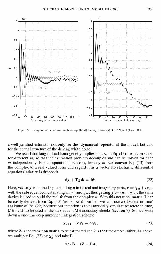
where the integrals are over a latitude circle. Estimates of the aperture functions hρ andhU are presented in Fig. 5, where it can be seen that hU tends to be highly non-local inphysical space and hρ tends to oscillate. Oscillations may be caused by the numericalscheme of the shallow-water model used, but the non-locality does not seem to be aresult of numerical approximation errors.

The non-locality of the advection (and, partly, dissipation) operator is a veryimportant ME feature because it implies that operator A (see Eq. (19)) appears to benot of differential type. Indeed, let A be a differential operator, A = ∑

k ak∂/∂xk, with

constant coefficients ak. Then, the action of the zero-order term (multiplication by areal number) can be represented as a convolution with the delta-function. The first-orderterm acts as (minus) the convolution with the first derivative of the delta-function, andso on. In general, a differential operator can be considered as a convolution with a linearcombination of the delta-function’s derivatives. On the other hand, in real problems,the delta-function manifests itself as a spike with small support and its derivatives ashighly localized damped ‘wavelets’ with the number of extrema equal to the order ofthe derivative plus one. Thus, the non-local behaviour of the hU aperture function visiblein Fig. 5 means that operator A cannot be even approximated by a differential operator.A practical consequence is that we have to be prepared to deal with an ME model that,in contrast to an atmospheric forecast model, is not of the differential-in-space type:

∂η(t, r)∂t

+∫

H(r, r′)η(t, r′) dr′ = α(t, r), (21)

where r is the spatial coordinate and H is the general (non-degenerate) aperture functionto be estimated from observations; this equation is a natural generalization of Eq. (20).

(c) Model FULL estimationThe most sophisticated (in this study) ME model FULL is estimated using a vector-

matrix extension to the above method-of-moments technique, which enables us to obtain


(a) (b)

Figure 5. Longitudinal aperture functions hU (bold) and hρ (thin): (a) at 30◦N, and (b) at 60◦N.

a well-justified estimator not only for the ‘dynamical’ operator of the model, but alsofor the spatial structure of the driving white noise.

We recall that longitudinal homogeneity implies that αm in Eq. (13) are uncorrelatedfor different m, so that the estimation problem decouples and can be solved for eachm independently. For computational reasons, for any m, we convert Eq. (13) fromthe complex to a real-valued form and regard it as a vector Ito stochastic differentialequation (index m is dropped),

dχ + Tχdt = dψ . (22)

Here, vector χ is defined by expanding η in its real and imaginary parts, η =: ηre + iηim,with the subsequent concatenating all ηre and ηim, thus getting χ := (ηre : ηim); the samedevice is used to build the real ψ from the complex α. With this notation, matrix T canbe easily derived from Eq. (13) (not shown). Further, we will use a (discrete in time)analogue of Eq. (22) because our intention is to numerically simulate (discrete in time)ME fields to be used in the subsequent ME adequacy checks (section 7). So, we writedown a one-time-step numerical integration scheme

χk+1 = Zχk +�ψk, (23)

where Z is the transition matrix to be estimated and k is the time-step number. As above,we multiply Eq. (23) by χT

k and take E :

�t · B = (Z − I)A, (24)


where A := E χk · χTk (E denotes time averaging over the ‘learning’ sample) is the

‘observed’ simultaneous covariance matrix, B := E (�χk/�t) ·χTk is another (cross-

covariance) matrix estimated from empirical data, �χk := χk+1 − χk, and I is theidentity matrix. In deriving Eq. (24) we used the fact that �ψk is uncorrelated withχk because, as noted, stochastic differential equation (22) is taken to be of the Ito type.

In scheme (23), we have to specify matrix Z and the covariance matrix of�ψk , ��ψ . Z can be obtained from (24), whilst ��ψ can be estimated using theLyapunov equation written in the discrete-in-time form. To derive the latter, we requirethat a numerical solution to Eq. (23) converge to some stationary regime and, in thisregime, its simultaneous covariance matrix be equal to the ‘observed’ one, A. To estab-lish this, we derive the covariance matrix of the r.h.s. of Eq. (23) and equate it to A:

A = ZAZT + ��ψ . (25)

Now, all we need to do is to solve Eqs. (24) and (25) for Z and��ψ . But, in addition,we have to establish that numerical scheme (23) is stable and matrix ��ψ is positivedefinite. We use the following ad hoc technique. First, with A and B being estimatedfrom ηemp, we solve Eq. (24) for Z. In so doing, it appeared to be necessary to regularizethe problem by artificially increasing the smallest eigenvalues of A, so that the conditionnumber of matrix A is not greater than some threshold νmax (about 104 for our dataand latitudinal grid). Then, we eigen-decompose Z and enforce stability by making alleigenvalues less than unity in modulus; if necessary, we multiply Z by a real number θthat is close to and less than unity, so that matrix θZ has all its eigenvalues within theunit circle on the complex plane. Next, we compute ��ψ from Eq. (25) and check itspositive definiteness. If it has negative eigenvalues, we somewhat decrease θ and repeatthe process several times. Since matrix ZAZT in Eq. (25) is positive definite, it is easyto understand that decreasing θ > 0 will eventually lead to positive definite ��ψ , whilethe eigenvalues of Z are retained within the unit circle.

Thus, model FULL is completely estimated. Now, we are going to check the valueof the three stochastic ME models in direct ensemble-based predictability experiments.

6. SIMULATION OF ME

The above ME models can be used as simulators of pseudo-random ME. The state-dependent part of ME is completely determined by the state and thus is simulatedstraightforwardly. To simulate the state-independent part of ME, η, using one of theabove ME models, we numerically solve the respective stochastic differential equation(11), (12), or (13) in space of Fourier coefficients in longitude. In the latter case, we usescheme (23). Otherwise, we use the backward Euler scheme. Note that, in general, onecannot use a deterministic numerical scheme to solve a stochastic differential equation,but in our case, we are allowed to do so because the diffusion coefficients (σ in Eq. (15))are non-random, see e.g. Pugachev and Sinitsin (1987).

All the ME-model estimation and ME simulation programs were self-checked;the output of a ME simulator was used as an input to the respective ME modelestimator. The programs were debugged until, in the chain ME model estimator →ME simulator → ME model estimator , the outputs of the two estimator runs were

reasonably similar (not shown).In Fig. 6, we compare patterns of the simulated field, ηsim, with those of its

empirical counterpart, ηemp. The similarity between ηemp (left) and ηsim (right) is


(a) (b)

(c) (d)

Figure 6. Realizations of state-independent ME: longitude–time cross-sections at 20◦N of (a) empirical and(b) simulated fields, and examples of instantaneous (c) empirical and (d) simulated longitude–latitude fields.

In all cases, negative contours are dashed.


better than expected. The simulated fields show small-scale detail, probably due tocomputational noise.

It is worth interpreting the results. In the longitude–time plot (Fig. 6(a)), one clearlysees signatures of propagating waves. From this point of view, our vorticity-equation‘model’ differs from the shallow-water ‘system’ in two respects: first, in contrast to the‘system’, the ‘model’ possesses no gravity waves, and second, the ‘model’ somewhatdistorts Rossby waves. Therefore, ME, as a difference of the ‘model’ and ‘system’right-hand sides, is (in the linear approximation) a superposition of Rossby-wave andgravity-wave contributions. The spatio-temporal behaviour of ME presented in Fig. 6(a)can be interpreted as a high-frequency chaotic gravity-wave-related field (as gravitywaves propagate in all directions) on the background of westward-propagating Rossby-wave-related field. In this respect, our ME models attempt to represent (i) the Rossby-wave-related field—by selecting and fitting the ‘dynamical’ operator of the ME model(in particular, by introducing the effective advection), and (ii) the gravity-wave-relatedfield—by introducing the driving random noise.

So, we see that our ME-model building strategy yields the ME field very similar inspatio-temporal structure to the ‘true’ one. At the same time, linearity and lack of onewave type makes the ME model quite simple, as desired. Now, we turn to the quantitativevalidation of our ME models.

7. ENSEMBLE VALIDATION OF THE ME MODELS

We utilize the proposed and estimated ME models as simulators of pseudo-randomME, replace actual ME with the simulated ones, and verify how well the forecast-errorstructure in response to simulated ME mimics the ‘true’ one.

(a) Validation methodologyWe obtain ‘true’ forecast errors induced by ME by starting ‘model’, Xm(t), and

‘system’, Xt(t), forecasts from the same initial conditions (taken from the referenceshallow-water solution in its quasi-stationary regime, see section 4(a)), so that theforecast error is X′

tru := Xm − Xt. To obtain simulated forecast errors, we substitute(a realization of) ηsim for η in Eq. (6) with X′(0)= 0 and g computed following Eq. (10),that is, we integrate the ‘model’ while subtracting the simulated ME (i.e. ηsim + g) fromthe ‘model’ r.h.s. every time step. In this way, we obtain an ensemble of ‘simulatedtruths’, Xe

i , i = 1, . . . , N , where N is the ensemble size. The simulated forecasterror is then X′

i := Xm − Xei . If an ME model is adequate, then all aspects of the

probability distribution of forecast errors, X′tru, are close to those of simulated forecast

errors, X′i . Note that the simulated forecast errors are stochastic by construction, whilst

the empirical ones are assumed to be so because our ‘system’ and ‘model’ are chaotic.As it follows from the theory presented in section 2, ‘true’ and simulated forecast

errors can be considered as samples from the respective conditional probability distri-butions given the initial forecast field, Xm(0). The unconditional distributions can beestimated by averaging over Xm(0) (over the attractor, if it exists). Instead, we make useof the spatial ergodicity of the forecast error field, which follows from the fact that itszonal correlation radii are much smaller than the earth radius (not shown) and replaceaveraging over Xm(0) by longitudinal averaging (Monin and Yaglom 1971, chapter 4).For ensemble covariances, we also average over the ensemble.

To compare the ensemble versus ‘true’ forecast-error distributions, we perform twochecks. First, we compare averaged over all ‘synoptic situations’ distributions, and


second, we examine flow-dependent aspects of the ensemble distribution against the‘truth’.

(i) Assessment of the averaged ensemble distribution. In ensemble forecasting, it iscommon to compare the point-wise ensemble with observed one-dimensional prob-ability distributions averaged over many cases using the so-called rank histograms(e.g. Hamill 2001). This technique allows detailed examination of the averaged ensem-ble distribution but only in one (point-wise) respect, all spatial (and temporal) aspectsbeing disregarded. In this study, we use a much simpler r.m.s. measure to compare thepoint-wise ensemble and ‘true’ distributions, but propose to examine also spatial andtemporal characteristics of the multi-dimensional ensemble forecast-error distribution—for two reasons. First, spatial forecast-error statistics are needed in data assimilation.Second, users of ensemble forecasts may be interested in probability forecasts not justof point-wise weather elements but also of some spatial/temporal averages or gradients.

So, we examine four aspects of the averaged spatio-temporal ensemble forecast-error probability distribution. First, we compare the ensemble and ‘true’ point-wisedistributions. Their means are checked below in the flow-dependent context.The ensemble mean is used to perform bias correction, after which r.m.s. ‘true’ and en-semble forecast errors, dens(ϑ, t) and dtru(ϑ, t), are compared. (Here and below, r.m.s.and corr operations involve averaging over longitude—for ‘true’ forecast errors, andboth longitudinal and ensemble averaging—for ensemble forecast errors.) We quantifythe globally and temporally averaged consistency between ensemble and ‘true’ forecast-error magnitudes as

μrms :=⟨⟨

min(dens(ϑ, t), dtru(ϑ, t))

max(dens(ϑ, t), dtru(ϑ, t))

⟩ϑ

⟩t

, (26)

where 〈.〉ϑ means latitudinal and 〈.〉t temporal averaging. Obviously, this consistencyscore is always between zero and one; the greater the score, the better the ensemble.

Second, we compare longitudinal, latitudinal, and temporal correlations. To do so,we estimate ‘true’ and ensemble forecast-error decorrelation length-scales, Llon, Llat,and Ltime (see appendix B); then, we calculate consistency scores μlon, μlat, and μtimeby replacing, in Eq. (26), d by the respective 0.7-decorrelation lengths.

Summarizing, we reduce the verification of the point-wise distribution to comparingensemble versus ‘true’ r.m.s. forecast-error values; however, we suggest examining notonly one-dimensional point-wise distributions but also important spatial and temporalaspects of the ensemble distribution.

(ii) Assessment of flow-dependent ensemble statistics. In data assimilation and en-semble forecasting, we wish an ensemble to produce not only correct averaged distribu-tions, but also correct flow-dependent statistics for any time and geographical point.In particular, we would expect that some important characteristics of the ensembleforecast-error distribution do correlate with the true ones. As above for the averaged(flow-independent) forecast-error distributions, we consider here spatial and tempo-ral aspects of the distributions as well as characteristics of point-wise distributions.We introduce five measures (scores). We define score (i) as the portion of the r.m.s.forecast error that can be explained (and thus removed) by the flow-dependent ensembleforecast-error bias, be := Xm − ∑

Xei /N :

γbias := 1 −⟨⟨

r.m.s. {X′tru − be(ϑ, ϕ, t)}

r.m.s. (X′tru)

⟩ϑ

⟩t

. (27)


TABLE 1. ENSEMBLE PERFORMANCE SCORES FOR THE CASE WHEN THE FORECAST MODEL IS NOTCORRECTED FOR STATE DEPENDENCE

Row Model μrms μlon μlat μtime γbias νrms νlon νlat νtime

1 NO STATE-DEP ME 0.84 0.85 0.80 0.88 0.01 0.30 0.21 0.27 0.162 NO STOCH ME 0.85 0.68 0.67 0.83 0.48 – – – –3 FULL 0.85 0.87 0.78 0.93 0.50 0.31 0.22 0.24 0.19

All scores are positively oriented: ‘the greater, the better’. μ denote averaged-distributional scores,γbias the effect of the ensemble-bias correction, and ν the flow-dependent scores.

Score (ii) is defined to be the widely-used skill-spread correlation (e.g. Whitakerand Loughe 1998) applied for ensemble-bias-corrected both the ensemble and ‘true’forecast errors, νrms (the correlation is again calculated using longitudinal averaging).Scores (iii)–(v), νlon, νlat, and νtime, are defined to be again skill-spread correlationsbut computed for the fields of local longitudinal, latitudinal, and temporal estimatedmicro-scales, λlon, λlat, and λtime, introduced in appendix B, e.g. νlon := corr (λlon

ens, λlontru )

etc. These new flow-dependent ensemble performance scores (iii)–(v) allow us toverify whether places and times where and when ensemble forecast errors are locallysmall-scale (large-scale) really indicate situations with the high (low) ‘true’ spatial andtemporal forecast-error variability. This is especially important in the data assimilationcontext.

Thus, we have presented several (known and new) ensemble performance scoresthat emphasize consistency of ensemble (versus ‘true’) forecast-error magnitudes, spa-tial, and temporal length-scales—in both the averaged and flow-dependent senses. Now,we are prepared to look at the results.

(b) ResultsWe use the above ensemble verification scores to judge the success of the ME

models proposed in this study. We investigate the roles of stochastic versus deterministic(state-dependent) ME components and the sensitivity of the ensemble performance tovarious aspects of an ME model.

In the following experiments the ensemble size is 150. Such a relatively largenumber of (non-paired) ensemble members appeared to be necessary to obtain stableflow-dependent verification scores; for the averaged-distributional scores, a size of 50 issufficient. Forecasts up to 8 days are examined. Several ‘learning’ and validation periodswere tested with the same qualitative results. Flow-dependent features in the ensembletake some time to develop (2 days in these experiments), so the respective scores arecomputed for the lead times from 2 to 8 days.

(i) The roles of state-dependent versus purely stochastic ME. First, we create anensemble without state-dependent ME (we estimate the above model FULL assuming—as can take place in practice—that g from Eqs. (4) and (10) is zero). The resultingensemble performance scores are given in Table 1, row 1 and thus represent the case ofpurely stochastic ME. Row 2 of Table 1 shows the results for purely deterministic state-dependent ME, g, without any contribution of stochastic ME, η, see Eq. (4)—stochasticMEs were simply nullified there. Of course, in this latter case, only averaged ensembleperformance scores can be calculated because without the stochastic part of ME, justone ensemble member can be generated. Finally, in row 3 of Table 1 we present resultsfor the ‘normal’ case with both ME components.

From Table 1, one can conclude that both state-dependent (deterministic) andstochastic parts of ME are critically important. Indeed, removing all the above stochastic


TABLE 2. AS TABLE 1, BUT FOR THE STATE-DEPENDENCE-CORRECTED FORECAST MODEL


1 PHYS 0.73 0.71 0.66 0.86 −0.01 0.20 0.18 0.13 0.162 LONSPE 0.67 0.79 0.46 0.87 0.00 0.24 0.17 0.16 0.163 FULL 0.84 0.87 0.78 0.93 0.04 0.31 0.22 0.24 0.194 Perfect ens. 0.80 0.80 0.79 0.91 0.02 0.33 0.25 0.26 0.19

modelling machinery, results (see row 2) in the substantially inferior spatial forecast-error statistics (as compared to the full-fledged ME model, row 3) but reasonable ensem-ble forecast-error magnitudes (measure μrms) and efficient ensemble-bias correction.On the other hand, the purely stochastic (state-dependence blind) ME model (row 1)yields adequate r.m.s. and spatio-temporal forecast-error statistics (measures μ and ν)but fails in ensemble-bias correction. So, in these experiments, the ensemble mean ismore accurate than the deterministic forecast mostly due to the state-dependent part ofthe ME model.

For some characteristics of the averaged distributions, the purely stochastic MEmodel looks even superior; this superiority is illusory and can be explained as follows.Without removing state-dependence, the ME model ‘considers’ the state-dependent partof ME as stochastic. But this part, linearly related to the vorticity field, is more large-scale because a field itself is normally more large-scale than its error field. Therefore, inthe case of the purely stochastic ME model, MEs appear to be more large-scale and socan be modelled more easily, hence giving better performance scores.

The above results suggest the need to look for state dependence when creating anME model. But, once some state dependence is found, it is worth using it to empiricallycorrect the forecast model itself. In the following experiments we do so and thus examineonly the stochastic part of the ME models.

(ii) Comparing the quality of the proposed ME stochastic models. In Table 2,we present the above ensemble performance scores for the three ME models, PHYS,LONSPE, and FULL, along with the perfect-ensemble scores. In the perfect ensem-ble, the ‘truth’ is replaced by one of the ensemble members; model FULL was used togenerate the perfect ensemble.

The results clearly demonstrate the superiority of model FULL, the most sophisti-cated ME model in this study. The performance of the two simpler models, however, isalso not bad. That some performance scores for model FULL are even slightly bet-ter than those for the perfect ensemble, does not imply an error or a program bug.The general reason why this can take place is that the distribution of the ‘true’ forecasterrors changes as a result of the replacement of the ‘truth’ by an ensemble member.But different distributions of the ‘truth’ may well result in different performance scoresof even perfect ensembles (and this is really observed if models PHYS or LONSPEare used to generate the perfect ensemble, not shown). So, we cannot rigorously com-pare ensemble performance scores for the cases with different ‘truths’, consequently theperfect ensemble ‘has the right’ to be slightly worse than a non-perfect ensemble.

Thus, we state that all the three proposed ME models are capable of inducingforecast errors whose structure resembles the ‘true’ one. Model FULL is found to havealmost perfect performance.

(iii) Sensitivity of ensemble forecasts to various aspects of ME models. To gainmore insight into the impact of ME on forecast errors, we deliberately distort sometemporal and spatial aspects of the ME models and look how much worse the ensemble


TABLE 3. AS TABLE 2, BUT FOR THE DELIBERATELY DISTORTED ME MODELS


0 FULL 0.84 0.87 0.78 0.93 0.04 0.31 0.22 0.24 0.191 CONST 0.72 0.78 0.71 0.88 −0.05 0.27 0.19 0.20 0.182 WHITE 0.75 0.84 0.74 0.73 0.02 0.28 0.20 0.23 0.143 PHYS 0.73 0.71 0.66 0.86 −0.01 0.20 0.18 0.13 0.164 s-WHITE 0.53 0.64 0.24 0.76 0.01 0.12 0.11 0.12 0.145 s-t-WHITE 0.59 0.09 0.16 0.27 0.00 −0.04 0.04 0.04 0.116 misPHYS (Uea = 0) 0.72 0.71 0.66 0.86 −0.01 0.19 0.17 0.14 0.16

forecasts become. First, we distort the temporal aspect of model FULL. Row 1 of Table 3shows the ensemble performance scores for model CONST whose spatial structure isfrom model FULL but MEs are constant in time. Row 2 demonstrates the results formodel WHITE whose spatial structure is again from model FULL but MEs are white intime.

Second, we distort the spatial structure of an ME model; we use model PHYS butchange the driving-noise spatial structure so that MEs become white in space (models-WHITE, row 4 of Table 3). In row 5, we display the results for model PHYS withboth spatial and temporal correlations enforced to be delta-correlated (white)—models-t-WHITE.

Finally, we distort the mixed spatio-temporal structure of an ME model; in modelPHYS, we nullify the effective advection velocity, Uea (model misPHYS, row 6).

For comparison, we also include, in Table 3, the above results for the referencemodels FULL and PHYS (rows 0 and 3, respectively).

From the results presented in Table 3, we see that ensemble forecasts are quitesensitive to the ME model characteristics. The most obvious consequence of reducingthe temporal time-scale is the decrease of the simulated forecast-error magnitude.Indeed, to a very first approximation, the forecast error induced by ME is the integralof the ME (the drift, see e.g. Orrell et al. 2001). On the other hand, one can verify that,again approximately, the variance of the integral of a stationary random process (recallthat MEs are assumed to be stationary) is proportional to the temporal macro-scale ofthe process (and to the length of the integration interval). So, decreasing the temporalmacro-scale of the ME field implies smaller forecast-error variance. For example, ifmodel WHITE is used, the forecast-error r.m.s. value becomes about five times less.For this reason, to make the distorted ME models more competitive, we multiply theirsimulated MEs by an empirically selected factor (which, of course, can always be donein a practical problem). The multiplication factor is 5 for model WHITE, 10 for model s-t-WHITE, and 3 for model s-WHITE. One may ask why we have to artificially enhanceME for spatially (and not temporally) white model s-WHITE. The answer is that thespatio-temporal ME field appears to possess the above-mentioned ‘proportionally ofscales’ property (e.g. Tsyroulnikov 2001); smaller spatial scales are associated withsmaller temporal scales. Therefore, decreasing the spatial scale results in decreasingthe temporal one, hence the decreased forecast-error variance, as discussed. Anotherquestion is why model s-t-WHITE yields even smaller forecast errors than modelWHITE (see the difference in the multiplication factors above in this paragraph). Apossible answer is that an equivalent linear forecast-error-evolution model is not just thedrift (the time integral) but involves some spatial averaging, hence the decrease in theerror variance for the spatially white ME model.

But even improved in such a way (with tuned magnitudes), the models withdistorted spatial or temporal ME structure (rows 1–2 and 4–6) turn out to be noticeably


worse than the non-distorted models (FULL or PHYS, respectively). The only exceptionis that nullifying Uea in model misPHYS yields only a minor deterioration of theensemble performance; the reason for this outcome is not quite clear. One can also noticethat model CONST shows relatively good results. This can be explained by the ratherlarge temporal scale of MEs in this study (the dissipation time-scale is about 2.5 days).

Summarizing, we state that specifying correct both spatial and temporal structureof MEs is critical for designing a skilful ME-dependent forecast ensemble. Errors inspatial/temporal structure of the ME model induce errors in both spatial and temporalforecast-error structure.

8. CONCLUSIONS

The main findings of this study are:

• In the setting with the barotropic vorticity equation as a forecast model and theshallow-water equations as a ‘truth’, model (tendency) errors (MEs) can be suc-cessfully modelled stochastically; this is verified in direct ensemble experiments.

• For a ME model to be adequate, accounting for (local) ME state dependence iscrucial.

• After removing local linear state dependence from the model-error field, theresidual can be modelled by a linear stochastic model, which has the followingprincipal features:

(i) The temporal order of the ME model can be selected as small as 1 (i.e. the modelis of the red-noise type) in spite of some indications of a higher-order behaviourin the ‘true’ ME fields. The (white) driving noise can be taken as Gaussian despitesome observed deviations of the multivariate Gaussianity.(ii) The salient feature of the ME model is that MEs are advecting (moving), withthe effective advection velocity being substantially different from the wind.(iii) Written in the advection-dissipation form, the ‘dynamical’ part of the stochas-tic ME model has advection velocity and dissipation rate which are both highlyscale-dependent, the former being qualitatively similar to the Rossby-wave phasevelocity.(iv) In the general physical-space form, the stochastic ME model can be viewed asa differential-in-time and integral-in-space system, the transition (from one timeinstant to the next) matrix being essentially not sparse.

• The forecast-error spatio-temporal structure (both averaged and flow-dependent)appears to be quite sensitive to the formulation of the ME model.

• As a by-product, we found that and explained why, in a shallow-water solution,divergence can correlate with meridional wind.

• We have proposed new ensemble verification scores that emphasize spatial andtemporal aspects of the ensemble forecast-error distribution.

We finish with a brief discussion on practical consequences of this study.The fact that a linear ME model driven by white Gaussian noise appeared to

be very successful has important consequences for data assimilation, as discussed inthe introduction. With an adequate ME model, we can properly set up the Kalmanfiltering equations and select the norm of the forecast-equation discrepancies in theweak-constraint 4D-Var. (It is the white-noise variable that should be penalized as asum of squares of its components.)


The selected ‘system-model’ pair used in this study reflects the realistic situation inthe sense that here the ME field contains a contribution from gravity waves (not resolvedby our vorticity-equation ‘model’), while MEs of a realistic primitive-equation forecastmodel contain, among others, a similar acoustic-wave field contribution. The results ofthis research indicate that, in an ME model, we are allowed to represent the impactof a non-resolved wave-field by the introduction of a random noise in the r.h.s. of theME-model equations.

The sensitivity of spatio-temporal forecast-error structure to the formulation of anME model and its parameters emphasizes the role of ME modelling because correctspatial and temporal forecast-error covariances are indispensable, not only in dataassimilation but in ensemble forecasting as well. For example, correct temporal structureis needed if one is interested in probabilistic forecasts of, say, the duration of somespecific weather conditions at some place, or some weather change. Similarly, correctspatial forecast-error covariances are necessary for probabilistic prediction of some area-averaged characteristics (say, precipitation) or spatial gradients.

The difference of a realistic ME-related problem from the idealized one consideredin this research is twofold. First, a weather-prediction model is more active (unstable)than the barotropic models used in this study. Second, in contrast to the presentcase, a realistic prediction model has numerous sources (components) of error, so thatdifferent components of ME may be governed by different kinds of stochastic models.This may require individual treatment of each ME component, which looks promisingin the future but too complicated now. Instead, we may speculate that for some large(sub)set of ME components, the structure of their sum could be less specific than thatof any single ME component. So, it seems meaningful to try to model the combinedeffect of many ME sources by just one ME model. We have attempted to investigatesome key features of such an ME model in the present study, albeit in a simplifiedsetting.

The results of this study suggest that for a practical weather-prediction model, it isworth seeking an ME model within the following class. First, one should look for alocally (in physical space) state-dependent ME component (state-dependence of thefirst kind). Second, the residual ME can be regarded as stochastic, satisfying a linearadvection-dissipation equation forced by the white-in-time noise. Finally, parameters ofthis equation (variance and local spatial length-scales of the driving noise, the effectiveadvection velocity vector, and the dissipation time-scale) are, most likely, also dependenton the local flow structure (state-dependence of the second kind).

Before the models developed in this study can be implemented in practical dataassimilation and ensemble weather prediction, practicable observation-based stochastic-model estimation techniques should be devised. If one has enough observations toexplicitly evaluate MEs for some forecast model, then the above estimation techniquescan be used to obtain a realistic ME model.

ACKNOWLEDGEMENTS

I would like to thank M. A. Tolstykh, who provided me with the shallow-watermodel and helped in using it. Many thanks to H. Anlauf for his helpful comments.I appreciate a discussion on model errors with D. Orrell. Valuable comments of the twoanonymous referees helped much in improving the paper. The figures were preparedwith the GrADS package. This study was supported by the Russian Foundation forBasic Research under grant 04-05-64481.


Figure A.1. Correlation (%, solid) between divergence and meridional wind, the mean flow (m s−1, dashed),and the effective advection velocity for geopotential (m s−1, dotted).

APPENDIX A

Correlation of divergence and meridional wind in a shallow-water modelThe first idea why this may happen is that the geostrophic divergence, δg, is

proportional to the geostrophic meridional wind: δg = −βvg/fc. But the sign of thelatitudinal dependence of cov (δg, vg)= −(β/fc)D vg differs drastically from what isobserved in the shallow-water solutions—see Fig. A.1 (the solid curve), where, to makethe picture more impressive than in the case of the statistically quieter quasi-steady-statedynamics (as above), we started the solution from realistic atmospheric wind and massfields. Besides, we note that in our experiments, divergence, δ, is of the order 10−7m s−2

in midlatitudes, whereas δg is about 4 × 10−7m s−2. As a result, δg is largely balancedby the ageostrophic divergence, so that δ is a small difference of large quantities andtherefore does not inherit their properties.

So, another explanation is needed. By visual inspection of the model fields(not shown), it was found that the ‘frozen turbulence’ hypothesis is largely applicable.So, for geopotential, to a first approximation and on small time-scales,

�(t, x, y)≈�0(x − Ueat, y), (A.1)

where�0 is some function of spatial coordinates only and Uea is the effective advectionvelocity. Hence, from quasi-geostrophy,

vg = 1

fc

∂�

∂x≈ 1

fc

∂�0

∂x. (A.2)


On the other hand, consider the mass conservation equation of the shallow-watersystem: ∂�/∂t + u∂�/∂x + v∂�/∂y = −�δ. In the quasi-geostrophic regime, theadvection terms on the l.h.s. of this equation mainly cancel, implying ∂�/∂t ≈ −�δ.But from Eq. (A.1), ∂�/∂t ≈ −Uea∂�0/∂x, whence

δ ≈ − 1

�

∂�

∂t≈ Uea

�

∂�0

∂x. (A.3)

Comparing Eqs. (A.2) and (A.3), we derive

δ ≈ fcUea

�v. (A.4)

Hence, the more quasi-geostrophic and ‘frozen’ the flow is, the stronger is thecorrelation between divergence and meridional wind, the sign of the correlation beingdetermined by the fcUea product. To demonstrate this, we also plotted in Fig. A.1 themean zonal velocity U0 and Uea for the geopotential field (estimated following thetechnique described in section 5(a)). One can see that the signs of corr (δ, v) and fcUeacoincide almost everywhere, which confirms our theoretical analysis. (Note that it is Ueaand not U0 that determines the sign of the correlation.)

Thus, we have explained why, in a shallow-water solution, divergence correlateswith meridional wind. This feature turns out to be a consequence of the combined effectof quasi-geostrophy and the ‘frozen turbulence’ hypothesis.

APPENDIX B

Spatial and temporal length-scales used in this study(i) To quantify spatial and temporal correlations of the forecast-error field, we use

0.7-decorrelation lengths defined as minimal distances at which the respective correla-tion functions equal 0.7. The correlation functions are estimated for the ‘true’ forecasterrors by longitudinal averaging, and for ensemble forecast errors by longitudinal andensemble averaging. The longitudinal correlation function is defined in the usual waybecause of longitudinal homogeneity, but the temporal and latitudinal correlation func-tions need to be defined in some other way in view of non-stationarity and latitudinalnon-homogeneity of forecast errors. We estimate two unidirectional correlation func-tions (for the time coordinate, these are E X′(t − τ )X′(t) and E X′(t)X′(t + τ ), witht being the reference time and τ the time shift; similarly for latitude), then estimatethe respective unidirectional 0.7-decorrelation lengths, and use their half-sum as a finalestimate.

(ii) To characterize flow-dependent forecast-error length scales at any point in spaceand time, we introduce approximate local micro-scales defined as follows. Along anycoordinate axis of the local coordinate system on the sphere, x and y, and also t , weassess the respective partial derivative using the central finite difference and average itsmodulus over the standard moving 5-point stencil over x, y, getting Dx ≈ |∂X′/∂x|,etc. Then, in the same way, we average (over the stencil) the absolute deviation ofthe forecast error from its global mean, getting the characteristic magnitude, s, of thefield at this particular point. Finally, we define the local micro-scale in direction x asλx ≡ λlon := s/Dx ; λy ≡ λlat and λtime are defined analogously. Note that only onerealization of the field in question is needed in order to compute the fields of theseapproximate local micro-scales.


REFERENCES

Buizza, R., Miller, M. andPalmer, T. N.

1999 Stochastic representation of model uncertainties in the ECMWFensemble prediction system. Q. J. R. Meteorol. Soc., 125,2887–2908

Cohn, S. E. 1997 An introduction to estimation theory. J. Meteorol. Soc. Jpn., 75,257–288

Daley, R. 1992 The effect of serially correlated observation and model erroron atmospheric data assimilation. Mon. Weather Rev., 120,164–177

DelSole, T. and Hou, A. Y. 1999 Empirical correction of a dynamical model. Part I: fundamentalissues. Mon. Weather Rev., 127, 2533–2545

Eckel, F. A. and Mass, C. F. 2005 Aspects of effective mesoscale, short-range ensemble forecasting.Weather and Forecasting, 20, 328–350

Hamill, T. M. 2001 Interpretation of rank histograms for verifying ensembleforecasts. Mon. Weather Rev., 129, 550–560

Hannan, E. J. 1970 Multiple time series. John Wiley, New York, USAHoutekamer, P.L., Lefaivre, L.,

Derome, J., Ritchie, H. andMitchell, H. L.

1996 A system simulation approach to ensemble prediction. Mon.Weather Rev., 124, 1225–1242

Jazwinski, A. H. 1970 Stochastic processes and filtering theory. Academic Press,New York and London

Menard, R., Cohn, S. E.,Chang, L.-P. and Lyster, P. M.

2000 Assimilation of stratospheric chemical tracer observations using aKalman filter. Part I: Formulation. Mon. Weather Rev., 128,2654–2671

Menemenlis, D. andChechelnitsky, M.

2000 Error estimates for an ocean general circulation model fromaltimeter and acoustic tomography data. Mon. Weather Rev.,128, 763–778

Mitchell, H. L. and Daley, R. 1997 Discretization error and signal/error correlation in atmosphericdata assimilation. I: All scales resolved. Tellus, 49A, 32–53

Monin, A. S. and Yaglom, A. M. 1971 Statistical fluid mechanics: mechanics of turbulence. Vol. 1.MIT Press, Cambridge, MA, USA

Nicolis, C. 2005 Can error source terms in forecasting models be representedas Gaussian Markov noises? Q. J. R. Meteorol. Soc., 131,2151–2170

Orrell, D., Smith, L., Barkmeijer, J.and Palmer, T. N.

2001 Model error in weather forecasting. Nonlinear Proc. Geophys., 8,357–371

Palmer, T. N. 1995 ‘Predictability of the atmosphere and oceans: From days todecades’. Pp. 83–140 in Proceedings of ECMWF Seminaron Predictability, 4–8 September 1995. Vol. 1. ECMWF,Reading, UK

2001 A nonlinear dynamical perspective on model error: A proposalfor non-local stochastic-dynamic parametrization in weatherand climate prediction models. Q. J. R. Meteorol. Soc., 127,279–304

Pedlosky, J. 1987 Geophysical fluid dynamics. Springer, New York, USAPugachev, V. S. and Sinitsin, I. N. 1987 Stochastic differential systems. Analysis and filtering. John Wiley,

New York, USARichtmyer, R. D. and Morton, K. 1967 Difference methods for initial value problems. Interscience-Wiley,

New York, USASura, P., Newman, M., Penland, C.

and Sardeshmukh, P.2005 Multiplicative noise and non-Gaussianity: a paradigm for atmos-

pheric regimes? J. Atmos. Sci., 62, 1391–1409Tolstykh, M. 2002 Vorticity-divergence semi-Lagrangian shallow-water model on

the sphere based on compact finite differences. J. Comput.Phys., 179, 180–200

Tsyroulnikov, M. D. 2001 Proportionality of scales: An isotropy-like property of geophysi-cal fields. Q. J. R. Meteorol. Soc., 127, 2741–2760

Whitaker, J. S. and Loughe, A. F. 1998 The relationship between ensemble spread and ensemble meanskill. Mon. Weather Rev., 126, 3292–3302

Xu, L., Rosmond, T. and Daley, R. 2005 Development of NAVDAS-AR: formulation and initial tests of thelinear problem. Tellus, 57A, 546–559

Yaglom, A. M. 1987 Correlation theory of stationary and related random functions.Vol. 1: Basic results. Springer, New York, USA

Zupanski, D. 1997 A general weak constraint applicable to operational 4D-Var dataassimilation. Mon. Weather Rev., 125, 2274–2292

Stochastic modelling of model errors: A simulation study

Documents

Transcript of Stochastic modelling of model errors: A simulation study