
Simulation Model Development of Electric Motor and Controller
73
Simulation Model Development of Electric Motor and Controller Master’s thesis in Systems, Control and Mechatronics Wang Han Department of Electrical Engineering CHALMERS UNIVERSITY OF TECHNOLOGY Gothenburg, Sweden 2017
-
Upload
khangminh22 -
Category
Documents
-
view
3 -
download
0
Transcript of Simulation Model Development of Electric Motor and Controller
Simulation Model Development ofElectric Motor and Controller
Master’s thesis in Systems, Control and Mechatronics
Wang Han
Department of Electrical EngineeringCHALMERS UNIVERSITY OF TECHNOLOGYGothenburg, Sweden 2017

Master’s thesis 2017: EX010
Simulation Model Development ofElectric Motor and Controller
Thesis for the Degree of Master of Science in Engineering
Wang Han
Department of Electrical EngineeringDivision of Systems and Control
Chalmers University of TechnologyGothenburg, Sweden 2017
Simulation Model Development of Electric Motor and ControllerThesis for the Degree of Master of Science in EngineeringWang Han
© Wang Han, 2017.
Supervisor: Michael Palander, CEVTExaminer: Jonas Fredriksson, Department of Electrical Engineering
Master’s Thesis EX010/2017Department of Electrical EngineeringDivision of Systems and ControlChalmers University of TechnologySE-412 96 GothenburgTelephone +46 31 772 1000
Cover: "GEELY EMGRAND EV " from CEVT
iv
Simulation Model Development of Electric Motor and ControllerThesis for the Degree of Master of Science in EngineeringWang HanDepartment of Electrical EngineeringChalmers University of Technology
Abstract
As a result of the high efficiency requirement and the limited battery’s capacity,the permanent magnent synchronous machine(PMSM) has become a popular al-ternative for electric motor drive system, especially for the plug-in hybrid electricvehicle(PHEV) in automotive applications. In this thesis, the salient PMSM is stud-ied. A mathematical model of PMSM is derived from abc three-phase coordinates todq rotating reference frame. The flux linkage, voltage and current equations whichare used to analyze the performance of PMSMs are described both in equation formand matrix form. A Field oriented contro method is adopted for the speed controlof the PMSM and a current regulator is designed using a method called InternalModel Control (IMC). The entire PMSM drive system, including plant model, cur-rent regulator, speed controller, sinusoidal pulse width modulation (SPWM) andinverter is designed, implemented and simulated using Matlab/Simulink software.The plant model of the PMSM and the motor control unit are also exported andincluded in CarMaker for complete vehicle verification. The simulation results arepresented and a good dynamic response is shown.
Keywords: Permanent magnet synchronous machine(PMSM), dq reference frame,FOC, IMC, Sinusoidal Pulse Width Modulator(SPWM), Inverter, Carmaker
v

Acknowledgements
CEVT (China Euro Vehicle Technology AB) supported the thesis project financiallyand technically, which is gratefully acknowledged.
Initially, I would like to thank my supervisor Michael Palander for giving me such asuperb opportunity to conduct my master thesis at CEVT. His caring, encourage-ment and guidance have been crucial throughout the project.
I also want to express my gratitude to my examiner Jonas Fredriksson for his greatsupport and academic experience. His valuable ideas and comments are gratefullyappreciated.
I am very grateful to my good friend Muddassar Zahid Piracha, CEVT specialistalso a Ph.D student at Chalmers, who provided me with great technical supprotfrom begining to the end. I would also like to thank Johan Hellsing, the expert atCEVT, who had helped me concerning technical issues at all times.
I appreciated all the people who have ever helped me. Without your help andsupport, I cannot successfully accomplish my master thesis.
Last but not least, I would love to thank my parents for their endless love andsupport. Because of them, my dream has come true. Love you now and forever!
Wang Han
Göteborg, August 2017
vii

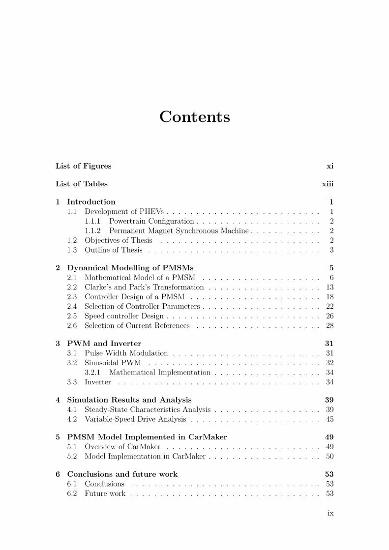
Contents
List of Figures xi
List of Tables xiii
1 Introduction 11.1 Development of PHEVs . . . . . . . . . . . . . . . . . . . . . . . . . . 1
1.1.1 Powertrain Configuration . . . . . . . . . . . . . . . . . . . . . 21.1.2 Permanent Magnet Synchronous Machine . . . . . . . . . . . . 2
1.2 Objectives of Thesis . . . . . . . . . . . . . . . . . . . . . . . . . . . 21.3 Outline of Thesis . . . . . . . . . . . . . . . . . . . . . . . . . . . . . 3
2 Dynamical Modelling of PMSMs 52.1 Mathematical Model of a PMSM . . . . . . . . . . . . . . . . . . . . 62.2 Clarke’s and Park’s Transformation . . . . . . . . . . . . . . . . . . . 132.3 Controller Design of a PMSM . . . . . . . . . . . . . . . . . . . . . . 182.4 Selection of Controller Parameters . . . . . . . . . . . . . . . . . . . . 222.5 Speed controller Design . . . . . . . . . . . . . . . . . . . . . . . . . . 262.6 Selection of Current References . . . . . . . . . . . . . . . . . . . . . 28
3 PWM and Inverter 313.1 Pulse Width Modulation . . . . . . . . . . . . . . . . . . . . . . . . . 313.2 Sinusoidal PWM . . . . . . . . . . . . . . . . . . . . . . . . . . . . . 32
3.2.1 Mathematical Implementation . . . . . . . . . . . . . . . . . . 343.3 Inverter . . . . . . . . . . . . . . . . . . . . . . . . . . . . . . . . . . 34
4 Simulation Results and Analysis 394.1 Steady-State Characteristics Analysis . . . . . . . . . . . . . . . . . . 394.2 Variable-Speed Drive Analysis . . . . . . . . . . . . . . . . . . . . . . 45
5 PMSM Model Implemented in CarMaker 495.1 Overview of CarMaker . . . . . . . . . . . . . . . . . . . . . . . . . . 495.2 Model Implementation in CarMaker . . . . . . . . . . . . . . . . . . . 50
6 Conclusions and future work 536.1 Conclusions . . . . . . . . . . . . . . . . . . . . . . . . . . . . . . . . 536.2 Future work . . . . . . . . . . . . . . . . . . . . . . . . . . . . . . . . 53
ix

Contents
Bibliography 55
A Appendix 1 I
B Appendix 2 III
x
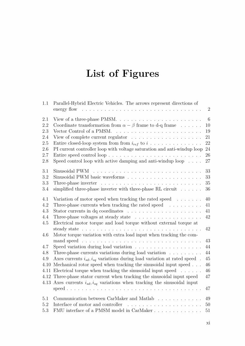
List of Figures
1.1 Parallel-Hybrid Electric Vehicles. The arrows represent directions ofenergy flow . . . . . . . . . . . . . . . . . . . . . . . . . . . . . . . . 2
2.1 View of a three-phase PMSM. . . . . . . . . . . . . . . . . . . . . . . 62.2 Coordinate transformation from α− β frame to d-q frame . . . . . . 102.3 Vector Control of a PMSM. . . . . . . . . . . . . . . . . . . . . . . . 192.4 View of complete current regulator . . . . . . . . . . . . . . . . . . . 212.5 Entire closed-loop system from from iref to i . . . . . . . . . . . . . . 222.6 PI current controller loop with voltage saturation and anti-windup loop 242.7 Entire speed control loop . . . . . . . . . . . . . . . . . . . . . . . . . 262.8 Speed control loop with active damping and anti-windup loop . . . . 27
3.1 Sinusoidal PWM . . . . . . . . . . . . . . . . . . . . . . . . . . . . . 333.2 Sinusoidal PWM basic waveforms . . . . . . . . . . . . . . . . . . . . 333.3 Three-phase inverter . . . . . . . . . . . . . . . . . . . . . . . . . . . 353.4 simplified three-phase inverter with three-phase RL circuit . . . . . . 36
4.1 Variation of motor speed when tracking the rated speed . . . . . . . 404.2 Three-phase currents when tracking the rated speed . . . . . . . . . 414.3 Stator currents in dq coordinates . . . . . . . . . . . . . . . . . . . . 414.4 Three-phase voltages at steady state . . . . . . . . . . . . . . . . . . 424.5 Electrical motor torque and load torque without external torque at
steady state . . . . . . . . . . . . . . . . . . . . . . . . . . . . . . . . 424.6 Motor torque variation with extra load input when tracking the com-
mand speed . . . . . . . . . . . . . . . . . . . . . . . . . . . . . . . . 434.7 Speed variation during load variation . . . . . . . . . . . . . . . . . . 444.8 Three-phase currents variations during load variation . . . . . . . . . 444.9 Axes currents isd, isq variations during load variation at rated speed . 454.10 Mechanical rotor speed when tracking the sinusoidal input speed . . . 464.11 Electrical torque when tracking the sinusoidal input speed . . . . . . 464.12 Three-phase stator current when tracking the sinusoidal input speed 474.13 Axes currents isd, isq variations when tracking the sinusoidal input
speed . . . . . . . . . . . . . . . . . . . . . . . . . . . . . . . . . . . . 47
5.1 Communication between CarMaker and Matlab . . . . . . . . . . . . 495.2 Interface of motor and controller . . . . . . . . . . . . . . . . . . . . 505.3 FMU interface of a PMSM model in CarMaker . . . . . . . . . . . . . 51
xi

List of Figures
5.4 FMU interface of a PMSM in CarMaker . . . . . . . . . . . . . . . . 51
xii

List of Tables
2.1 Control parameters . . . . . . . . . . . . . . . . . . . . . . . . . . . . 20
3.1 Inverter parameters . . . . . . . . . . . . . . . . . . . . . . . . . . . . 31
4.1 Motor parameters . . . . . . . . . . . . . . . . . . . . . . . . . . . . . 39
xiii

List of Tables
xiv
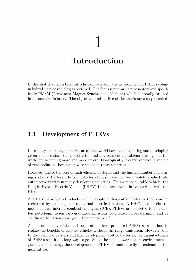
1Introduction
In this first chapter, a brief introduction regarding the development of PHEVs (plug-in hybrid electric vehicles) is reviewed. The focus is put on electric motors and specif-ically PMSM (Permanent Magnet Synchronous Machine) which is broadly utilizedin automotive industry. The objectives and outline of the thesis are also presented.
1.1 Development of PHEVs
In recent years, many countries across the world have been exploring and developinggreen vehicles since the petrol crisis and environmental problems throughout theworld are becoming more and more severe. Consequently, electric vehicles, a vehicleof zero pollution, becomes a wise choice in these countries.
However, due to the cost of high-efficient batteries and the limited number of charg-ing stations, Battery Electric Vehicles (BEVs) have not been widely applied intoautomotive market in many developing countries. Thus a more suitable vehicle, thePlug-in Hybrid Electric Vehicle (PHEV) is a better option in comparison with theBEV.
A PHEV is a hybrid vehicle which adopts rechargeable batteries that can berecharged by plugging it into external electrical outlets. A PHEV has an electricmotor and an internal combustion engine (ICE). PHEVs are expected to consumeless petroleum, lessen carbon dioxide emissions, counteract global warming, and beconducive to nations’ energy independence, see [1].
A number of universities and corporations have promoted PHEVs as a method torealize the benefits of electric vehicles without the range limitation. However, dueto the technical barriers and high development cost of batteries, the manufacturingof PHEVs still has a long way to go. Since the public awareness of environment isgradually increasing, the development of PHEVs is undoubtedly a tendency in thenear future.
1
1. Introduction
1.1.1 Powertrain Configuration
Plug-in hybrid electric vehicles have been already commercially launched into carmarket. Figure 1.1 illustrate a plug-in parallel-hybrid electric vehicles configuration.
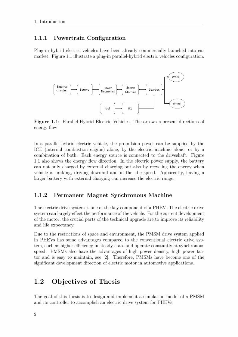
Figure 1.1: Parallel-Hybrid Electric Vehicles. The arrows represent directions ofenergy flow
In a parallel-hybrid electric vehicle, the propulsion power can be supplied by theICE (internal combustion engine) alone, by the electric machine alone, or by acombination of both. Each energy source is connected to the driveshaft. Figure1.1 also shows the energy flow direction. In the electric power supply, the batterycan not only charged by external charging but also by recycling the energy whenvehicle is braking, driving downhill and in the idle speed. Apparently, having alarger battery with external charging can increase the electric range.
1.1.2 Permanent Magnet Synchronous Machine
The electric drive system is one of the key component of a PHEV. The electric drivesystem can largely effect the performance of the vehicle. For the current developmentof the motor, the crucial parts of the technical upgrade are to improve its reliabilityand life expectancy.
Due to the restrictions of space and environment, the PMSM drive system appliedin PHEVs has some advantages compared to the conventional electric drive sys-tem, such as higher efficiency in steady-state and operate constantly at synchronousspeed. PMSMs also have the advantages of high power density, high power fac-tor and is easy to maintain, see [2]. Therefore, PMSMs have become one of thesignificant development direction of electric motor in automotive applications.
1.2 Objectives of Thesis
The goal of this thesis is to design and implement a simulation model of a PMSMand its controller to accomplish an electric drive system for PHEVs.
2

1. Introduction
The aim of this thesis is to simulate the complete electric drive system in a virtualsurrounding so as to shorten development time and save cost. It can also provide abetter basis for decisions regarding requirement setting and dimensioning.
The modeling of the PMSM and its controller is designed and implemented in Mat-lab/Simulink.
1.3 Outline of Thesis
The chapters are outlined below.
Chapter 2 presents the mathematical model of PMSM. FOC method and IMCmethod for controller design are introduced in detail.
chapter 3 reviews the basic principles of SPWM and inverter.
Chapter 4 demonstrates the simulation results and related analysis.
Chapter 5 focuses on the implementation of the plant model of PMSM and itscontroller in CarMaker.
Chapter 6 summarizes the conclusions of the work and brings up some interestingproblems which can be used for future research.
3

1. Introduction
4
2Dynamical Modelling of PMSMs
In order to design and develop control schemes for a PMSM drive system, the dy-namic model of a PMSM depending upon control would be necessary. The dynamicmodel may vary whey using them to design control and simulation algorithms of aPMSM, see[3].
It is well-known that the performance of a three-phase PMSM is described by thevoltage and inductance equations, see[4]. Conventionally, a two-phase equivalentcircuit model instead of a complicated three-phase model has been adopted to an-alyze reluctance synchronous machine. The theory is now applied in the analysisof different kinds of motors including PMSMs, induction motors etc, see[5]. Thetwo-phase(d-q) equivalent circuit model is able to effectively analyze a PMSM sinceit reduces the complexity of these differential equations as mentioned in [6].
In this chapter, the dynamical modelling and analysis of a PMSM are described.Based on well-known Clarke and Park transformation, the three-phase model of aPMSM is transformed to α− β stationary model in the first place, and then α− βstationary model is transformed to an equivalent two-phase(d-q) rotating model.Using these transformations, many properties of a PMSM can be studied withoutcomplexities in the voltage equations, see[4].
Throughout the derivation of d-q mathematical model of a PMSM, the followingassumptions are made [7]:
• Stator windings produce sinusoidal MMF distribution. Space harmonics inthe air-gap are neglected.
• There is no zero-component in the three-phase quantities.
• Balanced three-phase sinusoidal supply voltage is considered.
• Eddy current and hysteresis effects are neglected
• Iron losses are neglected.
• Resistances are independent of temperature and frequency.
5
2. Dynamical Modelling of PMSMs
2.1 Mathematical Model of a PMSM
According to [3], based on different rotor constructions, there are two major varietiesof PMSMs: namely interior PMSMs (with saliency) and surface-mounted PMSMs(without saliency). The main difference is that the inductance in an interior PMSMvary as a function of rotor angle, however a surface-mounted PMSM has quite afixed inductance for any rotor angle as mentioned in [8].
In automotive applications, a salient PMSM is a preference since it is easy to havesensorless control in case of sensor failure. Thus in this section, the mathematicalmodel of a PMSM with saliency is developed in detail.
A PMSM with more than one pole-pairs has stator windings comprising a cor-responding multiple set of coils. For the purpose of analysis, it is convenient toconsider only a single pole-pair and recognize that conditions associated with otherpole-pairs are identical to the conditons for only one pole-pair, see[9].
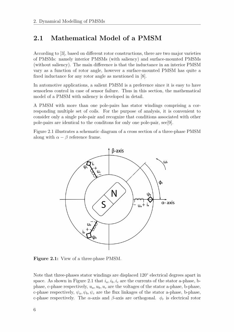
Figure 2.1 illustrates a schematic diagram of a cross section of a three-phase PMSMalong with α− β reference frame.
Figure 2.1: View of a three-phase PMSM.
Note that three-phases stator windings are displaced 120 electrical degrees apart inspace. As shown in Figure 2.1 that ia, ib, ic are the currents of the stator a-phase, b-phase, c-phase respectively, ua, ub, uc are the voltages of the stator a-phase, b-phase,c-phase respectively, ψa, ψb, ψc are the flux linkages of the stator a-phase, b-phase,c-phase respectively. The α-axis and β-axis are orthogonal. φr is electrical rotor
6
2. Dynamical Modelling of PMSMs
angle.
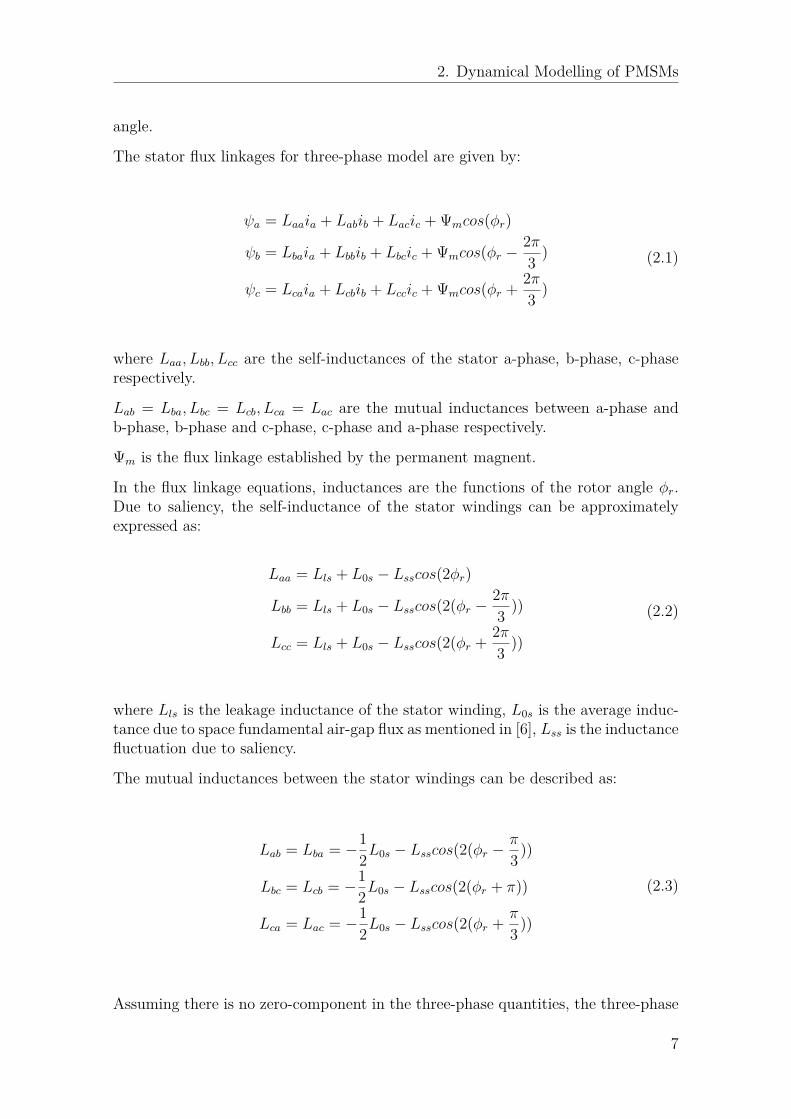
The stator flux linkages for three-phase model are given by:
ψa = Laaia + Labib + Lacic + Ψmcos(φr)
ψb = Lbaia + Lbbib + Lbcic + Ψmcos(φr −2π3 )
ψc = Lcaia + Lcbib + Lccic + Ψmcos(φr + 2π3 )
(2.1)
where Laa, Lbb, Lcc are the self-inductances of the stator a-phase, b-phase, c-phaserespectively.
Lab = Lba, Lbc = Lcb, Lca = Lac are the mutual inductances between a-phase andb-phase, b-phase and c-phase, c-phase and a-phase respectively.
Ψm is the flux linkage established by the permanent magnent.
In the flux linkage equations, inductances are the functions of the rotor angle φr.Due to saliency, the self-inductance of the stator windings can be approximatelyexpressed as:
Laa = Lls + L0s − Lsscos(2φr)
Lbb = Lls + L0s − Lsscos(2(φr −2π3 ))
Lcc = Lls + L0s − Lsscos(2(φr + 2π3 ))
(2.2)
where Lls is the leakage inductance of the stator winding, L0s is the average induc-tance due to space fundamental air-gap flux as mentioned in [6], Lss is the inductancefluctuation due to saliency.
The mutual inductances between the stator windings can be described as:
Lab = Lba = −12L0s − Lsscos(2(φr −
π
3 ))
Lbc = Lcb = −12L0s − Lsscos(2(φr + π))
Lca = Lac = −12L0s − Lsscos(2(φr + π
3 ))
(2.3)
Assuming there is no zero-component in the three-phase quantities, the three-phase
7
2. Dynamical Modelling of PMSMs
flux linkages can be expressed in this way:
ψa = (Lls + 32L0s −
32Lsscos(2φr))ia +
√3
2 Lsssin(2φr)(ic − ib) + Ψmcos(φr)
ψb = (Laa0 + 32L0s −
32Lsscos(2(φr −
2π3 ))ib +
√3
2 Lsssin(2(φr −2π3 ))(ia − ic)
+ Ψmcos(φr −2π3 )
ψc = (Laa0 + 32L0s −
32Lsscos(2(φr + 2π
3 ))ic +√
32 Lsssin(2(φr + 2π
3 ))(ib − ia)
+ Ψmcos(φr + 2π3 )
(2.4)For the coupled-circuit, the three-phase stator voltages can be expressed as:
ua = Raia + dψadt
ub = Rbib + dψbdt
uc = Rcic + dψcdt
(2.5)
where Ra, Rb, Rc are the resistances of the stator a-phase, b-phase, c-phase respec-tively. Ra = Rb = Rc = Rs is assumed under amplitude invariant transformation.
The zero sequence is neglected and the amplitude invariant transformation is used,then the stator voltage equation from three phase to α-β stationary reference frameis expressed by:
uss =usα + jusβ = 23(ua + ube
j 2π3 + uce
j 4π3 )
= 23(Raia + dψa
dt+ (Rbib + dψb
dt)ej 2π
3 + (Rcic + dψcdt
)ej 4π3 )
= Rs23(ia + ibe
j 2π3 + ice
j 4π3 ) + d
dt(23(ψa + ψbe
j 2π3 + ψce
j 4π3 )
(2.6)
uss can be simplified to be given as:
uss = Rsiss +
dψss
dt(2.7)
where uss, iss, ψss are space vector of the three-phase stator voltages, currents and fluxlinkages respectively, which are all described in α-β stationary reference frame.
Based on the equation above, the current in α-β model is definded as:
iss = isα + jisβ = 23(ia + ibe
j 2π3 + ice
j 4π3 ) (2.8)
8
2. Dynamical Modelling of PMSMs
Similarly, the flux linkage in α-β model is defined as:
ψss
= ψsα + jψsβ = 23(ψa + ψbe
j 2π3 + ψbe
j 4π3 ) (2.9)
The resultant voltage, current, and flux linkage space vectors shown in equations(2.7),(2.8),(2.9) for the stator are calculated by multiplying instantaneous phasevalues by the stator winding orientations in which the stator a-phase direction ischosen to the direction of maximum MMF, b-phase, c-phase are 120(electrical de-gree) ahead of the a-phase respectively, see[6].
In order to calculate the flux linkage ψss, the three-phase flux linkages can be ex-
pressed in a different way:
ψa = (Lls + 32L0s)ia + 3
2Lsscos(2φr)ia +√
32 Laa2sin(2φr)(ic − ib) + Ψmcos(φr)
ψb = (Lls + 32L0s)ib + 3
2Lsscos(2(φr −2π3 ))ib +
√3
2 Laa2sin(2(φr −2π3 ))(ia − ic)
+ Ψmcos(φr −2π3 )
ψc = (Lls + 32L0s)ic + 3
2Lsscos(2(φr + 2π3 ))ic +
√3
2 Laa2sin(2(φr + 2π3 ))(ib − ia)
+ Ψmcos(φr + 2π3 )
(2.10)
The transformation of the stator flux linkage can be described by splitting the fluxequations above into 4 parts and taking one at the time. Thus, the new four fluxlinkages equations are as follows: (superscirpt "*" indicates complex conjugate):
ψss,1 = 2
3((Lls + 32L0s)ia + (Lls + 3
2L0s)ibej2π3 + (Lls + 3
2L0s)icej4π3 ) = (Lls + 3
2L0s)iss
ψss,2 = 2
3(32Lsscos(2φr)ia + 3
2Lsscos(2(φr −2π3 ))ibej
2π3 + 3
2Lsscos(2(φr + 2π3 ))icej
4π3 )
= 34Lsse
j2φr 23(ia + ibe
−j 2π3 + ice
j 2π3 ) = 3
4Lssej2φris
∗
s
ψss,3 = 2
3(√
32 Lsssin(2φr)(ic − ib) +
√3
2 Lsssin(2(φr −2π3 ))(ia − ic)ej
2π3 +√
32 Lss
sin(2(φr + 2π3 ))(ib − ia)ej
4π3 ) = Lsse
j2φr
√3
2ej
2π3 − e−j 2π
3
2j is∗
s = 34Lsse
j2φris∗
s
ψss,4 = 2
3(Ψmcosφr + Ψmcos(φr −2π3 )ej 2π
3 + Ψmcos(φr + 2π3 )ej 4π
3 ) = Ψmejφr
(2.11)
The flux linkage ψssis the sum of ψs
s,1, ψss,2, ψ
ss,3, ψ
ss,4:
ψss
= ψss,1 + ψs
s,2 + ψss,3 + ψs
s,4 = (Lls + 32L0s)iss + 3
2Lssej2φris
∗
s + Ψmejφr (2.12)
9
2. Dynamical Modelling of PMSMs
By combining the first and second term of equation(2.12), the total flux linkage isgiven as:
ψss
= Lsiss + Ψme
jφr (2.13)where Ls is leakage and mutual inductance.
Now, the three-phase stator voltages, currents and flux linkages are all describedin α-β stationary reference frame. Multiplying the quantities with e−jθ will trans-form α-β stationary reference frame to d-q rotating reference frame. This leads tothe voltages, currents, flux linkages and inductance equations having time-invariantcoefficients, see[6].
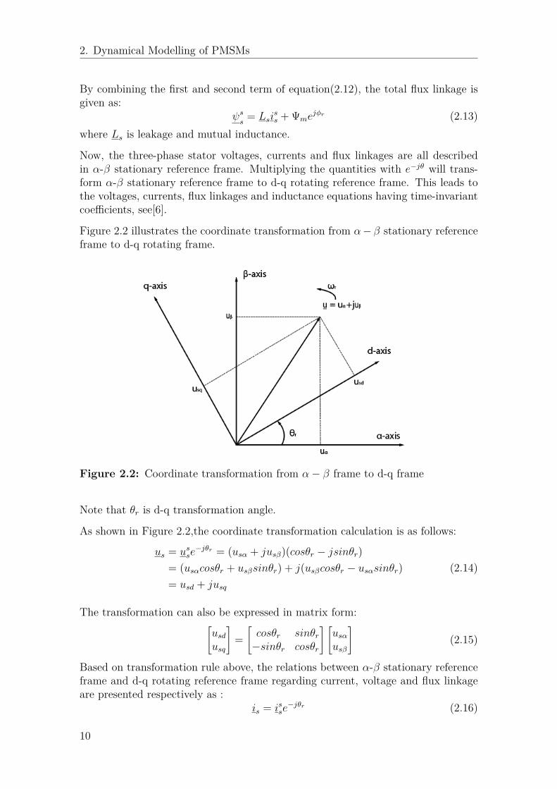
Figure 2.2 illustrates the coordinate transformation from α− β stationary referenceframe to d-q rotating frame.
Figure 2.2: Coordinate transformation from α− β frame to d-q frame
Note that θr is d-q transformation angle.
As shown in Figure 2.2,the coordinate transformation calculation is as follows:
us = usse−jθr = (usα + jusβ)(cosθr − jsinθr)
= (usαcosθr + usβsinθr) + j(usβcosθr − usαsinθr)= usd + jusq
(2.14)
The transformation can also be expressed in matrix form:[usdusq
]=
[cosθr sinθr−sinθr cosθr
] [usαusβ
](2.15)
Based on transformation rule above, the relations between α-β stationary referenceframe and d-q rotating reference frame regarding current, voltage and flux linkageare presented respectively as :
is = isse−jθr (2.16)
10

2. Dynamical Modelling of PMSMs
us = usse−jθr (2.17)
ψs
= ψsse−jθr (2.18)
According to equation(2.17), the stator voltage equation (2.7) in α-β stationarycoordinates is expressed as:
uss = usejθr = Rsise
jθr + d
dt(ψ
sejθr) = Rsise
jθr +dψ
s
dtejθr + jωrψse
jθr (2.19)
where ωr = dθrdt
is the electrical rotor speed
Therefore the voltage equation in d-q rotating coordinates is given by:
us = Rsis +dψ
s
dt+ jωrψs (2.20)
Likewise, based on equation (2.18), flux linkage equation (2.12) in α-β stationarycoordinates is expressed as:
ψss
= ψsejθr = (Lls + 3
2L0s)isejθr + 32Lsse
j2φr(isejθr)∗ + Ψmejφr (2.21)
Flux linkageψsin d-q rotating coordinates is thus given by:
ψs
= (Lls + 32L0s)is + 3
2Lssej(2φr−2θr)i∗s + Ψme
j(φr−θr) (2.22)
Perfect field field orientation is implemented in this thesis, therefore electric rotorangle is equal to the d-q transformation angle, θr = φr.
Hence the flux linkage ψsis
ψs
= (Lls + 32L0s)is + 3
2Lssi∗s + Ψm (2.23)
Now, the current and volatege are described in d-q coordinates, then is, i∗s, us canbe simply respectively defined as
is = isd + jisq (2.24)
i∗s = isd − jisq (2.25)
us = usd + jusq (2.26)
Flux linkage ψscan be further expressed as:
ψs
= (Lls + 32L0s + 3
2Lss)isd + j(Lls + 32L0s −
32Lss)isq + Ψm
= Lsdisd + jLsqisq + Ψm
(2.27)
11
2. Dynamical Modelling of PMSMs
where Lsd, Lsq can be named as the stator inductance in d coordinate and q coor-dinate respectively. Expanding stator voltage equation (2.20) based on equations(2.24),(2.26)and final flux linkage equation (2.27), then voltage equations in d-qrotating coordinates are given by:
usd = Rsisd + Lsddisddt− ωrLsqisq (2.28)
usq = Rsisq + Lsqdisqdt
+ ωrLsdisd + ωrΨm (2.29)
From the well-known relation power P = ReUI∗, for single-phase rms-value-scaledphasors U and I , it may be conjectured that the instantaneous power in a three-phase system is proportional to [10]:
Reussis∗
s = Reusejθr(isejθr)∗ = Reusi∗s (2.30)From the space-vector definition,
ussis∗
s = (2K3 )2(ua + ube
j 2π3 + uce
j 4π3 )(ia + ibe
j 2π3 + ice
j 4π3 )∗ (2.31)
Assuming that ia + ib + ic = 0 and observing that ej 4π3 = e−j
2π3 , the
ussis∗
s = (2K3 )2(uaia + ubib + ucic) (2.32)
So the instantaneous power is given by
P = 32K2Reussis
∗
s = 32K2Reusi∗s = uaia + ubib + ucic (2.33)
Thus the electric power to the shaft can be calculated as by following the equation(2.33)
Pe = 32K2Rejωrψsi
∗s (2.34)
Since for a complex number z = x+jy, the [Rejz = Rej(x+ jy) = −y = −Imz],see[10],thus the
Pe = − 3ωr2K2 Imψsi
∗s = 3ωr
2K2 Imψ∗sis (2.35)
The power can be expressed as:
Pe = TeΩr (2.36)
where Te is electrical torque, Ωr is mechanical rotor speed.
Mechanical rotor speed is expressed as:
Ωr = ωrnp
(2.37)
12
2. Dynamical Modelling of PMSMs
where ωr is electrical rotor speed, np is the number of pole pairs ,
Thus the following relation for the electrical torque is obtained:
Te = PeΩr
= npPeωr
= 3ωrnp2ωrK2 Imψ
∗
sis
= 3np2K2 Im(Lsdisd + jLsqisq + Ψm)∗is
= 3np2K2 Im(Lsdisd − jLsqisq)(isd + jisq) + Ψmis
= 3np2K2 (Lsdisdisq − Lsqisqisd + Ψmisq)
(2.38)
Thus, the electrical torque is:
Te = 3np2K2 ((Lsd − Lsq)isqisd + Ψmisq) (2.39)
The relation between electrical torque and load torque is given by
JdΩr
dt= J
np
dωrdt
= Te − TL (2.40)
where J is inertia of the motor. The complete load torque TL should consist oftwo parts, one is a speed independent part determined by the viscous cofficient B,another one is direct extra load torque input TL,extra.
TL = BΩr + TL,extra = Bωrnp
+ TL,extra (2.41)
Mechanical rotor position is given by:
Φr = φrnp
(2.42)
where φr is electric rotor position which is equal to the d-q transformation angle θrThe electrical rotor speed can be calculated by electric rotor position
ωr = dφrdt
(2.43)
2.2 Clarke’s and Park’s Transformation
This section reviews the principle of Clarke’s and Park’s Transformation. Actually,the theory of both transformation methods has been utilized last section when build-ing the mathematical model of a PMSM. In this section, the method will be simplydescribed in a more straightforward way, the voltages, currents and flux linkages arebased on matrix form and related calculations are also conducted in matrix form.
13
2. Dynamical Modelling of PMSMs
As mentioned last section, according to [4], the transformation of stationary circuitsto a stationary reference frame with two-phase variables α and β was developed byClarke. And Park’s transformation with two-phase variables d and q has the uniqueproperty of eliminating all time varying inductances from the three-phase voltageequations due to the rotor spinning.
For Clarke Transformation, in order to make the transformation be invertible, thezero-consequence component is added as a third variable. The resulting transforma-tion from a-b-c three-phase stationary frame to α-β reference frame is[
fαβ0]
= Tαβ0[fabc
](2.44)
where[fαβ0
]=
[fα fβ f0
]Tand
[fabc
]=
[fa fb fc
]Tf stands for voltage, current, flux linkage. The transformation matrix Tαβ0 is givenby [4]:
Tαβ0 = 23
1 −12 −1
21
√3
2 −√
32
12
12
12
(2.45)
The inverse transformation is given by[fabc
]= T−1
αβ0
[fαβ0
](2.46)
where inverse transformation matrix is described by
T−1αβ0 =
1 0 1−1
2
√3
2 1−1
2 −√
32 1
(2.47)
For Park Transformation, a reference frame fixed on the rotor, i.e, dq frame isadopted. Thus the stator and rotor variables can be observed as constant valuesfrom the rotor point of view.
The transformation equation from three-phase stationary frame to d − q referenceframe is given by
[fdq0
]= Tdq0
[fabc
](2.48)
where[fdq0
]=
[fd fq f0
]Tand
[fabc
]=
[fa fb fc
]TLikewise, f stands for voltage, current, flux linkage. The dq0 transformation matrixis defined as [4]:
Tdq0 = 23
cosθr cos(θr − 2π3 ) cos(θr + 2π
3 )−sinθr −sin(θr − 2π
3 ) −sin(θr + 2π3 )
12
12
12
(2.49)
14

2. Dynamical Modelling of PMSMs
The inverse transformation is given by[fabc
]= T−1
dq0
[fdq0
](2.50)
where dq0 inverse transformation matrix is described by
T−1dq0 = 2
3
cosθr −sinθr 1cos(θr − 2π
3 ) −sin(θr − 2π3 ) 1
cos(θr + 2π3 ) −sin(θr + 2π
3 ) 1
(2.51)
From the last modelling section, based on the self-inductance equations (2.2) andmutual inductance (2.3), all stator inductances are represented in matrix form below:
Lstator =
Laa Lab LacLba Lbb LbcLca Lcb Lcc
(2.52)
Due to the presence of permanent magnet on the rotor, the flux linkages in thestator windings are expressed as in matrix form :
[ψr
]=
Ψmcos(φr)Ψmcos(φr − 2π
3 )Ψmcos(φr + 2π
3 )
=
ψraψrbψrc
(2.53)
where ψra, ψrb, ψrc are flux linkages established by permanent magnet in the statora, b, c phase windings respectively.
Three-phase voltage equations can be rewritten as:[us
]= Rs
[is
]+ d
dt
[ψs
](2.54)
where [ψs
]=
[ψa ψb ψc
]T(2.55)[
us]
=[ua ub uc
]T(2.56)[
is]
=[ia ib ic
]T(2.57)
[ψs
],[us
],[is
]refer to the three-phase flux linkages, three-phase stator voltages and
three-phase currents.
The matrix flux linkages of the three-phase stator windings can also be expressedas: [
ψs]
= Lstator[is
]+
[ψr
](2.58)
where Lstator is the stator inductance matrix varying with rotor angle.[ψr
]is the
flux linkage matrix due to the permanent magnet.
15
2. Dynamical Modelling of PMSMs
Based on the original d-q Park’s transformation matrix Tdq0, the three-phase fluxlinkages, three-phase stator voltages and three-phase currents can be transformedas:
[ψdq0
]=
[Tdq0
] [ψs
](2.59)[
udq0]
=[Tdq0
] [us
](2.60)[
idq0]
=[Tdq0
] [is
](2.61)
The matrix flux linkages in dq reference frame is obtained by:
[ψdq0
]=
[Tdq0
]Lstator
[Tdq0
]−1 [idq0
]+
[Tdq0
] [ψr
](2.62)
where [ψdq0
]=
[ψsd ψsq ψ0
]T(2.63)[
idq0]
=[isd isq i0
]T(2.64)
The term[Tdq0
]Lstator
[Tdq0
]−1is the transformation matrix which transforms the
phase inductance matrix Lstator into the inductance matrix based on the dq referenceframe
[Ldq0
][Ldq0
]=
[Lsd Lsq L0
]T(2.65)
By simplifying the RHS of equation (2.62), the d-q axis flux linkages, ψsd and ψsq,the d-q axis inductances, Lsd andLsq, d-q axis currents isd, isq are obtained as follows:
ψsd = (Lls + 32(L0s + Lss))isd + Ψm = Lsdisd + Ψm (2.66)
ψsq = (Lls + 32(L0s − Lss))isq = Lsqisq (2.67)
ψ0 = Llsi0 (2.68)
The next part is the derivation of the dq axis voltages.
If the equations (2.59), (2.60), (2.61) are substituted into (2.54), then the statorvoltage equation is written in d-q coordinates as:
[udq0
]=
[Tdq0
]Rs
[Tdq0
]−1 [idq0
]+
[Tdq0
] ddt
([Tdq0
]−1 [φdqo
]) (2.69)
where [udq0
]=
[usd usq u0
]T(2.70)
16
2. Dynamical Modelling of PMSMs
Since the resistance Rs is a scalar, the second term has a derivative part, the statorvoltage equation can be further expressed as:
[udq0
]= Rs
[idq0
]+
[Tdq0
]( ddt
([Tdq0
]−1)
[φdqo
]+
[Tdq0
]−1 d
dt
[φdqo
]) (2.71)
Expanding the second term above equation, finally, the stator voltage equation ind-q coordinates is expressed as[
udq0]
= Rs
[idq0
]+
[Tdq0
]( ddt
[Tdq0
]−1)
[φdqo
]+ d
dt
[φdqo
](2.72)
Taking the derivative of[Tdq0
]−1, i.e., equation (2.49),the matrix is
d
dt
[Tdq0
]−1= ωr
−sinθr −cosθr 0−sin(θr − 2π
3 ) −cos(θr − 2π3 ) 0
−sin(θr + 2π3 ) −cos(θr + 2π
3 ) 0
(2.73)
where ωr is the elctrical rotor speed.
By using trigonometric reduction equations, a new matrix is obtained by multiplyingthe transformation matrix
[Tdq0
]and above equation
[Tdq0
] ddt
[Tdq0
]−1= ωr
0 −1 01 0 00 0 0
(2.74)
Combining equations (2.63), (2.64), (2.70), (2.74), the stator voltage equation (2.71)is written in expanded matrix form:
usdusqu0
= Rs
isdisqi0
+ ωr
0 −1 01 0 00 0 0
ψsdψsqψ0
+ d
dt
ψsdψsqψ0
(2.75)
The usd, usq can be expressed in equations based on the above matrix:
usd = Rsisd − ωrψsq + d
dtψsd
= Rsisd − ωrLsqisq + Lsdd
dtisd
(2.76)
usq = Rsisq + ωrψsd + d
dtψsq
= Rsisq + ωrLsdisd + ωrΨm + Lsqd
dtisq
(2.77)
The details of derivation of electrical torque Te are as follows:
17
2. Dynamical Modelling of PMSMs
The instantaneous input power P to the motor is used, which can be representedas:
P = uaia + ubib + ucic (2.78)
After the three-phase voltages and currents are transformed to d-q reference frame,the power can be expressed as:
P = 32(usqisq + usdisd) (2.79)
where the zero sequence quantities are neglected. The mechanical ouput power Peis obtained by replacing usq, usd as
Pe = 32(ψsdωrisq − ψsqωrisd) (2.80)
Based on equations (2.36), (2.37), the electrical power can be expressed as:
Te = PeΩr
= npPeωr
= 3npωr2ωr
(ψsdisq − ψsqisd)
= 3np2 (Lsdisdisq + Ψmisq + Lsqisqisd)
= 3np2 ((Lsd − Lsq)isqisd + Ψmisq)
2.3 Controller Design of a PMSM
In the three-phase PMSM control, a more complicated control method, vector con-trol is utilized since all three phases are conducting simultaneously. A sinusoidalwave drive generates less than 1% torque ripple only when both the back-EMF andphase current have sinusoidal waveformes. Because current in each phase is a sinu-soidal function of rotor position, separate PWM control for each individual phasecurrent is required, see[6].
Vector control is fundamentally based on two-axis theory. For sinusoidal wave drivemotors, the torque is produced by the interaction of the magnetic flux establishedby permanent magnet and the fundamental ampere-conductor distribution. Thereare multiple ways to create a two-axis system but generally the method operateswith the dq-axis current components, isd and isq which may be defined in a varietyof reference frames such as rotor or fixed to the stator. Figure 2.3 describes theblock diagram of vector control in a PMSM drive system.
18
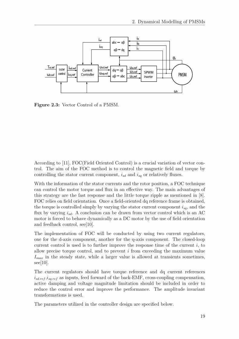
2. Dynamical Modelling of PMSMs
Figure 2.3: Vector Control of a PMSM.
According to [11], FOC(Field Oriented Control) is a crucial variation of vector con-trol. The aim of the FOC method is to control the magnetic field and torque bycontrolling the stator current component, isd and isq or relatively fluxes.
With the information of the stator currents and the rotor position, a FOC techniquecan control the motor torque and flux in an effective way. The main advantages ofthis strategy are the fast response and the little torque ripple as mentioned in [8].FOC relies on field orientation. Once a field-oriented dq reference frame is obtained,the torque is controlled simply by varying the stator current component isq, and theflux by varying isd. A conclusion can be drawn from vector control which is an ACmotor is forced to behave dynamically as a DC motor by the use of field orientationand feedback control, see[10].
The implementation of FOC will be conducted by using two current regulators,one for the d-axis component, another for the q-axis component. The closed-loopcurrent control is used is to further improve the response time of the current i, toallow precise torque control, and to prevent i from exceeding the maximum valueImax in the steady state, while a larger value is allowed at transients sometimes,see[10].
The current regulators should have torque reference and dq current referencesisd.ref ,isq.ref as inputs, feed forward of the back-EMF, cross-coupling compensation,active damping and voltage magnitude limitation should be included in order toreduce the control error and improve the performance. The amplitude invarianttransformations is used.
The parameters utilized in the controller design are specified below.
19
2. Dynamical Modelling of PMSMs
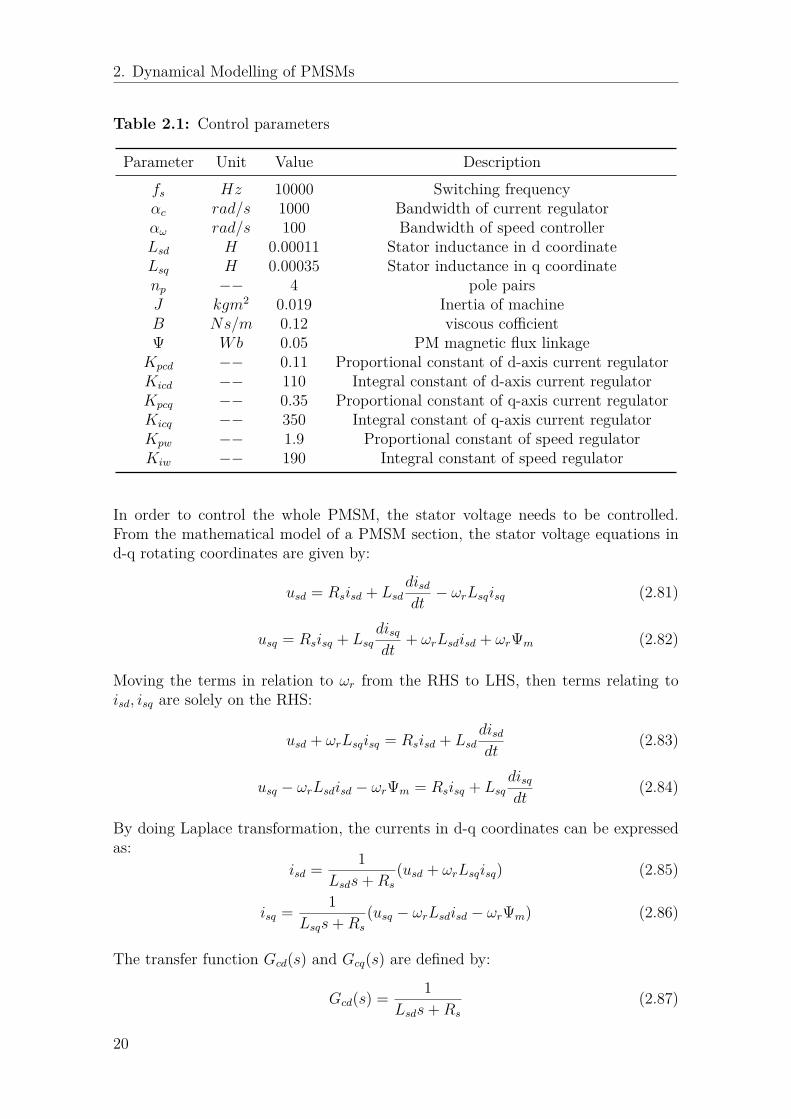
Table 2.1: Control parameters
Parameter Unit Value Descriptionfs Hz 10000 Switching frequencyαc rad/s 1000 Bandwidth of current regulatorαω rad/s 100 Bandwidth of speed controllerLsd H 0.00011 Stator inductance in d coordinateLsq H 0.00035 Stator inductance in q coordinatenp −− 4 pole pairsJ kgm2 0.019 Inertia of machineB Ns/m 0.12 viscous cofficientΨ Wb 0.05 PM magnetic flux linkageKpcd −− 0.11 Proportional constant of d-axis current regulatorKicd −− 110 Integral constant of d-axis current regulatorKpcq −− 0.35 Proportional constant of q-axis current regulatorKicq −− 350 Integral constant of q-axis current regulatorKpw −− 1.9 Proportional constant of speed regulatorKiw −− 190 Integral constant of speed regulator
In order to control the whole PMSM, the stator voltage needs to be controlled.From the mathematical model of a PMSM section, the stator voltage equations ind-q rotating coordinates are given by:
usd = Rsisd + Lsddisddt− ωrLsqisq (2.81)
usq = Rsisq + Lsqdisqdt
+ ωrLsdisd + ωrΨm (2.82)
Moving the terms in relation to ωr from the RHS to LHS, then terms relating toisd, isq are solely on the RHS:
usd + ωrLsqisq = Rsisd + Lsddisddt
(2.83)
usq − ωrLsdisd − ωrΨm = Rsisq + Lsqdisqdt
(2.84)
By doing Laplace transformation, the currents in d-q coordinates can be expressedas:
isd = 1Lsds+Rs
(usd + ωrLsqisq) (2.85)
isq = 1Lsqs+Rs
(usq − ωrLsdisd − ωrΨm) (2.86)
The transfer function Gcd(s) and Gcq(s) are defined by:
Gcd(s) = 1Lsds+Rs
(2.87)
20
2. Dynamical Modelling of PMSMs
Gcq(s) = 1Lsqs+Rs
(2.88)
Note that the equations (2.81) and (2.82) have cross-coupling parts ωrLsqisq andωrLsdisd respectively. And equation (2.82) has a Back-EMF ωrΨm. Thus in thefollowing controller design, the cross coupling parts needs to be compensated andfeed-forward back-EMF needs to be added.
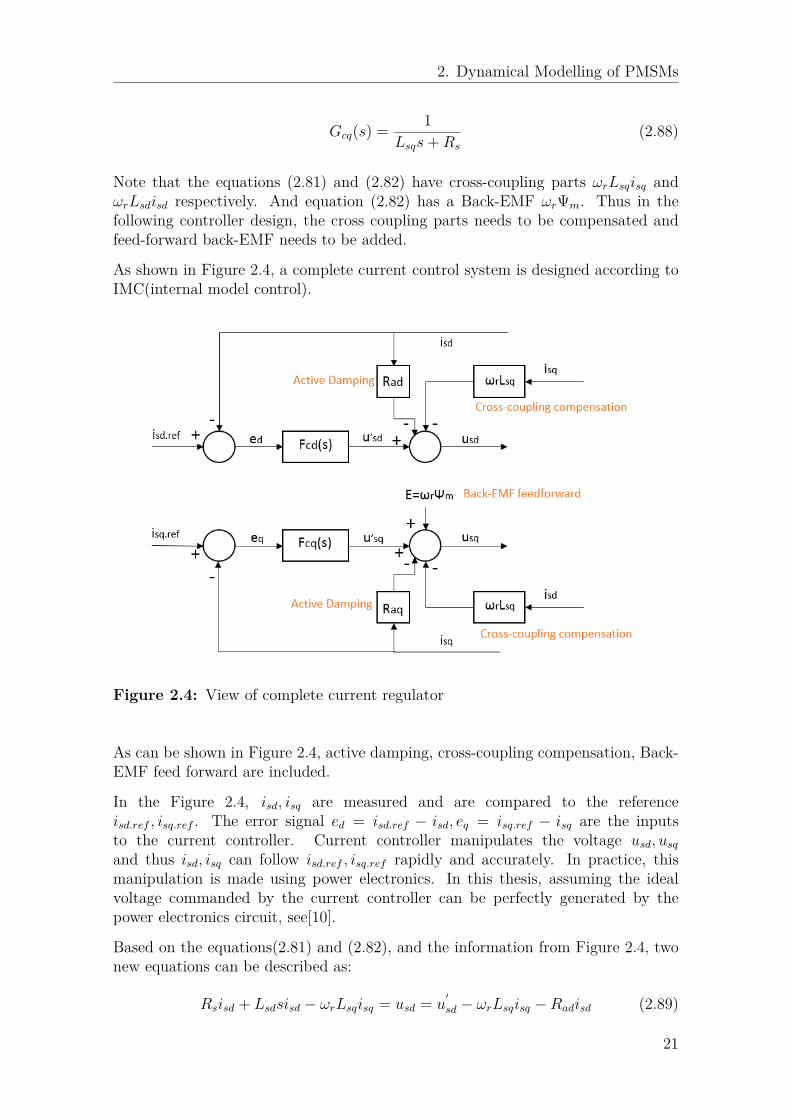
As shown in Figure 2.4, a complete current control system is designed according toIMC(internal model control).
Figure 2.4: View of complete current regulator
As can be shown in Figure 2.4, active damping, cross-coupling compensation, Back-EMF feed forward are included.
In the Figure 2.4, isd, isq are measured and are compared to the referenceisd.ref , isq.ref . The error signal ed = isd.ref − isd, eq = isq.ref − isq are the inputsto the current controller. Current controller manipulates the voltage usd, usqand thus isd, isq can follow isd.ref , isq.ref rapidly and accurately. In practice, thismanipulation is made using power electronics. In this thesis, assuming the idealvoltage commanded by the current controller can be perfectly generated by thepower electronics circuit, see[10].
Based on the equations(2.81) and (2.82), and the information from Figure 2.4, twonew equations can be described as:
Rsisd + Lsdsisd − ωrLsqisq = usd = u′
sd − ωrLsqisq −Radisd (2.89)
21
2. Dynamical Modelling of PMSMs
Rsisq + Lsqsisq + ωrLsdisd + ωrΨm = usq = u′
sq + ωrLsdisd −Raqisq + ωrΨm (2.90)
The isd, isq can be expressed as in this way:
isd = 1Lsds+Rs +Rad
u′
sd = G′
cd(s)u′
sd (2.91)
isq = 1Lsqs+Rs +Raq
u′
sq = G′
cq(s)u′
sq (2.92)
The transfer function G′cd(s) and G′cd(s) are defined by:
G′
cd(s) = 1Lsds+Rs +Rad
(2.93)
G′
cq(s) = 1Lsqs+Rs +Raq
(2.94)
2.4 Selection of Controller Parameters
The parameters of the current regulator Fcd(s), Fcq(s) can be determined accordingto IMC. From equations (2.93) and (2.94), G′cd(s), G
′cq(s) are the transfer functions
from u′sd, u
′sq to isd, isq respectively, which have been illustrated in the Figure 2.5
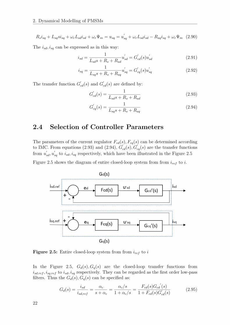
Figure 2.5 shows the diagram of entire closed-loop system from from iref to i.
Figure 2.5: Entire closed-loop system from from iref to i
In the Figure 2.5, Gd(s), Gq(s) are the closed-loop transfer functions fromisd.ref , isq.ref to isd, isq respectively. They can be regarded as the first order low-passfilters. Thus the Gd(s), Gq(s) can be specified as:
Gd(s) = isdisd,ref
= αcs+ αc
= αc/s
1 + αc/s= Fcd(s)Gcd
′(s)1 + Fcd(s)G′cd(s)
(2.95)
22
2. Dynamical Modelling of PMSMs
Gq(s) = isqisq,ref
= αcs+ αc
= αc/s
1 + αc/s= Fcq(s)Gcq
′(s)1 + Fcq(s)G′cq(s)
(2.96)
where αc is the closed-loop system bandwidth.
Based on equations (2.93) and (2.94), the transfer functions Fcd(s), Fcq(s) can beexpressed as:
Fcd(s) = αcsG′−1cd (s) = αc
s(sLsd +Rs +Rad) (2.97)
Fcq(s) = αcsG′−1cq (s) = αc
s(sLsq +Rs +Raq) (2.98)
By transforming transfer functions Fcd(s), Fcq(s) to PI control form, the new expres-sions can be described by:
Fcd(s) = αcLsd + αc(Rs +Rad)s
= kpcd + kicds
(2.99)
Fcq(s) = αcLsq + αc(Rs +Raq)s
= kpcq + kicqs
(2.100)
Therefore, the controller parameters kpcd, kpcq, kicd, kicq are:
kpcd = αcLsd, kpcq = αcLsq (2.101)
kicd = αc(Rs +Rad), kicq = αc(Rs +Raq) (2.102)
For the purpose of decreasing the control error, rather than adding more resistancewhich is highly undesirable due to increased losses, an active resistance is used asshown in 2.4, This technique may also be called "active damping", was proposedin[12].
In order to select "active resistance" Rad, Raq, it is useful to make the G′cd(s), G′cq(s)
as fast as as current regulator closed-loop function Gd(s), Gq(s),i.e.,with the samebandwidth αc. Then, the equations (2.93),(2.93) can be given as:
G′
cd(s) = 1sLsd +Rs +Rad
= 1/Lsds+ (Rs +Rad)/Lsd
= gαcs+ αc
(2.103)
G′
cq(s) = 1sLsq +Rs +Raq
= 1/Lsqs+ (Rs +Raq)/Lsd
= gαcs+ αc
(2.104)
where g is only a gain.
The bandwidth αc can be expressed as:
αc = Rs +Rad
Lsd(2.105)
αc = Rs +Rad
Lsq(2.106)
23
2. Dynamical Modelling of PMSMs
Thus, Rad, Raq can be calculated as:
Rad = αcLsd −Rs (2.107)
Raq = αcLsq −Rs (2.108)
This in turn yields the controller parameter
kpcd = αcLsd, kpcq = αcLsq (2.109)
kicd = α2cLsd, kicq = α2
cLsq (2.110)
According to [10], this described method gives a current regulator which has two in-puts: the control error, and also isd, isq directly via the "active resistance".Therefore,it can be called a two-degrees-of-freedom PI controller.
So far, the current control loop is treated as an ideal and linear system. In reality,it is not correct. The terminal voltage usd, usq which can be seen from Figure 2.4have to be limited to an upper and a lower value. The upper value should be Vmaxwhile the lower value is either 0 or −Vmax. When iref has a large step, the currentcontroller’s output voltage often exceeds Vmax, especially for higher rotor speed whenthe back-EMF is large, leading to a large terminal voltage, see[10]. Therefore, thetrue voltage, reference voltage, is a limitation of the ideal voltage. So the currentcontrol loop contains a nonlinearity (saturation) which is used to limit the voltage,as shown in Figure 2.6.
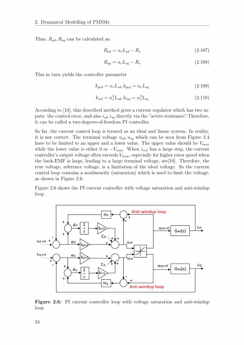
Figure 2.6 shows the PI current controller with voltage saturation and anti-winduploop .
Figure 2.6: PI current controller loop with voltage saturation and anti-winduploop
24
2. Dynamical Modelling of PMSMs
Additionally, integral term of the PI current controller keeps accumulating the con-trol error during the time of maximum voltage output„ it gets "overcharged". Wheni starts getting close to iref , the integrator has wound up so that u remains large.Therefore, i has to shoot over iref until the windup has been elimated by accumu-lating of negative control error, see[10].
The solution is to modify the error signal to integrator to limit the integration whenthe output voltage of the current controller is limited.
As the Figure 2.6 shown, a new error signal to integral term of PI controller iscreated.
ed = (usd.ref − usd)Hd + ed (2.111)
eq = (usq.ref − usq)Hq + eq (2.112)
The transfer function from usd.ref to usd is expressed by:
usd = kpcded + cd + kicds
(ed +Hd(usd.ref − usd)) (2.113)
= kpcded + cd + kicdsed + kicd
sHdusd.ref −
kicdsHdusd (2.114)
By combining like terms, usd is
usd = skpcd + kicds+Hdkicd
ed + s
s+Hdkicdcd + Hdkicd
s+Hdkicdusd.ref (2.115)
usd.ref can be treated as input and ed and cd can be regarded as disturbances.
The transfer function from usq.ref to usq is expressed by:
usq = kpcqed + cq + kicqs
(eq +Hq(usq.ref − usq)) (2.116)
= kpcqeq + cq + kicqseq + kicq
sHqusq.ref −
kicqsHqusq (2.117)
By combining like terms, usq is
usq = skpcq + kicqs+Hqkicq
eq + s
s+Hqkicqcq + Hqkicq
s+Hqkicqusq.ref (2.118)
Likewise, usq.ref can be treated as input and eq and cq can be regarded as distur-bances.
Parameters Hd and Hq are selected as 1kpcd
1kpcq
:
Hdkicd = kicdkpcd
= α2cLsdαcLsd
= αc (2.119)
Hqkicq = kicqkpcq
= α2cLsqαcLsq
= αc (2.120)
25
2. Dynamical Modelling of PMSMs
2.5 Speed controller Design
The mechanical dynamics of electric motor drive is given by equation (2.40)
JdΩr
dt= Te − TL = Te −BΩr − Textra (2.121)
Where J is the total moment of inertia, including the motor itself and mechanicalload, see[13]. Ωr is the mechanical rotor speed, Te is the electrical driving torque,TL is the load torque, B is the viscous coefficient. Textra is the extra torque input.
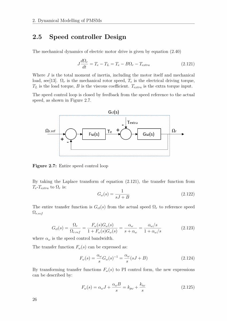
The speed control loop is closed by feedback from the speed reference to the actualspeed, as shown in Figure 2.7.
Figure 2.7: Entire speed control loop
By taking the Laplace transform of equation (2.121), the transfer function fromTe-Textra to Ωr is:
Gω(s) = 1sJ +B
(2.122)
The entire transfer function is Gcl(s) from the actual speed Ωr to reference speedΩr.ref
Gcl(s) = Ωr
Ωr.ref
= Fω(s)Gω(s)1 + Fω(s)Gω(s) = αω
s+ αω= αω/s
1 + αω/s(2.123)
where αω is the speed control bandwidth.
The transfer function Fω(s) can be expressed as:
Fω(s) = αωsGω(s)−1 = αω
s(sJ +B) (2.124)
By transforming transfer functions Fω(s) to PI control form, the new expressionscan be described by:
Fω(s) = αωJ + αωB
s= kpω + kiω
s(2.125)
26
2. Dynamical Modelling of PMSMs
Therefore, the speed controller parameters kpω, kiω are:
kpω = αωJ, kiω = αωB (2.126)
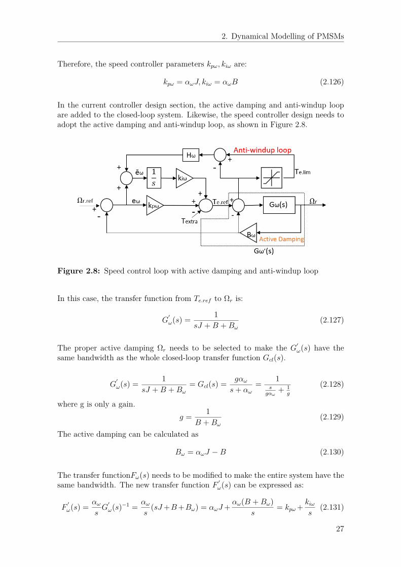
In the current controller design section, the active damping and anti-windup loopare added to the closed-loop system. Likewise, the speed controller design needs toadopt the active damping and anti-windup loop, as shown in Figure 2.8.
Figure 2.8: Speed control loop with active damping and anti-windup loop
In this case, the transfer function from Te.ref to Ωr is:
G′
ω(s) = 1sJ +B +Bω
(2.127)
The proper active damping Ωr needs to be selected to make the G′ω(s) have thesame bandwidth as the whole closed-loop transfer function Gcl(s).
G′
ω(s) = 1sJ +B +Bω
= Gcl(s) = gαωs+ αω
= 1s
gαω+ 1
g
(2.128)
where g is only a gain.g = 1
B +Bω
(2.129)
The active damping can be calculated as
Bω = αωJ −B (2.130)
The transfer functionFω(s) needs to be modified to make the entire system have thesame bandwidth. The new transfer function F ′ω(s) can be expressed as:
F′
ω(s) = αωsG′
ω(s)−1 = αωs
(sJ+B+Bω) = αωJ+ αω(B +Bω)s
= kpω + kiωs
(2.131)
27
2. Dynamical Modelling of PMSMs
Therefore, the new speed controller parameters kpω, kiω are:
kpω = αωJ, kiω = αω(B +Bω) (2.132)
The same method used in current controller anti-windup design is utilized. As theFigure 2.8 shown, a new error signal to integral term of PI controller is created.
eω = (Te.lim − Te.ref )Hω + eω (2.133)
The Te.ref is expressed by:
Te.ref = kpωeω − Textra + kiωs
(eω +Hω(Te.lim − Te.ref )) (2.134)
= kpωeω − Textra + kiωseω + kiω
sHωTe.lim −
kiωsHωTe.ref (2.135)
By combining like terms, Te.ref is
Te.ref = skpω + kiωs+Hωkiω
eω −s
s+HωkiωTextra + Hωkiω
s+HωkiωTe.lim (2.136)
Te.lim can be treated as input and eω and Textra can be regarded as disturbances.
Parameter Hω is selected as 1kpω
Hωkiω = kiωkpω
= α2ωJ
αωJ= αω (2.137)
2.6 Selection of Current References
Maximum Torque Per Ampere (MTPA) is adopted in the selection of current ref-erences. The torque production in a PMSM is a function of Ψm, Lsd, Lsq, isd, isq asdescribed in equation (2.39). There are infinite number of isd and isq combinationswhich can generate the same amount of torque.
The torque generation can be separated into two components. The componentproduced from the permanent magnent flux is called magnetic torque, which can beexpressed as:
Tmagnetic = 3np2 Ψmisq (2.138)
The other component produced from rotor saliency is called reluctance torque, whichcan be expressed as:
Treluctance = 3np2 (Lsd − Lsq)isqisd (2.139)
In this thesis, a salient PMSM is studied. Normally, inductance along the d-axisis lower than inductance along the q-axis, i.e., Lsd is smaller than Lsq. (Lsd - Lsq)
28
2. Dynamical Modelling of PMSMs
is always negative, thus a positive value of isd would produce a negative reluctancetorque, which is opposing the magnetic torque, hence a positive isd is never de-sired. Besides, a negative isd can reduce the required amount of isq by aiding in thereluctance torque, see[14].
The minimum phase currents can be generated by a particular isd, isq for any torquelevel. It is similar to maximizing the torque output for a specific amount of current.Thus, the operation principle is called Maximum Torque per Ampere(MTPA).
By introducing the current angle β, and stator current Is, the isd, isq can be expressedby:
isd = Iscosβ (2.140)isq = Issinβ (2.141)
The torque equation (2.39) can be represented by Is :
Te = 3np2 (ΨmIssinβ + (Lsd − Lsq)I2
s sinβcosβ) (2.142)
The derivative of torque Te with respect to current angle β is:
dTedβ
= 3np2 (ΨmIscosβ + (Lsd − Lsq)I2
s cos2β) (2.143)
Let the derivative dTedβ
equal to 0, then a fixed current angle β which can generatemaximum torque is calculated as:
β = cos−1(− Ψm
4(Lsd − Lsq)Is−
√√√√12 + ( Ψm
4(Lsd − Lsq)Is)2) (2.144)
Where Is could be rated current
Assuming a positive torque request is required, the current magnitude can be cal-culated as:
Is.ref = − Ψm
2(Lsd − Lsq)cosβ+
√√√√ 23np(Lsd − Lsq)sinβcosβ
Te.req + ( Ψm
2(Lsd − Lsq)cosβ)2
(2.145)
A limitation to current magnitude needs to added:
Is.ref.lim = LimIs.refImax0 (2.146)
Thus the reference current in d-q coordinates can be described as:
isd.ref = Is.ref.limcosβ (2.147)
isq.ref = Is.ref.limsinβ (2.148)
29

2. Dynamical Modelling of PMSMs
30
3PWM and Inverter
PWM (Pulse Width Modulation) inverter systems are widely used in a variety ofapplications as a power-conditioning unit in electric drives, e.g., high voltage DCtransmission, active power filters, electric vehicles, alternate energy systems andindustrial processes, see[15]. The inverters realize DC-AC power conversion. TheDC-input voltage Vdc can be obtained from the storage battery in PHEVs.
Inverter fed adjustable speed drives are needed in the PMSM drive system. Theswitching of inverter plays an significant role in the opertaion of the PMSM drivesystem, see[16].
In this chapter, the basic principles of PWM are presented in the first place, and afterthat sinusoidal PWM is illustrated in detail. The three-phase inverter is describedafter the SPWM is introduced and connections between the SPWM and inverterare also presented, which explains why the reference voltage signal generated fromcurrent controller is equal to the average voltage signal established from the inverter.
The parameters utilized in the inverter design are specified below.
Table 3.1: Inverter parameters
Parameter Unit Value DescriptionVbatt V 330 Battery voltageRbatt Ohm 0.25 Internal resistance of the batteryCdc F 500e− 6 DC capacitance of the converter
3.1 Pulse Width Modulation
According to [16], PWM is a modulation methodology which is based on the pulseduration width. This pulse changes along with the type of modulating signal. On theone hand, the PWMmethod can be utilized for signal communication or informationtransfer, on the other hand, it can provide the controller power for major electricaldevices particularly to motors. Compared with other available methodologies, thePWM technique has the advantages of less complexity on its implementation and
31
3. PWM and Inverter
control, no deviation in temperature and no variation in power due to senescence,see[16].
In order to obtain output AC voltages with the required amplitude and frequencyshaped as closely as possible to the sinusoidal wave, a variety of pulse width modu-lation strategies are used to control the voltage source inverter, see[15].
During the design and implementation of PWM and inverter, the following assump-tions are made [17]:
• No voltage drops in valves (diodes, transistors), which means conduction lossesare not considered.
• Blanking time is neglected.
• Swithcing losses and off-state losses of inverter are also neglected.
3.2 Sinusoidal PWM
The SPWM (sinusoidal pulse width modulation) technique is one of the most popularPWM techniques due to its benefits of reducing harmonic of inverters. The reasonis that three sinusoidal wave are used and displaced as 120 phase difference asreference signals for three phase inverter, see[18].
In this modulation, the modulation signal is a sinusoidal wave and the carrier waveis a triangular wave. The theory is to compare three-phase sinusoidal referencevoltages ua.ref , ub.ref , uc.ref established from current controller with carrier wave inorder to produce the logical signal, Sa, Sb, Sc. The logical signal can define switchinginstants of power transistor as mentioned in [19]. A sequence of voltage pulses areacquired by on and off of the power switches based on the given logical signals,which means the logical signals can trigger the respective inverter switches.
Normally, the frequency of carrier wave should be much higher than the frequencyof the phase voltages. In this way the phase voltage reference is assumed to beconstant during the switching period. The frequency of sinusoidal phase voltage ischosen based on the required inverter output frequency (50/60 Hz).
The constant amplitude pulses with distinct duty cycles in each period is the maincharacteristic of SPWM technique, see[18]. The width of these pulses vary to gainoutput voltage control from inverter and the reduction of harmonics, see[20].
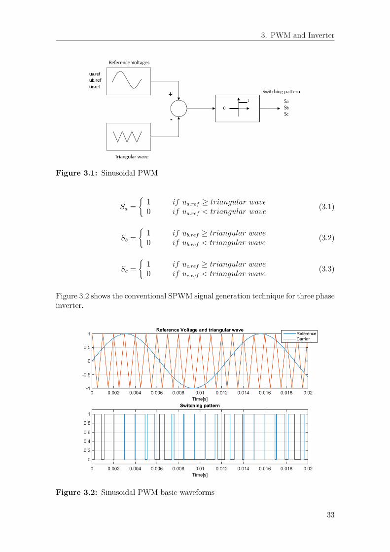
The principles of sinusoidal PWM is shown in Figure 3.1, i.e., the comparison be-tween reference voltages and the triangular wave and the generation of logical signalwhich can determine the switching patterns of inverter.
The logical signal Sa, Sb, Sc are generated by comparison between reference volt-ages and carrier wave. The switching patterns can be obtained by the equations(3.1),(3.2),(3.3).
32
3. PWM and Inverter
Figure 3.1: Sinusoidal PWM
Sa =
1 if ua.ref ≥ triangular wave0 if ua.ref < triangular wave
(3.1)
Sb =
1 if ub.ref ≥ triangular wave0 if ub.ref < triangular wave
(3.2)
Sc =
1 if uc.ref ≥ triangular wave0 if uc.ref < triangular wave
(3.3)
Figure 3.2 shows the conventional SPWM signal generation technique for three phaseinverter.
Figure 3.2: Sinusoidal PWM basic waveforms
33
3. PWM and Inverter
3.2.1 Mathematical Implementation
It is well-known that the the value of a duty cycle should be between 0 and 1. Themaximum sinusoidal phase voltage is Vdc
2 . The duty cycles da, db, dc can be calculatedfrom the phase voltage references ua.ref , ub.ref , uc.ref and the DC-link voltage Vdc as
da = 0.5 + ua.refVdc
(3.4)
db = 0.5 + ub.refVdc
(3.5)
dc = 0.5 + uc.refVdc
(3.6)
It is apparent that the values of duty cycles da, db, dc are between 0 and 1. Thelogical signals Sa, Sb, Sc can be obtained by comparing duty cycles and the carrierwave.
Sa =
1 if da ≥ carrier wave0 if da < carrier wave
(3.7)
Sa =
1 if db ≥ carrier wave0 if db < carrier wave
(3.8)
Sa =
1 if dc ≥ carrier wave0 if dc < carrier wave
(3.9)
In this case, the carrier wave is a triangular wave between 0 and 1. The width ofthe pulses Sa, Sb, Sc can be varied by changing the duty cycle of PWM.
3.3 Inverter
The VSI (voltage source inverter) has a DC input voltage Vdc obtained from battery.The magnitude of this DC input voltage is usually constant. The inverter is to utilizethis DC input voltage and reference voltage to produce AC output voltage, wherethe magnitude and frequency can be controlled, see[18].
The voltage and current are controlled with 120 different in each phase. Accordingto [15], the controlling signals of three-phase PWM inverters have many switchingpatterns. The operations of three-phase inverter can be defined in eight modes whichshows status of each switch in each operation mode.
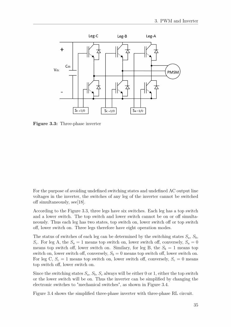
Figure 3.3 shows a block diagram of three-phase inverter
34
3. PWM and Inverter
Figure 3.3: Three-phase inverter
For the purpose of avoiding undefined switching states and undefined AC output linevoltages in the inverter, the switches of any leg of the inverter cannot be switchedoff simultaneously, see[18].
According to the Figure 3.3, three legs have six switches. Each leg has a top switchand a lower switch. The top switch and lower switch cannot be on or off simulta-neously. Thus each leg has two states, top switch on, lower switch off or top switchoff, lower switch on. Three legs therefore have eight operation modes.
The status of switches of each leg can be determined by the switching states Sa, Sb,Sc. For leg A, the Sa = 1 means top switch on, lower switch off, conversely, Sa = 0means top switch off, lower switch on. Similary, for leg B, the Sb = 1 means topswitch on, lower switch off, conversely, Sb = 0 means top switch off, lower switch on.For leg C, Sc = 1 means top switch on, lower switch off, conversely, Sc = 0 meanstop switch off, lower switch on.
Since the switching states Sa, Sb, Sc always will be either 0 or 1, either the top switchor the lower switch will be on. Thus the inverter can be simplified by changing theelectronic switches to "mechanical switches", as shown in Figure 3.4.
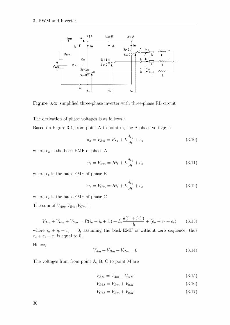
Figure 3.4 shows the simplified three-phase inverter with three-phase RL circuit.
35
3. PWM and Inverter
Figure 3.4: simplified three-phase inverter with three-phase RL circuit
The derivation of phase voltages is as follows :
Based on Figure 3.4, from point A to point m, the A phase voltage is
ua = VAm = Ria + Ldiadt
+ ea (3.10)
where ea is the back-EMF of phase A
ub = VBm = Rib + Ldibdt
+ eb (3.11)
where eb is the back-EMF of phase B
uc = VCm = Ric + Ldicdt
+ ec (3.12)
where ec is the back-EMF of phase C
The sum of VAm, VBm, VCm is
VAm + VBm + VCm = R(ia + ib + ic) + Lcd(ia + ibic)
dt+ (ea + eb + ec) (3.13)
where ia + ib + ic = 0, assuming the back-EMF is without zero sequence, thusea + eb + ec is equal to 0.
Hence,VAm + VBm + VCm = 0 (3.14)
The voltages from from point A, B, C to point M are
VAM = VAm + VmM (3.15)VBM = VBm + VnM (3.16)VCM = VBm + VnM (3.17)
36
3. PWM and Inverter
The sum of VAM , VBM , VCM is
VAM + VBM + VCM = (VAm + VBm + VCm) + 3VmM (3.18)
Due to VAm + VBm + VCm = 0, the VmM is
VmM = VAM + VBM + VCM3 (3.19)
Therefore the phase voltages ua, ub, uc can be expressed as:
ua = VAm = VAM − VmM = VAM −VAM + VBM + VCM
3 = 23VAM −
13(VBM + VCM)
(3.20)
ub = VBm = VBM − VmM = VBM −VAM + VBM + VCM
3 = 23VBM −
13(VAM + VCM)
(3.21)uc = VCm = VCM − VmM = VCM −
VAM + VBM + VCM3 = 2
3VCM −13(VAM + VBM)
(3.22)The average of VAM can be expressed by the DC-link voltage Vdc and duty cycle da:
VAM.avg = 1T
∫ T
0VAMdt = Vdcda (3.23)
Similarly, VBM , VCM can be expressed as:
VBM.avg = 1T
∫ T
0VBMdt = Vdcdb (3.24)
VCM.avg = 1T
∫ T
0VCMdt = Vdcdc (3.25)
The average of VnM is
VmM.avg = 1T
∫ Ts
0VmMdt = 1
T
∫ T
0
VAM + VBM + VCM3 dt = Vdc
3 (da + db + dc) (3.26)
Therefore the average phase voltage can be expressed as:
ua.avg = VAm.avg = VAM.avg − VmM.avg = Vdcda −Vdc3 (da + db + dc) (3.27)
ub.avg = VBm.avg = VBM.avg − VmM.avg = Vdcdb −Vdc3 (da + db + dc) (3.28)
uc.avg = VCm.avg = VCM.avg − VmM.avg = Vdcdc −Vdc3 (da + db + dc) (3.29)
Based on the duty cycle equations (3.4),(3.5),(3.6), the average phase voltage canbe further written as
37
3. PWM and Inverter
ua.avg = Vdcda−Vdc3 (da + db + dc) = 0.5Vdc + ua.ref − 0.5Vdc−
ua.ref + ua.ref + ua.ref3
(3.30)ub.avg = Vdcdb −
Vdc3 (da + db + dc) = 0.5Vdc + ub.ref − 0.5Vdc −
ua.ref + ua.ref + ua.ref3
(3.31)uc.avg = Vdcdc −
Vdc3 (da + db + dc) = 0.5Vdc + uc.ref − 0.5Vdc −
ua.ref + ua.ref + ua.ref3
(3.32)Becasue ua.ref + ua.ref + ua.ref is equal to zero, the phase voltages are:
ua.avg = ua.ref (3.33)
ub.avg = ua.ref (3.34)
uc.avg = ua.ref (3.35)
It shows that the reference voltage signal generated from current controller is equalto the average voltage signal established from the inverter.
From the Figure 3.4, the battery is assumed as a fixed voltage, Vbatt, the Rbatt is theresistance. For the DC-link capacitor,
CdcdVdcdt
= ic = ibatt − idc (3.36)
ibatt = Vbatt − VdcRbatt
(3.37)
Therefore,Cdc
dVdcdt
= Vbatt − VdcRbatt
− idc (3.38)
Taking the Laplace transform, then the DC-link voltage can be expressed as:
Vdc = (Vbatt − VdcRbatt
− idc)1Cdc
1s
(3.39)
The DC-link current idc is expressed as:
idc = isa + isa + isa = Saia + Sbib + Scic (3.40)
38
4Simulation Results and Analysis
In this chapter, for the purpose of verifying the effectiveness of the mathematicalmodel developed and algorithms adopted in the thesis, a number of simulation resultsare presented. The steady-state characteristics of a PMSM are analyzed. Moreover,the variable-speed drive analysis is carried out. The issues observed during thesimulation process are also demonstrated.
Simulation models are implemented in Matlab/Simulink, operating at a sample fre-quency of 10 kHz.
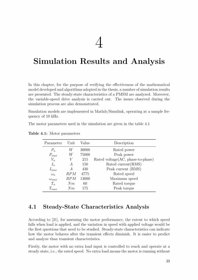
The motor parameters used in the simulation are given in the table 4.1
Table 4.1: Motor parameters
Parameter Unit Value DescriptionPn W 30000 Rated powerPmax W 75000 Peak powerVn V 215 Rated voltage(AC, phase-to-phase)In A 150 Rated current(RMS)Imax A 430 Peak current (RMS)ωn RPM 4775 Rated speedωmax RPM 13000 Maximum speedTn Nm 60 Rated torqueTmax Nm 175 Peak torque
4.1 Steady-State Characteristics Analysis
According to [21], for assessing the motor performance, the extent to which speedfalls when load is applied, and the variation in speed with applied voltage would bethe first questions that need to be studied. Steady-state characteristics can indicatehow the motor behaves after the transient effects diminish. It is easier to predictand analyze than transient characteristics.
Firstly, the motor with no extra load input is controlled to reach and operate at asteady state, i.e., the rated speed. No extra load means the motor is running without
39

4. Simulation Results and Analysis
external torque, the only mechanical resistance is that due to its own friction.
Figure 4.1 shows a variation of the rotor speed with time. The actual rotor speedreaches the reference speed in a short time with speed controller. The referencespeed is the rated speed, i.e. the steady-state speed.
Figure 4.1: Variation of motor speed when tracking the rated speed
Figure 4.2 shows the three-phase currents at the starting and at the steady state.From the Figure 4.2a, it is apparent that the currents are non-sinusoidal and notstable since the motor is attempting to reach the rated speed, see[22]. Figure 4.2bshows the currents become sinusoidal when the motor reaches the rated speed atsteady state.
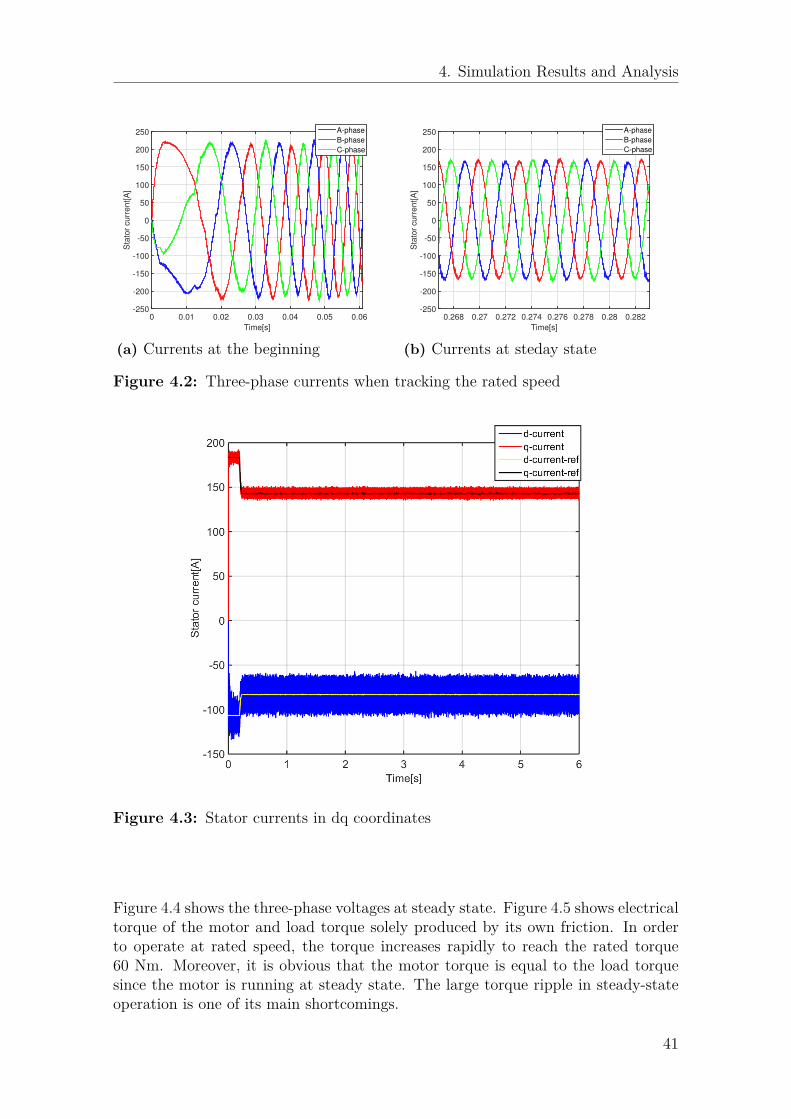
The corresponding dq component of current is given in Figure 4.3. Both d and qaxis current are present. It is clear that the isq, isd are following the isq.ref isd.refrespectively all the time from the beginning to the steady state. The isd is alwaysnegative in order to produce the positive reluctance torque, instead of opposing themagnetic torque.
40
4. Simulation Results and Analysis
Time[s]
0 0.01 0.02 0.03 0.04 0.05 0.06
Sta
tor
cu
rre
nt[
A]
-250
-200
-150
-100
-50
0
50
100
150
200
250 A-phase
B-phase
C-phase
(a) Currents at the beginningTime[s]
0.268 0.27 0.272 0.274 0.276 0.278 0.28 0.282
Sta
tor
cu
rre
nt[
A]
-250
-200
-150
-100
-50
0
50
100
150
200
250 A-phase
B-phase
C-phase
(b) Currents at steday state
Figure 4.2: Three-phase currents when tracking the rated speed
Figure 4.3: Stator currents in dq coordinates
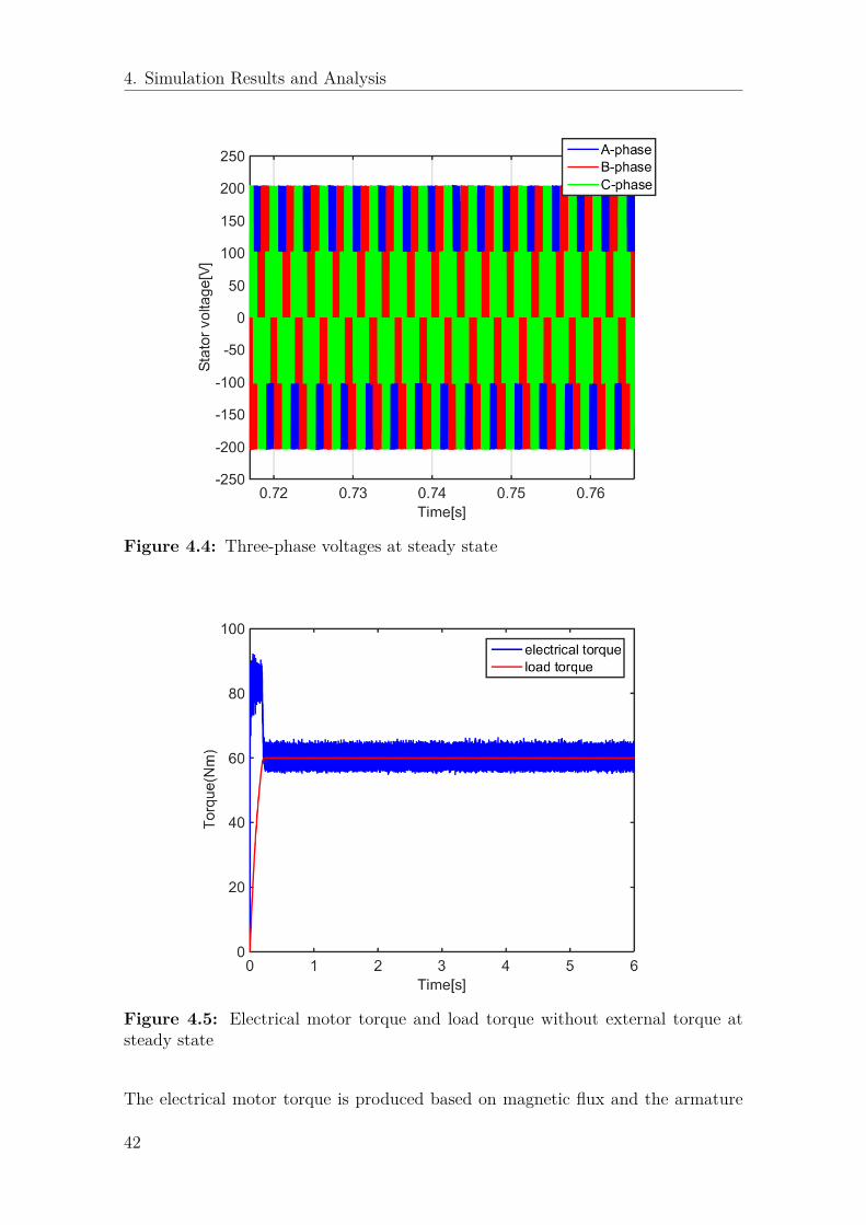
Figure 4.4 shows the three-phase voltages at steady state. Figure 4.5 shows electricaltorque of the motor and load torque solely produced by its own friction. In orderto operate at rated speed, the torque increases rapidly to reach the rated torque60 Nm. Moreover, it is obvious that the motor torque is equal to the load torquesince the motor is running at steady state. The large torque ripple in steady-stateoperation is one of its main shortcomings.
41
4. Simulation Results and Analysis
Figure 4.4: Three-phase voltages at steady state
Figure 4.5: Electrical motor torque and load torque without external torque atsteady state
The electrical motor torque is produced based on magnetic flux and the armature
42
4. Simulation Results and Analysis
current according to equation 2.39. Load torque is proportional to the productof force and distance. Motor current varies relating to the amount of load torqueexerted, see[21]. When the motor is running at steady state, the current is constant,and the motor torque is equal and opposite of the load torque.
Figure 4.5 shows when a motor is accelerating, the motor torque is higher than theload torque. Conversely, when a motor is decelerating, the motor torque is less thanthe load torque.
When the load on the shaft has been changed, exploring how the speed will vary isa necessity.
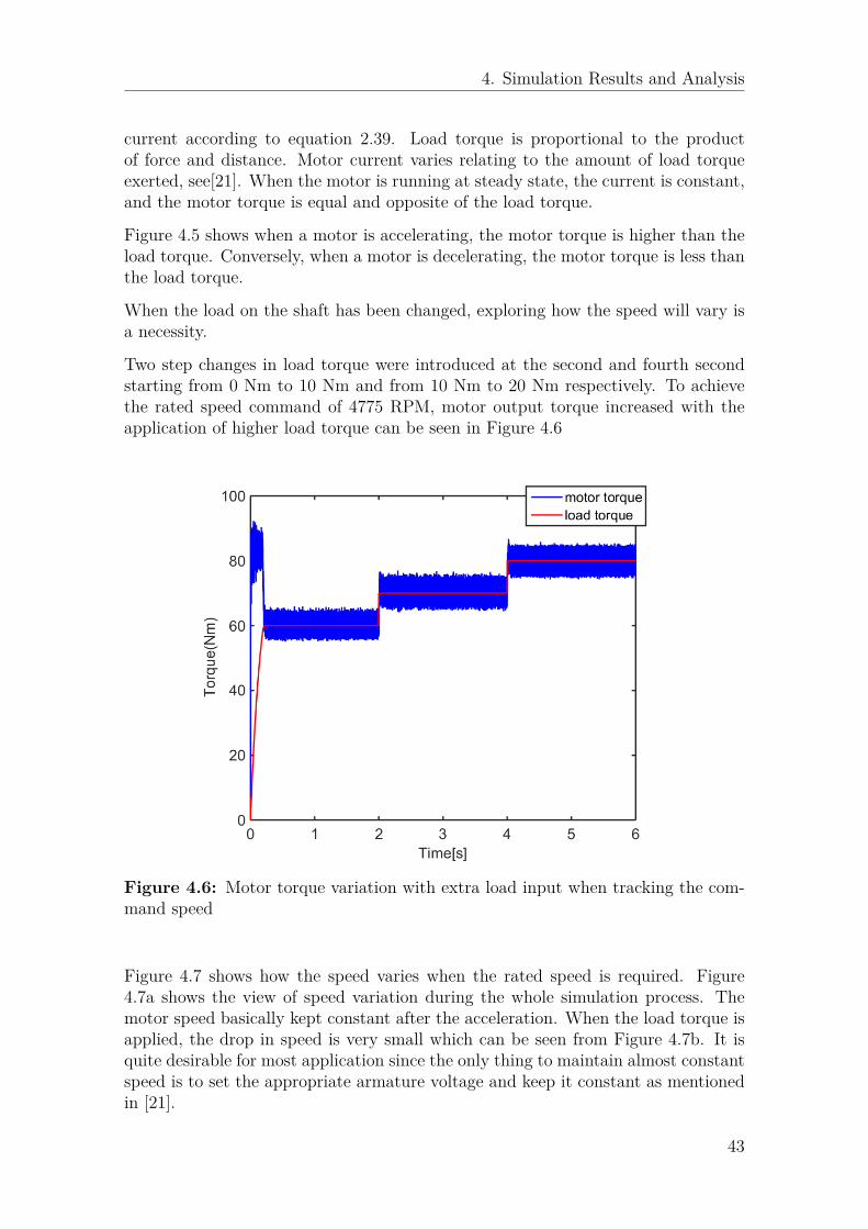
Two step changes in load torque were introduced at the second and fourth secondstarting from 0 Nm to 10 Nm and from 10 Nm to 20 Nm respectively. To achievethe rated speed command of 4775 RPM, motor output torque increased with theapplication of higher load torque can be seen in Figure 4.6
Figure 4.6: Motor torque variation with extra load input when tracking the com-mand speed
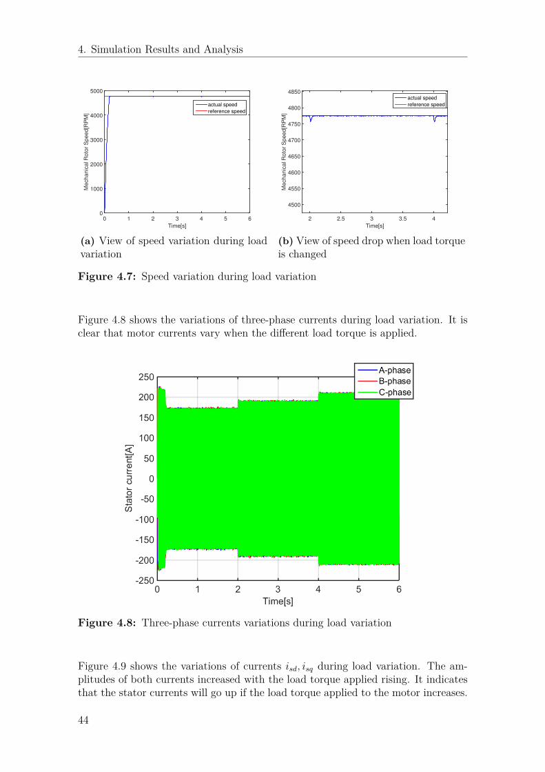
Figure 4.7 shows how the speed varies when the rated speed is required. Figure4.7a shows the view of speed variation during the whole simulation process. Themotor speed basically kept constant after the acceleration. When the load torque isapplied, the drop in speed is very small which can be seen from Figure 4.7b. It isquite desirable for most application since the only thing to maintain almost constantspeed is to set the appropriate armature voltage and keep it constant as mentionedin [21].
43
4. Simulation Results and Analysis
Time[s]
0 1 2 3 4 5 6
Me
ch
an
ica
l R
oto
r S
pe
ed
[RP
M]
0
1000
2000
3000
4000
5000
actual speed
reference speed
(a) View of speed variation during loadvariation
Time[s]
2 2.5 3 3.5 4
Me
ch
an
ica
l R
oto
r S
pe
ed
[RP
M]
4500
4550
4600
4650
4700
4750
4800
4850actual speed
reference speed
(b) View of speed drop when load torqueis changed
Figure 4.7: Speed variation during load variation
Figure 4.8 shows the variations of three-phase currents during load variation. It isclear that motor currents vary when the different load torque is applied.
Figure 4.8: Three-phase currents variations during load variation
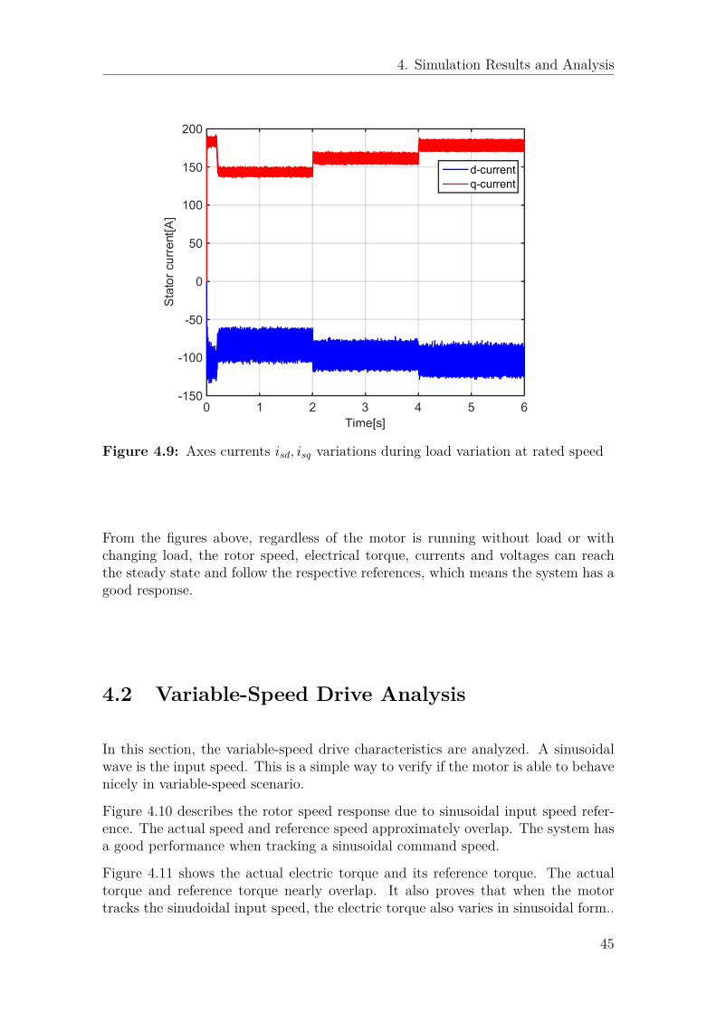
Figure 4.9 shows the variations of currents isd, isq during load variation. The am-plitudes of both currents increased with the load torque applied rising. It indicatesthat the stator currents will go up if the load torque applied to the motor increases.
44
4. Simulation Results and Analysis
Figure 4.9: Axes currents isd, isq variations during load variation at rated speed
From the figures above, regardless of the motor is running without load or withchanging load, the rotor speed, electrical torque, currents and voltages can reachthe steady state and follow the respective references, which means the system has agood response.
4.2 Variable-Speed Drive Analysis
In this section, the variable-speed drive characteristics are analyzed. A sinusoidalwave is the input speed. This is a simple way to verify if the motor is able to behavenicely in variable-speed scenario.
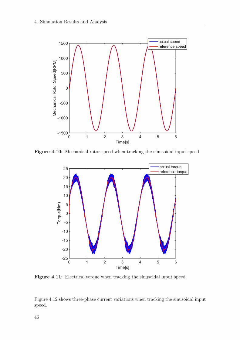
Figure 4.10 describes the rotor speed response due to sinusoidal input speed refer-ence. The actual speed and reference speed approximately overlap. The system hasa good performance when tracking a sinusoidal command speed.
Figure 4.11 shows the actual electric torque and its reference torque. The actualtorque and reference torque nearly overlap. It also proves that when the motortracks the sinudoidal input speed, the electric torque also varies in sinusoidal form..
45
4. Simulation Results and Analysis
Figure 4.10: Mechanical rotor speed when tracking the sinusoidal input speed
Figure 4.11: Electrical torque when tracking the sinusoidal input speed
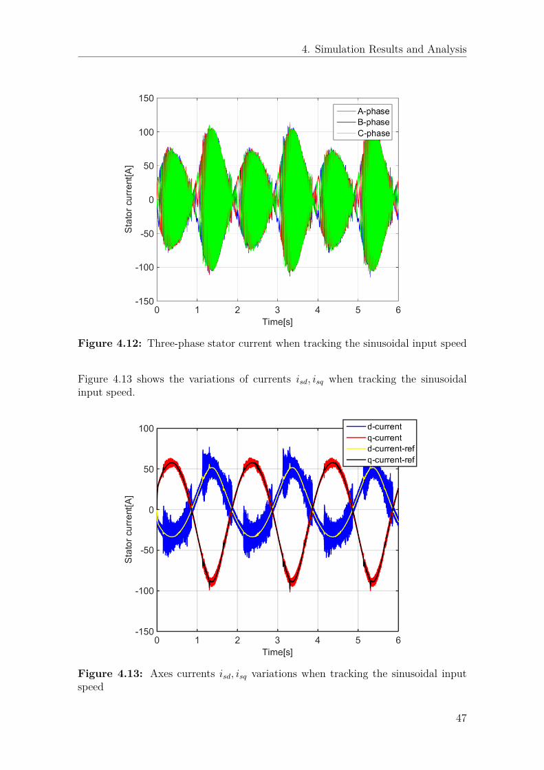
Figure 4.12 shows three-phase current variations when tracking the sinusoidal inputspeed.
46
4. Simulation Results and Analysis
Figure 4.12: Three-phase stator current when tracking the sinusoidal input speed
Figure 4.13 shows the variations of currents isd, isq when tracking the sinusoidalinput speed.
Figure 4.13: Axes currents isd, isq variations when tracking the sinusoidal inputspeed
47

4. Simulation Results and Analysis
48
5PMSM Model Implemented in
CarMaker
In this chapter, a brief introduction of CarMaker is conducted. More importantly,how the PMSM plant model and controller are implemented in CarMaker is pre-sented. Relevant results and analysis are also explained in this chapter.
5.1 Overview of CarMaker
According to [23], CarMaker is a simulation software for virtual test driving, specif-ically for testing passenger cars and light-duty vehicles. Virtual test driving can beused to develop and test the entire vehicle system and entire surrounding environ-ment in the realistic scenarios. A number of models for vehicles, roads, drivers andtraffic in CarMaker makes this possible.
CarMaker is a test platform with terrific performance, which guarantees flexibility,productivity and precision for all simulation tasks, thereby it is time-saving andcost-saving for vehicle development. Moreover, another advantage of CarMakeris that it can integrate with external models established from other software likeMatlab/Simulink to test the behavior of the various algorithms, see [23].
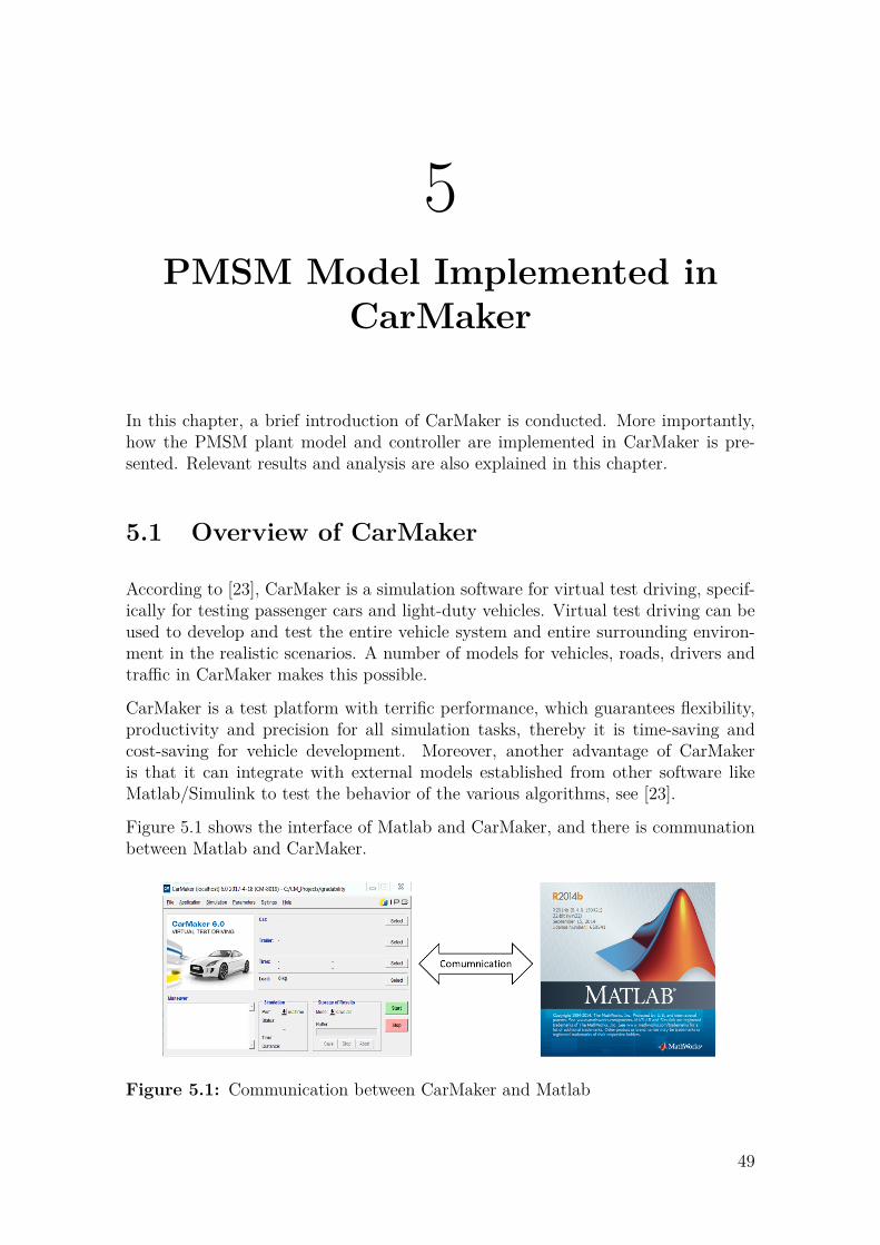
Figure 5.1 shows the interface of Matlab and CarMaker, and there is communationbetween Matlab and CarMaker.
Figure 5.1: Communication between CarMaker and Matlab
49
5. PMSM Model Implemented in CarMaker
5.2 Model Implementation in CarMaker
During the process of model implementation in CarMaker, the Functional Mock-upunit(FMU) is the key part. Some simulation programs or models can be packagedas FMUs in some simulation softwares, like Simulink. The FMU for co-simulationimport interface can be imported to CarMaker. Then CarMaker can conduct thetest based on the external models or programs.
The FMU interface complies with the Functional Mock-up Interface standard (FMI),which defines an open source standard used to build connections between differentsimulation programs. According to [24], each FMU includes a zip file containingsource code and a XML file with general information of the unit. FMI can enablethe integration with any FMI compliant software since it is an international standardand support morn than 70 tools, see [24]
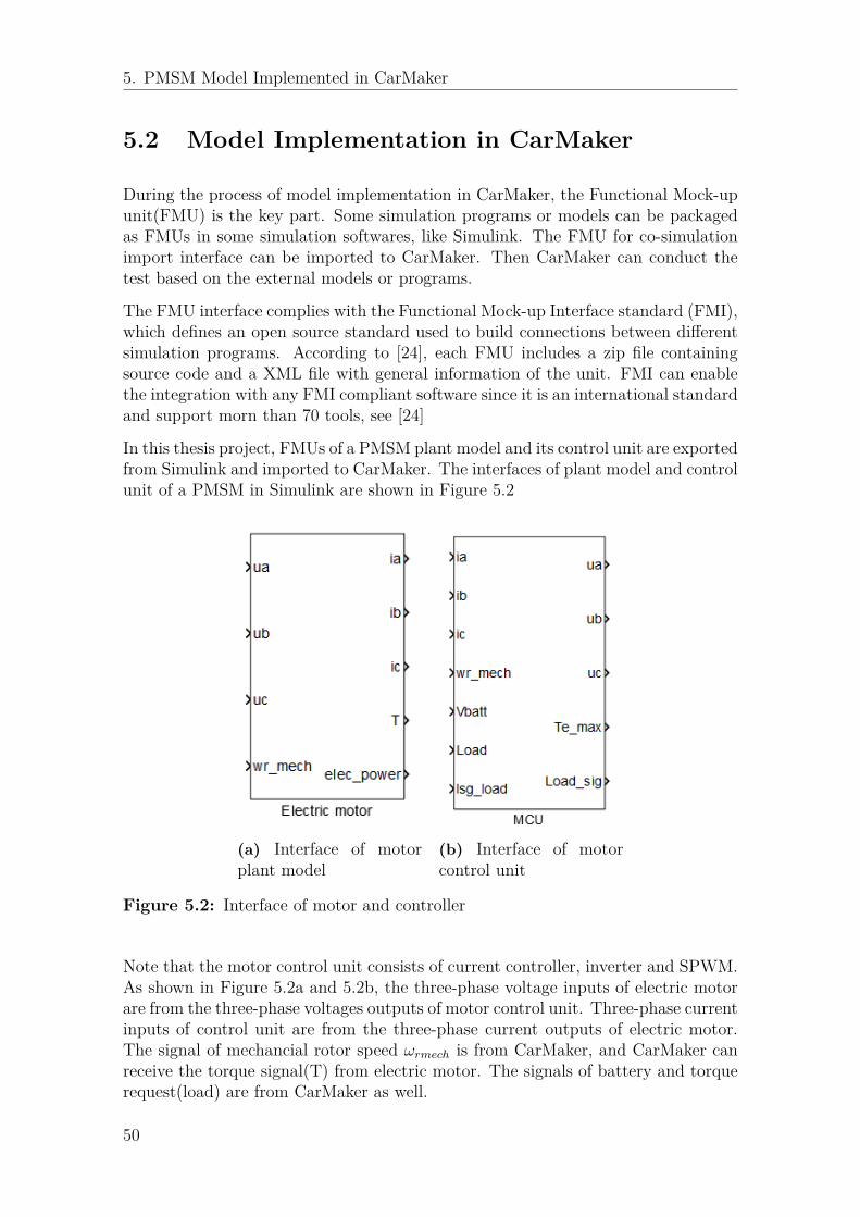
In this thesis project, FMUs of a PMSM plant model and its control unit are exportedfrom Simulink and imported to CarMaker. The interfaces of plant model and controlunit of a PMSM in Simulink are shown in Figure 5.2
(a) Interface of motorplant model
(b) Interface of motorcontrol unit
Figure 5.2: Interface of motor and controller
Note that the motor control unit consists of current controller, inverter and SPWM.As shown in Figure 5.2a and 5.2b, the three-phase voltage inputs of electric motorare from the three-phase voltages outputs of motor control unit. Three-phase currentinputs of control unit are from the three-phase current outputs of electric motor.The signal of mechancial rotor speed ωrmech is from CarMaker, and CarMaker canreceive the torque signal(T) from electric motor. The signals of battery and torquerequest(load) are from CarMaker as well.
50

5. PMSM Model Implemented in CarMaker
Figure 5.3 shows the FMU interface of plant model in CarMaker. Figure 5.4 showsthe FMU interface of plant model in CarMaker.
Figure 5.3: FMU interface of a PMSM model in CarMaker
Figure 5.4: FMU interface of a PMSM in CarMaker
It is apparent that the FMU inputs and outputs of motor model and its control unitin CarMaker comply with the inputs and outputs of motor model and controller inSimulink.
As a matter of fact, the motor plant model and motor control unit did not functionproperly in CarMaker, due to the limitations of model, the issues cannot be solvedin this thesis and have been put into the future research. However, some reasonswhich may cause the problem are as follows:
• When the two FMUs, motor plant model and motor control unit were exportedfrom Simulink and loaded back to Simulink for testing, the simulation resultedin an algebraic loop. The algebraic loop is created due to way of two modelsare connected. Plant model has outputs that are inputs to MCU and MCUoutputs are inputs to plant model. Simulink can handle original plant modeland control unit in Simulink since it can see what is inside the plant modeland control unit. But with FMUs, the Simulink cannot read the way of howthe different components connect inside the FMUs. This may lead to the sameproblem in CarMaker due to the connection of two models.
51

5. PMSM Model Implemented in CarMaker
• Fixed-step solver is used. And the step size must be smaller than the half ofswitching period of inverter. Otherwise, the carrier wave cannot be producedcorrectly, which means a smaller step size of plant model and control unit isused in CarMaker. CarMaker cannnot handle this kind of problem based onthe simulation results.
52
6Conclusions and future work
This chapter includes the conclusions and some proposals for further research.
6.1 Conclusions
This thesis presented the design, implementation and simulation of mathematicalmodel of PMSM and control algorithms for PMSM drives which can be applied toa number of automotive applications.
During the derivation of mathematical model of a PMSM, Clark’s and Park’s trans-formations were adopted to transform three-phase coordinates to two-phase(d-q)reference frame. Vector control was used throughout the control design. Currentregulator as well as speed controller were designed based on the IMC. The propercalculation of PI-controller parameters ensured correct operation and high precisionof controller. Sinusoidal pulse width modulation(SPWM) and inverter were assumedunder ideal situations.
The whole PMSM drive system is simulated by the use of Matlab/Simulink. Inorder to test the PMSM drive system in the entire vehicle in a virtual surroundingenvironment, CarMaker was used to import FMUs to conduct the test in realisticscenarios. Due to some limitations of the model and CarMaker, the test was notsuccessfully carried out. The possible causes were presented.
Finally, according to the simulation results it is shown that the simulation modelhas a good performance both in steady state and in variable-speed drive scenariowhen tracking the command speed, which verifies the PMSM model and controlalgorithms.
6.2 Future work
Some suggestions for future research in relation to either some issues which wereunsolved in the thesis or some ideas that can improve the performance of electricdrive system are demonstrated below.
53
6. Conclusions and future work
The modulation method can be improved. Sinusoidal pulse width modulation isadopted due to its simplicity and acceptable performances. Experimental testsshould be carried out to further verify the simulation results. However, a nicer mod-ulation alternative Space Vector Modulation(SVM) could be utilized and comparedwith the SPWM. The SVM is well-known for its effectiveness, simple implementationand harmonics reduction.
Regarding the problems of model running in CarMaker, future work could be toadjust the connections of two models to avoid the algebraic loop.
In the design and implementation of SPWM and inverter, no losses were consideredand SPWM was regards as in an ideal situation. In fact, the losses and blankingtime of inverter need to studied since they are quite important in practice.
That would be fascinating to investigate and test how the motor control unit behavesexperimentally[25].
54
Bibliography
[1] R. Curtin, Y. Shrago, and J. Mikkelsen, “Plug-in hybrid electric vehicles,”Reuters/University of Michigan, Surveys of Consumers, 2009.
[2] O. Wallmark, “Control of permanent-magnet synchronous machines in auto-motive applications,” Ph.D. dissertation, Chalmers University of Technology,2006.
[3] S. Chi, “Position-sensorless control of permanent magnet synchronous machinesover wide speed range,” Ph.D. dissertation, The Ohio State University, 2007.
[4] H. A. Toliyat and S. G. Campbell, DSP-based electromechanical motion control.CRC press, 2003.
[5] D. Y. Ohm, “Dynamic model of pm synchronous motors, drivetech,” Inc.Blacksburg, Virginia, 2000.
[6] S. B. Ozturk, “Modelling, simulation and analysis of low-cost direct torque con-trol of pmsm using hall-effect sensors,” Ph.D. dissertation, Texas A&M Univer-sity, 2007.
[7] J. Luukko et al., “Direct torque control of permanent magnet synchronousmachines-analysis and implementation,” Acta Universitatis Lappeenrantaensis,2000.
[8] D. Vindel, “Design, simulation and implementation of a pmsm drive system,”Master’s thesis, Chalmers University of Technology, 2011.
[9] P. Kundur, N. J. Balu, and M. G. Lauby, Power system stability and control.McGraw-hill New York, 1994, vol. 7.
[10] L. Harnefors, Control of variable-speed drives. Applied Signal Processing andControl, Department of Electronics, Mälardalen University, 2002.
[11] M. Merzoug, F. Naceri et al., “Comparison of field-oriented control and di-rect torque control for permanent magnet synchronous motor (pmsm),” WorldAcademy of Science, Engineering and Technology, vol. 45, pp. 299–304, 2008.
[12] F. B. Del Blanco, M. W. Degner, and R. D. Lorenz, “Dynamic analysis ofcurrent regulators for ac motors using complex vectors,” IEEE Transactions onIndustry Applications, vol. 35, no. 6, pp. 1424–1432, 1999.
55
Bibliography
[13] L. Harnefors, S. E. Saarakkala, and M. Hinkkanen, “Speed control of electricaldrives using classical control methods,” IEEE Transactions on Industry Appli-cations, vol. 49, no. 2, pp. 889–898, 2013.
[14] A. Ahmed, “Maximum torque per ampere (mtpa) control for permanent magnetsynchronous machine drive system,” Ph.D. dissertation, University of Akron,2013.
[15] G. Pandian and S. Rama Reddy, “Simulation and implementation of pwm in-verter fed induction motor drive,” International Journal of Innovative Researchin Science, Engineering and Technology, vol. 2, no. 11, pp. 6103–13, 2013.
[16] P. Thamizhazhagan and S. Sutha, “Analysis of pwm techniques for power qual-ity improvement in pmsm drives,” Indian Journal of Science and Technology,vol. 8, no. 24, 2015.
[17] J. Hellsing, Design and optimization of a permanent magnet motor for a hybridelectric vehicle. Chalmers University of Technology, 1998.
[18] M. S. Islam, N. I. Raju, and A. U. Ahmed, “Sinusoidal pwm signal generationtechnique for three phase voltage source inverter with analog circuit & simula-tion of pwm inverter for standalone load & micro-grid system,” InternationalJournal of Renewable Energy Research (IJRER), vol. 3, no. 3, pp. 647–658,2013.
[19] S. S. Lechat, “Voltage oriented control of three-phase boost pwm converters,”Master’s thesis, Chalmers University of Technology, 2010.
[20] H. Dehbonei, L. Borle, and C. Nayar, “A review and a proposal for optimalharmonic mitigation in single-phase pulse width modulation,” in Power Elec-tronics and Drive Systems, 2001. Proceedings., 2001 4th IEEE InternationalConference on, vol. 1. IEEE, 2001, pp. 408–414.
[21] A. Hughes and B. Drury, Electric motors and drives: fundamentals, types andapplications. Newnes, 2013.
[22] E. L. C. Arroyo, “Modeling and simulation of permanent magnet synchronousmotor drive system,” University of puerto rico, Mayagüez Campus, 2006.
[23] I. CarMaker, “User’s guide version 4.5. 2,” IPG Automotive, Karlsruhe, Ger-many, 2014.
[24] S. Rotger-Griful, S. Chatzivasileiadis, R. H. Jacobsen, E. M. Stewart, J. M.Domingo, and M. Wetter, “Hardware-in-the-loop co-simulation of distributiongrid for demand response,” in Power Systems Computation Conference (PSCC),2016. IEEE, 2016, pp. 1–7.
[25] C. Dubar, “Design and analysis of a fault-tolerant fractional slot pmsm for avehicle application,” Ph.D. dissertation, Chalmers University of Technology,2016.
56

AAppendix 1
I

A. Appendix 1
II

BAppendix 2
III