WATER RESOURCES BULLETIN VOL. 15, NO. 6 AMERICAN WATER RESOURCES ASSOCIATION DECEMBER 1979

GROUND WATER SIMULATION USING A ONE DIMENSIONAL FLOW MODEL'

Irfan A. Khan2

ABSTRACT: In projects involving ground water problems, dependence on the mathematical modeling of the ground water flow phenomena is inescapable. At present, two dimensional flow models, which require tremendous amounts of computer time and storage, are generally used. When such bulky models are used for planning purposes, the two requirements(c0mputer time and storage) can severely limit the number of alternatives that can be considered. A simple quantity and quality simulation model is developed here which requires considerably less com- puter time and storage and gives reasonably accurate results. The model was applied to simu- late a ground water basin in San Luis Rey River in Southern California. The results were com- pared with those obtained by a USGS model. It was found that the simple model gave results which were consistentaly within five percent of the USGS model results, while the requirements on computer time and storage were drastically reduced. (KEY TERMS: ground water; one dimensional flow model.)

INTRODUCTION The dependency on ground water for municipal, industrial, and agricultural water

supplies is increasing rapidly in many parts of theworld. This has brought special signifi- cance and importance to research related to ground water movement. The two dimen- sional unsteady state movement of water in a nonhomogeneous and anisotropic aquifer can be described by an equation of the form (Konikow and Bredehoeft, 1974).

a ah - ah - (T.. -) - S - + W(x,y,t) i j = 1,2 axi IJ a 3 at

Where Ti, is the transmissivity tensor, L2/T; h is the hydraulic head, L; S is the coefficient of storage (dimensionless); t is time; and W is the volume flux per unit area, L/T.

Also assuming that no chemical reactions occur between the water and the aquifer or soil materials, the equation describing the mass transport and dispersion of dissolved chemical constituents in a saturated porous medium may be written (Konikow and Bredenoeft, 1974).

Paper No. 79029 of the Water Resources Bulletin. Discussions are open until August 1, 1980. 'Assistant Professor, Department of Civil Engineering, Youngstown State University, Youngstown,

Ohio 44555.

1618

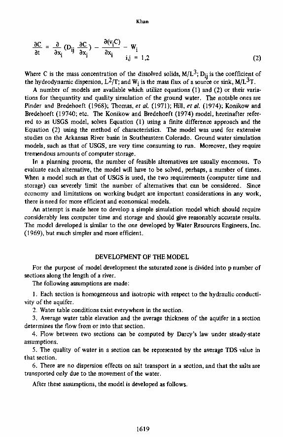
Khan

Where C is the mass concentration of the dissolved solids, M/L3; Dij is the coefficient of the hydrodynamic dispersion, L2/T; and Wi is the mass flux of a source or sink, M/L3T.

A number of models are available which utilize equations (1) and (2) or their varia- tions for thequantity and quality simulation of the ground water. The notable ones are Pinder and Bredehoeft (1 968); Thomas, et al. (1 97 1); Hill, et al. (1 974); Konikow and Bredehoeft (19740; etc. The Konikow and Bredehoeft (1974) model, hereinafter refer- red to as USGS model, solves Equation (1) using a finite difference approach and the Equation (2) using the method of characteristics. The model was used for extensive studies on the Arkansas River basin in Southeastern Colorado. Ground water simulation models, such as that of USGS, are very time consuming to run. Moreover, they require tremendous amounts of computer storage.

In a planning process, the number of feasible alternatives are usually enormous. To evaluate each alternative, the model will have to be solved, perhaps, a number of times. When a model such as that of USGS is used, the two requirements (computer time and storage) can severely limit the number of alternatives that can be considered. Since economy and limitations on working budget are important considerations in any work, there is need for more efficient and economical models.

An attempt is made here to develop a simple simulation model which should require considerably less computer time and storage and should give reasonably accurate results. The model developed is similar to the one developed by Water Resources Engineers, Inc. (1 969), but much simpler and more efficient.

DEVELOPMENT OF THE MODEL For the purpose of model development the saturated zone is divided into p number of

The following assumptions are made:

1. Each section is homogeneous and isotropic with respect to the hydraulic conducti-

2. Water table conditions exist everywhere in the section. 3. Average water table elevation and the average thickness of the aquifer in a section

4. Flow between two sections can be computed by Darcy’s law under steady-state

5 . The quality of water in a section can be represented by the average TDS value in

6. There are no dispersion effects on salt transport in a section, and that the salts are

After these assumptions, the model is developed as follows.

sections along the length of a river.

vity of the aquifer.

determines the flow from or into that section.

assumptions.

that section.

transported only due to the movement of the water.

1619

Ground Water Simulation Using a One Dimensional Flow Model

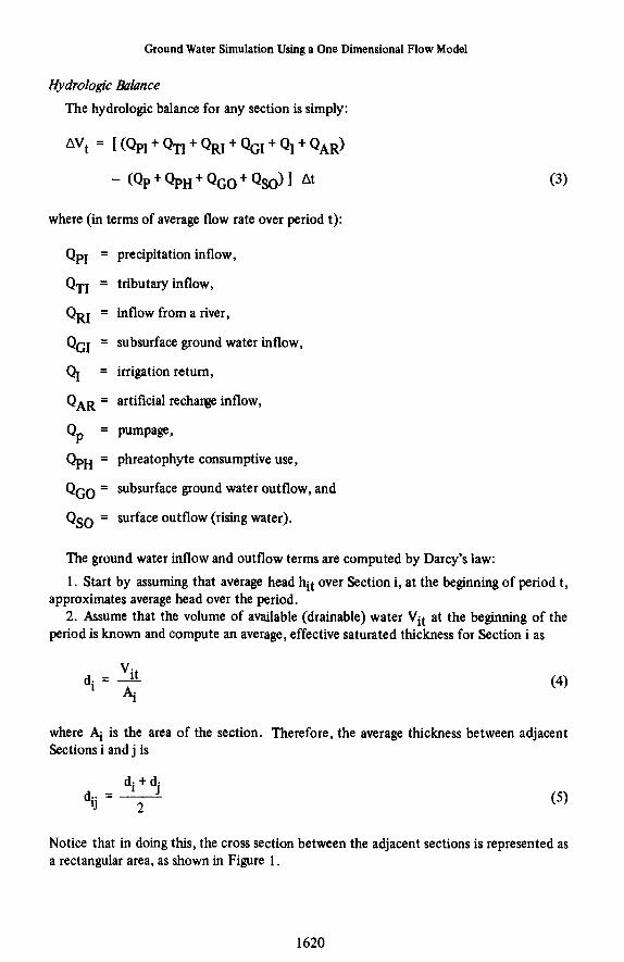
Hydrologic &lunce The hydrologic balance for any section is simply:

where (in terms of average flow rate over period t):

QpI = precipitation inflow,

QTI = tributary inflow,

QM = inflow from a river,

QGl = subsurface ground water inflow,

4 = irrigation return,

QAR = artificial recharge inflow,

Qp = pumpage,

Q ~ H = phreatophyte consumptive use,

QGO = subsurface ground water outflow, and

Qso = surface outflow (rising water).

The ground water inflow and outflow terms are computed by Darcy's law: 1. Start by assuming that average head hit over Section i, at the beginning of period t,

2. Assume that the volume of available (drainable) water Vit at the beginning of the approximates average head over the period.

period is known and compute an average, effective saturated thickness for Section i as

where Ai is the area of the section. Therefore, the average thickness between adjacent Sections i and j is

di + dj

4J =2 Notice that in doing this, the cross section between the adjacent sections is represented as a rectangular area, as shown in Figure 1.

1620

Khan

Normal Operating Range

Effective Cross Section for Simplified Model

Figure 1. Simplification of Cross Section.

3. Assuming (i) the average width between sections is given, (ii) computing average permeability between sections as

s+Kj 4J = 2

where Ki is the permeability associated with Section i, and (iii) estimating the hydraulic- gradient Axi, between the sections, subsurface flows between Sections i and j are com- puted by using Darcy's law.

Q.. = d . . W . . y . h . 9 9 9 J J

4. Assuming all other inflows and outflows are known, AVt in (3) is now computed. For this purpose, volume-depth curve for the ground water basin can be used. For small changes in depth, the volume depth relationship can be assumed linear. Then

- hit - A4t 'it ''it

or

(7)

We have assumed that the term in parentheses is constant for all periods and that &t is simply a linear function of AVit.

5 . We now compute

hi,ttl = hit ahit (9)

1621

Ground Water Simulation Using a One Dimensional Flow Model

and reestimate average head over period t as

- hiti-hi , t t l hit =

6. We now repeat steps 1 through 4 using new estimates of Fit, until successive values of hit computed by Equation (10) reasonably coincide.

Salt Balance The salt balance in each section is calculated by assigning a concentration value (c) to

pertinent inflows and outflows, and estimating fertilizer application. Thus, for any section:

where SF is the portion of the fertilizer application rate reaching the water table and S, is the salt balance. The ground water inflows and outflows are computed from the hydro- logic balance portion of the model. The concentration C m corresponds to the ground water concentration in the section being considered. Concentration CGI is that associated with the adjacent upstream section.

APPLICATION OF THE MODEL San Luis Rey River basin in Southern California (Figure 2) was used as a case study to

compare the results of the USGS model and the simplified model. Data from Moreland (1974) on the case study area were used for the purpose of comparison. Three subbasins, Pauma, Pala, and Bonsall were calibrated and each was divided into four sections. For Bonsall, a dry historical period (1958-65), an average period (1966-68), and a wet period (January to June 1969) were chosen for analysis. For Pauma and Pala a five-year period from 1973 to 1977 was used. For the initial year of 1958 in case of Bonsall and 1973 in case of Pauma and Pala, the node-by-node quantity and quality data used in USGS model were simply lumped together on a section-by-section basis for use in the simplified model. Inflows and outflows were totaled under the various categories for each section, and ground water concentrations were averaged. For the purpose of calibration, it was de- cided that only two parameters would be adjusted in the simplified model: (i) average width of cross section between sections my), and (ii) average permeability (Ki,) govern-

widths were first adjusted within reasonable limits, until a good match with the historical data was obtained. Average permeability was altered only slightly, and even this was probably unnecessary. The models were run on a ClYC 6400 computer at the Colorado State University.

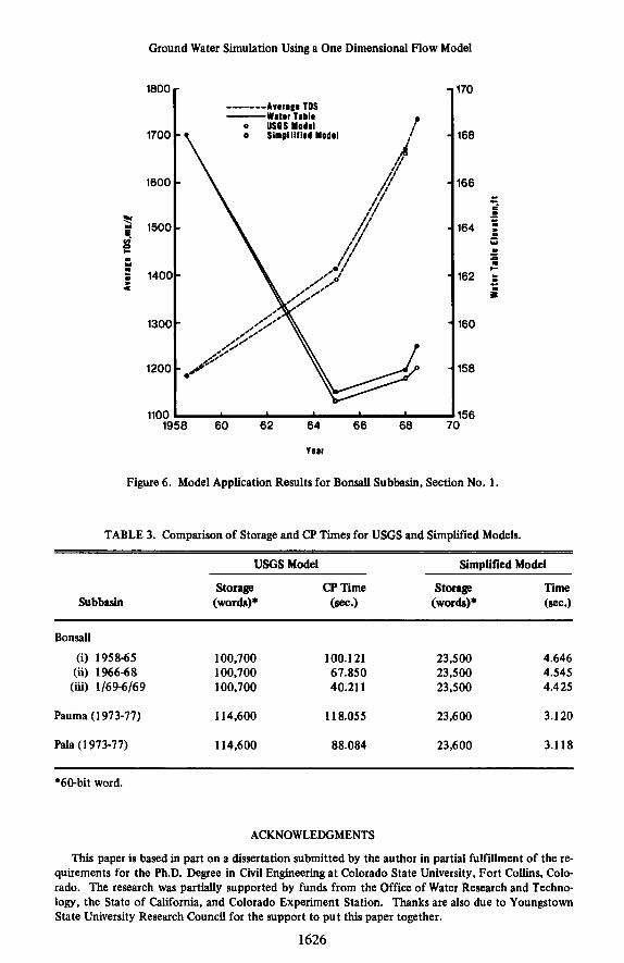
The comparison of USGS model output, as averaged over the sections with the output from the simplified model (as finally calibrated) are given in Figures 3 to 6 and Tables 1 and 2. Notice from Tables 1 and 2 that the output of the USGS model and the simplified

ing flow between sections. First guesses # or these values were simple averages. The

1622

Khan

model differ by less than one percent. The results of Bonsall subbasin are shown graphically to convey a pictorial impact on the reader. The error in this case is consistant- ly within five percent. Table 3 shows the computer rapid access (core) storage and ap- proximate central process (CP) execution times for the USGS and the simplified models. Notice from Table 3 that the storage requirements for the simplified model is approxi- mately 1/5th that of the USCS model and the CP time ranges from l/lOth to 1/40th that of the USCS model.

LEGEND GROUND WATER BASIN -

4 STREAM GAGING STATION r-- HYDROLOGIC BOUNDARY -- DRAINAGE BOUNDARY

DIVIDING SUBBASINS

S C A U YlltS

t

A r t Ch iHA’A

Figure 2. Subbasins in the Lower San Luis Rey River Basin.

------- Average TDS - Water Table USGSModsl

0 Simplified Model I

1600

1400

Y

ui

m

; 1200

0 c Y

E 1000 - <

800

265

255 - e 0

-. .-

245 5 0

W

Y

(.

- - a

235 rn ” i

!25

Figure 3. Model Application Results for Bonsall Subbasin, Section No. 4.

1623

Ground Water Simulation Using a One Dimensional Flow Model

1200

1100

7 1000

; 900

w- 0 c 0 u

*

800

-----.-- Average TDS -- Water Table 0 USGS Model 0 Simplified Model

700 I I 1 1

1958 60 62 64 66 68

Year

Figure 4. Model Application Results for B o n d Subbasin, Section No. 3.

TABLE 1. Water Table Elevations in Feet (1 977).

220

210 - -. r 0

c. em > Y

.-

200 = Y

a 4u I-

Y

- -

190 g

180 I

Subbasin

Pauma M a

USCS Simplified USGS Simplified Model Model Model Model

Section No. (ft) (ft) (ft) (ft)

1 666 666 27 8 278

2 704 704 336 337

3 712 714 36 2 360

4 830 834 4 24 4 26

CONCLUSIONS The simple one dimensional flow model described in this paper is extremely efficient.

The model was applied to simulate ground water basin in the San Luis Rey River area in Southern California. The results were compared with those obtained by the USGS Model. It was found that the simple model gave results which were consistently within five percent of the USGS model results, while the requirement on the computer time and storage were drastically reduced. The study shows that one dimensional ground water flow models can be very important and useful tools in the initial planning process where

1624

Khan

high accuracies are not warranted, and considerable time and money can be saved by using more efficient models.

Average TDS Water Table

------- SIX Yndrl

1500r - ? I

I

I - i . T.#"

1300 -

1200 -

1100 -

1000 -

.' v

900 1 I I I I I

1958 60 62 64 66 68

Year

Figure 5. Model Application Results for B o n d Subbasin, Section No. 2.

TABLE 2. TDS in MC/Q (1 977).

182

178

174 = zt 5 .- c a

170 s c b

c m

166 5

162

158

Subbasin

Pauma Pala

USGS Simplified USGS Simplified Model Model Model Model

Section No. (MG/Q) (MG/Q) (MC/Q) (MG1.9)

1 710 724 1550 1580 2 680 663 716 708 3 615 602 614 601 4 500 498 549 544

1625

Ground Water Simulation Using a One Dimensional Flow Model

1800

1700

1600

* p 150C a- 0 I- . Y

E 140( 2

130C

120c

1100 1s

-------AVOIIgO TDS

t -Water Tabla o U P S Yodml o Slnplllflrd Model

3 60 62 64 66 68

170

168

166 - 2 - -

164 - Y .I a I-

- a

162 : - i

160

158

156 1

Figure 6. Model Application Results for B o n d Subbasin, Section No. 1.

TABLE 3. Comparison of Storage and CP Times for USGS and Simplified Models.

USGS Model Simplified Model

Storage CP Time Storage Time Subbasin (words)* (=.I (words)' (=.I

B o n d

(i) 195865 100.700 100.121 23,500 4.646 (ii) 1966-68 100,700 67.850 23,500 4.545 (iii) 1/69-6/69 100,700 40.21 1 23,500 4.425

Pauma (1 973-77) 1 14,600 11 8.055 23,600 3.120

Pala (1 973-77) 114,600 88.084 23,600 3.118

*6Gbit word.

ACKNOWLEDGMENTS

This paper is based in part on a dissertation submitted by the author in partial fu l f i ien t of the re- quirements for the Ph.D. Degree in Civil Engineering at Colorado State University, Fort Collins, Colo- rado. The research was partially supported by funds from the Office of Water Research and Techno- logy, the State of California, and Colorado Experiment Station. Thanks are also due to Youngstown State University Research Council for the support to put this paper together.

1626

Khan

LITERATURE CITED

Hill, R. W., E. K. Israelson, and J. P. Riley, 1973. Computer Simulation of the Hydrologic and Salinity Flow Systems Within the Bear River Basin. Utah Water Research Laboratory, Utah State Univer- sity, Logan, PRWG 104-1.

Konikow, L. F. and J. D. Bredehoeft, 1974. Modeling Flow and Chemical Quality Changes in an Irri- gated Stream-Aquifer System. Water Resources Research 1 O(3): 546-562.

Labadie, J. W., I. A. Khan, and 0. J. Helweg, 1976. Salinity Management Strategies for the Lower San Luis Rey River Basin. Technical Report, Colorado State University, Fort Collins.

Moreland, J. A., 1974. Hydrologic and Salt-Balance Investigations Utilizing Digital Models, Lower San Luis Rey River Area, San Diego, California. USGS, Water Resources Investigations 24-74.

Pinder, G. F. and J. D. Bredehoeft, 1968. Application of Digital Computer for Aquifer Evaluation. Water Resources Research 4(5): 1069-1 093.

Thomas, J. L., J. P. Riley, and E. K. Israelson, 1971. A Computer Model of the Quantity and Chemical Quality of Return Flow. Utah Water Research Laboratory, Utah State University,

Water Resources Engineers, Inc., 1969. An Investigation of Salt Balance in the Upper Santa Ana River Basin. Presented to the State Water Resources Control and the Santa Ana River Basin Regional Water Quality Control Board.

Logan, PRWG 77-1.

1627