All-Weather Ground Surface Temperature Simulation

1

ST. ANTHONY FALLS LABORATORY Engineering, Environmental and Geophysical Fluid Dynamics

Project Report No. 478

All-Weather Ground Surface Temperature Simulation

by

William R. Herb, Ben Janke, Omid Mohseni, and Heinz G. Stefan

Prepared for

Minnesota Pollution Control Agency St. Paul, Minnesota

September, 2006 Minneapolis, Minnesota

2

The University of Minnesota is committed to the policy that all persons shall have equal access to its programs, facilities, and employment without regard to race, religion, color, sex, national origin, handicap, age or veteran status.

3

Abstract

Thermal pollution from urban runoff is considered to be a significant contributor to the degradation of coldwater ecosystems. Impervious surfaces (streets, parking lots and buildings) are characteristic of urban watersheds. A model for predicting temperature time series for dry and wet ground surfaces is described in this report. The model has been developed from basic principles. It is a portion of a larger project to develop a modeling tool to assess the impact of urban development on the temperature of coldwater streams. Heat transfer processes on impervious and pervious ground surfaces were investigated for both dry and wet weather periods. The principal goal of the effort was to formulate and test equations that quantify the heat fluxes across a ground surface before, during and after a rainfall event. These equations were combined with a numerical approximation of the 1-D unsteady heat diffusion equation to calculate temperature distributions in the ground beginning at the ground surface. Equations to predict the magnitude of the radiative, convective, conductive and evaporative heat fluxes at a dry or wet surface, using standard climate data as input, were developed. Plant canopies were included for surfaces covered by vegetation. The model can simulate the ground surface and sub-surface temperatures continuously throughout a specified time period (e.g. a summer season) or for a single rainfall event. Ground temperatures have been successfully simulated for pavements, bare soil, short and tall grass, trees and two agricultural crops (corn and soybeans). The simulations were first run for different locations and different years as imposed by the availability of measured soil temperature and climate data. Data came from sites in Minnesota, Illinois and Vermont. To clarify the effect of different land uses on ground temperatures, the calibrated coefficients for each land use and the same soil coefficients were used to simulate surface temperatures for a single climate data set from St. Paul, MN (2004). Asphalt and concrete give the highest surface temperatures, as expected, while vegetated surfaces gave the lowest. Bare soil gives surface temperatures that lie between those for pavements and plant-covered surfaces. The soil temperature and moisture model appears to model surface temperatures of bare soil and pavement with RMSEs of 1 to 2°C, and surface temperatures of vegetation-covered surfaces with RMSEs of 1 to 3oC. The plant canopy model used in this study, based on the work of Best and Deardorff, provides an adequate approximation for the effect of vegetation on surface heat transfer, using only a few additional parameters compared to bare surfaces. While further simplifications of the model are possible, such simplifications do not reduce the number of required input parameters, and do not eliminate the need for estimating the seasonal variation of the vegetation density. A model for roof temperatures was also developed, based on the surface heat transfer formulations used for pavement. The model has been calibrated for both a commercial tar/gravel roof and a residential roof. Compared to pavement, the roof surface reach similarly high maximum temperatures, but reach lower minimum temperature at night cool due to their lower thermal mass.

4

TABLE OF CONTENTS NOTATIONS AND UNITS .............................................................................................................. 5 1. INTRODUCTION ...................................................................................................................... 6 2. TEMPERATURE MODEL FORMULATION FOR BARE SURFACES ................................ 7

2.1 Model components................................................................................................................ 7 2.2 Boundary and initial conditions ............................................................................................ 7 2.3 Model input and output......................................................................................................... 7 2.4. Model equations................................................................................................................... 8

3. SIMULATED TEMPERATURES BELOW PAVED SURFACES ........................................ 10 3.1 Calibrated parameter values............................................................................................... 10 3.2 Parameter sensitivity analysis ............................................................................................ 11 3.3 Comparison of simulated and measured pavement temperatures...................................... 11

4. SIMULATED TEMPERATURES BELOW A BARE SOIL SURFACE ............................. 16 5. TEMPERATURE MODEL FORMULATIONS AND CALIBRATIONS FOR SURFACES WITH VEGETATION COVER................................................................................................... 20

5.1 Formulation of canopy model #1 (Deardorff’s model)..................................................... 20 5.2 Calibration of canopy model #1 (Deardorff’s model) ....................................................... 21 5.3 Formulation of canopy model #2 (Best’s model) .............................................................. 23 5.4 Calibration of canopy model #2 (Best’s model) ................................................................ 26 5.5 Soil temperature sensitivity to canopy model #2 parameters ............................................. 27

6. SIMULATED TEMPERATURES BELOW GRASS-, CROP- AND TREE-COVERS ........ 27 6.1 Lawns and grasslands ........................................................................................................ 27 6.2 Crop (agricultural) land....................................................................................................... 31 6.3 Forest.................................................................................................................................. 39

7. TEMPERATURE MODEL FORMULATIONS AND CALIBRATIONS FOR ROOFS ....... 41 7.1 Roof temperature model Formulation................................................................................ 41 7.2 Roof temperature model calibration .................................................................................. 41

8. SUMMARY AND CONCLUSIONS ...................................................................................... 44 ACKNOWLEDGMENTS ............................................................................................................ 49 REFERENCES ............................................................................................................................. 50 APPENDIX A. THERMAL PROPERTIES OF SOILS AND PAVEMENT ............................. 52 (from Janke et al. 2006) ............................................................................................................ 52 APPENDIX B. MODELING THE HEAT FLUX BETWEEN RUNOFF AND PAVEMENT SURFACE..................................................................................................................................... 54 APPENDIX C. SOIL MOISTURE TRANSPORT MODEL ...................................................... 56

5

NOTATIONS AND UNITS αs: reflectivity of a surface with respect to solar radiation [dimensionless] β: thickness ratio for surface runoff conduction ε: surface emissivity [dimensionless] θ: soil moisture content [dimensionless] θv: virtual air temperature [ºC] ρ: density [kg/m3] ρa: density [kg/m3] σ: Stefan-Boltzmann constant [kJ K-4 m-2 day-1] Ce: soil evaporation parameter [dimensionless] Cfc: forced convection bulk transfer coefficient [dimensionless] Cnc: free convection bulk transfer coefficient [dimensionless] CHf: foliage aerodynamic roughness [m] Cf: foliage bulk transfer coefficient [m] CSh: wind sheltering coefficient [dimensionless] Cp: specific heat [J/kg·K] CR : cloudiness factor [0-1, dimensionless] δ: conduction layer thickness [m] ∆t: analysis time step D: thermal diffusivity [m2/s] ea: atmospheric water vapor pressure [Pa] es: saturation vapor pressure at surface temperature [Pa] hli: incoming longwave radiation [W/m2] hlo: outgoing longwave radiation [W/m2] hs: net solar radiation [W/m2] hconv: convection between land or water surface and atmosphere [W/m2] hevap: evaporative heat transfer [W/m2] hnet: net (total) heat transfer at surface [W/m2] hrad: net shortwave and longwave radiation [W/m2] hro: surface runoff heat transfer [W/m2] Lv: latent heat of vaporization of water [J/kg] ν: vegetation density p: atmospheric pressure [Pa] p1: initial precipitation intensity [m/s] P: total precipitation depth [m] q: specific humidity [kgw/kga] ra: aerodynamic resistance [s/m] rs: stomatal resistance [s/m] Rs: observed solar radiation [W/m2] t: time [s] Ta: air temperature [°C] Taf: characteristic air-vegetation temperature [ºC] Tdp: dewpoint temperature [ºC] Tg: ground surface temperature [ºC] Ts: surface temperature [°C] uaf: characteristic ground-canopy wind speed [m/s] u: wind speed [m/s] uz: wind speed evaluated at a height of z meters [m/s]

6

1. INTRODUCTION Urbanization affects the temperature of cold water streams. Cold-water streams typically exist in well-shaded watersheds with large water inputs from groundwater. They are ecologically significant because they support coldwater fisheries and other wildlife that would be unable to survive in warmer streams. A threat to these streams is the conversion of land from existing agricultural use or natural conditions to urban/residential/commercial use. Urban expansion usually requires removing agricultural crops or natural vegetation, and replacing them with parking lots, roads, lawns, and buildings. These changes affect shading, heat transfer, and hydrology within the watershed. Currently, there are few tools available to project to what extent stream temperatures are influenced by development in the watershed. The thermal pollution of coldwater (trout) streams by surface runoff from impervious surfaces in residential and commercial urban areas can be assessed by simulation of hydrologic and heat transfer processes. To simulate the processes that give the quantity and the temperature of surface runoff from a rainfall event, an initial or dry weather condition of ground temperatures prior to the rainfall is needed. This information can be provided by measurements or by heat transfer analysis/simulation. One small but significant portion of a hydrothermal runoff model therefore is the creation of a sub-model that can predict the temperature of paved and unpaved portions of watersheds before, during and after a rainfall event. A number of models are currently available for the prediction of runoff temperature from paved surfaces, and even from entire urban or partially-developed watersheds. These models have been reviewed by Janke et al. (2006). We shall describe our approach to the problem in this report. The approach used in this study is to simulate surface temperatures using one-dimensional heat transfer analysis, and calibrate the model using measured surface temperatures. The calibrated model can then be used to simulate surface temperatures for any storm event in any location in the state, given suitable climate data. This study is closely related to an analysis of asphalt and concrete pavement temperatures recorded by MnDOT at the MNROAD site on I-94 near Albertville, MN. This analysis and the associated simulation of the pavement temperatures is summarized in a report by Herb, Marasteanu and Stefan (2006). Another related application is in the estimation of runoff temperatures as summarized in a report by Herb, Janke, Mohseni and Stefan (2006). The surface heat transfer model can also be used to assess the thermal impact of land use change on groundwater temperature. Specific issues that will be addressed in this report include: 1) Estimation of the surface and near-surface temperatures prior to rainfall events with sufficient temporal resolution to capture the rapid changes that occur as storm fronts approach. 2) Effects of ground surface properties on surface temperature, e.g. paved surface vs. grass-covered surface, asphalt vs. concrete, new pavement vs. weathered pavement. 3) Effects of vegetation on surface heat transfer and soil temperature profiles.

7

2. TEMPERATURE MODEL FORMULATION FOR BARE SURFACES In this section we describe the basic model formulation, calibration and application for predicting surface heat transfer and vertical temperature profiles below bare surfaces such as pavements and bare soil. The presence or absence of vegetation on a surface has a profound effect on the temperature of the underlying surface, because plants provide shading, wind sheltering, and evapotranspiration. A modification to the model to include the effects of vegetation is described in Section 3. The model is unsteady and one-dimensional, considering only vertical heat fluxes and the vertical variation of temperature.

2.1 Model components The major components of the model are: 1) Unsteady vertical heat conduction through a soil column with spatially varying thermal properties. Distinct surface layers such as asphalt or concrete pavement or crushed rock are assigned separate thermal properties from the underlying soil (thermal conductivity, specific heat, density). Typical thermal properties of ground layers are summarized in Appendix A. 2) A model for surface heat flux, based on the surface properties (roughness, albedo, and emissivity) and the weather conditions (e.g. solar irradiance, air temperature, wind speed, relative humidity or dewpoint temperature). Although the primary purpose of the model is to simulate surface temperatures during dry weather conditions, the model includes a simple model for heat transfer between the soil/pavement surface and precipitation runoff (Appendix B). As a result, the model can be used to simulate surface temperatures for a continuous sequence of dry and wet surface conditions/weather periods. 3) Infiltration and movement of moisture in the soil column (Appendix C). This component is needed for analysis of pervious surfaces such as bare soil, where surface evaporation contributes to the surface heat flux during both dry and wet weather conditions.

2.2 Boundary and initial conditions 1) An adiabatic boundary condition or a specified temperature at the lower boundary of the soil domain. At 10 m depth the year-round soil temperature can be assumed constant and equal to the mean annual air temperature, corrected by a constant. 2) The model is initiated at any time of year with a known soil temperature profile.

2.3 Model input and output Required input to the soil temperature model includes: 1) Climate data: air temperature (°C), relative humidity (%), wind speed (m/s), and solar radiation (W/m2). For dry weather periods, one hour time intervals are sufficient to simulate

8

surface temperatures. To accurately capture the dynamics of surface temperature prior to rainfall events, climate data at 10 to 15 minute interval is preferable. Latitude, longitude, and elevation for the site to be simulated are also required for the algorithm to estimate cloud cover. 2) Ground surface parameters: albedo, emissivity, and aerodynamic roughness. 3) Soil/pavement data: hydraulic conductivity, porosity, field capacity, wilting point, density, thermal conductivity and specific heat. For conventional pavements, infiltration is assumed to be zero, so that only density, thermal conductivity and specific heat are specified. 4) Initial conditions: Soil temperatures are specified at an arbitrary number of depths. Initial temperatures at the node locations of the model are determined by interpolation of the specified values. The computed temperature profile in the pavement and soil is stored for each time step.

2.4. Model equations 2.4.1 Heat conduction equation Vertical soil temperature profiles are obtained in successive time steps of 1 hr or less by solving the unsteady 1-D heat conduction equation using an implicit finite difference formulation. The model uses thin layers for the pavement or the near surface soil layers, e.g. 4 cm, and thicker layers towards the lower boundary, e.g. 1 m. As a result, good simulation results are possible with, e.g. 15 layers. The model includes advective heat transfer due to vertical soil moisture movement, e.g. infiltration, but does not presently include moisture dependent thermal properties. 2.4.2 Surface heat transfer/fluxes The net vertical heat transfer at the soil or pavement surface includes components due to long wave radiation, short wave (solar) radiation, evaporation, and convection. The heat transfer formulations used in this study are based on those given by Edinger et al. (1968, 1974) for lake and reservoir surfaces, but are applied to pavement and soil by adjusting parameters appropriately. Equations 2.1 through 2.10 give the formulations used to calculate the net surface heat flux, hnet, and Table 2.1 gives the definition of the variables used. The derivation for the runoff heat transfer, hro, is given in Appendix B. (2.1) roconvevapradnet hhhhh −−−=

(2.2) ( )( )asat33.0

vncsfcvaevap qqCuCLh −θ∆+ρ=

(2.3) ( )( )as33.0

vncsfcpaconv TTCuCch −θ∆+ρ=

(2.4) lolisrad hhhh −+= (2.5) ( ) ss R1h α−=

9

(2.6) ( )( ) 4ak

08.0ali TeCR167.0CRh −⋅+εσ=

(2.7) 4sklo Th εσ=

(2.8) us = CSh u10

(2.9) ( ) ( )( )( )

waterp

pavepdpswro cP2

c;

1TTcp

tPh

ρ

ρδ=β⎟⎟

⎠

⎞⎜⎜⎝

⎛β+

β−ρ

∆=

Many of the surface heat transfer terms are non-linear, i.e. the heat flux depends on the surface temperature, and the outgoing long wave radiation is strongly dependent on surface temperature. A simple linearization was used to help keep numerical stability at longer time steps. The outgoing long wave radiation is linearized as (2.10) ( )sksk

3sk

4sklo T'TT4Th −εσ+εσ=

where T’sk and Tsk are the value of the surface temperature for the current and previous time steps. Table 2.1. Surface heat transfer parameter definitions. Cfc forced convection transfer coefficient Tdp dew point temperature, °C Cnc free convection transfer coefficient Tak air temperature, °K CR cloud cover ratio (0 – 1) Ts surface temperature, °C CSh wind sheltering coefficient Tsk surface temperature, °K cp specific heat us adjusted wind velocity hrad net incoming surface radiation u10 wind velocity at 10 m above the surface hs short wave radiation absorbed at surface α surface albedo hli incoming long wave radiation ∆θ difference in virtual temperature hlo outgoing long wave radiation v between ground and air hro runoff heat transfer δ conduction layer thickness Lv latent heat of vaporization ε surface emissivity P precipitation depth ρ density Rs incoming solar radiation σ Stefan-Botzmann constant Ta air temperature, °C

10

3. SIMULATED TEMPERATURES BELOW PAVED SURFACES The bare surface temperature model was calibrated and verified using weather data as model input, and measured pavement temperature data for concrete and asphalt test sections from the MNROAD facility near Albertville, MN for model validation. Eight years (1998-2005) of 15 minute climate data were available, six years of asphalt temperature data and one year of concrete temperature data (2004). For pavement, the precipitation received in each time step is assumed to completely run off, so that no standing water is carried over to the next time step, and infiltration is assumed to be zero. The simulations were run using a total soil depth of 10 m, for the time period of April 1 to September 30 for each year using either a 15 minute or 60 minute time step.

3.1 Calibrated parameter values The following parameter values were obtained by minimizing the root-mean-square error of the simulated and measured pavement temperature values for the upper-most thermistor node (2.5 cm below the surface). Table 3.1. Calibrated parameter values. The same value was used for concrete and asphalt, except where noted. Parameter Description Value α solar albedo 0.12 (asphalt)

0.20 (concrete) Cfc surface heat/moisture transfer

coefficient for forced convection 0.0015

Cnc coefficient for natural convection 0.0015 CSh wind sheltering coefficient 1.0 ε pavement emissivity 0.94 (ρCp)pav (density · specific heat) pavement 2.0e06 J/m3/°C Dpav pavement thermal diffusivity 4.0e-07 m2/s (asphalt)

7.0e-07 m2/s (concrete) Dsoil soil thermal diffusivity 6.0e-07 m2/s

11

3.2 Parameter sensitivity analysis The sensitivity of the simulated temperatures to several key input parameters is given in Table 3.2. Overall, the emissivity of the pavement had the most influence on surface temperature. An increase in emissivity caused a rather uniform decrease in surface temperature, i.e. both the daytime and nighttime temperatures decreased. The simulated temperatures were relatively insensitive to the sub-soil parameters. Table 3.2. Temperature simulation parameter sensitivity for the asphalt test section. Each value in the table is the change in the response variable (surface temperature, °C) for a 10% increase in the input parameter listed in the first column. Average Max Min Amplitude ε -0.4967 -0.4217 -0.4368 0.0152CSh -0.2657 -0.5155 -0.0320 -0.4835Cnc -0.2397 -0.3979 -0.1125 -0.2853Cfc -0.2338 -0.4050 -0.0793 -0.3257α -0.1036 -0.1658 -0.0339 -0.1319Dpav -0.0098 -0.0595 0.0867 -0.1463(ρCp)pav 0.0096 -0.4384 0.4656 -0.9040Dsoil 0.0088 -0.0599 0.0679 -0.1278

3.3 Comparison of simulated and measured pavement temperatures Excellent agreement between simulated and measured asphalt and concrete temperature was obtained for all snow-free months using either 15 minute or 60 minute time steps. For 2004, the overall RMSE was 1.2 °C for concrete and 1.5 °C for asphalt. Figures 3.1 and 3.2 give time series of simulated and measured surface temperature for concrete and asphalt for June/July (Figure 3.1) and August/September (Figure 3.2). Figure 3.3 gives a direct comparison of simulated hourly surface temperatures versus hourly averaged measured temperatures. The slope of the relationship between measured and simulated surface temperature is very close to 1:1 and the intercept is less than 1°C. Tables 3.3, 3.4, and 3.5 summarize the accuracy of the temperature simulations (r2, RMSE) on a monthly basis and for the entire simulation period. The model was calibrated using 2004 data, but works quite well for the other five years of measured asphalt temperatures (Table 3.5).

12

0

10

20

30

40

50

60

7/1 7/6 7/11 7/16 7/21 7/26 7/31

Date

Tem

pera

ture

(C)

SimulatedMeasured

0

10

20

30

40

50

60

6/1 6/6 6/11 6/16 6/21 6/26

Tem

pera

ture

(C)

0

10

20

30

40

50

60

7/1 7/6 7/11 7/16 7/21 7/26 7/31

Date

Tem

pera

ture

(C)

SimulatedMeasured

0

10

20

30

40

50

60

6/1 6/6 6/11 6/16 6/21 6/26

Tem

pera

ture

(C)

Figure 3.1. Simulated and measured pavement temperature (2.5 cm depth) for June and July, 2004, MNROAD test sections 33 (asphalt) and 38 (concrete), 1 hour time step.

Concrete

Asphalt

13

0

10

20

30

40

50

60

9/1 9/6 9/11 9/16 9/21 9/26

Date

Tem

pera

ture

(C) Simulated

Measured

0

10

20

30

40

50

60

8/1 8/6 8/11 8/16 8/21 8/26 8/31

Tem

pera

ture

(C)

0

10

20

30

40

50

60

9/1 9/6 9/11 9/16 9/21 9/26

Date

Tem

pera

ture

(C) Simulated

Measured

0

10

20

30

40

50

60

8/1 8/6 8/11 8/16 8/21 8/26 8/31

Tem

pera

ture

(C)

Figure 3.2. Simulated and measured pavement temperature (2.5 cm depth) for August and September, 2004, MNROAD test sections 33 (asphalt) and 38 (concrete), 1 hour time step.

Asphalt

Concrete

14

Figure 3.3. Hourly simulated versus measured pavement temperature (2.5 cm depth) for April - September, 2004, MNROAD test sections 33 (asphalt) and 38 (concrete). The overall RMSE is 1.2 °C for concrete and 1.5 °C for asphalt.

15

Table 3.3. Summary of simulation accuracy for the MNROAD concrete test section for April – October, 2004, 1 hour time step. All RMSE values have units of °C. r2 RMSE RMSE RMSE RMSE RMSE overall overall daily max daily min daily mean daily ampl. April 0.975 1.43 1.14 0.91 0.99 1.22 May 0.980 1.13 1.23 0.91 0.76 1.15 June 0.988 0.96 1.02 0.85 0.51 1.39 July 0.987 1.05 1.29 1.14 0.67 1.56 August 0.982 1.17 1.71 0.82 0.76 1.84 September 0.982 1.19 1.91 0.93 0.72 2.28 All 0.986 1.17 1.42 0.93 0.75 1.62

Table 3.4. Summary of simulation accuracy for the MNROAD asphalt test section, for April – October, 2004, 1 hour time step. All RMSE values have units of °C. r2 RMSE RMSE RMSE RMSE RMSE overall overall daily max daily min daily mean daily ampl. April 0.983 1.47 1.42 1.09 1.13 1.30 May 0.973 1.45 1.43 1.13 0.96 1.58 June 0.976 1.50 1.23 0.67 0.58 1.55 July 0.979 1.51 1.08 0.77 0.59 1.42 August 0.975 1.59 2.02 0.81 0.93 1.97 September 0.978 1.50 1.94 0.89 0.94 2.19 All 0.982 1.51 1.57 0.90 0.88 1.70

Table 3.5. Summary of simulation accuracy for the MNROAD asphalt test section for six years of simulations (2000-2005), April 1 to October 31, 15 minute time step. All RMSE values have units of °C. r2 RMSE RMSE RMSE hourly hourly daily max daily min 2000 0.982 1.60 1.85 1.31 2001 0.981 1.58 2.52 1.43 2002 0.970 1.85 2.28 1.57 2003 0.980 1.44 2.13 1.51 2004 0.981 1.38 2.07 1.32 2005 0.962 1.73 1.90 1.27

16

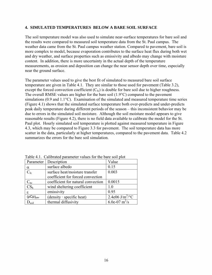
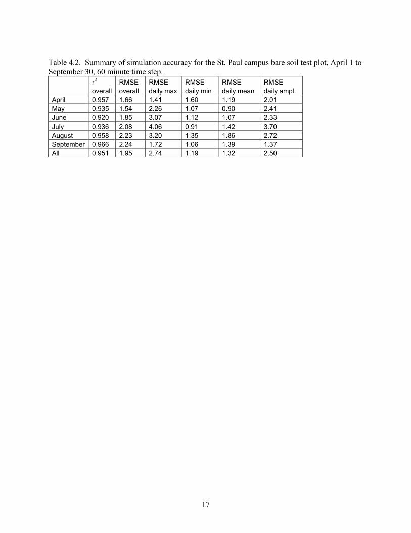
4. SIMULATED TEMPERATURES BELOW A BARE SOIL SURFACE The soil temperature model was also used to simulate near-surface temperatures for bare soil and the results were compared to measured soil temperature data from the St. Paul campus. The weather data came from the St. Paul campus weather station. Compared to pavement, bare soil is more complex to model, because evaporation contributes to the surface heat flux during both wet and dry weather, and surface properties such as emissivity and albedo may change with moisture content. In addition, there is more uncertainty in the actual depth of the temperature measurements, as erosion and deposition can change the near sensor depth over time, especially near the ground surface. The parameter values used to give the best fit of simulated to measured bare soil surface temperature are given in Table 4.1. They are similar to those used for pavement (Table 3.2), except the forced convection coefficient (Cfc) is double for bare soil due to higher roughness. The overall RMSE values are higher for the bare soil (1.9°C) compared to the pavement simulations (0.9 and 1.1°C). Examination of the simulated and measured temperature time series (Figure 4.1) shows that the simulated surface temperature both over-predicts and under-predicts peak daily temperature during different periods of the season – this inconsistent behavior may be due to errors in the simulated soil moisture. Although the soil moisture model appears to give reasonable results (Figure 4.2), there is no field data available to calibrate the model for the St. Paul plot. Hourly simulated soil temperature is plotted against measured temperature in Figure 4.3, which may be compared to Figure 3.3 for pavement. The soil temperature data has more scatter in the data, particularly at higher temperatures, compared to the pavement data. Table 4.2 summarizes the errors for the bare soil simulation. Table 4.1. Calibrated parameter values for the bare soil plot Parameter Description Value α surface albedo 0.15 Cfc surface heat/moisture transfer

coefficient for forced convection 0.003

Cnc coefficient for natural convection 0.0015 CSh wind sheltering coefficient 1.0 ε emissivity 0.95 (ρCp)pav (density · specific heat) 2.4e06 J/m3/°C Dsoil thermal diffusivity 6.0e-07 m2/s

17

Table 4.2. Summary of simulation accuracy for the St. Paul campus bare soil test plot, April 1 to September 30, 60 minute time step. r2 RMSE RMSE RMSE RMSE RMSE overall overall daily max daily min daily mean daily ampl. April 0.957 1.66 1.41 1.60 1.19 2.01 May 0.935 1.54 2.26 1.07 0.90 2.41 June 0.920 1.85 3.07 1.12 1.07 2.33 July 0.936 2.08 4.06 0.91 1.42 3.70 August 0.958 2.23 3.20 1.35 1.86 2.72 September 0.966 2.24 1.72 1.06 1.39 1.37 All 0.951 1.95 2.74 1.19 1.32 2.50

18

0

10

20

30

40

50

6/1 6/6 6/11 6/16 6/21 6/26

Tem

pera

ture

(C)

SimulatedMeasured

0

10

20

30

40

50

5/1 5/6 5/11 5/16 5/21 5/26 5/31

Tem

pera

ture

(C)

0

10

20

30

40

50

8/1 8/6 8/11 8/16 8/21 8/26 8/31

Date

Tem

pera

ture

(C)

SimulatedMeasured

0

10

20

30

40

50

7/1 7/6 7/11 7/16 7/21 7/26 7/31

Tem

pera

ture

(C)

Figure 4.1. Simulated and measured soil temperature (1 cm depth) for May - August, 2004, St. Paul campus bare soil plot, 1 hour time step.

19

Figure 4.2 Simulated soil moisture content in surface layer and precipitation versus time for bare soil plot at St. Paul campus, April - September, 2004.

Figure 4.3. Hourly simulated versus measured soil temperature (1 cm depth) for April - September, 2004. The overall RMSE is 1.9 °C.

20

5. TEMPERATURE MODEL FORMULATIONS AND CALIBRATIONS FOR SURFACES WITH VEGETATION COVER The basic equations, boundary and initial conditions, and model input variables are the same as given in Section 2 for bare surfaces. The model output has also the same format. What is different for surfaces with vegetation cover is the presence of a canopy (plant cover) that shields the ground/soil surface from solar radiation and wind, and provides an evaporative heat loss (evapotranspiration). These differences have a dramatic influence on the ground/soil temperatures. Ground/soil temperatures for surfaces with plant cover are often substantially cooler than those for bare surfaces, especially pavements. Therefore surfaces with vegetation cover are expected to contribute relatively little to the heating of surface runoff, compared to pavements. To quantify the surface heat budget for various types of vegetated surfaces, e.g. agricultural, forests, and lawns, it is necessary to understand the heat transfer processes in a canopy, and to formulate a model for these processes. For larger rainfall events, significant surface runoff from vegetated surfaces can occur as precipitation rates exceed infiltration rates. The potential for the heating of that runoff as it flows over a vegetated soil surface needs to be investigated. A reasonable estimate of the heat transfer and runoff processes for land with vegetation cover is needed to compare the heat export from developed and undeveloped land. The introduction of a plant canopy has several major effects on the surface heat transfer and temperature of the underlying soil or water:

1. The amount of short wave radiation reaching the soil/water surface is reduced by shading. 2. The plant canopy absorbs long wave radiation from the sky and re-radiates to the

underlying soil/water surface. 3. Convective and evaporative heat fluxes are reduced by wind sheltering. Evaporation

from the soil/water surface is replaced by plant transpiration. To adequately model the effect of a plant canopy on the net long wave radiation reaching the soil/water surface, it is necessary to write a separate heat budget equation for the plant canopy and solve for a canopy temperature, Tf. The plant canopy models used in this study are based on the work of Deardorff (1978) and Best (1998).

5.1 Formulation of canopy model #1 (Deardorff’s model) In Deardorff’s (1978) approach, a representative canopy temperature is estimated from a heat budget for the canopy. In addition, a temperature (Taf) and humidity level (eaf) for the air in the canopy is estimated, which is then used to calculate the evaporative and convective heat fluxes between 1) the soil surface and the atmosphere and 2) the foliage and the atmosphere. The plant canopy is assumed to have negligible heat capacity, so that the sum of the heat flux components must be zero at all times. The plant canopy is parameterized with a density factor, ν, which varies from 0 for no plants to 1 for a very dense canopy. The full set of equations used to implement Deardorff’s model is too lengthy to repeat here, but are given in Deardorff’s (1978)

21

paper. The heat flux components considered in the model are illustrated in Figure 5.1. The equations used to calculate the temperature (Taf) and humidity level (eaf) for the air in the canopy are given below, as they are unique and important to the formulation: (5.1) ( ) ( )ggffaaaaf TcTcTcT1T ++ν+ν−=

(5.2) ( ) ( )ggffaaaaf ececece1e ++ν+ν−= where T is temperature, e is humidity, the c values are weighting constants, and the subscripts a, f, and g denote air, foliage, and ground. The weighting constants are assigned nominal values of ca=0.3, cf=0.6, and cg=0.1 in Deardorff’s (1978) paper.

soil-waterdomain

Tf, Taf, eaf

hrad

hrad,g

Ts

canopylayer

hconv,f hevap,f

hevap,ghconv,g

Figure 5.1. Major heat flux components for canopy model #1 based on Deardorff’s work (1978).

5.2 Calibration of canopy model #1 (Deardorff’s model) The Deardorff vegetation model described above was implemented as a new surface heat flux model within the soil temperature model previously described. The model was used to simulate the soil and plant canopy temperatures of a grass plot on the St. Paul campus, where soil temperatures were recorded. One hour weather data measured on the St. Paul campus were available for the simulation, and a soil temperature profile measured on April 1, 2004 was used as the initial condition. Using the nominal parameter values given in Deardorff’s paper, the model overpredicted the amount of heat transfer to the soil, even with maximum canopy density (ν=1). To obtain better agreement of simulated and measured soil temperature values while using reasonable soil and foliage parameter values, it was necessary to change the weighting coefficient values to ca=0.1, cf=0.5, and cg=0.4. The simulation results obtained with these modifications for the St. Paul grass plot are given in Figure 5.2 and Table 5.1. The overall RMSE of the simulated soil surface temperature is 1.2 C. The range of surface temperatures for the grass plot is significantly lower than for the bare soil and the paved surfaces. The grass plot surface temperatures did not exceed 30oC.

22

The Deardorff model was also tested against data from a second test site at Batavia, IL, using climate and soil temperature data obtained from the Ameriflux web site (http://public.ornl.gov/ameriflux/). Reasonable simulation results (Figure 5.3) were obtained by keeping all parameters the same as the calibrated values for the St. Paul site, except for decreasing the canopy density parameter to 0.90 and reducing the soil heat capacity to 2.2E06 J/m3/°C. The simulation gave a consistent -2 °C temperature offset compared to the measured soil temperatures. This offset could be reduced by changing the weighting coefficients ca, cf, and cg, however, it is not desirable to use this level of calibration to match different measurement sites.

Figure 5.2. Simulated versus measured soil temperature (1 cm depth) for a grass plot on the St. Paul campus, April 1 – October 1, 2004.

23

Table 5.1. Errors of simulated versus measured grass plot temperature values, 1 cm depth, St. Paul 2004, using the full Deardorff model. r2 RMSE RMSE RMSE RMSE RMSE

hourly hourly daily max daily min daily mean

daily ampl.

April 0.907 1.30 1.48 0.80 1.04 1.23 May 0.870 0.98 1.04 0.47 0.69 0.94 June 0.878 0.81 0.44 0.74 0.35 0.89 July 0.878 0.79 0.65 0.71 0.51 0.54 August 0.896 0.73 0.49 0.44 0.39 0.49 September 0.896 1.89 1.40 0.42 0.84 1.27 All 0.970 1.15 0.99 0.60 0.67 0.92

Figure 5.3. Simulated versus measured soil temperature (2.5 cm depth) for a grass/prairie plot near Batavia, IL, April 1 – August 18, 2005.

5.3 Formulation of canopy model #2 (Best’s model) More recent work by Best (1998) produced a simplified version of the Deardorff model. In this model the convective and evaporative heat flux components between the ground and the canopy (hconv,g and hevap,g) are assumed to be negligible. As a result, the parameters Taf and eaf are not needed. The canopy temperature is calculated in a similar manner to the Deardorff model, and is

24

then used to calculate the net long wave radiation between the canopy and the ground (hrad,g). The heat flux components considered in the Best model are illustrated in Figure 5.4.

Tf

hrad hconv,f hevap,f

hrad,g

Ts

canopylayer

soil-waterdomain

Figure 5.4. Major heat flux components for canopy model #2 based on Best’s work (1998). Because the convective and evaporative components of the ground heat flux are assumed to be negligible, this formulation should be applied only to ground surfaces with dense vegetative cover. To address cases with partial vegetation canopies, Best’s formulation was modified to take a linear combination of the full canopy Best model and the previously developed bare soil model. The ability to handle partial canopies was found to be important for modeling soil temperatures for agricultural land use. The heat balance equation for the plant canopy is given by Equation 5.3. It assumes that the canopy has negligible heat capacity, so that heat flux components exactly balance each other. In the context of the soil temperature simulation, the heat balance equation is non-linear in a single unknown, Tf. The canopy density ν does not appear in the canopy heat budget, because all the heat flux quantities scale with the canopy density. (5.3) ( ) f,convf,evap

4fkf

4gkglfsff,net hhTThh10h −−σε−σε+ε+α−==

(5.4) ( ) ( )saafaaf,evap rrqquLh +−νρ= (5.5) ( ) aafapaf,conv rTTuch −νρ=

(5.6) ( )( ) 4ak

08.0al TeCR167.0CRh −⋅+σ=

The aerodynamic (ra) and stomata (rs) resistance coefficients are calculated using expressions similar to those of Deardorff (1978). The aerodynamic roughness, CHf, represents both a characteristic roughness of the foliage and a scaling factor due to higher overall surface area of the vegetation, e.g. with ν=1, the vegetation surface area may be 4 to 7 times higher than the land area it covers.

25

(5.7) sf

a uC1r⋅

=

(5.8) ( ) ( )ss Rgf

200r⋅θ

=

(5.9) ( )⎟⎟⎠

⎞⎜⎜⎝

⎛+=

3.0;umax3.01CCs

Hff

(5.10) ( ) ( )( )( )01.0;0.5;1minmaxf wprd θ−θ=θ

(5.11) ( ) ⎟⎟⎠

⎞⎜⎜⎝

⎛+⋅

= 01.0;R250R25.1

maxRgs

ss

The formulation for the ground convection and evaporative heat flux are similar to those used for bare soil and pavements, except that these heat flux components are reduced as the canopy density is increased. The constant Ce establishes the level of soil evaporation for fully dense canopies, e.g. setting Ce < 1 gives non-zero soil evaporation for the full canopy case. The factor θ’ in Equation 5.19 linearly decreases the rate of soil evaporation as the soil moisture content decreases from saturated. (5.12) g,convg,evapgo,lgi,lgi,sg,net hhhhhh −−−+=

(5.13) ( )( ) sggi,s R11h ν−α−=

(5.14) ( ) 4fkflgi,l Th1h σεν+ν−=

(5.15) 4gkggo,l Th σε=

(5.16) ( )( )ag33.0

vncsfcpag,conv TTCuCc'h −θ∆+ρ=

(5.17) ( )ν−= eg,convg,conv C1'hh

(5.18) ( ) ( )( )agsat33.0

vncsfcvag,evap qTqCuCL'h −θ∆+ρ=

(5.19) ( ) g,'hC1'h evapeg,evap ν−θ=

(5.20) θ’ = (θ−θwp)/θs

where θ = soil moisture, θrd = average soil moisture in rooted depth, θs = saturated soil moisture, and θwp = wilting point. To calculate the surface heat flux for each time step, Equations 5.3 to 5.20 are used to solve for a canopy temperature, based on the current values of air temperature, solar radiation, dew point, and wind speed. Since Equation 5.3 is non-linear in canopy temperature (Tf), it must be solved using an iterative procedure or Newton’s method. The calculated canopy temperature is then used to calculate the ground heat flux components. The soil evaporation and canopy evaporation are used to update the soil moisture content (Appendix C).

26

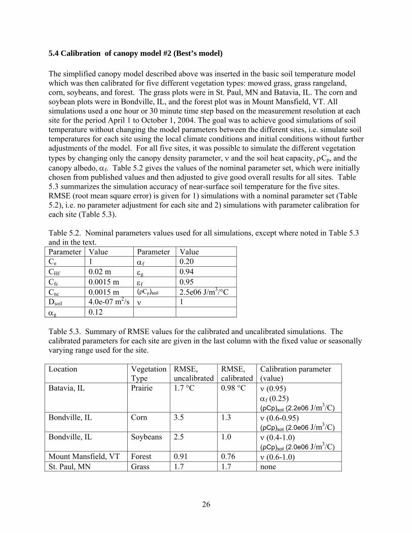
5.4 Calibration of canopy model #2 (Best’s model) The simplified canopy model described above was inserted in the basic soil temperature model which was then calibrated for five different vegetation types: mowed grass, grass rangeland, corn, soybeans, and forest. The grass plots were in St. Paul, MN and Batavia, IL. The corn and soybean plots were in Bondville, IL, and the forest plot was in Mount Mansfield, VT. All simulations used a one hour or 30 minute time step based on the measurement resolution at each site for the period April 1 to October 1, 2004. The goal was to achieve good simulations of soil temperature without changing the model parameters between the different sites, i.e. simulate soil temperatures for each site using the local climate conditions and initial conditions without further adjustments of the model. For all five sites, it was possible to simulate the different vegetation types by changing only the canopy density parameter, ν and the soil heat capacity, ρCp, and the canopy albedo, αf. Table 5.2 gives the values of the nominal parameter set, which were initially chosen from published values and then adjusted to give good overall results for all sites. Table 5.3 summarizes the simulation accuracy of near-surface soil temperature for the five sites. RMSE (root mean square error) is given for 1) simulations with a nominal parameter set (Table 5.2), i.e. no parameter adjustment for each site and 2) simulations with parameter calibration for each site (Table 5.3). Table 5.2. Nominal parameters values used for all simulations, except where noted in Table 5.3 and in the text. Parameter Value Parameter Value Ce 1 αf 0.20 CHf 0.02 m εg 0.94 Cfc 0.0015 m εf 0.95 Cnc 0.0015 m (ρCp)soil 2.5e06 J/m3/°C Dsoil 4.0e-07 m2/s ν 1 αg 0.12 Table 5.3. Summary of RMSE values for the calibrated and uncalibrated simulations. The calibrated parameters for each site are given in the last column with the fixed value or seasonally varying range used for the site. Location Vegetation

Type RMSE, uncalibrated

RMSE, calibrated

Calibration parameter (value)

Batavia, IL Prairie 1.7 °C 0.98 °C ν (0.95) αf (0.25) (ρCp)soil (2.2e06 J/m3/C)

Bondville, IL Corn 3.5 1.3 ν (0.6-0.95) (ρCp)soil (2.0e06 J/m3/C)

Bondville, IL Soybeans 2.5 1.0 ν (0.4-1.0) (ρCp)soil (2.0e06 J/m3/C)

Mount Mansfield, VT Forest 0.91 0.76 ν (0.6-1.0) St. Paul, MN Grass 1.7 1.7 none

27

5.5 Soil temperature sensitivity to canopy model #2 parameters The sensitivity of the simulated soil surface temperatures to several key input parameters in the canopy #2 model are given in Table 5.4. Overall, the emissivity of the foliage and soil had the most influence on surface temperature, with roughly equal and opposite effects, followed by the vegetation density (ν) and the soil evaporation/convection scaling parameter (Ce). An increase in foliage emissivity or a decrease in soil emissivity caused an increase in both day and night soil temperature, with relatively little effect on the diurnal amplitude. The soil surface temperature was relatively insensitive to the foliage albedo and the soil thermal and hydraulic parameters. Introducing a small amount of soil evaporation and convection, i.e. decreasing Ce from 1.0 to 0.9, caused a measurable decrease in soil temperature (0.5 °C). Table 5.4. Sensitivity of the temperature simulations for the St. Paul grass plot to parameter values. Each value in the table is the change in the response variable (surface temperature, °C) for a 10% increase in the input parameter listed in the first column. For parameters where the nominal value is the maximum value, e.g. ν=1, the value was decreased by 10% and the resulting response multiplied by -1. Ks is the saturated hydraulic conductivity of the soil. Average Max Min Amplitude εf 6.07 6.22 5.91 0.32εg -5.69 -5.77 -5.58 -0.19ν -1.07 -2.43 0.00 -2.43Ce 0.52 0.45 0.62 -0.17Dsoil -0.11 -0.25 0.03 -0.28αf -0.05 -0.06 -0.03 -0.03(ρCp)soil -0.04 -0.10 0.02 -0.12CHf -0.04 -0.08 0.00 -0.08Ks 0.00 0.00 0.01 0.00

6. SIMULATED TEMPERATURES BELOW GRASS-, CROP- AND TREE-COVERS In Section 5 two canopy models were introduced, tested and calibrated. The canopy model #2 (Best model) was applied to five types of plant covers on different test plots, and one set of nominal parameter values was determined (Table 5.2). The RMSE values for some of the five test plots were quite large (Table 5.3, RMSE, uncalibrated). Further model refinements were achieved by changing some parameter values, especially plant density ν, from the nominal values in Table 5.2. Refined parameter values and the (RMSE, calibrated) values are shown in Table 5.3. In this section we will give additional model results obtained with the refined model parameters. Results for three categories of land covers are given: grass, crops and trees.

6.1 Lawns and grasslands Soil temperature data from a grass plot at the UofM weather station on the St. Paul campus and from at an Ameriflux site at Batavia, Illinois were used to test the canopy model #2 (Best’s model). The grass plot in St. Paul is more representative of a mowed lawn, while the grass plot

28

at Batavia is more representative of tall grass prairie. For the Batavia site, soil temperature and climate data, including measured solar radiation, were obtained at 30 minute time increments for the period January 1 – August 17, 2005. For the St. Paul site, soil temperature and climate data, including measured solar radiation, were obtained at 1 hour time increments for the period January 1 – August 17. For both grass plots, the best agreement of simulated and measured soil temperatures was obtained using a full canopy (ν=0.95-1.0) and no soil evaporation/convection (Ce=1). For the St. Paul grass plot, good agreement between measured and simulated soil temperatures was obtained (Figures 6.1, 6.2 and Tables 6.1, 6.2) using the same soil parameters as those used for the bare soil plot and using foliage parameters within the expected range, i.e.. εf=0.95, α=0.20, CHf=0.02. The calibrated values of the soil foliage parameters used for the prairie grass plot in Batavia are given in Table 6.3. Although using the St. Paul vegetation and soil parameters produced reasonable simulation results for Batavia, minor adjustments to the canopy density, canopy albedo, and soil heat capacity improved the simulation RMSE from 1.7 °C to 0.98 °C (Table 5.3). An example of the simulated foliage temperature is given in Figure 6.3, along with air and surface soil temperatures. The foliage temperature largely tracks air temperature, but exceeds air temperature by up to 8 °C during mid-day on sunny days. For the St. Paul plot, replacing foliage temperature with air temperature in the surface heat transfer simulation increased the RMSE from 1.8 °C to 2.5 °C. Table 6.1. Summary of simulation accuracy for the Batavia, IL prairie plot, April – August 2005, 30 minute time step. All RMSE values have units of °C.

r2 RMSE RMSE RMSE RMSE RMSEoverall daily max daily min daily mean daily ampl.

April 0.941 1.48 1.11 1.64 1.40 0.93May 0.951 0.88 0.95 0.86 0.52 1.41June 0.919 1.03 1.62 0.57 0.44 1.99July 0.886 0.93 1.08 0.58 0.43 1.39August 0.888 0.90 0.59 0.73 0.77 0.32SeptemberAll 0.978 0.97 1.01 0.86 0.72 1.20 Table 6.2. Summary of simulation accuracy for the St. Paul, MN grass plot, April – October 2004, 1 hour time step. All RMSE values have units of °C. r2 RMSE RMSE RMSE RMSE RMSE

overall daily max

daily min

daily mean

daily ampl.


29

0

10

20

30

40

50

7/1 7/6 7/11 7/16 7/21 7/26 7/31

Tem

pera

ture

(C)

0

10

20

30

40

50

6/1 6/6 6/11 6/16 6/21 6/26

Tem

pera

ture

(C) Simulated

MeasuredJune 2004

1 cm depth, St. Paul

June 20041 cm depth, St. Paul

0

10

20

30

40

50

6/1 6/6 6/11 6/16 6/21 6/26

Tem

pera

ture

(C) Simulated

Measured

June 20051cm depth Batavia

0

10

20

30

40

50

7/1 7/6 7/11 7/16 7/21 7/26 7/31

Date

Tem

pera

ture

(C) Simulated

Measured

June 20051cm depth Batavia

Figure 6.1. Time series of simulated and measured soil near-surface soil temperatures for grass plots at St. Paul (upper panels) and at Ames, IA (lower panels).

30

Figure 6.2. Simulated versus measured near-surface soil temperature for grass plots at St. Paul (upper panel) and at Batavia, IL (lower panel). Soil temperatures for 1 cm soil depth, April – October, 2004 (St. Paul) and 2.5 cm soil depth, April – August, 2005 (Batavia).

31

0

10

20

30

40

50

7/1 7/6 7/11 7/16 7/21 7/26 7/31

Date

Tem

pera

ture

(C)

Soil SurfaceFoliageAir

Figure 6.3. Time series of simulated soil surface temperature, simulated foliage temperature, and measured air temperature for a grass plot at Batavia, IL, July 2005.

6.2 Crop (agricultural) land To evaluate the ability to model agricultural land surfaces, the vegetation/soil temperature model was applied to an Ameriflux data set for Bondville, IL, just west of Urbana/Champaign. The crop on the instrumented test plot is rotated each year between corn and soybeans. An extensive data record is available from 1996 to present, that includes climate data, soil temperatures, and soil moisture at 30 minute intervals. Data from 1999 (corn) and 2000 (soybeans) were used for this project. Application of the soil/vegetation model with the nominal parameter set (Table 5.2) lead to an overprediction of maximum surface temperatures in April and May, and relatively high RMSE values (Table 5.3). Much better simulation accuracy was achieved by introducing a seasonally varying canopy density (Figure 6.4), with slightly different characteristics for the corn and soybean crops. In addition, setting the scaling constant Ce = 0.5 further increased the simulation accuracy, e.g. setting evaporation and convection to 50% of the bare soil value. This suggests that a field that has been plowed and planted with a row crop may have significant soil evaporation, even with a relatively dense plant canopy. The simulated rates of soil evaporation and plant transpiration are given in Figures 6.5, which shows a decrease in soil evaporation and an increase in plant transpiration as the season progresses. Since there is no function in the model for plant senescence, simulated plant transpiration continues until October. The simulated and measured soil temperatures for the corn crop are compared as time series in Figures 6.6 and 6.7, for April through September. Good agreement of measured and simulated

32

surface temperature was achieved for the entire period. Figure 6.8 gives simulated versus measured surface temperature for the same periods, and for both a corn crop and a soybean crop

0

0.2

0.4

0.6

0.8

1

4/1 5/1 6/1 7/1 8/1 8/31 10/1

Can

opy

Den

sity

Corn

0

0.2

0.4

0.6

0.8

1

4/1 5/1 6/1 7/1 8/1 8/31 10/1

Date

Can

opy

Den

sity

Soybeans

Figure 6.4. Calibrated canopy density versus time for corn (upper panel) and soybeans (lower panel).

33

-1

0

1

2

3

4

5

6

4/1 5/1 6/1 7/1 8/1 8/31 10/1

Date

Dai

ly E

vapo

ratio

n (m

m) Soil Evaporation

Plant Transpiration

Figure 6.5. Simulated daily soil evaporation and plant transpiration for the Bondville, IL corn field (2000).

34

0

10

20

30

40

50

5/1 5/6 5/11 5/16 5/21 5/26 5/31

Tem

pera

ture

(C)

Simulated

Measured

0

10

20

30

40

50

4/1 4/6 4/11 4/16 4/21 4/26 5/1

Tem

pera

ture

(C)

0

10

20

30

40

50

7/1 7/6 7/11 7/16 7/21 7/26 7/31

Date

Tem

pera

ture

(C)

Simulated

Measured

0

10

20

30

40

50

6/1 6/6 6/11 6/16 6/21 6/26

Tem

pera

ture

(C)

Figure 6.6. Simulated versus measured soil temperature (1 cm depth), April – July 1999, at the Bondville, IL, site with corn crop, 30 minute time step.

35

0

10

20

30

40

50

9/1 9/6 9/11 9/16 9/21 9/26 10/1

Date

Tem

pera

ture

(C)

Simulated

Measured

0

10

20

30

40

50

8/1 8/6 8/11 8/16 8/21 8/26 8/31

Tem

pera

ture

(C)

Figure 6.7. Simulated versus measured soil temperature (1 cm depth), April – October 1999, at the Bondville, IL, site with corn crop, 30 minute time step.

36

Figure 6.8. Simulated versus measured soil temperature (1 cm depth) for a field with corn (upper panel) and soybeans (lower panel), 30 minute intervals, April 1 – October 1.

37

Table 6.3 summarizes the error coefficients. The RMSE is quite low, 1.3 °C for corn and 1.0 °C for soybeans. For the corn crop, maximum surface temperatures approach 40 °C, which is higher than for the grass plots. This is due to the reduced canopy coverage in the early part of the year (Figure 6.4), which allows more solar heat flux to reach the soil surface. In comparison, the soybean canopy developed more rapidly, giving maximum soil temperatures of about 30°C, close to those measured at the St. Paul grass plot. Table 6.3. Summary of simulation accuracy for the Bondville, IL agricultural plot, April – October, 30 minute time step. All RMSE values have units of °C. Bondville, IL: Corn (1999) r2 RMSE RMSE RMSE RMSE RMSE

hourly hourly daily max

daily min

daily mean

daily ampl.


Bondville, IL: Soybeans (2000) r2 RMSE RMSE RMSE RMSE RMSE

hourly hourly daily max

daily min

daily mean

daily ampl.


The Ameriflux data set includes soil moisture. It is therefore possible to evaluate the soil moisture model. Figure 6.9 gives the measured and simulated soil moisture time series for the Bondville site with corn (1999) for the near-surface soil. Based on comparisons of measured and simulated soil moisture content, the soil hydraulic conductivity was adjusted to1.2e-6 m/s, and the percolation rate at the lower boundary (10 m deep) was reduced to 1.2e-7 m/s.

38

0.0

0.1

0.2

0.3

0.4

0.5

4/1 5/1 6/1 7/1 8/1 8/31 10/1

Date

Moi

stur

e C

onte

nt (f

ract

ion)

Figure 6.9 Simulated and measured soil moisture content for the Bondville, IL corn field (1999).

39

6.3 Forest The simplified vegetation/soil temperature model (Best’s model) was applied to forested land cover using data from a SCAN site at Mount Mansfield, VT with forest cover. The nominal parameters given in Table 5.2 were used, except for a seasonally varying vegetation density (Figure 6.10), which may represent an understory plus the development of a tree canopy. The simulation results were quite good, with an overall RMSE of 0.76 °C (Table 6.4 and Figure 6.11). Surface temperatures did not exceed 20°C for the period of simulation (April-October 2004), which may be attributed to the vegetation canopy and the relatively low air temperatures for the higher altitude site (680 m).

0

0.2

0.4

0.6

0.8

1

1.2

4/1 5/1 6/1 7/1 8/1 8/31 10/1

Date

Vege

tatio

n D

ensi

ty

Figure 6.10. Seasonal variation of the calibrated vegetation density for the Mount Mansfield,VT, site. Table 6.4. Summary of simulation accuracy for the Mount Mansfield,VT, forested plot for April – October 2004, 1 hour time step. All RMSE values have units of °C. r2 RMSE RMSE RMSE RMSE RMSE

overall daily max

daily min

daily mean

daily ampl.


40

Figure 6.11. Simulated versus measured soil temperature (5 cm depth) for a forested plot at Mount Mansfield, VT, April 1 – October 1, 2004.

41

7. TEMPERATURE MODEL FORMULATIONS AND CALIBRATIONS FOR ROOFS

7.1 Roof temperature model Formulation While typical residential roofs with asphalt shingles have little thermal mass, and therefore, little ability to influence the temperature of surface runoff, tar/gravel commercial roofs, residential tile roofs have significant thermal mass. As a result, a roof temperature model was developed and calibrated. The model has the following components: 1) The roof is represented as a thermal mass per unit area, which is a composite of the various roof layers. 2) Surface heat transfer with the atmosphere is applied as the loading, using an identical formulation to the pavement temperature model described previously. Heat transfer between the underside of the roof and the building (e.g. the attic) is assumed to be negligible. 3) Heat transfer between the roof surface and rainfall runoff is modeled using the same formulation as given in Appendix B, except that the thermal boundary layer thickness in the roof is limited by the roof thickness, e.g. 1 cm. The roof temperature is calculated for each time step using Equation 7.1:

7.1 ( )( )

⎟⎟⎠

⎞⎜⎜⎝

⎛ ∆∂∂

+

∆+⎟

⎟⎠

⎞⎜⎜⎝

⎛ ∆∂∂

+

=∆+

p

pp

C'mt

Th1

C'mth

C'mt

Th1tT

ttT

where m’ is the roof mass per unit area, Cp is the composite specific heat of the roof materials, and h and dh/dt are the surface heat transfer (e.g. W/m2) and surface heat transfer temperature derivative for the previous time step, respectively. The temperature derivative term helps take into account the variation of heat transfer with surface temperature over the time step, as discussed in Section 2.4.

7.2 Roof temperature model calibration The roof temperature model was calibrated for a commercial roof surface using 2006 roof temperature and climate data taken at the St. Anthony Falls Lab (SAFL) in Minneapolis, Minnesota, and for a residential roof using temperature data taken at a house in St. Anthony, Minnesota during 2005. Figure 7.1 gives the simulated and measured roof temperatures for the SAFL facility. The simulation was performed using SAFL weather data with a 15 minute time step for June 5 to September 20, 2006. The overall RMSE of the simulation was 2.6 °C for the period May 15 to September 20, 2006, using the calibrated parameter values given in Table 7.1. The house is approximately 5 miles from the SAFL weather station. Figure 7.2 gives the

42

simulated and measured roof temperatures for the residential roof. The simulation was also performed with a 15 minute time step, using the SAFL weather data, for June 5 to September 20, 2005. The overall RMSE of the simulation was 2.9 °C for the period June 25 to August 13, using the calibrated parameter values given in Table 7.1. Table 7.1. Model parameters for the commercial and residential roof calibrations. Parameter Commercial

Roof Residential Roof

Emissivity (εg) 0.90 0.90 Albedo (α) 0.20 0.18 Aerodynamic roughness (Cfc) 0.0032 m 0.0032 m Heat Capacity per Unit Area (m’Cp) 80 kJ/m2/°C 20 kJ/m2/°C

43

0

10

20

30

40

50

60

70

80

6/27 7/2 7/7 7/12 7/17

Date

Tem

pera

ture

(C)

SimulatedMeasured

Figure 7.1. Simulated and measured roof temperature versus time (upper panel) and simulated versus measured roof temperature (lower panel) for a commercial building (SAFL) with a tar/gravel roof.

44

0

10

20

30

40

50

60

70

80

6/27 7/2 7/7 7/12 7/17

Date

Tem

pera

ture

(C)

MeasuredSimulated

Figure 7.2. Simulated and measured roof temperature versus time (upper panel) and simulated versus measured roof temperature (lower panel) for a house with an asphalt single roof in St. Anthony, MN. 8. SUMMARY AND CONCLUSIONS Ground surface temperatures have been successfully simulated for a variety of land surfaces, including pavements, bare soil, short and tall grass, trees and agricultural crops. However, the simulations were run for different locations and different years as imposed by the availability of measured soil temperature and climate data. To clarify the variation in surface temperature for

45

the different land uses, the calibrated coefficients for each land use (Tables 5.2 and 5.3) were used to simulate surface temperatures using the same climate data set from St. Paul, MN (2004) and the same soil coefficients. The results are given here as the seasonal variation of weekly averaged soil surface temperatures (Figure 8.1) and in a summary table by month (Table 8.1). Since surface temperatures in July may be of the most interest to thermal loading of trout streams, the rows of Table 8.1 are sorted by July temperature, from highest to lowest. Asphalt and concrete give the highest surface temperatures. Roof surfaces similarly high maximum surface temperatures to asphalt, but lower minimum temperatures due to the low thermal mass of roof structures. As a result, average roof temperatures are lower than average pavement temperatures. Short grass, corn, soybeans and forest give very similar surface temperatures, about 10°C lower than pavement in average temperature and 20°C lower in average daily maximum temperature. Bare soil gives surface temperatures that lie between those for pavements and plant-covered surfaces. Daily minimum temperatures were relatively similar across the different land uses, with only 3 to 6 °C separating the highest (concrete) from the lowest (grassland). While simulating heat transfer between pavement and surface runoff was not a focus of this study, the approximate method used to estimate this heat flux seems to give reasonable results, and the model reproduces pavement temperature during rainfall events quite well. The soil temperature and moisture model appears to model surface temperatures of bare soil and pavement quite well, with RMSEs of 1 to 2°C. The higher simulation error compared to pavement is likely due to inaccuracy of the simulated soil moisture content. However, this simulation accuracy should be sufficient to simulate surface and groundwater heat transfer processes for agricultural land use. The plant canopy model used in this study, based on the work of Best (1998) and Deardorff (1978), provides an adequate approximation for the effect of vegetation on surface heat transfer, using only a few additional parameters compared to bare surfaces. While further simplifications of the model are possible, e.g. assuming the foliage temperature to be equal to air temperature, such simplifications do not reduce the number of required input parameters, and do not eliminate the need for estimating the seasonal variation of the vegetation density.

46

0

10

20

30

40

4/1 5/1 6/1 7/1 8/1 8/31 10/1

Date

Tem

pera

ture

(C)

Aphalt Bare Soil Concrete

Corn Forest Grassland

Roof Lawn Soybeans

Figure 8.1 Simulated average weekly surface temperatures for nine land uses using hourly climate data from St. Paul (2004) as model input. The roof data plotted is for a commercial roof, which is very similar to the residential roof results for average weekly temperature.

47

Table 8.1a. Simulated monthly average surface temperature, average daily maximum and average daily minimum for ten land uses using hourly climate data (2004) from St. Paul. Month April May June July August September

Asphalt 17.7 21.7 28.8 32.6 27.3 25.7Concrete 16.8 21.0 27.8 31.7 26.7 24.8Com. Roof 12.3 16.5 24.3 28.3 23.1 20.9Res. Roof 12.5 16.7 23.5 27.1 21.8 20.3Pond 11.2 15.0 21.2 25.2 21.4 18.8Bare Soil 10.9 15.7 21.1 25.2 22.2 19.1Sod 9.0 13.3 18.1 21.5 19.2 16.3Forest 11.1 14.3 18.0 21.4 19.2 16.8Grassland 8.8 13.1 17.8 21.2 19.0 16.0Corn 10.2 14.5 19.0 21.2 18.2 16.7Soybeans 10.1 13.2 18.0 20.9 18.0 16.1

Asphalt 35.5 37.4 46.3 51.1 44.8 43.1Com. Roof 32.9 33.9 45.0 50.9 44.2 41.5Res. Roof 34.9 36.2 45.3 50.8 44.0 42.3Concrete 31.3 33.9 42.1 46.6 40.8 39.0Bare Soil 20.5 23.7 29.4 34.4 31.7 28.1Pond 15.9 19.3 25.6 30.0 26.4 23.5Corn 17.2 20.4 23.9 24.5 20.8 21.4Soybeans 16.7 16.8 21.2 23.9 20.3 19.8Sod 11.4 15.3 19.9 23.8 21.3 18.4Forest 17.4 17.4 19.7 23.4 21.1 19.8Grassland 10.9 14.8 19.4 23.2 20.9 17.9

Pond 7.4 11.5 16.8 21.2 17.2 14.9Concrete 6.6 11.8 16.7 21.4 17.3 14.8Asphalt 5.7 11.0 15.8 20.3 16.4 13.9Forest 5.9 11.4 15.8 19.4 17.3 14.0Sod 6.7 11.2 15.6 19.3 17.1 14.0Grassland 6.7 11.2 15.6 19.2 17.2 14.1Corn 4.6 9.3 14.3 18.2 15.5 12.5Bare Soil 3.8 9.2 13.8 18.2 15.4 12.1Soybeans 4.7 9.7 14.4 18.1 15.5 12.6Com. Roof -2.7 3.1 7.9 11.3 7.5 5.5Res. Roof -4.8 0.8 6.0 9.6 6.0 3.6

Average Surface Temp

Average Daily Maximum Surface Temp

Average Daily Minimum Surface Temp

48

Table 8.1b. Simulated monthly average daily amplitude and average maximum daily amplitude for ten land uses using hourly climate data (2004) from St. Paul. Month April May June July August September

Res. Roof 39.3 35.0 38.4 41.3 37.7 38.4Com. Roof 35.4 31.1 35.9 40.3 36.0 35.8Asphalt 29.7 26.5 29.7 31.3 28.1 29.1Concrete 6.6 22.1 24.7 25.7 23.2 24.1Bare Soil 16.7 14.5 15.1 16.5 16.2 15.8Pond 8.5 7.9 8.5 9.0 9.0 8.6Corn 12.6 11.0 9.6 6.4 5.2 8.9Soybeans 12.0 7.1 6.8 5.9 4.8 7.3Sod 4.7 4.1 4.2 4.6 4.2 4.4Forest 11.5 6.2 3.8 4.2 3.8 5.8Grassland 4.2 3.6 3.7 4.1 3.7 3.9

Res. Roof 56.8 66.3 61.1 57.2 57.1 66.3Com. Roof 50.8 53.8 56.2 52.5 57.2 57.2Asphalt 41.5 45.2 44.4 39.5 39.7 45.2Concrete 34.2 37.1 37.3 32.7 32.5 37.3Bare Soil 24.5 25.5 23.5 23.6 25.1 25.5Pond 16.0 14.6 15.2 13.7 13.7 16.0Corn 18.5 19.0 18.0 10.6 7.9 19.0Soybeans 21.3 13.0 12.3 9.1 7.0 21.3Sod 9.2 8.9 7.5 7.0 6.7 9.2Forest 18.4 11.1 6.7 6.3 5.9 18.4Grassland 8.5 7.7 6.5 6.2 5.7 8.5

Max Daily Amplitude (max-min) Surface Temp

Average Daily Amplitude (max-min) Surface Temp

49

ACKNOWLEDGMENTS This study was conducted with support from the Minnesota Pollution Control Agency, St. Paul, Minnesota, with Bruce Wilson as the project officer. Soil temperature and climate data used in this study were supplied by :

1) Dr. David Ruschy, University of Minnesota, Department of Soil, Climate and Water, made available the St. Paul soil and climate data. 2) Ben Worel and Tim Clyne, Minnesota Department of Transportation, made available

climate and pavement temperature data from the MnROAD site. 3) Climate and soil temperature data was obtained for sites at Ames, Iowa and Mount

Mansfield, Vermont from the Natural Resources Conservation Service Soil and Climate Analysis Network (http://www.wcc.nrcs.usda.gov/scan).

4) Climate and soil temperature data was obtained for sites at Bondville, Illinois and Batavia, Illinois from the Oak Ridge National Lab Ameriflux network (http://public.ornl.gov/ameriflux/). The PI responsible for the Bondville measurement site is Tilden Meyers NOAA/ARL, Atmospheric Turbulence and Diffusion Division. The PIs responsible for the Batavia site are Roser Matamala, David Cook, Julie Jastrow, and Barry Lesht (Argonne National Laboratory), Miquel Gonzalez-Meler (University of Illinois at Chicago), and Gabriel Katul (Duke University).

We are grateful to these individuals and organizations for their cooperation.

50

REFERENCES Abu-Hamdeh, N.H., Reeder, R.C., Khdair, A.I., and Al-Jalil, H.F. (2000). “Thermal Conductivity of Disturbed Soils Under Laboratory Conditions.” Transactions of the Am. Society of Ag. Engineers, 43(4): 855-860. Best, M.J. (1998). “A Model to Predict Surface Temperatures”, Boundary Layer Meteorology, 88: 279-306. Deardorff, J.W. (1978). “Efficient Prediction of Ground Surface Temperature and Moisture with

Inclusion of a Layer of Vegetation.” Journal of Geophysical Research, 83: 1889-903. Eckert, E.R.G. and Drake, R.M., Jr. (1972). Analysis of Heat and Mass Transfer. McGraw-Hill,

New York. Edinger, J.E., D.W. Duttweiler and J.C. Geyer. J.C. (1968). The Response of water Temperatures

to Meteorological Conditions. Water Resources Research 4(5):11337-1145. December 1968. Edinger, J.E., Brady, D.K. and Geyer. J.C. (1974). Heat Exchange in the Environment. Report

No. 14, Cooling Water Discharge Research Project RP-49, Electric Power Research Institute, Palo Alto, CA, 125 pp.

Herb, W.R., M. Marasteanu and H.G. Stefan (2006). Simulation and Characterization of Asphalt Pavement Temperatures. Project Report No 480, St. Anthony Falls Laboratory, University of Minnesota, September 2006. 41pp.

Herb, W.R., Janke, B., O. Mohseni and H.G. Stefan. Estimation of Runoff Temperatures from Various Ground Surfaces. Project Report No XXX, St. Anthony Falls Laboratory, University of Minnesota, October 2006. pp. (in preparation for JPO).

Herb, W.R., Janke, B., O. Mohseni and H.G. Stefan. Design Rainfall Event Selection for Hydrothermal Runoff Modeling. Project Report No XXX, St. Anthony Falls Laboratory, University of Minnesota, October 2006. pp. (in preparation for MPCA).

Incropera, F. P. and DeWitt, D. P. (2002). Fundamentals of Heat and Mass Transfer, Fifth Ed., John Wiley and Sons, New York.

Janke, B., W.R. Herb, O. Mohseni and H.G. Stefan. Model for Runoff Temperature from a Paved Surface. Project Report No 477, St. Anthony Falls Laboratory, University of Minnesota, August 2006. 76pp.

Kersten, M.S. (1948). “The Thermal Conductivity of Soils.” Proceedings of the Highway

Research Board, 28: 210–218. Kustas, W.P. and Norman, J.M. (1999). “Evaluation of Soil and Vegetation Heat Flux

Predictions Using a Simple Two-Source Model With Radiometric Temperatures for Partial Canopy Cover.” Agricultural and Forest Meteorology, 94(1): 13-29.

51

Luca, J. and Mrawira, D. (2005). “New Measurement of Thermal Properties of Superpave

Asphalt Concrete.” Journal of Materials in Civil Engineering, 17(1): 72-79. Monteith, J. L. (1973). Principles of Environmental Physics. Edward Arnold, London. Rawls, W.J., Ahuja, L.R., Brakensiek, D.L., and A. Shirmohammadi. 1993. “Infiltration and Soil

Water Movement.” In: D.R. Maidment (Editor), Handbook of Hydrology. McGraw-Hill, New York, pp. 5.1-5.51.

Solaimanian, M., and Kennedy, T.W. (1993). “Predicting Maximum Pavement Surface

Temperature Using Maximum Air Temperature and Hourly Solar Radiation.” In Transportation Research Record 1417, National Research Council, Washington, D.C., 2001, 1-11.

52

APPENDIX A. THERMAL PROPERTIES OF SOILS AND PAVEMENT (from Janke et al. 2006) Both the heat and mass balances rely on the estimation of a number of properties of pavements and soils. Thermal and hydrologic properties of paved surfaces and various types of soils can be found in a number of literature sources (Kersten, 1948; Rawls et al., 1989; Abu-Hamdeh et al., 2000; Luca and Mrawira, 2005). Thermal properties are summarized in Tables A.1 and A.2. The pavement consists of a pavement layer and a sub-grade layer. The thermal properties of each remain constant with depth, and are a function of temperature only. In the special case of soil beneath a paved surface, infiltration and subsurface water flow can be assumed negligible. Thus the moisture content would be expected to be roughly constant throughout the soil column, making the soil properties also a function of temperature only. The calculation of temperature profiles in the soil relies heavily upon determination of a thermal diffusivity for various types of soils. Soil properties can be a function of soil type, moisture content, and temperature. A significant amount of research has been done, but many results are highly empirical because of the generally complicated nature of soil structure and composition. In the general case of a permeable ground surface, a soil moisture model - however simplified - requires knowledge of the saturated hydraulic conductivity, wilting point, field capacity, and porosity or saturated moisture content

Table A.1. Thermal properties of pavements.

Parameter Value Range Units Source

Concrete Specific Heat (Cp) 880 n/a J/kg*K Incropera and Dewitt (2002) Thermal Conductivity (k) 1.4 n/a W/m*K Incropera and Dewitt (2002) Density (ρ) 2300 n/a kg/m3 Incropera and Dewitt (2002)

Asphalt Thermal Diffusivity (D) 5.40E-07 4.4 - 6.4E-7 m2/s Luca and Mrawira (2005) Specific Heat (Cp) 1225 1100 - 1350 J/kg*K Luca and Mrawira (2005) Thermal Conductivity (k) 1.6 1.4 - 1.8 W/m*K Luca and Mrawira (2005) Density (ρ) 2375 2300 - 2450 kg/m3 Luca and Mrawira (2005)

53

Table A.2. Thermal properties of soils.

Parameter Value Range Units Source

Sand Specific Heat (Cp) 1840* n/a J/kg*K Incropera and Dewitt (2002) Thermal Conductivity (k) 0.7 0.43 - 0.98 W/m*K Abu-Hamdeh et al. (2000) Density (ρ) 1400 1300 - 1500 kg/m^3 Abu-Hamdeh et al. (2000)

Sandy Loam Specific Heat (Cp) 1840* n/a J/kg*K Incropera and Dewitt (2002) Thermal Conductivity (k) 0.45 0.35 - 0.55 W/m*K Abu-Hamdeh et al. (2000) Density (ρ) 1400 1300 - 1500 kg/m^3 Abu-Hamdeh et al. (2000)

Loam Specific Heat (Cp) 1840* n/a J/kg*K Incropera and Dewitt (2002) Thermal Conductivity (k) 0.42 0.34 - 0.50 W/m*K Abu-Hamdeh et al. (2000) Density (ρ) 1400 1300 - 1500 kg/m^3 Abu-Hamdeh et al. (2000)

Clay Loam Specific Heat (Cp) 1840* n/a J/kg*K Incropera and Dewitt (2002) Thermal Conductivity (k) 0.37 0.29 - 0.44 W/m*K Abu-Hamdeh et al. (2000) Density (ρ) 1400 1300 - 1500 kg/m^3 Abu-Hamdeh et al. (2000)

* value of Cp from Incropera and Dewitt (2002) for a ‘generic soil’.

54

APPENDIX B. MODELING THE HEAT FLUX BETWEEN RUNOFF AND PAVEMENT SURFACE.

Pavement

Surface Runoff

δ Qro

h

Dep

th

Tro TsoT(t)

Dep

th

Ts T(t+∆t)

Figure B.1. Schematic of the formulation for heat transfer between surface runoff and the underlying pavement. Example temperature profiles show the temperatures in the pavement prior to a rainfall event (T(t)) and after a rainfall event (T(t+∆t), where the initial surface temperature (Tso) has equilibrated with the initial runoff temperature (Tro) to yield the new surface and runoff temperature (Ts). The heat transfer model assumes that the surface runoff, assumed to be initially at dew point temperature, and pavement surface must equilibrate to the same temperature over the time step (∆t), as shown in Figure B.1. To achieve this equilibrium, a convective heat flux Qro can be calculated, which draws heat out of a thin layer of pavement at the surface with thickness δ. The size of δ can be estimated from the thermal properties of the pavement and the time step, based on analytic solutions for heat conduction into an infinite slab subject to a change in surface temperature (Eckert and Drake, 1972). (B.1) t4 ∆α=δ where α is the thermal diffusivity and ∆t is the time step. For a time step of 15 minutes and a thermal diffusivity of 4 x 10-6 m2/s, δ = 3.8 cm. An equation for the heat balance for the water film layer and the pavement may then be written as:

(B.2) ( ) ( ) ( ) ( )sospproswpro TTc2

TTchh −ρδ

−=−ρ= (J/m2)

where (ρcp)p and (ρcp)w are (density · specific heat) for the pavement and water, and the factor (δ/2) takes into account that the temperature change in the pavement decreases with depth, whereas the temperature change in the water film as assumed to be uniform across the thickness

55

h. If the dew point temperature and the initial surface temperature are know, so Equation B.2 can be solved for Ts and hro.

(B.3) β+

β+=

1T1

T sos , where

( )( )wp

pp

ch2

c

ρ

ρδ=β

(B.4) ( ) ( ) ⎟⎟⎠

⎞⎜⎜⎝

⎛β+

β−ρ=

1TTcphh dpsowro (J/m2)

Using Equation B.4, the heat flux from the pavement to the runoff may be estimated for each time step based on the total precipitation in each time step, and is simply added to the atmospheric heat flux components. At any given time, the actual runoff depth is typically much less than the total precipitation depth, but the entire precipitation depth can still be expected to equilibrate with the pavement surface, so that applying the entire precipitation depth over the time step is equivalent to applying the same amount as a series of thin layers over shorter time steps. For the one-dimensional model, there is no consideration of lateral variations in runoff temperature from upstream to downstream points.

56

APPENDIX C. SOIL MOISTURE TRANSPORT MODEL

∆ziδzi

θi, Φi, Ki

θi+1, Φi+1 , Ki+1

∆Di

Figure A.3.1. Schematic diagram of the model for soil moisture movement. Soil moisture is modeled over depth using the same layer structure as the thermal model. The transport of moisture between layers is modeled with a simple discretized version of Darcy’s law.

⎟⎟⎠

⎞⎜⎜⎝

⎛δ

Φ−Φ+=

∆∆ +

i

i1iiz

1Kt

D

where ∆D is depth of water moving between layers i and i+1 in the time step ∆t, K is the average hydraulic conductivity, Φ is potential (head), and δzi is the distance between the center of layers i and i+1. The average conductivity is estimated as

1ii

1i1iiizz

KzKzK

+

++∆+∆

∆+∆=

The average hydraulic conductivity and potential in each layer is estimated from the soil water content θ from the previous time step.

3b2

s

isi KK

+

⎟⎟⎠

⎞⎜⎜⎝

⎛θθ

=b

wps

wpibi

−

⎟⎟⎠

⎞⎜⎜⎝

⎛

θ−θ

θ−θΦ=Φ

where Ks is the saturated hydraulic conductivity, Φb is the bubbling pressure, θwp is the wilting point soil moisture, and b is a soil specific constant. If water is ponded at the surface, infiltration into the top soil layer is estimated as Ks·∆t. Plant transpiration is withdrawn from each layer over the specified rooting depth weighted by the available water in each layer, DAi.

57

ii

ii

DAET:DAET

ETDADA

ET:DAET

=>

=<

( ) iwpii zDA ∆θ−θ=

where DA and ET are the total available soil water depth and total plant transpiration, respectively.

All-Weather Ground Surface Temperature Simulation

Documents

Transcript of All-Weather Ground Surface Temperature Simulation