
Two-Dimensional Nonlinear Earthquake Response Analysis of a Bridge-Foundation-Ground System
44
Two-Dimensional Nonlinear Earthquake Response Analysis of a Bridge-Foundation-Ground System Yuyi Zhang, a) Joel P. Conte, b) Zhaohui Yang, c) Ahmed Elgamal, d) Jacobo Bielak, e) and Gabriel Acero f) This paper presents a two-dimensional advanced nonlinear FE model of an actual bridge, the Humboldt Bay Middle Channel (HBMC) Bridge, and its response to seismic input motions. This computational model is developed in the new structural analysis software framework OpenSees. The foundation soil is included to incorporate soil-foundation-structure interaction effects. Realistic nonlinear constitutive models for cyclic loading are used for the structural (concrete and reinforcing steel) and soil materials. The materials in the various soil layers are modeled using multi-yield-surface plasticity models incorporating liquefaction effects. Lysmer-type absorbing/transmitting boundaries are employed to avoid spurious wave reflections along the boundaries of the computational soil domain. Both procedures and results of earthquake response analysis are presented. The simulation results indicate that the earthquake response of the bridge is significantly affected by inelastic deformations of the supporting soil medium due to lateral spreading induced by soil liquefaction. DOI: 10.1193/1.2923925 INTRODUCTION Earthquake-resistant design of a structural system requires analysis to predict its de- formations and internal forces due to potential earthquakes. A wide range of seismic structural analysis methods (from simple to sophisticated ones) is available. The level of sophistication required depends on the purpose of the analysis in the design process. However, an appropriate model of the structure and realistic representation of the earth- quake ground motion are essential in all methods. The model should represent with suf- ficient fidelity the spatial distribution and/or possible evolution of the stiffness, strength, deformation capacity, and mass of the structure. Nonlinear relations between forces and deformations/displacements due to material and/or geometric nonlinearities are now widely used in structural analysis. The structural response history due to an earthquake can be computed through dynamic analysis. This paper presents an advanced nonlinear a) Research Scientist, ANATECH Corp., 5435 Oberlin Dr., San Diego, CA 92121 b) Prof., Dept. of Structural Eng., Univ. of California, San Diego, La Jolla, CA 92093-0085 c) Engineer, URS Corporation, 1333 Broadway, Suite 800, Oakland, CA 94612 d) Prof., Dept. of Structural Eng., Univ. of California, San Diego, La Jolla, CA 92093-0085 e) Prof., Dept. of Civil and Env. Eng., Carnegie-Mellon Univ., Pittsburgh, PA 15213 f) Design Engineer, Myers, Houghton & Partners, 4500 E. Pacific Coast Hwy., Ste. 100, Long Beach, CA 90804 343 Earthquake Spectra, Volume 24, No. 2, pages 343–386, May 2008; © 2008, Earthquake Engineering Research Institute
Transcript of Two-Dimensional Nonlinear Earthquake Response Analysis of a Bridge-Foundation-Ground System
Two-Dimensional NonlinearEarthquake Response Analysisof a Bridge-Foundation-Ground System
Yuyi Zhang,a) Joel P. Conte,b) Zhaohui Yang,c) Ahmed Elgamal,d)
Jacobo Bielak,e) and Gabriel Acerof)
This paper presents a two-dimensional advanced nonlinear FE model of anactual bridge, the Humboldt Bay Middle Channel (HBMC) Bridge, and itsresponse to seismic input motions. This computational model is developed inthe new structural analysis software framework OpenSees. The foundation soilis included to incorporate soil-foundation-structure interaction effects.Realistic nonlinear constitutive models for cyclic loading are used for thestructural (concrete and reinforcing steel) and soil materials. The materials inthe various soil layers are modeled using multi-yield-surface plasticity modelsincorporating liquefaction effects. Lysmer-type absorbing/transmittingboundaries are employed to avoid spurious wave reflections along theboundaries of the computational soil domain. Both procedures and results ofearthquake response analysis are presented. The simulation results indicatethat the earthquake response of the bridge is significantly affected by inelasticdeformations of the supporting soil medium due to lateral spreading inducedby soil liquefaction. �DOI: 10.1193/1.2923925�
INTRODUCTION
Earthquake-resistant design of a structural system requires analysis to predict its de-formations and internal forces due to potential earthquakes. A wide range of seismicstructural analysis methods (from simple to sophisticated ones) is available. The level ofsophistication required depends on the purpose of the analysis in the design process.However, an appropriate model of the structure and realistic representation of the earth-quake ground motion are essential in all methods. The model should represent with suf-ficient fidelity the spatial distribution and/or possible evolution of the stiffness, strength,deformation capacity, and mass of the structure. Nonlinear relations between forces anddeformations/displacements due to material and/or geometric nonlinearities are nowwidely used in structural analysis. The structural response history due to an earthquakecan be computed through dynamic analysis. This paper presents an advanced nonlinear
a) Research Scientist, ANATECH Corp., 5435 Oberlin Dr., San Diego, CA 92121b) Prof., Dept. of Structural Eng., Univ. of California, San Diego, La Jolla, CA 92093-0085c) Engineer, URS Corporation, 1333 Broadway, Suite 800, Oakland, CA 94612d) Prof., Dept. of Structural Eng., Univ. of California, San Diego, La Jolla, CA 92093-0085e) Prof., Dept. of Civil and Env. Eng., Carnegie-Mellon Univ., Pittsburgh, PA 15213f)
Design Engineer, Myers, Houghton & Partners, 4500 E. Pacific Coast Hwy., Ste. 100, Long Beach, CA 90804343Earthquake Spectra, Volume 24, No. 2, pages 343–386, May 2008; © 2008, Earthquake Engineering Research Institute
344 ZHANG ET AL.
time history analysis of a bridge-foundation-ground (BFG) system subjected to seismicexcitation. The modeling and analysis method used can be readily applied to other typesof structures.
A number of researchers have recently investigated through analytical studies theseismic behavior of bridges including the effects of soil-structure interaction (SSI).Some of them used motions of bridges recorded during actual earthquake events andperformed system identification studies to estimate the actual vibration properties of thebridge systems and to elucidate the effects of the abutments, approach embankments(ramps), and soil-foundation-structure interaction on the seismic response of thesebridges. It was found that for short-span overpass bridges, the bridge superstructure,abutments and approach embankment soil behave as an integrated system during earth-quakes. Furthermore, the dynamic behavior of the foundation soil and embankment soilwere found to have significant influence on the seismic response of the bridge super-structure (Werner et al. 1987, 1990, and 1994; Wilson and Tan 1990a and 1990b). Goel(1997) and Goel and Chopra (1997) identified the vibration properties of a two-spanconcrete bridge with integral abutments from its response recorded during real earth-quake events to study the effects of the abutments on the seismic behavior of this bridge.Their results indicate that abutment participation as well as nonlinear soil behavior andSSI plays a significant role in the seismic response of the bridge.
Dynamic analysis is used increasingly to assess the safety of existing bridges in lo-cations of high seismic risk and to develop appropriate retrofit strategies. In particular,Dendrou et al. (1985) developed a methodology to analyze the effects of traveling seis-mic waves on the dynamic response of an elastic concrete bridge. In their analysis, thebridge system is represented using a three-dimensional finite element (FE) model, whilethe underlying soil medium is modeled using a boundary integral method. A sub-structuring approach is used to model the bridge-soil dynamic interaction. Seismic ex-citations are induced by plane shear and Rayleigh waves and their effects on the concretedeck are evaluated in terms of various displacement response quantities. Mylonakis et al.(1997) also implemented a sub-structuring method for the seismic analysis of bridgepiers founded on vertical piles and pile groups in multi-layered soil. For typical bridgepiers founded on soft soil, they explore the importance of soil-pile-bridge interactionthrough a parameter study.
In other studies (Spyrakos 1992; Ciampoli and Pinto 1995; Mylonakis and Gazetas2000; Zhang and Makris 2002; Kappos et al. 2002; Jeremic et al. 2004), a detailedmodel of the bridge structure (aboveground) is developed including material nonlineari-ties, with the foundation soil replaced by equivalent springs and dampers, and dynamicanalyses of the structure, spring and damper system are performed. This approach par-tially accounts for soil-foundation-structure interaction effects at minimum additionalcomputational cost. However, in reality the dynamic behavior (both linear and nonlinear)of the foundation soil is too complicated to be simplified into springs and dampers withconstant parameters. In addition, due to SSI effects, the earthquake ground motion alongthe soil-structure interface differs from the free-field motion, which is commonly used inthese studies as input seismic excitation applied at the fixed-end of the springs anddampers. Surface ground motions at different locations at any given instant are generally

2-D NONLINEAR EARTHQUAKE RESPONSE ANALYSIS OF BRIDGE-FOUNDATION-GROUND SYSTEM 345
different in both amplitude and phase due to the propagating nature of seismic waves.This effect is very important for bridges, which generally have spatially extended foun-dations. Thus, it is important to represent the foundation soil explicitly in an analyticalbridge model in order to fully capture the SSI mechanism (Clough and Penzien 2003). Ina comprehensive study, McCallen and Romstadt (1994) developed a detailed nonlinear(material) three-dimensional FE model of an actual soil-foundation-bridge system, mod-eling explicitly the soil and pile group foundations. Using this model, they performed aneigenvalue analysis (at the initial stiffness properties) and nonlinear seismic responsehistory analyses, obtained some enlightening results such as the significant effects of thestiffness and inertia of the soil embankments on the natural vibration properties and seis-mic behavior of the overall system, and calibrated the high-level modal damping to beused in an equivalent linear elastic stick model of the bridge (as typically used in engi-neering practice). The model used to determine the system natural vibration propertiesextends vertically to a depth corresponding to the nominal pile tip elevation. However, intheir seismic response calculations, they truncated the detailed model at approximatelythe original grade elevation (i.e., only the bridge structure above ground surface and thesoil embankment were retained) and utilized the free field ground motion directly as uni-form input at the fixed base of the truncated model. A simple Ramberg-Osgood elasto-plastic model was fitted to the standard shear modulus reduction and damping curvesdeveloped by Seed et al. (1984) to represent the nonlinear hysteretic behavior of the soilembankments.
This paper focuses on the Humboldt Bay Middle Channel (HBMC) Bridge near Eu-reka in northern California, which was selected as a bridge testbed by the Pacific Earth-quake Engineering Research (PEER) Center in order to apply and evaluate the PEERperformance-based earthquake engineering (PBEE) methodology (Porter 2003). A two-dimensional, advanced nonlinear FE model of this bridge system including the structure,pile group foundations, approach embankments and foundation soil is developed inOpenSees (McKenna and Fenves 2001), the new software framework for advanced non-linear modeling and analysis of structural and/or geotechnical systems developed byPEER. In the present model, the foundation soil is modeled explicitly as a multi-layeredelastoplastic continuum, with incorporation of liquefaction effects. This model is alsothe basis from which large ensembles of nonlinear response history analyses are to beperformed to predict the seismic demand of the bridge system in probabilistic terms asone of the analytical steps of the PEER PBEE methodology. Thus, in order to benefitfrom a FE model that is numerically robust to the implicit integration of the equations ofmotion for ensembles of seismic inputs, as well as to achieve an acceptable computa-tional time (not exceeding 18 hours per response history analysis on a regular PC), atwo-dimensional, instead of three-dimensional, model of the bridge system is developedherein. This provides a first step towards a more realistic three-dimensional representa-tion of the earthquake response behavior of the bridge system. This paper focuses onlyon the longitudinal response of the bridge system assuming plane strain condition for thesoil domain, which does not imply that the transversal response of the bridge is insig-nificant or irrelevant and should be ignored. Realistic nonlinear inelastic constitutivemodels are used for the structural (concrete and reinforcing steel) and soil materials un-der cyclic loading. Lysmer-type transmitting/absorbing boundaries are implemented in

346 ZHANG ET AL.
this model and special measures are taken to define the seismic input at the base of thecomputational soil domain. For each response history analysis, a staged analysis proce-dure is adopted in which the gravity forces of the soil (first) and bridge (second) areapplied quasi-statically followed by the dynamic application of the seismic excitation.Representative responses of the model to an occasional earthquake (with a probability ofexceedance of 50% in 50 years, return period of 72.5 years) and a very rare earthquake(with a probability of exceedance of 2% in 50 years, return period of 2,475 years) arepresented and discussed.
HUMBOLDT BAY MIDDLE CHANNEL BRIDGE
DESCRIPTION OF STRUCTURE
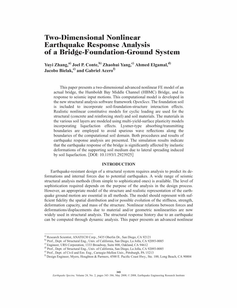
The Humboldt Bay Bridge site, located near Eureka in northern California, includesthree bridges, Eureka Channel Bridge, Middle Channel Bridge and Samoa ChannelBridge, over waterways crossing Woodley Island and Indian Island. The Middle ChannelBridge (Figure 1) is 330-meter long, 10-meter wide, and 12-meter high (average heightover mean water level). The nine span superstructure consists of four precast prestressedconcrete I-girders and cast-in-place concrete slabs, as shown in Figure 2. The bridge su-perstructure is supported by two seat-type abutments and eight bents founded on pilegroup foundations, each bent consisting of a single column and hammer head cap beam.The height of the columns/piers ranges from 11 m to 14 m. The deep foundations con-sist of driven precast prestressed concrete pile groups supporting pile caps. Each abut-ment is supported on two rows of piles, with 7 front batter square piles (356 mm/14 inside), and 5 rear vertical square piles �356 mm/14 in�, of 400 kN capacity per pile. Forconvenience, the piers are numbered #1 through 8 from the left (South-East, WoodleyIsland side) to the right (North-West, Indian Island side). Piers #2 through 6 are sup-ported on five 1372 mm �54 in� diameter, 1800 kN circular piles, while piers #1, 7 and8 are supported on sixteen (4 rows of 4 piles) 356 mm �14 in�, 625 kN square piles. Allpiers and piles have continuous moment connection at the pile-cap-pier joints. The su-perstructure is continuous over piers #1, 2, 4, 5, 7 and 8. There are expansion joints atthe abutments and on top of piers #3 and 6. At these expansion joints, there are shear
Woodley Island Indian Island
Figure 1. Aerial view of Humboldt Bay Middle Channel Bridge (courtesy of California De-partment of Transportation (Caltrans)).
2-D NONLINEAR EARTHQUAKE RESPONSE ANALYSIS OF BRIDGE-FOUNDATION-GROUND SYSTEM 347
keys with gaps on both sides; while at the continuous joints, a shear key with #4 dowelsconnects the superstructure to the cap beam of the single column bent (i.e., shear keywithout gap). Thus, the bridge structure consists of three frames interconnected throughshear keys with gaps at the two interior expansion joints.
DESCRIPTION OF SITE CONDITIONS
Ten rotary auger borings were drilled to a maximum depth of about 30 m below theexisting ground surface in 1967. These borings were almost evenly distributed betweenthe two abutments along the centerline of the bridge. Another rotary auger boring to adepth of about 64 m below the existing ground surface was drilled near the second spanof the bridge from the Eureka side by the Caltrans’ Office of Structural Foundations in1994. Based on these data (Caltrans 2000), a generalized soil profile was developed. Thebridge alignment, to the maximum explored depth, is underlain by Tertiary and Quater-nary Alluvial deposits (soil layer 1 in Figure 3). A 1.5 to 3.0 m thick surficial soil layerconsisting of mainly soft to very soft organic silt with clay and some construction debrisblankets the entire bridge alignment (soil layer 8 in Figure 3). This surficial layer fromnear the left abutment to near pier #2 is underlain by about 10.8 m of medium dense todense silty sand and sand with some organic matter (soil layer 5 in Figure 3). The surfi-cial layer from the vicinity of pier #7 to the vicinity of the right abutment is underlain bya layer of soft or loose sandy silt or silty sand with organic matter (soil layer 7 in Figure3). The thickness of this layer varies significantly and ranges from about 1.5 m near pier#7 to over 15 m near the right abutment. The surficial layer along the remainder of the
Figure 2. Superstructure of Humboldt Bay Middle Channel Bridge.

348 ZHANG ET AL.
bridge alignment in the middle of the river channel is underlain by about 9.2 m ofmainly dense silty sand and sand (soil layer 6 in Figure 3). A 7.6 to 10.7 m thick layerof mainly very dense sand underlies the above soil layers along the entire bridge align-ment (soil layer 3 in Figure 3). This very dense sand layer is underlain, to the maximumexplored depth �64 m�, by mainly medium dense organic silt, sandy silt and stiff siltyclay (soil layer 2 in Figure 3). Groundwater was encountered at ground surface in theland borings drilled in 1967. Recent field observations also showed that the water in thechannel is near the ground surface level.
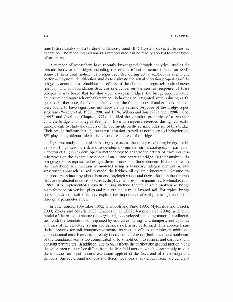
Borehole 1 at Caltrans Samoa Bridge geotechnical downhole array (approximately0.25 mile north-west of the west abutment of the HBMC Bridge) provides a shear wavevelocity profile down to a depth of 220 meters (see Figure 4), where the borehole en-countered bedrock (shear wave velocity �850 m/sec). The shear wave velocities areabout 180 m/sec in the upper 20 m, lie in the range of 200 to 400 m/sec in the depthrange of 20 to 60 m, and lie in the range of 400 to 600 m/sec in the depth range of60 to 220 m (Somerville and Collins 2002). The Humboldt Bay bridge site is suscep-tible to soil liquefaction under strong ground shaking. Soil liquefaction, approach fillsettlement and lateral spreading are issues of interest in this study.
Figure 3. Two-dimensional soil profile of HBMC Bridge site (layer 1: Tertiary and QuaternaryAlluvial deposits; layer 2: medium dense organic silt, sandy silt and stiff silty clay; layer 3:dense sand; layer 4: silt; layer 5: medium dense to dense silty sand and sand with some organicmatter; layer 6: dense silty sand and sand; layer 7: soft or loose sandy silt or silty sand withorganic matter; layer 8: soft to very soft organic silt with clay; and layer 9: abutment fill. Layers5 and 7 are susceptible to soil liquefaction.
2-D NONLINEAR EARTHQUAKE RESPONSE ANALYSIS OF BRIDGE-FOUNDATION-GROUND SYSTEM 349
FAULTING AND SEISMICITY
The Humboldt Bay bridges are located in an area of complex tectonic interactionamong the Gorda, North American and Pacific Plates. The “Little Salmon” fault, whichis categorized by the California Department of Mines and Geology as one of the prin-cipal active fault in California, is the nearest seismic source from the site. This fault islocated about 5 km from the Humboldt Bay Bridges and is capable of generating aMaximum Credible Earthquake of Moment Magnitude 7.5. According to the site-specific seismic ground motion study conducted by Geomatrix Consultants (1994)for Caltrans, the Peak Bedrock Acceleration at the bridge location was estimated toabout 0.9 g.
SEISMIC RETROFITS
The HBMC Bridge was designed in 1968 and built in 1971 and has been the objectof two Caltrans seismic retrofit efforts, the first one completed in 1995, and the secondone completed in 2005. The objectives of the first retrofit effort were to mitigate the po-tential for unseating and diaphragm damage and to strengthen the shear keys by enlarg-ing and reinforcing the superstructure. In this retrofit, the transverse end diaphragms ontop of all piers (at both expansion and continuous joints) were replaced by stronger ones;cable restrainers and pipe seat extenders were installed at the expansion joints to connectadjacent superstructures; seat width at the abutments and interior expansion joints wasincreased; and shear keys at all joints were strengthened. The objective of the secondretrofit was to strengthen the substructure (piers, pile caps, and pile groups) and con-sisted of (Caltrans 2002): (1) placing reinforced concrete casings around each pier; (2)increasing the horizontal size of the pile cap and adding four 900 mm �36 in� diametercast-in-steel shell piles at each pier; and (3) adding a 450 mm �18 in� thick reinforcedconcrete top mat to the pile cap of each pier.
0 200 400 600 800 1000
−200
−150
−100
−50
0
Shear Wave Velocity [m/sec]
Dep
th[m
]
Borehole 1Simulation model
Figure 4. Shear wave velocity profile near HBMC Bridge site.
350 ZHANG ET AL.
COMPUTATIONAL MODEL
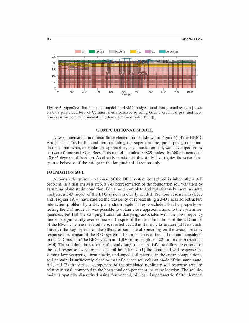
A two-dimensional nonlinear finite element model (shown in Figure 5) of the HBMCBridge in its “as-built” condition, including the superstructure, piers, pile group foun-dations, abutments, embankment approaches, and foundation soil, was developed in thesoftware framework OpenSees. This model includes 10,889 nodes, 10,600 elements and20,686 degrees of freedom. As already mentioned, this study investigates the seismic re-sponse behavior of the bridge in the longitudinal direction only.
FOUNDATION SOIL
Although the seismic response of the BFG system considered is inherently a 3-Dproblem, in a first analysis step, a 2-D representation of the foundation soil was used byassuming plane strain condition. For a more complete and quantitatively more accurateanalysis, a 3-D model of the BFG system is clearly needed. Previous researchers (Lucoand Hadjian 1974) have studied the feasibility of representing a 3-D linear soil-structureinteraction problem by a 2-D plane strain model. They concluded that by properly se-lecting the 2-D model, it was possible to obtain close approximations to the system fre-quencies, but that the damping (radiation damping) associated with the low-frequencymodes is significantly over-estimated. In spite of the clear limitations of the 2-D modelof the BFG system considered here, it is believed that it is able to capture (at least quali-tatively) the key aspects of the effects of soil lateral spreading on the overall seismicresponse mechanism of the BFG system. The dimensions of the soil domain consideredin the 2-D model of the BFG system are 1,050 m in length and 220 m in depth (bedrocklevel). The soil domain is taken sufficiently long so as to satisfy the following criteria forthe soil response away from its lateral boundaries: (1) the simulated soil response as-suming homogeneous, linear elastic, undamped soil material in the entire computationalsoil domain, is sufficiently close to that of a shear soil column made of the same mate-rial; and (2) the vertical component of the simulated nonlinear soil response remainsrelatively small compared to the horizontal component at the same location. The soil do-main is spatially discretized using four-noded, bilinear, isoparametric finite elements
0 100 200 300 400 500 600 700 800 900 10000
50
100
150
200
250
Unit [m]
SP SP/SM OL/SM CL OL Abutment
Figure 5. OpenSees finite element model of HBMC bridge-foundation-ground system [basedon blue prints courtesy of Caltrans, mesh constructed using GID, a graphical pre- and post-processor for computer simulation (Dominguez and Soler 1999)].

2-D NONLINEAR EARTHQUAKE RESPONSE ANALYSIS OF BRIDGE-FOUNDATION-GROUND SYSTEM 351
with four integration points each. The size of the finite elements throughout the soil do-main is controlled by the soil shear wave velocity profile (see Figure 4) such that shearwaves up to about 15 Hz can be propagated with sufficient accuracy through the soilmesh. The (out of plane) thickness of the soil domain below the water table (i.e., groundsurface) is taken as 6.10 m, which corresponds to the width of the 1372 mm �54 in.�pile groups supporting the bridge piers, while a thickness of 10.4 m, equal to the sepa-ration distance between the abutment wing walls, is used for the approach embankments.The selection of the out-of-plane thickness of the foundation soil was based on the con-sideration of two opposing effects: (1) piles near the longitudinal axis of the bridge de-form more, longitudinally, than the piles further away (i.e., the effective width of a pilegroup is smaller than its actual width), and (2) soil outside the (out-of-plane) width ofthe foundation groups also contributes to the seismic response of the BFG system (i.e.,contributes to added/entrained mass of soil) in the longitudinal direction.
According to the idealized soil profile developed above (see Figure 3), the soil do-main is divided into the following layers as shown in Figure 5 (from bedrock to groundsurface): (1) dense to very dense, fine to medium grained sand (SP), (2) organic silt(OL), (3) dense to very dense, fine to medium grained sand (SP), (4) very stiff clay(CL), (5) medium dense, silty sand (SP/SM), (6) dense sand (SP), (7) loose sandy silt,silty sand with organic matter (OL/SM), (8) soft organic silt (OL), and (9) abutment fill,compact medium dense sand.
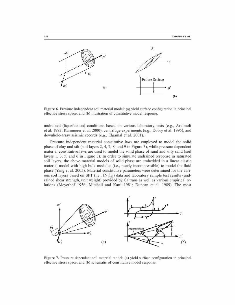
The abutment fill is modeled as dry material, while the other soil layers, which arebelow the water table, are modeled as saturated materials with simplified treatment ofliquefaction effects based on the assumption of undrained conditions. Two types of soilmaterial constitutive models are used in this study: pressure independent and pressuredependent material models. These models are formulated in effective stress space andare based on multi-yield-surface (i.e., nested yield surfaces) plasticity. The pressure in-dependent model is an elastoplastic model for simulating monotonic and cyclic responseof materials whose shear behavior is insensitive to changes in the confining pressure. Inthis model, a set of Von Mises yield surfaces with different sizes form the hardeningzone as shown in Figure 6. The outermost surface defines the shear strength (or failure)envelope. Nonlinear kinematic hardening and associative flow rules (Prevost 1985) areemployed to reproduce Masing-type hysteretic behavior. The pressure dependent modelis an elastoplastic model for simulating the monotonic and cyclic key response charac-teristics of soil materials with mechanical (properties) behavior that depends on the con-fining pressure. Such characteristics include dilatancy (shear-induced volume contrac-tion or dilation) and non-flow liquefaction (cyclic mobility), typically exhibited inmedium to dense sands or silts during monotonic and cyclic loading. In this model, a setof Drucker-Prager nested yield surfaces with a common apex and different sizes formthe hardening zone as shown in Figure 7. The outermost surface defines the shearstrength (or failure) envelope. Nonlinear kinematic hardening and non-associative flowrules are employed to reproduce the dilatancy effect (Elgamal et al. 2003). These soilmodels have been extensively calibrated and validated for both drained (dry) and
352 ZHANG ET AL.
undrained (liquefaction) conditions based on various laboratory tests (e.g., Arulmoliet al. 1992; Kammerer et al. 2000), centrifuge experiments (e.g., Dobry et al. 1995), anddownhole-array seismic records (e.g., Elgamal et al. 2001).
Pressure independent material constitutive laws are employed to model the solidphase of clay and silt (soil layers 2, 4, 7, 8, and 9 in Figure 3), while pressure dependentmaterial constitutive laws are used to model the solid phase of sand and silty sand (soillayers 1, 3, 5, and 6 in Figure 3). In order to simulate undrained response in saturatedsoil layers, the above material models of solid phase are embedded in a linear elasticmaterial model with high bulk modulus (i.e., nearly incompressible) to model the fluidphase (Yang et al. 2005). Material constitutive parameters were determined for the vari-ous soil layers based on SPT (i.e., �N1�60) data and laboratory sample test results (und-rained shear strength, unit weight) provided by Caltrans as well as various empirical re-lations (Meyerhof 1956; Mitchell and Katti 1981; Duncan et al. 1989). The most
Figure 6. Pressure independent soil material model: (a) yield surface configuration in principaleffective stress space, and (b) illustration of constitutive model response.
Figure 7. Pressure dependent soil material model: (a) yield surface configuration in principal
effective stress space, and (b) schematic of constitutive model response.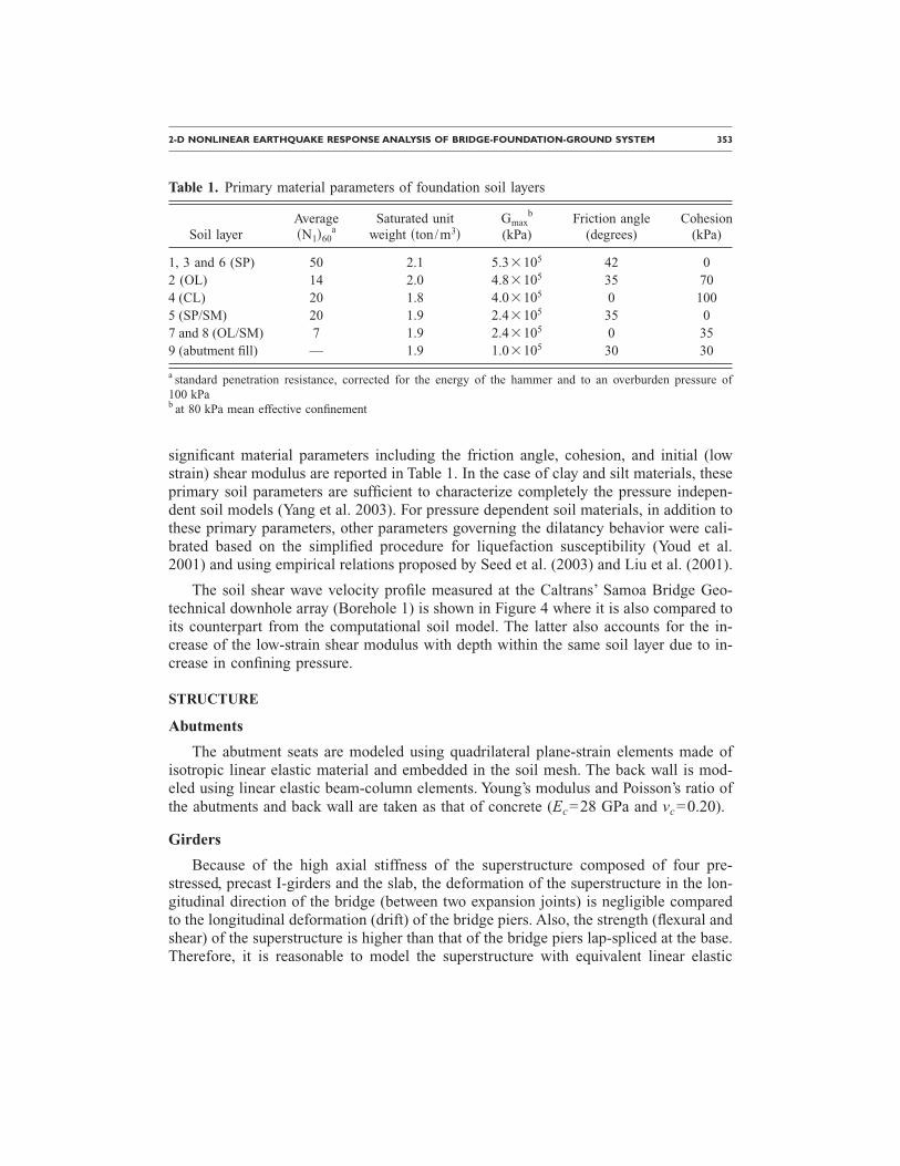
2-D NONLINEAR EARTHQUAKE RESPONSE ANALYSIS OF BRIDGE-FOUNDATION-GROUND SYSTEM 353
significant material parameters including the friction angle, cohesion, and initial (lowstrain) shear modulus are reported in Table 1. In the case of clay and silt materials, theseprimary soil parameters are sufficient to characterize completely the pressure indepen-dent soil models (Yang et al. 2003). For pressure dependent soil materials, in addition tothese primary parameters, other parameters governing the dilatancy behavior were cali-brated based on the simplified procedure for liquefaction susceptibility (Youd et al.2001) and using empirical relations proposed by Seed et al. (2003) and Liu et al. (2001).
The soil shear wave velocity profile measured at the Caltrans’ Samoa Bridge Geo-technical downhole array (Borehole 1) is shown in Figure 4 where it is also compared toits counterpart from the computational soil model. The latter also accounts for the in-crease of the low-strain shear modulus with depth within the same soil layer due to in-crease in confining pressure.
STRUCTURE
Abutments
The abutment seats are modeled using quadrilateral plane-strain elements made ofisotropic linear elastic material and embedded in the soil mesh. The back wall is mod-eled using linear elastic beam-column elements. Young’s modulus and Poisson’s ratio ofthe abutments and back wall are taken as that of concrete (Ec=28 GPa and vc=0.20).
Girders
Because of the high axial stiffness of the superstructure composed of four pre-stressed, precast I-girders and the slab, the deformation of the superstructure in the lon-gitudinal direction of the bridge (between two expansion joints) is negligible comparedto the longitudinal deformation (drift) of the bridge piers. Also, the strength (flexural andshear) of the superstructure is higher than that of the bridge piers lap-spliced at the base.Therefore, it is reasonable to model the superstructure with equivalent linear elastic
Table 1. Primary material parameters of foundation soil layers
Soil layerAverage�N1�60
aSaturated unit
weight �ton/m3�Gmax
b
(kPa)Friction angle
(degrees)Cohesion
(kPa)
1, 3 and 6 (SP) 50 2.1 5.3�105 42 02 (OL) 14 2.0 4.8�105 35 704 (CL) 20 1.8 4.0�105 0 1005 (SP/SM) 20 1.9 2.4�105 35 07 and 8 (OL/SM) 7 1.9 2.4�105 0 359 (abutment fill) — 1.9 1.0�105 30 30
a standard penetration resistance, corrected for the energy of the hammer and to an overburden pressure of100 kPab at 80 kPa mean effective confinement
354 ZHANG ET AL.
beam-column elements (one per span). The cross sectional area �A� of this equivalentbeam element is 3.45 m2, while its moment of inertia is 1.68 m4. Young’s modulus ofthe superstructure is also taken as that of concrete �Ec=28 GPa�.
Lap Spliced Piers
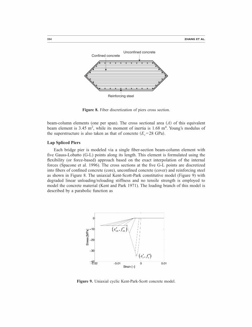
Each bridge pier is modeled via a single fiber-section beam-column element withfive Gauss-Lobatto (G-L) points along its length. This element is formulated using theflexibility (or force-based) approach based on the exact interpolation of the internalforces (Spacone et al. 1996). The cross sections at the five G-L points are discretizedinto fibers of confined concrete (core), unconfined concrete (cover) and reinforcing steelas shown in Figure 8. The uniaxial Kent-Scott-Park constitutive model (Figure 9) withdegraded linear unloading/reloading stiffness and no tensile strength is employed tomodel the concrete material (Kent and Park 1971). The loading branch of this model isdescribed by a parabolic function as
Confined concreteUnconfined concrete
Reinforcing steel
Figure 8. Fiber discretization of piers cross section.
Figure 9. Uniaxial cyclic Kent-Park-Scott concrete model.

2-D NONLINEAR EARTHQUAKE RESPONSE ANALYSIS OF BRIDGE-FOUNDATION-GROUND SYSTEM 355
fc = fc��2�
�c�− � �
�c��2� when � � �c� �1�
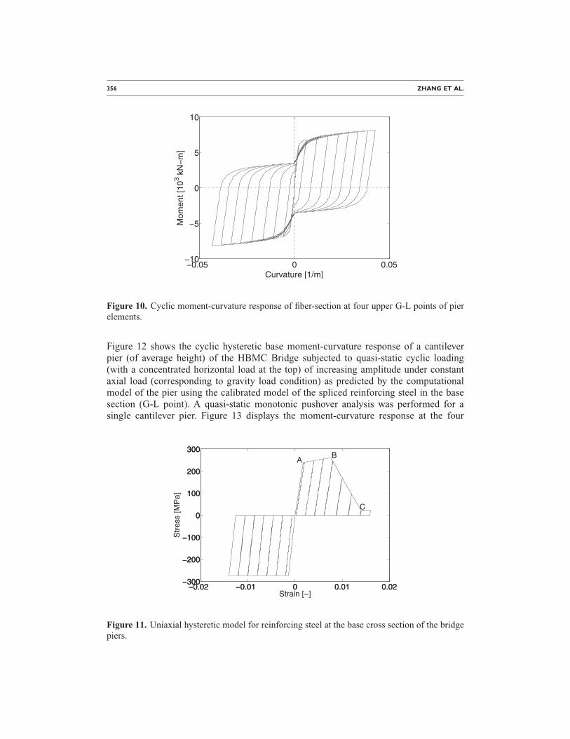
where fc, �, fc� and �c� denote the stress, the corresponding strain, the compressivestrength and the strain at peak strength, respectively. Softening beyond the compressivestrength is approximated as a linear function. A residual strength (or crushing strength),fcu� , and the corresponding strain �cu� (strain at crushing strength) are also specified. Theparameters of the confined and unconfined concrete materials in the piers are given inTable 2. For the cross sections at the upper four G-L points of each pier element, theuniaxial bilinear material model (or uniaxial J2 plasticity model with linear kinematichardening) is used to model the reinforcing steel with the following material parameters:Young’s modulus Es=200 GPa �29000 ksi�, yield strength fy=276 MPa �40 ksi� andpost-yield hardening ratio b=0.8%. Figure 10 shows the cyclic moment-curvature re-sponse of the pier fiber-section defined at the upper four G-L points of each pier ele-ment. At the base of the eight piers, all the longitudinal reinforcing bars are lap spliced.The uniaxial tri-linear hysteretic material model shown in Figure 11 is used to model thereinforcing steel in the lap spliced region. The compression branch is the same as that ofthe reinforcement steel model used at the upper four G-L points. Points A, B and C onthe tension branch correspond to the yield strength, the peak capacity and the residualstrength, respectively, of this hysteretic material model. The material properties for thishysteretic material model, given in Table 3, were calibrated based on the envelope (skel-eton curve) of the lateral force-deformation (drift) response of the bridge piers as pre-dicted using a detailed mechanics-based model of lap spliced columns (Acero 2005),which accounts for (1) the force transfer mechanism between spliced rebars, (2) thebond-slip degradation, (3) the length of the yield plateau in the stress-strain law of thespliced reinforcing steel, (4) the length of the spliced region, (5) the strain penetration ofthe longitudinal reinforcement into the foundation, and (6) the axial load ratio. Thismechanics-based model was itself calibrated using experimental data on lap-spliced col-umns. The pier lateral drift (also called tangential drift) is defined herein as the relativetop-to-bottom horizontal displacement of the pier, minus the horizontal displacement atthe top of the pier due to a rigid body rotation of the pier equal to the rotation of its base.
Table 2. Material parameters for concrete in bridge piers, pile foundations and pile caps
ComponentConcretematerial
Compressivestrength fc�
(kPa)
Strain atcompressivestrength, �c�
Crushing strengthfcu� (kPa)
Strain atcrushing
strength, �cu�
Piers Confined −34485 �−5.00 ksi� −0.002 −6897 �−1.00 ksi� −0.006Unconfined −27588 �−4.00 ksi� −0.002 0.0 −0.005
356 mmpiles
Confined −57039 �−8.27 ksi� −0.005 −43728 �−6.34 ksi� −0.019Unconfined −41383 �−6.00 ksi� −0.002 −13794 �−2.00 ksi� −0.006
1372 mmpiles
Confined −41383 �−6.00 ksi� −0.004 −27588 �−4.00 ksi� −0.014Unconfined −27588 �−4.00 ksi� −0.002 0.0 −0.008
Pile caps Unconfined −34486 �−5.00 ksi� −0.004 0.0 −0.006
356 ZHANG ET AL.
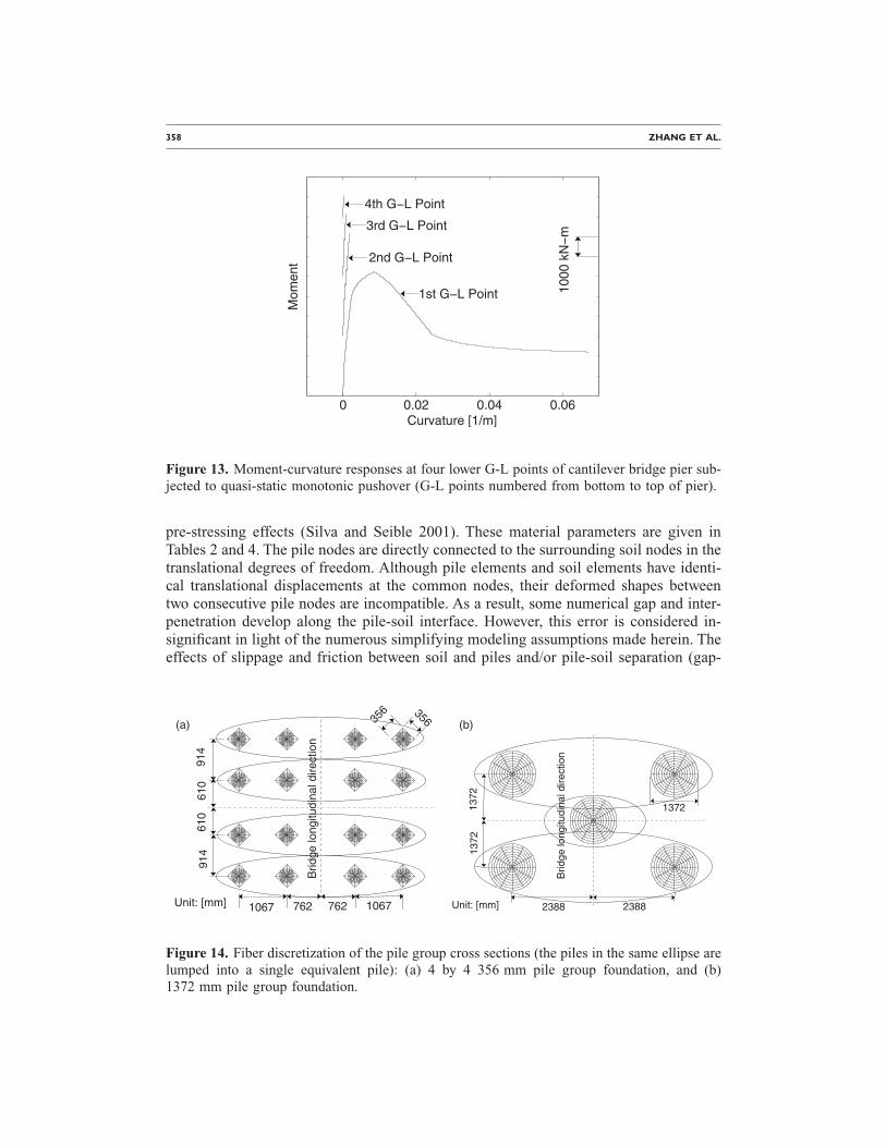
Figure 12 shows the cyclic hysteretic base moment-curvature response of a cantileverpier (of average height) of the HBMC Bridge subjected to quasi-static cyclic loading(with a concentrated horizontal load at the top) of increasing amplitude under constantaxial load (corresponding to gravity load condition) as predicted by the computationalmodel of the pier using the calibrated model of the spliced reinforcing steel in the basesection (G-L point). A quasi-static monotonic pushover analysis was performed for asingle cantilever pier. Figure 13 displays the moment-curvature response at the four
−0.05 0 0.05−10
−5
0
5
10
Curvature [1/m]
Mom
ent[
103
kN−
m]
Figure 10. Cyclic moment-curvature response of fiber-section at four upper G-L points of pierelements.
−0.02 −0.01 0 0.01 0.02−300
−200
−100
0
100
200
300
Strain [−]
Str
ess
[MP
a]
−0.02 −0.01 0 0.01 0.02−300
−200
−100
0
100
200
300A
B
C
Figure 11. Uniaxial hysteretic model for reinforcing steel at the base cross section of the bridge
piers.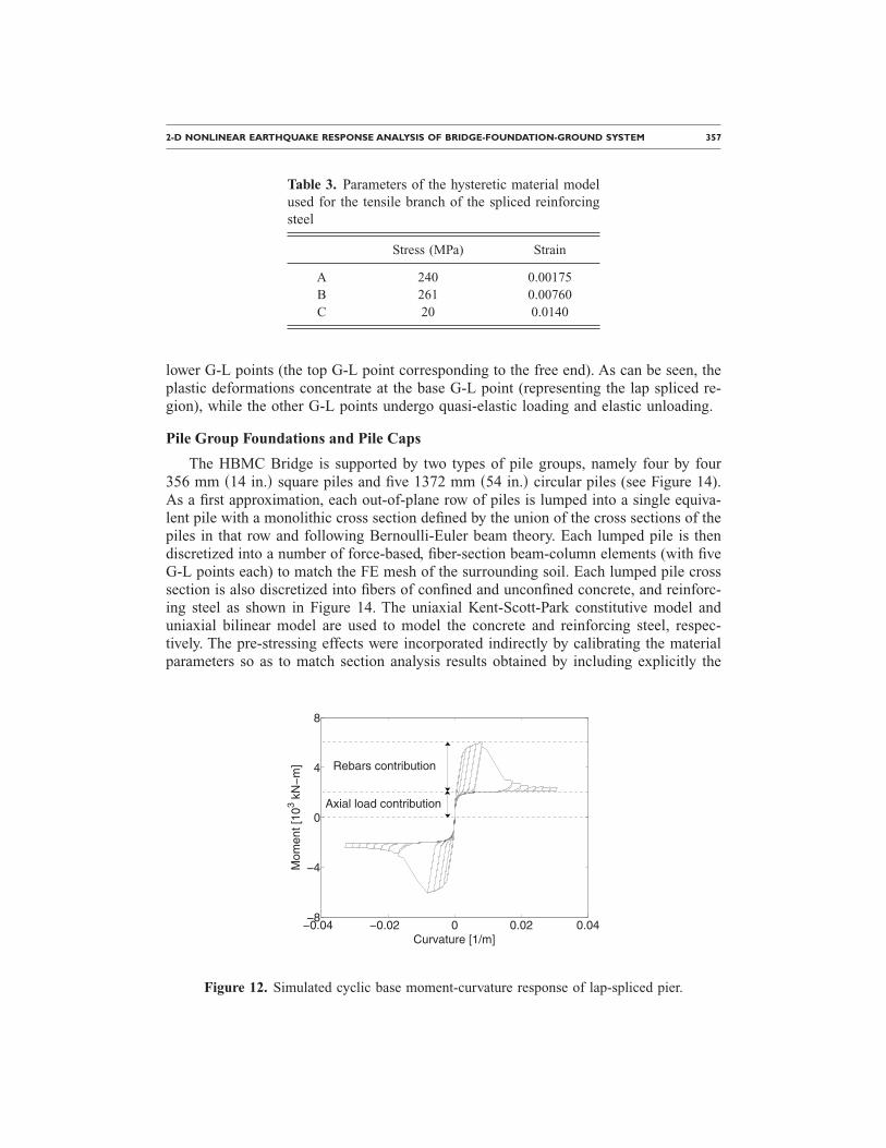
2-D NONLINEAR EARTHQUAKE RESPONSE ANALYSIS OF BRIDGE-FOUNDATION-GROUND SYSTEM 357
lower G-L points (the top G-L point corresponding to the free end). As can be seen, theplastic deformations concentrate at the base G-L point (representing the lap spliced re-gion), while the other G-L points undergo quasi-elastic loading and elastic unloading.
Pile Group Foundations and Pile Caps
The HBMC Bridge is supported by two types of pile groups, namely four by four356 mm �14 in.� square piles and five 1372 mm �54 in.� circular piles (see Figure 14).As a first approximation, each out-of-plane row of piles is lumped into a single equiva-lent pile with a monolithic cross section defined by the union of the cross sections of thepiles in that row and following Bernoulli-Euler beam theory. Each lumped pile is thendiscretized into a number of force-based, fiber-section beam-column elements (with fiveG-L points each) to match the FE mesh of the surrounding soil. Each lumped pile crosssection is also discretized into fibers of confined and unconfined concrete, and reinforc-ing steel as shown in Figure 14. The uniaxial Kent-Scott-Park constitutive model anduniaxial bilinear model are used to model the concrete and reinforcing steel, respec-tively. The pre-stressing effects were incorporated indirectly by calibrating the materialparameters so as to match section analysis results obtained by including explicitly the
Table 3. Parameters of the hysteretic material modelused for the tensile branch of the spliced reinforcingsteel
Stress (MPa) Strain
A 240 0.00175B 261 0.00760C 20 0.0140
−0.04 −0.02 0 0.02 0.04−8
−4
0
4
8
Curvature [1/m]
Mom
ent[
103
kN−
m]
Axial load contribution
Rebars contribution
Figure 12. Simulated cyclic base moment-curvature response of lap-spliced pier.
358 ZHANG ET AL.
pre-stressing effects (Silva and Seible 2001). These material parameters are given inTables 2 and 4. The pile nodes are directly connected to the surrounding soil nodes in thetranslational degrees of freedom. Although pile elements and soil elements have identi-cal translational displacements at the common nodes, their deformed shapes betweentwo consecutive pile nodes are incompatible. As a result, some numerical gap and inter-penetration develop along the pile-soil interface. However, this error is considered in-significant in light of the numerous simplifying modeling assumptions made herein. Theeffects of slippage and friction between soil and piles and/or pile-soil separation (gap-
0 0.02 0.04 0.06Curvature [1/m]
Mom
ent
1st G−L Point
2nd G−L Point
3rd G−L Point
4th G−L Point
1000
kN−
m
Figure 13. Moment-curvature responses at four lower G-L points of cantilever bridge pier sub-jected to quasi-static monotonic pushover (G-L points numbered from bottom to top of pier).
914
610
610
914
1067 762 762 1067
356356
Brid
gelo
ngitu
dina
ldire
ctio
n
Unit: [mm] Unit: [mm] 2388 2388
1372
1372
Brid
gelo
ngitu
dina
ldire
ctio
n
1372
(a) (b)
Figure 14. Fiber discretization of the pile group cross sections (the piles in the same ellipse arelumped into a single equivalent pile): (a) 4 by 4 356 mm pile group foundation, and (b)
1372 mm pile group foundation.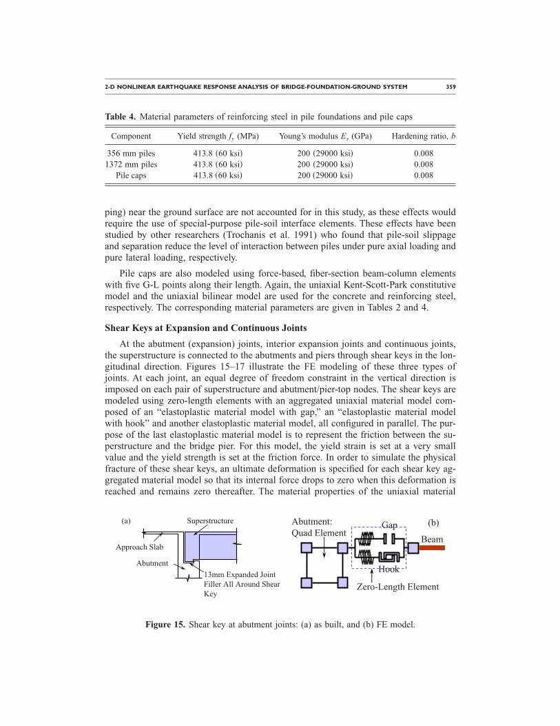
2-D NONLINEAR EARTHQUAKE RESPONSE ANALYSIS OF BRIDGE-FOUNDATION-GROUND SYSTEM 359
ping) near the ground surface are not accounted for in this study, as these effects wouldrequire the use of special-purpose pile-soil interface elements. These effects have beenstudied by other researchers (Trochanis et al. 1991) who found that pile-soil slippageand separation reduce the level of interaction between piles under pure axial loading andpure lateral loading, respectively.
Pile caps are also modeled using force-based, fiber-section beam-column elementswith five G-L points along their length. Again, the uniaxial Kent-Scott-Park constitutivemodel and the uniaxial bilinear model are used for the concrete and reinforcing steel,respectively. The corresponding material parameters are given in Tables 2 and 4.
Shear Keys at Expansion and Continuous Joints
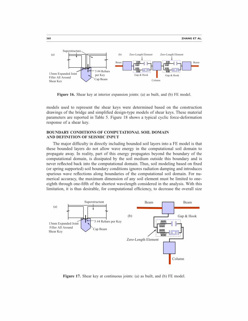
At the abutment (expansion) joints, interior expansion joints and continuous joints,the superstructure is connected to the abutments and piers through shear keys in the lon-gitudinal direction. Figures 15–17 illustrate the FE modeling of these three types ofjoints. At each joint, an equal degree of freedom constraint in the vertical direction isimposed on each pair of superstructure and abutment/pier-top nodes. The shear keys aremodeled using zero-length elements with an aggregated uniaxial material model com-posed of an “elastoplastic material model with gap,” an “elastoplastic material modelwith hook” and another elastoplastic material model, all configured in parallel. The pur-pose of the last elastoplastic material model is to represent the friction between the su-perstructure and the bridge pier. For this model, the yield strain is set at a very smallvalue and the yield strength is set at the friction force. In order to simulate the physicalfracture of these shear keys, an ultimate deformation is specified for each shear key ag-gregated material model so that its internal force drops to zero when this deformation isreached and remains zero thereafter. The material properties of the uniaxial material
13mm Expanded JointFiller All Around ShearKey
Abutment
Superstructure
Approach Slab
(a)
Beam
Abutment:Quad Element
Hook
Gap
Zero-Length Element
(b)
Table 4. Material parameters of reinforcing steel in pile foundations and pile caps
Component Yield strength fy (MPa) Young’s modulus Es (GPa) Hardening ratio, b
356 mm piles 413.8 �60 ksi� 200 �29000 ksi� 0.0081372 mm piles 413.8 �60 ksi� 200 �29000 ksi� 0.008
Pile caps 413.8 �60 ksi� 200 �29000 ksi� 0.008
Figure 15. Shear key at abutment joints: (a) as built, and (b) FE model.
360 ZHANG ET AL.
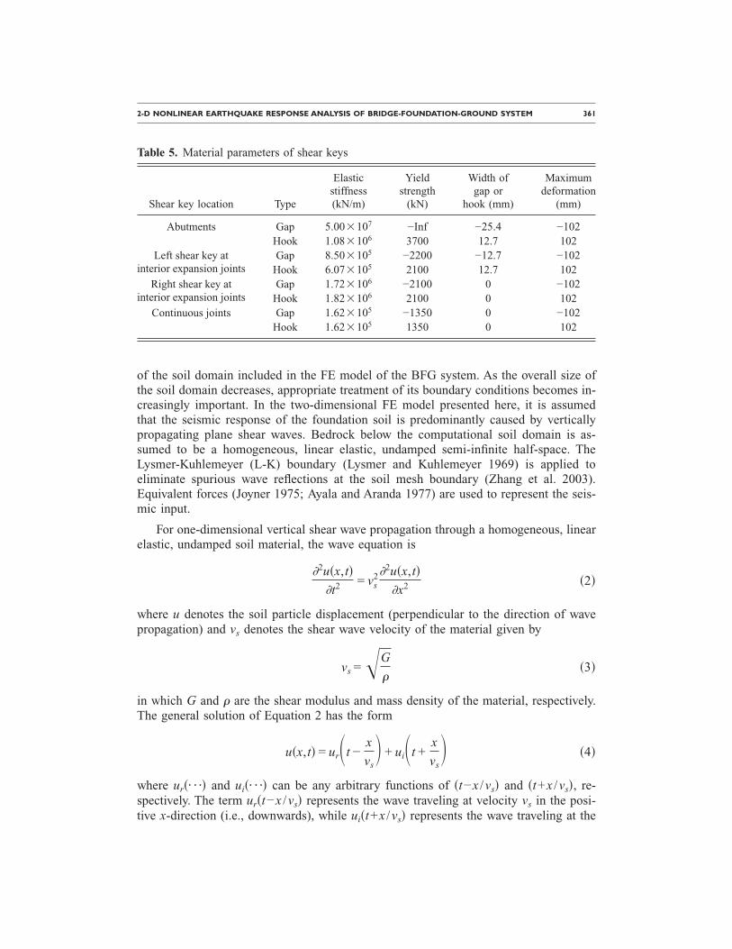
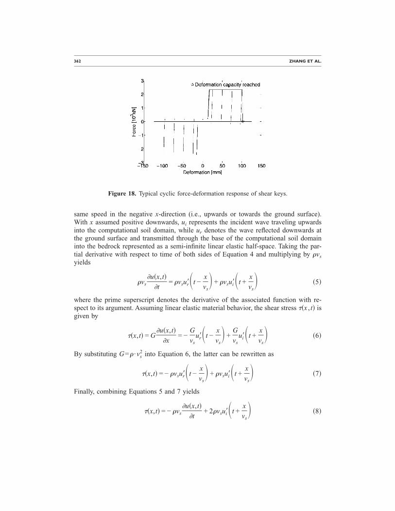
models used to represent the shear keys were determined based on the constructiondrawings of the bridge and simplified design-type models of shear keys. These materialparameters are reported in Table 5. Figure 18 shows a typical cyclic force-deformationresponse of a shear key.
BOUNDARY CONDITIONS OF COMPUTATIONAL SOIL DOMAINAND DEFINITION OF SEISMIC INPUT
The major difficulty in directly including bounded soil layers into a FE model is thatthese bounded layers do not allow wave energy in the computational soil domain topropagate away. In reality, part of this energy propagates beyond the boundary of thecomputational domain, is dissipated by the soil medium outside this boundary and isnever reflected back into the computational domain. Thus, soil modeling based on fixed(or spring supported) soil boundary conditions ignores radiation damping and introducesspurious wave reflections along boundaries of the computational soil domain. For nu-merical accuracy, the maximum dimension of any soil element must be limited to one-eighth through one-fifth of the shortest wavelength considered in the analysis. With thislimitation, it is thus desirable, for computational efficiency, to decrease the overall size
13mm Expanded JointFiller All AroundShear Key
5 #4 Rebarsper KeyCap Beam
Superstructure(a)
Column
Beam
Gap & Hook
Beam
Zero-Length Element Zero-Length Element
Gap & Hook
(b)
Figure 16. Shear key at interior expansion joints: (a) as built, and (b) FE model.
Superstructure
13mm Expanded JointFiller All AroundShear Key
5 #4 Rebars per Key
Cap Beam
(a)
Column
Gap & Hook
Beam
Zero-Length Element
Beam
(b)
Figure 17. Shear key at continuous joints: (a) as built, and (b) FE model.
2-D NONLINEAR EARTHQUAKE RESPONSE ANALYSIS OF BRIDGE-FOUNDATION-GROUND SYSTEM 361
of the soil domain included in the FE model of the BFG system. As the overall size ofthe soil domain decreases, appropriate treatment of its boundary conditions becomes in-creasingly important. In the two-dimensional FE model presented here, it is assumedthat the seismic response of the foundation soil is predominantly caused by verticallypropagating plane shear waves. Bedrock below the computational soil domain is as-sumed to be a homogeneous, linear elastic, undamped semi-infinite half-space. TheLysmer-Kuhlemeyer (L-K) boundary (Lysmer and Kuhlemeyer 1969) is applied toeliminate spurious wave reflections at the soil mesh boundary (Zhang et al. 2003).Equivalent forces (Joyner 1975; Ayala and Aranda 1977) are used to represent the seis-mic input.
For one-dimensional vertical shear wave propagation through a homogeneous, linearelastic, undamped soil material, the wave equation is
�2u�x,t��t2 = vs
2�2u�x,t��x2 �2�
where u denotes the soil particle displacement (perpendicular to the direction of wavepropagation) and vs denotes the shear wave velocity of the material given by
vs =G
��3�
in which G and � are the shear modulus and mass density of the material, respectively.The general solution of Equation 2 has the form
u�x,t� = ur�t −x
vs� + ui�t +
x
vs� �4�
where ur�¯� and ui�¯� can be any arbitrary functions of �t−x /vs� and �t+x /vs�, re-spectively. The term ur�t−x /vs� represents the wave traveling at velocity vs in the posi-
Table 5. Material parameters of shear keys
Shear key location Type
Elasticstiffness(kN/m)
Yieldstrength
(kN)
Width ofgap or
hook (mm)
Maximumdeformation
(mm)
Abutments Gap 5.00�107 −Inf −25.4 −102Hook 1.08�106 3700 12.7 102
Left shear key atinterior expansion joints
Gap 8.50�105 −2200 −12.7 −102Hook 6.07�105 2100 12.7 102
Right shear key atinterior expansion joints
Gap 1.72�106 −2100 0 −102Hook 1.82�106 2100 0 102
Continuous joints Gap 1.62�105 −1350 0 −102Hook 1.62�105 1350 0 102
tive x-direction (i.e., downwards), while ui�t+x /vs� represents the wave traveling at the
362 ZHANG ET AL.
same speed in the negative x-direction (i.e., upwards or towards the ground surface).With x assumed positive downwards, ui represents the incident wave traveling upwardsinto the computational soil domain, while ur denotes the wave reflected downwards atthe ground surface and transmitted through the base of the computational soil domaininto the bedrock represented as a semi-infinite linear elastic half-space. Taking the par-tial derivative with respect to time of both sides of Equation 4 and multiplying by �vs
yields
�vs
�u�x,t��t
= �vsur��t −x
vs� + �vsui��t +
x
vs� �5�
where the prime superscript denotes the derivative of the associated function with re-spect to its argument. Assuming linear elastic material behavior, the shear stress ��x , t� isgiven by
��x,t� = G�u�x,t�
�x= −
G
vsur��t −
x
vs� +
G
vsui��t +
x
vs� �6�
By substituting G=� ·vs2 into Equation 6, the latter can be rewritten as
��x,t� = − �vsur��t −x
vs� + �vsui��t +
x
vs� �7�
Finally, combining Equations 5 and 7 yields
��x,t� = − �vs
�u�x,t��t
+ 2�vsui��t +x
vs� �8�
Figure 18. Typical cyclic force-deformation response of shear keys.

2-D NONLINEAR EARTHQUAKE RESPONSE ANALYSIS OF BRIDGE-FOUNDATION-GROUND SYSTEM 363
This is the same expression reported by Ayala and Aranda (1977). Note that �u�x , t� /�trepresents the velocity of the total soil particle motion, while ui��t+x /vs�=�ui�t+x /vs� /�t is the velocity of the incident soil particle motion. Therefore, according toEquation 8, the shear stress at any point of a linear elastic soil column can be expressedas the summation of two terms. The first term is equivalent to a force (per unit area)generated by a viscous damper with a constant damping coefficient �vs (per unit area),while the second term is given by a force (per unit area) proportional to the velocity ofthe incident soil particle motion. As a result, the soil (assumed homogeneous, linearelastic, undamped) below that point (considered at the boundary between the computa-tional soil domain and the bedrock) can be replaced with a dashpot and an equivalentforce, which defines the seismic input at the base of the computational soil domain. Thistreatment of the boundary conditions allows transmission, without reflection, of the ver-tically incident seismic waves and descending waves (after reflection at the ground sur-face) through the base boundary of the computational soil domain, thus accounting forradiation damping. This modeling approach assumes that the bedrock underlying thebridge site is made of homogeneous, linear elastic, undamped material. There is no spa-tial variability of the incident wave motion at bedrock level based on the assumption ofvertically propagating plane shear waves. At each node along the base and lateral bound-aries of the soil domain, a horizontal dashpot is set to transmit the shear waves (at thebase) and compressive waves (at the lateral boundaries), respectively. The coefficient ofthe dashpots at the base is �vsA, while that of the dashpots on the lateral boundaries is�vpA, where �, vs and vp denote the mass density, shear wave velocity, and compressivewave velocity, respectively, of the soil material outside the boundary (i.e., bedrock), andA is the tributary surface area of the corresponding node. The earthquake excitation isapplied as equivalent horizontal forces at the nodes along the base of the computationalsoil domain. Seismic inputs, however, are usually expressed in terms of accelerogramsrecorded at the free-field ground surface. Consequently, the free-field motion consideredneeds to be deconvolved in order to obtain the corresponding incident wave motion atthe base of the computational soil domain.
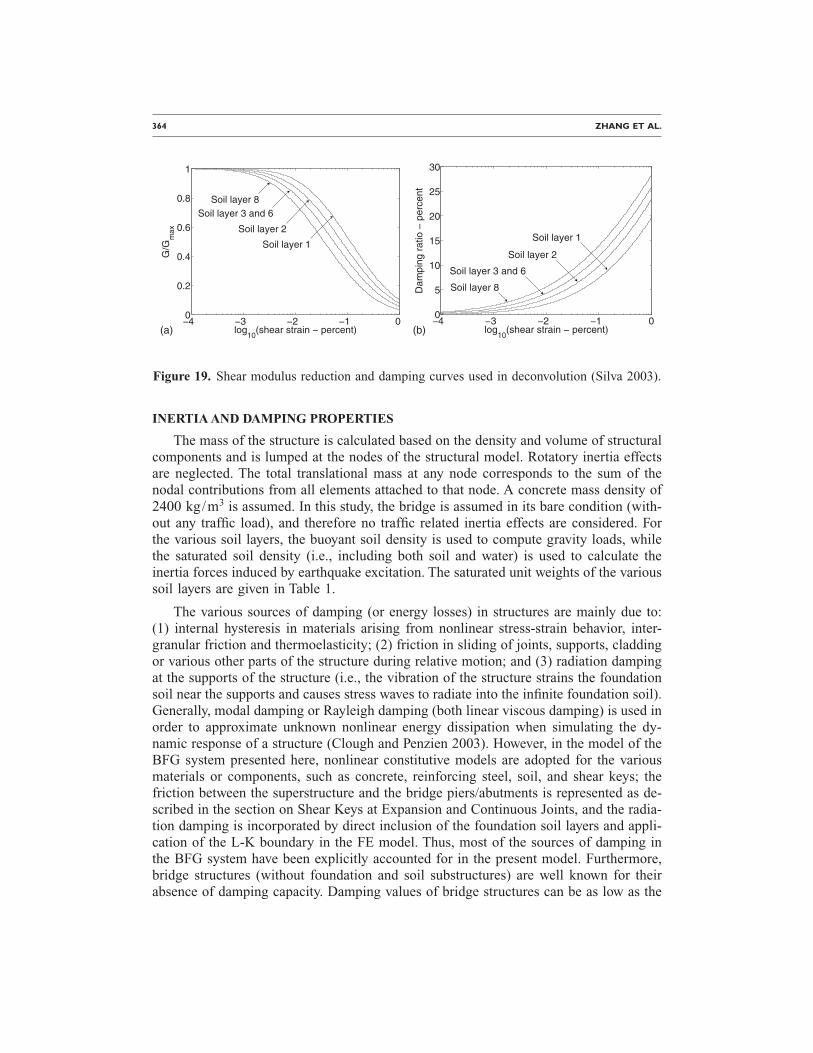
Deconvolution of the free-field ground motion records downwards to the bedrocklevel consists of computing the incident vertical shear wave motion at bedrock level thatcauses the specified free-field motion after propagation through the deformable soil lay-ers between bedrock and ground surface. A one-dimensional soil column with five hori-zontal layers, matching the soil profile at the center of the river channel, was used todeconvolve the free-field surface motions using SHAKE91 (Idriss and Sun 1993). Thisprogram computes the response of a system defined by homogeneous, visco-elastic lay-ers of infinite horizontal extent subjected to vertically traveling shear waves. It is basedon the continuous solution to the wave equation adapted for use with transient motionsthrough the Fast Fourier Transform algorithm. The nonlinearity of the soil behavior,manifested by a shear modulus and damping ratio that depend on the magnitude of theeffective shear strain at a given point in the soil, is accounted for by the use of equivalentlinear soil properties through an iterative procedure to obtain values for shear modulusand damping ratio that are compatible with the effective shear strain in each layer. Theshear modulus reduction and damping curves of sand (Figure 19) as well as the decon-volution procedure recommended by Silva (2003) were used in this study.
364 ZHANG ET AL.
INERTIA AND DAMPING PROPERTIES
The mass of the structure is calculated based on the density and volume of structuralcomponents and is lumped at the nodes of the structural model. Rotatory inertia effectsare neglected. The total translational mass at any node corresponds to the sum of thenodal contributions from all elements attached to that node. A concrete mass density of2400 kg/m3 is assumed. In this study, the bridge is assumed in its bare condition (with-out any traffic load), and therefore no traffic related inertia effects are considered. Forthe various soil layers, the buoyant soil density is used to compute gravity loads, whilethe saturated soil density (i.e., including both soil and water) is used to calculate theinertia forces induced by earthquake excitation. The saturated unit weights of the varioussoil layers are given in Table 1.
The various sources of damping (or energy losses) in structures are mainly due to:(1) internal hysteresis in materials arising from nonlinear stress-strain behavior, inter-granular friction and thermoelasticity; (2) friction in sliding of joints, supports, claddingor various other parts of the structure during relative motion; and (3) radiation dampingat the supports of the structure (i.e., the vibration of the structure strains the foundationsoil near the supports and causes stress waves to radiate into the infinite foundation soil).Generally, modal damping or Rayleigh damping (both linear viscous damping) is used inorder to approximate unknown nonlinear energy dissipation when simulating the dy-namic response of a structure (Clough and Penzien 2003). However, in the model of theBFG system presented here, nonlinear constitutive models are adopted for the variousmaterials or components, such as concrete, reinforcing steel, soil, and shear keys; thefriction between the superstructure and the bridge piers/abutments is represented as de-scribed in the section on Shear Keys at Expansion and Continuous Joints, and the radia-tion damping is incorporated by direct inclusion of the foundation soil layers and appli-cation of the L-K boundary in the FE model. Thus, most of the sources of damping inthe BFG system have been explicitly accounted for in the present model. Furthermore,bridge structures (without foundation and soil substructures) are well known for theirabsence of damping capacity. Damping values of bridge structures can be as low as the
−4 −3 −2 −1 00
0.2
0.4
0.6
0.8
1
log10
(shear strain − percent)
G/G
max
Soil layer 8Soil layer 3 and 6
Soil layer 2
Soil layer 1
−4 −3 −2 −1 00
5
10
15
20
25
30
log10
(shear strain − percent)
Dam
ping
ratio
−pe
rcen
t
Soil layer 8
Soil layer 3 and 6
Soil layer 2
Soil layer 1
(a) (b)
Figure 19. Shear modulus reduction and damping curves used in deconvolution (Silva 2003).
2-D NONLINEAR EARTHQUAKE RESPONSE ANALYSIS OF BRIDGE-FOUNDATION-GROUND SYSTEM 365
inherent material damping in some cases, although generally there are quite wide varia-tions, chiefly due to relative motions at the supports (Eyre and Tilly 1977). Therefore,based on the above considerations, no additional modal/Rayleigh damping was incorpo-rated in the FE model so as to avoid artificial excessive energy dissipation in the modelof the BFG system, especially in light of the fact that, as already mentioned, a 2-D rep-resentation of the soil foundation over-estimates the radiation damping associated withlow frequency modes.
STAGED ANALYSIS PROCEDURE
Since pressure dependent elastoplastic material constitutive models are used to simu-late the behavior of some soil layers, lateral confinement is needed for these soil layersto develop some initial strength. However, the dashpots along the L-K boundaries of thecomputational soil domain cannot provide any lateral static constraint. Therefore, in or-der to conduct a seismic response analysis of the nonlinear BFG system, the followingstaged analysis procedure is followed. (1) The FE mesh of the soil domain only, includ-ing the abutments, is created with its base fixed in both the horizontal and vertical di-rections and lateral boundaries fixed in the horizontal direction only. The various soilconstitutive models are set as linear elastic, and soil gravity is applied statically in asingle linear elastic analysis step. (2) The soil constitutive models are switched fromlinear elastic to elastoplastic (with liquefaction effects incorporated) using theupdateMaterialStage command in OpenSees, which is unique to the soil models usedherein. Then, the new static equilibrium state under soil gravity is obtained iteratively.(3) The nonlinear model of the bridge superstructure, piers and pile group foundations isadded to the soil mesh and bridge gravity is applied statically to the nonlinear model ofthe BFG system. (4) All horizontal displacement constraints along the base and lateralboundaries of the soil domain are removed and replaced with the corresponding supportreactions recorded at the end of the previous stage of analysis. After confirming thatstatic equilibrium under gravity load is still satisfied, a horizontal dashpot is added toeach node along the boundaries of the computational soil domain to implement the L-Kboundary conditions. (5) Finally, from the static equilibrium configuration under gravityloads, the seismic excitation is applied in the form of equivalent horizontal nodal forcesapplied along the base of the computational soil domain as defined earlier.
SMALL AMPLITUDE VIBRATION ANALYSIS
Since the BFG model has no horizontal displacement restraints after the L-K bound-ary conditions are implemented, its global static stiffness matrix is singular. Thus, con-ventional eigensolvers can not be applied to the model to determine its eigenvalues andeigenvectors. In order to study the natural vibration characteristics of the nonlinear sys-tem corresponding to its initial stiffness properties (after application of gravity loads), itis necessary to linearize the material properties of the BFG model. In this study, linear-ization of the system after application of the gravity load was achieved by applyingsmall amplitude dynamic excitations to the BFG model. The amplitude of these excita-tions was made sufficiently small (peak ground acceleration of the order of 1 mm/sec2)such that the system response remains quasi-linear. A check of quasi-linearity was per-
366 ZHANG ET AL.
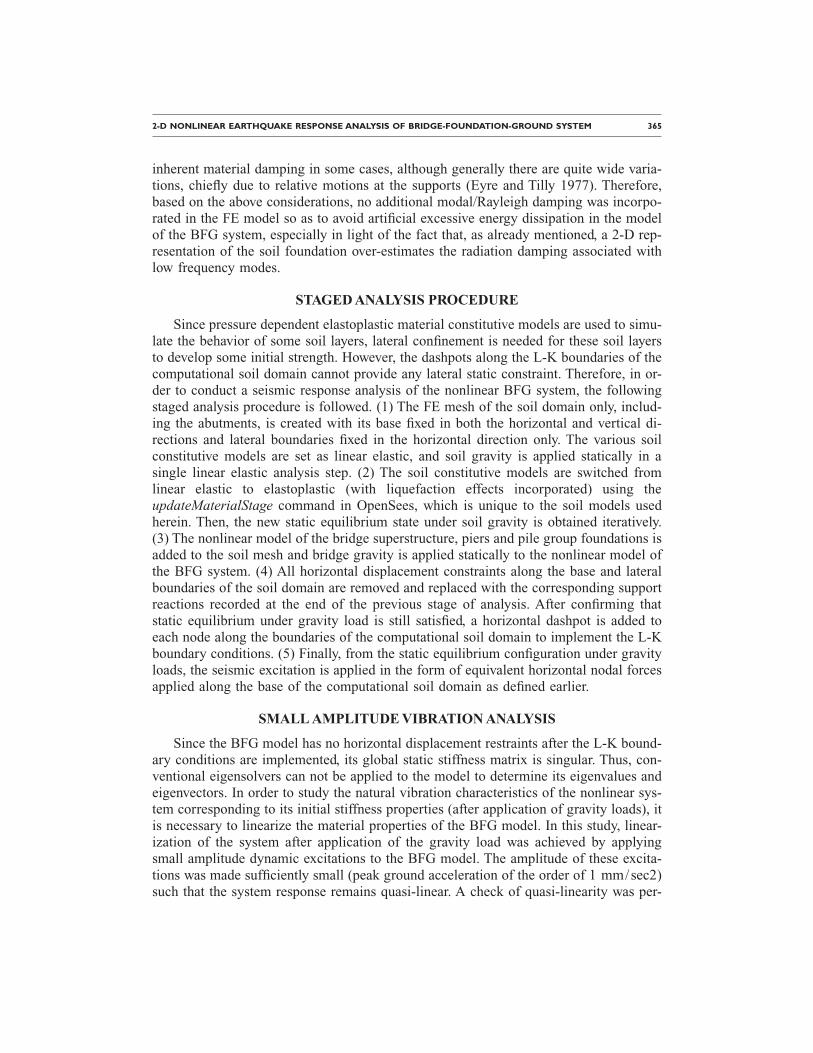
formed for global response quantities (e.g., pier lateral drifts) by verifying that these re-sponse quantities are exactly doubled for double amplitude excitations. The natural fre-quencies of the system were then obtained from transfer functions between inputs andoutputs. Comparison of the transfer functions obtained for different excitations indicatesthat they are in good agreement. Figure 20 shows the transfer functions between the in-cident seismic wave particle velocity (to which the equivalent seismic forces applied atthe base of the computational soil domain are proportional) and the total horizontal dis-placement of the top of all piers. The transfer functions are characterized by two low andbroad spectral peaks at 0.60 Hz and 1.05 Hz, respectively, four high and narrow spectralpeaks at 1.40 Hz, 1.70 Hz, 1.90 Hz and 1.98 Hz, respectively, and other smaller spec-tral peaks above 2.0 Hz; and they become negligibly small beyond 5.0 Hz. Figure 21
Figure 20. Transfer functions of BFG system between incident seismic wave particle velocity(input) and total horizontal displacement at pier tops (outputs).
1 2 3 4 50
1
2
3
4
5
Frequency [Hz]
Tra
nsfe
rfu
nctio
n
Pier 1Pier 2Pier 3Pier 4Pier 5Pier 6Pier 7Pier 8
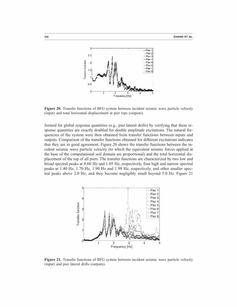
Figure 21. Transfer functions of BFG system between incident seismic wave particle velocity
(input) and pier lateral drifts (outputs).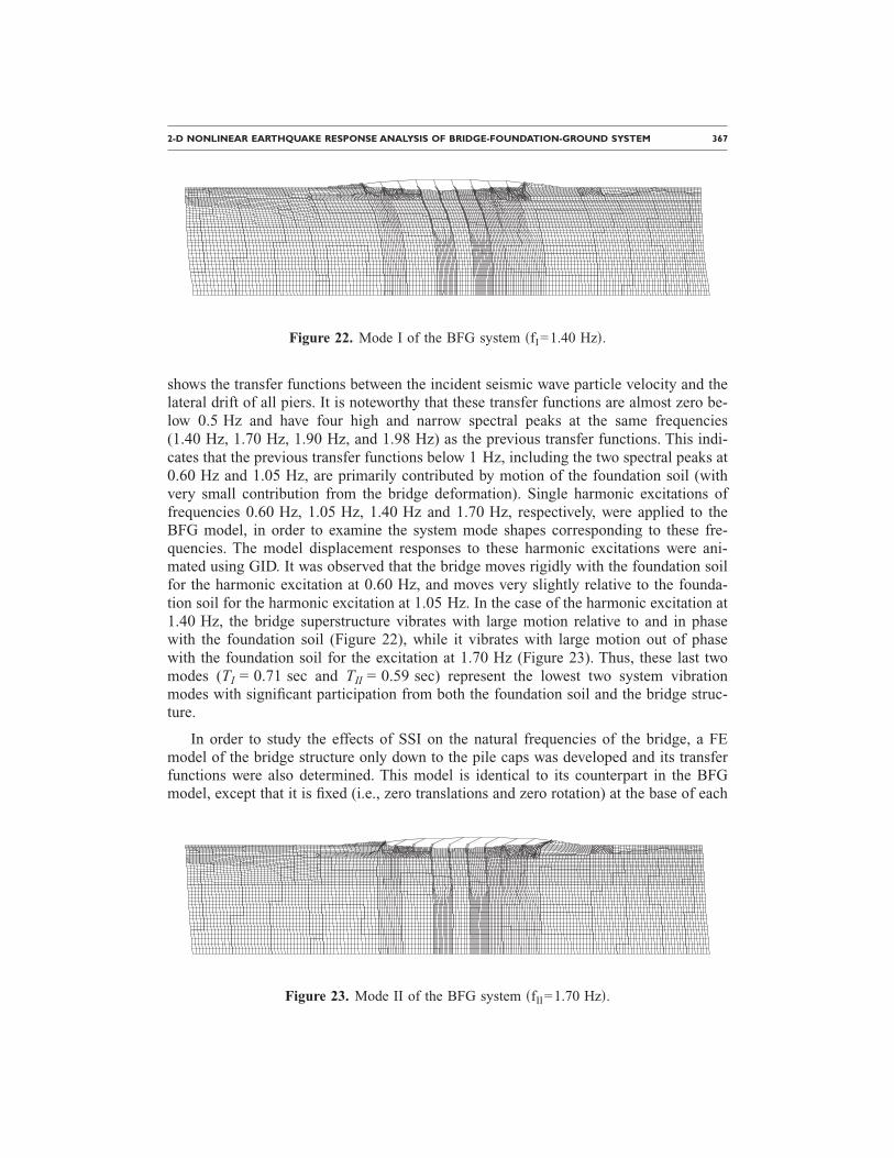
2-D NONLINEAR EARTHQUAKE RESPONSE ANALYSIS OF BRIDGE-FOUNDATION-GROUND SYSTEM 367
shows the transfer functions between the incident seismic wave particle velocity and thelateral drift of all piers. It is noteworthy that these transfer functions are almost zero be-low 0.5 Hz and have four high and narrow spectral peaks at the same frequencies(1.40 Hz, 1.70 Hz, 1.90 Hz, and 1.98 Hz) as the previous transfer functions. This indi-cates that the previous transfer functions below 1 Hz, including the two spectral peaks at0.60 Hz and 1.05 Hz, are primarily contributed by motion of the foundation soil (withvery small contribution from the bridge deformation). Single harmonic excitations offrequencies 0.60 Hz, 1.05 Hz, 1.40 Hz and 1.70 Hz, respectively, were applied to theBFG model, in order to examine the system mode shapes corresponding to these fre-quencies. The model displacement responses to these harmonic excitations were ani-mated using GID. It was observed that the bridge moves rigidly with the foundation soilfor the harmonic excitation at 0.60 Hz, and moves very slightly relative to the founda-tion soil for the harmonic excitation at 1.05 Hz. In the case of the harmonic excitation at1.40 Hz, the bridge superstructure vibrates with large motion relative to and in phasewith the foundation soil (Figure 22), while it vibrates with large motion out of phasewith the foundation soil for the excitation at 1.70 Hz (Figure 23). Thus, these last twomodes (TI = 0.71 sec and TII = 0.59 sec) represent the lowest two system vibrationmodes with significant participation from both the foundation soil and the bridge struc-ture.
In order to study the effects of SSI on the natural frequencies of the bridge, a FEmodel of the bridge structure only down to the pile caps was developed and its transferfunctions were also determined. This model is identical to its counterpart in the BFGmodel, except that it is fixed (i.e., zero translations and zero rotation) at the base of each
Figure 22. Mode I of the BFG system �fI=1.40 Hz�.
Figure 23. Mode II of the BFG system �fII=1.70 Hz�.
368 ZHANG ET AL.
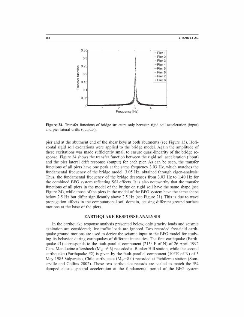
pier and at the abutment end of the shear keys at both abutments (see Figure 15). Hori-zontal rigid soil excitations were applied to the bridge model. Again the amplitude ofthese excitations was made sufficiently small to ensure quasi-linearity of the bridge re-sponse. Figure 24 shows the transfer function between the rigid soil acceleration (input)and the pier lateral drift response (output) for each pier. As can be seen, the transferfunctions of all piers have one peak at the same frequency 3.03 Hz, which matches thefundamental frequency of the bridge model, 3.05 Hz, obtained through eigen-analysis.Thus, the fundamental frequency of the bridge decreases from 3.03 Hz to 1.40 Hz forthe combined BFG system reflecting SSI effects. It is also noteworthy that the transferfunctions of all piers in the model of the bridge on rigid soil have the same shape (seeFigure 24), while those of the piers in the model of the BFG system have the same shapebelow 2.5 Hz but differ significantly above 2.5 Hz (see Figure 21). This is due to wavepropagation effects in the computational soil domain, causing different ground surfacemotions at the base of the piers.
EARTHQUAKE RESPONSE ANALYSIS
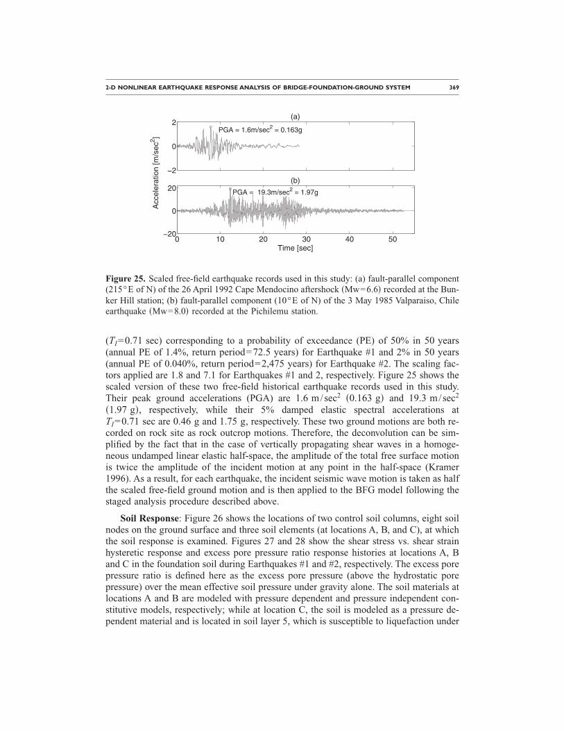
In the earthquake response analysis presented below, only gravity loads and seismicexcitation are considered; live traffic loads are ignored. Two recorded free-field earth-quake ground motions are used to derive the seismic input to the BFG model for study-ing its behavior during earthquakes of different intensities. The first earthquake (Earth-quake #1) corresponds to the fault-parallel component (215° E of N) of 26 April 1992Cape Mendocino aftershock (Mw=6.6) recorded at Bunker Hill station, while the secondearthquake (Earthquake #2) is given by the fault-parallel component (10°E of N) of 3May 1985 Valparaiso, Chile earthquake �Mw=8.0� recorded at Pichilemu station (Som-erville and Collins 2002). These two earthquake records are scaled to match the 5%damped elastic spectral acceleration at the fundamental period of the BFG system
1 2 3 4 50
0.05
0.1
0.15
0.2
0.25
0.3
0.35
Frequency [Hz]
Tra
nsfe
rfu
nctio
n
Pier 1Pier 2Pier 3Pier 4Pier 5Pier 6Pier 7Pier 8
Figure 24. Transfer functions of bridge structure only between rigid soil acceleration (input)and pier lateral drifts (outputs).
2-D NONLINEAR EARTHQUAKE RESPONSE ANALYSIS OF BRIDGE-FOUNDATION-GROUND SYSTEM 369
(TI=0.71 sec) corresponding to a probability of exceedance (PE) of 50% in 50 years(annual PE of 1.4%, return period=72.5 years) for Earthquake #1 and 2% in 50 years(annual PE of 0.040%, return period=2,475 years) for Earthquake #2. The scaling fac-tors applied are 1.8 and 7.1 for Earthquakes #1 and 2, respectively. Figure 25 shows thescaled version of these two free-field historical earthquake records used in this study.Their peak ground accelerations (PGA) are 1.6 m/sec2 �0.163 g� and 19.3 m/sec2
�1.97 g�, respectively, while their 5% damped elastic spectral accelerations atTI=0.71 sec are 0.46 g and 1.75 g, respectively. These two ground motions are both re-corded on rock site as rock outcrop motions. Therefore, the deconvolution can be sim-plified by the fact that in the case of vertically propagating shear waves in a homoge-neous undamped linear elastic half-space, the amplitude of the total free surface motionis twice the amplitude of the incident motion at any point in the half-space (Kramer1996). As a result, for each earthquake, the incident seismic wave motion is taken as halfthe scaled free-field ground motion and is then applied to the BFG model following thestaged analysis procedure described above.
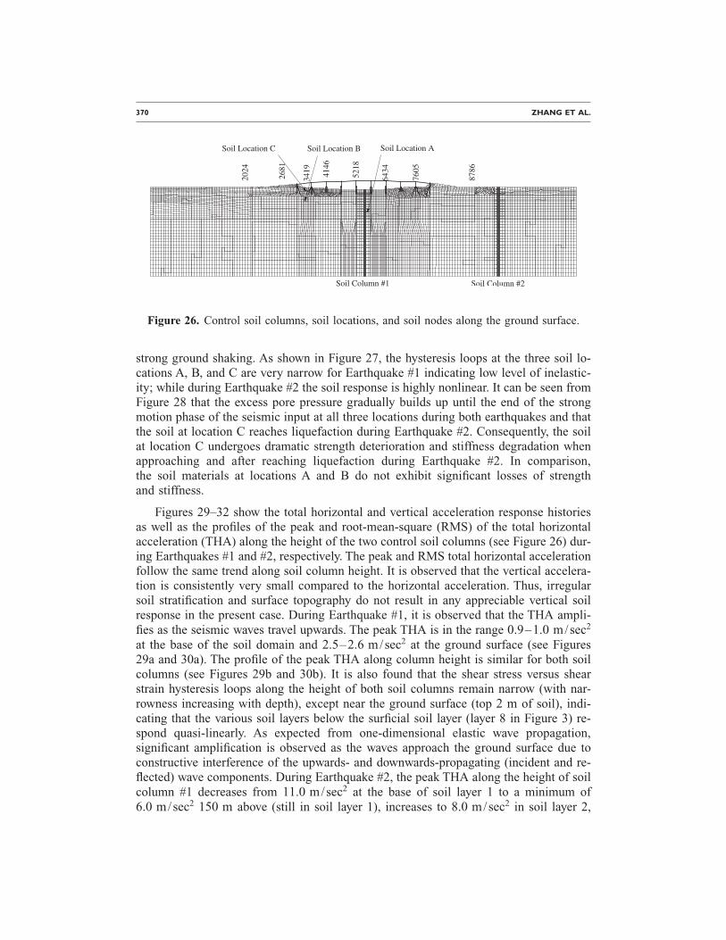
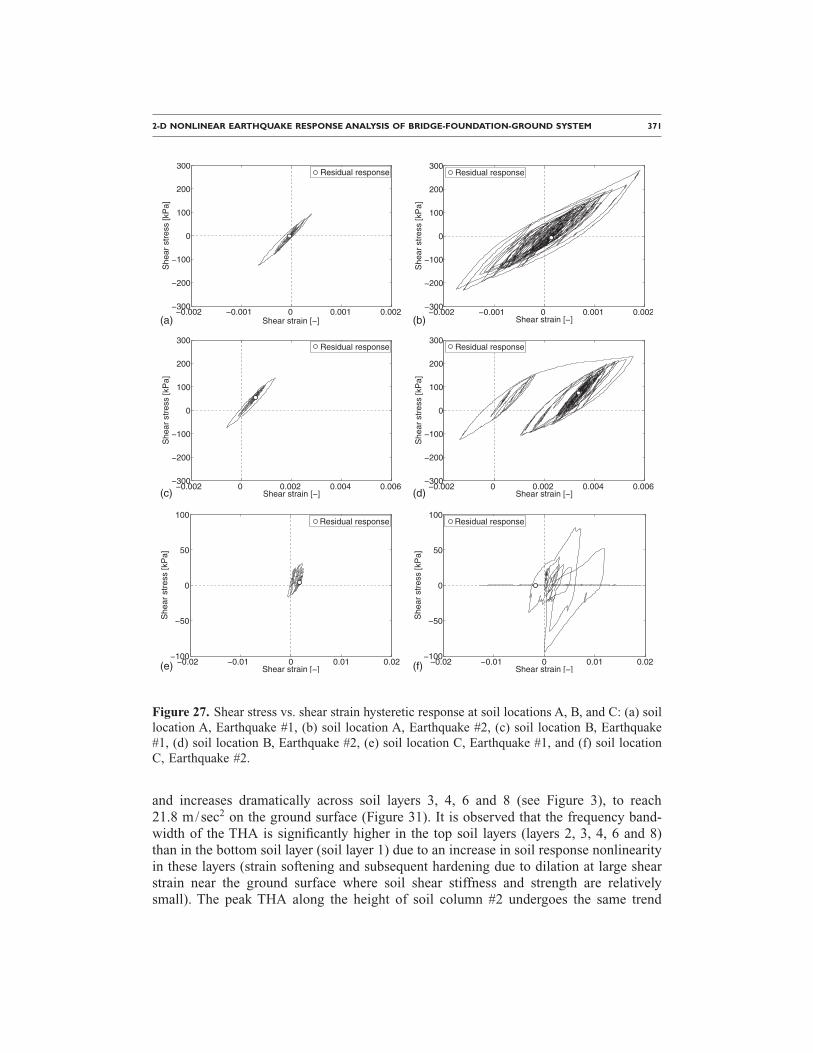
Soil Response: Figure 26 shows the locations of two control soil columns, eight soilnodes on the ground surface and three soil elements (at locations A, B, and C), at whichthe soil response is examined. Figures 27 and 28 show the shear stress vs. shear strainhysteretic response and excess pore pressure ratio response histories at locations A, Band C in the foundation soil during Earthquakes #1 and #2, respectively. The excess porepressure ratio is defined here as the excess pore pressure (above the hydrostatic porepressure) over the mean effective soil pressure under gravity alone. The soil materials atlocations A and B are modeled with pressure dependent and pressure independent con-stitutive models, respectively; while at location C, the soil is modeled as a pressure de-pendent material and is located in soil layer 5, which is susceptible to liquefaction under
−2
0
2(a)
0 10 20 30 40 50−20
0
20
Time [sec]
Acc
eler
atio
n[m
/sec
2 ]
(b)
PGA = 1.6m/sec2 = 0.163g
PGA = 19.3m/sec2 = 1.97g
Figure 25. Scaled free-field earthquake records used in this study: (a) fault-parallel component(215°E of N) of the 26 April 1992 Cape Mendocino aftershock �Mw=6.6� recorded at the Bun-ker Hill station; (b) fault-parallel component (10°E of N) of the 3 May 1985 Valparaiso, Chileearthquake �Mw=8.0� recorded at the Pichilemu station.
370 ZHANG ET AL.
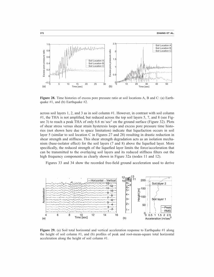
strong ground shaking. As shown in Figure 27, the hysteresis loops at the three soil lo-cations A, B, and C are very narrow for Earthquake #1 indicating low level of inelastic-ity; while during Earthquake #2 the soil response is highly nonlinear. It can be seen fromFigure 28 that the excess pore pressure gradually builds up until the end of the strongmotion phase of the seismic input at all three locations during both earthquakes and thatthe soil at location C reaches liquefaction during Earthquake #2. Consequently, the soilat location C undergoes dramatic strength deterioration and stiffness degradation whenapproaching and after reaching liquefaction during Earthquake #2. In comparison,the soil materials at locations A and B do not exhibit significant losses of strengthand stiffness.
Figures 29–32 show the total horizontal and vertical acceleration response historiesas well as the profiles of the peak and root-mean-square (RMS) of the total horizontalacceleration (THA) along the height of the two control soil columns (see Figure 26) dur-ing Earthquakes #1 and #2, respectively. The peak and RMS total horizontal accelerationfollow the same trend along soil column height. It is observed that the vertical accelera-tion is consistently very small compared to the horizontal acceleration. Thus, irregularsoil stratification and surface topography do not result in any appreciable vertical soilresponse in the present case. During Earthquake #1, it is observed that the THA ampli-fies as the seismic waves travel upwards. The peak THA is in the range 0.9–1.0 m/sec2
at the base of the soil domain and 2.5–2.6 m/sec2 at the ground surface (see Figures29a and 30a). The profile of the peak THA along column height is similar for both soilcolumns (see Figures 29b and 30b). It is also found that the shear stress versus shearstrain hysteresis loops along the height of both soil columns remain narrow (with nar-rowness increasing with depth), except near the ground surface (top 2 m of soil), indi-cating that the various soil layers below the surficial soil layer (layer 8 in Figure 3) re-spond quasi-linearly. As expected from one-dimensional elastic wave propagation,significant amplification is observed as the waves approach the ground surface due toconstructive interference of the upwards- and downwards-propagating (incident and re-flected) wave components. During Earthquake #2, the peak THA along the height of soilcolumn #1 decreases from 11.0 m/sec2 at the base of soil layer 1 to a minimum of6.0 m/sec2 150 m above (still in soil layer 1), increases to 8.0 m/sec2 in soil layer 2,
2024
2681
3419 4146
5218
6434
7605
8786
Soil Column #1 Soil Column #2
Soil Location ASoil Location BSoil Location C
Figure 26. Control soil columns, soil locations, and soil nodes along the ground surface.
2-D NONLINEAR EARTHQUAKE RESPONSE ANALYSIS OF BRIDGE-FOUNDATION-GROUND SYSTEM 371
and increases dramatically across soil layers 3, 4, 6 and 8 (see Figure 3), to reach21.8 m/sec2 on the ground surface (Figure 31). It is observed that the frequency band-width of the THA is significantly higher in the top soil layers (layers 2, 3, 4, 6 and 8)than in the bottom soil layer (soil layer 1) due to an increase in soil response nonlinearityin these layers (strain softening and subsequent hardening due to dilation at large shearstrain near the ground surface where soil shear stiffness and strength are relativelysmall). The peak THA along the height of soil column #2 undergoes the same trend
−0.002 −0.001 0 0.001 0.002−300
−200
−100
0
100
200
300
Shear strain [−]
She
arst
ress
[kP
a]Residual response
−0.002 −0.001 0 0.001 0.002−300
−200
−100
0
100
200
300
Shear strain [−]
She
arst
ress
[kP
a]
Residual response
−0.002 0 0.002 0.004 0.006−300
−200
−100
0
100
200
300
Shear strain [−]
She
arst
ress
[kP
a]
Residual response
−0.002 0 0.002 0.004 0.006−300
−200
−100
0
100
200
300
Shear strain [−]
She
arst
ress
[kP
a]
Residual response
−0.02 −0.01 0 0.01 0.02−100
−50
0
50
100
Shear strain [−]
She
arst
ress
[kP
a]
Residual response
−0.02 −0.01 0 0.01 0.02−100
−50
0
50
100
Shear strain [−]
She
arst
ress
[kP
a]
Residual response
(a)
(c)
(e)
(b)
(d)
(f)
Figure 27. Shear stress vs. shear strain hysteretic response at soil locations A, B, and C: (a) soillocation A, Earthquake #1, (b) soil location A, Earthquake #2, (c) soil location B, Earthquake#1, (d) soil location B, Earthquake #2, (e) soil location C, Earthquake #1, and (f) soil locationC, Earthquake #2.
372 ZHANG ET AL.
across soil layers 1, 2, and 3 as in soil column #1. However, in contrast with soil column#1, the THA is not amplified, but reduced across the top soil layers 5, 7, and 8 (see Fig-ure 3) to reach a peak THA of only 6.6 m/sec2 on the ground surface (Figure 32). Plotsof shear stress versus shear strain hysteresis loops and excess pore pressure time histo-ries (not shown here due to space limitation) indicate that liquefaction occurs in soillayer 5 (similar to soil location C in Figures 27 and 28) resulting in drastic reduction inshear strength and stiffness. This shear strength degradation acts as an isolation mecha-nism (base-isolator effect) for the soil layers (7 and 8) above the liquefied layer. Morespecifically, the reduced strength of the liquefied layer limits the force/acceleration thatcan be transmitted to the overlaying soil layers and its reduced stiffness filters out thehigh frequency components as clearly shown in Figure 32a (nodes 11 and 12).
Figures 33 and 34 show the recorded free-field ground acceleration used to derive
0 5 10 15 20 25 30−0.2
0
0.2
0.4
0.6
0.8
1.0
Time [sec]
Exc
ess
pore
pres
sure
ratio
Soil Location ASoil Location BSoil Location C
0 10 20 30 40 500
0.5
1
1.5
2
2.5
Time [sec]
Exc
ess
pore
pres
sure
ratio
Soil Location ASoil Location BSoil Location C
(a) (b)
Figure 28. Time histories of excess pore pressure ratio at soil locations A, B and C: (a) Earth-quake #1, and (b) Earthquake #2.
Figure 29. (a) Soil total horizontal and vertical acceleration response to Earthquake #1 alongthe height of soil column #1, and (b) profiles of peak and root-mean-square total horizontal
acceleration along the height of soil column #1.
2-D NONLINEAR EARTHQUAKE RESPONSE ANALYSIS OF BRIDGE-FOUNDATION-GROUND SYSTEM 373
the seismic input (parent free-field surface motion) and the simulated THA response ateight control points on the ground surface (shown in Figure 26) during Earthquake #1and #2, respectively. Figure 35 displays the 5 percent damped linear elastic pseudo-acceleration response spectra corresponding to the parent free-field record and the simu-lated surface ground acceleration at several control points. From Figures 33–35, it is ob-served that the amplitude and frequency content of the surface ground acceleration canvary significantly from location to location during the same earthquake, especially whenthe soil undergoes significant nonlinear response (as in Earthquake #2). This illustratesthe importance of local site condition and surface topography. It is also seen that forEarthquake #1, the overall amplitude of the simulated horizontal ground surface accel-eration is larger than that of the parent recorded free-field motion, whereas this relationis inverted for Earthquake #2. This is consistent with the distinct trends in amplification
4 6 8 10 12 14 16Time [sec]
Acc
eler
atio
nHorizontal Vertical
12
34
56
78
910
1112
0 0.5 1 1.5 2 2.50
50
100
150
200
Acceleration [m/sec2]
Hei
ght[
m]
PeakRMS
1
2
345
67
89 1011
12
Soil layer 1
Soil layer 2
(a) (b)
Figure 30. (a) Soil total horizontal and vertical acceleration response to Earthquake #1 alongthe height of soil column #2, and (b) profiles of peak and root-mean-square total horizontalacceleration along the height of soil column #2.
10 15 20 25Time [sec]
Acc
eler
atio
n
Horizontal Vertical
12
34
56
78
910
1112
13
0 5 10 15 20 250
50
100
150
200
Acceleration [m/sec2]
Hei
ght[
m]
PeakRMS1
10
2
3
456
78
91112 13
Soil layer 1
Soil layer 2
(a) (b)
Figure 31. (a) Soil total horizontal and vertical acceleration response to Earthquake #2 alongthe height of soil column #1, and (b) profiles of peak and root-mean-square total horizontal
acceleration along the height of soil column #1.
374 ZHANG ET AL.
behavior of soil sites observed by other researchers (Seed et al. 1976; Idriss 1990). Theyfound that at low to moderate acceleration levels (less than about 0.4 g), peak accelera-tions at soft sites are likely to be greater than those on rock sites. At higher accelerationlevels, however, the low stiffness and nonlinearity of soft soils often prevent them fromdeveloping peak ground accelerations as large as those measured on rock.
Figure 36a shows a color map of the soil shear stress ratio of the BFG system att=10.22 sec into Earthquake #2. Here, the shear stress ratio is defined as the octahedralshear stress demand over the shear strength under the current confinement pressure (i.e.,mean normal effective stress). Soil elements that have reached their shear strength aredenoted in dark red. Clearly, at this instant, a large portion of the foundation soil is un-
10 15 20 25Time [sec]
Acc
eler
atio
nHorizontal Vertical
12
34
56
78
910
1112
0 5 10 15 20 250
50
100
150
200
Acceleration [m/sec2]
Hei
ght[
m]
PeakRMS
1
10
2
3
45
67
8911
12
Soil layer1
Soil layer 2
(a) (b)
Figure 32. (a) Soil total horizontal and vertical acceleration response to Earthquake #2 alongthe height of soil column #2, and (b) profiles of peak and root-mean-square total horizontalacceleration along the height of soil column #2.
2 4 6 8 10 12 14 16 18 20Time [sec]
Acc
eler
atio
n
Input free−field motion
Soil node 2024, PGA = 2.7 m/sec2
Soil node 2681, PGA = 3.7 m/sec2
Soil node 3419, PGA = 2.6 m/sec2
Soil node 4146, PGA = 4.2 m/sec2
Soil node 5218, PGA = 2.2 m/sec2
Soil node 6434, PGA = 3.5 m/sec2
Soil node 7605, PGA = 2.1 m/sec2
Soil node 8786, PGA = 2.8 m/sec2
Figure 33. Total horizontal acceleration response histories along the ground surface for Earth-
quake #1.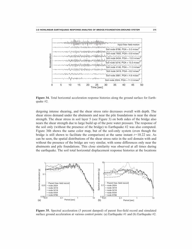
2-D NONLINEAR EARTHQUAKE RESPONSE ANALYSIS OF BRIDGE-FOUNDATION-GROUND SYSTEM 375
dergoing intense shearing, and the shear stress ratio decreases overall with depth. Theshear stress demand under the abutments and near the pile foundations is near the shearstrength. The shear stress in soil layer 5 (see Figure 3) on both sides of the bridge alsonears the shear strength due to large build up of the pore water pressure. The response ofthe soil only (without the presence of the bridge) to Earthquake #2 was also computed.Figure 36b shows the same color map, but of the soil-only system (even though thebridge is still shown to facilitate the comparison) at the same instant t=10.22 sec. Ascan be seen, the spatial distributions of the shear stress ratio in the soil domain with andwithout the presence of the bridge are very similar, with some differences only near theabutments and pile foundations. This close similarity was observed at all times duringthe earthquake. The soil total horizontal displacement response histories at the locations
0 5 10 15 20 25 30 35 40 45 50Time [sec]
Acc
eler
atio
n
Input free−field motion
Soil node 2024, PGA = 11.3 m/sec2
Soil node 2681, PGA = 4.6 m/sec2
Soil node 3419, PGA = 8.2 m/sec2
Soil node 4146, PGA = 11.3 m/sec2
Soil node 5218, PGA = 13.3 m/sec2
Soil node 6434, PGA = 13.0 m/sec2
Soil node 7605, PGA = 9.9 m/sec2
Soil node 8786, PGA = 5.0 m/sec2
Figure 34. Total horizontal acceleration response histories along the ground surface for Earth-quake #2.
0.01 0.1 1 100.001
0.01
0.1
1
Period [sec]
Spe
ctra
lacc
eler
atio
n[g
]
Parent free−field recordnode 2024node 3419node 5218node 6434node 8786
0.01 0.1 1 100.01
0.1
1
10
Period [sec]
Spe
ctra
lacc
eler
atio
n[g
]
Parent free−field recordnode 2024node 3419node 5218node 6434node 8786
(a) (b)
Figure 35. Spectral acceleration (5 percent damped) of parent free-field record and simulated
surface ground acceleration at various control points: (a) Earthquake #1 and (b) Earthquake #2.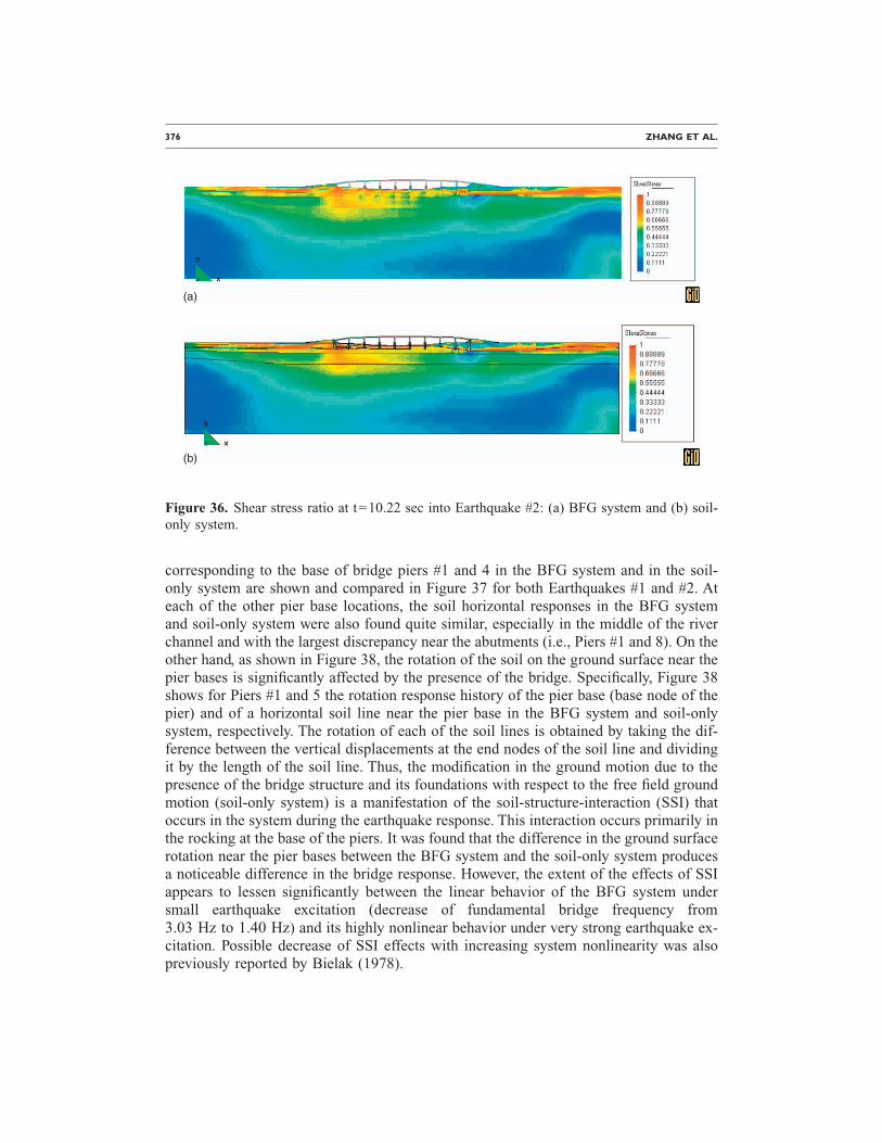
376 ZHANG ET AL.
corresponding to the base of bridge piers #1 and 4 in the BFG system and in the soil-only system are shown and compared in Figure 37 for both Earthquakes #1 and #2. Ateach of the other pier base locations, the soil horizontal responses in the BFG systemand soil-only system were also found quite similar, especially in the middle of the riverchannel and with the largest discrepancy near the abutments (i.e., Piers #1 and 8). On theother hand, as shown in Figure 38, the rotation of the soil on the ground surface near thepier bases is significantly affected by the presence of the bridge. Specifically, Figure 38shows for Piers #1 and 5 the rotation response history of the pier base (base node of thepier) and of a horizontal soil line near the pier base in the BFG system and soil-onlysystem, respectively. The rotation of each of the soil lines is obtained by taking the dif-ference between the vertical displacements at the end nodes of the soil line and dividingit by the length of the soil line. Thus, the modification in the ground motion due to thepresence of the bridge structure and its foundations with respect to the free field groundmotion (soil-only system) is a manifestation of the soil-structure-interaction (SSI) thatoccurs in the system during the earthquake response. This interaction occurs primarily inthe rocking at the base of the piers. It was found that the difference in the ground surfacerotation near the pier bases between the BFG system and the soil-only system producesa noticeable difference in the bridge response. However, the extent of the effects of SSIappears to lessen significantly between the linear behavior of the BFG system undersmall earthquake excitation (decrease of fundamental bridge frequency from3.03 Hz to 1.40 Hz) and its highly nonlinear behavior under very strong earthquake ex-citation. Possible decrease of SSI effects with increasing system nonlinearity was alsopreviously reported by Bielak (1978).
(a)
(b)
Figure 36. Shear stress ratio at t=10.22 sec into Earthquake #2: (a) BFG system and (b) soil-only system.
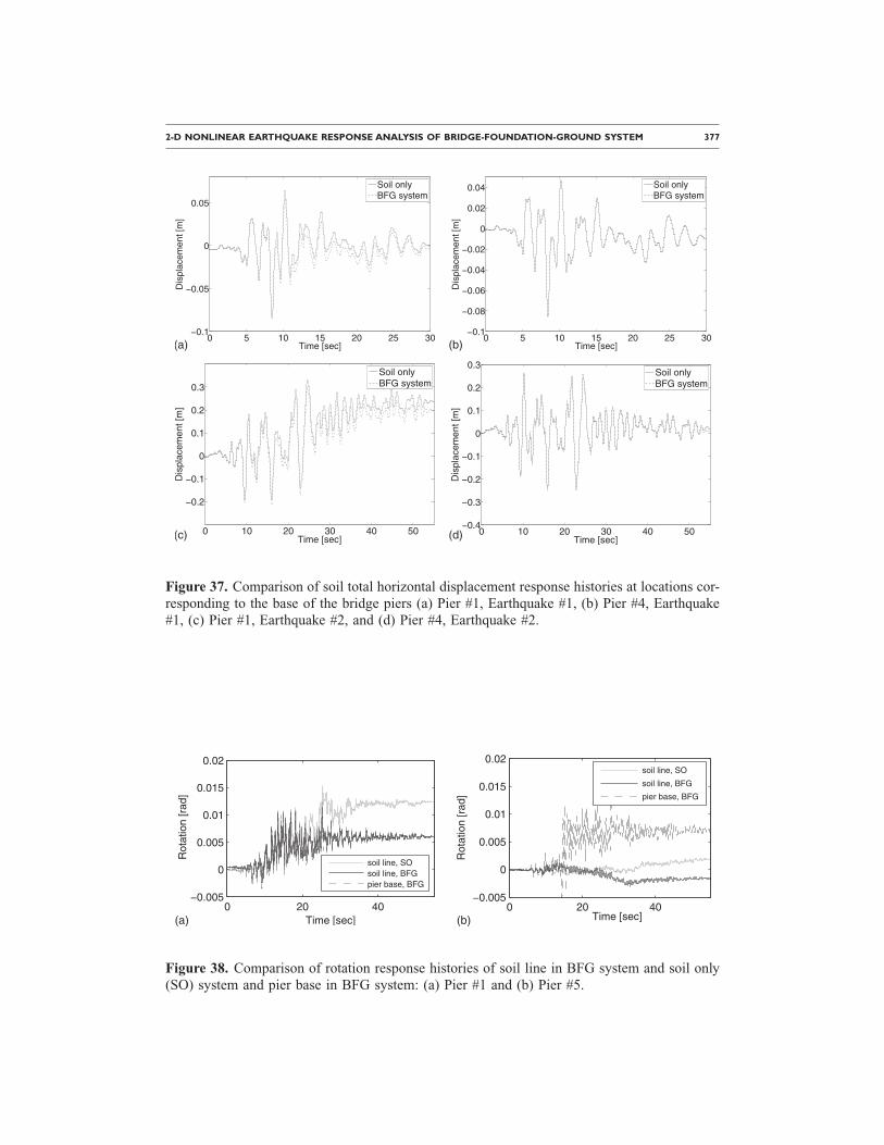
2-D NONLINEAR EARTHQUAKE RESPONSE ANALYSIS OF BRIDGE-FOUNDATION-GROUND SYSTEM 377
0 5 10 15 20 25 30−0.1
−0.05
0
0.05
Time [sec]
Dis
plac
emen
t[m
]Soil onlyBFG system
0 5 10 15 20 25 30−0.1
−0.08
−0.06
−0.04
−0.02
0
0.02
0.04
Time [sec]
Dis
plac
emen
t[m
]
Soil onlyBFG system
0 10 20 30 40 50
−0.2
−0.1
0
0.1
0.2
0.3
Time [sec]
Dis
plac
emen
t[m
]
Soil onlyBFG system
0 10 20 30 40 50−0.4
−0.3
−0.2
−0.1
0
0.1
0.2
0.3
Time [sec]
Dis
plac
emen
t[m
]
Soil onlyBFG system
(a) (b)
(c) (d)
Figure 37. Comparison of soil total horizontal displacement response histories at locations cor-responding to the base of the bridge piers (a) Pier #1, Earthquake #1, (b) Pier #4, Earthquake
#1, (c) Pier #1, Earthquake #2, and (d) Pier #4, Earthquake #2.0 20 40−0.005
0
0.005
0.01
0.015
0.02
Time [sec]
Rot
atio
n[r
ad]
soil line, SOsoil line, BFGpier base, BFG
0 20 40−0.005
0
0.005
0.01
0.015
0.02
Time [sec]
Rot
atio
n[r
ad]
soil line, SO
soil line, BFG
pier base, BFG
(a) (b)
Figure 38. Comparison of rotation response histories of soil line in BFG system and soil only
(SO) system and pier base in BFG system: (a) Pier #1 and (b) Pier #5.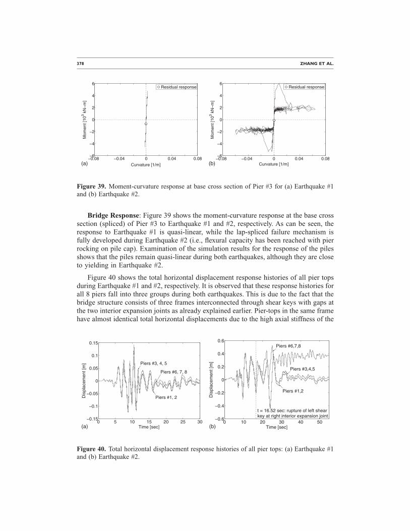
378 ZHANG ET AL.
Bridge Response: Figure 39 shows the moment-curvature response at the base crosssection (spliced) of Pier #3 to Earthquake #1 and #2, respectively. As can be seen, theresponse to Earthquake #1 is quasi-linear, while the lap-spliced failure mechanism isfully developed during Earthquake #2 (i.e., flexural capacity has been reached with pierrocking on pile cap). Examination of the simulation results for the response of the pilesshows that the piles remain quasi-linear during both earthquakes, although they are closeto yielding in Earthquake #2.
Figure 40 shows the total horizontal displacement response histories of all pier topsduring Earthquake #1 and #2, respectively. It is observed that these response histories forall 8 piers fall into three groups during both earthquakes. This is due to the fact that thebridge structure consists of three frames interconnected through shear keys with gaps atthe two interior expansion joints as already explained earlier. Pier-tops in the same framehave almost identical total horizontal displacements due to the high axial stiffness of the
−0.08 −0.04 0 0.04 0.08−6
−4
−2
0
2
4
6
Curvature [1/m]
Mom
ent[
103
kN−
m]
Residual response
−0.08 −0.04 0 0.04 0.08−6
−4
−2
0
2
4
6
Curvature [1/m]
Mom
ent[
103
kN−
m]
Residual response
(a) (b)
Figure 39. Moment-curvature response at base cross section of Pier #3 for (a) Earthquake #1and (b) Earthquake #2.
0 5 10 15 20 25 30−0.15
−0.1
−0.05
0
0.05
0.1
0.15
Time [sec]
Dis
plac
emen
t[m
] Piers #3, 4, 5
Piers #6, 7, 8
Piers #1, 2
0 10 20 30 40 50−0.6
−0.4
−0.2
0
0.2
0.4
0.6
Time [sec]
Dis
plac
emen
t[m
]
t = 16.52 sec: rupture of left shearkey at right interior expansion joint
Piers #6,7,8
Piers #3,4,5
Piers #1,2
(a) (b)
Figure 40. Total horizontal displacement response histories of all pier tops: (a) Earthquake #1
and (b) Earthquake #2.
2-D NONLINEAR EARTHQUAKE RESPONSE ANALYSIS OF BRIDGE-FOUNDATION-GROUND SYSTEM 379
bridge superstructure (girders and slab). In Earthquake #1, no shear key fails. Therefore,the difference in total horizontal displacement among the three response groups remainssmall (see Figure 40a). However, during Earthquake #2, the shear key at the left abut-ment and the left shear key at the right interior expansion joint (above Pier #6) ruptureat t=10.50 sec and t=16.52 sec, respectively, as shown in Figure 41. After the shear keyfailure at the interior expansion joint, the right frame undergoes significant horizontaldisplacement relative to the other two frames (see Figure 40b). Unseating may occur atthose joints where shear keys fail (i.e., reach their ultimate deformation capacities). Thetime history of the relative horizontal displacement between superstructure (girders) andabutment or pier top at the left abutment and right interior expansion joint are plotted inFigure 42 for Earthquake #2. The unseating limit, taken as the full width of the abutmentseat or half the width of the pier, is also represented in Figure 42. It is observed that thepeak (positive) relative horizontal displacement between the superstructure and left abut-
−0.1 0 0.1 0.2 0.3 0.4 0.5 0.6−1
0
1
2
3
4
Deformation [m]
For
ce[1
03kN
]shear key ruptureresidual deformation
0 0.1 0.2 0.3 0.4 0.5 0.6 0.7−3
−2
−1
0
1
2
3
Deformation [m]
For
ce[1
03kN
]
shear key ruptureresidual deformation
(a) (b)
Figure 41. Force-deformation response of shear keys at (a) left abutment, and (b) right interiorexpansion joint (left shear key), during Earthquake #2.
0 10 20 30 40 50
0
0.2
0.4
0.6
0.8
1
Time [sec]
Dis
plac
emen
t[m
]
Unseating limit
0 10 20 30 40 50
0
0.2
0.4
0.6
0.8
Time [sec]
Dis
plac
emen
t[m
]
Unseating limit
(a) (b)
Figure 42. Relative horizontal displacement response histories between superstructure (girders)
and abutment seat or pier at (a) left abutment, and (b) right interior expansion joint.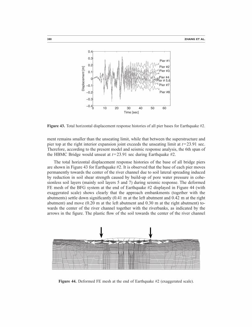
380 ZHANG ET AL.
ment remains smaller than the unseating limit, while that between the superstructure andpier top at the right interior expansion joint exceeds the unseating limit at t=23.91 sec.Therefore, according to the present model and seismic response analysis, the 6th span ofthe HBMC Bridge would unseat at t=23.91 sec during Earthquake #2.
The total horizontal displacement response histories of the base of all bridge piersare shown in Figure 43 for Earthquake #2. It is observed that the base of each pier movespermanently towards the center of the river channel due to soil lateral spreading inducedby reduction in soil shear strength caused by build-up of pore water pressure in cohe-sionless soil layers (mainly soil layers 5 and 7) during seismic response. The deformedFE mesh of the BFG system at the end of Earthquake #2 displayed in Figure 44 (withexaggerated scale) shows clearly that the approach embankments (together with theabutments) settle down significantly (0.41 m at the left abutment and 0.42 m at the rightabutment) and move (0.20 m at the left abutment and 0.30 m at the right abutment) to-wards the center of the river channel together with the riverbanks, as indicated by thearrows in the figure. The plastic flow of the soil towards the center of the river channel
0 10 20 30 40 50 60−0.4
−0.3
−0.2
−0.1
0
0.1
0.2
0.3
0.4
Time [sec]
Dis
plac
emen
t[m
]
Pier #1
Pier #2Pier #3
Pier #4Pier # 5,6
Pier #7
Pier #8
Figure 43. Total horizontal displacement response histories of all pier bases for Earthquake #2.
Figure 44. Deformed FE mesh at the end of Earthquake #2 (exaggerated scale).
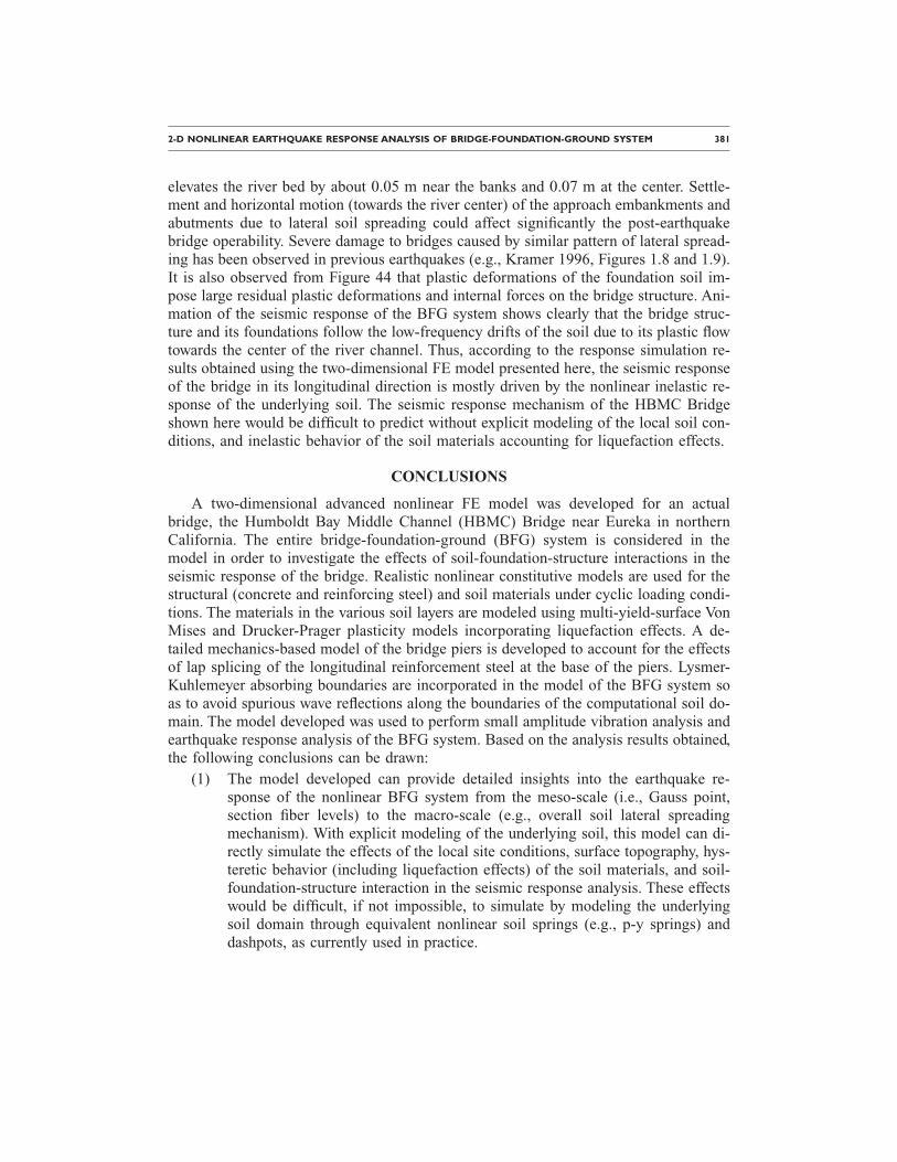
2-D NONLINEAR EARTHQUAKE RESPONSE ANALYSIS OF BRIDGE-FOUNDATION-GROUND SYSTEM 381
elevates the river bed by about 0.05 m near the banks and 0.07 m at the center. Settle-ment and horizontal motion (towards the river center) of the approach embankments andabutments due to lateral soil spreading could affect significantly the post-earthquakebridge operability. Severe damage to bridges caused by similar pattern of lateral spread-ing has been observed in previous earthquakes (e.g., Kramer 1996, Figures 1.8 and 1.9).It is also observed from Figure 44 that plastic deformations of the foundation soil im-pose large residual plastic deformations and internal forces on the bridge structure. Ani-mation of the seismic response of the BFG system shows clearly that the bridge struc-ture and its foundations follow the low-frequency drifts of the soil due to its plastic flowtowards the center of the river channel. Thus, according to the response simulation re-sults obtained using the two-dimensional FE model presented here, the seismic responseof the bridge in its longitudinal direction is mostly driven by the nonlinear inelastic re-sponse of the underlying soil. The seismic response mechanism of the HBMC Bridgeshown here would be difficult to predict without explicit modeling of the local soil con-ditions, and inelastic behavior of the soil materials accounting for liquefaction effects.
CONCLUSIONS
A two-dimensional advanced nonlinear FE model was developed for an actualbridge, the Humboldt Bay Middle Channel (HBMC) Bridge near Eureka in northernCalifornia. The entire bridge-foundation-ground (BFG) system is considered in themodel in order to investigate the effects of soil-foundation-structure interactions in theseismic response of the bridge. Realistic nonlinear constitutive models are used for thestructural (concrete and reinforcing steel) and soil materials under cyclic loading condi-tions. The materials in the various soil layers are modeled using multi-yield-surface VonMises and Drucker-Prager plasticity models incorporating liquefaction effects. A de-tailed mechanics-based model of the bridge piers is developed to account for the effectsof lap splicing of the longitudinal reinforcement steel at the base of the piers. Lysmer-Kuhlemeyer absorbing boundaries are incorporated in the model of the BFG system soas to avoid spurious wave reflections along the boundaries of the computational soil do-main. The model developed was used to perform small amplitude vibration analysis andearthquake response analysis of the BFG system. Based on the analysis results obtained,the following conclusions can be drawn:
(1) The model developed can provide detailed insights into the earthquake re-sponse of the nonlinear BFG system from the meso-scale (i.e., Gauss point,section fiber levels) to the macro-scale (e.g., overall soil lateral spreadingmechanism). With explicit modeling of the underlying soil, this model can di-rectly simulate the effects of the local site conditions, surface topography, hys-teretic behavior (including liquefaction effects) of the soil materials, and soil-foundation-structure interaction in the seismic response analysis. These effectswould be difficult, if not impossible, to simulate by modeling the underlyingsoil domain through equivalent nonlinear soil springs (e.g., p-y springs) anddashpots, as currently used in practice.

382 ZHANG ET AL.
(2) It was found that the response of the bridge structure is governed primarily bythe nonlinear inelastic response of the underlying soil (i.e., inelastic site re-sponse) during earthquakes and that the plastic soil deformations impose largeresidual deformations and internal forces on the bridge structure after strongearthquakes. Effects of soil-foundation-structure interaction were observedmainly in the rocking at the base of the piers, with little SSI lateral effects.
(3) The response of the bridge piers remains quasi-linear for earthquakes with aprobability of exceedance of 50% in 50 years. This conclusion is also sup-ported by other response simulations presented elsewhere (Zhang et al. 2006).However, the bridge shows significant vulnerabilities to earthquakes at the 2%in 50 years seismic hazard level. During such strong earthquakes, the analysesperformed predict that the bridge piers would undergo extensive plastic defor-mations; the lap-spliced mechanism would be fully developed at the base of thepiers with piers rocking on pile caps. Shear keys at the abutments and interiorexpansion joints would likely rupture, and as a result, unseating would also belikely to occur at these joints. Due to soil lateral spreading, the approach em-bankments and abutments would settle significantly and the underlying soilwould “flow” plastically from each approach embankment to the back of theembankment and mainly to the center of the river channel. These predicteddamage scenarios justify Caltrans’ retrofit efforts described herein.
The modeling and analysis efforts presented here are integral parts of the ongoingdevelopment of a performance-based earthquake engineering (PBEE) methodology forbridge and building structures at the Pacific Earthquake Engineering Research (PEER)center. This methodology integrates probabilistic seismic hazard analysis, probabilisticseismic demand analysis, probabilistic seismic damage analysis, and probabilistic seis-mic loss analysis (Cornell and Krawinkler 2000). The HBMC Bridge modeled hereserves as a bridge testbed in the development of this methodology. The model presentedin this paper is used to predict probabilistically the seismic demand to be experienced bythe HBMC Bridge at different seismic hazard levels, which is presented elsewhere(Zhang 2006).
It should be emphasized that the seismic analysis results presented in this study arebased on a limited/restricted 2-D idealization of an actual 3-D bridge-foundation-groundsystem. However, it is expected that even with these limiting assumptions, the 2-Dmodel presented is able to capture (at least qualitatively) the key features of the effectsof SSI and soil lateral spreading on the seismic response of a BFG system with foun-dation soils vulnerable to liquefaction. This study provides a first step towards the de-velopment of more realistic and more accurate 3-D models.
Finally, it is worth mentioning that a number of factors such as ground motion spatialvariability (wave passage and incoherency effects), spatial variation of soil dynamicproperties within soil layers, and uncertainties in soil dynamic properties, which mayaffect the results of the present study, have not been considered.
2-D NONLINEAR EARTHQUAKE RESPONSE ANALYSIS OF BRIDGE-FOUNDATION-GROUND SYSTEM 383
ACKNOWLEDGMENTS
Support of this research by the Pacific Earthquake Engineering Research (PEER)Center through the Earthquake Engineering Research Centers Program of the NationalScience Foundation under Award No. EEC-9701568 is gratefully acknowledged. The au-thors wish to thank Mr. Patrick Hipley, Dr. Cliff Roblee, Mr. Tom Shantz, Dr. CharlesSikorsky, and Mr. Mark Yashinsky of Caltrans for providing all the requested informa-tion regarding the initial design and retrofits of the Humboldt Bay Middle ChannelBridge. Prof. Gregory Fenves and Dr. Frank McKenna (U.C. Berkeley), Prof. MichaelScott (Oregon State University), and Prof. Jose Restrepo (U.C. San Diego) helped withthe structural modeling and analysis aspects of this work. Their assistance was mostvaluable, and is highly appreciated. The authors would also like to thank the reviewersfor their thoughtful and constructive comments. Any opinions, findings, and conclusionsor recommendations expressed in this material are those of the authors and do not nec-essarily reflect those of the sponsor.
REFERENCES
Acero, G., 2005. Seismic Response of Columns with Unconfined Lap-Splices, M.S. thesis, Uni-versity of California at San Diego, CA.
Arulmoli, K., Muraleetharan, K. K., Hossain, M. M., and Fruth, L. S., 1992. VELACS: Verifi-cation of liquefaction analyses by centrifuge studies, laboratory testing program, soil datareport, Project No. 90-0562, The Earth Technology Corporation, Irvine, California.
Ayala, G. A., and Aranda, G. R., 1977. Boundary conditions in soil amplification studies, inProceedings of the 6th World Conference on Earthquake Engineering, Vol. 6, New Dehli,India.
Bielak, J., 1978. Dynamic response of nonlinear building-foundation systems, Earthquake Eng.Struct. Dyn. 6, 17–30.
Caltrans, 2000. Memorandum, Humboldt Bay Middle Channel Bridge, File 01-Hum-255-0.7,Engineering Service Center, Division of Structural Foundation -MS 5, California Depart-ment of Transportation.
––—, 2002. Humboldt Bay bridges seismic substructure retrofit, http://www.dot.ca.gov/dist1/d1projects/humbaybridges, November 29, 2005.
Ciampoli, M., and Pinto, P., 1995. Effects of soil-structure interaction on inelastic seismic re-sponse of bridge piers, J. Struct. Eng. 121, 806–814.
Clough, R., and Penzien, J., 2003. Dynamics of Structures, 2nd edition, Computers and Struc-tures Inc., Berkeley, California.
Cornell, C. A., and Krawinkler, H., 2000. Progress and challenges in seismic performance as-sessment, PEER Center News, Vol. 3, No. 2, Spring 2000.
Dendrou, B., Werner, S., and Toridis, T., 1985. Three-dimensional response of a concrete bridgesystem to traveling seismic waves, Comput. Struct. 20, 593–603.
Dobry, R., Taboada, V., and Liu, L., 1995. Centrifuge modeling of liquefaction effects duringearthquakes, Keynote Lecture, Proceedings of the 1st International Conference on Earth-quake Geotechnical Engineering (IS-Tokyo), Ishihara, K., (editor), vol. 3, Balkema, Nether-lands, 1291–1324.
384 ZHANG ET AL.
Dominguez, N. D., and Soler, P. A., 1999. GID User Manual, International Center for Numeri-cal Methods in Engineering, Barcelona, Spain.
Duncan, J., Horz, R., and Yang, T., 1989. Shear strength correlations for geotechnical engineer-ing, Report, Department of Civil Engineering, Virginia Tech.
Elgamal, A., Lai, T., Yang, Z., and He, L., 2001. Dynamic soil properties, seismic downholearrays and applications in practice (CD-ROM), State-of-the-art paper, in Proceedings of the4th International Conference. on Recent Advances in Geotechnical Earthquake Engineeringand Soil Dynamics, S. Prakash (editor), San Diego, California, March 26–31.
Elgamal, A., Yang, Z., Parra, E., and Ragheb, A., 2003. Modeling of cyclic mobility in satu-rated cohesionless soils, Int. J. Plast. 19, 883–905.
Eyre, R., and Tilly, G. P., 1977. Damping measurements on steel and composite bridges, inSymposium on Dynamic Behavior of Bridges, Supplementary Report 275, Transport andRoad Research Laboratory, Crowthorne, UK.
Geomatrix Consultants, 1994. Seismic ground motion study for Humboldt Bay bridges onRoute 225, Humboldt County, California, Contract No. 59N772. Report prepared for Cal-trans Division of Structures.
Goel, R. K., 1997. Earthquake characteristics of bridges with integral abutments, J. Struct. Eng.123, 1435–1443.
Goel, R. K., and Chopra, A. K., 1997. Evaluation of bridge abutment capacity and stiffnessduring earthquakes, Earthquake Spectra 13, 1–21.
Idriss, I. M., 1990. Response of soft soil sites during earthquakes, in Proceedings, H. BoltonSeed Memorial Symposium, J. M. Duncan (editor), vol. 2, BiTech Publishers, Vancouver,British Columbia, 273–289.
Idriss, I. M., and Sun, J. I., 1993. User’s Manual for SHAKE91: A computer program for con-ducting equivalent linear seismic response analyses of horizontally layered soil deposits.Center for geotechnical modeling, University of California, Davis, California.
Jeremic, B., Kunnath, S., and Xiong, F., 2004. Influence of soil-foundation-structure interactionon seismic response of the I-880 viaduct, Eng. Struct. 263, 391–402.
Joyner, W. B., 1975. Method for calculating nonlinear seismic response in 2-dimensions, Bull.Seismol. Soc. Am. 65, 1337–1357.
Kammerer, A., Wu, J., Pestana, J., Riemer, M., and Seed, R., 2000. Cyclic simple shear testingof Nevada sand for PEER Center project 2051999, Research Report No. UCB/GT/00–02,University of California at Berkeley, California.
Kappos, A. J., Manolis, G. D., and Moschonas, I. F., 2002. Seismic assessment and design ofR/C bridges with irregular configuration, including SSI effects, Eng. Struct. 24, 1337–1348.
Kent, D. C., and Park, R., 1971. Flexural members with confined concrete, J. Struct. Div. 97,1969–1990.
Kramer, S. L., 1996. Geotechnical Earthquake Engineering, Prentice Hall, Upper Saddle River,NJ, 653 pp.
Liu, A., Stewart, J., Abrahamson, N., and Moriwaki, Y., 2001. Equivalent number of uniformstress cycles for soil liquefaction analysis, J. Geotech. Geoenviron. Eng. 127, 1017–1026.
Luco, J. E., and Hadjian, A. H., 1974. Two-dimensional approximations to the three-dimensional soil-structure interaction problem, Nucl. Eng. Des. 31, 195–203.
Lysmer, J., and Kuhlemeyer, R. L., 1969. Finite dynamic model for infinite media, J. Engrg.Mech. Div. 95, 859–877.

2-D NONLINEAR EARTHQUAKE RESPONSE ANALYSIS OF BRIDGE-FOUNDATION-GROUND SYSTEM 385
McCallen, D. B., and Romstad, K. M., 1994. Analysis of a skewed short-span, box-girder over-pass, Earthquake Spectra 10, 729–755.
McKenna, F., and Fenves, G. L., 2001. The OpenSees command language manual, version 1.2,http://opensees.berkeley.edu, Pacific Earthquake Engineering Research Center, University ofCalifornia, Berkeley.
Meyerhof, G. G., 1956. Penetration tests and bearing capacity of cohesionless soils, J. SoilMech. and Found. Div. 82(SM1), 1–19.
Mitchell, J., and Katti, R., 1981. Soil improvement state-of-the-art report, General Reports, inProceedings of 10th International Conference of Soil Mechanics and Foundation Engineer-ing, vol. 4, Stockholm, 264–320.
Mylonakis, G., and Gazetas, G., 2000. Seismic soil-structure interaction: beneficial or detri-mental? J. Earthquake Eng. 4, 277–301.
Mylonakis, G., Nikolaou, A., and Gazetas, G., 1997. Soil-pile-bridge seismic interaction: kine-matic and inertial effects. Part I: soft soil, Earthquake Eng. Struct. Dyn. 26, 337–359.
Porter, K. A., 2003. An overview of PEER’s performance-based earthquake engineering meth-odology, in Proceedings of the 9th International Conference on Applications of Statisticsand Probability in Civil Engineering, San Francisco, California, July 6–9.
Prevost, J. H., 1985. A simple plasticity theory for frictional cohesionless soils, Soil Dyn.Earthquake Eng. 4, 9–17.
Seed, H. B., Ugas, C., and Lysmer, J., 1976. Site-dependent spectra for earthquake-resistant de-sign, Bull. Seismol. Soc. Am. 66, 221–243.
Seed, H. B., Wong, R. T., Idriss, I. M., and Tokimatsu, K., 1984. Moduli and damping factorsfor dynamic analysis of cohesionless soils, Report UCB/EERC-84/14, Earthquake Engineer-ing Research Center, University of California, Berkeley, California.
Seed, R., Cetin, K., Moss, R., Kammerer, A., Wu, J., Pestana, J., Riemer, M., Sancio, R., Bray,J., Kayen, R., and Faris, A., 2003. Recent advances in soil liquefaction engineering: a unifiedand consistent framework, Keynote Presentation, 26th Annual ASCE Los Angeles Geotech-nical Spring Seminar, H.M.S. Queen Mary, Long Beach, CA.
Silva, P. F., and Seible, F., 2001. Seismic performance evaluation of CISS piles, ACI Struct. J.98, 36–49.
Silva, W., 2003. Soil response to earthquake ground motion, Research Project RP2556-07 FinalReport, Woodward-Clyde Consultants, Walnut Creek, CA.
Somerville, P., and Collins, N., 2002. Ground motion time histories for the Humboldt BayBridge, Report of the PEER Performance Based Earthquake Engineering Methodology Test-bed Program, Pacific Earthquake Engineering Research Center, University of California atBerkeley, Berkeley, California.
Spacone, E., Filippou, F. C., and Taucer, F. F., 1996. Fibre beam-column model for non-linearanalysis of R/C frames: Part I. Formulation, Earthquake Eng. Struct. Dyn. 25, 711–725.
Spyrakos, C., 1992. Seismic behavior of bridge piers including soil-structure interaction, Com-put. Struct. 43, 373–384.
Trochanis, A. M., Bielak, J., and Christiano, P., 1991. Three-dimensional nonlinear study ofpiles, J. Geotech. Engrg. 117, 429–447.
Werner, S. D., Beck, J. L., and Levine, M. B., 1987. Seismic refraction evaluation of Melolandroad overpass using the 1979 Imperial Valley earthquake records, Earthquake Eng. Struct.Dyn. 15, 249–274.
386 ZHANG ET AL.
Werner, S. D., Beck, J. L., and Nisar, A., 1990. Dynamic tests and seismic excitation of a bridgestructure, Proceedings of 4th U.S. National Conference on Earthquake Engineering, 1,1037–1046.
Werner, S. D., Crouse, D. B., Katafygiotis, L. S., and Beck, J. L., 1994. Use of strong motionrecords for model evaluation and seismic analysis of a bridge structure, in Proceedings of the5th U.S. National Conference on Earthquake Engineering, Vol. 1, 511–520.
Wilson, J. C., and Tan, B. S., 1990a. Bridge abutments: formulation of simple model for earth-quake response analysis, J. Eng. Mech. 116, 1828–1837.
––—, 1990b. Bridge abutments: assessing their influence on earthquake response of Melolandroad overpass, J. Eng. Mech. 116, 1838–1856.
Yang, Z., Elgamal, A., and Parra, E., 2003. Computational model for cyclic mobility and asso-ciated shear deformation, J. Geotech. Geoenviron. Eng. 129, 1119–1127.
Yang, Z., Lu, J., and Elgamal, A., 2005. OpenSees geotechnical capabilities developed at U.C.San Diego. User Manual, http://cyclic.ucsd.edu/opensees, November 29.
Youd, T. et al., 2001. Liquefaction resistance of soils: summary report from the 1996 NCEERand 1998 NCEER/NSF workshops on evaluation of liquefaction resistance of soils, J. Geo-tech. Geoenviron. Eng. 127, 817–833.
Zhang, J., and Makris, N., 2002. Seismic response analysis of highway overcrossings includingsoil-structure interaction, Earthquake Eng. Struct. Dyn. 31, 1967–1991.
Zhang, Y., Yang, Z., Bielak, J., Conte, J. P., and Elgamal, A., 2003. Treatment of seismic inputand boundary conditions in nonlinear seismic analysis of a bridge ground system, in Pro-ceedings of the 16th ASCE Engineering Mechanics Conference, University of Washington,Seattle, July 16–18.
Zhang, Y., 2006. Probabilistic Structural Seismic Performance Assessment Methodology andApplication to an Actual Bridge-Foundation-Ground System, Ph.D. thesis, University ofCalifornia at San Diego, CA.
(Received 15 March 2006; accepted 9 January 2008�