1

2D analysis of earthquake ground motion in Haifa Bay, Israel

Zohar Gvirtzman (1), John, N. Louie (2)

1. Geological Survey of Israel, Jerusalem, (zohar@gsi.gov.il)

2. Nevada Seismological Laboratory, University of Nevada, Reno, (louie@seismo.unr.edu)

Abstract

We study the earthquake response of the Zevulun Valley basin, underlying northern

Israel‘s largest urban area with two-dimensional viscoelastic seismic modeling of a detailed

geological section. We found that amplification of the horizontal vibrations, the ratio of basin to

no-basin response spectra, correlates with basin depth. In the deepest portion of the basin (Qishon

graben) long periods (2-5 sec) are amplified by 400% and in the shallowest portion of the basin

(Afeq horst) shorter periods (~0.5 sec) are amplified by 300-400%. These resonances in the

vertical direction through the basin are strong enough that their amplitude overwhelms the

amplitude of a previously recognized basin-edge effect. H/V Fourier spectral ratios based on 124

ambient noise measurements do not fully coincide with the basin-to-no-basin Fourier spectral

ratios of the simulation, but the resonance frequencies found in both methods are alike. Moreover,

the relation between the resonance frequency and the depth of the corresponding seismic reflector

in the simulation is almost identical to the empirical frequency-depth relations obtained from

measurements. This indicates that the average shear-wave velocity of the sedimentary column in

the model is consistent with measurements. To evaluate the necessity of 2D analysis we performed

additional 1D simulation at two locations along the section. For the Qishon graben 1D analysis

underestimates the amplification factor relative to 2D by 25%, whereas for the Afeq horst 1D and

2D simulations are similar. For a hard layer within the soft Qishon graben fill, we found that when

the hard layer is thinner than ~50 m its influence on ground motion is small.

2

Geological and Seismological Background

The coastal plain of Haifa Bay (Zevulun Valley) is a densely populated urban zone, the

largest in northern Israel, with well-developed industrial facilities such as a marine port, oil

refineries, and other chemical plants containing hazardous materials. The Bay area includes the

city of Haifa in the south, the city of Akko in the north, and several large towns in between, with a

total population of nearly half a million people. In recent years multi-storey buildings, industrial

plants, roads, and bridges have rapidly developed in the area. The unique combination of seismic

hazard, industry, and population has prompted the Committee for Earthquake Preparedness in

Israel to encourage research in this area; this paper is a part of that effort.

Haifa Bay is the marine outlet of several inland basins (Harod, Yisre'el, Qishon, and

Zevulun valleys) branching from the Jordan Rift Valley northwestwards towards the

Mediterranean coast (Fig. 1). The present seismic activity along these valleys is related to the left-

lateral motion along the Dead Sea Transform (DST; Hofstetter et al., 1996; Shamir et al., 2000).

However, the early formation of these valleys predates the formation of the DST (Shaliv, 1991;

Matmon et al., 2003; Schattner et al., 2006).

The present structure of Zevulun Valley is best demonstrated by the top Judea Group

structural map (Figure 2) that reveals steep subsurface relief buried under the present flat valleys.

The map also shows many faults displacing the top of the Judea Group, but it is unclear at this

stage which faults are currently active and which faults have ceased to operate.

The Judea Group is composed of very hard limestone and dolomite and its top forms a

distinct seismic reflector with an impedance ratio of at least 2 against the overlying formations. For

the purposes of seismic modeling we define the top of the Judea Group as the bottom of the basin

(Figure 3a). The overlying Mount Scopus and Avedat Groups (mainly chalks and relatively soft

limestone) are preserved in the Qishon and Hilazon grabens and are partly missing (eroded) in the

Afeq horst. The Saqiye Group – composed of marls (Bet Guvrin Fm.), shales (Yafo Fm.), and hard

3

layers of limestone (Ziqlag or Patish Fm.) and gypsum (Mavqiim Fm.) – is only present in the

grabens. The Kurkar Group (contains unconsolidated sands) covers the entire basin leaving no

surface expression for the previously uplifted horst.

Though Haifa Bay and Zevulun Valley are located within a seismically active zone

(Figure 1), characterization of specific faults in the basin is still not available. High resolution

seismic surveys conducted in recent years have shown that some of the faults marked in Figure 3

have ceased to operate (Zilberman et al., 2008), but the main faults bounding the basin continued

their activity at least in the Pleistocene and are potentially active. The Carmel fault, at the south,

forms steep topographic relief (Figure 1). Near the coastline it vertically displaces the Cretaceous

Judea Group by approximately 2 km; and a few kilometers to the southeast it displaces Pliocene

sediments by at least a few tens of meters. But, in spite of its proven post-Pliocene activity and in

spite of its present steep topographic expression, paleoseimic studies still have not found any proof

of Holocene activity along the Carmel fault (Heimann et al., 2001).

In August 1984 a magnitude 5.3 earthquake occurred in the Yisre'el Valley, about 10 km

east of the Zevulun valley (marked in Figure 1 by one of the larger red circles), but the relation

between this earthquake and the Carmel fault is unclear. (No recordings of this earthquake exist

from within Zevulun Valley.) For seismic hazard analysis it has been suggested to treat the Carmel

fault and its southeast continuation as a one seismogenic zone regardless of its detailed structure

(Shamir et al., 2000). Also suggested is that this seismogenic zone is capable of producing

earthquakes with magnitude up to M6.5, and that the return periods for this zone are 32 years for

M>5 and 300 years for M>6 (Seismicity Parameters of Seismogenic Zones, see Data and

Resources Section).

The main fault bounding Haifa Bay in the north is the Ahihud fault, which is also

considered as potentially active (Figure 1). Cosmogenic dating of a fault scarp along the system

east of the Ahihud fault supports this conclusion, showing several Holocene displacement events

4

(Mitchell et al., 2001). For hazard assessments it has been suggested (Shamir et al., 2000;

Seismicity Parameters of Seismogenic Zones, see Data and Resources Section) that the Galilee

area is capable of producing earthquakes with magnitude up to M=5.5 with return period of 400

years.

In addition to nearby potential seismic sources, Zevulun Valley is also threatened by

more distant earthquakes along the DST, where several major historic earthquakes occurred

(historic earthquakes are not included in Figure 1). For seismic hazard assessment it has been

suggested (Shamir et al., 2000; Seismicity Parameters of Seismogenic Zones, see Data and

Resources Section) that the Jordan valley and the Hula-Kineret basins are capable of producing

earthquakes with magnitudes up to M7.5. Return periods for each of these basins were estimated as

25 (Jordan Valley) and 35 (Hula-Kineret) years, for M>5; 230 and 340 years, respectively, for

M>6; and 3000 and 4500 years, respectively, for M>7.

Based on these estimates the horizontal Peak Ground Acceleration (PGA) in Zevulun

Valley that has a probability of occurrence in 50 years larger then 10% was estimated as 0.175g

(Updated map of peak ground acceleration for Israel Building Code 413, see Data and Resources

Section). It should be noted, however, that this value does not consider strong (M7.5) earthquakes

along the DST having a probability of occurrence of less than 10% in 50 years; nor does it

consider any site or basin effects.

In terms of the site classification used by the International Building Code, the Judea

Group belongs to Site Class A (hard rock), the Mount Scopus and Avedat Groups are defined as

Site Class B (soft rock), and the shallow valley fill of the Kurkar Group (clayey and sandy soils,

sand dunes, consolidated sandstones and silts, and conglomerates) show site classes C, D, and E.

Consequently, for PGA=0.175g the site amplification factor, estimated using the simple relations

of Borcherdt and Glassmoyer (1992) within the valley, varies between 1.2 and 3.5 (and a bit lower

for stronger and less frequent rock motions that could trigger soil non-linearity).

5

On the other hand, a recent site-specific survey conducted by the Geophysical Institute of

Israel (Zaslavsky et al., 2006a;b;c) suggests that the minimum site amplification in Zevulun Valley

is 2 and in some places it reaches 10. This survey is based on single-station spot microtremor

recordings conducted at 480 locations within the densely populated area of the Bay (~50 km2,

which is about a third of the entire Bay area). At each site the horizontal and vertical components

of microtremor were measured and spectral ratios were derived. The results reveal two H/V peaks

at most of the measured sites, consistent with resonances generated by shallow and deep seismic

reflectors. The low frequency peaks related to the deeper reflectors vary between 0.5 Hz in the

deep Qishon graben and 5 Hz on the shallow Afeq horst; the peak frequencies related to the

shallower reflectors vary between 1 Hz in the graben and 8 Hz on the horst. The corresponding

H/V ratios are 2-3 for the deep reflectors and 2-10 for the shallow reflectors.

Though Zaslavsky and his coauthors note that non-linearity should reduce their measured

amplification factors for strong ground motions, the difference between their measurements and

the amplification values in standard building codes (1.2-3.5) is still huge. This difference is not

only related to the question of whether or not the H/V method derives reliable amplification

values; it also reflects the question of how to consider the deep geological structure of sedimentary

basins.

The purpose of this study is to model the response of the Zevulun Valley basin to

earthquake sources. However, lacking any earthquake records to constrain the model and being

unable to compare basin records to rock records from outside the basin, we emphasize the potential

of the ambient noise measurements to help us validate our results. H/V ratios derived from these

measurements are used not only to evaluate the ground motion amplification, but also to identify

the major seismic reflectors in the basin and constrain its velocity structure.

6

Basin Modeling

Background

Three-dimensional modeling of basin response has been used to study earthquake-

shaking hazard in a limited number of basins. Hartzel et al. (1999) combined 3D finite-difference

modeling at <1 Hz with stochastic Green’s functions at >1 Hz to successfully model the records of

the 1994 Northridge earthquake. The long durations of low-frequency shaking required inclusion

of the local, deep sedimentary basin structure. Olsen (2000) established with 3D basin models and

0- to 0.5-Hz finite-difference computations the amplification due to basin structure from nine

scenario earthquakes for Los Angeles. He found higher amplifications associated with greater

basin depths as well as the steepest-dipping parts of the basin floor. McPhee et al. (2007) suggest

more recently from earthquake damage patterns and gravity-derived basin geometry in Santa Rosa,

California that areas above the deepest parts of basins, and above steeply dipping basin edges, will

experience the strongest shaking, regardless of earthquake scenario or the azimuth to the event. On

the other hand, in a 3D finite-difference simulation for the Basel area (Switzerland), Oprsal et al.

(2005) found that the position of the damage belts and the position of the large-amplification zones

depended on the position and orientation of the double-couple source.

In this paper we will suggest from our 2D synthetics the types of basin amplification

phenomena that may be present in Zevulun Valley. Two-dimensional seismic modeling can

actually have a few benefits over 3D modeling. Computational costs increase rapidly as the

minimum velocity that is represented on the computational grid is pushed down, and also as the

target upper limit of frequency is increased. The increased costs are not as severe in 2D

computations as in 3D computations, allowing our 2D computations to make effective use of the

numerous H/V results of Zaslavsky et al. (2006a;b;c, 2007) and the detailed reflection-survey

results in matching spectral peaks up to 6 Hz. Olsen et al. (1996) successfully employed 2D P-SV

finite-difference simulation to model the large amplifications and long durations recorded in the

7

Salt Lake basin, Utah, from mine blasts. The increased detail possible with his 2D model,

especially the 410 m/s soil shear velocity that could be used at the surface, much lower than he

could achieve with a 3D model, allowed Olsen to resolve order-of-magnitude discrepancies

between data and 3D results. Two-dimensional modeling of high-frequency wave-propagation

effects at basin edges has also contributed substantially to the understanding of unexpected

earthquake damage and amplification patterns (e.g., Gao et al., 1996; Graves et al., 1998).

Model setup

Our 2D study explores the basin and basin-edge effects on seismic shaking in Zevulun

Valley. These computations employed Shawn Larsen's E3D code (Larsen et al., 2001) from

Lawrence Livermore National Laboratory (LLNL), USA. E3D is listed by the OECD's Nuclear

Energy Agency at http://www.nea.fr/abs/html/ests1300.html. This code was most recently vetted at

the March 24-25, 2004 Next Generation Attenuation (NGA) Workshop as part of the Pacific

Earthquake Engineering Research Center (PEER)/Southern California Earthquake Center (SCEC)

3D Ground Motion Project Team led by S. Day. Larsen had also participated in the 3D Modeling

Workshop sponsored by N. Abrahamson and SCEC held in Santa Ana, Calif., October 2-3, 1997.

Work with E3D on 3D modeling and synthetics for the San Francisco Bay region was published by

Stidham et al. (1999). Larsen’s E3D computation platform has proven to be a reliable seismic

synthetic generator for more than a decade. We simulate here wave propagation along a detailed

geological section using the E3D software in 2D mode. In particular, we compare the 2D results

with 1D models in order to better understand the necessity, benefits, and drawbacks of the 2D

analysis.

The modeled geological cross section extends 35 km north-northeast from Mount Carmel

to the western flanks of the Upper Galilee through the central part of Zevulun Valley including the

Qhishon Garben, the Afeq horst, and the Hilazon graben (Figure 1). The detailed geology is based

on the structural map of Fleischer and Gafsou (2003) and on Gvirtzman and Peleg (2006). To

8

simplify the numerical calculations in E3D, the topography of the geological cross section was

flattened to a level of 26 meters above sea level (Figure 3b). This elevation is the true maximal

elevation in the basin part of the section, thus, at some places a few meters of Kurkar Group were

added, thickening the surface layer; at the south, Mount Carmel (~300 m elevation) was totally

removed; and at the north a few tens of meters were subtracted, thinning the surface layer.

Therefore, the results of our simulation should only be applied to the basin itself and not to its

unreal boundaries, which might have a topographic effect that we did not consider.

Based on site effect studies in the Haifa Bay and in the coastal plain of Israel (Zaslavsky

et al., 2006a;b;c; Gvirtzman, 2004), the following shear-wave velocities and densities were used:

Judea Group – 2.0 km/s, 2.7 g/cc; Mount Scopus Group – 0.9 km/s, 2.5 g/cc; Avedat Group – 1.1

km/s, 2.5 g/cc; Bet Guvrin Formation – 0.8 km/s, 2.5 g/cc; Ziglag and Mavqiim Formations – 1.5

km/s, 2.5 g/cc; Yafo Formation – 0.6 km/s, 2.2 g/cc; Kurkar Group – 0.3 km/s, 2.0 g/cc. In our 2D

models we were able to fully incorporate the low 0.3 m/s shear velocity of the Kurkar Group

estuarine sediments near the surface. In addition, we used Vp = √3•Vs but imposed a minimum Vp

of 1.5 km/s, which gives more realistic Vp/Vs ratios of up to 5 for shallow, saturated ground. We

also set Qs = 20•Vs (in km/s) for Vs<1.5 km/s, Qs = 100•Vs (in km/s) for Vs>1.5 km/s, and Qp =

1.5•Qs, after Olsen et al. (2003).

The modeled earthquake source is located at a depth of 8 km beneath the southern fault of

the Qishon graben (the Carmel fault) on a 60° northeast-dipping normal-fault plane. The fault

plane extends 4 km in the dip direction, and rising to a depth of 5 km below the surface at its

shallowest. From a hypocenter at 8 km depth, the normal-faulting double-couple rupture front

propagates radially from the hypocenter along the fault plane, at a constant rupture velocity of 2.8

km/s. In this 2D model, the fault plane has an infinite length in the strike direction. All the (2D)

elements on the fault plane were given identical moment and source time functions. The time

functions were a summation of two band-limited Ricker wavelets having central frequencies of 0.5

9

and 3.0 Hz respectively. This resulted in a source spectrum useful between 0.2 Hz and 6 Hz. The

total source moment approximated that of the magnitude 5.3 event from 1984. As the second

derivative of a Gaussian function, the Ricker-wavelet source time function is effective at

simulating the gross effects of a more realistic complex rupture distribution than the smooth,

constant-slip plane we used.

Wave propagation is modeled in a 2D grid with a node spacing of 5 meters, having a

horizontal dimension of 7000 nodes (35 km) and a vertical dimension of 2000 nodes (10 km). The

Courant condition reported by E3D for finite-difference stability of our models required a time

step of 0.8333 ms or less, which we rationalized down to 0.8125 ms; and each model ran for

24,615 time steps, for 20 seconds total modeled time. Each run could be completed on an available

Sun Sparc4u machine with 3 Gb RAM in about 33 hours. E3D is able to avoid grid-dispersion

artifacts if a minimum of ten grid nodes per wavelength is maintained (Larsen et al., 2001), for a

minimum wavelength in our models of 50 m. In the lowest-velocity formation in the sections, the

Kurkar Group, which we have given a velocity of 300 m/s, this translates to a maximum error-free

frequency of 6 Hz to maintain 10 grid points per minimum wavelength. A clear benefit of our 2D

analysis is that we can examine basin and basin-edge effects up to this very high frequency.

To convert the seismograms from the 2D cylindrically-symmetric system, where the

sources extend infinitely along strike, to a true 3D geometry, we follow the method of Vidale et al.

(1985, equation 14 on p. 1769). This approximation convolves the √t with the velocity

seismogram yielded by E3D. The velocity seismogram is then differentiated to an accelerogram. A

very smooth, gradual numerical bias creeps into the E3D computation of ground velocities. This

bias does not affect the PGV values, and it has no effect on the converted 3D accelerograms,

except at the very end of the 20-second differentiated accelerograms, after 19.7 seconds.

Simulation output is displayed as a time–distance section, accelerograms, and as spectral

amplifications. However, instead of expressing the amplification as the spectral ratio between the

10

acceleration in a basin station to the acceleration in a rock station (as done in empiric studies), here

we express the amplification as the spectral ratio between the acceleration simulated for a basin

site and the acceleration simulated for the same exact location in a no-basin reference model

having constant Vp, Vs, and density throughout, corresponding to the properties of the Judea Gp.

To evaluate the necessity, benefits, and drawbacks of a 2D analysis, the E3D simulation

in two locations along the modeled cross section is compared to a 1D simulation by ProShake (a

ground-response analysis program by EduPro Civil Systems, Inc.). The input for the 1D simulation

is taken as the E3D output of the no-basin reference model. Also, we use ProShake to explore the

importance of hard layers within a thick sedimentary fill on surface ground motion, and

particularly the influence of its thickness and depth.

ProShake is based on the same computational procedure used by the original version of

SHAKE (Schnabel et al., 1972) and was verified with its most popular version SHAKE91 (Idriss

and Sun, 1992). A detailed description of this computation procedure is given by Kramer (1996).

In brief, it is assumed that the soil column is composed of uniform layers extending horizontally to

infinity and that these layers are situated on an elastic rock extending to infinite depth (half space).

Each layer is characterized by its thickness, density, shear wave velocity, maximum shear

modulus, and damping ratio. Though ProShake allows an approximation for soil non-linearity

(equivalent non-linear approach of Schnabel et al., 1972; Idriss and Sun, 1992; Kramer, 1996), for

the purpose of this study, we ignore non-linearity that is not considered by including finite Q

values in E3D.

Results

A summary result provided by E3D is the horizontal peak ground velocity (PGV), which

is calculated for each surface cell in the cross section. The solid line in Figure 3c shows that PGV

in the basin is much stronger than PGV on its rocky rims and much stronger than the PGV of the

no-basin reference model (dashed line). The no-basin model approximates a half-space. The ratio

11

between the basin PGV curve and the no-basin PGV curve (Figure 3d) indicates 200-300%

amplification in the Qishon graben, ~300% in the Hilazon graben, and less than 200% in the Afeq

horst. Note that PGV variations across the no-basin model are entirely due to the radiation pattern

from the 60°-dipping normal-fault double-couple source.

To better understand the frequency content of the vibrations and the nature of

amplification, we first examine a time-distance plot of seismograms. The summary image in

Figure 4 has a trace for each of the 7000 nodes across the basin model, though it has been sub-

sampled in time for simplicity. As time increases downwards in the image, it is clear that a strong

resonance dominates the amplitude response within the Qishon graben, with a period of 2 seconds,

following the arrival of the shear wave at the surface of the basin. As the waves are almost flat in

the time-distance plot, the resonance must be vertical. A similar but slightly shorter-period

resonance occurs in the Hilazon graben.

Figure 4 also shows waves tilting inward toward the grabens in the time-distance plot,

which are surface waves propagating slowly at the surface in the Kurkar Group soft sediments,

inward from the graben edges. The basin-edge amplification at the intersection of the upcoming S

wave in the basin with this edge-generated surface wave is identical to the basin-edge

amplification modeled by Graves et al. (1998). In our Zevulun Valley model, however, the high

amplitude of the ~2-sec vertical resonance overwhelms the amplification due to the basin-edge

mechanism, despite our inclusion of frequencies up to 6 Hz in the synthetics.

For further analysis, we examine time traces simulated for 13 stations along the cross

section (Figure 5, station locations in Figure 3b). These traces demonstrate that duration of shaking

in the Qishon graben is significantly long relative to other locations and relative to the no-basin

reference model. Also, the strong amplification in the Qishon graben is noticed in the horizontal

traces more than in the vertical traces, though, it should be noted that this is not solely a basin

effect, because the no-basin reference model also shows that the horizontal motions are stronger.

12

The total amplification includes the effects of the source double-couple, with nodal-plane motions

projecting to the no-basin model's minimum motions in Figure 3c.

For engineering purposes we point out the amplification factors deduced from response

spectral ratios of the horizontal acceleration (Figure 6). In the Qishon graben amplification is

noticed in all periods but the strongest amplification (400%) is found at periods of 2 to 5 seconds.

In the Hilazon graben amplification is noticed over a wide period range (0.5-2.5 sec) peaking at

700% at 0.6 Hz and reaching 300-500% at around 1 second. On the Afeq horst amplification is

mainly concentrated at 0.5 seconds (300-400%). Figure 7 additionally shows that in the Qishon

graben the vertical acceleration is also somewhat amplified (250%) as discussed below.

To demonstrate simulation results along the modeled geological cross section some

discrete values of the spectral amplification are used to generate amplification cross sections. The

3- and 4-second curves (Figure 3g) peak in the Qishon graben (at an amplification factor of 4),

level down to no amplification (a factor of 1) above the Afeq horst and rise again within the

Hilazon graben (amplification of 2). The 1-second curve (Figure 3f) peaks to its maximum

(amplification of 4.5) in the Hilazon graben and the 0.5-second curve (Figure 3e) peaks to its

maximum (amplification of 4) on the Afeq horst.

The amplification of the vertical motion in the Qishon graben (Figure 7c) raises the

question regarding the significance of the ratio between horizontal and vertical components of

ground motion (the H/V method). The common use of H/V ratio as a proxy for basin amplification

(e.g., Nakamura, 1989, Lermo and Chavez-Gracia, 1993; Field and Jacob, 1995) is based on the

assumption that while a vertically propagating S wave travels through soft sediments, its horizontal

component increases whereas its vertical component does not. The results of our simulation

provide an opportunity to check the validity of this assumption in a 2D simulation.

Figure 8 demonstrates that at some stations the vertical component of the basin model

(red curves) is indeed quite similar to the horizontal component of the no-basin reference model

13

(blue curves). For station 11, at least, the H/V ratios (dashed curves in Figure 9) are similar to the

basin/no-basin ratios (solid). In other cases, such as at stations 4, 5, 7, and 9, the frequencies of the

peak amplification match, but not the intensities. In some other cases, such as in stations 3, 6, and

12, the H/V curves may not resemble the basin amplification at all. At this stage we cannot

confirm whether this difference is related to the 2D nature of our computations. However,

regardless of the inconsistency between H/V and basin/no-basin ratios within the simulation, in the

next section we analyze H/V ratios of ambient noise measurements and compare them to the

simulation results.

Ambient noise measurements

Ambient noise measurements were conducted by the Geophysical Institute of Israel (GII)

at 124 sites along the studied cross section (location of measure points in Figure 2, detailed results

in Zaslavsky et al., 2007). Comparison of the basin/no-basin spectral ratios obtained by simulation

(black curves in Figure 9) to the H/V spectral ratios of the noise measurements (red curve in Figure

9) reveals matches in the frequency peaks, as well as some significant differences in the curves.

Such differences are well known in comparisons between soil/rock ratios and H/V ratios, so

mismatches between measurements and simulation are certainly not a surprise. In our case some

inaccuracies are related to small differences in location between measured and simulated sites and

others to thickness inaccuracies introduced to the model by the flattening its surface. The relevant

question is, therefore, not if the modeled and measured spectral ratios coincide, but how similar

they are and what is the significance of the similarity. Figures 10b and 10c show the frequency and

the amplitude of the measured H/V peak resonances as a function of the distance along the

geological cross section. Lower frequency peaks are plotted in red and higher frequency peaks in

blue (a table of all peak values can be found in Zaslavsky et al., 2007). The result demonstrates the

consistency of these measurements by showing that almost all sites have two resonance peaks and

14

that the amplitudes of the peaks are certainly not random. In most of the area the higher frequency

peak (blues) is stronger except for the Qishon Graben .

To identify the stratigraphical boundaries that produce the dominant reflections, we use

an empirical depth-peak frequency relation f0=36H-0.696 obtained from a study of hundreds of

ambient noise measurements in Central Israel's foothill region (Gvirtzman, 2004), where f0 is the

peak frequency and H is the depth of the seismic reflector. Applying this relation to each measured

point in the Zevulun Valley cross section, we get a first approximation for the depths of the

seismic reflectors. The calculated depths are marked by the dots in Figure 10a, which are

concentrated along the base of the Kurkar Group (blue) and along the top of the Judea Group (red).

In the Qishon Graben, where the top of the Judea Group is deeper than about 750 m, the lower

frequency peak (red) corresponds to the base of the Bet Guvrin Formation, which is a regional

unconformity surface well known in the Israel coastal plain and offshore.

After this quick correlation of H/V peak frequencies to the depths of the major seismic

reflectors in Zevulun Valley, we can generate a new frequency–depth relation for the 124 sites

measured here. For this we use the geological cross section and measure the depth of each seismic

reflector in our model section at each measuring site (most measurements consist of two peak

values corresponding to two reflectors, so the number of points in the regression is nearly double

the number of sites). Interestingly, the empirical frequency-depth relation obtained for the Zevulun

Valley (f0=26H-0.629) is quite similar to what has been found earlier (f0 =36H-0.696) for the foothill

region. Figure 11 demonstrates this similarity and the corresponding similarity in the average shear

wave velocities (assuming f0=Vs/4H).

Similarly, plotting the lower frequency peak values in the Fourier spectral ratio of the

simulation (Figure 9) against the depth to the top of the Judea Group; and plotting the higher

simulated frequency peak values against the base of the Kurkar Group allows us to derive a third

frequency-depth relation based on 15 resonance peaks of the simulation. Figure 11 shows that this

15

frequency-depth curve f0=26H-0.637 almost coincides with the curve obtained from the Zevulun

Valley measurements, indicating that the seismic velocities chosen for the simulation are

consistent with the average seismic shear-wave velocities above basin reflectors deduced from

ambient noise measurements. Figure 10b additionally shows that these average velocities vary

from about 300 m/s for a 20 m thick section to 1100-1300 m/s for a 1000 m thick section.

Discussion

2D vs. 1D simulation

Our fundamental observation is that amplification peaks at certain frequencies indicate

resonance, but the relative influence of the lateral vs. the vertical dimensions of the basin is still

unclear. Figure 4 shows a record section of synthetic velocity seismograms recorded at the surface

across the model. Where seismic phases have low velocities, similar to the Rayleigh-wave

velocities in the basin, they tilt steeply in this section. Where the phases have high apparent

horizontal velocities, indicating near-vertical propagation, they tilt only gently in the section. In

Figure 4, the strongest amplification arises near the centers of the two grabens, with the gently

tilted phases marker with "V." The basin-edge amplifications involve steeply tilted surface waves

and are marked with "E." The strongest amplifications, at the "V"s, arise later than the S-wave

arrival and are close to vertically propagating, suggesting that the vertical resonances deliver the

highest ground motions. However, the horizontal resonances are important in creating the long

shaking durations. To better understand the role of 2D wave propagation and consequently to

evaluate the necessity of 2D analysis we now compare the 2D results with a 1D analysis carried

out in ProShake. For this exercise the columnar sections of station 3 (Qishon graben) and station 7

(Afeq horst) were simulated with the same rock properties as listed above and with the input

motions of the no-basin simulation.

16

This comparison demonstrates that for the deep basin (station 3) the 1D analysis

significantly underestimates basin amplification (Figure 12), whereas for station 7 in the Afeq

horst (Figure 13) the difference between the two simulations is smaller. We note, however, that the

1D approximation may be less appropriate closer to the basin edges.

Influence of hard layers within a basin

The superposition of two resonance frequencies related to two seismic reflectors (top

Judea and top Avedat or Mt Scopus Groups) on the Afeq horst raises the question of what is the

influence of the hard layer within the Qishon graben (Mavqiim and Ziqlag Fms.). For this purpose

we ran two additional sets of 1D simulations (Figure 14). The first set was conducted on a

simplified sedimentary column that includes two strong impedance contrasts; one at depth of 1150

m (basin bottom treated as a half space) and the second at depth of 50 m (the top of a hard layer).

The changing parameter in this set of simulations was the thickness of the hard layer (Figure 14a

models 1-4). Results are presented as transfer functions (Figure 14b) that include two basic peaks

of amplification and their second third and forth modes. One basic mode is around 0.19 Hz,

consistent with the basin bottom reflector; the second is at around 1.15 Hz consistent with the top

hard layer reflector. This set of simulations show that when the hard layer thins to 50 m (model 1)

its related peak of amplification at 1.15 Hz is very weak. This explains why the hard layer in our

2D simulation is not important. It also indicates that farther to the west where the hard layer

thickens its influence is probably much more important.

To explore the influence of the hard layer's depth we chose the case of a 200-m-thick

layer at various depths (Figure 14a models 5-8). Results (Figure 14c) reveal, again, the basic mode

of amplification caused by basin bottom at around 0.19 Hz as in the first set of simulations. In

addition, this simulation reveals a second basic mode at frequencies between 0.5 Hz and 1.5 Hz

according to the hard layer's depth. The double reflection explains the wide period range of

17

amplification in the Hilazon graben (0.5-2.5 sec), which is related to interference of reflections

from the top of the Judea Group and from the base of the Kurkar Group.

Summary and Conclusions

Our two-dimensional modeling of the detailed geological and geophysical information

for the Zevulun Valley basin underlying the largest urban zone in northern Israel has allowed us to

identify several prominent amplification effects of the basin structure:

1. Amplification of horizontal vibrations based on the ratio of basin to no-basin response

spectra in the 2D simulation correlates with basin depth. In the deepest portion of the basin

(Qishon graben) long periods (2-5 sec) are amplified (400%); in the shallowest portion of

the basin (Afeq horst) shorter periods (~0.5 sec) are amplified (300-400%); and in the

Hilazon graben (and to some extent in station 6 as well) a wide period range (0.5-2.5 sec) is

amplified (300-600%) due to interference of reflections from 2 stratigraphic boundaries-

the top of the Judea Group (impedance ratio of ~2) and the base of the Kurkar Group,

where it overlies the Mt. Scopus or Avedat Groups (impedance ration of ~3). These

resonances in the vertical direction through the basins are strong enough that their

amplitude overwhelms the amplitude of the basin-edge effect documented by Graves et al.

(1998).

2. In the Afeq horst the base Kurkar reflector is very shallow (5-15m). Amplification based on

Fourier spectra ratios at that location is characterized by several peaks generated by the

same two reflectors. However, in the response spectra ratios the amplification

corresponding to the shallow reflector (>3 Hz, <0.3 sec) weakens (150-200%), whereas the

amplification corresponding to the deeper reflector (~2Hz, ~0.5 sec) dominates (400%).

3. Amplification of the vertical vibrations is observed in simulations of the Qishon graben

(250%), questioning the validity of H/V ratio as a proxy for amplification of horizontal

18

vibrations. Accordingly, at several stations H/V ratios are very different from basin/no-

basin ratios. On the other hand, at some stations H/V ratios do resemble basin/no basin

ratios, at least in their spectral shape. At this stage we cannot generalize these observations

beyond the theoretical simulation performed here.

4. H/V ambient noise measurements conducted along the modeled geological section are

characterized by two resonance peaks corresponding to the base of the Kurkar Group and

to the top of the Judea Group. Within the Qishon graben, where the Judea Group is about

900 m deep, the lower frequency peak corresponds to the base of the Bet Guvrin Fm. at a

depth of about 400 m.

5. Though H/V spectral ratios based on ambient noise measurements do not exactly coincide

with basin to no-basin ratios, the resonance frequencies found in both methods are alike.

The frequency-depth relations obtained from both methods are almost identical, indicating

that the average shear wave velocity of the sedimentary column in the model is consistent

with measurements.

6. Amplification related to the presence of a hard layer within the soft sedimentary fill in the

Qishon graben is not observed, because the hard layer in the case modeled here is thinner

than 50 meters. It should be noted, however, that this layer thickens westwards outside the

modeled section.

7. 1D simulation of the Qishon graben underestimates the amplification factor relative to 2D

analysis by 25%, though the spectral pattern of the two amplification curves is quite

similar. In contrast, for the Afeq horst 1D and 2D simulations provide very similar results.

At this stage we cannot generalize this observation beyond the case studied here.

19

Figure Captions

Figure 1: Location map showing topography, population (in Israel), seismicity (Earthquake

Catalog of the Geophysical Institute of Israel, see Data and Resources Section), and active or

potentially active faults (after Bartov et at., 2002).

Figure 2: Structural map of the top of the Judea Group in the study area (from Fleischer and

Gafsou, 3003). Active or potentially active faults from Bartov et al. (2002)

Figure 3: (a) Geological cross section (location in Figures 1-2). (b) The flattened (i.e., no

topography) section used as input for simulation of a 5.5M earthquake. Hypocenter of the rupture

is located beneath the southern fault of the Qishon Graben (Carmel Fault) at 8 km depth on a 60°-

dipping normal-fault plane extending from 5 to 10 km depth. Thirteen stations for which ground

motion time traces histories were calculated are marked in red. Gray scale indicates seismic

velocities, with lower Vs lighter. (c) PGV calculated for each model surface cell (black line) and

similar corresponding curve calculated for the reference no-basin model having constant Vp, Vs,

and density throughout, corresponding to the properties of the Judea Fm. PGV variations for the

no-basin model are entirely due to radiation pattern of the same 60°-dipping normal-fault plane

source. (d) Amplification of PGV (basin to no-basin ratios). (e-g) Amplification of horizontal

acceleration. In contrast with (d) the curves in e-g are based on 13 discreet values and not on all

the model's surface cells. Amplification here is defined as the ratio between horizontal response

spectra of the basin model relative to the no-basin reference model. Time traces of basin and no-

basin models are presented in Figure 4. Note that the large amplification of long periods (f, g) in

Station 13, resulting from division of two very small numbers, is misleading. It represents very

weak surface waves that leak from the basin edge into the bedrock and are totally missing in the

no-basin model.

20

Figure 4. Time-disance plot of 7000 horizontal velocity seismograms from the 2D Zevulun Valley

basin model, with time increasing downward. Superimposed on the top of the section is the

velocity section from fig. 3, at the same horizontal scale as the time section. Gray is no ground

motion; black is positive motion in the X direction (NNE), and white is negative-X motion (SSW).

The gray scale saturates at ±0.1 m/s motions for clarity, so the PGVs of almost 1.0 m/s are not

shown. The V marks denote the vertical resonances and the E marks show edge-generated surface

waves.

Figure 5: Synthetic accelerograms of the basin model (a) and the no-basin reference model (b).

Station numbers correspond to the numbering in Figure 3b.

Figure 6: Amplification of horizontal acceleration in the basin relative to the no-basin reference

model. Amplification is calculated as the spectral ratio of response spectras.

Figure 7: Amplification of vertical acceleration in the basin relative to the no-basin reference

model. Amplification is calculated as the spectral ratio of response spectras.

Figure 8: Fourier spectra of horizontal acceleration in basin (black) and no-basin (blue) models.

Red curve shows the vertical component in the basin model, which is somewhat similar to the

horizontal component in a no-basin model.

Figure 9: Spectral ratios of the Fourier series shown in Figure 8. Black curves show the

amplification of simulated horizontal acceleration relative to the no-basin model. Solid circles are

the resonance peaks related to the seismic reflectors formed by the top Judea Group and the base

Kurkar-top Avedat or Mt. Scopus Groups (frequency-depth correlation in Figure 10). Blue curves

are the ratios between the horizontal and the vertical components of the basin simulation (H/V).

Red curves are H/V spectral rations from ambient noise measurements conducted at nearby sites.

Differences and similarities between curves are discussed in text. Note that the large amplification

of long periods in Station 13, resulting from division of two very small numbers, is misleading. It

21

represents very weak surface waves that leak from the basin edge into the bedrock and are totally

missing in the no-basin model.

Figure 10: Frequency and amplitude of the H/V peak resonances (a, b) as a function of the distance

along the geological cross section (a). Lower-frequency peaks are plotted in red and higher

frequency peaks in blue (a table of all peak values can be found in Zaslavsky et al., 2007). Red and

blue dots in (a) are the depths of the dominant seismic reflectors as calculated from the measured

frequency peaks using f0=36H-0.696 where f0 is the peak frequency and H is the depth of the seismic

reflector (empiric relations from Gvirtzman, 2004).

Figure 11: (a) Correlation between the depth to major seismic reflectors and resonance frequency.

Dots represent ambient noise measurements. Red points correspond to the top of the Judea Gp.,

blue to the base of the Kurkar Gp., and orange to the base of the Bet Guvrin Fm. (Qishon graben).

Rectangles represent simulation results (figures are station numbers and peaks marked in Figure

9). For stations 3-12 the lowest frequency peak is plotted against the depth to the top of the Judea

Group (black). In stations 6-10, where the Kurkar Group overlies the Avedat or Mount Scopus

Groups, the frequency of the second lowest peak is plotted against the depth to the top Mt. Scopus

or Avedat Groups. (b) Average shear wave velocities of the sedimentary section as a function of its

thickness.

Figure 12: Comparison between 2D and 1D analysis of station number 3 within the Qishon graben.

The 2D results are the same as presented in Figures 4-8. 1D analysis was performed by ProShake

using the no-basin reference model simulated by e3d for station 3 as input motion (no-basin

simulation for station 4 is quite similar, Figure 5). The modeled profile is the columnar section at

station 3 with the same rock properties as in the 2D analysis. The comparison is presented in time

series (a), Fourier spectra (b), and response spectra (d) all showing that the 1D analysis

underestimate the intensity of vibrations. Amplification factors calculated as ratios of Fourier and

response spectras both show similar spectral shape, but with weaker amplification of the 1D curve.

22

Figure 13: Comparison between 2D and 1D analysis of station number 7 on the Afeq horst. The

2D results are the same as presented in Figures 4-8. 1D analysis was performed by ProShake using

the no-basin reference model simulated by e3d for station 7 as input motion. The modeled profile

is the columnar section at station 7 with the same rock properties as in the 2D analysis. The

comparison is presented in time series (a), Fourier spectra (b), and response spectra (d) all showing

that the 1D analysis underestimate the intensity of vibrations. Amplification factors calculated as

ratios of Fourier and response spectras both show similar spectral shape, but with weaker

amplification of the 1D curve.

Figure 14: The influence of a hard layer within a soft sedimentary basin fill on ground motion. (a)

Varying thickness of hard layer with its top fixed at 50 m depth. (b) Varying depth of layer's top

with a fixed thickness of 200 m. (c) Calculated spectral amplification of the models in a

demonstrating that when the hard layer thins to 50 m (model 1) its related peak of amplification at

1.15 Hz is very weak. (d) Calculated spectral amplification of the models in b demonstrating that

interference of reflections from two seismic reflectors produces more than one peak of

amplification as observed in the Hilazon garben (Figure 6).

Data and resources

• Seismicity Parameters of Seismogenic Zones in Israel explained by A. Shapira and A.

Hofstetter are in the website (www.relemr-merc.org) of the US-AID-MERC project on

Earthquake Hazard Assessments for Building Codes.

• Updated map of peak ground acceleration for Israel Building Code 413 by A. Shapira

described in the website of the Geophysical Institute of Israel (www.gii.co.il).

• Earthquake Catalog of the Geophysical Institute of Israel (www.gii.co.il).

Acknowledgements

23

The authors are grateful to the Dr Yuli Zaslavsky from the Geophysical Institute of Israel and his

group for performing the ambient noise measurements and generating the H/V spectral ratios. We

also thank the Steering Committee for National Earthquake Preparedness in Israel for supporting

this research.

References

Bartov, Y., Sneh, A., Fleischer, L., Arad, V. and Rosensaft, M., 2002. Potentially active faults in Israel, Stage B. Rep. GSI/29/2002, Geological Survey of Israel, Jerusalem.

Borcherdt, R. D., and Glassmoyer, G., 1992, On the characteristics of local geology and their influence on ground motions generated by the Loma Prieta earthquake in the San Francisco Bay region, California, Bulletin of the Seismological Society of America, 82, 603-641.

Davis, P. M. Davis, Rubinstein, J. L. Rubinstein, Liu, K. H. Liu, Gao, S. S. Gao, and L. Knopoff, 2000, Northridge Earthquake Damage Caused by Geologic Focusing of Seismic Waves, Science, 289(5485),,1746-1750.

Field, E.H. and Jacob, K.H., 1995. A comparison and test of various site-response estimation techniques, including three that are not reference-site dependent, Bulletin of the Seismological Society of America, 85, 1127-1143.

Fleischer, L. and Gafsou, R., 2003. Top Judea Group - digital structural map of Israel. 753/312/03, The Geophysical Institute of Israel.

Gao, S., Liu, H., Davis, P. M. and L. Knopoff, 1996, Localized Amplification of Seismic Waves and Correlation with Damage due to the Northridge Earthquake: Evidence for Focusing in Santa Monica, Bulletin of the Seismological Society of America, 86, 209-230.

Graves, R. W., Pitarka, A., and Somerville, P.G., 1998, Ground mtion amplification in the Santa Monica area: effects of shallow basin edge structure, Bulletin of Seismological Society of America, 88, 1224-1242.

Graves, R.W., 1995, Preliminary analysis of long period basin response in the Los Angeles region from the 1994 Northridge earthquake, Geophysical Research Letters,22, 101-104.

Gvirtzman, Z. and Peleg, N., 2006. The potential of ground motion amplificationin Zevulun Valley. GSI/11/06, Geological Survey of Israel, Jerusalem.

Gvirtzman, Z., 2004. Ground motion amplification in the Israeli foothills: empiric relations between ambient noise measurements and geological structure. GSI/17/04 (in Hebrew), Israel Geological Survey, Jerusalem.

Hartzell, S. Hartzell, Harmsen, S. Harmsen, Frankel, A. Frankel, and S. Larsen, 1999, Calculation of broadband time histories of ground motion: Comparison of methods and validation using strong-ground motion from the 1994 Northridge earthquake, Bulletin of the Seismological Society of America, 89, 1484 - 1504.

Harzell, S., Cranswick, A., Frankel, A., Carver, D., and Meremonte, M., 1997, Variability of site response in the Los Angeles urban area, Bulletin of the Seismological Society of America, 87, 1377-1400.

24

Heimann, A., S, Frydman, D., Wachs, and P., Talawani, 2001, Seismic hazard evaluation of Haifa and Eilat Bay areas, Israel, Geological Survey of Israel, Report GSI/40/2001, 109 pp.

Hofsttetter, A, Eck, T., and Shapira, A., 1996, Seismic activity along the fault branches of the Dead Sea-Jordan transform system: The Carmel-Tirza fault system, Tectonophysics, 267, 317-330.

Irdiss, I.M. and Sun, J.I., 1992, "SHAKE91": a computer program for conducting equivalent linear seismic response analyses of horizontally layered soil deposits, "User Guids, University of California< Davis, California, 13 pp.

Kramer, S.L., 1996, Geotechnical Erathquake Engineering, Prentice Hall, New Jersey, 653 pp.

Larsen, S., Wiley, R., Roberts, P., and House, L., 2001. Next-generation numerical modeling: incorporating elasticity, anisotropy and attenuation. Society of Exploration Geophysicists Annual International Meeting, Expanded Abstracts, 1218-1221.

Lermo, J. and Chavez-Garcia, F.J., 1993. Site effect evaluation using spectral ratios with only one station. Bulletin of the Seismological Society of America, 83, 1574-1594.

Matmon, A., Wdowinski, S. and Hall, J.K., 2003. Morphological and structural relations in the Galilee extensional domain, northern Israel. Tectonophysics, 371, 323-241.

McPhee, D. K., Langenheim, V. E. Langenheim, Hartzell S. Hartzell, McLaughlin R. J. McLaughlin, Aagaard B. T. Aagaard, Jachens R. C. Jachens, and C. McCabe, 2007, Basin Structure beneath the Santa Rosa Plain, Northern California: Implications for Damage Caused by the 1969 Santa Rosa and 1906 San Francisco Earthquakes, Bulletin of the Seismological Society of America, 97, 1449-1457.

Mitchell. S.G., Matmon, A., Bierman, P.R., Enzel, Y., Caffee, M., and Rizzo, D., 2001, Displacement history of a limestone normal fault scarp, northern Israel, from cosmogenic 36Cl, Journal of Geophysical Research, 106, 4247-4264.

Nakamura, Y., 1989. A method for dynamic characteristics estimation of subsurface using microtremor on the ground surface. QR of RTRI, 30(1), 25-33.

Olsen, K. B., 2000, Site Amplification in the Los Angeles Basin from Three-Dimensional Modeling of Ground Motion, Bulletin of the Seismological Society of America, 90, S77-S94.

Olsen, K. B., Day, S. M., and Bradley, C. R., 2003, Estimation of Q for Long-Period (>2 sec) Waves in the Los Angeles Basin, Bulletin of the Seismological Society of America, 93, 627-638.

Olsen, Kim B., James C. Pechmann, and Gerard T. Schuster, 1996, An analysis of simulated and observed blast records in the Salt Lake Basin, Bulletin of the Seismological Society of America, 86, 1061-1076.

Oprsal, I., Faeh, D., Mai, M., Giardini, D., 2005. Deterministic earthquake scenario for the Basel area: Simulating strong motions and site effects for Basel, Switzerland, J. Geophys. Res., Vol. 110, No. B4, B04305, DOI:10.1029/2004JB003188

Pitarka, A., Irikura, K., 1996, Basin structure effects on long period strong motions in the San Fernando valley and the Los Angeles basin from the 1994 Northridge earthquake and an aftershock, Bulletin of the Seismological Society of America, 86, S126-S137.

Rotstein, Y., Bruner, I., Kafri, U., 1993, High resolution seismic imaging of the Carmel fault and its implications for the structure of Mt. Carmel, Israel Journal of Earth Science, 42, 55-70.

25

Rotstein, Y., Shaliv, G., Rybakov, M., 2004, Active tectonics of the Yizre'el Valley, Israel, using high resolution seismic reflection data, Tectonophysics, 382, 31-50.

Schattner, U., Ben Avraham, Z., Reshef, M., Bar-Am, G. and Lazar, M., 2006. Oligocene-Miocene formation of the Haifa basin: Qishon-Sirhan rifting coeval with the Red Sea-Suez rift system. Tectonophysics, 419, 1-12.

Schnabel, P.B., Lysmer, J. and Seed, H.B., 1972, SHAKE: A computer program for earthquake response analysis of horizontally layered sites, report UCB/EERC-72/12, Earthquake Engineering Research Center, University of California, Berkeley, 102 pp.

Shaliv, G., 1991. Stages in the tectonic and volcanic history of the Neogene basin in the Lower Galilee and the valleys. GSI/11/91, Geological Survey of Israel, Jerusalem.

Shamir, G., Bartov, Y., Sneh, A., Fleischer, V., Rosensaft, M., 2000. Preliminary seismic zonation in Israel, Geophysical Institute of Israel Report 550/95/01, 10 pp.

Stewart, S.P., Bray, J.D., Seed, R.B., and Sitar, N., 1994, Preliminary report on the principal geotechnical aspects of the January 17, 1994 Northridge earthquake, Earthquake Engineering Research Center Rep. No. UCB/EERC 94-08, University of California, Berkeley, 245 pp.

Stidham, C., Antolik, M., Dreger, D., Larsen, S., Romanowicz, B., 1999, Three-dimensional structure influences on the strong-motion wavefield of the 1989 Loma Prieta earthquake, Bulletin of the Seismological Society of America, 89, 1187-1202.

Vidale, J., D. Helmberger, R. and W. Clayton (1985). Finite-difference seismograms for SH waves, Bulletin of the Seismological Society of America, 75, 1765-1782.

Zaslavsky, Y., et al., 2006a, Empirical Determinations of local site effect using ambient vibration measurements for the earthquake hazard and risk assesment to Qrayot-Haifa Bay areas. Geophysical Institute of Israel Report 595/064/06.

Zaslavsky, Y., et al., 2006b, Site effect and seismic hazard assesment for Petah Tikva, Hod Hasharon and Rosh Haayin towns: continuation of measurements in the HaShefela area. Geophysical Institute of Israel Report 569/273/06.

Zaslavsky, Y., et al., 2006c, Empirical determination of the local site effect using ambient vibration measurements for the earthquake hazard and risk assessment to Qerayoy-Haifa bay area, Geophysical Institute of Israel Report 595/064/06, 79 pp.

Zaslavsky, Y., et al., 2007. Use of ambient vibration measurements for reconstruction of subsurface structure along three profiles in the Zevulun Plain, Geophysical Institute of Israel, Report 571/240/07, 49 pp.

Zilberman, E., Gvirtzman, Z. and Nahmias, Y., 2008, The young history of faults in the western lower Galilee: Geomorphological analysis and paleoseismological evidence, Geological Survey of Israel, Report GSI/25/2008, 52 pp.

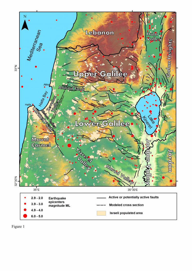
Figure 1

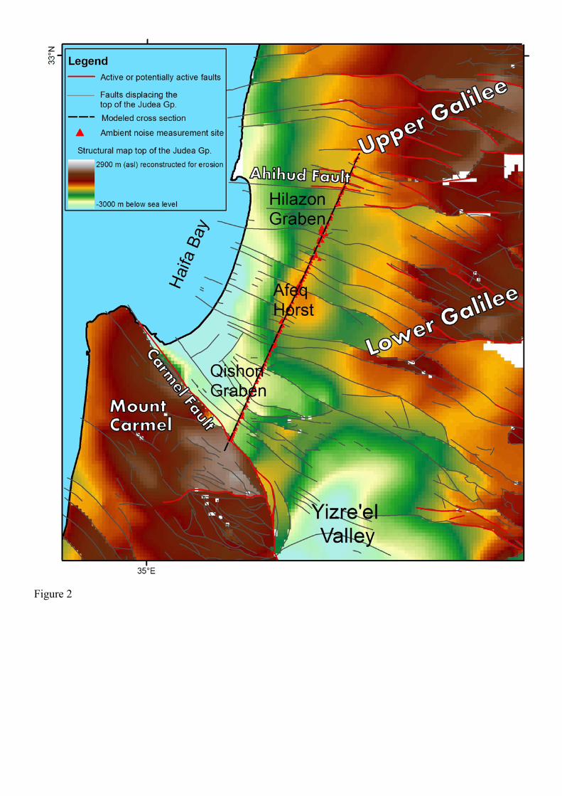
Figure 2

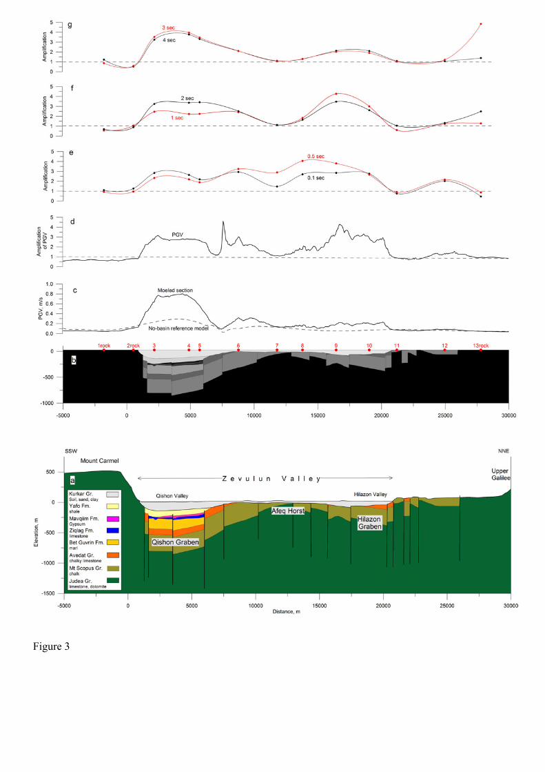
Figure 3

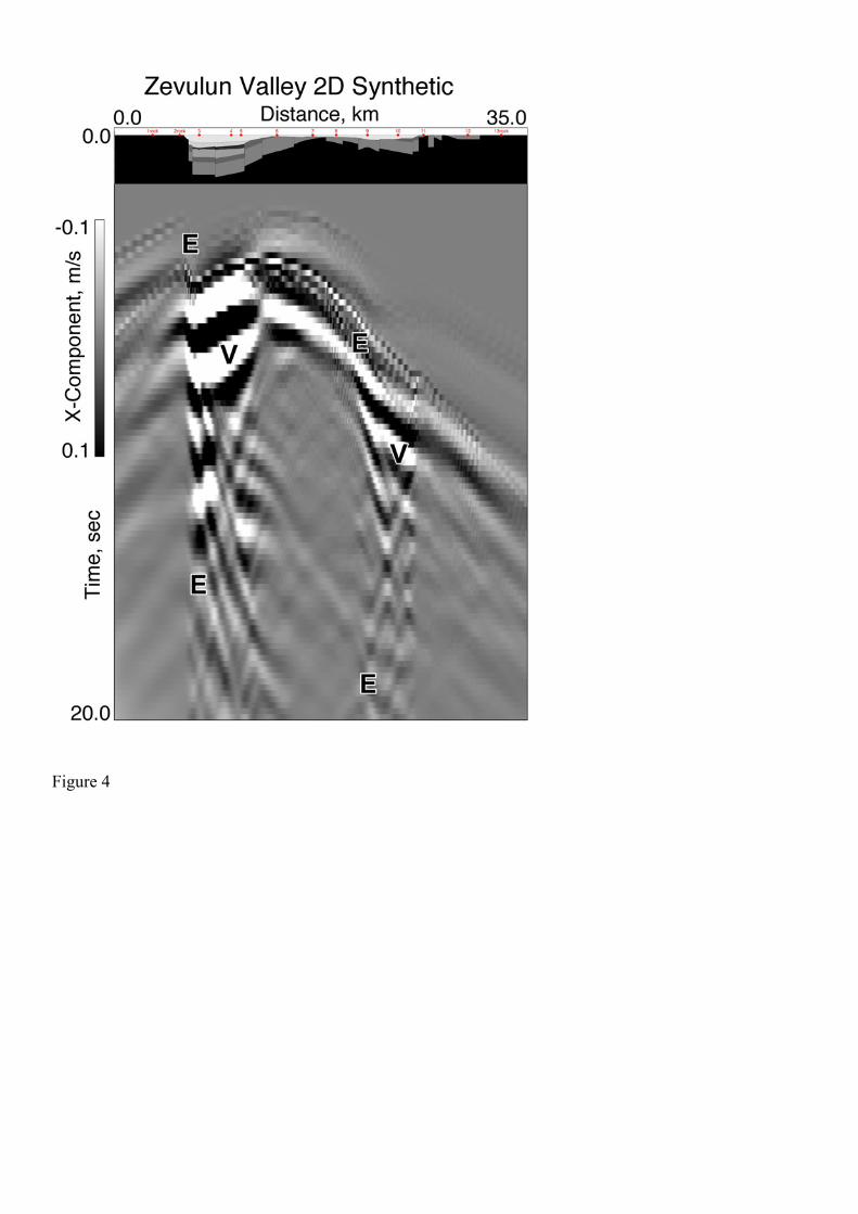
Figure 4

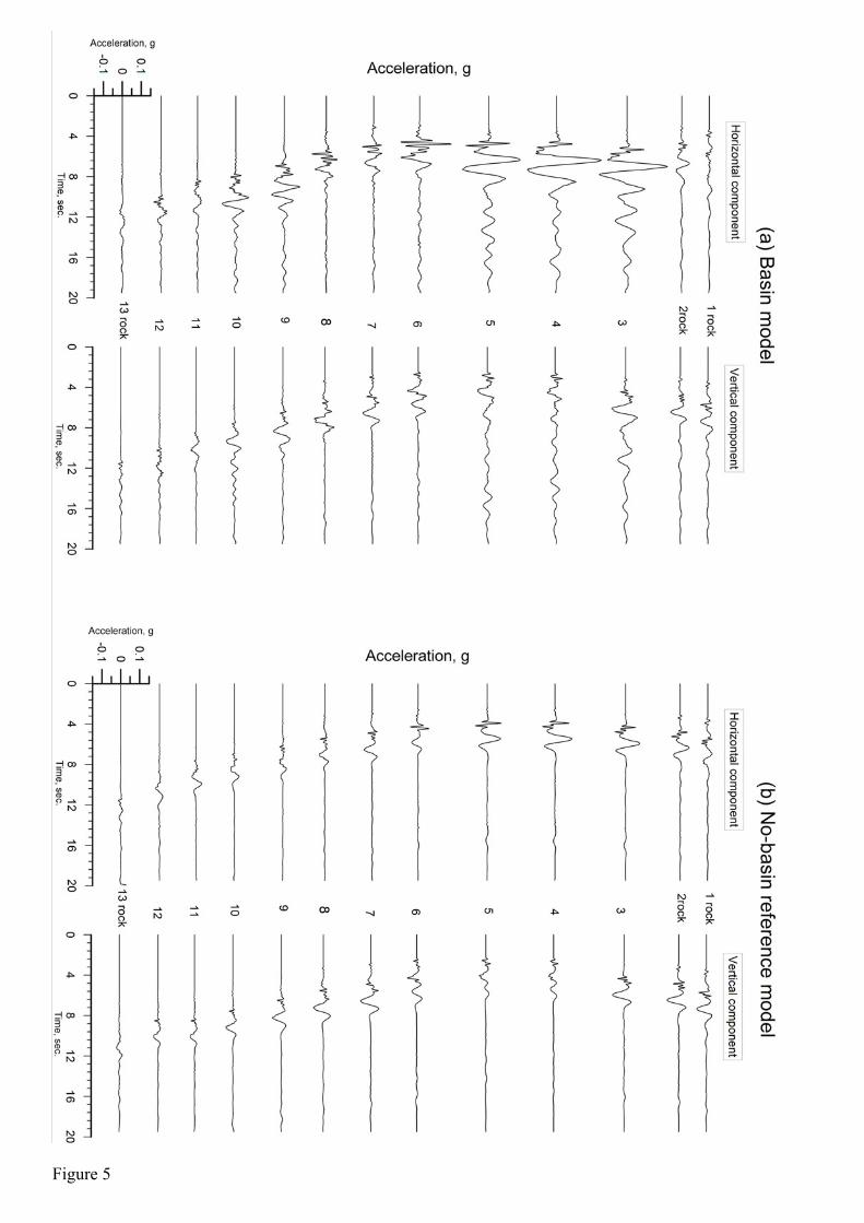
Figure 5

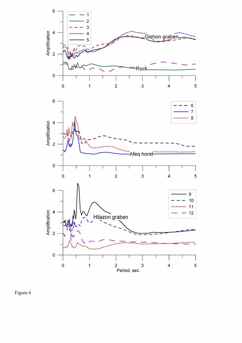
Figure 6

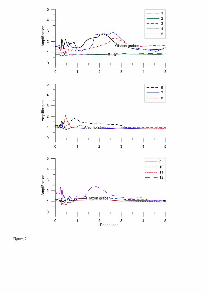
Figure 7

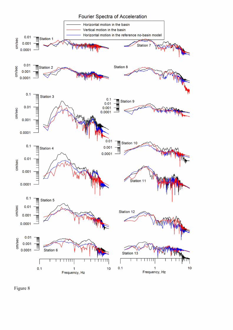
Figure 8

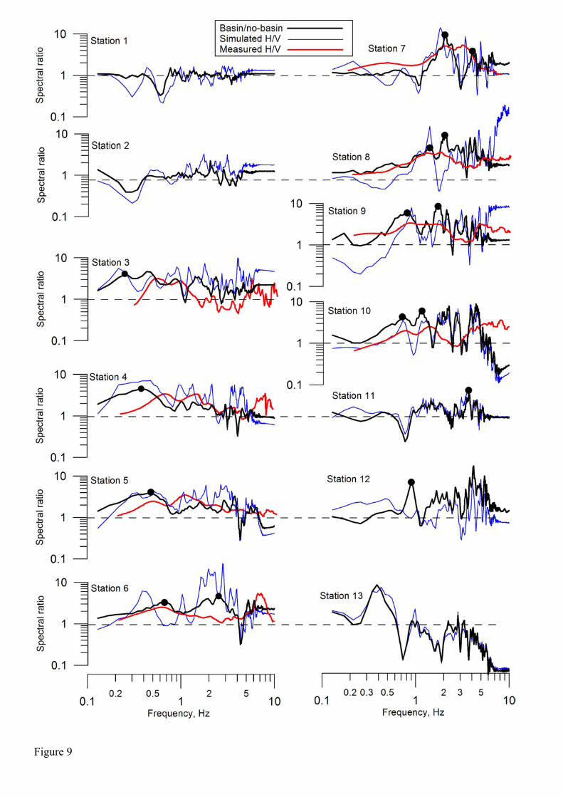
Figure 9

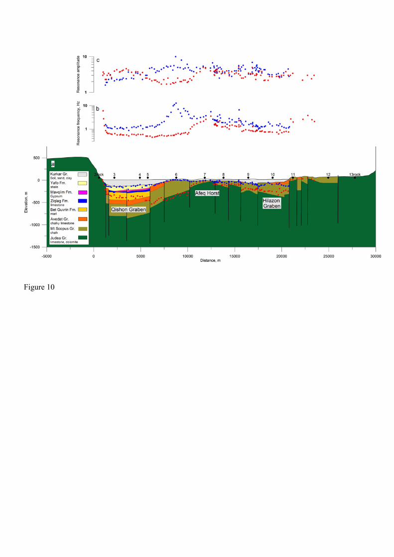
Figure 10

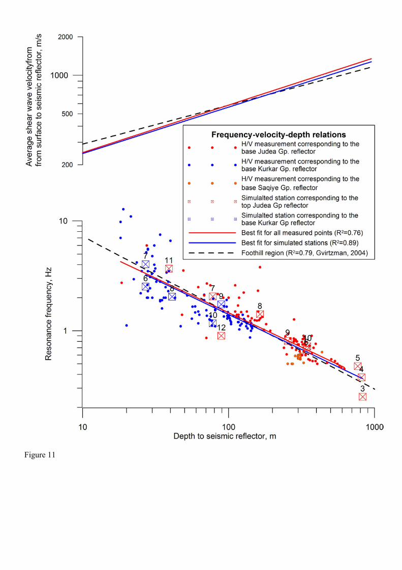
Figure 11

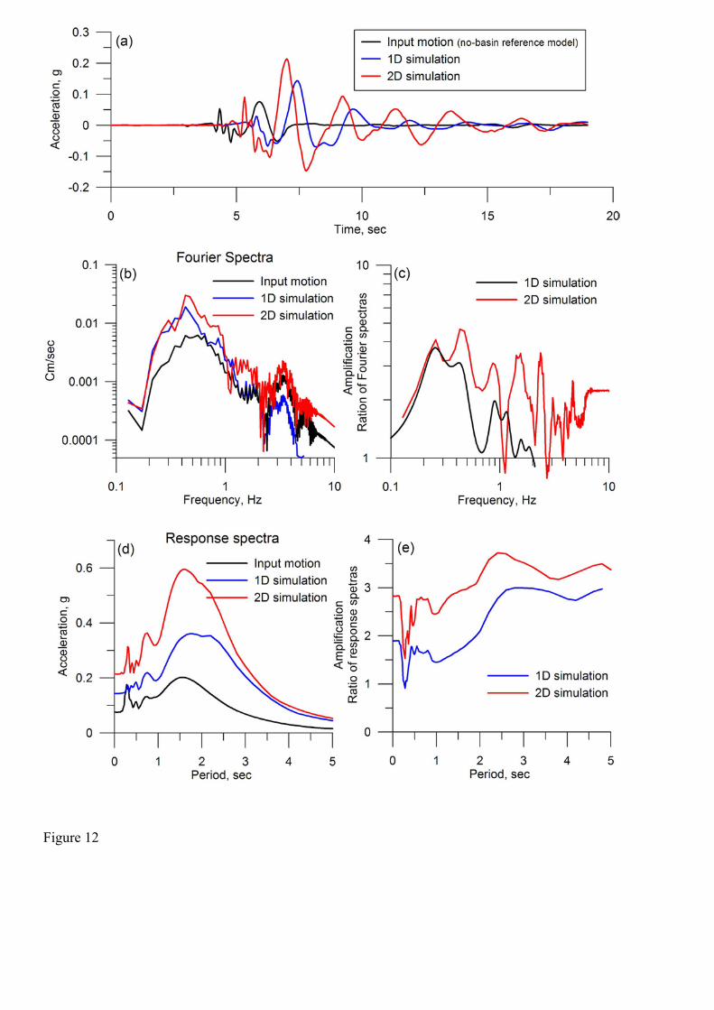
Figure 12

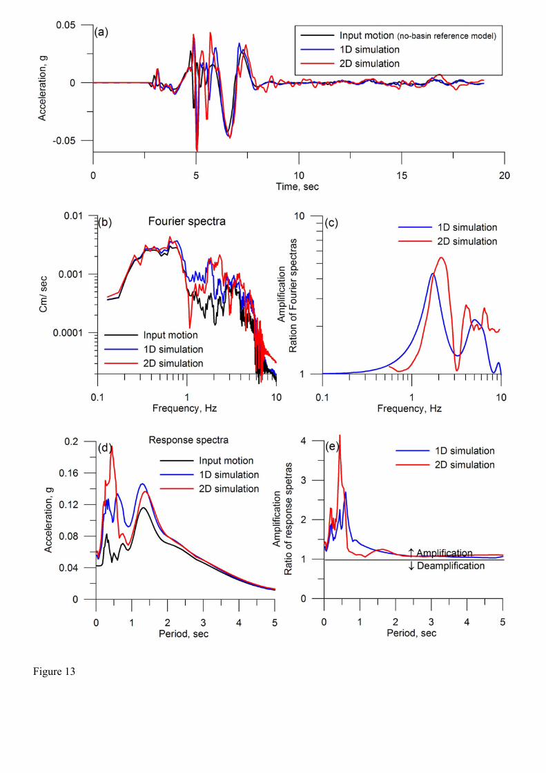
Figure 13

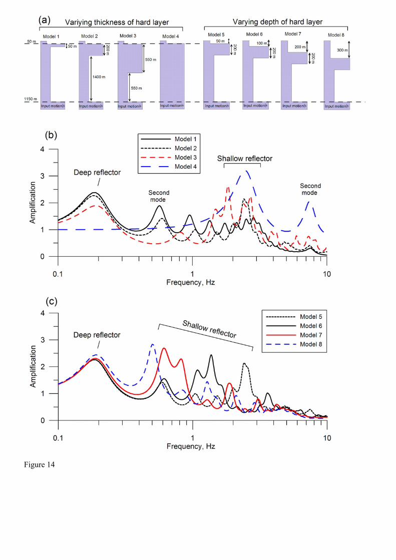
Figure 14