Simulation of Ground-Water Flow in the ... - CiteSeerX

Simulation of Ground-Water Flow in the Intermediate and Floridan Aquifer Systems in Peninsular Florida

U.S. GEOLOGICAL SURVEYWater-Resources Investigations Report

By Nicasio Sepúlveda

Tallahassee, Florida2002

Prepared in cooperation with the

South Florida Water Management DistrictSt. Johns River Water Management District

02-4009

Copies of this report can be purchased from:

U.S. Geological SurveyBranch of Information ServicesBox 25286Denver, CO 80225-0286888-ASK-USGS

The use of firm, trade, and brand names in this report is for identification purposes only and does not constitute endorsement by the U.S. Geological Survey.

For additional informationwrite to:

District ChiefU.S. Geological SurveySuite 3015227 N. Bronough StreetTallahassee, FL 32301

Additional information about water resources in Florida is available on the Internet at http://fl.water.usgs.gov

U.S. DEPARTMENT OF THE INTERIORGALE A. NORTON, Secretary

U.S. GEOLOGICAL SURVEYCHARLES G. GROAT, Director

CONTENTS

Abstract.................................................................................................................................................................................. 1Introduction ........................................................................................................................................................................... 2

Purpose and Scope....................................................................................................................................................... 4Previous Studies........................................................................................................................................................... 4Acknowledgments ....................................................................................................................................................... 4

Description of Study Area ..................................................................................................................................................... 6

Groups of Physiographic Regions ............................................................................................................................... 6Climate......................................................................................................................................................................... 6

Hydrogeologic Framework.................................................................................................................................................... 6Ground-Water Flow System .................................................................................................................................................. 15

Altitude of the Water Table of the Surficial Aquifer System ...................................................................................... 18Potentiometric Surface of the Intermediate Aquifer System....................................................................................... 22Potentiometric Surface of the Upper Floridan Aquifer ............................................................................................... 25Water-Level Measurements in the Lower Floridan Aquifer ........................................................................................ 27Chloride Concentrations in Ground Water .................................................................................................................. 27Recharge to and Discharge from the Upper Floridan Aquifer .................................................................................... 30

Water Use........................................................................................................................................................... 30Artificial Recharge from Drainage and Injection Wells .................................................................................... 34Spring Flow ....................................................................................................................................................... 35Recharge to the Unconfined Upper Floridan Aquifer ....................................................................................... 37Discharge to Swamps ........................................................................................................................................ 39

Simulation of Ground-Water Flow ........................................................................................................................................ 42Steady-State Approximation........................................................................................................................................ 42Conceptual Model........................................................................................................................................................ 46Boundary Conditions................................................................................................................................................... 55Recharge and Discharge .............................................................................................................................................. 57Initial Distribution of Hydraulic Properties from Local Models ................................................................................. 60Calibration of Ground-Water Flow Model .................................................................................................................. 67

Transmissivity of the Intermediate Aquifer System .......................................................................................... 70Transmissivity of the Upper Floridan Aquifer .................................................................................................. 70Transmissivity of the Lower Floridan Aquifer .................................................................................................. 71Leakance of the Upper Confining Unit of the Intermediate Aquifer System.................................................... 74Leakance of the Intermediate Confining Unit ................................................................................................... 75Leakance of the Middle Confining and Middle Semiconfining Units .............................................................. 77Recharge and Discharge Areas of the Upper Floridan Aquifer......................................................................... 77Spring Flow ....................................................................................................................................................... 86Potentiometric Surfaces ..................................................................................................................................... 91Ground-Water Flow Budget............................................................................................................................... 93Sensitivity Analyses........................................................................................................................................... 93

Effects of Projected 2020 Ground-Water Withdrawals ............................................................................................... 93Projected 2020 Ground-Water Withdrawals and Artificial Recharge................................................................ 97Simulated 2020 Scenarios and Boundary Conditions ....................................................................................... 99Projected 2020 Drawdowns ............................................................................................................................... 102Projected 2020 River and Spring Flow.............................................................................................................. 106Projected 2020 Ground-Water Flow Budget ..................................................................................................... 110

Model Limitations ................................................................................................................................................................. 110Summary and Conclusions .................................................................................................................................................... 112

Contents III

References ............................................................................................................................................................................. 113Appendixes............................................................................................................................................................................ 117

A1. Location and extent of simulated areas in the intermediate aquifer system or intermediate confining unit compiled from local ground-water flow models ..................................................................................... 118

A2. Location and extent of simulated areas in the Upper Floridan aquifer compiled from local ground-water flow models.............................................................................................................................. 120

A3. Location and extent of simulated areas in the Lower Floridan aquifer compiled from local ground-water flow models.............................................................................................................................. 122

B. Description of wells equipped with continuous water-level recorders........................................................... 123C. Description and flow measurements of Upper Floridan aquifer springs........................................................ 128

FIGURES

1-3. Maps showing:1. Location of study area and Water Management District boundaries.............................................................. 32. Groups of physiographic regions.................................................................................................................... 73. Measured rainfall at National Oceanic and Atmospheric Administration stations from August 1993

through July 1994 ........................................................................................................................................... 84. Diagram showing stratigraphic units, general lithology, and hydrogeologic units ................................................. 9

5-8. Maps showing:5. Generalized extent of the unconfined areas of the Upper Floridan aquifer, the intermediate aquifer

system, and thickness of the intermediate confining unit............................................................................... 116. Altitude of the top of the Upper Floridan aquifer........................................................................................... 127. Altitude of the base of the Upper Floridan aquifer......................................................................................... 138. Extent and areal configuration of the top of the Lower Floridan aquifer ....................................................... 14

9. Diagram showing generalized hydrogeologic sections A-A' and B-B' showing conceptualized ground-water flow ................................................................................................................................................... 16

10-11. Maps showing:10. Altitude of the base of the Floridan aquifer system ....................................................................................... 1711. Lakes, streams, locations of stream gaging stations, and surficial-aquifer wells used to estimate

the altitude of the water table of the surficial aquifer system......................................................................... 1912. Diagram showing relations among water table, minimum water table, and land-surface altitude ......................... 20

13-14. Graphs showing:13. Regressed and measured water-table altitudes for all groups of physiographic regions......................................... 2114. Correlation between water table, minimum water table, and difference between land-surface altitude

and minimum water table for group 4 and group 9 of physiographic regions ........................................................ 2215-23. Maps showing:

15. Estimated altitude of the water table of the surficial aquifer system, average conditions for August 1993 through July 1994 ..................................................................................................................... 23

16. Location of wells equipped with continuous water-level recorders ............................................................... 2417. Estimated potentiometric surface of the intermediate aquifer system, average conditions for

August 1993 through July 1994 ..................................................................................................................... 2618. Estimated potentiometric surface of the Upper Floridan aquifer, average conditions for

August 1993 through July 1994 ..................................................................................................................... 2819. Estimated altitude of water containing a chloride concentration of 5,000 milligrams per liter in the

Floridan aquifer system .................................................................................................................................. 2920. Distribution of recharge and discharge areas of the Upper Floridan aquifer, average conditions for

August 1993 through July 1994 ..................................................................................................................... 3121. Locations of Upper Floridan aquifer drainage and injection wells ................................................................ 3222. Locations of Upper Floridan aquifer springs.................................................................................................. 3623. Rivers in the unconfined areas of the Upper Floridan aquifer and locations of stream gaging stations ........ 38

24. Graphs showing approximation of base flow and surface runoff from daily recorded discharges at Suwannee River gaging stations 02319500, 02320500, and 02323500.................................................................. 40

IV Contents

25-27. Maps showing:25. Estimated minimum and maximum net recharge rates in the unconfined areas of the

Upper Floridan aquifer ................................................................................................................................... 4126. Areal extent of swamps in the unconfined areas of the Upper Floridan aquifer ............................................ 4227. Parts of the uniform grid used to develop the ground-water flow model, shown in the vicinity

Duval and Orange Counties............................................................................................................................ 4428. Hydrographs showing water-level fluctuations in wells tapping unconfined areas of the

Upper Floridan aquifer ............................................................................................................................................ 4529-36. Diagrams showing:

29. Layering scheme and representation of geologic units in local models 1 and 3, and corresponding layering scheme in the regional model ........................................................................................................... 47

30. Layering scheme and representation of geologic units in local models 2, 7, 10, and 13, and corresponding layering scheme in the regional model ................................................................................... 48



33. Layering scheme and representation of geologic units in local model 6, and corresponding layering scheme in the regional model ......................................................................................................................... 51



36. Layering scheme and representation of geologic units in local model 14, and corresponding layering scheme in the regional model ........................................................................................................... 54

37-46. Maps showing:37. Specified heads along the lateral boundary cells of the Upper Floridan aquifer............................................ 5638. Average ground-water withdrawal rates from the intermediate aquifer system, August 1993

through July 1994 ........................................................................................................................................... 5739. Average ground-water withdrawal rates from and injection rates to the Upper Floridan aquifer,

August 1993 through July 1994 ..................................................................................................................... 5840. Average ground-water withdrawal rates from the Lower Floridan aquifer, August 1993

through July 1994 ........................................................................................................................................... 5941. Cells where transmissivity of the intermediate aquifer system in some local models is either less

than one-half or greater than twice the geometric mean of all transmissivities for the same cell.................. 6142. Cells where transmissivity of the Upper Floridan aquifer in some local models is either less

than one-half or greater than twice the geometric mean of all transmissivities for the same cell.................. 6243. Cells where transmissivity of the Lower Floridan aquifer in some local models is either less

than one-half or greater than twice the geometric mean of all transmissivities for the same cell.................. 6344. Cells where leakance of the upper confining unit of the intermediate aquifer system in some

local models is not within one order of magnitude of the geometric mean of all leakances for the same cell ................................................................................................................................................... 64

45. Cells where leakance of the intermediate confining unit in some local models is not within one order of magnitude of the geometric mean of all leakances for the same cell ............................................... 65

46. Cells where leakance of the middle semiconfining unit in some local models is not within one order magnitude of the geometric mean of all leakances for the same cell ............................................................. 66

47-48. Graphs showing:47. Bilinear interpolation used to determine simulated water levels at observation wells from simulated

water levels at the center of cells............................................................................................................................. 6848. Comparison of simulated to measured water levels in the intermediate aquifer system, Upper

Floridan aquifer, and Lower Floridan aquifer for the calibrated model.................................................................. 6949-65. Maps showing:

49. Transmissivity of the intermediate aquifer system from the calibrated model............................................... 7150. Transmissivity of the Upper Floridan aquifer from the calibrated model ...................................................... 7251. Transmissivity of the Lower Floridan aquifer from the calibrated model...................................................... 73

Contents V

52. Leakance of the upper confining unit of the intermediate aquifer system from the calibrated model ........... 74

53. Simulated vertical leakage rates to and from the intermediate aquifer system through the upperconfining unit, average August 1993 through July 1994 conditions .............................................................. 75

54. Leakance of the intermediate confining unit and the lower confining unit of the intermediateaquifer system from the calibrated model ...................................................................................................... 76

55. Simulated vertical leakage rates to and from the Upper Floridan aquifer, average August 1993through July 1994 conditions ......................................................................................................................... 78

56. Leakance of the middle confining and middle semiconfining units from the calibrated model .................... 79

57. Simulated vertical leakage rates to and from the Lower Floridan aquifer through the middleconfining and middle semiconfining units, average August 1993 through July 1994 conditions.................. 80

58. Specified stages along the simulated river cells in the unconfined areas of the Upper Floridan aquifer,average August 1993 through July 1994 conditions....................................................................................... 81

59. Simulated riverbed conductance of river cells in the unconfined areas of the Upper Floridan aquifer ......... 82

60. Simulated lateral flow to and from the Upper Floridan aquifer across model boundaries,average August 1993 through July 1994 conditions....................................................................................... 84

61. Location of differences between simulated and estimated recharge and discharge cells in theUpper Floridan aquifer, average August 1993 through July 1994 conditions................................................ 85

62. Simulated recharge rates to the unconfined areas of the Upper Floridan aquifer, averageAugust 1993 through July 1994 conditions.................................................................................................... 86

63. Simulated potentiometric surface of the intermediate aquifer system, average August 1993through July 1994 conditions ......................................................................................................................... 91

64. Simulated potentiometric surface of the Upper Floridan aquifer, average August 1993 throughJuly 1994 conditions....................................................................................................................................... 92

65. Simulated potentiometric surface of the Lower Floridan aquifer, average August 1993 throughJuly 1994 conditions....................................................................................................................................... 94

66. Diagram showing simulated volumetric flow budget for the intermediate aquifer system, Upper Floridan aquifer, and Lower Floridan aquifer, average August 1993 through July 1994 conditions .................................... 95

67. Graphs showing model sensitivity to changes in selected model parameters ......................................................... 96

68-73. Maps showing:

68. Projected 2020 ground-water withdrawal rates from the intermediate aquifer system .................................. 99

69. Projected 2020 ground-water withdrawal rates from and injection rates to the Upper Floridan aquifer ....... 100

70. Projected 2020 ground-water withdrawal rates from the Lower Floridan aquifer ......................................... 101

71. Simulated intermediate aquifer system drawdowns from average August 1993 through July 1994conditions to projected 2020 conditions......................................................................................................... 103

72. Simulated Upper Floridan aquifer drawdowns from average August 1993 through July 1994conditions to projected 2020 conditions......................................................................................................... 104

73. Simulated Lower Floridan aquifer drawdowns from average August 1993 through July 1994conditions to projected 2020 conditions......................................................................................................... 105

74. Diagram showing simulated volumetric flow budget for the intermediate aquifer system, Upper Floridan aquifer, and Lower Floridan aquifer for projected 2020 conditions for the specified-flux boundary conditions ................................................................................................................................................ 111

VI Contents

TABLES

1. Description of ground-water flow models considered in the study area ................................................................ 52. Multiple linear regression coefficients for the minimum water table and the difference between

land-surface altitude and minimum water table...................................................................................................... 213. Multiple linear regression coefficients for September 1993 and May 1994 water-level averages in the

Upper Floridan aquifer for each group of physiographic regions .......................................................................... 264. Estimated ground-water withdrawals and uses, by county and by Water Management District, from

the intermediate aquifer system, Upper Floridan aquifer, and Lower Floridan aquifer, August 1993 through July 1994 ................................................................................................................................................... 33

5. Estimated discharge rates from free-flowing wells, by county, in the Upper Floridan aquifer in the St. Johns River Water Management District, August 1993 through July 1994 ...................................................... 34

6. Estimated recharge rates for drainage wells to the Upper Floridan aquifer, by county, August 1993 through July 1994 ................................................................................................................................................... 35

7. Surface-runoff rates calculated from hydrograph separation approximations applied to August 1993 through July 1994 daily discharge data obtained from stream gaging stations in the unconfined areas of the Upper Floridan aquifer ................................................................................................................................. 39

8. Geographical information system coordinates of the corners of the ground-water flow model grid..................... 439. Differences in water levels measured at wells tapping the unconfined areas of the Upper Floridan aquifer

and equipped with continuous water-level recorders.............................................................................................. 4610. Water-level residual statistics for the calibrated model .......................................................................................... 7011. Estimated and simulated base flow of rivers in the unconfined areas of the Upper Floridan aquifer,

average August 1993 through July 1994 conditions............................................................................................... 8312. Comparison of measured or estimated and residual flows from Upper Floridan aquifer springs,

average August 1993 through July 1994 conditions............................................................................................... 8713. Projected 2020 ground-water withdrawals and uses, by county and by Water Management District,

from the intermediate aquifer system, Upper Floridan aquifer, and Lower Floridan aquifer ................................ 9814. Projected 2020 recharge rates for drainage wells to the Upper Floridan aquifer by county .................................. 10215. Projected 2020 base flow of rivers in the unconfined areas of the Upper Floridan aquifer for

specified-flux boundary conditions ........................................................................................................................ 10616. Comparison of simulated 2020 and simulated August 1993 through July 1994 flow of

Upper Floridan aquifer springs for specified-flux boundary conditions ................................................................ 107

Contents VII

CONVERSION FACTORS AND VERTICAL DATUM

*Transmissivity: The standard unit for transmissivity is cubic foot per day per square foot times foot of aquifer thickness [(ft3/d)/ft2]ft. In this report, the mathematically reduced form, foot squared per day (ft2/d), is used for convenience.

Temperature in degrees Fahrenheit (°F) may be converted to degrees Celsius (°C) as follows:°C=(°F-32)/1.8

Sea level: In this report, “sea level” refers to the National Geodetic Vertical Datum of 1929 (NGVD of 1929)--a geodetic datumderived from a general adjustment of the first-order level nets of both the United States and Canada, formerly called Sea LevelDatum of 1929.

Horizontal coordinate information (latitude-longitude) is referenced to the North American Datum of 1927 (NAD27).

Multiply By To obtain

Length

inch (in.) 2.54 centimeterfoot (ft) 0.3048 meter

mile (mi) 1.609 kilometer

Areaacre 0.4047 hectare

square mile (mi2) 2.590 square kilometer

Flow Rate

cubic foot per second (ft3/s) 0.02832 cubic meter per second million gallons per day (Mgal/d) 0.04381 cubic meter per second

inch per year (in/yr) 25.4 millimeter per yearHydraulic Conductivity

foot per day (ft/d) 0.3048 meter per day*Transmissivity

foot squared per day (ft2/d) 0.09290 meter squared per day Leakance

foot per day per foot [(ft/d)/ft] 1.0 meter per day per meter

Acronyms and additional abbreviations used in report:DEM digital elevation modelFPZ Fernandina permeable zone

FDEP Florida Department of Environmental ProtectionFAS Floridan aquifer systemIAS intermediate aquifer system ICU intermediate confining unitLFA Lower Floridan aquifer

MCU middle confining unitMSCU middle semiconfining unit

mg/L milligrams per literMODFLOW U.S. Geological Survey Modular Three-Dimensional Ground-Water Flow Model

NOAA National Oceanic and Atmospheric AdministrationROMP Regional Observation and Monitoring Well Program

RMS root mean squareSJRWMD St. Johns River Water Management DistrictSFWMD South Florida Water Management District

SWFWMD Southwest Florida Water Management DistrictSR surface runoff

SAS surficial aquifer systemSRWMD Suwannee River Water Management District

UFA Upper Floridan aquifer USGS U.S. Geological SurveyUTM Universal Transverse Mercator

VIII Contents

Simulation of Ground-Water Flow in the Intermediate and Floridan Aquifer Systems in Peninsular FloridaBy Nicasio Sepúlveda

estimating hydraulic properties for different areas.
Abstract
A numerical model of the intermediate and Floridan aquifer systems in peninsular Florida was used to (1) test and refine the conceptual under-standing of the regional ground-water flow sys-tem; (2) develop a data base to support subregional ground-water flow modeling; and (3) evaluate effects of projected 2020 ground-water withdraw-als on ground-water levels. The four-layer model was based on the computer code MODFLOW-96, developed by the U.S. Geological Survey. The top layer consists of specified-head cells simulating the surficial aquifer system as a source-sink layer. The second layer simulates the intermediate aqui-fer system in southwest Florida and the intermedi-ate confining unit where it is present. The third and fourth layers simulate the Upper and Lower Flori-dan aquifers, respectively. Steady-state ground-water flow conditions were approximated for time-averaged hydrologic conditions from August 1993 through July 1994 (1993-94). This period was selected based on data from Upper Floridan aquifer wells equipped with continuous water-level recorders. The grid used for the ground-water flow model was uniform and composed of square 5,000-foot cells, with 210 columns and 300 rows.

The active model area, which encompasses about 40,800 square miles in peninsular Florida, includes areas of various physiographic regions classified according to natural features. Hydrogeo-logic conditions vary among physiographic regions, requiring different approaches to

The altitudes of water levels for the surficial aqui-fer system and heads in the Upper Floridan aqui-fer, for time-averaged 1993-94 conditions, were computed by using a multiple linear regression of measured water levels in each of the physiographic regions.

Ground-water flow simulation was limited vertically to depths containing water with chloride concentrations less than 5,000 milligrams per liter. Water-level altitudes in the Floridan aquifer sys-tem beneath which chloride concentrations exceed 5,000 milligrams per liter were estimated from previously developed maps and analytical results of ground-water samples. Flow across the inter-face represented by this chloride concentration was assumed to be negligible.

The ground-water flow model was cali-brated using time-averaged data for 1993-94 at 1,624 control points, flow measurements or esti-mates at 156 springs in the study area, and base-flow estimates of rivers in the unconfined areas of the Upper Floridan aquifer obtained by using a generalized hydrograph separation of recorded discharge data. Transmissivity of the intermediate aquifer system, Upper Floridan aquifer, and Lower Floridan aquifer; leakance of the upper and lower confining units of the intermediate aquifer system, the intermediate confining unit, the middle confin-ing unit, and the middle semiconfining unit; spring and riverbed conductances; and net recharge rates to unconfined areas of the Upper Floridan aquifer were adjusted until a reasonable fit was obtained.

Abstract 1

Root-mean-square residuals between computed and simulated heads in the intermediate aquifer system, Upper Floridan aquifer, and Lower Flori-dan aquifer were 3.47, 3.41, and 2.89 feet, respec-tively. The overall root-mean-square residual was 3.40 feet. Simulated spring flow was 96 percent of the total measured (or estimated) spring flow in the study area.

Simulations were made to project water-level declines from 1993-94 to 2020 conditions. The calibrated flow model was used to simulate the potentiometric surfaces of the intermediate aquifer system, Upper Floridan aquifer, and Lower Floridan aquifer for 2020 using water-use projec-tions provided by the Water Supply Assessment plans of the State Water Management Districts. Water-use projections for 2020 were based on esti-mated population growth and 1995 withdrawals. Heads in the Upper Floridan aquifer under pro-jected 2020 water-use stresses were simulated for two scenarios: (1) assigning interpolated 1993-94 heads along the lateral boundaries of the Upper Floridan aquifer; and (2) assigning 1993-94 simu-lated flux rates across the same boundaries.

Projected 2020 ground-water withdrawals for municipal, industrial, commercial, agricul-tural, and self-supplied domestic uses was approx-imately 3,400 million gallons per day, an increase of about 36 percent from 1993-94. The largest pro-jected drawdown in the potentiometric surface of the Upper Floridan aquifer, for both scenarios, was simulated in Orange County, with a drawdown of 10 feet in the central part of the County. Projected drawdowns of 6 feet were simulated in parts of Duval and Polk Counties.

INTRODUCTION

The intermediate and Floridan aquifer systems are the principal sources of water supply in much of peninsular Florida. As the population of the State continues to grow, the demand for water continues to increase. In some areas of Florida, decreasing water levels and increasing mineralization of ground water have become problems for local and state water-man-agement officials. Ground-water flow models are important tools for assessing the effects of present and

2 Simulation of Ground-Water Flow in the Intermediate and Flo

future ground-water development. For this reason, a number of ground-water flow models have been devel-oped for areas within peninsular Florida; however, these areally extensive models are of a relatively coarse resolution. In addition, because Florida comprises sev-eral Water Management Districts, most ground-water modeling efforts have been focused within the bound-aries of individual Districts, thus reducing the potential to simulate inter-District ground-water flow under current and projected stresses. This is particularly true along the common boundaries of the St. Johns River Water Management District (SJRWMD), Southwest Florida Water Management District (SWFWMD), South Florida Water Management District (SFWMD), and the Suwannee River Water Management District (SRWMD). Present and projected development of the ground-water resources in these Districts require reli-able estimates of inter-District ground-water flow. As a result, the U.S. Geological Survey (USGS) began a 5-year project in 1996 in cooperation with SJRWMD and SFWMD to develop a fine-resolution, areally extensive ground-water flow model of the intermediate and Floridan aquifer systems extending from Camden and Charlton Counties, Georgia, to just south of Martin County in south Florida (fig. 1).

The objective of developing such a model is to refine the conceptual understanding of regional ground-water flow in the intermediate aquifer system and the Floridan aquifer system. The data base of hydraulic properties resulting from the model could be used as input to an interpolation algorithm that extracts specific hydraulic properties and data to obtain appro-priate general-head boundaries, specified fluxes, or ini-tial estimates of hydraulic properties needed to develop fine-resolution ground-water flow studies on smaller scales. Leake and Claar (1999) developed computer programs to generate input files for a local model of finer resolution from the input files of a regional model of coarser resolution.

Hydrologic conditions reflected by the time average from August 1993 to July 1994 (1993-94) potentiometric-surface maps, ground-water withdraw-als, and water-level and spring flow measurements con-stitute the steady-state approximation referenced in this report. The rationale for selecting the 1993-94 period is explained later in the report.

ridan Aquifer Systems in Peninsular Florida

Figure 1. Location of study area and Water Management District boundaries.

Introduction 3

Purpose and Scope

This report presents the results of a numerical model used to simulate the regional ground-water flow system in peninsular Florida. The model was used to (1) refine the conceptual understanding of the interme-diate aquifer system and the Floridan aquifer system; (2) develop a data base to support subregional ground-water flow modeling; and (3) evaluate relative effects of 2020 ground-water withdrawals on ground-water levels for which the model was constructed. Hydrogeo-logic data are presented, including a conceptual model of the flow system and applications of a finite-differ-ence flow model based on this conceptualization. The flow model simulations are designed to characterize the complex four layer aquifer system that underlies the study area. Discussions in this report include modeling procedures, imposition of boundary conditions, cali-bration strategies, rationale for a steady-state assump-tion, sensitivity analyses, volumetric flow estimates among hydrogeologic units, and specific areas where substantial water-level declines could occur based on 2020 projected ground-water withdrawals.

Geographical information system data bases or coverages (Environmental Systems Research Institute, Inc., 1997) were developed to manage spatially distrib-uted information of hypsography and hydrography that covered the study area. Digital coverages were pro-jected into the same coordinate system to achieve con-sistency of coordinate systems among coverages. The coordinate system of all coverages was the Universal Transverse Mercator (UTM) projection, zone 17 of the Florida coordinate system, west zone (Snyder, 1983). The 1927 North American Datum was used for all coverages generated in this study; the unit length was feet (ft).

Multiple linear regressions were used to generate the altitude of the water table of the surficial aquifer system, and the time-averaged heads in the intermedi-ate aquifer system and the Floridan aquifer system, which comprises the Upper Floridan aquifer and the Lower Floridan aquifer. The regressions applied to the surficial aquifer system allowed for the estimation of the altitude of the water table at any point in the study area. The regressions applied to the intermediate aqui-fer system and the Upper Floridan aquifer allowed for the generation of the potentiometric surfaces of these two aquifers.

4 Simulation of Ground-Water Flow in the Intermediate and Fl

Previous Studies

Numerous investigations of ground-water flow in the intermediate aquifer system and the Floridan aquifer system in peninsular Florida have been con-ducted. Fourteen flow models, developed from these investigations, provided initial estimates of the areal distribution of hydraulic properties for the regional model discussed in this report (table 1). The extent of those flow models encompasses a large part of the study area (appendix A). Conceptualizations of the ground-water flow system differed among the various models.

The surficial aquifer system was simulated as a constant-head source-sink bed in 12 of the 14 ground-water flow models listed in table 1. Models developed by Hancock and Basso (1993) and Yobbi (1996) simu-lated the surficial aquifer system as an active layer, and calibrated to water levels measured at wells tapping the surficial aquifer, stream stages, and lake elevations.

Flow in parts of the intermediate aquifer system was simulated in southwest Florida (appendix A1) by Ryder (1985), Barcelo and Basso (1993), Metz (1995), and Yobbi (1996), and in parts of north-central Florida by Groszos and others (1992). The simulated transmis-sivity value for the intermediate aquifer system in north-central Florida was characteristic of a low-per-meability confining unit (Motz, 1995). In this study, the intermediate aquifer system in north-central Florida is simulated as part of the intermediate confining unit.

Ground-water flow in the Upper Floridan aquifer was simulated by models developed in all of the studies listed in table 1 (appendix A2). The Upper Floridan aquifer is the most developed aquifer in the study area (Ryder, 1985; Tibbals, 1990). Simulation of ground-water flow in the Lower Floridan aquifer (appendix A3) was limited because of a substantially smaller number of observation wells tapping the Lower Floridan aquifer.

Acknowledgments

The author would like to thank the SFWMD, SJRWMD, and SWFWMD for providing the water-use, water-quality, and ground-water flow model data bases used in this study. The author also wants to thank Ronald Ceryak of SRWMD for providing information on hydraulic properties of aquifers in the SRWMD area.

oridan Aquifer Systems in Peninsular Florida

Table 1. Description of ground-water flow models considered in the study area[Abbreviations used in layering description: SAS, surficial aquifer system; IAS, intermediate aquifer system; UFA, Upper Floridan aquifer; LFA, Lower Floridan aquifer; SH, specified head; UT, uniform transmissivity; FPZ, Fernandina Permeable Zone]

Modelnumber

Authors(year) General location

Number ofGrid type Layering

descriptionrows columns

1 Grubb and Rutledge (1979)

Parts of Polk, Lake, Sumter, Hernando, and Pasco Counties

36 40 Uniform cell size of 5,400 by 6,075 feet

SAS, layer 1, SHUFA, layer 2

2 Ryder (1985)

West-central Florida 49 32 Uniform cell size of 4 miles by 4 miles

SAS, layer 3, SHIAS, layer 2UFA, layer 1

3 Fretwell (1988)

Pasco County 38 54 Uniform cell size of 1 square mile

SAS, layer 1, SHUFA, layer 2

4 Yobbi (1989)

Citrus and Hernando Counties

22 18 Uniform cell size of 2 miles by 2 miles

UFA, one-layer model

5 Tibbals (1990)

East-central Florida 50 24 Uniform cell size of 4 miles by 4 miles

SAS, layer 3, SHUFA, layer 2LFA, layer 1

6 Lukasiewicz (1992)

Martin and St. Lucie Counties

54 53 Uniform cell size of 1 square mile

SAS, layer 1, SHUFA, layer 2LFA, layer 3LFA, layer 4, SH

7 Barcelo and Basso (1993)

Southwest Florida 56 60 Uniform cell size of 2 miles by 2 miles


8 Blanford and Birdie (1993)

Hernando County 33 43 Uniform cell size of 1 square mile

UFA, one-layer model

9 Hancock and Basso (1993)

Parts of Hernando, Pasco, Hillsborough, and Pinellas Counties

62 69 Variable cell size, ranging from 2,640 by 2,640 feet to 1 square mile

SAS, layer 1UFA, layer 2UFA, layer 3

10 Metz (1995)

Hardee and DeSoto Counties



11 Motz (1995)

North-central Florida 53 54 Variable cell size, ranging from 5,000 by 5,000 feet to 15,000 by 20,000 feet

SAS, layer 1, SHIAS, layer 2, UTUFA, layer 3LFA, layer 4FPZ, layer 5

12 Murray and Halford (1996)

Orange, Seminole, and parts of Volusia, Lake, and Osceola Counties


SAS, layer 1, SHUFA, layer 2LFA, layer 3

13 Yobbi (1996)

Parts of Polk, Osceola, Hardee, De Soto, High-lands, and Glades Counties

86 41 Uniform cell size of 1 square mile

SAS, layer 1IAS, layer 2UFA, layer 3

14 Durden (1997)

Northeast Florida 68 35 Variable cell size, ranging from 5,222 by 6,057 feet to 18,280 by 23,499 feet

SAS, layer 1, SHUFA, layer 2LFA, layer 3FPZ, layer 4

Introduction 5

DESCRIPTION OF STUDY AREA

The study area (fig. 1) extends about 284 miles (mi) from Charlton and Camden Counties, Georgia, in the north to near the Palm Beach - Martin County line in south Florida. The west-to-east extent of the study area spans about 200 mi from the Gulf of Mexico to the Atlantic Ocean. The study area encompassed about 40,800 square miles (mi2). Some offshore areas in northeast and southwest Florida are considered to be part of the study area because hydraulic data suggest these areas may affect ground-water flow in the Upper Floridan aquifer.

The land-surface altitude in the study area ranges from sea level to about 285 ft in an area in south-central Polk County. About 75 percent of the land surface in the study area has an altitude less than 100 ft, and about 40 percent has an altitude less than 50 ft.

Groups of Physiographic Regions

The study area is subdivided into 52 distinct physiographic regions (White, 1970). Although the main physiographic regions of the study area generally correspond to distinct hydrogeologic regions, the delin-eation of physiographic features in an area of low relief, such as Florida, can be difficult. The delineations of physiographic regions by White (1970), therefore, were based on a combination of natural features, rather than on single elevation contours. The 52 physiographic regions delineated by White (1970) were grouped into 10 generalized regions based on geomorphology and the correlation of water levels between physiographic regions (fig. 2). Not all regions are contiguous.

Climate

The climate of the study area is classified as subtropical and is characterized by warm, normally wet summers and mild, dry winters. Maximum temper-atures usually exceed 90 °F during the summer, but may fall below freezing for several days in the winter in the northern and central parts of the study area (fig. 1). The 30-year average (1961-90) annual rainfall for the study area, computed from rainfall data col-lected from National Oceanic and Atmospheric Administration (NOAA) stations, is 51.20 inches per year (in/yr). Measured rainfall at 53 NOAA stations in the study area averaged 53.23 inches (in.) from August 1993 to July 1994 (fig. 3), which was 4 percent higher than the 30-year average. Absolute differences between rainfall measured in 1993-94 and the long-term average

6 Simulation of Ground-Water Flow in the Intermediate and Flo

(1961-90) at individual stations were less than 10 in. at all but five stations.

HYDROGEOLOGIC FRAMEWORK

Comprehensive descriptions of the hydrogeol-ogy in all or in parts of the study area were presented by Ryder (1985), Miller (1986), Meyer (1989), Sprin-kle (1989), Tibbals (1990), and Arthur and others (2001). This report presents a brief description of the hydrogeologic framework of the Floridan Aquifer system (FAS) and underlying and overlying units, including areal variations in thickness and occur-rence throughout Florida.

The surficial aquifer system (SAS), which is the uppermost water-bearing hydrogeologic unit, includes sediments of Holocene, Pleistocene, and Pliocene ages (fig. 4). The SAS mostly consists of variable amounts of sand, sandy clay, shell beds, silt, and clay. Limestone units within the SAS are primarily in southwest Flor-ida. In coastal areas, the SAS consists of cemented shell and shelly marl. The SAS extends throughout most of the study area, except where the Upper Flori-dan aquifer (UFA) is unconfined, and is used for water supply only in coastal areas where the UFA contains brackish water. The SAS is used primarily for individ-ual household water supply in areas where the interme-diate aquifer system (IAS) and the FAS are deep or contain poor quality water. In some places the clays in the SAS are thick and continuous enough to divide the SAS into two or three separate layers, but generally the aquifer system is undivided. In most parts of central, east, and northeast Florida, the SAS either provides recharge or receives discharge from the UFA.

Carbonate rocks of Miocene age within the inter-mediate confining unit (ICU) in southwest Florida are permeable enough to form a productive aquifer, the IAS. The IAS underlies the SAS and extends through-out most of southwest Florida. The unit consists mainly of clastic sediments interbedded with carbonate rocks that generally coincide with the Hawthorn Group (fig. 4). Although the IAS is less permeable than the underlying UFA, the carbonate rock units within the IAS are sufficiently permeable and productive to con-stitute a water-supply source. Confining beds that over-lie the UFA and underlie the SAS limit the vertical extent of the IAS in west-central Florida. The thickness of the IAS varies from about 25 ft in parts of Hillsbor-ough and Polk Counties to about 400 ft in Charlotte County (Ryder, 1985). The thickness generally increases north to south (Ryder, 1985).

ridan Aquifer Systems in Peninsular Florida

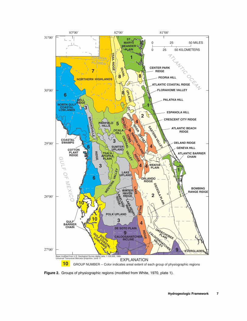
Figure 2. Groups of physiographic regions (modified from White, 1970, plate 1).

Hydrogeologic Framework 7

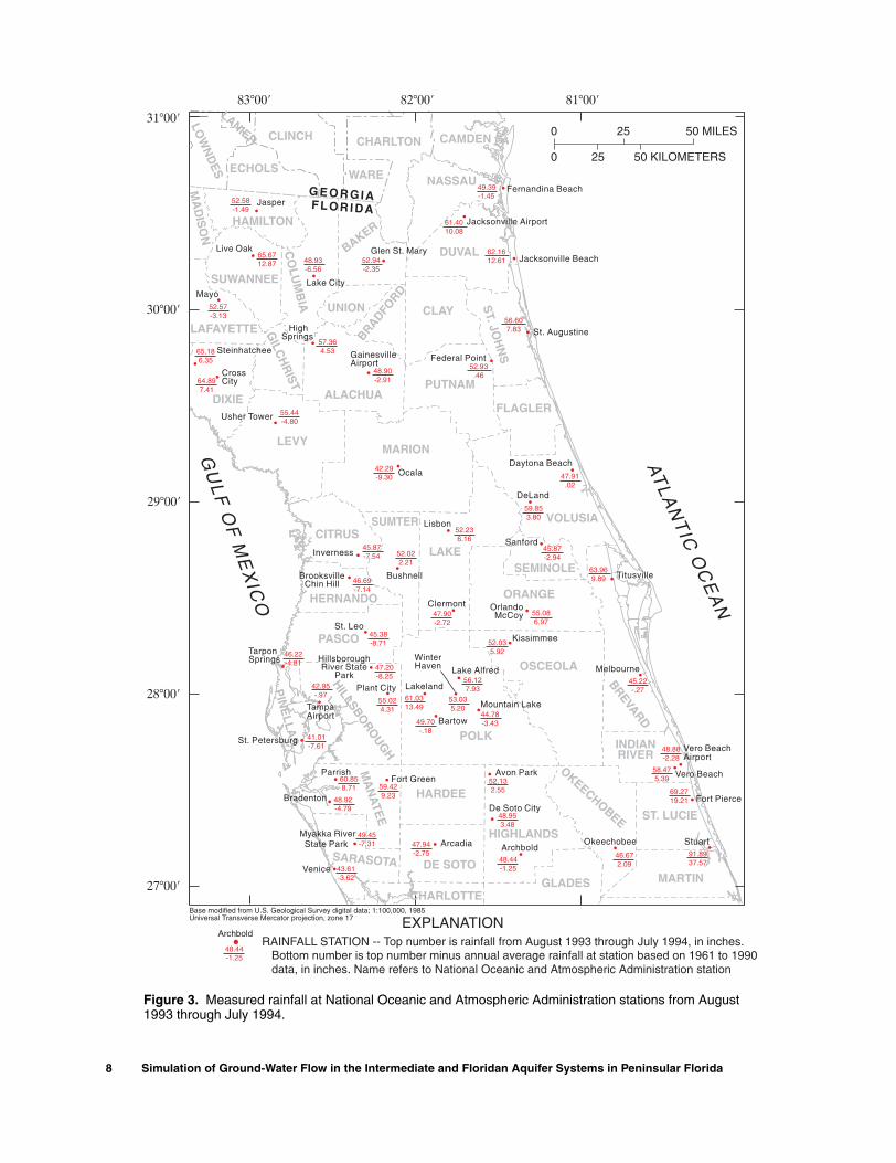
Figure 3. Measured rainfall at National Oceanic and Atmospheric Administration stations from August 1993 through July 1994.

8 Simulation of Ground-Water Flow in the Intermediate and Floridan Aquifer Systems in Peninsular Florida

Figure 4. Stratigraphic units, general lithology, and hydrogeologic units.


In areas away from southwest Florida, beds of clay and carbonate rocks of Pliocene and Miocene ages form the ICU. The hydrogeologic units, ICU and IAS, within the Hawthorn Group (fig. 4) are differentiated based on the permeability of the rock. In contrast to the IAS, the ICU is considerably less permeable. The ICU and the IAS coalesce at the boundaries of the IAS. The map showing the estimated thickness of the ICU generated by Miller (1986) was highly regionalized and based on sparse data. The more localized maps of Planert and Aucott (1985), Lukasiewicz (1992), and Spechler (1995) were used to modify Miller’s (1986) map of the ICU thickness in southwest, east-central, south, and northeast Florida, respectively. The resulting map shows that thickness varies from 0 ft in the north-west part of the study area (fig. 5) to about 750 ft in the southeast. The UFA is considered to be unconfined in areas where the ICU is absent or very thin, including areas along the Withlacoochee River in west-central Florida and along parts of the Hillsborough River. The thickness of the ICU within the areal extent of the IAS represents the cumulative thickness of the IAS and overlying and underlying confining beds of the IAS (fig. 5). The seaward extent of the IAS coincides with those areas where the transmissivity was simulated to be higher than 100 feet squared per day (ft2/d) by Barcelo and Basso (1993).

A thick sequence of limestone and dolomitic limestone of Oligocene and Eocene ages and having variable permeability forms the FAS. The FAS is the principal source of ground water in the study area. The aquifer system ranges in thickness from about 1,300 ft in the northwest part of the study area to about 3,500 ft in southwest Florida (Miller, 1986). The FAS is divided into two aquifers of relatively high permeability, referred to as the UFA and the Lower Floridan aquifer (LFA). These aquifers are separated by a less permeable unit called the middle confining unit (MCU) in west-central Florida and in the northwest part of the study area, and the middle semiconfining unit (MSCU) in east-central Florida. The altitude of the top of the UFA, defined as the first occurrence of vertically persistent, permeable, con-solidated carbonate rocks, ranges from 100 ft above to 850 ft below sea level (fig. 6). The top of the UFA coin-cides either with the top of the Suwannee Limestone or the top of the Ocala Limestone, depending on location (fig. 4). The map in figure 6 showing the altitude of the top of the UFA, as identified by Miller (1986), was refined using the results of more localized studies by Knochenmus and Hughes (1976), Buono and Rutledge (1979), Shaw and Trost (1984), Planert and Aucott (1985), Navoy and Bradner (1987), Schiner and others (1988), Phelps (1990), Lukasiewicz (1992), Spechler (1993, plate 1), and Bradner (1994).

10 Simulation of Ground-Water Flow in the Intermediate and F

Lithologic data that establish the base of the UFA are less numerous than data defining the top of the UFA. A generalized contour map of the base of the UFA (fig. 7) was revised from Miller (1986) using additional information from Tibbals (1990) and files of the SJRWMD (Brian McGurk, SJRWMD, written com-mun., 1997). The base of the UFA ranges in depth from about 250 ft below sea level in parts of Marion and Sumter Counties to 2,100 ft below sea level in Charlton County, Ga., and in Charlotte County, Fla. (fig. 7). The base of the UFA is marked by the top of either the MCU, denoted analogously to Miller’s (1986) notation by units II, III, and IV in west-central Florida and the northwest part of the study area, or the top of the MSCU, denoted by unit I in east-central Florida.

Rather than a single low-permeability unit sepa-rating the UFA and the LFA, several units of regional extent separate the UFA from the LFA (figs. 7 and 8). Common boundaries of the MCU and MSCU delineate the approximate updip limit of the Lower Floridan aquifer (fig. 8). Any of these regionally extensive low-permeability units may contain thin layers of moderate to high permeability. These confining units are not con-tinuous and do not necessarily consist of the same rock type everywhere.

In east-central Florida, the UFA and LFA are separated by the MSCU, a sequence of somewhat permeable, soft, chalky limestone that locally contains some gypsum and chert and commonly is partially dolomitized (fig. 4). Although the MSCU, zone I in fig-ure 7, is considered to be the leakiest of all confining units in the study area (Miller, 1986), the hydraulic connection between the MSCU and the LFA varies from place to place. This semiconfining unit is thin or absent in the northwest part of the study area (fig. 8), but is as much as 600 to 800 ft thick in the south-central part of the study area (Tibbals, 1990).

In west-central Florida and in the northwest part of the study area, the UFA and LFA are separated by the MCU, which is composed of gypsiferous dolomite and dolomitic limestone of considerably lower permeabil-ity than that of the MSCU in east-central Florida (Miller, 1986). The MCU, zones II through IV in figure 7, limits the movement of ground water between the UFA and LFA. At some locations, the confining unit is a very fine-grained limestone; in other places the MCU is a dolomite with pore spaces filled with anhy-drite. The presence of intergranular evaporites in the MCU suggests that the exchange of vertical fluxes between the UFA and LFA could be higher in east-cen-tral Florida than in west-central Florida. The UFA and LFA merge vertically into one aquifer where no MCU or MSCU is present (fig. 8).

loridan Aquifer Systems in Peninsular Florida

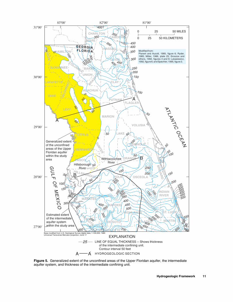
Figure 5. Generalized extent of the unconfined areas of the Upper Floridan aquifer, the intermediate aquifer system, and thickness of the intermediate confining unit.


Figure 6. Altitude of the top of the Upper Floridan aquifer.


Figure 7. Altitude of the base of the Upper Floridan aquifer.


Figure 8. Extent and areal configuration of the top of the Lower Floridan aquifer.


A discontinuity in the surface of the MCU can be seen along section in figure 9. Although it is not certain whether the MCU in southwest Florida and the MSCU in east-central Florida merge, the information shown in section does not preclude this possibility (fig. 9). Given the contrast in permeability between the MCU and the MSCU, ground-water exchange between the UFA and LFA could be quite variable in areas near this discontinuity (fig. 9). For example, exchange of ground water between the UFA and LFA probably is higher in east-central Florida than in southwest Florida because the permeability of the MSCU is higher than the permeability of the MCU.

The altitude of the top of the LFA ranges from -400 ft in Marion County to -2,500 ft along the Gulf Coast near Sarasota County (Miller, 1986; fig. 8). Discontinuities in the configuration of the top of the LFA are due to discontinuities in the configurations of the MCU and the MSCU in the study area. In northeast Florida, the LFA is subdivided into two zones, the upper zone of the LFA and the Fernandina permeable zone (FPZ). In southeast-central Florida, a localized produc-tive zone called the Boulder zone occurs within the LFA.

A base of generally low-permeability dolomite and evaporite beds of Paleocene age form the sub-Flori-dan confining unit, or the base of the FAS. This base is defined as the first occurrence of vertically persistent beds of anhydrite or, in their absence, the top of the tran-sition from generally permeable carbonate rocks to much less permeable gypsiferous and anhydritic carbon-ate beds (Miller, 1986). These beds of very low permeability serve as the hydraulic base of the FAS and, in the study area, range in altitude from about -1,200 ft in the northwest part of the study area to about -4,100 feet in south Florida (Miller, 1986; fig. 10).

GROUND-WATER FLOW SYSTEM

Average hydrologic conditions from August 1993 to July 1994 were used as the basis for discussion of the general ground-water flow characteristics in the study area. Hydrologic conditions may change from one time frame to another depending on rainfall amounts, ground-water withdrawal patterns, and substantial changes in surface-water discharge or recharge patterns. The rationale for selecting this period is presented later in the report. Unless otherwise specified, the term “aver-age hydrologic conditions” in this report refers to 1993-94 average conditions.

A-A'

B-B'

The assessment of ground-water flow was achieved by estimating the altitude of the water table of the SAS, and the potentiometric surfaces of the IAS and the UFA. The SAS generally is recharged by rainfall, irrigation, and, in areas where the water table is below the potentiometric surface of the underlying UFA, by diffuse upward leakage from the UFA. The assessment of vertical flow between the UFA and the LFA and flow within the LFA itself could be conducted only at a few sites because of the paucity of water-level measure-ments available for the LFA.

Ground-water flow in areas where chloride con-centration exceeds 5,000 milligrams per liter (mg/L) was not considered to be part of the flow system in this study, based on the fact that advective flow in such areas is considered to be lower than in areas where chloride concentrations are lower than 5,000 mg/L. Ground-water density increases associated with higher chloride concentrations generally decrease the potential of water movement. Thus, transmissivity is lower than would be the case if the entire FAS contained freshwater.

Recharge to or discharge from the UFA occurs mostly through infiltration to or from the ICU, where this unit is present. The leakage rate to the UFA in con-fined areas is a function of the hydraulic gradient between the SAS and UFA and the vertical conductance of the ICU. Recharge to the UFA in the northwest part of the study area, where the ICU is absent, occurs in the form of net aquifer recharge from rainfall infiltration (Ryder, 1985; Fretwell, 1988; Yobbi, 1989; Blandford and Birdie, 1993; and Motz, 1995).

The spatial variability of transmissivities, as well as vertical leakance, in the FAS is quite high. Transmis-sivities of the UFA, derived from the models listed in table 1, range from 2,000 ft2/d in St. Lucie County (Lukasiewicz, 1992) to 13,000,000 ft2/d in Citrus County (Yobbi, 1989). Simulated transmissivities in the LFA range from 33,000 ft2/d in parts of east-central Florida (Tibbals, 1990) to 780,000 ft2/d in parts of northeast Florida (Durden, 1997). Vertical leakance of the upper confining unit of the IAS, based on models in table 1, range from 1.0 x 10-6 (ft/d)/ft in parts of Hardee and De Soto Counties (Metz, 1995) to 1.3 x 10-1 (ft/d)/ft in the Gulf of Mexico (Barcelo and Basso, 1993). Simi-larly, simulated vertical leakance values of the ICU and the MSCU range over five orders of magnitude (Durden, 1997; Motz, 1995; Lukasiewicz, 1992).

Ground-Water Flow System 15

Fig

ure

9.

Gen

eral

ized

hyd

roge

olog

ic s

ectio

ns A

-A' a

nd B

-B' s

how

ing

conc

eptu

aliz

ed g

roun

d-w

ater

flow

(m

odifi

ed fr

om M

iller

, 198

6; r

efer

to fi

gure

5 fo

r lo

catio

ns o

f se

ctio

ns).


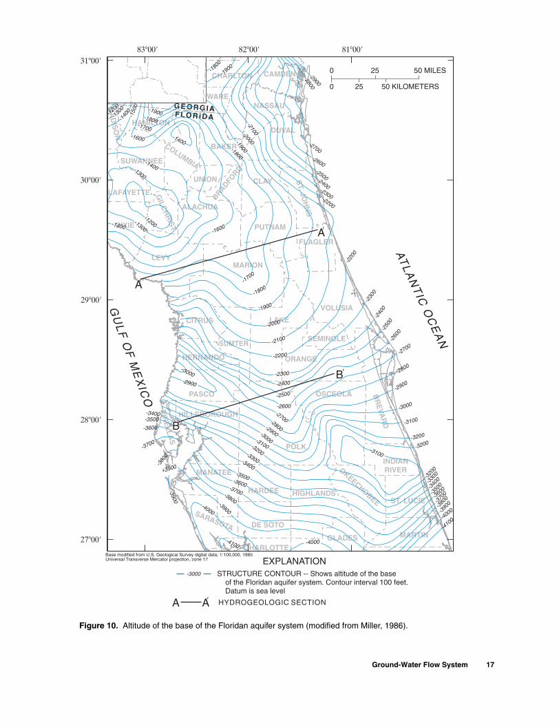
Figure 10. Altitude of the base of the Floridan aquifer system (modified from Miller, 1986).


Altitude of the Water Table of the Surficial Aquifer System

In this study, the altitude of the water table was estimated to specify the water levels in the SAS. Water levels in the SAS are not actively simulated in this model. Instead, the SAS was simulated as a source-sink layer with specified heads as one of the hydraulic properties determining the leakage rates to and from the underlying layer, namely the ICU or the IAS.

A commonly used algorithm for generating the altitude of the water table in an unconfined aquifer is to perform a linear regression between the measured water levels and the land-surface altitude. This algorithm, however, generally fails to provide reli-able estimates in upland areas of low recharge or high hydraulic conductivity. In such areas, land-surface altitudes and water levels generally are not correlated.

The algorithm presented herein introduces the concept of the “minimum water table” to refer to the surface interpolated strictly from the measured alti-tude at drains in the SAS such as streams and lakes. This minimum water table becomes one of the vari-ables used in the regression of the water table. To account for areas where the water table emulates land-surface altitude, a second variable is added to the regression: the vertical distance between land-surface altitude and the minimum water table. A lim-itation of this algorithm is its inability to estimate the water table in areas where ground-water mounds are formed by perched layers in the SAS.

The altitude of the water table was approxi-mated by using a series of multiple linear regressions (one for each group of physiographic regions) among the measured levels in SAS wells, the interpolated minimum water table, and the difference between land-surface altitude and the minimum water table. Water-level measurements at SAS wells were com-piled from data bases of the SJRWMD, SFWMD, SWFWMD, SRWMD, and USGS. The minimum water-table surface was interpolated from measured or estimated stages at lakes and streams (fig. 11). A digital land-surface elevation model was generated from digitized hypsography obtained from the SJRWMD, SFWMD, SWFWMD, and USGS.


Average lake elevations for 1993-94 were computed for 544 gaged lakes in the study area (fig. 11). Average river stages for the same period were computed for 233 stream gaging stations (fig. 11). Gaged rivers were divided in segments according to the location of the stream gaging sta-tions. In cases where upstream or downstream end nodes of the river segments coincided with a lake, the lake elevation was used as the river stage at the node. The river stage was computed at all discrete nodes located along the meander of each river segment through linear interpolation of measured river stages. The computed lake elevations and river stages were assumed to be representative of the water-table ele-vation at the same sites. All lake elevations, river stages, and water levels were referenced to the National Geodetic Vertical Datum of 1929.

The digital representation of hypsography for the study area was generated from 5-ft contour inter-val hypsography digitized by SJRWMD, SFWMD, SWFWMD, and SRWMD from 7.5-minute USGS topographic quadrangle maps. A digital elevation model (DEM) of square cells 100-ft wide was gener-ated by using the digitized hypsography, lake eleva-tions from gaged lakes, and river stages computed along the meanderings of gaged rivers. The DEM was generated by using quintic splines. Using the DEM, the land-surface altitude could be interpolated at any point in the study area. The maximum abso-lute difference between the estimated land-surface altitude from the DEM and the land-surface altitude at surveyed points was 5.75 ft.

Elevations for ungaged lakes and stages along ungaged rivers were interpolated by using the DEM. Although some of the ungaged lakes may not be rep-resentative of the regional water table (some of the lakes may be perched), determining which lakes to exclude was beyond the scope of this study.

The minimum water table was generated from the interpolation of lake elevations, river stages, and the ocean shoreline (which was assigned a water-table alti-tude of zero feet). The relations among minimum water table, water table, and land-surface altitude are shown in figure 12. The minimum water table was bounded above by land-surface altitude and below by the bottom of the SAS, defined to be the sum of the thickness of the ICU (fig. 5) and the altitude of the top of the UFA (fig. 6).


Figure 11. Lakes, streams, locations of stream gaging stations, and surficial-aquifer wells used to estimate the altitude of the water table of the surficial aquifer system.


le, and land-surface altitude.

Elevations of the minimum water table at 1,050 wells tapping the SAS were interpolated from the generated minimum water-table surface. Water-table measurements at the SAS wells were grouped by the physiographic region (fig. 2) in which each well was located. Land-surface altitudes at the SAS wells were interpolated from the DEM. Multiple linear regressions for each group of physiographic regions were com-puted based on the equation:

, (1)

whereWTi is the water-table measurement at SAS

well i, in feet,MINWTi is the minimum water table interpolated at

SAS well i, in feet,LSAi is the land-surface altitude interpolated at

SAS well i, in feet, andβ1 and β2 are the dimensionless regression coeffi-

cients of the multiple linear regression.Multiple linear regressions computed for each group of physiographic regions indicated a strong correlation between the response variable WTi and the regressor variables MINWTi and LSAi - MINWTi in equation 1 (table 2). The root-mean-square (RMS) residual between measured and linearly regressed water-table

Figure 12. Relations among water table, minimum water tab

WTi β1 MINWTi β2 ( LSAi - MINWTi )+=


altitudes was computed for all groups of physiographic regions, resulting in a weighted average residual of 3.53 ft, with the difference between the regressed and measured water-table altitudes ranging from -17.20 to 18.49 ft (table 2). The linearly regressed and measured water-table altitudes were strongly correlated (fig. 13). Although the overall improvement to the RMS residu-als resulting from computing a multiple linear regres-sion for each group, instead of one regression for all groups, of physiographic regions does not seem con-siderable, the results show that for some physiographic groups, the regression coefficient for variable LSAi - MINWTi is not negligible. For groups 3, 4, 5,

and 7, the same regression coefficient is small (table 2). Groups 3, 4, and 7 are classified as uplands and ridges, whereas group 5 is classified as a valley (fig. 2). A leaky ICU or a high SAS hydraulic conductivity could result in a lack of correlation between the water table and the land-surface altitude. The water table increasingly emulates land-surface altitude as regression coefficient β2 in equation 1 increases. As

the value of β2 decreases, the water table becomes

increasingly correlated with the minimum water table.

In areas where the minimum water table, the land-surface altitude, and the water table coincide, the water table was redefined as the minimum water table in order to correct small errors introduced by values of β1


Table 2. Multiple linear regression coefficients for the minimum water table and the difference between land-surface altitude and minimum water table[Group number refers to figure 2. Refer to equation 1 for the definition of regression coefficients; na, not applicable]

Number of

surficial aquifer systemwells

Regression coefficient

of minimum water table

(β1)

Regression coefficient of

difference between digital

elevation and minimum

water table (β2)

Root-mean-square

residual (feet)

Range of values of difference

between regressed and

measured water table (feet)

Correlation coefficient

Group number

Multiple linear regressions

1 23 1.00 0.48 3.36 [-6.04, 6.60] 0.972 226 1.04 .39 3.29 [-7.68, 18.49] .993 94 1.06 .10 4.10 [-12.09, 7.35] .994 364 1.09 .04 4.07 [-17.20, 12.76] .995 74 1.09 .14 3.88 [-9.68, 11.54] .996 140 1.06 .28 2.53 [-7.45, 7.61] .997 14 1.05 .06 4.32 [-8.32, 5.74] .998 16 1.02 .49 3.72 [-6.59, 7.51] .999 37 .96 .85 1.79 [-3.28, 4.29] .99

10 62 1.02 .42 1.83 [-6.28, 4.04] .99Weighted mean 1,050 na na 3.53 [-17.20, 18.49] na

Regression coefficient

Regressions without grouping

β1 = 0 1,050 0.00 2.27 50.79 [-79.17, 330.31] 0.39β1 = 1 1,050 1.00 .26 5.68 [-19.26, 41.37] .42β1 = β2 1,050 .83 .83 13.88 [-28.81, 25.23] .88β2 = 0 1,050 1.11 .00 4.76 [-24.25, 21.10] .99β1 ≠ β2 ≠ 0 1,050 1.08 .10 4.27 [-21.88, 19.32] .99

in table 2 that deviate from unity. Setting the value of β1 in equation 1 to unity would lower substantially the cor-relation coefficient of the resulting linear regression. Similarly, a nonunity value of β2 is needed to maintain a reliable correlation coefficient.

If only one multiple linear regression were com-puted to approximate the water table, instead of one for each group of physiographic regions, then the wrong conclusion could be drawn that WTi was weakly corre-lated with LSAi - MINWTi over the study area, reduc-ing equation 1 to a linear regression. The correlation between variables WTi and LSAi - MINWTi tends to increase as the correlation between variables WTi and MINWTi decreases; the correlation between variables WTi and LSAi - MINWTi is variable across the study area (fig. 14). The inclusion of only MINWTi or LSAi - MINWTi in equation 1 significantly reduces the correlation coefficient of the water-table regression.

Figure 13. Regressed and measured water-table altitudes for all groups of physiographic regions.


The application of equation 1, and the regression coefficients in table 2, resulted in an estimated water- table altitude that ranged from 0 to 240 ft (fig. 15). The estimated water table for average 1993-94 condi-tions was greater than 150 ft in areas of Alachua, Baker, Bradford, Clay, Columbia, Polk, and Suwannee Coun-ties (fig. 15). Water-table altitudes generally decrease coastward. Water-table altitudes beyond the shoreline were assumed to be the equivalent freshwater head of the water column obtained from the digitized bathym-etry. Areas where the UFA is considered unconfined (fig. 5) were excluded from the water-table map (fig. 15) because, in general, the SAS is absent in this area or its areal extent is minimal.

Potentiometric Surface of the Intermediate Aquifer System

A data base of well hydrographs from continu-ous water-level recorders was generated for the purpose of assessing hydrologic conditions in the study area. Data from the SJRWMD, SRWMD, and USGS were used to generate hydrographs for sites throughout the study area (fig. 16; appendix B).

Daily measurements from 11 wells tapping the IAS in southwest Florida (fig. 16; appendix B) equipped with continuous water-level recorders were used to obtain monthly average water levels for September 1993 and May 1994 and average water levels for the period from August 1993 to July 1994.

Figure 14. Correlation between water table, minimum water table, and difference between land-surface altitude and minimum water table for (A) group 4 and (B) group 9 of physiographic regions (refer to figure 2 for physiographic regions).


Figure 15. Estimated altitude of the water table of the surficial aquifer system, average conditions for August 1993 through July 1994.


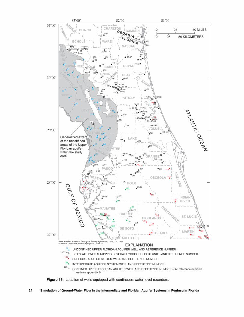
Figure 16. Location of wells equipped with continuous water-level recorders.


The average heads from August 1993 to July 1994 at these 11 wells were linearly regressed with the Septem-ber 1993 and May 1994 monthly averages according to the multiple linear regression:

, (2)

whereis the computed average water-level measurement at well i, in feet,is the computed monthly average for September 1993 at well i, in feet,is the computed monthly average for May 1994 at well i, in feet,

βI is the intercept of the multiple linear regression, in feet, and

βS and βM are the dimensionless regression coeffi-cients of the multiple linear regression.

Regression coefficients βS and βM represent the

influence of the September 1993 ( ) and May 1994

( ) averages on the resulting annual averages .Regression coefficients βI, βS, and βM, computed

by using data from the IAS wells equipped with contin-uous water-level recorders, were 0.54, 0.63, and 0.37, respectively. The correlation coefficient of this multiple linear regression was 0.99, implying a strong correla-tion between the annual averages and the monthly averages of September 1993 and May 1994 at the water-level recorder sites. Lack of sufficient water-level data in the IAS precluded the computation of separate multiple linear regressions for the groups of physio-graphic regions within the IAS, namely groups 2, 3, 4, 5, 9, and 10 (fig. 2).

A total of 107 water levels was measured in IAS observation wells during both the months of September 1993 (Mularoni, 1994a) and May 1994 (Metz and Brendle, 1994b). Water levels at these sites were compiled to esti-mate the potentiometric surface of the IAS. The assump-tion was made that the single measurement made at each of the IAS wells in September 1993 and May 1994 was representative of the monthly average at the site. Esti-mated annual average heads at these 107 observation wells were computed from equation 2 using the Septem-ber 1993 and May 1994 water levels and the regression coefficients βI, βS, and βM. The 107 estimated annual averages and the 11 annual average heads computed from continuous water-level data constituted the 118 control points used to generate the potentiometric-sur-face map of the IAS (fig. 17).

hi βI βS hSi βM hMi + +=

hi

hSi

hMi

hSihMi hi

The estimated average 1993-94 potentiometric surface of the IAS shows altitudes of 120 ft in south-central Polk County and in the area where Polk, Hills-borough, Hardee, and Manatee Counties meet (fig. 17). The thickness of the IAS decreases towards the northern, eastern, and western boundaries of the model. The IAS continues beyond the southern boundary of the model area. Ground water flows lat-erally from areas of potentiometric surface highs toward boundaries where the aquifer pinches out. In particular, upward leakage in discharge areas in parts of Sarasota, De Soto, Highlands, and Glades Counties causes ground water to move towards the eastern and western boundaries of the aquifer.

Potentiometric Surface of the Upper Floridan Aquifer

Daily measurements at UFA wells equipped with continuous water-level recorders were used to obtain monthly averages for September 1993 and May 1994 and averages for 1993-94. Regression coeffi-cients βI, βS, and βM for the UFA were obtained from the continuous water-level data by making a multiple linear regression (equation 2) for each group of phys-iographic regions (table 3). The regression coefficients βI, βS, and βM calculated for the UFA showed that the estimated annual averages were influenced more by the September 1993 averages than by the May 1994 averages for physiographic regions 3, 4, 5, 6, 9, and 10 (table 3). The correlation coefficients for all regres-sions indicated a strong correlation between the annual averages and the September 1993 and May 1994 averages (table 3).

Water-level measurements made during the months of September 1993 and May 1994 in the SJRWMD, SWFWMD, and parts of SFWMD to gen-erate potentiometric-surface maps for the UFA (Metz and Brendle, 1994a; Mularoni, 1994b; Schiffer and others, 1994; and Spechler and others, 1993) were assumed to represent monthly averages. Water-level measurements made in the SRWMD and the com-puted annual average heads at UFA wells equipped with continuous water-level recorders were used to increase the density of water-level measurements. Estimated annual average heads at UFA observation wells were computed from equation 2 using the com-piled September 1993 and May 1994 water-level data and the regression coefficients for the respective phys-iographic regions.



Table 3. Multiple linear regression coefficients for September 1993 and May 1994 water-level averages in the Upper Floridan aquifer for each group of physiographic regions[Group number refers to figure 2. Refer to equation 2 for the definition of regression coefficient; na, not applicable]

Group number

Number of Upper Floridan aquifer wells

Intercept (feet)(βI)

Regression coefficient of

September 1993 (βS)

Regressioncoefficient of

May 1994(βM)

Root-mean- square

residual (feet)

Range of values of dif-ference between

regressed and mea-sured heads (feet)

Correlation coefficient

1 9 0.77 0.08 0.90 0.60 [-0.80, 0.87] 0.992 16 .62 .39 .62 .22 [-0.33, 0.34] .993 16 .02 .68 .32 .36 [-0.73, 0.84] .994 15 .79 .58 .42 .39 [-0.7l, 0.60] .995 16 -.22 .55 .46 .21 [-0.48, 0.35] .996 23 .25 .64 .35 .46 [-1.34, 0.78] .997 32 -.57 .13 .87 .59 [-1.22, 1.17] .998 4 .39 .25 .75 .35 [0.21, 0.54] .999 4 -3.42 .77 .29 .25 [-0.19, 0.42] .99

10 8 -.12 .62 .36 .27 [-0.29, 0.53] .99Weighted mean 143 na na na .40 [-1.34, 1.17] naNo grouping 143 .22 .54 .46 .85 [-3.18, 4.62] .99

Figure 17. Estimated potentiometric surface of the intermediate aquifer system, average conditions for August 1993 through July 1994.

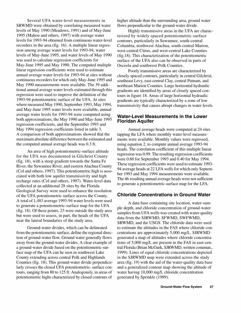
Several UFA water-level measurements in SRWMD were obtained by correlating measured water levels of May 1990 (Meadows, 1991) and of May-June 1995 (Mahon and others, 1997) with average water levels for 1993-94 obtained from continuous water-level recorders in the area (fig. 16). A multiple linear regres-sion among average water levels for 1993-94, water levels of May-June 1995, and water levels of May 1990 was used to calculate regression coefficients for May-June 1995 and May 1990. The computed multiple linear regression coefficients were used to estimate annual average water levels for 1993-94 at sites without continuous recorders for which only May-June 1995 and May 1990 measurements were available. The 39 addi-tional annual average water levels estimated through this regression were used to improve the definition of the 1993-94 potentiometric surface of the UFA. At sites where measured May 1990, September 1993, May 1994, and May-June 1995 water levels were available, annual average water levels for 1993-94 were computed using both approximations, the May 1990 and May-June 1995 regression coefficients, and the September 1993 and May 1994 regression coefficients listed in table 3. A comparison of both approximations showed that the maximum absolute difference between the estimated and the computed annual average heads was 0.3 ft.

An area of high potentiometric-surface altitude for the UFA was documented in Gilchrist County (fig. 18), with a steep gradient towards the Santa Fe River, the Suwannee River, and eastern Alachua County (Col and others, 1997). This potentiometric high is asso-ciated with both low aquifer transmissivity and high recharge rates (Col and others, 1997). Water-level data collected at an additional 28 sites by the Florida Geological Survey were used to enhance the resolution of the UFA potentiometric surface across the County. A total of 1,483 average 1993-94 water levels were used to generate a potentiometric-surface map for the UFA (fig. 18). Of these points, 23 were outside the study area but were used to assess, in part, the heads of the UFA near the lateral boundaries of the study area.

Ground-water divides, which can be delineated from the potentiometric surface, define the regional direc-tion of ground-water flow. Ground water generally flows away from the ground-water divides. A clear example of a ground-water divide based on the potentiometric-sur-face map of the UFA can be seen in southwest Lake County extending across central Polk and Highlands Counties (fig. 18). This ground-water divide perpendicu-larly crosses the closed UFA potentiometric- surface con-tours, ranging from 80 to 125 ft. Analogously, in areas of potentiometric highs characterized by closed contours of

higher altitude than the surrounding area, ground water flows perpendicular to the ground-water divide.

Highly transmissive areas in the UFA are charac-terized by widely spaced potentiometric-surface contours, particularly in Suwannee, south-central Columbia, northwest Alachua, south-central Marion, west-central Citrus, and west-central Lake Counties (fig.18). This characterization of the potentiometric surface of the UFA also can be observed in parts of Osceola and southwest Polk Counties.

Poorly transmissive areas are characterized by closely spaced contours, particularly in central Gilchrist, southeast Levy, east-central Clay, central Putnam, and northeast Marion Counties. Large horizontal hydraulic gradients are identified by areas of closely spaced con-tours in figure 18. Areas of large horizontal hydraulic gradients are typically characterized by a zone of low transmissivity that causes abrupt changes in water levels.

Water-Level Measurements in the Lower Floridan Aquifer

Annual average heads were computed at 24 sites tapping the LFA where monthly water-level measure-ments were available. Monthly values were regressed, using equation 2, to compute annual average 1993-94 heads. The correlation coefficient of this multiple linear regression was 0.99. The resulting regression coefficients were 0.60 for September 1993 and 0.40 for May 1994. These regression coefficients were used to estimate 1993-94 average heads at 22 LFA wells for which only Septem-ber 1993 and May 1994 measurements were available. The 46 resulting annual average heads were not sufficient to generate a potentiometric-surface map for the LFA.

Chloride Concentrations in Ground Water

A data base containing site location, water-sam-ple depth, and chloride concentration of ground-water samples from UFA wells was created with water-quality data from the SJRWMD, SFWMD, SWFWMD, SRWMD, and the USGS. The chloride data were used to estimate the altitudes in the FAS where chloride con-centrations are approximately 5,000 mg/L. SJRWMD generated a map of altitudes where chloride concentra-tions of 5,000 mg/L are present in the FAS in east-cen-tral Florida (Brian McGurk, SJRWMD, written commun., 1999). Lines of equal chloride concentrations depicted in the SJRWMD map were extended across the study area (fig. 19) with the aid of the water-quality data base and a generalized contour map showing the altitude of water having 10,000 mg/L chloride concentration generated by Sprinkle (1989).


Figure 18. Estimated potentiometric surface of the Upper Floridan aquifer, average conditions for August 1993 through July 1994.


EXPLANATION

ALTITUDE CONTOUR -- Shows estimated altitude of ground water with 5,000 milligramsper liter chloride concentration. Contour interval is variable. Datum is sea level

OBSERVATION WELLJ

-200

HYDROGEOLOGIC SECTIONA A

Extent of chlorideconcentration mapdeveloped by St. JohnsRiver Water ManagementDistrict

AT

LA

NT

ICO

CE

AN

GU

LF

OF

ME

XIC

O

BR

AD

FO

RD

OSCEOLA

BAKER DUVAL

BR

EVA

RD

INDIANRIVER

ST. LUCIE

MARTIN

OKEECHO

BEE

HIG

HLA

ND

S

GLADES

HARDEE

DE SOTO

CHARLOTTE

SARASOTA

MANATEE

HIL

LSB

OR

OU

GH

PIN

EL

LA

SPASCO

HERNANDO

CITRUS

ALACHUA

LEVY

DIXIE

GIL

CH

RIS

T

LAFAYETTE

UNION

CO

LU

MB

IA

SUWANNEE

MA

DIS

ON

HAMILTON

WARE

CHARLTON CAMDEN

NASSAU

CLAY ST.JO

HN

S

MARION

PUTNAM

FLAGLER

POLK

SUMTER

LAKESEMINOLE

ORANGE

VOLUSIA

GEORGIAFLORIDA

OldTampa Bay

HillsboroughBay

J

J

JJJ

JJ

JJ

J

JJJ

J

J

J J

J

JJ

JJ J

J

JJ

J

JJ

JJJ

JJJJJ J

JJJ

J

JJ

JJ

J

JJ

JJ J

J

J JJ J

JJJ

J JJ J

J J

JJ

JJ J J

JJ JJ JJJJJ J J

J JJJ J

JJ JJ J

J

J JJ J JJ J

J JJ

JJJ J

J

J

JJ

JJJJJ

JJ J

J J

J

JJ

JJ

J J

JJJ

J

J

JJ

JJ

J

J

J

J

JJ

J

JJJ

J

J

J

JJ

J

JJ

J

J

J

JJ

J JJ

JJ JJ J

JJ J

J

J JJ

JJJ

JJ

J J

J

JJJJJJJ

JJJ J

JJJ JJ J

JJ

J

J

J

J

JJJ

J

JJ

JJ

JJJ

J

JJJ

J

JJJ

J

J

JJ

JJJ

JJJJ

JJJ J

JJ JJ

JJJ JJ

JJ J

J JJJ JJ J JJ J JJJ JJJJ JJ

J JJJJ JJ JJJ JJJ

JJJ J J

JJ JJ JJJ

J

JJJ JJJ J

J JJJ

J J

J JJ

JJJJ

J JJJ

J JJ JJJJJ JJJ

J

JJ

JJ

JJJ

JJ J JJ JJ J JJJ JJ

JJJ JJJ

J J JJ JJ J

JJ JJJJ J

JJ J

JJJ

-2200

-2000

-1800

-1500

-1500

-1500

-1000

-1000

-1000

-500

-500

-500

-1800

-18

00

-2000

-2000

-2200

-2200

-2400

-1600

-1600

-1600

-1600

-1800

-1800 -1400

-1400

-1200

-1200

-1000

-800

-600

-400

-400

-400

-400

-200

-200

-150

-150

-600

-600

-600

-800

-800

-800

-1200

-1000

-1000

-1000

-200

-200

-150

-600

-600

-800

-800

-1400

-1000

0

0 25

25

50 MILES

50 KILOMETERS

��

��

��

��

��

��

Base modified from U.S. Geological Survey digital data; 1:100,000, 1985Universal Transverse Mercator projection, zone 17

A

B

A

B

SuwanneeRiver

Santa FeRiver

Figure 19. Estimated altitude of water containing a chloride concentration of 5,000 milligrams per liter in the Floridan aquifer system (modified from Brian McGurk, St. Johns River Water Management District, written commun., 1999; and Sprinkle, 1989).


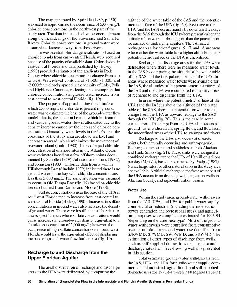
The map generated by Sprinkle (1989, p. I50) was used to approximate the occurrence of 5,000-mg/L chloride concentrations in the northwest part of the study area. The data indicated saltwater encroachment along the meanderings of the Suwannee and Santa Fe Rivers. Chloride concentrations in ground water were assumed to decrease away from these rivers.

In west-central Florida, generalizations based on chloride trends from east-central Florida were required because of the paucity of available data. Chloride data in east-central Florida and data published by Hickey (1990) provided estimates of the gradients in Polk County where chloride concentrations change from east to west. Water-level contours of -1,500; -1,800; and -2,000 ft are closely spaced in the vicinity of Lake, Polk, and Highlands Counties, reflecting the assumption that chloride concentrations in ground water increase from east-central to west-central Florida (fig. 19).

The purpose of approximating the altitude at which 5,000 mg/L of chloride is present in ground water was to estimate the base of the ground-water flow model; that is, the location beyond which horizontal and vertical ground-water flow is attenuated due to the density increase caused by the increased chloride con-centration. Generally, water levels in the UFA near the coastlines of the study area are above sea level and decrease seaward, which minimizes the movement of seawater inland (Todd, 1980). Lines of equal chloride concentration at offshore sites in the Atlantic Ocean were estimates based on a few offshore points docu-mented by Scholle (1979), Johnston and others (1982), and Johnston (1983). Chloride data from a well in Hillsborough Bay (Sinclair, 1979) indicated there is no ground water in the bay with chloride concentrations less than 5,000 mg/L. The same situation was assumed to occur in Old Tampa Bay (fig. 19) based on chloride trends obtained from Dames and Moore (1988).

Sulfate concentrations near the base of the UFA in southwest Florida tend to increase from east-central to west-central Florida (Hickey, 1990). Increases in sulfate concentrations in ground water also increase the density of ground water. There were insufficient sulfate data to assess specific areas where sulfate concentrations would cause increases in ground-water density equivalent to a chloride concentration of 5,000 mg/L; however, the occurrence of high sulfate concentrations in southwest Florida would have the equivalent effect of displacing the base of ground-water flow farther east (fig. 19).

Recharge to and Discharge from the Upper Floridan Aquifer

The areal distribution of recharge and discharge areas to the UFA were delineated by comparing the


altitude of the water table of the SAS and the potentio-metric surface of the UFA (fig. 20). Recharge to the UFA (and the IAS) occurs mainly by downward leakage from the SAS through the ICU (where present) when the altitude of the water table is higher than the potentiomet-ric surface of underlying aquifers. The estimated recharge areas, based on figures 15, 17, and 18, are areas where either the water table has a higher altitude than the potentiometric surface or the UFA is unconfined.

Recharge and discharge areas for the UFA were delineated where there were no measured water levels in the IAS by comparing the altitude of the water table of the SAS and the interpolated heads of the UFA. In areas where measured water levels were available for the IAS, the altitudes of the potentiometric surfaces of the IAS and the UFA were compared to identify areas of recharge to and discharge from the UFA.

In areas where the potentiometric surface of the UFA (and the IAS) is above the altitude of the water table of the SAS, there is a potential for water to dis-charge from the UFA as upward leakage to the SAS through the ICU (fig. 20). This is the case in some coastal areas. Discharge from the UFA also occurs as ground-water withdrawals, spring flows, and flow from the unconfined areas of the UFA to swamps and rivers.

Recharge to the UFA also occurs at discrete points, both naturally occurring and anthropogenic. Recharge occurs at natural sinkholes such as Alachua and Haile Sinks (fig. 21). These sinks were assigned a combined recharge rate to the UFA of 10 million gallons per day (Mgal/d), based on estimates by Phelps (1987). No recharge rates for other natural sinks in the study area are available. Artificial recharge to the freshwater part of the UFA occurs from drainage wells, injection wells in Alachua County, and rapid-infiltration basins.

Water Use

Within the study area, ground-water withdrawals from the IAS, UFA, and LFA for public-water supply, commercial or industrial (including thermoelectric-power generation and recreational uses), and agricul-tural purposes were compiled or estimated for 1993-94 (depending on the water-use type). Most of the ground-water withdrawals were compiled from consumptive user permit data bases and water-use data files from SJRWMD, SFWMD, SWFWMD, and SRWMD. The estimation of other types of discharge from wells, such as self-supplied domestic water-use data and discharge rates from free-flowing wells, is presented in this section.

Total estimated ground-water withdrawals from the IAS, UFA, and LFA for public-water supply, com-mercial and industrial, agricultural, and self-supplied domestic uses for 1993-94 were 2,488 Mgal/d (table 4).


Figure 20. Distribution of recharge and discharge aconditions for August 1993 through July 1994.

reas of the Upper Floridan aquifer, average


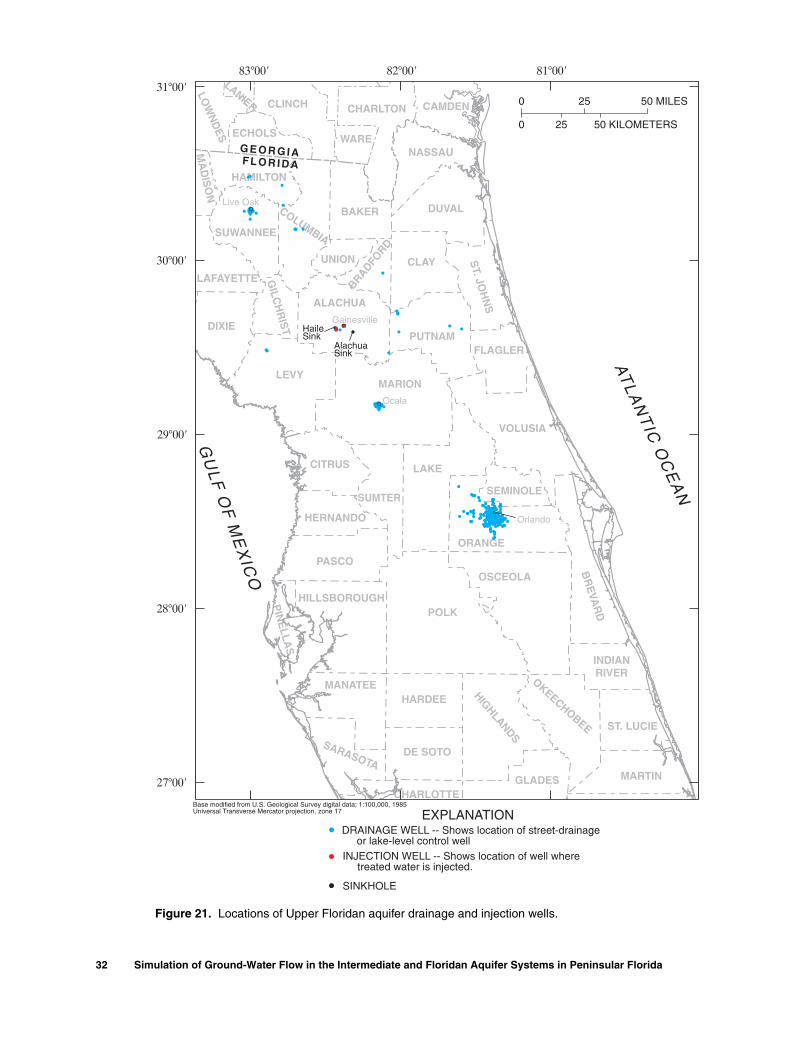
Figure 21. Locations of Upper Floridan aquifer drainage and injection wells.


Table 4. Estimated ground-water withdrawals and uses, by county and by Water Management District, from the intermediate aquifer system, Upper Floridan aquifer, and Lower Floridan aquifer, August 1993 through July 1994[Source: St. Johns River Water Management District (SJRWMD); South Florida Water Management District (SFWMD); Southwest Florida Water Manage-ment District (SWFWMD); Suwannee River Water Management District (SRWMD); and U.S. Geological Survey. All rates are in million gallons per day; -- indicates no wells are tapping the aquifer or aquifer is absent]

County

Intermediate aquifer system Upper Floridan aquifer Lower Floridan aquifer

Public- water

supply

Indus-trialand

com-merciala

aIncludes mining, thermoelectric power generation, recreational, and landscape irrigation uses.

Agricul-tural

Domes-tic

Public- water

supply

Indus-trial and

com-merciala

Agricul-tural

Domes-tic

Public- water

supply

Indus-trial and

commer-ciala

Agricul-tural

Alachua -- -- -- -- 24.62 5.99 34.96 6.93 -- -- -- Baker -- -- -- -- .80 .23 .14 1.24 0.31 -- 0.05Bradford -- -- -- -- 4.08 3.49 2.25 2.08 -- -- -- Brevard -- -- -- -- 2.61 1.02 13.75 0.52 -- -- -- Charlotte 0.11 0.07 14.29 1.17 .43 .07 4.91 -- -- -- -- Citrus -- -- -- -- 10.17 6.26 1.57 6.73 -- -- -- Clay -- -- -- -- 2.66 3.87 .77 2.90 7.43 1.77 -- Columbia -- -- -- -- 4.22 3.17 13.42 4.36 -- -- -- DeSoto .95 .24 6.12 0.52 .64 .16 53.87 .01 -- -- -- Dixie -- -- -- -- 1.69 .79 4.29 1.10 -- -- -- Duval -- -- -- -- 27.70 14.36 1.35 .08 73.42 12.34 .12Flagler -- -- -- -- 1.46 .08 6.25 .95 -- -- -- Gilchrist -- -- -- -- 2.32 .38 24.62 1.10 -- -- -- Glades -- -- 1.27 .01 .44 -- 6.36 -- -- -- .18Hamilton -- -- -- -- 16.94 14.80 16.54 .78 -- -- -- Hardee .04 .08 5.83 .42 1.39 .09 54.83 .01 -- -- -- Hernando -- -- -- -- 17.06 22.60 3.71 2.66 -- -- -- Highlands .33 .25 17.41 .21 6.91 2.01 96.22 .01 -- -- 18.54Hillsborough .01 .02 .95 .55 65.41 25.56 72.34 9.48 -- -- -- Indian River -- -- -- -- 5.21 .23 31.35 .09 -- -- -- Lafayette -- -- -- -- .59 .57 22.08 .71 -- -- -- Lake -- -- -- -- 26.01 27.80 29.43 9.55 1.73 .32 .32Levy -- -- -- -- 3.20 3.85 25.62 3.31 -- -- -- Madison -- -- -- -- .28 .26 7.79 .17 -- -- -- Manatee .16 .27 2.24 2.42 11.09 1.16 77.39 .02 -- -- -- Marion -- -- -- -- 18.54 6.44 8.46 21.76 -- -- .04Martin -- -- -- -- 1.20 .42 9.65 -- -- -- -- Nassau -- -- -- -- 4.46 34.00 .42 .13 -- 1.91 -- Okeechobee -- -- -- -- -- .39 24.42 .03 -- -- .34Orange -- -- -- -- 111.81 7.73 18.43 12.60 60.41 .40 .11Osceola -- -- -- -- 18.27 2.62 46.12 6.28 .97 -- .02Palm Beach -- -- -- -- .42 -- -- -- -- -- -- Pasco -- -- -- -- 95.89 16.00 20.07 8.07 -- -- -- Pinellas -- -- -- -- 40.69 1.87 .68 4.46 -- -- -- Polk .30 1.60 3.88 .80 59.39 90.61 127.12 5.69 .88 -- .47Putnam -- -- -- -- 3.38 7.22 6.58 9.42 -- .98 -- St. Johns -- -- -- -- 6.63 .01 21.01 2.12 .02 -- --St. Lucie -- -- -- -- 1.10 .25 11.42 .43 -- -- -- Sarasota 2.94 .83 .94 4.96 15.79 3.16 4.38 .03 -- -- -- Seminole -- -- -- -- 50.03 .39 7.90 7.90 6.91 -- -- Sumter -- -- -- -- 2.51 1.20 8.96 3.11 -- -- -- Suwannee -- -- -- -- 5.05 3.33 63.69 2.94 -- -- -- Union -- -- -- -- 1.11 .09 1.73 .72 -- -- -- Volusia -- -- -- -- 47.37 .71 16.53 7.39 -- .12 .01Camden, Ga. -- -- -- -- 2.43 34.36 .01 -- -- -- -- Charlton, Ga. -- -- -- -- .70 -- -- -- -- -- -- Total 4.84 3.36 52.93 11.06 724.70 349.60 1,003.39 147.87 152.08 17.84 20.20Water Management DistrictSJRWMD -- -- -- -- 289.61 98.91 156.44 69.93 135.09 17.48 0.63SFWMD 0.01 0.10 11.38 0.25 58.43 10.57 184.50 11.27 16.99 .36 19.57SWFWMD 4.83 3.26 41.55 10.81 332.24 171.26 452.50 45.92 -- -- --SRWMD -- -- -- -- 44.42 68.86 209.95 20.75 -- -- --

Interme-diate

aquifer system

Upper Floridan aquifer

Lower Floridan aquifer

Total by

aquifer

Public- water

supply

Industrial and

commer-cial

Agricul-tural Domestic

Total by

use

Total 72.19 2,225.56 190.12 2,487.87 881.62 370.80 1,076.52 158.93 2,487.87


Pumping rates were 72 Mgal/d from the IAS; 2,226 Mgal/d from the UFA; and 190 Mgal/d from the LFA. Corresponding withdrawals were 882 Mgal/d for pub-lic-water supply; 371 Mgal/d for commercial and industrial; 1,076 Mgal/d for agricultural uses; and 159 Mgal/d for self-supplied domestic uses. Estimated ground-water withdrawals from self-supplied domestic wells for 1993-94 were obtained from USGS data (Richard L. Marella, written commun., 1998).

Ground-water withdrawals for public-water supply and commercial or industrial purposes were compiled from the monthly operating reports of SJRWMD, SFWMD, SWFWMD, and SRWMD, which are based on meter readings. Ground-water withdrawals were distributed according to aquifer source by using the well locations, penetration depths of individual wells in each well field, well status, and well capacity from the consumptive user permit data base. Pumping rates for Camden, Charlton, and Ware Counties, Ga., for public-water supply and industrial purposes were obtained from the USGS.

Several assumptions were made to apportion total water withdrawals among individual wells in the same well field and between aquifers for wells with open intervals tapping more than one aquifer. At well fields where only the cumulative withdrawal was spec-ified, each active well was assigned a ground-water withdrawal equal to the total withdrawn multiplied by the ratio of the well capacity to the sum of well capac-ities for all active wells in the well field. Assigned water withdrawals from each aquifer from wells with open intervals tapping more than one aquifer were set equal to the total withdrawal rate multiplied by the ratio of the transmissivity of the interval open to a par-ticular aquifer to the transmissivity of the entire open interval of the well.

Ground-water withdrawal data for SRWMD were provided by SRWMD (Ronald Ceryak, written commun., 1997). Measured and estimated pumping rates from wells in SWFWMD were provided by the SWFWMD (Tabitha Ostow, written commun., 1999). Pumping rates from wells used for agricultural pur-poses in SJRWMD and SFWMD were estimated from the required application rates for each crop type, which depend on rainfall, watering needs, and estimated evapotranspiration rates. These application rates were computed by the Water Management Districts. The application rate for each cultivated acre, adjusted by the irrigation method, was multiplied by the number of cul-tivated acres to obtain the estimated pumping rate for a specific crop. Many wells pumped water for more than one crop type. Total ground-water withdrawals for well


fields were the sum of pumping rates for all crop types. When ground water was not the only source for irriga-tion, adjustments to pumping rates were made by using the estimated ground-water use percentage listed in the water-use permit data base.

Estimates of discharge rates from free-flowing UFA wells in SJRWMD were obtained from SJRWMD (Brian McGurk, written commun., 1997). Discharge rates for 1993-94 were estimated to be 6.81 Mgal/d, of which more than 50 percent occurred in Brevard County (table 5). No information is available about free-flowing wells, if any, outside SJRWMD.

Artificial Recharge from Drainage and Injection Wells

Artificial recharge to the UFA occurs through about 364 active drainage wells and 41 injection wells (fig. 21). Of these wells, 242 are concentrated in the Orlando metropolitan area and were verified to be active (CH2M Hill, 1997). These drainage wells, cased to the top of the UFA and then drilled open-hole into the UFA, generally are used as a means to dispose of street runoff from storm drains and to control lake lev-els. Total recharge to the UFA through drainage wells in the study area was estimated to be 68 Mgal/d (table 6) based on total rainfall for 1993-94. The recharge rate at drainage wells is strongly correlated to the amount of total rainfall for any period.

Recharge to the UFA through drainage wells in the Orlando metropolitan area for 1993-94 was approx-imated from recorded rainfall data at nearby NOAA stations (fig. 3) and from adjustments to previously estimated long-term recharge rates at these wells by CH2M Hill (1997) and Bradner (1996). Estimates of recharge rates from drainage wells were based on a water-budget analysis of the basins containing street-runoff and lake-level control wells.

Table 5. Estimated discharge rates from free-flowing wells, by county, in the Upper Floridan aquifer in the St. Johns River Water Management District, August 1993 through July 1994[Source: Brian McGurk, St. Johns River Water Management Dis-trict. Rates are in million gallons per day]

County Discharge

Brevard 3.44Indian River 2.00Putnam .03St. Johns .36Seminole .87Volusia .11Total 6.81


For street-runoff wells, the first step was to cal-culate a runoff coefficient for the drainage area. The runoff coefficient can be defined as the fraction of the total rainfall that becomes runoff over a given time period. CH2M Hill (1997) calculated an average runoff coefficient of 0.578 for a group of street-runoff drain-age wells in Orange County. An average runoff coeffi-cient, weighted by the contributing drainage areas of each well, was computed for the same group of street-runoff drainage wells used by CH2M Hill (1997). The resulting area-weighted average runoff coefficient used in this study was 0.478. An area-weighted average run-off coefficient lower than the 0.578 value computed by CH2M Hill (1997) is attributed to predominantly lower runoff coefficients for street-runoff drainage wells with larger contributing drainage areas.

The total area drained by street-runoff wells in metropolitan Orlando was estimated to be 6,083 acres (CH2M Hill, 1997). The 30-year average recharge rate to the UFA at street-runoff drainage wells, computed from the product of runoff coefficient, total rainfall at the Orlando McCoy station (fig. 3), and drainage area, was estimated to be 10.40 Mgal/d. The estimated recharge rate to the UFA from street-runoff drainage wells for 1993-94 was 11.91 Mgal/d, equal to 10.40 Mgal/d multiplied by the ratio of rainfall for this period (fig. 3) to the 30-year rainfall average.

A water-budget analysis of the basins contribut-ing drainage to 10 lake-level control wells (Bradner, 1996) showed a basin-area weighted recharge rate to the UFA of 10.84 in/yr. This recharge rate is lower than the non-weighted numerical average of 18.08 in/yr computed by CH2M Hill (1997) for the same basins. The total area drained by these lake-level control wells in metropolitan Orlando was estimated to be 33,031 acres (CH2M Hill, 1997). The 30-year average

Table 6. Estimated recharge rates for drainage wells to the Upper Floridan aquifer, by county, August 1993 through July 1994[Source: CH2M Hill, 1997; Bradner, 1996; Phelps, 1987. Rates, in million gallons per day, are rounded to integers]

County Recharge

Alachua 11Marion 4Orange 45Putnam 1Seminole 2Suwannee 5

Total 68

recharge rate to the UFA at lake-level control wells, computed from the product of drainage area and basin-area weighted recharge rate, was estimated to be 26.64 Mgal/d. The estimated recharge rate to the UFA for 1993-94 at lake-level control wells was 30.50 Mgal/d, equal to 26.64 Mgal/d multiplied by the ratio of rainfall for this period to the 30-year rainfall average.

Recharge to the UFA through drainage wells out-side the Orlando area but in Orange and Seminole Counties for 1993-94 was estimated to be 4.21 Mgal/d. Recharge to the UFA from drainage wells outside Orange and Seminole Counties (fig. 21), assuming all were street-runoff wells, was estimated to be 11.57 Mgal/d.

Additional recharge to the UFA occurs through injection wells monitored by the Florida Department of Environmental Protection (FDEP). Recharge rates from injection wells (fig. 21) were obtained from FDEP. A total of 10.62 Mgal/d recharged the UFA by injection wells in Alachua County during the 1993-94 period. The injection wells in Alachua County were the only FDEP wells recharging the freshwater part of the UFA.

Spring Flow

More than 150 springs discharge water from the UFA in the study area. A major factor in spring flow is the net aquifer recharge from rainfall; however, spring response is delayed by aquifer-matrix storage. Higher spring flows are common in late fall after the rainy sea-son, whereas lower flows occur in late spring when rainfall is low. Spring flows from the UFA tend to cre-ate depressions in the potentiometric surface, the areal extent of which depends on the magnitude of the spring flow and aquifer and confining-unit properties in the vicinity of the spring. A summary of spring-flow data for springs discharging from the UFA and the locations of these springs was compiled (fig. 22, appendix C) from Rosenau and others (1977), Yobbi (1989, 1992), USGS (1994, 1995, 1996, 1997, 1999), and Leel Knowles (USGS, written commun., 1999). The springs in the study area with the highest flows, based on mea-sured values or estimated flow measurements for 1993-94, are Silver Springs (number 66 in fig. 22), Rainbow Springs (number 72), Crystal River Spring Group (number 81), Alapaha Rise (number 2), and Ichetuck-nee Springs (combined flow of numbers 24 through 29 in fig. 22). Total spring flow from the UFA was approx-imately 6,380 cubic feet per second (ft3/s) or 4,130 Mgal/d (appendix C).


Figure 22. Locations of Upper Floridan aquifer spri


ngs.


Of the 156 springs in the study area, only 28 were measured during 1993-94 (U.S. Geological Sur-vey, 1994, 1995; appendix C). Average flows from the remaining 128 springs were estimated by using the fol-lowing approximations. Spring flow measurements by the USGS (1996, 1997, 1999) and Rosenau and others (1977) at 87 springs either prior to or after 1993-94 were used to estimate 1993-94 flows by multiplying the measured flow by the ratio of the 1993-94 rainfall to the rainfall that occurred during the year in which the mea-surement was made. Although the ratio between spring flow and rainfall is not constant from one year to the next, measured flows varied somewhat linearly with rainfall in those years when more than one flow mea-surement was available. Flows at nine unmeasured third and fourth magnitude springs were assigned flow values based on field reconnaissance (Leel Knowles, USGS, written commun., 1999). Flow at Crescent Beach submarine spring (spring 41, appendix C) also has never been measured; the estimated flow of 30 ft3/s is highly generalized (Rick Spechler, USGS, oral com-mun., 2000).

Average flows for 1993-94 at 31 springs in Citrus, Hernando, and Pasco Counties were esti-mated from the average May 1988 to April 1989 flows computed by Yobbi (1992). The average of the flow measurements at Weeki Wachee Springs (spring 138 in fig. 22) was 185 ft3/s from May 1988 to April 1989 (Yobbi, 1992), and 129 ft3/s from August 1993 to July 1994 (U.S. Geological Survey, 1994, 1995), or about 70 percent of the average flow from May 1988 to April 1989. Because of the lack of additional spring-flow measurements from May 1988 to April 1989 and from August 1993 to July 1994, average flows from August 1993 to July 1994 for springs in Citrus, Hernando, and Pasco Counties were estimated to be 70 percent of the flows deter-mined by Yobbi (1992) from May 1988 to April 1989. Similarly, the average flow in 1993-94 for additional springs listed by Yobbi (1989) was assumed to be 70 percent of the average flow for the period of record (appendix C).

Recharge to the Unconfined Upper Floridan Aquifer

A generalized water budget for unconfined areas of the UFA within the study area was used to estimate upper and lower bounds for the net aquifer recharge

rate in these areas. Total rainfall, direct runoff estimates derived from separation of discharge hydrographs, and evapotranspiration estimates based on physiographic regions were used to approximate the net aquifer recharge in unconfined areas of the UFA. The esti-mated net aquifer recharge rate to unconfined areas of the UFA for the 1993-94 period was computed from the equation:

, (3)

where

NR is net recharge to unconfined areas of the UFA, in inches per year,

TR is total rainfall, in inches per year,

ET is evapotranspiration, in inches per year, and

SR is surface runoff, in inches per year.

Equation 3 assumes that changes in storage were negli-gible, an assumption that is supported by data from continuous ground-water level recorders. Rainfall for the 1993-94 period was computed from data collected at NOAA stations (fig. 3). The unconfined areas of the UFA were divided into Thiessen (1911) polygons, which were based on the location of rain gages.

Net recharge to unconfined areas of the UFA is the subcomponent of the water budget that drives ground-water flow through the UFA when applied water exceeds evapotranspirative losses and overcomes capillary effects in the unsaturated zone. These recharge rates vary areally based on topography and physiography. Recharge rates to the aquifer are expected to be lower near coastal lowlands and swamps than in the Northern Highlands (fig. 2) or in other areas of high land-surface altitude. In low-lying areas, the potentiometric surface of the UFA is close to land sur-face and evapotranspiration (ET) rates probably are high. Recharge rates also are expected to be low near rivers, where surface runoff is more likely to discharge to rivers rather than recharge ground water. Aquifer recharge rates should decrease from the Northern High-lands (fig. 2) towards rivers in the unconfined areas of the UFA having the largest flows, namely, the Suwan-nee, Santa Fe, Steinhatchee, Waccasassa, and Withla-coochee Rivers, and parts of the Hillsborough River (fig. 23).

NR = TR - ET - SR


Several discharge areas along the Suwannee River in the unconfined areas of the UFA can be identified from the UFA potentiometric surface (fig. 18). The UFA discharges to the Suwannee River in areas where the stage at the Suwannee River is lower than the surrounding potentiometric surface. The Suwannee River recharges the UFA in areas where the river stage is higher that the surround-ing potentiometric surface of the UFA. Surface water from the coastal plains and swamps discharges to the Gulf of Mexico.

Evapotranspiration varies areally; a range of ET values was obtained from documented minimum and maximum measured rates. The minimum ET rate was assumed to be 27 in/yr, measured at a herbaceous, successional vegetation in a defor-ested area of the Lake Wales Ridge during the 1993-94 period (Sumner, 1996). The maximum ET rate was assumed to be 46 in/yr, the mean evapotranspiration measured at seven vegetated sites (rather than open water) in the Everglades (fig. 1) from January 1996 to December 1997 (German, 2000).

Estimates of surface runoff (SR) were computed by applying a generalized hydrograph separation approximation to calculate base flow and surface runoff from the daily dis-charge data obtained from 10 USGS stream gaging stations (table 7, fig. 23). Estimates of SR, normalized per unit area of each respective drain-age basin, ranged from 0.5 to 8 in/yr (table 7). The hydrograph separation approximation used in this study considered most hydrograph peaks to be part of SR (fig. 24). As a first approximation, the hydrograph separation code HYSEP (Sloto and Crouse, 1996) was used with a substantially larger drainage area

38 Simulation of Ground-Water Flow in t

Figure 23. Rivers in the unconfined areas of the Upper Floridan aquifer and locations of stream gaging stations.

he Intermediate and Floridan Aquifer Systems in Peninsular Florida

than the actual area in order to increase the number of days after which SR ceases. The resulting surface run-off from HYSEP at each gaging station was adjusted so that large areas of the hydrograph peaks were consid-ered to be part of SR. The frequency of storm events during the wet season, the large capacity of riverbank storage in the Suwannee, Withlacoochee, Waccasassa, Steinhatchee, Santa Fe, and Hillsborough Rivers, the large hydraulic connection between the UFA and these rivers, and the potential for slow overland drainage from swamps are some of the reasons why surface run-off would be underestimated if HYSEP was directly applied to these hydrographs. Surface runoff to the Suwannee River was estimated to be 7 in/yr, the rounded mean of the three stations on this river (table 7). The lowest surface-runoff rate, 0.5 in/yr, occurred at the Withlacoochee River in west-central Florida.

Because of the uncertainty of ET and SR and rather than computing a specific net recharge rate to unconfined areas of the UFA, ranges of values for the net recharge rate were estimated. These ranges were used to bracket final net recharge rates obtained during model calibration. The minimum net recharge rate was

estimated from equation 3 by using the maximum ET rate; the maximum net recharge rate was estimated by using the minimum ET rate. The application of equa-tion 3 to unconfined areas of the UFA resulted in net recharge rates that ranged from 0 to 18 in/yr in some areas, and from 13 to 32 in/yr in other areas (fig. 25). Estimated net recharge rates generally increased from the coastline inland.

Discharge to Swamps

Land-use maps indicate that about 12 percent of the unconfined areas of the UFA are swamps. These swamps include coastal or bay swamps, cypress and mangrove swamps, and river and lake swamps. Swamp areas located within the areal extent of the unconfined areas of the UFA were delineated to encompass all con-tiguous areas of swamp adjacent to the coast (fig. 26). Inland swamp areas also were delineated. Hydrologi-cally, swamps generally are areas where the potentio-metric surface of the UFA is at or near land surface. Swamps generally are considered to be discharge areas of the UFA because water drains out of the UFA into the swamps.

Table 7. Surface-runoff rates calculated from hydrograph separation approximations applied to August 1993 through July 1994 daily discharge data obtained from stream gaging stations in the unconfined areas of the Upper Floridan aquifer

[Station number refers to figure 23; USGS, U.S. Geological Survey. Average surface-runoff flow rates are rounded to one significant figure; mi2, square miles; ft3/s, cubic feet per second; in/yr, inches per year]

USGSstation number

Station nameDrainage

area (mi2)

Average daily

discharge(ft3/s)

Estimated average base

flow (ft3/s)

Estimatedaverage

surface-runoff flow (ft3/s)

Average surface-runoff flow per unit area (in/yr)

02303000 Hillsborough River near Zephyrhills 220 123 67 56 3.0

02312000 Withlacoochee River at Trilby 570 47 25 22 .5

02313000 Withlacoochee River near Holder 1,825 319 252 67 .5

02313700 Waccasassa River near Gulf Hammock 480 193 89 104 3.0

02319000 Withlacoochee River near Pinetta 2,120 1,714 621 1,093 7.0

02319500 Suwannee River at Ellaville 6,970 5,961 1,933 4,028 8.0

02320500 Suwannee River at Branford 7,880 6,678 3,269 3,409 6.0

02322500 Santa Fe River near Fort White 1,017 1,067 925 142 2.0

02323500 Suwannee River near Wilcox 9,640 9,410 5,056 4,354 6.0

02324000 Steinhatchee River near Cross City 350 205 36 169 7.0


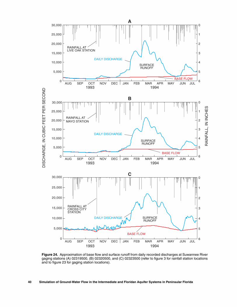
Figure 24. Approximation of base flow and surface runoff from daily recorded discharges at Suwannee River gaging stations (A) 02319500, (B) 02320500, and (C) 02323500 (refer to figure 3 for rainfall station locations and to figure 23 for gaging station locations).


Figure 25. Estimated minimum and maximum net recharge rates in the unconfined areas of the Upper Floridan aquifer.


the Upper
Figure 26. Areal extent of swamps in the unconfined areas of Floridan aquifer.
42 Simulation of Ground-Water Flow in the Intermediate and Floridan Aquifer Sy

SIMULATION OF GROUND-WATER FLOW

A steady-state ground-water flow model of the ground-water flow in the IAS and FAS was constructed and calibrated to time-averaged data for the period August 1993 through July 1994. The rationale for calibrating the model for this time period is explained in this section. Estimates of hydraulic properties obtained from local and regional ground-water flow models (table 1) were integrated with the hydrogeo-logic data discussed in previous sec-tions. The model was developed using the USGS finite-difference ground-water flow code MOD-FLOW-96 (Harbaugh and McDonald, 1996). The calibrated model was used to analyze the response of the FAS to projected ground-water withdrawals in 2020.

A uniformly spaced grid of square 5,000-ft cells was used as the framework to discretize the ground-water flow system horizontally. The UTM coordinates of the grid corners given in table 8 facilitate reproduction of the grid. Grid spacing (fig. 27) resulted from the need to use a finer grid resolution than in previous models (table 1). The grid consisted of 300 rows and 210 columns and was oriented along a north-south axis for simplicity because the majority of stresses or boundary conditions were not aligned along any particular axis.

Steady-State Approximation

The program MODFLOW-96 (Harbaugh and McDonald, 1996), used to simulate flow in the FAS, solves the

stems in Peninsular Florida

three-dimensional ground-water flow equation using finite-difference approximation and a block-centered grid. The equation solved by MODFLOW-96 can be written, after time averaging, as:

(4)

where

Kxx, Kyy, Kzz are the hydraulic conductivities along the columns, rows, and layers, respectively, in feet per day,

h is the average head for the time interval [t1, t2], in feet,

W is the average flux per unit volume for the time interval [t1, t2] and denotes the sink or source of water, in (feet/days)/feet,

Ss is the specific storage of the aquifer, in feet-1,

x, y, z are the spatial coordinates, in feet,t is time, in days, and

t1, t2 are times at the beginning and end of the time interval, in days.

The term W represents: drainage to springs or swamps; aquifer-river interactions; withdrawals from pumping; recharge from injection or drainage wells; and net recharge rates from rainfall infiltration in the unconfined areas of the UFA.

Table 8. Geographical information system coordinates of the corners of the ground-water flow model grid

[X and Y coordinates refer to Universal Transverse Mer-cator projection (Snyder, 1983), zone 17]

Grid cornerX coordinate

(feet)Y coordinate

(feet)

Upper left 900000 11270000

Upper right 1950000 11270000

Lower right 1950000 9770000

Lower left 900000 9770000

x∂∂ Kxx

h∂x∂

-----

y∂∂ Kyy

h∂y∂

----- z∂

∂ Kzzh∂z∂

----- W–+ +

= Ssht2 ht1–( )t2 t1–

----------------------- ,

A steady-state approximation to equation 4 implies that the magnitude of the right-hand side, which also can be written as Ss ∆h / ∆ t , is small. The expression S ∆ h/∆ t was evaluated instead of Ss ∆h / ∆t in order to approximate the product of specific storage and aquifer thickness with a single value. The expression S ∆ h/∆ t , used to assess the error introduced in the model by a steady-state approximation, was estimated by using the measured UFA heads at the beginning and at the end of any 1-year interval, and the estimated storage coeffi-cient S for the UFA. Head data from UFA wells from October 1987 to September 1997 were used to evaluate the magnitude of S ∆ h/∆ t . Estimates of this value are much smaller in areas where the UFA is confined than in areas where the UFA is unconfined because the storage coefficient of the confined UFA can be two orders of magnitude smaller than the storage coefficient of unconfined areas of the UFA.

The 1-year interval having the smallest RMS water-level difference from the first to the last day of the interval, for 32 wells tapping the unconfined areas of the UFA, was August 1, 1993, through July 31, 1994. The RMS value for this period was 0.71 ft, with a mean of 0.22 ft. This RMS water-level difference amounts to a value of 0.86 in/yr for S ∆ h/∆ t , assuming a storage coefficient of 0.10. The RMS water-level difference for the same 1-year period in the IAS and in confined areas of the UFA were 2.46 and 2.15 ft, respectively, both of which resulted in values of approximately 0.03 in/yr for S ∆ h/∆ t assuming a storage coefficient of 0.001 for confined aquifers.

Although head fluctuations during this period (August 1, 1993, through July 31, 1994) were substan-tial in some wells in unconfined areas of the UFA wells (fig. 28), net head differences ranged from -1.07 to 1.66 ft (table 9). The locations of wells tapping the unconfined areas of the UFA (fig. 16) and the head dif-ferences listed in table 9 indicate that positive and neg-ative head differences were uniformly distributed in these areas. It was assumed, based on the relatively small 0.86 in/yr RMS water-level difference in the unconfined areas of the UFA, that for the period from August 1, 1993, through July 31, 1994, the FAS was at steady-state conditions.

Simulation of Ground-Water Flow 43

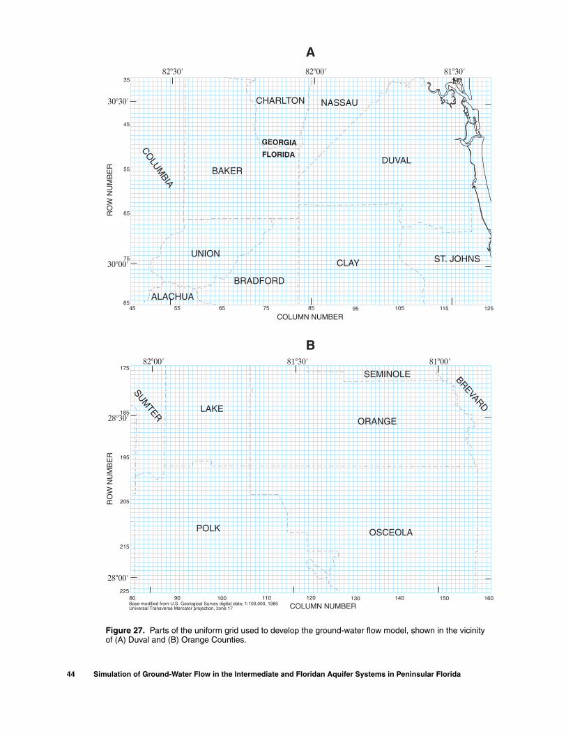
Figure 27. Parts of the uniform grid used to develop the ground-water flow model, shown in the vicinity of (A) Duval and (B) Orange Counties.


Figure 28. Hydrographs showing water-level fluctuations in wells tapping unconfined areas of the Upper Floridan aquifer (gaps indicate data not available; refer to figure 16 for well locations).


Table 9. Differences in water levels measured at wells tapping the unconfined areas of the Upper Floridan aquifer and equipped with continuous water-level recorders[Map location number refers to figure 16; --, data not available]

Map location number

Water level(feet above sea level) Difference

(feet)August 1, 1993 July 31, 1994

1 52.00 52.90 0.90

2 24.16 -- --

3 44.60 45.61 1.01

4 25.96 27.18 1.22

5 23.60 25.03 1.43

6 28.54 28.78 .24

7 21.59 22.49 .90

8 33.61 33.57 -.04

9 21.97 21.84 -.13

10 38.71 39.22 .51

11 33.86 35.52 1.66

12 41.37 41.05 -.32

13 43.18 42.85 -.33

14 2.16 3.56 1.40

15 45.14 45.14 .00

16 45.65 46.27 .62

17 43.32 42.89 -.43

18 10.17 9.60 -.57

19 -- 4.43 --

20 39.28 38.69 -.59

21 5.05 5.11 .06

22 43.18 43.16 -.02

23 31.87 32.13 .26

24 4.10 4.31 .21

25 6.15 6.71 .56

26 26.63 26.30 -.33

27 5.81 6.20 .39

28 14.90 14.98 .08

29 14.35 13.28 -1.07

30 12.97 12.78 -.19

31 10.62 10.60 -.02

32 14.87 14.04 -.83


Conceptual Model

The regional ground-water flow system was sim-ulated as a quasi three-dimensional ground-water flow model with four layers. A challenging aspect of model development was the synthesis of the layering schemes from the local or regional models into a single regional model (figs. 29-36). The SAS, IAS (or ICU in areas where the IAS is absent), the UFA, and the LFA were designated layers 1 through 4, respectively. The SAS (layer 1) was simulated as a source-sink layer. Confin-ing layers were simulated by using vertical leakance arrays, similar to the approach used in models 1-3, 5-7, and 9-14 (table 1). Model-simulated ground-water flow occurs horizontally within the aquifers and vertically through the confining units.

The IAS (layer 2) in southwest and south-central Florida was simulated as a single active aquifer bounded above and below by arrays of leakance values. Outside the areas where the IAS is a productive aquifer, a 1-ft thick layer was used to simulate the transition of the IAS into areas where this aquifer becomes the ICU. A transmissivity value of 0.01 ft2/d was used to simu-late negligible horizontal flow through the ICU. The combination of this low transmissivity and a vertical leakance between the SAS and the ICU equal to the vertical leakance between the ICU and the UFA allowed the ICU to be simulated as a single confining unit. The transmissivity value of 0.01 ft2/d does not necessarily represent the hydraulic conductivity of the ICU in the 1-ft thick layer.

Because this model is restricted to simulating the movement of freshwater within the aquifers, areas where the IAS, the UFA, and the LFA (layers 2-4) con-tain water with chloride concentrations exceeding 5,000 mg/L are considered inactive, thus minimizing potential errors introduced by simulating aquifer areas containing water of variable density. In general, the thickness of the UFA (layer 3) is the difference between the top (fig. 6) and the bottom of the UFA (fig. 7). In areas where chloride concentrations in the UFA are greater than 5,000 mg/L (fig. 19), however, the thick-ness is assumed to be the difference between the top of the UFA (fig. 6) and the base of freshwater. The effec-tive freshwater thickness of the LFA (layer 4) is the dif-ference between the top of the LFA (fig. 8) and either the altitude at which water with chloride concentrations exceeding 5,000 mg/L occur (fig. 19) or the base of the LFA (fig. 10), whichever is higher. Some offshore areas in the UFA, estimated to have chloride concentrations less than 5,000 mg/L, were considered active areas.


Fig

ure

29.

Lay

erin

g sc

hem

e an

d re

pres

enta

tion

of g

eolo

gic

units

in lo

cal m

odel

s 1

and

3, a

nd c

orre

spon

ding

laye

ring

sche

me

in th

e re

gion

al m

odel

(re

fer

to

tabl

e 1

for

mod

el n

umbe

rs).


Fig

ure

30.

Lay

erin

g sc

hem

e an

d re

pres

enta

tion

of g

eolo

gic

units

in lo

cal m

odel

s 2,

7, 1

0, a

nd 1

3, a

nd c

orre

spon

ding

laye

ring

sche

me

in th

e re

gion

al m

odel

(re

fer

to

tabl

e 1

for

mod

el n

umbe

rs).


Fig

ure

31.

Lay

erin

g sc

hem

e an

d re

pres

enta

tion

of g

eolo

gic

units

in lo

cal m

odel

s 4

and

8, a

nd c

orre

spon

ding

laye

ring

sche

me

in th

e re

gion

al m

odel

(re

fer

to ta

ble

1 fo

r m

odel

num

bers

).


Fig

ure

32.

Lay

erin

g sc

hem

e an

d re

pres

enta

tion

of g

eolo

gic

units

in lo

cal m

odel

s 5

and

12, a

nd c

orre

spon

ding

laye

ring

sche

me

in th

e re

gion

al m

odel

(re

fer

to ta

ble

1 fo

r m

odel

num

bers

).


Fig

ure

33.

Lay

erin

g sc

hem

e an

d re

pres

enta

tion

of g

eolo

gic

units

in lo

cal m

odel

6, a

nd c

orre

spon

ding

laye

ring

sche

me

in th

e re

gion

al m

odel

(re

fer

to ta

ble

1 fo

r m

odel

num

ber)

.


Fig

ure

34.

Lay

erin

g sc

hem

e an

d re

pres

enta

tion

of g

eolo

gic

units

in lo

cal m

odel

9, a

nd c

orre

spon

ding

laye

ring

sche

me

in th

e re

gion

al m

odel

(re

fer

to ta

ble

1 fo

r m

odel

nu

mbe

r).


Fig

ure

35.

Lay

erin

g sc

hem

e an

d re

pres

enta

tion

of g

eolo

gic

units

in lo

cal m

odel

11,

and

cor

resp

ondi

ng la

yerin

g sc

hem

e in

the

regi

onal

mod

el (r

efer

to ta

ble

1 fo

r m

odel

num

ber)

.


Fig

ure

36.

Lay

erin

g sc

hem

e an

d re

pres

enta

tion

of g

eolo

gic

units

in lo

cal m

odel

14,

and

cor

resp

ondi

ng la

yerin

g sc

hem

e in

the

regi

onal

mod

el (

refe

r to

tabl

e 1

for

mod

el n

umbe

r).


In offshore areas, water is discharged from the UFA to the SAS, which was simulated with a water table equal to the equivalent freshwater head of the sea water column. The saltwater part of the FAS was not included in the model because the interface is relatively sharp and movement of the interface is assumed to have little or no effect on simulated heads (fig. 9). The assumption was made that a sharp freshwater-saltwater interface occurs laterally and that flow across this interface is negligible. This sharp interface determined which model areas were considered inactive.

Recharge to or discharge from the IAS is assumed to occur through the upper or lower confining units of the IAS. Physiographic regions identified as ridges are simulated with higher leakance values than plains and valley because confining units along ridges are thinner and more permeable. As a result, leakage rates along Lake Wales Ridge, DeLand Ridge, Orlando Ridge, and Crescent City Ridge are higher than those of the Osceola Plain or De Soto Plain (fig. 2). Flow enter-ing or leaving the IAS across the southern or western boundaries of the model is simulated by the difference in hydraulic heads between the IAS and UFA and the vertical leakance of the confining units. Flow entering or leaving the IAS through the northern or eastern boundaries is determined by the water exchanges between the IAS and ICU along these boundaries.

The MCU was represented by vertical leakance values that limit water exchange between the UFA (layer 3) and the LFA (layer 4) in west-central and southwest Florida, and in the northwest part of the study area to a greater degree than in areas where the MSCU is present (fig. 9). However, the rate of water exchange between the UFA and LFA in areas where the MCU is present should not be zero, as suggested by Hickey (1990). The MSCU in east-central, southeast, and northeast Florida was represented by an array of vertical leakance values that allows water exchange between the UFA and the LFA. In areas where no MSCU or MCU is present, the vertical exchange of water between the UFA and the LFA was simulated at a rate that depends on the vertical hydraulic conductivity of the two aqui-fers, which was assumed to be proportional to the horizontal hydraulic conductivity of the aquifers.

The River, Drain, and Recharge packages (Harbaugh and McDonald, 1996) were used in this ground-water flow model. The River package was used to simulate the discharge of water to and from rivers in unconfined areas of the UFA (fig. 23). The discharge of ground water to swamps in unconfined areas of the UFA (fig. 26) and the flow from UFA springs located outside river cells were simulated by using the Drain

package. Flow from springs was simulated as discharge to drain cells using the measured or estimated spring pool altitude as the drain elevation. Flow from UFA springs located in river cells was simulated as the base flow of the river at the respective river cells. The net recharge rates to unconfined areas of the UFA were assigned using the Recharge package.

The solution of the ground-water flow equation (eq. 4) allows areal variations in transmissivity to sim-ulate regional heterogeneities. No estimates of anisot-ropy were available, however, so a lateral anisotropy ratio of 1:1 was assumed.

Boundary Conditions

Model boundaries were assigned to approximate the true ground-water flow system as accurately as possible. The SAS (layer 1) was simulated as a layer of constant heads. This allows the UFA to discharge to the SAS or to receive leakage from the SAS at rates dic-tated by the relative difference in head between the water table and the UFA and the vertical leakance of the ICU in areas where this unit exists. The altitude of the water table was used to define these constant heads. A no-flow boundary condition was applied along all lat-eral boundaries of layer 2 (the IAS or ICU). Flow enter-ing or leaving cells in layer 2 is assumed to occur as either horizontal flow to neighboring cells or vertical flow to either the SAS (layer 1) or the UFA (layer 3).

Lateral boundary conditions for the UFA (layer 3) and the LFA (layer 4) were either no-flow or specified-head. For the UFA (layer 3), a combination of no-flow and specified-head boundaries were used. Along the Gulf of Mexico in Citrus, Hernando, and Pasco Counties, most of the lateral flow in the UFA is assumed to be discharged by numerous springs. Based on this observation, no-flow conditions were applied to the boundary of layer 3 in those areas (fig. 37). For the LFA (layer 4) no-flow conditions were applied along all lateral boundaries. The eastern and western boundaries of the LFA coincided with the location at which the chloride concentration in the LFA exceeds 5,000 mg/L. Specified heads in the UFA along the northeastern boundary of the model, from about 70 mi offshore from Camden County, Ga., to about 20 mi offshore from St. Johns County (fig. 37), were set equal to the equiv-alent freshwater head. The application of this boundary condition limits water exchange between the simulated SAS and the UFA along these boundary cells. Specified heads, interpolated or extrapolated from the 1993-94 potentiometric surface of the UFA, were assigned to the remaining lateral boundaries of the UFA.


Figure 37. Specified heads along the lateral boundary cells of the Upper Floridan aquifer.


Recharge and Discharge

Total discharge from the UFA as spring flow for average 1993-94 conditions was estimated to be approximately 4,130 Mgal/d (appendix C). Additional discharge, in the form of ground-water withdrawals from the IAS, UFA, and LFA for the 1993-94 time period, was estimated to be approximately 2,490 Mgal/d (tables 4 and 5). These withdrawals were applied to the corresponding model cells of their respective aquifers, and the resulting areal distributions are shown in figures 38 through 40. Ground-water withdrawals from the IAS exceeded 0.5 Mgal/d in grid cells in Charlotte, De Soto, Highlands, and Sarasota Counties (fig. 38). Ground-water withdrawals from the UFA exceeded

5 Mgal/d in grid cells in Alachua, Hamilton, Her-nando, Hillsborough, Lake, Manatee, Marion, Nas-sau, Orange, Pasco, Pinellas, and Polk Counties, and in Camden County, Ga (fig. 39). The largest ground-water withdrawals (greater than 5 Mgal/d) from the LFA were in Orange and Duval Counties (fig. 40).

Artificial recharge to the UFA occurs through drainage and injection wells and rapid-infiltration basins. Drainage and injection wells (fig. 21) were simulated as recharge wells at the respective cell locations of the various wells. Recharge rates from drainage and injection wells to the UFA (layer 3) were highest in Orange County (fig. 39). Rapid-infiltration basins were simulated by increased leakance values of the ICU rather than directly applied recharge or injection wells to the UFA.

Figure 38. Average ground-water withdrawal rates from the intermediate aquifer system, August 1993 through July 1994.


Figure 39. Average ground-water withdrawal rates from and injection rates to the Upper Floridan aquifer, August 1993 through July 1994.


Figure 40. Average ground-water withdrawal rates from the Lower Floridan aquifer, August 1993 through July 1994.


Initial Distribution of Hydraulic Properties from Local Models

The initial estimate of transmissivity and lea-kance values for the model area was obtained from the previously calibrated local models (table 1). The model grid developed in this study (fig. 27), referred to as the “regional model grid,” was used as a framework for storing and analyzing transmissivity and leakance val-ues obtained from the local models. The data set of all transmissivity and leakance values from local models was used to generate the initial distribution of these properties and to identify areas of discrepancy where model areas overlap.

The initial distribution of transmissivity and leakance values for the regional model was obtained from local models by overlaying the set of center points and model grid cells of both the regional model and the local models. The center points of the regional model grid cells were intersected with the local model grid cells; transmissivity and leakance assigned by the local models at the center points of the regional model grid were stored in corresponding regional grid cells. In addition, center points of the local model grid cells were intersected with the regional model grid cells; transmissivity and leakance values assigned by the local models at the center points of the local model grid cells also were stored in the corresponding regional grid cells.

Transmissivity of the UFA and leakance values of the ICU from local models 1 and 3 (appendix A2, fig. 29) were stored in the regional model grid. Lea-kance values for the ICU in the regional model in the areas of local models 1 and 3 were computed by multi-plying by 2 the leakance from those models. A factor of 2 was used because the true vertical thickness of the ICU was divided into two units of equal thickness (an upper unit between the SAS and the ICU and a lower unit between the ICU and the UFA). The equivalent leakance of each unit is twice the total leakance of the ICU based on the definition of vertical leakance. The resulting value was applied as the leakance between the SAS and ICU and between the ICU and UFA. This pro-cess was repeated in all models that simulate vertical leakance of the ICU. Consequently, the vertical lea-kance of the ICU in areas outside the IAS, to be used in areas where there is no IAS, should be equal to one-half the simulated vertical leakance in the regional model.

Transmissivity of the IAS and UFA and leakance of the upper and lower confining units of the IAS from


local models 2, 7, 10, and 13 (appendixes A1 and A2; fig. 30) were stored in the regional model grid. Transmissivity of the LFA in these areas, as well as in all areas where flow in the LFA was actively simulated in the regional model but not in the local models, was calculated by multiplying the estimated thickness of the LFA (figs. 8 and 10) by the value of hydraulic conduc-tivity computed from adjacent models.

Transmissivity values for the UFA in west-cen-tral Florida, as well as directly applied net recharge rates to the UFA, were the hydraulic parameters from local models 4 and 8 (appendix A2, fig. 31) stored in the regional model grid. Directly applied net recharge rates to the UFA were bracketed by the ranges shown in figure 25.

Transmissivity values for the UFA and LFA and leakance of the ICU and MSCU in east-central Florida were the hydraulic properties from local models 5 and 12 (fig. 32) that were stored in the regional model grid. The main difference between the layering schemes of models 5 and 12, compared to model 6, was that model 6 simulated the LFA with two layers, the lower of which was a constant-head layer (fig. 33).

Transmissivity values for the UFA and leakance of the ICU were the hydraulic properties from local model 9 that were stored in the regional model grid (fig. 34). The transmissivity values of the UFA in the area encompassed by model 9 were the sum of the model-derived transmissivities for layers 2 and 3 (fig. 34). A study of the simulated hydraulic gradients between layers 2 and 3 of the UFA in model 9 found these gradients to be minimal (Hancock and Basso, 1993; Sepúlveda, 2001); accordingly, layers 2 and 3 were treated in the regional model as a single layer and the assigned leakance between layers 2 and 3 was not used for this study.

The hydraulic properties from local models 11 and 14 stored in the regional model grid were transmis-sivity of the UFA and LFA, and leakance from the ICU and the MSCU (figs. 35 and 36). The areal extent of the IAS in north-central Florida was simulated in the regional model as part of the ICU because the simulated transmissivity in local model 11 for the IAS (Motz, 1995) was characteristic of a confining unit. The simu-lation of the IAS in model 11 coincides with areas where the ICU is present (appendix A1). The transmis-sivity of the FPZ simulated in models 11 and 14 was added to the transmissivity of the LFA only in areas where this zone contains water with chloride concentra-tions less than 5,000 mg/L; otherwise, the FPZ was


excluded from the simulation area (figs. 35 and 36). The main difference between the layering schemes of models 11 and 14 was that model 11 simulated the IAS in parts of north-central Florida as a separate layer, whereas model 14 simulated only the ICU (with verti-cal leakance) because the IAS is absent in northeast Florida.

A regional model grid cell, in an area of overlap-ping local models, for which the transmissivity of the IAS, UFA, or LFA in a local model was either less than one-half or greater than twice the resulting geometric mean of transmissivities from local models, was desig-nated as a cell with a transmissivity discrepancy. The

geometric mean was assumed to give a better estimate of the true mean in heterogeneous media than the arith-metic or harmonic mean (Bouwer, 1978, p. 133). Areas of transmissivity discrepancy in the IAS were found mainly in parts of Charlotte, De Soto, Polk, Manatee, Hardee, and Sarasota Counties (fig. 41). Areas of trans-missivity discrepancy in the UFA were mostly in parts of Marion, Hernando, Lake, Orange, Hillsborough, Hardee, Highlands, Okeechobee, Indian River, and St. Lucie Counties (fig. 42). Areas of transmissivity discrepancy in the LFA were mostly in parts of Alachua, Clay, St. Johns, Putnam, Marion, and Orange Counties (fig. 43).

Figure 41. Cells where transmissivity of the intermediate aquifer system in some local models is either less than one-half or greater than twice the geometric mean of all transmissivities for the same cell.


Figure 42. Cells where transmissivity of the Upper Floridan aquifer in some local models is either less than one-half or greater than twice the geometric mean of all transmissivities for the same cell.


Figure 43. Cells where transmissivity of the Lower Floridan aquifer in some local models is either less than one-half or greater than twice the geometric mean of all transmissivities for the same cell.


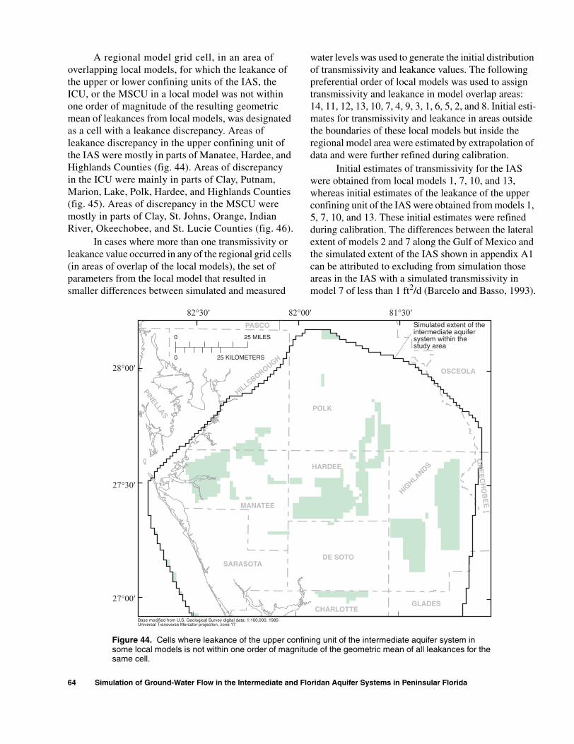
A regional model grid cell, in an area of overlapping local models, for which the leakance of the upper or lower confining units of the IAS, the ICU, or the MSCU in a local model was not within one order of magnitude of the resulting geometric mean of leakances from local models, was designated as a cell with a leakance discrepancy. Areas of leakance discrepancy in the upper confining unit of the IAS were mostly in parts of Manatee, Hardee, and Highlands Counties (fig. 44). Areas of discrepancy in the ICU were mainly in parts of Clay, Putnam, Marion, Lake, Polk, Hardee, and Highlands Counties (fig. 45). Areas of discrepancy in the MSCU were mostly in parts of Clay, St. Johns, Orange, Indian River, Okeechobee, and St. Lucie Counties (fig. 46).

In cases where more than one transmissivity or leakance value occurred in any of the regional grid cells (in areas of overlap of the local models), the set of parameters from the local model that resulted in smaller differences between simulated and measured

water levels was used to generate the initial distribution of transmissivity and leakance values. The following preferential order of local models was used to assign transmissivity and leakance in model overlap areas: 14, 11, 12, 13, 10, 7, 4, 9, 3, 1, 6, 5, 2, and 8. Initial esti-mates for transmissivity and leakance in areas outside the boundaries of these local models but inside the regional model area were estimated by extrapolation of data and were further refined during calibration.

Initial estimates of transmissivity for the IAS were obtained from local models 1, 7, 10, and 13, whereas initial estimates of the leakance of the upper confining unit of the IAS were obtained from models 1, 5, 7, 10, and 13. These initial estimates were refined during calibration. The differences between the lateral extent of models 2 and 7 along the Gulf of Mexico and the simulated extent of the IAS shown in appendix A1 can be attributed to excluding from simulation those areas in the IAS with a simulated transmissivity in model 7 of less than 1 ft2/d (Barcelo and Basso, 1993).

Figure 44. Cells where leakance of the upper confining unit of the intermediate aquifer system in some local models is not within one order of magnitude of the geometric mean of all leakances for the same cell.


Figure 45. Cells where leakance of the intermediate confining unit in some local models is not within one order of magnitude of the geometric mean of all leakances for the same cell.


Figure 46. Cells where leakance of the middle semiconfining unit in some local models is not within one order of magnitude of the geometric mean of all leakances for the same cell.


The distribution of transmissivity for the UFA was initially selected from models 1 through 14 (appendix A2) and was refined during calibration. All local models, except for the one-layer local models 4 and 8, were used to generate the initial estimates of the leakance of the ICU and the lower confining unit of the IAS. A large area in the SRWMD was not simulated by the ground-water flow models shown in appendix A2. The western lateral boundary of the IAS and that of the UFA were assumed to coincide along the Gulf of Mexico, an assumption made because the lack of chloride data precluded mapping the altitude at which 5,000-mg/L concentrations of chloride are present in the Gulf of Mexico. The IAS and UFA share a common western boundary, which is the reason for the differ-ences between the lateral extent of the UFA along the Gulf of Mexico in models 2 and 7 and that simulated in the regional model (appendix A2). Differences between the lateral extent of the simulated area in the regional model and the lateral extent of models 4, 5, and 6 in the Gulf of Mexico and the Atlantic Ocean are due to differences between the grid resolution of these models and that of the regional model grid.

Local models 5, 6, 11, 12, and 14 (appendix A3) were used to generate the initial distribution of trans-missivity of the LFA and the leakance of the MSCU. Large differences between the lateral extent of models 5, 6, and 14 along the Atlantic Ocean and the simulated extent of the LFA (fig. 40) in the regional model are due to the exclusion from simulation of aquifer areas con-taining water with chloride concentrations greater than 5,000 mg/L.

Calibration of Ground-Water Flow Model

Computed average heads in the IAS, UFA, and LFA for the August 1, 1993, to July 31, 1994, steady-state period were the control points used to calibrate the ground-water flow model. The number of control points for the IAS, UFA, and LFA respectively were: 118; 1,460; and 46. The measured or estimated spring flows (appendix C) and base-flow estimates of rivers in the unconfined areas of the UFA also were used for comparison to calibrate the model. No parameter estimation technique was used to achieve model calibration.

Calibration of the regional ground-water flow model was accomplished by adjusting input hydraulic parameters within reasonable ranges from the initial distribution of values until the model closely approxi-

mated observed field conditions based on aquifer heads, spring flows, and river flows. The “goodness” or improvement of the calibration generally is based on the differences between simulated and measured or estimated heads, spring flows, and stream discharges. Simulated heads and flows from a calibrated, determin-istic ground-water model commonly depart from mea-sured heads and flows, even after a diligent calibration effort. The difference between model results and what actually occurs in the aquifers, referred to as model error, is the cumulative result of simplification of the conceptual model, grid scale, measurement errors, and the difficulty in obtaining sufficient measurements to account for all of the spatial variation in hydraulic properties throughout the model area. Calibration was considered to be achieved when the RMS residual for water levels was comparable to the error associated with the time average of measurements used to cali-brate the model, namely the RMS residual associated with the approximation of the altitude of the water table of the SAS (3.53 ft, table 2). The calibration criterion used for spring flows was to be as close as possible to the measured or estimated flow of major springs, as long as none of the hydraulic values used deviated sub-stantially from the initial distribution of values.

Hydraulic parameters that were adjusted during calibration of the ground-water flow model included: the net recharge rate to unconfined areas of the UFA; the transmissivity of the IAS, UFA, and LFA; the river-bed conductance (where the UFA is unconfined); the leakance of the upper and lower confining units of the IAS, ICU, MCU, and MSCU; and the conductance of swamps and springs in the UFA.

The calibration process was iterative and con-sisted of (1) assigning initial hydraulic parameters from local models; (2) comparing simulated and aver-age heads and simulated and estimated spring flows for the steady-state period of 1993-94; and (3) adjusting hydraulic parameters aimed at minimizing the differ-ences between simulated and average heads and between simulated and estimated spring flows for 1993-94. The guiding principle of calibration was that the model parameter with the highest sensitivity for a given area or aquifer was adjusted first; other less sensitive parameters were adjusted only if reasonable residuals were not achieved. In cases where two parameters were about equally sensitive, each was adjusted separately.


The initial distribution of hydraulic parameters from the local model was used to define contiguous zones of equal values. The areal extents of the transmis-sivity zones for the IAS, UFA, and LFA were indepen-dent from each other. The areal extents of the leakance zones for the upper and lower confining units of the IAS, ICU, MCU, and MSCU were also independent from each other. The areal extents of these zones were modified during calibration.

Because measured water levels rarely coincide with the center of a cell, simulated water levels at obser-vation wells were interpolated laterally from simulated heads at the centers of the four cells surrounding the observation well (fig. 47) to allow for a continuous dis-tribution of water levels. The neighboring cells used in the bilinear interpolation were those for which the coor-

dinates of the center of the cells completely encom-passed the coordinates of the observation well (fig. 47). Vertical interpolation was not necessary because of the discontinuity and associated refraction of potential fields across zones of differing transmissivities.

Simulated and measured water levels in the IAS, UFA, and LFA agree reasonably well throughout most of the study area (fig. 48). About 85 percent of simu-lated water levels are within 5 ft of measured values, with RMS values of 3.47, 3.41, and 2.89 ft for the IAS, UFA, and LFA, respectively (table 10). The RMS resid-ual for all layers in the model was 3.40 ft. The histo-gram of residuals for the UFA appears to be normally distributed (fig. 48), indicating the error in the model also is normally distributed.

Figure 47. Bilinear interpolation used to determine simulated water levels at observation wells from simulated water levels at the center of cells.


Figure 48. Comparison of simulated to measured water levels in the (A) intermediate aquifer system, (B) Upper Floridan aquifer, and (C) Lower Floridan aquifer for the calibrated model.


Transmissivity of the Intermediate Aquifer System

The process of modifying the initial transmissiv-ity distribution of the IAS during calibration included: (1) testing all IAS transmissivity values from local models in the discrepancy areas shown in figure 41; (2) finding values that decreased the absolute value of residuals at control points within the discrepancy areas; (3) using recent transmissivity estimates for Sarasota County (Knochenmus and Bowman, 1998); (4) assigning low transmissivity values along the west-ern, eastern, and northern boundaries of the IAS to sim-ulate decreasing aquifer thickness; (5) making limited transmissivity changes in and near areas of potentio-metric-surface highs (fig. 17) to reduce residuals at nearby control points; and (6) making transmissivity changes to areas in the IAS where residuals were unreasonably large and sensitive to changes in transmissivity.

Transmissivity in the IAS from the calibrated model ranged from 100 ft2/d along the northern, east-ern, and western boundaries of the IAS to 30,000 ft2/d in parts of Sarasota County (fig. 49). All transmissivity values for this model were rounded to two significant figures to simplify the calibration process because more significant figures for transmissivity values gen-erally did not result in meaningful changes in simulated water levels. Changes made to the initial distribution of transmissivity of the IAS (fig. 49) generally were small because heads in the IAS were more sensitive to changes in the leakance of the confining units of the IAS.

Transmissivity of the Upper Floridan Aquifer

Substantial changes to the initial distribution of transmissivity of the UFA were required to decrease the absolute value of differences between simulated and

computed average heads for the calibration period. Procedures in addition to those discussed in the previ-ous section for the IAS were required to modify the transmissivity of the UFA during model calibration. The simulation of flow from several springs not included in any of the local models resulted in a higher transmissivity in the vicinity of these springs than the initial values. Steep hydraulic gradients in the potenti-ometric surface of the UFA in some areas needed to be simulated with “barriers” of low transmissivity zones not included in the initial distribution of transmissivity. The effects of replacing specified- or general-head boundaries used in local models with internally simu-lated heads in the regional model generally required changes to the initial transmissivity distribution. The effects of including ground-water withdrawals in areas of the regional model that were not included in local models also required changes to the initial transmissiv-ity distribution for the UFA.

Transmissivity of the UFA from the calibrated model ranged from 3,000 ft2/d in areas where either limestone comprising the aquifer has low permeability or where the UFA is thin to 12,000,000 ft2/d in areas of cavernous limestone near springs. Transmissivity val-ues were low in recharge areas in north-central Lafay-ette County, central Gilchrist County, east-central Bradford County, parts of Levy and Marion Counties, north Lake County, and north-central Volusia County (fig. 50). Areas in the vicinity of springs were given higher transmissivity values than the surrounding areas, which allowed more water to reach the springs. The highest transmissivity values were in the vicinity of Alapaha Rise, Silver Springs, Rainbow Springs, and Crystal River Spring Group (figs. 22 and 50). These springs all had estimated or measured flows in excess of 400 ft3/s (appendix C).

Table 10. Water-level residual statistics for the calibrated model

AquiferNumber of water-level

measurements

Minimum residual

(feet)

Maximum residual

(feet)

Mean residual

(feet)

Root-mean-square

residual(feet)

Intermediate aquifer system

118 -9.62 6.89 -0.18 3.47

Upper Floridan aquifer 1,460 -9.90 9.90 -.19 3.41

Lower Floridan aquifer 46 -6.90 5.21 .17 2.89

Entire model 1,624 -9.90 9.90 -.18 3.40


system from the calibrated model.

Transmissivity of the Lower Floridan Aquifer

The distribution of transmissivity of the LFA from the calibrated model (fig. 51) was generated, in part, by identifying the values that decreased the absolute value of residuals at control points within the discrepancy areas (fig. 43). Simulated transmis-sivity values in Orange, Seminole, and Lake Counties (Brian McGurk, SJRWMD, 2000, written commun.) were evaluated and incorporated in the LFA transmis-sivity distribution in areas where these values decreased the residuals at control points. Transmis-sivity values in west-central Florida and in the north-west areas of the model depended on the thickness of the LFA and the equivalent hydraulic conductivity assigned in adjacent models in east-central Florida (figs. 29-31).

Figure 49. Transmissivity of the intermediate aquifer

Changes to the initial distribution of transmissiv-ity values for the LFA were made in zones where resid-uals at control points were unreasonably large; these changes were of regional scale because of the paucity of water levels available from the LFA. Transmissivity val-ues for the LFA in areally extensive parts of northeast Florida agreed with those used by Durden (1997).

Transmissivity values for the LFA and derived from the calibrated model ranged from 5,000 ft2/d along parts of the lateral boundaries of the LFA to 760,000 ft2/d in northeast Florida. High transmissivity values also were simulated in parts of Orange County and south Florida (fig. 51). Transmissivities are low (5,000 ft2/d) along the lateral boundary of the LFA, reflecting a limited movement of freshwater through a thin part of the aquifer because of proximity to the fresh-water-saltwater interface.


Figure 50. Transmissivity of the Upper Floridan aquifer from the calibrated model.


Figure 51. Transmissivity of the Lower Floridan aquifer from the calibrated model.


Leakance of the Upper Confining Unit of the Intermediate Aquifer System

Prescribing the distribution of the water table of the SAS (as discussed previously) rather than using the water-table altitudes from local models required modi-fying the initial distribution of leakances. Simulated heads in the IAS were sensitive to simulated leakance values of the upper confining unit. Leakance values were adjusted so that the simulated leakage rates were within the range of values of simulated leakage rates in models 7, 10, and 13.

As shown in figure 52, simulated leakance of the upper confining unit of the IAS ranged from 1.0 x 10-6 (ft/d)/ft to 1.4 x 10-3 (ft/d)/ft. These lea-kance values resulted in simulated leakage rates to the IAS that ranged from upward leakage of about 60 in/yr

in parts of Hardee County to downward leakage of about 34 in/yr in parts of Highlands County (fig. 53). Most of Hardee County, however, is a recharge area of the IAS. The highest leakance values are in the Lake Wales Ridge physiographic area (fig. 2), where aquifer recharge is highest and confining beds are relatively thin and permeable (fig. 53). Simulated leakance values within the De Soto Plain physiographic area (fig. 2) that were approximately the same magnitude as those of the Lake Wales Ridge area, resulted in downward vertical leakage rates lower than in the Lake Wales Ridge area (fig. 53). This indicates that the vertical hydraulic gradients between the SAS and the IAS in the Lake Wales Ridge area are higher than those in the De Soto Plain. Large areas of the IAS have simulated ver-tical leakage rates (upward or downward) less than or

Figure 52. Leakance of the upper confining unit of the intermediate aquifer system from the calibrated model.


equal to 1.0 in/yr (fig. 53), resulting from a relatively low leakance value for the upper confining unit of the intermediate aquifer system.

Leakance of the Intermediate Confining Unit

The initial leakance distribution of the ICU was modified in some areas to reduce the simulated down-ward leakage rates to a fraction of the 1993-94 rainfall, except in areas of artificial recharge such as rapid-infil-tration basins. In such areas, leakance values were adjusted so that the simulated leakage rates were within the range of simulated leakage rates for models shown in appendix A1. The range of simulated leakage rates was used to determine the sensitivity of simulated

heads to the vertical leakance values. If changes in leakage rates did not substantially reduce the magni-tude of the residuals, then transmissivity was adjusted.

Simulated leakance values of the ICU ranged from 1.0 x 10-6 (ft/d)/ft to 7.0 x 10-3 (ft/d)/ft (fig. 54). This range of values included simulated leakance values of the lower confining unit of the IAS as an extension of the ICU throughout the simulated extent of the IAS. The largest leakance values were simulated in parts of Orange, Pasco, Hillsborough, and Hardee Counties. The initial leakance values were increased in recharge areas of the UFA to increase simulated water levels as needed to match water levels at control points. In discharge areas of the UFA, leakance values of the

Figure 53. Simulated vertical leakage rates to and from the intermediate aquifer system through the upper confining unit, average August 1993 through July 1994 conditions.


Figure 54. Leakance of the intermediate confining unit and the lower confining unit of the intermediate aquifer system from the calibrated model.


ICU were decreased from initial values to increase sim-ulated heads as needed. Changes in simulated heads in the UFA caused by adjustments to transmissivity values were assessed in separate runs of the model. The main reasons for the spatial variability in leakance values of the ICU are the spatial variability in ICU thick-ness, and in vertical hydraulic gradients between the SAS and the UFA and between the IAS and the UFA (where the IAS is present).

Upward leakage was as high as 80 in/yr in parts of coastal Hillsborough County near Hillsborough Bay, whereas downward leakage was as high as 108 in/yr in southwest Orange County (fig. 55). The largest downward leakage rates to the UFA were simulated in areas where artificial recharge occurs through rapid-infiltration basins (O’Reilly, 1998). Most of the leakage rates to and from the UFA were less than 10 in/yr. High downward leakage rates to the UFA also were simulated in parts of physio-graphic region 4 (fig. 2), particularly along the Lake Wales Ridge region (fig. 55). Simulated leakage rates to the UFA in SFWMD were consistent with previous estimates by Fairbank and Hohner (1995, plate VI).

Leakance of the Middle Confining and Middle Semiconfining Units

The presence or absence of evaporites is the main reason for a marked difference in leakance for the MCU as compared to the MSCU (Miller, 1986). The simulated leakance of the MCU ranged from 6.2 x 10-6 to 1.4 x 10-4 (ft/d)/ft (fig. 56). The largest simulated leakance of the MSCU was 2.0 x 10-3 (ft/d)/ft. As indicated by Hickey (1990), the leakance of the MCU could be as high as 5.0 x 10-4 (ft/d)/ft, assuming a uniform thickness of 200 ft for the MCU and a vertical hydraulic conductivity of 0.1 ft/d. Areas where neither the MCU or the MSCU are present were simulated with larger leakance values than those simulated for the MCU (fig. 56). Leakance values in those areas were derived from the simulated transmissivity of the UFA, the estimated freshwater thickness of the UFA, and an estimated ratio of 100:1 between horizontal and vertical hydraulic conductivity.

Large leakance values also were simulated in areas of strong hydraulic connection between the

UFA and LFA, indicated by the relatively small hydraulic gradients between these two aquifers. These areas include parts of Brevard, Duval, Indian River, Marion, Nassau, and Orange Counties, and Charlton County, Ga. The simulated large leakance values in areas of Baker, Nassau, Duval, and Clay Counties, and Charlton and Ware Counties, Ga., combined with large transmissivities in the LFA for the same areas (fig. 51), could explain the source of water withdrawn from the LFA in discharge areas of Duval County.

The simulated vertical leakage rate in areas where the MCU is present was mostly less than 1.0 in/yr (fig. 57), a consequence of the low simulated lea-kance for the MCU. In contrast, high simulated leak-age to the LFA occurred in parts of Alachua, Clay, Highlands, Lake, Orange, Polk, and Putnam Counties (fig. 57). Some parts of Highlands County, adjacent to the MCU-MSCU transition zone, had simulated downward leakage rates to the LFA that ranged from 5 to 8 in/yr.

Recharge and Discharge Areas of the Upper Floridan Aquifer

Rivers represent a feature where both recharge to and discharge from the UFA can occur. Flow between the aquifer and rivers in unconfined areas of the UFA was simulated using the River package of the MODFLOW-96 River Package (Harbaugh and McDonald, 1996). Simulated flow between the aqui-fer and the river is determined by riverbed conduc-tance and the difference between river stage and the simulated water level in the river cell. The river stage and altitude of the riverbed bottom were assigned by using linear interpolation of measured stages at gaging stations (fig. 58).

Conductance values assigned to riverbed cells depended on the interaction between the UFA and the rivers. The potentiometric surface of the UFA suggests that river-aquifer interactions along the meanderings of the Steinhatchee River, Waccasassa River, and parts of the Withlacoochee and Hillsborough Rivers in west-central Florida is not as strong as the interactions along the Suwan-nee, Santa Fe, and Ichetucknee Rivers, and the Withlacoochee River in Madison County (figs. 18 and 58).


EXPLANATIONVERTICAL LEAKAGE RATE, IN INCHES PER YEAR -- Negative leakage rates indicateupward leakage and positive leakage rates indicate downward leakage

-19.990.013.01

10.01

25.01 - 108.003.0010.00

25.00

--

-

--

-

-10.00-9.99

-80.00 -20.00

0.00

0

0 25

25

50 MILES

50 KILOMETERS

AT

LA

NT

ICO

CE

AN

GU

LF

OF

ME

XIC

O

��

��

��

��

��

��

FLORIDA

GEORGIA

BR

AD

FO

RD

OSCEOLA

BAKER

DUVAL

BR

EV

AR

D

INDIAN

RIVER

ST. LUCIE

MARTIN

OKEECHO

BEE

HIG

HL

AN

DS

GLADES

HARDEE

DE SOTO

CHARLOTTE

SARASOTA

MANATEE

HILLSBOROUGH

PIN

EL

LA

S

PASCO

HERNANDO

CITRUS

ALACHUA

LEVY

DIXIE

GIL

CH

RIS

T

LAFAYETTE

UNION

CO

LUM

BIA

SU

WA

NN

EE

MA

DIS

ON

HAMILTON

WARE

CHARLTON CAMDEN

NASSAU

CLAY ST.JO

HN

S

MARION

PUTNAM

FLAGLER

POLK

SUMTER

LAKE

SEMINOLE

ORANGE

VOLUSIA

HillsboroughBay

Simulated extent of theintermediate confining unitwithin the study area

Simulatedextent of theintermediateaquifer systemwithin thestudy area


Extent ofsimulated area

Figure 55. Simulated vertical leakage rates to and from the Upper Floridan aquifer, average August 1993 through July 1994 conditions.


Figure 56. Leakance of the middle confining and middle semiconfining units from the calibrated model.


Figure 57. Simulated vertical leakage rates to and from the Lower Floridan aquifer through the middle confining and middle semiconfining units, average August 1993 through July 1994 conditions.


Figure 58. Specified stages along the simulated river cells in the unconfined areas of the Upper Floridan aquifer, average August 1993 through July 1994 conditions.


Figure 59. Simulated riverbed conductance of river cells in the unconfined areas of the Upper Floridan aquifer.

82 Simulation of Ground-Water Flow in the Intermediate and Floridan Aquifer Sys

A strong hydraulic connection between the karstic aquifer and a river cell was reflected by a large riverbed conductance. For example, water levels in the UFA near some sections of the Suwannee River are nearly the same as the river stage, supporting the large riverbed con-ductance values. The simulated riverbed conductance of a cell that did not contain a UFA spring gener-ally was lower than that of a cell that contained a spring (fig. 59). The riverbed conductance of a cell with a spring was adjusted based on the estimated or measured spring flow and the head difference between the river stage and the simulated head at the river cell.

A comparison of estimated and simulated base flows of rivers in the unconfined areas of the UFA (table 11) shows that the simulated base flow generally is lower than the estimated base flow. Reasons for this include the fact that riverbank stor-age is not accounted for in the simu-lated base flow. Also, the drainage area for four of the seven rivers is larger than the drainage area of the unconfined simulated sections of the rivers. Finally, the simulated base flow does not reflect the hydraulic routing of discharge from UFA springs and swamps to river cells.

Simulated recharge to and dis-charge from the UFA occurs across lateral boundaries of the model at specified-head cells (fig. 37). Simu-lated hydraulic gradients in the vicin-ity of the boundaries and simulated transmissivity values at the specified head cells determine the flux and direction across these boundaries. Simulated flows leaving or entering the model area along the eastern and most of the northern, southern and western boundaries were less than 1 ft3/s per cell (fig. 60). Water enters the model area at rates equal to

tems in Peninsular Florida

aBased on October 1998 through September 1999 discharge data.bIncludes base flow of Withlacoochee River - SRWMD.cIncludes base flow of Santa Fe River and Withlacoochee River - SRWMD.dIncludes base flow of Ichetucknee River.

Table 11. Estimated and simulated base flow of rivers in the unconfined areas of the Upper Floridan aquifer, average August 1993 through July 1994 conditions

[Station number refers to figure 23. Simulated base flow is flow captured by river cells in unconfined areas of the Upper Floridan aquifer, which generally have a smaller drainage area than the river basins. SRWMD, Suwannee River Water Management District; SWFWMD, Southwest Florida Water Manage-ment District; mi2, square miles; ft3/s, cubic feet per second; --, does not apply or not available]

USGSstation number

Station name Drainage area (mi2)

Average daily discharge

(ft3/s)

Estimated average base

flow (ft3/s)

Simulated base flow

(ft3/s)02303000 Hillsborough River near Zephyrhills 220 123 67 3502312000 Withlacoochee River at Trilby 570 47 25 3002313000 Withlacoochee River near Holder 1,825 319 252 12102313700 Waccasassa River near Gulf Hammock 480 a193 a89 7902319000 Withlacoochee River near Pinetta 2,120 1,714 621 602319500 Suwannee River at Ellaville 6,970 5,961 b1,933 b68302320500 Suwannee River at Branford 7,880 6,678 b3,269 b1,43002322500 Santa Fe River near Fort White 1,017 1,067 925 27502323500 Suwannee River near Wilcox 9,640 9,410 c5,056 c2,50202324000 Steinhatchee River near Cross City 350 205 36 17

-- Unconfined sections of Hillsborough River -- -- -- 68-- Unconfined sections of Withlacoochee River - SWFWMD -- -- -- 92-- Unconfined sections of Withlacoochee River - SRWMD -- -- -- 90-- Ichetucknee River -- -- -- 305-- Unconfined sections of Santa Fe River -- -- -- d 872-- Unconfined sections of Suwannee River -- -- -- c2,585

or greater than 2 ft3/s per cell across a few cells on the northern and western boundaries, and some cells on the southern boundaries in Charlotte County. Flow rates of similar magnitude leave the model area across cells on the northern boundary and in coastal Pinellas County (fig. 60). Flow leaving the model area totaled 462 ft3/s, with 113 ft3/s across the northern boundary, 40 ft3/s across the eastern boundary, 53 ft3/s across the southern boundary, and 256 across the western boundary. Flow entering the model area totaled 317 ft3/s, with the high-est flow rate (151 ft3/s) across the southern boundary and the lowest flow rate (18 ft3/s) across the eastern boundary. Flow entering the model area across the northern boundary totaled 52 ft3/s, whereas 96 ft3/s entered across the western boundary. entering the model area along the Gulf of Mexico (western bound-ary) totaled 5 ft3/s. Flows entering the model area across cells in the Gulf of Mexico and Atlantic Ocean probably are induced by pumping from the UFA near these boundaries (fig. 39).

Mapped recharge and discharge areas were compared with areas in which vertical recharge to and

discharge from the UFA were simulated (fig. 20). Dis-crepancies between the areal distributions of mapped and model-simulated recharge and discharge areas of the UFA (figs. 20 and 61) are isolated throughout the model area and occur mainly at cells where the hydrau-lic gradient between the SAS and the UFA (or the SAS and the IAS) is relatively small. In the unconfined areas of the UFA, discrepancies between mapped and simu-lated recharge and discharge areas occurred at some river and swamp cells. Some swamp cells in Sumter County, mapped as discharge areas, were identified as recharge areas because the simulated net recharge rate at each cell exceeded the simulated flux drained out of the cell.

Simulated net recharge rates to unconfined areas of the UFA were adjusted from a range of values estab-lished by the maximum and minimum recharge rates presented previously (fig. 25), average water levels, and spring flow. Net recharge rates are high near areas where the water table is deep, as is the case in the Northern Highlands region (fig. 2), and generally decrease coastward where evapotranspiration is high.


Figure 60. Simulated lateral flow to and from the Upper Floridan aquifer across model boundaries, average August 1993 through July 1994 conditions.


Figure 61. Location of differences between simulated and estimated recharge and discharge cells in the Upper Floridan aquifer, average August 1993 through July 1994 conditions.


Net recharge rates to the aquifer, which ranged from 0 to 24 in/yr (fig. 62), were rounded off to integers. Cells with specified heads along lat-eral boundaries of the UFA were not assigned recharge rates (fig. 62). The highest recharge rate, 24 in/yr, was simulated in parts of Suwannee and Columbia Counties. The average of all net recharge rates was about 13.6 in/yr for 6,364 cells in the uncon-fined areas of the UFA (approximately 5,700 mi2). Total recharge to uncon-fined areas of the UFA was about 5,720 ft3/s.

Spring Flow

Flow from springs (fig. 22) located outside river cells was simu-lated by drain cells; flow from springs in river cells was simulated as the flow from the aquifer to the river (fig. 59). Spring-pool elevation (table 12) was used as the drain-cell elevation. The simulated spring-pool elevation of springs in river cells was the com-puted river stage of the cell. Con-ductance at either drain or river cells was adjusted to reduce the differ-ence between estimated or measured and simulated spring flow.

Of the 156 springs in the study area, 130 had flows simulated with a residual (difference between mea-sured or estimated and simulated flow) of less than 5 ft3/s; 11 spring flows were simulated with a residual between 5 and 10 ft3/s; 10 spring flows were simulated with a residual between 10 and 20 ft3/s; and 5 had residuals greater than 20 ft3/s. The largest residuals occurred at springs simulated as river cells. Simulated flows at Blue Springs and Alapaha Rise (springs 1 and 2, respectively, fig. 22) were underestimated by about 28 and 54 ft3/s, respectively (table 12). Simulated spring flow was 96 per-cent of the total estimated 6,380 ft3/s spring flow for 1993-94.

86 Simulation of Ground-Water Flow in the

Figure 62. Simulated recharge rates to the unconfined areas of the Upper Floridan aquifer, average August 1993 through July 1994 conditions.

Intermediate and Floridan Aquifer Systems in Peninsular Florida

Table 12. Comparison of measured or estimated and residual flows from Upper Floridan aquifer springs, average August 1993 through July 1994 conditions[Spring number refers to figure 22. Row and column refer to model grid. Flows from springs in the same row and column were combined. River cells: WNW, Withlacoochee River in northwest Florida; WWC, Withlacoochee River in west-central Florida; SUR, Suwannee River; ICH, Ichetucknee River; STR, Steinhatchee River; SFR, Santa Fe River; WAC, Waccasassa River; and HIR, Hillsborough River. Springs simulated as river cells are indicated by the name of the nearest river; drain, indicates spring was simulated as drain cell. Residual flow is simulated flow minus measured or estimated flow; ft3/s, cubic feet per second]

Spring number Spring name Row Column River

cell

Measured or

estimated flow

(ft3/s)

Residual flow

(ft3/s)

Pool elevation or river stage (feet)

1 Blue Spring near Madison 41 7 WNW 118.0 -28.2 42.02 Alapaha Rise near Fort Union 44 17 SUR 427.0 -54.1 36.23 Holton Spring near Fort Union 44 19 drain 12.5 .0 38.34 Suwannee Springs near Live Oak 47 27 SUR 9.8 5.2 41.55, 6 Suwanacoochee Spring and Ellaville Spring at Ellaville 48 12 SUR 112.0 -.8 33.07 Falmouth Spring at Falmouth 49 14 drain 134.0 7.8 32.58 White Sulphur Springs at White Springs 52 37 drain 42.3 11.1 50.09 Charles Springs near Dell 63 8 drain 4.7 -.1 24.510 Allen Mill Pond Spring near Dell 64 7 SUR 12.2 -1.1 23.811 Wadesboro Spring near Orange Park 65 103 drain 1.0 .1 24.012 Blue Spring near Dell 66 8 SUR 70.0 -16.0 23.613 Peacock Springs 67 14 drain 81.1 .4 19.014 Telford Spring at Luraville 68 12 SUR 35.8 -3.8 21.615 Running Springs (East and West) near Luraville 68 15 SUR 88.0 -.4 19.916 Convict Spring near Mayo 69 16 SUR 1.1 .2 19.617 Royal Spring near Alton 70 17 SUR 1.9 -.3 19.018 Owens Spring 72 19 SUR 43.3 -1.2 17.419 Mearson Spring near Mayo 73 20 SUR 51.0 -1.2 17.020 Troy Spring near Branford 75 22 SUR 132.0 -18.3 16.021 Little River Springs near Branford 76 24 SUR 67.0 -7.8 14.922 Ruth Spring near Branford 76 23 drain 7.5 .1 16.523 Green Cove Springs at Green Cove Springs 77 106 drain 3.0 .1 21.024, 25 Ichetucknee Head Spring near Fort White and Cedar Head

Spring 77 37 drain 49.0 6.9 22.0

26-29 Blue Hole, Roaring, Singing, Boiling, Mill Pond, Grassy Hole, and Coffee Springs (parts of Ichetucknee Springs)

78 37 ICH 258.0 .5 19.0

30 Branford Springs at Branford 79 26 SUR 35.8 -5.3 13.231 Jamison Spring 81 37 drain 3.0 .0 16.532 Hornsby Spring near High Springs 87 48 drain 49.8 1.3 30.533, 34 Turtle Spring near Hatchbend and Fletcher Spring 87 29 SUR 61.9 -10.1 9.335 Steinhatchee Spring near Clara 87 2 STR .7 .5 21.136 Ginnie Spring near High Springs 88 41 SFR 57.1 -.9 23.337 Blue Springs near High Springs (including Lilly Springs) 89 42 drain 41.2 .3 24.538 Poe Springs near High Springs 89 44 SFR 53.6 -.3 26.339 Rock Bluff Springs near Bell 91 27 SUR 33.2 -7.2 9.040 Guaranto Spring near Rock Bluff Landing 92 26 SUR 12.0 -1.6 7.941 Crescent Beach Submarine Spring 94 135 drain 30.0 12.6 0.5


42, 43 Lumbercamp Springs and Sun Springs near Wannee 97 26 drain 46.3 -1.7 4.044 Hart Springs near Wilcox 100 25 drain 90.8 -2.0 4.245 Otter Springs near Wilcox 102 25 drain 16.0 -.3 2.046 Whitewater Springs 103 107 drain 1.2 .2 23.547 Copper Springs near Oldtown (including Little Copper

Spring)104 23 SUR 25.4 -6.8 4.7

48 Bell Springs 105 25 drain 5.1 -.1 2.049 Fannin Springs near Wilcox (including Little Fannin

Spring)106 26 drain 97.7 -.3 .5

50 Satsuma Spring 111 106 drain 1.1 .0 18.051 Blue Springs near Orange Springs 112 94 drain .5 .0 31.052 Orange Spring at Orange Springs 112 89 drain 2.0 -.5 54.553 Camp Seminole Spring at Orange Springs 113 88 drain .8 -.4 54.554 Welaka Spring near Welaka 114 106 drain 1.0 -1.0 11.055 Manatee Spring near Chiefland 113 23 drain 187.0 -9.3 2.856 Mud Spring near Welaka 116 106 drain 2.3 .2 8.357 Blue Spring near Bronson 116 40 WAC 8.0 -.5 38.458 Beecher Springs near Fruitland 117 107 drain 6.3 .0 2.059 Croaker Hole Spring near Welaka 118 105 drain 90.3 1.5 6.860 Tobacco Patch Landing Spring Group near Fort McCoy 118 90 drain 1.0 .0 30.861 Wells Landing Springs near Fort McCoy 119 90 drain 5.0 -.1 30.862 Salt Springs near Eureka 124 102 drain 79.0 .3 1.863 Wekiva Springs near Gulf Hammock 129 43 drain 45.4 -.2 24.564 Silver Glen Springs near Astor 132 108 drain 100.0 -21.2 1.965 Sweetwater Springs along Juniper Creek 134 106 drain 12.5 2.5 7.066 Silver Springs near Ocala 134 81 drain 640.0 -19.7 40.067, 68 Morman Branch Seepage into Juniper Creek and Juniper

Creek Tributary near Astor136 107 drain 3.0 3.3 14.0

69, 70 Juniper Springs and Fern Hammock Springs near Ocala 136 103 drain 18.8 -10.9 23.571 Ponce de Leon Springs near De Land 140 125 drain 24.3 -.6 4.072 Rainbow Springs near Dunnellon 142 57 drain 637.0 -16.6 30.8

73 Alexander Springs near Astor 144 112 drain 113.0 -10.6 10.574 Mosquito Springs Run, Alexander Springs Wilderness 147 121 drain 2.0 -.6 16.075 Wilson Head Spring near Holder 151 64 WWC 1.9 .5 29.476 Blue Spring near Holder 151 65 WWC 10.6 .1 29.777 Gum Springs near Holder 152 70 drain 67.6 3.5 35.578 Camp La No Che Springs near Paisley 153 114 drain 1.0 -.3 41.379 Blue Spring near Orange City 153 127 drain 135.0 -8.9 2.5

Table 12. Comparison of measured or estimated and residual flows from Upper Floridan aquifer springs, average August 1993 through July 1994 conditions--Continued[Spring number refers to figure 22. Row and column refer to model grid. Flows from springs in the same row and column were combined. River cells: WNW, Withlacoochee River in northwest Florida; WWC, Withlacoochee River in west-central Florida; SUR, Suwannee River; ICH, Ichetucknee River; STR, Steinhatchee River; SFR, Santa Fe River; WAC, Waccasassa River; and HIR, Hillsborough River. Springs simulated as river cells are indicated by the name of the nearest river; drain, indicates spring was simulated as drain cell. Residual flow is simulated flow minus measured or estimated flow; ft3/s, cubic feet per second]


cell

Measured or

estimated flow

(ft3/s)

Residual flow

(ft3/s)



80 Blackwater Springs near Cassia 158 117 drain 1.4 -1.4 38.581 Crystal River Spring Group 157 46 drain 613.2 50.6 1.582 Little Jones Creek Head Spring near Wildwood 159 79 drain 8.0 .1 42.083 Green Springs 160 133 drain .3 .0 17.084 Gemini Springs near DeBary (all 3) 160 129 drain 10.5 -.8 2.885 Little Jones Creek Spring No. 2 near Wildwood 160 79 drain 5.0 .0 42.086 Messant Spring near Sorrento 160 117 drain 12.0 -.6 30.087 Seminole Springs near Sorrento 161 115 drain 37.0 -22.5 40.088 Palm Springs Seminole State Forest 161 120 drain .5 .2 28.589 Little Jones Creek Spring No. 3 near Wildwood 161 80 drain 3.0 .0 43.090 Droty Springs near Sorrento 162 116 drain .6 -.6 39.091 Halls River Head Spring 162 47 drain 4.8 -.2 1.592 Island Spring near Sanford 162 122 drain 6.4 .0 16.093 Halls River Springs 163 46 drain 102.2 .5 1.594-96 Homosassa Springs, Southeast Fork of Homosassa

Springs, and Trotter Spring at Homosassa Springs164 47 drain 120.7 .8 1.5

97 Fenney Springs near Coleman, Head Spring of Shady Brook Creek

164 82 drain 15.0 -3.0 48.0

98, 99 Shady Brook Creek Springs No. 2 and 3 165 82 drain 5.8 .0 44.5100 Shady Brook Creek Spring No. 4 166 80 drain 2.9 .1 46.0101 Sulphur Camp Springs 166 116 drain .6 -.1 34.0102 Hidden River Springs near Homosassa (including Hidden

River Head Spring)166 47 drain 6.7 -.1 2.0

103 Rock Springs near Apopka 167 116 drain 53.0 -1.5 26.5104 Shady Brook Creek Spring No. 5 167 79 drain 2.9 .2 47.0105 Bugg Spring at Okahumpka 167 91 drain 8.6 -.1 63.0106, 108 Blue Springs near Yalaha and Holiday Springs at Yalaha 168 96 drain 6.6 -1.9 65.0107 Mooring Cove Springs near Yalaha 168 95 drain .4 -.4 68.5109 Potter Spring near Chassahowitzka (including Ruth

Spring)168 46 drain 14.4 -.2 1.5

110 Witherington Spring near Apopka 169 117 drain 1.0 .0 32.0111 Salt Creek Head Spring 169 47 drain .4 .0 1.5112 Lettuce Creek Spring 169 48 drain 3.7 -.1 2.5113, 115 Crab Creek Spring and Chassahowitzka Springs near

Chassahowitzka170 48 drain 99.6 -.3 1.5

114, 119 Unnamed Tributary above Chassahowitzka Springs and Baird Creek Head Spring near Chassahowitzka

170 47 drain 23.7 .0 1.5

116 Wekiwa Springs in State Park near Apopka 171 119 drain 56.5 -.9 13.5117 Miami Springs near Longwood 171 120 drain 4.0 -.1 15.0



cell

Measured or

estimated flow

(ft3/s)

Residual flow

(ft3/s)



118 Lake Jesup Spring near Wagner 171 131 drain .6 .6 32.0120 Clifton Springs near Oviedo 172 133 drain 1.5 .9 30.0121 Starbuck Spring near Longwood 172 124 drain 12.3 -.2 23.0122 Beteejay Lower Spring near Chassahowitzka (including

Beteejay Head Spring)171 46 drain 7.3 .0 1.8

123, 125 Palm Springs and Sanlando Springs near Longwood 172 123 drain 22.6 .0 23.0124 Rita Maria Spring near Chassahowitzka 171 47 drain 3.3 .0 2.0126, 127 Unnamed Spring No. 10, 11, 12, Ryle Creek Lower

Spring, and Ryle Creek Head Spring near Bayport172 45 drain 27.3 1.0 1.5

128 Blue Run Head Spring near Chassahowitzka 172 46 drain 4.6 .0 1.2129 Double Run Road Seepage near Astatula 173 101 drain 2.0 .1 67.0130 Unnamed Spring No. 8 173 44 drain 4.9 .2 1.5131 Blind Creek Springs (including unnamed spring No. 7 and

Blind Creek Head Spring)174 44 drain 42.7 -15.1 1.3

132 Apopka (Gourdneck) Spring near Oakland 181 105 drain 31.4 -1.2 69.0133 Unnamed Spring No. 6 182 44 drain 2.8 .0 1.5134, 135 Salt Spring and Mud Spring near Bayport 182 45 drain 39.3 -1.5 1.5136, 137 Jenkins Creek Spring No. 5 and Unnamed Spring No. 4 184 44 drain 21.6 -.1 1.5138 Weeki Wachee Springs near Brooksville 184 48 drain 129.0 1.9 9.8139 Unnamed Spring No. 2 188 43 drain .7 .0 8.0140, 142, 143

Boat Spring, Unnamed Spring No. 1, and Magnolia Springs at Aripeka

190 42 drain 7.2 .0 1.5

141 Bobhill Springs 190 43 drain 1.8 .0 8.0144 Unnamed Spring No. 3 near Aripeka 193 41 drain 17.8 -1.4 1.5145 Horseshoe Spring near Hudson 193 40 drain 9.7 -3.5 .5146 Salt Springs near Port Richey 200 38 drain 8.2 2.3 1.0147 Crystal Springs near Zephyrhills 209 72 HIR 37.0 -5.1 52.0148 Sulphur Springs at Sulphur Springs 220 55 drain 25.0 -.5 5.0149 Lettuce Lake Spring 221 61 drain 8.3 -.4 14.5150, 151 Six-Mile Creek Spring and Eureka Springs near Tampa 221 62 drain 2.6 -.1 14.5152 Buckhorn Spring near Riverview 230 64 drain 15.0 -3.1 10.0153, 154 Lithia Springs Minor and Lithia Springs Major near Lithia 232 69 drain 39.1 -5.0 9.5155 Little Salt Spring near Murdock 289 68 drain .9 .0 25.0156 Warm Mineral Springs near Woodmere 290 67 drain 6.7 -.1 6.0

Totals 6,383.8 -224.7



cell

Measured or

estimated flow

(ft3/s)

Residual flow

(ft3/s)



Potentiometric Surfaces

The simulated potentiometric surface of the IAS for the average August 1993 through July 1994 condi-tions generally reflects the main features of the esti-mated potentiometric surface of the IAS (figs. 17 and 63). The potentiometric-surface highs in southwest and south-central Polk County were reasonably simulated, as were the decreasing heads west and south of the potentiometric highs. A potentiometric-surface high was simulated in northwest Highlands County; there were an insufficient number of measured water levels to determine whether this high in the estimated potentio-metric surface exists. The RMS residual between

simulated and computed heads in the IAS was 3.47 ft, with differences ranging from -9.62 ft in Charlotte County to 6.89 ft in Sarasota County. About 85 percent of the water-level measurements in the IAS were simu-lated within 5 ft. The largest residuals in the IAS were located in the parts of Charlotte, Sarasota, and De Soto Counties (figs. 17 and 63).

The simulated potentiometric surface of the UFA for 1993-94 replicated the main features of the estimated potentiometric surface (figs. 18 and 64). Both simulated and estimated potentiometric surfaces of the UFA show the potentiometric highs in Lafayette, Gilchrist, northwest Putnam, southeast Levy, central Volusia, east-central and west-central Pasco, and north-central Polk Counties.

Figure 63. Simulated potentiometric surface of the intermediate aquifer system, average August 1993 through July 1994 conditions.


Figure 64. Simulated potentiometric surface of the Upper Floridan aquifer, average August 1993 through July 1994 conditions.


The simulated surface shows the depressions present in numerous areas across the Florida peninsula. Ground-water flow in the UFA was simulated reasonably well by the model, including the locations of the main recharge and discharge areas of the UFA. The RMS residual between simulated and computed heads in the UFA was 3.41 ft, with differences ranging from -9.90 ft in Manatee County to 9.90 ft in Camden County, Ga. About 85 percent of water-level measurements in the UFA were simulated within 5 ft.

The RMS residual between simulated and com-puted heads in the LFA for 1993-94 was 2.89 ft, with differences ranging from -6.90 ft in Okeechobee County to 5.21 ft in Orange County. About 91 percent of the water-level measurements in the LFA were simulated within 5 ft (fig. 65). Differences in heads between the UFA and the LFA (figs. 64 and 65) in areas where the MSCU is present are smaller than in areas where the aquifers are separated by the MCU, implying that the hydraulic gradients between the two aquifers are deter-mined mainly by the permeability of the intervening confining unit. Small differences in heads exist between the two aquifers in areas where no MCU or MSCU is present.

Ground-Water Flow Budget

Volumetric flow rates simulated in the IAS, UFA, and LFA were computed to quantify contributions of each component of the ground-water flow system (fig. 66). Separate net flow rates were computed for the unconfined and confined areas of the UFA. Spring flow represented the largest discharge flux in the model area (4,559 ft3/s simulated from drain cells and 1,600 ft3/s from river cells). The second largest discharge was from water withdrawals from all aquifers (3,860 ft3/s). Total recharge to the UFA, from both net recharge to the unconfined areas and from leakage through the IAS-ICU layer, was 11,855 ft3/s.

Sensitivity Analyses

Sensitivity analyses were conducted to assess the response of simulated heads to specified changes in selected model parameters. Those parameters consid-ered for sensitivity analysis included the transmissivities of the IAS, UFA, and LFA; the leakances of the upper confining unit of the IAS, the ICU, and the MSCU; the net recharge rate to unconfined areas of the UFA; and the specified heads along segments of lateral boundaries

of the UFA. Parameters were varied from the values used to achieve calibration in order to assess the response of simulated heads to changes in model param-eters. The RMS errors of the differences between simu-lated and computed heads were used as the criterion to assess the effects of changes made to parameter values used in the calibrated model.

The effect each parameter had on simulation results was assessed by varying independently from 0.2 to 2.0 times the values of transmissivity and net recharge rates, from 0.5 to 1.5 times the specified heads along lat-eral boundaries of the UFA, and from 0.01 to 10.0 times the leakance values (fig. 67). These ranges of values may not include all the uncertainties associated with some of the parameters; the ranges were aimed at pro-viding a perspective on parameter sensitivity.

The sensitivity analyses indicated that simulated heads were sensitive to changes in specific ranges of values for leakance and transmissivity. Simulated heads were more sensitive to changes in leakance values of the upper confining unit of the IAS, the ICU, and the MSCU between 1.0 x 10-5 and 1.0 x 10-3 (ft/d)/ft than to changes in leakance values either less than 1.0 x 10-5 or greater than 1.0 x 10-3 (ft/d)/ft (fig. 67). Simulated heads were sensitive to all transmissivity value ranges tested for the UFA. Simulated heads were more sensi-tive to changes in transmissivity values of the LFA greater than 100,000 ft2/d than to changes in transmissivities less than or equal to 100,000 ft2/d. Changes in net recharge rates to unconfined areas of the UFA of 10 in/yr or greater caused larger RMS residuals than changes to rates less than 10 in/yr. Changes in RMS residuals were not sensitive to changes in transmissivity values of the IAS or to changes in specified heads in the UFA (fig. 67).

Effects of Projected 2020 Ground-Water Withdrawals

The calibrated model was used to evaluate the potential effects of projected 2020 ground-water with-drawals on water levels in the IAS, UFA, and LFA and on spring flow from the UFA. Boundary conditions sim-ulating the greatest and smallest possible drawdowns that could occur were used to bracket the effects of projected 2020 withdrawals.


Figure 65. Simulated potentiometric surface of the Lower Floridan aquifer, average August 1993 through July 1994 conditions.


Figure 66. Simulated volumetric flow budget for the intermediate aquifer system, Upper Floridan aquifer, and Lower Floridan aquifer, average August 1993 through July 1994 conditions.


Figure 67. Model sensitivity to changes in selected model parameters.


Projected 2020 Ground-Water Withdrawals and

Artificial Recharge

Projected ground-water withdrawals from the IAS, UFA, and LFA for 2020 were estimated from the Water-Supply Assessment plans of the SJRWMD, SFWMD, SWFWMD, SRWMD (St. Johns River Water Management District, 1998; South Florida Water Management District, 1998; Southwest Florida Water Management District, 1998; Suwannee River Water Management District, 1998), water-use data for 1995, and USGS data. Measured and estimated pumping rates from wells in SWFWMD for 1995 were provided by SWFWMD (Tabitha Ostow, written commun., 2000). Water-use data from wells in SRWMD for 1995 were provided by SRWMD (Ronald Ceryak, written commun., 1999). Projected 2020 water-use data for municipal well fields in SJRWMD and SFWMD were estimated by the water-supply utilities, whereas other uses in SJRWMD and SFWMD were estimated from com-piled 1995 water-use data from files of the SJRWMD, SFWMD, and USGS; and the Water-Supply Assessment plans. Projected 2020 withdrawal estimates were based on projected population increases from 1995 to 2020 and projected changes in water use trends.

Projected 2020 ground-water withdrawals for public-water supply, industrial and commercial, agricultural, and self-supplied domestic uses totaled 96 Mgal/d from the IAS; 2,989 Mgal/d from the UFA; and 308 Mgal/d from the LFA (table 13). These totals represent increases from 1993-94 water withdrawals of 33, 34, and 62 percent from the IAS, UFA, and LFA, respectively (tables 4 and 13). Orange County had the largest projected increase in withdrawals, from 211 Mgal/d in 1993-94 to 391 Mgal/d in 2020 (tables 4 and 13). The smallest increase, from 3.65 to 4.82 Mgal/d, was projected for Union County. Pro-jected self-supplied domestic water use for 2020 was calculated based on 1995 estimates by Marella (1999) and by using multipliers for each county based on pro-jected population increases. Projected ground-water withdrawals from self-supplied domestic wells in the IAS and UFA were approximately 17 and 196 Mgal/d, respectively (table 13).

Projected increases in withdrawal rates from the respective aquifers vary from one part of the study area to another. Ground-water withdrawals from the IAS are expected to increase from 72 Mgal/d in 1993-94 to 96 Mgal/d in 2020. The most substantial increases are projected in central Glades, northeast Charlotte, and west-central Sarasota Counties (figs. 38 and 68). Smaller increases are anticipated for north-central Sarasota and west-central Polk Counties. Ground-water withdrawals from the UFA are antici-pated to increase from 2,226 Mgal/d in 1993-94 to 2,989 Mgal/d in 2020. In particular, total projected withdrawals in Orange, Seminole, and Volusia Coun-ties are estimated to increase from 289 Mgal/d in 1993-94 to 485 Mgal/d in 2020 (tables 4 and 13). Pro-jected increases in withdrawals from the UFA in St. Lucie and Duval Counties were 13 and 27 Mgal/d, respectively, from 1993-94 to 2020 rates. No signifi-cant increases in ground-water withdrawals are antic-ipated in southwest, south-central, northwest, or north-central Florida (figs. 39 and 69). Ground-water withdrawals from the LFA are anticipated to increase from 190 Mgal/d in 1993-94 to 308 Mgal/d in 2020 (tables 4 and 13). Projected withdrawals from the LFA in Orange and Duval Counties are expected to increase in 2020 by 69 and 21 Mgal/d, respectively, from 1993-94 rates (tables 4 and 13); increases in cen-tral Orange County and central Duval County are particularly apparent (figs. 40 and 70). Smaller increases are projected for Lake and Highlands Counties.

Recharge to the UFA from drainage wells for 2020 was estimated, assuming rainfall was equal to the 1961-90 average at NOAA stations near drainage wells (figs. 3 and 21), by using the weighted-average runoff coefficient of 0.478, and the procedure pre-sented previously to calculate 1993-94 rates. Recharge from drainage wells was estimated to be about 62 Mgal/d (table 14). Recharge to the UFA through injection wells for 2020 in Alachua County was assumed to be 10.62 Mgal/d, the same as for the calibration period. The amount of recharge to the UFA from drainage wells is largely dependent on rainfall, but recharge from injection wells could increase with population. No relation, however, has been estab-lished that could be used to estimate recharge to the UFA from injection wells due to population increases.


Table 13. Projected 2020 ground-water withdrawals and uses, by county and by Water Management District, from the intermediate aquifer system, Upper Floridan aquifer, and Lower Floridan aquifer[Source: St. Johns River Water Management District (SJRWMD); South Florida Water Management District (SFWMD); Southwest Florida Water Manage-ment District (SWFWMD); Suwannee River Water Management District (SRWMD); and US Geological Survey. All rates are in million gallons per day; -- indicates no wells are tapping the aquifer or aquifer is absent]

County

Intermediate aquifer system Upper Floridan aquifer Lower Floridan aquiferPublic- water

supply

Industrial and

commerciala

aIncludes mining, thermoelectric power generation, recreational, and landscape irrigation uses.

Agricul-tural

Domes-tic

Public- water

supply

Industrial and

commercialaAgricul-

turalDomes-

tic

Public- water

supply

Industrial and

commercialaAgricul-

tural

Alachua -- -- -- -- 39.97 7.46 24.52 9.16 -- -- --Baker -- -- -- -- 1.22 .31 .24 1.55 0.55 -- 0.12Bradford -- -- -- -- 5.33 3.57 2.64 2.54 -- -- --Brevard -- -- -- -- 8.09 1.02 10.51 .16 -- -- --Charlotte 0.03 0.16 17.85 1.76 .56 -- 5.47 -- -- -- --Citrus -- -- -- -- 18.97 7.05 1.39 12.03 -- -- --Clay -- -- -- -- 4.39 3.68 1.90 3.46 15.40 0.51 --Columbia -- -- -- -- 7.03 4.43 14.42 6.96 -- -- --DeSoto 2.03 .59 6.96 .79 1.01 .22 60.43 .03 -- -- --Dixie -- -- -- -- 2.87 1.46 8.45 1.87 -- -- --Duval -- -- -- -- 45.80 21.70 2.80 .04 89.76 16.92 .33Flagler -- -- -- -- 5.00 .11 4.69 .11 -- -- --Gilchrist -- -- -- -- 4.33 .63 43.20 2.05 -- -- --Glades -- -- 9.48 .02 .80 -- 13.66 -- -- -- .19Hamilton -- -- -- -- 18.24 14.93 19.52 1.39 -- -- --Hardee .17 .12 6.86 .71 2.88 2.28 48.59 .02 -- -- --Hernando -- -- -- -- 31.74 20.30 2.81 4.71 -- -- --Highlands .56 .30 15.14 .36 14.16 3.12 120.42 .02 -- .14 25.49Hillsborough .02 .01 .69 .76 79.38 18.32 76.05 13.00 -- -- --Indian River -- -- -- -- 20.96 .07 34.94 .06 -- -- --Lafayette -- -- -- -- 2.61 .42 16.96 1.27 -- -- --Lake -- -- -- -- 90.11 25.55 40.65 2.25 3.54 .56 .53Levy -- -- -- -- 5.65 6.03 62.99 5.62 -- -- --Madison -- -- -- -- .38 .37 11.17 .23 -- -- --Manatee .31 .39 1.76 3.61 18.52 1.96 93.30 .04 -- -- --Marion -- -- -- -- 41.73 5.10 10.60 30.92 .01 -- .04Martin -- -- -- -- 5.06 .58 10.58 -- -- -- --Nassau -- -- -- -- 11.50 29.24 2.62 .09 -- 1.29 --Okeechobee -- -- -- -- 1.19 .71 32.68 .05 -- -- .49Orange -- -- -- -- 207.34 15.85 17.93 19.85 128.81 1.31 .15Osceola -- -- -- -- 30.44 1.95 54.81 11.32 9.04 -- .02Palm Beach -- -- -- -- 1.38 -- -- -- -- -- --Pasco -- -- -- -- 115.58 11.86 18.26 11.07 -- -- --Pinellas -- -- -- -- 43.28 2.04 .58 6.11 -- -- --Polk .71 .82 4.11 1.25 103.69 76.27 127.23 8.51 .72 -- .61Putnam -- -- -- -- 4.24 8.80 11.57 10.27 -- 1.09 --St. Johns -- -- -- -- 17.49 .02 29.20 1.39 -- -- --St. Lucie -- -- -- -- 12.58 .39 13.26 .43 -- -- --Sarasota 8.76 .96 .41 7.40 30.08 4.80 4.76 .06 -- -- --Seminole -- -- -- -- 86.99 .36 6.71 6.56 10.44 -- --Sumter -- -- -- -- 4.18 2.92 11.66 5.58 -- -- --Suwannee -- -- -- -- 8.09 4.55 81.55 4.99 -- -- --Union -- -- -- -- 1.57 .14 2.11 1.00Volusia -- -- -- -- 94.79 1.27 18.14 8.94 -- .18 .01Camden, Ga. -- -- -- -- 3.52 49.82 .20 -- -- -- --Charlton, Ga. -- -- -- -- 1.01 -- -- -- -- -- --Total 12.59 3.35 63.26 16.66 1,255.73 361.67 1,176.17 195.71 258.27 22.00 27.98Water Management DistrictSJRWMD -- -- -- -- 615.96 103.59 193.62 75.43 196.13 20.58 1.16SFWMD -- .02 20.90 .40 102.36 16.07 234.40 18.81 62.14 1.42 26.82SWFWMD 12.59 3.33 42.36 16.26 474.83 151.39 471.92 69.43 -- -- --SRWMD -- -- -- -- 62.58 90.62 276.23 32.04 -- -- --

Interme-diate

aquifer system

Upper Floridan aquifer

Lower Floridan aquifer

Total by

aquifer

Public- water

supply

Industrial and

commercial

Agricul-tural

Domes-tic

Total by

use

Total 95.86 2,989.28 308.25 3,393.39 1,526.59 387.02 1,267.41 212.37 3,393.39


Figure 68. Projected 2020 ground-water withdrawal rates from the intermediate aquifer system.

Simulated 2020 Scenarios and Boundary Conditions

Specified heads interpolated from the estimated potentiometric-surface map (fig. 18) were applied along the lateral boundaries of the UFA for the 1993-94 steady-state calibration. Increased withdrawals in 2020 could potentially affect heads along the lateral bound-aries of the model. Fluxes across the lateral boundaries may increase due to projected increases in withdrawals.

Consequently, conditions in 2020 were brack-eted by simulating two scenarios, one with specified 1993-94 lateral boundary heads and another with spec-ified 1993-94 lateral boundary fluxes. The 1993-94

specified-head boundaries allowed as much water as was needed to enter the model area to maintain heads at the boundaries for projected 2020 conditions, which may not be realistic and could have underestimated drawdowns. Specified-head boundaries can be regarded as the best-case drawdown scenario for 2020 simulations. On the other hand, the 1993-94 specified-flux boundaries limited the flow of water across the boundary to the rates for 1993-94 conditions. Increased withdrawals result in lower water levels because no additional flow is allowed to enter the model area across the lateral boundaries to supply water needed to support additional withdrawals. Specified-flux bound-aries can be regarded as the worst-case drawdownscenario for 2020 simulations.


Figure 69. Projected 2020 ground-water withdrawal rates from and injection rates to the Upper Floridan aquifer.


Figure 70. Projected 2020 ground-water withdrawal rates from the Lower Floridan aquifer.


The 1993-94 water-table altitude was used for the 2020 simulations by again modeling the SAS as a constant-head layer. This assumption allowed for induced increases in vertical leakage to the UFA result-ing from projected pumping increases. Simulated net recharge rates to unconfined areas of the UFA in 2020 were assumed to be equal to the 1993-94 calibrated rates, which is consistent with applying the altitude of the SAS from 1993-94 for the 2020 simulations.

As with the 1993-94 simulation, no-flow boundary conditions were imposed along the lateral boundaries of the IAS or ICU and LFA layers for 2020 simulations. Similarly, no-flow boundaries in the UFA established along coastal Citrus, Hernando, and Pasco Counties during model calibration also were applied for the 2020 simulations.

Projected 2020 Drawdowns

Simulated 2020 drawdowns (compared to 1993-94 heads) were computed at each model grid cell for each aquifer layer. Very few cells had increases in water levels from 1993-94 conditions, and therefore, were not shown in the drawdown maps. The greatest water level increase was 2 ft.

A projected drawdown of 20 ft in the IAS poten-tiometric surface for 2020 was simulated in central Glades County (fig. 71), regardless of which lateral boundary condition was used for the UFA. In that area, withdrawals are projected to increase substantially from 1993-94 to 2020. Drawdowns of 12 and 14 ft were simulated in west-central Sarasota County and west-central Polk County, respectively. Very little dif-ference was observed between the simulated IAS heads for the two lateral boundary conditions used for the UFA (specified-head and specified-flux).

The two scenarios for simulating boundary con-ditions in the UFA (specified-head and specified-flux) had relatively the same effect on simulated water levels in some areas of the model. For example, a drawdown of 10 ft was simulated in central Orange County using either method; however, the extent of the 10-ft draw-down area was greater for the specified-flux condition. The same was true for the 6-ft drawdown in Seminole, Osceola, and Duval Counties. In western Polk County, the maximum drawdown for the specified-flux scenario was 6 ft, whereas the maximum for the specified-head scenario was 4 ft. Drawdowns of 4 ft were projected in an areally extensive part of northeast Florida, and in northeast Volusia, west-central Polk, and central Manatee Counties. No substantial projected draw-downs were simulated in the northwest and west-central parts of the model area (fig. 72), due to relatively small projected increases in ground-water withdrawals from the UFA.

Simulated drawdowns in the southeastern part of the model area (St. Lucie and Okeechobee Counties) were much more sensitive to the lateral boundary con-ditions in the UFA. A projected drawdown of 12 ft was simulated in the UFA in parts of St. Lucie County with the specified-flux boundary, compared to simulated drawdowns of only 2 ft with the specified-head bound-ary (fig. 72). A low transmissivity combined with a relatively large increase in ground-water withdrawals, as is the case in St. Lucie County, results in larger draw-downs, whereas high transmissivity combined with a small increase in ground-water withdrawals results in smaller drawdowns, as is the case in Marion County.

The largest projected drawdown in the potentio-metric surface of the LFA for 2020 was simulated in Orange County (fig. 73) using either of the two lateral boundary conditions for the UFA. A drawdown of 10 ft extends through the central part of Orange County for the specified-flux boundary condition, whereas a max-imum drawdown of 8 ft was simulated using the specified-head boundary. Drawdowns up to 8 ft also extend into parts of Osceola and Seminole Counties for both lateral boundary conditions. For both boundary conditions, a drawdown of 4 ft extends through a large area in Duval County, with a maximum of 6 ft simulated for specified-flux conditions. Simulated drawdowns in the potentiometric surfaces of the UFA and LFA in Orange and Duval Counties were consistent with projected increases in ground-water withdrawals from these aquifers. No substantial projected

Table 14. Projected 2020 recharge rates for drainage wells to the Upper Floridan aquifer by county

[Source: CH2M Hill, 1997; Bradner, 1996; Phelps, 1987. Rates, in million gallons per day, are rounded to integers]

County Recharge

Alachua 11Marion 5Orange 39Putnam 1Seminole 1Suwannee 5

Total 62


downs from average August 1993 through July 1994

drawdowns were simulated in the northwest and west-central parts of the model area (fig. 73) owing to the absence of ground-water withdrawals from the LFA.

Upward flow from the LFA to the UFA is less in the southeastern part of the model for the specified-head lateral boundary condition in the UFA, as com-pared to the specified-flux boundary condition. Simu-lation with the specified-flux lateral boundary results in drawdowns of 6 ft extending through a large area in the

Figure 71. Simulated intermediate aquifer system drawconditions to projected 2020 conditions.

southeastern part of the model area. The simulation of the specified-head lateral boundary condition results in drawdowns of only 2 ft for the same area (fig. 73). A no-flow condition along the lateral boundary of the LFA, combined with the fact that no water is withdrawn from the LFA in the southeast part of the model area (fig. 70), indicates that the projected draw-down in the LFA was due solely to increased upward flow from the LFA to the UFA.


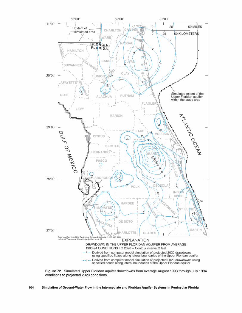
Figure 72. Simulated Upper Floridan aquifer drawdowns from average August 1993 through July 1994 conditions to projected 2020 conditions.


Figure 73. Simulated Lower Floridan aquifer drawdowns from average August 1993 through July 1994 conditions to projected 2020 conditions.


Projected 2020 River and Spring Flow

The Hillsborough, Waccasassa, Steinhatchee, and Withlacoochee Rivers had minor changes in simu-lated base flow from 1993-94 to 2020 (table 15). The reduction in base flow for 2020 in the Suwannee and Santa Fe Rivers of about 4 percent compared to 1993-94 conditions can be attributed solely to projected increases in ground-water withdrawals because no other hydraulic properties changed from the calibrated model for 1993-94 conditions. There were no signifi-cant differences between 2020 base flows of rivers in unconfined areas of the UFA simulated with specified-flux lateral boundaries in the UFA (table 15) and the base flows simulated with specified-head lateral boundaries.

Simulated 2020 spring flows at 145 of the 156 UFA springs were within 10 ft3/s of the 1993-94 flows. Simulated flows at Manatee Spring and Silver

Springs decreased by more than 20 ft3/s relative to simulated 1993-94 flows (fig. 22; table 16). This is a decrease of 16 percent for Manatee Spring and 8 per-cent for Silver Springs. Simulated flows at Blue Spring near Orange City, Rock Springs, Apopka Spring, and Weeki Wachee Springs decreased between 15 and 17 ft3/s relative to simulated 1993-94 flows because of projected increases in ground-water withdrawals in 2020. Total simulated spring flow for the specified-flux boundary condition was about 20 ft3/s less than that simulated with the specified-head boundary condition. Total simulated spring flow for 2020 for the worst-case drawdown scenario was about 5,800 ft3/s, which was 94 percent of the simulated spring flow for 1993-94 (table 16). In the confined areas of the UFA, simulated spring flow for 2020 decreased 14 percent from the 1993-94 simulated flow, whereas spring flow decreased 5 percent in the unconfined areas.

Table 15. Projected 2020 base flow of rivers in the unconfined areas of the Upper Floridan aquifer for specified-flux boundary conditions[Station number refers to figure 23. Simulated base flow is flow captured by river cells in unconfined areas of the Upper Floridan aquifer, which generally have a smaller drainage area than the river basins; difference in base flow is simulated 2020 base flow minus simulated 1993-94 base flow. SRWMD, Suwannee River Water Management District; SWFWMD, Southwest Florida Water Management District; mi2, square miles; ft3/s, cubic feet per second; --, does not apply or not available]

USGSstation number

Station nameDrainage

area (mi2)

Simulated 2020

base flow (ft3/s)

Simulated 1993-94

base flow (ft3/s)

Difference in

base flow (ft3/s)

02303000 Hillsborough River near Zephyrhills 220 35 35 0

02312000 Withlacoochee River at Trilby 570 32 30 2

02313000 Withlacoochee River near Holder 1,825 115 121 -6

02313700 Waccasassa River near Gulf Hammock 480 77 79 -2

02319000 Withlacoochee River near Pinetta 2,120 5 6 -1

02319500 Suwannee River at Ellaville 6,970 a660 a683 -23

02320500 Suwannee River at Branford 7,880 a1,386 a1,430 -44

02322500 Santa Fe River near Fort White 1,017 266 275 -9

02323500 Suwannee River near Wilcox 9,640 b2,420 b2,502 -82

02324000 Steinhatchee River near Cross City 350 17 17 0

-- Unconfined sections of Hillsborough River -- 69 68 1

-- Unconfined sections of Withlacoochee River - SWFWMD -- 86 92 -6

-- Unconfined sections of Withlacoochee River - SRWMD -- 83 90 -7

-- Ichetucknee River -- 298 305 -7

-- Unconfined sections of Santa Fe River -- c851 c872 -21

-- Unconfined sections of Suwannee River -- b2,494 b2,585 -91aIncludes base flow of Withlacoochee River - SRWMD.bIncludes base flow of Santa Fe River and Withlacoochee River - SRWMD.cIncludes base flow of Ichetucknee River.


Table 16. Comparison of simulated 2020 and simulated August 1993 through July 1994 flow of Upper Floridan aquifer springs for specified-flux boundary conditions[Spring number refers to figure 22. Row and column refer to model grid. Flows from springs in the same row and column are combined. River cells: WNW, Withlacoochee River in northwest Florida; WWC, Withlacoochee River in west-central Florida; SUR, Suwannee River; ICH, Ichetucknee River; STR, Steinhatchee River; SFR, Santa Fe River; WAC, Waccasassa River; and HIR, Hillsborough River. Springs simulated as river cells are indicated by the name of the nearest river; drain, indicates spring was simulated as drain cell; flow difference is simulated 2020 flow minus simulated 1993-94 flow; ft3/s, cubic feet per second]


cell

Simulated2020 flow

( ft3/s)

Simulated1993-94

flow (ft3/s)

Flow difference

( ft3/s)

1 Blue Spring near Madison 41 7 WNW 85.2 89.8 -4.62 Alapaha Rise near Fort Union 44 17 SUR 366.1 372.9 -6.83 Holton Spring near Fort Union 44 19 drain 11.9 12.5 -.64 Suwannee Springs near Live Oak 47 27 SUR 14.0 14.9 -.9

5, 6 Suwanacoochee Spring and Ellaville Spring at Ellaville 48 12 SUR 108.1 111.2 -3.17 Falmouth Spring at Falmouth 49 14 drain 138.2 141.8 -3.68 White Sulphur Springs at White Springs 52 37 drain 45.1 53.5 -8.49 Charles Springs near Dell 63 8 drain 4.5 4.6 -.1

10 Allen Mill Pond Spring near Dell 64 7 SUR 10.9 11.1 -.211 Wadesboro Spring near Orange Park 65 103 drain .0 1.1 -1.112 Blue Spring near Dell 66 8 SUR 53.4 54.0 -.613 Peacock Springs 67 14 drain 79.8 81.5 -1.714 Telford Spring at Luraville 68 12 SUR 31.3 32.0 -.715 Running Springs (East and West) near Luraville 68 15 SUR 84.4 87.6 -3.216 Convict Spring near Mayo 69 16 SUR 1.3 1.3 .017 Royal Spring near Alton 70 17 SUR 1.5 1.6 -.118 Owens Spring 72 19 SUR 40.6 42.1 -1.519 Mearson Spring near Mayo 73 20 SUR 48.0 49.8 -1.820 Troy Spring near Branford 75 22 SUR 110.5 113.7 -3.221 Little River Springs near Branford 76 24 SUR 57.5 59.2 -1.722 Ruth Spring near Branford 76 23 drain 7.2 7.6 -.423 Green Cove Springs at Green Cove Springs 77 106 drain 1.6 3.1 -1.5

24, 25 Ichetucknee Head Spring near Fort White and Cedar Head Spring

77 37 drain 50.6 55.9 -5.3

26-29 Blue Hole, Roaring, Singing, Boiling, Mill Pond, Grassy Hole, and Coffee Springs (parts of Ichetucknee Springs)

78 37 ICH 252.4 258.5 -6.1

30 Branford Springs at Branford 79 26 SUR 29.7 30.4 -.731 Jamison Spring 81 37 drain 3.0 3.0 .032 Hornsby Spring near High Springs 87 48 drain 48.1 51.1 -3.0

33, 34 Turtle Spring near Hatchbend and Fletcher Spring 87 29 SUR 50.3 51.8 -1.535 Steinhatchee Spring near Clara 87 2 STR 1.2 1.2 .036 Ginnie Spring near High Springs 88 41 SFR 54.5 56.2 -1.737 Blue Springs near High Springs (including Lilly Springs) 89 42 drain 40.4 41.5 -1.138 Poe Springs near High Springs 89 44 SFR 51.7 53.3 -1.639 Rock Bluff Springs near Bell 91 27 SUR 23.7 26.0 -2.340 Guaranto Spring near Rock Bluff Landing 92 26 SUR 9.7 10.4 -.741 Crescent Beach Submarine Spring 94 135 drain 37.3 42.6 -5.3

42, 43 Lumbercamp Springs and Sun Springs near Wannee 97 26 drain 42.6 44.6 -2.044 Hart Springs near Wilcox 100 25 drain 80.3 88.8 -8.545 Otter Springs near Wilcox 102 25 drain 15.0 15.7 -.746 Whitewater Springs 103 107 drain .5 1.4 -.947 Copper Springs near Oldtown (including Little Copper Spring) 104 23 SUR 15.6 18.6 -3.048 Bell Springs 105 25 drain 4.5 5.0 -.549 Fannin Springs near Wilcox (including Little Fannin Spring) 106 26 drain 87.1 97.4 -10.350 Satsuma Spring 111 106 drain 1.0 1.1 -.151 Blue Springs near Orange Springs 112 94 drain .5 0.5 .052 Orange Spring at Orange Springs 112 89 drain .9 1.5 -.653 Camp Seminole Spring at Orange Springs 113 88 drain .1 .4 -.354 Welaka Spring near Welaka 114 106 drain .0 .0 .055 Manatee Spring near Chiefland 113 23 drain 149.6 177.7 -28.1


56 Mud Spring near Welaka 116 106 drain 2.3 2.5 -.257 Blue Spring near Bronson 116 40 WAC 6.2 7.5 -1.358 Beecher Springs near Fruitland 117 107 drain 6.3 6.3 .059 Croaker Hole Spring near Welaka 118 105 drain 90.4 91.8 -1.460 Tobacco Patch Landing Spring Group near Fort McCoy 118 90 drain 1.0 1.0 .061 Wells Landing Springs near Fort McCoy 119 90 drain 4.6 4.9 -.362 Salt Springs near Eureka 124 102 drain 78.8 79.3 -.563 Wekiva Springs near Gulf Hammock 129 43 drain 44.4 45.2 -.864 Silver Glen Springs near Astor 132 108 drain 78.4 78.8 -.465 Sweetwater Springs along Juniper Creek 134 106 drain 14.9 15.0 -.166 Silver Springs near Ocala 134 81 drain 570.7 620.3 -49.6

67, 68 Morman Branch Seepage into Juniper Creek and Juniper Creek Tributary near Astor

136 107 drain 6.2 6.3 -.1

69, 70 Juniper Springs and Fern Hammock Springs near Ocala 136 103 drain 7.8 8.0 -.271 Ponce de Leon Springs near De Land 140 125 drain 23.2 23.7 -.572 Rainbow Springs near Dunnellon 142 57 drain 606.6 620.4 -13.873 Alexander Springs near Astor 144 112 drain 101.1 102.3 -1.274 Mosquito Springs Run, Alexander Springs Wilderness 147 121 drain .9 1.4 -.575 Wilson Head Spring near Holder 151 64 WWC 2.2 2.4 -.276 Blue Spring near Holder 151 65 WWC 10.4 10.7 -.377 Gum Springs near Holder 152 70 drain 67.6 71.1 -3.578 Camp La No Che Springs near Paisley 153 114 drain .0 .7 -.779 Blue Spring near Orange City 153 127 drain 110.5 126.1 -15.680 Blackwater Springs near Cassia 158 117 drain .0 .0 .081 Crystal River Spring Group 157 46 drain 650.5 663.8 -13.382 Little Jones Creek Head Spring near Wildwood 159 79 drain 7.2 8.1 -.983 Green Springs 160 133 drain .0 .3 -.384 Gemini Springs near DeBary (all 3) 160 129 drain 7.8 9.8 -2.085 Little Jones Creek Spring No. 2 near Wildwood 160 79 drain 4.6 5.0 -.486 Messant Spring near Sorrento 160 117 drain 10.4 11.4 -1.087 Seminole Springs near Sorrento 161 115 drain 6.1 14.5 -8.488 Palm Springs Seminole State Forest 161 120 drain .0 .7 -.789 Little Jones Creek Spring No. 3 near Wildwood 161 80 drain 2.8 3.0 -.290 Droty Springs near Sorrento 162 116 drain .0 .0 .091 Halls River Head Spring 162 47 drain 4.6 4.7 -.192 Island Spring near Sanford 162 122 drain 4.9 6.4 -1.593 Halls River Springs 163 46 drain 101.0 102.7 -1.7

94-96 Homosassa Springs, Southeast Fork of Homosassa Springs, and Trotter Spring at Homosassa Springs

164 47 drain 119.6 121.5 -1.9

97 Fenney Springs near Coleman, Head Spring of Shady Brook Creek

164 82 drain 10.7 12.0 -1.3

98, 99 Shady Brook Creek Springs No. 2 and 3 165 82 drain 5.7 5.8 -.1100 Shady Brook Creek Spring No. 4 166 80 drain 2.8 3.0 -.2101 Sulphur Camp Springs 166 116 drain .0 .5 -.5102 Hidden River Springs near Homosassa (including Hidden

River Head Spring)166 47 drain 6.5 6.6 -.1

103 Rock Springs near Apopka 167 116 drain 35.7 51.5 -15.8104 Shady Brook Creek Spring No. 5 167 79 drain 2.9 3.1 -.2105 Bugg Spring at Okahumpka 167 91 drain 6.2 8.5 -2.3

106, 108 Blue Springs near Yalaha and Holiday Springs at Yalaha 168 96 drain .0 4.7 -4.7

Table 16. Comparison of simulated 2020 and simulated August 1993 through July 1994 flow of Upper Floridan aquifer springs for specified-flux boundary conditions--Continued[Spring number refers to figure 22. Row and column refer to model grid. Flows from springs in the same row and column are combined. River cells: WNW, Withlacoochee River in northwest Florida; WWC, Withlacoochee River in west-central Florida; SUR, Suwannee River; ICH, Ichetucknee River; STR, Steinhatchee River; SFR, Santa Fe River; WAC, Waccasassa River; and HIR, Hillsborough River. Springs simulated as river cells are indicated by the name of the nearest river; drain, indicates spring was simulated as drain cell; flow difference is simulated 2020 flow minus simulated 1993-94 flow; ft3/s, cubic feet per second]


cell

Simulated2020 flow

( ft3/s)

Simulated1993-94

flow (ft3/s)

Flow difference

( ft3/s)


107 Mooring Cove Springs near Yalaha 168 95 drain .0 .0 .0109 Potter Spring near Chassahowitzka (including Ruth Spring) 168 46 drain 14.0 14.3 -.3110 Witherington Spring near Apopka 169 117 drain .1 1.0 -.9111 Salt Creek Head Spring 169 47 drain .4 .4 .0112 Lettuce Creek Spring 169 48 drain 3.5 3.6 -.1

113, 115 Crab Creek Spring and Chassahowitzka Springs near Chassahowitzka

170 48 drain 97.9 99.3 -1.4

114, 119 Unnamed Tributary above Chassahowitzka Springs and Baird Creek Head Spring near Chassahowitzka

170 47 drain 23.4 23.7 -.3

116 Wekiwa Springs in State Park near Apopka 171 119 drain 43.0 55.6 -12.6117 Miami Springs near Longwood 171 120 drain 2.9 3.9 -1.0118 Lake Jesup Spring near Wagner 171 131 drain .0 1.2 -1.2120 Clifton Springs near Oviedo 172 133 drain .0 2.4 -2.4121 Starbuck Spring near Longwood 172 124 drain 5.9 12.1 -6.2122 Beteejay Lower Spring near Chassahowitzka (including

Beteejay Head Spring)171 46 drain 7.2 7.3 -.1

123, 125 Palm Springs and Sanlando Springs near Longwood 172 123 drain 11.5 22.6 -11.1124 Rita Maria Spring near Chassahowitzka 171 47 drain 3.2 3.3 -.1

126, 127 Unnamed Spring No. 10, 11, 12, Ryle Creek Lower Spring, and Ryle Creek Head Spring near Bayport

172 45 drain 27.9 28.3 -.4

128 Blue Run Head Spring near Chassahowitzka 172 46 drain 4.6 4.6 .0129 Double Run Road Seepage near Astatula 173 101 drain .0 2.0 -2.0130 Unnamed Spring No. 8 173 44 drain 5.1 5.1 .0131 Blind Creek Springs (including unnamed spring No. 7 and

Blind Creek Head Spring)174 44 drain 27.3 27.6 -.3

132 Apopka (Gourdneck) Spring near Oakland 181 105 drain 13.9 30.2 -16.3133 Unnamed Spring No. 6 182 44 drain 2.8 2.8 .0

134, 135 Salt Spring and Mud Spring near Bayport 182 45 drain 37.2 37.8 -.6136, 137 Jenkins Creek Spring No. 5 and Unnamed Spring No. 4 184 44 drain 21.0 21.6 -.6

138 Weeki Wachee Springs near Brooksville 184 48 drain 115.6 130.9 -15.3139 Unnamed Spring No. 2 188 43 drain .6 .7 -.1

140, 142, 143

Boat Spring, Unnamed Spring No. 1, and Magnolia Springs at Aripeka

190 42 drain 7.0 7.2 -.2

141 Bobhill Springs 190 43 drain 1.6 1.8 -.2144 Unnamed Spring No. 3 near Aripeka 193 41 drain 16.0 16.4 -.4145 Horseshoe Spring near Hudson 193 40 drain 6.1 6.2 -.1146 Salt Springs near Port Richey 200 38 drain 9.8 10.5 -.7147 Crystal Springs near Zephyrhills 209 72 HIR 31.9 31.9 .0148 Sulphur Springs at Sulphur Springs 220 55 drain 23.9 24.5 -.6149 Lettuce Lake Spring 221 61 drain 7.5 7.8 -.3

150, 151 Six-Mile Creek Spring and Eureka Springs near Tampa 221 62 drain 2.4 2.5 -.1152 Buckhorn Spring near Riverview 230 64 drain 10.1 11.9 -1.8

153, 154 Lithia Springs Minor and Lithia Springs Major near Lithia 232 69 drain 30.0 34.1 -4.1155 Little Salt Spring near Murdock 289 68 drain .1 .9 -.8156 Warm Mineral Springs near Woodmere 290 67 drain 5.3 6.6 -1.3

Total 5,796.6 6,159.4 -362.8

Table 16. Comparison of simulated 2020 and simulated August 1993 through July 1994 flow of Upper Floridan aquifer springs for specified-flux boundary conditions--Continued[Spring number refers to figure 22. Row and column refer to model grid. Flows from springs in the same row and column are combined. River cells: WNW, Withlacoochee River in northwest Florida; WWC, Withlacoochee River in west-central Florida; SUR, Suwannee River; ICH, Ichetucknee River; STR, Steinhatchee River; SFR, Santa Fe River; WAC, Waccasassa River; and HIR, Hillsborough River. Springs simulated as river cells are indicated by the name of the nearest river; drain, indicates spring was simulated as drain cell; flow difference is simulated 2020 flow minus simulated 1993-94 flow; ft3/s, cubic feet per second]


cell

Simulated2020 flow

( ft3/s)

Simulated1993-94

flow (ft3/s)

Flow difference

( ft3/s)


Projected 2020 Ground-Water Flow Budget

A comparison of the projected flow budget for 2020 to 1993-94 conditions showed a reduction in spring flow for 2020 in both confined and unconfined areas of the UFA, mainly due to projected increases in ground-water withdrawals in the UFA. An increase in projected ground-water withdrawals in the confined areas of the UFA of 946 ft3/s induced an increase in net downward leakage from the IAS or ICU layer to the UFA layer of 937 ft3/s, almost equal to the increase in water withdrawals (figs. 66 and 74). Total recharge to the UFA, in the form of both net recharge or net down-ward leakage through the IAS or ICU layer, was 12,792 ft3/s, an increase of about 8 percent from 1993-94 conditions. Changes in net flow across the uncon-fined-confined boundary of the UFA (fig. 5) were not significant because net simulated flow to unconfined areas from confined areas decreased only 3 percent in 2020 from 1993-94 conditions (figs. 66 and 74).

MODEL LIMITATIONS

Some of the limiting factors of the ground-water flow model presented in this report are: simplifications in the conceptual model, inherent model assumptions, lack of water-level and flow measurements in areas where spatial variability of hydraulic and hydrologic properties is poorly known, and inaccuracies in land-surface altitude measurements. Model simulations are based on the assignment of hydraulic properties to grid cells, the use of specified heads in the UFA along lateral boundaries of the model, the grid resolution, the esti-mated average water table and Floridan aquifer heads, the estimated ground-water withdrawals, and the assumption of steady-state conditions in the Floridan aquifer for 1993-94. An error in any of these can limit the accuracy of model simulations.

Ground-water flow simulations generally are based on conceptual models that are simplified repre-sentations of complex heterogeneous ground-water flow systems. Assumptions such as isotropy, vertical homogeneity within each layer, and the absence of preferential flow zones are examples of simplified rep-resentations that can be sources of error in a ground-water flow model. The lack of sufficient measurements to account for the spatial variation of hydraulic proper-ties throughout the model area necessitated these sim-plifications. Simplifying the model does not invalidate

110 Simulation of Ground-Water Flow in the Intermediate and

model results, although model results should be inter-preted at scales larger than the representative grid cell.The ground-water flow equation solved by the model (equation 4) is the continuity equation for flow derived from the principal of conservation of mass and the assumptions that water is incompressible and of con-stant viscosity, incorporated with Darcy’s law (Bouwer, 1978, p. 202). This equation is valid for ground-water flow conditions where the velocity of ground water is low and flow is laminar. In karstic terrains, it is possible for flow through caverns and solution channels to be turbulent. Thus, the equation is not valid for the entire Floridan aquifer system. Sim-plifications made in this study were the assumptions that laminar flow was everywhere and that effective transmissivity was uniform throughout each grid cell of the model such that mass is conserved, along with known hydraulic gradients.

Inaccuracies inherent in the algorithm used to estimate the water table distribution or the estimated potentiometric surface of the UFA, such as lack of data and residual errors, could lead to errors in the delinea-tion of recharge or discharge areas. In turn, these inac-curacies can lead to inaccuracies in leakance and leakage rates among the SAS, IAS or ICU, and UFA.

The assumption of constant water levels in areas where the SAS is present may introduce error into the model. Temporal changes in the water table of the SAS would bring temporal changes in leakage rates between the SAS and the IAS or ICU. In particular, in the vicin-ity of some cells, induced leakage due to large ground-water withdrawals from the UFA could cause these cells to go dry. Simulating active cells in the SAS, how-ever, was beyond the scope of this study. The water table of the SAS was generated for a year when total rainfall was nearly equal to the overall 30-year average rainfall computed from NOAA rainfall stations. The estimated water table for the SAS in this study should be modified for local or regional ground-water flow studies for which simulation periods correspond to hydrologic conditions that deviate from average rainfall conditions.

The assumption of uniform heads throughout the vertical thickness of each grid cell is another possible source of error in the simulated heads. Vertical hydrau-lic gradients between the SAS and the UFA suggest that simulated heads in the ICU could represent, at best, a value within the range of heads observed throughout the thickness of the ICU. The simulated heads in the ICU should be interpreted as an interpolation from the hydraulic gradients between the SAS and the UFA.

Floridan Aquifer Systems in Peninsular Florida

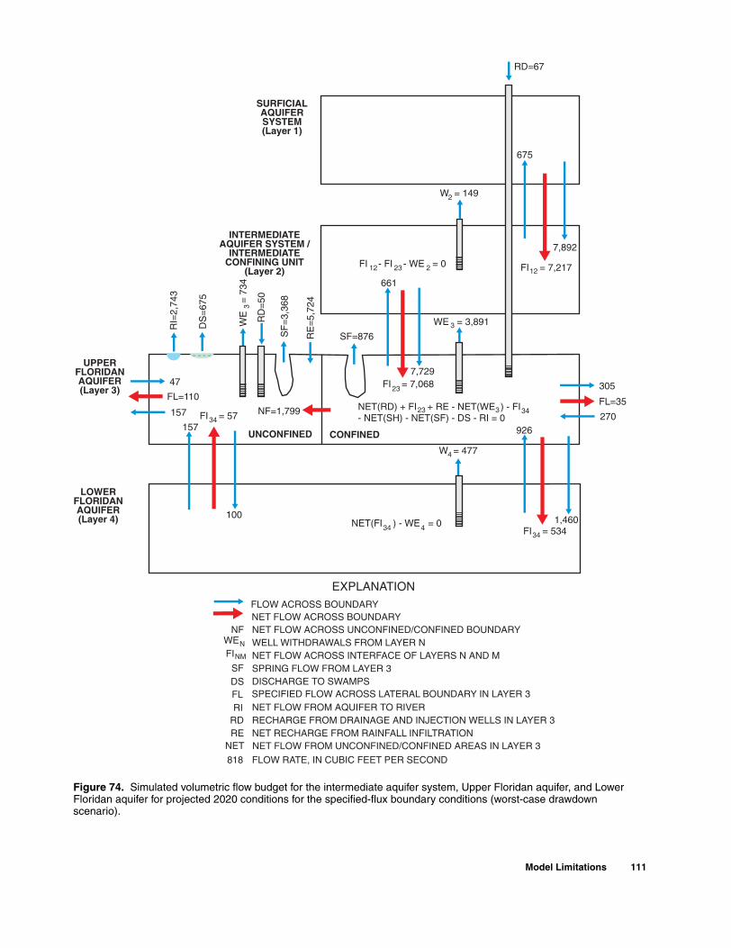
Figure 74. Simulated volumetric flow budget for the intermediate aquifer system, Upper Floridan aquifer, and Lower Floridan aquifer for projected 2020 conditions for the specified-flux boundary conditions (worst-case drawdown scenario).

Model Limitations 111

Simulation of the observed hydraulic gradients in the ICU would require additional layering of this hydro-geologic unit, which is beyond the scope of this study.

The simulated transmissivities in the IAS, UFA, and LFA and the leakances of the upper confining unit of the IAS, ICU, and MSCU in this study may vary from values in previously published local ground-water flow models. Many of the modifications to transmissiv-ity values from previous ground-water flow models were based on additional data available from aquifer tests and on the need to reduce differences between simulated and measured heads. Areas in the IAS, UFA, or LFA where ground-water withdrawals were minimal for 1993-94 may require changes to simulated values of transmissivity and leakance as future aquifer stresses from increased ground-water withdrawals reflect aqui-fer responses in areas previously not stressed.

Lack of data for the MSCU and LFA precludes a reliable estimation of their respective leakance and transmissivity values; only 46 LFA control points were available during this study. The no-flow boundaries specified along the perimeter of active cells in the LFA was based on the assumption of minimal ground-water flow across the estimated surface beneath which the FAS contains water with chloride concentrations greater than 5,000 mg/L. The estimated surface shown in figure 19 can be updated as more water-quality data become available. In addition, flow in the LFA might be understood better as the potentiometric surface of the LFA becomes better defined by more head mea-surements as additional wells are drilled. The assump-tion of a stationary freshwater-saltwater interface also could introduce error in the model if ground-water withdrawals or lack of recharge induce movement of this interface.

In spite of the limitations, the model can indicate the general movement of ground water in the study area. By providing estimates to hydraulic parameters, this model can be used to generate initial estimates of the hydraulic properties needed for more localized studies. In addition, the model also can provide a good assessment of drawdowns in response to projected ground-water withdrawals.

SUMMARY AND CONCLUSIONS

A four-layer, finite-difference steady-state ground-water flow model of the intermediate aquifer system (IAS) and the Floridan aquifer system (FAS) in peninsular Florida was developed and calibrated.


Hydraulic properties were extracted from this model for smaller-scale ground-water flow models within the study area. The active model area is about 40,800 square miles (mi2) and extends approximately 284 miles (mi) from Charlton and Camden Counties, Georgia, to just south of the Palm Beach - Martin County line in Florida. The west-to-east extent of the study area spans about 200 miles from the Gulf of Mexico to the Atlantic Ocean.

The hydrogeologic framework of the study area includes sediments that form the surficial aquifer system (SAS); the less permeable clay and carbonate rocks that form the intermediate confining unit (ICU), the accumulation of more permeable carbonate rocks than those of the ICU that form the IAS in southwest Florida; and a thick sequence of carbonate rocks of variable permeability that form the FAS. A base of generally low permeability dolomite and evaporite beds form the sub-Floridan confining unit. In east-cen-tral Florida, the Upper Floridan aquifer (UFA) and Lower Floridan aquifer (LFA) are separated by the mid-dle semiconfining unit (MSCU), a less permeable, commonly partially dolomitized limestone that locally contains some gypsum and chert. The MSCU is thin or absent in the northwest part of the study area, but is as much as 600 to 800 ft thick in the south-central part of the study area. In west-central Florida, the UFA and LFA are separated by the middle confining unit (MCU), a gypsiferous dolomite and dolomitic lime-stone of considerably lower permeability than the MSCU in east-central Florida.

The IAS and FAS were approximately at steady-state conditions for the period August 1, 1993, through July 31, 1994. Errors introduced by this steady-state approximation were estimated to be minimal. A uni-formly spaced grid of 5,000-foot square cells (210 columns and 300 rows) was used to discretize the hydraulic properties of the SAS, IAS or ICU, UFA, and LFA, and to implement the ground-water flow model. The flow model was calibrated using average heads for the IAS, UFA, and LFA for 1993-94, mea-sured or estimated spring flows, and measured river flows in the unconfined areas of the UFA.

The time-averaged altitude of the water table of the SAS and time-averaged heads of the IAS, UFA, and LFA were generated from computed average heads for the August 1993 through July 1994 period. Multiple linear regressions among the water-level measurements at SAS wells, an interpolated minimum water-table surface, and the difference between land-surface


altitude and the interpolated minimum water table were used to approximate the altitude of the water table in the study area where the SAS is present.

The altitude of the water table and the potentio-metric surfaces of the IAS and UFA were used to iden-tify the areal extent of recharge and discharge areas within the UFA. Recharge to the UFA occurs mainly from downward leakage from the SAS through the ICU when the water table is higher than the potentiometric level of the UFA. Artificial recharge to the UFA occurs from drainage wells, injection wells, and rapid-infiltra-tion basins.With the exception of swamps, springs, and some river segments in the unconfined areas of the UFA, most of the unconfined areas of the UFA is recharged by rainfall. Discharge from the UFA occurs mainly by upward leakage to the SAS through the ICU when the potentiometric surface is higher than the water table. Discharge from the UFA also occurs as ground-water withdrawals, spring flows, and flow from the unconfined areas of the UFA to swamps and rivers.

Boundary conditions varied among the various aquifer layers. The SAS was simulated as a layer of constant heads. No-flow conditions were imposed along the lateral boundaries of the ICU layer. Lateral boundaries of the UFA generally were specified heads. Areas of the UFA and LFA containing water with chlo-ride concentrations greater than 5,000 milligrams per liter (mg/L) were considered inactive and delineated by no-flow boundaries. All lateral boundaries of the LFA in the model were assumed to be no flow.

Ground-water withdrawals for 1993-94 within the study area from the IAS, UFA, and LFA totaled 2,488 million gallons per day (Mgal/d). Additional dis-charge from the UFA occurred from spring flow which, for 1993-94, was estimated to be about 4,126 Mgal/d. Total recharge to the UFA from 364 drainage wells in the study area was estimated to be 68 Mgal/d, based on rainfall data for 1993-94. Artificial recharge to the UFA from injection wells in Alachua County was estimated to be 10.62 Mgal/d.

The ground-water flow model was calibrated by independently varying the following parameters: net recharge rate to unconfined areas of the UFA; transmis-sivity of the IAS, UFA, and LFA; riverbed conductance of rivers in the unconfined areas of the UFA; leakance of the upper confining unit of the IAS, the ICU, the MCU, and the MSCU; and the conductance of swamps and springs in the UFA that were simulated as drain cells. Simulated and measured heads at control points of the IAS, UFA, and LFA showed a close agreement

across most of the study area, with residuals of less than 5 feet (ft) in about 85 percent of the control points. The root-mean-square residuals for the IAS, UFA, and LFA were 3.47, 3.41, and 2.89 ft, respectively. Simulated spring flow was within 5 cubic feet per second (ft3/s) of the estimated flow in about 83 percent of the springs. The largest spring-flow residuals occurred in springs simulated as river cells. Simulated flow was about 96 percent of an approximate total estimated spring flow of 6,380 ft3/s for 1993-94.

The effects of projected increases in ground-water withdrawals for 2020 relative to 1993-94 rates were analyzed by using, in two separate simulations, specified-head and specified-flux boundary conditions for lateral boundaries of the UFA. Projected 2020 ground-water withdrawals from the IAS, UFA, and LFA were estimated to be 3,394 Mgal/d, which repre-sents an increase of about 36 percent from 1993-94. A projected drawdown of 20 ft in the IAS potentiometric surface for 2020 was simulated in central Glades County, resulting from projected increases in ground-water withdrawals. A projected drawdown of 10 ft in the UFA potentiometric surface for 2020 was simulated in central Orange County using either of the two lateral boundary conditions for the UFA, with a projected 8 ft drawdown extending to parts of Osceola and Seminole Counties. A projected drawdown of 6 ft in the UFA for 2020 was simulated for Duval County for both lateral boundary conditions. A projected drawdown of 10 ft in the LFA potentiometric surface for 2020 was simulated in Orange County. Simulated drawdowns in the poten-tiometric surfaces of the UFA and LFA in Orange and Duval Counties were consistent with projected increases in ground-water withdrawals from these aquifers. No substantial projected drawdowns in the UFA or LFA were simulated in the northwest and west-central parts of the model area.

REFERENCES

Arthur, J.D., Lee, R.A., and Li, Li, 2001, Lithostratigraphic and hydrostratigraphic cross sections through Levy-Marion to Pasco Counties, southwest Florida: Tallahas-see, Florida Geological Survey Open File Report 81, 31 p.

Barcelo, Mark, and Basso, Ron, 1993, Computer model of ground-water flow in the Eastern Tampa Bay Water Use Caution Area: Brooksville, Southwest Florida Water Management District, 102 p.

References 113

Blandford, T.N., and Birdie, T.R., 1993, Development of wellhead protection areas for the major public supply wells in Hernando County, Florida: Herndon, Va., HydroGeoLogic, 90 p.

Bouwer, Herman, 1978, Groundwater hydrology: New York, McGraw-Hill, 480 p.

Bradner, L.A., 1994, Ground-water resources of Okeechobee County, Florida: U.S. Geological Survey Water-Resources Investigations Report 92-4166, 41 p.

———1996, Estimation of recharge through selected drain-age wells and the potential effects from well closure, Orange County, Florida: U.S. Geological Survey Open-File Report 96-316, 30 p.

Buono, Anthony, and Rutledge, A.T., 1979, Configuration of the top of the Floridan aquifer, Southwest Florida Water Management District and adjacent areas: U.S. Geolog-ical Survey Water-Resources Investigations Open-File Report 78-34, 1 sheet.

CH2M Hill, 1997, Artificial recharge of the Floridan aquifer through drainage or injection wells in Orange and Seminole Counties: Prepared for St. Johns River Water Management District, 103 p.

Col, Nolan, Rupert, Frank, Enright, Meryl, and Horvath, Glenn, 1997, Reappraisal of the geology and hydroge-ology of Gilchrist County, Florida, with emphasis on the Waccasassa Flats: Tallahassee, Florida Geological Survey Report of Investigations 99, 76 p.

Dames & Moore, 1988, Tri-County saltwater intrusion model Volume 1: Project report: Prepared for South-west Florida Water Management District, Brooksville, 133 p.

Durden, D.W., 1997, Finite-difference simulation of the Floridan aquifer system in northeast Florida and Camden County, Georgia: Palatka, St. Johns River Water Management District Technical Publication 97-2, 253 p.

Environmental Systems Research Institute, Inc., 1997, ARC/INFO, version 8.0.2: Redlands, Calif.

Fairbank, P.K., and Hohner, S.M., 1995, Mapping recharge (infiltration/leakage) throughout the South Florida Water Management District: West Palm Beach, South Florida Water Management District Technical Publica-tion 95-02, 38 p.

Fretwell, J.D., 1988, Water resources and effects of ground-water development in Pasco County, Florida: U.S. Geo-logical Survey Water-Resources Investigations Report 87-4188, 209 p.

German, E.R., 2000, Regional evaluation of evapotranspira-tion in the Everglades: U.S. Geological Survey Water-Resources Investigations Report 00-4217, 48 p.

Groszos, Mark, Ceryak, Ron, Alison, David, Cooper, Renee, Weinberg, Mike, Macesich, Milena, Enright, M.M., and Rupert, Frank, 1992, Carbonate units of the intermedi-ate aquifer system in the Suwannee River Water


Management District: Tallahassee, Florida Geological Survey Open File Report 54, 22 p.

Grubb, H.F., and Rutledge, A.T., 1979, Long-term water supply potential, Green Swamp area, Florida: U.S. Geological Survey Water-Resources Investigations Report 78-99, 76 p.

Hancock, Michael, and Basso, Ron, 1993, Computer model of ground-water flow in the Northern Tampa Bay: Brooksville, Southwest Florida Water Management District, 120 p.

Harbaugh, A.W., and McDonald, M.G., 1996, User’s docu-mentation for MODFLOW-96, an update of the U.S. Geological Survey modular finite-difference ground-water flow model: U.S. Geological Survey Open-File Report 96-485, 56 p.

Hickey, J.J., 1990, An assessment of the flow of variable-salinity ground water in the middle confining unit of the Floridan aquifer system, west-central Florida: U.S. Geological Survey Water-Resources Investigations Report 89-4142, 13 p.

Johnston, R.H., 1983, The saltwater-freshwater interface in the Tertiary Limestone aquifer, southeast Atlantic outer-continental shelf of the U.S.A.: Journal of Hydrology, v. 61, p. 239-249.

Johnston, R.H., Bush, P.W., Krause, R.E., and Miller, J.A., 1982, Summary of hydrologic testing in Tertiary Lime-stone aquifer, Tenneco offshore exploratory well -- Atlantic OCS, Lease-Block 427 (Jacksonville NH 17-5): U.S. Geological Survey Water-Supply Paper 2180, 15 p.

Knochenmus, D.D, and Hughes, G.H., 1976, Hydrology of Lake County, Florida: U.S. Geological Survey Water-Resources Investigations 76-72, 100 p.

Knochenmus, L.A., and Bowman, Geronia, 1998, Transmis-sivity and water-quality of water-producing zones in the intermediate aquifer system, Sarasota County, Florida: U.S. Geological Survey Water-Resources Investiga-tions Report 98-4091, 27 p.

Leake, S.A., and Claar, D.V., 1999, Procedures and com-puter programs for telescopic mesh refinement using MODFLOW: U.S. Geological Survey Open-File Report 99-238, 53 p.

Lukasiewicz, John, 1992, A three-dimensional finite differ-ence ground water flow model of the Floridan aquifer system in Martin, St. Lucie and eastern Okeechobee Counties, Florida: West Palm Beach, South Florida Water Management District Technical Publication 92-03, 292 p.

Mahon, G.L., Choquette, A.F., and Sepúlveda, A.A., 1997, Potentiometric surface of the Upper Floridan aquifer in the Suwannee River Water Management District, Florida, May and June 1995: U.S. Geological Survey Open-File Report 96-617, 1 sheet.


Marella, R.L., 1999, Water withdrawals, use, discharge, and trends in Florida, 1995: U.S. Geological Survey Water-Resources Investigations Report 99-4002, 90 p.

Meadows, P.E., 1991, Potentiometric surface of the Upper Floridan aquifer in the Suwannee River Water Manage-ment District, Florida, May 1990: U.S. Geological Survey Open-File Report 90-582, 1 sheet.

Metz, P.A., 1995, Hydrogeology and simulated effects of ground-water withdrawals for citrus irrigation, Hardee and De Soto Counties, Florida: U.S. Geological Survey Water-Resources Investigations Report 93-4158, 83 p.

Metz, P.A., and Brendle, D.L., 1994a, Potentiometric surface of the Upper Floridan aquifer, west-central Florida, May 1994: U.S. Geological Survey Open-File Report 94-528, 1 sheet.

———1994b, Potentiometric surfaces of the intermediate aquifer system, west-central Florida, May 1994: U.S. Geological Survey Open-File Report 94-529, 1 sheet.

Meyer, F.W., 1989, Hydrogeology, ground-water movement, and subsurface storage in the Floridan aquifer system in southern Florida: U.S. Geological Survey Professional Paper 1403-G, 59 p.

Miller, J.A., 1986, Hydrogeologic framework of the Floridan aquifer system in Florida and in parts of Georgia, Alabama, and South Carolina: U.S. Geological Survey Professional Paper 1403-B, 91 p.

Motz, L.H., 1995, North-central Florida regional ground-water investigation and flow model: Palatka, St. Johns River Water Management District Special Publica-tion SJ95-SP7, 255 p.

Mularoni, R.A., 1994a, Potentiometric surfaces of the inter-mediate aquifer system, west-central Florida, Septem-ber 1993: U.S. Geological Survey Open-File Report 94-80, 1 sheet.

———1994b, Potentiometric surface of the Upper Floridan aquifer, west-central Florida, September 1993: U.S. Geological Survey Open-File Report 94-81, 1 sheet.

Murray, L.C., Jr., and Halford, K.J., 1996, Hydrogeologic conditions and simulation of ground-water flow in the greater Orlando metropolitan area, east-central Florida: U.S. Geological Survey Water-Resources Investiga-tions Report 96-4181, 100 p.

Navoy, A.S., and Bradner, L.A., 1987, Ground-water resources of Flagler County, Florida: U.S. Geological Survey Water-Resources Investigations Report 87-4021, 45 p.

O’Reilly, A.M., 1998, Hydrogeology and simulation of the effects of reclaimed-water application in west Orange and southeast Lake Counties, Florida: U.S. Geological Survey Water-Resources Investigations Report 97-4199, 91 p.

Phelps, G.G., 1987, Effects of surface runoff and treated wastewater recharge on quality of water in the Floridan aquifer system, Gainesville area, Alachua County,

Florida: U.S. Geological Survey Water-Resources Investigations Report 87-4099, 57 p.

———1990, Geology, hydrology, and water quality of the surficial aquifer system in Volusia County, Florida: U.S. Geological Survey Water-Resources Investiga-tions Report 90-4069, 67 p.

Planert, Michael, and Aucott, W.R., 1985, Water supply potential of the Floridan aquifer in Osceola, eastern Orange, and southwestern Brevard Counties, Florida: U.S. Geological Survey Water-Resources Investiga-tions Report 87-4135, 69 p.

Rosenau, J.C., Faulkner, G.L., Hendry, C.W., and Hull, R.W., 1977, Springs of Florida (2d ed.): Tallahassee, Bureau of Geology Bulletin 31, 461 p.

Ryder, P.D., 1985, Hydrology of the Floridan aquifer system in west-central Florida: U.S. Geological Survey Profes-sional Paper 1403-F, 63 p.

St. Johns River Water Management District, 1998, Water supply assessment 1998: Palatka, St. Johns River Water Management District Technical Publication SJ98-2, 96 p.

Schiffer, D.M., O’Reilly, A.M., Phelps, G.G., Bradner, L.A., Halford, K.J., and Spechler, R.M., 1994, Potentiometric surface of the Upper Floridan aquifer in the St. Johns River Water Management District and vicinity, Florida, May 1994: U.S. Geological Survey Open-File Report 94-495, 1 sheet.

Schiner, G.R., Laughlin, C.P., and Toth, D.J., 1988, Geohy-drology of Indian River County, Florida: U.S. Geologi-cal Survey Water-Resources Investigations Report 88-4073, 110 p.

Scholle, P.A., 1979, Geological studies of the COST GE-1 well, United States South Atlantic Outer Continental Shelf area: U.S. Geological Survey Circular 800, 108 p.

Sepúlveda, Nicasio, 2001, Comparisons among ground-water flow models and analysis of discrepancies in sim-ulated transmissivity of the Upper Floridan aquifer in ground-water flow model overlap areas, in Kuniansky, E.L., ed., U.S. Geological Survey Karst Interest Group Proceedings, St. Petersburg, Florida, February 13-16, 2001: U.S. Geological Survey Water-Resources Investi-gations Report 01-4011, p. 58-67.

Shaw, J.E., and Trost, S.M., 1984, Hydrogeology of the Kissimmee Planning Area, South Florida Water Management District: West Palm Beach, South Florida Water Management District Technical Publication 84-1, 235 p.

Sinclair, W.C., 1979, Field data from an observation well in Hillsborough Bay near Tampa, Florida, drilled March 14 to April 5, 1978: U.S. Geological Survey Open-File Report 78-984, 20 p.

Sloto, R.A., and Crouse, M.Y., 1996, HYSEP: A computer program for streamflow hydrograph separation and analysis: U.S. Geological Survey Water-Resources Investigations Report 96-4040, 46 p.

References 115

Snyder, J.P., 1983, Map projections used by the U.S. Geolog-ical Survey: U.S. Geological Survey Bulletin B-1532, 313 p.

South Florida Water Management District, 1998, District-wide Water Supply Assessment: West Palm Beach, 249 p.

Southwest Florida Water Management District, 1998, Water Supply Assessment 1995-2020, Southwest Florida Water Management District: Brooksville, 48 p.

Spechler, R.M., 1993, Salt water intrusion and quality of water in the Floridan aquifer system, northeastern Florida: U.S. Geological Survey Water-Resources Investigations Report 92-4174, 76 p.

———1995, Estimated discharge and chemical-constituent loading from the Upper Floridan aquifer to the lower St. Johns River, northeastern Florida, 1990-91: U.S. Geological Survey Water-Resources Investigations Report 94-4132, 32 p.

Spechler, R.M., Phelps, G.G., Bradner, L.A., Halford, K.J., and Murray, L.C., Jr., 1993, Potentiometric surface of the Upper Floridan aquifer in the St. Johns River Water Management District and vicinity, Florida, September 1993: U.S. Geological Survey Open-File Report 94-33, 1 sheet.

Sprinkle, C.L., 1989, Geochemistry of the Floridan aquifer system in Florida and in parts of Georgia, South Caro-lina, and Alabama: U.S. Geological Survey Profes-sional Paper 1403-I, 105 p.

Sumner, D.M., 1996, Evapotranspiration from successional vegetation in a deforested area of the Lake Wales Ridge, Florida: U.S. Geological Survey Water-Resources Investigations Report 96-4244, 38 p.

Suwannee River Water Management District, 1998, SRWMD Water supply assessment: Live Oak, 31 p.

Thiessen, A.H., 1911, Precipitation for large areas: Monthly Weather Review, v. 39, no. 7, 1082-1084 p.

Tibbals, C.H., 1990, Hydrology of the Floridan aquifer system in east-central Florida: U.S. Geological Survey Professional Paper 1403-E, 98 p.


Todd, D.K., 1980, Groundwater hydrology (2d ed.):, N.Y., John Wiley 535 p.

U.S. Geological Survey, 1994, Water resources data for Florida, water year 1993, v. 3A, southwest Florida, sur-face water: U.S. Geological Survey Water-Data Report, FL-93-3A, 245 p.

———1995, Water resources data for Florida, water year 1994, v. 3A, southwest Florida, surface water: U.S. Geological Survey Water-Data Report, FL-94-3A, 259 p.

———1996, Water resources data for Florida, water year 1995, v. 4, northwest Florida, U.S. Geological Survey Water-Data Report, FL-95-4, 166 p.



White, W.A., 1970, The geomorphology of the Florida Peninsula: Tallahassee, Florida Geological Survey Bul-letin 51, 164 p.

Yobbi, D.K., 1989, Simulation of steady-state ground water and spring flow in the upper Floridan aquifer of coastal Citrus and Hernando Counties, Florida: U.S. Geologi-cal Survey Water-Resources Investigations Report 88-4036, 33 p.

———1992, Effects of tidal stage and ground-water levels on the discharge and water quality of springs in coastal Citrus and Hernando Counties, Florida: U.S. Geologi-cal Survey Water-Resources Investigations Report 92-4069, 44 p.

———1996, Analysis and simulation of ground-water flow in Lake Wales Ridge and adjacent areas of central Flor-ida: U.S. Geological Survey Water-Resources Investi-gations Report 94-4254, 82 p.


APPENDIXES

CLINCH

ECHOLS

LANIE

R

WARE

CHARLTON CAMDEN

LO

WN

DE

S

MARTINGLADES

ST. LUCIE

INDIAN

RIVER

BR

EV

AR

D

OKEECHO

BEE

HIG

HLA

ND

S

HARDEE

OSCEOLA

POLK

DE SOTO

CHARLOTTE

SARASOTA

MANATEE

HILLSBOROUGH

PASCO

ORANGE

SEMINOLE

VOLUSIA

LAKE

SUMTER

CITRUS

HERNANDO

LEVY

PUTNAM

NASSAU

DUVAL

CLAY ST.JO

HN

SALACHUA

BRADFO

RD

CO

LU

MB

IA

SUWANNEE

MA

DIS

ON

HAMILTON BAKER

FLAGLER

DIXIE GIL

CH

RIS

TLAFAYETTE

PIN

EL

LA

S

UNION

FLORIDA

GEORGIA

MARION

Estimated extent ofthe intermediateconfining unit withinthe study area

Estimated extent ofthe unconfined areasin the Upper Floridanaquifer

Estimatedextent of theintermediateaquifersystemwithin thestudy area

Extent of thestudy area

14Durden(1997)

5

Tibbals (1990)

1Grubb

andRutledge

(1979)2Ryder

(1985)

10Metz

(1995)

0

0 25

25

50 MILES

50 KILOMETERS

81°00′82°00′83°00′

30°0 ′0

31°0 ′0

29°00′

28°00′

27°00′

AT

LA

NT

ICO

CE

AN

GU

LF

OF

ME

XIC

O


Appendix A1. Location and extent of simulated areas in the intermediate aquifer system or intermediate confining unit compiled from local ground-water flow models (refer to table 1 for general description of models).


CLINCH

ECHOLS

LANIE

R

WARE

CHARLTON CAMDEN

LO

WN

DE

S

GEORGIAFLORIDA

MARTINGLADES

ST. LUCIE

INDIAN

RIVER

BR

EV

AR

D

OKEECHO

BEE

HIGHLANDS

HARDEE

OSCEOLA

POLK

DE SOTO

CHARLOTTE

SARASOTA

MANATEE

HILLSBOROUGH

PASCO

ORANGE

SEMINOLE

VOLUSIA

LAKE

SUMTER

CITRUS

HERNANDO

MARION

LEVY

PUTNAM

NASSAU

DUVAL

CLAY ST.JO

HN

S

ALACHUA

BRADFO

RD

CO

LU

MB

IA

SUWANNEE

MA

DIS

ON

HAMILTON

BAKER

FLAGLERDIXIE

GIL

CH

RIS

T

LAFAYETTE

PIN

EL

LA

S

UNION

Estimated extent ofthe intermediateconfining unit withinthe study area

Estimated extentof the unconfinedareas in the UpperFloridan aquifer

Estimatedextent of theintermediateaquifersystemwithin thestudy area


7 Lukasiewicz(1992)

6

Murray and Halford (1996)12

Yobbi (1996)

13

Barcelo and Basso (1993)

11Motz (1995)

Hancockand

Basso (1993)

9

3

Fretwell (1988)

0

0 25

25

50 MILES

50 KILOMETERS

81°00′82°00′83°00′

30°0 ′0

31°0 ′0

29°00′

28°00′

27°00′

AT

LA

NT

ICO

CE

AN

GU

LF

OF

ME

XIC

O


Appendix A1. Location and extent of simulated areas in the intermediate aquifer system or intermediate confining unit compiled from local ground-water flow models (refer to table 1 for general description of models)--Continued.

Appendix A1 119

0

0 25

25

50 MILES

50 KILOMETERS

81°00′82°00′83°00′

30°0 ′0

31°0 ′0

29°00′

28°00′

27°00′

AT

LA

NT

ICO

CE

AN

GU

LF

OF

ME

XIC

O


CLINCH

ECHOLS

LANIE

R

WARE

CHARLTON CAMDEN

LO

WN

DE

S

FLORIDA

MARTINGLADES

ST. LUCIE

INDIAN

RIVER

BR

EV

AR

D

OKEECHO

BEE

HIG

HL

AN

DS

HARDEE

OSCEOLA

POLK

DE SOTO

CHARLOTTE

SARASOTA

MANATEE

HILLSBOROUGH

PASCO

ORANGE

SEMINOLE

VOLUSIA

LAKE

SUMTER

CITRUS

HERNANDO

MARION

LEVY

PUTNAM

NASSAU

DUVAL

CLAY ST.JO

HN

SALACHUA

BRADFO

RD

CO

LU

MB

IA

SUWANNEE

MA

DIS

ON

HAMILTON

BAKER

FLAGLER

DIXIE GIL

CH

RIS

TLAFAYETTE

PIN

EL

LA

S

UNION

GEORGIA

5

Tibbals (1990)

14

1

10

3

4

2

Durden(1997)

Yobbi

(1989)

Ryder

(1985)

Grubband

Rutledge(1979)

Fretwell

(1988)

Metz(1995)

Estimated extent of theUpper Floridan aquiferwithin the study area


Appendix A2. Location and extent of simulated areas in the Upper Floridan aquifer compiled from local ground-water flow models (refer to table 1 for general description of models).


CLINCH

ECHOLS

LANIE

R

WARE

CHARLTON CAMDEN

LO

WN

DE

S

FLORIDA

MARTINGLADES

ST. LUCIE

INDIAN

RIVER

BR

EV

AR

D

OKEECHO

BEE

HIG

HLA

ND

S

HARDEE

OSCEOLA

POLK

DE SOTO

CHARLOTTE

SARASOTA

MANATEE

HILLSBOROUGH

PASCO

ORANGE

SEMINOLE

VOLUSIA

LAKE

SUMTER

CITRUS

HERNANDO

MARIONLEVY

PUTNAM

NASSAU

DUVAL

CLAY ST.JO

HN

SALACHUA

BRADFO

RD

CO

LU

MB

IA

SUWANNEE

MA

DIS

ON

HAMILTON

BAKER

FLAGLER

DIXIE GIL

CH

RIS

T

LAFAYETTE

PIN

EL

LA

S

UNION

GEORGIA

0

0 25

25

50 MILES

50 KILOMETERS

81°00′82°00′83°00′

30°0 ′0

31°0 ′0

29°00′

28°00′

27°00′

AT

LA

NT

ICO

CE

AN

GU

LF

OF

ME

XIC

O


7

8

Lukasiewicz(1992)

6


Yobbi(1996)

13

Barcelo and Basso (1993)

Blandford andBirdie (1993)

Hancock and Basso (1993)9

11Motz (1995)

Estimated extent of theUpper Floridan aquiferwithin the study area


Appendix A2. Location and extent of simulated areas in the Upper Floridan aquifer compiled from local ground-water flow models (refer to table 1 for general description of models)--Continued.

Appendix A2 121

14

5

Durden(1997)

Tibbals (1990)

Motz (1995)11

Lukasiewicz(1992)

6


CLINCH

ECHOLS

LANIE

R

WARE

CHARLTON CAMDEN

LO

WN

DE

S

GEORGIAFLORIDA

MARTINGLADES

ST. LUCIE

INDIAN

RIVER

BR

EV

AR

D

OKEECHO

BEE

HIGHLANDS

HARDEE

OSCEOLA

POLK

DE SOTO

CHARLOTTE

SARASOTA

MANATEE

HILLSBOROUGH

PASCO

SEMINOLE

VOLUSIA

LAKE

SUMTER

CITRUS

HERNANDO

MARIONLEVY

PUTNAM

NASSAU

DUVAL

CLAY ST.JO

HN

SALACHUA

BRADFO

RD

CO

LU

MB

IA

SUWANNEE

MA

DIS

ON

HAMILTON

BAKER

FLAGLER

DIXIE GIL

CH

RIS

TLAFAYETTE

PIN

EL

LA

S

UNION

ORANGE

0

0 25

25

50 MILES

50 KILOMETERS

81°00′82°00′83°00′

30°0 ′0

31°0 ′0

29°00′

28°00′

27°00′

AT

LA

NT

ICO

CE

AN

GU

LF

OF

ME

XIC

O


Appendix A3. Location and extent of simulated areas in the Lower Floridan aquifer compiled from local ground-water flow models (refer to table 1 for general description of models).


Appendix B. Description of wells equipped with continuous water-level recorders[Well number refers to figure 16. Site numbers with 13 digits indicate data source was St. Johns River Water Management District; site numbers ending with 85 indicate data source was Suwannee River Water Management District (SRWMD); data source of all other site numbers was U.S. Geological Survey (USGS). Hydrogeologic units: CUFA, confined Upper Floridan aquifer; UUFA, unconfined Upper Floridan aquifer; SAS, surficial aquifer system; ICU, intermediate confining unit; IAS, intermediate aquifer system; LFA, Lower Floridan aquifer. --, data not available; ROMP, Regional Observation and Monitoring Well Program]

Well number Site number Well name Latitude Longitude

Well depth (feet)

Hydrogeo-logic unit

1 302127082475885 Morgan 302127 824758 260 UUFA2 301458083141985 Advent Christian Village 301458 831419 60 UUFA3 301610082591585 Brickles 301610 825915 180 UUFA4 300904083100985 Moore 300904 831009 144 UUFA5 300629083024185 Suwannee Farms 300629 830241 247 UUFA6 300403083081785 Koon 300403 830817 -- UUFA7 300117082554285 Daniel 300117 825542 -- UUFA8 294928082355385 08S17E03 High Springs City 294928 823553 300 UUFA9 294654082581085 Georgia Pacific 294654 825810 35 UUFA

10 294458083142885 DOF Hines Lookout Tower 294458 831428 92 UUFA11 293731083061885 City of Cross City 293731 830618 145 UUFA12 293619082362385 USGS Alachua County 293619 823623 252 UUFA13 293252082292385 Straughn 293252 822923 60 UUFA14 292921082583285 DNR Manatee Springs State Park 292921 825832 99 UUFA15 292615082272601 ROMP 134 near Williston 292615 822726 1,185 UUFA16 2921380820616 M-0012 Johnston C.C. 292138 820616 63 UUFA17 291910082341185 USGS Levy County 291910 823411 86 UUFA18 291414082560985 DOF Rosewood Tower 291414 825609 254 UUFA19 290230082412501 ROMP 125 at Crackertown 290230 824125 280 UUFA20 290312082250801 USGS CE 14 near Dunnellon 290312 822508 190 UUFA21 290112082371101 USGS CE 5 near Inglis 290112 823711 125 UUFA22 290133082140901 ROMP 119 near Ocala 290133 821409 502 UUFA23 285720082201301 ROMP 116 near Tsala Apopka Lake 285720 822013 55 UUFA24 285414082284201 North Lecanto near Lecanto 285414 822842 335 UUFA25 285124082245601 ROMP 113 near Inverness 285124 822456 150 UUFA26 285102082204001 DOT Highway 41 near Inverness 285102 822040 450 UUFA27 284317082330601 Chassahowitzka 1 near Chassahowitzka 284317 823306 176 UUFA28 284330082215401 ROMP 109 near Floral City 284330 822154 260 UUFA29 283201082315601 Weeki Wachee 283201 823156 259 UUFA30 282742082375901 ROMP TR18-1 near Aripeka 282742 823759 580 UUFA31 282613082381701 ROMP TR18-3 near Aripeka 282613 823817 622 UUFA32 282605082345801 ROMP 97 near Aripeka 282605 823458 355 UUFA33 3032350822035 BA0059 Eddy Fire Tower 1151 303235 822035 20 SAS34 3032350822035 BA0058 Eddy Fire Tower 1153 303235 822035 40 ICU35 3032350822035 BA0057 Eddy Fire Tower 1152 303235 822035 360 CUFA36 302416081522601 D-0348 J-0413 302416 815226 708 CUFA37 302416081522602 D-0349 J-0414 302416 815226 2,230 LFA38 302301081295001 DS-522 Ft. Caroline Park 302301 812950 34 SAS39 302301081295002 DS-523 Ft. Caroline Park 302301 812950 204 ICU40 301710081323601 DS-520 301710 813236 60 SAS41 301710081323602 DS-521 301710 813236 120 ICU42 301710081323603 D-3824 301710 813236 740 CUFA43 3016180821109 BA0056 Macclenny 1160 301618 821109 40 SAS44 3016180821109 BA0055 Macclenny 1161 301618 821109 60 ICU45 3016180821109 BA0054 Macclenny 1162 301618 821109 368 CUFA

46 3005070812727 SJ0030 Durbin Firetower 300507 812727 120 SAS

Appendix B 123

47 3005070812727 SJ0029 Durbin Firetower 300507 812727 603 CUFA48 2958510815553 C-0127 Penney Farms Tower 295851 815553 136 SAS49 2958510815553 C-0128 Penney Farms Tower 295851 815553 405 CUFA50 2951160820058 C-0456 Lake Lowery 295116 820058 20 SAS51 2951160820058 C-0440 Lake Lowery 295116 820058 124 ICU52 2951160820058 C-0439 Lake Lowery 295116 820058 198 CUFA53 2949110815726 C-0455 Gold Head 3 294911 815726 42 SAS54 2949110815726 C-0454 Gold Head 2 294911 815726 110 ICU55 2949110815726 C-0453 Gold Head 1 294911 815726 375 CUFA56 2947280820109 C-0444 Chester Moody 294728 820109 87 SAS57 2947280820109 C-0443 Chester Moody 294728 820109 131 ICU58 2947280820109 C-0442 Chester Moody 294728 820109 240 CUFA59 2946110820049 C-0438 Lake Geneva 3 294611 820049 20 SAS60 2946110820049 C-0437 Lake Geneva 2 294611 820049 85 ICU61 2946110820049 C-0436 Lake Geneva 1 294611 820049 146 CUFA62 2937540811219 F-0191 Washington Oaks State Park 293754 811219 36 SAS63 2937540811219 F-0200 Washington Oaks State Park 293754 811219 148 CUFA64 2928590813757 P-0409 Fruitland 292859 813757 55 SAS65 2928590813757 P-0408 Fruitland 292859 813757 148 CUFA66 2926030810825 F-0177 Bulow Ruins 292603 810825 43 SAS67 2926030810825 F-0176 Bulow Ruins 292603 810825 120 CUFA68 2924470813706 P-0778 Marvin Jones Road 292447 813706 50 SAS69 2924470813706 P-0777 Marvin Jones Road 292447 813706 110 ICU70 2924470813706 P-0776 Marvin Jones Road 292447 813706 160 CUFA71 2924180813309 P-0742 Niles Road 292418 813309 27 SAS72 2924180813309 P-0143 Niles Road 292418 813309 66 ICU73 2924180813309 P-0705 Niles Road 292418 813309 400 CUFA74 2922390813137 P-0724 Silver Pond 292239 813137 25 SAS75 2922390813137 P-0146 Silver Pond 292239 813137 55 ICU76 2922390813137 P-0696 Silver Pond 292239 813137 400 CUFA77 2921240813452 P-0734 Middle Road 292124 813452 20 SAS78 2921240813452 P-0736 Middle Road 292124 813452 100 ICU79 2921240813452 P-0735 Middle Road 292124 813452 360 CUFA80 2914580812942 V-0525 West Pierson 291458 812942 14 SAS81 2914580812942 V-0524 West Pierson 291458 812942 39 ICU82 2914580812942 V-0068 West Pierson 291458 812942 125 CUFA83 2914480812749 V-0528 Pierson Airport 291448 812749 23 SAS84 2914480812749 V-0557 Pierson Airport 291448 812749 98 ICU85 2914480812749 V-0531 Pierson Airport 291448 812749 210 CUFA86 2914480812749 V-0530 Pierson Airport 291448 812749 1,060 LFA87 2913230811912 V-0770 State Road 40 and State Road 11 291323 811912 35 SAS88 2913230811912 V-0501 State Road 40 and State Road 11 291323 811912 70 ICU89 2913230811912 V-0769 State Road 40 and State Road 11 291323 811912 440 CUFA90 2906140811833 V-0744 Lee Airport 290614 811833 36 SAS91 2906140811833 V-0743 Lee Airport 290614 811833 72 ICU

92 2906140811833 V-0742 Lee Airport 290614 811833 460 CUFA

Appendix B. Description of wells equipped with continuous water-level recorders--Continued[Well number refers to figure 16. Site numbers with 13 digits indicate data source was St. Johns River Water Management District; site numbers ending with 85 indicate data source was Suwannee River Water Management District (SRWMD); data source of all other site numbers was U.S. Geological Survey (USGS). Hydrogeologic units: CUFA, confined Upper Floridan aquifer; UUFA, unconfined Upper Floridan aquifer; SAS, surficial aquifer system; ICU, intermediate confining unit; IAS, intermediate aquifer system; LFA, Lower Floridan aquifer. --, data not available; ROMP, Regional Observation and Monitoring Well Program]


Well depth (feet)

Hydrogeo-logic unit


93 283204081544902 Mascotte near Mascotte 283204 815449 30 SAS94 283204081544901 Mascotte near Mascotte 283204 815449 160 CUFA95 282202081384602 Lake Oliver near Vineland 282202 813846 30 SAS96 282202081384601 Lake Oliver near Vineland 282202 813846 318 CUFA97 275411081372002 ROMP 57 near Lake Wales 275411 813720 140 SAS98 275411081372001 ROMP 57 near Lake Wales 275411 813720 634 CUFA99 274240082212702 ROMP 50 near Wimauma 274240 822127 37 SAS

100 274240082212701 ROMP 50 near Wimauma 274240 822127 562 CUFA101 274240082212703 ROMP 50 Avon Park near Wimauma 274240 822127 1,430 LFA102 272728081474703 ROMP 30 near Zolfo Springs 272728 814747 15 SAS103 272728081474701 ROMP 30 Avon Park near Zolfo Springs 272728 814747 1,266 CUFA104 270959082203003 ROMP 19 near Sarasota 270959 822030 67 SAS105 270959082203002 ROMP 19 near Sarasota 270959 822030 205 IAS106 270959082203001 ROMP 19 near Sarasota 270959 822030 425 CUFA107 270952080135202 M-1183 270952 801352 21 SAS108 270952080135201 M-1141 270952 801352 109 ICU109 2933130811352 F-0164 Levitt Development 293313 811352 90 SAS110 2913530811604 V-0088 Union Camp 291353 811604 20 SAS111 282210081352601 Disney at tree farm near Vineland 282210 813526 18 SAS112 281722080543001 USGS OS171 near Deer Park 281722 805430 19 SAS113 280619080542601 USGS OS179 at Deer Park 280619 805426 18 SAS114 280132082452803 ROMP TR14-2 near Dunedin 280132 824528 22 SAS115 275458082464004 ROMP TR13-1A near Largo 275458 824640 20 SAS116 275430082431403 ROMP TR13-2 near Largo 275430 824314 16 SAS117 274812081190301 P49 near Frostproof 274812 811903 17 SAS118 273923080471801 IR 25 USGS near Yeehaw Junction 273923 804718 19 SAS119 272504081120101 H11A near Lake Placid 272504 811201 16 SAS120 272258082181701 KME water table 09 near Verna 272258 821817 42 SAS121 271559081242501 Lake Groves Road near Lake Placid 271559 812425 23 SAS122 271226081194301 Bairs Den near Lake Placid 271226 811943 35 SAS123 271007080142101 M-1179 271007 801421 20 SAS124 270913080284901 M-1255 270913 802849 28 SAS125 270609080163401 M-1261 270609 801634 20 SAS126 270157081203101 USGS H15A near Palmdale 270157 812031 23 SAS127 270124080280202 M-1048 270124 802802 80 SAS128 265812080053901 PB-565 265812 800539 22 SAS129 265725080141801 M-1234 265725 801418 18 SAS130 275314081514202 ROMP 59 Hawthorn near Bartow 275314 815142 142 IAS131 273851082031502 ROMP 40 Hawthorn near Duette 273851 820315 180 IAS132 273156081451401 Rowell 273156 814514 267 IAS133 272258082195301 KME 04 272258 821953 440 IAS134 272058082143701 Verna T O-2 near Verna 272058 821437 530 IAS135 271832082064801 Edgeville 3 at Edgeville 271832 820648 600 IAS136 271757081493003 ROMP 26 Hawthorn near Gardner 271757 814930 180 IAS137 271118082285301 Osprey 9 271118 22853 255 IAS

138 270952082095901 Carlton 13 near Arca 270952 820959 287 IAS



Well depth (feet)

Hydrogeo-logic unit

Appendix B 125

139 270137082235301 Manasota 14 270137 822353 305 IAS140 304942082213801 USGS OK-9 304943 822138 700 CUFA141 304756081311101 U.S. Navy in Kings Bay 304756 813111 990 CUFA142 304512081343601 Huntley-Jiffy (Davis) 304510 813438 -- CUFA143 304213081270801 N-19 Ft. Clinch, Fernandina Beach 304210 812708 710 CUFA144 3038230812733 N-0190 Fernandina Beach ITT 8 303823 812733 1,020 CUFA145 303510083054985 Prescott 303510 830549 188 CUFA146 303425082473685 Cypress Creek 303425 824736 200 CUFA147 303224083101785 Santa Deas 303224 831017 195 CUFA148 303158082562985 Stafford Scaff at Jasper 303158 825629 279 CUFA149 302859083015085 Carter 302859 830150 167 CUFA150 302833082542985 Deas 302833 825429 105 CUFA151 302550081331501 D-3840 St. John’s River Power Park 302550 813315 750 CUFA152 302251082194985 USGS ONF 6A 302251 821949 338 CUFA153 302243082360285 ONF University of Florida 1 302241 823604 227 CUFA154 301933082350585 USGS ONF 2V 301939 823526 262 CUFA155 301423082261185 USGS Ocean Pond 301423 822611 134 CUFA156 301031082381085 DOT 301031 823810 836 CUFA157 301006082461785 St. Regis Paper Company 301006 824617 250 CUFA158 300747082225885 USGS Lake Butler 300747 822258 35 CUFA159 300706082402285 Vernon Norton 300706 824022 140 CUFA160 300635082295985 Lulu Community Center 300635 822959 214 CUFA161 300220082103085 USGS Railford 300220 821030 294 CUFA162 300101082245285 USGS Lake Butler 300101 822452 254 CUFA163 295257082045785 USGS Starke 295257 820457 324 CUFA164 295055082130885 USGS Graham 295055 821308 206 CUFA165 294920082044585 SRWMD Santa Fe Swamp 294920 820445 208 CUFA166 294807082020903 Keystone Heights 294807 820209 250 CUFA167 2947010812633 SJ0317 SKYES 294701 812633 290 CUFA168 294530082232085 City of Gainsville 294530 822320 284 CUFA169 294402082262185 DNR San Felasco Hammock 294402 822621 168 CUFA170 294330082445085 USGS Trenton 294330 824450 103 CUFA171 294313082024685 USGS Melrose 294313 820246 259 CUFA172 293857082203985 University of Florida 293857 822039 406 CUFA173 2937290812212 SJ0115 Countyline 293729 812212 609 CUFA174 2935290811917 F-0165 ITT-LW-20 293529 811917 140 CUFA175 2933130811324 F-0158 ITT Palm Coast 293313 811324 284 CUFA176 2922040820228 M-0052 Fort McCoy 292204 820228 160 CUFA177 2918180811904 F-0251 Relay Tower 291818 811904 147 CUFA178 2917480812903 V-0510 Mew 291748 812903 130 CUFA179 2917400815620 M-0025 C354 Gores Landing 291740 815620 280 CUFA180 2913440811557 V-0090 Union Camp 291344 811557 151 CUFA181 2913430812546 V-0089 Jones near Pierson 291343 812546 414 CUFA182 2911300820150 M-0026 CE47 near Silver Springs 291130 820150 192 CUFA183 290743082341501 Tidewater 1 near Dunnellon 290743 823415 784 CUFA

184 290455081530401 USGS Moss Bluff Park 290455 815304 225 CUFA



Well depth (feet)

Hydrogeo-logic unit


185 2901030805519 V-0508 Smith Street and US 1 290103 805519 210 CUFA186 285745081054001 USGS at Alamana 285745 810540 21 CUFA187 2856380812031 V-0083 Blue Springs 285638 812031 432 CUFA188 284842081533001 College Street at Leesburg 284842 815330 245 CUFA189 284725081361901 Wolf Sink near Sorrento 284725 813619 205 CUFA190 284147081220201 USGS SEM 125 at Longwood 284147 812202 146 CUFA191 283314081455501 City of Clermont 283314 814555 525 CUFA192 283253081283401 USGS OR47 at Orlo Vista 283252 812835 350 CUFA193 283249081053201 Bithlo 1 at Bithlo 283249 810532 492 CUFA194 282835081305201 Palm Lake Drive near Windermere 282839 813026 235 CUFA195 282738081341401 Lake Sawyer near Windermere 282738 813414 178 CUFA196 282717081553101 ROMP 101 near Bay Lake 282717 815531 404 CUFA197 282623081153801 Cocoa-P near Taft 282623 811538 439 CUFA198 282531081095701 USGS Cocoa D near Narcoossee 282531 810957 300 CUFA199 282528081340901 Bay Lake near Windermere 282528 813409 223 CUFA200 282434081283102 Sea World Drive near Vineland 282434 812831 239 CUFA201 282341081040101 USGS Cocoa A near Bithlo 282341 810401 516 CUFA202 282127082022501 Cumpressco Ranch near Tarrytown 282127 820225 143 CUFA203 281949082332001 State Highway 52 near Fivay Junction 281949 823320 73 CUFA204 281926082212901 Junction of 52 and 581 near Darby 281926 822129 113 CUFA205 281714081093001 Lake Joel near Ashton 281714 810930 750 CUFA206 281558082264601 Pasco 13 near Drexel 281558 822646 49 CUFA207 281532081345001 Loughman near Loughman 281532 813450 250 CUFA208 281222082393401 Seven Springs near Odessa 281222 823934 301 CUFA209 281202081391701 PO-1 Thornhill near Davenport 281202 813847 151 CUFA210 281022082400201 Eldr Wild 3 281022 824002 350 CUFA211 281008081441801 Lake Alfred near Lake Alfred 281008 814418 425 CUFA212 280734082442101 ROMP TR15-3 near Tarpon Springs 280734 824421 150 CUFA213 280655082193001 Morris Bridge 3a near Branchton 280659 821943 600 CUFA214 280652082195101 Morris Bridge WF 3C near Thonotosassa 280652 821951 1,037 CUFA215 280053082350202 Sheldon Road near Citrus Park 280053 823502 330 CUFA216 280022082210501 SWFWMD west of Vandenburg Apt. 280022 822105 37 CUFA217 275959081552501 Sanlon Ranch near Eaton Park 275959 815525 1,220 CUFA218 275815082440401 Pinellas 665 275815 824404 299 CUFA219 275429082093901 ROMP 61 near Pleasant Grove 275429 820939 1,000 CUFA220 274409082015001 Bethlehem Road near Bradley Junction 274409 820150 1,000 CUFA221 273718082315501 FP&L at Piney Point 273718 823155 950 CUFA222 272255082172202 KME near Verna 272255 821722 1,200 CUFA223 272053082320202 City of Sarasota injection well 2 at Sarasota 272053 823202 1,500 CUFA224 272012081482501 Marshall near Gardner 272012 814825 478 CUFA225 271938082251801 Sarasota 9 271938 822518 730 CUFA226 271232081392201 ROMP 15 Avon Park near Arcadia 271232 813922 1,360 CUFA



Well depth (feet)

Hydrogeo-logic unit

Appendix B 127

Appendix C. Description and flow measurements of Upper Floridan aquifer springs[Spring number refers to figure 22. If more than one date of measurement is listed, measured flow is an average of measurements; ft3/s, cubic feet per second; dates are shown in month-year format]

Spring num-ber

Spring name Latitude Longitude County

Measured or estimated

flow(ft3/s)

Date(s)of

measure-ment(s)

1 Blue Spring near Madison 302849 831440 Madison a 118.0 07-95, 11-952 Alapaha Rise near Fort Union 302614 830513 Hamilton a427.0 08-95, 11-953 Holton Spring near Fort Union 302615 830327 Hamilton a12.5 07-95, 11-954 Suwannee Springs near Live Oak 302339 825604 Suwannee a 9.8 07-955 Suwanacoochee Spring at Ellaville 302309 831018 Madison b 43.0 11-736 Ellaville Spring at Ellaville 302303 831021 Suwannee b69.0 11-737 Falmouth Spring at Falmouth 302140 830807 Suwannee b134.0 11-738 White Sulphur Springs at White Springs 301947 824540 Hamilton a42.3 06-989 Charles Springs near Dell 301002 831350 Suwannee a4.7 07-95, 11-95

10 Allen Mill Pond Spring near Dell 300945 831433 Lafayette a12.2 07-95, 11-9511 Wadesboro Spring near Orange Park 300925 814320 Clay b1.0 03-7212 Blue Spring near Dell 300733 831334 Lafayette a70.0 07-95, 11-9513 Peacock Springs 300718 830757 Suwannee a81.1 06-9814 Telford Spring at Luraville 300624 830957 Suwannee a35.8 07-95, 11-9515 Running Springs (East and West) near Luraville 300615 830659 Suwannee a88.0 07-95, 11-9516 Convict Spring near Mayo 300518 830546 Lafayette a1.1 07-95, 11-9517 Royal Spring near Alton 300501 830430 Suwannee a1.9 07-9518 Owens Spring 300244 830229 Lafayette b43.3 09-7319 Mearson Spring near Mayo 300228 830132 Lafayette a51.0 07-95, 11-9520 Troy Spring near Branford 300021 825951 Lafayette a132.0 07-95, 11-9521 Little River Springs near Branford 295947 825759 Suwannee a67.0 07-95, 11-9522 Ruth Spring near Branford 295944 825838 Lafayette a7.5 07-95, 11-9523 Green Cove Springs at Green Cove Springs 295936 814040 Clay b3.0 03-7224 Ichetucknee Head Spring near Fort White 295902 824543 Suwannee c 41.0 07-95, 11-9525 Cedar Head (or Alligator Hole) Spring 295900 824532 Columbia c8.0 07-95, 11-9526 Blue Hole (or Jug) Spring 295847 824531 Columbia c77.0 07-95, 11-9527 Roaring Springs (including Singing Spring) 295835 824531 Columbia c48.0 07-95, 11-9528 Boiling Spring 295825 824537 Suwannee c116.0 07-95, 11-9529 Mill Pond Spring (including Grassy Hole Springs and Coffee

Spring)295804 824537 Columbia c17.0 07-95, 11-95

30 Branford Springs at Branford 295717 825544 Suwannee a35.8 05-98, 06-9831 Jamison Spring 295532 824556 Columbia b3.0 04-7732 Hornsby Spring near High Springs 295059 823536 Alachua a49.8 07-95, 12-9533 Turtle Spring near Hatchbend 295055 825324 Lafayette a27.9 07-95, 11-9534 Fletcher Spring 295048 825334 Lafayette b34.0 11-7235 Steinhatchee Spring near Clara 295028 831829 Lafayette b0.7 10-7236 Ginnie Spring near High Springs 295010 824201 Gilchrist a57.1 07-95, 12-9537 Blue Springs near High Springs (including Lilly Springs) 294947 824059 Gilchrist a41.2 07-95, 12-9538 Poe Springs near High Springs 294933 823858 Alachua a53.6 07-95, 12-9539 Rock Bluff Springs near Bell 294756 825508 Gilchrist a33.2 08-95, 12-9540 Guaranto Spring near Rock Bluff Landing 294646 825624 Dixie b12.0 11-7241 Crescent Beach Submarine Spring 294606 811230 offshore d 30.042 Lumbercamp Springs 294227 825608 Gilchrist b6.2 11-7243 Sun Springs near Wannee 294216 825601 Gilchrist a40.1 08-95, 12-9544 Hart Springs near Wilcox 294030 825705 Gilchrist a90.8 08-95, 12-9545 Otter Springs near Wilcox 293840 825636 Gilchrist b16.0 11-7246 Whitewater Springs 293806 813853 Putnam b1.2 04-7247 Copper Springs near Oldtown (including Little Copper Spring) 293650 825826 Dixie b25.4 11-7548 Bell Springs 293550 825630 Gilchrist b5.1 10-7249 Fannin Springs near Wilcox (including Little Fannin Spring) 293515 825608 Levy a97.7 07-95, 12-9550 Satsuma Spring 293159 814036 Putnam b1.1 03-7251 Blue Springs near Orange Springs 293051 815125 Marion a.5 05-9952 Orange Spring at Orange Springs 293038 815638 Marion a2.0 05-9953 Camp Seminole Spring at Orange Springs 293021 815706 Marion a.8 05-9954 Welaka Spring near Welaka 292935 814025 Putnam e 1.055 Manatee Spring near Chiefland 292922 825837 Levy a187.0 07-95, 12-9556 Mud Spring near Welaka 292735 813945 Putnam b2.3 06-7257 Blue Spring near Bronson 292702 824157 Levy b8.0 06-7458 Beecher Springs near Fruitland 292654 813849 Putnam 6.3 09-93


59 Croaker Hole Spring near Welaka 292618 814121 Putnam 90.3 09-9360 Tobacco Patch Landing Spring Group near Fort McCoy 292542 815526 Marion a1.0 05-9961 Wells Landing Springs near Fort McCoy 292521 815512 Marion a5.0 05-9962 Salt Springs near Eureka 292100 814358 Marion 79.0 09-93, 05-9463 Wekiva Springs near Gulf Hammock 291649 823923 Levy b45.4 06-6764 Silver Glen Springs near Astor 291443 813837 Marion 100.0 09-93, 05-9465 Sweetwater Springs along Juniper Creek 291307 813936 Marion 12.5 09-93, 05-9466 Silver Springs near Ocala 291257 820311 Marion 640.0 09-93, 05-9467 Morman Branch Seepage into Juniper Creek near Astor 291129 813858 Marion a1.0 06-9768 Juniper Creek Tributary near Astor 291104 813845 Lake a2.0 06-9769 Juniper Springs near Ocala 291101 814246 Marion 8.1 09-93, 05-9470 Fern Hammock Springs near Ocala 291100 814229 Marion 10.7 09-93, 05-9471 Ponce de Leon Springs near De Land 290802 812147 Volusia 24.3 09-93, 05-9472 Rainbow Springs near Dunnellon 290608 822616 Marion 637.0 09-93, 05-9473 Alexander Springs near Astor 290450 813430 Lake 113.0 09-93, 05-9474 Mosquito Springs Run, Alexander Springs Wildnerness 290220 812604 Lake a2.0 06-9775 Wilson Head Spring near Holder 285840 821908 Marion b1.9 06-7276 Blue Spring near Holder 285809 821852 Citrus b10.6 05-7277 Gum Springs near Holder 285731 821354 Sumter b67.6 06-7278 Camp La No Che Springs near Paisley 285702 813224 Lake a1.0 06-9779 Blue Spring near Orange City 285650 812023 Volusia 135.0 09-93, 05-9480 Blackwater Springs near Cassia 285318 812952 Lake e1.481 Crystal River Spring Group 285300 823600 Citrus f 613.082 Little Jones Creek Head Spring near Wildwood 285208 820541 Sumter e8.083 Green Springs 285145 811455 Volusia b.3 04-7284 Gemini Springs near DeBary (all 3) 285144 811839 Volusia 10.5 09-93, 05-9485 Little Jones Creek Spring No. 2 near Wildwood 285134 820518 Sumter e5.086 Messant Spring near Sorrento 285121 812956 Lake 12.0 09-93, 05-9487 Seminole Springs near Sorrento 285044 813122 Lake 37.0 09-93, 05-9488 Palm Springs Seminole State Forest 285038 812701 Lake a.5 06-9789 Little Jones Creek Spring No. 3 near Wildwood 285011 820349 Sumter e3.090 Droty Springs near Sorrento 284940 813038 Lake a.6 06-9791 Halls River Head Spring 284935 823450 Citrus g 4.892 Island Spring near Sanford 284922 812503 Seminole a6.4 04-97, 08-9793 Halls River Springs 284804 823610 Citrus f102.294 Homosassa Springs at Homosassa Springs 284758 823520 Citrus g72.495 Southeast Fork of Homosassa Springs at Homosassa Spring 284751 823523 Citrus f43.196 Trotter Spring at Homosassa Springs 284747 823510 Citrus g5.297 Fenney Springs near Coleman, Head Spring of Shady Brook

Creek284742 820219 Sumter b15.0 03-72

98 Shady Brook Creek Spring No. 2 284708 820246 Sumter e2.999 Shady Brook Creek Spring No. 3 284646 820238 Sumter e2.9

100 Shady Brook Creek Spring No. 4 284612 820420 Sumter e2.9101 Sulphur Camp Springs 284612 813034 Orange a.6 06-97102 Hidden River Springs near Homosassa (including Hidden River

Head Spring)284559 823520 Citrus g6.7

103 Rock Springs near Apopka 284521 813004 Orange 53.0 09-93, 05-94104 Shady Brook Creek Spring No. 5 284515 820501 Sumter e2.9105 Bugg Spring at Okahumpka 284507 815406 Lake 8.6 09-93, 05-94106 Blue Springs near Yalaha 284455 814941 Lake a3.0 09-97107 Mooring Cove Springs near Yalaha 284452 814954 Lake a.4 06-97108 Holiday Springs at Yalaha 284424 814905 Lake a3.6 09-96109 Potter Spring near Chassahowitzka (including Ruth Spring) 284354 823548 Citrus g14.4110 Witherington Spring near Apopka 284353 812922 Orange 1.0 05-93111 Salt Creek Head Spring 284323 823506 Citrus g.4112 Lettuce Creek Spring 284308 823437 Citrus g3.7113 Crab Creek Spring 284300 823434 Citrus g34.8114 Unnamed Tributary above Chassahowitzka Springs (including

Bubba Spring)284254 823438 Citrus g20.5

Appendix C. Description and flow measurements of Upper Floridan aquifer springs--Continued[Spring number refers to figure 22. If more than one date of measurement is listed, measured flow is an average of measurements; ft3/s, cubic feet per second; dates are shown in month-year format]

Spring num-ber



flow(ft3/s)

Date(s)of

measure-ment(s)

Appendix C 129

115 Chassahowitzka Springs near Chassahowitzka 284254 823435 Citrus g64.8116 Wekiwa Springs in State Park near Apopka 284243 812736 Orange 56.5 09-93, 05-94117 Miami Springs near Longwood 284236 812634 Seminole 4.0 09-93, 05-94118 Lake Jessup Spring near Wagner 284236 811605 Seminole b.6 05-72119 Baird Creek Head Spring near Chassahowitzka 284230 823440 Citrus g3.2120 Clifton Springs near Oviedo 284156 811414 Seminole b1.5 06-72121 Starbuck Spring near Longwood 284148 812328 Seminole 12.3 09-93, 05-94122 Beteejay Lower Spring near Chassahowitzka (including Betee-

jay Head Spring)284131 823535 Citrus g7.3

123 Palm Springs near Longwood 284127 812334 Seminole 4.1 09-93, 05-94124 Rita Maria Spring near Chassahowitzka 284126 823528 Hernando g3.3125 Sanlando Springs near Longwood 284119 812345 Seminole 18.5 09-93, 05-94126 Unnamed Spring No. 10 (including No. 11 and No.12) 284114 823652 Hernando f19.0127 Ryle Creek Lower Spring near Bayport (including Ryle Creek

Head Spring)284113 823650 Hernando g8.3

128 Blue Run Head Spring near Chassahowitzka 284113 823606 Hernando g4.6129 Double Run Road Seepage near Astatula 284039 814425 Lake a2.0 06-96130 Unnamed Spring No. 8 284017 823808 Hernando f4.9131 Blind Creek Springs (including unnamed spring No. 7 and

Blind Creek Head Spring)283932 823806 Hernando f42.7

132 Apopka (Gourdneck) Spring near Oakland 283400 814051 Lake a31.4 12-92133 Unnamed Spring No. 6 283254 823737 Hernando f2.8134 Salt Spring near Bayport 283246 823709 Hernando g22.3135 Mud Spring near Bayport 283240 823701 Hernando g17.0136 Jenkins Creek Spring No. 5 283120 823804 Hernando g15.3137 Unnamed Spring No. 4 283118 823806 Hernando f6.3138 Weeki Wachee Springs near Brooksville 283100 823425 Hernando 129.0 09-93, 05-94139 Unnamed Spring No. 2 282720 823830 Hernando f.7140 Boat Spring at Aripeka 282621 823929 Hernando g.4141 Bobhill Springs 282607 823834 Hernando g1.8142 Unnamed Spring No. 1 282600 823926 Hernando f6.3143 Magnolia Springs at Aripeka 282558 823926 Pasco g.5144 Unnamed Spring No. 3 near Aripeka 282352 824027 Pasco b17.8 08-60145 Horseshoe Spring near Hudson 282350 824121 Pasco b9.7 12-72146 Salt Springs near Port Richey 281733 824306 Pasco b8.2 12-72147 Crystal Springs near Zephyrhills 281030 821120 Pasco 37.0 09-93, 05-94148 Sulphur Springs at Sulphur Springs 280115 822705 Hillsborough 25.0 10-93, 05-94149 Lettuce Lake Spring 280104 822102 Hillsborough b8.3 05-73150 Six-Mile Creek Spring 280104 822018 Hillsborough b1.3 05-71, 10-71151 Eureka Springs near Tampa 280022 822039 Hillsborough b1.3 05-73152 Buckhorn Spring near Riverview 275322 821810 Hillsborough b15.0 06-72153 Lithia Springs Minor near Lithia 275201 821349 Hillsborough 8.0 09-93, 05-94154 Lithia Springs Major near Lithia 275158 821352 Hillsborough 31.1 09-93, 05-94155 Little Salt Spring near Murdock 270430 821400 Sarasota b.9 05-72156 Warm Mineral Springs near Woodmere 270333 821540 Sarasota b6.7 05-74

Total 6,383.8aEstimated as the product of measured flow and the ratio of August 1993 through July 1994 rainfall that occurred during the year in which actual flow

measurement(s) were made.bEstimated as the product of measured flow from Rosenau and others (1977) and ratio of August 1993 through July 1994 rainfall that occurred during

the year in which actual flow measurement(s) were made.cTotal flow of Ichetucknee Springs is the combined flow, in downstream order, from Ichetucknee Head Spring, Cedar Head Spring, Blue Hole Spring,

Roaring Springs, Boiling Spring, and Mill Pond Spring. Estimated flow of 307 ft3/s from Ichetucknee Springs for 1993-94 was obtained as the product of combined flow of 287 ft3/s for 1995 and the ratio of August 1993 through July 1994 rainfall to 1995 rainfall.

dHighly generalized estimate.eEstimated flow from Leel Knowles (USGS, written commun., 2000).fEstimated to be 70 percent of average of flow measurements from Yobbi (1989).gEstimated to be 70 percent of average of flow measurements from Yobbi (1992).

Appendix C. Description and flow measurements of Upper Floridan aquifer springs--Continued[Spring number refers to figure 22. If more than one date of measurement is listed, measured flow is an average of measurements; ft3/s, cubic feet per second; dates are shown in month-year format]

Spring num-ber



flow(ft3/s)

Date(s)of

measure-ment(s)


Simulation of Ground-Water Flow in the ... - CiteSeerX

Documents

Transcript of Simulation of Ground-Water Flow in the ... - CiteSeerX