1

MODEL-BASED AVIONICS SYSTEMS FAULT SIMULATION AND DETECTION

Chetan Kulkarni, Gautam Biswas

Dept. of EECS/ISIS, Box 351829 Station B, Vanderbilt University, Nashville, TN 37235

chetan.kulkarni, gautam.biswas @vanderbilt.edu Fax: (615)-343-7440; Tel: (615)-343-6204

Kyusung Kim and Raj Mohan Bharadwaj

Honeywell Aerospace-Advance Technology 1985 Douglas Drive N, MN10-112B

Golden Valley, MN 55422 kyusung.kim, raj.bharadwaj@honeywell.com

Tel: (763) 954-6537

Abstract: This paper proposes a combined energy-based model with an empirical physics of failure model for degradation analysis and prognosis of electrolytic capacitors in DC-DC power converters. Electrolytic capacitors and MOSFET’s have higher failure rates than other components in DC-DC converter systems. For example, in avionics systems where the power supply drives a GPS unit, ripple currents can cause glitches in the GPS position and velocity output, and this may cause errors in the navigation solution causing the aircraft to fly off course. A model based approach to studying degradation phenomena enables us to combine the energy based modeling of the DC-DC converter with physics of failure models of capacitor degradation, and predict using stochastic simulation methods how system performance deteriorates with time. We have employed a topological energy based modeling scheme based on the bond graph (BG) modeling language for building parametric models of multi-domain physical systems. Our current work adopts a physics of failure model (Arrhenius Law) for equivalent series resistance (ESR) increase in electrolytic capacitors subjected to electrical and thermal stresses. The derived degradation model of the capacitor is reintroduced into the DC-DC converter system model to study changes in the system performance using Monte Carlo simulation methods. Key words: Bond Graphs, DC-DC converters, Electrolytic Capacitors, ESR, Fault Detection, Fault Isolation, GPS, Prognosis. Introduction: This paper proposes a model based approach to study the degradation effects of power supply converters on avionics systems. Avionics systems combine physical processes, computational hardware, and software systems, and present unique challenges to performing root cause analysis when faults occur, and also for establishing the effects of faults on overall system behavior and performance. However, systematic analysis of these conditions is very important for analysis of safety and also to avoid catastrophic failures in navigation systems.

2

In avionics systems, degradations and faults in the DC-DC converter unit propagate to the GPS and Inertial Navigation systems. Capacitors and MOSFETs are the two major components which degrade/fail in a DC-DC converter system. These can cause a variety of faults in these systems, e.g., ripple voltage/voltage surge at the power supply output can cause glitches in the GPS position and velocity output, and this, in turn, if not corrected will propagate this errors in the navigation solution. One of the faults we have been studying in detail is electrolytic capacitor degradation in the power supply, and its effects on the functioning of the GPS unit. The literature reports a number of operating conditions that cause capacitor degradation, such as High Voltage conditions, Transients, Reverse Bias, Strong Vibrations and high ripple current. Many of these conditions have been observed in the power supplies embedded in the avionics systems. In this work, we study the effects of thermal and electrical stress that lead to capacitor degradation. A topological energy based modeling scheme developed on the bond graph (BG) modeling language for building parametric models of multi-domain physical systems has been implemented. The bond graph models are also used to derive models for diagnostic and prognostic analysis. Further, we have also developed models of the software and hardware components of the GPS and navigation solution as Matlab/ SIMULINK™ modules. A combined energy-based and physics of failure model approach is adopted for degradation analysis and prognosis of degrading components in DC-DC power converters. In this work, we have simulated the GPS reset events due to voltage fluctuations. We have demonstrated using our simulation models the effects of power supply faults on the overall performance of the GPS solution. The complete system for studying the behaviors of the avionics system is implemented as a set of integrated Simulink modules. We apply qualitative fault signature methods for detecting and isolating faults in all three components of the avionics system. Fault signature generation is based on establishing causal relations between system parameters and measurements, and estimating the effect of a parameter value change (representing a fault) on the measured values. The paper is organized as follows. Section II describes in detail the DC-DC converter model. In section III we discuss the GPS model on which the degradation effect of Power Supply is to be observed. Section IV discusses the Fault Detection and Isolation (FDI) methods and algorithms implemented in this work. A case study of the DC-DC converter for fault detection and isolation is discussed in section V. The paper concludes with discussion of the results and future work. DC-DC Converters: Switched-mode power supplies are widely used in DC-DC converters because of their high efficiency and compact size. DC-DC converters are important in portable electronic devices, which derive their power primarily from batteries. Such electronic devices often contain several sub-circuits with different voltage requirements (sometimes higher and sometimes lower than the supply voltage, and

3

possibly even negative voltage). DC-DC converters can provide additional functionality for boosting the battery voltage as the battery charge declines. A typical buck-boost DC-DC converter circuit is illustrated in Fig. 1. Such converters step the voltage up or down, by storing the input energy temporarily in inductors when switch sw1 is ON and switch sw2 is OFF, and then releasing that energy to the output at a different voltage value when sw2 is ON and sw1 is turned OFF. The efficiency of conversion ranges from 75% to 98%. This high efficiency is typically achieved by using power MOSFET’s (metal oxide semiconductor field-effect transistor), which can provide high frequency switching more efficiently than power bipolar transistors, which, in addition to greater switching losses require more complex drive circuits. Overall, MOSFET switches increases the battery life in such devices. A buck boost approach is used for conversion to the required dc voltage output. Our particular application has an input of 28V DC from a battery source, and the required output voltage is 5V. The switches sw1 and sw2 are power MOSFET’s, which are controlled by an external controller. Fig. 2 shows the external controller box, which controls the switching of the MOSFET’s to maintain the required output voltage.

MOSFETSW1 MOSFETSW2

R

C

L

isw1isw2

iLiC

Vc

iR

External controller

Vs

ESR

Figure 1: Buck Boost Converter Circuit We develop a systematic approach for reliable diagnostics and prognostics for the converter system. For this we need to capture the topological and functional dependence of the system in addition to component level faults and capturing the causal flow in time to account for transient failures. The bond graph modeling paradigm provides the framework for building the system models from components. A detailed description of the bond graph models for the DC-DC converter and capacitor are discussed in the next section. Bond Graph Modeling: Model-based identification methodologies require system models that accurately represent system dynamics and are also capable of linking system measurements to damage in the components of the model. The bond graph (BG) modeling framework provides both these features [1]. BGs provide a systematic framework for lumped parameter modeling across multiple domains that include the electrical, mechanical, hydraulic, and thermal domains [2], [3]. They are an explicit

4

topological modeling language for capturing the dynamic energy transfer among components of a systems based on the principles of continuity of power and conservation of energy. This energy distribution reflects the history of the system and, therefore, defines its state at a point in time. Behavior of the system at future time points is determined by the current state description and subsequent input to the system [3]. Changes in the state of the physical system are related to energy exchange among its components, which can be expressed in terms of power. The basic working principle of bond graphs is that power transmitted between connected components can be expressed as a product of ‘effort’ and ‘flow’, irrespective of the application domain [2].

Table 1: Basic Bond graph elements

Symbol Type of element Name of element Electric Domain capacitance capacitor C

L storage inductance inductor R dissipator resistance resistor

transformer TF GY transducer gyrator transformer

effort source voltage source Se Sf source flow source current source

1-junction series connection 1 0 junction 0-junction parallel connection

Bond graph elements are classified into one of five basic elements, (1) energy storage elements, Capacitance (C), the Inertia (I), (2) the dissipative element, Resistor (R), (3) two idealized energy transformation elements, the transformer (TF) and the Gyrator (GY), (4) two source elements, Se, source of effort and Sf , source of flow, and (5) two junction elements, 0 (for parallel connections) and 1 (for series connections). All these elements exchange energy with other elements through ports or bonds. Bonds are energy transfer pathways that connect elements and junctions and are represented as half arrows. Effort and flow signals are the information transferred through these pathways. The two ideal source elements model energy flow in and out of a system, and are active elements since they introduce energy into the system. All the other elements are passive. DC-DC converter model: A passivity based approach discussed in [4], [5] is used for deriving the BG model of the buck boost converter. This approach models the system behavior in two stages: (i) an energy shaping stage, where the closed loop total energy of the system is modified, and (ii) a damping injection stage, where the required dissipation is added in order to achieve asymptotic stability. The bond graph of the passivity based buck boost converter model is shown in Fig. 2. Se:Vs is the battery voltage. The switching elements sw1 and sw2 are replaced by modulating transformers (MTFs). The representation of the switching devices as MTFs is derived directly from the algebraic relations of the effort and flow variables. In an average model of the buck-boost

5

converter, the switching bond is replaced by a ‘duty-ratio-modulated bond’. This ‘average’ bond can be effectively interpreted as an ideal lossless transformer with turns ratio specified by the complementary duty ratio function associated with the controlling scheme. The switching frequency of the MTFs depends upon the value α. The value of α is calculated from the values of R2, C, L and the input/output voltage requirements. [4] provides the detailed equations used for deriving the value of α.

Figure 2: Buck Boost Converter Bond Graph Model

The regulation of the converter output at a desired output voltage vCd depends on the steady state value of the average inductor current iL. This is determined by replacing dynamic element L (inductor) of the average bond graph by a SS-element (source-sensor element), represented as flow source Sf in the BG. The desired steady state value for the current can then be obtained as iL = (1 + vCd/vs)vCd /R2. An input injection from the external passivity controller to the modulated effort source is added to the bond graph model of DC-DC converter in the form of a Se element. [5] provides more details.

Figure 3: Buck Boost Converter Simulink Model

For conversion of the topological bond graph model to its equivalent MATLAB/ SIMULINK®

model we use the approach presented in [6]. An interpreter is used for

6

converting the BG model into an intermittent block diagram model from which the simulation model is derived. In its first stage, the interpreter navigates through the model hierarchy, mapping all the BG elements to block diagram (BD) elements. The second stage of the interpretation process consists of generating the simulation components from the BD model. The BD has all the required information for generating the simulation model. The generated simulation model from the BG model is shown in Fig. 3. Once the MATLAB/ SIMULINK

®model is generated, the required simulation results for the DC-

DC converter can be observed under different operating conditions.

Our approach in the paper is to run degradation experiments on capacitors and use the results to validate an empirical capacitor degradation model reported in the literature. In addition, we will also derive more accurate parameter values for the capacitors employed in our DC-DC converter system, and, therefore, generate better estimates of converter degradation over time. GPS Model: An abstract GPS model is developed to compute the position of a GPS receiver’s Earth-Centered, Earth-Fixed (ECEF) reference frame. The module is implemented in Simulink and is based on the GPS Easy Suite [7, 8]. The input data of the model is obtained from Receiver Independent Exchange Format (RINEX) O and N files. The purpose of the RINEX file format is to enable easy exchange of the GPS data among different GPS receivers [7]. The format consists of six ASCII file types and we use two of them to extract data as the input to our GPS abstract model; 1) O file - Observation Data File, and 2) N file - Navigation Message File. The observation data file contains the GPS measurements data and the navigation message file contains the ephemeris – the orbit information. Note that the RINEX files are parsed by a MATLAB script to extract the model inputs, thus using a different input format correspond to modifying the initialization script to fill the model inputs and not modifying the model itself. The RINEX O and N files to compute the receiver position using iterative least squares procedure. Figure 4 below shows the inputs for the GPS receiver model. The equation for receiver position is:

PRk = dk + cdt - (1)

where PRk is the pseudo-range for satellite k, dk is receiver distance from satellite k and cdt is the receiver clock offset. It should be noted that in the current form the GPS model essentially simulates the GPS receiver low frequency hardware and software functions. The high frequency portions of the GPS receiver such as the antenna are not directly simulated. However, the faults in the high frequency components are modeled by simulating their effects on the respective pseudoranges.

7

sats

Satell ites

svPos

Satell ite Positions

pr

Pseudorange

obs

sats

sv Pos

5VDC

gnss

gnss_nea

GPS_BIT

GPS

gn

Figure 4: GPS Receiver Model

Component Degradation/Failure: It has been reported in the literature that electrolytic capacitors are the leading cause for breakdowns in power supply system’s [9], [10]. The performance of the electrolytic capacitor is strongly affected by its operating conditions, which includes voltage, current, frequency, and working temperature. A degraded electrolytic capacitor cannot provide a low impedance path for the ac current in the output filter of these converters, thus introducing a ripple voltage on top of the desired DC voltage. Continued degradation of the capacitor leads the converter output voltage to drop below specifications, and in some cases it may even damage the converter itself. The literature indicates that the fluctuation in power supply voltage and excessive ripple currents could lead to various failures in the GPS receiver module. In this work we have simulated the GPS reset events due to voltage fluctuations. We have also simulated the loss of receiver lock due to excessive ripple current. We have demonstrated using our simulation models the effects of power supply faults on the overall performance of the GPS solution. The detailed analysis for fault diagnosis and prognosis is carried out in several steps. These are outlined in the next section Fault Detection/Isolation: All performance degradation and fault diagnosis methods can be broadly classified into two types, quantitative and qualitative [12]. The quantitative approach relies on advance information processing techniques such as state and parameter estimation and adaptive filtering. The qualitative approach makes use of causal analysis which links individual component malfunctions expressed in qualitative form with deviations in measured values. This approach is usually used when a precise numerical model for the system is not available. For our work we will be implementing the qualitative approach for fault detection and isolation. Fault Detection: The fundamentals of fault diagnosis presented here are based on the following works [12], [15], [16] and [17]. We focus on small abrupt changes and degradation in components of the system. A component fault manifests as a change in the value of a bond-graph element parameter. These faults affect the coefficients of the system matrix in the state-space or transfer function representation of the system, that is, they have multiplicative effects on the system dynamics. The bond graph representation preserves a one-to-one correspondence between the component parameters and the physical components of the system. As a contrast, in state-space or transfer function

8

representations the model coefficients are typically functions of more than one physical component parameter. For fault isolation this implies that the bond graph representation creates a direct link between the changes in a parameter value with a fault in a specific system component. We present a brief overview of the methodology in this section. The work in this paper describes an approach for model-based FDI of abrupt faults in component parameters of a continuous dynamic system. Abrupt faults correspond to changes that occur at time scales much faster than the nominal dynamics of the system. We model abrupt faults as discrete and persistent changes in the value of component parameters [15]. An abrupt fault in a component parameter results in transients in the system variables. Typically, the transient behavior vanishes after an interval, and for certain faults no evidence of the fault is observable in the measurements after some time. Our approach, named TRANSCEND, is based on the analysis of the fault transient. A model-based fault isolation scheme for qualitative analysis of the fault transients developed by [15] has been implemented. Fault Isolation: Qualitative reasoning using bond graphs is based on an analysis of the Temporal Causal Graph (TCG) structure. TCGs capture causal and temporal relations among the system variables that characterize dynamic system behavior. They are an extended form of Signal Flow Graphs [15], with vertices representing the system variables (e.g., pressures, temperatures, and flow rates) and labeled directed edges capturing the relations between the variables. Labels on the edges further qualify the relations between the vertices. A label of +/-1 on an edge implies a direct (inverse) directional proportionality between the associated variables, and ‘=’ implies an equality relation between the associated variables. Component parameters, R’s, TF’s, GY’s, C’s and I’s appear on links, and play a role in establishing the relations between the associated variables. R, TF, and GY impose algebraic relations, whereas the energy-storage elements, C and I, impose integral, i.e., temporal delay relations between the associated variables. The algorithm to derive the TCG from a BG model utilizes the Sequential Causality Assignment Procedure (SCAP). The SCAP algorithm, outlined in [15], sequentially assigns causality to all of the bonds in the BG model. This causal structure is then unfolded into a directed graph. We start from the source effort and flow values, and sequentially following the algebraic (direct, inverse, and equality) as well as the temporal relations imposed by the constituent elements till all of the bonds and nodes have been traversed. The fault isolation engine follows the generate-and-test approach to residual evaluation using the TCG structure. Qualitative transient behavior is expressed as a fault signature that describes the expected fault transient immediately after fault occurrence. The signature corresponds to a qualitative interpretation of the Taylor series expansion of the residual around the time point of fault occurrence [13]. The order of the signature is defined by the highest derivative computed (a design parameter). Symbolic values for the elements of a signature are: ‘+’ for a positive or increasing value, ‘0’ for a zero or unchanged value, and ‘-’ for a negative or decreasing value. An unknown value is

9

represented by ‘*’. The description of a fault signature in terms of the behavior around the point of fault occurrence is unique to the TRANSCEND [13], [15] approach. Fault isolation is triggered by the first non-zero magnitude symbol that is output by the signal-to-symbol generation module. This initial symbol reflects the magnitude deviation in the residual at the onset of the fault transient. The hypo-thesis generation step produces a set of fault hypotheses that can explain the observed deviation. A fault hypothesis consists of a candidate parameter with a direction of change for the parameter value and a fault signature for each of the measured variables. During hypothesis refinement, the sig-natures are compared with symbolic values computed from the measurements using a scheme called progressive monitoring. When a match fails, the candidate is dropped. Further details of the qualitative fault isolation scheme are presented in [15]. Case Study DC-DC converter: As discussed earlier we employ the method to derive fault signatures on measured variables using our Temporal Causal Graph (TCG) scheme. The TCG is automatically derived from a bond graph model of a system. Figure 6 shows the TCG for the DC-DC converter which is derived from the BG model as shown in Figure 3. To diagnose and isolate the faults their fault signatures should be unique, i.e. no two faults should have the same fault signatures for all measured values. At present, we are focusing on capacitor faults in the DC-DC converters. We derive the fault signatures for the two capacitor-related faults that can occur: (1) decrease in capacitance, and (2) increase in equivalent series resistance (ESR). The Fault Detection and Identification (FDI) method [13] in this paper is implemented using bond graphs as the underlying modeling language. Dynamic characteristics of system behavior derived from the bond graph are represented as a temporal causal graph. The algorithms [13] for monitoring, fault isolation, and prediction are based on this representation. The fault analysis and refinement process continues till fault transients are masked by interactions or the system reaches a steady state. The goal is to uniquely identify the true fault using a combination of transient and steady state analysis. The fault detection mechanism was tested for an abrupt fault in the DC-DC converter model. The steps below show the procedure for fault injection in the converter system and implementation of the fault detection algorithm.

• Run the nominal DC-DC converter MATLAB/SIMULINK® model and record the sensor readings.

• Run the model with an abrupt fault case. • A fault was introduced in the system at 250th time step. • In this case a fault is introduced in the capacitor which is shown in Figure 5. A

glitch is observed in the output voltage of the DC-DC converter. • The residuals are generated from the nominal and faulty data. • This residual data is passed through the Fault detector algorithm. • The fault detector detects the fault from the residual at 252nd time step.

10

Figure 5 shows the nominal behavior of the DC-DC converter where the residuals are around zero. At the 250th time step there is an abrupt change in the residual as seen in the plot where the fault is injected.

250-0.2

-0.15

-0.1

-0.05

0

0.05

Time

Res

idua

l Vol

tage

(m

V)

Fault InjectionFault Detection

Figure 5: Residual Plot for the DC-DC converter

We implement the fault isolation algorithm discussed earlier for isolating the fault component in the system. In this case this component is the capacitor in the DC-DC converter. Figure 6 shows the TCG of DC-DC converter system derived from the bond graph model.

Figure 6: TCG of the Power Supply Model from BG

11

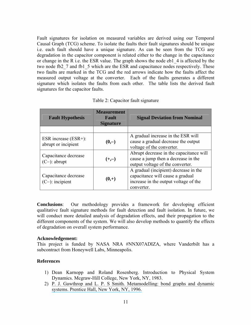
Fault signatures for isolation on measured variables are derived using our Temporal Causal Graph (TCG) scheme. To isolate the faults their fault signatures should be unique i.e. each fault should have a unique signature. As can be seen from the TCG any degradation in the capacitor component is related either to the change in the capacitance or change in the R i.e. the ESR value. The graph shows the node eb1_4 is affected by the two node fb2_7 and fb1_5 which are the ESR and capacitance nodes respectively. These two faults are marked in the TCG and the red arrows indicate how the faults affect the measured output voltage at the converter. Each of the faults generates a different signature which isolates the faults from each other. The table lists the derived fault signatures for the capacitor faults.

Table 2: Capacitor fault signature

Fault Hypothesis Measurement

Fault Signature

Signal Deviation from Nominal

ESR increase (ESR+): abrupt or incipient (0,−)

A gradual increase in the ESR will cause a gradual decrease the output voltage of the converter.

Capacitance decrease (C−): abrupt (+,−)

Abrupt decrease in the capacitance will cause a jump then a decrease in the output voltage of the converter.

Capacitance decrease (C−): incipient (0,+)

A gradual (incipient) decrease in the capacitance will cause a gradual increase in the output voltage of the converter.

Conclusions: Our methodology provides a framework for developing efficient qualitative fault signature methods for fault detection and fault isolation. In future, we will conduct more detailed analysis of degradation effects, and their propagation to the different components of the system. We will also develop methods to quantify the effects of degradation on overall system performance. Acknowledgement: This project is funded by NASA NRA #NNX07ADIZA, where Vanderbilt has a subcontract from Honeywell Labs, Minneapolis. References

1) Dean Karnopp and Roland Rosenberg. Introduction to Physical System Dynamics. Mcgraw-Hill College, New York, NY, 1983.

2) P. J. Gawthrop and L. P. S Smith. Metamodelling: bond graphs and dynamic systems. Prentice Hall, New York, NY, 1996.

12

3) Biljana Vidojkovic Dragan Antic and Miljana Mladenovic. An introduction to bond graph modelling of dynamic systems. TELSIKS’99, Oct 1999.

4) Garcia-Gomez, S. Rimaux, and M. Delgado. Bond graphs in the design of adaptive passivity-based controllers for dc/dc power converters. IEEE International Conference on Industrial Technology, 2006. ICIT 2006, pages 132–137, Dec 2006.

5) Marisol Delgadoa and Hebertt Sira-Ramrez. A bond graph approach to the modeling and simulation of switch regulated dc-to-dc power supplies. Simulation Practice and Theory, page 631- 646, November 1998.

6) Roychoudhury, M. Daigle, G. Biswas, and X. Koutsoukos, "An Efficient Method for Simulating Complex Systems with Switching Behaviors Using Hybrid Bond Graphs," Simulation News Europe , vol. 18, no. 3-4, pp. 5-13, December 2008

7) Borre, Kai, “The Easy Suite – Matlab Code for the GPS Newcomer,” http://www.ngs.noaa.gov/gps-toolbox/Borre2.htm.

8) Borre, Kai, “"The Easy Suite - Matlab code for the GPS newcomer,” GPS Solutions, Volume 7, Number 1, 2003, pp 47-51.

9) A.M. Imam, T.G. Habetler, R.G. Harley, and D.M. Divan. Condition monitoring of electrolytic capacitor in power electronic circuits using adaptive filter modeling. IEEE 36th Power Electronics Specialists Conference, 2005. PESC ’05, pages 601–607, June 2005.

10) Yaow-Ming Chen. Electrolytic capacitor failure prediction of LC filters for switching-mode power converters. Industry Applications Conference, 2005. Fortieth IAS Annual Meeting, 2(2):1464 – 1469, Oct 2005

11) Biswas G. and G. Bloor, “A Model Based Approach to Constructing Performance Degradation Monitoring Systems,” Paper no. 1269, IEEE Aerospace Conference, Big Sky, Montana, March 2006.

12) Narasimhan S. and G. Biswas, Model-Based Diagnosis of Hybrid Systems, IEEE Transaction on Systems, Man and Cybernetics, Part A: Systems and Humans Vol. 37, No. 3, May 2007

13) Manders, E.J., Narasimhan, S., Biswas, G., and Mosterman, P.J., A combined qualitative/quantitative approach for fault isolation in continuous dynamic systems, Proc. IFAC Safeprocess 2000, vol. 1, Budapest, Hungary, pp. 1074-1079, June 2000.

14) Biswas, G. and Manders, E.J., Integrated Systems Health Management to achieve autonomy in Complex Systems, 2006 American Control Conference, Minneapolis, MN, June 2006.

15) Mosterman, P.J. and Biswas, G., Diagnosis of continuous valued systems in transient operating regions‘, IEEE Trans. Systems, Man, and Cybernetics, Part A, vol. 29, no. 6, pp. 554–565, 1999.

16) Manders, E.J., Biswas, G., Ramirez, J., Mahadevan, N., Wu J., and Abdelwahed, S., “A Model Integrated Computing Tool-Suite for Fault-Adaptive Control, Proc. 15th Annual Workshop on Principles of Diagnosis, L. Trave Massuyes, ed., Carcassonne, France, pp. 137-142, June 2004.

17) Mosterman, P.J. and Biswas, G., A theory of discontinuities in physical system models‘, J Franklin Institute, vol. 335B no. 3, pp. 401–439, 1998.