Tectonics

RESEARCH ARTICLE10.1002/2013TC003450

Key Points:• Glacially induced faults were critically

stressed before glaciation• Steep-dipping faults can be activated

with a low friction value in the crust• Low-dipping glacially induced faults

may slip up to 63 m

Supporting Information:• Readme• Tables S1–S3

Correspondence to:R. Steffen,rebekka.steffen@geo.uu.se

Citation:Steffen, R., H. Steffen, P. Wu, andD. W. Eaton (2014), Stress and faultparameters affecting fault slipmagnitude and activation timeduring a glacial cycle, Tec-tonics, 33, 1461–1476,doi:10.1002/2013TC003450.

Received 30 SEP 2013

Accepted 11 JUL 2014

Accepted article online 17 JUL 2014

Published online 31 JUL 2014

Stress and fault parameters affecting fault slip magnitudeand activation time during a glacial cycleRebekka Steffen1,2, Holger Steffen1,3, Patrick Wu1,4, and David W. Eaton1

1Department of Geoscience, University of Calgary, Calgary, Alberta, Canada, 2Department of Earth Sciences,Uppsala University, Uppsala, Sweden, 3Lantmäteriet, Gävle, Sweden, 4Department of Earth Sciences,University of Hong Kong, Hong Kong

Abstract The growing and melting of continental ice sheets during a glacial cycle is accompanied bystress changes and reactivation of faults. To better understand the relationship between stress changes,fault activation time, fault parameters, and fault slip magnitude, a new physics-based two-dimensionalnumerical model is used. In this study, tectonic background stress magnitudes and fault parameters aretested as well as the angle of the fault and the fault locations relative to the ice sheet. Our results show thatfault slip magnitude for all faults is mainly affected by the coefficient of friction within the crust and alongthe fault and also by the depth of the fault tip and angle of the fault. Within a compressional stress regime,we find that steeply dipping faults (∼75◦) can be activated after glacial unloading, and fault activitycontinues thereafter. Furthermore, our results indicate that low-angle faults (dipping at 30◦) may slip upto 63 m, equivalent to an earthquake with a minimum moment magnitude of 7.0. Finally, our results implythat the crust beneath formerly glaciated regions was close to a critically stressed state, in order to enableactivation of faults by small changes in stress during a glacial cycle.

1. Introduction

The stress state along a fault affects its stability, and if it is changed, faults that were formerly inactive can bereactivated. Several factors, such as change in pore fluid pressure, may alter stress condition. Additionally,changes in the stress field can be induced by the glacial isostatic adjustment (GIA) process. GIA includes allprocesses related to uplift and subsidence of the crust induced by surface loading and unloading of an icesheet. Crust and mantle are affected by GIA, and the observations of GIA (e.g., relative sea level, land-upliftrate by GPS, and gravity data) below formerly and currently glaciated regions are used to infer the viscosityof the mantle and thickness of lithosphere, which is the outer layer of the Earth with an elastic rheology(see Steffen and Wu [2011] for a summary).

During glaciation, the weight of the ice sheet generates a vertical stress in the lithosphere, but the flexureof the lithosphere induces horizontal bending stresses as well, which change all components of the stresstensor [e.g., Johnston, 1987]. Depending on the size of the ice sheet, the vertical stress can be either largeror smaller than the horizontal stress [e.g., Johnston et al., 1998]. During deglaciation, the ice sheet meltsand the vertical stress decreases. However, the horizontal stress in the lithosphere decreases much moreslowly due to the viscoelastic properties of the lithosphere and the associated upward migration of stress asthe mantle relaxes. At the end of deglaciation, vertical stresses due to GIA and the ice sheet vanish, but thehorizontal stresses still exist, thus affecting fault stability in deglaciated regions such as Europe and NorthAmerica. In both regions, faults reactivated during and after the end of deglaciation at the last Ice Age havebeen identified due to visible fault offsets of glacially abraded rocks [e.g., Kujansuu, 1964; Lagerbäck, 1978;Olesen, 1988; Muir-Wood, 1993] or Pleistocene unconsolidated sediments [Brandes et al., 2012]. Moreover,fault offsets and activation times were also inferred from relative sea level data and dating of mudslump-ing events [e.g., Dyke et al., 1991; Shilts et al., 1992; Fenton, 1994]. These faults are called glacially inducedfaults (GIFs).

In North America, estimated GIF offsets vary between a few decimeters and 100 m [e.g., Dyke et al., 1991;Fenton, 1994], of which the latter is located in the Canadian Arctic and is the largest inferred GIF offset[Dyke et al., 1991]. In Fennoscandia, fault offsets of up to 30 m are found and are mostly located in theLapland Province (northern Sweden/Finland/Norway [e.g., Kujansuu, 1964; Lagerbäck, 1978; Olesen, 1988;

STEFFEN ET AL. ©2014. American Geophysical Union. All Rights Reserved. 1461

Tectonics 10.1002/2013TC003450

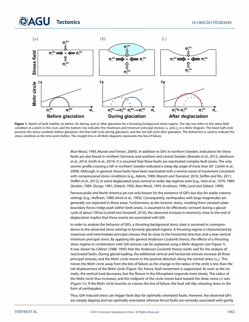
Figure 1. Sketch of fault stability (a) before, (b) during, and (c) after glaciation for a thrusting background stress regime. The top row refers to the stress fieldcondition at a point in the crust, and the bottom row indicates the maximum and minimum principal stresses 𝜎1 and 𝜎3 in a Mohr diagram. The black half circlepresents the stress condition before glaciation, the blue half circle during glaciation, and the red half circle after glaciation. The dotted line is used to indicate thestress condition at the time point before. The straight line in all Mohr diagrams represents the line of failure.

Muir-Wood, 1993; Munier and Fenton, 2004]). In addition to GIFs in northern Sweden, indications for thesefaults are also found in northern Germany and southern and central Sweden [Brandes et al., 2012; Jakobssonet al., 2014; Smith et al., 2014]. It is assumed that these faults are reactivated complex fault zones. The onlyseismic profile crossing a GIF in northern Sweden indicated a steep dip angle of more than 50◦ [Juhlin et al.,2009]. Although, in general, these faults have been reactivated with a reverse sense of movement consistentwith compressional stress conditions [e.g., Adams, 1989; Mazotti and Townend, 2010; Steffen and Wu, 2011;Steffen et al., 2012], in some deglaciated areas normal or strike-slip regimes exist [e.g., Stein et al., 1979, 1989;Quinlan, 1984; Slunga, 1991; Zoback, 1992; Muir-Wood, 1993; Arvidsson, 1996; Lund and Zoback, 1999].

Fennoscandia and North America are not only known for the existence of GIFs but also for stable cratonicsettings [e.g., Hoffman, 1989; Kinck et al., 1993]. Consequently, earthquakes with large magnitudes aregenerally not expected in these areas. Furthermore, as the tectonic stress, resulting from constant plateboundary forces (ridge push within both areas), is assumed to be effectively constant during a glacialcycle of about 100 ka [Luttrell and Sandwell, 2010], the observed increase in seismicity close to the end ofdeglaciation implies that these events are associated with GIA.

In order to analyze the behavior of GIFs, a thrusting background stress state is assumed in correspon-dence to the observed stress settings in formerly glaciated regions. A thrusting regime is characterized bymaximum and intermediate principal stresses that lie close to the horizontal direction and a near-verticalminimum principal stress. By applying the general Anderson-Coulomb theory, the effects of a thrustingstress regime in combination with GIA stresses can be explained using a Mohr diagram (see Figure 1).It was shown by Célérier [1988, 1995] that the Anderson-Coulomb theory works well for the analysis ofreactivated faults. During glacial loading, the additional vertical and horizontal stresses increase all threeprincipal stresses, and the Mohr circle moves in the positive direction along the normal stress (𝜎n). Thismoves the Mohr circle away from the line of failure, as the change in the radius of the circle is less than thenet displacement of the Mohr circle (Figure 1b); hence, fault movement is suppressed. As soon as the icemelts, the vertical load decreases, but the flexure in the lithosphere responds more slowly. The radius ofthe Mohr circle thus increases, and the midpoint of the circle moves back toward the shear stress (𝜏) axis(Figure 1c). If the Mohr circle touches or crosses the line of failure, the fault will slip, releasing stress in theform of earthquakes.

Thus, GIA-induced stress can trigger fault slips for optimally orientated faults. However, the observed GIFsare steeply dipping and not optimally orientated, whereas thrust faults are normally associated with gently

STEFFEN ET AL. ©2014. American Geophysical Union. All Rights Reserved. 1462

Tectonics 10.1002/2013TC003450

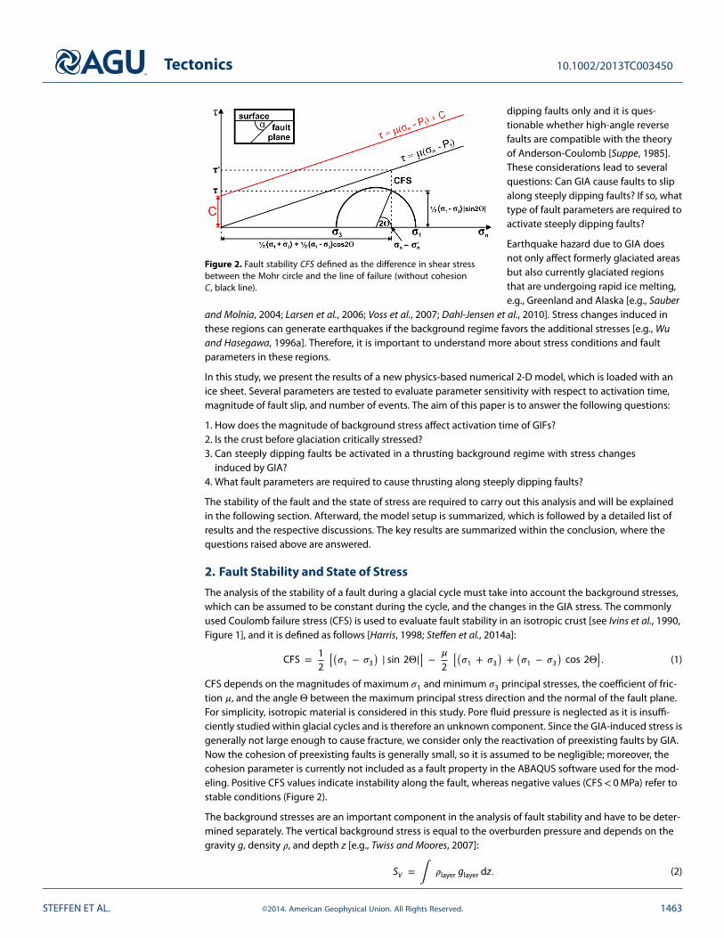
Figure 2. Fault stability CFS defined as the difference in shear stressbetween the Mohr circle and the line of failure (without cohesionC, black line).

dipping faults only and it is ques-tionable whether high-angle reversefaults are compatible with the theoryof Anderson-Coulomb [Suppe, 1985].These considerations lead to severalquestions: Can GIA cause faults to slipalong steeply dipping faults? If so, whattype of fault parameters are required toactivate steeply dipping faults?

Earthquake hazard due to GIA doesnot only affect formerly glaciated areasbut also currently glaciated regionsthat are undergoing rapid ice melting,e.g., Greenland and Alaska [e.g., Sauber

and Molnia, 2004; Larsen et al., 2006; Voss et al., 2007; Dahl-Jensen et al., 2010]. Stress changes induced inthese regions can generate earthquakes if the background regime favors the additional stresses [e.g., Wuand Hasegawa, 1996a]. Therefore, it is important to understand more about stress conditions and faultparameters in these regions.

In this study, we present the results of a new physics-based numerical 2-D model, which is loaded with anice sheet. Several parameters are tested to evaluate parameter sensitivity with respect to activation time,magnitude of fault slip, and number of events. The aim of this paper is to answer the following questions:

1. How does the magnitude of background stress affect activation time of GIFs?2. Is the crust before glaciation critically stressed?3. Can steeply dipping faults be activated in a thrusting background regime with stress changes

induced by GIA?4. What fault parameters are required to cause thrusting along steeply dipping faults?

The stability of the fault and the state of stress are required to carry out this analysis and will be explainedin the following section. Afterward, the model setup is summarized, which is followed by a detailed list ofresults and the respective discussions. The key results are summarized within the conclusion, where thequestions raised above are answered.

2. Fault Stability and State of Stress

The analysis of the stability of a fault during a glacial cycle must take into account the background stresses,which can be assumed to be constant during the cycle, and the changes in the GIA stress. The commonlyused Coulomb failure stress (CFS) is used to evaluate fault stability in an isotropic crust [see Ivins et al., 1990,Figure 1], and it is defined as follows [Harris, 1998; Steffen et al., 2014a]:

CFS = 12

[(𝜎1 − 𝜎3

) | sin 2Θ|] − 𝜇

2

[(𝜎1 + 𝜎3

)+(𝜎1 − 𝜎3

)cos 2Θ

]. (1)

CFS depends on the magnitudes of maximum 𝜎1 and minimum 𝜎3 principal stresses, the coefficient of fric-tion 𝜇, and the angle Θ between the maximum principal stress direction and the normal of the fault plane.For simplicity, isotropic material is considered in this study. Pore fluid pressure is neglected as it is insuffi-ciently studied within glacial cycles and is therefore an unknown component. Since the GIA-induced stress isgenerally not large enough to cause fracture, we consider only the reactivation of preexisting faults by GIA.Now the cohesion of preexisting faults is generally small, so it is assumed to be negligible; moreover, thecohesion parameter is currently not included as a fault property in the ABAQUS software used for the mod-eling. Positive CFS values indicate instability along the fault, whereas negative values (CFS< 0 MPa) refer tostable conditions (Figure 2).

The background stresses are an important component in the analysis of fault stability and have to be deter-mined separately. The vertical background stress is equal to the overburden pressure and depends on thegravity g, density 𝜌, and depth z [e.g., Twiss and Moores, 2007]:

SV = ∫ 𝜌layer glayer dz. (2)

STEFFEN ET AL. ©2014. American Geophysical Union. All Rights Reserved. 1463

Tectonics 10.1002/2013TC003450

The overburden pressure is also included in the horizontal background stress, but an additional tectoniccomponent has to be taken into account. As preexisting faults are not assumed to be optimally orientatedbut were close to neutral stability before the onset of glaciation, the horizontal background stress has todepend on the fault angle [Steffen et al., 2014a]. In this preliminary study, we consider only one fault, orequivalently, we assume that other faults that are more optimally oriented are nonexistent or have a verylarge cohesion. Furthermore, as no other constraints are given for the crust outside of the fault, the samestress conditions have to be assumed. Taking all these assumptions into account, but allowing us to studywhether the isotropic crust was critically stressed before deglaciation, a more general expression for thehorizontal background stress is used [Steffen et al., 2014a]:

SH =𝛽([𝜇 − 𝜇 cos 2Θ + | sin 2Θ|] SV + 2 CFSBG )

− [𝜇 + 𝜇 cos 2Θ − | sin 2Θ|] + (1 − 𝛽) SV . (3)

The additional parameters 𝛽 and CFSBG are defined to allow greater variation in the magnitude of the back-ground stress in order to investigate whether the crust was critically stressed initially. The 𝛽 is a scaling factordefining the magnitude of tectonic background stress in the horizontal stress component. If 𝛽 takes a valueof 1, the horizontal stress component consists of maximum tectonic background stress and the crust is crit-ically stressed. However, the tectonic background stress still depends on the vertical stress SV . In general, adecrease in 𝛽 promotes greater stability along the fault. The minimum 𝛽 value is 0, in which case horizontalstress becomes equal to the vertical stress and tectonic stresses are not included. A variation of this parame-ter enables exploration of the stress conditions before glaciation. As part of our parameter selection process,several values were tested between 0 and 1. However, if a preexisting fault with a certain 𝛼 and 𝜇 is not acti-vated for one 𝛽 value, lower values were not tested for this fault as a decrease in 𝛽 relates to a decrease in themagnitude of tectonic background stress and more stable conditions before glaciation. Therefore, 𝛽 givesthe possibility to decrease tectonic background stresses and test if fault reactivation occurs.

CFSBG represents the fault stability before glaciation (BG). A negative CFSBG increases the distance betweenline of failure and Mohr circle and therefore leads to more stable conditions. The tectonic background stressdecreases in this case, as it can be lowered to reach the state given by the Mohr circle. However, a positiveCFSBG value assumes movement of the fault before glaciation and therefore increased magnitudes in thetectonic background stress. In former studies, the factor CFSBG was set to 0 MPa [e.g., Wu, 1996, 1997; Wuand Hasegawa, 1996a, 1996b; Lund, 2005; Lund et al., 2009].

A third parameter, which is allowed to change, is the coefficient of friction for the tectonic background stress𝜇back. The parameter varies between 0 and 1 but lies mostly in the range between 0.2 and 0.6. We remarkthat the coefficient of friction can also be applied as a surface parameter of the fault [Nüchter and Ellis, 2010],and we use the symbol 𝜇fault here. Different values can be assumed for both coefficients of friction, and for-mer studies suggest values between 0.4 and 0.6 [Byerlee, 1978; Rivera and Kanamori, 2002]. However, 𝜇back

also influences the angle of the fault that can be (re-)activated in a rock mass, and with a decrease in the fric-tion the range of possible fault angles increases [Abers, 2009]. As the dip angle of GIFs is not known exceptfor one case (i.e., more than 50◦ in Juhlin et al. [2009]), the relationship between the coefficient of frictionand the dip angle of GIFs is not well known, so we can only make assumptions concerning the coefficient offriction of the crust.

The above mentioned parameters show a wide range of expected values and affect the magnitude of thehorizontal stress and the fault itself but have no effect on the GIA model. The aim of this paper is to increaseour understanding about these parameters and how they affect fault slip magnitude and activation timeduring a glacial cycle. An increased knowledge is important to the development of more advanced and real-istic models for estimation of the hazard of glacially induced earthquakes. Note that parameters within theGIA model are not changed in this paper, because a sensitivity of these values has already been studied in anaccompanying paper [Steffen et al., 2014b]. In that paper, it is demonstrated that the crustal and lithosphericthickness do not affect the magnitude of fault slip whereas the thickness of the ice sheet has no effect onthe fault slip magnitude, while the timing of fault reactivation is controlled by the ice sheet width.

3. Model Setup

The GIA-fault model used within this study contains a viscoelastic earth model with an ice load appliedon its surface. The earth model is represented by a six-layer finite element mesh (Figure 3). The upper two

STEFFEN ET AL. ©2014. American Geophysical Union. All Rights Reserved. 1464

Tectonics 10.1002/2013TC003450

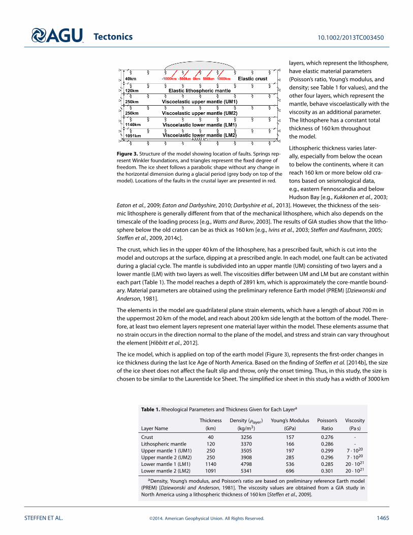
Figure 3. Structure of the model showing location of faults. Springs rep-resent Winkler foundations, and triangles represent the fixed degree offreedom. The ice sheet follows a parabolic shape without any change inthe horizontal dimension during a glacial period (grey body on top of themodel). Locations of the faults in the crustal layer are presented in red.

layers, which represent the lithosphere,have elastic material parameters(Poisson’s ratio, Young’s modulus, anddensity; see Table 1 for values), and theother four layers, which represent themantle, behave viscoelastically with theviscosity as an additional parameter.The lithosphere has a constant totalthickness of 160 km throughoutthe model.

Lithospheric thickness varies later-ally, especially from below the oceanto below the continents, where it canreach 160 km or more below old cra-tons based on seismological data,e.g., eastern Fennoscandia and belowHudson Bay [e.g., Kukkonen et al., 2003;

Eaton et al., 2009; Eaton and Darbyshire, 2010; Darbyshire et al., 2013]. However, the thickness of the seis-mic lithosphere is generally different from that of the mechanical lithosphere, which also depends on thetimescale of the loading process [e.g., Watts and Burov, 2003]. The results of GIA studies show that the litho-sphere below the old craton can be as thick as 160 km [e.g., Ivins et al., 2003; Steffen and Kaufmann, 2005;Steffen et al., 2009, 2014c].

The crust, which lies in the upper 40 km of the lithosphere, has a prescribed fault, which is cut into themodel and outcrops at the surface, dipping at a prescribed angle. In each model, one fault can be activatedduring a glacial cycle. The mantle is subdivided into an upper mantle (UM) consisting of two layers and alower mantle (LM) with two layers as well. The viscosities differ between UM and LM but are constant withineach part (Table 1). The model reaches a depth of 2891 km, which is approximately the core-mantle bound-ary. Material parameters are obtained using the preliminary reference Earth model (PREM) [Dziewonski andAnderson, 1981].

The elements in the model are quadrilateral plane strain elements, which have a length of about 700 m inthe uppermost 20 km of the model, and reach about 200 km side length at the bottom of the model. There-fore, at least two element layers represent one material layer within the model. These elements assume thatno strain occurs in the direction normal to the plane of the model, and stress and strain can vary throughoutthe element [Hibbitt et al., 2012].

The ice model, which is applied on top of the earth model (Figure 3), represents the first-order changes inice thickness during the last Ice Age of North America. Based on the finding of Steffen et al. [2014b], the sizeof the ice sheet does not affect the fault slip and throw, only the onset timing. Thus, in this study, the size ischosen to be similar to the Laurentide Ice Sheet. The simplified ice sheet in this study has a width of 3000 km

Table 1. Rheological Parameters and Thickness Given for Each Layera

Thickness Density (𝜌layer) Young’s Modulus Poisson’s Viscosity

Layer Name (km) (kg/m3) (GPa) Ratio (Pa s)

Crust 40 3256 157 0.276 -Lithospheric mantle 120 3370 166 0.286 -Upper mantle 1 (UM1) 250 3505 197 0.299 7 ⋅ 1020

Upper mantle 2 (UM2) 250 3908 285 0.296 7 ⋅ 1020

Lower mantle 1 (LM1) 1140 4798 536 0.285 20 ⋅ 1021

Lower mantle 2 (LM2) 1091 5341 696 0.301 20 ⋅ 1021

aDensity, Young’s modulus, and Poisson’s ratio are based on preliminary reference Earth model(PREM) [Dziewonski and Anderson, 1981]. The viscosity values are obtained from a GIA study inNorth America using a lithospheric thickness of 160 km [Steffen et al., 2009].

STEFFEN ET AL. ©2014. American Geophysical Union. All Rights Reserved. 1465

Tectonics 10.1002/2013TC003450

and a thickness of 3500 m and follows a parabolic shape. For simplicity, the ice margin is not allowed tomigrate outward during glaciation nor inward during deglaciation. The glacial cycle has a duration of 130 kaconsisting of a 100 ka glaciation phase, 10 ka deglaciation phase, and a 20 ka postglacial phase. During thepostglacial phase no ice load is applied to the model. A single time step has a duration of 1 ka. Therefore,the accuracy of the activation times is ±500 a. The simplicity of our ice models implies that conclusionsdrawn from this study might change if multiple ice domes exist, the geometry of the ice follows the coast-line, or timing of ice collapsing is complex. Nevertheless, general insights concerning the behavior of faultproperties and magnitudes of tectonic background stress can be taken from this pilot study.

The GIA-fault model is similar to other models used in GIA studies but has fault surfaces included, which areallowed to release stresses induced by GIA. As commercial finite element software (e.g., ABAQUS [Hibbitt etal., 2012]) only allow the solution of simple equations of motion and do not include the advection of pre-stress term, which represents a buoyancy return force and is of primary importance in geoscientific studies,the method has been modified to include a stress transformation [Wu, 2004]. This modification implies thatthe stress output from the finite element model has to be adjusted to give a true estimate of GIA stress. Toovercome this and other problems, a new approach has been developed [Steffen et al., 2014a]. This consistsof a three-step cascaded model that uses the GIA model as the first model, which computes displacementand stress distributions during a glacial cycle. The results are used in the second and third models, whichare created if fault instability exists (CFS> 0). Each finite element in the second and third models containsa stress magnitude determined from the first model including the GIA stress component, and each node isdisplaced based on the displacement obtained from the first model. Fault slip and the release of GIA stressesin the third model is enabled using an open fault contact and the application of a friction value betweenopposing fault surfaces. The slip of the fault creates an offset between hanging wall and footwall. A detaileddescription of this approach can be found in Steffen et al. [2014a]. The advantage of this new model [Steffenet al., 2014a] is that the role of GIA-induced stress is explicitly included and not mixed in with the effect ofplate motion.

A similar approach was developed by Hampel and Hetzel [2006] and numerous thrust-fault results were pre-sented in Turpeinen et al. [2008], but their models simplify the effects of GIA stress and neglect the effectof the viscoelastic mantle. However, the mantle is the driving force of the viscoelastic behavior of GIA, andwithout the mantle, only an elastic GIA effect is taken into account. Furthermore, fault slips in their mod-els are a result of the combined effects of a stress related to GIA and a converging horizontal displacementboundary condition.

4. Results and DiscussionThe earth and ice model are not changed within this study, and therefore, the GIA signal is the same for allvariations. The magnitude in tectonic background stress depends on the fault angle (see equation (3)) andalso on the parameters 𝜇back (coefficient of friction in the crust), CFSBG (fault stability before glaciation), and𝛽 (ratio of tectonic background stress in horizontal stress). The angle is varied within all tests as well as thelocation of the fault.

Four different fault dip angles are tested: 30◦, 45◦, 60◦, and 75◦. In addition, the fault location is variedbetween −1000 km, −500 km, 0 km, 500 km, and 1000 km (Figure 3). All faults are incorporated into themodel for all tests; however, only the contact of the specific fault investigated in a test is open, while allother fault contacts are tied and no motion is possible. The variation of the other tectonic background stressparameters is listed in Table 2, with the reference model having a coefficient of friction for the crust (𝜇back) of0.4, a fault stability before glaciation (CFSBG) of 0 MPa, which indicates a critically stressed crust, and 100 %tectonic stress in the horizontal stress component (𝛽 = 1). Positive values of CFSBG and values of above 1 for𝛽 are not considered as observations indicate that GIFs were probably not active for several million of yearsand were not active before glaciation started [Lagerbäck and Sundh, 2008].

Furthermore, the depth of the fault tip and the coefficient of friction between opposing fault surfaces(𝜇fault) are varied (Table 2). The fault tip is defined mathematically as the point where both fault surfacesend in the crust and fault movement terminates. The fault tip remains fixed during each test; hence, faultsurface growth is not considered. The reference model consists of a fault that extends from the surface toa depth of 8 km and a 𝜇fault of 0.4. Further parameters (cohesion C and pore fluid factor 𝜆) are neglectedand set to 0 to decrease the number of potential factors of fault slip and activation time in this study[see Steffen et al., 2014a].

STEFFEN ET AL. ©2014. American Geophysical Union. All Rights Reserved. 1466

Tectonics 10.1002/2013TC003450

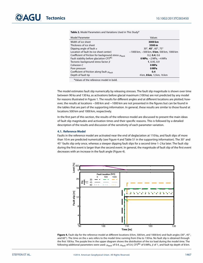
Table 2. Model Parameters and Variations Used in This Studya

Model Parameter Values

Width of ice sheet 3000 kmThickness of ice sheet 3500 mDipping angle of fault 𝛼 30◦ , 45◦ , 60◦, 75◦

Location of fault (to ice sheet center) −1000 km, −500 km, 0 km, 500 km, 1000 kmCoefficient of friction for background stress 𝜇back 0.2, 0.4, 0.6Fault stability before glaciation CFSBG 0 MPa, −2 MPa, −4 MPaTectonic background stress factor 𝛽 1, 0.95, 0.9Cohesion C 0 MPaPore pressure 0 MPaCoefficient of friction along fault 𝜇fault 0.4Depth of fault tip 4 km, 8 km, 12 km, 16 km

aValues of the reference model in bold.

The model estimates fault slip numerically by releasing stresses. The fault slip magnitude is shown over timebetween 90 ka and 130 ka, as activations before glacial maximum (100 ka) are not predicted by any modelfor reasons illustrated in Figure 1. The results for different angles and at different locations are plotted; how-ever, the results at locations −500 km and −1000 km are not presented in the figures but can be found inthe tables that are part of the supporting information. In general, these results are similar to those found atlocations 500 km and 1000 km, respectively.

In the first part of this section, the results of the reference model are discussed to present the main ideasof fault slip magnitudes and activation times and their specific reasons. This is followed by a detaileddescription of the results and discussion of the sensitivity of each parameter variation.

4.1. Reference ModelFaults in the reference model are activated near the end of deglaciation at 110 ka, and fault slips of morethan 10 m are predicted numerically (see Figure 4 and Table S1 in the supporting information). The 30◦ and45◦ faults slip only once, whereas a steeper dipping fault slips for a second time 1–2 ka later. The fault slipduring the first event is larger than the second event. In general, the magnitude of fault slip of the first eventdecreases with an increase in the fault angle (Figure 4).

Figure 4. Fault slip for the reference model at different locations (0 km, 500 km, and 1000 km) and fault angles (30◦ , 45◦,and 60◦). The time on the x axis refers to the model time running from 0 ka to 130 ka. No fault slip is obtained throughthe first 100 ka. The purple line in the upper diagram shows the distribution of the ice load during the model time. Thefollowing additional parameters were used: 𝜇back of 0.4, 𝜇fault of 0.4, CFSBG of 0 MPa, 𝛽 of 1, and fault tip depth of 8 km.

STEFFEN ET AL. ©2014. American Geophysical Union. All Rights Reserved. 1467

Tectonics 10.1002/2013TC003450

Table 3. Stress Magnitudes Depending on Fault Angle and Coefficientof Frictiona

Fault Angle 𝛼 𝜇back SH (MPa) SV (MPa) 𝜏 (MPa) 𝜎n (MPa)

30◦ 0.2 244 160 36 18145◦ 0.2 240 160 40 20060◦ 0.2 273 160 49 24575◦ 0.2 666 160 127 63230◦ 0.4 353 160 84 20845◦ 0.4 374 160 107 26760◦ 0.4 642 160 209 52230◦ 0.6 500 160 147 24545◦ 0.6 641 160 241 401

aHorizontal (SH) and vertical (SV ) background stresses as well asnormal (𝜎n) and shear (𝜏) stresses for different fault angles 𝛼 andcoefficient of internal frictions of the crust 𝜇back at a depth of 5 km.

The amount of fault slip is affectedby the normal and shear stressesalong the fault, which depend onthe fault angle and the relationshipbetween maximum and minimumprincipal stresses 𝜎1 and 𝜎3, respec-tively. The shear stress acts parallelto the fault and causes the sliding ofthe fault, whereas the normal stressacts perpendicular to the fault sur-faces, pressing the surfaces togetherand preventing fault movement. As𝜎3 is the vertical stress in a thrust-ing regime, it is mainly determinedby the overburden pressure and theweight of the ice sheet. Commencingat the start of deglaciation, 𝜎3 begins

to decrease. After the load is completely gone (at 110 ka), the vertical stress is the same as before glaciation,and only overburden pressure is present. The 𝜎1 is the horizontal stress and is affected by the backgroundstress and the flexure of the lithosphere induced by GIA. The latter starts to decrease at the start of deglacia-tion, but the rate of decrease is much slower than that of 𝜎3. Therefore, after the end of deglaciation, onlyhorizontal rebound stress remains in addition to the tectonic background stress. The rebound stressesdepend only on the ice and earth model [Steffen et al., 2014b], are independent of the fault angle, and arenot changed within this study.

However, the horizontal background stresses required to keep the fault at frictional equilibrium dependson the angles of the fault (see equation (3)). This is shown in Table 3. A 60◦-dipping fault implies higher hor-izontal background stresses in order to be close to initial frictional equilibrium (about 4 times the verticalstress for a coefficient of friction of 0.4; see equation (3)) than 30◦ and 45◦ faults with only about 2.2 timesand 2.3 times the vertical stress, respectively. However, the fault slip magnitude decreases with an increasein fault angle and an accompanying increase in tectonic background stress (Table 3).

The change in the magnitudes of normal and shear stresses on the fault as a consequence of the stress statein the crust is related to the principal stresses and the fault angle (𝛼 = 90◦ − Θ) by

𝜏 = 0.5(𝜎1 − 𝜎3

) | sin 2Θ|, (4a)

𝜎n = 0.5(𝜎1 + 𝜎3

)+ 0.5

(𝜎1 − 𝜎3

)cos 2Θ. (4b)

This leads to the following equations for each fault angle used in this study:

𝛼 = 30◦ ∶ 𝜏 = 0.433(𝜎1 − 𝜎3

),

𝜎n = 0.25 𝜎1 + 0.75 𝜎3,

𝛼 = 45◦ ∶ 𝜏 = 0.5(𝜎1 − 𝜎3

),

𝜎n = 0.5 𝜎1 + 0.5 𝜎3,

𝛼 = 60◦ ∶ 𝜏 = 0.433(𝜎1 − 𝜎3

),

𝜎n = 0.75 𝜎1 + 0.25 𝜎3,

𝛼 = 75◦ ∶ 𝜏 = 0.25(𝜎1 − 𝜎3

),

𝜎n = 0.933 𝜎1 + 0.067 𝜎3.

The equations above show that with an increase in the fault angle, the normal stress, which opposes faultmovement, has an increasing contribution from the horizontal stress. For the shear stress, which drives thefault slip, the coefficient in front of the stress difference (𝜎1 − 𝜎3) reaches maximum at 45◦, but because thestress difference increases with 𝛼 (see Table 3), the value of shear also increases with steeper dipping faultangle, but its value is always less than that of the normal stress. As a consequence, a steeper dipping faultangle means a smaller fault slip in one event. The length of the fault also increases with a decrease in the

STEFFEN ET AL. ©2014. American Geophysical Union. All Rights Reserved. 1468

Tectonics 10.1002/2013TC003450

angle as the modeled faults are constrained to extend between depth of fault tip and the Earth’s surface. A30◦ dipping fault is 16 km long, whereas a 60◦ fault has a length of only 9.24 km. A longer fault slips moreand produces larger fault throws [e.g., Kim and Sanderson, 2005].

Differences in the fault slip between different locations are related to their specific position of the faultwith respect to the ice sheet center. All faults dip in the same direction (see Figure 3), which results in a diptoward the ice sheet center for faults at +500 km and +1000 km (on the positive/right side of the model), anda dip away from the center at −500 km and −1000 km (on the negative/left side of the model). As reboundstresses increase toward the ice sheet center, faults closer to the center slip more. Furthermore, faults on thepositive side of the model have more ice applied on the hanging wall, and if the fault is activated during thedeglaciation phase, the fault slips less than faults on the negative side of the model. These faults have lessice applied on the hanging wall. However, as soon as deglaciation ends and no ice load is applied on thehanging wall or footwall, the rebound stress plays a more important role, and faults with their tips closer tothe center slip more than faults farther away.

In summary, the differences in fault throw for different fault angles and locations can be explained by nor-mal and shear stress directions and magnitudes. The location of a fault with respect to the ice center resultsin different amounts of ice loading between the hanging wall and the footwall, which determine whetherthe fault slips more during or after deglaciation.

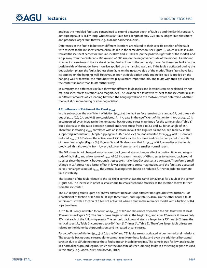
4.2. Influence of Friction of the Crust 𝝁back

In this subsection, the coefficient of friction (𝜇fault) at the fault surface remains constant at 0.4, but three val-ues of 𝜇back (0.2, 0.4, and 0.6) are considered. An increase in the coefficient of friction for the crust (𝜇back) isaccompanied by an increase in the horizontal background stress magnitude for the same angles (Table 3)but a decrease in the ratio between normal and shear stress from 5 to 2.5 and 1.7 for an angle of 45◦.Therefore, increasing 𝜇back correlates with an increase in fault slip (Figures 5a and 5b; see Table S2 in thesupporting information). Steeply dipping faults (60◦ and 75◦) are not activated for a 𝜇back of 0.6. However,reduced 𝜇back of 0.2 allows the activation of 75◦ faults for the first time and can be compared to resultsof lower fault angles (Figure 5b). Figures 5a and 5b also show that for 𝜇back of 0.2, an earlier activation ispredicted; this also results from lower background stresses and a smaller normal stress.

The GIA stress is not changed; only tectonic background stress changes affect activation time and magni-tude of fault slip, and a low value of 𝜇back of 0.2 increases the ratio of GIA stresses to tectonic backgroundstresses since the tectonic background stresses are smaller but GIA stresses are constant. Therefore, a smallchange in GIA stress has a larger effect in lower background stress magnitudes, and the faults are activatedearlier. For larger values of 𝜇back, the vertical loading stress has to be reduced further in order to promotefault instability.

The location of the fault relative to the ice sheet center shows the same behavior as for a fault at the center(Figure 5a). The increase in offset is smaller due to smaller rebound stresses as the location moves fartherfrom the ice center.

The 60◦ dipping fault (Figure 5b) shows different behaviors for different background stress frictions. Fora coefficient of friction of 0.2, the fault slips three times, and slip totals 5.48 m. On the other hand, a faultwithin a crust with a friction of 0.6 is not activated, while a fault in the reference model with a friction of 0.4slips two times.

A 75◦ fault is only activated for a friction (𝜇back) of 0.2 and slips more often than the 60◦ fault with at least22 events (see Figure 5b). The fault shows larger offsets at the beginning, and after 12 events, it moves only17 cm at each of the following events. The tectonic background stress is larger for a 75◦ fault (4.2 times thevertical stress SV , Table 3) compared to a 60◦ fault (1.7 times SV , Table 3). Therefore, larger fault offsets arerelated to the higher background stress and increased shear stresses.

For a coefficient of friction (𝜇back) of 0.6, the 60◦ and 75◦ faults are not activated in our numerical simulations.The tectonic background stresses alone cannot reactivate these faults, and even the additional horizontalstresses due to GIA do not move these faults into an instability regime. The same is true for low-angle faultsin a normal background regime, which are the opposite of steep-dipping faults in a thrusting regime as usedin this study [e.g., Abers, 2009; Bonini et al., 2012].

STEFFEN ET AL. ©2014. American Geophysical Union. All Rights Reserved. 1469

Tectonics 10.1002/2013TC003450

Figure 5. The effect of the following parameters on the activation time and magnitude of fault slip: (a and b) the coefficient of friction in the crust (𝜇back),(c and d) CFSBG, and (e and f) 𝛽 in addition to fault location (Figures 5a, 5c, and 5e) and fault angle (Figures 5b, 5d, and 5f ). The time on the x axis refers to themodel time running from 0 ka to 130 ka. No fault slip is obtained through the first 100 ka. The purple line in the upper diagram shows the distribution of the iceload during the model time. The following additional parameters were used: 𝜇fault of 0.4 and fault tip depth of 8 km.

In summary, fault throw and activation time are sensitive to the friction in the crust (𝜇back), and large offsets

of up to ∼30 m can be produced by a coefficient of friction of 0.6. However, not all faults in a crust with this

friction value are activated. On the other hand, steeply dipping faults with lower friction values do not reach

a state of stability as evidenced by Figure 5b.

STEFFEN ET AL. ©2014. American Geophysical Union. All Rights Reserved. 1470

Tectonics 10.1002/2013TC003450

4.3. Influence of Change in Tectonic Background Stress (CFSBG and 𝜷)When the tectonic background stress falls below critical stress conditions, the activation of most faults isaffected, and only faults below or close to the ice sheet center and with dips of 30◦ and 45◦ are activated(Figures 5c and 5d; see Table S2 in the supporting information).

A decrease in the tectonic background stress before glaciation leads to no fault activation for fault dipsof 60◦ or more or if the faults are located at −1000 km or +1000 km away from the center of the model. Ifunstable conditions are obtained along the fault, a reduction in tectonic background stress causes the acti-vation time to move from before to after the end of deglaciation. The later activation time correlates with anincrease in fault slip as vertical stresses due to the load are smaller or no longer existent (see equations (4a)and (4b)). A CFSBG of −2 MPa generates stress conditions such that a fault at ±500 km can be activatedby GIA, but a further decrease to −4 MPa shows stable conditions for the whole glacial cycle. Thus, thecrust along the weak zone in Laurentia and Fennoscandia cannot have initial fault stability much less than−2 MPa. In other words, to explain the localization of paleo and current intraplate earthquakes in Laurentia,we only need to assume that the initial fault stability is −4 MPa or more outside the earthquake zones.

A change in the parameter 𝛽 from 1 to 0.95 shows that fault instability is not obtained for all faults testedin the model, and only 30◦ and 45◦ faults at the center or at ±500 km can be activated by GIA (Figure 5f ).The activation time moves from before the end of deglaciation to a time point at or after it, which results inhigher fault throws. For an even lower 𝛽 of 0.9, no fault is activated. Therefore, lower values of 𝛽 were nottested as stable conditions are predicted to prevail during the entire glacial cycle and afterward.

Assuming lower tectonic stress conditions at the beginning of the glacial cycle, some faults are not acti-vated (e.g., 60◦-dipping faults). Only below the ice sheet center, faults can be activated when the faultstability before glaciation was −4 MPa, which is accompanied by a decrease of horizontal stress of 4 MPa.Thus, the stress conditions before glaciation have to be close to the state of a critically stressed crust. Lowerbackground stress conditions than for critical stress conditions show that most faults are not activated dueto GIA. However, fault reactivation is observed in North America and Europe, implying that critical stressconditions are valid along the observed earthquake zones. Additionally, near-surface stress relief phenom-ena have been documented in formerly glaciated regions [Pascal et al., 2010] indicating that the crust iscritically stressed.

In summary, steeply dipping faults and faults located away from the ice sheet center are not activated if thecrust is not critically stressed. Our models suggest that the horizontal background stresses were sufficientlylow that without GIA no major earthquakes would have occurred along these faults. Earthquakes occur onlywhen the crust is sufficiently close to a critical state that GIA can trigger fault reactivation, producing severalmeters of fault slip.

4.4. Influence of Friction of the Fault 𝝁fault

Fault slip magnitude increases with a decrease in coefficient of friction for the fault 𝜇fault. However, as tec-tonic background and GIA stresses are constant, the activation time is not changed (Figures 6a and 6b; seeTable S3 in the supporting information).

The friction between opposing fault surfaces (𝜇fault) gives an estimate of the resistance to displacement.Higher frictions lead to smaller movement, and therefore, smaller fault throws are obtained. This applies toall fault angles and locations. However, the difference in the slip between minimum and maximum frictiondecreases with a decreasing fault angle.

4.5. Influence of Depth of Fault TipThe increase in the depth of the fault tip is accompanied by an increase in fault slip; however, the activa-tion time of the fault remains constant, as tectonic background and GIA stresses are not changed by thisparameter (Figures 6c and 6d; see Table S3 in the supporting information).

The fault slip magnitude is affected by the fault angle and depth of fault tip as the length of the fault is deter-mined by these two parameters. A low-dipping fault is longer than a more steeply dipping fault with the tipsat the same depths. The increase in fault slip due to deeper fault tips is induced by the length of the faultand also due to larger tectonic background stresses at deeper depths, since the stress increases with depthaccording to equation (3).

STEFFEN ET AL. ©2014. American Geophysical Union. All Rights Reserved. 1471

Tectonics 10.1002/2013TC003450

Figure 6. Similar to Figure 5, except for the coefficient of friction at the (a and b) fault (𝜇fault) and (c and d) fault tip depth. The following additional parameterswere used: 𝜇back of 0.4, CFSBG of 0 MPa, and 𝛽 of 1.

Faults at a location of +500 km show a lower fault throw for all depths of the fault tip than faults at −500 km.The difference between offsets on both sides of the center increases with an increase in fault tip depth.Faults at +1000 km and tips at 4 km and 8 km slip less than faults with the same tips at −1000 km. For largerdepths of the fault tip, the behavior changes and faults at +1000 km slip up to 25 cm more than faults at−1000 km, but the activation time is constant. Faults on the positive side dip toward the ice sheet center,which induces higher stresses in the deeper parts of the faults. These stresses are higher compared to a faultat the same location on the other side of the ice sheet center (the negative side), as the fault tip is fartheraway from the ice sheet center due to the same dipping direction. The difference in the horizontal stress atfault tips on both sides of the model increases with an increase in the depth of the fault tip, and therefore,an increase in the difference of the fault throws is obtained or even a change in the maximum offset fromthe negative side to the positive side.

The activation time is the same for each fault and not sensitive to the depth of the fault tip. This is causedby a constant tectonic background stress and rebound stress applied to the model. However, the tectonicbackground stress increases with depth, and faults activated from deeper tips produce larger offsets as morestress is released, which controls the fault movement.

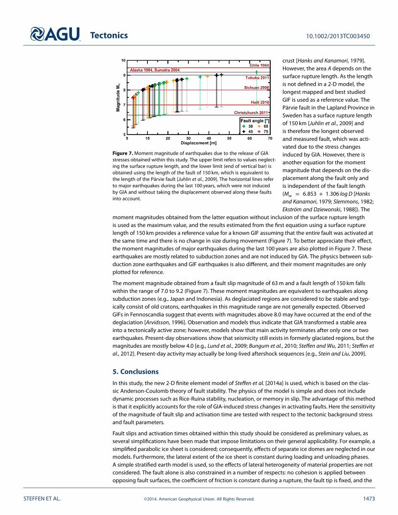
4.6. Relationship of Modeled Fault Slips to Earthquake Moment MagnitudesIn order to better appreciate the effects of GIA-induced fault slips along the GIF, we compute their earth-quake moment magnitudes and compare them with some well-known large events triggered not byGIA. Moment magnitude (Mw) of earthquakes can be expressed in terms of displacement (D) along faults:Mw = 2∕3 log(G ⋅ D ⋅ A) − 10.7, where A is the surface area of the fault and G is the shear modulus of the

STEFFEN ET AL. ©2014. American Geophysical Union. All Rights Reserved. 1472

Tectonics 10.1002/2013TC003450

Figure 7. Moment magnitude of earthquakes due to the release of GIAstresses obtained within this study. The upper limit refers to values neglect-ing the surface rupture length, and the lower limit (end of vertical bar) isobtained using the length of the fault of 150 km, which is equivalent tothe length of the Pärvie fault [Juhlin et al., 2009]. The horizontal lines referto major earthquakes during the last 100 years, which were not inducedby GIA and without taking the displacement observed along these faultsinto account.

crust [Hanks and Kanamori, 1979].However, the area A depends on thesurface rupture length. As the lengthis not defined in a 2-D model, thelongest mapped and best studiedGIF is used as a reference value. ThePärvie fault in the Lapland Province inSweden has a surface rupture lengthof 150 km [Juhlin et al., 2009] andis therefore the longest observedand measured fault, which was acti-vated due to the stress changesinduced by GIA. However, there isanother equation for the momentmagnitude that depends on the dis-placement along the fault only andis independent of the fault length(Mw = 6.853 + 1.306 log D [Hanksand Kanamori, 1979; Slemmons, 1982;Ekström and Dziewonski, 1988]). The

moment magnitudes obtained from the latter equation without inclusion of the surface rupture lengthis used as the maximum value, and the results estimated from the first equation using a surface rupturelength of 150 km provides a reference value for a known GIF assuming that the entire fault was activated atthe same time and there is no change in size during movement (Figure 7). To better appreciate their effect,the moment magnitudes of major earthquakes during the last 100 years are also plotted in Figure 7. Theseearthquakes are mostly related to subduction zones and are not induced by GIA. The physics between sub-duction zone earthquakes and GIF earthquakes is also different, and their moment magnitudes are onlyplotted for reference.

The moment magnitude obtained from a fault slip magnitude of 63 m and a fault length of 150 km fallswithin the range of 7.0 to 9.2 (Figure 7). These moment magnitudes are equivalent to earthquakes alongsubduction zones (e.g., Japan and Indonesia). As deglaciated regions are considered to be stable and typ-ically consist of old cratons, earthquakes in this magnitude range are not generally expected. ObservedGIFs in Fennoscandia suggest that events with magnitudes above 8.0 may have occurred at the end of thedeglaciation [Arvidsson, 1996]. Observation and models thus indicate that GIA transformed a stable areainto a tectonically active zone; however, models show that main activity terminates after only one or twoearthquakes. Present-day observations show that seismicity still exists in formerly glaciated regions, but themagnitudes are mostly below 4.0 [e.g., Lund et al., 2009; Bungum et al., 2010; Steffen and Wu, 2011; Steffen etal., 2012]. Present-day activity may actually be long-lived aftershock sequences [e.g., Stein and Liu, 2009].

5. Conclusions

In this study, the new 2-D finite element model of Steffen et al. [2014a] is used, which is based on the clas-sic Anderson-Coulomb theory of fault stability. The physics of the model is simple and does not includedynamic processes such as Rice-Ruina stability, nucleation, or memory in slip. The advantage of this methodis that it explicitly accounts for the role of GIA-induced stress changes in activating faults. Here the sensitivityof the magnitude of fault slip and activation time are tested with respect to the tectonic background stressand fault parameters.

Fault slips and activation times obtained within this study should be considered as preliminary values, asseveral simplifications have been made that impose limitations on their general applicability. For example, asimplified parabolic ice sheet is considered; consequently, effects of separate ice domes are neglected in ourmodels. Furthermore, the lateral extent of the ice sheet is constant during loading and unloading phases.A simple stratified earth model is used, so the effects of lateral heterogeneity of material properties are notconsidered. The fault alone is also constrained in a number of respects: no cohesion is applied betweenopposing fault surfaces, the coefficient of friction is constant during a rupture, the fault tip is fixed, and the

STEFFEN ET AL. ©2014. American Geophysical Union. All Rights Reserved. 1473

Tectonics 10.1002/2013TC003450

effects of pore fluid pressure are neglected. Nevertheless, our approach provides important new insightsconcerning GIF behavior in different stress settings and with respect to the dip angle of preexisting faults.

Faults are activated close to the end of deglaciation, and the slip magnitude depends mainly on the depthof the fault tip and, therefore, on the length of the fault. For consistency with prevailing stress regimes inFennoscandia and Laurentia, the background stress regime is assumed to be of thrust/reverse type. The faultslips obtained within this study imply large-magnitude earthquakes (≥5.9), which are not expected in stableand old cratonic areas like eastern Canada and in the absence of GIA-induced stress perturbations.

Our modeling indicates that a fault with low dip angle slips only once, but steeply dipping faults may slipmore. A limitation of our approach is that stress buildup at the fault tip is not accounted for. However, theslip magnitudes of subsequent events have smaller magnitudes compared to the main event. Observationsand also results from our GIA-fault models show that transient stress perturbations due to GIA transformed astable cratonic area into a tectonically active zone with earthquake magnitudes comparable to those foundin subduction zones (e.g., Japan and Indonesia).

Below we summarize the answers to the questions raised in section 1:

1. The magnitude in tectonic background stress affects the activation time but only by a few thousand yearsafter deglaciation.

2. The stress conditions before glaciation must be very close to a critically stressed crust; otherwise GIA isinsufficient to trigger the observed intraplate earthquakes.

3. Steeply dipping faults can be activated if the coefficient of friction of the crust is assumed to be equal toor lower than 0.4.

4. Depth of fault tip and coefficient of friction along the fault affect the fault slip magnitude but do notinfluence the activation time as the GIA and tectonic background stress magnitudes are not changed.

The modeled fault slips fit well to observed data in North America and Europe. Major fault offsets observedin formerly glaciated regions are obtained within this study. However, many smaller offsets in the centimeterrange exist [see Fenton, 1994] but are not produced by this model.

The answers of these questions have opened new problems, which need to be analyzed and tested toobtain a better understanding of fault slip magnitude and activation time due to GIA. For example, theeffect of a changing pore fluid pressure was neglected within this study, but this factor has the potential totrigger GIFs. However, this parameter is insufficiently studied and will be the topic of a forthcoming paper.Moreover, cohesion along the fault plane was neglected, in part because preexisting faults generally havelow cohesion. Nevertheless, this study has helped to answer several questions, and changes in fault slipmagnitude and activation time could be related to these parameters: e.g., dip angle, coefficient of friction,fault stability before glaciation, and tectonic background stress factor. Future investigations will include thementioned ideas above as well as the extension into a three-dimensional model.

ReferencesAbers, G. A. (2009), Slip on shallow-dipping normal faults, Geology, 37, 767–768, doi:10.1130/focus082009.1.Adams, J. (1989), Crustal stresses in eastern Canada, in Earthquakes at North Atlantic Passive Margins: Neotectonics and Postglacial

Rebound, edited by S. Gregersen and P. W. Basham, pp. 289–297, Kluwer, Dordrecht, Netherlands.Arvidsson, R. (1996), Fennoscandian earthquakes: Whole crustal rupturing related to postglacial rebound, Science, 274, 744–746,

doi:10.1126/science.274.5288.744.Bonini, M., F. Sani, and B. Antonielli (2012), Basin inversion and contractional reactivation of inherited normal faults: A review based on

previous and new experimental models, Tectonophysics, 522–523, 55–88, doi:10.1016/j.tecto.2011.11.014.Brandes, C., J. Winsemann, J. Roskosch, J. Meinsen, D. C. Tanner, S. Tsukamoto, M. Frechen, H. Steffen, and P. Wu (2012), Activity along

the Osning thrust in central Europe during the late Weichselian: Ice-sheet and lithosphere interactions, Quat. Sci. Rev., 38, 49–62,doi:10.1016/j.quascirev.2012.01.021.

Bungum, H., O. Olesen, C. Pascal, S. Gibbons, C. Lindholm, and O Vestøl (2010), To what extent is the present seismicity of Norway drivenby post-glacial rebound?, J. Geol. Soc. London, 167, 373–384, doi:10.1144/0016-76492009-009.

Byerlee, J. D. (1978), Friction of rock, Pure Appl. Geophys., 116, 615–626, doi:10.1007/BF00876528.Célérier, B. (1988), How much does slip on a reactivated fault plane constrain the stress tensor?, Tectonics, 7, 1257–1278,

doi:10.1029/TC007i006p01257.Célérier, B. (1995), Tectonic regime and slip orientation of reactivated faults, Geophys. J. Int., 121, 143–161,

doi:10.1111/j.1365-246X.1995.tb03517.x.Dahl-Jensen, T., T. B. Larsen, and P. Voss (2010), Greenland ice sheet monitoring network (GLISN): A seismological approach, Geol. Surv.

Den. Greenl., 20, 55–58.Darbyshire, F., D. W. Eaton, and I. D. Bastow (2013), Seismic imaging of the lithosphere beneath Hudson Bay: Episodic growth of the

Laurentian mantle keel, Earth Planet. Sci. Lett., 373, 179–193, doi:10.1016/j.epsl.2013.05.002.

AcknowledgmentsWe thank the Editors Onno Onckenand John Geissman and the review-ers Christophe Pascal and Erik Ivins fortheir constructive reviews and com-ments. We would like to thank BjörnLund (Uppsala University), Steffen Abe(RWTH Aachen), and Bernard Guest,Robert Taerum, and Len Hills (all fromUniversity of Calgary) for helpful dis-cussions, for providing data sets, andfor suggestions and comments on ear-lier versions of the manuscript. Theresearch is supported by NSERC Dis-covery Grants to David W. Eaton andPatrick Wu. Figures 4–6 were drawnusing the GMT graphics package[Wessel and Smith, 1998].

STEFFEN ET AL. ©2014. American Geophysical Union. All Rights Reserved. 1474

Tectonics 10.1002/2013TC003450

Dyke, A. S., T. F. Morris, and D. E. C. Green (1991), Postglacial tectonic and sea level history of the central Canadian Arctic, Bull. Geol. Surv.Can., 397, 56.

Dziewonski, A. M., and D. L. Anderson (1981), Preliminary reference Earth model, Phys. Earth planet. Inter., 25, 297–356,doi:10.1016/0031-9201(81)90046-7.

Eaton, D. W., and F. Darbyshire (2010), Lithospheric architecture and tectonic evolution of the Hudson Bay region, Tectonophysics, 480,1–22, doi:10.1016/j.tecto.2009.09.006.

Eaton, D. W., F. Darbyshire, R. L. Evans, H. Grutter, A. G. Jones, and X. Yuan (2009), The elusive lithosphere-asthenosphere boundary (LAB)beneath cratons, Lithos, 109, 1–22, doi:10.1016/j.lithos.2008.05.009.

Ekström, G., and A. M. Dziewonski (1988), Evidence of bias in estimations of earthquake size, Nature, 332, 319–323, doi:10.1038/332319a0.Fenton, C. (1994), Postglacial faulting in Eastern Canada, Geol. Surv. Canada Open File Rep. 2774, 94 pp., Natural Resources Canada.Hampel, A., and R. Hetzel (2006), Response of normal faults to glacial-interglacial fluctuations of ice and water masses on Earth’s surface,

J. Geophys. Res., 111, B06406, doi:10.1029/2005JB004124.Hanks, T. C., and H. Kanamori (1979), A moment magnitude scale, J. Geophys. Res., 84, 2358–2350, doi:10.1029/JB084iB05p02348.Harris, R. A. (1998), Introduction to special section: Stress triggers, stress shadows, and implications for seismic hazard, J. Geophys. Res.,

103, 24,347–24,358, doi:10.1029/98JB01576.Hibbitt, D., B. Karlsson, and P. Sorensen (2012), Getting Started With ABAQUS—Version (6.12), Hibbitt, Karlsson and Sorensen Inc,

Pawtucket, R. I.Hoffman, P. F. (1989), Precambrian geology and tectonic history of North America, in The Geology of North America—An overview, edited

by A. W. Bally and A. R. Palmer, pp. 447–512, Geol. Soc. of Am., Boulder, Colo.Ivins, E. R., T. H. Dixon, and M. P. Golombek (1990), Extensional reactivation of an abandoned thrust: A bound on shallowing in the brittle

regime, J. Struct. Geol., 12, 303–314, doi:10.1016/0191-8141(90)90015-Q.Ivins, E. R., T. S. James, and V. Klemann (2003), Glacial isostatic stress shadowing by the Antarctic ice sheet, J. Geophys. Res., 108(B12),

2560, doi:10.1029/2002JB002182.Jakobsson, M., S. Björck, M. O’Regan, T. Flodén, S. L. Greenwood, H. Swärd, A. Lif, L. Ampel, H. Koyi, and A. Skelton (2014), Major

earthquake at the Pleistocene-Holocene transition in Lake Vättern, southern Sweden, Geology, 42, 379–382, doi:10.1130/G35499.1.Johnston, A. C. (1987), Suppression of earthquakes by large continental ice sheets, Nature, 330, 467–469, doi:10.1038/330467a0.Johnston, P., P. Wu, and K. Lambeck (1998), Dependence of horizontal stress magnitude on load dimension in glacial rebound models,

Geophys. J. Int., 132, 41–60, doi:10.1046/j.1365-246x.1998.00387.x.Juhlin, C., M. Dehghannejad, B. Lund, A. Malehmir, and G. Pratt (2009), Reflection seismic imaging of the end-glacial Pärvie Fault system,

northern Sweden, J. Appl. Geophys., 70, 307–316, doi:10.1016/j.jappgeo.2009.06.004.Kim, Y.-S., and D. J. Sanderson (2005), The relationship between displacement and length of faults: A review, Earth Sci. Rev., 68, 317–334,

doi:10.1016/j.earscirev.2004.06.003.Kinck, J. J., E. S. Husbye, and F. R. Larsson (1993), The Moho depth distribution in Fennoscandia and the regional tectonic evolution from

Archean to Permian times, Precambrian Res., 64, 23–51, doi:10.1016/0301-9268(93)90067-C.Kujansuu, R. (1964), Nuorista siirroksista Lappissa. Summary: Recent faults in Lapland, Geologi, 16, 30–36.Kukkonen, I. T., K. A. Kinnunen, and P. Peltonen (2003), Mantle xenoliths and thick lithosphere in the Fennoscandian shield, Phys. Chem.

Earth, 28, 349–360, doi:10.1016/S1474-7065(03)00057-3.Lagerbäck, R. (1978), Neotectonic structures in northern Sweden, Geol. Foeren. Stockholm Foerh., 100, 263–269,

doi:10.1080/11035897809452533.Lagerbäck, R., and M. Sundh (2008), Early Holocene Faulting and Paleoseismicity in Northern Sweden, 836, Sveriges geologiska

undersökning—Research paper, Uppsala, Sweden.Larsen, T. B., T. Dahl-Jensen, P. Voss, T. M. Jørgensen, S. Gregersen, and H. P. Rasmussen (2006), Earthquake seismology in

Greenland—Improved data with multiple applications, Geol. Surv. Den. Greenl., 10, 57–60.Lund, B. (2005), Effects of deglaciation on the crustal stress field and implications for endglacial faulting: A parametric study of simple

Earth and ice models, Tech. Rep. TR-05-04, Swedish Nucl. Fuel. Waste Manage. Co., Stockholm, Sweden.Lund, B., and M. D. Zoback (1999), Orientation and magnitude of in situ stress to 6.5 km depth in the Baltic Shield, Int. J. Rock Mech. Min.

Sci., 36, 169–190, doi:10.1016/S0148-9062(98)00183-1.Lund, B., P. Schmidt, and C. Hieronymus (2009), Stress evolution and fault stability during the Weichselian glacial cycle, Tech. Rep.

TR-09-15, Swedish Nucl. Fuel. Waste Manage. Co., Stockholm, Sweden.Luttrell, K., and D. Sandwell (2010), Ocean loading effects on stress at near shore plate boundary fault systems, J. Geophys. Res., 115,

B08411, doi:10.1029/2009JB006541.Mazotti, S., and J. Townend (2010), State of stress in central and eastern North American seismic zones, Lithosphere, 2, 76–83,

doi:10.1130/L65.1.Muir-Wood, R. (1993), A review of the seismotectonics of Sweden, Tech. Rep. TR-93-13, Swedish Nucl. Fuel Waste Manage. Co.,

Stockholm, Sweden.Munier, R., and C. Fenton (2004), Review of postglacial faulting—Current understanding and directions for future studies, in Respect

Distances—Rationale and Means of Computation, Rep. R-04-17, 62 pp., Swedish Nucl. Fuel. Waste Manage. Co., Stockholm, Sweden.Nüchter, J.-A., and S. Ellis (2010), Complex states of stress during the normal faulting seismic cycle: Role of midcrustal postseismic creep,

J. Geophys. Res., 115, B12411, doi:10.1029/2010JB007557.Olesen, O. (1988), The Stuoragurra Fault, evidence of neotectonics in the Precambrian of Finnmark, northern Norway, Nor. Geol. Tidsskr.,

68, 107–118.Pascal, C., D. Roberts, and R. H. Gabrielsen (2010), Tectonic significance of present-day stress relief phenomena in formerly glaciated

regions, J. Geol. Soc. London, 167, 363–371, doi:10.1144/0016-76492009-136.Quinlan, G. (1984), Postglacial rebound and the focal mechanisms of eastern Canadian earthquakes, Can. J. Earth Sci., 21, 1018–1023,

doi:10.1139/e84-106.Rivera, L., and H. Kanamori (2002), Spatial heterogeneity of tectonic stress and friction in the crust, Geophys. Res. Lett., 29, 1088,

doi:10.1029/2001GL013803.Sauber, J., and B. Molnia (2004), Glacier ice mass fluctuations and fault instability in tectonically active southern Alaska, Global Planet.

Change, 42, 279–293, doi:10.1016/j.gloplacha.2003.11.012.Shilts, W. W., M. Rappol, and A. Blais (1992), Evidence of late and postglacial seismic activity in the Témiscouata–Madawaska Valley,

Quebec–New Brunswick, Canada, Can. J. Earth Sci., 29, 1043–1059, doi:10.1139/e92-085.Slemmons, D. B. (1982), Determination of design earthquake magnitudes for microzonation, in Proceedings of the 3rd International

Earthquake Microzination Conference, vol. 1, pp. 119–130, Seattle, Wash.

STEFFEN ET AL. ©2014. American Geophysical Union. All Rights Reserved. 1475

Tectonics 10.1002/2013TC003450

Slunga, R. (1991), The Baltic shield earthquakes, Tectonophysics, 189, 323–331, doi:10.1016/0040-1951(91)90505-M.Smith, C. A., M. Sundh, and H. Mikko (2014), Surficial geology indicates early Holocene faulting and seismicity, central Sweden, Int. J.

Earth Sci., doi:10.1007/s00531-014-1025-6.Steffen, H., and G. Kaufmann (2005), Glacial isostatic adjustment of Scandinavia and northwestern Europe and the radial viscosity

structure of the Earth’s mantle, Geophys. J. Int., 163, 801–812, doi:10.1111/j.1365-246X.2005.02740.x.Steffen, H., and P. Wu (2011), Glacial isostatic adjustment in Fennoscandia—A review of data and modeling, J. Geodyn., 52, 169–204,

doi:10.1016/j.jog.2011.03.002.Steffen, H., J. Müller, and H. Denker (2009), Analysis of mass variations in northern glacial rebound areas from GRACE data, in

Observing Our Changing Earth, IAG Symposia Ser., vol. 133, edited by M. G. Sideris, pp. 501–509, Springer, Berlin Heidelberg,doi:10.1007/978-3-540-85426-5_60.

Steffen, H., G. Kaufmann, and R. Lampe (2014c), Lithosphere and upper-mantle structure of the southern Baltic Sea estimated frommodelling relative sea-level data with glacial isostatic adjustment, Solid Earth, 5, 447–459, doi:10.5194/se-5-447-2014.

Steffen, R., D. W. Eaton, and P. Wu (2012), Moment tensors, state of stress and their relation to post-glacial rebound in northeasternCanada, Geophys. J. Int., 189, 1741–1752, doi:10.1111/j.1365-246X.2012.05452.x.

Steffen, R., P. Wu, H. Steffen, and D. W. Eaton (2014a), On the implementation of faults in finite-element glacial isostatic adjustmentmodels, Comput. Geosci., 62, 150–159, doi:10.1016/j.cageo.2013.06.012.

Steffen, R., P. Wu, H. Steffen, and D. W. Eaton (2014b), The effect of earth rheology and ice-sheet size on fault-slip and magnitude ofpostglacial earthquakes, Earth Planet. Sci. Lett., 388, 71–80, doi:10.1016/j.epsl.2013.11.058.

Stein, S., N. Sleep, R. Geller, S. Wang, and G. Kroeger (1979), Earthquakes along the passive margin of eastern Canada, Geophys. Res. Lett.,5, 537–540, doi:10.1029/GL006i007p00537.

Stein, S., S. Cloetingh, N. Sleep, and R. Wortel (1989), Passive margin earthquakes, stresses, and rheology, in Earthquakes at North AtlanticPassive Margins: Neotectonics and Postglacial Rebound, edited by S. Gregersen and P. W. Basham, pp. 231–259, Kluwer, Dordrecht.

Stein, S., and M. Liu (2009), Long aftershock sequences within continents and implications for earthquake hazard assessment, Nature,462, 87–89, doi:10.1038/nature08502.

Suppe, J. (1985), Principles of Structural Geology, pp. 537, Prentice-Hall, New Jersey.Turpeinen, H., A. Hampel, T. Karow, and G. Maniatis (2008), Effect of ice growth and melting on the slip evolution of thrust faults, Earth

Planet. Sci. Lett., 269, 230–241, doi:10.1016/j.epsl.2008.02.017.Twiss, R. J., and E. M. Moores (2007), Structural Geology, 2nd ed., W. H. Freeman, New York.Voss, P., S. K. Poulsen, S. B. Simonsen, and S. Gregersen (2007), Seismic hazard assessment of Greenland, Geol. Surv. Den. Greenl., 13,

57–60.Watts, A. B., and E. B. Burov (2003), Lithospheric strength and its relationship to the elastic and seismogenic layer thickness, Earth Planet.

Sci. Lett., 213, 113–131, doi:10.1016/S0012-821X(03)00289-9.Wessel, P., and W. H. F. Smith (1998), New, improved version of generic mapping tools released, Eos Trans. AGU, 79, 579.Wu, P. (1996), Changes in orientation of near-surface stress field as constraints to mantle viscosity and horizontal stress differences in

eastern Canada, Geophys. Res. Lett., 23, 2263–2266, doi:10.1029/96GL02149.Wu, P. (1997), Effect of viscosity structure on fault potential and stress orientations in eastern Canada, Geophys. J. Int., 130, 365–382,

doi:10.1111/j.1365-246X.1997.tb05653.x.Wu, P. (2004), Using commercial finite element packages for the study of earth deformations, sea levels and the state of stress, Geophys.

J. Int., 158, 401–408, doi:10.1111/j.1365-246X.2004.02338.x.Wu, P., and H. S. Hasegawa (1996a), Induced stresses and fault potential in Eastern Canada due to a disc load: A preliminary analysis,

Geophys. J. Int., 125, 415–430, doi:10.1111/j.1365-246X.1996.tb00008.x.Wu, P., and H. S. Hasegawa (1996b), Induced stresses and fault potential in eastern Canada due to a realistic load: A preliminary analysis,

Geophys. J. Int., 127, 215–229, doi:10.1111/j.1365-246X.1996.tb01546.x.Zoback, M. L. (1992), Stress field constraints on intraplate seismicity in eastern north America, J. Geophys. Res., 97, 11,761–11,782,

doi:10.1029/92JB00221.

STEFFEN ET AL. ©2014. American Geophysical Union. All Rights Reserved. 1476