High-resolution record of displacement accumulation on an active normal fault: implications for...

High-resolution record of displacement accumulation on an active

normal fault: implications for models of slip accumulation during

repeated earthquakes

J.M. Bull a,*, P.M. Barnes b, G. Lamarche b, D.J. Sanderson c, P.A. Cowie d, S.K. Taylor a, J.K. Dix a

a School of Ocean and Earth Science, University of Southampton, National Oceanography Centre, Southampton SO14 3ZH, UKb National Institute of Water and Atmospheric Research, 301 Evans Bay Parade, Greta Point, PO Box 14-901, Kilbirnie, Wellington, New Zealand

c Department of Earth Science and Engineering, Imperial College London SW7 2AZ, UKd Department of GeoSciences, University of Edinburgh, West Mains Road, Edinburgh EH9 3JW, UK

Received 24 November 2005; received in revised form 28 February 2006; accepted 2 March 2006

Available online 6 May 2006

Abstract

The spatial and temporal accumulation of slip from multiple earthquake cycles on active faults is poorly understood. Here, we describe a

methodology that can determine the time period of observation necessary to reliably constrain fault behaviour, using a high-resolution long-

timescale (the last 17 kyr) fault displacement dataset over the Rangitaiki Fault (Whakatane Graben, New Zealand). The fault linked at ca. 300 ka

BP and analysis of time periods within the last 17 kyr gives insight into steady-state behaviour for time intervals as short as ca. 2 kyr. The

maximum displacement rate observed on the Rangitaiki Fault is 3.6G1.1 mm yrK1 measured over 17 kyr. Displacement profiles of the last 9 ka of

fault movement are similar to profiles showing the last 300 ka of fault movement. In contrast, profiles determined for short time intervals (2–3 kyr)

are highly irregular and show points of zero displacement on the larger segments. This indicates temporal and spatial variability in incremental

displacement associated with surface-rupturing slip events. There is spatial variability in slip rates along fault segments, with minima at locations

of fault interaction or where fault linkage has occurred in the past. This evidence suggests that some earthquakes appear to have been confined to

specific segments, whereas larger composite ruptures have involved the entire fault. The short-term variability in fault behaviour suggests that

fault activity rates inferred from geodetic surveys or surface ruptures from a single earthquake may not adequately represent the longer-term

activity nor reflect its future behaviour. Different magnitude events may occur along the same fault segment, with asperities preventing whole

segment rupture for smaller magnitude events.

q 2006 Elsevier Ltd. All rights reserved.

Keywords: Earthquake recurrence intervals; Fault displacement rates; Fault linkage; Normal faulting

1. Introduction

Understanding the spatial accumulation of displacement

from multiple earthquake cycles on a single fault system is

important for seismic hazard analysis and for determining the

mechanics of earthquake rupture. Whilst surface breaks caused

by historical earthquake ruptures can be identified in the field

(e.g. Crone and Machette, 1984) and may give a reasonable

indication of rupture dimensions, these give little information

on the spatial and temporal variation in co-seismic displace-

ment on faults. Co-seismic surface displacement correlates

well with earthquake magnitude (Wells and Coppersmith,

0191-8141/$ - see front matter q 2006 Elsevier Ltd. All rights reserved.

doi:10.1016/j.jsg.2006.03.006

* Corresponding author. Fax: C44 (0)2380 593052.

E-mail address: [email protected] (J.M. Bull).

1994; Hemphill-Haley and Weldon, 1999), although reliable

measurements of surface displacement on a historical earth-

quake rupture are often irregularly distributed along the rupture

length (see, for example, Beanland et al., 1989; Manighetti

et al., 2005).

The distribution of surface displacement can be understood

through inversion of teleseismic, geodetic and strong ground

motion data (e.g. Wald and Heaton, 1994) or from inter-

ferometry combined with GPS data (e.g. Wright et al., 2004).

Whilst these methods are broadly successful in predicting the

magnitude of surface displacements, the shortness of the

instrumented earthquake catalogue has meant that there has

been insufficient modelling of repeated earthquakes on the

same fault system.

The longer-term accumulation of displacement on faults

is often modelled by assuming an idealised slip distribution

for a sequence of hypothetical earthquakes (e.g. Walsh and

Journal of Structural Geology 28 (2006) 1146–1166

www.elsevier.com/locate/jsg

http://www.elsevier.com/locate/jsg

mailto:[email protected]

J.M. Bull et al. / Journal of Structural Geology 28 (2006) 1146–1166 1147

Watterson, 1988; Cowie and Scholz, 1992; Peacock and

Sanderson, 1996; Manighetti et al., 2005). These slip

distributions are based on theoretical models for coseismic

rupture which predict elliptical or triangular slip variations for

each event.

Here we reconstruct the long-term accumulation of fault

displacement from repeated earthquakes using seismic reflec-

tion techniques to measure offsets in marker horizons in three

dimensions. We demonstrate for the first time how high

frequency seismic reflection data can be used to determine the

evolution of displacement on a linked active normal fault

system over a long time period (15–20 kyr) using varying

scales of temporal resolution, down to the distribution and

magnitude of slip in single earthquakes. We use these data to

assess how long a growing fault array must be observed for a

reliable representation of fault activity to be gained.

We study the Rangitaiki Fault, the most active structural

element of the Whakatane Graben, the offshore continuation of

the Taupo Volcanic Zone, New Zealand (Figs. 1 and 2). The

Whakatane Graben has a well-constrained stratigraphy based

on timescales of 104–106 years, which records the development

of a normal fault system that is young and active. A high

fidelity record of normal fault activity over the last 17 kyr is

available for the Rangitaiki Fault, with four horizons correlated

from footwall to hanging-wall. The sedimentation and dip-slip

rates on the faults are of the same order; and the sedimentary

history contains identifiable dated horizons. Thus our study

provides a much higher fidelity record than other studies of this

type (e.g. Nicol et al., 2005).

2. Tectonic setting and previous work

The Taupo Volcanic Zone (TVZ; Fig. 1) is the zone of

Quaternary back-arc rifting and volcanism associated with the

oblique subduction of the Pacific plate beneath the Australian

Plate at the Hikurangi margin. The TVZ extends northwards

beneath the continental shelf in the Bay of Plenty, where the

youngest rift system is the Whakatane Graben. The offshore

part of the graben extends for ca. 50 km to the White Island

Volcano and lies in less than 200 m water depth except for a

few deeply incised canyons in the north. The bathymetric

expression of the graben is a 15-km-wide subdued depression

bounded by the Motuhora scarp to the east and an area of

positive relief known as the Rurima Ridge on the west.

Seismicity in the Taupo Volcanic Zone is characterised by

shallow (!10 km) earthquakes, with most of the earthquakes

concentrated in a narrow band through the central and eastern

parts of the zone. The seismic activity includes localised

swarms followed by periods of relative quiescence (Bryan

et al., 1999). The Mw 6.5 1987 Edgecumbe earthquake

occurred under the Rangitaiki Plain, which represents the

onshore part of the Whakatane Graben, close to the coast and

caused 18 km of surface rupture, 7 km of which occurred on

the NE striking Edgecumbe Fault, in association with 10

secondary ruptures. Average net slip of the Edgecumbe Fault at

the ground surface was 1.7 m, with maximum observed vertical

and extensional displacements of 2.5 and 1.8 m, respectively,

producing a maximum dip-slip component of 3.1 m (Beanland

et al., 1989). The focal mechanism and aftershock sequence

indicate a fault dipping at 45G108 (Anderson andWebb, 1989)

and rupturing to 9–10 km depth. Dislocation modelling by

Beanland et al. (1990) suggested that the fault dipped at 408 to

ca. 6 km depth with 2.7 m of normal slip.

Analysis of seismic reflection data within the Whakatane

Graben has shown that there is widespread active normal

faulting within the top 2 km of the sedimentary section

(Wright, 1990; Lamarche et al., 2000; Taylor et al., 2004;

Lamarche et al., in press). The graben is infilled with up to

3 km of sediments overlying an irregular, poorly defined

basement, interpreted as Mesozoic greywackes with volcanic

intrusions (Davey et al., 1995). Average subsidence rates of

2 mm yrK1 were constrained by Wright (1990) within the

offshore graben, based on analysis of the post-last glacial

transgressive surface that they dated at 17 ka in the Whakatane

Graben. A surface extension rate of 2.9G0.7 mm yrK1 across

the graben was determined by summation of dip-slip

displacement and assuming an average fault dip of 458

(Lamarche et al., in press).

Within the Whakatane graben two major faults dominate

(Fig. 1): the White Island Fault bounds the eastern margin and

has a clear seabed expression with a scarp (Motuhora scarp) of

up to 80 m. The Rangitaiki Fault has the largest displacement

across the graben on the 17 ka surface (Wright, 1990; Taylor

et al., 2004). While the Rangitaiki Fault and subsidiary faults

have been a fully-filled system throughout their history,

determination of the history of the White Island Fault is

complicated by an incomplete footwall stratigraphy. The WIF

represents the boundary between dominantly dip-slip faulting

in the Whakatane Graben to the west and strike-slip behaviour

associated with the North Island Dextral Shear Belt.

The long-term growth history of the Rangitaiki Fault was

studied by Taylor et al. (2004). They demonstrated active

growth for the last 1.3G0.5 Myr and documented evolution

from five isolated fault segments to a fully linked fault system

(Fig. 2). The Rangitaiki Fault is a typical normal fault with

growth sedimentation in the hanging-wall. The maximum

displacement resolved on the fault is 830 m on a 1.3-Ma-old

surface (Taylor et al., 2004). Dip values calculated from depth

converted sections (Taylor, 2003) show that the lowest dip

within the top 2 km is 598.

Taylor et al. (2004) showed that in the early history of fault

growth the dominant process was tip propagation, with a

maximum displacement rate of 0.72G0.23 mm yrK1. They

found that interaction and linkage became more significant as

the faults grew towards each other, with a fully linked fault

system forming between 300 and 17 ka. An important finding

of this work was that following segment linkage there was a

marked increase in displacement rate, with the maximum rate

averaged over 17 ka increasing to 3.4G0.2 mm yrK1.

Taylor et al. (2004) mainly used conventional multichannel

seismic reflection data to constrain the evolution of the fault on

time periods of 100s of thousands of years. In this paper

we concentrate on post-linkage fault activity histories of

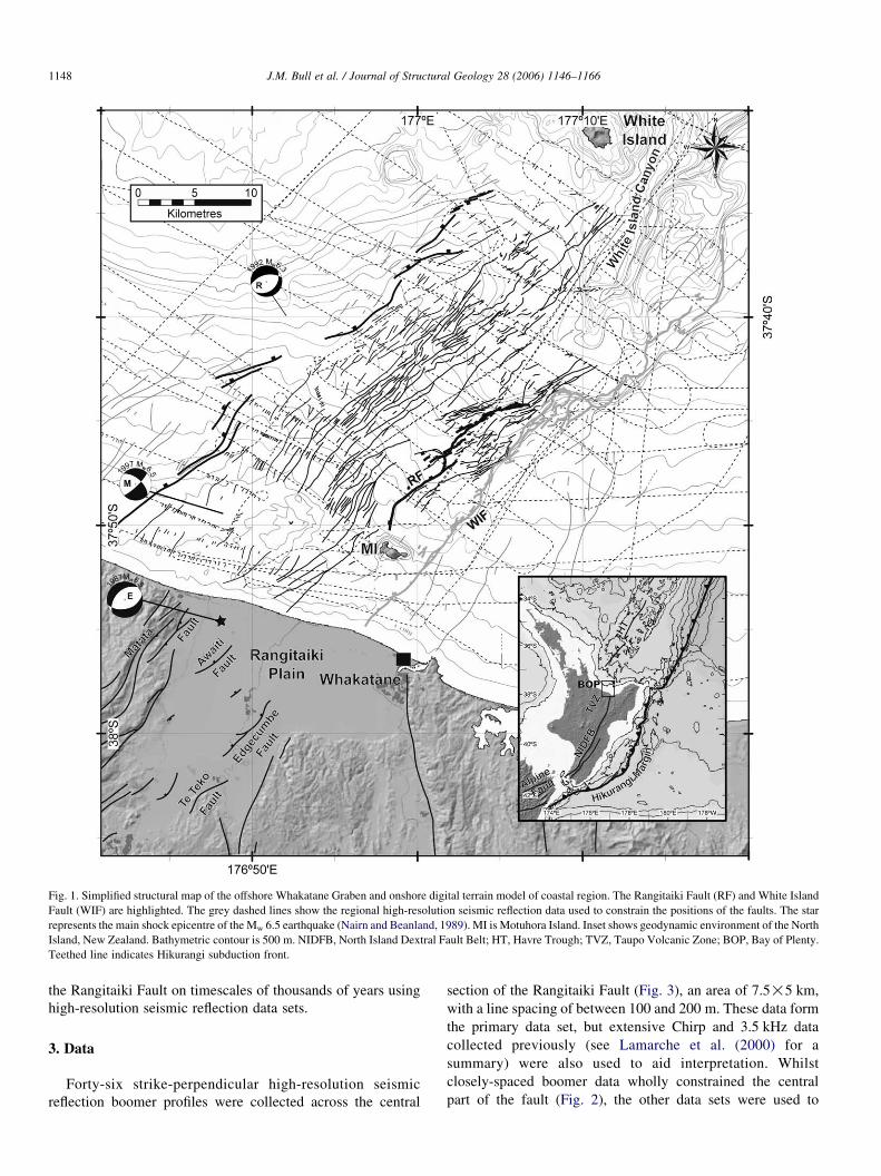
Fig. 1. Simplified structural map of the offshore Whakatane Graben and onshore digital terrain model of coastal region. The Rangitaiki Fault (RF) and White Island

Fault (WIF) are highlighted. The grey dashed lines show the regional high-resolution seismic reflection data used to constrain the positions of the faults. The star

represents the main shock epicentre of the Mw 6.5 earthquake (Nairn and Beanland, 1989). MI is Motuhora Island. Inset shows geodynamic environment of the North

Island, New Zealand. Bathymetric contour is 500 m. NIDFB, North Island Dextral Fault Belt; HT, Havre Trough; TVZ, Taupo Volcanic Zone; BOP, Bay of Plenty.

Teethed line indicates Hikurangi subduction front.

J.M. Bull et al. / Journal of Structural Geology 28 (2006) 1146–11661148

the Rangitaiki Fault on timescales of thousands of years using

high-resolution seismic reflection data sets.

3. Data

Forty-six strike-perpendicular high-resolution seismic

reflection boomer profiles were collected across the central

section of the Rangitaiki Fault (Fig. 3), an area of 7.5!5 km,

with a line spacing of between 100 and 200 m. These data form

the primary data set, but extensive Chirp and 3.5 kHz data

collected previously (see Lamarche et al. (2000) for a

summary) were also used to aid interpretation. Whilst

closely-spaced boomer data wholly constrained the central

part of the fault (Fig. 2), the other data sets were used to

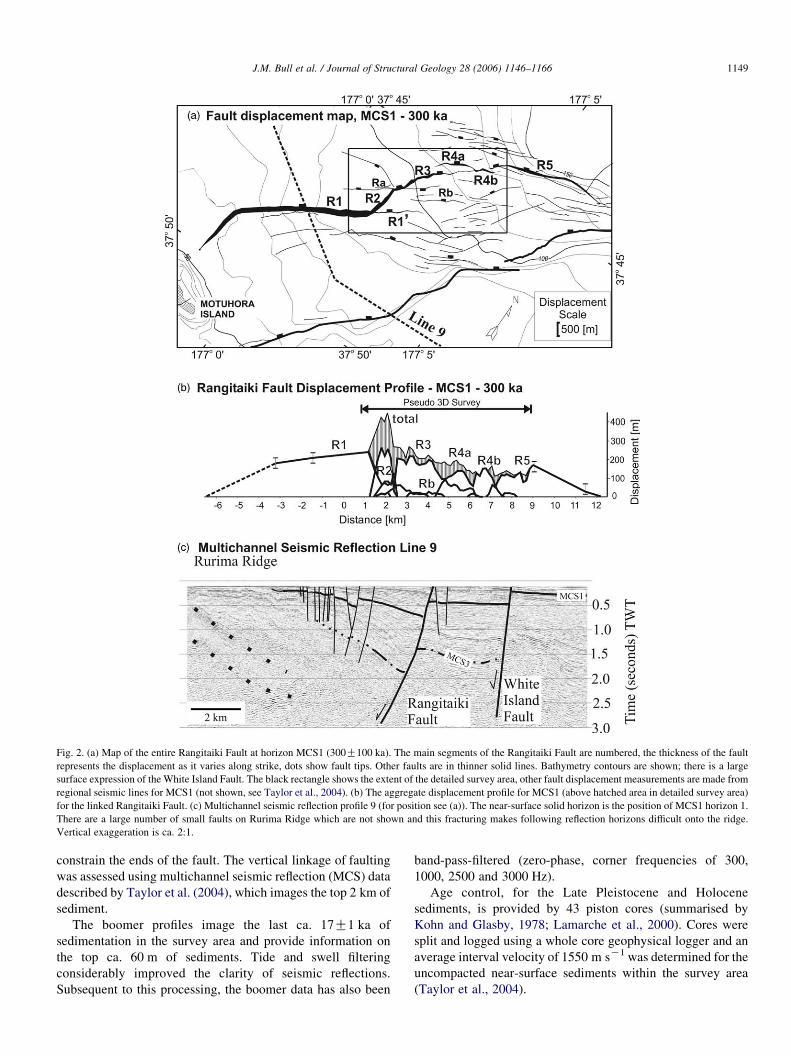
Fig. 2. (a) Map of the entire Rangitaiki Fault at horizon MCS1 (300G100 ka). The main segments of the Rangitaiki Fault are numbered, the thickness of the fault

represents the displacement as it varies along strike, dots show fault tips. Other faults are in thinner solid lines. Bathymetry contours are shown; there is a large

surface expression of the White Island Fault. The black rectangle shows the extent of the detailed survey area, other fault displacement measurements are made from

regional seismic lines for MCS1 (not shown, see Taylor et al., 2004). (b) The aggregate displacement profile for MCS1 (above hatched area in detailed survey area)

for the linked Rangitaiki Fault. (c) Multichannel seismic reflection profile 9 (for position see (a)). The near-surface solid horizon is the position of MCS1 horizon 1.

There are a large number of small faults on Rurima Ridge which are not shown and this fracturing makes following reflection horizons difficult onto the ridge.

Vertical exaggeration is ca. 2:1.


constrain the ends of the fault. The vertical linkage of faulting

was assessed using multichannel seismic reflection (MCS) data

described by Taylor et al. (2004), which images the top 2 km of

sediment.

The boomer profiles image the last ca. 17G1 ka of

sedimentation in the survey area and provide information on

the top ca. 60 m of sediments. Tide and swell filtering

considerably improved the clarity of seismic reflections.

Subsequent to this processing, the boomer data has also been

band-pass-filtered (zero-phase, corner frequencies of 300,

1000, 2500 and 3000 Hz).

Age control, for the Late Pleistocene and Holocene

sediments, is provided by 43 piston cores (summarised by

Kohn and Glasby, 1978; Lamarche et al., 2000). Cores were

split and logged using a whole core geophysical logger and an

average interval velocity of 1550 m sK1 was determined for the

uncompacted near-surface sediments within the survey area

(Taylor et al., 2004).

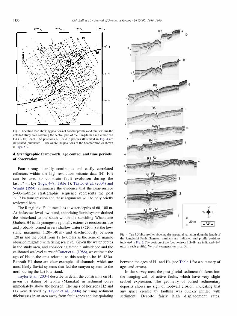
Fig. 4. Ten 3.5 kHz profiles showing the structural variation along the length of

the Rangitaiki Fault. Segment numbers are indicated and profile positions

indicated in Fig. 3. The position of the four horizons H1–H4 are indicated (1–4

next to each profile). Vertical exaggeration is ca. 50:1.

Fig. 3. Location map showing positions of boomer profiles and faults within the

detailed study area covering the central part of the Rangitaiki Fault at horizon

H4 (17 ka) level. The positions of 3.5 kHz profiles illustrated in Fig. 4 are

illustrated (numbered 1–10), as are the positions of the boomer profiles shown

in Figs. 5–7.


4. Stratigraphic framework, age control and time periods

of observation

Four strong laterally continuous and easily correlated

reflectors within the high-resolution seismic data (H1–H4)

can be used to constrain fault evolution during the

last 17G1 kyr (Figs. 4–7; Table 1). Taylor et al. (2004) and

Wright (1990) summarise the evidence that the near-surface

5–60-m-thick stratigraphic sequence represents the post

w17 ka transgression and these arguments will be only briefly

reviewed here.

The Rangitaiki Fault trace lies at water depths of 60–100 m.

At the last sea level low-stand, an incising fluvial system drained

the hinterland to the south within the subsiding Whakatane

Graben. H4 is the youngest regionally extensive erosion surface

and probably formed in very shallow water (!20 m) at the low-

stand maximum (120–140 m) and diachronously between

120 m and the coast from 17 to 6.5 ka as the zone of marine

abrasion migrated with rising sea level. Given the water depths

in the study area, and considering tectonic subsidence and the

calibrated sea level curve of Carter et al. (1986), we estimate the

age of H4 in the area relevant to this study to be 16–18 ka.

Beneath H4 there are clear examples of channels, which are

most likely fluvial systems that fed the canyon system to the

north during the last low-stand.

Taylor et al. (2004) describe in detail the constraints on H1

given by dating of tephra (Mamaku) in sediment cores

immediately above the horizon. The ages of horizons H2 and

H3 were derived by Taylor et al. (2004) by using sediment

thicknesses in an area away from fault zones and interpolating

between the ages of H1 and H4 (see Table 1 for a summary of

ages and errors).

In the survey area, the post-glacial sediment thickens into

the hanging-wall of active faults, which have very slight

seabed expression. The geometry of buried sedimentary

deposits shows no sign of footwall erosion, indicating that

any space created by faulting was quickly infilled with

sediment. Despite fairly high displacement rates,

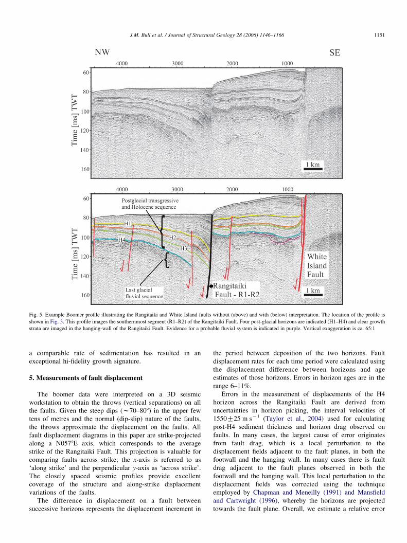
Fig. 5. Example Boomer profile illustrating the Rangitaiki and White Island faults without (above) and with (below) interpretation. The location of the profile is

shown in Fig. 3. This profile images the southernmost segment (R1–R2) of the Rangitaiki Fault. Four post-glacial horizons are indicated (H1–H4) and clear growth

strata are imaged in the hanging-wall of the Rangitaiki Fault. Evidence for a probable fluvial system is indicated in purple. Vertical exaggeration is ca. 65:1


a comparable rate of sedimentation has resulted in an

exceptional hi-fidelity growth signature.

5. Measurements of fault displacement

The boomer data were interpreted on a 3D seismic

workstation to obtain the throws (vertical separations) on all

the faults. Given the steep dips (w70–808) in the upper few

tens of metres and the normal (dip-slip) nature of the faults,

the throws approximate the displacement on the faults. All

fault displacement diagrams in this paper are strike-projected

along a N0578E axis, which corresponds to the average

strike of the Rangitaiki Fault. This projection is valuable for

comparing faults across strike; the x-axis is referred to as

‘along strike’ and the perpendicular y-axis as ‘across strike’.

The closely spaced seismic profiles provide excellent

coverage of the structure and along-strike displacement

variations of the faults.

The difference in displacement on a fault between

successive horizons represents the displacement increment in

the period between deposition of the two horizons. Fault

displacement rates for each time period were calculated using

the displacement difference between horizons and age

estimates of those horizons. Errors in horizon ages are in the

range 6–11%.

Errors in the measurement of displacements of the H4

horizon across the Rangitaiki Fault are derived from

uncertainties in horizon picking, the interval velocities of

1550G25 m sK1 (Taylor et al., 2004) used for calculating

post-H4 sediment thickness and horizon drag observed on

faults. In many cases, the largest cause of error originates

from fault drag, which is a local perturbation to the

displacement fields adjacent to the fault planes, in both the

footwall and the hanging wall. In many cases there is fault

drag adjacent to the fault planes observed in both the

footwall and the hanging wall. This local perturbation to the

displacement fields was corrected using the technique

employed by Chapman and Meneilly (1991) and Mansfield

and Cartwright (1996), whereby the horizons are projected

towards the fault plane. Overall, we estimate a relative error

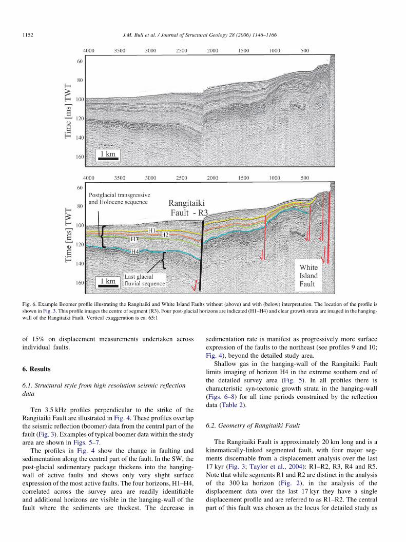
Fig. 6. Example Boomer profile illustrating the Rangitaiki and White Island Faults without (above) and with (below) interpretation. The location of the profile is

shown in Fig. 3. This profile images the centre of segment (R3). Four post-glacial horizons are indicated (H1–H4) and clear growth strata are imaged in the hanging-

wall of the Rangitaiki Fault. Vertical exaggeration is ca. 65:1


of 15% on displacement measurements undertaken across

individual faults.

6. Results

6.1. Structural style from high resolution seismic reflection

data

Ten 3.5 kHz profiles perpendicular to the strike of the

Rangitaiki Fault are illustrated in Fig. 4. These profiles overlap

the seismic reflection (boomer) data from the central part of the

fault (Fig. 3). Examples of typical boomer data within the study

area are shown in Figs. 5–7.

The profiles in Fig. 4 show the change in faulting and

sedimentation along the central part of the fault. In the SW, the

post-glacial sedimentary package thickens into the hanging-

wall of active faults and shows only very slight surface

expression of the most active faults. The four horizons, H1–H4,

correlated across the survey area are readily identifiable

and additional horizons are visible in the hanging-wall of the

fault where the sediments are thickest. The decrease in

sedimentation rate is manifest as progressively more surface

expression of the faults to the northeast (see profiles 9 and 10;

Fig. 4), beyond the detailed study area.

Shallow gas in the hanging-wall of the Rangitaiki Fault

limits imaging of horizon H4 in the extreme southern end of

the detailed survey area (Fig. 5). In all profiles there is

characteristic syn-tectonic growth strata in the hanging-wall

(Figs. 6–8) for all time periods constrained by the reflection

data (Table 2).

6.2. Geometry of Rangitaiki Fault

The Rangitaiki Fault is approximately 20 km long and is a

kinematically-linked segmented fault, with four major seg-

ments discernable from a displacement analysis over the last

17 kyr (Fig. 3; Taylor et al., 2004): R1–R2, R3, R4 and R5.

Note that while segments R1 and R2 are distinct in the analysis

of the 300 ka horizon (Fig. 2), in the analysis of the

displacement data over the last 17 kyr they have a single

displacement profile and are referred to as R1–R2. The central

part of this fault was chosen as the locus for detailed study as

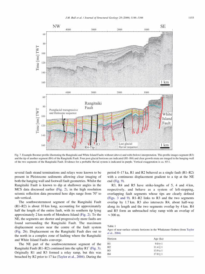
Fig. 7. Example Boomer profile illustrating the Rangitaiki andWhite Island Faults without (above) and with (below) interpretation. This profile images segment (R3)

and the tip of another segment (R4) of the Rangitaiki Fault. Four post-glacial horizons are indicated (H1–H4) and clear growth strata are imaged in the hanging-wall

of the two segments of the Rangitaiki Fault. Evidence for a probable fluvial system is indicated in purple. Vertical exaggeration is ca. 65:1.

Table 1

Ages of near-surface seismic horizons in the Whakatane Graben (from Taylor

et al., 2004)

Horizon Age (ka)

H1 9.0G1

H2 11.4G1

H3 13.9G1

H4 17.0G1


several fault strand terminations and relays were known to be

present in Pleistocene sediments allowing clear imaging of

both the hanging wall and footwall fault geometries. Whilst the

Rangitaiki Fault is known to dip at shallower angles in the

MCS data discussed earlier (Fig. 2), in the high resolution

seismic reflection data presented here dips range from 708 to

sub-vertical.

The southwesternmost segment of the Rangitaiki Fault

(R1–R2) is about 10 km long, accounting for approximately

half the length of the entire fault, with its southern tip lying

approximately 2 km north of Motuhora Island (Fig. 2). To the

NE, the segments are shorter and progressively more faults are

found surrounding the Rangitaiki Fault. The maximum

displacement occurs near the centre of the fault system

(Fig. 2b). Displacement on the Rangitaiki Fault dies out to

the north in a complex zone of faulting where the Rangitaiki

and White Island Faults converge.

The NE part of the southwesternmost segment of the

Rangitaiki Fault (R1–R2) continued into the splay R1 0 (Fig. 3).

Originally R1 and R3 formed a relay ramp, but this was

breached by R2 prior to 17 ka (Taylor et al., 2004). During the

period 0–17 ka, R1 and R2 behaved as a single fault (R1–R2)

with a continuous displacement gradient to a tip at the NE

end (Fig. 9).

R3, R4 and R5 have strike-lengths of 5, 4 and 4 km,

respectively, and behave as a system of left-stepping,

overlapping fault segments whose tips are clearly defined

(Figs. 3 and 9). R1–R2 links to R3 and the two segments

overlap by 1.7 km. R3 also intersects R4, about half-way

along its length and the two segments overlap by 4 km. R4

and R5 form an unbreached relay ramp with an overlap of

w300 m.

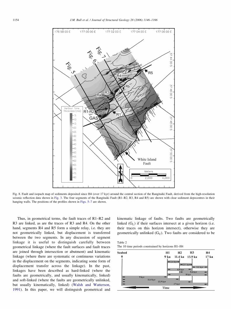
Fig. 8. Fault and isopach map of sediments deposited since H4 (over 17 kyr) around the central section of the Rangitaiki Fault, derived from the high-resolution

seismic reflection data shown in Fig. 3. The four segments of the Rangitaiki Fault (R1–R2, R3, R4 and R5) are shown with clear sediment depocentres in their

hanging walls. The positions of the profiles shown in Figs. 5–7 are shown.

Table 2

The 10 time periods constrained by horizons H1–H4


Thus, in geometrical terms, the fault traces of R1–R2 and

R3 are linked, as are the traces of R3 and R4. On the other

hand, segments R4 and R5 form a simple relay, i.e. they are

not geometrically linked, but displacement is transferred

between the two segments. In any discussion of segment

linkage it is useful to distinguish carefully between

geometrical linkage (where the fault surfaces and fault traces

are joined through intersection or abutment) and kinematic

linkage (where there are systematic or continuous variations

in the displacement on the segments, indicating some form of

displacement transfer across the linkage). In the past,

linkages have been described as hard-linked (where the

faults are geometrically, and usually kinematically, linked)

and soft-linked (where the faults are geometrically unlinked,

but usually kinematically, linked) (Walsh and Watterson,

1991). In this paper, we will distinguish geometrical and

kinematic linkage of faults. Two faults are geometrically

linked (GL) if their surfaces intersect at a given horizon (i.e.

their traces on this horizon intersect), otherwise they are

geometrically unlinked (GU). Two faults are considered to be

0

Dis

plac

emen

t (m

)

2000 4000 6000 8000

0

20

40

60

40

0

10

20

30

Along Strike Distance [km]

Total Fault Displacement Profile- H1- 9ka

R1-R2RbR3 R4

R5

total

Dis

plac

emen

t [m

]

2 3 4 5 6 7 8 1110-1-2-3-4-5-6 109 12

3D Survey

40

20

0

20

40

6017 ka

13.9 ka

11.4 ka

9 ka

Total

R1-R2

R4

R3

Strike Distance (m)

A

D

C

Bdi

stan

ce a

cros

sst

rike

[m]

E

2000

H4 fault map

R1-R2

R3

R4 R5

Ra

Rb

Rc

50 [m]

displacement scale

0

2000 4000 6000 8000

R1’

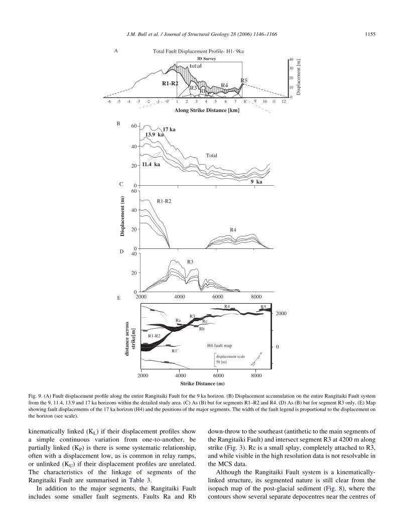
Fig. 9. (A) Fault displacement profile along the entire Rangitaiki Fault for the 9 ka horizon. (B) Displacement accumulation on the entire Rangitaiki Fault system

from the 9, 11.4, 13.9 and 17 ka horizons within the detailed study area. (C) As (B) but for segments R1–R2 and R4. (D) As (B) but for segment R3 only. (E) Map

showing fault displacements of the 17 ka horizon (H4) and the positions of the major segments. The width of the fault legend is proportional to the displacement on

the horizon (see scale).


kinematically linked (KL) if their displacement profiles show

a simple continuous variation from one-to-another, be

partially linked (KP) is there is some systematic relationship,

often with a displacement low, as is common in relay ramps,

or unlinked (KU) if their displacement profiles are unrelated.

The characteristics of the linkage of segments of the

Rangitaiki Fault are summarised in Table 3.

In addition to the major segments, the Rangitaiki Fault

includes some smaller fault segments. Faults Ra and Rb

down-throw to the southeast (antithetic to the main segments of

the Rangitaiki Fault) and intersect segment R3 at 4200 m along

strike (Fig. 3). Rc is a small splay, completely attached to R3,

and while visible in the high resolution data is not resolvable in

the MCS data.

Although the Rangitaiki Fault system is a kinematically-

linked structure, its segmented nature is still clear from the

isopach map of the post-glacial sediment (Fig. 8), where the

contours show several separate depocentres near the centres of

Table 3

Summary of fault segments and types of linkage on the Rangitaiki Fault in

the period 0–17 ka. GL—geometrically linked; KL—kinematically linked;

Kp—partially linked; GL/U—uncertainty whether geometrically unlinked or

linked

Fault Segment type Fault Linkage

R1 Long single segment R1

GL KL

R2 Branch splay from R1 R2

GL KP

R3 3 sub-segments with variable linkage R3

GL/U KP

R4 2 sub-segments, single fault since 17 ka R4

GU KP

R5 Single segment R5


the fault segments, marking the locations of high displacement

and increased sediment accommodation space. Note that the

main depocentre occurs at the link between R1 and R2,

supporting the idea that these acted as a single fault (R1–R2)

over, at least, the last 17 ka.

Throughout the post-glacial sedimentary sequence

(between H4 and the seabed) there is no observed lateral

fault propagation. However, the minimum distance of 100 m

between adjacent profiles means that only lateral propa-

gation rates of more than 6 mm yrK1 would be resolvable.

6.3. Fault displacements on the Rangitaiki Fault system

At horizon H4 (17 ka), the displacement on the Rangitaiki

Fault decreases fairly steadily from a maximum of 62 m near

the centre of the linked fault network (w2500 m along strike;

Fig. 9b) tow15 m on R4 (at 7500 m along strike; Fig. 9b). The

NE half of the fault comprises major segments that are

kinematically linked producing a displacement gradient of

w8!10K3 for the 17 ka horizon.

Fig. 9 shows the accumulation of displacement with time on

individual segments within the detailed study area and how this

contributes to the total displacement profile. The displacement-

distance variation of segments R3 and R4 on all four horizons

is completely constrained. To the north and south of the

detailed study area the 11.4, 13.9 and 17 ka horizons are less

well resolved and the displacement distribution along the entire

Rangitaiki Fault is known for only the 9 ka horizon.

There is a notch in the displacement profile of R3 at its

intersection with Ra and Rb (e.g. Fig. 10a); the sum of

displacements on Ra and Rb at the intersection point is the same

as the difference between the observed notched profile and a

projected smoothed profile for R3. Fault Rc is a small splay fault

in R3, with maximum displacement of 12 m at 5200 m along

strike on horizon H4. The displacement of Rc is complimentary

to a notch in the displacement profile of R3 (Fig. 10a).

6.4. Fault displacement history

The same fault segments (R1–R2, R3, R4 and R5) are present

throughout the post-glacial sequence and show no resolvable

lateral propagation. By comparing the displacement over

different time intervals (Fig. 10) the displacement history of the

fault segments can be examined. Fig. 10 shows the displacement

differences over time intervals: A (17 ka–present); B (17–

13.9 ka); C (13.9–11.4 ka); D (11.4–9 ka); and E (9 ka–present).

Knowledge of the time intervals between these horizons allows

the displacement rates to be calculated (Fig. 11).

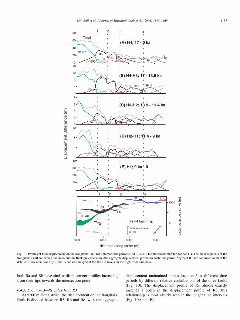
The aggregate displacement curve (grey lines in Fig. 10) is

fairly smooth on timescales greater than 9 kyr (Fig. 10A and E;

see also Fig. 2), whereas for shorter time intervals of 2–3 kyr

(e.g. Fig. 10B–D), the profiles are much more irregular, with

large differences in displacement rate being observed over

different time intervals and where the segments intersect and/or

interact. The aggregate displacement lows seen on the

Rangitaiki Fault segments at short timescales are not

compensated by activity on other faults (for example faults

in the footwall and hanging-wall) (Taylor, 2003).

The variations in displacement accumulation are described

with reference to four key locations (1–4; see Fig. 10 for

locations) along the strike of the fault.

6.4.1. Location 1—Overlapping tips of R1–R2 and R3

In the post-glacial sediment sequence, segments R1–R2 and

R3 overlap by 2 km and are spatially separated by 1 km

(Fig. 10F), with the tip of R1–R2 just intersecting R3 at

location 1. The maximum displacement is at the intersection of

R1 and R2 at 2900 m along strike (Fig. 10A), where R1

continues to the NE on R1 0, with a much reduced throw

(!20% of that on R1–R2). Over the entire interval 0–17 ka,

the displacement gradient across location 1 is smooth, as

displacement is transferred from R1–R2 to R3.

6.4.2. Location 2—R3 crossed by antithetic faults Ra and Rb

At location 2, the segment R3 intersects with two antithetic

fault segments, Ra and Rb, which may have formerly been the

same fault (Fig. 10F). Throughout the last 17 ka, the summed

throws on these faults has remained fairly constant. If heave is

proportional to throw (i.e. constant dip) then this suggests that

these faults accommodate a fairly constant extension rate at

this location and that R3, Ra and Rb are kinematically linked.

The opposite sense of downthrow on Ra and Rb will reduce the

net throw on the fault system at location 2, as is clearly seen in

the isopach map (Fig. 8).

Examination of Figs. 10 and 11 indicates variation in the

displacement and displacement rates over different time

intervals. Between 17 and 13.9 ka (Fig. 10B), the displacement

profile of R3 shows a notch at the intersection point, with

the drop in displacement being equal to the sum of the

displacements on Ra and Rb at this point. During the 13.9–9 ka

period (Fig. 10C and D), R3 is effectively pinned at the

intersection point, with no displacement accumulation for the

4000 year duration. During the 13.9–11.4 ka interval

(Fig. 10C), Ra has the highest displacement rate of

0.33 mm yrK1 at the intersection point, whereas in interval

11.4–9 ka (Fig. 10D), the displacement on Rb is high, with the

displacement on Ra being zero. During interval 9–0 ka

(Fig. 10E), R3 is reactivated at the intersection point and

R1'

R1-R2

Rc

Rb

RaR3

R4RcRbRa

R3

32 4

1

1

2 3 4

2000

50 [m]

displacement scale

0

2000 4000 6000 8000

(A) H4; 17 - 0 ka

Dis

plac

emen

t Diff

eren

ce (

m)

(B) H4-H3; 17 - 13.9 ka

(C) H3-H2; 13.9 - 11.4 ka

(D) H2-H1; 11.4 - 9 ka

(E) H1; 9 ka - 0

Total

R1-R2

R1Õ

R4N

Rd

R4S

R5

80

60

40

20

016

12

8

4

0

8

6

4

2

0

8

4

12

040

30

20

10

0

R5R4

dist

ance

acr

oss

strik

e (m

)

distance along strike (m)

(F) H4 fault map

Fig. 10. Profiles of total displacement on the Rangitaiki fault for different time periods ((A)–(E)). (F) Displacement map for horizon H4. The main segments of the

Rangitaiki Fault are named and in colour; the thick grey line shows the aggregate displacement profile for each time period. Segment R1–R2 continues south of the

detailed study area (see Fig. 2) but is not well imaged at the H2–H4 levels on the high-resolution data.


both Ra and Rb have similar displacement profiles increasing

from their tips towards the intersection point.

6.4.3. Location 3—Rc splay from R3

At 5200 m along strike, the displacement on the Rangitaiki

Fault is divided between R3, Rb and Rc, with the aggregate

displacement maintained across location 3 at different time

periods by different relative contributions of the three faults

(Fig. 10). The displacement profile of Rc almost exactly

matches a notch in the displacement profile of R3; this

relationship is most clearly seen in the longer time intervals

(Fig. 10A and E).

4

R4R3

1 2 3 4

(A) 17 kyr Time Interval - 17ka to present

(B) 3.1 kyr Time Interval - 17ka to 13.9 ka

R3

R4S R4N

Rd

R3

R4

R3R4

R3R4

Dis

plac

emen

t Rat

e [m

m/y

r]

(C) 2.5 kyr Time Interval - 13.9 ka to 11.4 ka

(D) 2.4 kyr Time Interval - 11.4 ka to 9 ka

(E) 9 kyr Time Interval - 9 ka to present

3

2

1

2000 4000 6000 8000

2000 4000 6000 8000

2000 4000 6000 8000

4

3

2

1

4

3

2

1

0

0

0

4

3

2

1

02000 4000 6000 8000

2000 4000 6000 8000

4

3

2

1

0

1 2 3 4

1 2 3 4

1 2 3 4

1 2 3 4

distance along strike (m)

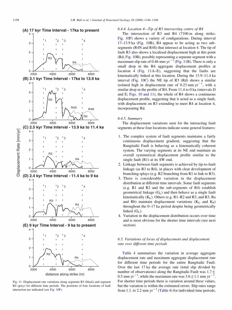
Fig. 11. Displacement rate variations along segments R3 (black) and segment

R4 (grey) for different time periods. The positions of four locations of fault

interaction are indicated (see Fig. 10F).


6.4.4. Location 4—Tip of R3 intersecting centre of R4

The intersection of R3 and R4 (7100 m along strike;

Fig. 10F) shows a variety of configurations. During interval

17–13.9 ka (Fig. 10B), R4 appear to be acting as two sub-

segments (R4N and R4S) that intersect at location 4. The tip of

fault R3 also shows a localised displacement high at this point

(Rd; Fig. 10B), possibly representing a separate segment with a

maximum slip rate of 0.46 mm yrK1 (Fig. 11B). There is only a

small drop in the R4 aggregate displacement profiles at

location 4 (Fig. 11A–E), suggesting that the faults are

kinematically linked at this location. During the 13.9–11.4 ka

interval (Fig. 10C) the NE tip of R3 (Rd) shows a similar

isolated high in displacement rate of 0.23 mm yrK1, with a

similar drop in the profile of R4. From 11.4 to 0 ka (intervals D

and E; Figs. 10 and 11), the whole of R4 shows a continuous

displacement profile, suggesting that it acted as a single fault,

with displacement on R3 extending to meet R4 at location 4,

incorporating Rd.

6.4.5. Summary

The displacement variations seen for the interacting fault

segments at these four locations indicate some general features:

1. The complex system of fault segments maintains a fairly

continuous displacement gradient, suggesting that the

Rangitaiki Fault is behaving as a kinematically coherent

system. The varying segments at its NE end maintain an

overall symmetrical displacement profile similar to the

single fault (R1) at its SW end.

2. Linkage between fault segments is achieved by tip-to-fault

linkage (as R3 to R4), in places with clear development of

branching splays (e.g. R2 branching from R1 to link to R3).

3. There is considerable variation in the displacement

distribution at different time intervals. Some fault segments

(e.g. R1 and R2 and the sub-segments of R4) establish

geometrical linkage (GL) and then behave as a single fault

kinematically (KL). Others (e.g. R1–R2 and R3, and R3, Ra

and Rb) maintain displacement variations (KU and KP)

throughout the 0–17 ka period despite being geometrically

linked (GL).

4. Variation in the displacement distribution occurs over time

and is most obvious for the shorter time intervals (see next

section).

6.5. Variations of locus of displacement and displacement

rate over different time periods

Table 4 summarises the variation in average aggregate

displacement rate and maximum aggregate displacement rate

for different time periods for the entire Rangitaiki Fault.

Over the last 17 ka the average rate (total slip divided by

number of observations) along the Rangitaiki Fault was 1.7G0.5 mm yrK1, while the maximum rate was 3.6G1.1 mm yrK1.

For shorter time periods there is variation around these values,

but the variation is within the estimated errors. Slip rates range

from 1.1. to 2.2 mm yrK1 (Table 4) for individual time periods,

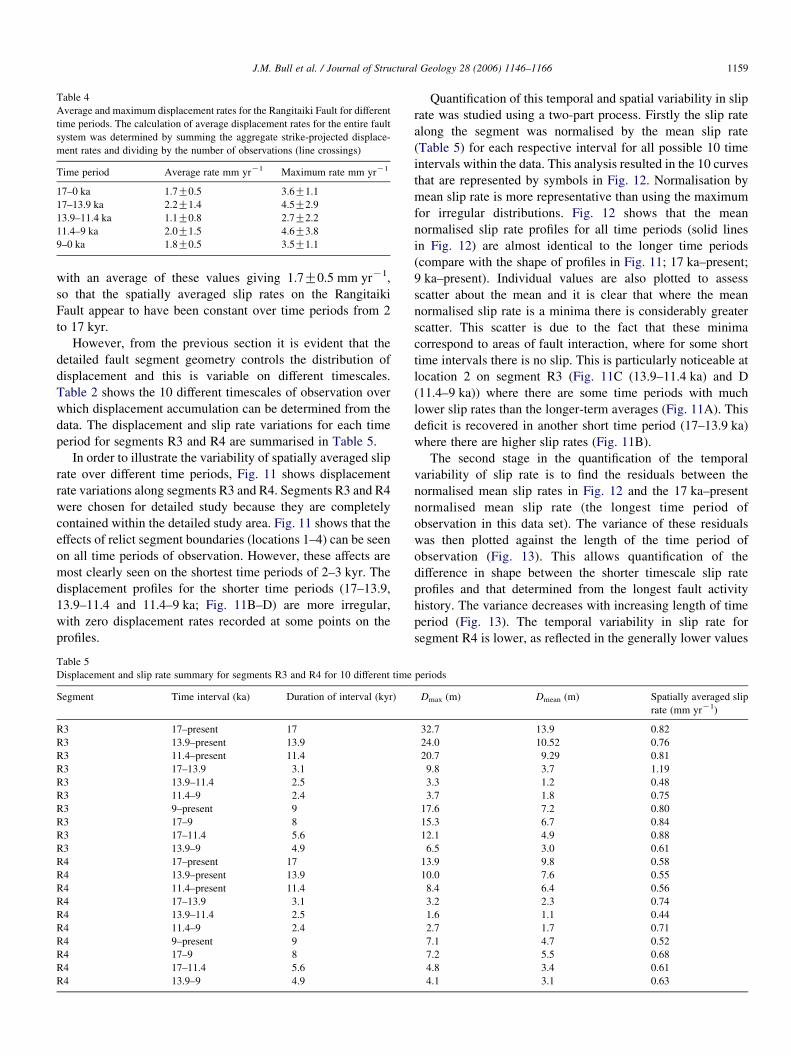
Table 4

Average and maximum displacement rates for the Rangitaiki Fault for different

time periods. The calculation of average displacement rates for the entire fault

system was determined by summing the aggregate strike-projected displace-

ment rates and dividing by the number of observations (line crossings)

Time period Average rate mm yrK1 Maximum rate mm yrK1

17–0 ka 1.7G0.5 3.6G1.1

17–13.9 ka 2.2G1.4 4.5G2.9

13.9–11.4 ka 1.1G0.8 2.7G2.2

11.4–9 ka 2.0G1.5 4.6G3.8

9–0 ka 1.8G0.5 3.5G1.1


with an average of these values giving 1.7G0.5 mm yrK1,

so that the spatially averaged slip rates on the Rangitaiki

Fault appear to have been constant over time periods from 2

to 17 kyr.

However, from the previous section it is evident that the

detailed fault segment geometry controls the distribution of

displacement and this is variable on different timescales.

Table 2 shows the 10 different timescales of observation over

which displacement accumulation can be determined from the

data. The displacement and slip rate variations for each time

period for segments R3 and R4 are summarised in Table 5.

In order to illustrate the variability of spatially averaged slip

rate over different time periods, Fig. 11 shows displacement

rate variations along segments R3 and R4. Segments R3 and R4

were chosen for detailed study because they are completely

contained within the detailed study area. Fig. 11 shows that the

effects of relict segment boundaries (locations 1–4) can be seen

on all time periods of observation. However, these affects are

most clearly seen on the shortest time periods of 2–3 kyr. The

displacement profiles for the shorter time periods (17–13.9,

13.9–11.4 and 11.4–9 ka; Fig. 11B–D) are more irregular,

with zero displacement rates recorded at some points on the

profiles.

Table 5

Displacement and slip rate summary for segments R3 and R4 for 10 different time

Segment Time interval (ka) Duration of interval (kyr)

R3 17–present 17

R3 13.9–present 13.9


R3 17–13.9 3.1

R3 13.9–11.4 2.5

R3 11.4–9 2.4

R3 9–present 9

R3 17–9 8

R3 17–11.4 5.6

R3 13.9–9 4.9

R4 17–present 17



R4 17–13.9 3.1

R4 13.9–11.4 2.5

R4 11.4–9 2.4

R4 9–present 9

R4 17–9 8

R4 17–11.4 5.6

R4 13.9–9 4.9

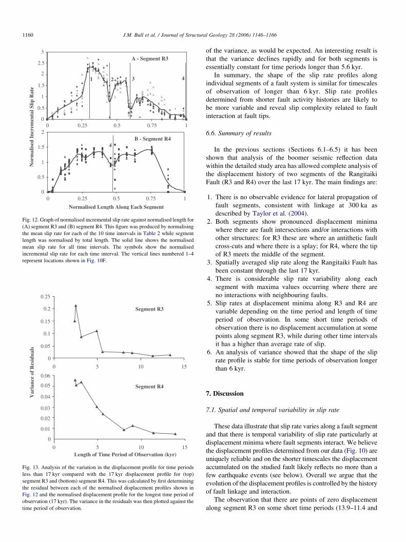
Quantification of this temporal and spatial variability in slip

rate was studied using a two-part process. Firstly the slip rate

along the segment was normalised by the mean slip rate

(Table 5) for each respective interval for all possible 10 time

intervals within the data. This analysis resulted in the 10 curves

that are represented by symbols in Fig. 12. Normalisation by

mean slip rate is more representative than using the maximum

for irregular distributions. Fig. 12 shows that the mean

normalised slip rate profiles for all time periods (solid lines

in Fig. 12) are almost identical to the longer time periods

(compare with the shape of profiles in Fig. 11; 17 ka–present;

9 ka–present). Individual values are also plotted to assess

scatter about the mean and it is clear that where the mean

normalised slip rate is a minima there is considerably greater

scatter. This scatter is due to the fact that these minima

correspond to areas of fault interaction, where for some short

time intervals there is no slip. This is particularly noticeable at

location 2 on segment R3 (Fig. 11C (13.9–11.4 ka) and D

(11.4–9 ka)) where there are some time periods with much

lower slip rates than the longer-term averages (Fig. 11A). This

deficit is recovered in another short time period (17–13.9 ka)

where there are higher slip rates (Fig. 11B).

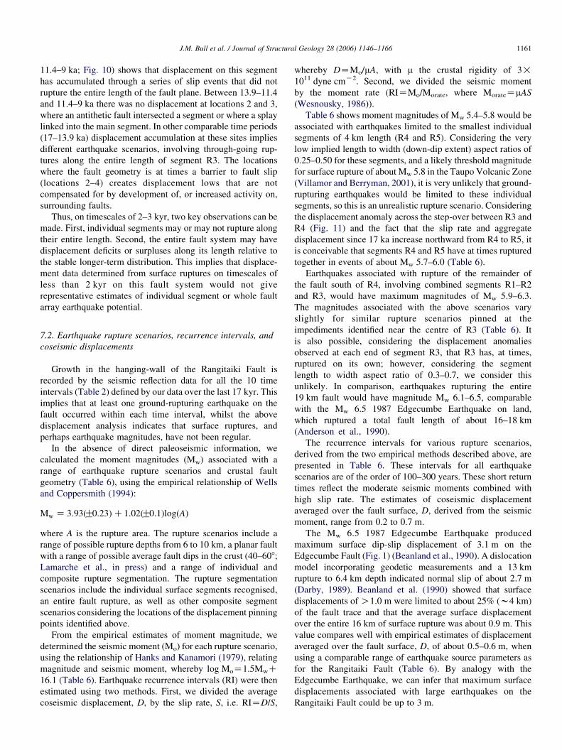
The second stage in the quantification of the temporal

variability of slip rate is to find the residuals between the

normalised mean slip rates in Fig. 12 and the 17 ka–present

normalised mean slip rate (the longest time period of

observation in this data set). The variance of these residuals

was then plotted against the length of the time period of

observation (Fig. 13). This allows quantification of the

difference in shape between the shorter timescale slip rate

profiles and that determined from the longest fault activity

history. The variance decreases with increasing length of time

period (Fig. 13). The temporal variability in slip rate for

segment R4 is lower, as reflected in the generally lower values

periods

Dmax (m) Dmean (m) Spatially averaged slip

rate (mm yrK1)

32.7 13.9 0.82

24.0 10.52 0.76

20.7 9.29 0.81

9.8 3.7 1.19

3.3 1.2 0.48

3.7 1.8 0.75

17.6 7.2 0.80

15.3 6.7 0.84

12.1 4.9 0.88

6.5 3.0 0.61

13.9 9.8 0.58

10.0 7.6 0.55

8.4 6.4 0.56

3.2 2.3 0.74

1.6 1.1 0.44

2.7 1.7 0.71

7.1 4.7 0.52

7.2 5.5 0.68

4.8 3.4 0.61

4.1 3.1 0.63

B - Segment R4

0

0.5

1

1.5

2

0 0.25 0.5 0.75 1

A - Segment R3

0

0.5

1

1.5

2

2.5

3

0 0.25 0.5 0.75 1

Nor

mal

ised

Inc

rem

enta

l Slip

Rat

e

Normalised Length Along Each Segment

4

321 4

Fig. 12. Graph of normalised incremental slip rate against normalised length for

(A) segment R3 and (B) segment R4. This figure was produced by normalising

the mean slip rate for each of the 10 time intervals in Table 2 while segment

length was normalised by total length. The solid line shows the normalised

mean slip rate for all time intervals. The symbols show the normalised

incremental slip rate for each time interval. The vertical lines numbered 1–4

represent locations shown in Fig. 10F.

Segment R3

0

0.05

0.1

0.15

0.2

0.25

0 5 10 15

Var

ianc

e of

Res

idua

ls

0

0.01

0.02

0.03

0.04

0.05

0.06

0 5 10 15Length of Time Period of Observation (kyr)

Segment R4

Fig. 13. Analysis of the variation in the displacement profile for time periods

less than 17 kyr compared with the 17 kyr displacement profile for (top)

segment R3 and (bottom) segment R4. This was calculated by first determining

the residual between each of the normalised displacement profiles shown in

Fig. 12 and the normalised displacement profile for the longest time period of

observation (17 kyr). The variance in the residuals was then plotted against the

time period of observation.


of the variance, as would be expected. An interesting result is

that the variance declines rapidly and for both segments is

essentially constant for time periods longer than 5.6 kyr.

In summary, the shape of the slip rate profiles along

individual segments of a fault system is similar for timescales

of observation of longer than 6 kyr. Slip rate profiles

determined from shorter fault activity histories are likely to

be more variable and reveal slip complexity related to fault

interaction at fault tips.

6.6. Summary of results

In the previous sections (Sections 6.1–6.5) it has been

shown that analysis of the boomer seismic reflection data

within the detailed study area has allowed complete analysis of

the displacement history of two segments of the Rangitaiki

Fault (R3 and R4) over the last 17 kyr. The main findings are:

1. There is no observable evidence for lateral propagation of

fault segments, consistent with linkage at 300 ka as

described by Taylor et al. (2004).

2. Both segments show pronounced displacement minima

where there are fault intersections and/or interactions with

other structures: for R3 these are where an antithetic fault

cross-cuts and where there is a splay; for R4, where the tip

of R3 meets the middle of the segment.

3. Spatially averaged slip rate along the Rangitaiki Fault has

been constant through the last 17 kyr.

4. There is considerable slip rate variability along each

segment with maxima values occurring where there are

no interactions with neighbouring faults.

5. Slip rates at displacement minima along R3 and R4 are

variable depending on the time period and length of time

period of observation. In some short time periods of

observation there is no displacement accumulation at some

points along segment R3, while during other time intervals

it has a higher than average rate of slip.

6. An analysis of variance showed that the shape of the slip

rate profile is stable for time periods of observation longer

than 6 kyr.

7. Discussion

7.1. Spatial and temporal variability in slip rate

These data illustrate that slip rate varies along a fault segment

and that there is temporal variability of slip rate particularly at

displacement minima where fault segments interact. We believe

the displacement profiles determined from our data (Fig. 10) are

uniquely reliable and on the shorter timescales the displacement

accumulated on the studied fault likely reflects no more than a

few earthquake events (see below). Overall we argue that the

evolution of the displacement profiles is controlled by the history

of fault linkage and interaction.

The observation that there are points of zero displacement

along segment R3 on some short time periods (13.9–11.4 and


11.4–9 ka; Fig. 10) shows that displacement on this segment

has accumulated through a series of slip events that did not

rupture the entire length of the fault plane. Between 13.9–11.4

and 11.4–9 ka there was no displacement at locations 2 and 3,

where an antithetic fault intersected a segment or where a splay

linked into the main segment. In other comparable time periods

(17–13.9 ka) displacement accumulation at these sites implies

different earthquake scenarios, involving through-going rup-

tures along the entire length of segment R3. The locations

where the fault geometry is at times a barrier to fault slip

(locations 2–4) creates displacement lows that are not

compensated for by development of, or increased activity on,

surrounding faults.

Thus, on timescales of 2–3 kyr, two key observations can be

made. First, individual segments may or may not rupture along

their entire length. Second, the entire fault system may have

displacement deficits or surpluses along its length relative to

the stable longer-term distribution. This implies that displace-

ment data determined from surface ruptures on timescales of

less than 2 kyr on this fault system would not give

representative estimates of individual segment or whole fault

array earthquake potential.

7.2. Earthquake rupture scenarios, recurrence intervals, and

coseismic displacements

Growth in the hanging-wall of the Rangitaiki Fault is

recorded by the seismic reflection data for all the 10 time

intervals (Table 2) defined by our data over the last 17 kyr. This

implies that at least one ground-rupturing earthquake on the

fault occurred within each time interval, whilst the above

displacement analysis indicates that surface ruptures, and

perhaps earthquake magnitudes, have not been regular.

In the absence of direct paleoseismic information, we

calculated the moment magnitudes (Mw) associated with a

range of earthquake rupture scenarios and crustal fault

geometry (Table 6), using the empirical relationship of Wells

and Coppersmith (1994):

Mw Z 3:93ðG0:23ÞC1:02ðG0:1ÞlogðAÞ

where A is the rupture area. The rupture scenarios include a

range of possible rupture depths from 6 to 10 km, a planar fault

with a range of possible average fault dips in the crust (40–608;

Lamarche et al., in press) and a range of individual and

composite rupture segmentation. The rupture segmentation

scenarios include the individual surface segments recognised,

an entire fault rupture, as well as other composite segment

scenarios considering the locations of the displacement pinning

points identified above.

From the empirical estimates of moment magnitude, we

determined the seismic moment (Mo) for each rupture scenario,

using the relationship of Hanks and Kanamori (1979), relating

magnitude and seismic moment, whereby log MoZ1.5MwC16.1 (Table 6). Earthquake recurrence intervals (RI) were then

estimated using two methods. First, we divided the average

coseismic displacement, D, by the slip rate, S, i.e. RIZD/S,

whereby DZMo/mA, with m the crustal rigidity of 3!1011 dyne cmK2. Second, we divided the seismic moment

by the moment rate (RIZMo/Morate, where MorateZmAS

(Wesnousky, 1986)).

Table 6 shows moment magnitudes of Mw 5.4–5.8 would be

associated with earthquakes limited to the smallest individual

segments of 4 km length (R4 and R5). Considering the very

low implied length to width (down-dip extent) aspect ratios of

0.25–0.50 for these segments, and a likely threshold magnitude

for surface rupture of about Mw 5.8 in the Taupo Volcanic Zone

(Villamor and Berryman, 2001), it is very unlikely that ground-

rupturing earthquakes would be limited to these individual

segments, so this is an unrealistic rupture scenario. Considering

the displacement anomaly across the step-over between R3 and

R4 (Fig. 11) and the fact that the slip rate and aggregate

displacement since 17 ka increase northward from R4 to R5, it

is conceivable that segments R4 and R5 have at times ruptured

together in events of about Mw 5.7–6.0 (Table 6).

Earthquakes associated with rupture of the remainder of

the fault south of R4, involving combined segments R1–R2

and R3, would have maximum magnitudes of Mw 5.9–6.3.

The magnitudes associated with the above scenarios vary

slightly for similar rupture scenarios pinned at the

impediments identified near the centre of R3 (Table 6). It

is also possible, considering the displacement anomalies

observed at each end of segment R3, that R3 has, at times,

ruptured on its own; however, considering the segment

length to width aspect ratio of 0.3–0.7, we consider this

unlikely. In comparison, earthquakes rupturing the entire

19 km fault would have magnitude Mw 6.1–6.5, comparable

with the Mw 6.5 1987 Edgecumbe Earthquake on land,

which ruptured a total fault length of about 16–18 km

(Anderson et al., 1990).

The recurrence intervals for various rupture scenarios,

derived from the two empirical methods described above, are

presented in Table 6. These intervals for all earthquake

scenarios are of the order of 100–300 years. These short return

times reflect the moderate seismic moments combined with

high slip rate. The estimates of coseismic displacement

averaged over the fault surface, D, derived from the seismic

moment, range from 0.2 to 0.7 m.

The Mw 6.5 1987 Edgecumbe Earthquake produced

maximum surface dip-slip displacement of 3.1 m on the

Edgecumbe Fault (Fig. 1) (Beanland et al., 1990). A dislocation

model incorporating geodetic measurements and a 13 km

rupture to 6.4 km depth indicated normal slip of about 2.7 m

(Darby, 1989). Beanland et al. (1990) showed that surface

displacements of O1.0 m were limited to about 25% (w4 km)

of the fault trace and that the average surface displacement

over the entire 16 km of surface rupture was about 0.9 m. This

value compares well with empirical estimates of displacement

averaged over the fault surface, D, of about 0.5–0.6 m, when

using a comparable range of earthquake source parameters as

for the Rangitaiki Fault (Table 6). By analogy with the

Edgecumbe Earthquake, we can infer that maximum surface

displacements associated with large earthquakes on the

Rangitaiki Fault could be up to 3 m.

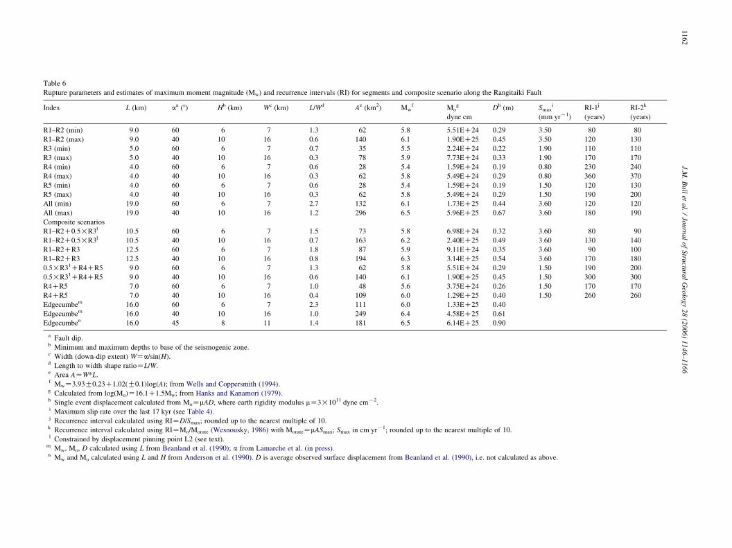
Table 6

Rupture parameters and estimates of maximum moment magnitude (Mw) and recurrence intervals (RI) for segments and composite scenario along the Rangitaiki Fault

Index L (km) aa (8) Hb (km) Wc (km) L/Wd Ae (km2) Mwf Mo

g

dyne cm

Dh (m) Smaxi

(mm yrK1)

RI-1j

(years)

RI-2k

(years)

R1–R2 (min) 9.0 60 6 7 1.3 62 5.8 5.51EC24 0.29 3.50 80 80

R1–R2 (max) 9.0 40 10 16 0.6 140 6.1 1.90EC25 0.45 3.50 120 130

R3 (min) 5.0 60 6 7 0.7 35 5.5 2.24EC24 0.22 1.90 110 110

R3 (max) 5.0 40 10 16 0.3 78 5.9 7.73EC24 0.33 1.90 170 170

R4 (min) 4.0 60 6 7 0.6 28 5.4 1.59EC24 0.19 0.80 230 240

R4 (max) 4.0 40 10 16 0.3 62 5.8 5.49EC24 0.29 0.80 360 370

R5 (min) 4.0 60 6 7 0.6 28 5.4 1.59EC24 0.19 1.50 120 130

R5 (max) 4.0 40 10 16 0.3 62 5.8 5.49EC24 0.29 1.50 190 200

All (min) 19.0 60 6 7 2.7 132 6.1 1.73EC25 0.44 3.60 120 120

All (max) 19.0 40 10 16 1.2 296 6.5 5.96EC25 0.67 3.60 180 190

Composite scenarios

R1–R2C0.5!R3l 10.5 60 6 7 1.5 73 5.8 6.98EC24 0.32 3.60 80 90

R1–R2C0.5!R3l 10.5 40 10 16 0.7 163 6.2 2.40EC25 0.49 3.60 130 140

R1–R2CR3 12.5 60 6 7 1.8 87 5.9 9.11EC24 0.35 3.60 90 100

R1–R2CR3 12.5 40 10 16 0.8 194 6.3 3.14EC25 0.54 3.60 170 180

0.5!R31CR4CR5 9.0 60 6 7 1.3 62 5.8 5.51EC24 0.29 1.50 190 200

0.5!R31CR4CR5 9.0 40 10 16 0.6 140 6.1 1.90EC25 0.45 1.50 300 300

R4CR5 7.0 60 6 7 1.0 48 5.6 3.75EC24 0.26 1.50 170 170

R4CR5 7.0 40 10 16 0.4 109 6.0 1.29EC25 0.40 1.50 260 260

Edgecumbem 16.0 60 6 7 2.3 111 6.0 1.33EC25 0.40

Edgecumbem 16.0 40 10 16 1.0 249 6.4 4.58EC25 0.61

Edgecumben 16.0 45 8 11 1.4 181 6.5 6.14EC25 0.90

a Fault dip.b Minimum and maximum depths to base of the seismogenic zone.c Width (down-dip extent) WZa/sin(H).d Length to width shape ratioZL/W.e Area AZW*L.f MwZ3.93G0.23C1.02(G0.1)log(A); from Wells and Coppersmith (1994).g Calculated from log(Mo)Z16.1C1.5Mw; from Hanks and Kanamori (1979).h Single event displacement calculated from MoZmAD, where earth rigidity modulus mZ3!1011 dyne cmK2.i Maximum slip rate over the last 17 kyr (see Table 4).j Recurrence interval calculated using RIZD/Smax; rounded up to the nearest multiple of 10.k Recurrence interval calculated using RIZMo/Morate (Wesnousky, 1986) with MorateZmASmax; Smax in cm yrK1; rounded up to the nearest multiple of 10.l Constrained by displacement pinning point L2 (see text).

m Mw, Mo, D calculated using L from Beanland et al. (1990); a from Lamarche et al. (in press).n Mw and Mo calculated using L and H from Anderson et al. (1990). D is average observed surface displacement from Beanland et al. (1990), i.e. not calculated as above.

J.M.

Bu

llet

al.

/Jo

urn

al

of

Stru

ctura

lG

eolo

gy

28

(20

06

)1

14

6–

11

66

1162


Beanland et al. (1989) identified at least two additional

faulting events in the last 1850 years B.P, from trenches

excavated across the Edgecumbe Fault. The earliest event is

uncertain, but was tentatively proposed to be around 1850

years B.P., while a later event occurred around 800 years

B.P. These data imply a minimum recurrence interval of

about 800–O1000 years. These longer recurrence intervals

are consistent with estimates of recurrence intervals for the

Rangitaiki Fault based on maximum displacement argu-

ments. The displacement value derived in Table 6 (column

10, derived via the seismic moment estimate) is the average

displacement over the whole fault plane, not the maximum

surface or sub-surface displacement. Hence the shorter

average recurrence intervals derived in Table 6 are due to

the use of the average displacement. In all likelihood, the

true average return time will vary between the short

intervals in Table 6 (100–400 years) and the longer return

time of ca. 1000 years predicted from the maximum

displacement.

The fact that we observe growth strata in the shortest

time intervals (Table 2) of 2400, 2500 and 3100 years on

the Rangitaiki Fault (Fig. 11) is consistent with the

estimated recurrence intervals (Table 6) and the preceding

discussion. Between 11.4 and 9 ka, segment R3 had a

maximum displacement of 3.3 m irregularly distributed over

its 7.3 km length. Between 13.9 and 11.4 ka, segment R3

had a maximum displacement of 3.1 m, while segment R4

had a maximum displacement of 1.6 m. From the above

discussion, these displacements could be explained by a

single ground-rupturing earthquake if associated with the

larger magnitude scenarios, i.e. with rupture occurring along

several segments. Alternatively, the displacements may have

accrued from the lower-displacement tips of larger

composite ruptures (e.g. R1–R2–R3, R4–R5), or from

several smaller earthquakes.

In contrast, during the period 17–13.9 ka, the mean slip

rate on R3, 1.2 mm yrK1, was the highest of any time

interval (Table 5; Fig. 11B) and a maximum displacement

of 9.8 m accumulated in 3.1 kyr. Whilst displacement along

R3 was accumulated irregularly during this period, the large

displacement at location 2 (w5.6 m, w1.8 mm yrK1) and

continuity of displacement accumulation from 0 to 5000 m

along strike indicates that earthquake ruptures involving R3

were not arrested at location 2 during this period.

Looking at the entire time frame resolved in our data, the

average displacement on the Rangitaiki Fault over the last

17 kyr is w29 m (which is around 50% of the maximum

displacement). Dividing the average total displacement by

the maximum slip of 3 m that can be expected during the

larger composite earthquakes, implies a minimum of about

10 large events on the fault.

7.3. Implications for models of slip accumulation during

repeated earthquakes

Several earthquake models have been proposed for slip

distribution and recurrence behaviour on segmented active

faults (Schwartz and Coppersmith, 1984). The characteristic

earthquake model assumes that the rupture length, magnitude

and distribution of slip from a ‘characteristic event’ along a

particular fault segment is repeated in successive events. Hence

for any point along the fault segment the incremental steps in

displacement are approximately constant. Furthermore when

repeated characteristic earthquakes occur, the slip distribution

will vary along the length of the segment, with largest co-

seismic slip where the highest long-term displacement occurs

and lowest displacement near segment boundaries (Schwartz,

1989). In contrast the uniform slip model (Schwartz and

Coppersmith, 1984) implies constant slip rate and displace-

ment per event at a given site, with relatively large earthquakes

interspersed with frequent moderate events that contribute to

smoothing out the aggregate displacement profile. In the

variable slip model (Schwartz and Coppersmith, 1984), there is

variation in earthquake size, displacement per event and

rupture location.

In this study we are able to directly evaluate these models

and determine which one best describes the displacement

accumulation over multiple earthquake cycles. The 17 kyr

displacement profile of the Rangitaiki Fault indicates two areas

of preferential displacement; the largest centred on the overlap

between segment R1–R2 and R3 and the second on R5

(Fig. 10A). This pattern closely matches that on an older

horizon estimated to be about 300 kyr old (Taylor et al., 2004)

(Fig. 2B). From our data on segments R3 and R4 we suggest

that the slip distribution along at least these segments is not

constant and depends on the time frame of observation. At

short time scales, displacement distribution is irregular.

However, over longer timescales the slip distribution geometry

becomes stable.

Inverse models of earthquakes show that slip can be

extremely heterogeneous, both along strike and down-dip

(for example the Landers earthquake (Wald and Heaton, 1994)

and the Denali earthquake (Wright et al., 2004)). The

variability of the sub-surface slip distribution is thought to

reflect ‘asperities’ on the fault plane at seismogenic depths.

This spatial heterogeneity in the slip is inferred not only from

inverse modelling, but also in surface offset data (e.g. Beanland

et al., 1989; Sieh et al., 1993). Hence short timescale variability

shown in these data for the Rangitaiki Fault could be reflecting

variability over the entire fault plane.

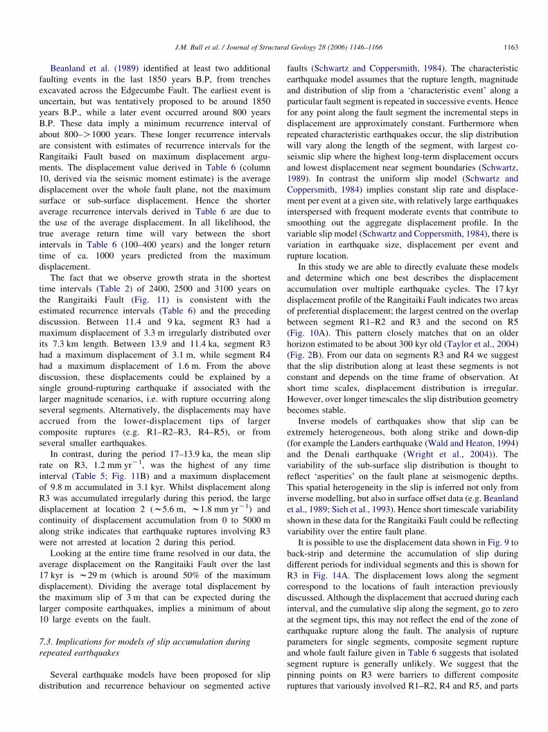
It is possible to use the displacement data shown in Fig. 9 to

back-strip and determine the accumulation of slip during

different periods for individual segments and this is shown for

R3 in Fig. 14A. The displacement lows along the segment

correspond to the locations of fault interaction previously

discussed. Although the displacement that accrued during each

interval, and the cumulative slip along the segment, go to zero

at the segment tips, this may not reflect the end of the zone of

earthquake rupture along the fault. The analysis of rupture

parameters for single segments, composite segment rupture

and whole fault failure given in Table 6 suggests that isolated

segment rupture is generally unlikely. We suggest that the

pinning points on R3 were barriers to different composite

ruptures that variously involved R1–R2, R4 and R5, and parts

Fig. 14. Slip accumulation on Segment R3 and a generic model. (A) Slip accumulation on R3 determined by back-stripping the displacement data illustrated in Fig. 9.

(B) Generic model of a three-segment fault that could produce the observed slip accumulation. The cumulative slip after five earthquakes (I–V) is shown along the

fault. Note that this is a model of steady-state behaviour (the fault has fully linked prior to any of the earthquakes shown). Earthquakes I, III and IV do not rupture the

entire fault plane but rupture two of the three segments and displacement is also pinned where a antithetic fault crosses the main fault (position 2) and where there is a

small splay from the main fault (position 3). Earthquakes II and V rupture the entire fault plane. The inset shows a map with the main fault segments (end points

denoted by circles) and minor faults highlighting fault interactions in the model. The positions of three hypothetical trench sites are also indicated (T1–T3) and

information on earthquakes recorded is shown in (C).


of R3. In different earthquakes the sections of surface rupture

may have jumped around, involving R1–R2–R3, R3–R4–R5

(or parts of R3), R4–R5, or just R1–R2. It is conceivable that

even just R3 may have ruptured, as a whole segment. It is also

likely that rupture along the whole Rangitaiki Fault occurred

with all segments failing in an event similar to the Edgecumbe

earthquake. This undoubtedly shows that many earthquake

cycles have built up the total displacement profile.


Fig. 14B shows a generic cartoon of the accumulation of

earthquake slip suggested by our data. The cartoon shows the

accumulation of slip after a three-segment fault has become

fully linked. The inset map shows the fault system with

locations of fault interactions numbered. Some earthquakes (II

and V in Fig. 14) rupture the entire fault and variable amounts

of slip are accumulated along strike. At other times (earth-

quakes I, III and IV) only two of the three segments ruptured

with locations of segment interactions variously impeding the

propagation of the earthquake rupture. The important point

here is that the fault growth and earthquake behaviour has been

variable in time. This has resulted in spatial and temporal

variability in slip accumulation within some single segments,

within short time intervals (w2–3 kyrs in the case of the

Rangitaiki Fault, i.e. approaching the return times of one or a

few earthquakes). The fault behaviour clearly does not support

a simple characteristic earthquake model, but some character-

istic type events may occur episodically. The data shows that

on occasions earthquake ruptures have been limited to only

parts of the fault network, whilst ruptures of the entire fault,

associated with the larger magnitudes, are also extremely likely

on occasions and may be consistent with the characteristic

model. The aggregate displacement profile is the sum of the

variability associated with many earthquake cycles.

The advantage of fully spatially sampling the fault system in

comparison with trenching studies is examined in Fig. 14C.

The positions of three hypothetical trench sites are shown, one

crossing each segment. While the trench sites reliably record

earthquake occurrence on each segment, there is unlikely to be

information on lateral variability in displacement, or on the role

of fault interaction in controlling displacement accumulation

on each segment.

Aki (1984) similarly describes two families of earthquakes

associated with activity at Volcano Usu in Japan. One of these

families of earthquakes exhibited consistent recurrence intervals

and slip, ruptured the entire fault plane and is consistent with the

characteristic earthquake model (Schwartz and Coppersmith,

1984). The other family of earthquakes shared the same fault

plane, but exhibited varying amounts of slip. Aki (1984) suggests

that this latter family may be explained by the presence of weak

barriers along the fault plane, whereas strong stable barriers to

rupture propagation persist through many earthquakes. The

complexity of fault geometry influences the propagation of

earthquake ruptures because of the formation of structural

heterogeneity that resists rupture propagation. We suggest that

our slip data for the last 17 kyrs is consistent with the observation

of Aki (1984). The larger magnitude events, or characteristic

events, which rupture the entire segment over longer timescales

(O6 kyr for segment R3), dominate the slip distribution.

These observations highlight that the time frame of

observation is of critical consideration when considering

fault system behaviour. If the time frame is much longer than

the recurrence interval of large earthquakes (greater than 6 kyr

for the Rangitaiki Fault; Fig. 13), then the total displacement

distribution (or range-front uplift) may be representative only

of the largest earthquakes. However if the time frame of

observation is of the same order as the recurrence interval of

any ground-rupturing earthquakes, or if the only data available

on a fault are surface displacement observations associated

with one or two coseismic events, then the observed slip

distribution (or uplift) may be unreliable for predicting long-

term earthquake behaviour on the fault.

8. Conclusions

We demonstrate that the application of marine high-

resolution seismic reflection data to an area with a constrained

stratigraphy has the potential to resolve the history of

displacement accumulation on active faults on timescales that

will shed light on cycles of earthquake activity. A method for

determining the length of time period of observation necessary

to reliably record fault system behaviour is explained and

applied to the Rangitaiki Fault.

1. Displacement profiles of the last 9 kyr of fault movement

are regular and similar to profiles showing the last 300 kyr

of fault movement. In contrast, profiles determined for short

time intervals (2–3 kyr) on two of the fault segments are

highly irregular and show points of zero displacement

within the larger segments. This indicates temporal and

spatial variability in incremental displacement associated

with ground-rupturing earthquakes. Some earthquakes

appear to have been confined to specific segments, whereas

larger composite ruptures have involved the entire fault.

2. The aggregate displacement profile of the entire Rangitaiki

Fault represents the sum of the variability associated with

many earthquake cycles involving individual segments. The

irregularity of fault displacement data on timescales of 2–

3 kyr revealed in this study demonstrates that observations

on this timescale may not give results that are representative

of the long-term evolution of this fault system. An analysis

of variance showed that the shape of the slip profiles does

not change for time periods of observation longer than 6 kyr.

Application of methodologies presented here can determine

over what timescales fault behaviour is fully sampled.

3. The distribution of displacement during the last 17 kyr along

the Rangitaiki Fault system is largely controlled by relict

segment boundaries that reflect the history of linkage of the

fault system. The largest magnitude earthquakes have

sufficient energy to rupture across these segment bound-

aries, whereas smaller magnitude events contribute to

irregular surface displacement accumulation. We present a

model for slip accumulation on a fault during repeated

earthquakes in which larger events rupture the entire fault

plane, with relatively smaller events having irregular slip

profiles and failing to rupture across segments or asperities

along the fault plane.

Acknowledgements

This work was funded by the Natural Environment Research

Council (GR3/11862), United Kingdom and the New Zealand

Foundation for Research Science and Technology (FRST-

CO1X0038). We are grateful to the officers and crew of R/V


Tangaroa and R/V Kaharoa for their dedication during TAN-

99-14 and KAH01-02, and to the technical team at NIWA for

their expertise in geophysical data acquisition. The manuscript

was improved by careful and constructive reviews from Gerald

Roberts and Andy Nicol. Ian Wright is thanked for his support.

References

Aki, K., 1984. Asperities, barriers, characteristic earthquakes and strong

motion prediction. Journal of Geophysical Research 89, 5867–5872.

Anderson, H.J., Webb, T.H., 1989. The rupture process of the Edgecumbe

earthquake, New Zealand. New Zealand Journal of Geology and

Geophysics 32, 43–52.

Anderson, H.J., Smith, E., Robinson, R., 1990. Normal faulting in a back-arc

basin: seismological characteristics of the March 2, 1987, Edgecumbe, New

Zealand, Earthquake. Journal of Geophysical Research 95, 4709–4723.

Beanland, S., Berryman, K.R., Blick, G.H., 1989. Geological investigations of

the 1987 Edgecumbe earthquake, New Zealand. New Zealand Journal of

Geology and Geophysics 32, 73–91.

Beanland, S., Blick, G.H., Darby, D.J., 1990. Normal faulting in a back-arc basin:

geological and geodetic characteristics of the 1987 Edgecumbe earthquake,

New Zealand. Journal of Geophysical Research 95, 4693–4707.

Bryan, C.J., Sherburn, S., Bibby, H.M., Bannister, S.C., Hurst, A.W., 1999.

Shallow seismicity of the central Taupo Volcano Zone, New Zealand: its

distribution and nature. New Zealand Journal of Geology and Geophysics

42, 533–542.

Carter, R.M., Carter, L., Johnson, D.P., 1986. Submergent shorelines, SW

Pacific: episodic post-glacial transgression. Sedimentology 33, 629–649.

Chapman, T.J., Meneilly, A.W., 1991. The displacement patterns associated

with a reverse-reactivated, normal growth fault. In: Roberts, A.M.,

Yielding, G., Freeman, B. (Eds.), The Geometry of Normal Faults

Geological Society Special Publication 56, pp. 183–191.

Cowie, P.A., Scholz, C.H., 1992. Growth of faults by accumulation of seismic

slip. Journal of Geophysical Research 97, 11085–11096.

Crone, A.J., Machette, M.N., 1984. Surface faulting accompanying the Borah

Peak earthquake, central Idaho. Geology 12, 664–667.

Darby, D.J., 1989. Dislocation modelling of the 1987 Edgecumbe earthquake,

NewZealand.NewZealand Journal ofGeology andGeophysics 32, 115–122.

Davey, F.J., Henrys, S.A., Lodolo, E., 1995. Asymmetric rifting in a

continental back-arc environment, North Island, New Zealand. Journal of

Volcanological and Geothermal Research 68, 209–238.

Hanks, T.C., Kanamori, H., 1979. A moment magnitude scale. Journal of

Geophysical Research 84, 2348–2350.

Hemphill-Haley, M.A., Weldon, R.J., 1999. Estimating prehistoric earthquake

magnitude from point measurements of surface rupture. Bulletin of the

Seismological Society of America 89, 1264–1279.

Kohn, B.P., Glasby, G.P., 1978. Tephra distribution and sedimentation rates in

the Bay of Plenty, New Zealand. New Zealand Journal of Geology and


Lamarche, G., Bull, J.M., Barnes, P.M., Taylor, S.K., Horgan, H., 2000.

Constraining fault growth rates and fault evolution in New Zealand. Eos

Transactions of the American Geophysical Union 81, 481–486.

Lamarche, G., Barnes, P.M., Bull, J.M., in press. Faulting and extension rate

over the last 20,000 years in the Offshore Whakatane Graben, New Zealand

Continental Shelf. Tectonics.

Manighetti, I., Campillo, M., Sammis, C., Mai, P.M., King, G., 2005. Evidence

for self-similar, triangular slip distributions on earthquakes; implications

for earthquake and fault mechanics. Journal of Geophysical Research 110,

B05302. doi:10.1029/2004JB003174.

Mansfield, C.S., Cartwright, J.A., 1996. High-resolution displacement mapping

from three-dimensional seismic data: evidence for dip linkage during fault

growth. Journal of Structural Geology 18, 249–263.

Nairn, I.A., Beanland, S., 1989. Geological setting of the 1987 Edgecumbe

earthquake, New Zealand. New Zealand Journal of Geology and


Nicol, A., Walsh, J.J., Berryman, K., Nodder, S., 2005. Growth of a normal

fault by the accumulation of slip over millions of years. Journal of

Structural Geology 27, 541–551.

Peacock, D.C.P., Sanderson, D.J., 1996. Effects of propagation rate on

displacement variations along faults. Journal of Structural Geology 18,

311–320.

Schwartz, D.P., 1989. Paleoseismicity, persistence of segments, and temporal

clustering of large earthquakes—examples from the San Andreas, Wasatch,

and lost River Fault Zones. In: Proceedings of Conference XLV, Fault

Segmentation and Controls of Rupture Initiation and Termination. U.S.

Geological Survey Open-file Report 89-315, pp. 361–375.

Schwartz, D.P., Coppersmith, K.J., 1984. Fault behavior and characteristic

earthquakes: examples from the Wasatch and San Andreas Fault Zones.

Journal of Geophysical Research 89, 5681–5698.

Sieh, K., Jones, L., Hauksson, E., Hudnut, K., Eberhart-Phillips, D.,

Heaton, T., Hough, S., Hutton, K., Kanamori, H., Lilje, A.,

Lindval, S., McGill, S.F., Mori, J., Rubin, C., Spotila, J.A.,

Stock, J., Thio, H., Treiman, J., Wernicke, B., Zachariasen, J., 1993.

Near-field investigation of the Landers earthquake sequence, April to

July, 1992. Science 260, 171–176.

Taylor, S.K., 2003. A long timescale high-resolution fault activity history of the

Whakatane Graben, New Zealand. Ph.D. thesis, University of South-

ampton, UK.

Taylor, S.K., Bull, J.M., Lamarche, G., Barnes, P.M., 2004. Normal fault

growth and linkage during the last 1.3 million years: an example from the

Whakatane Graben, New Zealand. Journal of Geophysical Research 109,

B02408. doi:10.1029/2003JB002412.

Villamor, P., Berryman, K., 2001. A late Quaternary extension rate in the

Taupo Volcanic Zone, New Zealand, derived from fault slip data. New

Zealand Journal of Geology and Geophysics 44, 243–269.

Wald, D.J., Heaton, T.H., 1994. Spatial and temporal distribution of slip for the

1992 Landers California Earthquake. Bulletin of the Seismological Society

of America 84, 668–691.

Walsh, J.J., Watterson, J., 1988. Analysis of the relationship between

displacements and dimensions of faults. Journal of Structural Geology. 10,

238–247.

Walsh, J.J., Watterson, J., 1991. Geometric and kinematic coherence and scale

effects in normal fault systems. In: Roberts, A.M., Yielding, G.,

Freeman, B. (Eds.), The Geometry of Normal Faults Special Publication,

Geological Society of London 56, pp. 193–203.

Wells, D.L., Coppersmith, K.J., 1994. New empirical relationships among

magnitude, rupture length, rupture width, rupture area and surface

displacement. Bulletin of the Seismological Society of America 84,

974–1002.

Wesnousky, S.G., 1986. Earthquakes, Quaternary faults and seismic hazard in

California. Journal of Geophysical Research 91, 12587–12631.

Wright, I.C., 1990. Late Quaternary faulting of the offshoreWhakatane Graben,

Taupo Volcanic Zone, New Zealand. New Zealand Journal of Geology and


Wright, T.J., Lu, Z., Wicks, C., 2004. Constraining the slip distribution and

fault geometry of the Mw 7.9, 3 November 2002, Denali Fault

earthquake with interferometric synthetic aperture radar and global

positioning system data. Bulletin of the Seismological Society of

America 94, S175–S189.

http://dx.doi.org/10.1029/2004JB003174

http://dx.doi.org/10.1029/2003JB002412

High-resolution record of displacement accumulation on an active normal fault: implications for...

Documents

Transcript of High-resolution record of displacement accumulation on an active normal fault: implications for...