* We would like to thank seminar participants at AREUEA Virtual Seminar, Baruch College, CFDM Lab Group, CU Boulder finance lunch, FDIC Consumer Research Symposium, Finance in the Cloud Conference, MIT Sloan Junior Finance Conference, NBER SI Corporate Finance 2020, and Stanford GSB Finance. We would also like to thank Adrien Auclert, Claes Backman, Bo Becker, John Beshears, Matteo Benetton, John Campbell, Taha Choukhmane, Tony Cookson, Anthony DeFusco, Daniel Fernandes, John Lynch, Marco Di Maggio, Anastassia Fedyk, Nicolae Garleanu, Amir Kermani, Benjamin Keys, Laura Kodres, Arvind Krishnamurthy, Deborah Lucas, Gustavo Manso, Patrick Moran, Jordan Nickerson, Terrance Odean, Michaela Pagel, Christopher Palmer, Jonathan Parker, Daniel Paravisini, Giorgia Piacentino, Kasper Roszbach, Antoinette Schoar, David Schoenherr, Felipe Severino, Amir Sufi, David Sraer, Daan Struyven, Jialan Wang, Emil Verner, and Erkki Vihriala for helpful comments. †(corresponding author) University of Colorado at Boulder & NBER; asaf.bernstein@colorado.edu ‡ Stanford GSB and NBER; koudijs@stanford.edu

Mortgage Amortization and Wealth Accumulation

Asaf Bernstein† Peter Koudijs‡

December 2020

Abstract Standard mortgage contracts include periodic debt repayment (amortization) schedules designed to build-up illiquid savings in the form of home equity. These are substantial even from a macroeconomic standpoint. For example, U.S. households contribute hundreds of ($) billions each year into mortgage amortization plans – making them comparable in size to pension program contributions. We provide the first empirical evidence on the causal effects of mortgage amortization on wealth accumulation. Ex-ante, effects are unclear. If increased debt repayments crowd-out households’ non-mortgage savings, rather than alter their consumption or labor supply, there would be no effect on wealth. We use individual administrative data and plausibly exogenous variation in the timing of home purchases surrounding an interest-only mortgage reform in the Netherlands. We find little-to-no change in the accumulation of non-mortgage savings, even five years later when amortization-induced home equity is larger than all other non-pension financial assets. This lack of crowding-out implies a surprising near 1-for-1 rise in net worth and little savings-debt fungibility, financed via increased labor supply and reduced expenditures. Results hold using life-events (ex. birth of a child) as an instrument for the timing of home purchase, and appear unaffected by potential selection or confounded treatment concerns. Findings hold for buyers with substantial liquid savings and across ages, suggesting general applicability beyond just non-savers and the young. Our findings suggest that homeownership, when coupled with amortizing mortgages, is a key driver of household wealth building and inequality, and that the amortization-wealth elasticity is a crucial consideration for macroprudential policies.

JEL Classifications: G4, G5, G19, G21, G51, J3, R2

Keywords: Mortgage, Amortization, Homeownership, Wealth, Savings, Fungibility, Macroprudential

1

"One nice thing about investing in a house is that you're committed to a mortgage payment. So if you don't take out a home equity line of credit or do something like that, you will accumulate wealth."

Nobel Laureate Robert Shiller (CNN Dec 4th, 2014)

---- When households purchase a home with a standard mortgage contract, they not only sign-up for a loan,

but also a periodic debt repayment plan, called an amortization schedule. These plans are designed to

build-up substantial illiquid savings in the form of home equity prior to maturity of the loan. Amortization

plans are ubiquitous in most countries and typically not only substantial for each individual borrower, but

also at a macroeconomic level. For example, in the U.S., households contribute hundreds of billions of

dollars each year to mortgage amortization plans, which make them comparable in size with other major

illiquid savings contributions, such as pension programs.1

In this paper, we examine the effect of mortgage amortization on wealth accumulation. If

households act as if mortgage repayments and non-mortgage savings are fungible, then there will be no

effect on wealth accumulation – increases in mortgage repayments will perfectly crowd-out other savings.

If on the other hand, they are not fungible, then mortgage amortization could lead to substantial household

wealth accumulation. While there is a broad literature on the effects of pension programs on savings and

wealth accumulation (e.g. Poterba et al. 1995, 1996; Madrian and Shea 2001; Chetty et al. 2014; Beshears

et al. 2019; Choukhmane 2019), there is no causal evidence on the effects of mortgage amortization.

Empirical evidence on the elasticity between amortization and wealth accumulation ( ) is

critical for our understanding of the underlying mechanisms that alter household savings decisions, the

impact of macroprudential policies, and the importance of homeownership for household wealth building,

retirement savings, and inequality. For example, if households compensate for increased debt repayments

by reducing their non-mortgage savings, policies intended to encourage building up home equity could

actually hurt financial stability. By contrast, if households do not treat mortgage amortization and non-

mortgage savings as fungible, such policies could improve stability. Moreover, encouraging

homeownership financed with amortizing mortgages could stimulate wealth accumulation.

The empirical identification of is challenging though. Households endogenously select into

homeownership and their choice of mortgage contract. Renters are typically unlikely to be a valid

1 In 2016, there were $10.3 trillion in U.S. residential mortgages (https://fred.stlouisfed.org/) with 2.5% of principal scheduled to be amortized and 2.8% actually repaid in 2016 (CoreLogic), equating to $250-300 billion in savings via mortgage amortization. By comparison, there were around $398 billion in 401(k) pension contributions reported to the Department of Labor in 2016 (including both employee and employer contributions).

2

counterfactual for households able and willing to buy a home2. The existing literature also shows that

households who limit amortization by taking up interest-only (IO) or alternative mortgage products

(AMPs) often differ systematically in terms of their liquidity constraints, financial sophistication, savings

preferences, and future income expectations (Cocco 2013; Cox et al. 2015; Kuchler 2015).

In this paper, we overcome these challenges and provide the first empirical evidence on the causal

effects of mortgage amortization on wealth accumulation. We use individual administrative data to

examine the January 2013 implementation of a mortgage reform in the Netherlands aimed at improving

financial stability. Prior to the reform, first-time home buyers (FTHBs) typically borrowed half of the

mortgage sum as an interest-only loan. Afterwards, the vast majority borrowed the full amount through a

standard fully amortizing mortgage. The caused a substantial rise in required monthly debt repayments.

This novel quasi-experiment provides a unique opportunity to examine the role that mortgage

amortization plays in wealth accumulation. Not only does the regulatory change provide plausibly

exogenous variation in amortization schedules for FTHBs, our administrative data gives us precise

measures of household wealth and its decomposition for every person reporting taxes in the Netherlands

from 2006 to 2016.

We compare all FTHBs with a mortgage right around the implementation of the reform and find

little-to-no difference in non-mortgage savings (the accumulation of bank deposits, stocks, or bonds),

despite a significant increase in observed debt repayment. This holds even five years after the reform

when for the average treated household, the additional mortgage debt repayment over this period exceeds

the stock of non-mortgage savings. This implies a near one-for-one rise in net worth – a response

consistent with little savings-debt repayment fungibility (F~0) and a substantial effect of amortization on

wealth accumulation ( ). We find that around 26-36% of the increased wealth accumulation is

financed with higher future household labor income, driven entirely by increases in household hours

worked, despite no difference in income growth between the groups prior to home purchase. The

remainder comes from a reduction in household expenditures.3 We find no differences between observed

and predicted (based on contract terms) amortization over this period, suggesting little “leakage” of

treatment via differential home equity withdrawals or prepayment for those buying before vs. after the

reform.

We look at all FTHBs who bought around the end of 2012 and beginning of 2013 and compare

their wealth accumulation over the same later years (ex. January to December 2015). Differences in

2 Older households often have substantial home equity, but little liquid savings (ex. Kaplan et al. 2014). This in itself could suggest a high . However, this could also simply reflect the fact that these households have substantial housing wealth and therefore little need for other forms of savings. 3 Given how much of the household income statement we can observe, this likely reflects changes in consumption.

3

wealth accumulation are smooth and flat as a function of mortgage age before the reform, then jump up

suddenly and persistently the month the reform takes effect. This indicates that results are not driven by

differences in mortgage age. The reform was based on the time of going under contract on a house

purchase and not the closing date, which typically takes at least two months. Therefore, households

closing on their properties in January and February of 2013 were unlikely to be affected by the reform,

while those closing in March and April 2013 were. We find similar effects comparing households closing

in this narrow four-month window.

Despite this evidence strongly supportive of a causal interpretation of our findings, a key

remaining concern for our identification is heterogeneous sorting. That is, our estimates would be biased

if FTHBs strategically timed their home purchase to avoid the reform, and if this behavior is

systematically correlated with their subsequent savings decisions (ex. those who buy earlier intend to save

less).

First of all, we find no evidence that the reform affected the timing of home purchase. There is no

apparent bunching in the number of transactions in the months prior to the reform. Moreover, the reform

did not change the probability of a household eventually buying its first home after experiencing a life-

event (ex. birth of a child). The timing of home purchase after a life-event also did not change. These

findings may be at least partially explained by the fact that even prior to the reform, loan-to-income

requirements were computed as if the loan was fully amortizing over 30 years, even if it was not. As such,

the reform did not change the maximum mortgage sum a household could borrow based on its income.4

Second, we find no systematic differences in the observable characteristics of households

purchasing a home before or after the reform. House purchase values, origination LTVs, income, and

income growth are smooth around the reform, and do not have differential pre-trends. Moreover, in the

years before the reform, wealth and wealth growth are the same for those buying before vs. after. To

confirm there are no systematic differences, we compare FTHBs with non-FTHBs who were partially

grandfathered in under the old mortgage rules. This means that the jump in mortgage repayment was

substantially smaller for this group (even conditional on buying in the same month). We find that, relative

to non-FTHBs, the change in observables for FTHBs is smooth across the reform. FTHBs also show no

differential change in future non-mortgage savings, again consistent with no significant heterogeneous

sorting.

4 By contrast, DeFusco et al. (2020) and Backman and van Santen (2020) show that in settings where regulatory constraints on leverage bind substantial bunching can occur. As we show later on and has been argued by Van Bekkum et al. (2019) Dutch households tend to borrow almost as much as they can up to the regulatory limit, which is unlikely to be a circumstance unique to just the Dutch setting.

4

Though suggestive, it is still possible that there was heterogeneous sorting on unobservables

around the reform. We therefore re-run our analysis focusing FTHBs who also had a “life-event” in the

months surrounding the reform. The high-quality nature of administrative data in the Netherlands lets us

identify the exact month when there are changes in the number of members of the household, such as the

birth of a child. We show that the timing of a life-event is a strong predictor of the timing of home

purchase. Moreover, the timing of life-events among our sub-group of FTHBs is unrelated with pre-

reform household income, changes in non-mortgage savings, or wealth accumulation (nor the

appreciation of their house value after purchase). Using the month of a household life-event as an

instrumental variable, we find that life-events after the reform are associated with increases in mortgage

debt repayments, still matched one-for-one with changes in wealth accumulation. Given the sudden and

persistent rise in wealth accumulation based on life-events around the reform, and the implausibility that

households were timing life-events to avoid the reform, we conclude that there was indeed a causal effect

of wealth accumulation consistent with an for FTHBs.

Apart from selection, it is possible that the reform changed the supply-side of the Dutch mortgage

market. The lack of sorting around the reform suggests it is unlikely there were sudden changes in

screening by lenders in response to the regulation. This is at least partially a function of the relatively low

concern about default in the Netherlands and the wide use of floating rate mortgages. This may explain

why we find no differential change in mortgage rates around the reform for FTHBs, suggesting that other

supply effects were limited.

Another concern for identification is that our treatment could be confounded by other major

changes around the regulation which also alter wealth accumulation. First of all, there could be seasonal

effects if early year buyers systematically differ in their wealth accumulation patterns. That does not

appear to be the case. Effects are persistent for those who went under contract after the regulation, even

for those who bought at the end of 2013, but there are no effects for those same months of the year in

2012. Second, as of January 2013, the maximum allowed loan-to-value (LTV) ratio dropped by one

percentage point. Despite this, there is no change in average LTV ratios. For completeness, we re-run our

analysis among households with origination LTV ratios far below the regulatory thresholds and again find

that .

A remaining concern is that the reform had liquidity and wealth effects that could explain our

results. In particular, by forcing households to pay down more of their mortgage, the reform effectively

reduces mortgage interest deductibility (MID) for those buying after. This means a reduction in future

5

liquidity and life-time wealth, and a greater need to save.5 The complete absence of any effects on non-

mortgage savings in our setting suggests this is a minor concern – it seems implausible that liquidity or

wealth effects would lead to an increase in wealth accumulation via increased mortgage repayment, but

no change at all in non-mortgage savings. Nevertheless, we take additional steps to evaluate the

importance of the reduction in MID.

First, we show that wealth effects are unlikely to explain our results. In a standard life-cycle

model where households smooth consumption over time, a one-time reduction in life-time wealth should

lead to a one-time permanent reduction in consumption. To make sure that such a response is not driving

our results, we take advantage of the typical structure of the mortgage amortization schedule: mortgage

repayment increases over the life of the mortgage. This allows us to compute the increase in the mortgage

debt repayment within a given household over 2014 vs. 2016 and relate it to the change in household

wealth (delta-in-delta). Again, we find an elasticity of about 1, suggesting it is unlikely our effects are

confounded by a one-time wealth effect coming from the reduction in MID, or for that matter, any other

one-time shock occurring at the time of going under contract.

We can further evaluate the possible impact of wealth effects by focusing on non-FTHBs. The

reform’s grandfather clause was only partial. Existing homeowners could only benefit from the old rules

for the duration of their existing mortgage – the maturity could not be extended. Therefore, any perceived

negative wealth effect from the reform should be larger for those with a shorter period to benefit from the

more extensive MID. In other words, for the same amortization effect, this can give variation in the

potential for MIDs. In particular, we compare non-FTHBs with a remaining maturity on their mortgage of

more or less than ten years. Comparing these groups, we find no difference in wealth accumulation. This

is consistent with wealth effects playing little observable role in confounding our estimates.

Next, we show that liquidity effects are unlikely to explain our results. Our estimates of are

consistent across years looking at wealth accumulation in 2014, 2015, and 2016 separately. If liquidity

effects were important, we would expect to see substantial differences between those years. In 2014,

mortgages were barely amortized and differences in MID between those buying before or after the reform

would have been minor. Yet, we still find an effect not different from an elasticity of 1.

Also, we show that our results are the same even among households with more than enough

liquid assets, either in terms of the flow or in their overall level, so that they could easily offset their

5 We expect the relative wealth and liquidity effects to be small. Because of the convex amortization schedule of annuity mortgages, most of the tax benefits accrue in the future. It is unclear whether existing homeowners expected MID rules to stay the same. At the time of the 2013 regulation, it was hotly debated whether the MID reduction should not also apply to existing home owners. Moreover, the mortgage regulation was the first significant MID reduction in decades, and signaled more reductions to come, which were eventually implemented starting in 2014.

6

mortgage repayment by altering their non-mortgage savings. This holds either using their actual non-

mortgage savings in a year, or instrumenting for that using their non-mortgage savings in the years before

they bought the house. We have also found similar results for those with low loan-to-values, who should

be more easily able to access this home equity. The lack of any substantial variation based on the amount

of liquidity available, again suggests little role for liquidity effects in explaining our observed elasticity

estimates.

While there is compelling evidence in our setting of a substantial causal effect of mortgage

amortization on wealth accumulation, it is unclear what potential mechanisms could plausibly cause such

a large response. Since our results are not just driven by non-savers, one possible explanation is that there

is a substantial (perceived) liquidity difference between mortgage debt repayment and non-mortgage

savings. Extracting home equity is generally costly, and may even be infeasible in economic downturns

when house prices and incomes fall, making it a poor substitute for non-mortgage savings in bad times

(DeFusco and Mondragon 2019). This may be exacerbated if households are unwilling (or unable) to tap

other forms of credit (Hundtofte et al. 2018). Our finding of no response in non-mortgage savings to the

rise in debt repayment does suggest a rather less standard model – households appear willing to cut

consumption and increase labor supply substantially today in order to avoid any possible reduction in

marginal consumption or increase in their labor supply in the future.

This suggests behavioral channels may play a role. In Section 5 we discuss which of these

channels might be most relevant. Since most FTHB mortgages were partially amortizing prior to the

reform, effects are likely attributable to increases in the amortization amount, not a complete lack of

familiarity with amortization. We consider the importance of default settings which have been shown to

increase pension contributions (Madrian and Shea 2001; Chetty et al. 2014; Beshears et al. 2019),

discussed in the context of mortgages as commitment devices (Beshears et al. 2015; Kovacs and Moran

2019; Attanasio et al. 2020; Vihriala 2020; Schlafmann 2020), the ease and simplicity of small monthly

payments to save (Beshears et al. 2013; Hershfield et al. 2019), and mental accounting causing

households to treat mortgage debt repayments as bills, not as wealth accumulation (Camanho and

Fernandes 2018).

Regardless of the underlying channel, the substantial effect of mortgage amortization on wealth

accumulation that we find across a broad set of household types has important policy implications.

First, our results speak to the costs and benefits of interest-only (IO) mortgages or alternative

mortgage products (AMP) (Mian and Sufi 2009; Adelino et al. 2016; Hertzberg et al. 2018). Ex-ante, one

might expect that households with smaller amortization amounts have more non-mortgage savings. These

households would therefore be less likely to default after a shock, leading IO mortgages and AMPs to

7

actually improve financial stability (Svensson 2019; Svensson 2020). Our results suggest that this is not

necessarily the case, as households do not seem to treat amortization and non-mortgage savings as perfect

substitutes.6 It seems likely that the rise in the use of these products in the U.S. before the Global

Financial Crisis likely had a detrimental effect on these borrowers’ ability to eventually repay their debts.

Second, our results speak to macroprudential policies during recessions (Piskorski and Seru

2018). Most of the existing literature has considered changes in interest rates (Di Maggio et al. 2017;

Zator 2019). There is a fundamental difference between our estimate of and the estimates from this

literature. Both examine changes in monthly mortgage payments. However, while a change in

amortization has no direct effect on net-wealth in and of itself, a change in interest rates does.7

Nevertheless, our analysis shows a remarkable similarity in response: households appear to treat these

fundamentally different forms of payments as equivalent. This has important microeconomic,

macroeconomic, and policy implications, which we discuss in more detail in Section 5. Most

importantly, policies that encourage contracts with countercyclical amortization (Campbell et al. 2019)

are likely to have an even bigger impact than implied by standard models. Given the size of mortgage

amortization in the U.S., this effect would be economically substantial. For example, freezing mortgage

amortization payments for two years would be roughly equal to the dollar amount of all TARP (Trouble

Asset Relief Program) payments in the four years following the Great Recession.

Third, our findings help reconcile different findings in the literature on the causal effect of

homeownership on household wealth. Kaplan et al. (2014) find that homeowners typically accumulate

substantial sums of housing wealth. However, Sodini et al. (2017), exploit plausibly exogenous variation

in homeownership funded with interest-only mortgages and find little evidence for this. Our results help

reconcile these seemingly inconsistent findings if the effect of homeownership on wealth accumulation is

substantially mediated through mortgage amortization.

Finally, our findings could also have potential implications for the optimal design of retirement

programs. Beshears et al. (2019) argue that the socially optimal retirement plan with taste shocks and

present-bias should have three accounts, including one with early liquidation costs. Homeownership with

mortgage amortization is such an account that appears to be a critical component of household wealth

6 Amromin et al. (2018) show that, controlling for income and credit score, people who took out AMPs in the U.S. were twice as likely to default than those with amortizing mortgages. This is suggestive that households in the U.S. did not use the extra funds available with interest-only mortgages to improve their non-mortgage savings, which they could then use to prevent a costly default. 7 The same argument holds comparing our work to papers looking at changes in anticipatable changes in mortgage interest rates, tax rebates and other governmental payouts (ex. Johnson et al. 2006; Agarwal et al. 2007; Parker et al. 2013; Kaplan and Violante 2014; Keung 2018, Cookson et al. 2019).

8

accumulation. Whether it is relevant for retirement will depend on whether those approaching such an age

are affected similarly and the persistence of any wealth accumulation.

Who are our results likely to apply to? We show that our elasticity holds for households with a

large amount of non-mortgage savings and across the spectrum of ages of FTHBs, including those more

than 50 years old, and non-FTHBs. This suggests that our effects are generally applicable and not

confined to young, financially constrained households far away from retirement.

Our findings appear consistent with related findings in other countries, suggesting a likely

applicability beyond just the Netherlands. Prior work looking at the U.S., Canada, Denmark, and Finland

does not examine wealth accumulation directly, but does find that reduced mortgage repayment increase

consumption and reduce labor supply, consistent with our findings. Ganong and Noel (2019) provide such

evidence for households in financial distress, Scholnik (2013), d’Astous (2019), and Andersen et al.

(2019) for households fully paying off their mortgages, Larsen et al. (2018), and Backman and

Khorunzhina (2020) for households choosing interest-only mortgages, and Vihriala (2020) for households

with an option ARM period ending.

One potential concern for external validity is that, because of our intent-to-treat design, we could

be measuring a local average treatment effect on compliers, and not an average treatment effect.8 This a

small concern in our setting, however, since virtually all homeowners are compliers. Before the reform,

the vast majority of homeowners had at least part of their mortgage interest-only, while afterwards most

had fully amortizing mortgages.

Wow long do the effects last? We find no evidence of any offsetting behavior in the first five

years after the reform, when our data end, even though differential mortgage repayment amounts are

substantial. As noted already, effects are similar for older households and those with high non-mortgage

savings. Moreover, homeowners who sell their house within five years (and buy another) do not appear to

cash out. This suggests effects are fairly persistent.9 Though not central to our analysis – an effect lasting

at least five years and substantially increasing wealth clearly has important economic and policy

implications – it is interesting to consider whether effects might last longer than that and what happens to

the considerable additional household wealth already accumulated.

Simple aggregate statistics can provide some suggestive evidence on this front. According to the

2016 Survey of Consumer Finances, “hand-to-mouth” homeowners in the U.S. (those with few non-

8 For example, in the U.S., the U.K. and Denmark the choice for an interest-only mortgage is relatively atypical (Cocco 2013; Cox et al. 2015; Kuchler 2015). 9 This stands in contrast with evidence that households undo an increase in current pension contributions (driven by some intervention) by reducing future contributions (Choukhmane 2019, Wang et al. 2020). This may be because undoing amortization, through refinancing or obtaining a second mortgage, is more costly than for pensions.

9

mortgage savings) appear to generally repay their mortgages over their life-cycle. Around 90% have a

mortgage in their 30s, but only 61% do by their mid-to-early 60s. This implies that they do not generally

undo their amortization schedules with home equity withdrawals or by re-levering at the time of moving.

By contrast, 94% of hand-to-mouth homeowners in the Netherlands still have a mortgage by their mid-to-

early 60s. This implies that they typically roll over their (pre-2013) interest-only mortgages, rather than

build up non-mortgage savings to pay them off at maturity. Of course, there are many other differences

between the U.S. and the Netherlands apart from different amortization standards, but if these tendencies

hold for those buying around the 2013 reform in the Netherlands, it would be suggestive of longer run

effects on wealth accumulation.

If amortization does happen to have life-time wealth effects, this could have additional important

implications. For example, it could help explain the black white-wealth gap. The existing literature

attributes this gap, at least in part, to historical differences in homeownership driven by differential access

to financing (e.g. Charles and Hurst 2002; Krivo and Kaufman 2004; Appel and Nickerson 2016;

Aaronson et al. 2017; Anders 2018; Krimmel 2018). Our results suggest that it may not just be the ability

to purchase a home, but also the differential access to mortgages, usually linked to a fixed amortizing

schedule, that may explain wealth differences.10 This would of course depend on the persistence of such

effects in the U.S. historically among these groups and the general external validity of our findings.

The rest of this paper is structured as follows. Section 1 discusses the mortgage environment in

the Netherlands. Section 2 describes the underlying data. Section 3 discussed theoretical predictions and

our empirical design. Section 4 has the main empirical results 5. Section 5 discusses the possible

mechanisms explaining our results. Section 6 concludes.

1. Mortgage Environment in the Netherlands 1.1. Pre-Regulation In the recent past, households in the Netherlands have had exceptionally high loan-to-value (LTV) ratios

for their mortgages. This is a combination of harsh recourse laws11, generous mortgage interest

10 This may be especially true if strong housing wealth bequest motives lead to substantial intergenerational transfers and persistence (McGee 2019). 11 When Moody’s ranked developed countries in terms of both the legal right for recourse and the practical application of recourse, the U.S. ranked as the weakest on both counts, while the Netherlands was ranked as “very strong” on the legal right of recourse and its application in practice, the highest ranking in either category (NVB 2014). The result is that foreclosure rates in the U.S. at their peak were almost a hundred times higher than in the Netherlands, even though a higher proportion of households had negative equity in the Netherlands in their relative Great Recession troughs.

10

deductibility (MID) for tax purposes in combination with a high marginal tax rate, and relatively loose

macroprudential policies. In the late 1990s, LTV ratios were usually in excess of 100% at origination and

often as high as 120%. This allowed household to maximize their MID for tax purposes. Money in excess

of the home value was used to finance moving costs including property transfer taxes, realtor fees,

explicit moving costs, and renovations and refurbishing.

Starting in 2001, the Dutch government began to place limits on these origination practices. In

order to be eligible for MID and the national mortgage insurance (NHG)12, the mortgage maturity was

limited to 30 years and the interest-only (IO) part was capped at 75% of the mortgage sum. In an effort to

keep MID tax benefits on the amortizing part, banks introduced linked savings accounts in which

homeowners put funds that would be invested to repay the mortgage at maturity. By 2008, most

homeowners opted for a simple contract that was virtually identical to a standard amortizing mortgage,

but with larger tax benefits. They deposited a monthly sum equal to a regular amortization amount into a

savings account with the same interest rate as the mortgage. They used the accumulated savings to cover

(part of) the mortgage’s interest cost and to repay the mortgage at maturity. They were not allowed to

access the savings during the duration of the mortgage. Returns on savings were not taxed.

In 2007, banks signed a Code of Conduct for Mortgage Loans (CCM) that further tightened

mortgage rules. Initially it set limits on payment-to-income (PTI) and LTV ratios. In August 2011, it set

the maximum IO component of new mortgages to 50%. The other half could be in the form of a mortgage

with a linked savings account, as long as it amortized over a period of 30 years (or less). Following this

regulation, the vast majority of mortgages originated had 50% IO and 50% linked accounts. In addition,

the revised CCM set maximum origination LTVs at 106%, with 1% reductions each year afterwards until

it finally reached 100% in January of 201813. Similar to the uptake of IO mortgages, households tended to

borrow up to the allowable regulatory limits. For FTHBs in 2013, more than 40% of mortgage offers were

within 5 percentage points of the regulatory LTV limit and around 20% of all mortgage offers were at

exactly the limit.

1.2. The 2013 Reform For new home purchase contracts signed after January 1st, 2013 the Dutch government implemented a

new macroprudential policy intended to promote “Financial Stability”. Proposed at the end of April 2012

and passed in October of that year, these new regulations required all new mortgages to be fully

12 The insurance was only available if the house value was less than a maximum amount (€320 k in 2012), and if the payment-to-income was below a certain limit. The insurance provided additional protection and liquidity from originating banks, resulting in a pass-through effect of substantially lower interest rates for borrowers. 13 See Struyven (2015) and van Bekkum et al. (2019) for more discussion of this regulatory change and its effects.

11

amortizing over 30 years in order to retain MID and to be eligible for national mortgage insurance.14

During most of 2012, it remained uncertain whether the plan would pass and if so in what form. In an

article published on August 31st, 2012 ABN Amro, one of the largest banks and residential mortgage

lenders in the Netherlands, noted that “[t]he future concerning the measures is far from certain, since it is

a very hot political issue. The election results on 12 September 2012 are crucial in this respect and could

change the situation drastically."15 In the end, the measure passed, applying completely to FTHB

mortgages and partially grandfathering in existing homeowners. The rules did not allow FTHBs to have

any IO mortgages (or to amortize via a linked savings account). Figure 1 shows that in the beginning of

2012, less than 5% of offers were for standard fully amortizing mortgages, while in the beginning of 2013

almost 95% were, causing a dramatic increase in the percentage of the mortgage balance expected to be

repaid. FTHBs’ expected (Figure A4) and actual observed repayments (Figure A8, Panel A black line)

both increase by 1.5% over 2014. This suggests households undo little-to-none of the treatment of the

regulation via differential voluntary repayment or home equity withdrawals.

Examining this reform has a number of benefits. First, almost all FTHBs were compliers both

before and after the regulation. This implies that our estimates are likely to apply to the broader

population, rather than a particular subset (as would be the case for households who endogenously choose

IO mortgages in many settings like the U.S.). Second, while the reform clearly increased monthly

amortization payments, it did not mechanically alter regulatory maximum PTI limits. Even prior to the

reform, the National Institute for Budget Information (NIBUD) would compute PTI limits as if the

mortgage was a standard fully amortizing 30-year fixed rate loan, regardless of the actual mortgage type

or terms. Third, mortgages were already partially amortizing, and had been for some time prior to the

regulation. This means we can contribute effects to increases in amortization, not the introduction of

amortization itself. Fourth, we do not see evidence of other dramatic changes in mortgage and

macroeconomic conditions around the reform. Figures A2 and A3 shows that house prices, average

origination loan-to-values, and mortgage rates varied smoothly around the reform. Even though increased

amortization implies shorter duration, average mortgage interest rates are also smooth. This likely reflects

the fact that default risk is limited (discussed previously), and that fixed rate periods are typically short

(85% of homeowners had rates that become floating within the first 10 years). Existing homeowners (non-FTHBs) were also affected by the reform, but to a smaller degree.

Non-FTHBs were fully grandfathered in the old rules for their outstanding mortgage balance on January

14 Parliamentary document 33405-29. “Wijziging van de Wet inkomstenbelasting 2001 en enige andere wetten in verband met de herziening van de fiscale behandeling van de eigen woning (Wet herziening fiscale behandeling eigen woning)”. 15 “Covered Bonds in the Netherlands”, ABN Amro (September 2012).

12

1, 2013. Those wanting to buy a new home had to meet the 2011 CCM requirements, but conditional on

meeting those requirements could otherwise carry-over their existing interest-only or linked-savings

mortgages. Any increase in the mortgage balance would fall under the new rules, and the maturity on

existing mortgages could not be extended. In practice, this meant that the effect of the reform was larger

for non-FTHBs with mortgages with shorter remaining maturities.

2. Data description 2.1. Datasets and Sample Our primary analysis takes advantage of administrative datasets from Statistics Netherlands (CBS), with

individual-level financial information on every person living in the Netherlands from 2006-2017. The

datasets are the transactions of the existing purchase dwellings registry (Bestaande Koopwoningen), the

universe of spells for individual addresses (Adresbus) and family structure (Huishoudensbus), household

balance sheets (Integraal Vermogen) and the population socio-demographic characteristics (Persoontab).

From the household spell registry, we obtain variables such as the household size, the type of household

(e.g. married without children) as well as the position of the individual in the household (e.g. partner in

married couple without children). These household structure variables allow us to pin down the timing of

changes in family structure, such as the birth of child, death of family member, divorce, etc. Housing

transactions are based on the month a household is registered as taking ownership of the property, which

typically differs by at least 2 months from the date they went under contract. Housing data comes from

the Kadaster (deeds office), social and demographic characteristics come from the Bevolkingsregister

(civil register, administered by local municipalities), while household balance sheets come from the

national tax records and the national credit registry.

We focus our analysis on all 111,523 people in the Netherlands who bought their first home

financed with any kind of mortgage in either 2012 or 2013 and examine their outcomes in the years

surrounding the house purchase. Simple summary statistics on these households are provided in Table 1.

As we noted in Section 2, the strict recourse laws and enforcement of those laws in the Netherlands is

associated with high initial loan-to-value (LTV) ratios, usually in excess of 1, and this is true for our

buyers as well, who have a median LTV of about 1.05. We also find that in line with the overall

population of homeowners, mortgage liabilities are by far the largest component of the average Dutch

household’s debt. For our group the median mortgage balance is €187k, while their overall liabilities,

including the mortgage, are €193k. As first-time home buyers these households tend to be fairly young,

13

with a median age of 36 years for the oldest household member, and have fairly high income, which is

why they are able to buy a house, with a median household gross income in 2014 of about €54k.

2.2. Variability in Liquid Assets Consistent with their relatively high income, the households in our sample have on average a non-

negligible amount of liquid assets with substantial variability. We measure liquid assets as the

combination of all their deposits (money in all their checking and savings accounts) and financial

instruments like stocks and bonds. The Netherlands has a wealth tax which means that information on

liquid assets are collected comprehensively at the household level and verified by financial institutions.

Table 1 shows that the median household has close to €8k in liquid assets, with the 25th percentile at

€2.6k. The within household year-over-year standard deviation in liquid assets between 2006 and 2017 is

about €14k (not reported). In 2014 this was about €9k. This variation appears to be driven by changes in

economic conditions faced by households. In appendix Figure A1, we plot yearly changes in liquid assets

in the years around a decline in gross household income, after including household fixed effects and time

fixed effects. As expected, there is a substantial reduction in the year of the income decline as households

likely use their liquid assets as a buffer. This provides some validation of the administrative data collected

and verified by the Dutch government, and shows that households appear to have non-negligible stocks,

flows, and variability in their liquid assets.

2.3. Measuring Wealth Accumulation One of the advantages of exploring this reform in the Netherlands is the presence of detailed

administrative data on wealth and its components at the household-level. In this paper we focus on wealth

accumulation defined as the year-over-year change in a household’s assets minus their liabilities.

For our primary analysis we include all assets reported by CBS that represent wealth

accumulation decisions of the household. We consider the change in all liquid assets, as discussed in

Section 2.2, as well as implied voluntary pension contributions, which together we refer to as financial

assets.16 The changing value of household real estate is measured with substantial noise and most of the

16 In the Netherlands, most pension contributions are mandatory and collected by employers. If these mandatory payments are below the statutory limit, individuals can make voluntary pension contributions. For tax purposes these are subtracted from a household’s gross income, leading to a lower taxable income. We can observe each household’s gross and taxable incomes, as well as other factors which cause differences between those two (ex. mortgage interest payments) allowing us to back out their voluntary pension contributions. We verify that that these contributions are positively correlated with household income and are generally distributed in way consistent with maximum contribution cut-offs providing validity for our calculations.

14

variation is not driven by household wealth accumulation decisions, so we explore that separately within

our analysis.17 Our measure is meant to capture wealth accumulation decisions by the household, not their

total wealth, so it does not include the current discounted value of human capital (ex. income), mandatory

pension contributions, implicit guarantees, etc. Apart from income, we do not expect any of these to

change systematically around the reform. We explore income separately within our analysis.

Liabilities include the outstanding mortgage balance and all other non-mortgage liabilities. Non-

mortgage liabilities are provided by CBS and are based on national credit registry data merged to the

household. Outstanding mortgage liabilities are based on administrative tax records from CBS filed by

households and verified by banks. These data do not include information about amortization within the

linked savings accounts discussed in Section 1. To overcome this issue, we use information provided by

the Mortgage Data Network (HDN) dataset of mortgage offers. This data covers around 75% of mortgage

offers as of December 2014. The dataset contains detailed information on loan characteristics including

the size of the mortgage and mortgage contract type (ex. fully amortizing, interest-only, etc.). As we

noted previously, prior to the 2013 reform, new mortgages had to be at least 50% amortizing to be eligible

for interest deductibility and national mortgage insurance. We verify that most mortgages qualified,

usually with amortization through a linked savings account. Therefore, if in CBS we observe a mortgage

without a year-over-year change in its mortgage balance, we make the assumption that the household has

an (amortizing) linked savings account for 50% of their mortgage.18 We then impute the amortization the

household effectively made within the linked account, assuming these mortgages amortize as an annuity,

using an interest rate of 4.50%. As we noted previously, households were unable to access linked savings

before the end of the mortgage. Using a matching method to link these datasets across groups of buyers,

we verify that this approach accurately measures the linked accounts of the FTHBs in our sample. In our

analysis we also show that our elasticities of interest are unchanged using the matched dataset or under

alternative assumptions.

2.4. Life Events Another benefit of examining this regulation in the Netherlands is that CBS collects and provides accurate

and up-to-date information about household life circumstances. For our purposes, we use detailed

information on the number of members of a household over time. This allows us to limit our sample to

17 Another issue is that since house prices are the discounted present value of future rental rates, house price changes may not reflect changes in wealth, if costs of living in that area rise as well. That being said, we show that our results are unchanged including real estate changes as well in our measure of wealth. 18 In our robustness checks we show that our estimated elasticities are virtually unchanged changing these assumptions.

15

households who had life events between 2012 and 2013 and also bought their first home with a mortgage

during that period. We define life events as any month where the number of members of the household

changes (ex. birth of a child, death in the family, divorce, child moving out, etc.). For this sub-group, the

timing of the first-home purchase is likely to by driven by the timing of these life-events and so unlikely

to be timed strategically to avoid the reform. We verify that the timing of life-events strongly predicts the

timing of home purchase. We use the timing of life-events, rather than home purchase, as an instrument

for the reform-induced additional mortgage amortization.

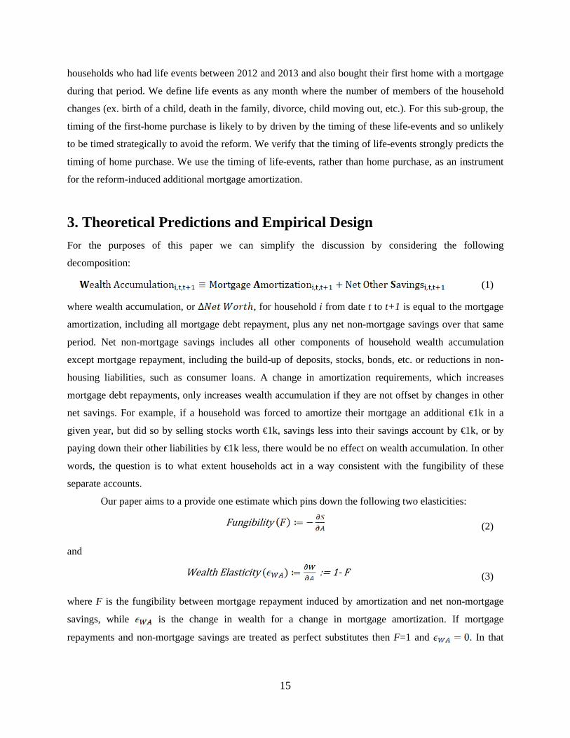
3. Theoretical Predictions and Empirical Design For the purposes of this paper we can simplify the discussion by considering the following

decomposition:

(1) where wealth accumulation, or , for household i from date t to t+1 is equal to the mortgage

amortization, including all mortgage debt repayment, plus any net non-mortgage savings over that same

period. Net non-mortgage savings includes all other components of household wealth accumulation

except mortgage repayment, including the build-up of deposits, stocks, bonds, etc. or reductions in non-

housing liabilities, such as consumer loans. A change in amortization requirements, which increases

mortgage debt repayments, only increases wealth accumulation if they are not offset by changes in other

net savings. For example, if a household was forced to amortize their mortgage an additional €1k in a

given year, but did so by selling stocks worth €1k, savings less into their savings account by €1k, or by

paying down their other liabilities by €1k less, there would be no effect on wealth accumulation. In other

words, the question is to what extent households act in a way consistent with the fungibility of these

separate accounts.

Our paper aims to a provide one estimate which pins down the following two elasticities:

(2)

and

(3)

where F is the fungibility between mortgage repayment induced by amortization and net non-mortgage

savings, while is the change in wealth for a change in mortgage amortization. If mortgage

repayments and non-mortgage savings are treated as perfect substitutes then F=1 and . In that

Fungibility

Wealth Elasticity := 1- F

16

case, any changes in mortgage repayments are offset by changes in non-mortgage wealth, leading to no

change in wealth accumulation. On the other hand, if F=0 then households do not alter their behavior in

their other accounts which means increased debt repayments speed up wealth accumulation.

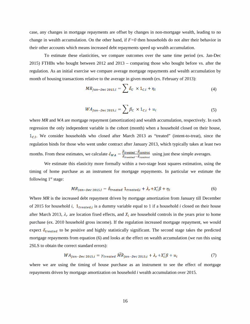
To estimate these elasticities, we compare outcomes over the same time period (ex. Jan-Dec

2015) FTHBs who bought between 2012 and 2013 – comparing those who bought before vs. after the

regulation. As an initial exercise we compare average mortgage repayments and wealth accumulation by

month of housing transactions relative to the average in given month (ex. February of 2013):

(4)

(5) where MR and WA are mortgage repayment (amortization) and wealth accumulation, respectively. In each

regression the only independent variable is the cohort (month) when a household closed on their house,

. We consider households who closed after March 2013 as “treated” (intent-to-treat), since the

regulation binds for those who went under contract after January 2013, which typically takes at least two

months. From these estimates, we calculate using just these simple averages.

We estimate this elasticity more formally within a two-stage least squares estimation, using the

timing of home purchase as an instrument for mortgage repayments. In particular we estimate the

following 1st stage:

(6) Where MR is the increased debt repayment driven by mortgage amortization from January till December

of 2015 for household i, is a dummy variable equal to 1 if a household i closed on their house

after March 2013, are location fixed effects, and are household controls in the years prior to home

purchase (ex. 2010 household gross income). If the regulation increased mortgage repayment, we would

expect to be positive and highly statistically significant. The second stage takes the predicted

mortgage repayments from equation (6) and looks at the effect on wealth accumulation (we run this using

2SLS to obtain the correct standard errors):

(7) where we are using the timing of house purchase as an instrument to see the effect of mortgage

repayments driven by mortgage amortization on household i wealth accumulation over 2015.

17

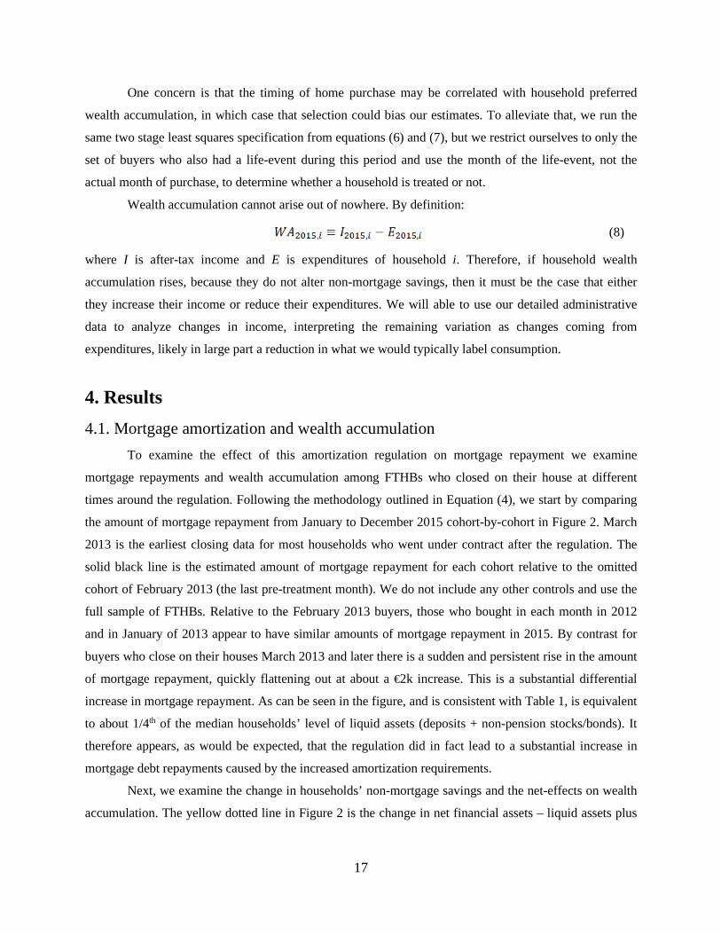
One concern is that the timing of home purchase may be correlated with household preferred

wealth accumulation, in which case that selection could bias our estimates. To alleviate that, we run the

same two stage least squares specification from equations (6) and (7), but we restrict ourselves to only the

set of buyers who also had a life-event during this period and use the month of the life-event, not the

actual month of purchase, to determine whether a household is treated or not.

Wealth accumulation cannot arise out of nowhere. By definition:

(8) where I is after-tax income and E is expenditures of household i. Therefore, if household wealth

accumulation rises, because they do not alter non-mortgage savings, then it must be the case that either

they increase their income or reduce their expenditures. We will able to use our detailed administrative

data to analyze changes in income, interpreting the remaining variation as changes coming from

expenditures, likely in large part a reduction in what we would typically label consumption.

4. Results 4.1. Mortgage amortization and wealth accumulation To examine the effect of this amortization regulation on mortgage repayment we examine

mortgage repayments and wealth accumulation among FTHBs who closed on their house at different

times around the regulation. Following the methodology outlined in Equation (4), we start by comparing

the amount of mortgage repayment from January to December 2015 cohort-by-cohort in Figure 2. March

2013 is the earliest closing data for most households who went under contract after the regulation. The

solid black line is the estimated amount of mortgage repayment for each cohort relative to the omitted

cohort of February 2013 (the last pre-treatment month). We do not include any other controls and use the

full sample of FTHBs. Relative to the February 2013 buyers, those who bought in each month in 2012

and in January of 2013 appear to have similar amounts of mortgage repayment in 2015. By contrast for

buyers who close on their houses March 2013 and later there is a sudden and persistent rise in the amount

of mortgage repayment, quickly flattening out at about a €2k increase. This is a substantial differential

increase in mortgage repayment. As can be seen in the figure, and is consistent with Table 1, is equivalent

to about 1/4th of the median households’ level of liquid assets (deposits + non-pension stocks/bonds). It

therefore appears, as would be expected, that the regulation did in fact lead to a substantial increase in

mortgage debt repayments caused by the increased amortization requirements.

Next, we examine the change in households’ non-mortgage savings and the net-effects on wealth

accumulation. The yellow dotted line in Figure 2 is the change in net financial assets – liquid assets plus

18

voluntary pension contributions minus non-mortgage liabilities – over 2015 for these same buyers, again

relative to the omitted February 2013 cohort. Again, we find little systematic differences in net financial

savings by cohort in the months leading up to the regulation, but in contrast to the change in mortgage

repayment, we find little evidence of a change for the households who bought after the regulation.

Households do not appear to act as if these accounts are fungible (𝐹𝐹~0), since they do not compensate for

the increased regular debt repayments by reducing wealth accumulation in their other accounts. The net

results, as can be seen with the dashed gray line in Figure 2, is a near 1-for-1 increase in wealth

accumulation with increased mortgage repayment driven by the amortization changes.

In Table 2 we formalize this analysis following the two-stage least squares procedure outlined in

Equations (6) and (7). This table includes the subset of ~42k FTHBs who bought near the regulation after

October 2012 and before September 2013, but not during the months when households experienced only

partial treatment (March and April 2013). In Column 1 we show that being part of a cohort that almost

surely bought after the regulation is associated with a ~€2k higher mortgage debt repayment in 2015. This

is our first stage estimate. In Column 2 we find a nearly identical effect on wealth accumulation, so it is

not surprising that in Column 3 we find an estimate of the mortgage amortization-wealth accumulation

elasticity, , of 0.993, which is statistically different from 0, but not from 1 (the 95% confidence

interval is between 0.88 and 1.10). In Column 4 we find no statistically significant effect on net financial

savings for these same households over 2015. In appendix Figures A5 and A6, we separate this effect into

changes in financial assets (A5) and non-mortgage liabilities (A6) – neither display an offsetting effect.19

In Table 3 we examine exactly how households adjust to the increased mortgage repayment. We

use the framework of the income/consumption/savings identity from Equation (8). In Column 1, we show

that within a given household, gross income rises by about ~€1,270k from 2012 to 2015 for those who

bought after, relative to before the regulation. This is about 62% of the increase in mortgage amortization

and wealth accumulation in Table 2, Columns 1 and 2. In appendix Tables A5 and A6 we use detailed

information on hours worked to show that these changes in household gross labor income come from

19 In appendix Table A1, we show that these results are robust to including an alternative measure of voluntary pension contributions that includes all imputed values (Column 1), including the appraised value of real estate in our measure of wealth (Column 2), including both (Column 3), running the analysis over the sum of all mortgage repayment and wealth accumulation for 2014 and 2015 (Column 4), or running a levels-on-levels regression of the households’ home equity value on net worth (total assets – liabilities) as of the end of 2015. Findings are also robust to using an alternative sample (Table A2), that includes even unusually large wealth (Column 1) or mortgage (Column 2) changes, or every single household in our sample that buys a home, including those with large changes in wealth/mortgage balances and those who are not buying a house for the first time (Column 3). Findings are equally robust to varying the amortization and interest rate assumptions for unobserved linked mortgage accounts (Table A3) or the choice of method to compute standard errors (Table A4).

19

changes in hours worked by the household.20 In appendix Table A5, we show an increase in the number

of wage earners in the household, both overall (Column 1) and for those households with at least two

working age members (Column 2). This results in a reduction in the probability a household has only a

single earner from around 27% of households to only around 25% (Column 3) and also holds

conditioning on households that experience a change in single earner status (Column 4). Consistent with

these results, in Table A6 Columns 3 and 4 we find increases in total household hours worked from 2012

to 2015. In fact, in Column 5 we show that controlling for changes in hours worked, the effect of the

reform on income growth falls dramatically in magnitude and is no longer statistically significant. This

suggests that virtually all of the future rise in household gross income for those buying after the

regulation, relative to before, comes via increased hours worked, consistent with an increase in a labor

supply.

In Column 2 of Table 3, we formally run the two-stage least squares estimate to look at effects on

household gross income without any controls. We get an estimate of 0.621. Since marginal tax rates are

about 42% in the Netherlands for our group of buyers, this would suggest that approximately 0.621 x (1-

42%) ~ 36% of the increase in wealth accumulation can be paid for by an increase in after-tax household

income, with the 95% confidence interval between 22 and 51%. We obtain similar estimates in Column 3

after controlling for household financial circumstances well before the regulation, in particular the log of

gross household income and financial assets in 2011, and location fixed effects. In Columns 4 and 5, we

show that the increase in income is caused by an increase in income in 2015, not a decrease right before

the regulation in 2012. Consistent with these results, in Column 6 we show that our initial findings for the

elasticity on wealth are unchanged including those same set of pre-regulation and location controls. The

estimate in Column 5 suggests that around 26% of the increase in debt repayment was paid for by a rise in

after-tax household income. Taken together, our point estimates suggest that household compensated

around 1/4 - 1/3 of the rise in mortgage amortization and wealth accumulation by increasing after-tax

household income. By omission, the remainder must be driven by reductions in household expenditures.

4.2. Addressing selection concerns Our findings are consistent with a large response of wealth accumulation to mortgage amortization.

However, since the timing of home purchases is not randomly assigned it is possible that our estimates

are confounded by selection concerns. If households who mostly want to save less are able to

20 Information on hours worked by employees are mandated to be reported monthly by employers to the Ministry of Social Affairs in order to track required social benefits (ex. UI insurance, et al.) and are linked into the primary data sources via unique person-level identifiers by CBS. We validate in columns 1 and 2 of appendix Table AVI that in levels and changes hours worked are highly correlated with household income.

20

systematically buy before the reform, leaving only those that do not mind saving more to buy after, then

this would bias our estimates upwards. In appendix Figure A7, we examine the number of home purchase

closings per month for our group of buyers and do not find any evidence consistent with bunching around

the regulation.21

That being said, it is theoretically possible (though not ex-ante obvious) that sorting could shift

transactions across time, without any variation in the total level of transactions, in a way that causes

systematic bias in our estimates. Evidence presented in appendix Figure A8 suggests such concerns are

unlikely to be a major factor in this setting. We conduct the same analysis, based on the purchase cohort

month, carried out previously, but break-out our analysis into FTHBs and all other homebuyers around

the 2013 regulation. FTHBs are treated more than all other homebuyers (Panel A), so if there is selection

around the regulation cut-off, that keeps the total number of buyers smooth, but systematically sorted, we

would expect to see a sudden non-linear change in FTHBs confounding co-variates right around the

regulatory change, matching Panel A. We would also expect to see a similar non-linear movement but

likely smaller change in these variables for non-FTHBs, since they are treated, but not quite as much.

Across all variables though, whether it is house value (Panel B) or pre-regulation financial assets (Panel

E), gross household income (Panel F), financial asset accumulation (Panel G), or income growth (Panel

H) we see no evidence of sharp non-linear changes in the co-variates of FTHBs, non-FTHBs, and the

differences between them in the cohorts surrounding the regulation.22 We also see no evidence for

changes in financial assets for either group around the reform (Panels C and D). Again, this is consistent

with a large effect of mortgage amortization on wealth accumulation which is pervasive across multiple

buyer types.

While unlikely, it is possible that there was a sudden change in unobservable buyer

characteristics. To alleviate these concerns, we use a novel feature of our setting and data: the occurrence

of life events. These are changes in the number of people in a household, for example caused by the birth

of a child. Households are much more likely to move after such an event. We focus on the subset of our

original sample of FTHBs who experience a life-event during the same period when they purchase their

homes (2012-2013). The high-quality nature of the administrative data in the Netherlands lets us identify

21 The spike in transactions in June of 2012 is driven by concerns about an increase in the transaction tax for new house purchases. This stands in stark contrast to the lack of any spikes or dips around the 2013 regulation, suggesting households do sometimes respond to changes in mortgage regulation, but clearly did not appear to do so for this regulation. 22 In Panel F, there is a slow downward trend in FTHBs that is steeper than for non-FTHBs. However, there is little evidence of a sharp non-linear change around the reform. Moreover, the lack of any difference for non-FTHBs buying before vs. after (and no differential future financial asset accumulation for either group) make it unlikely this is driven by the reform.

21

the exact month such events took place. In Figure 3, we re-estimate the exact same analysis from Figure

2, focusing on this subset of buyers. Because of the reduced sample size we focus on cohorts grouped by

quarter. We plot the effects by the quarter of the life-event, not the actual purchase of their home. In

Figure 3 we show that relative to the omitted cohorts - Q4 of 2012 and Q1 of 2013 – mortgage

amortization over 2015 is similar for 2012 cohorts (gray points). For 2013 cohorts we find substantially

higher mortgage repayments. Similar to Figure 2, increases in mortgage amortization are matched nearly

one-for-one with increases in in wealth accumulation over 2015.

We rerun this analysis formally in Table 4 using the two-stage least squares methodology

implemented previously, now on the subset of buyers with life-events and using the month of their life-

event, not closing of home purchase, as instrument. In Columns 1-3 we first show no difference in pre-

regulation household income, net financial asset accumulation, or overall wealth accumulation in 2010. In

Columns 4 and 5, we do find significant increases in the amount of mortgage repayment and wealth

accumulation. In Column 6, we show that these differences are not offset by changes in the assessed value

of homes, indicating it is unlikely that these effects are driven by differential home investment or better

timing of purchase.

We find little evidence that the reform changed homeownership rates. In Column 7, we consider

the sample of all households who do not own a home at the end of 2011 (not only those buying one in

2012/2013), and who have life-event between 2012 and 2013. In a linear regression, we predict whether

these households own any real estate by the end of 2016 (which occurs 16.9% of the time) with the

occurrence of a life event. We find little predictive power. We show this even more clearly in Figure A9

where we estimate the regression month-by-month. We see no evidence of any effect around the reform.

As before, in the IV specification in Column 8, we find an estimate of the mortgage amortization-

wealth accumulation elasticity ( ) of 0.864, which is statistically different from 0, but not from 1 (the

95% confidence interval is between 0.54 and 1.19).23 One potential concern is that municipal records for household members are more likely to be

updated when there is a move. In that case we would still be relying on variation that, at least in part,

comes from the timing of the home purchase. To alleviate this concern, we re-run our analysis in Column

9 focusing on the subset of households who have a life-event month that differs from the month of the

house transfer. We again find an estimate of close to 1 (0.931, with the 95% confidence interval

between 0.41 and 1.45).

23 We show in Table A1 column 6 that we also obtain consistent results running the analysis in levels of home equity on net worth as of the end of 2016 (instead of in changes) and including the appraised value of the home.

22

To sum up: we find little evidence for bunching of transactions before the regulation, suggesting

that selection is not a first order concern. This is confirmed by an analysis where we use life-events,

which are unlikely to be selected strategically around the regulation, as a different source of variation. We

obtain very similar estimates with close to 1. This suggests that the overall findings are unlikely to

be contaminated by selection effects.

4.3. Addressing confounded treatment concerns Given the analyses in the previous sections, we interpret our findings as a causal effect on those who

bought their house after versus before the reform. Nevertheless, it is still possible that concurrent

treatments confound the results. For example, households who bought later have by definition spent less

time in their new home. Since we compare household behavior over the same period, this might matter.

We make this explicit in Figures 1 and 2 which include the “age” (months since their respective events,

house transfer or life-event) on the horizontal axis, which ranges between 12 and 32 months since we

compare behavior over 2015. The figures suggest that age is not a likely confound in our setting. There

appears to be no effect of age on wealth accumulation for those with house transfers prior to the

regulation, with wealth accumulation for those ages basically flat for each month from 29 till 23 months,

relative to the omitted age of 22 months (which is the February 2013 cohort). There is then a sudden rise,

concurrent with the timing of the regulation, from ages 21 to 20 months, at which point the curve flattens

out again at a higher level, and remains flat from ages 19 to 12 months. We observe a similar pattern

using variation based on life-events in Figure 3. Along similar lines, the results in Figure 2 do not suggest

that our effect is driven by seasonal factors. For age to be a confound, it would need to be the case that the

concurrent treatment takes place in exactly the same month as the reform. Given our discussion of the

general economic environment in Section 1, this seems implausible.

One potential confound might come from differences between groups at year-end that arise from

the date of closing (rather than going under contract) occurring before or after year-end. One such

candidate is the Dutch wealth tax that is levied on mortgage savings as of January 1st. There were no

changes in the wealth tax from 2012 to 2013. However, those households who closed after January 1st

2013 might have had more non-housing savings on that date than those who closed earlier, and therefore

had to pay a higher wealth tax (at 1.2%). It is unlikely that this had effects lasting until 2015.

Nevertheless, in our setting there is a straightforward way but to address this issue and other issues arising

from similar year-end effects. In Table 5 Column 1, we re-estimate our primary specification focusing on

households who closed in 2013, either in January and February or March and April. The reform is based

on the time of going under contract, not the date of closing, with typically takes place at least two months

23

later. Therefore, the former group is unlikely to be affected by the reform, while the latter group is.

Results are virtually the same as before, suggesting that any year-end policies that were based on the date

of the date of closing are unlikely to drive results. This exercise also confirms that age, which is very

similar for the two groups, is not a likely confound.

Another potential confound are other effects from the reform itself. In particular, households who

purchased their homes under the new regulation lose part of the mortgage interest deductibility (MID).

The regulation stipulates that only standard 30-year amortizing mortgages qualify for interest

deductibility. Mortgages with linked savings account and interest-only mortgages are ineligible.

Moreover, these non-conforming mortgages lose access to the national mortgage insurance. That means

that households purchasing after the regulation can expect larger tax payments, all else equal, since faster

repayment reduces the euro MID amount, especially later in the life of the mortgage. This would affect

both the liquidity and life-time wealth of home buyers.

There are several reasons why these effects might be small in our setting. Given the convex

amortization scheme of annuity mortgages, the liquidity effect will be small in the first few years of the

mortgage, amounting to substantially less than the €2000 baseline effect we find. The life-time wealth

effect is potentially larger. However, because most of the differences in tax deductibility accrue later in

the mortgage this depends on homeowners’ expectations of what would happen with the MID in the

future. Prospects were highly uncertain. The Raad van State, the Dutch Council of State, was highly

concerned about the reform leading to an unequal treatment of FTHBs and non-FHTBs that was hard to

justify.24 This might have raised expectations that existing homebuyers would lose part of the MID as

well. Moreover, the regulation was the first substantial change in the Dutch MID regime in decades,

suggesting more restrictions were to follow.25 As we discussed previously in appendix Figure A8, we find

no evidence of bunching around the 2013 regulation, but we do around an expected increase in the

transaction tax in June of 2012. This confirms that households did not interpret the 2013 reform as a

wealth shock similar to the June 2012 transaction tax.26

24 Advies Raad van State betreffende wijziging van de Wet inkomstenbelasting 2001 en enige andere wetten in verband met de herziening van de fiscale behandeling van de eigen woning (Wet herziening fiscale behandeling eigen woning), 10 September 2012. 25 In fact, starting in 2014, the maximum marginal tax rate at which people could deduct interest payments was reduced by 0.5% each year until it reached the tax rate of the lowest tax bracket. In October 2017, a new government decided to speed this up to 3% per year. 26 It may also be that the MID had relatively little effect on household decisions to buy a home or not. The existing literature has been somewhat mixed with Jappelli and Pistaferri (2007) finding no effect of the MID on mortgage debt at either the extensive or intensive margin in response to an Italian reform, while Gruber et al. (2019) analyzed a reform in Denmark and found no changes in homeownership decisions, but did find changes for some households in the size of houses purchased.

24

Nevertheless, differences in MIDs are still a concern worth addressing. First, we consider

liquidity. In Table 5 Columns 2 and 3, we show that our estimates of are similar if we estimate it for

2014 or 2016 (rather than 2015). If liquidity effects from tax differences were important, we would expect

to see substantial differences between those years. Also, in 2014, tax differences should have been minor

since an annuity mortgage hardly amortizes anything in the first few months after origination.

Nevertheless, we still find an effect not different from an elasticity of 1. Second, we explore life-time

wealth effects. According to the life-time income hypothesis, the effects on consumption and savings

from a one-time change in expected wealth are smoothed across the life cycle. That means that

households purchasing after the reform would be expected to permanently increase their savings (reduce

their borrowings) in anticipation of lower tax deductibility in the future. To address that concern we take

advantage of the convexity of the amortization schedule of annuity mortgages. Each month, the

amortization amount increases. In other words, our treatment grows over the life of the mortgage. This

allows us to compute the increase in the mortgage debt repayment within a given household over 2014 vs.

2016, letting us use the increased amortization amount over time as our endogenous variable of interest

instead of the average increase in debt repayment. Again, in Column 4 we find an elasticity of about 1.

This suggests that it is unlikely our effects are confounded by one-time wealth shocks occurring at the

time of going under contract. Also, we find that findings persist until five years after the reform (Table

A7), and that households do adjust in terms of their labor supply (Table 3). This means our results are

unlikely to be driven by a lack of familiarity with the new rules or slow adjustment.27

4.5. Not just non-savers For the correct interpretation of our findings it is important to pin down what type of households drive our

results. We investigate whether our effect is isolated to non-savers and the young, or whether it holds

more generally.

Households with few liquid assets might be forced to accumulate wealth since there is no easy

way of undoing higher amortization payments. If such households represented the majority of cases in our

sample, our results would certainly still be important, but less generally applicable. As we discuss in

27 In appendix Figure A10 we also compare non-FTHBs with different previous residence housing spell lengths (average of 16 years). In particular, we compare buyers who lived in their prior residence for more versus less than 10 years. Given how much longer the second group lived in their prior residence, it seems likely they would have shorter maturities remaining on their mortgage and therefore less to gain or lose from any potential perceived future loss of the MID. Despite this, even though they face similar short-run changes in mortgage debt repayment (Panel A), they show no differences in house size purchased (Panel B), or non-mortgage wealth accumulation (Panels C and D). This again suggests expected far in the future wealth benefits of the MID are unlikely to be biasing our estimated elasticity in a meaningful way.

25

Section 2.2, most households in our sample have more than enough liquid assets to pay for the increased

mortgage amortization using just the money in their checking or savings accounts. In Table 6 we show

that our results are consistent for households that do not appear to be financially constrained. In Columns

1 and 2 we consider households with loan-to-value ratios at the end of 2014 of less than 90% and loan-to-

income ratios below 4. In both cases, households are putting down significantly more funds than they

need to at the time of initial home purchase, which makes it appear less likely that they are liquidity

constrained.28 In Column 3 limit ourselves to the subset of households who either have at least €10k in

liquid assets at the end of 2015 or save at least €3k in that year. Both groups would be capable of paying

for the increased mortgage repayment out of their liquid assets, suggesting they are unlikely to be up

against their financial constraints. Results are unchanged. It is possible that high liquid assets signal a

high need for precautionary savings (or a high demand for some sort of indivisible consumption). In that

case, this group would still be unwilling to reduce its liquid assets in response to increased mortgage debt

repayments. We address this concern in Columns 4-6. We show that a household’s liquid assets are

highly persistent and use their lagged liquid assets as the source of variation. In particular, we require that

all households have a minimum of €10k in liquid assets at the end of 2011. This group has on average

€43k more than other households at the end of 2011 (Column 4) and €26k more by the end of 2015

(Column 5). In Column 6, we find that our elasticity is unchanged for this subgroup. It is still possible

these households have a large need for liquid assets, which they are unwilling to reduce in response to

increased mortgage debt repayments. Nevertheless, the results in Table 6 do suggest our elasticity

estimates are likely to apply to a broad set of households, not just those with no or low liquid savings.

4.6. Persistence So far, we have shown that increases persistently after the regulation, even in the face of substantial

additional amortization. In appendix Table A7, we examine this further. In Columns 1 and 2, we show

that over the four years from December 2013 to December 2017, FTHBs buying after the regulation have

accumulated more than €8k in additional home equity through increased amortization, without an

offsetting reduction in net financial assets. In Column 3, we compute the ratio of mortgage repayment

over those four years divided by the level of all liquid assets at the end of 2017.29 We find that the

increase in wealth due to increased amortization is on average larger than the stock of liquid assets. This

28 This also provides additional evidence that our effects are unlikely to be confounded by concurrent mortgage policy changes that affected maximum LTV and LTI ratios, since these groups should be largely unaffected by such constraints. 29 We exclude households with less than €100 and a ratio greater than 2 to makes sure that outliers do not drive the effects. If anything, this reduces the size and significance of the effect.

26

implies a high degree of persistence. 30 It also indicates that households do not undo the effects of

increased amortization over the length of a typical business cycle.31 Our paper therefore makes an

important contribution establishing substantial effects of amortization on household wealth, with

important implications for debt repayment-savings fungibility, macroprudential policies, and the life-

cycle dynamics of household savings, consumption, and labor supply decisions.

Though not the primary focus of this paper, it is still interesting to consider longer run effects. Do

affected households access the extra funds prior to or upon retirement, or do they pass it on as bequests to

the next generation? Since the regulation only occurred a few years ago, we are of course unable to track

the lifetime of wealth accumulation by these households, let alone those of the next generation. Therefore,

any discussion of these long-run effects will by their very nature be less precise than the primary focus of

the paper, but not without merit.

First, we explore whether effects change as households approach retirement. In Table 7 we show

that our results appear to be pervasive across age groups. In Columns 1-4 we re-run our primary analysis

but focus on households where the maximum age in a household is above 30, 40, and 50 respectively. In

all cases we find elasticities in line with our baseline estimates. In the Netherlands, there are few multi-

generation households so it is unlikely we misclassify households. Nevertheless, in Column 4 we try to

alleviate such concerns by re-running the analysis of Column 3 on households with a maximum age above

50, excluding households with age differences of more than 20 years. Our results are consistent.

Next, we examine whether moving represents an opportunity for households to re-lever, extract

any additional home equity, and in doing some access and perhaps consume the additional wealth. Since

our sample includes FTHBs from 2012 and 2013, there is only a relatively small group that buy and sell

another home during our period. In appendix Table A8, we consider the sub-sample of 1,768 people who

have resold their home by December 2016. By December 2017 those buying after the regulation have

substantially more home equity caused by increased mortgaged repayment (Columns 2 and 3).

Nevertheless, they do not appear to extract more of this home equity when moving (Column 1). This

likely explains why we do not see any additional financial assets for these households (Columns 4 and 5),

nor a significantly different (Column 6).

30 Persistence could be consistent with existing findings of near-zero marginal propensities to consume (MPCs) and alter income via labor supply out of home equity gains (Skinner 1994, 1996; Engelhardt 1996; Poterba et al. 2013; Bernstein 2020; Ganong and Noel 2020) for a wide range of differing borrower leverage, savings, and liquidity (Farrell et al. 2020). Even unusually high MPCs in the U.S. during the financial crisis, imply that the vast majority of net housing wealth changes are retained (Mian et al. 2013). That said, it is important to note that MPCs neither directly imply nor are implied by or its persistence. MPCs estimate how much of additional wealth given is spent, whereas amortization gives no additional wealth and estimates how much wealth is endogenously chosen. 31 Over the past half-century the average NBER dated business cycle was around 5 years.

27

These subsample results line up well with results for Dutch homeowners overall. For all repeat

buyers over 40 who purchase a home in 2012-2013, the median LTV the year after purchase is only 86%

and the 25th percentile is only 59%, well below the median and 25th percentile for FTHBs of 105% and

101% respectively. In other words, it does not appear that households who sell one house and buy another

re-lever to anywhere near the regulatory LTV limits. Results are also consistent with general patterns in

the U.S., where repeat buyers do not appear to re-lever back-up to regulatory limits or those of FTHBs

(Patrabansh 2013; Patrabansh 2015; Bai et al. 2015). Based on the sample of homeowners who sell and

buy a house in the PSID (Panel Survey of Income Dynamics) we find relatively little systematic

“undoing” of home equity accumulation.32 Each $1 of additional home equity at the time of sale is

associated with on average $0.88 of additional home equity at the time of the purchase of the new home.

That would suggest most home equity accumulation is passed through when moving.33 Taken together,

this is suggestive that moving houses may not necessarily be an event that leads to substantial drawing

down of wealth accumulated due to increased mortgage amortization.

Finally, we examine households’ general tendency to repay their mortgages over the life cycle.

We compare the Netherlands, where mortgages pre-2013 had a substantial interest-only component with

the U.S., where most mortgages were fully amortizing. Appendix Figure A11 shows the percentage of

Dutch and U.S. homeowners with relatively few liquid assets (“hand-to-mouth”) that have a mortgage. In

both countries, FTHBs typically finance house purchases with mortgages, as can be seen for individuals

ages 25-30 in Panel B. Nevertheless, older Dutch homeowners are much more likely to still have

mortgages than their U.S. counterparts. In their early-to-mid 60s only about 61% of U.S. homeowners

still have mortgage debt, while this is about 94% for Dutch homeowners. If anything, Dutch FTHBs

purchase a home earlier in life, giving them more time to repay their mortgages. This suggests that Dutch

homeowners with interest-only mortgages do not save in a separate account to repay their mortgage34, and

that American homeowners with amortizing mortgages generally do not undo the amortization through

home equity withdrawals. This is supported by evidence from the PSID. Fully amortizing 30-year

mortgages repay about 3.3% of principal per year (excluding the final year). Among U.S. non-movers in

the PSID, who own a home in concurrent waves and have a mortgage in the prior wave, the average

(median) mortgage balance falls by 4.4% (4.6%). Since waves are one-to-two years apart, this seems

largely consistent with households not undoing amortization between moves. Of course, there are many

32 This is based on families in the 1999 wave and their housing decisions from 1969-2017. 33 A similarly important role for “passive” wealth accumulation is also documented for Norwegian households by Fagereng et al. (2019). 34 In fact, among all Dutch homeowners aged 60-65 with a mortgage, the average amount of accessible financial assets is only about €26k.

28

other differences between the U.S. and the Netherlands apart from different amortization standards, but if

these tendencies hold for those buying around the 2013 reform in the Netherlands, it would be suggestive

of longer run effects on wealth accumulation.

In summary, we provide evidence that mortgage amortization causes substantial increase in

wealth accumulation in the first several years following home purchases. These effects are similar for

those with substantial home equity, across age groups, and for movers suggesting a general applicability

and importance of our findings. That said it seems entirely plausible that households may eventually

access some of this additional amortization-induced wealth, but aggregate statistics among elderly

households are also consistent with a substantial persistence of these effects across the life-cycle.

5. Discussion 5.1. Plausible mechanisms If our finding of an close to 1 is not driven by non-savers and the young, then there must be other

mechanisms that induce households to act as if there is little-to-no fungibility between mortgage

repayments and savings in their other accounts. Here we discuss (rational) liquidity wedges, and a number

of behavioral factors, such as mental accounting, default settings and pre-commitment.

One possible mechanism could be a liquidity wedge. Extracting home equity involves non-trivial

cost and time (Campbell et al. 2019). In addition, if house values fall during economic downturns, then

funds paid into reducing mortgage debt could be inaccessible (DeFusco and Mondragon 2019). This

could be exacerbated if refinancing costs or interest rates would be too high, especially for households

with high loan-to-income ratios. Moreover, states of the world in which a household might want to tap

into its savings (ex. a job loss) might actually be situations when constraints make it costly or impossible

to access home equity. In that case, households might rationally treat mortgage repayment and liquid

assets as not fungible from a short (or medium)-term consumption smoothing standpoint, even if they

have similar effects for long-term wealth accumulation. It is possible that households with more liquid

savings have them because they face higher precautionary savings needs, which is why the elasticities are

high for this group as well.

While a liquidity wedge undoubtedly plays a role in our findings, it is not clear it supported by

the full set of our findings. First, households appear willing to cut consumption substantially today in

order to avoid any increased risk in the need to cut that marginal consumption in the future, even though

they are able and willing to alter labor supply in the present and have chosen their current level of

precautionary savings as a buffer against shocks. Second, as noted earlier we see no evidence of bunching

29

around the regulatory change. If households were this averse to illiquid wealth accumulation, we might

expect them to avoid a policy forcing to engage in exactly that.

Another possibility is that household behaviors may deviate slightly from strictly fully rational

models, overestimating their need for liquidity in the future. D’Acunto et al. (2020) for example, find that

when given access to an overdraft facility even very liquid users act as if they are severely constrained.

This is consistent with the large observed consumption response of individuals to randomized credit line

expansions, even if they have substantial liquidity (Aydin 2019), and to income payments (Olafsson and

Pagel 2017). This could also correspond to boundedly rational agents following the kind of simple saving

heuristic suggested by financial advisers in many countries. In the Netherlands, for example, the National

Institute for Budget Information (NIBUD) introduced an online tool in 2008 to advise people on their

optimal savings. This simple heuristic, mainly depending on the size of the household and income.35

Apart from this perceived or heuristic precautionary savings motive, there is a wider range of

behavior models that could explain our findings. Kovacs and Moran (2019), Attanasio et al. (2020), and

Vihriala (2020) provide theoretical arguments supporting the idea that mortgages could act as a

commitment device for present-biased households with self-control problems. Beshears et al. (2015) find

in an experimental setting that people appear to value commitment devices. Yet Laibson (2015) notes

that, based on the empirical evidence, there are far fewer such devices than one would expect. Our works

suggests that amortizing mortgages might be just such a mechanism. Vihriala (2020) provides evidence

from Finland consistent with households purposefully picking a mortgage contract that commits them to

saving. If this mechanism is at play in our setting though, our findings suggest that the problems with

self-control are specific to longer term wealth accumulation, since we find a similar effects even among

households able to build-up substantial liquidity.

Another plausible mechanism is that households may, for mental accounting reasons, treat

mortgage repayments as bills instead of wealth accumulation. This is consistent with what Camanho and

Fernandes (2018) call the “mortgage illusion”. In an experimental setting they show that households

compare rental payments to mortgage payments when deciding to own or rent and do not account for the

fact that some of the mortgage payment is amortization. In fact, they are less likely to buy a house when

the choices include a shorter duration mortgage, just because the amortizing component of the payments

are higher making the regular monthly payment higher. These findings are also consistent with Argyle et

al. (2019) who document that auto loan borrowers have substantial sensitivity to changes in maturity,

likely reflecting strong sensitivity to monthly payment sizes, even if they are just amortizing payments.

35 https://www.nibud.nl/beroepsmatig/vernieuwde-bufferberekenaar/

30

Just like in our setting these results hold even among unconstrained borrowers, which may suggest that

liquidity constraints by themselves may only offer a partial explanation.

Another possible behavioral mechanism could be that amortization constitutes a “default” setting

to accumulate wealth. A broad literature in multiple countries has shown evidence that default settings

with passive choice, such as automatically signing individuals up for pension contributions unless they

opt out, can have substantial effects on wealth accumulation (Madrian and Shea 2001; Chetty et al. 2014).

These substantial wealth accumulation effects are rarely seen for policies that require active choice (opt-in

policies) such as voluntary debt repayments (Kuchler and Pagel 2019). In our setting, after 2013

amortizing mortgages become the default contract, and with them increased mortgage repayments.

Beshears et al. (2019) explore whether default settings that increase U.S. individual pension contributions

are offset by increased liabilities. They find only limited evidence, suggestive of a potentially low

fungibility between savings and liabilities. Our results support these conclusions using more detailed data

on household balance sheets, including home equity, financial assets, and other liabilities.36

Moreover, our results suggest that this low fungibility is symmetric, which is not clear ex-ante.

Even if default settings for pension contributions don’t alter liabilities, increased amortization

requirements could still alter net non-mortgage savings decisions. As noted by Chetty et al. (2014), the

mechanism by which households are encouraged to wealth accumulate has critical implications for its

effectiveness. As we have noted, there are multiple channels by which amortization might encourage

households to wealth accumulate, with default settings being one. All we can say with more certainty is

that it appears that our evidence is consistent with low fungibility for the effects of mortgage amortization

on net non-mortgage savings, leading to substantial effects on wealth accumulation.

Within this particular design it is hard to disentangle exactly which of these potential drivers are

at work. What we can say is that households do not seem to treat mortgage debt repayments and other

more liquid accounts as substitutes, even among those with large liquid assets and the old, causing

increases in mortgage amortization to substantially raise wealth accumulation.

5.2. External Validity There is no silver-bullet to verify the external validity of our results outside the Netherlands.

Nevertheless, prior work looking at other countries is broadly consistent, suggesting that even if exact

elasticities may vary in other mortgage environments or populations, the finding of a large effect of

mortgage amortization on wealth accumulation is likely to hold. Ganong and Noel (2019) look at

36 Garcia et al. (2020) also do not find any evidence that savings nudges increase high-interest unsecured borrowing in a setting where they observe a higher frequency picture of household balance sheets.

31

mortgage modifications in the U.S. that grant maturity extensions, which reduce mortgage amortization.

This also leads to substantial reductions in consumption. Scholnik (2013), d’Astous (2019), and Andersen

et al. (2019) look at mortgage run-offs using administrative data in the U.S., Canada, and Denmark. They

show increases in consumption and decreases in labor income after people have fully paid off their

mortgage debt. Though supportive (at least qualitatively), these papers differ substantially from our work.

First of all, they do not look at the effects on wealth accumulation. Moreover, mortgage modifications for

distressed households, or mortgage run-offs for older households, may be special events in a lifecycle that

do not directly speak to the general effects of mortgage amortization on wealth accumulation.37

Closest to our work are Larsen et al. (2018) and Backman and Khorunzhina (2020) who analyze

the introduction of interest-only mortgages (IO) in Denmark in 2003. Backman and Khorunzhina (2020)

find that financially constrained households, who are more likely to refinance using IO mortgages, appear

to have higher consumption growth. Larsen et al. (2018) find that those who choose to take out IO

mortgages consumed more afterwards, but did not alter their financial assets. This is consistent with our

findings. However, the selection into IO mortgages in Denmark was likely endogenous. Kuchler (2015)

shows that households who choose to use IO mortgages have ex-ante lower savings rates and higher loan-

to-value ratios. Moreover, the timing of refinancing into an IO mortgage is almost certainly related to

household time-varying conditions.

Findings from a literature on alternative mortgage products (AMPs), such as interest-only loans

and option adjustable-rate mortgages, are also broadly consistent. Amromin et al. (2018) show that when

you control for the fact that people who took out AMPs in the U.S. had higher incomes and credit scores

(Cocco 2013), default rates were twice as high as those for normal mortgages. Though the choice of

mortgage type is endogenous, these results suggest that U.S. households do not use the extra funds

available from option ARMs to increase their non-mortgage savings that they could use to prevent a

costly default. This raises the question whether option ARMs are as attractive in reality as some models

might suggest (Piskorski 2010).

Aggregate statistics on retired households also suggest that our findings holding in other settings.

Households appear to use their home equity as a primary form of savings, with real estate accounting for

over 70% of U.S. households assets (Campbell 2006). Even among retirement age households, real estate

is by far their largest single component of savings, making up 47.9% of all non-annuitized household net

worth, and is more than twice as large as all assets held in personal retirement accounts (PRA) such as

37 Households in sufficient distress to file for mortgage assistance might be especially financial constrained. Households about to pay-off their mortgage appear to increase bank loans and already start to reduce their labor income even in the years prior to the run-off, making it difficult to assign all effects to just the amortization component.

32

individual retirement accounts (IRA) or 401(k) plans (Poterba et al. 2013). Using survey data for the

U.S., Canada, Australia, the U.K., Germany, France, Italy, and Spain, Kaplan et al. (2014) document that

households with substantial illiquid wealth (such as housing) often hold little or no liquid wealth. This is

consistent with households treating home equity and liquid savings differently, although there are of

course other explanations.38

Even though our results are broadly consistent with findings from these other studies, the exact

might differ across periods, settings, and sub-groups. To provide some additional structure to this

discussion we can decompose into the change in debt repayment for a change in amortization

schedule, , times the change in wealth accumulation for a change in debt repayment, :

. First consider . This elasticity will differ according to how easy it is for

households to undo the effects of amortization through home equity withdrawals. In settings where this is

hard, say the Netherlands, will be higher. Next consider . If this elasticity is driven by fairly

universal behavioral factors, such as different mental accounts for home equity and other savings that

(Camanho and Fernandes 2018), then we would expect to be close to 1 in other settings as well. On

the other hand, if is primarily driven by rational liquidity differences between home equity and other

savings, then low-cost access to home equity may lead to lower levels of . Both elasticities might

differ over the life cycle. In our setting, both elasticities appear to be close to 1, but this may be lower in

other settings. This emphasizes the importance of prior and future work examining how debt-savings

fungibility, home equity withdrawals, housing leverage, and refinancing differ across economic

conditions, life-cycles, and regulatory environments (ex. Keys et al. 2016; Bhutta and Keys 2016;

DeFusco 2018; Keys and Wang 2019; Beshears et al. 2019; Amromin et al. 2020; Andersen et al. 2020;

DeFusco et al. 2020).

5.3. Policy Implications Our results, as well as any future work on how effects may differ in other circumstances, have important

implications for macroprudential policies. In the context of the specific policy we study in this paper, the

Dutch government was hoping that amortizing mortgages would improve financial stability. If households

responded to the regulation by transferring liquid assets, such as deposits, into mortgage repayment, with

no change in net-wealth, it is unlikely such a policy would improve financial stability. By contrast, our

38 Households may to prefer to invest in housing as an asset, either because they believe it has a higher risk adjusted return (Kaplan and Violante 2014), or acts as a hedge for local rental rates (Sinai and Souleles 2005). Alternatively, households may prefer to pay down mortgage debt quickly because they are debt averse, and since they have built up substantial wealth in housing, they do not need any other wealth.

33

findings confirm that increased amortization has increased household home equity, with potential benefits

from reduced housing lock (Bernstein and Struyven 2019), without reducing financial assets. In other

words, the regulation worked as intended, with important implications for other countries currently

considering related policies (Svensson 2019; Svensson 2020).39 Unlike our setting, amortization policies

also often bring with them concurrent changes in regulatory DTI limits (e.g. Amromin et al. 2018; Dokko

et al. 2019), which prior work has shown excludes certain borrowers (Backman and van Santen 2020).

Our findings suggest that such exclusions are likely to have substantial causal effects on their wealth

accumulation, highlighting the importance of continued research understanding how regulatory

constraints can alter borrower composition.

Our findings also suggest that proposed macroprudential policies, such as changing amortizing

mortgages into interest-only during recessions (Campbell et al. 2019), are likely to have even larger

effects that might be expected in more standard economic models. In contrast to these models, we find no

substitutability between debt repayment and non-mortgage savings meaning. This suggests that

countercyclical amortization reductions could have consumption and labor responses similar to those seen

for mortgage designs with countercyclical interest rates (ex. Guren et al. 2019), but with very different

costs and wealth implications. In fact, the labor response we document in this paper is quantitatively

similar to what Zator (2019) finds for interest rates changes in Poland, despite completely different shocks

at play.

Our results also have implications for the debate about the benefits of homeownership, with some

arguing that that owning a home is the main way in which households accumulate wealth (Li and Yang

2010). The evidence to support that view is mixed. Homeowners do save more (ex. Belsky & Prakken

2004; Rossi & Sierminksa 2018), but are of course systematically different across observables and likely

unobservable dimensions as well. By contrast, Sodini et al. (2017) show that plausibly exogenous

variation in homeownership in Sweden had little effect on wealth accumulation. Barrot et al. (2019) show

that households tend to extract and “spend” substantive house price appreciation via changes in

expenditures and income40. Sodini et al. (2017) study condos, for which mortgages in the period under

study were close to interest-only, with an average expected repayment period of 186 years in 2007

(Hullgren and Soderberg 2016, Swedish Financial Supervisory Authority Report 2008). Taking their and

our results together suggest that a critical mechanism for homeownership to lead to wealth accumulation

39 This has of course come at the cost of reduced consumption and increased household labor supply. Without further analysis, which is outside the scope of this paper, we cannot make any welfare statements. 40 By contrast Leth-Petersen (2010) find relatively little effect of allowance of home equity withdrawals for consumption purposes when they were first allowed in Denmark among households with relatively little house price appreciation. Brown et al. (2015) and Kovacs and Moran (2019) find some more evidence in the U.S. setting, but do not clearly separate out the effects of house price appreciation from mortgage repayment due to amortization.

34

may be the coupling with amortizing mortgages.41 This would also be broadly consistent with the

aforementioned observed aggregate statistics, with households at retirement having substantial illiquid

wealth in the form of housing and few liquid financial assets. On the flip-side, different access to

homeownership either overall or for specific groups could help to explain historical differences in wealth

accumulation (Charles and Hurst 2002; Krivo and Kaufman 2004; Stein and Yannelis 2020).

Finally, our results have potential implications for optimal design of retirement programs and the

types of mechanisms likely to lead them to achieve their goals. Beshears et al. (2019) argue that the social

optimal mandatory contribution plan with tastes shocks and present bias is one with three accounts

including one liquid account, one illiquid account, and one with costly early liquidation. To the extent

these assumptions hold, homeownership with mortgage amortization is an account with costly liquidation

that might be a critical component of the optimal policy to stimulate long-run household wealth

accumulation. In the context of pensions, Choukhmane (2019) shows that default autoenrollments, which

appear to substantially raise short-run contributions (ex. Madrian and Shea 2001), may be at least partially

offset by lower contributions later on. While pension contributions, at least in the U.S., might be

relatively easy to undo, this is not the case for additional amortization. Building up additional home

equity does not preclude the need to still make amortizing principal repayments in subsequent periods. At

any point, accessing that additional home equity via home equity withdrawals requires substantial implicit

and explicit costs. They also typically require debt-to-income and loan-to-value requirements which may

not be met for unemployed or retired households, or during periods of severe macroeconomic distress.

This illiquidity may be costly, but may also be a potential benefit discussed that has been discussed in the

context of personal retirement accounts (PRAs), since it can increase long-run wealth accumulation (ex.

Beshears et al. 2015b; Beshears et al. 2019b).42

6. Conclusion In this paper we provide the first empirical evidence on the effects of mortgage amortization on wealth

accumulation by examining a 2013 amortization regulation in the Netherlands for first-time home buyers.

Using detailed individual-level administrative data and variation in the timing of purchases by first-time

home buyers surrounding the regulation, we find that even five years later there is no observable change

41 This is not to say that systematic variation in housing asset performance among subgroups could not drive some degree of wealth differences between those groups, and potentially even wealth accumulation depending on long-run labor and consumption responses (ex. Goldsmith-Pinkham and Shue 2020). 42 Perhaps not surprisingly, in the absence of inciting events PRA leakage is relatively limited, but can be substantial during relevant events, such as job transition and old age, especially approaching and after retirement (Huurd and Panis 2006; Poterba et al. 2013; Argento et al. 2014; Wang et al. 2019).

35

in non-housing savings, leading to a near 1-for-1 rise in net worth with the rise in mortgage debt

repayments. The effects occur suddenly, and only for cohorts who are exposed to the regulation. We find

no evidence of bunching and results are unchanged using the timing of life-events (ex. birth of a child) as

an instrument for buying before vs. after the regulation. The rise in wealth accumulation is achieved

through an increase in labor supply and reduction in expenditures among the group of buyers exposed to

the regulation. Our findings hold looking at households with substantial liquid assets, suggesting results

are not caused by just non-savers, and across a broad range of ages, suggesting a general applicability of

our estimated elasticity. Our results can either be consistent with a relatively atypical rational model of

household liquidity preferences, or behavioral models that have been shown to help drive wealth

accumulation in other settings (such as pension contributions), including commitment devices, mental

accounting, and default settings.

Regardless of the underlying mechanism, the finding of a substantial effect of mortgage

amortization and debt repayment on wealth accumulation has important economic implications. Our

estimated elasticity suggests that ex-ante macroprudential polices aimed at building up household home

equity through amortization may not significantly reduce household liquidity. Ex-post macroprudential

policies that reduce principal repayments during recessions are also likely to have larger effects than

might be expected in more standard models of the household. More broadly, our results suggest that

homeownership can be a critical driver of household wealth accumulation when coupled with an

amortizing mortgage. Therefore, variation in homeownership and amortization rates across time and

groups, are likely important factors drivers of differential wealth accumulation. For many households, the

home is the single largest asset they have available in retirement. It may not be surprising then that our

findings suggest that mortgage design may play a key role in our understanding of the life-cycle of

household wealth accumulation.

36

References Aaronson, D., Hartley, D., and Mazumder, B. 2017. The Effects of the 1930s HOLC “Redlining” Maps.

Federal Reserve of Chicago Working Paper.

Adelino, Manuel, Felipe Severino, and Antoinette Schoar. 2016. Loan Originations and Defaults in the Mortgage Crisis: The Role of the Middle Class. The Review of Financial Studies, 29(7): 1635-1670.

Amromin, Gene, Neil Bhutta, and Benjamin Keys. 2020. Refinancing, Monetary Policy, and the Credit Cycle. Annual Review of Financial Economics.

Amromin, Gene, Jennifer Huang, Clemens Sialm, and Edward Zhong. 2018. Complex Mortgages. Review of Finance. 22.6:1987-2007.

Anders, John. 2018. The Long Run Effects of De Jure Discrimination in the Credit Market: How Redlining Increased Crime. Working Paper.

Andersen, Steffen, Philippe d’Astous, Jimmy Martinez-Correa, and Stephen H. Shore. 2019. Responses to Saving Commitments: Evidence from Mortgage Run-offs. Working Paper.

Andersen S, Campbell JY, Nielsen KM, Ramadorai T. 2020. Sources of Inaction in Household Finance: Evidence from the Danish Mortgage Market”. Forthcoming. American Economic Review.

Appel, Ian and Jordan Nickerson. 2016. Pockets of Poverty: The Long-Term Effects of Redlining. Working Paper.

Argento, Robert, Victoria L. Bryant, and John Sabelhaus. 2014. Early Withdrawals from Retirement Accounts during the Great Recession. Contemporary Economic Policy. 33(1):1-16.

Argyle, Bronson, Christopher Palmer, and Taylor Nadauld. 2019. Monthly Payment Targeting and the Demand for Maturity. Review of Financial Studies. Forthcoming.

Attanasio, O. P , Agnes Kovacs, and Patrick Moran. 2020. Temptation and Commitment: Understanding the Demand for Illiquidity. NBER Working Paper 2794.

Aydin, Deniz. 2019. Consumption Response to Credit Expansions: Evidence from Experimental Assignment of 45,307 Credit Lines. Working Paper.

Backman, Claes, and Chandler Lutz, 2020. The impact of interest-only loans on affordability. Regional Science and Urban Economics 80 (1).

Backman, Claes and Khorunzhina, Natalia. 2020. Interest-Only Mortgages and Consumption Growth: Evidence from a Mortgage Market Reform. Working Paper.

Backman, Claes and Peter van Santen. 2020. The Amortization Elasticity of Mortgage Demand. Working Paper.

Bai, Bing, Jun Zhu, and Laurie Goodman. 2015. A Closer Look at the Data on First-Time Homebuyers. 2015. Housing Finance Policy Center Brief.

Barlevy, Gadi and Jonas D.M. Fisher. 2018. Mortgages choices during the U.S. housing boom. Federal Reserve of Chicago Working Paper.

Baker, Scott, Lorenz Kung, Michaela Pagel, and Steffen Meyer. 2019. Measurement Error in Imputed Consumption Data. Working Paper.

Barrot, Jean-Noel, Erik Loualiche, Matthew Plosser, and Julien Sauvagnat. 2019. Import Competition and Household Debt. Working Paper.

37

Bernstein, Asaf. 2020. Negative Home Equity and Household Labor Supply. Journal of Finance. forthcoming.

Beshears, J., Choi, J. J., Harris, C., Laibson, D., & Madrian, B. C. 2013. Simplification and saving. Journal of Economic Behavior and Organization. 95: 130-145.

Beshears, J., Choi, J. J., Harris, C., Laibson, D., Madrian, B. C., & Sakong, J. 2015. Self Control and Commitment: Can Decreasing the Liquidity of a Savings Account Increase Deposits?. National Bureau of Economic Research Working Paper 21474.

Beshears, John, James J. Choi, Joshua Hurwitz, David Laibson, and Brigitte C. Madrian. 2015. Liquidity in Retirement Savings Systems: An International Comparison. American Economic Review: Papers and Proceedings 105, no. 5 (May 2015): 420–425.

Beshears, J., Choi, J. J., Laibson, D., Madrian, B. C., & Skimmyhorn, W. 2019. Borrowing to Save? The Impact of Automatic Enrollment on Debt. National Bureau of Economic Research Working Paper 25876.

Beshears, John, James Choi, Christopher Clayton, Christopher Harris, David Laibson, and Brigitte Madrian. 2019. Optimal illiquidity. Working paper. 2019

Bhutta, Neil and Benjamin Keys. 2016. Interest Rates and Equity Extraction During the Housing Boom. 2016. American Economic Review. 106(7): 1742-1772.

Brown, Meta, Sarah Stein, and Basit Zafar. 2015. The Impact of Housing Markets on Consumer Debt: Credit Report Evidence from 1999 to 2012. Journal of Money Credit and Banking 175-213.

Brueckner, Jan K, Calem, Paul S, and Nakamura, Leonard I. 2016. House Price Expectations, Alternative Mortgage Products, and Default. Journal of Money, Credit and Banking, 48(1), 81–112

Camanho, Nelson and Daniel Fernandes. 2018. The Mortgage Illusion. Working Paper.

Campbell, John, Nuno Clara, and Joao Cocco. 2019. Structuring Mortgages for Macroeconomic Stability. Working paper.

Carroll, Christopher D., 1997. Buffer-stock saving and the life-cycle/permanent income hypothesis, Quarterly Journal of Economics 114, 433–495.

Chetty, R., J. N. Friedman, S. Leth-Petersen, T. H. Nielsen, and T. Olsen. 2014. Active Vs. Passive Decisions and Crowd-Out in Retirement Savings Accounts: Evidence from Denmark. The Quarterly Journal of Economics 129 (3) (May 9): 1141–1219.

Chiang, Y.-M., Sa-Aadu, J., 2014. Optimal mortgage contract choice decision in the presence of pay option adjustable rate mortgage and the balloon mortgage. Journal of Real Estate Finance and Economics 48, 709–753.

Charles, Kerwin and Erik Hurst. 2002. The Transition to Home Ownership and the Black-White Wealth Gap, Review of Economics and Statistics 84(2), 281-297.

Choukhmane, Taha. 2019. Default Options and Retirement Savings Dynamics. Working Paper.

Cookson, J. Anthony, Erik Gilje, and Rawley Heimer. 2019. Shale Shocked: The Long Run Effect of Wealth on Household Debt. Working Paper.

Cocco, Joao F., 2013. Evidence on the benefits of alternative mortgage products. Journal of Finance 68 (4), 1663–1690.

Cox, R., Brounen, D., Neuteboom, P., 2015. Financial literacy, risk aversion and choice of mortgage type by households. Journal of Real Estate Finance and Economics 50, 74–112

38

d’Astous, Philippe. 2019. Responses to an Anticipated Increase in Cash-on-Hand: Evidence from Term Loan Repayments, Journal of Banking and Finance, 108.

DeFusco, Anthony. 2018. Homeowner Borrowing and Housing Collateral: New Evidence from Expiring Price Controls. 2018. The Journal of Finance, 73(20): 523-573.

DeFusco, Anthony and John Mondragon. 2019. No Job, No Money, No Refi: Frictions to Refinancing in a Recession. Forthcoming at Journal of Finance.

DeFusco, Anthony, Stephanie Johnson, and John Mondragon. 2020. Regulating Household Leverage, Review of Economic Studies 87(2), 914-958.

Di Maggio, Marco, Kermani, Amir, Keys, Benjamin J, Piskorski, Tomasz, Ramcharan, Rodney, Seru, Amit, and Yao, Vincent. 2017. Interest rate pass-through: Mortgage rates, household consumption, and voluntary deleveraging. American Economic Review, 107(11), 3550–88.

Dokko, Jane, Benjamin Keys, and Lindsay Relihan. 2019. Affordability, Financial Innovation, and the Start of the Housing Boom. Working Paper.

Dutch Banking Association (NVB). 2014. The Dutch Mortgage Market.

Engelhardt, G. V. 1996. House Prices and Home Owner Saving Behavior. Regional Science and Urban Economics, 26, 313-336.

Fagereng, Adreas, Martin Blomhoff Holm, Benjamin Moll, and Gisle Natvik. 2019. Saving Behavior Across the Wealth Distribution: The Importance of Capital Gains. NBER Working Paper 26588.

Farrell, Diana, Fiona Greig, and Chen Zhao. 2020. The Housing Wealth Effect in the Post-Great Recession Period: Evidence from Big Data. Working Paper.

Friedman, Milton. 1957. A Theory of the Consumption Function. Princeton University Press (Princeton, NJ).

Ganong, Peter and Pascal Noel. 2020. Liquidity vs. Wealth in Household Debt Obligations: Evidence from Housing Policy in the Great Recession. Forthcoming American Economic Review.

Garcia, Isidoro, Paolina Median, and Michaela Pagel. 2020. Does Saving Cause Borrowing? Working Paper.

Gathergood, J., Weber, J., 2017. Financial literacy, present bias and alternative mortgage products. Journal of Banking & Finance 78, 58–83.

Goldsmith-Pinkham, Paul and Kelly Shue. 2020. The Gender Gap in Housing Returns. Working Paper.

Gruber, Jonathan, Jensen, Amalie, Kleven, Henrik, 2019. Do People Respond to the Mortgage Interest Deduction? Quasi-Experimental Evidence from Denmark. Forthcoming. American Economic Journal: Economic Policy.

Guren, Adam, Arvind Krishnamurthy, and Timothy McQuade. 2019. Mortgage Design in an Equilibrium Model of the Housing Market. Forthcoming at The Journal of Finance.

Hertzberg, Andrew, Andres Liberman, and Daniel Paravisini. 2018. Screening on Loan Terms: Evidence from Maturity Choice in Consumer Credit. Review of Financial Studies, 31: 3532-3567.

Hershfield, Hal, Stephen Shu, and Shlomo Benartzi. 2019. Temporal Reframing and Participation in a Savings Program: A Field Experiment. Working Paper.

Hundtofte, Sean, Arna Olafsson, and Michaela Pagel. 2018. Credit Smoothing. Working Paper.

39

Hurd, Michael and Constantijn Panis. 2006. The Choice to Cash Out Pension Rights at Job Change or Retirement. Journal of Public Economics 90 (12):2213-2227.

Jappelli, Tullio and Luigi Pistaferri. 2007. Do People Respond to Tax Incentives? An Analysis of the Italian Reform to the Deductibility of Home Mortgage Interests. European Economic Review, 51, 247–271.

Keys, Benjamin, Devin G. Pope, and Jaren C. Pope. 2016. Failure to Refinance. Journal of Financial Economics. 122 (3): 482-499.

Keys, Benjamin and Jialan Wang. 2019. Minimum Payments and Debt Paydown in Consumer Credit Cards. Journal of Financial Economics. 131 (3): 528-548.

Kovacs, Agnes and Patrick Moran. 2020. Breaking the commitment device: The effect of home equity withdrawal on consumption, saving, and welfare. Working paper.

Krimmel, Jacob. 2018. Persistence of Prejudice: Estimating the Long Term Effects of Redlining. Working Paper.

Kuchler, Andreas. 2015. Loan types, leverage, and savings behaviour of Danish households. Danmarks Nationalbank Working Paper 97.

Kuchler, Theresa and Michaela Pagel. 2019. Sticking To Your Plan: Empirical Evidence on the Role of Present Bias for Credit Card Debt Payment. Journal of Financial Economics. Forthcoming.

Kueng, Lorenz. 2018. Excess Sensitivity of High-Income Consumers. The Quarterly Journal of Economics, 133(4):1693-1751.

LaCour-Little, Michael and Jing Yang. 2010. Pay Me Now or Pay Me Later: Alternative Mortgage Products and the Mortgage Crisis. Real Estate Economics 38.4: 687-732.

Laibson, D., 2015. Why Don’t Present-Biased Agents Make Commitments? American Economic Review 105, 267–272.

Larsen, L. S., Munk, C., Sejer Nielsen, R., and Rangvid, J. 2018. How do homeowners use interest-only mortgages? Working paper.

Leth-Petersen, S. 2010. Intertemporal consumption and credit constraints: Does total expenditure respond to an exogenous shock to credit? American Economic Review, 100(3):1080–1103.

Lusardi, Annamaria, and Olivia Mitchell. 2007. Baby boomer retirement security: The roles of planning, financial literacy, and housing wealth. Journal of Monetary Economics54, 205–224.

Mian, Atif, and Amir Sufi. 2009. The consequences of mortgage credit expansion: Evidence from the U.S. mortgage default crisis. Quarterly Journal of Economics 124:1449-96.

McGee, Rory. 2019. Old Age Savings and House Price Shocks. Working Paper.

Olafsson, Arna and Michaela Pagel. 2018. The Liquid Hand-to-Mouth: Evidence from Personal Financial Management Software. Review of Financial Studies.

Piskorski, Tomasz, and Amit Seru. 2018. Mortgage Market Design: Lessons from the Great Recession. Brookings Papers on Economic Activity.

Poterba, James, Steven F. Venti, and David A. Wise. 2013. The Drawdown of Personal Retirement Assets. NBER Working paper 16675.

Kaplan, Greg, Violante, Giovanni L., Weidner, Justin. 2014. The Wealthy Hand-to-mouth. Brookings papers on economic activity, pp. 77–153.

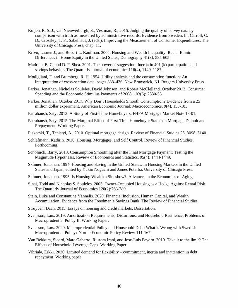
40

Koijen, R. S. J., van Nieuwerburgh, S., Vestman, R., 2015. Judging the quality of survey data by comparison with truth as measured by administrative records: Evidence from Sweden. In: Carroll, C. D., Crossley, T. F., Sabelhaus, J. (eds.), Improving the Measurement of Consumer Expenditures, The University of Chicago Press, chap. 11.

Krivo, Lauren J., and Robert L. Kaufman. 2004. Housing and Wealth Inequality: Racial Ethnic Differences in Home Equity in the United States, Demography 41(3), 585-605.

Madrian, B. C. and D. F. Shea. 2001. The power of suggestion: Inertia in 401 (k) participation and savings behavior. The Quarterly journal of economics 116(4), 1149–1187.

Modigliani, F. and Brumberg, R. H. 1954. Utility analysis and the consumption function: An interpretation of cross-section data, pages 388–436. New Brunswick, NJ. Rutgers University Press.

Parker, Jonathan, Nicholas Souleles, David Johnson, and Robert McClelland. October 2013. Consumer Spending and the Economic Stimulus Payments of 2008, 103(6): 2530-53.

Parker, Jonathan. October 2017. Why Don’t Households Smooth Consumption? Evidence from a 25 million dollar experiment. American Economic Journal: Macroeconomics, 9(4), 153-183.

Patrabansh, Saty. 2013. A Study of First-Time Homebuyers. FHFA Mortgage Market Note 13-01.

Patrabansh, Saty. 2015. The Marginal Effect of First-Time Homebuyer Status on Mortgage Default and Prepayment. Working Paper.

Piskorski, T., Tchistyi, A., 2010. Optimal mortgage design. Review of Financial Studies 23, 3098–3140.

Schlafmann, Kathrin. 2020. Housing, Mortgages, and Self Control. Review of Financial Studies. Forthcoming.

Scholnick, Barry, 2013. Consumption Smoothing after the Final Mortgage Payment: Testing the Magnitude Hypothesis. Review of Economics and Statistics, 95(4): 1444-1449.

Skinner, Jonathan. 1994. Housing and Saving in the United States. In Housing Markets in the United States and Japan, edited by Yukio Noguchi and James Poterba. University of Chicago Press.

Skinner, Jonathan. 1995. Is Housing Wealth a Sideshow?. Advances in the Economics of Aging.

Sinai, Todd and Nicholas S. Souleles. 2005. Owner-Occupied Housing as a Hedge Against Rental Risk. The Quarterly Journal of Economics 120(2):763-789.

Stein, Luke and Constantine Yannelis. 2020. Financial Inclusion, Human Capital, and Wealth Accumulation: Evidence from the Freedman’s Savings Bank. The Review of Financial Studies.

Struyven, Daan. 2015. Essays on housing and credit markets. Dissertation.

Svensson, Lars. 2019. Amortization Requirements, Distortions, and Household Resilience: Problems of Macroprudential Policy II. Working Paper.

Svensson, Lars. 2020. Macroprudential Policy and Household Debt: What is Wrong with Swedish Macroprudential Policy? Nordic Economic Policy Review 111-167.

Van Bekkum, Sjoerd, Marc Gabarro, Rustom Irani, and Jose-Luis Peydro. 2019. Take it to the limit? The Effects of Household Leverage Caps. Working Paper.

Vihriala, Erkki. 2020. Limited demand for flexibility – commitment, inertia and inattention in debt repayment. Working paper

41

Wang, Yanwen, Muxin Zhai, and John G. Lynch. 2019. Generous to a Fault? The Effect of Generosity of Employers’ Retirement Plan Contributions on Leakage from Cashing Out at Job Separation. Working Paper.

Zator, Michal. 2019. Working More to Pay the Mortgage: Household Debt, Consumption Commitments, and Labor Supply. Working paper.

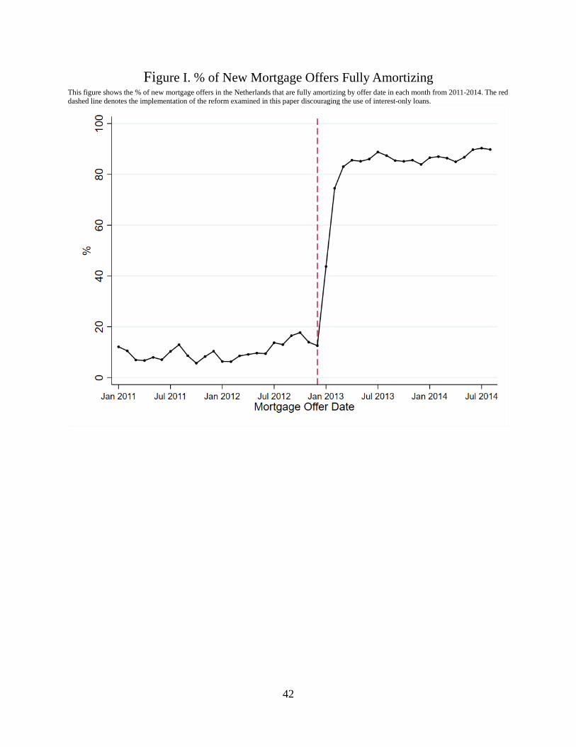
42

Figure I. % of New Mortgage Offers Fully Amortizing This figure shows the % of new mortgage offers in the Netherlands that are fully amortizing by offer date in each month from 2011-2014. The red dashed line denotes the implementation of the reform examined in this paper discouraging the use of interest-only loans.

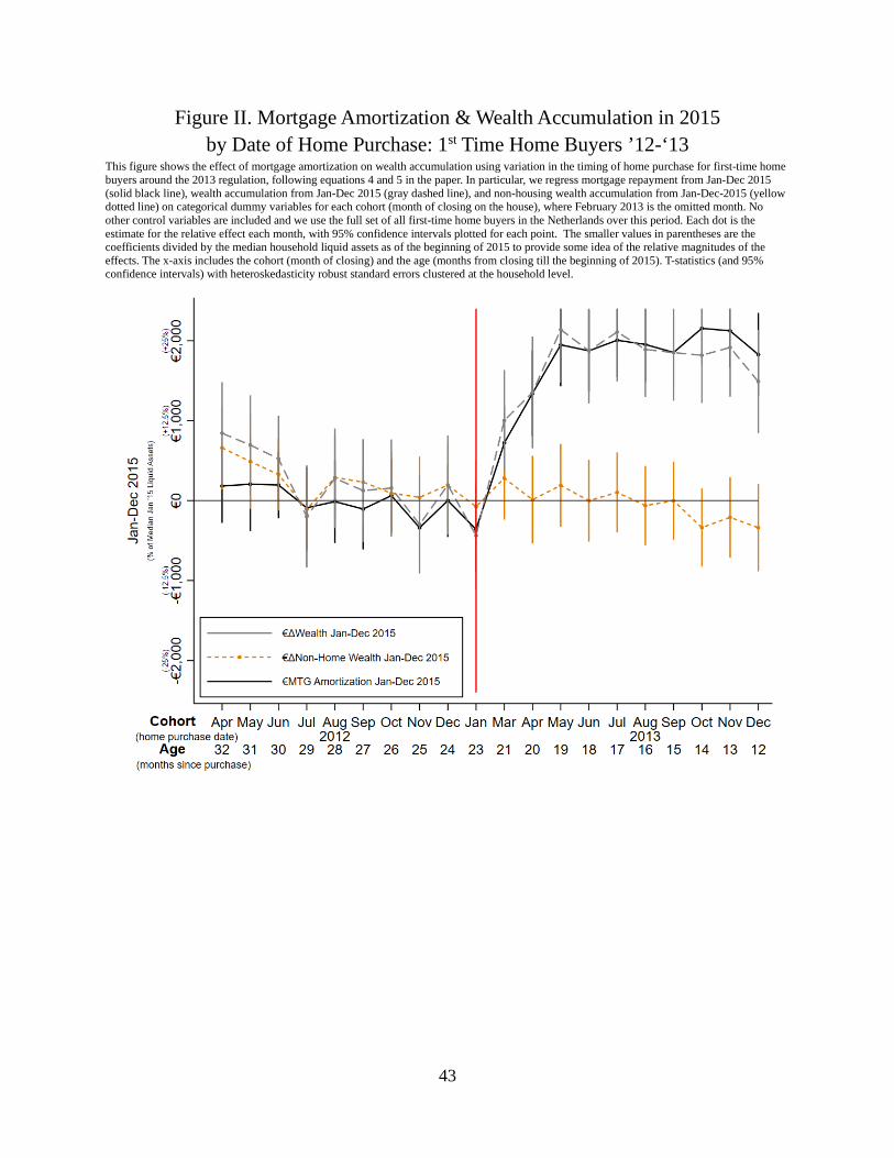
43

Figure II. Mortgage Amortization & Wealth Accumulation in 2015 by Date of Home Purchase: 1st Time Home Buyers ’12-‘13

This figure shows the effect of mortgage amortization on wealth accumulation using variation in the timing of home purchase for first-time home buyers around the 2013 regulation, following equations 4 and 5 in the paper. In particular, we regress mortgage repayment from Jan-Dec 2015 (solid black line), wealth accumulation from Jan-Dec 2015 (gray dashed line), and non-housing wealth accumulation from Jan-Dec-2015 (yellow dotted line) on categorical dummy variables for each cohort (month of closing on the house), where February 2013 is the omitted month. No other control variables are included and we use the full set of all first-time home buyers in the Netherlands over this period. Each dot is the estimate for the relative effect each month, with 95% confidence intervals plotted for each point. The smaller values in parentheses are the coefficients divided by the median household liquid assets as of the beginning of 2015 to provide some idea of the relative magnitudes of the effects. The x-axis includes the cohort (month of closing) and the age (months from closing till the beginning of 2015). T-statistics (and 95% confidence intervals) with heteroskedasticity robust standard errors clustered at the household level.

44

Figure III. Mortgage Amortization & Wealth Accumulation in 2015 by Date of Life-Event: 1st Time Home Buyers ’12-’13 w/ Life-Event

This figure shows the effect of mortgage amortization on wealth accumulation using the timing of a “life-event” as an instrument for the timing of home purchase around the 2013 regulation. Life-events are defined to be quarters with changes in the number of members of a household (ex. birth of a child), following equations 4 and 5 in the paper. In particular, we regress mortgage repayment from Jan-Dec 2015 (black) and wealth accumulation from Jan-Dec 2015 (gray) on categorical dummy variables for each life-event cohort (quarter of a life-event), where Q4 2012 and Q1 2013 are the omitted quarters. No other control variables are included and we use the full set of all first-time home buyers in the Netherlands over this period who have a life-event in 2012 or 2013. Each dot is the estimate for the relative effect each month, with 95% confidence intervals plotted for each point. The smaller values in parentheses are the coefficients divided by the median household liquid assets as of the beginning of 2015 to provide some idea of the relative magnitudes of the effects. The x-axis includes the cohort (quarter of life-event) and the age (quarters from life-event till the beginning of 2015). T-statistics (and 95% confidence intervals) with heteroskedasticity robust standard errors clustered at the household level.

45

Table I. Summary Statistics for 1st Time Home Buyers ’12-’13 in the Netherlands These are summary statistics for 2014 for the CBS administrative datasets of first-time home buyers in 2012 and 2013 in the Netherlands, who financed their purchase with a mortgage. This the population of all buyers in the Netherlands who we can identify as having no house or mortgage prior to these years, but do afterwards. This is the sample that is used for Figure 2 and a sub-sample of these for cohorts closer to the 2013 regulation is used in the subsequent regression tables, but under the same criteria.

Mean Median Stdev 25th 75th N Mtg LTV ‘14 1.02 1.05 0.19 1.01 1.09 111,523 Mtg Balance ’14 (€) 203k 187k 88k 151k 234k 111,523 Total Liabilities ’14 (€) 211k 193k 97k 155k 242k 111,523 Income ’14 (€) 73k 66k 36k 49k 88k 111,523 Liquid assets ’14 (€) 18k 7.8k 34k 2.6k 21k 111,523 ∆Liquid assets ’14 (€) 1.3k 0.3k 8.6k -1.2k 3.4k 111,523

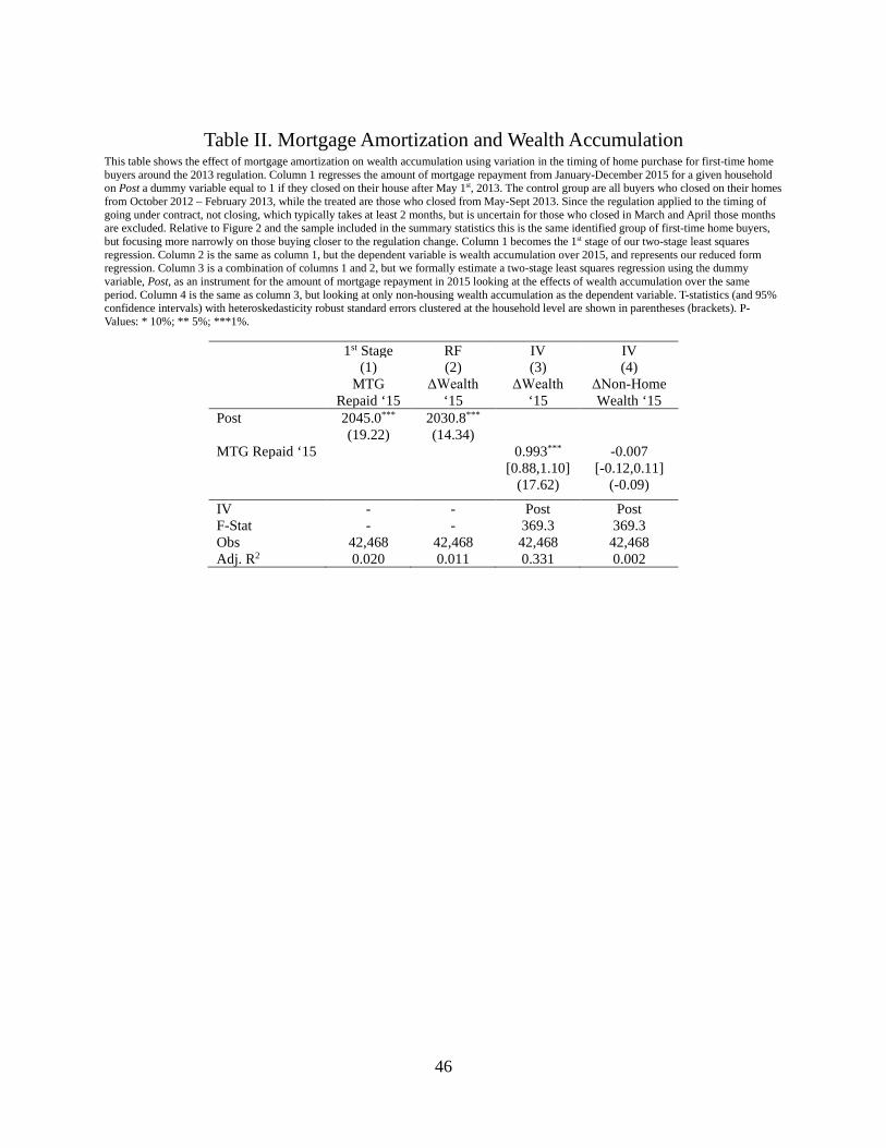
46

Table II. Mortgage Amortization and Wealth Accumulation

This table shows the effect of mortgage amortization on wealth accumulation using variation in the timing of home purchase for first-time home buyers around the 2013 regulation. Column 1 regresses the amount of mortgage repayment from January-December 2015 for a given household on Post a dummy variable equal to 1 if they closed on their house after May 1st, 2013. The control group are all buyers who closed on their homes from October 2012 – February 2013, while the treated are those who closed from May-Sept 2013. Since the regulation applied to the timing of going under contract, not closing, which typically takes at least 2 months, but is uncertain for those who closed in March and April those months are excluded. Relative to Figure 2 and the sample included in the summary statistics this is the same identified group of first-time home buyers, but focusing more narrowly on those buying closer to the regulation change. Column 1 becomes the 1st stage of our two-stage least squares regression. Column 2 is the same as column 1, but the dependent variable is wealth accumulation over 2015, and represents our reduced form regression. Column 3 is a combination of columns 1 and 2, but we formally estimate a two-stage least squares regression using the dummy variable, Post, as an instrument for the amount of mortgage repayment in 2015 looking at the effects of wealth accumulation over the same period. Column 4 is the same as column 3, but looking at only non-housing wealth accumulation as the dependent variable. T-statistics (and 95% confidence intervals) with heteroskedasticity robust standard errors clustered at the household level are shown in parentheses (brackets). P-Values: * 10%; ** 5%; ***1%.

1st Stage RF IV IV (1) (2) (3) (4) MTG

Repaid ‘15 ΔWealth

‘15 ΔWealth

‘15 ΔNon-Home Wealth ‘15

Post 2045.0*** 2030.8*** (19.22) (14.34) MTG Repaid ‘15 0.993*** -0.007 [0.88,1.10] [-0.12,0.11] (17.62) (-0.09)

IV - - Post Post F-Stat - - 369.3 369.3 Obs 42,468 42,468 42,468 42,468 Adj. R2 0.020 0.011 0.331 0.002

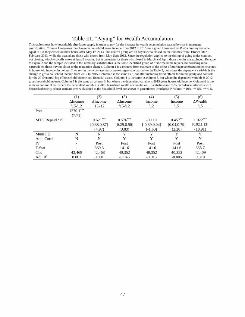
47

Table III. “Paying” for Wealth Accumulation

This table shows how households alter labor supply in order to pay for the increase in wealth accumulation caused by rise in mortgage amortization. Column 1 regresses the change in household gross income from 2012 to 2015 for a given household on Post a dummy variable equal to 1 if they closed on their house after May 1st, 2013. The control group are all buyers who closed on their homes from October 2012 – February 2013, while the treated are those who closed from May-Sept 2013. Since the regulation applied to the timing of going under contract, not closing, which typically takes at least 2 months, but is uncertain for those who closed in March and April those months are excluded. Relative to Figure 2 and the sample included in the summary statistics this is the same identified group of first-time home buyers, but focusing more narrowly on those buying closer to the regulation change. Column 1 is a reduced form estimate of the effect of mortgage amortization on changes in household income. In column 2 we re-run the two-stage least squares regression carried out in Table 2, but where the dependent variable is the change in gross household income from 2012 to 2015. Column 3 is the same as 2, but after including fixed effects for municipality and controls for the 2010 natural log of household income and financial assets. Column 4 is the same as column 3, but where the dependent variable is 2012 gross household income. Column 5 is the same as column 3, but where the dependent variable is 2015 gross household income. Column 6 is the same as column 3, but where the dependent variable is 2015 household wealth accumulation. T-statistics (and 95% confidence intervals) with heteroskedasticity robust standard errors clustered at the household level are shown in parentheses (brackets). P-Values: * 10%; ** 5%; ***1%.

(1) (2) (3) (4) (5) (6) ΔIncome

'15-'12 ΔIncome '15-'12

ΔIncome '15-'12

Income '12

Income '15

ΔWealth ‘15

Post 1270.1*** (7.71) MTG Repaid ‘15 0.621*** 0.576*** -0.119 0.457** 1.022*** [0.38,0.87] [0.29,0.90] [-0.39,0.04] [0.04,0.79] [0.92,1.13] (4.97) (3.83) (-1.60) (2.20) (18.91) Muni FE N N Y Y Y Y Add. Cntrls N N Y Y Y Y IV - Post Post Post Post Post F-Stat - 369.3 141.6 141.6 141.6 355.7 Obs 42,468 42,468 40,352 40,352 40,352 42,409 Adj. R2 0.001 0.001 -0.046 -0.015 -0.005 0.319

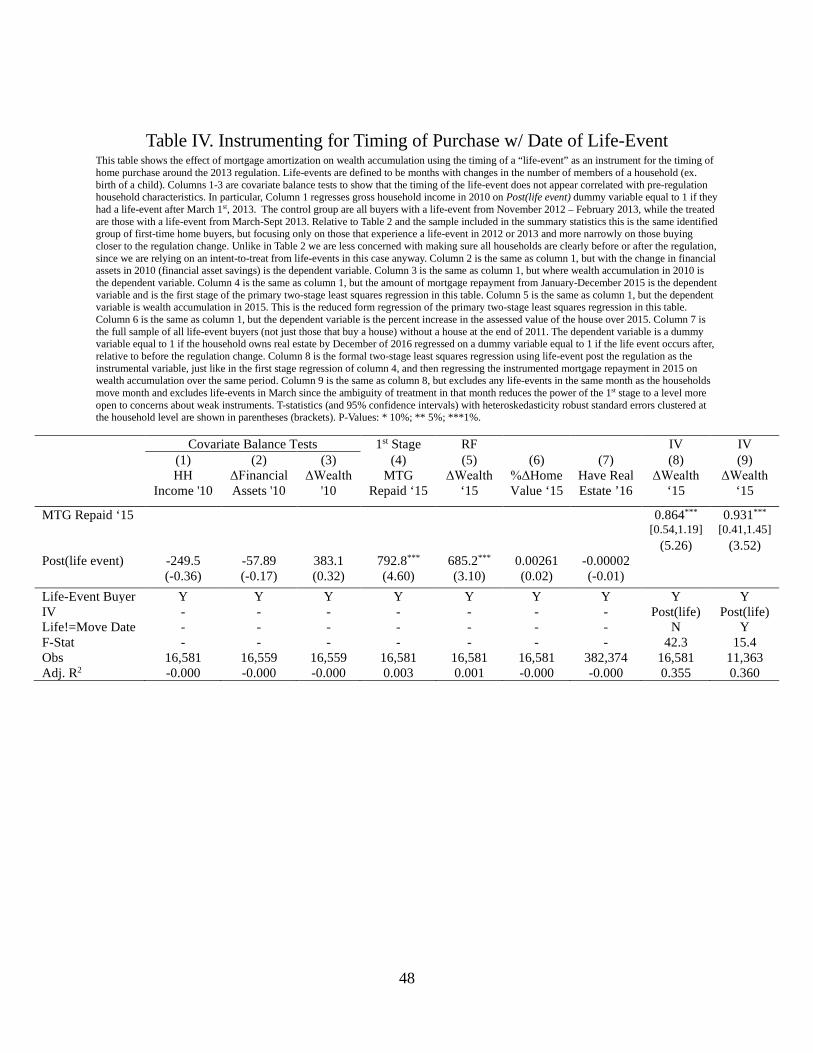
48

Table IV. Instrumenting for Timing of Purchase w/ Date of Life-Event This table shows the effect of mortgage amortization on wealth accumulation using the timing of a “life-event” as an instrument for the timing of home purchase around the 2013 regulation. Life-events are defined to be months with changes in the number of members of a household (ex. birth of a child). Columns 1-3 are covariate balance tests to show that the timing of the life-event does not appear correlated with pre-regulation household characteristics. In particular, Column 1 regresses gross household income in 2010 on Post(life event) dummy variable equal to 1 if they had a life-event after March 1st, 2013. The control group are all buyers with a life-event from November 2012 – February 2013, while the treated are those with a life-event from March-Sept 2013. Relative to Table 2 and the sample included in the summary statistics this is the same identified group of first-time home buyers, but focusing only on those that experience a life-event in 2012 or 2013 and more narrowly on those buying closer to the regulation change. Unlike in Table 2 we are less concerned with making sure all households are clearly before or after the regulation, since we are relying on an intent-to-treat from life-events in this case anyway. Column 2 is the same as column 1, but with the change in financial assets in 2010 (financial asset savings) is the dependent variable. Column 3 is the same as column 1, but where wealth accumulation in 2010 is the dependent variable. Column 4 is the same as column 1, but the amount of mortgage repayment from January-December 2015 is the dependent variable and is the first stage of the primary two-stage least squares regression in this table. Column 5 is the same as column 1, but the dependent variable is wealth accumulation in 2015. This is the reduced form regression of the primary two-stage least squares regression in this table. Column 6 is the same as column 1, but the dependent variable is the percent increase in the assessed value of the house over 2015. Column 7 is the full sample of all life-event buyers (not just those that buy a house) without a house at the end of 2011. The dependent variable is a dummy variable equal to 1 if the household owns real estate by December of 2016 regressed on a dummy variable equal to 1 if the life event occurs after, relative to before the regulation change. Column 8 is the formal two-stage least squares regression using life-event post the regulation as the instrumental variable, just like in the first stage regression of column 4, and then regressing the instrumented mortgage repayment in 2015 on wealth accumulation over the same period. Column 9 is the same as column 8, but excludes any life-events in the same month as the households move month and excludes life-events in March since the ambiguity of treatment in that month reduces the power of the 1st stage to a level more open to concerns about weak instruments. T-statistics (and 95% confidence intervals) with heteroskedasticity robust standard errors clustered at the household level are shown in parentheses (brackets). P-Values: * 10%; ** 5%; ***1%.

Covariate Balance Tests 1st Stage RF IV IV (1) (2) (3) (4) (5) (6) (7) (8) (9) HH

Income '10 ΔFinancial Assets '10

ΔWealth '10

MTG Repaid ‘15

ΔWealth ‘15

%ΔHome Value ‘15

Have Real Estate ’16

ΔWealth ‘15

ΔWealth ‘15

MTG Repaid ‘15 0.864*** 0.931*** [0.54,1.19] [0.41,1.45] (5.26) (3.52) Post(life event) -249.5 -57.89 383.1 792.8*** 685.2*** 0.00261 -0.00002 (-0.36) (-0.17) (0.32) (4.60) (3.10) (0.02) (-0.01) Life-Event Buyer Y Y Y Y Y Y Y Y Y IV - - - - - - - Post(life) Post(life) Life!=Move Date - - - - - - - N Y F-Stat - - - - - - - 42.3 15.4 Obs 16,581 16,559 16,559 16,581 16,581 16,581 382,374 16,581 11,363 Adj. R2 -0.000 -0.000 -0.000 0.003 0.001 -0.000 -0.000 0.355 0.360

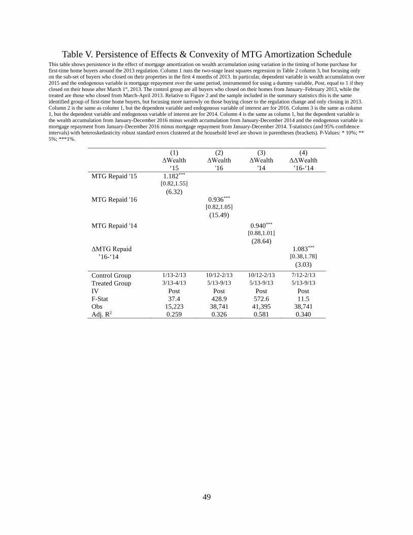
49

Table V. Persistence of Effects & Convexity of MTG Amortization Schedule This table shows persistence in the effect of mortgage amortization on wealth accumulation using variation in the timing of home purchase for first-time home buyers around the 2013 regulation. Column 1 runs the two-stage least squares regression in Table 2 column 3, but focusing only on the sub-set of buyers who closed on their properties in the first 4 months of 2013. In particular, dependent variable is wealth accumulation over 2015 and the endogenous variable is mortgage repayment over the same period, instrumented for using a dummy variable, Post, equal to 1 if they closed on their house after March 1st, 2013. The control group are all buyers who closed on their homes from January–February 2013, while the treated are those who closed from March-April 2013. Relative to Figure 2 and the sample included in the summary statistics this is the same identified group of first-time home buyers, but focusing more narrowly on those buying closer to the regulation change and only closing in 2013. Column 2 is the same as column 1, but the dependent variable and endogenous variable of interest are for 2016. Column 3 is the same as column 1, but the dependent variable and endogenous variable of interest are for 2014. Column 4 is the same as column 1, but the dependent variable is the wealth accumulation from January-December 2016 minus wealth accumulation from January-December 2014 and the endogenous variable is mortgage repayment from January-December 2016 minus mortgage repayment from January-December 2014. T-statistics (and 95% confidence intervals) with heteroskedasticity robust standard errors clustered at the household level are shown in parentheses (brackets). P-Values: * 10%; ** 5%; ***1%.

(1) (2) (3) (4) ΔWealth

‘15 ΔWealth

'16 ΔWealth

'14 ΔΔWealth

’16-‘14 MTG Repaid '15 1.182*** [0.82,1.55] (6.32) MTG Repaid '16 0.936*** [0.82,1.05] (15.49) MTG Repaid '14 0.940*** [0.88,1.01] (28.64) ΔMTG Repaid 1.083*** ’16-‘14 [0.38,1.78] (3.03) Control Group 1/13-2/13 10/12-2/13 10/12-2/13 7/12-2/13 Treated Group 3/13-4/13 5/13-9/13 5/13-9/13 5/13-9/13 IV Post Post Post Post F-Stat 37.4 428.9 572.6 11.5 Obs 15,223 38,741 41,395 38,741 Adj. R2 0.259 0.326 0.581 0.340

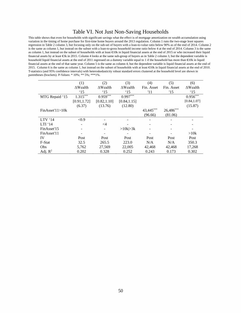
50

Table VI. Not Just Non-Saving Households This table shows that even for households with significant savings what the effect is of mortgage amortization on wealth accumulation using variation in the timing of home purchase for first-time home buyers around the 2013 regulation. Column 1 runs the two-stage least squares regression in Table 2 column 3, but focusing only on the sub-set of buyers with a loan-to-value ratio below 90% as of the end of 2014. Column 2 is the same as column 1, but instead on the subset with a loan-to-gross household income ratio below 4 at the end of 2014. Column 3 is the same as column 1, but instead on the subset of households with at least €10k in liquid financial assets at the end of 2015 or who increased their liquid financial assets by at least €3k in 2015. Column 4 looks at the same sub-group of buyers as in Table 2 column 3, but the dependent variable is household liquid financial assets at the end of 2011 regressed on a dummy variable equal to 1 if the household has more than €10k in liquid financial assets at the end of that same year. Column 5 is the same as column 4, but the dependent variable is liquid financial assets at the end of 2015. Column 6 is the same as column 1, but instead on the subset of households with at least €10k in liquid financial assets at the end of 2010. T-statistics (and 95% confidence intervals) with heteroskedasticity robust standard errors clustered at the household level are shown in parentheses (brackets). P-Values: * 10%; ** 5%; ***1%.

(1) (2) (3) (4) (5) (6) ΔWealth

‘15 ΔWealth

‘15 ΔWealth

‘15 Fin. Asset

'11 Fin. Asset

'15 ΔWealth

‘15 MTG Repaid ‘15 1.315*** 0.959*** 0.997*** 0.956*** [0.91,1.72] [0.82,1.10] [0.84,1.15] [0.84,1.07] (6.37) (13.76) (12.80) (15.87) FinAsset'11>10k 43,445*** 26,486*** (96.66) (81.06) LTV ‘14 <0.9 - - - - - LTI ‘14 - <4 - - - - FinAsset'15 - - >10k|>3k - - - FinAsset'11 - - - - - >10k IV Post Post Post Post Post Post F-Stat 32.5 265.5 223.0 N/A N/A 350.3 Obs 5,762 27,569 22,005 42,468 42,468 17,268 Adj. R2 0.202 0.328 0.252 0.243 0.173 0.302

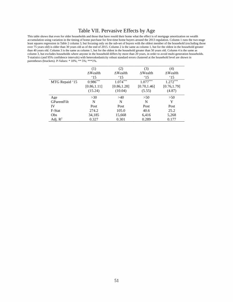
51

Table VII. Pervasive Effects by Age This table shows that even for older households and those that have resold their home what the effect is of mortgage amortization on wealth accumulation using variation in the timing of home purchase for first-time home buyers around the 2013 regulation. Column 1 runs the two-stage least squares regression in Table 2 column 3, but focusing only on the sub-set of buyers with the oldest member of the household (excluding those over 75 years old) is older than 30 years old as of the end of 2015. Column 2 is the same as column 1, but for the oldest in the household greater than 40 years old. Column 3 is the same as column 1, but for the oldest in the household greater than 50 years old. Column 4 is the same as column 3, but excludes households where anyone in the household differs by more than 20 years, in order to avoid multi-generation households. T-statistics (and 95% confidence intervals) with heteroskedasticity robust standard errors clustered at the household level are shown in parentheses (brackets). P-Values: * 10%; ** 5%; ***1%.

(1) (2) (3) (4) ΔWealth

‘15 ΔWealth

‘15 ΔWealth

‘15 ΔWealth

‘15 MTG Repaid ‘15 0.986*** 1.074*** 1.077*** 1.272*** [0.86,1.11] [0.86,1.28] [0.70,1.46] [0.76,1.79] (15.24) (10.04) (5.55) (4.87)

Age >30 >40 >50 >50 GParentFilt N N N Y IV Post Post Post Post F-Stat 274.2 105.0 40.6 25.2 Obs 34,185 15,668 6,416 5,268 Adj. R2 0.327 0.301 0.289 0.177

52

APPENDIX

53

Figure AI. Variability in Liquid Wealth Accumulation

For the full sample of first-time home buyers from Table 1 for all years 2006-2016 we compute the yearly change in liquid financial assets and regress those on dummy variables for years since a year with a decline in household gross income, after including household fixed effects and year fixed effects.

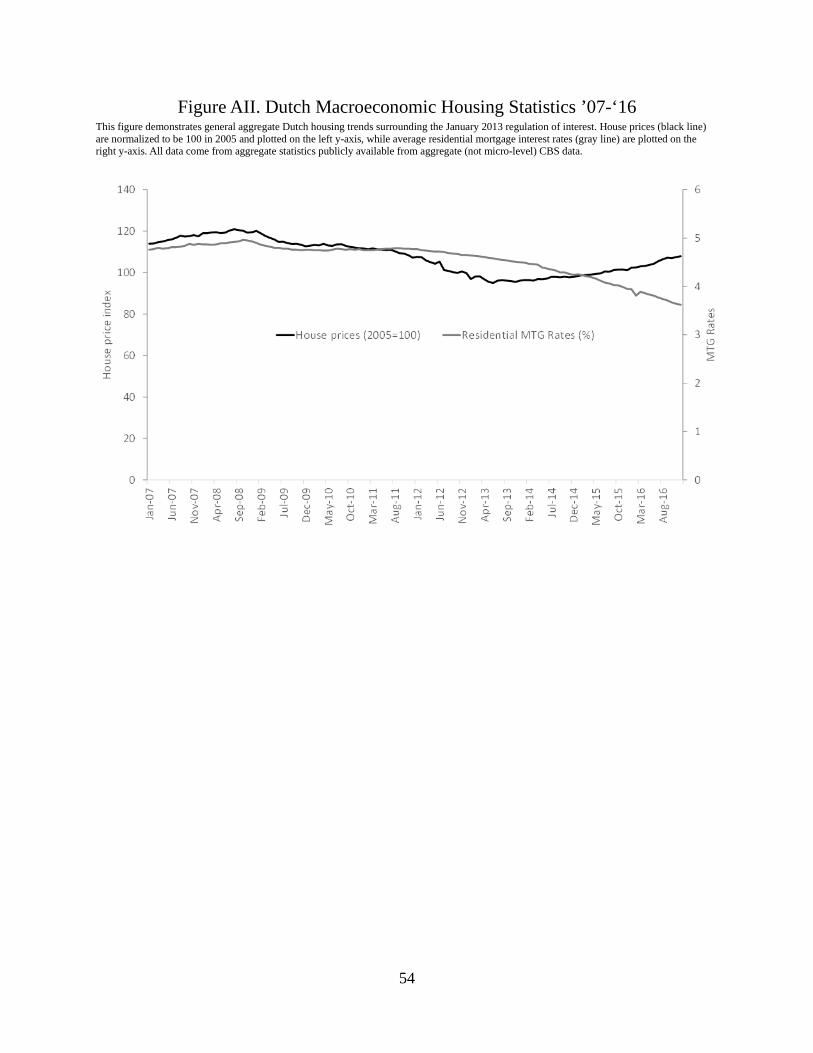
54

Figure AII. Dutch Macroeconomic Housing Statistics ’07-‘16 This figure demonstrates general aggregate Dutch housing trends surrounding the January 2013 regulation of interest. House prices (black line) are normalized to be 100 in 2005 and plotted on the left y-axis, while average residential mortgage interest rates (gray line) are plotted on the right y-axis. All data come from aggregate statistics publicly available from aggregate (not micro-level) CBS data.

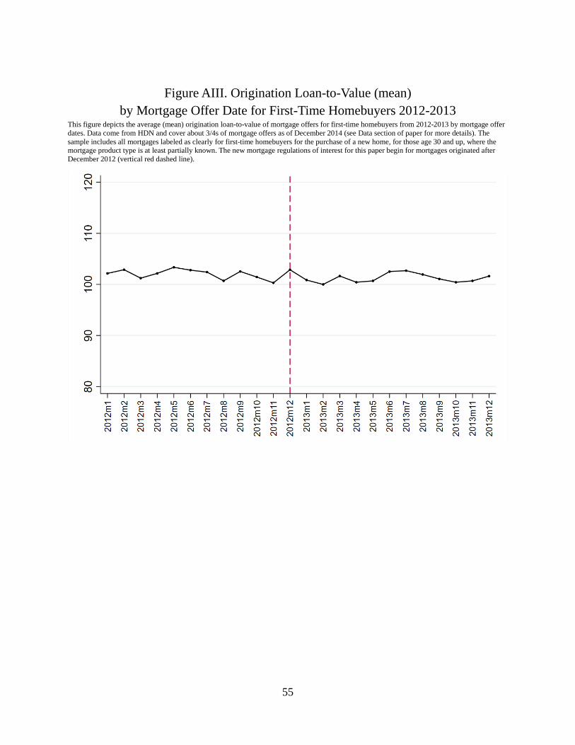
55

Figure AIII. Origination Loan-to-Value (mean)

by Mortgage Offer Date for First-Time Homebuyers 2012-2013 This figure depicts the average (mean) origination loan-to-value of mortgage offers for first-time homebuyers from 2012-2013 by mortgage offer dates. Data come from HDN and cover about 3/4s of mortgage offers as of December 2014 (see Data section of paper for more details). The sample includes all mortgages labeled as clearly for first-time homebuyers for the purchase of a new home, for those age 30 and up, where the mortgage product type is at least partially known. The new mortgage regulations of interest for this paper begin for mortgages originated after December 2012 (vertical red dashed line).

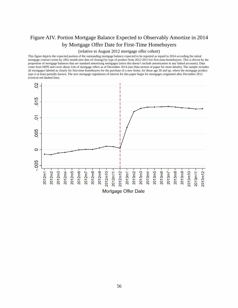
56

Figure AIV. Portion Mortgage Balance Expected to Observably Amortize in 2014

by Mortgage Offer Date for First-Time Homebuyers (relative to August 2012 mortgage offer cohort)

This figure depicts the expected portion of the outstanding mortgage balance expected to be reported as repaid in 2014 according the initial mortgage contract terms by offer month (not date of closing) by type of product from 2012-2013 for first-time-homebuyers. This is driven by the proportion of mortgage balances that are standard amortizing mortgages (since this doesn’t include amortization in any linked accounts). Data come from HDN and cover about 3/4s of mortgage offers as of December 2014 (see Data section of paper for more details). The sample includes all mortgages labeled as clearly for first-time homebuyers for the purchase of a new home, for those age 30 and up, where the mortgage product type is at least partially known. The new mortgage regulations of interest for this paper begin for mortgages originated after December 2012 (vertical red dashed line).

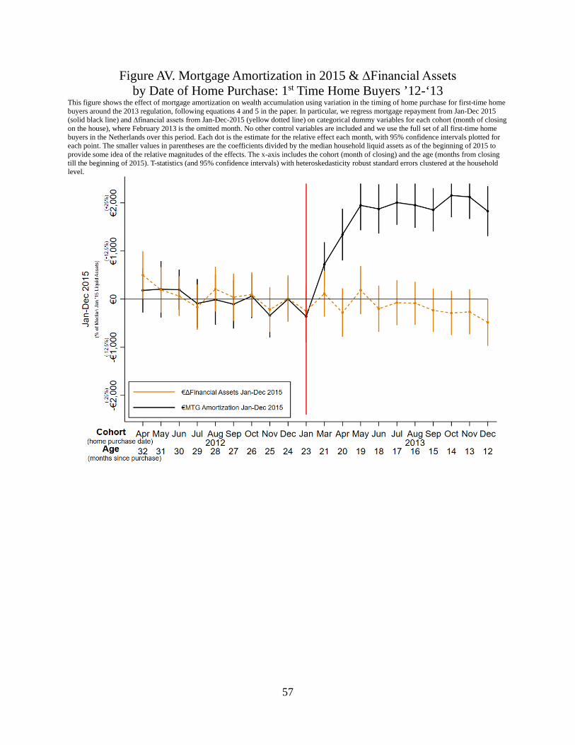
57

Figure AV. Mortgage Amortization in 2015 & ∆Financial Assets by Date of Home Purchase: 1st Time Home Buyers ’12-‘13

This figure shows the effect of mortgage amortization on wealth accumulation using variation in the timing of home purchase for first-time home buyers around the 2013 regulation, following equations 4 and 5 in the paper. In particular, we regress mortgage repayment from Jan-Dec 2015 (solid black line) and ∆financial assets from Jan-Dec-2015 (yellow dotted line) on categorical dummy variables for each cohort (month of closing on the house), where February 2013 is the omitted month. No other control variables are included and we use the full set of all first-time home buyers in the Netherlands over this period. Each dot is the estimate for the relative effect each month, with 95% confidence intervals plotted for each point. The smaller values in parentheses are the coefficients divided by the median household liquid assets as of the beginning of 2015 to provide some idea of the relative magnitudes of the effects. The x-axis includes the cohort (month of closing) and the age (months from closing till the beginning of 2015). T-statistics (and 95% confidence intervals) with heteroskedasticity robust standard errors clustered at the household level.

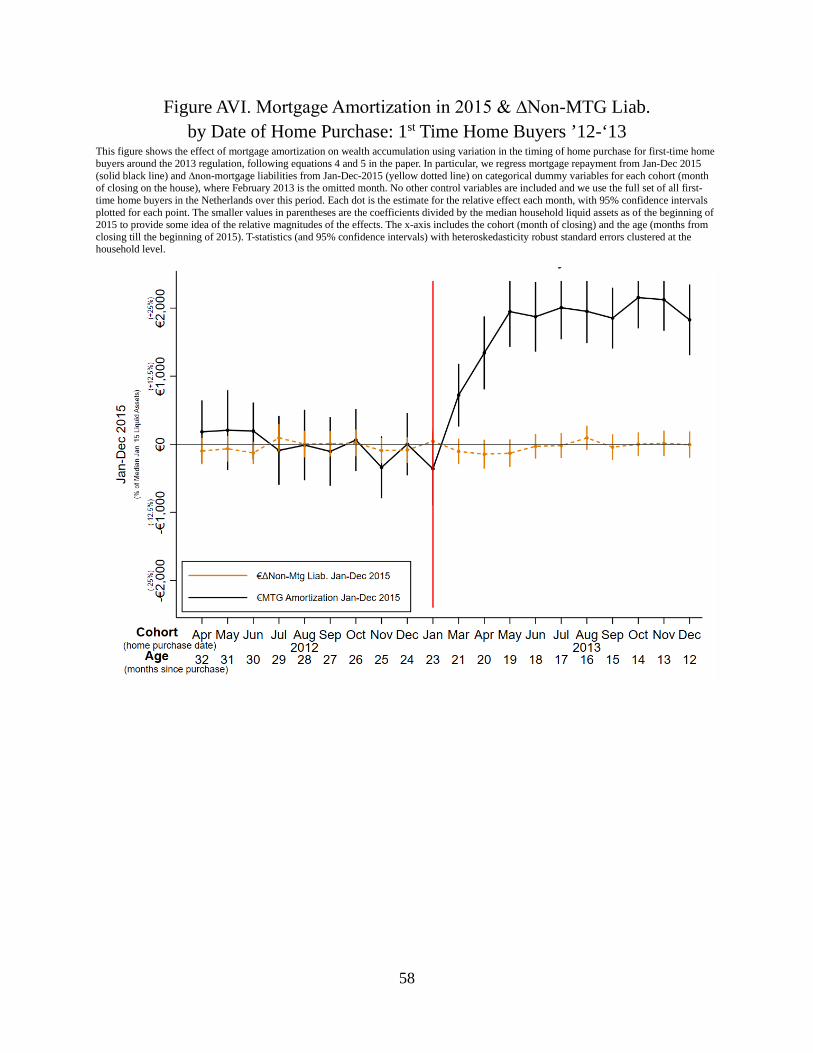
58

Figure AVI. Mortgage Amortization in 2015 & ∆Non-MTG Liab. by Date of Home Purchase: 1st Time Home Buyers ’12-‘13

This figure shows the effect of mortgage amortization on wealth accumulation using variation in the timing of home purchase for first-time home buyers around the 2013 regulation, following equations 4 and 5 in the paper. In particular, we regress mortgage repayment from Jan-Dec 2015 (solid black line) and ∆non-mortgage liabilities from Jan-Dec-2015 (yellow dotted line) on categorical dummy variables for each cohort (month of closing on the house), where February 2013 is the omitted month. No other control variables are included and we use the full set of all first-time home buyers in the Netherlands over this period. Each dot is the estimate for the relative effect each month, with 95% confidence intervals plotted for each point. The smaller values in parentheses are the coefficients divided by the median household liquid assets as of the beginning of 2015 to provide some idea of the relative magnitudes of the effects. The x-axis includes the cohort (month of closing) and the age (months from closing till the beginning of 2015). T-statistics (and 95% confidence intervals) with heteroskedasticity robust standard errors clustered at the household level.

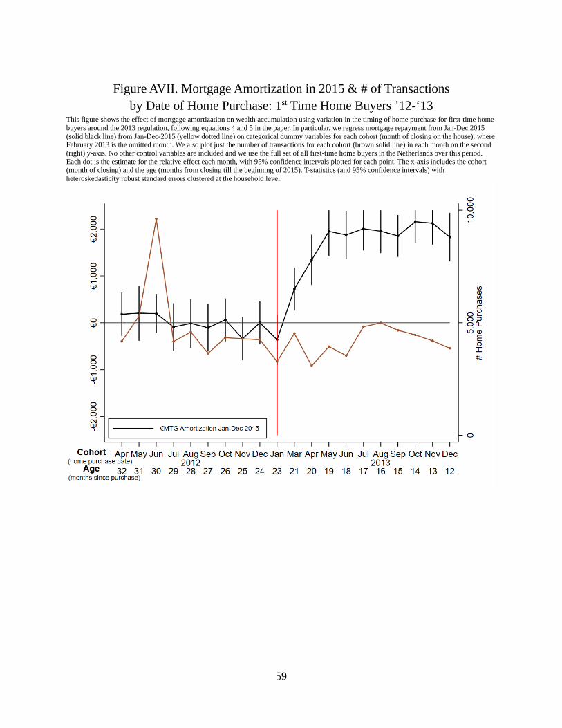
59

Figure AVII. Mortgage Amortization in 2015 & # of Transactions

by Date of Home Purchase: 1st Time Home Buyers ’12-‘13 This figure shows the effect of mortgage amortization on wealth accumulation using variation in the timing of home purchase for first-time home buyers around the 2013 regulation, following equations 4 and 5 in the paper. In particular, we regress mortgage repayment from Jan-Dec 2015 (solid black line) from Jan-Dec-2015 (yellow dotted line) on categorical dummy variables for each cohort (month of closing on the house), where February 2013 is the omitted month. We also plot just the number of transactions for each cohort (brown solid line) in each month on the second (right) y-axis. No other control variables are included and we use the full set of all first-time home buyers in the Netherlands over this period. Each dot is the estimate for the relative effect each month, with 95% confidence intervals plotted for each point. The x-axis includes the cohort (month of closing) and the age (months from closing till the beginning of 2015). T-statistics (and 95% confidence intervals) with heteroskedasticity robust standard errors clustered at the household level.

60

Figure AVIII. First-Time Homebuyers vs. All Other Buyers

This figure shows differential treatment for first-time homebuyers (FTHBs) vs. all other buyers of the 2013 regulation based on purchase cohorts (months), but no sharp jumps (in absolute terms or relative to each other) in other variables around that date. FTHBs (solid black lines) are defined to be those that purchase a home with a mortgage during the depicted month, but didn’t have real estate or a mortgage in the 2 years prior to that. By contrast All Other Buyers (dashed yellow lines) also purchase a house with a mortgage during the depicted month, but do have real estate and a mortgage in the 2 years prior. In panel A we regress the % of the mortgage balance repaid from Jan-Dec 2015 on categorical dummy variables for each cohort (month of closing on the house), where February 2013 is the omitted month. No other control variables are included and we use the full set of all first-time home buyers in the Netherlands over this period. Each dot is the estimate for the relative effect each month, with 95% confidence intervals plotted for each point. The x-axis includes the cohort (month of closing). T-statistics (and 95% confidence intervals) with heteroskedasticity robust standard errors clustered at the household level. Panels B-H are the same as panel A, but where the variable of interest are the initial home purchase price in thousands of euros (B), the change in the natural log of financial assets over 2015 (C), the change in financial assets over 2015 divided by the mortgage balance at the end of 2014 (D), the natural log of financial assets as of Dec 2010 (E), the natural log of household gross income as of Dec 2010 (F), the change in the natural log of financial assets over 2011 (G), and the change in the natural log of household gross income over 2011 (H).

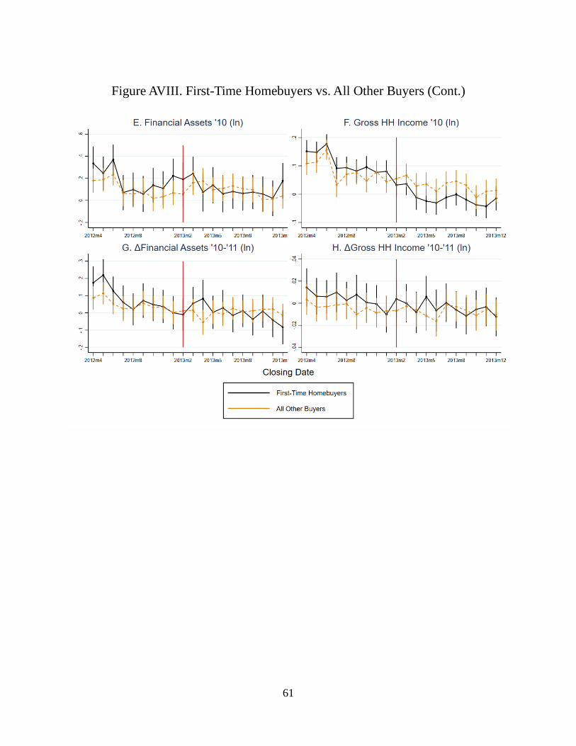
61

Figure AVIII. First-Time Homebuyers vs. All Other Buyers (Cont.)

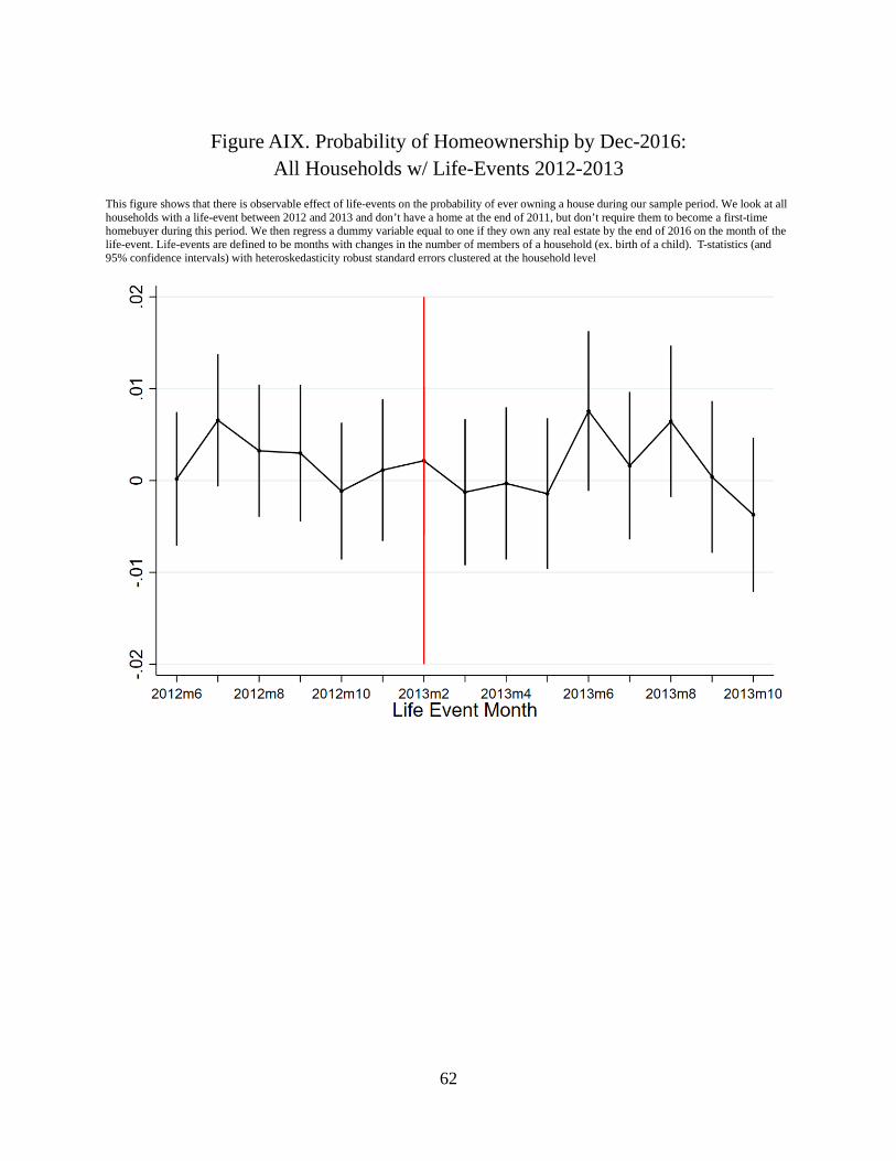
62

Figure AIX. Probability of Homeownership by Dec-2016:

All Households w/ Life-Events 2012-2013 This figure shows that there is observable effect of life-events on the probability of ever owning a house during our sample period. We look at all households with a life-event between 2012 and 2013 and don’t have a home at the end of 2011, but don’t require them to become a first-time homebuyer during this period. We then regress a dummy variable equal to one if they own any real estate by the end of 2016 on the month of the life-event. Life-events are defined to be months with changes in the number of members of a household (ex. birth of a child). T-statistics (and 95% confidence intervals) with heteroskedasticity robust standard errors clustered at the household level

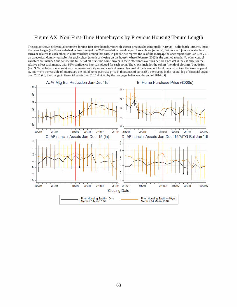
63

Figure AX. Non-First-Time Homebuyers by Previous Housing Tenure Length

This figure shows differential treatment for non-first-time homebuyers with shorter previous housing spells (<10 yrs – solid black lines) vs. those that were longer (>=10 yrs – dashed yellow lines) of the 2013 regulation based on purchase cohorts (months), but no sharp jumps (in absolute terms or relative to each other) in other variables around that date. In panel A we regress the % of the mortgage balance repaid from Jan-Dec 2015 on categorical dummy variables for each cohort (month of closing on the house), where February 2013 is the omitted month. No other control variables are included and we use the full set of all first-time home buyers in the Netherlands over this period. Each dot is the estimate for the relative effect each month, with 95% confidence intervals plotted for each point. The x-axis includes the cohort (month of closing). T-statistics (and 95% confidence intervals) with heteroskedasticity robust standard errors clustered at the household level. Panels B-D are the same as panel A, but where the variable of interest are the initial home purchase price in thousands of euros (B), the change in the natural log of financial assets over 2015 (C), the change in financial assets over 2015 divided by the mortgage balance at the end of 2014 (D).

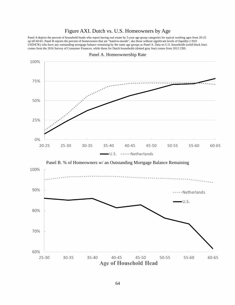
64

Figure AXI. Dutch vs. U.S. Homeowners by Age

Panel A depicts the percent of household heads who report having real estate by 5-year age group categories for typical working ages from 20-25 up till 60-65. Panel B reports the percent of homeowners that are “hand-to-mouth”, aka those without significant levels of liquidity (<$10 USD/€7K) who have any outstanding mortgage balance remaining by the same age groups as Panel A. Data on U.S. households (solid black line) comes from the 2016 Survey of Consumer Finances, while those for Dutch households (dotted gray line) comes from 2012 CBS.

Panel A. Homeownership Rate

Panel B. % of Homeowners w/ an Outstanding Mortgage Balance Remaining

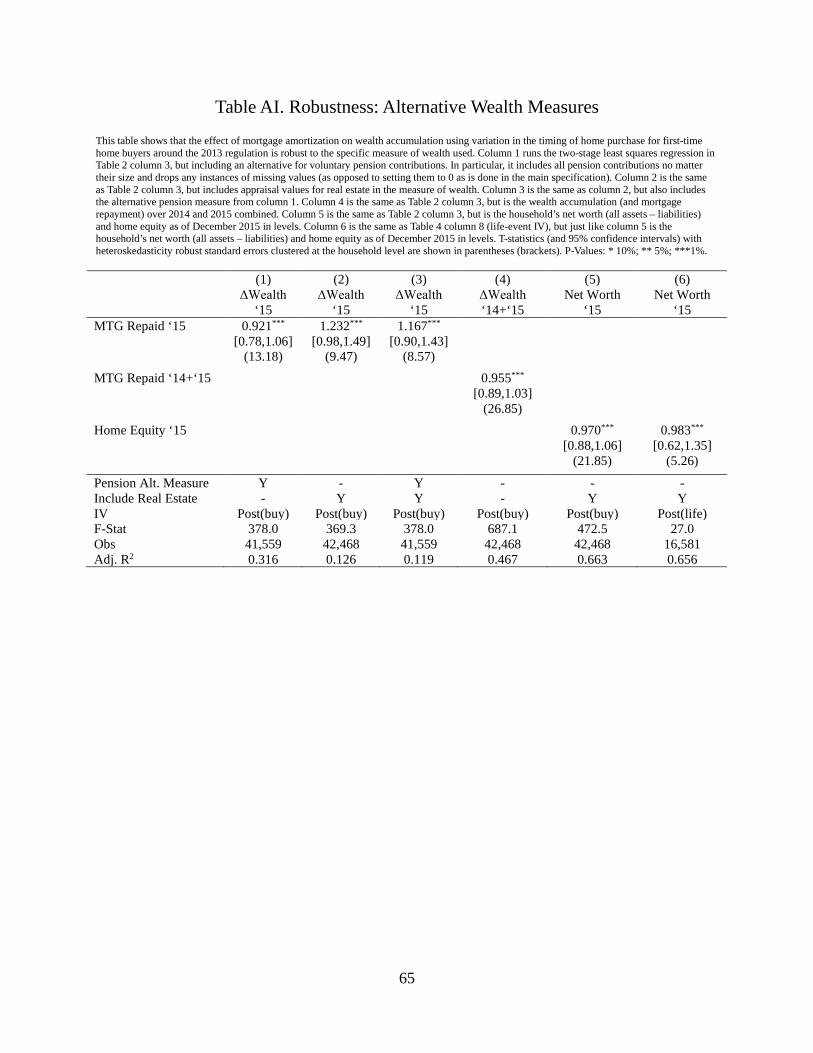
65

Table AI. Robustness: Alternative Wealth Measures

This table shows that the effect of mortgage amortization on wealth accumulation using variation in the timing of home purchase for first-time home buyers around the 2013 regulation is robust to the specific measure of wealth used. Column 1 runs the two-stage least squares regression in Table 2 column 3, but including an alternative for voluntary pension contributions. In particular, it includes all pension contributions no matter their size and drops any instances of missing values (as opposed to setting them to 0 as is done in the main specification). Column 2 is the same as Table 2 column 3, but includes appraisal values for real estate in the measure of wealth. Column 3 is the same as column 2, but also includes the alternative pension measure from column 1. Column 4 is the same as Table 2 column 3, but is the wealth accumulation (and mortgage repayment) over 2014 and 2015 combined. Column 5 is the same as Table 2 column 3, but is the household’s net worth (all assets – liabilities) and home equity as of December 2015 in levels. Column 6 is the same as Table 4 column 8 (life-event IV), but just like column 5 is the household’s net worth (all assets – liabilities) and home equity as of December 2015 in levels. T-statistics (and 95% confidence intervals) with heteroskedasticity robust standard errors clustered at the household level are shown in parentheses (brackets). P-Values: * 10%; ** 5%; ***1%.

(1) (2) (3) (4) (5) (6) ΔWealth

‘15 ΔWealth

‘15 ΔWealth

‘15 ΔWealth ‘14+‘15

Net Worth ‘15

Net Worth ‘15

MTG Repaid ‘15 0.921*** 1.232*** 1.167*** [0.78,1.06] [0.98,1.49] [0.90,1.43] (13.18) (9.47) (8.57) MTG Repaid ‘14+‘15 0.955*** [0.89,1.03] (26.85) Home Equity ‘15 0.970*** 0.983*** [0.88,1.06] [0.62,1.35] (21.85) (5.26)

Pension Alt. Measure Y - Y - - - Include Real Estate - Y Y - Y Y IV Post(buy) Post(buy) Post(buy) Post(buy) Post(buy) Post(life) F-Stat 378.0 369.3 378.0 687.1 472.5 27.0 Obs 41,559 42,468 41,559 42,468 42,468 16,581 Adj. R2 0.316 0.126 0.119 0.467 0.663 0.656

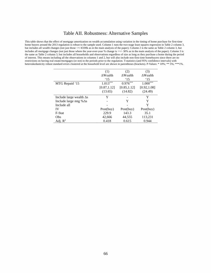
66

Table AII. Robustness: Alternative Samples

This table shows that the effect of mortgage amortization on wealth accumulation using variation in the timing of home purchase for first-time home buyers around the 2013 regulation is robust to the sample used. Column 1 runs the two-stage least squares regression in Table 2 column 3, but includes all wealth changes (not just those <+/-€100k as in the main analysis of the paper). Column 2 is the same as Table 2 column 3, but includes all mortgage changes (not just those where the year-over-year % change is <+/- 30% as in the main analysis of the paper). Column 3 is the same as Table 2 column 3, but includes all households and observations regardless of size as long as they purchase a home during the period of interest. This means including all the observations in columns 1 and 2, but will also include non-first-time homebuyers since there are no restrictions on having real estate/mortgages (or not) in the periods prior to the regulation. T-statistics (and 95% confidence intervals) with heteroskedasticity robust standard errors clustered at the household level are shown in parentheses (brackets). P-Values: * 10%; ** 5%; ***1%.

(1) (2) (3) ΔWealth

‘15 ΔWealth

‘15 ΔWealth

‘15 MTG Repaid ‘15 1.013*** 0.976*** 1.000*** [0.87,1.12] [0.85,1.12] [0.92,1.08] (13.65) (14.82) (24.49)

Include large wealth Δs Y - Y Include large mtg %Δs - Y Y Include all - - Y IV Post(buy) Post(buy) Post(buy) F-Stat 229.9 143.3 35.1 Obs 42,666 44,555 113,231 Adj. R2 0.418 0.615 0.944

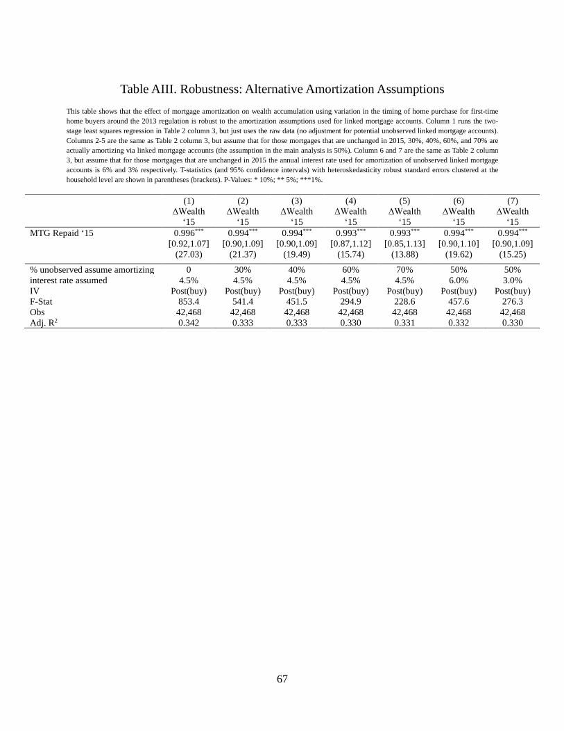
67

Table AIII. Robustness: Alternative Amortization Assumptions

This table shows that the effect of mortgage amortization on wealth accumulation using variation in the timing of home purchase for first-time home buyers around the 2013 regulation is robust to the amortization assumptions used for linked mortgage accounts. Column 1 runs the two-stage least squares regression in Table 2 column 3, but just uses the raw data (no adjustment for potential unobserved linked mortgage accounts). Columns 2-5 are the same as Table 2 column 3, but assume that for those mortgages that are unchanged in 2015, 30%, 40%, 60%, and 70% are actually amortizing via linked mortgage accounts (the assumption in the main analysis is 50%). Column 6 and 7 are the same as Table 2 column 3, but assume that for those mortgages that are unchanged in 2015 the annual interest rate used for amortization of unobserved linked mortgage accounts is 6% and 3% respectively. T-statistics (and 95% confidence intervals) with heteroskedasticity robust standard errors clustered at the household level are shown in parentheses (brackets). P-Values: * 10%; ** 5%; ***1%.

(1) (2) (3) (4) (5) (6) (7) ΔWealth

‘15 ΔWealth

‘15 ΔWealth

‘15 ΔWealth

‘15 ΔWealth

‘15 ΔWealth

‘15 ΔWealth

‘15 MTG Repaid ‘15 0.996*** 0.994*** 0.994*** 0.993*** 0.993*** 0.994*** 0.994*** [0.92,1.07] [0.90,1.09] [0.90,1.09] [0.87,1.12] [0.85,1.13] [0.90,1.10] [0.90,1.09] (27.03) (21.37) (19.49) (15.74) (13.88) (19.62) (15.25)

% unobserved assume amortizing 0 30% 40% 60% 70% 50% 50% interest rate assumed 4.5% 4.5% 4.5% 4.5% 4.5% 6.0% 3.0% IV Post(buy) Post(buy) Post(buy) Post(buy) Post(buy) Post(buy) Post(buy) F-Stat 853.4 541.4 451.5 294.9 228.6 457.6 276.3 Obs 42,468 42,468 42,468 42,468 42,468 42,468 42,468 Adj. R2 0.342 0.333 0.333 0.330 0.331 0.332 0.330

68

Table AIV. Robustness: Standard Errors

This table shows that the effect of mortgage amortization on wealth accumulation using variation in the timing of home purchase for first-time home buyers around the 2013 regulation is robust to method of computing standard errors. Column 1 runs the two-stage least squares regression in Table 2 column 3, but computes heteroskedasticity robust standard errors without any clustering (main analysis clusters at the household-level). Column 3 and 4 are the same as Table 2 column 3, but cluster at the level of 4-digit postal code and municipality (gemeente) respectively. Column 4 is the same as column 3, but observations are collapsed to include only the 1 observation per household per year (the household head). T-statistics (and 95% confidence intervals) with heteroskedasticity robust standard errors clustered at the household level are shown in parentheses (brackets). P-Values: * 10%; ** 5%; ***1%.

(1) (2) (3) (4) ΔWealth

‘15 ΔWealth

‘15 ΔWealth

‘15 ΔWealth

‘15 MTG Repaid ‘15 0.993*** 0.993*** 0.993*** 0.978*** [0.92,1.07] [0.89,1.11] [0.88,1.11] [0.87,1.09] (25.97) (17.29) (17.26) (18.00)

Standard Error Clustering None (robust) PC4 Muni Muni Collapse - - - HH-level IV Post(buy) Post(buy) Post(buy) Post(buy) F-Stat 847.7 336.3 322.3 458.1 Obs 42,468 42,468 42,468 25,248 Adj. R2 0.331 0.331 0.331 0.321

69

Table AV. Labor Supply: # of HH Earners

This table shows how households alter the number of household members working in order to pay for the increase in wealth accumulation caused by rise in mortgage amortization. Column 1 regresses the change in the number of household members who are reported as working at least an average of 10 hours per week over a given year from 2012 to 2015 for a given household on Post a dummy variable equal to 1 if they closed on their house after May 1st, 2013. The control group are all buyers who closed on their homes from October 2012 – February 2013, while the treated are those who closed from May-Sept 2013. Since the regulation applied to the timing of going under contract, not closing, which typically takes at least 2 months, but is uncertain for those who closed in March and April those months are excluded. Relative to Figure 2 and the sample included in the summary statistics this is the same identified group of first-time home buyers, but focusing more narrowly on those buying closer to the regulation change. Column 2 is the same as column 1, but focused on the subset of households with at least 2 working age people living the household as of 2012. Column 3 is the same as column 2, but looking at the change in a dummy variable equal to 1 if there is only a single earner in the household. Column 4 is the same as column 3, but focusing on only those households who experience a change from single earner to not, or the reverse. T-statistics with heteroskedasticity robust standard errors clustered at the household level are shown in parentheses. P-Values: * 10%; ** 5%; ***1%.

(1) (2) (3) (4) Δ#HH

Earners '15-'12

Δ#HH Earners '15-'12

ΔSingle Earner HH

'15-'12

ΔSingle Earner HH

'15-'12 Post 0.0239*** 0.0299*** -0.0223*** -0.146*** (3.36) (2.65) (-2.60) (-2.65) >1 Working Age in HH - Y Y Y Chg in #Single Earner - - - Y F-Stat - 369.3 141.6 141.6 Obs 42,468 24,424 24,424 3,805 R2 0.001 0.001 0.001 0.005 Mean '12 Dep Var 1.38 1.69 0.27 0.48

70

Table AVI. Labor Supply: Hours Worked This table shows how households alter the amount of hours worked to pay for the increase in wealth accumulation caused by the rise in mortgage amortization and that this rise in hours worked explains all of the observed future rise in household gross income. Column 1 regresses 2012 household gross income for first-time homebuyers in our main sample on the administrative record of their total household hours worked in 2012. Column 2 is the same as column 1, but looks at changes in gross household income and household hours worked from 2012 to 2015. Column 3 is the same as Table 3 column 1, but where the variable of interest is the change in total household hours worked from 2012 to 2015. Column 4 is the same as column 3, but is the change in the natural log of total household hours worked from 2012 to 2015. Column 5 is the same as Table 3 column 1, but includes a control for the change in total household hours worked from 2012 to 2015. T-statistics with heteroskedasticity robust standard errors clustered at the household level are shown in parentheses. P-Values: * 10%; ** 5%; ***1%.

(1) (2) (3) (4) (5) Income

'12 ΔIncome '15-'12

ΔHrs Worked '15-'12

ΔHrs Worked '15-'12 (ln)

ΔIncome '15-'12

Post 86.12*** 0.0492*** 364.2 (8.35) (3.22) (1.59) ΔHrs Worked 10.54*** 10.52*** '15-'12 (40.79) (40.62)

Hrs Worked '12 15.64*** (74.63)

Obs 42,468 42,468 42,468 42,468 42,468 R2 0.310 0.175 0.004 0.000 0.175

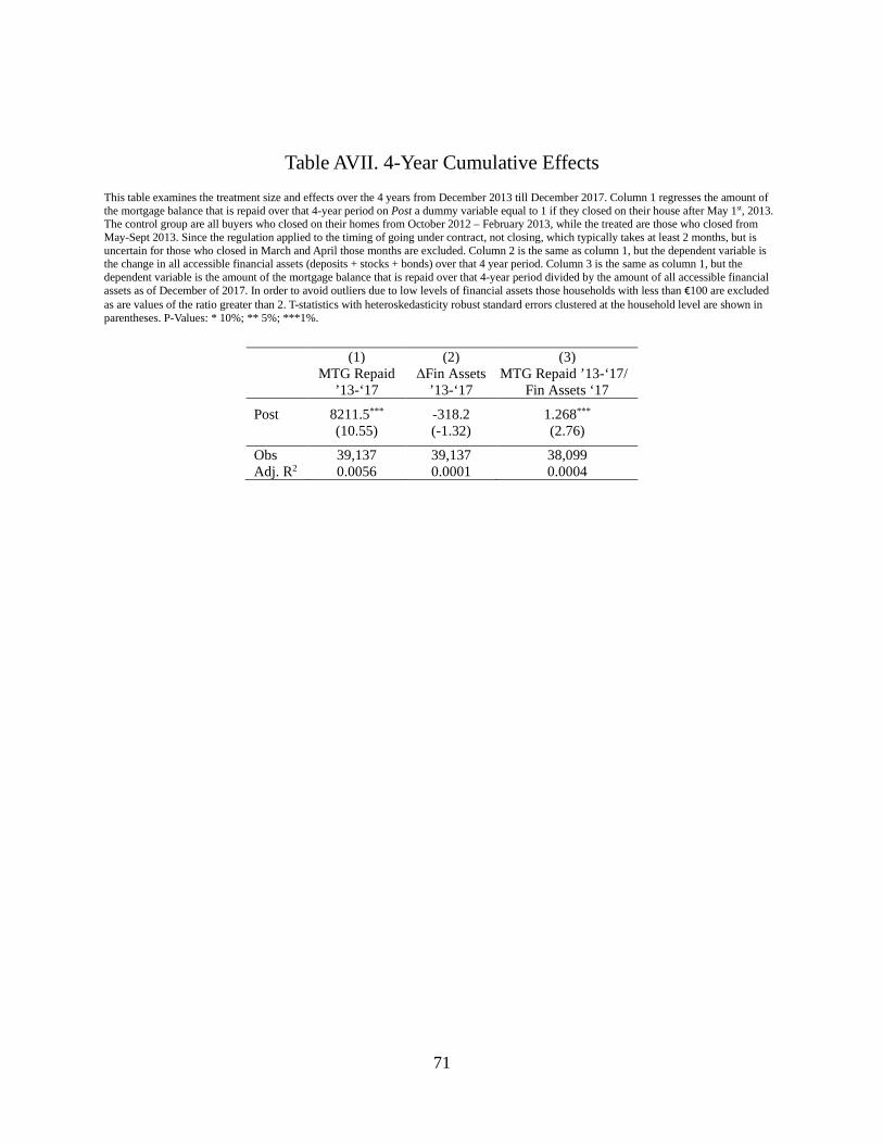
71

Table AVII. 4-Year Cumulative Effects This table examines the treatment size and effects over the 4 years from December 2013 till December 2017. Column 1 regresses the amount of the mortgage balance that is repaid over that 4-year period on Post a dummy variable equal to 1 if they closed on their house after May 1st, 2013. The control group are all buyers who closed on their homes from October 2012 – February 2013, while the treated are those who closed from May-Sept 2013. Since the regulation applied to the timing of going under contract, not closing, which typically takes at least 2 months, but is uncertain for those who closed in March and April those months are excluded. Column 2 is the same as column 1, but the dependent variable is the change in all accessible financial assets (deposits + stocks + bonds) over that 4 year period. Column 3 is the same as column 1, but the dependent variable is the amount of the mortgage balance that is repaid over that 4-year period divided by the amount of all accessible financial assets as of December of 2017. In order to avoid outliers due to low levels of financial assets those households with less than €100 are excluded as are values of the ratio greater than 2. T-statistics with heteroskedasticity robust standard errors clustered at the household level are shown in parentheses. P-Values: * 10%; ** 5%; ***1%.

(1) (2) (3) MTG Repaid

’13-‘17 ΔFin Assets

’13-‘17 MTG Repaid ’13-‘17/

Fin Assets ‘17

Post 8211.5*** -318.2 1.268*** (10.55) (-1.32) (2.76)

Obs 39,137 39,137 38,099 Adj. R2 0.0056 0.0001 0.0004

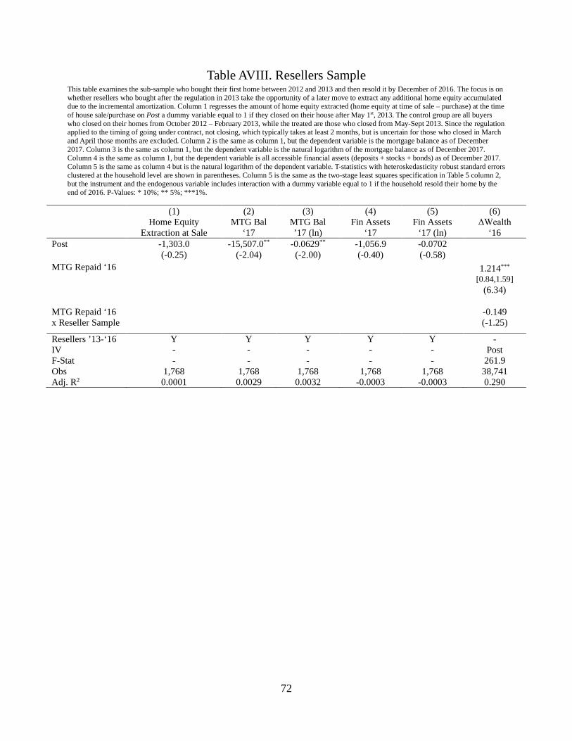
72

Table AVIII. Resellers Sample This table examines the sub-sample who bought their first home between 2012 and 2013 and then resold it by December of 2016. The focus is on whether resellers who bought after the regulation in 2013 take the opportunity of a later move to extract any additional home equity accumulated due to the incremental amortization. Column 1 regresses the amount of home equity extracted (home equity at time of sale – purchase) at the time of house sale/purchase on Post a dummy variable equal to 1 if they closed on their house after May 1st, 2013. The control group are all buyers who closed on their homes from October 2012 – February 2013, while the treated are those who closed from May-Sept 2013. Since the regulation applied to the timing of going under contract, not closing, which typically takes at least 2 months, but is uncertain for those who closed in March and April those months are excluded. Column 2 is the same as column 1, but the dependent variable is the mortgage balance as of December 2017. Column 3 is the same as column 1, but the dependent variable is the natural logarithm of the mortgage balance as of December 2017. Column 4 is the same as column 1, but the dependent variable is all accessible financial assets (deposits + stocks + bonds) as of December 2017. Column 5 is the same as column 4 but is the natural logarithm of the dependent variable. T-statistics with heteroskedasticity robust standard errors clustered at the household level are shown in parentheses. Column 5 is the same as the two-stage least squares specification in Table 5 column 2, but the instrument and the endogenous variable includes interaction with a dummy variable equal to 1 if the household resold their home by the end of 2016. P-Values: * 10%; ** 5%; ***1%.

(1) (2) (3) (4) (5) (6) Home Equity

Extraction at Sale MTG Bal

‘17 MTG Bal ’17 (ln)

Fin Assets ‘17

Fin Assets ‘17 (ln)

ΔWealth ‘16

Post -1,303.0 -15,507.0** -0.0629** -1,056.9 -0.0702 (-0.25) (-2.04) (-2.00) (-0.40) (-0.58) MTG Repaid ‘16 1.214*** [0.84,1.59] (6.34)

MTG Repaid ‘16 -0.149 x Reseller Sample (-1.25)

Resellers ’13-‘16 Y Y Y Y Y - IV - - - - - Post F-Stat - - - - - 261.9 Obs 1,768 1,768 1,768 1,768 1,768 38,741 Adj. R2 0.0001 0.0029 0.0032 -0.0003 -0.0003 0.290