Understanding the timing and magnitude of advertising ... - Lirias

Understanding the timing and magnitude of advertising spending patterns

M.J. Gijsenberg, H.J. van Heerde, M.G. Dekimpe, J.-B.E.M. Steenkamp and V.R.Nijs

DEPARTMENT OF MARKETING AND ORGANISATION STUDIES (MO)

Faculty of Business and Economics

OR 0901

UNDERSTANDING THE TIMING AND MAGNITUDE

OF ADVERTISING SPENDING PATTERNS

Maarten J. Gijsenberg

Harald J. van Heerde

Marnik G. Dekimpe

Jan-Benedict E.M. Steenkamp

Vincent R. Nijs

June 11, 2009 Maarten J. Gijsenberg is a Doctoral Candidate at the Catholic University of Leuven and Researcher in Marketing at the Louvain School of Management & FUCaM (e-mail: [email protected]). Harald J. van Heerde is Professor of Marketing at the Waikato Management School, University of Waikato (e-mail: [email protected]). Marnik G. Dekimpe is Research Professor of Marketing & CentER Fellow at Tilburg University, and Professor of Marketing at the Catholic University of Leuven (e-mail: [email protected]). Jan-Benedict E.M. Steenkamp is C. Knox Massey Distinguished Professor of Marketing and Marketing Area Chair, Kenan-Flager Business School, University of North Carolina at Chapel Hill (e-mail: [email protected]). Vincent R. Nijs is Assistant Professor of Marketing at the Kellogg School of Management, Northwestern University (e-mail: [email protected]).

1

UNDERSTANDING THE TIMING AND MAGNITUDE

OF ADVERTISING SPENDING PATTERNS

Abstract

Notwithstanding the fact that advertising is one of the most used marketing tools, little is

known about what is driving (i) the timing and (ii) the magnitude of advertising actions. Building

on normative theory, the authors develop a parsimonious model that captures this dual investment

process. They explain advertising spending patterns as observed in the market, and investigate the

impact of company, competitive, and category-related factors on these decisions, thereby

introducing the novel concept of Ad-sensor. Analyses are based on a unique combination of (i)

weekly advertising data on 748 CPG brands in 129 product categories in the UK, (ii) household

panel purchase data, and (iii) data on new product introductions. The analyzed brands include

both large and small brands, both frequent and infrequent advertisers, thus providing a more

complete and correct overview of the market. The results show that advertising spending patterns

can be explained as real-life applications of the normative literature, in which advertising and

advertising goodwill management are embedded in dynamic (s,S) inventory systems. Adstock

and Ad-sensor show a positive effect on both timing and magnitude decision. Competitive

reasoning is found to have little to no effect on advertising decisions, whereas category-related

factors do show an impact. The extent to which campaigning strategies are more or less the

outcome of advertising goodwill management systems, however, varies across brands as a

function of their relative size and advertising frequency.

Key words: Advertising, timing, competition, Tobit-II, Bayesian inference

2

1. Introduction

Advertising is one of the most important marketing instruments. For example, in 2006,

US adspend totaled $285.1 billion, representing 2.2% of the country’s GDP. Companies as

Procter & Gamble and AT&T spend billions of dollars per year on advertising (AdAge, 2007).

Given its prominent position, it should come as no surprise that advertising, and the way it affects

people’s decisions, has been the subject of an extensive body of prior research (see e.g. Tellis and

Ambler 2007 for a recent review). The main focus of these studies was on the quantification of

advertising’s effectiveness. Studies explaining observed advertising spending patterns, in

contrast, have received much less attention. Still, insights into why brands start/stop advertising

are very relevant to advertising media and advertisers alike. The former will benefit from a

profound understanding of the purchase behavior of their customers, i.e. the spending patterns of

advertising brands. Advertisers, in turn, are interested in accurate predictions on the expected

timing and size of their competitors’ spending in order to gauge the extent of competitive

interference they may expect (cfr. Danaher et al., 2008).

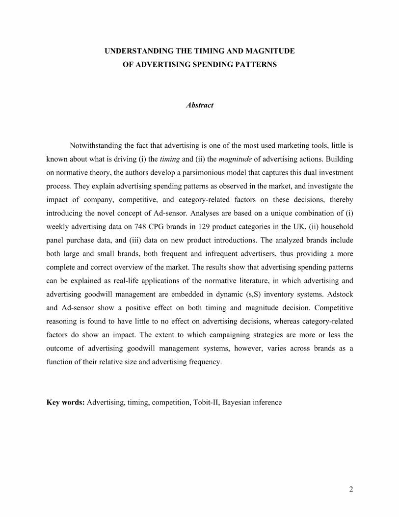
Figure 1. Weekly advertising for three brands in the UK soft drink and cleanser markets

The figures between brackets show the percentage of weeks with advertising actions and the average magnitude of these actions

Softdrink A (100%, £347,348) Softdrink B (59%, £134,481) Softdrink C (42%, £44,784)

0

200000

400000

600000

800000

1000000

1200000

1400000

1 8 15 22 29 36 43 50 57 64 71 78 85 92 99 106 113 120 127 134 141 148 1550

200000

400000

600000

800000

1000000

1200000

1400000

1 8 15 22 29 36 43 50 57 64 71 78 85 92 99 106 113 120 127 134 141 148 1550

200000

400000

600000

800000

1000000

1200000

1400000

1 8 1 5 2 2 29 3 6 4 3 50 5 7 64 71 7 8 85 92 9 9 1 06 11 3 12 0 1 27 13 4 14 1 14 8 15 5

0

200000

400000

600000

800000

1000000

1200000

1400000

1 9 17 25 33 41 49 57 65 73 81 89 97 105 113 121 129 137 145 1530

200000

400000

600000

800000

1000000

1200000

1400000

1 9 17 25 33 41 49 57 65 73 81 89 97 105 113 121 129 137 145 1530

200000

400000

600000

800000

1000000

1200000

1400000

1 9 17 25 33 41 49 57 65 73 81 89 97 105 113 121 129 137 145 153

Cleanser A (81%, £120,737) Cleanser B (53%, £86,982) Cleanser C (34%, £79,999)

3

As shown in Figure 1, considerable variation exists along both the timing and size

dimension. The first three panels exhibit the weekly advertising expenditures for three soft-drink

brands in the UK. Brand A is a frequent and heavy advertiser (100% of the time, average

spending £347,348 per week), while brand C is situated at the other end of the spectrum. It

engages only occasionally in advertising actions (42% of the time), and when doing so, spends

only small amounts (£44,784 on average). Brand B takes an intermediate position: it advertises

less often than brand A (59% of the time), but spends a larger amount on these sparse actions

than C (£134,481 on average). The bottom panels of Figure 1 depict three brands in the UK

cleanser market. Also in that market, considerable variability is observed in both the timing and

the size dimension. Moreover, the absolute spending level appears to be considerably lower than

in the soft-drink market. What is driving this over-time variation within a given brand? Why do

we find such substantial differences across brands? Or across industries?

Some features of these observed patterns may have emerged as the result of applying the

guidelines of a series of normative studies which have shown that, in most instances, pulsed

advertising is an optimal strategy (e.g. Mahajan and Muller, 1986; Mesak, 1992; Park and Hahn,

1992; Villas-Boas, 1993; Naik et al.,1998). These studies, however, although insightful on the

optimality of pulsed over even spending, remain vague on some crucial implementation issues,

including (i) how often to advertise, (ii) how many weeks an advertising pulse or campaign

should last, and (iii) how much should be spent. Moreover, (iv) they do not provide insights on

the observed behavioral differences between brands and categories. As such, and differing from

our study, their objective is not to explain the variation found in observed behavior. Such real

world behavior, in contrast, was the focus of a body of empirical studies (e.g. Metwally, 1978;

Jones, 1990; Hanssens, 1980a+b; Chandy et al., 2001; Steenkamp et al., 2005). These studies

manage to capture and explain very well the behavior under examination, but are weaker in the

theoretical foundations of their explanations, thus almost being the opposite of the normative

studies.

We build on the normative literature, and develop a framework which allows us to

describe and understand the advertising behavior as observed in the market, and this along two

dimensions: (i) the timing of advertising actions (i.e. whether or not to advertise), and (ii) the

4

magnitude of these actions. We subsequently relate observed differential behavior across brands

to the size of the brands, and the experience they have in advertising.

We begin with an overview of the relevant literature. We subsequently present our

conceptual framework, and introduce the core concepts of this study. We describe our

econometric model, and give some initial insights in our data. We then present our empirical

results, and conclude with a discussion of the key managerial insights and some areas for future

research.

2. Relevant Literature

The current paper can be positioned against two research streams: (i) normative studies on

optimal advertising behavior, (ii) empirical studies on advertising and its effectiveness.

Normative literature

Over the past decades, the preponderance of the prescriptions from normative studies on

the optimal timing of advertising has shifted from constant advertising schedules (Zielske, 1959;

Sasieni, 1971; 1989) to pulsing advertising schedules (e.g. Mahajan and Muller, 1986) as more

and more real-world effects were included in the analyses. For example, Katz (1980) introduced

learning and forgetting effects, while Mesak (1992) and Naik et al. (1998) added, respectively,

wear-out effects and quality restoration. Park and Hahn (1992), Villas-Boas (1993) and Dubé et

al. (2005), in turn, extended the analyses to competitive settings. In most instances, pulsed

advertising is now considered to be the optimal strategy for firms. Whereas pulsing is used as a

generic term describing advertising schedules alternating high and low levels of advertising,

flighting (e.g. Katz, 1980) is more strict in its definition as it refers to alternation between high

and zero levels of advertising. As such, it is an extreme case of pulsing. Finally, the concept of

campaigning (Doganoglu and Klapper, 2006) was introduced to describe the fact that advertising

pulses are often not one-time spikes, but regularly last several weeks.

Pulsing strategies appear to be frequently applied by managers (Feinberg, 1992).

Recently, Dubé et al. (2005) found evidence that the observed behavior in the US Frozen Entrée

category could be explained as a pulsing strategy based on a dynamic competitive game.

5

Doganoglu and Klapper (2006), covering the German Detergent Market, found similar support

for the application of the normative guidelines in the real world decisions they studied. Finally,

such patterns are also widely present in our own dataset (cfr figure 1), in which only 6 of the 748

included brands advertise permanently, alternating between high and low levels of advertising.

However, in contrast with their general agreement on the optimality of pulsed advertising

strategies, these normative studies provide less clarity on a number of issues related to the actual

implementation of the advocated strategies. Analysis of real world advertising spending patterns

indeed showed that, although pulsing strategies are often encountered, large differences are

observed both within and between brands in (i) the actual timing of advertising campaigns, (ii)

the number of weeks such campaigns last, and (iii) the monetary value of campaigns. Overall,

very few normative studies go into that level of detail, and three limitations of these studies thus

appear. First, these studies mainly focus on the timing of advertising actions within campaigns,

thereby leaving especially decisions on the magnitude of these actions uncovered. Second, they

provide guidelines for a single brand, thereby ignoring differences in individual brands’

advertising preferences as well as factors that may systematically affect advertising decisions

across different brands and categories. Finally, as a corollary of this single-brand focus, only very

few studies allow advertising decisions to be correlated with the decisions of other brands (Park

and Hahn, 1992; Villas-Boas, 1993; Dubé et al., 2005).

Empirical literature

In a wide series of econometric studies on advertising, measuring the effectiveness of

advertising takes a central position. Performance was treated as a function of advertising

expenditures in so-called single equation models (e.g. Lambin and Palda, 1969; Lambin, Naert

and Bultez, 1975). These models treated advertising as exogenous, without investigating how

spending patterns were formed. This exogeneity assumption was relaxed in subsequent

simultaneous equation models, starting with Bass (1969) and including work by Bass and Parsons

(1969) and Hanssens (1980a), as in more recent VAR models (Dekimpe and Hanssens, 1995a;

1999). The latter not only allow for feedback effects (when past own performance helps explain

current spending), but also competitive interactions. A recent study in this field is Steenkamp et

al. (2005), who used vector-autoregressive models to study advertising reaction strategies in 442

packaged goods categories.

6

A major strength of these studies is that they, in contrast to the normative studies, look

further than the explanation of the behavior of just one brand, and try to explain patterns across

brands and categories. However, this body of research shares three important limitations. First of

all, the theoretical background in these studies is often rather limited. Often, observed patterns are

explained without a concise and consistent theoretical framework grounded in the normative

literature. Second, although advertising expenditures are no longer treated as exogenous, no

distinction is made between the decisions to advertise or not (timing), and how much to spend

when advertising (magnitude), even though the factors that drive both decisions could (partly) be

different or have different weights. Finally, most (if not all) of these studies show a bias towards

large and frequently acting brands. This is due to the fact that most time-series techniques have

problems with large numbers of zeros and irregular patterns (e.g. in advertising spending), as is

often the case with smaller brands. Steenkamp et al. (2005), for example, limited themselves to

those top-3 brands in each category that also had an average share larger than 5%, and that

advertised at least more than 12% of the time (25 out of 208 weeks). Zanutto and Bradlow (2006)

showed that such data pruning may bias the overall inferences, as the included brands are only

representative for a small subset of all brands in the market. Hence, the empirical generalizations

derived in these studies may only be valid for that specific subset.

Our study

We build upon the insights of the existing normative literature on optimal advertising

scheduling by including campaigning in our framework. Two crucial elements in our work are

the concepts of Adstock and Ad-sensor, capturing the campaigning state dependence of brands

and their dynamic pulsing behavior, respectively.

The definition of campaigning implies two basic conditions. First of all, campaigns are

defined as prolonged periods of advertising, alternated by periods without advertising. Once

advertising has begun, it will be continued for some time. This state dependence will be captured

by the Adstock concept, a concept which is widely known and used in advertising research (e.g.

Broadbent, 1984; Hanssens et al., 2001). The probability of a new advertising action will be

higher if a brand was also advertising in the previous weeks, which has resulted in higher

Adstock. Conversely, the probability of no new advertising action will be higher if the brand was

7

not advertising in the previous weeks, during which Adstock was depleting, resulting in a lower

Adstock level. The second condition holds that, at a certain moment in time, one has to start a

new campaign, i.e. start advertising. Conversely, at a certain moment in time, a campaign will

end, and one has to stop advertising. Managers want to keep their Adstock above a certain level.

As soon as the Adstock, built by previous campaigns, has depreciated to a that level, one will

start advertising. Similarly, one is likely to stop advertising once a desired (higher) level has been

reached again. Such advertising reasoning shows close resemblance to so-called (s,S) inventory

management systems. Such systems keep the stock of a certain item between a minimum level s

and a maximum level S, by repurchasing if the stock becomes too small, up to the desired

maximum level. Although very popular and widely used in logistics (e.g. Silver et al., 1998),

applications in advertising research are rather scarce (Zufryden, 1979; Doganoglu and Klapper,

2006).

As such, we build a parsimonious and flexible model which captures in a straightforward

way how observed advertising spending patterns could result from dynamic advertising

adjustment strategies. We address weaknesses of previous research by incorporating four main

challenges in our model specification: (i) we allow for differential processes driving the timing

and magnitude decisions, (ii) we accommodate heterogeneous preferences and behavior across

brands, (iii) we examine the effect of moderating variables across brands and categories, and (iv)

we accommodate correlations between the brands decisions within the same category.

Our study, in addition, is unique in its empirical scope, covering advertising decisions on

a weekly basis for 748 brands in 129 CPG categories. We include all brands in these categories

that advertise in our study, regardless of their advertising intensity (provided that they advertise

at least once, otherwise the issue becomes moot) and their Brand market share. An illustration of

the relative importance of this issue can be found in figure 2. This figure depicts the

consequences of the application of the decisions rules as used in Steenkamp et al. (2005) to our

dataset. We categorize all brands according to their compliance (Y/N) with the size (top 3,

minimum 5% market share) and frequency limitation (minimum advertising frequency of 12%).

8

Figure 2. Application of the Steenkamp et al. (2005) data pruning rules to our dataset

N = 151Combined share of advertising = 63.9%

Mean market share = 18.4%Mean combined market share = 32.7%Mean advertising share in category = 41.2%Mean number of advertising weeks = 82




Mean market share = 1.0%Mean combined market share = 3.2%Mean advertising share in category = 3.9% Mean number of advertising weeks = 6



Advertising Frequency > 12% Advertising Frequency ≤ 12%

Top 3 AND

Market share > 5%

Not Top 3 OR

Market share ≤ 5%

For each block we report the Number of brands (N); their Combined share of advertising

in our dataset; Mean market share; Mean combined market share; Mean advertising share in their

category; and the Mean number of advertising weeks. If we only include the brands in our

empirical dataset that fulfill both requirements, we would cover only 63.9% of all advertising

expenditures. Brands would have an average market share of 18.4%, and an advertising share of

41.2%, advertising on average 82 out of 156 weeks. However, these brands, on average, account

for only 32.7% of the total market, covering, on average, between 0.6% and 99% of category

advertising expenditures as included in our dataset. Limiting the number of included brands

would clearly lead to the omission of a major part of the observed advertising actions and

expenditures from our analyses. Relaxing the aforementioned requirements hence appears

recommended. Relaxing the size limitation, would enable us to cover over 98% of all advertising

expenditures. In addition, although infrequent advertisers represent only a very small percentage

of advertising expenditures, they still account for almost 50% of the advertising brands, and

nearly 10% of all advertising actions. Understanding how their behavior may differ from more

frequently acting brands is consequently warranted if we want to understand advertising as we

observe it in the market. The unique dataset we thus obtain, allows us to formulate a set of

insightful empirical generalizations on the timing and magnitude of observed advertising

patterns.

9

3. Drivers of Advertising Investment Decisions

Advertising decisions can be seen as a multiple decision process. Two key decisions

which have to be taken, are when to advertise, and how much to spend (Tellis, 2004 p 72;

Danaher, 2007 p 645; Danaher et al., 2008). This dual advertising decision is treated as an

investment decision process, which is in line with the growing stream of literature claiming that

marketing expenditures are more and more considered to be investments (Srivastava et al., 1999).

At each point in time, the brand therefore chooses (i) whether or not to advertise (timing), and,

(ii) conditional upon this decision, how much to spend (magnitude) (e.g. Bar-Ilan and Strange,

1999).

Adstock

Central to our model are the concepts of Adstock and Ad-sensor, which in itself is also

derived from Adstock. These concepts capture two crucial aspects of advertising investments.

The tendency to concentrate advertising investments in longer pulses or campaigns, as we will

show, is captured by our Adstock variable (Broadbent (1984). Ad-sensor is subsequently

introduced as a feedback variable mimicking the brand’s decision rule to start and stop

advertising campaigns. This basic advertising investment decision process is depicted in figure 3.

Figure 3. Basic advertising decision process.

Timing of Advertising

Action

Size of Advertising

Action

Advertising Decisions

Adstock Management

• Adstock• Ad-sensor

Advertising Drivers

The Adstock concept was originally developed to assess the dynamic effects of

advertising. It rests on the assumption that advertising helps to build a stock of advertising

goodwill (Broadbent, 1984). In the absence of further advertising spending, however, this

Adstock decays at a constant rate (see e.g. Dekimpe and Hanssens, 2007). In the past, it has been

10

used in studies on e.g. advertising awareness (Brown, 1986), television advertising effectiveness

(Tellis and Weiss, 1995), television scheduling (Broadbent et al., 1997; Ephron and McDonald,

2002), trial of new products (Steenkamp and Gielens, 2003), product-harm crises (Cleeren et al.,

2007) and competitive advertising interference (Danaher et al., 2008). In line with these studies,

we follow the definition by Broadbent (1984) and operationalize Adstock of brand b as:

(1) 1,,, )1( −+−= tbbtbbtb AdstockgAdvertisinAdstock λλ

Advertising is often scheduled in campaigns of several consecutive weeks, followed by

zero advertising during a number of weeks. The likelihood of a brand advertising in week t will

consequently be higher when it was also advertising in the weeks before. During this period,

Adstock will be built by means of advertising actions. So, a brand which is in a campaign keeps

advertising when its Adstock is at relatively high levels. Conversely, the likelihood of a brand not

advertising in week t will be lower when it was not advertising in the previous weeks. During

such periods, Adstock will be considerably lower as it decays when no new advertising

investments are made. We therefore expect a positive effect of Adstock on the likelihood of a

new advertising action in week t.

Conditional upon their decision to advertise, brands still have to determine the amount

they will spend on their action. As decision making processes are often characterized by a strong

preference for the status quo (e.g. Samuelson and Zeckhauser, 1988), previous behavior is a

particularly good predictor of new actions (e.g. Srinivasan et al., 2007). Higher advertising levels

during the previous weeks of a campaign are therefore likely to be followed by higher levels in a

subsequent action, provided that the brand chooses to advertise. Higher previous advertising

expenditures during a campaign, in turn, are reflected in relatively higher Adstock levels,

whereas lower advertising levels will have resulted in relatively lower Adstock levels. We

therefore can expect that brands, conditional on the decision to advertise, will spend more on

such new actions when their Adstock level is higher.

Together, these two effects, both in timing and magnitude of advertising actions, show

how Adstock captures the state dependence of brands in their advertising decisions.

11

Ad-sensor

Although Adstock provides a better understanding of the campaigning state dependencies,

it is less insightful on why brands would start or stop an advertising campaign. What triggers the

launch of new campaigns? Why and when do they end? Answers to these questions can be found

by analyzing the goals of advertising investments. By means of advertising, brands build

advertising goodwill among consumers. This goodwill is expected to translate into sales, and

should consequently not fall below a certain level. If this, however, would be the case, new

advertising investments become necessary to preserve and strengthen sales. At that moment, a

new campaign will be launched. The ultimate goal of any brand would be to achieve unlimited

goodwill. However, advertising budgets are not unlimited. We therefore assume that a specific

target level of goodwill will be determined for each campaign, the level of which is unknowng to

us. In the beginning of a campaign, when goodwill build-up has just started, incentives to stop

will be rather small. The closer to that target level, however, the lower will be the need to

continue investing. In addition, once it has been reached, there is a clear incentive to stop

investing. The pressure a brand feels to start a campaign as soon as its goodwill among

consumers becomes too low, and to stop that same campaign when the desired (higher) goodwill

level is reached, is the essence of our Ad-sensor concept.

We define our Ad-sensor by integrating the Adstock concept in an (s,S) stock

replenishment system. As such, s represents the minimum Adstock level a brand wants to

maintain, whereas S is the (higher) target level. The implicit goal of such (s,S) systems is hence

to maintain the stock between the two levels. These levels are known to the brand manager, but

unknown to the researcher. In addition, managers can apply dynamic strategies in their choice of

these minimum and maximum levels, thus allowing for different levels in different campaigns.

We therefore consider the observed minimum and maximum levels as the actual outcomes of

managers’ utility maximization calculi.

To model this (s,S) behavior, we first consider what happens when the Adstock of brand b

falls below the minimum desired level. At that moment, the brand should start advertising again.

The brand will launch a new campaign, and will continue to invest in advertising until the target

is reached. At that maximum, the first derivative of Adstock to time is zero, at least in continuous

time. Since we are using discrete time observations, however, at time t the researcher can only

observe up to time t-1, so the first order condition is equivalent to:

12

(3) 01, =Δ

Δ −

tAdstock tb .

this becomes:

(4) 02,1, =Δ

− −−

tAdstockAdstock tbtb

(5) 02,1, =−⇔ −− tbtb AdstockAdstock .

Given our additive Adstock function, this is satisfied if:

(6) 0)1( 2,2,1, =−+− −−− tbtbbtbb AdstockAdstockAdvert λλ

(7) 2,1, )1()1( −− −=−⇔ tbbtbb AdstockAdvert λλ

(8) 2,1, −− =⇔ tbtb AdstockAdvert

The second-order condition for a maximum requires that in the period before the maximum, t-1,

Adstock is still increasing, which requires that . Based on these

observations, we define our Ad-sensor variable as the difference between Adstock in time t-1 and

Adstock in t-2:

3,2, −− > tbtb AdstockAdvert

(9) 2,1,, −− −= tbtbtb AdstockAdstockAdsensor

The full mathematical derivation of Ad-sensor is given in appendix A. As such, the Ad-sensor

allows us to capture the evolution of a brand’s Adstock, and the associated pressure to advertise.

During the build-up of Adstock, Ad-sensor will have positive values. Over time, as Adstock

increases, these values start to decrease. Once the target maximum Adstock level S was reached,

Adstock becomes negative, a clear incentive to stop advertising. Over time, Adstock depletes,

and Ad-sensor increases again, implying an increasing pressure for the brand to advertise again.

To provide better insights in the functioning of this system, we simulate a series of

advertising actions. In our simulation, we impose values on the carry-over parameter λ, which is

used to calculate Adstock and consequently Ad-sensor, and the minimum and maximum Adstock

levels s and S. In practice, however, we estimate all parameters based on the observed advertising

patterns. The numerical build-up of this example is included in appendix B. The evolution of the

associated Ad-sensor is represented in figure 4. The solid grey line represents the advertising

expenditures, the dotted black line the created Adstock and the solid black line the Ad-sensor. As

indicated by equation 9, the latter represents the recent change in Adstock due to advertising

investments.

13

Figure 4. Advertising, Adstock and Ad-sensor

In week 4, the brand launches a new campaign, as Adstock has fallen below the allowed

minimum level s. As a corollary of our Adstock definition, Adstock will increase as long as the

advertising investments are larger than the previous Adstock level (see appendix A). The first

investments start building Adstock, but at the same time as well increase the pressure not to stop

the campaign prematurely (captured by the Ad-sensor), as the desired level S is still far away. By

period 6, the Adstock level is increasingly approaching the advertising level, and increases in

Adstock start becoming smaller. Gradually, the brand is approaching the target Adstock level S.

This is also reflected in the Ad-sensor, which slowly starts to decay from period 7 on. Stopping

becomes less harmful, as the target level is getting closer. In week 10, the maximum (desired)

Adstock level has been reached. By week 11, Ad-stock starts to decay. Ad-sensor, in turn,

becomes strongly negative in the next period: the target of the campaign was attained, continued

investments make little sense. However, still some smaller amounts of advertising are typically

found at the end of advertising campaigns. These are often due to so-called make-goods (see e.g.

Doganoglu and Klapper, 2006), smaller actions often added at the end of campaigns in order to

compensate for lost opportunities during the campaign itself. Over time, Adstock depletes at a

constant rate λ (see equation 1), but not in constant absolute terms. When Adstock levels are still

high, depletion will be large in absolute terms, causing strong negative Ad-sensor values. Over

time, the Adstock level becomes smaller, and depletion will be smaller in absolute terms. This

results in a gradual increase of the Ad-sensor.

In sum: the Ad-sensor variable is essentially a feedback variable mimicking the brand's

decision rule to start and stop advertising. We thus expect a positive effect of the Ad-sensor on

the timing decision (yes or no). In addition, a similar effect is hypothesized for the magnitude

decision (given timing). A wider gap between the actual and the target Adstock level requires

14

stronger efforts to rapidly bridge this gap. As the brand gets closer to the target level, however,

this pressure becomes smaller, as the gap has become much smaller. Beyond the point in time

during which the target level was reached, the relevance of continued spending can be

questioned. The Ad-sensor tells brand that, if they still would be spending on advertising actions,

it should at least be small amounts.

Moderating factors of Adstock and Ad-sensor

The combination of Adstock and Ad-sensor creates a new model for the analysis of

advertising decisions. A subsequent investigation of the general applicability of this model across

a large set of brands is hence asked for. However, the extent to which Adstock is managed

between s and S may differ across brands. In this paper, we focus on two important brand

characteristics: Brand market share and Advertising frequency. The motivation for this choice is

threefold. First of all, both factors have commonly been used in the past as a basis for data

selection rules (e.g. Steenkamp et al., 2005). Brands typically included in previous studies on the

basis of such selection rules, however, are not representative for the market as a whole

(Slotegraaf and Pauwels, 2008), and inferences based on these subsets could be biased (Zanutto

and Bradlow, 2006). As we include all types of brands, understanding to what extent behavior

may differ for types of brands which were previously excluded from analyses is essential, and

can in addition provide insights on the extent to which data pruning rules could have altered our

findings. In addition, two other motivations explain our choice. Brand market share has emerged

from previous research as a key characteristic in advertising decisions (e.g. Patti and Blasko,

1981; Lynch and Hooley, 1990). Advertising decision making and its outcome will depend on the

market share a brand has and wants to maintain. Advertising frequency, in turn, may create

learning effects. An examination of the effect of advertising frequency consequently helps us to

understand if, and to what extent, more experienced brands have gained a relative advantage over

time in managing their Adstock.

Larger brands have more means at their disposal, and marketing budgets, moreover, are

often determined on a percentage of sales basis (Allenby and Hanssens, 2005). This will affect

the advertising decision process in two ways. These brands can reserve larger budgets for

marketing research compared to their smaller counterparts. They thus can be expected to be better

informed on how their advertising goodwill level is evolving, and can consequently better react

15

to it. We therefore expect a positive effect of Brand market share on the effect of Ad-sensor in

both decisions. In addition, their larger budgets allow them to pursue longer and more intense

advertising campaigns. The state dependence effect as implied by the Adstock will consequently

be higher for such brands.

Experience enables brands to adapt their organizations and processes in order to perform

optimally. The advertising decision process is no exception to this. More experienced brands

have become more efficient through learning effects and have established effective advertising

decision processes. On the organizational level, these decision processes tend to stay very similar

over time (Frederickson and Iaquinto, 1989), as organizations have to be reliable, accountable

and reproducible (Boeker, 1988). What has proven to be effective, will be continued. A

consistent closer monitoring of the advertising goodwill evolution as well as reactance to it can

consequently be expected. We therefore expect the effect of Ad-sensor to be positively affected

by Advertising frequency. This experience, built by more intense advertising strategies in the

past, moreover, will as well enable brands to better pursue longer and more intense advertising

campaigns. The effect of Adstock is consequently expected to be stronger for more experienced

brands.

Covariates

However, it is unlikely that advertising decisions are only influenced by brands’ own

internal advertising reasoning. Three main sets of factors are commonly considered: (i) Company

factors, (ii) Competitive factors, and (iii) Category or marketplace factors (Montgomery et al.,

2005).

First of all, brands will look at themselves. As advertising theory tells that New product

introductions should be combined with more intense advertising campaigns (e.g. Rossiter and

Percy, 1997; Kotler and Armstrong, 2004), especially because advertising has shown to be more

effective for new products (Lodish et al., 1995), we can expect a positive effect of such

introductions on the advertising decisions, resulting in a higher likelihood of advertising and

higher actual expenditures. Overall, however, advertising budgets are often set on a yearly basis

(e.g. Farris and West, 2007). In the course of the year, these budgets get depleted, most often

faster than expected, sometimes slower, creating relative shortage or slack resources by the end

of the year respectively. Given the common knowledge that having money leads to spending it,

16

we expect brands to spend their budgets relatively faster in the beginning of the year. This leaves

them with relatively fewer means at the end, and thus a negative impact of an End of year dummy

on the advertising decisions, resulting in fewer and smaller advertising actions, is hypothesized.

Next to themselves, brands will monitor their competitors and their own performance

relative to the latter. Competitive adstock captures the likelihood of competitive advertising

campaigns. The effect of this factor on the decision outcome is not clear a priori, as arguments in

both directions can be found, with brands clearly reacting on each other (e.g. Metwally, 1978;

Chen and MacMillan, 1992), or trying to avoid competitive clutter (Danaher et al., 2008). In

addition, brands frequently make decisions in order to perform well relative to their competitors,

on e.g. market share (e.g. Metwally, 1978; Armstrong and Collopy, 1996). However, as budgets

are often set as a percentage of past sales (see e.g. Allenby and Hanssens, 2005), a negative

Relative performance evolution versus competitors as expressed by a decrease in market share

may at the same time create a stronger urge to react and lower the ability to react. Here as well,

the effect on the advertising decisions is not clear a priori.

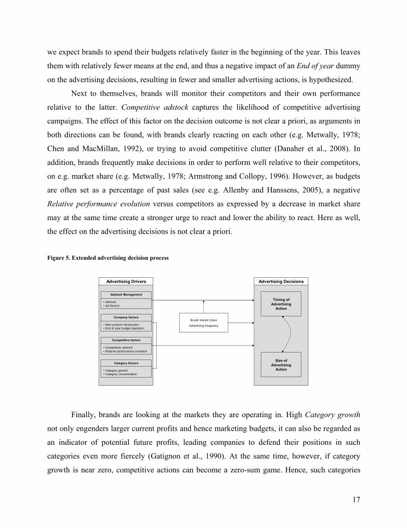
Figure 5. Extended advertising decision process

Timing of Advertising

Action

Size of Advertising

Action

Advertising Decisions

Adstock Management

• Adstock• Ad-Sensor

Company factors

• New product introduction• End of year budget depletion

Brand market share

Advertising frequency

Advertising Drivers

Competitive factors

• Competit ive adstock• Relative performance evolution

Category factors

• Category growth• Category concentration

Finally, brands are looking at the markets they are operating in. High Category growth

not only engenders larger current profits and hence marketing budgets, it can also be regarded as

an indicator of potential future profits, leading companies to defend their positions in such

categories even more fiercely (Gatignon et al., 1990). At the same time, however, if category

growth is near zero, competitive actions can become a zero-sum game. Hence, such categories

17

can be characterized by intense competition, also with advertising, to protect sales volumes

(Aaker and Day, 1986). Given the well-known detrimental impact of such strategies on the

profits of the brands, we hypothesize that the indicator-of-future-profit effect will be stronger

than the zero-sum effect, leading to a positive effect of category growth on the advertising

decisions. Categories with higher Category concentration are more open to collusive behavior,

leading to lower competitive interactions (e.g. Steenkamp et al., 2005), and thus likely as well to

lower advertising spending. We therefore expect to find a negative effect of concentration on the

advertising decisions.

The conceptual framework presented here is summarized in figure 5. We investigate the

ability of Adstock and Ad-sensor to explain advertising decisions, test the influence of

moderating factors Brand market share and Advertising frequency, while controlling for an

extensive set of other variables. We relate our results further to the literature when reporting our

empirical findings.

4. Model Development

Our conceptual framework implies four modeling requirements. First, we need to model

both the timing (yes/no) and spending decisions (monetary value), while allowing for different

response parameters for both decisions1. Second, these response parameters are allowed to vary

across brands. Third, we need to accommodate the effects of the moderating variables, preferably

in a simultaneous estimation step for maximal statistical efficiency. Fourth, the decisions of when

and how much to spend may be interrelated between brands within a category, and hence we

need to specify a full error covariance structure.

To meet these requirements we link the drivers to the two decision variables (i.e. timing

and magnitude) through a new multivariate Hierarchical Tobit-II model, which extends the

models of Fox et al. (2004) and Van Heerde et al. (2008) as these models do not comply with all

1 A similar framework, investigating timing and magnitude of capital stock investments, was introduced by Bar-Ilan and Strange (1999). The authors allowed the company to decide on both when and how much to invest, thereby going beyond existing literature that focused on either timing or intensity of investments. Bowman, Farley and Schmittlein (2000) extended this reasoning to the choice and level of use of international service providers. Dekimpe, Parker and Sarvary (2000), in turn, introduced a similar dual but also more sequential reasoning to international new product adoption processes. Finally, Gielens and Dekimpe (2007) applied a resembling framework to the entry strategy of retail firms into transition economies.

18

four requirements2. In the subsequent exposition, c refers to category (c=1,…,C) and b to brand

(b=1,…,BB

c).

Timing

An advertising decision in category c by brand b in week t ( ) is described by a

multivariate probit model:

cbtz

(10) ⎩⎨⎧ >

=otherwise

zifz cbt

cbt 001 *

Previous work suggests analyzing the decisions at a weekly level. In general, less data

aggregation provides more accurate results (Tellis and Franses, 2006). In addition, the managerial

survey reported by Steenkamp et al. (2005) indicated that brands can react to events as fast as

within one week, but generally not faster.

The latent variable , describing the timing decision process of the brand, is modeled

through a linear model:

*cbtz

(11) ,

cbttcb

tcb

tcb

tcb

tcb

tccb

tccb

tcbcb

tcbcb

tcbcb

tcbcb

tcbcb

tcbcbcb

cbt

TrendζQrtr3ζ

Qrtr2ζQrtr1ζHolidayζCatConcζ

CatGrowthζEOYζNPIζPerfEvolζ

kCompAdstocζsensorAdζAdstockζζz

μ+++

++++

++++

+−++=

−

−−

−−

5,24,2

3,22,21,21,8,1

1,7,1,6,1,5,11,4,1

1,3,1,2,11,1,10,1*

In equation (11) we first include a set of time-varying variables, i.e. Adstock and Ad-sensor and

the covariates Competitive adstock, Relative performance evolution, New product introduction,

End of year budget depletion, Category growth and Category concentration. In addition, we

control for holidays, seasonality, and possible trending behavior. As advertising decisions for

time t will be based on information available up to time t-1, we include 1 period lagged versions

of most time-varying explanatory variables.

Amount spent

Conditional on the decision to advertise ( = 1), we model , the natural logarithm

of the amount spent on advertising by brand b in category c during week t as:

cbtz cbty

2 These models do not allow for effects of moderating variables on the response parameters. In addition, in the work of Fox et al. (2004) no full error covariance structure is specified across the two equations; error covariance structures are separated for incidence and timing.

19

(12)

cbttcb

tcb

tcb

tcb

tcb

tccb

tccb

tcbcb

tcbcb

tcbcb

tcbcb

tcbcb

tcbcbcb

cbt

TrendQrtr3

Qrtr2Qrtr1HolidayCatConc

CatGrowthEOYNPIPerfEvol

kCompAdstocsensorAdAdstocky

εωω

ωωωω

ωωωω

ωωωω

+++

++++

++++

+−++=

−

−−

−−

5,24,2

3,22,21,21,8,1

1,7,1,6,1,5,11,4,1

1,3,1,2,11,1,10,1

We include the same explanatory variables in the magnitude equation as in the timing equation.

Although there is no specific requirement to have the same set in both equations, we include

them in an exploratory way to investigate whether all factors have an effect in both decisions.

Moderating factors

In their specific baseline advertising preferences (the intercepts) and their reactions to

their Adstock and Ad-sensor, brands may be guided by a number of own-company, and category

factors, as these may shape both the ability and the necessity to react. We therefore relate a subset

of the response parameters and to a set of moderator variables: cb1ζ

cb1ω

(13) cb

ccc

cbcbcb

uCosmeticsDrinksFood

AdvFreqtShareBrandMarkeζ

0,15,0,14,0,13,0,1

2,0,11,0,10,0,10,1

++++

++=

ζζζ

ζζζ

(14) .2,1,,12,,11,,10,,1,1 =+++= iforuAdvFreqtShareBrandMarkeζ cbicbicbii

cbi ζζζ

and

(15) cb

ccc

cbcbcb

eCosmeticsDrinksFood

AdvFreqtShareBrandMarke

0,15,0,14,0,13,0,1

2,0,11,0,10,0,10,1

++++

++=

ωωω

ωωωω

(16) .2,1,,12,,11,,10,,1,1 =+++= iforeAdvFreqtShareBrandMarke cbicbicbii

cbi ωωωω

The included moderator variables are time-invariant and allow us to measure the cross-sectional

variance in baseline advertising preferences as expressed by the intercept included in (11)-(12).

The categories included in our sample, can be categorized under four main product classes, i.e.

Household Products, Food, Drinks and Cosmetics. We control for the preferences of these four

product classes, using Household Products as reference category. In addition, we investigate the

possible moderating effect Brand market share and Advertising frequency can have on both the

baseline advertising preferences and the impact of Adstock and Ad-sensor on the advertising

decisions. Mean-centering of both variables allows us to examine the effects of deviations

relative to an ‘average’ brand. The effects of the covariates, captured by and (for i = cbi,1ζ

cbi,1ω

20

3…8), are related to the hyperparameters 0,,1 iζ and 0,,1 iω , and the brand-specific error terms

and .

cbiu ,1

cbie ,1

Decisions by one brand on when and how much to advertise are likely to impact those of

other brands. We therefore assume that the error vectors )',,( 1 tcBtcct cμμ K=μ and

)',,( 1 tcBtcct cεε K=ε follow a joint multivariate normal distribution, with a full variance-

covariance matrix: ~ ) . Finally, unobserved drivers of model parameters may

cause the error terms in (13) up to (16) to be correlated as well: ~ .

)',( ''ctct με ,0( cMVN Σ

)',( ''cbcb ue ),0( ΩMVN

We estimate model (11)-(16) with Bayesian techniques, i.e., Gibbs sampling. The benefit

of this approach over classical approaches is that it, at the same time, (i) accommodates the

multivariate nature of our dependent variable, (ii) allows for full variance-covariance between all

decisions by brands within the same category, and (iii) estimates the moderator effects

simultaneously with the other parameters rather than in a two-step approach. An overview of this

procedure is given in appendix C.

To operationalize the Adstock and Ad-sensor variables, we need to know the brand-

specific carry-over parameter bλ (see equation 2). To estimate these carry-over parameters, we use

the following traditional partial adjustment model (Hanssens et al., 2001 p147):

(17) tbtbbtbbbtb SalesAdvSales ,1,,, ln ελβα +++= −

Here as well, we use Gibbs sampling to obtain draws for bλ . For more details, we refer to

appendix D.

5. Data description

We estimate our model on 129 CPG categories in the UK. These categories cover nearly

completely the assortment offered in a typical supermarket. An overview of the included product

categories, along with the range of included brands, is given in table 1.

21

Table 1. Overview of included product types

Product Fields Examples No. of Categories Range of Brands

Assorted Foods Breakfast cereals, dry pasta, flour 23 1-11

Beverages Brandy, mineral waters, softdrinks 20 1-27

Cakes Oatcakes, crumpets pickelets and muffins 4 1-9

Candy Cereal bars, countline chocolate, fruit bars 7 1-15

Canned/bottled foods Canned fish, canned fruit 8 1-9

Care products Deodorants, shampoo, toilet tissue 22 1-27

Cleaning products Descalers, scouring powders, drain care 14 1-14

Dairy products Butter, cream, yoghurt 7 1-11

Frozen foods Frozen fish, frozen vegetables 4 2-6

Household supplies Batteries, car freshener 3 1-9

Pet products Dog food, cat litter 3 2-21

Taste enhancers Mustard, vinegar, Worcester sauce 14 1-30

Total 129 748

Four years of weekly advertising spending data were obtained from NielsenMedia, from

which we use one year (52 weeks) as initialization period, and three years (156 weeks) as

estimation period. All brands that (i) advertised at least once during the estimation period, and

(ii) were present in the market during the whole estimation period, were included. As such, both

small and large brands were considered, as reflected in the range of their average (across the three

years estimation period) market-shares, which varied from a low of 0.0002% to a high of

97.76%. We focused on national brands, as private labels have a very different positioning and

advertising strategy (Kumar and Steenkamp, 2007). Still, private labels were considered in the

derivation of certain covariates, as the concentration level in the industry or the national brands’

market shares. These decision rules resulted in a sample of 748 brands. Even though the focus

of the current paper is to study the spending pattern of brands that advertise, it is interesting to

note that 1855 brands never advertised during the considered three years, even though they were

in the market for the entire period.

Among the 748 brands that did advertise at least once, considerable variability exists in

their advertising behavior, as was already indicated in figure 2. First, the number of advertised

weeks varies greatly. About one out of ten brands advertised only once, while a few brands (6 in

total) advertised every week. However, the distribution is quite skewed, as nearly half of the

brands advertised less than 10% of the time (see figure 6).

22

Figure 6. Advertising weeks.

number of advertising weeks

339

117

63 5438 38

2615 22 21 15

1-15 16-30 31-45 46-60 61-75 76-90 91-105 106-120 121-135 136-150 151-156

Frequency of advertising across brands (# weeks out of 156)

Table 2 also provides evidence for the large variability in actual spending, even when

conditioning on those weeks where a given brand advertises. Some brands typically spend large

amounts (with an average level of £814,536 per week), while others spend only a limited amount

per week (£19).

Table 2. Advertising behavior of the Included Brands

Range Average Standard deviation

Number of Advertising Weeks 1-156 37 42

Average Spending per Advertising Week (in £) 19-814,536 56,756 72,150

Combining both dimensions (using a median split on, respectively, the number of weeks

of non-zero spending and the average value of such non-zero spending), we observe two main

types of advertisers in Figure 7: Heavy advertisers, who spend large amounts per week for

multiple weeks; and Light advertisers, limiting themselves to fewer actions and smaller amounts.

Even though the heavy advertisers in the top-left cell only account for 39.57% of the brands, they

represent 96.15% of the total advertising over the 3-year estimation period. Of these 296 brands,

only 140 would comply with the Steenkamp et al. (2005) decision rules. These 140 brands

account for 63.76% of all advertising expenditures. The remaining 11 of the 151 brands which

would comply with these rules would account for only 0.16%. Limiting ourselves to these 151

brands would hence result in a loss of information on more than 1/3 of all advertising

expenditures by branded products, in which especially the focus on large brands appears to have

23

strong consequences for the amount of advertising that is covered by the analyses. However, even

though infrequent advertisers account for only a small part of total advertising expenditures, they

still represent a large number of players, and hence in total as well a large number of advertising

actions. By including them as well in our analyses, we can provide a better understanding of

advertising in the market as a whole, thereby also providing evidence on how behavior may differ

for smaller vs larger and more vs less frequently acting brands.

Figure 7. Brands in dataset classified by Number of Advertising Weeks vs Average Spending per Advertising Week, Based

on Median Split

Numbers between brackets show the number of brands which comply with the Steenkamp et al. (2005) decision rules.

As a second main data source, we had access (through TNS) to consumer panel purchase

data covering all purchases for over 17,000 families. These were used to calculate (i) the market

shares of the different players, (ii) the category concentration and, (iii) the extent of category

growth. Finally data on new product introductions (see e.g. Sorescu and Spanjol, 2008) were

obtained through ProductScan©.

Measurement

We now turn to the measurement of the different constructs. In section 4, we already

provided an in-depth discussion of the Adstock and Ad-sensor concepts. The brand-specific

lambdas were obtained by a Bayesian regression estimation of a partial adjustment sales model

(Hanssens et al., 2001 p. 147), thereby allowing for correlations between brands’ sales within the

same category. An overview of the procedure can be found in appendix D. To account for the

uncertainty in the estimated lambdas, we use each of the 60,000 draws of the lambdas obtained

24

after burn-in of 30,000 draws to calculate brand-specific Adstock and Ad-sensor series. These

60,000 series are subsequently used in the actual model estimation, with a burn in of 30,000 and

sample of 30,000 draws for inference.

Advertising frequency equals the percentage of time the brand was advertised during the

52-week initialization period. In the choice of the data range to determine this factor, the aim is to

match as closely as possible the estimation sample. However, as we analyze advertising

decisions, Advertising frequency could suffer from endogeneity problems when estimated on the

156-week estimation period. This made us opt to determine the factor based on the 52-week

initialization period. These endogeneity problems, however, are not as severe for Brand market

share, which is consequently defined as the average market share over the 156-week estimation

period.

The first four weeks a new product is on the market, New product introduction will equal

1; the other weeks 0. Similarly, the last four weeks of the year, the End of year budget depletion

dummy variable will equal 1; the other weeks 0. Competitive adstock is defined as the weighted

average of the competitors’ Adstock values. The weights are dynamic, and based on the market

share in volume terms over the previous 26 weeks (see e.g. Nijs et al., 2001; 2007). Relative

performance evolution is expressed by the first difference of the logarithm of the brand volume

shares (see e.g. Deleersnyder et al. 2004), also defined over a moving window of the previous 26

weeks. Category growth is measured as the first difference of the log-transformed category

volume sales (cfr Franses and Koop, 1998). Finally, the Herfindahl index of volume shares over

the previous 26 weeks period is used to quantify the Category concentration. All

operationalizations are summarized in appendix E.

6. Empirical analysis

The coefficient estimates are shown in tables 3 and 4. They show the 95% posterior

density intervals for the estimates, the latter printed in bold if zero is not included in the interval.

Adstock Management

Adstock. Table 3 shows the expected positive effect of Adstock on the likelihood of

advertising actions ( 0,1,1ζ = 0.241). The conclusions of the stream of normative literature that

advertising in most instances can best be scheduled in pulses or campaigns, appear to be adopted

25

by the market. Brands show a clear state dependency, with periods of advertising during which

the Adstock is rebuilt followed by periods during which it is allowed to deplete again. This state

dependency, moreover, is also shown by the positive effect of Adstock on the magnitude of

advertising actions ( 0,1,1ω = 0.011). More intense actions during the previous weeks of an

advertising campaign, resulting in higher Adstock levels, will be followed by higher spending in

subsequent actions, implying that brands either opt for consistently high or low intensity

campaigns.

Table 3. Adstock Management: parameter estimates

Timing Magnitude

2.5th

percentile median

97.5th

percentile

2.5th

percentile median

97.5th

percentile

Adstock 0,1,1ζ 0.198 0.241 0.289 0,1,1ω 0.006 0.011 0.017

x Brand market share 1,1,1ζ 0.512 1.009 1.529 1,1,1ω -0.028 0.004 0.035

x Advertising frequency 2,1,1ζ 0.638 0.781 0.933 2,1,1ω 0.028 0.041 0.052

Ad-sensor 0,2,1ζ 0.107 0.130 0.150 0,2,1ω 0.066 0245 0.454

x Brand market share 1,2,1ζ 0.417 0.663 0.915 1,2,1ω -0.002 0.019 0.041

x Advertising frequency 2,2,1ζ 0.131 0.208 0.295 2,2,1ω 0.009 0.017 0.025

Brand market share 1,0,1ζ -0.089 0.822 2.325 1,0,1ω 0.066 0.245 0.454

Advertising frequency 2,0,1ζ 4.735 5.192 5.586 2,0,1ω 0.512 0.592 0.670

Ad-sensor shows a significant positive effect in the starting and stopping of advertising

campaigns ( 0,2,1ζ = 0.130). When the Ad-sensor values become too high, a brand will start

advertising. The closer to the desired maximum goodwill level in the campaign, the more likely

the brand will stop advertising. Once the target has been reached, negative values of the Ad-

sensor will increase the pressure to stop advertising even further. Over time, however, the

pressure to start a new campaign will start building again. Moreover, as long as one is still far

away from the goal level of Adstock for that specific campaign, i.e. when the Ad-sensor has

26

relatively higher levels, it will also remain a source of pressure to spend more in order to reach

the desired level faster ( 0,2,1ω = 0.006). Once the desired target has been reached, it gives clear

indications to no longer spend large amounts in case the brand would still decide to advertise.

This also captures quite well the phenomenon of make goods: the target level was reached, but

still some smaller remaining advertising can still be found at the end of the campaign.

The effects of Adstock and Ad-sensor for our numerical example, as well as their

combined effect, are represented in figure 8. This is an illustration for an ‘average’ brand, with

zero-effects of the mean-centered moderators. The first panel of figure 8 shows the effects on the

timing decision, in which the period during which advertising is taking place is indicated by the

grey zone. The second panel subsequently shows the effects on the magnitude decision

Figure 8. Effects of Adstock and Ad-sensor on Timing and Magnitude decision for our example

Moderators of Adstock and Ad-sensor

Brand market share. The larger brands in our set are likely to spend more on individual

advertising actions ( 1,0,1ω = 0.245). As marketing budgets are often set as a percentage of sales of

previous periods (e.g. Allenby and Hanssens, 2005), more powerful brands will have larger

budgets at their disposal, leading to more intense behavior. These brands, however, do not show

differential baseline preferences in relation to their timing decisions.

Larger brands are better able to respond to their internal advertising pressure relative to

smaller brands. Our results show that this is certainly the case in the timing decision ( 1,1,1ζ =

1.009, 1,2,1ζ = 0.663). However, in the magnitude decision, no significant effects could be found.

27

Advertising frequency. Brands advertising more frequently in the past will continue to do

so ( 2,0,1ζ = 5.192). This is in line with previous research showing that current brand actions are

often strongly influenced by previous behavior due to inertia effects (e.g. Frederickson and

Iaquinto, 1989; Nijs et al., 2007). In addition, these brands will also spend more when advertising

( 2,0,1ω = 0.592), confirming that basically two types of advertisers can be found: high-intensity

(advertising often, spending more per decision) and low-intensity (advertising less often,

spending less on single actions), as was already argued in the data section.

Our findings confirm the hypotheses that the effects of both Adstock and Ad-sensor are

stronger for more experienced brands, and this for both the timing and magnitude decisions

( 2,1,1ζ = 0.781 and 2,1,1ω = 0.041, respectively; 2,2,1ζ = 0.663 and 2,2,1ω = 0.017, respectively).

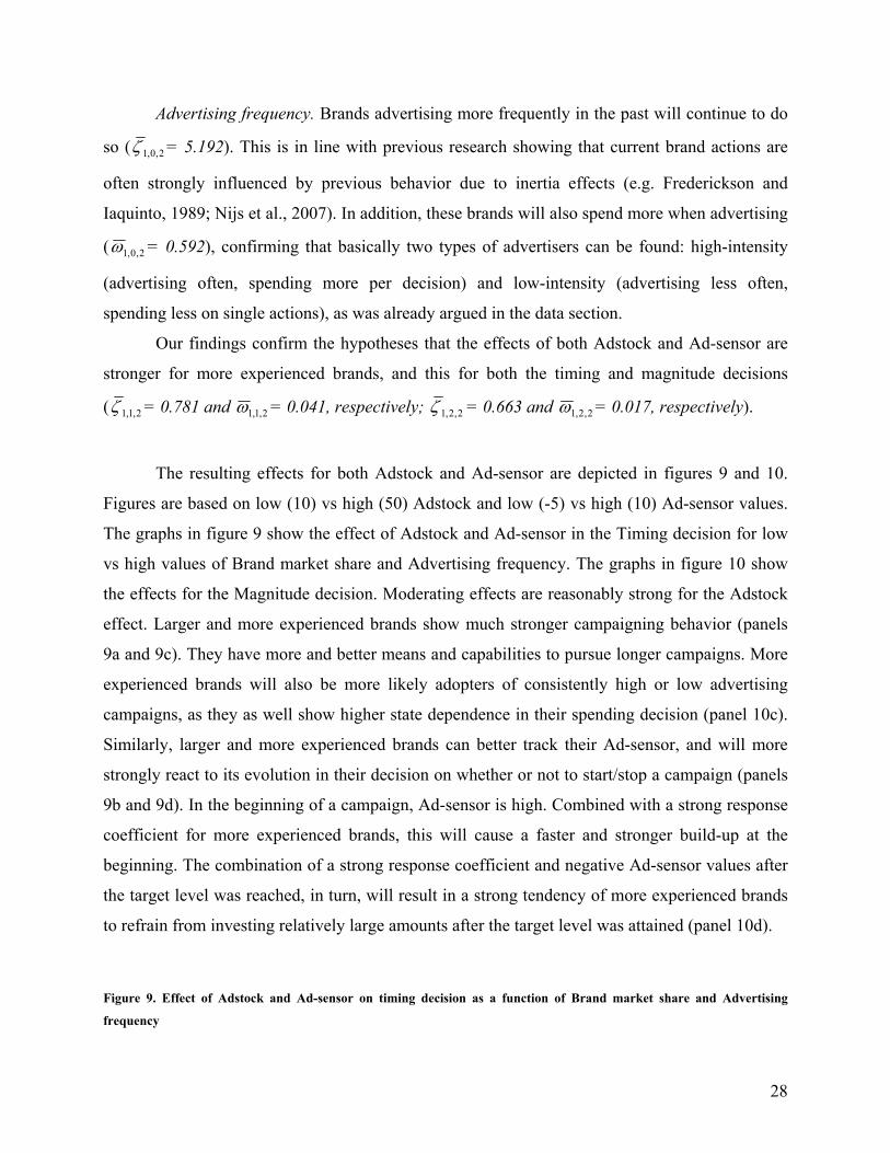
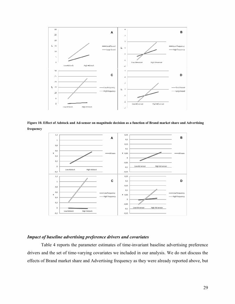
The resulting effects for both Adstock and Ad-sensor are depicted in figures 9 and 10.

Figures are based on low (10) vs high (50) Adstock and low (-5) vs high (10) Ad-sensor values.

The graphs in figure 9 show the effect of Adstock and Ad-sensor in the Timing decision for low

vs high values of Brand market share and Advertising frequency. The graphs in figure 10 show

the effects for the Magnitude decision. Moderating effects are reasonably strong for the Adstock

effect. Larger and more experienced brands show much stronger campaigning behavior (panels

9a and 9c). They have more and better means and capabilities to pursue longer campaigns. More

experienced brands will also be more likely adopters of consistently high or low advertising

campaigns, as they as well show higher state dependence in their spending decision (panel 10c).

Similarly, larger and more experienced brands can better track their Ad-sensor, and will more

strongly react to its evolution in their decision on whether or not to start/stop a campaign (panels

9b and 9d). In the beginning of a campaign, Ad-sensor is high. Combined with a strong response

coefficient for more experienced brands, this will cause a faster and stronger build-up at the

beginning. The combination of a strong response coefficient and negative Ad-sensor values after

the target level was reached, in turn, will result in a strong tendency of more experienced brands

to refrain from investing relatively large amounts after the target level was attained (panel 10d).

Figure 9. Effect of Adstock and Ad-sensor on timing decision as a function of Brand market share and Advertising

frequency

28

B A

C D

Figure 10. Effect of Adstock and Ad-sensor on magnitude decision as a function of Brand market share and Advertising

frequency

‐0,2

0

0,2

0,4

0,6

0,8

1

1,2

Low Adstock High Adstock

Y All sizes

‐0,15

‐0,1

‐0,05

0

0,05

0,1

0,15

0,2

0,25

Low Ad‐sensor High Ad‐sensor

Y All sizes

‐0,2

0

0,2

0,4

0,6

0,8

1

1,2

Low Adstock High Adstock

YLow frequency

High frequency

‐0,15

‐0,1

‐0,05

0

0,05

0,1

0,15

0,2

0,25

Low Ad‐sensor High Ad‐sensor

YLow frequency

high frequency

B A

C D

Impact of baseline advertising preference drivers and covariates

Table 4 reports the parameter estimates of time-invariant baseline advertising preference

drivers and the set of time-varying covariates we included in our analysis. We do not discuss the

effects of Brand market share and Advertising frequency as they were already reported above, but

29

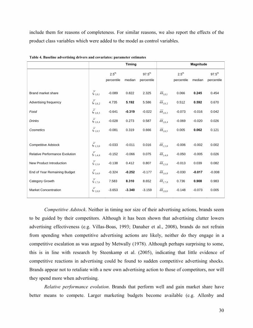
include them for reasons of completeness. For similar reasons, we also report the effects of the

product class variables which were added to the model as control variables.

Table 4. Baseline advertising drivers and covariates: parameter estimates

Timing Magnitude

2.5th

percentile median

97.5th

percentile

2.5th

percentile median

97.5th

percentile

Brand market share 1,0,1ζ -0.089 0.822 2.325 1,0,1ω 0.066 0.245 0.454

Advertising frequency 2,0,1ζ 4.735 5.192 5.586 2,0,1ω 0.512 0.592 0.670

Food 3,0,1ζ -0.641 -0.319 -0.022 3,0,1ω -0.073 -0.016 0.042

Drinks 4,0,1ζ -0.028 0.273 0.587 4,0,1ω -0.069 -0.020 0.026

Cosmetics 5,0,1ζ -0.081 0.319 0.666 5,0,1ω 0.005 0.062 0.121

Competitive Adstock 0,3,1ζ -0.033 -0.011 0.016 0,3,1ω -0.006 -0.002 0.002

Relative Performance Evolution 0,4,1ζ -0.152 -0.066 0.075 0,4,1ω -0.050 -0.005 0.026

New Product Introduction 0,5,1ζ -0.138 0.412 0.807 0,5,1ω -0.013 0.039 0.082

End of Year Remaining Budget 0,6,1ζ -0.324 -0.252 -0.177 0,6,1ω -0.030 -0.017 -0.008

Category Growth 0,7,1ζ 7.583 8.310 8.652 0,7,1ω 0.736 0.908 0.983

Market Concentration 0,8,1ζ -3.653 -3.340 -3.159 0,8,1ω -0.148 -0.073 0.005

Competitive Adstock. Neither in timing nor size of their advertising actions, brands seem

to be guided by their competitors. Although it has been shown that advertising clutter lowers

advertising effectiveness (e.g. Villas-Boas, 1993; Danaher et al., 2008), brands do not refrain

from spending when competitive advertising actions are likely, neither do they engage in a

competitive escalation as was argued by Metwally (1978). Although perhaps surprising to some,

this is in line with research by Steenkamp et al. (2005), indicating that little evidence of

competitive reactions in advertising could be found to sudden competitive advertising shocks.

Brands appear not to retaliate with a new own advertising action to those of competitors, nor will

they spend more when advertising.

Relative performance evolution. Brands that perform well and gain market share have

better means to compete. Larger marketing budgets become available (e.g. Allenby and

30

Hanssens, 2005), enabling them to advertise more often and spend more. Conversely, the idea

prevails that brands act in order to correct for a negative performance evolution relative to

competitors (e.g. Metwally, 1978; Armstrong and Collopy, 1996). These theories are countered

by our findings, as brands do not react with increased spending to make up for short term

negative sales evolutions. Advertising budgets, on the other hand, are not adjusted immediately

according to increased sales, leading to overall insignificance of short term performance

evolution on advertising behavior. Advertising thus proves to be a strategic means of competition

rather than a short term tactic means.

New product introduction. Advertising has been shown to be most effective for new

products (Lodish et al., 1995) as it, e.g., increases trial probability of such products (Steenkamp

and Gielens, 2003). New products still need to persuade customers into buying them. As

advertising is an effective means to build awareness and convey product information, new

products should be advertised more heavily (Tellis, 2004; Kotler and Armstrong, 2005).

However, although our findings point in that direction, no such significant effects could be found

on the actual advertising decisions.

End of year budget depletion. Advertising budgets are mostly set on a yearly basis, based

on rules of thumb (e.g. percentage of sales of the previous year), formal advertising response

modeling and management judgments (Farris and West, 2007). During the year, these budgets are

used for advertising campaigns, driven by a wide set of factors (e.g. Montgomery et al., 2005).

Thus, these financial resources become depleted. Our results indicate that managers tend to spend

relatively more in the beginning of the year, making them advertise less often and spending less

on single actions at the end ( 0,6,1ζ = -0.252 and 0,6,1ω = -0.017), after accounting for Holiday

season spending. Having money seemingly leads to spending it. In the beginning of the year,

resources are still large, so one can more easily engage in more intense actions. As resources get

depleted, one has to become more careful in when and what to spend, especially if one has spent

relatively more in the beginning and hence has already used ‘too much’ of the resources.

Category growth. When category growth is higher, brands will be more inclined to

advertise ( 0,7,1ζ = 8.310), and their subsequent actions will as well be more intense ( 0,7,1ω =

0.908). High growth categories are often younger product categories, requiring more advertising

to inform and convince new customers (Narayanan et al., 2005). Consumers in more mature

markets, with lower to zero growth, relay mostly on own experiences, and pay less attention to

31

advertising (Chandy et al., 2001). Higher growth, in addition, can be considered an indicator of

potential future profits, leading brands to defend their position even more fiercely (Gatignon et

al., 1990).

Category concentration. Economic theory tells that more concentrated markets show

higher profits as such oligopolistic markets are often characterized by barriers to entry (e.g. Bain,

1951; Modigliani, 1958; Karakaya and Stahl, 1989). Combined with the easy monitoring of

competitors’ actions in such markets, this may lead to collusive behavior and the use of non-price

forms of competition such as advertising in order not to compete away these attractive margins

(Ramaswamy et al., 1994; Lipczynski and Wilson, 2001). Our findings, however, indicate that

brands appear to be less inclined to advertise in more concentrated categories ( 0,8,1ζ = -3.340).

This is in line with previous research by Steenkamp et al. (2005) showing less overall

competitive interaction behavior in such categories. Brands thus advertise less often, although no

effect on their actual spending when advertising could be found.

Validation

To find guidance on the relative performance of our model, we compare the proposed

model (Model 0) to two other plausible specifications. In the first competing model (Model 1),

we restrict all covariances between error terms to zero. Model 2 is specified with only the

Adstock level but without the Ad-sensor, thus only accounting for the state dependency and not

for the pressure to start or stop advertising.

To compare these models, we assess to what extent they are capable of predicting both

timing and magnitude of advertising actions. We compare the models regarding their

performance on four different prediction statistics. The first statistic we consider, is the Mean

Squared Error, one of the most widely used loss functions in statistics. Theil U allows us to judge

the performance of the models relative to a naïve no-change model. The closer the value to zero,

the better the model performance over the naïve no-change model in which . We

implement the so-called U2 specification (Theil, 1966), which allows to make a distinction

between models performing better or worse, as it allows values beyond 1. The hit rate provides

evidence on the percentage correctly predicted Timing (0/1) decisions. Finally, we report the

correlation between the predicted and observed advertising expenditures. Higher values for the

1−= cbtcbt yy

32

latter two statistics prove better fit of the model. The best values on each summary statistic are

underlined

The model performance statistics are considered both in- and out-of-sample. Indeed, as

Van Heerde and Bijmolt (2005) argue, such time-based split provides us with a model robustness

check as the estimation and validation samples may differ in a systematic way. Parameter

estimates are based on a 130 week (2½ year) estimation period. The remaining 26 weeks (½ year)

are used as a time hold-out sample. In the spirit of e.g. Brodie and de Kluyver (1987), we include

observed Competitive Adstock, i.e. we assume that competitive actions are known. An overview

of these statistics is given in table 5.

Table 5. Model Comparison

Model Description In-Sample MSE Theil’s U Hit Rate Correlation

Model 0 Proposed model 0.078 0.552 0.891 0.779

Model 1 No correlations 0.120 0.684 0.893 0.675

Model 2 No Ad-sensor 0.094 0.608 0.870 0.739

Model Description Out-of-Sample

MSE Theil’s U Hit Rate Correlation

Model 0 Proposed model 0.141 0.749 0.829 0.588

Model 1 No correlations 1.144 2.130 0.839 0.214

Model 2 No Ad-sensor 0.152 0.770 0.810 0.540

In-sample performance

Our specification (Model 0) outperforms the alternative specifications on three

diagnostics with regard to in-sample estimations. Although the hit rate (89%) is slightly lower

than in model 1, our result is still impressive, especially when compared to the expected result for

a random model. Given 24% of the observations showing advertising actions, a random model

would show an overall hit rate of no more than 64% (Morrison, 1969). By means of such random

model, we would a priori choose to classify α = 24% of the observations as actions. The

33

observations, in turn, have an a priori probability of being an advertising action of p = 24%. The

resulting hit rate would then equal α)(1*p)(1α*p −−+ = 0.24*0.24+0.76*0.76 = 0.64. In

addition, when we decompose our hit rate into the percentage of correctly predicted actions and

no-actions, we obtain results of 71% and 95% respectively, far beyond the expected values of

24% and 76%. Besides a good predictor of the timing decisions, our model as well proves high

in-sample fit when correlating the predicted with the actually observed expenditures, with a

correlation equal to 0.779. Out-of-sample performance

The second part of table 5 summarizes the out-of-sample performance statistics of our

validation models. Here as well, our focal model 0 outperforms the other models on 3 out of the 4

statistics. The hit rate (about 83%) and correlation (0.588) are still impressive. Decomposition of

the hit rate shows correct predictions of action in 60% of the cases, and a correct prediction of

non-actions in 90% of the cases. These are still far beyond the aforementioned expected values of

24% and 76% of a random model (Morrison, 1969). Overall, this provides evidence of the

excellent predictive validity of our model specification.

Timing and Magnitude

In our study, we allowed for differential decisions processes in the timing and magnitude

decisions. We already provided evidence of the good performance of our model in predicting the

timing decisions by means of an impressive hit rate. In addition, we reported the overall

correlation between observed and predicted advertising values. To more specifically assess the

relative value of the magnitude part, we now restrict ourselves to those observations for which

the outcome of the timing decisions was positive. Thus we obtain the following in-sample (out-

of-sample) statistics: MSE = 0.199 (0.330); Theil U = 0.431 (0.548); correlation = 0.512 (0.407).

These results indicate that the large share of correctly predicted zero advertising in the overall

sample – and thus the good performance of the timing part – may inflate the overall correlation.

Our model consequently performs better in predicting the timing of the advertising actions

relative to predicting the actual amounts spent when advertising.

34

Based on these analyses, we can conclude that our model provides an encouraging

mimicking of advertising decisions in the marketplace. Not accounting for the correlations

between the error terms generally worsens the performance of our model. Finally, the inclusion

of our Ad-sensor, capturing the process leading to the start and stop of an advertising campaign,

clearly adds value compared to models including only the Adstock level.

8. Discussion

Summary

Notwithstanding the fact that advertising is one of the most used marketing tools, little is

known about what is driving the timing and magnitude of advertising actions. Building on

normative theory, we developed a parsimonious model that captures this dual investment process.

We explained advertising spending patterns as observed in the market, and investigated the

impact of company, competitive, and category-related factors on these decisions. Analyses were

based on a combination of (i) weekly advertising data from a wide variety of CPG brands from

the UK, (ii) household panel purchase data, and (iii) data on new product introductions. We

included both large and small brands, both frequent and infrequent advertisers in order to avoid

data pruning biases, and to obtain a more complete overview of the market.

The empirical findings provide broad support for our conceptual framework. Adstock and

Ad-sensor have a positive effect on both timing and magnitude decisions. Advertising spending

patterns can hence be considered a result of the application of campaigning strategies, based on

dynamic Adstock management systems. The extent to which such strategies are more or less the

outcome of such systems, however, varies across brands as a function of their size and

Advertising frequency, a clear indication that inclusion of all types of brands in our dataset was

warranted.

Discussion

In this study, we explained observed advertising spending patterns. Even strategies with

same amounts of advertising in every single week, as were advocated by early normative studies

(e.g. Zielske, 1959; Sasieni, 1971; 1989), are not observed in real world data. Pulsing strategies

on the other hand, characterized by an alternation of periods with higher advertising and periods

35

with lower to zero advertising (e.g. Mahajan and Muller, 1986) emerge as a dominant strategy.

Differing from previous advertising research, we argued these advertising investments to be the

outcome of a dual decision process, thereby distinguishing between two conceptually different

but at the same time closely linked decisions: whether to advertise or not (timing), and

conditional upon the choice to advertise, how much to spend (magnitude). As our results

indicated, differentiating between these two decisions is warranted. They are partly driven by

different factors, and common drivers have clearly different weights in both decisions.

Accounting for differential processes thus allows us to obtain a much richer view as well as a

more correct understanding of what is driving observed behavior.

Both decisions were subsequently embedded in an advertising goodwill stock

management system. Advertising investments are scheduled in campaigns of several weeks,

during which brands will build advertising goodwill among consumers. Carry-over effects of

advertising allow for longer periods without advertising, during which the goodwill will

gradually decay. As such, the created advertising goodwill is managed in a dynamic way. Similar

to strategies in other inventory management, this process can be described as an (s,S) inventory

management system, by means of which brands in a systematic way monitor and adjust their

advertising goodwill stock. Brands will decide to launch a new advertising action as soon as this

stock falls below a certain minimum desired level s, and stop advertising once the desired

(higher) target level S was reached. The Ad-sensor concept we developed in this study captures

this pressure, not only to launch and stop a new campaign, but also to spend more when still far

away from the target level in order to reach it faster. As such, it provides evidence of the

dynamics associated with advertising campaigns. The state dependencies of such campaigns, i.e.

the fact that they last for several weeks and that brands prefer consistent spending strategies

within each campaign, in turn, are well represented by the Adstock concept. Together, Ad-sensor

and Adstock allow us to explain observed advertising spending patterns as real-life applications

of the normative literature, in which advertising and advertising goodwill management are

embedded in dynamic (s,S) inventory systems.

However, the extent to which such systems affect the actual advertising decisions clearly

differs among different types of brands. Larger brands, as well as more frequently advertising

brands, show a greater reactance to changes in their advertising goodwill. The former have better

means to do so, whereas the latter may have learned from previous experience, resulting in a

36

closer advertising goodwill stock management. Both findings, taken together, provide clear

evidence that limiting the analyses to only the frequently acting large brands would have biased

our results. Our flexible model specification, in contrast to previous work, allowed us to cover

nearly all players in the market, thus avoiding data pruning biases. Given the number of brands

that otherwise would have been excluded from our analyses, this certainly gives extra weight to

our empirical generalizations.

Although advertising is often argued to be driven by competitive reasoning and reaction,

no such tendencies could be found. Not only did we not find any direct effects of competitive

advertising in the advertising decision making process, indirect effects through the relative

performance evolution of the brands did not show significant impact either. This may seem even

more surprising, as annual advertising budgets are often determined on a percentage of sales basis

(e.g. Allenby and Hanssens, 2005), and given the well-known argument that companies advertise

in order to retain market shares (e.g. Metwally, 1978; Armstrong and Collopy, 1996).

Advertising, characterized by small short run elasticities (e.g. Assmus et al., 1984; Sethuraman

and Tellis, 1991), takes time to build an effect in the mindset of customers (e.g. Assael, 1998;

Kardes, 2004). Price promotions, on the other hand, show much higher short run elasiticities

(Neslin, 2002; Bijmolt et al., 2005), making it a more interesting instrument to make up for

negative sales evolutions in the short run. This is also in line with the findings by Steenkamp et

al. (2005) who show that, in contrast to price promotions, advertising will hardly be used as a

means to react to competitors. Advertising thus appears not to be a tactic means to counter

negative evolutions in the short run, but rather a strategic means which builds goodwill that lasts.

Anecdotal evidence from practitioners adds to our findings, as several advertising agency account

managers confirmed that brands, in general, focus on their own internal advertising utility calculi,

and much less on what their competitors are doing in their actual advertising decisions.

Recent research has shown that new product introductions, combined with heavier

advertising, can result in higher sales and increased shareholder value (see e.g. Pauwels et al.,

2004; Srinivasan et al., 2009), combined with a rejuvenated brand (Slotegraaf and Pauwels,

2008). This may as well be a consequence of the fact that advertising is especially effective for

those new products (e.g. Lodish et al., 1995; Steenkamp and Gielens, 2003). However, no

significant link between such introductions and advertising decisions could be found, although

there were some weak indications in that direction. Overall, adopted strategies appear to be

37

continued in a similar fashion, without granting much extra support to new products relative to

those that are already present in the portfolio. Brands which already have intense advertising

strategies in place, are likely to continue these strategies for the new products as well, whereas

those with lower intensity strategies may simply not have the means to increase their efforts.

Directions for future research

In this work, we investigated and explained advertising spending patterns as observed in

the market. We did not aim at modeling the particular decision process of individual managers,

but mimic the advertising decisions as observed in the market by means of a paramorphic model

(e.g. Hoffman, 1960; Slovic and Lichtenstein, 1971; Steenkamp, 1989). Past research has proven

that such models, although showing deviations when applied to specific individual reasoning

processes, perform very well in capturing judgment and decision processes at a higher level (e.g.

Einhorn et al., 1979). Thus we are able to capture the phenomenon that is taking place in the

market, abstracting from short term individual deviations. However, this provides an avenue for

future research focusing on how individual managers in practice decide on their advertising

actions, and this by means of in-depth personal interactions with individual managers.

A second limitation of our work, is the fact that we limit ourselves to the dual decision of

timing and magnitude, thereby aggregating over all media. Media choice as such is not

investigated. This, however, would represent an interesting area for future research, as not all

media show the same effectiveness for different product categories, and as synergy effects can be

present in multimedia communications (see e.g. Naik and Raman, 2003). Moreover, media

effectiveness is not static, but does evolve as well as a consequence of the appearance of new

media. These phenomena can have far-reaching implications for the advertising decision process

and render it even more complicated.

Computing limitations (with the present runtime of our model on a fast Dell Precision

Workstation equaling 30 days) made us opt to include only time-invariant moderators in our

model. However, the inclusion of time-varying moderators like price-promotions would enrich

our analyses even further, and would also enable us to capture the interplay between Adstock and

advertising management and other instruments of the marketing mix.

Finally, we showed that commonly applied data pruning rules may engender results

which are only valid for that specific subsample of the market, raising questions to the validity of

38

the corresponding conclusions for the market as a whole. New econometric techniques enable us

to include all different types of players, even those that would have been excluded by these

pruning rules. An investigation as to what extent findings of previous research are valid for the

market as a whole can therefore be suggested.

39

References Aaker, D.A. & Day, G.S. (1986). The Perils of High-Growth Markets. Strategic Management

Journal, Vol 7 (5). pp 409-421. Advertising Age (2007). 100 Leading National Advertisers. The Ad Age Group. Allenby, G. & Hanssens, D. (2005). Advertising Response. Marketing Science Institute, Special

Report no 05-200. pp 8. Amemiya, T. (1984). Tobit Models: A Survey. Journal of Econometrics, Vol 24, pp 3-61. Armstrong, J.S. & Collopy, F. (1996) Competitor Orientation: Effects of Objectives and

Information on Managerial Decisions and Profitability. Journal of Marketing Research, Vol 33. pp 188-199.

Assmus, G., Farley, J.U. & Lehmann, D.R. (1984). How advertising affects sales: meta-analysis

of econometric results. Journal of Marketing Research, Vol 21 (February). pp 65-74. Assael, H. (1998). Consumer Behavior and Marketing Action, 6th Edition. SouthWestern College

Publishing, Cincinatti, Ohio. Bain, J.S. (1951). Relation of Profit Rate to Industry Concentration: American Manufacturing,

1936-1940. The Quarterly Journal of Economics, Vol 65 (3). pp 293-324. Bar-Ilan, A. & Strange, W.C. (1999). The Timing and Intensity of Investment. Journal of

Macroeconomics, Vol 21 (1). pp 57-77. Bass, F.M. (1969). A Simultaneous Equation Regression Study of Advertising and Sales of

Cigarettes. Journal of Marketing Research, Vol 6 (3). pp 291-300. Bass, F.M. & Parsons, L.J. (1969). Simultaneous-Equation Regression Analysis of Sales and

Advertising. Applied Economics, Vol 1 (2). pp 103-124. Bijmolt, T.H.A., Van Heerde, H.J. & Pieters, R.G.M. (2005). New Empirical Generalizations on

the Determinants of Price Elasticity. Journal of Marketing Research, Vol 42 (2). pp 141-156.

Boeker, W. (1988). Strategic Change: the Effects of Founding and History. The Academy of

Management Journal, Vol 32 (3). pp 489-515. Bowman, D., Farley, J.U. & Schmittlein, D.C. (2000). Cross-National Empirical Generalization

in Business Services Buying Behavior. Journal of International Business Studies, Vol 31 (4). pp 667-685.

Broadbent, S.S. (1984). Modeling with Adstock. Journal of the Market Research Society, Vol 26

(4). pp 295-312.

40

Broadbent, S.S., Spittler, J.Z. & Lynch, K. (1997). Building Better TV Schedules: New Light

from the Single Source. Journal of Advertising Research, Vol 37 (4). pp 27-31. Brodie, R.J. & De Kluyver, C.A. (1987). A Comparison of the Short Term Forecasting Accuracy

of Econometric and Naive Extrapolation Models of Market Share. International Journal of Forecasting, Vol 3. pp 423-437.

Brown, G. (1986). Modeling Advertising Awareness. The Statistician, Vol 35 (2). pp 289-299. Chandy, R.K., Tellis, G.J., MacInnis, D.J. & Thaivanich, P. (2001). What to Say When:

Advertising Appeals in Evolving Markets. Journal of Marketing Research, Vol 38 (4). pp 399-414.

Chen, M-J. & MacMillan, I.C. (1992). Nonresponse and Delayed Response to Competitive

Moves: The Roles of Competitor Dependence and Action Irreversibility. Academy of Management Journal, Vol 35. pp 539-560.

Cleeren, K., Dekimpe, M.G. & Helsen, K. (2007). Weathering Product-Harm Crises. Journal of

the Academy of Marketing Science, Published online. Danaher, P.J. (2007). Media Planning. In: Tellis, G.J & Ambler, T., eds. The SAGE Handbook of

Advertising. Sage Publications ltd, Thousand Oaks. Danaher, P.J., Bonfrer, A., & Dhar, S. (2008). The Effect of Competitive Advertising

Interference on Sales for Packaged Goods. Journal of Marketing Research, Vol 45 (2). pp 211-225.

Dekimpe, M.G. & Hanssens, D. (1995). The Persistence of Marketing Effects on Sales.

Marketing Science, Vol 14 (1). pp 1-21. Dekimpe, M.G. & Hanssens, D. (1999). Sustained Spending and Persistent Response: A New

Look at Long-Term Marketing Profitability. Journal of Marketing Research, Vol 36 (4). pp 397-412.

Dekimpe, M.G. & Hanssens, D. (2007). Advertising Response Models. In: Tellis, G.J & Ambler,

T., eds. The SAGE Handbook of Advertising. Sage Publications ltd, Thousand Oaks. Dekimpe, M.G., Parker, P.M. & Sarvary, M. (2000). Global Diffusion of Technological

Innovations: A Coupled-Hazard Approach. Journal of Marketing Research, Vol 37 (1). pp 47-59.

Deleersnyder, B., Dekimpe, M.G., Sarvary, M. & Parker, P.M. (2004). Weathering Tight

Economic Times: The Sales Evolution of Consumer Durables over the Business-Cycle. Quantitative Marketing and Economics, Vol 2 (4). pp 347-383.

41

Doganoglu, T. & Klapper, D. (2006). Goodwill and Dynamic Advertising Strategies. Quantitative Marketing and Economics, Vol 4 (1). pp 5-29.

Dubé, J-P., Hitsch, G.J. & Manchanda, P. (2005). An Empirical Model of Advertising Dynamics.

Quantitative Marketing and Economics, Vol 3 (2). pp 107-144. Einhorn, H.J., Kleinmuntz, D.N. & Kleinmuntz, B. (1979). Linear Regression and Process-

Tracing Models of Judgement. Psychological Review, Vol 86 (5). pp 465-485. Ephron, E. & McDonald, C. (2002). Media Scheduling and Carry-Over Effects: Is Adstock a

Useful TV Planning Tool? Journal of Advertising Research, Vol 42 (4). pp 66-71. Farris, P.W. & West, D.C. (2007). A Fresh View of the Advertising Budget. In: Tellis, G.J &

Ambler, T., eds. The SAGE Handbook of Advertising. Sage Publications ltd, Thousand Oaks.

Feinberg, F.M. (1992). Pulsing Policies for Aggregate Advertising Models. Marketing Science,

Vol 11 (3). pp 221-234. Fox, E.J., Montgomery, A.L. & Lodish, L.M. (2004). Consumer Shopping and Spending Across

Retail Formats. Journal of Business, Vol 77 (2). pp 25-60. Franses, P.H. & Koop, G. (1998). On the Sensitivity of Unit Root Inference to Nonlinear Data

Transformations. Economics Letters, Vol 59. pp 7-15. Frederickson, J.W. & Iaquinto, A.L. (1989). Inertia and Creeping Rationality in Strategic

Decision Processes. The Academy of Management Journal, Vol 32 (3). pp 516-542. Gatignon, H., Weitz, B. & Bansal, P. (1990). Brand Introduction Strategies and Competitive

Environments. Journal of Marketing Research, Vol 27 (November). pp 390-401. Gielens, K. & Dekimpe, M.G. (2007). The Entry Strategy of Retail Firms into Transition

Economies. Journal of Marketing, Vol 71 (2). pp 196-212. Hanssens, D.M. (1980). Bivariate Time-Series Analysis of the Relationship Between Advertising

and Sales. Applied Economics, Vol 12 (3). pp 329-339. Hanssens, D.M. (1980). Market Response, Competitive Behavior and Time-Series Analysis.

Journal of Marketing Research, Vol 17 (4). pp 470-485. Hanssens, D.M., Parsons, L.J. & Schultz, R.L. (2001). Market Response Models. International

Series in Quantitative Marketing. Kluwer Academic Publishers. Dordrecht. pp 501. Hoffman, P.J. (1960). The Paramorphic Representation of Clinical Judgement. Psychological

Bulletin, Vol 57. pp 116-131.

42

Jones, J.P. (1990). Advertising: Strong Force or Weak Force? Two Views an Ocean Apart. International Journal of Advertising, Vol 9 (3). pp 233-246.

Karakaya, F. & Stahl, M.J. (1989). Barriers to Entry and Market Entry Decisions in Consumer

and Industrial Goods Markets. Journal of Marketing, Vol 53 (2). pp 80-91. Kardes, F.R. (2002). Consumer Behavior and Managerial Decision Making. International

Edition. Second Edition. Pearson Education, Upper Saddle River, New Jersey. pp 457. Katz, W.A. (1980). A Sliding Schedule of Advertising Weight. Journal of Advertising Research,

Vol 20. pp 39-44. Kumar, N. & Steenkamp, J-B.E.M. (2007). Private Label Strategy: How to Meet the Store Brand

Challenge. Harvard Business School Press, Cambridge, MA. Kotler, P. & Armstrong, G. (2004). Principles of Marketing 10th ed. Pearson Education, Upper

Saddle River, New Jersey. pp 648. Lambin, J-J. & Palda, K.S. (1969). Measuring the Profitability of Advertising: An Empirical

Study. Journal of Industrial Economics, Vol 17 (2). pp 86-103. Lambin, J-J, Naert, P. & Bultez, A. (1975). What is the Real Impact of Advertising? Harvard

Business Review, Vol 53 (may-june). pp 139 -147. Lipczynski, J. & Wilson, J. (2001). Industrial Organization: An Analysis of Competitive Markets.

Pearson, Reading, MA. Lodish, L.M., Abraham, M., Kalmenson, S., Livelsberger, J., Lubetkin, B., Richardson, B. &

Stevens, M.E. (1995). How T.V. advertising works: A meta-analysis of 389 real world split cable T.V. advertising experiments. Journal of Marketing Research. Vol 32 (may 1995), pp 125-139.

Lynch, J.E. & Hooley, G.J. (1990). Increased Sophistication in Advertising Budget Setting.

Journal of Advertising Research, Vol 30 (1). pp 67-76. Mahajan, V. & Muller, E. (1986). Advertising Pulsing Policies for Generating Awareness for

New Products. Marketing Science, Vol 5 (2). pp 89-106. Mesak, H.I. (1992). An Aggregate Advertising Pulsing Model with Wearout Effects. Marketing

Science, Vol 11 (3). pp 310-326. Metwally, M.M. (1978). Escalation Tendencies of Advertising. Oxford Bulletin of Economics

and Statistics. May 78, Vol 40 (2) pp 153-164. Modigliani, F. (1958). New Developments on the Oligopoly Front. The Journal of Political

Economy, Vol 66 (3). pp 215-232.

43

Montgomery, D.B., Chapman Moore, M & Urbany, J.E. (2005). Reasoning About Competitive Reactions: Evidence from Executives. Marketing Science, Vol 24 (1). pp 138-149.

Morrison, D.G. (1969). On the Interpretaton of Discriminant Analysis. Journal of Marketing

Research, Vol 6 (2). pp 156-163. Naik, P.A., Mantrala, M.K. & Sawyer, A.G. (1998). Planning Media Schedules in the Presence of

Dynamic Advertising Quality. Marketing Science, Vol 17 (3). pp 214-235. Naik, P.A. & Raman, K. (2003). Understanding the Impact of Synergy in Multimedia

Communications. Journal of Marketing Research, Vol 40 (4). pp 375-388. Narayanan, S., Manchanda, P. & Chintagunta, P.K. (2005). Temporal Differences in the Role of

Marketing Communication in New Product Categories. Journal of Marketing Research, Vol 42 (August). pp 278-290.

Neslin, S. (2002). Sales Promotion. In: Weitz, B.A. & Wensley, R., eds. Handbook of Marketing.

Sage Publications ltd, Thousand Oaks. Nijs, V.R., Dekimpe, M.G., Steenkamp, J-B.E.M. & Hanssens, D.M. (2001). The Category-

Demand Effects of Price Promotions. Marketing Science, Vol 20 (1). pp 1-22. Nijs, V.,R. Srinivasan, S. & Pauwels, K. (2007). Retail Price Drivers and Retailer Profits.

Marketing Science, Vol 26 (4). pp 473-485. Park, S. & Hahn, M. (1991). Pulsing in a Discrete Model of Advertising Competition. Journal of

Marketing Research, Vol 28. pp 397-405. Patti, C.H. & Blasko, V.J. (1981). Budgeting Practices of Big Advertisers. Journal of Advertising

Research, Vol 21. pp 23-29. Pauwels, K., Silva-Risso, J., Srinivasan, S. & Hanssens, D.M. (2004). New Products, Sales

Promotions and Firm Value, With Applications to the Automobile Industry. Journal of Marketing, Vol 47 (Spring). pp 26-43.

Ramaswamy, V., Gatignon, H. & Reibstein, D.J. (1994). Competitive Marketing Behavior in

Industrial Markets. Journal of Marketing, Vol 58 (April). pp 45-55. Rossiter, J.R. & Percy, L. (1997). Advertising Communications & Promotion Management.

Second Edition. McGraw-Hill, New York. Samuelson, W. & Zeckhauser, R. (1988). Status Quo Bias in Decision Making. Journal of Risk

and Uncertainty, Vol 1 (1). pp 7-59. Sasieni, M.W. (1971). Optimal Advertising Expenditure. Management Science, Vol 18 (4). pp

64-72.

44

Sasieni, M.W. (1989). Optimal Advertising Strategies. Marketing Science, Vol 8 (4). pp 358-370. Sethuraman, R. & Tellis, G.J. (1991). An Analysis of the Trade-off between Advertising and

Price Discounting. Journal of Marketing Research, Vol 28 (2). pp 160-174. Silver, E.A., Pyke, D.F. & Peterson, R. (1998). Inventory Management and Production Planning

and Scheduling. John Wiley and Sons, New York. Slotegraaf, R.J. & Pauwels, K. (2008). The Impact of Brand Equity and Innovation on the Long-

Term Effectiveness of Promotions. Journal of Marketing Research, Vol 45 (3). pp 293-306. Slovic, P. & Lichtenstein, S. (1971). Comparison of Bayesian and Regression Approaches to the

Study of Information Processing in Judgement. Organizational Behavior and Human Performance, Vol 6 (6). pp 649-744.

Sorescu, A.B. & Spanjol, J. (2008). Innovation’s Effect on Firm Value and Risk: Insights from

Consumer Packaged Goods. Journal of Marketing, Vol 72 (2). pp 114-132. Srinivasan, S., Pauwels, K., Silva-Risso, J. & Hanssens, D.M. (2009). Product Innovations,

Marketing Investments and Stock Returns. Journal of Marketing, Vol 73 (1). pp 24-43.. Srinivasan, S., Pauwels, K. & Nijs, V.R. (2007) Retail-Price Drivers and Retailer Profits.

Marketing Science. Vol 26 (4). pp 473-487. Srivastava, R.K., Shervani, T.A. & Fahey, L. (1999). Marketing, Business Processes and

Shareholder Value: An Organizationally Embedded View of Marketing Activities and the Discipline of Marketing. Journal of Marketing, Vol 63 (Special Issue 1999). pp 168-179.

Steenkamp, J-B.E.M. (1989). Product Quality. Van Gorcum, Assen/Maastricht. Steenkamp, J-B.E.M. & Gielens, K. (2003). Consumer and Market Drivers of the Trial

Probability of New Consumer Packaged Goods. Journal of Consumer Research, Vol 30 (4). pp 368-384.

Steenkamp, J-B.E.M., Nijs, V.R., Hanssens, D.M. & Dekimpe, M.G. (2005). Competitive

Reactions to Advertising and Promotion Attacks. Marketing Science, Vol 24 (1). pp 35-54. Tellis, G.J. (2004). Effective Advertising: Understanding When How and Why Advertising Works.

Sage Publications ltd, Thousand Oaks. Tellis, G.J. & Weiss, D.L. (1995). Does TV Advertising Really Affect Sales? The Role of

Measures, Models and Data Aggregation. Journal of Advertising Research, Vol 24 (3). pp 1-12.

45

Tellis, G.J. & Ambler, T. (2007). The SAGE Handbook of Advertising. Sage Publications ltd, Thousand Oaks.

Theil, H. (1966). Applied Economic Forecasting. North Holland Publishing, Amsterdam. Van Heerde, H.J. & Bijmolt, T.H.A. (2005). Decomposing the Promotional Revenue Bump for

Loyalty Program Members Versus Nonmembers. Journal of Marketing Research, Vol 42 (4). pp 443-457.

Van Heerde, H.J., Gijsbrechts, E. & Pauwels, K. (2008). Winners and Losers in a Major Price

War. Journal of Marketing Research, forthcoming. Villas-Boas, J.M. (1993). Predicting Advertising Pulsing Policies in an Oligopoly: a Model and

Empirical Test. Marketing Science, Vol 12 (1). pp 88-102. Zanutto, E.L. & Bradlow, E.T. (2006). Data Pruning in Consumer Choice Models. Quantitative

Marketing and Economics, Vol 4 (3). pp 267-287. Zielske, H.A. (1959). The Remembering and Forgetting of Advertising. Journal of Marketing,

Vol 23. pp 239-243. Zufryden, F.S. (1973). Media Scheduling: A Stochastic Dynamic Model Approach. Management

Science, Vol 19 (12). pp 1395-1406.

46

Appendix A: Mathematical derivation of Ad-sensor

Ad-sensor captures the dynamics in the evolution of the brand’s Adstock. This Adstock is

defined as (Broadbent, 1984):

(A1) 1,,, )1( −+−= tbbtbbtb AdstockAdvertAdstock λλ

The first order condition for the optimum, i.e. the maximum Adstock level during a campaign,

given that we use discrete time observations and we can thus only observe up to time t-1, is:

(A2) 01, =Δ

Δ −

tAdstock tb

As we are analyzing discrete time data, this yields

(A3) 02,1, =Δ

− −−

tAdstockAdstock tbtb

(A4) 02,1, =−⇔ −− tbtb AdstockAdstock .

Given (A1), this is satisfied if:

(A5) 0)1( 2,2,1, =−+− −−− tbtbbtbb AdstockAdstockAdvert λλ

(A6) 2,1, )1()1( −− −=−⇔ tbbtbb AdstockAdvert λλ

(A7) 2,1, −− =⇔ tbtb AdstockAdvert

The second order condition for this maximum at t-1 then requires:

(A8) . 3,2, −− > tbtb AdstockAdvert

because Adstock will increase as long as Advertising is larger than Adstock:

(A9) 2,1, −− > tbtb AdstockAdstock

(A10) 2,2,1,)1( −−− >+−⇔ tbtbbtbb AdstockAdstockAdvert λλ

(A11) 2,1, )1()1( −− −>−⇔ tbbtbb AdstockAdvert λλ

(A12) 2,1, −− >⇔ tbtb AdstockAdvert

The starting point for our Ad-sensor at time t is hence:

(A13) > 0 if the maximum is reached after time t-1; 2,1, −− − tbtb AdstockAdvert

= 0 if the maximum is reached in t-1;

< 0 if the maximum was reached before t-1.

47

We subsequently rewrite (A1) in function of : 1, −tbAdvert

(A14) )1(

2,1,1,

b

tbbtbtb

AdstockAdstockAdvert

λλ

−

−= −−

− ,

which yields:

(A15) 2,1, −− − tbtb AdstockAdvert 2,2,1,

)1( −−− −

−

−= tb

b

tbbtb AdstockAdstockAdstock

λλ

(A16) 2,2,1, )1( −−− −−−≈ tbbtbbtb AdstockAdstockAdstock λλ

or

(A13) 2,1, −− − tbtb AdstockAdvert 2,1, −− −≈ tbtb AdstockAdstock

We therefore define our Ad-sensor variable as the difference between Adstock in time t-1 and

Adstock in t-2:

(A17) 2,1,, −− −= tbtbtb AdstockAdstockAdsensor

Ad-sensor thus captures the dynamics in the evolution of a brand’s Adstock. In the beginning of a

campaign, Adstock will increase very fast, causing high values of Ad-sensor. Closer to the

maximum, increases will become smaller as Adstock approaches the Advertising values. As a

consequence, the value of Ad-sensor starts to decrease. Once beyond the maximum, Adstock

starts to decline, and Ad-sensor takes relatively strong negative values. Adstock decays at a

constant rate λ, but not in constant absolute terms. When Adstock levels are still high, decay will

be large in absolute terms, causing strong negative Ad-sensor values. Over time, the Adstock

level becomes smaller, and decay will be smaller in absolute terms. The Ad-sensor values will

become less negative, indicating a growing pressure to start advertising again.

48

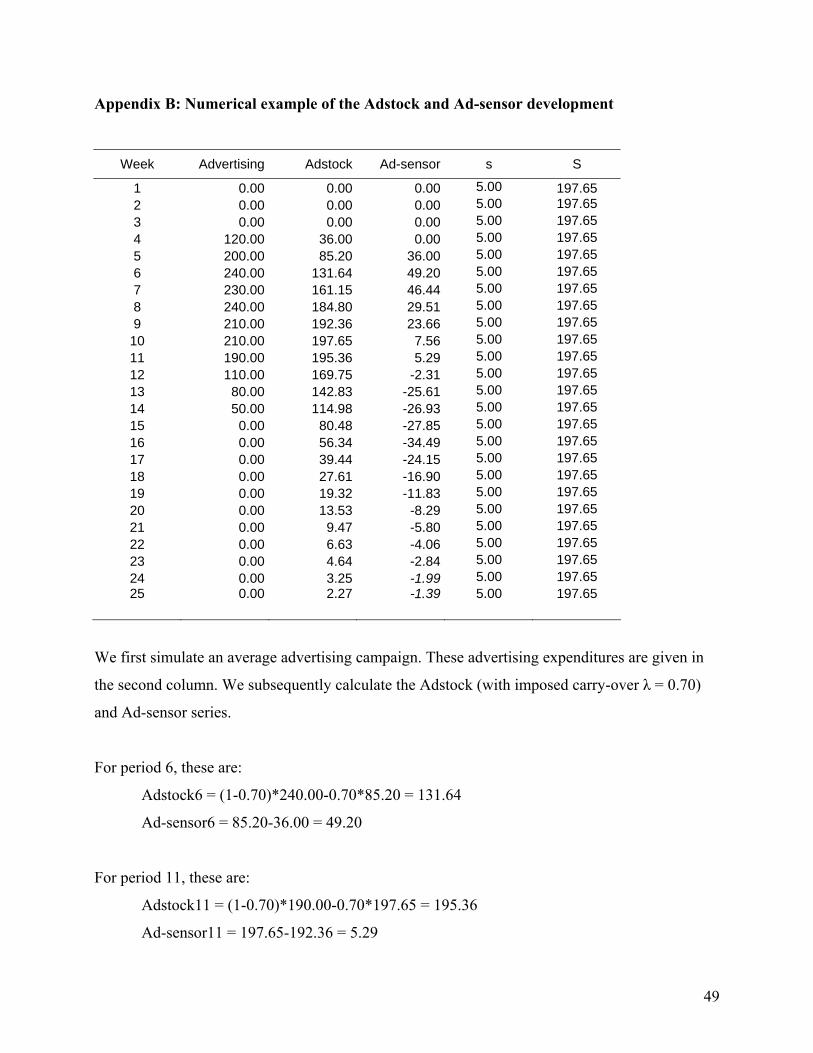
Appendix B: Numerical example of the Adstock and Ad-sensor development

Week Advertising Adstock Ad-sensor s S

1 0.00 0.00 0.00 5.00 197.65 2 0.00 0.00 0.00 5.00 197.65 3 0.00 0.00 0.00 5.00 197.65 4 120.00 36.00 0.00 5.00 197.65 5 200.00 85.20 36.00 5.00 197.65 6 240.00 131.64 49.20 5.00 197.65 7 230.00 161.15 46.44 5.00 197.65 8 240.00 184.80 29.51 5.00 197.65 9 210.00 192.36 23.66 5.00 197.65

10 210.00 197.65 7.56 5.00 197.65 11 190.00 195.36 5.29 5.00 197.65 12 110.00 169.75 -2.31 5.00 197.65 13 80.00 142.83 -25.61 5.00 197.65 14 50.00 114.98 -26.93 5.00 197.65 15 0.00 80.48 -27.85 5.00 197.65 16 0.00 56.34 -34.49 5.00 197.65 17 0.00 39.44 -24.15 5.00 197.65 18 0.00 27.61 -16.90 5.00 197.65 19 0.00 19.32 -11.83 5.00 197.65 20 0.00 13.53 -8.29 5.00 197.65 21 0.00 9.47 -5.80 5.00 197.65 22 0.00 6.63 -4.06 5.00 197.65 23 0.00 4.64 -2.84 5.00 197.65 24 0.00 3.25 -1.99 5.00 197.65 25 0.00 2.27 -1.39 5.00 197.65

We first simulate an average advertising campaign. These advertising expenditures are given in

the second column. We subsequently calculate the Adstock (with imposed carry-over λ = 0.70)

and Ad-sensor series.

For period 6, these are:

Adstock6 = (1-0.70)*240.00-0.70*85.20 = 131.64

Ad-sensor6 = 85.20-36.00 = 49.20


Adstock11 = (1-0.70)*190.00-0.70*197.65 = 195.36

Ad-sensor11 = 197.65-192.36 = 5.29

49


Adstock12 = (1-0.70)*110.00-0.70*195.36= 169.75

Ad-sensor12 = 195.36-197.65 = -2.31


Adstock15 = (1-0.70)*0.00-0.70*114.98 = 80.48

Ad-sensor15 = 142.83-114.98 = -27.85


Adstock16 = (1-0.70)*0.00-0.70*80.48 = 56.34

Ad-sensor16 = 114.98-80.48 = -34.49


Adstock20 = (1-0.70)*0.00-0.70*19.32 = 13.53

Ad-sensor20 = 19.32-27.61 = -8.29

The highest observed Adstock level in this series equals 197.65. We consequently assume that

this was the desired maximum level S. In this simulation, we impose s=5. In practice, we do not

know s and S, and derive these from the observed patterns. In addition, we estimate λ for each

individual brand.

50

Appendix C: MCMC Estimation of a Hierarchical Multivariate Type-2 Tobit Model

We will first briefly repeat the model specification.

An advertising decision in category c by brand b in week t ( ) is described by a multivariate

probit model:

cbtz

(C1) ⎩⎨⎧ >

=otherwise

zifz cbt

cbt 001 *

The latent variable is modeled through a linear model: *cbtz

(C2) cbtcbcbtcbcbtcbtz μ++= 2'21

'1

* ζxζx

Conditional on the decision to advertise ( = 1), we model , the ln of spending by brand b

in category c during week t as:

cbtz cbty

(C3) . cbtcbcbtcbcbtcbty ε++= 2'21

'1 ωvωv

where

(C4) ~ )',( ''ctct με ),0( ΣMVN

We relate the response parameters and to a set of second stage variables. cb1ζ cb1ω

(C5) cbcbcb uζQζ +=1

(C6) cbcbcb eωRω +=1

where

(C7) ~ . )',( ''cbcb ue ),0( ΩMVN

We stack the dependent variables of equations (C2) and (C3) for all brands b in category c

and time periods t so that the vector of ln expenditures is and the vector

of advertising action indicator variables is , (b) the predictor variables for

the advertising action equation, = [ v

],,,[ 1211 ′= TcBccc cyyy Ky

],,,[ **12

*11

* ′= TcBccc czzz Kz

'1cbtv 1cb1t,v1cb2t,…, v1cbMt ]′ and = [ v'

2cbtv 2cb1t,v2cb2t,…, v2cbMt

]′ ; the predictor variables for the ln expenditures equation, = [x'1cbtx 1cb1t,x1cb2t,…,x1cbMt ]′ and

= [x'2cbtx 2cb1t,x2cb2t,…,x2cbMt ]′; and (c) the error terms of these two equations for all brands b and

51

time periods t so that [ ]’= [εctct 'με ,′ c1t,εc2t,…,εcBct, µc1t,µc2t,…,µcBct]′ follows a (2BBc)-variate normal

distribution with zero mean and full covariance matrix

Σc = ⎥⎦

⎤⎢⎣

⎡′ 2212

1211

cc

cc

ΣΣΣΣ

where , cE ctctc ∀′= )(11 εεΣ cE ctctc ∀= )'(12 μεΣ , and cE ctctc ∀= )'(22 μμΣ , which has ones on the

diagonal since each selectivity mechanism is binary.

Next we specify the hierarchies associated with the two advertising decisions. We stack

(i) the parameter coefficients per category and per brand across equations (C2) and (C3) and (ii)

the error terms of the hierarchical equations for all brands b in a similar way. We model the

response parameters as follows:

( )ΩI

ue

ueue

ue

ueue

ζω

RQ

RQ

RQ

ζω

ζωζω

eu ⊗

⎥⎥⎥⎥⎥⎥⎥⎥

⎦

⎤

⎢⎢⎢⎢⎢⎢⎢⎢

⎣

⎡

⎥⎥⎥⎥⎥⎥⎥⎥

⎦

⎤

⎢⎢⎢⎢⎢⎢⎢⎢

⎣

⎡

+⎥⎦

⎤⎢⎣

⎡

⎥⎥⎥⎥⎥⎥⎥⎥

⎦

⎤

⎢⎢⎢⎢⎢⎢⎢⎢

⎣

⎡

=

⎥⎥⎥⎥⎥⎥⎥⎥

⎦

⎤

⎢⎢⎢⎢⎢⎢⎢⎢

⎣

⎡

+ ccc

c

c

c

c

c

c

c

c

B

cB

cB

c

c

c

c

cB

cB

c

c

c

c

cB

cB

c

c

c

c

cB

cB

c

c

c

c

~N ,0, ||||2

2

1

1

2

2

1

1

2

2

1

1

1

1

21

21

11

11

MMMM

,

with = = cbQ cbR cbM qI ′⊗ , where is an (M x M) identity matrix and is a 1 x (N/M)

vector of covariates. The hyperparameters relating these covariates to the actual first level

response parameters are stacked in [

MI cbq′

'ω 'ζ ]’=

[ ]M,NM2,1M1,N1,21,1MM,N2,1M1,N1,21,1 ζ,ζζ,ζ,ζω,ωω,ωω /11/111/11/111 KKKK , with ω and ζ both

being (N x 1) vectors.

Ω = is a full covariance matrix where , ⎥⎦

⎤⎢⎣

⎡

22'12

1211

ΩΩΩΩ

bcE cbcb ,)( '11 ∀= eeΩ bcE cbcb ,)'(12 ∀= ueΩ ,

and . bcE cbcb ,)'(22 ∀= uuΩ

We use an MCMC approach to estimate the marginal distributions of the latent dependent

variables, parameters and covariances. The MCMC algorithm involves sampling sequentially

from the relevant conditional distributions over a large number of iterations. These draws can be

52

shown to converge to the marginal posterior distributions. Our implementation of the MCMC

algorithm has 6 steps that are described below.

Conditional distributions The first implementation step requires that we specify conditional distributions of the

relevant variables. The solutions of these distributions follow from the normality assumption of

the disturbances terms. We employ natural conjugate priors. Specifications of the conditional

distributions are as follows:

1. is y*cbty cbt if zcbt =1, otherwise is drawn from a normal distribution: *

cbty

⎪⎩

⎪⎨

⎧

=−⎟⎟⎠

⎞⎜⎜⎝

⎛

−−

+′+′

=

∑

−≠≠−

≠

0|~')E(

)E(~(

1

~

,,,,

,1,,

)11(,

1,,2211 cbtcbcjcjcjcjcbcbcb*

ct*c,t

*b,tc,j

*b,tc,j

cjcjcjcbcbcbtcbcbt

cbtcbt

cbcbcb*ct

*b,tc,j

*cbt

z),σN

zy

αy

σΣσzzyy

Σσωvωv

ωzy ι

where⎥⎥⎥

⎦

⎤

⎢⎢⎢

⎣

⎡

−−−−=⎥⎥⎥

⎦

⎤

⎢⎢⎢

⎣

⎡

−−=

≠ cjcjcbcj

cjcbcbcb

c*

b,tc,j

*cbt

*ct

σy

,,

,)11(

,

~

' and

Σσ

σΣ

yy

As the notation suggests, the vector and ∑*cty c matrix are partitioned between the brand of

interest, cb, and all other brands cj, j ≠ b (the entries in ∑c corresponding to z are not

shuffled). Without loss of generality, we have assumed the brand of interest to be the first.

Each brand is then drawn in succession for category c, conditioning on , , and ∑*b,tc,j≠y *

ctz c.

2. We next draw the latent dependent variable values for the probit component of the model. If

the indicator variable zcbt = 1, then is drawn from a normal distribution, truncated below

at 0. Otherwise, is drawn from a normal distribution, truncated above at 0.

*cbtz

*cbtz

53

⎟⎟⎠

⎞⎜⎜⎝

⎛−⎟⎟

⎠

⎞⎜⎜⎝

⎛

−−

+′+′ −≠≠−

≠

cbcjcjcjcjcbcbcb*ct

*c,t

*b,tc,j

*b,tc,j

cjcjcjcbcbcbtcbbtcT

cbcbcb*ct

*b,tc,j

*cbt

,N

,ι,,

,1,

',,

1,,2211

~)E(

)E(~~

,,

σΣσyyzz

Σζxζx

Σζyzz

σσ

α

where: ⎥⎥⎥

⎦

⎤

⎢⎢⎢

⎣

⎡

−−−−=⎥⎥⎥

⎦

⎤

⎢⎢⎢

⎣

⎡

−−=

≠ cjcjcbcj

cjcbcbcb

c*

b,tc,j

*cbt

*ct

σzz

,,

,)22(

,

~

'and

Σσ

σΣ

z

The latent probit dependent variables are drawn using the inverse cdf method.

3. The parameters in [ ]′,112121,1111 ,,,,,cc cBcBcccc ζωζωζω K are drawn from a SUR model with

variance/covariance matrix of disturbances : cΣ

( ) [ ]

⎟⎟⎟⎟⎟⎟⎟⎟⎟⎟⎟⎟⎟⎟⎟⎟

⎠

⎞

⎜⎜⎜⎜⎜⎜⎜⎜⎜⎜⎜⎜⎜⎜⎜⎜

⎝

⎛

⎟⎟⎟⎟⎟⎟⎟⎟⎟⎟⎟⎟⎟⎟⎟⎟

⎠

⎞

⎜⎜⎜⎜⎜⎜⎜⎜⎜⎜⎜⎜⎜⎜⎜⎜

⎝

⎛

⎥⎦

⎤⎢⎣

⎡

⎥⎥⎥⎥⎥⎥⎥⎥

⎦

⎤

⎢⎢⎢⎢⎢⎢⎢⎢

⎣

⎡

⊗+

⎥⎥⎥⎥⎥⎥⎥⎥⎥⎥⎥⎥⎥⎥⎥

⎦

⎤

⎢⎢⎢⎢⎢⎢⎢⎢⎢⎢⎢⎢⎢⎢⎢

⎣

⎡

′−−

′−−

′−−

′−−

′−−

⊗

⎥⎥⎥⎥⎥⎥⎥⎥

⎦

⎤

⎢⎢⎢⎢⎢⎢⎢⎢

⎣

⎡

−−−c

cB

cB

c

c

c

c

B

cBTcB*(t)

TcB

cBTcB*(t)

TcB

cc*(t)c12

cc*(t)c12

cBcB*(t)

1cB

cBcB*(t)

1cB

cc*(t)c21

cc*(t)c21

cc*(t)c11

cc*(t)c11

Tcct

c*(t)*(t)

cB

cB

c

c

c

c

,

zy

zy

zy

zyzy

~N,

c

c

c

ccccc

ccccc

ccc

ccc

c

c

c

Oζω

RQ

RQ

RQ

ΩI

ζxωv

ζxωvζxωv

ζxωvζxωv

ΣIPOΣzy

ζω

ζωζω

M

M

M

M2

2

1

1

1

22

2'2

12122

12'

122

212

2'

12

22212

22'

212

12112

12'

112

1c

'1

)1(

1

1

21

21

11

11

,

where ,

⎥⎥⎥⎥⎥⎥⎥⎥⎥

⎦

⎤

⎢⎢⎢⎢⎢⎢⎢⎢⎢

⎣

⎡

=

ccBccBccBccB

ccBccBccBccB

cccBcccB

cccBcccB

cccc

cccc

cccc

cccc

ccBcccBc

ccBcccBc

cccc

cccc

cccc

cccc

zzyz

zyyy

zzyz

zyyy

zzyz

zyyy

zzyz

zyyy

zzyz

zyyy

zzyz

zyyy

zzyz

zyyy

c

σσσσ

σσσσ

σσσσ

σσσσ

σσσσ

σσσσ

σσσσ

11

11

2222

2222

1212

1212

11

11

2121

2121

1111

1111

OM

L

Σ

54

and , ( )( ) 111

'1

11 −−⊗+⊗=−−

ΩIPΣIPOc

)(t

c BccTcc

and .

⎥⎥⎥⎥⎥⎥⎥⎥⎥⎥⎥⎥⎥⎥⎥⎥⎥⎥⎥⎥⎥⎥⎥⎥⎥⎥⎥⎥⎥⎥⎥⎥⎥⎥⎥⎥⎥⎥

⎦

⎤

⎢⎢⎢⎢⎢⎢⎢⎢⎢⎢⎢⎢⎢⎢⎢⎢⎢⎢⎢⎢⎢⎢⎢⎢⎢⎢⎢⎢⎢⎢⎢⎢⎢⎢⎢⎢⎢⎢

⎣

⎡

=

'1

'1

'21

'21

'11

'11

'21

'21

'221

'221

'121

'121

'11

'11

'211

'211

'111

'111

1

cc

cc

c

c

c

c

c

c

c

c

TcB

TcB

Tc

Tc

Tc

Tc

cB

cB

c

c

c

c

cB

cB

c

c

c

c

c

xv

xv

xv

xv

xv

xv

xv

xv

xv

P

O

M

M

O

O

55

4. The vector of hyper-parameters, [ ]′′′ ζω , , is drawn from a SUR model with

variance/covariance matrix of disturbances

:Ω

⎟⎟⎟⎟⎟⎟⎟⎟⎟⎟⎟⎟⎟⎟⎟

⎠

⎞

⎜⎜⎜⎜⎜⎜⎜⎜⎜⎜⎜⎜⎜⎜⎜

⎝

⎛

⎟⎟⎟⎟⎟⎟⎟⎟⎟⎟⎟⎟⎟⎟⎟

⎠

⎞

⎜⎜⎜⎜⎜⎜⎜⎜⎜⎜⎜⎜⎜⎜⎜

⎝

⎛

⎥⎦

⎤⎢⎣

⎡+

⎥⎥⎥⎥⎥⎥⎥⎥⎥⎥⎥⎥⎥⎥⎥

⎦

⎤

⎢⎢⎢⎢⎢⎢⎢⎢⎢⎢⎢⎢⎢⎢⎢

⎣

⎡

⊗⎥⎦

⎤⎢⎣

⎡ −− Jζω

Ω

ζω

ζωζω

ζωζω

ΩISJΩζωζω

,~N,|

c

c

CB

CB

B

BB

t(t)(t)

(t)1

1

1

121

121

11

11

112

112

111

111

1')(

1

1)(,

M

M

,

where ( ) 111)(−

−− +⊗′= ΩSΩISJ B , ,

⎥⎥⎥⎥⎥⎥⎥⎥⎥⎥⎥⎥⎥⎥⎥

⎦

⎤

⎢⎢⎢⎢⎢⎢⎢⎢⎢⎢⎢⎢⎢⎢⎢

⎣

⎡

=

C

C

CB

CB

B

B

RQ

RQ

RQ

RQ

RQ

S

M

M

21

21

1

1

12

12

11

11

1

1

with B the sum of all BBc and hence the total number of brands.

5. The vector of parameters, [ ]′,222222,1212 ,,,,,cc cBcBcccc ζωζωζω K , is drawn from a Bayesian

regression model:

56

( )

⎟⎟⎟⎟⎟⎟⎟⎟⎟⎟⎟⎟⎟⎟⎟⎟

⎠

⎞

⎜⎜⎜⎜⎜⎜⎜⎜⎜⎜⎜⎜⎜⎜⎜⎜

⎝

⎛

⎟⎟⎟⎟⎟⎟⎟⎟⎟⎟⎟⎟⎟⎟⎟⎟

⎠

⎞

⎜⎜⎜⎜⎜⎜⎜⎜⎜⎜⎜⎜⎜⎜⎜⎜

⎝

⎛

⎥⎦

⎤⎢⎣

⎡+

⎥⎥⎥⎥⎥⎥⎥⎥⎥⎥⎥⎥⎥⎥⎥

⎦

⎤

⎢⎢⎢⎢⎢⎢⎢⎢⎢⎢⎢⎢⎢⎢⎢

⎣

⎡

′−−

′−−

′−−

′−−

′−−

⎥⎥⎥⎥⎥⎥⎥⎥⎥⎥⎥⎥⎥⎥⎥

⎦

⎤

⎢⎢⎢⎢⎢⎢⎢⎢⎢⎢⎢⎢⎢⎢⎢

⎣

⎡′−

⊗

⎥⎥⎥⎥⎥⎥⎥⎥

⎦

⎤

⎢⎢⎢⎢⎢⎢⎢⎢

⎣

⎡

−−c

cBTcB*(t)

TcB

cBTcB*(t)

TcB

cc*(t)c12

cc*(t)c12

cBcB*(t)

1cB

cBcB*(t)

1cB

cc*(t)c21

cc*(t)c21

cc*(t)c11

cc*(t)c11

*(t)TcB

*(t)TcB

*(t)c12

*(t)c12

*(t)1cB

*(t)1cB

*(t)c21

*(t)c21

c*(t)c11

*(t)c11

Tcct(t)

cB

cB

c

c

c

c

,

zy

zy

zy

zyzy

zy

zyzy

zy

zy

~N,|

ccccc

ccccc

ccc

ccc

cc

cc

c

c

c

c

c

22

212

11

1'1

11121

11'

121

111

1'

11

21211

21'

211

11111

11'

111

111111

1c

'22

)(11

2

2

22

22

12

12

JΩ

ζxωv

ζxωvζxωv

ζxωvζxωv

ζx

ΣIPJζω

ζω

ζωζω

ζω

M

M

M

M

M

,

where ( )1

122

1c22

−−− ⎟⎠⎞⎜

⎝⎛ +⊗′= ΩPΣIPJ cTcc c

,

57

⎥⎥⎥⎥⎥⎥⎥⎥⎥⎥⎥⎥⎥⎥⎥⎥⎥⎥⎥⎥⎥⎥⎥⎥⎥⎥⎥⎥⎥⎥⎥⎥⎥⎥⎥⎥⎥⎥

⎦

⎤

⎢⎢⎢⎢⎢⎢⎢⎢⎢⎢⎢⎢⎢⎢⎢⎢⎢⎢⎢⎢⎢⎢⎢⎢⎢⎢⎢⎢⎢⎢⎢⎢⎢⎢⎢⎢⎢⎢

⎣

⎡

=

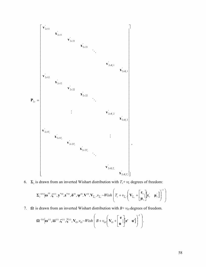
'2

'2

'22

'22

'12

'12

'22

'22

'222

'222

'122

'122

'12

'12

'212

'212

'112

'112

2

cc

cc

c

c

c

c

c

c

c

c

TcB

TcB

Tc

Tc

Tc

Tc

cB

cB

c

c

c

c

cB

cB

c

c

c

c

c

xv

xv

xv

xv

xv

xv

xv

xv

xv

P

O

M

M

O

O

,

6. is drawn from an inverted Wishart distribution with TcΣ c+νΣ degrees of freedom:

[ ] ⎟⎟

⎠

⎞

⎜⎜

⎝

⎛⎟⎟⎠

⎞⎜⎜⎝

⎛⎥⎦

⎤⎢⎣

⎡++

−

∑∑∑∑−

1

'')()1 ,,, ccc

cc

(t)(t)(t)*(t)*(t)t(t)(tc cccc

,νT~Wish ,ν,,,, μεμε

VVVψδzyζωΣ

7. is drawn from an inverted Wishart distribution with B+νΩ Ω degrees of freedom.

[ ] ⎟⎟

⎠

⎞

⎜⎜

⎝

⎛

⎟⎟⎠

⎞⎜⎜⎝

⎛⎥⎦

⎤⎢⎣

⎡++

−

ΩΩΩΩ−

1

)()()()(1 '',,, ueue

VVζζωωΩ ,νB~Wish ,ν, tttt(t) .

58

For identification purposes we need ones on the diagonal of incidence equation error

matrix (while ΣcE ctctc ∀= )'(22 μμΣ c is positive definite), and we need to rescale the parameters

from the incidence equation relative to . To achieve this, we follow the procedure proposed

by Edwards and Allenby (2003) and Rossi, Allenby, and McCulloch (2005, p. 108). That is, we

do not impose any restrictions when drawing . Instead, we postprocess the draws using the

following diagonal matrices:

22cΣ

cΣ

cc

B

cc

∀⎥⎥⎦

⎤

⎢⎢⎣

⎡= − ,

)(diag0

0

21

22

1Σ

IC ;

c

MBB

c

M

Mc

M

Mc

M

c

cc

∀

⎥⎥⎥⎥⎥⎥⎥⎥

⎦

⎤

⎢⎢⎢⎢⎢⎢⎢⎢

⎣

⎡

⋅

⋅

⋅

= ,

)/1(00

)/1(00

)/1(00

),(22

)2,2(22

)1,1(22

21

IΣI

IΣI

IΣI

CO

,

cn

LBB

c

L

Lc

L

Lc

L

c

cc

∀

⎥⎥⎥⎥⎥⎥⎥⎥

⎦

⎤

⎢⎢⎢⎢⎢⎢⎢⎢

⎣

⎡

⋅

⋅

⋅

= ,

)/1(00

)/1(00

)/1(00

),(22

)2,2(22

)1,1(22

22

IΣI

IΣI

IΣI

CO

,

⎥⎥⎦

⎤

⎢⎢⎣

⎡

⋅= −

Nc

N

IΣ

IC

))(mean(diag0

0

21

22

3 and ⎥⎥⎦

⎤

⎢⎢⎣

⎡

⋅= −

Mc

M

IΣ

IC

))(mean(diag0

0

21

22

4

After completing the Gibbs chain, we calculate for each saved Gibbs draw,

monitor its convergence, and use it for inference purposes. Analogously, for inferences we use

; ;

11*

cccc CΣCΣ ′=

cccccc ∀′⋅=′ ,),(*),( '1

'121

'1

'1 ζωCζω cccccc ∀′⋅=′ ,),(*),( '

2'222

'2

'2 ζωCζω ),.(*),( 3 ′′′=′′′ ζωCζω ,

and . 44* CΩCΩ ′=

Prior distributions

The second implementation step is to specify prior distributions for the parameters of

interest. Note that the priors are set to be non-informative so that inferences are driven by the

data.

59

The prior distribution of [ω′ , ζ′ ]’ is N([ω ′ , ζ′]’,Ω ), where [ω ′ , ζ′]=0 and Ω = diag(103).

The prior distribution of is Wishart: W(ν1−cΣ Σc,VΣc), where νΣ = 2 Bc +2 and VΣc = diag(10-3).

The prior distribution of is Wishart: W(ν1-Ω ω, ), where νΩV ω = 2M+2 and = diag(10ΩV -3).

Initial values The third implementation step is to set initial values for the parameters of the marginal

distributions. The starting values for ω and δ are computed by OLS, using ln(ycbt) as the

dependent variable of the regression. The covariance matrix, Σ11, is initiated by computing the

sample covariances of this regression’s residuals. In a similar fashion, the starting values for the

patronage equation parameters, ζ, are computed by OLS, using zcbt as the dependent variable, and

the residuals from this regression, µcbt, are used to compute the sample correlations, which serve

as the initial value for Σ22.

The final step is to generate N1+N2 random draws from the conditional distributions. We

use a “burn in” of N1 = 30.000 iterations. To reduce autocorrelation in the MCMC draws, we

“thin the line,” using every 50th draw in the final N2 = 30.000 draws for our estimation. In this

way, 600 draws are used to estimate marginal posterior distributions of the parameters of interest.

Test runs of our Gauss implementation of the MCMC draws show that we can retrieve

parameters used to simulate artificial data.

60

Appendix D: MCMC estimation of brand-specific carry-over parameter lambda

Basic sales model for each brand:

(D1) tcbtcbcbcbtcb AdstockSales ,,, εβα ++=

We transform this model:

(D2) *,1,,1,, )1( tcbtcbcbcbtcbcbcbcbtcbcbtcb AdstockAdstockSalesSales εβλβαλλ +−+−=− −−

Adstock definition:

(D3) )()1( 1,,, −+−= tcbcbtcbcbtcb AdstockAdvAdstock λλ

Inserting this in the transformed model:

(D4) *,,1,, )1()1( tcbtcbcbcbcbcbtcbcbtcb AdvSalesSales ελβαλλ +−+−=− −

or

(D5) *,,

**1,, tcbtcbcbcbtcbcbtcb AdvSalesSales εβαλ ++=− −

or

(D6) *,1,,

**, tcbtcbcbtcbcbcbtcb SalesAdvSales ελβα +++= −

which is the well-known Partial Adjustment Model (Hanssens et al., 2001 p147). From this

model, we can estimate the brand-specific lambda’s.

Estimation. *

,1,,**

, tcbtcbcbtcbcbcbtcb SalesAdvSales ελβα +++= − , with ~ ctε ),( λcMVN Σ0

and ααα cbcb e+=*

βββ cbcb e+=*

λλλ cbcb e+= with ~ )',,( λβαcbcbcb eee ),( λΩ0MVN

1. We draw the vector of parameters [ ]′ccc cBcBcBcccccc λβαλβαλβα ,,,,,,,,, **

2*2

*21

*1

*1 K from a SUR

model with variance/covariance matrix of disturbances : λcΣ

61

)1()(

*

*

2

*2

*2

1

*1

*1

, −

⎥⎥⎥⎥⎥⎥⎥⎥⎥⎥⎥⎥⎥

⎦

⎤

⎢⎢⎢⎢⎢⎢⎢⎢⎢⎢⎢⎢⎢

⎣

⎡

tc

t

cB

cB

cB

c

c

c

c

c

c

c

c

c

λ

λβα

λβαλβα

ΣSales

M

~[ ][ ]

⎟⎟⎟⎟⎟⎟⎟⎟⎟⎟⎟⎟⎟⎟⎟⎟⎟⎟⎟

⎠

⎞

⎜⎜⎜⎜⎜⎜⎜⎜⎜⎜⎜⎜⎜⎜⎜⎜⎜⎜⎜

⎝

⎛

⎟⎟⎟⎟⎟⎟⎟⎟⎟⎟⎟⎟⎟⎟⎟⎟⎟⎟⎟

⎠

⎞

⎜⎜⎜⎜⎜⎜⎜⎜⎜⎜⎜⎜⎜⎜⎜⎜⎜⎜⎜

⎝

⎛

⎥⎥⎥

⎦

⎤

⎢⎢⎢

⎣

⎡

⊗⊗+

⎥⎥⎥⎥⎥⎥⎥⎥⎥⎥⎥⎥⎥⎥⎥⎥⎥⎥

⎦

⎤

⎢⎢⎢⎢⎢⎢⎢⎢⎢⎢⎢⎢⎢⎢⎢⎢⎢⎢

⎣

⎡

⊗ −−cBB

TcB

Tc

Tc

cB

c

c

cB

c

c

cTcc cc

cc

c

c

c

c

c

Sales

SalesSales

Sales

SalesSalesSales

SalesSales

N KI1ΩIΣILK ,)(' 31

,

,2

,1

2,

2,2

2,1

1,

1,2

1,1

1

λβα

λλ

M

M

M

M

,

where ( )( ) 111'−−− ⊗+⊗= λ

λ ΩILΣILKcc BccTcc ,

and

⎥⎥⎥⎥⎥⎥⎥⎥⎥⎥⎥⎥⎥⎥⎥⎥⎥⎥⎥

⎦

⎤

⎢⎢⎢⎢⎢⎢⎢⎢⎢⎢⎢⎢⎢⎢⎢⎢⎢⎢⎢

⎣

⎡

=

−

−

−

1,,

1,2,2

1,1,1

1,2,

1,22,2

1,12,1

0,1,

0,21,2

2,11,1

1

11

1

11

1

11

'

cccc

cc

cc

cc

cc

TcBTcB

TcTc

TcTc

cBcB

cc

cc

cBcB

cc

cc

c

SalesAdv

SalesAdvSalesAdv

SalesAdv

SalesAdvSalesAdv

SalesAdv

SalesAdvSalesAdv

O

M

O

M

O

L

2. The vector of hyper-parameters, [ ]′λβα ,, is drawn from a SUR model with

variance/covariance matrix of disturbances : λΩ

62

λ

λβα

Ωλβα ,,, )(*)(*)(*

)(

)(

)(

ttt

t

t

t

⎥⎥⎥

⎦

⎤

⎢⎢⎢

⎣

⎡

~

⎟⎟⎟⎟⎟⎟⎟⎟⎟⎟⎟⎟⎟⎟⎟⎟⎟⎟⎟

⎠

⎞

⎜⎜⎜⎜⎜⎜⎜⎜⎜⎜⎜⎜⎜⎜⎜⎜⎜⎜⎜

⎝

⎛

⎟⎟⎟⎟⎟⎟⎟⎟⎟⎟⎟⎟⎟⎟⎟⎟⎟⎟⎟

⎠

⎞

⎜⎜⎜⎜⎜⎜⎜⎜⎜⎜⎜⎜⎜⎜⎜⎜⎜⎜⎜

⎝

⎛

⎥⎥⎥

⎦

⎤

⎢⎢⎢

⎣

⎡+

⎥⎥⎥⎥⎥⎥⎥⎥⎥⎥⎥⎥⎥⎥⎥⎥⎥⎥⎥

⎦

⎤

⎢⎢⎢⎢⎢⎢⎢⎢⎢⎢⎢⎢⎢⎢⎢⎢⎢⎢⎢

⎣

⎡

⊗′ −− FΩΩIGF ,)( 1

*

*

21

*21

*21

1

*1

*1

11

*11

*11

1 1

1

1

λβα

λβα

λβαλβα

λβα

λλ

C

C

C

CB

CB

CB

B

B

B

BN

M

M

,

where ( ) 111)( −−− +⊗′ λλ ΩGΩIG B 3I1=F , and G = ⊗B , with B the sum of all Bc and hence

the total number of brands.

3. We subsequently draw from an inverted Wishart distribution with degrees of

freedom:

λcΣ λν

ccT

Σ+

λλλ

cc

ttttc ΣΣ− νVSalesλβαΣ ,,,,, )()()()(1 ~ ( ) ⎟

⎠⎞⎜

⎝⎛ ++

−

ΣΣ

1', ccccc

TWish εεV λλν

4. is drawn from an inverted Wishart distribution with degrees of freedom: λΩλ

νΩ+B

λλλ ΩΩ

− νVλβαλβαΩ ,,,,,,, )()()()()()()(1 ttttttt ~ ( )( )1', −

ΩΩ ++ eeVλλ

νBWish

5. We specify prior distributions for the parameters of interest. These are set to be non-

informative so that inferences are driven by the data.

The prior distribution of is Wishart: 1−λcΣ ( )λλν

ccW

ΣΣV, ,

where λνcΣ

= 2Bc+2 and = diag(10λcΣ

V -3).

The prior distribution of is Wishart: 1−λΩ ( )

λλν ΩΩ V,W ,

63

where λ

νΩ = 3+2 and = diag(10λΩ

V -3).

64

Appendix E: Operationalization of the variables

Variable Measurement

Adstock management Adstock )()1( 1,,, −+−= tcbcbtcbcbtcb AdstockAdvAdstock λλ Ad-sensor 2,1,, −− −=− tbtbtb AdstockAdstocksensorAd

Moderators Brand market share Average volume share over the 156 weeks estimation period (cfr. Gatignon et al., 1990) Advertising frequency Percentage of time the brand was advertised during the 52 weeks initialization period

Company factors New product introduction Dummy variable; 1 = if within four weeks after product introduction, 0 = otherwise End of year budget depletion Dummy variable; 1 = if within last four weeks of the year, 0 = otherwise Competitive factors

Competitive Adstock ( )∑≠

=bi

tititb AdstockmskCompAdstoc ,,, *

Relative performance evolution First difference of the log-transformed volume share (cfr. Franses and Koop, 1998) Category factors Category growth First difference of the log-transformed category volume sales (cfr. Franses and Koop, 1998) Category concentration Herfindahl index of volume shares of the brand over a moving window of previous 26 weeks

65

Understanding the timing and magnitude of advertising ... - Lirias

Documents

Transcript of Understanding the timing and magnitude of advertising ... - Lirias