Cache-Timing Template Attacks

Billy Bob Brumley⋆ and Risto M. Hakala

Department of Information and Computer Science,Helsinki University of Technology,

P.O.Box 5400, FI-02015 TKK, Finland,{billy.brumley,risto.m.hakala}@tkk.fi

Abstract. Cache-timing attacks are a serious threat to security-criticalsoftware. We show that the combination of vector quantization and hid-den Markov model cryptanalysis is a powerful tool for automated analysisof cache-timing data; it can be used to recover critical algorithm statesuch as key material. We demonstrate its effectiveness by running anattack on the elliptic curve portion of OpenSSL (0.9.8k and under). Thisinvolves automated lattice attacks leading to key recovery within hours.We carry out the attack on live cache-timing data without simulatingthe side channel, showing these attacks are practical and realistic.

Key words: cache-timing attacks, side channel attacks, elliptic curvecryptography.

1 Introduction

Traditional cryptanalysis views cryptographic systems as mathematical abstrac-tions, which can be attacked using only the input and output data of the system.As opposed to attacks on the formal description of the system, side channel at-tacks [1, 2] are based on information that is gained from the physical implemen-tation of the system. Side channel leakages might reveal information about theinternal state of the system and can be used in conjunction with other crypt-analytic techniques to break the system. Side channel attacks can be based oninformation obtained from, for example, power consumption, timings, electro-magnetic radiation or even sound. Active attacks in which the attacker manip-ulates the operation of the system by physical means are also considered sidechannel attacks.

Our focus is on cache-timing attacks in which side channel information isgained by measuring cache access times; these are trace-driven attacks [3]. Weplace importance on automated analysis for processing large volumes of cache-timing data over many executions of a given algorithm. Hidden Markov models(HMMs) provide a framework, where the relationship between side channel ob-servations and the internal states of the system can be naturally modeled. HMMsfor side channel analysis was previously studied by Oswald [4], and models for

⋆ Supported in part by the European Commission’s Seventh Framework Programme(FP7) under contract number ICT-2007-216499 (CACE).

2 Billy Bob Brumley and Risto M. Hakala

key inference given by Karlof and Wagner [5] and Green et al. [6]. While theirproposed models make use of an abstract side channel, we are concerned withconcrete cache-timing data here.

The analysis additionally makes use of Vector Quantization (VQ) for classi-fication. Cache-timing data is viewed as vectors that are matched to predefinedtemplates, obtained by inducing the algorithm to perform in an unnatural man-ner. This can often easily be accomplished in software.

Abstractly, it is reasonable to consider the analysis shown here as a form oftemplate attack [7] used in power analysis of symmetric cryptographic primitiveimplementations, and more recently for asymmetric primitives [8]. Chari et al. [7]formalize exactly what a template is: A precise model for the noise and expectedsignal for all possible values for part of the key. Their attack is then carried outiteratively to recover successive parts of the key.

It is difficult and not particularly prudent to model cache-timing attacksaccordingly. In lieu of such explicit formalization, we borrow from them in nameand in spirit: The attacker has some device or code in their possession that theycan give input to, program, or modify in some way that forces it to perform ina certain manner, while at the same time obtaining measurements from the sidechannel.

Using the described analysis method, we carry out an attack on the ellipticcurve portion of OpenSSL (0.9.8k). Within hours, we are able to recover thelong-term private key in ECDSA by observing cache-timing data, signatures, andmessages. Our attack exploits a weakness that stems from the use of a low-weightsigned representation for scalars during point multiplication. The algorithm usesa precomputation table of points that are accessed during point addition steps.The lookups are reflected in the cache-timings, leaking critical algorithm state.A significant fraction of ECDSA nonce portions can be determined this way.Given enough such information, we are able to recover the private key using alattice attack.

The paper is structured as follows. In Sect. 2, we give background on cachearchitectures and various published cache attacks. In Sect. 3, we review ellipticcurve cryptography and the implementation in OpenSSL. Section 4 covers VQand how to apply it effectively to cache-timing data analysis. In Sect. 5, wediscuss HMMs and describe how they are used in our attack, but also how theycan be used to facilitate side channel attacks in general. We present our resultsin Sect. 6, and countermeasures briefly in Sect. 7. We conclude in Sect. 8.

2 Cache Attacks

We begin with a brief review of modern CPU cache architectures. This is followedby a selective literature review of cache attacks on cryptosystem implementa-tions.

Cache-Timing Template Attacks 3

2.1 Data Caches

A CPU has a limited number of working registers to store data. Modern proces-sors are equipped with a data cache to offset the high latency of loading datafrom main memory into these registers. When the CPU needs to access data,it first looks in the data cache, which is faster but with smaller capacity thanmain memory. If it finds the data in the cache, it is loaded with minimal latencyand this is known as a cache hit; otherwise, a cache miss occurs and the latencyis higher as the data is fetched from successive layers of caches or even mainmemory. Thus access to frequently used data has lower latency. Cache layers L1,L2, and L3 are commonplace, increasing with capacity and latency. We focus ondata caches here, but processors often have an instruction cache as well.

The cache replacement policy determines where data from main memory isstored in the cache. At opposite ends of the spectrum are a fully-associative cacheand a direct mapped cache. Respectively, these allow data from a given memorylocation to be stored in any location or one location in the cache. The trade-offis between complexity and latency. A compromise is an N -way associative cache,where each location in memory can be stored in one of N different locations inthe cache. The cache locations, or lines, then form a number of associative setsor congruency classes.

We give the L1 data cache details for the two example processors underconsideration here.

Intel Atom. The L1 data cache consists of 384 lines of 64B each for a total of24KB. It is 6-way associative, thus the lines are divided into 64 associativesets.

Intel Pentium 4. The L1 data cache consists of 128 lines of 64B each for a totalof 8KB. It is 4-way associative, thus the lines are divided into 32 associativesets.

We focus on these because they implement Intel’s HyperThreading, a formof Simultaneous Multithreading (SMT) that allows active execution of multiplethreads concurrently. In a cache-timing attack scenario, this relaxes the need toforce context switches since the threads naturally compete for shared resourcesduring execution, such as the data caches. The newly-released (Nov. 2008) Inteli7 also features HyperThreading; it has the same number of associative sets asthe Intel Atom.

2.2 Published Attacks

Percival [9] demonstrated a cache-timing attack on OpenSSL 0.9.7c (30 Sep.2003) where a classical sliding window was used twice for exponentiation for two512-bit exponents in combination with the CRT to carry out a 1024-bit RSAencryption operation. Sliding window exponentiation computes βe by slidinga width-w window across e with placement such that the value falling in thewindow is odd. It then uses a precomputation table βi for all odd 1 ≤ i < 2w,

4 Billy Bob Brumley and Risto M. Hakala

accessed during multiplication steps; this lookup is reflected in the cache-timings,demonstrated on a Pentium 4 with HyperThreading. The sequence of squaringsand multiplications yields significant key data: recovery of 200 bits out of each512-bit exponent, and [9] claimed an additional 110 bits from each exponent dueto fixed memory access patterns revealing information about the index to theprecomputation table and thus key data. Assuming the absence of errors, [9]reasoned how this allows the RSA modulus to be factored in reasonable time.OpenSSL responded to the vulnerability in 0.9.7h (11 Oct. 2005) by modifyingthe exponentiation routine.

Hlavac and Rosa [10] used a similar approach to demonstrate a lattice attackon DSA signatures with known nonce portions. They estimated that after ob-serving 6 authentications to an OpenSSH server, which uses OpenSSL (< 0.9.7h)for DSA signatures, an attacker will have a high success probability when run-ning a lattice attack to recover the private key. They state that the side channelwas emulated for the experiments.

The numerous published attacks against secret key implementations are note-worthy. Among others, these include attacks on AES by Bernstein [11] and Osviket al. [12]. Both papers present key recovery attacks on various implementations.

3 Elliptic Curve Cryptography

To demonstrate the effectiveness of the analysis method, we will look at oneparticular implementation of ECC. We stress that the scope of the analysis ismuch larger; this is merely one example of how it can be used.

Given a point P on an elliptic curve and scalar k, scalar multiplication com-putes kP . This operation is the performance benchmark for an elliptic curvecryptosystem. It is normally carried out using a double-and-add approach, ofwhich there are many varieties. We outline a common one later in this section.

Our attack is demonstrated on an implementation of scalar multiplicationused by ECDSA signature generation. A signature (r, s) on a message m isproduced using

r = x(kG) mod n (1)

s = k−1(h(m) + rd) mod n (2)

with point G of order n, nonce k chosen uniformly from [1, n), x(P ) the projectionof P to its x-coordinate, h a collision-resistant hash function, and d the long-termprivate key corresponding to the public key D = dG.

3.1 ECC in OpenSSL

OpenSSL treats two cases of elliptic curves over binary and prime fields sepa-rately and implements scalar multiplication in two ways accordingly. We consideronly the latter case, where a general multi-exponentiation algorithm is used [13,

Cache-Timing Template Attacks 5

14]. The algorithm works left-to-right and uses interleaving, where one accumu-lator is used for the result and point doublings are shared; low-weight signedrepresentations are used for individual scalars.

When only one scalar is passed, as in (1) or when creating a signature usingthe OpenSSL command line tool, it reduces to a rather textbook version of scalarmultiplication, in this case using the modified Non-Adjacent Form mNAFw (see,for example, [15]). This is reflected in the pseudocode below. OpenSSL has theability to store the precomputed points in memory, so with a fixed P such as agenerator they need not necessarily be recomputed for each invocation.

The representation mNAFw is very similar to the regular windowed NAFw .Each non-zero coefficient is followed by at least w − 1 zero coefficients, exceptfor the most significant digit which is allowed to violate this condition in somecases to reduce the length of the representation by one while still retaining thesame weight. Considering the MSBs of NAFw , one applies 10w−1δ 7→ 010w−2ǫwhere δ < 0 and ǫ = 2w−1 + δ when possible to obtain mNAFw .

Algorithm: Scalar Multiplication

Input: k ∈ Z, P ∈ E(Fp), width wOutput: kP(kℓ−1 . . . k0)←mNAFw(k)Precompute iP for all odd 0 < i < 2w−1

Q← kℓ−1Pfor i← ℓ− 2 to 0 do

Q← 2Qif ki 6= 0 then Q← Q + kiP

end

return Q

Algorithm: Modified NAFw

Input: window width w, k ∈ Z

Output: mNAFw(k)i← 0while k ≥ 1 do

if k is odd then ki ← k mods 2w,k← k − ki

else ki ← 0k← k/2, i← i + 1

end

if ki−1 = 1 and ki−1−w < 0 then

ki−1−w ← ki−1−w + 2w−1

ki−1 ← 0, ki−2 ← 1, i← i− 1end

return (ki−1, . . . , k0)

3.2 Cache Attack Vulnerability

Following the description of the mNAFw representation, knowledge of the curveoperation sequence corresponds directly to the algorithm state, yielding quite alot of key data. Point additions take place when a coefficient ki 6= 0 and theseare necessarily followed by w point doublings due to the scalar representation.From the side channel perspective, consecutive doublings allow inference of zerocoefficients, and more than w point doublings reveals non-trivial zero coefficients.

Without any countermeasures, the above scalar multiplication routine is vul-nerable to cache-timing attacks. The points in the precomputation phase arestored in memory; when a point addition takes place, the point to be added isloaded into the cache. An attacker can detect this by concurrently running a spyprocess [9] that does nothing more than continually load its own data into thecache and measure the time require to read from all cache lines in a cache set,

6 Billy Bob Brumley and Risto M. Hakala

iterating the process for all cache sets. Fast cache access times indicate cache hitsand the scalar multiplication routine has not aggressively accessed those cachelocations since the last iteration, which would evict the spy process data fromthose cache locations, cause a cache miss, and thus slower cache access times forthe spy process.

In Fig. 1, we illustrate typical cache timing data obtained from a spy pro-cess running on a Pentium 4 (Top) and Atom (Bottom) with OpenSSL 0.9.8kperforming an ECDSA signature operation concurrently. The top eight rows ofeach graph are metadata; the lower half represents the VQ label and the upperhalf the algorithm state. We show how we obtained the metadata in Sect. 4 andSect. 5, respectively. The remaining cells are the actual cache-timing data. Eachcell in these figures indicates a cache set access time. Technically, time moveswithin each individual cell, then from bottom to top through all cache sets, thenfrom left to right repeating the measurements. To visualize the data, it is ben-eficial to consider the data as vectors with length equal to the number of cachesets, and time simply moves left to right.

To manually analyze such traces and determine what operations are be-ing performed we look for (dis)similarities between neighboring vectors. Thesegraphs show seven (Top) and eight (Bottom) point additions, with repeated pointdoublings occurring between each addition. As an attacker, we hope to find cor-relation between these point additions and the cache access times—which weeasily find here. Additions in the top graph are visible at rows 13 and 24, amongothers; the bottom graph, rows 6, 7, 55, 56. The reader is encouraged to use thevector quantization label to help locate the point additions (black label).

4 Vector Quantization

Automated analysis of cache-timing data like that shown in Fig. 1 is not a trivialtask. When given just one trace, for simplistic algorithms it is sometimes possibleto interpret the data manually. For many traces or complex algorithms this isnot feasible. We aim to automate the process; the analysis begins with VQ.

A vector quantizer is a map V : Rn → C with C ⊂ Rn where the set C ={c1, . . . , cα} is called the codebook. A typical definition is V : v 7→ argminc∈C D(v, c)where D measures the n-dimensional Euclidean distance between v and c. Onealso associates a labelling L : C → L with the codebook vectors; this can be astrivial as L = {1, . . . , α} depending on the application.

Here, we are particularly interested in VQ classification; input vectors aremapped to the closest vector in the codebook, then applied the correspond-ing label for that codebook entry. In this manner, input vectors with the samelabelling share some user-defined quality and are grouped accordingly. The clas-sification quality depends on how well the codebook vectors approximate inputdata for their label. We elaborate on building the codebook C below.

Cache-Timing Template Attacks 7

Time

0

16

32C

ache

Set

130

140

150

160

170

180

190

200

Time

0

16

32

48

64

Cac

he S

et

160 170 180 190 200 210 220 230 240 250 260

Fig. 1. Cache-timing data from a spy process running concurrently with an OpenSSL0.9.8k ECDSA signature operation; 160-bit curve, mNAF4. Top: Pentium 4 timing data,seven point additions. Bottom: Atom timing data, eight point additions. Repeated pointdoublings occur between the additions. The top eight rows are metadata; the bottomhalf the VQ label (Sect. 4) and top half the HMM state (Sect. 5). All other cells arethe raw timing data, viewed as column vectors from left to right with time.

4.1 Learning Vector Quantization

To learn the codebook vectors, we employ LVQ [16]. This process begins with aset T = {(t1, l1), . . . , (tj , lj)} of training vectors and predetermined correspond-ing labels, as well as an approximation to C. This is commonly derived by takingthe k centroids resulting from k-means clustering [17] on all ti sharing the samelabel. LVQ in its simplest form then proceeds as follows. For each ti, li ∈ T ifL(V (ti)) = li the classification is correct and the matching codebook vector ispulled closer to ti; otherwise, incorrect and it is pushed away. This process isiterated until an acceptable error rate is achieved.

4.2 Cache-Timing Data Templates

We apply the above techniques to analyze cache-timing data. Taking the workingexample in Fig. 1, for the Pentium 4 we have n = 32 and Atom n = 64 thedimension of the cache-timing data vectors; this is the number of cache sets.For simplicity we define L = {D, A, E} to label vectors belonging to respectiveoperations double, addition, or beginning/end.

Next, we build the training data T . This is somewhat simplified for an at-tacker as they can create their own private key and generate signatures to pro-duce training data. Nevertheless, extracting individual vectors by hand proves

8 Billy Bob Brumley and Risto M. Hakala

quite tedious and error-prone. Also, if the spy process executes multiple times,there is no guarantee where the memory buffer for the timing data will be allo-cated. From execution to execution, the vectors will likely look quite different.

Inspired by template attacks [7], we instead modify the software in such a waythat it performs only a single task we would like to distinguish. For the scalarmultiplication routine shown in Sect. 3, we force the algorithm to perform onlypoint doubling (addition) and collect templates to be used as training vectorsby running the modified algorithm concurrently with the cache spy process,obtaining the needed cache-timing data. This provides large amounts of trainingvectors and corresponding labels to define T with minimal effort.

One might be tempted to use these vectors in their entirety for C. There area few disadvantages in doing so:

– This would cause VQ to run slower because #C would be sizable and containmany vectors such that L(ci) = L(cj) where D(ci, cj) is needlessly small;codebook redundancy in a sense. In practice we may need to analyze copiousvolumes of trace data.

– We cannot assume the obtained cache-timing data templates are completelyerror-free; we strive to curtail the effect of such erroneous vectors.

To circumvent these issues, we partition T =⋃

l∈L{(ti, li) : li = l} as subsets

of all training vectors corresponding to a single label and subsequently performk-means clustering on the vectors in each subset. The resulting centroids arethen added to C. Finally, with C and T realized we employ LVQ to refine C.This allows experimentation with different values for k in k-means to arrive ata suitably compact C with small vector classification error rate.

While we expect quality results from VQ classification, errors will neverthe-less occur. Furthermore, we are still left with the task of inferring algorithmstate. To solve this problem, we turn to hidden Markov models.

5 Hidden Markov Models

HMMs (see, e.g., [18]) are a common method for modeling discrete-time stochas-tic processes. An HMM is a statistical model in which the system being modeledis assumed to behave like a probabilistic finite state machine with directly unob-servable state. The only way of gaining information about the process is throughthe observations that are emitted from each state.

HMMs have been successfully used in many real life applications; for exam-ple, many modern speech recognition methods are based on HMMs [18]. Theirusability is based on the ability to model physical systems and gain informationabout the hidden causes of emitted observations. Thus, it is not very surprisingthat HMMs can be employed in side channel cryptanalysis as well: the target sys-tem can be viewed as the hidden part of the HMM and the emitted observationsas information leaked through the side channel. In the following sections, we givea formal definition of an HMM, discuss the three basic problems for HMMs anddescribe how HMMs are used in our attack. The methodology should give anidea of how to use HMMs in side channel attacks in general.

Cache-Timing Template Attacks 9

5.1 Elements of an HMM

An HMM models a discrete-time stochastic process with a finite number of pos-sible states. The state of the process is assumed to be directly unobservable, butinformation about it can be gained from symbols that are emitted from eachstate. The process changes its state based on a set of transition probabilitiesthat indicate the probability of moving from one state to another. An observ-able symbol is emitted from each process state according to a set of emissionprobabilities. An example of an HMM is illustrated in Fig. 2. This HMM modelsa system with three internal states, which are denoted by circles in the figure.Denoted by squares are the two symbols, which can be emitted from the inter-nal states. The state transition probabilities and the emission probabilities aredenoted by labeled arrows. For example, the probability of moving from states2 to s3 is a23; the probability of emitting symbol v2 from state s3 is b3(2). Inthis HMM, the process always starts from s1. Generally, however, there may beseveral possible first states. The initial state distribution defines the probabilitydistribution for the first state over the states of the HMM.

s1 s2 s3

v1 v2

a11

a12

a22

a23

a21

a33

a32

b1(1)

b2(1)

b3(1)b1(2)

b2(2)

b3(2)

Fig. 2. An example of an HMM.

Formally, an HMM is defined by the set of internal states, the set of observa-tion symbols, the transition probabilities between internal states, the emissionprobabilities for each observable, and the initial state distribution. We denotethe set of internal states by S = {s1, s2, . . . , sN} and the state at time t by wt.Correspondingly, the set of observables is denoted by V = {v1, v2, . . . , vM} andthe observation emitted at time t by ot. The set of transition probabilities isdenoted by A = {aij}, where

aij = Pr(wt+1 = sj|wt = si), 1 ≤ i, j ≤ N,

such that∑N

j=1 aij = 1 for all 1 ≤ i ≤ N . Whenever aij > 0, there is a directtransition from state si to state sj ; otherwise, it is not possible to reach sj from si

in a single step. An arrow in Fig. 3 denotes a positive transition probability. Thus,

10 Billy Bob Brumley and Risto M. Hakala

s3 cannot be reached from s1 in a single step. The set of emission probabilitiesis denoted by B = {bj(k)}, where

bj(k) = Pr(ot = vk|wt = sj), 1 ≤ j ≤ N, 1 ≤ k ≤ M.

The initial state distribution indicates the probability distribution for the firststate w1. It is denoted by π = {πi}, where

πi = Pr(w1 = si), 1 ≤ i ≤ N.

The first state of the HMM in Fig. 2 is always s1, so the initial state distributionfor this HMM is defined as π1 = 1 and πi = 0 for all i 6= 1. The three probabilitymeasures A, B and π are called the model parameters. For convenience, we willsimply write λ = (A, B, π) to indicate the complete parameter set of an HMM.

5.2 The Three Basic Problems for HMMs

The usefulness of HMMs is based on the ability to model relationships betweeninternal states and observations. Related to this are the following three problems,which are commonly called the three basic problems for HMMs in literature (e.g.,[18]):

Problem 1 Given an observation sequence O = o1o2 · · · oT and a model λ =(A, B, π), how do we efficiently compute Pr(O|λ), the probability of theobservation sequence given the model?

Problem 2 Given an observation sequence O = o1o2 · · · oT and a model λ,what is the most likely state sequence W = w1w2 · · ·wT that produced theobservations?

Problem 3 Given an observation sequence O = o1o2 · · · oT and a model λ, howdo we adjust the model parameters λ = (A, B, π) to maximize Pr(O|λ)?

We briefly review the methods used to solve these problems; the reader canrefer to [18] for a detailed overview. Problem 1 is sometimes called the evaluationproblem since it is concerned with finding the probability of a given sequence O.This problem is solved by the forward-backward algorithm (see, e.g., [18]), whichis able to efficiently compute the probability Pr(O|λ). Problem 2 poses a problemthat is very relevant to our work. It is the problem of finding the most likelyexplanation for the given observation sequence. The aim is to infer the most likelystate sequence W that has produced the given observation sequence O. Thereare other possible optimality criteria [18], but we are interested in finding W thatmaximizes Pr(W |O, λ). The problem is known as the decoding problem and it isefficiently solved by the Viterbi algorithm [19]. Another relevant question is posedby Problem 3, which asks how to adjust the model parameters λ = (A, B, π)to maximize the probability of the observation sequence O. Altough there isno known analytical method to adjust λ such that Pr(O|λ) is maximized, theBaum-Welch algorithm [20] provides one method to locally maximize Pr(O|λ).The process is often called training the HMM and it typically involves collectinga set of observation sequences from a real physical phenomenon, which are usedin training. This problem is known as the learning problem.

Cache-Timing Template Attacks 11

5.3 Use of HMMs in Side-Channel Attacks

HMMs are also useful tools for side channel analysis [4]. Karlof and Wagner [5]and Green et al. [6] use HMMs for modeling side channel attacks. Their researchis concerned with slightly different problems than ours. We outline the differencesbelow.

– They only consider Problem 1 and simulate the side channel. As a result,Problem 3 is not relevant to their work since the artificial side channel ac-tually defines the model that produces the observations. Thus their modelparameters are known a priori. This is not the case for our work; Problem 3is essential.

– They assume one state transition per key digit, in which case the key canbe inferred directly from the operation of the algorithm. In our case, theoperation sequence does not reveal the entire key, but a significant fractionof the key nevertheless. We use an HMM in which the states correspond onlyto possible algorithm states.

– They are additionally interested in derivation of the (secret) scalar k inscalar multiplication when the same scalar is used during several runs usinga process called belief propagation. This is not helpful in our case, since(EC)DSA uses nonces.

A practical drawback of the HMM presented by Karlof and Wagner was thata single observable needs to correspond to a single key digit (and internal state).Green et al. presented a model, where this is not required: multiple observablescan be emitted from each state. This is a more realistic model as one systemstate may emit variable length data through the side channel. Our model allowsthis also, but it is based on a different approach.

In the following sections, we describe the HMM used for modeling the OpenSSLscalar multiplication algorithm. We use this model in conjunction with VQ todescribe the relationship between the states of the algorithm and the side chan-nel observations. We also describe how to perform side channel data analysisusing VQ and the HMM. The aim is to find the most likely state sequence foreach trace that is obtained from the side channel. The analysis process can bedivided into two steps:

1. The VQ codebook is created and the HMM parameters are adjusted accord-ing to obtained training sequences.

2. The actual data analysis is performed. When a sequence of observationsis obtained from the side channel, we infer the most likely (hidden) statesequence that has emitted these observations using VQ and the HMM.

Since these states correspond to the internal states of the system, we areable to determine a good estimate of what operations have been done. Thisinformation allows us to recover the key.

The following sections give a framework for performing side channel attackson any system. The main requirements are that we know the specification ofthe system and have access to do experiments with it or are able to accuratelymodel it.

12 Billy Bob Brumley and Risto M. Hakala

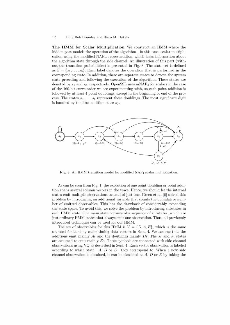
The HMM for Scalar Multiplication We construct an HMM where thehidden part models the operation of the algorithm—in this case, scalar multipli-cation using the modified NAFw representation, which leaks information aboutthe algorithm state through the side channel. An illustration of this part (with-out the transition probabilities) is presented in Fig. 3. The state set is definedas S = {s1, . . . , s8}. Each label denotes the operation that is performed in thecorresponding state. In addition, there are separate states to denote the systemstate preceding and following the execution of the algorithm. These states aredenoted by s1 and s8, respectively. OpenSSL uses mNAF4 for scalars in the caseof the 160-bit curve order we are experimenting with, so each point addition isfollowed by at least 4 point doublings, except in the beginning or end of the pro-cess. The states s3, . . . , s6 represent these doublings. The most significant digitis handled by the first addition state s2.

s1 s2

Q←kℓ−1P

s3

Q←2Q

s4

Q←2Q

s5

Q←2Q

s6

Q←2Q

s7

Q←Q+kiP

s8

ki=0

ki 6=0

Fig. 3. An HMM transition model for modified NAF4 scalar multiplication.

As can be seen from Fig. 1, the execution of one point doubling or point addi-tion spans several column vectors in the trace. Hence, we should let the internalstates emit multiple observations instead of just one. Green et al. [6] solved thisproblem by introducing an additional variable that counts the cumulative num-ber of emitted observables. This has the drawback of considerably expandingthe state space. To avoid this, we solve the problem by introducing substates ineach HMM state. One main state consists of a sequence of substates, which arejust ordinary HMM states that always emit one observation. Thus, all previouslyintroduced techniques can be used for our HMM.

The set of observables for this HMM is V = {D, A, E}, which is the sameset used for labeling cache-timing data vectors in Sect. 4. We assume that theadditions emit mainly As and the doublings mainly Ds. The s1 and s8 statesare assumed to emit mainly Es. These symbols are connected with side channelobservations using VQ as described in Sect. 4. Each vector observation is labeledaccording to which state—A, D or E—they correspond to. When a new sidechannel observation is obtained, it can be classified as A, D or E by taking the

Cache-Timing Template Attacks 13

label of the closest codebook vector. An example of this is shown in Fig. 1, wherethe rows directly above the observations represent the quantized values. SymbolsA and D are indicated using darker and lighter shades, respectively.

Training of the HMM Training starts by setting the initial model param-eters. These parameters can be rough estimates, since they will be improvedduring training. To train the model, we obtain a set of sequences in the HMMobservation domain. These sequences can be created from the side channel obser-vations as we know how the algorithm operates. The obtained sequences are usedfor model parameter re-estimation, which is performed using the Baum-Welchalgorithm [20]. Next, we create the codebook for VQ as shown in Sect. 4.

Inference of the State Sequence Given a set of side channel observationsequences from the real target system, we can infer the most likely hidden statesequence for each of them. The first step is to perform VQ, this is, to tag theobservations with the label of the closest codebook vector. Thus, we get a setof sequences in the HMM observation domain. By applying the Viterbi algo-rithm [19], we finally obtain the most likely state sequence for each observationsequence. These state sequences are actually sequences of substates; the actualoperation sequence can be recovered based on the transitions that are taken ineach state sequence. An example of this is shown in Fig. 1, where the upper rowsrepresent the main states of the algorithm. Additions are indicated using black;doublings are indicated using lighter shades. For example, the first addition onthe top trace in Fig. 1 is followed by five doublings.

The state sequences obtained in this step can be used in conjunction withsome other method to mount a key recovery attack. In the simplest case, thestate sequence reveals the secret key directly and no other methods are needed.However, with mNAF4 this is not the case; we discuss a few practical applicationsin the next section, as well as give our empirical results.

6 Results

Depending on the attack scenario and the number of traces available, there areat least two interesting ways to apply the analysis to the case of mNAF4 andOpenSSL. The first assumes access to only a single or similarly small number oftraces, while the second assumes access to a signature oracle and correspondingside channel information.

Solving Discrete Logs We consider special versions of the baby-step giant-step algorithm for searching restricted exponent spaces; see [21, Sect. 3.6] for agood overview.

The length-ℓ mNAFw representation has maximum weight ℓ/w and averageweight ℓ/(w+1); we denote this weight as t. We assume that the analysis providesus with the position of non-zero coefficients, but not their explicit value or sign;

14 Billy Bob Brumley and Risto M. Hakala

thus each coefficient gives w − 1 bits of uncertainty. One can then construct ababy-step giant-step algorithm to solve the ECDLP in this restricted keyspace.The time and space complexity is O(2(w−1)t/2); note that this does not directlydepend on ℓ (or further, the group order n). For the curve under consideration,this gives a worst case of O(260) and on average O(248), whereas the complexitywithout any such side channel information is O(280).

Lattice Attacks Despite this reduced complexity, an attacker cannot triviallycarry out the attack outlined above on a normal desktop PC. Known results onattacking signature schemes with partial knowledge of nonces include [22, 23]; the

approach is a lattice attack. Formally, the attacker obtains tuples (ri, si, mi, ki)consisting of a signature (2), message, and partial knowledge of the nonce kobtained through the timing data analysis. For our experiments, not all suchtuples are useful in the lattice attack. Using the formalization of [22], we assume

ki tells uski = z′i + 2αizi + 2βiz′′i

with zi the only unknown on the right. Our empirical timing data analysis resultsshow that the majority of errors occur when too many or few doubles are placedbetween an addition; a synchronization error in a sense. So the farther we movetowards the MSB, the more likely it is that we have erroneous indexing αi, βi

and the lattice attack will likely fail.To mitigate this issue, we instead focus only on the LSBs. We disregard the

upper term by setting z′′i = 0 and consider only tuples where ki indicates thatz′i = 0 and αi ≥ 6; that is, the LSBs of ki are 000000. For k chosen uniformly,this should happen with the reasonable probability of 2−6. Our empirical resultsare in line with those of [22]: For a 160-bit group order, 41 such tuples is usuallyenough for the lattice attack to succeed in this case.

Lattice attacks have no recourse to compensate for errors. If our analysisdetermines z′i = 0 but indeed z′i 6= 0 for some i, that instance of the latticeattack will fail. We thus adopt the naıve strategy of taking random samples ofsize 41 from the set of tuples until the attack succeeds; an attacker can alwayscheck the correctness of a guess by calculating the corresponding public key andcomparing it to the actual public key. This strategy is only feasible if the ratioof error-free tuples to erroneous tuples is high.

Finally, we present the automated lattice attack results; 8K signatures withmessages and traces were obtained in both cases.

Pentium 4 results. The analysis yielded 122 tuples indicating z′i = 0. Thelong-term private key d (2) was recovered after 1007 lattice attack iterations(107 correct, 15 incorrect). The analysis ran in less than an hour on a Core2 Duo.

Atom results. The analysis yielded 147 tuples indicating z′i = 0. We recoveredd after a total of 37196 lattice attack iterations (115 correct, 32 incorrect).Our analysis is less accurate in this case, but still accurate enough to recoverthe key in only a few hours on a Core 2 Duo.

Cache-Timing Template Attacks 15

Summary We omit strategies for finding correlation between the traces andspecific key digits. This can be tremendously helpful in further reducing thesearch space when trying to solve the ECDLP. As such, given only one or a fewtraces, this analysis method should be used as a tool in conjunction with otherheuristics to trim the search space. The lattice attack given here is proof-of-concept. The results suggest that significantly fewer signatures are needed. Inpractice one can perform a much more intelligent lattice attack, perhaps evenconsidering lattice attacks that account for key digit reuse [24].

7 Countermeasures

An implementation should not rely on any one countermeasure for side channelsecurity, but rather a combination. We briefly discuss countermeasures, with anemphasis on preventing the specific weakness we exploited in OpenSSL.

Scalar Blinding. One often-proposed strategy [1, 25–27] is to blind the scalar kfrom the point multiplication routine using randomization. One form is (k +mn+ m)P − mP with m, m small (e.g. 32-bit) and random. The calculationis then carried out using multi-exponentiation with interleaving. With sucha strategy, it suffices that m is low weight—not necessarily short.

Randomized Algorithms. Use random addition-subtraction chains instead ofhighly regular double-and-add routines. Oswald [28] gave an example anda subsequent attack [4]. Published algorithms tend to be geared towardshardware or resource restricted devices; see [29] for a good review. In asoftware package like OpenSSL that normally runs on systems with abundantmemory, one does not have to rely on simple randomized recoding and canbuild more flexible addition-subtraction chains.

Shared Context. In OpenSSL’s ECC implementation, the results and illustra-tion in Fig. 1 suggest what is most visible in the traces is not the lookup fromthe precomputation table, but the dynamic memory for variables in the pointaddition and doubling functions. OpenSSL is equipped with a shared con-text [30, pp. 106–107] responsible for allocating memory for curve and finitefield arithmetic. Memory from this context should be served up randomly toprevent a clear fixed memory access pattern.

Operation Balancing. In addition to the above shared context, coordinatesystems and point addition formulae that are balanced in the number andorder of operations are also useful; [31] gives an example.

The above countermeasures restrict to the software engineering view. Clearlyoperating system-level and hardware-level countermeasures are additionally pos-sible. We leave general countermeasures to this type of attack as an open ques-tion.

8 Conclusion

We summarize our contributions as follows:

16 Billy Bob Brumley and Risto M. Hakala

– We introduced a method for automated cache-timing data analysis, facilitat-ing discovery of critical algorithm state. This is the first work we are aware ofthat provides this at a framework level, e.g. not specific to one cryptosystem.Consequentially, it bridges the gap between cache attack vulnerabilities [9]and attacks requiring partial key material [22, 23].

– We showed how to apply HMM cryptanalysis to cache-timing data; to thebest of our knowledge, its first published application to real traces. Thisbuilds on existing work in the area of abstract side channel analysis usingHMMs [4–6], yet departs by tackling practical issues inherent to concreteside channels.

– We demonstrated the method is indeed practical by carrying out an attackon the elliptic curve portion of OpenSSL using live cache-timing data. Theattack resulted in complete key recovery, with the analysis running in amatter of hours on a normal desktop PC.

The method works by:

1. Creating cache-timing data vector templates that reflect the algorithm’scache access behavior.

2. Using VQ to match incoming cache-timing data to these existing templates.3. Using the output as observation input to an HMM that accurately models

the control flow of the algorithm.

The setup phase, including acquiring the templates used to build the VQcodebook vectors and learning the HMM parameters, is the only part by def-inition requiring any manual work, and the majority of that can in fact beautomated by simple modifications to the software under attack. This attackscenario is described for hardware power analysis in [7], but is perhaps even agreater practical threat in this case due to the inherent malleability of software.After the setup phase, cache-timing data analysis is fully automated and requiresnegligible time.

The analysis given here is not strictly meant for attacking implementations,but for defending them as well. We encourage software developers to analyzetheir implementations using these methods to discover memory access patternsand apply appropriate countermeasures.

Future Work

One might think to forego the VQ step and use the cache-timing data directly asthe sole input to the HMM. In our experience, this only complicates the modeland hampers quality results.

The example we gave was tailored to data caches, in particular the L1 datacache. Other data caches could prove equally fruitful. We also plan to apply theanalysis method to instruction caches.

While the attack results we gave were for one particular cryptosystem im-plementation, the analysis method has a much wider range of applications. We

Cache-Timing Template Attacks 17

in fact found a similar vulnerability in the NSS library’s implementation of el-liptic curves. Departing from elliptic curves and public key cryptography, weplan to apply the analysis to an assortment of implementations, asymmetric andsymmetric primitives alike.

One of the more interesting planned applications is to algorithms with goodside channel resistance properties, such as “Montgomery’s ladder”. While thismight be an overwhelming challenge for traditional power analysis, the workhere emphasizes the fact that cache-timing attacks are about memory accesspatterns; a fixed sequence of binary operations cannot be assumed sufficient tothwart cache-timing attacks.

Acknowledgments We thank the following people for comments and discus-sions: Dan Bernstein, Kimmo Jarvinen, Kaisa Nyberg, and Dan Page.

References

1. Kocher, P.C.: Timing attacks on implementations of Diffie-Hellman, RSA, DSS,and other systems. In Koblitz, N., ed.: CRYPTO 1996. Volume 1109 of LNCS.Springer (1996) 104–113

2. Kocher, P.C., Jaffe, J., Jun, B.: Differential power analysis. In Wiener, M.J., ed.:CRYPTO 1999. Volume 1666 of LNCS. Springer (1999) 388–397

3. Page, D.: Defending against cache based side-channel attacks. Information SecurityTechnical Report 8(1) (2003) 30–44

4. Oswald, E.: Enhancing simple power-analysis attacks on elliptic curve cryptosys-tems. In Kaliski, Jr, B.S., Koc, C.K., Paar, C., eds.: CHES 2002. Volume 2523 ofLNCS. Springer (2003) 82–97

5. Karlof, C., Wagner, D.: Hidden Markov model cryptanalysis. In Walter, C.D.,Koc, C.K., Paar, C., eds.: CHES 2003. Volume 2779 of LNCS. Springer (2003)17–34

6. Green, P.J., Noad, R., Smart, N.P.: Further hidden Markov model cryptanalysis.In Rao, J.R., Sunar, B., eds.: CHES 2005. Volume 3659 of LNCS. Springer (2005)61–74

7. Chari, S., Rao, J.R., Rohatgi, P.: Template attacks. In Kaliski, Jr, B.S., Koc, C.K.,Paar, C., eds.: CHES 2002. Volume 2523 of LNCS. Springer (2003) 13–28

8. Medwed, M., Oswald, E.: Template attacks on ECDSA. In Chung, K.I., Sohn, K.,Yung, M., eds.: WISA 2008. Volume 5379 of LNCS. Springer (2008) 14–27

9. Percival, C.: Cache missing for fun and profit. http://www.daemonology.net/

papers/cachemissing.pdf (2005)10. Hlavac, M., Rosa, T.: Extended hidden number problem and its cryptanalytic

applications. In Biham, E., Youssef, A.M., eds.: SAC 2006. Volume 4356 of LNCS.Springer (2006) 114–133

11. Bernstein, D.J.: Cache-timing attacks on AES. http://cr.yp.to/papers.html#

cachetiming (2004)12. Osvik, D.A., Shamir, A., Tromer, E.: Cache attacks and countermeasures: The case

of AES. In Pointcheval, D., ed.: CT-RSA 2006. Volume 3860 of LNCS. Springer(2006) 1–20

13. Moller, B.: Algorithms for multi-exponentiation. In Vaudenay, S., Youssef, A.,eds.: SAC 2001. Volume 2259 of LNCS. Springer (2001) 165–180

18 Billy Bob Brumley and Risto M. Hakala

14. Moller, B.: Improved techniques for fast exponentiation. In Lee, P.J., Lim, C.H.,eds.: ICISC 2002. Volume 2587 of LNCS. Springer (2003) 298–312

15. Bosma, W.: Signed bits and fast exponentiation. Journal de Theorie des Nombresde Bordeaux 13(1) (2001) 27–41

16. Kohonen, T.: Self-Organizing Maps. Springer (1995)17. Lloyd, S.: Least squares quantization in PCM. IEEE Transactions on Information

Theory 28(2) (1982) 129–13718. Rabiner, L.R.: A tutorial on hidden Markov models and selected applications in

speech recognition. Proceedings of the IEEE 77(2) (1989) 257–28619. Viterbi, A.J.: Error bounds for convolutional codes and an asymptotically optimum

decoding algorithm. IEEE Transactions on Information Theory 13(2) (1967) 260–269

20. Baum, L.E., Petrie, T., Soules, G., Weiss, N.: A maximization technique occurringin the statistical analysis of probabilistic functions of Markov chains. The Annalsof Mathematical Statistics 41(1) (1970) 164–171

21. Menezes, A., van Oorschot, P., Vanstone, S.: Handbook of Applied Cryptography.5 edn. CRC Press (2001)

22. Howgrave-Graham, N., Smart, N.P.: Lattice attacks on digital signature schemes.Designs, Codes and Cryptography 23(3) (2001) 283–290

23. Nguyen, P.Q., Shparlinski, I.: The insecurity of the elliptic curve digital signaturealgorithm with partially known nonces. Designs, Codes and Cryptography 30(2)(2003) 201–217

24. Leadbitter, P.J., Page, D., Smart, N.P.: Attacking DSA under a repeated bitsassumption. In Joye, M., Quisquater, J.J., eds.: CHES 2004. Volume 3156 ofLNCS. Springer (2004) 428–440

25. Coron, J.S.: Resistance against differential power analysis for elliptic curve cryp-tosystems. In Koc, C.K., Paar, C., eds.: CHES 1999. Volume 1717 of LNCS.Springer (1999) 292–302

26. Clavier, C., Joye, M.: Universal exponentiation algorithm: a first step towardsprovable SPA-resistance. In Koc, C.K., Naccache, D., Paar, C., eds.: CHES 2001.Volume 2162 of LNCS. Springer (2001) 300–308

27. Moller, B.: Parallelizable elliptic curve point multiplication method with resistanceagainst side-channel attacks. In Chan, A.H., Gligor, V.D., eds.: ISC 2002. Volume2433 of LNCS. Springer (2002) 402–413

28. Oswald, E., Aigner, M.: Randomized addition-subtraction chains as a counter-measure against power attacks. In Koc, C.K., Naccache, D., Paar, C., eds.: CHES2001. Volume 2162 of LNCS. Springer (2001) 39–50

29. Walter, C.D.: Randomized exponentiation algorithms. In Koc, C.K., ed.: Crypto-graphic Engineering. Springer (2009)

30. Viega, J., Messier, M., Chandra, P.: Network Security with OpenSSL. O’ReillyMedia, Inc. (2002)

31. Chevallier-Mames, B., Ciet, M., Joye, M.: Low-cost solutions for preventing simpleside-channel analysis: Side-channel atomicity. IEEE Transactions on Computers53(6) (2004) 760–768