A complex systems analysis of stick-slip dynamics of a laboratory faultDavid M. Walker, Antoinette Tordesillas, Michael Small, Robert P. Behringer, and Chi K. Tse Citation: Chaos: An Interdisciplinary Journal of Nonlinear Science 24, 013132 (2014); doi: 10.1063/1.4868275 View online: http://dx.doi.org/10.1063/1.4868275 View Table of Contents: http://scitation.aip.org/content/aip/journal/chaos/24/1?ver=pdfcov Published by the AIP Publishing

This article is copyrighted as indicated in the article. Reuse of AIP content is subject to the terms at: http://scitation.aip.org/termsconditions. Downloaded to IP:130.95.16.46 On: Fri, 14 Mar 2014 01:19:54

A complex systems analysis of stick-slip dynamics of a laboratory fault

David M. Walker,1 Antoinette Tordesillas,1,a) Michael Small,2 Robert P. Behringer,3

and Chi K. Tse4

1Department of Mathematics and Statistics, University of Melbourne, Parkville VIC 3010 Australia2School of Mathematics and Statistics, University of Western Australia, Crawley WA 6009, Australia3Department of Physics, Duke University, Durham, North Carolina 27708, USA4Department of Electronic and Information Engineering, Hong Kong Polytechnic University, Hung Hom,Kowloon, Hong Kong

(Received 18 June 2013; accepted 1 March 2014; published online 13 March 2014)

We study the stick-slip behavior of a granular bed of photoelastic disks sheared by a rough sliderpulled along the surface. Time series of a proxy for granular friction are examined using complexsystems methods to characterize the observed stick-slip dynamics of this laboratory fault.Nonlinear surrogate time series methods show that the stick-slip behavior appears more complexthan a periodic dynamics description. Phase space embedding methods show that the dynamics canbe locally captured within a four to six dimensional subspace. These slider time series also providean experimental test for recent complex network methods. Phase space networks, constructed byconnecting nearby phase space points, proved useful in capturing the key features of the dynamics.In particular, network communities could be associated to slip events and the ranking of smallnetwork subgraphs exhibited a heretofore unreported ordering. VC 2014 AIP Publishing LLC.[http://dx.doi.org/10.1063/1.4868275]

Inferring dynamical structure of a deterministic nonlin-ear system from bulk time series measurements contami-nated by noise remains a challenge, despite a number ofavailable and complementary methods for characteriza-tion. Here, we demonstrate a variety of complex systemmethods to a problem of particular interest to geophysics,i.e., granular friction. Knowledge of granular friction iscrucial for understanding not only the mechanisms re-sponsible for earthquake dynamics but also the details offorce transmission in granular-structure/solid interactionsystems (e.g., soil-vehicle interaction, building founda-tions, etc.). We study a slider experiment introduced toinvestigate such behavior. Our analysis indicates that thedynamics of granular friction within the slider are con-sistent with short term determinism, possibly quasi-periodic, but with no long-term memory. The observeddynamics also induce a complex network representationpossessing a previously unobserved prevalence rankingof small subgraphs, i.e., a new superfamily. Our charac-terization suggests that despite models based on periodic-ity being sufficient for some purposes, new models areneeded to fully capture the complex dynamics responsiblefor the observed slider behavior.

I. INTRODUCTION

When two frictional solid objects move relative to eachother, the motion of their surfaces often alternate betweenperiods of stick contact, when surfaces are locked together,and periods of sliding contact, when surfaces overcome“friction” and slip past each other. This phenomenon, known

commonly as stick-slip, arises in many aspects of everydaylife and is often implicated in damage and failure of materi-als. Stick-slip is by no means limited to the dry contact oftwo solid bodies: other examples include articular cartilagedamage,1 vibrations in vehicle suspensions and brake sys-tems,2,3 erratic motion in industrial machinery and tools,4

and the behavior of active geological faults.5–7 Indeed, stick-slip motion can arise in the presence of fluids between surfa-ces8 and in discrete granular materials.9–14 Regardless of thematerials involved, what makes stick-slip one of the mostchallenging dynamical phenomenon to characterize andmodel is that it is the result of an interaction between manycomplex entwined mechanical (and sometimes chemical)processes.1–17

Our interest here lies in the occurrence of stick-slip ingranular materials, which often manifest in fluctuations ofmacroscopic shear stresses—a measure of the strength of amaterial. For these highly ubiquitous and technologicallyimportant class of materials, understanding stick-slip is notonly of core importance to the study of granular frictionbut of a number of related processes, including: frictionalstrength of geological fault gouge, shear bands, the coexis-tence of stable solid-like and flowing liquid-like regimes,and the existence and uniqueness of a so-called “criticalstate” of a material (e.g., Refs. 9–16, 18, and 19). In manypractical settings, arguably the most valuable piece of in-formation embodied in stick-slip is the dynamics of energystorage and dissipation in the system. Understandingthe energetics and recurrence of earthquakes, and the opti-mal control of energy consumption in many particulateprocesses (e.g., comminution, dewatering, etc.), hingeson our ability to unravel the micromechanical detailsunderlying stick versus slip for a broad gamut of loadingconditions.18,20–23

a)Author to whom correspondence should be addressed. Electronic mail:atordesi@unimelb.edu.au

1054-1500/2014/24(1)/013132/10/$30.00 VC 2014 AIP Publishing LLC24, 013132-1

CHAOS 24, 013132 (2014)

This article is copyrighted as indicated in the article. Reuse of AIP content is subject to the terms at: http://scitation.aip.org/termsconditions. Downloaded to IP:130.95.16.46 On: Fri, 14 Mar 2014 01:19:54

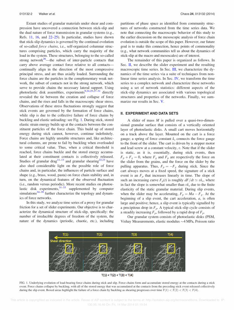
Extant studies of granular materials under shear and com-pression have uncovered a connection between stick-slip andthe dual nature of force transmission in granular systems (e.g.,Refs. 11, 16, and 22–25). In particular, studies have shownthat stick-slip dynamics is governed by the continual evolutionof so-called force chains, i.e., self-organized columnar struc-tures comprising particles, which carry the majority of theload in the system. These structures, belonging to the so-calledstrong network26—the subset of inter-particle contacts thatcarry above average contact force relative to all contacts—continually align in the direction of the most compressiveprincipal stress, and are thus axially loaded. Surrounding theforce chains are the particles in the complementary weak net-work, the subset of contacts not in the strong network, whichserve to provide chains the necessary lateral support. Usingphotoelastic disk assemblies, experiments9,24,25,27–31 directlyrevealed the tie between the creation and collapse of forcechains, and the rises and falls in the macroscopic shear stress.Observations of these stress fluctuations strongly suggest thatstick events are governed by the formation of force chains,while slip is due to the collective failure of force chains bybuckling and elastic unloading: see Fig. 1. During stick, storedelastic strain energy builds up at the contacts between the con-stituent particles of the force chain. This build up of storedenergy during stick cannot, however, continue indefinitely.Force chains are highly unstable structures and, like architec-tural columns, are prone to fail by buckling when overloadedto some critical value. Thus, when a critical threshold isreached, force chains buckle and the stored energy accumu-lated at their constituent contacts is collectively released.Studies of granular drag11–13 and granular shearing22,23 havealso shed considerable light on the possible role of forcechains and, in particular, the influences of particle surface andshape (e.g., brass, wood, pasta) on force chain stability and, inturn, on the dynamical features of the observed fluctuation(i.e., random versus periodic). More recent studies on photoe-lastic disk experiments,31–33 supplemented by computersimulations34–39 further characterize the topology and dynam-ics of force networks.

In this study, we analyze time series of a proxy for granularfriction for a set of slider experiments. Our objective is to char-acterize the dynamical structure of stick-slip, specifically: thenumber of irreducible degrees of freedom of the system, thenature of the dynamics (periodic, chaotic, etc.), including

partitions of phase space as identified from community struc-tures of networks constructed from the time series data. Wenote that connecting the macroscopic behavior of this study tothe earlier discussion on the mesoscopic analysis of force chainevolution is outside the scope of this paper. However, our futuregoal is to make this connection, hence points of commonality(e.g., what network communities tell us about the dynamics ofstick-slip at the macro and mesoscales) are of interest.

The remainder of this paper is organized as follows. InSec. II, we describe the slider experiment and the resultingmacroscopic time series. In Sec. III, we characterize the dy-namics of the time series via a suite of techniques from non-linear time series analysis. In Sec. IV, we transform the timeseries to a complex network and characterize these networksusing a set of network statistics: different aspects of thestick-slip dynamics are associated with various topologicalstructures and properties of the networks. Finally, we sum-marize our results in Sec. V.

II. EXPERIMENT AND DATA SETS

A slider of mass M is pulled over a quasi-two-dimen-sional granular surface that consists of a vertically orientedlayer of photoelastic disks. A small cart moves horizontallyon a track above the layer. Mounted on the cart is a forcegauge; a spring of force constant ks connects the force gaugeto the front of the slider. The cart is driven by a stepper motorand lead screw at a constant velocity, v. Note that if the slideris static, as it is, essentially, during stick events, thenFp þ Fg ¼ 0, where Fg and Fp are respectively the force onthe slider from the grains, and the force on the slider by thepulling apparatus. Thus, Fp ¼ #Fg during stick. Since thecart always moves at a fixed speed, the signature of a stickevent is an Fp that increases linearly in time. The slope ofsuch an increasing curve Fp(t) is roughly dF=dt ’ vks, wherein fact the slope is somewhat smaller than vks due to the finiteelasticity of the static granular material. During slip events,when the slider may be accelerating, Fp ¼ Ma# Fg. At thebeginning of a slip event, the cart acceleration, a, is oftenlarge and positive; hence, a slip event is typically signalled bya precipitous drop in Fp. A typical stick-slip cycle consists ofa steadily increasing Fp, followed by a rapid drop of Fp.

Our granular system consists of photoelastic disks (PSM,Vishay Measurements, elastic modulus $4 MPa, Poisson ratio

FIG. 1. Underlying evolution of load-bearing force chains during stick and slip. Force chains form and accumulate stored energy at the contacts during a stickevent. Force chains collapse by buckling, with all of the stored energy that was accumulated at the contacts from the preceding stick event released collectivelyduring the slip event. Boxed areas highlight the failure of a force chain by buckling as shearing progresses over time Tð1Þ < Tð2Þ < Tð3Þ < Tð4Þ.

013132-2 Walker et al. Chaos 24, 013132 (2014)

This article is copyrighted as indicated in the article. Reuse of AIP content is subject to the terms at: http://scitation.aip.org/termsconditions. Downloaded to IP:130.95.16.46 On: Fri, 14 Mar 2014 01:19:54

$0.4) that are placed in a channel between two vertically ori-ented Plexiglas sheets. This allows simultaneous measure-ment of Fp, motion of the slider, and the particle-scaleresponse within the granular layer. The channel is 1.5 mlong, 15.5 cm tall, and has a gap slightly greater than thethickness of the disks, which is 3.2 mm. The depth of thegranular layer corresponds to $20 mean grain diameters.The disks are bidisperse, with diameters 4 mm and 5 mm,and thickness 3.2 mm. The average particle size isd¼ 4.37 mm. The sliders are cut from either brass or alumi-num and are roughened on the bottom surface (which con-tacts the grains) by a series of half-round cut-outs, ofdiameter d. The sliders have lengths of 30d to 60d, andmasses between 50 g and 250 g.

The force gauge cart also carries an imaging system fordetermining the photoelastic response of the grains. Thisconsists of a circularly polarized light source that movesalong one side of the channel and a second crossed circularpolarizer that is placed in front of a high speed video camerathat operates at frame rates from 30 Hz to 500 Hz. Fp dataare acquired synchronously with camera frame grabs.Stressed photoelastic materials placed between crossedpolarizers show light and dark bands which provide quantita-tive information on inter-particle forces27,28,31 (see images inFig. 1). In this work, however, we concentrate solely on ananalysis of the time series data, leaving the coupled analysisof images and time series to a future exploration.

A number of time series were recorded with differentexperimental test parameters, in particular, duration ofexperiment, sampling frequency, cart mass, and cart speed.We report the results of a combined nonlinear time seriesand complex network analysis for a number of these runs tosee if there is consistency across each run, and attempt tocharacterize the underlying properties of a dynamical systemcapable of explaining the observed data.

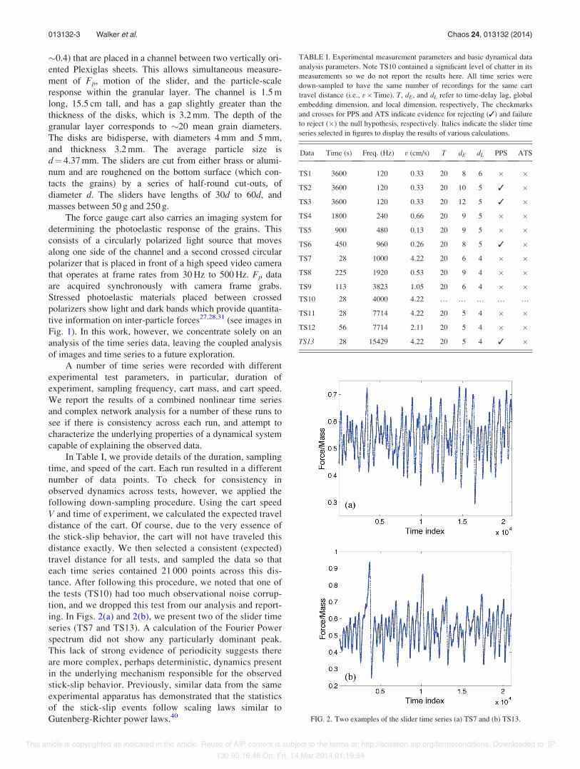
In Table I, we provide details of the duration, samplingtime, and speed of the cart. Each run resulted in a differentnumber of data points. To check for consistency inobserved dynamics across tests, however, we applied thefollowing down-sampling procedure. Using the cart speedV and time of experiment, we calculated the expected traveldistance of the cart. Of course, due to the very essence ofthe stick-slip behavior, the cart will not have traveled thisdistance exactly. We then selected a consistent (expected)travel distance for all tests, and sampled the data so thateach time series contained 21 000 points across this dis-tance. After following this procedure, we noted that one ofthe tests (TS10) had too much observational noise corrup-tion, and we dropped this test from our analysis and report-ing. In Figs. 2(a) and 2(b), we present two of the slider timeseries (TS7 and TS13). A calculation of the Fourier Powerspectrum did not show any particularly dominant peak.This lack of strong evidence of periodicity suggests thereare more complex, perhaps deterministic, dynamics presentin the underlying mechanism responsible for the observedstick-slip behavior. Previously, similar data from the sameexperimental apparatus has demonstrated that the statisticsof the stick-slip events follow scaling laws similar toGutenberg-Richter power laws.40 FIG. 2. Two examples of the slider time series (a) TS7 and (b) TS13.

TABLE I. Experimental measurement parameters and basic dynamical data

analysis parameters. Note TS10 contained a significant level of chatter in itsmeasurements so we do not report the results here. All time series weredown-sampled to have the same number of recordings for the same cart

travel distance (i.e., v'Time). T, dE, and dL refer to time-delay lag, globalembedding dimension, and local dimension, respectively, The checkmarks

and crosses for PPS and ATS indicate evidence for rejecting (✓) and failureto reject (') the null hypothesis, respectively. Italics indicate the slider timeseries selected in figures to display the results of various calculations.

Data Time (s) Freq. (Hz) v (cm/s) T dE dL PPS ATS

TS1 3600 120 0.33 20 8 6 ' '

TS2 3600 120 0.33 20 10 5 ✓ '

TS3 3600 120 0.33 20 12 5 ✓ '

TS4 1800 240 0.66 20 9 5 ' '

TS5 900 480 0.13 20 9 5 ' '

TS6 450 960 0.26 20 8 5 ✓ '

TS7 28 1000 4.22 20 6 4 ' '

TS8 225 1920 0.53 20 9 4 ' '

TS9 113 3823 1.05 20 6 4 ' 'TS10 28 4000 4.22 … … … … …

TS11 28 7714 4.22 20 5 4 ' '

TS12 56 7714 2.11 20 5 4 ' '

TS13 28 15429 4.22 20 5 4 ✓ '

013132-3 Walker et al. Chaos 24, 013132 (2014)

This article is copyrighted as indicated in the article. Reuse of AIP content is subject to the terms at: http://scitation.aip.org/termsconditions. Downloaded to IP:130.95.16.46 On: Fri, 14 Mar 2014 01:19:54

III. NONLINEAR TIME SERIES METHODS

We apply tools from nonlinear time series analysis togain more knowledge about the slider system and, in turn,stick-slip dynamics. It is important to first: (i) check whetherthe observed data is sufficiently stationary for nonlinearmethods to be usefully applied, and (ii) determine whether alinear approach does not already tell us everything of practi-cal interest about the data. A definitive check of stationarityof a finite length data set is impossible. However, a basic testis to determine whether the fluctuations of the sample meanover contiguous segments of the data are within the fluctua-tions observed in the data of each segment.41 By segmentingeach of the observed slider time series into contiguous datasets, each of length n, we found the fluctuations of the run-ning sample mean for n> 500 was within the sample stand-ard deviation. Thus, over segments of length n> 500, theslider data can be considered approximately stationary.

A. Linear surrogates

We test whether or not the observed data is fullyexplained by simple linear descriptions using the method ofsurrogate data. Surrogate data testing is a form of randomiza-tion testing. Additional data sets are generated which areconsistent with the observed data set and consistent with astated hypothesis.42,43 A hypothesis is tested by calculating atest statistic and comparing the value obtained from the orig-inal data to the distribution of test statistic values from thesurrogates. We use z-scores to measure the deviation of theoriginal data test value from the sample mean of the surro-gate values in terms of the surrogates sample standard devia-tion. If the z-score is high enough, we can reject the nullhypothesis under consideration. Z-scores rely on a Gaussianassumption and so other metrics such as the Kolmogorov-Smirnov test may be more reliable and appropriate.42

The three standard surrogate tests that we use are coinedAlgorithm 0, 1, and 2. In Alg. 0, the data set is tested againstthe hypothesis that it is independently and identically distrib-uted noise. This involves generating uncorrelated data withthe same probability distribution of the original data.Algorithm 1 tests the hypothesis that the data set is linearlyfiltered noise; hence, random surrogates with the same powerspectrum and autocorrelation function are generated.Algorithm 2 tests the hypothesis that the data are a mono-tonic nonlinear transformation of linearly filtered noise. Thehypotheses of Alg. 0 is a subset of Alg. 1, which is itself asubset of Alg. 2. However, the realizations obtained fromeach algorithm do not necessarily preserve this nesting (see,e.g., Small42 for a description of surrogate generation meth-ods for each algorithm).

Here, we reject null hypotheses for a z-score above 2;however, most runs and surrogate tests return z-score valuesabove 3. We used the average mutual information (AMI)44,45

at lag one as the test statistic. The average mutual informa-tion is a nonlinear measure over a range of lags. However, asin other studies,46 we found checking only lag one providedsufficient evidence to reject the null hypothesis for each test.We found we could reject each hypothesis, hence a simple

linear description of the observed slider time series does notfully explain the observed behavior.

B. Reconstructed state space

The analysis of time series using the methods of nonlin-ear dynamics is predominantly based around studying thedata in a reconstructed phase space.45 A common method offinding such a phase space is time-delay embedding, wherethe time series fytgN

t¼1 and delayed versions of itself are usedto form the coordinates.47 The state z 2 RdE of the recon-structed phase space is

zt ¼ ðyt#ðdE#1ÞT ;…; yt#T ; ytÞ; (1)

where the parameters of this reconstruction are the time-delay (T) and the embedding dimension (dE). There are pre-scriptions for selecting these parameters. The first minimumof the AMI determines the time delay lag. AMI can be con-sidered as a kind of nonlinear autocorrelation function44 andselecting T as the first minimum helps to identify more inde-pendent coordinates in the reconstructed space. For a givenT, the value of dE can be selected using the method of falsenearest neighbours45 (FNN). FNN attempts to find the small-est number of coordinates required to unfold the observeddata and minimize self-crossing of trajectories. That is, coor-dinates in phase space are close because of the dynamics andnot because of an insufficient projection to a lower dimen-sional space.

We found the first minimum of average mutual informa-tion at T¼ 20, although a clearer minimum occurred forhigher values of T in some tests. For the majority of the tests,however, T¼ 20 was closer to a quarter of the length of atypical stick-slip event. Fixing T¼ 20, we found a suitableglobal embedding dimension dE from false nearest neighborsto lie in the range 5–12 (see, Table I). However, dE¼ 8appeared to be adequate for all tests. Thus, for all future cal-culations, the parameters of the reconstructed phase spaceare T¼ 20 and dE¼ 8.

The global embedding dimension dE is based solely ongeometric arguments. Consequently, it will likely return avalue greater than the actual dimension of the system. It ispossible to determine the number of active degrees of free-dom of the system using the method of local false nearestneighbors48 (LFNN). LFNN adds to the geometric considera-tions of FNN by including the predictability of the dynamicalinformation inherent in the time series. The local dimensiondL provides the number of variables required to accuratelymodel the evolution of local neighborhoods of phase space.We can find the number of these variables by examiningPx—the ratio of the number of points poorly predicted by alocal model over T¼ 20 time steps to the number of points—for different-sized local neighborhoods across dimensions. Inthis context, a point is poorly predicted if the L1 predictionerror is larger than 10% of the spread of the data. These dy-namical variables are the ones which are active for a dynami-cal description of the physics. They differ from a morestandard interpretation of degrees of freedom, which wouldnot only include these active variables but also those

013132-4 Walker et al. Chaos 24, 013132 (2014)

This article is copyrighted as indicated in the article. Reuse of AIP content is subject to the terms at: http://scitation.aip.org/termsconditions. Downloaded to IP:130.95.16.46 On: Fri, 14 Mar 2014 01:19:54

variables deemed inactive with respect to the dynamics dueto, for example, damping.

In Fig. 3 and Table I, we see Px falls to a floor fordL ¼ 4# 6, i.e., the slider exhibits low dimensional dynam-ics with four to six dynamical degrees of freedom. Thus,models capable of capturing the macroscopic stick-slip dy-namics of granular friction should have no fewer than four-to-six dynamical variables.

C. Attractor trajectory surrogates (ATS)

Given a reconstructed state space, we can pose more spe-cific questions about the observed dynamics using pseudo-periodic surrogates (PPS) or ATS, depending on the specificnull hypothesis.42,49 For oscillatory time series, like thesequential stick-slip events in the slider (Fig. 2), PPS test forperiodic dynamics driven by uncorrelated noise. ATS testwhether pseudo-cycle (stick-slip events) dynamics is pre-served with no evidence for long term dynamical correlationsbetween cycles (cf. the cycle-shuffle surrogates in Ref. 50).For the slider, PPS are effectively testing whether the sliderdynamics within stick-slip events is consistent with noise-driven periodic dynamics or, more complicated nonlineardeterminism. In contrast, ATS test whether the dynamics ofstick-slip events is the result of the same underlying dynamicswith no long term correlations between the different events:that is, whether the granular bed only has short term memory.

PPS and ATS are a local phase space resampling of theoriginal time series with replacement based on the resolutionof resampling. A prescription for determining a resolution isbased on how many contiguous segments of the originaltime series, each of non-trivial length, appear within the sur-rogate. The length of contiguous segments determines thelevel of randomization in the algorithm. The length ofcontiguous segments, in turn, is determined by the level ofrandomization—or, equivalently, the neighborhood size.With a large neighborhood, sampling with replacement isessentially random and irrespective of the phase space struc-ture: this is equivalent to Alg. 0 surrogates—random re-sampling (albeit with replacement). At the other end of thescale, with a very small neighborhood, there is minimal

randomization and long segments of the dynamics are repro-duced. With a non-trivial level of randomization, this yieldsATS. In the trivial case (no noise), one just recovers the orig-inal time series. As the noise level (neighborhood size)increases, the original time series is segmented and the seg-ments are shuffled at locations where many similar statesoccur close to one another in phase space. This is what isrequired for the ATS algorithm. Increasing noise level(neighborhood size) has the effect of increasing dynamicalnoise contamination in the surrogate generation process untilonly the most basic macroscopic dynamical features areretained. That is, the pseudo-periodic structure and hence thePPS algorithm.

We use the nonlinear test statistic of algorithmic com-plexity to distinguish the observed data from PPS and ATSdata (see, e.g., Small42 for ways to calculate this complexitymeasure). In Table I, a “✓” indicates that there is sufficientevidence to reject the null hypothesis (i.e., z-scores above 2)and a “'” indicates failure to reject. We find mixed resultsfor the PPS hypothesis: periodic dynamics plus uncorrelatednoise often appears sufficient to describe the observed dy-namics. In all cases, we fail to reject the ATS null hypothe-sis. For the length of data, ATS are unable to detect longterm dynamical correlations between stick-slip events withrespect to the test statistic of algorithmic complexity. Thiscan be explained by the physical fact that disturbed andundisturbed sets of grains come into play as the slider movesunidirectionally along the granular bed.

We can view these findings side-by-side with resultsfrom an earlier study on the macroscopic stress responsebehavior of dense granular media undergoing deformation inthe presence of a fully developed shear band.19 In that work,a time series of the macroscopic stress ratio in the largestrain regime was studied using nonlinear methods. Theobserved response of this virtual system was “best”described by nonlinear models exhibiting a complicated non-periodic dynamics, as is suggested here by PPS for some ofthe sliders. Furthermore, local false nearest neighbors analy-sis of the virtual system similarly suggested 4–6 activedegrees of freedom are needed to describe the dynamics ofstick-slip. This is also consistent with Cosserat constitutiverelations based on force chain evolution developed for thelarge strain regime in the presence of a fully developed shearband.51

IV. COMPLEX NETWORK METHODS

In addition to surrogate testing and phase space recon-struction methods, the technique of obtaining a complex net-work from time series can garner useful information fromthe data. There are various ways of transforming an observedtime series into a complex network. Zhang and Small52

transformed oscillatory time series to a network by segment-ing the data into pseudo-cycles—the peak-to-peak segmentsof the time series which would correspond to the stick-slipcycles in the sliders—and calculating the correlationbetween pair-wise segments. Network nodes correspond tothe pseudo-cycles, and links are made if the correlations areabove a specified threshold. The visibility graph method of

FIG. 3. TS13: local false nearest neighbors for different number of nearneighbors (NB). Inset: zoomed in showing dL ¼ 4# 6 local dimensions. Atime-delay of T¼ 20 was used to embed the time series data.

013132-5 Walker et al. Chaos 24, 013132 (2014)

This article is copyrighted as indicated in the article. Reuse of AIP content is subject to the terms at: http://scitation.aip.org/termsconditions. Downloaded to IP:130.95.16.46 On: Fri, 14 Mar 2014 01:19:54

Lacasa et al.53 introduced another transformation method,whereby each scalar value of the time series corresponds to anetwork node and the links are drawn according to the rela-tive magnitude of each value. Both methods produce net-works whose respective properties help to characterize theunderlying processes that may be responsible for the time se-ries. Moreover, neither method requires a reconstructedphase space to be determined.

Xu et al.54 showed how a complex network can beobtained from a phase space reconstructed using a time-delay embedding. Network nodes are the individual phasespace points and connectivity is determined by relativecloseness of these points. They coined such a network aPhase Space Network (PSN), and this is the type of networkwe use to study the slider time series. In a similar vein,Marwan et al.55 recognized the likeness between a networkadjacency matrix and a recurrent plot matrix, and developeda recurrence-based network representation of a time series.A review by Donner et al.56 discusses the relationshipbetween phase space networks and recurrence-based net-works from a theoretical and practical standpoint.

The formation of a PSN can be seen as a first step in thedimension reduction process ISOMAP, in particulark-ISOMAP.57 ISOMAP has been used in dynamical systemsdata analysis to find a lower dimensional manifold where thedynamics evolve.58,59 One constructs this manifold by takinga PSN and forming a matrix from the shortest path lengthdistribution between each pair of nodes in a PSN. A multidi-mensional scaling step is performed on this matrix to form anew set of (lower dimensional) coordinates to study thedynamics. Notable success has been achieved when thesecoordinates result in a one-dimensional return map.58,59 Onedimensional return maps are appealing because they aremore amenable to examination by global analysis methodssuch as Ulam’s method for approximating the Perron-Frobenius transfer operator.60,61 The spectral properties ofmatrices approximating this operator help to identify globalstructures in the data, including almost invariant sets as wellas providing a means to estimate dynamical invariants.62,63

More generally, the Perron-Frobenius transfer operatorcan be approximated directly from a reconstructed phasespace using the Ulam-Galerkin method.64,65 In this case, thephase space is covered by regions and the dynamical flowfrom region to region is approximated by a Ulam-Galerkinmatrix that can be interpreted as a (weighted) directed graph.Nodes correspond to the regions and the weighted linksencode the transport mechanism. In contrast, the PSNs weconsider here do not explicitly encode the time evolution asonly closeness in phase space determines the connectivity.Furthermore, nodes in a PSN correspond to observed datapoints and not regions of phase space. A PSN differs fromthe Ulam-Galerkin approach by being an unweighted, undir-ected network although there are clear correspondences wor-thy of exploration.

For example, in the following, we consider a partition-ing of the PSNs using modularity-based methods. InSantitissadeekorn and Bollt,66 the network arising from theUlam-Galerkin matrix approximation is also partitionedusing a modularity score to reveal basins and basin barriers

in phase space. It is also intriguing to consider how eachapproach would compare with generating partitions,67 aswell as the symbolic dynamics68,69 within a low dimensionalmanifold identified via ISOMAP.

Here, we construct PSNs using a fixed connection rulewhere each node connects to its k closest phase space neigh-bors. We discount connections based on close temporal cor-relation, akin to applying a Theiler window to de-correlateclose neighbors within a correlation integral calculation.41 Asuitable de-correlation interval or size of Theiler windowcan be gauged from a space-time separation plot, wherebythe quantiles of the inter-point distance distribution are cal-culated for data separated by a given time span.41 We findthat the quantiles have started to separate from each other fora de-correlation interval of 100, so nodes representing recon-structed phase space points temporally closer than 100 timesteps are barred from connecting to each other. As before,we use the reconstructed phase space embedding parametersT¼ 20 and dE¼ 8 resulting in networks with 20860 nodes.We fix k¼ 4 neighbors to construct each PSN.

The structure of a PSN can be quantified and describedby standard network properties such as average degree (theaverage number of links connected to a node), average clus-tering coefficient (a measure of the closed triples in a net-work), degree assortativity (a correlation score of how nodeswith the same degree are connected to each other), averageshortest path lengths (the minimum number of links connect-ing two nodes), node closeness centrality (how closely con-nected a node is to all other nodes in the network) amongothers; see, e.g., Newman70 for more detailed descriptions.In Table II, these global properties are presented for eachPSN. We observe consistency across tests. Each networkappears disassortative (negative degree assortativity): i.e.,

TABLE II. Global network properties of the PSN constructed from the slider

time series using T ¼ 20; dE ¼ 8, and a Theiler, or de-correlation windowof 100. Each state space point (node) is connected to its 4 closest neighbors.N.B. this means that some nodes can have degree greater than 4 since they

may be within the 4 closest neighbors to another node but that node may notbe within the 4th closest neighbors of themselves. The clustering coefficient

for a node of degree ki being a part of ni triangles is calculated to be

ni=ki

2

! ".

Data Number Average Degree Average Averageof network degree assortativity clustering path

components coefficient length

TS1 1 6.9814 #0.3295 0.0349 16.3294

TS2 2 6.9567 #0.2689 0.0510 16.2198

TS3 1 6.9216 #0.2686 0.0873 21.8721

TS4 1 6.9406 #0.2259 0.0478 18.0717

TS5 1 6.9496 #0.3171 0.0415 17.6985

TS6 1 6.8206 #0.2906 0.0381 20.3626

TS7 1 6.6998 #0.3146 0.0400 38.8677

TS8 1 6.7826 #0.2210 0.0495 20.3710

TS9 1 6.7158 #0.2534 0.0266 28.4885

TS11 1 6.6814 #0.2424 0.0361 39.3600

TS12 1 6.5910 #0.2581 0.0407 36.8730

TS13 1 6.7371 #0.2269 0.0541 44.5371

013132-6 Walker et al. Chaos 24, 013132 (2014)

This article is copyrighted as indicated in the article. Reuse of AIP content is subject to the terms at: http://scitation.aip.org/termsconditions. Downloaded to IP:130.95.16.46 On: Fri, 14 Mar 2014 01:19:54

nodes of a given degree are typically connected to nodes ofdifferent degrees.

Closeness centrality measures how central a node iswithin a network. Centrality is based on how close the nodeis topologically to all other nodes. Distance is measuredthrough the inverse of shortest path length. Nodes with highcloseness centrality are closer to all other nodes. This mea-sure of centrality suffers from a lack of robustness as the re-moval or addition of a link can dramatically change itsvalue; however, we find it useful to highlight a feature of theslider PSNs. We use the Mathematica71 implementation ofthe following formula to calculate closeness centrality for anode i with degree ki

ccðiÞ ¼ kiXjdij

; (2)

where dij is the shortest path distance between nodes i and j.We can attribute a PSN node’s closeness centrality to its phasespace location. Nodes with low values of closeness centralityare more remote in phase space. In Fig. 4, we identify the sca-lar time series with a reconstructed phase space point, andcolor it based on its node’s closeness centrality value. Nodeswith lower closeness centrality are more associated with slipevents and, typically, with large slip events. By contrast,nodes with higher closeness centrality values are more associ-ated with the slow build up in force-to-mass ratio, indicativeof stick events. In other words, in phase space, trajectories ofthe dynamics during the stick phase slowly evolve throughsimilar areas of phase space, before dramatically separatingduring the inception and in the course of slip events.

The set of nodes V of a network can be partitioned intodisjoint communities Vi based on the relative propensity ofintra-community and inter-community connections, suchthat V ¼ [Vi. A measure of how well the partition promotesintra-community over inter-community links is modularityQ; for K communities, this is given by66

Q ¼XK

i¼1

ðeii # a2i Þ; (3)

where eii is the fraction of links which have both end-pointnodes within community Vi, and ai is the fraction of linkswith at least one end-point node in community Vi. The goalis to find a set of communities Vi which maximizes Q. Weuse the Mathematica71 implementation, which followsClauset72 by using a greedy algorithm to find an approximatesub-optimal partition. The implementation is initialized byassigning each node to its own community. Pairs of com-munities are merged and Q is re-evaluated. The pair of com-munities whose joining produces the greatest increase in Qare merged. The implementation stops when no joining ofpairs of communities increases Q. This implementation isdifferent to Santitissadeekorn and Bollt,66 which allows pairsthat lead to the smallest decrease in Q to merge when no pairleads to an increase in Q.

The time series can be visualized by coloring its valuesaccording to their associated PSN node community member-ship. Fig. 5(a) shows that the majority of points, and hencethe phase space dynamical behavior, are confined to a fewcommunities (similar color indicates the same communityassignment). Comparing with Fig. 4 reveals these points alsocorrespond to nodes with high closeness centrality. Localslip events appear to reside in their own communities distinctfrom the typical behavior. We can quantify this observation

FIG. 4. TS13: Network node closeness centrality values mapped back to theoriginal time series. Values have been scaled to lie in Refs. 1 and 64.

FIG. 5. TS13: (a) Community structure assignment of network nodesmapped back to the original time series. Similar color indicates membershipin the same network community. (b) Community membership of time seriespeaks indicating onset of slip events. Communities are ordered according tothe number of slip events they are associated with.

013132-7 Walker et al. Chaos 24, 013132 (2014)

This article is copyrighted as indicated in the article. Reuse of AIP content is subject to the terms at: http://scitation.aip.org/termsconditions. Downloaded to IP:130.95.16.46 On: Fri, 14 Mar 2014 01:19:54

by identifying each time series peak with the onset of a slipevent, and then examine how these slip events are distributedamongst the network communities. In Fig. 5(b), we see thatslip events typically lie in a small number of communitiessuggesting that the typical underlying dynamical behavior ofslip events is the same. There are also atypical slip eventsthat lie in their own small communities. These correspond tothe larger slip events or the very small slip events seenwithin the time series. Network community structure identifi-cation of PSNs appears to be able to partition the dynamicalbehavior apparent in the time series.

A. Network motifs

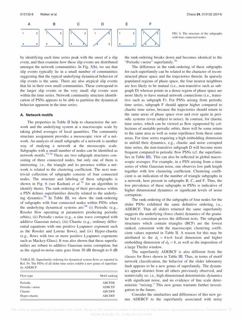
The properties in Table II help to characterize the net-work and the underlying system at a macroscopic scale bytaking global averages of local quantities. The communitystructure assignment provides a mesoscopic view of a net-work. An analysis of small subgraphs of a network is anotherway of studying a network at the mesoscopic scale.Subgraphs with a small number of nodes can be identified asnetwork motifs.73,74 There are two subgraph structures con-sisting of three connected nodes, but only one of them isinteresting, i.e., the triangle and its presence within a net-work is related to the clustering coefficient. The next non-trivial collection of subgraphs consists of four connectednodes. The structure and labeling of these subgraphs isshown in Fig. 6 (see Kashani et al.75 for an algorithm toidentify them). The rank-ordering of their prevalence withina PSN defines superfamilies directly related to the underly-ing dynamics.54 In Table III, we show the rank-orderingof subgraphs with four connected nodes within PSNs whenthe underlying dynamical systems are:54 (i) Periodic (e.g.,Rossler flow operating at parameters producing periodicorbits), (ii) Periodicþnoise (e.g., a sine wave corrupted withadditive Gaussian noise), (iii) Chaotic (e.g., ordinary differ-ential equations with one positive Lyapunov exponent suchas the Rossler and Lorenz flows), and (iv) Hyper-chaotic(e.g., flows with two or more positive Lyapunov exponentssuch as Mackey-Glass). It was also shown that these superfa-milies are robust to additive Gaussian noise corruption, butas the signal-to-noise ratio goes from 30 dB through to 0 dB

the rank-ordering breaks down and becomes identical to the“Periodicþnoise” superfamily.76

The difference in the rank-ordering of these subgraphsfor each superfamily can be related to the character of recon-structed phase space and the trajectories therein. In sparselypopulated regions of phase space, the four nearest neighborsare less likely to be mutual (i.e., non-transitive such as sub-graph D) whereas points in a dense region of phase space aremore likely to have mutual network connections (i.e., transi-tive such as subgraph F). For PSNs arising from periodictime series, subgraph F should appear higher compared tochaotic time series, because the trajectories should return tothe same areas of phase space over and over again in peri-odic systems (even subject to noise). In contrast, for chaotictime series, which can be viewed as flow signposted by col-lections of unstable periodic orbits, there will be some returnto the same area as well as some repellence from these sameareas. For time series requiring a high embedding dimensionto unfold their dynamics, e.g., chaotic and noise corruptedtime series, the non-transitive subgraph D will become morefrequent compared to periodic flow PSNs (cf. the superfami-lies in Table III). This can also be reflected in global macro-scopic averages. For example, in a PSN arising from a timeseries of white Gaussian noise, one observes low path lengthtogether with low clustering coefficient. Clustering coeffi-cient is an indication of the number of triangle subgraphs ina network, here present in subgraphs B, C, and F. Thus, thelow prevalence of these subgraphs in PSNs is indicative ofhigher dimensional dynamics or significant levels of noisecorruption.

The rank-ordering of the subgraphs of four nodes for theslider PSNs exhibited the same definitive ordering, i.e.,ADEBCF. That all sliders returned the same superfamilysuggests the underlying (force chain) dynamics of the granu-lar bed is consistent across the different tests. The subgraphstructures which contain triangles (BCF) are the lowestranked, consistent with the macroscopic clustering coeffi-cient values reported in Table II. A reason for this may beattributed to the dL ¼ 4 to 6 local dimension and higherembedding dimension of dE¼ 8, as well as the imposition ofa large Theiler window.

The superfamily ADEBCF is also different from theclasses for flows shown in Table III. Thus, in terms of motifnetwork classification, the behavior of the slider laboratoryfault appears to be a new genus of superfamily. The dynam-ics appear distinct from all others previously observed, andnontrivially so: i.e., high dimensional deterministic dynamicswith significant noise, and no evidence of fine scale deter-ministic “mixing.” This new genus warrants further investi-gation in the future.

Consider the similarities and differences of this new ge-nus ADEBCF to the superfamily associated with noisy

FIG. 6. The structure of the subgraphswith four connected nodes.

TABLE III. Superfamily ordering for dynamical system flows as reported inRef. 54. The PSNs of all slider time series exhibit a new genus of superfam-ily ADEBCF.

Flow type Motif ranking

Periodic ABCFDE

Periodicþnoise ADBCEF

Chaotic ABCDFE

Hyper-chaotic ABCDEF

013132-8 Walker et al. Chaos 24, 013132 (2014)

This article is copyrighted as indicated in the article. Reuse of AIP content is subject to the terms at: http://scitation.aip.org/termsconditions. Downloaded to IP:130.95.16.46 On: Fri, 14 Mar 2014 01:19:54

periodic dynamics, i.e., ADBCEF. The subgraph E, a squaretopology, is ranked higher than the subgraphs BCF, all ofwhich contain triangle topologies. This may be a signature ofdynamical non-stationarity and not just statistical drift, i.e.,one requires a long chain of connections before returning tosimilar states. A possible source of this subtle effect is thenature of the experiment. The dynamics of stick-slip isunderpinned by the continual formation and failure by buck-ling of force chains in the bed. However, following each slipevent, the slider moves to an undisturbed part of the bed witha new set of disks forming force chains that give rise to stick.It is possible that this leads to dynamical non-stationarityand the new superfamily. In contrast, superfamilies associ-ated with chaos were observed in data-based models ofstick-slip behavior within a biaxial compression test.19

There, however, the grains subject to deformation remain thesame, if not the self-organized network of force chains theyfacilitate.

V. CONCLUSION

Inspired by past studies which consider the stick-slip ofa laboratory fault as a proxy for stick-slip of a geologicalfault gouge, we analyzed the dynamics of stick-slip of agranular bed under shear from a slider. We complementedprevious statistical analysis focussed on the distribution ofthe size of slip events by exploiting the concepts and techni-ques of complex systems theory, in particular, nonlinear timeseries analysis and complex networks. The number of activedegrees of freedom detected from the data suggests that areal physical evolution law describing stick-slip should con-sider at least four to six state variables. Network communitystructures were able to partition the dynamical behaviorapparent in the time series, which proved to be strongly asso-ciated with slip events. We also discovered that individualstick-slip events exhibited dynamics richer than a lineardescription and can contain a nonlinear determinism.However, models capable of exhibiting periodic dynamicsare adequate for some tests. If we preserve the dynamicswithin a stick-slip event and effectively only shuffle the indi-vidual stick-slip cycles (ATS test), then there is insufficientevidence to reject the possibility that there are no long termdynamical correlations between the events. This makes phys-ical sense, as stick-slip events temporally far apart in theexperiment are due to force chain structures in different partsof the granular bed. That is, the bed has no long term mem-ory. This class of data whereby we have nonlinear determin-ism within each stick-slip cycle, but no long term memoryacross stick-slip cycles, appears to also present a new stratifi-cation of systems that the network motif superfamilyapproach can detect.

ACKNOWLEDGMENTS

We thank the anonymous referees whose commentshelped improve the manuscript. This work was supported byUS ARO (W911NF-11-1-0175), the ARC (DP0986876 andDP120104759), and the Melbourne Energy Institute (AT,DMW) and HKUGC grant number PolyU 5262/11E. M.S.

was supported by an ARC Future Fellowship (FT110100896)and thanks the Melbourne Energy Institute for travel support.We thank R. Xiang, X. Xu, and Y. Chang for discussions dur-ing the preparation of this manuscript.

1D. W. Lee, X. Banquy, and J. N. Israelachvili, Proc. Natl. Acad. Sci.U.S.A. 110, E567 (2013).

2U. Galvanetto, S. Bishop, and L. Briseghella, Int. J. Bifurcation ChaosAppl. Sci. Eng. 5, 637 (1995).

3K. Popp and P. Stelter, Philos. Trans. R. Soc. London, Ser. A 332, 89(1990).

4D. Karnopp, J. Dyn. Syst.-Trans. ASME 107, 100 (1985).5C. Collettini, A. Niemeijer, C. Viti, and C. Marone, Nature 462, 907(2009).

6K. Christensen, L. Danon, T. Scanlon, and P. Bak, Proc. Natl. Acad. Sci.U.S.A. 99, 2509 (2002).

7E. Aharonov and D. Sparks, J. Geophys. Res. 109, B09306,doi:10.1029/2003JB002597 (2004).

8M. L. Gee, P. M. McGuiggan, J. Israelachvili, and A. M. Homola,J. Chem. Phys. 93, 1895 (1990).

9J. Geng and R. P. Behringer, Phys. Rev. E 71, 011302 (2005).10Y. Guo and J. K. Morgan, J. Geophys. Res. 109, B12305,

doi:10.1029/2004JB003044 (2004).11I. Albert, P. Tegzes, R. Albert, A.-L. Barab!asi, T. Vicsek, B. Kahng, and

P. Schiffer, Phys. Rev. E 64, 031307 (2001).12I. Albert, B. Kahng, R. Albert, J. G. Sample, M. Pfeifer, A.-L. Barab!asi, T.

Vicsek, and P. Schiffer, Phys. Rev. Lett. 84, 5122 (2000).13R. Albert, M. A. Pfeifer, A.-L. Barab!asi, and P. Schiffer, Phys. Rev. Lett.

82, 205 (1999).14K. A. Alshibli and L. E. Roussel, Int. J. Numer. Anal. Met. 30, 1391

(2006).15F. B. Bowden and D. Tabor, The Friction and Lubrication of Solids

(Oxford University Press, New York, USA, 1950).16P. A. Johnson, H. Savage, M. Knuth, J. Gomberg, and C. Marone, Nature

451, 57 (2008).17M. Herrera, S. McCarthy, S. Slotterback, E. Cephas, W. Losert, and M.

Girvan, Phys. Rev. E 83, 061303 (2011).18E. Kolb, T. Mazoz, E. Clement, and J. Duran, Eur. Phys. J. B 8, 483

(1999).19M. Small, D. M. Walker, A. Tordesillas, and C. K. Tse, Chaos 23, 013113

(2013).20G. Chambon, J. Schmittbuhl, A. Corfdir, J. P. Vilotte, and S. Roux, Phys.

Rev. E 68, 011304 (2003).21F. Peer and T. Venter, J. South Afr. Inst. Min. Metall. 103, 403 (2003).22M. Knuth and C. Marone, Geochem., Geophys., Geosyst. 8, Q03012,

doi:10.1029/2006GC001327 (2007).23K. Mair, K. M. Frye, and C. Marone, J. Geophys. Res. 107, 2219,

doi:10.1029/2001JB000516 (2002).24K. E. Daniels and N. W. Hayman, J. Geophys. Res. 113, B11411,

doi:10.1029/2008JB005781 (2008).25N. W. Hayman, L. Duclou!e, K. L. Foco, and K. E. Daniels, Pure Appl.

Geophys. 168, 2239 (2011).26F. Radjai, D. E. Wolf, M. Jean, and J.-J. Moreau, Phys. Rev. Lett. 80, 61

(1998).27T. S. Majmudar and R. P. Behringer, Nature 435, 1079 (2005).28D. Howell, R. P. Behringer, and C. Veje, Phys. Rev. Lett. 82, 5241 (1999).29T. S. Majmudar, M. Sperl, S. Luding, and R. P. Behringer, Phys. Rev.

Lett. 98, 058001 (2007).30D. Bi, J. Zhang, B. Chakraborty, and R. P. Behringer, Nature 480, 355

(2011).31J. Zhang, T. Majmudar, A. Tordesillas, and R. P. Behringer, Granular

Matter 12, 159 (2010).32A. Tordesillas, D. M. Walker, F. G. J. Zhang, and R. P. Behringer, Phys.

Rev. E 86, 011306 (2012).33A. Tordesillas, Q. Lin, J. Zhang, R. P. Behringer, and J. Shi, J. Mech.

Phys. Solids 59, 265 (2011).34A. Tordesillas, Philos. Mag. 87, 4987 (2007).35D. M. Walker and A. Tordesillas, Int. J. Solids Struct. 47, 624 (2010).36A. Tordesillas, D. M. Walker, and Q. Lin, Phys. Rev. E 81, 011302

(2010).37D. M. Walker and A. Tordesillas, Phys. Rev. E 85, 011304 (2012).38L. Kondic, A. Goullet, C. S. O’Hern, M. Kramar, K. Mischaikow, and R.

P. Behringer, Europhys. Lett. 97, 54001 (2012).

013132-9 Walker et al. Chaos 24, 013132 (2014)

This article is copyrighted as indicated in the article. Reuse of AIP content is subject to the terms at: http://scitation.aip.org/termsconditions. Downloaded to IP:130.95.16.46 On: Fri, 14 Mar 2014 01:19:54

39M. Kramar, A. Goullet, L. Kondic, and K. Mischaikow, Phys. Rev. E 87,042207 (2013).

40J. Krim, P. Yu, and R. P. Behringer, Pure Appl. Geophys. 168, 2259 (2011).41H. Kantz and T. Schreiber, Nonlinear Time Series Analysis (Cambridge

University Press, Cambridge, 1997).42M. Small, Applied Nonlinear Time Series Analysis: Applications in

Physics, Physiology and Finance, Vol. 52 Nonlinear Science Series A(World Scientific, Singapore, 2005).

43M. Small and C. K. Tse, IEEE Trans. Circuits-I 50, 663 (2003).44A. M. Fraser and H. L. Swinney, Phys. Rev. A 33, 1134 (1986).45H. D. I. Abarbanel, Analysis of Observed Chaotic Data (Springer-Verlag,

New York, 1996).46T. Nakamura, M. Small, and Y. Hirata, Phys. Rev. E 74, 026205 (2006).47F. Takens, in Lecture Notes in Mathematics (Springer-Verlag, Berlin,

1981), Vol. 898, p. 366.48H. D. I. Abarbanel and M. B. Kennel, Phys. Rev. E 47, 3057 (1993).49M. Small, D. Yu, and R. G. Harrison, Phys. Rev. Lett. 87, 188101 (2001).50J. Theiler and P. E. Rapp, Electron Clin. Neuro. 98, 213 (1996).51A. Tordesillas, J. Shi, and J. F. Peters, Granular Matter 14, 295 (2012).52J. Zhang and M. Small, Phys. Rev. Lett. 96, 238701 (2006).53L. Lacasa, B. Luque, F. Ballesteros, J. Luque, and J. C. Nuno, Proc. Natl.

Acad. Sci. U.S.A. 105, 4972 (2008).54X. Xu, J. Zhang, and M. Small, Proc. Natl. Acad. Sci. U.S.A. 105, 19601

(2008).55N. Marwan, J. F. Donges, Y. Zou, R. V. Donner, and J. Kurths, Phys. Lett.

A 373, 4246 (2009).56R. V. Donner, M. Small, J. F. Donges, N. Marwan, Y. Zou, R. Xiang, and

J. Kurths, Int. J. Bifurcation Chaos Appl. Sci. Eng. 21, 1019 (2011).57J. B. Tenenbaum, V. de Silva, and J. C. Langford, Science 290, 2319 (2000).

58E. Bollt, Int. J. Bifurcation Chaos Appl. Sci. Eng. 17, 1199 (2007).59H. Suetani, K. Soejima, R. Matsuoka, U. Parlitz, and H. Hata, Phys. Rev.

E 86, 036209 (2012).60G. Froyland, Discret. Contin. Dyn. Syst. 17(3), 203 (2007).61M. Dellnitz, G. Froyland, and S. Sertl, Nonlinearity 13, 1171 (2000).62G. Froyland and M. Dellnitz, SIAM J. Sci. Comput. 24, 1839 (2003).63G. Froyland, Physica D 200, 205 (2005).64E. M. Bollt, L. Billings, and I. B. Schwartz, Physica D 173, 153 (2002).65E. M. Bollt, A. Luttman, S. Kramer, and R. Basnayake, Int. J. Bifurcation

Chaos Appl. Sci. Eng. 22, 1230012 (2012).66N. Santitissadeekorn and E. M. Bollt, Physica D 231, 95 (2007).67Y. Hirata, K. Judd, and D. Kilminster, Phys. Rev. E 70, 016215 (2004).68D. Lind and B. Marcus, An Introduction to Symbolic Dynamics and

Coding (Cambridge University Press, Cambridge, 1995).69B. P. Kitchens, Symbolic Dynamics: One-sided, Two-sided and Countable

State Markov Shifts (Springer-Verlag, Berlin, 1998).70M. E. J. Newman, Networks: An Introduction (Oxford University Press,

Oxford, 2010).71Wolfram-Research Mathematica, Version 7.0 (Wolfram Research, Inc.

Champaign, IL, 2008).72A. Clauset, Phys. Rev. E 72, 026132 (2005).73R. Milo, S. Shen-Orr, S. Itzkovitz, N. Kashtan, D. Chklovskii, and U.

Alon, Science 298, 824 (2002).74R. Milo, S. Itzkovitz, N. Kashtan, R. Levitt, S. Shen-Orr, I. Ayzenshtat, M.

Sheffer, and U. Alon, Science 303, 1538 (2004).75Z. R. M. Kashani, H. Ahrabian, E. Elahi, A. Nowzari-Dalini, E. S. Ansari,

S. Asadi, S. Mohammadi, F. Schreiber, and A. Masoudi-Nejad, BMCBioinform. 10, 318 (2009).

76R. Xiang, J. Zhang, X.-K. Xu, and M. Small, Chaos 22, 013107 (2012).

013132-10 Walker et al. Chaos 24, 013132 (2014)

This article is copyrighted as indicated in the article. Reuse of AIP content is subject to the terms at: http://scitation.aip.org/termsconditions. Downloaded to IP:130.95.16.46 On: Fri, 14 Mar 2014 01:19:54