Fault slip distribution of the 2014 Iquique, Chile,earthquake estimated from ocean-widetsunami waveforms and GPS dataAditya Riadi Gusman1, Satoko Murotani1, Kenji Satake1, Mohammad Heidarzadeh1, Endra Gunawan2,Shingo Watada1, and Bernd Schurr3

1Earthquake Research Institute, The University of Tokyo, Tokyo, Japan, 2Graduate School of Environmental Studies, NagoyaUniversity, Nagoya, Japan, 3GFZ Helmholtz Centre Potsdam, German Research Centre for Geosciences, Potsdam, Germany

Abstract We applied a new method to compute tsunami Green’s functions for slip inversion of the 1 April2014 Iquique earthquake using both near-field and far-field tsunami waveforms. Inclusion of the effects ofthe elastic loading of seafloor, compressibility of seawater, and the geopotential variation in the computedGreen’s functions reproduced the tsunami traveltime delay relative to long-wave simulation and allowed usto use far-field records in tsunami waveform inversion. Multiple time window inversion was applied totsunami waveforms iteratively until the result resembles the stable moment rate function from teleseismicinversion. We also used GPS data for a joint inversion of tsunami waveforms and coseismic crustal deformation.The major slip region with a size of 100 km×40 km is located downdip the epicenter at depth ~28 km,regardless of assumed rupture velocities. The total seismic moment estimated from the slip distribution is1.24× 1021Nm (Mw 8.0).

1. Introduction

The 2014 Iquique earthquake sequence began with a large foreshock (Mw 6.7) that occurred on 16 March2014. The main shock, occurred on 1 April 2014 at 23:46:47 (UTC), had a moment magnitude of Mw 8.2 and ahypocenter located at 19.642°S, 70.817°W with a depth of 23 km, according to the USGS (United StatesGeological Survey). Two days after, on 3 April, the largest aftershock with Mw 7.7 occurred southeast of themain shock epicenter. The 2014 Iquique main shock generated a tsunami that was recorded by Deep-oceanAssessment and Reporting of Tsunamis (DART) buoys [e.g., Heidarzadeh et al., 2014] (Figure 1) and tidegauges (Figure 2). Global Positioning System (GPS) networks recorded the coseismic displacement caused bythis earthquake [Schurr et al., 2014] (Figure 2).

The slip distribution for the 2014 Iquique earthquake has been estimated by teleseismic inversion [Lay et al.,2014; Yagi et al., 2014], tsunami inversion of offshore DART waveforms [Lay et al., 2014; An et al., 2014], and ajoint inversion of teleseismic, local strong motion records and GPS data [Schurr et al., 2014]. The momentmagnitudes estimated by these previous studies are in the range of Mw 8.0–8.2.

For tsunami waveform inversions, the linear shallow water wave, whose velocity solely depends on thebathymetry without dispersion, has been assumed to compute the Green’s functions [e.g., Fujii et al., 2011;Fujii and Satake, 2013]. However, the observed tsunami arrivals in the far field are significantly delayed relativeto the simulated tsunami waveforms [Rabinovich et al., 2011; Allgeyer and Cummins, 2014; Inazu and Saito,2013;Watada et al., 2014]. In addition, tsunami forerunners in the far field with a reversed polarity were alsoreported [Allgeyer and Cummins, 2014; Watada et al., 2014]. In general, arrival time and initial phase oftsunamis are very important for the tsunami waveform inversion. Because of the arrival time delay andpolarity reversal, previous studies on the sources of transoceanic tsunamis such as the 2010 Maule, Chile,tsunami [e.g., Lorito et al., 2011; Fujii and Satake, 2013], the 2011 Tohoku, Japan, tsunami [e.g., Fujii et al., 2011;Gusman et al., 2012; Romano et al., 2012; Satake et al., 2013], and the 2014 Iquique, Chile, tsunami [e.g., Anet al., 2014] did not use the tsunami waveforms in the far field.

Watada et al. [2014] attributed the observed tsunami traveltime delays and the initial negative depressions tothe elastic loading of the seafloor, the compressible seawater, and the geopotential variation due to themoving water mass and proposed a method to correct the waveforms of simulated linear shallow water

GUSMAN ET AL. ©2015. American Geophysical Union. All Rights Reserved. 1

PUBLICATIONSGeophysical Research Letters

RESEARCH LETTER10.1002/2014GL062604

Key Points:• Far-field tsunami waveforms, withphase correction for time delay,were inverted

• Stable moment rate from seismicinversion and stable spatial slip fromtsunami and GPS

• Largest slip located downdip nearshore well constrained by tsunamiand GPS

Supporting Information:• Figures S1–S4• Table S1

Correspondence to:A. R. Gusman,adit@eri.u-tokyo.ac.jp

Citation:Gusman, A. R., S. Murotani, K. Satake, M.Heidarzadeh, E. Gunawan, S. Watada,and B. Schurr (2015), Fault slipdistribution of the 2014 Iquique, Chile,earthquake estimated from ocean-widetsunami waveforms and GPS data,Geophys. Res. Lett., 42, doi:10.1002/2014GL062604.

Received 22 NOV 2014Accepted 21 JAN 2015Accepted article online 24 JAN 2015

Figure 1. (a) Distribution of maximum simulated tsunami heights from the estimated slip distribution of the 2014 Iquique earthquake from joint inversion of tsunamiwaveforms and GPS data. Maximum tsunami amplitude at each observation station is indicated by the size of the circle. Green color gradation shows the traveltimedelay produced by the shallow water simulation. Station names are indicated by black, blue numbers indicate the distance in kilometers of each station from theepicenter along the great circle, and green numbers indicate the traveltime delay relative to the tsunami shallow water simulation at each station. (b) Traveltimedifferences between simulated and the observed tsunami waveforms. Green triangles represent traveltime difference between observation and linear shallowwater wave. Red circles represent traveltime difference between observation and phase-corrected shallow water wave. (c) Comparison of tsunami waveformssimulated by solving the linear shallowwater equations from the estimated slip distribution (green lines), the phase-corrected tsunami waveforms (red lines), and theobserved tsunami waveforms (black lines). The blue bars indicate the time range used for tsunami waveform inversion. Purple line marks the observed traveltime ofthe first tsunami peak, which was used for tsunami back tracing (Figure 2b).

Geophysical Research Letters 10.1002/2014GL062604

GUSMAN ET AL. ©2015. American Geophysical Union. All Rights Reserved. 2

wave. In this study, we first use teleseismic body waves to estimate the source time (moment rate) function ofthe rupture then use the ocean-wide tsunami waveforms and the coseismic displacement data in a jointinversion to estimate the spatial and temporal slip distribution of the 2014 Iquique earthquake.

2. Teleseismic and Tsunami Waveforms and Coseismic Displacement Data2.1. Teleseismic Waveform Data

We used the teleseismic body waves of 54 P wave vertical components recorded at the epicentral distancesbetween 30° and 100° (Figure S1 in the supporting information). We applied a band-pass filter for thefrequency range between 0.003 and 1.0 Hz to the original waveforms provided by the Incorporated ResearchInstitutions for Seismology, Data Management Center (IRIS-DMC).

2.2. Tsunami Waveform Data

We used the tsunami waveforms recorded at 19 DART and five tide gauge stations (Figures 1 and 2).The Intergovernmental Oceanographic Commission (IOC) and the National Oceanic and AtmosphericAdministration (NOAA) provided the tide gauge and DART data, respectively. To obtain the tsunamiwaveforms, the ocean tides were approximated by fitting polynomial functions and removed from theoriginal records.

Figure 2. (a) Predicted coseismic crustal deformation from the estimated slip distribution from tsunami waveforms and GPS data (Vr = 1.5 km/s). Red and blue arrowsrepresent the synthetic and observed horizontal and vertical displacements, respectively. Green and orange contours respectively represent positive and negativevertical surface deformation (contour interval = 0.1m). Yellow triangles represent the tide gauge stations, and the blue star represents the epicenter of the 2014Iquique earthquake. (b) Travel timemap of back-traced tsunami based on the traveltimes of the first peaks of observed tsunami waveforms. Purple area indicates thesource area for the first peaks of observed tsunami waveforms. (c) Comparison of synthetic (red lines) and observed (black lines) tsunami waveforms at tide gaugestations. The blue bars indicate the time range used for tsunami waveform inversion. Purple line marks the observed traveltime of the first tsunami peak at eachstation, which was used for tsunami back tracing (Figure 2b).

Geophysical Research Letters 10.1002/2014GL062604

GUSMAN ET AL. ©2015. American Geophysical Union. All Rights Reserved. 3

The tsunami was recorded at seven tide gauge stations (Matarani, Arica, Iquique, Patache, Mejillones, Pisagua,and Tocopilla; Figure 2). The highest amplitude of the first tsunami cycles was 187.9 cm at Iquique (Figure 2c).We estimated the tsunami source region by applying Huygens’ principle for back tracing the tsunami fromeach observation station using the Geoware TTT (Tsunami Travel Time) program. The traveltime arcs for thefirst peaks of Pisagua and Tocopilla were inconsistent with other stations (Figure 2b), probably because ofpoor bathymetry data around these stations. Hence, we did not use the tsunami waveforms at Pisagua andTocopilla for the inversion but used them for validation purpose.

Tsunami amplitudes recorded at the DART stations are much smaller because they are located at deep water(3000–6000m). For example, tsunami amplitude of 24.89 cm was recorded by DART 32401, which is locatedat a water depth of 4865m and approximately 290 km from the epicenter (Figures 1a and 1c).

2.3. Coseismic Displacement Data

We used coseismic horizontal and vertical displacements at 13 GPS stations (Figure 2a) of the IntegratedPlate Boundary Observatory Chile (IPOC), the International Associated Laboratory, and the Central AndeanTectonic Observatory Geodetic Array projects in northern Chile [Schurr et al., 2014]. The horizontal andvertical displacements at stations within 200 km from the epicenter are ranging from 9.0 to 84.7 cm and from�24.4 to 0.4 cm, respectively.

3. Methodology3.1. Fault Geometry

We assumed a fault with a geometry based on the SLAB1.0 subduction zone model [Hayes et al., 2012]and the hypocenter of the aftershocks located by USGS, although the globally estimated depth may not bevery accurate (Figure S2). For each subfault, strike angle of 347°, rake angle of 90°, and subfault size of20 km×20 km are used.

3.2. Moment Rate Function From Teleseismic Inversion

The moment rate function and the slip distribution were estimated from teleseismic body wave inversionusing Kikuchi and Kanamori’s [1991] method. The rupture duration on each subfault is decomposed intoseven isosceles triangles with duration of 6 s at 3 s intervals, implying that rupture duration for each subfaultwas at most 24 s. We assumed three different constant rupture velocities, Vr = 1.5, 2.0, and 2.5 km/s, andestimated the moment rate functions and slip distributions.

3.3. Joint Inversion of Tsunami Waveforms and GPS Data

The slip distribution was estimated by a joint inversion of tsunami waveforms recorded at five tide gaugestations, 19 DART stations, and coseismic displacements at 13 GPS stations. We applied a multiple timewindow inversion [Satake et al., 2013] with two time windows with an interval of 15 s allowing each subfaultto slip up to 30 s. These parameters were selected so that the total rupture duration of the resulting momentrate function resembles that estimated by teleseismic body wave inversion. Like teleseismic inversion, weassumed three different constant rupture velocities: Vr = 1.5, 2.0, and 2.5 km/s. The Green’s functions alsocontain synthetics of horizontal and vertical displacements at GPS sites. We included a spatial smoothnessconstraint on the slip distribution into the inversion procedure [Gusman et al., 2010].

For the tsunami Green’s functions, first we solved the linear shallow water equations and then we correctedthe simulated offshore tsunami waveforms by including frequency-dependent dispersion using a methodproposed byWatada et al. [2014]. The nondispersive linear shallowwater equations are numerically solved bya finite different method with staggered grid scheme [Satake, 1995]. The bathymetry grid is based on the30 arc sec General Bathymetric Chart of the Oceans (GEBCO_08) bathymetric data [IntergovernmentalOceanographic Commission, International Hydrographic Organization, and British Oceanographic Data Centre,2003]. The tsunami waveforms at tide gauges and DART stations are computed on 30 arc sec and 5 arc minbathymetry grids, respectively. The ground deformation from each subfault is computed by Okada’s [1985]formula assuming that the solid ocean bottom is modeled as homogeneous elastic half-space. The seasurface deformation is assumed to be the same as the ocean bottom deformation. To include the effects ofseawater compressibility, the elasticity of the Earth, and the gravitational potential variation due to themass motion during the tsunami propagation, we utilized the frequency-dependent phase velocity

Geophysical Research Letters 10.1002/2014GL062604

GUSMAN ET AL. ©2015. American Geophysical Union. All Rights Reserved. 4

computed by the normal mode method [Watada and Kanamori, 2010] and corrected the phases of thesimulated long-wave tsunami waveforms in the frequency domain by the Fourier transform method[Watada et al., 2014]. With this procedure we account for the fact that waves of different wavelengths travelat different phase velocity. Phase-corrected Green’s functions are linear long waves with dispersion effects;hence, any linear inversion scheme for multiple subfaults can be applied.

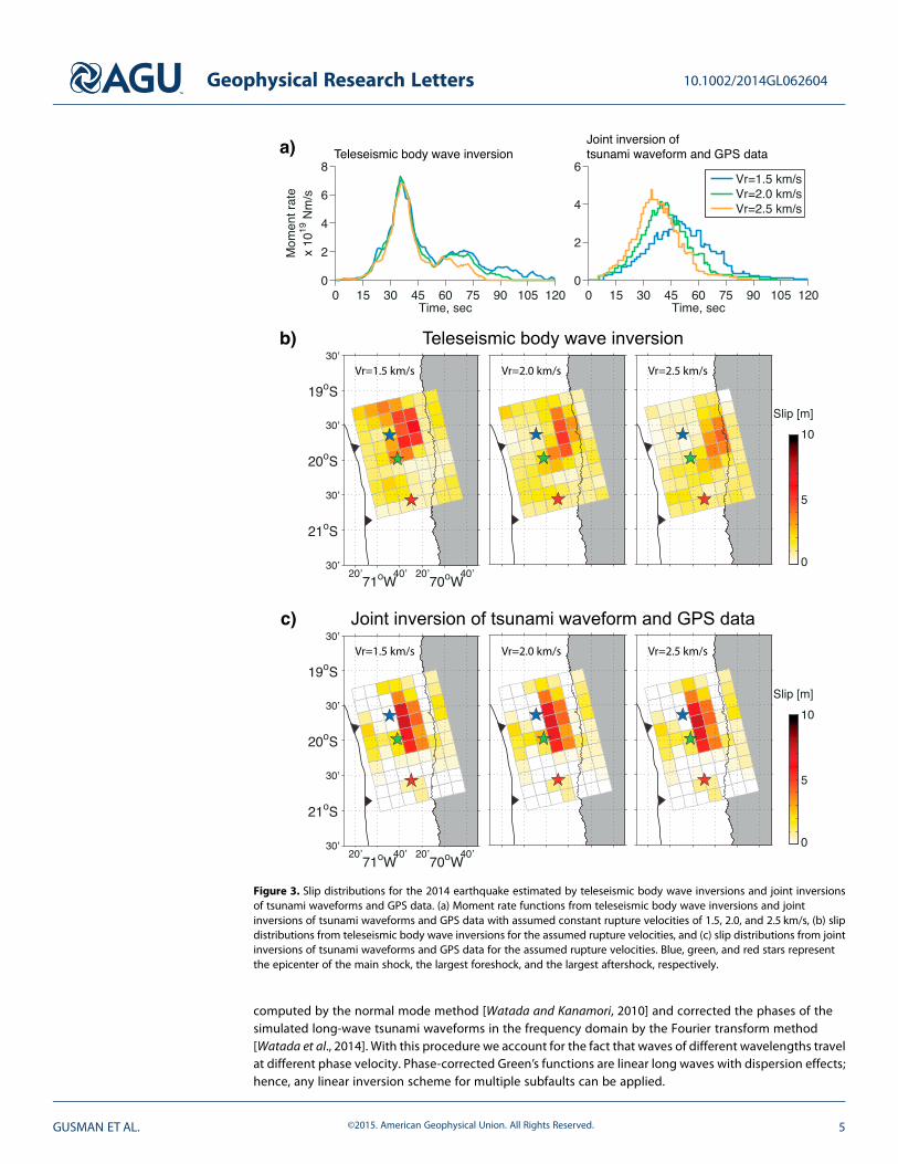
Figure 3. Slip distributions for the 2014 earthquake estimated by teleseismic body wave inversions and joint inversionsof tsunami waveforms and GPS data. (a) Moment rate functions from teleseismic body wave inversions and jointinversions of tsunami waveforms and GPS data with assumed constant rupture velocities of 1.5, 2.0, and 2.5 km/s, (b) slipdistributions from teleseismic body wave inversions for the assumed rupture velocities, and (c) slip distributions from jointinversions of tsunami waveforms and GPS data for the assumed rupture velocities. Blue, green, and red stars representthe epicenter of the main shock, the largest foreshock, and the largest aftershock, respectively.

Geophysical Research Letters 10.1002/2014GL062604

GUSMAN ET AL. ©2015. American Geophysical Union. All Rights Reserved. 5

Because the tsunami amplitudes recorded at DART stations located in the deep ocean are significantlysmaller than those at tide gauges, we weighted the tsunami waveforms at DART stations with a factor of 40.The weight factor is 1 for tsunami waveforms at tide gauge stations except for Iquique and Patache wherethe factor is 3 because the results are very sensitive to these waveforms. The weight factor for the horizontaland vertical displacements data at the GPS stations is 100.

4. Result and Discussion4.1. Comparison of Teleseismic and Joint Inversion Results

The moment rate functions estimated from the teleseismic body wave inversion with different rupturevelocities are quite similar with peaks at ~35 s (Figure 3a). The total rupture duration is different for theassumed rupture velocities, but most seismic moment release ended in ~80 s. This indicates that theteleseismic waveforms provide a robust estimate for the temporal changes of the earthquake source process.The moment rate function estimated from the joint inversion with Vr = 1.5 km/s has a peak at 47 s and theentire rupture process lasted for ~120 s (Figure 3a).

The estimated slip distributions from joint inversion of tsunami waveforms and GPS data are very similar fordifferent rupture velocities (Figure 3c). On the contrary, the spatial slip distributions from teleseismic bodywave inversions strongly depend on assumed rupture velocities (Figure 3b). Faster rupture velocity enforcesthe large slip patch moving toward the deeper part of the fault, beneath the land, although each solution canexplain the observed seismic waveforms equally well. Amongst the slip distributions from the teleseismicinversions with the three different rupture velocities, the one for 1.5 km/s is most similar to the slipdistribution from the joint inversion of tsunami waveforms and GPS data in terms of large slip area. Thus, thevelocity of 1.5 km/s may represent the rupture process of the 2014 Iquique earthquake.

Regardless of the assumed rupture velocities, tsunami waveform misfits from the joint inversions are similar,although the one for the rupture velocity of 1.5 km/s gives the smallest root-mean-square error (RMSE) values(RMSE_Vr1.5=0.433, RMSE_Vr2.0= 0.441, and RMSE_Vr2.5=0.443). The RMSE value is larger (RMSE_Vr∞=0.476)for the infinite rupture velocity than finite velocities. This may indicate that introduction of finite rupturevelocity instead of an instantaneous rupture process can better explain the tsunami waveforms, although theyare insensitive to the choice of rupture velocity, as indicated by Fujii and Satake [2007]. The tsunami inversionresults are insensitive to the assumed rupture velocity because the tsunami phase velocity is only 0.2 km/s at awater depth of 4 km, which is much slower than rupture velocity.

4.2. Rupture Process of the 2014 Iquique Earthquake

The joint inversion of tsunami waveform and GPS data result shows that the 2014 Iquique earthquakeruptured from the epicenter to the southeast direction toward the largest aftershock, which is located on theplate interface that did not rupture during the main shock (Figures 3c and S3). This is consistent with thebackprojection result by Schurr et al. [2014] and teleseismic inversion result by Yagi et al. [2014].

From the slip distribution obtained by the joint inversion of the tsunami and GPS data (Figure 3c andTable S1), the seismic moment (Vr= 1.5 km/s) is calculated as 1.24× 1021Nm (Mw 8.0) by assuming a rigidityof 4 × 1010N/m2. This seismic moment is slightly smaller than that from teleseismic waveform inversion(1.88× 1021Nm, Mw 8.1). The major slip region with slip amount larger than 3m extends 100 km×40 km, andthe maximum slip amount is approximately 7m for both inversions (Figures 3b and 3c). This major slip regionis located at downdip side of the hypocenter at depths between 20 and 35 km. The DART data off the coastof Iquique were used; hence, tsunami waveform can better constrain the slip in the shallow region near thetrench compared to inversion results of only teleseismic or land-based GPS data. Here we confirmed that thelargest slip of the 2014 Iquique earthquake did not reach the plate interface near the trench (Figure 3c).

Tsunami waveforms, land-based GPS data, and teleseismic body waves can provide accurate estimates ofoffshore slip distribution, slip distribution beneath land, and the precise timing of slip history, respectively,for interplate earthquakes. A slip distribution from only tsunami waveforms (Figure S4) has a very similarpattern to those from the joint inversions. Comparison of the results from the tsunami waveform inversionand joint inversions (tsunami and GPS) show that the tsunami waveform provided strong constraint to thesolution, and the GPS data mainly constrain the slip beneath land.

Geophysical Research Letters 10.1002/2014GL062604

GUSMAN ET AL. ©2015. American Geophysical Union. All Rights Reserved. 6

4.3. Tsunami Simulation and Calculated Surface Deformation

The estimated slip distribution from the joint inversion of tsunami and GPS data can explain the observedtsunami waveforms (Figures 1c and 2c) and coseismic displacements (Figure 2a) very well at most stations.Tsunami waveforms at Pisagua and Tocopilla that were not used in the inversion are compared with thesimulated ones (Figure 2c). Although the arrival times of the observed and simulated tsunami waveforms atTocopilla are significantly different, the period and amplitude of first waves are similar.

From the estimated slip distribution, we computed the tsunami waveforms at the DART stations by solvingthe linear shallow water equations. The arrival time differences between simulated and observed tsunamiwaveforms are calculated by the cross-correlation technique explained in Watada et al. [2014] and shownin Figure 1b. Without the tsunami phase velocity correction, the arrival time differences at stations more than12000 km away from the source (except for DART 52401) ranged from 10 to 20min (Figure 1a) or in the rangeof 1–2% of the traveltime (Figure 1b).

The calculated deformation pattern shows that tide gauge stations located very close to the epicenter(i.e., Pisagua and Iquique) were clearly subsided due to the main shock (Figure 2b). The maximum predictedland subsidence is approximately 30 cm (Figure 2b). While leading positive tsunami waves were recordedat all tide gauge stations (Figure 2c), it does not necessarily mean that there is no subsidence or uplift atnear-field stations such as Pisagua, Iquique, and Patache, because tide gauge station and water columnmovetogether with the ground during the seismic event.

5. Conclusions

The tsunami arrival time and polarity reversal observed at far-field DART stations can be accurately reproducedby solving shallow water equations and applying the phase velocity correction to the simulated waveforms[Watada et al., 2014]. The slip distribution of the 2014 Iquique earthquake from our joint inversion method canaccurately explain the tsunami waveform in the near field as well as in the far field. We propose the tsunamiphase velocity correction to be included as a standard procedure in inversion methods when using far-fieldtsunami waveforms.

Inversion of teleseismic body waves provides better temporal resolution, while the joint inversion of tsunamiand geodetic data provides a better spatial resolution. Hence, we may reach a more precise time-spacedistribution and rupture velocity from a combined use of teleseismic body waves, tsunami waveforms, andland-based GPS data. Our result shows that the slip distribution from teleseismic body wave inversion withrupture velocity of 1.5 km/s is consistent with the spatially stable slip distribution from the joint inversionof tsunami waveforms and GPS data.

ReferencesAllgeyer, S., and P. Cummins (2014), Numerical tsunami simulation including elastic loading and seawater density stratification, Geophys. Res.

Lett., 41, 2368–2375, doi:10.1002/2014GL059348.An, C., I. Sepúlveda, and P. L.-F. Liu (2014), Tsunami source and its validation of the 2014 Iquique, Chile, earthquake, Geophys. Res. Lett., 41,

3988–3994, doi:10.1002/2014GL060567.Fujii, Y., and K. Satake (2007), Tsunami source of the 2004 Sumatra-Andaman earthquake inferred from tide gauge and satellite data, Bull.

Seismol. Soc. Am., 97(1A), 192–207, doi:10.1785/0120050613.Fujii, Y., and K. Satake (2013), Slip distribution and seismic moment of the 2010 and 1960 Chilean earthquakes inferred from tsunami

waveforms and coastal geodetic data, Pure Appl. Geophys., doi:10.1007/s00024-012-0524-2.Fujii, Y., K. Satake, S. Sakai, M. Shinohara, and T. Kanazawa (2011), Tsunami source of the 2011 off the Pacific coast of Tohoku, earthquake,

Earth Planets Space, 63, 815–820, doi:10.5047/eps.2011.06.010.Gusman, A. R., Y. Tanioka, T. Kobayashi, H. Latief, and W. Pandoe (2010), Slip distribution of the 2007 Bengkulu earthquake inferred from

tsunami waveforms and InSAR data, J. Geophys. Res., 115, B12316, doi:10.1029/2010JB007565.Gusman, A. R., Y. Tanioka, S. Sakaia, and H. Tsushima (2012), Source model of the great 2011 Tohoku earthquake estimated from tsunami

waveforms and crustal deformation data, Earth Planet. Sci. Lett., 341–344, 234–242, doi:10.1016/j.epsl.2012.06.006.Hayes, G. P., D. J. Wald, and R. L. Johnson (2012), Slab1.0: A three-dimensional model of global subduction zone geometries, J. Geophys. Res.,

117, B01302, doi:10.1029/2011JB008524.Heidarzadeh, M., K. Satake, S. Murotani, A. R. Gusman, and S. Watada (2014), Deep-water characteristics of the trans-Pacific tsunami from the

1 April 2014 Mw 8.2 Iquique, Chile earthquake, Pure Appl. Geophys., doi:10.1007/s00024-014-0983-8.Inazu, D., and T. Saito (2013), Simulation of distant tsunami propagation with a radial loading deformation effect, Earth Planets Space, 65,

835–842, doi:10.5047/eps.2013.03.010.Intergovernmental Oceanographic Commission, International Hydrographic Organization, and BritishOceanographic Data Centre (2003), Centenary

Edition of the GEBCO Digital Atlas, published on CD- ROM on behalf of the Intergovernmental Oceanographic Commission and the InternationalHydrographic Organization as part of the general bathymetric chart of the oceans. British oceanographic data centre, Liverpool, U. K.

AcknowledgmentsTeleseismic waveforms weredownloaded from the IncorporatedResearch Institutions for Seismology,Data Management Center (IRIS-DMC)website (http://www.iris.edu/wilber3/find_event). Tide gauge and DARTdata were downloaded from theIntergovernmental OceanographicCommission (IOC) website (http://www.ioc-sealevelmonitoring.org) and theNational Oceanic and AtmosphericAdministration (NOAA) website (http://www.ndbc.noaa.gov/dart.shtml),respectively. GPS data were providedby the Integrated Plate BoundaryObservatory Chile (IPOC), theInternational Associated Laboratory,and the Central Andean TectonicObservatory Geodetic Array projects innorthern Chile. The coseismic horizontaland vertical displacements are providedby Schurr et al. [2014]. Some of thefigures were made using the publicdomain Generic Mapping Tools [Wesseland Smith, 1998]. We thank HirooKanamori for a discussion on slipinversion. We thank Andrew Newman(the Editor) and two anonymous reviewersfor their constructive comments.

The Editor thanks two anonymousreviewers for their assistance inevaluating this paper.

Geophysical Research Letters 10.1002/2014GL062604

GUSMAN ET AL. ©2015. American Geophysical Union. All Rights Reserved. 7

Kikuchi, M., and H. Kanamori (1991), Inversion of complex body waves—III, Bull. Seismol. Soc. Am., 81, 2335–2350.Lay, T., H. Yue, E. E. Brodsky, and C. An (2014), The 1 April 2014 Iquique, Chile, Mw 8.1 earthquake rupture sequence, Geophys. Res. Lett., 41,

3818–3825, doi:10.1002/2014GL060238.Lorito, S., F. Romano, S. Atzori, X. Tong, A. Avallone, J. McCloskey, E. Boschi, and A. Piatanesi (2011), Limited overlap between the seismic gap

and coseismic slip of the great 2010 Chile earthquake, Nat. Geosci., 4, 173–177, doi:10.1038/ngeo1073.Okada, Y. (1985), Surface deformation due to shear and tensile faults in half-space, Bull. Seismol. Soc. Am., 75–4, 1135–1154.Rabinovich, A. B., P. L. Woodworth, and V. V. Titov (2011), Deep-sea observations and modeling of the 2004 Sumatra tsunami in Drake

Passage, Geophys. Res. Lett., 38, L16604, doi:10.1029/2011GL048305.Romano, F., A. Piatanesi, S. Lorito, N. D’Agostino, K. Hirata, S. Atzori, Y. Yamazaki, andM. Cocco (2012), Clues from joint inversion of tsunami an

geodetic data of the 2011 Tohoku-oki earthquake, Sci. Rep., 2(385), 1–8, doi:10.1038/srep00385.Satake, K. (1995), Linear and nonlinear computations of the 1992 Nicaragua earthquake tsunami, Pure Appl. Geophys., 144, 455–470.Satake, K., Y. Fujii, T. Harada, and Y. Namegaya (2013), Time and space distribution of coseismic slip of the 2011 Tohoku earthquake as

inferred from tsunami waveform data, Bull. Seismol. Soc. Am., 103(2B), 1473–1492.Schurr, B., et al. (2014), Gradual unlocking of plate boundary controlled initiation of the 2014 Iquique earthquake, Nature, 512, 299–302,

doi:10.1038/nature13681.Watada, S., and H. Kanamori (2010), Acoustic resonant oscillations between the atmosphere and the solid earth during the 1991

Mt. Pinatubo eruption, J. Geophys. Res., 115, B12319, doi:10.1029/2010JB007747.Watada, S., S. Kusumoto, and K. Satake (2014), Traveltime delay and initial phase reversal of distant tsunamis coupled with the

self-gravitating elastic Earth, J. Geophys. Res. Solid Earth, 119, 4287–4310, doi:10.1002/2013JB010841.Wessel, P., and W. H. F. Smith (1998), New, improved version of generic mapping tools released, Eos Trans. AGU, 79, 579, doi:10.1029/

98EO00426.Yagi, Y., R. Okuwaki, B. Enescu, S. Hirano, Y. Yamagami, S. Endo, and T. Komoro (2014), Rupture process of the 2014 Iquique Chile Earthquake

in relation with the foreshock activity, Geophys. Res. Lett., 41, 4201–4206, doi:10.1002/2014GL060274.

Geophysical Research Letters 10.1002/2014GL062604

GUSMAN ET AL. ©2015. American Geophysical Union. All Rights Reserved. 8