How model equations are treated in Modelling languages (EcosimPro)
Digital Simulation
Methods and tools oriented to ldquoimitaterdquo or predict the responses of a systems against certain changes or ldquostimulusrdquo using a computer
Uses of Simulation
Study of a process what ifhellip analysis Design (process controlhellip) Testing a control system before actual
implementation in the plant Personnel training Operation optimization Essays in a virtual plant hellip
Advantages of the simulation
Perform changes that if implemented in the process will be o Very costly o Too slow fast o dangerous etc
Reproduces the experiment as many time as desired under the same conditions
Saves time Provides safety Allows sensitivity studies Provides a model that can be used for many purposes Allows experimenting with systems that are not built yet
Models
Simulation is based on mathematical models of the processes
Mathematical models are set of equations relating the variables of a process and being able to provide an adequate representation of its behaviour
They are always approximations of the real world Adequacy of a model depends on their intended use There are a wide variety of models according to the
processes they represent and their aims
Adequate representation
Proceso
u
time
y
time
Model
ym
timefidelity to the physical asset and facility of use in the intended application
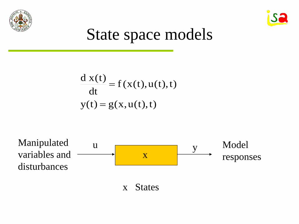
State space models
)t)t(ux(g)t(y
)t)t(u)t(x(fdt
)t(xd
=
=
Manipulated variables and disturbances
Model responses
u yx
x States
Stages of a simulation project
Study the process Set the simulation aims
ndash Specify the relevant variables Develop the model according to the simulation
aims Code the model in a simulation language Set the independent variables and choose the
numerical solvers Exploit the results of the simulation
Concepts
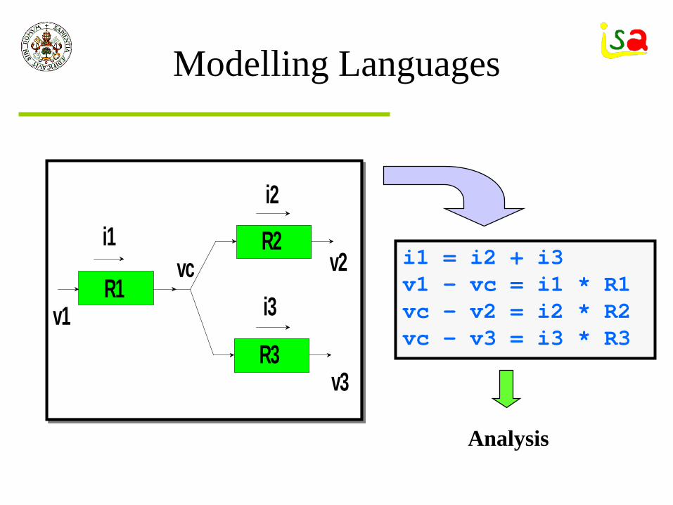
Process -gt ModelV - I R = 0 oacute I = VR oacute V = IR
Assignment of computational causalityV = I R
ExperimentR = 10 I = 2
Numerical solutionV = 210 = 20
Simulation Languages
Computer program providing tools forDescribing the model and assigning
computational causalityDefining the experiments to be performedSolving numerically the set of equationsVisualizing the results and communicating
with the external world
Advantages
Provide support in all phases of model development and exploitation
Allows concentrating in the problem and the results not spending time and efforts in programming
Gives reliability to the numerical results Allows saving time Allows the non-expert in computing or numerical
methods to solve complex models
First principles models
Based on knowledge of the process and nature laws (Physics chemistryhellip)
Sometimes are difficult to formulate from the scratch requiring trained people large development times costs
They need to be tested and validated
This may limit their use in many fields (Design decision making traininghellip
Buthellipwhich is the cost of non-using them
Solution Libraries of models
Models are built linking the tested modules or components of a model library
Each component of the library contains the mathematical model of a process and can be configured by parameterization to fit the user needs
Each component can be linked to others by an interface or port in order to built more complex models
Va Vb
Ia Ib Va Vb
Ia Ib
Va Vb
Ia Ib
R1
C1
R2
Physical properties data bases and good user interfaces are also required
Model Libraries
Sets of components representing different processes devices etc Each one contains its mathematical model and connections to the external
world Components can be parameterized to adapt them to the user requirements
mc_out
Tacha18
j_in1j_in2
j_in3v_in
va_out
c_out
mc_out
Tacha18
j_in1j_in2
j_in3v_in
va_out
c_out
mc_out
Tacha18
j_in1j_in2
j_in3v_in
va_out
c_out
mc_out
Tacha18
j_in1j_in2
j_in3v_in
va_out
c_out
mc_in
mp_out
mr_out
cristal_out
Turbinadiscontinua1
mc_in
mp_out
mr_out
cristal_out
Turbinadiscontinua1
mc_in
mp_out
mr_out
cristal_out
Turbinadiscontinua1
mc_in
mp_out
mr_out
cristal_out
Turbinadiscontinua1
mc_in
mp_out
mr_out
cristal_out
Turbinadiscontinua1
mc_in
mp_out
mr_out
cristal_out
Turbinadiscontinua1
mc_in
mp_out
mr_out
cristal_out
Turbinadiscontinua1
f_in1 f_in2 f_in3 f_in4 f_in5 f_in6 f_in7
f_out
niv
Deposito1
f_in1 f_in2 f_in3 f_in4 f_in5 f_in6 f_in7
f_out
niv
Deposito1
mc_in1 mc_in2
mc_out
Malaxador6 mc_in1 mc_in2
mc_out
Malaxador6
After parameterization simulation code is generated
Select and connect components as in the real world
Model Libraries
Model Libraries
Modular modellingndash Facilitates the re-use of models in different applicationsndash Facilitates the use of simulation to those non-experts in
simulation but knowing the system to be simulated Modularity Independent description of every module of
the library Abstraction Use the modules without knowing its internal
details (model equations etc) Hierarchy New modules can be built by linking the
existing ones
Types of simulation languages according to the way they support modularity
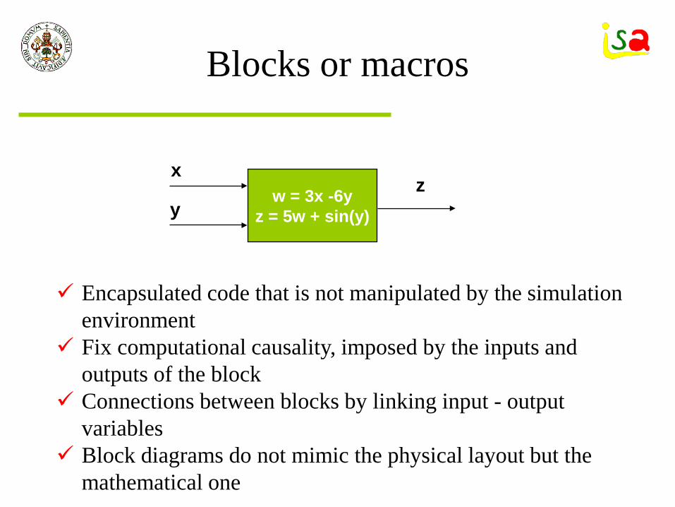
Each block has fix input and output variables and contains equations or code to compute the value of the output variables as a function of the value of the input ones
x
Blocks or macros
w = 3x -6yz = 5w + sin(y)
Encapsulated code that is not manipulated by the simulation environment
Fix computational causality imposed by the inputs and outputs of the block
Connections between blocks by linking input - output variables
Block diagrams do not mimic the physical layout but the mathematical one
x
yz
Simulink
+
R1 R2
C
Physical system
L
u
Model equations
Implementation of the model is done using predefined blocks that carry out specific operations and are linked together to perform the operations of the model equations
L U dtdi
C i dt
dUR2 i - U U
R1 )U - (U i
LL
CC
LL
CC
=
=
times==
LC
R2R1U
iLiC
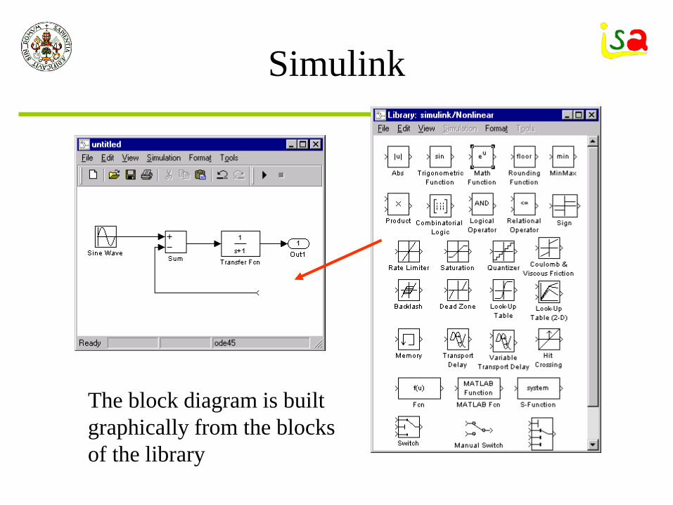
Simulink
The block diagram is built graphically from the blocks of the library
Block oriented languages Simulink
L U dtdi
C i dt
dUR2 i - U U
R1 )U - (U i
LL
CC
LL
CC
=
=
times==
Simulink
+
R1 R2
C
Physical system
L
u
With block oriented languages the user describes the mathematical model not the physical system
Block diagram
StructureBlock diagram edition
Error analysis
Block computational order
Sequential computation of the blockrsquos outputs
from its imputs
Results Display
End
CSMP 1130 SADS DSL90
hellip
EASY-5 TUTSIM Simulink
Integration t= t+h
t = tstop
Blockrsquos computational order
States or known values initially
2
83
64
75 9
1
1 Starting from the blocks with known initial values check which blocks can be executed as all their inputs are known
2 Write them down in a list and iterate with the new set of known blocks until all blocks are used up
3 If any new block is added to the list in a full iteration over all blocks an algebraic loop is detected
1 9 8 2 3 5 4 7 6 9 8Computational order
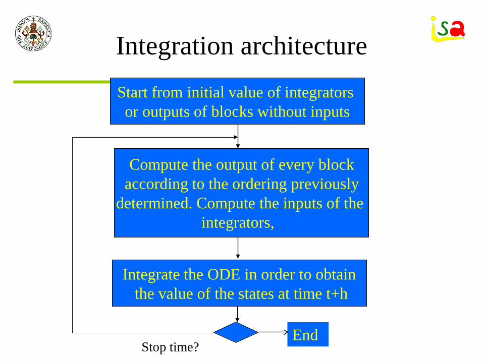
Integration architectureStart from initial value of integrators or outputs of blocks without inputs
Compute the output of every blockaccording to the ordering previously
determined Compute the inputs of the integrators
Integrate the ODE in order to obtainthe value of the states at time t+h
EndStop time
Sum1Sum
Sine Wave
Scope
eu
MathFunction
5
Gainf (z) zSolve
f(z) = 0Algebraic Constraint
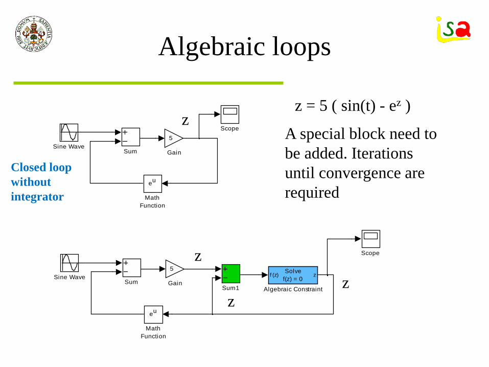
Algebraic loops
z = 5 ( sin(t) - ez )
SumSine Wave
Scope
eu
MathFunction
5
Gain
z
z
z
z
A special block need to be added Iterations until convergence are required
Closed loop without integrator
Hierarchical blocks
Modularity
Hierarchy
Block oriented languages
There are easy to use and intuitive Modular and hierarchical architectures Model description does not match neither the physical
process not the equations There are difficult to build and debug in case of models
with a large number of blocks Fix computational causality Slow interpreters Algebraic loops must be explicitly solved with additional
blocks Limited separation model-experiment
Expression oriented languages
Standard CSSLrsquo67 (Simulation 1967 Vol9 pp281-303)
Direct declaration of the model equationsModel description is given a temporal structure Separation model-experiment command languageCode generators compiled simulation code SpeedOpen to the outside world CallReuse of code Macros
CSSLrsquo67 Model editor
Errors Equation ordering
Fortran code
Compiler+ Libraries
Results
Executable codeCommand language
Text editor
BuilderCode translator
CSSLrsquo67Program
Initial
End
Dynamic
Derivative
End
Discrete
End
End
Terminal
End
End
Initial conditions Code executed once at t= 0
Continuous equations
Discrete equations
Final computations Code executed once at tstop
Description model structure
Fix computational causality
Simulation code similar to the mathematical model
Computations
Program
Initial
End
Dynamic
Derivative
End
Discrete
End
End
Terminal
End
End
Initialization of variables including states
Expressions evaluated at certain times (Synchronous or asynchronous modes) or when a event takes place
Expressions evaluated and integrated every integration interval
Global variables
Transfers to initial region are possible to create loops
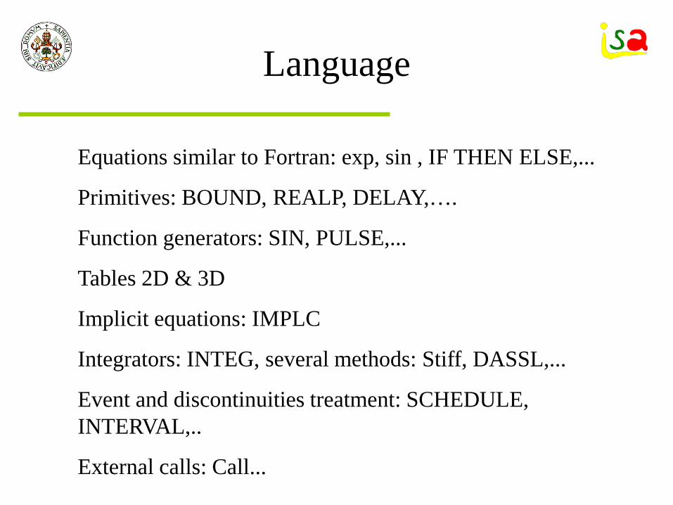
Language
Equations similar to Fortran exp sin IF THEN ELSE
Primitives BOUND REALP DELAYhellip
Function generators SIN PULSE
Tables 2D amp 3D
Implicit equations IMPLC
Integrators INTEG several methods Stiff DASSL
Event and discontinuities treatment SCHEDULE INTERVAL
External calls Call
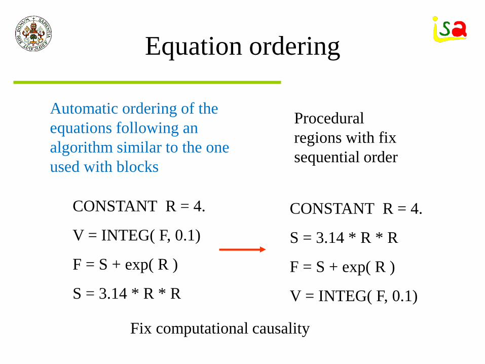
Equation ordering
Automatic ordering of the equations following an algorithm similar to the one used with blocks
CONSTANT R = 4
S = 314 R R
F = S + exp( R )
V = INTEG( F 01)
CONSTANT R = 4
V = INTEG( F 01)
F = S + exp( R )
S = 314 R R
Procedural regions with fix sequential order
Fix computational causality
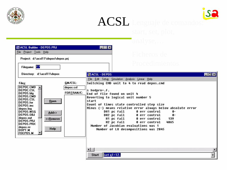
CSSLrsquo67 ACSL
program pruebainitial constant x0=01 tmax=3 cinterval cint=035 algorithm ialg=3endderivative constant tau=2 z = 5 x ndash 3y x = integ(tauy + sin(x) x0) y = bound(-11x) termt(tgttmax)endend
y3x5z
)x(sin)x(yτtdxd
minus=
+=
x
y
LimAlto
LimAltoLim Bajo
program prueba
initial
constant x0=01 tmax=3
cinterval cint=035
algorithm ialg=3
end
derivative
constant tau=2
z = 5 x ndash 3y
x = integ(tauy + sin(x) x0)
y = bound(-11x)
termt(tgttmax)
end
end
ACSL Lenguaje de comandos start set plot analysehellip
Ficheros de Procedimientos
Modularity
A modular approach provides support to the description of a complex system using pre-defined sub-systems
Helps library maintenanceHelps team workingHelps improving the readability and use of the
simulation code
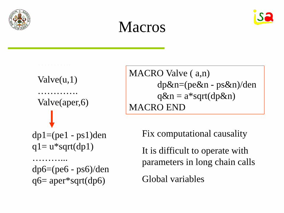
Macros
Macros encapsulate simulation code to facilitate its repetitive use in different places of the model description
There are different from subroutines The code of a macro is expanded and analysed with the other equations before compilationhelliphelliphellip
It is difficult to operate with parameters in long chain calls
Global variables
Modelling Languages
bull Direct declaration of the model equationsbull Model description is given a temporal structure bull Separation model-experimentbull Object orientedbull Code generators compiled simulation codebull True modular modelling They do not have fix
computational causality
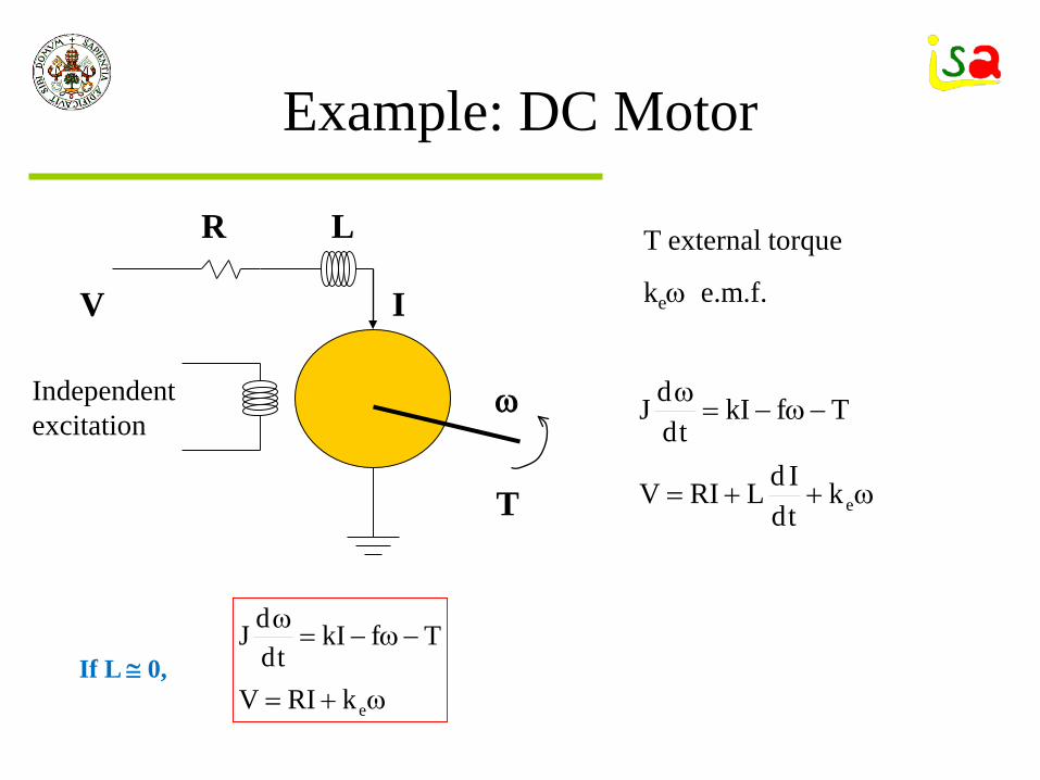
Example DC Motor
ω
LR
V
Independent excitation
ω++=
minusωminus=ω
ektdIdLRIV
TfkItd
dJ
I
T external torque
keω emf
T
If L cong 0 ω+=
minusωminus=ω
ekRIV
TfkItd
dJ
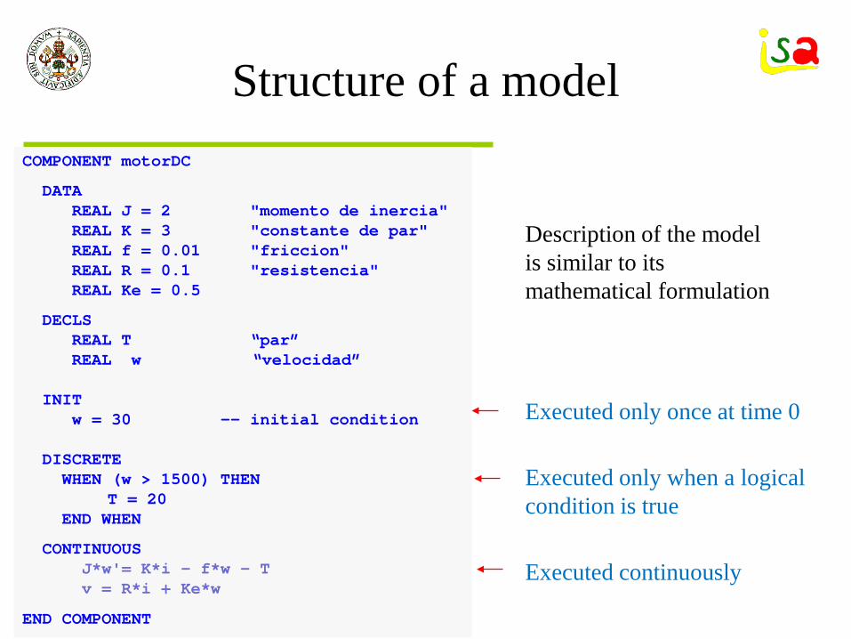
Structure of a modelCOMPONENT motorDC
DATAREAL J = 2 momento de inerciaREAL K = 3 constante de parREAL f = 001 friccionREAL R = 01 resistenciaREAL Ke = 05
DECLSREAL T ldquoparrdquoREAL w ldquovelocidadrdquo
INIT w = 30 -- initial condition
DISCRETEWHEN (w gt 1500) THEN
T = 20END WHEN
CONTINUOUSJw= Ki - fw ndash Tv = Ri + Kew
END COMPONENT
Description of the model is similar to its mathematical formulation
Executed only once at time 0
Executed only when a logical condition is true
Executed continuously
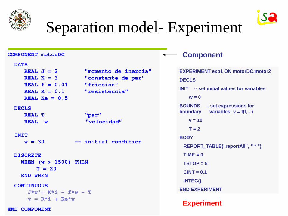
Separation model- Experiment
EXPERIMENT exp1 ON motorDCmotor2
DECLS
INIT -- set initial values for variables
w = 0
BOUNDS -- set expressions for boundary variables v = f(t)
v = 10
T = 2
BODY
REPORT_TABLE(reportAll )
TIME = 0
TSTOP = 5
CINT = 01
INTEG()
END EXPERIMENT
Experiment
Component
Model
COMPONENT motorDC
DATAREAL J = 2 momento de inerciaREAL K = 3 constante de parREAL f = 001 friccionREAL R = 01 resistenciaREAL Ke = 05
DECLSREAL T ldquoparrdquoREAL w ldquovelocidadrdquo
INIT w = 30 -- initial condition
DISCRETEWHEN (w gt 1500) THEN
T = 20END WHEN
CONTINUOUSJw= Ki - fw ndash Tv = Ri + Kew
END COMPONENT
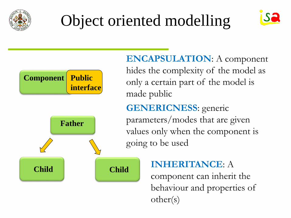
Object oriented modelling
Component
Father
Child Child INHERITANCE A component can inherit the behaviour and properties of other(s)
GENERICNESS generic parametersmodes that are given values only when the component is going to be used
Public interface
ENCAPSULATION A component hides the complexity of the model as only a certain part of the model is made public
Connecting modules by ports
COMPONENT motorDC
PORTSIN Elec ALIN Mech_rot eje
DATAREAL J = 2 momento de inerciaREAL K = 3 constante de parREAL f = 001 friccionREAL R = 01 resistenciaREAL Ke = 05
DECLSREAL T ldquoparrdquoREAL w ldquovelocidadrdquo
Electrical and mechanical ports have been definedhellip
Model
Body of theComponent
Port
Component 2
PORT Elec Electrical pin EQUAL REAL v Potential (V) SUM REAL i Current (amp)
END PORT
Hierarchical models
Modular modelling
Block oriented languages do not allow true modular modelling because they impose the computational causality at the model description stage
Modelling languages
They were developed to facilitate model reuse They do not have fix computational causality DYMOLA GPROMS MODELICA OMOLA
ECOSIMPRO ABACUS JACOBIAN ASPEN DYNAMICShellip
Code to be executed depends on the aims and boundaries of the problem
21 ppkq minus=
kqpp
2
12 minus=
Aim To have a description of the model of a component independent from its use in a specific case
p1
p2
q
If p1 and p2 are given
If p1 and q are given
Computational Causality
Different to the equation ordering
Example Two different implementations required for the resistor
Current is computed from Voltage is computed from the equation I = VR the equation V = IR
Vo
+
I=VR Io
+
V=IR
Computational causality assignmentWhich equation should be used to compute every unknown variable Modelling languages perform the assignment analysing the whole set of model equations as a function of the known boundaries
V = I R
Different to the equation ordering 13
13
Example Two different implementations required for the resistor13
13
Current is computed from13
13
Voltage is computed from13
13
the equation I = VR13
13
the equation V = IR13
13
13
13
13
13
13
13
13
13
13
13
13
13
Vo13
13
+13
13
I=VR13
13
Io13
13
+13
13
V=IR13
13
13
Modelling Languages
bull A model of a system is composed using a high level description linking pre-defined modules representing sub-systems
bull Each module contains the mathematical description of a sub-system
bull Each module is linked to others through an interface or port in the same way as in the physical world
bull BUT the mathematical model of the system is generated later on manipulating the whole set of equations as a function of the chosen systems boundaries
First version 1992 Unix ESA First version under Windows 1999 Object oriented tool Support continuous discrete and discrete event processes Models are built by textual description of from graphical
libraries Provides a software development environment Open code C++ ActiveX OPC FMIhellip Version 5 on 2013 multiplatform QT Proosis
Cesar de Prada ISA-UVA 54
EcosimPro
Cesar de Prada ISA-UVA 55
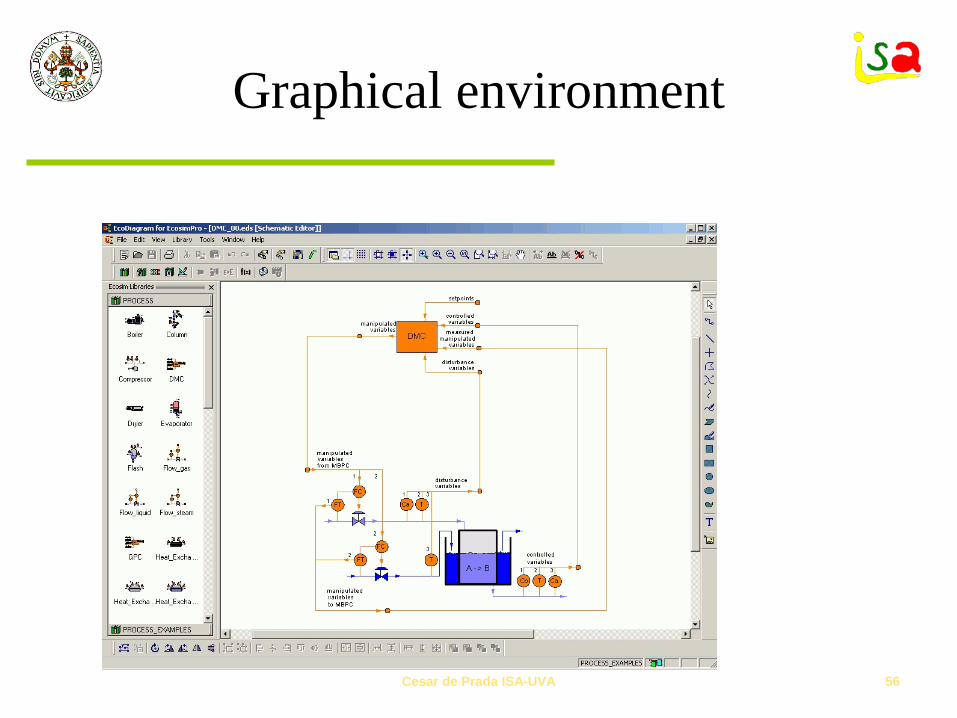
Graphical environment
Cesar de Prada ISA-UVA 56
Modelling steps
Library of non causal models
Model built linking components
Analysis and computational causality of the whole set of equations (Partition)
Model analysis and assignment of computational causality (Partition generation)
1 Specify the boundary conditions2 Is it feasible to solve the problem with the specified
boundaries (Detection of structural singularities Maximum Transversal Algorithm)1 Inadequate Boundaries2 High index models
3 Specify the equation that will be used to compute every variable and stablish the order in which the equations will be used (BLT Algorithm)1 Whenever possible work out every variable symbolically2 Identify the possible algebraic loops (Select tearing variables)
4 The partition is finished and ordered model equations are generated ready to be solved
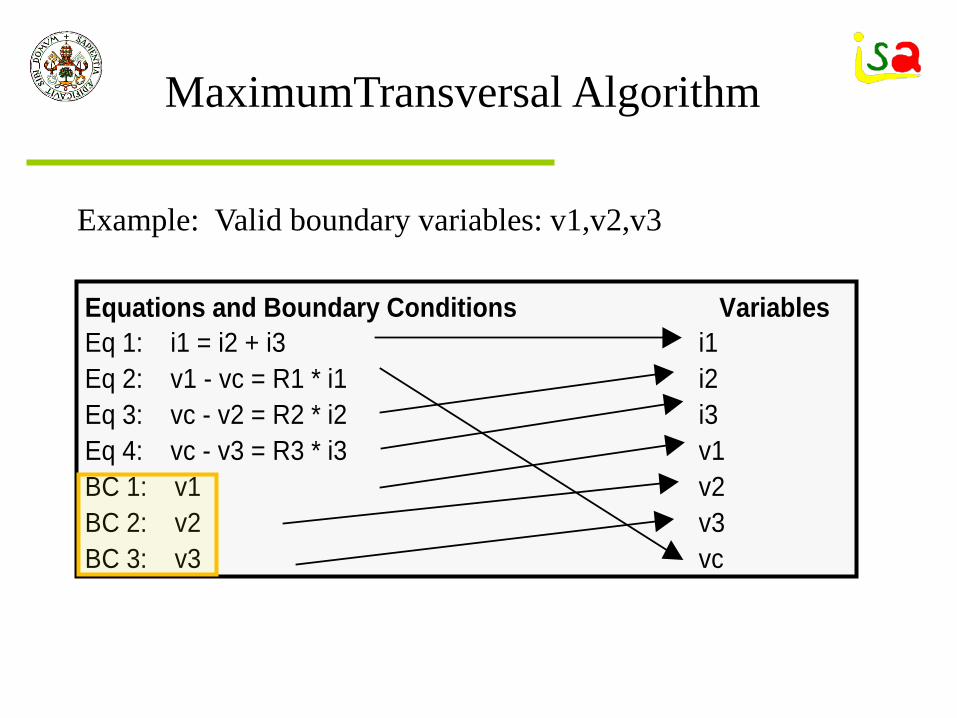
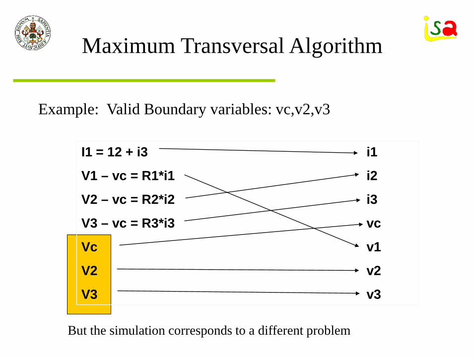
The number of required boundary conditions is determined as the difference between the number of variables and the number of equations Once a set of boundary variables is proposed by the user its validity is cheked with the Maximum Transversal algorithm
Mathematically correct system System with a structural singularity
Is the system with the selected boundary variables structurally correct A necessary condition for a model to be mathematically correct is the existence of a one to one correspondence between equations and variables
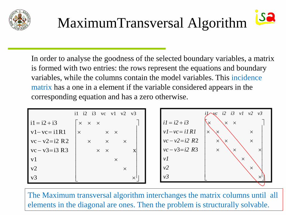
In order to analyse the goodness of the selected boundary variables a matrix is formed with two entries the rows represent the equations and boundary variables while the columns contain the model variables This incidencematrix has a one in a element if the variable considered appears in the corresponding equation and has a zero otherwise
The Maximum transversal algorithm interchanges the matrix columns until all elements in the diagonal are ones Then the problem is structurally solvable
MaximumTransversal Algorithm
Which model variables are included in the analysis performed by the Maximum Transversal algorithm
State variables x (which appear under the derivative sign) are considered known variables in the analysis because an initial value has to be assigned to them and consequently they are not included in the matrix of the Maximum Transversal
Derivatives of the state variables xrsquo are considered as unknown variables that must be evaluated for the integration of the system and consequently are in cluded in the matrix
xrsquo = dx dt = f(x t)
MaximumTransversal Algorithm
The boundary conditions are selected freely by the user but it is possible to suggest him a coherent set or check the user selection
When suggesting a set of boundary variables a first choice refers to the variables assigned to unconnected ports after checking that they satisfy the maximum transversal algorithm
If this choice fails another set is selected iterating on the remaining variables
Model analysis
Have the model equations the adequate mathematical format to be solved
The Maximum Transversal algorithm fails when a high index problem is present
0)uxx(g
)tuxx(ftd
xd
)tuxx(ftd
xd
21
2122
2111
=
=
=X1rsquo X2
rsquo
F1 xF2 xg
u boundary variable
DAEs ODEs Models
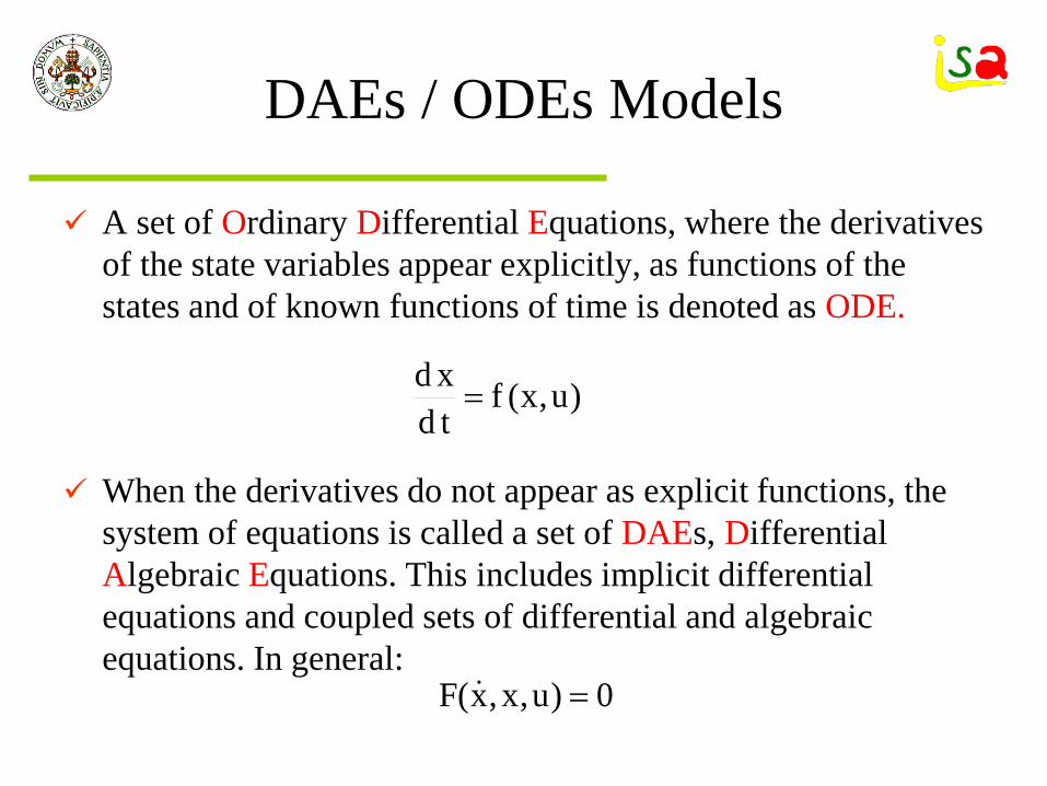
A set of Ordinary Differential Equations where the derivatives of the state variables appear explicitly as functions of the states and of known functions of time is denoted as ODE
When the derivatives do not appear as explicit functions the system of equations is called a set of DAEs Differential Algebraic Equations This includes implicit differential equations and coupled sets of differential and algebraic equations In general
)ux(ftdxd =
0)uxx(F =
Index Problems
Sometimes a set of DAEs can be converted to a set of ODEs managing the equations nevertheless if the matrix partFpartẋ is singular the transformation is not possible unless some of the equations are differentiated with respect to time
The index of a DAE is the number of times needed to differentiate the DAEs to get a system of ODEs
A differential index of 1 is called low index while it is called High index if it is 2 or larger
In systems with index 1 or larger the maximum transversal algorithm fails in finding a feasible set of boundary conditions
0)uxx(F = )ux(ftdxd =
Index problems
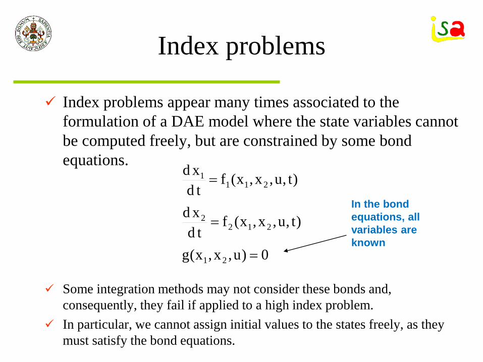
Index problems appear many times associated to the formulation of a DAE model where the state variables cannot be computed freely but are constrained by some bond equations
Some integration methods may not consider these bonds and consequently they fail if applied to a high index problem
In particular we cannot assign initial values to the states freely as they must satisfy the bond equations
0)uxx(g
)tuxx(ftd
xd
)tuxx(ftd
xd
21
2122
2111
=
=
=
In the bond equations all variables are known
21
211
1 TTdt
dJ
ω=ω
+++=ω
Index problems Examples
TTdt
dJ 212
2 +++=ω
High index problems can be generated when linking together two components of a library because of the bond equations added by the ports
ω1 ω2
Rigid shaft
Equation generated by the mechanical port
idtdVC =
22
2
11
1
idt
dVC
idt
dVC
=
=
21 VV =
Index problems Examples
Index problems can be generated when linking together two components of a library because of the bond equations added by the ports
V i
C
V1 V2
C1 C2
i1 i2
Index problems Examples
V1 V2
C1 C2
i1 i2 V0I0
20
210
21
222
111
VViiI
VViVCiVC
=+=
===
V1 V2 are state variables as theyappear under the derivative signI0 is chosen as boundary variable
Only 4 equations contain the 5 unknown variables This structure implies that there is no solution to the assignment problem with the maximum transversal algorithm
5 variables and 5 equations
but the bond equation V1 = V2creates a structural singularity
High Index problems Examples
Sometimes high index problems appear due to the formulation of the problem that does not follows the physical causality but corresponds to other problems like eg control
Which is the force that must be applied to a particle in order to move it according to a certain pre-specified trajectory
)tsin(e)t(xdt
xdmF
10
2
2
tminus=
=
There is a boundary condition specified on a state variable
High Index problems
The Maximum Transversal algorithm fails when a high index problem is
present Example
MAXIMUM TRANSVERSALF = m vrsquo vrsquo
xrsquo = v xrsquo
x = exp(-TIME10) sin(TIME) F
3 EquationsF = m vrsquo xrsquo= vx = exp(-TIME10) sin(TIME)
Known variablesv amp x state variablesm data 3 Unknown variables
F vrsquo xrsquo
Three variables that appearonly in twoequations Thelast one isuseless forestimating F
Pantelides algorithm
The Pantelides algorithm is used to transform high index problems into an equivalent lower index one
The algorithm adds new equations to the model obtained by differentiation of the ones that create the structural singularity (the bond equations) facilitating the application of the maximum transversal algorithm
As new equations are added one should either incorporate more variables or substitute the bond equations by its differentiate form to balance the number of equations and variables
The procedure is repeated until no structural singular set is found
0)uxx(ftd
xd211
1 =minus
0)uxx(g
0)uxx(ftd
xd
21
2122
=
=minus
0dt
)uxx(gd 21 =
Pantelides algorithm
One option to balance equations and variables is to substitute the bond equations by its differentiated form
Another option is not replacing the bond equations but adding some states as new variables As the initial values of the state equations cannot be chosen arbitrarily some state variables involved in the bonds are not computed by integration of the corresponding differential equation but from the bond equations This implies that these state variables can be considered as unknown and added to the list for the analysis of the maximum transversal algorithm
0)uxx(ftd
xd211
1 =minus
0)uxx(g
0)uxx(ftd
xd
21
2122
=
=minus
0dt
)uxx(gd 21 =
Example
V1 V2
C1 C2
i1 i2 V0I0
V1and V2 are state variablesI0 is chosen as boundary variable
Now there are 5 equations containing 5 unknown variables and the maximum transversal algorithm can be applied But coherent initialization is required or critical information can be lost about the initial values
5 variables and 5 equations
Vrsquo = d dt
Index one problem as the bond equation V1 = V2 has been differentiated only once20
This implies that the problem is now structurally solvable A different problem is finding the right assignment and order of calculus between variables and equations
x x
x x
x x
x x
x
Example
V1 V2
C1 C2
i1 i2 V0I0
20
210
21
21
222
111
VViiIVV
VViVCiVC
=+=
==
==
V2 is a state variable but it will be considered as a variable as it will not be computed from integration of V2rsquo but from V2= V1I0 is chosen as boundary variable
This implies that the problem is now structurally solvable A different problem is finding the right assignment and order of calculus between variables and equations
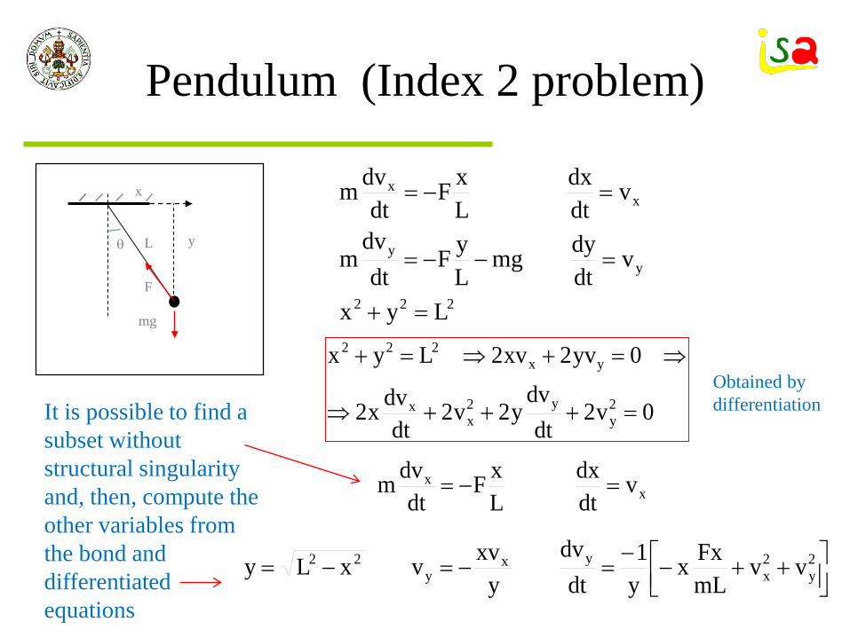
Pendulum (Index 2 problem)
222
y2
2
x2
2
Lyx
vdtdymg
LyF
dtydm
vdtdx
LxF
dtxdm
=+
=minusminus=
=minus=
mg
x
y
F
θ L
The structural singularity is created by inadequate modelling using cylindrical coordinate the problem can be described with a single variable θ without bonds
There are 4 useful equations and 4 unknowns xrsquoyrsquo vxrsquo vyrsquo but as we cannot initialize arbitrarily the four states the bond equation is differentiated twice to find equations that provide the value of two of them instead of using integration of the corresponding differential equations
Pendulum (Index 2 problem)
222
yy
xx
Lyx
vdtdymg
LyF
dtdv
m
vdtdx
LxF
dtdvm
=+
=minusminus=
=minus=
0v2dt
dvy2v2
dtdvx2
0yv2xv2Lyx
2y
y2x
x
yx222
=+++rArr
rArr=+rArr=+
xx v
dtdx
LxF
dtdvm =minus=
++minusminus=minus=minus= 2
y2x
yxy
22 vvmLFxx
y1
dtdv
yxvvxLy
mg
x
y
F
θ L
It is possible to find a subset without structural singularity and then compute the other variables from the bond and differentiated equations
Obtained by differentiation
Pendulum ( another choice of state variables)
yy v
dtdymg
LyF
dtdv
m =minusminus=
0v2dt
dvy2v2
dtdvx20yv2xv2Lyx 2
yy2
xx
yx222 =+++rArr=+rArr=+
++minusminusminus=minus=minus= 2
y2x
xyx
22 vvgmLFyy
x1
dtdv
xyv
vyLx
mg
x
y
F
θ L
222
yy
xx
Lyx
vdtdymg
LyF
dtdv
m
vdtdx
LxF
dtdvm
=+
=minusminus=
=minus=
If we select instead y vy as state variables it is possible to have divisions by zerohellip
1 Solving first the subset of equations 2 Thencomputing the remaining variables
from
Index problems Boundary conditions
When selecting the boundary variables care must be taken to avoid generating undesired index problems
If a state variable is selected as a boundary a bond is automatically created But as the Pantelides algorithm requires computing derivatives of the bond equations it needs a explicit form of the time dependency of the variable which is not given at the time of partition definition Because of this state variables are not allowed as boundary variables
If one wants to impose a certain time evolution to a state variable it must add the corresponding equation x = f(t) as part of the model so that its explicit form is known at partition generation time
The bond equation is differentiated twice generating two equations that allow computing xrsquo and vrsquo from them instead of by integration avoiding the problems associated to the need of consistent initial conditions
Index 2 problemF = m vrsquo F xrsquo= v vx = sin(TIME) xxrsquo = cos(TIME) xrsquovrsquo = -sin(TIME)) vrsquo
)tsin(e)t(xdt
xdmF
10
2
2
tminus=
=
Ordering of equations BLT Algorithm
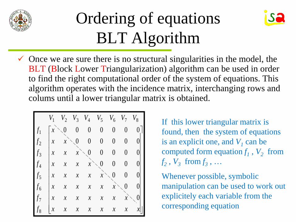
Once we are sure there is no structural singularities in the model the BLT (Block Lower Triangularization) algorithm can be used in order to find the right computational order of the system of equations This algorithm operates with the incidence matrix interchanging rows and colums until a lower triangular matrix is obtained
xxxxxxxxxxxxxxx
xxxxxxxxxxx
xxxxxxx
xxx
ffffffff
VVVVVVVV
0000000000000000000000000000
8
7
6
5
4
3
2
1
87654321 If this lower triangular matrix is found then the system of equations is an explicit one and V1 can be computed form equation f1 V2 from f2 V3 from f3 hellip
Whenever possible symbolic manipulation can be used to work out explicitely each variable from the corresponding equation
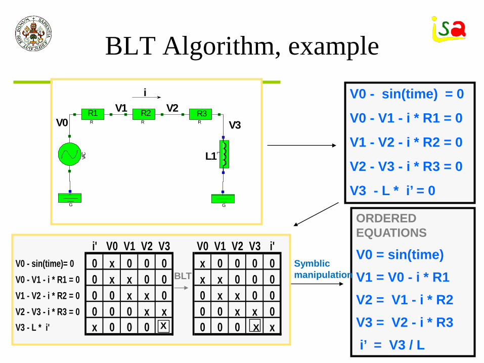
BLT Algorithm exampleV0 - sin(time) = 0
V0 - V1 - i R1 = 0
V1 - V2 - i R2 = 0
V2 - V3 - i R3 = 0
V3 - L irsquo = 0
ORDERED EQUATIONS
V0 = sin(time)V1 = V0 - i R1V2 = V1 - i R2V3 = V2 - i R3irsquo = V3 L
L
RRR
VAC
G G
V0V1
V3V2
i
R1 R3R2
L1
Symblic manipulationBLT
i V0 V1 V2 V3 V0 V1 V2 V3 iV0 - sin(time)= 0 0 x 0 0 0 x 0 0 0 0V0 - V1 - i R1 = 0 0 x x 0 0 x x 0 0 0V1 - V2 - i R2 = 0 0 0 x x 0 0 x x 0 0V2 - V3 - i R3 = 0 0 0 0 x x 0 0 x x 0V3 - L i x 0 0 0 0 0 0 0 0 x
BLT
X XX
Ordering of equations BLT Algorithm
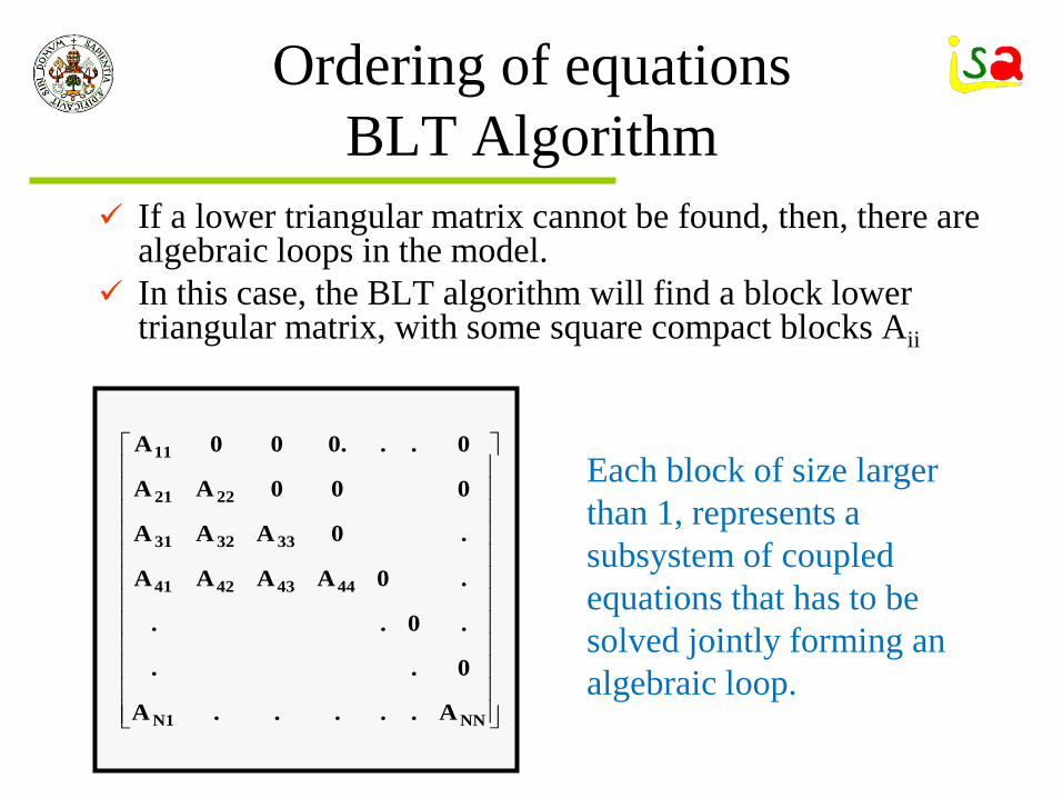
If a lower triangular matrix cannot be found then there are algebraic loops in the model
In this case the BLT algorithm will find a block lower triangular matrix with some square compact blocks Aii
NNN1
44434241
333231
2221
11
AA
0
0
0AAAA
0AAA
000AA
0000AEach block of size larger than 1 represents a subsystem of coupled equations that has to be solved jointly forming an algebraic loop
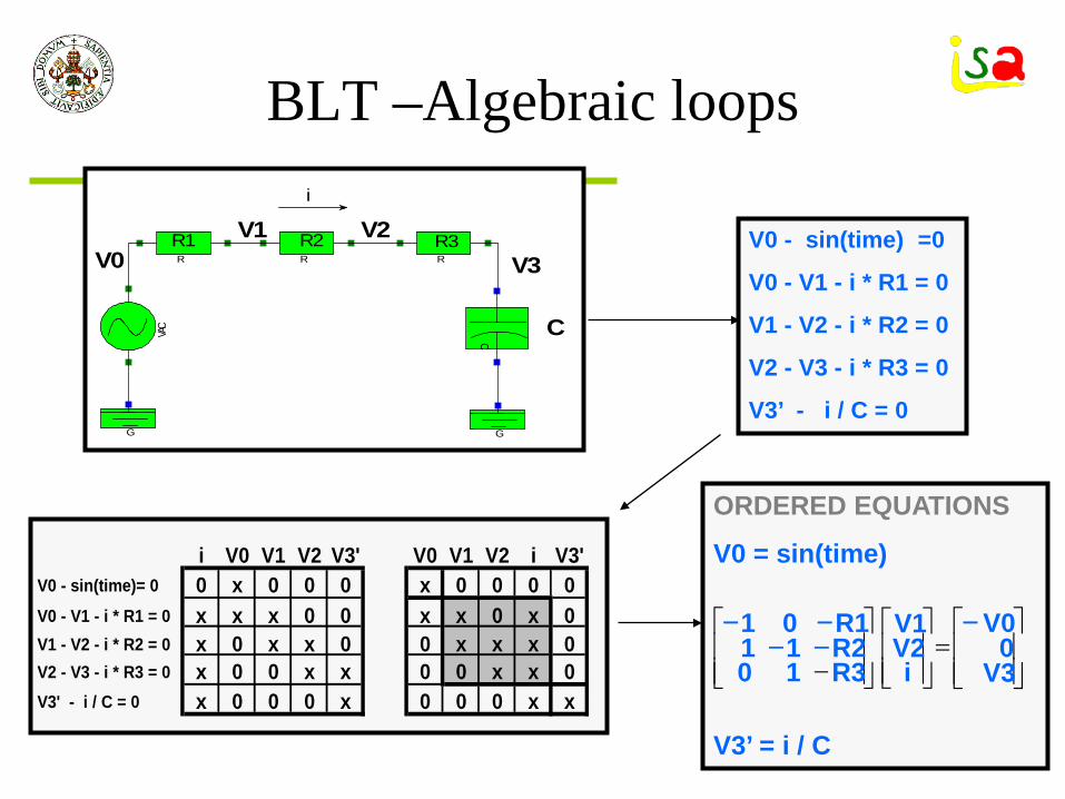
BLT ndashAlgebraic loops
V0 - sin(time) =0
V0 - V1 - i R1 = 0
V1 - V2 - i R2 = 0
V2 - V3 - i R3 = 0
V3rsquo - i C = 0
ORDERED EQUATIONS
V0 = sin(time)
V3rsquo = i C
BLT
RRR
VAC
G G
V0V1
V3V2
i
R1 R3R2
L1C C
i V0 V1 V2 V3 V0 V1 V2 i V3V0 - sin(time)= 0 0 x 0 0 0 x 0 0 0 0V0 - V1 - i R1 = 0 x x x 0 0 x x 0 x 0V1 - V2 - i R2 = 0 x 0 x x 0 0 x x x 0V2 - V3 - i R3 = 0 x 0 0 x x 0 0 x x 0V3 - i C = 0 x 0 0 0 x 0 0 0 x x
minus=
minusminusminusminusminus
V30
V0
iV2V1
R310R211R101
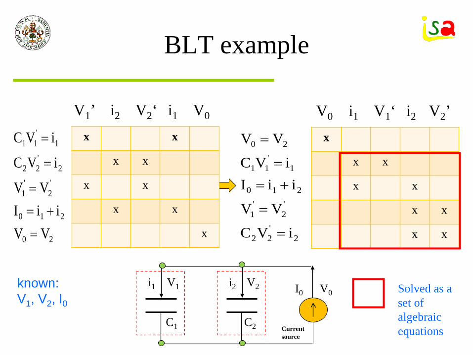
BLT example
V1rsquo i2 V2lsquo i1 V0
x x
x x
x x
x x
x
V1 V2
C1 C2
i1 i2 V0I0
Currentsource
20
210
2
1
222
1
11
VViiI
VV
iVC
iVC
=+=
=
=
=
V0 i1 V1lsquo i2 V2rsquo x
x x
x x
x x
x x
knownV1 V2 I0
222
2
1
210
1
11
20
iVC
VV
iiIiVC
VV
=
=
+==
=
Solved as a set of algebraic equations
Algebraic loops
The BLT algorithm finds an ordered set of equations including possible algebraic loops ( subsystems of coupled equations)
In order to solve the algebraic loops ndash If all equations of the block are linear it is possible to
work out explicitly the variables involved using a symbolic manipulator or solve the loop with an efficient linear solver
ndash If the algebraic loop is non-linear then the solution may require a non-linear solver based on Newton-Raphson besides the selection of the tearing variables
BLT example
V1 V2
C1 C2
i1 i2 V0I0
Currentsource
V0 i1 V1lsquo i2 V2rsquo x
x x
x x
x x
x x
knownV1 V2 I0
222
2
1
210
1
11
20
iVC
VV
iiIiVC
VV
=
=
+==
=
Solved as a set of algebraic equations
111
222
2
1
20
22
21
210
2
1
20
VCi
VCi
VV
VIVCVCiiI
VV
VV
=
=
=
rArr=+
+==
=
As system is linear using symbolic manipulations
Loop Tearing
Direct solution of an algebraic loop using Newton-Raphson method leads to an algorithm with a size of the Jacobian as large as the number of variables involved in the loop
The use of Equation Tearing techniques allows sustantial reductions of the size of the Jacobian
Some (tearing) variables are selected so that if given an initial value it is possible to compute explicitly the remaining variables of the loop As the initial value may be wrong there will be as many equations of the loop as tearing variables that will not compute equal to zero (residual equations) The Newton-Raphson algorithm will iterate modifying the tearing variables until the residual equations are satisfied but with a reduced Jacobian size
F1(x1 x2) = 0F2(x1 x2 x3) = 0F3(x1 x2 x3) = 0
x2 selected as tearing variable
x1 = f1(x2)x3 = f2(x1 x2)F3(x1 x2 x3) = residual
Loop TearingV0 - sin(time) =0
V0 - V1 - i2 R1 = 0
V1 - V2 - i2 R2 = 0
V2 - V3 - i2 R3 = 0
V3rsquo - i C = 0
ORDERED EQUATIONS
V0 = sin(time)
i tearing variableV1 = V0 - i2 R1
V2 = V1 - i2 R2
F(i) = V2 - V3 - i2 R3 = 0
V3rsquo = i C
BLT
RRR
VAC
G G
V0V1
V3V2
i
R1 R3R2
L1C C
i V0 V1 V2 V3 V0 V1 V2 i V3V0 - sin(time)= 0 0 x 0 0 0 x 0 0 0 0V0 - V1 - i R1 = 0 x x x 0 0 x x 0 x 0V1 - V2 - i R2 = 0 x 0 x x 0 0 x x x 0V2 - V3 - i R3 = 0 x 0 0 x x 0 0 x x 0V3 - i C = 0 x 0 0 0 x 0 0 0 x x
Residue equation
Loop Tearing
Loop Tearing methods have some weakness Tearing algorithms are based on heuristic rules There is no algorithm that provides the best choice among the
different possible sets of tearing variables As a consecuence the user can select a better set of tearing
variables if it is not satisfied with the selection made by the simulation environment
DAEs and algebraic loops
Solve algebraic loops
Initialization
Compute model residuals
Solve integrators
Residuals from algebraic equ
Initialization
Other residuals
Solve DASSL
Only one single Newton iteration is needed
DAE solvers do not require solving algebraic loops independently
Model editor and error cheking (Compile)
Selection of boundary variables and partition generation
C++ Class
Compiler + internal Libraries+ Calls to external software
Run-time Executable code
Specify experiment
Overall steps
Nuacutemero de diapositiva 1
Outline
Digital Simulation
Uses of Simulation
Advantages of the simulation
Models
Adequate representation
Nuacutemero de diapositiva 8
Stages of a simulation project
Concepts
Simulation Languages
Advantages
First principles models
Nuacutemero de diapositiva 14
Nuacutemero de diapositiva 15
Nuacutemero de diapositiva 16
Model Libraries
Types of simulation languages according to the way they support modularity
Block oriented languages
Blocks or macros
Simulink
Simulink
Block oriented languages Simulink
Simulink
Structure
Blockrsquos computational order
Integration architecture
Algebraic loops
Hierarchical blocks
Block oriented languages
Expression oriented languages
CSSLrsquo67
CSSLrsquo67
Computations
Language
Equation ordering
CSSLrsquo67 ACSL
ACSL
Modularity
Macros
Macros
Modelling Languages
Nuacutemero de diapositiva 43
Structure of a model
Separation model- Experiment
Nuacutemero de diapositiva 46
Nuacutemero de diapositiva 47
Nuacutemero de diapositiva 48
Modular modelling
Code to be executed depends on the aims and boundaries of the problem
Computational Causality
Nuacutemero de diapositiva 52
Modelling Languages
EcosimPro
EcosimPro
Graphical environment
Modelling steps
Modelling Languages
Model analysis and assignment of computational causality (Partition generation)
How model equations are treated in Modelling languages (EcosimPro)
Digital Simulation
Methods and tools oriented to ldquoimitaterdquo or predict the responses of a systems against certain changes or ldquostimulusrdquo using a computer
Uses of Simulation
Study of a process what ifhellip analysis Design (process controlhellip) Testing a control system before actual
implementation in the plant Personnel training Operation optimization Essays in a virtual plant hellip
Advantages of the simulation
Perform changes that if implemented in the process will be o Very costly o Too slow fast o dangerous etc
Reproduces the experiment as many time as desired under the same conditions
Saves time Provides safety Allows sensitivity studies Provides a model that can be used for many purposes Allows experimenting with systems that are not built yet
Models
Simulation is based on mathematical models of the processes
Mathematical models are set of equations relating the variables of a process and being able to provide an adequate representation of its behaviour
They are always approximations of the real world Adequacy of a model depends on their intended use There are a wide variety of models according to the
processes they represent and their aims
Adequate representation
Proceso
u
time
y
time
Model
ym
timefidelity to the physical asset and facility of use in the intended application
State space models
)t)t(ux(g)t(y
)t)t(u)t(x(fdt
)t(xd
=
=
Manipulated variables and disturbances
Model responses
u yx
x States
Stages of a simulation project
Study the process Set the simulation aims
ndash Specify the relevant variables Develop the model according to the simulation
aims Code the model in a simulation language Set the independent variables and choose the
numerical solvers Exploit the results of the simulation
Concepts
Process -gt ModelV - I R = 0 oacute I = VR oacute V = IR
Assignment of computational causalityV = I R
ExperimentR = 10 I = 2
Numerical solutionV = 210 = 20
Simulation Languages
Computer program providing tools forDescribing the model and assigning
computational causalityDefining the experiments to be performedSolving numerically the set of equationsVisualizing the results and communicating
with the external world
Advantages
Provide support in all phases of model development and exploitation
Allows concentrating in the problem and the results not spending time and efforts in programming
Gives reliability to the numerical results Allows saving time Allows the non-expert in computing or numerical
methods to solve complex models
First principles models
Based on knowledge of the process and nature laws (Physics chemistryhellip)
Sometimes are difficult to formulate from the scratch requiring trained people large development times costs
They need to be tested and validated
This may limit their use in many fields (Design decision making traininghellip
Buthellipwhich is the cost of non-using them
Solution Libraries of models
Models are built linking the tested modules or components of a model library
Each component of the library contains the mathematical model of a process and can be configured by parameterization to fit the user needs
Each component can be linked to others by an interface or port in order to built more complex models
Va Vb
Ia Ib Va Vb
Ia Ib
Va Vb
Ia Ib
R1
C1
R2
Physical properties data bases and good user interfaces are also required
Model Libraries
Sets of components representing different processes devices etc Each one contains its mathematical model and connections to the external
world Components can be parameterized to adapt them to the user requirements
mc_out
Tacha18
j_in1j_in2
j_in3v_in
va_out
c_out
mc_out
Tacha18
j_in1j_in2
j_in3v_in
va_out
c_out
mc_out
Tacha18
j_in1j_in2
j_in3v_in
va_out
c_out
mc_out
Tacha18
j_in1j_in2
j_in3v_in
va_out
c_out
mc_in
mp_out
mr_out
cristal_out
Turbinadiscontinua1
mc_in
mp_out
mr_out
cristal_out
Turbinadiscontinua1
mc_in
mp_out
mr_out
cristal_out
Turbinadiscontinua1
mc_in
mp_out
mr_out
cristal_out
Turbinadiscontinua1
mc_in
mp_out
mr_out
cristal_out
Turbinadiscontinua1
mc_in
mp_out
mr_out
cristal_out
Turbinadiscontinua1
mc_in
mp_out
mr_out
cristal_out
Turbinadiscontinua1
f_in1 f_in2 f_in3 f_in4 f_in5 f_in6 f_in7
f_out
niv
Deposito1
f_in1 f_in2 f_in3 f_in4 f_in5 f_in6 f_in7
f_out
niv
Deposito1
mc_in1 mc_in2
mc_out
Malaxador6 mc_in1 mc_in2
mc_out
Malaxador6
After parameterization simulation code is generated
Select and connect components as in the real world
Model Libraries
Model Libraries
Modular modellingndash Facilitates the re-use of models in different applicationsndash Facilitates the use of simulation to those non-experts in
simulation but knowing the system to be simulated Modularity Independent description of every module of
the library Abstraction Use the modules without knowing its internal
details (model equations etc) Hierarchy New modules can be built by linking the
existing ones
Types of simulation languages according to the way they support modularity
Each block has fix input and output variables and contains equations or code to compute the value of the output variables as a function of the value of the input ones
x
Blocks or macros
w = 3x -6yz = 5w + sin(y)
Encapsulated code that is not manipulated by the simulation environment
Fix computational causality imposed by the inputs and outputs of the block
Connections between blocks by linking input - output variables
Block diagrams do not mimic the physical layout but the mathematical one
x
yz
Simulink
+
R1 R2
C
Physical system
L
u
Model equations
Implementation of the model is done using predefined blocks that carry out specific operations and are linked together to perform the operations of the model equations
L U dtdi
C i dt
dUR2 i - U U
R1 )U - (U i
LL
CC
LL
CC
=
=
times==
LC
R2R1U
iLiC
Simulink
The block diagram is built graphically from the blocks of the library
Block oriented languages Simulink
L U dtdi
C i dt
dUR2 i - U U
R1 )U - (U i
LL
CC
LL
CC
=
=
times==
Simulink
+
R1 R2
C
Physical system
L
u
With block oriented languages the user describes the mathematical model not the physical system
Block diagram
StructureBlock diagram edition
Error analysis
Block computational order
Sequential computation of the blockrsquos outputs
from its imputs
Results Display
End
CSMP 1130 SADS DSL90
hellip
EASY-5 TUTSIM Simulink
Integration t= t+h
t = tstop
Blockrsquos computational order
States or known values initially
2
83
64
75 9
1
1 Starting from the blocks with known initial values check which blocks can be executed as all their inputs are known
2 Write them down in a list and iterate with the new set of known blocks until all blocks are used up
3 If any new block is added to the list in a full iteration over all blocks an algebraic loop is detected
1 9 8 2 3 5 4 7 6 9 8Computational order
Integration architectureStart from initial value of integrators or outputs of blocks without inputs
Compute the output of every blockaccording to the ordering previously
determined Compute the inputs of the integrators
Integrate the ODE in order to obtainthe value of the states at time t+h
EndStop time
Sum1Sum
Sine Wave
Scope
eu
MathFunction
5
Gainf (z) zSolve
f(z) = 0Algebraic Constraint
Algebraic loops
z = 5 ( sin(t) - ez )
SumSine Wave
Scope
eu
MathFunction
5
Gain
z
z
z
z
A special block need to be added Iterations until convergence are required
Closed loop without integrator
Hierarchical blocks
Modularity
Hierarchy
Block oriented languages
There are easy to use and intuitive Modular and hierarchical architectures Model description does not match neither the physical
process not the equations There are difficult to build and debug in case of models
with a large number of blocks Fix computational causality Slow interpreters Algebraic loops must be explicitly solved with additional
blocks Limited separation model-experiment
Expression oriented languages
Standard CSSLrsquo67 (Simulation 1967 Vol9 pp281-303)
Direct declaration of the model equationsModel description is given a temporal structure Separation model-experiment command languageCode generators compiled simulation code SpeedOpen to the outside world CallReuse of code Macros
CSSLrsquo67 Model editor
Errors Equation ordering
Fortran code
Compiler+ Libraries
Results
Executable codeCommand language
Text editor
BuilderCode translator
CSSLrsquo67Program
Initial
End
Dynamic
Derivative
End
Discrete
End
End
Terminal
End
End
Initial conditions Code executed once at t= 0
Continuous equations
Discrete equations
Final computations Code executed once at tstop
Description model structure
Fix computational causality
Simulation code similar to the mathematical model
Computations
Program
Initial
End
Dynamic
Derivative
End
Discrete
End
End
Terminal
End
End
Initialization of variables including states
Expressions evaluated at certain times (Synchronous or asynchronous modes) or when a event takes place
Expressions evaluated and integrated every integration interval
Global variables
Transfers to initial region are possible to create loops
Language
Equations similar to Fortran exp sin IF THEN ELSE
Primitives BOUND REALP DELAYhellip
Function generators SIN PULSE
Tables 2D amp 3D
Implicit equations IMPLC
Integrators INTEG several methods Stiff DASSL
Event and discontinuities treatment SCHEDULE INTERVAL
External calls Call
Equation ordering
Automatic ordering of the equations following an algorithm similar to the one used with blocks
CONSTANT R = 4
S = 314 R R
F = S + exp( R )
V = INTEG( F 01)
CONSTANT R = 4
V = INTEG( F 01)
F = S + exp( R )
S = 314 R R
Procedural regions with fix sequential order
Fix computational causality
CSSLrsquo67 ACSL
program pruebainitial constant x0=01 tmax=3 cinterval cint=035 algorithm ialg=3endderivative constant tau=2 z = 5 x ndash 3y x = integ(tauy + sin(x) x0) y = bound(-11x) termt(tgttmax)endend
y3x5z
)x(sin)x(yτtdxd
minus=
+=
x
y
LimAlto
LimAltoLim Bajo
program prueba
initial
constant x0=01 tmax=3
cinterval cint=035
algorithm ialg=3
end
derivative
constant tau=2
z = 5 x ndash 3y
x = integ(tauy + sin(x) x0)
y = bound(-11x)
termt(tgttmax)
end
end
ACSL Lenguaje de comandos start set plot analysehellip
Ficheros de Procedimientos
Modularity
A modular approach provides support to the description of a complex system using pre-defined sub-systems
Helps library maintenanceHelps team workingHelps improving the readability and use of the
simulation code
Macros
Macros encapsulate simulation code to facilitate its repetitive use in different places of the model description
There are different from subroutines The code of a macro is expanded and analysed with the other equations before compilationhelliphelliphellip
It is difficult to operate with parameters in long chain calls
Global variables
Modelling Languages
bull Direct declaration of the model equationsbull Model description is given a temporal structure bull Separation model-experimentbull Object orientedbull Code generators compiled simulation codebull True modular modelling They do not have fix
computational causality
Example DC Motor
ω
LR
V
Independent excitation
ω++=
minusωminus=ω
ektdIdLRIV
TfkItd
dJ
I
T external torque
keω emf
T
If L cong 0 ω+=
minusωminus=ω
ekRIV
TfkItd
dJ
Structure of a modelCOMPONENT motorDC
DATAREAL J = 2 momento de inerciaREAL K = 3 constante de parREAL f = 001 friccionREAL R = 01 resistenciaREAL Ke = 05
DECLSREAL T ldquoparrdquoREAL w ldquovelocidadrdquo
INIT w = 30 -- initial condition
DISCRETEWHEN (w gt 1500) THEN
T = 20END WHEN
CONTINUOUSJw= Ki - fw ndash Tv = Ri + Kew
END COMPONENT
Description of the model is similar to its mathematical formulation
Executed only once at time 0
Executed only when a logical condition is true
Executed continuously
Separation model- Experiment
EXPERIMENT exp1 ON motorDCmotor2
DECLS
INIT -- set initial values for variables
w = 0
BOUNDS -- set expressions for boundary variables v = f(t)
v = 10
T = 2
BODY
REPORT_TABLE(reportAll )
TIME = 0
TSTOP = 5
CINT = 01
INTEG()
END EXPERIMENT
Experiment
Component
Model
COMPONENT motorDC
DATAREAL J = 2 momento de inerciaREAL K = 3 constante de parREAL f = 001 friccionREAL R = 01 resistenciaREAL Ke = 05
DECLSREAL T ldquoparrdquoREAL w ldquovelocidadrdquo
INIT w = 30 -- initial condition
DISCRETEWHEN (w gt 1500) THEN
T = 20END WHEN
CONTINUOUSJw= Ki - fw ndash Tv = Ri + Kew
END COMPONENT
Object oriented modelling
Component
Father
Child Child INHERITANCE A component can inherit the behaviour and properties of other(s)
GENERICNESS generic parametersmodes that are given values only when the component is going to be used
Public interface
ENCAPSULATION A component hides the complexity of the model as only a certain part of the model is made public
Connecting modules by ports
COMPONENT motorDC
PORTSIN Elec ALIN Mech_rot eje
DATAREAL J = 2 momento de inerciaREAL K = 3 constante de parREAL f = 001 friccionREAL R = 01 resistenciaREAL Ke = 05
DECLSREAL T ldquoparrdquoREAL w ldquovelocidadrdquo
Electrical and mechanical ports have been definedhellip
Model
Body of theComponent
Port
Component 2
PORT Elec Electrical pin EQUAL REAL v Potential (V) SUM REAL i Current (amp)
END PORT
Hierarchical models
Modular modelling
Block oriented languages do not allow true modular modelling because they impose the computational causality at the model description stage
Modelling languages
They were developed to facilitate model reuse They do not have fix computational causality DYMOLA GPROMS MODELICA OMOLA
ECOSIMPRO ABACUS JACOBIAN ASPEN DYNAMICShellip
Code to be executed depends on the aims and boundaries of the problem
21 ppkq minus=
kqpp
2
12 minus=
Aim To have a description of the model of a component independent from its use in a specific case
p1
p2
q
If p1 and p2 are given
If p1 and q are given
Computational Causality
Different to the equation ordering
Example Two different implementations required for the resistor
Current is computed from Voltage is computed from the equation I = VR the equation V = IR
Vo
+
I=VR Io
+
V=IR
Computational causality assignmentWhich equation should be used to compute every unknown variable Modelling languages perform the assignment analysing the whole set of model equations as a function of the known boundaries
V = I R
Different to the equation ordering 13
13
Example Two different implementations required for the resistor13
13
Current is computed from13
13
Voltage is computed from13
13
the equation I = VR13
13
the equation V = IR13
13
13
13
13
13
13
13
13
13
13
13
13
13
Vo13
13
+13
13
I=VR13
13
Io13
13
+13
13
V=IR13
13
13
Modelling Languages
bull A model of a system is composed using a high level description linking pre-defined modules representing sub-systems
bull Each module contains the mathematical description of a sub-system
bull Each module is linked to others through an interface or port in the same way as in the physical world
bull BUT the mathematical model of the system is generated later on manipulating the whole set of equations as a function of the chosen systems boundaries
First version 1992 Unix ESA First version under Windows 1999 Object oriented tool Support continuous discrete and discrete event processes Models are built by textual description of from graphical
libraries Provides a software development environment Open code C++ ActiveX OPC FMIhellip Version 5 on 2013 multiplatform QT Proosis
Cesar de Prada ISA-UVA 54
EcosimPro
Cesar de Prada ISA-UVA 55
Graphical environment
Cesar de Prada ISA-UVA 56
Modelling steps
Library of non causal models
Model built linking components
Analysis and computational causality of the whole set of equations (Partition)
Model analysis and assignment of computational causality (Partition generation)
1 Specify the boundary conditions2 Is it feasible to solve the problem with the specified
boundaries (Detection of structural singularities Maximum Transversal Algorithm)1 Inadequate Boundaries2 High index models
3 Specify the equation that will be used to compute every variable and stablish the order in which the equations will be used (BLT Algorithm)1 Whenever possible work out every variable symbolically2 Identify the possible algebraic loops (Select tearing variables)
4 The partition is finished and ordered model equations are generated ready to be solved
The number of required boundary conditions is determined as the difference between the number of variables and the number of equations Once a set of boundary variables is proposed by the user its validity is cheked with the Maximum Transversal algorithm
Mathematically correct system System with a structural singularity
Is the system with the selected boundary variables structurally correct A necessary condition for a model to be mathematically correct is the existence of a one to one correspondence between equations and variables
In order to analyse the goodness of the selected boundary variables a matrix is formed with two entries the rows represent the equations and boundary variables while the columns contain the model variables This incidencematrix has a one in a element if the variable considered appears in the corresponding equation and has a zero otherwise
The Maximum transversal algorithm interchanges the matrix columns until all elements in the diagonal are ones Then the problem is structurally solvable
MaximumTransversal Algorithm
Which model variables are included in the analysis performed by the Maximum Transversal algorithm
State variables x (which appear under the derivative sign) are considered known variables in the analysis because an initial value has to be assigned to them and consequently they are not included in the matrix of the Maximum Transversal
Derivatives of the state variables xrsquo are considered as unknown variables that must be evaluated for the integration of the system and consequently are in cluded in the matrix
xrsquo = dx dt = f(x t)
MaximumTransversal Algorithm
The boundary conditions are selected freely by the user but it is possible to suggest him a coherent set or check the user selection
When suggesting a set of boundary variables a first choice refers to the variables assigned to unconnected ports after checking that they satisfy the maximum transversal algorithm
If this choice fails another set is selected iterating on the remaining variables
Model analysis
Have the model equations the adequate mathematical format to be solved
The Maximum Transversal algorithm fails when a high index problem is present
0)uxx(g
)tuxx(ftd
xd
)tuxx(ftd
xd
21
2122
2111
=
=
=X1rsquo X2
rsquo
F1 xF2 xg
u boundary variable
DAEs ODEs Models
A set of Ordinary Differential Equations where the derivatives of the state variables appear explicitly as functions of the states and of known functions of time is denoted as ODE
When the derivatives do not appear as explicit functions the system of equations is called a set of DAEs Differential Algebraic Equations This includes implicit differential equations and coupled sets of differential and algebraic equations In general
)ux(ftdxd =
0)uxx(F =
Index Problems
Sometimes a set of DAEs can be converted to a set of ODEs managing the equations nevertheless if the matrix partFpartẋ is singular the transformation is not possible unless some of the equations are differentiated with respect to time
The index of a DAE is the number of times needed to differentiate the DAEs to get a system of ODEs
A differential index of 1 is called low index while it is called High index if it is 2 or larger
In systems with index 1 or larger the maximum transversal algorithm fails in finding a feasible set of boundary conditions
0)uxx(F = )ux(ftdxd =
Index problems
Index problems appear many times associated to the formulation of a DAE model where the state variables cannot be computed freely but are constrained by some bond equations
Some integration methods may not consider these bonds and consequently they fail if applied to a high index problem
In particular we cannot assign initial values to the states freely as they must satisfy the bond equations
0)uxx(g
)tuxx(ftd
xd
)tuxx(ftd
xd
21
2122
2111
=
=
=
In the bond equations all variables are known
21
211
1 TTdt
dJ
ω=ω
+++=ω
Index problems Examples
TTdt
dJ 212
2 +++=ω
High index problems can be generated when linking together two components of a library because of the bond equations added by the ports
ω1 ω2
Rigid shaft
Equation generated by the mechanical port
idtdVC =
22
2
11
1
idt
dVC
idt
dVC
=
=
21 VV =
Index problems Examples
Index problems can be generated when linking together two components of a library because of the bond equations added by the ports
V i
C
V1 V2
C1 C2
i1 i2
Index problems Examples
V1 V2
C1 C2
i1 i2 V0I0
20
210
21
222
111
VViiI
VViVCiVC
=+=
===
V1 V2 are state variables as theyappear under the derivative signI0 is chosen as boundary variable
Only 4 equations contain the 5 unknown variables This structure implies that there is no solution to the assignment problem with the maximum transversal algorithm
5 variables and 5 equations
but the bond equation V1 = V2creates a structural singularity
High Index problems Examples
Sometimes high index problems appear due to the formulation of the problem that does not follows the physical causality but corresponds to other problems like eg control
Which is the force that must be applied to a particle in order to move it according to a certain pre-specified trajectory
)tsin(e)t(xdt
xdmF
10
2
2
tminus=
=
There is a boundary condition specified on a state variable
High Index problems
The Maximum Transversal algorithm fails when a high index problem is
present Example
MAXIMUM TRANSVERSALF = m vrsquo vrsquo
xrsquo = v xrsquo
x = exp(-TIME10) sin(TIME) F
3 EquationsF = m vrsquo xrsquo= vx = exp(-TIME10) sin(TIME)
Known variablesv amp x state variablesm data 3 Unknown variables
F vrsquo xrsquo
Three variables that appearonly in twoequations Thelast one isuseless forestimating F
Pantelides algorithm
The Pantelides algorithm is used to transform high index problems into an equivalent lower index one
The algorithm adds new equations to the model obtained by differentiation of the ones that create the structural singularity (the bond equations) facilitating the application of the maximum transversal algorithm
As new equations are added one should either incorporate more variables or substitute the bond equations by its differentiate form to balance the number of equations and variables
The procedure is repeated until no structural singular set is found
0)uxx(ftd
xd211
1 =minus
0)uxx(g
0)uxx(ftd
xd
21
2122
=
=minus
0dt
)uxx(gd 21 =
Pantelides algorithm
One option to balance equations and variables is to substitute the bond equations by its differentiated form
Another option is not replacing the bond equations but adding some states as new variables As the initial values of the state equations cannot be chosen arbitrarily some state variables involved in the bonds are not computed by integration of the corresponding differential equation but from the bond equations This implies that these state variables can be considered as unknown and added to the list for the analysis of the maximum transversal algorithm
0)uxx(ftd
xd211
1 =minus
0)uxx(g
0)uxx(ftd
xd
21
2122
=
=minus
0dt
)uxx(gd 21 =
Example
V1 V2
C1 C2
i1 i2 V0I0
V1and V2 are state variablesI0 is chosen as boundary variable
Now there are 5 equations containing 5 unknown variables and the maximum transversal algorithm can be applied But coherent initialization is required or critical information can be lost about the initial values
5 variables and 5 equations
Vrsquo = d dt
Index one problem as the bond equation V1 = V2 has been differentiated only once20
This implies that the problem is now structurally solvable A different problem is finding the right assignment and order of calculus between variables and equations
x x
x x
x x
x x
x
Example
V1 V2
C1 C2
i1 i2 V0I0
20
210
21
21
222
111
VViiIVV
VViVCiVC
=+=
==
==
V2 is a state variable but it will be considered as a variable as it will not be computed from integration of V2rsquo but from V2= V1I0 is chosen as boundary variable
This implies that the problem is now structurally solvable A different problem is finding the right assignment and order of calculus between variables and equations
Pendulum (Index 2 problem)
222
y2
2
x2
2
Lyx
vdtdymg
LyF
dtydm
vdtdx
LxF
dtxdm
=+
=minusminus=
=minus=
mg
x
y
F
θ L
The structural singularity is created by inadequate modelling using cylindrical coordinate the problem can be described with a single variable θ without bonds
There are 4 useful equations and 4 unknowns xrsquoyrsquo vxrsquo vyrsquo but as we cannot initialize arbitrarily the four states the bond equation is differentiated twice to find equations that provide the value of two of them instead of using integration of the corresponding differential equations
Pendulum (Index 2 problem)
222
yy
xx
Lyx
vdtdymg
LyF
dtdv
m
vdtdx
LxF
dtdvm
=+
=minusminus=
=minus=
0v2dt
dvy2v2
dtdvx2
0yv2xv2Lyx
2y
y2x
x
yx222
=+++rArr
rArr=+rArr=+
xx v
dtdx
LxF
dtdvm =minus=
++minusminus=minus=minus= 2
y2x
yxy
22 vvmLFxx
y1
dtdv
yxvvxLy
mg
x
y
F
θ L
It is possible to find a subset without structural singularity and then compute the other variables from the bond and differentiated equations
Obtained by differentiation
Pendulum ( another choice of state variables)
yy v
dtdymg
LyF
dtdv
m =minusminus=
0v2dt
dvy2v2
dtdvx20yv2xv2Lyx 2
yy2
xx
yx222 =+++rArr=+rArr=+
++minusminusminus=minus=minus= 2
y2x
xyx
22 vvgmLFyy
x1
dtdv
xyv
vyLx
mg
x
y
F
θ L
222
yy
xx
Lyx
vdtdymg
LyF
dtdv
m
vdtdx
LxF
dtdvm
=+
=minusminus=
=minus=
If we select instead y vy as state variables it is possible to have divisions by zerohellip
1 Solving first the subset of equations 2 Thencomputing the remaining variables
from
Index problems Boundary conditions
When selecting the boundary variables care must be taken to avoid generating undesired index problems
If a state variable is selected as a boundary a bond is automatically created But as the Pantelides algorithm requires computing derivatives of the bond equations it needs a explicit form of the time dependency of the variable which is not given at the time of partition definition Because of this state variables are not allowed as boundary variables
If one wants to impose a certain time evolution to a state variable it must add the corresponding equation x = f(t) as part of the model so that its explicit form is known at partition generation time
The bond equation is differentiated twice generating two equations that allow computing xrsquo and vrsquo from them instead of by integration avoiding the problems associated to the need of consistent initial conditions
Index 2 problemF = m vrsquo F xrsquo= v vx = sin(TIME) xxrsquo = cos(TIME) xrsquovrsquo = -sin(TIME)) vrsquo
)tsin(e)t(xdt
xdmF
10
2
2
tminus=
=
Ordering of equations BLT Algorithm
Once we are sure there is no structural singularities in the model the BLT (Block Lower Triangularization) algorithm can be used in order to find the right computational order of the system of equations This algorithm operates with the incidence matrix interchanging rows and colums until a lower triangular matrix is obtained
xxxxxxxxxxxxxxx
xxxxxxxxxxx
xxxxxxx
xxx
ffffffff
VVVVVVVV
0000000000000000000000000000
8
7
6
5
4
3
2
1
87654321 If this lower triangular matrix is found then the system of equations is an explicit one and V1 can be computed form equation f1 V2 from f2 V3 from f3 hellip
Whenever possible symbolic manipulation can be used to work out explicitely each variable from the corresponding equation
BLT Algorithm exampleV0 - sin(time) = 0
V0 - V1 - i R1 = 0
V1 - V2 - i R2 = 0
V2 - V3 - i R3 = 0
V3 - L irsquo = 0
ORDERED EQUATIONS
V0 = sin(time)V1 = V0 - i R1V2 = V1 - i R2V3 = V2 - i R3irsquo = V3 L
L
RRR
VAC
G G
V0V1
V3V2
i
R1 R3R2
L1
Symblic manipulationBLT
i V0 V1 V2 V3 V0 V1 V2 V3 iV0 - sin(time)= 0 0 x 0 0 0 x 0 0 0 0V0 - V1 - i R1 = 0 0 x x 0 0 x x 0 0 0V1 - V2 - i R2 = 0 0 0 x x 0 0 x x 0 0V2 - V3 - i R3 = 0 0 0 0 x x 0 0 x x 0V3 - L i x 0 0 0 0 0 0 0 0 x
BLT
X XX
Ordering of equations BLT Algorithm
If a lower triangular matrix cannot be found then there are algebraic loops in the model
In this case the BLT algorithm will find a block lower triangular matrix with some square compact blocks Aii
NNN1
44434241
333231
2221
11
AA
0
0
0AAAA
0AAA
000AA
0000AEach block of size larger than 1 represents a subsystem of coupled equations that has to be solved jointly forming an algebraic loop
BLT ndashAlgebraic loops
V0 - sin(time) =0
V0 - V1 - i R1 = 0
V1 - V2 - i R2 = 0
V2 - V3 - i R3 = 0
V3rsquo - i C = 0
ORDERED EQUATIONS
V0 = sin(time)
V3rsquo = i C
BLT
RRR
VAC
G G
V0V1
V3V2
i
R1 R3R2
L1C C
i V0 V1 V2 V3 V0 V1 V2 i V3V0 - sin(time)= 0 0 x 0 0 0 x 0 0 0 0V0 - V1 - i R1 = 0 x x x 0 0 x x 0 x 0V1 - V2 - i R2 = 0 x 0 x x 0 0 x x x 0V2 - V3 - i R3 = 0 x 0 0 x x 0 0 x x 0V3 - i C = 0 x 0 0 0 x 0 0 0 x x
minus=
minusminusminusminusminus
V30
V0
iV2V1
R310R211R101
BLT example
V1rsquo i2 V2lsquo i1 V0
x x
x x
x x
x x
x
V1 V2
C1 C2
i1 i2 V0I0
Currentsource
20
210
2
1
222
1
11
VViiI
VV
iVC
iVC
=+=
=
=
=
V0 i1 V1lsquo i2 V2rsquo x
x x
x x
x x
x x
knownV1 V2 I0
222
2
1
210
1
11
20
iVC
VV
iiIiVC
VV
=
=
+==
=
Solved as a set of algebraic equations
Algebraic loops
The BLT algorithm finds an ordered set of equations including possible algebraic loops ( subsystems of coupled equations)
In order to solve the algebraic loops ndash If all equations of the block are linear it is possible to
work out explicitly the variables involved using a symbolic manipulator or solve the loop with an efficient linear solver
ndash If the algebraic loop is non-linear then the solution may require a non-linear solver based on Newton-Raphson besides the selection of the tearing variables
BLT example
V1 V2
C1 C2
i1 i2 V0I0
Currentsource
V0 i1 V1lsquo i2 V2rsquo x
x x
x x
x x
x x
knownV1 V2 I0
222
2
1
210
1
11
20
iVC
VV
iiIiVC
VV
=
=
+==
=
Solved as a set of algebraic equations
111
222
2
1
20
22
21
210
2
1
20
VCi
VCi
VV
VIVCVCiiI
VV
VV
=
=
=
rArr=+
+==
=
As system is linear using symbolic manipulations
Loop Tearing
Direct solution of an algebraic loop using Newton-Raphson method leads to an algorithm with a size of the Jacobian as large as the number of variables involved in the loop
The use of Equation Tearing techniques allows sustantial reductions of the size of the Jacobian
Some (tearing) variables are selected so that if given an initial value it is possible to compute explicitly the remaining variables of the loop As the initial value may be wrong there will be as many equations of the loop as tearing variables that will not compute equal to zero (residual equations) The Newton-Raphson algorithm will iterate modifying the tearing variables until the residual equations are satisfied but with a reduced Jacobian size
F1(x1 x2) = 0F2(x1 x2 x3) = 0F3(x1 x2 x3) = 0
x2 selected as tearing variable
x1 = f1(x2)x3 = f2(x1 x2)F3(x1 x2 x3) = residual
Loop TearingV0 - sin(time) =0
V0 - V1 - i2 R1 = 0
V1 - V2 - i2 R2 = 0
V2 - V3 - i2 R3 = 0
V3rsquo - i C = 0
ORDERED EQUATIONS
V0 = sin(time)
i tearing variableV1 = V0 - i2 R1
V2 = V1 - i2 R2
F(i) = V2 - V3 - i2 R3 = 0
V3rsquo = i C
BLT
RRR
VAC
G G
V0V1
V3V2
i
R1 R3R2
L1C C
i V0 V1 V2 V3 V0 V1 V2 i V3V0 - sin(time)= 0 0 x 0 0 0 x 0 0 0 0V0 - V1 - i R1 = 0 x x x 0 0 x x 0 x 0V1 - V2 - i R2 = 0 x 0 x x 0 0 x x x 0V2 - V3 - i R3 = 0 x 0 0 x x 0 0 x x 0V3 - i C = 0 x 0 0 0 x 0 0 0 x x
Residue equation
Loop Tearing
Loop Tearing methods have some weakness Tearing algorithms are based on heuristic rules There is no algorithm that provides the best choice among the
different possible sets of tearing variables As a consecuence the user can select a better set of tearing
variables if it is not satisfied with the selection made by the simulation environment
DAEs and algebraic loops
Solve algebraic loops
Initialization
Compute model residuals
Solve integrators
Residuals from algebraic equ
Initialization
Other residuals
Solve DASSL
Only one single Newton iteration is needed
DAE solvers do not require solving algebraic loops independently
Model editor and error cheking (Compile)
Selection of boundary variables and partition generation
C++ Class
Compiler + internal Libraries+ Calls to external software
Run-time Executable code
Specify experiment
Overall steps
Nuacutemero de diapositiva 1
Outline
Digital Simulation
Uses of Simulation
Advantages of the simulation
Models
Adequate representation
Nuacutemero de diapositiva 8
Stages of a simulation project
Concepts
Simulation Languages
Advantages
First principles models
Nuacutemero de diapositiva 14
Nuacutemero de diapositiva 15
Nuacutemero de diapositiva 16
Model Libraries
Types of simulation languages according to the way they support modularity
Block oriented languages
Blocks or macros
Simulink
Simulink
Block oriented languages Simulink
Simulink
Structure
Blockrsquos computational order
Integration architecture
Algebraic loops
Hierarchical blocks
Block oriented languages
Expression oriented languages
CSSLrsquo67
CSSLrsquo67
Computations
Language
Equation ordering
CSSLrsquo67 ACSL
ACSL
Modularity
Macros
Macros
Modelling Languages
Nuacutemero de diapositiva 43
Structure of a model
Separation model- Experiment
Nuacutemero de diapositiva 46
Nuacutemero de diapositiva 47
Nuacutemero de diapositiva 48
Modular modelling
Code to be executed depends on the aims and boundaries of the problem
Computational Causality
Nuacutemero de diapositiva 52
Modelling Languages
EcosimPro
EcosimPro
Graphical environment
Modelling steps
Modelling Languages
Model analysis and assignment of computational causality (Partition generation)
MaximumTransversal Algorithm
Nuacutemero de diapositiva 61
Nuacutemero de diapositiva 62
Nuacutemero de diapositiva 63
Nuacutemero de diapositiva 64
MaximumTransversal Algorithm
MaximumTransversal Algorithm
MaximumTransversal Algorithm
Model analysis
DAEs ODEs Models
Index Problems
Index problems
Index problems Examples
Index problems Examples
Index problems Examples
High Index problems Examples
High Index problems
Pantelides algorithm
Pantelides algorithm
Example
Example
Nuacutemero de diapositiva 81
Nuacutemero de diapositiva 82
Nuacutemero de diapositiva 83
Pendulum (Index 2 problem)
Pendulum ( another choice of state variables)
Index problems Boundary conditions
High index example
Ordering of equations BLT Algorithm
BLT Algorithm example
Ordering of equations BLT Algorithm
BLT ndashAlgebraic loops
BLT example
Algebraic loops
Nuacutemero de diapositiva 94
Loop Tearing
Loop Tearing
Loop Tearing
Nuacutemero de diapositiva 98
Overall steps
Digital Simulation
Methods and tools oriented to ldquoimitaterdquo or predict the responses of a systems against certain changes or ldquostimulusrdquo using a computer
Uses of Simulation
Study of a process what ifhellip analysis Design (process controlhellip) Testing a control system before actual
implementation in the plant Personnel training Operation optimization Essays in a virtual plant hellip
Advantages of the simulation
Perform changes that if implemented in the process will be o Very costly o Too slow fast o dangerous etc
Reproduces the experiment as many time as desired under the same conditions
Saves time Provides safety Allows sensitivity studies Provides a model that can be used for many purposes Allows experimenting with systems that are not built yet
Models
Simulation is based on mathematical models of the processes
Mathematical models are set of equations relating the variables of a process and being able to provide an adequate representation of its behaviour
They are always approximations of the real world Adequacy of a model depends on their intended use There are a wide variety of models according to the
processes they represent and their aims
Adequate representation
Proceso
u
time
y
time
Model
ym
timefidelity to the physical asset and facility of use in the intended application
State space models
)t)t(ux(g)t(y
)t)t(u)t(x(fdt
)t(xd
=
=
Manipulated variables and disturbances
Model responses
u yx
x States
Stages of a simulation project
Study the process Set the simulation aims
ndash Specify the relevant variables Develop the model according to the simulation
aims Code the model in a simulation language Set the independent variables and choose the
numerical solvers Exploit the results of the simulation
Concepts
Process -gt ModelV - I R = 0 oacute I = VR oacute V = IR
Assignment of computational causalityV = I R
ExperimentR = 10 I = 2
Numerical solutionV = 210 = 20
Simulation Languages
Computer program providing tools forDescribing the model and assigning
computational causalityDefining the experiments to be performedSolving numerically the set of equationsVisualizing the results and communicating
with the external world
Advantages
Provide support in all phases of model development and exploitation
Allows concentrating in the problem and the results not spending time and efforts in programming
Gives reliability to the numerical results Allows saving time Allows the non-expert in computing or numerical
methods to solve complex models
First principles models
Based on knowledge of the process and nature laws (Physics chemistryhellip)
Sometimes are difficult to formulate from the scratch requiring trained people large development times costs
They need to be tested and validated
This may limit their use in many fields (Design decision making traininghellip
Buthellipwhich is the cost of non-using them
Solution Libraries of models
Models are built linking the tested modules or components of a model library
Each component of the library contains the mathematical model of a process and can be configured by parameterization to fit the user needs
Each component can be linked to others by an interface or port in order to built more complex models
Va Vb
Ia Ib Va Vb
Ia Ib
Va Vb
Ia Ib
R1
C1
R2
Physical properties data bases and good user interfaces are also required
Model Libraries
Sets of components representing different processes devices etc Each one contains its mathematical model and connections to the external
world Components can be parameterized to adapt them to the user requirements
mc_out
Tacha18
j_in1j_in2
j_in3v_in
va_out
c_out
mc_out
Tacha18
j_in1j_in2
j_in3v_in
va_out
c_out
mc_out
Tacha18
j_in1j_in2
j_in3v_in
va_out
c_out
mc_out
Tacha18
j_in1j_in2
j_in3v_in
va_out
c_out
mc_in
mp_out
mr_out
cristal_out
Turbinadiscontinua1
mc_in
mp_out
mr_out
cristal_out
Turbinadiscontinua1
mc_in
mp_out
mr_out
cristal_out
Turbinadiscontinua1
mc_in
mp_out
mr_out
cristal_out
Turbinadiscontinua1
mc_in
mp_out
mr_out
cristal_out
Turbinadiscontinua1
mc_in
mp_out
mr_out
cristal_out
Turbinadiscontinua1
mc_in
mp_out
mr_out
cristal_out
Turbinadiscontinua1
f_in1 f_in2 f_in3 f_in4 f_in5 f_in6 f_in7
f_out
niv
Deposito1
f_in1 f_in2 f_in3 f_in4 f_in5 f_in6 f_in7
f_out
niv
Deposito1
mc_in1 mc_in2
mc_out
Malaxador6 mc_in1 mc_in2
mc_out
Malaxador6
After parameterization simulation code is generated
Select and connect components as in the real world
Model Libraries
Model Libraries
Modular modellingndash Facilitates the re-use of models in different applicationsndash Facilitates the use of simulation to those non-experts in
simulation but knowing the system to be simulated Modularity Independent description of every module of
the library Abstraction Use the modules without knowing its internal
details (model equations etc) Hierarchy New modules can be built by linking the
existing ones
Types of simulation languages according to the way they support modularity
Each block has fix input and output variables and contains equations or code to compute the value of the output variables as a function of the value of the input ones
x
Blocks or macros
w = 3x -6yz = 5w + sin(y)
Encapsulated code that is not manipulated by the simulation environment
Fix computational causality imposed by the inputs and outputs of the block
Connections between blocks by linking input - output variables
Block diagrams do not mimic the physical layout but the mathematical one
x
yz
Simulink
+
R1 R2
C
Physical system
L
u
Model equations
Implementation of the model is done using predefined blocks that carry out specific operations and are linked together to perform the operations of the model equations
L U dtdi
C i dt
dUR2 i - U U
R1 )U - (U i
LL
CC
LL
CC
=
=
times==
LC
R2R1U
iLiC
Simulink
The block diagram is built graphically from the blocks of the library
Block oriented languages Simulink
L U dtdi
C i dt
dUR2 i - U U
R1 )U - (U i
LL
CC
LL
CC
=
=
times==
Simulink
+
R1 R2
C
Physical system
L
u
With block oriented languages the user describes the mathematical model not the physical system
Block diagram
StructureBlock diagram edition
Error analysis
Block computational order
Sequential computation of the blockrsquos outputs
from its imputs
Results Display
End
CSMP 1130 SADS DSL90
hellip
EASY-5 TUTSIM Simulink
Integration t= t+h
t = tstop
Blockrsquos computational order
States or known values initially
2
83
64
75 9
1
1 Starting from the blocks with known initial values check which blocks can be executed as all their inputs are known
2 Write them down in a list and iterate with the new set of known blocks until all blocks are used up
3 If any new block is added to the list in a full iteration over all blocks an algebraic loop is detected
1 9 8 2 3 5 4 7 6 9 8Computational order
Integration architectureStart from initial value of integrators or outputs of blocks without inputs
Compute the output of every blockaccording to the ordering previously
determined Compute the inputs of the integrators
Integrate the ODE in order to obtainthe value of the states at time t+h
EndStop time
Sum1Sum
Sine Wave
Scope
eu
MathFunction
5
Gainf (z) zSolve
f(z) = 0Algebraic Constraint
Algebraic loops
z = 5 ( sin(t) - ez )
SumSine Wave
Scope
eu
MathFunction
5
Gain
z
z
z
z
A special block need to be added Iterations until convergence are required
Closed loop without integrator
Hierarchical blocks
Modularity
Hierarchy
Block oriented languages
There are easy to use and intuitive Modular and hierarchical architectures Model description does not match neither the physical
process not the equations There are difficult to build and debug in case of models
with a large number of blocks Fix computational causality Slow interpreters Algebraic loops must be explicitly solved with additional
blocks Limited separation model-experiment
Expression oriented languages
Standard CSSLrsquo67 (Simulation 1967 Vol9 pp281-303)
Direct declaration of the model equationsModel description is given a temporal structure Separation model-experiment command languageCode generators compiled simulation code SpeedOpen to the outside world CallReuse of code Macros
CSSLrsquo67 Model editor
Errors Equation ordering
Fortran code
Compiler+ Libraries
Results
Executable codeCommand language
Text editor
BuilderCode translator
CSSLrsquo67Program
Initial
End
Dynamic
Derivative
End
Discrete
End
End
Terminal
End
End
Initial conditions Code executed once at t= 0
Continuous equations
Discrete equations
Final computations Code executed once at tstop
Description model structure
Fix computational causality
Simulation code similar to the mathematical model
Computations
Program
Initial
End
Dynamic
Derivative
End
Discrete
End
End
Terminal
End
End
Initialization of variables including states
Expressions evaluated at certain times (Synchronous or asynchronous modes) or when a event takes place
Expressions evaluated and integrated every integration interval
Global variables
Transfers to initial region are possible to create loops
Language
Equations similar to Fortran exp sin IF THEN ELSE
Primitives BOUND REALP DELAYhellip
Function generators SIN PULSE
Tables 2D amp 3D
Implicit equations IMPLC
Integrators INTEG several methods Stiff DASSL
Event and discontinuities treatment SCHEDULE INTERVAL
External calls Call
Equation ordering
Automatic ordering of the equations following an algorithm similar to the one used with blocks
CONSTANT R = 4
S = 314 R R
F = S + exp( R )
V = INTEG( F 01)
CONSTANT R = 4
V = INTEG( F 01)
F = S + exp( R )
S = 314 R R
Procedural regions with fix sequential order
Fix computational causality
CSSLrsquo67 ACSL
program pruebainitial constant x0=01 tmax=3 cinterval cint=035 algorithm ialg=3endderivative constant tau=2 z = 5 x ndash 3y x = integ(tauy + sin(x) x0) y = bound(-11x) termt(tgttmax)endend
y3x5z
)x(sin)x(yτtdxd
minus=
+=
x
y
LimAlto
LimAltoLim Bajo
program prueba
initial
constant x0=01 tmax=3
cinterval cint=035
algorithm ialg=3
end
derivative
constant tau=2
z = 5 x ndash 3y
x = integ(tauy + sin(x) x0)
y = bound(-11x)
termt(tgttmax)
end
end
ACSL Lenguaje de comandos start set plot analysehellip
Ficheros de Procedimientos
Modularity
A modular approach provides support to the description of a complex system using pre-defined sub-systems
Helps library maintenanceHelps team workingHelps improving the readability and use of the
simulation code
Macros
Macros encapsulate simulation code to facilitate its repetitive use in different places of the model description
There are different from subroutines The code of a macro is expanded and analysed with the other equations before compilationhelliphelliphellip
It is difficult to operate with parameters in long chain calls
Global variables
Modelling Languages
bull Direct declaration of the model equationsbull Model description is given a temporal structure bull Separation model-experimentbull Object orientedbull Code generators compiled simulation codebull True modular modelling They do not have fix
computational causality
Example DC Motor
ω
LR
V
Independent excitation
ω++=
minusωminus=ω
ektdIdLRIV
TfkItd
dJ
I
T external torque
keω emf
T
If L cong 0 ω+=
minusωminus=ω
ekRIV
TfkItd
dJ
Structure of a modelCOMPONENT motorDC
DATAREAL J = 2 momento de inerciaREAL K = 3 constante de parREAL f = 001 friccionREAL R = 01 resistenciaREAL Ke = 05
DECLSREAL T ldquoparrdquoREAL w ldquovelocidadrdquo
INIT w = 30 -- initial condition
DISCRETEWHEN (w gt 1500) THEN
T = 20END WHEN
CONTINUOUSJw= Ki - fw ndash Tv = Ri + Kew
END COMPONENT
Description of the model is similar to its mathematical formulation
Executed only once at time 0
Executed only when a logical condition is true
Executed continuously
Separation model- Experiment
EXPERIMENT exp1 ON motorDCmotor2
DECLS
INIT -- set initial values for variables
w = 0
BOUNDS -- set expressions for boundary variables v = f(t)
v = 10
T = 2
BODY
REPORT_TABLE(reportAll )
TIME = 0
TSTOP = 5
CINT = 01
INTEG()
END EXPERIMENT
Experiment
Component
Model
COMPONENT motorDC
DATAREAL J = 2 momento de inerciaREAL K = 3 constante de parREAL f = 001 friccionREAL R = 01 resistenciaREAL Ke = 05
DECLSREAL T ldquoparrdquoREAL w ldquovelocidadrdquo
INIT w = 30 -- initial condition
DISCRETEWHEN (w gt 1500) THEN
T = 20END WHEN
CONTINUOUSJw= Ki - fw ndash Tv = Ri + Kew
END COMPONENT
Object oriented modelling
Component
Father
Child Child INHERITANCE A component can inherit the behaviour and properties of other(s)
GENERICNESS generic parametersmodes that are given values only when the component is going to be used
Public interface
ENCAPSULATION A component hides the complexity of the model as only a certain part of the model is made public
Connecting modules by ports
COMPONENT motorDC
PORTSIN Elec ALIN Mech_rot eje
DATAREAL J = 2 momento de inerciaREAL K = 3 constante de parREAL f = 001 friccionREAL R = 01 resistenciaREAL Ke = 05
DECLSREAL T ldquoparrdquoREAL w ldquovelocidadrdquo
Electrical and mechanical ports have been definedhellip
Model
Body of theComponent
Port
Component 2
PORT Elec Electrical pin EQUAL REAL v Potential (V) SUM REAL i Current (amp)
END PORT
Hierarchical models
Modular modelling
Block oriented languages do not allow true modular modelling because they impose the computational causality at the model description stage
Modelling languages
They were developed to facilitate model reuse They do not have fix computational causality DYMOLA GPROMS MODELICA OMOLA
ECOSIMPRO ABACUS JACOBIAN ASPEN DYNAMICShellip
Code to be executed depends on the aims and boundaries of the problem
21 ppkq minus=
kqpp
2
12 minus=
Aim To have a description of the model of a component independent from its use in a specific case
p1
p2
q
If p1 and p2 are given
If p1 and q are given
Computational Causality
Different to the equation ordering
Example Two different implementations required for the resistor
Current is computed from Voltage is computed from the equation I = VR the equation V = IR
Vo
+
I=VR Io
+
V=IR
Computational causality assignmentWhich equation should be used to compute every unknown variable Modelling languages perform the assignment analysing the whole set of model equations as a function of the known boundaries
V = I R
Different to the equation ordering 13
13
Example Two different implementations required for the resistor13
13
Current is computed from13
13
Voltage is computed from13
13
the equation I = VR13
13
the equation V = IR13
13
13
13
13
13
13
13
13
13
13
13
13
13
Vo13
13
+13
13
I=VR13
13
Io13
13
+13
13
V=IR13
13
13
Modelling Languages
bull A model of a system is composed using a high level description linking pre-defined modules representing sub-systems
bull Each module contains the mathematical description of a sub-system
bull Each module is linked to others through an interface or port in the same way as in the physical world
bull BUT the mathematical model of the system is generated later on manipulating the whole set of equations as a function of the chosen systems boundaries
First version 1992 Unix ESA First version under Windows 1999 Object oriented tool Support continuous discrete and discrete event processes Models are built by textual description of from graphical
libraries Provides a software development environment Open code C++ ActiveX OPC FMIhellip Version 5 on 2013 multiplatform QT Proosis
Cesar de Prada ISA-UVA 54
EcosimPro
Cesar de Prada ISA-UVA 55
Graphical environment
Cesar de Prada ISA-UVA 56
Modelling steps
Library of non causal models
Model built linking components
Analysis and computational causality of the whole set of equations (Partition)
Model analysis and assignment of computational causality (Partition generation)
1 Specify the boundary conditions2 Is it feasible to solve the problem with the specified
boundaries (Detection of structural singularities Maximum Transversal Algorithm)1 Inadequate Boundaries2 High index models
3 Specify the equation that will be used to compute every variable and stablish the order in which the equations will be used (BLT Algorithm)1 Whenever possible work out every variable symbolically2 Identify the possible algebraic loops (Select tearing variables)
4 The partition is finished and ordered model equations are generated ready to be solved
The number of required boundary conditions is determined as the difference between the number of variables and the number of equations Once a set of boundary variables is proposed by the user its validity is cheked with the Maximum Transversal algorithm
Mathematically correct system System with a structural singularity
Is the system with the selected boundary variables structurally correct A necessary condition for a model to be mathematically correct is the existence of a one to one correspondence between equations and variables
In order to analyse the goodness of the selected boundary variables a matrix is formed with two entries the rows represent the equations and boundary variables while the columns contain the model variables This incidencematrix has a one in a element if the variable considered appears in the corresponding equation and has a zero otherwise
The Maximum transversal algorithm interchanges the matrix columns until all elements in the diagonal are ones Then the problem is structurally solvable
MaximumTransversal Algorithm
Which model variables are included in the analysis performed by the Maximum Transversal algorithm
State variables x (which appear under the derivative sign) are considered known variables in the analysis because an initial value has to be assigned to them and consequently they are not included in the matrix of the Maximum Transversal
Derivatives of the state variables xrsquo are considered as unknown variables that must be evaluated for the integration of the system and consequently are in cluded in the matrix
xrsquo = dx dt = f(x t)
MaximumTransversal Algorithm
The boundary conditions are selected freely by the user but it is possible to suggest him a coherent set or check the user selection
When suggesting a set of boundary variables a first choice refers to the variables assigned to unconnected ports after checking that they satisfy the maximum transversal algorithm
If this choice fails another set is selected iterating on the remaining variables
Model analysis
Have the model equations the adequate mathematical format to be solved
The Maximum Transversal algorithm fails when a high index problem is present
0)uxx(g
)tuxx(ftd
xd
)tuxx(ftd
xd
21
2122
2111
=
=
=X1rsquo X2
rsquo
F1 xF2 xg
u boundary variable
DAEs ODEs Models
A set of Ordinary Differential Equations where the derivatives of the state variables appear explicitly as functions of the states and of known functions of time is denoted as ODE
When the derivatives do not appear as explicit functions the system of equations is called a set of DAEs Differential Algebraic Equations This includes implicit differential equations and coupled sets of differential and algebraic equations In general
)ux(ftdxd =
0)uxx(F =
Index Problems
Sometimes a set of DAEs can be converted to a set of ODEs managing the equations nevertheless if the matrix partFpartẋ is singular the transformation is not possible unless some of the equations are differentiated with respect to time
The index of a DAE is the number of times needed to differentiate the DAEs to get a system of ODEs
A differential index of 1 is called low index while it is called High index if it is 2 or larger
In systems with index 1 or larger the maximum transversal algorithm fails in finding a feasible set of boundary conditions
0)uxx(F = )ux(ftdxd =
Index problems
Index problems appear many times associated to the formulation of a DAE model where the state variables cannot be computed freely but are constrained by some bond equations
Some integration methods may not consider these bonds and consequently they fail if applied to a high index problem
In particular we cannot assign initial values to the states freely as they must satisfy the bond equations
0)uxx(g
)tuxx(ftd
xd
)tuxx(ftd
xd
21
2122
2111
=
=
=
In the bond equations all variables are known
21
211
1 TTdt
dJ
ω=ω
+++=ω
Index problems Examples
TTdt
dJ 212
2 +++=ω
High index problems can be generated when linking together two components of a library because of the bond equations added by the ports
ω1 ω2
Rigid shaft
Equation generated by the mechanical port
idtdVC =
22
2
11
1
idt
dVC
idt
dVC
=
=
21 VV =
Index problems Examples
Index problems can be generated when linking together two components of a library because of the bond equations added by the ports
V i
C
V1 V2
C1 C2
i1 i2
Index problems Examples
V1 V2
C1 C2
i1 i2 V0I0
20
210
21
222
111
VViiI
VViVCiVC
=+=
===
V1 V2 are state variables as theyappear under the derivative signI0 is chosen as boundary variable
Only 4 equations contain the 5 unknown variables This structure implies that there is no solution to the assignment problem with the maximum transversal algorithm
5 variables and 5 equations
but the bond equation V1 = V2creates a structural singularity
High Index problems Examples
Sometimes high index problems appear due to the formulation of the problem that does not follows the physical causality but corresponds to other problems like eg control
Which is the force that must be applied to a particle in order to move it according to a certain pre-specified trajectory
)tsin(e)t(xdt
xdmF
10
2
2
tminus=
=
There is a boundary condition specified on a state variable
High Index problems
The Maximum Transversal algorithm fails when a high index problem is
present Example
MAXIMUM TRANSVERSALF = m vrsquo vrsquo
xrsquo = v xrsquo
x = exp(-TIME10) sin(TIME) F
3 EquationsF = m vrsquo xrsquo= vx = exp(-TIME10) sin(TIME)
Known variablesv amp x state variablesm data 3 Unknown variables
F vrsquo xrsquo
Three variables that appearonly in twoequations Thelast one isuseless forestimating F
Pantelides algorithm
The Pantelides algorithm is used to transform high index problems into an equivalent lower index one
The algorithm adds new equations to the model obtained by differentiation of the ones that create the structural singularity (the bond equations) facilitating the application of the maximum transversal algorithm
As new equations are added one should either incorporate more variables or substitute the bond equations by its differentiate form to balance the number of equations and variables
The procedure is repeated until no structural singular set is found
0)uxx(ftd
xd211
1 =minus
0)uxx(g
0)uxx(ftd
xd
21
2122
=
=minus
0dt
)uxx(gd 21 =
Pantelides algorithm
One option to balance equations and variables is to substitute the bond equations by its differentiated form
Another option is not replacing the bond equations but adding some states as new variables As the initial values of the state equations cannot be chosen arbitrarily some state variables involved in the bonds are not computed by integration of the corresponding differential equation but from the bond equations This implies that these state variables can be considered as unknown and added to the list for the analysis of the maximum transversal algorithm
0)uxx(ftd
xd211
1 =minus
0)uxx(g
0)uxx(ftd
xd
21
2122
=
=minus
0dt
)uxx(gd 21 =
Example
V1 V2
C1 C2
i1 i2 V0I0
V1and V2 are state variablesI0 is chosen as boundary variable
Now there are 5 equations containing 5 unknown variables and the maximum transversal algorithm can be applied But coherent initialization is required or critical information can be lost about the initial values
5 variables and 5 equations
Vrsquo = d dt
Index one problem as the bond equation V1 = V2 has been differentiated only once20
This implies that the problem is now structurally solvable A different problem is finding the right assignment and order of calculus between variables and equations
x x
x x
x x
x x
x
Example
V1 V2
C1 C2
i1 i2 V0I0
20
210
21
21
222
111
VViiIVV
VViVCiVC
=+=
==
==
V2 is a state variable but it will be considered as a variable as it will not be computed from integration of V2rsquo but from V2= V1I0 is chosen as boundary variable
This implies that the problem is now structurally solvable A different problem is finding the right assignment and order of calculus between variables and equations
Pendulum (Index 2 problem)
222
y2
2
x2
2
Lyx
vdtdymg
LyF
dtydm
vdtdx
LxF
dtxdm
=+
=minusminus=
=minus=
mg
x
y
F
θ L
The structural singularity is created by inadequate modelling using cylindrical coordinate the problem can be described with a single variable θ without bonds
There are 4 useful equations and 4 unknowns xrsquoyrsquo vxrsquo vyrsquo but as we cannot initialize arbitrarily the four states the bond equation is differentiated twice to find equations that provide the value of two of them instead of using integration of the corresponding differential equations
Pendulum (Index 2 problem)
222
yy
xx
Lyx
vdtdymg
LyF
dtdv
m
vdtdx
LxF
dtdvm
=+
=minusminus=
=minus=
0v2dt
dvy2v2
dtdvx2
0yv2xv2Lyx
2y
y2x
x
yx222
=+++rArr
rArr=+rArr=+
xx v
dtdx
LxF
dtdvm =minus=
++minusminus=minus=minus= 2
y2x
yxy
22 vvmLFxx
y1
dtdv
yxvvxLy
mg
x
y
F
θ L
It is possible to find a subset without structural singularity and then compute the other variables from the bond and differentiated equations
Obtained by differentiation
Pendulum ( another choice of state variables)
yy v
dtdymg
LyF
dtdv
m =minusminus=
0v2dt
dvy2v2
dtdvx20yv2xv2Lyx 2
yy2
xx
yx222 =+++rArr=+rArr=+
++minusminusminus=minus=minus= 2
y2x
xyx
22 vvgmLFyy
x1
dtdv
xyv
vyLx
mg
x
y
F
θ L
222
yy
xx
Lyx
vdtdymg
LyF
dtdv
m
vdtdx
LxF
dtdvm
=+
=minusminus=
=minus=
If we select instead y vy as state variables it is possible to have divisions by zerohellip
1 Solving first the subset of equations 2 Thencomputing the remaining variables
from
Index problems Boundary conditions
When selecting the boundary variables care must be taken to avoid generating undesired index problems
If a state variable is selected as a boundary a bond is automatically created But as the Pantelides algorithm requires computing derivatives of the bond equations it needs a explicit form of the time dependency of the variable which is not given at the time of partition definition Because of this state variables are not allowed as boundary variables
If one wants to impose a certain time evolution to a state variable it must add the corresponding equation x = f(t) as part of the model so that its explicit form is known at partition generation time
The bond equation is differentiated twice generating two equations that allow computing xrsquo and vrsquo from them instead of by integration avoiding the problems associated to the need of consistent initial conditions
Index 2 problemF = m vrsquo F xrsquo= v vx = sin(TIME) xxrsquo = cos(TIME) xrsquovrsquo = -sin(TIME)) vrsquo
)tsin(e)t(xdt
xdmF
10
2
2
tminus=
=
Ordering of equations BLT Algorithm
Once we are sure there is no structural singularities in the model the BLT (Block Lower Triangularization) algorithm can be used in order to find the right computational order of the system of equations This algorithm operates with the incidence matrix interchanging rows and colums until a lower triangular matrix is obtained
xxxxxxxxxxxxxxx
xxxxxxxxxxx
xxxxxxx
xxx
ffffffff
VVVVVVVV
0000000000000000000000000000
8
7
6
5
4
3
2
1
87654321 If this lower triangular matrix is found then the system of equations is an explicit one and V1 can be computed form equation f1 V2 from f2 V3 from f3 hellip
Whenever possible symbolic manipulation can be used to work out explicitely each variable from the corresponding equation
BLT Algorithm exampleV0 - sin(time) = 0
V0 - V1 - i R1 = 0
V1 - V2 - i R2 = 0
V2 - V3 - i R3 = 0
V3 - L irsquo = 0
ORDERED EQUATIONS
V0 = sin(time)V1 = V0 - i R1V2 = V1 - i R2V3 = V2 - i R3irsquo = V3 L
L
RRR
VAC
G G
V0V1
V3V2
i
R1 R3R2
L1
Symblic manipulationBLT
i V0 V1 V2 V3 V0 V1 V2 V3 iV0 - sin(time)= 0 0 x 0 0 0 x 0 0 0 0V0 - V1 - i R1 = 0 0 x x 0 0 x x 0 0 0V1 - V2 - i R2 = 0 0 0 x x 0 0 x x 0 0V2 - V3 - i R3 = 0 0 0 0 x x 0 0 x x 0V3 - L i x 0 0 0 0 0 0 0 0 x
BLT
X XX
Ordering of equations BLT Algorithm
If a lower triangular matrix cannot be found then there are algebraic loops in the model
In this case the BLT algorithm will find a block lower triangular matrix with some square compact blocks Aii
NNN1
44434241
333231
2221
11
AA
0
0
0AAAA
0AAA
000AA
0000AEach block of size larger than 1 represents a subsystem of coupled equations that has to be solved jointly forming an algebraic loop
BLT ndashAlgebraic loops
V0 - sin(time) =0
V0 - V1 - i R1 = 0
V1 - V2 - i R2 = 0
V2 - V3 - i R3 = 0
V3rsquo - i C = 0
ORDERED EQUATIONS
V0 = sin(time)
V3rsquo = i C
BLT
RRR
VAC
G G
V0V1
V3V2
i
R1 R3R2
L1C C
i V0 V1 V2 V3 V0 V1 V2 i V3V0 - sin(time)= 0 0 x 0 0 0 x 0 0 0 0V0 - V1 - i R1 = 0 x x x 0 0 x x 0 x 0V1 - V2 - i R2 = 0 x 0 x x 0 0 x x x 0V2 - V3 - i R3 = 0 x 0 0 x x 0 0 x x 0V3 - i C = 0 x 0 0 0 x 0 0 0 x x
minus=
minusminusminusminusminus
V30
V0
iV2V1
R310R211R101
BLT example
V1rsquo i2 V2lsquo i1 V0
x x
x x
x x
x x
x
V1 V2
C1 C2
i1 i2 V0I0
Currentsource
20
210
2
1
222
1
11
VViiI
VV
iVC
iVC
=+=
=
=
=
V0 i1 V1lsquo i2 V2rsquo x
x x
x x
x x
x x
knownV1 V2 I0
222
2
1
210
1
11
20
iVC
VV
iiIiVC
VV
=
=
+==
=
Solved as a set of algebraic equations
Algebraic loops
The BLT algorithm finds an ordered set of equations including possible algebraic loops ( subsystems of coupled equations)
In order to solve the algebraic loops ndash If all equations of the block are linear it is possible to
work out explicitly the variables involved using a symbolic manipulator or solve the loop with an efficient linear solver
ndash If the algebraic loop is non-linear then the solution may require a non-linear solver based on Newton-Raphson besides the selection of the tearing variables
BLT example
V1 V2
C1 C2
i1 i2 V0I0
Currentsource
V0 i1 V1lsquo i2 V2rsquo x
x x
x x
x x
x x
knownV1 V2 I0
222
2
1
210
1
11
20
iVC
VV
iiIiVC
VV
=
=
+==
=
Solved as a set of algebraic equations
111
222
2
1
20
22
21
210
2
1
20
VCi
VCi
VV
VIVCVCiiI
VV
VV
=
=
=
rArr=+
+==
=
As system is linear using symbolic manipulations
Loop Tearing
Direct solution of an algebraic loop using Newton-Raphson method leads to an algorithm with a size of the Jacobian as large as the number of variables involved in the loop
The use of Equation Tearing techniques allows sustantial reductions of the size of the Jacobian
Some (tearing) variables are selected so that if given an initial value it is possible to compute explicitly the remaining variables of the loop As the initial value may be wrong there will be as many equations of the loop as tearing variables that will not compute equal to zero (residual equations) The Newton-Raphson algorithm will iterate modifying the tearing variables until the residual equations are satisfied but with a reduced Jacobian size
F1(x1 x2) = 0F2(x1 x2 x3) = 0F3(x1 x2 x3) = 0
x2 selected as tearing variable
x1 = f1(x2)x3 = f2(x1 x2)F3(x1 x2 x3) = residual
Loop TearingV0 - sin(time) =0
V0 - V1 - i2 R1 = 0
V1 - V2 - i2 R2 = 0
V2 - V3 - i2 R3 = 0
V3rsquo - i C = 0
ORDERED EQUATIONS
V0 = sin(time)
i tearing variableV1 = V0 - i2 R1
V2 = V1 - i2 R2
F(i) = V2 - V3 - i2 R3 = 0
V3rsquo = i C
BLT
RRR
VAC
G G
V0V1
V3V2
i
R1 R3R2
L1C C
i V0 V1 V2 V3 V0 V1 V2 i V3V0 - sin(time)= 0 0 x 0 0 0 x 0 0 0 0V0 - V1 - i R1 = 0 x x x 0 0 x x 0 x 0V1 - V2 - i R2 = 0 x 0 x x 0 0 x x x 0V2 - V3 - i R3 = 0 x 0 0 x x 0 0 x x 0V3 - i C = 0 x 0 0 0 x 0 0 0 x x
Residue equation
Loop Tearing
Loop Tearing methods have some weakness Tearing algorithms are based on heuristic rules There is no algorithm that provides the best choice among the
different possible sets of tearing variables As a consecuence the user can select a better set of tearing
variables if it is not satisfied with the selection made by the simulation environment
DAEs and algebraic loops
Solve algebraic loops
Initialization
Compute model residuals
Solve integrators
Residuals from algebraic equ
Initialization
Other residuals
Solve DASSL
Only one single Newton iteration is needed
DAE solvers do not require solving algebraic loops independently
Model editor and error cheking (Compile)
Selection of boundary variables and partition generation
C++ Class
Compiler + internal Libraries+ Calls to external software
Run-time Executable code
Specify experiment
Overall steps
Nuacutemero de diapositiva 1
Outline
Digital Simulation
Uses of Simulation
Advantages of the simulation
Models
Adequate representation
Nuacutemero de diapositiva 8
Stages of a simulation project
Concepts
Simulation Languages
Advantages
First principles models
Nuacutemero de diapositiva 14
Nuacutemero de diapositiva 15
Nuacutemero de diapositiva 16
Model Libraries
Types of simulation languages according to the way they support modularity
Block oriented languages
Blocks or macros
Simulink
Simulink
Block oriented languages Simulink
Simulink
Structure
Blockrsquos computational order
Integration architecture
Algebraic loops
Hierarchical blocks
Block oriented languages
Expression oriented languages
CSSLrsquo67
CSSLrsquo67
Computations
Language
Equation ordering
CSSLrsquo67 ACSL
ACSL
Modularity
Macros
Macros
Modelling Languages
Nuacutemero de diapositiva 43
Structure of a model
Separation model- Experiment
Nuacutemero de diapositiva 46
Nuacutemero de diapositiva 47
Nuacutemero de diapositiva 48
Modular modelling
Code to be executed depends on the aims and boundaries of the problem
Computational Causality
Nuacutemero de diapositiva 52
Modelling Languages
EcosimPro
EcosimPro
Graphical environment
Modelling steps
Modelling Languages
Model analysis and assignment of computational causality (Partition generation)
MaximumTransversal Algorithm
Nuacutemero de diapositiva 61
Nuacutemero de diapositiva 62
Nuacutemero de diapositiva 63
Nuacutemero de diapositiva 64
MaximumTransversal Algorithm
MaximumTransversal Algorithm
MaximumTransversal Algorithm
Model analysis
DAEs ODEs Models
Index Problems
Index problems
Index problems Examples
Index problems Examples
Index problems Examples
High Index problems Examples
High Index problems
Pantelides algorithm
Pantelides algorithm
Example
Example
Nuacutemero de diapositiva 81
Nuacutemero de diapositiva 82
Nuacutemero de diapositiva 83
Pendulum (Index 2 problem)
Pendulum ( another choice of state variables)
Index problems Boundary conditions
High index example
Ordering of equations BLT Algorithm
BLT Algorithm example
Ordering of equations BLT Algorithm
BLT ndashAlgebraic loops
BLT example
Algebraic loops
Nuacutemero de diapositiva 94
Loop Tearing
Loop Tearing
Loop Tearing
Nuacutemero de diapositiva 98
Overall steps
Uses of Simulation
Study of a process what ifhellip analysis Design (process controlhellip) Testing a control system before actual
implementation in the plant Personnel training Operation optimization Essays in a virtual plant hellip
Advantages of the simulation
Perform changes that if implemented in the process will be o Very costly o Too slow fast o dangerous etc
Reproduces the experiment as many time as desired under the same conditions
Saves time Provides safety Allows sensitivity studies Provides a model that can be used for many purposes Allows experimenting with systems that are not built yet
Models
Simulation is based on mathematical models of the processes
Mathematical models are set of equations relating the variables of a process and being able to provide an adequate representation of its behaviour
They are always approximations of the real world Adequacy of a model depends on their intended use There are a wide variety of models according to the
processes they represent and their aims
Adequate representation
Proceso
u
time
y
time
Model
ym
timefidelity to the physical asset and facility of use in the intended application
State space models
)t)t(ux(g)t(y
)t)t(u)t(x(fdt
)t(xd
=
=
Manipulated variables and disturbances
Model responses
u yx
x States
Stages of a simulation project
Study the process Set the simulation aims
ndash Specify the relevant variables Develop the model according to the simulation
aims Code the model in a simulation language Set the independent variables and choose the
numerical solvers Exploit the results of the simulation
Concepts
Process -gt ModelV - I R = 0 oacute I = VR oacute V = IR
Assignment of computational causalityV = I R
ExperimentR = 10 I = 2
Numerical solutionV = 210 = 20
Simulation Languages
Computer program providing tools forDescribing the model and assigning
computational causalityDefining the experiments to be performedSolving numerically the set of equationsVisualizing the results and communicating
with the external world
Advantages
Provide support in all phases of model development and exploitation
Allows concentrating in the problem and the results not spending time and efforts in programming
Gives reliability to the numerical results Allows saving time Allows the non-expert in computing or numerical
methods to solve complex models
First principles models
Based on knowledge of the process and nature laws (Physics chemistryhellip)
Sometimes are difficult to formulate from the scratch requiring trained people large development times costs
They need to be tested and validated
This may limit their use in many fields (Design decision making traininghellip
Buthellipwhich is the cost of non-using them
Solution Libraries of models
Models are built linking the tested modules or components of a model library
Each component of the library contains the mathematical model of a process and can be configured by parameterization to fit the user needs
Each component can be linked to others by an interface or port in order to built more complex models
Va Vb
Ia Ib Va Vb
Ia Ib
Va Vb
Ia Ib
R1
C1
R2
Physical properties data bases and good user interfaces are also required
Model Libraries
Sets of components representing different processes devices etc Each one contains its mathematical model and connections to the external
world Components can be parameterized to adapt them to the user requirements
mc_out
Tacha18
j_in1j_in2
j_in3v_in
va_out
c_out
mc_out
Tacha18
j_in1j_in2
j_in3v_in
va_out
c_out
mc_out
Tacha18
j_in1j_in2
j_in3v_in
va_out
c_out
mc_out
Tacha18
j_in1j_in2
j_in3v_in
va_out
c_out
mc_in
mp_out
mr_out
cristal_out
Turbinadiscontinua1
mc_in
mp_out
mr_out
cristal_out
Turbinadiscontinua1
mc_in
mp_out
mr_out
cristal_out
Turbinadiscontinua1
mc_in
mp_out
mr_out
cristal_out
Turbinadiscontinua1
mc_in
mp_out
mr_out
cristal_out
Turbinadiscontinua1
mc_in
mp_out
mr_out
cristal_out
Turbinadiscontinua1
mc_in
mp_out
mr_out
cristal_out
Turbinadiscontinua1
f_in1 f_in2 f_in3 f_in4 f_in5 f_in6 f_in7
f_out
niv
Deposito1
f_in1 f_in2 f_in3 f_in4 f_in5 f_in6 f_in7
f_out
niv
Deposito1
mc_in1 mc_in2
mc_out
Malaxador6 mc_in1 mc_in2
mc_out
Malaxador6
After parameterization simulation code is generated
Select and connect components as in the real world
Model Libraries
Model Libraries
Modular modellingndash Facilitates the re-use of models in different applicationsndash Facilitates the use of simulation to those non-experts in
simulation but knowing the system to be simulated Modularity Independent description of every module of
the library Abstraction Use the modules without knowing its internal
details (model equations etc) Hierarchy New modules can be built by linking the
existing ones
Types of simulation languages according to the way they support modularity
Each block has fix input and output variables and contains equations or code to compute the value of the output variables as a function of the value of the input ones
x
Blocks or macros
w = 3x -6yz = 5w + sin(y)
Encapsulated code that is not manipulated by the simulation environment
Fix computational causality imposed by the inputs and outputs of the block
Connections between blocks by linking input - output variables
Block diagrams do not mimic the physical layout but the mathematical one
x
yz
Simulink
+
R1 R2
C
Physical system
L
u
Model equations
Implementation of the model is done using predefined blocks that carry out specific operations and are linked together to perform the operations of the model equations
L U dtdi
C i dt
dUR2 i - U U
R1 )U - (U i
LL
CC
LL
CC
=
=
times==
LC
R2R1U
iLiC
Simulink
The block diagram is built graphically from the blocks of the library
Block oriented languages Simulink
L U dtdi
C i dt
dUR2 i - U U
R1 )U - (U i
LL
CC
LL
CC
=
=
times==
Simulink
+
R1 R2
C
Physical system
L
u
With block oriented languages the user describes the mathematical model not the physical system
Block diagram
StructureBlock diagram edition
Error analysis
Block computational order
Sequential computation of the blockrsquos outputs
from its imputs
Results Display
End
CSMP 1130 SADS DSL90
hellip
EASY-5 TUTSIM Simulink
Integration t= t+h
t = tstop
Blockrsquos computational order
States or known values initially
2
83
64
75 9
1
1 Starting from the blocks with known initial values check which blocks can be executed as all their inputs are known
2 Write them down in a list and iterate with the new set of known blocks until all blocks are used up
3 If any new block is added to the list in a full iteration over all blocks an algebraic loop is detected
1 9 8 2 3 5 4 7 6 9 8Computational order
Integration architectureStart from initial value of integrators or outputs of blocks without inputs
Compute the output of every blockaccording to the ordering previously
determined Compute the inputs of the integrators
Integrate the ODE in order to obtainthe value of the states at time t+h
EndStop time
Sum1Sum
Sine Wave
Scope
eu
MathFunction
5
Gainf (z) zSolve
f(z) = 0Algebraic Constraint
Algebraic loops
z = 5 ( sin(t) - ez )
SumSine Wave
Scope
eu
MathFunction
5
Gain
z
z
z
z
A special block need to be added Iterations until convergence are required
Closed loop without integrator
Hierarchical blocks
Modularity
Hierarchy
Block oriented languages
There are easy to use and intuitive Modular and hierarchical architectures Model description does not match neither the physical
process not the equations There are difficult to build and debug in case of models
with a large number of blocks Fix computational causality Slow interpreters Algebraic loops must be explicitly solved with additional
blocks Limited separation model-experiment
Expression oriented languages
Standard CSSLrsquo67 (Simulation 1967 Vol9 pp281-303)
Direct declaration of the model equationsModel description is given a temporal structure Separation model-experiment command languageCode generators compiled simulation code SpeedOpen to the outside world CallReuse of code Macros
CSSLrsquo67 Model editor
Errors Equation ordering
Fortran code
Compiler+ Libraries
Results
Executable codeCommand language
Text editor
BuilderCode translator
CSSLrsquo67Program
Initial
End
Dynamic
Derivative
End
Discrete
End
End
Terminal
End
End
Initial conditions Code executed once at t= 0
Continuous equations
Discrete equations
Final computations Code executed once at tstop
Description model structure
Fix computational causality
Simulation code similar to the mathematical model
Computations
Program
Initial
End
Dynamic
Derivative
End
Discrete
End
End
Terminal
End
End
Initialization of variables including states
Expressions evaluated at certain times (Synchronous or asynchronous modes) or when a event takes place
Expressions evaluated and integrated every integration interval
Global variables
Transfers to initial region are possible to create loops
Language
Equations similar to Fortran exp sin IF THEN ELSE
Primitives BOUND REALP DELAYhellip
Function generators SIN PULSE
Tables 2D amp 3D
Implicit equations IMPLC
Integrators INTEG several methods Stiff DASSL
Event and discontinuities treatment SCHEDULE INTERVAL
External calls Call
Equation ordering
Automatic ordering of the equations following an algorithm similar to the one used with blocks
CONSTANT R = 4
S = 314 R R
F = S + exp( R )
V = INTEG( F 01)
CONSTANT R = 4
V = INTEG( F 01)
F = S + exp( R )
S = 314 R R
Procedural regions with fix sequential order
Fix computational causality
CSSLrsquo67 ACSL
program pruebainitial constant x0=01 tmax=3 cinterval cint=035 algorithm ialg=3endderivative constant tau=2 z = 5 x ndash 3y x = integ(tauy + sin(x) x0) y = bound(-11x) termt(tgttmax)endend
y3x5z
)x(sin)x(yτtdxd
minus=
+=
x
y
LimAlto
LimAltoLim Bajo
program prueba
initial
constant x0=01 tmax=3
cinterval cint=035
algorithm ialg=3
end
derivative
constant tau=2
z = 5 x ndash 3y
x = integ(tauy + sin(x) x0)
y = bound(-11x)
termt(tgttmax)
end
end
ACSL Lenguaje de comandos start set plot analysehellip
Ficheros de Procedimientos
Modularity
A modular approach provides support to the description of a complex system using pre-defined sub-systems
Helps library maintenanceHelps team workingHelps improving the readability and use of the
simulation code
Macros
Macros encapsulate simulation code to facilitate its repetitive use in different places of the model description
There are different from subroutines The code of a macro is expanded and analysed with the other equations before compilationhelliphelliphellip
It is difficult to operate with parameters in long chain calls
Global variables
Modelling Languages
bull Direct declaration of the model equationsbull Model description is given a temporal structure bull Separation model-experimentbull Object orientedbull Code generators compiled simulation codebull True modular modelling They do not have fix
computational causality
Example DC Motor
ω
LR
V
Independent excitation
ω++=
minusωminus=ω
ektdIdLRIV
TfkItd
dJ
I
T external torque
keω emf
T
If L cong 0 ω+=
minusωminus=ω
ekRIV
TfkItd
dJ
Structure of a modelCOMPONENT motorDC
DATAREAL J = 2 momento de inerciaREAL K = 3 constante de parREAL f = 001 friccionREAL R = 01 resistenciaREAL Ke = 05
DECLSREAL T ldquoparrdquoREAL w ldquovelocidadrdquo
INIT w = 30 -- initial condition
DISCRETEWHEN (w gt 1500) THEN
T = 20END WHEN
CONTINUOUSJw= Ki - fw ndash Tv = Ri + Kew
END COMPONENT
Description of the model is similar to its mathematical formulation
Executed only once at time 0
Executed only when a logical condition is true
Executed continuously
Separation model- Experiment
EXPERIMENT exp1 ON motorDCmotor2
DECLS
INIT -- set initial values for variables
w = 0
BOUNDS -- set expressions for boundary variables v = f(t)
v = 10
T = 2
BODY
REPORT_TABLE(reportAll )
TIME = 0
TSTOP = 5
CINT = 01
INTEG()
END EXPERIMENT
Experiment
Component
Model
COMPONENT motorDC
DATAREAL J = 2 momento de inerciaREAL K = 3 constante de parREAL f = 001 friccionREAL R = 01 resistenciaREAL Ke = 05
DECLSREAL T ldquoparrdquoREAL w ldquovelocidadrdquo
INIT w = 30 -- initial condition
DISCRETEWHEN (w gt 1500) THEN
T = 20END WHEN
CONTINUOUSJw= Ki - fw ndash Tv = Ri + Kew
END COMPONENT
Object oriented modelling
Component
Father
Child Child INHERITANCE A component can inherit the behaviour and properties of other(s)
GENERICNESS generic parametersmodes that are given values only when the component is going to be used
Public interface
ENCAPSULATION A component hides the complexity of the model as only a certain part of the model is made public
Connecting modules by ports
COMPONENT motorDC
PORTSIN Elec ALIN Mech_rot eje
DATAREAL J = 2 momento de inerciaREAL K = 3 constante de parREAL f = 001 friccionREAL R = 01 resistenciaREAL Ke = 05
DECLSREAL T ldquoparrdquoREAL w ldquovelocidadrdquo
Electrical and mechanical ports have been definedhellip
Model
Body of theComponent
Port
Component 2
PORT Elec Electrical pin EQUAL REAL v Potential (V) SUM REAL i Current (amp)
END PORT
Hierarchical models
Modular modelling
Block oriented languages do not allow true modular modelling because they impose the computational causality at the model description stage
Modelling languages
They were developed to facilitate model reuse They do not have fix computational causality DYMOLA GPROMS MODELICA OMOLA
ECOSIMPRO ABACUS JACOBIAN ASPEN DYNAMICShellip
Code to be executed depends on the aims and boundaries of the problem
21 ppkq minus=
kqpp
2
12 minus=
Aim To have a description of the model of a component independent from its use in a specific case
p1
p2
q
If p1 and p2 are given
If p1 and q are given
Computational Causality
Different to the equation ordering
Example Two different implementations required for the resistor
Current is computed from Voltage is computed from the equation I = VR the equation V = IR
Vo
+
I=VR Io
+
V=IR
Computational causality assignmentWhich equation should be used to compute every unknown variable Modelling languages perform the assignment analysing the whole set of model equations as a function of the known boundaries
V = I R
Different to the equation ordering 13
13
Example Two different implementations required for the resistor13
13
Current is computed from13
13
Voltage is computed from13
13
the equation I = VR13
13
the equation V = IR13
13
13
13
13
13
13
13
13
13
13
13
13
13
Vo13
13
+13
13
I=VR13
13
Io13
13
+13
13
V=IR13
13
13
Modelling Languages
bull A model of a system is composed using a high level description linking pre-defined modules representing sub-systems
bull Each module contains the mathematical description of a sub-system
bull Each module is linked to others through an interface or port in the same way as in the physical world
bull BUT the mathematical model of the system is generated later on manipulating the whole set of equations as a function of the chosen systems boundaries
First version 1992 Unix ESA First version under Windows 1999 Object oriented tool Support continuous discrete and discrete event processes Models are built by textual description of from graphical
libraries Provides a software development environment Open code C++ ActiveX OPC FMIhellip Version 5 on 2013 multiplatform QT Proosis
Cesar de Prada ISA-UVA 54
EcosimPro
Cesar de Prada ISA-UVA 55
Graphical environment
Cesar de Prada ISA-UVA 56
Modelling steps
Library of non causal models
Model built linking components
Analysis and computational causality of the whole set of equations (Partition)
Model analysis and assignment of computational causality (Partition generation)
1 Specify the boundary conditions2 Is it feasible to solve the problem with the specified
boundaries (Detection of structural singularities Maximum Transversal Algorithm)1 Inadequate Boundaries2 High index models
3 Specify the equation that will be used to compute every variable and stablish the order in which the equations will be used (BLT Algorithm)1 Whenever possible work out every variable symbolically2 Identify the possible algebraic loops (Select tearing variables)
4 The partition is finished and ordered model equations are generated ready to be solved
The number of required boundary conditions is determined as the difference between the number of variables and the number of equations Once a set of boundary variables is proposed by the user its validity is cheked with the Maximum Transversal algorithm
Mathematically correct system System with a structural singularity
Is the system with the selected boundary variables structurally correct A necessary condition for a model to be mathematically correct is the existence of a one to one correspondence between equations and variables
In order to analyse the goodness of the selected boundary variables a matrix is formed with two entries the rows represent the equations and boundary variables while the columns contain the model variables This incidencematrix has a one in a element if the variable considered appears in the corresponding equation and has a zero otherwise
The Maximum transversal algorithm interchanges the matrix columns until all elements in the diagonal are ones Then the problem is structurally solvable
MaximumTransversal Algorithm
Which model variables are included in the analysis performed by the Maximum Transversal algorithm
State variables x (which appear under the derivative sign) are considered known variables in the analysis because an initial value has to be assigned to them and consequently they are not included in the matrix of the Maximum Transversal
Derivatives of the state variables xrsquo are considered as unknown variables that must be evaluated for the integration of the system and consequently are in cluded in the matrix
xrsquo = dx dt = f(x t)
MaximumTransversal Algorithm
The boundary conditions are selected freely by the user but it is possible to suggest him a coherent set or check the user selection
When suggesting a set of boundary variables a first choice refers to the variables assigned to unconnected ports after checking that they satisfy the maximum transversal algorithm
If this choice fails another set is selected iterating on the remaining variables
Model analysis
Have the model equations the adequate mathematical format to be solved
The Maximum Transversal algorithm fails when a high index problem is present
0)uxx(g
)tuxx(ftd
xd
)tuxx(ftd
xd
21
2122
2111
=
=
=X1rsquo X2
rsquo
F1 xF2 xg
u boundary variable
DAEs ODEs Models
A set of Ordinary Differential Equations where the derivatives of the state variables appear explicitly as functions of the states and of known functions of time is denoted as ODE
When the derivatives do not appear as explicit functions the system of equations is called a set of DAEs Differential Algebraic Equations This includes implicit differential equations and coupled sets of differential and algebraic equations In general
)ux(ftdxd =
0)uxx(F =
Index Problems
Sometimes a set of DAEs can be converted to a set of ODEs managing the equations nevertheless if the matrix partFpartẋ is singular the transformation is not possible unless some of the equations are differentiated with respect to time
The index of a DAE is the number of times needed to differentiate the DAEs to get a system of ODEs
A differential index of 1 is called low index while it is called High index if it is 2 or larger
In systems with index 1 or larger the maximum transversal algorithm fails in finding a feasible set of boundary conditions
0)uxx(F = )ux(ftdxd =
Index problems
Index problems appear many times associated to the formulation of a DAE model where the state variables cannot be computed freely but are constrained by some bond equations
Some integration methods may not consider these bonds and consequently they fail if applied to a high index problem
In particular we cannot assign initial values to the states freely as they must satisfy the bond equations
0)uxx(g
)tuxx(ftd
xd
)tuxx(ftd
xd
21
2122
2111
=
=
=
In the bond equations all variables are known
21
211
1 TTdt
dJ
ω=ω
+++=ω
Index problems Examples
TTdt
dJ 212
2 +++=ω
High index problems can be generated when linking together two components of a library because of the bond equations added by the ports
ω1 ω2
Rigid shaft
Equation generated by the mechanical port
idtdVC =
22
2
11
1
idt
dVC
idt
dVC
=
=
21 VV =
Index problems Examples
Index problems can be generated when linking together two components of a library because of the bond equations added by the ports
V i
C
V1 V2
C1 C2
i1 i2
Index problems Examples
V1 V2
C1 C2
i1 i2 V0I0
20
210
21
222
111
VViiI
VViVCiVC
=+=
===
V1 V2 are state variables as theyappear under the derivative signI0 is chosen as boundary variable
Only 4 equations contain the 5 unknown variables This structure implies that there is no solution to the assignment problem with the maximum transversal algorithm
5 variables and 5 equations
but the bond equation V1 = V2creates a structural singularity
High Index problems Examples
Sometimes high index problems appear due to the formulation of the problem that does not follows the physical causality but corresponds to other problems like eg control
Which is the force that must be applied to a particle in order to move it according to a certain pre-specified trajectory
)tsin(e)t(xdt
xdmF
10
2
2
tminus=
=
There is a boundary condition specified on a state variable
High Index problems
The Maximum Transversal algorithm fails when a high index problem is
present Example
MAXIMUM TRANSVERSALF = m vrsquo vrsquo
xrsquo = v xrsquo
x = exp(-TIME10) sin(TIME) F
3 EquationsF = m vrsquo xrsquo= vx = exp(-TIME10) sin(TIME)
Known variablesv amp x state variablesm data 3 Unknown variables
F vrsquo xrsquo
Three variables that appearonly in twoequations Thelast one isuseless forestimating F
Pantelides algorithm
The Pantelides algorithm is used to transform high index problems into an equivalent lower index one
The algorithm adds new equations to the model obtained by differentiation of the ones that create the structural singularity (the bond equations) facilitating the application of the maximum transversal algorithm
As new equations are added one should either incorporate more variables or substitute the bond equations by its differentiate form to balance the number of equations and variables
The procedure is repeated until no structural singular set is found
0)uxx(ftd
xd211
1 =minus
0)uxx(g
0)uxx(ftd
xd
21
2122
=
=minus
0dt
)uxx(gd 21 =
Pantelides algorithm
One option to balance equations and variables is to substitute the bond equations by its differentiated form
Another option is not replacing the bond equations but adding some states as new variables As the initial values of the state equations cannot be chosen arbitrarily some state variables involved in the bonds are not computed by integration of the corresponding differential equation but from the bond equations This implies that these state variables can be considered as unknown and added to the list for the analysis of the maximum transversal algorithm
0)uxx(ftd
xd211
1 =minus
0)uxx(g
0)uxx(ftd
xd
21
2122
=
=minus
0dt
)uxx(gd 21 =
Example
V1 V2
C1 C2
i1 i2 V0I0
V1and V2 are state variablesI0 is chosen as boundary variable
Now there are 5 equations containing 5 unknown variables and the maximum transversal algorithm can be applied But coherent initialization is required or critical information can be lost about the initial values
5 variables and 5 equations
Vrsquo = d dt
Index one problem as the bond equation V1 = V2 has been differentiated only once20
This implies that the problem is now structurally solvable A different problem is finding the right assignment and order of calculus between variables and equations
x x
x x
x x
x x
x
Example
V1 V2
C1 C2
i1 i2 V0I0
20
210
21
21
222
111
VViiIVV
VViVCiVC
=+=
==
==
V2 is a state variable but it will be considered as a variable as it will not be computed from integration of V2rsquo but from V2= V1I0 is chosen as boundary variable
This implies that the problem is now structurally solvable A different problem is finding the right assignment and order of calculus between variables and equations
Pendulum (Index 2 problem)
222
y2
2
x2
2
Lyx
vdtdymg
LyF
dtydm
vdtdx
LxF
dtxdm
=+
=minusminus=
=minus=
mg
x
y
F
θ L
The structural singularity is created by inadequate modelling using cylindrical coordinate the problem can be described with a single variable θ without bonds
There are 4 useful equations and 4 unknowns xrsquoyrsquo vxrsquo vyrsquo but as we cannot initialize arbitrarily the four states the bond equation is differentiated twice to find equations that provide the value of two of them instead of using integration of the corresponding differential equations
Pendulum (Index 2 problem)
222
yy
xx
Lyx
vdtdymg
LyF
dtdv
m
vdtdx
LxF
dtdvm
=+
=minusminus=
=minus=
0v2dt
dvy2v2
dtdvx2
0yv2xv2Lyx
2y
y2x
x
yx222
=+++rArr
rArr=+rArr=+
xx v
dtdx
LxF
dtdvm =minus=
++minusminus=minus=minus= 2
y2x
yxy
22 vvmLFxx
y1
dtdv
yxvvxLy
mg
x
y
F
θ L
It is possible to find a subset without structural singularity and then compute the other variables from the bond and differentiated equations
Obtained by differentiation
Pendulum ( another choice of state variables)
yy v
dtdymg
LyF
dtdv
m =minusminus=
0v2dt
dvy2v2
dtdvx20yv2xv2Lyx 2
yy2
xx
yx222 =+++rArr=+rArr=+
++minusminusminus=minus=minus= 2
y2x
xyx
22 vvgmLFyy
x1
dtdv
xyv
vyLx
mg
x
y
F
θ L
222
yy
xx
Lyx
vdtdymg
LyF
dtdv
m
vdtdx
LxF
dtdvm
=+
=minusminus=
=minus=
If we select instead y vy as state variables it is possible to have divisions by zerohellip
1 Solving first the subset of equations 2 Thencomputing the remaining variables
from
Index problems Boundary conditions
When selecting the boundary variables care must be taken to avoid generating undesired index problems
If a state variable is selected as a boundary a bond is automatically created But as the Pantelides algorithm requires computing derivatives of the bond equations it needs a explicit form of the time dependency of the variable which is not given at the time of partition definition Because of this state variables are not allowed as boundary variables
If one wants to impose a certain time evolution to a state variable it must add the corresponding equation x = f(t) as part of the model so that its explicit form is known at partition generation time
The bond equation is differentiated twice generating two equations that allow computing xrsquo and vrsquo from them instead of by integration avoiding the problems associated to the need of consistent initial conditions
Index 2 problemF = m vrsquo F xrsquo= v vx = sin(TIME) xxrsquo = cos(TIME) xrsquovrsquo = -sin(TIME)) vrsquo
)tsin(e)t(xdt
xdmF
10
2
2
tminus=
=
Ordering of equations BLT Algorithm
Once we are sure there is no structural singularities in the model the BLT (Block Lower Triangularization) algorithm can be used in order to find the right computational order of the system of equations This algorithm operates with the incidence matrix interchanging rows and colums until a lower triangular matrix is obtained
xxxxxxxxxxxxxxx
xxxxxxxxxxx
xxxxxxx
xxx
ffffffff
VVVVVVVV
0000000000000000000000000000
8
7
6
5
4
3
2
1
87654321 If this lower triangular matrix is found then the system of equations is an explicit one and V1 can be computed form equation f1 V2 from f2 V3 from f3 hellip
Whenever possible symbolic manipulation can be used to work out explicitely each variable from the corresponding equation
BLT Algorithm exampleV0 - sin(time) = 0
V0 - V1 - i R1 = 0
V1 - V2 - i R2 = 0
V2 - V3 - i R3 = 0
V3 - L irsquo = 0
ORDERED EQUATIONS
V0 = sin(time)V1 = V0 - i R1V2 = V1 - i R2V3 = V2 - i R3irsquo = V3 L
L
RRR
VAC
G G
V0V1
V3V2
i
R1 R3R2
L1
Symblic manipulationBLT
i V0 V1 V2 V3 V0 V1 V2 V3 iV0 - sin(time)= 0 0 x 0 0 0 x 0 0 0 0V0 - V1 - i R1 = 0 0 x x 0 0 x x 0 0 0V1 - V2 - i R2 = 0 0 0 x x 0 0 x x 0 0V2 - V3 - i R3 = 0 0 0 0 x x 0 0 x x 0V3 - L i x 0 0 0 0 0 0 0 0 x
BLT
X XX
Ordering of equations BLT Algorithm
If a lower triangular matrix cannot be found then there are algebraic loops in the model
In this case the BLT algorithm will find a block lower triangular matrix with some square compact blocks Aii
NNN1
44434241
333231
2221
11
AA
0
0
0AAAA
0AAA
000AA
0000AEach block of size larger than 1 represents a subsystem of coupled equations that has to be solved jointly forming an algebraic loop
BLT ndashAlgebraic loops
V0 - sin(time) =0
V0 - V1 - i R1 = 0
V1 - V2 - i R2 = 0
V2 - V3 - i R3 = 0
V3rsquo - i C = 0
ORDERED EQUATIONS
V0 = sin(time)
V3rsquo = i C
BLT
RRR
VAC
G G
V0V1
V3V2
i
R1 R3R2
L1C C
i V0 V1 V2 V3 V0 V1 V2 i V3V0 - sin(time)= 0 0 x 0 0 0 x 0 0 0 0V0 - V1 - i R1 = 0 x x x 0 0 x x 0 x 0V1 - V2 - i R2 = 0 x 0 x x 0 0 x x x 0V2 - V3 - i R3 = 0 x 0 0 x x 0 0 x x 0V3 - i C = 0 x 0 0 0 x 0 0 0 x x
minus=
minusminusminusminusminus
V30
V0
iV2V1
R310R211R101
BLT example
V1rsquo i2 V2lsquo i1 V0
x x
x x
x x
x x
x
V1 V2
C1 C2
i1 i2 V0I0
Currentsource
20
210
2
1
222
1
11
VViiI
VV
iVC
iVC
=+=
=
=
=
V0 i1 V1lsquo i2 V2rsquo x
x x
x x
x x
x x
knownV1 V2 I0
222
2
1
210
1
11
20
iVC
VV
iiIiVC
VV
=
=
+==
=
Solved as a set of algebraic equations
Algebraic loops
The BLT algorithm finds an ordered set of equations including possible algebraic loops ( subsystems of coupled equations)
In order to solve the algebraic loops ndash If all equations of the block are linear it is possible to
work out explicitly the variables involved using a symbolic manipulator or solve the loop with an efficient linear solver
ndash If the algebraic loop is non-linear then the solution may require a non-linear solver based on Newton-Raphson besides the selection of the tearing variables
BLT example
V1 V2
C1 C2
i1 i2 V0I0
Currentsource
V0 i1 V1lsquo i2 V2rsquo x
x x
x x
x x
x x
knownV1 V2 I0
222
2
1
210
1
11
20
iVC
VV
iiIiVC
VV
=
=
+==
=
Solved as a set of algebraic equations
111
222
2
1
20
22
21
210
2
1
20
VCi
VCi
VV
VIVCVCiiI
VV
VV
=
=
=
rArr=+
+==
=
As system is linear using symbolic manipulations
Loop Tearing
Direct solution of an algebraic loop using Newton-Raphson method leads to an algorithm with a size of the Jacobian as large as the number of variables involved in the loop
The use of Equation Tearing techniques allows sustantial reductions of the size of the Jacobian
Some (tearing) variables are selected so that if given an initial value it is possible to compute explicitly the remaining variables of the loop As the initial value may be wrong there will be as many equations of the loop as tearing variables that will not compute equal to zero (residual equations) The Newton-Raphson algorithm will iterate modifying the tearing variables until the residual equations are satisfied but with a reduced Jacobian size
F1(x1 x2) = 0F2(x1 x2 x3) = 0F3(x1 x2 x3) = 0
x2 selected as tearing variable
x1 = f1(x2)x3 = f2(x1 x2)F3(x1 x2 x3) = residual
Loop TearingV0 - sin(time) =0
V0 - V1 - i2 R1 = 0
V1 - V2 - i2 R2 = 0
V2 - V3 - i2 R3 = 0
V3rsquo - i C = 0
ORDERED EQUATIONS
V0 = sin(time)
i tearing variableV1 = V0 - i2 R1
V2 = V1 - i2 R2
F(i) = V2 - V3 - i2 R3 = 0
V3rsquo = i C
BLT
RRR
VAC
G G
V0V1
V3V2
i
R1 R3R2
L1C C
i V0 V1 V2 V3 V0 V1 V2 i V3V0 - sin(time)= 0 0 x 0 0 0 x 0 0 0 0V0 - V1 - i R1 = 0 x x x 0 0 x x 0 x 0V1 - V2 - i R2 = 0 x 0 x x 0 0 x x x 0V2 - V3 - i R3 = 0 x 0 0 x x 0 0 x x 0V3 - i C = 0 x 0 0 0 x 0 0 0 x x
Residue equation
Loop Tearing
Loop Tearing methods have some weakness Tearing algorithms are based on heuristic rules There is no algorithm that provides the best choice among the
different possible sets of tearing variables As a consecuence the user can select a better set of tearing
variables if it is not satisfied with the selection made by the simulation environment
DAEs and algebraic loops
Solve algebraic loops
Initialization
Compute model residuals
Solve integrators
Residuals from algebraic equ
Initialization
Other residuals
Solve DASSL
Only one single Newton iteration is needed
DAE solvers do not require solving algebraic loops independently
Model editor and error cheking (Compile)
Selection of boundary variables and partition generation
C++ Class
Compiler + internal Libraries+ Calls to external software
Run-time Executable code
Specify experiment
Overall steps
Nuacutemero de diapositiva 1
Outline
Digital Simulation
Uses of Simulation
Advantages of the simulation
Models
Adequate representation
Nuacutemero de diapositiva 8
Stages of a simulation project
Concepts
Simulation Languages
Advantages
First principles models
Nuacutemero de diapositiva 14
Nuacutemero de diapositiva 15
Nuacutemero de diapositiva 16
Model Libraries
Types of simulation languages according to the way they support modularity
Block oriented languages
Blocks or macros
Simulink
Simulink
Block oriented languages Simulink
Simulink
Structure
Blockrsquos computational order
Integration architecture
Algebraic loops
Hierarchical blocks
Block oriented languages
Expression oriented languages
CSSLrsquo67
CSSLrsquo67
Computations
Language
Equation ordering
CSSLrsquo67 ACSL
ACSL
Modularity
Macros
Macros
Modelling Languages
Nuacutemero de diapositiva 43
Structure of a model
Separation model- Experiment
Nuacutemero de diapositiva 46
Nuacutemero de diapositiva 47
Nuacutemero de diapositiva 48
Modular modelling
Code to be executed depends on the aims and boundaries of the problem
Computational Causality
Nuacutemero de diapositiva 52
Modelling Languages
EcosimPro
EcosimPro
Graphical environment
Modelling steps
Modelling Languages
Model analysis and assignment of computational causality (Partition generation)
MaximumTransversal Algorithm
Nuacutemero de diapositiva 61
Nuacutemero de diapositiva 62
Nuacutemero de diapositiva 63
Nuacutemero de diapositiva 64
MaximumTransversal Algorithm
MaximumTransversal Algorithm
MaximumTransversal Algorithm
Model analysis
DAEs ODEs Models
Index Problems
Index problems
Index problems Examples
Index problems Examples
Index problems Examples
High Index problems Examples
High Index problems
Pantelides algorithm
Pantelides algorithm
Example
Example
Nuacutemero de diapositiva 81
Nuacutemero de diapositiva 82
Nuacutemero de diapositiva 83
Pendulum (Index 2 problem)
Pendulum ( another choice of state variables)
Index problems Boundary conditions
High index example
Ordering of equations BLT Algorithm
BLT Algorithm example
Ordering of equations BLT Algorithm
BLT ndashAlgebraic loops
BLT example
Algebraic loops
Nuacutemero de diapositiva 94
Loop Tearing
Loop Tearing
Loop Tearing
Nuacutemero de diapositiva 98
Overall steps
Advantages of the simulation
Perform changes that if implemented in the process will be o Very costly o Too slow fast o dangerous etc
Reproduces the experiment as many time as desired under the same conditions
Saves time Provides safety Allows sensitivity studies Provides a model that can be used for many purposes Allows experimenting with systems that are not built yet
Models
Simulation is based on mathematical models of the processes
Mathematical models are set of equations relating the variables of a process and being able to provide an adequate representation of its behaviour
They are always approximations of the real world Adequacy of a model depends on their intended use There are a wide variety of models according to the
processes they represent and their aims
Adequate representation
Proceso
u
time
y
time
Model
ym
timefidelity to the physical asset and facility of use in the intended application
State space models
)t)t(ux(g)t(y
)t)t(u)t(x(fdt
)t(xd
=
=
Manipulated variables and disturbances
Model responses
u yx
x States
Stages of a simulation project
Study the process Set the simulation aims
ndash Specify the relevant variables Develop the model according to the simulation
aims Code the model in a simulation language Set the independent variables and choose the
numerical solvers Exploit the results of the simulation
Concepts
Process -gt ModelV - I R = 0 oacute I = VR oacute V = IR
Assignment of computational causalityV = I R
ExperimentR = 10 I = 2
Numerical solutionV = 210 = 20
Simulation Languages
Computer program providing tools forDescribing the model and assigning
computational causalityDefining the experiments to be performedSolving numerically the set of equationsVisualizing the results and communicating
with the external world
Advantages
Provide support in all phases of model development and exploitation
Allows concentrating in the problem and the results not spending time and efforts in programming
Gives reliability to the numerical results Allows saving time Allows the non-expert in computing or numerical
methods to solve complex models
First principles models
Based on knowledge of the process and nature laws (Physics chemistryhellip)
Sometimes are difficult to formulate from the scratch requiring trained people large development times costs
They need to be tested and validated
This may limit their use in many fields (Design decision making traininghellip
Buthellipwhich is the cost of non-using them
Solution Libraries of models
Models are built linking the tested modules or components of a model library
Each component of the library contains the mathematical model of a process and can be configured by parameterization to fit the user needs
Each component can be linked to others by an interface or port in order to built more complex models
Va Vb
Ia Ib Va Vb
Ia Ib
Va Vb
Ia Ib
R1
C1
R2
Physical properties data bases and good user interfaces are also required
Model Libraries
Sets of components representing different processes devices etc Each one contains its mathematical model and connections to the external
world Components can be parameterized to adapt them to the user requirements
mc_out
Tacha18
j_in1j_in2
j_in3v_in
va_out
c_out
mc_out
Tacha18
j_in1j_in2
j_in3v_in
va_out
c_out
mc_out
Tacha18
j_in1j_in2
j_in3v_in
va_out
c_out
mc_out
Tacha18
j_in1j_in2
j_in3v_in
va_out
c_out
mc_in
mp_out
mr_out
cristal_out
Turbinadiscontinua1
mc_in
mp_out
mr_out
cristal_out
Turbinadiscontinua1
mc_in
mp_out
mr_out
cristal_out
Turbinadiscontinua1
mc_in
mp_out
mr_out
cristal_out
Turbinadiscontinua1
mc_in
mp_out
mr_out
cristal_out
Turbinadiscontinua1
mc_in
mp_out
mr_out
cristal_out
Turbinadiscontinua1
mc_in
mp_out
mr_out
cristal_out
Turbinadiscontinua1
f_in1 f_in2 f_in3 f_in4 f_in5 f_in6 f_in7
f_out
niv
Deposito1
f_in1 f_in2 f_in3 f_in4 f_in5 f_in6 f_in7
f_out
niv
Deposito1
mc_in1 mc_in2
mc_out
Malaxador6 mc_in1 mc_in2
mc_out
Malaxador6
After parameterization simulation code is generated
Select and connect components as in the real world
Model Libraries
Model Libraries
Modular modellingndash Facilitates the re-use of models in different applicationsndash Facilitates the use of simulation to those non-experts in
simulation but knowing the system to be simulated Modularity Independent description of every module of
the library Abstraction Use the modules without knowing its internal
details (model equations etc) Hierarchy New modules can be built by linking the
existing ones
Types of simulation languages according to the way they support modularity
Each block has fix input and output variables and contains equations or code to compute the value of the output variables as a function of the value of the input ones
x
Blocks or macros
w = 3x -6yz = 5w + sin(y)
Encapsulated code that is not manipulated by the simulation environment
Fix computational causality imposed by the inputs and outputs of the block
Connections between blocks by linking input - output variables
Block diagrams do not mimic the physical layout but the mathematical one
x
yz
Simulink
+
R1 R2
C
Physical system
L
u
Model equations
Implementation of the model is done using predefined blocks that carry out specific operations and are linked together to perform the operations of the model equations
L U dtdi
C i dt
dUR2 i - U U
R1 )U - (U i
LL
CC
LL
CC
=
=
times==
LC
R2R1U
iLiC
Simulink
The block diagram is built graphically from the blocks of the library
Block oriented languages Simulink
L U dtdi
C i dt
dUR2 i - U U
R1 )U - (U i
LL
CC
LL
CC
=
=
times==
Simulink
+
R1 R2
C
Physical system
L
u
With block oriented languages the user describes the mathematical model not the physical system
Block diagram
StructureBlock diagram edition
Error analysis
Block computational order
Sequential computation of the blockrsquos outputs
from its imputs
Results Display
End
CSMP 1130 SADS DSL90
hellip
EASY-5 TUTSIM Simulink
Integration t= t+h
t = tstop
Blockrsquos computational order
States or known values initially
2
83
64
75 9
1
1 Starting from the blocks with known initial values check which blocks can be executed as all their inputs are known
2 Write them down in a list and iterate with the new set of known blocks until all blocks are used up
3 If any new block is added to the list in a full iteration over all blocks an algebraic loop is detected
1 9 8 2 3 5 4 7 6 9 8Computational order
Integration architectureStart from initial value of integrators or outputs of blocks without inputs
Compute the output of every blockaccording to the ordering previously
determined Compute the inputs of the integrators
Integrate the ODE in order to obtainthe value of the states at time t+h
EndStop time
Sum1Sum
Sine Wave
Scope
eu
MathFunction
5
Gainf (z) zSolve
f(z) = 0Algebraic Constraint
Algebraic loops
z = 5 ( sin(t) - ez )
SumSine Wave
Scope
eu
MathFunction
5
Gain
z
z
z
z
A special block need to be added Iterations until convergence are required
Closed loop without integrator
Hierarchical blocks
Modularity
Hierarchy
Block oriented languages
There are easy to use and intuitive Modular and hierarchical architectures Model description does not match neither the physical
process not the equations There are difficult to build and debug in case of models
with a large number of blocks Fix computational causality Slow interpreters Algebraic loops must be explicitly solved with additional
blocks Limited separation model-experiment
Expression oriented languages
Standard CSSLrsquo67 (Simulation 1967 Vol9 pp281-303)
Direct declaration of the model equationsModel description is given a temporal structure Separation model-experiment command languageCode generators compiled simulation code SpeedOpen to the outside world CallReuse of code Macros
CSSLrsquo67 Model editor
Errors Equation ordering
Fortran code
Compiler+ Libraries
Results
Executable codeCommand language
Text editor
BuilderCode translator
CSSLrsquo67Program
Initial
End
Dynamic
Derivative
End
Discrete
End
End
Terminal
End
End
Initial conditions Code executed once at t= 0
Continuous equations
Discrete equations
Final computations Code executed once at tstop
Description model structure
Fix computational causality
Simulation code similar to the mathematical model
Computations
Program
Initial
End
Dynamic
Derivative
End
Discrete
End
End
Terminal
End
End
Initialization of variables including states
Expressions evaluated at certain times (Synchronous or asynchronous modes) or when a event takes place
Expressions evaluated and integrated every integration interval
Global variables
Transfers to initial region are possible to create loops
Language
Equations similar to Fortran exp sin IF THEN ELSE
Primitives BOUND REALP DELAYhellip
Function generators SIN PULSE
Tables 2D amp 3D
Implicit equations IMPLC
Integrators INTEG several methods Stiff DASSL
Event and discontinuities treatment SCHEDULE INTERVAL
External calls Call
Equation ordering
Automatic ordering of the equations following an algorithm similar to the one used with blocks
CONSTANT R = 4
S = 314 R R
F = S + exp( R )
V = INTEG( F 01)
CONSTANT R = 4
V = INTEG( F 01)
F = S + exp( R )
S = 314 R R
Procedural regions with fix sequential order
Fix computational causality
CSSLrsquo67 ACSL
program pruebainitial constant x0=01 tmax=3 cinterval cint=035 algorithm ialg=3endderivative constant tau=2 z = 5 x ndash 3y x = integ(tauy + sin(x) x0) y = bound(-11x) termt(tgttmax)endend
y3x5z
)x(sin)x(yτtdxd
minus=
+=
x
y
LimAlto
LimAltoLim Bajo
program prueba
initial
constant x0=01 tmax=3
cinterval cint=035
algorithm ialg=3
end
derivative
constant tau=2
z = 5 x ndash 3y
x = integ(tauy + sin(x) x0)
y = bound(-11x)
termt(tgttmax)
end
end
ACSL Lenguaje de comandos start set plot analysehellip
Ficheros de Procedimientos
Modularity
A modular approach provides support to the description of a complex system using pre-defined sub-systems
Helps library maintenanceHelps team workingHelps improving the readability and use of the
simulation code
Macros
Macros encapsulate simulation code to facilitate its repetitive use in different places of the model description
There are different from subroutines The code of a macro is expanded and analysed with the other equations before compilationhelliphelliphellip
It is difficult to operate with parameters in long chain calls
Global variables
Modelling Languages
bull Direct declaration of the model equationsbull Model description is given a temporal structure bull Separation model-experimentbull Object orientedbull Code generators compiled simulation codebull True modular modelling They do not have fix
computational causality
Example DC Motor
ω
LR
V
Independent excitation
ω++=
minusωminus=ω
ektdIdLRIV
TfkItd
dJ
I
T external torque
keω emf
T
If L cong 0 ω+=
minusωminus=ω
ekRIV
TfkItd
dJ
Structure of a modelCOMPONENT motorDC
DATAREAL J = 2 momento de inerciaREAL K = 3 constante de parREAL f = 001 friccionREAL R = 01 resistenciaREAL Ke = 05
DECLSREAL T ldquoparrdquoREAL w ldquovelocidadrdquo
INIT w = 30 -- initial condition
DISCRETEWHEN (w gt 1500) THEN
T = 20END WHEN
CONTINUOUSJw= Ki - fw ndash Tv = Ri + Kew
END COMPONENT
Description of the model is similar to its mathematical formulation
Executed only once at time 0
Executed only when a logical condition is true
Executed continuously
Separation model- Experiment
EXPERIMENT exp1 ON motorDCmotor2
DECLS
INIT -- set initial values for variables
w = 0
BOUNDS -- set expressions for boundary variables v = f(t)
v = 10
T = 2
BODY
REPORT_TABLE(reportAll )
TIME = 0
TSTOP = 5
CINT = 01
INTEG()
END EXPERIMENT
Experiment
Component
Model
COMPONENT motorDC
DATAREAL J = 2 momento de inerciaREAL K = 3 constante de parREAL f = 001 friccionREAL R = 01 resistenciaREAL Ke = 05
DECLSREAL T ldquoparrdquoREAL w ldquovelocidadrdquo
INIT w = 30 -- initial condition
DISCRETEWHEN (w gt 1500) THEN
T = 20END WHEN
CONTINUOUSJw= Ki - fw ndash Tv = Ri + Kew
END COMPONENT
Object oriented modelling
Component
Father
Child Child INHERITANCE A component can inherit the behaviour and properties of other(s)
GENERICNESS generic parametersmodes that are given values only when the component is going to be used
Public interface
ENCAPSULATION A component hides the complexity of the model as only a certain part of the model is made public
Connecting modules by ports
COMPONENT motorDC
PORTSIN Elec ALIN Mech_rot eje
DATAREAL J = 2 momento de inerciaREAL K = 3 constante de parREAL f = 001 friccionREAL R = 01 resistenciaREAL Ke = 05
DECLSREAL T ldquoparrdquoREAL w ldquovelocidadrdquo
Electrical and mechanical ports have been definedhellip
Model
Body of theComponent
Port
Component 2
PORT Elec Electrical pin EQUAL REAL v Potential (V) SUM REAL i Current (amp)
END PORT
Hierarchical models
Modular modelling
Block oriented languages do not allow true modular modelling because they impose the computational causality at the model description stage
Modelling languages
They were developed to facilitate model reuse They do not have fix computational causality DYMOLA GPROMS MODELICA OMOLA
ECOSIMPRO ABACUS JACOBIAN ASPEN DYNAMICShellip
Code to be executed depends on the aims and boundaries of the problem
21 ppkq minus=
kqpp
2
12 minus=
Aim To have a description of the model of a component independent from its use in a specific case
p1
p2
q
If p1 and p2 are given
If p1 and q are given
Computational Causality
Different to the equation ordering
Example Two different implementations required for the resistor
Current is computed from Voltage is computed from the equation I = VR the equation V = IR
Vo
+
I=VR Io
+
V=IR
Computational causality assignmentWhich equation should be used to compute every unknown variable Modelling languages perform the assignment analysing the whole set of model equations as a function of the known boundaries
V = I R
Different to the equation ordering 13
13
Example Two different implementations required for the resistor13
13
Current is computed from13
13
Voltage is computed from13
13
the equation I = VR13
13
the equation V = IR13
13
13
13
13
13
13
13
13
13
13
13
13
13
Vo13
13
+13
13
I=VR13
13
Io13
13
+13
13
V=IR13
13
13
Modelling Languages
bull A model of a system is composed using a high level description linking pre-defined modules representing sub-systems
bull Each module contains the mathematical description of a sub-system
bull Each module is linked to others through an interface or port in the same way as in the physical world
bull BUT the mathematical model of the system is generated later on manipulating the whole set of equations as a function of the chosen systems boundaries
First version 1992 Unix ESA First version under Windows 1999 Object oriented tool Support continuous discrete and discrete event processes Models are built by textual description of from graphical
libraries Provides a software development environment Open code C++ ActiveX OPC FMIhellip Version 5 on 2013 multiplatform QT Proosis
Cesar de Prada ISA-UVA 54
EcosimPro
Cesar de Prada ISA-UVA 55
Graphical environment
Cesar de Prada ISA-UVA 56
Modelling steps
Library of non causal models
Model built linking components
Analysis and computational causality of the whole set of equations (Partition)
Model analysis and assignment of computational causality (Partition generation)
1 Specify the boundary conditions2 Is it feasible to solve the problem with the specified
boundaries (Detection of structural singularities Maximum Transversal Algorithm)1 Inadequate Boundaries2 High index models
3 Specify the equation that will be used to compute every variable and stablish the order in which the equations will be used (BLT Algorithm)1 Whenever possible work out every variable symbolically2 Identify the possible algebraic loops (Select tearing variables)
4 The partition is finished and ordered model equations are generated ready to be solved
The number of required boundary conditions is determined as the difference between the number of variables and the number of equations Once a set of boundary variables is proposed by the user its validity is cheked with the Maximum Transversal algorithm
Mathematically correct system System with a structural singularity
Is the system with the selected boundary variables structurally correct A necessary condition for a model to be mathematically correct is the existence of a one to one correspondence between equations and variables
In order to analyse the goodness of the selected boundary variables a matrix is formed with two entries the rows represent the equations and boundary variables while the columns contain the model variables This incidencematrix has a one in a element if the variable considered appears in the corresponding equation and has a zero otherwise
The Maximum transversal algorithm interchanges the matrix columns until all elements in the diagonal are ones Then the problem is structurally solvable
MaximumTransversal Algorithm
Which model variables are included in the analysis performed by the Maximum Transversal algorithm
State variables x (which appear under the derivative sign) are considered known variables in the analysis because an initial value has to be assigned to them and consequently they are not included in the matrix of the Maximum Transversal
Derivatives of the state variables xrsquo are considered as unknown variables that must be evaluated for the integration of the system and consequently are in cluded in the matrix
xrsquo = dx dt = f(x t)
MaximumTransversal Algorithm
The boundary conditions are selected freely by the user but it is possible to suggest him a coherent set or check the user selection
When suggesting a set of boundary variables a first choice refers to the variables assigned to unconnected ports after checking that they satisfy the maximum transversal algorithm
If this choice fails another set is selected iterating on the remaining variables
Model analysis
Have the model equations the adequate mathematical format to be solved
The Maximum Transversal algorithm fails when a high index problem is present
0)uxx(g
)tuxx(ftd
xd
)tuxx(ftd
xd
21
2122
2111
=
=
=X1rsquo X2
rsquo
F1 xF2 xg
u boundary variable
DAEs ODEs Models
A set of Ordinary Differential Equations where the derivatives of the state variables appear explicitly as functions of the states and of known functions of time is denoted as ODE
When the derivatives do not appear as explicit functions the system of equations is called a set of DAEs Differential Algebraic Equations This includes implicit differential equations and coupled sets of differential and algebraic equations In general
)ux(ftdxd =
0)uxx(F =
Index Problems
Sometimes a set of DAEs can be converted to a set of ODEs managing the equations nevertheless if the matrix partFpartẋ is singular the transformation is not possible unless some of the equations are differentiated with respect to time
The index of a DAE is the number of times needed to differentiate the DAEs to get a system of ODEs
A differential index of 1 is called low index while it is called High index if it is 2 or larger
In systems with index 1 or larger the maximum transversal algorithm fails in finding a feasible set of boundary conditions
0)uxx(F = )ux(ftdxd =
Index problems
Index problems appear many times associated to the formulation of a DAE model where the state variables cannot be computed freely but are constrained by some bond equations
Some integration methods may not consider these bonds and consequently they fail if applied to a high index problem
In particular we cannot assign initial values to the states freely as they must satisfy the bond equations
0)uxx(g
)tuxx(ftd
xd
)tuxx(ftd
xd
21
2122
2111
=
=
=
In the bond equations all variables are known
21
211
1 TTdt
dJ
ω=ω
+++=ω
Index problems Examples
TTdt
dJ 212
2 +++=ω
High index problems can be generated when linking together two components of a library because of the bond equations added by the ports
ω1 ω2
Rigid shaft
Equation generated by the mechanical port
idtdVC =
22
2
11
1
idt
dVC
idt
dVC
=
=
21 VV =
Index problems Examples
Index problems can be generated when linking together two components of a library because of the bond equations added by the ports
V i
C
V1 V2
C1 C2
i1 i2
Index problems Examples
V1 V2
C1 C2
i1 i2 V0I0
20
210
21
222
111
VViiI
VViVCiVC
=+=
===
V1 V2 are state variables as theyappear under the derivative signI0 is chosen as boundary variable
Only 4 equations contain the 5 unknown variables This structure implies that there is no solution to the assignment problem with the maximum transversal algorithm
5 variables and 5 equations
but the bond equation V1 = V2creates a structural singularity
High Index problems Examples
Sometimes high index problems appear due to the formulation of the problem that does not follows the physical causality but corresponds to other problems like eg control
Which is the force that must be applied to a particle in order to move it according to a certain pre-specified trajectory
)tsin(e)t(xdt
xdmF
10
2
2
tminus=
=
There is a boundary condition specified on a state variable
High Index problems
The Maximum Transversal algorithm fails when a high index problem is
present Example
MAXIMUM TRANSVERSALF = m vrsquo vrsquo
xrsquo = v xrsquo
x = exp(-TIME10) sin(TIME) F
3 EquationsF = m vrsquo xrsquo= vx = exp(-TIME10) sin(TIME)
Known variablesv amp x state variablesm data 3 Unknown variables
F vrsquo xrsquo
Three variables that appearonly in twoequations Thelast one isuseless forestimating F
Pantelides algorithm
The Pantelides algorithm is used to transform high index problems into an equivalent lower index one
The algorithm adds new equations to the model obtained by differentiation of the ones that create the structural singularity (the bond equations) facilitating the application of the maximum transversal algorithm
As new equations are added one should either incorporate more variables or substitute the bond equations by its differentiate form to balance the number of equations and variables
The procedure is repeated until no structural singular set is found
0)uxx(ftd
xd211
1 =minus
0)uxx(g
0)uxx(ftd
xd
21
2122
=
=minus
0dt
)uxx(gd 21 =
Pantelides algorithm
One option to balance equations and variables is to substitute the bond equations by its differentiated form
Another option is not replacing the bond equations but adding some states as new variables As the initial values of the state equations cannot be chosen arbitrarily some state variables involved in the bonds are not computed by integration of the corresponding differential equation but from the bond equations This implies that these state variables can be considered as unknown and added to the list for the analysis of the maximum transversal algorithm
0)uxx(ftd
xd211
1 =minus
0)uxx(g
0)uxx(ftd
xd
21
2122
=
=minus
0dt
)uxx(gd 21 =
Example
V1 V2
C1 C2
i1 i2 V0I0
V1and V2 are state variablesI0 is chosen as boundary variable
Now there are 5 equations containing 5 unknown variables and the maximum transversal algorithm can be applied But coherent initialization is required or critical information can be lost about the initial values
5 variables and 5 equations
Vrsquo = d dt
Index one problem as the bond equation V1 = V2 has been differentiated only once20
This implies that the problem is now structurally solvable A different problem is finding the right assignment and order of calculus between variables and equations
x x
x x
x x
x x
x
Example
V1 V2
C1 C2
i1 i2 V0I0
20
210
21
21
222
111
VViiIVV
VViVCiVC
=+=
==
==
V2 is a state variable but it will be considered as a variable as it will not be computed from integration of V2rsquo but from V2= V1I0 is chosen as boundary variable
This implies that the problem is now structurally solvable A different problem is finding the right assignment and order of calculus between variables and equations
Pendulum (Index 2 problem)
222
y2
2
x2
2
Lyx
vdtdymg
LyF
dtydm
vdtdx
LxF
dtxdm
=+
=minusminus=
=minus=
mg
x
y
F
θ L
The structural singularity is created by inadequate modelling using cylindrical coordinate the problem can be described with a single variable θ without bonds
There are 4 useful equations and 4 unknowns xrsquoyrsquo vxrsquo vyrsquo but as we cannot initialize arbitrarily the four states the bond equation is differentiated twice to find equations that provide the value of two of them instead of using integration of the corresponding differential equations
Pendulum (Index 2 problem)
222
yy
xx
Lyx
vdtdymg
LyF
dtdv
m
vdtdx
LxF
dtdvm
=+
=minusminus=
=minus=
0v2dt
dvy2v2
dtdvx2
0yv2xv2Lyx
2y
y2x
x
yx222
=+++rArr
rArr=+rArr=+
xx v
dtdx
LxF
dtdvm =minus=
++minusminus=minus=minus= 2
y2x
yxy
22 vvmLFxx
y1
dtdv
yxvvxLy
mg
x
y
F
θ L
It is possible to find a subset without structural singularity and then compute the other variables from the bond and differentiated equations
Obtained by differentiation
Pendulum ( another choice of state variables)
yy v
dtdymg
LyF
dtdv
m =minusminus=
0v2dt
dvy2v2
dtdvx20yv2xv2Lyx 2
yy2
xx
yx222 =+++rArr=+rArr=+
++minusminusminus=minus=minus= 2
y2x
xyx
22 vvgmLFyy
x1
dtdv
xyv
vyLx
mg
x
y
F
θ L
222
yy
xx
Lyx
vdtdymg
LyF
dtdv
m
vdtdx
LxF
dtdvm
=+
=minusminus=
=minus=
If we select instead y vy as state variables it is possible to have divisions by zerohellip
1 Solving first the subset of equations 2 Thencomputing the remaining variables
from
Index problems Boundary conditions
When selecting the boundary variables care must be taken to avoid generating undesired index problems
If a state variable is selected as a boundary a bond is automatically created But as the Pantelides algorithm requires computing derivatives of the bond equations it needs a explicit form of the time dependency of the variable which is not given at the time of partition definition Because of this state variables are not allowed as boundary variables
If one wants to impose a certain time evolution to a state variable it must add the corresponding equation x = f(t) as part of the model so that its explicit form is known at partition generation time
The bond equation is differentiated twice generating two equations that allow computing xrsquo and vrsquo from them instead of by integration avoiding the problems associated to the need of consistent initial conditions
Index 2 problemF = m vrsquo F xrsquo= v vx = sin(TIME) xxrsquo = cos(TIME) xrsquovrsquo = -sin(TIME)) vrsquo
)tsin(e)t(xdt
xdmF
10
2
2
tminus=
=
Ordering of equations BLT Algorithm
Once we are sure there is no structural singularities in the model the BLT (Block Lower Triangularization) algorithm can be used in order to find the right computational order of the system of equations This algorithm operates with the incidence matrix interchanging rows and colums until a lower triangular matrix is obtained
xxxxxxxxxxxxxxx
xxxxxxxxxxx
xxxxxxx
xxx
ffffffff
VVVVVVVV
0000000000000000000000000000
8
7
6
5
4
3
2
1
87654321 If this lower triangular matrix is found then the system of equations is an explicit one and V1 can be computed form equation f1 V2 from f2 V3 from f3 hellip
Whenever possible symbolic manipulation can be used to work out explicitely each variable from the corresponding equation
BLT Algorithm exampleV0 - sin(time) = 0
V0 - V1 - i R1 = 0
V1 - V2 - i R2 = 0
V2 - V3 - i R3 = 0
V3 - L irsquo = 0
ORDERED EQUATIONS
V0 = sin(time)V1 = V0 - i R1V2 = V1 - i R2V3 = V2 - i R3irsquo = V3 L
L
RRR
VAC
G G
V0V1
V3V2
i
R1 R3R2
L1
Symblic manipulationBLT
i V0 V1 V2 V3 V0 V1 V2 V3 iV0 - sin(time)= 0 0 x 0 0 0 x 0 0 0 0V0 - V1 - i R1 = 0 0 x x 0 0 x x 0 0 0V1 - V2 - i R2 = 0 0 0 x x 0 0 x x 0 0V2 - V3 - i R3 = 0 0 0 0 x x 0 0 x x 0V3 - L i x 0 0 0 0 0 0 0 0 x
BLT
X XX
Ordering of equations BLT Algorithm
If a lower triangular matrix cannot be found then there are algebraic loops in the model
In this case the BLT algorithm will find a block lower triangular matrix with some square compact blocks Aii
NNN1
44434241
333231
2221
11
AA
0
0
0AAAA
0AAA
000AA
0000AEach block of size larger than 1 represents a subsystem of coupled equations that has to be solved jointly forming an algebraic loop
BLT ndashAlgebraic loops
V0 - sin(time) =0
V0 - V1 - i R1 = 0
V1 - V2 - i R2 = 0
V2 - V3 - i R3 = 0
V3rsquo - i C = 0
ORDERED EQUATIONS
V0 = sin(time)
V3rsquo = i C
BLT
RRR
VAC
G G
V0V1
V3V2
i
R1 R3R2
L1C C
i V0 V1 V2 V3 V0 V1 V2 i V3V0 - sin(time)= 0 0 x 0 0 0 x 0 0 0 0V0 - V1 - i R1 = 0 x x x 0 0 x x 0 x 0V1 - V2 - i R2 = 0 x 0 x x 0 0 x x x 0V2 - V3 - i R3 = 0 x 0 0 x x 0 0 x x 0V3 - i C = 0 x 0 0 0 x 0 0 0 x x
minus=
minusminusminusminusminus
V30
V0
iV2V1
R310R211R101
BLT example
V1rsquo i2 V2lsquo i1 V0
x x
x x
x x
x x
x
V1 V2
C1 C2
i1 i2 V0I0
Currentsource
20
210
2
1
222
1
11
VViiI
VV
iVC
iVC
=+=
=
=
=
V0 i1 V1lsquo i2 V2rsquo x
x x
x x
x x
x x
knownV1 V2 I0
222
2
1
210
1
11
20
iVC
VV
iiIiVC
VV
=
=
+==
=
Solved as a set of algebraic equations
Algebraic loops
The BLT algorithm finds an ordered set of equations including possible algebraic loops ( subsystems of coupled equations)
In order to solve the algebraic loops ndash If all equations of the block are linear it is possible to
work out explicitly the variables involved using a symbolic manipulator or solve the loop with an efficient linear solver
ndash If the algebraic loop is non-linear then the solution may require a non-linear solver based on Newton-Raphson besides the selection of the tearing variables
BLT example
V1 V2
C1 C2
i1 i2 V0I0
Currentsource
V0 i1 V1lsquo i2 V2rsquo x
x x
x x
x x
x x
knownV1 V2 I0
222
2
1
210
1
11
20
iVC
VV
iiIiVC
VV
=
=
+==
=
Solved as a set of algebraic equations
111
222
2
1
20
22
21
210
2
1
20
VCi
VCi
VV
VIVCVCiiI
VV
VV
=
=
=
rArr=+
+==
=
As system is linear using symbolic manipulations
Loop Tearing
Direct solution of an algebraic loop using Newton-Raphson method leads to an algorithm with a size of the Jacobian as large as the number of variables involved in the loop
The use of Equation Tearing techniques allows sustantial reductions of the size of the Jacobian
Some (tearing) variables are selected so that if given an initial value it is possible to compute explicitly the remaining variables of the loop As the initial value may be wrong there will be as many equations of the loop as tearing variables that will not compute equal to zero (residual equations) The Newton-Raphson algorithm will iterate modifying the tearing variables until the residual equations are satisfied but with a reduced Jacobian size
F1(x1 x2) = 0F2(x1 x2 x3) = 0F3(x1 x2 x3) = 0
x2 selected as tearing variable
x1 = f1(x2)x3 = f2(x1 x2)F3(x1 x2 x3) = residual
Loop TearingV0 - sin(time) =0
V0 - V1 - i2 R1 = 0
V1 - V2 - i2 R2 = 0
V2 - V3 - i2 R3 = 0
V3rsquo - i C = 0
ORDERED EQUATIONS
V0 = sin(time)
i tearing variableV1 = V0 - i2 R1
V2 = V1 - i2 R2
F(i) = V2 - V3 - i2 R3 = 0
V3rsquo = i C
BLT
RRR
VAC
G G
V0V1
V3V2
i
R1 R3R2
L1C C
i V0 V1 V2 V3 V0 V1 V2 i V3V0 - sin(time)= 0 0 x 0 0 0 x 0 0 0 0V0 - V1 - i R1 = 0 x x x 0 0 x x 0 x 0V1 - V2 - i R2 = 0 x 0 x x 0 0 x x x 0V2 - V3 - i R3 = 0 x 0 0 x x 0 0 x x 0V3 - i C = 0 x 0 0 0 x 0 0 0 x x
Residue equation
Loop Tearing
Loop Tearing methods have some weakness Tearing algorithms are based on heuristic rules There is no algorithm that provides the best choice among the
different possible sets of tearing variables As a consecuence the user can select a better set of tearing
variables if it is not satisfied with the selection made by the simulation environment
DAEs and algebraic loops
Solve algebraic loops
Initialization
Compute model residuals
Solve integrators
Residuals from algebraic equ
Initialization
Other residuals
Solve DASSL
Only one single Newton iteration is needed
DAE solvers do not require solving algebraic loops independently
Model editor and error cheking (Compile)
Selection of boundary variables and partition generation
C++ Class
Compiler + internal Libraries+ Calls to external software
Run-time Executable code
Specify experiment
Overall steps
Nuacutemero de diapositiva 1
Outline
Digital Simulation
Uses of Simulation
Advantages of the simulation
Models
Adequate representation
Nuacutemero de diapositiva 8
Stages of a simulation project
Concepts
Simulation Languages
Advantages
First principles models
Nuacutemero de diapositiva 14
Nuacutemero de diapositiva 15
Nuacutemero de diapositiva 16
Model Libraries
Types of simulation languages according to the way they support modularity
Block oriented languages
Blocks or macros
Simulink
Simulink
Block oriented languages Simulink
Simulink
Structure
Blockrsquos computational order
Integration architecture
Algebraic loops
Hierarchical blocks
Block oriented languages
Expression oriented languages
CSSLrsquo67
CSSLrsquo67
Computations
Language
Equation ordering
CSSLrsquo67 ACSL
ACSL
Modularity
Macros
Macros
Modelling Languages
Nuacutemero de diapositiva 43
Structure of a model
Separation model- Experiment
Nuacutemero de diapositiva 46
Nuacutemero de diapositiva 47
Nuacutemero de diapositiva 48
Modular modelling
Code to be executed depends on the aims and boundaries of the problem
Computational Causality
Nuacutemero de diapositiva 52
Modelling Languages
EcosimPro
EcosimPro
Graphical environment
Modelling steps
Modelling Languages
Model analysis and assignment of computational causality (Partition generation)
MaximumTransversal Algorithm
Nuacutemero de diapositiva 61
Nuacutemero de diapositiva 62
Nuacutemero de diapositiva 63
Nuacutemero de diapositiva 64
MaximumTransversal Algorithm
MaximumTransversal Algorithm
MaximumTransversal Algorithm
Model analysis
DAEs ODEs Models
Index Problems
Index problems
Index problems Examples
Index problems Examples
Index problems Examples
High Index problems Examples
High Index problems
Pantelides algorithm
Pantelides algorithm
Example
Example
Nuacutemero de diapositiva 81
Nuacutemero de diapositiva 82
Nuacutemero de diapositiva 83
Pendulum (Index 2 problem)
Pendulum ( another choice of state variables)
Index problems Boundary conditions
High index example
Ordering of equations BLT Algorithm
BLT Algorithm example
Ordering of equations BLT Algorithm
BLT ndashAlgebraic loops
BLT example
Algebraic loops
Nuacutemero de diapositiva 94
Loop Tearing
Loop Tearing
Loop Tearing
Nuacutemero de diapositiva 98
Overall steps
Models
Simulation is based on mathematical models of the processes
Mathematical models are set of equations relating the variables of a process and being able to provide an adequate representation of its behaviour
They are always approximations of the real world Adequacy of a model depends on their intended use There are a wide variety of models according to the
processes they represent and their aims
Adequate representation
Proceso
u
time
y
time
Model
ym
timefidelity to the physical asset and facility of use in the intended application
State space models
)t)t(ux(g)t(y
)t)t(u)t(x(fdt
)t(xd
=
=
Manipulated variables and disturbances
Model responses
u yx
x States
Stages of a simulation project
Study the process Set the simulation aims
ndash Specify the relevant variables Develop the model according to the simulation
aims Code the model in a simulation language Set the independent variables and choose the
numerical solvers Exploit the results of the simulation
Concepts
Process -gt ModelV - I R = 0 oacute I = VR oacute V = IR
Assignment of computational causalityV = I R
ExperimentR = 10 I = 2
Numerical solutionV = 210 = 20
Simulation Languages
Computer program providing tools forDescribing the model and assigning
computational causalityDefining the experiments to be performedSolving numerically the set of equationsVisualizing the results and communicating
with the external world
Advantages
Provide support in all phases of model development and exploitation
Allows concentrating in the problem and the results not spending time and efforts in programming
Gives reliability to the numerical results Allows saving time Allows the non-expert in computing or numerical
methods to solve complex models
First principles models
Based on knowledge of the process and nature laws (Physics chemistryhellip)
Sometimes are difficult to formulate from the scratch requiring trained people large development times costs
They need to be tested and validated
This may limit their use in many fields (Design decision making traininghellip
Buthellipwhich is the cost of non-using them
Solution Libraries of models
Models are built linking the tested modules or components of a model library
Each component of the library contains the mathematical model of a process and can be configured by parameterization to fit the user needs
Each component can be linked to others by an interface or port in order to built more complex models
Va Vb
Ia Ib Va Vb
Ia Ib
Va Vb
Ia Ib
R1
C1
R2
Physical properties data bases and good user interfaces are also required
Model Libraries
Sets of components representing different processes devices etc Each one contains its mathematical model and connections to the external
world Components can be parameterized to adapt them to the user requirements
mc_out
Tacha18
j_in1j_in2
j_in3v_in
va_out
c_out
mc_out
Tacha18
j_in1j_in2
j_in3v_in
va_out
c_out
mc_out
Tacha18
j_in1j_in2
j_in3v_in
va_out
c_out
mc_out
Tacha18
j_in1j_in2
j_in3v_in
va_out
c_out
mc_in
mp_out
mr_out
cristal_out
Turbinadiscontinua1
mc_in
mp_out
mr_out
cristal_out
Turbinadiscontinua1
mc_in
mp_out
mr_out
cristal_out
Turbinadiscontinua1
mc_in
mp_out
mr_out
cristal_out
Turbinadiscontinua1
mc_in
mp_out
mr_out
cristal_out
Turbinadiscontinua1
mc_in
mp_out
mr_out
cristal_out
Turbinadiscontinua1
mc_in
mp_out
mr_out
cristal_out
Turbinadiscontinua1
f_in1 f_in2 f_in3 f_in4 f_in5 f_in6 f_in7
f_out
niv
Deposito1
f_in1 f_in2 f_in3 f_in4 f_in5 f_in6 f_in7
f_out
niv
Deposito1
mc_in1 mc_in2
mc_out
Malaxador6 mc_in1 mc_in2
mc_out
Malaxador6
After parameterization simulation code is generated
Select and connect components as in the real world
Model Libraries
Model Libraries
Modular modellingndash Facilitates the re-use of models in different applicationsndash Facilitates the use of simulation to those non-experts in
simulation but knowing the system to be simulated Modularity Independent description of every module of
the library Abstraction Use the modules without knowing its internal
details (model equations etc) Hierarchy New modules can be built by linking the
existing ones
Types of simulation languages according to the way they support modularity
Each block has fix input and output variables and contains equations or code to compute the value of the output variables as a function of the value of the input ones
x
Blocks or macros
w = 3x -6yz = 5w + sin(y)
Encapsulated code that is not manipulated by the simulation environment
Fix computational causality imposed by the inputs and outputs of the block
Connections between blocks by linking input - output variables
Block diagrams do not mimic the physical layout but the mathematical one
x
yz
Simulink
+
R1 R2
C
Physical system
L
u
Model equations
Implementation of the model is done using predefined blocks that carry out specific operations and are linked together to perform the operations of the model equations
L U dtdi
C i dt
dUR2 i - U U
R1 )U - (U i
LL
CC
LL
CC
=
=
times==
LC
R2R1U
iLiC
Simulink
The block diagram is built graphically from the blocks of the library
Block oriented languages Simulink
L U dtdi
C i dt
dUR2 i - U U
R1 )U - (U i
LL
CC
LL
CC
=
=
times==
Simulink
+
R1 R2
C
Physical system
L
u
With block oriented languages the user describes the mathematical model not the physical system
Block diagram
StructureBlock diagram edition
Error analysis
Block computational order
Sequential computation of the blockrsquos outputs
from its imputs
Results Display
End
CSMP 1130 SADS DSL90
hellip
EASY-5 TUTSIM Simulink
Integration t= t+h
t = tstop
Blockrsquos computational order
States or known values initially
2
83
64
75 9
1
1 Starting from the blocks with known initial values check which blocks can be executed as all their inputs are known
2 Write them down in a list and iterate with the new set of known blocks until all blocks are used up
3 If any new block is added to the list in a full iteration over all blocks an algebraic loop is detected
1 9 8 2 3 5 4 7 6 9 8Computational order
Integration architectureStart from initial value of integrators or outputs of blocks without inputs
Compute the output of every blockaccording to the ordering previously
determined Compute the inputs of the integrators
Integrate the ODE in order to obtainthe value of the states at time t+h
EndStop time
Sum1Sum
Sine Wave
Scope
eu
MathFunction
5
Gainf (z) zSolve
f(z) = 0Algebraic Constraint
Algebraic loops
z = 5 ( sin(t) - ez )
SumSine Wave
Scope
eu
MathFunction
5
Gain
z
z
z
z
A special block need to be added Iterations until convergence are required
Closed loop without integrator
Hierarchical blocks
Modularity
Hierarchy
Block oriented languages
There are easy to use and intuitive Modular and hierarchical architectures Model description does not match neither the physical
process not the equations There are difficult to build and debug in case of models
with a large number of blocks Fix computational causality Slow interpreters Algebraic loops must be explicitly solved with additional
blocks Limited separation model-experiment
Expression oriented languages
Standard CSSLrsquo67 (Simulation 1967 Vol9 pp281-303)
Direct declaration of the model equationsModel description is given a temporal structure Separation model-experiment command languageCode generators compiled simulation code SpeedOpen to the outside world CallReuse of code Macros
CSSLrsquo67 Model editor
Errors Equation ordering
Fortran code
Compiler+ Libraries
Results
Executable codeCommand language
Text editor
BuilderCode translator
CSSLrsquo67Program
Initial
End
Dynamic
Derivative
End
Discrete
End
End
Terminal
End
End
Initial conditions Code executed once at t= 0
Continuous equations
Discrete equations
Final computations Code executed once at tstop
Description model structure
Fix computational causality
Simulation code similar to the mathematical model
Computations
Program
Initial
End
Dynamic
Derivative
End
Discrete
End
End
Terminal
End
End
Initialization of variables including states
Expressions evaluated at certain times (Synchronous or asynchronous modes) or when a event takes place
Expressions evaluated and integrated every integration interval
Global variables
Transfers to initial region are possible to create loops
Language
Equations similar to Fortran exp sin IF THEN ELSE
Primitives BOUND REALP DELAYhellip
Function generators SIN PULSE
Tables 2D amp 3D
Implicit equations IMPLC
Integrators INTEG several methods Stiff DASSL
Event and discontinuities treatment SCHEDULE INTERVAL
External calls Call
Equation ordering
Automatic ordering of the equations following an algorithm similar to the one used with blocks
CONSTANT R = 4
S = 314 R R
F = S + exp( R )
V = INTEG( F 01)
CONSTANT R = 4
V = INTEG( F 01)
F = S + exp( R )
S = 314 R R
Procedural regions with fix sequential order
Fix computational causality
CSSLrsquo67 ACSL
program pruebainitial constant x0=01 tmax=3 cinterval cint=035 algorithm ialg=3endderivative constant tau=2 z = 5 x ndash 3y x = integ(tauy + sin(x) x0) y = bound(-11x) termt(tgttmax)endend
y3x5z
)x(sin)x(yτtdxd
minus=
+=
x
y
LimAlto
LimAltoLim Bajo
program prueba
initial
constant x0=01 tmax=3
cinterval cint=035
algorithm ialg=3
end
derivative
constant tau=2
z = 5 x ndash 3y
x = integ(tauy + sin(x) x0)
y = bound(-11x)
termt(tgttmax)
end
end
ACSL Lenguaje de comandos start set plot analysehellip
Ficheros de Procedimientos
Modularity
A modular approach provides support to the description of a complex system using pre-defined sub-systems
Helps library maintenanceHelps team workingHelps improving the readability and use of the
simulation code
Macros
Macros encapsulate simulation code to facilitate its repetitive use in different places of the model description
There are different from subroutines The code of a macro is expanded and analysed with the other equations before compilationhelliphelliphellip
It is difficult to operate with parameters in long chain calls
Global variables
Modelling Languages
bull Direct declaration of the model equationsbull Model description is given a temporal structure bull Separation model-experimentbull Object orientedbull Code generators compiled simulation codebull True modular modelling They do not have fix
computational causality
Example DC Motor
ω
LR
V
Independent excitation
ω++=
minusωminus=ω
ektdIdLRIV
TfkItd
dJ
I
T external torque
keω emf
T
If L cong 0 ω+=
minusωminus=ω
ekRIV
TfkItd
dJ
Structure of a modelCOMPONENT motorDC
DATAREAL J = 2 momento de inerciaREAL K = 3 constante de parREAL f = 001 friccionREAL R = 01 resistenciaREAL Ke = 05
DECLSREAL T ldquoparrdquoREAL w ldquovelocidadrdquo
INIT w = 30 -- initial condition
DISCRETEWHEN (w gt 1500) THEN
T = 20END WHEN
CONTINUOUSJw= Ki - fw ndash Tv = Ri + Kew
END COMPONENT
Description of the model is similar to its mathematical formulation
Executed only once at time 0
Executed only when a logical condition is true
Executed continuously
Separation model- Experiment
EXPERIMENT exp1 ON motorDCmotor2
DECLS
INIT -- set initial values for variables
w = 0
BOUNDS -- set expressions for boundary variables v = f(t)
v = 10
T = 2
BODY
REPORT_TABLE(reportAll )
TIME = 0
TSTOP = 5
CINT = 01
INTEG()
END EXPERIMENT
Experiment
Component
Model
COMPONENT motorDC
DATAREAL J = 2 momento de inerciaREAL K = 3 constante de parREAL f = 001 friccionREAL R = 01 resistenciaREAL Ke = 05
DECLSREAL T ldquoparrdquoREAL w ldquovelocidadrdquo
INIT w = 30 -- initial condition
DISCRETEWHEN (w gt 1500) THEN
T = 20END WHEN
CONTINUOUSJw= Ki - fw ndash Tv = Ri + Kew
END COMPONENT
Object oriented modelling
Component
Father
Child Child INHERITANCE A component can inherit the behaviour and properties of other(s)
GENERICNESS generic parametersmodes that are given values only when the component is going to be used
Public interface
ENCAPSULATION A component hides the complexity of the model as only a certain part of the model is made public
Connecting modules by ports
COMPONENT motorDC
PORTSIN Elec ALIN Mech_rot eje
DATAREAL J = 2 momento de inerciaREAL K = 3 constante de parREAL f = 001 friccionREAL R = 01 resistenciaREAL Ke = 05
DECLSREAL T ldquoparrdquoREAL w ldquovelocidadrdquo
Electrical and mechanical ports have been definedhellip
Model
Body of theComponent
Port
Component 2
PORT Elec Electrical pin EQUAL REAL v Potential (V) SUM REAL i Current (amp)
END PORT
Hierarchical models
Modular modelling
Block oriented languages do not allow true modular modelling because they impose the computational causality at the model description stage
Modelling languages
They were developed to facilitate model reuse They do not have fix computational causality DYMOLA GPROMS MODELICA OMOLA
ECOSIMPRO ABACUS JACOBIAN ASPEN DYNAMICShellip
Code to be executed depends on the aims and boundaries of the problem
21 ppkq minus=
kqpp
2
12 minus=
Aim To have a description of the model of a component independent from its use in a specific case
p1
p2
q
If p1 and p2 are given
If p1 and q are given
Computational Causality
Different to the equation ordering
Example Two different implementations required for the resistor
Current is computed from Voltage is computed from the equation I = VR the equation V = IR
Vo
+
I=VR Io
+
V=IR
Computational causality assignmentWhich equation should be used to compute every unknown variable Modelling languages perform the assignment analysing the whole set of model equations as a function of the known boundaries
V = I R
Different to the equation ordering 13
13
Example Two different implementations required for the resistor13
13
Current is computed from13
13
Voltage is computed from13
13
the equation I = VR13
13
the equation V = IR13
13
13
13
13
13
13
13
13
13
13
13
13
13
Vo13
13
+13
13
I=VR13
13
Io13
13
+13
13
V=IR13
13
13
Modelling Languages
bull A model of a system is composed using a high level description linking pre-defined modules representing sub-systems
bull Each module contains the mathematical description of a sub-system
bull Each module is linked to others through an interface or port in the same way as in the physical world
bull BUT the mathematical model of the system is generated later on manipulating the whole set of equations as a function of the chosen systems boundaries
First version 1992 Unix ESA First version under Windows 1999 Object oriented tool Support continuous discrete and discrete event processes Models are built by textual description of from graphical
libraries Provides a software development environment Open code C++ ActiveX OPC FMIhellip Version 5 on 2013 multiplatform QT Proosis
Cesar de Prada ISA-UVA 54
EcosimPro
Cesar de Prada ISA-UVA 55
Graphical environment
Cesar de Prada ISA-UVA 56
Modelling steps
Library of non causal models
Model built linking components
Analysis and computational causality of the whole set of equations (Partition)
Model analysis and assignment of computational causality (Partition generation)
1 Specify the boundary conditions2 Is it feasible to solve the problem with the specified
boundaries (Detection of structural singularities Maximum Transversal Algorithm)1 Inadequate Boundaries2 High index models
3 Specify the equation that will be used to compute every variable and stablish the order in which the equations will be used (BLT Algorithm)1 Whenever possible work out every variable symbolically2 Identify the possible algebraic loops (Select tearing variables)
4 The partition is finished and ordered model equations are generated ready to be solved
The number of required boundary conditions is determined as the difference between the number of variables and the number of equations Once a set of boundary variables is proposed by the user its validity is cheked with the Maximum Transversal algorithm
Mathematically correct system System with a structural singularity
Is the system with the selected boundary variables structurally correct A necessary condition for a model to be mathematically correct is the existence of a one to one correspondence between equations and variables
In order to analyse the goodness of the selected boundary variables a matrix is formed with two entries the rows represent the equations and boundary variables while the columns contain the model variables This incidencematrix has a one in a element if the variable considered appears in the corresponding equation and has a zero otherwise
The Maximum transversal algorithm interchanges the matrix columns until all elements in the diagonal are ones Then the problem is structurally solvable
MaximumTransversal Algorithm
Which model variables are included in the analysis performed by the Maximum Transversal algorithm
State variables x (which appear under the derivative sign) are considered known variables in the analysis because an initial value has to be assigned to them and consequently they are not included in the matrix of the Maximum Transversal
Derivatives of the state variables xrsquo are considered as unknown variables that must be evaluated for the integration of the system and consequently are in cluded in the matrix
xrsquo = dx dt = f(x t)
MaximumTransversal Algorithm
The boundary conditions are selected freely by the user but it is possible to suggest him a coherent set or check the user selection
When suggesting a set of boundary variables a first choice refers to the variables assigned to unconnected ports after checking that they satisfy the maximum transversal algorithm
If this choice fails another set is selected iterating on the remaining variables
Model analysis
Have the model equations the adequate mathematical format to be solved
The Maximum Transversal algorithm fails when a high index problem is present
0)uxx(g
)tuxx(ftd
xd
)tuxx(ftd
xd
21
2122
2111
=
=
=X1rsquo X2
rsquo
F1 xF2 xg
u boundary variable
DAEs ODEs Models
A set of Ordinary Differential Equations where the derivatives of the state variables appear explicitly as functions of the states and of known functions of time is denoted as ODE
When the derivatives do not appear as explicit functions the system of equations is called a set of DAEs Differential Algebraic Equations This includes implicit differential equations and coupled sets of differential and algebraic equations In general
)ux(ftdxd =
0)uxx(F =
Index Problems
Sometimes a set of DAEs can be converted to a set of ODEs managing the equations nevertheless if the matrix partFpartẋ is singular the transformation is not possible unless some of the equations are differentiated with respect to time
The index of a DAE is the number of times needed to differentiate the DAEs to get a system of ODEs
A differential index of 1 is called low index while it is called High index if it is 2 or larger
In systems with index 1 or larger the maximum transversal algorithm fails in finding a feasible set of boundary conditions
0)uxx(F = )ux(ftdxd =
Index problems
Index problems appear many times associated to the formulation of a DAE model where the state variables cannot be computed freely but are constrained by some bond equations
Some integration methods may not consider these bonds and consequently they fail if applied to a high index problem
In particular we cannot assign initial values to the states freely as they must satisfy the bond equations
0)uxx(g
)tuxx(ftd
xd
)tuxx(ftd
xd
21
2122
2111
=
=
=
In the bond equations all variables are known
21
211
1 TTdt
dJ
ω=ω
+++=ω
Index problems Examples
TTdt
dJ 212
2 +++=ω
High index problems can be generated when linking together two components of a library because of the bond equations added by the ports
ω1 ω2
Rigid shaft
Equation generated by the mechanical port
idtdVC =
22
2
11
1
idt
dVC
idt
dVC
=
=
21 VV =
Index problems Examples
Index problems can be generated when linking together two components of a library because of the bond equations added by the ports
V i
C
V1 V2
C1 C2
i1 i2
Index problems Examples
V1 V2
C1 C2
i1 i2 V0I0
20
210
21
222
111
VViiI
VViVCiVC
=+=
===
V1 V2 are state variables as theyappear under the derivative signI0 is chosen as boundary variable
Only 4 equations contain the 5 unknown variables This structure implies that there is no solution to the assignment problem with the maximum transversal algorithm
5 variables and 5 equations
but the bond equation V1 = V2creates a structural singularity
High Index problems Examples
Sometimes high index problems appear due to the formulation of the problem that does not follows the physical causality but corresponds to other problems like eg control
Which is the force that must be applied to a particle in order to move it according to a certain pre-specified trajectory
)tsin(e)t(xdt
xdmF
10
2
2
tminus=
=
There is a boundary condition specified on a state variable
High Index problems
The Maximum Transversal algorithm fails when a high index problem is
present Example
MAXIMUM TRANSVERSALF = m vrsquo vrsquo
xrsquo = v xrsquo
x = exp(-TIME10) sin(TIME) F
3 EquationsF = m vrsquo xrsquo= vx = exp(-TIME10) sin(TIME)
Known variablesv amp x state variablesm data 3 Unknown variables
F vrsquo xrsquo
Three variables that appearonly in twoequations Thelast one isuseless forestimating F
Pantelides algorithm
The Pantelides algorithm is used to transform high index problems into an equivalent lower index one
The algorithm adds new equations to the model obtained by differentiation of the ones that create the structural singularity (the bond equations) facilitating the application of the maximum transversal algorithm
As new equations are added one should either incorporate more variables or substitute the bond equations by its differentiate form to balance the number of equations and variables
The procedure is repeated until no structural singular set is found
0)uxx(ftd
xd211
1 =minus
0)uxx(g
0)uxx(ftd
xd
21
2122
=
=minus
0dt
)uxx(gd 21 =
Pantelides algorithm
One option to balance equations and variables is to substitute the bond equations by its differentiated form
Another option is not replacing the bond equations but adding some states as new variables As the initial values of the state equations cannot be chosen arbitrarily some state variables involved in the bonds are not computed by integration of the corresponding differential equation but from the bond equations This implies that these state variables can be considered as unknown and added to the list for the analysis of the maximum transversal algorithm
0)uxx(ftd
xd211
1 =minus
0)uxx(g
0)uxx(ftd
xd
21
2122
=
=minus
0dt
)uxx(gd 21 =
Example
V1 V2
C1 C2
i1 i2 V0I0
V1and V2 are state variablesI0 is chosen as boundary variable
Now there are 5 equations containing 5 unknown variables and the maximum transversal algorithm can be applied But coherent initialization is required or critical information can be lost about the initial values
5 variables and 5 equations
Vrsquo = d dt
Index one problem as the bond equation V1 = V2 has been differentiated only once20
This implies that the problem is now structurally solvable A different problem is finding the right assignment and order of calculus between variables and equations
x x
x x
x x
x x
x
Example
V1 V2
C1 C2
i1 i2 V0I0
20
210
21
21
222
111
VViiIVV
VViVCiVC
=+=
==
==
V2 is a state variable but it will be considered as a variable as it will not be computed from integration of V2rsquo but from V2= V1I0 is chosen as boundary variable
This implies that the problem is now structurally solvable A different problem is finding the right assignment and order of calculus between variables and equations
Pendulum (Index 2 problem)
222
y2
2
x2
2
Lyx
vdtdymg
LyF
dtydm
vdtdx
LxF
dtxdm
=+
=minusminus=
=minus=
mg
x
y
F
θ L
The structural singularity is created by inadequate modelling using cylindrical coordinate the problem can be described with a single variable θ without bonds
There are 4 useful equations and 4 unknowns xrsquoyrsquo vxrsquo vyrsquo but as we cannot initialize arbitrarily the four states the bond equation is differentiated twice to find equations that provide the value of two of them instead of using integration of the corresponding differential equations
Pendulum (Index 2 problem)
222
yy
xx
Lyx
vdtdymg
LyF
dtdv
m
vdtdx
LxF
dtdvm
=+
=minusminus=
=minus=
0v2dt
dvy2v2
dtdvx2
0yv2xv2Lyx
2y
y2x
x
yx222
=+++rArr
rArr=+rArr=+
xx v
dtdx
LxF
dtdvm =minus=
++minusminus=minus=minus= 2
y2x
yxy
22 vvmLFxx
y1
dtdv
yxvvxLy
mg
x
y
F
θ L
It is possible to find a subset without structural singularity and then compute the other variables from the bond and differentiated equations
Obtained by differentiation
Pendulum ( another choice of state variables)
yy v
dtdymg
LyF
dtdv
m =minusminus=
0v2dt
dvy2v2
dtdvx20yv2xv2Lyx 2
yy2
xx
yx222 =+++rArr=+rArr=+
++minusminusminus=minus=minus= 2
y2x
xyx
22 vvgmLFyy
x1
dtdv
xyv
vyLx
mg
x
y
F
θ L
222
yy
xx
Lyx
vdtdymg
LyF
dtdv
m
vdtdx
LxF
dtdvm
=+
=minusminus=
=minus=
If we select instead y vy as state variables it is possible to have divisions by zerohellip
1 Solving first the subset of equations 2 Thencomputing the remaining variables
from
Index problems Boundary conditions
When selecting the boundary variables care must be taken to avoid generating undesired index problems
If a state variable is selected as a boundary a bond is automatically created But as the Pantelides algorithm requires computing derivatives of the bond equations it needs a explicit form of the time dependency of the variable which is not given at the time of partition definition Because of this state variables are not allowed as boundary variables
If one wants to impose a certain time evolution to a state variable it must add the corresponding equation x = f(t) as part of the model so that its explicit form is known at partition generation time
The bond equation is differentiated twice generating two equations that allow computing xrsquo and vrsquo from them instead of by integration avoiding the problems associated to the need of consistent initial conditions
Index 2 problemF = m vrsquo F xrsquo= v vx = sin(TIME) xxrsquo = cos(TIME) xrsquovrsquo = -sin(TIME)) vrsquo
)tsin(e)t(xdt
xdmF
10
2
2
tminus=
=
Ordering of equations BLT Algorithm
Once we are sure there is no structural singularities in the model the BLT (Block Lower Triangularization) algorithm can be used in order to find the right computational order of the system of equations This algorithm operates with the incidence matrix interchanging rows and colums until a lower triangular matrix is obtained
xxxxxxxxxxxxxxx
xxxxxxxxxxx
xxxxxxx
xxx
ffffffff
VVVVVVVV
0000000000000000000000000000
8
7
6
5
4
3
2
1
87654321 If this lower triangular matrix is found then the system of equations is an explicit one and V1 can be computed form equation f1 V2 from f2 V3 from f3 hellip
Whenever possible symbolic manipulation can be used to work out explicitely each variable from the corresponding equation
BLT Algorithm exampleV0 - sin(time) = 0
V0 - V1 - i R1 = 0
V1 - V2 - i R2 = 0
V2 - V3 - i R3 = 0
V3 - L irsquo = 0
ORDERED EQUATIONS
V0 = sin(time)V1 = V0 - i R1V2 = V1 - i R2V3 = V2 - i R3irsquo = V3 L
L
RRR
VAC
G G
V0V1
V3V2
i
R1 R3R2
L1
Symblic manipulationBLT
i V0 V1 V2 V3 V0 V1 V2 V3 iV0 - sin(time)= 0 0 x 0 0 0 x 0 0 0 0V0 - V1 - i R1 = 0 0 x x 0 0 x x 0 0 0V1 - V2 - i R2 = 0 0 0 x x 0 0 x x 0 0V2 - V3 - i R3 = 0 0 0 0 x x 0 0 x x 0V3 - L i x 0 0 0 0 0 0 0 0 x
BLT
X XX
Ordering of equations BLT Algorithm
If a lower triangular matrix cannot be found then there are algebraic loops in the model
In this case the BLT algorithm will find a block lower triangular matrix with some square compact blocks Aii
NNN1
44434241
333231
2221
11
AA
0
0
0AAAA
0AAA
000AA
0000AEach block of size larger than 1 represents a subsystem of coupled equations that has to be solved jointly forming an algebraic loop
BLT ndashAlgebraic loops
V0 - sin(time) =0
V0 - V1 - i R1 = 0
V1 - V2 - i R2 = 0
V2 - V3 - i R3 = 0
V3rsquo - i C = 0
ORDERED EQUATIONS
V0 = sin(time)
V3rsquo = i C
BLT
RRR
VAC
G G
V0V1
V3V2
i
R1 R3R2
L1C C
i V0 V1 V2 V3 V0 V1 V2 i V3V0 - sin(time)= 0 0 x 0 0 0 x 0 0 0 0V0 - V1 - i R1 = 0 x x x 0 0 x x 0 x 0V1 - V2 - i R2 = 0 x 0 x x 0 0 x x x 0V2 - V3 - i R3 = 0 x 0 0 x x 0 0 x x 0V3 - i C = 0 x 0 0 0 x 0 0 0 x x
minus=
minusminusminusminusminus
V30
V0
iV2V1
R310R211R101
BLT example
V1rsquo i2 V2lsquo i1 V0
x x
x x
x x
x x
x
V1 V2
C1 C2
i1 i2 V0I0
Currentsource
20
210
2
1
222
1
11
VViiI
VV
iVC
iVC
=+=
=
=
=
V0 i1 V1lsquo i2 V2rsquo x
x x
x x
x x
x x
knownV1 V2 I0
222
2
1
210
1
11
20
iVC
VV
iiIiVC
VV
=
=
+==
=
Solved as a set of algebraic equations
Algebraic loops
The BLT algorithm finds an ordered set of equations including possible algebraic loops ( subsystems of coupled equations)
In order to solve the algebraic loops ndash If all equations of the block are linear it is possible to
work out explicitly the variables involved using a symbolic manipulator or solve the loop with an efficient linear solver
ndash If the algebraic loop is non-linear then the solution may require a non-linear solver based on Newton-Raphson besides the selection of the tearing variables
BLT example
V1 V2
C1 C2
i1 i2 V0I0
Currentsource
V0 i1 V1lsquo i2 V2rsquo x
x x
x x
x x
x x
knownV1 V2 I0
222
2
1
210
1
11
20
iVC
VV
iiIiVC
VV
=
=
+==
=
Solved as a set of algebraic equations
111
222
2
1
20
22
21
210
2
1
20
VCi
VCi
VV
VIVCVCiiI
VV
VV
=
=
=
rArr=+
+==
=
As system is linear using symbolic manipulations
Loop Tearing
Direct solution of an algebraic loop using Newton-Raphson method leads to an algorithm with a size of the Jacobian as large as the number of variables involved in the loop
The use of Equation Tearing techniques allows sustantial reductions of the size of the Jacobian
Some (tearing) variables are selected so that if given an initial value it is possible to compute explicitly the remaining variables of the loop As the initial value may be wrong there will be as many equations of the loop as tearing variables that will not compute equal to zero (residual equations) The Newton-Raphson algorithm will iterate modifying the tearing variables until the residual equations are satisfied but with a reduced Jacobian size
F1(x1 x2) = 0F2(x1 x2 x3) = 0F3(x1 x2 x3) = 0
x2 selected as tearing variable
x1 = f1(x2)x3 = f2(x1 x2)F3(x1 x2 x3) = residual
Loop TearingV0 - sin(time) =0
V0 - V1 - i2 R1 = 0
V1 - V2 - i2 R2 = 0
V2 - V3 - i2 R3 = 0
V3rsquo - i C = 0
ORDERED EQUATIONS
V0 = sin(time)
i tearing variableV1 = V0 - i2 R1
V2 = V1 - i2 R2
F(i) = V2 - V3 - i2 R3 = 0
V3rsquo = i C
BLT
RRR
VAC
G G
V0V1
V3V2
i
R1 R3R2
L1C C
i V0 V1 V2 V3 V0 V1 V2 i V3V0 - sin(time)= 0 0 x 0 0 0 x 0 0 0 0V0 - V1 - i R1 = 0 x x x 0 0 x x 0 x 0V1 - V2 - i R2 = 0 x 0 x x 0 0 x x x 0V2 - V3 - i R3 = 0 x 0 0 x x 0 0 x x 0V3 - i C = 0 x 0 0 0 x 0 0 0 x x
Residue equation
Loop Tearing
Loop Tearing methods have some weakness Tearing algorithms are based on heuristic rules There is no algorithm that provides the best choice among the
different possible sets of tearing variables As a consecuence the user can select a better set of tearing
variables if it is not satisfied with the selection made by the simulation environment
DAEs and algebraic loops
Solve algebraic loops
Initialization
Compute model residuals
Solve integrators
Residuals from algebraic equ
Initialization
Other residuals
Solve DASSL
Only one single Newton iteration is needed
DAE solvers do not require solving algebraic loops independently
Model editor and error cheking (Compile)
Selection of boundary variables and partition generation
C++ Class
Compiler + internal Libraries+ Calls to external software
Run-time Executable code
Specify experiment
Overall steps
Nuacutemero de diapositiva 1
Outline
Digital Simulation
Uses of Simulation
Advantages of the simulation
Models
Adequate representation
Nuacutemero de diapositiva 8
Stages of a simulation project
Concepts
Simulation Languages
Advantages
First principles models
Nuacutemero de diapositiva 14
Nuacutemero de diapositiva 15
Nuacutemero de diapositiva 16
Model Libraries
Types of simulation languages according to the way they support modularity
Block oriented languages
Blocks or macros
Simulink
Simulink
Block oriented languages Simulink
Simulink
Structure
Blockrsquos computational order
Integration architecture
Algebraic loops
Hierarchical blocks
Block oriented languages
Expression oriented languages
CSSLrsquo67
CSSLrsquo67
Computations
Language
Equation ordering
CSSLrsquo67 ACSL
ACSL
Modularity
Macros
Macros
Modelling Languages
Nuacutemero de diapositiva 43
Structure of a model
Separation model- Experiment
Nuacutemero de diapositiva 46
Nuacutemero de diapositiva 47
Nuacutemero de diapositiva 48
Modular modelling
Code to be executed depends on the aims and boundaries of the problem
Computational Causality
Nuacutemero de diapositiva 52
Modelling Languages
EcosimPro
EcosimPro
Graphical environment
Modelling steps
Modelling Languages
Model analysis and assignment of computational causality (Partition generation)
MaximumTransversal Algorithm
Nuacutemero de diapositiva 61
Nuacutemero de diapositiva 62
Nuacutemero de diapositiva 63
Nuacutemero de diapositiva 64
MaximumTransversal Algorithm
MaximumTransversal Algorithm
MaximumTransversal Algorithm
Model analysis
DAEs ODEs Models
Index Problems
Index problems
Index problems Examples
Index problems Examples
Index problems Examples
High Index problems Examples
High Index problems
Pantelides algorithm
Pantelides algorithm
Example
Example
Nuacutemero de diapositiva 81
Nuacutemero de diapositiva 82
Nuacutemero de diapositiva 83
Pendulum (Index 2 problem)
Pendulum ( another choice of state variables)
Index problems Boundary conditions
High index example
Ordering of equations BLT Algorithm
BLT Algorithm example
Ordering of equations BLT Algorithm
BLT ndashAlgebraic loops
BLT example
Algebraic loops
Nuacutemero de diapositiva 94
Loop Tearing
Loop Tearing
Loop Tearing
Nuacutemero de diapositiva 98
Overall steps
Adequate representation
Proceso
u
time
y
time
Model
ym
timefidelity to the physical asset and facility of use in the intended application
State space models
)t)t(ux(g)t(y
)t)t(u)t(x(fdt
)t(xd
=
=
Manipulated variables and disturbances
Model responses
u yx
x States
Stages of a simulation project
Study the process Set the simulation aims
ndash Specify the relevant variables Develop the model according to the simulation
aims Code the model in a simulation language Set the independent variables and choose the
numerical solvers Exploit the results of the simulation
Concepts
Process -gt ModelV - I R = 0 oacute I = VR oacute V = IR
Assignment of computational causalityV = I R
ExperimentR = 10 I = 2
Numerical solutionV = 210 = 20
Simulation Languages
Computer program providing tools forDescribing the model and assigning
computational causalityDefining the experiments to be performedSolving numerically the set of equationsVisualizing the results and communicating
with the external world
Advantages
Provide support in all phases of model development and exploitation
Allows concentrating in the problem and the results not spending time and efforts in programming
Gives reliability to the numerical results Allows saving time Allows the non-expert in computing or numerical
methods to solve complex models
First principles models
Based on knowledge of the process and nature laws (Physics chemistryhellip)
Sometimes are difficult to formulate from the scratch requiring trained people large development times costs
They need to be tested and validated
This may limit their use in many fields (Design decision making traininghellip
Buthellipwhich is the cost of non-using them
Solution Libraries of models
Models are built linking the tested modules or components of a model library
Each component of the library contains the mathematical model of a process and can be configured by parameterization to fit the user needs
Each component can be linked to others by an interface or port in order to built more complex models
Va Vb
Ia Ib Va Vb
Ia Ib
Va Vb
Ia Ib
R1
C1
R2
Physical properties data bases and good user interfaces are also required
Model Libraries
Sets of components representing different processes devices etc Each one contains its mathematical model and connections to the external
world Components can be parameterized to adapt them to the user requirements
mc_out
Tacha18
j_in1j_in2
j_in3v_in
va_out
c_out
mc_out
Tacha18
j_in1j_in2
j_in3v_in
va_out
c_out
mc_out
Tacha18
j_in1j_in2
j_in3v_in
va_out
c_out
mc_out
Tacha18
j_in1j_in2
j_in3v_in
va_out
c_out
mc_in
mp_out
mr_out
cristal_out
Turbinadiscontinua1
mc_in
mp_out
mr_out
cristal_out
Turbinadiscontinua1
mc_in
mp_out
mr_out
cristal_out
Turbinadiscontinua1
mc_in
mp_out
mr_out
cristal_out
Turbinadiscontinua1
mc_in
mp_out
mr_out
cristal_out
Turbinadiscontinua1
mc_in
mp_out
mr_out
cristal_out
Turbinadiscontinua1
mc_in
mp_out
mr_out
cristal_out
Turbinadiscontinua1
f_in1 f_in2 f_in3 f_in4 f_in5 f_in6 f_in7
f_out
niv
Deposito1
f_in1 f_in2 f_in3 f_in4 f_in5 f_in6 f_in7
f_out
niv
Deposito1
mc_in1 mc_in2
mc_out
Malaxador6 mc_in1 mc_in2
mc_out
Malaxador6
After parameterization simulation code is generated
Select and connect components as in the real world
Model Libraries
Model Libraries
Modular modellingndash Facilitates the re-use of models in different applicationsndash Facilitates the use of simulation to those non-experts in
simulation but knowing the system to be simulated Modularity Independent description of every module of
the library Abstraction Use the modules without knowing its internal
details (model equations etc) Hierarchy New modules can be built by linking the
existing ones
Types of simulation languages according to the way they support modularity
Each block has fix input and output variables and contains equations or code to compute the value of the output variables as a function of the value of the input ones
x
Blocks or macros
w = 3x -6yz = 5w + sin(y)
Encapsulated code that is not manipulated by the simulation environment
Fix computational causality imposed by the inputs and outputs of the block
Connections between blocks by linking input - output variables
Block diagrams do not mimic the physical layout but the mathematical one
x
yz
Simulink
+
R1 R2
C
Physical system
L
u
Model equations
Implementation of the model is done using predefined blocks that carry out specific operations and are linked together to perform the operations of the model equations
L U dtdi
C i dt
dUR2 i - U U
R1 )U - (U i
LL
CC
LL
CC
=
=
times==
LC
R2R1U
iLiC
Simulink
The block diagram is built graphically from the blocks of the library
Block oriented languages Simulink
L U dtdi
C i dt
dUR2 i - U U
R1 )U - (U i
LL
CC
LL
CC
=
=
times==
Simulink
+
R1 R2
C
Physical system
L
u
With block oriented languages the user describes the mathematical model not the physical system
Block diagram
StructureBlock diagram edition
Error analysis
Block computational order
Sequential computation of the blockrsquos outputs
from its imputs
Results Display
End
CSMP 1130 SADS DSL90
hellip
EASY-5 TUTSIM Simulink
Integration t= t+h
t = tstop
Blockrsquos computational order
States or known values initially
2
83
64
75 9
1
1 Starting from the blocks with known initial values check which blocks can be executed as all their inputs are known
2 Write them down in a list and iterate with the new set of known blocks until all blocks are used up
3 If any new block is added to the list in a full iteration over all blocks an algebraic loop is detected
1 9 8 2 3 5 4 7 6 9 8Computational order
Integration architectureStart from initial value of integrators or outputs of blocks without inputs
Compute the output of every blockaccording to the ordering previously
determined Compute the inputs of the integrators
Integrate the ODE in order to obtainthe value of the states at time t+h
EndStop time
Sum1Sum
Sine Wave
Scope
eu
MathFunction
5
Gainf (z) zSolve
f(z) = 0Algebraic Constraint
Algebraic loops
z = 5 ( sin(t) - ez )
SumSine Wave
Scope
eu
MathFunction
5
Gain
z
z
z
z
A special block need to be added Iterations until convergence are required
Closed loop without integrator
Hierarchical blocks
Modularity
Hierarchy
Block oriented languages
There are easy to use and intuitive Modular and hierarchical architectures Model description does not match neither the physical
process not the equations There are difficult to build and debug in case of models
with a large number of blocks Fix computational causality Slow interpreters Algebraic loops must be explicitly solved with additional
blocks Limited separation model-experiment
Expression oriented languages
Standard CSSLrsquo67 (Simulation 1967 Vol9 pp281-303)
Direct declaration of the model equationsModel description is given a temporal structure Separation model-experiment command languageCode generators compiled simulation code SpeedOpen to the outside world CallReuse of code Macros
CSSLrsquo67 Model editor
Errors Equation ordering
Fortran code
Compiler+ Libraries
Results
Executable codeCommand language
Text editor
BuilderCode translator
CSSLrsquo67Program
Initial
End
Dynamic
Derivative
End
Discrete
End
End
Terminal
End
End
Initial conditions Code executed once at t= 0
Continuous equations
Discrete equations
Final computations Code executed once at tstop
Description model structure
Fix computational causality
Simulation code similar to the mathematical model
Computations
Program
Initial
End
Dynamic
Derivative
End
Discrete
End
End
Terminal
End
End
Initialization of variables including states
Expressions evaluated at certain times (Synchronous or asynchronous modes) or when a event takes place
Expressions evaluated and integrated every integration interval
Global variables
Transfers to initial region are possible to create loops
Language
Equations similar to Fortran exp sin IF THEN ELSE
Primitives BOUND REALP DELAYhellip
Function generators SIN PULSE
Tables 2D amp 3D
Implicit equations IMPLC
Integrators INTEG several methods Stiff DASSL
Event and discontinuities treatment SCHEDULE INTERVAL
External calls Call
Equation ordering
Automatic ordering of the equations following an algorithm similar to the one used with blocks
CONSTANT R = 4
S = 314 R R
F = S + exp( R )
V = INTEG( F 01)
CONSTANT R = 4
V = INTEG( F 01)
F = S + exp( R )
S = 314 R R
Procedural regions with fix sequential order
Fix computational causality
CSSLrsquo67 ACSL
program pruebainitial constant x0=01 tmax=3 cinterval cint=035 algorithm ialg=3endderivative constant tau=2 z = 5 x ndash 3y x = integ(tauy + sin(x) x0) y = bound(-11x) termt(tgttmax)endend
y3x5z
)x(sin)x(yτtdxd
minus=
+=
x
y
LimAlto
LimAltoLim Bajo
program prueba
initial
constant x0=01 tmax=3
cinterval cint=035
algorithm ialg=3
end
derivative
constant tau=2
z = 5 x ndash 3y
x = integ(tauy + sin(x) x0)
y = bound(-11x)
termt(tgttmax)
end
end
ACSL Lenguaje de comandos start set plot analysehellip
Ficheros de Procedimientos
Modularity
A modular approach provides support to the description of a complex system using pre-defined sub-systems
Helps library maintenanceHelps team workingHelps improving the readability and use of the
simulation code
Macros
Macros encapsulate simulation code to facilitate its repetitive use in different places of the model description
There are different from subroutines The code of a macro is expanded and analysed with the other equations before compilationhelliphelliphellip
It is difficult to operate with parameters in long chain calls
Global variables
Modelling Languages
bull Direct declaration of the model equationsbull Model description is given a temporal structure bull Separation model-experimentbull Object orientedbull Code generators compiled simulation codebull True modular modelling They do not have fix
computational causality
Example DC Motor
ω
LR
V
Independent excitation
ω++=
minusωminus=ω
ektdIdLRIV
TfkItd
dJ
I
T external torque
keω emf
T
If L cong 0 ω+=
minusωminus=ω
ekRIV
TfkItd
dJ
Structure of a modelCOMPONENT motorDC
DATAREAL J = 2 momento de inerciaREAL K = 3 constante de parREAL f = 001 friccionREAL R = 01 resistenciaREAL Ke = 05
DECLSREAL T ldquoparrdquoREAL w ldquovelocidadrdquo
INIT w = 30 -- initial condition
DISCRETEWHEN (w gt 1500) THEN
T = 20END WHEN
CONTINUOUSJw= Ki - fw ndash Tv = Ri + Kew
END COMPONENT
Description of the model is similar to its mathematical formulation
Executed only once at time 0
Executed only when a logical condition is true
Executed continuously
Separation model- Experiment
EXPERIMENT exp1 ON motorDCmotor2
DECLS
INIT -- set initial values for variables
w = 0
BOUNDS -- set expressions for boundary variables v = f(t)
v = 10
T = 2
BODY
REPORT_TABLE(reportAll )
TIME = 0
TSTOP = 5
CINT = 01
INTEG()
END EXPERIMENT
Experiment
Component
Model
COMPONENT motorDC
DATAREAL J = 2 momento de inerciaREAL K = 3 constante de parREAL f = 001 friccionREAL R = 01 resistenciaREAL Ke = 05
DECLSREAL T ldquoparrdquoREAL w ldquovelocidadrdquo
INIT w = 30 -- initial condition
DISCRETEWHEN (w gt 1500) THEN
T = 20END WHEN
CONTINUOUSJw= Ki - fw ndash Tv = Ri + Kew
END COMPONENT
Object oriented modelling
Component
Father
Child Child INHERITANCE A component can inherit the behaviour and properties of other(s)
GENERICNESS generic parametersmodes that are given values only when the component is going to be used
Public interface
ENCAPSULATION A component hides the complexity of the model as only a certain part of the model is made public
Connecting modules by ports
COMPONENT motorDC
PORTSIN Elec ALIN Mech_rot eje
DATAREAL J = 2 momento de inerciaREAL K = 3 constante de parREAL f = 001 friccionREAL R = 01 resistenciaREAL Ke = 05
DECLSREAL T ldquoparrdquoREAL w ldquovelocidadrdquo
Electrical and mechanical ports have been definedhellip
Model
Body of theComponent
Port
Component 2
PORT Elec Electrical pin EQUAL REAL v Potential (V) SUM REAL i Current (amp)
END PORT
Hierarchical models
Modular modelling
Block oriented languages do not allow true modular modelling because they impose the computational causality at the model description stage
Modelling languages
They were developed to facilitate model reuse They do not have fix computational causality DYMOLA GPROMS MODELICA OMOLA
ECOSIMPRO ABACUS JACOBIAN ASPEN DYNAMICShellip
Code to be executed depends on the aims and boundaries of the problem
21 ppkq minus=
kqpp
2
12 minus=
Aim To have a description of the model of a component independent from its use in a specific case
p1
p2
q
If p1 and p2 are given
If p1 and q are given
Computational Causality
Different to the equation ordering
Example Two different implementations required for the resistor
Current is computed from Voltage is computed from the equation I = VR the equation V = IR
Vo
+
I=VR Io
+
V=IR
Computational causality assignmentWhich equation should be used to compute every unknown variable Modelling languages perform the assignment analysing the whole set of model equations as a function of the known boundaries
V = I R
Different to the equation ordering 13
13
Example Two different implementations required for the resistor13
13
Current is computed from13
13
Voltage is computed from13
13
the equation I = VR13
13
the equation V = IR13
13
13
13
13
13
13
13
13
13
13
13
13
13
Vo13
13
+13
13
I=VR13
13
Io13
13
+13
13
V=IR13
13
13
Modelling Languages
bull A model of a system is composed using a high level description linking pre-defined modules representing sub-systems
bull Each module contains the mathematical description of a sub-system
bull Each module is linked to others through an interface or port in the same way as in the physical world
bull BUT the mathematical model of the system is generated later on manipulating the whole set of equations as a function of the chosen systems boundaries
First version 1992 Unix ESA First version under Windows 1999 Object oriented tool Support continuous discrete and discrete event processes Models are built by textual description of from graphical
libraries Provides a software development environment Open code C++ ActiveX OPC FMIhellip Version 5 on 2013 multiplatform QT Proosis
Cesar de Prada ISA-UVA 54
EcosimPro
Cesar de Prada ISA-UVA 55
Graphical environment
Cesar de Prada ISA-UVA 56
Modelling steps
Library of non causal models
Model built linking components
Analysis and computational causality of the whole set of equations (Partition)
Model analysis and assignment of computational causality (Partition generation)
1 Specify the boundary conditions2 Is it feasible to solve the problem with the specified
boundaries (Detection of structural singularities Maximum Transversal Algorithm)1 Inadequate Boundaries2 High index models
3 Specify the equation that will be used to compute every variable and stablish the order in which the equations will be used (BLT Algorithm)1 Whenever possible work out every variable symbolically2 Identify the possible algebraic loops (Select tearing variables)
4 The partition is finished and ordered model equations are generated ready to be solved
The number of required boundary conditions is determined as the difference between the number of variables and the number of equations Once a set of boundary variables is proposed by the user its validity is cheked with the Maximum Transversal algorithm
Mathematically correct system System with a structural singularity
Is the system with the selected boundary variables structurally correct A necessary condition for a model to be mathematically correct is the existence of a one to one correspondence between equations and variables
In order to analyse the goodness of the selected boundary variables a matrix is formed with two entries the rows represent the equations and boundary variables while the columns contain the model variables This incidencematrix has a one in a element if the variable considered appears in the corresponding equation and has a zero otherwise
The Maximum transversal algorithm interchanges the matrix columns until all elements in the diagonal are ones Then the problem is structurally solvable
MaximumTransversal Algorithm
Which model variables are included in the analysis performed by the Maximum Transversal algorithm
State variables x (which appear under the derivative sign) are considered known variables in the analysis because an initial value has to be assigned to them and consequently they are not included in the matrix of the Maximum Transversal
Derivatives of the state variables xrsquo are considered as unknown variables that must be evaluated for the integration of the system and consequently are in cluded in the matrix
xrsquo = dx dt = f(x t)
MaximumTransversal Algorithm
The boundary conditions are selected freely by the user but it is possible to suggest him a coherent set or check the user selection
When suggesting a set of boundary variables a first choice refers to the variables assigned to unconnected ports after checking that they satisfy the maximum transversal algorithm
If this choice fails another set is selected iterating on the remaining variables
Model analysis
Have the model equations the adequate mathematical format to be solved
The Maximum Transversal algorithm fails when a high index problem is present
0)uxx(g
)tuxx(ftd
xd
)tuxx(ftd
xd
21
2122
2111
=
=
=X1rsquo X2
rsquo
F1 xF2 xg
u boundary variable
DAEs ODEs Models
A set of Ordinary Differential Equations where the derivatives of the state variables appear explicitly as functions of the states and of known functions of time is denoted as ODE
When the derivatives do not appear as explicit functions the system of equations is called a set of DAEs Differential Algebraic Equations This includes implicit differential equations and coupled sets of differential and algebraic equations In general
)ux(ftdxd =
0)uxx(F =
Index Problems
Sometimes a set of DAEs can be converted to a set of ODEs managing the equations nevertheless if the matrix partFpartẋ is singular the transformation is not possible unless some of the equations are differentiated with respect to time
The index of a DAE is the number of times needed to differentiate the DAEs to get a system of ODEs
A differential index of 1 is called low index while it is called High index if it is 2 or larger
In systems with index 1 or larger the maximum transversal algorithm fails in finding a feasible set of boundary conditions
0)uxx(F = )ux(ftdxd =
Index problems
Index problems appear many times associated to the formulation of a DAE model where the state variables cannot be computed freely but are constrained by some bond equations
Some integration methods may not consider these bonds and consequently they fail if applied to a high index problem
In particular we cannot assign initial values to the states freely as they must satisfy the bond equations
0)uxx(g
)tuxx(ftd
xd
)tuxx(ftd
xd
21
2122
2111
=
=
=
In the bond equations all variables are known
21
211
1 TTdt
dJ
ω=ω
+++=ω
Index problems Examples
TTdt
dJ 212
2 +++=ω
High index problems can be generated when linking together two components of a library because of the bond equations added by the ports
ω1 ω2
Rigid shaft
Equation generated by the mechanical port
idtdVC =
22
2
11
1
idt
dVC
idt
dVC
=
=
21 VV =
Index problems Examples
Index problems can be generated when linking together two components of a library because of the bond equations added by the ports
V i
C
V1 V2
C1 C2
i1 i2
Index problems Examples
V1 V2
C1 C2
i1 i2 V0I0
20
210
21
222
111
VViiI
VViVCiVC
=+=
===
V1 V2 are state variables as theyappear under the derivative signI0 is chosen as boundary variable
Only 4 equations contain the 5 unknown variables This structure implies that there is no solution to the assignment problem with the maximum transversal algorithm
5 variables and 5 equations
but the bond equation V1 = V2creates a structural singularity
High Index problems Examples
Sometimes high index problems appear due to the formulation of the problem that does not follows the physical causality but corresponds to other problems like eg control
Which is the force that must be applied to a particle in order to move it according to a certain pre-specified trajectory
)tsin(e)t(xdt
xdmF
10
2
2
tminus=
=
There is a boundary condition specified on a state variable
High Index problems
The Maximum Transversal algorithm fails when a high index problem is
present Example
MAXIMUM TRANSVERSALF = m vrsquo vrsquo
xrsquo = v xrsquo
x = exp(-TIME10) sin(TIME) F
3 EquationsF = m vrsquo xrsquo= vx = exp(-TIME10) sin(TIME)
Known variablesv amp x state variablesm data 3 Unknown variables
F vrsquo xrsquo
Three variables that appearonly in twoequations Thelast one isuseless forestimating F
Pantelides algorithm
The Pantelides algorithm is used to transform high index problems into an equivalent lower index one
The algorithm adds new equations to the model obtained by differentiation of the ones that create the structural singularity (the bond equations) facilitating the application of the maximum transversal algorithm
As new equations are added one should either incorporate more variables or substitute the bond equations by its differentiate form to balance the number of equations and variables
The procedure is repeated until no structural singular set is found
0)uxx(ftd
xd211
1 =minus
0)uxx(g
0)uxx(ftd
xd
21
2122
=
=minus
0dt
)uxx(gd 21 =
Pantelides algorithm
One option to balance equations and variables is to substitute the bond equations by its differentiated form
Another option is not replacing the bond equations but adding some states as new variables As the initial values of the state equations cannot be chosen arbitrarily some state variables involved in the bonds are not computed by integration of the corresponding differential equation but from the bond equations This implies that these state variables can be considered as unknown and added to the list for the analysis of the maximum transversal algorithm
0)uxx(ftd
xd211
1 =minus
0)uxx(g
0)uxx(ftd
xd
21
2122
=
=minus
0dt
)uxx(gd 21 =
Example
V1 V2
C1 C2
i1 i2 V0I0
V1and V2 are state variablesI0 is chosen as boundary variable
Now there are 5 equations containing 5 unknown variables and the maximum transversal algorithm can be applied But coherent initialization is required or critical information can be lost about the initial values
5 variables and 5 equations
Vrsquo = d dt
Index one problem as the bond equation V1 = V2 has been differentiated only once20
This implies that the problem is now structurally solvable A different problem is finding the right assignment and order of calculus between variables and equations
x x
x x
x x
x x
x
Example
V1 V2
C1 C2
i1 i2 V0I0
20
210
21
21
222
111
VViiIVV
VViVCiVC
=+=
==
==
V2 is a state variable but it will be considered as a variable as it will not be computed from integration of V2rsquo but from V2= V1I0 is chosen as boundary variable
This implies that the problem is now structurally solvable A different problem is finding the right assignment and order of calculus between variables and equations
Pendulum (Index 2 problem)
222
y2
2
x2
2
Lyx
vdtdymg
LyF
dtydm
vdtdx
LxF
dtxdm
=+
=minusminus=
=minus=
mg
x
y
F
θ L
The structural singularity is created by inadequate modelling using cylindrical coordinate the problem can be described with a single variable θ without bonds
There are 4 useful equations and 4 unknowns xrsquoyrsquo vxrsquo vyrsquo but as we cannot initialize arbitrarily the four states the bond equation is differentiated twice to find equations that provide the value of two of them instead of using integration of the corresponding differential equations
Pendulum (Index 2 problem)
222
yy
xx
Lyx
vdtdymg
LyF
dtdv
m
vdtdx
LxF
dtdvm
=+
=minusminus=
=minus=
0v2dt
dvy2v2
dtdvx2
0yv2xv2Lyx
2y
y2x
x
yx222
=+++rArr
rArr=+rArr=+
xx v
dtdx
LxF
dtdvm =minus=
++minusminus=minus=minus= 2
y2x
yxy
22 vvmLFxx
y1
dtdv
yxvvxLy
mg
x
y
F
θ L
It is possible to find a subset without structural singularity and then compute the other variables from the bond and differentiated equations
Obtained by differentiation
Pendulum ( another choice of state variables)
yy v
dtdymg
LyF
dtdv
m =minusminus=
0v2dt
dvy2v2
dtdvx20yv2xv2Lyx 2
yy2
xx
yx222 =+++rArr=+rArr=+
++minusminusminus=minus=minus= 2
y2x
xyx
22 vvgmLFyy
x1
dtdv
xyv
vyLx
mg
x
y
F
θ L
222
yy
xx
Lyx
vdtdymg
LyF
dtdv
m
vdtdx
LxF
dtdvm
=+
=minusminus=
=minus=
If we select instead y vy as state variables it is possible to have divisions by zerohellip
1 Solving first the subset of equations 2 Thencomputing the remaining variables
from
Index problems Boundary conditions
When selecting the boundary variables care must be taken to avoid generating undesired index problems
If a state variable is selected as a boundary a bond is automatically created But as the Pantelides algorithm requires computing derivatives of the bond equations it needs a explicit form of the time dependency of the variable which is not given at the time of partition definition Because of this state variables are not allowed as boundary variables
If one wants to impose a certain time evolution to a state variable it must add the corresponding equation x = f(t) as part of the model so that its explicit form is known at partition generation time
The bond equation is differentiated twice generating two equations that allow computing xrsquo and vrsquo from them instead of by integration avoiding the problems associated to the need of consistent initial conditions
Index 2 problemF = m vrsquo F xrsquo= v vx = sin(TIME) xxrsquo = cos(TIME) xrsquovrsquo = -sin(TIME)) vrsquo
)tsin(e)t(xdt
xdmF
10
2
2
tminus=
=
Ordering of equations BLT Algorithm
Once we are sure there is no structural singularities in the model the BLT (Block Lower Triangularization) algorithm can be used in order to find the right computational order of the system of equations This algorithm operates with the incidence matrix interchanging rows and colums until a lower triangular matrix is obtained
xxxxxxxxxxxxxxx
xxxxxxxxxxx
xxxxxxx
xxx
ffffffff
VVVVVVVV
0000000000000000000000000000
8
7
6
5
4
3
2
1
87654321 If this lower triangular matrix is found then the system of equations is an explicit one and V1 can be computed form equation f1 V2 from f2 V3 from f3 hellip
Whenever possible symbolic manipulation can be used to work out explicitely each variable from the corresponding equation
BLT Algorithm exampleV0 - sin(time) = 0
V0 - V1 - i R1 = 0
V1 - V2 - i R2 = 0
V2 - V3 - i R3 = 0
V3 - L irsquo = 0
ORDERED EQUATIONS
V0 = sin(time)V1 = V0 - i R1V2 = V1 - i R2V3 = V2 - i R3irsquo = V3 L
L
RRR
VAC
G G
V0V1
V3V2
i
R1 R3R2
L1
Symblic manipulationBLT
i V0 V1 V2 V3 V0 V1 V2 V3 iV0 - sin(time)= 0 0 x 0 0 0 x 0 0 0 0V0 - V1 - i R1 = 0 0 x x 0 0 x x 0 0 0V1 - V2 - i R2 = 0 0 0 x x 0 0 x x 0 0V2 - V3 - i R3 = 0 0 0 0 x x 0 0 x x 0V3 - L i x 0 0 0 0 0 0 0 0 x
BLT
X XX
Ordering of equations BLT Algorithm
If a lower triangular matrix cannot be found then there are algebraic loops in the model
In this case the BLT algorithm will find a block lower triangular matrix with some square compact blocks Aii
NNN1
44434241
333231
2221
11
AA
0
0
0AAAA
0AAA
000AA
0000AEach block of size larger than 1 represents a subsystem of coupled equations that has to be solved jointly forming an algebraic loop
BLT ndashAlgebraic loops
V0 - sin(time) =0
V0 - V1 - i R1 = 0
V1 - V2 - i R2 = 0
V2 - V3 - i R3 = 0
V3rsquo - i C = 0
ORDERED EQUATIONS
V0 = sin(time)
V3rsquo = i C
BLT
RRR
VAC
G G
V0V1
V3V2
i
R1 R3R2
L1C C
i V0 V1 V2 V3 V0 V1 V2 i V3V0 - sin(time)= 0 0 x 0 0 0 x 0 0 0 0V0 - V1 - i R1 = 0 x x x 0 0 x x 0 x 0V1 - V2 - i R2 = 0 x 0 x x 0 0 x x x 0V2 - V3 - i R3 = 0 x 0 0 x x 0 0 x x 0V3 - i C = 0 x 0 0 0 x 0 0 0 x x
minus=
minusminusminusminusminus
V30
V0
iV2V1
R310R211R101
BLT example
V1rsquo i2 V2lsquo i1 V0
x x
x x
x x
x x
x
V1 V2
C1 C2
i1 i2 V0I0
Currentsource
20
210
2
1
222
1
11
VViiI
VV
iVC
iVC
=+=
=
=
=
V0 i1 V1lsquo i2 V2rsquo x
x x
x x
x x
x x
knownV1 V2 I0
222
2
1
210
1
11
20
iVC
VV
iiIiVC
VV
=
=
+==
=
Solved as a set of algebraic equations
Algebraic loops
The BLT algorithm finds an ordered set of equations including possible algebraic loops ( subsystems of coupled equations)
In order to solve the algebraic loops ndash If all equations of the block are linear it is possible to
work out explicitly the variables involved using a symbolic manipulator or solve the loop with an efficient linear solver
ndash If the algebraic loop is non-linear then the solution may require a non-linear solver based on Newton-Raphson besides the selection of the tearing variables
BLT example
V1 V2
C1 C2
i1 i2 V0I0
Currentsource
V0 i1 V1lsquo i2 V2rsquo x
x x
x x
x x
x x
knownV1 V2 I0
222
2
1
210
1
11
20
iVC
VV
iiIiVC
VV
=
=
+==
=
Solved as a set of algebraic equations
111
222
2
1
20
22
21
210
2
1
20
VCi
VCi
VV
VIVCVCiiI
VV
VV
=
=
=
rArr=+
+==
=
As system is linear using symbolic manipulations
Loop Tearing
Direct solution of an algebraic loop using Newton-Raphson method leads to an algorithm with a size of the Jacobian as large as the number of variables involved in the loop
The use of Equation Tearing techniques allows sustantial reductions of the size of the Jacobian
Some (tearing) variables are selected so that if given an initial value it is possible to compute explicitly the remaining variables of the loop As the initial value may be wrong there will be as many equations of the loop as tearing variables that will not compute equal to zero (residual equations) The Newton-Raphson algorithm will iterate modifying the tearing variables until the residual equations are satisfied but with a reduced Jacobian size
F1(x1 x2) = 0F2(x1 x2 x3) = 0F3(x1 x2 x3) = 0
x2 selected as tearing variable
x1 = f1(x2)x3 = f2(x1 x2)F3(x1 x2 x3) = residual
Loop TearingV0 - sin(time) =0
V0 - V1 - i2 R1 = 0
V1 - V2 - i2 R2 = 0
V2 - V3 - i2 R3 = 0
V3rsquo - i C = 0
ORDERED EQUATIONS
V0 = sin(time)
i tearing variableV1 = V0 - i2 R1
V2 = V1 - i2 R2
F(i) = V2 - V3 - i2 R3 = 0
V3rsquo = i C
BLT
RRR
VAC
G G
V0V1
V3V2
i
R1 R3R2
L1C C
i V0 V1 V2 V3 V0 V1 V2 i V3V0 - sin(time)= 0 0 x 0 0 0 x 0 0 0 0V0 - V1 - i R1 = 0 x x x 0 0 x x 0 x 0V1 - V2 - i R2 = 0 x 0 x x 0 0 x x x 0V2 - V3 - i R3 = 0 x 0 0 x x 0 0 x x 0V3 - i C = 0 x 0 0 0 x 0 0 0 x x
Residue equation
Loop Tearing
Loop Tearing methods have some weakness Tearing algorithms are based on heuristic rules There is no algorithm that provides the best choice among the
different possible sets of tearing variables As a consecuence the user can select a better set of tearing
variables if it is not satisfied with the selection made by the simulation environment
DAEs and algebraic loops
Solve algebraic loops
Initialization
Compute model residuals
Solve integrators
Residuals from algebraic equ
Initialization
Other residuals
Solve DASSL
Only one single Newton iteration is needed
DAE solvers do not require solving algebraic loops independently
Model editor and error cheking (Compile)
Selection of boundary variables and partition generation
C++ Class
Compiler + internal Libraries+ Calls to external software
Run-time Executable code
Specify experiment
Overall steps
Nuacutemero de diapositiva 1
Outline
Digital Simulation
Uses of Simulation
Advantages of the simulation
Models
Adequate representation
Nuacutemero de diapositiva 8
Stages of a simulation project
Concepts
Simulation Languages
Advantages
First principles models
Nuacutemero de diapositiva 14
Nuacutemero de diapositiva 15
Nuacutemero de diapositiva 16
Model Libraries
Types of simulation languages according to the way they support modularity
Block oriented languages
Blocks or macros
Simulink
Simulink
Block oriented languages Simulink
Simulink
Structure
Blockrsquos computational order
Integration architecture
Algebraic loops
Hierarchical blocks
Block oriented languages
Expression oriented languages
CSSLrsquo67
CSSLrsquo67
Computations
Language
Equation ordering
CSSLrsquo67 ACSL
ACSL
Modularity
Macros
Macros
Modelling Languages
Nuacutemero de diapositiva 43
Structure of a model
Separation model- Experiment
Nuacutemero de diapositiva 46
Nuacutemero de diapositiva 47
Nuacutemero de diapositiva 48
Modular modelling
Code to be executed depends on the aims and boundaries of the problem
Computational Causality
Nuacutemero de diapositiva 52
Modelling Languages
EcosimPro
EcosimPro
Graphical environment
Modelling steps
Modelling Languages
Model analysis and assignment of computational causality (Partition generation)
MaximumTransversal Algorithm
Nuacutemero de diapositiva 61
Nuacutemero de diapositiva 62
Nuacutemero de diapositiva 63
Nuacutemero de diapositiva 64
MaximumTransversal Algorithm
MaximumTransversal Algorithm
MaximumTransversal Algorithm
Model analysis
DAEs ODEs Models
Index Problems
Index problems
Index problems Examples
Index problems Examples
Index problems Examples
High Index problems Examples
High Index problems
Pantelides algorithm
Pantelides algorithm
Example
Example
Nuacutemero de diapositiva 81
Nuacutemero de diapositiva 82
Nuacutemero de diapositiva 83
Pendulum (Index 2 problem)
Pendulum ( another choice of state variables)
Index problems Boundary conditions
High index example
Ordering of equations BLT Algorithm
BLT Algorithm example
Ordering of equations BLT Algorithm
BLT ndashAlgebraic loops
BLT example
Algebraic loops
Nuacutemero de diapositiva 94
Loop Tearing
Loop Tearing
Loop Tearing
Nuacutemero de diapositiva 98
Overall steps
Stages of a simulation project
Study the process Set the simulation aims
ndash Specify the relevant variables Develop the model according to the simulation
aims Code the model in a simulation language Set the independent variables and choose the
numerical solvers Exploit the results of the simulation
Concepts
Process -gt ModelV - I R = 0 oacute I = VR oacute V = IR
Assignment of computational causalityV = I R
ExperimentR = 10 I = 2
Numerical solutionV = 210 = 20
Simulation Languages
Computer program providing tools forDescribing the model and assigning
computational causalityDefining the experiments to be performedSolving numerically the set of equationsVisualizing the results and communicating
with the external world
Advantages
Provide support in all phases of model development and exploitation
Allows concentrating in the problem and the results not spending time and efforts in programming
Gives reliability to the numerical results Allows saving time Allows the non-expert in computing or numerical
methods to solve complex models
First principles models
Based on knowledge of the process and nature laws (Physics chemistryhellip)
Sometimes are difficult to formulate from the scratch requiring trained people large development times costs
They need to be tested and validated
This may limit their use in many fields (Design decision making traininghellip
Buthellipwhich is the cost of non-using them
Solution Libraries of models
Models are built linking the tested modules or components of a model library
Each component of the library contains the mathematical model of a process and can be configured by parameterization to fit the user needs
Each component can be linked to others by an interface or port in order to built more complex models
Va Vb
Ia Ib Va Vb
Ia Ib
Va Vb
Ia Ib
R1
C1
R2
Physical properties data bases and good user interfaces are also required
Model Libraries
Sets of components representing different processes devices etc Each one contains its mathematical model and connections to the external
world Components can be parameterized to adapt them to the user requirements
mc_out
Tacha18
j_in1j_in2
j_in3v_in
va_out
c_out
mc_out
Tacha18
j_in1j_in2
j_in3v_in
va_out
c_out
mc_out
Tacha18
j_in1j_in2
j_in3v_in
va_out
c_out
mc_out
Tacha18
j_in1j_in2
j_in3v_in
va_out
c_out
mc_in
mp_out
mr_out
cristal_out
Turbinadiscontinua1
mc_in
mp_out
mr_out
cristal_out
Turbinadiscontinua1
mc_in
mp_out
mr_out
cristal_out
Turbinadiscontinua1
mc_in
mp_out
mr_out
cristal_out
Turbinadiscontinua1
mc_in
mp_out
mr_out
cristal_out
Turbinadiscontinua1
mc_in
mp_out
mr_out
cristal_out
Turbinadiscontinua1
mc_in
mp_out
mr_out
cristal_out
Turbinadiscontinua1
f_in1 f_in2 f_in3 f_in4 f_in5 f_in6 f_in7
f_out
niv
Deposito1
f_in1 f_in2 f_in3 f_in4 f_in5 f_in6 f_in7
f_out
niv
Deposito1
mc_in1 mc_in2
mc_out
Malaxador6 mc_in1 mc_in2
mc_out
Malaxador6
After parameterization simulation code is generated
Select and connect components as in the real world
Model Libraries
Model Libraries
Modular modellingndash Facilitates the re-use of models in different applicationsndash Facilitates the use of simulation to those non-experts in
simulation but knowing the system to be simulated Modularity Independent description of every module of
the library Abstraction Use the modules without knowing its internal
details (model equations etc) Hierarchy New modules can be built by linking the
existing ones
Types of simulation languages according to the way they support modularity
Each block has fix input and output variables and contains equations or code to compute the value of the output variables as a function of the value of the input ones
x
Blocks or macros
w = 3x -6yz = 5w + sin(y)
Encapsulated code that is not manipulated by the simulation environment
Fix computational causality imposed by the inputs and outputs of the block
Connections between blocks by linking input - output variables
Block diagrams do not mimic the physical layout but the mathematical one
x
yz
Simulink
+
R1 R2
C
Physical system
L
u
Model equations
Implementation of the model is done using predefined blocks that carry out specific operations and are linked together to perform the operations of the model equations
L U dtdi
C i dt
dUR2 i - U U
R1 )U - (U i
LL
CC
LL
CC
=
=
times==
LC
R2R1U
iLiC
Simulink
The block diagram is built graphically from the blocks of the library
Block oriented languages Simulink
L U dtdi
C i dt
dUR2 i - U U
R1 )U - (U i
LL
CC
LL
CC
=
=
times==
Simulink
+
R1 R2
C
Physical system
L
u
With block oriented languages the user describes the mathematical model not the physical system
Block diagram
StructureBlock diagram edition
Error analysis
Block computational order
Sequential computation of the blockrsquos outputs
from its imputs
Results Display
End
CSMP 1130 SADS DSL90
hellip
EASY-5 TUTSIM Simulink
Integration t= t+h
t = tstop
Blockrsquos computational order
States or known values initially
2
83
64
75 9
1
1 Starting from the blocks with known initial values check which blocks can be executed as all their inputs are known
2 Write them down in a list and iterate with the new set of known blocks until all blocks are used up
3 If any new block is added to the list in a full iteration over all blocks an algebraic loop is detected
1 9 8 2 3 5 4 7 6 9 8Computational order
Integration architectureStart from initial value of integrators or outputs of blocks without inputs
Compute the output of every blockaccording to the ordering previously
determined Compute the inputs of the integrators
Integrate the ODE in order to obtainthe value of the states at time t+h
EndStop time
Sum1Sum
Sine Wave
Scope
eu
MathFunction
5
Gainf (z) zSolve
f(z) = 0Algebraic Constraint
Algebraic loops
z = 5 ( sin(t) - ez )
SumSine Wave
Scope
eu
MathFunction
5
Gain
z
z
z
z
A special block need to be added Iterations until convergence are required
Closed loop without integrator
Hierarchical blocks
Modularity
Hierarchy
Block oriented languages
There are easy to use and intuitive Modular and hierarchical architectures Model description does not match neither the physical
process not the equations There are difficult to build and debug in case of models
with a large number of blocks Fix computational causality Slow interpreters Algebraic loops must be explicitly solved with additional
blocks Limited separation model-experiment
Expression oriented languages
Standard CSSLrsquo67 (Simulation 1967 Vol9 pp281-303)
Direct declaration of the model equationsModel description is given a temporal structure Separation model-experiment command languageCode generators compiled simulation code SpeedOpen to the outside world CallReuse of code Macros
CSSLrsquo67 Model editor
Errors Equation ordering
Fortran code
Compiler+ Libraries
Results
Executable codeCommand language
Text editor
BuilderCode translator
CSSLrsquo67Program
Initial
End
Dynamic
Derivative
End
Discrete
End
End
Terminal
End
End
Initial conditions Code executed once at t= 0
Continuous equations
Discrete equations
Final computations Code executed once at tstop
Description model structure
Fix computational causality
Simulation code similar to the mathematical model
Computations
Program
Initial
End
Dynamic
Derivative
End
Discrete
End
End
Terminal
End
End
Initialization of variables including states
Expressions evaluated at certain times (Synchronous or asynchronous modes) or when a event takes place
Expressions evaluated and integrated every integration interval
Global variables
Transfers to initial region are possible to create loops
Language
Equations similar to Fortran exp sin IF THEN ELSE
Primitives BOUND REALP DELAYhellip
Function generators SIN PULSE
Tables 2D amp 3D
Implicit equations IMPLC
Integrators INTEG several methods Stiff DASSL
Event and discontinuities treatment SCHEDULE INTERVAL
External calls Call
Equation ordering
Automatic ordering of the equations following an algorithm similar to the one used with blocks
CONSTANT R = 4
S = 314 R R
F = S + exp( R )
V = INTEG( F 01)
CONSTANT R = 4
V = INTEG( F 01)
F = S + exp( R )
S = 314 R R
Procedural regions with fix sequential order
Fix computational causality
CSSLrsquo67 ACSL
program pruebainitial constant x0=01 tmax=3 cinterval cint=035 algorithm ialg=3endderivative constant tau=2 z = 5 x ndash 3y x = integ(tauy + sin(x) x0) y = bound(-11x) termt(tgttmax)endend
y3x5z
)x(sin)x(yτtdxd
minus=
+=
x
y
LimAlto
LimAltoLim Bajo
program prueba
initial
constant x0=01 tmax=3
cinterval cint=035
algorithm ialg=3
end
derivative
constant tau=2
z = 5 x ndash 3y
x = integ(tauy + sin(x) x0)
y = bound(-11x)
termt(tgttmax)
end
end
ACSL Lenguaje de comandos start set plot analysehellip
Ficheros de Procedimientos
Modularity
A modular approach provides support to the description of a complex system using pre-defined sub-systems
Helps library maintenanceHelps team workingHelps improving the readability and use of the
simulation code
Macros
Macros encapsulate simulation code to facilitate its repetitive use in different places of the model description
There are different from subroutines The code of a macro is expanded and analysed with the other equations before compilationhelliphelliphellip
It is difficult to operate with parameters in long chain calls
Global variables
Modelling Languages
bull Direct declaration of the model equationsbull Model description is given a temporal structure bull Separation model-experimentbull Object orientedbull Code generators compiled simulation codebull True modular modelling They do not have fix
computational causality
Example DC Motor
ω
LR
V
Independent excitation
ω++=
minusωminus=ω
ektdIdLRIV
TfkItd
dJ
I
T external torque
keω emf
T
If L cong 0 ω+=
minusωminus=ω
ekRIV
TfkItd
dJ
Structure of a modelCOMPONENT motorDC
DATAREAL J = 2 momento de inerciaREAL K = 3 constante de parREAL f = 001 friccionREAL R = 01 resistenciaREAL Ke = 05
DECLSREAL T ldquoparrdquoREAL w ldquovelocidadrdquo
INIT w = 30 -- initial condition
DISCRETEWHEN (w gt 1500) THEN
T = 20END WHEN
CONTINUOUSJw= Ki - fw ndash Tv = Ri + Kew
END COMPONENT
Description of the model is similar to its mathematical formulation
Executed only once at time 0
Executed only when a logical condition is true
Executed continuously
Separation model- Experiment
EXPERIMENT exp1 ON motorDCmotor2
DECLS
INIT -- set initial values for variables
w = 0
BOUNDS -- set expressions for boundary variables v = f(t)
v = 10
T = 2
BODY
REPORT_TABLE(reportAll )
TIME = 0
TSTOP = 5
CINT = 01
INTEG()
END EXPERIMENT
Experiment
Component
Model
COMPONENT motorDC
DATAREAL J = 2 momento de inerciaREAL K = 3 constante de parREAL f = 001 friccionREAL R = 01 resistenciaREAL Ke = 05
DECLSREAL T ldquoparrdquoREAL w ldquovelocidadrdquo
INIT w = 30 -- initial condition
DISCRETEWHEN (w gt 1500) THEN
T = 20END WHEN
CONTINUOUSJw= Ki - fw ndash Tv = Ri + Kew
END COMPONENT
Object oriented modelling
Component
Father
Child Child INHERITANCE A component can inherit the behaviour and properties of other(s)
GENERICNESS generic parametersmodes that are given values only when the component is going to be used
Public interface
ENCAPSULATION A component hides the complexity of the model as only a certain part of the model is made public
Connecting modules by ports
COMPONENT motorDC
PORTSIN Elec ALIN Mech_rot eje
DATAREAL J = 2 momento de inerciaREAL K = 3 constante de parREAL f = 001 friccionREAL R = 01 resistenciaREAL Ke = 05
DECLSREAL T ldquoparrdquoREAL w ldquovelocidadrdquo
Electrical and mechanical ports have been definedhellip
Model
Body of theComponent
Port
Component 2
PORT Elec Electrical pin EQUAL REAL v Potential (V) SUM REAL i Current (amp)
END PORT
Hierarchical models
Modular modelling
Block oriented languages do not allow true modular modelling because they impose the computational causality at the model description stage
Modelling languages
They were developed to facilitate model reuse They do not have fix computational causality DYMOLA GPROMS MODELICA OMOLA
ECOSIMPRO ABACUS JACOBIAN ASPEN DYNAMICShellip
Code to be executed depends on the aims and boundaries of the problem
21 ppkq minus=
kqpp
2
12 minus=
Aim To have a description of the model of a component independent from its use in a specific case
p1
p2
q
If p1 and p2 are given
If p1 and q are given
Computational Causality
Different to the equation ordering
Example Two different implementations required for the resistor
Current is computed from Voltage is computed from the equation I = VR the equation V = IR
Vo
+
I=VR Io
+
V=IR
Computational causality assignmentWhich equation should be used to compute every unknown variable Modelling languages perform the assignment analysing the whole set of model equations as a function of the known boundaries
V = I R
Different to the equation ordering 13
13
Example Two different implementations required for the resistor13
13
Current is computed from13
13
Voltage is computed from13
13
the equation I = VR13
13
the equation V = IR13
13
13
13
13
13
13
13
13
13
13
13
13
13
Vo13
13
+13
13
I=VR13
13
Io13
13
+13
13
V=IR13
13
13
Modelling Languages
bull A model of a system is composed using a high level description linking pre-defined modules representing sub-systems
bull Each module contains the mathematical description of a sub-system
bull Each module is linked to others through an interface or port in the same way as in the physical world
bull BUT the mathematical model of the system is generated later on manipulating the whole set of equations as a function of the chosen systems boundaries
First version 1992 Unix ESA First version under Windows 1999 Object oriented tool Support continuous discrete and discrete event processes Models are built by textual description of from graphical
libraries Provides a software development environment Open code C++ ActiveX OPC FMIhellip Version 5 on 2013 multiplatform QT Proosis
Cesar de Prada ISA-UVA 54
EcosimPro
Cesar de Prada ISA-UVA 55
Graphical environment
Cesar de Prada ISA-UVA 56
Modelling steps
Library of non causal models
Model built linking components
Analysis and computational causality of the whole set of equations (Partition)
Model analysis and assignment of computational causality (Partition generation)
1 Specify the boundary conditions2 Is it feasible to solve the problem with the specified
boundaries (Detection of structural singularities Maximum Transversal Algorithm)1 Inadequate Boundaries2 High index models
3 Specify the equation that will be used to compute every variable and stablish the order in which the equations will be used (BLT Algorithm)1 Whenever possible work out every variable symbolically2 Identify the possible algebraic loops (Select tearing variables)
4 The partition is finished and ordered model equations are generated ready to be solved
The number of required boundary conditions is determined as the difference between the number of variables and the number of equations Once a set of boundary variables is proposed by the user its validity is cheked with the Maximum Transversal algorithm
Mathematically correct system System with a structural singularity
Is the system with the selected boundary variables structurally correct A necessary condition for a model to be mathematically correct is the existence of a one to one correspondence between equations and variables
In order to analyse the goodness of the selected boundary variables a matrix is formed with two entries the rows represent the equations and boundary variables while the columns contain the model variables This incidencematrix has a one in a element if the variable considered appears in the corresponding equation and has a zero otherwise
The Maximum transversal algorithm interchanges the matrix columns until all elements in the diagonal are ones Then the problem is structurally solvable
MaximumTransversal Algorithm
Which model variables are included in the analysis performed by the Maximum Transversal algorithm
State variables x (which appear under the derivative sign) are considered known variables in the analysis because an initial value has to be assigned to them and consequently they are not included in the matrix of the Maximum Transversal
Derivatives of the state variables xrsquo are considered as unknown variables that must be evaluated for the integration of the system and consequently are in cluded in the matrix
xrsquo = dx dt = f(x t)
MaximumTransversal Algorithm
The boundary conditions are selected freely by the user but it is possible to suggest him a coherent set or check the user selection
When suggesting a set of boundary variables a first choice refers to the variables assigned to unconnected ports after checking that they satisfy the maximum transversal algorithm
If this choice fails another set is selected iterating on the remaining variables
Model analysis
Have the model equations the adequate mathematical format to be solved
The Maximum Transversal algorithm fails when a high index problem is present
0)uxx(g
)tuxx(ftd
xd
)tuxx(ftd
xd
21
2122
2111
=
=
=X1rsquo X2
rsquo
F1 xF2 xg
u boundary variable
DAEs ODEs Models
A set of Ordinary Differential Equations where the derivatives of the state variables appear explicitly as functions of the states and of known functions of time is denoted as ODE
When the derivatives do not appear as explicit functions the system of equations is called a set of DAEs Differential Algebraic Equations This includes implicit differential equations and coupled sets of differential and algebraic equations In general
)ux(ftdxd =
0)uxx(F =
Index Problems
Sometimes a set of DAEs can be converted to a set of ODEs managing the equations nevertheless if the matrix partFpartẋ is singular the transformation is not possible unless some of the equations are differentiated with respect to time
The index of a DAE is the number of times needed to differentiate the DAEs to get a system of ODEs
A differential index of 1 is called low index while it is called High index if it is 2 or larger
In systems with index 1 or larger the maximum transversal algorithm fails in finding a feasible set of boundary conditions
0)uxx(F = )ux(ftdxd =
Index problems
Index problems appear many times associated to the formulation of a DAE model where the state variables cannot be computed freely but are constrained by some bond equations
Some integration methods may not consider these bonds and consequently they fail if applied to a high index problem
In particular we cannot assign initial values to the states freely as they must satisfy the bond equations
0)uxx(g
)tuxx(ftd
xd
)tuxx(ftd
xd
21
2122
2111
=
=
=
In the bond equations all variables are known
21
211
1 TTdt
dJ
ω=ω
+++=ω
Index problems Examples
TTdt
dJ 212
2 +++=ω
High index problems can be generated when linking together two components of a library because of the bond equations added by the ports
ω1 ω2
Rigid shaft
Equation generated by the mechanical port
idtdVC =
22
2
11
1
idt
dVC
idt
dVC
=
=
21 VV =
Index problems Examples
Index problems can be generated when linking together two components of a library because of the bond equations added by the ports
V i
C
V1 V2
C1 C2
i1 i2
Index problems Examples
V1 V2
C1 C2
i1 i2 V0I0
20
210
21
222
111
VViiI
VViVCiVC
=+=
===
V1 V2 are state variables as theyappear under the derivative signI0 is chosen as boundary variable
Only 4 equations contain the 5 unknown variables This structure implies that there is no solution to the assignment problem with the maximum transversal algorithm
5 variables and 5 equations
but the bond equation V1 = V2creates a structural singularity
High Index problems Examples
Sometimes high index problems appear due to the formulation of the problem that does not follows the physical causality but corresponds to other problems like eg control
Which is the force that must be applied to a particle in order to move it according to a certain pre-specified trajectory
)tsin(e)t(xdt
xdmF
10
2
2
tminus=
=
There is a boundary condition specified on a state variable
High Index problems
The Maximum Transversal algorithm fails when a high index problem is
present Example
MAXIMUM TRANSVERSALF = m vrsquo vrsquo
xrsquo = v xrsquo
x = exp(-TIME10) sin(TIME) F
3 EquationsF = m vrsquo xrsquo= vx = exp(-TIME10) sin(TIME)
Known variablesv amp x state variablesm data 3 Unknown variables
F vrsquo xrsquo
Three variables that appearonly in twoequations Thelast one isuseless forestimating F
Pantelides algorithm
The Pantelides algorithm is used to transform high index problems into an equivalent lower index one
The algorithm adds new equations to the model obtained by differentiation of the ones that create the structural singularity (the bond equations) facilitating the application of the maximum transversal algorithm
As new equations are added one should either incorporate more variables or substitute the bond equations by its differentiate form to balance the number of equations and variables
The procedure is repeated until no structural singular set is found
0)uxx(ftd
xd211
1 =minus
0)uxx(g
0)uxx(ftd
xd
21
2122
=
=minus
0dt
)uxx(gd 21 =
Pantelides algorithm
One option to balance equations and variables is to substitute the bond equations by its differentiated form
Another option is not replacing the bond equations but adding some states as new variables As the initial values of the state equations cannot be chosen arbitrarily some state variables involved in the bonds are not computed by integration of the corresponding differential equation but from the bond equations This implies that these state variables can be considered as unknown and added to the list for the analysis of the maximum transversal algorithm
0)uxx(ftd
xd211
1 =minus
0)uxx(g
0)uxx(ftd
xd
21
2122
=
=minus
0dt
)uxx(gd 21 =
Example
V1 V2
C1 C2
i1 i2 V0I0
V1and V2 are state variablesI0 is chosen as boundary variable
Now there are 5 equations containing 5 unknown variables and the maximum transversal algorithm can be applied But coherent initialization is required or critical information can be lost about the initial values
5 variables and 5 equations
Vrsquo = d dt
Index one problem as the bond equation V1 = V2 has been differentiated only once20
This implies that the problem is now structurally solvable A different problem is finding the right assignment and order of calculus between variables and equations
x x
x x
x x
x x
x
Example
V1 V2
C1 C2
i1 i2 V0I0
20
210
21
21
222
111
VViiIVV
VViVCiVC
=+=
==
==
V2 is a state variable but it will be considered as a variable as it will not be computed from integration of V2rsquo but from V2= V1I0 is chosen as boundary variable
This implies that the problem is now structurally solvable A different problem is finding the right assignment and order of calculus between variables and equations
Pendulum (Index 2 problem)
222
y2
2
x2
2
Lyx
vdtdymg
LyF
dtydm
vdtdx
LxF
dtxdm
=+
=minusminus=
=minus=
mg
x
y
F
θ L
The structural singularity is created by inadequate modelling using cylindrical coordinate the problem can be described with a single variable θ without bonds
There are 4 useful equations and 4 unknowns xrsquoyrsquo vxrsquo vyrsquo but as we cannot initialize arbitrarily the four states the bond equation is differentiated twice to find equations that provide the value of two of them instead of using integration of the corresponding differential equations
Pendulum (Index 2 problem)
222
yy
xx
Lyx
vdtdymg
LyF
dtdv
m
vdtdx
LxF
dtdvm
=+
=minusminus=
=minus=
0v2dt
dvy2v2
dtdvx2
0yv2xv2Lyx
2y
y2x
x
yx222
=+++rArr
rArr=+rArr=+
xx v
dtdx
LxF
dtdvm =minus=
++minusminus=minus=minus= 2
y2x
yxy
22 vvmLFxx
y1
dtdv
yxvvxLy
mg
x
y
F
θ L
It is possible to find a subset without structural singularity and then compute the other variables from the bond and differentiated equations
Obtained by differentiation
Pendulum ( another choice of state variables)
yy v
dtdymg
LyF
dtdv
m =minusminus=
0v2dt
dvy2v2
dtdvx20yv2xv2Lyx 2
yy2
xx
yx222 =+++rArr=+rArr=+
++minusminusminus=minus=minus= 2
y2x
xyx
22 vvgmLFyy
x1
dtdv
xyv
vyLx
mg
x
y
F
θ L
222
yy
xx
Lyx
vdtdymg
LyF
dtdv
m
vdtdx
LxF
dtdvm
=+
=minusminus=
=minus=
If we select instead y vy as state variables it is possible to have divisions by zerohellip
1 Solving first the subset of equations 2 Thencomputing the remaining variables
from
Index problems Boundary conditions
When selecting the boundary variables care must be taken to avoid generating undesired index problems
If a state variable is selected as a boundary a bond is automatically created But as the Pantelides algorithm requires computing derivatives of the bond equations it needs a explicit form of the time dependency of the variable which is not given at the time of partition definition Because of this state variables are not allowed as boundary variables
If one wants to impose a certain time evolution to a state variable it must add the corresponding equation x = f(t) as part of the model so that its explicit form is known at partition generation time
The bond equation is differentiated twice generating two equations that allow computing xrsquo and vrsquo from them instead of by integration avoiding the problems associated to the need of consistent initial conditions
Index 2 problemF = m vrsquo F xrsquo= v vx = sin(TIME) xxrsquo = cos(TIME) xrsquovrsquo = -sin(TIME)) vrsquo
)tsin(e)t(xdt
xdmF
10
2
2
tminus=
=
Ordering of equations BLT Algorithm
Once we are sure there is no structural singularities in the model the BLT (Block Lower Triangularization) algorithm can be used in order to find the right computational order of the system of equations This algorithm operates with the incidence matrix interchanging rows and colums until a lower triangular matrix is obtained
xxxxxxxxxxxxxxx
xxxxxxxxxxx
xxxxxxx
xxx
ffffffff
VVVVVVVV
0000000000000000000000000000
8
7
6
5
4
3
2
1
87654321 If this lower triangular matrix is found then the system of equations is an explicit one and V1 can be computed form equation f1 V2 from f2 V3 from f3 hellip
Whenever possible symbolic manipulation can be used to work out explicitely each variable from the corresponding equation
BLT Algorithm exampleV0 - sin(time) = 0
V0 - V1 - i R1 = 0
V1 - V2 - i R2 = 0
V2 - V3 - i R3 = 0
V3 - L irsquo = 0
ORDERED EQUATIONS
V0 = sin(time)V1 = V0 - i R1V2 = V1 - i R2V3 = V2 - i R3irsquo = V3 L
L
RRR
VAC
G G
V0V1
V3V2
i
R1 R3R2
L1
Symblic manipulationBLT
i V0 V1 V2 V3 V0 V1 V2 V3 iV0 - sin(time)= 0 0 x 0 0 0 x 0 0 0 0V0 - V1 - i R1 = 0 0 x x 0 0 x x 0 0 0V1 - V2 - i R2 = 0 0 0 x x 0 0 x x 0 0V2 - V3 - i R3 = 0 0 0 0 x x 0 0 x x 0V3 - L i x 0 0 0 0 0 0 0 0 x
BLT
X XX
Ordering of equations BLT Algorithm
If a lower triangular matrix cannot be found then there are algebraic loops in the model
In this case the BLT algorithm will find a block lower triangular matrix with some square compact blocks Aii
NNN1
44434241
333231
2221
11
AA
0
0
0AAAA
0AAA
000AA
0000AEach block of size larger than 1 represents a subsystem of coupled equations that has to be solved jointly forming an algebraic loop
BLT ndashAlgebraic loops
V0 - sin(time) =0
V0 - V1 - i R1 = 0
V1 - V2 - i R2 = 0
V2 - V3 - i R3 = 0
V3rsquo - i C = 0
ORDERED EQUATIONS
V0 = sin(time)
V3rsquo = i C
BLT
RRR
VAC
G G
V0V1
V3V2
i
R1 R3R2
L1C C
i V0 V1 V2 V3 V0 V1 V2 i V3V0 - sin(time)= 0 0 x 0 0 0 x 0 0 0 0V0 - V1 - i R1 = 0 x x x 0 0 x x 0 x 0V1 - V2 - i R2 = 0 x 0 x x 0 0 x x x 0V2 - V3 - i R3 = 0 x 0 0 x x 0 0 x x 0V3 - i C = 0 x 0 0 0 x 0 0 0 x x
minus=
minusminusminusminusminus
V30
V0
iV2V1
R310R211R101
BLT example
V1rsquo i2 V2lsquo i1 V0
x x
x x
x x
x x
x
V1 V2
C1 C2
i1 i2 V0I0
Currentsource
20
210
2
1
222
1
11
VViiI
VV
iVC
iVC
=+=
=
=
=
V0 i1 V1lsquo i2 V2rsquo x
x x
x x
x x
x x
knownV1 V2 I0
222
2
1
210
1
11
20
iVC
VV
iiIiVC
VV
=
=
+==
=
Solved as a set of algebraic equations
Algebraic loops
The BLT algorithm finds an ordered set of equations including possible algebraic loops ( subsystems of coupled equations)
In order to solve the algebraic loops ndash If all equations of the block are linear it is possible to
work out explicitly the variables involved using a symbolic manipulator or solve the loop with an efficient linear solver
ndash If the algebraic loop is non-linear then the solution may require a non-linear solver based on Newton-Raphson besides the selection of the tearing variables
BLT example
V1 V2
C1 C2
i1 i2 V0I0
Currentsource
V0 i1 V1lsquo i2 V2rsquo x
x x
x x
x x
x x
knownV1 V2 I0
222
2
1
210
1
11
20
iVC
VV
iiIiVC
VV
=
=
+==
=
Solved as a set of algebraic equations
111
222
2
1
20
22
21
210
2
1
20
VCi
VCi
VV
VIVCVCiiI
VV
VV
=
=
=
rArr=+
+==
=
As system is linear using symbolic manipulations
Loop Tearing
Direct solution of an algebraic loop using Newton-Raphson method leads to an algorithm with a size of the Jacobian as large as the number of variables involved in the loop
The use of Equation Tearing techniques allows sustantial reductions of the size of the Jacobian
Some (tearing) variables are selected so that if given an initial value it is possible to compute explicitly the remaining variables of the loop As the initial value may be wrong there will be as many equations of the loop as tearing variables that will not compute equal to zero (residual equations) The Newton-Raphson algorithm will iterate modifying the tearing variables until the residual equations are satisfied but with a reduced Jacobian size
F1(x1 x2) = 0F2(x1 x2 x3) = 0F3(x1 x2 x3) = 0
x2 selected as tearing variable
x1 = f1(x2)x3 = f2(x1 x2)F3(x1 x2 x3) = residual
Loop TearingV0 - sin(time) =0
V0 - V1 - i2 R1 = 0
V1 - V2 - i2 R2 = 0
V2 - V3 - i2 R3 = 0
V3rsquo - i C = 0
ORDERED EQUATIONS
V0 = sin(time)
i tearing variableV1 = V0 - i2 R1
V2 = V1 - i2 R2
F(i) = V2 - V3 - i2 R3 = 0
V3rsquo = i C
BLT
RRR
VAC
G G
V0V1
V3V2
i
R1 R3R2
L1C C
i V0 V1 V2 V3 V0 V1 V2 i V3V0 - sin(time)= 0 0 x 0 0 0 x 0 0 0 0V0 - V1 - i R1 = 0 x x x 0 0 x x 0 x 0V1 - V2 - i R2 = 0 x 0 x x 0 0 x x x 0V2 - V3 - i R3 = 0 x 0 0 x x 0 0 x x 0V3 - i C = 0 x 0 0 0 x 0 0 0 x x
Residue equation
Loop Tearing
Loop Tearing methods have some weakness Tearing algorithms are based on heuristic rules There is no algorithm that provides the best choice among the
different possible sets of tearing variables As a consecuence the user can select a better set of tearing
variables if it is not satisfied with the selection made by the simulation environment
DAEs and algebraic loops
Solve algebraic loops
Initialization
Compute model residuals
Solve integrators
Residuals from algebraic equ
Initialization
Other residuals
Solve DASSL
Only one single Newton iteration is needed
DAE solvers do not require solving algebraic loops independently
Model editor and error cheking (Compile)
Selection of boundary variables and partition generation
C++ Class
Compiler + internal Libraries+ Calls to external software
Run-time Executable code
Specify experiment
Overall steps
Nuacutemero de diapositiva 1
Outline
Digital Simulation
Uses of Simulation
Advantages of the simulation
Models
Adequate representation
Nuacutemero de diapositiva 8
Stages of a simulation project
Concepts
Simulation Languages
Advantages
First principles models
Nuacutemero de diapositiva 14
Nuacutemero de diapositiva 15
Nuacutemero de diapositiva 16
Model Libraries
Types of simulation languages according to the way they support modularity
Block oriented languages
Blocks or macros
Simulink
Simulink
Block oriented languages Simulink
Simulink
Structure
Blockrsquos computational order
Integration architecture
Algebraic loops
Hierarchical blocks
Block oriented languages
Expression oriented languages
CSSLrsquo67
CSSLrsquo67
Computations
Language
Equation ordering
CSSLrsquo67 ACSL
ACSL
Modularity
Macros
Macros
Modelling Languages
Nuacutemero de diapositiva 43
Structure of a model
Separation model- Experiment
Nuacutemero de diapositiva 46
Nuacutemero de diapositiva 47
Nuacutemero de diapositiva 48
Modular modelling
Code to be executed depends on the aims and boundaries of the problem
Computational Causality
Nuacutemero de diapositiva 52
Modelling Languages
EcosimPro
EcosimPro
Graphical environment
Modelling steps
Modelling Languages
Model analysis and assignment of computational causality (Partition generation)
MaximumTransversal Algorithm
Nuacutemero de diapositiva 61
Nuacutemero de diapositiva 62
Nuacutemero de diapositiva 63
Nuacutemero de diapositiva 64
MaximumTransversal Algorithm
MaximumTransversal Algorithm
MaximumTransversal Algorithm
Model analysis
DAEs ODEs Models
Index Problems
Index problems
Index problems Examples
Index problems Examples
Index problems Examples
High Index problems Examples
High Index problems
Pantelides algorithm
Pantelides algorithm
Example
Example
Nuacutemero de diapositiva 81
Nuacutemero de diapositiva 82
Nuacutemero de diapositiva 83
Pendulum (Index 2 problem)
Pendulum ( another choice of state variables)
Index problems Boundary conditions
High index example
Ordering of equations BLT Algorithm
BLT Algorithm example
Ordering of equations BLT Algorithm
BLT ndashAlgebraic loops
BLT example
Algebraic loops
Nuacutemero de diapositiva 94
Loop Tearing
Loop Tearing
Loop Tearing
Nuacutemero de diapositiva 98
Overall steps
Concepts
Process -gt ModelV - I R = 0 oacute I = VR oacute V = IR
Assignment of computational causalityV = I R
ExperimentR = 10 I = 2
Numerical solutionV = 210 = 20
Simulation Languages
Computer program providing tools forDescribing the model and assigning
computational causalityDefining the experiments to be performedSolving numerically the set of equationsVisualizing the results and communicating
with the external world
Advantages
Provide support in all phases of model development and exploitation
Allows concentrating in the problem and the results not spending time and efforts in programming
Gives reliability to the numerical results Allows saving time Allows the non-expert in computing or numerical
methods to solve complex models
First principles models
Based on knowledge of the process and nature laws (Physics chemistryhellip)
Sometimes are difficult to formulate from the scratch requiring trained people large development times costs
They need to be tested and validated
This may limit their use in many fields (Design decision making traininghellip
Buthellipwhich is the cost of non-using them
Solution Libraries of models
Models are built linking the tested modules or components of a model library
Each component of the library contains the mathematical model of a process and can be configured by parameterization to fit the user needs
Each component can be linked to others by an interface or port in order to built more complex models
Va Vb
Ia Ib Va Vb
Ia Ib
Va Vb
Ia Ib
R1
C1
R2
Physical properties data bases and good user interfaces are also required
Model Libraries
Sets of components representing different processes devices etc Each one contains its mathematical model and connections to the external
world Components can be parameterized to adapt them to the user requirements
mc_out
Tacha18
j_in1j_in2
j_in3v_in
va_out
c_out
mc_out
Tacha18
j_in1j_in2
j_in3v_in
va_out
c_out
mc_out
Tacha18
j_in1j_in2
j_in3v_in
va_out
c_out
mc_out
Tacha18
j_in1j_in2
j_in3v_in
va_out
c_out
mc_in
mp_out
mr_out
cristal_out
Turbinadiscontinua1
mc_in
mp_out
mr_out
cristal_out
Turbinadiscontinua1
mc_in
mp_out
mr_out
cristal_out
Turbinadiscontinua1
mc_in
mp_out
mr_out
cristal_out
Turbinadiscontinua1
mc_in
mp_out
mr_out
cristal_out
Turbinadiscontinua1
mc_in
mp_out
mr_out
cristal_out
Turbinadiscontinua1
mc_in
mp_out
mr_out
cristal_out
Turbinadiscontinua1
f_in1 f_in2 f_in3 f_in4 f_in5 f_in6 f_in7
f_out
niv
Deposito1
f_in1 f_in2 f_in3 f_in4 f_in5 f_in6 f_in7
f_out
niv
Deposito1
mc_in1 mc_in2
mc_out
Malaxador6 mc_in1 mc_in2
mc_out
Malaxador6
After parameterization simulation code is generated
Select and connect components as in the real world
Model Libraries
Model Libraries
Modular modellingndash Facilitates the re-use of models in different applicationsndash Facilitates the use of simulation to those non-experts in
simulation but knowing the system to be simulated Modularity Independent description of every module of
the library Abstraction Use the modules without knowing its internal
details (model equations etc) Hierarchy New modules can be built by linking the
existing ones
Types of simulation languages according to the way they support modularity
Each block has fix input and output variables and contains equations or code to compute the value of the output variables as a function of the value of the input ones
x
Blocks or macros
w = 3x -6yz = 5w + sin(y)
Encapsulated code that is not manipulated by the simulation environment
Fix computational causality imposed by the inputs and outputs of the block
Connections between blocks by linking input - output variables
Block diagrams do not mimic the physical layout but the mathematical one
x
yz
Simulink
+
R1 R2
C
Physical system
L
u
Model equations
Implementation of the model is done using predefined blocks that carry out specific operations and are linked together to perform the operations of the model equations
L U dtdi
C i dt
dUR2 i - U U
R1 )U - (U i
LL
CC
LL
CC
=
=
times==
LC
R2R1U
iLiC
Simulink
The block diagram is built graphically from the blocks of the library
Block oriented languages Simulink
L U dtdi
C i dt
dUR2 i - U U
R1 )U - (U i
LL
CC
LL
CC
=
=
times==
Simulink
+
R1 R2
C
Physical system
L
u
With block oriented languages the user describes the mathematical model not the physical system
Block diagram
StructureBlock diagram edition
Error analysis
Block computational order
Sequential computation of the blockrsquos outputs
from its imputs
Results Display
End
CSMP 1130 SADS DSL90
hellip
EASY-5 TUTSIM Simulink
Integration t= t+h
t = tstop
Blockrsquos computational order
States or known values initially
2
83
64
75 9
1
1 Starting from the blocks with known initial values check which blocks can be executed as all their inputs are known
2 Write them down in a list and iterate with the new set of known blocks until all blocks are used up
3 If any new block is added to the list in a full iteration over all blocks an algebraic loop is detected
1 9 8 2 3 5 4 7 6 9 8Computational order
Integration architectureStart from initial value of integrators or outputs of blocks without inputs
Compute the output of every blockaccording to the ordering previously
determined Compute the inputs of the integrators
Integrate the ODE in order to obtainthe value of the states at time t+h
EndStop time
Sum1Sum
Sine Wave
Scope
eu
MathFunction
5
Gainf (z) zSolve
f(z) = 0Algebraic Constraint
Algebraic loops
z = 5 ( sin(t) - ez )
SumSine Wave
Scope
eu
MathFunction
5
Gain
z
z
z
z
A special block need to be added Iterations until convergence are required
Closed loop without integrator
Hierarchical blocks
Modularity
Hierarchy
Block oriented languages
There are easy to use and intuitive Modular and hierarchical architectures Model description does not match neither the physical
process not the equations There are difficult to build and debug in case of models
with a large number of blocks Fix computational causality Slow interpreters Algebraic loops must be explicitly solved with additional
blocks Limited separation model-experiment
Expression oriented languages
Standard CSSLrsquo67 (Simulation 1967 Vol9 pp281-303)
Direct declaration of the model equationsModel description is given a temporal structure Separation model-experiment command languageCode generators compiled simulation code SpeedOpen to the outside world CallReuse of code Macros
CSSLrsquo67 Model editor
Errors Equation ordering
Fortran code
Compiler+ Libraries
Results
Executable codeCommand language
Text editor
BuilderCode translator
CSSLrsquo67Program
Initial
End
Dynamic
Derivative
End
Discrete
End
End
Terminal
End
End
Initial conditions Code executed once at t= 0
Continuous equations
Discrete equations
Final computations Code executed once at tstop
Description model structure
Fix computational causality
Simulation code similar to the mathematical model
Computations
Program
Initial
End
Dynamic
Derivative
End
Discrete
End
End
Terminal
End
End
Initialization of variables including states
Expressions evaluated at certain times (Synchronous or asynchronous modes) or when a event takes place
Expressions evaluated and integrated every integration interval
Global variables
Transfers to initial region are possible to create loops
Language
Equations similar to Fortran exp sin IF THEN ELSE
Primitives BOUND REALP DELAYhellip
Function generators SIN PULSE
Tables 2D amp 3D
Implicit equations IMPLC
Integrators INTEG several methods Stiff DASSL
Event and discontinuities treatment SCHEDULE INTERVAL
External calls Call
Equation ordering
Automatic ordering of the equations following an algorithm similar to the one used with blocks
CONSTANT R = 4
S = 314 R R
F = S + exp( R )
V = INTEG( F 01)
CONSTANT R = 4
V = INTEG( F 01)
F = S + exp( R )
S = 314 R R
Procedural regions with fix sequential order
Fix computational causality
CSSLrsquo67 ACSL
program pruebainitial constant x0=01 tmax=3 cinterval cint=035 algorithm ialg=3endderivative constant tau=2 z = 5 x ndash 3y x = integ(tauy + sin(x) x0) y = bound(-11x) termt(tgttmax)endend
y3x5z
)x(sin)x(yτtdxd
minus=
+=
x
y
LimAlto
LimAltoLim Bajo
program prueba
initial
constant x0=01 tmax=3
cinterval cint=035
algorithm ialg=3
end
derivative
constant tau=2
z = 5 x ndash 3y
x = integ(tauy + sin(x) x0)
y = bound(-11x)
termt(tgttmax)
end
end
ACSL Lenguaje de comandos start set plot analysehellip
Ficheros de Procedimientos
Modularity
A modular approach provides support to the description of a complex system using pre-defined sub-systems
Helps library maintenanceHelps team workingHelps improving the readability and use of the
simulation code
Macros
Macros encapsulate simulation code to facilitate its repetitive use in different places of the model description
There are different from subroutines The code of a macro is expanded and analysed with the other equations before compilationhelliphelliphellip
It is difficult to operate with parameters in long chain calls
Global variables
Modelling Languages
bull Direct declaration of the model equationsbull Model description is given a temporal structure bull Separation model-experimentbull Object orientedbull Code generators compiled simulation codebull True modular modelling They do not have fix
computational causality
Example DC Motor
ω
LR
V
Independent excitation
ω++=
minusωminus=ω
ektdIdLRIV
TfkItd
dJ
I
T external torque
keω emf
T
If L cong 0 ω+=
minusωminus=ω
ekRIV
TfkItd
dJ
Structure of a modelCOMPONENT motorDC
DATAREAL J = 2 momento de inerciaREAL K = 3 constante de parREAL f = 001 friccionREAL R = 01 resistenciaREAL Ke = 05
DECLSREAL T ldquoparrdquoREAL w ldquovelocidadrdquo
INIT w = 30 -- initial condition
DISCRETEWHEN (w gt 1500) THEN
T = 20END WHEN
CONTINUOUSJw= Ki - fw ndash Tv = Ri + Kew
END COMPONENT
Description of the model is similar to its mathematical formulation
Executed only once at time 0
Executed only when a logical condition is true
Executed continuously
Separation model- Experiment
EXPERIMENT exp1 ON motorDCmotor2
DECLS
INIT -- set initial values for variables
w = 0
BOUNDS -- set expressions for boundary variables v = f(t)
v = 10
T = 2
BODY
REPORT_TABLE(reportAll )
TIME = 0
TSTOP = 5
CINT = 01
INTEG()
END EXPERIMENT
Experiment
Component
Model
COMPONENT motorDC
DATAREAL J = 2 momento de inerciaREAL K = 3 constante de parREAL f = 001 friccionREAL R = 01 resistenciaREAL Ke = 05
DECLSREAL T ldquoparrdquoREAL w ldquovelocidadrdquo
INIT w = 30 -- initial condition
DISCRETEWHEN (w gt 1500) THEN
T = 20END WHEN
CONTINUOUSJw= Ki - fw ndash Tv = Ri + Kew
END COMPONENT
Object oriented modelling
Component
Father
Child Child INHERITANCE A component can inherit the behaviour and properties of other(s)
GENERICNESS generic parametersmodes that are given values only when the component is going to be used
Public interface
ENCAPSULATION A component hides the complexity of the model as only a certain part of the model is made public
Connecting modules by ports
COMPONENT motorDC
PORTSIN Elec ALIN Mech_rot eje
DATAREAL J = 2 momento de inerciaREAL K = 3 constante de parREAL f = 001 friccionREAL R = 01 resistenciaREAL Ke = 05
DECLSREAL T ldquoparrdquoREAL w ldquovelocidadrdquo
Electrical and mechanical ports have been definedhellip
Model
Body of theComponent
Port
Component 2
PORT Elec Electrical pin EQUAL REAL v Potential (V) SUM REAL i Current (amp)
END PORT
Hierarchical models
Modular modelling
Block oriented languages do not allow true modular modelling because they impose the computational causality at the model description stage
Modelling languages
They were developed to facilitate model reuse They do not have fix computational causality DYMOLA GPROMS MODELICA OMOLA
ECOSIMPRO ABACUS JACOBIAN ASPEN DYNAMICShellip
Code to be executed depends on the aims and boundaries of the problem
21 ppkq minus=
kqpp
2
12 minus=
Aim To have a description of the model of a component independent from its use in a specific case
p1
p2
q
If p1 and p2 are given
If p1 and q are given
Computational Causality
Different to the equation ordering
Example Two different implementations required for the resistor
Current is computed from Voltage is computed from the equation I = VR the equation V = IR
Vo
+
I=VR Io
+
V=IR
Computational causality assignmentWhich equation should be used to compute every unknown variable Modelling languages perform the assignment analysing the whole set of model equations as a function of the known boundaries
V = I R
Different to the equation ordering 13
13
Example Two different implementations required for the resistor13
13
Current is computed from13
13
Voltage is computed from13
13
the equation I = VR13
13
the equation V = IR13
13
13
13
13
13
13
13
13
13
13
13
13
13
Vo13
13
+13
13
I=VR13
13
Io13
13
+13
13
V=IR13
13
13
Modelling Languages
bull A model of a system is composed using a high level description linking pre-defined modules representing sub-systems
bull Each module contains the mathematical description of a sub-system
bull Each module is linked to others through an interface or port in the same way as in the physical world
bull BUT the mathematical model of the system is generated later on manipulating the whole set of equations as a function of the chosen systems boundaries
First version 1992 Unix ESA First version under Windows 1999 Object oriented tool Support continuous discrete and discrete event processes Models are built by textual description of from graphical
libraries Provides a software development environment Open code C++ ActiveX OPC FMIhellip Version 5 on 2013 multiplatform QT Proosis
Cesar de Prada ISA-UVA 54
EcosimPro
Cesar de Prada ISA-UVA 55
Graphical environment
Cesar de Prada ISA-UVA 56
Modelling steps
Library of non causal models
Model built linking components
Analysis and computational causality of the whole set of equations (Partition)
Model analysis and assignment of computational causality (Partition generation)
1 Specify the boundary conditions2 Is it feasible to solve the problem with the specified
boundaries (Detection of structural singularities Maximum Transversal Algorithm)1 Inadequate Boundaries2 High index models
3 Specify the equation that will be used to compute every variable and stablish the order in which the equations will be used (BLT Algorithm)1 Whenever possible work out every variable symbolically2 Identify the possible algebraic loops (Select tearing variables)
4 The partition is finished and ordered model equations are generated ready to be solved
The number of required boundary conditions is determined as the difference between the number of variables and the number of equations Once a set of boundary variables is proposed by the user its validity is cheked with the Maximum Transversal algorithm
Mathematically correct system System with a structural singularity
Is the system with the selected boundary variables structurally correct A necessary condition for a model to be mathematically correct is the existence of a one to one correspondence between equations and variables
In order to analyse the goodness of the selected boundary variables a matrix is formed with two entries the rows represent the equations and boundary variables while the columns contain the model variables This incidencematrix has a one in a element if the variable considered appears in the corresponding equation and has a zero otherwise
The Maximum transversal algorithm interchanges the matrix columns until all elements in the diagonal are ones Then the problem is structurally solvable
MaximumTransversal Algorithm
Which model variables are included in the analysis performed by the Maximum Transversal algorithm
State variables x (which appear under the derivative sign) are considered known variables in the analysis because an initial value has to be assigned to them and consequently they are not included in the matrix of the Maximum Transversal
Derivatives of the state variables xrsquo are considered as unknown variables that must be evaluated for the integration of the system and consequently are in cluded in the matrix
xrsquo = dx dt = f(x t)
MaximumTransversal Algorithm
The boundary conditions are selected freely by the user but it is possible to suggest him a coherent set or check the user selection
When suggesting a set of boundary variables a first choice refers to the variables assigned to unconnected ports after checking that they satisfy the maximum transversal algorithm
If this choice fails another set is selected iterating on the remaining variables
Model analysis
Have the model equations the adequate mathematical format to be solved
The Maximum Transversal algorithm fails when a high index problem is present
0)uxx(g
)tuxx(ftd
xd
)tuxx(ftd
xd
21
2122
2111
=
=
=X1rsquo X2
rsquo
F1 xF2 xg
u boundary variable
DAEs ODEs Models
A set of Ordinary Differential Equations where the derivatives of the state variables appear explicitly as functions of the states and of known functions of time is denoted as ODE
When the derivatives do not appear as explicit functions the system of equations is called a set of DAEs Differential Algebraic Equations This includes implicit differential equations and coupled sets of differential and algebraic equations In general
)ux(ftdxd =
0)uxx(F =
Index Problems
Sometimes a set of DAEs can be converted to a set of ODEs managing the equations nevertheless if the matrix partFpartẋ is singular the transformation is not possible unless some of the equations are differentiated with respect to time
The index of a DAE is the number of times needed to differentiate the DAEs to get a system of ODEs
A differential index of 1 is called low index while it is called High index if it is 2 or larger
In systems with index 1 or larger the maximum transversal algorithm fails in finding a feasible set of boundary conditions
0)uxx(F = )ux(ftdxd =
Index problems
Index problems appear many times associated to the formulation of a DAE model where the state variables cannot be computed freely but are constrained by some bond equations
Some integration methods may not consider these bonds and consequently they fail if applied to a high index problem
In particular we cannot assign initial values to the states freely as they must satisfy the bond equations
0)uxx(g
)tuxx(ftd
xd
)tuxx(ftd
xd
21
2122
2111
=
=
=
In the bond equations all variables are known
21
211
1 TTdt
dJ
ω=ω
+++=ω
Index problems Examples
TTdt
dJ 212
2 +++=ω
High index problems can be generated when linking together two components of a library because of the bond equations added by the ports
ω1 ω2
Rigid shaft
Equation generated by the mechanical port
idtdVC =
22
2
11
1
idt
dVC
idt
dVC
=
=
21 VV =
Index problems Examples
Index problems can be generated when linking together two components of a library because of the bond equations added by the ports
V i
C
V1 V2
C1 C2
i1 i2
Index problems Examples
V1 V2
C1 C2
i1 i2 V0I0
20
210
21
222
111
VViiI
VViVCiVC
=+=
===
V1 V2 are state variables as theyappear under the derivative signI0 is chosen as boundary variable
Only 4 equations contain the 5 unknown variables This structure implies that there is no solution to the assignment problem with the maximum transversal algorithm
5 variables and 5 equations
but the bond equation V1 = V2creates a structural singularity
High Index problems Examples
Sometimes high index problems appear due to the formulation of the problem that does not follows the physical causality but corresponds to other problems like eg control
Which is the force that must be applied to a particle in order to move it according to a certain pre-specified trajectory
)tsin(e)t(xdt
xdmF
10
2
2
tminus=
=
There is a boundary condition specified on a state variable
High Index problems
The Maximum Transversal algorithm fails when a high index problem is
present Example
MAXIMUM TRANSVERSALF = m vrsquo vrsquo
xrsquo = v xrsquo
x = exp(-TIME10) sin(TIME) F
3 EquationsF = m vrsquo xrsquo= vx = exp(-TIME10) sin(TIME)
Known variablesv amp x state variablesm data 3 Unknown variables
F vrsquo xrsquo
Three variables that appearonly in twoequations Thelast one isuseless forestimating F
Pantelides algorithm
The Pantelides algorithm is used to transform high index problems into an equivalent lower index one
The algorithm adds new equations to the model obtained by differentiation of the ones that create the structural singularity (the bond equations) facilitating the application of the maximum transversal algorithm
As new equations are added one should either incorporate more variables or substitute the bond equations by its differentiate form to balance the number of equations and variables
The procedure is repeated until no structural singular set is found
0)uxx(ftd
xd211
1 =minus
0)uxx(g
0)uxx(ftd
xd
21
2122
=
=minus
0dt
)uxx(gd 21 =
Pantelides algorithm
One option to balance equations and variables is to substitute the bond equations by its differentiated form
Another option is not replacing the bond equations but adding some states as new variables As the initial values of the state equations cannot be chosen arbitrarily some state variables involved in the bonds are not computed by integration of the corresponding differential equation but from the bond equations This implies that these state variables can be considered as unknown and added to the list for the analysis of the maximum transversal algorithm
0)uxx(ftd
xd211
1 =minus
0)uxx(g
0)uxx(ftd
xd
21
2122
=
=minus
0dt
)uxx(gd 21 =
Example
V1 V2
C1 C2
i1 i2 V0I0
V1and V2 are state variablesI0 is chosen as boundary variable
Now there are 5 equations containing 5 unknown variables and the maximum transversal algorithm can be applied But coherent initialization is required or critical information can be lost about the initial values
5 variables and 5 equations
Vrsquo = d dt
Index one problem as the bond equation V1 = V2 has been differentiated only once20
This implies that the problem is now structurally solvable A different problem is finding the right assignment and order of calculus between variables and equations
x x
x x
x x
x x
x
Example
V1 V2
C1 C2
i1 i2 V0I0
20
210
21
21
222
111
VViiIVV
VViVCiVC
=+=
==
==
V2 is a state variable but it will be considered as a variable as it will not be computed from integration of V2rsquo but from V2= V1I0 is chosen as boundary variable
This implies that the problem is now structurally solvable A different problem is finding the right assignment and order of calculus between variables and equations
Pendulum (Index 2 problem)
222
y2
2
x2
2
Lyx
vdtdymg
LyF
dtydm
vdtdx
LxF
dtxdm
=+
=minusminus=
=minus=
mg
x
y
F
θ L
The structural singularity is created by inadequate modelling using cylindrical coordinate the problem can be described with a single variable θ without bonds
There are 4 useful equations and 4 unknowns xrsquoyrsquo vxrsquo vyrsquo but as we cannot initialize arbitrarily the four states the bond equation is differentiated twice to find equations that provide the value of two of them instead of using integration of the corresponding differential equations
Pendulum (Index 2 problem)
222
yy
xx
Lyx
vdtdymg
LyF
dtdv
m
vdtdx
LxF
dtdvm
=+
=minusminus=
=minus=
0v2dt
dvy2v2
dtdvx2
0yv2xv2Lyx
2y
y2x
x
yx222
=+++rArr
rArr=+rArr=+
xx v
dtdx
LxF
dtdvm =minus=
++minusminus=minus=minus= 2
y2x
yxy
22 vvmLFxx
y1
dtdv
yxvvxLy
mg
x
y
F
θ L
It is possible to find a subset without structural singularity and then compute the other variables from the bond and differentiated equations
Obtained by differentiation
Pendulum ( another choice of state variables)
yy v
dtdymg
LyF
dtdv
m =minusminus=
0v2dt
dvy2v2
dtdvx20yv2xv2Lyx 2
yy2
xx
yx222 =+++rArr=+rArr=+
++minusminusminus=minus=minus= 2
y2x
xyx
22 vvgmLFyy
x1
dtdv
xyv
vyLx
mg
x
y
F
θ L
222
yy
xx
Lyx
vdtdymg
LyF
dtdv
m
vdtdx
LxF
dtdvm
=+
=minusminus=
=minus=
If we select instead y vy as state variables it is possible to have divisions by zerohellip
1 Solving first the subset of equations 2 Thencomputing the remaining variables
from
Index problems Boundary conditions
When selecting the boundary variables care must be taken to avoid generating undesired index problems
If a state variable is selected as a boundary a bond is automatically created But as the Pantelides algorithm requires computing derivatives of the bond equations it needs a explicit form of the time dependency of the variable which is not given at the time of partition definition Because of this state variables are not allowed as boundary variables
If one wants to impose a certain time evolution to a state variable it must add the corresponding equation x = f(t) as part of the model so that its explicit form is known at partition generation time
The bond equation is differentiated twice generating two equations that allow computing xrsquo and vrsquo from them instead of by integration avoiding the problems associated to the need of consistent initial conditions
Index 2 problemF = m vrsquo F xrsquo= v vx = sin(TIME) xxrsquo = cos(TIME) xrsquovrsquo = -sin(TIME)) vrsquo
)tsin(e)t(xdt
xdmF
10
2
2
tminus=
=
Ordering of equations BLT Algorithm
Once we are sure there is no structural singularities in the model the BLT (Block Lower Triangularization) algorithm can be used in order to find the right computational order of the system of equations This algorithm operates with the incidence matrix interchanging rows and colums until a lower triangular matrix is obtained
xxxxxxxxxxxxxxx
xxxxxxxxxxx
xxxxxxx
xxx
ffffffff
VVVVVVVV
0000000000000000000000000000
8
7
6
5
4
3
2
1
87654321 If this lower triangular matrix is found then the system of equations is an explicit one and V1 can be computed form equation f1 V2 from f2 V3 from f3 hellip
Whenever possible symbolic manipulation can be used to work out explicitely each variable from the corresponding equation
BLT Algorithm exampleV0 - sin(time) = 0
V0 - V1 - i R1 = 0
V1 - V2 - i R2 = 0
V2 - V3 - i R3 = 0
V3 - L irsquo = 0
ORDERED EQUATIONS
V0 = sin(time)V1 = V0 - i R1V2 = V1 - i R2V3 = V2 - i R3irsquo = V3 L
L
RRR
VAC
G G
V0V1
V3V2
i
R1 R3R2
L1
Symblic manipulationBLT
i V0 V1 V2 V3 V0 V1 V2 V3 iV0 - sin(time)= 0 0 x 0 0 0 x 0 0 0 0V0 - V1 - i R1 = 0 0 x x 0 0 x x 0 0 0V1 - V2 - i R2 = 0 0 0 x x 0 0 x x 0 0V2 - V3 - i R3 = 0 0 0 0 x x 0 0 x x 0V3 - L i x 0 0 0 0 0 0 0 0 x
BLT
X XX
Ordering of equations BLT Algorithm
If a lower triangular matrix cannot be found then there are algebraic loops in the model
In this case the BLT algorithm will find a block lower triangular matrix with some square compact blocks Aii
NNN1
44434241
333231
2221
11
AA
0
0
0AAAA
0AAA
000AA
0000AEach block of size larger than 1 represents a subsystem of coupled equations that has to be solved jointly forming an algebraic loop
BLT ndashAlgebraic loops
V0 - sin(time) =0
V0 - V1 - i R1 = 0
V1 - V2 - i R2 = 0
V2 - V3 - i R3 = 0
V3rsquo - i C = 0
ORDERED EQUATIONS
V0 = sin(time)
V3rsquo = i C
BLT
RRR
VAC
G G
V0V1
V3V2
i
R1 R3R2
L1C C
i V0 V1 V2 V3 V0 V1 V2 i V3V0 - sin(time)= 0 0 x 0 0 0 x 0 0 0 0V0 - V1 - i R1 = 0 x x x 0 0 x x 0 x 0V1 - V2 - i R2 = 0 x 0 x x 0 0 x x x 0V2 - V3 - i R3 = 0 x 0 0 x x 0 0 x x 0V3 - i C = 0 x 0 0 0 x 0 0 0 x x
minus=
minusminusminusminusminus
V30
V0
iV2V1
R310R211R101
BLT example
V1rsquo i2 V2lsquo i1 V0
x x
x x
x x
x x
x
V1 V2
C1 C2
i1 i2 V0I0
Currentsource
20
210
2
1
222
1
11
VViiI
VV
iVC
iVC
=+=
=
=
=
V0 i1 V1lsquo i2 V2rsquo x
x x
x x
x x
x x
knownV1 V2 I0
222
2
1
210
1
11
20
iVC
VV
iiIiVC
VV
=
=
+==
=
Solved as a set of algebraic equations
Algebraic loops
The BLT algorithm finds an ordered set of equations including possible algebraic loops ( subsystems of coupled equations)
In order to solve the algebraic loops ndash If all equations of the block are linear it is possible to
work out explicitly the variables involved using a symbolic manipulator or solve the loop with an efficient linear solver
ndash If the algebraic loop is non-linear then the solution may require a non-linear solver based on Newton-Raphson besides the selection of the tearing variables
BLT example
V1 V2
C1 C2
i1 i2 V0I0
Currentsource
V0 i1 V1lsquo i2 V2rsquo x
x x
x x
x x
x x
knownV1 V2 I0
222
2
1
210
1
11
20
iVC
VV
iiIiVC
VV
=
=
+==
=
Solved as a set of algebraic equations
111
222
2
1
20
22
21
210
2
1
20
VCi
VCi
VV
VIVCVCiiI
VV
VV
=
=
=
rArr=+
+==
=
As system is linear using symbolic manipulations
Loop Tearing
Direct solution of an algebraic loop using Newton-Raphson method leads to an algorithm with a size of the Jacobian as large as the number of variables involved in the loop
The use of Equation Tearing techniques allows sustantial reductions of the size of the Jacobian
Some (tearing) variables are selected so that if given an initial value it is possible to compute explicitly the remaining variables of the loop As the initial value may be wrong there will be as many equations of the loop as tearing variables that will not compute equal to zero (residual equations) The Newton-Raphson algorithm will iterate modifying the tearing variables until the residual equations are satisfied but with a reduced Jacobian size
F1(x1 x2) = 0F2(x1 x2 x3) = 0F3(x1 x2 x3) = 0
x2 selected as tearing variable
x1 = f1(x2)x3 = f2(x1 x2)F3(x1 x2 x3) = residual
Loop TearingV0 - sin(time) =0
V0 - V1 - i2 R1 = 0
V1 - V2 - i2 R2 = 0
V2 - V3 - i2 R3 = 0
V3rsquo - i C = 0
ORDERED EQUATIONS
V0 = sin(time)
i tearing variableV1 = V0 - i2 R1
V2 = V1 - i2 R2
F(i) = V2 - V3 - i2 R3 = 0
V3rsquo = i C
BLT
RRR
VAC
G G
V0V1
V3V2
i
R1 R3R2
L1C C
i V0 V1 V2 V3 V0 V1 V2 i V3V0 - sin(time)= 0 0 x 0 0 0 x 0 0 0 0V0 - V1 - i R1 = 0 x x x 0 0 x x 0 x 0V1 - V2 - i R2 = 0 x 0 x x 0 0 x x x 0V2 - V3 - i R3 = 0 x 0 0 x x 0 0 x x 0V3 - i C = 0 x 0 0 0 x 0 0 0 x x
Residue equation
Loop Tearing
Loop Tearing methods have some weakness Tearing algorithms are based on heuristic rules There is no algorithm that provides the best choice among the
different possible sets of tearing variables As a consecuence the user can select a better set of tearing
variables if it is not satisfied with the selection made by the simulation environment
DAEs and algebraic loops
Solve algebraic loops
Initialization
Compute model residuals
Solve integrators
Residuals from algebraic equ
Initialization
Other residuals
Solve DASSL
Only one single Newton iteration is needed
DAE solvers do not require solving algebraic loops independently
Model editor and error cheking (Compile)
Selection of boundary variables and partition generation
C++ Class
Compiler + internal Libraries+ Calls to external software
Run-time Executable code
Specify experiment
Overall steps
Nuacutemero de diapositiva 1
Outline
Digital Simulation
Uses of Simulation
Advantages of the simulation
Models
Adequate representation
Nuacutemero de diapositiva 8
Stages of a simulation project
Concepts
Simulation Languages
Advantages
First principles models
Nuacutemero de diapositiva 14
Nuacutemero de diapositiva 15
Nuacutemero de diapositiva 16
Model Libraries
Types of simulation languages according to the way they support modularity
Block oriented languages
Blocks or macros
Simulink
Simulink
Block oriented languages Simulink
Simulink
Structure
Blockrsquos computational order
Integration architecture
Algebraic loops
Hierarchical blocks
Block oriented languages
Expression oriented languages
CSSLrsquo67
CSSLrsquo67
Computations
Language
Equation ordering
CSSLrsquo67 ACSL
ACSL
Modularity
Macros
Macros
Modelling Languages
Nuacutemero de diapositiva 43
Structure of a model
Separation model- Experiment
Nuacutemero de diapositiva 46
Nuacutemero de diapositiva 47
Nuacutemero de diapositiva 48
Modular modelling
Code to be executed depends on the aims and boundaries of the problem
Computational Causality
Nuacutemero de diapositiva 52
Modelling Languages
EcosimPro
EcosimPro
Graphical environment
Modelling steps
Modelling Languages
Model analysis and assignment of computational causality (Partition generation)
MaximumTransversal Algorithm
Nuacutemero de diapositiva 61
Nuacutemero de diapositiva 62
Nuacutemero de diapositiva 63
Nuacutemero de diapositiva 64
MaximumTransversal Algorithm
MaximumTransversal Algorithm
MaximumTransversal Algorithm
Model analysis
DAEs ODEs Models
Index Problems
Index problems
Index problems Examples
Index problems Examples
Index problems Examples
High Index problems Examples
High Index problems
Pantelides algorithm
Pantelides algorithm
Example
Example
Nuacutemero de diapositiva 81
Nuacutemero de diapositiva 82
Nuacutemero de diapositiva 83
Pendulum (Index 2 problem)
Pendulum ( another choice of state variables)
Index problems Boundary conditions
High index example
Ordering of equations BLT Algorithm
BLT Algorithm example
Ordering of equations BLT Algorithm
BLT ndashAlgebraic loops
BLT example
Algebraic loops
Nuacutemero de diapositiva 94
Loop Tearing
Loop Tearing
Loop Tearing
Nuacutemero de diapositiva 98
Overall steps
Simulation Languages
Computer program providing tools forDescribing the model and assigning
computational causalityDefining the experiments to be performedSolving numerically the set of equationsVisualizing the results and communicating
with the external world
Advantages
Provide support in all phases of model development and exploitation
Allows concentrating in the problem and the results not spending time and efforts in programming
Gives reliability to the numerical results Allows saving time Allows the non-expert in computing or numerical
methods to solve complex models
First principles models
Based on knowledge of the process and nature laws (Physics chemistryhellip)
Sometimes are difficult to formulate from the scratch requiring trained people large development times costs
They need to be tested and validated
This may limit their use in many fields (Design decision making traininghellip
Buthellipwhich is the cost of non-using them
Solution Libraries of models
Models are built linking the tested modules or components of a model library
Each component of the library contains the mathematical model of a process and can be configured by parameterization to fit the user needs
Each component can be linked to others by an interface or port in order to built more complex models
Va Vb
Ia Ib Va Vb
Ia Ib
Va Vb
Ia Ib
R1
C1
R2
Physical properties data bases and good user interfaces are also required
Model Libraries
Sets of components representing different processes devices etc Each one contains its mathematical model and connections to the external
world Components can be parameterized to adapt them to the user requirements
mc_out
Tacha18
j_in1j_in2
j_in3v_in
va_out
c_out
mc_out
Tacha18
j_in1j_in2
j_in3v_in
va_out
c_out
mc_out
Tacha18
j_in1j_in2
j_in3v_in
va_out
c_out
mc_out
Tacha18
j_in1j_in2
j_in3v_in
va_out
c_out
mc_in
mp_out
mr_out
cristal_out
Turbinadiscontinua1
mc_in
mp_out
mr_out
cristal_out
Turbinadiscontinua1
mc_in
mp_out
mr_out
cristal_out
Turbinadiscontinua1
mc_in
mp_out
mr_out
cristal_out
Turbinadiscontinua1
mc_in
mp_out
mr_out
cristal_out
Turbinadiscontinua1
mc_in
mp_out
mr_out
cristal_out
Turbinadiscontinua1
mc_in
mp_out
mr_out
cristal_out
Turbinadiscontinua1
f_in1 f_in2 f_in3 f_in4 f_in5 f_in6 f_in7
f_out
niv
Deposito1
f_in1 f_in2 f_in3 f_in4 f_in5 f_in6 f_in7
f_out
niv
Deposito1
mc_in1 mc_in2
mc_out
Malaxador6 mc_in1 mc_in2
mc_out
Malaxador6
After parameterization simulation code is generated
Select and connect components as in the real world
Model Libraries
Model Libraries
Modular modellingndash Facilitates the re-use of models in different applicationsndash Facilitates the use of simulation to those non-experts in
simulation but knowing the system to be simulated Modularity Independent description of every module of
the library Abstraction Use the modules without knowing its internal
details (model equations etc) Hierarchy New modules can be built by linking the
existing ones
Types of simulation languages according to the way they support modularity
Each block has fix input and output variables and contains equations or code to compute the value of the output variables as a function of the value of the input ones
x
Blocks or macros
w = 3x -6yz = 5w + sin(y)
Encapsulated code that is not manipulated by the simulation environment
Fix computational causality imposed by the inputs and outputs of the block
Connections between blocks by linking input - output variables
Block diagrams do not mimic the physical layout but the mathematical one
x
yz
Simulink
+
R1 R2
C
Physical system
L
u
Model equations
Implementation of the model is done using predefined blocks that carry out specific operations and are linked together to perform the operations of the model equations
L U dtdi
C i dt
dUR2 i - U U
R1 )U - (U i
LL
CC
LL
CC
=
=
times==
LC
R2R1U
iLiC
Simulink
The block diagram is built graphically from the blocks of the library
Block oriented languages Simulink
L U dtdi
C i dt
dUR2 i - U U
R1 )U - (U i
LL
CC
LL
CC
=
=
times==
Simulink
+
R1 R2
C
Physical system
L
u
With block oriented languages the user describes the mathematical model not the physical system
Block diagram
StructureBlock diagram edition
Error analysis
Block computational order
Sequential computation of the blockrsquos outputs
from its imputs
Results Display
End
CSMP 1130 SADS DSL90
hellip
EASY-5 TUTSIM Simulink
Integration t= t+h
t = tstop
Blockrsquos computational order
States or known values initially
2
83
64
75 9
1
1 Starting from the blocks with known initial values check which blocks can be executed as all their inputs are known
2 Write them down in a list and iterate with the new set of known blocks until all blocks are used up
3 If any new block is added to the list in a full iteration over all blocks an algebraic loop is detected
1 9 8 2 3 5 4 7 6 9 8Computational order
Integration architectureStart from initial value of integrators or outputs of blocks without inputs
Compute the output of every blockaccording to the ordering previously
determined Compute the inputs of the integrators
Integrate the ODE in order to obtainthe value of the states at time t+h
EndStop time
Sum1Sum
Sine Wave
Scope
eu
MathFunction
5
Gainf (z) zSolve
f(z) = 0Algebraic Constraint
Algebraic loops
z = 5 ( sin(t) - ez )
SumSine Wave
Scope
eu
MathFunction
5
Gain
z
z
z
z
A special block need to be added Iterations until convergence are required
Closed loop without integrator
Hierarchical blocks
Modularity
Hierarchy
Block oriented languages
There are easy to use and intuitive Modular and hierarchical architectures Model description does not match neither the physical
process not the equations There are difficult to build and debug in case of models
with a large number of blocks Fix computational causality Slow interpreters Algebraic loops must be explicitly solved with additional
blocks Limited separation model-experiment
Expression oriented languages
Standard CSSLrsquo67 (Simulation 1967 Vol9 pp281-303)
Direct declaration of the model equationsModel description is given a temporal structure Separation model-experiment command languageCode generators compiled simulation code SpeedOpen to the outside world CallReuse of code Macros
CSSLrsquo67 Model editor
Errors Equation ordering
Fortran code
Compiler+ Libraries
Results
Executable codeCommand language
Text editor
BuilderCode translator
CSSLrsquo67Program
Initial
End
Dynamic
Derivative
End
Discrete
End
End
Terminal
End
End
Initial conditions Code executed once at t= 0
Continuous equations
Discrete equations
Final computations Code executed once at tstop
Description model structure
Fix computational causality
Simulation code similar to the mathematical model
Computations
Program
Initial
End
Dynamic
Derivative
End
Discrete
End
End
Terminal
End
End
Initialization of variables including states
Expressions evaluated at certain times (Synchronous or asynchronous modes) or when a event takes place
Expressions evaluated and integrated every integration interval
Global variables
Transfers to initial region are possible to create loops
Language
Equations similar to Fortran exp sin IF THEN ELSE
Primitives BOUND REALP DELAYhellip
Function generators SIN PULSE
Tables 2D amp 3D
Implicit equations IMPLC
Integrators INTEG several methods Stiff DASSL
Event and discontinuities treatment SCHEDULE INTERVAL
External calls Call
Equation ordering
Automatic ordering of the equations following an algorithm similar to the one used with blocks
CONSTANT R = 4
S = 314 R R
F = S + exp( R )
V = INTEG( F 01)
CONSTANT R = 4
V = INTEG( F 01)
F = S + exp( R )
S = 314 R R
Procedural regions with fix sequential order
Fix computational causality
CSSLrsquo67 ACSL
program pruebainitial constant x0=01 tmax=3 cinterval cint=035 algorithm ialg=3endderivative constant tau=2 z = 5 x ndash 3y x = integ(tauy + sin(x) x0) y = bound(-11x) termt(tgttmax)endend
y3x5z
)x(sin)x(yτtdxd
minus=
+=
x
y
LimAlto
LimAltoLim Bajo
program prueba
initial
constant x0=01 tmax=3
cinterval cint=035
algorithm ialg=3
end
derivative
constant tau=2
z = 5 x ndash 3y
x = integ(tauy + sin(x) x0)
y = bound(-11x)
termt(tgttmax)
end
end
ACSL Lenguaje de comandos start set plot analysehellip
Ficheros de Procedimientos
Modularity
A modular approach provides support to the description of a complex system using pre-defined sub-systems
Helps library maintenanceHelps team workingHelps improving the readability and use of the
simulation code
Macros
Macros encapsulate simulation code to facilitate its repetitive use in different places of the model description
There are different from subroutines The code of a macro is expanded and analysed with the other equations before compilationhelliphelliphellip
It is difficult to operate with parameters in long chain calls
Global variables
Modelling Languages
bull Direct declaration of the model equationsbull Model description is given a temporal structure bull Separation model-experimentbull Object orientedbull Code generators compiled simulation codebull True modular modelling They do not have fix
computational causality
Example DC Motor
ω
LR
V
Independent excitation
ω++=
minusωminus=ω
ektdIdLRIV
TfkItd
dJ
I
T external torque
keω emf
T
If L cong 0 ω+=
minusωminus=ω
ekRIV
TfkItd
dJ
Structure of a modelCOMPONENT motorDC
DATAREAL J = 2 momento de inerciaREAL K = 3 constante de parREAL f = 001 friccionREAL R = 01 resistenciaREAL Ke = 05
DECLSREAL T ldquoparrdquoREAL w ldquovelocidadrdquo
INIT w = 30 -- initial condition
DISCRETEWHEN (w gt 1500) THEN
T = 20END WHEN
CONTINUOUSJw= Ki - fw ndash Tv = Ri + Kew
END COMPONENT
Description of the model is similar to its mathematical formulation
Executed only once at time 0
Executed only when a logical condition is true
Executed continuously
Separation model- Experiment
EXPERIMENT exp1 ON motorDCmotor2
DECLS
INIT -- set initial values for variables
w = 0
BOUNDS -- set expressions for boundary variables v = f(t)
v = 10
T = 2
BODY
REPORT_TABLE(reportAll )
TIME = 0
TSTOP = 5
CINT = 01
INTEG()
END EXPERIMENT
Experiment
Component
Model
COMPONENT motorDC
DATAREAL J = 2 momento de inerciaREAL K = 3 constante de parREAL f = 001 friccionREAL R = 01 resistenciaREAL Ke = 05
DECLSREAL T ldquoparrdquoREAL w ldquovelocidadrdquo
INIT w = 30 -- initial condition
DISCRETEWHEN (w gt 1500) THEN
T = 20END WHEN
CONTINUOUSJw= Ki - fw ndash Tv = Ri + Kew
END COMPONENT
Object oriented modelling
Component
Father
Child Child INHERITANCE A component can inherit the behaviour and properties of other(s)
GENERICNESS generic parametersmodes that are given values only when the component is going to be used
Public interface
ENCAPSULATION A component hides the complexity of the model as only a certain part of the model is made public
Connecting modules by ports
COMPONENT motorDC
PORTSIN Elec ALIN Mech_rot eje
DATAREAL J = 2 momento de inerciaREAL K = 3 constante de parREAL f = 001 friccionREAL R = 01 resistenciaREAL Ke = 05
DECLSREAL T ldquoparrdquoREAL w ldquovelocidadrdquo
Electrical and mechanical ports have been definedhellip
Model
Body of theComponent
Port
Component 2
PORT Elec Electrical pin EQUAL REAL v Potential (V) SUM REAL i Current (amp)
END PORT
Hierarchical models
Modular modelling
Block oriented languages do not allow true modular modelling because they impose the computational causality at the model description stage
Modelling languages
They were developed to facilitate model reuse They do not have fix computational causality DYMOLA GPROMS MODELICA OMOLA
ECOSIMPRO ABACUS JACOBIAN ASPEN DYNAMICShellip
Code to be executed depends on the aims and boundaries of the problem
21 ppkq minus=
kqpp
2
12 minus=
Aim To have a description of the model of a component independent from its use in a specific case
p1
p2
q
If p1 and p2 are given
If p1 and q are given
Computational Causality
Different to the equation ordering
Example Two different implementations required for the resistor
Current is computed from Voltage is computed from the equation I = VR the equation V = IR
Vo
+
I=VR Io
+
V=IR
Computational causality assignmentWhich equation should be used to compute every unknown variable Modelling languages perform the assignment analysing the whole set of model equations as a function of the known boundaries
V = I R
Different to the equation ordering 13
13
Example Two different implementations required for the resistor13
13
Current is computed from13
13
Voltage is computed from13
13
the equation I = VR13
13
the equation V = IR13
13
13
13
13
13
13
13
13
13
13
13
13
13
Vo13
13
+13
13
I=VR13
13
Io13
13
+13
13
V=IR13
13
13
Modelling Languages
bull A model of a system is composed using a high level description linking pre-defined modules representing sub-systems
bull Each module contains the mathematical description of a sub-system
bull Each module is linked to others through an interface or port in the same way as in the physical world
bull BUT the mathematical model of the system is generated later on manipulating the whole set of equations as a function of the chosen systems boundaries
First version 1992 Unix ESA First version under Windows 1999 Object oriented tool Support continuous discrete and discrete event processes Models are built by textual description of from graphical
libraries Provides a software development environment Open code C++ ActiveX OPC FMIhellip Version 5 on 2013 multiplatform QT Proosis
Cesar de Prada ISA-UVA 54
EcosimPro
Cesar de Prada ISA-UVA 55
Graphical environment
Cesar de Prada ISA-UVA 56
Modelling steps
Library of non causal models
Model built linking components
Analysis and computational causality of the whole set of equations (Partition)
Model analysis and assignment of computational causality (Partition generation)
1 Specify the boundary conditions2 Is it feasible to solve the problem with the specified
boundaries (Detection of structural singularities Maximum Transversal Algorithm)1 Inadequate Boundaries2 High index models
3 Specify the equation that will be used to compute every variable and stablish the order in which the equations will be used (BLT Algorithm)1 Whenever possible work out every variable symbolically2 Identify the possible algebraic loops (Select tearing variables)
4 The partition is finished and ordered model equations are generated ready to be solved
The number of required boundary conditions is determined as the difference between the number of variables and the number of equations Once a set of boundary variables is proposed by the user its validity is cheked with the Maximum Transversal algorithm
Mathematically correct system System with a structural singularity
Is the system with the selected boundary variables structurally correct A necessary condition for a model to be mathematically correct is the existence of a one to one correspondence between equations and variables
In order to analyse the goodness of the selected boundary variables a matrix is formed with two entries the rows represent the equations and boundary variables while the columns contain the model variables This incidencematrix has a one in a element if the variable considered appears in the corresponding equation and has a zero otherwise
The Maximum transversal algorithm interchanges the matrix columns until all elements in the diagonal are ones Then the problem is structurally solvable
MaximumTransversal Algorithm
Which model variables are included in the analysis performed by the Maximum Transversal algorithm
State variables x (which appear under the derivative sign) are considered known variables in the analysis because an initial value has to be assigned to them and consequently they are not included in the matrix of the Maximum Transversal
Derivatives of the state variables xrsquo are considered as unknown variables that must be evaluated for the integration of the system and consequently are in cluded in the matrix
xrsquo = dx dt = f(x t)
MaximumTransversal Algorithm
The boundary conditions are selected freely by the user but it is possible to suggest him a coherent set or check the user selection
When suggesting a set of boundary variables a first choice refers to the variables assigned to unconnected ports after checking that they satisfy the maximum transversal algorithm
If this choice fails another set is selected iterating on the remaining variables
Model analysis
Have the model equations the adequate mathematical format to be solved
The Maximum Transversal algorithm fails when a high index problem is present
0)uxx(g
)tuxx(ftd
xd
)tuxx(ftd
xd
21
2122
2111
=
=
=X1rsquo X2
rsquo
F1 xF2 xg
u boundary variable
DAEs ODEs Models
A set of Ordinary Differential Equations where the derivatives of the state variables appear explicitly as functions of the states and of known functions of time is denoted as ODE
When the derivatives do not appear as explicit functions the system of equations is called a set of DAEs Differential Algebraic Equations This includes implicit differential equations and coupled sets of differential and algebraic equations In general
)ux(ftdxd =
0)uxx(F =
Index Problems
Sometimes a set of DAEs can be converted to a set of ODEs managing the equations nevertheless if the matrix partFpartẋ is singular the transformation is not possible unless some of the equations are differentiated with respect to time
The index of a DAE is the number of times needed to differentiate the DAEs to get a system of ODEs
A differential index of 1 is called low index while it is called High index if it is 2 or larger
In systems with index 1 or larger the maximum transversal algorithm fails in finding a feasible set of boundary conditions
0)uxx(F = )ux(ftdxd =
Index problems
Index problems appear many times associated to the formulation of a DAE model where the state variables cannot be computed freely but are constrained by some bond equations
Some integration methods may not consider these bonds and consequently they fail if applied to a high index problem
In particular we cannot assign initial values to the states freely as they must satisfy the bond equations
0)uxx(g
)tuxx(ftd
xd
)tuxx(ftd
xd
21
2122
2111
=
=
=
In the bond equations all variables are known
21
211
1 TTdt
dJ
ω=ω
+++=ω
Index problems Examples
TTdt
dJ 212
2 +++=ω
High index problems can be generated when linking together two components of a library because of the bond equations added by the ports
ω1 ω2
Rigid shaft
Equation generated by the mechanical port
idtdVC =
22
2
11
1
idt
dVC
idt
dVC
=
=
21 VV =
Index problems Examples
Index problems can be generated when linking together two components of a library because of the bond equations added by the ports
V i
C
V1 V2
C1 C2
i1 i2
Index problems Examples
V1 V2
C1 C2
i1 i2 V0I0
20
210
21
222
111
VViiI
VViVCiVC
=+=
===
V1 V2 are state variables as theyappear under the derivative signI0 is chosen as boundary variable
Only 4 equations contain the 5 unknown variables This structure implies that there is no solution to the assignment problem with the maximum transversal algorithm
5 variables and 5 equations
but the bond equation V1 = V2creates a structural singularity
High Index problems Examples
Sometimes high index problems appear due to the formulation of the problem that does not follows the physical causality but corresponds to other problems like eg control
Which is the force that must be applied to a particle in order to move it according to a certain pre-specified trajectory
)tsin(e)t(xdt
xdmF
10
2
2
tminus=
=
There is a boundary condition specified on a state variable
High Index problems
The Maximum Transversal algorithm fails when a high index problem is
present Example
MAXIMUM TRANSVERSALF = m vrsquo vrsquo
xrsquo = v xrsquo
x = exp(-TIME10) sin(TIME) F
3 EquationsF = m vrsquo xrsquo= vx = exp(-TIME10) sin(TIME)
Known variablesv amp x state variablesm data 3 Unknown variables
F vrsquo xrsquo
Three variables that appearonly in twoequations Thelast one isuseless forestimating F
Pantelides algorithm
The Pantelides algorithm is used to transform high index problems into an equivalent lower index one
The algorithm adds new equations to the model obtained by differentiation of the ones that create the structural singularity (the bond equations) facilitating the application of the maximum transversal algorithm
As new equations are added one should either incorporate more variables or substitute the bond equations by its differentiate form to balance the number of equations and variables
The procedure is repeated until no structural singular set is found
0)uxx(ftd
xd211
1 =minus
0)uxx(g
0)uxx(ftd
xd
21
2122
=
=minus
0dt
)uxx(gd 21 =
Pantelides algorithm
One option to balance equations and variables is to substitute the bond equations by its differentiated form
Another option is not replacing the bond equations but adding some states as new variables As the initial values of the state equations cannot be chosen arbitrarily some state variables involved in the bonds are not computed by integration of the corresponding differential equation but from the bond equations This implies that these state variables can be considered as unknown and added to the list for the analysis of the maximum transversal algorithm
0)uxx(ftd
xd211
1 =minus
0)uxx(g
0)uxx(ftd
xd
21
2122
=
=minus
0dt
)uxx(gd 21 =
Example
V1 V2
C1 C2
i1 i2 V0I0
V1and V2 are state variablesI0 is chosen as boundary variable
Now there are 5 equations containing 5 unknown variables and the maximum transversal algorithm can be applied But coherent initialization is required or critical information can be lost about the initial values
5 variables and 5 equations
Vrsquo = d dt
Index one problem as the bond equation V1 = V2 has been differentiated only once20
This implies that the problem is now structurally solvable A different problem is finding the right assignment and order of calculus between variables and equations
x x
x x
x x
x x
x
Example
V1 V2
C1 C2
i1 i2 V0I0
20
210
21
21
222
111
VViiIVV
VViVCiVC
=+=
==
==
V2 is a state variable but it will be considered as a variable as it will not be computed from integration of V2rsquo but from V2= V1I0 is chosen as boundary variable
This implies that the problem is now structurally solvable A different problem is finding the right assignment and order of calculus between variables and equations
Pendulum (Index 2 problem)
222
y2
2
x2
2
Lyx
vdtdymg
LyF
dtydm
vdtdx
LxF
dtxdm
=+
=minusminus=
=minus=
mg
x
y
F
θ L
The structural singularity is created by inadequate modelling using cylindrical coordinate the problem can be described with a single variable θ without bonds
There are 4 useful equations and 4 unknowns xrsquoyrsquo vxrsquo vyrsquo but as we cannot initialize arbitrarily the four states the bond equation is differentiated twice to find equations that provide the value of two of them instead of using integration of the corresponding differential equations
Pendulum (Index 2 problem)
222
yy
xx
Lyx
vdtdymg
LyF
dtdv
m
vdtdx
LxF
dtdvm
=+
=minusminus=
=minus=
0v2dt
dvy2v2
dtdvx2
0yv2xv2Lyx
2y
y2x
x
yx222
=+++rArr
rArr=+rArr=+
xx v
dtdx
LxF
dtdvm =minus=
++minusminus=minus=minus= 2
y2x
yxy
22 vvmLFxx
y1
dtdv
yxvvxLy
mg
x
y
F
θ L
It is possible to find a subset without structural singularity and then compute the other variables from the bond and differentiated equations
Obtained by differentiation
Pendulum ( another choice of state variables)
yy v
dtdymg
LyF
dtdv
m =minusminus=
0v2dt
dvy2v2
dtdvx20yv2xv2Lyx 2
yy2
xx
yx222 =+++rArr=+rArr=+
++minusminusminus=minus=minus= 2
y2x
xyx
22 vvgmLFyy
x1
dtdv
xyv
vyLx
mg
x
y
F
θ L
222
yy
xx
Lyx
vdtdymg
LyF
dtdv
m
vdtdx
LxF
dtdvm
=+
=minusminus=
=minus=
If we select instead y vy as state variables it is possible to have divisions by zerohellip
1 Solving first the subset of equations 2 Thencomputing the remaining variables
from
Index problems Boundary conditions
When selecting the boundary variables care must be taken to avoid generating undesired index problems
If a state variable is selected as a boundary a bond is automatically created But as the Pantelides algorithm requires computing derivatives of the bond equations it needs a explicit form of the time dependency of the variable which is not given at the time of partition definition Because of this state variables are not allowed as boundary variables
If one wants to impose a certain time evolution to a state variable it must add the corresponding equation x = f(t) as part of the model so that its explicit form is known at partition generation time
The bond equation is differentiated twice generating two equations that allow computing xrsquo and vrsquo from them instead of by integration avoiding the problems associated to the need of consistent initial conditions
Index 2 problemF = m vrsquo F xrsquo= v vx = sin(TIME) xxrsquo = cos(TIME) xrsquovrsquo = -sin(TIME)) vrsquo
)tsin(e)t(xdt
xdmF
10
2
2
tminus=
=
Ordering of equations BLT Algorithm
Once we are sure there is no structural singularities in the model the BLT (Block Lower Triangularization) algorithm can be used in order to find the right computational order of the system of equations This algorithm operates with the incidence matrix interchanging rows and colums until a lower triangular matrix is obtained
xxxxxxxxxxxxxxx
xxxxxxxxxxx
xxxxxxx
xxx
ffffffff
VVVVVVVV
0000000000000000000000000000
8
7
6
5
4
3
2
1
87654321 If this lower triangular matrix is found then the system of equations is an explicit one and V1 can be computed form equation f1 V2 from f2 V3 from f3 hellip
Whenever possible symbolic manipulation can be used to work out explicitely each variable from the corresponding equation
BLT Algorithm exampleV0 - sin(time) = 0
V0 - V1 - i R1 = 0
V1 - V2 - i R2 = 0
V2 - V3 - i R3 = 0
V3 - L irsquo = 0
ORDERED EQUATIONS
V0 = sin(time)V1 = V0 - i R1V2 = V1 - i R2V3 = V2 - i R3irsquo = V3 L
L
RRR
VAC
G G
V0V1
V3V2
i
R1 R3R2
L1
Symblic manipulationBLT
i V0 V1 V2 V3 V0 V1 V2 V3 iV0 - sin(time)= 0 0 x 0 0 0 x 0 0 0 0V0 - V1 - i R1 = 0 0 x x 0 0 x x 0 0 0V1 - V2 - i R2 = 0 0 0 x x 0 0 x x 0 0V2 - V3 - i R3 = 0 0 0 0 x x 0 0 x x 0V3 - L i x 0 0 0 0 0 0 0 0 x
BLT
X XX
Ordering of equations BLT Algorithm
If a lower triangular matrix cannot be found then there are algebraic loops in the model
In this case the BLT algorithm will find a block lower triangular matrix with some square compact blocks Aii
NNN1
44434241
333231
2221
11
AA
0
0
0AAAA
0AAA
000AA
0000AEach block of size larger than 1 represents a subsystem of coupled equations that has to be solved jointly forming an algebraic loop
BLT ndashAlgebraic loops
V0 - sin(time) =0
V0 - V1 - i R1 = 0
V1 - V2 - i R2 = 0
V2 - V3 - i R3 = 0
V3rsquo - i C = 0
ORDERED EQUATIONS
V0 = sin(time)
V3rsquo = i C
BLT
RRR
VAC
G G
V0V1
V3V2
i
R1 R3R2
L1C C
i V0 V1 V2 V3 V0 V1 V2 i V3V0 - sin(time)= 0 0 x 0 0 0 x 0 0 0 0V0 - V1 - i R1 = 0 x x x 0 0 x x 0 x 0V1 - V2 - i R2 = 0 x 0 x x 0 0 x x x 0V2 - V3 - i R3 = 0 x 0 0 x x 0 0 x x 0V3 - i C = 0 x 0 0 0 x 0 0 0 x x
minus=
minusminusminusminusminus
V30
V0
iV2V1
R310R211R101
BLT example
V1rsquo i2 V2lsquo i1 V0
x x
x x
x x
x x
x
V1 V2
C1 C2
i1 i2 V0I0
Currentsource
20
210
2
1
222
1
11
VViiI
VV
iVC
iVC
=+=
=
=
=
V0 i1 V1lsquo i2 V2rsquo x
x x
x x
x x
x x
knownV1 V2 I0
222
2
1
210
1
11
20
iVC
VV
iiIiVC
VV
=
=
+==
=
Solved as a set of algebraic equations
Algebraic loops
The BLT algorithm finds an ordered set of equations including possible algebraic loops ( subsystems of coupled equations)
In order to solve the algebraic loops ndash If all equations of the block are linear it is possible to
work out explicitly the variables involved using a symbolic manipulator or solve the loop with an efficient linear solver
ndash If the algebraic loop is non-linear then the solution may require a non-linear solver based on Newton-Raphson besides the selection of the tearing variables
BLT example
V1 V2
C1 C2
i1 i2 V0I0
Currentsource
V0 i1 V1lsquo i2 V2rsquo x
x x
x x
x x
x x
knownV1 V2 I0
222
2
1
210
1
11
20
iVC
VV
iiIiVC
VV
=
=
+==
=
Solved as a set of algebraic equations
111
222
2
1
20
22
21
210
2
1
20
VCi
VCi
VV
VIVCVCiiI
VV
VV
=
=
=
rArr=+
+==
=
As system is linear using symbolic manipulations
Loop Tearing
Direct solution of an algebraic loop using Newton-Raphson method leads to an algorithm with a size of the Jacobian as large as the number of variables involved in the loop
The use of Equation Tearing techniques allows sustantial reductions of the size of the Jacobian
Some (tearing) variables are selected so that if given an initial value it is possible to compute explicitly the remaining variables of the loop As the initial value may be wrong there will be as many equations of the loop as tearing variables that will not compute equal to zero (residual equations) The Newton-Raphson algorithm will iterate modifying the tearing variables until the residual equations are satisfied but with a reduced Jacobian size
F1(x1 x2) = 0F2(x1 x2 x3) = 0F3(x1 x2 x3) = 0
x2 selected as tearing variable
x1 = f1(x2)x3 = f2(x1 x2)F3(x1 x2 x3) = residual
Loop TearingV0 - sin(time) =0
V0 - V1 - i2 R1 = 0
V1 - V2 - i2 R2 = 0
V2 - V3 - i2 R3 = 0
V3rsquo - i C = 0
ORDERED EQUATIONS
V0 = sin(time)
i tearing variableV1 = V0 - i2 R1
V2 = V1 - i2 R2
F(i) = V2 - V3 - i2 R3 = 0
V3rsquo = i C
BLT
RRR
VAC
G G
V0V1
V3V2
i
R1 R3R2
L1C C
i V0 V1 V2 V3 V0 V1 V2 i V3V0 - sin(time)= 0 0 x 0 0 0 x 0 0 0 0V0 - V1 - i R1 = 0 x x x 0 0 x x 0 x 0V1 - V2 - i R2 = 0 x 0 x x 0 0 x x x 0V2 - V3 - i R3 = 0 x 0 0 x x 0 0 x x 0V3 - i C = 0 x 0 0 0 x 0 0 0 x x
Residue equation
Loop Tearing
Loop Tearing methods have some weakness Tearing algorithms are based on heuristic rules There is no algorithm that provides the best choice among the
different possible sets of tearing variables As a consecuence the user can select a better set of tearing
variables if it is not satisfied with the selection made by the simulation environment
DAEs and algebraic loops
Solve algebraic loops
Initialization
Compute model residuals
Solve integrators
Residuals from algebraic equ
Initialization
Other residuals
Solve DASSL
Only one single Newton iteration is needed
DAE solvers do not require solving algebraic loops independently
Model editor and error cheking (Compile)
Selection of boundary variables and partition generation
C++ Class
Compiler + internal Libraries+ Calls to external software
Run-time Executable code
Specify experiment
Overall steps
Nuacutemero de diapositiva 1
Outline
Digital Simulation
Uses of Simulation
Advantages of the simulation
Models
Adequate representation
Nuacutemero de diapositiva 8
Stages of a simulation project
Concepts
Simulation Languages
Advantages
First principles models
Nuacutemero de diapositiva 14
Nuacutemero de diapositiva 15
Nuacutemero de diapositiva 16
Model Libraries
Types of simulation languages according to the way they support modularity
Block oriented languages
Blocks or macros
Simulink
Simulink
Block oriented languages Simulink
Simulink
Structure
Blockrsquos computational order
Integration architecture
Algebraic loops
Hierarchical blocks
Block oriented languages
Expression oriented languages
CSSLrsquo67
CSSLrsquo67
Computations
Language
Equation ordering
CSSLrsquo67 ACSL
ACSL
Modularity
Macros
Macros
Modelling Languages
Nuacutemero de diapositiva 43
Structure of a model
Separation model- Experiment
Nuacutemero de diapositiva 46
Nuacutemero de diapositiva 47
Nuacutemero de diapositiva 48
Modular modelling
Code to be executed depends on the aims and boundaries of the problem
Computational Causality
Nuacutemero de diapositiva 52
Modelling Languages
EcosimPro
EcosimPro
Graphical environment
Modelling steps
Modelling Languages
Model analysis and assignment of computational causality (Partition generation)
MaximumTransversal Algorithm
Nuacutemero de diapositiva 61
Nuacutemero de diapositiva 62
Nuacutemero de diapositiva 63
Nuacutemero de diapositiva 64
MaximumTransversal Algorithm
MaximumTransversal Algorithm
MaximumTransversal Algorithm
Model analysis
DAEs ODEs Models
Index Problems
Index problems
Index problems Examples
Index problems Examples
Index problems Examples
High Index problems Examples
High Index problems
Pantelides algorithm
Pantelides algorithm
Example
Example
Nuacutemero de diapositiva 81
Nuacutemero de diapositiva 82
Nuacutemero de diapositiva 83
Pendulum (Index 2 problem)
Pendulum ( another choice of state variables)
Index problems Boundary conditions
High index example
Ordering of equations BLT Algorithm
BLT Algorithm example
Ordering of equations BLT Algorithm
BLT ndashAlgebraic loops
BLT example
Algebraic loops
Nuacutemero de diapositiva 94
Loop Tearing
Loop Tearing
Loop Tearing
Nuacutemero de diapositiva 98
Overall steps
Advantages
Provide support in all phases of model development and exploitation
Allows concentrating in the problem and the results not spending time and efforts in programming
Gives reliability to the numerical results Allows saving time Allows the non-expert in computing or numerical
methods to solve complex models
First principles models
Based on knowledge of the process and nature laws (Physics chemistryhellip)
Sometimes are difficult to formulate from the scratch requiring trained people large development times costs
They need to be tested and validated
This may limit their use in many fields (Design decision making traininghellip
Buthellipwhich is the cost of non-using them
Solution Libraries of models
Models are built linking the tested modules or components of a model library
Each component of the library contains the mathematical model of a process and can be configured by parameterization to fit the user needs
Each component can be linked to others by an interface or port in order to built more complex models
Va Vb
Ia Ib Va Vb
Ia Ib
Va Vb
Ia Ib
R1
C1
R2
Physical properties data bases and good user interfaces are also required
Model Libraries
Sets of components representing different processes devices etc Each one contains its mathematical model and connections to the external
world Components can be parameterized to adapt them to the user requirements
mc_out
Tacha18
j_in1j_in2
j_in3v_in
va_out
c_out
mc_out
Tacha18
j_in1j_in2
j_in3v_in
va_out
c_out
mc_out
Tacha18
j_in1j_in2
j_in3v_in
va_out
c_out
mc_out
Tacha18
j_in1j_in2
j_in3v_in
va_out
c_out
mc_in
mp_out
mr_out
cristal_out
Turbinadiscontinua1
mc_in
mp_out
mr_out
cristal_out
Turbinadiscontinua1
mc_in
mp_out
mr_out
cristal_out
Turbinadiscontinua1
mc_in
mp_out
mr_out
cristal_out
Turbinadiscontinua1
mc_in
mp_out
mr_out
cristal_out
Turbinadiscontinua1
mc_in
mp_out
mr_out
cristal_out
Turbinadiscontinua1
mc_in
mp_out
mr_out
cristal_out
Turbinadiscontinua1
f_in1 f_in2 f_in3 f_in4 f_in5 f_in6 f_in7
f_out
niv
Deposito1
f_in1 f_in2 f_in3 f_in4 f_in5 f_in6 f_in7
f_out
niv
Deposito1
mc_in1 mc_in2
mc_out
Malaxador6 mc_in1 mc_in2
mc_out
Malaxador6
After parameterization simulation code is generated
Select and connect components as in the real world
Model Libraries
Model Libraries
Modular modellingndash Facilitates the re-use of models in different applicationsndash Facilitates the use of simulation to those non-experts in
simulation but knowing the system to be simulated Modularity Independent description of every module of
the library Abstraction Use the modules without knowing its internal
details (model equations etc) Hierarchy New modules can be built by linking the
existing ones
Types of simulation languages according to the way they support modularity
Each block has fix input and output variables and contains equations or code to compute the value of the output variables as a function of the value of the input ones
x
Blocks or macros
w = 3x -6yz = 5w + sin(y)
Encapsulated code that is not manipulated by the simulation environment
Fix computational causality imposed by the inputs and outputs of the block
Connections between blocks by linking input - output variables
Block diagrams do not mimic the physical layout but the mathematical one
x
yz
Simulink
+
R1 R2
C
Physical system
L
u
Model equations
Implementation of the model is done using predefined blocks that carry out specific operations and are linked together to perform the operations of the model equations
L U dtdi
C i dt
dUR2 i - U U
R1 )U - (U i
LL
CC
LL
CC
=
=
times==
LC
R2R1U
iLiC
Simulink
The block diagram is built graphically from the blocks of the library
Block oriented languages Simulink
L U dtdi
C i dt
dUR2 i - U U
R1 )U - (U i
LL
CC
LL
CC
=
=
times==
Simulink
+
R1 R2
C
Physical system
L
u
With block oriented languages the user describes the mathematical model not the physical system
Block diagram
StructureBlock diagram edition
Error analysis
Block computational order
Sequential computation of the blockrsquos outputs
from its imputs
Results Display
End
CSMP 1130 SADS DSL90
hellip
EASY-5 TUTSIM Simulink
Integration t= t+h
t = tstop
Blockrsquos computational order
States or known values initially
2
83
64
75 9
1
1 Starting from the blocks with known initial values check which blocks can be executed as all their inputs are known
2 Write them down in a list and iterate with the new set of known blocks until all blocks are used up
3 If any new block is added to the list in a full iteration over all blocks an algebraic loop is detected
1 9 8 2 3 5 4 7 6 9 8Computational order
Integration architectureStart from initial value of integrators or outputs of blocks without inputs
Compute the output of every blockaccording to the ordering previously
determined Compute the inputs of the integrators
Integrate the ODE in order to obtainthe value of the states at time t+h
EndStop time
Sum1Sum
Sine Wave
Scope
eu
MathFunction
5
Gainf (z) zSolve
f(z) = 0Algebraic Constraint
Algebraic loops
z = 5 ( sin(t) - ez )
SumSine Wave
Scope
eu
MathFunction
5
Gain
z
z
z
z
A special block need to be added Iterations until convergence are required
Closed loop without integrator
Hierarchical blocks
Modularity
Hierarchy
Block oriented languages
There are easy to use and intuitive Modular and hierarchical architectures Model description does not match neither the physical
process not the equations There are difficult to build and debug in case of models
with a large number of blocks Fix computational causality Slow interpreters Algebraic loops must be explicitly solved with additional
blocks Limited separation model-experiment
Expression oriented languages
Standard CSSLrsquo67 (Simulation 1967 Vol9 pp281-303)
Direct declaration of the model equationsModel description is given a temporal structure Separation model-experiment command languageCode generators compiled simulation code SpeedOpen to the outside world CallReuse of code Macros
CSSLrsquo67 Model editor
Errors Equation ordering
Fortran code
Compiler+ Libraries
Results
Executable codeCommand language
Text editor
BuilderCode translator
CSSLrsquo67Program
Initial
End
Dynamic
Derivative
End
Discrete
End
End
Terminal
End
End
Initial conditions Code executed once at t= 0
Continuous equations
Discrete equations
Final computations Code executed once at tstop
Description model structure
Fix computational causality
Simulation code similar to the mathematical model
Computations
Program
Initial
End
Dynamic
Derivative
End
Discrete
End
End
Terminal
End
End
Initialization of variables including states
Expressions evaluated at certain times (Synchronous or asynchronous modes) or when a event takes place
Expressions evaluated and integrated every integration interval
Global variables
Transfers to initial region are possible to create loops
Language
Equations similar to Fortran exp sin IF THEN ELSE
Primitives BOUND REALP DELAYhellip
Function generators SIN PULSE
Tables 2D amp 3D
Implicit equations IMPLC
Integrators INTEG several methods Stiff DASSL
Event and discontinuities treatment SCHEDULE INTERVAL
External calls Call
Equation ordering
Automatic ordering of the equations following an algorithm similar to the one used with blocks
CONSTANT R = 4
S = 314 R R
F = S + exp( R )
V = INTEG( F 01)
CONSTANT R = 4
V = INTEG( F 01)
F = S + exp( R )
S = 314 R R
Procedural regions with fix sequential order
Fix computational causality
CSSLrsquo67 ACSL
program pruebainitial constant x0=01 tmax=3 cinterval cint=035 algorithm ialg=3endderivative constant tau=2 z = 5 x ndash 3y x = integ(tauy + sin(x) x0) y = bound(-11x) termt(tgttmax)endend
y3x5z
)x(sin)x(yτtdxd
minus=
+=
x
y
LimAlto
LimAltoLim Bajo
program prueba
initial
constant x0=01 tmax=3
cinterval cint=035
algorithm ialg=3
end
derivative
constant tau=2
z = 5 x ndash 3y
x = integ(tauy + sin(x) x0)
y = bound(-11x)
termt(tgttmax)
end
end
ACSL Lenguaje de comandos start set plot analysehellip
Ficheros de Procedimientos
Modularity
A modular approach provides support to the description of a complex system using pre-defined sub-systems
Helps library maintenanceHelps team workingHelps improving the readability and use of the
simulation code
Macros
Macros encapsulate simulation code to facilitate its repetitive use in different places of the model description
There are different from subroutines The code of a macro is expanded and analysed with the other equations before compilationhelliphelliphellip
It is difficult to operate with parameters in long chain calls
Global variables
Modelling Languages
bull Direct declaration of the model equationsbull Model description is given a temporal structure bull Separation model-experimentbull Object orientedbull Code generators compiled simulation codebull True modular modelling They do not have fix
computational causality
Example DC Motor
ω
LR
V
Independent excitation
ω++=
minusωminus=ω
ektdIdLRIV
TfkItd
dJ
I
T external torque
keω emf
T
If L cong 0 ω+=
minusωminus=ω
ekRIV
TfkItd
dJ
Structure of a modelCOMPONENT motorDC
DATAREAL J = 2 momento de inerciaREAL K = 3 constante de parREAL f = 001 friccionREAL R = 01 resistenciaREAL Ke = 05
DECLSREAL T ldquoparrdquoREAL w ldquovelocidadrdquo
INIT w = 30 -- initial condition
DISCRETEWHEN (w gt 1500) THEN
T = 20END WHEN
CONTINUOUSJw= Ki - fw ndash Tv = Ri + Kew
END COMPONENT
Description of the model is similar to its mathematical formulation
Executed only once at time 0
Executed only when a logical condition is true
Executed continuously
Separation model- Experiment
EXPERIMENT exp1 ON motorDCmotor2
DECLS
INIT -- set initial values for variables
w = 0
BOUNDS -- set expressions for boundary variables v = f(t)
v = 10
T = 2
BODY
REPORT_TABLE(reportAll )
TIME = 0
TSTOP = 5
CINT = 01
INTEG()
END EXPERIMENT
Experiment
Component
Model
COMPONENT motorDC
DATAREAL J = 2 momento de inerciaREAL K = 3 constante de parREAL f = 001 friccionREAL R = 01 resistenciaREAL Ke = 05
DECLSREAL T ldquoparrdquoREAL w ldquovelocidadrdquo
INIT w = 30 -- initial condition
DISCRETEWHEN (w gt 1500) THEN
T = 20END WHEN
CONTINUOUSJw= Ki - fw ndash Tv = Ri + Kew
END COMPONENT
Object oriented modelling
Component
Father
Child Child INHERITANCE A component can inherit the behaviour and properties of other(s)
GENERICNESS generic parametersmodes that are given values only when the component is going to be used
Public interface
ENCAPSULATION A component hides the complexity of the model as only a certain part of the model is made public
Connecting modules by ports
COMPONENT motorDC
PORTSIN Elec ALIN Mech_rot eje
DATAREAL J = 2 momento de inerciaREAL K = 3 constante de parREAL f = 001 friccionREAL R = 01 resistenciaREAL Ke = 05
DECLSREAL T ldquoparrdquoREAL w ldquovelocidadrdquo
Electrical and mechanical ports have been definedhellip
Model
Body of theComponent
Port
Component 2
PORT Elec Electrical pin EQUAL REAL v Potential (V) SUM REAL i Current (amp)
END PORT
Hierarchical models
Modular modelling
Block oriented languages do not allow true modular modelling because they impose the computational causality at the model description stage
Modelling languages
They were developed to facilitate model reuse They do not have fix computational causality DYMOLA GPROMS MODELICA OMOLA
ECOSIMPRO ABACUS JACOBIAN ASPEN DYNAMICShellip
Code to be executed depends on the aims and boundaries of the problem
21 ppkq minus=
kqpp
2
12 minus=
Aim To have a description of the model of a component independent from its use in a specific case
p1
p2
q
If p1 and p2 are given
If p1 and q are given
Computational Causality
Different to the equation ordering
Example Two different implementations required for the resistor
Current is computed from Voltage is computed from the equation I = VR the equation V = IR
Vo
+
I=VR Io
+
V=IR
Computational causality assignmentWhich equation should be used to compute every unknown variable Modelling languages perform the assignment analysing the whole set of model equations as a function of the known boundaries
V = I R
Different to the equation ordering 13
13
Example Two different implementations required for the resistor13
13
Current is computed from13
13
Voltage is computed from13
13
the equation I = VR13
13
the equation V = IR13
13
13
13
13
13
13
13
13
13
13
13
13
13
Vo13
13
+13
13
I=VR13
13
Io13
13
+13
13
V=IR13
13
13
Modelling Languages
bull A model of a system is composed using a high level description linking pre-defined modules representing sub-systems
bull Each module contains the mathematical description of a sub-system
bull Each module is linked to others through an interface or port in the same way as in the physical world
bull BUT the mathematical model of the system is generated later on manipulating the whole set of equations as a function of the chosen systems boundaries
First version 1992 Unix ESA First version under Windows 1999 Object oriented tool Support continuous discrete and discrete event processes Models are built by textual description of from graphical
libraries Provides a software development environment Open code C++ ActiveX OPC FMIhellip Version 5 on 2013 multiplatform QT Proosis
Cesar de Prada ISA-UVA 54
EcosimPro
Cesar de Prada ISA-UVA 55
Graphical environment
Cesar de Prada ISA-UVA 56
Modelling steps
Library of non causal models
Model built linking components
Analysis and computational causality of the whole set of equations (Partition)
Model analysis and assignment of computational causality (Partition generation)
1 Specify the boundary conditions2 Is it feasible to solve the problem with the specified
boundaries (Detection of structural singularities Maximum Transversal Algorithm)1 Inadequate Boundaries2 High index models
3 Specify the equation that will be used to compute every variable and stablish the order in which the equations will be used (BLT Algorithm)1 Whenever possible work out every variable symbolically2 Identify the possible algebraic loops (Select tearing variables)
4 The partition is finished and ordered model equations are generated ready to be solved
The number of required boundary conditions is determined as the difference between the number of variables and the number of equations Once a set of boundary variables is proposed by the user its validity is cheked with the Maximum Transversal algorithm
Mathematically correct system System with a structural singularity
Is the system with the selected boundary variables structurally correct A necessary condition for a model to be mathematically correct is the existence of a one to one correspondence between equations and variables
In order to analyse the goodness of the selected boundary variables a matrix is formed with two entries the rows represent the equations and boundary variables while the columns contain the model variables This incidencematrix has a one in a element if the variable considered appears in the corresponding equation and has a zero otherwise
The Maximum transversal algorithm interchanges the matrix columns until all elements in the diagonal are ones Then the problem is structurally solvable
MaximumTransversal Algorithm
Which model variables are included in the analysis performed by the Maximum Transversal algorithm
State variables x (which appear under the derivative sign) are considered known variables in the analysis because an initial value has to be assigned to them and consequently they are not included in the matrix of the Maximum Transversal
Derivatives of the state variables xrsquo are considered as unknown variables that must be evaluated for the integration of the system and consequently are in cluded in the matrix
xrsquo = dx dt = f(x t)
MaximumTransversal Algorithm
The boundary conditions are selected freely by the user but it is possible to suggest him a coherent set or check the user selection
When suggesting a set of boundary variables a first choice refers to the variables assigned to unconnected ports after checking that they satisfy the maximum transversal algorithm
If this choice fails another set is selected iterating on the remaining variables
Model analysis
Have the model equations the adequate mathematical format to be solved
The Maximum Transversal algorithm fails when a high index problem is present
0)uxx(g
)tuxx(ftd
xd
)tuxx(ftd
xd
21
2122
2111
=
=
=X1rsquo X2
rsquo
F1 xF2 xg
u boundary variable
DAEs ODEs Models
A set of Ordinary Differential Equations where the derivatives of the state variables appear explicitly as functions of the states and of known functions of time is denoted as ODE
When the derivatives do not appear as explicit functions the system of equations is called a set of DAEs Differential Algebraic Equations This includes implicit differential equations and coupled sets of differential and algebraic equations In general
)ux(ftdxd =
0)uxx(F =
Index Problems
Sometimes a set of DAEs can be converted to a set of ODEs managing the equations nevertheless if the matrix partFpartẋ is singular the transformation is not possible unless some of the equations are differentiated with respect to time
The index of a DAE is the number of times needed to differentiate the DAEs to get a system of ODEs
A differential index of 1 is called low index while it is called High index if it is 2 or larger
In systems with index 1 or larger the maximum transversal algorithm fails in finding a feasible set of boundary conditions
0)uxx(F = )ux(ftdxd =
Index problems
Index problems appear many times associated to the formulation of a DAE model where the state variables cannot be computed freely but are constrained by some bond equations
Some integration methods may not consider these bonds and consequently they fail if applied to a high index problem
In particular we cannot assign initial values to the states freely as they must satisfy the bond equations
0)uxx(g
)tuxx(ftd
xd
)tuxx(ftd
xd
21
2122
2111
=
=
=
In the bond equations all variables are known
21
211
1 TTdt
dJ
ω=ω
+++=ω
Index problems Examples
TTdt
dJ 212
2 +++=ω
High index problems can be generated when linking together two components of a library because of the bond equations added by the ports
ω1 ω2
Rigid shaft
Equation generated by the mechanical port
idtdVC =
22
2
11
1
idt
dVC
idt
dVC
=
=
21 VV =
Index problems Examples
Index problems can be generated when linking together two components of a library because of the bond equations added by the ports
V i
C
V1 V2
C1 C2
i1 i2
Index problems Examples
V1 V2
C1 C2
i1 i2 V0I0
20
210
21
222
111
VViiI
VViVCiVC
=+=
===
V1 V2 are state variables as theyappear under the derivative signI0 is chosen as boundary variable
Only 4 equations contain the 5 unknown variables This structure implies that there is no solution to the assignment problem with the maximum transversal algorithm
5 variables and 5 equations
but the bond equation V1 = V2creates a structural singularity
High Index problems Examples
Sometimes high index problems appear due to the formulation of the problem that does not follows the physical causality but corresponds to other problems like eg control
Which is the force that must be applied to a particle in order to move it according to a certain pre-specified trajectory
)tsin(e)t(xdt
xdmF
10
2
2
tminus=
=
There is a boundary condition specified on a state variable
High Index problems
The Maximum Transversal algorithm fails when a high index problem is
present Example
MAXIMUM TRANSVERSALF = m vrsquo vrsquo
xrsquo = v xrsquo
x = exp(-TIME10) sin(TIME) F
3 EquationsF = m vrsquo xrsquo= vx = exp(-TIME10) sin(TIME)
Known variablesv amp x state variablesm data 3 Unknown variables
F vrsquo xrsquo
Three variables that appearonly in twoequations Thelast one isuseless forestimating F
Pantelides algorithm
The Pantelides algorithm is used to transform high index problems into an equivalent lower index one
The algorithm adds new equations to the model obtained by differentiation of the ones that create the structural singularity (the bond equations) facilitating the application of the maximum transversal algorithm
As new equations are added one should either incorporate more variables or substitute the bond equations by its differentiate form to balance the number of equations and variables
The procedure is repeated until no structural singular set is found
0)uxx(ftd
xd211
1 =minus
0)uxx(g
0)uxx(ftd
xd
21
2122
=
=minus
0dt
)uxx(gd 21 =
Pantelides algorithm
One option to balance equations and variables is to substitute the bond equations by its differentiated form
Another option is not replacing the bond equations but adding some states as new variables As the initial values of the state equations cannot be chosen arbitrarily some state variables involved in the bonds are not computed by integration of the corresponding differential equation but from the bond equations This implies that these state variables can be considered as unknown and added to the list for the analysis of the maximum transversal algorithm
0)uxx(ftd
xd211
1 =minus
0)uxx(g
0)uxx(ftd
xd
21
2122
=
=minus
0dt
)uxx(gd 21 =
Example
V1 V2
C1 C2
i1 i2 V0I0
V1and V2 are state variablesI0 is chosen as boundary variable
Now there are 5 equations containing 5 unknown variables and the maximum transversal algorithm can be applied But coherent initialization is required or critical information can be lost about the initial values
5 variables and 5 equations
Vrsquo = d dt
Index one problem as the bond equation V1 = V2 has been differentiated only once20
This implies that the problem is now structurally solvable A different problem is finding the right assignment and order of calculus between variables and equations
x x
x x
x x
x x
x
Example
V1 V2
C1 C2
i1 i2 V0I0
20
210
21
21
222
111
VViiIVV
VViVCiVC
=+=
==
==
V2 is a state variable but it will be considered as a variable as it will not be computed from integration of V2rsquo but from V2= V1I0 is chosen as boundary variable
This implies that the problem is now structurally solvable A different problem is finding the right assignment and order of calculus between variables and equations
Pendulum (Index 2 problem)
222
y2
2
x2
2
Lyx
vdtdymg
LyF
dtydm
vdtdx
LxF
dtxdm
=+
=minusminus=
=minus=
mg
x
y
F
θ L
The structural singularity is created by inadequate modelling using cylindrical coordinate the problem can be described with a single variable θ without bonds
There are 4 useful equations and 4 unknowns xrsquoyrsquo vxrsquo vyrsquo but as we cannot initialize arbitrarily the four states the bond equation is differentiated twice to find equations that provide the value of two of them instead of using integration of the corresponding differential equations
Pendulum (Index 2 problem)
222
yy
xx
Lyx
vdtdymg
LyF
dtdv
m
vdtdx
LxF
dtdvm
=+
=minusminus=
=minus=
0v2dt
dvy2v2
dtdvx2
0yv2xv2Lyx
2y
y2x
x
yx222
=+++rArr
rArr=+rArr=+
xx v
dtdx
LxF
dtdvm =minus=
++minusminus=minus=minus= 2
y2x
yxy
22 vvmLFxx
y1
dtdv
yxvvxLy
mg
x
y
F
θ L
It is possible to find a subset without structural singularity and then compute the other variables from the bond and differentiated equations
Obtained by differentiation
Pendulum ( another choice of state variables)
yy v
dtdymg
LyF
dtdv
m =minusminus=
0v2dt
dvy2v2
dtdvx20yv2xv2Lyx 2
yy2
xx
yx222 =+++rArr=+rArr=+
++minusminusminus=minus=minus= 2
y2x
xyx
22 vvgmLFyy
x1
dtdv
xyv
vyLx
mg
x
y
F
θ L
222
yy
xx
Lyx
vdtdymg
LyF
dtdv
m
vdtdx
LxF
dtdvm
=+
=minusminus=
=minus=
If we select instead y vy as state variables it is possible to have divisions by zerohellip
1 Solving first the subset of equations 2 Thencomputing the remaining variables
from
Index problems Boundary conditions
When selecting the boundary variables care must be taken to avoid generating undesired index problems
If a state variable is selected as a boundary a bond is automatically created But as the Pantelides algorithm requires computing derivatives of the bond equations it needs a explicit form of the time dependency of the variable which is not given at the time of partition definition Because of this state variables are not allowed as boundary variables
If one wants to impose a certain time evolution to a state variable it must add the corresponding equation x = f(t) as part of the model so that its explicit form is known at partition generation time
The bond equation is differentiated twice generating two equations that allow computing xrsquo and vrsquo from them instead of by integration avoiding the problems associated to the need of consistent initial conditions
Index 2 problemF = m vrsquo F xrsquo= v vx = sin(TIME) xxrsquo = cos(TIME) xrsquovrsquo = -sin(TIME)) vrsquo
)tsin(e)t(xdt
xdmF
10
2
2
tminus=
=
Ordering of equations BLT Algorithm
Once we are sure there is no structural singularities in the model the BLT (Block Lower Triangularization) algorithm can be used in order to find the right computational order of the system of equations This algorithm operates with the incidence matrix interchanging rows and colums until a lower triangular matrix is obtained
xxxxxxxxxxxxxxx
xxxxxxxxxxx
xxxxxxx
xxx
ffffffff
VVVVVVVV
0000000000000000000000000000
8
7
6
5
4
3
2
1
87654321 If this lower triangular matrix is found then the system of equations is an explicit one and V1 can be computed form equation f1 V2 from f2 V3 from f3 hellip
Whenever possible symbolic manipulation can be used to work out explicitely each variable from the corresponding equation
BLT Algorithm exampleV0 - sin(time) = 0
V0 - V1 - i R1 = 0
V1 - V2 - i R2 = 0
V2 - V3 - i R3 = 0
V3 - L irsquo = 0
ORDERED EQUATIONS
V0 = sin(time)V1 = V0 - i R1V2 = V1 - i R2V3 = V2 - i R3irsquo = V3 L
L
RRR
VAC
G G
V0V1
V3V2
i
R1 R3R2
L1
Symblic manipulationBLT
i V0 V1 V2 V3 V0 V1 V2 V3 iV0 - sin(time)= 0 0 x 0 0 0 x 0 0 0 0V0 - V1 - i R1 = 0 0 x x 0 0 x x 0 0 0V1 - V2 - i R2 = 0 0 0 x x 0 0 x x 0 0V2 - V3 - i R3 = 0 0 0 0 x x 0 0 x x 0V3 - L i x 0 0 0 0 0 0 0 0 x
BLT
X XX
Ordering of equations BLT Algorithm
If a lower triangular matrix cannot be found then there are algebraic loops in the model
In this case the BLT algorithm will find a block lower triangular matrix with some square compact blocks Aii
NNN1
44434241
333231
2221
11
AA
0
0
0AAAA
0AAA
000AA
0000AEach block of size larger than 1 represents a subsystem of coupled equations that has to be solved jointly forming an algebraic loop
BLT ndashAlgebraic loops
V0 - sin(time) =0
V0 - V1 - i R1 = 0
V1 - V2 - i R2 = 0
V2 - V3 - i R3 = 0
V3rsquo - i C = 0
ORDERED EQUATIONS
V0 = sin(time)
V3rsquo = i C
BLT
RRR
VAC
G G
V0V1
V3V2
i
R1 R3R2
L1C C
i V0 V1 V2 V3 V0 V1 V2 i V3V0 - sin(time)= 0 0 x 0 0 0 x 0 0 0 0V0 - V1 - i R1 = 0 x x x 0 0 x x 0 x 0V1 - V2 - i R2 = 0 x 0 x x 0 0 x x x 0V2 - V3 - i R3 = 0 x 0 0 x x 0 0 x x 0V3 - i C = 0 x 0 0 0 x 0 0 0 x x
minus=
minusminusminusminusminus
V30
V0
iV2V1
R310R211R101
BLT example
V1rsquo i2 V2lsquo i1 V0
x x
x x
x x
x x
x
V1 V2
C1 C2
i1 i2 V0I0
Currentsource
20
210
2
1
222
1
11
VViiI
VV
iVC
iVC
=+=
=
=
=
V0 i1 V1lsquo i2 V2rsquo x
x x
x x
x x
x x
knownV1 V2 I0
222
2
1
210
1
11
20
iVC
VV
iiIiVC
VV
=
=
+==
=
Solved as a set of algebraic equations
Algebraic loops
The BLT algorithm finds an ordered set of equations including possible algebraic loops ( subsystems of coupled equations)
In order to solve the algebraic loops ndash If all equations of the block are linear it is possible to
work out explicitly the variables involved using a symbolic manipulator or solve the loop with an efficient linear solver
ndash If the algebraic loop is non-linear then the solution may require a non-linear solver based on Newton-Raphson besides the selection of the tearing variables
BLT example
V1 V2
C1 C2
i1 i2 V0I0
Currentsource
V0 i1 V1lsquo i2 V2rsquo x
x x
x x
x x
x x
knownV1 V2 I0
222
2
1
210
1
11
20
iVC
VV
iiIiVC
VV
=
=
+==
=
Solved as a set of algebraic equations
111
222
2
1
20
22
21
210
2
1
20
VCi
VCi
VV
VIVCVCiiI
VV
VV
=
=
=
rArr=+
+==
=
As system is linear using symbolic manipulations
Loop Tearing
Direct solution of an algebraic loop using Newton-Raphson method leads to an algorithm with a size of the Jacobian as large as the number of variables involved in the loop
The use of Equation Tearing techniques allows sustantial reductions of the size of the Jacobian
Some (tearing) variables are selected so that if given an initial value it is possible to compute explicitly the remaining variables of the loop As the initial value may be wrong there will be as many equations of the loop as tearing variables that will not compute equal to zero (residual equations) The Newton-Raphson algorithm will iterate modifying the tearing variables until the residual equations are satisfied but with a reduced Jacobian size
F1(x1 x2) = 0F2(x1 x2 x3) = 0F3(x1 x2 x3) = 0
x2 selected as tearing variable
x1 = f1(x2)x3 = f2(x1 x2)F3(x1 x2 x3) = residual
Loop TearingV0 - sin(time) =0
V0 - V1 - i2 R1 = 0
V1 - V2 - i2 R2 = 0
V2 - V3 - i2 R3 = 0
V3rsquo - i C = 0
ORDERED EQUATIONS
V0 = sin(time)
i tearing variableV1 = V0 - i2 R1
V2 = V1 - i2 R2
F(i) = V2 - V3 - i2 R3 = 0
V3rsquo = i C
BLT
RRR
VAC
G G
V0V1
V3V2
i
R1 R3R2
L1C C
i V0 V1 V2 V3 V0 V1 V2 i V3V0 - sin(time)= 0 0 x 0 0 0 x 0 0 0 0V0 - V1 - i R1 = 0 x x x 0 0 x x 0 x 0V1 - V2 - i R2 = 0 x 0 x x 0 0 x x x 0V2 - V3 - i R3 = 0 x 0 0 x x 0 0 x x 0V3 - i C = 0 x 0 0 0 x 0 0 0 x x
Residue equation
Loop Tearing
Loop Tearing methods have some weakness Tearing algorithms are based on heuristic rules There is no algorithm that provides the best choice among the
different possible sets of tearing variables As a consecuence the user can select a better set of tearing
variables if it is not satisfied with the selection made by the simulation environment
DAEs and algebraic loops
Solve algebraic loops
Initialization
Compute model residuals
Solve integrators
Residuals from algebraic equ
Initialization
Other residuals
Solve DASSL
Only one single Newton iteration is needed
DAE solvers do not require solving algebraic loops independently
Model editor and error cheking (Compile)
Selection of boundary variables and partition generation
C++ Class
Compiler + internal Libraries+ Calls to external software
Run-time Executable code
Specify experiment
Overall steps
Nuacutemero de diapositiva 1
Outline
Digital Simulation
Uses of Simulation
Advantages of the simulation
Models
Adequate representation
Nuacutemero de diapositiva 8
Stages of a simulation project
Concepts
Simulation Languages
Advantages
First principles models
Nuacutemero de diapositiva 14
Nuacutemero de diapositiva 15
Nuacutemero de diapositiva 16
Model Libraries
Types of simulation languages according to the way they support modularity
Block oriented languages
Blocks or macros
Simulink
Simulink
Block oriented languages Simulink
Simulink
Structure
Blockrsquos computational order
Integration architecture
Algebraic loops
Hierarchical blocks
Block oriented languages
Expression oriented languages
CSSLrsquo67
CSSLrsquo67
Computations
Language
Equation ordering
CSSLrsquo67 ACSL
ACSL
Modularity
Macros
Macros
Modelling Languages
Nuacutemero de diapositiva 43
Structure of a model
Separation model- Experiment
Nuacutemero de diapositiva 46
Nuacutemero de diapositiva 47
Nuacutemero de diapositiva 48
Modular modelling
Code to be executed depends on the aims and boundaries of the problem
Computational Causality
Nuacutemero de diapositiva 52
Modelling Languages
EcosimPro
EcosimPro
Graphical environment
Modelling steps
Modelling Languages
Model analysis and assignment of computational causality (Partition generation)
MaximumTransversal Algorithm
Nuacutemero de diapositiva 61
Nuacutemero de diapositiva 62
Nuacutemero de diapositiva 63
Nuacutemero de diapositiva 64
MaximumTransversal Algorithm
MaximumTransversal Algorithm
MaximumTransversal Algorithm
Model analysis
DAEs ODEs Models
Index Problems
Index problems
Index problems Examples
Index problems Examples
Index problems Examples
High Index problems Examples
High Index problems
Pantelides algorithm
Pantelides algorithm
Example
Example
Nuacutemero de diapositiva 81
Nuacutemero de diapositiva 82
Nuacutemero de diapositiva 83
Pendulum (Index 2 problem)
Pendulum ( another choice of state variables)
Index problems Boundary conditions
High index example
Ordering of equations BLT Algorithm
BLT Algorithm example
Ordering of equations BLT Algorithm
BLT ndashAlgebraic loops
BLT example
Algebraic loops
Nuacutemero de diapositiva 94
Loop Tearing
Loop Tearing
Loop Tearing
Nuacutemero de diapositiva 98
Overall steps
First principles models
Based on knowledge of the process and nature laws (Physics chemistryhellip)
Sometimes are difficult to formulate from the scratch requiring trained people large development times costs
They need to be tested and validated
This may limit their use in many fields (Design decision making traininghellip
Buthellipwhich is the cost of non-using them
Solution Libraries of models
Models are built linking the tested modules or components of a model library
Each component of the library contains the mathematical model of a process and can be configured by parameterization to fit the user needs
Each component can be linked to others by an interface or port in order to built more complex models
Va Vb
Ia Ib Va Vb
Ia Ib
Va Vb
Ia Ib
R1
C1
R2
Physical properties data bases and good user interfaces are also required
Model Libraries
Sets of components representing different processes devices etc Each one contains its mathematical model and connections to the external
world Components can be parameterized to adapt them to the user requirements
mc_out
Tacha18
j_in1j_in2
j_in3v_in
va_out
c_out
mc_out
Tacha18
j_in1j_in2
j_in3v_in
va_out
c_out
mc_out
Tacha18
j_in1j_in2
j_in3v_in
va_out
c_out
mc_out
Tacha18
j_in1j_in2
j_in3v_in
va_out
c_out
mc_in
mp_out
mr_out
cristal_out
Turbinadiscontinua1
mc_in
mp_out
mr_out
cristal_out
Turbinadiscontinua1
mc_in
mp_out
mr_out
cristal_out
Turbinadiscontinua1
mc_in
mp_out
mr_out
cristal_out
Turbinadiscontinua1
mc_in
mp_out
mr_out
cristal_out
Turbinadiscontinua1
mc_in
mp_out
mr_out
cristal_out
Turbinadiscontinua1
mc_in
mp_out
mr_out
cristal_out
Turbinadiscontinua1
f_in1 f_in2 f_in3 f_in4 f_in5 f_in6 f_in7
f_out
niv
Deposito1
f_in1 f_in2 f_in3 f_in4 f_in5 f_in6 f_in7
f_out
niv
Deposito1
mc_in1 mc_in2
mc_out
Malaxador6 mc_in1 mc_in2
mc_out
Malaxador6
After parameterization simulation code is generated
Select and connect components as in the real world
Model Libraries
Model Libraries
Modular modellingndash Facilitates the re-use of models in different applicationsndash Facilitates the use of simulation to those non-experts in
simulation but knowing the system to be simulated Modularity Independent description of every module of
the library Abstraction Use the modules without knowing its internal
details (model equations etc) Hierarchy New modules can be built by linking the
existing ones
Types of simulation languages according to the way they support modularity
Each block has fix input and output variables and contains equations or code to compute the value of the output variables as a function of the value of the input ones
x
Blocks or macros
w = 3x -6yz = 5w + sin(y)
Encapsulated code that is not manipulated by the simulation environment
Fix computational causality imposed by the inputs and outputs of the block
Connections between blocks by linking input - output variables
Block diagrams do not mimic the physical layout but the mathematical one
x
yz
Simulink
+
R1 R2
C
Physical system
L
u
Model equations
Implementation of the model is done using predefined blocks that carry out specific operations and are linked together to perform the operations of the model equations
L U dtdi
C i dt
dUR2 i - U U
R1 )U - (U i
LL
CC
LL
CC
=
=
times==
LC
R2R1U
iLiC
Simulink
The block diagram is built graphically from the blocks of the library
Block oriented languages Simulink
L U dtdi
C i dt
dUR2 i - U U
R1 )U - (U i
LL
CC
LL
CC
=
=
times==
Simulink
+
R1 R2
C
Physical system
L
u
With block oriented languages the user describes the mathematical model not the physical system
Block diagram
StructureBlock diagram edition
Error analysis
Block computational order
Sequential computation of the blockrsquos outputs
from its imputs
Results Display
End
CSMP 1130 SADS DSL90
hellip
EASY-5 TUTSIM Simulink
Integration t= t+h
t = tstop
Blockrsquos computational order
States or known values initially
2
83
64
75 9
1
1 Starting from the blocks with known initial values check which blocks can be executed as all their inputs are known
2 Write them down in a list and iterate with the new set of known blocks until all blocks are used up
3 If any new block is added to the list in a full iteration over all blocks an algebraic loop is detected
1 9 8 2 3 5 4 7 6 9 8Computational order
Integration architectureStart from initial value of integrators or outputs of blocks without inputs
Compute the output of every blockaccording to the ordering previously
determined Compute the inputs of the integrators
Integrate the ODE in order to obtainthe value of the states at time t+h
EndStop time
Sum1Sum
Sine Wave
Scope
eu
MathFunction
5
Gainf (z) zSolve
f(z) = 0Algebraic Constraint
Algebraic loops
z = 5 ( sin(t) - ez )
SumSine Wave
Scope
eu
MathFunction
5
Gain
z
z
z
z
A special block need to be added Iterations until convergence are required
Closed loop without integrator
Hierarchical blocks
Modularity
Hierarchy
Block oriented languages
There are easy to use and intuitive Modular and hierarchical architectures Model description does not match neither the physical
process not the equations There are difficult to build and debug in case of models
with a large number of blocks Fix computational causality Slow interpreters Algebraic loops must be explicitly solved with additional
blocks Limited separation model-experiment
Expression oriented languages
Standard CSSLrsquo67 (Simulation 1967 Vol9 pp281-303)
Direct declaration of the model equationsModel description is given a temporal structure Separation model-experiment command languageCode generators compiled simulation code SpeedOpen to the outside world CallReuse of code Macros
CSSLrsquo67 Model editor
Errors Equation ordering
Fortran code
Compiler+ Libraries
Results
Executable codeCommand language
Text editor
BuilderCode translator
CSSLrsquo67Program
Initial
End
Dynamic
Derivative
End
Discrete
End
End
Terminal
End
End
Initial conditions Code executed once at t= 0
Continuous equations
Discrete equations
Final computations Code executed once at tstop
Description model structure
Fix computational causality
Simulation code similar to the mathematical model
Computations
Program
Initial
End
Dynamic
Derivative
End
Discrete
End
End
Terminal
End
End
Initialization of variables including states
Expressions evaluated at certain times (Synchronous or asynchronous modes) or when a event takes place
Expressions evaluated and integrated every integration interval
Global variables
Transfers to initial region are possible to create loops
Language
Equations similar to Fortran exp sin IF THEN ELSE
Primitives BOUND REALP DELAYhellip
Function generators SIN PULSE
Tables 2D amp 3D
Implicit equations IMPLC
Integrators INTEG several methods Stiff DASSL
Event and discontinuities treatment SCHEDULE INTERVAL
External calls Call
Equation ordering
Automatic ordering of the equations following an algorithm similar to the one used with blocks
CONSTANT R = 4
S = 314 R R
F = S + exp( R )
V = INTEG( F 01)
CONSTANT R = 4
V = INTEG( F 01)
F = S + exp( R )
S = 314 R R
Procedural regions with fix sequential order
Fix computational causality
CSSLrsquo67 ACSL
program pruebainitial constant x0=01 tmax=3 cinterval cint=035 algorithm ialg=3endderivative constant tau=2 z = 5 x ndash 3y x = integ(tauy + sin(x) x0) y = bound(-11x) termt(tgttmax)endend
y3x5z
)x(sin)x(yτtdxd
minus=
+=
x
y
LimAlto
LimAltoLim Bajo
program prueba
initial
constant x0=01 tmax=3
cinterval cint=035
algorithm ialg=3
end
derivative
constant tau=2
z = 5 x ndash 3y
x = integ(tauy + sin(x) x0)
y = bound(-11x)
termt(tgttmax)
end
end
ACSL Lenguaje de comandos start set plot analysehellip
Ficheros de Procedimientos
Modularity
A modular approach provides support to the description of a complex system using pre-defined sub-systems
Helps library maintenanceHelps team workingHelps improving the readability and use of the
simulation code
Macros
Macros encapsulate simulation code to facilitate its repetitive use in different places of the model description
There are different from subroutines The code of a macro is expanded and analysed with the other equations before compilationhelliphelliphellip
It is difficult to operate with parameters in long chain calls
Global variables
Modelling Languages
bull Direct declaration of the model equationsbull Model description is given a temporal structure bull Separation model-experimentbull Object orientedbull Code generators compiled simulation codebull True modular modelling They do not have fix
computational causality
Example DC Motor
ω
LR
V
Independent excitation
ω++=
minusωminus=ω
ektdIdLRIV
TfkItd
dJ
I
T external torque
keω emf
T
If L cong 0 ω+=
minusωminus=ω
ekRIV
TfkItd
dJ
Structure of a modelCOMPONENT motorDC
DATAREAL J = 2 momento de inerciaREAL K = 3 constante de parREAL f = 001 friccionREAL R = 01 resistenciaREAL Ke = 05
DECLSREAL T ldquoparrdquoREAL w ldquovelocidadrdquo
INIT w = 30 -- initial condition
DISCRETEWHEN (w gt 1500) THEN
T = 20END WHEN
CONTINUOUSJw= Ki - fw ndash Tv = Ri + Kew
END COMPONENT
Description of the model is similar to its mathematical formulation
Executed only once at time 0
Executed only when a logical condition is true
Executed continuously
Separation model- Experiment
EXPERIMENT exp1 ON motorDCmotor2
DECLS
INIT -- set initial values for variables
w = 0
BOUNDS -- set expressions for boundary variables v = f(t)
v = 10
T = 2
BODY
REPORT_TABLE(reportAll )
TIME = 0
TSTOP = 5
CINT = 01
INTEG()
END EXPERIMENT
Experiment
Component
Model
COMPONENT motorDC
DATAREAL J = 2 momento de inerciaREAL K = 3 constante de parREAL f = 001 friccionREAL R = 01 resistenciaREAL Ke = 05
DECLSREAL T ldquoparrdquoREAL w ldquovelocidadrdquo
INIT w = 30 -- initial condition
DISCRETEWHEN (w gt 1500) THEN
T = 20END WHEN
CONTINUOUSJw= Ki - fw ndash Tv = Ri + Kew
END COMPONENT
Object oriented modelling
Component
Father
Child Child INHERITANCE A component can inherit the behaviour and properties of other(s)
GENERICNESS generic parametersmodes that are given values only when the component is going to be used
Public interface
ENCAPSULATION A component hides the complexity of the model as only a certain part of the model is made public
Connecting modules by ports
COMPONENT motorDC
PORTSIN Elec ALIN Mech_rot eje
DATAREAL J = 2 momento de inerciaREAL K = 3 constante de parREAL f = 001 friccionREAL R = 01 resistenciaREAL Ke = 05
DECLSREAL T ldquoparrdquoREAL w ldquovelocidadrdquo
Electrical and mechanical ports have been definedhellip
Model
Body of theComponent
Port
Component 2
PORT Elec Electrical pin EQUAL REAL v Potential (V) SUM REAL i Current (amp)
END PORT
Hierarchical models
Modular modelling
Block oriented languages do not allow true modular modelling because they impose the computational causality at the model description stage
Modelling languages
They were developed to facilitate model reuse They do not have fix computational causality DYMOLA GPROMS MODELICA OMOLA
ECOSIMPRO ABACUS JACOBIAN ASPEN DYNAMICShellip
Code to be executed depends on the aims and boundaries of the problem
21 ppkq minus=
kqpp
2
12 minus=
Aim To have a description of the model of a component independent from its use in a specific case
p1
p2
q
If p1 and p2 are given
If p1 and q are given
Computational Causality
Different to the equation ordering
Example Two different implementations required for the resistor
Current is computed from Voltage is computed from the equation I = VR the equation V = IR
Vo
+
I=VR Io
+
V=IR
Computational causality assignmentWhich equation should be used to compute every unknown variable Modelling languages perform the assignment analysing the whole set of model equations as a function of the known boundaries
V = I R
Different to the equation ordering 13
13
Example Two different implementations required for the resistor13
13
Current is computed from13
13
Voltage is computed from13
13
the equation I = VR13
13
the equation V = IR13
13
13
13
13
13
13
13
13
13
13
13
13
13
Vo13
13
+13
13
I=VR13
13
Io13
13
+13
13
V=IR13
13
13
Modelling Languages
bull A model of a system is composed using a high level description linking pre-defined modules representing sub-systems
bull Each module contains the mathematical description of a sub-system
bull Each module is linked to others through an interface or port in the same way as in the physical world
bull BUT the mathematical model of the system is generated later on manipulating the whole set of equations as a function of the chosen systems boundaries
First version 1992 Unix ESA First version under Windows 1999 Object oriented tool Support continuous discrete and discrete event processes Models are built by textual description of from graphical
libraries Provides a software development environment Open code C++ ActiveX OPC FMIhellip Version 5 on 2013 multiplatform QT Proosis
Cesar de Prada ISA-UVA 54
EcosimPro
Cesar de Prada ISA-UVA 55
Graphical environment
Cesar de Prada ISA-UVA 56
Modelling steps
Library of non causal models
Model built linking components
Analysis and computational causality of the whole set of equations (Partition)
Model analysis and assignment of computational causality (Partition generation)
1 Specify the boundary conditions2 Is it feasible to solve the problem with the specified
boundaries (Detection of structural singularities Maximum Transversal Algorithm)1 Inadequate Boundaries2 High index models
3 Specify the equation that will be used to compute every variable and stablish the order in which the equations will be used (BLT Algorithm)1 Whenever possible work out every variable symbolically2 Identify the possible algebraic loops (Select tearing variables)
4 The partition is finished and ordered model equations are generated ready to be solved
The number of required boundary conditions is determined as the difference between the number of variables and the number of equations Once a set of boundary variables is proposed by the user its validity is cheked with the Maximum Transversal algorithm
Mathematically correct system System with a structural singularity
Is the system with the selected boundary variables structurally correct A necessary condition for a model to be mathematically correct is the existence of a one to one correspondence between equations and variables
In order to analyse the goodness of the selected boundary variables a matrix is formed with two entries the rows represent the equations and boundary variables while the columns contain the model variables This incidencematrix has a one in a element if the variable considered appears in the corresponding equation and has a zero otherwise
The Maximum transversal algorithm interchanges the matrix columns until all elements in the diagonal are ones Then the problem is structurally solvable
MaximumTransversal Algorithm
Which model variables are included in the analysis performed by the Maximum Transversal algorithm
State variables x (which appear under the derivative sign) are considered known variables in the analysis because an initial value has to be assigned to them and consequently they are not included in the matrix of the Maximum Transversal
Derivatives of the state variables xrsquo are considered as unknown variables that must be evaluated for the integration of the system and consequently are in cluded in the matrix
xrsquo = dx dt = f(x t)
MaximumTransversal Algorithm
The boundary conditions are selected freely by the user but it is possible to suggest him a coherent set or check the user selection
When suggesting a set of boundary variables a first choice refers to the variables assigned to unconnected ports after checking that they satisfy the maximum transversal algorithm
If this choice fails another set is selected iterating on the remaining variables
Model analysis
Have the model equations the adequate mathematical format to be solved
The Maximum Transversal algorithm fails when a high index problem is present
0)uxx(g
)tuxx(ftd
xd
)tuxx(ftd
xd
21
2122
2111
=
=
=X1rsquo X2
rsquo
F1 xF2 xg
u boundary variable
DAEs ODEs Models
A set of Ordinary Differential Equations where the derivatives of the state variables appear explicitly as functions of the states and of known functions of time is denoted as ODE
When the derivatives do not appear as explicit functions the system of equations is called a set of DAEs Differential Algebraic Equations This includes implicit differential equations and coupled sets of differential and algebraic equations In general
)ux(ftdxd =
0)uxx(F =
Index Problems
Sometimes a set of DAEs can be converted to a set of ODEs managing the equations nevertheless if the matrix partFpartẋ is singular the transformation is not possible unless some of the equations are differentiated with respect to time
The index of a DAE is the number of times needed to differentiate the DAEs to get a system of ODEs
A differential index of 1 is called low index while it is called High index if it is 2 or larger
In systems with index 1 or larger the maximum transversal algorithm fails in finding a feasible set of boundary conditions
0)uxx(F = )ux(ftdxd =
Index problems
Index problems appear many times associated to the formulation of a DAE model where the state variables cannot be computed freely but are constrained by some bond equations
Some integration methods may not consider these bonds and consequently they fail if applied to a high index problem
In particular we cannot assign initial values to the states freely as they must satisfy the bond equations
0)uxx(g
)tuxx(ftd
xd
)tuxx(ftd
xd
21
2122
2111
=
=
=
In the bond equations all variables are known
21
211
1 TTdt
dJ
ω=ω
+++=ω
Index problems Examples
TTdt
dJ 212
2 +++=ω
High index problems can be generated when linking together two components of a library because of the bond equations added by the ports
ω1 ω2
Rigid shaft
Equation generated by the mechanical port
idtdVC =
22
2
11
1
idt
dVC
idt
dVC
=
=
21 VV =
Index problems Examples
Index problems can be generated when linking together two components of a library because of the bond equations added by the ports
V i
C
V1 V2
C1 C2
i1 i2
Index problems Examples
V1 V2
C1 C2
i1 i2 V0I0
20
210
21
222
111
VViiI
VViVCiVC
=+=
===
V1 V2 are state variables as theyappear under the derivative signI0 is chosen as boundary variable
Only 4 equations contain the 5 unknown variables This structure implies that there is no solution to the assignment problem with the maximum transversal algorithm
5 variables and 5 equations
but the bond equation V1 = V2creates a structural singularity
High Index problems Examples
Sometimes high index problems appear due to the formulation of the problem that does not follows the physical causality but corresponds to other problems like eg control
Which is the force that must be applied to a particle in order to move it according to a certain pre-specified trajectory
)tsin(e)t(xdt
xdmF
10
2
2
tminus=
=
There is a boundary condition specified on a state variable
High Index problems
The Maximum Transversal algorithm fails when a high index problem is
present Example
MAXIMUM TRANSVERSALF = m vrsquo vrsquo
xrsquo = v xrsquo
x = exp(-TIME10) sin(TIME) F
3 EquationsF = m vrsquo xrsquo= vx = exp(-TIME10) sin(TIME)
Known variablesv amp x state variablesm data 3 Unknown variables
F vrsquo xrsquo
Three variables that appearonly in twoequations Thelast one isuseless forestimating F
Pantelides algorithm
The Pantelides algorithm is used to transform high index problems into an equivalent lower index one
The algorithm adds new equations to the model obtained by differentiation of the ones that create the structural singularity (the bond equations) facilitating the application of the maximum transversal algorithm
As new equations are added one should either incorporate more variables or substitute the bond equations by its differentiate form to balance the number of equations and variables
The procedure is repeated until no structural singular set is found
0)uxx(ftd
xd211
1 =minus
0)uxx(g
0)uxx(ftd
xd
21
2122
=
=minus
0dt
)uxx(gd 21 =
Pantelides algorithm
One option to balance equations and variables is to substitute the bond equations by its differentiated form
Another option is not replacing the bond equations but adding some states as new variables As the initial values of the state equations cannot be chosen arbitrarily some state variables involved in the bonds are not computed by integration of the corresponding differential equation but from the bond equations This implies that these state variables can be considered as unknown and added to the list for the analysis of the maximum transversal algorithm
0)uxx(ftd
xd211
1 =minus
0)uxx(g
0)uxx(ftd
xd
21
2122
=
=minus
0dt
)uxx(gd 21 =
Example
V1 V2
C1 C2
i1 i2 V0I0
V1and V2 are state variablesI0 is chosen as boundary variable
Now there are 5 equations containing 5 unknown variables and the maximum transversal algorithm can be applied But coherent initialization is required or critical information can be lost about the initial values
5 variables and 5 equations
Vrsquo = d dt
Index one problem as the bond equation V1 = V2 has been differentiated only once20
This implies that the problem is now structurally solvable A different problem is finding the right assignment and order of calculus between variables and equations
x x
x x
x x
x x
x
Example
V1 V2
C1 C2
i1 i2 V0I0
20
210
21
21
222
111
VViiIVV
VViVCiVC
=+=
==
==
V2 is a state variable but it will be considered as a variable as it will not be computed from integration of V2rsquo but from V2= V1I0 is chosen as boundary variable
This implies that the problem is now structurally solvable A different problem is finding the right assignment and order of calculus between variables and equations
Pendulum (Index 2 problem)
222
y2
2
x2
2
Lyx
vdtdymg
LyF
dtydm
vdtdx
LxF
dtxdm
=+
=minusminus=
=minus=
mg
x
y
F
θ L
The structural singularity is created by inadequate modelling using cylindrical coordinate the problem can be described with a single variable θ without bonds
There are 4 useful equations and 4 unknowns xrsquoyrsquo vxrsquo vyrsquo but as we cannot initialize arbitrarily the four states the bond equation is differentiated twice to find equations that provide the value of two of them instead of using integration of the corresponding differential equations
Pendulum (Index 2 problem)
222
yy
xx
Lyx
vdtdymg
LyF
dtdv
m
vdtdx
LxF
dtdvm
=+
=minusminus=
=minus=
0v2dt
dvy2v2
dtdvx2
0yv2xv2Lyx
2y
y2x
x
yx222
=+++rArr
rArr=+rArr=+
xx v
dtdx
LxF
dtdvm =minus=
++minusminus=minus=minus= 2
y2x
yxy
22 vvmLFxx
y1
dtdv
yxvvxLy
mg
x
y
F
θ L
It is possible to find a subset without structural singularity and then compute the other variables from the bond and differentiated equations
Obtained by differentiation
Pendulum ( another choice of state variables)
yy v
dtdymg
LyF
dtdv
m =minusminus=
0v2dt
dvy2v2
dtdvx20yv2xv2Lyx 2
yy2
xx
yx222 =+++rArr=+rArr=+
++minusminusminus=minus=minus= 2
y2x
xyx
22 vvgmLFyy
x1
dtdv
xyv
vyLx
mg
x
y
F
θ L
222
yy
xx
Lyx
vdtdymg
LyF
dtdv
m
vdtdx
LxF
dtdvm
=+
=minusminus=
=minus=
If we select instead y vy as state variables it is possible to have divisions by zerohellip
1 Solving first the subset of equations 2 Thencomputing the remaining variables
from
Index problems Boundary conditions
When selecting the boundary variables care must be taken to avoid generating undesired index problems
If a state variable is selected as a boundary a bond is automatically created But as the Pantelides algorithm requires computing derivatives of the bond equations it needs a explicit form of the time dependency of the variable which is not given at the time of partition definition Because of this state variables are not allowed as boundary variables
If one wants to impose a certain time evolution to a state variable it must add the corresponding equation x = f(t) as part of the model so that its explicit form is known at partition generation time
The bond equation is differentiated twice generating two equations that allow computing xrsquo and vrsquo from them instead of by integration avoiding the problems associated to the need of consistent initial conditions
Index 2 problemF = m vrsquo F xrsquo= v vx = sin(TIME) xxrsquo = cos(TIME) xrsquovrsquo = -sin(TIME)) vrsquo
)tsin(e)t(xdt
xdmF
10
2
2
tminus=
=
Ordering of equations BLT Algorithm
Once we are sure there is no structural singularities in the model the BLT (Block Lower Triangularization) algorithm can be used in order to find the right computational order of the system of equations This algorithm operates with the incidence matrix interchanging rows and colums until a lower triangular matrix is obtained
xxxxxxxxxxxxxxx
xxxxxxxxxxx
xxxxxxx
xxx
ffffffff
VVVVVVVV
0000000000000000000000000000
8
7
6
5
4
3
2
1
87654321 If this lower triangular matrix is found then the system of equations is an explicit one and V1 can be computed form equation f1 V2 from f2 V3 from f3 hellip
Whenever possible symbolic manipulation can be used to work out explicitely each variable from the corresponding equation
BLT Algorithm exampleV0 - sin(time) = 0
V0 - V1 - i R1 = 0
V1 - V2 - i R2 = 0
V2 - V3 - i R3 = 0
V3 - L irsquo = 0
ORDERED EQUATIONS
V0 = sin(time)V1 = V0 - i R1V2 = V1 - i R2V3 = V2 - i R3irsquo = V3 L
L
RRR
VAC
G G
V0V1
V3V2
i
R1 R3R2
L1
Symblic manipulationBLT
i V0 V1 V2 V3 V0 V1 V2 V3 iV0 - sin(time)= 0 0 x 0 0 0 x 0 0 0 0V0 - V1 - i R1 = 0 0 x x 0 0 x x 0 0 0V1 - V2 - i R2 = 0 0 0 x x 0 0 x x 0 0V2 - V3 - i R3 = 0 0 0 0 x x 0 0 x x 0V3 - L i x 0 0 0 0 0 0 0 0 x
BLT
X XX
Ordering of equations BLT Algorithm
If a lower triangular matrix cannot be found then there are algebraic loops in the model
In this case the BLT algorithm will find a block lower triangular matrix with some square compact blocks Aii
NNN1
44434241
333231
2221
11
AA
0
0
0AAAA
0AAA
000AA
0000AEach block of size larger than 1 represents a subsystem of coupled equations that has to be solved jointly forming an algebraic loop
BLT ndashAlgebraic loops
V0 - sin(time) =0
V0 - V1 - i R1 = 0
V1 - V2 - i R2 = 0
V2 - V3 - i R3 = 0
V3rsquo - i C = 0
ORDERED EQUATIONS
V0 = sin(time)
V3rsquo = i C
BLT
RRR
VAC
G G
V0V1
V3V2
i
R1 R3R2
L1C C
i V0 V1 V2 V3 V0 V1 V2 i V3V0 - sin(time)= 0 0 x 0 0 0 x 0 0 0 0V0 - V1 - i R1 = 0 x x x 0 0 x x 0 x 0V1 - V2 - i R2 = 0 x 0 x x 0 0 x x x 0V2 - V3 - i R3 = 0 x 0 0 x x 0 0 x x 0V3 - i C = 0 x 0 0 0 x 0 0 0 x x
minus=
minusminusminusminusminus
V30
V0
iV2V1
R310R211R101
BLT example
V1rsquo i2 V2lsquo i1 V0
x x
x x
x x
x x
x
V1 V2
C1 C2
i1 i2 V0I0
Currentsource
20
210
2
1
222
1
11
VViiI
VV
iVC
iVC
=+=
=
=
=
V0 i1 V1lsquo i2 V2rsquo x
x x
x x
x x
x x
knownV1 V2 I0
222
2
1
210
1
11
20
iVC
VV
iiIiVC
VV
=
=
+==
=
Solved as a set of algebraic equations
Algebraic loops
The BLT algorithm finds an ordered set of equations including possible algebraic loops ( subsystems of coupled equations)
In order to solve the algebraic loops ndash If all equations of the block are linear it is possible to
work out explicitly the variables involved using a symbolic manipulator or solve the loop with an efficient linear solver
ndash If the algebraic loop is non-linear then the solution may require a non-linear solver based on Newton-Raphson besides the selection of the tearing variables
BLT example
V1 V2
C1 C2
i1 i2 V0I0
Currentsource
V0 i1 V1lsquo i2 V2rsquo x
x x
x x
x x
x x
knownV1 V2 I0
222
2
1
210
1
11
20
iVC
VV
iiIiVC
VV
=
=
+==
=
Solved as a set of algebraic equations
111
222
2
1
20
22
21
210
2
1
20
VCi
VCi
VV
VIVCVCiiI
VV
VV
=
=
=
rArr=+
+==
=
As system is linear using symbolic manipulations
Loop Tearing
Direct solution of an algebraic loop using Newton-Raphson method leads to an algorithm with a size of the Jacobian as large as the number of variables involved in the loop
The use of Equation Tearing techniques allows sustantial reductions of the size of the Jacobian
Some (tearing) variables are selected so that if given an initial value it is possible to compute explicitly the remaining variables of the loop As the initial value may be wrong there will be as many equations of the loop as tearing variables that will not compute equal to zero (residual equations) The Newton-Raphson algorithm will iterate modifying the tearing variables until the residual equations are satisfied but with a reduced Jacobian size
F1(x1 x2) = 0F2(x1 x2 x3) = 0F3(x1 x2 x3) = 0
x2 selected as tearing variable
x1 = f1(x2)x3 = f2(x1 x2)F3(x1 x2 x3) = residual
Loop TearingV0 - sin(time) =0
V0 - V1 - i2 R1 = 0
V1 - V2 - i2 R2 = 0
V2 - V3 - i2 R3 = 0
V3rsquo - i C = 0
ORDERED EQUATIONS
V0 = sin(time)
i tearing variableV1 = V0 - i2 R1
V2 = V1 - i2 R2
F(i) = V2 - V3 - i2 R3 = 0
V3rsquo = i C
BLT
RRR
VAC
G G
V0V1
V3V2
i
R1 R3R2
L1C C
i V0 V1 V2 V3 V0 V1 V2 i V3V0 - sin(time)= 0 0 x 0 0 0 x 0 0 0 0V0 - V1 - i R1 = 0 x x x 0 0 x x 0 x 0V1 - V2 - i R2 = 0 x 0 x x 0 0 x x x 0V2 - V3 - i R3 = 0 x 0 0 x x 0 0 x x 0V3 - i C = 0 x 0 0 0 x 0 0 0 x x
Residue equation
Loop Tearing
Loop Tearing methods have some weakness Tearing algorithms are based on heuristic rules There is no algorithm that provides the best choice among the
different possible sets of tearing variables As a consecuence the user can select a better set of tearing
variables if it is not satisfied with the selection made by the simulation environment
DAEs and algebraic loops
Solve algebraic loops
Initialization
Compute model residuals
Solve integrators
Residuals from algebraic equ
Initialization
Other residuals
Solve DASSL
Only one single Newton iteration is needed
DAE solvers do not require solving algebraic loops independently
Model editor and error cheking (Compile)
Selection of boundary variables and partition generation
C++ Class
Compiler + internal Libraries+ Calls to external software
Run-time Executable code
Specify experiment
Overall steps
Nuacutemero de diapositiva 1
Outline
Digital Simulation
Uses of Simulation
Advantages of the simulation
Models
Adequate representation
Nuacutemero de diapositiva 8
Stages of a simulation project
Concepts
Simulation Languages
Advantages
First principles models
Nuacutemero de diapositiva 14
Nuacutemero de diapositiva 15
Nuacutemero de diapositiva 16
Model Libraries
Types of simulation languages according to the way they support modularity
Block oriented languages
Blocks or macros
Simulink
Simulink
Block oriented languages Simulink
Simulink
Structure
Blockrsquos computational order
Integration architecture
Algebraic loops
Hierarchical blocks
Block oriented languages
Expression oriented languages
CSSLrsquo67
CSSLrsquo67
Computations
Language
Equation ordering
CSSLrsquo67 ACSL
ACSL
Modularity
Macros
Macros
Modelling Languages
Nuacutemero de diapositiva 43
Structure of a model
Separation model- Experiment
Nuacutemero de diapositiva 46
Nuacutemero de diapositiva 47
Nuacutemero de diapositiva 48
Modular modelling
Code to be executed depends on the aims and boundaries of the problem
Computational Causality
Nuacutemero de diapositiva 52
Modelling Languages
EcosimPro
EcosimPro
Graphical environment
Modelling steps
Modelling Languages
Model analysis and assignment of computational causality (Partition generation)
MaximumTransversal Algorithm
Nuacutemero de diapositiva 61
Nuacutemero de diapositiva 62
Nuacutemero de diapositiva 63
Nuacutemero de diapositiva 64
MaximumTransversal Algorithm
MaximumTransversal Algorithm
MaximumTransversal Algorithm
Model analysis
DAEs ODEs Models
Index Problems
Index problems
Index problems Examples
Index problems Examples
Index problems Examples
High Index problems Examples
High Index problems
Pantelides algorithm
Pantelides algorithm
Example
Example
Nuacutemero de diapositiva 81
Nuacutemero de diapositiva 82
Nuacutemero de diapositiva 83
Pendulum (Index 2 problem)
Pendulum ( another choice of state variables)
Index problems Boundary conditions
High index example
Ordering of equations BLT Algorithm
BLT Algorithm example
Ordering of equations BLT Algorithm
BLT ndashAlgebraic loops
BLT example
Algebraic loops
Nuacutemero de diapositiva 94
Loop Tearing
Loop Tearing
Loop Tearing
Nuacutemero de diapositiva 98
Overall steps
Model Libraries
Sets of components representing different processes devices etc Each one contains its mathematical model and connections to the external
world Components can be parameterized to adapt them to the user requirements
mc_out
Tacha18
j_in1j_in2
j_in3v_in
va_out
c_out
mc_out
Tacha18
j_in1j_in2
j_in3v_in
va_out
c_out
mc_out
Tacha18
j_in1j_in2
j_in3v_in
va_out
c_out
mc_out
Tacha18
j_in1j_in2
j_in3v_in
va_out
c_out
mc_in
mp_out
mr_out
cristal_out
Turbinadiscontinua1
mc_in
mp_out
mr_out
cristal_out
Turbinadiscontinua1
mc_in
mp_out
mr_out
cristal_out
Turbinadiscontinua1
mc_in
mp_out
mr_out
cristal_out
Turbinadiscontinua1
mc_in
mp_out
mr_out
cristal_out
Turbinadiscontinua1
mc_in
mp_out
mr_out
cristal_out
Turbinadiscontinua1
mc_in
mp_out
mr_out
cristal_out
Turbinadiscontinua1
f_in1 f_in2 f_in3 f_in4 f_in5 f_in6 f_in7
f_out
niv
Deposito1
f_in1 f_in2 f_in3 f_in4 f_in5 f_in6 f_in7
f_out
niv
Deposito1
mc_in1 mc_in2
mc_out
Malaxador6 mc_in1 mc_in2
mc_out
Malaxador6
After parameterization simulation code is generated
Select and connect components as in the real world
Model Libraries
Model Libraries
Modular modellingndash Facilitates the re-use of models in different applicationsndash Facilitates the use of simulation to those non-experts in
simulation but knowing the system to be simulated Modularity Independent description of every module of
the library Abstraction Use the modules without knowing its internal
details (model equations etc) Hierarchy New modules can be built by linking the
existing ones
Types of simulation languages according to the way they support modularity
Each block has fix input and output variables and contains equations or code to compute the value of the output variables as a function of the value of the input ones
x
Blocks or macros
w = 3x -6yz = 5w + sin(y)
Encapsulated code that is not manipulated by the simulation environment
Fix computational causality imposed by the inputs and outputs of the block
Connections between blocks by linking input - output variables
Block diagrams do not mimic the physical layout but the mathematical one
x
yz
Simulink
+
R1 R2
C
Physical system
L
u
Model equations
Implementation of the model is done using predefined blocks that carry out specific operations and are linked together to perform the operations of the model equations
L U dtdi
C i dt
dUR2 i - U U
R1 )U - (U i
LL
CC
LL
CC
=
=
times==
LC
R2R1U
iLiC
Simulink
The block diagram is built graphically from the blocks of the library
Block oriented languages Simulink
L U dtdi
C i dt
dUR2 i - U U
R1 )U - (U i
LL
CC
LL
CC
=
=
times==
Simulink
+
R1 R2
C
Physical system
L
u
With block oriented languages the user describes the mathematical model not the physical system
Block diagram
StructureBlock diagram edition
Error analysis
Block computational order
Sequential computation of the blockrsquos outputs
from its imputs
Results Display
End
CSMP 1130 SADS DSL90
hellip
EASY-5 TUTSIM Simulink
Integration t= t+h
t = tstop
Blockrsquos computational order
States or known values initially
2
83
64
75 9
1
1 Starting from the blocks with known initial values check which blocks can be executed as all their inputs are known
2 Write them down in a list and iterate with the new set of known blocks until all blocks are used up
3 If any new block is added to the list in a full iteration over all blocks an algebraic loop is detected
1 9 8 2 3 5 4 7 6 9 8Computational order
Integration architectureStart from initial value of integrators or outputs of blocks without inputs
Compute the output of every blockaccording to the ordering previously
determined Compute the inputs of the integrators
Integrate the ODE in order to obtainthe value of the states at time t+h
EndStop time
Sum1Sum
Sine Wave
Scope
eu
MathFunction
5
Gainf (z) zSolve
f(z) = 0Algebraic Constraint
Algebraic loops
z = 5 ( sin(t) - ez )
SumSine Wave
Scope
eu
MathFunction
5
Gain
z
z
z
z
A special block need to be added Iterations until convergence are required
Closed loop without integrator
Hierarchical blocks
Modularity
Hierarchy
Block oriented languages
There are easy to use and intuitive Modular and hierarchical architectures Model description does not match neither the physical
process not the equations There are difficult to build and debug in case of models
with a large number of blocks Fix computational causality Slow interpreters Algebraic loops must be explicitly solved with additional
blocks Limited separation model-experiment
Expression oriented languages
Standard CSSLrsquo67 (Simulation 1967 Vol9 pp281-303)
Direct declaration of the model equationsModel description is given a temporal structure Separation model-experiment command languageCode generators compiled simulation code SpeedOpen to the outside world CallReuse of code Macros
CSSLrsquo67 Model editor
Errors Equation ordering
Fortran code
Compiler+ Libraries
Results
Executable codeCommand language
Text editor
BuilderCode translator
CSSLrsquo67Program
Initial
End
Dynamic
Derivative
End
Discrete
End
End
Terminal
End
End
Initial conditions Code executed once at t= 0
Continuous equations
Discrete equations
Final computations Code executed once at tstop
Description model structure
Fix computational causality
Simulation code similar to the mathematical model
Computations
Program
Initial
End
Dynamic
Derivative
End
Discrete
End
End
Terminal
End
End
Initialization of variables including states
Expressions evaluated at certain times (Synchronous or asynchronous modes) or when a event takes place
Expressions evaluated and integrated every integration interval
Global variables
Transfers to initial region are possible to create loops
Language
Equations similar to Fortran exp sin IF THEN ELSE
Primitives BOUND REALP DELAYhellip
Function generators SIN PULSE
Tables 2D amp 3D
Implicit equations IMPLC
Integrators INTEG several methods Stiff DASSL
Event and discontinuities treatment SCHEDULE INTERVAL
External calls Call
Equation ordering
Automatic ordering of the equations following an algorithm similar to the one used with blocks
CONSTANT R = 4
S = 314 R R
F = S + exp( R )
V = INTEG( F 01)
CONSTANT R = 4
V = INTEG( F 01)
F = S + exp( R )
S = 314 R R
Procedural regions with fix sequential order
Fix computational causality
CSSLrsquo67 ACSL
program pruebainitial constant x0=01 tmax=3 cinterval cint=035 algorithm ialg=3endderivative constant tau=2 z = 5 x ndash 3y x = integ(tauy + sin(x) x0) y = bound(-11x) termt(tgttmax)endend
y3x5z
)x(sin)x(yτtdxd
minus=
+=
x
y
LimAlto
LimAltoLim Bajo
program prueba
initial
constant x0=01 tmax=3
cinterval cint=035
algorithm ialg=3
end
derivative
constant tau=2
z = 5 x ndash 3y
x = integ(tauy + sin(x) x0)
y = bound(-11x)
termt(tgttmax)
end
end
ACSL Lenguaje de comandos start set plot analysehellip
Ficheros de Procedimientos
Modularity
A modular approach provides support to the description of a complex system using pre-defined sub-systems
Helps library maintenanceHelps team workingHelps improving the readability and use of the
simulation code
Macros
Macros encapsulate simulation code to facilitate its repetitive use in different places of the model description
There are different from subroutines The code of a macro is expanded and analysed with the other equations before compilationhelliphelliphellip
It is difficult to operate with parameters in long chain calls
Global variables
Modelling Languages
bull Direct declaration of the model equationsbull Model description is given a temporal structure bull Separation model-experimentbull Object orientedbull Code generators compiled simulation codebull True modular modelling They do not have fix
computational causality
Example DC Motor
ω
LR
V
Independent excitation
ω++=
minusωminus=ω
ektdIdLRIV
TfkItd
dJ
I
T external torque
keω emf
T
If L cong 0 ω+=
minusωminus=ω
ekRIV
TfkItd
dJ
Structure of a modelCOMPONENT motorDC
DATAREAL J = 2 momento de inerciaREAL K = 3 constante de parREAL f = 001 friccionREAL R = 01 resistenciaREAL Ke = 05
DECLSREAL T ldquoparrdquoREAL w ldquovelocidadrdquo
INIT w = 30 -- initial condition
DISCRETEWHEN (w gt 1500) THEN
T = 20END WHEN
CONTINUOUSJw= Ki - fw ndash Tv = Ri + Kew
END COMPONENT
Description of the model is similar to its mathematical formulation
Executed only once at time 0
Executed only when a logical condition is true
Executed continuously
Separation model- Experiment
EXPERIMENT exp1 ON motorDCmotor2
DECLS
INIT -- set initial values for variables
w = 0
BOUNDS -- set expressions for boundary variables v = f(t)
v = 10
T = 2
BODY
REPORT_TABLE(reportAll )
TIME = 0
TSTOP = 5
CINT = 01
INTEG()
END EXPERIMENT
Experiment
Component
Model
COMPONENT motorDC
DATAREAL J = 2 momento de inerciaREAL K = 3 constante de parREAL f = 001 friccionREAL R = 01 resistenciaREAL Ke = 05
DECLSREAL T ldquoparrdquoREAL w ldquovelocidadrdquo
INIT w = 30 -- initial condition
DISCRETEWHEN (w gt 1500) THEN
T = 20END WHEN
CONTINUOUSJw= Ki - fw ndash Tv = Ri + Kew
END COMPONENT
Object oriented modelling
Component
Father
Child Child INHERITANCE A component can inherit the behaviour and properties of other(s)
GENERICNESS generic parametersmodes that are given values only when the component is going to be used
Public interface
ENCAPSULATION A component hides the complexity of the model as only a certain part of the model is made public
Connecting modules by ports
COMPONENT motorDC
PORTSIN Elec ALIN Mech_rot eje
DATAREAL J = 2 momento de inerciaREAL K = 3 constante de parREAL f = 001 friccionREAL R = 01 resistenciaREAL Ke = 05
DECLSREAL T ldquoparrdquoREAL w ldquovelocidadrdquo
Electrical and mechanical ports have been definedhellip
Model
Body of theComponent
Port
Component 2
PORT Elec Electrical pin EQUAL REAL v Potential (V) SUM REAL i Current (amp)
END PORT
Hierarchical models
Modular modelling
Block oriented languages do not allow true modular modelling because they impose the computational causality at the model description stage
Modelling languages
They were developed to facilitate model reuse They do not have fix computational causality DYMOLA GPROMS MODELICA OMOLA
ECOSIMPRO ABACUS JACOBIAN ASPEN DYNAMICShellip
Code to be executed depends on the aims and boundaries of the problem
21 ppkq minus=
kqpp
2
12 minus=
Aim To have a description of the model of a component independent from its use in a specific case
p1
p2
q
If p1 and p2 are given
If p1 and q are given
Computational Causality
Different to the equation ordering
Example Two different implementations required for the resistor
Current is computed from Voltage is computed from the equation I = VR the equation V = IR
Vo
+
I=VR Io
+
V=IR
Computational causality assignmentWhich equation should be used to compute every unknown variable Modelling languages perform the assignment analysing the whole set of model equations as a function of the known boundaries
V = I R
Different to the equation ordering 13
13
Example Two different implementations required for the resistor13
13
Current is computed from13
13
Voltage is computed from13
13
the equation I = VR13
13
the equation V = IR13
13
13
13
13
13
13
13
13
13
13
13
13
13
Vo13
13
+13
13
I=VR13
13
Io13
13
+13
13
V=IR13
13
13
Modelling Languages
bull A model of a system is composed using a high level description linking pre-defined modules representing sub-systems
bull Each module contains the mathematical description of a sub-system
bull Each module is linked to others through an interface or port in the same way as in the physical world
bull BUT the mathematical model of the system is generated later on manipulating the whole set of equations as a function of the chosen systems boundaries
First version 1992 Unix ESA First version under Windows 1999 Object oriented tool Support continuous discrete and discrete event processes Models are built by textual description of from graphical
libraries Provides a software development environment Open code C++ ActiveX OPC FMIhellip Version 5 on 2013 multiplatform QT Proosis
Cesar de Prada ISA-UVA 54
EcosimPro
Cesar de Prada ISA-UVA 55
Graphical environment
Cesar de Prada ISA-UVA 56
Modelling steps
Library of non causal models
Model built linking components
Analysis and computational causality of the whole set of equations (Partition)
Model analysis and assignment of computational causality (Partition generation)
1 Specify the boundary conditions2 Is it feasible to solve the problem with the specified
boundaries (Detection of structural singularities Maximum Transversal Algorithm)1 Inadequate Boundaries2 High index models
3 Specify the equation that will be used to compute every variable and stablish the order in which the equations will be used (BLT Algorithm)1 Whenever possible work out every variable symbolically2 Identify the possible algebraic loops (Select tearing variables)
4 The partition is finished and ordered model equations are generated ready to be solved
The number of required boundary conditions is determined as the difference between the number of variables and the number of equations Once a set of boundary variables is proposed by the user its validity is cheked with the Maximum Transversal algorithm
Mathematically correct system System with a structural singularity
Is the system with the selected boundary variables structurally correct A necessary condition for a model to be mathematically correct is the existence of a one to one correspondence between equations and variables
In order to analyse the goodness of the selected boundary variables a matrix is formed with two entries the rows represent the equations and boundary variables while the columns contain the model variables This incidencematrix has a one in a element if the variable considered appears in the corresponding equation and has a zero otherwise
The Maximum transversal algorithm interchanges the matrix columns until all elements in the diagonal are ones Then the problem is structurally solvable
MaximumTransversal Algorithm
Which model variables are included in the analysis performed by the Maximum Transversal algorithm
State variables x (which appear under the derivative sign) are considered known variables in the analysis because an initial value has to be assigned to them and consequently they are not included in the matrix of the Maximum Transversal
Derivatives of the state variables xrsquo are considered as unknown variables that must be evaluated for the integration of the system and consequently are in cluded in the matrix
xrsquo = dx dt = f(x t)
MaximumTransversal Algorithm
The boundary conditions are selected freely by the user but it is possible to suggest him a coherent set or check the user selection
When suggesting a set of boundary variables a first choice refers to the variables assigned to unconnected ports after checking that they satisfy the maximum transversal algorithm
If this choice fails another set is selected iterating on the remaining variables
Model analysis
Have the model equations the adequate mathematical format to be solved
The Maximum Transversal algorithm fails when a high index problem is present
0)uxx(g
)tuxx(ftd
xd
)tuxx(ftd
xd
21
2122
2111
=
=
=X1rsquo X2
rsquo
F1 xF2 xg
u boundary variable
DAEs ODEs Models
A set of Ordinary Differential Equations where the derivatives of the state variables appear explicitly as functions of the states and of known functions of time is denoted as ODE
When the derivatives do not appear as explicit functions the system of equations is called a set of DAEs Differential Algebraic Equations This includes implicit differential equations and coupled sets of differential and algebraic equations In general
)ux(ftdxd =
0)uxx(F =
Index Problems
Sometimes a set of DAEs can be converted to a set of ODEs managing the equations nevertheless if the matrix partFpartẋ is singular the transformation is not possible unless some of the equations are differentiated with respect to time
The index of a DAE is the number of times needed to differentiate the DAEs to get a system of ODEs
A differential index of 1 is called low index while it is called High index if it is 2 or larger
In systems with index 1 or larger the maximum transversal algorithm fails in finding a feasible set of boundary conditions
0)uxx(F = )ux(ftdxd =
Index problems
Index problems appear many times associated to the formulation of a DAE model where the state variables cannot be computed freely but are constrained by some bond equations
Some integration methods may not consider these bonds and consequently they fail if applied to a high index problem
In particular we cannot assign initial values to the states freely as they must satisfy the bond equations
0)uxx(g
)tuxx(ftd
xd
)tuxx(ftd
xd
21
2122
2111
=
=
=
In the bond equations all variables are known
21
211
1 TTdt
dJ
ω=ω
+++=ω
Index problems Examples
TTdt
dJ 212
2 +++=ω
High index problems can be generated when linking together two components of a library because of the bond equations added by the ports
ω1 ω2
Rigid shaft
Equation generated by the mechanical port
idtdVC =
22
2
11
1
idt
dVC
idt
dVC
=
=
21 VV =
Index problems Examples
Index problems can be generated when linking together two components of a library because of the bond equations added by the ports
V i
C
V1 V2
C1 C2
i1 i2
Index problems Examples
V1 V2
C1 C2
i1 i2 V0I0
20
210
21
222
111
VViiI
VViVCiVC
=+=
===
V1 V2 are state variables as theyappear under the derivative signI0 is chosen as boundary variable
Only 4 equations contain the 5 unknown variables This structure implies that there is no solution to the assignment problem with the maximum transversal algorithm
5 variables and 5 equations
but the bond equation V1 = V2creates a structural singularity
High Index problems Examples
Sometimes high index problems appear due to the formulation of the problem that does not follows the physical causality but corresponds to other problems like eg control
Which is the force that must be applied to a particle in order to move it according to a certain pre-specified trajectory
)tsin(e)t(xdt
xdmF
10
2
2
tminus=
=
There is a boundary condition specified on a state variable
High Index problems
The Maximum Transversal algorithm fails when a high index problem is
present Example
MAXIMUM TRANSVERSALF = m vrsquo vrsquo
xrsquo = v xrsquo
x = exp(-TIME10) sin(TIME) F
3 EquationsF = m vrsquo xrsquo= vx = exp(-TIME10) sin(TIME)
Known variablesv amp x state variablesm data 3 Unknown variables
F vrsquo xrsquo
Three variables that appearonly in twoequations Thelast one isuseless forestimating F
Pantelides algorithm
The Pantelides algorithm is used to transform high index problems into an equivalent lower index one
The algorithm adds new equations to the model obtained by differentiation of the ones that create the structural singularity (the bond equations) facilitating the application of the maximum transversal algorithm
As new equations are added one should either incorporate more variables or substitute the bond equations by its differentiate form to balance the number of equations and variables
The procedure is repeated until no structural singular set is found
0)uxx(ftd
xd211
1 =minus
0)uxx(g
0)uxx(ftd
xd
21
2122
=
=minus
0dt
)uxx(gd 21 =
Pantelides algorithm
One option to balance equations and variables is to substitute the bond equations by its differentiated form
Another option is not replacing the bond equations but adding some states as new variables As the initial values of the state equations cannot be chosen arbitrarily some state variables involved in the bonds are not computed by integration of the corresponding differential equation but from the bond equations This implies that these state variables can be considered as unknown and added to the list for the analysis of the maximum transversal algorithm
0)uxx(ftd
xd211
1 =minus
0)uxx(g
0)uxx(ftd
xd
21
2122
=
=minus
0dt
)uxx(gd 21 =
Example
V1 V2
C1 C2
i1 i2 V0I0
V1and V2 are state variablesI0 is chosen as boundary variable
Now there are 5 equations containing 5 unknown variables and the maximum transversal algorithm can be applied But coherent initialization is required or critical information can be lost about the initial values
5 variables and 5 equations
Vrsquo = d dt
Index one problem as the bond equation V1 = V2 has been differentiated only once20
This implies that the problem is now structurally solvable A different problem is finding the right assignment and order of calculus between variables and equations
x x
x x
x x
x x
x
Example
V1 V2
C1 C2
i1 i2 V0I0
20
210
21
21
222
111
VViiIVV
VViVCiVC
=+=
==
==
V2 is a state variable but it will be considered as a variable as it will not be computed from integration of V2rsquo but from V2= V1I0 is chosen as boundary variable
This implies that the problem is now structurally solvable A different problem is finding the right assignment and order of calculus between variables and equations
Pendulum (Index 2 problem)
222
y2
2
x2
2
Lyx
vdtdymg
LyF
dtydm
vdtdx
LxF
dtxdm
=+
=minusminus=
=minus=
mg
x
y
F
θ L
The structural singularity is created by inadequate modelling using cylindrical coordinate the problem can be described with a single variable θ without bonds
There are 4 useful equations and 4 unknowns xrsquoyrsquo vxrsquo vyrsquo but as we cannot initialize arbitrarily the four states the bond equation is differentiated twice to find equations that provide the value of two of them instead of using integration of the corresponding differential equations
Pendulum (Index 2 problem)
222
yy
xx
Lyx
vdtdymg
LyF
dtdv
m
vdtdx
LxF
dtdvm
=+
=minusminus=
=minus=
0v2dt
dvy2v2
dtdvx2
0yv2xv2Lyx
2y
y2x
x
yx222
=+++rArr
rArr=+rArr=+
xx v
dtdx
LxF
dtdvm =minus=
++minusminus=minus=minus= 2
y2x
yxy
22 vvmLFxx
y1
dtdv
yxvvxLy
mg
x
y
F
θ L
It is possible to find a subset without structural singularity and then compute the other variables from the bond and differentiated equations
Obtained by differentiation
Pendulum ( another choice of state variables)
yy v
dtdymg
LyF
dtdv
m =minusminus=
0v2dt
dvy2v2
dtdvx20yv2xv2Lyx 2
yy2
xx
yx222 =+++rArr=+rArr=+
++minusminusminus=minus=minus= 2
y2x
xyx
22 vvgmLFyy
x1
dtdv
xyv
vyLx
mg
x
y
F
θ L
222
yy
xx
Lyx
vdtdymg
LyF
dtdv
m
vdtdx
LxF
dtdvm
=+
=minusminus=
=minus=
If we select instead y vy as state variables it is possible to have divisions by zerohellip
1 Solving first the subset of equations 2 Thencomputing the remaining variables
from
Index problems Boundary conditions
When selecting the boundary variables care must be taken to avoid generating undesired index problems
If a state variable is selected as a boundary a bond is automatically created But as the Pantelides algorithm requires computing derivatives of the bond equations it needs a explicit form of the time dependency of the variable which is not given at the time of partition definition Because of this state variables are not allowed as boundary variables
If one wants to impose a certain time evolution to a state variable it must add the corresponding equation x = f(t) as part of the model so that its explicit form is known at partition generation time
The bond equation is differentiated twice generating two equations that allow computing xrsquo and vrsquo from them instead of by integration avoiding the problems associated to the need of consistent initial conditions
Index 2 problemF = m vrsquo F xrsquo= v vx = sin(TIME) xxrsquo = cos(TIME) xrsquovrsquo = -sin(TIME)) vrsquo
)tsin(e)t(xdt
xdmF
10
2
2
tminus=
=
Ordering of equations BLT Algorithm
Once we are sure there is no structural singularities in the model the BLT (Block Lower Triangularization) algorithm can be used in order to find the right computational order of the system of equations This algorithm operates with the incidence matrix interchanging rows and colums until a lower triangular matrix is obtained
xxxxxxxxxxxxxxx
xxxxxxxxxxx
xxxxxxx
xxx
ffffffff
VVVVVVVV
0000000000000000000000000000
8
7
6
5
4
3
2
1
87654321 If this lower triangular matrix is found then the system of equations is an explicit one and V1 can be computed form equation f1 V2 from f2 V3 from f3 hellip
Whenever possible symbolic manipulation can be used to work out explicitely each variable from the corresponding equation
BLT Algorithm exampleV0 - sin(time) = 0
V0 - V1 - i R1 = 0
V1 - V2 - i R2 = 0
V2 - V3 - i R3 = 0
V3 - L irsquo = 0
ORDERED EQUATIONS
V0 = sin(time)V1 = V0 - i R1V2 = V1 - i R2V3 = V2 - i R3irsquo = V3 L
L
RRR
VAC
G G
V0V1
V3V2
i
R1 R3R2
L1
Symblic manipulationBLT
i V0 V1 V2 V3 V0 V1 V2 V3 iV0 - sin(time)= 0 0 x 0 0 0 x 0 0 0 0V0 - V1 - i R1 = 0 0 x x 0 0 x x 0 0 0V1 - V2 - i R2 = 0 0 0 x x 0 0 x x 0 0V2 - V3 - i R3 = 0 0 0 0 x x 0 0 x x 0V3 - L i x 0 0 0 0 0 0 0 0 x
BLT
X XX
Ordering of equations BLT Algorithm
If a lower triangular matrix cannot be found then there are algebraic loops in the model
In this case the BLT algorithm will find a block lower triangular matrix with some square compact blocks Aii
NNN1
44434241
333231
2221
11
AA
0
0
0AAAA
0AAA
000AA
0000AEach block of size larger than 1 represents a subsystem of coupled equations that has to be solved jointly forming an algebraic loop
BLT ndashAlgebraic loops
V0 - sin(time) =0
V0 - V1 - i R1 = 0
V1 - V2 - i R2 = 0
V2 - V3 - i R3 = 0
V3rsquo - i C = 0
ORDERED EQUATIONS
V0 = sin(time)
V3rsquo = i C
BLT
RRR
VAC
G G
V0V1
V3V2
i
R1 R3R2
L1C C
i V0 V1 V2 V3 V0 V1 V2 i V3V0 - sin(time)= 0 0 x 0 0 0 x 0 0 0 0V0 - V1 - i R1 = 0 x x x 0 0 x x 0 x 0V1 - V2 - i R2 = 0 x 0 x x 0 0 x x x 0V2 - V3 - i R3 = 0 x 0 0 x x 0 0 x x 0V3 - i C = 0 x 0 0 0 x 0 0 0 x x
minus=
minusminusminusminusminus
V30
V0
iV2V1
R310R211R101
BLT example
V1rsquo i2 V2lsquo i1 V0
x x
x x
x x
x x
x
V1 V2
C1 C2
i1 i2 V0I0
Currentsource
20
210
2
1
222
1
11
VViiI
VV
iVC
iVC
=+=
=
=
=
V0 i1 V1lsquo i2 V2rsquo x
x x
x x
x x
x x
knownV1 V2 I0
222
2
1
210
1
11
20
iVC
VV
iiIiVC
VV
=
=
+==
=
Solved as a set of algebraic equations
Algebraic loops
The BLT algorithm finds an ordered set of equations including possible algebraic loops ( subsystems of coupled equations)
In order to solve the algebraic loops ndash If all equations of the block are linear it is possible to
work out explicitly the variables involved using a symbolic manipulator or solve the loop with an efficient linear solver
ndash If the algebraic loop is non-linear then the solution may require a non-linear solver based on Newton-Raphson besides the selection of the tearing variables
BLT example
V1 V2
C1 C2
i1 i2 V0I0
Currentsource
V0 i1 V1lsquo i2 V2rsquo x
x x
x x
x x
x x
knownV1 V2 I0
222
2
1
210
1
11
20
iVC
VV
iiIiVC
VV
=
=
+==
=
Solved as a set of algebraic equations
111
222
2
1
20
22
21
210
2
1
20
VCi
VCi
VV
VIVCVCiiI
VV
VV
=
=
=
rArr=+
+==
=
As system is linear using symbolic manipulations
Loop Tearing
Direct solution of an algebraic loop using Newton-Raphson method leads to an algorithm with a size of the Jacobian as large as the number of variables involved in the loop
The use of Equation Tearing techniques allows sustantial reductions of the size of the Jacobian
Some (tearing) variables are selected so that if given an initial value it is possible to compute explicitly the remaining variables of the loop As the initial value may be wrong there will be as many equations of the loop as tearing variables that will not compute equal to zero (residual equations) The Newton-Raphson algorithm will iterate modifying the tearing variables until the residual equations are satisfied but with a reduced Jacobian size
F1(x1 x2) = 0F2(x1 x2 x3) = 0F3(x1 x2 x3) = 0
x2 selected as tearing variable
x1 = f1(x2)x3 = f2(x1 x2)F3(x1 x2 x3) = residual
Loop TearingV0 - sin(time) =0
V0 - V1 - i2 R1 = 0
V1 - V2 - i2 R2 = 0
V2 - V3 - i2 R3 = 0
V3rsquo - i C = 0
ORDERED EQUATIONS
V0 = sin(time)
i tearing variableV1 = V0 - i2 R1
V2 = V1 - i2 R2
F(i) = V2 - V3 - i2 R3 = 0
V3rsquo = i C
BLT
RRR
VAC
G G
V0V1
V3V2
i
R1 R3R2
L1C C
i V0 V1 V2 V3 V0 V1 V2 i V3V0 - sin(time)= 0 0 x 0 0 0 x 0 0 0 0V0 - V1 - i R1 = 0 x x x 0 0 x x 0 x 0V1 - V2 - i R2 = 0 x 0 x x 0 0 x x x 0V2 - V3 - i R3 = 0 x 0 0 x x 0 0 x x 0V3 - i C = 0 x 0 0 0 x 0 0 0 x x
Residue equation
Loop Tearing
Loop Tearing methods have some weakness Tearing algorithms are based on heuristic rules There is no algorithm that provides the best choice among the
different possible sets of tearing variables As a consecuence the user can select a better set of tearing
variables if it is not satisfied with the selection made by the simulation environment
DAEs and algebraic loops
Solve algebraic loops
Initialization
Compute model residuals
Solve integrators
Residuals from algebraic equ
Initialization
Other residuals
Solve DASSL
Only one single Newton iteration is needed
DAE solvers do not require solving algebraic loops independently
Model editor and error cheking (Compile)
Selection of boundary variables and partition generation
C++ Class
Compiler + internal Libraries+ Calls to external software
Run-time Executable code
Specify experiment
Overall steps
Nuacutemero de diapositiva 1
Outline
Digital Simulation
Uses of Simulation
Advantages of the simulation
Models
Adequate representation
Nuacutemero de diapositiva 8
Stages of a simulation project
Concepts
Simulation Languages
Advantages
First principles models
Nuacutemero de diapositiva 14
Nuacutemero de diapositiva 15
Nuacutemero de diapositiva 16
Model Libraries
Types of simulation languages according to the way they support modularity
Block oriented languages
Blocks or macros
Simulink
Simulink
Block oriented languages Simulink
Simulink
Structure
Blockrsquos computational order
Integration architecture
Algebraic loops
Hierarchical blocks
Block oriented languages
Expression oriented languages
CSSLrsquo67
CSSLrsquo67
Computations
Language
Equation ordering
CSSLrsquo67 ACSL
ACSL
Modularity
Macros
Macros
Modelling Languages
Nuacutemero de diapositiva 43
Structure of a model
Separation model- Experiment
Nuacutemero de diapositiva 46
Nuacutemero de diapositiva 47
Nuacutemero de diapositiva 48
Modular modelling
Code to be executed depends on the aims and boundaries of the problem
Computational Causality
Nuacutemero de diapositiva 52
Modelling Languages
EcosimPro
EcosimPro
Graphical environment
Modelling steps
Modelling Languages
Model analysis and assignment of computational causality (Partition generation)
MaximumTransversal Algorithm
Nuacutemero de diapositiva 61
Nuacutemero de diapositiva 62
Nuacutemero de diapositiva 63
Nuacutemero de diapositiva 64
MaximumTransversal Algorithm
MaximumTransversal Algorithm
MaximumTransversal Algorithm
Model analysis
DAEs ODEs Models
Index Problems
Index problems
Index problems Examples
Index problems Examples
Index problems Examples
High Index problems Examples
High Index problems
Pantelides algorithm
Pantelides algorithm
Example
Example
Nuacutemero de diapositiva 81
Nuacutemero de diapositiva 82
Nuacutemero de diapositiva 83
Pendulum (Index 2 problem)
Pendulum ( another choice of state variables)
Index problems Boundary conditions
High index example
Ordering of equations BLT Algorithm
BLT Algorithm example
Ordering of equations BLT Algorithm
BLT ndashAlgebraic loops
BLT example
Algebraic loops
Nuacutemero de diapositiva 94
Loop Tearing
Loop Tearing
Loop Tearing
Nuacutemero de diapositiva 98
Overall steps
mc_out
Tacha18
j_in1j_in2
j_in3v_in
va_out
c_out
mc_out
Tacha18
j_in1j_in2
j_in3v_in
va_out
c_out
mc_out
Tacha18
j_in1j_in2
j_in3v_in
va_out
c_out
mc_out
Tacha18
j_in1j_in2
j_in3v_in
va_out
c_out
mc_in
mp_out
mr_out
cristal_out
Turbinadiscontinua1
mc_in
mp_out
mr_out
cristal_out
Turbinadiscontinua1
mc_in
mp_out
mr_out
cristal_out
Turbinadiscontinua1
mc_in
mp_out
mr_out
cristal_out
Turbinadiscontinua1
mc_in
mp_out
mr_out
cristal_out
Turbinadiscontinua1
mc_in
mp_out
mr_out
cristal_out
Turbinadiscontinua1
mc_in
mp_out
mr_out
cristal_out
Turbinadiscontinua1
f_in1 f_in2 f_in3 f_in4 f_in5 f_in6 f_in7
f_out
niv
Deposito1
f_in1 f_in2 f_in3 f_in4 f_in5 f_in6 f_in7
f_out
niv
Deposito1
mc_in1 mc_in2
mc_out
Malaxador6 mc_in1 mc_in2
mc_out
Malaxador6
After parameterization simulation code is generated
Select and connect components as in the real world
Model Libraries
Model Libraries
Modular modellingndash Facilitates the re-use of models in different applicationsndash Facilitates the use of simulation to those non-experts in
simulation but knowing the system to be simulated Modularity Independent description of every module of
the library Abstraction Use the modules without knowing its internal
details (model equations etc) Hierarchy New modules can be built by linking the
existing ones
Types of simulation languages according to the way they support modularity
Each block has fix input and output variables and contains equations or code to compute the value of the output variables as a function of the value of the input ones
x
Blocks or macros
w = 3x -6yz = 5w + sin(y)
Encapsulated code that is not manipulated by the simulation environment
Fix computational causality imposed by the inputs and outputs of the block
Connections between blocks by linking input - output variables
Block diagrams do not mimic the physical layout but the mathematical one
x
yz
Simulink
+
R1 R2
C
Physical system
L
u
Model equations
Implementation of the model is done using predefined blocks that carry out specific operations and are linked together to perform the operations of the model equations
L U dtdi
C i dt
dUR2 i - U U
R1 )U - (U i
LL
CC
LL
CC
=
=
times==
LC
R2R1U
iLiC
Simulink
The block diagram is built graphically from the blocks of the library
Block oriented languages Simulink
L U dtdi
C i dt
dUR2 i - U U
R1 )U - (U i
LL
CC
LL
CC
=
=
times==
Simulink
+
R1 R2
C
Physical system
L
u
With block oriented languages the user describes the mathematical model not the physical system
Block diagram
StructureBlock diagram edition
Error analysis
Block computational order
Sequential computation of the blockrsquos outputs
from its imputs
Results Display
End
CSMP 1130 SADS DSL90
hellip
EASY-5 TUTSIM Simulink
Integration t= t+h
t = tstop
Blockrsquos computational order
States or known values initially
2
83
64
75 9
1
1 Starting from the blocks with known initial values check which blocks can be executed as all their inputs are known
2 Write them down in a list and iterate with the new set of known blocks until all blocks are used up
3 If any new block is added to the list in a full iteration over all blocks an algebraic loop is detected
1 9 8 2 3 5 4 7 6 9 8Computational order
Integration architectureStart from initial value of integrators or outputs of blocks without inputs
Compute the output of every blockaccording to the ordering previously
determined Compute the inputs of the integrators
Integrate the ODE in order to obtainthe value of the states at time t+h
EndStop time
Sum1Sum
Sine Wave
Scope
eu
MathFunction
5
Gainf (z) zSolve
f(z) = 0Algebraic Constraint
Algebraic loops
z = 5 ( sin(t) - ez )
SumSine Wave
Scope
eu
MathFunction
5
Gain
z
z
z
z
A special block need to be added Iterations until convergence are required
Closed loop without integrator
Hierarchical blocks
Modularity
Hierarchy
Block oriented languages
There are easy to use and intuitive Modular and hierarchical architectures Model description does not match neither the physical
process not the equations There are difficult to build and debug in case of models
with a large number of blocks Fix computational causality Slow interpreters Algebraic loops must be explicitly solved with additional
blocks Limited separation model-experiment
Expression oriented languages
Standard CSSLrsquo67 (Simulation 1967 Vol9 pp281-303)
Direct declaration of the model equationsModel description is given a temporal structure Separation model-experiment command languageCode generators compiled simulation code SpeedOpen to the outside world CallReuse of code Macros
CSSLrsquo67 Model editor
Errors Equation ordering
Fortran code
Compiler+ Libraries
Results
Executable codeCommand language
Text editor
BuilderCode translator
CSSLrsquo67Program
Initial
End
Dynamic
Derivative
End
Discrete
End
End
Terminal
End
End
Initial conditions Code executed once at t= 0
Continuous equations
Discrete equations
Final computations Code executed once at tstop
Description model structure
Fix computational causality
Simulation code similar to the mathematical model
Computations
Program
Initial
End
Dynamic
Derivative
End
Discrete
End
End
Terminal
End
End
Initialization of variables including states
Expressions evaluated at certain times (Synchronous or asynchronous modes) or when a event takes place
Expressions evaluated and integrated every integration interval
Global variables
Transfers to initial region are possible to create loops
Language
Equations similar to Fortran exp sin IF THEN ELSE
Primitives BOUND REALP DELAYhellip
Function generators SIN PULSE
Tables 2D amp 3D
Implicit equations IMPLC
Integrators INTEG several methods Stiff DASSL
Event and discontinuities treatment SCHEDULE INTERVAL
External calls Call
Equation ordering
Automatic ordering of the equations following an algorithm similar to the one used with blocks
CONSTANT R = 4
S = 314 R R
F = S + exp( R )
V = INTEG( F 01)
CONSTANT R = 4
V = INTEG( F 01)
F = S + exp( R )
S = 314 R R
Procedural regions with fix sequential order
Fix computational causality
CSSLrsquo67 ACSL
program pruebainitial constant x0=01 tmax=3 cinterval cint=035 algorithm ialg=3endderivative constant tau=2 z = 5 x ndash 3y x = integ(tauy + sin(x) x0) y = bound(-11x) termt(tgttmax)endend
y3x5z
)x(sin)x(yτtdxd
minus=
+=
x
y
LimAlto
LimAltoLim Bajo
program prueba
initial
constant x0=01 tmax=3
cinterval cint=035
algorithm ialg=3
end
derivative
constant tau=2
z = 5 x ndash 3y
x = integ(tauy + sin(x) x0)
y = bound(-11x)
termt(tgttmax)
end
end
ACSL Lenguaje de comandos start set plot analysehellip
Ficheros de Procedimientos
Modularity
A modular approach provides support to the description of a complex system using pre-defined sub-systems
Helps library maintenanceHelps team workingHelps improving the readability and use of the
simulation code
Macros
Macros encapsulate simulation code to facilitate its repetitive use in different places of the model description
There are different from subroutines The code of a macro is expanded and analysed with the other equations before compilationhelliphelliphellip
It is difficult to operate with parameters in long chain calls
Global variables
Modelling Languages
bull Direct declaration of the model equationsbull Model description is given a temporal structure bull Separation model-experimentbull Object orientedbull Code generators compiled simulation codebull True modular modelling They do not have fix
computational causality
Example DC Motor
ω
LR
V
Independent excitation
ω++=
minusωminus=ω
ektdIdLRIV
TfkItd
dJ
I
T external torque
keω emf
T
If L cong 0 ω+=
minusωminus=ω
ekRIV
TfkItd
dJ
Structure of a modelCOMPONENT motorDC
DATAREAL J = 2 momento de inerciaREAL K = 3 constante de parREAL f = 001 friccionREAL R = 01 resistenciaREAL Ke = 05
DECLSREAL T ldquoparrdquoREAL w ldquovelocidadrdquo
INIT w = 30 -- initial condition
DISCRETEWHEN (w gt 1500) THEN
T = 20END WHEN
CONTINUOUSJw= Ki - fw ndash Tv = Ri + Kew
END COMPONENT
Description of the model is similar to its mathematical formulation
Executed only once at time 0
Executed only when a logical condition is true
Executed continuously
Separation model- Experiment
EXPERIMENT exp1 ON motorDCmotor2
DECLS
INIT -- set initial values for variables
w = 0
BOUNDS -- set expressions for boundary variables v = f(t)
v = 10
T = 2
BODY
REPORT_TABLE(reportAll )
TIME = 0
TSTOP = 5
CINT = 01
INTEG()
END EXPERIMENT
Experiment
Component
Model
COMPONENT motorDC
DATAREAL J = 2 momento de inerciaREAL K = 3 constante de parREAL f = 001 friccionREAL R = 01 resistenciaREAL Ke = 05
DECLSREAL T ldquoparrdquoREAL w ldquovelocidadrdquo
INIT w = 30 -- initial condition
DISCRETEWHEN (w gt 1500) THEN
T = 20END WHEN
CONTINUOUSJw= Ki - fw ndash Tv = Ri + Kew
END COMPONENT
Object oriented modelling
Component
Father
Child Child INHERITANCE A component can inherit the behaviour and properties of other(s)
GENERICNESS generic parametersmodes that are given values only when the component is going to be used
Public interface
ENCAPSULATION A component hides the complexity of the model as only a certain part of the model is made public
Connecting modules by ports
COMPONENT motorDC
PORTSIN Elec ALIN Mech_rot eje
DATAREAL J = 2 momento de inerciaREAL K = 3 constante de parREAL f = 001 friccionREAL R = 01 resistenciaREAL Ke = 05
DECLSREAL T ldquoparrdquoREAL w ldquovelocidadrdquo
Electrical and mechanical ports have been definedhellip
Model
Body of theComponent
Port
Component 2
PORT Elec Electrical pin EQUAL REAL v Potential (V) SUM REAL i Current (amp)
END PORT
Hierarchical models
Modular modelling
Block oriented languages do not allow true modular modelling because they impose the computational causality at the model description stage
Modelling languages
They were developed to facilitate model reuse They do not have fix computational causality DYMOLA GPROMS MODELICA OMOLA
ECOSIMPRO ABACUS JACOBIAN ASPEN DYNAMICShellip
Code to be executed depends on the aims and boundaries of the problem
21 ppkq minus=
kqpp
2
12 minus=
Aim To have a description of the model of a component independent from its use in a specific case
p1
p2
q
If p1 and p2 are given
If p1 and q are given
Computational Causality
Different to the equation ordering
Example Two different implementations required for the resistor
Current is computed from Voltage is computed from the equation I = VR the equation V = IR
Vo
+
I=VR Io
+
V=IR
Computational causality assignmentWhich equation should be used to compute every unknown variable Modelling languages perform the assignment analysing the whole set of model equations as a function of the known boundaries
V = I R
Different to the equation ordering 13
13
Example Two different implementations required for the resistor13
13
Current is computed from13
13
Voltage is computed from13
13
the equation I = VR13
13
the equation V = IR13
13
13
13
13
13
13
13
13
13
13
13
13
13
Vo13
13
+13
13
I=VR13
13
Io13
13
+13
13
V=IR13
13
13
Modelling Languages
bull A model of a system is composed using a high level description linking pre-defined modules representing sub-systems
bull Each module contains the mathematical description of a sub-system
bull Each module is linked to others through an interface or port in the same way as in the physical world
bull BUT the mathematical model of the system is generated later on manipulating the whole set of equations as a function of the chosen systems boundaries
First version 1992 Unix ESA First version under Windows 1999 Object oriented tool Support continuous discrete and discrete event processes Models are built by textual description of from graphical
libraries Provides a software development environment Open code C++ ActiveX OPC FMIhellip Version 5 on 2013 multiplatform QT Proosis
Cesar de Prada ISA-UVA 54
EcosimPro
Cesar de Prada ISA-UVA 55
Graphical environment
Cesar de Prada ISA-UVA 56
Modelling steps
Library of non causal models
Model built linking components
Analysis and computational causality of the whole set of equations (Partition)
Model analysis and assignment of computational causality (Partition generation)
1 Specify the boundary conditions2 Is it feasible to solve the problem with the specified
boundaries (Detection of structural singularities Maximum Transversal Algorithm)1 Inadequate Boundaries2 High index models
3 Specify the equation that will be used to compute every variable and stablish the order in which the equations will be used (BLT Algorithm)1 Whenever possible work out every variable symbolically2 Identify the possible algebraic loops (Select tearing variables)
4 The partition is finished and ordered model equations are generated ready to be solved
The number of required boundary conditions is determined as the difference between the number of variables and the number of equations Once a set of boundary variables is proposed by the user its validity is cheked with the Maximum Transversal algorithm
Mathematically correct system System with a structural singularity
Is the system with the selected boundary variables structurally correct A necessary condition for a model to be mathematically correct is the existence of a one to one correspondence between equations and variables
In order to analyse the goodness of the selected boundary variables a matrix is formed with two entries the rows represent the equations and boundary variables while the columns contain the model variables This incidencematrix has a one in a element if the variable considered appears in the corresponding equation and has a zero otherwise
The Maximum transversal algorithm interchanges the matrix columns until all elements in the diagonal are ones Then the problem is structurally solvable
MaximumTransversal Algorithm
Which model variables are included in the analysis performed by the Maximum Transversal algorithm
State variables x (which appear under the derivative sign) are considered known variables in the analysis because an initial value has to be assigned to them and consequently they are not included in the matrix of the Maximum Transversal
Derivatives of the state variables xrsquo are considered as unknown variables that must be evaluated for the integration of the system and consequently are in cluded in the matrix
xrsquo = dx dt = f(x t)
MaximumTransversal Algorithm
The boundary conditions are selected freely by the user but it is possible to suggest him a coherent set or check the user selection
When suggesting a set of boundary variables a first choice refers to the variables assigned to unconnected ports after checking that they satisfy the maximum transversal algorithm
If this choice fails another set is selected iterating on the remaining variables
Model analysis
Have the model equations the adequate mathematical format to be solved
The Maximum Transversal algorithm fails when a high index problem is present
0)uxx(g
)tuxx(ftd
xd
)tuxx(ftd
xd
21
2122
2111
=
=
=X1rsquo X2
rsquo
F1 xF2 xg
u boundary variable
DAEs ODEs Models
A set of Ordinary Differential Equations where the derivatives of the state variables appear explicitly as functions of the states and of known functions of time is denoted as ODE
When the derivatives do not appear as explicit functions the system of equations is called a set of DAEs Differential Algebraic Equations This includes implicit differential equations and coupled sets of differential and algebraic equations In general
)ux(ftdxd =
0)uxx(F =
Index Problems
Sometimes a set of DAEs can be converted to a set of ODEs managing the equations nevertheless if the matrix partFpartẋ is singular the transformation is not possible unless some of the equations are differentiated with respect to time
The index of a DAE is the number of times needed to differentiate the DAEs to get a system of ODEs
A differential index of 1 is called low index while it is called High index if it is 2 or larger
In systems with index 1 or larger the maximum transversal algorithm fails in finding a feasible set of boundary conditions
0)uxx(F = )ux(ftdxd =
Index problems
Index problems appear many times associated to the formulation of a DAE model where the state variables cannot be computed freely but are constrained by some bond equations
Some integration methods may not consider these bonds and consequently they fail if applied to a high index problem
In particular we cannot assign initial values to the states freely as they must satisfy the bond equations
0)uxx(g
)tuxx(ftd
xd
)tuxx(ftd
xd
21
2122
2111
=
=
=
In the bond equations all variables are known
21
211
1 TTdt
dJ
ω=ω
+++=ω
Index problems Examples
TTdt
dJ 212
2 +++=ω
High index problems can be generated when linking together two components of a library because of the bond equations added by the ports
ω1 ω2
Rigid shaft
Equation generated by the mechanical port
idtdVC =
22
2
11
1
idt
dVC
idt
dVC
=
=
21 VV =
Index problems Examples
Index problems can be generated when linking together two components of a library because of the bond equations added by the ports
V i
C
V1 V2
C1 C2
i1 i2
Index problems Examples
V1 V2
C1 C2
i1 i2 V0I0
20
210
21
222
111
VViiI
VViVCiVC
=+=
===
V1 V2 are state variables as theyappear under the derivative signI0 is chosen as boundary variable
Only 4 equations contain the 5 unknown variables This structure implies that there is no solution to the assignment problem with the maximum transversal algorithm
5 variables and 5 equations
but the bond equation V1 = V2creates a structural singularity
High Index problems Examples
Sometimes high index problems appear due to the formulation of the problem that does not follows the physical causality but corresponds to other problems like eg control
Which is the force that must be applied to a particle in order to move it according to a certain pre-specified trajectory
)tsin(e)t(xdt
xdmF
10
2
2
tminus=
=
There is a boundary condition specified on a state variable
High Index problems
The Maximum Transversal algorithm fails when a high index problem is
present Example
MAXIMUM TRANSVERSALF = m vrsquo vrsquo
xrsquo = v xrsquo
x = exp(-TIME10) sin(TIME) F
3 EquationsF = m vrsquo xrsquo= vx = exp(-TIME10) sin(TIME)
Known variablesv amp x state variablesm data 3 Unknown variables
F vrsquo xrsquo
Three variables that appearonly in twoequations Thelast one isuseless forestimating F
Pantelides algorithm
The Pantelides algorithm is used to transform high index problems into an equivalent lower index one
The algorithm adds new equations to the model obtained by differentiation of the ones that create the structural singularity (the bond equations) facilitating the application of the maximum transversal algorithm
As new equations are added one should either incorporate more variables or substitute the bond equations by its differentiate form to balance the number of equations and variables
The procedure is repeated until no structural singular set is found
0)uxx(ftd
xd211
1 =minus
0)uxx(g
0)uxx(ftd
xd
21
2122
=
=minus
0dt
)uxx(gd 21 =
Pantelides algorithm
One option to balance equations and variables is to substitute the bond equations by its differentiated form
Another option is not replacing the bond equations but adding some states as new variables As the initial values of the state equations cannot be chosen arbitrarily some state variables involved in the bonds are not computed by integration of the corresponding differential equation but from the bond equations This implies that these state variables can be considered as unknown and added to the list for the analysis of the maximum transversal algorithm
0)uxx(ftd
xd211
1 =minus
0)uxx(g
0)uxx(ftd
xd
21
2122
=
=minus
0dt
)uxx(gd 21 =
Example
V1 V2
C1 C2
i1 i2 V0I0
V1and V2 are state variablesI0 is chosen as boundary variable
Now there are 5 equations containing 5 unknown variables and the maximum transversal algorithm can be applied But coherent initialization is required or critical information can be lost about the initial values
5 variables and 5 equations
Vrsquo = d dt
Index one problem as the bond equation V1 = V2 has been differentiated only once20
This implies that the problem is now structurally solvable A different problem is finding the right assignment and order of calculus between variables and equations
x x
x x
x x
x x
x
Example
V1 V2
C1 C2
i1 i2 V0I0
20
210
21
21
222
111
VViiIVV
VViVCiVC
=+=
==
==
V2 is a state variable but it will be considered as a variable as it will not be computed from integration of V2rsquo but from V2= V1I0 is chosen as boundary variable
This implies that the problem is now structurally solvable A different problem is finding the right assignment and order of calculus between variables and equations
Pendulum (Index 2 problem)
222
y2
2
x2
2
Lyx
vdtdymg
LyF
dtydm
vdtdx
LxF
dtxdm
=+
=minusminus=
=minus=
mg
x
y
F
θ L
The structural singularity is created by inadequate modelling using cylindrical coordinate the problem can be described with a single variable θ without bonds
There are 4 useful equations and 4 unknowns xrsquoyrsquo vxrsquo vyrsquo but as we cannot initialize arbitrarily the four states the bond equation is differentiated twice to find equations that provide the value of two of them instead of using integration of the corresponding differential equations
Pendulum (Index 2 problem)
222
yy
xx
Lyx
vdtdymg
LyF
dtdv
m
vdtdx
LxF
dtdvm
=+
=minusminus=
=minus=
0v2dt
dvy2v2
dtdvx2
0yv2xv2Lyx
2y
y2x
x
yx222
=+++rArr
rArr=+rArr=+
xx v
dtdx
LxF
dtdvm =minus=
++minusminus=minus=minus= 2
y2x
yxy
22 vvmLFxx
y1
dtdv
yxvvxLy
mg
x
y
F
θ L
It is possible to find a subset without structural singularity and then compute the other variables from the bond and differentiated equations
Obtained by differentiation
Pendulum ( another choice of state variables)
yy v
dtdymg
LyF
dtdv
m =minusminus=
0v2dt
dvy2v2
dtdvx20yv2xv2Lyx 2
yy2
xx
yx222 =+++rArr=+rArr=+
++minusminusminus=minus=minus= 2
y2x
xyx
22 vvgmLFyy
x1
dtdv
xyv
vyLx
mg
x
y
F
θ L
222
yy
xx
Lyx
vdtdymg
LyF
dtdv
m
vdtdx
LxF
dtdvm
=+
=minusminus=
=minus=
If we select instead y vy as state variables it is possible to have divisions by zerohellip
1 Solving first the subset of equations 2 Thencomputing the remaining variables
from
Index problems Boundary conditions
When selecting the boundary variables care must be taken to avoid generating undesired index problems
If a state variable is selected as a boundary a bond is automatically created But as the Pantelides algorithm requires computing derivatives of the bond equations it needs a explicit form of the time dependency of the variable which is not given at the time of partition definition Because of this state variables are not allowed as boundary variables
If one wants to impose a certain time evolution to a state variable it must add the corresponding equation x = f(t) as part of the model so that its explicit form is known at partition generation time
The bond equation is differentiated twice generating two equations that allow computing xrsquo and vrsquo from them instead of by integration avoiding the problems associated to the need of consistent initial conditions
Index 2 problemF = m vrsquo F xrsquo= v vx = sin(TIME) xxrsquo = cos(TIME) xrsquovrsquo = -sin(TIME)) vrsquo
)tsin(e)t(xdt
xdmF
10
2
2
tminus=
=
Ordering of equations BLT Algorithm
Once we are sure there is no structural singularities in the model the BLT (Block Lower Triangularization) algorithm can be used in order to find the right computational order of the system of equations This algorithm operates with the incidence matrix interchanging rows and colums until a lower triangular matrix is obtained
xxxxxxxxxxxxxxx
xxxxxxxxxxx
xxxxxxx
xxx
ffffffff
VVVVVVVV
0000000000000000000000000000
8
7
6
5
4
3
2
1
87654321 If this lower triangular matrix is found then the system of equations is an explicit one and V1 can be computed form equation f1 V2 from f2 V3 from f3 hellip
Whenever possible symbolic manipulation can be used to work out explicitely each variable from the corresponding equation
BLT Algorithm exampleV0 - sin(time) = 0
V0 - V1 - i R1 = 0
V1 - V2 - i R2 = 0
V2 - V3 - i R3 = 0
V3 - L irsquo = 0
ORDERED EQUATIONS
V0 = sin(time)V1 = V0 - i R1V2 = V1 - i R2V3 = V2 - i R3irsquo = V3 L
L
RRR
VAC
G G
V0V1
V3V2
i
R1 R3R2
L1
Symblic manipulationBLT
i V0 V1 V2 V3 V0 V1 V2 V3 iV0 - sin(time)= 0 0 x 0 0 0 x 0 0 0 0V0 - V1 - i R1 = 0 0 x x 0 0 x x 0 0 0V1 - V2 - i R2 = 0 0 0 x x 0 0 x x 0 0V2 - V3 - i R3 = 0 0 0 0 x x 0 0 x x 0V3 - L i x 0 0 0 0 0 0 0 0 x
BLT
X XX
Ordering of equations BLT Algorithm
If a lower triangular matrix cannot be found then there are algebraic loops in the model
In this case the BLT algorithm will find a block lower triangular matrix with some square compact blocks Aii
NNN1
44434241
333231
2221
11
AA
0
0
0AAAA
0AAA
000AA
0000AEach block of size larger than 1 represents a subsystem of coupled equations that has to be solved jointly forming an algebraic loop
BLT ndashAlgebraic loops
V0 - sin(time) =0
V0 - V1 - i R1 = 0
V1 - V2 - i R2 = 0
V2 - V3 - i R3 = 0
V3rsquo - i C = 0
ORDERED EQUATIONS
V0 = sin(time)
V3rsquo = i C
BLT
RRR
VAC
G G
V0V1
V3V2
i
R1 R3R2
L1C C
i V0 V1 V2 V3 V0 V1 V2 i V3V0 - sin(time)= 0 0 x 0 0 0 x 0 0 0 0V0 - V1 - i R1 = 0 x x x 0 0 x x 0 x 0V1 - V2 - i R2 = 0 x 0 x x 0 0 x x x 0V2 - V3 - i R3 = 0 x 0 0 x x 0 0 x x 0V3 - i C = 0 x 0 0 0 x 0 0 0 x x
minus=
minusminusminusminusminus
V30
V0
iV2V1
R310R211R101
BLT example
V1rsquo i2 V2lsquo i1 V0
x x
x x
x x
x x
x
V1 V2
C1 C2
i1 i2 V0I0
Currentsource
20
210
2
1
222
1
11
VViiI
VV
iVC
iVC
=+=
=
=
=
V0 i1 V1lsquo i2 V2rsquo x
x x
x x
x x
x x
knownV1 V2 I0
222
2
1
210
1
11
20
iVC
VV
iiIiVC
VV
=
=
+==
=
Solved as a set of algebraic equations
Algebraic loops
The BLT algorithm finds an ordered set of equations including possible algebraic loops ( subsystems of coupled equations)
In order to solve the algebraic loops ndash If all equations of the block are linear it is possible to
work out explicitly the variables involved using a symbolic manipulator or solve the loop with an efficient linear solver
ndash If the algebraic loop is non-linear then the solution may require a non-linear solver based on Newton-Raphson besides the selection of the tearing variables
BLT example
V1 V2
C1 C2
i1 i2 V0I0
Currentsource
V0 i1 V1lsquo i2 V2rsquo x
x x
x x
x x
x x
knownV1 V2 I0
222
2
1
210
1
11
20
iVC
VV
iiIiVC
VV
=
=
+==
=
Solved as a set of algebraic equations
111
222
2
1
20
22
21
210
2
1
20
VCi
VCi
VV
VIVCVCiiI
VV
VV
=
=
=
rArr=+
+==
=
As system is linear using symbolic manipulations
Loop Tearing
Direct solution of an algebraic loop using Newton-Raphson method leads to an algorithm with a size of the Jacobian as large as the number of variables involved in the loop
The use of Equation Tearing techniques allows sustantial reductions of the size of the Jacobian
Some (tearing) variables are selected so that if given an initial value it is possible to compute explicitly the remaining variables of the loop As the initial value may be wrong there will be as many equations of the loop as tearing variables that will not compute equal to zero (residual equations) The Newton-Raphson algorithm will iterate modifying the tearing variables until the residual equations are satisfied but with a reduced Jacobian size
F1(x1 x2) = 0F2(x1 x2 x3) = 0F3(x1 x2 x3) = 0
x2 selected as tearing variable
x1 = f1(x2)x3 = f2(x1 x2)F3(x1 x2 x3) = residual
Loop TearingV0 - sin(time) =0
V0 - V1 - i2 R1 = 0
V1 - V2 - i2 R2 = 0
V2 - V3 - i2 R3 = 0
V3rsquo - i C = 0
ORDERED EQUATIONS
V0 = sin(time)
i tearing variableV1 = V0 - i2 R1
V2 = V1 - i2 R2
F(i) = V2 - V3 - i2 R3 = 0
V3rsquo = i C
BLT
RRR
VAC
G G
V0V1
V3V2
i
R1 R3R2
L1C C
i V0 V1 V2 V3 V0 V1 V2 i V3V0 - sin(time)= 0 0 x 0 0 0 x 0 0 0 0V0 - V1 - i R1 = 0 x x x 0 0 x x 0 x 0V1 - V2 - i R2 = 0 x 0 x x 0 0 x x x 0V2 - V3 - i R3 = 0 x 0 0 x x 0 0 x x 0V3 - i C = 0 x 0 0 0 x 0 0 0 x x
Residue equation
Loop Tearing
Loop Tearing methods have some weakness Tearing algorithms are based on heuristic rules There is no algorithm that provides the best choice among the
different possible sets of tearing variables As a consecuence the user can select a better set of tearing
variables if it is not satisfied with the selection made by the simulation environment
DAEs and algebraic loops
Solve algebraic loops
Initialization
Compute model residuals
Solve integrators
Residuals from algebraic equ
Initialization
Other residuals
Solve DASSL
Only one single Newton iteration is needed
DAE solvers do not require solving algebraic loops independently
Model editor and error cheking (Compile)
Selection of boundary variables and partition generation
C++ Class
Compiler + internal Libraries+ Calls to external software
Run-time Executable code
Specify experiment
Overall steps
Nuacutemero de diapositiva 1
Outline
Digital Simulation
Uses of Simulation
Advantages of the simulation
Models
Adequate representation
Nuacutemero de diapositiva 8
Stages of a simulation project
Concepts
Simulation Languages
Advantages
First principles models
Nuacutemero de diapositiva 14
Nuacutemero de diapositiva 15
Nuacutemero de diapositiva 16
Model Libraries
Types of simulation languages according to the way they support modularity
Block oriented languages
Blocks or macros
Simulink
Simulink
Block oriented languages Simulink
Simulink
Structure
Blockrsquos computational order
Integration architecture
Algebraic loops
Hierarchical blocks
Block oriented languages
Expression oriented languages
CSSLrsquo67
CSSLrsquo67
Computations
Language
Equation ordering
CSSLrsquo67 ACSL
ACSL
Modularity
Macros
Macros
Modelling Languages
Nuacutemero de diapositiva 43
Structure of a model
Separation model- Experiment
Nuacutemero de diapositiva 46
Nuacutemero de diapositiva 47
Nuacutemero de diapositiva 48
Modular modelling
Code to be executed depends on the aims and boundaries of the problem
Computational Causality
Nuacutemero de diapositiva 52
Modelling Languages
EcosimPro
EcosimPro
Graphical environment
Modelling steps
Modelling Languages
Model analysis and assignment of computational causality (Partition generation)
MaximumTransversal Algorithm
Nuacutemero de diapositiva 61
Nuacutemero de diapositiva 62
Nuacutemero de diapositiva 63
Nuacutemero de diapositiva 64
MaximumTransversal Algorithm
MaximumTransversal Algorithm
MaximumTransversal Algorithm
Model analysis
DAEs ODEs Models
Index Problems
Index problems
Index problems Examples
Index problems Examples
Index problems Examples
High Index problems Examples
High Index problems
Pantelides algorithm
Pantelides algorithm
Example
Example
Nuacutemero de diapositiva 81
Nuacutemero de diapositiva 82
Nuacutemero de diapositiva 83
Pendulum (Index 2 problem)
Pendulum ( another choice of state variables)
Index problems Boundary conditions
High index example
Ordering of equations BLT Algorithm
BLT Algorithm example
Ordering of equations BLT Algorithm
BLT ndashAlgebraic loops
BLT example
Algebraic loops
Nuacutemero de diapositiva 94
Loop Tearing
Loop Tearing
Loop Tearing
Nuacutemero de diapositiva 98
Overall steps
Model Libraries
Modular modellingndash Facilitates the re-use of models in different applicationsndash Facilitates the use of simulation to those non-experts in
simulation but knowing the system to be simulated Modularity Independent description of every module of
the library Abstraction Use the modules without knowing its internal
details (model equations etc) Hierarchy New modules can be built by linking the
existing ones
Types of simulation languages according to the way they support modularity
Each block has fix input and output variables and contains equations or code to compute the value of the output variables as a function of the value of the input ones
x
Blocks or macros
w = 3x -6yz = 5w + sin(y)
Encapsulated code that is not manipulated by the simulation environment
Fix computational causality imposed by the inputs and outputs of the block
Connections between blocks by linking input - output variables
Block diagrams do not mimic the physical layout but the mathematical one
x
yz
Simulink
+
R1 R2
C
Physical system
L
u
Model equations
Implementation of the model is done using predefined blocks that carry out specific operations and are linked together to perform the operations of the model equations
L U dtdi
C i dt
dUR2 i - U U
R1 )U - (U i
LL
CC
LL
CC
=
=
times==
LC
R2R1U
iLiC
Simulink
The block diagram is built graphically from the blocks of the library
Block oriented languages Simulink
L U dtdi
C i dt
dUR2 i - U U
R1 )U - (U i
LL
CC
LL
CC
=
=
times==
Simulink
+
R1 R2
C
Physical system
L
u
With block oriented languages the user describes the mathematical model not the physical system
Block diagram
StructureBlock diagram edition
Error analysis
Block computational order
Sequential computation of the blockrsquos outputs
from its imputs
Results Display
End
CSMP 1130 SADS DSL90
hellip
EASY-5 TUTSIM Simulink
Integration t= t+h
t = tstop
Blockrsquos computational order
States or known values initially
2
83
64
75 9
1
1 Starting from the blocks with known initial values check which blocks can be executed as all their inputs are known
2 Write them down in a list and iterate with the new set of known blocks until all blocks are used up
3 If any new block is added to the list in a full iteration over all blocks an algebraic loop is detected
1 9 8 2 3 5 4 7 6 9 8Computational order
Integration architectureStart from initial value of integrators or outputs of blocks without inputs
Compute the output of every blockaccording to the ordering previously
determined Compute the inputs of the integrators
Integrate the ODE in order to obtainthe value of the states at time t+h
EndStop time
Sum1Sum
Sine Wave
Scope
eu
MathFunction
5
Gainf (z) zSolve
f(z) = 0Algebraic Constraint
Algebraic loops
z = 5 ( sin(t) - ez )
SumSine Wave
Scope
eu
MathFunction
5
Gain
z
z
z
z
A special block need to be added Iterations until convergence are required
Closed loop without integrator
Hierarchical blocks
Modularity
Hierarchy
Block oriented languages
There are easy to use and intuitive Modular and hierarchical architectures Model description does not match neither the physical
process not the equations There are difficult to build and debug in case of models
with a large number of blocks Fix computational causality Slow interpreters Algebraic loops must be explicitly solved with additional
blocks Limited separation model-experiment
Expression oriented languages
Standard CSSLrsquo67 (Simulation 1967 Vol9 pp281-303)
Direct declaration of the model equationsModel description is given a temporal structure Separation model-experiment command languageCode generators compiled simulation code SpeedOpen to the outside world CallReuse of code Macros
CSSLrsquo67 Model editor
Errors Equation ordering
Fortran code
Compiler+ Libraries
Results
Executable codeCommand language
Text editor
BuilderCode translator
CSSLrsquo67Program
Initial
End
Dynamic
Derivative
End
Discrete
End
End
Terminal
End
End
Initial conditions Code executed once at t= 0
Continuous equations
Discrete equations
Final computations Code executed once at tstop
Description model structure
Fix computational causality
Simulation code similar to the mathematical model
Computations
Program
Initial
End
Dynamic
Derivative
End
Discrete
End
End
Terminal
End
End
Initialization of variables including states
Expressions evaluated at certain times (Synchronous or asynchronous modes) or when a event takes place
Expressions evaluated and integrated every integration interval
Global variables
Transfers to initial region are possible to create loops
Language
Equations similar to Fortran exp sin IF THEN ELSE
Primitives BOUND REALP DELAYhellip
Function generators SIN PULSE
Tables 2D amp 3D
Implicit equations IMPLC
Integrators INTEG several methods Stiff DASSL
Event and discontinuities treatment SCHEDULE INTERVAL
External calls Call
Equation ordering
Automatic ordering of the equations following an algorithm similar to the one used with blocks
CONSTANT R = 4
S = 314 R R
F = S + exp( R )
V = INTEG( F 01)
CONSTANT R = 4
V = INTEG( F 01)
F = S + exp( R )
S = 314 R R
Procedural regions with fix sequential order
Fix computational causality
CSSLrsquo67 ACSL
program pruebainitial constant x0=01 tmax=3 cinterval cint=035 algorithm ialg=3endderivative constant tau=2 z = 5 x ndash 3y x = integ(tauy + sin(x) x0) y = bound(-11x) termt(tgttmax)endend
y3x5z
)x(sin)x(yτtdxd
minus=
+=
x
y
LimAlto
LimAltoLim Bajo
program prueba
initial
constant x0=01 tmax=3
cinterval cint=035
algorithm ialg=3
end
derivative
constant tau=2
z = 5 x ndash 3y
x = integ(tauy + sin(x) x0)
y = bound(-11x)
termt(tgttmax)
end
end
ACSL Lenguaje de comandos start set plot analysehellip
Ficheros de Procedimientos
Modularity
A modular approach provides support to the description of a complex system using pre-defined sub-systems
Helps library maintenanceHelps team workingHelps improving the readability and use of the
simulation code
Macros
Macros encapsulate simulation code to facilitate its repetitive use in different places of the model description
There are different from subroutines The code of a macro is expanded and analysed with the other equations before compilationhelliphelliphellip
It is difficult to operate with parameters in long chain calls
Global variables
Modelling Languages
bull Direct declaration of the model equationsbull Model description is given a temporal structure bull Separation model-experimentbull Object orientedbull Code generators compiled simulation codebull True modular modelling They do not have fix
computational causality
Example DC Motor
ω
LR
V
Independent excitation
ω++=
minusωminus=ω
ektdIdLRIV
TfkItd
dJ
I
T external torque
keω emf
T
If L cong 0 ω+=
minusωminus=ω
ekRIV
TfkItd
dJ
Structure of a modelCOMPONENT motorDC
DATAREAL J = 2 momento de inerciaREAL K = 3 constante de parREAL f = 001 friccionREAL R = 01 resistenciaREAL Ke = 05
DECLSREAL T ldquoparrdquoREAL w ldquovelocidadrdquo
INIT w = 30 -- initial condition
DISCRETEWHEN (w gt 1500) THEN
T = 20END WHEN
CONTINUOUSJw= Ki - fw ndash Tv = Ri + Kew
END COMPONENT
Description of the model is similar to its mathematical formulation
Executed only once at time 0
Executed only when a logical condition is true
Executed continuously
Separation model- Experiment
EXPERIMENT exp1 ON motorDCmotor2
DECLS
INIT -- set initial values for variables
w = 0
BOUNDS -- set expressions for boundary variables v = f(t)
v = 10
T = 2
BODY
REPORT_TABLE(reportAll )
TIME = 0
TSTOP = 5
CINT = 01
INTEG()
END EXPERIMENT
Experiment
Component
Model
COMPONENT motorDC
DATAREAL J = 2 momento de inerciaREAL K = 3 constante de parREAL f = 001 friccionREAL R = 01 resistenciaREAL Ke = 05
DECLSREAL T ldquoparrdquoREAL w ldquovelocidadrdquo
INIT w = 30 -- initial condition
DISCRETEWHEN (w gt 1500) THEN
T = 20END WHEN
CONTINUOUSJw= Ki - fw ndash Tv = Ri + Kew
END COMPONENT
Object oriented modelling
Component
Father
Child Child INHERITANCE A component can inherit the behaviour and properties of other(s)
GENERICNESS generic parametersmodes that are given values only when the component is going to be used
Public interface
ENCAPSULATION A component hides the complexity of the model as only a certain part of the model is made public
Connecting modules by ports
COMPONENT motorDC
PORTSIN Elec ALIN Mech_rot eje
DATAREAL J = 2 momento de inerciaREAL K = 3 constante de parREAL f = 001 friccionREAL R = 01 resistenciaREAL Ke = 05
DECLSREAL T ldquoparrdquoREAL w ldquovelocidadrdquo
Electrical and mechanical ports have been definedhellip
Model
Body of theComponent
Port
Component 2
PORT Elec Electrical pin EQUAL REAL v Potential (V) SUM REAL i Current (amp)
END PORT
Hierarchical models
Modular modelling
Block oriented languages do not allow true modular modelling because they impose the computational causality at the model description stage
Modelling languages
They were developed to facilitate model reuse They do not have fix computational causality DYMOLA GPROMS MODELICA OMOLA
ECOSIMPRO ABACUS JACOBIAN ASPEN DYNAMICShellip
Code to be executed depends on the aims and boundaries of the problem
21 ppkq minus=
kqpp
2
12 minus=
Aim To have a description of the model of a component independent from its use in a specific case
p1
p2
q
If p1 and p2 are given
If p1 and q are given
Computational Causality
Different to the equation ordering
Example Two different implementations required for the resistor
Current is computed from Voltage is computed from the equation I = VR the equation V = IR
Vo
+
I=VR Io
+
V=IR
Computational causality assignmentWhich equation should be used to compute every unknown variable Modelling languages perform the assignment analysing the whole set of model equations as a function of the known boundaries
V = I R
Different to the equation ordering 13
13
Example Two different implementations required for the resistor13
13
Current is computed from13
13
Voltage is computed from13
13
the equation I = VR13
13
the equation V = IR13
13
13
13
13
13
13
13
13
13
13
13
13
13
Vo13
13
+13
13
I=VR13
13
Io13
13
+13
13
V=IR13
13
13
Modelling Languages
bull A model of a system is composed using a high level description linking pre-defined modules representing sub-systems
bull Each module contains the mathematical description of a sub-system
bull Each module is linked to others through an interface or port in the same way as in the physical world
bull BUT the mathematical model of the system is generated later on manipulating the whole set of equations as a function of the chosen systems boundaries
First version 1992 Unix ESA First version under Windows 1999 Object oriented tool Support continuous discrete and discrete event processes Models are built by textual description of from graphical
libraries Provides a software development environment Open code C++ ActiveX OPC FMIhellip Version 5 on 2013 multiplatform QT Proosis
Cesar de Prada ISA-UVA 54
EcosimPro
Cesar de Prada ISA-UVA 55
Graphical environment
Cesar de Prada ISA-UVA 56
Modelling steps
Library of non causal models
Model built linking components
Analysis and computational causality of the whole set of equations (Partition)
Model analysis and assignment of computational causality (Partition generation)
1 Specify the boundary conditions2 Is it feasible to solve the problem with the specified
boundaries (Detection of structural singularities Maximum Transversal Algorithm)1 Inadequate Boundaries2 High index models
3 Specify the equation that will be used to compute every variable and stablish the order in which the equations will be used (BLT Algorithm)1 Whenever possible work out every variable symbolically2 Identify the possible algebraic loops (Select tearing variables)
4 The partition is finished and ordered model equations are generated ready to be solved
The number of required boundary conditions is determined as the difference between the number of variables and the number of equations Once a set of boundary variables is proposed by the user its validity is cheked with the Maximum Transversal algorithm
Mathematically correct system System with a structural singularity
Is the system with the selected boundary variables structurally correct A necessary condition for a model to be mathematically correct is the existence of a one to one correspondence between equations and variables
In order to analyse the goodness of the selected boundary variables a matrix is formed with two entries the rows represent the equations and boundary variables while the columns contain the model variables This incidencematrix has a one in a element if the variable considered appears in the corresponding equation and has a zero otherwise
The Maximum transversal algorithm interchanges the matrix columns until all elements in the diagonal are ones Then the problem is structurally solvable
MaximumTransversal Algorithm
Which model variables are included in the analysis performed by the Maximum Transversal algorithm
State variables x (which appear under the derivative sign) are considered known variables in the analysis because an initial value has to be assigned to them and consequently they are not included in the matrix of the Maximum Transversal
Derivatives of the state variables xrsquo are considered as unknown variables that must be evaluated for the integration of the system and consequently are in cluded in the matrix
xrsquo = dx dt = f(x t)
MaximumTransversal Algorithm
The boundary conditions are selected freely by the user but it is possible to suggest him a coherent set or check the user selection
When suggesting a set of boundary variables a first choice refers to the variables assigned to unconnected ports after checking that they satisfy the maximum transversal algorithm
If this choice fails another set is selected iterating on the remaining variables
Model analysis
Have the model equations the adequate mathematical format to be solved
The Maximum Transversal algorithm fails when a high index problem is present
0)uxx(g
)tuxx(ftd
xd
)tuxx(ftd
xd
21
2122
2111
=
=
=X1rsquo X2
rsquo
F1 xF2 xg
u boundary variable
DAEs ODEs Models
A set of Ordinary Differential Equations where the derivatives of the state variables appear explicitly as functions of the states and of known functions of time is denoted as ODE
When the derivatives do not appear as explicit functions the system of equations is called a set of DAEs Differential Algebraic Equations This includes implicit differential equations and coupled sets of differential and algebraic equations In general
)ux(ftdxd =
0)uxx(F =
Index Problems
Sometimes a set of DAEs can be converted to a set of ODEs managing the equations nevertheless if the matrix partFpartẋ is singular the transformation is not possible unless some of the equations are differentiated with respect to time
The index of a DAE is the number of times needed to differentiate the DAEs to get a system of ODEs
A differential index of 1 is called low index while it is called High index if it is 2 or larger
In systems with index 1 or larger the maximum transversal algorithm fails in finding a feasible set of boundary conditions
0)uxx(F = )ux(ftdxd =
Index problems
Index problems appear many times associated to the formulation of a DAE model where the state variables cannot be computed freely but are constrained by some bond equations
Some integration methods may not consider these bonds and consequently they fail if applied to a high index problem
In particular we cannot assign initial values to the states freely as they must satisfy the bond equations
0)uxx(g
)tuxx(ftd
xd
)tuxx(ftd
xd
21
2122
2111
=
=
=
In the bond equations all variables are known
21
211
1 TTdt
dJ
ω=ω
+++=ω
Index problems Examples
TTdt
dJ 212
2 +++=ω
High index problems can be generated when linking together two components of a library because of the bond equations added by the ports
ω1 ω2
Rigid shaft
Equation generated by the mechanical port
idtdVC =
22
2
11
1
idt
dVC
idt
dVC
=
=
21 VV =
Index problems Examples
Index problems can be generated when linking together two components of a library because of the bond equations added by the ports
V i
C
V1 V2
C1 C2
i1 i2
Index problems Examples
V1 V2
C1 C2
i1 i2 V0I0
20
210
21
222
111
VViiI
VViVCiVC
=+=
===
V1 V2 are state variables as theyappear under the derivative signI0 is chosen as boundary variable
Only 4 equations contain the 5 unknown variables This structure implies that there is no solution to the assignment problem with the maximum transversal algorithm
5 variables and 5 equations
but the bond equation V1 = V2creates a structural singularity
High Index problems Examples
Sometimes high index problems appear due to the formulation of the problem that does not follows the physical causality but corresponds to other problems like eg control
Which is the force that must be applied to a particle in order to move it according to a certain pre-specified trajectory
)tsin(e)t(xdt
xdmF
10
2
2
tminus=
=
There is a boundary condition specified on a state variable
High Index problems
The Maximum Transversal algorithm fails when a high index problem is
present Example
MAXIMUM TRANSVERSALF = m vrsquo vrsquo
xrsquo = v xrsquo
x = exp(-TIME10) sin(TIME) F
3 EquationsF = m vrsquo xrsquo= vx = exp(-TIME10) sin(TIME)
Known variablesv amp x state variablesm data 3 Unknown variables
F vrsquo xrsquo
Three variables that appearonly in twoequations Thelast one isuseless forestimating F
Pantelides algorithm
The Pantelides algorithm is used to transform high index problems into an equivalent lower index one
The algorithm adds new equations to the model obtained by differentiation of the ones that create the structural singularity (the bond equations) facilitating the application of the maximum transversal algorithm
As new equations are added one should either incorporate more variables or substitute the bond equations by its differentiate form to balance the number of equations and variables
The procedure is repeated until no structural singular set is found
0)uxx(ftd
xd211
1 =minus
0)uxx(g
0)uxx(ftd
xd
21
2122
=
=minus
0dt
)uxx(gd 21 =
Pantelides algorithm
One option to balance equations and variables is to substitute the bond equations by its differentiated form
Another option is not replacing the bond equations but adding some states as new variables As the initial values of the state equations cannot be chosen arbitrarily some state variables involved in the bonds are not computed by integration of the corresponding differential equation but from the bond equations This implies that these state variables can be considered as unknown and added to the list for the analysis of the maximum transversal algorithm
0)uxx(ftd
xd211
1 =minus
0)uxx(g
0)uxx(ftd
xd
21
2122
=
=minus
0dt
)uxx(gd 21 =
Example
V1 V2
C1 C2
i1 i2 V0I0
V1and V2 are state variablesI0 is chosen as boundary variable
Now there are 5 equations containing 5 unknown variables and the maximum transversal algorithm can be applied But coherent initialization is required or critical information can be lost about the initial values
5 variables and 5 equations
Vrsquo = d dt
Index one problem as the bond equation V1 = V2 has been differentiated only once20
This implies that the problem is now structurally solvable A different problem is finding the right assignment and order of calculus between variables and equations
x x
x x
x x
x x
x
Example
V1 V2
C1 C2
i1 i2 V0I0
20
210
21
21
222
111
VViiIVV
VViVCiVC
=+=
==
==
V2 is a state variable but it will be considered as a variable as it will not be computed from integration of V2rsquo but from V2= V1I0 is chosen as boundary variable
This implies that the problem is now structurally solvable A different problem is finding the right assignment and order of calculus between variables and equations
Pendulum (Index 2 problem)
222
y2
2
x2
2
Lyx
vdtdymg
LyF
dtydm
vdtdx
LxF
dtxdm
=+
=minusminus=
=minus=
mg
x
y
F
θ L
The structural singularity is created by inadequate modelling using cylindrical coordinate the problem can be described with a single variable θ without bonds
There are 4 useful equations and 4 unknowns xrsquoyrsquo vxrsquo vyrsquo but as we cannot initialize arbitrarily the four states the bond equation is differentiated twice to find equations that provide the value of two of them instead of using integration of the corresponding differential equations
Pendulum (Index 2 problem)
222
yy
xx
Lyx
vdtdymg
LyF
dtdv
m
vdtdx
LxF
dtdvm
=+
=minusminus=
=minus=
0v2dt
dvy2v2
dtdvx2
0yv2xv2Lyx
2y
y2x
x
yx222
=+++rArr
rArr=+rArr=+
xx v
dtdx
LxF
dtdvm =minus=
++minusminus=minus=minus= 2
y2x
yxy
22 vvmLFxx
y1
dtdv
yxvvxLy
mg
x
y
F
θ L
It is possible to find a subset without structural singularity and then compute the other variables from the bond and differentiated equations
Obtained by differentiation
Pendulum ( another choice of state variables)
yy v
dtdymg
LyF
dtdv
m =minusminus=
0v2dt
dvy2v2
dtdvx20yv2xv2Lyx 2
yy2
xx
yx222 =+++rArr=+rArr=+
++minusminusminus=minus=minus= 2
y2x
xyx
22 vvgmLFyy
x1
dtdv
xyv
vyLx
mg
x
y
F
θ L
222
yy
xx
Lyx
vdtdymg
LyF
dtdv
m
vdtdx
LxF
dtdvm
=+
=minusminus=
=minus=
If we select instead y vy as state variables it is possible to have divisions by zerohellip
1 Solving first the subset of equations 2 Thencomputing the remaining variables
from
Index problems Boundary conditions
When selecting the boundary variables care must be taken to avoid generating undesired index problems
If a state variable is selected as a boundary a bond is automatically created But as the Pantelides algorithm requires computing derivatives of the bond equations it needs a explicit form of the time dependency of the variable which is not given at the time of partition definition Because of this state variables are not allowed as boundary variables
If one wants to impose a certain time evolution to a state variable it must add the corresponding equation x = f(t) as part of the model so that its explicit form is known at partition generation time
The bond equation is differentiated twice generating two equations that allow computing xrsquo and vrsquo from them instead of by integration avoiding the problems associated to the need of consistent initial conditions
Index 2 problemF = m vrsquo F xrsquo= v vx = sin(TIME) xxrsquo = cos(TIME) xrsquovrsquo = -sin(TIME)) vrsquo
)tsin(e)t(xdt
xdmF
10
2
2
tminus=
=
Ordering of equations BLT Algorithm
Once we are sure there is no structural singularities in the model the BLT (Block Lower Triangularization) algorithm can be used in order to find the right computational order of the system of equations This algorithm operates with the incidence matrix interchanging rows and colums until a lower triangular matrix is obtained
xxxxxxxxxxxxxxx
xxxxxxxxxxx
xxxxxxx
xxx
ffffffff
VVVVVVVV
0000000000000000000000000000
8
7
6
5
4
3
2
1
87654321 If this lower triangular matrix is found then the system of equations is an explicit one and V1 can be computed form equation f1 V2 from f2 V3 from f3 hellip
Whenever possible symbolic manipulation can be used to work out explicitely each variable from the corresponding equation
BLT Algorithm exampleV0 - sin(time) = 0
V0 - V1 - i R1 = 0
V1 - V2 - i R2 = 0
V2 - V3 - i R3 = 0
V3 - L irsquo = 0
ORDERED EQUATIONS
V0 = sin(time)V1 = V0 - i R1V2 = V1 - i R2V3 = V2 - i R3irsquo = V3 L
L
RRR
VAC
G G
V0V1
V3V2
i
R1 R3R2
L1
Symblic manipulationBLT
i V0 V1 V2 V3 V0 V1 V2 V3 iV0 - sin(time)= 0 0 x 0 0 0 x 0 0 0 0V0 - V1 - i R1 = 0 0 x x 0 0 x x 0 0 0V1 - V2 - i R2 = 0 0 0 x x 0 0 x x 0 0V2 - V3 - i R3 = 0 0 0 0 x x 0 0 x x 0V3 - L i x 0 0 0 0 0 0 0 0 x
BLT
X XX
Ordering of equations BLT Algorithm
If a lower triangular matrix cannot be found then there are algebraic loops in the model
In this case the BLT algorithm will find a block lower triangular matrix with some square compact blocks Aii
NNN1
44434241
333231
2221
11
AA
0
0
0AAAA
0AAA
000AA
0000AEach block of size larger than 1 represents a subsystem of coupled equations that has to be solved jointly forming an algebraic loop
BLT ndashAlgebraic loops
V0 - sin(time) =0
V0 - V1 - i R1 = 0
V1 - V2 - i R2 = 0
V2 - V3 - i R3 = 0
V3rsquo - i C = 0
ORDERED EQUATIONS
V0 = sin(time)
V3rsquo = i C
BLT
RRR
VAC
G G
V0V1
V3V2
i
R1 R3R2
L1C C
i V0 V1 V2 V3 V0 V1 V2 i V3V0 - sin(time)= 0 0 x 0 0 0 x 0 0 0 0V0 - V1 - i R1 = 0 x x x 0 0 x x 0 x 0V1 - V2 - i R2 = 0 x 0 x x 0 0 x x x 0V2 - V3 - i R3 = 0 x 0 0 x x 0 0 x x 0V3 - i C = 0 x 0 0 0 x 0 0 0 x x
minus=
minusminusminusminusminus
V30
V0
iV2V1
R310R211R101
BLT example
V1rsquo i2 V2lsquo i1 V0
x x
x x
x x
x x
x
V1 V2
C1 C2
i1 i2 V0I0
Currentsource
20
210
2
1
222
1
11
VViiI
VV
iVC
iVC
=+=
=
=
=
V0 i1 V1lsquo i2 V2rsquo x
x x
x x
x x
x x
knownV1 V2 I0
222
2
1
210
1
11
20
iVC
VV
iiIiVC
VV
=
=
+==
=
Solved as a set of algebraic equations
Algebraic loops
The BLT algorithm finds an ordered set of equations including possible algebraic loops ( subsystems of coupled equations)
In order to solve the algebraic loops ndash If all equations of the block are linear it is possible to
work out explicitly the variables involved using a symbolic manipulator or solve the loop with an efficient linear solver
ndash If the algebraic loop is non-linear then the solution may require a non-linear solver based on Newton-Raphson besides the selection of the tearing variables
BLT example
V1 V2
C1 C2
i1 i2 V0I0
Currentsource
V0 i1 V1lsquo i2 V2rsquo x
x x
x x
x x
x x
knownV1 V2 I0
222
2
1
210
1
11
20
iVC
VV
iiIiVC
VV
=
=
+==
=
Solved as a set of algebraic equations
111
222
2
1
20
22
21
210
2
1
20
VCi
VCi
VV
VIVCVCiiI
VV
VV
=
=
=
rArr=+
+==
=
As system is linear using symbolic manipulations
Loop Tearing
Direct solution of an algebraic loop using Newton-Raphson method leads to an algorithm with a size of the Jacobian as large as the number of variables involved in the loop
The use of Equation Tearing techniques allows sustantial reductions of the size of the Jacobian
Some (tearing) variables are selected so that if given an initial value it is possible to compute explicitly the remaining variables of the loop As the initial value may be wrong there will be as many equations of the loop as tearing variables that will not compute equal to zero (residual equations) The Newton-Raphson algorithm will iterate modifying the tearing variables until the residual equations are satisfied but with a reduced Jacobian size
F1(x1 x2) = 0F2(x1 x2 x3) = 0F3(x1 x2 x3) = 0
x2 selected as tearing variable
x1 = f1(x2)x3 = f2(x1 x2)F3(x1 x2 x3) = residual
Loop TearingV0 - sin(time) =0
V0 - V1 - i2 R1 = 0
V1 - V2 - i2 R2 = 0
V2 - V3 - i2 R3 = 0
V3rsquo - i C = 0
ORDERED EQUATIONS
V0 = sin(time)
i tearing variableV1 = V0 - i2 R1
V2 = V1 - i2 R2
F(i) = V2 - V3 - i2 R3 = 0
V3rsquo = i C
BLT
RRR
VAC
G G
V0V1
V3V2
i
R1 R3R2
L1C C
i V0 V1 V2 V3 V0 V1 V2 i V3V0 - sin(time)= 0 0 x 0 0 0 x 0 0 0 0V0 - V1 - i R1 = 0 x x x 0 0 x x 0 x 0V1 - V2 - i R2 = 0 x 0 x x 0 0 x x x 0V2 - V3 - i R3 = 0 x 0 0 x x 0 0 x x 0V3 - i C = 0 x 0 0 0 x 0 0 0 x x
Residue equation
Loop Tearing
Loop Tearing methods have some weakness Tearing algorithms are based on heuristic rules There is no algorithm that provides the best choice among the
different possible sets of tearing variables As a consecuence the user can select a better set of tearing
variables if it is not satisfied with the selection made by the simulation environment
DAEs and algebraic loops
Solve algebraic loops
Initialization
Compute model residuals
Solve integrators
Residuals from algebraic equ
Initialization
Other residuals
Solve DASSL
Only one single Newton iteration is needed
DAE solvers do not require solving algebraic loops independently
Model editor and error cheking (Compile)
Selection of boundary variables and partition generation
C++ Class
Compiler + internal Libraries+ Calls to external software
Run-time Executable code
Specify experiment
Overall steps
Nuacutemero de diapositiva 1
Outline
Digital Simulation
Uses of Simulation
Advantages of the simulation
Models
Adequate representation
Nuacutemero de diapositiva 8
Stages of a simulation project
Concepts
Simulation Languages
Advantages
First principles models
Nuacutemero de diapositiva 14
Nuacutemero de diapositiva 15
Nuacutemero de diapositiva 16
Model Libraries
Types of simulation languages according to the way they support modularity
Block oriented languages
Blocks or macros
Simulink
Simulink
Block oriented languages Simulink
Simulink
Structure
Blockrsquos computational order
Integration architecture
Algebraic loops
Hierarchical blocks
Block oriented languages
Expression oriented languages
CSSLrsquo67
CSSLrsquo67
Computations
Language
Equation ordering
CSSLrsquo67 ACSL
ACSL
Modularity
Macros
Macros
Modelling Languages
Nuacutemero de diapositiva 43
Structure of a model
Separation model- Experiment
Nuacutemero de diapositiva 46
Nuacutemero de diapositiva 47
Nuacutemero de diapositiva 48
Modular modelling
Code to be executed depends on the aims and boundaries of the problem
Computational Causality
Nuacutemero de diapositiva 52
Modelling Languages
EcosimPro
EcosimPro
Graphical environment
Modelling steps
Modelling Languages
Model analysis and assignment of computational causality (Partition generation)
MaximumTransversal Algorithm
Nuacutemero de diapositiva 61
Nuacutemero de diapositiva 62
Nuacutemero de diapositiva 63
Nuacutemero de diapositiva 64
MaximumTransversal Algorithm
MaximumTransversal Algorithm
MaximumTransversal Algorithm
Model analysis
DAEs ODEs Models
Index Problems
Index problems
Index problems Examples
Index problems Examples
Index problems Examples
High Index problems Examples
High Index problems
Pantelides algorithm
Pantelides algorithm
Example
Example
Nuacutemero de diapositiva 81
Nuacutemero de diapositiva 82
Nuacutemero de diapositiva 83
Pendulum (Index 2 problem)
Pendulum ( another choice of state variables)
Index problems Boundary conditions
High index example
Ordering of equations BLT Algorithm
BLT Algorithm example
Ordering of equations BLT Algorithm
BLT ndashAlgebraic loops
BLT example
Algebraic loops
Nuacutemero de diapositiva 94
Loop Tearing
Loop Tearing
Loop Tearing
Nuacutemero de diapositiva 98
Overall steps
Types of simulation languages according to the way they support modularity
Each block has fix input and output variables and contains equations or code to compute the value of the output variables as a function of the value of the input ones
x
Blocks or macros
w = 3x -6yz = 5w + sin(y)
Encapsulated code that is not manipulated by the simulation environment
Fix computational causality imposed by the inputs and outputs of the block
Connections between blocks by linking input - output variables
Block diagrams do not mimic the physical layout but the mathematical one
x
yz
Simulink
+
R1 R2
C
Physical system
L
u
Model equations
Implementation of the model is done using predefined blocks that carry out specific operations and are linked together to perform the operations of the model equations
L U dtdi
C i dt
dUR2 i - U U
R1 )U - (U i
LL
CC
LL
CC
=
=
times==
LC
R2R1U
iLiC
Simulink
The block diagram is built graphically from the blocks of the library
Block oriented languages Simulink
L U dtdi
C i dt
dUR2 i - U U
R1 )U - (U i
LL
CC
LL
CC
=
=
times==
Simulink
+
R1 R2
C
Physical system
L
u
With block oriented languages the user describes the mathematical model not the physical system
Block diagram
StructureBlock diagram edition
Error analysis
Block computational order
Sequential computation of the blockrsquos outputs
from its imputs
Results Display
End
CSMP 1130 SADS DSL90
hellip
EASY-5 TUTSIM Simulink
Integration t= t+h
t = tstop
Blockrsquos computational order
States or known values initially
2
83
64
75 9
1
1 Starting from the blocks with known initial values check which blocks can be executed as all their inputs are known
2 Write them down in a list and iterate with the new set of known blocks until all blocks are used up
3 If any new block is added to the list in a full iteration over all blocks an algebraic loop is detected
1 9 8 2 3 5 4 7 6 9 8Computational order
Integration architectureStart from initial value of integrators or outputs of blocks without inputs
Compute the output of every blockaccording to the ordering previously
determined Compute the inputs of the integrators
Integrate the ODE in order to obtainthe value of the states at time t+h
EndStop time
Sum1Sum
Sine Wave
Scope
eu
MathFunction
5
Gainf (z) zSolve
f(z) = 0Algebraic Constraint
Algebraic loops
z = 5 ( sin(t) - ez )
SumSine Wave
Scope
eu
MathFunction
5
Gain
z
z
z
z
A special block need to be added Iterations until convergence are required
Closed loop without integrator
Hierarchical blocks
Modularity
Hierarchy
Block oriented languages
There are easy to use and intuitive Modular and hierarchical architectures Model description does not match neither the physical
process not the equations There are difficult to build and debug in case of models
with a large number of blocks Fix computational causality Slow interpreters Algebraic loops must be explicitly solved with additional
blocks Limited separation model-experiment
Expression oriented languages
Standard CSSLrsquo67 (Simulation 1967 Vol9 pp281-303)
Direct declaration of the model equationsModel description is given a temporal structure Separation model-experiment command languageCode generators compiled simulation code SpeedOpen to the outside world CallReuse of code Macros
CSSLrsquo67 Model editor
Errors Equation ordering
Fortran code
Compiler+ Libraries
Results
Executable codeCommand language
Text editor
BuilderCode translator
CSSLrsquo67Program
Initial
End
Dynamic
Derivative
End
Discrete
End
End
Terminal
End
End
Initial conditions Code executed once at t= 0
Continuous equations
Discrete equations
Final computations Code executed once at tstop
Description model structure
Fix computational causality
Simulation code similar to the mathematical model
Computations
Program
Initial
End
Dynamic
Derivative
End
Discrete
End
End
Terminal
End
End
Initialization of variables including states
Expressions evaluated at certain times (Synchronous or asynchronous modes) or when a event takes place
Expressions evaluated and integrated every integration interval
Global variables
Transfers to initial region are possible to create loops
Language
Equations similar to Fortran exp sin IF THEN ELSE
Primitives BOUND REALP DELAYhellip
Function generators SIN PULSE
Tables 2D amp 3D
Implicit equations IMPLC
Integrators INTEG several methods Stiff DASSL
Event and discontinuities treatment SCHEDULE INTERVAL
External calls Call
Equation ordering
Automatic ordering of the equations following an algorithm similar to the one used with blocks
CONSTANT R = 4
S = 314 R R
F = S + exp( R )
V = INTEG( F 01)
CONSTANT R = 4
V = INTEG( F 01)
F = S + exp( R )
S = 314 R R
Procedural regions with fix sequential order
Fix computational causality
CSSLrsquo67 ACSL
program pruebainitial constant x0=01 tmax=3 cinterval cint=035 algorithm ialg=3endderivative constant tau=2 z = 5 x ndash 3y x = integ(tauy + sin(x) x0) y = bound(-11x) termt(tgttmax)endend
y3x5z
)x(sin)x(yτtdxd
minus=
+=
x
y
LimAlto
LimAltoLim Bajo
program prueba
initial
constant x0=01 tmax=3
cinterval cint=035
algorithm ialg=3
end
derivative
constant tau=2
z = 5 x ndash 3y
x = integ(tauy + sin(x) x0)
y = bound(-11x)
termt(tgttmax)
end
end
ACSL Lenguaje de comandos start set plot analysehellip
Ficheros de Procedimientos
Modularity
A modular approach provides support to the description of a complex system using pre-defined sub-systems
Helps library maintenanceHelps team workingHelps improving the readability and use of the
simulation code
Macros
Macros encapsulate simulation code to facilitate its repetitive use in different places of the model description
There are different from subroutines The code of a macro is expanded and analysed with the other equations before compilationhelliphelliphellip
It is difficult to operate with parameters in long chain calls
Global variables
Modelling Languages
bull Direct declaration of the model equationsbull Model description is given a temporal structure bull Separation model-experimentbull Object orientedbull Code generators compiled simulation codebull True modular modelling They do not have fix
computational causality
Example DC Motor
ω
LR
V
Independent excitation
ω++=
minusωminus=ω
ektdIdLRIV
TfkItd
dJ
I
T external torque
keω emf
T
If L cong 0 ω+=
minusωminus=ω
ekRIV
TfkItd
dJ
Structure of a modelCOMPONENT motorDC
DATAREAL J = 2 momento de inerciaREAL K = 3 constante de parREAL f = 001 friccionREAL R = 01 resistenciaREAL Ke = 05
DECLSREAL T ldquoparrdquoREAL w ldquovelocidadrdquo
INIT w = 30 -- initial condition
DISCRETEWHEN (w gt 1500) THEN
T = 20END WHEN
CONTINUOUSJw= Ki - fw ndash Tv = Ri + Kew
END COMPONENT
Description of the model is similar to its mathematical formulation
Executed only once at time 0
Executed only when a logical condition is true
Executed continuously
Separation model- Experiment
EXPERIMENT exp1 ON motorDCmotor2
DECLS
INIT -- set initial values for variables
w = 0
BOUNDS -- set expressions for boundary variables v = f(t)
v = 10
T = 2
BODY
REPORT_TABLE(reportAll )
TIME = 0
TSTOP = 5
CINT = 01
INTEG()
END EXPERIMENT
Experiment
Component
Model
COMPONENT motorDC
DATAREAL J = 2 momento de inerciaREAL K = 3 constante de parREAL f = 001 friccionREAL R = 01 resistenciaREAL Ke = 05
DECLSREAL T ldquoparrdquoREAL w ldquovelocidadrdquo
INIT w = 30 -- initial condition
DISCRETEWHEN (w gt 1500) THEN
T = 20END WHEN
CONTINUOUSJw= Ki - fw ndash Tv = Ri + Kew
END COMPONENT
Object oriented modelling
Component
Father
Child Child INHERITANCE A component can inherit the behaviour and properties of other(s)
GENERICNESS generic parametersmodes that are given values only when the component is going to be used
Public interface
ENCAPSULATION A component hides the complexity of the model as only a certain part of the model is made public
Connecting modules by ports
COMPONENT motorDC
PORTSIN Elec ALIN Mech_rot eje
DATAREAL J = 2 momento de inerciaREAL K = 3 constante de parREAL f = 001 friccionREAL R = 01 resistenciaREAL Ke = 05
DECLSREAL T ldquoparrdquoREAL w ldquovelocidadrdquo
Electrical and mechanical ports have been definedhellip
Model
Body of theComponent
Port
Component 2
PORT Elec Electrical pin EQUAL REAL v Potential (V) SUM REAL i Current (amp)
END PORT
Hierarchical models
Modular modelling
Block oriented languages do not allow true modular modelling because they impose the computational causality at the model description stage
Modelling languages
They were developed to facilitate model reuse They do not have fix computational causality DYMOLA GPROMS MODELICA OMOLA
ECOSIMPRO ABACUS JACOBIAN ASPEN DYNAMICShellip
Code to be executed depends on the aims and boundaries of the problem
21 ppkq minus=
kqpp
2
12 minus=
Aim To have a description of the model of a component independent from its use in a specific case
p1
p2
q
If p1 and p2 are given
If p1 and q are given
Computational Causality
Different to the equation ordering
Example Two different implementations required for the resistor
Current is computed from Voltage is computed from the equation I = VR the equation V = IR
Vo
+
I=VR Io
+
V=IR
Computational causality assignmentWhich equation should be used to compute every unknown variable Modelling languages perform the assignment analysing the whole set of model equations as a function of the known boundaries
V = I R
Different to the equation ordering 13
13
Example Two different implementations required for the resistor13
13
Current is computed from13
13
Voltage is computed from13
13
the equation I = VR13
13
the equation V = IR13
13
13
13
13
13
13
13
13
13
13
13
13
13
Vo13
13
+13
13
I=VR13
13
Io13
13
+13
13
V=IR13
13
13
Modelling Languages
bull A model of a system is composed using a high level description linking pre-defined modules representing sub-systems
bull Each module contains the mathematical description of a sub-system
bull Each module is linked to others through an interface or port in the same way as in the physical world
bull BUT the mathematical model of the system is generated later on manipulating the whole set of equations as a function of the chosen systems boundaries
First version 1992 Unix ESA First version under Windows 1999 Object oriented tool Support continuous discrete and discrete event processes Models are built by textual description of from graphical
libraries Provides a software development environment Open code C++ ActiveX OPC FMIhellip Version 5 on 2013 multiplatform QT Proosis
Cesar de Prada ISA-UVA 54
EcosimPro
Cesar de Prada ISA-UVA 55
Graphical environment
Cesar de Prada ISA-UVA 56
Modelling steps
Library of non causal models
Model built linking components
Analysis and computational causality of the whole set of equations (Partition)
Model analysis and assignment of computational causality (Partition generation)
1 Specify the boundary conditions2 Is it feasible to solve the problem with the specified
boundaries (Detection of structural singularities Maximum Transversal Algorithm)1 Inadequate Boundaries2 High index models
3 Specify the equation that will be used to compute every variable and stablish the order in which the equations will be used (BLT Algorithm)1 Whenever possible work out every variable symbolically2 Identify the possible algebraic loops (Select tearing variables)
4 The partition is finished and ordered model equations are generated ready to be solved
The number of required boundary conditions is determined as the difference between the number of variables and the number of equations Once a set of boundary variables is proposed by the user its validity is cheked with the Maximum Transversal algorithm
Mathematically correct system System with a structural singularity
Is the system with the selected boundary variables structurally correct A necessary condition for a model to be mathematically correct is the existence of a one to one correspondence between equations and variables
In order to analyse the goodness of the selected boundary variables a matrix is formed with two entries the rows represent the equations and boundary variables while the columns contain the model variables This incidencematrix has a one in a element if the variable considered appears in the corresponding equation and has a zero otherwise
The Maximum transversal algorithm interchanges the matrix columns until all elements in the diagonal are ones Then the problem is structurally solvable
MaximumTransversal Algorithm
Which model variables are included in the analysis performed by the Maximum Transversal algorithm
State variables x (which appear under the derivative sign) are considered known variables in the analysis because an initial value has to be assigned to them and consequently they are not included in the matrix of the Maximum Transversal
Derivatives of the state variables xrsquo are considered as unknown variables that must be evaluated for the integration of the system and consequently are in cluded in the matrix
xrsquo = dx dt = f(x t)
MaximumTransversal Algorithm
The boundary conditions are selected freely by the user but it is possible to suggest him a coherent set or check the user selection
When suggesting a set of boundary variables a first choice refers to the variables assigned to unconnected ports after checking that they satisfy the maximum transversal algorithm
If this choice fails another set is selected iterating on the remaining variables
Model analysis
Have the model equations the adequate mathematical format to be solved
The Maximum Transversal algorithm fails when a high index problem is present
0)uxx(g
)tuxx(ftd
xd
)tuxx(ftd
xd
21
2122
2111
=
=
=X1rsquo X2
rsquo
F1 xF2 xg
u boundary variable
DAEs ODEs Models
A set of Ordinary Differential Equations where the derivatives of the state variables appear explicitly as functions of the states and of known functions of time is denoted as ODE
When the derivatives do not appear as explicit functions the system of equations is called a set of DAEs Differential Algebraic Equations This includes implicit differential equations and coupled sets of differential and algebraic equations In general
)ux(ftdxd =
0)uxx(F =
Index Problems
Sometimes a set of DAEs can be converted to a set of ODEs managing the equations nevertheless if the matrix partFpartẋ is singular the transformation is not possible unless some of the equations are differentiated with respect to time
The index of a DAE is the number of times needed to differentiate the DAEs to get a system of ODEs
A differential index of 1 is called low index while it is called High index if it is 2 or larger
In systems with index 1 or larger the maximum transversal algorithm fails in finding a feasible set of boundary conditions
0)uxx(F = )ux(ftdxd =
Index problems
Index problems appear many times associated to the formulation of a DAE model where the state variables cannot be computed freely but are constrained by some bond equations
Some integration methods may not consider these bonds and consequently they fail if applied to a high index problem
In particular we cannot assign initial values to the states freely as they must satisfy the bond equations
0)uxx(g
)tuxx(ftd
xd
)tuxx(ftd
xd
21
2122
2111
=
=
=
In the bond equations all variables are known
21
211
1 TTdt
dJ
ω=ω
+++=ω
Index problems Examples
TTdt
dJ 212
2 +++=ω
High index problems can be generated when linking together two components of a library because of the bond equations added by the ports
ω1 ω2
Rigid shaft
Equation generated by the mechanical port
idtdVC =
22
2
11
1
idt
dVC
idt
dVC
=
=
21 VV =
Index problems Examples
Index problems can be generated when linking together two components of a library because of the bond equations added by the ports
V i
C
V1 V2
C1 C2
i1 i2
Index problems Examples
V1 V2
C1 C2
i1 i2 V0I0
20
210
21
222
111
VViiI
VViVCiVC
=+=
===
V1 V2 are state variables as theyappear under the derivative signI0 is chosen as boundary variable
Only 4 equations contain the 5 unknown variables This structure implies that there is no solution to the assignment problem with the maximum transversal algorithm
5 variables and 5 equations
but the bond equation V1 = V2creates a structural singularity
High Index problems Examples
Sometimes high index problems appear due to the formulation of the problem that does not follows the physical causality but corresponds to other problems like eg control
Which is the force that must be applied to a particle in order to move it according to a certain pre-specified trajectory
)tsin(e)t(xdt
xdmF
10
2
2
tminus=
=
There is a boundary condition specified on a state variable
High Index problems
The Maximum Transversal algorithm fails when a high index problem is
present Example
MAXIMUM TRANSVERSALF = m vrsquo vrsquo
xrsquo = v xrsquo
x = exp(-TIME10) sin(TIME) F
3 EquationsF = m vrsquo xrsquo= vx = exp(-TIME10) sin(TIME)
Known variablesv amp x state variablesm data 3 Unknown variables
F vrsquo xrsquo
Three variables that appearonly in twoequations Thelast one isuseless forestimating F
Pantelides algorithm
The Pantelides algorithm is used to transform high index problems into an equivalent lower index one
The algorithm adds new equations to the model obtained by differentiation of the ones that create the structural singularity (the bond equations) facilitating the application of the maximum transversal algorithm
As new equations are added one should either incorporate more variables or substitute the bond equations by its differentiate form to balance the number of equations and variables
The procedure is repeated until no structural singular set is found
0)uxx(ftd
xd211
1 =minus
0)uxx(g
0)uxx(ftd
xd
21
2122
=
=minus
0dt
)uxx(gd 21 =
Pantelides algorithm
One option to balance equations and variables is to substitute the bond equations by its differentiated form
Another option is not replacing the bond equations but adding some states as new variables As the initial values of the state equations cannot be chosen arbitrarily some state variables involved in the bonds are not computed by integration of the corresponding differential equation but from the bond equations This implies that these state variables can be considered as unknown and added to the list for the analysis of the maximum transversal algorithm
0)uxx(ftd
xd211
1 =minus
0)uxx(g
0)uxx(ftd
xd
21
2122
=
=minus
0dt
)uxx(gd 21 =
Example
V1 V2
C1 C2
i1 i2 V0I0
V1and V2 are state variablesI0 is chosen as boundary variable
Now there are 5 equations containing 5 unknown variables and the maximum transversal algorithm can be applied But coherent initialization is required or critical information can be lost about the initial values
5 variables and 5 equations
Vrsquo = d dt
Index one problem as the bond equation V1 = V2 has been differentiated only once20
This implies that the problem is now structurally solvable A different problem is finding the right assignment and order of calculus between variables and equations
x x
x x
x x
x x
x
Example
V1 V2
C1 C2
i1 i2 V0I0
20
210
21
21
222
111
VViiIVV
VViVCiVC
=+=
==
==
V2 is a state variable but it will be considered as a variable as it will not be computed from integration of V2rsquo but from V2= V1I0 is chosen as boundary variable
This implies that the problem is now structurally solvable A different problem is finding the right assignment and order of calculus between variables and equations
Pendulum (Index 2 problem)
222
y2
2
x2
2
Lyx
vdtdymg
LyF
dtydm
vdtdx
LxF
dtxdm
=+
=minusminus=
=minus=
mg
x
y
F
θ L
The structural singularity is created by inadequate modelling using cylindrical coordinate the problem can be described with a single variable θ without bonds
There are 4 useful equations and 4 unknowns xrsquoyrsquo vxrsquo vyrsquo but as we cannot initialize arbitrarily the four states the bond equation is differentiated twice to find equations that provide the value of two of them instead of using integration of the corresponding differential equations
Pendulum (Index 2 problem)
222
yy
xx
Lyx
vdtdymg
LyF
dtdv
m
vdtdx
LxF
dtdvm
=+
=minusminus=
=minus=
0v2dt
dvy2v2
dtdvx2
0yv2xv2Lyx
2y
y2x
x
yx222
=+++rArr
rArr=+rArr=+
xx v
dtdx
LxF
dtdvm =minus=
++minusminus=minus=minus= 2
y2x
yxy
22 vvmLFxx
y1
dtdv
yxvvxLy
mg
x
y
F
θ L
It is possible to find a subset without structural singularity and then compute the other variables from the bond and differentiated equations
Obtained by differentiation
Pendulum ( another choice of state variables)
yy v
dtdymg
LyF
dtdv
m =minusminus=
0v2dt
dvy2v2
dtdvx20yv2xv2Lyx 2
yy2
xx
yx222 =+++rArr=+rArr=+
++minusminusminus=minus=minus= 2
y2x
xyx
22 vvgmLFyy
x1
dtdv
xyv
vyLx
mg
x
y
F
θ L
222
yy
xx
Lyx
vdtdymg
LyF
dtdv
m
vdtdx
LxF
dtdvm
=+
=minusminus=
=minus=
If we select instead y vy as state variables it is possible to have divisions by zerohellip
1 Solving first the subset of equations 2 Thencomputing the remaining variables
from
Index problems Boundary conditions
When selecting the boundary variables care must be taken to avoid generating undesired index problems
If a state variable is selected as a boundary a bond is automatically created But as the Pantelides algorithm requires computing derivatives of the bond equations it needs a explicit form of the time dependency of the variable which is not given at the time of partition definition Because of this state variables are not allowed as boundary variables
If one wants to impose a certain time evolution to a state variable it must add the corresponding equation x = f(t) as part of the model so that its explicit form is known at partition generation time
The bond equation is differentiated twice generating two equations that allow computing xrsquo and vrsquo from them instead of by integration avoiding the problems associated to the need of consistent initial conditions
Index 2 problemF = m vrsquo F xrsquo= v vx = sin(TIME) xxrsquo = cos(TIME) xrsquovrsquo = -sin(TIME)) vrsquo
)tsin(e)t(xdt
xdmF
10
2
2
tminus=
=
Ordering of equations BLT Algorithm
Once we are sure there is no structural singularities in the model the BLT (Block Lower Triangularization) algorithm can be used in order to find the right computational order of the system of equations This algorithm operates with the incidence matrix interchanging rows and colums until a lower triangular matrix is obtained
xxxxxxxxxxxxxxx
xxxxxxxxxxx
xxxxxxx
xxx
ffffffff
VVVVVVVV
0000000000000000000000000000
8
7
6
5
4
3
2
1
87654321 If this lower triangular matrix is found then the system of equations is an explicit one and V1 can be computed form equation f1 V2 from f2 V3 from f3 hellip
Whenever possible symbolic manipulation can be used to work out explicitely each variable from the corresponding equation
BLT Algorithm exampleV0 - sin(time) = 0
V0 - V1 - i R1 = 0
V1 - V2 - i R2 = 0
V2 - V3 - i R3 = 0
V3 - L irsquo = 0
ORDERED EQUATIONS
V0 = sin(time)V1 = V0 - i R1V2 = V1 - i R2V3 = V2 - i R3irsquo = V3 L
L
RRR
VAC
G G
V0V1
V3V2
i
R1 R3R2
L1
Symblic manipulationBLT
i V0 V1 V2 V3 V0 V1 V2 V3 iV0 - sin(time)= 0 0 x 0 0 0 x 0 0 0 0V0 - V1 - i R1 = 0 0 x x 0 0 x x 0 0 0V1 - V2 - i R2 = 0 0 0 x x 0 0 x x 0 0V2 - V3 - i R3 = 0 0 0 0 x x 0 0 x x 0V3 - L i x 0 0 0 0 0 0 0 0 x
BLT
X XX
Ordering of equations BLT Algorithm
If a lower triangular matrix cannot be found then there are algebraic loops in the model
In this case the BLT algorithm will find a block lower triangular matrix with some square compact blocks Aii
NNN1
44434241
333231
2221
11
AA
0
0
0AAAA
0AAA
000AA
0000AEach block of size larger than 1 represents a subsystem of coupled equations that has to be solved jointly forming an algebraic loop
BLT ndashAlgebraic loops
V0 - sin(time) =0
V0 - V1 - i R1 = 0
V1 - V2 - i R2 = 0
V2 - V3 - i R3 = 0
V3rsquo - i C = 0
ORDERED EQUATIONS
V0 = sin(time)
V3rsquo = i C
BLT
RRR
VAC
G G
V0V1
V3V2
i
R1 R3R2
L1C C
i V0 V1 V2 V3 V0 V1 V2 i V3V0 - sin(time)= 0 0 x 0 0 0 x 0 0 0 0V0 - V1 - i R1 = 0 x x x 0 0 x x 0 x 0V1 - V2 - i R2 = 0 x 0 x x 0 0 x x x 0V2 - V3 - i R3 = 0 x 0 0 x x 0 0 x x 0V3 - i C = 0 x 0 0 0 x 0 0 0 x x
minus=
minusminusminusminusminus
V30
V0
iV2V1
R310R211R101
BLT example
V1rsquo i2 V2lsquo i1 V0
x x
x x
x x
x x
x
V1 V2
C1 C2
i1 i2 V0I0
Currentsource
20
210
2
1
222
1
11
VViiI
VV
iVC
iVC
=+=
=
=
=
V0 i1 V1lsquo i2 V2rsquo x
x x
x x
x x
x x
knownV1 V2 I0
222
2
1
210
1
11
20
iVC
VV
iiIiVC
VV
=
=
+==
=
Solved as a set of algebraic equations
Algebraic loops
The BLT algorithm finds an ordered set of equations including possible algebraic loops ( subsystems of coupled equations)
In order to solve the algebraic loops ndash If all equations of the block are linear it is possible to
work out explicitly the variables involved using a symbolic manipulator or solve the loop with an efficient linear solver
ndash If the algebraic loop is non-linear then the solution may require a non-linear solver based on Newton-Raphson besides the selection of the tearing variables
BLT example
V1 V2
C1 C2
i1 i2 V0I0
Currentsource
V0 i1 V1lsquo i2 V2rsquo x
x x
x x
x x
x x
knownV1 V2 I0
222
2
1
210
1
11
20
iVC
VV
iiIiVC
VV
=
=
+==
=
Solved as a set of algebraic equations
111
222
2
1
20
22
21
210
2
1
20
VCi
VCi
VV
VIVCVCiiI
VV
VV
=
=
=
rArr=+
+==
=
As system is linear using symbolic manipulations
Loop Tearing
Direct solution of an algebraic loop using Newton-Raphson method leads to an algorithm with a size of the Jacobian as large as the number of variables involved in the loop
The use of Equation Tearing techniques allows sustantial reductions of the size of the Jacobian
Some (tearing) variables are selected so that if given an initial value it is possible to compute explicitly the remaining variables of the loop As the initial value may be wrong there will be as many equations of the loop as tearing variables that will not compute equal to zero (residual equations) The Newton-Raphson algorithm will iterate modifying the tearing variables until the residual equations are satisfied but with a reduced Jacobian size
F1(x1 x2) = 0F2(x1 x2 x3) = 0F3(x1 x2 x3) = 0
x2 selected as tearing variable
x1 = f1(x2)x3 = f2(x1 x2)F3(x1 x2 x3) = residual
Loop TearingV0 - sin(time) =0
V0 - V1 - i2 R1 = 0
V1 - V2 - i2 R2 = 0
V2 - V3 - i2 R3 = 0
V3rsquo - i C = 0
ORDERED EQUATIONS
V0 = sin(time)
i tearing variableV1 = V0 - i2 R1
V2 = V1 - i2 R2
F(i) = V2 - V3 - i2 R3 = 0
V3rsquo = i C
BLT
RRR
VAC
G G
V0V1
V3V2
i
R1 R3R2
L1C C
i V0 V1 V2 V3 V0 V1 V2 i V3V0 - sin(time)= 0 0 x 0 0 0 x 0 0 0 0V0 - V1 - i R1 = 0 x x x 0 0 x x 0 x 0V1 - V2 - i R2 = 0 x 0 x x 0 0 x x x 0V2 - V3 - i R3 = 0 x 0 0 x x 0 0 x x 0V3 - i C = 0 x 0 0 0 x 0 0 0 x x
Residue equation
Loop Tearing
Loop Tearing methods have some weakness Tearing algorithms are based on heuristic rules There is no algorithm that provides the best choice among the
different possible sets of tearing variables As a consecuence the user can select a better set of tearing
variables if it is not satisfied with the selection made by the simulation environment
DAEs and algebraic loops
Solve algebraic loops
Initialization
Compute model residuals
Solve integrators
Residuals from algebraic equ
Initialization
Other residuals
Solve DASSL
Only one single Newton iteration is needed
DAE solvers do not require solving algebraic loops independently
Model editor and error cheking (Compile)
Selection of boundary variables and partition generation
C++ Class
Compiler + internal Libraries+ Calls to external software
Run-time Executable code
Specify experiment
Overall steps
Nuacutemero de diapositiva 1
Outline
Digital Simulation
Uses of Simulation
Advantages of the simulation
Models
Adequate representation
Nuacutemero de diapositiva 8
Stages of a simulation project
Concepts
Simulation Languages
Advantages
First principles models
Nuacutemero de diapositiva 14
Nuacutemero de diapositiva 15
Nuacutemero de diapositiva 16
Model Libraries
Types of simulation languages according to the way they support modularity
Block oriented languages
Blocks or macros
Simulink
Simulink
Block oriented languages Simulink
Simulink
Structure
Blockrsquos computational order
Integration architecture
Algebraic loops
Hierarchical blocks
Block oriented languages
Expression oriented languages
CSSLrsquo67
CSSLrsquo67
Computations
Language
Equation ordering
CSSLrsquo67 ACSL
ACSL
Modularity
Macros
Macros
Modelling Languages
Nuacutemero de diapositiva 43
Structure of a model
Separation model- Experiment
Nuacutemero de diapositiva 46
Nuacutemero de diapositiva 47
Nuacutemero de diapositiva 48
Modular modelling
Code to be executed depends on the aims and boundaries of the problem
Computational Causality
Nuacutemero de diapositiva 52
Modelling Languages
EcosimPro
EcosimPro
Graphical environment
Modelling steps
Modelling Languages
Model analysis and assignment of computational causality (Partition generation)
MaximumTransversal Algorithm
Nuacutemero de diapositiva 61
Nuacutemero de diapositiva 62
Nuacutemero de diapositiva 63
Nuacutemero de diapositiva 64
MaximumTransversal Algorithm
MaximumTransversal Algorithm
MaximumTransversal Algorithm
Model analysis
DAEs ODEs Models
Index Problems
Index problems
Index problems Examples
Index problems Examples
Index problems Examples
High Index problems Examples
High Index problems
Pantelides algorithm
Pantelides algorithm
Example
Example
Nuacutemero de diapositiva 81
Nuacutemero de diapositiva 82
Nuacutemero de diapositiva 83
Pendulum (Index 2 problem)
Pendulum ( another choice of state variables)
Index problems Boundary conditions
High index example
Ordering of equations BLT Algorithm
BLT Algorithm example
Ordering of equations BLT Algorithm
BLT ndashAlgebraic loops
BLT example
Algebraic loops
Nuacutemero de diapositiva 94
Loop Tearing
Loop Tearing
Loop Tearing
Nuacutemero de diapositiva 98
Overall steps
Block oriented languages
Simulink blocksTutsim blocks
s y z
Each block has fix input and output variables and contains equations or code to compute the value of the output variables as a function of the value of the input ones
x
Blocks or macros
w = 3x -6yz = 5w + sin(y)
Encapsulated code that is not manipulated by the simulation environment
Fix computational causality imposed by the inputs and outputs of the block
Connections between blocks by linking input - output variables
Block diagrams do not mimic the physical layout but the mathematical one
x
yz
Simulink
+
R1 R2
C
Physical system
L
u
Model equations
Implementation of the model is done using predefined blocks that carry out specific operations and are linked together to perform the operations of the model equations
L U dtdi
C i dt
dUR2 i - U U
R1 )U - (U i
LL
CC
LL
CC
=
=
times==
LC
R2R1U
iLiC
Simulink
The block diagram is built graphically from the blocks of the library
Block oriented languages Simulink
L U dtdi
C i dt
dUR2 i - U U
R1 )U - (U i
LL
CC
LL
CC
=
=
times==
Simulink
+
R1 R2
C
Physical system
L
u
With block oriented languages the user describes the mathematical model not the physical system
Block diagram
StructureBlock diagram edition
Error analysis
Block computational order
Sequential computation of the blockrsquos outputs
from its imputs
Results Display
End
CSMP 1130 SADS DSL90
hellip
EASY-5 TUTSIM Simulink
Integration t= t+h
t = tstop
Blockrsquos computational order
States or known values initially
2
83
64
75 9
1
1 Starting from the blocks with known initial values check which blocks can be executed as all their inputs are known
2 Write them down in a list and iterate with the new set of known blocks until all blocks are used up
3 If any new block is added to the list in a full iteration over all blocks an algebraic loop is detected
1 9 8 2 3 5 4 7 6 9 8Computational order
Integration architectureStart from initial value of integrators or outputs of blocks without inputs
Compute the output of every blockaccording to the ordering previously
determined Compute the inputs of the integrators
Integrate the ODE in order to obtainthe value of the states at time t+h
EndStop time
Sum1Sum
Sine Wave
Scope
eu
MathFunction
5
Gainf (z) zSolve
f(z) = 0Algebraic Constraint
Algebraic loops
z = 5 ( sin(t) - ez )
SumSine Wave
Scope
eu
MathFunction
5
Gain
z
z
z
z
A special block need to be added Iterations until convergence are required
Closed loop without integrator
Hierarchical blocks
Modularity
Hierarchy
Block oriented languages
There are easy to use and intuitive Modular and hierarchical architectures Model description does not match neither the physical
process not the equations There are difficult to build and debug in case of models
with a large number of blocks Fix computational causality Slow interpreters Algebraic loops must be explicitly solved with additional
blocks Limited separation model-experiment
Expression oriented languages
Standard CSSLrsquo67 (Simulation 1967 Vol9 pp281-303)
Direct declaration of the model equationsModel description is given a temporal structure Separation model-experiment command languageCode generators compiled simulation code SpeedOpen to the outside world CallReuse of code Macros
CSSLrsquo67 Model editor
Errors Equation ordering
Fortran code
Compiler+ Libraries
Results
Executable codeCommand language
Text editor
BuilderCode translator
CSSLrsquo67Program
Initial
End
Dynamic
Derivative
End
Discrete
End
End
Terminal
End
End
Initial conditions Code executed once at t= 0
Continuous equations
Discrete equations
Final computations Code executed once at tstop
Description model structure
Fix computational causality
Simulation code similar to the mathematical model
Computations
Program
Initial
End
Dynamic
Derivative
End
Discrete
End
End
Terminal
End
End
Initialization of variables including states
Expressions evaluated at certain times (Synchronous or asynchronous modes) or when a event takes place
Expressions evaluated and integrated every integration interval
Global variables
Transfers to initial region are possible to create loops
Language
Equations similar to Fortran exp sin IF THEN ELSE
Primitives BOUND REALP DELAYhellip
Function generators SIN PULSE
Tables 2D amp 3D
Implicit equations IMPLC
Integrators INTEG several methods Stiff DASSL
Event and discontinuities treatment SCHEDULE INTERVAL
External calls Call
Equation ordering
Automatic ordering of the equations following an algorithm similar to the one used with blocks
CONSTANT R = 4
S = 314 R R
F = S + exp( R )
V = INTEG( F 01)
CONSTANT R = 4
V = INTEG( F 01)
F = S + exp( R )
S = 314 R R
Procedural regions with fix sequential order
Fix computational causality
CSSLrsquo67 ACSL
program pruebainitial constant x0=01 tmax=3 cinterval cint=035 algorithm ialg=3endderivative constant tau=2 z = 5 x ndash 3y x = integ(tauy + sin(x) x0) y = bound(-11x) termt(tgttmax)endend
y3x5z
)x(sin)x(yτtdxd
minus=
+=
x
y
LimAlto
LimAltoLim Bajo
program prueba
initial
constant x0=01 tmax=3
cinterval cint=035
algorithm ialg=3
end
derivative
constant tau=2
z = 5 x ndash 3y
x = integ(tauy + sin(x) x0)
y = bound(-11x)
termt(tgttmax)
end
end
ACSL Lenguaje de comandos start set plot analysehellip
Ficheros de Procedimientos
Modularity
A modular approach provides support to the description of a complex system using pre-defined sub-systems
Helps library maintenanceHelps team workingHelps improving the readability and use of the
simulation code
Macros
Macros encapsulate simulation code to facilitate its repetitive use in different places of the model description
There are different from subroutines The code of a macro is expanded and analysed with the other equations before compilationhelliphelliphellip
It is difficult to operate with parameters in long chain calls
Global variables
Modelling Languages
bull Direct declaration of the model equationsbull Model description is given a temporal structure bull Separation model-experimentbull Object orientedbull Code generators compiled simulation codebull True modular modelling They do not have fix
computational causality
Example DC Motor
ω
LR
V
Independent excitation
ω++=
minusωminus=ω
ektdIdLRIV
TfkItd
dJ
I
T external torque
keω emf
T
If L cong 0 ω+=
minusωminus=ω
ekRIV
TfkItd
dJ
Structure of a modelCOMPONENT motorDC
DATAREAL J = 2 momento de inerciaREAL K = 3 constante de parREAL f = 001 friccionREAL R = 01 resistenciaREAL Ke = 05
DECLSREAL T ldquoparrdquoREAL w ldquovelocidadrdquo
INIT w = 30 -- initial condition
DISCRETEWHEN (w gt 1500) THEN
T = 20END WHEN
CONTINUOUSJw= Ki - fw ndash Tv = Ri + Kew
END COMPONENT
Description of the model is similar to its mathematical formulation
Executed only once at time 0
Executed only when a logical condition is true
Executed continuously
Separation model- Experiment
EXPERIMENT exp1 ON motorDCmotor2
DECLS
INIT -- set initial values for variables
w = 0
BOUNDS -- set expressions for boundary variables v = f(t)
v = 10
T = 2
BODY
REPORT_TABLE(reportAll )
TIME = 0
TSTOP = 5
CINT = 01
INTEG()
END EXPERIMENT
Experiment
Component
Model
COMPONENT motorDC
DATAREAL J = 2 momento de inerciaREAL K = 3 constante de parREAL f = 001 friccionREAL R = 01 resistenciaREAL Ke = 05
DECLSREAL T ldquoparrdquoREAL w ldquovelocidadrdquo
INIT w = 30 -- initial condition
DISCRETEWHEN (w gt 1500) THEN
T = 20END WHEN
CONTINUOUSJw= Ki - fw ndash Tv = Ri + Kew
END COMPONENT
Object oriented modelling
Component
Father
Child Child INHERITANCE A component can inherit the behaviour and properties of other(s)
GENERICNESS generic parametersmodes that are given values only when the component is going to be used
Public interface
ENCAPSULATION A component hides the complexity of the model as only a certain part of the model is made public
Connecting modules by ports
COMPONENT motorDC
PORTSIN Elec ALIN Mech_rot eje
DATAREAL J = 2 momento de inerciaREAL K = 3 constante de parREAL f = 001 friccionREAL R = 01 resistenciaREAL Ke = 05
DECLSREAL T ldquoparrdquoREAL w ldquovelocidadrdquo
Electrical and mechanical ports have been definedhellip
Model
Body of theComponent
Port
Component 2
PORT Elec Electrical pin EQUAL REAL v Potential (V) SUM REAL i Current (amp)
END PORT
Hierarchical models
Modular modelling
Block oriented languages do not allow true modular modelling because they impose the computational causality at the model description stage
Modelling languages
They were developed to facilitate model reuse They do not have fix computational causality DYMOLA GPROMS MODELICA OMOLA
ECOSIMPRO ABACUS JACOBIAN ASPEN DYNAMICShellip
Code to be executed depends on the aims and boundaries of the problem
21 ppkq minus=
kqpp
2
12 minus=
Aim To have a description of the model of a component independent from its use in a specific case
p1
p2
q
If p1 and p2 are given
If p1 and q are given
Computational Causality
Different to the equation ordering
Example Two different implementations required for the resistor
Current is computed from Voltage is computed from the equation I = VR the equation V = IR
Vo
+
I=VR Io
+
V=IR
Computational causality assignmentWhich equation should be used to compute every unknown variable Modelling languages perform the assignment analysing the whole set of model equations as a function of the known boundaries
V = I R
Different to the equation ordering 13
13
Example Two different implementations required for the resistor13
13
Current is computed from13
13
Voltage is computed from13
13
the equation I = VR13
13
the equation V = IR13
13
13
13
13
13
13
13
13
13
13
13
13
13
Vo13
13
+13
13
I=VR13
13
Io13
13
+13
13
V=IR13
13
13
Modelling Languages
bull A model of a system is composed using a high level description linking pre-defined modules representing sub-systems
bull Each module contains the mathematical description of a sub-system
bull Each module is linked to others through an interface or port in the same way as in the physical world
bull BUT the mathematical model of the system is generated later on manipulating the whole set of equations as a function of the chosen systems boundaries
First version 1992 Unix ESA First version under Windows 1999 Object oriented tool Support continuous discrete and discrete event processes Models are built by textual description of from graphical
libraries Provides a software development environment Open code C++ ActiveX OPC FMIhellip Version 5 on 2013 multiplatform QT Proosis
Cesar de Prada ISA-UVA 54
EcosimPro
Cesar de Prada ISA-UVA 55
Graphical environment
Cesar de Prada ISA-UVA 56
Modelling steps
Library of non causal models
Model built linking components
Analysis and computational causality of the whole set of equations (Partition)
Model analysis and assignment of computational causality (Partition generation)
1 Specify the boundary conditions2 Is it feasible to solve the problem with the specified
boundaries (Detection of structural singularities Maximum Transversal Algorithm)1 Inadequate Boundaries2 High index models
3 Specify the equation that will be used to compute every variable and stablish the order in which the equations will be used (BLT Algorithm)1 Whenever possible work out every variable symbolically2 Identify the possible algebraic loops (Select tearing variables)
4 The partition is finished and ordered model equations are generated ready to be solved
The number of required boundary conditions is determined as the difference between the number of variables and the number of equations Once a set of boundary variables is proposed by the user its validity is cheked with the Maximum Transversal algorithm
Mathematically correct system System with a structural singularity
Is the system with the selected boundary variables structurally correct A necessary condition for a model to be mathematically correct is the existence of a one to one correspondence between equations and variables
In order to analyse the goodness of the selected boundary variables a matrix is formed with two entries the rows represent the equations and boundary variables while the columns contain the model variables This incidencematrix has a one in a element if the variable considered appears in the corresponding equation and has a zero otherwise
The Maximum transversal algorithm interchanges the matrix columns until all elements in the diagonal are ones Then the problem is structurally solvable
MaximumTransversal Algorithm
Which model variables are included in the analysis performed by the Maximum Transversal algorithm
State variables x (which appear under the derivative sign) are considered known variables in the analysis because an initial value has to be assigned to them and consequently they are not included in the matrix of the Maximum Transversal
Derivatives of the state variables xrsquo are considered as unknown variables that must be evaluated for the integration of the system and consequently are in cluded in the matrix
xrsquo = dx dt = f(x t)
MaximumTransversal Algorithm
The boundary conditions are selected freely by the user but it is possible to suggest him a coherent set or check the user selection
When suggesting a set of boundary variables a first choice refers to the variables assigned to unconnected ports after checking that they satisfy the maximum transversal algorithm
If this choice fails another set is selected iterating on the remaining variables
Model analysis
Have the model equations the adequate mathematical format to be solved
The Maximum Transversal algorithm fails when a high index problem is present
0)uxx(g
)tuxx(ftd
xd
)tuxx(ftd
xd
21
2122
2111
=
=
=X1rsquo X2
rsquo
F1 xF2 xg
u boundary variable
DAEs ODEs Models
A set of Ordinary Differential Equations where the derivatives of the state variables appear explicitly as functions of the states and of known functions of time is denoted as ODE
When the derivatives do not appear as explicit functions the system of equations is called a set of DAEs Differential Algebraic Equations This includes implicit differential equations and coupled sets of differential and algebraic equations In general
)ux(ftdxd =
0)uxx(F =
Index Problems
Sometimes a set of DAEs can be converted to a set of ODEs managing the equations nevertheless if the matrix partFpartẋ is singular the transformation is not possible unless some of the equations are differentiated with respect to time
The index of a DAE is the number of times needed to differentiate the DAEs to get a system of ODEs
A differential index of 1 is called low index while it is called High index if it is 2 or larger
In systems with index 1 or larger the maximum transversal algorithm fails in finding a feasible set of boundary conditions
0)uxx(F = )ux(ftdxd =
Index problems
Index problems appear many times associated to the formulation of a DAE model where the state variables cannot be computed freely but are constrained by some bond equations
Some integration methods may not consider these bonds and consequently they fail if applied to a high index problem
In particular we cannot assign initial values to the states freely as they must satisfy the bond equations
0)uxx(g
)tuxx(ftd
xd
)tuxx(ftd
xd
21
2122
2111
=
=
=
In the bond equations all variables are known
21
211
1 TTdt
dJ
ω=ω
+++=ω
Index problems Examples
TTdt
dJ 212
2 +++=ω
High index problems can be generated when linking together two components of a library because of the bond equations added by the ports
ω1 ω2
Rigid shaft
Equation generated by the mechanical port
idtdVC =
22
2
11
1
idt
dVC
idt
dVC
=
=
21 VV =
Index problems Examples
Index problems can be generated when linking together two components of a library because of the bond equations added by the ports
V i
C
V1 V2
C1 C2
i1 i2
Index problems Examples
V1 V2
C1 C2
i1 i2 V0I0
20
210
21
222
111
VViiI
VViVCiVC
=+=
===
V1 V2 are state variables as theyappear under the derivative signI0 is chosen as boundary variable
Only 4 equations contain the 5 unknown variables This structure implies that there is no solution to the assignment problem with the maximum transversal algorithm
5 variables and 5 equations
but the bond equation V1 = V2creates a structural singularity
High Index problems Examples
Sometimes high index problems appear due to the formulation of the problem that does not follows the physical causality but corresponds to other problems like eg control
Which is the force that must be applied to a particle in order to move it according to a certain pre-specified trajectory
)tsin(e)t(xdt
xdmF
10
2
2
tminus=
=
There is a boundary condition specified on a state variable
High Index problems
The Maximum Transversal algorithm fails when a high index problem is
present Example
MAXIMUM TRANSVERSALF = m vrsquo vrsquo
xrsquo = v xrsquo
x = exp(-TIME10) sin(TIME) F
3 EquationsF = m vrsquo xrsquo= vx = exp(-TIME10) sin(TIME)
Known variablesv amp x state variablesm data 3 Unknown variables
F vrsquo xrsquo
Three variables that appearonly in twoequations Thelast one isuseless forestimating F
Pantelides algorithm
The Pantelides algorithm is used to transform high index problems into an equivalent lower index one
The algorithm adds new equations to the model obtained by differentiation of the ones that create the structural singularity (the bond equations) facilitating the application of the maximum transversal algorithm
As new equations are added one should either incorporate more variables or substitute the bond equations by its differentiate form to balance the number of equations and variables
The procedure is repeated until no structural singular set is found
0)uxx(ftd
xd211
1 =minus
0)uxx(g
0)uxx(ftd
xd
21
2122
=
=minus
0dt
)uxx(gd 21 =
Pantelides algorithm
One option to balance equations and variables is to substitute the bond equations by its differentiated form
Another option is not replacing the bond equations but adding some states as new variables As the initial values of the state equations cannot be chosen arbitrarily some state variables involved in the bonds are not computed by integration of the corresponding differential equation but from the bond equations This implies that these state variables can be considered as unknown and added to the list for the analysis of the maximum transversal algorithm
0)uxx(ftd
xd211
1 =minus
0)uxx(g
0)uxx(ftd
xd
21
2122
=
=minus
0dt
)uxx(gd 21 =
Example
V1 V2
C1 C2
i1 i2 V0I0
V1and V2 are state variablesI0 is chosen as boundary variable
Now there are 5 equations containing 5 unknown variables and the maximum transversal algorithm can be applied But coherent initialization is required or critical information can be lost about the initial values
5 variables and 5 equations
Vrsquo = d dt
Index one problem as the bond equation V1 = V2 has been differentiated only once20
This implies that the problem is now structurally solvable A different problem is finding the right assignment and order of calculus between variables and equations
x x
x x
x x
x x
x
Example
V1 V2
C1 C2
i1 i2 V0I0
20
210
21
21
222
111
VViiIVV
VViVCiVC
=+=
==
==
V2 is a state variable but it will be considered as a variable as it will not be computed from integration of V2rsquo but from V2= V1I0 is chosen as boundary variable
This implies that the problem is now structurally solvable A different problem is finding the right assignment and order of calculus between variables and equations
Pendulum (Index 2 problem)
222
y2
2
x2
2
Lyx
vdtdymg
LyF
dtydm
vdtdx
LxF
dtxdm
=+
=minusminus=
=minus=
mg
x
y
F
θ L
The structural singularity is created by inadequate modelling using cylindrical coordinate the problem can be described with a single variable θ without bonds
There are 4 useful equations and 4 unknowns xrsquoyrsquo vxrsquo vyrsquo but as we cannot initialize arbitrarily the four states the bond equation is differentiated twice to find equations that provide the value of two of them instead of using integration of the corresponding differential equations
Pendulum (Index 2 problem)
222
yy
xx
Lyx
vdtdymg
LyF
dtdv
m
vdtdx
LxF
dtdvm
=+
=minusminus=
=minus=
0v2dt
dvy2v2
dtdvx2
0yv2xv2Lyx
2y
y2x
x
yx222
=+++rArr
rArr=+rArr=+
xx v
dtdx
LxF
dtdvm =minus=
++minusminus=minus=minus= 2
y2x
yxy
22 vvmLFxx
y1
dtdv
yxvvxLy
mg
x
y
F
θ L
It is possible to find a subset without structural singularity and then compute the other variables from the bond and differentiated equations
Obtained by differentiation
Pendulum ( another choice of state variables)
yy v
dtdymg
LyF
dtdv
m =minusminus=
0v2dt
dvy2v2
dtdvx20yv2xv2Lyx 2
yy2
xx
yx222 =+++rArr=+rArr=+
++minusminusminus=minus=minus= 2
y2x
xyx
22 vvgmLFyy
x1
dtdv
xyv
vyLx
mg
x
y
F
θ L
222
yy
xx
Lyx
vdtdymg
LyF
dtdv
m
vdtdx
LxF
dtdvm
=+
=minusminus=
=minus=
If we select instead y vy as state variables it is possible to have divisions by zerohellip
1 Solving first the subset of equations 2 Thencomputing the remaining variables
from
Index problems Boundary conditions
When selecting the boundary variables care must be taken to avoid generating undesired index problems
If a state variable is selected as a boundary a bond is automatically created But as the Pantelides algorithm requires computing derivatives of the bond equations it needs a explicit form of the time dependency of the variable which is not given at the time of partition definition Because of this state variables are not allowed as boundary variables
If one wants to impose a certain time evolution to a state variable it must add the corresponding equation x = f(t) as part of the model so that its explicit form is known at partition generation time
The bond equation is differentiated twice generating two equations that allow computing xrsquo and vrsquo from them instead of by integration avoiding the problems associated to the need of consistent initial conditions
Index 2 problemF = m vrsquo F xrsquo= v vx = sin(TIME) xxrsquo = cos(TIME) xrsquovrsquo = -sin(TIME)) vrsquo
)tsin(e)t(xdt
xdmF
10
2
2
tminus=
=
Ordering of equations BLT Algorithm
Once we are sure there is no structural singularities in the model the BLT (Block Lower Triangularization) algorithm can be used in order to find the right computational order of the system of equations This algorithm operates with the incidence matrix interchanging rows and colums until a lower triangular matrix is obtained
xxxxxxxxxxxxxxx
xxxxxxxxxxx
xxxxxxx
xxx
ffffffff
VVVVVVVV
0000000000000000000000000000
8
7
6
5
4
3
2
1
87654321 If this lower triangular matrix is found then the system of equations is an explicit one and V1 can be computed form equation f1 V2 from f2 V3 from f3 hellip
Whenever possible symbolic manipulation can be used to work out explicitely each variable from the corresponding equation
BLT Algorithm exampleV0 - sin(time) = 0
V0 - V1 - i R1 = 0
V1 - V2 - i R2 = 0
V2 - V3 - i R3 = 0
V3 - L irsquo = 0
ORDERED EQUATIONS
V0 = sin(time)V1 = V0 - i R1V2 = V1 - i R2V3 = V2 - i R3irsquo = V3 L
L
RRR
VAC
G G
V0V1
V3V2
i
R1 R3R2
L1
Symblic manipulationBLT
i V0 V1 V2 V3 V0 V1 V2 V3 iV0 - sin(time)= 0 0 x 0 0 0 x 0 0 0 0V0 - V1 - i R1 = 0 0 x x 0 0 x x 0 0 0V1 - V2 - i R2 = 0 0 0 x x 0 0 x x 0 0V2 - V3 - i R3 = 0 0 0 0 x x 0 0 x x 0V3 - L i x 0 0 0 0 0 0 0 0 x
BLT
X XX
Ordering of equations BLT Algorithm
If a lower triangular matrix cannot be found then there are algebraic loops in the model
In this case the BLT algorithm will find a block lower triangular matrix with some square compact blocks Aii
NNN1
44434241
333231
2221
11
AA
0
0
0AAAA
0AAA
000AA
0000AEach block of size larger than 1 represents a subsystem of coupled equations that has to be solved jointly forming an algebraic loop
BLT ndashAlgebraic loops
V0 - sin(time) =0
V0 - V1 - i R1 = 0
V1 - V2 - i R2 = 0
V2 - V3 - i R3 = 0
V3rsquo - i C = 0
ORDERED EQUATIONS
V0 = sin(time)
V3rsquo = i C
BLT
RRR
VAC
G G
V0V1
V3V2
i
R1 R3R2
L1C C
i V0 V1 V2 V3 V0 V1 V2 i V3V0 - sin(time)= 0 0 x 0 0 0 x 0 0 0 0V0 - V1 - i R1 = 0 x x x 0 0 x x 0 x 0V1 - V2 - i R2 = 0 x 0 x x 0 0 x x x 0V2 - V3 - i R3 = 0 x 0 0 x x 0 0 x x 0V3 - i C = 0 x 0 0 0 x 0 0 0 x x
minus=
minusminusminusminusminus
V30
V0
iV2V1
R310R211R101
BLT example
V1rsquo i2 V2lsquo i1 V0
x x
x x
x x
x x
x
V1 V2
C1 C2
i1 i2 V0I0
Currentsource
20
210
2
1
222
1
11
VViiI
VV
iVC
iVC
=+=
=
=
=
V0 i1 V1lsquo i2 V2rsquo x
x x
x x
x x
x x
knownV1 V2 I0
222
2
1
210
1
11
20
iVC
VV
iiIiVC
VV
=
=
+==
=
Solved as a set of algebraic equations
Algebraic loops
The BLT algorithm finds an ordered set of equations including possible algebraic loops ( subsystems of coupled equations)
In order to solve the algebraic loops ndash If all equations of the block are linear it is possible to
work out explicitly the variables involved using a symbolic manipulator or solve the loop with an efficient linear solver
ndash If the algebraic loop is non-linear then the solution may require a non-linear solver based on Newton-Raphson besides the selection of the tearing variables
BLT example
V1 V2
C1 C2
i1 i2 V0I0
Currentsource
V0 i1 V1lsquo i2 V2rsquo x
x x
x x
x x
x x
knownV1 V2 I0
222
2
1
210
1
11
20
iVC
VV
iiIiVC
VV
=
=
+==
=
Solved as a set of algebraic equations
111
222
2
1
20
22
21
210
2
1
20
VCi
VCi
VV
VIVCVCiiI
VV
VV
=
=
=
rArr=+
+==
=
As system is linear using symbolic manipulations
Loop Tearing
Direct solution of an algebraic loop using Newton-Raphson method leads to an algorithm with a size of the Jacobian as large as the number of variables involved in the loop
The use of Equation Tearing techniques allows sustantial reductions of the size of the Jacobian
Some (tearing) variables are selected so that if given an initial value it is possible to compute explicitly the remaining variables of the loop As the initial value may be wrong there will be as many equations of the loop as tearing variables that will not compute equal to zero (residual equations) The Newton-Raphson algorithm will iterate modifying the tearing variables until the residual equations are satisfied but with a reduced Jacobian size
F1(x1 x2) = 0F2(x1 x2 x3) = 0F3(x1 x2 x3) = 0
x2 selected as tearing variable
x1 = f1(x2)x3 = f2(x1 x2)F3(x1 x2 x3) = residual
Loop TearingV0 - sin(time) =0
V0 - V1 - i2 R1 = 0
V1 - V2 - i2 R2 = 0
V2 - V3 - i2 R3 = 0
V3rsquo - i C = 0
ORDERED EQUATIONS
V0 = sin(time)
i tearing variableV1 = V0 - i2 R1
V2 = V1 - i2 R2
F(i) = V2 - V3 - i2 R3 = 0
V3rsquo = i C
BLT
RRR
VAC
G G
V0V1
V3V2
i
R1 R3R2
L1C C
i V0 V1 V2 V3 V0 V1 V2 i V3V0 - sin(time)= 0 0 x 0 0 0 x 0 0 0 0V0 - V1 - i R1 = 0 x x x 0 0 x x 0 x 0V1 - V2 - i R2 = 0 x 0 x x 0 0 x x x 0V2 - V3 - i R3 = 0 x 0 0 x x 0 0 x x 0V3 - i C = 0 x 0 0 0 x 0 0 0 x x
Residue equation
Loop Tearing
Loop Tearing methods have some weakness Tearing algorithms are based on heuristic rules There is no algorithm that provides the best choice among the
different possible sets of tearing variables As a consecuence the user can select a better set of tearing
variables if it is not satisfied with the selection made by the simulation environment
DAEs and algebraic loops
Solve algebraic loops
Initialization
Compute model residuals
Solve integrators
Residuals from algebraic equ
Initialization
Other residuals
Solve DASSL
Only one single Newton iteration is needed
DAE solvers do not require solving algebraic loops independently
Model editor and error cheking (Compile)
Selection of boundary variables and partition generation
C++ Class
Compiler + internal Libraries+ Calls to external software
Run-time Executable code
Specify experiment
Overall steps
Nuacutemero de diapositiva 1
Outline
Digital Simulation
Uses of Simulation
Advantages of the simulation
Models
Adequate representation
Nuacutemero de diapositiva 8
Stages of a simulation project
Concepts
Simulation Languages
Advantages
First principles models
Nuacutemero de diapositiva 14
Nuacutemero de diapositiva 15
Nuacutemero de diapositiva 16
Model Libraries
Types of simulation languages according to the way they support modularity
Block oriented languages
Blocks or macros
Simulink
Simulink
Block oriented languages Simulink
Simulink
Structure
Blockrsquos computational order
Integration architecture
Algebraic loops
Hierarchical blocks
Block oriented languages
Expression oriented languages
CSSLrsquo67
CSSLrsquo67
Computations
Language
Equation ordering
CSSLrsquo67 ACSL
ACSL
Modularity
Macros
Macros
Modelling Languages
Nuacutemero de diapositiva 43
Structure of a model
Separation model- Experiment
Nuacutemero de diapositiva 46
Nuacutemero de diapositiva 47
Nuacutemero de diapositiva 48
Modular modelling
Code to be executed depends on the aims and boundaries of the problem
Computational Causality
Nuacutemero de diapositiva 52
Modelling Languages
EcosimPro
EcosimPro
Graphical environment
Modelling steps
Modelling Languages
Model analysis and assignment of computational causality (Partition generation)
MaximumTransversal Algorithm
Nuacutemero de diapositiva 61
Nuacutemero de diapositiva 62
Nuacutemero de diapositiva 63
Nuacutemero de diapositiva 64
MaximumTransversal Algorithm
MaximumTransversal Algorithm
MaximumTransversal Algorithm
Model analysis
DAEs ODEs Models
Index Problems
Index problems
Index problems Examples
Index problems Examples
Index problems Examples
High Index problems Examples
High Index problems
Pantelides algorithm
Pantelides algorithm
Example
Example
Nuacutemero de diapositiva 81
Nuacutemero de diapositiva 82
Nuacutemero de diapositiva 83
Pendulum (Index 2 problem)
Pendulum ( another choice of state variables)
Index problems Boundary conditions
High index example
Ordering of equations BLT Algorithm
BLT Algorithm example
Ordering of equations BLT Algorithm
BLT ndashAlgebraic loops
BLT example
Algebraic loops
Nuacutemero de diapositiva 94
Loop Tearing
Loop Tearing
Loop Tearing
Nuacutemero de diapositiva 98
Overall steps
Blocks or macros
w = 3x -6yz = 5w + sin(y)
Encapsulated code that is not manipulated by the simulation environment
Fix computational causality imposed by the inputs and outputs of the block
Connections between blocks by linking input - output variables
Block diagrams do not mimic the physical layout but the mathematical one
x
yz
Simulink
+
R1 R2
C
Physical system
L
u
Model equations
Implementation of the model is done using predefined blocks that carry out specific operations and are linked together to perform the operations of the model equations
L U dtdi
C i dt
dUR2 i - U U
R1 )U - (U i
LL
CC
LL
CC
=
=
times==
LC
R2R1U
iLiC
Simulink
The block diagram is built graphically from the blocks of the library
Block oriented languages Simulink
L U dtdi
C i dt
dUR2 i - U U
R1 )U - (U i
LL
CC
LL
CC
=
=
times==
Simulink
+
R1 R2
C
Physical system
L
u
With block oriented languages the user describes the mathematical model not the physical system
Block diagram
StructureBlock diagram edition
Error analysis
Block computational order
Sequential computation of the blockrsquos outputs
from its imputs
Results Display
End
CSMP 1130 SADS DSL90
hellip
EASY-5 TUTSIM Simulink
Integration t= t+h
t = tstop
Blockrsquos computational order
States or known values initially
2
83
64
75 9
1
1 Starting from the blocks with known initial values check which blocks can be executed as all their inputs are known
2 Write them down in a list and iterate with the new set of known blocks until all blocks are used up
3 If any new block is added to the list in a full iteration over all blocks an algebraic loop is detected
1 9 8 2 3 5 4 7 6 9 8Computational order
Integration architectureStart from initial value of integrators or outputs of blocks without inputs
Compute the output of every blockaccording to the ordering previously
determined Compute the inputs of the integrators
Integrate the ODE in order to obtainthe value of the states at time t+h
EndStop time
Sum1Sum
Sine Wave
Scope
eu
MathFunction
5
Gainf (z) zSolve
f(z) = 0Algebraic Constraint
Algebraic loops
z = 5 ( sin(t) - ez )
SumSine Wave
Scope
eu
MathFunction
5
Gain
z
z
z
z
A special block need to be added Iterations until convergence are required
Closed loop without integrator
Hierarchical blocks
Modularity
Hierarchy
Block oriented languages
There are easy to use and intuitive Modular and hierarchical architectures Model description does not match neither the physical
process not the equations There are difficult to build and debug in case of models
with a large number of blocks Fix computational causality Slow interpreters Algebraic loops must be explicitly solved with additional
blocks Limited separation model-experiment
Expression oriented languages
Standard CSSLrsquo67 (Simulation 1967 Vol9 pp281-303)
Direct declaration of the model equationsModel description is given a temporal structure Separation model-experiment command languageCode generators compiled simulation code SpeedOpen to the outside world CallReuse of code Macros
CSSLrsquo67 Model editor
Errors Equation ordering
Fortran code
Compiler+ Libraries
Results
Executable codeCommand language
Text editor
BuilderCode translator
CSSLrsquo67Program
Initial
End
Dynamic
Derivative
End
Discrete
End
End
Terminal
End
End
Initial conditions Code executed once at t= 0
Continuous equations
Discrete equations
Final computations Code executed once at tstop
Description model structure
Fix computational causality
Simulation code similar to the mathematical model
Computations
Program
Initial
End
Dynamic
Derivative
End
Discrete
End
End
Terminal
End
End
Initialization of variables including states
Expressions evaluated at certain times (Synchronous or asynchronous modes) or when a event takes place
Expressions evaluated and integrated every integration interval
Global variables
Transfers to initial region are possible to create loops
Language
Equations similar to Fortran exp sin IF THEN ELSE
Primitives BOUND REALP DELAYhellip
Function generators SIN PULSE
Tables 2D amp 3D
Implicit equations IMPLC
Integrators INTEG several methods Stiff DASSL
Event and discontinuities treatment SCHEDULE INTERVAL
External calls Call
Equation ordering
Automatic ordering of the equations following an algorithm similar to the one used with blocks
CONSTANT R = 4
S = 314 R R
F = S + exp( R )
V = INTEG( F 01)
CONSTANT R = 4
V = INTEG( F 01)
F = S + exp( R )
S = 314 R R
Procedural regions with fix sequential order
Fix computational causality
CSSLrsquo67 ACSL
program pruebainitial constant x0=01 tmax=3 cinterval cint=035 algorithm ialg=3endderivative constant tau=2 z = 5 x ndash 3y x = integ(tauy + sin(x) x0) y = bound(-11x) termt(tgttmax)endend
y3x5z
)x(sin)x(yτtdxd
minus=
+=
x
y
LimAlto
LimAltoLim Bajo
program prueba
initial
constant x0=01 tmax=3
cinterval cint=035
algorithm ialg=3
end
derivative
constant tau=2
z = 5 x ndash 3y
x = integ(tauy + sin(x) x0)
y = bound(-11x)
termt(tgttmax)
end
end
ACSL Lenguaje de comandos start set plot analysehellip
Ficheros de Procedimientos
Modularity
A modular approach provides support to the description of a complex system using pre-defined sub-systems
Helps library maintenanceHelps team workingHelps improving the readability and use of the
simulation code
Macros
Macros encapsulate simulation code to facilitate its repetitive use in different places of the model description
There are different from subroutines The code of a macro is expanded and analysed with the other equations before compilationhelliphelliphellip
It is difficult to operate with parameters in long chain calls
Global variables
Modelling Languages
bull Direct declaration of the model equationsbull Model description is given a temporal structure bull Separation model-experimentbull Object orientedbull Code generators compiled simulation codebull True modular modelling They do not have fix
computational causality
Example DC Motor
ω
LR
V
Independent excitation
ω++=
minusωminus=ω
ektdIdLRIV
TfkItd
dJ
I
T external torque
keω emf
T
If L cong 0 ω+=
minusωminus=ω
ekRIV
TfkItd
dJ
Structure of a modelCOMPONENT motorDC
DATAREAL J = 2 momento de inerciaREAL K = 3 constante de parREAL f = 001 friccionREAL R = 01 resistenciaREAL Ke = 05
DECLSREAL T ldquoparrdquoREAL w ldquovelocidadrdquo
INIT w = 30 -- initial condition
DISCRETEWHEN (w gt 1500) THEN
T = 20END WHEN
CONTINUOUSJw= Ki - fw ndash Tv = Ri + Kew
END COMPONENT
Description of the model is similar to its mathematical formulation
Executed only once at time 0
Executed only when a logical condition is true
Executed continuously
Separation model- Experiment
EXPERIMENT exp1 ON motorDCmotor2
DECLS
INIT -- set initial values for variables
w = 0
BOUNDS -- set expressions for boundary variables v = f(t)
v = 10
T = 2
BODY
REPORT_TABLE(reportAll )
TIME = 0
TSTOP = 5
CINT = 01
INTEG()
END EXPERIMENT
Experiment
Component
Model
COMPONENT motorDC
DATAREAL J = 2 momento de inerciaREAL K = 3 constante de parREAL f = 001 friccionREAL R = 01 resistenciaREAL Ke = 05
DECLSREAL T ldquoparrdquoREAL w ldquovelocidadrdquo
INIT w = 30 -- initial condition
DISCRETEWHEN (w gt 1500) THEN
T = 20END WHEN
CONTINUOUSJw= Ki - fw ndash Tv = Ri + Kew
END COMPONENT
Object oriented modelling
Component
Father
Child Child INHERITANCE A component can inherit the behaviour and properties of other(s)
GENERICNESS generic parametersmodes that are given values only when the component is going to be used
Public interface
ENCAPSULATION A component hides the complexity of the model as only a certain part of the model is made public
Connecting modules by ports
COMPONENT motorDC
PORTSIN Elec ALIN Mech_rot eje
DATAREAL J = 2 momento de inerciaREAL K = 3 constante de parREAL f = 001 friccionREAL R = 01 resistenciaREAL Ke = 05
DECLSREAL T ldquoparrdquoREAL w ldquovelocidadrdquo
Electrical and mechanical ports have been definedhellip
Model
Body of theComponent
Port
Component 2
PORT Elec Electrical pin EQUAL REAL v Potential (V) SUM REAL i Current (amp)
END PORT
Hierarchical models
Modular modelling
Block oriented languages do not allow true modular modelling because they impose the computational causality at the model description stage
Modelling languages
They were developed to facilitate model reuse They do not have fix computational causality DYMOLA GPROMS MODELICA OMOLA
ECOSIMPRO ABACUS JACOBIAN ASPEN DYNAMICShellip
Code to be executed depends on the aims and boundaries of the problem
21 ppkq minus=
kqpp
2
12 minus=
Aim To have a description of the model of a component independent from its use in a specific case
p1
p2
q
If p1 and p2 are given
If p1 and q are given
Computational Causality
Different to the equation ordering
Example Two different implementations required for the resistor
Current is computed from Voltage is computed from the equation I = VR the equation V = IR
Vo
+
I=VR Io
+
V=IR
Computational causality assignmentWhich equation should be used to compute every unknown variable Modelling languages perform the assignment analysing the whole set of model equations as a function of the known boundaries
V = I R
Different to the equation ordering 13
13
Example Two different implementations required for the resistor13
13
Current is computed from13
13
Voltage is computed from13
13
the equation I = VR13
13
the equation V = IR13
13
13
13
13
13
13
13
13
13
13
13
13
13
Vo13
13
+13
13
I=VR13
13
Io13
13
+13
13
V=IR13
13
13
Modelling Languages
bull A model of a system is composed using a high level description linking pre-defined modules representing sub-systems
bull Each module contains the mathematical description of a sub-system
bull Each module is linked to others through an interface or port in the same way as in the physical world
bull BUT the mathematical model of the system is generated later on manipulating the whole set of equations as a function of the chosen systems boundaries
First version 1992 Unix ESA First version under Windows 1999 Object oriented tool Support continuous discrete and discrete event processes Models are built by textual description of from graphical
libraries Provides a software development environment Open code C++ ActiveX OPC FMIhellip Version 5 on 2013 multiplatform QT Proosis
Cesar de Prada ISA-UVA 54
EcosimPro
Cesar de Prada ISA-UVA 55
Graphical environment
Cesar de Prada ISA-UVA 56
Modelling steps
Library of non causal models
Model built linking components
Analysis and computational causality of the whole set of equations (Partition)
Model analysis and assignment of computational causality (Partition generation)
1 Specify the boundary conditions2 Is it feasible to solve the problem with the specified
boundaries (Detection of structural singularities Maximum Transversal Algorithm)1 Inadequate Boundaries2 High index models
3 Specify the equation that will be used to compute every variable and stablish the order in which the equations will be used (BLT Algorithm)1 Whenever possible work out every variable symbolically2 Identify the possible algebraic loops (Select tearing variables)
4 The partition is finished and ordered model equations are generated ready to be solved
The number of required boundary conditions is determined as the difference between the number of variables and the number of equations Once a set of boundary variables is proposed by the user its validity is cheked with the Maximum Transversal algorithm
Mathematically correct system System with a structural singularity
Is the system with the selected boundary variables structurally correct A necessary condition for a model to be mathematically correct is the existence of a one to one correspondence between equations and variables
In order to analyse the goodness of the selected boundary variables a matrix is formed with two entries the rows represent the equations and boundary variables while the columns contain the model variables This incidencematrix has a one in a element if the variable considered appears in the corresponding equation and has a zero otherwise
The Maximum transversal algorithm interchanges the matrix columns until all elements in the diagonal are ones Then the problem is structurally solvable
MaximumTransversal Algorithm
Which model variables are included in the analysis performed by the Maximum Transversal algorithm
State variables x (which appear under the derivative sign) are considered known variables in the analysis because an initial value has to be assigned to them and consequently they are not included in the matrix of the Maximum Transversal
Derivatives of the state variables xrsquo are considered as unknown variables that must be evaluated for the integration of the system and consequently are in cluded in the matrix
xrsquo = dx dt = f(x t)
MaximumTransversal Algorithm
The boundary conditions are selected freely by the user but it is possible to suggest him a coherent set or check the user selection
When suggesting a set of boundary variables a first choice refers to the variables assigned to unconnected ports after checking that they satisfy the maximum transversal algorithm
If this choice fails another set is selected iterating on the remaining variables
Model analysis
Have the model equations the adequate mathematical format to be solved
The Maximum Transversal algorithm fails when a high index problem is present
0)uxx(g
)tuxx(ftd
xd
)tuxx(ftd
xd
21
2122
2111
=
=
=X1rsquo X2
rsquo
F1 xF2 xg
u boundary variable
DAEs ODEs Models
A set of Ordinary Differential Equations where the derivatives of the state variables appear explicitly as functions of the states and of known functions of time is denoted as ODE
When the derivatives do not appear as explicit functions the system of equations is called a set of DAEs Differential Algebraic Equations This includes implicit differential equations and coupled sets of differential and algebraic equations In general
)ux(ftdxd =
0)uxx(F =
Index Problems
Sometimes a set of DAEs can be converted to a set of ODEs managing the equations nevertheless if the matrix partFpartẋ is singular the transformation is not possible unless some of the equations are differentiated with respect to time
The index of a DAE is the number of times needed to differentiate the DAEs to get a system of ODEs
A differential index of 1 is called low index while it is called High index if it is 2 or larger
In systems with index 1 or larger the maximum transversal algorithm fails in finding a feasible set of boundary conditions
0)uxx(F = )ux(ftdxd =
Index problems
Index problems appear many times associated to the formulation of a DAE model where the state variables cannot be computed freely but are constrained by some bond equations
Some integration methods may not consider these bonds and consequently they fail if applied to a high index problem
In particular we cannot assign initial values to the states freely as they must satisfy the bond equations
0)uxx(g
)tuxx(ftd
xd
)tuxx(ftd
xd
21
2122
2111
=
=
=
In the bond equations all variables are known
21
211
1 TTdt
dJ
ω=ω
+++=ω
Index problems Examples
TTdt
dJ 212
2 +++=ω
High index problems can be generated when linking together two components of a library because of the bond equations added by the ports
ω1 ω2
Rigid shaft
Equation generated by the mechanical port
idtdVC =
22
2
11
1
idt
dVC
idt
dVC
=
=
21 VV =
Index problems Examples
Index problems can be generated when linking together two components of a library because of the bond equations added by the ports
V i
C
V1 V2
C1 C2
i1 i2
Index problems Examples
V1 V2
C1 C2
i1 i2 V0I0
20
210
21
222
111
VViiI
VViVCiVC
=+=
===
V1 V2 are state variables as theyappear under the derivative signI0 is chosen as boundary variable
Only 4 equations contain the 5 unknown variables This structure implies that there is no solution to the assignment problem with the maximum transversal algorithm
5 variables and 5 equations
but the bond equation V1 = V2creates a structural singularity
High Index problems Examples
Sometimes high index problems appear due to the formulation of the problem that does not follows the physical causality but corresponds to other problems like eg control
Which is the force that must be applied to a particle in order to move it according to a certain pre-specified trajectory
)tsin(e)t(xdt
xdmF
10
2
2
tminus=
=
There is a boundary condition specified on a state variable
High Index problems
The Maximum Transversal algorithm fails when a high index problem is
present Example
MAXIMUM TRANSVERSALF = m vrsquo vrsquo
xrsquo = v xrsquo
x = exp(-TIME10) sin(TIME) F
3 EquationsF = m vrsquo xrsquo= vx = exp(-TIME10) sin(TIME)
Known variablesv amp x state variablesm data 3 Unknown variables
F vrsquo xrsquo
Three variables that appearonly in twoequations Thelast one isuseless forestimating F
Pantelides algorithm
The Pantelides algorithm is used to transform high index problems into an equivalent lower index one
The algorithm adds new equations to the model obtained by differentiation of the ones that create the structural singularity (the bond equations) facilitating the application of the maximum transversal algorithm
As new equations are added one should either incorporate more variables or substitute the bond equations by its differentiate form to balance the number of equations and variables
The procedure is repeated until no structural singular set is found
0)uxx(ftd
xd211
1 =minus
0)uxx(g
0)uxx(ftd
xd
21
2122
=
=minus
0dt
)uxx(gd 21 =
Pantelides algorithm
One option to balance equations and variables is to substitute the bond equations by its differentiated form
Another option is not replacing the bond equations but adding some states as new variables As the initial values of the state equations cannot be chosen arbitrarily some state variables involved in the bonds are not computed by integration of the corresponding differential equation but from the bond equations This implies that these state variables can be considered as unknown and added to the list for the analysis of the maximum transversal algorithm
0)uxx(ftd
xd211
1 =minus
0)uxx(g
0)uxx(ftd
xd
21
2122
=
=minus
0dt
)uxx(gd 21 =
Example
V1 V2
C1 C2
i1 i2 V0I0
V1and V2 are state variablesI0 is chosen as boundary variable
Now there are 5 equations containing 5 unknown variables and the maximum transversal algorithm can be applied But coherent initialization is required or critical information can be lost about the initial values
5 variables and 5 equations
Vrsquo = d dt
Index one problem as the bond equation V1 = V2 has been differentiated only once20
This implies that the problem is now structurally solvable A different problem is finding the right assignment and order of calculus between variables and equations
x x
x x
x x
x x
x
Example
V1 V2
C1 C2
i1 i2 V0I0
20
210
21
21
222
111
VViiIVV
VViVCiVC
=+=
==
==
V2 is a state variable but it will be considered as a variable as it will not be computed from integration of V2rsquo but from V2= V1I0 is chosen as boundary variable
This implies that the problem is now structurally solvable A different problem is finding the right assignment and order of calculus between variables and equations
Pendulum (Index 2 problem)
222
y2
2
x2
2
Lyx
vdtdymg
LyF
dtydm
vdtdx
LxF
dtxdm
=+
=minusminus=
=minus=
mg
x
y
F
θ L
The structural singularity is created by inadequate modelling using cylindrical coordinate the problem can be described with a single variable θ without bonds
There are 4 useful equations and 4 unknowns xrsquoyrsquo vxrsquo vyrsquo but as we cannot initialize arbitrarily the four states the bond equation is differentiated twice to find equations that provide the value of two of them instead of using integration of the corresponding differential equations
Pendulum (Index 2 problem)
222
yy
xx
Lyx
vdtdymg
LyF
dtdv
m
vdtdx
LxF
dtdvm
=+
=minusminus=
=minus=
0v2dt
dvy2v2
dtdvx2
0yv2xv2Lyx
2y
y2x
x
yx222
=+++rArr
rArr=+rArr=+
xx v
dtdx
LxF
dtdvm =minus=
++minusminus=minus=minus= 2
y2x
yxy
22 vvmLFxx
y1
dtdv
yxvvxLy
mg
x
y
F
θ L
It is possible to find a subset without structural singularity and then compute the other variables from the bond and differentiated equations
Obtained by differentiation
Pendulum ( another choice of state variables)
yy v
dtdymg
LyF
dtdv
m =minusminus=
0v2dt
dvy2v2
dtdvx20yv2xv2Lyx 2
yy2
xx
yx222 =+++rArr=+rArr=+
++minusminusminus=minus=minus= 2
y2x
xyx
22 vvgmLFyy
x1
dtdv
xyv
vyLx
mg
x
y
F
θ L
222
yy
xx
Lyx
vdtdymg
LyF
dtdv
m
vdtdx
LxF
dtdvm
=+
=minusminus=
=minus=
If we select instead y vy as state variables it is possible to have divisions by zerohellip
1 Solving first the subset of equations 2 Thencomputing the remaining variables
from
Index problems Boundary conditions
When selecting the boundary variables care must be taken to avoid generating undesired index problems
If a state variable is selected as a boundary a bond is automatically created But as the Pantelides algorithm requires computing derivatives of the bond equations it needs a explicit form of the time dependency of the variable which is not given at the time of partition definition Because of this state variables are not allowed as boundary variables
If one wants to impose a certain time evolution to a state variable it must add the corresponding equation x = f(t) as part of the model so that its explicit form is known at partition generation time
The bond equation is differentiated twice generating two equations that allow computing xrsquo and vrsquo from them instead of by integration avoiding the problems associated to the need of consistent initial conditions
Index 2 problemF = m vrsquo F xrsquo= v vx = sin(TIME) xxrsquo = cos(TIME) xrsquovrsquo = -sin(TIME)) vrsquo
)tsin(e)t(xdt
xdmF
10
2
2
tminus=
=
Ordering of equations BLT Algorithm
Once we are sure there is no structural singularities in the model the BLT (Block Lower Triangularization) algorithm can be used in order to find the right computational order of the system of equations This algorithm operates with the incidence matrix interchanging rows and colums until a lower triangular matrix is obtained
xxxxxxxxxxxxxxx
xxxxxxxxxxx
xxxxxxx
xxx
ffffffff
VVVVVVVV
0000000000000000000000000000
8
7
6
5
4
3
2
1
87654321 If this lower triangular matrix is found then the system of equations is an explicit one and V1 can be computed form equation f1 V2 from f2 V3 from f3 hellip
Whenever possible symbolic manipulation can be used to work out explicitely each variable from the corresponding equation
BLT Algorithm exampleV0 - sin(time) = 0
V0 - V1 - i R1 = 0
V1 - V2 - i R2 = 0
V2 - V3 - i R3 = 0
V3 - L irsquo = 0
ORDERED EQUATIONS
V0 = sin(time)V1 = V0 - i R1V2 = V1 - i R2V3 = V2 - i R3irsquo = V3 L
L
RRR
VAC
G G
V0V1
V3V2
i
R1 R3R2
L1
Symblic manipulationBLT
i V0 V1 V2 V3 V0 V1 V2 V3 iV0 - sin(time)= 0 0 x 0 0 0 x 0 0 0 0V0 - V1 - i R1 = 0 0 x x 0 0 x x 0 0 0V1 - V2 - i R2 = 0 0 0 x x 0 0 x x 0 0V2 - V3 - i R3 = 0 0 0 0 x x 0 0 x x 0V3 - L i x 0 0 0 0 0 0 0 0 x
BLT
X XX
Ordering of equations BLT Algorithm
If a lower triangular matrix cannot be found then there are algebraic loops in the model
In this case the BLT algorithm will find a block lower triangular matrix with some square compact blocks Aii
NNN1
44434241
333231
2221
11
AA
0
0
0AAAA
0AAA
000AA
0000AEach block of size larger than 1 represents a subsystem of coupled equations that has to be solved jointly forming an algebraic loop
BLT ndashAlgebraic loops
V0 - sin(time) =0
V0 - V1 - i R1 = 0
V1 - V2 - i R2 = 0
V2 - V3 - i R3 = 0
V3rsquo - i C = 0
ORDERED EQUATIONS
V0 = sin(time)
V3rsquo = i C
BLT
RRR
VAC
G G
V0V1
V3V2
i
R1 R3R2
L1C C
i V0 V1 V2 V3 V0 V1 V2 i V3V0 - sin(time)= 0 0 x 0 0 0 x 0 0 0 0V0 - V1 - i R1 = 0 x x x 0 0 x x 0 x 0V1 - V2 - i R2 = 0 x 0 x x 0 0 x x x 0V2 - V3 - i R3 = 0 x 0 0 x x 0 0 x x 0V3 - i C = 0 x 0 0 0 x 0 0 0 x x
minus=
minusminusminusminusminus
V30
V0
iV2V1
R310R211R101
BLT example
V1rsquo i2 V2lsquo i1 V0
x x
x x
x x
x x
x
V1 V2
C1 C2
i1 i2 V0I0
Currentsource
20
210
2
1
222
1
11
VViiI
VV
iVC
iVC
=+=
=
=
=
V0 i1 V1lsquo i2 V2rsquo x
x x
x x
x x
x x
knownV1 V2 I0
222
2
1
210
1
11
20
iVC
VV
iiIiVC
VV
=
=
+==
=
Solved as a set of algebraic equations
Algebraic loops
The BLT algorithm finds an ordered set of equations including possible algebraic loops ( subsystems of coupled equations)
In order to solve the algebraic loops ndash If all equations of the block are linear it is possible to
work out explicitly the variables involved using a symbolic manipulator or solve the loop with an efficient linear solver
ndash If the algebraic loop is non-linear then the solution may require a non-linear solver based on Newton-Raphson besides the selection of the tearing variables
BLT example
V1 V2
C1 C2
i1 i2 V0I0
Currentsource
V0 i1 V1lsquo i2 V2rsquo x
x x
x x
x x
x x
knownV1 V2 I0
222
2
1
210
1
11
20
iVC
VV
iiIiVC
VV
=
=
+==
=
Solved as a set of algebraic equations
111
222
2
1
20
22
21
210
2
1
20
VCi
VCi
VV
VIVCVCiiI
VV
VV
=
=
=
rArr=+
+==
=
As system is linear using symbolic manipulations
Loop Tearing
Direct solution of an algebraic loop using Newton-Raphson method leads to an algorithm with a size of the Jacobian as large as the number of variables involved in the loop
The use of Equation Tearing techniques allows sustantial reductions of the size of the Jacobian
Some (tearing) variables are selected so that if given an initial value it is possible to compute explicitly the remaining variables of the loop As the initial value may be wrong there will be as many equations of the loop as tearing variables that will not compute equal to zero (residual equations) The Newton-Raphson algorithm will iterate modifying the tearing variables until the residual equations are satisfied but with a reduced Jacobian size
F1(x1 x2) = 0F2(x1 x2 x3) = 0F3(x1 x2 x3) = 0
x2 selected as tearing variable
x1 = f1(x2)x3 = f2(x1 x2)F3(x1 x2 x3) = residual
Loop TearingV0 - sin(time) =0
V0 - V1 - i2 R1 = 0
V1 - V2 - i2 R2 = 0
V2 - V3 - i2 R3 = 0
V3rsquo - i C = 0
ORDERED EQUATIONS
V0 = sin(time)
i tearing variableV1 = V0 - i2 R1
V2 = V1 - i2 R2
F(i) = V2 - V3 - i2 R3 = 0
V3rsquo = i C
BLT
RRR
VAC
G G
V0V1
V3V2
i
R1 R3R2
L1C C
i V0 V1 V2 V3 V0 V1 V2 i V3V0 - sin(time)= 0 0 x 0 0 0 x 0 0 0 0V0 - V1 - i R1 = 0 x x x 0 0 x x 0 x 0V1 - V2 - i R2 = 0 x 0 x x 0 0 x x x 0V2 - V3 - i R3 = 0 x 0 0 x x 0 0 x x 0V3 - i C = 0 x 0 0 0 x 0 0 0 x x
Residue equation
Loop Tearing
Loop Tearing methods have some weakness Tearing algorithms are based on heuristic rules There is no algorithm that provides the best choice among the
different possible sets of tearing variables As a consecuence the user can select a better set of tearing
variables if it is not satisfied with the selection made by the simulation environment
DAEs and algebraic loops
Solve algebraic loops
Initialization
Compute model residuals
Solve integrators
Residuals from algebraic equ
Initialization
Other residuals
Solve DASSL
Only one single Newton iteration is needed
DAE solvers do not require solving algebraic loops independently
Model editor and error cheking (Compile)
Selection of boundary variables and partition generation
C++ Class
Compiler + internal Libraries+ Calls to external software
Run-time Executable code
Specify experiment
Overall steps
Nuacutemero de diapositiva 1
Outline
Digital Simulation
Uses of Simulation
Advantages of the simulation
Models
Adequate representation
Nuacutemero de diapositiva 8
Stages of a simulation project
Concepts
Simulation Languages
Advantages
First principles models
Nuacutemero de diapositiva 14
Nuacutemero de diapositiva 15
Nuacutemero de diapositiva 16
Model Libraries
Types of simulation languages according to the way they support modularity
Block oriented languages
Blocks or macros
Simulink
Simulink
Block oriented languages Simulink
Simulink
Structure
Blockrsquos computational order
Integration architecture
Algebraic loops
Hierarchical blocks
Block oriented languages
Expression oriented languages
CSSLrsquo67
CSSLrsquo67
Computations
Language
Equation ordering
CSSLrsquo67 ACSL
ACSL
Modularity
Macros
Macros
Modelling Languages
Nuacutemero de diapositiva 43
Structure of a model
Separation model- Experiment
Nuacutemero de diapositiva 46
Nuacutemero de diapositiva 47
Nuacutemero de diapositiva 48
Modular modelling
Code to be executed depends on the aims and boundaries of the problem
Computational Causality
Nuacutemero de diapositiva 52
Modelling Languages
EcosimPro
EcosimPro
Graphical environment
Modelling steps
Modelling Languages
Model analysis and assignment of computational causality (Partition generation)
MaximumTransversal Algorithm
Nuacutemero de diapositiva 61
Nuacutemero de diapositiva 62
Nuacutemero de diapositiva 63
Nuacutemero de diapositiva 64
MaximumTransversal Algorithm
MaximumTransversal Algorithm
MaximumTransversal Algorithm
Model analysis
DAEs ODEs Models
Index Problems
Index problems
Index problems Examples
Index problems Examples
Index problems Examples
High Index problems Examples
High Index problems
Pantelides algorithm
Pantelides algorithm
Example
Example
Nuacutemero de diapositiva 81
Nuacutemero de diapositiva 82
Nuacutemero de diapositiva 83
Pendulum (Index 2 problem)
Pendulum ( another choice of state variables)
Index problems Boundary conditions
High index example
Ordering of equations BLT Algorithm
BLT Algorithm example
Ordering of equations BLT Algorithm
BLT ndashAlgebraic loops
BLT example
Algebraic loops
Nuacutemero de diapositiva 94
Loop Tearing
Loop Tearing
Loop Tearing
Nuacutemero de diapositiva 98
Overall steps
Simulink
+
R1 R2
C
Physical system
L
u
Model equations
Implementation of the model is done using predefined blocks that carry out specific operations and are linked together to perform the operations of the model equations
L U dtdi
C i dt
dUR2 i - U U
R1 )U - (U i
LL
CC
LL
CC
=
=
times==
LC
R2R1U
iLiC
Simulink
The block diagram is built graphically from the blocks of the library
Block oriented languages Simulink
L U dtdi
C i dt
dUR2 i - U U
R1 )U - (U i
LL
CC
LL
CC
=
=
times==
Simulink
+
R1 R2
C
Physical system
L
u
With block oriented languages the user describes the mathematical model not the physical system
Block diagram
StructureBlock diagram edition
Error analysis
Block computational order
Sequential computation of the blockrsquos outputs
from its imputs
Results Display
End
CSMP 1130 SADS DSL90
hellip
EASY-5 TUTSIM Simulink
Integration t= t+h
t = tstop
Blockrsquos computational order
States or known values initially
2
83
64
75 9
1
1 Starting from the blocks with known initial values check which blocks can be executed as all their inputs are known
2 Write them down in a list and iterate with the new set of known blocks until all blocks are used up
3 If any new block is added to the list in a full iteration over all blocks an algebraic loop is detected
1 9 8 2 3 5 4 7 6 9 8Computational order
Integration architectureStart from initial value of integrators or outputs of blocks without inputs
Compute the output of every blockaccording to the ordering previously
determined Compute the inputs of the integrators
Integrate the ODE in order to obtainthe value of the states at time t+h
EndStop time
Sum1Sum
Sine Wave
Scope
eu
MathFunction
5
Gainf (z) zSolve
f(z) = 0Algebraic Constraint
Algebraic loops
z = 5 ( sin(t) - ez )
SumSine Wave
Scope
eu
MathFunction
5
Gain
z
z
z
z
A special block need to be added Iterations until convergence are required
Closed loop without integrator
Hierarchical blocks
Modularity
Hierarchy
Block oriented languages
There are easy to use and intuitive Modular and hierarchical architectures Model description does not match neither the physical
process not the equations There are difficult to build and debug in case of models
with a large number of blocks Fix computational causality Slow interpreters Algebraic loops must be explicitly solved with additional
blocks Limited separation model-experiment
Expression oriented languages
Standard CSSLrsquo67 (Simulation 1967 Vol9 pp281-303)
Direct declaration of the model equationsModel description is given a temporal structure Separation model-experiment command languageCode generators compiled simulation code SpeedOpen to the outside world CallReuse of code Macros
CSSLrsquo67 Model editor
Errors Equation ordering
Fortran code
Compiler+ Libraries
Results
Executable codeCommand language
Text editor
BuilderCode translator
CSSLrsquo67Program
Initial
End
Dynamic
Derivative
End
Discrete
End
End
Terminal
End
End
Initial conditions Code executed once at t= 0
Continuous equations
Discrete equations
Final computations Code executed once at tstop
Description model structure
Fix computational causality
Simulation code similar to the mathematical model
Computations
Program
Initial
End
Dynamic
Derivative
End
Discrete
End
End
Terminal
End
End
Initialization of variables including states
Expressions evaluated at certain times (Synchronous or asynchronous modes) or when a event takes place
Expressions evaluated and integrated every integration interval
Global variables
Transfers to initial region are possible to create loops
Language
Equations similar to Fortran exp sin IF THEN ELSE
Primitives BOUND REALP DELAYhellip
Function generators SIN PULSE
Tables 2D amp 3D
Implicit equations IMPLC
Integrators INTEG several methods Stiff DASSL
Event and discontinuities treatment SCHEDULE INTERVAL
External calls Call
Equation ordering
Automatic ordering of the equations following an algorithm similar to the one used with blocks
CONSTANT R = 4
S = 314 R R
F = S + exp( R )
V = INTEG( F 01)
CONSTANT R = 4
V = INTEG( F 01)
F = S + exp( R )
S = 314 R R
Procedural regions with fix sequential order
Fix computational causality
CSSLrsquo67 ACSL
program pruebainitial constant x0=01 tmax=3 cinterval cint=035 algorithm ialg=3endderivative constant tau=2 z = 5 x ndash 3y x = integ(tauy + sin(x) x0) y = bound(-11x) termt(tgttmax)endend
y3x5z
)x(sin)x(yτtdxd
minus=
+=
x
y
LimAlto
LimAltoLim Bajo
program prueba
initial
constant x0=01 tmax=3
cinterval cint=035
algorithm ialg=3
end
derivative
constant tau=2
z = 5 x ndash 3y
x = integ(tauy + sin(x) x0)
y = bound(-11x)
termt(tgttmax)
end
end
ACSL Lenguaje de comandos start set plot analysehellip
Ficheros de Procedimientos
Modularity
A modular approach provides support to the description of a complex system using pre-defined sub-systems
Helps library maintenanceHelps team workingHelps improving the readability and use of the
simulation code
Macros
Macros encapsulate simulation code to facilitate its repetitive use in different places of the model description
There are different from subroutines The code of a macro is expanded and analysed with the other equations before compilationhelliphelliphellip
It is difficult to operate with parameters in long chain calls
Global variables
Modelling Languages
bull Direct declaration of the model equationsbull Model description is given a temporal structure bull Separation model-experimentbull Object orientedbull Code generators compiled simulation codebull True modular modelling They do not have fix
computational causality
Example DC Motor
ω
LR
V
Independent excitation
ω++=
minusωminus=ω
ektdIdLRIV
TfkItd
dJ
I
T external torque
keω emf
T
If L cong 0 ω+=
minusωminus=ω
ekRIV
TfkItd
dJ
Structure of a modelCOMPONENT motorDC
DATAREAL J = 2 momento de inerciaREAL K = 3 constante de parREAL f = 001 friccionREAL R = 01 resistenciaREAL Ke = 05
DECLSREAL T ldquoparrdquoREAL w ldquovelocidadrdquo
INIT w = 30 -- initial condition
DISCRETEWHEN (w gt 1500) THEN
T = 20END WHEN
CONTINUOUSJw= Ki - fw ndash Tv = Ri + Kew
END COMPONENT
Description of the model is similar to its mathematical formulation
Executed only once at time 0
Executed only when a logical condition is true
Executed continuously
Separation model- Experiment
EXPERIMENT exp1 ON motorDCmotor2
DECLS
INIT -- set initial values for variables
w = 0
BOUNDS -- set expressions for boundary variables v = f(t)
v = 10
T = 2
BODY
REPORT_TABLE(reportAll )
TIME = 0
TSTOP = 5
CINT = 01
INTEG()
END EXPERIMENT
Experiment
Component
Model
COMPONENT motorDC
DATAREAL J = 2 momento de inerciaREAL K = 3 constante de parREAL f = 001 friccionREAL R = 01 resistenciaREAL Ke = 05
DECLSREAL T ldquoparrdquoREAL w ldquovelocidadrdquo
INIT w = 30 -- initial condition
DISCRETEWHEN (w gt 1500) THEN
T = 20END WHEN
CONTINUOUSJw= Ki - fw ndash Tv = Ri + Kew
END COMPONENT
Object oriented modelling
Component
Father
Child Child INHERITANCE A component can inherit the behaviour and properties of other(s)
GENERICNESS generic parametersmodes that are given values only when the component is going to be used
Public interface
ENCAPSULATION A component hides the complexity of the model as only a certain part of the model is made public
Connecting modules by ports
COMPONENT motorDC
PORTSIN Elec ALIN Mech_rot eje
DATAREAL J = 2 momento de inerciaREAL K = 3 constante de parREAL f = 001 friccionREAL R = 01 resistenciaREAL Ke = 05
DECLSREAL T ldquoparrdquoREAL w ldquovelocidadrdquo
Electrical and mechanical ports have been definedhellip
Model
Body of theComponent
Port
Component 2
PORT Elec Electrical pin EQUAL REAL v Potential (V) SUM REAL i Current (amp)
END PORT
Hierarchical models
Modular modelling
Block oriented languages do not allow true modular modelling because they impose the computational causality at the model description stage
Modelling languages
They were developed to facilitate model reuse They do not have fix computational causality DYMOLA GPROMS MODELICA OMOLA
ECOSIMPRO ABACUS JACOBIAN ASPEN DYNAMICShellip
Code to be executed depends on the aims and boundaries of the problem
21 ppkq minus=
kqpp
2
12 minus=
Aim To have a description of the model of a component independent from its use in a specific case
p1
p2
q
If p1 and p2 are given
If p1 and q are given
Computational Causality
Different to the equation ordering
Example Two different implementations required for the resistor
Current is computed from Voltage is computed from the equation I = VR the equation V = IR
Vo
+
I=VR Io
+
V=IR
Computational causality assignmentWhich equation should be used to compute every unknown variable Modelling languages perform the assignment analysing the whole set of model equations as a function of the known boundaries
V = I R
Different to the equation ordering 13
13
Example Two different implementations required for the resistor13
13
Current is computed from13
13
Voltage is computed from13
13
the equation I = VR13
13
the equation V = IR13
13
13
13
13
13
13
13
13
13
13
13
13
13
Vo13
13
+13
13
I=VR13
13
Io13
13
+13
13
V=IR13
13
13
Modelling Languages
bull A model of a system is composed using a high level description linking pre-defined modules representing sub-systems
bull Each module contains the mathematical description of a sub-system
bull Each module is linked to others through an interface or port in the same way as in the physical world
bull BUT the mathematical model of the system is generated later on manipulating the whole set of equations as a function of the chosen systems boundaries
First version 1992 Unix ESA First version under Windows 1999 Object oriented tool Support continuous discrete and discrete event processes Models are built by textual description of from graphical
libraries Provides a software development environment Open code C++ ActiveX OPC FMIhellip Version 5 on 2013 multiplatform QT Proosis
Cesar de Prada ISA-UVA 54
EcosimPro
Cesar de Prada ISA-UVA 55
Graphical environment
Cesar de Prada ISA-UVA 56
Modelling steps
Library of non causal models
Model built linking components
Analysis and computational causality of the whole set of equations (Partition)
Model analysis and assignment of computational causality (Partition generation)
1 Specify the boundary conditions2 Is it feasible to solve the problem with the specified
boundaries (Detection of structural singularities Maximum Transversal Algorithm)1 Inadequate Boundaries2 High index models
3 Specify the equation that will be used to compute every variable and stablish the order in which the equations will be used (BLT Algorithm)1 Whenever possible work out every variable symbolically2 Identify the possible algebraic loops (Select tearing variables)
4 The partition is finished and ordered model equations are generated ready to be solved
The number of required boundary conditions is determined as the difference between the number of variables and the number of equations Once a set of boundary variables is proposed by the user its validity is cheked with the Maximum Transversal algorithm
Mathematically correct system System with a structural singularity
Is the system with the selected boundary variables structurally correct A necessary condition for a model to be mathematically correct is the existence of a one to one correspondence between equations and variables
In order to analyse the goodness of the selected boundary variables a matrix is formed with two entries the rows represent the equations and boundary variables while the columns contain the model variables This incidencematrix has a one in a element if the variable considered appears in the corresponding equation and has a zero otherwise
The Maximum transversal algorithm interchanges the matrix columns until all elements in the diagonal are ones Then the problem is structurally solvable
MaximumTransversal Algorithm
Which model variables are included in the analysis performed by the Maximum Transversal algorithm
State variables x (which appear under the derivative sign) are considered known variables in the analysis because an initial value has to be assigned to them and consequently they are not included in the matrix of the Maximum Transversal
Derivatives of the state variables xrsquo are considered as unknown variables that must be evaluated for the integration of the system and consequently are in cluded in the matrix
xrsquo = dx dt = f(x t)
MaximumTransversal Algorithm
The boundary conditions are selected freely by the user but it is possible to suggest him a coherent set or check the user selection
When suggesting a set of boundary variables a first choice refers to the variables assigned to unconnected ports after checking that they satisfy the maximum transversal algorithm
If this choice fails another set is selected iterating on the remaining variables
Model analysis
Have the model equations the adequate mathematical format to be solved
The Maximum Transversal algorithm fails when a high index problem is present
0)uxx(g
)tuxx(ftd
xd
)tuxx(ftd
xd
21
2122
2111
=
=
=X1rsquo X2
rsquo
F1 xF2 xg
u boundary variable
DAEs ODEs Models
A set of Ordinary Differential Equations where the derivatives of the state variables appear explicitly as functions of the states and of known functions of time is denoted as ODE
When the derivatives do not appear as explicit functions the system of equations is called a set of DAEs Differential Algebraic Equations This includes implicit differential equations and coupled sets of differential and algebraic equations In general
)ux(ftdxd =
0)uxx(F =
Index Problems
Sometimes a set of DAEs can be converted to a set of ODEs managing the equations nevertheless if the matrix partFpartẋ is singular the transformation is not possible unless some of the equations are differentiated with respect to time
The index of a DAE is the number of times needed to differentiate the DAEs to get a system of ODEs
A differential index of 1 is called low index while it is called High index if it is 2 or larger
In systems with index 1 or larger the maximum transversal algorithm fails in finding a feasible set of boundary conditions
0)uxx(F = )ux(ftdxd =
Index problems
Index problems appear many times associated to the formulation of a DAE model where the state variables cannot be computed freely but are constrained by some bond equations
Some integration methods may not consider these bonds and consequently they fail if applied to a high index problem
In particular we cannot assign initial values to the states freely as they must satisfy the bond equations
0)uxx(g
)tuxx(ftd
xd
)tuxx(ftd
xd
21
2122
2111
=
=
=
In the bond equations all variables are known
21
211
1 TTdt
dJ
ω=ω
+++=ω
Index problems Examples
TTdt
dJ 212
2 +++=ω
High index problems can be generated when linking together two components of a library because of the bond equations added by the ports
ω1 ω2
Rigid shaft
Equation generated by the mechanical port
idtdVC =
22
2
11
1
idt
dVC
idt
dVC
=
=
21 VV =
Index problems Examples
Index problems can be generated when linking together two components of a library because of the bond equations added by the ports
V i
C
V1 V2
C1 C2
i1 i2
Index problems Examples
V1 V2
C1 C2
i1 i2 V0I0
20
210
21
222
111
VViiI
VViVCiVC
=+=
===
V1 V2 are state variables as theyappear under the derivative signI0 is chosen as boundary variable
Only 4 equations contain the 5 unknown variables This structure implies that there is no solution to the assignment problem with the maximum transversal algorithm
5 variables and 5 equations
but the bond equation V1 = V2creates a structural singularity
High Index problems Examples
Sometimes high index problems appear due to the formulation of the problem that does not follows the physical causality but corresponds to other problems like eg control
Which is the force that must be applied to a particle in order to move it according to a certain pre-specified trajectory
)tsin(e)t(xdt
xdmF
10
2
2
tminus=
=
There is a boundary condition specified on a state variable
High Index problems
The Maximum Transversal algorithm fails when a high index problem is
present Example
MAXIMUM TRANSVERSALF = m vrsquo vrsquo
xrsquo = v xrsquo
x = exp(-TIME10) sin(TIME) F
3 EquationsF = m vrsquo xrsquo= vx = exp(-TIME10) sin(TIME)
Known variablesv amp x state variablesm data 3 Unknown variables
F vrsquo xrsquo
Three variables that appearonly in twoequations Thelast one isuseless forestimating F
Pantelides algorithm
The Pantelides algorithm is used to transform high index problems into an equivalent lower index one
The algorithm adds new equations to the model obtained by differentiation of the ones that create the structural singularity (the bond equations) facilitating the application of the maximum transversal algorithm
As new equations are added one should either incorporate more variables or substitute the bond equations by its differentiate form to balance the number of equations and variables
The procedure is repeated until no structural singular set is found
0)uxx(ftd
xd211
1 =minus
0)uxx(g
0)uxx(ftd
xd
21
2122
=
=minus
0dt
)uxx(gd 21 =
Pantelides algorithm
One option to balance equations and variables is to substitute the bond equations by its differentiated form
Another option is not replacing the bond equations but adding some states as new variables As the initial values of the state equations cannot be chosen arbitrarily some state variables involved in the bonds are not computed by integration of the corresponding differential equation but from the bond equations This implies that these state variables can be considered as unknown and added to the list for the analysis of the maximum transversal algorithm
0)uxx(ftd
xd211
1 =minus
0)uxx(g
0)uxx(ftd
xd
21
2122
=
=minus
0dt
)uxx(gd 21 =
Example
V1 V2
C1 C2
i1 i2 V0I0
V1and V2 are state variablesI0 is chosen as boundary variable
Now there are 5 equations containing 5 unknown variables and the maximum transversal algorithm can be applied But coherent initialization is required or critical information can be lost about the initial values
5 variables and 5 equations
Vrsquo = d dt
Index one problem as the bond equation V1 = V2 has been differentiated only once20
This implies that the problem is now structurally solvable A different problem is finding the right assignment and order of calculus between variables and equations
x x
x x
x x
x x
x
Example
V1 V2
C1 C2
i1 i2 V0I0
20
210
21
21
222
111
VViiIVV
VViVCiVC
=+=
==
==
V2 is a state variable but it will be considered as a variable as it will not be computed from integration of V2rsquo but from V2= V1I0 is chosen as boundary variable
This implies that the problem is now structurally solvable A different problem is finding the right assignment and order of calculus between variables and equations
Pendulum (Index 2 problem)
222
y2
2
x2
2
Lyx
vdtdymg
LyF
dtydm
vdtdx
LxF
dtxdm
=+
=minusminus=
=minus=
mg
x
y
F
θ L
The structural singularity is created by inadequate modelling using cylindrical coordinate the problem can be described with a single variable θ without bonds
There are 4 useful equations and 4 unknowns xrsquoyrsquo vxrsquo vyrsquo but as we cannot initialize arbitrarily the four states the bond equation is differentiated twice to find equations that provide the value of two of them instead of using integration of the corresponding differential equations
Pendulum (Index 2 problem)
222
yy
xx
Lyx
vdtdymg
LyF
dtdv
m
vdtdx
LxF
dtdvm
=+
=minusminus=
=minus=
0v2dt
dvy2v2
dtdvx2
0yv2xv2Lyx
2y
y2x
x
yx222
=+++rArr
rArr=+rArr=+
xx v
dtdx
LxF
dtdvm =minus=
++minusminus=minus=minus= 2
y2x
yxy
22 vvmLFxx
y1
dtdv
yxvvxLy
mg
x
y
F
θ L
It is possible to find a subset without structural singularity and then compute the other variables from the bond and differentiated equations
Obtained by differentiation
Pendulum ( another choice of state variables)
yy v
dtdymg
LyF
dtdv
m =minusminus=
0v2dt
dvy2v2
dtdvx20yv2xv2Lyx 2
yy2
xx
yx222 =+++rArr=+rArr=+
++minusminusminus=minus=minus= 2
y2x
xyx
22 vvgmLFyy
x1
dtdv
xyv
vyLx
mg
x
y
F
θ L
222
yy
xx
Lyx
vdtdymg
LyF
dtdv
m
vdtdx
LxF
dtdvm
=+
=minusminus=
=minus=
If we select instead y vy as state variables it is possible to have divisions by zerohellip
1 Solving first the subset of equations 2 Thencomputing the remaining variables
from
Index problems Boundary conditions
When selecting the boundary variables care must be taken to avoid generating undesired index problems
If a state variable is selected as a boundary a bond is automatically created But as the Pantelides algorithm requires computing derivatives of the bond equations it needs a explicit form of the time dependency of the variable which is not given at the time of partition definition Because of this state variables are not allowed as boundary variables
If one wants to impose a certain time evolution to a state variable it must add the corresponding equation x = f(t) as part of the model so that its explicit form is known at partition generation time
The bond equation is differentiated twice generating two equations that allow computing xrsquo and vrsquo from them instead of by integration avoiding the problems associated to the need of consistent initial conditions
Index 2 problemF = m vrsquo F xrsquo= v vx = sin(TIME) xxrsquo = cos(TIME) xrsquovrsquo = -sin(TIME)) vrsquo
)tsin(e)t(xdt
xdmF
10
2
2
tminus=
=
Ordering of equations BLT Algorithm
Once we are sure there is no structural singularities in the model the BLT (Block Lower Triangularization) algorithm can be used in order to find the right computational order of the system of equations This algorithm operates with the incidence matrix interchanging rows and colums until a lower triangular matrix is obtained
xxxxxxxxxxxxxxx
xxxxxxxxxxx
xxxxxxx
xxx
ffffffff
VVVVVVVV
0000000000000000000000000000
8
7
6
5
4
3
2
1
87654321 If this lower triangular matrix is found then the system of equations is an explicit one and V1 can be computed form equation f1 V2 from f2 V3 from f3 hellip
Whenever possible symbolic manipulation can be used to work out explicitely each variable from the corresponding equation
BLT Algorithm exampleV0 - sin(time) = 0
V0 - V1 - i R1 = 0
V1 - V2 - i R2 = 0
V2 - V3 - i R3 = 0
V3 - L irsquo = 0
ORDERED EQUATIONS
V0 = sin(time)V1 = V0 - i R1V2 = V1 - i R2V3 = V2 - i R3irsquo = V3 L
L
RRR
VAC
G G
V0V1
V3V2
i
R1 R3R2
L1
Symblic manipulationBLT
i V0 V1 V2 V3 V0 V1 V2 V3 iV0 - sin(time)= 0 0 x 0 0 0 x 0 0 0 0V0 - V1 - i R1 = 0 0 x x 0 0 x x 0 0 0V1 - V2 - i R2 = 0 0 0 x x 0 0 x x 0 0V2 - V3 - i R3 = 0 0 0 0 x x 0 0 x x 0V3 - L i x 0 0 0 0 0 0 0 0 x
BLT
X XX
Ordering of equations BLT Algorithm
If a lower triangular matrix cannot be found then there are algebraic loops in the model
In this case the BLT algorithm will find a block lower triangular matrix with some square compact blocks Aii
NNN1
44434241
333231
2221
11
AA
0
0
0AAAA
0AAA
000AA
0000AEach block of size larger than 1 represents a subsystem of coupled equations that has to be solved jointly forming an algebraic loop
BLT ndashAlgebraic loops
V0 - sin(time) =0
V0 - V1 - i R1 = 0
V1 - V2 - i R2 = 0
V2 - V3 - i R3 = 0
V3rsquo - i C = 0
ORDERED EQUATIONS
V0 = sin(time)
V3rsquo = i C
BLT
RRR
VAC
G G
V0V1
V3V2
i
R1 R3R2
L1C C
i V0 V1 V2 V3 V0 V1 V2 i V3V0 - sin(time)= 0 0 x 0 0 0 x 0 0 0 0V0 - V1 - i R1 = 0 x x x 0 0 x x 0 x 0V1 - V2 - i R2 = 0 x 0 x x 0 0 x x x 0V2 - V3 - i R3 = 0 x 0 0 x x 0 0 x x 0V3 - i C = 0 x 0 0 0 x 0 0 0 x x
minus=
minusminusminusminusminus
V30
V0
iV2V1
R310R211R101
BLT example
V1rsquo i2 V2lsquo i1 V0
x x
x x
x x
x x
x
V1 V2
C1 C2
i1 i2 V0I0
Currentsource
20
210
2
1
222
1
11
VViiI
VV
iVC
iVC
=+=
=
=
=
V0 i1 V1lsquo i2 V2rsquo x
x x
x x
x x
x x
knownV1 V2 I0
222
2
1
210
1
11
20
iVC
VV
iiIiVC
VV
=
=
+==
=
Solved as a set of algebraic equations
Algebraic loops
The BLT algorithm finds an ordered set of equations including possible algebraic loops ( subsystems of coupled equations)
In order to solve the algebraic loops ndash If all equations of the block are linear it is possible to
work out explicitly the variables involved using a symbolic manipulator or solve the loop with an efficient linear solver
ndash If the algebraic loop is non-linear then the solution may require a non-linear solver based on Newton-Raphson besides the selection of the tearing variables
BLT example
V1 V2
C1 C2
i1 i2 V0I0
Currentsource
V0 i1 V1lsquo i2 V2rsquo x
x x
x x
x x
x x
knownV1 V2 I0
222
2
1
210
1
11
20
iVC
VV
iiIiVC
VV
=
=
+==
=
Solved as a set of algebraic equations
111
222
2
1
20
22
21
210
2
1
20
VCi
VCi
VV
VIVCVCiiI
VV
VV
=
=
=
rArr=+
+==
=
As system is linear using symbolic manipulations
Loop Tearing
Direct solution of an algebraic loop using Newton-Raphson method leads to an algorithm with a size of the Jacobian as large as the number of variables involved in the loop
The use of Equation Tearing techniques allows sustantial reductions of the size of the Jacobian
Some (tearing) variables are selected so that if given an initial value it is possible to compute explicitly the remaining variables of the loop As the initial value may be wrong there will be as many equations of the loop as tearing variables that will not compute equal to zero (residual equations) The Newton-Raphson algorithm will iterate modifying the tearing variables until the residual equations are satisfied but with a reduced Jacobian size
F1(x1 x2) = 0F2(x1 x2 x3) = 0F3(x1 x2 x3) = 0
x2 selected as tearing variable
x1 = f1(x2)x3 = f2(x1 x2)F3(x1 x2 x3) = residual
Loop TearingV0 - sin(time) =0
V0 - V1 - i2 R1 = 0
V1 - V2 - i2 R2 = 0
V2 - V3 - i2 R3 = 0
V3rsquo - i C = 0
ORDERED EQUATIONS
V0 = sin(time)
i tearing variableV1 = V0 - i2 R1
V2 = V1 - i2 R2
F(i) = V2 - V3 - i2 R3 = 0
V3rsquo = i C
BLT
RRR
VAC
G G
V0V1
V3V2
i
R1 R3R2
L1C C
i V0 V1 V2 V3 V0 V1 V2 i V3V0 - sin(time)= 0 0 x 0 0 0 x 0 0 0 0V0 - V1 - i R1 = 0 x x x 0 0 x x 0 x 0V1 - V2 - i R2 = 0 x 0 x x 0 0 x x x 0V2 - V3 - i R3 = 0 x 0 0 x x 0 0 x x 0V3 - i C = 0 x 0 0 0 x 0 0 0 x x
Residue equation
Loop Tearing
Loop Tearing methods have some weakness Tearing algorithms are based on heuristic rules There is no algorithm that provides the best choice among the
different possible sets of tearing variables As a consecuence the user can select a better set of tearing
variables if it is not satisfied with the selection made by the simulation environment
DAEs and algebraic loops
Solve algebraic loops
Initialization
Compute model residuals
Solve integrators
Residuals from algebraic equ
Initialization
Other residuals
Solve DASSL
Only one single Newton iteration is needed
DAE solvers do not require solving algebraic loops independently
Model editor and error cheking (Compile)
Selection of boundary variables and partition generation
C++ Class
Compiler + internal Libraries+ Calls to external software
Run-time Executable code
Specify experiment
Overall steps
Nuacutemero de diapositiva 1
Outline
Digital Simulation
Uses of Simulation
Advantages of the simulation
Models
Adequate representation
Nuacutemero de diapositiva 8
Stages of a simulation project
Concepts
Simulation Languages
Advantages
First principles models
Nuacutemero de diapositiva 14
Nuacutemero de diapositiva 15
Nuacutemero de diapositiva 16
Model Libraries
Types of simulation languages according to the way they support modularity
Block oriented languages
Blocks or macros
Simulink
Simulink
Block oriented languages Simulink
Simulink
Structure
Blockrsquos computational order
Integration architecture
Algebraic loops
Hierarchical blocks
Block oriented languages
Expression oriented languages
CSSLrsquo67
CSSLrsquo67
Computations
Language
Equation ordering
CSSLrsquo67 ACSL
ACSL
Modularity
Macros
Macros
Modelling Languages
Nuacutemero de diapositiva 43
Structure of a model
Separation model- Experiment
Nuacutemero de diapositiva 46
Nuacutemero de diapositiva 47
Nuacutemero de diapositiva 48
Modular modelling
Code to be executed depends on the aims and boundaries of the problem
Computational Causality
Nuacutemero de diapositiva 52
Modelling Languages
EcosimPro
EcosimPro
Graphical environment
Modelling steps
Modelling Languages
Model analysis and assignment of computational causality (Partition generation)
MaximumTransversal Algorithm
Nuacutemero de diapositiva 61
Nuacutemero de diapositiva 62
Nuacutemero de diapositiva 63
Nuacutemero de diapositiva 64
MaximumTransversal Algorithm
MaximumTransversal Algorithm
MaximumTransversal Algorithm
Model analysis
DAEs ODEs Models
Index Problems
Index problems
Index problems Examples
Index problems Examples
Index problems Examples
High Index problems Examples
High Index problems
Pantelides algorithm
Pantelides algorithm
Example
Example
Nuacutemero de diapositiva 81
Nuacutemero de diapositiva 82
Nuacutemero de diapositiva 83
Pendulum (Index 2 problem)
Pendulum ( another choice of state variables)
Index problems Boundary conditions
High index example
Ordering of equations BLT Algorithm
BLT Algorithm example
Ordering of equations BLT Algorithm
BLT ndashAlgebraic loops
BLT example
Algebraic loops
Nuacutemero de diapositiva 94
Loop Tearing
Loop Tearing
Loop Tearing
Nuacutemero de diapositiva 98
Overall steps
Simulink
The block diagram is built graphically from the blocks of the library
Block oriented languages Simulink
L U dtdi
C i dt
dUR2 i - U U
R1 )U - (U i
LL
CC
LL
CC
=
=
times==
Simulink
+
R1 R2
C
Physical system
L
u
With block oriented languages the user describes the mathematical model not the physical system
Block diagram
StructureBlock diagram edition
Error analysis
Block computational order
Sequential computation of the blockrsquos outputs
from its imputs
Results Display
End
CSMP 1130 SADS DSL90
hellip
EASY-5 TUTSIM Simulink
Integration t= t+h
t = tstop
Blockrsquos computational order
States or known values initially
2
83
64
75 9
1
1 Starting from the blocks with known initial values check which blocks can be executed as all their inputs are known
2 Write them down in a list and iterate with the new set of known blocks until all blocks are used up
3 If any new block is added to the list in a full iteration over all blocks an algebraic loop is detected
1 9 8 2 3 5 4 7 6 9 8Computational order
Integration architectureStart from initial value of integrators or outputs of blocks without inputs
Compute the output of every blockaccording to the ordering previously
determined Compute the inputs of the integrators
Integrate the ODE in order to obtainthe value of the states at time t+h
EndStop time
Sum1Sum
Sine Wave
Scope
eu
MathFunction
5
Gainf (z) zSolve
f(z) = 0Algebraic Constraint
Algebraic loops
z = 5 ( sin(t) - ez )
SumSine Wave
Scope
eu
MathFunction
5
Gain
z
z
z
z
A special block need to be added Iterations until convergence are required
Closed loop without integrator
Hierarchical blocks
Modularity
Hierarchy
Block oriented languages
There are easy to use and intuitive Modular and hierarchical architectures Model description does not match neither the physical
process not the equations There are difficult to build and debug in case of models
with a large number of blocks Fix computational causality Slow interpreters Algebraic loops must be explicitly solved with additional
blocks Limited separation model-experiment
Expression oriented languages
Standard CSSLrsquo67 (Simulation 1967 Vol9 pp281-303)
Direct declaration of the model equationsModel description is given a temporal structure Separation model-experiment command languageCode generators compiled simulation code SpeedOpen to the outside world CallReuse of code Macros
CSSLrsquo67 Model editor
Errors Equation ordering
Fortran code
Compiler+ Libraries
Results
Executable codeCommand language
Text editor
BuilderCode translator
CSSLrsquo67Program
Initial
End
Dynamic
Derivative
End
Discrete
End
End
Terminal
End
End
Initial conditions Code executed once at t= 0
Continuous equations
Discrete equations
Final computations Code executed once at tstop
Description model structure
Fix computational causality
Simulation code similar to the mathematical model
Computations
Program
Initial
End
Dynamic
Derivative
End
Discrete
End
End
Terminal
End
End
Initialization of variables including states
Expressions evaluated at certain times (Synchronous or asynchronous modes) or when a event takes place
Expressions evaluated and integrated every integration interval
Global variables
Transfers to initial region are possible to create loops
Language
Equations similar to Fortran exp sin IF THEN ELSE
Primitives BOUND REALP DELAYhellip
Function generators SIN PULSE
Tables 2D amp 3D
Implicit equations IMPLC
Integrators INTEG several methods Stiff DASSL
Event and discontinuities treatment SCHEDULE INTERVAL
External calls Call
Equation ordering
Automatic ordering of the equations following an algorithm similar to the one used with blocks
CONSTANT R = 4
S = 314 R R
F = S + exp( R )
V = INTEG( F 01)
CONSTANT R = 4
V = INTEG( F 01)
F = S + exp( R )
S = 314 R R
Procedural regions with fix sequential order
Fix computational causality
CSSLrsquo67 ACSL
program pruebainitial constant x0=01 tmax=3 cinterval cint=035 algorithm ialg=3endderivative constant tau=2 z = 5 x ndash 3y x = integ(tauy + sin(x) x0) y = bound(-11x) termt(tgttmax)endend
y3x5z
)x(sin)x(yτtdxd
minus=
+=
x
y
LimAlto
LimAltoLim Bajo
program prueba
initial
constant x0=01 tmax=3
cinterval cint=035
algorithm ialg=3
end
derivative
constant tau=2
z = 5 x ndash 3y
x = integ(tauy + sin(x) x0)
y = bound(-11x)
termt(tgttmax)
end
end
ACSL Lenguaje de comandos start set plot analysehellip
Ficheros de Procedimientos
Modularity
A modular approach provides support to the description of a complex system using pre-defined sub-systems
Helps library maintenanceHelps team workingHelps improving the readability and use of the
simulation code
Macros
Macros encapsulate simulation code to facilitate its repetitive use in different places of the model description
There are different from subroutines The code of a macro is expanded and analysed with the other equations before compilationhelliphelliphellip
It is difficult to operate with parameters in long chain calls
Global variables
Modelling Languages
bull Direct declaration of the model equationsbull Model description is given a temporal structure bull Separation model-experimentbull Object orientedbull Code generators compiled simulation codebull True modular modelling They do not have fix
computational causality
Example DC Motor
ω
LR
V
Independent excitation
ω++=
minusωminus=ω
ektdIdLRIV
TfkItd
dJ
I
T external torque
keω emf
T
If L cong 0 ω+=
minusωminus=ω
ekRIV
TfkItd
dJ
Structure of a modelCOMPONENT motorDC
DATAREAL J = 2 momento de inerciaREAL K = 3 constante de parREAL f = 001 friccionREAL R = 01 resistenciaREAL Ke = 05
DECLSREAL T ldquoparrdquoREAL w ldquovelocidadrdquo
INIT w = 30 -- initial condition
DISCRETEWHEN (w gt 1500) THEN
T = 20END WHEN
CONTINUOUSJw= Ki - fw ndash Tv = Ri + Kew
END COMPONENT
Description of the model is similar to its mathematical formulation
Executed only once at time 0
Executed only when a logical condition is true
Executed continuously
Separation model- Experiment
EXPERIMENT exp1 ON motorDCmotor2
DECLS
INIT -- set initial values for variables
w = 0
BOUNDS -- set expressions for boundary variables v = f(t)
v = 10
T = 2
BODY
REPORT_TABLE(reportAll )
TIME = 0
TSTOP = 5
CINT = 01
INTEG()
END EXPERIMENT
Experiment
Component
Model
COMPONENT motorDC
DATAREAL J = 2 momento de inerciaREAL K = 3 constante de parREAL f = 001 friccionREAL R = 01 resistenciaREAL Ke = 05
DECLSREAL T ldquoparrdquoREAL w ldquovelocidadrdquo
INIT w = 30 -- initial condition
DISCRETEWHEN (w gt 1500) THEN
T = 20END WHEN
CONTINUOUSJw= Ki - fw ndash Tv = Ri + Kew
END COMPONENT
Object oriented modelling
Component
Father
Child Child INHERITANCE A component can inherit the behaviour and properties of other(s)
GENERICNESS generic parametersmodes that are given values only when the component is going to be used
Public interface
ENCAPSULATION A component hides the complexity of the model as only a certain part of the model is made public
Connecting modules by ports
COMPONENT motorDC
PORTSIN Elec ALIN Mech_rot eje
DATAREAL J = 2 momento de inerciaREAL K = 3 constante de parREAL f = 001 friccionREAL R = 01 resistenciaREAL Ke = 05
DECLSREAL T ldquoparrdquoREAL w ldquovelocidadrdquo
Electrical and mechanical ports have been definedhellip
Model
Body of theComponent
Port
Component 2
PORT Elec Electrical pin EQUAL REAL v Potential (V) SUM REAL i Current (amp)
END PORT
Hierarchical models
Modular modelling
Block oriented languages do not allow true modular modelling because they impose the computational causality at the model description stage
Modelling languages
They were developed to facilitate model reuse They do not have fix computational causality DYMOLA GPROMS MODELICA OMOLA
ECOSIMPRO ABACUS JACOBIAN ASPEN DYNAMICShellip
Code to be executed depends on the aims and boundaries of the problem
21 ppkq minus=
kqpp
2
12 minus=
Aim To have a description of the model of a component independent from its use in a specific case
p1
p2
q
If p1 and p2 are given
If p1 and q are given
Computational Causality
Different to the equation ordering
Example Two different implementations required for the resistor
Current is computed from Voltage is computed from the equation I = VR the equation V = IR
Vo
+
I=VR Io
+
V=IR
Computational causality assignmentWhich equation should be used to compute every unknown variable Modelling languages perform the assignment analysing the whole set of model equations as a function of the known boundaries
V = I R
Different to the equation ordering 13
13
Example Two different implementations required for the resistor13
13
Current is computed from13
13
Voltage is computed from13
13
the equation I = VR13
13
the equation V = IR13
13
13
13
13
13
13
13
13
13
13
13
13
13
Vo13
13
+13
13
I=VR13
13
Io13
13
+13
13
V=IR13
13
13
Modelling Languages
bull A model of a system is composed using a high level description linking pre-defined modules representing sub-systems
bull Each module contains the mathematical description of a sub-system
bull Each module is linked to others through an interface or port in the same way as in the physical world
bull BUT the mathematical model of the system is generated later on manipulating the whole set of equations as a function of the chosen systems boundaries
First version 1992 Unix ESA First version under Windows 1999 Object oriented tool Support continuous discrete and discrete event processes Models are built by textual description of from graphical
libraries Provides a software development environment Open code C++ ActiveX OPC FMIhellip Version 5 on 2013 multiplatform QT Proosis
Cesar de Prada ISA-UVA 54
EcosimPro
Cesar de Prada ISA-UVA 55
Graphical environment
Cesar de Prada ISA-UVA 56
Modelling steps
Library of non causal models
Model built linking components
Analysis and computational causality of the whole set of equations (Partition)
Model analysis and assignment of computational causality (Partition generation)
1 Specify the boundary conditions2 Is it feasible to solve the problem with the specified
boundaries (Detection of structural singularities Maximum Transversal Algorithm)1 Inadequate Boundaries2 High index models
3 Specify the equation that will be used to compute every variable and stablish the order in which the equations will be used (BLT Algorithm)1 Whenever possible work out every variable symbolically2 Identify the possible algebraic loops (Select tearing variables)
4 The partition is finished and ordered model equations are generated ready to be solved
The number of required boundary conditions is determined as the difference between the number of variables and the number of equations Once a set of boundary variables is proposed by the user its validity is cheked with the Maximum Transversal algorithm
Mathematically correct system System with a structural singularity
Is the system with the selected boundary variables structurally correct A necessary condition for a model to be mathematically correct is the existence of a one to one correspondence between equations and variables
In order to analyse the goodness of the selected boundary variables a matrix is formed with two entries the rows represent the equations and boundary variables while the columns contain the model variables This incidencematrix has a one in a element if the variable considered appears in the corresponding equation and has a zero otherwise
The Maximum transversal algorithm interchanges the matrix columns until all elements in the diagonal are ones Then the problem is structurally solvable
MaximumTransversal Algorithm
Which model variables are included in the analysis performed by the Maximum Transversal algorithm
State variables x (which appear under the derivative sign) are considered known variables in the analysis because an initial value has to be assigned to them and consequently they are not included in the matrix of the Maximum Transversal
Derivatives of the state variables xrsquo are considered as unknown variables that must be evaluated for the integration of the system and consequently are in cluded in the matrix
xrsquo = dx dt = f(x t)
MaximumTransversal Algorithm
The boundary conditions are selected freely by the user but it is possible to suggest him a coherent set or check the user selection
When suggesting a set of boundary variables a first choice refers to the variables assigned to unconnected ports after checking that they satisfy the maximum transversal algorithm
If this choice fails another set is selected iterating on the remaining variables
Model analysis
Have the model equations the adequate mathematical format to be solved
The Maximum Transversal algorithm fails when a high index problem is present
0)uxx(g
)tuxx(ftd
xd
)tuxx(ftd
xd
21
2122
2111
=
=
=X1rsquo X2
rsquo
F1 xF2 xg
u boundary variable
DAEs ODEs Models
A set of Ordinary Differential Equations where the derivatives of the state variables appear explicitly as functions of the states and of known functions of time is denoted as ODE
When the derivatives do not appear as explicit functions the system of equations is called a set of DAEs Differential Algebraic Equations This includes implicit differential equations and coupled sets of differential and algebraic equations In general
)ux(ftdxd =
0)uxx(F =
Index Problems
Sometimes a set of DAEs can be converted to a set of ODEs managing the equations nevertheless if the matrix partFpartẋ is singular the transformation is not possible unless some of the equations are differentiated with respect to time
The index of a DAE is the number of times needed to differentiate the DAEs to get a system of ODEs
A differential index of 1 is called low index while it is called High index if it is 2 or larger
In systems with index 1 or larger the maximum transversal algorithm fails in finding a feasible set of boundary conditions
0)uxx(F = )ux(ftdxd =
Index problems
Index problems appear many times associated to the formulation of a DAE model where the state variables cannot be computed freely but are constrained by some bond equations
Some integration methods may not consider these bonds and consequently they fail if applied to a high index problem
In particular we cannot assign initial values to the states freely as they must satisfy the bond equations
0)uxx(g
)tuxx(ftd
xd
)tuxx(ftd
xd
21
2122
2111
=
=
=
In the bond equations all variables are known
21
211
1 TTdt
dJ
ω=ω
+++=ω
Index problems Examples
TTdt
dJ 212
2 +++=ω
High index problems can be generated when linking together two components of a library because of the bond equations added by the ports
ω1 ω2
Rigid shaft
Equation generated by the mechanical port
idtdVC =
22
2
11
1
idt
dVC
idt
dVC
=
=
21 VV =
Index problems Examples
Index problems can be generated when linking together two components of a library because of the bond equations added by the ports
V i
C
V1 V2
C1 C2
i1 i2
Index problems Examples
V1 V2
C1 C2
i1 i2 V0I0
20
210
21
222
111
VViiI
VViVCiVC
=+=
===
V1 V2 are state variables as theyappear under the derivative signI0 is chosen as boundary variable
Only 4 equations contain the 5 unknown variables This structure implies that there is no solution to the assignment problem with the maximum transversal algorithm
5 variables and 5 equations
but the bond equation V1 = V2creates a structural singularity
High Index problems Examples
Sometimes high index problems appear due to the formulation of the problem that does not follows the physical causality but corresponds to other problems like eg control
Which is the force that must be applied to a particle in order to move it according to a certain pre-specified trajectory
)tsin(e)t(xdt
xdmF
10
2
2
tminus=
=
There is a boundary condition specified on a state variable
High Index problems
The Maximum Transversal algorithm fails when a high index problem is
present Example
MAXIMUM TRANSVERSALF = m vrsquo vrsquo
xrsquo = v xrsquo
x = exp(-TIME10) sin(TIME) F
3 EquationsF = m vrsquo xrsquo= vx = exp(-TIME10) sin(TIME)
Known variablesv amp x state variablesm data 3 Unknown variables
F vrsquo xrsquo
Three variables that appearonly in twoequations Thelast one isuseless forestimating F
Pantelides algorithm
The Pantelides algorithm is used to transform high index problems into an equivalent lower index one
The algorithm adds new equations to the model obtained by differentiation of the ones that create the structural singularity (the bond equations) facilitating the application of the maximum transversal algorithm
As new equations are added one should either incorporate more variables or substitute the bond equations by its differentiate form to balance the number of equations and variables
The procedure is repeated until no structural singular set is found
0)uxx(ftd
xd211
1 =minus
0)uxx(g
0)uxx(ftd
xd
21
2122
=
=minus
0dt
)uxx(gd 21 =
Pantelides algorithm
One option to balance equations and variables is to substitute the bond equations by its differentiated form
Another option is not replacing the bond equations but adding some states as new variables As the initial values of the state equations cannot be chosen arbitrarily some state variables involved in the bonds are not computed by integration of the corresponding differential equation but from the bond equations This implies that these state variables can be considered as unknown and added to the list for the analysis of the maximum transversal algorithm
0)uxx(ftd
xd211
1 =minus
0)uxx(g
0)uxx(ftd
xd
21
2122
=
=minus
0dt
)uxx(gd 21 =
Example
V1 V2
C1 C2
i1 i2 V0I0
V1and V2 are state variablesI0 is chosen as boundary variable
Now there are 5 equations containing 5 unknown variables and the maximum transversal algorithm can be applied But coherent initialization is required or critical information can be lost about the initial values
5 variables and 5 equations
Vrsquo = d dt
Index one problem as the bond equation V1 = V2 has been differentiated only once20
This implies that the problem is now structurally solvable A different problem is finding the right assignment and order of calculus between variables and equations
x x
x x
x x
x x
x
Example
V1 V2
C1 C2
i1 i2 V0I0
20
210
21
21
222
111
VViiIVV
VViVCiVC
=+=
==
==
V2 is a state variable but it will be considered as a variable as it will not be computed from integration of V2rsquo but from V2= V1I0 is chosen as boundary variable
This implies that the problem is now structurally solvable A different problem is finding the right assignment and order of calculus between variables and equations
Pendulum (Index 2 problem)
222
y2
2
x2
2
Lyx
vdtdymg
LyF
dtydm
vdtdx
LxF
dtxdm
=+
=minusminus=
=minus=
mg
x
y
F
θ L
The structural singularity is created by inadequate modelling using cylindrical coordinate the problem can be described with a single variable θ without bonds
There are 4 useful equations and 4 unknowns xrsquoyrsquo vxrsquo vyrsquo but as we cannot initialize arbitrarily the four states the bond equation is differentiated twice to find equations that provide the value of two of them instead of using integration of the corresponding differential equations
Pendulum (Index 2 problem)
222
yy
xx
Lyx
vdtdymg
LyF
dtdv
m
vdtdx
LxF
dtdvm
=+
=minusminus=
=minus=
0v2dt
dvy2v2
dtdvx2
0yv2xv2Lyx
2y
y2x
x
yx222
=+++rArr
rArr=+rArr=+
xx v
dtdx
LxF
dtdvm =minus=
++minusminus=minus=minus= 2
y2x
yxy
22 vvmLFxx
y1
dtdv
yxvvxLy
mg
x
y
F
θ L
It is possible to find a subset without structural singularity and then compute the other variables from the bond and differentiated equations
Obtained by differentiation
Pendulum ( another choice of state variables)
yy v
dtdymg
LyF
dtdv
m =minusminus=
0v2dt
dvy2v2
dtdvx20yv2xv2Lyx 2
yy2
xx
yx222 =+++rArr=+rArr=+
++minusminusminus=minus=minus= 2
y2x
xyx
22 vvgmLFyy
x1
dtdv
xyv
vyLx
mg
x
y
F
θ L
222
yy
xx
Lyx
vdtdymg
LyF
dtdv
m
vdtdx
LxF
dtdvm
=+
=minusminus=
=minus=
If we select instead y vy as state variables it is possible to have divisions by zerohellip
1 Solving first the subset of equations 2 Thencomputing the remaining variables
from
Index problems Boundary conditions
When selecting the boundary variables care must be taken to avoid generating undesired index problems
If a state variable is selected as a boundary a bond is automatically created But as the Pantelides algorithm requires computing derivatives of the bond equations it needs a explicit form of the time dependency of the variable which is not given at the time of partition definition Because of this state variables are not allowed as boundary variables
If one wants to impose a certain time evolution to a state variable it must add the corresponding equation x = f(t) as part of the model so that its explicit form is known at partition generation time
The bond equation is differentiated twice generating two equations that allow computing xrsquo and vrsquo from them instead of by integration avoiding the problems associated to the need of consistent initial conditions
Index 2 problemF = m vrsquo F xrsquo= v vx = sin(TIME) xxrsquo = cos(TIME) xrsquovrsquo = -sin(TIME)) vrsquo
)tsin(e)t(xdt
xdmF
10
2
2
tminus=
=
Ordering of equations BLT Algorithm
Once we are sure there is no structural singularities in the model the BLT (Block Lower Triangularization) algorithm can be used in order to find the right computational order of the system of equations This algorithm operates with the incidence matrix interchanging rows and colums until a lower triangular matrix is obtained
xxxxxxxxxxxxxxx
xxxxxxxxxxx
xxxxxxx
xxx
ffffffff
VVVVVVVV
0000000000000000000000000000
8
7
6
5
4
3
2
1
87654321 If this lower triangular matrix is found then the system of equations is an explicit one and V1 can be computed form equation f1 V2 from f2 V3 from f3 hellip
Whenever possible symbolic manipulation can be used to work out explicitely each variable from the corresponding equation
BLT Algorithm exampleV0 - sin(time) = 0
V0 - V1 - i R1 = 0
V1 - V2 - i R2 = 0
V2 - V3 - i R3 = 0
V3 - L irsquo = 0
ORDERED EQUATIONS
V0 = sin(time)V1 = V0 - i R1V2 = V1 - i R2V3 = V2 - i R3irsquo = V3 L
L
RRR
VAC
G G
V0V1
V3V2
i
R1 R3R2
L1
Symblic manipulationBLT
i V0 V1 V2 V3 V0 V1 V2 V3 iV0 - sin(time)= 0 0 x 0 0 0 x 0 0 0 0V0 - V1 - i R1 = 0 0 x x 0 0 x x 0 0 0V1 - V2 - i R2 = 0 0 0 x x 0 0 x x 0 0V2 - V3 - i R3 = 0 0 0 0 x x 0 0 x x 0V3 - L i x 0 0 0 0 0 0 0 0 x
BLT
X XX
Ordering of equations BLT Algorithm
If a lower triangular matrix cannot be found then there are algebraic loops in the model
In this case the BLT algorithm will find a block lower triangular matrix with some square compact blocks Aii
NNN1
44434241
333231
2221
11
AA
0
0
0AAAA
0AAA
000AA
0000AEach block of size larger than 1 represents a subsystem of coupled equations that has to be solved jointly forming an algebraic loop
BLT ndashAlgebraic loops
V0 - sin(time) =0
V0 - V1 - i R1 = 0
V1 - V2 - i R2 = 0
V2 - V3 - i R3 = 0
V3rsquo - i C = 0
ORDERED EQUATIONS
V0 = sin(time)
V3rsquo = i C
BLT
RRR
VAC
G G
V0V1
V3V2
i
R1 R3R2
L1C C
i V0 V1 V2 V3 V0 V1 V2 i V3V0 - sin(time)= 0 0 x 0 0 0 x 0 0 0 0V0 - V1 - i R1 = 0 x x x 0 0 x x 0 x 0V1 - V2 - i R2 = 0 x 0 x x 0 0 x x x 0V2 - V3 - i R3 = 0 x 0 0 x x 0 0 x x 0V3 - i C = 0 x 0 0 0 x 0 0 0 x x
minus=
minusminusminusminusminus
V30
V0
iV2V1
R310R211R101
BLT example
V1rsquo i2 V2lsquo i1 V0
x x
x x
x x
x x
x
V1 V2
C1 C2
i1 i2 V0I0
Currentsource
20
210
2
1
222
1
11
VViiI
VV
iVC
iVC
=+=
=
=
=
V0 i1 V1lsquo i2 V2rsquo x
x x
x x
x x
x x
knownV1 V2 I0
222
2
1
210
1
11
20
iVC
VV
iiIiVC
VV
=
=
+==
=
Solved as a set of algebraic equations
Algebraic loops
The BLT algorithm finds an ordered set of equations including possible algebraic loops ( subsystems of coupled equations)
In order to solve the algebraic loops ndash If all equations of the block are linear it is possible to
work out explicitly the variables involved using a symbolic manipulator or solve the loop with an efficient linear solver
ndash If the algebraic loop is non-linear then the solution may require a non-linear solver based on Newton-Raphson besides the selection of the tearing variables
BLT example
V1 V2
C1 C2
i1 i2 V0I0
Currentsource
V0 i1 V1lsquo i2 V2rsquo x
x x
x x
x x
x x
knownV1 V2 I0
222
2
1
210
1
11
20
iVC
VV
iiIiVC
VV
=
=
+==
=
Solved as a set of algebraic equations
111
222
2
1
20
22
21
210
2
1
20
VCi
VCi
VV
VIVCVCiiI
VV
VV
=
=
=
rArr=+
+==
=
As system is linear using symbolic manipulations
Loop Tearing
Direct solution of an algebraic loop using Newton-Raphson method leads to an algorithm with a size of the Jacobian as large as the number of variables involved in the loop
The use of Equation Tearing techniques allows sustantial reductions of the size of the Jacobian
Some (tearing) variables are selected so that if given an initial value it is possible to compute explicitly the remaining variables of the loop As the initial value may be wrong there will be as many equations of the loop as tearing variables that will not compute equal to zero (residual equations) The Newton-Raphson algorithm will iterate modifying the tearing variables until the residual equations are satisfied but with a reduced Jacobian size
F1(x1 x2) = 0F2(x1 x2 x3) = 0F3(x1 x2 x3) = 0
x2 selected as tearing variable
x1 = f1(x2)x3 = f2(x1 x2)F3(x1 x2 x3) = residual
Loop TearingV0 - sin(time) =0
V0 - V1 - i2 R1 = 0
V1 - V2 - i2 R2 = 0
V2 - V3 - i2 R3 = 0
V3rsquo - i C = 0
ORDERED EQUATIONS
V0 = sin(time)
i tearing variableV1 = V0 - i2 R1
V2 = V1 - i2 R2
F(i) = V2 - V3 - i2 R3 = 0
V3rsquo = i C
BLT
RRR
VAC
G G
V0V1
V3V2
i
R1 R3R2
L1C C
i V0 V1 V2 V3 V0 V1 V2 i V3V0 - sin(time)= 0 0 x 0 0 0 x 0 0 0 0V0 - V1 - i R1 = 0 x x x 0 0 x x 0 x 0V1 - V2 - i R2 = 0 x 0 x x 0 0 x x x 0V2 - V3 - i R3 = 0 x 0 0 x x 0 0 x x 0V3 - i C = 0 x 0 0 0 x 0 0 0 x x
Residue equation
Loop Tearing
Loop Tearing methods have some weakness Tearing algorithms are based on heuristic rules There is no algorithm that provides the best choice among the
different possible sets of tearing variables As a consecuence the user can select a better set of tearing
variables if it is not satisfied with the selection made by the simulation environment
DAEs and algebraic loops
Solve algebraic loops
Initialization
Compute model residuals
Solve integrators
Residuals from algebraic equ
Initialization
Other residuals
Solve DASSL
Only one single Newton iteration is needed
DAE solvers do not require solving algebraic loops independently
Model editor and error cheking (Compile)
Selection of boundary variables and partition generation
C++ Class
Compiler + internal Libraries+ Calls to external software
Run-time Executable code
Specify experiment
Overall steps
Nuacutemero de diapositiva 1
Outline
Digital Simulation
Uses of Simulation
Advantages of the simulation
Models
Adequate representation
Nuacutemero de diapositiva 8
Stages of a simulation project
Concepts
Simulation Languages
Advantages
First principles models
Nuacutemero de diapositiva 14
Nuacutemero de diapositiva 15
Nuacutemero de diapositiva 16
Model Libraries
Types of simulation languages according to the way they support modularity
Block oriented languages
Blocks or macros
Simulink
Simulink
Block oriented languages Simulink
Simulink
Structure
Blockrsquos computational order
Integration architecture
Algebraic loops
Hierarchical blocks
Block oriented languages
Expression oriented languages
CSSLrsquo67
CSSLrsquo67
Computations
Language
Equation ordering
CSSLrsquo67 ACSL
ACSL
Modularity
Macros
Macros
Modelling Languages
Nuacutemero de diapositiva 43
Structure of a model
Separation model- Experiment
Nuacutemero de diapositiva 46
Nuacutemero de diapositiva 47
Nuacutemero de diapositiva 48
Modular modelling
Code to be executed depends on the aims and boundaries of the problem
Computational Causality
Nuacutemero de diapositiva 52
Modelling Languages
EcosimPro
EcosimPro
Graphical environment
Modelling steps
Modelling Languages
Model analysis and assignment of computational causality (Partition generation)
MaximumTransversal Algorithm
Nuacutemero de diapositiva 61
Nuacutemero de diapositiva 62
Nuacutemero de diapositiva 63
Nuacutemero de diapositiva 64
MaximumTransversal Algorithm
MaximumTransversal Algorithm
MaximumTransversal Algorithm
Model analysis
DAEs ODEs Models
Index Problems
Index problems
Index problems Examples
Index problems Examples
Index problems Examples
High Index problems Examples
High Index problems
Pantelides algorithm
Pantelides algorithm
Example
Example
Nuacutemero de diapositiva 81
Nuacutemero de diapositiva 82
Nuacutemero de diapositiva 83
Pendulum (Index 2 problem)
Pendulum ( another choice of state variables)
Index problems Boundary conditions
High index example
Ordering of equations BLT Algorithm
BLT Algorithm example
Ordering of equations BLT Algorithm
BLT ndashAlgebraic loops
BLT example
Algebraic loops
Nuacutemero de diapositiva 94
Loop Tearing
Loop Tearing
Loop Tearing
Nuacutemero de diapositiva 98
Overall steps
Block oriented languages Simulink
L U dtdi
C i dt
dUR2 i - U U
R1 )U - (U i
LL
CC
LL
CC
=
=
times==
Simulink
+
R1 R2
C
Physical system
L
u
With block oriented languages the user describes the mathematical model not the physical system
Block diagram
StructureBlock diagram edition
Error analysis
Block computational order
Sequential computation of the blockrsquos outputs
from its imputs
Results Display
End
CSMP 1130 SADS DSL90
hellip
EASY-5 TUTSIM Simulink
Integration t= t+h
t = tstop
Blockrsquos computational order
States or known values initially
2
83
64
75 9
1
1 Starting from the blocks with known initial values check which blocks can be executed as all their inputs are known
2 Write them down in a list and iterate with the new set of known blocks until all blocks are used up
3 If any new block is added to the list in a full iteration over all blocks an algebraic loop is detected
1 9 8 2 3 5 4 7 6 9 8Computational order
Integration architectureStart from initial value of integrators or outputs of blocks without inputs
Compute the output of every blockaccording to the ordering previously
determined Compute the inputs of the integrators
Integrate the ODE in order to obtainthe value of the states at time t+h
EndStop time
Sum1Sum
Sine Wave
Scope
eu
MathFunction
5
Gainf (z) zSolve
f(z) = 0Algebraic Constraint
Algebraic loops
z = 5 ( sin(t) - ez )
SumSine Wave
Scope
eu
MathFunction
5
Gain
z
z
z
z
A special block need to be added Iterations until convergence are required
Closed loop without integrator
Hierarchical blocks
Modularity
Hierarchy
Block oriented languages
There are easy to use and intuitive Modular and hierarchical architectures Model description does not match neither the physical
process not the equations There are difficult to build and debug in case of models
with a large number of blocks Fix computational causality Slow interpreters Algebraic loops must be explicitly solved with additional
blocks Limited separation model-experiment
Expression oriented languages
Standard CSSLrsquo67 (Simulation 1967 Vol9 pp281-303)
Direct declaration of the model equationsModel description is given a temporal structure Separation model-experiment command languageCode generators compiled simulation code SpeedOpen to the outside world CallReuse of code Macros
CSSLrsquo67 Model editor
Errors Equation ordering
Fortran code
Compiler+ Libraries
Results
Executable codeCommand language
Text editor
BuilderCode translator
CSSLrsquo67Program
Initial
End
Dynamic
Derivative
End
Discrete
End
End
Terminal
End
End
Initial conditions Code executed once at t= 0
Continuous equations
Discrete equations
Final computations Code executed once at tstop
Description model structure
Fix computational causality
Simulation code similar to the mathematical model
Computations
Program
Initial
End
Dynamic
Derivative
End
Discrete
End
End
Terminal
End
End
Initialization of variables including states
Expressions evaluated at certain times (Synchronous or asynchronous modes) or when a event takes place
Expressions evaluated and integrated every integration interval
Global variables
Transfers to initial region are possible to create loops
Language
Equations similar to Fortran exp sin IF THEN ELSE
Primitives BOUND REALP DELAYhellip
Function generators SIN PULSE
Tables 2D amp 3D
Implicit equations IMPLC
Integrators INTEG several methods Stiff DASSL
Event and discontinuities treatment SCHEDULE INTERVAL
External calls Call
Equation ordering
Automatic ordering of the equations following an algorithm similar to the one used with blocks
CONSTANT R = 4
S = 314 R R
F = S + exp( R )
V = INTEG( F 01)
CONSTANT R = 4
V = INTEG( F 01)
F = S + exp( R )
S = 314 R R
Procedural regions with fix sequential order
Fix computational causality
CSSLrsquo67 ACSL
program pruebainitial constant x0=01 tmax=3 cinterval cint=035 algorithm ialg=3endderivative constant tau=2 z = 5 x ndash 3y x = integ(tauy + sin(x) x0) y = bound(-11x) termt(tgttmax)endend
y3x5z
)x(sin)x(yτtdxd
minus=
+=
x
y
LimAlto
LimAltoLim Bajo
program prueba
initial
constant x0=01 tmax=3
cinterval cint=035
algorithm ialg=3
end
derivative
constant tau=2
z = 5 x ndash 3y
x = integ(tauy + sin(x) x0)
y = bound(-11x)
termt(tgttmax)
end
end
ACSL Lenguaje de comandos start set plot analysehellip
Ficheros de Procedimientos
Modularity
A modular approach provides support to the description of a complex system using pre-defined sub-systems
Helps library maintenanceHelps team workingHelps improving the readability and use of the
simulation code
Macros
Macros encapsulate simulation code to facilitate its repetitive use in different places of the model description
There are different from subroutines The code of a macro is expanded and analysed with the other equations before compilationhelliphelliphellip
It is difficult to operate with parameters in long chain calls
Global variables
Modelling Languages
bull Direct declaration of the model equationsbull Model description is given a temporal structure bull Separation model-experimentbull Object orientedbull Code generators compiled simulation codebull True modular modelling They do not have fix
computational causality
Example DC Motor
ω
LR
V
Independent excitation
ω++=
minusωminus=ω
ektdIdLRIV
TfkItd
dJ
I
T external torque
keω emf
T
If L cong 0 ω+=
minusωminus=ω
ekRIV
TfkItd
dJ
Structure of a modelCOMPONENT motorDC
DATAREAL J = 2 momento de inerciaREAL K = 3 constante de parREAL f = 001 friccionREAL R = 01 resistenciaREAL Ke = 05
DECLSREAL T ldquoparrdquoREAL w ldquovelocidadrdquo
INIT w = 30 -- initial condition
DISCRETEWHEN (w gt 1500) THEN
T = 20END WHEN
CONTINUOUSJw= Ki - fw ndash Tv = Ri + Kew
END COMPONENT
Description of the model is similar to its mathematical formulation
Executed only once at time 0
Executed only when a logical condition is true
Executed continuously
Separation model- Experiment
EXPERIMENT exp1 ON motorDCmotor2
DECLS
INIT -- set initial values for variables
w = 0
BOUNDS -- set expressions for boundary variables v = f(t)
v = 10
T = 2
BODY
REPORT_TABLE(reportAll )
TIME = 0
TSTOP = 5
CINT = 01
INTEG()
END EXPERIMENT
Experiment
Component
Model
COMPONENT motorDC
DATAREAL J = 2 momento de inerciaREAL K = 3 constante de parREAL f = 001 friccionREAL R = 01 resistenciaREAL Ke = 05
DECLSREAL T ldquoparrdquoREAL w ldquovelocidadrdquo
INIT w = 30 -- initial condition
DISCRETEWHEN (w gt 1500) THEN
T = 20END WHEN
CONTINUOUSJw= Ki - fw ndash Tv = Ri + Kew
END COMPONENT
Object oriented modelling
Component
Father
Child Child INHERITANCE A component can inherit the behaviour and properties of other(s)
GENERICNESS generic parametersmodes that are given values only when the component is going to be used
Public interface
ENCAPSULATION A component hides the complexity of the model as only a certain part of the model is made public
Connecting modules by ports
COMPONENT motorDC
PORTSIN Elec ALIN Mech_rot eje
DATAREAL J = 2 momento de inerciaREAL K = 3 constante de parREAL f = 001 friccionREAL R = 01 resistenciaREAL Ke = 05
DECLSREAL T ldquoparrdquoREAL w ldquovelocidadrdquo
Electrical and mechanical ports have been definedhellip
Model
Body of theComponent
Port
Component 2
PORT Elec Electrical pin EQUAL REAL v Potential (V) SUM REAL i Current (amp)
END PORT
Hierarchical models
Modular modelling
Block oriented languages do not allow true modular modelling because they impose the computational causality at the model description stage
Modelling languages
They were developed to facilitate model reuse They do not have fix computational causality DYMOLA GPROMS MODELICA OMOLA
ECOSIMPRO ABACUS JACOBIAN ASPEN DYNAMICShellip
Code to be executed depends on the aims and boundaries of the problem
21 ppkq minus=
kqpp
2
12 minus=
Aim To have a description of the model of a component independent from its use in a specific case
p1
p2
q
If p1 and p2 are given
If p1 and q are given
Computational Causality
Different to the equation ordering
Example Two different implementations required for the resistor
Current is computed from Voltage is computed from the equation I = VR the equation V = IR
Vo
+
I=VR Io
+
V=IR
Computational causality assignmentWhich equation should be used to compute every unknown variable Modelling languages perform the assignment analysing the whole set of model equations as a function of the known boundaries
V = I R
Different to the equation ordering 13
13
Example Two different implementations required for the resistor13
13
Current is computed from13
13
Voltage is computed from13
13
the equation I = VR13
13
the equation V = IR13
13
13
13
13
13
13
13
13
13
13
13
13
13
Vo13
13
+13
13
I=VR13
13
Io13
13
+13
13
V=IR13
13
13
Modelling Languages
bull A model of a system is composed using a high level description linking pre-defined modules representing sub-systems
bull Each module contains the mathematical description of a sub-system
bull Each module is linked to others through an interface or port in the same way as in the physical world
bull BUT the mathematical model of the system is generated later on manipulating the whole set of equations as a function of the chosen systems boundaries
First version 1992 Unix ESA First version under Windows 1999 Object oriented tool Support continuous discrete and discrete event processes Models are built by textual description of from graphical
libraries Provides a software development environment Open code C++ ActiveX OPC FMIhellip Version 5 on 2013 multiplatform QT Proosis
Cesar de Prada ISA-UVA 54
EcosimPro
Cesar de Prada ISA-UVA 55
Graphical environment
Cesar de Prada ISA-UVA 56
Modelling steps
Library of non causal models
Model built linking components
Analysis and computational causality of the whole set of equations (Partition)
Model analysis and assignment of computational causality (Partition generation)
1 Specify the boundary conditions2 Is it feasible to solve the problem with the specified
boundaries (Detection of structural singularities Maximum Transversal Algorithm)1 Inadequate Boundaries2 High index models
3 Specify the equation that will be used to compute every variable and stablish the order in which the equations will be used (BLT Algorithm)1 Whenever possible work out every variable symbolically2 Identify the possible algebraic loops (Select tearing variables)
4 The partition is finished and ordered model equations are generated ready to be solved
The number of required boundary conditions is determined as the difference between the number of variables and the number of equations Once a set of boundary variables is proposed by the user its validity is cheked with the Maximum Transversal algorithm
Mathematically correct system System with a structural singularity
Is the system with the selected boundary variables structurally correct A necessary condition for a model to be mathematically correct is the existence of a one to one correspondence between equations and variables
In order to analyse the goodness of the selected boundary variables a matrix is formed with two entries the rows represent the equations and boundary variables while the columns contain the model variables This incidencematrix has a one in a element if the variable considered appears in the corresponding equation and has a zero otherwise
The Maximum transversal algorithm interchanges the matrix columns until all elements in the diagonal are ones Then the problem is structurally solvable
MaximumTransversal Algorithm
Which model variables are included in the analysis performed by the Maximum Transversal algorithm
State variables x (which appear under the derivative sign) are considered known variables in the analysis because an initial value has to be assigned to them and consequently they are not included in the matrix of the Maximum Transversal
Derivatives of the state variables xrsquo are considered as unknown variables that must be evaluated for the integration of the system and consequently are in cluded in the matrix
xrsquo = dx dt = f(x t)
MaximumTransversal Algorithm
The boundary conditions are selected freely by the user but it is possible to suggest him a coherent set or check the user selection
When suggesting a set of boundary variables a first choice refers to the variables assigned to unconnected ports after checking that they satisfy the maximum transversal algorithm
If this choice fails another set is selected iterating on the remaining variables
Model analysis
Have the model equations the adequate mathematical format to be solved
The Maximum Transversal algorithm fails when a high index problem is present
0)uxx(g
)tuxx(ftd
xd
)tuxx(ftd
xd
21
2122
2111
=
=
=X1rsquo X2
rsquo
F1 xF2 xg
u boundary variable
DAEs ODEs Models
A set of Ordinary Differential Equations where the derivatives of the state variables appear explicitly as functions of the states and of known functions of time is denoted as ODE
When the derivatives do not appear as explicit functions the system of equations is called a set of DAEs Differential Algebraic Equations This includes implicit differential equations and coupled sets of differential and algebraic equations In general
)ux(ftdxd =
0)uxx(F =
Index Problems
Sometimes a set of DAEs can be converted to a set of ODEs managing the equations nevertheless if the matrix partFpartẋ is singular the transformation is not possible unless some of the equations are differentiated with respect to time
The index of a DAE is the number of times needed to differentiate the DAEs to get a system of ODEs
A differential index of 1 is called low index while it is called High index if it is 2 or larger
In systems with index 1 or larger the maximum transversal algorithm fails in finding a feasible set of boundary conditions
0)uxx(F = )ux(ftdxd =
Index problems
Index problems appear many times associated to the formulation of a DAE model where the state variables cannot be computed freely but are constrained by some bond equations
Some integration methods may not consider these bonds and consequently they fail if applied to a high index problem
In particular we cannot assign initial values to the states freely as they must satisfy the bond equations
0)uxx(g
)tuxx(ftd
xd
)tuxx(ftd
xd
21
2122
2111
=
=
=
In the bond equations all variables are known
21
211
1 TTdt
dJ
ω=ω
+++=ω
Index problems Examples
TTdt
dJ 212
2 +++=ω
High index problems can be generated when linking together two components of a library because of the bond equations added by the ports
ω1 ω2
Rigid shaft
Equation generated by the mechanical port
idtdVC =
22
2
11
1
idt
dVC
idt
dVC
=
=
21 VV =
Index problems Examples
Index problems can be generated when linking together two components of a library because of the bond equations added by the ports
V i
C
V1 V2
C1 C2
i1 i2
Index problems Examples
V1 V2
C1 C2
i1 i2 V0I0
20
210
21
222
111
VViiI
VViVCiVC
=+=
===
V1 V2 are state variables as theyappear under the derivative signI0 is chosen as boundary variable
Only 4 equations contain the 5 unknown variables This structure implies that there is no solution to the assignment problem with the maximum transversal algorithm
5 variables and 5 equations
but the bond equation V1 = V2creates a structural singularity
High Index problems Examples
Sometimes high index problems appear due to the formulation of the problem that does not follows the physical causality but corresponds to other problems like eg control
Which is the force that must be applied to a particle in order to move it according to a certain pre-specified trajectory
)tsin(e)t(xdt
xdmF
10
2
2
tminus=
=
There is a boundary condition specified on a state variable
High Index problems
The Maximum Transversal algorithm fails when a high index problem is
present Example
MAXIMUM TRANSVERSALF = m vrsquo vrsquo
xrsquo = v xrsquo
x = exp(-TIME10) sin(TIME) F
3 EquationsF = m vrsquo xrsquo= vx = exp(-TIME10) sin(TIME)
Known variablesv amp x state variablesm data 3 Unknown variables
F vrsquo xrsquo
Three variables that appearonly in twoequations Thelast one isuseless forestimating F
Pantelides algorithm
The Pantelides algorithm is used to transform high index problems into an equivalent lower index one
The algorithm adds new equations to the model obtained by differentiation of the ones that create the structural singularity (the bond equations) facilitating the application of the maximum transversal algorithm
As new equations are added one should either incorporate more variables or substitute the bond equations by its differentiate form to balance the number of equations and variables
The procedure is repeated until no structural singular set is found
0)uxx(ftd
xd211
1 =minus
0)uxx(g
0)uxx(ftd
xd
21
2122
=
=minus
0dt
)uxx(gd 21 =
Pantelides algorithm
One option to balance equations and variables is to substitute the bond equations by its differentiated form
Another option is not replacing the bond equations but adding some states as new variables As the initial values of the state equations cannot be chosen arbitrarily some state variables involved in the bonds are not computed by integration of the corresponding differential equation but from the bond equations This implies that these state variables can be considered as unknown and added to the list for the analysis of the maximum transversal algorithm
0)uxx(ftd
xd211
1 =minus
0)uxx(g
0)uxx(ftd
xd
21
2122
=
=minus
0dt
)uxx(gd 21 =
Example
V1 V2
C1 C2
i1 i2 V0I0
V1and V2 are state variablesI0 is chosen as boundary variable
Now there are 5 equations containing 5 unknown variables and the maximum transversal algorithm can be applied But coherent initialization is required or critical information can be lost about the initial values
5 variables and 5 equations
Vrsquo = d dt
Index one problem as the bond equation V1 = V2 has been differentiated only once20
This implies that the problem is now structurally solvable A different problem is finding the right assignment and order of calculus between variables and equations
x x
x x
x x
x x
x
Example
V1 V2
C1 C2
i1 i2 V0I0
20
210
21
21
222
111
VViiIVV
VViVCiVC
=+=
==
==
V2 is a state variable but it will be considered as a variable as it will not be computed from integration of V2rsquo but from V2= V1I0 is chosen as boundary variable
This implies that the problem is now structurally solvable A different problem is finding the right assignment and order of calculus between variables and equations
Pendulum (Index 2 problem)
222
y2
2
x2
2
Lyx
vdtdymg
LyF
dtydm
vdtdx
LxF
dtxdm
=+
=minusminus=
=minus=
mg
x
y
F
θ L
The structural singularity is created by inadequate modelling using cylindrical coordinate the problem can be described with a single variable θ without bonds
There are 4 useful equations and 4 unknowns xrsquoyrsquo vxrsquo vyrsquo but as we cannot initialize arbitrarily the four states the bond equation is differentiated twice to find equations that provide the value of two of them instead of using integration of the corresponding differential equations
Pendulum (Index 2 problem)
222
yy
xx
Lyx
vdtdymg
LyF
dtdv
m
vdtdx
LxF
dtdvm
=+
=minusminus=
=minus=
0v2dt
dvy2v2
dtdvx2
0yv2xv2Lyx
2y
y2x
x
yx222
=+++rArr
rArr=+rArr=+
xx v
dtdx
LxF
dtdvm =minus=
++minusminus=minus=minus= 2
y2x
yxy
22 vvmLFxx
y1
dtdv
yxvvxLy
mg
x
y
F
θ L
It is possible to find a subset without structural singularity and then compute the other variables from the bond and differentiated equations
Obtained by differentiation
Pendulum ( another choice of state variables)
yy v
dtdymg
LyF
dtdv
m =minusminus=
0v2dt
dvy2v2
dtdvx20yv2xv2Lyx 2
yy2
xx
yx222 =+++rArr=+rArr=+
++minusminusminus=minus=minus= 2
y2x
xyx
22 vvgmLFyy
x1
dtdv
xyv
vyLx
mg
x
y
F
θ L
222
yy
xx
Lyx
vdtdymg
LyF
dtdv
m
vdtdx
LxF
dtdvm
=+
=minusminus=
=minus=
If we select instead y vy as state variables it is possible to have divisions by zerohellip
1 Solving first the subset of equations 2 Thencomputing the remaining variables
from
Index problems Boundary conditions
When selecting the boundary variables care must be taken to avoid generating undesired index problems
If a state variable is selected as a boundary a bond is automatically created But as the Pantelides algorithm requires computing derivatives of the bond equations it needs a explicit form of the time dependency of the variable which is not given at the time of partition definition Because of this state variables are not allowed as boundary variables
If one wants to impose a certain time evolution to a state variable it must add the corresponding equation x = f(t) as part of the model so that its explicit form is known at partition generation time
The bond equation is differentiated twice generating two equations that allow computing xrsquo and vrsquo from them instead of by integration avoiding the problems associated to the need of consistent initial conditions
Index 2 problemF = m vrsquo F xrsquo= v vx = sin(TIME) xxrsquo = cos(TIME) xrsquovrsquo = -sin(TIME)) vrsquo
)tsin(e)t(xdt
xdmF
10
2
2
tminus=
=
Ordering of equations BLT Algorithm
Once we are sure there is no structural singularities in the model the BLT (Block Lower Triangularization) algorithm can be used in order to find the right computational order of the system of equations This algorithm operates with the incidence matrix interchanging rows and colums until a lower triangular matrix is obtained
xxxxxxxxxxxxxxx
xxxxxxxxxxx
xxxxxxx
xxx
ffffffff
VVVVVVVV
0000000000000000000000000000
8
7
6
5
4
3
2
1
87654321 If this lower triangular matrix is found then the system of equations is an explicit one and V1 can be computed form equation f1 V2 from f2 V3 from f3 hellip
Whenever possible symbolic manipulation can be used to work out explicitely each variable from the corresponding equation
BLT Algorithm exampleV0 - sin(time) = 0
V0 - V1 - i R1 = 0
V1 - V2 - i R2 = 0
V2 - V3 - i R3 = 0
V3 - L irsquo = 0
ORDERED EQUATIONS
V0 = sin(time)V1 = V0 - i R1V2 = V1 - i R2V3 = V2 - i R3irsquo = V3 L
L
RRR
VAC
G G
V0V1
V3V2
i
R1 R3R2
L1
Symblic manipulationBLT
i V0 V1 V2 V3 V0 V1 V2 V3 iV0 - sin(time)= 0 0 x 0 0 0 x 0 0 0 0V0 - V1 - i R1 = 0 0 x x 0 0 x x 0 0 0V1 - V2 - i R2 = 0 0 0 x x 0 0 x x 0 0V2 - V3 - i R3 = 0 0 0 0 x x 0 0 x x 0V3 - L i x 0 0 0 0 0 0 0 0 x
BLT
X XX
Ordering of equations BLT Algorithm
If a lower triangular matrix cannot be found then there are algebraic loops in the model
In this case the BLT algorithm will find a block lower triangular matrix with some square compact blocks Aii
NNN1
44434241
333231
2221
11
AA
0
0
0AAAA
0AAA
000AA
0000AEach block of size larger than 1 represents a subsystem of coupled equations that has to be solved jointly forming an algebraic loop
BLT ndashAlgebraic loops
V0 - sin(time) =0
V0 - V1 - i R1 = 0
V1 - V2 - i R2 = 0
V2 - V3 - i R3 = 0
V3rsquo - i C = 0
ORDERED EQUATIONS
V0 = sin(time)
V3rsquo = i C
BLT
RRR
VAC
G G
V0V1
V3V2
i
R1 R3R2
L1C C
i V0 V1 V2 V3 V0 V1 V2 i V3V0 - sin(time)= 0 0 x 0 0 0 x 0 0 0 0V0 - V1 - i R1 = 0 x x x 0 0 x x 0 x 0V1 - V2 - i R2 = 0 x 0 x x 0 0 x x x 0V2 - V3 - i R3 = 0 x 0 0 x x 0 0 x x 0V3 - i C = 0 x 0 0 0 x 0 0 0 x x
minus=
minusminusminusminusminus
V30
V0
iV2V1
R310R211R101
BLT example
V1rsquo i2 V2lsquo i1 V0
x x
x x
x x
x x
x
V1 V2
C1 C2
i1 i2 V0I0
Currentsource
20
210
2
1
222
1
11
VViiI
VV
iVC
iVC
=+=
=
=
=
V0 i1 V1lsquo i2 V2rsquo x
x x
x x
x x
x x
knownV1 V2 I0
222
2
1
210
1
11
20
iVC
VV
iiIiVC
VV
=
=
+==
=
Solved as a set of algebraic equations
Algebraic loops
The BLT algorithm finds an ordered set of equations including possible algebraic loops ( subsystems of coupled equations)
In order to solve the algebraic loops ndash If all equations of the block are linear it is possible to
work out explicitly the variables involved using a symbolic manipulator or solve the loop with an efficient linear solver
ndash If the algebraic loop is non-linear then the solution may require a non-linear solver based on Newton-Raphson besides the selection of the tearing variables
BLT example
V1 V2
C1 C2
i1 i2 V0I0
Currentsource
V0 i1 V1lsquo i2 V2rsquo x
x x
x x
x x
x x
knownV1 V2 I0
222
2
1
210
1
11
20
iVC
VV
iiIiVC
VV
=
=
+==
=
Solved as a set of algebraic equations
111
222
2
1
20
22
21
210
2
1
20
VCi
VCi
VV
VIVCVCiiI
VV
VV
=
=
=
rArr=+
+==
=
As system is linear using symbolic manipulations
Loop Tearing
Direct solution of an algebraic loop using Newton-Raphson method leads to an algorithm with a size of the Jacobian as large as the number of variables involved in the loop
The use of Equation Tearing techniques allows sustantial reductions of the size of the Jacobian
Some (tearing) variables are selected so that if given an initial value it is possible to compute explicitly the remaining variables of the loop As the initial value may be wrong there will be as many equations of the loop as tearing variables that will not compute equal to zero (residual equations) The Newton-Raphson algorithm will iterate modifying the tearing variables until the residual equations are satisfied but with a reduced Jacobian size
F1(x1 x2) = 0F2(x1 x2 x3) = 0F3(x1 x2 x3) = 0
x2 selected as tearing variable
x1 = f1(x2)x3 = f2(x1 x2)F3(x1 x2 x3) = residual
Loop TearingV0 - sin(time) =0
V0 - V1 - i2 R1 = 0
V1 - V2 - i2 R2 = 0
V2 - V3 - i2 R3 = 0
V3rsquo - i C = 0
ORDERED EQUATIONS
V0 = sin(time)
i tearing variableV1 = V0 - i2 R1
V2 = V1 - i2 R2
F(i) = V2 - V3 - i2 R3 = 0
V3rsquo = i C
BLT
RRR
VAC
G G
V0V1
V3V2
i
R1 R3R2
L1C C
i V0 V1 V2 V3 V0 V1 V2 i V3V0 - sin(time)= 0 0 x 0 0 0 x 0 0 0 0V0 - V1 - i R1 = 0 x x x 0 0 x x 0 x 0V1 - V2 - i R2 = 0 x 0 x x 0 0 x x x 0V2 - V3 - i R3 = 0 x 0 0 x x 0 0 x x 0V3 - i C = 0 x 0 0 0 x 0 0 0 x x
Residue equation
Loop Tearing
Loop Tearing methods have some weakness Tearing algorithms are based on heuristic rules There is no algorithm that provides the best choice among the
different possible sets of tearing variables As a consecuence the user can select a better set of tearing
variables if it is not satisfied with the selection made by the simulation environment
DAEs and algebraic loops
Solve algebraic loops
Initialization
Compute model residuals
Solve integrators
Residuals from algebraic equ
Initialization
Other residuals
Solve DASSL
Only one single Newton iteration is needed
DAE solvers do not require solving algebraic loops independently
Model editor and error cheking (Compile)
Selection of boundary variables and partition generation
C++ Class
Compiler + internal Libraries+ Calls to external software
Run-time Executable code
Specify experiment
Overall steps
Nuacutemero de diapositiva 1
Outline
Digital Simulation
Uses of Simulation
Advantages of the simulation
Models
Adequate representation
Nuacutemero de diapositiva 8
Stages of a simulation project
Concepts
Simulation Languages
Advantages
First principles models
Nuacutemero de diapositiva 14
Nuacutemero de diapositiva 15
Nuacutemero de diapositiva 16
Model Libraries
Types of simulation languages according to the way they support modularity
Block oriented languages
Blocks or macros
Simulink
Simulink
Block oriented languages Simulink
Simulink
Structure
Blockrsquos computational order
Integration architecture
Algebraic loops
Hierarchical blocks
Block oriented languages
Expression oriented languages
CSSLrsquo67
CSSLrsquo67
Computations
Language
Equation ordering
CSSLrsquo67 ACSL
ACSL
Modularity
Macros
Macros
Modelling Languages
Nuacutemero de diapositiva 43
Structure of a model
Separation model- Experiment
Nuacutemero de diapositiva 46
Nuacutemero de diapositiva 47
Nuacutemero de diapositiva 48
Modular modelling
Code to be executed depends on the aims and boundaries of the problem
Computational Causality
Nuacutemero de diapositiva 52
Modelling Languages
EcosimPro
EcosimPro
Graphical environment
Modelling steps
Modelling Languages
Model analysis and assignment of computational causality (Partition generation)
MaximumTransversal Algorithm
Nuacutemero de diapositiva 61
Nuacutemero de diapositiva 62
Nuacutemero de diapositiva 63
Nuacutemero de diapositiva 64
MaximumTransversal Algorithm
MaximumTransversal Algorithm
MaximumTransversal Algorithm
Model analysis
DAEs ODEs Models
Index Problems
Index problems
Index problems Examples
Index problems Examples
Index problems Examples
High Index problems Examples
High Index problems
Pantelides algorithm
Pantelides algorithm
Example
Example
Nuacutemero de diapositiva 81
Nuacutemero de diapositiva 82
Nuacutemero de diapositiva 83
Pendulum (Index 2 problem)
Pendulum ( another choice of state variables)
Index problems Boundary conditions
High index example
Ordering of equations BLT Algorithm
BLT Algorithm example
Ordering of equations BLT Algorithm
BLT ndashAlgebraic loops
BLT example
Algebraic loops
Nuacutemero de diapositiva 94
Loop Tearing
Loop Tearing
Loop Tearing
Nuacutemero de diapositiva 98
Overall steps
Simulink
+
R1 R2
C
Physical system
L
u
With block oriented languages the user describes the mathematical model not the physical system
Block diagram
StructureBlock diagram edition
Error analysis
Block computational order
Sequential computation of the blockrsquos outputs
from its imputs
Results Display
End
CSMP 1130 SADS DSL90
hellip
EASY-5 TUTSIM Simulink
Integration t= t+h
t = tstop
Blockrsquos computational order
States or known values initially
2
83
64
75 9
1
1 Starting from the blocks with known initial values check which blocks can be executed as all their inputs are known
2 Write them down in a list and iterate with the new set of known blocks until all blocks are used up
3 If any new block is added to the list in a full iteration over all blocks an algebraic loop is detected
1 9 8 2 3 5 4 7 6 9 8Computational order
Integration architectureStart from initial value of integrators or outputs of blocks without inputs
Compute the output of every blockaccording to the ordering previously
determined Compute the inputs of the integrators
Integrate the ODE in order to obtainthe value of the states at time t+h
EndStop time
Sum1Sum
Sine Wave
Scope
eu
MathFunction
5
Gainf (z) zSolve
f(z) = 0Algebraic Constraint
Algebraic loops
z = 5 ( sin(t) - ez )
SumSine Wave
Scope
eu
MathFunction
5
Gain
z
z
z
z
A special block need to be added Iterations until convergence are required
Closed loop without integrator
Hierarchical blocks
Modularity
Hierarchy
Block oriented languages
There are easy to use and intuitive Modular and hierarchical architectures Model description does not match neither the physical
process not the equations There are difficult to build and debug in case of models
with a large number of blocks Fix computational causality Slow interpreters Algebraic loops must be explicitly solved with additional
blocks Limited separation model-experiment
Expression oriented languages
Standard CSSLrsquo67 (Simulation 1967 Vol9 pp281-303)
Direct declaration of the model equationsModel description is given a temporal structure Separation model-experiment command languageCode generators compiled simulation code SpeedOpen to the outside world CallReuse of code Macros
CSSLrsquo67 Model editor
Errors Equation ordering
Fortran code
Compiler+ Libraries
Results
Executable codeCommand language
Text editor
BuilderCode translator
CSSLrsquo67Program
Initial
End
Dynamic
Derivative
End
Discrete
End
End
Terminal
End
End
Initial conditions Code executed once at t= 0
Continuous equations
Discrete equations
Final computations Code executed once at tstop
Description model structure
Fix computational causality
Simulation code similar to the mathematical model
Computations
Program
Initial
End
Dynamic
Derivative
End
Discrete
End
End
Terminal
End
End
Initialization of variables including states
Expressions evaluated at certain times (Synchronous or asynchronous modes) or when a event takes place
Expressions evaluated and integrated every integration interval
Global variables
Transfers to initial region are possible to create loops
Language
Equations similar to Fortran exp sin IF THEN ELSE
Primitives BOUND REALP DELAYhellip
Function generators SIN PULSE
Tables 2D amp 3D
Implicit equations IMPLC
Integrators INTEG several methods Stiff DASSL
Event and discontinuities treatment SCHEDULE INTERVAL
External calls Call
Equation ordering
Automatic ordering of the equations following an algorithm similar to the one used with blocks
CONSTANT R = 4
S = 314 R R
F = S + exp( R )
V = INTEG( F 01)
CONSTANT R = 4
V = INTEG( F 01)
F = S + exp( R )
S = 314 R R
Procedural regions with fix sequential order
Fix computational causality
CSSLrsquo67 ACSL
program pruebainitial constant x0=01 tmax=3 cinterval cint=035 algorithm ialg=3endderivative constant tau=2 z = 5 x ndash 3y x = integ(tauy + sin(x) x0) y = bound(-11x) termt(tgttmax)endend
y3x5z
)x(sin)x(yτtdxd
minus=
+=
x
y
LimAlto
LimAltoLim Bajo
program prueba
initial
constant x0=01 tmax=3
cinterval cint=035
algorithm ialg=3
end
derivative
constant tau=2
z = 5 x ndash 3y
x = integ(tauy + sin(x) x0)
y = bound(-11x)
termt(tgttmax)
end
end
ACSL Lenguaje de comandos start set plot analysehellip
Ficheros de Procedimientos
Modularity
A modular approach provides support to the description of a complex system using pre-defined sub-systems
Helps library maintenanceHelps team workingHelps improving the readability and use of the
simulation code
Macros
Macros encapsulate simulation code to facilitate its repetitive use in different places of the model description
There are different from subroutines The code of a macro is expanded and analysed with the other equations before compilationhelliphelliphellip
It is difficult to operate with parameters in long chain calls
Global variables
Modelling Languages
bull Direct declaration of the model equationsbull Model description is given a temporal structure bull Separation model-experimentbull Object orientedbull Code generators compiled simulation codebull True modular modelling They do not have fix
computational causality
Example DC Motor
ω
LR
V
Independent excitation
ω++=
minusωminus=ω
ektdIdLRIV
TfkItd
dJ
I
T external torque
keω emf
T
If L cong 0 ω+=
minusωminus=ω
ekRIV
TfkItd
dJ
Structure of a modelCOMPONENT motorDC
DATAREAL J = 2 momento de inerciaREAL K = 3 constante de parREAL f = 001 friccionREAL R = 01 resistenciaREAL Ke = 05
DECLSREAL T ldquoparrdquoREAL w ldquovelocidadrdquo
INIT w = 30 -- initial condition
DISCRETEWHEN (w gt 1500) THEN
T = 20END WHEN
CONTINUOUSJw= Ki - fw ndash Tv = Ri + Kew
END COMPONENT
Description of the model is similar to its mathematical formulation
Executed only once at time 0
Executed only when a logical condition is true
Executed continuously
Separation model- Experiment
EXPERIMENT exp1 ON motorDCmotor2
DECLS
INIT -- set initial values for variables
w = 0
BOUNDS -- set expressions for boundary variables v = f(t)
v = 10
T = 2
BODY
REPORT_TABLE(reportAll )
TIME = 0
TSTOP = 5
CINT = 01
INTEG()
END EXPERIMENT
Experiment
Component
Model
COMPONENT motorDC
DATAREAL J = 2 momento de inerciaREAL K = 3 constante de parREAL f = 001 friccionREAL R = 01 resistenciaREAL Ke = 05
DECLSREAL T ldquoparrdquoREAL w ldquovelocidadrdquo
INIT w = 30 -- initial condition
DISCRETEWHEN (w gt 1500) THEN
T = 20END WHEN
CONTINUOUSJw= Ki - fw ndash Tv = Ri + Kew
END COMPONENT
Object oriented modelling
Component
Father
Child Child INHERITANCE A component can inherit the behaviour and properties of other(s)
GENERICNESS generic parametersmodes that are given values only when the component is going to be used
Public interface
ENCAPSULATION A component hides the complexity of the model as only a certain part of the model is made public
Connecting modules by ports
COMPONENT motorDC
PORTSIN Elec ALIN Mech_rot eje
DATAREAL J = 2 momento de inerciaREAL K = 3 constante de parREAL f = 001 friccionREAL R = 01 resistenciaREAL Ke = 05
DECLSREAL T ldquoparrdquoREAL w ldquovelocidadrdquo
Electrical and mechanical ports have been definedhellip
Model
Body of theComponent
Port
Component 2
PORT Elec Electrical pin EQUAL REAL v Potential (V) SUM REAL i Current (amp)
END PORT
Hierarchical models
Modular modelling
Block oriented languages do not allow true modular modelling because they impose the computational causality at the model description stage
Modelling languages
They were developed to facilitate model reuse They do not have fix computational causality DYMOLA GPROMS MODELICA OMOLA
ECOSIMPRO ABACUS JACOBIAN ASPEN DYNAMICShellip
Code to be executed depends on the aims and boundaries of the problem
21 ppkq minus=
kqpp
2
12 minus=
Aim To have a description of the model of a component independent from its use in a specific case
p1
p2
q
If p1 and p2 are given
If p1 and q are given
Computational Causality
Different to the equation ordering
Example Two different implementations required for the resistor
Current is computed from Voltage is computed from the equation I = VR the equation V = IR
Vo
+
I=VR Io
+
V=IR
Computational causality assignmentWhich equation should be used to compute every unknown variable Modelling languages perform the assignment analysing the whole set of model equations as a function of the known boundaries
V = I R
Different to the equation ordering 13
13
Example Two different implementations required for the resistor13
13
Current is computed from13
13
Voltage is computed from13
13
the equation I = VR13
13
the equation V = IR13
13
13
13
13
13
13
13
13
13
13
13
13
13
Vo13
13
+13
13
I=VR13
13
Io13
13
+13
13
V=IR13
13
13
Modelling Languages
bull A model of a system is composed using a high level description linking pre-defined modules representing sub-systems
bull Each module contains the mathematical description of a sub-system
bull Each module is linked to others through an interface or port in the same way as in the physical world
bull BUT the mathematical model of the system is generated later on manipulating the whole set of equations as a function of the chosen systems boundaries
First version 1992 Unix ESA First version under Windows 1999 Object oriented tool Support continuous discrete and discrete event processes Models are built by textual description of from graphical
libraries Provides a software development environment Open code C++ ActiveX OPC FMIhellip Version 5 on 2013 multiplatform QT Proosis
Cesar de Prada ISA-UVA 54
EcosimPro
Cesar de Prada ISA-UVA 55
Graphical environment
Cesar de Prada ISA-UVA 56
Modelling steps
Library of non causal models
Model built linking components
Analysis and computational causality of the whole set of equations (Partition)
Model analysis and assignment of computational causality (Partition generation)
1 Specify the boundary conditions2 Is it feasible to solve the problem with the specified
boundaries (Detection of structural singularities Maximum Transversal Algorithm)1 Inadequate Boundaries2 High index models
3 Specify the equation that will be used to compute every variable and stablish the order in which the equations will be used (BLT Algorithm)1 Whenever possible work out every variable symbolically2 Identify the possible algebraic loops (Select tearing variables)
4 The partition is finished and ordered model equations are generated ready to be solved
The number of required boundary conditions is determined as the difference between the number of variables and the number of equations Once a set of boundary variables is proposed by the user its validity is cheked with the Maximum Transversal algorithm
Mathematically correct system System with a structural singularity
Is the system with the selected boundary variables structurally correct A necessary condition for a model to be mathematically correct is the existence of a one to one correspondence between equations and variables
In order to analyse the goodness of the selected boundary variables a matrix is formed with two entries the rows represent the equations and boundary variables while the columns contain the model variables This incidencematrix has a one in a element if the variable considered appears in the corresponding equation and has a zero otherwise
The Maximum transversal algorithm interchanges the matrix columns until all elements in the diagonal are ones Then the problem is structurally solvable
MaximumTransversal Algorithm
Which model variables are included in the analysis performed by the Maximum Transversal algorithm
State variables x (which appear under the derivative sign) are considered known variables in the analysis because an initial value has to be assigned to them and consequently they are not included in the matrix of the Maximum Transversal
Derivatives of the state variables xrsquo are considered as unknown variables that must be evaluated for the integration of the system and consequently are in cluded in the matrix
xrsquo = dx dt = f(x t)
MaximumTransversal Algorithm
The boundary conditions are selected freely by the user but it is possible to suggest him a coherent set or check the user selection
When suggesting a set of boundary variables a first choice refers to the variables assigned to unconnected ports after checking that they satisfy the maximum transversal algorithm
If this choice fails another set is selected iterating on the remaining variables
Model analysis
Have the model equations the adequate mathematical format to be solved
The Maximum Transversal algorithm fails when a high index problem is present
0)uxx(g
)tuxx(ftd
xd
)tuxx(ftd
xd
21
2122
2111
=
=
=X1rsquo X2
rsquo
F1 xF2 xg
u boundary variable
DAEs ODEs Models
A set of Ordinary Differential Equations where the derivatives of the state variables appear explicitly as functions of the states and of known functions of time is denoted as ODE
When the derivatives do not appear as explicit functions the system of equations is called a set of DAEs Differential Algebraic Equations This includes implicit differential equations and coupled sets of differential and algebraic equations In general
)ux(ftdxd =
0)uxx(F =
Index Problems
Sometimes a set of DAEs can be converted to a set of ODEs managing the equations nevertheless if the matrix partFpartẋ is singular the transformation is not possible unless some of the equations are differentiated with respect to time
The index of a DAE is the number of times needed to differentiate the DAEs to get a system of ODEs
A differential index of 1 is called low index while it is called High index if it is 2 or larger
In systems with index 1 or larger the maximum transversal algorithm fails in finding a feasible set of boundary conditions
0)uxx(F = )ux(ftdxd =
Index problems
Index problems appear many times associated to the formulation of a DAE model where the state variables cannot be computed freely but are constrained by some bond equations
Some integration methods may not consider these bonds and consequently they fail if applied to a high index problem
In particular we cannot assign initial values to the states freely as they must satisfy the bond equations
0)uxx(g
)tuxx(ftd
xd
)tuxx(ftd
xd
21
2122
2111
=
=
=
In the bond equations all variables are known
21
211
1 TTdt
dJ
ω=ω
+++=ω
Index problems Examples
TTdt
dJ 212
2 +++=ω
High index problems can be generated when linking together two components of a library because of the bond equations added by the ports
ω1 ω2
Rigid shaft
Equation generated by the mechanical port
idtdVC =
22
2
11
1
idt
dVC
idt
dVC
=
=
21 VV =
Index problems Examples
Index problems can be generated when linking together two components of a library because of the bond equations added by the ports
V i
C
V1 V2
C1 C2
i1 i2
Index problems Examples
V1 V2
C1 C2
i1 i2 V0I0
20
210
21
222
111
VViiI
VViVCiVC
=+=
===
V1 V2 are state variables as theyappear under the derivative signI0 is chosen as boundary variable
Only 4 equations contain the 5 unknown variables This structure implies that there is no solution to the assignment problem with the maximum transversal algorithm
5 variables and 5 equations
but the bond equation V1 = V2creates a structural singularity
High Index problems Examples
Sometimes high index problems appear due to the formulation of the problem that does not follows the physical causality but corresponds to other problems like eg control
Which is the force that must be applied to a particle in order to move it according to a certain pre-specified trajectory
)tsin(e)t(xdt
xdmF
10
2
2
tminus=
=
There is a boundary condition specified on a state variable
High Index problems
The Maximum Transversal algorithm fails when a high index problem is
present Example
MAXIMUM TRANSVERSALF = m vrsquo vrsquo
xrsquo = v xrsquo
x = exp(-TIME10) sin(TIME) F
3 EquationsF = m vrsquo xrsquo= vx = exp(-TIME10) sin(TIME)
Known variablesv amp x state variablesm data 3 Unknown variables
F vrsquo xrsquo
Three variables that appearonly in twoequations Thelast one isuseless forestimating F
Pantelides algorithm
The Pantelides algorithm is used to transform high index problems into an equivalent lower index one
The algorithm adds new equations to the model obtained by differentiation of the ones that create the structural singularity (the bond equations) facilitating the application of the maximum transversal algorithm
As new equations are added one should either incorporate more variables or substitute the bond equations by its differentiate form to balance the number of equations and variables
The procedure is repeated until no structural singular set is found
0)uxx(ftd
xd211
1 =minus
0)uxx(g
0)uxx(ftd
xd
21
2122
=
=minus
0dt
)uxx(gd 21 =
Pantelides algorithm
One option to balance equations and variables is to substitute the bond equations by its differentiated form
Another option is not replacing the bond equations but adding some states as new variables As the initial values of the state equations cannot be chosen arbitrarily some state variables involved in the bonds are not computed by integration of the corresponding differential equation but from the bond equations This implies that these state variables can be considered as unknown and added to the list for the analysis of the maximum transversal algorithm
0)uxx(ftd
xd211
1 =minus
0)uxx(g
0)uxx(ftd
xd
21
2122
=
=minus
0dt
)uxx(gd 21 =
Example
V1 V2
C1 C2
i1 i2 V0I0
V1and V2 are state variablesI0 is chosen as boundary variable
Now there are 5 equations containing 5 unknown variables and the maximum transversal algorithm can be applied But coherent initialization is required or critical information can be lost about the initial values
5 variables and 5 equations
Vrsquo = d dt
Index one problem as the bond equation V1 = V2 has been differentiated only once20
This implies that the problem is now structurally solvable A different problem is finding the right assignment and order of calculus between variables and equations
x x
x x
x x
x x
x
Example
V1 V2
C1 C2
i1 i2 V0I0
20
210
21
21
222
111
VViiIVV
VViVCiVC
=+=
==
==
V2 is a state variable but it will be considered as a variable as it will not be computed from integration of V2rsquo but from V2= V1I0 is chosen as boundary variable
This implies that the problem is now structurally solvable A different problem is finding the right assignment and order of calculus between variables and equations
Pendulum (Index 2 problem)
222
y2
2
x2
2
Lyx
vdtdymg
LyF
dtydm
vdtdx
LxF
dtxdm
=+
=minusminus=
=minus=
mg
x
y
F
θ L
The structural singularity is created by inadequate modelling using cylindrical coordinate the problem can be described with a single variable θ without bonds
There are 4 useful equations and 4 unknowns xrsquoyrsquo vxrsquo vyrsquo but as we cannot initialize arbitrarily the four states the bond equation is differentiated twice to find equations that provide the value of two of them instead of using integration of the corresponding differential equations
Pendulum (Index 2 problem)
222
yy
xx
Lyx
vdtdymg
LyF
dtdv
m
vdtdx
LxF
dtdvm
=+
=minusminus=
=minus=
0v2dt
dvy2v2
dtdvx2
0yv2xv2Lyx
2y
y2x
x
yx222
=+++rArr
rArr=+rArr=+
xx v
dtdx
LxF
dtdvm =minus=
++minusminus=minus=minus= 2
y2x
yxy
22 vvmLFxx
y1
dtdv
yxvvxLy
mg
x
y
F
θ L
It is possible to find a subset without structural singularity and then compute the other variables from the bond and differentiated equations
Obtained by differentiation
Pendulum ( another choice of state variables)
yy v
dtdymg
LyF
dtdv
m =minusminus=
0v2dt
dvy2v2
dtdvx20yv2xv2Lyx 2
yy2
xx
yx222 =+++rArr=+rArr=+
++minusminusminus=minus=minus= 2
y2x
xyx
22 vvgmLFyy
x1
dtdv
xyv
vyLx
mg
x
y
F
θ L
222
yy
xx
Lyx
vdtdymg
LyF
dtdv
m
vdtdx
LxF
dtdvm
=+
=minusminus=
=minus=
If we select instead y vy as state variables it is possible to have divisions by zerohellip
1 Solving first the subset of equations 2 Thencomputing the remaining variables
from
Index problems Boundary conditions
When selecting the boundary variables care must be taken to avoid generating undesired index problems
If a state variable is selected as a boundary a bond is automatically created But as the Pantelides algorithm requires computing derivatives of the bond equations it needs a explicit form of the time dependency of the variable which is not given at the time of partition definition Because of this state variables are not allowed as boundary variables
If one wants to impose a certain time evolution to a state variable it must add the corresponding equation x = f(t) as part of the model so that its explicit form is known at partition generation time
The bond equation is differentiated twice generating two equations that allow computing xrsquo and vrsquo from them instead of by integration avoiding the problems associated to the need of consistent initial conditions
Index 2 problemF = m vrsquo F xrsquo= v vx = sin(TIME) xxrsquo = cos(TIME) xrsquovrsquo = -sin(TIME)) vrsquo
)tsin(e)t(xdt
xdmF
10
2
2
tminus=
=
Ordering of equations BLT Algorithm
Once we are sure there is no structural singularities in the model the BLT (Block Lower Triangularization) algorithm can be used in order to find the right computational order of the system of equations This algorithm operates with the incidence matrix interchanging rows and colums until a lower triangular matrix is obtained
xxxxxxxxxxxxxxx
xxxxxxxxxxx
xxxxxxx
xxx
ffffffff
VVVVVVVV
0000000000000000000000000000
8
7
6
5
4
3
2
1
87654321 If this lower triangular matrix is found then the system of equations is an explicit one and V1 can be computed form equation f1 V2 from f2 V3 from f3 hellip
Whenever possible symbolic manipulation can be used to work out explicitely each variable from the corresponding equation
BLT Algorithm exampleV0 - sin(time) = 0
V0 - V1 - i R1 = 0
V1 - V2 - i R2 = 0
V2 - V3 - i R3 = 0
V3 - L irsquo = 0
ORDERED EQUATIONS
V0 = sin(time)V1 = V0 - i R1V2 = V1 - i R2V3 = V2 - i R3irsquo = V3 L
L
RRR
VAC
G G
V0V1
V3V2
i
R1 R3R2
L1
Symblic manipulationBLT
i V0 V1 V2 V3 V0 V1 V2 V3 iV0 - sin(time)= 0 0 x 0 0 0 x 0 0 0 0V0 - V1 - i R1 = 0 0 x x 0 0 x x 0 0 0V1 - V2 - i R2 = 0 0 0 x x 0 0 x x 0 0V2 - V3 - i R3 = 0 0 0 0 x x 0 0 x x 0V3 - L i x 0 0 0 0 0 0 0 0 x
BLT
X XX
Ordering of equations BLT Algorithm
If a lower triangular matrix cannot be found then there are algebraic loops in the model
In this case the BLT algorithm will find a block lower triangular matrix with some square compact blocks Aii
NNN1
44434241
333231
2221
11
AA
0
0
0AAAA
0AAA
000AA
0000AEach block of size larger than 1 represents a subsystem of coupled equations that has to be solved jointly forming an algebraic loop
BLT ndashAlgebraic loops
V0 - sin(time) =0
V0 - V1 - i R1 = 0
V1 - V2 - i R2 = 0
V2 - V3 - i R3 = 0
V3rsquo - i C = 0
ORDERED EQUATIONS
V0 = sin(time)
V3rsquo = i C
BLT
RRR
VAC
G G
V0V1
V3V2
i
R1 R3R2
L1C C
i V0 V1 V2 V3 V0 V1 V2 i V3V0 - sin(time)= 0 0 x 0 0 0 x 0 0 0 0V0 - V1 - i R1 = 0 x x x 0 0 x x 0 x 0V1 - V2 - i R2 = 0 x 0 x x 0 0 x x x 0V2 - V3 - i R3 = 0 x 0 0 x x 0 0 x x 0V3 - i C = 0 x 0 0 0 x 0 0 0 x x
minus=
minusminusminusminusminus
V30
V0
iV2V1
R310R211R101
BLT example
V1rsquo i2 V2lsquo i1 V0
x x
x x
x x
x x
x
V1 V2
C1 C2
i1 i2 V0I0
Currentsource
20
210
2
1
222
1
11
VViiI
VV
iVC
iVC
=+=
=
=
=
V0 i1 V1lsquo i2 V2rsquo x
x x
x x
x x
x x
knownV1 V2 I0
222
2
1
210
1
11
20
iVC
VV
iiIiVC
VV
=
=
+==
=
Solved as a set of algebraic equations
Algebraic loops
The BLT algorithm finds an ordered set of equations including possible algebraic loops ( subsystems of coupled equations)
In order to solve the algebraic loops ndash If all equations of the block are linear it is possible to
work out explicitly the variables involved using a symbolic manipulator or solve the loop with an efficient linear solver
ndash If the algebraic loop is non-linear then the solution may require a non-linear solver based on Newton-Raphson besides the selection of the tearing variables
BLT example
V1 V2
C1 C2
i1 i2 V0I0
Currentsource
V0 i1 V1lsquo i2 V2rsquo x
x x
x x
x x
x x
knownV1 V2 I0
222
2
1
210
1
11
20
iVC
VV
iiIiVC
VV
=
=
+==
=
Solved as a set of algebraic equations
111
222
2
1
20
22
21
210
2
1
20
VCi
VCi
VV
VIVCVCiiI
VV
VV
=
=
=
rArr=+
+==
=
As system is linear using symbolic manipulations
Loop Tearing
Direct solution of an algebraic loop using Newton-Raphson method leads to an algorithm with a size of the Jacobian as large as the number of variables involved in the loop
The use of Equation Tearing techniques allows sustantial reductions of the size of the Jacobian
Some (tearing) variables are selected so that if given an initial value it is possible to compute explicitly the remaining variables of the loop As the initial value may be wrong there will be as many equations of the loop as tearing variables that will not compute equal to zero (residual equations) The Newton-Raphson algorithm will iterate modifying the tearing variables until the residual equations are satisfied but with a reduced Jacobian size
F1(x1 x2) = 0F2(x1 x2 x3) = 0F3(x1 x2 x3) = 0
x2 selected as tearing variable
x1 = f1(x2)x3 = f2(x1 x2)F3(x1 x2 x3) = residual
Loop TearingV0 - sin(time) =0
V0 - V1 - i2 R1 = 0
V1 - V2 - i2 R2 = 0
V2 - V3 - i2 R3 = 0
V3rsquo - i C = 0
ORDERED EQUATIONS
V0 = sin(time)
i tearing variableV1 = V0 - i2 R1
V2 = V1 - i2 R2
F(i) = V2 - V3 - i2 R3 = 0
V3rsquo = i C
BLT
RRR
VAC
G G
V0V1
V3V2
i
R1 R3R2
L1C C
i V0 V1 V2 V3 V0 V1 V2 i V3V0 - sin(time)= 0 0 x 0 0 0 x 0 0 0 0V0 - V1 - i R1 = 0 x x x 0 0 x x 0 x 0V1 - V2 - i R2 = 0 x 0 x x 0 0 x x x 0V2 - V3 - i R3 = 0 x 0 0 x x 0 0 x x 0V3 - i C = 0 x 0 0 0 x 0 0 0 x x
Residue equation
Loop Tearing
Loop Tearing methods have some weakness Tearing algorithms are based on heuristic rules There is no algorithm that provides the best choice among the
different possible sets of tearing variables As a consecuence the user can select a better set of tearing
variables if it is not satisfied with the selection made by the simulation environment
DAEs and algebraic loops
Solve algebraic loops
Initialization
Compute model residuals
Solve integrators
Residuals from algebraic equ
Initialization
Other residuals
Solve DASSL
Only one single Newton iteration is needed
DAE solvers do not require solving algebraic loops independently
Model editor and error cheking (Compile)
Selection of boundary variables and partition generation
C++ Class
Compiler + internal Libraries+ Calls to external software
Run-time Executable code
Specify experiment
Overall steps
Nuacutemero de diapositiva 1
Outline
Digital Simulation
Uses of Simulation
Advantages of the simulation
Models
Adequate representation
Nuacutemero de diapositiva 8
Stages of a simulation project
Concepts
Simulation Languages
Advantages
First principles models
Nuacutemero de diapositiva 14
Nuacutemero de diapositiva 15
Nuacutemero de diapositiva 16
Model Libraries
Types of simulation languages according to the way they support modularity
Block oriented languages
Blocks or macros
Simulink
Simulink
Block oriented languages Simulink
Simulink
Structure
Blockrsquos computational order
Integration architecture
Algebraic loops
Hierarchical blocks
Block oriented languages
Expression oriented languages
CSSLrsquo67
CSSLrsquo67
Computations
Language
Equation ordering
CSSLrsquo67 ACSL
ACSL
Modularity
Macros
Macros
Modelling Languages
Nuacutemero de diapositiva 43
Structure of a model
Separation model- Experiment
Nuacutemero de diapositiva 46
Nuacutemero de diapositiva 47
Nuacutemero de diapositiva 48
Modular modelling
Code to be executed depends on the aims and boundaries of the problem
Computational Causality
Nuacutemero de diapositiva 52
Modelling Languages
EcosimPro
EcosimPro
Graphical environment
Modelling steps
Modelling Languages
Model analysis and assignment of computational causality (Partition generation)
MaximumTransversal Algorithm
Nuacutemero de diapositiva 61
Nuacutemero de diapositiva 62
Nuacutemero de diapositiva 63
Nuacutemero de diapositiva 64
MaximumTransversal Algorithm
MaximumTransversal Algorithm
MaximumTransversal Algorithm
Model analysis
DAEs ODEs Models
Index Problems
Index problems
Index problems Examples
Index problems Examples
Index problems Examples
High Index problems Examples
High Index problems
Pantelides algorithm
Pantelides algorithm
Example
Example
Nuacutemero de diapositiva 81
Nuacutemero de diapositiva 82
Nuacutemero de diapositiva 83
Pendulum (Index 2 problem)
Pendulum ( another choice of state variables)
Index problems Boundary conditions
High index example
Ordering of equations BLT Algorithm
BLT Algorithm example
Ordering of equations BLT Algorithm
BLT ndashAlgebraic loops
BLT example
Algebraic loops
Nuacutemero de diapositiva 94
Loop Tearing
Loop Tearing
Loop Tearing
Nuacutemero de diapositiva 98
Overall steps
Blockrsquos computational order
States or known values initially
2
83
64
75 9
1
1 Starting from the blocks with known initial values check which blocks can be executed as all their inputs are known
2 Write them down in a list and iterate with the new set of known blocks until all blocks are used up
3 If any new block is added to the list in a full iteration over all blocks an algebraic loop is detected
1 9 8 2 3 5 4 7 6 9 8Computational order
Integration architectureStart from initial value of integrators or outputs of blocks without inputs
Compute the output of every blockaccording to the ordering previously
determined Compute the inputs of the integrators
Integrate the ODE in order to obtainthe value of the states at time t+h
EndStop time
Sum1Sum
Sine Wave
Scope
eu
MathFunction
5
Gainf (z) zSolve
f(z) = 0Algebraic Constraint
Algebraic loops
z = 5 ( sin(t) - ez )
SumSine Wave
Scope
eu
MathFunction
5
Gain
z
z
z
z
A special block need to be added Iterations until convergence are required
Closed loop without integrator
Hierarchical blocks
Modularity
Hierarchy
Block oriented languages
There are easy to use and intuitive Modular and hierarchical architectures Model description does not match neither the physical
process not the equations There are difficult to build and debug in case of models
with a large number of blocks Fix computational causality Slow interpreters Algebraic loops must be explicitly solved with additional
blocks Limited separation model-experiment
Expression oriented languages
Standard CSSLrsquo67 (Simulation 1967 Vol9 pp281-303)
Direct declaration of the model equationsModel description is given a temporal structure Separation model-experiment command languageCode generators compiled simulation code SpeedOpen to the outside world CallReuse of code Macros
CSSLrsquo67 Model editor
Errors Equation ordering
Fortran code
Compiler+ Libraries
Results
Executable codeCommand language
Text editor
BuilderCode translator
CSSLrsquo67Program
Initial
End
Dynamic
Derivative
End
Discrete
End
End
Terminal
End
End
Initial conditions Code executed once at t= 0
Continuous equations
Discrete equations
Final computations Code executed once at tstop
Description model structure
Fix computational causality
Simulation code similar to the mathematical model
Computations
Program
Initial
End
Dynamic
Derivative
End
Discrete
End
End
Terminal
End
End
Initialization of variables including states
Expressions evaluated at certain times (Synchronous or asynchronous modes) or when a event takes place
Expressions evaluated and integrated every integration interval
Global variables
Transfers to initial region are possible to create loops
Language
Equations similar to Fortran exp sin IF THEN ELSE
Primitives BOUND REALP DELAYhellip
Function generators SIN PULSE
Tables 2D amp 3D
Implicit equations IMPLC
Integrators INTEG several methods Stiff DASSL
Event and discontinuities treatment SCHEDULE INTERVAL
External calls Call
Equation ordering
Automatic ordering of the equations following an algorithm similar to the one used with blocks
CONSTANT R = 4
S = 314 R R
F = S + exp( R )
V = INTEG( F 01)
CONSTANT R = 4
V = INTEG( F 01)
F = S + exp( R )
S = 314 R R
Procedural regions with fix sequential order
Fix computational causality
CSSLrsquo67 ACSL
program pruebainitial constant x0=01 tmax=3 cinterval cint=035 algorithm ialg=3endderivative constant tau=2 z = 5 x ndash 3y x = integ(tauy + sin(x) x0) y = bound(-11x) termt(tgttmax)endend
y3x5z
)x(sin)x(yτtdxd
minus=
+=
x
y
LimAlto
LimAltoLim Bajo
program prueba
initial
constant x0=01 tmax=3
cinterval cint=035
algorithm ialg=3
end
derivative
constant tau=2
z = 5 x ndash 3y
x = integ(tauy + sin(x) x0)
y = bound(-11x)
termt(tgttmax)
end
end
ACSL Lenguaje de comandos start set plot analysehellip
Ficheros de Procedimientos
Modularity
A modular approach provides support to the description of a complex system using pre-defined sub-systems
Helps library maintenanceHelps team workingHelps improving the readability and use of the
simulation code
Macros
Macros encapsulate simulation code to facilitate its repetitive use in different places of the model description
There are different from subroutines The code of a macro is expanded and analysed with the other equations before compilationhelliphelliphellip
It is difficult to operate with parameters in long chain calls
Global variables
Modelling Languages
bull Direct declaration of the model equationsbull Model description is given a temporal structure bull Separation model-experimentbull Object orientedbull Code generators compiled simulation codebull True modular modelling They do not have fix
computational causality
Example DC Motor
ω
LR
V
Independent excitation
ω++=
minusωminus=ω
ektdIdLRIV
TfkItd
dJ
I
T external torque
keω emf
T
If L cong 0 ω+=
minusωminus=ω
ekRIV
TfkItd
dJ
Structure of a modelCOMPONENT motorDC
DATAREAL J = 2 momento de inerciaREAL K = 3 constante de parREAL f = 001 friccionREAL R = 01 resistenciaREAL Ke = 05
DECLSREAL T ldquoparrdquoREAL w ldquovelocidadrdquo
INIT w = 30 -- initial condition
DISCRETEWHEN (w gt 1500) THEN
T = 20END WHEN
CONTINUOUSJw= Ki - fw ndash Tv = Ri + Kew
END COMPONENT
Description of the model is similar to its mathematical formulation
Executed only once at time 0
Executed only when a logical condition is true
Executed continuously
Separation model- Experiment
EXPERIMENT exp1 ON motorDCmotor2
DECLS
INIT -- set initial values for variables
w = 0
BOUNDS -- set expressions for boundary variables v = f(t)
v = 10
T = 2
BODY
REPORT_TABLE(reportAll )
TIME = 0
TSTOP = 5
CINT = 01
INTEG()
END EXPERIMENT
Experiment
Component
Model
COMPONENT motorDC
DATAREAL J = 2 momento de inerciaREAL K = 3 constante de parREAL f = 001 friccionREAL R = 01 resistenciaREAL Ke = 05
DECLSREAL T ldquoparrdquoREAL w ldquovelocidadrdquo
INIT w = 30 -- initial condition
DISCRETEWHEN (w gt 1500) THEN
T = 20END WHEN
CONTINUOUSJw= Ki - fw ndash Tv = Ri + Kew
END COMPONENT
Object oriented modelling
Component
Father
Child Child INHERITANCE A component can inherit the behaviour and properties of other(s)
GENERICNESS generic parametersmodes that are given values only when the component is going to be used
Public interface
ENCAPSULATION A component hides the complexity of the model as only a certain part of the model is made public
Connecting modules by ports
COMPONENT motorDC
PORTSIN Elec ALIN Mech_rot eje
DATAREAL J = 2 momento de inerciaREAL K = 3 constante de parREAL f = 001 friccionREAL R = 01 resistenciaREAL Ke = 05
DECLSREAL T ldquoparrdquoREAL w ldquovelocidadrdquo
Electrical and mechanical ports have been definedhellip
Model
Body of theComponent
Port
Component 2
PORT Elec Electrical pin EQUAL REAL v Potential (V) SUM REAL i Current (amp)
END PORT
Hierarchical models
Modular modelling
Block oriented languages do not allow true modular modelling because they impose the computational causality at the model description stage
Modelling languages
They were developed to facilitate model reuse They do not have fix computational causality DYMOLA GPROMS MODELICA OMOLA
ECOSIMPRO ABACUS JACOBIAN ASPEN DYNAMICShellip
Code to be executed depends on the aims and boundaries of the problem
21 ppkq minus=
kqpp
2
12 minus=
Aim To have a description of the model of a component independent from its use in a specific case
p1
p2
q
If p1 and p2 are given
If p1 and q are given
Computational Causality
Different to the equation ordering
Example Two different implementations required for the resistor
Current is computed from Voltage is computed from the equation I = VR the equation V = IR
Vo
+
I=VR Io
+
V=IR
Computational causality assignmentWhich equation should be used to compute every unknown variable Modelling languages perform the assignment analysing the whole set of model equations as a function of the known boundaries
V = I R
Different to the equation ordering 13
13
Example Two different implementations required for the resistor13
13
Current is computed from13
13
Voltage is computed from13
13
the equation I = VR13
13
the equation V = IR13
13
13
13
13
13
13
13
13
13
13
13
13
13
Vo13
13
+13
13
I=VR13
13
Io13
13
+13
13
V=IR13
13
13
Modelling Languages
bull A model of a system is composed using a high level description linking pre-defined modules representing sub-systems
bull Each module contains the mathematical description of a sub-system
bull Each module is linked to others through an interface or port in the same way as in the physical world
bull BUT the mathematical model of the system is generated later on manipulating the whole set of equations as a function of the chosen systems boundaries
First version 1992 Unix ESA First version under Windows 1999 Object oriented tool Support continuous discrete and discrete event processes Models are built by textual description of from graphical
libraries Provides a software development environment Open code C++ ActiveX OPC FMIhellip Version 5 on 2013 multiplatform QT Proosis
Cesar de Prada ISA-UVA 54
EcosimPro
Cesar de Prada ISA-UVA 55
Graphical environment
Cesar de Prada ISA-UVA 56
Modelling steps
Library of non causal models
Model built linking components
Analysis and computational causality of the whole set of equations (Partition)
Model analysis and assignment of computational causality (Partition generation)
1 Specify the boundary conditions2 Is it feasible to solve the problem with the specified
boundaries (Detection of structural singularities Maximum Transversal Algorithm)1 Inadequate Boundaries2 High index models
3 Specify the equation that will be used to compute every variable and stablish the order in which the equations will be used (BLT Algorithm)1 Whenever possible work out every variable symbolically2 Identify the possible algebraic loops (Select tearing variables)
4 The partition is finished and ordered model equations are generated ready to be solved
The number of required boundary conditions is determined as the difference between the number of variables and the number of equations Once a set of boundary variables is proposed by the user its validity is cheked with the Maximum Transversal algorithm
Mathematically correct system System with a structural singularity
Is the system with the selected boundary variables structurally correct A necessary condition for a model to be mathematically correct is the existence of a one to one correspondence between equations and variables
In order to analyse the goodness of the selected boundary variables a matrix is formed with two entries the rows represent the equations and boundary variables while the columns contain the model variables This incidencematrix has a one in a element if the variable considered appears in the corresponding equation and has a zero otherwise
The Maximum transversal algorithm interchanges the matrix columns until all elements in the diagonal are ones Then the problem is structurally solvable
MaximumTransversal Algorithm
Which model variables are included in the analysis performed by the Maximum Transversal algorithm
State variables x (which appear under the derivative sign) are considered known variables in the analysis because an initial value has to be assigned to them and consequently they are not included in the matrix of the Maximum Transversal
Derivatives of the state variables xrsquo are considered as unknown variables that must be evaluated for the integration of the system and consequently are in cluded in the matrix
xrsquo = dx dt = f(x t)
MaximumTransversal Algorithm
The boundary conditions are selected freely by the user but it is possible to suggest him a coherent set or check the user selection
When suggesting a set of boundary variables a first choice refers to the variables assigned to unconnected ports after checking that they satisfy the maximum transversal algorithm
If this choice fails another set is selected iterating on the remaining variables
Model analysis
Have the model equations the adequate mathematical format to be solved
The Maximum Transversal algorithm fails when a high index problem is present
0)uxx(g
)tuxx(ftd
xd
)tuxx(ftd
xd
21
2122
2111
=
=
=X1rsquo X2
rsquo
F1 xF2 xg
u boundary variable
DAEs ODEs Models
A set of Ordinary Differential Equations where the derivatives of the state variables appear explicitly as functions of the states and of known functions of time is denoted as ODE
When the derivatives do not appear as explicit functions the system of equations is called a set of DAEs Differential Algebraic Equations This includes implicit differential equations and coupled sets of differential and algebraic equations In general
)ux(ftdxd =
0)uxx(F =
Index Problems
Sometimes a set of DAEs can be converted to a set of ODEs managing the equations nevertheless if the matrix partFpartẋ is singular the transformation is not possible unless some of the equations are differentiated with respect to time
The index of a DAE is the number of times needed to differentiate the DAEs to get a system of ODEs
A differential index of 1 is called low index while it is called High index if it is 2 or larger
In systems with index 1 or larger the maximum transversal algorithm fails in finding a feasible set of boundary conditions
0)uxx(F = )ux(ftdxd =
Index problems
Index problems appear many times associated to the formulation of a DAE model where the state variables cannot be computed freely but are constrained by some bond equations
Some integration methods may not consider these bonds and consequently they fail if applied to a high index problem
In particular we cannot assign initial values to the states freely as they must satisfy the bond equations
0)uxx(g
)tuxx(ftd
xd
)tuxx(ftd
xd
21
2122
2111
=
=
=
In the bond equations all variables are known
21
211
1 TTdt
dJ
ω=ω
+++=ω
Index problems Examples
TTdt
dJ 212
2 +++=ω
High index problems can be generated when linking together two components of a library because of the bond equations added by the ports
ω1 ω2
Rigid shaft
Equation generated by the mechanical port
idtdVC =
22
2
11
1
idt
dVC
idt
dVC
=
=
21 VV =
Index problems Examples
Index problems can be generated when linking together two components of a library because of the bond equations added by the ports
V i
C
V1 V2
C1 C2
i1 i2
Index problems Examples
V1 V2
C1 C2
i1 i2 V0I0
20
210
21
222
111
VViiI
VViVCiVC
=+=
===
V1 V2 are state variables as theyappear under the derivative signI0 is chosen as boundary variable
Only 4 equations contain the 5 unknown variables This structure implies that there is no solution to the assignment problem with the maximum transversal algorithm
5 variables and 5 equations
but the bond equation V1 = V2creates a structural singularity
High Index problems Examples
Sometimes high index problems appear due to the formulation of the problem that does not follows the physical causality but corresponds to other problems like eg control
Which is the force that must be applied to a particle in order to move it according to a certain pre-specified trajectory
)tsin(e)t(xdt
xdmF
10
2
2
tminus=
=
There is a boundary condition specified on a state variable
High Index problems
The Maximum Transversal algorithm fails when a high index problem is
present Example
MAXIMUM TRANSVERSALF = m vrsquo vrsquo
xrsquo = v xrsquo
x = exp(-TIME10) sin(TIME) F
3 EquationsF = m vrsquo xrsquo= vx = exp(-TIME10) sin(TIME)
Known variablesv amp x state variablesm data 3 Unknown variables
F vrsquo xrsquo
Three variables that appearonly in twoequations Thelast one isuseless forestimating F
Pantelides algorithm
The Pantelides algorithm is used to transform high index problems into an equivalent lower index one
The algorithm adds new equations to the model obtained by differentiation of the ones that create the structural singularity (the bond equations) facilitating the application of the maximum transversal algorithm
As new equations are added one should either incorporate more variables or substitute the bond equations by its differentiate form to balance the number of equations and variables
The procedure is repeated until no structural singular set is found
0)uxx(ftd
xd211
1 =minus
0)uxx(g
0)uxx(ftd
xd
21
2122
=
=minus
0dt
)uxx(gd 21 =
Pantelides algorithm
One option to balance equations and variables is to substitute the bond equations by its differentiated form
Another option is not replacing the bond equations but adding some states as new variables As the initial values of the state equations cannot be chosen arbitrarily some state variables involved in the bonds are not computed by integration of the corresponding differential equation but from the bond equations This implies that these state variables can be considered as unknown and added to the list for the analysis of the maximum transversal algorithm
0)uxx(ftd
xd211
1 =minus
0)uxx(g
0)uxx(ftd
xd
21
2122
=
=minus
0dt
)uxx(gd 21 =
Example
V1 V2
C1 C2
i1 i2 V0I0
V1and V2 are state variablesI0 is chosen as boundary variable
Now there are 5 equations containing 5 unknown variables and the maximum transversal algorithm can be applied But coherent initialization is required or critical information can be lost about the initial values
5 variables and 5 equations
Vrsquo = d dt
Index one problem as the bond equation V1 = V2 has been differentiated only once20
This implies that the problem is now structurally solvable A different problem is finding the right assignment and order of calculus between variables and equations
x x
x x
x x
x x
x
Example
V1 V2
C1 C2
i1 i2 V0I0
20
210
21
21
222
111
VViiIVV
VViVCiVC
=+=
==
==
V2 is a state variable but it will be considered as a variable as it will not be computed from integration of V2rsquo but from V2= V1I0 is chosen as boundary variable
This implies that the problem is now structurally solvable A different problem is finding the right assignment and order of calculus between variables and equations
Pendulum (Index 2 problem)
222
y2
2
x2
2
Lyx
vdtdymg
LyF
dtydm
vdtdx
LxF
dtxdm
=+
=minusminus=
=minus=
mg
x
y
F
θ L
The structural singularity is created by inadequate modelling using cylindrical coordinate the problem can be described with a single variable θ without bonds
There are 4 useful equations and 4 unknowns xrsquoyrsquo vxrsquo vyrsquo but as we cannot initialize arbitrarily the four states the bond equation is differentiated twice to find equations that provide the value of two of them instead of using integration of the corresponding differential equations
Pendulum (Index 2 problem)
222
yy
xx
Lyx
vdtdymg
LyF
dtdv
m
vdtdx
LxF
dtdvm
=+
=minusminus=
=minus=
0v2dt
dvy2v2
dtdvx2
0yv2xv2Lyx
2y
y2x
x
yx222
=+++rArr
rArr=+rArr=+
xx v
dtdx
LxF
dtdvm =minus=
++minusminus=minus=minus= 2
y2x
yxy
22 vvmLFxx
y1
dtdv
yxvvxLy
mg
x
y
F
θ L
It is possible to find a subset without structural singularity and then compute the other variables from the bond and differentiated equations
Obtained by differentiation
Pendulum ( another choice of state variables)
yy v
dtdymg
LyF
dtdv
m =minusminus=
0v2dt
dvy2v2
dtdvx20yv2xv2Lyx 2
yy2
xx
yx222 =+++rArr=+rArr=+
++minusminusminus=minus=minus= 2
y2x
xyx
22 vvgmLFyy
x1
dtdv
xyv
vyLx
mg
x
y
F
θ L
222
yy
xx
Lyx
vdtdymg
LyF
dtdv
m
vdtdx
LxF
dtdvm
=+
=minusminus=
=minus=
If we select instead y vy as state variables it is possible to have divisions by zerohellip
1 Solving first the subset of equations 2 Thencomputing the remaining variables
from
Index problems Boundary conditions
When selecting the boundary variables care must be taken to avoid generating undesired index problems
If a state variable is selected as a boundary a bond is automatically created But as the Pantelides algorithm requires computing derivatives of the bond equations it needs a explicit form of the time dependency of the variable which is not given at the time of partition definition Because of this state variables are not allowed as boundary variables
If one wants to impose a certain time evolution to a state variable it must add the corresponding equation x = f(t) as part of the model so that its explicit form is known at partition generation time
The bond equation is differentiated twice generating two equations that allow computing xrsquo and vrsquo from them instead of by integration avoiding the problems associated to the need of consistent initial conditions
Index 2 problemF = m vrsquo F xrsquo= v vx = sin(TIME) xxrsquo = cos(TIME) xrsquovrsquo = -sin(TIME)) vrsquo
)tsin(e)t(xdt
xdmF
10
2
2
tminus=
=
Ordering of equations BLT Algorithm
Once we are sure there is no structural singularities in the model the BLT (Block Lower Triangularization) algorithm can be used in order to find the right computational order of the system of equations This algorithm operates with the incidence matrix interchanging rows and colums until a lower triangular matrix is obtained
xxxxxxxxxxxxxxx
xxxxxxxxxxx
xxxxxxx
xxx
ffffffff
VVVVVVVV
0000000000000000000000000000
8
7
6
5
4
3
2
1
87654321 If this lower triangular matrix is found then the system of equations is an explicit one and V1 can be computed form equation f1 V2 from f2 V3 from f3 hellip
Whenever possible symbolic manipulation can be used to work out explicitely each variable from the corresponding equation
BLT Algorithm exampleV0 - sin(time) = 0
V0 - V1 - i R1 = 0
V1 - V2 - i R2 = 0
V2 - V3 - i R3 = 0
V3 - L irsquo = 0
ORDERED EQUATIONS
V0 = sin(time)V1 = V0 - i R1V2 = V1 - i R2V3 = V2 - i R3irsquo = V3 L
L
RRR
VAC
G G
V0V1
V3V2
i
R1 R3R2
L1
Symblic manipulationBLT
i V0 V1 V2 V3 V0 V1 V2 V3 iV0 - sin(time)= 0 0 x 0 0 0 x 0 0 0 0V0 - V1 - i R1 = 0 0 x x 0 0 x x 0 0 0V1 - V2 - i R2 = 0 0 0 x x 0 0 x x 0 0V2 - V3 - i R3 = 0 0 0 0 x x 0 0 x x 0V3 - L i x 0 0 0 0 0 0 0 0 x
BLT
X XX
Ordering of equations BLT Algorithm
If a lower triangular matrix cannot be found then there are algebraic loops in the model
In this case the BLT algorithm will find a block lower triangular matrix with some square compact blocks Aii
NNN1
44434241
333231
2221
11
AA
0
0
0AAAA
0AAA
000AA
0000AEach block of size larger than 1 represents a subsystem of coupled equations that has to be solved jointly forming an algebraic loop
BLT ndashAlgebraic loops
V0 - sin(time) =0
V0 - V1 - i R1 = 0
V1 - V2 - i R2 = 0
V2 - V3 - i R3 = 0
V3rsquo - i C = 0
ORDERED EQUATIONS
V0 = sin(time)
V3rsquo = i C
BLT
RRR
VAC
G G
V0V1
V3V2
i
R1 R3R2
L1C C
i V0 V1 V2 V3 V0 V1 V2 i V3V0 - sin(time)= 0 0 x 0 0 0 x 0 0 0 0V0 - V1 - i R1 = 0 x x x 0 0 x x 0 x 0V1 - V2 - i R2 = 0 x 0 x x 0 0 x x x 0V2 - V3 - i R3 = 0 x 0 0 x x 0 0 x x 0V3 - i C = 0 x 0 0 0 x 0 0 0 x x
minus=
minusminusminusminusminus
V30
V0
iV2V1
R310R211R101
BLT example
V1rsquo i2 V2lsquo i1 V0
x x
x x
x x
x x
x
V1 V2
C1 C2
i1 i2 V0I0
Currentsource
20
210
2
1
222
1
11
VViiI
VV
iVC
iVC
=+=
=
=
=
V0 i1 V1lsquo i2 V2rsquo x
x x
x x
x x
x x
knownV1 V2 I0
222
2
1
210
1
11
20
iVC
VV
iiIiVC
VV
=
=
+==
=
Solved as a set of algebraic equations
Algebraic loops
The BLT algorithm finds an ordered set of equations including possible algebraic loops ( subsystems of coupled equations)
In order to solve the algebraic loops ndash If all equations of the block are linear it is possible to
work out explicitly the variables involved using a symbolic manipulator or solve the loop with an efficient linear solver
ndash If the algebraic loop is non-linear then the solution may require a non-linear solver based on Newton-Raphson besides the selection of the tearing variables
BLT example
V1 V2
C1 C2
i1 i2 V0I0
Currentsource
V0 i1 V1lsquo i2 V2rsquo x
x x
x x
x x
x x
knownV1 V2 I0
222
2
1
210
1
11
20
iVC
VV
iiIiVC
VV
=
=
+==
=
Solved as a set of algebraic equations
111
222
2
1
20
22
21
210
2
1
20
VCi
VCi
VV
VIVCVCiiI
VV
VV
=
=
=
rArr=+
+==
=
As system is linear using symbolic manipulations
Loop Tearing
Direct solution of an algebraic loop using Newton-Raphson method leads to an algorithm with a size of the Jacobian as large as the number of variables involved in the loop
The use of Equation Tearing techniques allows sustantial reductions of the size of the Jacobian
Some (tearing) variables are selected so that if given an initial value it is possible to compute explicitly the remaining variables of the loop As the initial value may be wrong there will be as many equations of the loop as tearing variables that will not compute equal to zero (residual equations) The Newton-Raphson algorithm will iterate modifying the tearing variables until the residual equations are satisfied but with a reduced Jacobian size
F1(x1 x2) = 0F2(x1 x2 x3) = 0F3(x1 x2 x3) = 0
x2 selected as tearing variable
x1 = f1(x2)x3 = f2(x1 x2)F3(x1 x2 x3) = residual
Loop TearingV0 - sin(time) =0
V0 - V1 - i2 R1 = 0
V1 - V2 - i2 R2 = 0
V2 - V3 - i2 R3 = 0
V3rsquo - i C = 0
ORDERED EQUATIONS
V0 = sin(time)
i tearing variableV1 = V0 - i2 R1
V2 = V1 - i2 R2
F(i) = V2 - V3 - i2 R3 = 0
V3rsquo = i C
BLT
RRR
VAC
G G
V0V1
V3V2
i
R1 R3R2
L1C C
i V0 V1 V2 V3 V0 V1 V2 i V3V0 - sin(time)= 0 0 x 0 0 0 x 0 0 0 0V0 - V1 - i R1 = 0 x x x 0 0 x x 0 x 0V1 - V2 - i R2 = 0 x 0 x x 0 0 x x x 0V2 - V3 - i R3 = 0 x 0 0 x x 0 0 x x 0V3 - i C = 0 x 0 0 0 x 0 0 0 x x
Residue equation
Loop Tearing
Loop Tearing methods have some weakness Tearing algorithms are based on heuristic rules There is no algorithm that provides the best choice among the
different possible sets of tearing variables As a consecuence the user can select a better set of tearing
variables if it is not satisfied with the selection made by the simulation environment
DAEs and algebraic loops
Solve algebraic loops
Initialization
Compute model residuals
Solve integrators
Residuals from algebraic equ
Initialization
Other residuals
Solve DASSL
Only one single Newton iteration is needed
DAE solvers do not require solving algebraic loops independently
Model editor and error cheking (Compile)
Selection of boundary variables and partition generation
C++ Class
Compiler + internal Libraries+ Calls to external software
Run-time Executable code
Specify experiment
Overall steps
Nuacutemero de diapositiva 1
Outline
Digital Simulation
Uses of Simulation
Advantages of the simulation
Models
Adequate representation
Nuacutemero de diapositiva 8
Stages of a simulation project
Concepts
Simulation Languages
Advantages
First principles models
Nuacutemero de diapositiva 14
Nuacutemero de diapositiva 15
Nuacutemero de diapositiva 16
Model Libraries
Types of simulation languages according to the way they support modularity
Block oriented languages
Blocks or macros
Simulink
Simulink
Block oriented languages Simulink
Simulink
Structure
Blockrsquos computational order
Integration architecture
Algebraic loops
Hierarchical blocks
Block oriented languages
Expression oriented languages
CSSLrsquo67
CSSLrsquo67
Computations
Language
Equation ordering
CSSLrsquo67 ACSL
ACSL
Modularity
Macros
Macros
Modelling Languages
Nuacutemero de diapositiva 43
Structure of a model
Separation model- Experiment
Nuacutemero de diapositiva 46
Nuacutemero de diapositiva 47
Nuacutemero de diapositiva 48
Modular modelling
Code to be executed depends on the aims and boundaries of the problem
Computational Causality
Nuacutemero de diapositiva 52
Modelling Languages
EcosimPro
EcosimPro
Graphical environment
Modelling steps
Modelling Languages
Model analysis and assignment of computational causality (Partition generation)
MaximumTransversal Algorithm
Nuacutemero de diapositiva 61
Nuacutemero de diapositiva 62
Nuacutemero de diapositiva 63
Nuacutemero de diapositiva 64
MaximumTransversal Algorithm
MaximumTransversal Algorithm
MaximumTransversal Algorithm
Model analysis
DAEs ODEs Models
Index Problems
Index problems
Index problems Examples
Index problems Examples
Index problems Examples
High Index problems Examples
High Index problems
Pantelides algorithm
Pantelides algorithm
Example
Example
Nuacutemero de diapositiva 81
Nuacutemero de diapositiva 82
Nuacutemero de diapositiva 83
Pendulum (Index 2 problem)
Pendulum ( another choice of state variables)
Index problems Boundary conditions
High index example
Ordering of equations BLT Algorithm
BLT Algorithm example
Ordering of equations BLT Algorithm
BLT ndashAlgebraic loops
BLT example
Algebraic loops
Nuacutemero de diapositiva 94
Loop Tearing
Loop Tearing
Loop Tearing
Nuacutemero de diapositiva 98
Overall steps
Hierarchical blocks
Modularity
Hierarchy
Block oriented languages
There are easy to use and intuitive Modular and hierarchical architectures Model description does not match neither the physical
process not the equations There are difficult to build and debug in case of models
with a large number of blocks Fix computational causality Slow interpreters Algebraic loops must be explicitly solved with additional
blocks Limited separation model-experiment
Expression oriented languages
Standard CSSLrsquo67 (Simulation 1967 Vol9 pp281-303)
Direct declaration of the model equationsModel description is given a temporal structure Separation model-experiment command languageCode generators compiled simulation code SpeedOpen to the outside world CallReuse of code Macros
CSSLrsquo67 Model editor
Errors Equation ordering
Fortran code
Compiler+ Libraries
Results
Executable codeCommand language
Text editor
BuilderCode translator
CSSLrsquo67Program
Initial
End
Dynamic
Derivative
End
Discrete
End
End
Terminal
End
End
Initial conditions Code executed once at t= 0
Continuous equations
Discrete equations
Final computations Code executed once at tstop
Description model structure
Fix computational causality
Simulation code similar to the mathematical model
Computations
Program
Initial
End
Dynamic
Derivative
End
Discrete
End
End
Terminal
End
End
Initialization of variables including states
Expressions evaluated at certain times (Synchronous or asynchronous modes) or when a event takes place
Expressions evaluated and integrated every integration interval
Global variables
Transfers to initial region are possible to create loops
Language
Equations similar to Fortran exp sin IF THEN ELSE
Primitives BOUND REALP DELAYhellip
Function generators SIN PULSE
Tables 2D amp 3D
Implicit equations IMPLC
Integrators INTEG several methods Stiff DASSL
Event and discontinuities treatment SCHEDULE INTERVAL
External calls Call
Equation ordering
Automatic ordering of the equations following an algorithm similar to the one used with blocks
CONSTANT R = 4
S = 314 R R
F = S + exp( R )
V = INTEG( F 01)
CONSTANT R = 4
V = INTEG( F 01)
F = S + exp( R )
S = 314 R R
Procedural regions with fix sequential order
Fix computational causality
CSSLrsquo67 ACSL
program pruebainitial constant x0=01 tmax=3 cinterval cint=035 algorithm ialg=3endderivative constant tau=2 z = 5 x ndash 3y x = integ(tauy + sin(x) x0) y = bound(-11x) termt(tgttmax)endend
y3x5z
)x(sin)x(yτtdxd
minus=
+=
x
y
LimAlto
LimAltoLim Bajo
program prueba
initial
constant x0=01 tmax=3
cinterval cint=035
algorithm ialg=3
end
derivative
constant tau=2
z = 5 x ndash 3y
x = integ(tauy + sin(x) x0)
y = bound(-11x)
termt(tgttmax)
end
end
ACSL Lenguaje de comandos start set plot analysehellip
Ficheros de Procedimientos
Modularity
A modular approach provides support to the description of a complex system using pre-defined sub-systems
Helps library maintenanceHelps team workingHelps improving the readability and use of the
simulation code
Macros
Macros encapsulate simulation code to facilitate its repetitive use in different places of the model description
There are different from subroutines The code of a macro is expanded and analysed with the other equations before compilationhelliphelliphellip
It is difficult to operate with parameters in long chain calls
Global variables
Modelling Languages
bull Direct declaration of the model equationsbull Model description is given a temporal structure bull Separation model-experimentbull Object orientedbull Code generators compiled simulation codebull True modular modelling They do not have fix
computational causality
Example DC Motor
ω
LR
V
Independent excitation
ω++=
minusωminus=ω
ektdIdLRIV
TfkItd
dJ
I
T external torque
keω emf
T
If L cong 0 ω+=
minusωminus=ω
ekRIV
TfkItd
dJ
Structure of a modelCOMPONENT motorDC
DATAREAL J = 2 momento de inerciaREAL K = 3 constante de parREAL f = 001 friccionREAL R = 01 resistenciaREAL Ke = 05
DECLSREAL T ldquoparrdquoREAL w ldquovelocidadrdquo
INIT w = 30 -- initial condition
DISCRETEWHEN (w gt 1500) THEN
T = 20END WHEN
CONTINUOUSJw= Ki - fw ndash Tv = Ri + Kew
END COMPONENT
Description of the model is similar to its mathematical formulation
Executed only once at time 0
Executed only when a logical condition is true
Executed continuously
Separation model- Experiment
EXPERIMENT exp1 ON motorDCmotor2
DECLS
INIT -- set initial values for variables
w = 0
BOUNDS -- set expressions for boundary variables v = f(t)
v = 10
T = 2
BODY
REPORT_TABLE(reportAll )
TIME = 0
TSTOP = 5
CINT = 01
INTEG()
END EXPERIMENT
Experiment
Component
Model
COMPONENT motorDC
DATAREAL J = 2 momento de inerciaREAL K = 3 constante de parREAL f = 001 friccionREAL R = 01 resistenciaREAL Ke = 05
DECLSREAL T ldquoparrdquoREAL w ldquovelocidadrdquo
INIT w = 30 -- initial condition
DISCRETEWHEN (w gt 1500) THEN
T = 20END WHEN
CONTINUOUSJw= Ki - fw ndash Tv = Ri + Kew
END COMPONENT
Object oriented modelling
Component
Father
Child Child INHERITANCE A component can inherit the behaviour and properties of other(s)
GENERICNESS generic parametersmodes that are given values only when the component is going to be used
Public interface
ENCAPSULATION A component hides the complexity of the model as only a certain part of the model is made public
Connecting modules by ports
COMPONENT motorDC
PORTSIN Elec ALIN Mech_rot eje
DATAREAL J = 2 momento de inerciaREAL K = 3 constante de parREAL f = 001 friccionREAL R = 01 resistenciaREAL Ke = 05
DECLSREAL T ldquoparrdquoREAL w ldquovelocidadrdquo
Electrical and mechanical ports have been definedhellip
Model
Body of theComponent
Port
Component 2
PORT Elec Electrical pin EQUAL REAL v Potential (V) SUM REAL i Current (amp)
END PORT
Hierarchical models
Modular modelling
Block oriented languages do not allow true modular modelling because they impose the computational causality at the model description stage
Modelling languages
They were developed to facilitate model reuse They do not have fix computational causality DYMOLA GPROMS MODELICA OMOLA
ECOSIMPRO ABACUS JACOBIAN ASPEN DYNAMICShellip
Code to be executed depends on the aims and boundaries of the problem
21 ppkq minus=
kqpp
2
12 minus=
Aim To have a description of the model of a component independent from its use in a specific case
p1
p2
q
If p1 and p2 are given
If p1 and q are given
Computational Causality
Different to the equation ordering
Example Two different implementations required for the resistor
Current is computed from Voltage is computed from the equation I = VR the equation V = IR
Vo
+
I=VR Io
+
V=IR
Computational causality assignmentWhich equation should be used to compute every unknown variable Modelling languages perform the assignment analysing the whole set of model equations as a function of the known boundaries
V = I R
Different to the equation ordering 13
13
Example Two different implementations required for the resistor13
13
Current is computed from13
13
Voltage is computed from13
13
the equation I = VR13
13
the equation V = IR13
13
13
13
13
13
13
13
13
13
13
13
13
13
Vo13
13
+13
13
I=VR13
13
Io13
13
+13
13
V=IR13
13
13
Modelling Languages
bull A model of a system is composed using a high level description linking pre-defined modules representing sub-systems
bull Each module contains the mathematical description of a sub-system
bull Each module is linked to others through an interface or port in the same way as in the physical world
bull BUT the mathematical model of the system is generated later on manipulating the whole set of equations as a function of the chosen systems boundaries
First version 1992 Unix ESA First version under Windows 1999 Object oriented tool Support continuous discrete and discrete event processes Models are built by textual description of from graphical
libraries Provides a software development environment Open code C++ ActiveX OPC FMIhellip Version 5 on 2013 multiplatform QT Proosis
Cesar de Prada ISA-UVA 54
EcosimPro
Cesar de Prada ISA-UVA 55
Graphical environment
Cesar de Prada ISA-UVA 56
Modelling steps
Library of non causal models
Model built linking components
Analysis and computational causality of the whole set of equations (Partition)
Model analysis and assignment of computational causality (Partition generation)
1 Specify the boundary conditions2 Is it feasible to solve the problem with the specified
boundaries (Detection of structural singularities Maximum Transversal Algorithm)1 Inadequate Boundaries2 High index models
3 Specify the equation that will be used to compute every variable and stablish the order in which the equations will be used (BLT Algorithm)1 Whenever possible work out every variable symbolically2 Identify the possible algebraic loops (Select tearing variables)
4 The partition is finished and ordered model equations are generated ready to be solved
The number of required boundary conditions is determined as the difference between the number of variables and the number of equations Once a set of boundary variables is proposed by the user its validity is cheked with the Maximum Transversal algorithm
Mathematically correct system System with a structural singularity
Is the system with the selected boundary variables structurally correct A necessary condition for a model to be mathematically correct is the existence of a one to one correspondence between equations and variables
In order to analyse the goodness of the selected boundary variables a matrix is formed with two entries the rows represent the equations and boundary variables while the columns contain the model variables This incidencematrix has a one in a element if the variable considered appears in the corresponding equation and has a zero otherwise
The Maximum transversal algorithm interchanges the matrix columns until all elements in the diagonal are ones Then the problem is structurally solvable
MaximumTransversal Algorithm
Which model variables are included in the analysis performed by the Maximum Transversal algorithm
State variables x (which appear under the derivative sign) are considered known variables in the analysis because an initial value has to be assigned to them and consequently they are not included in the matrix of the Maximum Transversal
Derivatives of the state variables xrsquo are considered as unknown variables that must be evaluated for the integration of the system and consequently are in cluded in the matrix
xrsquo = dx dt = f(x t)
MaximumTransversal Algorithm
The boundary conditions are selected freely by the user but it is possible to suggest him a coherent set or check the user selection
When suggesting a set of boundary variables a first choice refers to the variables assigned to unconnected ports after checking that they satisfy the maximum transversal algorithm
If this choice fails another set is selected iterating on the remaining variables
Model analysis
Have the model equations the adequate mathematical format to be solved
The Maximum Transversal algorithm fails when a high index problem is present
0)uxx(g
)tuxx(ftd
xd
)tuxx(ftd
xd
21
2122
2111
=
=
=X1rsquo X2
rsquo
F1 xF2 xg
u boundary variable
DAEs ODEs Models
A set of Ordinary Differential Equations where the derivatives of the state variables appear explicitly as functions of the states and of known functions of time is denoted as ODE
When the derivatives do not appear as explicit functions the system of equations is called a set of DAEs Differential Algebraic Equations This includes implicit differential equations and coupled sets of differential and algebraic equations In general
)ux(ftdxd =
0)uxx(F =
Index Problems
Sometimes a set of DAEs can be converted to a set of ODEs managing the equations nevertheless if the matrix partFpartẋ is singular the transformation is not possible unless some of the equations are differentiated with respect to time
The index of a DAE is the number of times needed to differentiate the DAEs to get a system of ODEs
A differential index of 1 is called low index while it is called High index if it is 2 or larger
In systems with index 1 or larger the maximum transversal algorithm fails in finding a feasible set of boundary conditions
0)uxx(F = )ux(ftdxd =
Index problems
Index problems appear many times associated to the formulation of a DAE model where the state variables cannot be computed freely but are constrained by some bond equations
Some integration methods may not consider these bonds and consequently they fail if applied to a high index problem
In particular we cannot assign initial values to the states freely as they must satisfy the bond equations
0)uxx(g
)tuxx(ftd
xd
)tuxx(ftd
xd
21
2122
2111
=
=
=
In the bond equations all variables are known
21
211
1 TTdt
dJ
ω=ω
+++=ω
Index problems Examples
TTdt
dJ 212
2 +++=ω
High index problems can be generated when linking together two components of a library because of the bond equations added by the ports
ω1 ω2
Rigid shaft
Equation generated by the mechanical port
idtdVC =
22
2
11
1
idt
dVC
idt
dVC
=
=
21 VV =
Index problems Examples
Index problems can be generated when linking together two components of a library because of the bond equations added by the ports
V i
C
V1 V2
C1 C2
i1 i2
Index problems Examples
V1 V2
C1 C2
i1 i2 V0I0
20
210
21
222
111
VViiI
VViVCiVC
=+=
===
V1 V2 are state variables as theyappear under the derivative signI0 is chosen as boundary variable
Only 4 equations contain the 5 unknown variables This structure implies that there is no solution to the assignment problem with the maximum transversal algorithm
5 variables and 5 equations
but the bond equation V1 = V2creates a structural singularity
High Index problems Examples
Sometimes high index problems appear due to the formulation of the problem that does not follows the physical causality but corresponds to other problems like eg control
Which is the force that must be applied to a particle in order to move it according to a certain pre-specified trajectory
)tsin(e)t(xdt
xdmF
10
2
2
tminus=
=
There is a boundary condition specified on a state variable
High Index problems
The Maximum Transversal algorithm fails when a high index problem is
present Example
MAXIMUM TRANSVERSALF = m vrsquo vrsquo
xrsquo = v xrsquo
x = exp(-TIME10) sin(TIME) F
3 EquationsF = m vrsquo xrsquo= vx = exp(-TIME10) sin(TIME)
Known variablesv amp x state variablesm data 3 Unknown variables
F vrsquo xrsquo
Three variables that appearonly in twoequations Thelast one isuseless forestimating F
Pantelides algorithm
The Pantelides algorithm is used to transform high index problems into an equivalent lower index one
The algorithm adds new equations to the model obtained by differentiation of the ones that create the structural singularity (the bond equations) facilitating the application of the maximum transversal algorithm
As new equations are added one should either incorporate more variables or substitute the bond equations by its differentiate form to balance the number of equations and variables
The procedure is repeated until no structural singular set is found
0)uxx(ftd
xd211
1 =minus
0)uxx(g
0)uxx(ftd
xd
21
2122
=
=minus
0dt
)uxx(gd 21 =
Pantelides algorithm
One option to balance equations and variables is to substitute the bond equations by its differentiated form
Another option is not replacing the bond equations but adding some states as new variables As the initial values of the state equations cannot be chosen arbitrarily some state variables involved in the bonds are not computed by integration of the corresponding differential equation but from the bond equations This implies that these state variables can be considered as unknown and added to the list for the analysis of the maximum transversal algorithm
0)uxx(ftd
xd211
1 =minus
0)uxx(g
0)uxx(ftd
xd
21
2122
=
=minus
0dt
)uxx(gd 21 =
Example
V1 V2
C1 C2
i1 i2 V0I0
V1and V2 are state variablesI0 is chosen as boundary variable
Now there are 5 equations containing 5 unknown variables and the maximum transversal algorithm can be applied But coherent initialization is required or critical information can be lost about the initial values
5 variables and 5 equations
Vrsquo = d dt
Index one problem as the bond equation V1 = V2 has been differentiated only once20
This implies that the problem is now structurally solvable A different problem is finding the right assignment and order of calculus between variables and equations
x x
x x
x x
x x
x
Example
V1 V2
C1 C2
i1 i2 V0I0
20
210
21
21
222
111
VViiIVV
VViVCiVC
=+=
==
==
V2 is a state variable but it will be considered as a variable as it will not be computed from integration of V2rsquo but from V2= V1I0 is chosen as boundary variable
This implies that the problem is now structurally solvable A different problem is finding the right assignment and order of calculus between variables and equations
Pendulum (Index 2 problem)
222
y2
2
x2
2
Lyx
vdtdymg
LyF
dtydm
vdtdx
LxF
dtxdm
=+
=minusminus=
=minus=
mg
x
y
F
θ L
The structural singularity is created by inadequate modelling using cylindrical coordinate the problem can be described with a single variable θ without bonds
There are 4 useful equations and 4 unknowns xrsquoyrsquo vxrsquo vyrsquo but as we cannot initialize arbitrarily the four states the bond equation is differentiated twice to find equations that provide the value of two of them instead of using integration of the corresponding differential equations
Pendulum (Index 2 problem)
222
yy
xx
Lyx
vdtdymg
LyF
dtdv
m
vdtdx
LxF
dtdvm
=+
=minusminus=
=minus=
0v2dt
dvy2v2
dtdvx2
0yv2xv2Lyx
2y
y2x
x
yx222
=+++rArr
rArr=+rArr=+
xx v
dtdx
LxF
dtdvm =minus=
++minusminus=minus=minus= 2
y2x
yxy
22 vvmLFxx
y1
dtdv
yxvvxLy
mg
x
y
F
θ L
It is possible to find a subset without structural singularity and then compute the other variables from the bond and differentiated equations
Obtained by differentiation
Pendulum ( another choice of state variables)
yy v
dtdymg
LyF
dtdv
m =minusminus=
0v2dt
dvy2v2
dtdvx20yv2xv2Lyx 2
yy2
xx
yx222 =+++rArr=+rArr=+
++minusminusminus=minus=minus= 2
y2x
xyx
22 vvgmLFyy
x1
dtdv
xyv
vyLx
mg
x
y
F
θ L
222
yy
xx
Lyx
vdtdymg
LyF
dtdv
m
vdtdx
LxF
dtdvm
=+
=minusminus=
=minus=
If we select instead y vy as state variables it is possible to have divisions by zerohellip
1 Solving first the subset of equations 2 Thencomputing the remaining variables
from
Index problems Boundary conditions
When selecting the boundary variables care must be taken to avoid generating undesired index problems
If a state variable is selected as a boundary a bond is automatically created But as the Pantelides algorithm requires computing derivatives of the bond equations it needs a explicit form of the time dependency of the variable which is not given at the time of partition definition Because of this state variables are not allowed as boundary variables
If one wants to impose a certain time evolution to a state variable it must add the corresponding equation x = f(t) as part of the model so that its explicit form is known at partition generation time
The bond equation is differentiated twice generating two equations that allow computing xrsquo and vrsquo from them instead of by integration avoiding the problems associated to the need of consistent initial conditions
Index 2 problemF = m vrsquo F xrsquo= v vx = sin(TIME) xxrsquo = cos(TIME) xrsquovrsquo = -sin(TIME)) vrsquo
)tsin(e)t(xdt
xdmF
10
2
2
tminus=
=
Ordering of equations BLT Algorithm
Once we are sure there is no structural singularities in the model the BLT (Block Lower Triangularization) algorithm can be used in order to find the right computational order of the system of equations This algorithm operates with the incidence matrix interchanging rows and colums until a lower triangular matrix is obtained
xxxxxxxxxxxxxxx
xxxxxxxxxxx
xxxxxxx
xxx
ffffffff
VVVVVVVV
0000000000000000000000000000
8
7
6
5
4
3
2
1
87654321 If this lower triangular matrix is found then the system of equations is an explicit one and V1 can be computed form equation f1 V2 from f2 V3 from f3 hellip
Whenever possible symbolic manipulation can be used to work out explicitely each variable from the corresponding equation
BLT Algorithm exampleV0 - sin(time) = 0
V0 - V1 - i R1 = 0
V1 - V2 - i R2 = 0
V2 - V3 - i R3 = 0
V3 - L irsquo = 0
ORDERED EQUATIONS
V0 = sin(time)V1 = V0 - i R1V2 = V1 - i R2V3 = V2 - i R3irsquo = V3 L
L
RRR
VAC
G G
V0V1
V3V2
i
R1 R3R2
L1
Symblic manipulationBLT
i V0 V1 V2 V3 V0 V1 V2 V3 iV0 - sin(time)= 0 0 x 0 0 0 x 0 0 0 0V0 - V1 - i R1 = 0 0 x x 0 0 x x 0 0 0V1 - V2 - i R2 = 0 0 0 x x 0 0 x x 0 0V2 - V3 - i R3 = 0 0 0 0 x x 0 0 x x 0V3 - L i x 0 0 0 0 0 0 0 0 x
BLT
X XX
Ordering of equations BLT Algorithm
If a lower triangular matrix cannot be found then there are algebraic loops in the model
In this case the BLT algorithm will find a block lower triangular matrix with some square compact blocks Aii
NNN1
44434241
333231
2221
11
AA
0
0
0AAAA
0AAA
000AA
0000AEach block of size larger than 1 represents a subsystem of coupled equations that has to be solved jointly forming an algebraic loop
BLT ndashAlgebraic loops
V0 - sin(time) =0
V0 - V1 - i R1 = 0
V1 - V2 - i R2 = 0
V2 - V3 - i R3 = 0
V3rsquo - i C = 0
ORDERED EQUATIONS
V0 = sin(time)
V3rsquo = i C
BLT
RRR
VAC
G G
V0V1
V3V2
i
R1 R3R2
L1C C
i V0 V1 V2 V3 V0 V1 V2 i V3V0 - sin(time)= 0 0 x 0 0 0 x 0 0 0 0V0 - V1 - i R1 = 0 x x x 0 0 x x 0 x 0V1 - V2 - i R2 = 0 x 0 x x 0 0 x x x 0V2 - V3 - i R3 = 0 x 0 0 x x 0 0 x x 0V3 - i C = 0 x 0 0 0 x 0 0 0 x x
minus=
minusminusminusminusminus
V30
V0
iV2V1
R310R211R101
BLT example
V1rsquo i2 V2lsquo i1 V0
x x
x x
x x
x x
x
V1 V2
C1 C2
i1 i2 V0I0
Currentsource
20
210
2
1
222
1
11
VViiI
VV
iVC
iVC
=+=
=
=
=
V0 i1 V1lsquo i2 V2rsquo x
x x
x x
x x
x x
knownV1 V2 I0
222
2
1
210
1
11
20
iVC
VV
iiIiVC
VV
=
=
+==
=
Solved as a set of algebraic equations
Algebraic loops
The BLT algorithm finds an ordered set of equations including possible algebraic loops ( subsystems of coupled equations)
In order to solve the algebraic loops ndash If all equations of the block are linear it is possible to
work out explicitly the variables involved using a symbolic manipulator or solve the loop with an efficient linear solver
ndash If the algebraic loop is non-linear then the solution may require a non-linear solver based on Newton-Raphson besides the selection of the tearing variables
BLT example
V1 V2
C1 C2
i1 i2 V0I0
Currentsource
V0 i1 V1lsquo i2 V2rsquo x
x x
x x
x x
x x
knownV1 V2 I0
222
2
1
210
1
11
20
iVC
VV
iiIiVC
VV
=
=
+==
=
Solved as a set of algebraic equations
111
222
2
1
20
22
21
210
2
1
20
VCi
VCi
VV
VIVCVCiiI
VV
VV
=
=
=
rArr=+
+==
=
As system is linear using symbolic manipulations
Loop Tearing
Direct solution of an algebraic loop using Newton-Raphson method leads to an algorithm with a size of the Jacobian as large as the number of variables involved in the loop
The use of Equation Tearing techniques allows sustantial reductions of the size of the Jacobian
Some (tearing) variables are selected so that if given an initial value it is possible to compute explicitly the remaining variables of the loop As the initial value may be wrong there will be as many equations of the loop as tearing variables that will not compute equal to zero (residual equations) The Newton-Raphson algorithm will iterate modifying the tearing variables until the residual equations are satisfied but with a reduced Jacobian size
F1(x1 x2) = 0F2(x1 x2 x3) = 0F3(x1 x2 x3) = 0
x2 selected as tearing variable
x1 = f1(x2)x3 = f2(x1 x2)F3(x1 x2 x3) = residual
Loop TearingV0 - sin(time) =0
V0 - V1 - i2 R1 = 0
V1 - V2 - i2 R2 = 0
V2 - V3 - i2 R3 = 0
V3rsquo - i C = 0
ORDERED EQUATIONS
V0 = sin(time)
i tearing variableV1 = V0 - i2 R1
V2 = V1 - i2 R2
F(i) = V2 - V3 - i2 R3 = 0
V3rsquo = i C
BLT
RRR
VAC
G G
V0V1
V3V2
i
R1 R3R2
L1C C
i V0 V1 V2 V3 V0 V1 V2 i V3V0 - sin(time)= 0 0 x 0 0 0 x 0 0 0 0V0 - V1 - i R1 = 0 x x x 0 0 x x 0 x 0V1 - V2 - i R2 = 0 x 0 x x 0 0 x x x 0V2 - V3 - i R3 = 0 x 0 0 x x 0 0 x x 0V3 - i C = 0 x 0 0 0 x 0 0 0 x x
Residue equation
Loop Tearing
Loop Tearing methods have some weakness Tearing algorithms are based on heuristic rules There is no algorithm that provides the best choice among the
different possible sets of tearing variables As a consecuence the user can select a better set of tearing
variables if it is not satisfied with the selection made by the simulation environment
DAEs and algebraic loops
Solve algebraic loops
Initialization
Compute model residuals
Solve integrators
Residuals from algebraic equ
Initialization
Other residuals
Solve DASSL
Only one single Newton iteration is needed
DAE solvers do not require solving algebraic loops independently
Model editor and error cheking (Compile)
Selection of boundary variables and partition generation
C++ Class
Compiler + internal Libraries+ Calls to external software
Run-time Executable code
Specify experiment
Overall steps
Nuacutemero de diapositiva 1
Outline
Digital Simulation
Uses of Simulation
Advantages of the simulation
Models
Adequate representation
Nuacutemero de diapositiva 8
Stages of a simulation project
Concepts
Simulation Languages
Advantages
First principles models
Nuacutemero de diapositiva 14
Nuacutemero de diapositiva 15
Nuacutemero de diapositiva 16
Model Libraries
Types of simulation languages according to the way they support modularity
Block oriented languages
Blocks or macros
Simulink
Simulink
Block oriented languages Simulink
Simulink
Structure
Blockrsquos computational order
Integration architecture
Algebraic loops
Hierarchical blocks
Block oriented languages
Expression oriented languages
CSSLrsquo67
CSSLrsquo67
Computations
Language
Equation ordering
CSSLrsquo67 ACSL
ACSL
Modularity
Macros
Macros
Modelling Languages
Nuacutemero de diapositiva 43
Structure of a model
Separation model- Experiment
Nuacutemero de diapositiva 46
Nuacutemero de diapositiva 47
Nuacutemero de diapositiva 48
Modular modelling
Code to be executed depends on the aims and boundaries of the problem
Computational Causality
Nuacutemero de diapositiva 52
Modelling Languages
EcosimPro
EcosimPro
Graphical environment
Modelling steps
Modelling Languages
Model analysis and assignment of computational causality (Partition generation)
MaximumTransversal Algorithm
Nuacutemero de diapositiva 61
Nuacutemero de diapositiva 62
Nuacutemero de diapositiva 63
Nuacutemero de diapositiva 64
MaximumTransversal Algorithm
MaximumTransversal Algorithm
MaximumTransversal Algorithm
Model analysis
DAEs ODEs Models
Index Problems
Index problems
Index problems Examples
Index problems Examples
Index problems Examples
High Index problems Examples
High Index problems
Pantelides algorithm
Pantelides algorithm
Example
Example
Nuacutemero de diapositiva 81
Nuacutemero de diapositiva 82
Nuacutemero de diapositiva 83
Pendulum (Index 2 problem)
Pendulum ( another choice of state variables)
Index problems Boundary conditions
High index example
Ordering of equations BLT Algorithm
BLT Algorithm example
Ordering of equations BLT Algorithm
BLT ndashAlgebraic loops
BLT example
Algebraic loops
Nuacutemero de diapositiva 94
Loop Tearing
Loop Tearing
Loop Tearing
Nuacutemero de diapositiva 98
Overall steps
Block oriented languages
There are easy to use and intuitive Modular and hierarchical architectures Model description does not match neither the physical
process not the equations There are difficult to build and debug in case of models
with a large number of blocks Fix computational causality Slow interpreters Algebraic loops must be explicitly solved with additional
blocks Limited separation model-experiment
Expression oriented languages
Standard CSSLrsquo67 (Simulation 1967 Vol9 pp281-303)
Direct declaration of the model equationsModel description is given a temporal structure Separation model-experiment command languageCode generators compiled simulation code SpeedOpen to the outside world CallReuse of code Macros
CSSLrsquo67 Model editor
Errors Equation ordering
Fortran code
Compiler+ Libraries
Results
Executable codeCommand language
Text editor
BuilderCode translator
CSSLrsquo67Program
Initial
End
Dynamic
Derivative
End
Discrete
End
End
Terminal
End
End
Initial conditions Code executed once at t= 0
Continuous equations
Discrete equations
Final computations Code executed once at tstop
Description model structure
Fix computational causality
Simulation code similar to the mathematical model
Computations
Program
Initial
End
Dynamic
Derivative
End
Discrete
End
End
Terminal
End
End
Initialization of variables including states
Expressions evaluated at certain times (Synchronous or asynchronous modes) or when a event takes place
Expressions evaluated and integrated every integration interval
Global variables
Transfers to initial region are possible to create loops
Language
Equations similar to Fortran exp sin IF THEN ELSE
Primitives BOUND REALP DELAYhellip
Function generators SIN PULSE
Tables 2D amp 3D
Implicit equations IMPLC
Integrators INTEG several methods Stiff DASSL
Event and discontinuities treatment SCHEDULE INTERVAL
External calls Call
Equation ordering
Automatic ordering of the equations following an algorithm similar to the one used with blocks
CONSTANT R = 4
S = 314 R R
F = S + exp( R )
V = INTEG( F 01)
CONSTANT R = 4
V = INTEG( F 01)
F = S + exp( R )
S = 314 R R
Procedural regions with fix sequential order
Fix computational causality
CSSLrsquo67 ACSL
program pruebainitial constant x0=01 tmax=3 cinterval cint=035 algorithm ialg=3endderivative constant tau=2 z = 5 x ndash 3y x = integ(tauy + sin(x) x0) y = bound(-11x) termt(tgttmax)endend
y3x5z
)x(sin)x(yτtdxd
minus=
+=
x
y
LimAlto
LimAltoLim Bajo
program prueba
initial
constant x0=01 tmax=3
cinterval cint=035
algorithm ialg=3
end
derivative
constant tau=2
z = 5 x ndash 3y
x = integ(tauy + sin(x) x0)
y = bound(-11x)
termt(tgttmax)
end
end
ACSL Lenguaje de comandos start set plot analysehellip
Ficheros de Procedimientos
Modularity
A modular approach provides support to the description of a complex system using pre-defined sub-systems
Helps library maintenanceHelps team workingHelps improving the readability and use of the
simulation code
Macros
Macros encapsulate simulation code to facilitate its repetitive use in different places of the model description
There are different from subroutines The code of a macro is expanded and analysed with the other equations before compilationhelliphelliphellip
It is difficult to operate with parameters in long chain calls
Global variables
Modelling Languages
bull Direct declaration of the model equationsbull Model description is given a temporal structure bull Separation model-experimentbull Object orientedbull Code generators compiled simulation codebull True modular modelling They do not have fix
computational causality
Example DC Motor
ω
LR
V
Independent excitation
ω++=
minusωminus=ω
ektdIdLRIV
TfkItd
dJ
I
T external torque
keω emf
T
If L cong 0 ω+=
minusωminus=ω
ekRIV
TfkItd
dJ
Structure of a modelCOMPONENT motorDC
DATAREAL J = 2 momento de inerciaREAL K = 3 constante de parREAL f = 001 friccionREAL R = 01 resistenciaREAL Ke = 05
DECLSREAL T ldquoparrdquoREAL w ldquovelocidadrdquo
INIT w = 30 -- initial condition
DISCRETEWHEN (w gt 1500) THEN
T = 20END WHEN
CONTINUOUSJw= Ki - fw ndash Tv = Ri + Kew
END COMPONENT
Description of the model is similar to its mathematical formulation
Executed only once at time 0
Executed only when a logical condition is true
Executed continuously
Separation model- Experiment
EXPERIMENT exp1 ON motorDCmotor2
DECLS
INIT -- set initial values for variables
w = 0
BOUNDS -- set expressions for boundary variables v = f(t)
v = 10
T = 2
BODY
REPORT_TABLE(reportAll )
TIME = 0
TSTOP = 5
CINT = 01
INTEG()
END EXPERIMENT
Experiment
Component
Model
COMPONENT motorDC
DATAREAL J = 2 momento de inerciaREAL K = 3 constante de parREAL f = 001 friccionREAL R = 01 resistenciaREAL Ke = 05
DECLSREAL T ldquoparrdquoREAL w ldquovelocidadrdquo
INIT w = 30 -- initial condition
DISCRETEWHEN (w gt 1500) THEN
T = 20END WHEN
CONTINUOUSJw= Ki - fw ndash Tv = Ri + Kew
END COMPONENT
Object oriented modelling
Component
Father
Child Child INHERITANCE A component can inherit the behaviour and properties of other(s)
GENERICNESS generic parametersmodes that are given values only when the component is going to be used
Public interface
ENCAPSULATION A component hides the complexity of the model as only a certain part of the model is made public
Connecting modules by ports
COMPONENT motorDC
PORTSIN Elec ALIN Mech_rot eje
DATAREAL J = 2 momento de inerciaREAL K = 3 constante de parREAL f = 001 friccionREAL R = 01 resistenciaREAL Ke = 05
DECLSREAL T ldquoparrdquoREAL w ldquovelocidadrdquo
Electrical and mechanical ports have been definedhellip
Model
Body of theComponent
Port
Component 2
PORT Elec Electrical pin EQUAL REAL v Potential (V) SUM REAL i Current (amp)
END PORT
Hierarchical models
Modular modelling
Block oriented languages do not allow true modular modelling because they impose the computational causality at the model description stage
Modelling languages
They were developed to facilitate model reuse They do not have fix computational causality DYMOLA GPROMS MODELICA OMOLA
ECOSIMPRO ABACUS JACOBIAN ASPEN DYNAMICShellip
Code to be executed depends on the aims and boundaries of the problem
21 ppkq minus=
kqpp
2
12 minus=
Aim To have a description of the model of a component independent from its use in a specific case
p1
p2
q
If p1 and p2 are given
If p1 and q are given
Computational Causality
Different to the equation ordering
Example Two different implementations required for the resistor
Current is computed from Voltage is computed from the equation I = VR the equation V = IR
Vo
+
I=VR Io
+
V=IR
Computational causality assignmentWhich equation should be used to compute every unknown variable Modelling languages perform the assignment analysing the whole set of model equations as a function of the known boundaries
V = I R
Different to the equation ordering 13
13
Example Two different implementations required for the resistor13
13
Current is computed from13
13
Voltage is computed from13
13
the equation I = VR13
13
the equation V = IR13
13
13
13
13
13
13
13
13
13
13
13
13
13
Vo13
13
+13
13
I=VR13
13
Io13
13
+13
13
V=IR13
13
13
Modelling Languages
bull A model of a system is composed using a high level description linking pre-defined modules representing sub-systems
bull Each module contains the mathematical description of a sub-system
bull Each module is linked to others through an interface or port in the same way as in the physical world
bull BUT the mathematical model of the system is generated later on manipulating the whole set of equations as a function of the chosen systems boundaries
First version 1992 Unix ESA First version under Windows 1999 Object oriented tool Support continuous discrete and discrete event processes Models are built by textual description of from graphical
libraries Provides a software development environment Open code C++ ActiveX OPC FMIhellip Version 5 on 2013 multiplatform QT Proosis
Cesar de Prada ISA-UVA 54
EcosimPro
Cesar de Prada ISA-UVA 55
Graphical environment
Cesar de Prada ISA-UVA 56
Modelling steps
Library of non causal models
Model built linking components
Analysis and computational causality of the whole set of equations (Partition)
Model analysis and assignment of computational causality (Partition generation)
1 Specify the boundary conditions2 Is it feasible to solve the problem with the specified
boundaries (Detection of structural singularities Maximum Transversal Algorithm)1 Inadequate Boundaries2 High index models
3 Specify the equation that will be used to compute every variable and stablish the order in which the equations will be used (BLT Algorithm)1 Whenever possible work out every variable symbolically2 Identify the possible algebraic loops (Select tearing variables)
4 The partition is finished and ordered model equations are generated ready to be solved
The number of required boundary conditions is determined as the difference between the number of variables and the number of equations Once a set of boundary variables is proposed by the user its validity is cheked with the Maximum Transversal algorithm
Mathematically correct system System with a structural singularity
Is the system with the selected boundary variables structurally correct A necessary condition for a model to be mathematically correct is the existence of a one to one correspondence between equations and variables
In order to analyse the goodness of the selected boundary variables a matrix is formed with two entries the rows represent the equations and boundary variables while the columns contain the model variables This incidencematrix has a one in a element if the variable considered appears in the corresponding equation and has a zero otherwise
The Maximum transversal algorithm interchanges the matrix columns until all elements in the diagonal are ones Then the problem is structurally solvable
MaximumTransversal Algorithm
Which model variables are included in the analysis performed by the Maximum Transversal algorithm
State variables x (which appear under the derivative sign) are considered known variables in the analysis because an initial value has to be assigned to them and consequently they are not included in the matrix of the Maximum Transversal
Derivatives of the state variables xrsquo are considered as unknown variables that must be evaluated for the integration of the system and consequently are in cluded in the matrix
xrsquo = dx dt = f(x t)
MaximumTransversal Algorithm
The boundary conditions are selected freely by the user but it is possible to suggest him a coherent set or check the user selection
When suggesting a set of boundary variables a first choice refers to the variables assigned to unconnected ports after checking that they satisfy the maximum transversal algorithm
If this choice fails another set is selected iterating on the remaining variables
Model analysis
Have the model equations the adequate mathematical format to be solved
The Maximum Transversal algorithm fails when a high index problem is present
0)uxx(g
)tuxx(ftd
xd
)tuxx(ftd
xd
21
2122
2111
=
=
=X1rsquo X2
rsquo
F1 xF2 xg
u boundary variable
DAEs ODEs Models
A set of Ordinary Differential Equations where the derivatives of the state variables appear explicitly as functions of the states and of known functions of time is denoted as ODE
When the derivatives do not appear as explicit functions the system of equations is called a set of DAEs Differential Algebraic Equations This includes implicit differential equations and coupled sets of differential and algebraic equations In general
)ux(ftdxd =
0)uxx(F =
Index Problems
Sometimes a set of DAEs can be converted to a set of ODEs managing the equations nevertheless if the matrix partFpartẋ is singular the transformation is not possible unless some of the equations are differentiated with respect to time
The index of a DAE is the number of times needed to differentiate the DAEs to get a system of ODEs
A differential index of 1 is called low index while it is called High index if it is 2 or larger
In systems with index 1 or larger the maximum transversal algorithm fails in finding a feasible set of boundary conditions
0)uxx(F = )ux(ftdxd =
Index problems
Index problems appear many times associated to the formulation of a DAE model where the state variables cannot be computed freely but are constrained by some bond equations
Some integration methods may not consider these bonds and consequently they fail if applied to a high index problem
In particular we cannot assign initial values to the states freely as they must satisfy the bond equations
0)uxx(g
)tuxx(ftd
xd
)tuxx(ftd
xd
21
2122
2111
=
=
=
In the bond equations all variables are known
21
211
1 TTdt
dJ
ω=ω
+++=ω
Index problems Examples
TTdt
dJ 212
2 +++=ω
High index problems can be generated when linking together two components of a library because of the bond equations added by the ports
ω1 ω2
Rigid shaft
Equation generated by the mechanical port
idtdVC =
22
2
11
1
idt
dVC
idt
dVC
=
=
21 VV =
Index problems Examples
Index problems can be generated when linking together two components of a library because of the bond equations added by the ports
V i
C
V1 V2
C1 C2
i1 i2
Index problems Examples
V1 V2
C1 C2
i1 i2 V0I0
20
210
21
222
111
VViiI
VViVCiVC
=+=
===
V1 V2 are state variables as theyappear under the derivative signI0 is chosen as boundary variable
Only 4 equations contain the 5 unknown variables This structure implies that there is no solution to the assignment problem with the maximum transversal algorithm
5 variables and 5 equations
but the bond equation V1 = V2creates a structural singularity
High Index problems Examples
Sometimes high index problems appear due to the formulation of the problem that does not follows the physical causality but corresponds to other problems like eg control
Which is the force that must be applied to a particle in order to move it according to a certain pre-specified trajectory
)tsin(e)t(xdt
xdmF
10
2
2
tminus=
=
There is a boundary condition specified on a state variable
High Index problems
The Maximum Transversal algorithm fails when a high index problem is
present Example
MAXIMUM TRANSVERSALF = m vrsquo vrsquo
xrsquo = v xrsquo
x = exp(-TIME10) sin(TIME) F
3 EquationsF = m vrsquo xrsquo= vx = exp(-TIME10) sin(TIME)
Known variablesv amp x state variablesm data 3 Unknown variables
F vrsquo xrsquo
Three variables that appearonly in twoequations Thelast one isuseless forestimating F
Pantelides algorithm
The Pantelides algorithm is used to transform high index problems into an equivalent lower index one
The algorithm adds new equations to the model obtained by differentiation of the ones that create the structural singularity (the bond equations) facilitating the application of the maximum transversal algorithm
As new equations are added one should either incorporate more variables or substitute the bond equations by its differentiate form to balance the number of equations and variables
The procedure is repeated until no structural singular set is found
0)uxx(ftd
xd211
1 =minus
0)uxx(g
0)uxx(ftd
xd
21
2122
=
=minus
0dt
)uxx(gd 21 =
Pantelides algorithm
One option to balance equations and variables is to substitute the bond equations by its differentiated form
Another option is not replacing the bond equations but adding some states as new variables As the initial values of the state equations cannot be chosen arbitrarily some state variables involved in the bonds are not computed by integration of the corresponding differential equation but from the bond equations This implies that these state variables can be considered as unknown and added to the list for the analysis of the maximum transversal algorithm
0)uxx(ftd
xd211
1 =minus
0)uxx(g
0)uxx(ftd
xd
21
2122
=
=minus
0dt
)uxx(gd 21 =
Example
V1 V2
C1 C2
i1 i2 V0I0
V1and V2 are state variablesI0 is chosen as boundary variable
Now there are 5 equations containing 5 unknown variables and the maximum transversal algorithm can be applied But coherent initialization is required or critical information can be lost about the initial values
5 variables and 5 equations
Vrsquo = d dt
Index one problem as the bond equation V1 = V2 has been differentiated only once20
This implies that the problem is now structurally solvable A different problem is finding the right assignment and order of calculus between variables and equations
x x
x x
x x
x x
x
Example
V1 V2
C1 C2
i1 i2 V0I0
20
210
21
21
222
111
VViiIVV
VViVCiVC
=+=
==
==
V2 is a state variable but it will be considered as a variable as it will not be computed from integration of V2rsquo but from V2= V1I0 is chosen as boundary variable
This implies that the problem is now structurally solvable A different problem is finding the right assignment and order of calculus between variables and equations
Pendulum (Index 2 problem)
222
y2
2
x2
2
Lyx
vdtdymg
LyF
dtydm
vdtdx
LxF
dtxdm
=+
=minusminus=
=minus=
mg
x
y
F
θ L
The structural singularity is created by inadequate modelling using cylindrical coordinate the problem can be described with a single variable θ without bonds
There are 4 useful equations and 4 unknowns xrsquoyrsquo vxrsquo vyrsquo but as we cannot initialize arbitrarily the four states the bond equation is differentiated twice to find equations that provide the value of two of them instead of using integration of the corresponding differential equations
Pendulum (Index 2 problem)
222
yy
xx
Lyx
vdtdymg
LyF
dtdv
m
vdtdx
LxF
dtdvm
=+
=minusminus=
=minus=
0v2dt
dvy2v2
dtdvx2
0yv2xv2Lyx
2y
y2x
x
yx222
=+++rArr
rArr=+rArr=+
xx v
dtdx
LxF
dtdvm =minus=
++minusminus=minus=minus= 2
y2x
yxy
22 vvmLFxx
y1
dtdv
yxvvxLy
mg
x
y
F
θ L
It is possible to find a subset without structural singularity and then compute the other variables from the bond and differentiated equations
Obtained by differentiation
Pendulum ( another choice of state variables)
yy v
dtdymg
LyF
dtdv
m =minusminus=
0v2dt
dvy2v2
dtdvx20yv2xv2Lyx 2
yy2
xx
yx222 =+++rArr=+rArr=+
++minusminusminus=minus=minus= 2
y2x
xyx
22 vvgmLFyy
x1
dtdv
xyv
vyLx
mg
x
y
F
θ L
222
yy
xx
Lyx
vdtdymg
LyF
dtdv
m
vdtdx
LxF
dtdvm
=+
=minusminus=
=minus=
If we select instead y vy as state variables it is possible to have divisions by zerohellip
1 Solving first the subset of equations 2 Thencomputing the remaining variables
from
Index problems Boundary conditions
When selecting the boundary variables care must be taken to avoid generating undesired index problems
If a state variable is selected as a boundary a bond is automatically created But as the Pantelides algorithm requires computing derivatives of the bond equations it needs a explicit form of the time dependency of the variable which is not given at the time of partition definition Because of this state variables are not allowed as boundary variables
If one wants to impose a certain time evolution to a state variable it must add the corresponding equation x = f(t) as part of the model so that its explicit form is known at partition generation time
The bond equation is differentiated twice generating two equations that allow computing xrsquo and vrsquo from them instead of by integration avoiding the problems associated to the need of consistent initial conditions
Index 2 problemF = m vrsquo F xrsquo= v vx = sin(TIME) xxrsquo = cos(TIME) xrsquovrsquo = -sin(TIME)) vrsquo
)tsin(e)t(xdt
xdmF
10
2
2
tminus=
=
Ordering of equations BLT Algorithm
Once we are sure there is no structural singularities in the model the BLT (Block Lower Triangularization) algorithm can be used in order to find the right computational order of the system of equations This algorithm operates with the incidence matrix interchanging rows and colums until a lower triangular matrix is obtained
xxxxxxxxxxxxxxx
xxxxxxxxxxx
xxxxxxx
xxx
ffffffff
VVVVVVVV
0000000000000000000000000000
8
7
6
5
4
3
2
1
87654321 If this lower triangular matrix is found then the system of equations is an explicit one and V1 can be computed form equation f1 V2 from f2 V3 from f3 hellip
Whenever possible symbolic manipulation can be used to work out explicitely each variable from the corresponding equation
BLT Algorithm exampleV0 - sin(time) = 0
V0 - V1 - i R1 = 0
V1 - V2 - i R2 = 0
V2 - V3 - i R3 = 0
V3 - L irsquo = 0
ORDERED EQUATIONS
V0 = sin(time)V1 = V0 - i R1V2 = V1 - i R2V3 = V2 - i R3irsquo = V3 L
L
RRR
VAC
G G
V0V1
V3V2
i
R1 R3R2
L1
Symblic manipulationBLT
i V0 V1 V2 V3 V0 V1 V2 V3 iV0 - sin(time)= 0 0 x 0 0 0 x 0 0 0 0V0 - V1 - i R1 = 0 0 x x 0 0 x x 0 0 0V1 - V2 - i R2 = 0 0 0 x x 0 0 x x 0 0V2 - V3 - i R3 = 0 0 0 0 x x 0 0 x x 0V3 - L i x 0 0 0 0 0 0 0 0 x
BLT
X XX
Ordering of equations BLT Algorithm
If a lower triangular matrix cannot be found then there are algebraic loops in the model
In this case the BLT algorithm will find a block lower triangular matrix with some square compact blocks Aii
NNN1
44434241
333231
2221
11
AA
0
0
0AAAA
0AAA
000AA
0000AEach block of size larger than 1 represents a subsystem of coupled equations that has to be solved jointly forming an algebraic loop
BLT ndashAlgebraic loops
V0 - sin(time) =0
V0 - V1 - i R1 = 0
V1 - V2 - i R2 = 0
V2 - V3 - i R3 = 0
V3rsquo - i C = 0
ORDERED EQUATIONS
V0 = sin(time)
V3rsquo = i C
BLT
RRR
VAC
G G
V0V1
V3V2
i
R1 R3R2
L1C C
i V0 V1 V2 V3 V0 V1 V2 i V3V0 - sin(time)= 0 0 x 0 0 0 x 0 0 0 0V0 - V1 - i R1 = 0 x x x 0 0 x x 0 x 0V1 - V2 - i R2 = 0 x 0 x x 0 0 x x x 0V2 - V3 - i R3 = 0 x 0 0 x x 0 0 x x 0V3 - i C = 0 x 0 0 0 x 0 0 0 x x
minus=
minusminusminusminusminus
V30
V0
iV2V1
R310R211R101
BLT example
V1rsquo i2 V2lsquo i1 V0
x x
x x
x x
x x
x
V1 V2
C1 C2
i1 i2 V0I0
Currentsource
20
210
2
1
222
1
11
VViiI
VV
iVC
iVC
=+=
=
=
=
V0 i1 V1lsquo i2 V2rsquo x
x x
x x
x x
x x
knownV1 V2 I0
222
2
1
210
1
11
20
iVC
VV
iiIiVC
VV
=
=
+==
=
Solved as a set of algebraic equations
Algebraic loops
The BLT algorithm finds an ordered set of equations including possible algebraic loops ( subsystems of coupled equations)
In order to solve the algebraic loops ndash If all equations of the block are linear it is possible to
work out explicitly the variables involved using a symbolic manipulator or solve the loop with an efficient linear solver
ndash If the algebraic loop is non-linear then the solution may require a non-linear solver based on Newton-Raphson besides the selection of the tearing variables
BLT example
V1 V2
C1 C2
i1 i2 V0I0
Currentsource
V0 i1 V1lsquo i2 V2rsquo x
x x
x x
x x
x x
knownV1 V2 I0
222
2
1
210
1
11
20
iVC
VV
iiIiVC
VV
=
=
+==
=
Solved as a set of algebraic equations
111
222
2
1
20
22
21
210
2
1
20
VCi
VCi
VV
VIVCVCiiI
VV
VV
=
=
=
rArr=+
+==
=
As system is linear using symbolic manipulations
Loop Tearing
Direct solution of an algebraic loop using Newton-Raphson method leads to an algorithm with a size of the Jacobian as large as the number of variables involved in the loop
The use of Equation Tearing techniques allows sustantial reductions of the size of the Jacobian
Some (tearing) variables are selected so that if given an initial value it is possible to compute explicitly the remaining variables of the loop As the initial value may be wrong there will be as many equations of the loop as tearing variables that will not compute equal to zero (residual equations) The Newton-Raphson algorithm will iterate modifying the tearing variables until the residual equations are satisfied but with a reduced Jacobian size
F1(x1 x2) = 0F2(x1 x2 x3) = 0F3(x1 x2 x3) = 0
x2 selected as tearing variable
x1 = f1(x2)x3 = f2(x1 x2)F3(x1 x2 x3) = residual
Loop TearingV0 - sin(time) =0
V0 - V1 - i2 R1 = 0
V1 - V2 - i2 R2 = 0
V2 - V3 - i2 R3 = 0
V3rsquo - i C = 0
ORDERED EQUATIONS
V0 = sin(time)
i tearing variableV1 = V0 - i2 R1
V2 = V1 - i2 R2
F(i) = V2 - V3 - i2 R3 = 0
V3rsquo = i C
BLT
RRR
VAC
G G
V0V1
V3V2
i
R1 R3R2
L1C C
i V0 V1 V2 V3 V0 V1 V2 i V3V0 - sin(time)= 0 0 x 0 0 0 x 0 0 0 0V0 - V1 - i R1 = 0 x x x 0 0 x x 0 x 0V1 - V2 - i R2 = 0 x 0 x x 0 0 x x x 0V2 - V3 - i R3 = 0 x 0 0 x x 0 0 x x 0V3 - i C = 0 x 0 0 0 x 0 0 0 x x
Residue equation
Loop Tearing
Loop Tearing methods have some weakness Tearing algorithms are based on heuristic rules There is no algorithm that provides the best choice among the
different possible sets of tearing variables As a consecuence the user can select a better set of tearing
variables if it is not satisfied with the selection made by the simulation environment
DAEs and algebraic loops
Solve algebraic loops
Initialization
Compute model residuals
Solve integrators
Residuals from algebraic equ
Initialization
Other residuals
Solve DASSL
Only one single Newton iteration is needed
DAE solvers do not require solving algebraic loops independently
Model editor and error cheking (Compile)
Selection of boundary variables and partition generation
C++ Class
Compiler + internal Libraries+ Calls to external software
Run-time Executable code
Specify experiment
Overall steps
Nuacutemero de diapositiva 1
Outline
Digital Simulation
Uses of Simulation
Advantages of the simulation
Models
Adequate representation
Nuacutemero de diapositiva 8
Stages of a simulation project
Concepts
Simulation Languages
Advantages
First principles models
Nuacutemero de diapositiva 14
Nuacutemero de diapositiva 15
Nuacutemero de diapositiva 16
Model Libraries
Types of simulation languages according to the way they support modularity
Block oriented languages
Blocks or macros
Simulink
Simulink
Block oriented languages Simulink
Simulink
Structure
Blockrsquos computational order
Integration architecture
Algebraic loops
Hierarchical blocks
Block oriented languages
Expression oriented languages
CSSLrsquo67
CSSLrsquo67
Computations
Language
Equation ordering
CSSLrsquo67 ACSL
ACSL
Modularity
Macros
Macros
Modelling Languages
Nuacutemero de diapositiva 43
Structure of a model
Separation model- Experiment
Nuacutemero de diapositiva 46
Nuacutemero de diapositiva 47
Nuacutemero de diapositiva 48
Modular modelling
Code to be executed depends on the aims and boundaries of the problem
Computational Causality
Nuacutemero de diapositiva 52
Modelling Languages
EcosimPro
EcosimPro
Graphical environment
Modelling steps
Modelling Languages
Model analysis and assignment of computational causality (Partition generation)
MaximumTransversal Algorithm
Nuacutemero de diapositiva 61
Nuacutemero de diapositiva 62
Nuacutemero de diapositiva 63
Nuacutemero de diapositiva 64
MaximumTransversal Algorithm
MaximumTransversal Algorithm
MaximumTransversal Algorithm
Model analysis
DAEs ODEs Models
Index Problems
Index problems
Index problems Examples
Index problems Examples
Index problems Examples
High Index problems Examples
High Index problems
Pantelides algorithm
Pantelides algorithm
Example
Example
Nuacutemero de diapositiva 81
Nuacutemero de diapositiva 82
Nuacutemero de diapositiva 83
Pendulum (Index 2 problem)
Pendulum ( another choice of state variables)
Index problems Boundary conditions
High index example
Ordering of equations BLT Algorithm
BLT Algorithm example
Ordering of equations BLT Algorithm
BLT ndashAlgebraic loops
BLT example
Algebraic loops
Nuacutemero de diapositiva 94
Loop Tearing
Loop Tearing
Loop Tearing
Nuacutemero de diapositiva 98
Overall steps
Expression oriented languages
Standard CSSLrsquo67 (Simulation 1967 Vol9 pp281-303)
Direct declaration of the model equationsModel description is given a temporal structure Separation model-experiment command languageCode generators compiled simulation code SpeedOpen to the outside world CallReuse of code Macros
CSSLrsquo67 Model editor
Errors Equation ordering
Fortran code
Compiler+ Libraries
Results
Executable codeCommand language
Text editor
BuilderCode translator
CSSLrsquo67Program
Initial
End
Dynamic
Derivative
End
Discrete
End
End
Terminal
End
End
Initial conditions Code executed once at t= 0
Continuous equations
Discrete equations
Final computations Code executed once at tstop
Description model structure
Fix computational causality
Simulation code similar to the mathematical model
Computations
Program
Initial
End
Dynamic
Derivative
End
Discrete
End
End
Terminal
End
End
Initialization of variables including states
Expressions evaluated at certain times (Synchronous or asynchronous modes) or when a event takes place
Expressions evaluated and integrated every integration interval
Global variables
Transfers to initial region are possible to create loops
Language
Equations similar to Fortran exp sin IF THEN ELSE
Primitives BOUND REALP DELAYhellip
Function generators SIN PULSE
Tables 2D amp 3D
Implicit equations IMPLC
Integrators INTEG several methods Stiff DASSL
Event and discontinuities treatment SCHEDULE INTERVAL
External calls Call
Equation ordering
Automatic ordering of the equations following an algorithm similar to the one used with blocks
CONSTANT R = 4
S = 314 R R
F = S + exp( R )
V = INTEG( F 01)
CONSTANT R = 4
V = INTEG( F 01)
F = S + exp( R )
S = 314 R R
Procedural regions with fix sequential order
Fix computational causality
CSSLrsquo67 ACSL
program pruebainitial constant x0=01 tmax=3 cinterval cint=035 algorithm ialg=3endderivative constant tau=2 z = 5 x ndash 3y x = integ(tauy + sin(x) x0) y = bound(-11x) termt(tgttmax)endend
y3x5z
)x(sin)x(yτtdxd
minus=
+=
x
y
LimAlto
LimAltoLim Bajo
program prueba
initial
constant x0=01 tmax=3
cinterval cint=035
algorithm ialg=3
end
derivative
constant tau=2
z = 5 x ndash 3y
x = integ(tauy + sin(x) x0)
y = bound(-11x)
termt(tgttmax)
end
end
ACSL Lenguaje de comandos start set plot analysehellip
Ficheros de Procedimientos
Modularity
A modular approach provides support to the description of a complex system using pre-defined sub-systems
Helps library maintenanceHelps team workingHelps improving the readability and use of the
simulation code
Macros
Macros encapsulate simulation code to facilitate its repetitive use in different places of the model description
There are different from subroutines The code of a macro is expanded and analysed with the other equations before compilationhelliphelliphellip
It is difficult to operate with parameters in long chain calls
Global variables
Modelling Languages
bull Direct declaration of the model equationsbull Model description is given a temporal structure bull Separation model-experimentbull Object orientedbull Code generators compiled simulation codebull True modular modelling They do not have fix
computational causality
Example DC Motor
ω
LR
V
Independent excitation
ω++=
minusωminus=ω
ektdIdLRIV
TfkItd
dJ
I
T external torque
keω emf
T
If L cong 0 ω+=
minusωminus=ω
ekRIV
TfkItd
dJ
Structure of a modelCOMPONENT motorDC
DATAREAL J = 2 momento de inerciaREAL K = 3 constante de parREAL f = 001 friccionREAL R = 01 resistenciaREAL Ke = 05
DECLSREAL T ldquoparrdquoREAL w ldquovelocidadrdquo
INIT w = 30 -- initial condition
DISCRETEWHEN (w gt 1500) THEN
T = 20END WHEN
CONTINUOUSJw= Ki - fw ndash Tv = Ri + Kew
END COMPONENT
Description of the model is similar to its mathematical formulation
Executed only once at time 0
Executed only when a logical condition is true
Executed continuously
Separation model- Experiment
EXPERIMENT exp1 ON motorDCmotor2
DECLS
INIT -- set initial values for variables
w = 0
BOUNDS -- set expressions for boundary variables v = f(t)
v = 10
T = 2
BODY
REPORT_TABLE(reportAll )
TIME = 0
TSTOP = 5
CINT = 01
INTEG()
END EXPERIMENT
Experiment
Component
Model
COMPONENT motorDC
DATAREAL J = 2 momento de inerciaREAL K = 3 constante de parREAL f = 001 friccionREAL R = 01 resistenciaREAL Ke = 05
DECLSREAL T ldquoparrdquoREAL w ldquovelocidadrdquo
INIT w = 30 -- initial condition
DISCRETEWHEN (w gt 1500) THEN
T = 20END WHEN
CONTINUOUSJw= Ki - fw ndash Tv = Ri + Kew
END COMPONENT
Object oriented modelling
Component
Father
Child Child INHERITANCE A component can inherit the behaviour and properties of other(s)
GENERICNESS generic parametersmodes that are given values only when the component is going to be used
Public interface
ENCAPSULATION A component hides the complexity of the model as only a certain part of the model is made public
Connecting modules by ports
COMPONENT motorDC
PORTSIN Elec ALIN Mech_rot eje
DATAREAL J = 2 momento de inerciaREAL K = 3 constante de parREAL f = 001 friccionREAL R = 01 resistenciaREAL Ke = 05
DECLSREAL T ldquoparrdquoREAL w ldquovelocidadrdquo
Electrical and mechanical ports have been definedhellip
Model
Body of theComponent
Port
Component 2
PORT Elec Electrical pin EQUAL REAL v Potential (V) SUM REAL i Current (amp)
END PORT
Hierarchical models
Modular modelling
Block oriented languages do not allow true modular modelling because they impose the computational causality at the model description stage
Modelling languages
They were developed to facilitate model reuse They do not have fix computational causality DYMOLA GPROMS MODELICA OMOLA
ECOSIMPRO ABACUS JACOBIAN ASPEN DYNAMICShellip
Code to be executed depends on the aims and boundaries of the problem
21 ppkq minus=
kqpp
2
12 minus=
Aim To have a description of the model of a component independent from its use in a specific case
p1
p2
q
If p1 and p2 are given
If p1 and q are given
Computational Causality
Different to the equation ordering
Example Two different implementations required for the resistor
Current is computed from Voltage is computed from the equation I = VR the equation V = IR
Vo
+
I=VR Io
+
V=IR
Computational causality assignmentWhich equation should be used to compute every unknown variable Modelling languages perform the assignment analysing the whole set of model equations as a function of the known boundaries
V = I R
Different to the equation ordering 13
13
Example Two different implementations required for the resistor13
13
Current is computed from13
13
Voltage is computed from13
13
the equation I = VR13
13
the equation V = IR13
13
13
13
13
13
13
13
13
13
13
13
13
13
Vo13
13
+13
13
I=VR13
13
Io13
13
+13
13
V=IR13
13
13
Modelling Languages
bull A model of a system is composed using a high level description linking pre-defined modules representing sub-systems
bull Each module contains the mathematical description of a sub-system
bull Each module is linked to others through an interface or port in the same way as in the physical world
bull BUT the mathematical model of the system is generated later on manipulating the whole set of equations as a function of the chosen systems boundaries
First version 1992 Unix ESA First version under Windows 1999 Object oriented tool Support continuous discrete and discrete event processes Models are built by textual description of from graphical
libraries Provides a software development environment Open code C++ ActiveX OPC FMIhellip Version 5 on 2013 multiplatform QT Proosis
Cesar de Prada ISA-UVA 54
EcosimPro
Cesar de Prada ISA-UVA 55
Graphical environment
Cesar de Prada ISA-UVA 56
Modelling steps
Library of non causal models
Model built linking components
Analysis and computational causality of the whole set of equations (Partition)
Model analysis and assignment of computational causality (Partition generation)
1 Specify the boundary conditions2 Is it feasible to solve the problem with the specified
boundaries (Detection of structural singularities Maximum Transversal Algorithm)1 Inadequate Boundaries2 High index models
3 Specify the equation that will be used to compute every variable and stablish the order in which the equations will be used (BLT Algorithm)1 Whenever possible work out every variable symbolically2 Identify the possible algebraic loops (Select tearing variables)
4 The partition is finished and ordered model equations are generated ready to be solved
The number of required boundary conditions is determined as the difference between the number of variables and the number of equations Once a set of boundary variables is proposed by the user its validity is cheked with the Maximum Transversal algorithm
Mathematically correct system System with a structural singularity
Is the system with the selected boundary variables structurally correct A necessary condition for a model to be mathematically correct is the existence of a one to one correspondence between equations and variables
In order to analyse the goodness of the selected boundary variables a matrix is formed with two entries the rows represent the equations and boundary variables while the columns contain the model variables This incidencematrix has a one in a element if the variable considered appears in the corresponding equation and has a zero otherwise
The Maximum transversal algorithm interchanges the matrix columns until all elements in the diagonal are ones Then the problem is structurally solvable
MaximumTransversal Algorithm
Which model variables are included in the analysis performed by the Maximum Transversal algorithm
State variables x (which appear under the derivative sign) are considered known variables in the analysis because an initial value has to be assigned to them and consequently they are not included in the matrix of the Maximum Transversal
Derivatives of the state variables xrsquo are considered as unknown variables that must be evaluated for the integration of the system and consequently are in cluded in the matrix
xrsquo = dx dt = f(x t)
MaximumTransversal Algorithm
The boundary conditions are selected freely by the user but it is possible to suggest him a coherent set or check the user selection
When suggesting a set of boundary variables a first choice refers to the variables assigned to unconnected ports after checking that they satisfy the maximum transversal algorithm
If this choice fails another set is selected iterating on the remaining variables
Model analysis
Have the model equations the adequate mathematical format to be solved
The Maximum Transversal algorithm fails when a high index problem is present
0)uxx(g
)tuxx(ftd
xd
)tuxx(ftd
xd
21
2122
2111
=
=
=X1rsquo X2
rsquo
F1 xF2 xg
u boundary variable
DAEs ODEs Models
A set of Ordinary Differential Equations where the derivatives of the state variables appear explicitly as functions of the states and of known functions of time is denoted as ODE
When the derivatives do not appear as explicit functions the system of equations is called a set of DAEs Differential Algebraic Equations This includes implicit differential equations and coupled sets of differential and algebraic equations In general
)ux(ftdxd =
0)uxx(F =
Index Problems
Sometimes a set of DAEs can be converted to a set of ODEs managing the equations nevertheless if the matrix partFpartẋ is singular the transformation is not possible unless some of the equations are differentiated with respect to time
The index of a DAE is the number of times needed to differentiate the DAEs to get a system of ODEs
A differential index of 1 is called low index while it is called High index if it is 2 or larger
In systems with index 1 or larger the maximum transversal algorithm fails in finding a feasible set of boundary conditions
0)uxx(F = )ux(ftdxd =
Index problems
Index problems appear many times associated to the formulation of a DAE model where the state variables cannot be computed freely but are constrained by some bond equations
Some integration methods may not consider these bonds and consequently they fail if applied to a high index problem
In particular we cannot assign initial values to the states freely as they must satisfy the bond equations
0)uxx(g
)tuxx(ftd
xd
)tuxx(ftd
xd
21
2122
2111
=
=
=
In the bond equations all variables are known
21
211
1 TTdt
dJ
ω=ω
+++=ω
Index problems Examples
TTdt
dJ 212
2 +++=ω
High index problems can be generated when linking together two components of a library because of the bond equations added by the ports
ω1 ω2
Rigid shaft
Equation generated by the mechanical port
idtdVC =
22
2
11
1
idt
dVC
idt
dVC
=
=
21 VV =
Index problems Examples
Index problems can be generated when linking together two components of a library because of the bond equations added by the ports
V i
C
V1 V2
C1 C2
i1 i2
Index problems Examples
V1 V2
C1 C2
i1 i2 V0I0
20
210
21
222
111
VViiI
VViVCiVC
=+=
===
V1 V2 are state variables as theyappear under the derivative signI0 is chosen as boundary variable
Only 4 equations contain the 5 unknown variables This structure implies that there is no solution to the assignment problem with the maximum transversal algorithm
5 variables and 5 equations
but the bond equation V1 = V2creates a structural singularity
High Index problems Examples
Sometimes high index problems appear due to the formulation of the problem that does not follows the physical causality but corresponds to other problems like eg control
Which is the force that must be applied to a particle in order to move it according to a certain pre-specified trajectory
)tsin(e)t(xdt
xdmF
10
2
2
tminus=
=
There is a boundary condition specified on a state variable
High Index problems
The Maximum Transversal algorithm fails when a high index problem is
present Example
MAXIMUM TRANSVERSALF = m vrsquo vrsquo
xrsquo = v xrsquo
x = exp(-TIME10) sin(TIME) F
3 EquationsF = m vrsquo xrsquo= vx = exp(-TIME10) sin(TIME)
Known variablesv amp x state variablesm data 3 Unknown variables
F vrsquo xrsquo
Three variables that appearonly in twoequations Thelast one isuseless forestimating F
Pantelides algorithm
The Pantelides algorithm is used to transform high index problems into an equivalent lower index one
The algorithm adds new equations to the model obtained by differentiation of the ones that create the structural singularity (the bond equations) facilitating the application of the maximum transversal algorithm
As new equations are added one should either incorporate more variables or substitute the bond equations by its differentiate form to balance the number of equations and variables
The procedure is repeated until no structural singular set is found
0)uxx(ftd
xd211
1 =minus
0)uxx(g
0)uxx(ftd
xd
21
2122
=
=minus
0dt
)uxx(gd 21 =
Pantelides algorithm
One option to balance equations and variables is to substitute the bond equations by its differentiated form
Another option is not replacing the bond equations but adding some states as new variables As the initial values of the state equations cannot be chosen arbitrarily some state variables involved in the bonds are not computed by integration of the corresponding differential equation but from the bond equations This implies that these state variables can be considered as unknown and added to the list for the analysis of the maximum transversal algorithm
0)uxx(ftd
xd211
1 =minus
0)uxx(g
0)uxx(ftd
xd
21
2122
=
=minus
0dt
)uxx(gd 21 =
Example
V1 V2
C1 C2
i1 i2 V0I0
V1and V2 are state variablesI0 is chosen as boundary variable
Now there are 5 equations containing 5 unknown variables and the maximum transversal algorithm can be applied But coherent initialization is required or critical information can be lost about the initial values
5 variables and 5 equations
Vrsquo = d dt
Index one problem as the bond equation V1 = V2 has been differentiated only once20
This implies that the problem is now structurally solvable A different problem is finding the right assignment and order of calculus between variables and equations
x x
x x
x x
x x
x
Example
V1 V2
C1 C2
i1 i2 V0I0
20
210
21
21
222
111
VViiIVV
VViVCiVC
=+=
==
==
V2 is a state variable but it will be considered as a variable as it will not be computed from integration of V2rsquo but from V2= V1I0 is chosen as boundary variable
This implies that the problem is now structurally solvable A different problem is finding the right assignment and order of calculus between variables and equations
Pendulum (Index 2 problem)
222
y2
2
x2
2
Lyx
vdtdymg
LyF
dtydm
vdtdx
LxF
dtxdm
=+
=minusminus=
=minus=
mg
x
y
F
θ L
The structural singularity is created by inadequate modelling using cylindrical coordinate the problem can be described with a single variable θ without bonds
There are 4 useful equations and 4 unknowns xrsquoyrsquo vxrsquo vyrsquo but as we cannot initialize arbitrarily the four states the bond equation is differentiated twice to find equations that provide the value of two of them instead of using integration of the corresponding differential equations
Pendulum (Index 2 problem)
222
yy
xx
Lyx
vdtdymg
LyF
dtdv
m
vdtdx
LxF
dtdvm
=+
=minusminus=
=minus=
0v2dt
dvy2v2
dtdvx2
0yv2xv2Lyx
2y
y2x
x
yx222
=+++rArr
rArr=+rArr=+
xx v
dtdx
LxF
dtdvm =minus=
++minusminus=minus=minus= 2
y2x
yxy
22 vvmLFxx
y1
dtdv
yxvvxLy
mg
x
y
F
θ L
It is possible to find a subset without structural singularity and then compute the other variables from the bond and differentiated equations
Obtained by differentiation
Pendulum ( another choice of state variables)
yy v
dtdymg
LyF
dtdv
m =minusminus=
0v2dt
dvy2v2
dtdvx20yv2xv2Lyx 2
yy2
xx
yx222 =+++rArr=+rArr=+
++minusminusminus=minus=minus= 2
y2x
xyx
22 vvgmLFyy
x1
dtdv
xyv
vyLx
mg
x
y
F
θ L
222
yy
xx
Lyx
vdtdymg
LyF
dtdv
m
vdtdx
LxF
dtdvm
=+
=minusminus=
=minus=
If we select instead y vy as state variables it is possible to have divisions by zerohellip
1 Solving first the subset of equations 2 Thencomputing the remaining variables
from
Index problems Boundary conditions
When selecting the boundary variables care must be taken to avoid generating undesired index problems
If a state variable is selected as a boundary a bond is automatically created But as the Pantelides algorithm requires computing derivatives of the bond equations it needs a explicit form of the time dependency of the variable which is not given at the time of partition definition Because of this state variables are not allowed as boundary variables
If one wants to impose a certain time evolution to a state variable it must add the corresponding equation x = f(t) as part of the model so that its explicit form is known at partition generation time
The bond equation is differentiated twice generating two equations that allow computing xrsquo and vrsquo from them instead of by integration avoiding the problems associated to the need of consistent initial conditions
Index 2 problemF = m vrsquo F xrsquo= v vx = sin(TIME) xxrsquo = cos(TIME) xrsquovrsquo = -sin(TIME)) vrsquo
)tsin(e)t(xdt
xdmF
10
2
2
tminus=
=
Ordering of equations BLT Algorithm
Once we are sure there is no structural singularities in the model the BLT (Block Lower Triangularization) algorithm can be used in order to find the right computational order of the system of equations This algorithm operates with the incidence matrix interchanging rows and colums until a lower triangular matrix is obtained
xxxxxxxxxxxxxxx
xxxxxxxxxxx
xxxxxxx
xxx
ffffffff
VVVVVVVV
0000000000000000000000000000
8
7
6
5
4
3
2
1
87654321 If this lower triangular matrix is found then the system of equations is an explicit one and V1 can be computed form equation f1 V2 from f2 V3 from f3 hellip
Whenever possible symbolic manipulation can be used to work out explicitely each variable from the corresponding equation
BLT Algorithm exampleV0 - sin(time) = 0
V0 - V1 - i R1 = 0
V1 - V2 - i R2 = 0
V2 - V3 - i R3 = 0
V3 - L irsquo = 0
ORDERED EQUATIONS
V0 = sin(time)V1 = V0 - i R1V2 = V1 - i R2V3 = V2 - i R3irsquo = V3 L
L
RRR
VAC
G G
V0V1
V3V2
i
R1 R3R2
L1
Symblic manipulationBLT
i V0 V1 V2 V3 V0 V1 V2 V3 iV0 - sin(time)= 0 0 x 0 0 0 x 0 0 0 0V0 - V1 - i R1 = 0 0 x x 0 0 x x 0 0 0V1 - V2 - i R2 = 0 0 0 x x 0 0 x x 0 0V2 - V3 - i R3 = 0 0 0 0 x x 0 0 x x 0V3 - L i x 0 0 0 0 0 0 0 0 x
BLT
X XX
Ordering of equations BLT Algorithm
If a lower triangular matrix cannot be found then there are algebraic loops in the model
In this case the BLT algorithm will find a block lower triangular matrix with some square compact blocks Aii
NNN1
44434241
333231
2221
11
AA
0
0
0AAAA
0AAA
000AA
0000AEach block of size larger than 1 represents a subsystem of coupled equations that has to be solved jointly forming an algebraic loop
BLT ndashAlgebraic loops
V0 - sin(time) =0
V0 - V1 - i R1 = 0
V1 - V2 - i R2 = 0
V2 - V3 - i R3 = 0
V3rsquo - i C = 0
ORDERED EQUATIONS
V0 = sin(time)
V3rsquo = i C
BLT
RRR
VAC
G G
V0V1
V3V2
i
R1 R3R2
L1C C
i V0 V1 V2 V3 V0 V1 V2 i V3V0 - sin(time)= 0 0 x 0 0 0 x 0 0 0 0V0 - V1 - i R1 = 0 x x x 0 0 x x 0 x 0V1 - V2 - i R2 = 0 x 0 x x 0 0 x x x 0V2 - V3 - i R3 = 0 x 0 0 x x 0 0 x x 0V3 - i C = 0 x 0 0 0 x 0 0 0 x x
minus=
minusminusminusminusminus
V30
V0
iV2V1
R310R211R101
BLT example
V1rsquo i2 V2lsquo i1 V0
x x
x x
x x
x x
x
V1 V2
C1 C2
i1 i2 V0I0
Currentsource
20
210
2
1
222
1
11
VViiI
VV
iVC
iVC
=+=
=
=
=
V0 i1 V1lsquo i2 V2rsquo x
x x
x x
x x
x x
knownV1 V2 I0
222
2
1
210
1
11
20
iVC
VV
iiIiVC
VV
=
=
+==
=
Solved as a set of algebraic equations
Algebraic loops
The BLT algorithm finds an ordered set of equations including possible algebraic loops ( subsystems of coupled equations)
In order to solve the algebraic loops ndash If all equations of the block are linear it is possible to
work out explicitly the variables involved using a symbolic manipulator or solve the loop with an efficient linear solver
ndash If the algebraic loop is non-linear then the solution may require a non-linear solver based on Newton-Raphson besides the selection of the tearing variables
BLT example
V1 V2
C1 C2
i1 i2 V0I0
Currentsource
V0 i1 V1lsquo i2 V2rsquo x
x x
x x
x x
x x
knownV1 V2 I0
222
2
1
210
1
11
20
iVC
VV
iiIiVC
VV
=
=
+==
=
Solved as a set of algebraic equations
111
222
2
1
20
22
21
210
2
1
20
VCi
VCi
VV
VIVCVCiiI
VV
VV
=
=
=
rArr=+
+==
=
As system is linear using symbolic manipulations
Loop Tearing
Direct solution of an algebraic loop using Newton-Raphson method leads to an algorithm with a size of the Jacobian as large as the number of variables involved in the loop
The use of Equation Tearing techniques allows sustantial reductions of the size of the Jacobian
Some (tearing) variables are selected so that if given an initial value it is possible to compute explicitly the remaining variables of the loop As the initial value may be wrong there will be as many equations of the loop as tearing variables that will not compute equal to zero (residual equations) The Newton-Raphson algorithm will iterate modifying the tearing variables until the residual equations are satisfied but with a reduced Jacobian size
F1(x1 x2) = 0F2(x1 x2 x3) = 0F3(x1 x2 x3) = 0
x2 selected as tearing variable
x1 = f1(x2)x3 = f2(x1 x2)F3(x1 x2 x3) = residual
Loop TearingV0 - sin(time) =0
V0 - V1 - i2 R1 = 0
V1 - V2 - i2 R2 = 0
V2 - V3 - i2 R3 = 0
V3rsquo - i C = 0
ORDERED EQUATIONS
V0 = sin(time)
i tearing variableV1 = V0 - i2 R1
V2 = V1 - i2 R2
F(i) = V2 - V3 - i2 R3 = 0
V3rsquo = i C
BLT
RRR
VAC
G G
V0V1
V3V2
i
R1 R3R2
L1C C
i V0 V1 V2 V3 V0 V1 V2 i V3V0 - sin(time)= 0 0 x 0 0 0 x 0 0 0 0V0 - V1 - i R1 = 0 x x x 0 0 x x 0 x 0V1 - V2 - i R2 = 0 x 0 x x 0 0 x x x 0V2 - V3 - i R3 = 0 x 0 0 x x 0 0 x x 0V3 - i C = 0 x 0 0 0 x 0 0 0 x x
Residue equation
Loop Tearing
Loop Tearing methods have some weakness Tearing algorithms are based on heuristic rules There is no algorithm that provides the best choice among the
different possible sets of tearing variables As a consecuence the user can select a better set of tearing
variables if it is not satisfied with the selection made by the simulation environment
DAEs and algebraic loops
Solve algebraic loops
Initialization
Compute model residuals
Solve integrators
Residuals from algebraic equ
Initialization
Other residuals
Solve DASSL
Only one single Newton iteration is needed
DAE solvers do not require solving algebraic loops independently
Model editor and error cheking (Compile)
Selection of boundary variables and partition generation
C++ Class
Compiler + internal Libraries+ Calls to external software
Run-time Executable code
Specify experiment
Overall steps
Nuacutemero de diapositiva 1
Outline
Digital Simulation
Uses of Simulation
Advantages of the simulation
Models
Adequate representation
Nuacutemero de diapositiva 8
Stages of a simulation project
Concepts
Simulation Languages
Advantages
First principles models
Nuacutemero de diapositiva 14
Nuacutemero de diapositiva 15
Nuacutemero de diapositiva 16
Model Libraries
Types of simulation languages according to the way they support modularity
Block oriented languages
Blocks or macros
Simulink
Simulink
Block oriented languages Simulink
Simulink
Structure
Blockrsquos computational order
Integration architecture
Algebraic loops
Hierarchical blocks
Block oriented languages
Expression oriented languages
CSSLrsquo67
CSSLrsquo67
Computations
Language
Equation ordering
CSSLrsquo67 ACSL
ACSL
Modularity
Macros
Macros
Modelling Languages
Nuacutemero de diapositiva 43
Structure of a model
Separation model- Experiment
Nuacutemero de diapositiva 46
Nuacutemero de diapositiva 47
Nuacutemero de diapositiva 48
Modular modelling
Code to be executed depends on the aims and boundaries of the problem
Computational Causality
Nuacutemero de diapositiva 52
Modelling Languages
EcosimPro
EcosimPro
Graphical environment
Modelling steps
Modelling Languages
Model analysis and assignment of computational causality (Partition generation)
MaximumTransversal Algorithm
Nuacutemero de diapositiva 61
Nuacutemero de diapositiva 62
Nuacutemero de diapositiva 63
Nuacutemero de diapositiva 64
MaximumTransversal Algorithm
MaximumTransversal Algorithm
MaximumTransversal Algorithm
Model analysis
DAEs ODEs Models
Index Problems
Index problems
Index problems Examples
Index problems Examples
Index problems Examples
High Index problems Examples
High Index problems
Pantelides algorithm
Pantelides algorithm
Example
Example
Nuacutemero de diapositiva 81
Nuacutemero de diapositiva 82
Nuacutemero de diapositiva 83
Pendulum (Index 2 problem)
Pendulum ( another choice of state variables)
Index problems Boundary conditions
High index example
Ordering of equations BLT Algorithm
BLT Algorithm example
Ordering of equations BLT Algorithm
BLT ndashAlgebraic loops
BLT example
Algebraic loops
Nuacutemero de diapositiva 94
Loop Tearing
Loop Tearing
Loop Tearing
Nuacutemero de diapositiva 98
Overall steps
Computations
Program
Initial
End
Dynamic
Derivative
End
Discrete
End
End
Terminal
End
End
Initialization of variables including states
Expressions evaluated at certain times (Synchronous or asynchronous modes) or when a event takes place
Expressions evaluated and integrated every integration interval
Global variables
Transfers to initial region are possible to create loops
Language
Equations similar to Fortran exp sin IF THEN ELSE
Primitives BOUND REALP DELAYhellip
Function generators SIN PULSE
Tables 2D amp 3D
Implicit equations IMPLC
Integrators INTEG several methods Stiff DASSL
Event and discontinuities treatment SCHEDULE INTERVAL
External calls Call
Equation ordering
Automatic ordering of the equations following an algorithm similar to the one used with blocks
CONSTANT R = 4
S = 314 R R
F = S + exp( R )
V = INTEG( F 01)
CONSTANT R = 4
V = INTEG( F 01)
F = S + exp( R )
S = 314 R R
Procedural regions with fix sequential order
Fix computational causality
CSSLrsquo67 ACSL
program pruebainitial constant x0=01 tmax=3 cinterval cint=035 algorithm ialg=3endderivative constant tau=2 z = 5 x ndash 3y x = integ(tauy + sin(x) x0) y = bound(-11x) termt(tgttmax)endend
y3x5z
)x(sin)x(yτtdxd
minus=
+=
x
y
LimAlto
LimAltoLim Bajo
program prueba
initial
constant x0=01 tmax=3
cinterval cint=035
algorithm ialg=3
end
derivative
constant tau=2
z = 5 x ndash 3y
x = integ(tauy + sin(x) x0)
y = bound(-11x)
termt(tgttmax)
end
end
ACSL Lenguaje de comandos start set plot analysehellip
Ficheros de Procedimientos
Modularity
A modular approach provides support to the description of a complex system using pre-defined sub-systems
Helps library maintenanceHelps team workingHelps improving the readability and use of the
simulation code
Macros
Macros encapsulate simulation code to facilitate its repetitive use in different places of the model description
There are different from subroutines The code of a macro is expanded and analysed with the other equations before compilationhelliphelliphellip
It is difficult to operate with parameters in long chain calls
Global variables
Modelling Languages
bull Direct declaration of the model equationsbull Model description is given a temporal structure bull Separation model-experimentbull Object orientedbull Code generators compiled simulation codebull True modular modelling They do not have fix
computational causality
Example DC Motor
ω
LR
V
Independent excitation
ω++=
minusωminus=ω
ektdIdLRIV
TfkItd
dJ
I
T external torque
keω emf
T
If L cong 0 ω+=
minusωminus=ω
ekRIV
TfkItd
dJ
Structure of a modelCOMPONENT motorDC
DATAREAL J = 2 momento de inerciaREAL K = 3 constante de parREAL f = 001 friccionREAL R = 01 resistenciaREAL Ke = 05
DECLSREAL T ldquoparrdquoREAL w ldquovelocidadrdquo
INIT w = 30 -- initial condition
DISCRETEWHEN (w gt 1500) THEN
T = 20END WHEN
CONTINUOUSJw= Ki - fw ndash Tv = Ri + Kew
END COMPONENT
Description of the model is similar to its mathematical formulation
Executed only once at time 0
Executed only when a logical condition is true
Executed continuously
Separation model- Experiment
EXPERIMENT exp1 ON motorDCmotor2
DECLS
INIT -- set initial values for variables
w = 0
BOUNDS -- set expressions for boundary variables v = f(t)
v = 10
T = 2
BODY
REPORT_TABLE(reportAll )
TIME = 0
TSTOP = 5
CINT = 01
INTEG()
END EXPERIMENT
Experiment
Component
Model
COMPONENT motorDC
DATAREAL J = 2 momento de inerciaREAL K = 3 constante de parREAL f = 001 friccionREAL R = 01 resistenciaREAL Ke = 05
DECLSREAL T ldquoparrdquoREAL w ldquovelocidadrdquo
INIT w = 30 -- initial condition
DISCRETEWHEN (w gt 1500) THEN
T = 20END WHEN
CONTINUOUSJw= Ki - fw ndash Tv = Ri + Kew
END COMPONENT
Object oriented modelling
Component
Father
Child Child INHERITANCE A component can inherit the behaviour and properties of other(s)
GENERICNESS generic parametersmodes that are given values only when the component is going to be used
Public interface
ENCAPSULATION A component hides the complexity of the model as only a certain part of the model is made public
Connecting modules by ports
COMPONENT motorDC
PORTSIN Elec ALIN Mech_rot eje
DATAREAL J = 2 momento de inerciaREAL K = 3 constante de parREAL f = 001 friccionREAL R = 01 resistenciaREAL Ke = 05
DECLSREAL T ldquoparrdquoREAL w ldquovelocidadrdquo
Electrical and mechanical ports have been definedhellip
Model
Body of theComponent
Port
Component 2
PORT Elec Electrical pin EQUAL REAL v Potential (V) SUM REAL i Current (amp)
END PORT
Hierarchical models
Modular modelling
Block oriented languages do not allow true modular modelling because they impose the computational causality at the model description stage
Modelling languages
They were developed to facilitate model reuse They do not have fix computational causality DYMOLA GPROMS MODELICA OMOLA
ECOSIMPRO ABACUS JACOBIAN ASPEN DYNAMICShellip
Code to be executed depends on the aims and boundaries of the problem
21 ppkq minus=
kqpp
2
12 minus=
Aim To have a description of the model of a component independent from its use in a specific case
p1
p2
q
If p1 and p2 are given
If p1 and q are given
Computational Causality
Different to the equation ordering
Example Two different implementations required for the resistor
Current is computed from Voltage is computed from the equation I = VR the equation V = IR
Vo
+
I=VR Io
+
V=IR
Computational causality assignmentWhich equation should be used to compute every unknown variable Modelling languages perform the assignment analysing the whole set of model equations as a function of the known boundaries
V = I R
Different to the equation ordering 13
13
Example Two different implementations required for the resistor13
13
Current is computed from13
13
Voltage is computed from13
13
the equation I = VR13
13
the equation V = IR13
13
13
13
13
13
13
13
13
13
13
13
13
13
Vo13
13
+13
13
I=VR13
13
Io13
13
+13
13
V=IR13
13
13
Modelling Languages
bull A model of a system is composed using a high level description linking pre-defined modules representing sub-systems
bull Each module contains the mathematical description of a sub-system
bull Each module is linked to others through an interface or port in the same way as in the physical world
bull BUT the mathematical model of the system is generated later on manipulating the whole set of equations as a function of the chosen systems boundaries
First version 1992 Unix ESA First version under Windows 1999 Object oriented tool Support continuous discrete and discrete event processes Models are built by textual description of from graphical
libraries Provides a software development environment Open code C++ ActiveX OPC FMIhellip Version 5 on 2013 multiplatform QT Proosis
Cesar de Prada ISA-UVA 54
EcosimPro
Cesar de Prada ISA-UVA 55
Graphical environment
Cesar de Prada ISA-UVA 56
Modelling steps
Library of non causal models
Model built linking components
Analysis and computational causality of the whole set of equations (Partition)
Model analysis and assignment of computational causality (Partition generation)
1 Specify the boundary conditions2 Is it feasible to solve the problem with the specified
boundaries (Detection of structural singularities Maximum Transversal Algorithm)1 Inadequate Boundaries2 High index models
3 Specify the equation that will be used to compute every variable and stablish the order in which the equations will be used (BLT Algorithm)1 Whenever possible work out every variable symbolically2 Identify the possible algebraic loops (Select tearing variables)
4 The partition is finished and ordered model equations are generated ready to be solved
The number of required boundary conditions is determined as the difference between the number of variables and the number of equations Once a set of boundary variables is proposed by the user its validity is cheked with the Maximum Transversal algorithm
Mathematically correct system System with a structural singularity
Is the system with the selected boundary variables structurally correct A necessary condition for a model to be mathematically correct is the existence of a one to one correspondence between equations and variables
In order to analyse the goodness of the selected boundary variables a matrix is formed with two entries the rows represent the equations and boundary variables while the columns contain the model variables This incidencematrix has a one in a element if the variable considered appears in the corresponding equation and has a zero otherwise
The Maximum transversal algorithm interchanges the matrix columns until all elements in the diagonal are ones Then the problem is structurally solvable
MaximumTransversal Algorithm
Which model variables are included in the analysis performed by the Maximum Transversal algorithm
State variables x (which appear under the derivative sign) are considered known variables in the analysis because an initial value has to be assigned to them and consequently they are not included in the matrix of the Maximum Transversal
Derivatives of the state variables xrsquo are considered as unknown variables that must be evaluated for the integration of the system and consequently are in cluded in the matrix
xrsquo = dx dt = f(x t)
MaximumTransversal Algorithm
The boundary conditions are selected freely by the user but it is possible to suggest him a coherent set or check the user selection
When suggesting a set of boundary variables a first choice refers to the variables assigned to unconnected ports after checking that they satisfy the maximum transversal algorithm
If this choice fails another set is selected iterating on the remaining variables
Model analysis
Have the model equations the adequate mathematical format to be solved
The Maximum Transversal algorithm fails when a high index problem is present
0)uxx(g
)tuxx(ftd
xd
)tuxx(ftd
xd
21
2122
2111
=
=
=X1rsquo X2
rsquo
F1 xF2 xg
u boundary variable
DAEs ODEs Models
A set of Ordinary Differential Equations where the derivatives of the state variables appear explicitly as functions of the states and of known functions of time is denoted as ODE
When the derivatives do not appear as explicit functions the system of equations is called a set of DAEs Differential Algebraic Equations This includes implicit differential equations and coupled sets of differential and algebraic equations In general
)ux(ftdxd =
0)uxx(F =
Index Problems
Sometimes a set of DAEs can be converted to a set of ODEs managing the equations nevertheless if the matrix partFpartẋ is singular the transformation is not possible unless some of the equations are differentiated with respect to time
The index of a DAE is the number of times needed to differentiate the DAEs to get a system of ODEs
A differential index of 1 is called low index while it is called High index if it is 2 or larger
In systems with index 1 or larger the maximum transversal algorithm fails in finding a feasible set of boundary conditions
0)uxx(F = )ux(ftdxd =
Index problems
Index problems appear many times associated to the formulation of a DAE model where the state variables cannot be computed freely but are constrained by some bond equations
Some integration methods may not consider these bonds and consequently they fail if applied to a high index problem
In particular we cannot assign initial values to the states freely as they must satisfy the bond equations
0)uxx(g
)tuxx(ftd
xd
)tuxx(ftd
xd
21
2122
2111
=
=
=
In the bond equations all variables are known
21
211
1 TTdt
dJ
ω=ω
+++=ω
Index problems Examples
TTdt
dJ 212
2 +++=ω
High index problems can be generated when linking together two components of a library because of the bond equations added by the ports
ω1 ω2
Rigid shaft
Equation generated by the mechanical port
idtdVC =
22
2
11
1
idt
dVC
idt
dVC
=
=
21 VV =
Index problems Examples
Index problems can be generated when linking together two components of a library because of the bond equations added by the ports
V i
C
V1 V2
C1 C2
i1 i2
Index problems Examples
V1 V2
C1 C2
i1 i2 V0I0
20
210
21
222
111
VViiI
VViVCiVC
=+=
===
V1 V2 are state variables as theyappear under the derivative signI0 is chosen as boundary variable
Only 4 equations contain the 5 unknown variables This structure implies that there is no solution to the assignment problem with the maximum transversal algorithm
5 variables and 5 equations
but the bond equation V1 = V2creates a structural singularity
High Index problems Examples
Sometimes high index problems appear due to the formulation of the problem that does not follows the physical causality but corresponds to other problems like eg control
Which is the force that must be applied to a particle in order to move it according to a certain pre-specified trajectory
)tsin(e)t(xdt
xdmF
10
2
2
tminus=
=
There is a boundary condition specified on a state variable
High Index problems
The Maximum Transversal algorithm fails when a high index problem is
present Example
MAXIMUM TRANSVERSALF = m vrsquo vrsquo
xrsquo = v xrsquo
x = exp(-TIME10) sin(TIME) F
3 EquationsF = m vrsquo xrsquo= vx = exp(-TIME10) sin(TIME)
Known variablesv amp x state variablesm data 3 Unknown variables
F vrsquo xrsquo
Three variables that appearonly in twoequations Thelast one isuseless forestimating F
Pantelides algorithm
The Pantelides algorithm is used to transform high index problems into an equivalent lower index one
The algorithm adds new equations to the model obtained by differentiation of the ones that create the structural singularity (the bond equations) facilitating the application of the maximum transversal algorithm
As new equations are added one should either incorporate more variables or substitute the bond equations by its differentiate form to balance the number of equations and variables
The procedure is repeated until no structural singular set is found
0)uxx(ftd
xd211
1 =minus
0)uxx(g
0)uxx(ftd
xd
21
2122
=
=minus
0dt
)uxx(gd 21 =
Pantelides algorithm
One option to balance equations and variables is to substitute the bond equations by its differentiated form
Another option is not replacing the bond equations but adding some states as new variables As the initial values of the state equations cannot be chosen arbitrarily some state variables involved in the bonds are not computed by integration of the corresponding differential equation but from the bond equations This implies that these state variables can be considered as unknown and added to the list for the analysis of the maximum transversal algorithm
0)uxx(ftd
xd211
1 =minus
0)uxx(g
0)uxx(ftd
xd
21
2122
=
=minus
0dt
)uxx(gd 21 =
Example
V1 V2
C1 C2
i1 i2 V0I0
V1and V2 are state variablesI0 is chosen as boundary variable
Now there are 5 equations containing 5 unknown variables and the maximum transversal algorithm can be applied But coherent initialization is required or critical information can be lost about the initial values
5 variables and 5 equations
Vrsquo = d dt
Index one problem as the bond equation V1 = V2 has been differentiated only once20
This implies that the problem is now structurally solvable A different problem is finding the right assignment and order of calculus between variables and equations
x x
x x
x x
x x
x
Example
V1 V2
C1 C2
i1 i2 V0I0
20
210
21
21
222
111
VViiIVV
VViVCiVC
=+=
==
==
V2 is a state variable but it will be considered as a variable as it will not be computed from integration of V2rsquo but from V2= V1I0 is chosen as boundary variable
This implies that the problem is now structurally solvable A different problem is finding the right assignment and order of calculus between variables and equations
Pendulum (Index 2 problem)
222
y2
2
x2
2
Lyx
vdtdymg
LyF
dtydm
vdtdx
LxF
dtxdm
=+
=minusminus=
=minus=
mg
x
y
F
θ L
The structural singularity is created by inadequate modelling using cylindrical coordinate the problem can be described with a single variable θ without bonds
There are 4 useful equations and 4 unknowns xrsquoyrsquo vxrsquo vyrsquo but as we cannot initialize arbitrarily the four states the bond equation is differentiated twice to find equations that provide the value of two of them instead of using integration of the corresponding differential equations
Pendulum (Index 2 problem)
222
yy
xx
Lyx
vdtdymg
LyF
dtdv
m
vdtdx
LxF
dtdvm
=+
=minusminus=
=minus=
0v2dt
dvy2v2
dtdvx2
0yv2xv2Lyx
2y
y2x
x
yx222
=+++rArr
rArr=+rArr=+
xx v
dtdx
LxF
dtdvm =minus=
++minusminus=minus=minus= 2
y2x
yxy
22 vvmLFxx
y1
dtdv
yxvvxLy
mg
x
y
F
θ L
It is possible to find a subset without structural singularity and then compute the other variables from the bond and differentiated equations
Obtained by differentiation
Pendulum ( another choice of state variables)
yy v
dtdymg
LyF
dtdv
m =minusminus=
0v2dt
dvy2v2
dtdvx20yv2xv2Lyx 2
yy2
xx
yx222 =+++rArr=+rArr=+
++minusminusminus=minus=minus= 2
y2x
xyx
22 vvgmLFyy
x1
dtdv
xyv
vyLx
mg
x
y
F
θ L
222
yy
xx
Lyx
vdtdymg
LyF
dtdv
m
vdtdx
LxF
dtdvm
=+
=minusminus=
=minus=
If we select instead y vy as state variables it is possible to have divisions by zerohellip
1 Solving first the subset of equations 2 Thencomputing the remaining variables
from
Index problems Boundary conditions
When selecting the boundary variables care must be taken to avoid generating undesired index problems
If a state variable is selected as a boundary a bond is automatically created But as the Pantelides algorithm requires computing derivatives of the bond equations it needs a explicit form of the time dependency of the variable which is not given at the time of partition definition Because of this state variables are not allowed as boundary variables
If one wants to impose a certain time evolution to a state variable it must add the corresponding equation x = f(t) as part of the model so that its explicit form is known at partition generation time
The bond equation is differentiated twice generating two equations that allow computing xrsquo and vrsquo from them instead of by integration avoiding the problems associated to the need of consistent initial conditions
Index 2 problemF = m vrsquo F xrsquo= v vx = sin(TIME) xxrsquo = cos(TIME) xrsquovrsquo = -sin(TIME)) vrsquo
)tsin(e)t(xdt
xdmF
10
2
2
tminus=
=
Ordering of equations BLT Algorithm
Once we are sure there is no structural singularities in the model the BLT (Block Lower Triangularization) algorithm can be used in order to find the right computational order of the system of equations This algorithm operates with the incidence matrix interchanging rows and colums until a lower triangular matrix is obtained
xxxxxxxxxxxxxxx
xxxxxxxxxxx
xxxxxxx
xxx
ffffffff
VVVVVVVV
0000000000000000000000000000
8
7
6
5
4
3
2
1
87654321 If this lower triangular matrix is found then the system of equations is an explicit one and V1 can be computed form equation f1 V2 from f2 V3 from f3 hellip
Whenever possible symbolic manipulation can be used to work out explicitely each variable from the corresponding equation
BLT Algorithm exampleV0 - sin(time) = 0
V0 - V1 - i R1 = 0
V1 - V2 - i R2 = 0
V2 - V3 - i R3 = 0
V3 - L irsquo = 0
ORDERED EQUATIONS
V0 = sin(time)V1 = V0 - i R1V2 = V1 - i R2V3 = V2 - i R3irsquo = V3 L
L
RRR
VAC
G G
V0V1
V3V2
i
R1 R3R2
L1
Symblic manipulationBLT
i V0 V1 V2 V3 V0 V1 V2 V3 iV0 - sin(time)= 0 0 x 0 0 0 x 0 0 0 0V0 - V1 - i R1 = 0 0 x x 0 0 x x 0 0 0V1 - V2 - i R2 = 0 0 0 x x 0 0 x x 0 0V2 - V3 - i R3 = 0 0 0 0 x x 0 0 x x 0V3 - L i x 0 0 0 0 0 0 0 0 x
BLT
X XX
Ordering of equations BLT Algorithm
If a lower triangular matrix cannot be found then there are algebraic loops in the model
In this case the BLT algorithm will find a block lower triangular matrix with some square compact blocks Aii
NNN1
44434241
333231
2221
11
AA
0
0
0AAAA
0AAA
000AA
0000AEach block of size larger than 1 represents a subsystem of coupled equations that has to be solved jointly forming an algebraic loop
BLT ndashAlgebraic loops
V0 - sin(time) =0
V0 - V1 - i R1 = 0
V1 - V2 - i R2 = 0
V2 - V3 - i R3 = 0
V3rsquo - i C = 0
ORDERED EQUATIONS
V0 = sin(time)
V3rsquo = i C
BLT
RRR
VAC
G G
V0V1
V3V2
i
R1 R3R2
L1C C
i V0 V1 V2 V3 V0 V1 V2 i V3V0 - sin(time)= 0 0 x 0 0 0 x 0 0 0 0V0 - V1 - i R1 = 0 x x x 0 0 x x 0 x 0V1 - V2 - i R2 = 0 x 0 x x 0 0 x x x 0V2 - V3 - i R3 = 0 x 0 0 x x 0 0 x x 0V3 - i C = 0 x 0 0 0 x 0 0 0 x x
minus=
minusminusminusminusminus
V30
V0
iV2V1
R310R211R101
BLT example
V1rsquo i2 V2lsquo i1 V0
x x
x x
x x
x x
x
V1 V2
C1 C2
i1 i2 V0I0
Currentsource
20
210
2
1
222
1
11
VViiI
VV
iVC
iVC
=+=
=
=
=
V0 i1 V1lsquo i2 V2rsquo x
x x
x x
x x
x x
knownV1 V2 I0
222
2
1
210
1
11
20
iVC
VV
iiIiVC
VV
=
=
+==
=
Solved as a set of algebraic equations
Algebraic loops
The BLT algorithm finds an ordered set of equations including possible algebraic loops ( subsystems of coupled equations)
In order to solve the algebraic loops ndash If all equations of the block are linear it is possible to
work out explicitly the variables involved using a symbolic manipulator or solve the loop with an efficient linear solver
ndash If the algebraic loop is non-linear then the solution may require a non-linear solver based on Newton-Raphson besides the selection of the tearing variables
BLT example
V1 V2
C1 C2
i1 i2 V0I0
Currentsource
V0 i1 V1lsquo i2 V2rsquo x
x x
x x
x x
x x
knownV1 V2 I0
222
2
1
210
1
11
20
iVC
VV
iiIiVC
VV
=
=
+==
=
Solved as a set of algebraic equations
111
222
2
1
20
22
21
210
2
1
20
VCi
VCi
VV
VIVCVCiiI
VV
VV
=
=
=
rArr=+
+==
=
As system is linear using symbolic manipulations
Loop Tearing
Direct solution of an algebraic loop using Newton-Raphson method leads to an algorithm with a size of the Jacobian as large as the number of variables involved in the loop
The use of Equation Tearing techniques allows sustantial reductions of the size of the Jacobian
Some (tearing) variables are selected so that if given an initial value it is possible to compute explicitly the remaining variables of the loop As the initial value may be wrong there will be as many equations of the loop as tearing variables that will not compute equal to zero (residual equations) The Newton-Raphson algorithm will iterate modifying the tearing variables until the residual equations are satisfied but with a reduced Jacobian size
F1(x1 x2) = 0F2(x1 x2 x3) = 0F3(x1 x2 x3) = 0
x2 selected as tearing variable
x1 = f1(x2)x3 = f2(x1 x2)F3(x1 x2 x3) = residual
Loop TearingV0 - sin(time) =0
V0 - V1 - i2 R1 = 0
V1 - V2 - i2 R2 = 0
V2 - V3 - i2 R3 = 0
V3rsquo - i C = 0
ORDERED EQUATIONS
V0 = sin(time)
i tearing variableV1 = V0 - i2 R1
V2 = V1 - i2 R2
F(i) = V2 - V3 - i2 R3 = 0
V3rsquo = i C
BLT
RRR
VAC
G G
V0V1
V3V2
i
R1 R3R2
L1C C
i V0 V1 V2 V3 V0 V1 V2 i V3V0 - sin(time)= 0 0 x 0 0 0 x 0 0 0 0V0 - V1 - i R1 = 0 x x x 0 0 x x 0 x 0V1 - V2 - i R2 = 0 x 0 x x 0 0 x x x 0V2 - V3 - i R3 = 0 x 0 0 x x 0 0 x x 0V3 - i C = 0 x 0 0 0 x 0 0 0 x x
Residue equation
Loop Tearing
Loop Tearing methods have some weakness Tearing algorithms are based on heuristic rules There is no algorithm that provides the best choice among the
different possible sets of tearing variables As a consecuence the user can select a better set of tearing
variables if it is not satisfied with the selection made by the simulation environment
DAEs and algebraic loops
Solve algebraic loops
Initialization
Compute model residuals
Solve integrators
Residuals from algebraic equ
Initialization
Other residuals
Solve DASSL
Only one single Newton iteration is needed
DAE solvers do not require solving algebraic loops independently
Model editor and error cheking (Compile)
Selection of boundary variables and partition generation
C++ Class
Compiler + internal Libraries+ Calls to external software
Run-time Executable code
Specify experiment
Overall steps
Nuacutemero de diapositiva 1
Outline
Digital Simulation
Uses of Simulation
Advantages of the simulation
Models
Adequate representation
Nuacutemero de diapositiva 8
Stages of a simulation project
Concepts
Simulation Languages
Advantages
First principles models
Nuacutemero de diapositiva 14
Nuacutemero de diapositiva 15
Nuacutemero de diapositiva 16
Model Libraries
Types of simulation languages according to the way they support modularity
Block oriented languages
Blocks or macros
Simulink
Simulink
Block oriented languages Simulink
Simulink
Structure
Blockrsquos computational order
Integration architecture
Algebraic loops
Hierarchical blocks
Block oriented languages
Expression oriented languages
CSSLrsquo67
CSSLrsquo67
Computations
Language
Equation ordering
CSSLrsquo67 ACSL
ACSL
Modularity
Macros
Macros
Modelling Languages
Nuacutemero de diapositiva 43
Structure of a model
Separation model- Experiment
Nuacutemero de diapositiva 46
Nuacutemero de diapositiva 47
Nuacutemero de diapositiva 48
Modular modelling
Code to be executed depends on the aims and boundaries of the problem
Computational Causality
Nuacutemero de diapositiva 52
Modelling Languages
EcosimPro
EcosimPro
Graphical environment
Modelling steps
Modelling Languages
Model analysis and assignment of computational causality (Partition generation)
MaximumTransversal Algorithm
Nuacutemero de diapositiva 61
Nuacutemero de diapositiva 62
Nuacutemero de diapositiva 63
Nuacutemero de diapositiva 64
MaximumTransversal Algorithm
MaximumTransversal Algorithm
MaximumTransversal Algorithm
Model analysis
DAEs ODEs Models
Index Problems
Index problems
Index problems Examples
Index problems Examples
Index problems Examples
High Index problems Examples
High Index problems
Pantelides algorithm
Pantelides algorithm
Example
Example
Nuacutemero de diapositiva 81
Nuacutemero de diapositiva 82
Nuacutemero de diapositiva 83
Pendulum (Index 2 problem)
Pendulum ( another choice of state variables)
Index problems Boundary conditions
High index example
Ordering of equations BLT Algorithm
BLT Algorithm example
Ordering of equations BLT Algorithm
BLT ndashAlgebraic loops
BLT example
Algebraic loops
Nuacutemero de diapositiva 94
Loop Tearing
Loop Tearing
Loop Tearing
Nuacutemero de diapositiva 98
Overall steps
Language
Equations similar to Fortran exp sin IF THEN ELSE
Primitives BOUND REALP DELAYhellip
Function generators SIN PULSE
Tables 2D amp 3D
Implicit equations IMPLC
Integrators INTEG several methods Stiff DASSL
Event and discontinuities treatment SCHEDULE INTERVAL
External calls Call
Equation ordering
Automatic ordering of the equations following an algorithm similar to the one used with blocks
CONSTANT R = 4
S = 314 R R
F = S + exp( R )
V = INTEG( F 01)
CONSTANT R = 4
V = INTEG( F 01)
F = S + exp( R )
S = 314 R R
Procedural regions with fix sequential order
Fix computational causality
CSSLrsquo67 ACSL
program pruebainitial constant x0=01 tmax=3 cinterval cint=035 algorithm ialg=3endderivative constant tau=2 z = 5 x ndash 3y x = integ(tauy + sin(x) x0) y = bound(-11x) termt(tgttmax)endend
y3x5z
)x(sin)x(yτtdxd
minus=
+=
x
y
LimAlto
LimAltoLim Bajo
program prueba
initial
constant x0=01 tmax=3
cinterval cint=035
algorithm ialg=3
end
derivative
constant tau=2
z = 5 x ndash 3y
x = integ(tauy + sin(x) x0)
y = bound(-11x)
termt(tgttmax)
end
end
ACSL Lenguaje de comandos start set plot analysehellip
Ficheros de Procedimientos
Modularity
A modular approach provides support to the description of a complex system using pre-defined sub-systems
Helps library maintenanceHelps team workingHelps improving the readability and use of the
simulation code
Macros
Macros encapsulate simulation code to facilitate its repetitive use in different places of the model description
There are different from subroutines The code of a macro is expanded and analysed with the other equations before compilationhelliphelliphellip
It is difficult to operate with parameters in long chain calls
Global variables
Modelling Languages
bull Direct declaration of the model equationsbull Model description is given a temporal structure bull Separation model-experimentbull Object orientedbull Code generators compiled simulation codebull True modular modelling They do not have fix
computational causality
Example DC Motor
ω
LR
V
Independent excitation
ω++=
minusωminus=ω
ektdIdLRIV
TfkItd
dJ
I
T external torque
keω emf
T
If L cong 0 ω+=
minusωminus=ω
ekRIV
TfkItd
dJ
Structure of a modelCOMPONENT motorDC
DATAREAL J = 2 momento de inerciaREAL K = 3 constante de parREAL f = 001 friccionREAL R = 01 resistenciaREAL Ke = 05
DECLSREAL T ldquoparrdquoREAL w ldquovelocidadrdquo
INIT w = 30 -- initial condition
DISCRETEWHEN (w gt 1500) THEN
T = 20END WHEN
CONTINUOUSJw= Ki - fw ndash Tv = Ri + Kew
END COMPONENT
Description of the model is similar to its mathematical formulation
Executed only once at time 0
Executed only when a logical condition is true
Executed continuously
Separation model- Experiment
EXPERIMENT exp1 ON motorDCmotor2
DECLS
INIT -- set initial values for variables
w = 0
BOUNDS -- set expressions for boundary variables v = f(t)
v = 10
T = 2
BODY
REPORT_TABLE(reportAll )
TIME = 0
TSTOP = 5
CINT = 01
INTEG()
END EXPERIMENT
Experiment
Component
Model
COMPONENT motorDC
DATAREAL J = 2 momento de inerciaREAL K = 3 constante de parREAL f = 001 friccionREAL R = 01 resistenciaREAL Ke = 05
DECLSREAL T ldquoparrdquoREAL w ldquovelocidadrdquo
INIT w = 30 -- initial condition
DISCRETEWHEN (w gt 1500) THEN
T = 20END WHEN
CONTINUOUSJw= Ki - fw ndash Tv = Ri + Kew
END COMPONENT
Object oriented modelling
Component
Father
Child Child INHERITANCE A component can inherit the behaviour and properties of other(s)
GENERICNESS generic parametersmodes that are given values only when the component is going to be used
Public interface
ENCAPSULATION A component hides the complexity of the model as only a certain part of the model is made public
Connecting modules by ports
COMPONENT motorDC
PORTSIN Elec ALIN Mech_rot eje
DATAREAL J = 2 momento de inerciaREAL K = 3 constante de parREAL f = 001 friccionREAL R = 01 resistenciaREAL Ke = 05
DECLSREAL T ldquoparrdquoREAL w ldquovelocidadrdquo
Electrical and mechanical ports have been definedhellip
Model
Body of theComponent
Port
Component 2
PORT Elec Electrical pin EQUAL REAL v Potential (V) SUM REAL i Current (amp)
END PORT
Hierarchical models
Modular modelling
Block oriented languages do not allow true modular modelling because they impose the computational causality at the model description stage
Modelling languages
They were developed to facilitate model reuse They do not have fix computational causality DYMOLA GPROMS MODELICA OMOLA
ECOSIMPRO ABACUS JACOBIAN ASPEN DYNAMICShellip
Code to be executed depends on the aims and boundaries of the problem
21 ppkq minus=
kqpp
2
12 minus=
Aim To have a description of the model of a component independent from its use in a specific case
p1
p2
q
If p1 and p2 are given
If p1 and q are given
Computational Causality
Different to the equation ordering
Example Two different implementations required for the resistor
Current is computed from Voltage is computed from the equation I = VR the equation V = IR
Vo
+
I=VR Io
+
V=IR
Computational causality assignmentWhich equation should be used to compute every unknown variable Modelling languages perform the assignment analysing the whole set of model equations as a function of the known boundaries
V = I R
Different to the equation ordering 13
13
Example Two different implementations required for the resistor13
13
Current is computed from13
13
Voltage is computed from13
13
the equation I = VR13
13
the equation V = IR13
13
13
13
13
13
13
13
13
13
13
13
13
13
Vo13
13
+13
13
I=VR13
13
Io13
13
+13
13
V=IR13
13
13
Modelling Languages
bull A model of a system is composed using a high level description linking pre-defined modules representing sub-systems
bull Each module contains the mathematical description of a sub-system
bull Each module is linked to others through an interface or port in the same way as in the physical world
bull BUT the mathematical model of the system is generated later on manipulating the whole set of equations as a function of the chosen systems boundaries
First version 1992 Unix ESA First version under Windows 1999 Object oriented tool Support continuous discrete and discrete event processes Models are built by textual description of from graphical
libraries Provides a software development environment Open code C++ ActiveX OPC FMIhellip Version 5 on 2013 multiplatform QT Proosis
Cesar de Prada ISA-UVA 54
EcosimPro
Cesar de Prada ISA-UVA 55
Graphical environment
Cesar de Prada ISA-UVA 56
Modelling steps
Library of non causal models
Model built linking components
Analysis and computational causality of the whole set of equations (Partition)
Model analysis and assignment of computational causality (Partition generation)
1 Specify the boundary conditions2 Is it feasible to solve the problem with the specified
boundaries (Detection of structural singularities Maximum Transversal Algorithm)1 Inadequate Boundaries2 High index models
3 Specify the equation that will be used to compute every variable and stablish the order in which the equations will be used (BLT Algorithm)1 Whenever possible work out every variable symbolically2 Identify the possible algebraic loops (Select tearing variables)
4 The partition is finished and ordered model equations are generated ready to be solved
The number of required boundary conditions is determined as the difference between the number of variables and the number of equations Once a set of boundary variables is proposed by the user its validity is cheked with the Maximum Transversal algorithm
Mathematically correct system System with a structural singularity
Is the system with the selected boundary variables structurally correct A necessary condition for a model to be mathematically correct is the existence of a one to one correspondence between equations and variables
In order to analyse the goodness of the selected boundary variables a matrix is formed with two entries the rows represent the equations and boundary variables while the columns contain the model variables This incidencematrix has a one in a element if the variable considered appears in the corresponding equation and has a zero otherwise
The Maximum transversal algorithm interchanges the matrix columns until all elements in the diagonal are ones Then the problem is structurally solvable
MaximumTransversal Algorithm
Which model variables are included in the analysis performed by the Maximum Transversal algorithm
State variables x (which appear under the derivative sign) are considered known variables in the analysis because an initial value has to be assigned to them and consequently they are not included in the matrix of the Maximum Transversal
Derivatives of the state variables xrsquo are considered as unknown variables that must be evaluated for the integration of the system and consequently are in cluded in the matrix
xrsquo = dx dt = f(x t)
MaximumTransversal Algorithm
The boundary conditions are selected freely by the user but it is possible to suggest him a coherent set or check the user selection
When suggesting a set of boundary variables a first choice refers to the variables assigned to unconnected ports after checking that they satisfy the maximum transversal algorithm
If this choice fails another set is selected iterating on the remaining variables
Model analysis
Have the model equations the adequate mathematical format to be solved
The Maximum Transversal algorithm fails when a high index problem is present
0)uxx(g
)tuxx(ftd
xd
)tuxx(ftd
xd
21
2122
2111
=
=
=X1rsquo X2
rsquo
F1 xF2 xg
u boundary variable
DAEs ODEs Models
A set of Ordinary Differential Equations where the derivatives of the state variables appear explicitly as functions of the states and of known functions of time is denoted as ODE
When the derivatives do not appear as explicit functions the system of equations is called a set of DAEs Differential Algebraic Equations This includes implicit differential equations and coupled sets of differential and algebraic equations In general
)ux(ftdxd =
0)uxx(F =
Index Problems
Sometimes a set of DAEs can be converted to a set of ODEs managing the equations nevertheless if the matrix partFpartẋ is singular the transformation is not possible unless some of the equations are differentiated with respect to time
The index of a DAE is the number of times needed to differentiate the DAEs to get a system of ODEs
A differential index of 1 is called low index while it is called High index if it is 2 or larger
In systems with index 1 or larger the maximum transversal algorithm fails in finding a feasible set of boundary conditions
0)uxx(F = )ux(ftdxd =
Index problems
Index problems appear many times associated to the formulation of a DAE model where the state variables cannot be computed freely but are constrained by some bond equations
Some integration methods may not consider these bonds and consequently they fail if applied to a high index problem
In particular we cannot assign initial values to the states freely as they must satisfy the bond equations
0)uxx(g
)tuxx(ftd
xd
)tuxx(ftd
xd
21
2122
2111
=
=
=
In the bond equations all variables are known
21
211
1 TTdt
dJ
ω=ω
+++=ω
Index problems Examples
TTdt
dJ 212
2 +++=ω
High index problems can be generated when linking together two components of a library because of the bond equations added by the ports
ω1 ω2
Rigid shaft
Equation generated by the mechanical port
idtdVC =
22
2
11
1
idt
dVC
idt
dVC
=
=
21 VV =
Index problems Examples
Index problems can be generated when linking together two components of a library because of the bond equations added by the ports
V i
C
V1 V2
C1 C2
i1 i2
Index problems Examples
V1 V2
C1 C2
i1 i2 V0I0
20
210
21
222
111
VViiI
VViVCiVC
=+=
===
V1 V2 are state variables as theyappear under the derivative signI0 is chosen as boundary variable
Only 4 equations contain the 5 unknown variables This structure implies that there is no solution to the assignment problem with the maximum transversal algorithm
5 variables and 5 equations
but the bond equation V1 = V2creates a structural singularity
High Index problems Examples
Sometimes high index problems appear due to the formulation of the problem that does not follows the physical causality but corresponds to other problems like eg control
Which is the force that must be applied to a particle in order to move it according to a certain pre-specified trajectory
)tsin(e)t(xdt
xdmF
10
2
2
tminus=
=
There is a boundary condition specified on a state variable
High Index problems
The Maximum Transversal algorithm fails when a high index problem is
present Example
MAXIMUM TRANSVERSALF = m vrsquo vrsquo
xrsquo = v xrsquo
x = exp(-TIME10) sin(TIME) F
3 EquationsF = m vrsquo xrsquo= vx = exp(-TIME10) sin(TIME)
Known variablesv amp x state variablesm data 3 Unknown variables
F vrsquo xrsquo
Three variables that appearonly in twoequations Thelast one isuseless forestimating F
Pantelides algorithm
The Pantelides algorithm is used to transform high index problems into an equivalent lower index one
The algorithm adds new equations to the model obtained by differentiation of the ones that create the structural singularity (the bond equations) facilitating the application of the maximum transversal algorithm
As new equations are added one should either incorporate more variables or substitute the bond equations by its differentiate form to balance the number of equations and variables
The procedure is repeated until no structural singular set is found
0)uxx(ftd
xd211
1 =minus
0)uxx(g
0)uxx(ftd
xd
21
2122
=
=minus
0dt
)uxx(gd 21 =
Pantelides algorithm
One option to balance equations and variables is to substitute the bond equations by its differentiated form
Another option is not replacing the bond equations but adding some states as new variables As the initial values of the state equations cannot be chosen arbitrarily some state variables involved in the bonds are not computed by integration of the corresponding differential equation but from the bond equations This implies that these state variables can be considered as unknown and added to the list for the analysis of the maximum transversal algorithm
0)uxx(ftd
xd211
1 =minus
0)uxx(g
0)uxx(ftd
xd
21
2122
=
=minus
0dt
)uxx(gd 21 =
Example
V1 V2
C1 C2
i1 i2 V0I0
V1and V2 are state variablesI0 is chosen as boundary variable
Now there are 5 equations containing 5 unknown variables and the maximum transversal algorithm can be applied But coherent initialization is required or critical information can be lost about the initial values
5 variables and 5 equations
Vrsquo = d dt
Index one problem as the bond equation V1 = V2 has been differentiated only once20
This implies that the problem is now structurally solvable A different problem is finding the right assignment and order of calculus between variables and equations
x x
x x
x x
x x
x
Example
V1 V2
C1 C2
i1 i2 V0I0
20
210
21
21
222
111
VViiIVV
VViVCiVC
=+=
==
==
V2 is a state variable but it will be considered as a variable as it will not be computed from integration of V2rsquo but from V2= V1I0 is chosen as boundary variable
This implies that the problem is now structurally solvable A different problem is finding the right assignment and order of calculus between variables and equations
Pendulum (Index 2 problem)
222
y2
2
x2
2
Lyx
vdtdymg
LyF
dtydm
vdtdx
LxF
dtxdm
=+
=minusminus=
=minus=
mg
x
y
F
θ L
The structural singularity is created by inadequate modelling using cylindrical coordinate the problem can be described with a single variable θ without bonds
There are 4 useful equations and 4 unknowns xrsquoyrsquo vxrsquo vyrsquo but as we cannot initialize arbitrarily the four states the bond equation is differentiated twice to find equations that provide the value of two of them instead of using integration of the corresponding differential equations
Pendulum (Index 2 problem)
222
yy
xx
Lyx
vdtdymg
LyF
dtdv
m
vdtdx
LxF
dtdvm
=+
=minusminus=
=minus=
0v2dt
dvy2v2
dtdvx2
0yv2xv2Lyx
2y
y2x
x
yx222
=+++rArr
rArr=+rArr=+
xx v
dtdx
LxF
dtdvm =minus=
++minusminus=minus=minus= 2
y2x
yxy
22 vvmLFxx
y1
dtdv
yxvvxLy
mg
x
y
F
θ L
It is possible to find a subset without structural singularity and then compute the other variables from the bond and differentiated equations
Obtained by differentiation
Pendulum ( another choice of state variables)
yy v
dtdymg
LyF
dtdv
m =minusminus=
0v2dt
dvy2v2
dtdvx20yv2xv2Lyx 2
yy2
xx
yx222 =+++rArr=+rArr=+
++minusminusminus=minus=minus= 2
y2x
xyx
22 vvgmLFyy
x1
dtdv
xyv
vyLx
mg
x
y
F
θ L
222
yy
xx
Lyx
vdtdymg
LyF
dtdv
m
vdtdx
LxF
dtdvm
=+
=minusminus=
=minus=
If we select instead y vy as state variables it is possible to have divisions by zerohellip
1 Solving first the subset of equations 2 Thencomputing the remaining variables
from
Index problems Boundary conditions
When selecting the boundary variables care must be taken to avoid generating undesired index problems
If a state variable is selected as a boundary a bond is automatically created But as the Pantelides algorithm requires computing derivatives of the bond equations it needs a explicit form of the time dependency of the variable which is not given at the time of partition definition Because of this state variables are not allowed as boundary variables
If one wants to impose a certain time evolution to a state variable it must add the corresponding equation x = f(t) as part of the model so that its explicit form is known at partition generation time
The bond equation is differentiated twice generating two equations that allow computing xrsquo and vrsquo from them instead of by integration avoiding the problems associated to the need of consistent initial conditions
Index 2 problemF = m vrsquo F xrsquo= v vx = sin(TIME) xxrsquo = cos(TIME) xrsquovrsquo = -sin(TIME)) vrsquo
)tsin(e)t(xdt
xdmF
10
2
2
tminus=
=
Ordering of equations BLT Algorithm
Once we are sure there is no structural singularities in the model the BLT (Block Lower Triangularization) algorithm can be used in order to find the right computational order of the system of equations This algorithm operates with the incidence matrix interchanging rows and colums until a lower triangular matrix is obtained
xxxxxxxxxxxxxxx
xxxxxxxxxxx
xxxxxxx
xxx
ffffffff
VVVVVVVV
0000000000000000000000000000
8
7
6
5
4
3
2
1
87654321 If this lower triangular matrix is found then the system of equations is an explicit one and V1 can be computed form equation f1 V2 from f2 V3 from f3 hellip
Whenever possible symbolic manipulation can be used to work out explicitely each variable from the corresponding equation
BLT Algorithm exampleV0 - sin(time) = 0
V0 - V1 - i R1 = 0
V1 - V2 - i R2 = 0
V2 - V3 - i R3 = 0
V3 - L irsquo = 0
ORDERED EQUATIONS
V0 = sin(time)V1 = V0 - i R1V2 = V1 - i R2V3 = V2 - i R3irsquo = V3 L
L
RRR
VAC
G G
V0V1
V3V2
i
R1 R3R2
L1
Symblic manipulationBLT
i V0 V1 V2 V3 V0 V1 V2 V3 iV0 - sin(time)= 0 0 x 0 0 0 x 0 0 0 0V0 - V1 - i R1 = 0 0 x x 0 0 x x 0 0 0V1 - V2 - i R2 = 0 0 0 x x 0 0 x x 0 0V2 - V3 - i R3 = 0 0 0 0 x x 0 0 x x 0V3 - L i x 0 0 0 0 0 0 0 0 x
BLT
X XX
Ordering of equations BLT Algorithm
If a lower triangular matrix cannot be found then there are algebraic loops in the model
In this case the BLT algorithm will find a block lower triangular matrix with some square compact blocks Aii
NNN1
44434241
333231
2221
11
AA
0
0
0AAAA
0AAA
000AA
0000AEach block of size larger than 1 represents a subsystem of coupled equations that has to be solved jointly forming an algebraic loop
BLT ndashAlgebraic loops
V0 - sin(time) =0
V0 - V1 - i R1 = 0
V1 - V2 - i R2 = 0
V2 - V3 - i R3 = 0
V3rsquo - i C = 0
ORDERED EQUATIONS
V0 = sin(time)
V3rsquo = i C
BLT
RRR
VAC
G G
V0V1
V3V2
i
R1 R3R2
L1C C
i V0 V1 V2 V3 V0 V1 V2 i V3V0 - sin(time)= 0 0 x 0 0 0 x 0 0 0 0V0 - V1 - i R1 = 0 x x x 0 0 x x 0 x 0V1 - V2 - i R2 = 0 x 0 x x 0 0 x x x 0V2 - V3 - i R3 = 0 x 0 0 x x 0 0 x x 0V3 - i C = 0 x 0 0 0 x 0 0 0 x x
minus=
minusminusminusminusminus
V30
V0
iV2V1
R310R211R101
BLT example
V1rsquo i2 V2lsquo i1 V0
x x
x x
x x
x x
x
V1 V2
C1 C2
i1 i2 V0I0
Currentsource
20
210
2
1
222
1
11
VViiI
VV
iVC
iVC
=+=
=
=
=
V0 i1 V1lsquo i2 V2rsquo x
x x
x x
x x
x x
knownV1 V2 I0
222
2
1
210
1
11
20
iVC
VV
iiIiVC
VV
=
=
+==
=
Solved as a set of algebraic equations
Algebraic loops
The BLT algorithm finds an ordered set of equations including possible algebraic loops ( subsystems of coupled equations)
In order to solve the algebraic loops ndash If all equations of the block are linear it is possible to
work out explicitly the variables involved using a symbolic manipulator or solve the loop with an efficient linear solver
ndash If the algebraic loop is non-linear then the solution may require a non-linear solver based on Newton-Raphson besides the selection of the tearing variables
BLT example
V1 V2
C1 C2
i1 i2 V0I0
Currentsource
V0 i1 V1lsquo i2 V2rsquo x
x x
x x
x x
x x
knownV1 V2 I0
222
2
1
210
1
11
20
iVC
VV
iiIiVC
VV
=
=
+==
=
Solved as a set of algebraic equations
111
222
2
1
20
22
21
210
2
1
20
VCi
VCi
VV
VIVCVCiiI
VV
VV
=
=
=
rArr=+
+==
=
As system is linear using symbolic manipulations
Loop Tearing
Direct solution of an algebraic loop using Newton-Raphson method leads to an algorithm with a size of the Jacobian as large as the number of variables involved in the loop
The use of Equation Tearing techniques allows sustantial reductions of the size of the Jacobian
Some (tearing) variables are selected so that if given an initial value it is possible to compute explicitly the remaining variables of the loop As the initial value may be wrong there will be as many equations of the loop as tearing variables that will not compute equal to zero (residual equations) The Newton-Raphson algorithm will iterate modifying the tearing variables until the residual equations are satisfied but with a reduced Jacobian size
F1(x1 x2) = 0F2(x1 x2 x3) = 0F3(x1 x2 x3) = 0
x2 selected as tearing variable
x1 = f1(x2)x3 = f2(x1 x2)F3(x1 x2 x3) = residual
Loop TearingV0 - sin(time) =0
V0 - V1 - i2 R1 = 0
V1 - V2 - i2 R2 = 0
V2 - V3 - i2 R3 = 0
V3rsquo - i C = 0
ORDERED EQUATIONS
V0 = sin(time)
i tearing variableV1 = V0 - i2 R1
V2 = V1 - i2 R2
F(i) = V2 - V3 - i2 R3 = 0
V3rsquo = i C
BLT
RRR
VAC
G G
V0V1
V3V2
i
R1 R3R2
L1C C
i V0 V1 V2 V3 V0 V1 V2 i V3V0 - sin(time)= 0 0 x 0 0 0 x 0 0 0 0V0 - V1 - i R1 = 0 x x x 0 0 x x 0 x 0V1 - V2 - i R2 = 0 x 0 x x 0 0 x x x 0V2 - V3 - i R3 = 0 x 0 0 x x 0 0 x x 0V3 - i C = 0 x 0 0 0 x 0 0 0 x x
Residue equation
Loop Tearing
Loop Tearing methods have some weakness Tearing algorithms are based on heuristic rules There is no algorithm that provides the best choice among the
different possible sets of tearing variables As a consecuence the user can select a better set of tearing
variables if it is not satisfied with the selection made by the simulation environment
DAEs and algebraic loops
Solve algebraic loops
Initialization
Compute model residuals
Solve integrators
Residuals from algebraic equ
Initialization
Other residuals
Solve DASSL
Only one single Newton iteration is needed
DAE solvers do not require solving algebraic loops independently
Model editor and error cheking (Compile)
Selection of boundary variables and partition generation
C++ Class
Compiler + internal Libraries+ Calls to external software
Run-time Executable code
Specify experiment
Overall steps
Nuacutemero de diapositiva 1
Outline
Digital Simulation
Uses of Simulation
Advantages of the simulation
Models
Adequate representation
Nuacutemero de diapositiva 8
Stages of a simulation project
Concepts
Simulation Languages
Advantages
First principles models
Nuacutemero de diapositiva 14
Nuacutemero de diapositiva 15
Nuacutemero de diapositiva 16
Model Libraries
Types of simulation languages according to the way they support modularity
Block oriented languages
Blocks or macros
Simulink
Simulink
Block oriented languages Simulink
Simulink
Structure
Blockrsquos computational order
Integration architecture
Algebraic loops
Hierarchical blocks
Block oriented languages
Expression oriented languages
CSSLrsquo67
CSSLrsquo67
Computations
Language
Equation ordering
CSSLrsquo67 ACSL
ACSL
Modularity
Macros
Macros
Modelling Languages
Nuacutemero de diapositiva 43
Structure of a model
Separation model- Experiment
Nuacutemero de diapositiva 46
Nuacutemero de diapositiva 47
Nuacutemero de diapositiva 48
Modular modelling
Code to be executed depends on the aims and boundaries of the problem
Computational Causality
Nuacutemero de diapositiva 52
Modelling Languages
EcosimPro
EcosimPro
Graphical environment
Modelling steps
Modelling Languages
Model analysis and assignment of computational causality (Partition generation)
MaximumTransversal Algorithm
Nuacutemero de diapositiva 61
Nuacutemero de diapositiva 62
Nuacutemero de diapositiva 63
Nuacutemero de diapositiva 64
MaximumTransversal Algorithm
MaximumTransversal Algorithm
MaximumTransversal Algorithm
Model analysis
DAEs ODEs Models
Index Problems
Index problems
Index problems Examples
Index problems Examples
Index problems Examples
High Index problems Examples
High Index problems
Pantelides algorithm
Pantelides algorithm
Example
Example
Nuacutemero de diapositiva 81
Nuacutemero de diapositiva 82
Nuacutemero de diapositiva 83
Pendulum (Index 2 problem)
Pendulum ( another choice of state variables)
Index problems Boundary conditions
High index example
Ordering of equations BLT Algorithm
BLT Algorithm example
Ordering of equations BLT Algorithm
BLT ndashAlgebraic loops
BLT example
Algebraic loops
Nuacutemero de diapositiva 94
Loop Tearing
Loop Tearing
Loop Tearing
Nuacutemero de diapositiva 98
Overall steps
Equation ordering
Automatic ordering of the equations following an algorithm similar to the one used with blocks
CONSTANT R = 4
S = 314 R R
F = S + exp( R )
V = INTEG( F 01)
CONSTANT R = 4
V = INTEG( F 01)
F = S + exp( R )
S = 314 R R
Procedural regions with fix sequential order
Fix computational causality
CSSLrsquo67 ACSL
program pruebainitial constant x0=01 tmax=3 cinterval cint=035 algorithm ialg=3endderivative constant tau=2 z = 5 x ndash 3y x = integ(tauy + sin(x) x0) y = bound(-11x) termt(tgttmax)endend
y3x5z
)x(sin)x(yτtdxd
minus=
+=
x
y
LimAlto
LimAltoLim Bajo
program prueba
initial
constant x0=01 tmax=3
cinterval cint=035
algorithm ialg=3
end
derivative
constant tau=2
z = 5 x ndash 3y
x = integ(tauy + sin(x) x0)
y = bound(-11x)
termt(tgttmax)
end
end
ACSL Lenguaje de comandos start set plot analysehellip
Ficheros de Procedimientos
Modularity
A modular approach provides support to the description of a complex system using pre-defined sub-systems
Helps library maintenanceHelps team workingHelps improving the readability and use of the
simulation code
Macros
Macros encapsulate simulation code to facilitate its repetitive use in different places of the model description
There are different from subroutines The code of a macro is expanded and analysed with the other equations before compilationhelliphelliphellip
It is difficult to operate with parameters in long chain calls
Global variables
Modelling Languages
bull Direct declaration of the model equationsbull Model description is given a temporal structure bull Separation model-experimentbull Object orientedbull Code generators compiled simulation codebull True modular modelling They do not have fix
computational causality
Example DC Motor
ω
LR
V
Independent excitation
ω++=
minusωminus=ω
ektdIdLRIV
TfkItd
dJ
I
T external torque
keω emf
T
If L cong 0 ω+=
minusωminus=ω
ekRIV
TfkItd
dJ
Structure of a modelCOMPONENT motorDC
DATAREAL J = 2 momento de inerciaREAL K = 3 constante de parREAL f = 001 friccionREAL R = 01 resistenciaREAL Ke = 05
DECLSREAL T ldquoparrdquoREAL w ldquovelocidadrdquo
INIT w = 30 -- initial condition
DISCRETEWHEN (w gt 1500) THEN
T = 20END WHEN
CONTINUOUSJw= Ki - fw ndash Tv = Ri + Kew
END COMPONENT
Description of the model is similar to its mathematical formulation
Executed only once at time 0
Executed only when a logical condition is true
Executed continuously
Separation model- Experiment
EXPERIMENT exp1 ON motorDCmotor2
DECLS
INIT -- set initial values for variables
w = 0
BOUNDS -- set expressions for boundary variables v = f(t)
v = 10
T = 2
BODY
REPORT_TABLE(reportAll )
TIME = 0
TSTOP = 5
CINT = 01
INTEG()
END EXPERIMENT
Experiment
Component
Model
COMPONENT motorDC
DATAREAL J = 2 momento de inerciaREAL K = 3 constante de parREAL f = 001 friccionREAL R = 01 resistenciaREAL Ke = 05
DECLSREAL T ldquoparrdquoREAL w ldquovelocidadrdquo
INIT w = 30 -- initial condition
DISCRETEWHEN (w gt 1500) THEN
T = 20END WHEN
CONTINUOUSJw= Ki - fw ndash Tv = Ri + Kew
END COMPONENT
Object oriented modelling
Component
Father
Child Child INHERITANCE A component can inherit the behaviour and properties of other(s)
GENERICNESS generic parametersmodes that are given values only when the component is going to be used
Public interface
ENCAPSULATION A component hides the complexity of the model as only a certain part of the model is made public
Connecting modules by ports
COMPONENT motorDC
PORTSIN Elec ALIN Mech_rot eje
DATAREAL J = 2 momento de inerciaREAL K = 3 constante de parREAL f = 001 friccionREAL R = 01 resistenciaREAL Ke = 05
DECLSREAL T ldquoparrdquoREAL w ldquovelocidadrdquo
Electrical and mechanical ports have been definedhellip
Model
Body of theComponent
Port
Component 2
PORT Elec Electrical pin EQUAL REAL v Potential (V) SUM REAL i Current (amp)
END PORT
Hierarchical models
Modular modelling
Block oriented languages do not allow true modular modelling because they impose the computational causality at the model description stage
Modelling languages
They were developed to facilitate model reuse They do not have fix computational causality DYMOLA GPROMS MODELICA OMOLA
ECOSIMPRO ABACUS JACOBIAN ASPEN DYNAMICShellip
Code to be executed depends on the aims and boundaries of the problem
21 ppkq minus=
kqpp
2
12 minus=
Aim To have a description of the model of a component independent from its use in a specific case
p1
p2
q
If p1 and p2 are given
If p1 and q are given
Computational Causality
Different to the equation ordering
Example Two different implementations required for the resistor
Current is computed from Voltage is computed from the equation I = VR the equation V = IR
Vo
+
I=VR Io
+
V=IR
Computational causality assignmentWhich equation should be used to compute every unknown variable Modelling languages perform the assignment analysing the whole set of model equations as a function of the known boundaries
V = I R
Different to the equation ordering 13
13
Example Two different implementations required for the resistor13
13
Current is computed from13
13
Voltage is computed from13
13
the equation I = VR13
13
the equation V = IR13
13
13
13
13
13
13
13
13
13
13
13
13
13
Vo13
13
+13
13
I=VR13
13
Io13
13
+13
13
V=IR13
13
13
Modelling Languages
bull A model of a system is composed using a high level description linking pre-defined modules representing sub-systems
bull Each module contains the mathematical description of a sub-system
bull Each module is linked to others through an interface or port in the same way as in the physical world
bull BUT the mathematical model of the system is generated later on manipulating the whole set of equations as a function of the chosen systems boundaries
First version 1992 Unix ESA First version under Windows 1999 Object oriented tool Support continuous discrete and discrete event processes Models are built by textual description of from graphical
libraries Provides a software development environment Open code C++ ActiveX OPC FMIhellip Version 5 on 2013 multiplatform QT Proosis
Cesar de Prada ISA-UVA 54
EcosimPro
Cesar de Prada ISA-UVA 55
Graphical environment
Cesar de Prada ISA-UVA 56
Modelling steps
Library of non causal models
Model built linking components
Analysis and computational causality of the whole set of equations (Partition)
Model analysis and assignment of computational causality (Partition generation)
1 Specify the boundary conditions2 Is it feasible to solve the problem with the specified
boundaries (Detection of structural singularities Maximum Transversal Algorithm)1 Inadequate Boundaries2 High index models
3 Specify the equation that will be used to compute every variable and stablish the order in which the equations will be used (BLT Algorithm)1 Whenever possible work out every variable symbolically2 Identify the possible algebraic loops (Select tearing variables)
4 The partition is finished and ordered model equations are generated ready to be solved
The number of required boundary conditions is determined as the difference between the number of variables and the number of equations Once a set of boundary variables is proposed by the user its validity is cheked with the Maximum Transversal algorithm
Mathematically correct system System with a structural singularity
Is the system with the selected boundary variables structurally correct A necessary condition for a model to be mathematically correct is the existence of a one to one correspondence between equations and variables
In order to analyse the goodness of the selected boundary variables a matrix is formed with two entries the rows represent the equations and boundary variables while the columns contain the model variables This incidencematrix has a one in a element if the variable considered appears in the corresponding equation and has a zero otherwise
The Maximum transversal algorithm interchanges the matrix columns until all elements in the diagonal are ones Then the problem is structurally solvable
MaximumTransversal Algorithm
Which model variables are included in the analysis performed by the Maximum Transversal algorithm
State variables x (which appear under the derivative sign) are considered known variables in the analysis because an initial value has to be assigned to them and consequently they are not included in the matrix of the Maximum Transversal
Derivatives of the state variables xrsquo are considered as unknown variables that must be evaluated for the integration of the system and consequently are in cluded in the matrix
xrsquo = dx dt = f(x t)
MaximumTransversal Algorithm
The boundary conditions are selected freely by the user but it is possible to suggest him a coherent set or check the user selection
When suggesting a set of boundary variables a first choice refers to the variables assigned to unconnected ports after checking that they satisfy the maximum transversal algorithm
If this choice fails another set is selected iterating on the remaining variables
Model analysis
Have the model equations the adequate mathematical format to be solved
The Maximum Transversal algorithm fails when a high index problem is present
0)uxx(g
)tuxx(ftd
xd
)tuxx(ftd
xd
21
2122
2111
=
=
=X1rsquo X2
rsquo
F1 xF2 xg
u boundary variable
DAEs ODEs Models
A set of Ordinary Differential Equations where the derivatives of the state variables appear explicitly as functions of the states and of known functions of time is denoted as ODE
When the derivatives do not appear as explicit functions the system of equations is called a set of DAEs Differential Algebraic Equations This includes implicit differential equations and coupled sets of differential and algebraic equations In general
)ux(ftdxd =
0)uxx(F =
Index Problems
Sometimes a set of DAEs can be converted to a set of ODEs managing the equations nevertheless if the matrix partFpartẋ is singular the transformation is not possible unless some of the equations are differentiated with respect to time
The index of a DAE is the number of times needed to differentiate the DAEs to get a system of ODEs
A differential index of 1 is called low index while it is called High index if it is 2 or larger
In systems with index 1 or larger the maximum transversal algorithm fails in finding a feasible set of boundary conditions
0)uxx(F = )ux(ftdxd =
Index problems
Index problems appear many times associated to the formulation of a DAE model where the state variables cannot be computed freely but are constrained by some bond equations
Some integration methods may not consider these bonds and consequently they fail if applied to a high index problem
In particular we cannot assign initial values to the states freely as they must satisfy the bond equations
0)uxx(g
)tuxx(ftd
xd
)tuxx(ftd
xd
21
2122
2111
=
=
=
In the bond equations all variables are known
21
211
1 TTdt
dJ
ω=ω
+++=ω
Index problems Examples
TTdt
dJ 212
2 +++=ω
High index problems can be generated when linking together two components of a library because of the bond equations added by the ports
ω1 ω2
Rigid shaft
Equation generated by the mechanical port
idtdVC =
22
2
11
1
idt
dVC
idt
dVC
=
=
21 VV =
Index problems Examples
Index problems can be generated when linking together two components of a library because of the bond equations added by the ports
V i
C
V1 V2
C1 C2
i1 i2
Index problems Examples
V1 V2
C1 C2
i1 i2 V0I0
20
210
21
222
111
VViiI
VViVCiVC
=+=
===
V1 V2 are state variables as theyappear under the derivative signI0 is chosen as boundary variable
Only 4 equations contain the 5 unknown variables This structure implies that there is no solution to the assignment problem with the maximum transversal algorithm
5 variables and 5 equations
but the bond equation V1 = V2creates a structural singularity
High Index problems Examples
Sometimes high index problems appear due to the formulation of the problem that does not follows the physical causality but corresponds to other problems like eg control
Which is the force that must be applied to a particle in order to move it according to a certain pre-specified trajectory
)tsin(e)t(xdt
xdmF
10
2
2
tminus=
=
There is a boundary condition specified on a state variable
High Index problems
The Maximum Transversal algorithm fails when a high index problem is
present Example
MAXIMUM TRANSVERSALF = m vrsquo vrsquo
xrsquo = v xrsquo
x = exp(-TIME10) sin(TIME) F
3 EquationsF = m vrsquo xrsquo= vx = exp(-TIME10) sin(TIME)
Known variablesv amp x state variablesm data 3 Unknown variables
F vrsquo xrsquo
Three variables that appearonly in twoequations Thelast one isuseless forestimating F
Pantelides algorithm
The Pantelides algorithm is used to transform high index problems into an equivalent lower index one
The algorithm adds new equations to the model obtained by differentiation of the ones that create the structural singularity (the bond equations) facilitating the application of the maximum transversal algorithm
As new equations are added one should either incorporate more variables or substitute the bond equations by its differentiate form to balance the number of equations and variables
The procedure is repeated until no structural singular set is found
0)uxx(ftd
xd211
1 =minus
0)uxx(g
0)uxx(ftd
xd
21
2122
=
=minus
0dt
)uxx(gd 21 =
Pantelides algorithm
One option to balance equations and variables is to substitute the bond equations by its differentiated form
Another option is not replacing the bond equations but adding some states as new variables As the initial values of the state equations cannot be chosen arbitrarily some state variables involved in the bonds are not computed by integration of the corresponding differential equation but from the bond equations This implies that these state variables can be considered as unknown and added to the list for the analysis of the maximum transversal algorithm
0)uxx(ftd
xd211
1 =minus
0)uxx(g
0)uxx(ftd
xd
21
2122
=
=minus
0dt
)uxx(gd 21 =
Example
V1 V2
C1 C2
i1 i2 V0I0
V1and V2 are state variablesI0 is chosen as boundary variable
Now there are 5 equations containing 5 unknown variables and the maximum transversal algorithm can be applied But coherent initialization is required or critical information can be lost about the initial values
5 variables and 5 equations
Vrsquo = d dt
Index one problem as the bond equation V1 = V2 has been differentiated only once20
This implies that the problem is now structurally solvable A different problem is finding the right assignment and order of calculus between variables and equations
x x
x x
x x
x x
x
Example
V1 V2
C1 C2
i1 i2 V0I0
20
210
21
21
222
111
VViiIVV
VViVCiVC
=+=
==
==
V2 is a state variable but it will be considered as a variable as it will not be computed from integration of V2rsquo but from V2= V1I0 is chosen as boundary variable
This implies that the problem is now structurally solvable A different problem is finding the right assignment and order of calculus between variables and equations
Pendulum (Index 2 problem)
222
y2
2
x2
2
Lyx
vdtdymg
LyF
dtydm
vdtdx
LxF
dtxdm
=+
=minusminus=
=minus=
mg
x
y
F
θ L
The structural singularity is created by inadequate modelling using cylindrical coordinate the problem can be described with a single variable θ without bonds
There are 4 useful equations and 4 unknowns xrsquoyrsquo vxrsquo vyrsquo but as we cannot initialize arbitrarily the four states the bond equation is differentiated twice to find equations that provide the value of two of them instead of using integration of the corresponding differential equations
Pendulum (Index 2 problem)
222
yy
xx
Lyx
vdtdymg
LyF
dtdv
m
vdtdx
LxF
dtdvm
=+
=minusminus=
=minus=
0v2dt
dvy2v2
dtdvx2
0yv2xv2Lyx
2y
y2x
x
yx222
=+++rArr
rArr=+rArr=+
xx v
dtdx
LxF
dtdvm =minus=
++minusminus=minus=minus= 2
y2x
yxy
22 vvmLFxx
y1
dtdv
yxvvxLy
mg
x
y
F
θ L
It is possible to find a subset without structural singularity and then compute the other variables from the bond and differentiated equations
Obtained by differentiation
Pendulum ( another choice of state variables)
yy v
dtdymg
LyF
dtdv
m =minusminus=
0v2dt
dvy2v2
dtdvx20yv2xv2Lyx 2
yy2
xx
yx222 =+++rArr=+rArr=+
++minusminusminus=minus=minus= 2
y2x
xyx
22 vvgmLFyy
x1
dtdv
xyv
vyLx
mg
x
y
F
θ L
222
yy
xx
Lyx
vdtdymg
LyF
dtdv
m
vdtdx
LxF
dtdvm
=+
=minusminus=
=minus=
If we select instead y vy as state variables it is possible to have divisions by zerohellip
1 Solving first the subset of equations 2 Thencomputing the remaining variables
from
Index problems Boundary conditions
When selecting the boundary variables care must be taken to avoid generating undesired index problems
If a state variable is selected as a boundary a bond is automatically created But as the Pantelides algorithm requires computing derivatives of the bond equations it needs a explicit form of the time dependency of the variable which is not given at the time of partition definition Because of this state variables are not allowed as boundary variables
If one wants to impose a certain time evolution to a state variable it must add the corresponding equation x = f(t) as part of the model so that its explicit form is known at partition generation time
The bond equation is differentiated twice generating two equations that allow computing xrsquo and vrsquo from them instead of by integration avoiding the problems associated to the need of consistent initial conditions
Index 2 problemF = m vrsquo F xrsquo= v vx = sin(TIME) xxrsquo = cos(TIME) xrsquovrsquo = -sin(TIME)) vrsquo
)tsin(e)t(xdt
xdmF
10
2
2
tminus=
=
Ordering of equations BLT Algorithm
Once we are sure there is no structural singularities in the model the BLT (Block Lower Triangularization) algorithm can be used in order to find the right computational order of the system of equations This algorithm operates with the incidence matrix interchanging rows and colums until a lower triangular matrix is obtained
xxxxxxxxxxxxxxx
xxxxxxxxxxx
xxxxxxx
xxx
ffffffff
VVVVVVVV
0000000000000000000000000000
8
7
6
5
4
3
2
1
87654321 If this lower triangular matrix is found then the system of equations is an explicit one and V1 can be computed form equation f1 V2 from f2 V3 from f3 hellip
Whenever possible symbolic manipulation can be used to work out explicitely each variable from the corresponding equation
BLT Algorithm exampleV0 - sin(time) = 0
V0 - V1 - i R1 = 0
V1 - V2 - i R2 = 0
V2 - V3 - i R3 = 0
V3 - L irsquo = 0
ORDERED EQUATIONS
V0 = sin(time)V1 = V0 - i R1V2 = V1 - i R2V3 = V2 - i R3irsquo = V3 L
L
RRR
VAC
G G
V0V1
V3V2
i
R1 R3R2
L1
Symblic manipulationBLT
i V0 V1 V2 V3 V0 V1 V2 V3 iV0 - sin(time)= 0 0 x 0 0 0 x 0 0 0 0V0 - V1 - i R1 = 0 0 x x 0 0 x x 0 0 0V1 - V2 - i R2 = 0 0 0 x x 0 0 x x 0 0V2 - V3 - i R3 = 0 0 0 0 x x 0 0 x x 0V3 - L i x 0 0 0 0 0 0 0 0 x
BLT
X XX
Ordering of equations BLT Algorithm
If a lower triangular matrix cannot be found then there are algebraic loops in the model
In this case the BLT algorithm will find a block lower triangular matrix with some square compact blocks Aii
NNN1
44434241
333231
2221
11
AA
0
0
0AAAA
0AAA
000AA
0000AEach block of size larger than 1 represents a subsystem of coupled equations that has to be solved jointly forming an algebraic loop
BLT ndashAlgebraic loops
V0 - sin(time) =0
V0 - V1 - i R1 = 0
V1 - V2 - i R2 = 0
V2 - V3 - i R3 = 0
V3rsquo - i C = 0
ORDERED EQUATIONS
V0 = sin(time)
V3rsquo = i C
BLT
RRR
VAC
G G
V0V1
V3V2
i
R1 R3R2
L1C C
i V0 V1 V2 V3 V0 V1 V2 i V3V0 - sin(time)= 0 0 x 0 0 0 x 0 0 0 0V0 - V1 - i R1 = 0 x x x 0 0 x x 0 x 0V1 - V2 - i R2 = 0 x 0 x x 0 0 x x x 0V2 - V3 - i R3 = 0 x 0 0 x x 0 0 x x 0V3 - i C = 0 x 0 0 0 x 0 0 0 x x
minus=
minusminusminusminusminus
V30
V0
iV2V1
R310R211R101
BLT example
V1rsquo i2 V2lsquo i1 V0
x x
x x
x x
x x
x
V1 V2
C1 C2
i1 i2 V0I0
Currentsource
20
210
2
1
222
1
11
VViiI
VV
iVC
iVC
=+=
=
=
=
V0 i1 V1lsquo i2 V2rsquo x
x x
x x
x x
x x
knownV1 V2 I0
222
2
1
210
1
11
20
iVC
VV
iiIiVC
VV
=
=
+==
=
Solved as a set of algebraic equations
Algebraic loops
The BLT algorithm finds an ordered set of equations including possible algebraic loops ( subsystems of coupled equations)
In order to solve the algebraic loops ndash If all equations of the block are linear it is possible to
work out explicitly the variables involved using a symbolic manipulator or solve the loop with an efficient linear solver
ndash If the algebraic loop is non-linear then the solution may require a non-linear solver based on Newton-Raphson besides the selection of the tearing variables
BLT example
V1 V2
C1 C2
i1 i2 V0I0
Currentsource
V0 i1 V1lsquo i2 V2rsquo x
x x
x x
x x
x x
knownV1 V2 I0
222
2
1
210
1
11
20
iVC
VV
iiIiVC
VV
=
=
+==
=
Solved as a set of algebraic equations
111
222
2
1
20
22
21
210
2
1
20
VCi
VCi
VV
VIVCVCiiI
VV
VV
=
=
=
rArr=+
+==
=
As system is linear using symbolic manipulations
Loop Tearing
Direct solution of an algebraic loop using Newton-Raphson method leads to an algorithm with a size of the Jacobian as large as the number of variables involved in the loop
The use of Equation Tearing techniques allows sustantial reductions of the size of the Jacobian
Some (tearing) variables are selected so that if given an initial value it is possible to compute explicitly the remaining variables of the loop As the initial value may be wrong there will be as many equations of the loop as tearing variables that will not compute equal to zero (residual equations) The Newton-Raphson algorithm will iterate modifying the tearing variables until the residual equations are satisfied but with a reduced Jacobian size
F1(x1 x2) = 0F2(x1 x2 x3) = 0F3(x1 x2 x3) = 0
x2 selected as tearing variable
x1 = f1(x2)x3 = f2(x1 x2)F3(x1 x2 x3) = residual
Loop TearingV0 - sin(time) =0
V0 - V1 - i2 R1 = 0
V1 - V2 - i2 R2 = 0
V2 - V3 - i2 R3 = 0
V3rsquo - i C = 0
ORDERED EQUATIONS
V0 = sin(time)
i tearing variableV1 = V0 - i2 R1
V2 = V1 - i2 R2
F(i) = V2 - V3 - i2 R3 = 0
V3rsquo = i C
BLT
RRR
VAC
G G
V0V1
V3V2
i
R1 R3R2
L1C C
i V0 V1 V2 V3 V0 V1 V2 i V3V0 - sin(time)= 0 0 x 0 0 0 x 0 0 0 0V0 - V1 - i R1 = 0 x x x 0 0 x x 0 x 0V1 - V2 - i R2 = 0 x 0 x x 0 0 x x x 0V2 - V3 - i R3 = 0 x 0 0 x x 0 0 x x 0V3 - i C = 0 x 0 0 0 x 0 0 0 x x
Residue equation
Loop Tearing
Loop Tearing methods have some weakness Tearing algorithms are based on heuristic rules There is no algorithm that provides the best choice among the
different possible sets of tearing variables As a consecuence the user can select a better set of tearing
variables if it is not satisfied with the selection made by the simulation environment
DAEs and algebraic loops
Solve algebraic loops
Initialization
Compute model residuals
Solve integrators
Residuals from algebraic equ
Initialization
Other residuals
Solve DASSL
Only one single Newton iteration is needed
DAE solvers do not require solving algebraic loops independently
Model editor and error cheking (Compile)
Selection of boundary variables and partition generation
C++ Class
Compiler + internal Libraries+ Calls to external software
Run-time Executable code
Specify experiment
Overall steps
Nuacutemero de diapositiva 1
Outline
Digital Simulation
Uses of Simulation
Advantages of the simulation
Models
Adequate representation
Nuacutemero de diapositiva 8
Stages of a simulation project
Concepts
Simulation Languages
Advantages
First principles models
Nuacutemero de diapositiva 14
Nuacutemero de diapositiva 15
Nuacutemero de diapositiva 16
Model Libraries
Types of simulation languages according to the way they support modularity
Block oriented languages
Blocks or macros
Simulink
Simulink
Block oriented languages Simulink
Simulink
Structure
Blockrsquos computational order
Integration architecture
Algebraic loops
Hierarchical blocks
Block oriented languages
Expression oriented languages
CSSLrsquo67
CSSLrsquo67
Computations
Language
Equation ordering
CSSLrsquo67 ACSL
ACSL
Modularity
Macros
Macros
Modelling Languages
Nuacutemero de diapositiva 43
Structure of a model
Separation model- Experiment
Nuacutemero de diapositiva 46
Nuacutemero de diapositiva 47
Nuacutemero de diapositiva 48
Modular modelling
Code to be executed depends on the aims and boundaries of the problem
Computational Causality
Nuacutemero de diapositiva 52
Modelling Languages
EcosimPro
EcosimPro
Graphical environment
Modelling steps
Modelling Languages
Model analysis and assignment of computational causality (Partition generation)
MaximumTransversal Algorithm
Nuacutemero de diapositiva 61
Nuacutemero de diapositiva 62
Nuacutemero de diapositiva 63
Nuacutemero de diapositiva 64
MaximumTransversal Algorithm
MaximumTransversal Algorithm
MaximumTransversal Algorithm
Model analysis
DAEs ODEs Models
Index Problems
Index problems
Index problems Examples
Index problems Examples
Index problems Examples
High Index problems Examples
High Index problems
Pantelides algorithm
Pantelides algorithm
Example
Example
Nuacutemero de diapositiva 81
Nuacutemero de diapositiva 82
Nuacutemero de diapositiva 83
Pendulum (Index 2 problem)
Pendulum ( another choice of state variables)
Index problems Boundary conditions
High index example
Ordering of equations BLT Algorithm
BLT Algorithm example
Ordering of equations BLT Algorithm
BLT ndashAlgebraic loops
BLT example
Algebraic loops
Nuacutemero de diapositiva 94
Loop Tearing
Loop Tearing
Loop Tearing
Nuacutemero de diapositiva 98
Overall steps
CSSLrsquo67 ACSL
program pruebainitial constant x0=01 tmax=3 cinterval cint=035 algorithm ialg=3endderivative constant tau=2 z = 5 x ndash 3y x = integ(tauy + sin(x) x0) y = bound(-11x) termt(tgttmax)endend
y3x5z
)x(sin)x(yτtdxd
minus=
+=
x
y
LimAlto
LimAltoLim Bajo
program prueba
initial
constant x0=01 tmax=3
cinterval cint=035
algorithm ialg=3
end
derivative
constant tau=2
z = 5 x ndash 3y
x = integ(tauy + sin(x) x0)
y = bound(-11x)
termt(tgttmax)
end
end
ACSL Lenguaje de comandos start set plot analysehellip
Ficheros de Procedimientos
Modularity
A modular approach provides support to the description of a complex system using pre-defined sub-systems
Helps library maintenanceHelps team workingHelps improving the readability and use of the
simulation code
Macros
Macros encapsulate simulation code to facilitate its repetitive use in different places of the model description
There are different from subroutines The code of a macro is expanded and analysed with the other equations before compilationhelliphelliphellip
It is difficult to operate with parameters in long chain calls
Global variables
Modelling Languages
bull Direct declaration of the model equationsbull Model description is given a temporal structure bull Separation model-experimentbull Object orientedbull Code generators compiled simulation codebull True modular modelling They do not have fix
computational causality
Example DC Motor
ω
LR
V
Independent excitation
ω++=
minusωminus=ω
ektdIdLRIV
TfkItd
dJ
I
T external torque
keω emf
T
If L cong 0 ω+=
minusωminus=ω
ekRIV
TfkItd
dJ
Structure of a modelCOMPONENT motorDC
DATAREAL J = 2 momento de inerciaREAL K = 3 constante de parREAL f = 001 friccionREAL R = 01 resistenciaREAL Ke = 05
DECLSREAL T ldquoparrdquoREAL w ldquovelocidadrdquo
INIT w = 30 -- initial condition
DISCRETEWHEN (w gt 1500) THEN
T = 20END WHEN
CONTINUOUSJw= Ki - fw ndash Tv = Ri + Kew
END COMPONENT
Description of the model is similar to its mathematical formulation
Executed only once at time 0
Executed only when a logical condition is true
Executed continuously
Separation model- Experiment
EXPERIMENT exp1 ON motorDCmotor2
DECLS
INIT -- set initial values for variables
w = 0
BOUNDS -- set expressions for boundary variables v = f(t)
v = 10
T = 2
BODY
REPORT_TABLE(reportAll )
TIME = 0
TSTOP = 5
CINT = 01
INTEG()
END EXPERIMENT
Experiment
Component
Model
COMPONENT motorDC
DATAREAL J = 2 momento de inerciaREAL K = 3 constante de parREAL f = 001 friccionREAL R = 01 resistenciaREAL Ke = 05
DECLSREAL T ldquoparrdquoREAL w ldquovelocidadrdquo
INIT w = 30 -- initial condition
DISCRETEWHEN (w gt 1500) THEN
T = 20END WHEN
CONTINUOUSJw= Ki - fw ndash Tv = Ri + Kew
END COMPONENT
Object oriented modelling
Component
Father
Child Child INHERITANCE A component can inherit the behaviour and properties of other(s)
GENERICNESS generic parametersmodes that are given values only when the component is going to be used
Public interface
ENCAPSULATION A component hides the complexity of the model as only a certain part of the model is made public
Connecting modules by ports
COMPONENT motorDC
PORTSIN Elec ALIN Mech_rot eje
DATAREAL J = 2 momento de inerciaREAL K = 3 constante de parREAL f = 001 friccionREAL R = 01 resistenciaREAL Ke = 05
DECLSREAL T ldquoparrdquoREAL w ldquovelocidadrdquo
Electrical and mechanical ports have been definedhellip
Model
Body of theComponent
Port
Component 2
PORT Elec Electrical pin EQUAL REAL v Potential (V) SUM REAL i Current (amp)
END PORT
Hierarchical models
Modular modelling
Block oriented languages do not allow true modular modelling because they impose the computational causality at the model description stage
Modelling languages
They were developed to facilitate model reuse They do not have fix computational causality DYMOLA GPROMS MODELICA OMOLA
ECOSIMPRO ABACUS JACOBIAN ASPEN DYNAMICShellip
Code to be executed depends on the aims and boundaries of the problem
21 ppkq minus=
kqpp
2
12 minus=
Aim To have a description of the model of a component independent from its use in a specific case
p1
p2
q
If p1 and p2 are given
If p1 and q are given
Computational Causality
Different to the equation ordering
Example Two different implementations required for the resistor
Current is computed from Voltage is computed from the equation I = VR the equation V = IR
Vo
+
I=VR Io
+
V=IR
Computational causality assignmentWhich equation should be used to compute every unknown variable Modelling languages perform the assignment analysing the whole set of model equations as a function of the known boundaries
V = I R
Different to the equation ordering 13
13
Example Two different implementations required for the resistor13
13
Current is computed from13
13
Voltage is computed from13
13
the equation I = VR13
13
the equation V = IR13
13
13
13
13
13
13
13
13
13
13
13
13
13
Vo13
13
+13
13
I=VR13
13
Io13
13
+13
13
V=IR13
13
13
Modelling Languages
bull A model of a system is composed using a high level description linking pre-defined modules representing sub-systems
bull Each module contains the mathematical description of a sub-system
bull Each module is linked to others through an interface or port in the same way as in the physical world
bull BUT the mathematical model of the system is generated later on manipulating the whole set of equations as a function of the chosen systems boundaries
First version 1992 Unix ESA First version under Windows 1999 Object oriented tool Support continuous discrete and discrete event processes Models are built by textual description of from graphical
libraries Provides a software development environment Open code C++ ActiveX OPC FMIhellip Version 5 on 2013 multiplatform QT Proosis
Cesar de Prada ISA-UVA 54
EcosimPro
Cesar de Prada ISA-UVA 55
Graphical environment
Cesar de Prada ISA-UVA 56
Modelling steps
Library of non causal models
Model built linking components
Analysis and computational causality of the whole set of equations (Partition)
Model analysis and assignment of computational causality (Partition generation)
1 Specify the boundary conditions2 Is it feasible to solve the problem with the specified
boundaries (Detection of structural singularities Maximum Transversal Algorithm)1 Inadequate Boundaries2 High index models
3 Specify the equation that will be used to compute every variable and stablish the order in which the equations will be used (BLT Algorithm)1 Whenever possible work out every variable symbolically2 Identify the possible algebraic loops (Select tearing variables)
4 The partition is finished and ordered model equations are generated ready to be solved
The number of required boundary conditions is determined as the difference between the number of variables and the number of equations Once a set of boundary variables is proposed by the user its validity is cheked with the Maximum Transversal algorithm
Mathematically correct system System with a structural singularity
Is the system with the selected boundary variables structurally correct A necessary condition for a model to be mathematically correct is the existence of a one to one correspondence between equations and variables
In order to analyse the goodness of the selected boundary variables a matrix is formed with two entries the rows represent the equations and boundary variables while the columns contain the model variables This incidencematrix has a one in a element if the variable considered appears in the corresponding equation and has a zero otherwise
The Maximum transversal algorithm interchanges the matrix columns until all elements in the diagonal are ones Then the problem is structurally solvable
MaximumTransversal Algorithm
Which model variables are included in the analysis performed by the Maximum Transversal algorithm
State variables x (which appear under the derivative sign) are considered known variables in the analysis because an initial value has to be assigned to them and consequently they are not included in the matrix of the Maximum Transversal
Derivatives of the state variables xrsquo are considered as unknown variables that must be evaluated for the integration of the system and consequently are in cluded in the matrix
xrsquo = dx dt = f(x t)
MaximumTransversal Algorithm
The boundary conditions are selected freely by the user but it is possible to suggest him a coherent set or check the user selection
When suggesting a set of boundary variables a first choice refers to the variables assigned to unconnected ports after checking that they satisfy the maximum transversal algorithm
If this choice fails another set is selected iterating on the remaining variables
Model analysis
Have the model equations the adequate mathematical format to be solved
The Maximum Transversal algorithm fails when a high index problem is present
0)uxx(g
)tuxx(ftd
xd
)tuxx(ftd
xd
21
2122
2111
=
=
=X1rsquo X2
rsquo
F1 xF2 xg
u boundary variable
DAEs ODEs Models
A set of Ordinary Differential Equations where the derivatives of the state variables appear explicitly as functions of the states and of known functions of time is denoted as ODE
When the derivatives do not appear as explicit functions the system of equations is called a set of DAEs Differential Algebraic Equations This includes implicit differential equations and coupled sets of differential and algebraic equations In general
)ux(ftdxd =
0)uxx(F =
Index Problems
Sometimes a set of DAEs can be converted to a set of ODEs managing the equations nevertheless if the matrix partFpartẋ is singular the transformation is not possible unless some of the equations are differentiated with respect to time
The index of a DAE is the number of times needed to differentiate the DAEs to get a system of ODEs
A differential index of 1 is called low index while it is called High index if it is 2 or larger
In systems with index 1 or larger the maximum transversal algorithm fails in finding a feasible set of boundary conditions
0)uxx(F = )ux(ftdxd =
Index problems
Index problems appear many times associated to the formulation of a DAE model where the state variables cannot be computed freely but are constrained by some bond equations
Some integration methods may not consider these bonds and consequently they fail if applied to a high index problem
In particular we cannot assign initial values to the states freely as they must satisfy the bond equations
0)uxx(g
)tuxx(ftd
xd
)tuxx(ftd
xd
21
2122
2111
=
=
=
In the bond equations all variables are known
21
211
1 TTdt
dJ
ω=ω
+++=ω
Index problems Examples
TTdt
dJ 212
2 +++=ω
High index problems can be generated when linking together two components of a library because of the bond equations added by the ports
ω1 ω2
Rigid shaft
Equation generated by the mechanical port
idtdVC =
22
2
11
1
idt
dVC
idt
dVC
=
=
21 VV =
Index problems Examples
Index problems can be generated when linking together two components of a library because of the bond equations added by the ports
V i
C
V1 V2
C1 C2
i1 i2
Index problems Examples
V1 V2
C1 C2
i1 i2 V0I0
20
210
21
222
111
VViiI
VViVCiVC
=+=
===
V1 V2 are state variables as theyappear under the derivative signI0 is chosen as boundary variable
Only 4 equations contain the 5 unknown variables This structure implies that there is no solution to the assignment problem with the maximum transversal algorithm
5 variables and 5 equations
but the bond equation V1 = V2creates a structural singularity
High Index problems Examples
Sometimes high index problems appear due to the formulation of the problem that does not follows the physical causality but corresponds to other problems like eg control
Which is the force that must be applied to a particle in order to move it according to a certain pre-specified trajectory
)tsin(e)t(xdt
xdmF
10
2
2
tminus=
=
There is a boundary condition specified on a state variable
High Index problems
The Maximum Transversal algorithm fails when a high index problem is
present Example
MAXIMUM TRANSVERSALF = m vrsquo vrsquo
xrsquo = v xrsquo
x = exp(-TIME10) sin(TIME) F
3 EquationsF = m vrsquo xrsquo= vx = exp(-TIME10) sin(TIME)
Known variablesv amp x state variablesm data 3 Unknown variables
F vrsquo xrsquo
Three variables that appearonly in twoequations Thelast one isuseless forestimating F
Pantelides algorithm
The Pantelides algorithm is used to transform high index problems into an equivalent lower index one
The algorithm adds new equations to the model obtained by differentiation of the ones that create the structural singularity (the bond equations) facilitating the application of the maximum transversal algorithm
As new equations are added one should either incorporate more variables or substitute the bond equations by its differentiate form to balance the number of equations and variables
The procedure is repeated until no structural singular set is found
0)uxx(ftd
xd211
1 =minus
0)uxx(g
0)uxx(ftd
xd
21
2122
=
=minus
0dt
)uxx(gd 21 =
Pantelides algorithm
One option to balance equations and variables is to substitute the bond equations by its differentiated form
Another option is not replacing the bond equations but adding some states as new variables As the initial values of the state equations cannot be chosen arbitrarily some state variables involved in the bonds are not computed by integration of the corresponding differential equation but from the bond equations This implies that these state variables can be considered as unknown and added to the list for the analysis of the maximum transversal algorithm
0)uxx(ftd
xd211
1 =minus
0)uxx(g
0)uxx(ftd
xd
21
2122
=
=minus
0dt
)uxx(gd 21 =
Example
V1 V2
C1 C2
i1 i2 V0I0
V1and V2 are state variablesI0 is chosen as boundary variable
Now there are 5 equations containing 5 unknown variables and the maximum transversal algorithm can be applied But coherent initialization is required or critical information can be lost about the initial values
5 variables and 5 equations
Vrsquo = d dt
Index one problem as the bond equation V1 = V2 has been differentiated only once20
This implies that the problem is now structurally solvable A different problem is finding the right assignment and order of calculus between variables and equations
x x
x x
x x
x x
x
Example
V1 V2
C1 C2
i1 i2 V0I0
20
210
21
21
222
111
VViiIVV
VViVCiVC
=+=
==
==
V2 is a state variable but it will be considered as a variable as it will not be computed from integration of V2rsquo but from V2= V1I0 is chosen as boundary variable
This implies that the problem is now structurally solvable A different problem is finding the right assignment and order of calculus between variables and equations
Pendulum (Index 2 problem)
222
y2
2
x2
2
Lyx
vdtdymg
LyF
dtydm
vdtdx
LxF
dtxdm
=+
=minusminus=
=minus=
mg
x
y
F
θ L
The structural singularity is created by inadequate modelling using cylindrical coordinate the problem can be described with a single variable θ without bonds
There are 4 useful equations and 4 unknowns xrsquoyrsquo vxrsquo vyrsquo but as we cannot initialize arbitrarily the four states the bond equation is differentiated twice to find equations that provide the value of two of them instead of using integration of the corresponding differential equations
Pendulum (Index 2 problem)
222
yy
xx
Lyx
vdtdymg
LyF
dtdv
m
vdtdx
LxF
dtdvm
=+
=minusminus=
=minus=
0v2dt
dvy2v2
dtdvx2
0yv2xv2Lyx
2y
y2x
x
yx222
=+++rArr
rArr=+rArr=+
xx v
dtdx
LxF
dtdvm =minus=
++minusminus=minus=minus= 2
y2x
yxy
22 vvmLFxx
y1
dtdv
yxvvxLy
mg
x
y
F
θ L
It is possible to find a subset without structural singularity and then compute the other variables from the bond and differentiated equations
Obtained by differentiation
Pendulum ( another choice of state variables)
yy v
dtdymg
LyF
dtdv
m =minusminus=
0v2dt
dvy2v2
dtdvx20yv2xv2Lyx 2
yy2
xx
yx222 =+++rArr=+rArr=+
++minusminusminus=minus=minus= 2
y2x
xyx
22 vvgmLFyy
x1
dtdv
xyv
vyLx
mg
x
y
F
θ L
222
yy
xx
Lyx
vdtdymg
LyF
dtdv
m
vdtdx
LxF
dtdvm
=+
=minusminus=
=minus=
If we select instead y vy as state variables it is possible to have divisions by zerohellip
1 Solving first the subset of equations 2 Thencomputing the remaining variables
from
Index problems Boundary conditions
When selecting the boundary variables care must be taken to avoid generating undesired index problems
If a state variable is selected as a boundary a bond is automatically created But as the Pantelides algorithm requires computing derivatives of the bond equations it needs a explicit form of the time dependency of the variable which is not given at the time of partition definition Because of this state variables are not allowed as boundary variables
If one wants to impose a certain time evolution to a state variable it must add the corresponding equation x = f(t) as part of the model so that its explicit form is known at partition generation time
The bond equation is differentiated twice generating two equations that allow computing xrsquo and vrsquo from them instead of by integration avoiding the problems associated to the need of consistent initial conditions
Index 2 problemF = m vrsquo F xrsquo= v vx = sin(TIME) xxrsquo = cos(TIME) xrsquovrsquo = -sin(TIME)) vrsquo
)tsin(e)t(xdt
xdmF
10
2
2
tminus=
=
Ordering of equations BLT Algorithm
Once we are sure there is no structural singularities in the model the BLT (Block Lower Triangularization) algorithm can be used in order to find the right computational order of the system of equations This algorithm operates with the incidence matrix interchanging rows and colums until a lower triangular matrix is obtained
xxxxxxxxxxxxxxx
xxxxxxxxxxx
xxxxxxx
xxx
ffffffff
VVVVVVVV
0000000000000000000000000000
8
7
6
5
4
3
2
1
87654321 If this lower triangular matrix is found then the system of equations is an explicit one and V1 can be computed form equation f1 V2 from f2 V3 from f3 hellip
Whenever possible symbolic manipulation can be used to work out explicitely each variable from the corresponding equation
BLT Algorithm exampleV0 - sin(time) = 0
V0 - V1 - i R1 = 0
V1 - V2 - i R2 = 0
V2 - V3 - i R3 = 0
V3 - L irsquo = 0
ORDERED EQUATIONS
V0 = sin(time)V1 = V0 - i R1V2 = V1 - i R2V3 = V2 - i R3irsquo = V3 L
L
RRR
VAC
G G
V0V1
V3V2
i
R1 R3R2
L1
Symblic manipulationBLT
i V0 V1 V2 V3 V0 V1 V2 V3 iV0 - sin(time)= 0 0 x 0 0 0 x 0 0 0 0V0 - V1 - i R1 = 0 0 x x 0 0 x x 0 0 0V1 - V2 - i R2 = 0 0 0 x x 0 0 x x 0 0V2 - V3 - i R3 = 0 0 0 0 x x 0 0 x x 0V3 - L i x 0 0 0 0 0 0 0 0 x
BLT
X XX
Ordering of equations BLT Algorithm
If a lower triangular matrix cannot be found then there are algebraic loops in the model
In this case the BLT algorithm will find a block lower triangular matrix with some square compact blocks Aii
NNN1
44434241
333231
2221
11
AA
0
0
0AAAA
0AAA
000AA
0000AEach block of size larger than 1 represents a subsystem of coupled equations that has to be solved jointly forming an algebraic loop
BLT ndashAlgebraic loops
V0 - sin(time) =0
V0 - V1 - i R1 = 0
V1 - V2 - i R2 = 0
V2 - V3 - i R3 = 0
V3rsquo - i C = 0
ORDERED EQUATIONS
V0 = sin(time)
V3rsquo = i C
BLT
RRR
VAC
G G
V0V1
V3V2
i
R1 R3R2
L1C C
i V0 V1 V2 V3 V0 V1 V2 i V3V0 - sin(time)= 0 0 x 0 0 0 x 0 0 0 0V0 - V1 - i R1 = 0 x x x 0 0 x x 0 x 0V1 - V2 - i R2 = 0 x 0 x x 0 0 x x x 0V2 - V3 - i R3 = 0 x 0 0 x x 0 0 x x 0V3 - i C = 0 x 0 0 0 x 0 0 0 x x
minus=
minusminusminusminusminus
V30
V0
iV2V1
R310R211R101
BLT example
V1rsquo i2 V2lsquo i1 V0
x x
x x
x x
x x
x
V1 V2
C1 C2
i1 i2 V0I0
Currentsource
20
210
2
1
222
1
11
VViiI
VV
iVC
iVC
=+=
=
=
=
V0 i1 V1lsquo i2 V2rsquo x
x x
x x
x x
x x
knownV1 V2 I0
222
2
1
210
1
11
20
iVC
VV
iiIiVC
VV
=
=
+==
=
Solved as a set of algebraic equations
Algebraic loops
The BLT algorithm finds an ordered set of equations including possible algebraic loops ( subsystems of coupled equations)
In order to solve the algebraic loops ndash If all equations of the block are linear it is possible to
work out explicitly the variables involved using a symbolic manipulator or solve the loop with an efficient linear solver
ndash If the algebraic loop is non-linear then the solution may require a non-linear solver based on Newton-Raphson besides the selection of the tearing variables
BLT example
V1 V2
C1 C2
i1 i2 V0I0
Currentsource
V0 i1 V1lsquo i2 V2rsquo x
x x
x x
x x
x x
knownV1 V2 I0
222
2
1
210
1
11
20
iVC
VV
iiIiVC
VV
=
=
+==
=
Solved as a set of algebraic equations
111
222
2
1
20
22
21
210
2
1
20
VCi
VCi
VV
VIVCVCiiI
VV
VV
=
=
=
rArr=+
+==
=
As system is linear using symbolic manipulations
Loop Tearing
Direct solution of an algebraic loop using Newton-Raphson method leads to an algorithm with a size of the Jacobian as large as the number of variables involved in the loop
The use of Equation Tearing techniques allows sustantial reductions of the size of the Jacobian
Some (tearing) variables are selected so that if given an initial value it is possible to compute explicitly the remaining variables of the loop As the initial value may be wrong there will be as many equations of the loop as tearing variables that will not compute equal to zero (residual equations) The Newton-Raphson algorithm will iterate modifying the tearing variables until the residual equations are satisfied but with a reduced Jacobian size
F1(x1 x2) = 0F2(x1 x2 x3) = 0F3(x1 x2 x3) = 0
x2 selected as tearing variable
x1 = f1(x2)x3 = f2(x1 x2)F3(x1 x2 x3) = residual
Loop TearingV0 - sin(time) =0
V0 - V1 - i2 R1 = 0
V1 - V2 - i2 R2 = 0
V2 - V3 - i2 R3 = 0
V3rsquo - i C = 0
ORDERED EQUATIONS
V0 = sin(time)
i tearing variableV1 = V0 - i2 R1
V2 = V1 - i2 R2
F(i) = V2 - V3 - i2 R3 = 0
V3rsquo = i C
BLT
RRR
VAC
G G
V0V1
V3V2
i
R1 R3R2
L1C C
i V0 V1 V2 V3 V0 V1 V2 i V3V0 - sin(time)= 0 0 x 0 0 0 x 0 0 0 0V0 - V1 - i R1 = 0 x x x 0 0 x x 0 x 0V1 - V2 - i R2 = 0 x 0 x x 0 0 x x x 0V2 - V3 - i R3 = 0 x 0 0 x x 0 0 x x 0V3 - i C = 0 x 0 0 0 x 0 0 0 x x
Residue equation
Loop Tearing
Loop Tearing methods have some weakness Tearing algorithms are based on heuristic rules There is no algorithm that provides the best choice among the
different possible sets of tearing variables As a consecuence the user can select a better set of tearing
variables if it is not satisfied with the selection made by the simulation environment
DAEs and algebraic loops
Solve algebraic loops
Initialization
Compute model residuals
Solve integrators
Residuals from algebraic equ
Initialization
Other residuals
Solve DASSL
Only one single Newton iteration is needed
DAE solvers do not require solving algebraic loops independently
Model editor and error cheking (Compile)
Selection of boundary variables and partition generation
C++ Class
Compiler + internal Libraries+ Calls to external software
Run-time Executable code
Specify experiment
Overall steps
Nuacutemero de diapositiva 1
Outline
Digital Simulation
Uses of Simulation
Advantages of the simulation
Models
Adequate representation
Nuacutemero de diapositiva 8
Stages of a simulation project
Concepts
Simulation Languages
Advantages
First principles models
Nuacutemero de diapositiva 14
Nuacutemero de diapositiva 15
Nuacutemero de diapositiva 16
Model Libraries
Types of simulation languages according to the way they support modularity
Block oriented languages
Blocks or macros
Simulink
Simulink
Block oriented languages Simulink
Simulink
Structure
Blockrsquos computational order
Integration architecture
Algebraic loops
Hierarchical blocks
Block oriented languages
Expression oriented languages
CSSLrsquo67
CSSLrsquo67
Computations
Language
Equation ordering
CSSLrsquo67 ACSL
ACSL
Modularity
Macros
Macros
Modelling Languages
Nuacutemero de diapositiva 43
Structure of a model
Separation model- Experiment
Nuacutemero de diapositiva 46
Nuacutemero de diapositiva 47
Nuacutemero de diapositiva 48
Modular modelling
Code to be executed depends on the aims and boundaries of the problem
Computational Causality
Nuacutemero de diapositiva 52
Modelling Languages
EcosimPro
EcosimPro
Graphical environment
Modelling steps
Modelling Languages
Model analysis and assignment of computational causality (Partition generation)
MaximumTransversal Algorithm
Nuacutemero de diapositiva 61
Nuacutemero de diapositiva 62
Nuacutemero de diapositiva 63
Nuacutemero de diapositiva 64
MaximumTransversal Algorithm
MaximumTransversal Algorithm
MaximumTransversal Algorithm
Model analysis
DAEs ODEs Models
Index Problems
Index problems
Index problems Examples
Index problems Examples
Index problems Examples
High Index problems Examples
High Index problems
Pantelides algorithm
Pantelides algorithm
Example
Example
Nuacutemero de diapositiva 81
Nuacutemero de diapositiva 82
Nuacutemero de diapositiva 83
Pendulum (Index 2 problem)
Pendulum ( another choice of state variables)
Index problems Boundary conditions
High index example
Ordering of equations BLT Algorithm
BLT Algorithm example
Ordering of equations BLT Algorithm
BLT ndashAlgebraic loops
BLT example
Algebraic loops
Nuacutemero de diapositiva 94
Loop Tearing
Loop Tearing
Loop Tearing
Nuacutemero de diapositiva 98
Overall steps
Modularity
A modular approach provides support to the description of a complex system using pre-defined sub-systems
Helps library maintenanceHelps team workingHelps improving the readability and use of the
simulation code
Macros
Macros encapsulate simulation code to facilitate its repetitive use in different places of the model description
There are different from subroutines The code of a macro is expanded and analysed with the other equations before compilationhelliphelliphellip
It is difficult to operate with parameters in long chain calls
Global variables
Modelling Languages
bull Direct declaration of the model equationsbull Model description is given a temporal structure bull Separation model-experimentbull Object orientedbull Code generators compiled simulation codebull True modular modelling They do not have fix
computational causality
Example DC Motor
ω
LR
V
Independent excitation
ω++=
minusωminus=ω
ektdIdLRIV
TfkItd
dJ
I
T external torque
keω emf
T
If L cong 0 ω+=
minusωminus=ω
ekRIV
TfkItd
dJ
Structure of a modelCOMPONENT motorDC
DATAREAL J = 2 momento de inerciaREAL K = 3 constante de parREAL f = 001 friccionREAL R = 01 resistenciaREAL Ke = 05
DECLSREAL T ldquoparrdquoREAL w ldquovelocidadrdquo
INIT w = 30 -- initial condition
DISCRETEWHEN (w gt 1500) THEN
T = 20END WHEN
CONTINUOUSJw= Ki - fw ndash Tv = Ri + Kew
END COMPONENT
Description of the model is similar to its mathematical formulation
Executed only once at time 0
Executed only when a logical condition is true
Executed continuously
Separation model- Experiment
EXPERIMENT exp1 ON motorDCmotor2
DECLS
INIT -- set initial values for variables
w = 0
BOUNDS -- set expressions for boundary variables v = f(t)
v = 10
T = 2
BODY
REPORT_TABLE(reportAll )
TIME = 0
TSTOP = 5
CINT = 01
INTEG()
END EXPERIMENT
Experiment
Component
Model
COMPONENT motorDC
DATAREAL J = 2 momento de inerciaREAL K = 3 constante de parREAL f = 001 friccionREAL R = 01 resistenciaREAL Ke = 05
DECLSREAL T ldquoparrdquoREAL w ldquovelocidadrdquo
INIT w = 30 -- initial condition
DISCRETEWHEN (w gt 1500) THEN
T = 20END WHEN
CONTINUOUSJw= Ki - fw ndash Tv = Ri + Kew
END COMPONENT
Object oriented modelling
Component
Father
Child Child INHERITANCE A component can inherit the behaviour and properties of other(s)
GENERICNESS generic parametersmodes that are given values only when the component is going to be used
Public interface
ENCAPSULATION A component hides the complexity of the model as only a certain part of the model is made public
Connecting modules by ports
COMPONENT motorDC
PORTSIN Elec ALIN Mech_rot eje
DATAREAL J = 2 momento de inerciaREAL K = 3 constante de parREAL f = 001 friccionREAL R = 01 resistenciaREAL Ke = 05
DECLSREAL T ldquoparrdquoREAL w ldquovelocidadrdquo
Electrical and mechanical ports have been definedhellip
Model
Body of theComponent
Port
Component 2
PORT Elec Electrical pin EQUAL REAL v Potential (V) SUM REAL i Current (amp)
END PORT
Hierarchical models
Modular modelling
Block oriented languages do not allow true modular modelling because they impose the computational causality at the model description stage
Modelling languages
They were developed to facilitate model reuse They do not have fix computational causality DYMOLA GPROMS MODELICA OMOLA
ECOSIMPRO ABACUS JACOBIAN ASPEN DYNAMICShellip
Code to be executed depends on the aims and boundaries of the problem
21 ppkq minus=
kqpp
2
12 minus=
Aim To have a description of the model of a component independent from its use in a specific case
p1
p2
q
If p1 and p2 are given
If p1 and q are given
Computational Causality
Different to the equation ordering
Example Two different implementations required for the resistor
Current is computed from Voltage is computed from the equation I = VR the equation V = IR
Vo
+
I=VR Io
+
V=IR
Computational causality assignmentWhich equation should be used to compute every unknown variable Modelling languages perform the assignment analysing the whole set of model equations as a function of the known boundaries
V = I R
Different to the equation ordering 13
13
Example Two different implementations required for the resistor13
13
Current is computed from13
13
Voltage is computed from13
13
the equation I = VR13
13
the equation V = IR13
13
13
13
13
13
13
13
13
13
13
13
13
13
Vo13
13
+13
13
I=VR13
13
Io13
13
+13
13
V=IR13
13
13
Modelling Languages
bull A model of a system is composed using a high level description linking pre-defined modules representing sub-systems
bull Each module contains the mathematical description of a sub-system
bull Each module is linked to others through an interface or port in the same way as in the physical world
bull BUT the mathematical model of the system is generated later on manipulating the whole set of equations as a function of the chosen systems boundaries
First version 1992 Unix ESA First version under Windows 1999 Object oriented tool Support continuous discrete and discrete event processes Models are built by textual description of from graphical
libraries Provides a software development environment Open code C++ ActiveX OPC FMIhellip Version 5 on 2013 multiplatform QT Proosis
Cesar de Prada ISA-UVA 54
EcosimPro
Cesar de Prada ISA-UVA 55
Graphical environment
Cesar de Prada ISA-UVA 56
Modelling steps
Library of non causal models
Model built linking components
Analysis and computational causality of the whole set of equations (Partition)
Model analysis and assignment of computational causality (Partition generation)
1 Specify the boundary conditions2 Is it feasible to solve the problem with the specified
boundaries (Detection of structural singularities Maximum Transversal Algorithm)1 Inadequate Boundaries2 High index models
3 Specify the equation that will be used to compute every variable and stablish the order in which the equations will be used (BLT Algorithm)1 Whenever possible work out every variable symbolically2 Identify the possible algebraic loops (Select tearing variables)
4 The partition is finished and ordered model equations are generated ready to be solved
The number of required boundary conditions is determined as the difference between the number of variables and the number of equations Once a set of boundary variables is proposed by the user its validity is cheked with the Maximum Transversal algorithm
Mathematically correct system System with a structural singularity
Is the system with the selected boundary variables structurally correct A necessary condition for a model to be mathematically correct is the existence of a one to one correspondence between equations and variables
In order to analyse the goodness of the selected boundary variables a matrix is formed with two entries the rows represent the equations and boundary variables while the columns contain the model variables This incidencematrix has a one in a element if the variable considered appears in the corresponding equation and has a zero otherwise
The Maximum transversal algorithm interchanges the matrix columns until all elements in the diagonal are ones Then the problem is structurally solvable
MaximumTransversal Algorithm
Which model variables are included in the analysis performed by the Maximum Transversal algorithm
State variables x (which appear under the derivative sign) are considered known variables in the analysis because an initial value has to be assigned to them and consequently they are not included in the matrix of the Maximum Transversal
Derivatives of the state variables xrsquo are considered as unknown variables that must be evaluated for the integration of the system and consequently are in cluded in the matrix
xrsquo = dx dt = f(x t)
MaximumTransversal Algorithm
The boundary conditions are selected freely by the user but it is possible to suggest him a coherent set or check the user selection
When suggesting a set of boundary variables a first choice refers to the variables assigned to unconnected ports after checking that they satisfy the maximum transversal algorithm
If this choice fails another set is selected iterating on the remaining variables
Model analysis
Have the model equations the adequate mathematical format to be solved
The Maximum Transversal algorithm fails when a high index problem is present
0)uxx(g
)tuxx(ftd
xd
)tuxx(ftd
xd
21
2122
2111
=
=
=X1rsquo X2
rsquo
F1 xF2 xg
u boundary variable
DAEs ODEs Models
A set of Ordinary Differential Equations where the derivatives of the state variables appear explicitly as functions of the states and of known functions of time is denoted as ODE
When the derivatives do not appear as explicit functions the system of equations is called a set of DAEs Differential Algebraic Equations This includes implicit differential equations and coupled sets of differential and algebraic equations In general
)ux(ftdxd =
0)uxx(F =
Index Problems
Sometimes a set of DAEs can be converted to a set of ODEs managing the equations nevertheless if the matrix partFpartẋ is singular the transformation is not possible unless some of the equations are differentiated with respect to time
The index of a DAE is the number of times needed to differentiate the DAEs to get a system of ODEs
A differential index of 1 is called low index while it is called High index if it is 2 or larger
In systems with index 1 or larger the maximum transversal algorithm fails in finding a feasible set of boundary conditions
0)uxx(F = )ux(ftdxd =
Index problems
Index problems appear many times associated to the formulation of a DAE model where the state variables cannot be computed freely but are constrained by some bond equations
Some integration methods may not consider these bonds and consequently they fail if applied to a high index problem
In particular we cannot assign initial values to the states freely as they must satisfy the bond equations
0)uxx(g
)tuxx(ftd
xd
)tuxx(ftd
xd
21
2122
2111
=
=
=
In the bond equations all variables are known
21
211
1 TTdt
dJ
ω=ω
+++=ω
Index problems Examples
TTdt
dJ 212
2 +++=ω
High index problems can be generated when linking together two components of a library because of the bond equations added by the ports
ω1 ω2
Rigid shaft
Equation generated by the mechanical port
idtdVC =
22
2
11
1
idt
dVC
idt
dVC
=
=
21 VV =
Index problems Examples
Index problems can be generated when linking together two components of a library because of the bond equations added by the ports
V i
C
V1 V2
C1 C2
i1 i2
Index problems Examples
V1 V2
C1 C2
i1 i2 V0I0
20
210
21
222
111
VViiI
VViVCiVC
=+=
===
V1 V2 are state variables as theyappear under the derivative signI0 is chosen as boundary variable
Only 4 equations contain the 5 unknown variables This structure implies that there is no solution to the assignment problem with the maximum transversal algorithm
5 variables and 5 equations
but the bond equation V1 = V2creates a structural singularity
High Index problems Examples
Sometimes high index problems appear due to the formulation of the problem that does not follows the physical causality but corresponds to other problems like eg control
Which is the force that must be applied to a particle in order to move it according to a certain pre-specified trajectory
)tsin(e)t(xdt
xdmF
10
2
2
tminus=
=
There is a boundary condition specified on a state variable
High Index problems
The Maximum Transversal algorithm fails when a high index problem is
present Example
MAXIMUM TRANSVERSALF = m vrsquo vrsquo
xrsquo = v xrsquo
x = exp(-TIME10) sin(TIME) F
3 EquationsF = m vrsquo xrsquo= vx = exp(-TIME10) sin(TIME)
Known variablesv amp x state variablesm data 3 Unknown variables
F vrsquo xrsquo
Three variables that appearonly in twoequations Thelast one isuseless forestimating F
Pantelides algorithm
The Pantelides algorithm is used to transform high index problems into an equivalent lower index one
The algorithm adds new equations to the model obtained by differentiation of the ones that create the structural singularity (the bond equations) facilitating the application of the maximum transversal algorithm
As new equations are added one should either incorporate more variables or substitute the bond equations by its differentiate form to balance the number of equations and variables
The procedure is repeated until no structural singular set is found
0)uxx(ftd
xd211
1 =minus
0)uxx(g
0)uxx(ftd
xd
21
2122
=
=minus
0dt
)uxx(gd 21 =
Pantelides algorithm
One option to balance equations and variables is to substitute the bond equations by its differentiated form
Another option is not replacing the bond equations but adding some states as new variables As the initial values of the state equations cannot be chosen arbitrarily some state variables involved in the bonds are not computed by integration of the corresponding differential equation but from the bond equations This implies that these state variables can be considered as unknown and added to the list for the analysis of the maximum transversal algorithm
0)uxx(ftd
xd211
1 =minus
0)uxx(g
0)uxx(ftd
xd
21
2122
=
=minus
0dt
)uxx(gd 21 =
Example
V1 V2
C1 C2
i1 i2 V0I0
V1and V2 are state variablesI0 is chosen as boundary variable
Now there are 5 equations containing 5 unknown variables and the maximum transversal algorithm can be applied But coherent initialization is required or critical information can be lost about the initial values
5 variables and 5 equations
Vrsquo = d dt
Index one problem as the bond equation V1 = V2 has been differentiated only once20
This implies that the problem is now structurally solvable A different problem is finding the right assignment and order of calculus between variables and equations
x x
x x
x x
x x
x
Example
V1 V2
C1 C2
i1 i2 V0I0
20
210
21
21
222
111
VViiIVV
VViVCiVC
=+=
==
==
V2 is a state variable but it will be considered as a variable as it will not be computed from integration of V2rsquo but from V2= V1I0 is chosen as boundary variable
This implies that the problem is now structurally solvable A different problem is finding the right assignment and order of calculus between variables and equations
Pendulum (Index 2 problem)
222
y2
2
x2
2
Lyx
vdtdymg
LyF
dtydm
vdtdx
LxF
dtxdm
=+
=minusminus=
=minus=
mg
x
y
F
θ L
The structural singularity is created by inadequate modelling using cylindrical coordinate the problem can be described with a single variable θ without bonds
There are 4 useful equations and 4 unknowns xrsquoyrsquo vxrsquo vyrsquo but as we cannot initialize arbitrarily the four states the bond equation is differentiated twice to find equations that provide the value of two of them instead of using integration of the corresponding differential equations
Pendulum (Index 2 problem)
222
yy
xx
Lyx
vdtdymg
LyF
dtdv
m
vdtdx
LxF
dtdvm
=+
=minusminus=
=minus=
0v2dt
dvy2v2
dtdvx2
0yv2xv2Lyx
2y
y2x
x
yx222
=+++rArr
rArr=+rArr=+
xx v
dtdx
LxF
dtdvm =minus=
++minusminus=minus=minus= 2
y2x
yxy
22 vvmLFxx
y1
dtdv
yxvvxLy
mg
x
y
F
θ L
It is possible to find a subset without structural singularity and then compute the other variables from the bond and differentiated equations
Obtained by differentiation
Pendulum ( another choice of state variables)
yy v
dtdymg
LyF
dtdv
m =minusminus=
0v2dt
dvy2v2
dtdvx20yv2xv2Lyx 2
yy2
xx
yx222 =+++rArr=+rArr=+
++minusminusminus=minus=minus= 2
y2x
xyx
22 vvgmLFyy
x1
dtdv
xyv
vyLx
mg
x
y
F
θ L
222
yy
xx
Lyx
vdtdymg
LyF
dtdv
m
vdtdx
LxF
dtdvm
=+
=minusminus=
=minus=
If we select instead y vy as state variables it is possible to have divisions by zerohellip
1 Solving first the subset of equations 2 Thencomputing the remaining variables
from
Index problems Boundary conditions
When selecting the boundary variables care must be taken to avoid generating undesired index problems
If a state variable is selected as a boundary a bond is automatically created But as the Pantelides algorithm requires computing derivatives of the bond equations it needs a explicit form of the time dependency of the variable which is not given at the time of partition definition Because of this state variables are not allowed as boundary variables
If one wants to impose a certain time evolution to a state variable it must add the corresponding equation x = f(t) as part of the model so that its explicit form is known at partition generation time
The bond equation is differentiated twice generating two equations that allow computing xrsquo and vrsquo from them instead of by integration avoiding the problems associated to the need of consistent initial conditions
Index 2 problemF = m vrsquo F xrsquo= v vx = sin(TIME) xxrsquo = cos(TIME) xrsquovrsquo = -sin(TIME)) vrsquo
)tsin(e)t(xdt
xdmF
10
2
2
tminus=
=
Ordering of equations BLT Algorithm
Once we are sure there is no structural singularities in the model the BLT (Block Lower Triangularization) algorithm can be used in order to find the right computational order of the system of equations This algorithm operates with the incidence matrix interchanging rows and colums until a lower triangular matrix is obtained
xxxxxxxxxxxxxxx
xxxxxxxxxxx
xxxxxxx
xxx
ffffffff
VVVVVVVV
0000000000000000000000000000
8
7
6
5
4
3
2
1
87654321 If this lower triangular matrix is found then the system of equations is an explicit one and V1 can be computed form equation f1 V2 from f2 V3 from f3 hellip
Whenever possible symbolic manipulation can be used to work out explicitely each variable from the corresponding equation
BLT Algorithm exampleV0 - sin(time) = 0
V0 - V1 - i R1 = 0
V1 - V2 - i R2 = 0
V2 - V3 - i R3 = 0
V3 - L irsquo = 0
ORDERED EQUATIONS
V0 = sin(time)V1 = V0 - i R1V2 = V1 - i R2V3 = V2 - i R3irsquo = V3 L
L
RRR
VAC
G G
V0V1
V3V2
i
R1 R3R2
L1
Symblic manipulationBLT
i V0 V1 V2 V3 V0 V1 V2 V3 iV0 - sin(time)= 0 0 x 0 0 0 x 0 0 0 0V0 - V1 - i R1 = 0 0 x x 0 0 x x 0 0 0V1 - V2 - i R2 = 0 0 0 x x 0 0 x x 0 0V2 - V3 - i R3 = 0 0 0 0 x x 0 0 x x 0V3 - L i x 0 0 0 0 0 0 0 0 x
BLT
X XX
Ordering of equations BLT Algorithm
If a lower triangular matrix cannot be found then there are algebraic loops in the model
In this case the BLT algorithm will find a block lower triangular matrix with some square compact blocks Aii
NNN1
44434241
333231
2221
11
AA
0
0
0AAAA
0AAA
000AA
0000AEach block of size larger than 1 represents a subsystem of coupled equations that has to be solved jointly forming an algebraic loop
BLT ndashAlgebraic loops
V0 - sin(time) =0
V0 - V1 - i R1 = 0
V1 - V2 - i R2 = 0
V2 - V3 - i R3 = 0
V3rsquo - i C = 0
ORDERED EQUATIONS
V0 = sin(time)
V3rsquo = i C
BLT
RRR
VAC
G G
V0V1
V3V2
i
R1 R3R2
L1C C
i V0 V1 V2 V3 V0 V1 V2 i V3V0 - sin(time)= 0 0 x 0 0 0 x 0 0 0 0V0 - V1 - i R1 = 0 x x x 0 0 x x 0 x 0V1 - V2 - i R2 = 0 x 0 x x 0 0 x x x 0V2 - V3 - i R3 = 0 x 0 0 x x 0 0 x x 0V3 - i C = 0 x 0 0 0 x 0 0 0 x x
minus=
minusminusminusminusminus
V30
V0
iV2V1
R310R211R101
BLT example
V1rsquo i2 V2lsquo i1 V0
x x
x x
x x
x x
x
V1 V2
C1 C2
i1 i2 V0I0
Currentsource
20
210
2
1
222
1
11
VViiI
VV
iVC
iVC
=+=
=
=
=
V0 i1 V1lsquo i2 V2rsquo x
x x
x x
x x
x x
knownV1 V2 I0
222
2
1
210
1
11
20
iVC
VV
iiIiVC
VV
=
=
+==
=
Solved as a set of algebraic equations
Algebraic loops
The BLT algorithm finds an ordered set of equations including possible algebraic loops ( subsystems of coupled equations)
In order to solve the algebraic loops ndash If all equations of the block are linear it is possible to
work out explicitly the variables involved using a symbolic manipulator or solve the loop with an efficient linear solver
ndash If the algebraic loop is non-linear then the solution may require a non-linear solver based on Newton-Raphson besides the selection of the tearing variables
BLT example
V1 V2
C1 C2
i1 i2 V0I0
Currentsource
V0 i1 V1lsquo i2 V2rsquo x
x x
x x
x x
x x
knownV1 V2 I0
222
2
1
210
1
11
20
iVC
VV
iiIiVC
VV
=
=
+==
=
Solved as a set of algebraic equations
111
222
2
1
20
22
21
210
2
1
20
VCi
VCi
VV
VIVCVCiiI
VV
VV
=
=
=
rArr=+
+==
=
As system is linear using symbolic manipulations
Loop Tearing
Direct solution of an algebraic loop using Newton-Raphson method leads to an algorithm with a size of the Jacobian as large as the number of variables involved in the loop
The use of Equation Tearing techniques allows sustantial reductions of the size of the Jacobian
Some (tearing) variables are selected so that if given an initial value it is possible to compute explicitly the remaining variables of the loop As the initial value may be wrong there will be as many equations of the loop as tearing variables that will not compute equal to zero (residual equations) The Newton-Raphson algorithm will iterate modifying the tearing variables until the residual equations are satisfied but with a reduced Jacobian size
F1(x1 x2) = 0F2(x1 x2 x3) = 0F3(x1 x2 x3) = 0
x2 selected as tearing variable
x1 = f1(x2)x3 = f2(x1 x2)F3(x1 x2 x3) = residual
Loop TearingV0 - sin(time) =0
V0 - V1 - i2 R1 = 0
V1 - V2 - i2 R2 = 0
V2 - V3 - i2 R3 = 0
V3rsquo - i C = 0
ORDERED EQUATIONS
V0 = sin(time)
i tearing variableV1 = V0 - i2 R1
V2 = V1 - i2 R2
F(i) = V2 - V3 - i2 R3 = 0
V3rsquo = i C
BLT
RRR
VAC
G G
V0V1
V3V2
i
R1 R3R2
L1C C
i V0 V1 V2 V3 V0 V1 V2 i V3V0 - sin(time)= 0 0 x 0 0 0 x 0 0 0 0V0 - V1 - i R1 = 0 x x x 0 0 x x 0 x 0V1 - V2 - i R2 = 0 x 0 x x 0 0 x x x 0V2 - V3 - i R3 = 0 x 0 0 x x 0 0 x x 0V3 - i C = 0 x 0 0 0 x 0 0 0 x x
Residue equation
Loop Tearing
Loop Tearing methods have some weakness Tearing algorithms are based on heuristic rules There is no algorithm that provides the best choice among the
different possible sets of tearing variables As a consecuence the user can select a better set of tearing
variables if it is not satisfied with the selection made by the simulation environment
DAEs and algebraic loops
Solve algebraic loops
Initialization
Compute model residuals
Solve integrators
Residuals from algebraic equ
Initialization
Other residuals
Solve DASSL
Only one single Newton iteration is needed
DAE solvers do not require solving algebraic loops independently
Model editor and error cheking (Compile)
Selection of boundary variables and partition generation
C++ Class
Compiler + internal Libraries+ Calls to external software
Run-time Executable code
Specify experiment
Overall steps
Nuacutemero de diapositiva 1
Outline
Digital Simulation
Uses of Simulation
Advantages of the simulation
Models
Adequate representation
Nuacutemero de diapositiva 8
Stages of a simulation project
Concepts
Simulation Languages
Advantages
First principles models
Nuacutemero de diapositiva 14
Nuacutemero de diapositiva 15
Nuacutemero de diapositiva 16
Model Libraries
Types of simulation languages according to the way they support modularity
Block oriented languages
Blocks or macros
Simulink
Simulink
Block oriented languages Simulink
Simulink
Structure
Blockrsquos computational order
Integration architecture
Algebraic loops
Hierarchical blocks
Block oriented languages
Expression oriented languages
CSSLrsquo67
CSSLrsquo67
Computations
Language
Equation ordering
CSSLrsquo67 ACSL
ACSL
Modularity
Macros
Macros
Modelling Languages
Nuacutemero de diapositiva 43
Structure of a model
Separation model- Experiment
Nuacutemero de diapositiva 46
Nuacutemero de diapositiva 47
Nuacutemero de diapositiva 48
Modular modelling
Code to be executed depends on the aims and boundaries of the problem
Computational Causality
Nuacutemero de diapositiva 52
Modelling Languages
EcosimPro
EcosimPro
Graphical environment
Modelling steps
Modelling Languages
Model analysis and assignment of computational causality (Partition generation)
MaximumTransversal Algorithm
Nuacutemero de diapositiva 61
Nuacutemero de diapositiva 62
Nuacutemero de diapositiva 63
Nuacutemero de diapositiva 64
MaximumTransversal Algorithm
MaximumTransversal Algorithm
MaximumTransversal Algorithm
Model analysis
DAEs ODEs Models
Index Problems
Index problems
Index problems Examples
Index problems Examples
Index problems Examples
High Index problems Examples
High Index problems
Pantelides algorithm
Pantelides algorithm
Example
Example
Nuacutemero de diapositiva 81
Nuacutemero de diapositiva 82
Nuacutemero de diapositiva 83
Pendulum (Index 2 problem)
Pendulum ( another choice of state variables)
Index problems Boundary conditions
High index example
Ordering of equations BLT Algorithm
BLT Algorithm example
Ordering of equations BLT Algorithm
BLT ndashAlgebraic loops
BLT example
Algebraic loops
Nuacutemero de diapositiva 94
Loop Tearing
Loop Tearing
Loop Tearing
Nuacutemero de diapositiva 98
Overall steps
Macros
Macros encapsulate simulation code to facilitate its repetitive use in different places of the model description
There are different from subroutines The code of a macro is expanded and analysed with the other equations before compilationhelliphelliphellip
It is difficult to operate with parameters in long chain calls
Global variables
Modelling Languages
bull Direct declaration of the model equationsbull Model description is given a temporal structure bull Separation model-experimentbull Object orientedbull Code generators compiled simulation codebull True modular modelling They do not have fix
computational causality
Example DC Motor
ω
LR
V
Independent excitation
ω++=
minusωminus=ω
ektdIdLRIV
TfkItd
dJ
I
T external torque
keω emf
T
If L cong 0 ω+=
minusωminus=ω
ekRIV
TfkItd
dJ
Structure of a modelCOMPONENT motorDC
DATAREAL J = 2 momento de inerciaREAL K = 3 constante de parREAL f = 001 friccionREAL R = 01 resistenciaREAL Ke = 05
DECLSREAL T ldquoparrdquoREAL w ldquovelocidadrdquo
INIT w = 30 -- initial condition
DISCRETEWHEN (w gt 1500) THEN
T = 20END WHEN
CONTINUOUSJw= Ki - fw ndash Tv = Ri + Kew
END COMPONENT
Description of the model is similar to its mathematical formulation
Executed only once at time 0
Executed only when a logical condition is true
Executed continuously
Separation model- Experiment
EXPERIMENT exp1 ON motorDCmotor2
DECLS
INIT -- set initial values for variables
w = 0
BOUNDS -- set expressions for boundary variables v = f(t)
v = 10
T = 2
BODY
REPORT_TABLE(reportAll )
TIME = 0
TSTOP = 5
CINT = 01
INTEG()
END EXPERIMENT
Experiment
Component
Model
COMPONENT motorDC
DATAREAL J = 2 momento de inerciaREAL K = 3 constante de parREAL f = 001 friccionREAL R = 01 resistenciaREAL Ke = 05
DECLSREAL T ldquoparrdquoREAL w ldquovelocidadrdquo
INIT w = 30 -- initial condition
DISCRETEWHEN (w gt 1500) THEN
T = 20END WHEN
CONTINUOUSJw= Ki - fw ndash Tv = Ri + Kew
END COMPONENT
Object oriented modelling
Component
Father
Child Child INHERITANCE A component can inherit the behaviour and properties of other(s)
GENERICNESS generic parametersmodes that are given values only when the component is going to be used
Public interface
ENCAPSULATION A component hides the complexity of the model as only a certain part of the model is made public
Connecting modules by ports
COMPONENT motorDC
PORTSIN Elec ALIN Mech_rot eje
DATAREAL J = 2 momento de inerciaREAL K = 3 constante de parREAL f = 001 friccionREAL R = 01 resistenciaREAL Ke = 05
DECLSREAL T ldquoparrdquoREAL w ldquovelocidadrdquo
Electrical and mechanical ports have been definedhellip
Model
Body of theComponent
Port
Component 2
PORT Elec Electrical pin EQUAL REAL v Potential (V) SUM REAL i Current (amp)
END PORT
Hierarchical models
Modular modelling
Block oriented languages do not allow true modular modelling because they impose the computational causality at the model description stage
Modelling languages
They were developed to facilitate model reuse They do not have fix computational causality DYMOLA GPROMS MODELICA OMOLA
ECOSIMPRO ABACUS JACOBIAN ASPEN DYNAMICShellip
Code to be executed depends on the aims and boundaries of the problem
21 ppkq minus=
kqpp
2
12 minus=
Aim To have a description of the model of a component independent from its use in a specific case
p1
p2
q
If p1 and p2 are given
If p1 and q are given
Computational Causality
Different to the equation ordering
Example Two different implementations required for the resistor
Current is computed from Voltage is computed from the equation I = VR the equation V = IR
Vo
+
I=VR Io
+
V=IR
Computational causality assignmentWhich equation should be used to compute every unknown variable Modelling languages perform the assignment analysing the whole set of model equations as a function of the known boundaries
V = I R
Different to the equation ordering 13
13
Example Two different implementations required for the resistor13
13
Current is computed from13
13
Voltage is computed from13
13
the equation I = VR13
13
the equation V = IR13
13
13
13
13
13
13
13
13
13
13
13
13
13
Vo13
13
+13
13
I=VR13
13
Io13
13
+13
13
V=IR13
13
13
Modelling Languages
bull A model of a system is composed using a high level description linking pre-defined modules representing sub-systems
bull Each module contains the mathematical description of a sub-system
bull Each module is linked to others through an interface or port in the same way as in the physical world
bull BUT the mathematical model of the system is generated later on manipulating the whole set of equations as a function of the chosen systems boundaries
First version 1992 Unix ESA First version under Windows 1999 Object oriented tool Support continuous discrete and discrete event processes Models are built by textual description of from graphical
libraries Provides a software development environment Open code C++ ActiveX OPC FMIhellip Version 5 on 2013 multiplatform QT Proosis
Cesar de Prada ISA-UVA 54
EcosimPro
Cesar de Prada ISA-UVA 55
Graphical environment
Cesar de Prada ISA-UVA 56
Modelling steps
Library of non causal models
Model built linking components
Analysis and computational causality of the whole set of equations (Partition)
Model analysis and assignment of computational causality (Partition generation)
1 Specify the boundary conditions2 Is it feasible to solve the problem with the specified
boundaries (Detection of structural singularities Maximum Transversal Algorithm)1 Inadequate Boundaries2 High index models
3 Specify the equation that will be used to compute every variable and stablish the order in which the equations will be used (BLT Algorithm)1 Whenever possible work out every variable symbolically2 Identify the possible algebraic loops (Select tearing variables)
4 The partition is finished and ordered model equations are generated ready to be solved
The number of required boundary conditions is determined as the difference between the number of variables and the number of equations Once a set of boundary variables is proposed by the user its validity is cheked with the Maximum Transversal algorithm
Mathematically correct system System with a structural singularity
Is the system with the selected boundary variables structurally correct A necessary condition for a model to be mathematically correct is the existence of a one to one correspondence between equations and variables
In order to analyse the goodness of the selected boundary variables a matrix is formed with two entries the rows represent the equations and boundary variables while the columns contain the model variables This incidencematrix has a one in a element if the variable considered appears in the corresponding equation and has a zero otherwise
The Maximum transversal algorithm interchanges the matrix columns until all elements in the diagonal are ones Then the problem is structurally solvable
MaximumTransversal Algorithm
Which model variables are included in the analysis performed by the Maximum Transversal algorithm
State variables x (which appear under the derivative sign) are considered known variables in the analysis because an initial value has to be assigned to them and consequently they are not included in the matrix of the Maximum Transversal
Derivatives of the state variables xrsquo are considered as unknown variables that must be evaluated for the integration of the system and consequently are in cluded in the matrix
xrsquo = dx dt = f(x t)
MaximumTransversal Algorithm
The boundary conditions are selected freely by the user but it is possible to suggest him a coherent set or check the user selection
When suggesting a set of boundary variables a first choice refers to the variables assigned to unconnected ports after checking that they satisfy the maximum transversal algorithm
If this choice fails another set is selected iterating on the remaining variables
Model analysis
Have the model equations the adequate mathematical format to be solved
The Maximum Transversal algorithm fails when a high index problem is present
0)uxx(g
)tuxx(ftd
xd
)tuxx(ftd
xd
21
2122
2111
=
=
=X1rsquo X2
rsquo
F1 xF2 xg
u boundary variable
DAEs ODEs Models
A set of Ordinary Differential Equations where the derivatives of the state variables appear explicitly as functions of the states and of known functions of time is denoted as ODE
When the derivatives do not appear as explicit functions the system of equations is called a set of DAEs Differential Algebraic Equations This includes implicit differential equations and coupled sets of differential and algebraic equations In general
)ux(ftdxd =
0)uxx(F =
Index Problems
Sometimes a set of DAEs can be converted to a set of ODEs managing the equations nevertheless if the matrix partFpartẋ is singular the transformation is not possible unless some of the equations are differentiated with respect to time
The index of a DAE is the number of times needed to differentiate the DAEs to get a system of ODEs
A differential index of 1 is called low index while it is called High index if it is 2 or larger
In systems with index 1 or larger the maximum transversal algorithm fails in finding a feasible set of boundary conditions
0)uxx(F = )ux(ftdxd =
Index problems
Index problems appear many times associated to the formulation of a DAE model where the state variables cannot be computed freely but are constrained by some bond equations
Some integration methods may not consider these bonds and consequently they fail if applied to a high index problem
In particular we cannot assign initial values to the states freely as they must satisfy the bond equations
0)uxx(g
)tuxx(ftd
xd
)tuxx(ftd
xd
21
2122
2111
=
=
=
In the bond equations all variables are known
21
211
1 TTdt
dJ
ω=ω
+++=ω
Index problems Examples
TTdt
dJ 212
2 +++=ω
High index problems can be generated when linking together two components of a library because of the bond equations added by the ports
ω1 ω2
Rigid shaft
Equation generated by the mechanical port
idtdVC =
22
2
11
1
idt
dVC
idt
dVC
=
=
21 VV =
Index problems Examples
Index problems can be generated when linking together two components of a library because of the bond equations added by the ports
V i
C
V1 V2
C1 C2
i1 i2
Index problems Examples
V1 V2
C1 C2
i1 i2 V0I0
20
210
21
222
111
VViiI
VViVCiVC
=+=
===
V1 V2 are state variables as theyappear under the derivative signI0 is chosen as boundary variable
Only 4 equations contain the 5 unknown variables This structure implies that there is no solution to the assignment problem with the maximum transversal algorithm
5 variables and 5 equations
but the bond equation V1 = V2creates a structural singularity
High Index problems Examples
Sometimes high index problems appear due to the formulation of the problem that does not follows the physical causality but corresponds to other problems like eg control
Which is the force that must be applied to a particle in order to move it according to a certain pre-specified trajectory
)tsin(e)t(xdt
xdmF
10
2
2
tminus=
=
There is a boundary condition specified on a state variable
High Index problems
The Maximum Transversal algorithm fails when a high index problem is
present Example
MAXIMUM TRANSVERSALF = m vrsquo vrsquo
xrsquo = v xrsquo
x = exp(-TIME10) sin(TIME) F
3 EquationsF = m vrsquo xrsquo= vx = exp(-TIME10) sin(TIME)
Known variablesv amp x state variablesm data 3 Unknown variables
F vrsquo xrsquo
Three variables that appearonly in twoequations Thelast one isuseless forestimating F
Pantelides algorithm
The Pantelides algorithm is used to transform high index problems into an equivalent lower index one
The algorithm adds new equations to the model obtained by differentiation of the ones that create the structural singularity (the bond equations) facilitating the application of the maximum transversal algorithm
As new equations are added one should either incorporate more variables or substitute the bond equations by its differentiate form to balance the number of equations and variables
The procedure is repeated until no structural singular set is found
0)uxx(ftd
xd211
1 =minus
0)uxx(g
0)uxx(ftd
xd
21
2122
=
=minus
0dt
)uxx(gd 21 =
Pantelides algorithm
One option to balance equations and variables is to substitute the bond equations by its differentiated form
Another option is not replacing the bond equations but adding some states as new variables As the initial values of the state equations cannot be chosen arbitrarily some state variables involved in the bonds are not computed by integration of the corresponding differential equation but from the bond equations This implies that these state variables can be considered as unknown and added to the list for the analysis of the maximum transversal algorithm
0)uxx(ftd
xd211
1 =minus
0)uxx(g
0)uxx(ftd
xd
21
2122
=
=minus
0dt
)uxx(gd 21 =
Example
V1 V2
C1 C2
i1 i2 V0I0
V1and V2 are state variablesI0 is chosen as boundary variable
Now there are 5 equations containing 5 unknown variables and the maximum transversal algorithm can be applied But coherent initialization is required or critical information can be lost about the initial values
5 variables and 5 equations
Vrsquo = d dt
Index one problem as the bond equation V1 = V2 has been differentiated only once20
This implies that the problem is now structurally solvable A different problem is finding the right assignment and order of calculus between variables and equations
x x
x x
x x
x x
x
Example
V1 V2
C1 C2
i1 i2 V0I0
20
210
21
21
222
111
VViiIVV
VViVCiVC
=+=
==
==
V2 is a state variable but it will be considered as a variable as it will not be computed from integration of V2rsquo but from V2= V1I0 is chosen as boundary variable
This implies that the problem is now structurally solvable A different problem is finding the right assignment and order of calculus between variables and equations
Pendulum (Index 2 problem)
222
y2
2
x2
2
Lyx
vdtdymg
LyF
dtydm
vdtdx
LxF
dtxdm
=+
=minusminus=
=minus=
mg
x
y
F
θ L
The structural singularity is created by inadequate modelling using cylindrical coordinate the problem can be described with a single variable θ without bonds
There are 4 useful equations and 4 unknowns xrsquoyrsquo vxrsquo vyrsquo but as we cannot initialize arbitrarily the four states the bond equation is differentiated twice to find equations that provide the value of two of them instead of using integration of the corresponding differential equations
Pendulum (Index 2 problem)
222
yy
xx
Lyx
vdtdymg
LyF
dtdv
m
vdtdx
LxF
dtdvm
=+
=minusminus=
=minus=
0v2dt
dvy2v2
dtdvx2
0yv2xv2Lyx
2y
y2x
x
yx222
=+++rArr
rArr=+rArr=+
xx v
dtdx
LxF
dtdvm =minus=
++minusminus=minus=minus= 2
y2x
yxy
22 vvmLFxx
y1
dtdv
yxvvxLy
mg
x
y
F
θ L
It is possible to find a subset without structural singularity and then compute the other variables from the bond and differentiated equations
Obtained by differentiation
Pendulum ( another choice of state variables)
yy v
dtdymg
LyF
dtdv
m =minusminus=
0v2dt
dvy2v2
dtdvx20yv2xv2Lyx 2
yy2
xx
yx222 =+++rArr=+rArr=+
++minusminusminus=minus=minus= 2
y2x
xyx
22 vvgmLFyy
x1
dtdv
xyv
vyLx
mg
x
y
F
θ L
222
yy
xx
Lyx
vdtdymg
LyF
dtdv
m
vdtdx
LxF
dtdvm
=+
=minusminus=
=minus=
If we select instead y vy as state variables it is possible to have divisions by zerohellip
1 Solving first the subset of equations 2 Thencomputing the remaining variables
from
Index problems Boundary conditions
When selecting the boundary variables care must be taken to avoid generating undesired index problems
If a state variable is selected as a boundary a bond is automatically created But as the Pantelides algorithm requires computing derivatives of the bond equations it needs a explicit form of the time dependency of the variable which is not given at the time of partition definition Because of this state variables are not allowed as boundary variables
If one wants to impose a certain time evolution to a state variable it must add the corresponding equation x = f(t) as part of the model so that its explicit form is known at partition generation time
The bond equation is differentiated twice generating two equations that allow computing xrsquo and vrsquo from them instead of by integration avoiding the problems associated to the need of consistent initial conditions
Index 2 problemF = m vrsquo F xrsquo= v vx = sin(TIME) xxrsquo = cos(TIME) xrsquovrsquo = -sin(TIME)) vrsquo
)tsin(e)t(xdt
xdmF
10
2
2
tminus=
=
Ordering of equations BLT Algorithm
Once we are sure there is no structural singularities in the model the BLT (Block Lower Triangularization) algorithm can be used in order to find the right computational order of the system of equations This algorithm operates with the incidence matrix interchanging rows and colums until a lower triangular matrix is obtained
xxxxxxxxxxxxxxx
xxxxxxxxxxx
xxxxxxx
xxx
ffffffff
VVVVVVVV
0000000000000000000000000000
8
7
6
5
4
3
2
1
87654321 If this lower triangular matrix is found then the system of equations is an explicit one and V1 can be computed form equation f1 V2 from f2 V3 from f3 hellip
Whenever possible symbolic manipulation can be used to work out explicitely each variable from the corresponding equation
BLT Algorithm exampleV0 - sin(time) = 0
V0 - V1 - i R1 = 0
V1 - V2 - i R2 = 0
V2 - V3 - i R3 = 0
V3 - L irsquo = 0
ORDERED EQUATIONS
V0 = sin(time)V1 = V0 - i R1V2 = V1 - i R2V3 = V2 - i R3irsquo = V3 L
L
RRR
VAC
G G
V0V1
V3V2
i
R1 R3R2
L1
Symblic manipulationBLT
i V0 V1 V2 V3 V0 V1 V2 V3 iV0 - sin(time)= 0 0 x 0 0 0 x 0 0 0 0V0 - V1 - i R1 = 0 0 x x 0 0 x x 0 0 0V1 - V2 - i R2 = 0 0 0 x x 0 0 x x 0 0V2 - V3 - i R3 = 0 0 0 0 x x 0 0 x x 0V3 - L i x 0 0 0 0 0 0 0 0 x
BLT
X XX
Ordering of equations BLT Algorithm
If a lower triangular matrix cannot be found then there are algebraic loops in the model
In this case the BLT algorithm will find a block lower triangular matrix with some square compact blocks Aii
NNN1
44434241
333231
2221
11
AA
0
0
0AAAA
0AAA
000AA
0000AEach block of size larger than 1 represents a subsystem of coupled equations that has to be solved jointly forming an algebraic loop
BLT ndashAlgebraic loops
V0 - sin(time) =0
V0 - V1 - i R1 = 0
V1 - V2 - i R2 = 0
V2 - V3 - i R3 = 0
V3rsquo - i C = 0
ORDERED EQUATIONS
V0 = sin(time)
V3rsquo = i C
BLT
RRR
VAC
G G
V0V1
V3V2
i
R1 R3R2
L1C C
i V0 V1 V2 V3 V0 V1 V2 i V3V0 - sin(time)= 0 0 x 0 0 0 x 0 0 0 0V0 - V1 - i R1 = 0 x x x 0 0 x x 0 x 0V1 - V2 - i R2 = 0 x 0 x x 0 0 x x x 0V2 - V3 - i R3 = 0 x 0 0 x x 0 0 x x 0V3 - i C = 0 x 0 0 0 x 0 0 0 x x
minus=
minusminusminusminusminus
V30
V0
iV2V1
R310R211R101
BLT example
V1rsquo i2 V2lsquo i1 V0
x x
x x
x x
x x
x
V1 V2
C1 C2
i1 i2 V0I0
Currentsource
20
210
2
1
222
1
11
VViiI
VV
iVC
iVC
=+=
=
=
=
V0 i1 V1lsquo i2 V2rsquo x
x x
x x
x x
x x
knownV1 V2 I0
222
2
1
210
1
11
20
iVC
VV
iiIiVC
VV
=
=
+==
=
Solved as a set of algebraic equations
Algebraic loops
The BLT algorithm finds an ordered set of equations including possible algebraic loops ( subsystems of coupled equations)
In order to solve the algebraic loops ndash If all equations of the block are linear it is possible to
work out explicitly the variables involved using a symbolic manipulator or solve the loop with an efficient linear solver
ndash If the algebraic loop is non-linear then the solution may require a non-linear solver based on Newton-Raphson besides the selection of the tearing variables
BLT example
V1 V2
C1 C2
i1 i2 V0I0
Currentsource
V0 i1 V1lsquo i2 V2rsquo x
x x
x x
x x
x x
knownV1 V2 I0
222
2
1
210
1
11
20
iVC
VV
iiIiVC
VV
=
=
+==
=
Solved as a set of algebraic equations
111
222
2
1
20
22
21
210
2
1
20
VCi
VCi
VV
VIVCVCiiI
VV
VV
=
=
=
rArr=+
+==
=
As system is linear using symbolic manipulations
Loop Tearing
Direct solution of an algebraic loop using Newton-Raphson method leads to an algorithm with a size of the Jacobian as large as the number of variables involved in the loop
The use of Equation Tearing techniques allows sustantial reductions of the size of the Jacobian
Some (tearing) variables are selected so that if given an initial value it is possible to compute explicitly the remaining variables of the loop As the initial value may be wrong there will be as many equations of the loop as tearing variables that will not compute equal to zero (residual equations) The Newton-Raphson algorithm will iterate modifying the tearing variables until the residual equations are satisfied but with a reduced Jacobian size
F1(x1 x2) = 0F2(x1 x2 x3) = 0F3(x1 x2 x3) = 0
x2 selected as tearing variable
x1 = f1(x2)x3 = f2(x1 x2)F3(x1 x2 x3) = residual
Loop TearingV0 - sin(time) =0
V0 - V1 - i2 R1 = 0
V1 - V2 - i2 R2 = 0
V2 - V3 - i2 R3 = 0
V3rsquo - i C = 0
ORDERED EQUATIONS
V0 = sin(time)
i tearing variableV1 = V0 - i2 R1
V2 = V1 - i2 R2
F(i) = V2 - V3 - i2 R3 = 0
V3rsquo = i C
BLT
RRR
VAC
G G
V0V1
V3V2
i
R1 R3R2
L1C C
i V0 V1 V2 V3 V0 V1 V2 i V3V0 - sin(time)= 0 0 x 0 0 0 x 0 0 0 0V0 - V1 - i R1 = 0 x x x 0 0 x x 0 x 0V1 - V2 - i R2 = 0 x 0 x x 0 0 x x x 0V2 - V3 - i R3 = 0 x 0 0 x x 0 0 x x 0V3 - i C = 0 x 0 0 0 x 0 0 0 x x
Residue equation
Loop Tearing
Loop Tearing methods have some weakness Tearing algorithms are based on heuristic rules There is no algorithm that provides the best choice among the
different possible sets of tearing variables As a consecuence the user can select a better set of tearing
variables if it is not satisfied with the selection made by the simulation environment
DAEs and algebraic loops
Solve algebraic loops
Initialization
Compute model residuals
Solve integrators
Residuals from algebraic equ
Initialization
Other residuals
Solve DASSL
Only one single Newton iteration is needed
DAE solvers do not require solving algebraic loops independently
Model editor and error cheking (Compile)
Selection of boundary variables and partition generation
C++ Class
Compiler + internal Libraries+ Calls to external software
Run-time Executable code
Specify experiment
Overall steps
Nuacutemero de diapositiva 1
Outline
Digital Simulation
Uses of Simulation
Advantages of the simulation
Models
Adequate representation
Nuacutemero de diapositiva 8
Stages of a simulation project
Concepts
Simulation Languages
Advantages
First principles models
Nuacutemero de diapositiva 14
Nuacutemero de diapositiva 15
Nuacutemero de diapositiva 16
Model Libraries
Types of simulation languages according to the way they support modularity
Block oriented languages
Blocks or macros
Simulink
Simulink
Block oriented languages Simulink
Simulink
Structure
Blockrsquos computational order
Integration architecture
Algebraic loops
Hierarchical blocks
Block oriented languages
Expression oriented languages
CSSLrsquo67
CSSLrsquo67
Computations
Language
Equation ordering
CSSLrsquo67 ACSL
ACSL
Modularity
Macros
Macros
Modelling Languages
Nuacutemero de diapositiva 43
Structure of a model
Separation model- Experiment
Nuacutemero de diapositiva 46
Nuacutemero de diapositiva 47
Nuacutemero de diapositiva 48
Modular modelling
Code to be executed depends on the aims and boundaries of the problem
Computational Causality
Nuacutemero de diapositiva 52
Modelling Languages
EcosimPro
EcosimPro
Graphical environment
Modelling steps
Modelling Languages
Model analysis and assignment of computational causality (Partition generation)
MaximumTransversal Algorithm
Nuacutemero de diapositiva 61
Nuacutemero de diapositiva 62
Nuacutemero de diapositiva 63
Nuacutemero de diapositiva 64
MaximumTransversal Algorithm
MaximumTransversal Algorithm
MaximumTransversal Algorithm
Model analysis
DAEs ODEs Models
Index Problems
Index problems
Index problems Examples
Index problems Examples
Index problems Examples
High Index problems Examples
High Index problems
Pantelides algorithm
Pantelides algorithm
Example
Example
Nuacutemero de diapositiva 81
Nuacutemero de diapositiva 82
Nuacutemero de diapositiva 83
Pendulum (Index 2 problem)
Pendulum ( another choice of state variables)
Index problems Boundary conditions
High index example
Ordering of equations BLT Algorithm
BLT Algorithm example
Ordering of equations BLT Algorithm
BLT ndashAlgebraic loops
BLT example
Algebraic loops
Nuacutemero de diapositiva 94
Loop Tearing
Loop Tearing
Loop Tearing
Nuacutemero de diapositiva 98
Overall steps
Modelling Languages
bull Direct declaration of the model equationsbull Model description is given a temporal structure bull Separation model-experimentbull Object orientedbull Code generators compiled simulation codebull True modular modelling They do not have fix
computational causality
Example DC Motor
ω
LR
V
Independent excitation
ω++=
minusωminus=ω
ektdIdLRIV
TfkItd
dJ
I
T external torque
keω emf
T
If L cong 0 ω+=
minusωminus=ω
ekRIV
TfkItd
dJ
Structure of a modelCOMPONENT motorDC
DATAREAL J = 2 momento de inerciaREAL K = 3 constante de parREAL f = 001 friccionREAL R = 01 resistenciaREAL Ke = 05
DECLSREAL T ldquoparrdquoREAL w ldquovelocidadrdquo
INIT w = 30 -- initial condition
DISCRETEWHEN (w gt 1500) THEN
T = 20END WHEN
CONTINUOUSJw= Ki - fw ndash Tv = Ri + Kew
END COMPONENT
Description of the model is similar to its mathematical formulation
Executed only once at time 0
Executed only when a logical condition is true
Executed continuously
Separation model- Experiment
EXPERIMENT exp1 ON motorDCmotor2
DECLS
INIT -- set initial values for variables
w = 0
BOUNDS -- set expressions for boundary variables v = f(t)
v = 10
T = 2
BODY
REPORT_TABLE(reportAll )
TIME = 0
TSTOP = 5
CINT = 01
INTEG()
END EXPERIMENT
Experiment
Component
Model
COMPONENT motorDC
DATAREAL J = 2 momento de inerciaREAL K = 3 constante de parREAL f = 001 friccionREAL R = 01 resistenciaREAL Ke = 05
DECLSREAL T ldquoparrdquoREAL w ldquovelocidadrdquo
INIT w = 30 -- initial condition
DISCRETEWHEN (w gt 1500) THEN
T = 20END WHEN
CONTINUOUSJw= Ki - fw ndash Tv = Ri + Kew
END COMPONENT
Object oriented modelling
Component
Father
Child Child INHERITANCE A component can inherit the behaviour and properties of other(s)
GENERICNESS generic parametersmodes that are given values only when the component is going to be used
Public interface
ENCAPSULATION A component hides the complexity of the model as only a certain part of the model is made public
Connecting modules by ports
COMPONENT motorDC
PORTSIN Elec ALIN Mech_rot eje
DATAREAL J = 2 momento de inerciaREAL K = 3 constante de parREAL f = 001 friccionREAL R = 01 resistenciaREAL Ke = 05
DECLSREAL T ldquoparrdquoREAL w ldquovelocidadrdquo
Electrical and mechanical ports have been definedhellip
Model
Body of theComponent
Port
Component 2
PORT Elec Electrical pin EQUAL REAL v Potential (V) SUM REAL i Current (amp)
END PORT
Hierarchical models
Modular modelling
Block oriented languages do not allow true modular modelling because they impose the computational causality at the model description stage
Modelling languages
They were developed to facilitate model reuse They do not have fix computational causality DYMOLA GPROMS MODELICA OMOLA
ECOSIMPRO ABACUS JACOBIAN ASPEN DYNAMICShellip
Code to be executed depends on the aims and boundaries of the problem
21 ppkq minus=
kqpp
2
12 minus=
Aim To have a description of the model of a component independent from its use in a specific case
p1
p2
q
If p1 and p2 are given
If p1 and q are given
Computational Causality
Different to the equation ordering
Example Two different implementations required for the resistor
Current is computed from Voltage is computed from the equation I = VR the equation V = IR
Vo
+
I=VR Io
+
V=IR
Computational causality assignmentWhich equation should be used to compute every unknown variable Modelling languages perform the assignment analysing the whole set of model equations as a function of the known boundaries
V = I R
Different to the equation ordering 13
13
Example Two different implementations required for the resistor13
13
Current is computed from13
13
Voltage is computed from13
13
the equation I = VR13
13
the equation V = IR13
13
13
13
13
13
13
13
13
13
13
13
13
13
Vo13
13
+13
13
I=VR13
13
Io13
13
+13
13
V=IR13
13
13
Modelling Languages
bull A model of a system is composed using a high level description linking pre-defined modules representing sub-systems
bull Each module contains the mathematical description of a sub-system
bull Each module is linked to others through an interface or port in the same way as in the physical world
bull BUT the mathematical model of the system is generated later on manipulating the whole set of equations as a function of the chosen systems boundaries
First version 1992 Unix ESA First version under Windows 1999 Object oriented tool Support continuous discrete and discrete event processes Models are built by textual description of from graphical
libraries Provides a software development environment Open code C++ ActiveX OPC FMIhellip Version 5 on 2013 multiplatform QT Proosis
Cesar de Prada ISA-UVA 54
EcosimPro
Cesar de Prada ISA-UVA 55
Graphical environment
Cesar de Prada ISA-UVA 56
Modelling steps
Library of non causal models
Model built linking components
Analysis and computational causality of the whole set of equations (Partition)
Model analysis and assignment of computational causality (Partition generation)
1 Specify the boundary conditions2 Is it feasible to solve the problem with the specified
boundaries (Detection of structural singularities Maximum Transversal Algorithm)1 Inadequate Boundaries2 High index models
3 Specify the equation that will be used to compute every variable and stablish the order in which the equations will be used (BLT Algorithm)1 Whenever possible work out every variable symbolically2 Identify the possible algebraic loops (Select tearing variables)
4 The partition is finished and ordered model equations are generated ready to be solved
The number of required boundary conditions is determined as the difference between the number of variables and the number of equations Once a set of boundary variables is proposed by the user its validity is cheked with the Maximum Transversal algorithm
Mathematically correct system System with a structural singularity
Is the system with the selected boundary variables structurally correct A necessary condition for a model to be mathematically correct is the existence of a one to one correspondence between equations and variables
In order to analyse the goodness of the selected boundary variables a matrix is formed with two entries the rows represent the equations and boundary variables while the columns contain the model variables This incidencematrix has a one in a element if the variable considered appears in the corresponding equation and has a zero otherwise
The Maximum transversal algorithm interchanges the matrix columns until all elements in the diagonal are ones Then the problem is structurally solvable
MaximumTransversal Algorithm
Which model variables are included in the analysis performed by the Maximum Transversal algorithm
State variables x (which appear under the derivative sign) are considered known variables in the analysis because an initial value has to be assigned to them and consequently they are not included in the matrix of the Maximum Transversal
Derivatives of the state variables xrsquo are considered as unknown variables that must be evaluated for the integration of the system and consequently are in cluded in the matrix
xrsquo = dx dt = f(x t)
MaximumTransversal Algorithm
The boundary conditions are selected freely by the user but it is possible to suggest him a coherent set or check the user selection
When suggesting a set of boundary variables a first choice refers to the variables assigned to unconnected ports after checking that they satisfy the maximum transversal algorithm
If this choice fails another set is selected iterating on the remaining variables
Model analysis
Have the model equations the adequate mathematical format to be solved
The Maximum Transversal algorithm fails when a high index problem is present
0)uxx(g
)tuxx(ftd
xd
)tuxx(ftd
xd
21
2122
2111
=
=
=X1rsquo X2
rsquo
F1 xF2 xg
u boundary variable
DAEs ODEs Models
A set of Ordinary Differential Equations where the derivatives of the state variables appear explicitly as functions of the states and of known functions of time is denoted as ODE
When the derivatives do not appear as explicit functions the system of equations is called a set of DAEs Differential Algebraic Equations This includes implicit differential equations and coupled sets of differential and algebraic equations In general
)ux(ftdxd =
0)uxx(F =
Index Problems
Sometimes a set of DAEs can be converted to a set of ODEs managing the equations nevertheless if the matrix partFpartẋ is singular the transformation is not possible unless some of the equations are differentiated with respect to time
The index of a DAE is the number of times needed to differentiate the DAEs to get a system of ODEs
A differential index of 1 is called low index while it is called High index if it is 2 or larger
In systems with index 1 or larger the maximum transversal algorithm fails in finding a feasible set of boundary conditions
0)uxx(F = )ux(ftdxd =
Index problems
Index problems appear many times associated to the formulation of a DAE model where the state variables cannot be computed freely but are constrained by some bond equations
Some integration methods may not consider these bonds and consequently they fail if applied to a high index problem
In particular we cannot assign initial values to the states freely as they must satisfy the bond equations
0)uxx(g
)tuxx(ftd
xd
)tuxx(ftd
xd
21
2122
2111
=
=
=
In the bond equations all variables are known
21
211
1 TTdt
dJ
ω=ω
+++=ω
Index problems Examples
TTdt
dJ 212
2 +++=ω
High index problems can be generated when linking together two components of a library because of the bond equations added by the ports
ω1 ω2
Rigid shaft
Equation generated by the mechanical port
idtdVC =
22
2
11
1
idt
dVC
idt
dVC
=
=
21 VV =
Index problems Examples
Index problems can be generated when linking together two components of a library because of the bond equations added by the ports
V i
C
V1 V2
C1 C2
i1 i2
Index problems Examples
V1 V2
C1 C2
i1 i2 V0I0
20
210
21
222
111
VViiI
VViVCiVC
=+=
===
V1 V2 are state variables as theyappear under the derivative signI0 is chosen as boundary variable
Only 4 equations contain the 5 unknown variables This structure implies that there is no solution to the assignment problem with the maximum transversal algorithm
5 variables and 5 equations
but the bond equation V1 = V2creates a structural singularity
High Index problems Examples
Sometimes high index problems appear due to the formulation of the problem that does not follows the physical causality but corresponds to other problems like eg control
Which is the force that must be applied to a particle in order to move it according to a certain pre-specified trajectory
)tsin(e)t(xdt
xdmF
10
2
2
tminus=
=
There is a boundary condition specified on a state variable
High Index problems
The Maximum Transversal algorithm fails when a high index problem is
present Example
MAXIMUM TRANSVERSALF = m vrsquo vrsquo
xrsquo = v xrsquo
x = exp(-TIME10) sin(TIME) F
3 EquationsF = m vrsquo xrsquo= vx = exp(-TIME10) sin(TIME)
Known variablesv amp x state variablesm data 3 Unknown variables
F vrsquo xrsquo
Three variables that appearonly in twoequations Thelast one isuseless forestimating F
Pantelides algorithm
The Pantelides algorithm is used to transform high index problems into an equivalent lower index one
The algorithm adds new equations to the model obtained by differentiation of the ones that create the structural singularity (the bond equations) facilitating the application of the maximum transversal algorithm
As new equations are added one should either incorporate more variables or substitute the bond equations by its differentiate form to balance the number of equations and variables
The procedure is repeated until no structural singular set is found
0)uxx(ftd
xd211
1 =minus
0)uxx(g
0)uxx(ftd
xd
21
2122
=
=minus
0dt
)uxx(gd 21 =
Pantelides algorithm
One option to balance equations and variables is to substitute the bond equations by its differentiated form
Another option is not replacing the bond equations but adding some states as new variables As the initial values of the state equations cannot be chosen arbitrarily some state variables involved in the bonds are not computed by integration of the corresponding differential equation but from the bond equations This implies that these state variables can be considered as unknown and added to the list for the analysis of the maximum transversal algorithm
0)uxx(ftd
xd211
1 =minus
0)uxx(g
0)uxx(ftd
xd
21
2122
=
=minus
0dt
)uxx(gd 21 =
Example
V1 V2
C1 C2
i1 i2 V0I0
V1and V2 are state variablesI0 is chosen as boundary variable
Now there are 5 equations containing 5 unknown variables and the maximum transversal algorithm can be applied But coherent initialization is required or critical information can be lost about the initial values
5 variables and 5 equations
Vrsquo = d dt
Index one problem as the bond equation V1 = V2 has been differentiated only once20
This implies that the problem is now structurally solvable A different problem is finding the right assignment and order of calculus between variables and equations
x x
x x
x x
x x
x
Example
V1 V2
C1 C2
i1 i2 V0I0
20
210
21
21
222
111
VViiIVV
VViVCiVC
=+=
==
==
V2 is a state variable but it will be considered as a variable as it will not be computed from integration of V2rsquo but from V2= V1I0 is chosen as boundary variable
This implies that the problem is now structurally solvable A different problem is finding the right assignment and order of calculus between variables and equations
Pendulum (Index 2 problem)
222
y2
2
x2
2
Lyx
vdtdymg
LyF
dtydm
vdtdx
LxF
dtxdm
=+
=minusminus=
=minus=
mg
x
y
F
θ L
The structural singularity is created by inadequate modelling using cylindrical coordinate the problem can be described with a single variable θ without bonds
There are 4 useful equations and 4 unknowns xrsquoyrsquo vxrsquo vyrsquo but as we cannot initialize arbitrarily the four states the bond equation is differentiated twice to find equations that provide the value of two of them instead of using integration of the corresponding differential equations
Pendulum (Index 2 problem)
222
yy
xx
Lyx
vdtdymg
LyF
dtdv
m
vdtdx
LxF
dtdvm
=+
=minusminus=
=minus=
0v2dt
dvy2v2
dtdvx2
0yv2xv2Lyx
2y
y2x
x
yx222
=+++rArr
rArr=+rArr=+
xx v
dtdx
LxF
dtdvm =minus=
++minusminus=minus=minus= 2
y2x
yxy
22 vvmLFxx
y1
dtdv
yxvvxLy
mg
x
y
F
θ L
It is possible to find a subset without structural singularity and then compute the other variables from the bond and differentiated equations
Obtained by differentiation
Pendulum ( another choice of state variables)
yy v
dtdymg
LyF
dtdv
m =minusminus=
0v2dt
dvy2v2
dtdvx20yv2xv2Lyx 2
yy2
xx
yx222 =+++rArr=+rArr=+
++minusminusminus=minus=minus= 2
y2x
xyx
22 vvgmLFyy
x1
dtdv
xyv
vyLx
mg
x
y
F
θ L
222
yy
xx
Lyx
vdtdymg
LyF
dtdv
m
vdtdx
LxF
dtdvm
=+
=minusminus=
=minus=
If we select instead y vy as state variables it is possible to have divisions by zerohellip
1 Solving first the subset of equations 2 Thencomputing the remaining variables
from
Index problems Boundary conditions
When selecting the boundary variables care must be taken to avoid generating undesired index problems
If a state variable is selected as a boundary a bond is automatically created But as the Pantelides algorithm requires computing derivatives of the bond equations it needs a explicit form of the time dependency of the variable which is not given at the time of partition definition Because of this state variables are not allowed as boundary variables
If one wants to impose a certain time evolution to a state variable it must add the corresponding equation x = f(t) as part of the model so that its explicit form is known at partition generation time
The bond equation is differentiated twice generating two equations that allow computing xrsquo and vrsquo from them instead of by integration avoiding the problems associated to the need of consistent initial conditions
Index 2 problemF = m vrsquo F xrsquo= v vx = sin(TIME) xxrsquo = cos(TIME) xrsquovrsquo = -sin(TIME)) vrsquo
)tsin(e)t(xdt
xdmF
10
2
2
tminus=
=
Ordering of equations BLT Algorithm
Once we are sure there is no structural singularities in the model the BLT (Block Lower Triangularization) algorithm can be used in order to find the right computational order of the system of equations This algorithm operates with the incidence matrix interchanging rows and colums until a lower triangular matrix is obtained
xxxxxxxxxxxxxxx
xxxxxxxxxxx
xxxxxxx
xxx
ffffffff
VVVVVVVV
0000000000000000000000000000
8
7
6
5
4
3
2
1
87654321 If this lower triangular matrix is found then the system of equations is an explicit one and V1 can be computed form equation f1 V2 from f2 V3 from f3 hellip
Whenever possible symbolic manipulation can be used to work out explicitely each variable from the corresponding equation
BLT Algorithm exampleV0 - sin(time) = 0
V0 - V1 - i R1 = 0
V1 - V2 - i R2 = 0
V2 - V3 - i R3 = 0
V3 - L irsquo = 0
ORDERED EQUATIONS
V0 = sin(time)V1 = V0 - i R1V2 = V1 - i R2V3 = V2 - i R3irsquo = V3 L
L
RRR
VAC
G G
V0V1
V3V2
i
R1 R3R2
L1
Symblic manipulationBLT
i V0 V1 V2 V3 V0 V1 V2 V3 iV0 - sin(time)= 0 0 x 0 0 0 x 0 0 0 0V0 - V1 - i R1 = 0 0 x x 0 0 x x 0 0 0V1 - V2 - i R2 = 0 0 0 x x 0 0 x x 0 0V2 - V3 - i R3 = 0 0 0 0 x x 0 0 x x 0V3 - L i x 0 0 0 0 0 0 0 0 x
BLT
X XX
Ordering of equations BLT Algorithm
If a lower triangular matrix cannot be found then there are algebraic loops in the model
In this case the BLT algorithm will find a block lower triangular matrix with some square compact blocks Aii
NNN1
44434241
333231
2221
11
AA
0
0
0AAAA
0AAA
000AA
0000AEach block of size larger than 1 represents a subsystem of coupled equations that has to be solved jointly forming an algebraic loop
BLT ndashAlgebraic loops
V0 - sin(time) =0
V0 - V1 - i R1 = 0
V1 - V2 - i R2 = 0
V2 - V3 - i R3 = 0
V3rsquo - i C = 0
ORDERED EQUATIONS
V0 = sin(time)
V3rsquo = i C
BLT
RRR
VAC
G G
V0V1
V3V2
i
R1 R3R2
L1C C
i V0 V1 V2 V3 V0 V1 V2 i V3V0 - sin(time)= 0 0 x 0 0 0 x 0 0 0 0V0 - V1 - i R1 = 0 x x x 0 0 x x 0 x 0V1 - V2 - i R2 = 0 x 0 x x 0 0 x x x 0V2 - V3 - i R3 = 0 x 0 0 x x 0 0 x x 0V3 - i C = 0 x 0 0 0 x 0 0 0 x x
minus=
minusminusminusminusminus
V30
V0
iV2V1
R310R211R101
BLT example
V1rsquo i2 V2lsquo i1 V0
x x
x x
x x
x x
x
V1 V2
C1 C2
i1 i2 V0I0
Currentsource
20
210
2
1
222
1
11
VViiI
VV
iVC
iVC
=+=
=
=
=
V0 i1 V1lsquo i2 V2rsquo x
x x
x x
x x
x x
knownV1 V2 I0
222
2
1
210
1
11
20
iVC
VV
iiIiVC
VV
=
=
+==
=
Solved as a set of algebraic equations
Algebraic loops
The BLT algorithm finds an ordered set of equations including possible algebraic loops ( subsystems of coupled equations)
In order to solve the algebraic loops ndash If all equations of the block are linear it is possible to
work out explicitly the variables involved using a symbolic manipulator or solve the loop with an efficient linear solver
ndash If the algebraic loop is non-linear then the solution may require a non-linear solver based on Newton-Raphson besides the selection of the tearing variables
BLT example
V1 V2
C1 C2
i1 i2 V0I0
Currentsource
V0 i1 V1lsquo i2 V2rsquo x
x x
x x
x x
x x
knownV1 V2 I0
222
2
1
210
1
11
20
iVC
VV
iiIiVC
VV
=
=
+==
=
Solved as a set of algebraic equations
111
222
2
1
20
22
21
210
2
1
20
VCi
VCi
VV
VIVCVCiiI
VV
VV
=
=
=
rArr=+
+==
=
As system is linear using symbolic manipulations
Loop Tearing
Direct solution of an algebraic loop using Newton-Raphson method leads to an algorithm with a size of the Jacobian as large as the number of variables involved in the loop
The use of Equation Tearing techniques allows sustantial reductions of the size of the Jacobian
Some (tearing) variables are selected so that if given an initial value it is possible to compute explicitly the remaining variables of the loop As the initial value may be wrong there will be as many equations of the loop as tearing variables that will not compute equal to zero (residual equations) The Newton-Raphson algorithm will iterate modifying the tearing variables until the residual equations are satisfied but with a reduced Jacobian size
F1(x1 x2) = 0F2(x1 x2 x3) = 0F3(x1 x2 x3) = 0
x2 selected as tearing variable
x1 = f1(x2)x3 = f2(x1 x2)F3(x1 x2 x3) = residual
Loop TearingV0 - sin(time) =0
V0 - V1 - i2 R1 = 0
V1 - V2 - i2 R2 = 0
V2 - V3 - i2 R3 = 0
V3rsquo - i C = 0
ORDERED EQUATIONS
V0 = sin(time)
i tearing variableV1 = V0 - i2 R1
V2 = V1 - i2 R2
F(i) = V2 - V3 - i2 R3 = 0
V3rsquo = i C
BLT
RRR
VAC
G G
V0V1
V3V2
i
R1 R3R2
L1C C
i V0 V1 V2 V3 V0 V1 V2 i V3V0 - sin(time)= 0 0 x 0 0 0 x 0 0 0 0V0 - V1 - i R1 = 0 x x x 0 0 x x 0 x 0V1 - V2 - i R2 = 0 x 0 x x 0 0 x x x 0V2 - V3 - i R3 = 0 x 0 0 x x 0 0 x x 0V3 - i C = 0 x 0 0 0 x 0 0 0 x x
Residue equation
Loop Tearing
Loop Tearing methods have some weakness Tearing algorithms are based on heuristic rules There is no algorithm that provides the best choice among the
different possible sets of tearing variables As a consecuence the user can select a better set of tearing
variables if it is not satisfied with the selection made by the simulation environment
DAEs and algebraic loops
Solve algebraic loops
Initialization
Compute model residuals
Solve integrators
Residuals from algebraic equ
Initialization
Other residuals
Solve DASSL
Only one single Newton iteration is needed
DAE solvers do not require solving algebraic loops independently
Model editor and error cheking (Compile)
Selection of boundary variables and partition generation
C++ Class
Compiler + internal Libraries+ Calls to external software
Run-time Executable code
Specify experiment
Overall steps
Nuacutemero de diapositiva 1
Outline
Digital Simulation
Uses of Simulation
Advantages of the simulation
Models
Adequate representation
Nuacutemero de diapositiva 8
Stages of a simulation project
Concepts
Simulation Languages
Advantages
First principles models
Nuacutemero de diapositiva 14
Nuacutemero de diapositiva 15
Nuacutemero de diapositiva 16
Model Libraries
Types of simulation languages according to the way they support modularity
Block oriented languages
Blocks or macros
Simulink
Simulink
Block oriented languages Simulink
Simulink
Structure
Blockrsquos computational order
Integration architecture
Algebraic loops
Hierarchical blocks
Block oriented languages
Expression oriented languages
CSSLrsquo67
CSSLrsquo67
Computations
Language
Equation ordering
CSSLrsquo67 ACSL
ACSL
Modularity
Macros
Macros
Modelling Languages
Nuacutemero de diapositiva 43
Structure of a model
Separation model- Experiment
Nuacutemero de diapositiva 46
Nuacutemero de diapositiva 47
Nuacutemero de diapositiva 48
Modular modelling
Code to be executed depends on the aims and boundaries of the problem
Computational Causality
Nuacutemero de diapositiva 52
Modelling Languages
EcosimPro
EcosimPro
Graphical environment
Modelling steps
Modelling Languages
Model analysis and assignment of computational causality (Partition generation)
MaximumTransversal Algorithm
Nuacutemero de diapositiva 61
Nuacutemero de diapositiva 62
Nuacutemero de diapositiva 63
Nuacutemero de diapositiva 64
MaximumTransversal Algorithm
MaximumTransversal Algorithm
MaximumTransversal Algorithm
Model analysis
DAEs ODEs Models
Index Problems
Index problems
Index problems Examples
Index problems Examples
Index problems Examples
High Index problems Examples
High Index problems
Pantelides algorithm
Pantelides algorithm
Example
Example
Nuacutemero de diapositiva 81
Nuacutemero de diapositiva 82
Nuacutemero de diapositiva 83
Pendulum (Index 2 problem)
Pendulum ( another choice of state variables)
Index problems Boundary conditions
High index example
Ordering of equations BLT Algorithm
BLT Algorithm example
Ordering of equations BLT Algorithm
BLT ndashAlgebraic loops
BLT example
Algebraic loops
Nuacutemero de diapositiva 94
Loop Tearing
Loop Tearing
Loop Tearing
Nuacutemero de diapositiva 98
Overall steps
Separation model- Experiment
EXPERIMENT exp1 ON motorDCmotor2
DECLS
INIT -- set initial values for variables
w = 0
BOUNDS -- set expressions for boundary variables v = f(t)
v = 10
T = 2
BODY
REPORT_TABLE(reportAll )
TIME = 0
TSTOP = 5
CINT = 01
INTEG()
END EXPERIMENT
Experiment
Component
Model
COMPONENT motorDC
DATAREAL J = 2 momento de inerciaREAL K = 3 constante de parREAL f = 001 friccionREAL R = 01 resistenciaREAL Ke = 05
DECLSREAL T ldquoparrdquoREAL w ldquovelocidadrdquo
INIT w = 30 -- initial condition
DISCRETEWHEN (w gt 1500) THEN
T = 20END WHEN
CONTINUOUSJw= Ki - fw ndash Tv = Ri + Kew
END COMPONENT
Object oriented modelling
Component
Father
Child Child INHERITANCE A component can inherit the behaviour and properties of other(s)
GENERICNESS generic parametersmodes that are given values only when the component is going to be used
Public interface
ENCAPSULATION A component hides the complexity of the model as only a certain part of the model is made public
Connecting modules by ports
COMPONENT motorDC
PORTSIN Elec ALIN Mech_rot eje
DATAREAL J = 2 momento de inerciaREAL K = 3 constante de parREAL f = 001 friccionREAL R = 01 resistenciaREAL Ke = 05
DECLSREAL T ldquoparrdquoREAL w ldquovelocidadrdquo
Electrical and mechanical ports have been definedhellip
Model
Body of theComponent
Port
Component 2
PORT Elec Electrical pin EQUAL REAL v Potential (V) SUM REAL i Current (amp)
END PORT
Hierarchical models
Modular modelling
Block oriented languages do not allow true modular modelling because they impose the computational causality at the model description stage
Modelling languages
They were developed to facilitate model reuse They do not have fix computational causality DYMOLA GPROMS MODELICA OMOLA
ECOSIMPRO ABACUS JACOBIAN ASPEN DYNAMICShellip
Code to be executed depends on the aims and boundaries of the problem
21 ppkq minus=
kqpp
2
12 minus=
Aim To have a description of the model of a component independent from its use in a specific case
p1
p2
q
If p1 and p2 are given
If p1 and q are given
Computational Causality
Different to the equation ordering
Example Two different implementations required for the resistor
Current is computed from Voltage is computed from the equation I = VR the equation V = IR
Vo
+
I=VR Io
+
V=IR
Computational causality assignmentWhich equation should be used to compute every unknown variable Modelling languages perform the assignment analysing the whole set of model equations as a function of the known boundaries
V = I R
Different to the equation ordering 13
13
Example Two different implementations required for the resistor13
13
Current is computed from13
13
Voltage is computed from13
13
the equation I = VR13
13
the equation V = IR13
13
13
13
13
13
13
13
13
13
13
13
13
13
Vo13
13
+13
13
I=VR13
13
Io13
13
+13
13
V=IR13
13
13
Modelling Languages
bull A model of a system is composed using a high level description linking pre-defined modules representing sub-systems
bull Each module contains the mathematical description of a sub-system
bull Each module is linked to others through an interface or port in the same way as in the physical world
bull BUT the mathematical model of the system is generated later on manipulating the whole set of equations as a function of the chosen systems boundaries
First version 1992 Unix ESA First version under Windows 1999 Object oriented tool Support continuous discrete and discrete event processes Models are built by textual description of from graphical
libraries Provides a software development environment Open code C++ ActiveX OPC FMIhellip Version 5 on 2013 multiplatform QT Proosis
Cesar de Prada ISA-UVA 54
EcosimPro
Cesar de Prada ISA-UVA 55
Graphical environment
Cesar de Prada ISA-UVA 56
Modelling steps
Library of non causal models
Model built linking components
Analysis and computational causality of the whole set of equations (Partition)
Model analysis and assignment of computational causality (Partition generation)
1 Specify the boundary conditions2 Is it feasible to solve the problem with the specified
boundaries (Detection of structural singularities Maximum Transversal Algorithm)1 Inadequate Boundaries2 High index models
3 Specify the equation that will be used to compute every variable and stablish the order in which the equations will be used (BLT Algorithm)1 Whenever possible work out every variable symbolically2 Identify the possible algebraic loops (Select tearing variables)
4 The partition is finished and ordered model equations are generated ready to be solved
The number of required boundary conditions is determined as the difference between the number of variables and the number of equations Once a set of boundary variables is proposed by the user its validity is cheked with the Maximum Transversal algorithm
Mathematically correct system System with a structural singularity
Is the system with the selected boundary variables structurally correct A necessary condition for a model to be mathematically correct is the existence of a one to one correspondence between equations and variables
In order to analyse the goodness of the selected boundary variables a matrix is formed with two entries the rows represent the equations and boundary variables while the columns contain the model variables This incidencematrix has a one in a element if the variable considered appears in the corresponding equation and has a zero otherwise
The Maximum transversal algorithm interchanges the matrix columns until all elements in the diagonal are ones Then the problem is structurally solvable
MaximumTransversal Algorithm
Which model variables are included in the analysis performed by the Maximum Transversal algorithm
State variables x (which appear under the derivative sign) are considered known variables in the analysis because an initial value has to be assigned to them and consequently they are not included in the matrix of the Maximum Transversal
Derivatives of the state variables xrsquo are considered as unknown variables that must be evaluated for the integration of the system and consequently are in cluded in the matrix
xrsquo = dx dt = f(x t)
MaximumTransversal Algorithm
The boundary conditions are selected freely by the user but it is possible to suggest him a coherent set or check the user selection
When suggesting a set of boundary variables a first choice refers to the variables assigned to unconnected ports after checking that they satisfy the maximum transversal algorithm
If this choice fails another set is selected iterating on the remaining variables
Model analysis
Have the model equations the adequate mathematical format to be solved
The Maximum Transversal algorithm fails when a high index problem is present
0)uxx(g
)tuxx(ftd
xd
)tuxx(ftd
xd
21
2122
2111
=
=
=X1rsquo X2
rsquo
F1 xF2 xg
u boundary variable
DAEs ODEs Models
A set of Ordinary Differential Equations where the derivatives of the state variables appear explicitly as functions of the states and of known functions of time is denoted as ODE
When the derivatives do not appear as explicit functions the system of equations is called a set of DAEs Differential Algebraic Equations This includes implicit differential equations and coupled sets of differential and algebraic equations In general
)ux(ftdxd =
0)uxx(F =
Index Problems
Sometimes a set of DAEs can be converted to a set of ODEs managing the equations nevertheless if the matrix partFpartẋ is singular the transformation is not possible unless some of the equations are differentiated with respect to time
The index of a DAE is the number of times needed to differentiate the DAEs to get a system of ODEs
A differential index of 1 is called low index while it is called High index if it is 2 or larger
In systems with index 1 or larger the maximum transversal algorithm fails in finding a feasible set of boundary conditions
0)uxx(F = )ux(ftdxd =
Index problems
Index problems appear many times associated to the formulation of a DAE model where the state variables cannot be computed freely but are constrained by some bond equations
Some integration methods may not consider these bonds and consequently they fail if applied to a high index problem
In particular we cannot assign initial values to the states freely as they must satisfy the bond equations
0)uxx(g
)tuxx(ftd
xd
)tuxx(ftd
xd
21
2122
2111
=
=
=
In the bond equations all variables are known
21
211
1 TTdt
dJ
ω=ω
+++=ω
Index problems Examples
TTdt
dJ 212
2 +++=ω
High index problems can be generated when linking together two components of a library because of the bond equations added by the ports
ω1 ω2
Rigid shaft
Equation generated by the mechanical port
idtdVC =
22
2
11
1
idt
dVC
idt
dVC
=
=
21 VV =
Index problems Examples
Index problems can be generated when linking together two components of a library because of the bond equations added by the ports
V i
C
V1 V2
C1 C2
i1 i2
Index problems Examples
V1 V2
C1 C2
i1 i2 V0I0
20
210
21
222
111
VViiI
VViVCiVC
=+=
===
V1 V2 are state variables as theyappear under the derivative signI0 is chosen as boundary variable
Only 4 equations contain the 5 unknown variables This structure implies that there is no solution to the assignment problem with the maximum transversal algorithm
5 variables and 5 equations
but the bond equation V1 = V2creates a structural singularity
High Index problems Examples
Sometimes high index problems appear due to the formulation of the problem that does not follows the physical causality but corresponds to other problems like eg control
Which is the force that must be applied to a particle in order to move it according to a certain pre-specified trajectory
)tsin(e)t(xdt
xdmF
10
2
2
tminus=
=
There is a boundary condition specified on a state variable
High Index problems
The Maximum Transversal algorithm fails when a high index problem is
present Example
MAXIMUM TRANSVERSALF = m vrsquo vrsquo
xrsquo = v xrsquo
x = exp(-TIME10) sin(TIME) F
3 EquationsF = m vrsquo xrsquo= vx = exp(-TIME10) sin(TIME)
Known variablesv amp x state variablesm data 3 Unknown variables
F vrsquo xrsquo
Three variables that appearonly in twoequations Thelast one isuseless forestimating F
Pantelides algorithm
The Pantelides algorithm is used to transform high index problems into an equivalent lower index one
The algorithm adds new equations to the model obtained by differentiation of the ones that create the structural singularity (the bond equations) facilitating the application of the maximum transversal algorithm
As new equations are added one should either incorporate more variables or substitute the bond equations by its differentiate form to balance the number of equations and variables
The procedure is repeated until no structural singular set is found
0)uxx(ftd
xd211
1 =minus
0)uxx(g
0)uxx(ftd
xd
21
2122
=
=minus
0dt
)uxx(gd 21 =
Pantelides algorithm
One option to balance equations and variables is to substitute the bond equations by its differentiated form
Another option is not replacing the bond equations but adding some states as new variables As the initial values of the state equations cannot be chosen arbitrarily some state variables involved in the bonds are not computed by integration of the corresponding differential equation but from the bond equations This implies that these state variables can be considered as unknown and added to the list for the analysis of the maximum transversal algorithm
0)uxx(ftd
xd211
1 =minus
0)uxx(g
0)uxx(ftd
xd
21
2122
=
=minus
0dt
)uxx(gd 21 =
Example
V1 V2
C1 C2
i1 i2 V0I0
V1and V2 are state variablesI0 is chosen as boundary variable
Now there are 5 equations containing 5 unknown variables and the maximum transversal algorithm can be applied But coherent initialization is required or critical information can be lost about the initial values
5 variables and 5 equations
Vrsquo = d dt
Index one problem as the bond equation V1 = V2 has been differentiated only once20
This implies that the problem is now structurally solvable A different problem is finding the right assignment and order of calculus between variables and equations
x x
x x
x x
x x
x
Example
V1 V2
C1 C2
i1 i2 V0I0
20
210
21
21
222
111
VViiIVV
VViVCiVC
=+=
==
==
V2 is a state variable but it will be considered as a variable as it will not be computed from integration of V2rsquo but from V2= V1I0 is chosen as boundary variable
This implies that the problem is now structurally solvable A different problem is finding the right assignment and order of calculus between variables and equations
Pendulum (Index 2 problem)
222
y2
2
x2
2
Lyx
vdtdymg
LyF
dtydm
vdtdx
LxF
dtxdm
=+
=minusminus=
=minus=
mg
x
y
F
θ L
The structural singularity is created by inadequate modelling using cylindrical coordinate the problem can be described with a single variable θ without bonds
There are 4 useful equations and 4 unknowns xrsquoyrsquo vxrsquo vyrsquo but as we cannot initialize arbitrarily the four states the bond equation is differentiated twice to find equations that provide the value of two of them instead of using integration of the corresponding differential equations
Pendulum (Index 2 problem)
222
yy
xx
Lyx
vdtdymg
LyF
dtdv
m
vdtdx
LxF
dtdvm
=+
=minusminus=
=minus=
0v2dt
dvy2v2
dtdvx2
0yv2xv2Lyx
2y
y2x
x
yx222
=+++rArr
rArr=+rArr=+
xx v
dtdx
LxF
dtdvm =minus=
++minusminus=minus=minus= 2
y2x
yxy
22 vvmLFxx
y1
dtdv
yxvvxLy
mg
x
y
F
θ L
It is possible to find a subset without structural singularity and then compute the other variables from the bond and differentiated equations
Obtained by differentiation
Pendulum ( another choice of state variables)
yy v
dtdymg
LyF
dtdv
m =minusminus=
0v2dt
dvy2v2
dtdvx20yv2xv2Lyx 2
yy2
xx
yx222 =+++rArr=+rArr=+
++minusminusminus=minus=minus= 2
y2x
xyx
22 vvgmLFyy
x1
dtdv
xyv
vyLx
mg
x
y
F
θ L
222
yy
xx
Lyx
vdtdymg
LyF
dtdv
m
vdtdx
LxF
dtdvm
=+
=minusminus=
=minus=
If we select instead y vy as state variables it is possible to have divisions by zerohellip
1 Solving first the subset of equations 2 Thencomputing the remaining variables
from
Index problems Boundary conditions
When selecting the boundary variables care must be taken to avoid generating undesired index problems
If a state variable is selected as a boundary a bond is automatically created But as the Pantelides algorithm requires computing derivatives of the bond equations it needs a explicit form of the time dependency of the variable which is not given at the time of partition definition Because of this state variables are not allowed as boundary variables
If one wants to impose a certain time evolution to a state variable it must add the corresponding equation x = f(t) as part of the model so that its explicit form is known at partition generation time
The bond equation is differentiated twice generating two equations that allow computing xrsquo and vrsquo from them instead of by integration avoiding the problems associated to the need of consistent initial conditions
Index 2 problemF = m vrsquo F xrsquo= v vx = sin(TIME) xxrsquo = cos(TIME) xrsquovrsquo = -sin(TIME)) vrsquo
)tsin(e)t(xdt
xdmF
10
2
2
tminus=
=
Ordering of equations BLT Algorithm
Once we are sure there is no structural singularities in the model the BLT (Block Lower Triangularization) algorithm can be used in order to find the right computational order of the system of equations This algorithm operates with the incidence matrix interchanging rows and colums until a lower triangular matrix is obtained
xxxxxxxxxxxxxxx
xxxxxxxxxxx
xxxxxxx
xxx
ffffffff
VVVVVVVV
0000000000000000000000000000
8
7
6
5
4
3
2
1
87654321 If this lower triangular matrix is found then the system of equations is an explicit one and V1 can be computed form equation f1 V2 from f2 V3 from f3 hellip
Whenever possible symbolic manipulation can be used to work out explicitely each variable from the corresponding equation
BLT Algorithm exampleV0 - sin(time) = 0
V0 - V1 - i R1 = 0
V1 - V2 - i R2 = 0
V2 - V3 - i R3 = 0
V3 - L irsquo = 0
ORDERED EQUATIONS
V0 = sin(time)V1 = V0 - i R1V2 = V1 - i R2V3 = V2 - i R3irsquo = V3 L
L
RRR
VAC
G G
V0V1
V3V2
i
R1 R3R2
L1
Symblic manipulationBLT
i V0 V1 V2 V3 V0 V1 V2 V3 iV0 - sin(time)= 0 0 x 0 0 0 x 0 0 0 0V0 - V1 - i R1 = 0 0 x x 0 0 x x 0 0 0V1 - V2 - i R2 = 0 0 0 x x 0 0 x x 0 0V2 - V3 - i R3 = 0 0 0 0 x x 0 0 x x 0V3 - L i x 0 0 0 0 0 0 0 0 x
BLT
X XX
Ordering of equations BLT Algorithm
If a lower triangular matrix cannot be found then there are algebraic loops in the model
In this case the BLT algorithm will find a block lower triangular matrix with some square compact blocks Aii
NNN1
44434241
333231
2221
11
AA
0
0
0AAAA
0AAA
000AA
0000AEach block of size larger than 1 represents a subsystem of coupled equations that has to be solved jointly forming an algebraic loop
BLT ndashAlgebraic loops
V0 - sin(time) =0
V0 - V1 - i R1 = 0
V1 - V2 - i R2 = 0
V2 - V3 - i R3 = 0
V3rsquo - i C = 0
ORDERED EQUATIONS
V0 = sin(time)
V3rsquo = i C
BLT
RRR
VAC
G G
V0V1
V3V2
i
R1 R3R2
L1C C
i V0 V1 V2 V3 V0 V1 V2 i V3V0 - sin(time)= 0 0 x 0 0 0 x 0 0 0 0V0 - V1 - i R1 = 0 x x x 0 0 x x 0 x 0V1 - V2 - i R2 = 0 x 0 x x 0 0 x x x 0V2 - V3 - i R3 = 0 x 0 0 x x 0 0 x x 0V3 - i C = 0 x 0 0 0 x 0 0 0 x x
minus=
minusminusminusminusminus
V30
V0
iV2V1
R310R211R101
BLT example
V1rsquo i2 V2lsquo i1 V0
x x
x x
x x
x x
x
V1 V2
C1 C2
i1 i2 V0I0
Currentsource
20
210
2
1
222
1
11
VViiI
VV
iVC
iVC
=+=
=
=
=
V0 i1 V1lsquo i2 V2rsquo x
x x
x x
x x
x x
knownV1 V2 I0
222
2
1
210
1
11
20
iVC
VV
iiIiVC
VV
=
=
+==
=
Solved as a set of algebraic equations
Algebraic loops
The BLT algorithm finds an ordered set of equations including possible algebraic loops ( subsystems of coupled equations)
In order to solve the algebraic loops ndash If all equations of the block are linear it is possible to
work out explicitly the variables involved using a symbolic manipulator or solve the loop with an efficient linear solver
ndash If the algebraic loop is non-linear then the solution may require a non-linear solver based on Newton-Raphson besides the selection of the tearing variables
BLT example
V1 V2
C1 C2
i1 i2 V0I0
Currentsource
V0 i1 V1lsquo i2 V2rsquo x
x x
x x
x x
x x
knownV1 V2 I0
222
2
1
210
1
11
20
iVC
VV
iiIiVC
VV
=
=
+==
=
Solved as a set of algebraic equations
111
222
2
1
20
22
21
210
2
1
20
VCi
VCi
VV
VIVCVCiiI
VV
VV
=
=
=
rArr=+
+==
=
As system is linear using symbolic manipulations
Loop Tearing
Direct solution of an algebraic loop using Newton-Raphson method leads to an algorithm with a size of the Jacobian as large as the number of variables involved in the loop
The use of Equation Tearing techniques allows sustantial reductions of the size of the Jacobian
Some (tearing) variables are selected so that if given an initial value it is possible to compute explicitly the remaining variables of the loop As the initial value may be wrong there will be as many equations of the loop as tearing variables that will not compute equal to zero (residual equations) The Newton-Raphson algorithm will iterate modifying the tearing variables until the residual equations are satisfied but with a reduced Jacobian size
F1(x1 x2) = 0F2(x1 x2 x3) = 0F3(x1 x2 x3) = 0
x2 selected as tearing variable
x1 = f1(x2)x3 = f2(x1 x2)F3(x1 x2 x3) = residual
Loop TearingV0 - sin(time) =0
V0 - V1 - i2 R1 = 0
V1 - V2 - i2 R2 = 0
V2 - V3 - i2 R3 = 0
V3rsquo - i C = 0
ORDERED EQUATIONS
V0 = sin(time)
i tearing variableV1 = V0 - i2 R1
V2 = V1 - i2 R2
F(i) = V2 - V3 - i2 R3 = 0
V3rsquo = i C
BLT
RRR
VAC
G G
V0V1
V3V2
i
R1 R3R2
L1C C
i V0 V1 V2 V3 V0 V1 V2 i V3V0 - sin(time)= 0 0 x 0 0 0 x 0 0 0 0V0 - V1 - i R1 = 0 x x x 0 0 x x 0 x 0V1 - V2 - i R2 = 0 x 0 x x 0 0 x x x 0V2 - V3 - i R3 = 0 x 0 0 x x 0 0 x x 0V3 - i C = 0 x 0 0 0 x 0 0 0 x x
Residue equation
Loop Tearing
Loop Tearing methods have some weakness Tearing algorithms are based on heuristic rules There is no algorithm that provides the best choice among the
different possible sets of tearing variables As a consecuence the user can select a better set of tearing
variables if it is not satisfied with the selection made by the simulation environment
DAEs and algebraic loops
Solve algebraic loops
Initialization
Compute model residuals
Solve integrators
Residuals from algebraic equ
Initialization
Other residuals
Solve DASSL
Only one single Newton iteration is needed
DAE solvers do not require solving algebraic loops independently
Model editor and error cheking (Compile)
Selection of boundary variables and partition generation
C++ Class
Compiler + internal Libraries+ Calls to external software
Run-time Executable code
Specify experiment
Overall steps
Nuacutemero de diapositiva 1
Outline
Digital Simulation
Uses of Simulation
Advantages of the simulation
Models
Adequate representation
Nuacutemero de diapositiva 8
Stages of a simulation project
Concepts
Simulation Languages
Advantages
First principles models
Nuacutemero de diapositiva 14
Nuacutemero de diapositiva 15
Nuacutemero de diapositiva 16
Model Libraries
Types of simulation languages according to the way they support modularity
Block oriented languages
Blocks or macros
Simulink
Simulink
Block oriented languages Simulink
Simulink
Structure
Blockrsquos computational order
Integration architecture
Algebraic loops
Hierarchical blocks
Block oriented languages
Expression oriented languages
CSSLrsquo67
CSSLrsquo67
Computations
Language
Equation ordering
CSSLrsquo67 ACSL
ACSL
Modularity
Macros
Macros
Modelling Languages
Nuacutemero de diapositiva 43
Structure of a model
Separation model- Experiment
Nuacutemero de diapositiva 46
Nuacutemero de diapositiva 47
Nuacutemero de diapositiva 48
Modular modelling
Code to be executed depends on the aims and boundaries of the problem
Computational Causality
Nuacutemero de diapositiva 52
Modelling Languages
EcosimPro
EcosimPro
Graphical environment
Modelling steps
Modelling Languages
Model analysis and assignment of computational causality (Partition generation)
MaximumTransversal Algorithm
Nuacutemero de diapositiva 61
Nuacutemero de diapositiva 62
Nuacutemero de diapositiva 63
Nuacutemero de diapositiva 64
MaximumTransversal Algorithm
MaximumTransversal Algorithm
MaximumTransversal Algorithm
Model analysis
DAEs ODEs Models
Index Problems
Index problems
Index problems Examples
Index problems Examples
Index problems Examples
High Index problems Examples
High Index problems
Pantelides algorithm
Pantelides algorithm
Example
Example
Nuacutemero de diapositiva 81
Nuacutemero de diapositiva 82
Nuacutemero de diapositiva 83
Pendulum (Index 2 problem)
Pendulum ( another choice of state variables)
Index problems Boundary conditions
High index example
Ordering of equations BLT Algorithm
BLT Algorithm example
Ordering of equations BLT Algorithm
BLT ndashAlgebraic loops
BLT example
Algebraic loops
Nuacutemero de diapositiva 94
Loop Tearing
Loop Tearing
Loop Tearing
Nuacutemero de diapositiva 98
Overall steps
Modular modelling
Block oriented languages do not allow true modular modelling because they impose the computational causality at the model description stage
Modelling languages
They were developed to facilitate model reuse They do not have fix computational causality DYMOLA GPROMS MODELICA OMOLA
ECOSIMPRO ABACUS JACOBIAN ASPEN DYNAMICShellip
Code to be executed depends on the aims and boundaries of the problem
21 ppkq minus=
kqpp
2
12 minus=
Aim To have a description of the model of a component independent from its use in a specific case
p1
p2
q
If p1 and p2 are given
If p1 and q are given
Computational Causality
Different to the equation ordering
Example Two different implementations required for the resistor
Current is computed from Voltage is computed from the equation I = VR the equation V = IR
Vo
+
I=VR Io
+
V=IR
Computational causality assignmentWhich equation should be used to compute every unknown variable Modelling languages perform the assignment analysing the whole set of model equations as a function of the known boundaries
V = I R
Different to the equation ordering 13
13
Example Two different implementations required for the resistor13
13
Current is computed from13
13
Voltage is computed from13
13
the equation I = VR13
13
the equation V = IR13
13
13
13
13
13
13
13
13
13
13
13
13
13
Vo13
13
+13
13
I=VR13
13
Io13
13
+13
13
V=IR13
13
13
Modelling Languages
bull A model of a system is composed using a high level description linking pre-defined modules representing sub-systems
bull Each module contains the mathematical description of a sub-system
bull Each module is linked to others through an interface or port in the same way as in the physical world
bull BUT the mathematical model of the system is generated later on manipulating the whole set of equations as a function of the chosen systems boundaries
First version 1992 Unix ESA First version under Windows 1999 Object oriented tool Support continuous discrete and discrete event processes Models are built by textual description of from graphical
libraries Provides a software development environment Open code C++ ActiveX OPC FMIhellip Version 5 on 2013 multiplatform QT Proosis
Cesar de Prada ISA-UVA 54
EcosimPro
Cesar de Prada ISA-UVA 55
Graphical environment
Cesar de Prada ISA-UVA 56
Modelling steps
Library of non causal models
Model built linking components
Analysis and computational causality of the whole set of equations (Partition)
Model analysis and assignment of computational causality (Partition generation)
1 Specify the boundary conditions2 Is it feasible to solve the problem with the specified
boundaries (Detection of structural singularities Maximum Transversal Algorithm)1 Inadequate Boundaries2 High index models
3 Specify the equation that will be used to compute every variable and stablish the order in which the equations will be used (BLT Algorithm)1 Whenever possible work out every variable symbolically2 Identify the possible algebraic loops (Select tearing variables)
4 The partition is finished and ordered model equations are generated ready to be solved
The number of required boundary conditions is determined as the difference between the number of variables and the number of equations Once a set of boundary variables is proposed by the user its validity is cheked with the Maximum Transversal algorithm
Mathematically correct system System with a structural singularity
Is the system with the selected boundary variables structurally correct A necessary condition for a model to be mathematically correct is the existence of a one to one correspondence between equations and variables
In order to analyse the goodness of the selected boundary variables a matrix is formed with two entries the rows represent the equations and boundary variables while the columns contain the model variables This incidencematrix has a one in a element if the variable considered appears in the corresponding equation and has a zero otherwise
The Maximum transversal algorithm interchanges the matrix columns until all elements in the diagonal are ones Then the problem is structurally solvable
MaximumTransversal Algorithm
Which model variables are included in the analysis performed by the Maximum Transversal algorithm
State variables x (which appear under the derivative sign) are considered known variables in the analysis because an initial value has to be assigned to them and consequently they are not included in the matrix of the Maximum Transversal
Derivatives of the state variables xrsquo are considered as unknown variables that must be evaluated for the integration of the system and consequently are in cluded in the matrix
xrsquo = dx dt = f(x t)
MaximumTransversal Algorithm
The boundary conditions are selected freely by the user but it is possible to suggest him a coherent set or check the user selection
When suggesting a set of boundary variables a first choice refers to the variables assigned to unconnected ports after checking that they satisfy the maximum transversal algorithm
If this choice fails another set is selected iterating on the remaining variables
Model analysis
Have the model equations the adequate mathematical format to be solved
The Maximum Transversal algorithm fails when a high index problem is present
0)uxx(g
)tuxx(ftd
xd
)tuxx(ftd
xd
21
2122
2111
=
=
=X1rsquo X2
rsquo
F1 xF2 xg
u boundary variable
DAEs ODEs Models
A set of Ordinary Differential Equations where the derivatives of the state variables appear explicitly as functions of the states and of known functions of time is denoted as ODE
When the derivatives do not appear as explicit functions the system of equations is called a set of DAEs Differential Algebraic Equations This includes implicit differential equations and coupled sets of differential and algebraic equations In general
)ux(ftdxd =
0)uxx(F =
Index Problems
Sometimes a set of DAEs can be converted to a set of ODEs managing the equations nevertheless if the matrix partFpartẋ is singular the transformation is not possible unless some of the equations are differentiated with respect to time
The index of a DAE is the number of times needed to differentiate the DAEs to get a system of ODEs
A differential index of 1 is called low index while it is called High index if it is 2 or larger
In systems with index 1 or larger the maximum transversal algorithm fails in finding a feasible set of boundary conditions
0)uxx(F = )ux(ftdxd =
Index problems
Index problems appear many times associated to the formulation of a DAE model where the state variables cannot be computed freely but are constrained by some bond equations
Some integration methods may not consider these bonds and consequently they fail if applied to a high index problem
In particular we cannot assign initial values to the states freely as they must satisfy the bond equations
0)uxx(g
)tuxx(ftd
xd
)tuxx(ftd
xd
21
2122
2111
=
=
=
In the bond equations all variables are known
21
211
1 TTdt
dJ
ω=ω
+++=ω
Index problems Examples
TTdt
dJ 212
2 +++=ω
High index problems can be generated when linking together two components of a library because of the bond equations added by the ports
ω1 ω2
Rigid shaft
Equation generated by the mechanical port
idtdVC =
22
2
11
1
idt
dVC
idt
dVC
=
=
21 VV =
Index problems Examples
Index problems can be generated when linking together two components of a library because of the bond equations added by the ports
V i
C
V1 V2
C1 C2
i1 i2
Index problems Examples
V1 V2
C1 C2
i1 i2 V0I0
20
210
21
222
111
VViiI
VViVCiVC
=+=
===
V1 V2 are state variables as theyappear under the derivative signI0 is chosen as boundary variable
Only 4 equations contain the 5 unknown variables This structure implies that there is no solution to the assignment problem with the maximum transversal algorithm
5 variables and 5 equations
but the bond equation V1 = V2creates a structural singularity
High Index problems Examples
Sometimes high index problems appear due to the formulation of the problem that does not follows the physical causality but corresponds to other problems like eg control
Which is the force that must be applied to a particle in order to move it according to a certain pre-specified trajectory
)tsin(e)t(xdt
xdmF
10
2
2
tminus=
=
There is a boundary condition specified on a state variable
High Index problems
The Maximum Transversal algorithm fails when a high index problem is
present Example
MAXIMUM TRANSVERSALF = m vrsquo vrsquo
xrsquo = v xrsquo
x = exp(-TIME10) sin(TIME) F
3 EquationsF = m vrsquo xrsquo= vx = exp(-TIME10) sin(TIME)
Known variablesv amp x state variablesm data 3 Unknown variables
F vrsquo xrsquo
Three variables that appearonly in twoequations Thelast one isuseless forestimating F
Pantelides algorithm
The Pantelides algorithm is used to transform high index problems into an equivalent lower index one
The algorithm adds new equations to the model obtained by differentiation of the ones that create the structural singularity (the bond equations) facilitating the application of the maximum transversal algorithm
As new equations are added one should either incorporate more variables or substitute the bond equations by its differentiate form to balance the number of equations and variables
The procedure is repeated until no structural singular set is found
0)uxx(ftd
xd211
1 =minus
0)uxx(g
0)uxx(ftd
xd
21
2122
=
=minus
0dt
)uxx(gd 21 =
Pantelides algorithm
One option to balance equations and variables is to substitute the bond equations by its differentiated form
Another option is not replacing the bond equations but adding some states as new variables As the initial values of the state equations cannot be chosen arbitrarily some state variables involved in the bonds are not computed by integration of the corresponding differential equation but from the bond equations This implies that these state variables can be considered as unknown and added to the list for the analysis of the maximum transversal algorithm
0)uxx(ftd
xd211
1 =minus
0)uxx(g
0)uxx(ftd
xd
21
2122
=
=minus
0dt
)uxx(gd 21 =
Example
V1 V2
C1 C2
i1 i2 V0I0
V1and V2 are state variablesI0 is chosen as boundary variable
Now there are 5 equations containing 5 unknown variables and the maximum transversal algorithm can be applied But coherent initialization is required or critical information can be lost about the initial values
5 variables and 5 equations
Vrsquo = d dt
Index one problem as the bond equation V1 = V2 has been differentiated only once20
This implies that the problem is now structurally solvable A different problem is finding the right assignment and order of calculus between variables and equations
x x
x x
x x
x x
x
Example
V1 V2
C1 C2
i1 i2 V0I0
20
210
21
21
222
111
VViiIVV
VViVCiVC
=+=
==
==
V2 is a state variable but it will be considered as a variable as it will not be computed from integration of V2rsquo but from V2= V1I0 is chosen as boundary variable
This implies that the problem is now structurally solvable A different problem is finding the right assignment and order of calculus between variables and equations
Pendulum (Index 2 problem)
222
y2
2
x2
2
Lyx
vdtdymg
LyF
dtydm
vdtdx
LxF
dtxdm
=+
=minusminus=
=minus=
mg
x
y
F
θ L
The structural singularity is created by inadequate modelling using cylindrical coordinate the problem can be described with a single variable θ without bonds
There are 4 useful equations and 4 unknowns xrsquoyrsquo vxrsquo vyrsquo but as we cannot initialize arbitrarily the four states the bond equation is differentiated twice to find equations that provide the value of two of them instead of using integration of the corresponding differential equations
Pendulum (Index 2 problem)
222
yy
xx
Lyx
vdtdymg
LyF
dtdv
m
vdtdx
LxF
dtdvm
=+
=minusminus=
=minus=
0v2dt
dvy2v2
dtdvx2
0yv2xv2Lyx
2y
y2x
x
yx222
=+++rArr
rArr=+rArr=+
xx v
dtdx
LxF
dtdvm =minus=
++minusminus=minus=minus= 2
y2x
yxy
22 vvmLFxx
y1
dtdv
yxvvxLy
mg
x
y
F
θ L
It is possible to find a subset without structural singularity and then compute the other variables from the bond and differentiated equations
Obtained by differentiation
Pendulum ( another choice of state variables)
yy v
dtdymg
LyF
dtdv
m =minusminus=
0v2dt
dvy2v2
dtdvx20yv2xv2Lyx 2
yy2
xx
yx222 =+++rArr=+rArr=+
++minusminusminus=minus=minus= 2
y2x
xyx
22 vvgmLFyy
x1
dtdv
xyv
vyLx
mg
x
y
F
θ L
222
yy
xx
Lyx
vdtdymg
LyF
dtdv
m
vdtdx
LxF
dtdvm
=+
=minusminus=
=minus=
If we select instead y vy as state variables it is possible to have divisions by zerohellip
1 Solving first the subset of equations 2 Thencomputing the remaining variables
from
Index problems Boundary conditions
When selecting the boundary variables care must be taken to avoid generating undesired index problems
If a state variable is selected as a boundary a bond is automatically created But as the Pantelides algorithm requires computing derivatives of the bond equations it needs a explicit form of the time dependency of the variable which is not given at the time of partition definition Because of this state variables are not allowed as boundary variables
If one wants to impose a certain time evolution to a state variable it must add the corresponding equation x = f(t) as part of the model so that its explicit form is known at partition generation time
The bond equation is differentiated twice generating two equations that allow computing xrsquo and vrsquo from them instead of by integration avoiding the problems associated to the need of consistent initial conditions
Index 2 problemF = m vrsquo F xrsquo= v vx = sin(TIME) xxrsquo = cos(TIME) xrsquovrsquo = -sin(TIME)) vrsquo
)tsin(e)t(xdt
xdmF
10
2
2
tminus=
=
Ordering of equations BLT Algorithm
Once we are sure there is no structural singularities in the model the BLT (Block Lower Triangularization) algorithm can be used in order to find the right computational order of the system of equations This algorithm operates with the incidence matrix interchanging rows and colums until a lower triangular matrix is obtained
xxxxxxxxxxxxxxx
xxxxxxxxxxx
xxxxxxx
xxx
ffffffff
VVVVVVVV
0000000000000000000000000000
8
7
6
5
4
3
2
1
87654321 If this lower triangular matrix is found then the system of equations is an explicit one and V1 can be computed form equation f1 V2 from f2 V3 from f3 hellip
Whenever possible symbolic manipulation can be used to work out explicitely each variable from the corresponding equation
BLT Algorithm exampleV0 - sin(time) = 0
V0 - V1 - i R1 = 0
V1 - V2 - i R2 = 0
V2 - V3 - i R3 = 0
V3 - L irsquo = 0
ORDERED EQUATIONS
V0 = sin(time)V1 = V0 - i R1V2 = V1 - i R2V3 = V2 - i R3irsquo = V3 L
L
RRR
VAC
G G
V0V1
V3V2
i
R1 R3R2
L1
Symblic manipulationBLT
i V0 V1 V2 V3 V0 V1 V2 V3 iV0 - sin(time)= 0 0 x 0 0 0 x 0 0 0 0V0 - V1 - i R1 = 0 0 x x 0 0 x x 0 0 0V1 - V2 - i R2 = 0 0 0 x x 0 0 x x 0 0V2 - V3 - i R3 = 0 0 0 0 x x 0 0 x x 0V3 - L i x 0 0 0 0 0 0 0 0 x
BLT
X XX
Ordering of equations BLT Algorithm
If a lower triangular matrix cannot be found then there are algebraic loops in the model
In this case the BLT algorithm will find a block lower triangular matrix with some square compact blocks Aii
NNN1
44434241
333231
2221
11
AA
0
0
0AAAA
0AAA
000AA
0000AEach block of size larger than 1 represents a subsystem of coupled equations that has to be solved jointly forming an algebraic loop
BLT ndashAlgebraic loops
V0 - sin(time) =0
V0 - V1 - i R1 = 0
V1 - V2 - i R2 = 0
V2 - V3 - i R3 = 0
V3rsquo - i C = 0
ORDERED EQUATIONS
V0 = sin(time)
V3rsquo = i C
BLT
RRR
VAC
G G
V0V1
V3V2
i
R1 R3R2
L1C C
i V0 V1 V2 V3 V0 V1 V2 i V3V0 - sin(time)= 0 0 x 0 0 0 x 0 0 0 0V0 - V1 - i R1 = 0 x x x 0 0 x x 0 x 0V1 - V2 - i R2 = 0 x 0 x x 0 0 x x x 0V2 - V3 - i R3 = 0 x 0 0 x x 0 0 x x 0V3 - i C = 0 x 0 0 0 x 0 0 0 x x
minus=
minusminusminusminusminus
V30
V0
iV2V1
R310R211R101
BLT example
V1rsquo i2 V2lsquo i1 V0
x x
x x
x x
x x
x
V1 V2
C1 C2
i1 i2 V0I0
Currentsource
20
210
2
1
222
1
11
VViiI
VV
iVC
iVC
=+=
=
=
=
V0 i1 V1lsquo i2 V2rsquo x
x x
x x
x x
x x
knownV1 V2 I0
222
2
1
210
1
11
20
iVC
VV
iiIiVC
VV
=
=
+==
=
Solved as a set of algebraic equations
Algebraic loops
The BLT algorithm finds an ordered set of equations including possible algebraic loops ( subsystems of coupled equations)
In order to solve the algebraic loops ndash If all equations of the block are linear it is possible to
work out explicitly the variables involved using a symbolic manipulator or solve the loop with an efficient linear solver
ndash If the algebraic loop is non-linear then the solution may require a non-linear solver based on Newton-Raphson besides the selection of the tearing variables
BLT example
V1 V2
C1 C2
i1 i2 V0I0
Currentsource
V0 i1 V1lsquo i2 V2rsquo x
x x
x x
x x
x x
knownV1 V2 I0
222
2
1
210
1
11
20
iVC
VV
iiIiVC
VV
=
=
+==
=
Solved as a set of algebraic equations
111
222
2
1
20
22
21
210
2
1
20
VCi
VCi
VV
VIVCVCiiI
VV
VV
=
=
=
rArr=+
+==
=
As system is linear using symbolic manipulations
Loop Tearing
Direct solution of an algebraic loop using Newton-Raphson method leads to an algorithm with a size of the Jacobian as large as the number of variables involved in the loop
The use of Equation Tearing techniques allows sustantial reductions of the size of the Jacobian
Some (tearing) variables are selected so that if given an initial value it is possible to compute explicitly the remaining variables of the loop As the initial value may be wrong there will be as many equations of the loop as tearing variables that will not compute equal to zero (residual equations) The Newton-Raphson algorithm will iterate modifying the tearing variables until the residual equations are satisfied but with a reduced Jacobian size
F1(x1 x2) = 0F2(x1 x2 x3) = 0F3(x1 x2 x3) = 0
x2 selected as tearing variable
x1 = f1(x2)x3 = f2(x1 x2)F3(x1 x2 x3) = residual
Loop TearingV0 - sin(time) =0
V0 - V1 - i2 R1 = 0
V1 - V2 - i2 R2 = 0
V2 - V3 - i2 R3 = 0
V3rsquo - i C = 0
ORDERED EQUATIONS
V0 = sin(time)
i tearing variableV1 = V0 - i2 R1
V2 = V1 - i2 R2
F(i) = V2 - V3 - i2 R3 = 0
V3rsquo = i C
BLT
RRR
VAC
G G
V0V1
V3V2
i
R1 R3R2
L1C C
i V0 V1 V2 V3 V0 V1 V2 i V3V0 - sin(time)= 0 0 x 0 0 0 x 0 0 0 0V0 - V1 - i R1 = 0 x x x 0 0 x x 0 x 0V1 - V2 - i R2 = 0 x 0 x x 0 0 x x x 0V2 - V3 - i R3 = 0 x 0 0 x x 0 0 x x 0V3 - i C = 0 x 0 0 0 x 0 0 0 x x
Residue equation
Loop Tearing
Loop Tearing methods have some weakness Tearing algorithms are based on heuristic rules There is no algorithm that provides the best choice among the
different possible sets of tearing variables As a consecuence the user can select a better set of tearing
variables if it is not satisfied with the selection made by the simulation environment
DAEs and algebraic loops
Solve algebraic loops
Initialization
Compute model residuals
Solve integrators
Residuals from algebraic equ
Initialization
Other residuals
Solve DASSL
Only one single Newton iteration is needed
DAE solvers do not require solving algebraic loops independently
Model editor and error cheking (Compile)
Selection of boundary variables and partition generation
C++ Class
Compiler + internal Libraries+ Calls to external software
Run-time Executable code
Specify experiment
Overall steps
Nuacutemero de diapositiva 1
Outline
Digital Simulation
Uses of Simulation
Advantages of the simulation
Models
Adequate representation
Nuacutemero de diapositiva 8
Stages of a simulation project
Concepts
Simulation Languages
Advantages
First principles models
Nuacutemero de diapositiva 14
Nuacutemero de diapositiva 15
Nuacutemero de diapositiva 16
Model Libraries
Types of simulation languages according to the way they support modularity
Block oriented languages
Blocks or macros
Simulink
Simulink
Block oriented languages Simulink
Simulink
Structure
Blockrsquos computational order
Integration architecture
Algebraic loops
Hierarchical blocks
Block oriented languages
Expression oriented languages
CSSLrsquo67
CSSLrsquo67
Computations
Language
Equation ordering
CSSLrsquo67 ACSL
ACSL
Modularity
Macros
Macros
Modelling Languages
Nuacutemero de diapositiva 43
Structure of a model
Separation model- Experiment
Nuacutemero de diapositiva 46
Nuacutemero de diapositiva 47
Nuacutemero de diapositiva 48
Modular modelling
Code to be executed depends on the aims and boundaries of the problem
Computational Causality
Nuacutemero de diapositiva 52
Modelling Languages
EcosimPro
EcosimPro
Graphical environment
Modelling steps
Modelling Languages
Model analysis and assignment of computational causality (Partition generation)
MaximumTransversal Algorithm
Nuacutemero de diapositiva 61
Nuacutemero de diapositiva 62
Nuacutemero de diapositiva 63
Nuacutemero de diapositiva 64
MaximumTransversal Algorithm
MaximumTransversal Algorithm
MaximumTransversal Algorithm
Model analysis
DAEs ODEs Models
Index Problems
Index problems
Index problems Examples
Index problems Examples
Index problems Examples
High Index problems Examples
High Index problems
Pantelides algorithm
Pantelides algorithm
Example
Example
Nuacutemero de diapositiva 81
Nuacutemero de diapositiva 82
Nuacutemero de diapositiva 83
Pendulum (Index 2 problem)
Pendulum ( another choice of state variables)
Index problems Boundary conditions
High index example
Ordering of equations BLT Algorithm
BLT Algorithm example
Ordering of equations BLT Algorithm
BLT ndashAlgebraic loops
BLT example
Algebraic loops
Nuacutemero de diapositiva 94
Loop Tearing
Loop Tearing
Loop Tearing
Nuacutemero de diapositiva 98
Overall steps
Code to be executed depends on the aims and boundaries of the problem
21 ppkq minus=
kqpp
2
12 minus=
Aim To have a description of the model of a component independent from its use in a specific case
p1
p2
q
If p1 and p2 are given
If p1 and q are given
Computational Causality
Different to the equation ordering
Example Two different implementations required for the resistor
Current is computed from Voltage is computed from the equation I = VR the equation V = IR
Vo
+
I=VR Io
+
V=IR
Computational causality assignmentWhich equation should be used to compute every unknown variable Modelling languages perform the assignment analysing the whole set of model equations as a function of the known boundaries
V = I R
Different to the equation ordering 13
13
Example Two different implementations required for the resistor13
13
Current is computed from13
13
Voltage is computed from13
13
the equation I = VR13
13
the equation V = IR13
13
13
13
13
13
13
13
13
13
13
13
13
13
Vo13
13
+13
13
I=VR13
13
Io13
13
+13
13
V=IR13
13
13
Modelling Languages
bull A model of a system is composed using a high level description linking pre-defined modules representing sub-systems
bull Each module contains the mathematical description of a sub-system
bull Each module is linked to others through an interface or port in the same way as in the physical world
bull BUT the mathematical model of the system is generated later on manipulating the whole set of equations as a function of the chosen systems boundaries
First version 1992 Unix ESA First version under Windows 1999 Object oriented tool Support continuous discrete and discrete event processes Models are built by textual description of from graphical
libraries Provides a software development environment Open code C++ ActiveX OPC FMIhellip Version 5 on 2013 multiplatform QT Proosis
Cesar de Prada ISA-UVA 54
EcosimPro
Cesar de Prada ISA-UVA 55
Graphical environment
Cesar de Prada ISA-UVA 56
Modelling steps
Library of non causal models
Model built linking components
Analysis and computational causality of the whole set of equations (Partition)
Model analysis and assignment of computational causality (Partition generation)
1 Specify the boundary conditions2 Is it feasible to solve the problem with the specified
boundaries (Detection of structural singularities Maximum Transversal Algorithm)1 Inadequate Boundaries2 High index models
3 Specify the equation that will be used to compute every variable and stablish the order in which the equations will be used (BLT Algorithm)1 Whenever possible work out every variable symbolically2 Identify the possible algebraic loops (Select tearing variables)
4 The partition is finished and ordered model equations are generated ready to be solved
The number of required boundary conditions is determined as the difference between the number of variables and the number of equations Once a set of boundary variables is proposed by the user its validity is cheked with the Maximum Transversal algorithm
Mathematically correct system System with a structural singularity
Is the system with the selected boundary variables structurally correct A necessary condition for a model to be mathematically correct is the existence of a one to one correspondence between equations and variables
In order to analyse the goodness of the selected boundary variables a matrix is formed with two entries the rows represent the equations and boundary variables while the columns contain the model variables This incidencematrix has a one in a element if the variable considered appears in the corresponding equation and has a zero otherwise
The Maximum transversal algorithm interchanges the matrix columns until all elements in the diagonal are ones Then the problem is structurally solvable
MaximumTransversal Algorithm
Which model variables are included in the analysis performed by the Maximum Transversal algorithm
State variables x (which appear under the derivative sign) are considered known variables in the analysis because an initial value has to be assigned to them and consequently they are not included in the matrix of the Maximum Transversal
Derivatives of the state variables xrsquo are considered as unknown variables that must be evaluated for the integration of the system and consequently are in cluded in the matrix
xrsquo = dx dt = f(x t)
MaximumTransversal Algorithm
The boundary conditions are selected freely by the user but it is possible to suggest him a coherent set or check the user selection
When suggesting a set of boundary variables a first choice refers to the variables assigned to unconnected ports after checking that they satisfy the maximum transversal algorithm
If this choice fails another set is selected iterating on the remaining variables
Model analysis
Have the model equations the adequate mathematical format to be solved
The Maximum Transversal algorithm fails when a high index problem is present
0)uxx(g
)tuxx(ftd
xd
)tuxx(ftd
xd
21
2122
2111
=
=
=X1rsquo X2
rsquo
F1 xF2 xg
u boundary variable
DAEs ODEs Models
A set of Ordinary Differential Equations where the derivatives of the state variables appear explicitly as functions of the states and of known functions of time is denoted as ODE
When the derivatives do not appear as explicit functions the system of equations is called a set of DAEs Differential Algebraic Equations This includes implicit differential equations and coupled sets of differential and algebraic equations In general
)ux(ftdxd =
0)uxx(F =
Index Problems
Sometimes a set of DAEs can be converted to a set of ODEs managing the equations nevertheless if the matrix partFpartẋ is singular the transformation is not possible unless some of the equations are differentiated with respect to time
The index of a DAE is the number of times needed to differentiate the DAEs to get a system of ODEs
A differential index of 1 is called low index while it is called High index if it is 2 or larger
In systems with index 1 or larger the maximum transversal algorithm fails in finding a feasible set of boundary conditions
0)uxx(F = )ux(ftdxd =
Index problems
Index problems appear many times associated to the formulation of a DAE model where the state variables cannot be computed freely but are constrained by some bond equations
Some integration methods may not consider these bonds and consequently they fail if applied to a high index problem
In particular we cannot assign initial values to the states freely as they must satisfy the bond equations
0)uxx(g
)tuxx(ftd
xd
)tuxx(ftd
xd
21
2122
2111
=
=
=
In the bond equations all variables are known
21
211
1 TTdt
dJ
ω=ω
+++=ω
Index problems Examples
TTdt
dJ 212
2 +++=ω
High index problems can be generated when linking together two components of a library because of the bond equations added by the ports
ω1 ω2
Rigid shaft
Equation generated by the mechanical port
idtdVC =
22
2
11
1
idt
dVC
idt
dVC
=
=
21 VV =
Index problems Examples
Index problems can be generated when linking together two components of a library because of the bond equations added by the ports
V i
C
V1 V2
C1 C2
i1 i2
Index problems Examples
V1 V2
C1 C2
i1 i2 V0I0
20
210
21
222
111
VViiI
VViVCiVC
=+=
===
V1 V2 are state variables as theyappear under the derivative signI0 is chosen as boundary variable
Only 4 equations contain the 5 unknown variables This structure implies that there is no solution to the assignment problem with the maximum transversal algorithm
5 variables and 5 equations
but the bond equation V1 = V2creates a structural singularity
High Index problems Examples
Sometimes high index problems appear due to the formulation of the problem that does not follows the physical causality but corresponds to other problems like eg control
Which is the force that must be applied to a particle in order to move it according to a certain pre-specified trajectory
)tsin(e)t(xdt
xdmF
10
2
2
tminus=
=
There is a boundary condition specified on a state variable
High Index problems
The Maximum Transversal algorithm fails when a high index problem is
present Example
MAXIMUM TRANSVERSALF = m vrsquo vrsquo
xrsquo = v xrsquo
x = exp(-TIME10) sin(TIME) F
3 EquationsF = m vrsquo xrsquo= vx = exp(-TIME10) sin(TIME)
Known variablesv amp x state variablesm data 3 Unknown variables
F vrsquo xrsquo
Three variables that appearonly in twoequations Thelast one isuseless forestimating F
Pantelides algorithm
The Pantelides algorithm is used to transform high index problems into an equivalent lower index one
The algorithm adds new equations to the model obtained by differentiation of the ones that create the structural singularity (the bond equations) facilitating the application of the maximum transversal algorithm
As new equations are added one should either incorporate more variables or substitute the bond equations by its differentiate form to balance the number of equations and variables
The procedure is repeated until no structural singular set is found
0)uxx(ftd
xd211
1 =minus
0)uxx(g
0)uxx(ftd
xd
21
2122
=
=minus
0dt
)uxx(gd 21 =
Pantelides algorithm
One option to balance equations and variables is to substitute the bond equations by its differentiated form
Another option is not replacing the bond equations but adding some states as new variables As the initial values of the state equations cannot be chosen arbitrarily some state variables involved in the bonds are not computed by integration of the corresponding differential equation but from the bond equations This implies that these state variables can be considered as unknown and added to the list for the analysis of the maximum transversal algorithm
0)uxx(ftd
xd211
1 =minus
0)uxx(g
0)uxx(ftd
xd
21
2122
=
=minus
0dt
)uxx(gd 21 =
Example
V1 V2
C1 C2
i1 i2 V0I0
V1and V2 are state variablesI0 is chosen as boundary variable
Now there are 5 equations containing 5 unknown variables and the maximum transversal algorithm can be applied But coherent initialization is required or critical information can be lost about the initial values
5 variables and 5 equations
Vrsquo = d dt
Index one problem as the bond equation V1 = V2 has been differentiated only once20
This implies that the problem is now structurally solvable A different problem is finding the right assignment and order of calculus between variables and equations
x x
x x
x x
x x
x
Example
V1 V2
C1 C2
i1 i2 V0I0
20
210
21
21
222
111
VViiIVV
VViVCiVC
=+=
==
==
V2 is a state variable but it will be considered as a variable as it will not be computed from integration of V2rsquo but from V2= V1I0 is chosen as boundary variable
This implies that the problem is now structurally solvable A different problem is finding the right assignment and order of calculus between variables and equations
Pendulum (Index 2 problem)
222
y2
2
x2
2
Lyx
vdtdymg
LyF
dtydm
vdtdx
LxF
dtxdm
=+
=minusminus=
=minus=
mg
x
y
F
θ L
The structural singularity is created by inadequate modelling using cylindrical coordinate the problem can be described with a single variable θ without bonds
There are 4 useful equations and 4 unknowns xrsquoyrsquo vxrsquo vyrsquo but as we cannot initialize arbitrarily the four states the bond equation is differentiated twice to find equations that provide the value of two of them instead of using integration of the corresponding differential equations
Pendulum (Index 2 problem)
222
yy
xx
Lyx
vdtdymg
LyF
dtdv
m
vdtdx
LxF
dtdvm
=+
=minusminus=
=minus=
0v2dt
dvy2v2
dtdvx2
0yv2xv2Lyx
2y
y2x
x
yx222
=+++rArr
rArr=+rArr=+
xx v
dtdx
LxF
dtdvm =minus=
++minusminus=minus=minus= 2
y2x
yxy
22 vvmLFxx
y1
dtdv
yxvvxLy
mg
x
y
F
θ L
It is possible to find a subset without structural singularity and then compute the other variables from the bond and differentiated equations
Obtained by differentiation
Pendulum ( another choice of state variables)
yy v
dtdymg
LyF
dtdv
m =minusminus=
0v2dt
dvy2v2
dtdvx20yv2xv2Lyx 2
yy2
xx
yx222 =+++rArr=+rArr=+
++minusminusminus=minus=minus= 2
y2x
xyx
22 vvgmLFyy
x1
dtdv
xyv
vyLx
mg
x
y
F
θ L
222
yy
xx
Lyx
vdtdymg
LyF
dtdv
m
vdtdx
LxF
dtdvm
=+
=minusminus=
=minus=
If we select instead y vy as state variables it is possible to have divisions by zerohellip
1 Solving first the subset of equations 2 Thencomputing the remaining variables
from
Index problems Boundary conditions
When selecting the boundary variables care must be taken to avoid generating undesired index problems
If a state variable is selected as a boundary a bond is automatically created But as the Pantelides algorithm requires computing derivatives of the bond equations it needs a explicit form of the time dependency of the variable which is not given at the time of partition definition Because of this state variables are not allowed as boundary variables
If one wants to impose a certain time evolution to a state variable it must add the corresponding equation x = f(t) as part of the model so that its explicit form is known at partition generation time
The bond equation is differentiated twice generating two equations that allow computing xrsquo and vrsquo from them instead of by integration avoiding the problems associated to the need of consistent initial conditions
Index 2 problemF = m vrsquo F xrsquo= v vx = sin(TIME) xxrsquo = cos(TIME) xrsquovrsquo = -sin(TIME)) vrsquo
)tsin(e)t(xdt
xdmF
10
2
2
tminus=
=
Ordering of equations BLT Algorithm
Once we are sure there is no structural singularities in the model the BLT (Block Lower Triangularization) algorithm can be used in order to find the right computational order of the system of equations This algorithm operates with the incidence matrix interchanging rows and colums until a lower triangular matrix is obtained
xxxxxxxxxxxxxxx
xxxxxxxxxxx
xxxxxxx
xxx
ffffffff
VVVVVVVV
0000000000000000000000000000
8
7
6
5
4
3
2
1
87654321 If this lower triangular matrix is found then the system of equations is an explicit one and V1 can be computed form equation f1 V2 from f2 V3 from f3 hellip
Whenever possible symbolic manipulation can be used to work out explicitely each variable from the corresponding equation
BLT Algorithm exampleV0 - sin(time) = 0
V0 - V1 - i R1 = 0
V1 - V2 - i R2 = 0
V2 - V3 - i R3 = 0
V3 - L irsquo = 0
ORDERED EQUATIONS
V0 = sin(time)V1 = V0 - i R1V2 = V1 - i R2V3 = V2 - i R3irsquo = V3 L
L
RRR
VAC
G G
V0V1
V3V2
i
R1 R3R2
L1
Symblic manipulationBLT
i V0 V1 V2 V3 V0 V1 V2 V3 iV0 - sin(time)= 0 0 x 0 0 0 x 0 0 0 0V0 - V1 - i R1 = 0 0 x x 0 0 x x 0 0 0V1 - V2 - i R2 = 0 0 0 x x 0 0 x x 0 0V2 - V3 - i R3 = 0 0 0 0 x x 0 0 x x 0V3 - L i x 0 0 0 0 0 0 0 0 x
BLT
X XX
Ordering of equations BLT Algorithm
If a lower triangular matrix cannot be found then there are algebraic loops in the model
In this case the BLT algorithm will find a block lower triangular matrix with some square compact blocks Aii
NNN1
44434241
333231
2221
11
AA
0
0
0AAAA
0AAA
000AA
0000AEach block of size larger than 1 represents a subsystem of coupled equations that has to be solved jointly forming an algebraic loop
BLT ndashAlgebraic loops
V0 - sin(time) =0
V0 - V1 - i R1 = 0
V1 - V2 - i R2 = 0
V2 - V3 - i R3 = 0
V3rsquo - i C = 0
ORDERED EQUATIONS
V0 = sin(time)
V3rsquo = i C
BLT
RRR
VAC
G G
V0V1
V3V2
i
R1 R3R2
L1C C
i V0 V1 V2 V3 V0 V1 V2 i V3V0 - sin(time)= 0 0 x 0 0 0 x 0 0 0 0V0 - V1 - i R1 = 0 x x x 0 0 x x 0 x 0V1 - V2 - i R2 = 0 x 0 x x 0 0 x x x 0V2 - V3 - i R3 = 0 x 0 0 x x 0 0 x x 0V3 - i C = 0 x 0 0 0 x 0 0 0 x x
minus=
minusminusminusminusminus
V30
V0
iV2V1
R310R211R101
BLT example
V1rsquo i2 V2lsquo i1 V0
x x
x x
x x
x x
x
V1 V2
C1 C2
i1 i2 V0I0
Currentsource
20
210
2
1
222
1
11
VViiI
VV
iVC
iVC
=+=
=
=
=
V0 i1 V1lsquo i2 V2rsquo x
x x
x x
x x
x x
knownV1 V2 I0
222
2
1
210
1
11
20
iVC
VV
iiIiVC
VV
=
=
+==
=
Solved as a set of algebraic equations
Algebraic loops
The BLT algorithm finds an ordered set of equations including possible algebraic loops ( subsystems of coupled equations)
In order to solve the algebraic loops ndash If all equations of the block are linear it is possible to
work out explicitly the variables involved using a symbolic manipulator or solve the loop with an efficient linear solver
ndash If the algebraic loop is non-linear then the solution may require a non-linear solver based on Newton-Raphson besides the selection of the tearing variables
BLT example
V1 V2
C1 C2
i1 i2 V0I0
Currentsource
V0 i1 V1lsquo i2 V2rsquo x
x x
x x
x x
x x
knownV1 V2 I0
222
2
1
210
1
11
20
iVC
VV
iiIiVC
VV
=
=
+==
=
Solved as a set of algebraic equations
111
222
2
1
20
22
21
210
2
1
20
VCi
VCi
VV
VIVCVCiiI
VV
VV
=
=
=
rArr=+
+==
=
As system is linear using symbolic manipulations
Loop Tearing
Direct solution of an algebraic loop using Newton-Raphson method leads to an algorithm with a size of the Jacobian as large as the number of variables involved in the loop
The use of Equation Tearing techniques allows sustantial reductions of the size of the Jacobian
Some (tearing) variables are selected so that if given an initial value it is possible to compute explicitly the remaining variables of the loop As the initial value may be wrong there will be as many equations of the loop as tearing variables that will not compute equal to zero (residual equations) The Newton-Raphson algorithm will iterate modifying the tearing variables until the residual equations are satisfied but with a reduced Jacobian size
F1(x1 x2) = 0F2(x1 x2 x3) = 0F3(x1 x2 x3) = 0
x2 selected as tearing variable
x1 = f1(x2)x3 = f2(x1 x2)F3(x1 x2 x3) = residual
Loop TearingV0 - sin(time) =0
V0 - V1 - i2 R1 = 0
V1 - V2 - i2 R2 = 0
V2 - V3 - i2 R3 = 0
V3rsquo - i C = 0
ORDERED EQUATIONS
V0 = sin(time)
i tearing variableV1 = V0 - i2 R1
V2 = V1 - i2 R2
F(i) = V2 - V3 - i2 R3 = 0
V3rsquo = i C
BLT
RRR
VAC
G G
V0V1
V3V2
i
R1 R3R2
L1C C
i V0 V1 V2 V3 V0 V1 V2 i V3V0 - sin(time)= 0 0 x 0 0 0 x 0 0 0 0V0 - V1 - i R1 = 0 x x x 0 0 x x 0 x 0V1 - V2 - i R2 = 0 x 0 x x 0 0 x x x 0V2 - V3 - i R3 = 0 x 0 0 x x 0 0 x x 0V3 - i C = 0 x 0 0 0 x 0 0 0 x x
Residue equation
Loop Tearing
Loop Tearing methods have some weakness Tearing algorithms are based on heuristic rules There is no algorithm that provides the best choice among the
different possible sets of tearing variables As a consecuence the user can select a better set of tearing
variables if it is not satisfied with the selection made by the simulation environment
DAEs and algebraic loops
Solve algebraic loops
Initialization
Compute model residuals
Solve integrators
Residuals from algebraic equ
Initialization
Other residuals
Solve DASSL
Only one single Newton iteration is needed
DAE solvers do not require solving algebraic loops independently
Model editor and error cheking (Compile)
Selection of boundary variables and partition generation
C++ Class
Compiler + internal Libraries+ Calls to external software
Run-time Executable code
Specify experiment
Overall steps
Nuacutemero de diapositiva 1
Outline
Digital Simulation
Uses of Simulation
Advantages of the simulation
Models
Adequate representation
Nuacutemero de diapositiva 8
Stages of a simulation project
Concepts
Simulation Languages
Advantages
First principles models
Nuacutemero de diapositiva 14
Nuacutemero de diapositiva 15
Nuacutemero de diapositiva 16
Model Libraries
Types of simulation languages according to the way they support modularity
Block oriented languages
Blocks or macros
Simulink
Simulink
Block oriented languages Simulink
Simulink
Structure
Blockrsquos computational order
Integration architecture
Algebraic loops
Hierarchical blocks
Block oriented languages
Expression oriented languages
CSSLrsquo67
CSSLrsquo67
Computations
Language
Equation ordering
CSSLrsquo67 ACSL
ACSL
Modularity
Macros
Macros
Modelling Languages
Nuacutemero de diapositiva 43
Structure of a model
Separation model- Experiment
Nuacutemero de diapositiva 46
Nuacutemero de diapositiva 47
Nuacutemero de diapositiva 48
Modular modelling
Code to be executed depends on the aims and boundaries of the problem
Computational Causality
Nuacutemero de diapositiva 52
Modelling Languages
EcosimPro
EcosimPro
Graphical environment
Modelling steps
Modelling Languages
Model analysis and assignment of computational causality (Partition generation)
MaximumTransversal Algorithm
Nuacutemero de diapositiva 61
Nuacutemero de diapositiva 62
Nuacutemero de diapositiva 63
Nuacutemero de diapositiva 64
MaximumTransversal Algorithm
MaximumTransversal Algorithm
MaximumTransversal Algorithm
Model analysis
DAEs ODEs Models
Index Problems
Index problems
Index problems Examples
Index problems Examples
Index problems Examples
High Index problems Examples
High Index problems
Pantelides algorithm
Pantelides algorithm
Example
Example
Nuacutemero de diapositiva 81
Nuacutemero de diapositiva 82
Nuacutemero de diapositiva 83
Pendulum (Index 2 problem)
Pendulum ( another choice of state variables)
Index problems Boundary conditions
High index example
Ordering of equations BLT Algorithm
BLT Algorithm example
Ordering of equations BLT Algorithm
BLT ndashAlgebraic loops
BLT example
Algebraic loops
Nuacutemero de diapositiva 94
Loop Tearing
Loop Tearing
Loop Tearing
Nuacutemero de diapositiva 98
Overall steps
Computational Causality
Different to the equation ordering
Example Two different implementations required for the resistor
Current is computed from Voltage is computed from the equation I = VR the equation V = IR
Vo
+
I=VR Io
+
V=IR
Computational causality assignmentWhich equation should be used to compute every unknown variable Modelling languages perform the assignment analysing the whole set of model equations as a function of the known boundaries
V = I R
Different to the equation ordering 13
13
Example Two different implementations required for the resistor13
13
Current is computed from13
13
Voltage is computed from13
13
the equation I = VR13
13
the equation V = IR13
13
13
13
13
13
13
13
13
13
13
13
13
13
Vo13
13
+13
13
I=VR13
13
Io13
13
+13
13
V=IR13
13
13
Modelling Languages
bull A model of a system is composed using a high level description linking pre-defined modules representing sub-systems
bull Each module contains the mathematical description of a sub-system
bull Each module is linked to others through an interface or port in the same way as in the physical world
bull BUT the mathematical model of the system is generated later on manipulating the whole set of equations as a function of the chosen systems boundaries
First version 1992 Unix ESA First version under Windows 1999 Object oriented tool Support continuous discrete and discrete event processes Models are built by textual description of from graphical
libraries Provides a software development environment Open code C++ ActiveX OPC FMIhellip Version 5 on 2013 multiplatform QT Proosis
Cesar de Prada ISA-UVA 54
EcosimPro
Cesar de Prada ISA-UVA 55
Graphical environment
Cesar de Prada ISA-UVA 56
Modelling steps
Library of non causal models
Model built linking components
Analysis and computational causality of the whole set of equations (Partition)
Model analysis and assignment of computational causality (Partition generation)
1 Specify the boundary conditions2 Is it feasible to solve the problem with the specified
boundaries (Detection of structural singularities Maximum Transversal Algorithm)1 Inadequate Boundaries2 High index models
3 Specify the equation that will be used to compute every variable and stablish the order in which the equations will be used (BLT Algorithm)1 Whenever possible work out every variable symbolically2 Identify the possible algebraic loops (Select tearing variables)
4 The partition is finished and ordered model equations are generated ready to be solved
The number of required boundary conditions is determined as the difference between the number of variables and the number of equations Once a set of boundary variables is proposed by the user its validity is cheked with the Maximum Transversal algorithm
Mathematically correct system System with a structural singularity
Is the system with the selected boundary variables structurally correct A necessary condition for a model to be mathematically correct is the existence of a one to one correspondence between equations and variables
In order to analyse the goodness of the selected boundary variables a matrix is formed with two entries the rows represent the equations and boundary variables while the columns contain the model variables This incidencematrix has a one in a element if the variable considered appears in the corresponding equation and has a zero otherwise
The Maximum transversal algorithm interchanges the matrix columns until all elements in the diagonal are ones Then the problem is structurally solvable
MaximumTransversal Algorithm
Which model variables are included in the analysis performed by the Maximum Transversal algorithm
State variables x (which appear under the derivative sign) are considered known variables in the analysis because an initial value has to be assigned to them and consequently they are not included in the matrix of the Maximum Transversal
Derivatives of the state variables xrsquo are considered as unknown variables that must be evaluated for the integration of the system and consequently are in cluded in the matrix
xrsquo = dx dt = f(x t)
MaximumTransversal Algorithm
The boundary conditions are selected freely by the user but it is possible to suggest him a coherent set or check the user selection
When suggesting a set of boundary variables a first choice refers to the variables assigned to unconnected ports after checking that they satisfy the maximum transversal algorithm
If this choice fails another set is selected iterating on the remaining variables
Model analysis
Have the model equations the adequate mathematical format to be solved
The Maximum Transversal algorithm fails when a high index problem is present
0)uxx(g
)tuxx(ftd
xd
)tuxx(ftd
xd
21
2122
2111
=
=
=X1rsquo X2
rsquo
F1 xF2 xg
u boundary variable
DAEs ODEs Models
A set of Ordinary Differential Equations where the derivatives of the state variables appear explicitly as functions of the states and of known functions of time is denoted as ODE
When the derivatives do not appear as explicit functions the system of equations is called a set of DAEs Differential Algebraic Equations This includes implicit differential equations and coupled sets of differential and algebraic equations In general
)ux(ftdxd =
0)uxx(F =
Index Problems
Sometimes a set of DAEs can be converted to a set of ODEs managing the equations nevertheless if the matrix partFpartẋ is singular the transformation is not possible unless some of the equations are differentiated with respect to time
The index of a DAE is the number of times needed to differentiate the DAEs to get a system of ODEs
A differential index of 1 is called low index while it is called High index if it is 2 or larger
In systems with index 1 or larger the maximum transversal algorithm fails in finding a feasible set of boundary conditions
0)uxx(F = )ux(ftdxd =
Index problems
Index problems appear many times associated to the formulation of a DAE model where the state variables cannot be computed freely but are constrained by some bond equations
Some integration methods may not consider these bonds and consequently they fail if applied to a high index problem
In particular we cannot assign initial values to the states freely as they must satisfy the bond equations
0)uxx(g
)tuxx(ftd
xd
)tuxx(ftd
xd
21
2122
2111
=
=
=
In the bond equations all variables are known
21
211
1 TTdt
dJ
ω=ω
+++=ω
Index problems Examples
TTdt
dJ 212
2 +++=ω
High index problems can be generated when linking together two components of a library because of the bond equations added by the ports
ω1 ω2
Rigid shaft
Equation generated by the mechanical port
idtdVC =
22
2
11
1
idt
dVC
idt
dVC
=
=
21 VV =
Index problems Examples
Index problems can be generated when linking together two components of a library because of the bond equations added by the ports
V i
C
V1 V2
C1 C2
i1 i2
Index problems Examples
V1 V2
C1 C2
i1 i2 V0I0
20
210
21
222
111
VViiI
VViVCiVC
=+=
===
V1 V2 are state variables as theyappear under the derivative signI0 is chosen as boundary variable
Only 4 equations contain the 5 unknown variables This structure implies that there is no solution to the assignment problem with the maximum transversal algorithm
5 variables and 5 equations
but the bond equation V1 = V2creates a structural singularity
High Index problems Examples
Sometimes high index problems appear due to the formulation of the problem that does not follows the physical causality but corresponds to other problems like eg control
Which is the force that must be applied to a particle in order to move it according to a certain pre-specified trajectory
)tsin(e)t(xdt
xdmF
10
2
2
tminus=
=
There is a boundary condition specified on a state variable
High Index problems
The Maximum Transversal algorithm fails when a high index problem is
present Example
MAXIMUM TRANSVERSALF = m vrsquo vrsquo
xrsquo = v xrsquo
x = exp(-TIME10) sin(TIME) F
3 EquationsF = m vrsquo xrsquo= vx = exp(-TIME10) sin(TIME)
Known variablesv amp x state variablesm data 3 Unknown variables
F vrsquo xrsquo
Three variables that appearonly in twoequations Thelast one isuseless forestimating F
Pantelides algorithm
The Pantelides algorithm is used to transform high index problems into an equivalent lower index one
The algorithm adds new equations to the model obtained by differentiation of the ones that create the structural singularity (the bond equations) facilitating the application of the maximum transversal algorithm
As new equations are added one should either incorporate more variables or substitute the bond equations by its differentiate form to balance the number of equations and variables
The procedure is repeated until no structural singular set is found
0)uxx(ftd
xd211
1 =minus
0)uxx(g
0)uxx(ftd
xd
21
2122
=
=minus
0dt
)uxx(gd 21 =
Pantelides algorithm
One option to balance equations and variables is to substitute the bond equations by its differentiated form
Another option is not replacing the bond equations but adding some states as new variables As the initial values of the state equations cannot be chosen arbitrarily some state variables involved in the bonds are not computed by integration of the corresponding differential equation but from the bond equations This implies that these state variables can be considered as unknown and added to the list for the analysis of the maximum transversal algorithm
0)uxx(ftd
xd211
1 =minus
0)uxx(g
0)uxx(ftd
xd
21
2122
=
=minus
0dt
)uxx(gd 21 =
Example
V1 V2
C1 C2
i1 i2 V0I0
V1and V2 are state variablesI0 is chosen as boundary variable
Now there are 5 equations containing 5 unknown variables and the maximum transversal algorithm can be applied But coherent initialization is required or critical information can be lost about the initial values
5 variables and 5 equations
Vrsquo = d dt
Index one problem as the bond equation V1 = V2 has been differentiated only once20
This implies that the problem is now structurally solvable A different problem is finding the right assignment and order of calculus between variables and equations
x x
x x
x x
x x
x
Example
V1 V2
C1 C2
i1 i2 V0I0
20
210
21
21
222
111
VViiIVV
VViVCiVC
=+=
==
==
V2 is a state variable but it will be considered as a variable as it will not be computed from integration of V2rsquo but from V2= V1I0 is chosen as boundary variable
This implies that the problem is now structurally solvable A different problem is finding the right assignment and order of calculus between variables and equations
Pendulum (Index 2 problem)
222
y2
2
x2
2
Lyx
vdtdymg
LyF
dtydm
vdtdx
LxF
dtxdm
=+
=minusminus=
=minus=
mg
x
y
F
θ L
The structural singularity is created by inadequate modelling using cylindrical coordinate the problem can be described with a single variable θ without bonds
There are 4 useful equations and 4 unknowns xrsquoyrsquo vxrsquo vyrsquo but as we cannot initialize arbitrarily the four states the bond equation is differentiated twice to find equations that provide the value of two of them instead of using integration of the corresponding differential equations
Pendulum (Index 2 problem)
222
yy
xx
Lyx
vdtdymg
LyF
dtdv
m
vdtdx
LxF
dtdvm
=+
=minusminus=
=minus=
0v2dt
dvy2v2
dtdvx2
0yv2xv2Lyx
2y
y2x
x
yx222
=+++rArr
rArr=+rArr=+
xx v
dtdx
LxF
dtdvm =minus=
++minusminus=minus=minus= 2
y2x
yxy
22 vvmLFxx
y1
dtdv
yxvvxLy
mg
x
y
F
θ L
It is possible to find a subset without structural singularity and then compute the other variables from the bond and differentiated equations
Obtained by differentiation
Pendulum ( another choice of state variables)
yy v
dtdymg
LyF
dtdv
m =minusminus=
0v2dt
dvy2v2
dtdvx20yv2xv2Lyx 2
yy2
xx
yx222 =+++rArr=+rArr=+
++minusminusminus=minus=minus= 2
y2x
xyx
22 vvgmLFyy
x1
dtdv
xyv
vyLx
mg
x
y
F
θ L
222
yy
xx
Lyx
vdtdymg
LyF
dtdv
m
vdtdx
LxF
dtdvm
=+
=minusminus=
=minus=
If we select instead y vy as state variables it is possible to have divisions by zerohellip
1 Solving first the subset of equations 2 Thencomputing the remaining variables
from
Index problems Boundary conditions
When selecting the boundary variables care must be taken to avoid generating undesired index problems
If a state variable is selected as a boundary a bond is automatically created But as the Pantelides algorithm requires computing derivatives of the bond equations it needs a explicit form of the time dependency of the variable which is not given at the time of partition definition Because of this state variables are not allowed as boundary variables
If one wants to impose a certain time evolution to a state variable it must add the corresponding equation x = f(t) as part of the model so that its explicit form is known at partition generation time
The bond equation is differentiated twice generating two equations that allow computing xrsquo and vrsquo from them instead of by integration avoiding the problems associated to the need of consistent initial conditions
Index 2 problemF = m vrsquo F xrsquo= v vx = sin(TIME) xxrsquo = cos(TIME) xrsquovrsquo = -sin(TIME)) vrsquo
)tsin(e)t(xdt
xdmF
10
2
2
tminus=
=
Ordering of equations BLT Algorithm
Once we are sure there is no structural singularities in the model the BLT (Block Lower Triangularization) algorithm can be used in order to find the right computational order of the system of equations This algorithm operates with the incidence matrix interchanging rows and colums until a lower triangular matrix is obtained
xxxxxxxxxxxxxxx
xxxxxxxxxxx
xxxxxxx
xxx
ffffffff
VVVVVVVV
0000000000000000000000000000
8
7
6
5
4
3
2
1
87654321 If this lower triangular matrix is found then the system of equations is an explicit one and V1 can be computed form equation f1 V2 from f2 V3 from f3 hellip
Whenever possible symbolic manipulation can be used to work out explicitely each variable from the corresponding equation
BLT Algorithm exampleV0 - sin(time) = 0
V0 - V1 - i R1 = 0
V1 - V2 - i R2 = 0
V2 - V3 - i R3 = 0
V3 - L irsquo = 0
ORDERED EQUATIONS
V0 = sin(time)V1 = V0 - i R1V2 = V1 - i R2V3 = V2 - i R3irsquo = V3 L
L
RRR
VAC
G G
V0V1
V3V2
i
R1 R3R2
L1
Symblic manipulationBLT
i V0 V1 V2 V3 V0 V1 V2 V3 iV0 - sin(time)= 0 0 x 0 0 0 x 0 0 0 0V0 - V1 - i R1 = 0 0 x x 0 0 x x 0 0 0V1 - V2 - i R2 = 0 0 0 x x 0 0 x x 0 0V2 - V3 - i R3 = 0 0 0 0 x x 0 0 x x 0V3 - L i x 0 0 0 0 0 0 0 0 x
BLT
X XX
Ordering of equations BLT Algorithm
If a lower triangular matrix cannot be found then there are algebraic loops in the model
In this case the BLT algorithm will find a block lower triangular matrix with some square compact blocks Aii
NNN1
44434241
333231
2221
11
AA
0
0
0AAAA
0AAA
000AA
0000AEach block of size larger than 1 represents a subsystem of coupled equations that has to be solved jointly forming an algebraic loop
BLT ndashAlgebraic loops
V0 - sin(time) =0
V0 - V1 - i R1 = 0
V1 - V2 - i R2 = 0
V2 - V3 - i R3 = 0
V3rsquo - i C = 0
ORDERED EQUATIONS
V0 = sin(time)
V3rsquo = i C
BLT
RRR
VAC
G G
V0V1
V3V2
i
R1 R3R2
L1C C
i V0 V1 V2 V3 V0 V1 V2 i V3V0 - sin(time)= 0 0 x 0 0 0 x 0 0 0 0V0 - V1 - i R1 = 0 x x x 0 0 x x 0 x 0V1 - V2 - i R2 = 0 x 0 x x 0 0 x x x 0V2 - V3 - i R3 = 0 x 0 0 x x 0 0 x x 0V3 - i C = 0 x 0 0 0 x 0 0 0 x x
minus=
minusminusminusminusminus
V30
V0
iV2V1
R310R211R101
BLT example
V1rsquo i2 V2lsquo i1 V0
x x
x x
x x
x x
x
V1 V2
C1 C2
i1 i2 V0I0
Currentsource
20
210
2
1
222
1
11
VViiI
VV
iVC
iVC
=+=
=
=
=
V0 i1 V1lsquo i2 V2rsquo x
x x
x x
x x
x x
knownV1 V2 I0
222
2
1
210
1
11
20
iVC
VV
iiIiVC
VV
=
=
+==
=
Solved as a set of algebraic equations
Algebraic loops
The BLT algorithm finds an ordered set of equations including possible algebraic loops ( subsystems of coupled equations)
In order to solve the algebraic loops ndash If all equations of the block are linear it is possible to
work out explicitly the variables involved using a symbolic manipulator or solve the loop with an efficient linear solver
ndash If the algebraic loop is non-linear then the solution may require a non-linear solver based on Newton-Raphson besides the selection of the tearing variables
BLT example
V1 V2
C1 C2
i1 i2 V0I0
Currentsource
V0 i1 V1lsquo i2 V2rsquo x
x x
x x
x x
x x
knownV1 V2 I0
222
2
1
210
1
11
20
iVC
VV
iiIiVC
VV
=
=
+==
=
Solved as a set of algebraic equations
111
222
2
1
20
22
21
210
2
1
20
VCi
VCi
VV
VIVCVCiiI
VV
VV
=
=
=
rArr=+
+==
=
As system is linear using symbolic manipulations
Loop Tearing
Direct solution of an algebraic loop using Newton-Raphson method leads to an algorithm with a size of the Jacobian as large as the number of variables involved in the loop
The use of Equation Tearing techniques allows sustantial reductions of the size of the Jacobian
Some (tearing) variables are selected so that if given an initial value it is possible to compute explicitly the remaining variables of the loop As the initial value may be wrong there will be as many equations of the loop as tearing variables that will not compute equal to zero (residual equations) The Newton-Raphson algorithm will iterate modifying the tearing variables until the residual equations are satisfied but with a reduced Jacobian size
F1(x1 x2) = 0F2(x1 x2 x3) = 0F3(x1 x2 x3) = 0
x2 selected as tearing variable
x1 = f1(x2)x3 = f2(x1 x2)F3(x1 x2 x3) = residual
Loop TearingV0 - sin(time) =0
V0 - V1 - i2 R1 = 0
V1 - V2 - i2 R2 = 0
V2 - V3 - i2 R3 = 0
V3rsquo - i C = 0
ORDERED EQUATIONS
V0 = sin(time)
i tearing variableV1 = V0 - i2 R1
V2 = V1 - i2 R2
F(i) = V2 - V3 - i2 R3 = 0
V3rsquo = i C
BLT
RRR
VAC
G G
V0V1
V3V2
i
R1 R3R2
L1C C
i V0 V1 V2 V3 V0 V1 V2 i V3V0 - sin(time)= 0 0 x 0 0 0 x 0 0 0 0V0 - V1 - i R1 = 0 x x x 0 0 x x 0 x 0V1 - V2 - i R2 = 0 x 0 x x 0 0 x x x 0V2 - V3 - i R3 = 0 x 0 0 x x 0 0 x x 0V3 - i C = 0 x 0 0 0 x 0 0 0 x x
Residue equation
Loop Tearing
Loop Tearing methods have some weakness Tearing algorithms are based on heuristic rules There is no algorithm that provides the best choice among the
different possible sets of tearing variables As a consecuence the user can select a better set of tearing
variables if it is not satisfied with the selection made by the simulation environment
DAEs and algebraic loops
Solve algebraic loops
Initialization
Compute model residuals
Solve integrators
Residuals from algebraic equ
Initialization
Other residuals
Solve DASSL
Only one single Newton iteration is needed
DAE solvers do not require solving algebraic loops independently
Model editor and error cheking (Compile)
Selection of boundary variables and partition generation
C++ Class
Compiler + internal Libraries+ Calls to external software
Run-time Executable code
Specify experiment
Overall steps
Nuacutemero de diapositiva 1
Outline
Digital Simulation
Uses of Simulation
Advantages of the simulation
Models
Adequate representation
Nuacutemero de diapositiva 8
Stages of a simulation project
Concepts
Simulation Languages
Advantages
First principles models
Nuacutemero de diapositiva 14
Nuacutemero de diapositiva 15
Nuacutemero de diapositiva 16
Model Libraries
Types of simulation languages according to the way they support modularity
Block oriented languages
Blocks or macros
Simulink
Simulink
Block oriented languages Simulink
Simulink
Structure
Blockrsquos computational order
Integration architecture
Algebraic loops
Hierarchical blocks
Block oriented languages
Expression oriented languages
CSSLrsquo67
CSSLrsquo67
Computations
Language
Equation ordering
CSSLrsquo67 ACSL
ACSL
Modularity
Macros
Macros
Modelling Languages
Nuacutemero de diapositiva 43
Structure of a model
Separation model- Experiment
Nuacutemero de diapositiva 46
Nuacutemero de diapositiva 47
Nuacutemero de diapositiva 48
Modular modelling
Code to be executed depends on the aims and boundaries of the problem
Computational Causality
Nuacutemero de diapositiva 52
Modelling Languages
EcosimPro
EcosimPro
Graphical environment
Modelling steps
Modelling Languages
Model analysis and assignment of computational causality (Partition generation)
MaximumTransversal Algorithm
Nuacutemero de diapositiva 61
Nuacutemero de diapositiva 62
Nuacutemero de diapositiva 63
Nuacutemero de diapositiva 64
MaximumTransversal Algorithm
MaximumTransversal Algorithm
MaximumTransversal Algorithm
Model analysis
DAEs ODEs Models
Index Problems
Index problems
Index problems Examples
Index problems Examples
Index problems Examples
High Index problems Examples
High Index problems
Pantelides algorithm
Pantelides algorithm
Example
Example
Nuacutemero de diapositiva 81
Nuacutemero de diapositiva 82
Nuacutemero de diapositiva 83
Pendulum (Index 2 problem)
Pendulum ( another choice of state variables)
Index problems Boundary conditions
High index example
Ordering of equations BLT Algorithm
BLT Algorithm example
Ordering of equations BLT Algorithm
BLT ndashAlgebraic loops
BLT example
Algebraic loops
Nuacutemero de diapositiva 94
Loop Tearing
Loop Tearing
Loop Tearing
Nuacutemero de diapositiva 98
Overall steps
Modelling Languages
bull A model of a system is composed using a high level description linking pre-defined modules representing sub-systems
bull Each module contains the mathematical description of a sub-system
bull Each module is linked to others through an interface or port in the same way as in the physical world
bull BUT the mathematical model of the system is generated later on manipulating the whole set of equations as a function of the chosen systems boundaries
First version 1992 Unix ESA First version under Windows 1999 Object oriented tool Support continuous discrete and discrete event processes Models are built by textual description of from graphical
libraries Provides a software development environment Open code C++ ActiveX OPC FMIhellip Version 5 on 2013 multiplatform QT Proosis
Cesar de Prada ISA-UVA 54
EcosimPro
Cesar de Prada ISA-UVA 55
Graphical environment
Cesar de Prada ISA-UVA 56
Modelling steps
Library of non causal models
Model built linking components
Analysis and computational causality of the whole set of equations (Partition)
Model analysis and assignment of computational causality (Partition generation)
1 Specify the boundary conditions2 Is it feasible to solve the problem with the specified
boundaries (Detection of structural singularities Maximum Transversal Algorithm)1 Inadequate Boundaries2 High index models
3 Specify the equation that will be used to compute every variable and stablish the order in which the equations will be used (BLT Algorithm)1 Whenever possible work out every variable symbolically2 Identify the possible algebraic loops (Select tearing variables)
4 The partition is finished and ordered model equations are generated ready to be solved
The number of required boundary conditions is determined as the difference between the number of variables and the number of equations Once a set of boundary variables is proposed by the user its validity is cheked with the Maximum Transversal algorithm
Mathematically correct system System with a structural singularity
Is the system with the selected boundary variables structurally correct A necessary condition for a model to be mathematically correct is the existence of a one to one correspondence between equations and variables
In order to analyse the goodness of the selected boundary variables a matrix is formed with two entries the rows represent the equations and boundary variables while the columns contain the model variables This incidencematrix has a one in a element if the variable considered appears in the corresponding equation and has a zero otherwise
The Maximum transversal algorithm interchanges the matrix columns until all elements in the diagonal are ones Then the problem is structurally solvable
MaximumTransversal Algorithm
Which model variables are included in the analysis performed by the Maximum Transversal algorithm
State variables x (which appear under the derivative sign) are considered known variables in the analysis because an initial value has to be assigned to them and consequently they are not included in the matrix of the Maximum Transversal
Derivatives of the state variables xrsquo are considered as unknown variables that must be evaluated for the integration of the system and consequently are in cluded in the matrix
xrsquo = dx dt = f(x t)
MaximumTransversal Algorithm
The boundary conditions are selected freely by the user but it is possible to suggest him a coherent set or check the user selection
When suggesting a set of boundary variables a first choice refers to the variables assigned to unconnected ports after checking that they satisfy the maximum transversal algorithm
If this choice fails another set is selected iterating on the remaining variables
Model analysis
Have the model equations the adequate mathematical format to be solved
The Maximum Transversal algorithm fails when a high index problem is present
0)uxx(g
)tuxx(ftd
xd
)tuxx(ftd
xd
21
2122
2111
=
=
=X1rsquo X2
rsquo
F1 xF2 xg
u boundary variable
DAEs ODEs Models
A set of Ordinary Differential Equations where the derivatives of the state variables appear explicitly as functions of the states and of known functions of time is denoted as ODE
When the derivatives do not appear as explicit functions the system of equations is called a set of DAEs Differential Algebraic Equations This includes implicit differential equations and coupled sets of differential and algebraic equations In general
)ux(ftdxd =
0)uxx(F =
Index Problems
Sometimes a set of DAEs can be converted to a set of ODEs managing the equations nevertheless if the matrix partFpartẋ is singular the transformation is not possible unless some of the equations are differentiated with respect to time
The index of a DAE is the number of times needed to differentiate the DAEs to get a system of ODEs
A differential index of 1 is called low index while it is called High index if it is 2 or larger
In systems with index 1 or larger the maximum transversal algorithm fails in finding a feasible set of boundary conditions
0)uxx(F = )ux(ftdxd =
Index problems
Index problems appear many times associated to the formulation of a DAE model where the state variables cannot be computed freely but are constrained by some bond equations
Some integration methods may not consider these bonds and consequently they fail if applied to a high index problem
In particular we cannot assign initial values to the states freely as they must satisfy the bond equations
0)uxx(g
)tuxx(ftd
xd
)tuxx(ftd
xd
21
2122
2111
=
=
=
In the bond equations all variables are known
21
211
1 TTdt
dJ
ω=ω
+++=ω
Index problems Examples
TTdt
dJ 212
2 +++=ω
High index problems can be generated when linking together two components of a library because of the bond equations added by the ports
ω1 ω2
Rigid shaft
Equation generated by the mechanical port
idtdVC =
22
2
11
1
idt
dVC
idt
dVC
=
=
21 VV =
Index problems Examples
Index problems can be generated when linking together two components of a library because of the bond equations added by the ports
V i
C
V1 V2
C1 C2
i1 i2
Index problems Examples
V1 V2
C1 C2
i1 i2 V0I0
20
210
21
222
111
VViiI
VViVCiVC
=+=
===
V1 V2 are state variables as theyappear under the derivative signI0 is chosen as boundary variable
Only 4 equations contain the 5 unknown variables This structure implies that there is no solution to the assignment problem with the maximum transversal algorithm
5 variables and 5 equations
but the bond equation V1 = V2creates a structural singularity
High Index problems Examples
Sometimes high index problems appear due to the formulation of the problem that does not follows the physical causality but corresponds to other problems like eg control
Which is the force that must be applied to a particle in order to move it according to a certain pre-specified trajectory
)tsin(e)t(xdt
xdmF
10
2
2
tminus=
=
There is a boundary condition specified on a state variable
High Index problems
The Maximum Transversal algorithm fails when a high index problem is
present Example
MAXIMUM TRANSVERSALF = m vrsquo vrsquo
xrsquo = v xrsquo
x = exp(-TIME10) sin(TIME) F
3 EquationsF = m vrsquo xrsquo= vx = exp(-TIME10) sin(TIME)
Known variablesv amp x state variablesm data 3 Unknown variables
F vrsquo xrsquo
Three variables that appearonly in twoequations Thelast one isuseless forestimating F
Pantelides algorithm
The Pantelides algorithm is used to transform high index problems into an equivalent lower index one
The algorithm adds new equations to the model obtained by differentiation of the ones that create the structural singularity (the bond equations) facilitating the application of the maximum transversal algorithm
As new equations are added one should either incorporate more variables or substitute the bond equations by its differentiate form to balance the number of equations and variables
The procedure is repeated until no structural singular set is found
0)uxx(ftd
xd211
1 =minus
0)uxx(g
0)uxx(ftd
xd
21
2122
=
=minus
0dt
)uxx(gd 21 =
Pantelides algorithm
One option to balance equations and variables is to substitute the bond equations by its differentiated form
Another option is not replacing the bond equations but adding some states as new variables As the initial values of the state equations cannot be chosen arbitrarily some state variables involved in the bonds are not computed by integration of the corresponding differential equation but from the bond equations This implies that these state variables can be considered as unknown and added to the list for the analysis of the maximum transversal algorithm
0)uxx(ftd
xd211
1 =minus
0)uxx(g
0)uxx(ftd
xd
21
2122
=
=minus
0dt
)uxx(gd 21 =
Example
V1 V2
C1 C2
i1 i2 V0I0
V1and V2 are state variablesI0 is chosen as boundary variable
Now there are 5 equations containing 5 unknown variables and the maximum transversal algorithm can be applied But coherent initialization is required or critical information can be lost about the initial values
5 variables and 5 equations
Vrsquo = d dt
Index one problem as the bond equation V1 = V2 has been differentiated only once20
This implies that the problem is now structurally solvable A different problem is finding the right assignment and order of calculus between variables and equations
x x
x x
x x
x x
x
Example
V1 V2
C1 C2
i1 i2 V0I0
20
210
21
21
222
111
VViiIVV
VViVCiVC
=+=
==
==
V2 is a state variable but it will be considered as a variable as it will not be computed from integration of V2rsquo but from V2= V1I0 is chosen as boundary variable
This implies that the problem is now structurally solvable A different problem is finding the right assignment and order of calculus between variables and equations
Pendulum (Index 2 problem)
222
y2
2
x2
2
Lyx
vdtdymg
LyF
dtydm
vdtdx
LxF
dtxdm
=+
=minusminus=
=minus=
mg
x
y
F
θ L
The structural singularity is created by inadequate modelling using cylindrical coordinate the problem can be described with a single variable θ without bonds
There are 4 useful equations and 4 unknowns xrsquoyrsquo vxrsquo vyrsquo but as we cannot initialize arbitrarily the four states the bond equation is differentiated twice to find equations that provide the value of two of them instead of using integration of the corresponding differential equations
Pendulum (Index 2 problem)
222
yy
xx
Lyx
vdtdymg
LyF
dtdv
m
vdtdx
LxF
dtdvm
=+
=minusminus=
=minus=
0v2dt
dvy2v2
dtdvx2
0yv2xv2Lyx
2y
y2x
x
yx222
=+++rArr
rArr=+rArr=+
xx v
dtdx
LxF
dtdvm =minus=
++minusminus=minus=minus= 2
y2x
yxy
22 vvmLFxx
y1
dtdv
yxvvxLy
mg
x
y
F
θ L
It is possible to find a subset without structural singularity and then compute the other variables from the bond and differentiated equations
Obtained by differentiation
Pendulum ( another choice of state variables)
yy v
dtdymg
LyF
dtdv
m =minusminus=
0v2dt
dvy2v2
dtdvx20yv2xv2Lyx 2
yy2
xx
yx222 =+++rArr=+rArr=+
++minusminusminus=minus=minus= 2
y2x
xyx
22 vvgmLFyy
x1
dtdv
xyv
vyLx
mg
x
y
F
θ L
222
yy
xx
Lyx
vdtdymg
LyF
dtdv
m
vdtdx
LxF
dtdvm
=+
=minusminus=
=minus=
If we select instead y vy as state variables it is possible to have divisions by zerohellip
1 Solving first the subset of equations 2 Thencomputing the remaining variables
from
Index problems Boundary conditions
When selecting the boundary variables care must be taken to avoid generating undesired index problems
If a state variable is selected as a boundary a bond is automatically created But as the Pantelides algorithm requires computing derivatives of the bond equations it needs a explicit form of the time dependency of the variable which is not given at the time of partition definition Because of this state variables are not allowed as boundary variables
If one wants to impose a certain time evolution to a state variable it must add the corresponding equation x = f(t) as part of the model so that its explicit form is known at partition generation time
The bond equation is differentiated twice generating two equations that allow computing xrsquo and vrsquo from them instead of by integration avoiding the problems associated to the need of consistent initial conditions
Index 2 problemF = m vrsquo F xrsquo= v vx = sin(TIME) xxrsquo = cos(TIME) xrsquovrsquo = -sin(TIME)) vrsquo
)tsin(e)t(xdt
xdmF
10
2
2
tminus=
=
Ordering of equations BLT Algorithm
Once we are sure there is no structural singularities in the model the BLT (Block Lower Triangularization) algorithm can be used in order to find the right computational order of the system of equations This algorithm operates with the incidence matrix interchanging rows and colums until a lower triangular matrix is obtained
xxxxxxxxxxxxxxx
xxxxxxxxxxx
xxxxxxx
xxx
ffffffff
VVVVVVVV
0000000000000000000000000000
8
7
6
5
4
3
2
1
87654321 If this lower triangular matrix is found then the system of equations is an explicit one and V1 can be computed form equation f1 V2 from f2 V3 from f3 hellip
Whenever possible symbolic manipulation can be used to work out explicitely each variable from the corresponding equation
BLT Algorithm exampleV0 - sin(time) = 0
V0 - V1 - i R1 = 0
V1 - V2 - i R2 = 0
V2 - V3 - i R3 = 0
V3 - L irsquo = 0
ORDERED EQUATIONS
V0 = sin(time)V1 = V0 - i R1V2 = V1 - i R2V3 = V2 - i R3irsquo = V3 L
L
RRR
VAC
G G
V0V1
V3V2
i
R1 R3R2
L1
Symblic manipulationBLT
i V0 V1 V2 V3 V0 V1 V2 V3 iV0 - sin(time)= 0 0 x 0 0 0 x 0 0 0 0V0 - V1 - i R1 = 0 0 x x 0 0 x x 0 0 0V1 - V2 - i R2 = 0 0 0 x x 0 0 x x 0 0V2 - V3 - i R3 = 0 0 0 0 x x 0 0 x x 0V3 - L i x 0 0 0 0 0 0 0 0 x
BLT
X XX
Ordering of equations BLT Algorithm
If a lower triangular matrix cannot be found then there are algebraic loops in the model
In this case the BLT algorithm will find a block lower triangular matrix with some square compact blocks Aii
NNN1
44434241
333231
2221
11
AA
0
0
0AAAA
0AAA
000AA
0000AEach block of size larger than 1 represents a subsystem of coupled equations that has to be solved jointly forming an algebraic loop
BLT ndashAlgebraic loops
V0 - sin(time) =0
V0 - V1 - i R1 = 0
V1 - V2 - i R2 = 0
V2 - V3 - i R3 = 0
V3rsquo - i C = 0
ORDERED EQUATIONS
V0 = sin(time)
V3rsquo = i C
BLT
RRR
VAC
G G
V0V1
V3V2
i
R1 R3R2
L1C C
i V0 V1 V2 V3 V0 V1 V2 i V3V0 - sin(time)= 0 0 x 0 0 0 x 0 0 0 0V0 - V1 - i R1 = 0 x x x 0 0 x x 0 x 0V1 - V2 - i R2 = 0 x 0 x x 0 0 x x x 0V2 - V3 - i R3 = 0 x 0 0 x x 0 0 x x 0V3 - i C = 0 x 0 0 0 x 0 0 0 x x
minus=
minusminusminusminusminus
V30
V0
iV2V1
R310R211R101
BLT example
V1rsquo i2 V2lsquo i1 V0
x x
x x
x x
x x
x
V1 V2
C1 C2
i1 i2 V0I0
Currentsource
20
210
2
1
222
1
11
VViiI
VV
iVC
iVC
=+=
=
=
=
V0 i1 V1lsquo i2 V2rsquo x
x x
x x
x x
x x
knownV1 V2 I0
222
2
1
210
1
11
20
iVC
VV
iiIiVC
VV
=
=
+==
=
Solved as a set of algebraic equations
Algebraic loops
The BLT algorithm finds an ordered set of equations including possible algebraic loops ( subsystems of coupled equations)
In order to solve the algebraic loops ndash If all equations of the block are linear it is possible to
work out explicitly the variables involved using a symbolic manipulator or solve the loop with an efficient linear solver
ndash If the algebraic loop is non-linear then the solution may require a non-linear solver based on Newton-Raphson besides the selection of the tearing variables
BLT example
V1 V2
C1 C2
i1 i2 V0I0
Currentsource
V0 i1 V1lsquo i2 V2rsquo x
x x
x x
x x
x x
knownV1 V2 I0
222
2
1
210
1
11
20
iVC
VV
iiIiVC
VV
=
=
+==
=
Solved as a set of algebraic equations
111
222
2
1
20
22
21
210
2
1
20
VCi
VCi
VV
VIVCVCiiI
VV
VV
=
=
=
rArr=+
+==
=
As system is linear using symbolic manipulations
Loop Tearing
Direct solution of an algebraic loop using Newton-Raphson method leads to an algorithm with a size of the Jacobian as large as the number of variables involved in the loop
The use of Equation Tearing techniques allows sustantial reductions of the size of the Jacobian
Some (tearing) variables are selected so that if given an initial value it is possible to compute explicitly the remaining variables of the loop As the initial value may be wrong there will be as many equations of the loop as tearing variables that will not compute equal to zero (residual equations) The Newton-Raphson algorithm will iterate modifying the tearing variables until the residual equations are satisfied but with a reduced Jacobian size
F1(x1 x2) = 0F2(x1 x2 x3) = 0F3(x1 x2 x3) = 0
x2 selected as tearing variable
x1 = f1(x2)x3 = f2(x1 x2)F3(x1 x2 x3) = residual
Loop TearingV0 - sin(time) =0
V0 - V1 - i2 R1 = 0
V1 - V2 - i2 R2 = 0
V2 - V3 - i2 R3 = 0
V3rsquo - i C = 0
ORDERED EQUATIONS
V0 = sin(time)
i tearing variableV1 = V0 - i2 R1
V2 = V1 - i2 R2
F(i) = V2 - V3 - i2 R3 = 0
V3rsquo = i C
BLT
RRR
VAC
G G
V0V1
V3V2
i
R1 R3R2
L1C C
i V0 V1 V2 V3 V0 V1 V2 i V3V0 - sin(time)= 0 0 x 0 0 0 x 0 0 0 0V0 - V1 - i R1 = 0 x x x 0 0 x x 0 x 0V1 - V2 - i R2 = 0 x 0 x x 0 0 x x x 0V2 - V3 - i R3 = 0 x 0 0 x x 0 0 x x 0V3 - i C = 0 x 0 0 0 x 0 0 0 x x
Residue equation
Loop Tearing
Loop Tearing methods have some weakness Tearing algorithms are based on heuristic rules There is no algorithm that provides the best choice among the
different possible sets of tearing variables As a consecuence the user can select a better set of tearing
variables if it is not satisfied with the selection made by the simulation environment
DAEs and algebraic loops
Solve algebraic loops
Initialization
Compute model residuals
Solve integrators
Residuals from algebraic equ
Initialization
Other residuals
Solve DASSL
Only one single Newton iteration is needed
DAE solvers do not require solving algebraic loops independently
Model editor and error cheking (Compile)
Selection of boundary variables and partition generation
C++ Class
Compiler + internal Libraries+ Calls to external software
Run-time Executable code
Specify experiment
Overall steps
Nuacutemero de diapositiva 1
Outline
Digital Simulation
Uses of Simulation
Advantages of the simulation
Models
Adequate representation
Nuacutemero de diapositiva 8
Stages of a simulation project
Concepts
Simulation Languages
Advantages
First principles models
Nuacutemero de diapositiva 14
Nuacutemero de diapositiva 15
Nuacutemero de diapositiva 16
Model Libraries
Types of simulation languages according to the way they support modularity
Block oriented languages
Blocks or macros
Simulink
Simulink
Block oriented languages Simulink
Simulink
Structure
Blockrsquos computational order
Integration architecture
Algebraic loops
Hierarchical blocks
Block oriented languages
Expression oriented languages
CSSLrsquo67
CSSLrsquo67
Computations
Language
Equation ordering
CSSLrsquo67 ACSL
ACSL
Modularity
Macros
Macros
Modelling Languages
Nuacutemero de diapositiva 43
Structure of a model
Separation model- Experiment
Nuacutemero de diapositiva 46
Nuacutemero de diapositiva 47
Nuacutemero de diapositiva 48
Modular modelling
Code to be executed depends on the aims and boundaries of the problem
Computational Causality
Nuacutemero de diapositiva 52
Modelling Languages
EcosimPro
EcosimPro
Graphical environment
Modelling steps
Modelling Languages
Model analysis and assignment of computational causality (Partition generation)
MaximumTransversal Algorithm
Nuacutemero de diapositiva 61
Nuacutemero de diapositiva 62
Nuacutemero de diapositiva 63
Nuacutemero de diapositiva 64
MaximumTransversal Algorithm
MaximumTransversal Algorithm
MaximumTransversal Algorithm
Model analysis
DAEs ODEs Models
Index Problems
Index problems
Index problems Examples
Index problems Examples
Index problems Examples
High Index problems Examples
High Index problems
Pantelides algorithm
Pantelides algorithm
Example
Example
Nuacutemero de diapositiva 81
Nuacutemero de diapositiva 82
Nuacutemero de diapositiva 83
Pendulum (Index 2 problem)
Pendulum ( another choice of state variables)
Index problems Boundary conditions
High index example
Ordering of equations BLT Algorithm
BLT Algorithm example
Ordering of equations BLT Algorithm
BLT ndashAlgebraic loops
BLT example
Algebraic loops
Nuacutemero de diapositiva 94
Loop Tearing
Loop Tearing
Loop Tearing
Nuacutemero de diapositiva 98
Overall steps
EcosimPro
Cesar de Prada ISA-UVA 55
Graphical environment
Cesar de Prada ISA-UVA 56
Modelling steps
Library of non causal models
Model built linking components
Analysis and computational causality of the whole set of equations (Partition)
Model analysis and assignment of computational causality (Partition generation)
1 Specify the boundary conditions2 Is it feasible to solve the problem with the specified
boundaries (Detection of structural singularities Maximum Transversal Algorithm)1 Inadequate Boundaries2 High index models
3 Specify the equation that will be used to compute every variable and stablish the order in which the equations will be used (BLT Algorithm)1 Whenever possible work out every variable symbolically2 Identify the possible algebraic loops (Select tearing variables)
4 The partition is finished and ordered model equations are generated ready to be solved
The number of required boundary conditions is determined as the difference between the number of variables and the number of equations Once a set of boundary variables is proposed by the user its validity is cheked with the Maximum Transversal algorithm
Mathematically correct system System with a structural singularity
Is the system with the selected boundary variables structurally correct A necessary condition for a model to be mathematically correct is the existence of a one to one correspondence between equations and variables
In order to analyse the goodness of the selected boundary variables a matrix is formed with two entries the rows represent the equations and boundary variables while the columns contain the model variables This incidencematrix has a one in a element if the variable considered appears in the corresponding equation and has a zero otherwise
The Maximum transversal algorithm interchanges the matrix columns until all elements in the diagonal are ones Then the problem is structurally solvable
MaximumTransversal Algorithm
Which model variables are included in the analysis performed by the Maximum Transversal algorithm
State variables x (which appear under the derivative sign) are considered known variables in the analysis because an initial value has to be assigned to them and consequently they are not included in the matrix of the Maximum Transversal
Derivatives of the state variables xrsquo are considered as unknown variables that must be evaluated for the integration of the system and consequently are in cluded in the matrix
xrsquo = dx dt = f(x t)
MaximumTransversal Algorithm
The boundary conditions are selected freely by the user but it is possible to suggest him a coherent set or check the user selection
When suggesting a set of boundary variables a first choice refers to the variables assigned to unconnected ports after checking that they satisfy the maximum transversal algorithm
If this choice fails another set is selected iterating on the remaining variables
Model analysis
Have the model equations the adequate mathematical format to be solved
The Maximum Transversal algorithm fails when a high index problem is present
0)uxx(g
)tuxx(ftd
xd
)tuxx(ftd
xd
21
2122
2111
=
=
=X1rsquo X2
rsquo
F1 xF2 xg
u boundary variable
DAEs ODEs Models
A set of Ordinary Differential Equations where the derivatives of the state variables appear explicitly as functions of the states and of known functions of time is denoted as ODE
When the derivatives do not appear as explicit functions the system of equations is called a set of DAEs Differential Algebraic Equations This includes implicit differential equations and coupled sets of differential and algebraic equations In general
)ux(ftdxd =
0)uxx(F =
Index Problems
Sometimes a set of DAEs can be converted to a set of ODEs managing the equations nevertheless if the matrix partFpartẋ is singular the transformation is not possible unless some of the equations are differentiated with respect to time
The index of a DAE is the number of times needed to differentiate the DAEs to get a system of ODEs
A differential index of 1 is called low index while it is called High index if it is 2 or larger
In systems with index 1 or larger the maximum transversal algorithm fails in finding a feasible set of boundary conditions
0)uxx(F = )ux(ftdxd =
Index problems
Index problems appear many times associated to the formulation of a DAE model where the state variables cannot be computed freely but are constrained by some bond equations
Some integration methods may not consider these bonds and consequently they fail if applied to a high index problem
In particular we cannot assign initial values to the states freely as they must satisfy the bond equations
0)uxx(g
)tuxx(ftd
xd
)tuxx(ftd
xd
21
2122
2111
=
=
=
In the bond equations all variables are known
21
211
1 TTdt
dJ
ω=ω
+++=ω
Index problems Examples
TTdt
dJ 212
2 +++=ω
High index problems can be generated when linking together two components of a library because of the bond equations added by the ports
ω1 ω2
Rigid shaft
Equation generated by the mechanical port
idtdVC =
22
2
11
1
idt
dVC
idt
dVC
=
=
21 VV =
Index problems Examples
Index problems can be generated when linking together two components of a library because of the bond equations added by the ports
V i
C
V1 V2
C1 C2
i1 i2
Index problems Examples
V1 V2
C1 C2
i1 i2 V0I0
20
210
21
222
111
VViiI
VViVCiVC
=+=
===
V1 V2 are state variables as theyappear under the derivative signI0 is chosen as boundary variable
Only 4 equations contain the 5 unknown variables This structure implies that there is no solution to the assignment problem with the maximum transversal algorithm
5 variables and 5 equations
but the bond equation V1 = V2creates a structural singularity
High Index problems Examples
Sometimes high index problems appear due to the formulation of the problem that does not follows the physical causality but corresponds to other problems like eg control
Which is the force that must be applied to a particle in order to move it according to a certain pre-specified trajectory
)tsin(e)t(xdt
xdmF
10
2
2
tminus=
=
There is a boundary condition specified on a state variable
High Index problems
The Maximum Transversal algorithm fails when a high index problem is
present Example
MAXIMUM TRANSVERSALF = m vrsquo vrsquo
xrsquo = v xrsquo
x = exp(-TIME10) sin(TIME) F
3 EquationsF = m vrsquo xrsquo= vx = exp(-TIME10) sin(TIME)
Known variablesv amp x state variablesm data 3 Unknown variables
F vrsquo xrsquo
Three variables that appearonly in twoequations Thelast one isuseless forestimating F
Pantelides algorithm
The Pantelides algorithm is used to transform high index problems into an equivalent lower index one
The algorithm adds new equations to the model obtained by differentiation of the ones that create the structural singularity (the bond equations) facilitating the application of the maximum transversal algorithm
As new equations are added one should either incorporate more variables or substitute the bond equations by its differentiate form to balance the number of equations and variables
The procedure is repeated until no structural singular set is found
0)uxx(ftd
xd211
1 =minus
0)uxx(g
0)uxx(ftd
xd
21
2122
=
=minus
0dt
)uxx(gd 21 =
Pantelides algorithm
One option to balance equations and variables is to substitute the bond equations by its differentiated form
Another option is not replacing the bond equations but adding some states as new variables As the initial values of the state equations cannot be chosen arbitrarily some state variables involved in the bonds are not computed by integration of the corresponding differential equation but from the bond equations This implies that these state variables can be considered as unknown and added to the list for the analysis of the maximum transversal algorithm
0)uxx(ftd
xd211
1 =minus
0)uxx(g
0)uxx(ftd
xd
21
2122
=
=minus
0dt
)uxx(gd 21 =
Example
V1 V2
C1 C2
i1 i2 V0I0
V1and V2 are state variablesI0 is chosen as boundary variable
Now there are 5 equations containing 5 unknown variables and the maximum transversal algorithm can be applied But coherent initialization is required or critical information can be lost about the initial values
5 variables and 5 equations
Vrsquo = d dt
Index one problem as the bond equation V1 = V2 has been differentiated only once20
This implies that the problem is now structurally solvable A different problem is finding the right assignment and order of calculus between variables and equations
x x
x x
x x
x x
x
Example
V1 V2
C1 C2
i1 i2 V0I0
20
210
21
21
222
111
VViiIVV
VViVCiVC
=+=
==
==
V2 is a state variable but it will be considered as a variable as it will not be computed from integration of V2rsquo but from V2= V1I0 is chosen as boundary variable
This implies that the problem is now structurally solvable A different problem is finding the right assignment and order of calculus between variables and equations
Pendulum (Index 2 problem)
222
y2
2
x2
2
Lyx
vdtdymg
LyF
dtydm
vdtdx
LxF
dtxdm
=+
=minusminus=
=minus=
mg
x
y
F
θ L
The structural singularity is created by inadequate modelling using cylindrical coordinate the problem can be described with a single variable θ without bonds
There are 4 useful equations and 4 unknowns xrsquoyrsquo vxrsquo vyrsquo but as we cannot initialize arbitrarily the four states the bond equation is differentiated twice to find equations that provide the value of two of them instead of using integration of the corresponding differential equations
Pendulum (Index 2 problem)
222
yy
xx
Lyx
vdtdymg
LyF
dtdv
m
vdtdx
LxF
dtdvm
=+
=minusminus=
=minus=
0v2dt
dvy2v2
dtdvx2
0yv2xv2Lyx
2y
y2x
x
yx222
=+++rArr
rArr=+rArr=+
xx v
dtdx
LxF
dtdvm =minus=
++minusminus=minus=minus= 2
y2x
yxy
22 vvmLFxx
y1
dtdv
yxvvxLy
mg
x
y
F
θ L
It is possible to find a subset without structural singularity and then compute the other variables from the bond and differentiated equations
Obtained by differentiation
Pendulum ( another choice of state variables)
yy v
dtdymg
LyF
dtdv
m =minusminus=
0v2dt
dvy2v2
dtdvx20yv2xv2Lyx 2
yy2
xx
yx222 =+++rArr=+rArr=+
++minusminusminus=minus=minus= 2
y2x
xyx
22 vvgmLFyy
x1
dtdv
xyv
vyLx
mg
x
y
F
θ L
222
yy
xx
Lyx
vdtdymg
LyF
dtdv
m
vdtdx
LxF
dtdvm
=+
=minusminus=
=minus=
If we select instead y vy as state variables it is possible to have divisions by zerohellip
1 Solving first the subset of equations 2 Thencomputing the remaining variables
from
Index problems Boundary conditions
When selecting the boundary variables care must be taken to avoid generating undesired index problems
If a state variable is selected as a boundary a bond is automatically created But as the Pantelides algorithm requires computing derivatives of the bond equations it needs a explicit form of the time dependency of the variable which is not given at the time of partition definition Because of this state variables are not allowed as boundary variables
If one wants to impose a certain time evolution to a state variable it must add the corresponding equation x = f(t) as part of the model so that its explicit form is known at partition generation time
The bond equation is differentiated twice generating two equations that allow computing xrsquo and vrsquo from them instead of by integration avoiding the problems associated to the need of consistent initial conditions
Index 2 problemF = m vrsquo F xrsquo= v vx = sin(TIME) xxrsquo = cos(TIME) xrsquovrsquo = -sin(TIME)) vrsquo
)tsin(e)t(xdt
xdmF
10
2
2
tminus=
=
Ordering of equations BLT Algorithm
Once we are sure there is no structural singularities in the model the BLT (Block Lower Triangularization) algorithm can be used in order to find the right computational order of the system of equations This algorithm operates with the incidence matrix interchanging rows and colums until a lower triangular matrix is obtained
xxxxxxxxxxxxxxx
xxxxxxxxxxx
xxxxxxx
xxx
ffffffff
VVVVVVVV
0000000000000000000000000000
8
7
6
5
4
3
2
1
87654321 If this lower triangular matrix is found then the system of equations is an explicit one and V1 can be computed form equation f1 V2 from f2 V3 from f3 hellip
Whenever possible symbolic manipulation can be used to work out explicitely each variable from the corresponding equation
BLT Algorithm exampleV0 - sin(time) = 0
V0 - V1 - i R1 = 0
V1 - V2 - i R2 = 0
V2 - V3 - i R3 = 0
V3 - L irsquo = 0
ORDERED EQUATIONS
V0 = sin(time)V1 = V0 - i R1V2 = V1 - i R2V3 = V2 - i R3irsquo = V3 L
L
RRR
VAC
G G
V0V1
V3V2
i
R1 R3R2
L1
Symblic manipulationBLT
i V0 V1 V2 V3 V0 V1 V2 V3 iV0 - sin(time)= 0 0 x 0 0 0 x 0 0 0 0V0 - V1 - i R1 = 0 0 x x 0 0 x x 0 0 0V1 - V2 - i R2 = 0 0 0 x x 0 0 x x 0 0V2 - V3 - i R3 = 0 0 0 0 x x 0 0 x x 0V3 - L i x 0 0 0 0 0 0 0 0 x
BLT
X XX
Ordering of equations BLT Algorithm
If a lower triangular matrix cannot be found then there are algebraic loops in the model
In this case the BLT algorithm will find a block lower triangular matrix with some square compact blocks Aii
NNN1
44434241
333231
2221
11
AA
0
0
0AAAA
0AAA
000AA
0000AEach block of size larger than 1 represents a subsystem of coupled equations that has to be solved jointly forming an algebraic loop
BLT ndashAlgebraic loops
V0 - sin(time) =0
V0 - V1 - i R1 = 0
V1 - V2 - i R2 = 0
V2 - V3 - i R3 = 0
V3rsquo - i C = 0
ORDERED EQUATIONS
V0 = sin(time)
V3rsquo = i C
BLT
RRR
VAC
G G
V0V1
V3V2
i
R1 R3R2
L1C C
i V0 V1 V2 V3 V0 V1 V2 i V3V0 - sin(time)= 0 0 x 0 0 0 x 0 0 0 0V0 - V1 - i R1 = 0 x x x 0 0 x x 0 x 0V1 - V2 - i R2 = 0 x 0 x x 0 0 x x x 0V2 - V3 - i R3 = 0 x 0 0 x x 0 0 x x 0V3 - i C = 0 x 0 0 0 x 0 0 0 x x
minus=
minusminusminusminusminus
V30
V0
iV2V1
R310R211R101
BLT example
V1rsquo i2 V2lsquo i1 V0
x x
x x
x x
x x
x
V1 V2
C1 C2
i1 i2 V0I0
Currentsource
20
210
2
1
222
1
11
VViiI
VV
iVC
iVC
=+=
=
=
=
V0 i1 V1lsquo i2 V2rsquo x
x x
x x
x x
x x
knownV1 V2 I0
222
2
1
210
1
11
20
iVC
VV
iiIiVC
VV
=
=
+==
=
Solved as a set of algebraic equations
Algebraic loops
The BLT algorithm finds an ordered set of equations including possible algebraic loops ( subsystems of coupled equations)
In order to solve the algebraic loops ndash If all equations of the block are linear it is possible to
work out explicitly the variables involved using a symbolic manipulator or solve the loop with an efficient linear solver
ndash If the algebraic loop is non-linear then the solution may require a non-linear solver based on Newton-Raphson besides the selection of the tearing variables
BLT example
V1 V2
C1 C2
i1 i2 V0I0
Currentsource
V0 i1 V1lsquo i2 V2rsquo x
x x
x x
x x
x x
knownV1 V2 I0
222
2
1
210
1
11
20
iVC
VV
iiIiVC
VV
=
=
+==
=
Solved as a set of algebraic equations
111
222
2
1
20
22
21
210
2
1
20
VCi
VCi
VV
VIVCVCiiI
VV
VV
=
=
=
rArr=+
+==
=
As system is linear using symbolic manipulations
Loop Tearing
Direct solution of an algebraic loop using Newton-Raphson method leads to an algorithm with a size of the Jacobian as large as the number of variables involved in the loop
The use of Equation Tearing techniques allows sustantial reductions of the size of the Jacobian
Some (tearing) variables are selected so that if given an initial value it is possible to compute explicitly the remaining variables of the loop As the initial value may be wrong there will be as many equations of the loop as tearing variables that will not compute equal to zero (residual equations) The Newton-Raphson algorithm will iterate modifying the tearing variables until the residual equations are satisfied but with a reduced Jacobian size
F1(x1 x2) = 0F2(x1 x2 x3) = 0F3(x1 x2 x3) = 0
x2 selected as tearing variable
x1 = f1(x2)x3 = f2(x1 x2)F3(x1 x2 x3) = residual
Loop TearingV0 - sin(time) =0
V0 - V1 - i2 R1 = 0
V1 - V2 - i2 R2 = 0
V2 - V3 - i2 R3 = 0
V3rsquo - i C = 0
ORDERED EQUATIONS
V0 = sin(time)
i tearing variableV1 = V0 - i2 R1
V2 = V1 - i2 R2
F(i) = V2 - V3 - i2 R3 = 0
V3rsquo = i C
BLT
RRR
VAC
G G
V0V1
V3V2
i
R1 R3R2
L1C C
i V0 V1 V2 V3 V0 V1 V2 i V3V0 - sin(time)= 0 0 x 0 0 0 x 0 0 0 0V0 - V1 - i R1 = 0 x x x 0 0 x x 0 x 0V1 - V2 - i R2 = 0 x 0 x x 0 0 x x x 0V2 - V3 - i R3 = 0 x 0 0 x x 0 0 x x 0V3 - i C = 0 x 0 0 0 x 0 0 0 x x
Residue equation
Loop Tearing
Loop Tearing methods have some weakness Tearing algorithms are based on heuristic rules There is no algorithm that provides the best choice among the
different possible sets of tearing variables As a consecuence the user can select a better set of tearing
variables if it is not satisfied with the selection made by the simulation environment
DAEs and algebraic loops
Solve algebraic loops
Initialization
Compute model residuals
Solve integrators
Residuals from algebraic equ
Initialization
Other residuals
Solve DASSL
Only one single Newton iteration is needed
DAE solvers do not require solving algebraic loops independently
Model editor and error cheking (Compile)
Selection of boundary variables and partition generation
C++ Class
Compiler + internal Libraries+ Calls to external software
Run-time Executable code
Specify experiment
Overall steps
Nuacutemero de diapositiva 1
Outline
Digital Simulation
Uses of Simulation
Advantages of the simulation
Models
Adequate representation
Nuacutemero de diapositiva 8
Stages of a simulation project
Concepts
Simulation Languages
Advantages
First principles models
Nuacutemero de diapositiva 14
Nuacutemero de diapositiva 15
Nuacutemero de diapositiva 16
Model Libraries
Types of simulation languages according to the way they support modularity
Block oriented languages
Blocks or macros
Simulink
Simulink
Block oriented languages Simulink
Simulink
Structure
Blockrsquos computational order
Integration architecture
Algebraic loops
Hierarchical blocks
Block oriented languages
Expression oriented languages
CSSLrsquo67
CSSLrsquo67
Computations
Language
Equation ordering
CSSLrsquo67 ACSL
ACSL
Modularity
Macros
Macros
Modelling Languages
Nuacutemero de diapositiva 43
Structure of a model
Separation model- Experiment
Nuacutemero de diapositiva 46
Nuacutemero de diapositiva 47
Nuacutemero de diapositiva 48
Modular modelling
Code to be executed depends on the aims and boundaries of the problem
Computational Causality
Nuacutemero de diapositiva 52
Modelling Languages
EcosimPro
EcosimPro
Graphical environment
Modelling steps
Modelling Languages
Model analysis and assignment of computational causality (Partition generation)
MaximumTransversal Algorithm
Nuacutemero de diapositiva 61
Nuacutemero de diapositiva 62
Nuacutemero de diapositiva 63
Nuacutemero de diapositiva 64
MaximumTransversal Algorithm
MaximumTransversal Algorithm
MaximumTransversal Algorithm
Model analysis
DAEs ODEs Models
Index Problems
Index problems
Index problems Examples
Index problems Examples
Index problems Examples
High Index problems Examples
High Index problems
Pantelides algorithm
Pantelides algorithm
Example
Example
Nuacutemero de diapositiva 81
Nuacutemero de diapositiva 82
Nuacutemero de diapositiva 83
Pendulum (Index 2 problem)
Pendulum ( another choice of state variables)
Index problems Boundary conditions
High index example
Ordering of equations BLT Algorithm
BLT Algorithm example
Ordering of equations BLT Algorithm
BLT ndashAlgebraic loops
BLT example
Algebraic loops
Nuacutemero de diapositiva 94
Loop Tearing
Loop Tearing
Loop Tearing
Nuacutemero de diapositiva 98
Overall steps
Graphical environment
Cesar de Prada ISA-UVA 56
Modelling steps
Library of non causal models
Model built linking components
Analysis and computational causality of the whole set of equations (Partition)
Model analysis and assignment of computational causality (Partition generation)
1 Specify the boundary conditions2 Is it feasible to solve the problem with the specified
boundaries (Detection of structural singularities Maximum Transversal Algorithm)1 Inadequate Boundaries2 High index models
3 Specify the equation that will be used to compute every variable and stablish the order in which the equations will be used (BLT Algorithm)1 Whenever possible work out every variable symbolically2 Identify the possible algebraic loops (Select tearing variables)
4 The partition is finished and ordered model equations are generated ready to be solved
The number of required boundary conditions is determined as the difference between the number of variables and the number of equations Once a set of boundary variables is proposed by the user its validity is cheked with the Maximum Transversal algorithm
Mathematically correct system System with a structural singularity
Is the system with the selected boundary variables structurally correct A necessary condition for a model to be mathematically correct is the existence of a one to one correspondence between equations and variables
In order to analyse the goodness of the selected boundary variables a matrix is formed with two entries the rows represent the equations and boundary variables while the columns contain the model variables This incidencematrix has a one in a element if the variable considered appears in the corresponding equation and has a zero otherwise
The Maximum transversal algorithm interchanges the matrix columns until all elements in the diagonal are ones Then the problem is structurally solvable
MaximumTransversal Algorithm
Which model variables are included in the analysis performed by the Maximum Transversal algorithm
State variables x (which appear under the derivative sign) are considered known variables in the analysis because an initial value has to be assigned to them and consequently they are not included in the matrix of the Maximum Transversal
Derivatives of the state variables xrsquo are considered as unknown variables that must be evaluated for the integration of the system and consequently are in cluded in the matrix
xrsquo = dx dt = f(x t)
MaximumTransversal Algorithm
The boundary conditions are selected freely by the user but it is possible to suggest him a coherent set or check the user selection
When suggesting a set of boundary variables a first choice refers to the variables assigned to unconnected ports after checking that they satisfy the maximum transversal algorithm
If this choice fails another set is selected iterating on the remaining variables
Model analysis
Have the model equations the adequate mathematical format to be solved
The Maximum Transversal algorithm fails when a high index problem is present
0)uxx(g
)tuxx(ftd
xd
)tuxx(ftd
xd
21
2122
2111
=
=
=X1rsquo X2
rsquo
F1 xF2 xg
u boundary variable
DAEs ODEs Models
A set of Ordinary Differential Equations where the derivatives of the state variables appear explicitly as functions of the states and of known functions of time is denoted as ODE
When the derivatives do not appear as explicit functions the system of equations is called a set of DAEs Differential Algebraic Equations This includes implicit differential equations and coupled sets of differential and algebraic equations In general
)ux(ftdxd =
0)uxx(F =
Index Problems
Sometimes a set of DAEs can be converted to a set of ODEs managing the equations nevertheless if the matrix partFpartẋ is singular the transformation is not possible unless some of the equations are differentiated with respect to time
The index of a DAE is the number of times needed to differentiate the DAEs to get a system of ODEs
A differential index of 1 is called low index while it is called High index if it is 2 or larger
In systems with index 1 or larger the maximum transversal algorithm fails in finding a feasible set of boundary conditions
0)uxx(F = )ux(ftdxd =
Index problems
Index problems appear many times associated to the formulation of a DAE model where the state variables cannot be computed freely but are constrained by some bond equations
Some integration methods may not consider these bonds and consequently they fail if applied to a high index problem
In particular we cannot assign initial values to the states freely as they must satisfy the bond equations
0)uxx(g
)tuxx(ftd
xd
)tuxx(ftd
xd
21
2122
2111
=
=
=
In the bond equations all variables are known
21
211
1 TTdt
dJ
ω=ω
+++=ω
Index problems Examples
TTdt
dJ 212
2 +++=ω
High index problems can be generated when linking together two components of a library because of the bond equations added by the ports
ω1 ω2
Rigid shaft
Equation generated by the mechanical port
idtdVC =
22
2
11
1
idt
dVC
idt
dVC
=
=
21 VV =
Index problems Examples
Index problems can be generated when linking together two components of a library because of the bond equations added by the ports
V i
C
V1 V2
C1 C2
i1 i2
Index problems Examples
V1 V2
C1 C2
i1 i2 V0I0
20
210
21
222
111
VViiI
VViVCiVC
=+=
===
V1 V2 are state variables as theyappear under the derivative signI0 is chosen as boundary variable
Only 4 equations contain the 5 unknown variables This structure implies that there is no solution to the assignment problem with the maximum transversal algorithm
5 variables and 5 equations
but the bond equation V1 = V2creates a structural singularity
High Index problems Examples
Sometimes high index problems appear due to the formulation of the problem that does not follows the physical causality but corresponds to other problems like eg control
Which is the force that must be applied to a particle in order to move it according to a certain pre-specified trajectory
)tsin(e)t(xdt
xdmF
10
2
2
tminus=
=
There is a boundary condition specified on a state variable
High Index problems
The Maximum Transversal algorithm fails when a high index problem is
present Example
MAXIMUM TRANSVERSALF = m vrsquo vrsquo
xrsquo = v xrsquo
x = exp(-TIME10) sin(TIME) F
3 EquationsF = m vrsquo xrsquo= vx = exp(-TIME10) sin(TIME)
Known variablesv amp x state variablesm data 3 Unknown variables
F vrsquo xrsquo
Three variables that appearonly in twoequations Thelast one isuseless forestimating F
Pantelides algorithm
The Pantelides algorithm is used to transform high index problems into an equivalent lower index one
The algorithm adds new equations to the model obtained by differentiation of the ones that create the structural singularity (the bond equations) facilitating the application of the maximum transversal algorithm
As new equations are added one should either incorporate more variables or substitute the bond equations by its differentiate form to balance the number of equations and variables
The procedure is repeated until no structural singular set is found
0)uxx(ftd
xd211
1 =minus
0)uxx(g
0)uxx(ftd
xd
21
2122
=
=minus
0dt
)uxx(gd 21 =
Pantelides algorithm
One option to balance equations and variables is to substitute the bond equations by its differentiated form
Another option is not replacing the bond equations but adding some states as new variables As the initial values of the state equations cannot be chosen arbitrarily some state variables involved in the bonds are not computed by integration of the corresponding differential equation but from the bond equations This implies that these state variables can be considered as unknown and added to the list for the analysis of the maximum transversal algorithm
0)uxx(ftd
xd211
1 =minus
0)uxx(g
0)uxx(ftd
xd
21
2122
=
=minus
0dt
)uxx(gd 21 =
Example
V1 V2
C1 C2
i1 i2 V0I0
V1and V2 are state variablesI0 is chosen as boundary variable
Now there are 5 equations containing 5 unknown variables and the maximum transversal algorithm can be applied But coherent initialization is required or critical information can be lost about the initial values
5 variables and 5 equations
Vrsquo = d dt
Index one problem as the bond equation V1 = V2 has been differentiated only once20
This implies that the problem is now structurally solvable A different problem is finding the right assignment and order of calculus between variables and equations
x x
x x
x x
x x
x
Example
V1 V2
C1 C2
i1 i2 V0I0
20
210
21
21
222
111
VViiIVV
VViVCiVC
=+=
==
==
V2 is a state variable but it will be considered as a variable as it will not be computed from integration of V2rsquo but from V2= V1I0 is chosen as boundary variable
This implies that the problem is now structurally solvable A different problem is finding the right assignment and order of calculus between variables and equations
Pendulum (Index 2 problem)
222
y2
2
x2
2
Lyx
vdtdymg
LyF
dtydm
vdtdx
LxF
dtxdm
=+
=minusminus=
=minus=
mg
x
y
F
θ L
The structural singularity is created by inadequate modelling using cylindrical coordinate the problem can be described with a single variable θ without bonds
There are 4 useful equations and 4 unknowns xrsquoyrsquo vxrsquo vyrsquo but as we cannot initialize arbitrarily the four states the bond equation is differentiated twice to find equations that provide the value of two of them instead of using integration of the corresponding differential equations
Pendulum (Index 2 problem)
222
yy
xx
Lyx
vdtdymg
LyF
dtdv
m
vdtdx
LxF
dtdvm
=+
=minusminus=
=minus=
0v2dt
dvy2v2
dtdvx2
0yv2xv2Lyx
2y
y2x
x
yx222
=+++rArr
rArr=+rArr=+
xx v
dtdx
LxF
dtdvm =minus=
++minusminus=minus=minus= 2
y2x
yxy
22 vvmLFxx
y1
dtdv
yxvvxLy
mg
x
y
F
θ L
It is possible to find a subset without structural singularity and then compute the other variables from the bond and differentiated equations
Obtained by differentiation
Pendulum ( another choice of state variables)
yy v
dtdymg
LyF
dtdv
m =minusminus=
0v2dt
dvy2v2
dtdvx20yv2xv2Lyx 2
yy2
xx
yx222 =+++rArr=+rArr=+
++minusminusminus=minus=minus= 2
y2x
xyx
22 vvgmLFyy
x1
dtdv
xyv
vyLx
mg
x
y
F
θ L
222
yy
xx
Lyx
vdtdymg
LyF
dtdv
m
vdtdx
LxF
dtdvm
=+
=minusminus=
=minus=
If we select instead y vy as state variables it is possible to have divisions by zerohellip
1 Solving first the subset of equations 2 Thencomputing the remaining variables
from
Index problems Boundary conditions
When selecting the boundary variables care must be taken to avoid generating undesired index problems
If a state variable is selected as a boundary a bond is automatically created But as the Pantelides algorithm requires computing derivatives of the bond equations it needs a explicit form of the time dependency of the variable which is not given at the time of partition definition Because of this state variables are not allowed as boundary variables
If one wants to impose a certain time evolution to a state variable it must add the corresponding equation x = f(t) as part of the model so that its explicit form is known at partition generation time
The bond equation is differentiated twice generating two equations that allow computing xrsquo and vrsquo from them instead of by integration avoiding the problems associated to the need of consistent initial conditions
Index 2 problemF = m vrsquo F xrsquo= v vx = sin(TIME) xxrsquo = cos(TIME) xrsquovrsquo = -sin(TIME)) vrsquo
)tsin(e)t(xdt
xdmF
10
2
2
tminus=
=
Ordering of equations BLT Algorithm
Once we are sure there is no structural singularities in the model the BLT (Block Lower Triangularization) algorithm can be used in order to find the right computational order of the system of equations This algorithm operates with the incidence matrix interchanging rows and colums until a lower triangular matrix is obtained
xxxxxxxxxxxxxxx
xxxxxxxxxxx
xxxxxxx
xxx
ffffffff
VVVVVVVV
0000000000000000000000000000
8
7
6
5
4
3
2
1
87654321 If this lower triangular matrix is found then the system of equations is an explicit one and V1 can be computed form equation f1 V2 from f2 V3 from f3 hellip
Whenever possible symbolic manipulation can be used to work out explicitely each variable from the corresponding equation
BLT Algorithm exampleV0 - sin(time) = 0
V0 - V1 - i R1 = 0
V1 - V2 - i R2 = 0
V2 - V3 - i R3 = 0
V3 - L irsquo = 0
ORDERED EQUATIONS
V0 = sin(time)V1 = V0 - i R1V2 = V1 - i R2V3 = V2 - i R3irsquo = V3 L
L
RRR
VAC
G G
V0V1
V3V2
i
R1 R3R2
L1
Symblic manipulationBLT
i V0 V1 V2 V3 V0 V1 V2 V3 iV0 - sin(time)= 0 0 x 0 0 0 x 0 0 0 0V0 - V1 - i R1 = 0 0 x x 0 0 x x 0 0 0V1 - V2 - i R2 = 0 0 0 x x 0 0 x x 0 0V2 - V3 - i R3 = 0 0 0 0 x x 0 0 x x 0V3 - L i x 0 0 0 0 0 0 0 0 x
BLT
X XX
Ordering of equations BLT Algorithm
If a lower triangular matrix cannot be found then there are algebraic loops in the model
In this case the BLT algorithm will find a block lower triangular matrix with some square compact blocks Aii
NNN1
44434241
333231
2221
11
AA
0
0
0AAAA
0AAA
000AA
0000AEach block of size larger than 1 represents a subsystem of coupled equations that has to be solved jointly forming an algebraic loop
BLT ndashAlgebraic loops
V0 - sin(time) =0
V0 - V1 - i R1 = 0
V1 - V2 - i R2 = 0
V2 - V3 - i R3 = 0
V3rsquo - i C = 0
ORDERED EQUATIONS
V0 = sin(time)
V3rsquo = i C
BLT
RRR
VAC
G G
V0V1
V3V2
i
R1 R3R2
L1C C
i V0 V1 V2 V3 V0 V1 V2 i V3V0 - sin(time)= 0 0 x 0 0 0 x 0 0 0 0V0 - V1 - i R1 = 0 x x x 0 0 x x 0 x 0V1 - V2 - i R2 = 0 x 0 x x 0 0 x x x 0V2 - V3 - i R3 = 0 x 0 0 x x 0 0 x x 0V3 - i C = 0 x 0 0 0 x 0 0 0 x x
minus=
minusminusminusminusminus
V30
V0
iV2V1
R310R211R101
BLT example
V1rsquo i2 V2lsquo i1 V0
x x
x x
x x
x x
x
V1 V2
C1 C2
i1 i2 V0I0
Currentsource
20
210
2
1
222
1
11
VViiI
VV
iVC
iVC
=+=
=
=
=
V0 i1 V1lsquo i2 V2rsquo x
x x
x x
x x
x x
knownV1 V2 I0
222
2
1
210
1
11
20
iVC
VV
iiIiVC
VV
=
=
+==
=
Solved as a set of algebraic equations
Algebraic loops
The BLT algorithm finds an ordered set of equations including possible algebraic loops ( subsystems of coupled equations)
In order to solve the algebraic loops ndash If all equations of the block are linear it is possible to
work out explicitly the variables involved using a symbolic manipulator or solve the loop with an efficient linear solver
ndash If the algebraic loop is non-linear then the solution may require a non-linear solver based on Newton-Raphson besides the selection of the tearing variables
BLT example
V1 V2
C1 C2
i1 i2 V0I0
Currentsource
V0 i1 V1lsquo i2 V2rsquo x
x x
x x
x x
x x
knownV1 V2 I0
222
2
1
210
1
11
20
iVC
VV
iiIiVC
VV
=
=
+==
=
Solved as a set of algebraic equations
111
222
2
1
20
22
21
210
2
1
20
VCi
VCi
VV
VIVCVCiiI
VV
VV
=
=
=
rArr=+
+==
=
As system is linear using symbolic manipulations
Loop Tearing
Direct solution of an algebraic loop using Newton-Raphson method leads to an algorithm with a size of the Jacobian as large as the number of variables involved in the loop
The use of Equation Tearing techniques allows sustantial reductions of the size of the Jacobian
Some (tearing) variables are selected so that if given an initial value it is possible to compute explicitly the remaining variables of the loop As the initial value may be wrong there will be as many equations of the loop as tearing variables that will not compute equal to zero (residual equations) The Newton-Raphson algorithm will iterate modifying the tearing variables until the residual equations are satisfied but with a reduced Jacobian size
F1(x1 x2) = 0F2(x1 x2 x3) = 0F3(x1 x2 x3) = 0
x2 selected as tearing variable
x1 = f1(x2)x3 = f2(x1 x2)F3(x1 x2 x3) = residual
Loop TearingV0 - sin(time) =0
V0 - V1 - i2 R1 = 0
V1 - V2 - i2 R2 = 0
V2 - V3 - i2 R3 = 0
V3rsquo - i C = 0
ORDERED EQUATIONS
V0 = sin(time)
i tearing variableV1 = V0 - i2 R1
V2 = V1 - i2 R2
F(i) = V2 - V3 - i2 R3 = 0
V3rsquo = i C
BLT
RRR
VAC
G G
V0V1
V3V2
i
R1 R3R2
L1C C
i V0 V1 V2 V3 V0 V1 V2 i V3V0 - sin(time)= 0 0 x 0 0 0 x 0 0 0 0V0 - V1 - i R1 = 0 x x x 0 0 x x 0 x 0V1 - V2 - i R2 = 0 x 0 x x 0 0 x x x 0V2 - V3 - i R3 = 0 x 0 0 x x 0 0 x x 0V3 - i C = 0 x 0 0 0 x 0 0 0 x x
Residue equation
Loop Tearing
Loop Tearing methods have some weakness Tearing algorithms are based on heuristic rules There is no algorithm that provides the best choice among the
different possible sets of tearing variables As a consecuence the user can select a better set of tearing
variables if it is not satisfied with the selection made by the simulation environment
DAEs and algebraic loops
Solve algebraic loops
Initialization
Compute model residuals
Solve integrators
Residuals from algebraic equ
Initialization
Other residuals
Solve DASSL
Only one single Newton iteration is needed
DAE solvers do not require solving algebraic loops independently
Model editor and error cheking (Compile)
Selection of boundary variables and partition generation
C++ Class
Compiler + internal Libraries+ Calls to external software
Run-time Executable code
Specify experiment
Overall steps
Nuacutemero de diapositiva 1
Outline
Digital Simulation
Uses of Simulation
Advantages of the simulation
Models
Adequate representation
Nuacutemero de diapositiva 8
Stages of a simulation project
Concepts
Simulation Languages
Advantages
First principles models
Nuacutemero de diapositiva 14
Nuacutemero de diapositiva 15
Nuacutemero de diapositiva 16
Model Libraries
Types of simulation languages according to the way they support modularity
Block oriented languages
Blocks or macros
Simulink
Simulink
Block oriented languages Simulink
Simulink
Structure
Blockrsquos computational order
Integration architecture
Algebraic loops
Hierarchical blocks
Block oriented languages
Expression oriented languages
CSSLrsquo67
CSSLrsquo67
Computations
Language
Equation ordering
CSSLrsquo67 ACSL
ACSL
Modularity
Macros
Macros
Modelling Languages
Nuacutemero de diapositiva 43
Structure of a model
Separation model- Experiment
Nuacutemero de diapositiva 46
Nuacutemero de diapositiva 47
Nuacutemero de diapositiva 48
Modular modelling
Code to be executed depends on the aims and boundaries of the problem
Computational Causality
Nuacutemero de diapositiva 52
Modelling Languages
EcosimPro
EcosimPro
Graphical environment
Modelling steps
Modelling Languages
Model analysis and assignment of computational causality (Partition generation)
MaximumTransversal Algorithm
Nuacutemero de diapositiva 61
Nuacutemero de diapositiva 62
Nuacutemero de diapositiva 63
Nuacutemero de diapositiva 64
MaximumTransversal Algorithm
MaximumTransversal Algorithm
MaximumTransversal Algorithm
Model analysis
DAEs ODEs Models
Index Problems
Index problems
Index problems Examples
Index problems Examples
Index problems Examples
High Index problems Examples
High Index problems
Pantelides algorithm
Pantelides algorithm
Example
Example
Nuacutemero de diapositiva 81
Nuacutemero de diapositiva 82
Nuacutemero de diapositiva 83
Pendulum (Index 2 problem)
Pendulum ( another choice of state variables)
Index problems Boundary conditions
High index example
Ordering of equations BLT Algorithm
BLT Algorithm example
Ordering of equations BLT Algorithm
BLT ndashAlgebraic loops
BLT example
Algebraic loops
Nuacutemero de diapositiva 94
Loop Tearing
Loop Tearing
Loop Tearing
Nuacutemero de diapositiva 98
Overall steps
Modelling steps
Library of non causal models
Model built linking components
Analysis and computational causality of the whole set of equations (Partition)
Model analysis and assignment of computational causality (Partition generation)
1 Specify the boundary conditions2 Is it feasible to solve the problem with the specified
boundaries (Detection of structural singularities Maximum Transversal Algorithm)1 Inadequate Boundaries2 High index models
3 Specify the equation that will be used to compute every variable and stablish the order in which the equations will be used (BLT Algorithm)1 Whenever possible work out every variable symbolically2 Identify the possible algebraic loops (Select tearing variables)
4 The partition is finished and ordered model equations are generated ready to be solved
The number of required boundary conditions is determined as the difference between the number of variables and the number of equations Once a set of boundary variables is proposed by the user its validity is cheked with the Maximum Transversal algorithm
Mathematically correct system System with a structural singularity
Is the system with the selected boundary variables structurally correct A necessary condition for a model to be mathematically correct is the existence of a one to one correspondence between equations and variables
In order to analyse the goodness of the selected boundary variables a matrix is formed with two entries the rows represent the equations and boundary variables while the columns contain the model variables This incidencematrix has a one in a element if the variable considered appears in the corresponding equation and has a zero otherwise
The Maximum transversal algorithm interchanges the matrix columns until all elements in the diagonal are ones Then the problem is structurally solvable
MaximumTransversal Algorithm
Which model variables are included in the analysis performed by the Maximum Transversal algorithm
State variables x (which appear under the derivative sign) are considered known variables in the analysis because an initial value has to be assigned to them and consequently they are not included in the matrix of the Maximum Transversal
Derivatives of the state variables xrsquo are considered as unknown variables that must be evaluated for the integration of the system and consequently are in cluded in the matrix
xrsquo = dx dt = f(x t)
MaximumTransversal Algorithm
The boundary conditions are selected freely by the user but it is possible to suggest him a coherent set or check the user selection
When suggesting a set of boundary variables a first choice refers to the variables assigned to unconnected ports after checking that they satisfy the maximum transversal algorithm
If this choice fails another set is selected iterating on the remaining variables
Model analysis
Have the model equations the adequate mathematical format to be solved
The Maximum Transversal algorithm fails when a high index problem is present
0)uxx(g
)tuxx(ftd
xd
)tuxx(ftd
xd
21
2122
2111
=
=
=X1rsquo X2
rsquo
F1 xF2 xg
u boundary variable
DAEs ODEs Models
A set of Ordinary Differential Equations where the derivatives of the state variables appear explicitly as functions of the states and of known functions of time is denoted as ODE
When the derivatives do not appear as explicit functions the system of equations is called a set of DAEs Differential Algebraic Equations This includes implicit differential equations and coupled sets of differential and algebraic equations In general
)ux(ftdxd =
0)uxx(F =
Index Problems
Sometimes a set of DAEs can be converted to a set of ODEs managing the equations nevertheless if the matrix partFpartẋ is singular the transformation is not possible unless some of the equations are differentiated with respect to time
The index of a DAE is the number of times needed to differentiate the DAEs to get a system of ODEs
A differential index of 1 is called low index while it is called High index if it is 2 or larger
In systems with index 1 or larger the maximum transversal algorithm fails in finding a feasible set of boundary conditions
0)uxx(F = )ux(ftdxd =
Index problems
Index problems appear many times associated to the formulation of a DAE model where the state variables cannot be computed freely but are constrained by some bond equations
Some integration methods may not consider these bonds and consequently they fail if applied to a high index problem
In particular we cannot assign initial values to the states freely as they must satisfy the bond equations
0)uxx(g
)tuxx(ftd
xd
)tuxx(ftd
xd
21
2122
2111
=
=
=
In the bond equations all variables are known
21
211
1 TTdt
dJ
ω=ω
+++=ω
Index problems Examples
TTdt
dJ 212
2 +++=ω
High index problems can be generated when linking together two components of a library because of the bond equations added by the ports
ω1 ω2
Rigid shaft
Equation generated by the mechanical port
idtdVC =
22
2
11
1
idt
dVC
idt
dVC
=
=
21 VV =
Index problems Examples
Index problems can be generated when linking together two components of a library because of the bond equations added by the ports
V i
C
V1 V2
C1 C2
i1 i2
Index problems Examples
V1 V2
C1 C2
i1 i2 V0I0
20
210
21
222
111
VViiI
VViVCiVC
=+=
===
V1 V2 are state variables as theyappear under the derivative signI0 is chosen as boundary variable
Only 4 equations contain the 5 unknown variables This structure implies that there is no solution to the assignment problem with the maximum transversal algorithm
5 variables and 5 equations
but the bond equation V1 = V2creates a structural singularity
High Index problems Examples
Sometimes high index problems appear due to the formulation of the problem that does not follows the physical causality but corresponds to other problems like eg control
Which is the force that must be applied to a particle in order to move it according to a certain pre-specified trajectory
)tsin(e)t(xdt
xdmF
10
2
2
tminus=
=
There is a boundary condition specified on a state variable
High Index problems
The Maximum Transversal algorithm fails when a high index problem is
present Example
MAXIMUM TRANSVERSALF = m vrsquo vrsquo
xrsquo = v xrsquo
x = exp(-TIME10) sin(TIME) F
3 EquationsF = m vrsquo xrsquo= vx = exp(-TIME10) sin(TIME)
Known variablesv amp x state variablesm data 3 Unknown variables
F vrsquo xrsquo
Three variables that appearonly in twoequations Thelast one isuseless forestimating F
Pantelides algorithm
The Pantelides algorithm is used to transform high index problems into an equivalent lower index one
The algorithm adds new equations to the model obtained by differentiation of the ones that create the structural singularity (the bond equations) facilitating the application of the maximum transversal algorithm
As new equations are added one should either incorporate more variables or substitute the bond equations by its differentiate form to balance the number of equations and variables
The procedure is repeated until no structural singular set is found
0)uxx(ftd
xd211
1 =minus
0)uxx(g
0)uxx(ftd
xd
21
2122
=
=minus
0dt
)uxx(gd 21 =
Pantelides algorithm
One option to balance equations and variables is to substitute the bond equations by its differentiated form
Another option is not replacing the bond equations but adding some states as new variables As the initial values of the state equations cannot be chosen arbitrarily some state variables involved in the bonds are not computed by integration of the corresponding differential equation but from the bond equations This implies that these state variables can be considered as unknown and added to the list for the analysis of the maximum transversal algorithm
0)uxx(ftd
xd211
1 =minus
0)uxx(g
0)uxx(ftd
xd
21
2122
=
=minus
0dt
)uxx(gd 21 =
Example
V1 V2
C1 C2
i1 i2 V0I0
V1and V2 are state variablesI0 is chosen as boundary variable
Now there are 5 equations containing 5 unknown variables and the maximum transversal algorithm can be applied But coherent initialization is required or critical information can be lost about the initial values
5 variables and 5 equations
Vrsquo = d dt
Index one problem as the bond equation V1 = V2 has been differentiated only once20
This implies that the problem is now structurally solvable A different problem is finding the right assignment and order of calculus between variables and equations
x x
x x
x x
x x
x
Example
V1 V2
C1 C2
i1 i2 V0I0
20
210
21
21
222
111
VViiIVV
VViVCiVC
=+=
==
==
V2 is a state variable but it will be considered as a variable as it will not be computed from integration of V2rsquo but from V2= V1I0 is chosen as boundary variable
This implies that the problem is now structurally solvable A different problem is finding the right assignment and order of calculus between variables and equations
Pendulum (Index 2 problem)
222
y2
2
x2
2
Lyx
vdtdymg
LyF
dtydm
vdtdx
LxF
dtxdm
=+
=minusminus=
=minus=
mg
x
y
F
θ L
The structural singularity is created by inadequate modelling using cylindrical coordinate the problem can be described with a single variable θ without bonds
There are 4 useful equations and 4 unknowns xrsquoyrsquo vxrsquo vyrsquo but as we cannot initialize arbitrarily the four states the bond equation is differentiated twice to find equations that provide the value of two of them instead of using integration of the corresponding differential equations
Pendulum (Index 2 problem)
222
yy
xx
Lyx
vdtdymg
LyF
dtdv
m
vdtdx
LxF
dtdvm
=+
=minusminus=
=minus=
0v2dt
dvy2v2
dtdvx2
0yv2xv2Lyx
2y
y2x
x
yx222
=+++rArr
rArr=+rArr=+
xx v
dtdx
LxF
dtdvm =minus=
++minusminus=minus=minus= 2
y2x
yxy
22 vvmLFxx
y1
dtdv
yxvvxLy
mg
x
y
F
θ L
It is possible to find a subset without structural singularity and then compute the other variables from the bond and differentiated equations
Obtained by differentiation
Pendulum ( another choice of state variables)
yy v
dtdymg
LyF
dtdv
m =minusminus=
0v2dt
dvy2v2
dtdvx20yv2xv2Lyx 2
yy2
xx
yx222 =+++rArr=+rArr=+
++minusminusminus=minus=minus= 2
y2x
xyx
22 vvgmLFyy
x1
dtdv
xyv
vyLx
mg
x
y
F
θ L
222
yy
xx
Lyx
vdtdymg
LyF
dtdv
m
vdtdx
LxF
dtdvm
=+
=minusminus=
=minus=
If we select instead y vy as state variables it is possible to have divisions by zerohellip
1 Solving first the subset of equations 2 Thencomputing the remaining variables
from
Index problems Boundary conditions
When selecting the boundary variables care must be taken to avoid generating undesired index problems
If a state variable is selected as a boundary a bond is automatically created But as the Pantelides algorithm requires computing derivatives of the bond equations it needs a explicit form of the time dependency of the variable which is not given at the time of partition definition Because of this state variables are not allowed as boundary variables
If one wants to impose a certain time evolution to a state variable it must add the corresponding equation x = f(t) as part of the model so that its explicit form is known at partition generation time
The bond equation is differentiated twice generating two equations that allow computing xrsquo and vrsquo from them instead of by integration avoiding the problems associated to the need of consistent initial conditions
Index 2 problemF = m vrsquo F xrsquo= v vx = sin(TIME) xxrsquo = cos(TIME) xrsquovrsquo = -sin(TIME)) vrsquo
)tsin(e)t(xdt
xdmF
10
2
2
tminus=
=
Ordering of equations BLT Algorithm
Once we are sure there is no structural singularities in the model the BLT (Block Lower Triangularization) algorithm can be used in order to find the right computational order of the system of equations This algorithm operates with the incidence matrix interchanging rows and colums until a lower triangular matrix is obtained
xxxxxxxxxxxxxxx
xxxxxxxxxxx
xxxxxxx
xxx
ffffffff
VVVVVVVV
0000000000000000000000000000
8
7
6
5
4
3
2
1
87654321 If this lower triangular matrix is found then the system of equations is an explicit one and V1 can be computed form equation f1 V2 from f2 V3 from f3 hellip
Whenever possible symbolic manipulation can be used to work out explicitely each variable from the corresponding equation
BLT Algorithm exampleV0 - sin(time) = 0
V0 - V1 - i R1 = 0
V1 - V2 - i R2 = 0
V2 - V3 - i R3 = 0
V3 - L irsquo = 0
ORDERED EQUATIONS
V0 = sin(time)V1 = V0 - i R1V2 = V1 - i R2V3 = V2 - i R3irsquo = V3 L
L
RRR
VAC
G G
V0V1
V3V2
i
R1 R3R2
L1
Symblic manipulationBLT
i V0 V1 V2 V3 V0 V1 V2 V3 iV0 - sin(time)= 0 0 x 0 0 0 x 0 0 0 0V0 - V1 - i R1 = 0 0 x x 0 0 x x 0 0 0V1 - V2 - i R2 = 0 0 0 x x 0 0 x x 0 0V2 - V3 - i R3 = 0 0 0 0 x x 0 0 x x 0V3 - L i x 0 0 0 0 0 0 0 0 x
BLT
X XX
Ordering of equations BLT Algorithm
If a lower triangular matrix cannot be found then there are algebraic loops in the model
In this case the BLT algorithm will find a block lower triangular matrix with some square compact blocks Aii
NNN1
44434241
333231
2221
11
AA
0
0
0AAAA
0AAA
000AA
0000AEach block of size larger than 1 represents a subsystem of coupled equations that has to be solved jointly forming an algebraic loop
BLT ndashAlgebraic loops
V0 - sin(time) =0
V0 - V1 - i R1 = 0
V1 - V2 - i R2 = 0
V2 - V3 - i R3 = 0
V3rsquo - i C = 0
ORDERED EQUATIONS
V0 = sin(time)
V3rsquo = i C
BLT
RRR
VAC
G G
V0V1
V3V2
i
R1 R3R2
L1C C
i V0 V1 V2 V3 V0 V1 V2 i V3V0 - sin(time)= 0 0 x 0 0 0 x 0 0 0 0V0 - V1 - i R1 = 0 x x x 0 0 x x 0 x 0V1 - V2 - i R2 = 0 x 0 x x 0 0 x x x 0V2 - V3 - i R3 = 0 x 0 0 x x 0 0 x x 0V3 - i C = 0 x 0 0 0 x 0 0 0 x x
minus=
minusminusminusminusminus
V30
V0
iV2V1
R310R211R101
BLT example
V1rsquo i2 V2lsquo i1 V0
x x
x x
x x
x x
x
V1 V2
C1 C2
i1 i2 V0I0
Currentsource
20
210
2
1
222
1
11
VViiI
VV
iVC
iVC
=+=
=
=
=
V0 i1 V1lsquo i2 V2rsquo x
x x
x x
x x
x x
knownV1 V2 I0
222
2
1
210
1
11
20
iVC
VV
iiIiVC
VV
=
=
+==
=
Solved as a set of algebraic equations
Algebraic loops
The BLT algorithm finds an ordered set of equations including possible algebraic loops ( subsystems of coupled equations)
In order to solve the algebraic loops ndash If all equations of the block are linear it is possible to
work out explicitly the variables involved using a symbolic manipulator or solve the loop with an efficient linear solver
ndash If the algebraic loop is non-linear then the solution may require a non-linear solver based on Newton-Raphson besides the selection of the tearing variables
BLT example
V1 V2
C1 C2
i1 i2 V0I0
Currentsource
V0 i1 V1lsquo i2 V2rsquo x
x x
x x
x x
x x
knownV1 V2 I0
222
2
1
210
1
11
20
iVC
VV
iiIiVC
VV
=
=
+==
=
Solved as a set of algebraic equations
111
222
2
1
20
22
21
210
2
1
20
VCi
VCi
VV
VIVCVCiiI
VV
VV
=
=
=
rArr=+
+==
=
As system is linear using symbolic manipulations
Loop Tearing
Direct solution of an algebraic loop using Newton-Raphson method leads to an algorithm with a size of the Jacobian as large as the number of variables involved in the loop
The use of Equation Tearing techniques allows sustantial reductions of the size of the Jacobian
Some (tearing) variables are selected so that if given an initial value it is possible to compute explicitly the remaining variables of the loop As the initial value may be wrong there will be as many equations of the loop as tearing variables that will not compute equal to zero (residual equations) The Newton-Raphson algorithm will iterate modifying the tearing variables until the residual equations are satisfied but with a reduced Jacobian size
F1(x1 x2) = 0F2(x1 x2 x3) = 0F3(x1 x2 x3) = 0
x2 selected as tearing variable
x1 = f1(x2)x3 = f2(x1 x2)F3(x1 x2 x3) = residual
Loop TearingV0 - sin(time) =0
V0 - V1 - i2 R1 = 0
V1 - V2 - i2 R2 = 0
V2 - V3 - i2 R3 = 0
V3rsquo - i C = 0
ORDERED EQUATIONS
V0 = sin(time)
i tearing variableV1 = V0 - i2 R1
V2 = V1 - i2 R2
F(i) = V2 - V3 - i2 R3 = 0
V3rsquo = i C
BLT
RRR
VAC
G G
V0V1
V3V2
i
R1 R3R2
L1C C
i V0 V1 V2 V3 V0 V1 V2 i V3V0 - sin(time)= 0 0 x 0 0 0 x 0 0 0 0V0 - V1 - i R1 = 0 x x x 0 0 x x 0 x 0V1 - V2 - i R2 = 0 x 0 x x 0 0 x x x 0V2 - V3 - i R3 = 0 x 0 0 x x 0 0 x x 0V3 - i C = 0 x 0 0 0 x 0 0 0 x x
Residue equation
Loop Tearing
Loop Tearing methods have some weakness Tearing algorithms are based on heuristic rules There is no algorithm that provides the best choice among the
different possible sets of tearing variables As a consecuence the user can select a better set of tearing
variables if it is not satisfied with the selection made by the simulation environment
DAEs and algebraic loops
Solve algebraic loops
Initialization
Compute model residuals
Solve integrators
Residuals from algebraic equ
Initialization
Other residuals
Solve DASSL
Only one single Newton iteration is needed
DAE solvers do not require solving algebraic loops independently
Model editor and error cheking (Compile)
Selection of boundary variables and partition generation
C++ Class
Compiler + internal Libraries+ Calls to external software
Run-time Executable code
Specify experiment
Overall steps
Nuacutemero de diapositiva 1
Outline
Digital Simulation
Uses of Simulation
Advantages of the simulation
Models
Adequate representation
Nuacutemero de diapositiva 8
Stages of a simulation project
Concepts
Simulation Languages
Advantages
First principles models
Nuacutemero de diapositiva 14
Nuacutemero de diapositiva 15
Nuacutemero de diapositiva 16
Model Libraries
Types of simulation languages according to the way they support modularity
Block oriented languages
Blocks or macros
Simulink
Simulink
Block oriented languages Simulink
Simulink
Structure
Blockrsquos computational order
Integration architecture
Algebraic loops
Hierarchical blocks
Block oriented languages
Expression oriented languages
CSSLrsquo67
CSSLrsquo67
Computations
Language
Equation ordering
CSSLrsquo67 ACSL
ACSL
Modularity
Macros
Macros
Modelling Languages
Nuacutemero de diapositiva 43
Structure of a model
Separation model- Experiment
Nuacutemero de diapositiva 46
Nuacutemero de diapositiva 47
Nuacutemero de diapositiva 48
Modular modelling
Code to be executed depends on the aims and boundaries of the problem
Computational Causality
Nuacutemero de diapositiva 52
Modelling Languages
EcosimPro
EcosimPro
Graphical environment
Modelling steps
Modelling Languages
Model analysis and assignment of computational causality (Partition generation)
Model analysis and assignment of computational causality (Partition generation)
1 Specify the boundary conditions2 Is it feasible to solve the problem with the specified
boundaries (Detection of structural singularities Maximum Transversal Algorithm)1 Inadequate Boundaries2 High index models
3 Specify the equation that will be used to compute every variable and stablish the order in which the equations will be used (BLT Algorithm)1 Whenever possible work out every variable symbolically2 Identify the possible algebraic loops (Select tearing variables)
4 The partition is finished and ordered model equations are generated ready to be solved
The number of required boundary conditions is determined as the difference between the number of variables and the number of equations Once a set of boundary variables is proposed by the user its validity is cheked with the Maximum Transversal algorithm
Mathematically correct system System with a structural singularity
Is the system with the selected boundary variables structurally correct A necessary condition for a model to be mathematically correct is the existence of a one to one correspondence between equations and variables
In order to analyse the goodness of the selected boundary variables a matrix is formed with two entries the rows represent the equations and boundary variables while the columns contain the model variables This incidencematrix has a one in a element if the variable considered appears in the corresponding equation and has a zero otherwise
The Maximum transversal algorithm interchanges the matrix columns until all elements in the diagonal are ones Then the problem is structurally solvable
MaximumTransversal Algorithm
Which model variables are included in the analysis performed by the Maximum Transversal algorithm
State variables x (which appear under the derivative sign) are considered known variables in the analysis because an initial value has to be assigned to them and consequently they are not included in the matrix of the Maximum Transversal
Derivatives of the state variables xrsquo are considered as unknown variables that must be evaluated for the integration of the system and consequently are in cluded in the matrix
xrsquo = dx dt = f(x t)
MaximumTransversal Algorithm
The boundary conditions are selected freely by the user but it is possible to suggest him a coherent set or check the user selection
When suggesting a set of boundary variables a first choice refers to the variables assigned to unconnected ports after checking that they satisfy the maximum transversal algorithm
If this choice fails another set is selected iterating on the remaining variables
Model analysis
Have the model equations the adequate mathematical format to be solved
The Maximum Transversal algorithm fails when a high index problem is present
0)uxx(g
)tuxx(ftd
xd
)tuxx(ftd
xd
21
2122
2111
=
=
=X1rsquo X2
rsquo
F1 xF2 xg
u boundary variable
DAEs ODEs Models
A set of Ordinary Differential Equations where the derivatives of the state variables appear explicitly as functions of the states and of known functions of time is denoted as ODE
When the derivatives do not appear as explicit functions the system of equations is called a set of DAEs Differential Algebraic Equations This includes implicit differential equations and coupled sets of differential and algebraic equations In general
)ux(ftdxd =
0)uxx(F =
Index Problems
Sometimes a set of DAEs can be converted to a set of ODEs managing the equations nevertheless if the matrix partFpartẋ is singular the transformation is not possible unless some of the equations are differentiated with respect to time
The index of a DAE is the number of times needed to differentiate the DAEs to get a system of ODEs
A differential index of 1 is called low index while it is called High index if it is 2 or larger
In systems with index 1 or larger the maximum transversal algorithm fails in finding a feasible set of boundary conditions
0)uxx(F = )ux(ftdxd =
Index problems
Index problems appear many times associated to the formulation of a DAE model where the state variables cannot be computed freely but are constrained by some bond equations
Some integration methods may not consider these bonds and consequently they fail if applied to a high index problem
In particular we cannot assign initial values to the states freely as they must satisfy the bond equations
0)uxx(g
)tuxx(ftd
xd
)tuxx(ftd
xd
21
2122
2111
=
=
=
In the bond equations all variables are known
21
211
1 TTdt
dJ
ω=ω
+++=ω
Index problems Examples
TTdt
dJ 212
2 +++=ω
High index problems can be generated when linking together two components of a library because of the bond equations added by the ports
ω1 ω2
Rigid shaft
Equation generated by the mechanical port
idtdVC =
22
2
11
1
idt
dVC
idt
dVC
=
=
21 VV =
Index problems Examples
Index problems can be generated when linking together two components of a library because of the bond equations added by the ports
V i
C
V1 V2
C1 C2
i1 i2
Index problems Examples
V1 V2
C1 C2
i1 i2 V0I0
20
210
21
222
111
VViiI
VViVCiVC
=+=
===
V1 V2 are state variables as theyappear under the derivative signI0 is chosen as boundary variable
Only 4 equations contain the 5 unknown variables This structure implies that there is no solution to the assignment problem with the maximum transversal algorithm
5 variables and 5 equations
but the bond equation V1 = V2creates a structural singularity
High Index problems Examples
Sometimes high index problems appear due to the formulation of the problem that does not follows the physical causality but corresponds to other problems like eg control
Which is the force that must be applied to a particle in order to move it according to a certain pre-specified trajectory
)tsin(e)t(xdt
xdmF
10
2
2
tminus=
=
There is a boundary condition specified on a state variable
High Index problems
The Maximum Transversal algorithm fails when a high index problem is
present Example
MAXIMUM TRANSVERSALF = m vrsquo vrsquo
xrsquo = v xrsquo
x = exp(-TIME10) sin(TIME) F
3 EquationsF = m vrsquo xrsquo= vx = exp(-TIME10) sin(TIME)
Known variablesv amp x state variablesm data 3 Unknown variables
F vrsquo xrsquo
Three variables that appearonly in twoequations Thelast one isuseless forestimating F
Pantelides algorithm
The Pantelides algorithm is used to transform high index problems into an equivalent lower index one
The algorithm adds new equations to the model obtained by differentiation of the ones that create the structural singularity (the bond equations) facilitating the application of the maximum transversal algorithm
As new equations are added one should either incorporate more variables or substitute the bond equations by its differentiate form to balance the number of equations and variables
The procedure is repeated until no structural singular set is found
0)uxx(ftd
xd211
1 =minus
0)uxx(g
0)uxx(ftd
xd
21
2122
=
=minus
0dt
)uxx(gd 21 =
Pantelides algorithm
One option to balance equations and variables is to substitute the bond equations by its differentiated form
Another option is not replacing the bond equations but adding some states as new variables As the initial values of the state equations cannot be chosen arbitrarily some state variables involved in the bonds are not computed by integration of the corresponding differential equation but from the bond equations This implies that these state variables can be considered as unknown and added to the list for the analysis of the maximum transversal algorithm
0)uxx(ftd
xd211
1 =minus
0)uxx(g
0)uxx(ftd
xd
21
2122
=
=minus
0dt
)uxx(gd 21 =
Example
V1 V2
C1 C2
i1 i2 V0I0
V1and V2 are state variablesI0 is chosen as boundary variable
Now there are 5 equations containing 5 unknown variables and the maximum transversal algorithm can be applied But coherent initialization is required or critical information can be lost about the initial values
5 variables and 5 equations
Vrsquo = d dt
Index one problem as the bond equation V1 = V2 has been differentiated only once20
This implies that the problem is now structurally solvable A different problem is finding the right assignment and order of calculus between variables and equations
x x
x x
x x
x x
x
Example
V1 V2
C1 C2
i1 i2 V0I0
20
210
21
21
222
111
VViiIVV
VViVCiVC
=+=
==
==
V2 is a state variable but it will be considered as a variable as it will not be computed from integration of V2rsquo but from V2= V1I0 is chosen as boundary variable
This implies that the problem is now structurally solvable A different problem is finding the right assignment and order of calculus between variables and equations
Pendulum (Index 2 problem)
222
y2
2
x2
2
Lyx
vdtdymg
LyF
dtydm
vdtdx
LxF
dtxdm
=+
=minusminus=
=minus=
mg
x
y
F
θ L
The structural singularity is created by inadequate modelling using cylindrical coordinate the problem can be described with a single variable θ without bonds
There are 4 useful equations and 4 unknowns xrsquoyrsquo vxrsquo vyrsquo but as we cannot initialize arbitrarily the four states the bond equation is differentiated twice to find equations that provide the value of two of them instead of using integration of the corresponding differential equations
Pendulum (Index 2 problem)
222
yy
xx
Lyx
vdtdymg
LyF
dtdv
m
vdtdx
LxF
dtdvm
=+
=minusminus=
=minus=
0v2dt
dvy2v2
dtdvx2
0yv2xv2Lyx
2y
y2x
x
yx222
=+++rArr
rArr=+rArr=+
xx v
dtdx
LxF
dtdvm =minus=
++minusminus=minus=minus= 2
y2x
yxy
22 vvmLFxx
y1
dtdv
yxvvxLy
mg
x
y
F
θ L
It is possible to find a subset without structural singularity and then compute the other variables from the bond and differentiated equations
Obtained by differentiation
Pendulum ( another choice of state variables)
yy v
dtdymg
LyF
dtdv
m =minusminus=
0v2dt
dvy2v2
dtdvx20yv2xv2Lyx 2
yy2
xx
yx222 =+++rArr=+rArr=+
++minusminusminus=minus=minus= 2
y2x
xyx
22 vvgmLFyy
x1
dtdv
xyv
vyLx
mg
x
y
F
θ L
222
yy
xx
Lyx
vdtdymg
LyF
dtdv
m
vdtdx
LxF
dtdvm
=+
=minusminus=
=minus=
If we select instead y vy as state variables it is possible to have divisions by zerohellip
1 Solving first the subset of equations 2 Thencomputing the remaining variables
from
Index problems Boundary conditions
When selecting the boundary variables care must be taken to avoid generating undesired index problems
If a state variable is selected as a boundary a bond is automatically created But as the Pantelides algorithm requires computing derivatives of the bond equations it needs a explicit form of the time dependency of the variable which is not given at the time of partition definition Because of this state variables are not allowed as boundary variables
If one wants to impose a certain time evolution to a state variable it must add the corresponding equation x = f(t) as part of the model so that its explicit form is known at partition generation time
The bond equation is differentiated twice generating two equations that allow computing xrsquo and vrsquo from them instead of by integration avoiding the problems associated to the need of consistent initial conditions
Index 2 problemF = m vrsquo F xrsquo= v vx = sin(TIME) xxrsquo = cos(TIME) xrsquovrsquo = -sin(TIME)) vrsquo
)tsin(e)t(xdt
xdmF
10
2
2
tminus=
=
Ordering of equations BLT Algorithm
Once we are sure there is no structural singularities in the model the BLT (Block Lower Triangularization) algorithm can be used in order to find the right computational order of the system of equations This algorithm operates with the incidence matrix interchanging rows and colums until a lower triangular matrix is obtained
xxxxxxxxxxxxxxx
xxxxxxxxxxx
xxxxxxx
xxx
ffffffff
VVVVVVVV
0000000000000000000000000000
8
7
6
5
4
3
2
1
87654321 If this lower triangular matrix is found then the system of equations is an explicit one and V1 can be computed form equation f1 V2 from f2 V3 from f3 hellip
Whenever possible symbolic manipulation can be used to work out explicitely each variable from the corresponding equation
BLT Algorithm exampleV0 - sin(time) = 0
V0 - V1 - i R1 = 0
V1 - V2 - i R2 = 0
V2 - V3 - i R3 = 0
V3 - L irsquo = 0
ORDERED EQUATIONS
V0 = sin(time)V1 = V0 - i R1V2 = V1 - i R2V3 = V2 - i R3irsquo = V3 L
L
RRR
VAC
G G
V0V1
V3V2
i
R1 R3R2
L1
Symblic manipulationBLT
i V0 V1 V2 V3 V0 V1 V2 V3 iV0 - sin(time)= 0 0 x 0 0 0 x 0 0 0 0V0 - V1 - i R1 = 0 0 x x 0 0 x x 0 0 0V1 - V2 - i R2 = 0 0 0 x x 0 0 x x 0 0V2 - V3 - i R3 = 0 0 0 0 x x 0 0 x x 0V3 - L i x 0 0 0 0 0 0 0 0 x
BLT
X XX
Ordering of equations BLT Algorithm
If a lower triangular matrix cannot be found then there are algebraic loops in the model
In this case the BLT algorithm will find a block lower triangular matrix with some square compact blocks Aii
NNN1
44434241
333231
2221
11
AA
0
0
0AAAA
0AAA
000AA
0000AEach block of size larger than 1 represents a subsystem of coupled equations that has to be solved jointly forming an algebraic loop
BLT ndashAlgebraic loops
V0 - sin(time) =0
V0 - V1 - i R1 = 0
V1 - V2 - i R2 = 0
V2 - V3 - i R3 = 0
V3rsquo - i C = 0
ORDERED EQUATIONS
V0 = sin(time)
V3rsquo = i C
BLT
RRR
VAC
G G
V0V1
V3V2
i
R1 R3R2
L1C C
i V0 V1 V2 V3 V0 V1 V2 i V3V0 - sin(time)= 0 0 x 0 0 0 x 0 0 0 0V0 - V1 - i R1 = 0 x x x 0 0 x x 0 x 0V1 - V2 - i R2 = 0 x 0 x x 0 0 x x x 0V2 - V3 - i R3 = 0 x 0 0 x x 0 0 x x 0V3 - i C = 0 x 0 0 0 x 0 0 0 x x
minus=
minusminusminusminusminus
V30
V0
iV2V1
R310R211R101
BLT example
V1rsquo i2 V2lsquo i1 V0
x x
x x
x x
x x
x
V1 V2
C1 C2
i1 i2 V0I0
Currentsource
20
210
2
1
222
1
11
VViiI
VV
iVC
iVC
=+=
=
=
=
V0 i1 V1lsquo i2 V2rsquo x
x x
x x
x x
x x
knownV1 V2 I0
222
2
1
210
1
11
20
iVC
VV
iiIiVC
VV
=
=
+==
=
Solved as a set of algebraic equations
Algebraic loops
The BLT algorithm finds an ordered set of equations including possible algebraic loops ( subsystems of coupled equations)
In order to solve the algebraic loops ndash If all equations of the block are linear it is possible to
work out explicitly the variables involved using a symbolic manipulator or solve the loop with an efficient linear solver
ndash If the algebraic loop is non-linear then the solution may require a non-linear solver based on Newton-Raphson besides the selection of the tearing variables
BLT example
V1 V2
C1 C2
i1 i2 V0I0
Currentsource
V0 i1 V1lsquo i2 V2rsquo x
x x
x x
x x
x x
knownV1 V2 I0
222
2
1
210
1
11
20
iVC
VV
iiIiVC
VV
=
=
+==
=
Solved as a set of algebraic equations
111
222
2
1
20
22
21
210
2
1
20
VCi
VCi
VV
VIVCVCiiI
VV
VV
=
=
=
rArr=+
+==
=
As system is linear using symbolic manipulations
Loop Tearing
Direct solution of an algebraic loop using Newton-Raphson method leads to an algorithm with a size of the Jacobian as large as the number of variables involved in the loop
The use of Equation Tearing techniques allows sustantial reductions of the size of the Jacobian
Some (tearing) variables are selected so that if given an initial value it is possible to compute explicitly the remaining variables of the loop As the initial value may be wrong there will be as many equations of the loop as tearing variables that will not compute equal to zero (residual equations) The Newton-Raphson algorithm will iterate modifying the tearing variables until the residual equations are satisfied but with a reduced Jacobian size
F1(x1 x2) = 0F2(x1 x2 x3) = 0F3(x1 x2 x3) = 0
x2 selected as tearing variable
x1 = f1(x2)x3 = f2(x1 x2)F3(x1 x2 x3) = residual
Loop TearingV0 - sin(time) =0
V0 - V1 - i2 R1 = 0
V1 - V2 - i2 R2 = 0
V2 - V3 - i2 R3 = 0
V3rsquo - i C = 0
ORDERED EQUATIONS
V0 = sin(time)
i tearing variableV1 = V0 - i2 R1
V2 = V1 - i2 R2
F(i) = V2 - V3 - i2 R3 = 0
V3rsquo = i C
BLT
RRR
VAC
G G
V0V1
V3V2
i
R1 R3R2
L1C C
i V0 V1 V2 V3 V0 V1 V2 i V3V0 - sin(time)= 0 0 x 0 0 0 x 0 0 0 0V0 - V1 - i R1 = 0 x x x 0 0 x x 0 x 0V1 - V2 - i R2 = 0 x 0 x x 0 0 x x x 0V2 - V3 - i R3 = 0 x 0 0 x x 0 0 x x 0V3 - i C = 0 x 0 0 0 x 0 0 0 x x
Residue equation
Loop Tearing
Loop Tearing methods have some weakness Tearing algorithms are based on heuristic rules There is no algorithm that provides the best choice among the
different possible sets of tearing variables As a consecuence the user can select a better set of tearing
variables if it is not satisfied with the selection made by the simulation environment
DAEs and algebraic loops
Solve algebraic loops
Initialization
Compute model residuals
Solve integrators
Residuals from algebraic equ
Initialization
Other residuals
Solve DASSL
Only one single Newton iteration is needed
DAE solvers do not require solving algebraic loops independently
Model editor and error cheking (Compile)
Selection of boundary variables and partition generation
C++ Class
Compiler + internal Libraries+ Calls to external software
Run-time Executable code
Specify experiment
Overall steps
Nuacutemero de diapositiva 1
Outline
Digital Simulation
Uses of Simulation
Advantages of the simulation
Models
Adequate representation
Nuacutemero de diapositiva 8
Stages of a simulation project
Concepts
Simulation Languages
Advantages
First principles models
Nuacutemero de diapositiva 14
Nuacutemero de diapositiva 15
Nuacutemero de diapositiva 16
Model Libraries
Types of simulation languages according to the way they support modularity
Block oriented languages
Blocks or macros
Simulink
Simulink
Block oriented languages Simulink
Simulink
Structure
Blockrsquos computational order
Integration architecture
Algebraic loops
Hierarchical blocks
Block oriented languages
Expression oriented languages
CSSLrsquo67
CSSLrsquo67
Computations
Language
Equation ordering
CSSLrsquo67 ACSL
ACSL
Modularity
Macros
Macros
Modelling Languages
Nuacutemero de diapositiva 43
Structure of a model
Separation model- Experiment
Nuacutemero de diapositiva 46
Nuacutemero de diapositiva 47
Nuacutemero de diapositiva 48
Modular modelling
Code to be executed depends on the aims and boundaries of the problem
Computational Causality
Nuacutemero de diapositiva 52
Modelling Languages
EcosimPro
EcosimPro
Graphical environment
Modelling steps
Modelling Languages
Model analysis and assignment of computational causality (Partition generation)
MaximumTransversal Algorithm
Nuacutemero de diapositiva 61
Nuacutemero de diapositiva 62
Nuacutemero de diapositiva 63
Nuacutemero de diapositiva 64
MaximumTransversal Algorithm
MaximumTransversal Algorithm
MaximumTransversal Algorithm
Model analysis
DAEs ODEs Models
Index Problems
Index problems
Index problems Examples
Index problems Examples
Index problems Examples
High Index problems Examples
High Index problems
Pantelides algorithm
Pantelides algorithm
Example
Example
Nuacutemero de diapositiva 81
Nuacutemero de diapositiva 82
Nuacutemero de diapositiva 83
Pendulum (Index 2 problem)
Pendulum ( another choice of state variables)
Index problems Boundary conditions
High index example
Ordering of equations BLT Algorithm
BLT Algorithm example
Ordering of equations BLT Algorithm
BLT ndashAlgebraic loops
BLT example
Algebraic loops
Nuacutemero de diapositiva 94
Loop Tearing
Loop Tearing
Loop Tearing
Nuacutemero de diapositiva 98
Overall steps
Model analysis and assignment of computational causality (Partition generation)
1 Specify the boundary conditions2 Is it feasible to solve the problem with the specified
boundaries (Detection of structural singularities Maximum Transversal Algorithm)1 Inadequate Boundaries2 High index models
3 Specify the equation that will be used to compute every variable and stablish the order in which the equations will be used (BLT Algorithm)1 Whenever possible work out every variable symbolically2 Identify the possible algebraic loops (Select tearing variables)
4 The partition is finished and ordered model equations are generated ready to be solved
The number of required boundary conditions is determined as the difference between the number of variables and the number of equations Once a set of boundary variables is proposed by the user its validity is cheked with the Maximum Transversal algorithm
Mathematically correct system System with a structural singularity
Is the system with the selected boundary variables structurally correct A necessary condition for a model to be mathematically correct is the existence of a one to one correspondence between equations and variables
In order to analyse the goodness of the selected boundary variables a matrix is formed with two entries the rows represent the equations and boundary variables while the columns contain the model variables This incidencematrix has a one in a element if the variable considered appears in the corresponding equation and has a zero otherwise
The Maximum transversal algorithm interchanges the matrix columns until all elements in the diagonal are ones Then the problem is structurally solvable
MaximumTransversal Algorithm
Which model variables are included in the analysis performed by the Maximum Transversal algorithm
State variables x (which appear under the derivative sign) are considered known variables in the analysis because an initial value has to be assigned to them and consequently they are not included in the matrix of the Maximum Transversal
Derivatives of the state variables xrsquo are considered as unknown variables that must be evaluated for the integration of the system and consequently are in cluded in the matrix
xrsquo = dx dt = f(x t)
MaximumTransversal Algorithm
The boundary conditions are selected freely by the user but it is possible to suggest him a coherent set or check the user selection
When suggesting a set of boundary variables a first choice refers to the variables assigned to unconnected ports after checking that they satisfy the maximum transversal algorithm
If this choice fails another set is selected iterating on the remaining variables
Model analysis
Have the model equations the adequate mathematical format to be solved
The Maximum Transversal algorithm fails when a high index problem is present
0)uxx(g
)tuxx(ftd
xd
)tuxx(ftd
xd
21
2122
2111
=
=
=X1rsquo X2
rsquo
F1 xF2 xg
u boundary variable
DAEs ODEs Models
A set of Ordinary Differential Equations where the derivatives of the state variables appear explicitly as functions of the states and of known functions of time is denoted as ODE
When the derivatives do not appear as explicit functions the system of equations is called a set of DAEs Differential Algebraic Equations This includes implicit differential equations and coupled sets of differential and algebraic equations In general
)ux(ftdxd =
0)uxx(F =
Index Problems
Sometimes a set of DAEs can be converted to a set of ODEs managing the equations nevertheless if the matrix partFpartẋ is singular the transformation is not possible unless some of the equations are differentiated with respect to time
The index of a DAE is the number of times needed to differentiate the DAEs to get a system of ODEs
A differential index of 1 is called low index while it is called High index if it is 2 or larger
In systems with index 1 or larger the maximum transversal algorithm fails in finding a feasible set of boundary conditions
0)uxx(F = )ux(ftdxd =
Index problems
Index problems appear many times associated to the formulation of a DAE model where the state variables cannot be computed freely but are constrained by some bond equations
Some integration methods may not consider these bonds and consequently they fail if applied to a high index problem
In particular we cannot assign initial values to the states freely as they must satisfy the bond equations
0)uxx(g
)tuxx(ftd
xd
)tuxx(ftd
xd
21
2122
2111
=
=
=
In the bond equations all variables are known
21
211
1 TTdt
dJ
ω=ω
+++=ω
Index problems Examples
TTdt
dJ 212
2 +++=ω
High index problems can be generated when linking together two components of a library because of the bond equations added by the ports
ω1 ω2
Rigid shaft
Equation generated by the mechanical port
idtdVC =
22
2
11
1
idt
dVC
idt
dVC
=
=
21 VV =
Index problems Examples
Index problems can be generated when linking together two components of a library because of the bond equations added by the ports
V i
C
V1 V2
C1 C2
i1 i2
Index problems Examples
V1 V2
C1 C2
i1 i2 V0I0
20
210
21
222
111
VViiI
VViVCiVC
=+=
===
V1 V2 are state variables as theyappear under the derivative signI0 is chosen as boundary variable
Only 4 equations contain the 5 unknown variables This structure implies that there is no solution to the assignment problem with the maximum transversal algorithm
5 variables and 5 equations
but the bond equation V1 = V2creates a structural singularity
High Index problems Examples
Sometimes high index problems appear due to the formulation of the problem that does not follows the physical causality but corresponds to other problems like eg control
Which is the force that must be applied to a particle in order to move it according to a certain pre-specified trajectory
)tsin(e)t(xdt
xdmF
10
2
2
tminus=
=
There is a boundary condition specified on a state variable
High Index problems
The Maximum Transversal algorithm fails when a high index problem is
present Example
MAXIMUM TRANSVERSALF = m vrsquo vrsquo
xrsquo = v xrsquo
x = exp(-TIME10) sin(TIME) F
3 EquationsF = m vrsquo xrsquo= vx = exp(-TIME10) sin(TIME)
Known variablesv amp x state variablesm data 3 Unknown variables
F vrsquo xrsquo
Three variables that appearonly in twoequations Thelast one isuseless forestimating F
Pantelides algorithm
The Pantelides algorithm is used to transform high index problems into an equivalent lower index one
The algorithm adds new equations to the model obtained by differentiation of the ones that create the structural singularity (the bond equations) facilitating the application of the maximum transversal algorithm
As new equations are added one should either incorporate more variables or substitute the bond equations by its differentiate form to balance the number of equations and variables
The procedure is repeated until no structural singular set is found
0)uxx(ftd
xd211
1 =minus
0)uxx(g
0)uxx(ftd
xd
21
2122
=
=minus
0dt
)uxx(gd 21 =
Pantelides algorithm
One option to balance equations and variables is to substitute the bond equations by its differentiated form
Another option is not replacing the bond equations but adding some states as new variables As the initial values of the state equations cannot be chosen arbitrarily some state variables involved in the bonds are not computed by integration of the corresponding differential equation but from the bond equations This implies that these state variables can be considered as unknown and added to the list for the analysis of the maximum transversal algorithm
0)uxx(ftd
xd211
1 =minus
0)uxx(g
0)uxx(ftd
xd
21
2122
=
=minus
0dt
)uxx(gd 21 =
Example
V1 V2
C1 C2
i1 i2 V0I0
V1and V2 are state variablesI0 is chosen as boundary variable
Now there are 5 equations containing 5 unknown variables and the maximum transversal algorithm can be applied But coherent initialization is required or critical information can be lost about the initial values
5 variables and 5 equations
Vrsquo = d dt
Index one problem as the bond equation V1 = V2 has been differentiated only once20
This implies that the problem is now structurally solvable A different problem is finding the right assignment and order of calculus between variables and equations
x x
x x
x x
x x
x
Example
V1 V2
C1 C2
i1 i2 V0I0
20
210
21
21
222
111
VViiIVV
VViVCiVC
=+=
==
==
V2 is a state variable but it will be considered as a variable as it will not be computed from integration of V2rsquo but from V2= V1I0 is chosen as boundary variable
This implies that the problem is now structurally solvable A different problem is finding the right assignment and order of calculus between variables and equations
Pendulum (Index 2 problem)
222
y2
2
x2
2
Lyx
vdtdymg
LyF
dtydm
vdtdx
LxF
dtxdm
=+
=minusminus=
=minus=
mg
x
y
F
θ L
The structural singularity is created by inadequate modelling using cylindrical coordinate the problem can be described with a single variable θ without bonds
There are 4 useful equations and 4 unknowns xrsquoyrsquo vxrsquo vyrsquo but as we cannot initialize arbitrarily the four states the bond equation is differentiated twice to find equations that provide the value of two of them instead of using integration of the corresponding differential equations
Pendulum (Index 2 problem)
222
yy
xx
Lyx
vdtdymg
LyF
dtdv
m
vdtdx
LxF
dtdvm
=+
=minusminus=
=minus=
0v2dt
dvy2v2
dtdvx2
0yv2xv2Lyx
2y
y2x
x
yx222
=+++rArr
rArr=+rArr=+
xx v
dtdx
LxF
dtdvm =minus=
++minusminus=minus=minus= 2
y2x
yxy
22 vvmLFxx
y1
dtdv
yxvvxLy
mg
x
y
F
θ L
It is possible to find a subset without structural singularity and then compute the other variables from the bond and differentiated equations
Obtained by differentiation
Pendulum ( another choice of state variables)
yy v
dtdymg
LyF
dtdv
m =minusminus=
0v2dt
dvy2v2
dtdvx20yv2xv2Lyx 2
yy2
xx
yx222 =+++rArr=+rArr=+
++minusminusminus=minus=minus= 2
y2x
xyx
22 vvgmLFyy
x1
dtdv
xyv
vyLx
mg
x
y
F
θ L
222
yy
xx
Lyx
vdtdymg
LyF
dtdv
m
vdtdx
LxF
dtdvm
=+
=minusminus=
=minus=
If we select instead y vy as state variables it is possible to have divisions by zerohellip
1 Solving first the subset of equations 2 Thencomputing the remaining variables
from
Index problems Boundary conditions
When selecting the boundary variables care must be taken to avoid generating undesired index problems
If a state variable is selected as a boundary a bond is automatically created But as the Pantelides algorithm requires computing derivatives of the bond equations it needs a explicit form of the time dependency of the variable which is not given at the time of partition definition Because of this state variables are not allowed as boundary variables
If one wants to impose a certain time evolution to a state variable it must add the corresponding equation x = f(t) as part of the model so that its explicit form is known at partition generation time
The bond equation is differentiated twice generating two equations that allow computing xrsquo and vrsquo from them instead of by integration avoiding the problems associated to the need of consistent initial conditions
Index 2 problemF = m vrsquo F xrsquo= v vx = sin(TIME) xxrsquo = cos(TIME) xrsquovrsquo = -sin(TIME)) vrsquo
)tsin(e)t(xdt
xdmF
10
2
2
tminus=
=
Ordering of equations BLT Algorithm
Once we are sure there is no structural singularities in the model the BLT (Block Lower Triangularization) algorithm can be used in order to find the right computational order of the system of equations This algorithm operates with the incidence matrix interchanging rows and colums until a lower triangular matrix is obtained
xxxxxxxxxxxxxxx
xxxxxxxxxxx
xxxxxxx
xxx
ffffffff
VVVVVVVV
0000000000000000000000000000
8
7
6
5
4
3
2
1
87654321 If this lower triangular matrix is found then the system of equations is an explicit one and V1 can be computed form equation f1 V2 from f2 V3 from f3 hellip
Whenever possible symbolic manipulation can be used to work out explicitely each variable from the corresponding equation
BLT Algorithm exampleV0 - sin(time) = 0
V0 - V1 - i R1 = 0
V1 - V2 - i R2 = 0
V2 - V3 - i R3 = 0
V3 - L irsquo = 0
ORDERED EQUATIONS
V0 = sin(time)V1 = V0 - i R1V2 = V1 - i R2V3 = V2 - i R3irsquo = V3 L
L
RRR
VAC
G G
V0V1
V3V2
i
R1 R3R2
L1
Symblic manipulationBLT
i V0 V1 V2 V3 V0 V1 V2 V3 iV0 - sin(time)= 0 0 x 0 0 0 x 0 0 0 0V0 - V1 - i R1 = 0 0 x x 0 0 x x 0 0 0V1 - V2 - i R2 = 0 0 0 x x 0 0 x x 0 0V2 - V3 - i R3 = 0 0 0 0 x x 0 0 x x 0V3 - L i x 0 0 0 0 0 0 0 0 x
BLT
X XX
Ordering of equations BLT Algorithm
If a lower triangular matrix cannot be found then there are algebraic loops in the model
In this case the BLT algorithm will find a block lower triangular matrix with some square compact blocks Aii
NNN1
44434241
333231
2221
11
AA
0
0
0AAAA
0AAA
000AA
0000AEach block of size larger than 1 represents a subsystem of coupled equations that has to be solved jointly forming an algebraic loop
BLT ndashAlgebraic loops
V0 - sin(time) =0
V0 - V1 - i R1 = 0
V1 - V2 - i R2 = 0
V2 - V3 - i R3 = 0
V3rsquo - i C = 0
ORDERED EQUATIONS
V0 = sin(time)
V3rsquo = i C
BLT
RRR
VAC
G G
V0V1
V3V2
i
R1 R3R2
L1C C
i V0 V1 V2 V3 V0 V1 V2 i V3V0 - sin(time)= 0 0 x 0 0 0 x 0 0 0 0V0 - V1 - i R1 = 0 x x x 0 0 x x 0 x 0V1 - V2 - i R2 = 0 x 0 x x 0 0 x x x 0V2 - V3 - i R3 = 0 x 0 0 x x 0 0 x x 0V3 - i C = 0 x 0 0 0 x 0 0 0 x x
minus=
minusminusminusminusminus
V30
V0
iV2V1
R310R211R101
BLT example
V1rsquo i2 V2lsquo i1 V0
x x
x x
x x
x x
x
V1 V2
C1 C2
i1 i2 V0I0
Currentsource
20
210
2
1
222
1
11
VViiI
VV
iVC
iVC
=+=
=
=
=
V0 i1 V1lsquo i2 V2rsquo x
x x
x x
x x
x x
knownV1 V2 I0
222
2
1
210
1
11
20
iVC
VV
iiIiVC
VV
=
=
+==
=
Solved as a set of algebraic equations
Algebraic loops
The BLT algorithm finds an ordered set of equations including possible algebraic loops ( subsystems of coupled equations)
In order to solve the algebraic loops ndash If all equations of the block are linear it is possible to
work out explicitly the variables involved using a symbolic manipulator or solve the loop with an efficient linear solver
ndash If the algebraic loop is non-linear then the solution may require a non-linear solver based on Newton-Raphson besides the selection of the tearing variables
BLT example
V1 V2
C1 C2
i1 i2 V0I0
Currentsource
V0 i1 V1lsquo i2 V2rsquo x
x x
x x
x x
x x
knownV1 V2 I0
222
2
1
210
1
11
20
iVC
VV
iiIiVC
VV
=
=
+==
=
Solved as a set of algebraic equations
111
222
2
1
20
22
21
210
2
1
20
VCi
VCi
VV
VIVCVCiiI
VV
VV
=
=
=
rArr=+
+==
=
As system is linear using symbolic manipulations
Loop Tearing
Direct solution of an algebraic loop using Newton-Raphson method leads to an algorithm with a size of the Jacobian as large as the number of variables involved in the loop
The use of Equation Tearing techniques allows sustantial reductions of the size of the Jacobian
Some (tearing) variables are selected so that if given an initial value it is possible to compute explicitly the remaining variables of the loop As the initial value may be wrong there will be as many equations of the loop as tearing variables that will not compute equal to zero (residual equations) The Newton-Raphson algorithm will iterate modifying the tearing variables until the residual equations are satisfied but with a reduced Jacobian size
F1(x1 x2) = 0F2(x1 x2 x3) = 0F3(x1 x2 x3) = 0
x2 selected as tearing variable
x1 = f1(x2)x3 = f2(x1 x2)F3(x1 x2 x3) = residual
Loop TearingV0 - sin(time) =0
V0 - V1 - i2 R1 = 0
V1 - V2 - i2 R2 = 0
V2 - V3 - i2 R3 = 0
V3rsquo - i C = 0
ORDERED EQUATIONS
V0 = sin(time)
i tearing variableV1 = V0 - i2 R1
V2 = V1 - i2 R2
F(i) = V2 - V3 - i2 R3 = 0
V3rsquo = i C
BLT
RRR
VAC
G G
V0V1
V3V2
i
R1 R3R2
L1C C
i V0 V1 V2 V3 V0 V1 V2 i V3V0 - sin(time)= 0 0 x 0 0 0 x 0 0 0 0V0 - V1 - i R1 = 0 x x x 0 0 x x 0 x 0V1 - V2 - i R2 = 0 x 0 x x 0 0 x x x 0V2 - V3 - i R3 = 0 x 0 0 x x 0 0 x x 0V3 - i C = 0 x 0 0 0 x 0 0 0 x x
Residue equation
Loop Tearing
Loop Tearing methods have some weakness Tearing algorithms are based on heuristic rules There is no algorithm that provides the best choice among the
different possible sets of tearing variables As a consecuence the user can select a better set of tearing
variables if it is not satisfied with the selection made by the simulation environment
DAEs and algebraic loops
Solve algebraic loops
Initialization
Compute model residuals
Solve integrators
Residuals from algebraic equ
Initialization
Other residuals
Solve DASSL
Only one single Newton iteration is needed
DAE solvers do not require solving algebraic loops independently
Model editor and error cheking (Compile)
Selection of boundary variables and partition generation
C++ Class
Compiler + internal Libraries+ Calls to external software
Run-time Executable code
Specify experiment
Overall steps
Nuacutemero de diapositiva 1
Outline
Digital Simulation
Uses of Simulation
Advantages of the simulation
Models
Adequate representation
Nuacutemero de diapositiva 8
Stages of a simulation project
Concepts
Simulation Languages
Advantages
First principles models
Nuacutemero de diapositiva 14
Nuacutemero de diapositiva 15
Nuacutemero de diapositiva 16
Model Libraries
Types of simulation languages according to the way they support modularity
Block oriented languages
Blocks or macros
Simulink
Simulink
Block oriented languages Simulink
Simulink
Structure
Blockrsquos computational order
Integration architecture
Algebraic loops
Hierarchical blocks
Block oriented languages
Expression oriented languages
CSSLrsquo67
CSSLrsquo67
Computations
Language
Equation ordering
CSSLrsquo67 ACSL
ACSL
Modularity
Macros
Macros
Modelling Languages
Nuacutemero de diapositiva 43
Structure of a model
Separation model- Experiment
Nuacutemero de diapositiva 46
Nuacutemero de diapositiva 47
Nuacutemero de diapositiva 48
Modular modelling
Code to be executed depends on the aims and boundaries of the problem
Computational Causality
Nuacutemero de diapositiva 52
Modelling Languages
EcosimPro
EcosimPro
Graphical environment
Modelling steps
Modelling Languages
Model analysis and assignment of computational causality (Partition generation)
MaximumTransversal Algorithm
Nuacutemero de diapositiva 61
Nuacutemero de diapositiva 62
Nuacutemero de diapositiva 63
Nuacutemero de diapositiva 64
MaximumTransversal Algorithm
MaximumTransversal Algorithm
MaximumTransversal Algorithm
Model analysis
DAEs ODEs Models
Index Problems
Index problems
Index problems Examples
Index problems Examples
Index problems Examples
High Index problems Examples
High Index problems
Pantelides algorithm
Pantelides algorithm
Example
Example
Nuacutemero de diapositiva 81
Nuacutemero de diapositiva 82
Nuacutemero de diapositiva 83
Pendulum (Index 2 problem)
Pendulum ( another choice of state variables)
Index problems Boundary conditions
High index example
Ordering of equations BLT Algorithm
BLT Algorithm example
Ordering of equations BLT Algorithm
BLT ndashAlgebraic loops
BLT example
Algebraic loops
Nuacutemero de diapositiva 94
Loop Tearing
Loop Tearing
Loop Tearing
Nuacutemero de diapositiva 98
Overall steps
Example Valid Boundary variables vcv2v3
I1 = 12 + i3 i1
V1 ndash vc = R1i1 i2
V2 ndash vc = R2i2 i3
V3 ndash vc = R3i3 vc
Vc v1
V2 v2
V3 v3
Maximum Transversal Algorithm
But the simulation corresponds to a different problem
In order to analyse the goodness of the selected boundary variables a matrix is formed with two entries the rows represent the equations and boundary variables while the columns contain the model variables This incidencematrix has a one in a element if the variable considered appears in the corresponding equation and has a zero otherwise
The Maximum transversal algorithm interchanges the matrix columns until all elements in the diagonal are ones Then the problem is structurally solvable
MaximumTransversal Algorithm
Which model variables are included in the analysis performed by the Maximum Transversal algorithm
State variables x (which appear under the derivative sign) are considered known variables in the analysis because an initial value has to be assigned to them and consequently they are not included in the matrix of the Maximum Transversal
Derivatives of the state variables xrsquo are considered as unknown variables that must be evaluated for the integration of the system and consequently are in cluded in the matrix
xrsquo = dx dt = f(x t)
MaximumTransversal Algorithm
The boundary conditions are selected freely by the user but it is possible to suggest him a coherent set or check the user selection
When suggesting a set of boundary variables a first choice refers to the variables assigned to unconnected ports after checking that they satisfy the maximum transversal algorithm
If this choice fails another set is selected iterating on the remaining variables
Model analysis
Have the model equations the adequate mathematical format to be solved
The Maximum Transversal algorithm fails when a high index problem is present
0)uxx(g
)tuxx(ftd
xd
)tuxx(ftd
xd
21
2122
2111
=
=
=X1rsquo X2
rsquo
F1 xF2 xg
u boundary variable
DAEs ODEs Models
A set of Ordinary Differential Equations where the derivatives of the state variables appear explicitly as functions of the states and of known functions of time is denoted as ODE
When the derivatives do not appear as explicit functions the system of equations is called a set of DAEs Differential Algebraic Equations This includes implicit differential equations and coupled sets of differential and algebraic equations In general
)ux(ftdxd =
0)uxx(F =
Index Problems
Sometimes a set of DAEs can be converted to a set of ODEs managing the equations nevertheless if the matrix partFpartẋ is singular the transformation is not possible unless some of the equations are differentiated with respect to time
The index of a DAE is the number of times needed to differentiate the DAEs to get a system of ODEs
A differential index of 1 is called low index while it is called High index if it is 2 or larger
In systems with index 1 or larger the maximum transversal algorithm fails in finding a feasible set of boundary conditions
0)uxx(F = )ux(ftdxd =
Index problems
Index problems appear many times associated to the formulation of a DAE model where the state variables cannot be computed freely but are constrained by some bond equations
Some integration methods may not consider these bonds and consequently they fail if applied to a high index problem
In particular we cannot assign initial values to the states freely as they must satisfy the bond equations
0)uxx(g
)tuxx(ftd
xd
)tuxx(ftd
xd
21
2122
2111
=
=
=
In the bond equations all variables are known
21
211
1 TTdt
dJ
ω=ω
+++=ω
Index problems Examples
TTdt
dJ 212
2 +++=ω
High index problems can be generated when linking together two components of a library because of the bond equations added by the ports
ω1 ω2
Rigid shaft
Equation generated by the mechanical port
idtdVC =
22
2
11
1
idt
dVC
idt
dVC
=
=
21 VV =
Index problems Examples
Index problems can be generated when linking together two components of a library because of the bond equations added by the ports
V i
C
V1 V2
C1 C2
i1 i2
Index problems Examples
V1 V2
C1 C2
i1 i2 V0I0
20
210
21
222
111
VViiI
VViVCiVC
=+=
===
V1 V2 are state variables as theyappear under the derivative signI0 is chosen as boundary variable
Only 4 equations contain the 5 unknown variables This structure implies that there is no solution to the assignment problem with the maximum transversal algorithm
5 variables and 5 equations
but the bond equation V1 = V2creates a structural singularity
High Index problems Examples
Sometimes high index problems appear due to the formulation of the problem that does not follows the physical causality but corresponds to other problems like eg control
Which is the force that must be applied to a particle in order to move it according to a certain pre-specified trajectory
)tsin(e)t(xdt
xdmF
10
2
2
tminus=
=
There is a boundary condition specified on a state variable
High Index problems
The Maximum Transversal algorithm fails when a high index problem is
present Example
MAXIMUM TRANSVERSALF = m vrsquo vrsquo
xrsquo = v xrsquo
x = exp(-TIME10) sin(TIME) F
3 EquationsF = m vrsquo xrsquo= vx = exp(-TIME10) sin(TIME)
Known variablesv amp x state variablesm data 3 Unknown variables
F vrsquo xrsquo
Three variables that appearonly in twoequations Thelast one isuseless forestimating F
Pantelides algorithm
The Pantelides algorithm is used to transform high index problems into an equivalent lower index one
The algorithm adds new equations to the model obtained by differentiation of the ones that create the structural singularity (the bond equations) facilitating the application of the maximum transversal algorithm
As new equations are added one should either incorporate more variables or substitute the bond equations by its differentiate form to balance the number of equations and variables
The procedure is repeated until no structural singular set is found
0)uxx(ftd
xd211
1 =minus
0)uxx(g
0)uxx(ftd
xd
21
2122
=
=minus
0dt
)uxx(gd 21 =
Pantelides algorithm
One option to balance equations and variables is to substitute the bond equations by its differentiated form
Another option is not replacing the bond equations but adding some states as new variables As the initial values of the state equations cannot be chosen arbitrarily some state variables involved in the bonds are not computed by integration of the corresponding differential equation but from the bond equations This implies that these state variables can be considered as unknown and added to the list for the analysis of the maximum transversal algorithm
0)uxx(ftd
xd211
1 =minus
0)uxx(g
0)uxx(ftd
xd
21
2122
=
=minus
0dt
)uxx(gd 21 =
Example
V1 V2
C1 C2
i1 i2 V0I0
V1and V2 are state variablesI0 is chosen as boundary variable
Now there are 5 equations containing 5 unknown variables and the maximum transversal algorithm can be applied But coherent initialization is required or critical information can be lost about the initial values
5 variables and 5 equations
Vrsquo = d dt
Index one problem as the bond equation V1 = V2 has been differentiated only once20
This implies that the problem is now structurally solvable A different problem is finding the right assignment and order of calculus between variables and equations
x x
x x
x x
x x
x
Example
V1 V2
C1 C2
i1 i2 V0I0
20
210
21
21
222
111
VViiIVV
VViVCiVC
=+=
==
==
V2 is a state variable but it will be considered as a variable as it will not be computed from integration of V2rsquo but from V2= V1I0 is chosen as boundary variable
This implies that the problem is now structurally solvable A different problem is finding the right assignment and order of calculus between variables and equations
Pendulum (Index 2 problem)
222
y2
2
x2
2
Lyx
vdtdymg
LyF
dtydm
vdtdx
LxF
dtxdm
=+
=minusminus=
=minus=
mg
x
y
F
θ L
The structural singularity is created by inadequate modelling using cylindrical coordinate the problem can be described with a single variable θ without bonds
There are 4 useful equations and 4 unknowns xrsquoyrsquo vxrsquo vyrsquo but as we cannot initialize arbitrarily the four states the bond equation is differentiated twice to find equations that provide the value of two of them instead of using integration of the corresponding differential equations
Pendulum (Index 2 problem)
222
yy
xx
Lyx
vdtdymg
LyF
dtdv
m
vdtdx
LxF
dtdvm
=+
=minusminus=
=minus=
0v2dt
dvy2v2
dtdvx2
0yv2xv2Lyx
2y
y2x
x
yx222
=+++rArr
rArr=+rArr=+
xx v
dtdx
LxF
dtdvm =minus=
++minusminus=minus=minus= 2
y2x
yxy
22 vvmLFxx
y1
dtdv
yxvvxLy
mg
x
y
F
θ L
It is possible to find a subset without structural singularity and then compute the other variables from the bond and differentiated equations
Obtained by differentiation
Pendulum ( another choice of state variables)
yy v
dtdymg
LyF
dtdv
m =minusminus=
0v2dt
dvy2v2
dtdvx20yv2xv2Lyx 2
yy2
xx
yx222 =+++rArr=+rArr=+
++minusminusminus=minus=minus= 2
y2x
xyx
22 vvgmLFyy
x1
dtdv
xyv
vyLx
mg
x
y
F
θ L
222
yy
xx
Lyx
vdtdymg
LyF
dtdv
m
vdtdx
LxF
dtdvm
=+
=minusminus=
=minus=
If we select instead y vy as state variables it is possible to have divisions by zerohellip
1 Solving first the subset of equations 2 Thencomputing the remaining variables
from
Index problems Boundary conditions
When selecting the boundary variables care must be taken to avoid generating undesired index problems
If a state variable is selected as a boundary a bond is automatically created But as the Pantelides algorithm requires computing derivatives of the bond equations it needs a explicit form of the time dependency of the variable which is not given at the time of partition definition Because of this state variables are not allowed as boundary variables
If one wants to impose a certain time evolution to a state variable it must add the corresponding equation x = f(t) as part of the model so that its explicit form is known at partition generation time
The bond equation is differentiated twice generating two equations that allow computing xrsquo and vrsquo from them instead of by integration avoiding the problems associated to the need of consistent initial conditions
Index 2 problemF = m vrsquo F xrsquo= v vx = sin(TIME) xxrsquo = cos(TIME) xrsquovrsquo = -sin(TIME)) vrsquo
)tsin(e)t(xdt
xdmF
10
2
2
tminus=
=
Ordering of equations BLT Algorithm
Once we are sure there is no structural singularities in the model the BLT (Block Lower Triangularization) algorithm can be used in order to find the right computational order of the system of equations This algorithm operates with the incidence matrix interchanging rows and colums until a lower triangular matrix is obtained
xxxxxxxxxxxxxxx
xxxxxxxxxxx
xxxxxxx
xxx
ffffffff
VVVVVVVV
0000000000000000000000000000
8
7
6
5
4
3
2
1
87654321 If this lower triangular matrix is found then the system of equations is an explicit one and V1 can be computed form equation f1 V2 from f2 V3 from f3 hellip
Whenever possible symbolic manipulation can be used to work out explicitely each variable from the corresponding equation
BLT Algorithm exampleV0 - sin(time) = 0
V0 - V1 - i R1 = 0
V1 - V2 - i R2 = 0
V2 - V3 - i R3 = 0
V3 - L irsquo = 0
ORDERED EQUATIONS
V0 = sin(time)V1 = V0 - i R1V2 = V1 - i R2V3 = V2 - i R3irsquo = V3 L
L
RRR
VAC
G G
V0V1
V3V2
i
R1 R3R2
L1
Symblic manipulationBLT
i V0 V1 V2 V3 V0 V1 V2 V3 iV0 - sin(time)= 0 0 x 0 0 0 x 0 0 0 0V0 - V1 - i R1 = 0 0 x x 0 0 x x 0 0 0V1 - V2 - i R2 = 0 0 0 x x 0 0 x x 0 0V2 - V3 - i R3 = 0 0 0 0 x x 0 0 x x 0V3 - L i x 0 0 0 0 0 0 0 0 x
BLT
X XX
Ordering of equations BLT Algorithm
If a lower triangular matrix cannot be found then there are algebraic loops in the model
In this case the BLT algorithm will find a block lower triangular matrix with some square compact blocks Aii
NNN1
44434241
333231
2221
11
AA
0
0
0AAAA
0AAA
000AA
0000AEach block of size larger than 1 represents a subsystem of coupled equations that has to be solved jointly forming an algebraic loop
BLT ndashAlgebraic loops
V0 - sin(time) =0
V0 - V1 - i R1 = 0
V1 - V2 - i R2 = 0
V2 - V3 - i R3 = 0
V3rsquo - i C = 0
ORDERED EQUATIONS
V0 = sin(time)
V3rsquo = i C
BLT
RRR
VAC
G G
V0V1
V3V2
i
R1 R3R2
L1C C
i V0 V1 V2 V3 V0 V1 V2 i V3V0 - sin(time)= 0 0 x 0 0 0 x 0 0 0 0V0 - V1 - i R1 = 0 x x x 0 0 x x 0 x 0V1 - V2 - i R2 = 0 x 0 x x 0 0 x x x 0V2 - V3 - i R3 = 0 x 0 0 x x 0 0 x x 0V3 - i C = 0 x 0 0 0 x 0 0 0 x x
minus=
minusminusminusminusminus
V30
V0
iV2V1
R310R211R101
BLT example
V1rsquo i2 V2lsquo i1 V0
x x
x x
x x
x x
x
V1 V2
C1 C2
i1 i2 V0I0
Currentsource
20
210
2
1
222
1
11
VViiI
VV
iVC
iVC
=+=
=
=
=
V0 i1 V1lsquo i2 V2rsquo x
x x
x x
x x
x x
knownV1 V2 I0
222
2
1
210
1
11
20
iVC
VV
iiIiVC
VV
=
=
+==
=
Solved as a set of algebraic equations
Algebraic loops
The BLT algorithm finds an ordered set of equations including possible algebraic loops ( subsystems of coupled equations)
In order to solve the algebraic loops ndash If all equations of the block are linear it is possible to
work out explicitly the variables involved using a symbolic manipulator or solve the loop with an efficient linear solver
ndash If the algebraic loop is non-linear then the solution may require a non-linear solver based on Newton-Raphson besides the selection of the tearing variables
BLT example
V1 V2
C1 C2
i1 i2 V0I0
Currentsource
V0 i1 V1lsquo i2 V2rsquo x
x x
x x
x x
x x
knownV1 V2 I0
222
2
1
210
1
11
20
iVC
VV
iiIiVC
VV
=
=
+==
=
Solved as a set of algebraic equations
111
222
2
1
20
22
21
210
2
1
20
VCi
VCi
VV
VIVCVCiiI
VV
VV
=
=
=
rArr=+
+==
=
As system is linear using symbolic manipulations
Loop Tearing
Direct solution of an algebraic loop using Newton-Raphson method leads to an algorithm with a size of the Jacobian as large as the number of variables involved in the loop
The use of Equation Tearing techniques allows sustantial reductions of the size of the Jacobian
Some (tearing) variables are selected so that if given an initial value it is possible to compute explicitly the remaining variables of the loop As the initial value may be wrong there will be as many equations of the loop as tearing variables that will not compute equal to zero (residual equations) The Newton-Raphson algorithm will iterate modifying the tearing variables until the residual equations are satisfied but with a reduced Jacobian size
F1(x1 x2) = 0F2(x1 x2 x3) = 0F3(x1 x2 x3) = 0
x2 selected as tearing variable
x1 = f1(x2)x3 = f2(x1 x2)F3(x1 x2 x3) = residual
Loop TearingV0 - sin(time) =0
V0 - V1 - i2 R1 = 0
V1 - V2 - i2 R2 = 0
V2 - V3 - i2 R3 = 0
V3rsquo - i C = 0
ORDERED EQUATIONS
V0 = sin(time)
i tearing variableV1 = V0 - i2 R1
V2 = V1 - i2 R2
F(i) = V2 - V3 - i2 R3 = 0
V3rsquo = i C
BLT
RRR
VAC
G G
V0V1
V3V2
i
R1 R3R2
L1C C
i V0 V1 V2 V3 V0 V1 V2 i V3V0 - sin(time)= 0 0 x 0 0 0 x 0 0 0 0V0 - V1 - i R1 = 0 x x x 0 0 x x 0 x 0V1 - V2 - i R2 = 0 x 0 x x 0 0 x x x 0V2 - V3 - i R3 = 0 x 0 0 x x 0 0 x x 0V3 - i C = 0 x 0 0 0 x 0 0 0 x x
Residue equation
Loop Tearing
Loop Tearing methods have some weakness Tearing algorithms are based on heuristic rules There is no algorithm that provides the best choice among the
different possible sets of tearing variables As a consecuence the user can select a better set of tearing
variables if it is not satisfied with the selection made by the simulation environment
DAEs and algebraic loops
Solve algebraic loops
Initialization
Compute model residuals
Solve integrators
Residuals from algebraic equ
Initialization
Other residuals
Solve DASSL
Only one single Newton iteration is needed
DAE solvers do not require solving algebraic loops independently
Model editor and error cheking (Compile)
Selection of boundary variables and partition generation
C++ Class
Compiler + internal Libraries+ Calls to external software
Run-time Executable code
Specify experiment
Overall steps
Nuacutemero de diapositiva 1
Outline
Digital Simulation
Uses of Simulation
Advantages of the simulation
Models
Adequate representation
Nuacutemero de diapositiva 8
Stages of a simulation project
Concepts
Simulation Languages
Advantages
First principles models
Nuacutemero de diapositiva 14
Nuacutemero de diapositiva 15
Nuacutemero de diapositiva 16
Model Libraries
Types of simulation languages according to the way they support modularity
Block oriented languages
Blocks or macros
Simulink
Simulink
Block oriented languages Simulink
Simulink
Structure
Blockrsquos computational order
Integration architecture
Algebraic loops
Hierarchical blocks
Block oriented languages
Expression oriented languages
CSSLrsquo67
CSSLrsquo67
Computations
Language
Equation ordering
CSSLrsquo67 ACSL
ACSL
Modularity
Macros
Macros
Modelling Languages
Nuacutemero de diapositiva 43
Structure of a model
Separation model- Experiment
Nuacutemero de diapositiva 46
Nuacutemero de diapositiva 47
Nuacutemero de diapositiva 48
Modular modelling
Code to be executed depends on the aims and boundaries of the problem
Computational Causality
Nuacutemero de diapositiva 52
Modelling Languages
EcosimPro
EcosimPro
Graphical environment
Modelling steps
Modelling Languages
Model analysis and assignment of computational causality (Partition generation)
MaximumTransversal Algorithm
Nuacutemero de diapositiva 61
Nuacutemero de diapositiva 62
Nuacutemero de diapositiva 63
Nuacutemero de diapositiva 64
MaximumTransversal Algorithm
MaximumTransversal Algorithm
MaximumTransversal Algorithm
Model analysis
DAEs ODEs Models
Index Problems
Index problems
Index problems Examples
Index problems Examples
Index problems Examples
High Index problems Examples
High Index problems
Pantelides algorithm
Pantelides algorithm
Example
Example
Nuacutemero de diapositiva 81
Nuacutemero de diapositiva 82
Nuacutemero de diapositiva 83
Pendulum (Index 2 problem)
Pendulum ( another choice of state variables)
Index problems Boundary conditions
High index example
Ordering of equations BLT Algorithm
BLT Algorithm example
Ordering of equations BLT Algorithm
BLT ndashAlgebraic loops
BLT example
Algebraic loops
Nuacutemero de diapositiva 94
Loop Tearing
Loop Tearing
Loop Tearing
Nuacutemero de diapositiva 98
Overall steps
MaximumTransversal Algorithm
timestimes
timestimestimestimes
timestimestimestimestimestimes
timestimestimes
=minus=minus=minus+=
v3v2v1
Ri2vvcRi2v2vc
R1i1vcv1i3i2i1
v3v2v1i3i2vci1
332
timestimes
timestimestimes
timestimestimestimestimestimes
timestimestimes
=minus=minus=minus+=
x
v3v2v1
3R3i3vvc2Ri2v2vc
R1i1vcv1i3i2i1
v3v2v1vci3i2i1
In order to analyse the goodness of the selected boundary variables a matrix is formed with two entries the rows represent the equations and boundary variables while the columns contain the model variables This incidencematrix has a one in a element if the variable considered appears in the corresponding equation and has a zero otherwise
The Maximum transversal algorithm interchanges the matrix columns until all elements in the diagonal are ones Then the problem is structurally solvable
MaximumTransversal Algorithm
Which model variables are included in the analysis performed by the Maximum Transversal algorithm
State variables x (which appear under the derivative sign) are considered known variables in the analysis because an initial value has to be assigned to them and consequently they are not included in the matrix of the Maximum Transversal
Derivatives of the state variables xrsquo are considered as unknown variables that must be evaluated for the integration of the system and consequently are in cluded in the matrix
xrsquo = dx dt = f(x t)
MaximumTransversal Algorithm
The boundary conditions are selected freely by the user but it is possible to suggest him a coherent set or check the user selection
When suggesting a set of boundary variables a first choice refers to the variables assigned to unconnected ports after checking that they satisfy the maximum transversal algorithm
If this choice fails another set is selected iterating on the remaining variables
Model analysis
Have the model equations the adequate mathematical format to be solved
The Maximum Transversal algorithm fails when a high index problem is present
0)uxx(g
)tuxx(ftd
xd
)tuxx(ftd
xd
21
2122
2111
=
=
=X1rsquo X2
rsquo
F1 xF2 xg
u boundary variable
DAEs ODEs Models
A set of Ordinary Differential Equations where the derivatives of the state variables appear explicitly as functions of the states and of known functions of time is denoted as ODE
When the derivatives do not appear as explicit functions the system of equations is called a set of DAEs Differential Algebraic Equations This includes implicit differential equations and coupled sets of differential and algebraic equations In general
)ux(ftdxd =
0)uxx(F =
Index Problems
Sometimes a set of DAEs can be converted to a set of ODEs managing the equations nevertheless if the matrix partFpartẋ is singular the transformation is not possible unless some of the equations are differentiated with respect to time
The index of a DAE is the number of times needed to differentiate the DAEs to get a system of ODEs
A differential index of 1 is called low index while it is called High index if it is 2 or larger
In systems with index 1 or larger the maximum transversal algorithm fails in finding a feasible set of boundary conditions
0)uxx(F = )ux(ftdxd =
Index problems
Index problems appear many times associated to the formulation of a DAE model where the state variables cannot be computed freely but are constrained by some bond equations
Some integration methods may not consider these bonds and consequently they fail if applied to a high index problem
In particular we cannot assign initial values to the states freely as they must satisfy the bond equations
0)uxx(g
)tuxx(ftd
xd
)tuxx(ftd
xd
21
2122
2111
=
=
=
In the bond equations all variables are known
21
211
1 TTdt
dJ
ω=ω
+++=ω
Index problems Examples
TTdt
dJ 212
2 +++=ω
High index problems can be generated when linking together two components of a library because of the bond equations added by the ports
ω1 ω2
Rigid shaft
Equation generated by the mechanical port
idtdVC =
22
2
11
1
idt
dVC
idt
dVC
=
=
21 VV =
Index problems Examples
Index problems can be generated when linking together two components of a library because of the bond equations added by the ports
V i
C
V1 V2
C1 C2
i1 i2
Index problems Examples
V1 V2
C1 C2
i1 i2 V0I0
20
210
21
222
111
VViiI
VViVCiVC
=+=
===
V1 V2 are state variables as theyappear under the derivative signI0 is chosen as boundary variable
Only 4 equations contain the 5 unknown variables This structure implies that there is no solution to the assignment problem with the maximum transversal algorithm
5 variables and 5 equations
but the bond equation V1 = V2creates a structural singularity
High Index problems Examples
Sometimes high index problems appear due to the formulation of the problem that does not follows the physical causality but corresponds to other problems like eg control
Which is the force that must be applied to a particle in order to move it according to a certain pre-specified trajectory
)tsin(e)t(xdt
xdmF
10
2
2
tminus=
=
There is a boundary condition specified on a state variable
High Index problems
The Maximum Transversal algorithm fails when a high index problem is
present Example
MAXIMUM TRANSVERSALF = m vrsquo vrsquo
xrsquo = v xrsquo
x = exp(-TIME10) sin(TIME) F
3 EquationsF = m vrsquo xrsquo= vx = exp(-TIME10) sin(TIME)
Known variablesv amp x state variablesm data 3 Unknown variables
F vrsquo xrsquo
Three variables that appearonly in twoequations Thelast one isuseless forestimating F
Pantelides algorithm
The Pantelides algorithm is used to transform high index problems into an equivalent lower index one
The algorithm adds new equations to the model obtained by differentiation of the ones that create the structural singularity (the bond equations) facilitating the application of the maximum transversal algorithm
As new equations are added one should either incorporate more variables or substitute the bond equations by its differentiate form to balance the number of equations and variables
The procedure is repeated until no structural singular set is found
0)uxx(ftd
xd211
1 =minus
0)uxx(g
0)uxx(ftd
xd
21
2122
=
=minus
0dt
)uxx(gd 21 =
Pantelides algorithm
One option to balance equations and variables is to substitute the bond equations by its differentiated form
Another option is not replacing the bond equations but adding some states as new variables As the initial values of the state equations cannot be chosen arbitrarily some state variables involved in the bonds are not computed by integration of the corresponding differential equation but from the bond equations This implies that these state variables can be considered as unknown and added to the list for the analysis of the maximum transversal algorithm
0)uxx(ftd
xd211
1 =minus
0)uxx(g
0)uxx(ftd
xd
21
2122
=
=minus
0dt
)uxx(gd 21 =
Example
V1 V2
C1 C2
i1 i2 V0I0
V1and V2 are state variablesI0 is chosen as boundary variable
Now there are 5 equations containing 5 unknown variables and the maximum transversal algorithm can be applied But coherent initialization is required or critical information can be lost about the initial values
5 variables and 5 equations
Vrsquo = d dt
Index one problem as the bond equation V1 = V2 has been differentiated only once20
This implies that the problem is now structurally solvable A different problem is finding the right assignment and order of calculus between variables and equations
x x
x x
x x
x x
x
Example
V1 V2
C1 C2
i1 i2 V0I0
20
210
21
21
222
111
VViiIVV
VViVCiVC
=+=
==
==
V2 is a state variable but it will be considered as a variable as it will not be computed from integration of V2rsquo but from V2= V1I0 is chosen as boundary variable
This implies that the problem is now structurally solvable A different problem is finding the right assignment and order of calculus between variables and equations
Pendulum (Index 2 problem)
222
y2
2
x2
2
Lyx
vdtdymg
LyF
dtydm
vdtdx
LxF
dtxdm
=+
=minusminus=
=minus=
mg
x
y
F
θ L
The structural singularity is created by inadequate modelling using cylindrical coordinate the problem can be described with a single variable θ without bonds
There are 4 useful equations and 4 unknowns xrsquoyrsquo vxrsquo vyrsquo but as we cannot initialize arbitrarily the four states the bond equation is differentiated twice to find equations that provide the value of two of them instead of using integration of the corresponding differential equations
Pendulum (Index 2 problem)
222
yy
xx
Lyx
vdtdymg
LyF
dtdv
m
vdtdx
LxF
dtdvm
=+
=minusminus=
=minus=
0v2dt
dvy2v2
dtdvx2
0yv2xv2Lyx
2y
y2x
x
yx222
=+++rArr
rArr=+rArr=+
xx v
dtdx
LxF
dtdvm =minus=
++minusminus=minus=minus= 2
y2x
yxy
22 vvmLFxx
y1
dtdv
yxvvxLy
mg
x
y
F
θ L
It is possible to find a subset without structural singularity and then compute the other variables from the bond and differentiated equations
Obtained by differentiation
Pendulum ( another choice of state variables)
yy v
dtdymg
LyF
dtdv
m =minusminus=
0v2dt
dvy2v2
dtdvx20yv2xv2Lyx 2
yy2
xx
yx222 =+++rArr=+rArr=+
++minusminusminus=minus=minus= 2
y2x
xyx
22 vvgmLFyy
x1
dtdv
xyv
vyLx
mg
x
y
F
θ L
222
yy
xx
Lyx
vdtdymg
LyF
dtdv
m
vdtdx
LxF
dtdvm
=+
=minusminus=
=minus=
If we select instead y vy as state variables it is possible to have divisions by zerohellip
1 Solving first the subset of equations 2 Thencomputing the remaining variables
from
Index problems Boundary conditions
When selecting the boundary variables care must be taken to avoid generating undesired index problems
If a state variable is selected as a boundary a bond is automatically created But as the Pantelides algorithm requires computing derivatives of the bond equations it needs a explicit form of the time dependency of the variable which is not given at the time of partition definition Because of this state variables are not allowed as boundary variables
If one wants to impose a certain time evolution to a state variable it must add the corresponding equation x = f(t) as part of the model so that its explicit form is known at partition generation time
The bond equation is differentiated twice generating two equations that allow computing xrsquo and vrsquo from them instead of by integration avoiding the problems associated to the need of consistent initial conditions
Index 2 problemF = m vrsquo F xrsquo= v vx = sin(TIME) xxrsquo = cos(TIME) xrsquovrsquo = -sin(TIME)) vrsquo
)tsin(e)t(xdt
xdmF
10
2
2
tminus=
=
Ordering of equations BLT Algorithm
Once we are sure there is no structural singularities in the model the BLT (Block Lower Triangularization) algorithm can be used in order to find the right computational order of the system of equations This algorithm operates with the incidence matrix interchanging rows and colums until a lower triangular matrix is obtained
xxxxxxxxxxxxxxx
xxxxxxxxxxx
xxxxxxx
xxx
ffffffff
VVVVVVVV
0000000000000000000000000000
8
7
6
5
4
3
2
1
87654321 If this lower triangular matrix is found then the system of equations is an explicit one and V1 can be computed form equation f1 V2 from f2 V3 from f3 hellip
Whenever possible symbolic manipulation can be used to work out explicitely each variable from the corresponding equation
BLT Algorithm exampleV0 - sin(time) = 0
V0 - V1 - i R1 = 0
V1 - V2 - i R2 = 0
V2 - V3 - i R3 = 0
V3 - L irsquo = 0
ORDERED EQUATIONS
V0 = sin(time)V1 = V0 - i R1V2 = V1 - i R2V3 = V2 - i R3irsquo = V3 L
L
RRR
VAC
G G
V0V1
V3V2
i
R1 R3R2
L1
Symblic manipulationBLT
i V0 V1 V2 V3 V0 V1 V2 V3 iV0 - sin(time)= 0 0 x 0 0 0 x 0 0 0 0V0 - V1 - i R1 = 0 0 x x 0 0 x x 0 0 0V1 - V2 - i R2 = 0 0 0 x x 0 0 x x 0 0V2 - V3 - i R3 = 0 0 0 0 x x 0 0 x x 0V3 - L i x 0 0 0 0 0 0 0 0 x
BLT
X XX
Ordering of equations BLT Algorithm
If a lower triangular matrix cannot be found then there are algebraic loops in the model
In this case the BLT algorithm will find a block lower triangular matrix with some square compact blocks Aii
NNN1
44434241
333231
2221
11
AA
0
0
0AAAA
0AAA
000AA
0000AEach block of size larger than 1 represents a subsystem of coupled equations that has to be solved jointly forming an algebraic loop
BLT ndashAlgebraic loops
V0 - sin(time) =0
V0 - V1 - i R1 = 0
V1 - V2 - i R2 = 0
V2 - V3 - i R3 = 0
V3rsquo - i C = 0
ORDERED EQUATIONS
V0 = sin(time)
V3rsquo = i C
BLT
RRR
VAC
G G
V0V1
V3V2
i
R1 R3R2
L1C C
i V0 V1 V2 V3 V0 V1 V2 i V3V0 - sin(time)= 0 0 x 0 0 0 x 0 0 0 0V0 - V1 - i R1 = 0 x x x 0 0 x x 0 x 0V1 - V2 - i R2 = 0 x 0 x x 0 0 x x x 0V2 - V3 - i R3 = 0 x 0 0 x x 0 0 x x 0V3 - i C = 0 x 0 0 0 x 0 0 0 x x
minus=
minusminusminusminusminus
V30
V0
iV2V1
R310R211R101
BLT example
V1rsquo i2 V2lsquo i1 V0
x x
x x
x x
x x
x
V1 V2
C1 C2
i1 i2 V0I0
Currentsource
20
210
2
1
222
1
11
VViiI
VV
iVC
iVC
=+=
=
=
=
V0 i1 V1lsquo i2 V2rsquo x
x x
x x
x x
x x
knownV1 V2 I0
222
2
1
210
1
11
20
iVC
VV
iiIiVC
VV
=
=
+==
=
Solved as a set of algebraic equations
Algebraic loops
The BLT algorithm finds an ordered set of equations including possible algebraic loops ( subsystems of coupled equations)
In order to solve the algebraic loops ndash If all equations of the block are linear it is possible to
work out explicitly the variables involved using a symbolic manipulator or solve the loop with an efficient linear solver
ndash If the algebraic loop is non-linear then the solution may require a non-linear solver based on Newton-Raphson besides the selection of the tearing variables
BLT example
V1 V2
C1 C2
i1 i2 V0I0
Currentsource
V0 i1 V1lsquo i2 V2rsquo x
x x
x x
x x
x x
knownV1 V2 I0
222
2
1
210
1
11
20
iVC
VV
iiIiVC
VV
=
=
+==
=
Solved as a set of algebraic equations
111
222
2
1
20
22
21
210
2
1
20
VCi
VCi
VV
VIVCVCiiI
VV
VV
=
=
=
rArr=+
+==
=
As system is linear using symbolic manipulations
Loop Tearing
Direct solution of an algebraic loop using Newton-Raphson method leads to an algorithm with a size of the Jacobian as large as the number of variables involved in the loop
The use of Equation Tearing techniques allows sustantial reductions of the size of the Jacobian
Some (tearing) variables are selected so that if given an initial value it is possible to compute explicitly the remaining variables of the loop As the initial value may be wrong there will be as many equations of the loop as tearing variables that will not compute equal to zero (residual equations) The Newton-Raphson algorithm will iterate modifying the tearing variables until the residual equations are satisfied but with a reduced Jacobian size
F1(x1 x2) = 0F2(x1 x2 x3) = 0F3(x1 x2 x3) = 0
x2 selected as tearing variable
x1 = f1(x2)x3 = f2(x1 x2)F3(x1 x2 x3) = residual
Loop TearingV0 - sin(time) =0
V0 - V1 - i2 R1 = 0
V1 - V2 - i2 R2 = 0
V2 - V3 - i2 R3 = 0
V3rsquo - i C = 0
ORDERED EQUATIONS
V0 = sin(time)
i tearing variableV1 = V0 - i2 R1
V2 = V1 - i2 R2
F(i) = V2 - V3 - i2 R3 = 0
V3rsquo = i C
BLT
RRR
VAC
G G
V0V1
V3V2
i
R1 R3R2
L1C C
i V0 V1 V2 V3 V0 V1 V2 i V3V0 - sin(time)= 0 0 x 0 0 0 x 0 0 0 0V0 - V1 - i R1 = 0 x x x 0 0 x x 0 x 0V1 - V2 - i R2 = 0 x 0 x x 0 0 x x x 0V2 - V3 - i R3 = 0 x 0 0 x x 0 0 x x 0V3 - i C = 0 x 0 0 0 x 0 0 0 x x
Residue equation
Loop Tearing
Loop Tearing methods have some weakness Tearing algorithms are based on heuristic rules There is no algorithm that provides the best choice among the
different possible sets of tearing variables As a consecuence the user can select a better set of tearing
variables if it is not satisfied with the selection made by the simulation environment
DAEs and algebraic loops
Solve algebraic loops
Initialization
Compute model residuals
Solve integrators
Residuals from algebraic equ
Initialization
Other residuals
Solve DASSL
Only one single Newton iteration is needed
DAE solvers do not require solving algebraic loops independently
Model editor and error cheking (Compile)
Selection of boundary variables and partition generation
C++ Class
Compiler + internal Libraries+ Calls to external software
Run-time Executable code
Specify experiment
Overall steps
Nuacutemero de diapositiva 1
Outline
Digital Simulation
Uses of Simulation
Advantages of the simulation
Models
Adequate representation
Nuacutemero de diapositiva 8
Stages of a simulation project
Concepts
Simulation Languages
Advantages
First principles models
Nuacutemero de diapositiva 14
Nuacutemero de diapositiva 15
Nuacutemero de diapositiva 16
Model Libraries
Types of simulation languages according to the way they support modularity
Block oriented languages
Blocks or macros
Simulink
Simulink
Block oriented languages Simulink
Simulink
Structure
Blockrsquos computational order
Integration architecture
Algebraic loops
Hierarchical blocks
Block oriented languages
Expression oriented languages
CSSLrsquo67
CSSLrsquo67
Computations
Language
Equation ordering
CSSLrsquo67 ACSL
ACSL
Modularity
Macros
Macros
Modelling Languages
Nuacutemero de diapositiva 43
Structure of a model
Separation model- Experiment
Nuacutemero de diapositiva 46
Nuacutemero de diapositiva 47
Nuacutemero de diapositiva 48
Modular modelling
Code to be executed depends on the aims and boundaries of the problem
Computational Causality
Nuacutemero de diapositiva 52
Modelling Languages
EcosimPro
EcosimPro
Graphical environment
Modelling steps
Modelling Languages
Model analysis and assignment of computational causality (Partition generation)
MaximumTransversal Algorithm
Nuacutemero de diapositiva 61
Nuacutemero de diapositiva 62
Nuacutemero de diapositiva 63
Nuacutemero de diapositiva 64
MaximumTransversal Algorithm
MaximumTransversal Algorithm
MaximumTransversal Algorithm
Model analysis
DAEs ODEs Models
Index Problems
Index problems
Index problems Examples
Index problems Examples
Index problems Examples
High Index problems Examples
High Index problems
Pantelides algorithm
Pantelides algorithm
Example
Example
Nuacutemero de diapositiva 81
Nuacutemero de diapositiva 82
Nuacutemero de diapositiva 83
Pendulum (Index 2 problem)
Pendulum ( another choice of state variables)
Index problems Boundary conditions
High index example
Ordering of equations BLT Algorithm
BLT Algorithm example
Ordering of equations BLT Algorithm
BLT ndashAlgebraic loops
BLT example
Algebraic loops
Nuacutemero de diapositiva 94
Loop Tearing
Loop Tearing
Loop Tearing
Nuacutemero de diapositiva 98
Overall steps
MaximumTransversal Algorithm
The boundary conditions are selected freely by the user but it is possible to suggest him a coherent set or check the user selection
When suggesting a set of boundary variables a first choice refers to the variables assigned to unconnected ports after checking that they satisfy the maximum transversal algorithm
If this choice fails another set is selected iterating on the remaining variables
Model analysis
Have the model equations the adequate mathematical format to be solved
The Maximum Transversal algorithm fails when a high index problem is present
0)uxx(g
)tuxx(ftd
xd
)tuxx(ftd
xd
21
2122
2111
=
=
=X1rsquo X2
rsquo
F1 xF2 xg
u boundary variable
DAEs ODEs Models
A set of Ordinary Differential Equations where the derivatives of the state variables appear explicitly as functions of the states and of known functions of time is denoted as ODE
When the derivatives do not appear as explicit functions the system of equations is called a set of DAEs Differential Algebraic Equations This includes implicit differential equations and coupled sets of differential and algebraic equations In general
)ux(ftdxd =
0)uxx(F =
Index Problems
Sometimes a set of DAEs can be converted to a set of ODEs managing the equations nevertheless if the matrix partFpartẋ is singular the transformation is not possible unless some of the equations are differentiated with respect to time
The index of a DAE is the number of times needed to differentiate the DAEs to get a system of ODEs
A differential index of 1 is called low index while it is called High index if it is 2 or larger
In systems with index 1 or larger the maximum transversal algorithm fails in finding a feasible set of boundary conditions
0)uxx(F = )ux(ftdxd =
Index problems
Index problems appear many times associated to the formulation of a DAE model where the state variables cannot be computed freely but are constrained by some bond equations
Some integration methods may not consider these bonds and consequently they fail if applied to a high index problem
In particular we cannot assign initial values to the states freely as they must satisfy the bond equations
0)uxx(g
)tuxx(ftd
xd
)tuxx(ftd
xd
21
2122
2111
=
=
=
In the bond equations all variables are known
21
211
1 TTdt
dJ
ω=ω
+++=ω
Index problems Examples
TTdt
dJ 212
2 +++=ω
High index problems can be generated when linking together two components of a library because of the bond equations added by the ports
ω1 ω2
Rigid shaft
Equation generated by the mechanical port
idtdVC =
22
2
11
1
idt
dVC
idt
dVC
=
=
21 VV =
Index problems Examples
Index problems can be generated when linking together two components of a library because of the bond equations added by the ports
V i
C
V1 V2
C1 C2
i1 i2
Index problems Examples
V1 V2
C1 C2
i1 i2 V0I0
20
210
21
222
111
VViiI
VViVCiVC
=+=
===
V1 V2 are state variables as theyappear under the derivative signI0 is chosen as boundary variable
Only 4 equations contain the 5 unknown variables This structure implies that there is no solution to the assignment problem with the maximum transversal algorithm
5 variables and 5 equations
but the bond equation V1 = V2creates a structural singularity
High Index problems Examples
Sometimes high index problems appear due to the formulation of the problem that does not follows the physical causality but corresponds to other problems like eg control
Which is the force that must be applied to a particle in order to move it according to a certain pre-specified trajectory
)tsin(e)t(xdt
xdmF
10
2
2
tminus=
=
There is a boundary condition specified on a state variable
High Index problems
The Maximum Transversal algorithm fails when a high index problem is
present Example
MAXIMUM TRANSVERSALF = m vrsquo vrsquo
xrsquo = v xrsquo
x = exp(-TIME10) sin(TIME) F
3 EquationsF = m vrsquo xrsquo= vx = exp(-TIME10) sin(TIME)
Known variablesv amp x state variablesm data 3 Unknown variables
F vrsquo xrsquo
Three variables that appearonly in twoequations Thelast one isuseless forestimating F
Pantelides algorithm
The Pantelides algorithm is used to transform high index problems into an equivalent lower index one
The algorithm adds new equations to the model obtained by differentiation of the ones that create the structural singularity (the bond equations) facilitating the application of the maximum transversal algorithm
As new equations are added one should either incorporate more variables or substitute the bond equations by its differentiate form to balance the number of equations and variables
The procedure is repeated until no structural singular set is found
0)uxx(ftd
xd211
1 =minus
0)uxx(g
0)uxx(ftd
xd
21
2122
=
=minus
0dt
)uxx(gd 21 =
Pantelides algorithm
One option to balance equations and variables is to substitute the bond equations by its differentiated form
Another option is not replacing the bond equations but adding some states as new variables As the initial values of the state equations cannot be chosen arbitrarily some state variables involved in the bonds are not computed by integration of the corresponding differential equation but from the bond equations This implies that these state variables can be considered as unknown and added to the list for the analysis of the maximum transversal algorithm
0)uxx(ftd
xd211
1 =minus
0)uxx(g
0)uxx(ftd
xd
21
2122
=
=minus
0dt
)uxx(gd 21 =
Example
V1 V2
C1 C2
i1 i2 V0I0
V1and V2 are state variablesI0 is chosen as boundary variable
Now there are 5 equations containing 5 unknown variables and the maximum transversal algorithm can be applied But coherent initialization is required or critical information can be lost about the initial values
5 variables and 5 equations
Vrsquo = d dt
Index one problem as the bond equation V1 = V2 has been differentiated only once20
This implies that the problem is now structurally solvable A different problem is finding the right assignment and order of calculus between variables and equations
x x
x x
x x
x x
x
Example
V1 V2
C1 C2
i1 i2 V0I0
20
210
21
21
222
111
VViiIVV
VViVCiVC
=+=
==
==
V2 is a state variable but it will be considered as a variable as it will not be computed from integration of V2rsquo but from V2= V1I0 is chosen as boundary variable
This implies that the problem is now structurally solvable A different problem is finding the right assignment and order of calculus between variables and equations
Pendulum (Index 2 problem)
222
y2
2
x2
2
Lyx
vdtdymg
LyF
dtydm
vdtdx
LxF
dtxdm
=+
=minusminus=
=minus=
mg
x
y
F
θ L
The structural singularity is created by inadequate modelling using cylindrical coordinate the problem can be described with a single variable θ without bonds
There are 4 useful equations and 4 unknowns xrsquoyrsquo vxrsquo vyrsquo but as we cannot initialize arbitrarily the four states the bond equation is differentiated twice to find equations that provide the value of two of them instead of using integration of the corresponding differential equations
Pendulum (Index 2 problem)
222
yy
xx
Lyx
vdtdymg
LyF
dtdv
m
vdtdx
LxF
dtdvm
=+
=minusminus=
=minus=
0v2dt
dvy2v2
dtdvx2
0yv2xv2Lyx
2y
y2x
x
yx222
=+++rArr
rArr=+rArr=+
xx v
dtdx
LxF
dtdvm =minus=
++minusminus=minus=minus= 2
y2x
yxy
22 vvmLFxx
y1
dtdv
yxvvxLy
mg
x
y
F
θ L
It is possible to find a subset without structural singularity and then compute the other variables from the bond and differentiated equations
Obtained by differentiation
Pendulum ( another choice of state variables)
yy v
dtdymg
LyF
dtdv
m =minusminus=
0v2dt
dvy2v2
dtdvx20yv2xv2Lyx 2
yy2
xx
yx222 =+++rArr=+rArr=+
++minusminusminus=minus=minus= 2
y2x
xyx
22 vvgmLFyy
x1
dtdv
xyv
vyLx
mg
x
y
F
θ L
222
yy
xx
Lyx
vdtdymg
LyF
dtdv
m
vdtdx
LxF
dtdvm
=+
=minusminus=
=minus=
If we select instead y vy as state variables it is possible to have divisions by zerohellip
1 Solving first the subset of equations 2 Thencomputing the remaining variables
from
Index problems Boundary conditions
When selecting the boundary variables care must be taken to avoid generating undesired index problems
If a state variable is selected as a boundary a bond is automatically created But as the Pantelides algorithm requires computing derivatives of the bond equations it needs a explicit form of the time dependency of the variable which is not given at the time of partition definition Because of this state variables are not allowed as boundary variables
If one wants to impose a certain time evolution to a state variable it must add the corresponding equation x = f(t) as part of the model so that its explicit form is known at partition generation time
The bond equation is differentiated twice generating two equations that allow computing xrsquo and vrsquo from them instead of by integration avoiding the problems associated to the need of consistent initial conditions
Index 2 problemF = m vrsquo F xrsquo= v vx = sin(TIME) xxrsquo = cos(TIME) xrsquovrsquo = -sin(TIME)) vrsquo
)tsin(e)t(xdt
xdmF
10
2
2
tminus=
=
Ordering of equations BLT Algorithm
Once we are sure there is no structural singularities in the model the BLT (Block Lower Triangularization) algorithm can be used in order to find the right computational order of the system of equations This algorithm operates with the incidence matrix interchanging rows and colums until a lower triangular matrix is obtained
xxxxxxxxxxxxxxx
xxxxxxxxxxx
xxxxxxx
xxx
ffffffff
VVVVVVVV
0000000000000000000000000000
8
7
6
5
4
3
2
1
87654321 If this lower triangular matrix is found then the system of equations is an explicit one and V1 can be computed form equation f1 V2 from f2 V3 from f3 hellip
Whenever possible symbolic manipulation can be used to work out explicitely each variable from the corresponding equation
BLT Algorithm exampleV0 - sin(time) = 0
V0 - V1 - i R1 = 0
V1 - V2 - i R2 = 0
V2 - V3 - i R3 = 0
V3 - L irsquo = 0
ORDERED EQUATIONS
V0 = sin(time)V1 = V0 - i R1V2 = V1 - i R2V3 = V2 - i R3irsquo = V3 L
L
RRR
VAC
G G
V0V1
V3V2
i
R1 R3R2
L1
Symblic manipulationBLT
i V0 V1 V2 V3 V0 V1 V2 V3 iV0 - sin(time)= 0 0 x 0 0 0 x 0 0 0 0V0 - V1 - i R1 = 0 0 x x 0 0 x x 0 0 0V1 - V2 - i R2 = 0 0 0 x x 0 0 x x 0 0V2 - V3 - i R3 = 0 0 0 0 x x 0 0 x x 0V3 - L i x 0 0 0 0 0 0 0 0 x
BLT
X XX
Ordering of equations BLT Algorithm
If a lower triangular matrix cannot be found then there are algebraic loops in the model
In this case the BLT algorithm will find a block lower triangular matrix with some square compact blocks Aii
NNN1
44434241
333231
2221
11
AA
0
0
0AAAA
0AAA
000AA
0000AEach block of size larger than 1 represents a subsystem of coupled equations that has to be solved jointly forming an algebraic loop
BLT ndashAlgebraic loops
V0 - sin(time) =0
V0 - V1 - i R1 = 0
V1 - V2 - i R2 = 0
V2 - V3 - i R3 = 0
V3rsquo - i C = 0
ORDERED EQUATIONS
V0 = sin(time)
V3rsquo = i C
BLT
RRR
VAC
G G
V0V1
V3V2
i
R1 R3R2
L1C C
i V0 V1 V2 V3 V0 V1 V2 i V3V0 - sin(time)= 0 0 x 0 0 0 x 0 0 0 0V0 - V1 - i R1 = 0 x x x 0 0 x x 0 x 0V1 - V2 - i R2 = 0 x 0 x x 0 0 x x x 0V2 - V3 - i R3 = 0 x 0 0 x x 0 0 x x 0V3 - i C = 0 x 0 0 0 x 0 0 0 x x
minus=
minusminusminusminusminus
V30
V0
iV2V1
R310R211R101
BLT example
V1rsquo i2 V2lsquo i1 V0
x x
x x
x x
x x
x
V1 V2
C1 C2
i1 i2 V0I0
Currentsource
20
210
2
1
222
1
11
VViiI
VV
iVC
iVC
=+=
=
=
=
V0 i1 V1lsquo i2 V2rsquo x
x x
x x
x x
x x
knownV1 V2 I0
222
2
1
210
1
11
20
iVC
VV
iiIiVC
VV
=
=
+==
=
Solved as a set of algebraic equations
Algebraic loops
The BLT algorithm finds an ordered set of equations including possible algebraic loops ( subsystems of coupled equations)
In order to solve the algebraic loops ndash If all equations of the block are linear it is possible to
work out explicitly the variables involved using a symbolic manipulator or solve the loop with an efficient linear solver
ndash If the algebraic loop is non-linear then the solution may require a non-linear solver based on Newton-Raphson besides the selection of the tearing variables
BLT example
V1 V2
C1 C2
i1 i2 V0I0
Currentsource
V0 i1 V1lsquo i2 V2rsquo x
x x
x x
x x
x x
knownV1 V2 I0
222
2
1
210
1
11
20
iVC
VV
iiIiVC
VV
=
=
+==
=
Solved as a set of algebraic equations
111
222
2
1
20
22
21
210
2
1
20
VCi
VCi
VV
VIVCVCiiI
VV
VV
=
=
=
rArr=+
+==
=
As system is linear using symbolic manipulations
Loop Tearing
Direct solution of an algebraic loop using Newton-Raphson method leads to an algorithm with a size of the Jacobian as large as the number of variables involved in the loop
The use of Equation Tearing techniques allows sustantial reductions of the size of the Jacobian
Some (tearing) variables are selected so that if given an initial value it is possible to compute explicitly the remaining variables of the loop As the initial value may be wrong there will be as many equations of the loop as tearing variables that will not compute equal to zero (residual equations) The Newton-Raphson algorithm will iterate modifying the tearing variables until the residual equations are satisfied but with a reduced Jacobian size
F1(x1 x2) = 0F2(x1 x2 x3) = 0F3(x1 x2 x3) = 0
x2 selected as tearing variable
x1 = f1(x2)x3 = f2(x1 x2)F3(x1 x2 x3) = residual
Loop TearingV0 - sin(time) =0
V0 - V1 - i2 R1 = 0
V1 - V2 - i2 R2 = 0
V2 - V3 - i2 R3 = 0
V3rsquo - i C = 0
ORDERED EQUATIONS
V0 = sin(time)
i tearing variableV1 = V0 - i2 R1
V2 = V1 - i2 R2
F(i) = V2 - V3 - i2 R3 = 0
V3rsquo = i C
BLT
RRR
VAC
G G
V0V1
V3V2
i
R1 R3R2
L1C C
i V0 V1 V2 V3 V0 V1 V2 i V3V0 - sin(time)= 0 0 x 0 0 0 x 0 0 0 0V0 - V1 - i R1 = 0 x x x 0 0 x x 0 x 0V1 - V2 - i R2 = 0 x 0 x x 0 0 x x x 0V2 - V3 - i R3 = 0 x 0 0 x x 0 0 x x 0V3 - i C = 0 x 0 0 0 x 0 0 0 x x
Residue equation
Loop Tearing
Loop Tearing methods have some weakness Tearing algorithms are based on heuristic rules There is no algorithm that provides the best choice among the
different possible sets of tearing variables As a consecuence the user can select a better set of tearing
variables if it is not satisfied with the selection made by the simulation environment
DAEs and algebraic loops
Solve algebraic loops
Initialization
Compute model residuals
Solve integrators
Residuals from algebraic equ
Initialization
Other residuals
Solve DASSL
Only one single Newton iteration is needed
DAE solvers do not require solving algebraic loops independently
Model editor and error cheking (Compile)
Selection of boundary variables and partition generation
C++ Class
Compiler + internal Libraries+ Calls to external software
Run-time Executable code
Specify experiment
Overall steps
Nuacutemero de diapositiva 1
Outline
Digital Simulation
Uses of Simulation
Advantages of the simulation
Models
Adequate representation
Nuacutemero de diapositiva 8
Stages of a simulation project
Concepts
Simulation Languages
Advantages
First principles models
Nuacutemero de diapositiva 14
Nuacutemero de diapositiva 15
Nuacutemero de diapositiva 16
Model Libraries
Types of simulation languages according to the way they support modularity
Block oriented languages
Blocks or macros
Simulink
Simulink
Block oriented languages Simulink
Simulink
Structure
Blockrsquos computational order
Integration architecture
Algebraic loops
Hierarchical blocks
Block oriented languages
Expression oriented languages
CSSLrsquo67
CSSLrsquo67
Computations
Language
Equation ordering
CSSLrsquo67 ACSL
ACSL
Modularity
Macros
Macros
Modelling Languages
Nuacutemero de diapositiva 43
Structure of a model
Separation model- Experiment
Nuacutemero de diapositiva 46
Nuacutemero de diapositiva 47
Nuacutemero de diapositiva 48
Modular modelling
Code to be executed depends on the aims and boundaries of the problem
Computational Causality
Nuacutemero de diapositiva 52
Modelling Languages
EcosimPro
EcosimPro
Graphical environment
Modelling steps
Modelling Languages
Model analysis and assignment of computational causality (Partition generation)
MaximumTransversal Algorithm
Nuacutemero de diapositiva 61
Nuacutemero de diapositiva 62
Nuacutemero de diapositiva 63
Nuacutemero de diapositiva 64
MaximumTransversal Algorithm
MaximumTransversal Algorithm
MaximumTransversal Algorithm
Model analysis
DAEs ODEs Models
Index Problems
Index problems
Index problems Examples
Index problems Examples
Index problems Examples
High Index problems Examples
High Index problems
Pantelides algorithm
Pantelides algorithm
Example
Example
Nuacutemero de diapositiva 81
Nuacutemero de diapositiva 82
Nuacutemero de diapositiva 83
Pendulum (Index 2 problem)
Pendulum ( another choice of state variables)
Index problems Boundary conditions
High index example
Ordering of equations BLT Algorithm
BLT Algorithm example
Ordering of equations BLT Algorithm
BLT ndashAlgebraic loops
BLT example
Algebraic loops
Nuacutemero de diapositiva 94
Loop Tearing
Loop Tearing
Loop Tearing
Nuacutemero de diapositiva 98
Overall steps
Model analysis
Have the model equations the adequate mathematical format to be solved
The Maximum Transversal algorithm fails when a high index problem is present
0)uxx(g
)tuxx(ftd
xd
)tuxx(ftd
xd
21
2122
2111
=
=
=X1rsquo X2
rsquo
F1 xF2 xg
u boundary variable
DAEs ODEs Models
A set of Ordinary Differential Equations where the derivatives of the state variables appear explicitly as functions of the states and of known functions of time is denoted as ODE
When the derivatives do not appear as explicit functions the system of equations is called a set of DAEs Differential Algebraic Equations This includes implicit differential equations and coupled sets of differential and algebraic equations In general
)ux(ftdxd =
0)uxx(F =
Index Problems
Sometimes a set of DAEs can be converted to a set of ODEs managing the equations nevertheless if the matrix partFpartẋ is singular the transformation is not possible unless some of the equations are differentiated with respect to time
The index of a DAE is the number of times needed to differentiate the DAEs to get a system of ODEs
A differential index of 1 is called low index while it is called High index if it is 2 or larger
In systems with index 1 or larger the maximum transversal algorithm fails in finding a feasible set of boundary conditions
0)uxx(F = )ux(ftdxd =
Index problems
Index problems appear many times associated to the formulation of a DAE model where the state variables cannot be computed freely but are constrained by some bond equations
Some integration methods may not consider these bonds and consequently they fail if applied to a high index problem
In particular we cannot assign initial values to the states freely as they must satisfy the bond equations
0)uxx(g
)tuxx(ftd
xd
)tuxx(ftd
xd
21
2122
2111
=
=
=
In the bond equations all variables are known
21
211
1 TTdt
dJ
ω=ω
+++=ω
Index problems Examples
TTdt
dJ 212
2 +++=ω
High index problems can be generated when linking together two components of a library because of the bond equations added by the ports
ω1 ω2
Rigid shaft
Equation generated by the mechanical port
idtdVC =
22
2
11
1
idt
dVC
idt
dVC
=
=
21 VV =
Index problems Examples
Index problems can be generated when linking together two components of a library because of the bond equations added by the ports
V i
C
V1 V2
C1 C2
i1 i2
Index problems Examples
V1 V2
C1 C2
i1 i2 V0I0
20
210
21
222
111
VViiI
VViVCiVC
=+=
===
V1 V2 are state variables as theyappear under the derivative signI0 is chosen as boundary variable
Only 4 equations contain the 5 unknown variables This structure implies that there is no solution to the assignment problem with the maximum transversal algorithm
5 variables and 5 equations
but the bond equation V1 = V2creates a structural singularity
High Index problems Examples
Sometimes high index problems appear due to the formulation of the problem that does not follows the physical causality but corresponds to other problems like eg control
Which is the force that must be applied to a particle in order to move it according to a certain pre-specified trajectory
)tsin(e)t(xdt
xdmF
10
2
2
tminus=
=
There is a boundary condition specified on a state variable
High Index problems
The Maximum Transversal algorithm fails when a high index problem is
present Example
MAXIMUM TRANSVERSALF = m vrsquo vrsquo
xrsquo = v xrsquo
x = exp(-TIME10) sin(TIME) F
3 EquationsF = m vrsquo xrsquo= vx = exp(-TIME10) sin(TIME)
Known variablesv amp x state variablesm data 3 Unknown variables
F vrsquo xrsquo
Three variables that appearonly in twoequations Thelast one isuseless forestimating F
Pantelides algorithm
The Pantelides algorithm is used to transform high index problems into an equivalent lower index one
The algorithm adds new equations to the model obtained by differentiation of the ones that create the structural singularity (the bond equations) facilitating the application of the maximum transversal algorithm
As new equations are added one should either incorporate more variables or substitute the bond equations by its differentiate form to balance the number of equations and variables
The procedure is repeated until no structural singular set is found
0)uxx(ftd
xd211
1 =minus
0)uxx(g
0)uxx(ftd
xd
21
2122
=
=minus
0dt
)uxx(gd 21 =
Pantelides algorithm
One option to balance equations and variables is to substitute the bond equations by its differentiated form
Another option is not replacing the bond equations but adding some states as new variables As the initial values of the state equations cannot be chosen arbitrarily some state variables involved in the bonds are not computed by integration of the corresponding differential equation but from the bond equations This implies that these state variables can be considered as unknown and added to the list for the analysis of the maximum transversal algorithm
0)uxx(ftd
xd211
1 =minus
0)uxx(g
0)uxx(ftd
xd
21
2122
=
=minus
0dt
)uxx(gd 21 =
Example
V1 V2
C1 C2
i1 i2 V0I0
V1and V2 are state variablesI0 is chosen as boundary variable
Now there are 5 equations containing 5 unknown variables and the maximum transversal algorithm can be applied But coherent initialization is required or critical information can be lost about the initial values
5 variables and 5 equations
Vrsquo = d dt
Index one problem as the bond equation V1 = V2 has been differentiated only once20
This implies that the problem is now structurally solvable A different problem is finding the right assignment and order of calculus between variables and equations
x x
x x
x x
x x
x
Example
V1 V2
C1 C2
i1 i2 V0I0
20
210
21
21
222
111
VViiIVV
VViVCiVC
=+=
==
==
V2 is a state variable but it will be considered as a variable as it will not be computed from integration of V2rsquo but from V2= V1I0 is chosen as boundary variable
This implies that the problem is now structurally solvable A different problem is finding the right assignment and order of calculus between variables and equations
Pendulum (Index 2 problem)
222
y2
2
x2
2
Lyx
vdtdymg
LyF
dtydm
vdtdx
LxF
dtxdm
=+
=minusminus=
=minus=
mg
x
y
F
θ L
The structural singularity is created by inadequate modelling using cylindrical coordinate the problem can be described with a single variable θ without bonds
There are 4 useful equations and 4 unknowns xrsquoyrsquo vxrsquo vyrsquo but as we cannot initialize arbitrarily the four states the bond equation is differentiated twice to find equations that provide the value of two of them instead of using integration of the corresponding differential equations
Pendulum (Index 2 problem)
222
yy
xx
Lyx
vdtdymg
LyF
dtdv
m
vdtdx
LxF
dtdvm
=+
=minusminus=
=minus=
0v2dt
dvy2v2
dtdvx2
0yv2xv2Lyx
2y
y2x
x
yx222
=+++rArr
rArr=+rArr=+
xx v
dtdx
LxF
dtdvm =minus=
++minusminus=minus=minus= 2
y2x
yxy
22 vvmLFxx
y1
dtdv
yxvvxLy
mg
x
y
F
θ L
It is possible to find a subset without structural singularity and then compute the other variables from the bond and differentiated equations
Obtained by differentiation
Pendulum ( another choice of state variables)
yy v
dtdymg
LyF
dtdv
m =minusminus=
0v2dt
dvy2v2
dtdvx20yv2xv2Lyx 2
yy2
xx
yx222 =+++rArr=+rArr=+
++minusminusminus=minus=minus= 2
y2x
xyx
22 vvgmLFyy
x1
dtdv
xyv
vyLx
mg
x
y
F
θ L
222
yy
xx
Lyx
vdtdymg
LyF
dtdv
m
vdtdx
LxF
dtdvm
=+
=minusminus=
=minus=
If we select instead y vy as state variables it is possible to have divisions by zerohellip
1 Solving first the subset of equations 2 Thencomputing the remaining variables
from
Index problems Boundary conditions
When selecting the boundary variables care must be taken to avoid generating undesired index problems
If a state variable is selected as a boundary a bond is automatically created But as the Pantelides algorithm requires computing derivatives of the bond equations it needs a explicit form of the time dependency of the variable which is not given at the time of partition definition Because of this state variables are not allowed as boundary variables
If one wants to impose a certain time evolution to a state variable it must add the corresponding equation x = f(t) as part of the model so that its explicit form is known at partition generation time
The bond equation is differentiated twice generating two equations that allow computing xrsquo and vrsquo from them instead of by integration avoiding the problems associated to the need of consistent initial conditions
Index 2 problemF = m vrsquo F xrsquo= v vx = sin(TIME) xxrsquo = cos(TIME) xrsquovrsquo = -sin(TIME)) vrsquo
)tsin(e)t(xdt
xdmF
10
2
2
tminus=
=
Ordering of equations BLT Algorithm
Once we are sure there is no structural singularities in the model the BLT (Block Lower Triangularization) algorithm can be used in order to find the right computational order of the system of equations This algorithm operates with the incidence matrix interchanging rows and colums until a lower triangular matrix is obtained
xxxxxxxxxxxxxxx
xxxxxxxxxxx
xxxxxxx
xxx
ffffffff
VVVVVVVV
0000000000000000000000000000
8
7
6
5
4
3
2
1
87654321 If this lower triangular matrix is found then the system of equations is an explicit one and V1 can be computed form equation f1 V2 from f2 V3 from f3 hellip
Whenever possible symbolic manipulation can be used to work out explicitely each variable from the corresponding equation
BLT Algorithm exampleV0 - sin(time) = 0
V0 - V1 - i R1 = 0
V1 - V2 - i R2 = 0
V2 - V3 - i R3 = 0
V3 - L irsquo = 0
ORDERED EQUATIONS
V0 = sin(time)V1 = V0 - i R1V2 = V1 - i R2V3 = V2 - i R3irsquo = V3 L
L
RRR
VAC
G G
V0V1
V3V2
i
R1 R3R2
L1
Symblic manipulationBLT
i V0 V1 V2 V3 V0 V1 V2 V3 iV0 - sin(time)= 0 0 x 0 0 0 x 0 0 0 0V0 - V1 - i R1 = 0 0 x x 0 0 x x 0 0 0V1 - V2 - i R2 = 0 0 0 x x 0 0 x x 0 0V2 - V3 - i R3 = 0 0 0 0 x x 0 0 x x 0V3 - L i x 0 0 0 0 0 0 0 0 x
BLT
X XX
Ordering of equations BLT Algorithm
If a lower triangular matrix cannot be found then there are algebraic loops in the model
In this case the BLT algorithm will find a block lower triangular matrix with some square compact blocks Aii
NNN1
44434241
333231
2221
11
AA
0
0
0AAAA
0AAA
000AA
0000AEach block of size larger than 1 represents a subsystem of coupled equations that has to be solved jointly forming an algebraic loop
BLT ndashAlgebraic loops
V0 - sin(time) =0
V0 - V1 - i R1 = 0
V1 - V2 - i R2 = 0
V2 - V3 - i R3 = 0
V3rsquo - i C = 0
ORDERED EQUATIONS
V0 = sin(time)
V3rsquo = i C
BLT
RRR
VAC
G G
V0V1
V3V2
i
R1 R3R2
L1C C
i V0 V1 V2 V3 V0 V1 V2 i V3V0 - sin(time)= 0 0 x 0 0 0 x 0 0 0 0V0 - V1 - i R1 = 0 x x x 0 0 x x 0 x 0V1 - V2 - i R2 = 0 x 0 x x 0 0 x x x 0V2 - V3 - i R3 = 0 x 0 0 x x 0 0 x x 0V3 - i C = 0 x 0 0 0 x 0 0 0 x x
minus=
minusminusminusminusminus
V30
V0
iV2V1
R310R211R101
BLT example
V1rsquo i2 V2lsquo i1 V0
x x
x x
x x
x x
x
V1 V2
C1 C2
i1 i2 V0I0
Currentsource
20
210
2
1
222
1
11
VViiI
VV
iVC
iVC
=+=
=
=
=
V0 i1 V1lsquo i2 V2rsquo x
x x
x x
x x
x x
knownV1 V2 I0
222
2
1
210
1
11
20
iVC
VV
iiIiVC
VV
=
=
+==
=
Solved as a set of algebraic equations
Algebraic loops
The BLT algorithm finds an ordered set of equations including possible algebraic loops ( subsystems of coupled equations)
In order to solve the algebraic loops ndash If all equations of the block are linear it is possible to
work out explicitly the variables involved using a symbolic manipulator or solve the loop with an efficient linear solver
ndash If the algebraic loop is non-linear then the solution may require a non-linear solver based on Newton-Raphson besides the selection of the tearing variables
BLT example
V1 V2
C1 C2
i1 i2 V0I0
Currentsource
V0 i1 V1lsquo i2 V2rsquo x
x x
x x
x x
x x
knownV1 V2 I0
222
2
1
210
1
11
20
iVC
VV
iiIiVC
VV
=
=
+==
=
Solved as a set of algebraic equations
111
222
2
1
20
22
21
210
2
1
20
VCi
VCi
VV
VIVCVCiiI
VV
VV
=
=
=
rArr=+
+==
=
As system is linear using symbolic manipulations
Loop Tearing
Direct solution of an algebraic loop using Newton-Raphson method leads to an algorithm with a size of the Jacobian as large as the number of variables involved in the loop
The use of Equation Tearing techniques allows sustantial reductions of the size of the Jacobian
Some (tearing) variables are selected so that if given an initial value it is possible to compute explicitly the remaining variables of the loop As the initial value may be wrong there will be as many equations of the loop as tearing variables that will not compute equal to zero (residual equations) The Newton-Raphson algorithm will iterate modifying the tearing variables until the residual equations are satisfied but with a reduced Jacobian size
F1(x1 x2) = 0F2(x1 x2 x3) = 0F3(x1 x2 x3) = 0
x2 selected as tearing variable
x1 = f1(x2)x3 = f2(x1 x2)F3(x1 x2 x3) = residual
Loop TearingV0 - sin(time) =0
V0 - V1 - i2 R1 = 0
V1 - V2 - i2 R2 = 0
V2 - V3 - i2 R3 = 0
V3rsquo - i C = 0
ORDERED EQUATIONS
V0 = sin(time)
i tearing variableV1 = V0 - i2 R1
V2 = V1 - i2 R2
F(i) = V2 - V3 - i2 R3 = 0
V3rsquo = i C
BLT
RRR
VAC
G G
V0V1
V3V2
i
R1 R3R2
L1C C
i V0 V1 V2 V3 V0 V1 V2 i V3V0 - sin(time)= 0 0 x 0 0 0 x 0 0 0 0V0 - V1 - i R1 = 0 x x x 0 0 x x 0 x 0V1 - V2 - i R2 = 0 x 0 x x 0 0 x x x 0V2 - V3 - i R3 = 0 x 0 0 x x 0 0 x x 0V3 - i C = 0 x 0 0 0 x 0 0 0 x x
Residue equation
Loop Tearing
Loop Tearing methods have some weakness Tearing algorithms are based on heuristic rules There is no algorithm that provides the best choice among the
different possible sets of tearing variables As a consecuence the user can select a better set of tearing
variables if it is not satisfied with the selection made by the simulation environment
DAEs and algebraic loops
Solve algebraic loops
Initialization
Compute model residuals
Solve integrators
Residuals from algebraic equ
Initialization
Other residuals
Solve DASSL
Only one single Newton iteration is needed
DAE solvers do not require solving algebraic loops independently
Model editor and error cheking (Compile)
Selection of boundary variables and partition generation
C++ Class
Compiler + internal Libraries+ Calls to external software
Run-time Executable code
Specify experiment
Overall steps
Nuacutemero de diapositiva 1
Outline
Digital Simulation
Uses of Simulation
Advantages of the simulation
Models
Adequate representation
Nuacutemero de diapositiva 8
Stages of a simulation project
Concepts
Simulation Languages
Advantages
First principles models
Nuacutemero de diapositiva 14
Nuacutemero de diapositiva 15
Nuacutemero de diapositiva 16
Model Libraries
Types of simulation languages according to the way they support modularity
Block oriented languages
Blocks or macros
Simulink
Simulink
Block oriented languages Simulink
Simulink
Structure
Blockrsquos computational order
Integration architecture
Algebraic loops
Hierarchical blocks
Block oriented languages
Expression oriented languages
CSSLrsquo67
CSSLrsquo67
Computations
Language
Equation ordering
CSSLrsquo67 ACSL
ACSL
Modularity
Macros
Macros
Modelling Languages
Nuacutemero de diapositiva 43
Structure of a model
Separation model- Experiment
Nuacutemero de diapositiva 46
Nuacutemero de diapositiva 47
Nuacutemero de diapositiva 48
Modular modelling
Code to be executed depends on the aims and boundaries of the problem
Computational Causality
Nuacutemero de diapositiva 52
Modelling Languages
EcosimPro
EcosimPro
Graphical environment
Modelling steps
Modelling Languages
Model analysis and assignment of computational causality (Partition generation)
MaximumTransversal Algorithm
Nuacutemero de diapositiva 61
Nuacutemero de diapositiva 62
Nuacutemero de diapositiva 63
Nuacutemero de diapositiva 64
MaximumTransversal Algorithm
MaximumTransversal Algorithm
MaximumTransversal Algorithm
Model analysis
DAEs ODEs Models
Index Problems
Index problems
Index problems Examples
Index problems Examples
Index problems Examples
High Index problems Examples
High Index problems
Pantelides algorithm
Pantelides algorithm
Example
Example
Nuacutemero de diapositiva 81
Nuacutemero de diapositiva 82
Nuacutemero de diapositiva 83
Pendulum (Index 2 problem)
Pendulum ( another choice of state variables)
Index problems Boundary conditions
High index example
Ordering of equations BLT Algorithm
BLT Algorithm example
Ordering of equations BLT Algorithm
BLT ndashAlgebraic loops
BLT example
Algebraic loops
Nuacutemero de diapositiva 94
Loop Tearing
Loop Tearing
Loop Tearing
Nuacutemero de diapositiva 98
Overall steps
DAEs ODEs Models
A set of Ordinary Differential Equations where the derivatives of the state variables appear explicitly as functions of the states and of known functions of time is denoted as ODE
When the derivatives do not appear as explicit functions the system of equations is called a set of DAEs Differential Algebraic Equations This includes implicit differential equations and coupled sets of differential and algebraic equations In general
)ux(ftdxd =
0)uxx(F =
Index Problems
Sometimes a set of DAEs can be converted to a set of ODEs managing the equations nevertheless if the matrix partFpartẋ is singular the transformation is not possible unless some of the equations are differentiated with respect to time
The index of a DAE is the number of times needed to differentiate the DAEs to get a system of ODEs
A differential index of 1 is called low index while it is called High index if it is 2 or larger
In systems with index 1 or larger the maximum transversal algorithm fails in finding a feasible set of boundary conditions
0)uxx(F = )ux(ftdxd =
Index problems
Index problems appear many times associated to the formulation of a DAE model where the state variables cannot be computed freely but are constrained by some bond equations
Some integration methods may not consider these bonds and consequently they fail if applied to a high index problem
In particular we cannot assign initial values to the states freely as they must satisfy the bond equations
0)uxx(g
)tuxx(ftd
xd
)tuxx(ftd
xd
21
2122
2111
=
=
=
In the bond equations all variables are known
21
211
1 TTdt
dJ
ω=ω
+++=ω
Index problems Examples
TTdt
dJ 212
2 +++=ω
High index problems can be generated when linking together two components of a library because of the bond equations added by the ports
ω1 ω2
Rigid shaft
Equation generated by the mechanical port
idtdVC =
22
2
11
1
idt
dVC
idt
dVC
=
=
21 VV =
Index problems Examples
Index problems can be generated when linking together two components of a library because of the bond equations added by the ports
V i
C
V1 V2
C1 C2
i1 i2
Index problems Examples
V1 V2
C1 C2
i1 i2 V0I0
20
210
21
222
111
VViiI
VViVCiVC
=+=
===
V1 V2 are state variables as theyappear under the derivative signI0 is chosen as boundary variable
Only 4 equations contain the 5 unknown variables This structure implies that there is no solution to the assignment problem with the maximum transversal algorithm
5 variables and 5 equations
but the bond equation V1 = V2creates a structural singularity
High Index problems Examples
Sometimes high index problems appear due to the formulation of the problem that does not follows the physical causality but corresponds to other problems like eg control
Which is the force that must be applied to a particle in order to move it according to a certain pre-specified trajectory
)tsin(e)t(xdt
xdmF
10
2
2
tminus=
=
There is a boundary condition specified on a state variable
High Index problems
The Maximum Transversal algorithm fails when a high index problem is
present Example
MAXIMUM TRANSVERSALF = m vrsquo vrsquo
xrsquo = v xrsquo
x = exp(-TIME10) sin(TIME) F
3 EquationsF = m vrsquo xrsquo= vx = exp(-TIME10) sin(TIME)
Known variablesv amp x state variablesm data 3 Unknown variables
F vrsquo xrsquo
Three variables that appearonly in twoequations Thelast one isuseless forestimating F
Pantelides algorithm
The Pantelides algorithm is used to transform high index problems into an equivalent lower index one
The algorithm adds new equations to the model obtained by differentiation of the ones that create the structural singularity (the bond equations) facilitating the application of the maximum transversal algorithm
As new equations are added one should either incorporate more variables or substitute the bond equations by its differentiate form to balance the number of equations and variables
The procedure is repeated until no structural singular set is found
0)uxx(ftd
xd211
1 =minus
0)uxx(g
0)uxx(ftd
xd
21
2122
=
=minus
0dt
)uxx(gd 21 =
Pantelides algorithm
One option to balance equations and variables is to substitute the bond equations by its differentiated form
Another option is not replacing the bond equations but adding some states as new variables As the initial values of the state equations cannot be chosen arbitrarily some state variables involved in the bonds are not computed by integration of the corresponding differential equation but from the bond equations This implies that these state variables can be considered as unknown and added to the list for the analysis of the maximum transversal algorithm
0)uxx(ftd
xd211
1 =minus
0)uxx(g
0)uxx(ftd
xd
21
2122
=
=minus
0dt
)uxx(gd 21 =
Example
V1 V2
C1 C2
i1 i2 V0I0
V1and V2 are state variablesI0 is chosen as boundary variable
Now there are 5 equations containing 5 unknown variables and the maximum transversal algorithm can be applied But coherent initialization is required or critical information can be lost about the initial values
5 variables and 5 equations
Vrsquo = d dt
Index one problem as the bond equation V1 = V2 has been differentiated only once20
This implies that the problem is now structurally solvable A different problem is finding the right assignment and order of calculus between variables and equations
x x
x x
x x
x x
x
Example
V1 V2
C1 C2
i1 i2 V0I0
20
210
21
21
222
111
VViiIVV
VViVCiVC
=+=
==
==
V2 is a state variable but it will be considered as a variable as it will not be computed from integration of V2rsquo but from V2= V1I0 is chosen as boundary variable
This implies that the problem is now structurally solvable A different problem is finding the right assignment and order of calculus between variables and equations
Pendulum (Index 2 problem)
222
y2
2
x2
2
Lyx
vdtdymg
LyF
dtydm
vdtdx
LxF
dtxdm
=+
=minusminus=
=minus=
mg
x
y
F
θ L
The structural singularity is created by inadequate modelling using cylindrical coordinate the problem can be described with a single variable θ without bonds
There are 4 useful equations and 4 unknowns xrsquoyrsquo vxrsquo vyrsquo but as we cannot initialize arbitrarily the four states the bond equation is differentiated twice to find equations that provide the value of two of them instead of using integration of the corresponding differential equations
Pendulum (Index 2 problem)
222
yy
xx
Lyx
vdtdymg
LyF
dtdv
m
vdtdx
LxF
dtdvm
=+
=minusminus=
=minus=
0v2dt
dvy2v2
dtdvx2
0yv2xv2Lyx
2y
y2x
x
yx222
=+++rArr
rArr=+rArr=+
xx v
dtdx
LxF
dtdvm =minus=
++minusminus=minus=minus= 2
y2x
yxy
22 vvmLFxx
y1
dtdv
yxvvxLy
mg
x
y
F
θ L
It is possible to find a subset without structural singularity and then compute the other variables from the bond and differentiated equations
Obtained by differentiation
Pendulum ( another choice of state variables)
yy v
dtdymg
LyF
dtdv
m =minusminus=
0v2dt
dvy2v2
dtdvx20yv2xv2Lyx 2
yy2
xx
yx222 =+++rArr=+rArr=+
++minusminusminus=minus=minus= 2
y2x
xyx
22 vvgmLFyy
x1
dtdv
xyv
vyLx
mg
x
y
F
θ L
222
yy
xx
Lyx
vdtdymg
LyF
dtdv
m
vdtdx
LxF
dtdvm
=+
=minusminus=
=minus=
If we select instead y vy as state variables it is possible to have divisions by zerohellip
1 Solving first the subset of equations 2 Thencomputing the remaining variables
from
Index problems Boundary conditions
When selecting the boundary variables care must be taken to avoid generating undesired index problems
If a state variable is selected as a boundary a bond is automatically created But as the Pantelides algorithm requires computing derivatives of the bond equations it needs a explicit form of the time dependency of the variable which is not given at the time of partition definition Because of this state variables are not allowed as boundary variables
If one wants to impose a certain time evolution to a state variable it must add the corresponding equation x = f(t) as part of the model so that its explicit form is known at partition generation time
The bond equation is differentiated twice generating two equations that allow computing xrsquo and vrsquo from them instead of by integration avoiding the problems associated to the need of consistent initial conditions
Index 2 problemF = m vrsquo F xrsquo= v vx = sin(TIME) xxrsquo = cos(TIME) xrsquovrsquo = -sin(TIME)) vrsquo
)tsin(e)t(xdt
xdmF
10
2
2
tminus=
=
Ordering of equations BLT Algorithm
Once we are sure there is no structural singularities in the model the BLT (Block Lower Triangularization) algorithm can be used in order to find the right computational order of the system of equations This algorithm operates with the incidence matrix interchanging rows and colums until a lower triangular matrix is obtained
xxxxxxxxxxxxxxx
xxxxxxxxxxx
xxxxxxx
xxx
ffffffff
VVVVVVVV
0000000000000000000000000000
8
7
6
5
4
3
2
1
87654321 If this lower triangular matrix is found then the system of equations is an explicit one and V1 can be computed form equation f1 V2 from f2 V3 from f3 hellip
Whenever possible symbolic manipulation can be used to work out explicitely each variable from the corresponding equation
BLT Algorithm exampleV0 - sin(time) = 0
V0 - V1 - i R1 = 0
V1 - V2 - i R2 = 0
V2 - V3 - i R3 = 0
V3 - L irsquo = 0
ORDERED EQUATIONS
V0 = sin(time)V1 = V0 - i R1V2 = V1 - i R2V3 = V2 - i R3irsquo = V3 L
L
RRR
VAC
G G
V0V1
V3V2
i
R1 R3R2
L1
Symblic manipulationBLT
i V0 V1 V2 V3 V0 V1 V2 V3 iV0 - sin(time)= 0 0 x 0 0 0 x 0 0 0 0V0 - V1 - i R1 = 0 0 x x 0 0 x x 0 0 0V1 - V2 - i R2 = 0 0 0 x x 0 0 x x 0 0V2 - V3 - i R3 = 0 0 0 0 x x 0 0 x x 0V3 - L i x 0 0 0 0 0 0 0 0 x
BLT
X XX
Ordering of equations BLT Algorithm
If a lower triangular matrix cannot be found then there are algebraic loops in the model
In this case the BLT algorithm will find a block lower triangular matrix with some square compact blocks Aii
NNN1
44434241
333231
2221
11
AA
0
0
0AAAA
0AAA
000AA
0000AEach block of size larger than 1 represents a subsystem of coupled equations that has to be solved jointly forming an algebraic loop
BLT ndashAlgebraic loops
V0 - sin(time) =0
V0 - V1 - i R1 = 0
V1 - V2 - i R2 = 0
V2 - V3 - i R3 = 0
V3rsquo - i C = 0
ORDERED EQUATIONS
V0 = sin(time)
V3rsquo = i C
BLT
RRR
VAC
G G
V0V1
V3V2
i
R1 R3R2
L1C C
i V0 V1 V2 V3 V0 V1 V2 i V3V0 - sin(time)= 0 0 x 0 0 0 x 0 0 0 0V0 - V1 - i R1 = 0 x x x 0 0 x x 0 x 0V1 - V2 - i R2 = 0 x 0 x x 0 0 x x x 0V2 - V3 - i R3 = 0 x 0 0 x x 0 0 x x 0V3 - i C = 0 x 0 0 0 x 0 0 0 x x
minus=
minusminusminusminusminus
V30
V0
iV2V1
R310R211R101
BLT example
V1rsquo i2 V2lsquo i1 V0
x x
x x
x x
x x
x
V1 V2
C1 C2
i1 i2 V0I0
Currentsource
20
210
2
1
222
1
11
VViiI
VV
iVC
iVC
=+=
=
=
=
V0 i1 V1lsquo i2 V2rsquo x
x x
x x
x x
x x
knownV1 V2 I0
222
2
1
210
1
11
20
iVC
VV
iiIiVC
VV
=
=
+==
=
Solved as a set of algebraic equations
Algebraic loops
The BLT algorithm finds an ordered set of equations including possible algebraic loops ( subsystems of coupled equations)
In order to solve the algebraic loops ndash If all equations of the block are linear it is possible to
work out explicitly the variables involved using a symbolic manipulator or solve the loop with an efficient linear solver
ndash If the algebraic loop is non-linear then the solution may require a non-linear solver based on Newton-Raphson besides the selection of the tearing variables
BLT example
V1 V2
C1 C2
i1 i2 V0I0
Currentsource
V0 i1 V1lsquo i2 V2rsquo x
x x
x x
x x
x x
knownV1 V2 I0
222
2
1
210
1
11
20
iVC
VV
iiIiVC
VV
=
=
+==
=
Solved as a set of algebraic equations
111
222
2
1
20
22
21
210
2
1
20
VCi
VCi
VV
VIVCVCiiI
VV
VV
=
=
=
rArr=+
+==
=
As system is linear using symbolic manipulations
Loop Tearing
Direct solution of an algebraic loop using Newton-Raphson method leads to an algorithm with a size of the Jacobian as large as the number of variables involved in the loop
The use of Equation Tearing techniques allows sustantial reductions of the size of the Jacobian
Some (tearing) variables are selected so that if given an initial value it is possible to compute explicitly the remaining variables of the loop As the initial value may be wrong there will be as many equations of the loop as tearing variables that will not compute equal to zero (residual equations) The Newton-Raphson algorithm will iterate modifying the tearing variables until the residual equations are satisfied but with a reduced Jacobian size
F1(x1 x2) = 0F2(x1 x2 x3) = 0F3(x1 x2 x3) = 0
x2 selected as tearing variable
x1 = f1(x2)x3 = f2(x1 x2)F3(x1 x2 x3) = residual
Loop TearingV0 - sin(time) =0
V0 - V1 - i2 R1 = 0
V1 - V2 - i2 R2 = 0
V2 - V3 - i2 R3 = 0
V3rsquo - i C = 0
ORDERED EQUATIONS
V0 = sin(time)
i tearing variableV1 = V0 - i2 R1
V2 = V1 - i2 R2
F(i) = V2 - V3 - i2 R3 = 0
V3rsquo = i C
BLT
RRR
VAC
G G
V0V1
V3V2
i
R1 R3R2
L1C C
i V0 V1 V2 V3 V0 V1 V2 i V3V0 - sin(time)= 0 0 x 0 0 0 x 0 0 0 0V0 - V1 - i R1 = 0 x x x 0 0 x x 0 x 0V1 - V2 - i R2 = 0 x 0 x x 0 0 x x x 0V2 - V3 - i R3 = 0 x 0 0 x x 0 0 x x 0V3 - i C = 0 x 0 0 0 x 0 0 0 x x
Residue equation
Loop Tearing
Loop Tearing methods have some weakness Tearing algorithms are based on heuristic rules There is no algorithm that provides the best choice among the
different possible sets of tearing variables As a consecuence the user can select a better set of tearing
variables if it is not satisfied with the selection made by the simulation environment
DAEs and algebraic loops
Solve algebraic loops
Initialization
Compute model residuals
Solve integrators
Residuals from algebraic equ
Initialization
Other residuals
Solve DASSL
Only one single Newton iteration is needed
DAE solvers do not require solving algebraic loops independently
Model editor and error cheking (Compile)
Selection of boundary variables and partition generation
C++ Class
Compiler + internal Libraries+ Calls to external software
Run-time Executable code
Specify experiment
Overall steps
Nuacutemero de diapositiva 1
Outline
Digital Simulation
Uses of Simulation
Advantages of the simulation
Models
Adequate representation
Nuacutemero de diapositiva 8
Stages of a simulation project
Concepts
Simulation Languages
Advantages
First principles models
Nuacutemero de diapositiva 14
Nuacutemero de diapositiva 15
Nuacutemero de diapositiva 16
Model Libraries
Types of simulation languages according to the way they support modularity
Block oriented languages
Blocks or macros
Simulink
Simulink
Block oriented languages Simulink
Simulink
Structure
Blockrsquos computational order
Integration architecture
Algebraic loops
Hierarchical blocks
Block oriented languages
Expression oriented languages
CSSLrsquo67
CSSLrsquo67
Computations
Language
Equation ordering
CSSLrsquo67 ACSL
ACSL
Modularity
Macros
Macros
Modelling Languages
Nuacutemero de diapositiva 43
Structure of a model
Separation model- Experiment
Nuacutemero de diapositiva 46
Nuacutemero de diapositiva 47
Nuacutemero de diapositiva 48
Modular modelling
Code to be executed depends on the aims and boundaries of the problem
Computational Causality
Nuacutemero de diapositiva 52
Modelling Languages
EcosimPro
EcosimPro
Graphical environment
Modelling steps
Modelling Languages
Model analysis and assignment of computational causality (Partition generation)
MaximumTransversal Algorithm
Nuacutemero de diapositiva 61
Nuacutemero de diapositiva 62
Nuacutemero de diapositiva 63
Nuacutemero de diapositiva 64
MaximumTransversal Algorithm
MaximumTransversal Algorithm
MaximumTransversal Algorithm
Model analysis
DAEs ODEs Models
Index Problems
Index problems
Index problems Examples
Index problems Examples
Index problems Examples
High Index problems Examples
High Index problems
Pantelides algorithm
Pantelides algorithm
Example
Example
Nuacutemero de diapositiva 81
Nuacutemero de diapositiva 82
Nuacutemero de diapositiva 83
Pendulum (Index 2 problem)
Pendulum ( another choice of state variables)
Index problems Boundary conditions
High index example
Ordering of equations BLT Algorithm
BLT Algorithm example
Ordering of equations BLT Algorithm
BLT ndashAlgebraic loops
BLT example
Algebraic loops
Nuacutemero de diapositiva 94
Loop Tearing
Loop Tearing
Loop Tearing
Nuacutemero de diapositiva 98
Overall steps
Index Problems
Sometimes a set of DAEs can be converted to a set of ODEs managing the equations nevertheless if the matrix partFpartẋ is singular the transformation is not possible unless some of the equations are differentiated with respect to time
The index of a DAE is the number of times needed to differentiate the DAEs to get a system of ODEs
A differential index of 1 is called low index while it is called High index if it is 2 or larger
In systems with index 1 or larger the maximum transversal algorithm fails in finding a feasible set of boundary conditions
0)uxx(F = )ux(ftdxd =
Index problems
Index problems appear many times associated to the formulation of a DAE model where the state variables cannot be computed freely but are constrained by some bond equations
Some integration methods may not consider these bonds and consequently they fail if applied to a high index problem
In particular we cannot assign initial values to the states freely as they must satisfy the bond equations
0)uxx(g
)tuxx(ftd
xd
)tuxx(ftd
xd
21
2122
2111
=
=
=
In the bond equations all variables are known
21
211
1 TTdt
dJ
ω=ω
+++=ω
Index problems Examples
TTdt
dJ 212
2 +++=ω
High index problems can be generated when linking together two components of a library because of the bond equations added by the ports
ω1 ω2
Rigid shaft
Equation generated by the mechanical port
idtdVC =
22
2
11
1
idt
dVC
idt
dVC
=
=
21 VV =
Index problems Examples
Index problems can be generated when linking together two components of a library because of the bond equations added by the ports
V i
C
V1 V2
C1 C2
i1 i2
Index problems Examples
V1 V2
C1 C2
i1 i2 V0I0
20
210
21
222
111
VViiI
VViVCiVC
=+=
===
V1 V2 are state variables as theyappear under the derivative signI0 is chosen as boundary variable
Only 4 equations contain the 5 unknown variables This structure implies that there is no solution to the assignment problem with the maximum transversal algorithm
5 variables and 5 equations
but the bond equation V1 = V2creates a structural singularity
High Index problems Examples
Sometimes high index problems appear due to the formulation of the problem that does not follows the physical causality but corresponds to other problems like eg control
Which is the force that must be applied to a particle in order to move it according to a certain pre-specified trajectory
)tsin(e)t(xdt
xdmF
10
2
2
tminus=
=
There is a boundary condition specified on a state variable
High Index problems
The Maximum Transversal algorithm fails when a high index problem is
present Example
MAXIMUM TRANSVERSALF = m vrsquo vrsquo
xrsquo = v xrsquo
x = exp(-TIME10) sin(TIME) F
3 EquationsF = m vrsquo xrsquo= vx = exp(-TIME10) sin(TIME)
Known variablesv amp x state variablesm data 3 Unknown variables
F vrsquo xrsquo
Three variables that appearonly in twoequations Thelast one isuseless forestimating F
Pantelides algorithm
The Pantelides algorithm is used to transform high index problems into an equivalent lower index one
The algorithm adds new equations to the model obtained by differentiation of the ones that create the structural singularity (the bond equations) facilitating the application of the maximum transversal algorithm
As new equations are added one should either incorporate more variables or substitute the bond equations by its differentiate form to balance the number of equations and variables
The procedure is repeated until no structural singular set is found
0)uxx(ftd
xd211
1 =minus
0)uxx(g
0)uxx(ftd
xd
21
2122
=
=minus
0dt
)uxx(gd 21 =
Pantelides algorithm
One option to balance equations and variables is to substitute the bond equations by its differentiated form
Another option is not replacing the bond equations but adding some states as new variables As the initial values of the state equations cannot be chosen arbitrarily some state variables involved in the bonds are not computed by integration of the corresponding differential equation but from the bond equations This implies that these state variables can be considered as unknown and added to the list for the analysis of the maximum transversal algorithm
0)uxx(ftd
xd211
1 =minus
0)uxx(g
0)uxx(ftd
xd
21
2122
=
=minus
0dt
)uxx(gd 21 =
Example
V1 V2
C1 C2
i1 i2 V0I0
V1and V2 are state variablesI0 is chosen as boundary variable
Now there are 5 equations containing 5 unknown variables and the maximum transversal algorithm can be applied But coherent initialization is required or critical information can be lost about the initial values
5 variables and 5 equations
Vrsquo = d dt
Index one problem as the bond equation V1 = V2 has been differentiated only once20
This implies that the problem is now structurally solvable A different problem is finding the right assignment and order of calculus between variables and equations
x x
x x
x x
x x
x
Example
V1 V2
C1 C2
i1 i2 V0I0
20
210
21
21
222
111
VViiIVV
VViVCiVC
=+=
==
==
V2 is a state variable but it will be considered as a variable as it will not be computed from integration of V2rsquo but from V2= V1I0 is chosen as boundary variable
This implies that the problem is now structurally solvable A different problem is finding the right assignment and order of calculus between variables and equations
Pendulum (Index 2 problem)
222
y2
2
x2
2
Lyx
vdtdymg
LyF
dtydm
vdtdx
LxF
dtxdm
=+
=minusminus=
=minus=
mg
x
y
F
θ L
The structural singularity is created by inadequate modelling using cylindrical coordinate the problem can be described with a single variable θ without bonds
There are 4 useful equations and 4 unknowns xrsquoyrsquo vxrsquo vyrsquo but as we cannot initialize arbitrarily the four states the bond equation is differentiated twice to find equations that provide the value of two of them instead of using integration of the corresponding differential equations
Pendulum (Index 2 problem)
222
yy
xx
Lyx
vdtdymg
LyF
dtdv
m
vdtdx
LxF
dtdvm
=+
=minusminus=
=minus=
0v2dt
dvy2v2
dtdvx2
0yv2xv2Lyx
2y
y2x
x
yx222
=+++rArr
rArr=+rArr=+
xx v
dtdx
LxF
dtdvm =minus=
++minusminus=minus=minus= 2
y2x
yxy
22 vvmLFxx
y1
dtdv
yxvvxLy
mg
x
y
F
θ L
It is possible to find a subset without structural singularity and then compute the other variables from the bond and differentiated equations
Obtained by differentiation
Pendulum ( another choice of state variables)
yy v
dtdymg
LyF
dtdv
m =minusminus=
0v2dt
dvy2v2
dtdvx20yv2xv2Lyx 2
yy2
xx
yx222 =+++rArr=+rArr=+
++minusminusminus=minus=minus= 2
y2x
xyx
22 vvgmLFyy
x1
dtdv
xyv
vyLx
mg
x
y
F
θ L
222
yy
xx
Lyx
vdtdymg
LyF
dtdv
m
vdtdx
LxF
dtdvm
=+
=minusminus=
=minus=
If we select instead y vy as state variables it is possible to have divisions by zerohellip
1 Solving first the subset of equations 2 Thencomputing the remaining variables
from
Index problems Boundary conditions
When selecting the boundary variables care must be taken to avoid generating undesired index problems
If a state variable is selected as a boundary a bond is automatically created But as the Pantelides algorithm requires computing derivatives of the bond equations it needs a explicit form of the time dependency of the variable which is not given at the time of partition definition Because of this state variables are not allowed as boundary variables
If one wants to impose a certain time evolution to a state variable it must add the corresponding equation x = f(t) as part of the model so that its explicit form is known at partition generation time
The bond equation is differentiated twice generating two equations that allow computing xrsquo and vrsquo from them instead of by integration avoiding the problems associated to the need of consistent initial conditions
Index 2 problemF = m vrsquo F xrsquo= v vx = sin(TIME) xxrsquo = cos(TIME) xrsquovrsquo = -sin(TIME)) vrsquo
)tsin(e)t(xdt
xdmF
10
2
2
tminus=
=
Ordering of equations BLT Algorithm
Once we are sure there is no structural singularities in the model the BLT (Block Lower Triangularization) algorithm can be used in order to find the right computational order of the system of equations This algorithm operates with the incidence matrix interchanging rows and colums until a lower triangular matrix is obtained
xxxxxxxxxxxxxxx
xxxxxxxxxxx
xxxxxxx
xxx
ffffffff
VVVVVVVV
0000000000000000000000000000
8
7
6
5
4
3
2
1
87654321 If this lower triangular matrix is found then the system of equations is an explicit one and V1 can be computed form equation f1 V2 from f2 V3 from f3 hellip
Whenever possible symbolic manipulation can be used to work out explicitely each variable from the corresponding equation
BLT Algorithm exampleV0 - sin(time) = 0
V0 - V1 - i R1 = 0
V1 - V2 - i R2 = 0
V2 - V3 - i R3 = 0
V3 - L irsquo = 0
ORDERED EQUATIONS
V0 = sin(time)V1 = V0 - i R1V2 = V1 - i R2V3 = V2 - i R3irsquo = V3 L
L
RRR
VAC
G G
V0V1
V3V2
i
R1 R3R2
L1
Symblic manipulationBLT
i V0 V1 V2 V3 V0 V1 V2 V3 iV0 - sin(time)= 0 0 x 0 0 0 x 0 0 0 0V0 - V1 - i R1 = 0 0 x x 0 0 x x 0 0 0V1 - V2 - i R2 = 0 0 0 x x 0 0 x x 0 0V2 - V3 - i R3 = 0 0 0 0 x x 0 0 x x 0V3 - L i x 0 0 0 0 0 0 0 0 x
BLT
X XX
Ordering of equations BLT Algorithm
If a lower triangular matrix cannot be found then there are algebraic loops in the model
In this case the BLT algorithm will find a block lower triangular matrix with some square compact blocks Aii
NNN1
44434241
333231
2221
11
AA
0
0
0AAAA
0AAA
000AA
0000AEach block of size larger than 1 represents a subsystem of coupled equations that has to be solved jointly forming an algebraic loop
BLT ndashAlgebraic loops
V0 - sin(time) =0
V0 - V1 - i R1 = 0
V1 - V2 - i R2 = 0
V2 - V3 - i R3 = 0
V3rsquo - i C = 0
ORDERED EQUATIONS
V0 = sin(time)
V3rsquo = i C
BLT
RRR
VAC
G G
V0V1
V3V2
i
R1 R3R2
L1C C
i V0 V1 V2 V3 V0 V1 V2 i V3V0 - sin(time)= 0 0 x 0 0 0 x 0 0 0 0V0 - V1 - i R1 = 0 x x x 0 0 x x 0 x 0V1 - V2 - i R2 = 0 x 0 x x 0 0 x x x 0V2 - V3 - i R3 = 0 x 0 0 x x 0 0 x x 0V3 - i C = 0 x 0 0 0 x 0 0 0 x x
minus=
minusminusminusminusminus
V30
V0
iV2V1
R310R211R101
BLT example
V1rsquo i2 V2lsquo i1 V0
x x
x x
x x
x x
x
V1 V2
C1 C2
i1 i2 V0I0
Currentsource
20
210
2
1
222
1
11
VViiI
VV
iVC
iVC
=+=
=
=
=
V0 i1 V1lsquo i2 V2rsquo x
x x
x x
x x
x x
knownV1 V2 I0
222
2
1
210
1
11
20
iVC
VV
iiIiVC
VV
=
=
+==
=
Solved as a set of algebraic equations
Algebraic loops
The BLT algorithm finds an ordered set of equations including possible algebraic loops ( subsystems of coupled equations)
In order to solve the algebraic loops ndash If all equations of the block are linear it is possible to
work out explicitly the variables involved using a symbolic manipulator or solve the loop with an efficient linear solver
ndash If the algebraic loop is non-linear then the solution may require a non-linear solver based on Newton-Raphson besides the selection of the tearing variables
BLT example
V1 V2
C1 C2
i1 i2 V0I0
Currentsource
V0 i1 V1lsquo i2 V2rsquo x
x x
x x
x x
x x
knownV1 V2 I0
222
2
1
210
1
11
20
iVC
VV
iiIiVC
VV
=
=
+==
=
Solved as a set of algebraic equations
111
222
2
1
20
22
21
210
2
1
20
VCi
VCi
VV
VIVCVCiiI
VV
VV
=
=
=
rArr=+
+==
=
As system is linear using symbolic manipulations
Loop Tearing
Direct solution of an algebraic loop using Newton-Raphson method leads to an algorithm with a size of the Jacobian as large as the number of variables involved in the loop
The use of Equation Tearing techniques allows sustantial reductions of the size of the Jacobian
Some (tearing) variables are selected so that if given an initial value it is possible to compute explicitly the remaining variables of the loop As the initial value may be wrong there will be as many equations of the loop as tearing variables that will not compute equal to zero (residual equations) The Newton-Raphson algorithm will iterate modifying the tearing variables until the residual equations are satisfied but with a reduced Jacobian size
F1(x1 x2) = 0F2(x1 x2 x3) = 0F3(x1 x2 x3) = 0
x2 selected as tearing variable
x1 = f1(x2)x3 = f2(x1 x2)F3(x1 x2 x3) = residual
Loop TearingV0 - sin(time) =0
V0 - V1 - i2 R1 = 0
V1 - V2 - i2 R2 = 0
V2 - V3 - i2 R3 = 0
V3rsquo - i C = 0
ORDERED EQUATIONS
V0 = sin(time)
i tearing variableV1 = V0 - i2 R1
V2 = V1 - i2 R2
F(i) = V2 - V3 - i2 R3 = 0
V3rsquo = i C
BLT
RRR
VAC
G G
V0V1
V3V2
i
R1 R3R2
L1C C
i V0 V1 V2 V3 V0 V1 V2 i V3V0 - sin(time)= 0 0 x 0 0 0 x 0 0 0 0V0 - V1 - i R1 = 0 x x x 0 0 x x 0 x 0V1 - V2 - i R2 = 0 x 0 x x 0 0 x x x 0V2 - V3 - i R3 = 0 x 0 0 x x 0 0 x x 0V3 - i C = 0 x 0 0 0 x 0 0 0 x x
Residue equation
Loop Tearing
Loop Tearing methods have some weakness Tearing algorithms are based on heuristic rules There is no algorithm that provides the best choice among the
different possible sets of tearing variables As a consecuence the user can select a better set of tearing
variables if it is not satisfied with the selection made by the simulation environment
DAEs and algebraic loops
Solve algebraic loops
Initialization
Compute model residuals
Solve integrators
Residuals from algebraic equ
Initialization
Other residuals
Solve DASSL
Only one single Newton iteration is needed
DAE solvers do not require solving algebraic loops independently
Model editor and error cheking (Compile)
Selection of boundary variables and partition generation
C++ Class
Compiler + internal Libraries+ Calls to external software
Run-time Executable code
Specify experiment
Overall steps
Nuacutemero de diapositiva 1
Outline
Digital Simulation
Uses of Simulation
Advantages of the simulation
Models
Adequate representation
Nuacutemero de diapositiva 8
Stages of a simulation project
Concepts
Simulation Languages
Advantages
First principles models
Nuacutemero de diapositiva 14
Nuacutemero de diapositiva 15
Nuacutemero de diapositiva 16
Model Libraries
Types of simulation languages according to the way they support modularity
Block oriented languages
Blocks or macros
Simulink
Simulink
Block oriented languages Simulink
Simulink
Structure
Blockrsquos computational order
Integration architecture
Algebraic loops
Hierarchical blocks
Block oriented languages
Expression oriented languages
CSSLrsquo67
CSSLrsquo67
Computations
Language
Equation ordering
CSSLrsquo67 ACSL
ACSL
Modularity
Macros
Macros
Modelling Languages
Nuacutemero de diapositiva 43
Structure of a model
Separation model- Experiment
Nuacutemero de diapositiva 46
Nuacutemero de diapositiva 47
Nuacutemero de diapositiva 48
Modular modelling
Code to be executed depends on the aims and boundaries of the problem
Computational Causality
Nuacutemero de diapositiva 52
Modelling Languages
EcosimPro
EcosimPro
Graphical environment
Modelling steps
Modelling Languages
Model analysis and assignment of computational causality (Partition generation)
MaximumTransversal Algorithm
Nuacutemero de diapositiva 61
Nuacutemero de diapositiva 62
Nuacutemero de diapositiva 63
Nuacutemero de diapositiva 64
MaximumTransversal Algorithm
MaximumTransversal Algorithm
MaximumTransversal Algorithm
Model analysis
DAEs ODEs Models
Index Problems
Index problems
Index problems Examples
Index problems Examples
Index problems Examples
High Index problems Examples
High Index problems
Pantelides algorithm
Pantelides algorithm
Example
Example
Nuacutemero de diapositiva 81
Nuacutemero de diapositiva 82
Nuacutemero de diapositiva 83
Pendulum (Index 2 problem)
Pendulum ( another choice of state variables)
Index problems Boundary conditions
High index example
Ordering of equations BLT Algorithm
BLT Algorithm example
Ordering of equations BLT Algorithm
BLT ndashAlgebraic loops
BLT example
Algebraic loops
Nuacutemero de diapositiva 94
Loop Tearing
Loop Tearing
Loop Tearing
Nuacutemero de diapositiva 98
Overall steps
Index problems
Index problems appear many times associated to the formulation of a DAE model where the state variables cannot be computed freely but are constrained by some bond equations
Some integration methods may not consider these bonds and consequently they fail if applied to a high index problem
In particular we cannot assign initial values to the states freely as they must satisfy the bond equations
0)uxx(g
)tuxx(ftd
xd
)tuxx(ftd
xd
21
2122
2111
=
=
=
In the bond equations all variables are known
21
211
1 TTdt
dJ
ω=ω
+++=ω
Index problems Examples
TTdt
dJ 212
2 +++=ω
High index problems can be generated when linking together two components of a library because of the bond equations added by the ports
ω1 ω2
Rigid shaft
Equation generated by the mechanical port
idtdVC =
22
2
11
1
idt
dVC
idt
dVC
=
=
21 VV =
Index problems Examples
Index problems can be generated when linking together two components of a library because of the bond equations added by the ports
V i
C
V1 V2
C1 C2
i1 i2
Index problems Examples
V1 V2
C1 C2
i1 i2 V0I0
20
210
21
222
111
VViiI
VViVCiVC
=+=
===
V1 V2 are state variables as theyappear under the derivative signI0 is chosen as boundary variable
Only 4 equations contain the 5 unknown variables This structure implies that there is no solution to the assignment problem with the maximum transversal algorithm
5 variables and 5 equations
but the bond equation V1 = V2creates a structural singularity
High Index problems Examples
Sometimes high index problems appear due to the formulation of the problem that does not follows the physical causality but corresponds to other problems like eg control
Which is the force that must be applied to a particle in order to move it according to a certain pre-specified trajectory
)tsin(e)t(xdt
xdmF
10
2
2
tminus=
=
There is a boundary condition specified on a state variable
High Index problems
The Maximum Transversal algorithm fails when a high index problem is
present Example
MAXIMUM TRANSVERSALF = m vrsquo vrsquo
xrsquo = v xrsquo
x = exp(-TIME10) sin(TIME) F
3 EquationsF = m vrsquo xrsquo= vx = exp(-TIME10) sin(TIME)
Known variablesv amp x state variablesm data 3 Unknown variables
F vrsquo xrsquo
Three variables that appearonly in twoequations Thelast one isuseless forestimating F
Pantelides algorithm
The Pantelides algorithm is used to transform high index problems into an equivalent lower index one
The algorithm adds new equations to the model obtained by differentiation of the ones that create the structural singularity (the bond equations) facilitating the application of the maximum transversal algorithm
As new equations are added one should either incorporate more variables or substitute the bond equations by its differentiate form to balance the number of equations and variables
The procedure is repeated until no structural singular set is found
0)uxx(ftd
xd211
1 =minus
0)uxx(g
0)uxx(ftd
xd
21
2122
=
=minus
0dt
)uxx(gd 21 =
Pantelides algorithm
One option to balance equations and variables is to substitute the bond equations by its differentiated form
Another option is not replacing the bond equations but adding some states as new variables As the initial values of the state equations cannot be chosen arbitrarily some state variables involved in the bonds are not computed by integration of the corresponding differential equation but from the bond equations This implies that these state variables can be considered as unknown and added to the list for the analysis of the maximum transversal algorithm
0)uxx(ftd
xd211
1 =minus
0)uxx(g
0)uxx(ftd
xd
21
2122
=
=minus
0dt
)uxx(gd 21 =
Example
V1 V2
C1 C2
i1 i2 V0I0
V1and V2 are state variablesI0 is chosen as boundary variable
Now there are 5 equations containing 5 unknown variables and the maximum transversal algorithm can be applied But coherent initialization is required or critical information can be lost about the initial values
5 variables and 5 equations
Vrsquo = d dt
Index one problem as the bond equation V1 = V2 has been differentiated only once20
This implies that the problem is now structurally solvable A different problem is finding the right assignment and order of calculus between variables and equations
x x
x x
x x
x x
x
Example
V1 V2
C1 C2
i1 i2 V0I0
20
210
21
21
222
111
VViiIVV
VViVCiVC
=+=
==
==
V2 is a state variable but it will be considered as a variable as it will not be computed from integration of V2rsquo but from V2= V1I0 is chosen as boundary variable
This implies that the problem is now structurally solvable A different problem is finding the right assignment and order of calculus between variables and equations
Pendulum (Index 2 problem)
222
y2
2
x2
2
Lyx
vdtdymg
LyF
dtydm
vdtdx
LxF
dtxdm
=+
=minusminus=
=minus=
mg
x
y
F
θ L
The structural singularity is created by inadequate modelling using cylindrical coordinate the problem can be described with a single variable θ without bonds
There are 4 useful equations and 4 unknowns xrsquoyrsquo vxrsquo vyrsquo but as we cannot initialize arbitrarily the four states the bond equation is differentiated twice to find equations that provide the value of two of them instead of using integration of the corresponding differential equations
Pendulum (Index 2 problem)
222
yy
xx
Lyx
vdtdymg
LyF
dtdv
m
vdtdx
LxF
dtdvm
=+
=minusminus=
=minus=
0v2dt
dvy2v2
dtdvx2
0yv2xv2Lyx
2y
y2x
x
yx222
=+++rArr
rArr=+rArr=+
xx v
dtdx
LxF
dtdvm =minus=
++minusminus=minus=minus= 2
y2x
yxy
22 vvmLFxx
y1
dtdv
yxvvxLy
mg
x
y
F
θ L
It is possible to find a subset without structural singularity and then compute the other variables from the bond and differentiated equations
Obtained by differentiation
Pendulum ( another choice of state variables)
yy v
dtdymg
LyF
dtdv
m =minusminus=
0v2dt
dvy2v2
dtdvx20yv2xv2Lyx 2
yy2
xx
yx222 =+++rArr=+rArr=+
++minusminusminus=minus=minus= 2
y2x
xyx
22 vvgmLFyy
x1
dtdv
xyv
vyLx
mg
x
y
F
θ L
222
yy
xx
Lyx
vdtdymg
LyF
dtdv
m
vdtdx
LxF
dtdvm
=+
=minusminus=
=minus=
If we select instead y vy as state variables it is possible to have divisions by zerohellip
1 Solving first the subset of equations 2 Thencomputing the remaining variables
from
Index problems Boundary conditions
When selecting the boundary variables care must be taken to avoid generating undesired index problems
If a state variable is selected as a boundary a bond is automatically created But as the Pantelides algorithm requires computing derivatives of the bond equations it needs a explicit form of the time dependency of the variable which is not given at the time of partition definition Because of this state variables are not allowed as boundary variables
If one wants to impose a certain time evolution to a state variable it must add the corresponding equation x = f(t) as part of the model so that its explicit form is known at partition generation time
The bond equation is differentiated twice generating two equations that allow computing xrsquo and vrsquo from them instead of by integration avoiding the problems associated to the need of consistent initial conditions
Index 2 problemF = m vrsquo F xrsquo= v vx = sin(TIME) xxrsquo = cos(TIME) xrsquovrsquo = -sin(TIME)) vrsquo
)tsin(e)t(xdt
xdmF
10
2
2
tminus=
=
Ordering of equations BLT Algorithm
Once we are sure there is no structural singularities in the model the BLT (Block Lower Triangularization) algorithm can be used in order to find the right computational order of the system of equations This algorithm operates with the incidence matrix interchanging rows and colums until a lower triangular matrix is obtained
xxxxxxxxxxxxxxx
xxxxxxxxxxx
xxxxxxx
xxx
ffffffff
VVVVVVVV
0000000000000000000000000000
8
7
6
5
4
3
2
1
87654321 If this lower triangular matrix is found then the system of equations is an explicit one and V1 can be computed form equation f1 V2 from f2 V3 from f3 hellip
Whenever possible symbolic manipulation can be used to work out explicitely each variable from the corresponding equation
BLT Algorithm exampleV0 - sin(time) = 0
V0 - V1 - i R1 = 0
V1 - V2 - i R2 = 0
V2 - V3 - i R3 = 0
V3 - L irsquo = 0
ORDERED EQUATIONS
V0 = sin(time)V1 = V0 - i R1V2 = V1 - i R2V3 = V2 - i R3irsquo = V3 L
L
RRR
VAC
G G
V0V1
V3V2
i
R1 R3R2
L1
Symblic manipulationBLT
i V0 V1 V2 V3 V0 V1 V2 V3 iV0 - sin(time)= 0 0 x 0 0 0 x 0 0 0 0V0 - V1 - i R1 = 0 0 x x 0 0 x x 0 0 0V1 - V2 - i R2 = 0 0 0 x x 0 0 x x 0 0V2 - V3 - i R3 = 0 0 0 0 x x 0 0 x x 0V3 - L i x 0 0 0 0 0 0 0 0 x
BLT
X XX
Ordering of equations BLT Algorithm
If a lower triangular matrix cannot be found then there are algebraic loops in the model
In this case the BLT algorithm will find a block lower triangular matrix with some square compact blocks Aii
NNN1
44434241
333231
2221
11
AA
0
0
0AAAA
0AAA
000AA
0000AEach block of size larger than 1 represents a subsystem of coupled equations that has to be solved jointly forming an algebraic loop
BLT ndashAlgebraic loops
V0 - sin(time) =0
V0 - V1 - i R1 = 0
V1 - V2 - i R2 = 0
V2 - V3 - i R3 = 0
V3rsquo - i C = 0
ORDERED EQUATIONS
V0 = sin(time)
V3rsquo = i C
BLT
RRR
VAC
G G
V0V1
V3V2
i
R1 R3R2
L1C C
i V0 V1 V2 V3 V0 V1 V2 i V3V0 - sin(time)= 0 0 x 0 0 0 x 0 0 0 0V0 - V1 - i R1 = 0 x x x 0 0 x x 0 x 0V1 - V2 - i R2 = 0 x 0 x x 0 0 x x x 0V2 - V3 - i R3 = 0 x 0 0 x x 0 0 x x 0V3 - i C = 0 x 0 0 0 x 0 0 0 x x
minus=
minusminusminusminusminus
V30
V0
iV2V1
R310R211R101
BLT example
V1rsquo i2 V2lsquo i1 V0
x x
x x
x x
x x
x
V1 V2
C1 C2
i1 i2 V0I0
Currentsource
20
210
2
1
222
1
11
VViiI
VV
iVC
iVC
=+=
=
=
=
V0 i1 V1lsquo i2 V2rsquo x
x x
x x
x x
x x
knownV1 V2 I0
222
2
1
210
1
11
20
iVC
VV
iiIiVC
VV
=
=
+==
=
Solved as a set of algebraic equations
Algebraic loops
The BLT algorithm finds an ordered set of equations including possible algebraic loops ( subsystems of coupled equations)
In order to solve the algebraic loops ndash If all equations of the block are linear it is possible to
work out explicitly the variables involved using a symbolic manipulator or solve the loop with an efficient linear solver
ndash If the algebraic loop is non-linear then the solution may require a non-linear solver based on Newton-Raphson besides the selection of the tearing variables
BLT example
V1 V2
C1 C2
i1 i2 V0I0
Currentsource
V0 i1 V1lsquo i2 V2rsquo x
x x
x x
x x
x x
knownV1 V2 I0
222
2
1
210
1
11
20
iVC
VV
iiIiVC
VV
=
=
+==
=
Solved as a set of algebraic equations
111
222
2
1
20
22
21
210
2
1
20
VCi
VCi
VV
VIVCVCiiI
VV
VV
=
=
=
rArr=+
+==
=
As system is linear using symbolic manipulations
Loop Tearing
Direct solution of an algebraic loop using Newton-Raphson method leads to an algorithm with a size of the Jacobian as large as the number of variables involved in the loop
The use of Equation Tearing techniques allows sustantial reductions of the size of the Jacobian
Some (tearing) variables are selected so that if given an initial value it is possible to compute explicitly the remaining variables of the loop As the initial value may be wrong there will be as many equations of the loop as tearing variables that will not compute equal to zero (residual equations) The Newton-Raphson algorithm will iterate modifying the tearing variables until the residual equations are satisfied but with a reduced Jacobian size
F1(x1 x2) = 0F2(x1 x2 x3) = 0F3(x1 x2 x3) = 0
x2 selected as tearing variable
x1 = f1(x2)x3 = f2(x1 x2)F3(x1 x2 x3) = residual
Loop TearingV0 - sin(time) =0
V0 - V1 - i2 R1 = 0
V1 - V2 - i2 R2 = 0
V2 - V3 - i2 R3 = 0
V3rsquo - i C = 0
ORDERED EQUATIONS
V0 = sin(time)
i tearing variableV1 = V0 - i2 R1
V2 = V1 - i2 R2
F(i) = V2 - V3 - i2 R3 = 0
V3rsquo = i C
BLT
RRR
VAC
G G
V0V1
V3V2
i
R1 R3R2
L1C C
i V0 V1 V2 V3 V0 V1 V2 i V3V0 - sin(time)= 0 0 x 0 0 0 x 0 0 0 0V0 - V1 - i R1 = 0 x x x 0 0 x x 0 x 0V1 - V2 - i R2 = 0 x 0 x x 0 0 x x x 0V2 - V3 - i R3 = 0 x 0 0 x x 0 0 x x 0V3 - i C = 0 x 0 0 0 x 0 0 0 x x
Residue equation
Loop Tearing
Loop Tearing methods have some weakness Tearing algorithms are based on heuristic rules There is no algorithm that provides the best choice among the
different possible sets of tearing variables As a consecuence the user can select a better set of tearing
variables if it is not satisfied with the selection made by the simulation environment
DAEs and algebraic loops
Solve algebraic loops
Initialization
Compute model residuals
Solve integrators
Residuals from algebraic equ
Initialization
Other residuals
Solve DASSL
Only one single Newton iteration is needed
DAE solvers do not require solving algebraic loops independently
Model editor and error cheking (Compile)
Selection of boundary variables and partition generation
C++ Class
Compiler + internal Libraries+ Calls to external software
Run-time Executable code
Specify experiment
Overall steps
Nuacutemero de diapositiva 1
Outline
Digital Simulation
Uses of Simulation
Advantages of the simulation
Models
Adequate representation
Nuacutemero de diapositiva 8
Stages of a simulation project
Concepts
Simulation Languages
Advantages
First principles models
Nuacutemero de diapositiva 14
Nuacutemero de diapositiva 15
Nuacutemero de diapositiva 16
Model Libraries
Types of simulation languages according to the way they support modularity
Block oriented languages
Blocks or macros
Simulink
Simulink
Block oriented languages Simulink
Simulink
Structure
Blockrsquos computational order
Integration architecture
Algebraic loops
Hierarchical blocks
Block oriented languages
Expression oriented languages
CSSLrsquo67
CSSLrsquo67
Computations
Language
Equation ordering
CSSLrsquo67 ACSL
ACSL
Modularity
Macros
Macros
Modelling Languages
Nuacutemero de diapositiva 43
Structure of a model
Separation model- Experiment
Nuacutemero de diapositiva 46
Nuacutemero de diapositiva 47
Nuacutemero de diapositiva 48
Modular modelling
Code to be executed depends on the aims and boundaries of the problem
Computational Causality
Nuacutemero de diapositiva 52
Modelling Languages
EcosimPro
EcosimPro
Graphical environment
Modelling steps
Modelling Languages
Model analysis and assignment of computational causality (Partition generation)
MaximumTransversal Algorithm
Nuacutemero de diapositiva 61
Nuacutemero de diapositiva 62
Nuacutemero de diapositiva 63
Nuacutemero de diapositiva 64
MaximumTransversal Algorithm
MaximumTransversal Algorithm
MaximumTransversal Algorithm
Model analysis
DAEs ODEs Models
Index Problems
Index problems
Index problems Examples
Index problems Examples
Index problems Examples
High Index problems Examples
High Index problems
Pantelides algorithm
Pantelides algorithm
Example
Example
Nuacutemero de diapositiva 81
Nuacutemero de diapositiva 82
Nuacutemero de diapositiva 83
Pendulum (Index 2 problem)
Pendulum ( another choice of state variables)
Index problems Boundary conditions
High index example
Ordering of equations BLT Algorithm
BLT Algorithm example
Ordering of equations BLT Algorithm
BLT ndashAlgebraic loops
BLT example
Algebraic loops
Nuacutemero de diapositiva 94
Loop Tearing
Loop Tearing
Loop Tearing
Nuacutemero de diapositiva 98
Overall steps
21
211
1 TTdt
dJ
ω=ω
+++=ω
Index problems Examples
TTdt
dJ 212
2 +++=ω
High index problems can be generated when linking together two components of a library because of the bond equations added by the ports
ω1 ω2
Rigid shaft
Equation generated by the mechanical port
idtdVC =
22
2
11
1
idt
dVC
idt
dVC
=
=
21 VV =
Index problems Examples
Index problems can be generated when linking together two components of a library because of the bond equations added by the ports
V i
C
V1 V2
C1 C2
i1 i2
Index problems Examples
V1 V2
C1 C2
i1 i2 V0I0
20
210
21
222
111
VViiI
VViVCiVC
=+=
===
V1 V2 are state variables as theyappear under the derivative signI0 is chosen as boundary variable
Only 4 equations contain the 5 unknown variables This structure implies that there is no solution to the assignment problem with the maximum transversal algorithm
5 variables and 5 equations
but the bond equation V1 = V2creates a structural singularity
High Index problems Examples
Sometimes high index problems appear due to the formulation of the problem that does not follows the physical causality but corresponds to other problems like eg control
Which is the force that must be applied to a particle in order to move it according to a certain pre-specified trajectory
)tsin(e)t(xdt
xdmF
10
2
2
tminus=
=
There is a boundary condition specified on a state variable
High Index problems
The Maximum Transversal algorithm fails when a high index problem is
present Example
MAXIMUM TRANSVERSALF = m vrsquo vrsquo
xrsquo = v xrsquo
x = exp(-TIME10) sin(TIME) F
3 EquationsF = m vrsquo xrsquo= vx = exp(-TIME10) sin(TIME)
Known variablesv amp x state variablesm data 3 Unknown variables
F vrsquo xrsquo
Three variables that appearonly in twoequations Thelast one isuseless forestimating F
Pantelides algorithm
The Pantelides algorithm is used to transform high index problems into an equivalent lower index one
The algorithm adds new equations to the model obtained by differentiation of the ones that create the structural singularity (the bond equations) facilitating the application of the maximum transversal algorithm
As new equations are added one should either incorporate more variables or substitute the bond equations by its differentiate form to balance the number of equations and variables
The procedure is repeated until no structural singular set is found
0)uxx(ftd
xd211
1 =minus
0)uxx(g
0)uxx(ftd
xd
21
2122
=
=minus
0dt
)uxx(gd 21 =
Pantelides algorithm
One option to balance equations and variables is to substitute the bond equations by its differentiated form
Another option is not replacing the bond equations but adding some states as new variables As the initial values of the state equations cannot be chosen arbitrarily some state variables involved in the bonds are not computed by integration of the corresponding differential equation but from the bond equations This implies that these state variables can be considered as unknown and added to the list for the analysis of the maximum transversal algorithm
0)uxx(ftd
xd211
1 =minus
0)uxx(g
0)uxx(ftd
xd
21
2122
=
=minus
0dt
)uxx(gd 21 =
Example
V1 V2
C1 C2
i1 i2 V0I0
V1and V2 are state variablesI0 is chosen as boundary variable
Now there are 5 equations containing 5 unknown variables and the maximum transversal algorithm can be applied But coherent initialization is required or critical information can be lost about the initial values
5 variables and 5 equations
Vrsquo = d dt
Index one problem as the bond equation V1 = V2 has been differentiated only once20
This implies that the problem is now structurally solvable A different problem is finding the right assignment and order of calculus between variables and equations
x x
x x
x x
x x
x
Example
V1 V2
C1 C2
i1 i2 V0I0
20
210
21
21
222
111
VViiIVV
VViVCiVC
=+=
==
==
V2 is a state variable but it will be considered as a variable as it will not be computed from integration of V2rsquo but from V2= V1I0 is chosen as boundary variable
This implies that the problem is now structurally solvable A different problem is finding the right assignment and order of calculus between variables and equations
Pendulum (Index 2 problem)
222
y2
2
x2
2
Lyx
vdtdymg
LyF
dtydm
vdtdx
LxF
dtxdm
=+
=minusminus=
=minus=
mg
x
y
F
θ L
The structural singularity is created by inadequate modelling using cylindrical coordinate the problem can be described with a single variable θ without bonds
There are 4 useful equations and 4 unknowns xrsquoyrsquo vxrsquo vyrsquo but as we cannot initialize arbitrarily the four states the bond equation is differentiated twice to find equations that provide the value of two of them instead of using integration of the corresponding differential equations
Pendulum (Index 2 problem)
222
yy
xx
Lyx
vdtdymg
LyF
dtdv
m
vdtdx
LxF
dtdvm
=+
=minusminus=
=minus=
0v2dt
dvy2v2
dtdvx2
0yv2xv2Lyx
2y
y2x
x
yx222
=+++rArr
rArr=+rArr=+
xx v
dtdx
LxF
dtdvm =minus=
++minusminus=minus=minus= 2
y2x
yxy
22 vvmLFxx
y1
dtdv
yxvvxLy
mg
x
y
F
θ L
It is possible to find a subset without structural singularity and then compute the other variables from the bond and differentiated equations
Obtained by differentiation
Pendulum ( another choice of state variables)
yy v
dtdymg
LyF
dtdv
m =minusminus=
0v2dt
dvy2v2
dtdvx20yv2xv2Lyx 2
yy2
xx
yx222 =+++rArr=+rArr=+
++minusminusminus=minus=minus= 2
y2x
xyx
22 vvgmLFyy
x1
dtdv
xyv
vyLx
mg
x
y
F
θ L
222
yy
xx
Lyx
vdtdymg
LyF
dtdv
m
vdtdx
LxF
dtdvm
=+
=minusminus=
=minus=
If we select instead y vy as state variables it is possible to have divisions by zerohellip
1 Solving first the subset of equations 2 Thencomputing the remaining variables
from
Index problems Boundary conditions
When selecting the boundary variables care must be taken to avoid generating undesired index problems
If a state variable is selected as a boundary a bond is automatically created But as the Pantelides algorithm requires computing derivatives of the bond equations it needs a explicit form of the time dependency of the variable which is not given at the time of partition definition Because of this state variables are not allowed as boundary variables
If one wants to impose a certain time evolution to a state variable it must add the corresponding equation x = f(t) as part of the model so that its explicit form is known at partition generation time
The bond equation is differentiated twice generating two equations that allow computing xrsquo and vrsquo from them instead of by integration avoiding the problems associated to the need of consistent initial conditions
Index 2 problemF = m vrsquo F xrsquo= v vx = sin(TIME) xxrsquo = cos(TIME) xrsquovrsquo = -sin(TIME)) vrsquo
)tsin(e)t(xdt
xdmF
10
2
2
tminus=
=
Ordering of equations BLT Algorithm
Once we are sure there is no structural singularities in the model the BLT (Block Lower Triangularization) algorithm can be used in order to find the right computational order of the system of equations This algorithm operates with the incidence matrix interchanging rows and colums until a lower triangular matrix is obtained
xxxxxxxxxxxxxxx
xxxxxxxxxxx
xxxxxxx
xxx
ffffffff
VVVVVVVV
0000000000000000000000000000
8
7
6
5
4
3
2
1
87654321 If this lower triangular matrix is found then the system of equations is an explicit one and V1 can be computed form equation f1 V2 from f2 V3 from f3 hellip
Whenever possible symbolic manipulation can be used to work out explicitely each variable from the corresponding equation
BLT Algorithm exampleV0 - sin(time) = 0
V0 - V1 - i R1 = 0
V1 - V2 - i R2 = 0
V2 - V3 - i R3 = 0
V3 - L irsquo = 0
ORDERED EQUATIONS
V0 = sin(time)V1 = V0 - i R1V2 = V1 - i R2V3 = V2 - i R3irsquo = V3 L
L
RRR
VAC
G G
V0V1
V3V2
i
R1 R3R2
L1
Symblic manipulationBLT
i V0 V1 V2 V3 V0 V1 V2 V3 iV0 - sin(time)= 0 0 x 0 0 0 x 0 0 0 0V0 - V1 - i R1 = 0 0 x x 0 0 x x 0 0 0V1 - V2 - i R2 = 0 0 0 x x 0 0 x x 0 0V2 - V3 - i R3 = 0 0 0 0 x x 0 0 x x 0V3 - L i x 0 0 0 0 0 0 0 0 x
BLT
X XX
Ordering of equations BLT Algorithm
If a lower triangular matrix cannot be found then there are algebraic loops in the model
In this case the BLT algorithm will find a block lower triangular matrix with some square compact blocks Aii
NNN1
44434241
333231
2221
11
AA
0
0
0AAAA
0AAA
000AA
0000AEach block of size larger than 1 represents a subsystem of coupled equations that has to be solved jointly forming an algebraic loop
BLT ndashAlgebraic loops
V0 - sin(time) =0
V0 - V1 - i R1 = 0
V1 - V2 - i R2 = 0
V2 - V3 - i R3 = 0
V3rsquo - i C = 0
ORDERED EQUATIONS
V0 = sin(time)
V3rsquo = i C
BLT
RRR
VAC
G G
V0V1
V3V2
i
R1 R3R2
L1C C
i V0 V1 V2 V3 V0 V1 V2 i V3V0 - sin(time)= 0 0 x 0 0 0 x 0 0 0 0V0 - V1 - i R1 = 0 x x x 0 0 x x 0 x 0V1 - V2 - i R2 = 0 x 0 x x 0 0 x x x 0V2 - V3 - i R3 = 0 x 0 0 x x 0 0 x x 0V3 - i C = 0 x 0 0 0 x 0 0 0 x x
minus=
minusminusminusminusminus
V30
V0
iV2V1
R310R211R101
BLT example
V1rsquo i2 V2lsquo i1 V0
x x
x x
x x
x x
x
V1 V2
C1 C2
i1 i2 V0I0
Currentsource
20
210
2
1
222
1
11
VViiI
VV
iVC
iVC
=+=
=
=
=
V0 i1 V1lsquo i2 V2rsquo x
x x
x x
x x
x x
knownV1 V2 I0
222
2
1
210
1
11
20
iVC
VV
iiIiVC
VV
=
=
+==
=
Solved as a set of algebraic equations
Algebraic loops
The BLT algorithm finds an ordered set of equations including possible algebraic loops ( subsystems of coupled equations)
In order to solve the algebraic loops ndash If all equations of the block are linear it is possible to
work out explicitly the variables involved using a symbolic manipulator or solve the loop with an efficient linear solver
ndash If the algebraic loop is non-linear then the solution may require a non-linear solver based on Newton-Raphson besides the selection of the tearing variables
BLT example
V1 V2
C1 C2
i1 i2 V0I0
Currentsource
V0 i1 V1lsquo i2 V2rsquo x
x x
x x
x x
x x
knownV1 V2 I0
222
2
1
210
1
11
20
iVC
VV
iiIiVC
VV
=
=
+==
=
Solved as a set of algebraic equations
111
222
2
1
20
22
21
210
2
1
20
VCi
VCi
VV
VIVCVCiiI
VV
VV
=
=
=
rArr=+
+==
=
As system is linear using symbolic manipulations
Loop Tearing
Direct solution of an algebraic loop using Newton-Raphson method leads to an algorithm with a size of the Jacobian as large as the number of variables involved in the loop
The use of Equation Tearing techniques allows sustantial reductions of the size of the Jacobian
Some (tearing) variables are selected so that if given an initial value it is possible to compute explicitly the remaining variables of the loop As the initial value may be wrong there will be as many equations of the loop as tearing variables that will not compute equal to zero (residual equations) The Newton-Raphson algorithm will iterate modifying the tearing variables until the residual equations are satisfied but with a reduced Jacobian size
F1(x1 x2) = 0F2(x1 x2 x3) = 0F3(x1 x2 x3) = 0
x2 selected as tearing variable
x1 = f1(x2)x3 = f2(x1 x2)F3(x1 x2 x3) = residual
Loop TearingV0 - sin(time) =0
V0 - V1 - i2 R1 = 0
V1 - V2 - i2 R2 = 0
V2 - V3 - i2 R3 = 0
V3rsquo - i C = 0
ORDERED EQUATIONS
V0 = sin(time)
i tearing variableV1 = V0 - i2 R1
V2 = V1 - i2 R2
F(i) = V2 - V3 - i2 R3 = 0
V3rsquo = i C
BLT
RRR
VAC
G G
V0V1
V3V2
i
R1 R3R2
L1C C
i V0 V1 V2 V3 V0 V1 V2 i V3V0 - sin(time)= 0 0 x 0 0 0 x 0 0 0 0V0 - V1 - i R1 = 0 x x x 0 0 x x 0 x 0V1 - V2 - i R2 = 0 x 0 x x 0 0 x x x 0V2 - V3 - i R3 = 0 x 0 0 x x 0 0 x x 0V3 - i C = 0 x 0 0 0 x 0 0 0 x x
Residue equation
Loop Tearing
Loop Tearing methods have some weakness Tearing algorithms are based on heuristic rules There is no algorithm that provides the best choice among the
different possible sets of tearing variables As a consecuence the user can select a better set of tearing
variables if it is not satisfied with the selection made by the simulation environment
DAEs and algebraic loops
Solve algebraic loops
Initialization
Compute model residuals
Solve integrators
Residuals from algebraic equ
Initialization
Other residuals
Solve DASSL
Only one single Newton iteration is needed
DAE solvers do not require solving algebraic loops independently
Model editor and error cheking (Compile)
Selection of boundary variables and partition generation
C++ Class
Compiler + internal Libraries+ Calls to external software
Run-time Executable code
Specify experiment
Overall steps
Nuacutemero de diapositiva 1
Outline
Digital Simulation
Uses of Simulation
Advantages of the simulation
Models
Adequate representation
Nuacutemero de diapositiva 8
Stages of a simulation project
Concepts
Simulation Languages
Advantages
First principles models
Nuacutemero de diapositiva 14
Nuacutemero de diapositiva 15
Nuacutemero de diapositiva 16
Model Libraries
Types of simulation languages according to the way they support modularity
Block oriented languages
Blocks or macros
Simulink
Simulink
Block oriented languages Simulink
Simulink
Structure
Blockrsquos computational order
Integration architecture
Algebraic loops
Hierarchical blocks
Block oriented languages
Expression oriented languages
CSSLrsquo67
CSSLrsquo67
Computations
Language
Equation ordering
CSSLrsquo67 ACSL
ACSL
Modularity
Macros
Macros
Modelling Languages
Nuacutemero de diapositiva 43
Structure of a model
Separation model- Experiment
Nuacutemero de diapositiva 46
Nuacutemero de diapositiva 47
Nuacutemero de diapositiva 48
Modular modelling
Code to be executed depends on the aims and boundaries of the problem
Computational Causality
Nuacutemero de diapositiva 52
Modelling Languages
EcosimPro
EcosimPro
Graphical environment
Modelling steps
Modelling Languages
Model analysis and assignment of computational causality (Partition generation)
MaximumTransversal Algorithm
Nuacutemero de diapositiva 61
Nuacutemero de diapositiva 62
Nuacutemero de diapositiva 63
Nuacutemero de diapositiva 64
MaximumTransversal Algorithm
MaximumTransversal Algorithm
MaximumTransversal Algorithm
Model analysis
DAEs ODEs Models
Index Problems
Index problems
Index problems Examples
Index problems Examples
Index problems Examples
High Index problems Examples
High Index problems
Pantelides algorithm
Pantelides algorithm
Example
Example
Nuacutemero de diapositiva 81
Nuacutemero de diapositiva 82
Nuacutemero de diapositiva 83
Pendulum (Index 2 problem)
Pendulum ( another choice of state variables)
Index problems Boundary conditions
High index example
Ordering of equations BLT Algorithm
BLT Algorithm example
Ordering of equations BLT Algorithm
BLT ndashAlgebraic loops
BLT example
Algebraic loops
Nuacutemero de diapositiva 94
Loop Tearing
Loop Tearing
Loop Tearing
Nuacutemero de diapositiva 98
Overall steps
Index problems Examples
V1 V2
C1 C2
i1 i2 V0I0
20
210
21
222
111
VViiI
VViVCiVC
=+=
===
V1 V2 are state variables as theyappear under the derivative signI0 is chosen as boundary variable
Only 4 equations contain the 5 unknown variables This structure implies that there is no solution to the assignment problem with the maximum transversal algorithm
5 variables and 5 equations
but the bond equation V1 = V2creates a structural singularity
High Index problems Examples
Sometimes high index problems appear due to the formulation of the problem that does not follows the physical causality but corresponds to other problems like eg control
Which is the force that must be applied to a particle in order to move it according to a certain pre-specified trajectory
)tsin(e)t(xdt
xdmF
10
2
2
tminus=
=
There is a boundary condition specified on a state variable
High Index problems
The Maximum Transversal algorithm fails when a high index problem is
present Example
MAXIMUM TRANSVERSALF = m vrsquo vrsquo
xrsquo = v xrsquo
x = exp(-TIME10) sin(TIME) F
3 EquationsF = m vrsquo xrsquo= vx = exp(-TIME10) sin(TIME)
Known variablesv amp x state variablesm data 3 Unknown variables
F vrsquo xrsquo
Three variables that appearonly in twoequations Thelast one isuseless forestimating F
Pantelides algorithm
The Pantelides algorithm is used to transform high index problems into an equivalent lower index one
The algorithm adds new equations to the model obtained by differentiation of the ones that create the structural singularity (the bond equations) facilitating the application of the maximum transversal algorithm
As new equations are added one should either incorporate more variables or substitute the bond equations by its differentiate form to balance the number of equations and variables
The procedure is repeated until no structural singular set is found
0)uxx(ftd
xd211
1 =minus
0)uxx(g
0)uxx(ftd
xd
21
2122
=
=minus
0dt
)uxx(gd 21 =
Pantelides algorithm
One option to balance equations and variables is to substitute the bond equations by its differentiated form
Another option is not replacing the bond equations but adding some states as new variables As the initial values of the state equations cannot be chosen arbitrarily some state variables involved in the bonds are not computed by integration of the corresponding differential equation but from the bond equations This implies that these state variables can be considered as unknown and added to the list for the analysis of the maximum transversal algorithm
0)uxx(ftd
xd211
1 =minus
0)uxx(g
0)uxx(ftd
xd
21
2122
=
=minus
0dt
)uxx(gd 21 =
Example
V1 V2
C1 C2
i1 i2 V0I0
V1and V2 are state variablesI0 is chosen as boundary variable
Now there are 5 equations containing 5 unknown variables and the maximum transversal algorithm can be applied But coherent initialization is required or critical information can be lost about the initial values
5 variables and 5 equations
Vrsquo = d dt
Index one problem as the bond equation V1 = V2 has been differentiated only once20
This implies that the problem is now structurally solvable A different problem is finding the right assignment and order of calculus between variables and equations
x x
x x
x x
x x
x
Example
V1 V2
C1 C2
i1 i2 V0I0
20
210
21
21
222
111
VViiIVV
VViVCiVC
=+=
==
==
V2 is a state variable but it will be considered as a variable as it will not be computed from integration of V2rsquo but from V2= V1I0 is chosen as boundary variable
This implies that the problem is now structurally solvable A different problem is finding the right assignment and order of calculus between variables and equations
Pendulum (Index 2 problem)
222
y2
2
x2
2
Lyx
vdtdymg
LyF
dtydm
vdtdx
LxF
dtxdm
=+
=minusminus=
=minus=
mg
x
y
F
θ L
The structural singularity is created by inadequate modelling using cylindrical coordinate the problem can be described with a single variable θ without bonds
There are 4 useful equations and 4 unknowns xrsquoyrsquo vxrsquo vyrsquo but as we cannot initialize arbitrarily the four states the bond equation is differentiated twice to find equations that provide the value of two of them instead of using integration of the corresponding differential equations
Pendulum (Index 2 problem)
222
yy
xx
Lyx
vdtdymg
LyF
dtdv
m
vdtdx
LxF
dtdvm
=+
=minusminus=
=minus=
0v2dt
dvy2v2
dtdvx2
0yv2xv2Lyx
2y
y2x
x
yx222
=+++rArr
rArr=+rArr=+
xx v
dtdx
LxF
dtdvm =minus=
++minusminus=minus=minus= 2
y2x
yxy
22 vvmLFxx
y1
dtdv
yxvvxLy
mg
x
y
F
θ L
It is possible to find a subset without structural singularity and then compute the other variables from the bond and differentiated equations
Obtained by differentiation
Pendulum ( another choice of state variables)
yy v
dtdymg
LyF
dtdv
m =minusminus=
0v2dt
dvy2v2
dtdvx20yv2xv2Lyx 2
yy2
xx
yx222 =+++rArr=+rArr=+
++minusminusminus=minus=minus= 2
y2x
xyx
22 vvgmLFyy
x1
dtdv
xyv
vyLx
mg
x
y
F
θ L
222
yy
xx
Lyx
vdtdymg
LyF
dtdv
m
vdtdx
LxF
dtdvm
=+
=minusminus=
=minus=
If we select instead y vy as state variables it is possible to have divisions by zerohellip
1 Solving first the subset of equations 2 Thencomputing the remaining variables
from
Index problems Boundary conditions
When selecting the boundary variables care must be taken to avoid generating undesired index problems
If a state variable is selected as a boundary a bond is automatically created But as the Pantelides algorithm requires computing derivatives of the bond equations it needs a explicit form of the time dependency of the variable which is not given at the time of partition definition Because of this state variables are not allowed as boundary variables
If one wants to impose a certain time evolution to a state variable it must add the corresponding equation x = f(t) as part of the model so that its explicit form is known at partition generation time
The bond equation is differentiated twice generating two equations that allow computing xrsquo and vrsquo from them instead of by integration avoiding the problems associated to the need of consistent initial conditions
Index 2 problemF = m vrsquo F xrsquo= v vx = sin(TIME) xxrsquo = cos(TIME) xrsquovrsquo = -sin(TIME)) vrsquo
)tsin(e)t(xdt
xdmF
10
2
2
tminus=
=
Ordering of equations BLT Algorithm
Once we are sure there is no structural singularities in the model the BLT (Block Lower Triangularization) algorithm can be used in order to find the right computational order of the system of equations This algorithm operates with the incidence matrix interchanging rows and colums until a lower triangular matrix is obtained
xxxxxxxxxxxxxxx
xxxxxxxxxxx
xxxxxxx
xxx
ffffffff
VVVVVVVV
0000000000000000000000000000
8
7
6
5
4
3
2
1
87654321 If this lower triangular matrix is found then the system of equations is an explicit one and V1 can be computed form equation f1 V2 from f2 V3 from f3 hellip
Whenever possible symbolic manipulation can be used to work out explicitely each variable from the corresponding equation
BLT Algorithm exampleV0 - sin(time) = 0
V0 - V1 - i R1 = 0
V1 - V2 - i R2 = 0
V2 - V3 - i R3 = 0
V3 - L irsquo = 0
ORDERED EQUATIONS
V0 = sin(time)V1 = V0 - i R1V2 = V1 - i R2V3 = V2 - i R3irsquo = V3 L
L
RRR
VAC
G G
V0V1
V3V2
i
R1 R3R2
L1
Symblic manipulationBLT
i V0 V1 V2 V3 V0 V1 V2 V3 iV0 - sin(time)= 0 0 x 0 0 0 x 0 0 0 0V0 - V1 - i R1 = 0 0 x x 0 0 x x 0 0 0V1 - V2 - i R2 = 0 0 0 x x 0 0 x x 0 0V2 - V3 - i R3 = 0 0 0 0 x x 0 0 x x 0V3 - L i x 0 0 0 0 0 0 0 0 x
BLT
X XX
Ordering of equations BLT Algorithm
If a lower triangular matrix cannot be found then there are algebraic loops in the model
In this case the BLT algorithm will find a block lower triangular matrix with some square compact blocks Aii
NNN1
44434241
333231
2221
11
AA
0
0
0AAAA
0AAA
000AA
0000AEach block of size larger than 1 represents a subsystem of coupled equations that has to be solved jointly forming an algebraic loop
BLT ndashAlgebraic loops
V0 - sin(time) =0
V0 - V1 - i R1 = 0
V1 - V2 - i R2 = 0
V2 - V3 - i R3 = 0
V3rsquo - i C = 0
ORDERED EQUATIONS
V0 = sin(time)
V3rsquo = i C
BLT
RRR
VAC
G G
V0V1
V3V2
i
R1 R3R2
L1C C
i V0 V1 V2 V3 V0 V1 V2 i V3V0 - sin(time)= 0 0 x 0 0 0 x 0 0 0 0V0 - V1 - i R1 = 0 x x x 0 0 x x 0 x 0V1 - V2 - i R2 = 0 x 0 x x 0 0 x x x 0V2 - V3 - i R3 = 0 x 0 0 x x 0 0 x x 0V3 - i C = 0 x 0 0 0 x 0 0 0 x x
minus=
minusminusminusminusminus
V30
V0
iV2V1
R310R211R101
BLT example
V1rsquo i2 V2lsquo i1 V0
x x
x x
x x
x x
x
V1 V2
C1 C2
i1 i2 V0I0
Currentsource
20
210
2
1
222
1
11
VViiI
VV
iVC
iVC
=+=
=
=
=
V0 i1 V1lsquo i2 V2rsquo x
x x
x x
x x
x x
knownV1 V2 I0
222
2
1
210
1
11
20
iVC
VV
iiIiVC
VV
=
=
+==
=
Solved as a set of algebraic equations
Algebraic loops
The BLT algorithm finds an ordered set of equations including possible algebraic loops ( subsystems of coupled equations)
In order to solve the algebraic loops ndash If all equations of the block are linear it is possible to
work out explicitly the variables involved using a symbolic manipulator or solve the loop with an efficient linear solver
ndash If the algebraic loop is non-linear then the solution may require a non-linear solver based on Newton-Raphson besides the selection of the tearing variables
BLT example
V1 V2
C1 C2
i1 i2 V0I0
Currentsource
V0 i1 V1lsquo i2 V2rsquo x
x x
x x
x x
x x
knownV1 V2 I0
222
2
1
210
1
11
20
iVC
VV
iiIiVC
VV
=
=
+==
=
Solved as a set of algebraic equations
111
222
2
1
20
22
21
210
2
1
20
VCi
VCi
VV
VIVCVCiiI
VV
VV
=
=
=
rArr=+
+==
=
As system is linear using symbolic manipulations
Loop Tearing
Direct solution of an algebraic loop using Newton-Raphson method leads to an algorithm with a size of the Jacobian as large as the number of variables involved in the loop
The use of Equation Tearing techniques allows sustantial reductions of the size of the Jacobian
Some (tearing) variables are selected so that if given an initial value it is possible to compute explicitly the remaining variables of the loop As the initial value may be wrong there will be as many equations of the loop as tearing variables that will not compute equal to zero (residual equations) The Newton-Raphson algorithm will iterate modifying the tearing variables until the residual equations are satisfied but with a reduced Jacobian size
F1(x1 x2) = 0F2(x1 x2 x3) = 0F3(x1 x2 x3) = 0
x2 selected as tearing variable
x1 = f1(x2)x3 = f2(x1 x2)F3(x1 x2 x3) = residual
Loop TearingV0 - sin(time) =0
V0 - V1 - i2 R1 = 0
V1 - V2 - i2 R2 = 0
V2 - V3 - i2 R3 = 0
V3rsquo - i C = 0
ORDERED EQUATIONS
V0 = sin(time)
i tearing variableV1 = V0 - i2 R1
V2 = V1 - i2 R2
F(i) = V2 - V3 - i2 R3 = 0
V3rsquo = i C
BLT
RRR
VAC
G G
V0V1
V3V2
i
R1 R3R2
L1C C
i V0 V1 V2 V3 V0 V1 V2 i V3V0 - sin(time)= 0 0 x 0 0 0 x 0 0 0 0V0 - V1 - i R1 = 0 x x x 0 0 x x 0 x 0V1 - V2 - i R2 = 0 x 0 x x 0 0 x x x 0V2 - V3 - i R3 = 0 x 0 0 x x 0 0 x x 0V3 - i C = 0 x 0 0 0 x 0 0 0 x x
Residue equation
Loop Tearing
Loop Tearing methods have some weakness Tearing algorithms are based on heuristic rules There is no algorithm that provides the best choice among the
different possible sets of tearing variables As a consecuence the user can select a better set of tearing
variables if it is not satisfied with the selection made by the simulation environment
DAEs and algebraic loops
Solve algebraic loops
Initialization
Compute model residuals
Solve integrators
Residuals from algebraic equ
Initialization
Other residuals
Solve DASSL
Only one single Newton iteration is needed
DAE solvers do not require solving algebraic loops independently
Model editor and error cheking (Compile)
Selection of boundary variables and partition generation
C++ Class
Compiler + internal Libraries+ Calls to external software
Run-time Executable code
Specify experiment
Overall steps
Nuacutemero de diapositiva 1
Outline
Digital Simulation
Uses of Simulation
Advantages of the simulation
Models
Adequate representation
Nuacutemero de diapositiva 8
Stages of a simulation project
Concepts
Simulation Languages
Advantages
First principles models
Nuacutemero de diapositiva 14
Nuacutemero de diapositiva 15
Nuacutemero de diapositiva 16
Model Libraries
Types of simulation languages according to the way they support modularity
Block oriented languages
Blocks or macros
Simulink
Simulink
Block oriented languages Simulink
Simulink
Structure
Blockrsquos computational order
Integration architecture
Algebraic loops
Hierarchical blocks
Block oriented languages
Expression oriented languages
CSSLrsquo67
CSSLrsquo67
Computations
Language
Equation ordering
CSSLrsquo67 ACSL
ACSL
Modularity
Macros
Macros
Modelling Languages
Nuacutemero de diapositiva 43
Structure of a model
Separation model- Experiment
Nuacutemero de diapositiva 46
Nuacutemero de diapositiva 47
Nuacutemero de diapositiva 48
Modular modelling
Code to be executed depends on the aims and boundaries of the problem
Computational Causality
Nuacutemero de diapositiva 52
Modelling Languages
EcosimPro
EcosimPro
Graphical environment
Modelling steps
Modelling Languages
Model analysis and assignment of computational causality (Partition generation)
MaximumTransversal Algorithm
Nuacutemero de diapositiva 61
Nuacutemero de diapositiva 62
Nuacutemero de diapositiva 63
Nuacutemero de diapositiva 64
MaximumTransversal Algorithm
MaximumTransversal Algorithm
MaximumTransversal Algorithm
Model analysis
DAEs ODEs Models
Index Problems
Index problems
Index problems Examples
Index problems Examples
Index problems Examples
High Index problems Examples
High Index problems
Pantelides algorithm
Pantelides algorithm
Example
Example
Nuacutemero de diapositiva 81
Nuacutemero de diapositiva 82
Nuacutemero de diapositiva 83
Pendulum (Index 2 problem)
Pendulum ( another choice of state variables)
Index problems Boundary conditions
High index example
Ordering of equations BLT Algorithm
BLT Algorithm example
Ordering of equations BLT Algorithm
BLT ndashAlgebraic loops
BLT example
Algebraic loops
Nuacutemero de diapositiva 94
Loop Tearing
Loop Tearing
Loop Tearing
Nuacutemero de diapositiva 98
Overall steps
High Index problems Examples
Sometimes high index problems appear due to the formulation of the problem that does not follows the physical causality but corresponds to other problems like eg control
Which is the force that must be applied to a particle in order to move it according to a certain pre-specified trajectory
)tsin(e)t(xdt
xdmF
10
2
2
tminus=
=
There is a boundary condition specified on a state variable
High Index problems
The Maximum Transversal algorithm fails when a high index problem is
present Example
MAXIMUM TRANSVERSALF = m vrsquo vrsquo
xrsquo = v xrsquo
x = exp(-TIME10) sin(TIME) F
3 EquationsF = m vrsquo xrsquo= vx = exp(-TIME10) sin(TIME)
Known variablesv amp x state variablesm data 3 Unknown variables
F vrsquo xrsquo
Three variables that appearonly in twoequations Thelast one isuseless forestimating F
Pantelides algorithm
The Pantelides algorithm is used to transform high index problems into an equivalent lower index one
The algorithm adds new equations to the model obtained by differentiation of the ones that create the structural singularity (the bond equations) facilitating the application of the maximum transversal algorithm
As new equations are added one should either incorporate more variables or substitute the bond equations by its differentiate form to balance the number of equations and variables
The procedure is repeated until no structural singular set is found
0)uxx(ftd
xd211
1 =minus
0)uxx(g
0)uxx(ftd
xd
21
2122
=
=minus
0dt
)uxx(gd 21 =
Pantelides algorithm
One option to balance equations and variables is to substitute the bond equations by its differentiated form
Another option is not replacing the bond equations but adding some states as new variables As the initial values of the state equations cannot be chosen arbitrarily some state variables involved in the bonds are not computed by integration of the corresponding differential equation but from the bond equations This implies that these state variables can be considered as unknown and added to the list for the analysis of the maximum transversal algorithm
0)uxx(ftd
xd211
1 =minus
0)uxx(g
0)uxx(ftd
xd
21
2122
=
=minus
0dt
)uxx(gd 21 =
Example
V1 V2
C1 C2
i1 i2 V0I0
V1and V2 are state variablesI0 is chosen as boundary variable
Now there are 5 equations containing 5 unknown variables and the maximum transversal algorithm can be applied But coherent initialization is required or critical information can be lost about the initial values
5 variables and 5 equations
Vrsquo = d dt
Index one problem as the bond equation V1 = V2 has been differentiated only once20
This implies that the problem is now structurally solvable A different problem is finding the right assignment and order of calculus between variables and equations
x x
x x
x x
x x
x
Example
V1 V2
C1 C2
i1 i2 V0I0
20
210
21
21
222
111
VViiIVV
VViVCiVC
=+=
==
==
V2 is a state variable but it will be considered as a variable as it will not be computed from integration of V2rsquo but from V2= V1I0 is chosen as boundary variable
This implies that the problem is now structurally solvable A different problem is finding the right assignment and order of calculus between variables and equations
Pendulum (Index 2 problem)
222
y2
2
x2
2
Lyx
vdtdymg
LyF
dtydm
vdtdx
LxF
dtxdm
=+
=minusminus=
=minus=
mg
x
y
F
θ L
The structural singularity is created by inadequate modelling using cylindrical coordinate the problem can be described with a single variable θ without bonds
There are 4 useful equations and 4 unknowns xrsquoyrsquo vxrsquo vyrsquo but as we cannot initialize arbitrarily the four states the bond equation is differentiated twice to find equations that provide the value of two of them instead of using integration of the corresponding differential equations
Pendulum (Index 2 problem)
222
yy
xx
Lyx
vdtdymg
LyF
dtdv
m
vdtdx
LxF
dtdvm
=+
=minusminus=
=minus=
0v2dt
dvy2v2
dtdvx2
0yv2xv2Lyx
2y
y2x
x
yx222
=+++rArr
rArr=+rArr=+
xx v
dtdx
LxF
dtdvm =minus=
++minusminus=minus=minus= 2
y2x
yxy
22 vvmLFxx
y1
dtdv
yxvvxLy
mg
x
y
F
θ L
It is possible to find a subset without structural singularity and then compute the other variables from the bond and differentiated equations
Obtained by differentiation
Pendulum ( another choice of state variables)
yy v
dtdymg
LyF
dtdv
m =minusminus=
0v2dt
dvy2v2
dtdvx20yv2xv2Lyx 2
yy2
xx
yx222 =+++rArr=+rArr=+
++minusminusminus=minus=minus= 2
y2x
xyx
22 vvgmLFyy
x1
dtdv
xyv
vyLx
mg
x
y
F
θ L
222
yy
xx
Lyx
vdtdymg
LyF
dtdv
m
vdtdx
LxF
dtdvm
=+
=minusminus=
=minus=
If we select instead y vy as state variables it is possible to have divisions by zerohellip
1 Solving first the subset of equations 2 Thencomputing the remaining variables
from
Index problems Boundary conditions
When selecting the boundary variables care must be taken to avoid generating undesired index problems
If a state variable is selected as a boundary a bond is automatically created But as the Pantelides algorithm requires computing derivatives of the bond equations it needs a explicit form of the time dependency of the variable which is not given at the time of partition definition Because of this state variables are not allowed as boundary variables
If one wants to impose a certain time evolution to a state variable it must add the corresponding equation x = f(t) as part of the model so that its explicit form is known at partition generation time
The bond equation is differentiated twice generating two equations that allow computing xrsquo and vrsquo from them instead of by integration avoiding the problems associated to the need of consistent initial conditions
Index 2 problemF = m vrsquo F xrsquo= v vx = sin(TIME) xxrsquo = cos(TIME) xrsquovrsquo = -sin(TIME)) vrsquo
)tsin(e)t(xdt
xdmF
10
2
2
tminus=
=
Ordering of equations BLT Algorithm
Once we are sure there is no structural singularities in the model the BLT (Block Lower Triangularization) algorithm can be used in order to find the right computational order of the system of equations This algorithm operates with the incidence matrix interchanging rows and colums until a lower triangular matrix is obtained
xxxxxxxxxxxxxxx
xxxxxxxxxxx
xxxxxxx
xxx
ffffffff
VVVVVVVV
0000000000000000000000000000
8
7
6
5
4
3
2
1
87654321 If this lower triangular matrix is found then the system of equations is an explicit one and V1 can be computed form equation f1 V2 from f2 V3 from f3 hellip
Whenever possible symbolic manipulation can be used to work out explicitely each variable from the corresponding equation
BLT Algorithm exampleV0 - sin(time) = 0
V0 - V1 - i R1 = 0
V1 - V2 - i R2 = 0
V2 - V3 - i R3 = 0
V3 - L irsquo = 0
ORDERED EQUATIONS
V0 = sin(time)V1 = V0 - i R1V2 = V1 - i R2V3 = V2 - i R3irsquo = V3 L
L
RRR
VAC
G G
V0V1
V3V2
i
R1 R3R2
L1
Symblic manipulationBLT
i V0 V1 V2 V3 V0 V1 V2 V3 iV0 - sin(time)= 0 0 x 0 0 0 x 0 0 0 0V0 - V1 - i R1 = 0 0 x x 0 0 x x 0 0 0V1 - V2 - i R2 = 0 0 0 x x 0 0 x x 0 0V2 - V3 - i R3 = 0 0 0 0 x x 0 0 x x 0V3 - L i x 0 0 0 0 0 0 0 0 x
BLT
X XX
Ordering of equations BLT Algorithm
If a lower triangular matrix cannot be found then there are algebraic loops in the model
In this case the BLT algorithm will find a block lower triangular matrix with some square compact blocks Aii
NNN1
44434241
333231
2221
11
AA
0
0
0AAAA
0AAA
000AA
0000AEach block of size larger than 1 represents a subsystem of coupled equations that has to be solved jointly forming an algebraic loop
BLT ndashAlgebraic loops
V0 - sin(time) =0
V0 - V1 - i R1 = 0
V1 - V2 - i R2 = 0
V2 - V3 - i R3 = 0
V3rsquo - i C = 0
ORDERED EQUATIONS
V0 = sin(time)
V3rsquo = i C
BLT
RRR
VAC
G G
V0V1
V3V2
i
R1 R3R2
L1C C
i V0 V1 V2 V3 V0 V1 V2 i V3V0 - sin(time)= 0 0 x 0 0 0 x 0 0 0 0V0 - V1 - i R1 = 0 x x x 0 0 x x 0 x 0V1 - V2 - i R2 = 0 x 0 x x 0 0 x x x 0V2 - V3 - i R3 = 0 x 0 0 x x 0 0 x x 0V3 - i C = 0 x 0 0 0 x 0 0 0 x x
minus=
minusminusminusminusminus
V30
V0
iV2V1
R310R211R101
BLT example
V1rsquo i2 V2lsquo i1 V0
x x
x x
x x
x x
x
V1 V2
C1 C2
i1 i2 V0I0
Currentsource
20
210
2
1
222
1
11
VViiI
VV
iVC
iVC
=+=
=
=
=
V0 i1 V1lsquo i2 V2rsquo x
x x
x x
x x
x x
knownV1 V2 I0
222
2
1
210
1
11
20
iVC
VV
iiIiVC
VV
=
=
+==
=
Solved as a set of algebraic equations
Algebraic loops
The BLT algorithm finds an ordered set of equations including possible algebraic loops ( subsystems of coupled equations)
In order to solve the algebraic loops ndash If all equations of the block are linear it is possible to
work out explicitly the variables involved using a symbolic manipulator or solve the loop with an efficient linear solver
ndash If the algebraic loop is non-linear then the solution may require a non-linear solver based on Newton-Raphson besides the selection of the tearing variables
BLT example
V1 V2
C1 C2
i1 i2 V0I0
Currentsource
V0 i1 V1lsquo i2 V2rsquo x
x x
x x
x x
x x
knownV1 V2 I0
222
2
1
210
1
11
20
iVC
VV
iiIiVC
VV
=
=
+==
=
Solved as a set of algebraic equations
111
222
2
1
20
22
21
210
2
1
20
VCi
VCi
VV
VIVCVCiiI
VV
VV
=
=
=
rArr=+
+==
=
As system is linear using symbolic manipulations
Loop Tearing
Direct solution of an algebraic loop using Newton-Raphson method leads to an algorithm with a size of the Jacobian as large as the number of variables involved in the loop
The use of Equation Tearing techniques allows sustantial reductions of the size of the Jacobian
Some (tearing) variables are selected so that if given an initial value it is possible to compute explicitly the remaining variables of the loop As the initial value may be wrong there will be as many equations of the loop as tearing variables that will not compute equal to zero (residual equations) The Newton-Raphson algorithm will iterate modifying the tearing variables until the residual equations are satisfied but with a reduced Jacobian size
F1(x1 x2) = 0F2(x1 x2 x3) = 0F3(x1 x2 x3) = 0
x2 selected as tearing variable
x1 = f1(x2)x3 = f2(x1 x2)F3(x1 x2 x3) = residual
Loop TearingV0 - sin(time) =0
V0 - V1 - i2 R1 = 0
V1 - V2 - i2 R2 = 0
V2 - V3 - i2 R3 = 0
V3rsquo - i C = 0
ORDERED EQUATIONS
V0 = sin(time)
i tearing variableV1 = V0 - i2 R1
V2 = V1 - i2 R2
F(i) = V2 - V3 - i2 R3 = 0
V3rsquo = i C
BLT
RRR
VAC
G G
V0V1
V3V2
i
R1 R3R2
L1C C
i V0 V1 V2 V3 V0 V1 V2 i V3V0 - sin(time)= 0 0 x 0 0 0 x 0 0 0 0V0 - V1 - i R1 = 0 x x x 0 0 x x 0 x 0V1 - V2 - i R2 = 0 x 0 x x 0 0 x x x 0V2 - V3 - i R3 = 0 x 0 0 x x 0 0 x x 0V3 - i C = 0 x 0 0 0 x 0 0 0 x x
Residue equation
Loop Tearing
Loop Tearing methods have some weakness Tearing algorithms are based on heuristic rules There is no algorithm that provides the best choice among the
different possible sets of tearing variables As a consecuence the user can select a better set of tearing
variables if it is not satisfied with the selection made by the simulation environment
DAEs and algebraic loops
Solve algebraic loops
Initialization
Compute model residuals
Solve integrators
Residuals from algebraic equ
Initialization
Other residuals
Solve DASSL
Only one single Newton iteration is needed
DAE solvers do not require solving algebraic loops independently
Model editor and error cheking (Compile)
Selection of boundary variables and partition generation
C++ Class
Compiler + internal Libraries+ Calls to external software
Run-time Executable code
Specify experiment
Overall steps
Nuacutemero de diapositiva 1
Outline
Digital Simulation
Uses of Simulation
Advantages of the simulation
Models
Adequate representation
Nuacutemero de diapositiva 8
Stages of a simulation project
Concepts
Simulation Languages
Advantages
First principles models
Nuacutemero de diapositiva 14
Nuacutemero de diapositiva 15
Nuacutemero de diapositiva 16
Model Libraries
Types of simulation languages according to the way they support modularity
Block oriented languages
Blocks or macros
Simulink
Simulink
Block oriented languages Simulink
Simulink
Structure
Blockrsquos computational order
Integration architecture
Algebraic loops
Hierarchical blocks
Block oriented languages
Expression oriented languages
CSSLrsquo67
CSSLrsquo67
Computations
Language
Equation ordering
CSSLrsquo67 ACSL
ACSL
Modularity
Macros
Macros
Modelling Languages
Nuacutemero de diapositiva 43
Structure of a model
Separation model- Experiment
Nuacutemero de diapositiva 46
Nuacutemero de diapositiva 47
Nuacutemero de diapositiva 48
Modular modelling
Code to be executed depends on the aims and boundaries of the problem
Computational Causality
Nuacutemero de diapositiva 52
Modelling Languages
EcosimPro
EcosimPro
Graphical environment
Modelling steps
Modelling Languages
Model analysis and assignment of computational causality (Partition generation)
MaximumTransversal Algorithm
Nuacutemero de diapositiva 61
Nuacutemero de diapositiva 62
Nuacutemero de diapositiva 63
Nuacutemero de diapositiva 64
MaximumTransversal Algorithm
MaximumTransversal Algorithm
MaximumTransversal Algorithm
Model analysis
DAEs ODEs Models
Index Problems
Index problems
Index problems Examples
Index problems Examples
Index problems Examples
High Index problems Examples
High Index problems
Pantelides algorithm
Pantelides algorithm
Example
Example
Nuacutemero de diapositiva 81
Nuacutemero de diapositiva 82
Nuacutemero de diapositiva 83
Pendulum (Index 2 problem)
Pendulum ( another choice of state variables)
Index problems Boundary conditions
High index example
Ordering of equations BLT Algorithm
BLT Algorithm example
Ordering of equations BLT Algorithm
BLT ndashAlgebraic loops
BLT example
Algebraic loops
Nuacutemero de diapositiva 94
Loop Tearing
Loop Tearing
Loop Tearing
Nuacutemero de diapositiva 98
Overall steps
High Index problems
The Maximum Transversal algorithm fails when a high index problem is
present Example
MAXIMUM TRANSVERSALF = m vrsquo vrsquo
xrsquo = v xrsquo
x = exp(-TIME10) sin(TIME) F
3 EquationsF = m vrsquo xrsquo= vx = exp(-TIME10) sin(TIME)
Known variablesv amp x state variablesm data 3 Unknown variables
F vrsquo xrsquo
Three variables that appearonly in twoequations Thelast one isuseless forestimating F
Pantelides algorithm
The Pantelides algorithm is used to transform high index problems into an equivalent lower index one
The algorithm adds new equations to the model obtained by differentiation of the ones that create the structural singularity (the bond equations) facilitating the application of the maximum transversal algorithm
As new equations are added one should either incorporate more variables or substitute the bond equations by its differentiate form to balance the number of equations and variables
The procedure is repeated until no structural singular set is found
0)uxx(ftd
xd211
1 =minus
0)uxx(g
0)uxx(ftd
xd
21
2122
=
=minus
0dt
)uxx(gd 21 =
Pantelides algorithm
One option to balance equations and variables is to substitute the bond equations by its differentiated form
Another option is not replacing the bond equations but adding some states as new variables As the initial values of the state equations cannot be chosen arbitrarily some state variables involved in the bonds are not computed by integration of the corresponding differential equation but from the bond equations This implies that these state variables can be considered as unknown and added to the list for the analysis of the maximum transversal algorithm
0)uxx(ftd
xd211
1 =minus
0)uxx(g
0)uxx(ftd
xd
21
2122
=
=minus
0dt
)uxx(gd 21 =
Example
V1 V2
C1 C2
i1 i2 V0I0
V1and V2 are state variablesI0 is chosen as boundary variable
Now there are 5 equations containing 5 unknown variables and the maximum transversal algorithm can be applied But coherent initialization is required or critical information can be lost about the initial values
5 variables and 5 equations
Vrsquo = d dt
Index one problem as the bond equation V1 = V2 has been differentiated only once20
This implies that the problem is now structurally solvable A different problem is finding the right assignment and order of calculus between variables and equations
x x
x x
x x
x x
x
Example
V1 V2
C1 C2
i1 i2 V0I0
20
210
21
21
222
111
VViiIVV
VViVCiVC
=+=
==
==
V2 is a state variable but it will be considered as a variable as it will not be computed from integration of V2rsquo but from V2= V1I0 is chosen as boundary variable
This implies that the problem is now structurally solvable A different problem is finding the right assignment and order of calculus between variables and equations
Pendulum (Index 2 problem)
222
y2
2
x2
2
Lyx
vdtdymg
LyF
dtydm
vdtdx
LxF
dtxdm
=+
=minusminus=
=minus=
mg
x
y
F
θ L
The structural singularity is created by inadequate modelling using cylindrical coordinate the problem can be described with a single variable θ without bonds
There are 4 useful equations and 4 unknowns xrsquoyrsquo vxrsquo vyrsquo but as we cannot initialize arbitrarily the four states the bond equation is differentiated twice to find equations that provide the value of two of them instead of using integration of the corresponding differential equations
Pendulum (Index 2 problem)
222
yy
xx
Lyx
vdtdymg
LyF
dtdv
m
vdtdx
LxF
dtdvm
=+
=minusminus=
=minus=
0v2dt
dvy2v2
dtdvx2
0yv2xv2Lyx
2y
y2x
x
yx222
=+++rArr
rArr=+rArr=+
xx v
dtdx
LxF
dtdvm =minus=
++minusminus=minus=minus= 2
y2x
yxy
22 vvmLFxx
y1
dtdv
yxvvxLy
mg
x
y
F
θ L
It is possible to find a subset without structural singularity and then compute the other variables from the bond and differentiated equations
Obtained by differentiation
Pendulum ( another choice of state variables)
yy v
dtdymg
LyF
dtdv
m =minusminus=
0v2dt
dvy2v2
dtdvx20yv2xv2Lyx 2
yy2
xx
yx222 =+++rArr=+rArr=+
++minusminusminus=minus=minus= 2
y2x
xyx
22 vvgmLFyy
x1
dtdv
xyv
vyLx
mg
x
y
F
θ L
222
yy
xx
Lyx
vdtdymg
LyF
dtdv
m
vdtdx
LxF
dtdvm
=+
=minusminus=
=minus=
If we select instead y vy as state variables it is possible to have divisions by zerohellip
1 Solving first the subset of equations 2 Thencomputing the remaining variables
from
Index problems Boundary conditions
When selecting the boundary variables care must be taken to avoid generating undesired index problems
If a state variable is selected as a boundary a bond is automatically created But as the Pantelides algorithm requires computing derivatives of the bond equations it needs a explicit form of the time dependency of the variable which is not given at the time of partition definition Because of this state variables are not allowed as boundary variables
If one wants to impose a certain time evolution to a state variable it must add the corresponding equation x = f(t) as part of the model so that its explicit form is known at partition generation time
The bond equation is differentiated twice generating two equations that allow computing xrsquo and vrsquo from them instead of by integration avoiding the problems associated to the need of consistent initial conditions
Index 2 problemF = m vrsquo F xrsquo= v vx = sin(TIME) xxrsquo = cos(TIME) xrsquovrsquo = -sin(TIME)) vrsquo
)tsin(e)t(xdt
xdmF
10
2
2
tminus=
=
Ordering of equations BLT Algorithm
Once we are sure there is no structural singularities in the model the BLT (Block Lower Triangularization) algorithm can be used in order to find the right computational order of the system of equations This algorithm operates with the incidence matrix interchanging rows and colums until a lower triangular matrix is obtained
xxxxxxxxxxxxxxx
xxxxxxxxxxx
xxxxxxx
xxx
ffffffff
VVVVVVVV
0000000000000000000000000000
8
7
6
5
4
3
2
1
87654321 If this lower triangular matrix is found then the system of equations is an explicit one and V1 can be computed form equation f1 V2 from f2 V3 from f3 hellip
Whenever possible symbolic manipulation can be used to work out explicitely each variable from the corresponding equation
BLT Algorithm exampleV0 - sin(time) = 0
V0 - V1 - i R1 = 0
V1 - V2 - i R2 = 0
V2 - V3 - i R3 = 0
V3 - L irsquo = 0
ORDERED EQUATIONS
V0 = sin(time)V1 = V0 - i R1V2 = V1 - i R2V3 = V2 - i R3irsquo = V3 L
L
RRR
VAC
G G
V0V1
V3V2
i
R1 R3R2
L1
Symblic manipulationBLT
i V0 V1 V2 V3 V0 V1 V2 V3 iV0 - sin(time)= 0 0 x 0 0 0 x 0 0 0 0V0 - V1 - i R1 = 0 0 x x 0 0 x x 0 0 0V1 - V2 - i R2 = 0 0 0 x x 0 0 x x 0 0V2 - V3 - i R3 = 0 0 0 0 x x 0 0 x x 0V3 - L i x 0 0 0 0 0 0 0 0 x
BLT
X XX
Ordering of equations BLT Algorithm
If a lower triangular matrix cannot be found then there are algebraic loops in the model
In this case the BLT algorithm will find a block lower triangular matrix with some square compact blocks Aii
NNN1
44434241
333231
2221
11
AA
0
0
0AAAA
0AAA
000AA
0000AEach block of size larger than 1 represents a subsystem of coupled equations that has to be solved jointly forming an algebraic loop
BLT ndashAlgebraic loops
V0 - sin(time) =0
V0 - V1 - i R1 = 0
V1 - V2 - i R2 = 0
V2 - V3 - i R3 = 0
V3rsquo - i C = 0
ORDERED EQUATIONS
V0 = sin(time)
V3rsquo = i C
BLT
RRR
VAC
G G
V0V1
V3V2
i
R1 R3R2
L1C C
i V0 V1 V2 V3 V0 V1 V2 i V3V0 - sin(time)= 0 0 x 0 0 0 x 0 0 0 0V0 - V1 - i R1 = 0 x x x 0 0 x x 0 x 0V1 - V2 - i R2 = 0 x 0 x x 0 0 x x x 0V2 - V3 - i R3 = 0 x 0 0 x x 0 0 x x 0V3 - i C = 0 x 0 0 0 x 0 0 0 x x
minus=
minusminusminusminusminus
V30
V0
iV2V1
R310R211R101
BLT example
V1rsquo i2 V2lsquo i1 V0
x x
x x
x x
x x
x
V1 V2
C1 C2
i1 i2 V0I0
Currentsource
20
210
2
1
222
1
11
VViiI
VV
iVC
iVC
=+=
=
=
=
V0 i1 V1lsquo i2 V2rsquo x
x x
x x
x x
x x
knownV1 V2 I0
222
2
1
210
1
11
20
iVC
VV
iiIiVC
VV
=
=
+==
=
Solved as a set of algebraic equations
Algebraic loops
The BLT algorithm finds an ordered set of equations including possible algebraic loops ( subsystems of coupled equations)
In order to solve the algebraic loops ndash If all equations of the block are linear it is possible to
work out explicitly the variables involved using a symbolic manipulator or solve the loop with an efficient linear solver
ndash If the algebraic loop is non-linear then the solution may require a non-linear solver based on Newton-Raphson besides the selection of the tearing variables
BLT example
V1 V2
C1 C2
i1 i2 V0I0
Currentsource
V0 i1 V1lsquo i2 V2rsquo x
x x
x x
x x
x x
knownV1 V2 I0
222
2
1
210
1
11
20
iVC
VV
iiIiVC
VV
=
=
+==
=
Solved as a set of algebraic equations
111
222
2
1
20
22
21
210
2
1
20
VCi
VCi
VV
VIVCVCiiI
VV
VV
=
=
=
rArr=+
+==
=
As system is linear using symbolic manipulations
Loop Tearing
Direct solution of an algebraic loop using Newton-Raphson method leads to an algorithm with a size of the Jacobian as large as the number of variables involved in the loop
The use of Equation Tearing techniques allows sustantial reductions of the size of the Jacobian
Some (tearing) variables are selected so that if given an initial value it is possible to compute explicitly the remaining variables of the loop As the initial value may be wrong there will be as many equations of the loop as tearing variables that will not compute equal to zero (residual equations) The Newton-Raphson algorithm will iterate modifying the tearing variables until the residual equations are satisfied but with a reduced Jacobian size
F1(x1 x2) = 0F2(x1 x2 x3) = 0F3(x1 x2 x3) = 0
x2 selected as tearing variable
x1 = f1(x2)x3 = f2(x1 x2)F3(x1 x2 x3) = residual
Loop TearingV0 - sin(time) =0
V0 - V1 - i2 R1 = 0
V1 - V2 - i2 R2 = 0
V2 - V3 - i2 R3 = 0
V3rsquo - i C = 0
ORDERED EQUATIONS
V0 = sin(time)
i tearing variableV1 = V0 - i2 R1
V2 = V1 - i2 R2
F(i) = V2 - V3 - i2 R3 = 0
V3rsquo = i C
BLT
RRR
VAC
G G
V0V1
V3V2
i
R1 R3R2
L1C C
i V0 V1 V2 V3 V0 V1 V2 i V3V0 - sin(time)= 0 0 x 0 0 0 x 0 0 0 0V0 - V1 - i R1 = 0 x x x 0 0 x x 0 x 0V1 - V2 - i R2 = 0 x 0 x x 0 0 x x x 0V2 - V3 - i R3 = 0 x 0 0 x x 0 0 x x 0V3 - i C = 0 x 0 0 0 x 0 0 0 x x
Residue equation
Loop Tearing
Loop Tearing methods have some weakness Tearing algorithms are based on heuristic rules There is no algorithm that provides the best choice among the
different possible sets of tearing variables As a consecuence the user can select a better set of tearing
variables if it is not satisfied with the selection made by the simulation environment
DAEs and algebraic loops
Solve algebraic loops
Initialization
Compute model residuals
Solve integrators
Residuals from algebraic equ
Initialization
Other residuals
Solve DASSL
Only one single Newton iteration is needed
DAE solvers do not require solving algebraic loops independently
Model editor and error cheking (Compile)
Selection of boundary variables and partition generation
C++ Class
Compiler + internal Libraries+ Calls to external software
Run-time Executable code
Specify experiment
Overall steps
Nuacutemero de diapositiva 1
Outline
Digital Simulation
Uses of Simulation
Advantages of the simulation
Models
Adequate representation
Nuacutemero de diapositiva 8
Stages of a simulation project
Concepts
Simulation Languages
Advantages
First principles models
Nuacutemero de diapositiva 14
Nuacutemero de diapositiva 15
Nuacutemero de diapositiva 16
Model Libraries
Types of simulation languages according to the way they support modularity
Block oriented languages
Blocks or macros
Simulink
Simulink
Block oriented languages Simulink
Simulink
Structure
Blockrsquos computational order
Integration architecture
Algebraic loops
Hierarchical blocks
Block oriented languages
Expression oriented languages
CSSLrsquo67
CSSLrsquo67
Computations
Language
Equation ordering
CSSLrsquo67 ACSL
ACSL
Modularity
Macros
Macros
Modelling Languages
Nuacutemero de diapositiva 43
Structure of a model
Separation model- Experiment
Nuacutemero de diapositiva 46
Nuacutemero de diapositiva 47
Nuacutemero de diapositiva 48
Modular modelling
Code to be executed depends on the aims and boundaries of the problem
Computational Causality
Nuacutemero de diapositiva 52
Modelling Languages
EcosimPro
EcosimPro
Graphical environment
Modelling steps
Modelling Languages
Model analysis and assignment of computational causality (Partition generation)
MaximumTransversal Algorithm
Nuacutemero de diapositiva 61
Nuacutemero de diapositiva 62
Nuacutemero de diapositiva 63
Nuacutemero de diapositiva 64
MaximumTransversal Algorithm
MaximumTransversal Algorithm
MaximumTransversal Algorithm
Model analysis
DAEs ODEs Models
Index Problems
Index problems
Index problems Examples
Index problems Examples
Index problems Examples
High Index problems Examples
High Index problems
Pantelides algorithm
Pantelides algorithm
Example
Example
Nuacutemero de diapositiva 81
Nuacutemero de diapositiva 82
Nuacutemero de diapositiva 83
Pendulum (Index 2 problem)
Pendulum ( another choice of state variables)
Index problems Boundary conditions
High index example
Ordering of equations BLT Algorithm
BLT Algorithm example
Ordering of equations BLT Algorithm
BLT ndashAlgebraic loops
BLT example
Algebraic loops
Nuacutemero de diapositiva 94
Loop Tearing
Loop Tearing
Loop Tearing
Nuacutemero de diapositiva 98
Overall steps
Pantelides algorithm
One option to balance equations and variables is to substitute the bond equations by its differentiated form
Another option is not replacing the bond equations but adding some states as new variables As the initial values of the state equations cannot be chosen arbitrarily some state variables involved in the bonds are not computed by integration of the corresponding differential equation but from the bond equations This implies that these state variables can be considered as unknown and added to the list for the analysis of the maximum transversal algorithm
0)uxx(ftd
xd211
1 =minus
0)uxx(g
0)uxx(ftd
xd
21
2122
=
=minus
0dt
)uxx(gd 21 =
Example
V1 V2
C1 C2
i1 i2 V0I0
V1and V2 are state variablesI0 is chosen as boundary variable
Now there are 5 equations containing 5 unknown variables and the maximum transversal algorithm can be applied But coherent initialization is required or critical information can be lost about the initial values
5 variables and 5 equations
Vrsquo = d dt
Index one problem as the bond equation V1 = V2 has been differentiated only once20
This implies that the problem is now structurally solvable A different problem is finding the right assignment and order of calculus between variables and equations
x x
x x
x x
x x
x
Example
V1 V2
C1 C2
i1 i2 V0I0
20
210
21
21
222
111
VViiIVV
VViVCiVC
=+=
==
==
V2 is a state variable but it will be considered as a variable as it will not be computed from integration of V2rsquo but from V2= V1I0 is chosen as boundary variable
This implies that the problem is now structurally solvable A different problem is finding the right assignment and order of calculus between variables and equations
Pendulum (Index 2 problem)
222
y2
2
x2
2
Lyx
vdtdymg
LyF
dtydm
vdtdx
LxF
dtxdm
=+
=minusminus=
=minus=
mg
x
y
F
θ L
The structural singularity is created by inadequate modelling using cylindrical coordinate the problem can be described with a single variable θ without bonds
There are 4 useful equations and 4 unknowns xrsquoyrsquo vxrsquo vyrsquo but as we cannot initialize arbitrarily the four states the bond equation is differentiated twice to find equations that provide the value of two of them instead of using integration of the corresponding differential equations
Pendulum (Index 2 problem)
222
yy
xx
Lyx
vdtdymg
LyF
dtdv
m
vdtdx
LxF
dtdvm
=+
=minusminus=
=minus=
0v2dt
dvy2v2
dtdvx2
0yv2xv2Lyx
2y
y2x
x
yx222
=+++rArr
rArr=+rArr=+
xx v
dtdx
LxF
dtdvm =minus=
++minusminus=minus=minus= 2
y2x
yxy
22 vvmLFxx
y1
dtdv
yxvvxLy
mg
x
y
F
θ L
It is possible to find a subset without structural singularity and then compute the other variables from the bond and differentiated equations
Obtained by differentiation
Pendulum ( another choice of state variables)
yy v
dtdymg
LyF
dtdv
m =minusminus=
0v2dt
dvy2v2
dtdvx20yv2xv2Lyx 2
yy2
xx
yx222 =+++rArr=+rArr=+
++minusminusminus=minus=minus= 2
y2x
xyx
22 vvgmLFyy
x1
dtdv
xyv
vyLx
mg
x
y
F
θ L
222
yy
xx
Lyx
vdtdymg
LyF
dtdv
m
vdtdx
LxF
dtdvm
=+
=minusminus=
=minus=
If we select instead y vy as state variables it is possible to have divisions by zerohellip
1 Solving first the subset of equations 2 Thencomputing the remaining variables
from
Index problems Boundary conditions
When selecting the boundary variables care must be taken to avoid generating undesired index problems
If a state variable is selected as a boundary a bond is automatically created But as the Pantelides algorithm requires computing derivatives of the bond equations it needs a explicit form of the time dependency of the variable which is not given at the time of partition definition Because of this state variables are not allowed as boundary variables
If one wants to impose a certain time evolution to a state variable it must add the corresponding equation x = f(t) as part of the model so that its explicit form is known at partition generation time
The bond equation is differentiated twice generating two equations that allow computing xrsquo and vrsquo from them instead of by integration avoiding the problems associated to the need of consistent initial conditions
Index 2 problemF = m vrsquo F xrsquo= v vx = sin(TIME) xxrsquo = cos(TIME) xrsquovrsquo = -sin(TIME)) vrsquo
)tsin(e)t(xdt
xdmF
10
2
2
tminus=
=
Ordering of equations BLT Algorithm
Once we are sure there is no structural singularities in the model the BLT (Block Lower Triangularization) algorithm can be used in order to find the right computational order of the system of equations This algorithm operates with the incidence matrix interchanging rows and colums until a lower triangular matrix is obtained
xxxxxxxxxxxxxxx
xxxxxxxxxxx
xxxxxxx
xxx
ffffffff
VVVVVVVV
0000000000000000000000000000
8
7
6
5
4
3
2
1
87654321 If this lower triangular matrix is found then the system of equations is an explicit one and V1 can be computed form equation f1 V2 from f2 V3 from f3 hellip
Whenever possible symbolic manipulation can be used to work out explicitely each variable from the corresponding equation
BLT Algorithm exampleV0 - sin(time) = 0
V0 - V1 - i R1 = 0
V1 - V2 - i R2 = 0
V2 - V3 - i R3 = 0
V3 - L irsquo = 0
ORDERED EQUATIONS
V0 = sin(time)V1 = V0 - i R1V2 = V1 - i R2V3 = V2 - i R3irsquo = V3 L
L
RRR
VAC
G G
V0V1
V3V2
i
R1 R3R2
L1
Symblic manipulationBLT
i V0 V1 V2 V3 V0 V1 V2 V3 iV0 - sin(time)= 0 0 x 0 0 0 x 0 0 0 0V0 - V1 - i R1 = 0 0 x x 0 0 x x 0 0 0V1 - V2 - i R2 = 0 0 0 x x 0 0 x x 0 0V2 - V3 - i R3 = 0 0 0 0 x x 0 0 x x 0V3 - L i x 0 0 0 0 0 0 0 0 x
BLT
X XX
Ordering of equations BLT Algorithm
If a lower triangular matrix cannot be found then there are algebraic loops in the model
In this case the BLT algorithm will find a block lower triangular matrix with some square compact blocks Aii
NNN1
44434241
333231
2221
11
AA
0
0
0AAAA
0AAA
000AA
0000AEach block of size larger than 1 represents a subsystem of coupled equations that has to be solved jointly forming an algebraic loop
BLT ndashAlgebraic loops
V0 - sin(time) =0
V0 - V1 - i R1 = 0
V1 - V2 - i R2 = 0
V2 - V3 - i R3 = 0
V3rsquo - i C = 0
ORDERED EQUATIONS
V0 = sin(time)
V3rsquo = i C
BLT
RRR
VAC
G G
V0V1
V3V2
i
R1 R3R2
L1C C
i V0 V1 V2 V3 V0 V1 V2 i V3V0 - sin(time)= 0 0 x 0 0 0 x 0 0 0 0V0 - V1 - i R1 = 0 x x x 0 0 x x 0 x 0V1 - V2 - i R2 = 0 x 0 x x 0 0 x x x 0V2 - V3 - i R3 = 0 x 0 0 x x 0 0 x x 0V3 - i C = 0 x 0 0 0 x 0 0 0 x x
minus=
minusminusminusminusminus
V30
V0
iV2V1
R310R211R101
BLT example
V1rsquo i2 V2lsquo i1 V0
x x
x x
x x
x x
x
V1 V2
C1 C2
i1 i2 V0I0
Currentsource
20
210
2
1
222
1
11
VViiI
VV
iVC
iVC
=+=
=
=
=
V0 i1 V1lsquo i2 V2rsquo x
x x
x x
x x
x x
knownV1 V2 I0
222
2
1
210
1
11
20
iVC
VV
iiIiVC
VV
=
=
+==
=
Solved as a set of algebraic equations
Algebraic loops
The BLT algorithm finds an ordered set of equations including possible algebraic loops ( subsystems of coupled equations)
In order to solve the algebraic loops ndash If all equations of the block are linear it is possible to
work out explicitly the variables involved using a symbolic manipulator or solve the loop with an efficient linear solver
ndash If the algebraic loop is non-linear then the solution may require a non-linear solver based on Newton-Raphson besides the selection of the tearing variables
BLT example
V1 V2
C1 C2
i1 i2 V0I0
Currentsource
V0 i1 V1lsquo i2 V2rsquo x
x x
x x
x x
x x
knownV1 V2 I0
222
2
1
210
1
11
20
iVC
VV
iiIiVC
VV
=
=
+==
=
Solved as a set of algebraic equations
111
222
2
1
20
22
21
210
2
1
20
VCi
VCi
VV
VIVCVCiiI
VV
VV
=
=
=
rArr=+
+==
=
As system is linear using symbolic manipulations
Loop Tearing
Direct solution of an algebraic loop using Newton-Raphson method leads to an algorithm with a size of the Jacobian as large as the number of variables involved in the loop
The use of Equation Tearing techniques allows sustantial reductions of the size of the Jacobian
Some (tearing) variables are selected so that if given an initial value it is possible to compute explicitly the remaining variables of the loop As the initial value may be wrong there will be as many equations of the loop as tearing variables that will not compute equal to zero (residual equations) The Newton-Raphson algorithm will iterate modifying the tearing variables until the residual equations are satisfied but with a reduced Jacobian size
F1(x1 x2) = 0F2(x1 x2 x3) = 0F3(x1 x2 x3) = 0
x2 selected as tearing variable
x1 = f1(x2)x3 = f2(x1 x2)F3(x1 x2 x3) = residual
Loop TearingV0 - sin(time) =0
V0 - V1 - i2 R1 = 0
V1 - V2 - i2 R2 = 0
V2 - V3 - i2 R3 = 0
V3rsquo - i C = 0
ORDERED EQUATIONS
V0 = sin(time)
i tearing variableV1 = V0 - i2 R1
V2 = V1 - i2 R2
F(i) = V2 - V3 - i2 R3 = 0
V3rsquo = i C
BLT
RRR
VAC
G G
V0V1
V3V2
i
R1 R3R2
L1C C
i V0 V1 V2 V3 V0 V1 V2 i V3V0 - sin(time)= 0 0 x 0 0 0 x 0 0 0 0V0 - V1 - i R1 = 0 x x x 0 0 x x 0 x 0V1 - V2 - i R2 = 0 x 0 x x 0 0 x x x 0V2 - V3 - i R3 = 0 x 0 0 x x 0 0 x x 0V3 - i C = 0 x 0 0 0 x 0 0 0 x x
Residue equation
Loop Tearing
Loop Tearing methods have some weakness Tearing algorithms are based on heuristic rules There is no algorithm that provides the best choice among the
different possible sets of tearing variables As a consecuence the user can select a better set of tearing
variables if it is not satisfied with the selection made by the simulation environment
DAEs and algebraic loops
Solve algebraic loops
Initialization
Compute model residuals
Solve integrators
Residuals from algebraic equ
Initialization
Other residuals
Solve DASSL
Only one single Newton iteration is needed
DAE solvers do not require solving algebraic loops independently
Model editor and error cheking (Compile)
Selection of boundary variables and partition generation
C++ Class
Compiler + internal Libraries+ Calls to external software
Run-time Executable code
Specify experiment
Overall steps
Nuacutemero de diapositiva 1
Outline
Digital Simulation
Uses of Simulation
Advantages of the simulation
Models
Adequate representation
Nuacutemero de diapositiva 8
Stages of a simulation project
Concepts
Simulation Languages
Advantages
First principles models
Nuacutemero de diapositiva 14
Nuacutemero de diapositiva 15
Nuacutemero de diapositiva 16
Model Libraries
Types of simulation languages according to the way they support modularity
Block oriented languages
Blocks or macros
Simulink
Simulink
Block oriented languages Simulink
Simulink
Structure
Blockrsquos computational order
Integration architecture
Algebraic loops
Hierarchical blocks
Block oriented languages
Expression oriented languages
CSSLrsquo67
CSSLrsquo67
Computations
Language
Equation ordering
CSSLrsquo67 ACSL
ACSL
Modularity
Macros
Macros
Modelling Languages
Nuacutemero de diapositiva 43
Structure of a model
Separation model- Experiment
Nuacutemero de diapositiva 46
Nuacutemero de diapositiva 47
Nuacutemero de diapositiva 48
Modular modelling
Code to be executed depends on the aims and boundaries of the problem
Computational Causality
Nuacutemero de diapositiva 52
Modelling Languages
EcosimPro
EcosimPro
Graphical environment
Modelling steps
Modelling Languages
Model analysis and assignment of computational causality (Partition generation)
MaximumTransversal Algorithm
Nuacutemero de diapositiva 61
Nuacutemero de diapositiva 62
Nuacutemero de diapositiva 63
Nuacutemero de diapositiva 64
MaximumTransversal Algorithm
MaximumTransversal Algorithm
MaximumTransversal Algorithm
Model analysis
DAEs ODEs Models
Index Problems
Index problems
Index problems Examples
Index problems Examples
Index problems Examples
High Index problems Examples
High Index problems
Pantelides algorithm
Pantelides algorithm
Example
Example
Nuacutemero de diapositiva 81
Nuacutemero de diapositiva 82
Nuacutemero de diapositiva 83
Pendulum (Index 2 problem)
Pendulum ( another choice of state variables)
Index problems Boundary conditions
High index example
Ordering of equations BLT Algorithm
BLT Algorithm example
Ordering of equations BLT Algorithm
BLT ndashAlgebraic loops
BLT example
Algebraic loops
Nuacutemero de diapositiva 94
Loop Tearing
Loop Tearing
Loop Tearing
Nuacutemero de diapositiva 98
Overall steps
Example
V1 V2
C1 C2
i1 i2 V0I0
V1and V2 are state variablesI0 is chosen as boundary variable
Now there are 5 equations containing 5 unknown variables and the maximum transversal algorithm can be applied But coherent initialization is required or critical information can be lost about the initial values
5 variables and 5 equations
Vrsquo = d dt
Index one problem as the bond equation V1 = V2 has been differentiated only once20
This implies that the problem is now structurally solvable A different problem is finding the right assignment and order of calculus between variables and equations
x x
x x
x x
x x
x
Example
V1 V2
C1 C2
i1 i2 V0I0
20
210
21
21
222
111
VViiIVV
VViVCiVC
=+=
==
==
V2 is a state variable but it will be considered as a variable as it will not be computed from integration of V2rsquo but from V2= V1I0 is chosen as boundary variable
This implies that the problem is now structurally solvable A different problem is finding the right assignment and order of calculus between variables and equations
Pendulum (Index 2 problem)
222
y2
2
x2
2
Lyx
vdtdymg
LyF
dtydm
vdtdx
LxF
dtxdm
=+
=minusminus=
=minus=
mg
x
y
F
θ L
The structural singularity is created by inadequate modelling using cylindrical coordinate the problem can be described with a single variable θ without bonds
There are 4 useful equations and 4 unknowns xrsquoyrsquo vxrsquo vyrsquo but as we cannot initialize arbitrarily the four states the bond equation is differentiated twice to find equations that provide the value of two of them instead of using integration of the corresponding differential equations
Pendulum (Index 2 problem)
222
yy
xx
Lyx
vdtdymg
LyF
dtdv
m
vdtdx
LxF
dtdvm
=+
=minusminus=
=minus=
0v2dt
dvy2v2
dtdvx2
0yv2xv2Lyx
2y
y2x
x
yx222
=+++rArr
rArr=+rArr=+
xx v
dtdx
LxF
dtdvm =minus=
++minusminus=minus=minus= 2
y2x
yxy
22 vvmLFxx
y1
dtdv
yxvvxLy
mg
x
y
F
θ L
It is possible to find a subset without structural singularity and then compute the other variables from the bond and differentiated equations
Obtained by differentiation
Pendulum ( another choice of state variables)
yy v
dtdymg
LyF
dtdv
m =minusminus=
0v2dt
dvy2v2
dtdvx20yv2xv2Lyx 2
yy2
xx
yx222 =+++rArr=+rArr=+
++minusminusminus=minus=minus= 2
y2x
xyx
22 vvgmLFyy
x1
dtdv
xyv
vyLx
mg
x
y
F
θ L
222
yy
xx
Lyx
vdtdymg
LyF
dtdv
m
vdtdx
LxF
dtdvm
=+
=minusminus=
=minus=
If we select instead y vy as state variables it is possible to have divisions by zerohellip
1 Solving first the subset of equations 2 Thencomputing the remaining variables
from
Index problems Boundary conditions
When selecting the boundary variables care must be taken to avoid generating undesired index problems
If a state variable is selected as a boundary a bond is automatically created But as the Pantelides algorithm requires computing derivatives of the bond equations it needs a explicit form of the time dependency of the variable which is not given at the time of partition definition Because of this state variables are not allowed as boundary variables
If one wants to impose a certain time evolution to a state variable it must add the corresponding equation x = f(t) as part of the model so that its explicit form is known at partition generation time
The bond equation is differentiated twice generating two equations that allow computing xrsquo and vrsquo from them instead of by integration avoiding the problems associated to the need of consistent initial conditions
Index 2 problemF = m vrsquo F xrsquo= v vx = sin(TIME) xxrsquo = cos(TIME) xrsquovrsquo = -sin(TIME)) vrsquo
)tsin(e)t(xdt
xdmF
10
2
2
tminus=
=
Ordering of equations BLT Algorithm
Once we are sure there is no structural singularities in the model the BLT (Block Lower Triangularization) algorithm can be used in order to find the right computational order of the system of equations This algorithm operates with the incidence matrix interchanging rows and colums until a lower triangular matrix is obtained
xxxxxxxxxxxxxxx
xxxxxxxxxxx
xxxxxxx
xxx
ffffffff
VVVVVVVV
0000000000000000000000000000
8
7
6
5
4
3
2
1
87654321 If this lower triangular matrix is found then the system of equations is an explicit one and V1 can be computed form equation f1 V2 from f2 V3 from f3 hellip
Whenever possible symbolic manipulation can be used to work out explicitely each variable from the corresponding equation
BLT Algorithm exampleV0 - sin(time) = 0
V0 - V1 - i R1 = 0
V1 - V2 - i R2 = 0
V2 - V3 - i R3 = 0
V3 - L irsquo = 0
ORDERED EQUATIONS
V0 = sin(time)V1 = V0 - i R1V2 = V1 - i R2V3 = V2 - i R3irsquo = V3 L
L
RRR
VAC
G G
V0V1
V3V2
i
R1 R3R2
L1
Symblic manipulationBLT
i V0 V1 V2 V3 V0 V1 V2 V3 iV0 - sin(time)= 0 0 x 0 0 0 x 0 0 0 0V0 - V1 - i R1 = 0 0 x x 0 0 x x 0 0 0V1 - V2 - i R2 = 0 0 0 x x 0 0 x x 0 0V2 - V3 - i R3 = 0 0 0 0 x x 0 0 x x 0V3 - L i x 0 0 0 0 0 0 0 0 x
BLT
X XX
Ordering of equations BLT Algorithm
If a lower triangular matrix cannot be found then there are algebraic loops in the model
In this case the BLT algorithm will find a block lower triangular matrix with some square compact blocks Aii
NNN1
44434241
333231
2221
11
AA
0
0
0AAAA
0AAA
000AA
0000AEach block of size larger than 1 represents a subsystem of coupled equations that has to be solved jointly forming an algebraic loop
BLT ndashAlgebraic loops
V0 - sin(time) =0
V0 - V1 - i R1 = 0
V1 - V2 - i R2 = 0
V2 - V3 - i R3 = 0
V3rsquo - i C = 0
ORDERED EQUATIONS
V0 = sin(time)
V3rsquo = i C
BLT
RRR
VAC
G G
V0V1
V3V2
i
R1 R3R2
L1C C
i V0 V1 V2 V3 V0 V1 V2 i V3V0 - sin(time)= 0 0 x 0 0 0 x 0 0 0 0V0 - V1 - i R1 = 0 x x x 0 0 x x 0 x 0V1 - V2 - i R2 = 0 x 0 x x 0 0 x x x 0V2 - V3 - i R3 = 0 x 0 0 x x 0 0 x x 0V3 - i C = 0 x 0 0 0 x 0 0 0 x x
minus=
minusminusminusminusminus
V30
V0
iV2V1
R310R211R101
BLT example
V1rsquo i2 V2lsquo i1 V0
x x
x x
x x
x x
x
V1 V2
C1 C2
i1 i2 V0I0
Currentsource
20
210
2
1
222
1
11
VViiI
VV
iVC
iVC
=+=
=
=
=
V0 i1 V1lsquo i2 V2rsquo x
x x
x x
x x
x x
knownV1 V2 I0
222
2
1
210
1
11
20
iVC
VV
iiIiVC
VV
=
=
+==
=
Solved as a set of algebraic equations
Algebraic loops
The BLT algorithm finds an ordered set of equations including possible algebraic loops ( subsystems of coupled equations)
In order to solve the algebraic loops ndash If all equations of the block are linear it is possible to
work out explicitly the variables involved using a symbolic manipulator or solve the loop with an efficient linear solver
ndash If the algebraic loop is non-linear then the solution may require a non-linear solver based on Newton-Raphson besides the selection of the tearing variables
BLT example
V1 V2
C1 C2
i1 i2 V0I0
Currentsource
V0 i1 V1lsquo i2 V2rsquo x
x x
x x
x x
x x
knownV1 V2 I0
222
2
1
210
1
11
20
iVC
VV
iiIiVC
VV
=
=
+==
=
Solved as a set of algebraic equations
111
222
2
1
20
22
21
210
2
1
20
VCi
VCi
VV
VIVCVCiiI
VV
VV
=
=
=
rArr=+
+==
=
As system is linear using symbolic manipulations
Loop Tearing
Direct solution of an algebraic loop using Newton-Raphson method leads to an algorithm with a size of the Jacobian as large as the number of variables involved in the loop
The use of Equation Tearing techniques allows sustantial reductions of the size of the Jacobian
Some (tearing) variables are selected so that if given an initial value it is possible to compute explicitly the remaining variables of the loop As the initial value may be wrong there will be as many equations of the loop as tearing variables that will not compute equal to zero (residual equations) The Newton-Raphson algorithm will iterate modifying the tearing variables until the residual equations are satisfied but with a reduced Jacobian size
F1(x1 x2) = 0F2(x1 x2 x3) = 0F3(x1 x2 x3) = 0
x2 selected as tearing variable
x1 = f1(x2)x3 = f2(x1 x2)F3(x1 x2 x3) = residual
Loop TearingV0 - sin(time) =0
V0 - V1 - i2 R1 = 0
V1 - V2 - i2 R2 = 0
V2 - V3 - i2 R3 = 0
V3rsquo - i C = 0
ORDERED EQUATIONS
V0 = sin(time)
i tearing variableV1 = V0 - i2 R1
V2 = V1 - i2 R2
F(i) = V2 - V3 - i2 R3 = 0
V3rsquo = i C
BLT
RRR
VAC
G G
V0V1
V3V2
i
R1 R3R2
L1C C
i V0 V1 V2 V3 V0 V1 V2 i V3V0 - sin(time)= 0 0 x 0 0 0 x 0 0 0 0V0 - V1 - i R1 = 0 x x x 0 0 x x 0 x 0V1 - V2 - i R2 = 0 x 0 x x 0 0 x x x 0V2 - V3 - i R3 = 0 x 0 0 x x 0 0 x x 0V3 - i C = 0 x 0 0 0 x 0 0 0 x x
Residue equation
Loop Tearing
Loop Tearing methods have some weakness Tearing algorithms are based on heuristic rules There is no algorithm that provides the best choice among the
different possible sets of tearing variables As a consecuence the user can select a better set of tearing
variables if it is not satisfied with the selection made by the simulation environment
DAEs and algebraic loops
Solve algebraic loops
Initialization
Compute model residuals
Solve integrators
Residuals from algebraic equ
Initialization
Other residuals
Solve DASSL
Only one single Newton iteration is needed
DAE solvers do not require solving algebraic loops independently
Model editor and error cheking (Compile)
Selection of boundary variables and partition generation
C++ Class
Compiler + internal Libraries+ Calls to external software
Run-time Executable code
Specify experiment
Overall steps
Nuacutemero de diapositiva 1
Outline
Digital Simulation
Uses of Simulation
Advantages of the simulation
Models
Adequate representation
Nuacutemero de diapositiva 8
Stages of a simulation project
Concepts
Simulation Languages
Advantages
First principles models
Nuacutemero de diapositiva 14
Nuacutemero de diapositiva 15
Nuacutemero de diapositiva 16
Model Libraries
Types of simulation languages according to the way they support modularity
Block oriented languages
Blocks or macros
Simulink
Simulink
Block oriented languages Simulink
Simulink
Structure
Blockrsquos computational order
Integration architecture
Algebraic loops
Hierarchical blocks
Block oriented languages
Expression oriented languages
CSSLrsquo67
CSSLrsquo67
Computations
Language
Equation ordering
CSSLrsquo67 ACSL
ACSL
Modularity
Macros
Macros
Modelling Languages
Nuacutemero de diapositiva 43
Structure of a model
Separation model- Experiment
Nuacutemero de diapositiva 46
Nuacutemero de diapositiva 47
Nuacutemero de diapositiva 48
Modular modelling
Code to be executed depends on the aims and boundaries of the problem
Computational Causality
Nuacutemero de diapositiva 52
Modelling Languages
EcosimPro
EcosimPro
Graphical environment
Modelling steps
Modelling Languages
Model analysis and assignment of computational causality (Partition generation)
This implies that the problem is now structurally solvable A different problem is finding the right assignment and order of calculus between variables and equations
x x
x x
x x
x x
x
Example
V1 V2
C1 C2
i1 i2 V0I0
20
210
21
21
222
111
VViiIVV
VViVCiVC
=+=
==
==
V2 is a state variable but it will be considered as a variable as it will not be computed from integration of V2rsquo but from V2= V1I0 is chosen as boundary variable
This implies that the problem is now structurally solvable A different problem is finding the right assignment and order of calculus between variables and equations
Pendulum (Index 2 problem)
222
y2
2
x2
2
Lyx
vdtdymg
LyF
dtydm
vdtdx
LxF
dtxdm
=+
=minusminus=
=minus=
mg
x
y
F
θ L
The structural singularity is created by inadequate modelling using cylindrical coordinate the problem can be described with a single variable θ without bonds
There are 4 useful equations and 4 unknowns xrsquoyrsquo vxrsquo vyrsquo but as we cannot initialize arbitrarily the four states the bond equation is differentiated twice to find equations that provide the value of two of them instead of using integration of the corresponding differential equations
Pendulum (Index 2 problem)
222
yy
xx
Lyx
vdtdymg
LyF
dtdv
m
vdtdx
LxF
dtdvm
=+
=minusminus=
=minus=
0v2dt
dvy2v2
dtdvx2
0yv2xv2Lyx
2y
y2x
x
yx222
=+++rArr
rArr=+rArr=+
xx v
dtdx
LxF
dtdvm =minus=
++minusminus=minus=minus= 2
y2x
yxy
22 vvmLFxx
y1
dtdv
yxvvxLy
mg
x
y
F
θ L
It is possible to find a subset without structural singularity and then compute the other variables from the bond and differentiated equations
Obtained by differentiation
Pendulum ( another choice of state variables)
yy v
dtdymg
LyF
dtdv
m =minusminus=
0v2dt
dvy2v2
dtdvx20yv2xv2Lyx 2
yy2
xx
yx222 =+++rArr=+rArr=+
++minusminusminus=minus=minus= 2
y2x
xyx
22 vvgmLFyy
x1
dtdv
xyv
vyLx
mg
x
y
F
θ L
222
yy
xx
Lyx
vdtdymg
LyF
dtdv
m
vdtdx
LxF
dtdvm
=+
=minusminus=
=minus=
If we select instead y vy as state variables it is possible to have divisions by zerohellip
1 Solving first the subset of equations 2 Thencomputing the remaining variables
from
Index problems Boundary conditions
When selecting the boundary variables care must be taken to avoid generating undesired index problems
If a state variable is selected as a boundary a bond is automatically created But as the Pantelides algorithm requires computing derivatives of the bond equations it needs a explicit form of the time dependency of the variable which is not given at the time of partition definition Because of this state variables are not allowed as boundary variables
If one wants to impose a certain time evolution to a state variable it must add the corresponding equation x = f(t) as part of the model so that its explicit form is known at partition generation time
The bond equation is differentiated twice generating two equations that allow computing xrsquo and vrsquo from them instead of by integration avoiding the problems associated to the need of consistent initial conditions
Index 2 problemF = m vrsquo F xrsquo= v vx = sin(TIME) xxrsquo = cos(TIME) xrsquovrsquo = -sin(TIME)) vrsquo
)tsin(e)t(xdt
xdmF
10
2
2
tminus=
=
Ordering of equations BLT Algorithm
Once we are sure there is no structural singularities in the model the BLT (Block Lower Triangularization) algorithm can be used in order to find the right computational order of the system of equations This algorithm operates with the incidence matrix interchanging rows and colums until a lower triangular matrix is obtained
xxxxxxxxxxxxxxx
xxxxxxxxxxx
xxxxxxx
xxx
ffffffff
VVVVVVVV
0000000000000000000000000000
8
7
6
5
4
3
2
1
87654321 If this lower triangular matrix is found then the system of equations is an explicit one and V1 can be computed form equation f1 V2 from f2 V3 from f3 hellip
Whenever possible symbolic manipulation can be used to work out explicitely each variable from the corresponding equation
BLT Algorithm exampleV0 - sin(time) = 0
V0 - V1 - i R1 = 0
V1 - V2 - i R2 = 0
V2 - V3 - i R3 = 0
V3 - L irsquo = 0
ORDERED EQUATIONS
V0 = sin(time)V1 = V0 - i R1V2 = V1 - i R2V3 = V2 - i R3irsquo = V3 L
L
RRR
VAC
G G
V0V1
V3V2
i
R1 R3R2
L1
Symblic manipulationBLT
i V0 V1 V2 V3 V0 V1 V2 V3 iV0 - sin(time)= 0 0 x 0 0 0 x 0 0 0 0V0 - V1 - i R1 = 0 0 x x 0 0 x x 0 0 0V1 - V2 - i R2 = 0 0 0 x x 0 0 x x 0 0V2 - V3 - i R3 = 0 0 0 0 x x 0 0 x x 0V3 - L i x 0 0 0 0 0 0 0 0 x
BLT
X XX
Ordering of equations BLT Algorithm
If a lower triangular matrix cannot be found then there are algebraic loops in the model
In this case the BLT algorithm will find a block lower triangular matrix with some square compact blocks Aii
NNN1
44434241
333231
2221
11
AA
0
0
0AAAA
0AAA
000AA
0000AEach block of size larger than 1 represents a subsystem of coupled equations that has to be solved jointly forming an algebraic loop
BLT ndashAlgebraic loops
V0 - sin(time) =0
V0 - V1 - i R1 = 0
V1 - V2 - i R2 = 0
V2 - V3 - i R3 = 0
V3rsquo - i C = 0
ORDERED EQUATIONS
V0 = sin(time)
V3rsquo = i C
BLT
RRR
VAC
G G
V0V1
V3V2
i
R1 R3R2
L1C C
i V0 V1 V2 V3 V0 V1 V2 i V3V0 - sin(time)= 0 0 x 0 0 0 x 0 0 0 0V0 - V1 - i R1 = 0 x x x 0 0 x x 0 x 0V1 - V2 - i R2 = 0 x 0 x x 0 0 x x x 0V2 - V3 - i R3 = 0 x 0 0 x x 0 0 x x 0V3 - i C = 0 x 0 0 0 x 0 0 0 x x
minus=
minusminusminusminusminus
V30
V0
iV2V1
R310R211R101
BLT example
V1rsquo i2 V2lsquo i1 V0
x x
x x
x x
x x
x
V1 V2
C1 C2
i1 i2 V0I0
Currentsource
20
210
2
1
222
1
11
VViiI
VV
iVC
iVC
=+=
=
=
=
V0 i1 V1lsquo i2 V2rsquo x
x x
x x
x x
x x
knownV1 V2 I0
222
2
1
210
1
11
20
iVC
VV
iiIiVC
VV
=
=
+==
=
Solved as a set of algebraic equations
Algebraic loops
The BLT algorithm finds an ordered set of equations including possible algebraic loops ( subsystems of coupled equations)
In order to solve the algebraic loops ndash If all equations of the block are linear it is possible to
work out explicitly the variables involved using a symbolic manipulator or solve the loop with an efficient linear solver
ndash If the algebraic loop is non-linear then the solution may require a non-linear solver based on Newton-Raphson besides the selection of the tearing variables
BLT example
V1 V2
C1 C2
i1 i2 V0I0
Currentsource
V0 i1 V1lsquo i2 V2rsquo x
x x
x x
x x
x x
knownV1 V2 I0
222
2
1
210
1
11
20
iVC
VV
iiIiVC
VV
=
=
+==
=
Solved as a set of algebraic equations
111
222
2
1
20
22
21
210
2
1
20
VCi
VCi
VV
VIVCVCiiI
VV
VV
=
=
=
rArr=+
+==
=
As system is linear using symbolic manipulations
Loop Tearing
Direct solution of an algebraic loop using Newton-Raphson method leads to an algorithm with a size of the Jacobian as large as the number of variables involved in the loop
The use of Equation Tearing techniques allows sustantial reductions of the size of the Jacobian
Some (tearing) variables are selected so that if given an initial value it is possible to compute explicitly the remaining variables of the loop As the initial value may be wrong there will be as many equations of the loop as tearing variables that will not compute equal to zero (residual equations) The Newton-Raphson algorithm will iterate modifying the tearing variables until the residual equations are satisfied but with a reduced Jacobian size
F1(x1 x2) = 0F2(x1 x2 x3) = 0F3(x1 x2 x3) = 0
x2 selected as tearing variable
x1 = f1(x2)x3 = f2(x1 x2)F3(x1 x2 x3) = residual
Loop TearingV0 - sin(time) =0
V0 - V1 - i2 R1 = 0
V1 - V2 - i2 R2 = 0
V2 - V3 - i2 R3 = 0
V3rsquo - i C = 0
ORDERED EQUATIONS
V0 = sin(time)
i tearing variableV1 = V0 - i2 R1
V2 = V1 - i2 R2
F(i) = V2 - V3 - i2 R3 = 0
V3rsquo = i C
BLT
RRR
VAC
G G
V0V1
V3V2
i
R1 R3R2
L1C C
i V0 V1 V2 V3 V0 V1 V2 i V3V0 - sin(time)= 0 0 x 0 0 0 x 0 0 0 0V0 - V1 - i R1 = 0 x x x 0 0 x x 0 x 0V1 - V2 - i R2 = 0 x 0 x x 0 0 x x x 0V2 - V3 - i R3 = 0 x 0 0 x x 0 0 x x 0V3 - i C = 0 x 0 0 0 x 0 0 0 x x
Residue equation
Loop Tearing
Loop Tearing methods have some weakness Tearing algorithms are based on heuristic rules There is no algorithm that provides the best choice among the
different possible sets of tearing variables As a consecuence the user can select a better set of tearing
variables if it is not satisfied with the selection made by the simulation environment
DAEs and algebraic loops
Solve algebraic loops
Initialization
Compute model residuals
Solve integrators
Residuals from algebraic equ
Initialization
Other residuals
Solve DASSL
Only one single Newton iteration is needed
DAE solvers do not require solving algebraic loops independently
Model editor and error cheking (Compile)
Selection of boundary variables and partition generation
C++ Class
Compiler + internal Libraries+ Calls to external software
Run-time Executable code
Specify experiment
Overall steps
Nuacutemero de diapositiva 1
Outline
Digital Simulation
Uses of Simulation
Advantages of the simulation
Models
Adequate representation
Nuacutemero de diapositiva 8
Stages of a simulation project
Concepts
Simulation Languages
Advantages
First principles models
Nuacutemero de diapositiva 14
Nuacutemero de diapositiva 15
Nuacutemero de diapositiva 16
Model Libraries
Types of simulation languages according to the way they support modularity
Block oriented languages
Blocks or macros
Simulink
Simulink
Block oriented languages Simulink
Simulink
Structure
Blockrsquos computational order
Integration architecture
Algebraic loops
Hierarchical blocks
Block oriented languages
Expression oriented languages
CSSLrsquo67
CSSLrsquo67
Computations
Language
Equation ordering
CSSLrsquo67 ACSL
ACSL
Modularity
Macros
Macros
Modelling Languages
Nuacutemero de diapositiva 43
Structure of a model
Separation model- Experiment
Nuacutemero de diapositiva 46
Nuacutemero de diapositiva 47
Nuacutemero de diapositiva 48
Modular modelling
Code to be executed depends on the aims and boundaries of the problem
Computational Causality
Nuacutemero de diapositiva 52
Modelling Languages
EcosimPro
EcosimPro
Graphical environment
Modelling steps
Modelling Languages
Model analysis and assignment of computational causality (Partition generation)
MaximumTransversal Algorithm
Nuacutemero de diapositiva 61
Nuacutemero de diapositiva 62
Nuacutemero de diapositiva 63
Nuacutemero de diapositiva 64
MaximumTransversal Algorithm
MaximumTransversal Algorithm
MaximumTransversal Algorithm
Model analysis
DAEs ODEs Models
Index Problems
Index problems
Index problems Examples
Index problems Examples
Index problems Examples
High Index problems Examples
High Index problems
Pantelides algorithm
Pantelides algorithm
Example
Example
Nuacutemero de diapositiva 81
Nuacutemero de diapositiva 82
Nuacutemero de diapositiva 83
Pendulum (Index 2 problem)
Pendulum ( another choice of state variables)
Index problems Boundary conditions
High index example
Ordering of equations BLT Algorithm
BLT Algorithm example
Ordering of equations BLT Algorithm
BLT ndashAlgebraic loops
BLT example
Algebraic loops
Nuacutemero de diapositiva 94
Loop Tearing
Loop Tearing
Loop Tearing
Nuacutemero de diapositiva 98
Overall steps
Example
V1 V2
C1 C2
i1 i2 V0I0
20
210
21
21
222
111
VViiIVV
VViVCiVC
=+=
==
==
V2 is a state variable but it will be considered as a variable as it will not be computed from integration of V2rsquo but from V2= V1I0 is chosen as boundary variable
This implies that the problem is now structurally solvable A different problem is finding the right assignment and order of calculus between variables and equations
Pendulum (Index 2 problem)
222
y2
2
x2
2
Lyx
vdtdymg
LyF
dtydm
vdtdx
LxF
dtxdm
=+
=minusminus=
=minus=
mg
x
y
F
θ L
The structural singularity is created by inadequate modelling using cylindrical coordinate the problem can be described with a single variable θ without bonds
There are 4 useful equations and 4 unknowns xrsquoyrsquo vxrsquo vyrsquo but as we cannot initialize arbitrarily the four states the bond equation is differentiated twice to find equations that provide the value of two of them instead of using integration of the corresponding differential equations
Pendulum (Index 2 problem)
222
yy
xx
Lyx
vdtdymg
LyF
dtdv
m
vdtdx
LxF
dtdvm
=+
=minusminus=
=minus=
0v2dt
dvy2v2
dtdvx2
0yv2xv2Lyx
2y
y2x
x
yx222
=+++rArr
rArr=+rArr=+
xx v
dtdx
LxF
dtdvm =minus=
++minusminus=minus=minus= 2
y2x
yxy
22 vvmLFxx
y1
dtdv
yxvvxLy
mg
x
y
F
θ L
It is possible to find a subset without structural singularity and then compute the other variables from the bond and differentiated equations
Obtained by differentiation
Pendulum ( another choice of state variables)
yy v
dtdymg
LyF
dtdv
m =minusminus=
0v2dt
dvy2v2
dtdvx20yv2xv2Lyx 2
yy2
xx
yx222 =+++rArr=+rArr=+
++minusminusminus=minus=minus= 2
y2x
xyx
22 vvgmLFyy
x1
dtdv
xyv
vyLx
mg
x
y
F
θ L
222
yy
xx
Lyx
vdtdymg
LyF
dtdv
m
vdtdx
LxF
dtdvm
=+
=minusminus=
=minus=
If we select instead y vy as state variables it is possible to have divisions by zerohellip
1 Solving first the subset of equations 2 Thencomputing the remaining variables
from
Index problems Boundary conditions
When selecting the boundary variables care must be taken to avoid generating undesired index problems
If a state variable is selected as a boundary a bond is automatically created But as the Pantelides algorithm requires computing derivatives of the bond equations it needs a explicit form of the time dependency of the variable which is not given at the time of partition definition Because of this state variables are not allowed as boundary variables
If one wants to impose a certain time evolution to a state variable it must add the corresponding equation x = f(t) as part of the model so that its explicit form is known at partition generation time
The bond equation is differentiated twice generating two equations that allow computing xrsquo and vrsquo from them instead of by integration avoiding the problems associated to the need of consistent initial conditions
Index 2 problemF = m vrsquo F xrsquo= v vx = sin(TIME) xxrsquo = cos(TIME) xrsquovrsquo = -sin(TIME)) vrsquo
)tsin(e)t(xdt
xdmF
10
2
2
tminus=
=
Ordering of equations BLT Algorithm
Once we are sure there is no structural singularities in the model the BLT (Block Lower Triangularization) algorithm can be used in order to find the right computational order of the system of equations This algorithm operates with the incidence matrix interchanging rows and colums until a lower triangular matrix is obtained
xxxxxxxxxxxxxxx
xxxxxxxxxxx
xxxxxxx
xxx
ffffffff
VVVVVVVV
0000000000000000000000000000
8
7
6
5
4
3
2
1
87654321 If this lower triangular matrix is found then the system of equations is an explicit one and V1 can be computed form equation f1 V2 from f2 V3 from f3 hellip
Whenever possible symbolic manipulation can be used to work out explicitely each variable from the corresponding equation
BLT Algorithm exampleV0 - sin(time) = 0
V0 - V1 - i R1 = 0
V1 - V2 - i R2 = 0
V2 - V3 - i R3 = 0
V3 - L irsquo = 0
ORDERED EQUATIONS
V0 = sin(time)V1 = V0 - i R1V2 = V1 - i R2V3 = V2 - i R3irsquo = V3 L
L
RRR
VAC
G G
V0V1
V3V2
i
R1 R3R2
L1
Symblic manipulationBLT
i V0 V1 V2 V3 V0 V1 V2 V3 iV0 - sin(time)= 0 0 x 0 0 0 x 0 0 0 0V0 - V1 - i R1 = 0 0 x x 0 0 x x 0 0 0V1 - V2 - i R2 = 0 0 0 x x 0 0 x x 0 0V2 - V3 - i R3 = 0 0 0 0 x x 0 0 x x 0V3 - L i x 0 0 0 0 0 0 0 0 x
BLT
X XX
Ordering of equations BLT Algorithm
If a lower triangular matrix cannot be found then there are algebraic loops in the model
In this case the BLT algorithm will find a block lower triangular matrix with some square compact blocks Aii
NNN1
44434241
333231
2221
11
AA
0
0
0AAAA
0AAA
000AA
0000AEach block of size larger than 1 represents a subsystem of coupled equations that has to be solved jointly forming an algebraic loop
BLT ndashAlgebraic loops
V0 - sin(time) =0
V0 - V1 - i R1 = 0
V1 - V2 - i R2 = 0
V2 - V3 - i R3 = 0
V3rsquo - i C = 0
ORDERED EQUATIONS
V0 = sin(time)
V3rsquo = i C
BLT
RRR
VAC
G G
V0V1
V3V2
i
R1 R3R2
L1C C
i V0 V1 V2 V3 V0 V1 V2 i V3V0 - sin(time)= 0 0 x 0 0 0 x 0 0 0 0V0 - V1 - i R1 = 0 x x x 0 0 x x 0 x 0V1 - V2 - i R2 = 0 x 0 x x 0 0 x x x 0V2 - V3 - i R3 = 0 x 0 0 x x 0 0 x x 0V3 - i C = 0 x 0 0 0 x 0 0 0 x x
minus=
minusminusminusminusminus
V30
V0
iV2V1
R310R211R101
BLT example
V1rsquo i2 V2lsquo i1 V0
x x
x x
x x
x x
x
V1 V2
C1 C2
i1 i2 V0I0
Currentsource
20
210
2
1
222
1
11
VViiI
VV
iVC
iVC
=+=
=
=
=
V0 i1 V1lsquo i2 V2rsquo x
x x
x x
x x
x x
knownV1 V2 I0
222
2
1
210
1
11
20
iVC
VV
iiIiVC
VV
=
=
+==
=
Solved as a set of algebraic equations
Algebraic loops
The BLT algorithm finds an ordered set of equations including possible algebraic loops ( subsystems of coupled equations)
In order to solve the algebraic loops ndash If all equations of the block are linear it is possible to
work out explicitly the variables involved using a symbolic manipulator or solve the loop with an efficient linear solver
ndash If the algebraic loop is non-linear then the solution may require a non-linear solver based on Newton-Raphson besides the selection of the tearing variables
BLT example
V1 V2
C1 C2
i1 i2 V0I0
Currentsource
V0 i1 V1lsquo i2 V2rsquo x
x x
x x
x x
x x
knownV1 V2 I0
222
2
1
210
1
11
20
iVC
VV
iiIiVC
VV
=
=
+==
=
Solved as a set of algebraic equations
111
222
2
1
20
22
21
210
2
1
20
VCi
VCi
VV
VIVCVCiiI
VV
VV
=
=
=
rArr=+
+==
=
As system is linear using symbolic manipulations
Loop Tearing
Direct solution of an algebraic loop using Newton-Raphson method leads to an algorithm with a size of the Jacobian as large as the number of variables involved in the loop
The use of Equation Tearing techniques allows sustantial reductions of the size of the Jacobian
Some (tearing) variables are selected so that if given an initial value it is possible to compute explicitly the remaining variables of the loop As the initial value may be wrong there will be as many equations of the loop as tearing variables that will not compute equal to zero (residual equations) The Newton-Raphson algorithm will iterate modifying the tearing variables until the residual equations are satisfied but with a reduced Jacobian size
F1(x1 x2) = 0F2(x1 x2 x3) = 0F3(x1 x2 x3) = 0
x2 selected as tearing variable
x1 = f1(x2)x3 = f2(x1 x2)F3(x1 x2 x3) = residual
Loop TearingV0 - sin(time) =0
V0 - V1 - i2 R1 = 0
V1 - V2 - i2 R2 = 0
V2 - V3 - i2 R3 = 0
V3rsquo - i C = 0
ORDERED EQUATIONS
V0 = sin(time)
i tearing variableV1 = V0 - i2 R1
V2 = V1 - i2 R2
F(i) = V2 - V3 - i2 R3 = 0
V3rsquo = i C
BLT
RRR
VAC
G G
V0V1
V3V2
i
R1 R3R2
L1C C
i V0 V1 V2 V3 V0 V1 V2 i V3V0 - sin(time)= 0 0 x 0 0 0 x 0 0 0 0V0 - V1 - i R1 = 0 x x x 0 0 x x 0 x 0V1 - V2 - i R2 = 0 x 0 x x 0 0 x x x 0V2 - V3 - i R3 = 0 x 0 0 x x 0 0 x x 0V3 - i C = 0 x 0 0 0 x 0 0 0 x x
Residue equation
Loop Tearing
Loop Tearing methods have some weakness Tearing algorithms are based on heuristic rules There is no algorithm that provides the best choice among the
different possible sets of tearing variables As a consecuence the user can select a better set of tearing
variables if it is not satisfied with the selection made by the simulation environment
DAEs and algebraic loops
Solve algebraic loops
Initialization
Compute model residuals
Solve integrators
Residuals from algebraic equ
Initialization
Other residuals
Solve DASSL
Only one single Newton iteration is needed
DAE solvers do not require solving algebraic loops independently
Model editor and error cheking (Compile)
Selection of boundary variables and partition generation
C++ Class
Compiler + internal Libraries+ Calls to external software
Run-time Executable code
Specify experiment
Overall steps
Nuacutemero de diapositiva 1
Outline
Digital Simulation
Uses of Simulation
Advantages of the simulation
Models
Adequate representation
Nuacutemero de diapositiva 8
Stages of a simulation project
Concepts
Simulation Languages
Advantages
First principles models
Nuacutemero de diapositiva 14
Nuacutemero de diapositiva 15
Nuacutemero de diapositiva 16
Model Libraries
Types of simulation languages according to the way they support modularity
Block oriented languages
Blocks or macros
Simulink
Simulink
Block oriented languages Simulink
Simulink
Structure
Blockrsquos computational order
Integration architecture
Algebraic loops
Hierarchical blocks
Block oriented languages
Expression oriented languages
CSSLrsquo67
CSSLrsquo67
Computations
Language
Equation ordering
CSSLrsquo67 ACSL
ACSL
Modularity
Macros
Macros
Modelling Languages
Nuacutemero de diapositiva 43
Structure of a model
Separation model- Experiment
Nuacutemero de diapositiva 46
Nuacutemero de diapositiva 47
Nuacutemero de diapositiva 48
Modular modelling
Code to be executed depends on the aims and boundaries of the problem
Computational Causality
Nuacutemero de diapositiva 52
Modelling Languages
EcosimPro
EcosimPro
Graphical environment
Modelling steps
Modelling Languages
Model analysis and assignment of computational causality (Partition generation)
MaximumTransversal Algorithm
Nuacutemero de diapositiva 61
Nuacutemero de diapositiva 62
Nuacutemero de diapositiva 63
Nuacutemero de diapositiva 64
MaximumTransversal Algorithm
MaximumTransversal Algorithm
MaximumTransversal Algorithm
Model analysis
DAEs ODEs Models
Index Problems
Index problems
Index problems Examples
Index problems Examples
Index problems Examples
High Index problems Examples
High Index problems
Pantelides algorithm
Pantelides algorithm
Example
Example
Nuacutemero de diapositiva 81
Nuacutemero de diapositiva 82
Nuacutemero de diapositiva 83
Pendulum (Index 2 problem)
Pendulum ( another choice of state variables)
Index problems Boundary conditions
High index example
Ordering of equations BLT Algorithm
BLT Algorithm example
Ordering of equations BLT Algorithm
BLT ndashAlgebraic loops
BLT example
Algebraic loops
Nuacutemero de diapositiva 94
Loop Tearing
Loop Tearing
Loop Tearing
Nuacutemero de diapositiva 98
Overall steps
Pendulum (Index 2 problem)
222
yy
xx
Lyx
vdtdymg
LyF
dtdv
m
vdtdx
LxF
dtdvm
=+
=minusminus=
=minus=
0v2dt
dvy2v2
dtdvx2
0yv2xv2Lyx
2y
y2x
x
yx222
=+++rArr
rArr=+rArr=+
xx v
dtdx
LxF
dtdvm =minus=
++minusminus=minus=minus= 2
y2x
yxy
22 vvmLFxx
y1
dtdv
yxvvxLy
mg
x
y
F
θ L
It is possible to find a subset without structural singularity and then compute the other variables from the bond and differentiated equations
Obtained by differentiation
Pendulum ( another choice of state variables)
yy v
dtdymg
LyF
dtdv
m =minusminus=
0v2dt
dvy2v2
dtdvx20yv2xv2Lyx 2
yy2
xx
yx222 =+++rArr=+rArr=+
++minusminusminus=minus=minus= 2
y2x
xyx
22 vvgmLFyy
x1
dtdv
xyv
vyLx
mg
x
y
F
θ L
222
yy
xx
Lyx
vdtdymg
LyF
dtdv
m
vdtdx
LxF
dtdvm
=+
=minusminus=
=minus=
If we select instead y vy as state variables it is possible to have divisions by zerohellip
1 Solving first the subset of equations 2 Thencomputing the remaining variables
from
Index problems Boundary conditions
When selecting the boundary variables care must be taken to avoid generating undesired index problems
If a state variable is selected as a boundary a bond is automatically created But as the Pantelides algorithm requires computing derivatives of the bond equations it needs a explicit form of the time dependency of the variable which is not given at the time of partition definition Because of this state variables are not allowed as boundary variables
If one wants to impose a certain time evolution to a state variable it must add the corresponding equation x = f(t) as part of the model so that its explicit form is known at partition generation time
The bond equation is differentiated twice generating two equations that allow computing xrsquo and vrsquo from them instead of by integration avoiding the problems associated to the need of consistent initial conditions
Index 2 problemF = m vrsquo F xrsquo= v vx = sin(TIME) xxrsquo = cos(TIME) xrsquovrsquo = -sin(TIME)) vrsquo
)tsin(e)t(xdt
xdmF
10
2
2
tminus=
=
Ordering of equations BLT Algorithm
Once we are sure there is no structural singularities in the model the BLT (Block Lower Triangularization) algorithm can be used in order to find the right computational order of the system of equations This algorithm operates with the incidence matrix interchanging rows and colums until a lower triangular matrix is obtained
xxxxxxxxxxxxxxx
xxxxxxxxxxx
xxxxxxx
xxx
ffffffff
VVVVVVVV
0000000000000000000000000000
8
7
6
5
4
3
2
1
87654321 If this lower triangular matrix is found then the system of equations is an explicit one and V1 can be computed form equation f1 V2 from f2 V3 from f3 hellip
Whenever possible symbolic manipulation can be used to work out explicitely each variable from the corresponding equation
BLT Algorithm exampleV0 - sin(time) = 0
V0 - V1 - i R1 = 0
V1 - V2 - i R2 = 0
V2 - V3 - i R3 = 0
V3 - L irsquo = 0
ORDERED EQUATIONS
V0 = sin(time)V1 = V0 - i R1V2 = V1 - i R2V3 = V2 - i R3irsquo = V3 L
L
RRR
VAC
G G
V0V1
V3V2
i
R1 R3R2
L1
Symblic manipulationBLT
i V0 V1 V2 V3 V0 V1 V2 V3 iV0 - sin(time)= 0 0 x 0 0 0 x 0 0 0 0V0 - V1 - i R1 = 0 0 x x 0 0 x x 0 0 0V1 - V2 - i R2 = 0 0 0 x x 0 0 x x 0 0V2 - V3 - i R3 = 0 0 0 0 x x 0 0 x x 0V3 - L i x 0 0 0 0 0 0 0 0 x
BLT
X XX
Ordering of equations BLT Algorithm
If a lower triangular matrix cannot be found then there are algebraic loops in the model
In this case the BLT algorithm will find a block lower triangular matrix with some square compact blocks Aii
NNN1
44434241
333231
2221
11
AA
0
0
0AAAA
0AAA
000AA
0000AEach block of size larger than 1 represents a subsystem of coupled equations that has to be solved jointly forming an algebraic loop
BLT ndashAlgebraic loops
V0 - sin(time) =0
V0 - V1 - i R1 = 0
V1 - V2 - i R2 = 0
V2 - V3 - i R3 = 0
V3rsquo - i C = 0
ORDERED EQUATIONS
V0 = sin(time)
V3rsquo = i C
BLT
RRR
VAC
G G
V0V1
V3V2
i
R1 R3R2
L1C C
i V0 V1 V2 V3 V0 V1 V2 i V3V0 - sin(time)= 0 0 x 0 0 0 x 0 0 0 0V0 - V1 - i R1 = 0 x x x 0 0 x x 0 x 0V1 - V2 - i R2 = 0 x 0 x x 0 0 x x x 0V2 - V3 - i R3 = 0 x 0 0 x x 0 0 x x 0V3 - i C = 0 x 0 0 0 x 0 0 0 x x
minus=
minusminusminusminusminus
V30
V0
iV2V1
R310R211R101
BLT example
V1rsquo i2 V2lsquo i1 V0
x x
x x
x x
x x
x
V1 V2
C1 C2
i1 i2 V0I0
Currentsource
20
210
2
1
222
1
11
VViiI
VV
iVC
iVC
=+=
=
=
=
V0 i1 V1lsquo i2 V2rsquo x
x x
x x
x x
x x
knownV1 V2 I0
222
2
1
210
1
11
20
iVC
VV
iiIiVC
VV
=
=
+==
=
Solved as a set of algebraic equations
Algebraic loops
The BLT algorithm finds an ordered set of equations including possible algebraic loops ( subsystems of coupled equations)
In order to solve the algebraic loops ndash If all equations of the block are linear it is possible to
work out explicitly the variables involved using a symbolic manipulator or solve the loop with an efficient linear solver
ndash If the algebraic loop is non-linear then the solution may require a non-linear solver based on Newton-Raphson besides the selection of the tearing variables
BLT example
V1 V2
C1 C2
i1 i2 V0I0
Currentsource
V0 i1 V1lsquo i2 V2rsquo x
x x
x x
x x
x x
knownV1 V2 I0
222
2
1
210
1
11
20
iVC
VV
iiIiVC
VV
=
=
+==
=
Solved as a set of algebraic equations
111
222
2
1
20
22
21
210
2
1
20
VCi
VCi
VV
VIVCVCiiI
VV
VV
=
=
=
rArr=+
+==
=
As system is linear using symbolic manipulations
Loop Tearing
Direct solution of an algebraic loop using Newton-Raphson method leads to an algorithm with a size of the Jacobian as large as the number of variables involved in the loop
The use of Equation Tearing techniques allows sustantial reductions of the size of the Jacobian
Some (tearing) variables are selected so that if given an initial value it is possible to compute explicitly the remaining variables of the loop As the initial value may be wrong there will be as many equations of the loop as tearing variables that will not compute equal to zero (residual equations) The Newton-Raphson algorithm will iterate modifying the tearing variables until the residual equations are satisfied but with a reduced Jacobian size
F1(x1 x2) = 0F2(x1 x2 x3) = 0F3(x1 x2 x3) = 0
x2 selected as tearing variable
x1 = f1(x2)x3 = f2(x1 x2)F3(x1 x2 x3) = residual
Loop TearingV0 - sin(time) =0
V0 - V1 - i2 R1 = 0
V1 - V2 - i2 R2 = 0
V2 - V3 - i2 R3 = 0
V3rsquo - i C = 0
ORDERED EQUATIONS
V0 = sin(time)
i tearing variableV1 = V0 - i2 R1
V2 = V1 - i2 R2
F(i) = V2 - V3 - i2 R3 = 0
V3rsquo = i C
BLT
RRR
VAC
G G
V0V1
V3V2
i
R1 R3R2
L1C C
i V0 V1 V2 V3 V0 V1 V2 i V3V0 - sin(time)= 0 0 x 0 0 0 x 0 0 0 0V0 - V1 - i R1 = 0 x x x 0 0 x x 0 x 0V1 - V2 - i R2 = 0 x 0 x x 0 0 x x x 0V2 - V3 - i R3 = 0 x 0 0 x x 0 0 x x 0V3 - i C = 0 x 0 0 0 x 0 0 0 x x
Residue equation
Loop Tearing
Loop Tearing methods have some weakness Tearing algorithms are based on heuristic rules There is no algorithm that provides the best choice among the
different possible sets of tearing variables As a consecuence the user can select a better set of tearing
variables if it is not satisfied with the selection made by the simulation environment
DAEs and algebraic loops
Solve algebraic loops
Initialization
Compute model residuals
Solve integrators
Residuals from algebraic equ
Initialization
Other residuals
Solve DASSL
Only one single Newton iteration is needed
DAE solvers do not require solving algebraic loops independently
Model editor and error cheking (Compile)
Selection of boundary variables and partition generation
C++ Class
Compiler + internal Libraries+ Calls to external software
Run-time Executable code
Specify experiment
Overall steps
Nuacutemero de diapositiva 1
Outline
Digital Simulation
Uses of Simulation
Advantages of the simulation
Models
Adequate representation
Nuacutemero de diapositiva 8
Stages of a simulation project
Concepts
Simulation Languages
Advantages
First principles models
Nuacutemero de diapositiva 14
Nuacutemero de diapositiva 15
Nuacutemero de diapositiva 16
Model Libraries
Types of simulation languages according to the way they support modularity
Block oriented languages
Blocks or macros
Simulink
Simulink
Block oriented languages Simulink
Simulink
Structure
Blockrsquos computational order
Integration architecture
Algebraic loops
Hierarchical blocks
Block oriented languages
Expression oriented languages
CSSLrsquo67
CSSLrsquo67
Computations
Language
Equation ordering
CSSLrsquo67 ACSL
ACSL
Modularity
Macros
Macros
Modelling Languages
Nuacutemero de diapositiva 43
Structure of a model
Separation model- Experiment
Nuacutemero de diapositiva 46
Nuacutemero de diapositiva 47
Nuacutemero de diapositiva 48
Modular modelling
Code to be executed depends on the aims and boundaries of the problem
Computational Causality
Nuacutemero de diapositiva 52
Modelling Languages
EcosimPro
EcosimPro
Graphical environment
Modelling steps
Modelling Languages
Model analysis and assignment of computational causality (Partition generation)
MaximumTransversal Algorithm
Nuacutemero de diapositiva 61
Nuacutemero de diapositiva 62
Nuacutemero de diapositiva 63
Nuacutemero de diapositiva 64
MaximumTransversal Algorithm
MaximumTransversal Algorithm
MaximumTransversal Algorithm
Model analysis
DAEs ODEs Models
Index Problems
Index problems
Index problems Examples
Index problems Examples
Index problems Examples
High Index problems Examples
High Index problems
Pantelides algorithm
Pantelides algorithm
Example
Example
Nuacutemero de diapositiva 81
Nuacutemero de diapositiva 82
Nuacutemero de diapositiva 83
Pendulum (Index 2 problem)
Pendulum ( another choice of state variables)
Index problems Boundary conditions
High index example
Ordering of equations BLT Algorithm
BLT Algorithm example
Ordering of equations BLT Algorithm
BLT ndashAlgebraic loops
BLT example
Algebraic loops
Nuacutemero de diapositiva 94
Loop Tearing
Loop Tearing
Loop Tearing
Nuacutemero de diapositiva 98
Overall steps
Pendulum ( another choice of state variables)
yy v
dtdymg
LyF
dtdv
m =minusminus=
0v2dt
dvy2v2
dtdvx20yv2xv2Lyx 2
yy2
xx
yx222 =+++rArr=+rArr=+
++minusminusminus=minus=minus= 2
y2x
xyx
22 vvgmLFyy
x1
dtdv
xyv
vyLx
mg
x
y
F
θ L
222
yy
xx
Lyx
vdtdymg
LyF
dtdv
m
vdtdx
LxF
dtdvm
=+
=minusminus=
=minus=
If we select instead y vy as state variables it is possible to have divisions by zerohellip
1 Solving first the subset of equations 2 Thencomputing the remaining variables
from
Index problems Boundary conditions
When selecting the boundary variables care must be taken to avoid generating undesired index problems
If a state variable is selected as a boundary a bond is automatically created But as the Pantelides algorithm requires computing derivatives of the bond equations it needs a explicit form of the time dependency of the variable which is not given at the time of partition definition Because of this state variables are not allowed as boundary variables
If one wants to impose a certain time evolution to a state variable it must add the corresponding equation x = f(t) as part of the model so that its explicit form is known at partition generation time
The bond equation is differentiated twice generating two equations that allow computing xrsquo and vrsquo from them instead of by integration avoiding the problems associated to the need of consistent initial conditions
Index 2 problemF = m vrsquo F xrsquo= v vx = sin(TIME) xxrsquo = cos(TIME) xrsquovrsquo = -sin(TIME)) vrsquo
)tsin(e)t(xdt
xdmF
10
2
2
tminus=
=
Ordering of equations BLT Algorithm
Once we are sure there is no structural singularities in the model the BLT (Block Lower Triangularization) algorithm can be used in order to find the right computational order of the system of equations This algorithm operates with the incidence matrix interchanging rows and colums until a lower triangular matrix is obtained
xxxxxxxxxxxxxxx
xxxxxxxxxxx
xxxxxxx
xxx
ffffffff
VVVVVVVV
0000000000000000000000000000
8
7
6
5
4
3
2
1
87654321 If this lower triangular matrix is found then the system of equations is an explicit one and V1 can be computed form equation f1 V2 from f2 V3 from f3 hellip
Whenever possible symbolic manipulation can be used to work out explicitely each variable from the corresponding equation
BLT Algorithm exampleV0 - sin(time) = 0
V0 - V1 - i R1 = 0
V1 - V2 - i R2 = 0
V2 - V3 - i R3 = 0
V3 - L irsquo = 0
ORDERED EQUATIONS
V0 = sin(time)V1 = V0 - i R1V2 = V1 - i R2V3 = V2 - i R3irsquo = V3 L
L
RRR
VAC
G G
V0V1
V3V2
i
R1 R3R2
L1
Symblic manipulationBLT
i V0 V1 V2 V3 V0 V1 V2 V3 iV0 - sin(time)= 0 0 x 0 0 0 x 0 0 0 0V0 - V1 - i R1 = 0 0 x x 0 0 x x 0 0 0V1 - V2 - i R2 = 0 0 0 x x 0 0 x x 0 0V2 - V3 - i R3 = 0 0 0 0 x x 0 0 x x 0V3 - L i x 0 0 0 0 0 0 0 0 x
BLT
X XX
Ordering of equations BLT Algorithm
If a lower triangular matrix cannot be found then there are algebraic loops in the model
In this case the BLT algorithm will find a block lower triangular matrix with some square compact blocks Aii
NNN1
44434241
333231
2221
11
AA
0
0
0AAAA
0AAA
000AA
0000AEach block of size larger than 1 represents a subsystem of coupled equations that has to be solved jointly forming an algebraic loop
BLT ndashAlgebraic loops
V0 - sin(time) =0
V0 - V1 - i R1 = 0
V1 - V2 - i R2 = 0
V2 - V3 - i R3 = 0
V3rsquo - i C = 0
ORDERED EQUATIONS
V0 = sin(time)
V3rsquo = i C
BLT
RRR
VAC
G G
V0V1
V3V2
i
R1 R3R2
L1C C
i V0 V1 V2 V3 V0 V1 V2 i V3V0 - sin(time)= 0 0 x 0 0 0 x 0 0 0 0V0 - V1 - i R1 = 0 x x x 0 0 x x 0 x 0V1 - V2 - i R2 = 0 x 0 x x 0 0 x x x 0V2 - V3 - i R3 = 0 x 0 0 x x 0 0 x x 0V3 - i C = 0 x 0 0 0 x 0 0 0 x x
minus=
minusminusminusminusminus
V30
V0
iV2V1
R310R211R101
BLT example
V1rsquo i2 V2lsquo i1 V0
x x
x x
x x
x x
x
V1 V2
C1 C2
i1 i2 V0I0
Currentsource
20
210
2
1
222
1
11
VViiI
VV
iVC
iVC
=+=
=
=
=
V0 i1 V1lsquo i2 V2rsquo x
x x
x x
x x
x x
knownV1 V2 I0
222
2
1
210
1
11
20
iVC
VV
iiIiVC
VV
=
=
+==
=
Solved as a set of algebraic equations
Algebraic loops
The BLT algorithm finds an ordered set of equations including possible algebraic loops ( subsystems of coupled equations)
In order to solve the algebraic loops ndash If all equations of the block are linear it is possible to
work out explicitly the variables involved using a symbolic manipulator or solve the loop with an efficient linear solver
ndash If the algebraic loop is non-linear then the solution may require a non-linear solver based on Newton-Raphson besides the selection of the tearing variables
BLT example
V1 V2
C1 C2
i1 i2 V0I0
Currentsource
V0 i1 V1lsquo i2 V2rsquo x
x x
x x
x x
x x
knownV1 V2 I0
222
2
1
210
1
11
20
iVC
VV
iiIiVC
VV
=
=
+==
=
Solved as a set of algebraic equations
111
222
2
1
20
22
21
210
2
1
20
VCi
VCi
VV
VIVCVCiiI
VV
VV
=
=
=
rArr=+
+==
=
As system is linear using symbolic manipulations
Loop Tearing
Direct solution of an algebraic loop using Newton-Raphson method leads to an algorithm with a size of the Jacobian as large as the number of variables involved in the loop
The use of Equation Tearing techniques allows sustantial reductions of the size of the Jacobian
Some (tearing) variables are selected so that if given an initial value it is possible to compute explicitly the remaining variables of the loop As the initial value may be wrong there will be as many equations of the loop as tearing variables that will not compute equal to zero (residual equations) The Newton-Raphson algorithm will iterate modifying the tearing variables until the residual equations are satisfied but with a reduced Jacobian size
F1(x1 x2) = 0F2(x1 x2 x3) = 0F3(x1 x2 x3) = 0
x2 selected as tearing variable
x1 = f1(x2)x3 = f2(x1 x2)F3(x1 x2 x3) = residual
Loop TearingV0 - sin(time) =0
V0 - V1 - i2 R1 = 0
V1 - V2 - i2 R2 = 0
V2 - V3 - i2 R3 = 0
V3rsquo - i C = 0
ORDERED EQUATIONS
V0 = sin(time)
i tearing variableV1 = V0 - i2 R1
V2 = V1 - i2 R2
F(i) = V2 - V3 - i2 R3 = 0
V3rsquo = i C
BLT
RRR
VAC
G G
V0V1
V3V2
i
R1 R3R2
L1C C
i V0 V1 V2 V3 V0 V1 V2 i V3V0 - sin(time)= 0 0 x 0 0 0 x 0 0 0 0V0 - V1 - i R1 = 0 x x x 0 0 x x 0 x 0V1 - V2 - i R2 = 0 x 0 x x 0 0 x x x 0V2 - V3 - i R3 = 0 x 0 0 x x 0 0 x x 0V3 - i C = 0 x 0 0 0 x 0 0 0 x x
Residue equation
Loop Tearing
Loop Tearing methods have some weakness Tearing algorithms are based on heuristic rules There is no algorithm that provides the best choice among the
different possible sets of tearing variables As a consecuence the user can select a better set of tearing
variables if it is not satisfied with the selection made by the simulation environment
DAEs and algebraic loops
Solve algebraic loops
Initialization
Compute model residuals
Solve integrators
Residuals from algebraic equ
Initialization
Other residuals
Solve DASSL
Only one single Newton iteration is needed
DAE solvers do not require solving algebraic loops independently
Model editor and error cheking (Compile)
Selection of boundary variables and partition generation
C++ Class
Compiler + internal Libraries+ Calls to external software
Run-time Executable code
Specify experiment
Overall steps
Nuacutemero de diapositiva 1
Outline
Digital Simulation
Uses of Simulation
Advantages of the simulation
Models
Adequate representation
Nuacutemero de diapositiva 8
Stages of a simulation project
Concepts
Simulation Languages
Advantages
First principles models
Nuacutemero de diapositiva 14
Nuacutemero de diapositiva 15
Nuacutemero de diapositiva 16
Model Libraries
Types of simulation languages according to the way they support modularity
Block oriented languages
Blocks or macros
Simulink
Simulink
Block oriented languages Simulink
Simulink
Structure
Blockrsquos computational order
Integration architecture
Algebraic loops
Hierarchical blocks
Block oriented languages
Expression oriented languages
CSSLrsquo67
CSSLrsquo67
Computations
Language
Equation ordering
CSSLrsquo67 ACSL
ACSL
Modularity
Macros
Macros
Modelling Languages
Nuacutemero de diapositiva 43
Structure of a model
Separation model- Experiment
Nuacutemero de diapositiva 46
Nuacutemero de diapositiva 47
Nuacutemero de diapositiva 48
Modular modelling
Code to be executed depends on the aims and boundaries of the problem
Computational Causality
Nuacutemero de diapositiva 52
Modelling Languages
EcosimPro
EcosimPro
Graphical environment
Modelling steps
Modelling Languages
Model analysis and assignment of computational causality (Partition generation)
MaximumTransversal Algorithm
Nuacutemero de diapositiva 61
Nuacutemero de diapositiva 62
Nuacutemero de diapositiva 63
Nuacutemero de diapositiva 64
MaximumTransversal Algorithm
MaximumTransversal Algorithm
MaximumTransversal Algorithm
Model analysis
DAEs ODEs Models
Index Problems
Index problems
Index problems Examples
Index problems Examples
Index problems Examples
High Index problems Examples
High Index problems
Pantelides algorithm
Pantelides algorithm
Example
Example
Nuacutemero de diapositiva 81
Nuacutemero de diapositiva 82
Nuacutemero de diapositiva 83
Pendulum (Index 2 problem)
Pendulum ( another choice of state variables)
Index problems Boundary conditions
High index example
Ordering of equations BLT Algorithm
BLT Algorithm example
Ordering of equations BLT Algorithm
BLT ndashAlgebraic loops
BLT example
Algebraic loops
Nuacutemero de diapositiva 94
Loop Tearing
Loop Tearing
Loop Tearing
Nuacutemero de diapositiva 98
Overall steps
Index problems Boundary conditions
When selecting the boundary variables care must be taken to avoid generating undesired index problems
If a state variable is selected as a boundary a bond is automatically created But as the Pantelides algorithm requires computing derivatives of the bond equations it needs a explicit form of the time dependency of the variable which is not given at the time of partition definition Because of this state variables are not allowed as boundary variables
If one wants to impose a certain time evolution to a state variable it must add the corresponding equation x = f(t) as part of the model so that its explicit form is known at partition generation time
The bond equation is differentiated twice generating two equations that allow computing xrsquo and vrsquo from them instead of by integration avoiding the problems associated to the need of consistent initial conditions
Index 2 problemF = m vrsquo F xrsquo= v vx = sin(TIME) xxrsquo = cos(TIME) xrsquovrsquo = -sin(TIME)) vrsquo
)tsin(e)t(xdt
xdmF
10
2
2
tminus=
=
Ordering of equations BLT Algorithm
Once we are sure there is no structural singularities in the model the BLT (Block Lower Triangularization) algorithm can be used in order to find the right computational order of the system of equations This algorithm operates with the incidence matrix interchanging rows and colums until a lower triangular matrix is obtained
xxxxxxxxxxxxxxx
xxxxxxxxxxx
xxxxxxx
xxx
ffffffff
VVVVVVVV
0000000000000000000000000000
8
7
6
5
4
3
2
1
87654321 If this lower triangular matrix is found then the system of equations is an explicit one and V1 can be computed form equation f1 V2 from f2 V3 from f3 hellip
Whenever possible symbolic manipulation can be used to work out explicitely each variable from the corresponding equation
BLT Algorithm exampleV0 - sin(time) = 0
V0 - V1 - i R1 = 0
V1 - V2 - i R2 = 0
V2 - V3 - i R3 = 0
V3 - L irsquo = 0
ORDERED EQUATIONS
V0 = sin(time)V1 = V0 - i R1V2 = V1 - i R2V3 = V2 - i R3irsquo = V3 L
L
RRR
VAC
G G
V0V1
V3V2
i
R1 R3R2
L1
Symblic manipulationBLT
i V0 V1 V2 V3 V0 V1 V2 V3 iV0 - sin(time)= 0 0 x 0 0 0 x 0 0 0 0V0 - V1 - i R1 = 0 0 x x 0 0 x x 0 0 0V1 - V2 - i R2 = 0 0 0 x x 0 0 x x 0 0V2 - V3 - i R3 = 0 0 0 0 x x 0 0 x x 0V3 - L i x 0 0 0 0 0 0 0 0 x
BLT
X XX
Ordering of equations BLT Algorithm
If a lower triangular matrix cannot be found then there are algebraic loops in the model
In this case the BLT algorithm will find a block lower triangular matrix with some square compact blocks Aii
NNN1
44434241
333231
2221
11
AA
0
0
0AAAA
0AAA
000AA
0000AEach block of size larger than 1 represents a subsystem of coupled equations that has to be solved jointly forming an algebraic loop
BLT ndashAlgebraic loops
V0 - sin(time) =0
V0 - V1 - i R1 = 0
V1 - V2 - i R2 = 0
V2 - V3 - i R3 = 0
V3rsquo - i C = 0
ORDERED EQUATIONS
V0 = sin(time)
V3rsquo = i C
BLT
RRR
VAC
G G
V0V1
V3V2
i
R1 R3R2
L1C C
i V0 V1 V2 V3 V0 V1 V2 i V3V0 - sin(time)= 0 0 x 0 0 0 x 0 0 0 0V0 - V1 - i R1 = 0 x x x 0 0 x x 0 x 0V1 - V2 - i R2 = 0 x 0 x x 0 0 x x x 0V2 - V3 - i R3 = 0 x 0 0 x x 0 0 x x 0V3 - i C = 0 x 0 0 0 x 0 0 0 x x
minus=
minusminusminusminusminus
V30
V0
iV2V1
R310R211R101
BLT example
V1rsquo i2 V2lsquo i1 V0
x x
x x
x x
x x
x
V1 V2
C1 C2
i1 i2 V0I0
Currentsource
20
210
2
1
222
1
11
VViiI
VV
iVC
iVC
=+=
=
=
=
V0 i1 V1lsquo i2 V2rsquo x
x x
x x
x x
x x
knownV1 V2 I0
222
2
1
210
1
11
20
iVC
VV
iiIiVC
VV
=
=
+==
=
Solved as a set of algebraic equations
Algebraic loops
The BLT algorithm finds an ordered set of equations including possible algebraic loops ( subsystems of coupled equations)
In order to solve the algebraic loops ndash If all equations of the block are linear it is possible to
work out explicitly the variables involved using a symbolic manipulator or solve the loop with an efficient linear solver
ndash If the algebraic loop is non-linear then the solution may require a non-linear solver based on Newton-Raphson besides the selection of the tearing variables
BLT example
V1 V2
C1 C2
i1 i2 V0I0
Currentsource
V0 i1 V1lsquo i2 V2rsquo x
x x
x x
x x
x x
knownV1 V2 I0
222
2
1
210
1
11
20
iVC
VV
iiIiVC
VV
=
=
+==
=
Solved as a set of algebraic equations
111
222
2
1
20
22
21
210
2
1
20
VCi
VCi
VV
VIVCVCiiI
VV
VV
=
=
=
rArr=+
+==
=
As system is linear using symbolic manipulations
Loop Tearing
Direct solution of an algebraic loop using Newton-Raphson method leads to an algorithm with a size of the Jacobian as large as the number of variables involved in the loop
The use of Equation Tearing techniques allows sustantial reductions of the size of the Jacobian
Some (tearing) variables are selected so that if given an initial value it is possible to compute explicitly the remaining variables of the loop As the initial value may be wrong there will be as many equations of the loop as tearing variables that will not compute equal to zero (residual equations) The Newton-Raphson algorithm will iterate modifying the tearing variables until the residual equations are satisfied but with a reduced Jacobian size
F1(x1 x2) = 0F2(x1 x2 x3) = 0F3(x1 x2 x3) = 0
x2 selected as tearing variable
x1 = f1(x2)x3 = f2(x1 x2)F3(x1 x2 x3) = residual
Loop TearingV0 - sin(time) =0
V0 - V1 - i2 R1 = 0
V1 - V2 - i2 R2 = 0
V2 - V3 - i2 R3 = 0
V3rsquo - i C = 0
ORDERED EQUATIONS
V0 = sin(time)
i tearing variableV1 = V0 - i2 R1
V2 = V1 - i2 R2
F(i) = V2 - V3 - i2 R3 = 0
V3rsquo = i C
BLT
RRR
VAC
G G
V0V1
V3V2
i
R1 R3R2
L1C C
i V0 V1 V2 V3 V0 V1 V2 i V3V0 - sin(time)= 0 0 x 0 0 0 x 0 0 0 0V0 - V1 - i R1 = 0 x x x 0 0 x x 0 x 0V1 - V2 - i R2 = 0 x 0 x x 0 0 x x x 0V2 - V3 - i R3 = 0 x 0 0 x x 0 0 x x 0V3 - i C = 0 x 0 0 0 x 0 0 0 x x
Residue equation
Loop Tearing
Loop Tearing methods have some weakness Tearing algorithms are based on heuristic rules There is no algorithm that provides the best choice among the
different possible sets of tearing variables As a consecuence the user can select a better set of tearing
variables if it is not satisfied with the selection made by the simulation environment
DAEs and algebraic loops
Solve algebraic loops
Initialization
Compute model residuals
Solve integrators
Residuals from algebraic equ
Initialization
Other residuals
Solve DASSL
Only one single Newton iteration is needed
DAE solvers do not require solving algebraic loops independently
Model editor and error cheking (Compile)
Selection of boundary variables and partition generation
C++ Class
Compiler + internal Libraries+ Calls to external software
Run-time Executable code
Specify experiment
Overall steps
Nuacutemero de diapositiva 1
Outline
Digital Simulation
Uses of Simulation
Advantages of the simulation
Models
Adequate representation
Nuacutemero de diapositiva 8
Stages of a simulation project
Concepts
Simulation Languages
Advantages
First principles models
Nuacutemero de diapositiva 14
Nuacutemero de diapositiva 15
Nuacutemero de diapositiva 16
Model Libraries
Types of simulation languages according to the way they support modularity
Block oriented languages
Blocks or macros
Simulink
Simulink
Block oriented languages Simulink
Simulink
Structure
Blockrsquos computational order
Integration architecture
Algebraic loops
Hierarchical blocks
Block oriented languages
Expression oriented languages
CSSLrsquo67
CSSLrsquo67
Computations
Language
Equation ordering
CSSLrsquo67 ACSL
ACSL
Modularity
Macros
Macros
Modelling Languages
Nuacutemero de diapositiva 43
Structure of a model
Separation model- Experiment
Nuacutemero de diapositiva 46
Nuacutemero de diapositiva 47
Nuacutemero de diapositiva 48
Modular modelling
Code to be executed depends on the aims and boundaries of the problem
Computational Causality
Nuacutemero de diapositiva 52
Modelling Languages
EcosimPro
EcosimPro
Graphical environment
Modelling steps
Modelling Languages
Model analysis and assignment of computational causality (Partition generation)
MaximumTransversal Algorithm
Nuacutemero de diapositiva 61
Nuacutemero de diapositiva 62
Nuacutemero de diapositiva 63
Nuacutemero de diapositiva 64
MaximumTransversal Algorithm
MaximumTransversal Algorithm
MaximumTransversal Algorithm
Model analysis
DAEs ODEs Models
Index Problems
Index problems
Index problems Examples
Index problems Examples
Index problems Examples
High Index problems Examples
High Index problems
Pantelides algorithm
Pantelides algorithm
Example
Example
Nuacutemero de diapositiva 81
Nuacutemero de diapositiva 82
Nuacutemero de diapositiva 83
Pendulum (Index 2 problem)
Pendulum ( another choice of state variables)
Index problems Boundary conditions
High index example
Ordering of equations BLT Algorithm
BLT Algorithm example
Ordering of equations BLT Algorithm
BLT ndashAlgebraic loops
BLT example
Algebraic loops
Nuacutemero de diapositiva 94
Loop Tearing
Loop Tearing
Loop Tearing
Nuacutemero de diapositiva 98
Overall steps
Ordering of equations BLT Algorithm
Once we are sure there is no structural singularities in the model the BLT (Block Lower Triangularization) algorithm can be used in order to find the right computational order of the system of equations This algorithm operates with the incidence matrix interchanging rows and colums until a lower triangular matrix is obtained
xxxxxxxxxxxxxxx
xxxxxxxxxxx
xxxxxxx
xxx
ffffffff
VVVVVVVV
0000000000000000000000000000
8
7
6
5
4
3
2
1
87654321 If this lower triangular matrix is found then the system of equations is an explicit one and V1 can be computed form equation f1 V2 from f2 V3 from f3 hellip
Whenever possible symbolic manipulation can be used to work out explicitely each variable from the corresponding equation
BLT Algorithm exampleV0 - sin(time) = 0
V0 - V1 - i R1 = 0
V1 - V2 - i R2 = 0
V2 - V3 - i R3 = 0
V3 - L irsquo = 0
ORDERED EQUATIONS
V0 = sin(time)V1 = V0 - i R1V2 = V1 - i R2V3 = V2 - i R3irsquo = V3 L
L
RRR
VAC
G G
V0V1
V3V2
i
R1 R3R2
L1
Symblic manipulationBLT
i V0 V1 V2 V3 V0 V1 V2 V3 iV0 - sin(time)= 0 0 x 0 0 0 x 0 0 0 0V0 - V1 - i R1 = 0 0 x x 0 0 x x 0 0 0V1 - V2 - i R2 = 0 0 0 x x 0 0 x x 0 0V2 - V3 - i R3 = 0 0 0 0 x x 0 0 x x 0V3 - L i x 0 0 0 0 0 0 0 0 x
BLT
X XX
Ordering of equations BLT Algorithm
If a lower triangular matrix cannot be found then there are algebraic loops in the model
In this case the BLT algorithm will find a block lower triangular matrix with some square compact blocks Aii
NNN1
44434241
333231
2221
11
AA
0
0
0AAAA
0AAA
000AA
0000AEach block of size larger than 1 represents a subsystem of coupled equations that has to be solved jointly forming an algebraic loop
BLT ndashAlgebraic loops
V0 - sin(time) =0
V0 - V1 - i R1 = 0
V1 - V2 - i R2 = 0
V2 - V3 - i R3 = 0
V3rsquo - i C = 0
ORDERED EQUATIONS
V0 = sin(time)
V3rsquo = i C
BLT
RRR
VAC
G G
V0V1
V3V2
i
R1 R3R2
L1C C
i V0 V1 V2 V3 V0 V1 V2 i V3V0 - sin(time)= 0 0 x 0 0 0 x 0 0 0 0V0 - V1 - i R1 = 0 x x x 0 0 x x 0 x 0V1 - V2 - i R2 = 0 x 0 x x 0 0 x x x 0V2 - V3 - i R3 = 0 x 0 0 x x 0 0 x x 0V3 - i C = 0 x 0 0 0 x 0 0 0 x x
minus=
minusminusminusminusminus
V30
V0
iV2V1
R310R211R101
BLT example
V1rsquo i2 V2lsquo i1 V0
x x
x x
x x
x x
x
V1 V2
C1 C2
i1 i2 V0I0
Currentsource
20
210
2
1
222
1
11
VViiI
VV
iVC
iVC
=+=
=
=
=
V0 i1 V1lsquo i2 V2rsquo x
x x
x x
x x
x x
knownV1 V2 I0
222
2
1
210
1
11
20
iVC
VV
iiIiVC
VV
=
=
+==
=
Solved as a set of algebraic equations
Algebraic loops
The BLT algorithm finds an ordered set of equations including possible algebraic loops ( subsystems of coupled equations)
In order to solve the algebraic loops ndash If all equations of the block are linear it is possible to
work out explicitly the variables involved using a symbolic manipulator or solve the loop with an efficient linear solver
ndash If the algebraic loop is non-linear then the solution may require a non-linear solver based on Newton-Raphson besides the selection of the tearing variables
BLT example
V1 V2
C1 C2
i1 i2 V0I0
Currentsource
V0 i1 V1lsquo i2 V2rsquo x
x x
x x
x x
x x
knownV1 V2 I0
222
2
1
210
1
11
20
iVC
VV
iiIiVC
VV
=
=
+==
=
Solved as a set of algebraic equations
111
222
2
1
20
22
21
210
2
1
20
VCi
VCi
VV
VIVCVCiiI
VV
VV
=
=
=
rArr=+
+==
=
As system is linear using symbolic manipulations
Loop Tearing
Direct solution of an algebraic loop using Newton-Raphson method leads to an algorithm with a size of the Jacobian as large as the number of variables involved in the loop
The use of Equation Tearing techniques allows sustantial reductions of the size of the Jacobian
Some (tearing) variables are selected so that if given an initial value it is possible to compute explicitly the remaining variables of the loop As the initial value may be wrong there will be as many equations of the loop as tearing variables that will not compute equal to zero (residual equations) The Newton-Raphson algorithm will iterate modifying the tearing variables until the residual equations are satisfied but with a reduced Jacobian size
F1(x1 x2) = 0F2(x1 x2 x3) = 0F3(x1 x2 x3) = 0
x2 selected as tearing variable
x1 = f1(x2)x3 = f2(x1 x2)F3(x1 x2 x3) = residual
Loop TearingV0 - sin(time) =0
V0 - V1 - i2 R1 = 0
V1 - V2 - i2 R2 = 0
V2 - V3 - i2 R3 = 0
V3rsquo - i C = 0
ORDERED EQUATIONS
V0 = sin(time)
i tearing variableV1 = V0 - i2 R1
V2 = V1 - i2 R2
F(i) = V2 - V3 - i2 R3 = 0
V3rsquo = i C
BLT
RRR
VAC
G G
V0V1
V3V2
i
R1 R3R2
L1C C
i V0 V1 V2 V3 V0 V1 V2 i V3V0 - sin(time)= 0 0 x 0 0 0 x 0 0 0 0V0 - V1 - i R1 = 0 x x x 0 0 x x 0 x 0V1 - V2 - i R2 = 0 x 0 x x 0 0 x x x 0V2 - V3 - i R3 = 0 x 0 0 x x 0 0 x x 0V3 - i C = 0 x 0 0 0 x 0 0 0 x x
Residue equation
Loop Tearing
Loop Tearing methods have some weakness Tearing algorithms are based on heuristic rules There is no algorithm that provides the best choice among the
different possible sets of tearing variables As a consecuence the user can select a better set of tearing
variables if it is not satisfied with the selection made by the simulation environment
DAEs and algebraic loops
Solve algebraic loops
Initialization
Compute model residuals
Solve integrators
Residuals from algebraic equ
Initialization
Other residuals
Solve DASSL
Only one single Newton iteration is needed
DAE solvers do not require solving algebraic loops independently
Model editor and error cheking (Compile)
Selection of boundary variables and partition generation
C++ Class
Compiler + internal Libraries+ Calls to external software
Run-time Executable code
Specify experiment
Overall steps
Nuacutemero de diapositiva 1
Outline
Digital Simulation
Uses of Simulation
Advantages of the simulation
Models
Adequate representation
Nuacutemero de diapositiva 8
Stages of a simulation project
Concepts
Simulation Languages
Advantages
First principles models
Nuacutemero de diapositiva 14
Nuacutemero de diapositiva 15
Nuacutemero de diapositiva 16
Model Libraries
Types of simulation languages according to the way they support modularity
Block oriented languages
Blocks or macros
Simulink
Simulink
Block oriented languages Simulink
Simulink
Structure
Blockrsquos computational order
Integration architecture
Algebraic loops
Hierarchical blocks
Block oriented languages
Expression oriented languages
CSSLrsquo67
CSSLrsquo67
Computations
Language
Equation ordering
CSSLrsquo67 ACSL
ACSL
Modularity
Macros
Macros
Modelling Languages
Nuacutemero de diapositiva 43
Structure of a model
Separation model- Experiment
Nuacutemero de diapositiva 46
Nuacutemero de diapositiva 47
Nuacutemero de diapositiva 48
Modular modelling
Code to be executed depends on the aims and boundaries of the problem
Computational Causality
Nuacutemero de diapositiva 52
Modelling Languages
EcosimPro
EcosimPro
Graphical environment
Modelling steps
Modelling Languages
Model analysis and assignment of computational causality (Partition generation)
MaximumTransversal Algorithm
Nuacutemero de diapositiva 61
Nuacutemero de diapositiva 62
Nuacutemero de diapositiva 63
Nuacutemero de diapositiva 64
MaximumTransversal Algorithm
MaximumTransversal Algorithm
MaximumTransversal Algorithm
Model analysis
DAEs ODEs Models
Index Problems
Index problems
Index problems Examples
Index problems Examples
Index problems Examples
High Index problems Examples
High Index problems
Pantelides algorithm
Pantelides algorithm
Example
Example
Nuacutemero de diapositiva 81
Nuacutemero de diapositiva 82
Nuacutemero de diapositiva 83
Pendulum (Index 2 problem)
Pendulum ( another choice of state variables)
Index problems Boundary conditions
High index example
Ordering of equations BLT Algorithm
BLT Algorithm example
Ordering of equations BLT Algorithm
BLT ndashAlgebraic loops
BLT example
Algebraic loops
Nuacutemero de diapositiva 94
Loop Tearing
Loop Tearing
Loop Tearing
Nuacutemero de diapositiva 98
Overall steps
Ordering of equations BLT Algorithm
If a lower triangular matrix cannot be found then there are algebraic loops in the model
In this case the BLT algorithm will find a block lower triangular matrix with some square compact blocks Aii
NNN1
44434241
333231
2221
11
AA
0
0
0AAAA
0AAA
000AA
0000AEach block of size larger than 1 represents a subsystem of coupled equations that has to be solved jointly forming an algebraic loop
BLT ndashAlgebraic loops
V0 - sin(time) =0
V0 - V1 - i R1 = 0
V1 - V2 - i R2 = 0
V2 - V3 - i R3 = 0
V3rsquo - i C = 0
ORDERED EQUATIONS
V0 = sin(time)
V3rsquo = i C
BLT
RRR
VAC
G G
V0V1
V3V2
i
R1 R3R2
L1C C
i V0 V1 V2 V3 V0 V1 V2 i V3V0 - sin(time)= 0 0 x 0 0 0 x 0 0 0 0V0 - V1 - i R1 = 0 x x x 0 0 x x 0 x 0V1 - V2 - i R2 = 0 x 0 x x 0 0 x x x 0V2 - V3 - i R3 = 0 x 0 0 x x 0 0 x x 0V3 - i C = 0 x 0 0 0 x 0 0 0 x x
minus=
minusminusminusminusminus
V30
V0
iV2V1
R310R211R101
BLT example
V1rsquo i2 V2lsquo i1 V0
x x
x x
x x
x x
x
V1 V2
C1 C2
i1 i2 V0I0
Currentsource
20
210
2
1
222
1
11
VViiI
VV
iVC
iVC
=+=
=
=
=
V0 i1 V1lsquo i2 V2rsquo x
x x
x x
x x
x x
knownV1 V2 I0
222
2
1
210
1
11
20
iVC
VV
iiIiVC
VV
=
=
+==
=
Solved as a set of algebraic equations
Algebraic loops
The BLT algorithm finds an ordered set of equations including possible algebraic loops ( subsystems of coupled equations)
In order to solve the algebraic loops ndash If all equations of the block are linear it is possible to
work out explicitly the variables involved using a symbolic manipulator or solve the loop with an efficient linear solver
ndash If the algebraic loop is non-linear then the solution may require a non-linear solver based on Newton-Raphson besides the selection of the tearing variables
BLT example
V1 V2
C1 C2
i1 i2 V0I0
Currentsource
V0 i1 V1lsquo i2 V2rsquo x
x x
x x
x x
x x
knownV1 V2 I0
222
2
1
210
1
11
20
iVC
VV
iiIiVC
VV
=
=
+==
=
Solved as a set of algebraic equations
111
222
2
1
20
22
21
210
2
1
20
VCi
VCi
VV
VIVCVCiiI
VV
VV
=
=
=
rArr=+
+==
=
As system is linear using symbolic manipulations
Loop Tearing
Direct solution of an algebraic loop using Newton-Raphson method leads to an algorithm with a size of the Jacobian as large as the number of variables involved in the loop
The use of Equation Tearing techniques allows sustantial reductions of the size of the Jacobian
Some (tearing) variables are selected so that if given an initial value it is possible to compute explicitly the remaining variables of the loop As the initial value may be wrong there will be as many equations of the loop as tearing variables that will not compute equal to zero (residual equations) The Newton-Raphson algorithm will iterate modifying the tearing variables until the residual equations are satisfied but with a reduced Jacobian size
F1(x1 x2) = 0F2(x1 x2 x3) = 0F3(x1 x2 x3) = 0
x2 selected as tearing variable
x1 = f1(x2)x3 = f2(x1 x2)F3(x1 x2 x3) = residual
Loop TearingV0 - sin(time) =0
V0 - V1 - i2 R1 = 0
V1 - V2 - i2 R2 = 0
V2 - V3 - i2 R3 = 0
V3rsquo - i C = 0
ORDERED EQUATIONS
V0 = sin(time)
i tearing variableV1 = V0 - i2 R1
V2 = V1 - i2 R2
F(i) = V2 - V3 - i2 R3 = 0
V3rsquo = i C
BLT
RRR
VAC
G G
V0V1
V3V2
i
R1 R3R2
L1C C
i V0 V1 V2 V3 V0 V1 V2 i V3V0 - sin(time)= 0 0 x 0 0 0 x 0 0 0 0V0 - V1 - i R1 = 0 x x x 0 0 x x 0 x 0V1 - V2 - i R2 = 0 x 0 x x 0 0 x x x 0V2 - V3 - i R3 = 0 x 0 0 x x 0 0 x x 0V3 - i C = 0 x 0 0 0 x 0 0 0 x x
Residue equation
Loop Tearing
Loop Tearing methods have some weakness Tearing algorithms are based on heuristic rules There is no algorithm that provides the best choice among the
different possible sets of tearing variables As a consecuence the user can select a better set of tearing
variables if it is not satisfied with the selection made by the simulation environment
DAEs and algebraic loops
Solve algebraic loops
Initialization
Compute model residuals
Solve integrators
Residuals from algebraic equ
Initialization
Other residuals
Solve DASSL
Only one single Newton iteration is needed
DAE solvers do not require solving algebraic loops independently
Model editor and error cheking (Compile)
Selection of boundary variables and partition generation
C++ Class
Compiler + internal Libraries+ Calls to external software
Run-time Executable code
Specify experiment
Overall steps
Nuacutemero de diapositiva 1
Outline
Digital Simulation
Uses of Simulation
Advantages of the simulation
Models
Adequate representation
Nuacutemero de diapositiva 8
Stages of a simulation project
Concepts
Simulation Languages
Advantages
First principles models
Nuacutemero de diapositiva 14
Nuacutemero de diapositiva 15
Nuacutemero de diapositiva 16
Model Libraries
Types of simulation languages according to the way they support modularity
Block oriented languages
Blocks or macros
Simulink
Simulink
Block oriented languages Simulink
Simulink
Structure
Blockrsquos computational order
Integration architecture
Algebraic loops
Hierarchical blocks
Block oriented languages
Expression oriented languages
CSSLrsquo67
CSSLrsquo67
Computations
Language
Equation ordering
CSSLrsquo67 ACSL
ACSL
Modularity
Macros
Macros
Modelling Languages
Nuacutemero de diapositiva 43
Structure of a model
Separation model- Experiment
Nuacutemero de diapositiva 46
Nuacutemero de diapositiva 47
Nuacutemero de diapositiva 48
Modular modelling
Code to be executed depends on the aims and boundaries of the problem
Computational Causality
Nuacutemero de diapositiva 52
Modelling Languages
EcosimPro
EcosimPro
Graphical environment
Modelling steps
Modelling Languages
Model analysis and assignment of computational causality (Partition generation)
MaximumTransversal Algorithm
Nuacutemero de diapositiva 61
Nuacutemero de diapositiva 62
Nuacutemero de diapositiva 63
Nuacutemero de diapositiva 64
MaximumTransversal Algorithm
MaximumTransversal Algorithm
MaximumTransversal Algorithm
Model analysis
DAEs ODEs Models
Index Problems
Index problems
Index problems Examples
Index problems Examples
Index problems Examples
High Index problems Examples
High Index problems
Pantelides algorithm
Pantelides algorithm
Example
Example
Nuacutemero de diapositiva 81
Nuacutemero de diapositiva 82
Nuacutemero de diapositiva 83
Pendulum (Index 2 problem)
Pendulum ( another choice of state variables)
Index problems Boundary conditions
High index example
Ordering of equations BLT Algorithm
BLT Algorithm example
Ordering of equations BLT Algorithm
BLT ndashAlgebraic loops
BLT example
Algebraic loops
Nuacutemero de diapositiva 94
Loop Tearing
Loop Tearing
Loop Tearing
Nuacutemero de diapositiva 98
Overall steps
BLT ndashAlgebraic loops
V0 - sin(time) =0
V0 - V1 - i R1 = 0
V1 - V2 - i R2 = 0
V2 - V3 - i R3 = 0
V3rsquo - i C = 0
ORDERED EQUATIONS
V0 = sin(time)
V3rsquo = i C
BLT
RRR
VAC
G G
V0V1
V3V2
i
R1 R3R2
L1C C
i V0 V1 V2 V3 V0 V1 V2 i V3V0 - sin(time)= 0 0 x 0 0 0 x 0 0 0 0V0 - V1 - i R1 = 0 x x x 0 0 x x 0 x 0V1 - V2 - i R2 = 0 x 0 x x 0 0 x x x 0V2 - V3 - i R3 = 0 x 0 0 x x 0 0 x x 0V3 - i C = 0 x 0 0 0 x 0 0 0 x x
minus=
minusminusminusminusminus
V30
V0
iV2V1
R310R211R101
BLT example
V1rsquo i2 V2lsquo i1 V0
x x
x x
x x
x x
x
V1 V2
C1 C2
i1 i2 V0I0
Currentsource
20
210
2
1
222
1
11
VViiI
VV
iVC
iVC
=+=
=
=
=
V0 i1 V1lsquo i2 V2rsquo x
x x
x x
x x
x x
knownV1 V2 I0
222
2
1
210
1
11
20
iVC
VV
iiIiVC
VV
=
=
+==
=
Solved as a set of algebraic equations
Algebraic loops
The BLT algorithm finds an ordered set of equations including possible algebraic loops ( subsystems of coupled equations)
In order to solve the algebraic loops ndash If all equations of the block are linear it is possible to
work out explicitly the variables involved using a symbolic manipulator or solve the loop with an efficient linear solver
ndash If the algebraic loop is non-linear then the solution may require a non-linear solver based on Newton-Raphson besides the selection of the tearing variables
BLT example
V1 V2
C1 C2
i1 i2 V0I0
Currentsource
V0 i1 V1lsquo i2 V2rsquo x
x x
x x
x x
x x
knownV1 V2 I0
222
2
1
210
1
11
20
iVC
VV
iiIiVC
VV
=
=
+==
=
Solved as a set of algebraic equations
111
222
2
1
20
22
21
210
2
1
20
VCi
VCi
VV
VIVCVCiiI
VV
VV
=
=
=
rArr=+
+==
=
As system is linear using symbolic manipulations
Loop Tearing
Direct solution of an algebraic loop using Newton-Raphson method leads to an algorithm with a size of the Jacobian as large as the number of variables involved in the loop
The use of Equation Tearing techniques allows sustantial reductions of the size of the Jacobian
Some (tearing) variables are selected so that if given an initial value it is possible to compute explicitly the remaining variables of the loop As the initial value may be wrong there will be as many equations of the loop as tearing variables that will not compute equal to zero (residual equations) The Newton-Raphson algorithm will iterate modifying the tearing variables until the residual equations are satisfied but with a reduced Jacobian size
F1(x1 x2) = 0F2(x1 x2 x3) = 0F3(x1 x2 x3) = 0
x2 selected as tearing variable
x1 = f1(x2)x3 = f2(x1 x2)F3(x1 x2 x3) = residual
Loop TearingV0 - sin(time) =0
V0 - V1 - i2 R1 = 0
V1 - V2 - i2 R2 = 0
V2 - V3 - i2 R3 = 0
V3rsquo - i C = 0
ORDERED EQUATIONS
V0 = sin(time)
i tearing variableV1 = V0 - i2 R1
V2 = V1 - i2 R2
F(i) = V2 - V3 - i2 R3 = 0
V3rsquo = i C
BLT
RRR
VAC
G G
V0V1
V3V2
i
R1 R3R2
L1C C
i V0 V1 V2 V3 V0 V1 V2 i V3V0 - sin(time)= 0 0 x 0 0 0 x 0 0 0 0V0 - V1 - i R1 = 0 x x x 0 0 x x 0 x 0V1 - V2 - i R2 = 0 x 0 x x 0 0 x x x 0V2 - V3 - i R3 = 0 x 0 0 x x 0 0 x x 0V3 - i C = 0 x 0 0 0 x 0 0 0 x x
Residue equation
Loop Tearing
Loop Tearing methods have some weakness Tearing algorithms are based on heuristic rules There is no algorithm that provides the best choice among the
different possible sets of tearing variables As a consecuence the user can select a better set of tearing
variables if it is not satisfied with the selection made by the simulation environment
DAEs and algebraic loops
Solve algebraic loops
Initialization
Compute model residuals
Solve integrators
Residuals from algebraic equ
Initialization
Other residuals
Solve DASSL
Only one single Newton iteration is needed
DAE solvers do not require solving algebraic loops independently
Model editor and error cheking (Compile)
Selection of boundary variables and partition generation
C++ Class
Compiler + internal Libraries+ Calls to external software
Run-time Executable code
Specify experiment
Overall steps
Nuacutemero de diapositiva 1
Outline
Digital Simulation
Uses of Simulation
Advantages of the simulation
Models
Adequate representation
Nuacutemero de diapositiva 8
Stages of a simulation project
Concepts
Simulation Languages
Advantages
First principles models
Nuacutemero de diapositiva 14
Nuacutemero de diapositiva 15
Nuacutemero de diapositiva 16
Model Libraries
Types of simulation languages according to the way they support modularity
Block oriented languages
Blocks or macros
Simulink
Simulink
Block oriented languages Simulink
Simulink
Structure
Blockrsquos computational order
Integration architecture
Algebraic loops
Hierarchical blocks
Block oriented languages
Expression oriented languages
CSSLrsquo67
CSSLrsquo67
Computations
Language
Equation ordering
CSSLrsquo67 ACSL
ACSL
Modularity
Macros
Macros
Modelling Languages
Nuacutemero de diapositiva 43
Structure of a model
Separation model- Experiment
Nuacutemero de diapositiva 46
Nuacutemero de diapositiva 47
Nuacutemero de diapositiva 48
Modular modelling
Code to be executed depends on the aims and boundaries of the problem
Computational Causality
Nuacutemero de diapositiva 52
Modelling Languages
EcosimPro
EcosimPro
Graphical environment
Modelling steps
Modelling Languages
Model analysis and assignment of computational causality (Partition generation)
MaximumTransversal Algorithm
Nuacutemero de diapositiva 61
Nuacutemero de diapositiva 62
Nuacutemero de diapositiva 63
Nuacutemero de diapositiva 64
MaximumTransversal Algorithm
MaximumTransversal Algorithm
MaximumTransversal Algorithm
Model analysis
DAEs ODEs Models
Index Problems
Index problems
Index problems Examples
Index problems Examples
Index problems Examples
High Index problems Examples
High Index problems
Pantelides algorithm
Pantelides algorithm
Example
Example
Nuacutemero de diapositiva 81
Nuacutemero de diapositiva 82
Nuacutemero de diapositiva 83
Pendulum (Index 2 problem)
Pendulum ( another choice of state variables)
Index problems Boundary conditions
High index example
Ordering of equations BLT Algorithm
BLT Algorithm example
Ordering of equations BLT Algorithm
BLT ndashAlgebraic loops
BLT example
Algebraic loops
Nuacutemero de diapositiva 94
Loop Tearing
Loop Tearing
Loop Tearing
Nuacutemero de diapositiva 98
Overall steps
BLT example
V1rsquo i2 V2lsquo i1 V0
x x
x x
x x
x x
x
V1 V2
C1 C2
i1 i2 V0I0
Currentsource
20
210
2
1
222
1
11
VViiI
VV
iVC
iVC
=+=
=
=
=
V0 i1 V1lsquo i2 V2rsquo x
x x
x x
x x
x x
knownV1 V2 I0
222
2
1
210
1
11
20
iVC
VV
iiIiVC
VV
=
=
+==
=
Solved as a set of algebraic equations
Algebraic loops
The BLT algorithm finds an ordered set of equations including possible algebraic loops ( subsystems of coupled equations)
In order to solve the algebraic loops ndash If all equations of the block are linear it is possible to
work out explicitly the variables involved using a symbolic manipulator or solve the loop with an efficient linear solver
ndash If the algebraic loop is non-linear then the solution may require a non-linear solver based on Newton-Raphson besides the selection of the tearing variables
BLT example
V1 V2
C1 C2
i1 i2 V0I0
Currentsource
V0 i1 V1lsquo i2 V2rsquo x
x x
x x
x x
x x
knownV1 V2 I0
222
2
1
210
1
11
20
iVC
VV
iiIiVC
VV
=
=
+==
=
Solved as a set of algebraic equations
111
222
2
1
20
22
21
210
2
1
20
VCi
VCi
VV
VIVCVCiiI
VV
VV
=
=
=
rArr=+
+==
=
As system is linear using symbolic manipulations
Loop Tearing
Direct solution of an algebraic loop using Newton-Raphson method leads to an algorithm with a size of the Jacobian as large as the number of variables involved in the loop
The use of Equation Tearing techniques allows sustantial reductions of the size of the Jacobian
Some (tearing) variables are selected so that if given an initial value it is possible to compute explicitly the remaining variables of the loop As the initial value may be wrong there will be as many equations of the loop as tearing variables that will not compute equal to zero (residual equations) The Newton-Raphson algorithm will iterate modifying the tearing variables until the residual equations are satisfied but with a reduced Jacobian size
F1(x1 x2) = 0F2(x1 x2 x3) = 0F3(x1 x2 x3) = 0
x2 selected as tearing variable
x1 = f1(x2)x3 = f2(x1 x2)F3(x1 x2 x3) = residual
Loop TearingV0 - sin(time) =0
V0 - V1 - i2 R1 = 0
V1 - V2 - i2 R2 = 0
V2 - V3 - i2 R3 = 0
V3rsquo - i C = 0
ORDERED EQUATIONS
V0 = sin(time)
i tearing variableV1 = V0 - i2 R1
V2 = V1 - i2 R2
F(i) = V2 - V3 - i2 R3 = 0
V3rsquo = i C
BLT
RRR
VAC
G G
V0V1
V3V2
i
R1 R3R2
L1C C
i V0 V1 V2 V3 V0 V1 V2 i V3V0 - sin(time)= 0 0 x 0 0 0 x 0 0 0 0V0 - V1 - i R1 = 0 x x x 0 0 x x 0 x 0V1 - V2 - i R2 = 0 x 0 x x 0 0 x x x 0V2 - V3 - i R3 = 0 x 0 0 x x 0 0 x x 0V3 - i C = 0 x 0 0 0 x 0 0 0 x x
Residue equation
Loop Tearing
Loop Tearing methods have some weakness Tearing algorithms are based on heuristic rules There is no algorithm that provides the best choice among the
different possible sets of tearing variables As a consecuence the user can select a better set of tearing
variables if it is not satisfied with the selection made by the simulation environment
DAEs and algebraic loops
Solve algebraic loops
Initialization
Compute model residuals
Solve integrators
Residuals from algebraic equ
Initialization
Other residuals
Solve DASSL
Only one single Newton iteration is needed
DAE solvers do not require solving algebraic loops independently
Model editor and error cheking (Compile)
Selection of boundary variables and partition generation
C++ Class
Compiler + internal Libraries+ Calls to external software
Run-time Executable code
Specify experiment
Overall steps
Nuacutemero de diapositiva 1
Outline
Digital Simulation
Uses of Simulation
Advantages of the simulation
Models
Adequate representation
Nuacutemero de diapositiva 8
Stages of a simulation project
Concepts
Simulation Languages
Advantages
First principles models
Nuacutemero de diapositiva 14
Nuacutemero de diapositiva 15
Nuacutemero de diapositiva 16
Model Libraries
Types of simulation languages according to the way they support modularity
Block oriented languages
Blocks or macros
Simulink
Simulink
Block oriented languages Simulink
Simulink
Structure
Blockrsquos computational order
Integration architecture
Algebraic loops
Hierarchical blocks
Block oriented languages
Expression oriented languages
CSSLrsquo67
CSSLrsquo67
Computations
Language
Equation ordering
CSSLrsquo67 ACSL
ACSL
Modularity
Macros
Macros
Modelling Languages
Nuacutemero de diapositiva 43
Structure of a model
Separation model- Experiment
Nuacutemero de diapositiva 46
Nuacutemero de diapositiva 47
Nuacutemero de diapositiva 48
Modular modelling
Code to be executed depends on the aims and boundaries of the problem
Computational Causality
Nuacutemero de diapositiva 52
Modelling Languages
EcosimPro
EcosimPro
Graphical environment
Modelling steps
Modelling Languages
Model analysis and assignment of computational causality (Partition generation)
MaximumTransversal Algorithm
Nuacutemero de diapositiva 61
Nuacutemero de diapositiva 62
Nuacutemero de diapositiva 63
Nuacutemero de diapositiva 64
MaximumTransversal Algorithm
MaximumTransversal Algorithm
MaximumTransversal Algorithm
Model analysis
DAEs ODEs Models
Index Problems
Index problems
Index problems Examples
Index problems Examples
Index problems Examples
High Index problems Examples
High Index problems
Pantelides algorithm
Pantelides algorithm
Example
Example
Nuacutemero de diapositiva 81
Nuacutemero de diapositiva 82
Nuacutemero de diapositiva 83
Pendulum (Index 2 problem)
Pendulum ( another choice of state variables)
Index problems Boundary conditions
High index example
Ordering of equations BLT Algorithm
BLT Algorithm example
Ordering of equations BLT Algorithm
BLT ndashAlgebraic loops
BLT example
Algebraic loops
Nuacutemero de diapositiva 94
Loop Tearing
Loop Tearing
Loop Tearing
Nuacutemero de diapositiva 98
Overall steps
Algebraic loops
The BLT algorithm finds an ordered set of equations including possible algebraic loops ( subsystems of coupled equations)
In order to solve the algebraic loops ndash If all equations of the block are linear it is possible to
work out explicitly the variables involved using a symbolic manipulator or solve the loop with an efficient linear solver
ndash If the algebraic loop is non-linear then the solution may require a non-linear solver based on Newton-Raphson besides the selection of the tearing variables
BLT example
V1 V2
C1 C2
i1 i2 V0I0
Currentsource
V0 i1 V1lsquo i2 V2rsquo x
x x
x x
x x
x x
knownV1 V2 I0
222
2
1
210
1
11
20
iVC
VV
iiIiVC
VV
=
=
+==
=
Solved as a set of algebraic equations
111
222
2
1
20
22
21
210
2
1
20
VCi
VCi
VV
VIVCVCiiI
VV
VV
=
=
=
rArr=+
+==
=
As system is linear using symbolic manipulations
Loop Tearing
Direct solution of an algebraic loop using Newton-Raphson method leads to an algorithm with a size of the Jacobian as large as the number of variables involved in the loop
The use of Equation Tearing techniques allows sustantial reductions of the size of the Jacobian
Some (tearing) variables are selected so that if given an initial value it is possible to compute explicitly the remaining variables of the loop As the initial value may be wrong there will be as many equations of the loop as tearing variables that will not compute equal to zero (residual equations) The Newton-Raphson algorithm will iterate modifying the tearing variables until the residual equations are satisfied but with a reduced Jacobian size
F1(x1 x2) = 0F2(x1 x2 x3) = 0F3(x1 x2 x3) = 0
x2 selected as tearing variable
x1 = f1(x2)x3 = f2(x1 x2)F3(x1 x2 x3) = residual
Loop TearingV0 - sin(time) =0
V0 - V1 - i2 R1 = 0
V1 - V2 - i2 R2 = 0
V2 - V3 - i2 R3 = 0
V3rsquo - i C = 0
ORDERED EQUATIONS
V0 = sin(time)
i tearing variableV1 = V0 - i2 R1
V2 = V1 - i2 R2
F(i) = V2 - V3 - i2 R3 = 0
V3rsquo = i C
BLT
RRR
VAC
G G
V0V1
V3V2
i
R1 R3R2
L1C C
i V0 V1 V2 V3 V0 V1 V2 i V3V0 - sin(time)= 0 0 x 0 0 0 x 0 0 0 0V0 - V1 - i R1 = 0 x x x 0 0 x x 0 x 0V1 - V2 - i R2 = 0 x 0 x x 0 0 x x x 0V2 - V3 - i R3 = 0 x 0 0 x x 0 0 x x 0V3 - i C = 0 x 0 0 0 x 0 0 0 x x
Residue equation
Loop Tearing
Loop Tearing methods have some weakness Tearing algorithms are based on heuristic rules There is no algorithm that provides the best choice among the
different possible sets of tearing variables As a consecuence the user can select a better set of tearing
variables if it is not satisfied with the selection made by the simulation environment
DAEs and algebraic loops
Solve algebraic loops
Initialization
Compute model residuals
Solve integrators
Residuals from algebraic equ
Initialization
Other residuals
Solve DASSL
Only one single Newton iteration is needed
DAE solvers do not require solving algebraic loops independently
Model editor and error cheking (Compile)
Selection of boundary variables and partition generation
C++ Class
Compiler + internal Libraries+ Calls to external software
Run-time Executable code
Specify experiment
Overall steps
Nuacutemero de diapositiva 1
Outline
Digital Simulation
Uses of Simulation
Advantages of the simulation
Models
Adequate representation
Nuacutemero de diapositiva 8
Stages of a simulation project
Concepts
Simulation Languages
Advantages
First principles models
Nuacutemero de diapositiva 14
Nuacutemero de diapositiva 15
Nuacutemero de diapositiva 16
Model Libraries
Types of simulation languages according to the way they support modularity
Block oriented languages
Blocks or macros
Simulink
Simulink
Block oriented languages Simulink
Simulink
Structure
Blockrsquos computational order
Integration architecture
Algebraic loops
Hierarchical blocks
Block oriented languages
Expression oriented languages
CSSLrsquo67
CSSLrsquo67
Computations
Language
Equation ordering
CSSLrsquo67 ACSL
ACSL
Modularity
Macros
Macros
Modelling Languages
Nuacutemero de diapositiva 43
Structure of a model
Separation model- Experiment
Nuacutemero de diapositiva 46
Nuacutemero de diapositiva 47
Nuacutemero de diapositiva 48
Modular modelling
Code to be executed depends on the aims and boundaries of the problem
Computational Causality
Nuacutemero de diapositiva 52
Modelling Languages
EcosimPro
EcosimPro
Graphical environment
Modelling steps
Modelling Languages
Model analysis and assignment of computational causality (Partition generation)
MaximumTransversal Algorithm
Nuacutemero de diapositiva 61
Nuacutemero de diapositiva 62
Nuacutemero de diapositiva 63
Nuacutemero de diapositiva 64
MaximumTransversal Algorithm
MaximumTransversal Algorithm
MaximumTransversal Algorithm
Model analysis
DAEs ODEs Models
Index Problems
Index problems
Index problems Examples
Index problems Examples
Index problems Examples
High Index problems Examples
High Index problems
Pantelides algorithm
Pantelides algorithm
Example
Example
Nuacutemero de diapositiva 81
Nuacutemero de diapositiva 82
Nuacutemero de diapositiva 83
Pendulum (Index 2 problem)
Pendulum ( another choice of state variables)
Index problems Boundary conditions
High index example
Ordering of equations BLT Algorithm
BLT Algorithm example
Ordering of equations BLT Algorithm
BLT ndashAlgebraic loops
BLT example
Algebraic loops
Nuacutemero de diapositiva 94
Loop Tearing
Loop Tearing
Loop Tearing
Nuacutemero de diapositiva 98
Overall steps
BLT example
V1 V2
C1 C2
i1 i2 V0I0
Currentsource
V0 i1 V1lsquo i2 V2rsquo x
x x
x x
x x
x x
knownV1 V2 I0
222
2
1
210
1
11
20
iVC
VV
iiIiVC
VV
=
=
+==
=
Solved as a set of algebraic equations
111
222
2
1
20
22
21
210
2
1
20
VCi
VCi
VV
VIVCVCiiI
VV
VV
=
=
=
rArr=+
+==
=
As system is linear using symbolic manipulations
Loop Tearing
Direct solution of an algebraic loop using Newton-Raphson method leads to an algorithm with a size of the Jacobian as large as the number of variables involved in the loop
The use of Equation Tearing techniques allows sustantial reductions of the size of the Jacobian
Some (tearing) variables are selected so that if given an initial value it is possible to compute explicitly the remaining variables of the loop As the initial value may be wrong there will be as many equations of the loop as tearing variables that will not compute equal to zero (residual equations) The Newton-Raphson algorithm will iterate modifying the tearing variables until the residual equations are satisfied but with a reduced Jacobian size
F1(x1 x2) = 0F2(x1 x2 x3) = 0F3(x1 x2 x3) = 0
x2 selected as tearing variable
x1 = f1(x2)x3 = f2(x1 x2)F3(x1 x2 x3) = residual
Loop TearingV0 - sin(time) =0
V0 - V1 - i2 R1 = 0
V1 - V2 - i2 R2 = 0
V2 - V3 - i2 R3 = 0
V3rsquo - i C = 0
ORDERED EQUATIONS
V0 = sin(time)
i tearing variableV1 = V0 - i2 R1
V2 = V1 - i2 R2
F(i) = V2 - V3 - i2 R3 = 0
V3rsquo = i C
BLT
RRR
VAC
G G
V0V1
V3V2
i
R1 R3R2
L1C C
i V0 V1 V2 V3 V0 V1 V2 i V3V0 - sin(time)= 0 0 x 0 0 0 x 0 0 0 0V0 - V1 - i R1 = 0 x x x 0 0 x x 0 x 0V1 - V2 - i R2 = 0 x 0 x x 0 0 x x x 0V2 - V3 - i R3 = 0 x 0 0 x x 0 0 x x 0V3 - i C = 0 x 0 0 0 x 0 0 0 x x
Residue equation
Loop Tearing
Loop Tearing methods have some weakness Tearing algorithms are based on heuristic rules There is no algorithm that provides the best choice among the
different possible sets of tearing variables As a consecuence the user can select a better set of tearing
variables if it is not satisfied with the selection made by the simulation environment
DAEs and algebraic loops
Solve algebraic loops
Initialization
Compute model residuals
Solve integrators
Residuals from algebraic equ
Initialization
Other residuals
Solve DASSL
Only one single Newton iteration is needed
DAE solvers do not require solving algebraic loops independently
Model editor and error cheking (Compile)
Selection of boundary variables and partition generation
C++ Class
Compiler + internal Libraries+ Calls to external software
Run-time Executable code
Specify experiment
Overall steps
Nuacutemero de diapositiva 1
Outline
Digital Simulation
Uses of Simulation
Advantages of the simulation
Models
Adequate representation
Nuacutemero de diapositiva 8
Stages of a simulation project
Concepts
Simulation Languages
Advantages
First principles models
Nuacutemero de diapositiva 14
Nuacutemero de diapositiva 15
Nuacutemero de diapositiva 16
Model Libraries
Types of simulation languages according to the way they support modularity
Block oriented languages
Blocks or macros
Simulink
Simulink
Block oriented languages Simulink
Simulink
Structure
Blockrsquos computational order
Integration architecture
Algebraic loops
Hierarchical blocks
Block oriented languages
Expression oriented languages
CSSLrsquo67
CSSLrsquo67
Computations
Language
Equation ordering
CSSLrsquo67 ACSL
ACSL
Modularity
Macros
Macros
Modelling Languages
Nuacutemero de diapositiva 43
Structure of a model
Separation model- Experiment
Nuacutemero de diapositiva 46
Nuacutemero de diapositiva 47
Nuacutemero de diapositiva 48
Modular modelling
Code to be executed depends on the aims and boundaries of the problem
Computational Causality
Nuacutemero de diapositiva 52
Modelling Languages
EcosimPro
EcosimPro
Graphical environment
Modelling steps
Modelling Languages
Model analysis and assignment of computational causality (Partition generation)
MaximumTransversal Algorithm
Nuacutemero de diapositiva 61
Nuacutemero de diapositiva 62
Nuacutemero de diapositiva 63
Nuacutemero de diapositiva 64
MaximumTransversal Algorithm
MaximumTransversal Algorithm
MaximumTransversal Algorithm
Model analysis
DAEs ODEs Models
Index Problems
Index problems
Index problems Examples
Index problems Examples
Index problems Examples
High Index problems Examples
High Index problems
Pantelides algorithm
Pantelides algorithm
Example
Example
Nuacutemero de diapositiva 81
Nuacutemero de diapositiva 82
Nuacutemero de diapositiva 83
Pendulum (Index 2 problem)
Pendulum ( another choice of state variables)
Index problems Boundary conditions
High index example
Ordering of equations BLT Algorithm
BLT Algorithm example
Ordering of equations BLT Algorithm
BLT ndashAlgebraic loops
BLT example
Algebraic loops
Nuacutemero de diapositiva 94
Loop Tearing
Loop Tearing
Loop Tearing
Nuacutemero de diapositiva 98
Overall steps
Loop Tearing
Direct solution of an algebraic loop using Newton-Raphson method leads to an algorithm with a size of the Jacobian as large as the number of variables involved in the loop
The use of Equation Tearing techniques allows sustantial reductions of the size of the Jacobian
Some (tearing) variables are selected so that if given an initial value it is possible to compute explicitly the remaining variables of the loop As the initial value may be wrong there will be as many equations of the loop as tearing variables that will not compute equal to zero (residual equations) The Newton-Raphson algorithm will iterate modifying the tearing variables until the residual equations are satisfied but with a reduced Jacobian size
F1(x1 x2) = 0F2(x1 x2 x3) = 0F3(x1 x2 x3) = 0
x2 selected as tearing variable
x1 = f1(x2)x3 = f2(x1 x2)F3(x1 x2 x3) = residual
Loop TearingV0 - sin(time) =0
V0 - V1 - i2 R1 = 0
V1 - V2 - i2 R2 = 0
V2 - V3 - i2 R3 = 0
V3rsquo - i C = 0
ORDERED EQUATIONS
V0 = sin(time)
i tearing variableV1 = V0 - i2 R1
V2 = V1 - i2 R2
F(i) = V2 - V3 - i2 R3 = 0
V3rsquo = i C
BLT
RRR
VAC
G G
V0V1
V3V2
i
R1 R3R2
L1C C
i V0 V1 V2 V3 V0 V1 V2 i V3V0 - sin(time)= 0 0 x 0 0 0 x 0 0 0 0V0 - V1 - i R1 = 0 x x x 0 0 x x 0 x 0V1 - V2 - i R2 = 0 x 0 x x 0 0 x x x 0V2 - V3 - i R3 = 0 x 0 0 x x 0 0 x x 0V3 - i C = 0 x 0 0 0 x 0 0 0 x x
Residue equation
Loop Tearing
Loop Tearing methods have some weakness Tearing algorithms are based on heuristic rules There is no algorithm that provides the best choice among the
different possible sets of tearing variables As a consecuence the user can select a better set of tearing
variables if it is not satisfied with the selection made by the simulation environment
DAEs and algebraic loops
Solve algebraic loops
Initialization
Compute model residuals
Solve integrators
Residuals from algebraic equ
Initialization
Other residuals
Solve DASSL
Only one single Newton iteration is needed
DAE solvers do not require solving algebraic loops independently
Model editor and error cheking (Compile)
Selection of boundary variables and partition generation
C++ Class
Compiler + internal Libraries+ Calls to external software
Run-time Executable code
Specify experiment
Overall steps
Nuacutemero de diapositiva 1
Outline
Digital Simulation
Uses of Simulation
Advantages of the simulation
Models
Adequate representation
Nuacutemero de diapositiva 8
Stages of a simulation project
Concepts
Simulation Languages
Advantages
First principles models
Nuacutemero de diapositiva 14
Nuacutemero de diapositiva 15
Nuacutemero de diapositiva 16
Model Libraries
Types of simulation languages according to the way they support modularity
Block oriented languages
Blocks or macros
Simulink
Simulink
Block oriented languages Simulink
Simulink
Structure
Blockrsquos computational order
Integration architecture
Algebraic loops
Hierarchical blocks
Block oriented languages
Expression oriented languages
CSSLrsquo67
CSSLrsquo67
Computations
Language
Equation ordering
CSSLrsquo67 ACSL
ACSL
Modularity
Macros
Macros
Modelling Languages
Nuacutemero de diapositiva 43
Structure of a model
Separation model- Experiment
Nuacutemero de diapositiva 46
Nuacutemero de diapositiva 47
Nuacutemero de diapositiva 48
Modular modelling
Code to be executed depends on the aims and boundaries of the problem
Computational Causality
Nuacutemero de diapositiva 52
Modelling Languages
EcosimPro
EcosimPro
Graphical environment
Modelling steps
Modelling Languages
Model analysis and assignment of computational causality (Partition generation)
MaximumTransversal Algorithm
Nuacutemero de diapositiva 61
Nuacutemero de diapositiva 62
Nuacutemero de diapositiva 63
Nuacutemero de diapositiva 64
MaximumTransversal Algorithm
MaximumTransversal Algorithm
MaximumTransversal Algorithm
Model analysis
DAEs ODEs Models
Index Problems
Index problems
Index problems Examples
Index problems Examples
Index problems Examples
High Index problems Examples
High Index problems
Pantelides algorithm
Pantelides algorithm
Example
Example
Nuacutemero de diapositiva 81
Nuacutemero de diapositiva 82
Nuacutemero de diapositiva 83
Pendulum (Index 2 problem)
Pendulum ( another choice of state variables)
Index problems Boundary conditions
High index example
Ordering of equations BLT Algorithm
BLT Algorithm example
Ordering of equations BLT Algorithm
BLT ndashAlgebraic loops
BLT example
Algebraic loops
Nuacutemero de diapositiva 94
Loop Tearing
Loop Tearing
Loop Tearing
Nuacutemero de diapositiva 98
Overall steps
Loop Tearing
Loop Tearing methods have some weakness Tearing algorithms are based on heuristic rules There is no algorithm that provides the best choice among the
different possible sets of tearing variables As a consecuence the user can select a better set of tearing
variables if it is not satisfied with the selection made by the simulation environment
DAEs and algebraic loops
Solve algebraic loops
Initialization
Compute model residuals
Solve integrators
Residuals from algebraic equ
Initialization
Other residuals
Solve DASSL
Only one single Newton iteration is needed
DAE solvers do not require solving algebraic loops independently
Model editor and error cheking (Compile)
Selection of boundary variables and partition generation
C++ Class
Compiler + internal Libraries+ Calls to external software
Run-time Executable code
Specify experiment
Overall steps
Nuacutemero de diapositiva 1
Outline
Digital Simulation
Uses of Simulation
Advantages of the simulation
Models
Adequate representation
Nuacutemero de diapositiva 8
Stages of a simulation project
Concepts
Simulation Languages
Advantages
First principles models
Nuacutemero de diapositiva 14
Nuacutemero de diapositiva 15
Nuacutemero de diapositiva 16
Model Libraries
Types of simulation languages according to the way they support modularity
Block oriented languages
Blocks or macros
Simulink
Simulink
Block oriented languages Simulink
Simulink
Structure
Blockrsquos computational order
Integration architecture
Algebraic loops
Hierarchical blocks
Block oriented languages
Expression oriented languages
CSSLrsquo67
CSSLrsquo67
Computations
Language
Equation ordering
CSSLrsquo67 ACSL
ACSL
Modularity
Macros
Macros
Modelling Languages
Nuacutemero de diapositiva 43
Structure of a model
Separation model- Experiment
Nuacutemero de diapositiva 46
Nuacutemero de diapositiva 47
Nuacutemero de diapositiva 48
Modular modelling
Code to be executed depends on the aims and boundaries of the problem
Computational Causality
Nuacutemero de diapositiva 52
Modelling Languages
EcosimPro
EcosimPro
Graphical environment
Modelling steps
Modelling Languages
Model analysis and assignment of computational causality (Partition generation)
MaximumTransversal Algorithm
Nuacutemero de diapositiva 61
Nuacutemero de diapositiva 62
Nuacutemero de diapositiva 63
Nuacutemero de diapositiva 64
MaximumTransversal Algorithm
MaximumTransversal Algorithm
MaximumTransversal Algorithm
Model analysis
DAEs ODEs Models
Index Problems
Index problems
Index problems Examples
Index problems Examples
Index problems Examples
High Index problems Examples
High Index problems
Pantelides algorithm
Pantelides algorithm
Example
Example
Nuacutemero de diapositiva 81
Nuacutemero de diapositiva 82
Nuacutemero de diapositiva 83
Pendulum (Index 2 problem)
Pendulum ( another choice of state variables)
Index problems Boundary conditions
High index example
Ordering of equations BLT Algorithm
BLT Algorithm example
Ordering of equations BLT Algorithm
BLT ndashAlgebraic loops
BLT example
Algebraic loops
Nuacutemero de diapositiva 94
Loop Tearing
Loop Tearing
Loop Tearing
Nuacutemero de diapositiva 98
Overall steps
Model editor and error cheking (Compile)
Selection of boundary variables and partition generation
C++ Class
Compiler + internal Libraries+ Calls to external software
Run-time Executable code
Specify experiment
Overall steps
Nuacutemero de diapositiva 1
Outline
Digital Simulation
Uses of Simulation
Advantages of the simulation
Models
Adequate representation
Nuacutemero de diapositiva 8
Stages of a simulation project
Concepts
Simulation Languages
Advantages
First principles models
Nuacutemero de diapositiva 14
Nuacutemero de diapositiva 15
Nuacutemero de diapositiva 16
Model Libraries
Types of simulation languages according to the way they support modularity
Block oriented languages
Blocks or macros
Simulink
Simulink
Block oriented languages Simulink
Simulink
Structure
Blockrsquos computational order
Integration architecture
Algebraic loops
Hierarchical blocks
Block oriented languages
Expression oriented languages
CSSLrsquo67
CSSLrsquo67
Computations
Language
Equation ordering
CSSLrsquo67 ACSL
ACSL
Modularity
Macros
Macros
Modelling Languages
Nuacutemero de diapositiva 43
Structure of a model
Separation model- Experiment
Nuacutemero de diapositiva 46
Nuacutemero de diapositiva 47
Nuacutemero de diapositiva 48
Modular modelling
Code to be executed depends on the aims and boundaries of the problem
Computational Causality
Nuacutemero de diapositiva 52
Modelling Languages
EcosimPro
EcosimPro
Graphical environment
Modelling steps
Modelling Languages
Model analysis and assignment of computational causality (Partition generation)