
Simulating the Impact of Future Land Use and Climate Change on Soil Erosion and Deposition in the...
31
Sustainability 2013, 5, 3244-3274; doi:10.3390/su5083244 sustainability ISSN 2071-1050 www.mdpi.com/journal/sustainability Article Simulating the Impact of Future Land Use and Climate Change on Soil Erosion and Deposition in the Mae Nam Nan Sub-Catchment, Thailand Pheerawat Plangoen 1, *, Mukand Singh Babel 1 , Roberto S. Clemente 1 , Sangam Shrestha 1 and Nitin Kumar Tripathi 2 1 Water Engineering and Management Program, School of Engineering and Technology, Asian Institute of Technology, P.O. Box 4, Klong Luang, Pathumthani 12120, Thailand; E-Mails: [email protected] (M.S.B.); [email protected] (R.S.C.); [email protected] (S.S.) 2 Remote Sensing and Geographic Information Systems Program, School of Engineering and Technology, Asian Institute of Technology, P.O. Box 4, Klong Luang, Pathumthani 12120, Thailand; E-Mail: [email protected] * Author to whom correspondence should be addressed; E-Mail: [email protected]; Tel.: +66-858-138-081; Fax: +66-2516-2126. Received: 10 May 2013; in revised form: 5 July 2013 / Accepted: 16 July 2013/ Published: 31 July 2013 Abstract: This paper evaluates the possible impacts of climate change and land use change and its combined effects on soil loss and net soil loss (erosion and deposition) in the Mae Nam Nan sub-catchment, Thailand. Future climate from two general circulation models (GCMs) and a regional circulation model (RCM) consisting of HadCM3, NCAR CSSM3 and PRECIS RCM ware downscaled using a delta change approach. Cellular Automata/Markov (CA_Markov) model was used to characterize future land use. Soil loss modeling using Revised Universal Soil Loss Equation (RUSLE) and sedimentation modeling in Idrisi software were employed to estimate soil loss and net soil loss under direct impact (climate change), indirect impact (land use change) and full range of impact (climate and land use change) to generate results at a 10 year interval between 2020 and 2040. Results indicate that soil erosion and deposition increase or decrease, depending on which climate and land use scenarios are considered. The potential for climate change to increase soil loss rate, soil erosion and deposition in future periods was established, whereas considerable decreases in erosion are projected when land use is increased from baseline periods. The combined climate and land use change analysis revealed that land use OPEN ACCESS
Transcript of Simulating the Impact of Future Land Use and Climate Change on Soil Erosion and Deposition in the...
Sustainability 2013, 5, 3244-3274; doi:10.3390/su5083244
sustainability ISSN 2071-1050
www.mdpi.com/journal/sustainability
Article
Simulating the Impact of Future Land Use and Climate Change
on Soil Erosion and Deposition in the Mae Nam Nan
Sub-Catchment, Thailand
Pheerawat Plangoen 1,*, Mukand Singh Babel
1, Roberto S. Clemente
1, Sangam Shrestha
1 and
Nitin Kumar Tripathi 2
1 Water Engineering and Management Program, School of Engineering and Technology, Asian
Institute of Technology, P.O. Box 4, Klong Luang, Pathumthani 12120, Thailand;
E-Mails: [email protected] (M.S.B.); [email protected] (R.S.C.); [email protected] (S.S.) 2
Remote Sensing and Geographic Information Systems Program, School of Engineering and
Technology, Asian Institute of Technology, P.O. Box 4, Klong Luang, Pathumthani 12120,
Thailand; E-Mail: [email protected]
* Author to whom correspondence should be addressed; E-Mail: [email protected];
Tel.: +66-858-138-081; Fax: +66-2516-2126.
Received: 10 May 2013; in revised form: 5 July 2013 / Accepted: 16 July 2013/
Published: 31 July 2013
Abstract: This paper evaluates the possible impacts of climate change and land use change
and its combined effects on soil loss and net soil loss (erosion and deposition) in the Mae
Nam Nan sub-catchment, Thailand. Future climate from two general circulation models
(GCMs) and a regional circulation model (RCM) consisting of HadCM3, NCAR CSSM3
and PRECIS RCM ware downscaled using a delta change approach. Cellular
Automata/Markov (CA_Markov) model was used to characterize future land use. Soil loss
modeling using Revised Universal Soil Loss Equation (RUSLE) and sedimentation
modeling in Idrisi software were employed to estimate soil loss and net soil loss under
direct impact (climate change), indirect impact (land use change) and full range of impact
(climate and land use change) to generate results at a 10 year interval between 2020 and
2040. Results indicate that soil erosion and deposition increase or decrease, depending on
which climate and land use scenarios are considered. The potential for climate change to
increase soil loss rate, soil erosion and deposition in future periods was established,
whereas considerable decreases in erosion are projected when land use is increased from
baseline periods. The combined climate and land use change analysis revealed that land use
OPEN ACCESS
Sustainability 2013, 5 3245
planning could be adopted to mitigate soil erosion and deposition in the future, in
conjunction with the projected direct impact of climate change.
Keywords: soil erosion and deposition; climate change; land use change; RUSLE;
GCM/RCM
1. Introduction
Soil erosion is a major environmental threat to the sustainability and productive capacity of
agriculture [1,2]. It is considered as one of the major land degradation processes in the Upper Nan
watershed, Thailand, which is also the main source of environmental deterioration [3]. Soil loss creates
negative impacts on agricultural production [4] of crops such as corn and soybeans, infrastructure and
water quality. The potential causes of increased soil erosion could be increased temperatures, altered
precipitation patterns (strength, timing and altitude), changes in snow cover and seasonal snow melting
caused by climate change [5]. Climate change is expected to affect soil erosion based on a variety of
factors [6] including precipitation amount and intensity impacts on soil moisture and plant growth, and
direct fertilization effects on plants due to greater CO2 concentrations among others. Many studies
have shown that climate change could significantly affect soil erosion [7–11]. The most direct impact
of climate change on soil erosion is the change in the erosive power of rainfall [9–13]. The
contribution of water as an erosion agent can be represented by rainfall erosivity (R-factor). This factor
may be the most important and dominant in the Universal Soil Loss Equation (USLE) [14] and the
Revised Universal Soil Loss Equation (RUSLE) [15]. Both are sets of mathematical equations that
estimate average annual soil loss from interrill and rill erosion [16]. Rainfall is the driving force
affecting the energy balance of the soil erosion process [17]. The erosivity of rainfall and its
consecutive overland runoff is recognized as a crucial factor for erosion processes [18]. Rainfall
erosivity is described as the average annual sum of EI30 determined from rainfall records.
Global changes in temperature and precipitation patterns will impact soil erosion through multiple
pathways, including precipitation and rainfall erosivity changes [19]. Climate change is expected to affect
soil erosion based on a variety of factors, including precipitation amounts and intensities, temperature
impacts on soil moisture and plant growth [20]. The erosive power of rainfall has a direct impact on
soil loss. Current general circulation models (GCMs) and regional climate models (RCMs) [20,21]
cannot furnish detailed precipitation information that enables the computation of the rainfall erosivity
directly as a function of rainfall kinetic energy and rainfall intensity. Hence, the precipitation and
rainfall erosivity relationship was established on the basis of the GCMs/RCMs output [20,22].
Land use/land cover (LULC) is defined as the observed physical layer including natural and planted
vegetation and human constructions. The reduction of vegetation cover can increase soil erosion. This
relationship is the reason why vegetation cover and land use have been widely included in soil erosion
studies [23–28]. Previous studies have found that land use can greatly affect the intensity of runoff and
soil erosion [24,29,30]. Vegetation controls soil erosion by means of its canopy, roots and litter
components. Erosion also influences vegetation in terms of the composition, structure and growth
Sustainability 2013, 5 3246
pattern of the plant community [31]. Therefore, the modeling of land use change is important with
respect to the prediction of soil erosion.
Most previous studies concerning soil loss have been based on the USLE/RUSLE [14,15]. It is one
of the most commonly applied models to estimate soil erosion [32–34], although RUSLE was
developed to be applied to one dimensional hill slopes which do not examine the related process of
deposition [15,35] and, thus, RUSLE’s conceptualization only permits soil loss to be estimated. One of
the limitations of the RUSLE model is that it cannot estimate deposition. Thus, static assessments of
soil losses were used as inputs into an algorithm of deposition in a sedimentation model that models
the movement of sediment to the outlet. The sedimentation model is based on the results of the RUSLE
model to calculate the balance of erosion in each elementary plot considered homogeneous. Some
authors have asserted the possibility of identifying deposition zones using accurate DEMs [36,37].
Many studies [34,37,38] have extended RUSLE to also estimate sediment yield. The approach
presented here directly integrates RUSLE’s output data into a flow model, which allows soil loss rate,
erosion and deposition to be accessed within a GIS framework without additional data requirements. In
addition, a number of studies have integrated geographic information system (GIS) analysis with soil
erosion modeling for various geographic locations [39–43]. Remote sensing has proved to be a useful,
inexpensive and effective tool in LULC mapping and LULC change detection. It can provide the data
necessary for erosion modeling within a GIS. Given the complex nature of the erosion process, and the
challenges of quantifying these processes, an integrated RS, GIS and modeling based approach is
critical for the successful evaluation of the impact of land use change on land resources.
The main objective of this paper is to evaluate the simulated impacts of possible future climate, land
use change and full range of impacts (climate and land use change) on the soil erosion and deposition
in the Mae Nam Nan sub-catchment in Thailand.
2. Site Description
2.1. Study Area
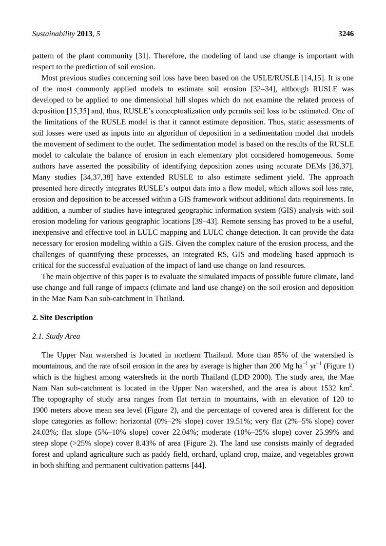
The Upper Nan watershed is located in northern Thailand. More than 85% of the watershed is
mountainous, and the rate of soil erosion in the area by average is higher than 200 Mg ha−1
yr−1
(Figure 1)
which is the highest among watersheds in the north Thailand (LDD 2000). The study area, the Mae
Nam Nan sub-catchment is located in the Upper Nan watershed, and the area is about 1532 km2.
The topography of study area ranges from flat terrain to mountains, with an elevation of 120 to
1900 meters above mean sea level (Figure 2), and the percentage of covered area is different for the
slope categories as follow: horizontal (0%–2% slope) cover 19.51%; very flat (2%–5% slope) cover
24.03%; flat slope (5%–10% slope) cover 22.04%; moderate (10%–25% slope) cover 25.99% and
steep slope (>25% slope) cover 8.43% of area (Figure 2). The land use consists mainly of degraded
forest and upland agriculture such as paddy field, orchard, upland crop, maize, and vegetables grown
in both shifting and permanent cultivation patterns [44].
Sustainability 2013, 5 3247
2.2. Geology and Soil Type
The geology of the Mae Nam Nan sub-catchment comprises various kinds of rocks and rock units
ranging in age from the Carboniferous. The study area consists mainly of Paleozoic and Mesozoic
sedimentary rocks and Mesozoic Igneous rocks. Paleozoic rocks ranging from Carboniferous rocks
consist mainly of sandstone and shale, Permian rocks consist mainly of limestone sandstone and shale,
Silurian Devonian rocks consist of Phyllite, Quartzite, Schist and greywacke locally, Mesozoic rocks
consist of conglomerate, sandstone and siltstone. The soils formed on low-lying landscape are mostly
young loamy soils and are classified as Alluvial soils. They are relatively fertile soils and mainly used
for rice cultivation or upland and tree crops [44,45]. Soils formed in the area vary widely in depth,
texture, color, fertility as well as in their agricultural potential depending largely upon the kind of
parent rock of each soil.
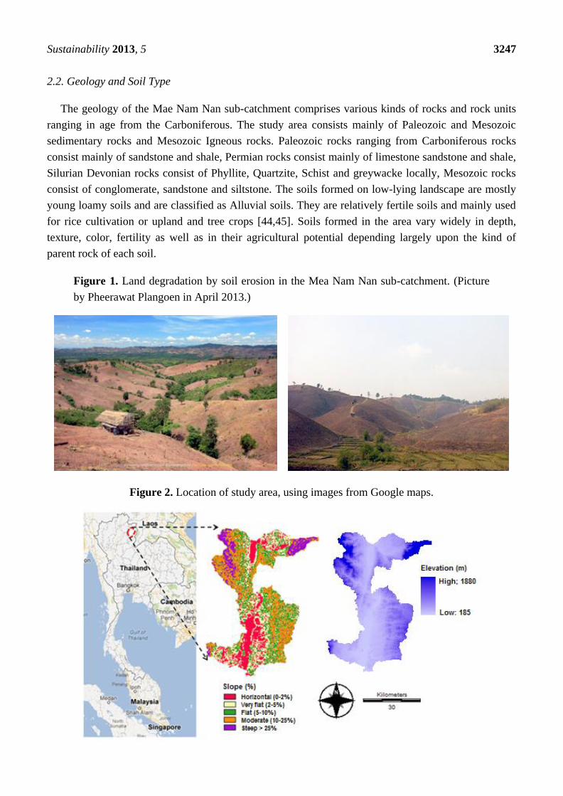
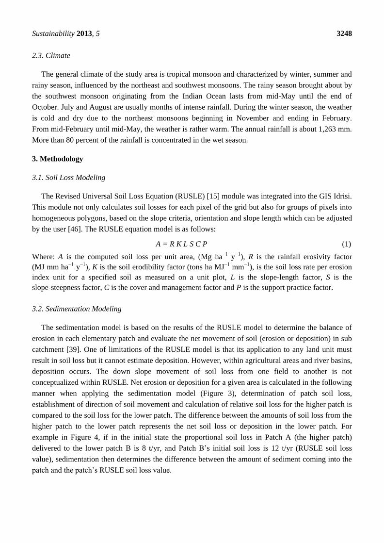
Figure 1. Land degradation by soil erosion in the Mea Nam Nan sub-catchment. (Picture
by Pheerawat Plangoen in April 2013.)
Figure 2. Location of study area, using images from Google maps.
Sustainability 2013, 5 3248
2.3. Climate
The general climate of the study area is tropical monsoon and characterized by winter, summer and
rainy season, influenced by the northeast and southwest monsoons. The rainy season brought about by
the southwest monsoon originating from the Indian Ocean lasts from mid-May until the end of
October. July and August are usually months of intense rainfall. During the winter season, the weather
is cold and dry due to the northeast monsoons beginning in November and ending in February.
From mid-February until mid-May, the weather is rather warm. The annual rainfall is about 1,263 mm.
More than 80 percent of the rainfall is concentrated in the wet season.
3. Methodology
3.1. Soil Loss Modeling
The Revised Universal Soil Loss Equation (RUSLE) [15] module was integrated into the GIS Idrisi.
This module not only calculates soil losses for each pixel of the grid but also for groups of pixels into
homogeneous polygons, based on the slope criteria, orientation and slope length which can be adjusted
by the user [46]. The RUSLE equation model is as follows:
A = R K L S C P (1)
Where: A is the computed soil loss per unit area, (Mg ha−1
y−1
), R is the rainfall erosivity factor
(MJ mm ha−1
y−1
), K is the soil erodibility factor (tons ha MJ−1
mm−1
), is the soil loss rate per erosion
index unit for a specified soil as measured on a unit plot, L is the slope-length factor, S is the
slope-steepness factor, C is the cover and management factor and P is the support practice factor.
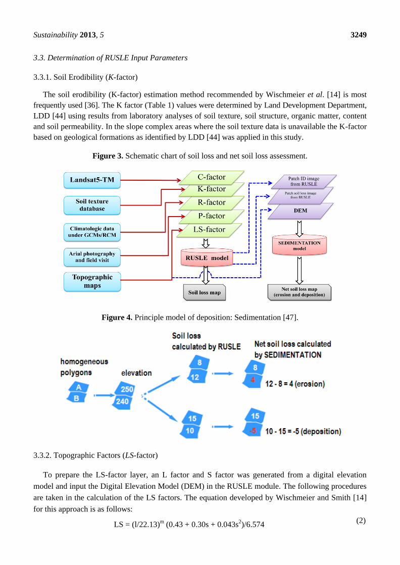
3.2. Sedimentation Modeling
The sedimentation model is based on the results of the RUSLE model to determine the balance of
erosion in each elementary patch and evaluate the net movement of soil (erosion or deposition) in sub
catchment [39]. One of limitations of the RUSLE model is that its application to any land unit must
result in soil loss but it cannot estimate deposition. However, within agricultural areas and river basins,
deposition occurs. The down slope movement of soil loss from one field to another is not
conceptualized within RUSLE. Net erosion or deposition for a given area is calculated in the following
manner when applying the sedimentation model (Figure 3), determination of patch soil loss,
establishment of direction of soil movement and calculation of relative soil loss for the higher patch is
compared to the soil loss for the lower patch. The difference between the amounts of soil loss from the
higher patch to the lower patch represents the net soil loss or deposition in the lower patch. For
example in Figure 4, if in the initial state the proportional soil loss in Patch A (the higher patch)
delivered to the lower patch B is 8 t/yr, and Patch B’s initial soil loss is 12 t/yr (RUSLE soil loss
value), sedimentation then determines the difference between the amount of sediment coming into the
patch and the patch’s RUSLE soil loss value.
Sustainability 2013, 5 3249
3.3. Determination of RUSLE Input Parameters
3.3.1. Soil Erodibility (K-factor)
The soil erodibility (K-factor) estimation method recommended by Wischmeier et al. [14] is most
frequently used [36]. The K factor (Table 1) values were determined by Land Development Department,
LDD [44] using results from laboratory analyses of soil texture, soil structure, organic matter, content
and soil permeability. In the slope complex areas where the soil texture data is unavailable the K-factor
based on geological formations as identified by LDD [44] was applied in this study.
Figure 3. Schematic chart of soil loss and net soil loss assessment.
Figure 4. Principle model of deposition: Sedimentation [47].
3.3.2. Topographic Factors (LS-factor)
To prepare the LS-factor layer, an L factor and S factor was generated from a digital elevation
model and input the Digital Elevation Model (DEM) in the RUSLE module. The following procedures
are taken in the calculation of the LS factors. The equation developed by Wischmeier and Smith [14]
for this approach is as follows:
LS = (l/22.13)m
(0.43 + 0.30s + 0.043s2)/6.574
(2)
Sustainability 2013, 5 3250
Where LS is the slope length and steepness factor, s is the field slope in percent, l is the slope length in
meters, and m is the dimensionless exponential.
Table 1. Attribute values of the soil erodibility (K factor, tons h MJ−1
mm−1
).
Textural class K-factor Geological formations K-factor
Clay C(low) 0.015 Phu Kradung Jpk 0.029
C(up) 0.024 Phra Wihan Form Jpw 0.029
Clay CL(up) 0.024 Sao Khua Form Jsk 0.029
Loam L(low) 0.026 Phu Phan Form Kpp 0.029
L(up) 0.024 Nam Duk Form., Pnd 0.013
Loamy LS(low) 0.026 Pha Nok Khao Form Ppn 0.013
LS(up) 0.024 Huai Hin Lat Form TRhl 0.029
Sandy Clay Loam SCL(low) 0.026 Nam Phong Form TRnp 0.024
SCL(up) 0.024 Urban area U 0
Silty Clay SiC(low) 0.015 Water body W 0
Silty Clay Loam SiCL(low) 0.035
SiCL(up) 0.025
Silty Loam SiL(up) 0.025
Sandy Loam SL(up) 0.024
3.3.3. Rainfall Erosivity (R-factor)
The concept of rainfall erosivity refers to the ability of any rainfall event to erode soil. The rainfall
erosivity is defined as the average annual value of the rainfall erosion index [48]. The monthly rainfall
erosivity value was computed by summing up EI30 values of storms that occurred during the month [49].
The RUSLE model uses the Brown and Foster [50] approach for calculating the average annual rainfall
erosivity, R (MJ mm ha−1
h−1
y−1
)
n
j
m
k
kk IEn
R1 1
30 )(1
(3)
where E is the total storm kinetic energy (MJ ha−1
), I30 is the maximum 30 minute rainfall intensity
(mm h−1
), j is an index of the number of years used to produce the average, k is an index of the number
of storms in each year, n is the number of years used to obtain the average R, and m is the number of
storms in each year.
The total storm kinetic energy (E) is determined using the relation,
m
r
rr VeE1
(4)
where re is the rainfall energy per unit depth of rainfall per unit area in megajoules per hectare per
millimeter (MJ ha−1
mm−1
), and rV is the depth of rainfall in millimeters (mm) for the thr increment
of the storm hyetograph which is divided into m parts, in which each part has a constant rainfall value.
Rainfall energy per unit depth of rainfall ( re ) can be calculated using the relation:
)05.0exp(72.0129.0 rr ie (5)
Sustainability 2013, 5 3251
where re has units of megajoules per hectare per millimeter of rain (MJ ha−1
mm−1
), and ri is rainfall
intensity (mm h−1
). Rainfall intensity for a particular increment of a rainfall event ( ri ) is calculated
using the relation.
r
r
rt
Vi
(6)
where rt is the depth of rain falling (mm) during the increment.
Estimation of the annual rainfall erosivity using the modified Fournier index (MFI) has been
proposed when only monthly precipitation data are available [51].
12
1
2i
i
i
P
pMFI (7)
where ip is the mean monthly rainfall of the month i, P is the mean annual rainfall
The relationship between MFI and the R factor showed better adjustment following an exponential
distribution [52]. The R factor values can be estimated from the MFI using the following equation.
baMFIR (8)
where a and b are empirical parameters and is a random, normally distributed error.
Estimation of future climate change provided by Global Circulation Models (GCMs) and RCM do
not provide the type of detailed storm information needed to directly calculate predicted R factor
changes. Therefore, statistical relationships between monthly precipitation and modified Fournier
index (MFI), and MFI versus rainfall erosivity were used to analyze the GCMs/RCMs outputs relative
to R factor changes [53] in order to analyze the spatial distribution of rainfall erosivity under future
climate. R factor values were calculated using the method described by Renard (1997) [15]. For the
study, the commonly used HadCM3, CCSM3 and PRECIS RCM were chosen to generate the future
precipitation scenarios.
3.3.4. General Circulation Models
For this study two GCMs were selected on the basis of their performance in the simulation of
precipitation. (1) The NCAR’s Community Climate System Model (CCSM3) was one of the global climate
models included in the Fourth Assessment Report (AR4) of the Intergovernmental Panel on Climate
Change (IPCC). NCAR’s GIS program provides GIS-compatible user access to CCSM3 AR4 global
(1.4 degree or 155 km). The selected GCMs were downloaded from the NCAR community climate
system model (CCSM) projections in GIS format, available at [54]. (2) HadCM3 was used to generate
the future precipitation scenarios. HadCM3 is a coupled atmospheric-ocean GCM developed at the
Hadley Centre of the United Kingdom National Meteorological Service that studies climate variability
and change. The atmospheric component of the model has 19 levels with a horizontal resolution of
2.5° latitude and 3.75° longitude. The ocean component of the model has 20 levels with horizontal
resolution 1.25° latitude 1.25° longitude.
Sustainability 2013, 5 3252
3.3.5. Regional Climate Model
The RCM used in this study was PRECIS, developed by the Hadley Centre of the UK Meteorological
Office. The PRECIS RCM is based on the atmospheric components of the ECHAM4 GCM from the
Max Planck Institute for Meteorology, Germany. The PRECIS data are produced by the Southeast
Asian System for Analysis, Research and Training (SEA START) Regional Center for 2225 grid cells
covering the entire Mae Nam Nan Sub-Catchment with the resolution of 0.2 × 0.2 degree
(approximately 22 × 22 km2). These data comprise two data sets for ECHAM4 SRES A2 and B2, daily
precipitation. The PRECIS RCM data over the periods of 1971–2000 (present) and 2011–2098
(future), for both A2 and B2 scenarios, were obtained from the Southeast Asian START Regional
Center [55].
Several statistical downscaling techniques have been developed to translate large-scale GCM/RCM
output into finer resolution [56]. In this study, the simplest method change factor or delta change
approach was applied. The change factor or delta change method has been used in many earlier climate
change impact studies [57–61]. Basically, this approach modifies the observed historical time series of
precipitation and is modified by multiplying the ratio of the monthly future and historic precipitations
simulated by NCAR CCSM3 (A2, A1b and B1 scenarios), HadCM3 and PRECIS RCM (A2 and
B2 scenarios) for each time period. The observational database used for this approach covers the
period of 1981–2000.
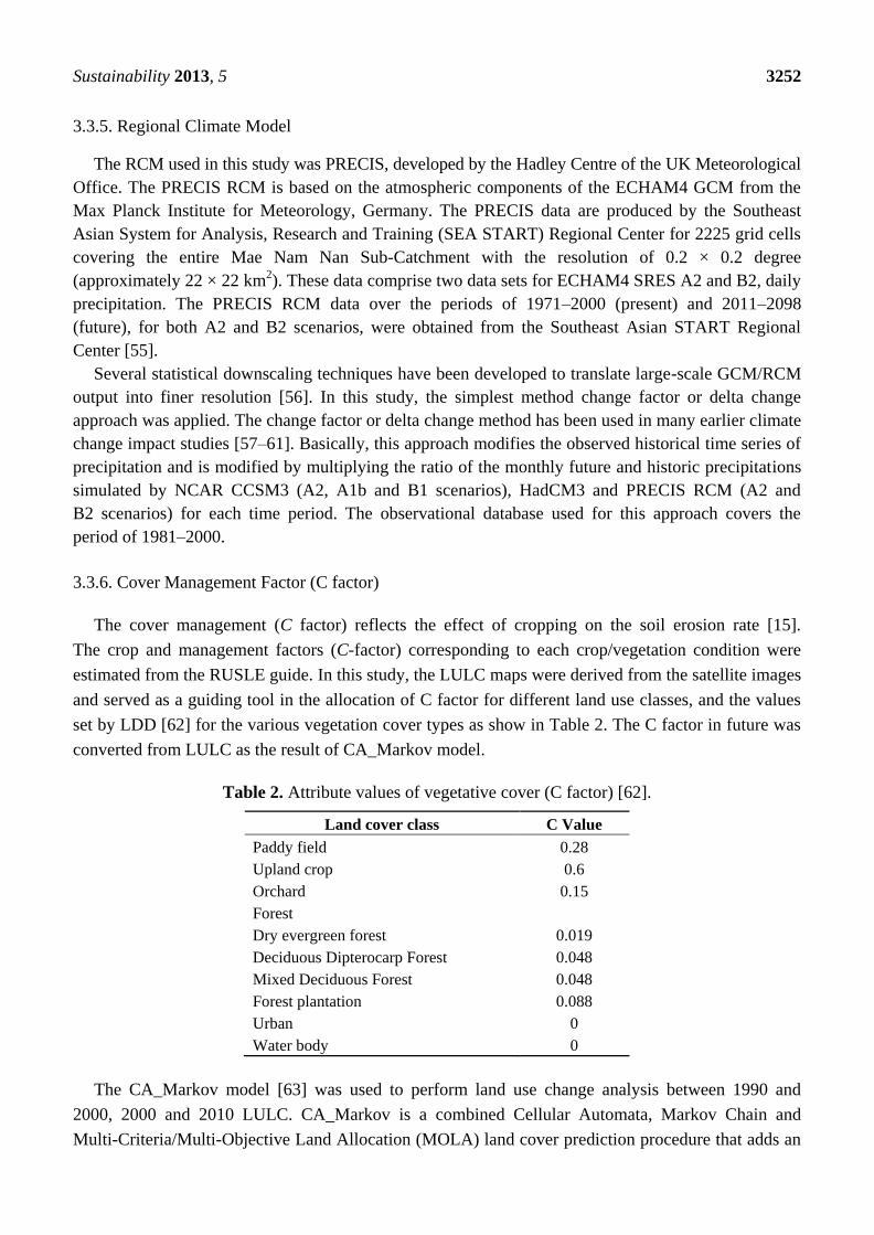
3.3.6. Cover Management Factor (C factor)
The cover management (C factor) reflects the effect of cropping on the soil erosion rate [15].
The crop and management factors (C-factor) corresponding to each crop/vegetation condition were
estimated from the RUSLE guide. In this study, the LULC maps were derived from the satellite images
and served as a guiding tool in the allocation of C factor for different land use classes, and the values
set by LDD [62] for the various vegetation cover types as show in Table 2. The C factor in future was
converted from LULC as the result of CA_Markov model.
Table 2. Attribute values of vegetative cover (C factor) [62].
Land cover class C Value
Paddy field 0.28
Upland crop 0.6
Orchard 0.15
Forest
Dry evergreen forest 0.019
Deciduous Dipterocarp Forest 0.048
Mixed Deciduous Forest 0.048
Forest plantation 0.088
Urban 0
Water body 0
The CA_Markov model [63] was used to perform land use change analysis between 1990 and
2000, 2000 and 2010 LULC. CA_Markov is a combined Cellular Automata, Markov Chain and
Multi-Criteria/Multi-Objective Land Allocation (MOLA) land cover prediction procedure that adds an
Sustainability 2013, 5 3253
element of spatial contiguity as well as knowledge of the likely spatial distribution of transitions to
Markov chain analysis. Therefore, the predicting land use/land cover in 2010 (based on land cover data
in 1990 and 2000) and 2020, 2030 and 2040 (based on land cover data in 2000 and 2010).
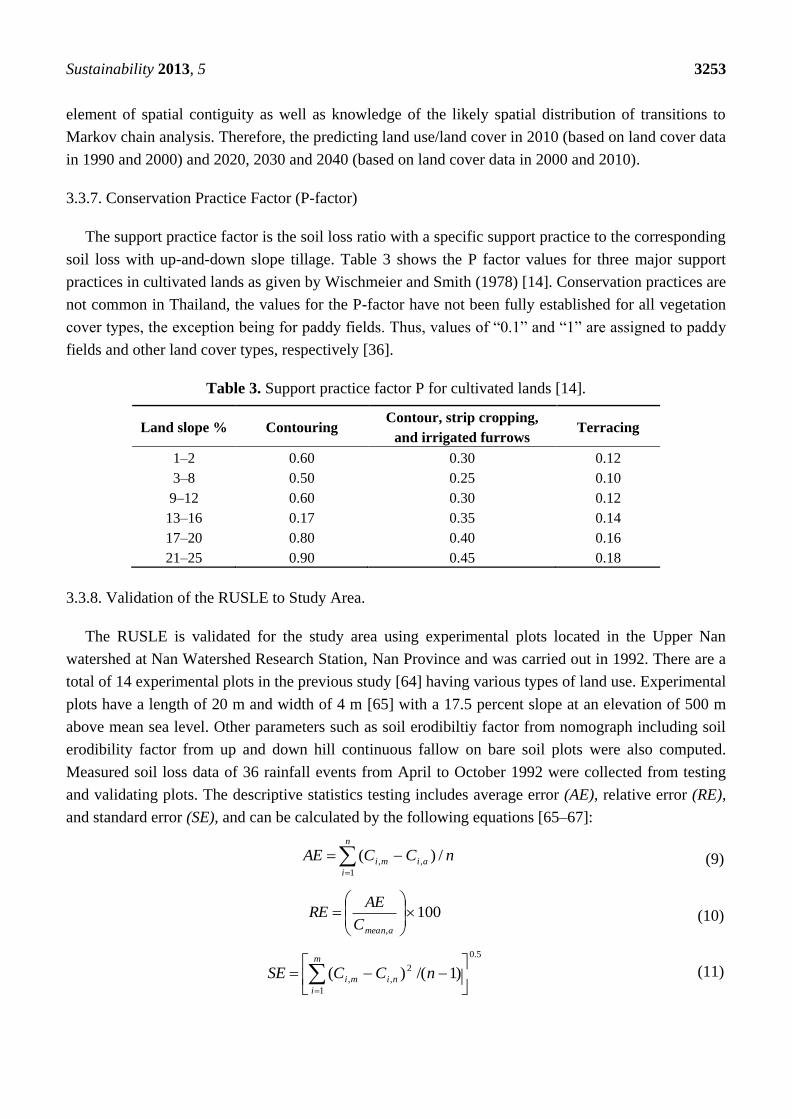
3.3.7. Conservation Practice Factor (P-factor)
The support practice factor is the soil loss ratio with a specific support practice to the corresponding
soil loss with up-and-down slope tillage. Table 3 shows the P factor values for three major support
practices in cultivated lands as given by Wischmeier and Smith (1978) [14]. Conservation practices are
not common in Thailand, the values for the P-factor have not been fully established for all vegetation
cover types, the exception being for paddy fields. Thus, values of ―0.1‖ and ―1‖ are assigned to paddy
fields and other land cover types, respectively [36].
Table 3. Support practice factor P for cultivated lands [14].
Land slope % Contouring Contour, strip cropping,
and irrigated furrows Terracing
1–2 0.60 0.30 0.12
3–8 0.50 0.25 0.10
9–12 0.60 0.30 0.12
13–16 0.17 0.35 0.14
17–20 0.80 0.40 0.16
21–25 0.90 0.45 0.18
3.3.8. Validation of the RUSLE to Study Area.
The RUSLE is validated for the study area using experimental plots located in the Upper Nan
watershed at Nan Watershed Research Station, Nan Province and was carried out in 1992. There are a
total of 14 experimental plots in the previous study [64] having various types of land use. Experimental
plots have a length of 20 m and width of 4 m [65] with a 17.5 percent slope at an elevation of 500 m
above mean sea level. Other parameters such as soil erodibiltiy factor from nomograph including soil
erodibility factor from up and down hill continuous fallow on bare soil plots were also computed.
Measured soil loss data of 36 rainfall events from April to October 1992 were collected from testing
and validating plots. The descriptive statistics testing includes average error (AE), relative error (RE),
and standard error (SE), and can be calculated by the following equations [65–67]:
a
n
i
aimi nCCAE1
,, /)( (9)
100,
ameanC
AERE (10)
5.0
1
2
,, )1/()(
m
i
nimi nCCSE (11)
Sustainability 2013, 5 3254
where Ci,m is the soil loss (ton ha−1
) from the model estimation rainfall event i, Ci,a is the soil loss
(ton ha−1
) from the actual experimental plot rainfall event i, n is the total amount of rainfall event on
the sample, and Cmean,a is the mean soil loss (ton ha−1
) from the experimental plot.
4. Results
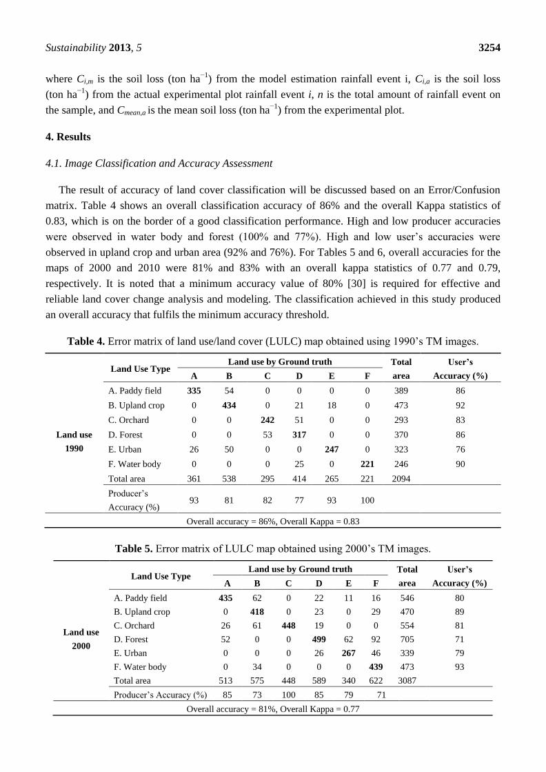
4.1. Image Classification and Accuracy Assessment
The result of accuracy of land cover classification will be discussed based on an Error/Confusion
matrix. Table 4 shows an overall classification accuracy of 86% and the overall Kappa statistics of
0.83, which is on the border of a good classification performance. High and low producer accuracies
were observed in water body and forest (100% and 77%). High and low user’s accuracies were
observed in upland crop and urban area (92% and 76%). For Tables 5 and 6, overall accuracies for the
maps of 2000 and 2010 were 81% and 83% with an overall kappa statistics of 0.77 and 0.79,
respectively. It is noted that a minimum accuracy value of 80% [30] is required for effective and
reliable land cover change analysis and modeling. The classification achieved in this study produced
an overall accuracy that fulfils the minimum accuracy threshold.
Table 4. Error matrix of land use/land cover (LULC) map obtained using 1990’s TM images.
Land Use Type
Land use by Ground truth Total
area
User’s
Accuracy (%)
Land use
1990
A B C D E F
A. Paddy field 335 54 0 0 0 0 389 86
B. Upland crop 0 434 0 21 18 0 473 92
C. Orchard 0 0 242 51 0 0 293 83
D. Forest 0 0 53 317 0 0 370 86
E. Urban 26 50 0 0 247 0 323 76
F. Water body 0 0 0 25 0 221 246 90
Total area 361 538 295 414 265 221 2094
Producer’s
Accuracy (%) 93 81 82 77 93 100
Overall accuracy = 86%, Overall Kappa = 0.83
Table 5. Error matrix of LULC map obtained using 2000’s TM images.
Land Use Type
Land use by Ground truth Total
area
User’s
Accuracy (%)
Land use
2000
A B C D E F
A. Paddy field 435 62 0 22 11 16 546 80
B. Upland crop 0 418 0 23 0 29 470 89
C. Orchard 26 61 448 19 0 0 554 81
D. Forest 52 0 0 499 62 92 705 71
E. Urban 0 0 0 26 267 46 339 79
F. Water body 0 34 0 0 0 439 473 93
Total area 513 575 448 589 340 622 3087
Producer’s Accuracy (%) 85 73 100 85 79 71
Overall accuracy = 81%, Overall Kappa = 0.77
Sustainability 2013, 5 3255
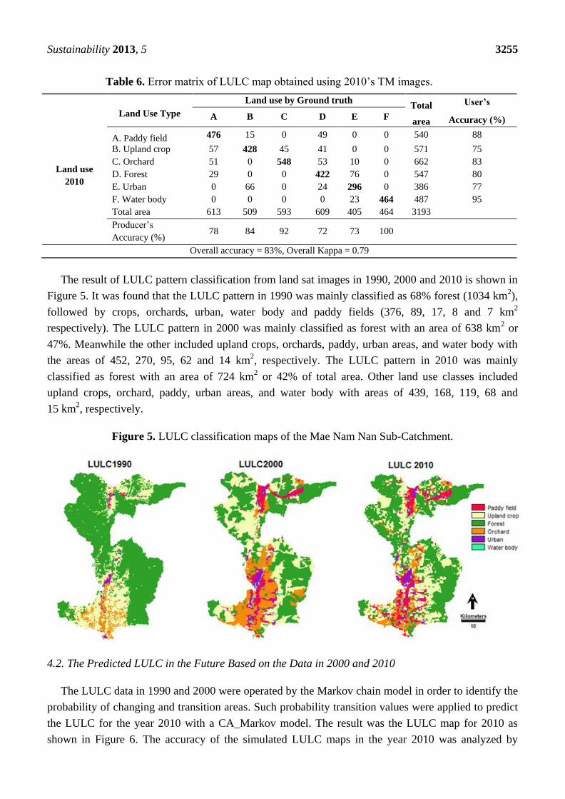
Table 6. Error matrix of LULC map obtained using 2010’s TM images.
Land Use Type
Land use by Ground truth Total
area
User’s
Accuracy (%)
Land use
2010
A B C D E F
A. Paddy field 476 15 0 49 0 0 540 88
B. Upland crop 57 428 45 41 0 0 571 75
C. Orchard 51 0 548 53 10 0 662 83
D. Forest 29 0 0 422 76 0 547 80
E. Urban 0 66 0 24 296 0 386 77
F. Water body 0 0 0 0 23 464 487 95
Total area 613 509 593 609 405 464 3193
Producer’s
Accuracy (%) 78 84 92 72 73 100
Overall accuracy = 83%, Overall Kappa = 0.79
The result of LULC pattern classification from land sat images in 1990, 2000 and 2010 is shown in
Figure 5. It was found that the LULC pattern in 1990 was mainly classified as 68% forest (1034 km2),
followed by crops, orchards, urban, water body and paddy fields (376, 89, 17, 8 and 7 km2
respectively). The LULC pattern in 2000 was mainly classified as forest with an area of 638 km2 or
47%. Meanwhile the other included upland crops, orchards, paddy, urban areas, and water body with
the areas of 452, 270, 95, 62 and 14 km2, respectively. The LULC pattern in 2010 was mainly
classified as forest with an area of 724 km2 or 42% of total area. Other land use classes included
upland crops, orchard, paddy, urban areas, and water body with areas of 439, 168, 119, 68 and
15 km2, respectively.
Figure 5. LULC classification maps of the Mae Nam Nan Sub-Catchment.
4.2. The Predicted LULC in the Future Based on the Data in 2000 and 2010
The LULC data in 1990 and 2000 were operated by the Markov chain model in order to identify the
probability of changing and transition areas. Such probability transition values were applied to predict
the LULC for the year 2010 with a CA_Markov model. The result was the LULC map for 2010 as
shown in Figure 6. The accuracy of the simulated LULC maps in the year 2010 was analyzed by
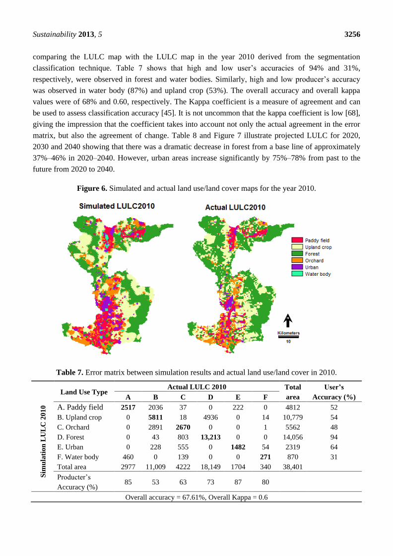
Sustainability 2013, 5 3256
comparing the LULC map with the LULC map in the year 2010 derived from the segmentation
classification technique. Table 7 shows that high and low user’s accuracies of 94% and 31%,
respectively, were observed in forest and water bodies. Similarly, high and low producer’s accuracy
was observed in water body (87%) and upland crop (53%). The overall accuracy and overall kappa
values were of 68% and 0.60, respectively. The Kappa coefficient is a measure of agreement and can
be used to assess classification accuracy [45]. It is not uncommon that the kappa coefficient is low [68],
giving the impression that the coefficient takes into account not only the actual agreement in the error
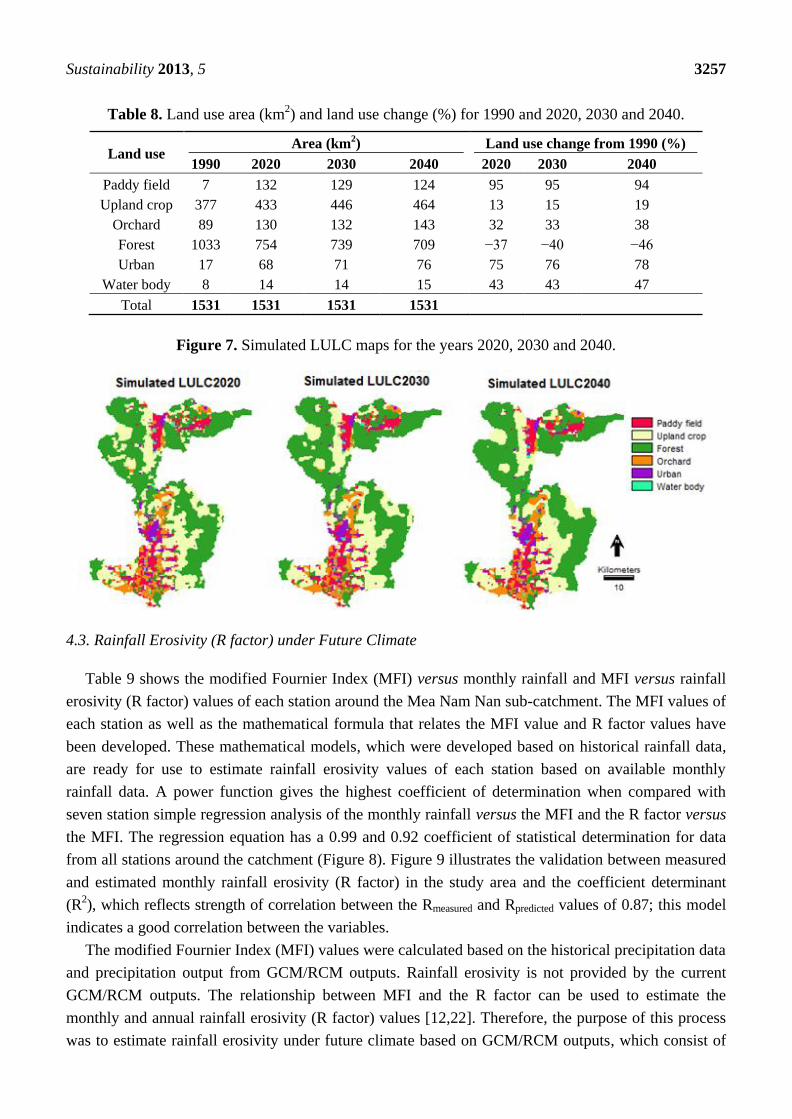
matrix, but also the agreement of change. Table 8 and Figure 7 illustrate projected LULC for 2020,
2030 and 2040 showing that there was a dramatic decrease in forest from a base line of approximately
37%–46% in 2020–2040. However, urban areas increase significantly by 75%–78% from past to the
future from 2020 to 2040.
Figure 6. Simulated and actual land use/land cover maps for the year 2010.
Table 7. Error matrix between simulation results and actual land use/land cover in 2010.
Land Use Type
Actual LULC 2010 Total
area
User’s
Accuracy (%)
Sim
ula
tio
n L
UL
C 2
01
0
A B C D E F
A. Paddy field 2517 2036 37 0 222 0 4812 52
B. Upland crop 0 5811 18 4936 0 14 10,779 54
C. Orchard 0 2891 2670 0 0 1 5562 48
D. Forest 0 43 803 13,213 0 0 14,056 94
E. Urban 0 228 555 0 1482 54 2319 64
F. Water body 460 0 139 0 0 271 870 31
Total area 2977 11,009 4222 18,149 1704 340 38,401
Producter’s
Accuracy (%) 85 53 63 73 87 80
Overall accuracy = 67.61%, Overall Kappa = 0.6
Sustainability 2013, 5 3257
Table 8. Land use area (km2) and land use change (%) for 1990 and 2020, 2030 and 2040.
Land use Area (km
2) Land use change from 1990 (%)
1990 2020 2030 2040 2020 2030 2040
Paddy field 7 132 129 124 95 95 94
Upland crop 377 433 446 464 13 15 19
Orchard 89 130 132 143 32 33 38
Forest 1033 754 739 709 −37 −40 −46
Urban 17 68 71 76 75 76 78
Water body 8 14 14 15 43 43 47
Total 1531 1531 1531 1531
Figure 7. Simulated LULC maps for the years 2020, 2030 and 2040.
4.3. Rainfall Erosivity (R factor) under Future Climate
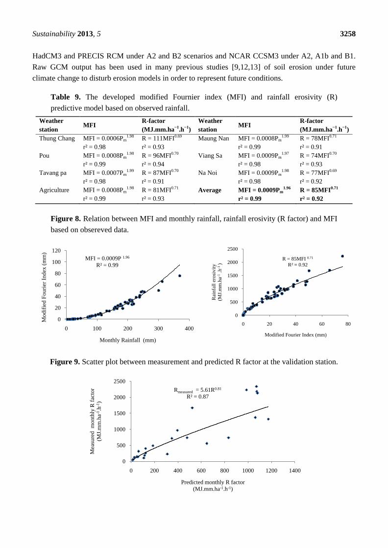
Table 9 shows the modified Fournier Index (MFI) versus monthly rainfall and MFI versus rainfall
erosivity (R factor) values of each station around the Mea Nam Nan sub-catchment. The MFI values of
each station as well as the mathematical formula that relates the MFI value and R factor values have
been developed. These mathematical models, which were developed based on historical rainfall data,
are ready for use to estimate rainfall erosivity values of each station based on available monthly
rainfall data. A power function gives the highest coefficient of determination when compared with
seven station simple regression analysis of the monthly rainfall versus the MFI and the R factor versus
the MFI. The regression equation has a 0.99 and 0.92 coefficient of statistical determination for data
from all stations around the catchment (Figure 8). Figure 9 illustrates the validation between measured
and estimated monthly rainfall erosivity (R factor) in the study area and the coefficient determinant
(R2), which reflects strength of correlation between the Rmeasured and Rpredicted values of 0.87; this model
indicates a good correlation between the variables.
The modified Fournier Index (MFI) values were calculated based on the historical precipitation data
and precipitation output from GCM/RCM outputs. Rainfall erosivity is not provided by the current
GCM/RCM outputs. The relationship between MFI and the R factor can be used to estimate the
monthly and annual rainfall erosivity (R factor) values [12,22]. Therefore, the purpose of this process
was to estimate rainfall erosivity under future climate based on GCM/RCM outputs, which consist of
Sustainability 2013, 5 3258
HadCM3 and PRECIS RCM under A2 and B2 scenarios and NCAR CCSM3 under A2, A1b and B1.
Raw GCM output has been used in many previous studies [9,12,13] of soil erosion under future
climate change to disturb erosion models in order to represent future conditions.
Table 9. The developed modified Fournier index (MFI) and rainfall erosivity (R)
predictive model based on observed rainfall.
Weather
station MFI
R-factor
(MJ.mm.ha−1
.h−1
)
Weather
station MFI
R-factor
(MJ.mm.ha−1
.h−1
)
Thung Chang MFI = 0.0006Pm1.98
r² = 0.98
R = 111MFI0.69
r² = 0.93
Maung Nan MFI = 0.0008Pm1.99
r² = 0.99
R = 78MFI0.71
r² = 0.91
Pou MFI = 0.0008Pm1.98
r² = 0.99
R = 96MFI0.70
r² = 0.94
Viang Sa MFI = 0.0009Pm1.97
r² = 0.98
R = 74MFI0.70
r² = 0.93
Tavang pa MFI = 0.0007Pm1.99
r² = 0.98
R = 87MFI0.70
r² = 0.91
Na Noi MFI = 0.0009Pm1.98
r² = 0.98
R = 77MFI0.69
r² = 0.92
Agriculture MFI = 0.0008Pm1.98
r² = 0.99
R = 81MFI0.71
r² = 0.93
Average MFI = 0.0009Pm1.96
r² = 0.99
R = 85MFI0.71
r² = 0.92
Figure 8. Relation between MFI and monthly rainfall, rainfall erosivity (R factor) and MFI
based on obsereved data.
Figure 9. Scatter plot between measurement and predicted R factor at the validation station.
MFI = 0.0009P 1.96
R² = 0.99
0
20
40
60
80
100
120
0 100 200 300 400
M
odif
ied F
ouri
er I
ndex
(m
m)
Monthly Rainfall (mm)
R = 85MFI 0.71
R² = 0.92
0
500
1000
1500
2000
2500
0 20 40 60 80
Rai
nfa
ll e
rosi
vit
y
(MJ.
mm
.ha-1
.h-1
)
Modified Fourier Index (mm)
Rmeasured = 5.61R0.81
R² = 0.87
0
500
1000
1500
2000
2500
0 200 400 600 800 1000 1200 1400
Mea
sure
d m
onth
ly R
fac
tor
(MJ.
mm
.ha-1
.h-1
)
Predicted monthly R factor
(MJ.mm.ha-1.h-1)

Sustainability 2013, 5 3259
The Figure 10a–c presents the average monthly precipitation cycle for all climate projections in the
three periods and baseline period between 1981 and 2000. Generally, there was a dramatic rise in the
precipitation from January until a peak in August was reached. After this, precipitation fell
significantly until December. It is clear that there is less monthly average precipitation from PRECIS
CCSM3 under A2 and B2 scenarios output than in the base period and other GCMs from March to
May, whereas it is equal in comparison with the baseline period from September to December. The
precipitation peak range in August of all climate projections is 198–238 mm in 2016–2025,
188–237 mm in 2026–2035 and 196–242 mm in 2036–2045. For annual precipitation the changes
range from (Table 11) −13%–9% in 2016–2025, −16%–10% in 2026–2035 and −10%–14% in
2036–2045 depending on the emission scenarios and climate models.
Figure 10. Average monthly precipitation (a–c) and rainfall erosivity (d–f) for all climate
projections for the 2016–2025, 2026–2035, 2035–2046 periods and baseline period
1981–2000 for the Mae Nam Nan sub-catchment.
Unlike precipitation, the changes in monthly rainfall erosivity are not unidirectional for all emission
scenarios, climate models and time periods. The intra-annual patterns of rainfall erosivity change from
the unimodal. For example, there was a decrease in rainfall erosivity from November to February and
an increase in the periods from March to October for all three time periods. Future change of rainfall
erosivity (Table 11) in comparison with a base period (5999 MJ mm ha−1
h−1
) was between
−12%–12% in 2016–2025, −15%–11% in 2026–2035 and −5%–19% in 2036–2045 depending on the
emission scenarios and climate models.
0
50
100
150
200
250
300
350
Jan
Feb
Mar
Ap
rM
ay Jun
Jul
Au
gS
epO
ctN
ov
Dec
Pre
cip
itati
on
(m
m)
(a) Precipitation 2016-2025
0
50
100
150
200
250
300
Jan Mar May Jul Sep Nov
(b) Precipitation 2025-2035
0
50
100
150
200
250
300
Jan Mar May Jul Sep Nov
(c) Precipitation 2036-2045
0
500
1000
1500
2000
Jan Mar May Jul Sep NovRa
infa
ll e
rosi
vit
y (M
J m
m
ha
-1h
-1)
(d) Rainfall erosivity 2016-2025
0
500
1000
1500
2000
Jan
Feb
Mar
Ap
r
May Jun
Jul
Au
g
Sep
Oct
No
v
Dec
(e) rainfall erosivity 2026-2035
0
500
1000
1500
2000
(f) Rainfall erosivity 2036-
2045
Sustainability 2013, 5 3260
4.4. Validation of the RUSLE
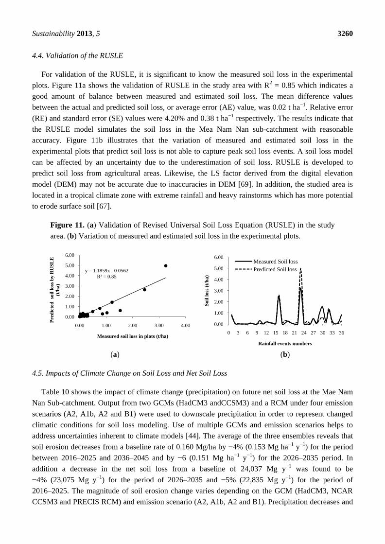
For validation of the RUSLE, it is significant to know the measured soil loss in the experimental
plots. Figure 11a shows the validation of RUSLE in the study area with R2 = 0.85 which indicates a
good amount of balance between measured and estimated soil loss. The mean difference values
between the actual and predicted soil loss, or average error (AE) value, was 0.02 t ha−1
. Relative error
(RE) and standard error (SE) values were 4.20% and 0.38 t ha−1
respectively. The results indicate that
the RUSLE model simulates the soil loss in the Mea Nam Nan sub-catchment with reasonable
accuracy. Figure 11b illustrates that the variation of measured and estimated soil loss in the
experimental plots that predict soil loss is not able to capture peak soil loss events. A soil loss model
can be affected by an uncertainty due to the underestimation of soil loss. RUSLE is developed to
predict soil loss from agricultural areas. Likewise, the LS factor derived from the digital elevation
model (DEM) may not be accurate due to inaccuracies in DEM [69]. In addition, the studied area is
located in a tropical climate zone with extreme rainfall and heavy rainstorms which has more potential
to erode surface soil [67].
Figure 11. (a) Validation of Revised Universal Soil Loss Equation (RUSLE) in the study
area. (b) Variation of measured and estimated soil loss in the experimental plots.
(a) (b)
4.5. Impacts of Climate Change on Soil Loss and Net Soil Loss
Table 10 shows the impact of climate change (precipitation) on future net soil loss at the Mae Nam
Nan Sub-catchment. Output from two GCMs (HadCM3 andCCSM3) and a RCM under four emission
scenarios (A2, A1b, A2 and B1) were used to downscale precipitation in order to represent changed
climatic conditions for soil loss modeling. Use of multiple GCMs and emission scenarios helps to
address uncertainties inherent to climate models [44]. The average of the three ensembles reveals that
soil erosion decreases from a baseline rate of 0.160 Mg/ha by −4% (0.153 Mg ha−1
y−1
) for the period
between 2016–2025 and 2036–2045 and by −6 (0.151 Mg ha−1
y−1
) for the 2026–2035 period. In
addition a decrease in the net soil loss from a baseline of 24,037 Mg y−1
was found to be
−4% (23,075 Mg y−1
) for the period of 2026–2035 and −5% (22,835 Mg y−1
) for the period of
2016–2025. The magnitude of soil erosion change varies depending on the GCM (HadCM3, NCAR
CCSM3 and PRECIS RCM) and emission scenario (A2, A1b, A2 and B1). Precipitation decreases and
y = 1.1859x - 0.0562
R² = 0.85
0.00
1.00
2.00
3.00
4.00
5.00
6.00
0.00 1.00 2.00 3.00 4.00
Pre
dic
ted
so
il l
oss
by
RU
SL
E
(t/h
a)
Measured soil loss in plots (t/ha)
0.00
1.00
2.00
3.00
4.00
5.00
6.00
0 3 6 9 12 15 18 21 24 27 30 33 36
So
il l
oss
(t/
ha)
Rainfall events numbers
Measured Soil loss
Predicted Soil loss
Sustainability 2013, 5 3261
increases of −14% (1078 mm) in the NCAR CCSM3-B1 scenario for the period of 2026–2035s and
16% (1450 mm) in NCAR CCSM3-A2 for the period of 2036–2045 illustrate the predominant factor
responsible for increasing and reducing soil erosion rates and net soil loss. Critically, however, it is the
timing of precipitation and the amount of daily precipitation intensity rather than merely the average
annual precipitation amount that generally controls the response of erosion to climate change.
Table 10. Change in average annual precipitation net soil loss and net soil loss rate
estimated by the sedimentation model for all climate projections under climate change
compared to the base period (1981–2000).
Climate models Precipitation
(mm)
Change
(%)
Total
erosion
(Mg y−1
)
Total
deposition
(Mg y−1
)
Net
soil loss
(Mg y−1
)
Change
(%)
Net
Soil loss rate
(Mg ha−1
y−1
)
Change
(%)
Base line 1250 40,547 16,510 24,037 0 0.160 0
2016–2025
HadCM3-A2 1277 2 44,873 17,689 27,184 13 0.180 13
HadCM3-B2 1275 2 42,945 17,172 25,774 7 0.170 6
NCAR CCSM3-A2 1282 3 38,993 15,443 23,551 −2 0.160 0
NCAR CCSM3-A1B 1369 10 40,753 16,042 24,711 3 0.160 0
NCAR CCSM3-B1 1327 6 42,191 16,617 25,574 6 0.170 6
PRECIS RCM-A2 1109 −11 23,543 9052 14,492 −40 0.100 −38
PRECIS RCM-B2 1113 −11 31,364 12,372 18,992 −21 0.130 −19
Average 1250 0 37,809 14,912 22,897 −5 0.153 −4
2026–2035
HadCM3-A2 1279 2 42,574 17,819 24,755 3 0.160 0
HadCM3-B2 1327 6 42,438 16,866 25,572 6 0.170 6
NCAR CCSM3-A2 1372 10 37,426 15,255 22,171 −8 0.160 0
NCAR CCSM3-A1B 1386 11 39,829 15,747 24,083 0 0.150 −6
NCAR CCSM3-B1 1078 −14 41,856 16,254 25,602 7 0.170 6
PRECIS RCM-A2 1131 −10 31,483 12,787 18,696 −22 0.120 −25
PRECIS RCM-B2 1164 −7 33,760 13,694 20,065 −17 0.130 −19
Average 1248 0 38,481 15,489 22,992 −4 0.151 −6
2036–2045
HadCM3-A2 1275 2 41,517 16,488 25,029 4 0.170 6
HadCM3-B2 1285 3 44,837 17,507 27,330 14 0.180 13
NCAR CCSM3-A2 1450 16 42,292 16,349 25,944 8 0.170 6
NCAR CCSM3-A1B 1278 2 39,415 15,503 23,911 −1 0.160 0
NCAR CCSM3-B1 1140 −9 39,198 15,646 23,552 −2 0.160 0
PRECIS RCM-A2 1197 −4 28,539 11,886 16,653 −31 0.110 −31
PRECIS RCM-B2 1165 −7 30,919 12,468 18,451 −23 0.120 −25
Average 1256 0 38,102 15,121 22,981 −4 0.153 −4
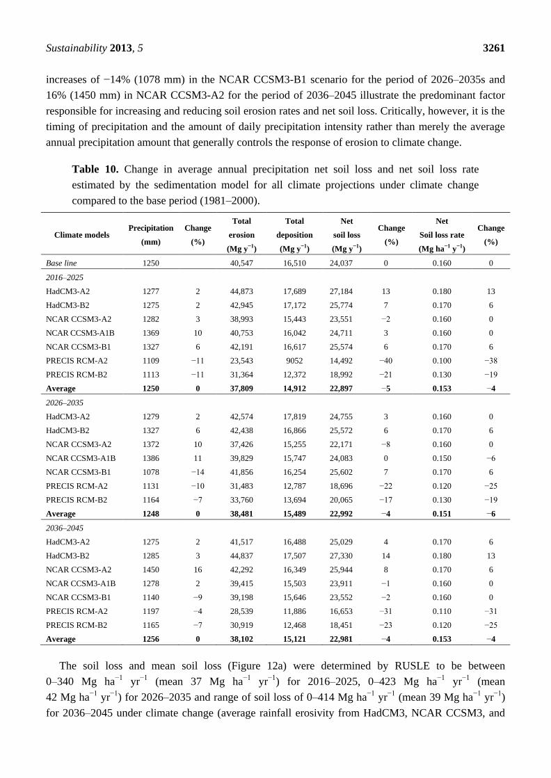
The soil loss and mean soil loss (Figure 12a) were determined by RUSLE to be between
0–340 Mg ha−1
yr−1
(mean 37 Mg ha−1
yr−1
) for 2016–2025, 0–423 Mg ha−1
yr−1
(mean
42 Mg ha−1
yr−1
) for 2026–2035 and range of soil loss of 0–414 Mg ha−1
yr−1
(mean 39 Mg ha−1
yr−1
)
for 2036–2045 under climate change (average rainfall erosivity from HadCM3, NCAR CCSM3, and
Sustainability 2013, 5 3262
PRECIS RCM). The net soil loss (erosion and deposition) values estimated by the sedimentation
model for 2016–2025, 2026–2035 and 2036–2045 under climate change (Figure 12b) were reclassified
into seven classes based on degree of severity [68]. The deposition and erosion risk areas of the
different climate change (precipitation) are shown in Figure 13 which illustrates that the percentage of
area under erosion risk is stable for the average three future time periods, 55% (83,727 ha) for
the period of 2026–2035 and 58% (88,904) for the period of 2016–2025, and that there is a high
erosion of 2% (37,766 ha) for the period of 2026–2035 and 3% (4037) for the period of 2036–2045.
Figure 12. Maps of soil loss and net soil loss under climate change (Average rainfall
erosivity from HadCM3, NCAR CCSM3, and PRECIS RCM).
(a) Predicted soil loss determined by the RUSLE model under climate change.
(b) Predicted net soil loss determined by a sedimentation model under climate change.
Sustainability 2013, 5 3263
Figure 13. Average monthly erosion and deposition risk areas for all climate projections
and for three future time periods.
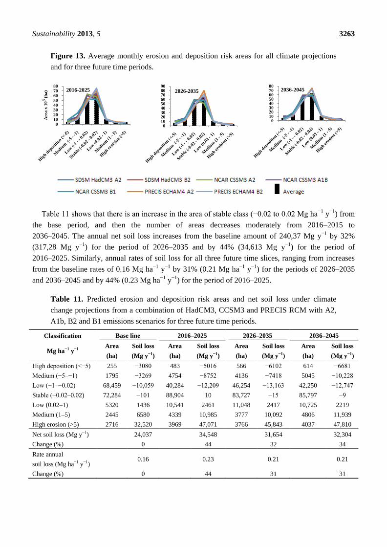
Table 11 shows that there is an increase in the area of stable class (−0.02 to 0.02 Mg ha−1
y−1
) from
the base period, and then the number of areas decreases moderately from 2016–2015 to
2036–2045. The annual net soil loss increases from the baseline amount of 240,37 Mg y−1
by 32%
(317,28 Mg y−1
) for the period of 2026–2035 and by 44% (34,613 Mg y−1
) for the period of
2016–2025. Similarly, annual rates of soil loss for all three future time slices, ranging from increases
from the baseline rates of 0.16 Mg ha−1
y−1
by 31% (0.21 Mg ha−1
y−1
) for the periods of 2026–2035
and 2036–2045 and by 44% (0.23 Mg ha−1
y−1
) for the period of 2016–2025.
Table 11. Predicted erosion and deposition risk areas and net soil loss under climate
change projections from a combination of HadCM3, CCSM3 and PRECIS RCM with A2,
A1b, B2 and B1 emissions scenarios for three future time periods.
Classification Base line 2016–2025 2026–2035 2036–2045
Mg ha−1
y−1
Area
(ha)
Soil loss
(Mg y−1
)
Area
(ha)
Soil loss
(Mg y−1
)
Area
(ha)
Soil loss
(Mg y−1
)
Area
(ha)
Soil loss
(Mg y−1
)
High deposition (<−5) 255 −3080 483 −5016 566 −6102 614 −6681
Medium (−5–−1) 1795 −3269 4754 −8752 4136 −7418 5045 −10,228
Low (−1–−0.02) 68,459 −10,059 40,284 −12,209 46,254 −13,163 42,250 −12,747
Stable (−0.02–0.02) 72,284 −101 88,904 10 83,727 −15 85,797 −9
Low (0.02–1) 5320 1436 10,541 2461 11,048 2417 10,725 2219
Medium (1–5) 2445 6580 4339 10,985 3777 10,092 4806 11,939
High erosion (>5) 2716 32,520 3969 47,071 3766 45,843 4037 47,810
Net soil loss (Mg y−1) 24,037 34,548 31,654 32,304
Change (%) 0 44 32 34
Rate annual
soil loss (Mg ha−1 y−1) 0.16 0.23 0.21 0.21
Change (%) 0 44 31 31
01020304050607080
Are
a x
10
3 (h
a) 2016-2025
0102030405060708090
2026-2035
01020304050607080
2036-2045
Sustainability 2013, 5 3264
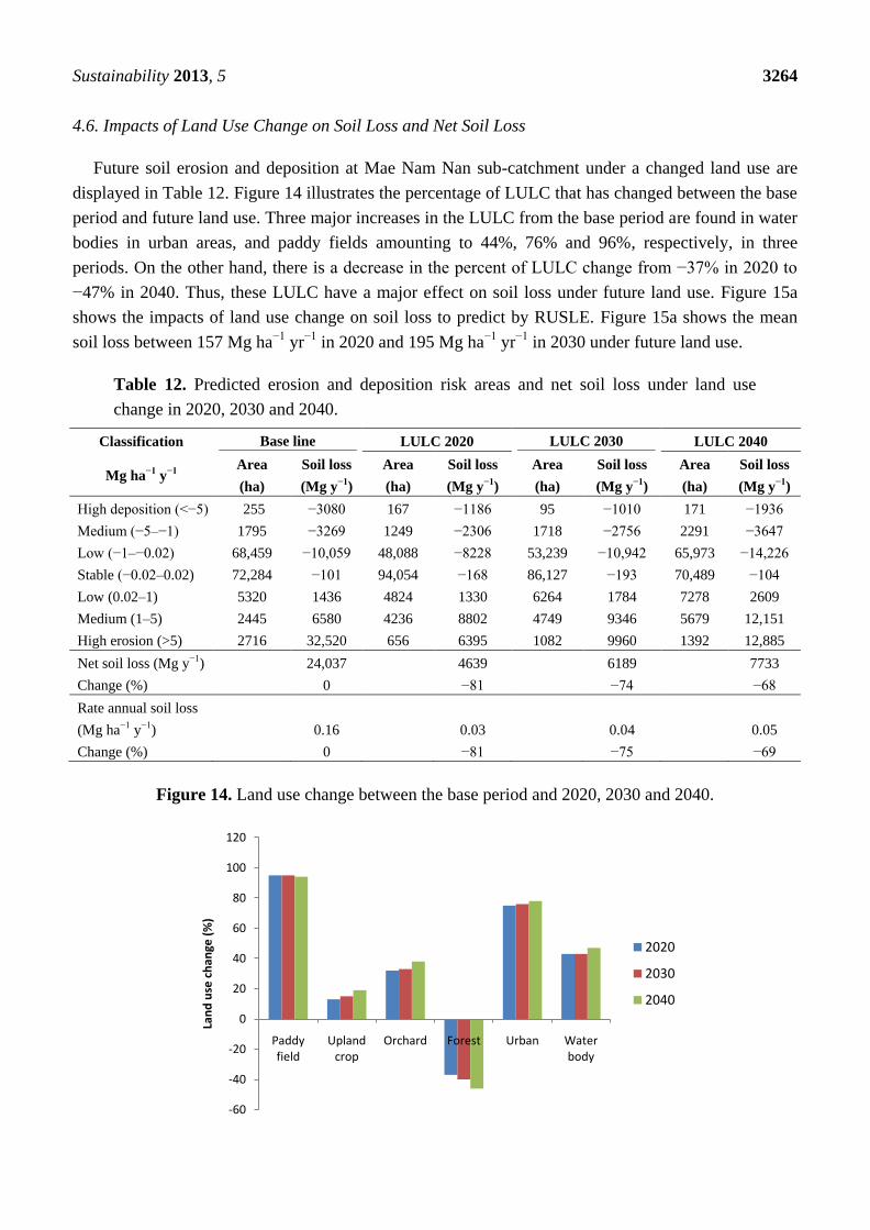
4.6. Impacts of Land Use Change on Soil Loss and Net Soil Loss
Future soil erosion and deposition at Mae Nam Nan sub-catchment under a changed land use are
displayed in Table 12. Figure 14 illustrates the percentage of LULC that has changed between the base
period and future land use. Three major increases in the LULC from the base period are found in water
bodies in urban areas, and paddy fields amounting to 44%, 76% and 96%, respectively, in three
periods. On the other hand, there is a decrease in the percent of LULC change from −37% in 2020 to
−47% in 2040. Thus, these LULC have a major effect on soil loss under future land use. Figure 15a
shows the impacts of land use change on soil loss to predict by RUSLE. Figure 15a shows the mean
soil loss between 157 Mg ha−1
yr−1
in 2020 and 195 Mg ha−1
yr−1
in 2030 under future land use.
Table 12. Predicted erosion and deposition risk areas and net soil loss under land use
change in 2020, 2030 and 2040.
Classification Base line LULC 2020 LULC 2030 LULC 2040
Mg ha−1
y−1
Area
(ha)
Soil loss
(Mg y−1
)
Area
(ha)
Soil loss
(Mg y−1
)
Area
(ha)
Soil loss
(Mg y−1
)
Area
(ha)
Soil loss
(Mg y−1
)
High deposition (<−5) 255 −3080 167 −1186 95 −1010 171 −1936
Medium (−5–−1) 1795 −3269 1249 −2306 1718 −2756 2291 −3647
Low (−1–−0.02) 68,459 −10,059 48,088 −8228 53,239 −10,942 65,973 −14,226
Stable (−0.02–0.02) 72,284 −101 94,054 −168 86,127 −193 70,489 −104
Low (0.02–1) 5320 1436 4824 1330 6264 1784 7278 2609
Medium (1–5) 2445 6580 4236 8802 4749 9346 5679 12,151
High erosion (>5) 2716 32,520 656 6395 1082 9960 1392 12,885
Net soil loss (Mg y−1) 24,037 4639 6189 7733
Change (%) 0 −81 −74 −68
Rate annual soil loss
(Mg ha−1 y−1) 0.16 0.03 0.04 0.05
Change (%) 0 −81 −75 −69
Figure 14. Land use change between the base period and 2020, 2030 and 2040.
-60
-40
-20
0
20
40
60
80
100
120
Paddy field
Upland crop
Orchard Forest Urban Water body
Lan
d u
se c
han
ge (
%)
2020
2030
2040
Sustainability 2013, 5 3265
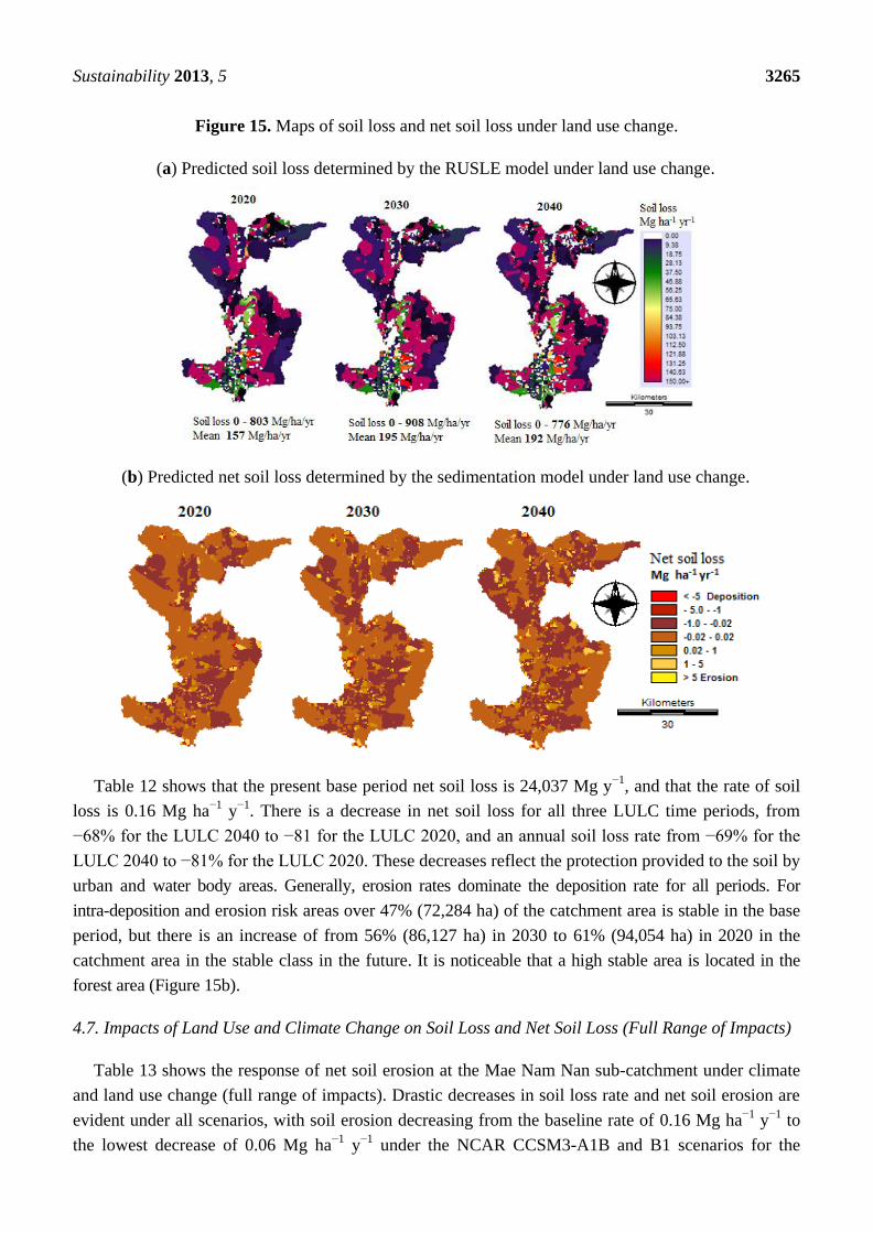
Figure 15. Maps of soil loss and net soil loss under land use change.
(a) Predicted soil loss determined by the RUSLE model under land use change.
(b) Predicted net soil loss determined by the sedimentation model under land use change.
Table 12 shows that the present base period net soil loss is 24,037 Mg y−1
, and that the rate of soil
loss is 0.16 Mg ha−1
y−1
. There is a decrease in net soil loss for all three LULC time periods, from
−68% for the LULC 2040 to −81 for the LULC 2020, and an annual soil loss rate from −69% for the
LULC 2040 to −81% for the LULC 2020. These decreases reflect the protection provided to the soil by
urban and water body areas. Generally, erosion rates dominate the deposition rate for all periods. For
intra-deposition and erosion risk areas over 47% (72,284 ha) of the catchment area is stable in the base
period, but there is an increase of from 56% (86,127 ha) in 2030 to 61% (94,054 ha) in 2020 in the
catchment area in the stable class in the future. It is noticeable that a high stable area is located in the
forest area (Figure 15b).
4.7. Impacts of Land Use and Climate Change on Soil Loss and Net Soil Loss (Full Range of Impacts)
Table 13 shows the response of net soil erosion at the Mae Nam Nan sub-catchment under climate
and land use change (full range of impacts). Drastic decreases in soil loss rate and net soil erosion are
evident under all scenarios, with soil erosion decreasing from the baseline rate of 0.16 Mg ha−1
y−1
to
the lowest decrease of 0.06 Mg ha−1
y−1
under the NCAR CCSM3-A1B and B1 scenarios for the
Sustainability 2013, 5 3266
2036–2045 period and up to the highest increase of 0.02 Mg ha−1
y−1
under the PRECIS RCM-A2
scenario for the 2016–2025 period. Similarly, there was a decrease in net soil loss from the base line of
24,037 Mg y−1
of between 8412 Mg y−1
under NCAR CCSM3-B1 (2036–2045) and 3125 Mg y−1
under PRECIS RCM-A2 for the (2016–2025).
Table 13. Changes in average annual rainfall erosivity, net soil loss estimated by the
sedimentation model under full range of impact (climate and land use change) compared to
the base period.
Climate models Rainfall erosivity
(MJ mm ha−1
h−1
)
Change
(%)
Total
erosion
(Mg/y)
Total
deposition
(Mg/y)
Net
soil loss
(Mg/y)
Change
(%)
Net
Soil loss rate
(Mg /ha)
Change
(%)
Base line 5999 0 40,547 16,510 24,037 0 0.16 0
2016–2025
HadCM3-A2 5808 −3 16,287 12,017 4270 −82 0.03 −81
HadCM3-B2 5800 −3 15,589 11,381 4208 −82 0.03 −81
NCAR CCSM3-A2 5868 −2 17,405 12,649 4756 −80 0.03 −81
NCAR CCSM3-A1B 6384 6 17,258 12,678 4580 −81 0.03 −81
NCAR CCSM3-B1 6144 2 17,106 12,368 4738 −80 0.03 −81
PRECIS RCM-A2 5015 −16 11,025 7986 3039 −87 0.02 −88
PRECIS RCM-B2 5244 −13 15,432 10,679 4753 −80 0.03 −81
Average 5752 −4 15,729 11,394 4335 −82 0.03 −81
2026–2035
HadCM3-A2 5838 −3 20,620 14,165 6455 −73 0.04 −75
HadCM3-B2 5822 −3 21,203 15,272 5931 −75 0.04 −75
NCAR CCSM3-A2 5917 −1 22,693 16,226 6467 −73 0.05 −69
NCAR CCSM3-A1B 6152 3 22,598 16,218 6380 −73 0.04 −75
NCAR CCSM3-B1 6322 5 21,715 15,538 6177 −74 0.04 −75
PRECIS RCM-A2 4866 −19 19,476 13,472 6004 −75 0.04 −75
PRECIS RCM-B2 5231 −13 20,039 13,944 6095 −75 0.04 −75
Average 5735 −4 21,192 14,976 6216 −74 0.04 −75
2036–2045
HadCM3-A2 5820 −3 29,010 21,657 7353 −69 0.05 −69
HadCM3-B2 5784 −4 27,809 20,326 7483 −69 0.05 −69
NCAR CCSM3-A2 5915 −1 28,785 21,099 7686 −68 0.05 −69
NCAR CCSM3-A1B 6917 15 29,801 21,865 7936 −67 0.06 −63
NCAR CCSM3-B1 5897 −2 31,321 22,949 8372 −65 0.06 −63
PRECIS RCM-A2 5321 −11 22,509 16,512 5997 −75 0.04 −75
PRECIS RCM-B2 5646 −6 24,745 18,304 6441 −73 0.04 −75
Average 5900 −2 27,711 20,387 7324 −70 0.05 −69
It is noticeable that the significant decrease in soil loss rates and net soil erosion reflects a
combination of all the factors discussed with respect to the aforementioned scenarios. The key factor is
the land-use change since there was an increase in urban and water body areas, which are affected by
crop and management factors. The highest decrease in soil loss under the full range of impacts occurs
because of change in land use. Figure 16a illustrates the spatial distribution patterns of the different
soil losses. It was estimated by RUSLE for impacts of land use and climate change (full range of
impact) based on future land use and combinations of two general circulation models (HadCM3 and
NCAR CCSM3) and a regional climate model (PRECIS RCM). There was an increase in mean soil
loss from 114 Mg ha−1
y−1
for 2016–2025) to 130 Mg ha−1
y−1
for the period of 2036–2045.
Sustainability 2013, 5 3267
Figure 16. Maps of soil loss and net soil loss under land use and climate change
(full range of impacts).
(a) Predicted soil loss determined by the RUSLE model under full range of impacts.
(b) Predicted net soil loss determined by the sedimentation model under land use change.
Figure 16b illustrates the spatial distribution of net soil loss risk (erosion and deposition) estimated
by the sedimentation model under the impacts of land use and climate change projections from a
combination of HadCM3, CCSM3 and PRECIS RCM with A2, A1b, B2 and B1 emission scenarios for
three future time periods. The dramatic decreases in erosion rates and net soil loss reflect a
combination of all the factors. Table 14 shows future erosion rates, which are displayed as total and
percentage changes with GCM/RCM emission scenario combinations. There was a dramatic decrease
in net soil loss from the baseline of 240,37 Mg y−1
of between 17,306 Mg y−1
for 2036–2045 and
11,778 Mg y−1
for 2016–2025. Similarly, the rate of soil loss decreased significantly from the base line
of 0.16 Mg/ha, ranging from 0.08 Mg ha−1
y−1
for 2016–2025 to 0.12 Mg ha−1
y−1
for 2036–2045.
Therefore, the full ranges of impacts have two factors, which consist of LULC conversion towards
decreased tillage (indirect impact) and the increased precipitation (direct impact), the combined result
of which is a large decrease in soil erosion at the Mea Nam Nan sub-catchment.
Sustainability 2013, 5 3268
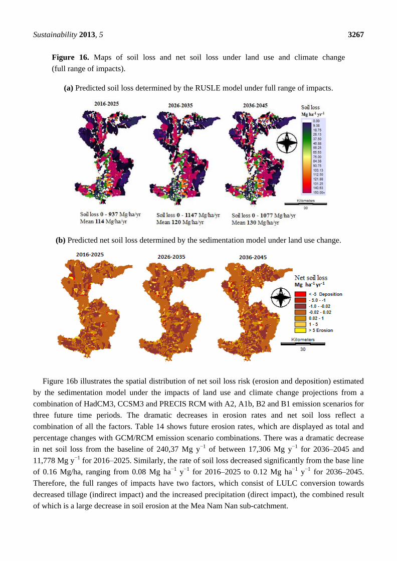
Table 14. Predicted soil loss rates and soil erosion/deposition risk areas under climate and
land use change projections (full range of impacts) from a combination of HadCM3,
CCSM3 and PRECIS RCM with A2, A1b, B2 and B1 emission scenarios for three future
time periods.
Classification Base line 2016-2025 2026-2035 2036-2045
Mg ha−1
y−1
Area
(ha)
Soil loss
(Mg y−1
)
Area
(ha)
Soil loss
(Mg y−1
)
Area
(ha)
Soil loss
(Mg y−1
)
Area
(ha)
Soil loss
(Mg y−1
)
High deposition (<−5) 255 −3080 598 −4958 750 −7598 610 −6964
Medium (−5–−1) 1795 −3269 4850 −8975 4706 −9454 8566 −15,969
Low (−1–−0.02) 68,459 −10,059 42,637 −11,971 51,000 −14,815 48,084 −13,622
Stable (−0.02–0.02) 72,284 −101 86,848 −46 76,494 −32 72,385 −21
Low (0.02–1) 5320 1436 10,281 3347 11,047 3236 12,132 3968
Medium (1–5) 2445 6580 5962 12,966 6836 17,020 8606 21,026
High erosion (>5) 2716 32,520 2098 21,439 2441 25,437 2891 28,824
Net soil loss (Mg y−1) 24,037 11,802 13,794 17,242
Change (%) 0 −51 −43 −28
Rate annual
soil loss (Mg ha−1 y−1)
0.16 0.08 0.1 0.12
Change (%) 0 −50 −38 −25
5. Discussion
The impacts of climate change on soil loss and net soil loss (erosion and deposition) may increase
or decrease at the Mae Nam Nan sub-catchment depending on the interacting effects of the factors
considered. It can be seen that the mean soil loss determined by the RUSLE model (Figure 12a) under
climate change projections from a combination of HadCM3, CCSM3 and PRECIS RCM with A2,
A1b, B2 and B1 emission scenarios for three future time slices are between 37 Mg ha−1
y−1
for
2016–2025 and 42 Mg ha−1
y−1
for 2026–2035. Table 11 shows that there is a increase in net soil loss
estimated by sedimentation model, ranging in increases from the base line of 24,037 Mg y−1
of
between 31,654 Mg y−1
for 2026–2035 and 34,548 Mg y−1
for 2016–2025. If downscaled climate
change projections are considered in isolation, then future rates of soil erosion and deposition are
generally projected to rise due to increases in precipitation and rainfall erosivity in the future. This is in
accordance with similar studies [7,8,10,12] on soil erosion, which suggest that increased precipitation
amounts and intensities will lead to greater rates of erosion. The expected increase in precipitation may
have significant effects on soil loss.
The mean soil loss was determined by the RUSLE model under a land use change between
157 Mg ha−1
y−1
in 2020 and 195 Mg ha−1
y−1
in 2030 (Figure 15a–b). Similarly, net soil losses
estimated by the sedimentation model for all three future time periods decrease dramatically from a
base line of 24,037 Mg y−1
to 4,639 Mg y−1
for 2020 and 7,733 Mg y−1
for 2040. Land use is the most
crucial element in the soil erosion model. Land use change factors are practically the most difficult to
predict with confidence. Soil loss and net soil loss potential maps were generated based on the past
(1990) and future land use (2020, 2030 and 2040) and other spatially derived parameters using the
RUSLE and sedimentation models. When land use change and management are added to the modeling
Sustainability 2013, 5 3269
process, however, then soil loss rate, soil erosion and deposition are projected to decrease significantly
from the baseline period, depending on the specific land use scenarios. Areas of high erosion can be
rapidly identified, and management efforts can be directed at these high priority areas. In this study,
high erosion and deposition zones indentified areas along the Nan River. Thus, improved vegetation
conditions such as vetiveria grass should be recommended to the farmers in order to reduce soil loss in
slope areas. For example, it should be recommended to plant vetiveria grass against the slope and
along the riverside to capture sedimentation and to grow it on check-dams, which helps to protect
against soil erosion.
It can be seen that there was a decrease in net soil loss estimated by sedimentation (Table 14) under
climate change projections from a combination of HadCM3, CCSM3 and PRECIS RCM with A2,
A1b, B2 and B1 emission scenarios for three future time periods from a baseline of 24,037 Mg y−1
of
between 11,802 Mg y−1
for 2020 and 17,733 Mg y−1
for 2040. When an additional R factor (climate
change) and C factor (land use change) are included in the modeling process, soil erosion rates and net
soil loss are projected to decrease dramatically. However, the increase in rainfall can be expected
through the increase in the number of rain days and the increase in rainfall intensity. The study
conducted by Pruski and Nearing [13] indicates that changes in rainfall that occur due to changes in
storm intensity can be expected to have a greater impact on erosion rates than those due to changes in
the number of rain days alone. Further studies are necessary to consider the impact of rainfall intensity
on potential changes in rainfall erosivity and soil erosion and deposition in the Mea Nam
Nan sub-catchment.
6. Limitations of This Study
There are several limitations in this paper. A major one is that uncertainties of a range of possible
climate change consist of uncertainty surrounding future climate change projections (emissions and
GCMs/RCMs) and downscaling methods. The downscaling method (delta change method) also creates
uncertainties in downscaled climate data sets in part because GCMs are optimized to forecast climate
change at their native resolutions [70]. The delta change method is a simple way to implement and
acquire information from just a GCMs/RCM monthly time scale. On the other hand, many statistical
downscaling methods need data from just GCMs on a daily time scale. Daily scale data from GCMs
are considered less accurate by many [71,72]. Also, bias correction and variance adjustment is often
needed to obtain adequate results, whereas with the change factor method, bias correction is implicitly
built into the approach [59]. Another limitation of this study is that the CA_Markov mode was the time
duration used for the LULC change prediction, although it should be the same time period for the
database used in the study. However, this paper studies land use change in the year 2010 derived from
the CA_Markov model compared with the results from LULC classification in 2010 by the
segmentation classification. Hence the result from the prediction is different from the time duration for
the LULC prediction in the years 2020, 2030 and 2040 estimated by the CA_Markov mode (for which
the time duration change was 20, 30 and 40 years) and was derived from LULC change for the period
of 10 years (from 1990 to 2000).

Sustainability 2013, 5 3270
7. Conclusions
This study simulates the impacts of climate change, land use change and their combined effects on
soil loss and net soil loss in the Mae Nam Nan sub-catchment, Thailand. In this study, a multi-climate
model and a multi-emission scenario approach for the estimation of climate change impacts are used.
The delta change method is used as a downscaling technique to generate future precipitation. The soil
loss model using Revised Universal Soil Loss Equation (RUSLE) and sedimentation model in Idrisi
software are used to simulate the present and future changes in soil erosion and deposition in the study
area. Results indicate that soil erosion and deposition changes are not unidirectional and vary
depending on the greenhouse gas emission scenarios and land use scenarios. The potential for climate
change to increase soil loss rate, soil erosion and deposition in future periods are established, whereas
considerable decreases in soil erosion and deposition are projected when land use is increased (paddy
fields, urban areas and water body) from baseline periods. The combined climate and land use change
analysis reveals that land use planning can be adopted to mitigate soil erosion and deposition in the
future, in conjunction with the projected direct impact of climate change. The results of this study may
be helpful to development planners and decision makers when planning and implemented suitable soil
erosion control and sediment management plans to adapt to land use and climate change.
Acknowledgements
The authors would like to thank Pornchai Mongkhonvanit for financial assistance. We are also
thankful to the PRECIS RCM data from the Southeast Asia START Regional Center [55], the NCAR
Community Climate System Model (CCSM) projections in GIS formats [54], Precipitation data from
Thai Meteorological Department and the Landsat TM data from US Geological Survey (USGS).
Conflict of Interest
The authors declare no conflict of interest.
References
1. Yang, D.; Kanae, S.; Oki, T.; Koike, T.; Musiake, K. Global potential soil erosion with reference
to land use and climate changes. Hydrol. Process. 2003, 17, 2913–2928.
2. Feng, X.; Wang, Y.; Chen, L.; Fu, B.; Bai, G. Modelling soil erosion and its response to land-use
change in hilly catchments of the Chinese Loess Plateau. Geomorphology 2010, 118, 239–248.
3. Land Development Department. Soil Erosion in Thailand (in Thai); Soil and Water Conservation
Division, Land Development Department: Bangkok, Thailand, 2002.
4. Schertz, D.L.; Moldenhauer, W.C.; Livingston, S.J.; Weesies, G.A.; Hintz, E.A. Effect of past soil
erosion on crop productivity in Indiana. J. Soil Water Conserv. 1989, 44, 604–608.
5. Beniston, M. Mountain weather and climate: A general overview and a focus on climatic change
in the Alps. Hydrobiologia 2006, 562, 3–16
6. Zhang, X.C.; Nearing, M.A. Impact of climate change on soil erosion, runoff and wheat
productivity in central Oklahoma. Catena 2005, 61, 185–195.
Sustainability 2013, 5 3271
7. Michael, A.; Schmidt, J.; Enke, W.; Deutschlander, T.; Maltiz, G. Impact of expected increase in
precipitation intensities on soil loss results of comparative model simulations. Catena 2005,
61,155–164.
8. Neal, M.R.; Nearing, M.A.; Vining, R.C.; Southworth, J.; Pfeifer, R.A. Climate change impacts
on soil erosion in Midwest United States with changes in crop management. Catena 2005, 61,
165–184.
9. Favis-Mortlock, D.T.; Boardman, J. Nonlinear responses of soil erosion to climate change: A
modelling study on the UK South Downs. Catena 1995, 25, 365–387.
10. Favis-Mortlock, D.T.; Guerra, A.J.T. The implications of general circulation model estimates of
rainfall for future erosion: A case study from Brazil. Catena 1999, 37, 329–354.
11. Mullan, D.; Favis-Mortlock, D.T.; Fealy, R. Addressing key limitations associated with modelling
soil erosion under the impacts of future climate change. Agric. Forest. Meteorol. 2012, 156, 18–30.
12. Shrestha, B.; Babel, M.S.; Maskey, S.; Griensven, A.V.; Uhlenbrook, S.; Green, A.; Akkharath, I.
Impact of climate change on sediment yield in the Mekong River basin: A case study of the Nam
Ou basin, Lao PDR. Hydrol. Earth Syst. Sci. 2013, 17, 1–20.
13. Pruski, F.F.; Nearing, M.A. Climate-induced changes in erosion during the 21st century for eight
U.S. locations. Water Resour. Res. 2002, 38, 34–44.
14. Wischmeier, W.H.; Smith, D.D. Predicting Rainfall Erosion Losses. In USDA Agric. Handbook;
Agricultural Research Service: Washington, DC, USA, 1978; Volume 537, p. 58.
15. Renard, K.G.; Foster, G.A.; Weesies, G.A.; McCool, D.K.; Yoder, D.C. Predicting Soil Erosion
by Water: A Guide to Conservation Planning with the Revised Universal Soil Loss Equation
(RUSLE). In USDA Agriculture Handbook; Agricultural Research Service: Washington, DC,
USA, 1997; Volume 703, p. 404.
16. Clemente, R.S.; Prasher, S.O.; Barrington, S.F. PESTFADE—A new pesticide fate and transport
model: Model development and verification. Trans. ASAE. 1993, 36, 357–367.
17. Sukhanovski, Y.P.; Ollesch, G.; Khan, K.Y.; Meissner, R. A new index for rainfall erosivity on a
physical basis. J. Plant Nutr. Soil Sci. 2001, 165, 51–57.
18. Mannaerts, C.M.; Gabriels, D. Rainfall erosivity in Cape Verde. Soil Till. Res. 2000, 55, 207–212.
19. IPCC. Summary for policy makers. In Climate Change 2007: The Physical Science Basis;
Proceedings of the 10th Working Group I Session; Paris, 29 January–1 February 2007;
Solomon, S.D., Qin, M.M., Chen, M.M., Marquis, K.B., Averyt, M.T., Millers, H.L., Eds.;
Cambridge University Press: Cambridge, UK, New York, NY, USA, 2007.
20. Nearing, A.M. Potential changes in rainfall erosivity in the U.S. with climate change during the
21st century. J. Soil Water Conserv. 2001, 56, 229–232.
21. Zhang, X.C. A comparison of explicit and implicit spatial downscaling of GCM output for soil
erosion and crop production assessments. Clim. Chang. 2007, 84, 337–363.
22. Renard, K.G.; Fremund, J.R. Using monthly precipitation data to estimate the R-factor in the
revised USLE. J. Hydrol. 1994, 157, 287–306.
23. Komas, C.; Danalatos, N.; Cammeraat, L.H.; Chabart, M.; Diamantopoulos, J.; Farand, R.;
Gutierrez, L.; Jacob, A.; Marques, H.; Martinez-Fernandez, J.; et al. The effect of land use on
runoff and soil erosion rates under Mediterranean conditions. Catena 1997, 29, 45–59.
Sustainability 2013, 5 3272
24. Szilassi, P.; Jordan, G.; van Rompaey, A.; Csillag, G. Impact of historical land use changes on
erosion and agricultural soil properties in Kali Basin at Lake Balaton, Hungary. Catena 2006, 68,
96–108.
25. Zhou, P.; Luukkanen, O.; Tokola, T.; Nieminen, J. Effect of vegetation cover on soil erosion in a
mountainous watershed. Catena 2008, 75, 319–325.
26. Solaimani, K.; Modallaldoust, S.; Lotfi, S. Investigation of land use changes on soil erosion
process using geographical information system. Int. J. Environ. Sci. Technol. 2009, 6, 415–424.
27. Su, Z.A.; Zhang, J.H.; Nie, X.J. Effect of soil erosion on soil properties and crop yields on slopes
in the Sichuan Basin, China. Pedosphere 2010, 20, 736–746.
28. Cotler, H.; Ortega-Larrocea, M.P. Effects of land use on soil erosion in a tropical dry forest
ecosystem, Chamela watershed, Mexico. Catena 2006, 65, 107–117.
29. Cebecauer, T.; Hofierka, J. The consequences of land-cover changes on soil erosion distribution
in Slovakia. Geomorphology 2008, 98, 187–198.
30. Mohammad, A.G.; Adam, M.A. The impact of vegetation cover type on runoff and soil erosion
under different land uses. Catena 2010, 81, 97–103.
31. Gyssels, G.; Poesen, J.; Bochet, E.; Li, Y. Impact of plant roots on the resistance of soils to
erosion by water: A review. Prog. in Phys. Geogr. 2005, 29, 189–217.
32. Bewket, W.; Teferi, E. Assessment of soil erosion hazard and prioritization for treatment at the
watershed level: Case study in the Chemoga watershed, Blue Nile basin, Ethiopia. Land. Degrad.
Dev. 2009, 20, 609–622.
33. López-Vicente, M.; Navas, A. Routing runoff and soil particles in a distributed model with GIS:
Implications for soil protection in mountain agricultural landscapes. Land. Degrad. Dev. 2010, 21,
100–109.
34. Mutua, B.M.; Klik, A.; Loiskandl, W. Modelling soil erosion and sediment yield at a catchment
scale: The case of Masinga catchment, Kenya. Land. Degrad. Dev. 2006, 17, 557–570.
35. Wischmeier, W.H. Use and misuse of the universal soil loss equation. J. Soil Water Conserv.
1976, 31, 5–9.
36. Land Development Department, Thailand. Land Use Map of Nan Province (in Thai); Land Use
Planning Division, Land Development Department: Bangkok, Thailand, 2006.
37. Moore, I.D.; Burch, G.J. Modelling erosion and deposition: Topographic effects. Trans. ASAE.
1986, 29, 1624–1640.
38. Fernandez, C.; Wu, J.Q.; McCool, D.K.; Stockle, C.O. Estimating water erosion and sediment
yield with GIS, RUSLE, and SEDD. J. Soil Water Conserv. 2003, 58, 128–136.
39. Lewis, L.A.; Verstraeten, G.; Zhu, H. RUSLE applied in a GIS framework: Calculating the LS
factor and deriving homogeneous patches for estimating soil loss. Int. J. Geogr. Inf. Sci. 2005, 19,
809–829.
40. Fu, B.J.; Zhao, W.W.; Chen, L.D.; Zhang, Q.J.; Lu, Y.H.; Gulinck, H.; Poesen, J. Assessment of
soil erosion at large watershed scale using RUSLE and GIS: A case study in the loess plateau of
China. Land. Degrad. Dev. 2005, 16, 73–85.
41. Fu, G.; Chen, S.; McCool, D.K. Modeling the impacts of no-till practice on soil erosion and
sediment yield with RUSLE, SEDD, and ArcView GIS. Soil Till. Res. 2006, 85, 38–49.
Sustainability 2013, 5 3273
42. Nekhay, O.; Arriaza, M.; Boerboom, L. Evaluation of soil erosion risk using analytic network
process and GIS: A case study from Spanish mountain olive plantations. J. Environ. Manag.
2009, 90, 3091–3104.
43. Capolongo, D.; Pennetta, L.; Piccarreta, M.; Fallacara, G.; Boenzi, F. Spatial and temporal
variations in soil erosion and deposition due to land-levelling in a semi-arid area of Basilicata
(Southern Italy). Earth Surf. Process. Landf. 2008, 33, 364–379.
44. Land Development Department. Group of Soil Series for Economic Crops of Thailand (in Thai);
Soil Survey and Land use Planning Division, Land Development Department: Bangkok,
Thailand, 2005.
45. Congalton, R.G. A review of assessing the accuracy of classifications of remotely sensed data.
Remote Sens. Environ. 1990, 37, 35–46.
46. Chen, H.; El Garouani, A.; Lewis, L.A. Modelling soil erosion and deposition within a
Mediterranean mountainous environment utilizing remote sensing and SIG- Wadi Tlata. Morocco.
Geogr. Helv. 2008, 63, 36–47.
47. EI Aroussi, O.; Mesrar, L.; Lakrim, M.; EI Garouani, A.; Jabrane, R. Methodological approach
for assessing the potential risk of soil erosion using remote sensing and GIS in the Oued EI
Malleh watershed. J. Mater. Environ. Sci. 2011, 2, 433–438.
48. Wischmeier, W.H.; Smith, D.D. Rainfall energy and its relationship to soil loss. Trans. Am.
Geophys. Union. 1958, 39, 285–291.
49. Foster, G.R.; McCool, D.K.; Renard, K.G.; Moldenhauer, W.C. Conversion of the universal soil
loss equation to SI metric units. J. Soil Water Consev. 1991, 36, 355–359.
50. Brown, L.C.; Foster, G.R. Strom erosivity using idealized intensity distributions. Trans. Am. Soc.
Agric. Eng. 1987, 30, 372–386.
51. Arnoldus, H.M.J. Methodology used to determine the maximum potential average annual soil loss
due to sheet and rill erosion in Morocco. FAO Soil Bull. 1977, 34, 39–51.
52. Ferro, V.; Porto, P.; Yu, B. A comparative study of rainfall erosivity estimation for southern Italy
and southeastern Australia. Hydrol. Sci. J. 1999, 44, 3–24.
53. Grazhdani, S.; Shumka, S. An approach to mapping soil erosion by water with application to
Albania. Desalination 2007, 213, 263–272.
54. Download NCAR Community Climate System Model (CCSM) Projections in GIS formats.
Available online: https://gisclimatechange.ucar.edu/gis-data (accessed on 12 December 2012).
55. View Regional Climate Change. Available online: http://cc.start.or.th/start2/default.asp (accessed
on 5 January 2013).
56. Fowler, H.J.; Blenkinsop, S.; Tebald, C. Linking climate change modelling to impacts studies:
Recent advances in downscaling techniques for hydrological modeling. Int. J. Climatol. 2007, 27,
1547–1578.
57. Hay, L.E.; Wilby, R.L.; Leavesly, H.H. Comparison of delta change and downscaled GCM
scenarios for three mountainous basins in the United States. J. Am. Water Resour. Assoc. 2000,
36, 387–397.
58. Diaz-Nieto, J.; Wilby, R.L. A comparison of statistical downscaling and climate change factor
methods: Impacts on low flows in the river Thames. United Kingdom. Clim. Chang. 2005, 69,
245–268.
Sustainability 2013, 5 3274
59. Akhtar, M.; Ahmad, N.; Booij, M.J. The impact of climate change on the water resources of
Hindukush-Karakorum-Himalaya region under different glacier coverage scenarios. J. Hydrol.
2008, 355, 148–163.
60. Minville, M.; Brissette, F.; Leconte, R. Uncertainty of the impact of climate change on the
hydrology of a Nordic watershed. J. Hydrol. 2008, 358, 70–83.
61. Chen, J.; Brissette, F.P.; Leconte, R. Uncertainty of downscaling method in quantifying the
impact of climate change on hydrology. J. Hydrol. 2011, 401, 190–202.
62. Land Development Department. Soil Erosion in Thailand (in Thai); Soil and Water Conservation
Division, Land Development Department: Bangkok, Thailand, 2000.
63. Eastman, J.R. Idrisi Taiga Guide to GIS and Image Processing; Clark University: Worcester,
MA, USA, 2009.
64. Thitirojanawat, P. Comparative Study of Soil Loss Estimation by Universal Soil Loss Equation
(USLE) and Runoff Plots at Nan Watershed Area, Northern Thailand. Master Thesis, Mahidol
University, Thailand, 1993.
65. Tangtham, N. Mathematical Models of Soil Erosion and Sediment Pollution in Watershed.
Department of Conservation, Faculty of Forestry; Kasetsart University: Bangkok, Thailand, 2002.
66. Rasmussen, S. An Introduction to Statistics with Data Analysis; Brooks/Cole: Pacific Grove, CA,
USA, 1992.
67. Pongsai, S.; Vogt, D.S.; Shrestha, R.P.; Clemente, R.S.; Eiumnoh, A. Calibration and validation
of the modified universal soil loss equation for estimating sediment yield on sloping plots: A case
study in Khun Satan catchment of northern Thailand. Can. J. Soil Sci. 2010, 90, 585–596.
68. Muzein, B.S. Remote sensing and GIS for land cover/land use change detection and analysis
in the semi-natural ecosystems and agriculture landscapes of the central Ethiopian Rift Valley.
Ph.D. Dissertation, Techniche Universität Dresden, Dresden, Germany, 2006.
69. Babel, M.S.; Shrestha, B.; Perret, S. Hydrological impact of biofuel production: A case study of
the Khlong Phlo Watershed in Thailand. Agric. Water Manag. 2011, 101, 8–26.
70. Wilby, R.L.; Charles, S.P.; Zorita, E.; Timbal, B.; Whetton, P.; Mearns, L.O. Guidelines for Use
of Climate Scenarios Developed from Statistical Downscaling Methods. IPCC Task Group on
Data and Scenario Support for Impact and Climate Analysis (TGICA). Available online:
http://ipcc-ddc.cru.uea.ac.uk/guidelines/StatDown_Guide.pdf (accessed on 20 December 2012).
71. Huth, R.; Kysely, J.; Dubrovsky, M. Time structure of observed, GCM-simulated, downscaled,
and stochastically generator daily temperature series. J. Climate. 2001, 14, 4047–4061.
72. Palutikof, J.P.; Winkler, J.A.; Goodess, C.M.; Andresen, J.A. The simulation of daily temperature
time series from GCM Output. Part 1: Comparison of model data with observations. J. Climate.
1997, 10, 2497–2513.
© 2013 by the authors; licensee MDPI, Basel, Switzerland. This article is an open access article
distributed under the terms and conditions of the Creative Commons Attribution license
(http://creativecommons.org/licenses/by/3.0/).