MAE 106 Mechanical Systems lab - 12000.org
372
University Course MAE 106 Mechanical Systems lab University Of California, Irvine (UCI) Winter 2005 My Class Notes Nasser M. Abbasi Winter 2005
-
Upload
khangminh22 -
Category
Documents
-
view
1 -
download
0
Transcript of MAE 106 Mechanical Systems lab - 12000.org

University Course
MAE 106Mechanical Systems lab
University Of California, Irvine (UCI)Winter 2005
My Class Notes
Nasser M. Abbasi
Winter 2005


Contents
1 Introduction 11.1 Links . . . . . . . . . . . . . . . . . . . . . . . . . . . . . . . . . . . . . . . . . 31.2 Syllabus . . . . . . . . . . . . . . . . . . . . . . . . . . . . . . . . . . . . . . . 41.3 Instructor . . . . . . . . . . . . . . . . . . . . . . . . . . . . . . . . . . . . . . 61.4 Course and Text book . . . . . . . . . . . . . . . . . . . . . . . . . . . . . . . 7
2 Lab reports 92.1 Lab 1 . . . . . . . . . . . . . . . . . . . . . . . . . . . . . . . . . . . . . . . . . 102.2 Lab 2 . . . . . . . . . . . . . . . . . . . . . . . . . . . . . . . . . . . . . . . . . 252.3 Lab 3 . . . . . . . . . . . . . . . . . . . . . . . . . . . . . . . . . . . . . . . . . 362.4 Lab 4 . . . . . . . . . . . . . . . . . . . . . . . . . . . . . . . . . . . . . . . . . 502.5 Lab 5 . . . . . . . . . . . . . . . . . . . . . . . . . . . . . . . . . . . . . . . . . 652.6 Lab 6 . . . . . . . . . . . . . . . . . . . . . . . . . . . . . . . . . . . . . . . . . 782.7 Lab 7 . . . . . . . . . . . . . . . . . . . . . . . . . . . . . . . . . . . . . . . . . 89
3 Exams 1053.1 Exam 1 . . . . . . . . . . . . . . . . . . . . . . . . . . . . . . . . . . . . . . . . 1063.2 final exam (design) . . . . . . . . . . . . . . . . . . . . . . . . . . . . . . . . . 111
4 Other class material 1374.1 Lab jack U21 user guide . . . . . . . . . . . . . . . . . . . . . . . . . . . . . . 1384.2 Professor Reinkensmeyer lecture notes given during class . . . . . . . . . . 2034.3 Professor Bobrow lecture notes given to use as reference . . . . . . . . . . . 2274.4 OLd exam to practice from . . . . . . . . . . . . . . . . . . . . . . . . . . . . 296
iii

Contents CONTENTS
iv

Chapter 1
Introduction
Local contents1.1 Links . . . . . . . . . . . . . . . . . . . . . . . . . . . . . . . . . . . . . . . . . . . 31.2 Syllabus . . . . . . . . . . . . . . . . . . . . . . . . . . . . . . . . . . . . . . . . . 41.3 Instructor . . . . . . . . . . . . . . . . . . . . . . . . . . . . . . . . . . . . . . . . 61.4 Course and Text book . . . . . . . . . . . . . . . . . . . . . . . . . . . . . . . . . 7
1

CHAPTER 1. INTRODUCTION
I took this course in winter 2005 at Univ. Of California, Irvine (UCI). This was an under-graduate course in the mechanical engineering dept.
The course is mainly a hands on course in designing basic control system using basicelectrical and mechanical components. The lab was a lot of work, many times we spentmost of the time trying to get the circuit to work after building it. Knowing how use theoscilliscope is really usefull for this course.
2

1.1. Links CHAPTER 1. INTRODUCTION
1.1 Links
1. Course web page http://www.eng.uci.edu/~dreinken/MAE106/mae106home.htm
3

1.2. Syllabus CHAPTER 1. INTRODUCTION
1.2 Syllabus
Required for Mechanical & Aerospace Engineering
MAE106: Mechanical Systems Laboratory Winter Quarter 2005
Catalog Data: MAE106 Mechanical Systems Laboratory Units: 4 Experiments in linear systems, including op-amp circuits, vibrations, and control systems. Introduction to digital sampling concepts. Emphasis on demonstrating that mathematical models are useful tools for analysis and design of electro-mechanical systems. Prerequisites: MAE140 or MAE147; ECE72 Course Overlap: MAE170 provides control theory useful for this course Cross Listed Course(s): none Restrictions: none (Design Units: 2) Lecture Location: PSCB 120, Tues Thurs 3:30-4:50 Lab Location: EG2102
Textbook: Modern Control Engineering, Fourth Edition, Katsuhiko Ogata, Prentice Hall, 2002 References:
Supplemental course notes will be at the Engineering copy center ET203. Course Web Site: http://www.eng.uci.edu/~dreinken/MAE106/mae106home.htm
Coordinator:
Professor David J. Reinkensmeyer Department of Mechanical and Aerospace Engineering Office: EG3225, 824-5218, [email protected] Hours: Tuesday 2-3 PM or by appointment TA’s: (Office hours to be announced) Daisuke Aoyagi [email protected] Jiayin Liu [email protected] Sadegh Dabiri [email protected]
Goals:
This course covers theory and experiments on motor control systems, electrical filters, amplifiers, structural resonance and vibration. These topics are important for building robots, mechatronic devices, and structures. These systems will be described by linear, ordinary, differential equations. A key goal of the class is to use these equations to predict, understand, and control the behavior of machines.
Prerequisites by Topics:
Introduction to Engineering Analysis II (MAE140) Vibrations (MAE147) Network Theory and Operational Amplifiers (ECE72)
Lecture Topics:
Week 1 (1/6): No lab scheduled Lecture 1: Overview, Design Exercise, Review of Circuit Analysis Reading: Section 3-8 Week 2 (1/11): Lab 1: Laboratory Tools and Motor Control Lecture 2: Time and Frequency Domains Lecture 3: First-Order Systems: DC Motors and Electrical Filters Reading: Chapter 2, Sections 3-1, 3-2, 5-1, 5-2 Week 3 (1/18): Lab 2: Electrical Filters and First-Order Systems Lecture 4: Lab 1 Quiz; Introduction to Control Theory Lecture 5: Example of Feedback Control: P-type Velocity Control of a Motor Reading: Chapter 1, Section 3-3 Week 4 (1/25): Lab 3: Feedback I: P-type Velocity Control of a Motor Lecture 6: Lab 2 Quiz; Second Order Systems: Time domain Lecture 7: Second Order systems: Frequency domain Reading: Sections 5-3, 8-1, 8-2 Week 5 (2/1): Lab 4: Vibration I: Lightly Damped Second Order Systems Lecture 8: Lab 3 Quiz and Midterm Lecture 9: PD Motor Control Reading: Section 5-8 Week 6 (2/8): Lab 5: Feedback II: P and PD Motor Position Control
4

1.2. Syllabus CHAPTER 1. INTRODUCTION
Lecture 10: Lab 4 Quiz; Systems with Two Modes of Vibration Lecture 11: Design of a Vibration Isolator Reading: Class Notes Week 7 (2/15): Lab 6: Vibration II: System with Two Masses Lecture 12: Lab 5 Quiz; Advanced Control Lecture 13: Advanced Control Reading: Class Notes Week 8 (2/22): Lab 7: Advanced Control Lecture 14: Lab 6 Quiz and Design Exam Lecture 15: Design Exam Review Week 9 (3/1): No Experiment This Week Lecture 16: Lab 7 Quiz/ Final Project Discussion Lecture 17: No Class Week 10 (3/8): Lecture-free week for working on final projects Week 11 (3/15): Finals Week – final project contest on day of scheduled final
Computer Usage: For laboratory write-ups and data acquisition. Laboratory Projects:
Laboratory Location: Engineering Gateway 2102 Laboratory times: Section A: Tues 11:00-01:50 Section B: Tues 06:00-08:50P Section C: Wed 04:00-06:50P Section D: Thurs 06:00-08:50P Section E: Friday 10:00-12:50 Laboratory Exercises: Handouts that describe the experiments will be made available on the course web site, along with their solutions. You should work through the lab, referring to the solution. The solution is provided to relieve time pressure and to act as a “consultant” if you get stuck. You can also ask the TA for help if you are confused. Be creative, explore, and have fun in the lab. This is your opportunity to build things that move and see how they work. Lab Pre-Quizzes: There will be a brief quiz at the beginning of each lab testing whether you have read the experiment handout before coming to laboratory. Lab Write-Up: Each student will be required to turn in a brief write-up for the lab. The write-up must be typed. You must use a computer graphing program (e.g. Microsoft Exel or Matlab) for all graphs. Zero credit if you don’t do this! Lab Post-Quizzes: There will be a 30-minute quiz in lecture the Tuesday following each laboratory.
Final Project There will be a final project competition involving the design and head-to-head testing of a robotic device. The final project tournament will take place on the day of the scheduled final exam, and will replace the final exam. There will be a write-up due on the day of the final project.
Design Content Description:
This course requires solution of design problems related to control and vibration, as well as design and construction of a robotic device for the final project.
Grading Criteria:
The grading scale will be: Lab Pre-Quizzes: 7% Lab Post-Quizzes: 14% Lab Write-Ups: 14% Mid-term exam: 20% Design exam: 20% Final project: 25%
Estimated ABET Category Content: Engineering Science: 2 credits or 50% Engineering Design: 2 credits or 50%
Prepared by: Prof. David Reinkensmeyer Date: 1/6/05
5

1.3. Instructor CHAPTER 1. INTRODUCTION
1.3 Instructor
https://engineering.uci.edu/users/david-reinkensmeyer
6

1.4. Course and Text book CHAPTER 1. INTRODUCTION
1.4 Course and Text book
Figure 1.1: course schedule
Figure 1.2: textbook
7

1.4. Course and Text book CHAPTER 1. INTRODUCTION
8

Chapter 2
Lab reports
Local contents2.1 Lab 1 . . . . . . . . . . . . . . . . . . . . . . . . . . . . . . . . . . . . . . . . . . . 102.2 Lab 2 . . . . . . . . . . . . . . . . . . . . . . . . . . . . . . . . . . . . . . . . . . . 252.3 Lab 3 . . . . . . . . . . . . . . . . . . . . . . . . . . . . . . . . . . . . . . . . . . . 362.4 Lab 4 . . . . . . . . . . . . . . . . . . . . . . . . . . . . . . . . . . . . . . . . . . . 502.5 Lab 5 . . . . . . . . . . . . . . . . . . . . . . . . . . . . . . . . . . . . . . . . . . . 652.6 Lab 6 . . . . . . . . . . . . . . . . . . . . . . . . . . . . . . . . . . . . . . . . . . . 782.7 Lab 7 . . . . . . . . . . . . . . . . . . . . . . . . . . . . . . . . . . . . . . . . . . . 89
9

2.1. Lab 1 CHAPTER 2. LAB REPORTS
2.1 Lab 1
Local contents2.1.1 questions . . . . . . . . . . . . . . . . . . . . . . . . . . . . . . . . . . . . . . . . 102.1.2 key solution . . . . . . . . . . . . . . . . . . . . . . . . . . . . . . . . . . . . . . 192.1.3 Lab post quizz solution . . . . . . . . . . . . . . . . . . . . . . . . . . . . . . . 222.1.4 my solution . . . . . . . . . . . . . . . . . . . . . . . . . . . . . . . . . . . . . . 23
2.1.1 questions
MAE 106 Laboratory Exercise #1 Laboratory Tools and Control of a Motor
University of California, Irvine
Department of Mechanical and Aerospace Engineering
Introduction There are two parts to this lab exercise. In the first part, you will learn how to use the oscilloscope, function generator, breadboard, ohmmeter and potentiometer. In the second part, you will learn how to use a low power signal and a power transistor to control the speed of a motor. There are 4 practical exams problems for which you will have to demonstrate something to the TA. There is also a brief write-up (read the last page now to see what it is!!). Note: When making electrical circuits in lab, a mistake in your wiring may result in a component getting “fried.” If you smell something burning, immediately turn off your proto-board and “debug” your circuit. PART 1: Laboratory Tools The oscilloscope and function generator are useful tools for making measurements and debugging machines. The solderless breadboard is useful for building circuits. Potentiometers are a very common circuit element for controlling a voltage or sensing a rotation. REQUIRED PARTS: Qty Parts Equipment
1 50K Potentiometer Trainer Kit (XK-550) 1 150Ω Resistor Oscilloscope with scope probe
Var. 22 gauge wire
Trigger set here
t
V(t)
Figure 1 – Trigger and Sweep Rate Figure 2 – Solderless Breadboard
1
10

2.1. Lab 1 CHAPTER 2. LAB REPORTS
1 The Oscilloscope and Function Generator The oscilloscope is used to measure and view voltage as a function of time. A voltage waveform such as v(t)=a sinωt will appear on the scope’s cathode ray tube much like you would plot it on a piece of paper. The voltage at which the trace begins is adjusted with the trigger level. The duration of the waveform that appears on the screen is determined by the sweep rate (or time scale) of the scope. You can refer to the HP oscilloscope user’s guide to better understand its basic operation. A function generator is a device that produces voltage waveforms such as sine, square, and triangle waves, all with variable amplitude, frequency, and offset. A function generator is often used to provide an input signal to the oscilloscope. For example, the function generator can produce a voltage with the form
v(t) = v0ffset + a sinωt where the amplitude a, the frequency ω, and the offset v0ffset are all adjustable. Connect the oscilloscope channel 1 input scope probe to the trainer kit function generator output (Freq.), with the scope alligator clip to GND (Note: A BNC connector is a common type of connector with a bayonet coupling mechanism. BNC stands for (Bayonet Neill Concelman), because the connector was invented by and named after Amphenol Engineer Carl Concelman and Bell Labs Engineer Paul Neill. It was developed in the late 1940's. Set the function generator to output a sine wave at about 100 Hz. Press the Auto-scale button on the scope. When you push the button, the scope measures the maximum and minimum values of the current signal, and sets the screen scaling to match these values. Get the scope to display the peak-to-peak voltage of the sine wave by pressing Voltage and then Vp-p (make sure the Source option for the Voltage function measurement is set at Line 1 – this will use channel 1 as the input line). Now adjust the function generator to output a 2 Vpp (volts peak-to-peak) sine wave at 100 Hz with no offset (DC offset button out). On the scope, make sure the Probe setting is 1 (so voltage is multiplied by 1; as explained, some probes divide the voltage by 10, and if you are using those probes rather than BNC cables, the Probe setting should be 10X). Make sure the coupling is set to DC (under channel 1).
P1. Plot the trace on the scope. (You should see the sine wave clearly now). Label
plot with the voltage and time scales. Q1. Using the utilities on the scope, obtain and record Vmax, Vmin, Vp-p, Vavg, Period,
frequency, and Duty Cycle (under Voltage and Time). Notice that these functions won’t work unless at least one period of the whole voltage signal appears on the screen.
Q2. Turn the Volts/Div, Time/Div, and position dials on the scope. Does the
Volts/Div dial change the amplitude of the sine wave? Does the Time/Div dial change the frequency of the sine wave? Does the position dial add a constant voltage to the signal? What do these dials do?
2
11

2.1. Lab 1 CHAPTER 2. LAB REPORTS
P2. Adjust the sine wave amplitude to 1Vpp at 200 Hz. Plot (on the same plot as for P1) the trace on scope using the same voltage/time scales as before.
Q3. Make the grid turn off and on (under Display). Change trigger (under Source)
from 1 to 2. What happened to the sine wave? Change it back to 1. Why does it do this? Hint: think about what the scope must do to make a sine wave appear without moving (rolling) across the screen.
Q4. Offset the sine wave by pushing the DC offset button on the function generator
and adjusting the dial. What does the trace do? On the scope, set the coupling to AC (under channel 1). Now what does the trace do when adjusting the DC offset? What is the purpose of using AC coupling?
P3. Remove the DC offset (DC offset button out) and get the function generator to
output square and then triangle waves. Plot the traces in one plot. Practical Exam 1: Ask the TA to come by your station and set the voltage and
frequency of a sine wave on the frequency generator. Demonstrate to the TA that you can measure the amplitude and frequency of the sine wave. If the TA is busy with another group, you can go ahead with the lab and ask the TA to come by later.
2 Solderless (Breadboards)
The electronic breadboard (solderless breadboard) is used to wire up temporary circuits. Electronic components and wires (use solid wires at 22-gauge thickness) are inserted into the numerous sockets (holes) on the board. The sockets (dots) are connected internally (lines) as shown in Figure 2. A good method for wiring complicated circuits is to connect the source voltage (+5V, ±15 V) and ground terminals from the trainer kit to the long narrow horizontal strips (Figure 2). Electronic chips now have ready access to power through short wires to sockets along the long strips.
After wiring your circuit to the solderless board, you may use the oscilloscope to measure voltages at various points on the circuit using the scope probe. Note that the scope probes will usually divide the voltage they read by 10, so you must compensate for this by setting Probe (under channel 1, or appropriate channel number) on the scope to 10 (this will multiply the voltage value by 10).
3 Potentiometer and Voltage Divider Circuits
Vin
+
-
Vout
R1
R2 +
-
Vin
+
-
Vout
R1
R2
+
-
BAD IDEA!!
Figure 3A & 3B – Potentiometer circuits, and actual potentiometer. In the circuit diagrams, the wiper is the wire with an arrow on it. For the actual pot, unless otherwise labeled, the
wiper is usually the middle connector (how could you check this with an ohmmeter?).
3
12

2.1. Lab 1 CHAPTER 2. LAB REPORTS
A potentiometer (also called pot) is a device that can provide a variable resistance between 2 of its leads. As you turn the knob of a pot, the wiper moves along a resistive element. Look at a broken pot in lab and see if you can figure out how it works. Figure 3A shows a pot being used to produce a variable output voltage. Q5. Derive Vout as a function of Vin ,R1, and R2 for Figure 3A. Q6. Explain why you should never use the circuit in Figure 3B.
Vin = 5V
Rpot = 50KΩ
A
B
Vout
R = 150Ω
R1
R2
1st significant figure
2nd significant figure
MultiplierTolerance
1 0 2
Color Value Black 0 Brown 1 Red 2 Orange 3 Yellow 4 Green 5 Blue 6 Violet 7 Grey 8 White 9
=10x102= 1k
Color Tol (+ %) No color 20 Black 20 Silver 10 Gold 5 White 10 Green 5
Figure 4. Circuit for question 9 Figure 5. Resistor Color Code Using the color code at the bottom of the page, pick out a 150 ohm resistor. Confirm the resistor value by measuring it with an ohmmeter. Then wire the circuit shown in Figure 4 on the breadboard. With R = ∞ (i.e. an open circuit), measure Vout in five approximately equally spaced potentiometer positions (i.e. full clockwise, full counter-clockwise, the center, etc.). Repeat the test with R = 150Ω. P4. Sketch Vout vs. pot angle for both cases. Q7. One plot is linear and one is not. Using your knowledge of circuit theory, show
mathematically that this is the case by deriving the equation for Vout as a function of θ (don’t plug actual values in until you derive the equation!). Note: first derive the equations that relate R1 and R2 to pot angle (0 ≤ θ ≤ θmax). Assume that R1 varies linearly with θ. Under what conditions would a pot be a good way of making an adjustable voltage source? Brainstorm two possible uses for potentiometers on your final project.
Practical Exam 2: Show the TA that you can calculate the value of a resistor using the color code, and that you can measure it using the Ohmmeter. Explain to the TA why you will never wire a potentiometer as shown in Figure 3B. Explain to the TA how you might use a potentiometer for you final project.
4
13

2.1. Lab 1 CHAPTER 2. LAB REPORTS
PART 2: Control of an Electric Motor REQUIRED PARTS: Qty Parts Equipment
1 N-type Power MOSFET (IRF510 or NTE2382) Trainer Kit (XK-550) 1 LM324 Quad Op-amp chip Oscilloscope with scope probe 1 50kΩ potentiometer Small DC motor 1 470Ω resistor Integrated circuit puller 1 1kΩ resistor Grounding wrist strap 1 47K Resistor 1 100Ω resistor, 2 Watt (with smaller ga. wire
leads)
var 22 gauge (AWG) wire 1 Introduction Engineers use electric motors for a variety of applications requiring mechanical movement (robots, automation equipment, disk drives, etc.). A motor is only useful, however, if we know how to control it. Sometimes we want to control the motor’s position (computer disk drives, CD players, plotters), sometimes its speed (cruise control on autos, CD players), and sometimes its torque (robots, some heavy machinery). In this lab, we will investigate controlling the voltage across a motor, which, assuming there are not external forces acting on the motor, will control the speed of the motor. In other words, if the motor load is just inertial, then the steady-state speed of the motor is proportional to the voltage across its terminals. In this part of the lab, we will investigate two circuits that can control the voltage across a small electric motor. Each circuit will involve the use of a MOSFET and/or an operational amplifier (or op-amp). The op amp circuit will utilize “feedback” to control the motor voltage. So, in this experiment you will gain insight into how DC brushed motors behave, how to control the power supplied to a motor with a MOSFET, and how to regulate the behavior of the motor with an op-amp controller. 2 Voltage Follower for Voltage Control Op amps are often used in analog circuits. They take 2 input voltages at their inputs (the inverting input (V-) and the non-inverting input (V+)) and produce an output voltage
Vout = K(V+ - V-), where K≈1x10⁵. (3) They also have a very high input resistance, so for practical purposes they draw no current at their inputs. These characteristics of op amps allow them to serve many circuit functions, such as voltage addition and subtraction, feedback control, and buffering. The op amps used in this lab can output only tens of mA of current; you will calculate the exact value in the lab.
In Figure 2, an op amp is used in a voltage follower circuit. In this circuit, the op-amp attempts to adjust the output voltage (Vout) so that it “follows” (makes it equal to) Vin. This circuit is also called a buffer or isolation amplifier because the output current does not affect the input voltage (Vin). The load resistance (RL) draws current from the op-
5
14

2.1. Lab 1 CHAPTER 2. LAB REPORTS
amp. A small value of RL is considered a “large load.” A large value of RL is a “small load.” Note that large loads can cause a drop in voltage in a voltage source if the voltage source cannot supply sufficient current.
+ + --
+- + -
1
2
3
4
5
6
7 8
9
10-12V
11
12
13
14
+12V
“U” Cutout
Vout50kpot
-12V
+12V
+-
Vin RL
Figure 1 – LM324 Quad Op-Amp Chip Figure 2 – Voltage Follower Circuit.
Figure 3 – Suggested Layout of Circuit on Solderless Breadboard Construct the circuit shown in Figure 2 (suggested layout is in Figure 3). We will use the LM324 chip (Figure 1), which has 4 op-amps built on the chip. Power must be supplied at pin 4 (positive voltage) and pin 11 (negative voltage), else the chip will burn out. Q1 Using the op-amp equation above, derive the equation of Vout for the buffer circuit. Q2 There are limitations in the buffer circuit in Figure 2. That is, there are conditions
when the op-amp would not be able to make Vout = Vin. Discuss 2 limitations. P1 Measure Vout and Vin across the full range of pot angle positions, for several
values of the pot angle. Do this with RL = 1 kΩ and with RL = 470Ω. Sketch Vout vs. Vin for both RL values on one plot.
Q3 Which plot follows Vin more closely, particularly at the voltage extremes of Vin?
Explain. Using your results, calculate the maximum current that your op amp can supply. Is the 470Ω resistor close to blowing up (consider its power rating)?
6
15

2.1. Lab 1 CHAPTER 2. LAB REPORTS
Suppose you replace RL with a motor whose resistance is 30Ω, and you hold the shaft of the motor still. Would you be able to control the amount of torque that the motor can generate? Note: When to motor shaft is held still, the amount of torque that a DC motor generates is proportional to the current going through it.
Q4 THOUGHT EXPERIMENT: If you changed the power input to the LM324 chip to
+5V (pin 4) and 0V (pin 11), and adjusted Vin over the +12V to –12V range, do you think Vout would follow Vin? Explain. NOTE: DO NOT ATTEMPT THIS; IT CAN BLOW THE OP AMP AND POT!
3 Open-Loop MOSFET Voltage Control Circuit A MOSFET is a type of transistor that restricts or allows current flow through the source and drain leads based on voltage applied at its gate with respect to the source (VGS). It can be thought of as a variable resistor whose resistance value is determined by VGS. For the MOSFET’s used in class, the effective resistance between source and drain (RDS) varies between infinity (with VGS < 3 or 4 volts) and about ½ ohms (with VGS ~5-6 V). These characteristics allow MOSFETS (and other transistors) to be used as either current amplifying devices (power MOSFETS for motors, etc.) or switches (low power MOSFETS in computers). Construct the circuit shown in Figure 4 (make load resistance RL = 100Ω at 2 Watt rating). In this circuit, we directly control the MOSFET gate voltage (VG) by turning the potentiometer (recall that VGS will vary linearly with the pot angle), which ultimately controls the motor voltage (Vmotor). In this section, we will study how Vmotor varies as we vary VGS.
Vs = 12V
GS
D
RL47k
50kpot
VGS
VD
Vmotor =(Vs-VD)
G D S
Figure 4 – MOSFET voltage control circuit Figure 5 – MOSFET leads Q5 Derive the following formula relating the MOSFET resistance (RDS) to Vs, VD, and
RL. RDS = VDRL/(Vs – VD)
Q6 Consider the circuit in Figure 4 and assume that RL is a motor. Explain how turning
the pot (which we control) ultimately controls motor voltage (Vmotor). Include in your explanation the role of the pot and the MOSFET.
7
16

2.1. Lab 1 CHAPTER 2. LAB REPORTS
P2 Measure VGS, and VD at enough potentiometer positions to produce a nice plot of RDS vs. VGS and Vmotor vs. VGS (on same plot, not VD vs. VGS). Take more measurements in the area of pot positions where VD changes quickly. Use the equation above to compute RDS. Plot Vmotor with respect to VGS (i.e. the input voltage). Is this relationship linear?
Q7 Replace the load resistor (RL) with a small DC motor. Slowly increase VGS from a
value of zero and visually observe the resulting changes in motor speed. Try to make the motor shaft rotate at approximately once per second. Is it difficult? Does the speed of the motor relate linearly to the VGS? Explain why this is so. Would you say that you are controlling motor voltage well?
Q8 Measure the DC resistance of the motor with an ohmmeter and report the value.
You have just measured R for the equation 1. Disconnect your motor from the circuit and connect it to an oscilloscope. What is the maximum voltage you can generate by hand? Describe how B1 (in equation 1) can be measured experimentally. Be precise in describing the experiment you would perform.
Practical Exam 3: Demonstrate to the TA that you can control the speed of your
motor with the potentiometer. 4 Closed-Loop Voltage Control Circuit
Vout
50kpot
-12V
+12V
+-
VinG
S
D
Vcc= +12V
Figure 6 – Closed-Loop Voltage Control Circuit. (Note: Power connections to Op Amp not
shown!) In Part 2, we learned that an op-amp might not provide sufficient current to run a motor. MOSFET’s may be necessary to control higher levels of current required by devices such as heaters and electric motors, but they are highly non-linear to the input voltage. Now we will add “feedback” to our controller. A controller that uses feedback takes information about some state in our system (voltage, position, velocity, temperature, etc.) that is measured by a sensor (voltmeter, pot, tachometer, thermocouple, etc.), and uses it to compute a “control” (an input to the system that we control, often denoted “u”). The control is designed to make the state of the system be what we want it to be. Construct the circuit shown in Figure 6. Q9 Explain how turning the pot (which we control) ultimately controls motor voltage
(Vout). Include in your explanation the role of the pot, op-amp, and the MOSFET.
8
17

2.1. Lab 1 CHAPTER 2. LAB REPORTS
P3 Make about five measurements of vin and vout as vin varies between 0 and 13 volts. For each pot setting of vin, measure vout (let the motor shaft spin freely). Plot vout versus vin on the same plot as P2.
Q10 Try again to make the motor rotate at approximately one cycle per second. Explain
why it is easier than before. Explain why this is a better voltage control circuit than the previous one.
Practical Exam 4: Demonstrate to the TA that you can control the speed of your
motor with the potentiometer. You should be able to control it more precisely than in Practical Exam 3 – Explain why to the TA.
Q11 In this experiment, you focused on controlling the motor voltage, which controls the
motor speed when there are no disturbances on the motor shaft (e.g. when you are not holding the shaft). In the real world there are often unexpected disturbances that produce undesired changes in the motor speed (imagine an electric car that has to go up a hill, or, try stopping the motor with your hand). Suggest an improved method for controlling motor velocity (hint: consider how you might design a cruise control system a car using a tachometer).
WRITE-UP - due at your next laboratory session - each student must complete his or her own write-up - make sure to use your own words!! - include your name and laboratory time on the write-up - the write-up must be type-written - Graphs for the lab write-up must be generated using Excel or Matlab, and must
include labels on the axes, voltage and time scales used on the scope, and a legend for multiple-line plots.
- Page limit = 2 pages, including graph 1. Briefly explain uses for an:
a. oscilloscope b. function generator c. solderless breadboard d. potentiometer
2. Briefly explain how a low-power signal and a power MOSFET can be used to control the speed of a motor.
3. Briefly explain why the operational amplifier made it easier to control the speed of the motor
4. Turn in the graph for P2 and P3 from PART 2 of the laboratory exercise
9
18

2.1. Lab 1 CHAPTER 2. LAB REPORTS
2.1.2 key solution
MAE 106 Laboratory Exercise # 1 - Solution Laboratory Tools and Control of a Motor
Part 1: Laboratory Tools
P1 See below P2 below Q1 Vmax = 1V Vavg = 0V Duty cycle = 50% Vmin = -1V Frequency = 100 Hz Vpp = 2V Period = .01s Q2 They do NOT adjust the amplitude, frequency, and DC offset, respectively. Rather, they
adjust the voltage scale, time scale, and vertical position for the scope trace, respectively. P2
t V(t)
-2
2
Q3 The trigger is responsible for making the trace “stay still” on the screen, by capturing the
signal for a fixed duration of time whenever it crosses the trigger voltage, then displaying the captured signal with a predetermined temporal offset. If the trigger channel is set to 2, than signals on channel 1 will not be triggered properly because the scope is trying to align the signal based on the (floating) voltage being input into channel 2.
Q4 AC coupling removes the DC offset from the signal. P3
tV(t)
2
-2
Q5 Vout = R2/(R1 + R2) Vin Q6 If the pot is turned to the extreme end, there is no resistance to current flow and the pot
will be burned out. P4 In one plot, show Vout vs. pot angle for both cases.
1
19

2.1. Lab 1 CHAPTER 2. LAB REPORTS
θVout
5 V R=150R=∞
Q7 R1 = kθ; R2 = Rpot - kθ; with k=(50K/θmax), Rpot = 50K Vout = Vin (Rp)/(R1 + Rp), with Rp = R2*R/(R+R2); voltage divider rule Vout = Vin [1/1 + (R1/R) + (R1/R2)] Vout = Vin [1/1 + (kθ/R) + (kθ/(Rpot-kθ))]
Vout = Vin[(-k)θ/(-k2/R)θ2 + (Rpot/R)θ + (Rpot)] (linear divided by quadratic) A pot is a good way of making an adjustable voltage source if its output is connected to a high resistance. On your final project, you could use one pot to specify the desired angle of the motor (i.e. the “control knob” you hold in your hand), and another to sense the actual angle of the motor (i.e. the “sensor” that senses motor angle).
Part 2: Control of an Electric Motor Q1 Vout = K(V+ - V-), but Vout = V-, so Vout = K(V+ - Vout), so Vout = (K/(1+K)) Vin, and for K
>> 1, Vout ≈ Vin. Q2 RL cannot be so small as to draw more current than the op-amp can supply (> 20mA
usually) Vin cannot be greater than the voltage supplied to the op-amp chip. P1
Vin
Vout 15
-15
R=470R=1k
Q3 With large RL, the plot follows better. For large RL, Vout can go all the way to 15V (minus
some loss in the op-amp) since Iout = 15V/1k = 15mA, which is less than the maximum current the op amp can supply. The small RL draws at a maximum Iout = (observed peak voltage = 9.4V)/470Ω = 20mA peak, which is the maximum current the op-amp can supply (or “source”). Note that different op amps may have slightly different peak currents. Put another way, small RL draws too much current for the op-amp to maintain Vout. The power drawn by the 470Ω resistor is I2R = 0.19 W, which is less than the 0.25 W rating, but near it, so you should feel the resistor warming up.
2
20

2.1. Lab 1 CHAPTER 2. LAB REPORTS
A motor with a stationary shaft acts like a resistor. A motor with R=30 ohms would initially attempt to draw way too much current (15V/30Ω = 500mA) and the output voltage from the op amp would be very small (Vout=20mA*30Ω=0.6V). You could only control the torque of the motor across a small range of currents corresponding to 0-20 mA (see Equation 2).
Q4 The op-amp can only output ~0 – 5V (minus a small voltage loss) if powered between 0V
and 5V. Q5 RDS = VDRL/(Vs – VD) (ans: use voltage divider rule) Q6 We control the pot angle. The pot allows us to adjust VG. The MOSFET allows, through a
corresponding change in RDS the adjustment of VD. Motor voltage is (Vs – VD), where Vs is a constant, so we ultimately control Vmotor.
P2 Vmotor is not linear with respect to VG
Vin
Vmotor
10k
Vmotor RDS
4
15V RDS
Vout
Q7 It is difficult to make the motor turn at 1 Hz. The motor speed is not linear to VGS. This
results from non-linear input/output characteristics of the MOSFET (i.e., RDS is not linear to VGS). Since we are unable to control motor speed easily, and motor speed correlates with motor voltage in the steady state, it seems that we are able to control the voltage, but not easily.
Q8 The voltage VD increases when you stop the motor shaft since the back EMF term no
longer contributes to the voltage across the motor. Specifically, when the motor is allowed to accelerate to its no load speed, the back EMF builds up proportionally to angular velocity until i ≈ 0 (i never goes completely to zero because some torque is needed to overcome the motor’s friction). If i ≈ 0, then VD ≈ 0. If you stop the motor from turning, the back EMF term goes to zero, and more current is allowed to flow through the MOSFET, increasing VD.
Q9 We control pot angle, so we control Vin. The op-amp, having negative feedback, takes Vin and adjusts VGS so that Vout = Vin. That is, VGS is altered in such a way as to make the MOSFET’s RDS change so that Vout=Vin.
P3 See P2 above. Q10 It is easier due to feedback. The op-amp, since it has negative feedback, will try to adjust
VGS so that Vout is equal to Vin. In this way, the op-amp can “correct” for nonlinearities in the MOSFET and makes Vout linear with respect to Vin. Since we are able to get Vout to more closely parallel Vin, this is a better control system.
Q11 An improved method for controlling motor velocity would be to actually sense the motor’s velocity (for example, with a tachometer), then to make feedback adjustments to the current supplied to the motor based on the difference between the actual and desired velocity. We will explore this approach in a subsequent lab.
3
21

2.1. Lab 1 CHAPTER 2. LAB REPORTS
2.1.3 Lab post quizz solution
22

2.1. Lab 1 CHAPTER 2. LAB REPORTS
2.1.4 my solution
LAB #1 report. MAE 106. UCI. Winter 2005
Nasser Abbasi, LAB time: Tuesday 1/11/2005 11:00 AM-1:50 PM
January 18, 2005
1 Answer 1.
1. Oscilloscope: This is a device to allow one to analyze and display the electric signal in the circuit. One can useit to display the electric signal trace on the screen and to measure di¤erent properties about the signal. Onecan use it to display di¤erent properties about the voltage, such as the max/min, vpp. In addition it is used tomeasure the frequency properties of the signal.
2. Function generator: This device is attached to the training kit, and was used to generate electric signals ofdi¤erent time-domain shapes, such as square, triangular and sinusoidal signals. One can also adjust the frequency,amplitude and phase o¤set at which these signals are generated.
3. Solderless breadboard: This makes it convenient to quickly build and connect simple circuits since it eliminatesthe need to make soldering to connect di¤erent parts of the circuits together.
4. potentiometer: Also called pot. This allows one to adjust the voltage entering one branch of the circuit byallowing one to adjust the resistance by turning a knob. It is a Voltage divider.
2 Answer 2.
The MOSFET has 3 ports. G;D; S. We control the voltage supplied to the gate G by using a pot. When VG changes,this causes voltage at port D to change (VD) as well. But voltage across the motor depends on VD hence we cancontrol the voltage across the motor.By controlling the voltage across the motor, we control the torque generated by the motor.Note that the change between VG and VD is not linear. As VG changes, the internal MOSFET resistance RDS
changes, and this causes VD to change.The voltage across the motor depends on VD by the relation Vmotor = VsVD where Vs is the xed source voltage.By using MOSFET only to control voltage to the motor, it acted as an approximation to an on/o¤ switch. This
is because a small increment in VG caused a sudden large increase in Vm to appear. However, as VG continued toincrease, Vm did not continue to increase as well, but remained steady. See plot of Vm vs. VG. This shows that thenonlinearity of MOSFET makes it hard to use to control the speed of the motor.On the other hand, a small voltage at the gate caused a large voltage to appear across the motor, so this shows
that MOSFET acted as a device that can be use to supply power to other devices.
3 Answer 3.
When we used just the MOSFET to control the speed of the motor, it was hard to slow down or speed up the motorshaft spin. The motor will either spin or stop by changing the pot dial across the range of the dial. This is due to thenonlinearity of the MOSFET. So, to use MOSFET to supply power to the motor, we need to be able to better controlthe voltage it generates, and to do this, we use an Op-Amp.By using an OpAmp, using negative feedback, we feed the voltage output from MOSFET back into the opAmp.
This causes Voltage at the gate VG to adjust so that voltage output from MOSFET follows voltage input to the opAmp.So, by changing the input voltage to the OpAmp via the use of the pot, and having negative feedback, the voltage
output from MOSFET follows the input voltage more closely. Since output voltage from MOSFET is linearly relatedto the speed of the motor, we are now able to better control the speed of the motor. This circuit is shown in gure 6in LAB1 handout.
23

2.1. Lab 1 CHAPTER 2. LAB REPORTS
4 ANSWER 4
I have written a simple program to generate the diagrams required from the data collected in the Lab. This is thenal plot output. First, this is the data collected:
RdsVmotorVout
10000
24

2.2. Lab 2 CHAPTER 2. LAB REPORTS
2.2 Lab 2
Local contents2.2.1 questions . . . . . . . . . . . . . . . . . . . . . . . . . . . . . . . . . . . . . . . . 252.2.2 key solution . . . . . . . . . . . . . . . . . . . . . . . . . . . . . . . . . . . . . . 292.2.3 Lab post quizz solution . . . . . . . . . . . . . . . . . . . . . . . . . . . . . . . 302.2.4 my solution . . . . . . . . . . . . . . . . . . . . . . . . . . . . . . . . . . . . . . 32
2.2.1 questions
MAE 106 Laboratory Exercise #2
Electrical Filters and First Order Systems
University of California, Irvine Department of Mechanical and Aerospace Engineering
REQUIRED PARTS: Qty Parts Equipment
Breadboard 2 1 kΩ resistor Oscilloscope with scope probe 1 1µF capacitor LabJack
Var. Cables Small DC motor Var. Wires BNC T-Adapter
2 BNC cables Female BNC-to-Alligator clip breakout Digital Multimeter, 1 or 2/lab section Two scope probes IC puller
1 Introduction Filters are an important part of electrical signal processing. They are often found in stereos (cross-overs, graphic equalizers, etc.), control systems (to clean up sensor readings from strain gauges, tachometers, potentiometers, etc.), and many other applications. In control systems, filters can help remove unwanted high-frequency noise that may adversely affect the controller. Filters are important conceptually because we can view any system as a filter. For example, you can view the steering system of a new car in terms of how it responds to low, medium, and high frequency inputs. Understanding how systems respond to different input frequencies requires understanding how filters work. In this lab, we will study the RC circuit, which can be used as a low-pass or high-pass filter. Low-pass filters attenuate high frequency signals (i.e. reduce them in amplitude), but leave low frequency signals relatively unchanged. High pass filters attenuate low frequency signals. Low pass filters are often useful for filtering out high-frequency noise (due to electromagnetic interference from the lights or radio signals, for example.) Also, many objects and systems in the world act like low-pass filters. High pass filters are used to filter low frequency noise from signals. This lab also provides a chance for you to understand how first-order systems behave in the time and frequency domains. The RC circuit is a first-order system (i.e. it is described by a first-order differential equation).
1
25

2.2. Lab 2 CHAPTER 2. LAB REPORTS
2 Low-Pass Filter
Vin
R
C- + Vout
Figure 1 – RC Circuit Used As a Low-Pass Filter
Consider the response of the circuit in Figure 1 to a square wave input. The capacitor acts as a charge bucket, which is alternately charged (filled) and discharged. The capacitor (C) is charged by Vin (input voltage) until the voltage across the capacitor matches that of Vin. If Vin is then switched off (or to a lower voltage value) C begins to discharge through R so that Vout heads toward Vin again. It takes time, however, for the capacitor to charge and discharge through the resistor. That is, the capacitor has dynamics that slow down Vout and prevent it from exactly following Vin. Q1 Write down the differential equation relating Vout and its derivatives to Vin. Assume Vin is a
constant input and that Vc(0) = 0, and solve this equation for Vout as a function of time. Given C = 1 µF and R = 1KΩ, what is the time constant (τ) of the system?
P1 Draw the theoretical response (i.e., solve the differential equation above) to a square wave
input to this circuit. Assume the period of the square wave is large compared to τ. Construct the circuit in Figure 1 on the breadboard. Use R = 1KΩ and C = 1.0 µF. Q2 Use the function generator to apply a square wave input (4Vpeak-to=peak-p) and measure
the filter’s response to the square wave. Display both Vin and Vout on the oscilloscope. Adjust the input frequency and the voltage and time scales on the scope so that a nice waveform is displayed and record these values. Measure and record the time constant of the system by using the cursors on scope to find the time it takes for Vout to change 63% from its initial value to its final value. Explain using the equation from Q1 why the time constant corresponds to the time at which the output has gone 63% to its final value.
P2 Record the waveform that you see on the screen using a LabJack. Q3 Changing the amplitude of the square wave you use as the input affects the amplitude of the
output. Does it affect the shape? This is a property of a linear system. Q4 Increase the frequency of the square wave and observe the amplitude of Vout. Explain briefly
why this is a low-pass filter. P3 Now lets consider how such a filter might be useful in cleaning up the signal from a sensor.
Replace the function generator with the output of a DC motor, which will serve as a makeshift tachometer (velocity sensor). Spin the tachometer by hand to produce a voltage and display both Vin and Vout from the filter on the scope. Why does spinning the tachometer produce a voltage (remember the motor voltage equation?). What effect does the low pass filter have on the tachometer? Sketch and label the difference between the input and output voltage signals.
PRACTICAL EXAM 1: DEMONSTRATE TO THE TA THAT YOU CAN FILTER THE TACHOMETER OUTPUT.
2
26

2.2. Lab 2 CHAPTER 2. LAB REPORTS
t
V(t) ∆t
Figure 2 – Phase Shift Between 2 Sine Waves So far we have been looking at the time response of systems. Frequency response is the response of a system to a sine wave input over a range of frequencies. It is an important measure of how a system behaves, especially with respect to how it filters signals. For a linear system, the response to a sinusoidal input at some frequency is always a sinusoidal output at the same frequency, but with a different amplitude and a phase shift. In other words, linear systems don’t create new frequencies in the output, they only scale and phase shift their input frequencies. We will now characterize the frequency response of the low pass filter by inputting a sine wave over a range of different frequencies. On the oscilloscope, we will directly measure time shift (∆t) by placing the cursors (t1 & t2) on 2 corresponding points on the 2 signals (Figure 2). Phase shift can then be computed using the following formula, where T is the period (sec.), f is the frequency (Hz), and φ is phase shift (rad.).
∆t/T = φ/2π and f = 1/T
Q5 Switch the function generator from square wave to sine wave. Record the ratio of the output amplitude to the input amplitude and the phase lag of the output for input frequencies of 100, 200, 500, 1k, 2k, and 4k Hz.
P4 Plot the amplitude ratio vs. frequency. Plot the phase lag vs. frequency. On a third graph,
plot the log(amplitude ratio) vs. log(frequency) – This log-log plot is called a Bode plot, and is a common way to display frequency responses. Which of the two amplitude ratio plots makes it easier to see why this circuit is a low-pass filter and why?
P5 Now, read the output voltage across the resistor instead of the capacitor, as shown in Figure
3. Record the ratio of the output amplitude to the input amplitude and the phase lag of the output for input frequencies of 100, 200, 500, 1k, 2k, and 4k Hz. Repeat the plots that you did for P4. What type of filter is this?
Q6 What happens if you provide a triangle wave input into the circuit in Figure 3? Explain based
on the transfer function for the circuit.
Vin
R
C-+
Vout
Figure 3 – RC Circuit Used As Another Type of Filter
3
27

2.2. Lab 2 CHAPTER 2. LAB REPORTS
WRITE-UP - due at your next laboratory session - each student must complete his or her own write-up - make sure to use your own words!! - include your name and laboratory time on the write-up - the write-up must be type-written - Graphs for the lab write-up must be generated using Excel or Matlab, and must include labels
on the axes, voltage and time scales used on the scope, and a legend for multiple-line plots. - Page limit = 2 pages, including graphs
1. Briefly explain what the time constant of a first-order system is. 2. Briefly explain what the cut-off frequency of a first-order low-pass filter is. 3. Explain why a mass (i.e. a rock, a ball, a robot arm) acts like a low pass filter, if force is
considered its input and position its output. 4. Turn in the graph for P2, with an overlay of the theoretical step response. Label the time
constant. 5. Turn in the graphs for P4 and P5, with an overlay of the theoretical frequency responses.
Hint: To plot the theoretical frequency responses, you must derive the transfer functions H(s) = Vout(s)/Vin(s) for the circuits shown in Figure 1 and Figure 3. Find the magnitude and phase of the transfer function evaluated at s = jω. Plug in C = 1µF and all R = 1KΩ to get the actual values. Label the cut-off frequency on the graph.
How to read - Capacitor codes
This is for the reading of smaller capacitor codes, for example when you are confronted with a capacitor marked 103J etc. Some capacitors just have a two digit number printed on them, e.g. 47 printed on a small disc would usually be 47pF. The majority have a three digit number, this works in a similar manner to the resistor colour coding sytem, the first two numbers refering to the value in pF with the third digit being the multiplier or how many 0's follow. e.g. 104F is 10 with 4 more zeros 100000pF which is .1µF The letter refers to the tolerance value of the capacitor, so in the example above,104F is +/- 1%
first 2 digits
third digit multiplier Letter
symbol tolerance
XX 0 1 D +/- 0.5pF XX 1 10 F +/- 1% XX 2 100 G +/- 2% XX 3 1000 H +/- 3% XX 4 10000 J +/- 5% XX 5 100000 K +/- 10% XX 6 not used M +/- 20%
XX 7 not used P +100%, -0%
XX 8 .01 Z + 80%, -20%
XX 9 .1
....
.
4
28

2.2. Lab 2 CHAPTER 2. LAB REPORTS
2.2.2 key solution
MAE 106 Laboratory Exercise #2 (Solution)
Electrical Filters and First Order Systems Q1 Vout = Vin(1-e-t/RC) τ = RC = (1µF)(1kΩ) = .001 sec P1
tV(t)
Q2 τ ≈ RC ≈ (1µF)(1kΩ) ≈ .001 sec; when t = τ then Vout = A(1-e-1) = 0.63A P2 Record the waveform that you see on the screen. Ans: Same as P1. Q3 No – for a linear system, scaling the input just scales the output. Avin ⇒ AVout Q4 The output amplitude decreases as we increase frequency—a low pass filter. P3 You get a noisy and a less-noisy trace. Q5 Output should decrease in amplitude at higher frequencies. P4
log (f)
Log(A)
The bode plot makes it easier because the curves become lines.
P5
log (f)
Log(A)
Q6 G(s) = RCs/(RCs + 1) At low frequencies, RCs << 1, so G(s) → RCs (a differentiator). The derivative of the triangle
wave is a square wave.
1
29

2.2. Lab 2 CHAPTER 2. LAB REPORTS
2.2.3 Lab post quizz solution
30

2.2. Lab 2 CHAPTER 2. LAB REPORTS
31

2.2. Lab 2 CHAPTER 2. LAB REPORTS
2.2.4 my solution
LAB #2 report. MAE 106. UCI. Winter 2005
Nasser Abbasi, LAB time: Thursday 1/20/2005 6 PM
March 27, 2005
1 Answer 1.
Explain time constant: This is the time the output will take to reach 63% of its nal value.
2 Answer 2.
Cut-o¤ frequency is the frequency at which the output amplitude (Such as voltage) is 70:1% of the input. Thiscorresponds to a drop of 3db from the input. It is also the frequency at which the output power is 50% that of theinput. This frequency is usually taken as the boundary frequency between the highpass region and the low pass regionof the frequency response plot.
3 Answer 3
A heavy object has large inertia. Which means it will take time for it to accelerate when subjected to the same forceas compared to an object of low mass. When the force uctuates very quickly, the object will be slow to react due toits high mass, and by the time it starts to move in response to the force, the force will change its direction quickly,and the object will have to start to reverse its direction again in the direction of the force, and will again be slow indoing this new movement. So this mean the object will have a small motion amplitude of the same frequency as theinput force. This is a low pass lter.
4 Answer 4.
I collected the data using LabJack. This below shows the rst few lines of the text le collected:
Now I wrote a small script to plot the data and the theoretical response Vin1 e t
RC
on the same plot. this is
the result. I normalized both amplitudes to 1.
32

2.2. Lab 2 CHAPTER 2. LAB REPORTS
5 Answer 5.
For the circuit in gure 1, the ODE is Vo = ViCR dVodt . Take Laplace transform, we get Vo (s) = Vi (s)CRsVo (s))
Vo (s) [1 + CRs] = Vi (s) ) Vo(s)Vi(s)
= 11+CRs hence H (j!) = 1
1+jCR! hence, jHj = 1p1+(CR!)2
and phase is (H) =
tan1 (!CR) = tan1 (!CR)Hence for C = 106F , and R = 103 we get jHj = 1p
1+!2(106103)2= 1p
1+!21:0106
and (H) = tan1!106 103
= tan1 (0:001!)
The following is the data collected for P4, and the theoretical data based on above Laplace transform. This is alow pass lter.
Input Freq. (Hz) V pp input V pp output t T = tT 2
180 (degrees)
100 590 mV 662 mV 1.04 ms 10 ms 1:0410 2 180
= -37: 440
200 1.7 V 1.156 V 740 s 4.9 ms 7401064:9103 2
180 = -54: 367
500 1.59 V 562 mV 390 s 1.99 ms 3901061:99103 2
180 = 70: 553
1 K 1.562 V 312 mV 244 s 990 s 244990 2
180 = 88: 727
2 K 1.56 V 171 mV 126 s 515 s 126515 2
180 = 88: 078
4 K 2.8 V 500 mV 65 s 242 s 65242 2
180 = 96: 694
Theortical:Input Freq. (Hz) jHj (H) (degrees)100 1p
1+(2100)21:0106= 0:846 73 -tan1 (0:001 2 100) 180
= 32: 140
200 1p1+(2200)21:0106
= 0:622 68 -tan1 (0:001 2 200) 180 = 51: 488
500 1p1+(2500)21:0106
= 0:303 31 -tan1 (0:001 2 500) 180 = -72: 343
1 K 1p1+(21000)21:0106
= 0:157 18 -tan1 (0:001 2 1000) 180 = 80: 9572 K 1p
1+(22000)21:0106= 7: 932 7 102 tan1 (0:001 2 2000) 180 = 85: 45
4 K 1p1+(24000)21:0106
= 3: 975 7 102 tan1 (0:001 2 4000) 180 = 87: 721I now wrote a script to plot the needed plots as required by P4. This is the result. This shows that the amplitude
plot involving the log is more clear and it shows the low pass lter, this is because when using the log scaling, thebecomes straight lines.
33

2.2. Lab 2 CHAPTER 2. LAB REPORTS
The following is the data collected for P5.Since q = CVc for the capacitor, and for the circuit in gure 3, we get Vin Vo q
C = 0. Take derivative, we getdVidt
dVodt
1cdqdt = 0, but dq
dt = i = VoR , hence ODE becomes
dVidt
dVodt
1CVoR = 0 , take Laplace transform we get
sVi (s) sVo (s) Vo(s)RC ) sVi (s) = Vo (s)
s+ 1
RC
) Vo(s)
Vi(s)= s
s+ 1RC
= sRCsRC+1
Let s = j!, ) H (j!) = j!RCj!RC+1 ) jHj = !RCp
(!RC)2+1and (H) =
2 tan1 !RC
Hence for C = 106F , and R = 103 we get jHj = 0:001!p
(0:001!)2+1= 0:001!p
1+!21:0106
and (H) = 2
tan1 0:001!
This is a high pass lterInput Freq. (Hz) V pp output V pp input t T = t
T 2180 (degrees)
10 800 mV 10 V 38 ms 97 ms 3895 2
180 = 144:0
50 3 V 9.8 V 15 ms 20 ms 15202
180 = 270:0
100 5 V 9.18 V 8.24 ms 10 ms 8:2410 2
180 = 296: 64
200 6.6 V 8.25 V 4.34 ms 5.07 ms 4:345:072
180 = 308: 17
400 7.3 V 7.7 V 2.4 ms 2.52 ms 2:42:522
180 = 342: 86
1000 7.47 V 7.47 V 48 s 989 s 489892
180 = 17: 472
2000 7.57 V 7.47 V 8 s 500 s 85002
180 = 5: 76
4000 7.5 V 7.3 V 4 s 247 s 42472
180 = 5: 830 0
Theortical:
34

2.2. Lab 2 CHAPTER 2. LAB REPORTS
Input Freq. (Hz) jHj (H) = 2
tan1 0:001!
10 0:001210p
1+(210)21:0106= 6: 270 8 102
2 tan
1 (0:001 2 10)180 = 86: 4050
50 0:001250p1+(250)21:0106
= 0:179 832 tan
1 (0:001 2 50)180 = 72: 559
100 0:0012100p1+(2100)21:0106
=0:319 212 tan
1 (0:001 2 100)180 = 57: 858
200 0:0012200p1+(2200)21:0106
= 0:469 492 tan
1 (0:001 2 200)180 = 38: 512
400 0:0012400p1+(2400)21:0106
= 0:557 492 tan
1 (0:001 2 400)180 = 21: 697
1000 0:00121000p1+(21000)21:0106
= 0:592 542 tan
1 (0:001 2 1000)180 = 9: 043 1
2000 0:00122000p1+(22000)21:0106
= 0:598 112 tan
1 (0:001 2 2000)180 = 4: 549 9
4000 0:00124000p1+(24000)21:0106
= 0:599 532 tan
1 (0:001 2 4000)180 = 2: 278 5
35

2.3. Lab 3 CHAPTER 2. LAB REPORTS
2.3 Lab 3
Local contents2.3.1 questions . . . . . . . . . . . . . . . . . . . . . . . . . . . . . . . . . . . . . . . . 362.3.2 key solution . . . . . . . . . . . . . . . . . . . . . . . . . . . . . . . . . . . . . . 412.3.3 Lab post quizz solution . . . . . . . . . . . . . . . . . . . . . . . . . . . . . . . 422.3.4 my solution . . . . . . . . . . . . . . . . . . . . . . . . . . . . . . . . . . . . . . 47
2.3.1 questions
MAE 106 Laboratory Exercise #3 Feedback I: P-type Velocity Control of a Motor
University of California, Irvine
Department of Mechanical and Aerospace Engineering
REQUIRED PARTS: Qty Parts Equipment3 1KΩ resistor Breadboard 1 10KΩ resistor Oscilloscope 1 LM324 Quad op-amp DC Power Supply 2 100KΩ resistor Function generator 4 Banana –to-alligator-clip cable Motor-tachometer-amplifier combo 2 Banana-to-banana cable IC puller var. Wires wrist grounding strap scope probe 1 Introduction Engineers sometimes want to control the speed of a motor (for example, auto cruise control). In this lab, we will construct a circuit that will control the speed of a DC (direct current) motor using P-type (or proportional) velocity control. The resulting control system will be described by first order dynamics (i.e a first order differential equation). In the frequency domain, the system will behave like a first-order, low-pass filter (where desired velocity is the input and actual velocity the output). Thus, this lab not only shows you how to control the speed of the motor with feedback, it also shows you in general how a first-order control system respond. The velocity “control law” for the motor is:
u = - K (ωactual - ωd) (1) where u = the control (our input to the system) K = feedback gain ωactual = actual motor speed ωd = desired motor speed
A control law is an equation that computes an input (u, something we control that influences the system, sometimes called a “control”) to the system. In our circuit implementation of this controller (Figure 2), the motor speed variables are represented as voltages. ωd is represented by a voltage produced by the function generator. ωactual is represented by a voltage produced by a tachometer. Since this controller determines the input to the controlled system using sensed information about some state in our system, measured by a sensor (the tach), it is said to use “feedback.” Many types of sensors produce a voltage that is proportional to the variable that they sense.
Notice how equation 1 looks much like F=k∆x, the equation for a spring. Think of this controller as a spring, only in the motor velocity world instead of position world. Just as a spring constantly tries to return to its unstretched length, this controller drives the motor towards some desired speed. A bigger K is like having a stiffer spring. Given the appropriate system dynamics, this controller can drive ωactual to ωd, which is what we want!
1
36

2.3. Lab 3 CHAPTER 2. LAB REPORTS
2 Proportional Velocity Control System
Amplifier motor tach
DC supply
Control circuit
24VDC supply for amp
Command signal for motor (to “REFV”)
Feedback signal
+ + - -
+- + -
1
2
3
4
5
6
7 8
9
10 -15V
11
12
13
14
+15V
Figure 1 Motor-Amplifier set up Figure 2 – Top view of LM324 Quad-Op Amp
The motor in this experiment is attached to a built-in tachometer, which is really just another motor that is turned by the powered motor. The tachometer measures motor speed by producing a voltage proportional to rotational velocity (remember the back EMF term in the motor equation). The motor is connected to a relatively expensive amplifier (the motor was about $20 and the amplifier about $300) that is set up in “torque mode" which means that the amplifier takes an input voltage and passes a proportional current through the motor windings. The amplifier has an internal feedback loop that makes the current proportional to the input voltage. The resulting motor torque is proportional to the input voltage to the amplifier, independent of the motor's speed ivατ = , where α = BC , with B = the torque constant of the motor and C = calibration constant of the amplifier. Assuming that the motor drives an inertial load (i.e. the inertia of its own shaft), its dynamics are: ωτ &J= where J is the shaft inertia. The amplifier and motor thus together implement the equation: ivJ αω =& . By taking the Laplace Transform of this equation, we can find the transfer function of the
amplifier/motor system: s
KJs
sGsvs m
i
===αω )(
)()(
Where Km is a constant. Remember,
the transfer function relates the input (voltage) to the output (motor speed) in the complex frequency domain. We can now use this transfer function to draw a block diagram of the feedback system:
K Km/s ωd ωactual
+
-
-(ωactual-ωd)-K(ωactual-ωd)
+ -
100k
+-
100k Function Generator
Amp motor tach
+-
Rin
Rin
Rf
ωd -ωd -K(ωactual-ωd)
ωactual
Op-amp 1 Op-amp 2
Op-amp 3
Figure 3 – Block diagram and circuit implementation of P-type velocity control
2
37

2.3. Lab 3 CHAPTER 2. LAB REPORTS
The transfer function of the closed loop system shown in Figure 2 is ωactual(s)/ ωd(s) = KKm/(s + KKm)
where ωactual is the measured angular velocity of the shaft, and ωd is the desired (or “reference”) angular velocity that we input to the controller. The transfer function has the form of a first-order low-pass filter with a time constant of τ = 1/KKm Q1 Figure 3 shows a control circuit that can implement the block diagram for the
controller. The key thing to remember is that variables such as velocity and desired velocity are represented as voltages in the circuit. Describe the specific purpose of each op-amp. Find the equivalent K from the circuit diagram in terms of the resistor values. What physical features of the motor/amplifier does the Km/s term represent? (Hint: what does a 1/s term represent in the time domain and what is Km equal to?)
Construct the circuit in Figure 3. Copy the pin numbers for the LM324 op amp chip onto the Figure 3 diagram. Note: The motor/amplifier boards have room for a position sensing potentiometer to be coupled to the motor shaft: you do not need this pot for this lab – make sure it is not connected as you an easily break it. Important: wire your circuit neatly! A neat circuit requires little extra time to wire, and it’s easier to debug. In general, circuits take much more time to debug than they do to initially wire! With Rin = 1KΩ and Rf = 10KΩ, set the function generator to pass a 2Vpp (1V amplitude) 10 Hz sine wave to the system and to the oscilloscope. Also capture the tachometer output on the scope. If all is well, the motor’s velocity should follow the sine wave. If the motor doesn’t turn at all, the power supply to the amplifier may not be set up to provide enough current to the motor. Make sure the current switch on the power supply is set on “high,” and adjust the current knob to provide “enough” current to the motor. If the motor is running at full speed, something may be wrong with your circuit (for example, you may have implemented positive feedback instead of negative feedback). Turn off the power to the motor. Debug your circuit systematically, considering what each voltage should be. Verify that op-amp 1 is inverting and op-amp 3 is following. Verify that the output of op-amp 2 changes as you adjust ωd with ωactual constant. Practical Exam 1: Demonstrate to the TA that your motor follows the sine wave. Q2 Changing Rf changes the feedback gain of the system. Try to get intuition about
how the gain affects system performance by experimentally determining the following information. Report the results in a table such as this:
Rf =
10 KΩ
Rf = 1 KΩ
1 fc 2 τ = 1/ωc 3 τ 4 ess 5 Km 6 Open loop gain
1) The “cut-off” frequency. At this frequency, the output amplitude is .707 of the input amplitude and the output waveform lags the input by 45 degrees. frequency at the -3db point (ω-3db). The cutoff frequency is used by engineers to
3
38

2.3. Lab 3 CHAPTER 2. LAB REPORTS
describe when the frequency at which the control system performance starts to degrade. Sometimes this frequency is called the 3dB point. dB stands for “decibels” and is a unit commonly used by engineers to describe frequency responses. Amplitude in dB = 20log10(amplitude). The amplitude is decreased by 3dB at the cut-off frequency, since 20log10(0.707)=-3.0dB.
2) Compute time constant (τ = 1/ωc) where ωc (in rad/sec) is obtained from part 1. In other words, infer τ from the measured cut-off frequency. Memorize the fact that ωc [in radians] = 2πfc [in Hertz]
3) The time constant (τ) measured from the time response of the system. Display both the input square wave and output exponential response on the scope. Measure τ on the scope using the cursors.
4) The steady state error. Input 10V DC from the function generator and record the difference between the input and output voltages.
5) The predicted value of Km (Knowing K and knowing τ you can compute what Km ought to be).
6) The magnitude of the open loop gain of the system = K*Km/s P1 Using the Labjack, record the input voltage for the function generator (which
represents the “desired motor velocity”) and the output voltage from the tachometer (which is the “actual motor velocity”) at three input sinusoid frequencies: .1* ωc, ωc, and 10* ωc.
Q3 Get the function generator to pass a small constant (DC) voltage to the system and
try to move the motor shaft by hand. Why is it difficult to change its rotation? Power down the system and make Rf = 1KΩ. Turn the system back on. Can you stop the motor from turning now? Explain the difference.
Q4 How does the system behavior change as you changed Rf in question Q3? Q5 What do you think caused the steady state error measured above? Integral control
is one way to get rid of steady state error. Q6 In a previous lab, you implemented a voltage controller for a motor. In this lab, you
implemented a velocity controller. Explain why the two control circuits achieve the same thing (controlling velocity) if the motor load is constant. If you want to design a rotating sign that you can adjust the speed (e.g. UNOCAL 76 rotating ball), which circuit would you use? Consider the relative costs of the two circuits, and which circuit would be better for an indoor sign versus an outdoor sign where there are gusts of wind.
WRITE-UP - due at your next laboratory session - each student must complete his or her own write-up - make sure to use your own words!! - include your name and laboratory time on the write-up - the write-up must be type-written - Graphs for the lab write-up must be generated using Excel or Matlab, and must
include labels on the axes, voltage and time scales used on the scope, and a legend for multiple-line plots.
4
39

2.3. Lab 3 CHAPTER 2. LAB REPORTS
- Page limit = 2 pages, including graphs 1. What type of filter does the motor velocity control system act like? 2. Turn in a graph for P1, overlaying the desired velocity and the actual velocity at the
three input frequencies for several cycles of the input. 3. One of the major benefits of feedback is its ability to cancel the effects of unmodeled
“disturbances”. Disturbances are outside influences that affect the output of the system you are trying to control, keeping it from achieving the desired behavior. In the case of the system you built, the desired behavior was for the motor to track a desired reference velocity. Sometimes you tried to prevent the shaft from rotating at the desired velocity by using your hand. The forces applied by your hand can be viewed as a disturbance Fd, and can be incorporated into the block diagram in the following way:
K Km/s ωdωactual
+
-
-(ωactual-ωd)Fd
Derive an expression that relates ωactual to ωd and Fd. Explain why high-gain feedback (i.e. big K) was able to cancel the effects of the “hand disturbance” on the motor shaft.
5
40

2.3. Lab 3 CHAPTER 2. LAB REPORTS
2.3.2 key solution
MAE 106 Laboratory Exercise #3 (Solution) Feedback I: P-type Velocity Control of a Motor
Q1 Op-amp 1 inverts ωd to -ωd. This is necessary to get the correct sign for ωd on the
controller. Op-amp 2 adds ωactual and -ωd and multiplies by a gain. Op-amp 3 is a buffer, necessary so that little current is drawn from the tachometer. K = Rf/Rin. The Km/s term represents the dynamics of the amplifier and motor, and relates input voltage to the motor to output speed of the motor. The amplifier produces a current proportional to its input voltage I = Av, and the motor produces a torque proportional to its input current, τ = BI, and the motor accelerates proportional to its torque α = τ/J = B/J*I = B/J*A*v ≡ Kmv. Taking the Laplace transform gives ω/v = Km/s.The 1/s term is an integration term, and represents the fact that the motor integrates torque to get angular velocity.
Q2
Rf = 10 KΩ Rf = 1 KΩ f3db ~30-40 Hz ~2-4 Hz τ = 1/ω3db ~5 ms ~50 ms τ ~5-10 ms ~50-60 ms ess ~0 ~1.3V Km ~10-20 ~10-20 Gain ~100-200 ~10-20
Km = 1/τK Gain = K Km
Q3 The small DC voltage has commanded the motor to move slowly. When you try to
move the motor shaft by hand, you create a disturbance, which the controller tries to compensate for. At a lower feedback gain (Rf = 1k), the controller is less sensitive to disturbance, so you are able to disturb the shaft more easily.
Q4 The lower feedback gain resulted in a more sluggish controller: the –3dB point is
difficult to find, as the motor does not follow the desired velocity profile well. The time constant is larger for small gain, and the steady state error is larger.
Q5 The steady state error was caused by coulomb friction. Q6 The voltage controller controls velocity because motor speed is proportional to
velocity for an inertially loaded motor. The velocity controller explicitly tries to control velocity based on sensing from the tachometer. The voltage controller is cheaper because you do not need a tachometer, but would not perform well if there are external disturbances such as the wind since it does not sense velocity changes. (i.e. as long as the motor voltage is at the desired value, the circuit is “happy” and doesn’t try to change anything).
1
41

2.3. Lab 3 CHAPTER 2. LAB REPORTS
2.3.3 Lab post quizz solution
42

2.3. Lab 3 CHAPTER 2. LAB REPORTS
43

2.3. Lab 3 CHAPTER 2. LAB REPORTS
44

2.3. Lab 3 CHAPTER 2. LAB REPORTS
45

2.3. Lab 3 CHAPTER 2. LAB REPORTS
46

2.3. Lab 3 CHAPTER 2. LAB REPORTS
2.3.4 my solution
LAB #3 report. MAE 106. UCI. Winter 2005
Nasser Abbasi, LAB time: Thursday 1/27/2005 6 PM
March 27, 2005
1 Answer 1.
The motor velocity control system acts as a low pass lter.
2 Answer 2.
The cuto¤ frequency used was 44 HzFrom the 3 data les, I generated 3 plots. One for 0:1!c and one for !c and one for 10!c:From looking at the 3 plots, I see that the output of the tachmeter shows the amplitude is decreasing as the input
(function generator) frequency is increasing. This means the controller acts a a low pass lter.Below are the 3 plots geneated showing on each the actual and the velocity.
47

2.3. Lab 3 CHAPTER 2. LAB REPORTS
To make more clear, I also plot on the same plot, how the actual velocity changes as the input frequency changes.This is the result.
48

2.3. Lab 3 CHAPTER 2. LAB REPORTS
3 Answer 3
[k (!d !) + Fd]kms
= !
[k!d k! + Fd]kms
= !
k kms!d
k kms! +
Fd kms
= !
!
1 +
k kms
=
k kms!d +
Fd kms
Divide by1 + k km
s
! =
k kms !d
1 + k kms
+ Fd kms
1 + k kms
for k 1;
1 + k km
s
k km
s , hence we get
! =k kms !dk kms
+Fd kms
k kms
! = !d +Fd kmk km
! = !d +Fdk
But for k 1 , Fdk ! 0hence
! ! !d
Hence this shows that by using feeback, and by using very large gain k we can eliminate the e¤ect of the disturbances.
49

2.4. Lab 4 CHAPTER 2. LAB REPORTS
2.4 Lab 4
Local contents2.4.1 questions . . . . . . . . . . . . . . . . . . . . . . . . . . . . . . . . . . . . . . . . 502.4.2 key solution . . . . . . . . . . . . . . . . . . . . . . . . . . . . . . . . . . . . . . 572.4.3 Lab post quizz solution . . . . . . . . . . . . . . . . . . . . . . . . . . . . . . . 622.4.4 my solution . . . . . . . . . . . . . . . . . . . . . . . . . . . . . . . . . . . . . . 63
2.4.1 questions
MAE 106 Laboratory Exercise #4
Vibration I: Lightly Damped Second Order Systems
University of California, Irvine Department of Mechanical and Aerospace Engineering
Required Parts: QTY PART
1 50kΩ Potentiometer Oscilloscope Breadboard EQUIPMENT Vibrating beam experiment fixture BNC to Alligator Clip Breakout Accelerometer BNC Cable Accelerometer Amplifier Scope Probe 24V DC Power Supply Strobe Light
1 Introduction In this laboratory exercise you will look at the dynamic response of a cantilevered beam that supports a motor with an unbalanced load attached at its end. If you use your imagination, this system represents many typical problems in vibrations. For instance, a large rotating machine attached to a building floor can be analyzed in the same manner as this experiment, with the floor taking the place of the cantilevered beam. Alternatively, a building shaking during an earthquake can also be represented by the same equations, with the building acting as the beam itself. This lab is also the first lab that deals with a second order system. In other words the differential equation that describes the system has second derivatives, and the transfer function has s2 terms. Many mechanical systems behave as second order systems because of Newton’s second law (F = ma) because acceleration is the second derivative of position. In fact, you can view a vast number of mechanical and control systems as second order linear mass, spring, damper systems. Thus, developing intuition about how second-order systems behave is very important. One key difference between second and first order systems, as you will see in this lab, is that second order systems can oscillate. First order systems cannot oscillate.
Instrum. Amp
Scope
DC Supply
15V
A
L
Figure 1 - Vibrating Beam Fixture: Be gentle with the beam fixture. The accelerometer can be easily damaged by impulsive forces. Also, place the beam fixture on the floor, being careful to not to pull any short wires.
1
50

2.4. Lab 4 CHAPTER 2. LAB REPORTS
2 Time Domain Analysis (Transient Response) In this part of the lab, you will measure how the beam responds to an impulsive input. This is known as the “transient response”, and more specifically, as the “impulse response” of the beam, and is a typical way to look at the time-domain response.
An accelerometer is mounted at approximately the center of mass of the vibrating load at the beam end. For all the subsequent analysis, assume that the length of the beam is from the clamped end to the center of the accelerometer. The following analysis also assumes that the acceleration of the beam is a good measure of its position. The reason for this assumption is that the equation of motion of the unforced system has the form
0...
=++ kxxcxm ,
and if c ≈ 0, then . xmkx )/(..
−= Q1 Compute the theoretical natural frequency of the system. The motor weighs about 2.25 lb.,
the beam is made of carbon steel of dimensions 0.125 in. by 2.0 in. in cross-section. You need to measure the length of your beam as the distance from the base to the center of the accelerometer. (You can do the calculations at home but be sure to measure the length of your beam, since they are all different!)
Connect the accelerometer to the instrumentation amplifier. Attach the amplifier output to the oscilloscope and set the amplifier gain to x5. Q2 You need to calibrate the accelerometer to make sense of its output. “Calibrating” a sensor
refers to the process of measuring what voltage corresponds to what level of the measured variable. For the accelerometer, you need to know how the output voltage and acceleration correspond. You can use gravity as your known acceleration, and measure the voltage output corresponding to gravity. Set the zero voltage adjustment on the instrumentation amplifier to give zero volts on the oscilloscope. Then rotate the entire apparatus on its side so that the accelerometer reads the acceleration of gravity (1 g). Report the accelerometer output voltage corresponding to 1 g. You are now able to calculate actual acceleration by measuring the accelerometer voltage. Give an example of how you would do this. What assumptions are you making about the accelerometer and amplifier?
Q3 Twang the beam with your hand and set the oscilloscope so that a nice periodic waveform
appears on the screen. Report the frequency of vibration (both in rad/sec and Hz). Use the stop button on the scope for this.
Q4 Estimate the damping using the logarithmic decrement method. Use the stop button on the
scope and a slow sweep rate to obtain a good scope trace. After twanging the structure, measure the initial amplitude, the number of cycles, and the final amplitude. Repeat this process a few times to be certain of your measurement. Hint: use “Roll” (horizontal mode) and storage mode of the scope. Report you estimated value of ζ using both the exact and approximate formulas in Equation 3 of the notes.
P1 Using the LabJack, record the impulse response of the beam. You will turn this plot in.
2
51

2.4. Lab 4 CHAPTER 2. LAB REPORTS
3 Frequency Domain Analysis (Forced Response) In this part of the lab, you will determine how the beam responds when you apply sinusoidal forces to it at different frequencies. A key phenomenon that you will observe is resonance. Resonance is the increase in amplitude of oscillation of an electric or mechanical system exposed to a periodic force whose frequency is equal or very close to the undamped natural frequency of the system. You will use a motor with an off-balance load to apply the sinusoidal forces to the beam. The motor is driven by a high gain, velocity control system. The voltage into the amplifier and controller produces an angular velocity of the motor with a gain of about 300 rpm/volt (but you need to measure this to find the exact value). So if you input zero volts (a short) to the amplifier, you should get zero rpm out, while a 2 volt input would give 600 rpm out. Use a potentiometer in a voltage divider circuit on the breadboard, or the function generator, to provide a variable voltage input to the motor velocity control system. Q5 It is important to know the relation of the motor’s velocity to input voltage accurately for the
system (i.e. to calibrate the motor). Using the strobe light and an input voltage of 2 volts, determine the actual rpm of the motor. Be sure to hold the beam so that it does not vibrate much. Repeat the measurement with an input voltage of 4 volts. Based on these measurements, what is your estimate of the gain that relates voltage to velocity? State your answer in rpm/volt and in (rad/sec)/volt. Now that you’ve calibrated the system, you can estimate the motor velocity by measuring input voltage. Conversely, you can adjust motor velocity by adjusting the input voltage.
Q6 Try to estimate the natural frequency, ωn, for the system by getting it to resonate. The motor
angular velocity corresponding to the maximum amplitude response gives the resonant frequency (ωr = ωn). Try not to let the system shake too badly, i.e. do not let the system stay in resonance too long. Record the accelerometer voltage amplitude at resonance. What is the corresponding maximum acceleration? Also, estimate the amplitude of the tip beam motion in inches at resonance with a ruler as shown in Figure 1.
Q7 Increase the voltage to the motor controller so that you are exciting the system well past its
resonant frequency, but not to the point where new, higher frequency resonance is occurring (you can hear other things begin to shake). Record this input voltage. As above, record the accelerometer amplitude voltage and estimate the amplitude of the beam tip motion, Ahigh, with a ruler by eye.
PRACTICAL EXAM: Demonstrate to the TA that you can drive your beam into resonance. 3 Problems to Consider at Home You are now done with the experimental part of the lab. The rest is analytical. Q8 It was shown in lecture that the forcing function on the mass has the form
)sin()( 2 tatf ωω= . Therefore, the output must be of the form
)sin()(2 φωωω +tjGa , (1)
where 22
2
2)(
nn
n
sswsG
ωζω ++= .
3
52

2.4. Lab 4 CHAPTER 2. LAB REPORTS
When the beam is vibrating near resonance, )2/(1)( ζω =njG , and the amplitude of the output wave (that you measured with a ruler) is
ζω2
2n
resaA = .
In Q12, below you will prove that at higher frequencies, as ∞→ω ,
22 )( najGa ωωω → .
Therefore, the amplitude of the output wave (also measured with a ruler) is . From these two facts, the damping ratio ζ can be estimated as
2nhigh aA ω=
res
high
AA2
≈ζ . (2)
Using this formula and the amplitudes measured by eye in Q6 and Q7, estimate the damping ratio, ζ.
Q9 Prove that the resonant frequency ωr which is the frequency of maximum output vibration
amplitude, is given by
707.0,21 2 ≤−= ζζωω nr . Q10 Show that
2121)(
ζζω
−=rjG .
Q11 Show that as 0→ζ , nr ωω → , and that
ζωω
21)()( =→ njGjG .
Q12 Show that as ∞→ω , 22 )( njG ωωω → . Q13 Make a table of the estimates of the natural frequency ωn that you computed using the three
methods (Q1, Q3, and Q6) and compare them. Which do you think is the most accurate? Why?
Q14 Make a table of the estimates of the damping ratio ζ that you computed using the methods of
Q4, and Q8 and compare them. Which do you think is the most accurate? Why? Q15 Using your measured values of ζ, ωn, and m, estimate the viscous damping constant c from
the notes. Be sure to state your units. Q16 Show that if you know the natural frequency, ω1, for one beam of length l1, you can estimate
the natural frequency for any other beam of length l2 with the equation
21
3
2
122 ωω ⎟⎟
⎠
⎞⎜⎜⎝
⎛=
ll
.
Use this formula to estimate the natural frequency of a 15-in. long the beam with the same properties. Note: To use this equation, you must assume that tip mass is constant or that the beam is massless.
4
53

2.4. Lab 4 CHAPTER 2. LAB REPORTS
WRITE-UP - due at your next laboratory session - each student must complete his or her own write-up - make sure to use your own words!! - include your name and laboratory time on the write-up - the write-up must be type-written - Graphs for the lab write-up must be generated using Excel or Matlab, and must include labels
on the axes, voltage and time scales used on the scope, and a legend for multiple-line plots. - Page limit = 2 pages, including graphs 1. Plot the impulse response of the beam for several cycles (Plot P1). A schematic representation of the accelerometer used in the experiments is shown in Figure 2.
The variable is the position of the housing relative to a fixed reference frame, and y x is the position of the internal mass relative to the housing. The position of the internal mass with respect to a fixed reference frame is, therefore ntconstayx ++ . The acceleration causes the internal spring to deform some distance
..y
x . The spring deformation x is measured electrically with a capacitive distance sensor, and this voltage is output to the instrumentation amplifier.
m
k
c
x
y
moves with y
Figure 2 Schematic of accelerometer. Note the way in which the x-axis moves with the y-axis, i.e. if the entire accelerometer moves, the mass must move with it.
2. Derive the differential equation of motion for the accelerometer in terms of yx, , and their derivatives.
3. These acceleration measurement dynamics can be represented by a transfer function with acceleration, as the input and spring deformation Ys2 x as the output, as shown. Determine the transfer function . )(sG
4. The manufacturer's data sheet for the accelerometer is attached. The model we used is the (+/-)2-g nominal range unit. Determine the values of and for this accelerometer from the data sheet.
mk / mc /
G(s) s2Y X(s)
5
54

2.4. Lab 4 CHAPTER 2. LAB REPORTS
6
55

2.4. Lab 4 CHAPTER 2. LAB REPORTS
7 7
56

2.4. Lab 4 CHAPTER 2. LAB REPORTS
2.4.2 key solution
MAE 106 Laboratory Exercise #4 Solution
57

2.4. Lab 4 CHAPTER 2. LAB REPORTS
58

2.4. Lab 4 CHAPTER 2. LAB REPORTS
less than
59

2.4. Lab 4 CHAPTER 2. LAB REPORTS
60

2.4. Lab 4 CHAPTER 2. LAB REPORTS
61

2.4. Lab 4 CHAPTER 2. LAB REPORTS
2.4.3 Lab post quizz solution
62

2.4. Lab 4 CHAPTER 2. LAB REPORTS
2.4.4 my solution
LAB #4 report. MAE 106. UCI. Winter 2005
Nasser Abbasi, LAB time: Thursday 2/3/2005 6 PM
February 4, 2005
1 Answer 1.
2 Answer 2.
Using Newtons law F = Ma, then we get, when the origin of the coordinates systems is taken as the center of themass, and taking the upwards motions and forces as positive and downwards forces as negative
Mg + k x+ cdxdt= M d2x
dt2
WhereMg is the weight of the mass. This is the force that causes the mass to be displaced from its initial position.Let me call this force as F (which is constant in this case)When we take the origin of the coordinates system as the inertial reference of frame, whose origin is distant y from
the center of the mass, then we get
F =Md2 (x+ y)
dt2+ c
dx
dt+ k x
where d2(x+y)dt2 = d
dt
ddt (x+ y)
= d
dt ( _x+ _y) = x+ yHence the equation of motion becomes
F =M (x+ y) + cdx
dt+ k x
3 Answer 3
Apply Laplace transform to the above ODE, we get
63

2.4. Lab 4 CHAPTER 2. LAB REPORTS
F (s) = Ms2X (s) + s2Y (s)
+ csX (s) + kX (s)
F (s) = Ms2X (s) +Ms2Y (s) + csX (s) + kX (s)
F (s) = X (s)Ms2 + cs+ k
+Ms2Y (s)
So, to nd the transfer function between Y (s) and X (s) , set F (s) = 0 we get
Y (s)
X (s)= Ms
2 + Cs+ k
Ms2=
s2 + CM s+
kM
s2
4 Answer 4
For the 0.2 g nominal range, the specication sheet says that the natural frequency !n = 275 Hz and = 0:7
Hence since !n =q
km then
k
m= 2752 = 75 625
and
c
m= 2!n
= 2 :7 275= 385
64

2.5. Lab 5 CHAPTER 2. LAB REPORTS
2.5 Lab 5
Local contents2.5.1 questions . . . . . . . . . . . . . . . . . . . . . . . . . . . . . . . . . . . . . . . . 652.5.2 key solution . . . . . . . . . . . . . . . . . . . . . . . . . . . . . . . . . . . . . . 702.5.3 Lab post quizz solution . . . . . . . . . . . . . . . . . . . . . . . . . . . . . . . 722.5.4 my solution . . . . . . . . . . . . . . . . . . . . . . . . . . . . . . . . . . . . . . 74
2.5.1 questions
MAE 106 Laboratory Exercise #5 PD Control of Motor Position
University of California, Irvine Department of Mechanical and Aerospace Engineering
REQUIRED PARTS: Qty Parts Equipment 2 1kΩ resistor, ¼ W (brown/black/red) Breadboard 2 10kΩ resistor, ¼ W (brown/black/orange) Oscilloscope 2 100kΩ resistor, ¼ W (brown/black/yellow) Function Generator 1 LM 324 quad op amp chip Motor-Amp-Tach Console 4 1µF capacitors Position-sensing “pot” 1 BNC cable IC puller 1 breakout (BNC to alligator clips) wrist grounding strap 2 banana-to-banana cable (1 black, 1 red) multimeter 2 banana-to-alligator clip cable (1 black, 1 red) scope probe var wire, 22AWG 1 ∅1/4” shaft coupling (c.1/2”lg)
1 Introduction In this lab you will build a control system to make a motor shaft move to a position that you command. Controlling motor position is a common goal in automation (e.g. multi-joint robot arms, radars, numerically controlled milling machines, manufacturing systems). In addition, you will need a position controller for your final project. The controller that you will build is called a “Proportional Plus Derivative (PD) Position Feedback System,” and is the most common controller found in industry. The PD control law is: (1) θθθτ &
ddp KK −−−= )( Where θ = actual motor angular position θd = desired motor angular position = actual motor angular velocity &θ Kp = position error gain Kd = derivative gain τ = desired motor torque Note that the controller has two terms – one proportional to the position error (the “P” part), and one proportional to the derivative of position (i.e. velocity, the “D” part). Thus, it is called a “PD” controller.
1
65

2.5. Lab 5 CHAPTER 2. LAB REPORTS
Kp1/Js2
Kds
θd θ
+ +
- -
-(θ-θd) -Kp(θ-θd)
Kdθ.
-Kp(θ-θd) - Kdθ.
C=1µF
+ -
100k
+-
100k Function Generator
Amp motor pot
+-
R1= 1k
R1= 1k
R2= 10k
θd -θd -Kp(θ-θd) - Kdθ
.
θ
Op amp 1 Op amp 2
Op amp 3
Figure 1 – PD Motor Position Control System (Block Diagram and Circuit) Figure 1 shows the block diagram and op-amp circuit that you will implement to make the PD control law for the motor. J is the inertia of the motor shaft. The lab has the following four parts. You can do Parts 1 and 2 before coming to lab. Part 1: What is the theoretical behavior of the controlled system? The key point to understand here is that the controlled system obeys the same differential equation as a mass-spring-damper system. Thus, the controlled system acts dynamically like a mass-spring-damper system. The control gains Kp and Kd determine the equivalent stiffness and damping of the system. The desired angular position of the motor (θd) is equivalent to the rest length of the spring. Part 2: How can a circuit implement the control law? Op-amp circuits (adder, gain, inverter derivative circuits) can be used to implement the control law. The resistors and capacitors set the control gains Kp and Kd. Part 3: What is the step response of the actual system? One way to characterize the system behavior is to measure how it performs when it is commanded to move rapidly from one position to another (i.e. to follow a step function input). You will find that the motor will overshoot and oscillate if the damping is too small. Part 4: What is the frequency response of the actual system? Another common way to characterize the system behavior is to measure how it performs when it is commanded to follow a sinusoidal position. You will find that the controller acts like a low pass filter. It tracks low input frequencies well, and high frequencies poorly. Also, if the controller has low enough damping, it will resonate just like the spring-mass-damper system you experimented with in Lab 4.
2
66

2.5. Lab 5 CHAPTER 2. LAB REPORTS
2 What is the theoretical behavior of the controlled system? In this section, you will derive the theoretical behavior the PD position controlled motor. In the time domain, the theoretical behavior is described by a differential equation. In the frequency domain, the theoretical behavior is described by the frequency response. Q1 Derive the dynamical equation that describes how θ evolves with time when the
controller is attached to the motor. Assume θd is the input. Q2 Derive the differential equation for a spring-mass-damper system (assume force is
the input and position is the output). The differential equation for Q1 should be similar to the equation for Q2. This means that the PD position control system has the same dynamics as a spring-mass-damper system; i.e. it follows the same equations of motion. Thus, you can use your intuition about how the spring-mass-damper system works to design the PD controller. Explain what the mass (m), spring (k), damper (c) in the mechanical system correspond to in the PD system.
Q3 Derive the closed-loop transfer function, G(s), for the controlled system (the input is
θd, the output is θ). Use either block diagram algebra (applied to the block diagram from Figure 1) or take the Laplace Transform of the differential equation that you derived in Q1.
Q4 Express the damping ratio and natural frequency of the system in terms of the
control gains and motor inertia. The damping ratio is important because it determines whether the system oscillates. The natural frequency determines the frequency at which it oscillates.
P1 Plot the predicted response of the system to a step change in θd from 0 to 1
radians, for damping ratios of 0.1, 1.0, and 2.0. P2 Plot the predicted frequency response (both scaling and phase shift) for damping
ratios of 0.1, 1.0, and 2.0. Do this on a Bode plot by plotting 20log(output amplitude/input amplitude) vs. input frequency on a log scale, and phase shift vs. input frequency on a log scale.
3 How can a circuit implement the control law? To implement the PD control law, you need to build the circuit shown in Figure 1. Q5 By applying the op-amp golden rules, show that the input to the motor amplifier is:
θθθ &CRRRVout d 2
1
2 )( −−−=
The derivation will be easier if you substitute the impedance 1/sC for the capacitor then treat it as a resistor in the frequency domain, then transform back to the time domain.
3
67

2.5. Lab 5 CHAPTER 2. LAB REPORTS
Q6 Compare this equation with the control law of equation (1). What are KP and Kd in
terms of the electronic components (resistor and capacitor values)? How would you increase the damping of the system?.
Q7 Briefly describe the specific purpose for each of the op-amps in Figure 1. Part 3 What is the step response of the actual system? Construct the circuit in Figure 1. Important: wire your circuit neatly! A neat circuit requires little extra time to wire, and it’s easier to debug. Circuits often take much more time to debug than they do to initially wire! Make sure to hook up the potentiometer correctly! The wiper of the pot should not be connected to the power supply! If your circuit works correctly, the motor position should follow whatever input signal you provide with the function generator (square wave, sinusoid, constant voltage…). IMPORTANT: Sometimes the circuit will not work and the motor will run uncontrollably at a very high speed. This wrecks the pots. If this happens, turn the motor off right away by turning of the DC supply to the motor. First, try to fix the instability problem by reversing the polarity across the sensing pot (you may have positive feedback instead of negative feedback). If this doesn’t work, debug your circuit. Do not try to debug your circuit with the motor running! Debug your circuit systematically. Here are some debugging hints: • Compare your wiring diagram to your circuit to make sure all of the connections are
correct. • Make sure you don’t have any loose connections. • Verify that your output pot is working properly by connecting the scope to the wiper
and moving the motor shaft by hand. The scope trace should move up and down. • Verify that op-amp 1 is inverting and op-amp 3 is following. • Verify that the output of op-amp 2 changes as you adjust θd with θ constant. You
can adjust θd using the function generator or another pot. Q8 Provide a step-input by using the function generator (4V peak-peak, 1 Hz square
wave). Is the system underdamped or overdamped? Does the observed response agree with the theoretical one? Why is it different? What is the frequency at which is oscillates (the damped natural frequency, ω damped).
PRACTICAL EXAM: Demonstrate to the TA that your motor is following the step
input.
P3 Suppose you didn’t want your motor to oscillate so much. This is an important issue! PD controllers are used in many applications such as NC milling machines, plotters, etc. You usually want your motor to go to a desired value quickly and accurately without oscillating! Which variable would you change in your differential equation for the PD system to increase damping? Increase the total capacitance to 2µF by adding another capacitor (recall that capacitors add in parallel). Observe the response to a step input. Repeat this for a total capacitance of 3 µF and 4 µF. Record the step response using the LabJack for C = 1, 2, 3, and 4 µF.
4
68

2.5. Lab 5 CHAPTER 2. LAB REPORTS
P4 In a mechanical system, if you wanted to the system to respond more quickly, you
would increase the natural frequency (ωn) by picking a stiffer spring (higher k). Double ωn for the PD system by changing the appropriate resistor value. Keep C = 4 µF. Record the step response of the system using the LabJack, and plot it on the same plot as P3.
Part 4: What is the frequency response of the actual system? The goal of this last part of the lab is to characterize the frequency response of the system. In particular, you will explore how well the system tracks the desired input position when the input is a sinusoid, across a range of frequencies. Remember, you can view linear systems such as this one as “filters”. The PD controller acts like a low-pass filter, although it has a resonant peak if the damping is not great enough. Q9 Change R1 to 1 KΩ, R2 to 10 KΩ, and C = 1 µF. Now input a 1.0V amplitude sine
wave. Start at a low frequency. Keep the voltage scale on the scope the same for both input and output. What is the output amplitude and phase shift at 1, 2, 4, 8, 16, 32 Hz? Does the system have a resonant frequency? The amplitude should increase dramatically at this point. What is the resonant frequency and the output amplitude at resonance? Do you notice any high frequency oscillations in your output signal? What do you think might be causing those? Note: Don’t let the motor oscillate for a long time at resonance.
P5 Make a Bode plot of the frequency response of the system. Plot 20log(output
amplitude/input amplitude) vs. input frequency on a log scale, and phase shift vs. input frequency on a log scale.
WRITE-UP - due at your next laboratory session - each student must complete his or her own write-up - make sure to use your own words and to type the write-up!! - include your name and laboratory time on the write-up - Graphs for the lab write-up must be generated using Excel or Matlab, and must
include labels on the axes, voltage and time scales used on the scope, and a legend for multiple-line plots.
Page limit = 2 pages, including graphs 1. A controller that performs a little better than the PD controller used in this lab is the
following: )()( dddp KK θθθθτ && −−−−=
a. Derive the closed-loop transfer function for this controller. b. Provide a reason why this controller performs better in tracking a changing
desired position input. 2. Step Response: Turn in the plots for P1, P3 and P4 3. Frequency Response: Turn in the plot for P2 and P5.
5
69

2.5. Lab 5 CHAPTER 2. LAB REPORTS
2.5.2 key solution
MAE 106 Laboratory Exercise #5 Solution PD Control of Motor Position
University of California, Irvine
Department of Mechanical and Aerospace Engineering
Q1 Dynamics of motor and shaft: τθ =&&JDynamics of controller system: θθθθτ &&&
ddp KKJ −−−== )(
Re-writing to make input and output clear: dppd KKKJ θθθθ =++ &&&
Q2 FKBM =++ θθθ &&&
Mass = motor inertia (m = J), spring = Proportional control term (k = Kp) damper = Derivative control term (c = Kd)
Q3 pd
p
KsKJsK
sG++
= 2)(
Q4 J
K pn =ω
JKK
p
v
2=ζ
P1 P2
1
70

2.5. Lab 5 CHAPTER 2. LAB REPORTS
Q5 21 R
VZR
outd −=+
− θθ
csRR
scR
scR
Z1
1
1
1
11
1
+=
+=
θθθ CsRRRVout d 2
1
2 )( −−−=
Converting back to time domain:
θθθ &CRRRVout d 2
1
2 )( −−−=
Q6 KP = R2/R1 Kd = R2C; Increase damping by increasing R2 or C Q7 Op amp 1 creates -θd for use in the control law
Op amp 2 implements the control law equation as in Q5 Op amp 3 is a buffer so that the motor potentiometer is not loaded by the rest of the circuit
Q8 Underdamped: f damped ≈ 24 Hz ω damped=2π f damped
P3 As you add capacitors, the damping increases and the oscillations decreases. With 2 C’s
you should have about 2 oscillations, 3 C’ gives 1.5 oscillations, 4C’s gives about 1 oscillation.
P4 Rise time and peak time should be much faster now. Q9 Resonant frequency should be around 24 Hz, output amplitude should be about 1.5 times
input amplitude at resonance. Possible cause of the high frequency oscillations: compliance in the coupling between the potentiometer and motor.
P5 See plot on P1.
2
71

2.5. Lab 5 CHAPTER 2. LAB REPORTS
2.5.3 Lab post quizz solution
72

2.5. Lab 5 CHAPTER 2. LAB REPORTS
73

2.5. Lab 5 CHAPTER 2. LAB REPORTS
2.5.4 my solution
LAB #5 report. MAE 106. UCI. Winter 2005
Nasser Abbasi, LAB time: Thursday 2/10/2005 6 PM
February 14, 2005
1 Answer 1.
a) = Kp (d ) +Kd
_d _
The output is and the input is dBut = JTake Laplace transform we get
Js2 (s) = Kpd (s)Kp (s) +Kd (sd (s) s (s))Js2 (s) +Kp (s) +Kds (s) = Kpd (s) +Kdsd (s)
(s)Js2 + sKd +Kp
= d (s) [Kp +Kds]
Hence the transfer function
G (s) = (s)
d (s)=
Kp +Kds
Js2 + sKd +Kp
Compare this transfer function with
G1 (s) = (s)
d (s)=
Kp
Js2 + sKd +Kp
the one we used in the Lab. We see that new G (s) has a zero at s = Kp
Kdwhile G1 (s) has no zero. This controller
will perform better as it tracks speed error as well as position error. This will make it more sensitive to changes.
2 Answer 2.
For p1, we are asked to plot the predicted response of G (s) = Kp
Js2+Kds+Kpfor a step input for = 0:1; 1; 2
Write the equation in standard form, we get G (s) =KpJ
s2+KdJ s+
KpJ
=!2n
s2+2!n s+!2n
Hence !n =q
Kp
J and = Kd
2pJKp
Where Kp =R2
R1= 10k
1k = 10 and Kd = R2C = 10 103 1 103 = 10I will use J = 1 hence the transfer function becomes
G (s) =10
s2 + 20 s+ 10
The following are the plots generated by a small program
74

2.5. Lab 5 CHAPTER 2. LAB REPORTS
For p3, we are asked to show plots for step input response for C = 1; 2; 3; 4F These are plots:
for p4, we are asked to plot the step response with higher k on top of the step response using original gain. this is theresult
75

2.5. Lab 5 CHAPTER 2. LAB REPORTS
We see that with higher k, then the system responded more quickly.
3 Answer 3
Here we are asked to plot the frequency response for the predicted response. p2:
This is the result for p5
76

2.5. Lab 5 CHAPTER 2. LAB REPORTS
77

2.6. Lab 6 CHAPTER 2. LAB REPORTS
2.6 Lab 6
Local contents2.6.1 questions . . . . . . . . . . . . . . . . . . . . . . . . . . . . . . . . . . . . . . . . 782.6.2 key solution . . . . . . . . . . . . . . . . . . . . . . . . . . . . . . . . . . . . . . 812.6.3 Lab post quizz solution . . . . . . . . . . . . . . . . . . . . . . . . . . . . . . . 832.6.4 my solution . . . . . . . . . . . . . . . . . . . . . . . . . . . . . . . . . . . . . . 84
2.6.1 questions
MAE 106 Laboratory Exercise #6 Vibration II: System with Two Masses
University of California, Irvine
Department of Mechanical and Aerospace Engineering
REQUIRED PARTS QTY PARTS Oscilloscope
1 50kΩ Potentiometer Breadboard Vibrating beam experiment fixture EQUIPMENT Accelerometer BNC to Alligator Clip Breakout Accelerometer Amplifier BNC Cable 24V DC Power Supply Scope Probe Strobe Light Spring
1 Introduction The purpose of this laboratory exercise is to observe the free and forced dynamic response of a system of two, vibrating, cantilever beams connected by a spring. This experiment uses the same apparatus as the first vibration laboratory with a spring connecting the two vibrating masses. Our goal is to demonstrate that, although the mathematics that represent the vibrations of the system may appear complicated (4th order system, as opposed to the 1st and 2nd order systems that we have been examining), the non-intuitive, predicted results are very real and extremely useful for machine design. You will observe that the system has two dominant modes of vibration, and that there is a frequency at which forced vibrations of one mass can be completely eliminated. Many mechanical systems, including your washing machine, use the type of vibration isolation demonstrated in this experiment. Mathematically, the vibration isolation frequency corresponds to a zero in the transfer function. 2 What are the Theoretical Resonant and Vibration Isolation
Modes for the Beam System? You can do this part before coming to lab Q1 Derive the transfer function for the beam system, in matrix format. Note that this system has
two inputs (the external forces applied to each beam), and two outputs (the position of each beam).
Q2 Derive the equations for the 2 resonant frequencies, ω1 and ω2. Show your work clearly.
Then plug in numbers to obtain their values (in Hz). Assume that the second mass weighs 2.5 lb. and the spring constant of the center spring is 14 lb./in. You must also measure the beam lengths for the calculations.
Q3 Derive the vibration isolation frequency, ωo (in Hz), corresponding the zero in the transfer
function. Show your work clearly.
1
78

2.6. Lab 6 CHAPTER 2. LAB REPORTS
3 What are the Experimentally Measured Resonant and Vibration Isolation Modes for the Beam System?
You will now use a motor attached to one of the beams to create a sinusoidal forcing function. You will vary the frequency of the forcing function much as you did in the last vibration experiment. You will try to find the three frequencies of interest: the resonant frequency corresponding to the first mode, the frequency at which vibration isolation occurs, and the resonant frequency corresponding to the second mode of vibration. Q4 Calibrate the accelerometer. Set the zero voltage adjustment on the instrumentation
amplifier to give zero volts on the scope. Then rotate the entire apparatus on its side so that the accelerometer reads the acceleration of gravity (1 g). Report the accelerometer output voltage corresponding to 1 g. Explain the purpose of doing this task.
Q5 Using the strobe light and an input voltage of 2 volts from the function generator (with zero
amplitude), determine the actual rpm of the motor. Be sure to hold the beam so that it does not vibrate much. Repeat the measurement for an input of 4 volts. Based on these measurements, what is your estimate of the average gain? State your answer in hertz/volt. What is the purpose of doing this task?
Q6 Measure the resonance corresponding to the first mode by slowly increasing the speed of the
motor from rest. Report the motor voltage at this frequency and the corresponding frequency (in hertz).
Q7 Determine and report the vibration isolation frequency (in Hz) by increasing the frequency of
the forcing function beyond the first resonance. Describe the behavior of the system at this frequency and estimate the frequency of at which this behavior occurs.
Q8 While leaving the system operating at the vibration isolation frequency, what happens when
you hold the second mass from vibrating with your hand? Explain why this behavior occurs. Q9 Determine and report (in Hz) the second resonance by slowly increasing the motor speed. Q10 There is a third mode of vibration not predicted by the mathematics. Find it experimentally
and describe it in words. Q11 In a table, report the two resonant frequencies and vibration isolation frequency as derived in
your theoretical analysis and as measured from the forced response. Explain what might cause any observed differences in the experimental and theoretical values.
PRACTICAL EXAM: Demonstrate to the TA the first two resonant modes, the vibration
isolation phenomenon, and the third mode of vibration not predicted by the mathematics.
2
79

2.6. Lab 6 CHAPTER 2. LAB REPORTS
WRITE-UP - due at your next laboratory session - each student must complete his or her own write-up - make sure to use your own words and to type the write-up!! - include your name and laboratory time on the write-up 1. A more realistic model of the system has some damping represented for the beams. Suppose
that the two dampers are placed in parallel to the springs that represent the beams k1 and k3 in the notes. Denote them as c1 and c3 respectively.
a. Draw a schematic of the system and the necessary free-body diagrams. Derive the modified equations of motion for the system.
b. Determine the transfer function )()(1
sFsX
, where x1 is the displacement of the forced mass.
c. Show that it is no longer possible to get perfect vibration isolation of x1, but that if the damping is small as in our case, the amplitude of vibration of x1 can be made small.
2. A planar model of an automotive suspension is shown in Figure 1. The position of the center of mass, x, is zero when the springs are not deformed. The pitch motion, θ, is positive in the clockwise direction and is zero in the undeformed spring position. You can forget about gravity in the following questions since its effect only adds constant offset displacements to the equilibrium positions.
a. Derive the equations of motion for this system, assuming that the pitch motion is small.
Denote the mass of the car as m and the inertia about the center of mass as J. (Hint: Assume x and θ are both positive and draw a free-body diagram.)
Figure 1 A planar model of an automotive i
b. Set up the eigenvalue problem for this system, i.e. write the equations in the form
[ ]⎭⎬⎫
⎩⎨⎧
=⎭⎬⎫
⎩⎨⎧
−−
0021
θω
xIKM
c. Determine the natural frequencies and their corresponding mode shapes for a 2500 lb. car with
k1 = k2 = 4000 lb/ft l1 = 4 ft. l2 = 5 ft. inertia about the center of mass, J = mr2 (m is the mass of the car) radius of gyration, r = 3 ft.
3
80

2.6. Lab 6 CHAPTER 2. LAB REPORTS
2.6.2 key solution
MAE 106 Laboratory Exercise #6 Solution Vibration II: System with Two Masses
University of California, Irvine Department of Mechanical and Aerospace Engineering
Q1
⎥⎦
⎤⎢⎣
⎡=⎥
⎦
⎤⎢⎣
⎡⎥⎦
⎤⎢⎣
⎡+−
−++⎥
⎦
⎤⎢⎣
⎡⎥⎦
⎤⎢⎣
⎡
2
1
2
1
322
221
2
1
2
1
00
ff
xx
kkkkkk
xx
mm
&&
&& where f1 = forcing function, f2 = 0 for our system
fxKxM =+&& in matrix/vector notation; taking Laplace transform: FXKMs =+ )( 2
FKMsX 12 )( −+= the transfer function relates the input F to the output X 12 )()()( −+== KMssHFsHX
⎥⎦
⎤⎢⎣
⎡
++++
+++++++=
212
12
2322
2
3231212
3212124
21 ))()((1)(
kksmkkkksm
kkkkkkskkmkkmsmmsH
Q2 Resonant frequencies occur where H(jω) blows up (i.e. denominator ⇒ 0). Note that the denominator of H(jω) is of the form: cba ++ 24 ωωwith
32312132121221 ))()(( kkkkkkckkmkkmbmma ++=+++−== So we can use the quadratic equation to find where the denominator ⇒ 0 :
aacbb
aacbb
24
24 2
22
221
−+−=
−−−= ωω
Q3 The vibration isolation happens when the transfer function relating f1 to position x1 has a
zero. I.e. H11(jω)=0 where ⇒0)( 322
211 =++−= kkmjH ωω2
32
mkk
o+
=ω
Q4 The purpose of calibrating the accelerometer is so that you know what voltage corresponds to what acceleration.
Q5 The purpose of this task is to determine what motor voltage corresponds to what forcing
function frequency. Q6 At the first resonant frequency, the beams’ vibrations should get large, and the beams should
move in phase with each other. Q7 At the isolation frequency, the beam with the motor on it will stop moving while the other
beam moves a lot. Imagine the beam with the motor on it is the casing for your washing machine.
Q8 The beam with the motor on it starts moving again because you are removing the vibration
isolation.
1
81

2.6. Lab 6 CHAPTER 2. LAB REPORTS
Q9 At the second resonant frequency, the beams’ vibration should again get large, and the beams should move out of phase with each other.
Q10 The spring has mass so you can get the spring’s mass to start resonating at higher
frequencies. Q11 Differences in the experimental and theoretical values could be caused by errors in
calibrating the motor or accelerometer, by errors in estimating the beam parameters, and/or by no including some dynamics, such as friction and damping, in your model.
2
82

2.6. Lab 6 CHAPTER 2. LAB REPORTS
2.6.3 Lab post quizz solution
83

2.6. Lab 6 CHAPTER 2. LAB REPORTS
2.6.4 my solution
LAB #6 report. MAE 106. UCI. Winter 2005
Nasser Abbasi, LAB time: Thursday 2/17/2005 6 PM
February 23, 2005
1 Answer 1.
1.1 part(a)
m1 m2k2
Offbalanceload
Blockdiagrammodel
m1 m2k2k1 k3
Model (1)
m1m2
k2k1 k3
Model (2) more realistic
c1 c3
x1 x2
fÝtÞfÝtÞ
fÝtÞ
Free diagram for model (2) is the following (assuming m1 is moving to right faster than m2)
m1
k1x1
c1x% 1
k2Ýx1 ? x2ÞfÝtÞ
m2k2Ýx2 ? x1Þ k3x2
c3x% 2
Now derive equations. Take right to be positive.For m1:
F = ma
k1x1 c1 _x1 k2 (x1 x2) + f (t) = m1x1
m1x1 + k1x1 + c1 _x1 + k2 (x1 x2) = f (t)
m1x1 + k1x1 + c1 _x1 + k2x1 k2x2 = f (t)
m1x1 + x1 (k1 + k2) + c1 _x1 k2x2 = f (t)
For m2:
F = ma
k2 (x2 x1) k3x2 c3 _x2 = m2x2
m2x2 + k2 (x2 x1) + k3x2 + c3 _x2 = 0
m2x2 + x2 (k2 + k3) k2x1 + c3 _x2 = 0
84

2.6. Lab 6 CHAPTER 2. LAB REPORTS
1.2 part(b)
determine transfer function X1(s)F (s)
Write the dynamic equations in matrix form, we get24m1 0
0 m2
3524x1x2
35+24c1 0
0 c3
3524 _x1_x2
35+24k1 + k2 k2
k2 k2 + k3
3524x1x2
35 =24f (t)0
35Above can be written as
M X + C _X +KX = F
Hence , taking laplace transform we get
Ms2X (s) + CsX (s) +KX (s) = F (s)
X (s)Ms2 + Cs+K
= F (s)
X (s) =Ms2 + Cs+K
1F (s)
Now, Ms2 =
24m1s2 0
0 m2s2
35Cs =
24c1s 0
0 c3s
35K =
24k1 + k2 k2
k2 k2 + k3
35Hence
Ms2 + Cs+K
1=
0@24m1s2 0
0 m2s2
35+24c1s 0
0 c3s
35+24k1 + k2 k2
k2 k2 + k3
351A1
=
24m1s2 + c1s+ k1 + k2 k2
k2 m2s2 + c3s+ k2 + k3
351
Now A1 = adj(A)det(A)
But for the above,
det (A) =m1s
2 + c1s+ k1 + k2 m2s
2 + c3s+ k2 + k3 (k2 (k2))
=m1s
2 + c1s+ k1 + k2 m2s
2 + c3s+ k2 + k3 k22
adj (A) =
24m2s2 + c3s+ k2 + k3 k2
k2 m1s2 + c1s+ k1 + k2
35Hence
X (s)
F (s)=
Ms2 + Cs+K
1
=
24m2s2 + c3s+ k2 + k3 k2
k2 m1s2 + c1s+ k1 + k2
35(m1s2 + c1s+ k1 + k2) (m2s2 + c3s+ k2 + k3) k22
i.e.X1(s)
F (s)=
m2s2 + c3s+ k2 + k3
(m1s2 + c1s+ k1 + k2) (m2s2 + c3s+ k2 + k3) k22and
X2(s)
F (s)=
k2(m1s2 + c1s+ k1 + k2) (m2s2 + c3s+ k2 + k3) k22
85

2.6. Lab 6 CHAPTER 2. LAB REPORTS
1.3 part(c)
Let s = j! henceX1(s)
F (s)=
m2!2 + jc3! + k2 + k3
(m1!2 + jc1! + k1 + k2) (m2!2 + jc3! + k2 + k3) k22x1 will not move when X1(s)F (s)
= 0) m2!2 + jc3! + k2 + k3
= 0but
m2!2 + jc3! + k2 + k3
= 0 impliesq(m2!2 + k2 + k3)
2+ (c3!)
2= 0. i.e.
m2!
2 + k2 + k32+
(c3!)2= 0. But this is the sum of 2 positive quantities. So it is only possible to sum to zero only when each
quantity itself is zero. i.e.c3! = 0
But for non zero ! this means that c3 = 0. But c3 (the samping) is not zero, since we do have damping in the
systems, hence it is not possible thatX1(s)
F (s)
= 0 . In otherwords, there will not be an isolation fequency, and x1 willalways be non-zero.
But if c3 is very small, then c3! = 0 and in this caseX1(s)
F (s)
= 0 when m2!2+ k2+ k3 = 0 or when ! =
qk2+k3m2
2 Answer 2.
2.1 part(a)
Need to derive a mathematical model. First step is to make a block diagram as follows.
Center ofmass
L1 L2
Block diagramof system withno movment
Block diagramof system withpitch motiononly
S
k1k1
torque
k2 k2
M
Block diagramof system withpitch andverticalmotion
S
k1torque
k2
x
There are 2 motions. One rotational about the center of mass, and one translation, up and down.Free body diagrams are
86

2.6. Lab 6 CHAPTER 2. LAB REPORTS
Free bodydiagram forlinear motiononly
x
k1x k2xM S
k1
torque
k2
Free bodydiagram forrotationalmotion only
J
Now the equation of motion for the rotational motion is
= J
But = k1L1 sin k2L2 sin Hence we get for small , using sin t
k1L1 k2L2 = J
(k1L1 k2L2) = J
J + (k2L2 k1L1) = 0
For the translation motion, F = mahence
k1x k2x = mx
x (k1 k2) = mx
mx+ x (k1 + k2) = 0
2.2 part (b)
Write the above in matrix form, we get24m 0
0 J
3524x
35+24k2 + k1 0
0 k2L2 k1L1
3524x
35 =2400
35Take laplace transform we get
Let M =
24m 0
0 J
35A =
24x
35K =
24k2 + k1 0
0 k2L2 k1L1
35Hence above matrix equation can be written asM A+KA = 0Take laplace transform, we getMs2A+KA = 0Ms2 IK
A = 0 where I is the 2 2 identity matrix.
let s = j! we get!2M IK
A = 0
multiply both side by M1 we get!2I KM1A = 0i.e.!2I KM1 24x
35 =2400
35Which is what we are required to show.
87

2.6. Lab 6 CHAPTER 2. LAB REPORTS
2.3 Part (c)
k1 = k2 = 4000lb=ftL1 = 4ftL2 = 5ftm = 2500lbJ = mr2 = 25000 32 = 2: 25 105
!0 =q
KM =
pKM1
M1 =
24m 0
0 J
351 =242500 0
0 2: 25 105
351 =24 2: 2510525002: 25105 0
0 250025002: 25105
35 =240:000 4 0
0 444 4 106
35K =
24k2 + k1 0
0 k2L2 k1L1
35 =248000 0
0 4000 5 4000 4
35 =248000 0
0 4000:0
35Hence !0 =
vuuut248000 0
0 4000:0
35240:000 4 0
0 444 4 106
35 =vuuut243: 2 0
0 17: 776
35 =241: 788 9 0
0 4: 216 2
35Hence the natural frequency for the linear (translation) motion is 1.7889 rad/sec , and for the rotational motion
it is 4.2162 rad/sec .
88

2.7. Lab 7 CHAPTER 2. LAB REPORTS
2.7 Lab 7
Local contents2.7.1 questions . . . . . . . . . . . . . . . . . . . . . . . . . . . . . . . . . . . . . . . . 892.7.2 key solution . . . . . . . . . . . . . . . . . . . . . . . . . . . . . . . . . . . . . . 972.7.3 Lab post quizz solution . . . . . . . . . . . . . . . . . . . . . . . . . . . . . . . 982.7.4 my solution . . . . . . . . . . . . . . . . . . . . . . . . . . . . . . . . . . . . . . 99
2.7.1 questions
MAE 106 Laboratory Exercise #7 Computer Control of a Motor
University of California, Irvine Department of Mechanical and Aerospace Engineering
REQUIRED PARTS QTY PARTS
Switching current amplifier Breadboard Small Motor Labjack Wires
1 Introduction The purpose of this laboratory exercise is to learn how to use a computer to control a motor. In the previous labs, you used operational amplifiers to control motors. Op amps are inexpensive and respond quickly, but require changing resistors and capacitors to change the control gains. Another common way to implement a control law is to use a computer. One of the major benefits of using a computer is that you can express the control law and control gains in software. Then, changing the control law just involves typing in new software code. The basic idea is to: 1. electronically measure the system performance (e.g. the motor shaft’s position with a pot) 2. read this measurement into the computer using an analog-to-digital (AD) converter 3. calculate an appropriate control law in a program running on the computer. 4. generate a voltage output to the motor with a digital-to-analog (DA) convertor For this lab, you will use the LabJack and a PC for the analog-to-digital conversion (reading the motor shaft position in), and for the digital-to-analog conversion (sending a voltage command to the current amplifier/motor). The LabJack is a low-cost ($90) USB-based device that contains a chip in it that does A-to-D and D-to-A conversion. The LabJack has eight analog input channels (labeled AI0 through AI7), which can read in voltages between -10 and 10 volts, with 12 bit resolution (212 = 4096 discrete levels). It also has two analog output channels (labeled AO0 and AO1), which can output voltages between 0 and 5 volts, with 10 bit resolution (210 = 1024 voltage levels). It also has four digital input-output (labeled IO0 through iO3) channels that can either read in or put out “high” (5 volts) or “low” (0 volts) signals.
Picture from: Ch. 8 Data Acquisition, Introduction to Mechatronics and Measurement Systems, 2nd Edition, David G. Alciatore and Michael B. Histand, McGraw-Hill 2003
1
89

2.7. Lab 7 CHAPTER 2. LAB REPORTS
2 Analog-to-Digital Conversion In the first part of the lab, you will learn how to use the Labjack to read in a voltage waveform. Wire the function generator from the trainer kit to generate an approximately –2 to +2V, 2 Hz sinusoid into the AI0 input on the Labjack (use the osilloscope to check it – the amplitude and frequency don’t need to be exact). To read in the voltage, you need to run the Matlab program readvoltage.m, which can be found in the directory C:\mae106\lab7. You are going to modify this program, so make a new directory with your name under C:\mae106 (i.e. create C:\mae106\yourname), and copy readvoltage.m into that directory. Here is a copy of the program: % readvoltage.m % MAE106 Laboratory Exercise #7 % created by Prof. David Reinkensmeyer, 2-21-2005 %LabJack Parameters Idnum = 0; % which Labjack you are using -- default = 0 demo = 0; % if > 0, puts software in "demo mode" -- can call functions without a Labjack ADchannel = 0; % which analog-to-digital channel to read channelgain = 0; % 0 = gain of 1 numsamps = 100; % how many samples to read v = zeros(numsamps,1); % initializes an array to hold the voltage samples t0 = clock; % read the system clock for i = 1:numsamps % read the voltage from the Labjack AD converter [voltage OverVoltage errorcode Idnum] = EAnalogIn(Idnum, demo, ADchannel, channelgain); v(i)= voltage; % save the voltage in the array end; tf = etime(clock,t0); % read the system clock again samprate = numsamps/tf; % calculate how long it took on average to read each sample disp(['Samprate = ' num2str(samprate) ' Hz']);
Note that the “%” in Matlab denotes a comment. This program reads in 100 samples of the voltage on AI0 and stores the values in the array v. It also calls the PC’s clock to calculate how many samples per second it read. The program reads in data from the Labjack using the function EanalogIn. The documentation for the EanalogIn function is appended to the end of this lab so you can see what the its input and output parameters are. This function was written by the engineers at the company that makes the Labjack, and makes low level calls to the Labjack through the USB port. To run the program, start Matlab by clicking the Matlab icon on the desktop. Change the Matlab working directory to be the directory that you just created. You can do this by entering the following command into the Matlab command prompt: >> cd(‘c:\mae106\yourname’) Now, run the program by typing: >> readvoltage If the program is typed in correctly, it should run without an error, show you the sampling rate for the data you just took (i.e. how many samples per second the Labjack is returning). To see the data that you just collected, type: >> plot(v,’.-’) This will show a graph of the sine wave that you read into the computer. The ‘.-‘ tells Matlab to put a dot at each sample and to connect the dots.
2
90

2.7. Lab 7 CHAPTER 2. LAB REPORTS
Q1 The labjack sampling rate is limited because it takes time to process data in the AD converter, the USB port, and the Matlab program. What sampling rate did the readvoltage.m program calculate? The sampling rate is an important parameter because it determines what the maximum frequency is that can be read accurately. For example, imagine that you are reading data from an accelerometer that is measuring ground movement due to an earthquake. If you read in the data too slowly (say at 1 Hz), you would miss some of the oscillations of the earthquake. With your Labjack setup, what is the fastest sine wave that you can read in from the function generator and still get a reasonable representation when you plot the voltage? How does this frequency compare to the Nyquist frequency? 3 Digital-to-Analog Conversion The Labjack can also output a voltage between 0 and 5 volts on its DA channels (AO0 or AO1). You can make a call to the DA channel using the function EanalogOut. The documentation for this function is included at the end of the lab. Remove the function generator input to AI0, and wire the AO0 channel so that is the input to AI0. Now, you are going to use the computer to generate a sine wave voltage on DA0, and read it into AI0. Modify the “for” loop in your program so that it contains a call to the DA converter by inserting the following lines in your program. The required three NEW LINES are marked; you don’t need to type in the comments. t0 = clock; % read the system clock f = 2; % NEW LINE 1 determines how many oscillations of the sinusoid to put out for i = 1:numsamps analogOut0 = 1+sin(2*pi*f*i/numsamps); % NEW LINE 2 create a sine wave on AD0 analogOut1 = 0; % NEW LINE 3 put 0 volts out on AD1 [Errorcode Idnum] = EAnalogOut(Idnum, demo, analogOut0, analogOut1); % NEW LINE % read the voltage from the Labjack AD converter [voltage OverVoltage errorcode Idnum] = EAnalogIn(Idnum, demo, ADchannel, channelgain); v(i)= voltage; % save the voltage in the array end;
Save the program, run it, and plot the voltage that you measured. Q2: Why did the sampling rate change when you included a call to the DA convertor? PRACTICAL EXAM 1: Demonstrate to the TA that you can read in a sinusoid with five oscillations (you will have to modify the code slightly to read exactly five oscillations) 4 Computer Control of the Motor For the final part of this lab, you will use a Matlab program to implement a feedback controller for the motor. To provide power to the motor, you will use a low-cost current amplifier. This current amplifier is conceptually very similar to the one you used previously. You apply a low-power voltage (-5 to 5 volts) to the amplifier, and it provides a high-power current (0-3 amps, 12-55 Volts depending on the supply voltage) for the motor that is proportional to the voltage. There are a couple of details about the current amplifier that are different, however. First, the amplifier is a switching type amplifier. This means that it creates the desired current by rapidly switching on and off at an appropriate rate. The switching rate for switching amplifiers is typically more than 10 KHz. The advantage of a switching type amplifier is that it consumes less power because the power transistors inside it don’t heat up much when they are fully off (so I = 0 and Power = IV = 0), or when they are fully
3
91

2.7. Lab 7 CHAPTER 2. LAB REPORTS
on (so R = 0 and P=I2R=0). The other common type of amplifier that you used previously, a linear amplifier, biases power transistors between fully “off” and fully “on” (0<R<inifinity), and thus the transistors heat up. The disadvantage of a switching amplifier is that the rapid switching adds electrical noise (and sometimes audible noise – try to listen to see if you can hear the amplifier switching frequency). Second, the amplifier has the option to provide a unipolar input between 0 and 5 volts (instead of a bipolar one between –5 and 5 volts). If you do this, then you must provide a second input – the Direction input (which is either 0 or 5 Volts). The Direction input tells the motor which way to spin (i.e. it changes the direction of the current provided by the amplifier). This feature allows the amplifier to be controlled with two unipolar voltages, instead of one bipolar voltage. This is useful for this laboratory exercise because the Labjack DA output can only vary between 0 and 5 volts. We will use the second Labjack DA output to provide the Direction input to tell the motor which way to spin (you could also use a digital output from the Labjack). Wire up your motor, amplifier, Labjack, and power supply as follows:
Labjack AI0
GNDDAO0 AO1
Current Amplifier
+ - P G 1
D 2
Motor
Pot
Wiper
+12V GND
0V
+5V
Trainer Kit Power Supply
The current amplifier terminals are as follows: + = Positive power supply (connect to +12 V on trainer kit) - = Negative power supply (connect to Ground on trainer kit) P = Input into current amplifier (connect to Labjack AO0) G = Ground (connect to any Labjack ground terminal) 1,2 = leads through which current is generated (connect to motor) D = Direction input (connect to Labjack AO1) The following Matlab program is called controlmotor.m and can be found in C:\mae106\lab7. Copy it over to your directory, because you will need to modify it. This program implements a PD position feedback controller. It reads in the pot signal, calculates the control law, and then sends out the control signal to the motor amplifier. Notice that the derivative of the error is calculated by taking the difference between the current error and the previous error.
4
92

2.7. Lab 7 CHAPTER 2. LAB REPORTS
% controlmotor.m % MAE106 Laboratory Exercise #7 % This program implements a PD controller using the Labjack % Written by Prof. David Reinkensmeyer, 2/21/2005 %LabJack Parameters Idnum = 0; % which Labjack you are using -- default = 0 demo = 0; % if > 0, puts software in "demo mode" -- can call functions without a Labjack ADchannel = 0; % which analog-to-digital channel to read channelgain = 0; % 0 = gain of 1 analogOut0 = 1; %// analogOut0 - Voltage from 0.0 to 5.0 for AO0 analogOut1 = 1; %// analogOut1 - Voltage from 0.0 to 5.0 for AO1 % Control parameters desiredangle0 = 2.5; % can range from 0 to 5 volts, for 0 to angular range of potentiometer desiredfrequency = 0; % frequency of desired sinusoid to track desiredamplitude = 1; % amplitude of sinusoid to track pgain = .4; % proportional gain dgain = .2; % derivative gain numsamps = 60; % number of samples to read samplingrate = 30; % nominal sampling rate in Hz. % initialize data arrays and other variables to zero cv = zeros(numsamps,1); pv = zeros(numsamps,1); dv = zeros(numsamps,1); da = zeros(numsamps,1); poserror= 0; lastposerror = 0; poserrordot = 0; t0 = clock; % read the system clock for i =1:numsamps % calculate the desired angle to move the motor desiredangle= desiredangle0+desiredamplitude*sin(2*pi*desiredfrequency*i/samplingrate); % read in the pot voltage [voltage OverVoltage errorcode Idnum] = EAnalogIn(Idnum, demo, ADchannel, channelgain); % update control variables lastposerror = poserror; poserror = voltage-desiredangle; poserrordot = poserror-lastposerror; % calculate PD control law controlvoltage = -pgain*poserror-dgain*poserrordot; % save data in arrays cv(i)=controlvoltage; pv(i)=voltage; dv(i)=dgain*poserrordot; da(i) = desiredangle; % Calculate direction input for current amplifier if controlvoltage > 0 analogOut0 = controlvoltage; analogOut1 = 5; else analogOut0 = -controlvoltage; analogOut1 = 0; end % create the desired output voltages on the DA channels [Errorcode Idnum] = EAnalogOut(Idnum, demo, analogOut0, analogOut1); end % calculate sampling rate tf = etime(clock,t0); samprate = numsamps/tf; disp(['Samprate = ' num2str(samprate) ' Hz']); % zero motor ouput analogOut0 = 0; analogOut1 = 0; [Errorcode Idnum] = EAnalogOut(Idnum, demo, analogOut0, analogOut1); % plot results
5
93

2.7. Lab 7 CHAPTER 2. LAB REPORTS
figure(1); clf; subplot(221); plot(pv); hold on; plot(da,'r'); ylabel('Pot Voltage'); a = axis; legend('actual','desired'); %line(a(1:2), [desiredangle desiredangle]); ylim([0 5]); xlim([0 numsamps]); xlabel('Sample Number'); subplot(222); ylabel('Control Voltage'); plot(cv) hold on; plot(dv,'r'); legend('total voltage','voltage due to d-term'); ylim([-5 5]); xlim([0 numsamps]); xlabel('Sample Number'); ylabel('Control voltages') hold on; shg; % show the graph
Type “controlmotor” at the Matlab command prompt (or press F5 from the Matlab editor window to run the program), and the motor should move so that the pot is in its middle position (corresponding to an output voltage of 2.5 volts). The program should then plot the response of the motor. If the motor moves all the way to one extreme, then you probably have implemented positive feedback. You can correct this by changing the sign of the gains in the program, or by switching the 1 and 2 leads from the current amplifier to the motor. To measure the step response of the motor, manually turn the shaft away from the desired position, then start the program. PRACTICAL EXAM 2: Demonstrate to the TA that your motor is under control. Q3: Experiment with different proportional and derivative gains and see how they affect the step response of the controller. Can you make the system behave like an overdamped system? What happens when you decrease the P gain? What happens when you increase the P gain? What happens when you decrease the D gain? What happens when you increase the D gain? Modify the code so that the desired pot angle is a 2 Volt peak-to-peak sine wave at 1.0 Hz. (Hint: you can just change the desiredfrequency parameter in the program). Q4: Tune the proportional and derivative gains of the controller to get the best tracking you can for the 1.0 Hz sine wave. Record data showing how well your controller performs. You can use the Matlab command “save” to save your data to a file (type help save in the Matlab prompt for documentation).
6
94

2.7. Lab 7 CHAPTER 2. LAB REPORTS
WRITE-UP - due at your next laboratory session - each student must complete his or her own write-up - make sure to use your own words and to type the write-up!! - include your name and laboratory time on the write-up
1. Plot the best tracking performance of the 1 Hz sinusoid that you achieved. The plot should show the desired angle of the motor, and the actual angle for several cycles of the sinusoid. State the proportional and derivative gains that achieved this performance.
2. If you increased your gains too much, the motor went unstable. This result is not predicted by the continuous time model of the system (i.e. increasing Kp and Kd should not make the second order system go unstable). Provide an explanation. Hint: Model the effect of the Labjack as adding an e-sT in the forward loop of the controller (i.e. a pure delay). Approximate the e-St as 1-e-
St (1st order Taylor’s expansion), and calculate the closed loop transfer function. Show that the system goes unstable if the gains are too large.
7
95

2.7. Lab 7 CHAPTER 2. LAB REPORTS
Documentation for EAnalogIn and EAnalogOut %/*************************************************************************************************/ %// EAnalogIn %// %// Easy function. This is a simplified version of AISample. Reads the voltage from 1 analog input. %// Calling this function turns/leaves the status LED on. Execution time for this function is 50 ms %// or less. %// %// MATLAB Syntax: %// [voltage OverVoltage errorcode Idnum] = EAnalogIn(Idnum, demo, channel, gain) %// % // Inputs: %// idnum - Local Id, serial number, or -1 for first LJ found %// demo - 0 for normal operation, >0 for demo mode. Demo mode allows this function to be called %// without a LabJack. %// channel - Channel command is 0-7 for single-ended, or 8-11 for differential %// gain - Gain command is 0=1, 1=2, ..., 7=20. %// %// Outputs: %// voltage - Returns the voltage reading. %// OverVoltage - If >0 over voltage has been detected on one of the selected analog inputs %// errorcode - LabJack error codes or 0 for no error. %// idnum - Local ID number of Labjack, or -1 if no LabJack is found. /*************************************************************************************************/ // EAnalogOut // // Easy function. This is a simplified version of AOUpdate. Sets the voltage of both analog outputs. // Execution time for this function is 50 milliseconds or less. // // MATLAB Syntax: // [Errorcode Idnum] = EAnlaogOut(Idnum, demo, analogOut0, analogOut1) // // Inputs: // Idnum - Local Id, serial number, or -1 for first LJ found // demo - 0 for normal operation, >0 for demo mode. Demo mode allows this function to be // called without a LabJack. // analogOut0 - Voltage from 0.0 to 5.0 for AO0 // analogOut1 - Voltage from 0.0 to 5.0 for AO1 // // Outputs: // idnum - Local ID number of Labjack, or -1 if no LabJack is found. // errorcode - LabJack error codes or 0 for no error.
8
96

2.7. Lab 7 CHAPTER 2. LAB REPORTS
2.7.2 key solution
MAE 106 Laboratory Exercise #7 Computer Control of a Motor
SOLUTION University of California, Irvine
Department of Mechanical and Aerospace Engineering
Q1 The sampling rate for sampling a single channel from Matlab using the Labjack is about 63 Hz., but depends on the computer that you are using. The fastest input sinusoid that still looks like a sinusoid when you plot it is about a 10 Hz sinusoid. The sampling theorem states that to read a sinusoid of f Hz accurately, we need to sample at more than the Nyquist Frequency which is 2*f Hz. Since the Labjack samples at about 63 Hz, then we should be able to read in a 31.5 Hz sinusoid accurately. However, the Labjack sampling rate is not fixed – it varies from sample to sample because of the interference of the Windows operating system. So, in practice, a 10 Hz sinusoid is about the fastest sinusoid that we can accurately sample using Matlab function calls to the Labjack. Q2 The sampling rate halved (to about 31 Hz) because each call to the Labjack takes time. You are now making two calls, one for the DA and one for the AD conversion. Q3 One way to try to make the system act like an overdamped system is to increase the D gain. However, the system goes unstable before it becomes overdamped because of the time delay associated with sampling. Another way to make the system act like an overdamped system is to decrease the P gain, and make the D gain small or zero. The system will have a steady-state error if the P gain is small, due to the friction in the motor. Increasing the P gain makes the system respond more quickly with more overshoot. Increasing the P gain too much causes instability due to the sampling delay. Increasing the D gain provides a limited amount of damping of the oscillations before it causes time-delay related instability.
97

2.7. Lab 7 CHAPTER 2. LAB REPORTS
2.7.3 Lab post quizz solution
98

2.7. Lab 7 CHAPTER 2. LAB REPORTS
2.7.4 my solution
LAB #7 report. MAE 106. UCI. Winter 2005
Nasser Abbasi, LAB time: Friday 2/25/2005 10 AM
March 2, 2005
1 Answer 1.
I have tried a number of runs with di¤erent proportional and derivative gain constants running at 1Hz. This plot below shows few of the tests Ive run, and below them the one I think achieved thebest tracking.Derivative gain=0.4Proportional gain=0.4
99

2.7. Lab 7 CHAPTER 2. LAB REPORTS
2 Answer 2
First I need to derive the transfer function. I can decide to control the speed of the motor shaft, orits angular position. I need to decide on this since this a¤ect what the transfer function will be. i.e.wither I will select the position or the speed to be the output. In both cases I will take the motorvoltage supply as the input.
I selected to use position as the controller variable.
First, I show the model of the motor itself, then the block diagram. Next I show the block diagramwith a delay element added in the feedforward path, and the compare the transfer functions withand without delay and show that with delay, it is possible for the output to become unstable.
RL
V i TS
Vb
c Motorshaftdamping
Back emftorque
From the diagram below, using Kircho¤ law around the motor circle, we get
Vi = Ldi
dt+Ri+ Vb
Take Laplace transform we get
Vi (s) = sL+RI (s) + Vb (s) (1)
Now, we know that the backemf voltage Vb produced is proportional to the angular speed of theshaft. Let this proportionality constant be called Bb then we write
Vb = Bd
dt
Take Laplace transform of the above, we get
Vb (s) = Bbs (s) (2)
Substitute equation (2) into (1) we get
Vi (s) = sL+RI (s) +Bbs (s) (3)
Now consider the dynamic equation for the motor shaft, we get
T cddt= J
d2
dt2
Where J is the moment of inertial of the motor shaft around its axis of rotation. Take Laplacetransform of the above we get
T cs (s) = Js2 (s) (4)
100

2.7. Lab 7 CHAPTER 2. LAB REPORTS
We also know that the torque produced is proportional to the current in the motor. Lets call theproportionality constant Bt hence we write
T = Bti (5)
Take Laplace transform of (5) we get
T = BtI (s) (6)
Substitute (6) into (4) we get
BtI (s) cs (s) = Js2 (s)
I (s) =Js2 (s) + cs (s)
Bt
= (s) (Js2 + cs)
Bt(7)
Now substitute (7) into (3) we get
Vi (s) = sL+R (s) (Js2 + cs)
Bt+Bbs (s)
= sL+ (s)
R (Js2 + cs)
Bt+ sBb
(8)
Now L is usually very small compare to R so equation (8) can be written as
Vi (s) = (s)
R (Js2 + cs)
Bt+ sBb
Hence the transfer function between Vi and is
(s)
Vi (s)=
1R(Js2+cs)
Bt+ sBb
=Bt
R (Js2 + cs) + sBbBt
=BtRJ
s2 + scJ+ BbBt
RJ
This transfer function is in the standard form. It is a second order system. The above is the
transfer function of the plant itself. Now I put the above into the loopback block diagram, assumingthe controller we used is PD controller of the form Kp + kds we get this
Kp + Kds VÝsÞSdeÝsÞ
±S
BtRJ
s2+s cJ +
BbBtRJ
101

2.7. Lab 7 CHAPTER 2. LAB REPORTS
Nowwe do block simplication to obtain the closed loop transfer function. Let P (s) =BtRJ
s2+scJ+BbBtRJ
,hence the feedforward transfer function is Go (s) = (Kp +Kd)P hence the closed loop transfer func-tion is Gc (s) = Go
1+Go= (Kp+Kd)P
1+(Kp+Kd)P
Let Kp +Kd = K then we write Gc (s) = KP1+KP
The charaterstic equation is 1 +KP = 0. The closed loop poles are the roots of this equation.
Replace P above to be able to solve for the roots, we get
1 +KBtRJ
s2 + scJ+ BbBt
RJ
= 0
s2 + s
c
J+BbBtRJ
+K
BtRJ
= 0
the roots are
s =b
pb2 4ac2a
=cJ+ BbBt
RJ
2
qcJ+ BbBt
RJ
2 4K BtRJ
2
We see from the above, that independent of the values under the psign, the system will have itspoles in the left hand side. This is because the quantity c
J+ BbBt
RJis positive.
Hence the system is always stable no matter how large the gain K is.
Now let see what happens when we add the e¤ect of Labjack into the system, model this e¤ectas a time delay, which in the Laplace transform becomes esT where T is the time it takes Labjackto sample one data point, i.e. T is the sampling period. Hence now the block diagram becomes
Kp + KdsSdeÝsÞ
±Se?sTVÝsÞ VdÝsÞ
BtRJ
s2+s cJ +
BbBtRJ
Where I wrote Vd as the output from the labjack. (delayed voltage).
Now, since ex = 1 + x+ x2
2+ x3
3!
Then esT = 1 + (sT ) + (sT )22
+ (sT )33!
= 1 sT + s2T 2
2 s3T 3
3!
Now for very small T ; all terms with sn for n > 1 can be ignored. Hence we get an approximationesT = 1 sT
Hence the above system becomes
102

2.7. Lab 7 CHAPTER 2. LAB REPORTS
Kp + KdsSdeÝsÞ
±S
VÝsÞ VdÝsÞBtRJ
s2+s cJ +
BbBtRJ
1 ? sT
Now obtain the closed loop transfer function.
The open loop transfer function is Go (s) = (Kp +Kd) (1 sT )P (s)
As before, let (Kp +Kd) = K, hence we get Go (s) = K (1 sT )P (s)
Then the closed loop transfer function is
Gc (s) =Go
1 +Go=
K (1 sT )P (s)1 +K (1 sT )P (s)
The characteristic equation is
1 +K (1 sT )P (s) = 0
1 +K (1 sT )BtRJ
s2 + scJ+ BbBt
RJ
= 0
s2 + s
c
J+BbBtRJ
+K (1 sT ) Bt
RJ= 0
s2 + s
c
J+BbBtRJ
+K
BtRJ
KsT = 0
s2 + s
c
J+BbBtRJ
KT+K
BtRJ
= 0
The roots of this equation (i.e. the poles of the closed loop) now can be found as
s =b
pb2 4ac2a
=cJ+ BbBt
RJKT
2
qcJ+ BbBt
RJKT
2 4K BtRJ
2
Now we clearly see the e¤ect of the delay of the closed loop poles.
We see that the real part of the pole can occur at the positive side of the s plane, and this willhappen when c
J+ BbBt
RJKT < 0 or when KT > c
J+ BbBt
RJ
hence we see that as K is increased, the closed loop pole will move to the right until it will crossthe imaginary axes making the system unstable. In addition, for a xed gain K, as T is increased thesystem can become stable. An increase in T implies that the sampling frequency becomes smaller,since f = 1
T.
This is what we are asked to show.
103

2.7. Lab 7 CHAPTER 2. LAB REPORTS
104

Chapter 3
Exams
Local contents3.1 Exam 1 . . . . . . . . . . . . . . . . . . . . . . . . . . . . . . . . . . . . . . . . . . 1063.2 final exam (design) . . . . . . . . . . . . . . . . . . . . . . . . . . . . . . . . . . . 111
105

3.1. Exam 1 CHAPTER 3. EXAMS
3.1 Exam 1
Local contents3.1.1 Review sheet for midterm . . . . . . . . . . . . . . . . . . . . . . . . . . . . . . 1063.1.2 my exam . . . . . . . . . . . . . . . . . . . . . . . . . . . . . . . . . . . . . . . . 107
3.1.1 Review sheet for midterm
University of California at Irvine MAE106 Midterm Review Sheet
The Midterm is scheduled for Tuesday, February 1, 2005. There are several practice midterms on the course web site: http://www.eng.uci.edu/~dreinken/MAE106/mae106home.htm Circuit Analysis
Charge, voltage, current Kirchoff’s current and voltage laws Power Resistors
Ohm’s law Parallel and series resistances Voltage Divider Circuit
Potentiometers Operational Amplifiers
Input/output relationship (i.e high-gain differential amplifier) Golden rules (true only if op-amp has appropriately-connected negative feedback and is not
saturated) Design of op-amp circuits for amplifier, inverter, buffer, addition, subtraction, filters
Capacitors, Inductors RC circuits, time constants, cut-off frequency for low-pass and high-pass filters Solving a Linear Differential Equations Generals: Finding general solution to homogeneous equation Particular: Solving particular equation Initial Condition: Finding total solution by solving for initial conditions Doing the above steps for a 1st order differential equation DC Brush Motors How they work (Lorentz force law, commutation) Torque/ Current Relationship Mathematical model, back EMF, use as tachometer Torque versus velocity relationship, stall torque, no load speed, mechanical power Power Control MOSFETS – (n-type) voltage controlled resistor characteristic; gate resistance Use as a voltage-controlled switch Physical structure, basic description of how it works Control Theory Block Diagrams
Basic concepts of feedforward control and feedback control Using negative feedback for disturbance rejection and to compensate for plant variations Positive feedback/instability
Time Domain Analysis Time constant of a first-order system Frequency Domain Analysis Basic idea of frequency response; sine wave in ⇒ sine wave out, amplitude scaled and phase shifted 1st order low-pass and high-pass filter characteristic, corner frequency and relationship to time constant Complex variables Laplace Transform (of step function, exponential, sinusoid, derivative, integral) Transfer Functions (what are they how do you find them?) Impedances (of resistors, capacitors, and inductors) You should also review your lecture notes and laboratory exercises 1- 3.
106

3.1. Exam 1 CHAPTER 3. EXAMS
3.1.2 my exam
Part 2: Midterm
Problem 1 (10 Pts Extra Credit)
An oscilloscope is used to measure this:Answer ~ a) resistance b) voltage c) current d) power
The time constant of a first-order system tells when the output has gotten how far along the wayto its fmal value?
Answer C a) 37% b) 10% c) 63% d) 90%
jIf you put a sine way~ into a linear system, you get the following outAnswer cL a) square wave
b) sine wave at different frequencyc) triangle waved) sine wave at same frequency, scaled and shifted
A filter scales a sinusoidal input. The amount of scaling is determined by:Answer ~ a) the magnitude of the transfer function, evaluated at s=jo>
b) the magnitudeof the transferfunction,evaluatedat s =0>c) the phase of the transfer function, evaluated at s=jo>
A low pass filter attenuatesAnswer ~ a) low frequencies
b) high frequenciesc) a band of frequencies
107

3.1. Exam 1 CHAPTER 3. EXAMS
Problem 2 (25 pts)How close is Voutto Vinfor the following voltage follower circuit, if the op-amp gain is 1,000?(Hint, use the fact that V0 =K(V +-V_) for the op amp)
+12V
vo~ k(V-r-V-). ..L~u J_ - J b~k-
"7,,,c.L ~n~ r---
V~ = V_
~c) V()~ J«'I+-VD )~ ~=~I;-t-~v"
~ VI) (1;-1'-) = \<...V+
',,~ Vc) ( I-t-~):: l~ ~i1-
Iv Va _ I~ = 10"'" ~ 11-II ir1 - 11";:::'" t c)J1/
Problem 3 (25 pts) ~.., V" 0-/5 ~+ ~~ ~ t/;V].How does the following circuit filter ~ low frequ~ncy input? Specifically, fmd what the resulting
scaling and phase-shift would be for an input sinusoid with a frequency of...! =0.16 Hz.10">;. \Q) 21i
Assume R =1 kiloohm and C=lmilliFarad.(_ $'=() I
U1_R- ~l~ C~
-:VI
VI + C Vo
- v;. -~ (c ~~ )-v" :: cJ
50kpot
Vou!
-12V
/
'/"1,,(I+ RC£)
~ f)()h):-1
I(0= lii
. 4t'f:!It) -: o~ ~;\ Rc~
i ;;~\ ~T\J--- - - -
108

3.1. Exam 1 CHAPTER 3. EXAMS
a. Shown below is a diagram of a DC brushed motor. Assume that the commutation stopsworking, such that current flows only in the direction shown. At what angle e will thearmature come to rest? Assumethe armature is initially ate =0°as shown when thecommutation fails, and thatpositive e is defined clockwiselooking into the page, as shown.
b. For the rest of this problem, assume the commutation is working. Draw the circuit model,and write the circuit equation describing the moto!;
L
~/ ~=Bd.
~b. Solve this differential equation for the current through ~r as a function of time when:
. the shaft of the motor is held fixed
. a constant voltage v is applied across the motor at time =0
. the initial current i(t =0) through the inductor is zero
Problem 4: 25 pts
w~ ~h~ ft)(~ ~ ~ =/:).
5, 'v. - L ct; D. =-c).1(\ dt - 1''''-
~G) L Jv...' n. . ~_ T """ = v: ~ --J~-t-
11 - E.. f:i!J'Y/A"'~ ~ ,((-1-)=A~ L
~
)-f...L 1/.
?v\AL~ =-Ae T +~!S-
I -~-&J?, ri.+) = V1~ l ~ - : e T
I
I ,;.,(+)-
Vin-Wi - p..;,-8B~dt---=::;-
tYl~f/:c.J ~ij...
I
109
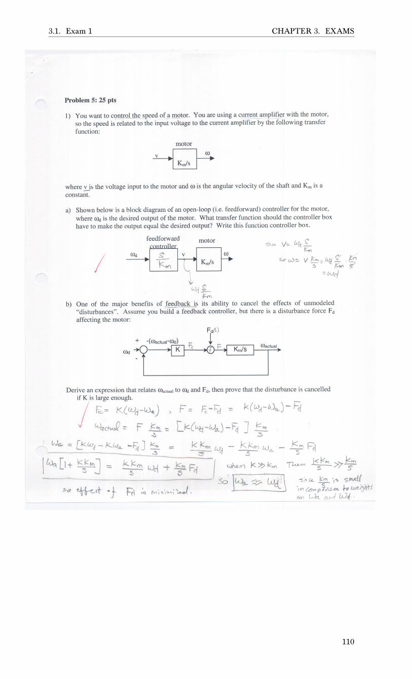
3.1. Exam 1 CHAPTER 3. EXAMS
Problem 5: 25 pts
1) You want to control the ~pee(of a motor. You are using a current ampli(kr with the motor,so the speed is related to the input voltage to the current amplifier by the following transferfunction:
motor
v 00
Kn/s
where v is the voltage input to the motor and rois the angular velocity of the shaft and Kmis a.--.constant.
a) Shown below is a block diagram of an open-loop (Le. feedforward) controller for the motor,where COdis the desired output of the motor. What transfer function should the controller boxhave to make the output equal the desired output? Write this function controller box.
feedforward
/00
motor
-Wcj~
~fr\
b) One of the major benefits of feedback is its ability to cancel the effects of unmodeled,"disturbances". Assume you build a feedback controller, but there is a disturbance force Fdaffecting the motor:
OOactual
Derive an expression that relates COactualto COdand Fd, then prove that the disturbance is cancelledif K is large enough.
I Fc.= K( lVd-tU.J ) F '" ~-J:;, = k ((,)r 0'" )- 1=iJLAJ~c~ = F h: [k(~-J~) -~ ] h
~ ~
We.. = [!:. loq- KW(L -J:4 J kt), = k ~ h1 tv - k /(('1')kI - k ~ \; \- - -- ~ _ __ _ _ ..:!I :5'" ~ .s a.. ~
\ ~ [It k;:] '" k;", ~~ ~" Gi ( ~/<.»kM, ~ 1<;" >7 ~..,
. So 1L0o.. ~ Wcl ~ ' -s ,> "- ~'" ',s slM!/IY\~,,~'~d)\ ~ wetjhtJ6\'1 ~ 0."'';/))4 .- - -- --
110

3.2. final exam (design) CHAPTER 3. EXAMS
3.2 nal exam (design)
Local contents3.2.1 Question . . . . . . . . . . . . . . . . . . . . . . . . . . . . . . . . . . . . . . . . 1113.2.2 Detailed description . . . . . . . . . . . . . . . . . . . . . . . . . . . . . . . . . 1123.2.3 key solution . . . . . . . . . . . . . . . . . . . . . . . . . . . . . . . . . . . . . . 1143.2.4 my solution . . . . . . . . . . . . . . . . . . . . . . . . . . . . . . . . . . . . . . 116
3.2.1 Question
MAE 106 Mechanical Systems LaboratoryWinter 2005 Design Exam
You have been hired as a control engineering consultant for ~SCAR, the car racing organization. Yourjob is to design a control circuit for a robotic camera that will ride on a rail along the straightaw~(i.e. thestraight part of the racetrack). The camera control system will receive a measurement of the velocity froma selected car. The velocity information will come from the car's own speedometer, via a wireless link.Your job is to (ha:ke-the-cameratrac~ the c~o that television viewers worldwide can "ride along" nextto the driver on'ttrestrafgIifaway. You are given the following information:. The motor that drives the robotic camera along its track is a DC brushed motor with a current
amplifier. It produces a force on the camera in response to a voltage input with a calibratiJ>n -w 1, I
coefficientofC\ N/volt. (-<.~M r v.u.J ~-o.s:€N'~.cc:::Ml~M~ -f-r ~c.- C::fm!:-:~. The robotic camera has a mass of M. ~ =:-.11 ~ - g. =M '?(..,
. There is a tachometer on the robotic camera, which returns the linear velocity of the cal!le-I~_a~Lvoltage with a calibration coefficient of Cz volts/meter/sec -
. The robotic rail system has some static friction, which can be modeled as constant force Fr. Dynamicfriction is negligible. -
· The wirelesslinkbeginsworkingwhenth~~meters awayfromthe camera. The robotshouldWbe moving at the right speed, rigbt next to the car, after it moves Dz meters. 7'" "pe«.! ..~~... '+? e-l
. You may assume that the ~oves at a constant velocity in the straightaway, and the maximum lUv D.tvelocity that it moves at i~~ ' jplv,""". You are to design the controller with the~west gains possible)because NASCAR plans to updateyour controller next year using a computer-based system. They believe the computer-based system
will work better if the controller you design has as low-as-possible gains, because of possible time t>delays in sampling with the planned computer-based system. \j =-~_~~:::;:,i
-t:.
Design an analog circuit to control the robotic camera. You will get full credit if you:1) Show your control law, in MKS units.2) Provide appropriate control gains with units.3) Show your control law, in units of volts4) Draw an op-amp circuit that can implement your controller. Label what the inputs and outputs of your
circuit should be connected to.5) Choose appropriate values for the resistors and capacitors in your circuit.
PLEASEENTERYOURANSWERSONTHEANSWERS~ D~.~~ f\.la-c\~~n" aee +c'''''''~'.' ~ .fJYY7f!= IT -5.:>5' 5-0) S"- S:=C/CL'_- .---
D,'t"D1. D\'"t'D2.
straightaway
. CJcar fill 1)) . -;
;11II1)1-0 : '
! camera ~ ~ Railfor camera0/ Camera is tracking by this location
-- ' "'"
111

3.2. final exam (design) CHAPTER 3. EXAMS
3.2.2 Detailed description
MAE 106 Mechanical Systems Laboratory Final Project Details 2005
HOME RUN DERBY
You will design a robotic system to play baseball. You will design a robot to bat, and a robot to pitch. The setup will be:
Strike Zone
Bat
Motor
Pneumatic cylinder
Ball
Home run Home run
Foul ball Foul ball
Labjack
Control Electronics
Computer
Labjack
Control Electronics
Computer
Pitcher Motion Signal
4 feet
4 feet
4”
3 feet
The pitching robot will be a pre-built pneumatic cylinder with an integrated, with a 6” stroke length, and a linear potentiometer to sense position. The air into the cylinder will be controlled with a pneumatic servovalve. You don’t have to build the pitching robot, but you must write a Matlab computer program to control the servovalve, allowing air into the cylinder so that the pitching robot moves and pitches the ball. The interface to the cylinder will be through a Labjack. You will not be allowed to take the pneumatic cylinder, valve, or Labjack home with you. There will be several pratice fields set up in the lab for testing. You will make the batting robot using a DC brushed motor and other items in a starter kit. You can control the batting robot using an op-amp circuit, using the Labjack, or using both – it’s up to you. You can use a computer algorithm to control the batting robot, or teleoperate it with a potentiometer – it’s up to you. To help time the swing of the batting robot, it will receive a copy of the signal from the linear potentiometer on the pitching robot. You will receive a small current amplifier to use with the batting robot (the same one that you are using in Lab7). Teams: You will work in teams of two or three. If you do not have a team, email Prof. Reinkensmeyer at [email protected] and he will assign you to a team. Competition Time and Place: On the day of the scheduled final (Tuesday, March 22, 4-6 PM) there will be a tournament testing your robotic baseball player. The tournament will be held in the MAE106 Laboratory (EG 2102). Lab Hours: The lab will be open from 8-12 A.M. and 1-5 P.M. on school days starting February 28th until the contest. If the lab door is locked, you must sign-in with Dave Hartwig in room EG2118 before the lab will be opened. For safety reasons, there must always be at least two students in lab for the door to be opened for you, so bring a partner. While you are in lab, do not leave the room unattended. You are responsible for all laboratory equipment while you are in the lab. Sign-out with Dave Hartwig when you leave. Contest Rules: 1) The contest will be a single-elimination, head-to-head tournament. Two teams will take turns batting and pitching, each
getting 10 pitches. The team with the most homeruns will advance to the next round. 2) The approximate dimensions of the course are shown in the figure.
112

3.2. final exam (design) CHAPTER 3. EXAMS
3) You may not modify the mechanical structure of the pitching robot, only its software. 4) The only actuator allowed on your batting robot is the DC motor provided in your kit. 5) You will be given three minutes to set-up your robot. 6) The strike zone will be 4” wide. 7) There will be no wall in the outfield. 8) There will be a connector that can quickly plug the Labjack into your protoboard on the trainer kit. The connector will
provide 2 DA channels, 2 AD channels, ground, and the pitching signal. 9) You will receive a specification sheet describing the pneumatic cylinder and valve. 10) The batting robot must be stationary when the “pitch” signal is given (i.e. it can’t spin continuously) Starter Kits: Starter kits may be purchased from David Hartwig in EG2118 for $20 beginning Monday February 28, 8 AM – 12 PM, 1 PM – 5 PM. You may pick up the motor today. IMPORTANT!: You must return the kit in order to receive your final grade. If the motor or trainer kit is carelessly damaged, you will be required to pay for them (~$200). Other Parts: You may wish to purchase other components for your project. Suggested vendors are: • Radio Shack: 4716 Barranca Parkway, Irvine (949)552-1091 (and other locations) • Marvac Electronics: 2001 Harbor Blvd., Costa Mesa (949)650-2001 • Fry’s Electronics: 10800 Kalama River Ave., Fountain Valley (714)378-4400 (and other locations) • C&H Sales (Pasadena), Ultimate Hobbies, Hobby Shack, Gyro Hobbies, Wright Hardware • Digikey: www.digikey.com • Newark Electronics: www.newark.com Grading: The final project is worth 25% of your grade. You can score a maximum of 120 pts on your final project. Your points will be based on:
1. The performance of your robot on the day of the contest • +10 pts if you have a plausible circuit and robot, but it doesn’t work • +20 pts if your robot works • +30 pts if you finish in the final four • +40 pts if you win the competition
2. A written final project report (80 pts maximum) • The goal of the written final project report is to describe your design as clearly as possible, and the effort you put
into building and testing the robot. • One write-up should be turned in per project group. • Your final project write-up should have the following sections:
1. Overview (brief summary of the design project and your controller design) (10 pts) 2. Block diagram of the controlled system (10 pts) 3. Circuit diagrams for the circuits that you built (10 pts) 4. Equations relating circuit and block diagram to controller (10 pts) 5. Methodology for choosing controller gain values (10 pts) 6. Mechanical design features (10 pts) 7. Parts list (10 pts) 8. Testing (Any tests that you performed to calibrate/verify/improve performance -- with graphs) (10 pts)
113

3.2. final exam (design) CHAPTER 3. EXAMS
3.2.3 key solution
MAE 106 Mechanical Systems Laboratory Winter 2005 Design Exam
You have been hired as a control engineering consultant for NASCAR, the car racing organization. Your job is to design a control circuit for a robotic camera that will ride on a rail along the straightaway (i.e. the straight part of the racetrack). The camera control system will receive a measurement of the velocity from a selected car. The velocity information will come from the car’s own speedometer, via a wireless link. Your job is to make the camera track the car, so that television viewers worldwide can “ride along” next to the driver on the straightaway. You are given the following information: • The motor that drives the robotic camera along its track is a DC brushed motor with a current
amplifier. It produces a force on the camera in response to a voltage input with a calibration coefficient of C1 N/volt.
• The robotic camera has a mass of M. • There is a tachometer on the robotic camera, which returns the linear velocity of the camera as a
voltage with a calibration coefficient of C2 volts/meter/sec • The robotic rail system has some static friction, which can be modeled as constant force Ff. Dynamic
friction is negligible. • The wireless link begins working when the car is D1 meters away from the camera. The robot should
be moving at the right speed, right next to the car, after it moves D2 meters. • You may assume that the car moves at a constant velocity in the straightaway, and the maximum
velocity that it moves at is S. • You are to design the controller with the lowest gains possible, because NASCAR plans to update
your controller next year using a computer-based system. They believe the computer-based system will work better if the controller you design has as low-as-possible gains, because of possible time delays in sampling with the planned computer-based system.
Design an analog circuit to control the robotic camera. You will get full credit if you: 1) Show your control law, in MKS units. 2) Provide appropriate control gains with units. 3) Show your control law, in units of volts 4) Draw an op-amp circuit that can implement your controller. Label what the inputs and outputs of your
circuit should be connected to. 5) Choose appropriate values for the resistors and capacitors in your circuit. PLEASE ENTER YOUR ANSWERS ON THE ANSWER SHEET
D2 D1
camera
car
straightaway
Rail for camera
Camera is tracking by this location
114

3.2. final exam (design) CHAPTER 3. EXAMS
115

3.2. final exam (design) CHAPTER 3. EXAMS
3.2.4 my solution
Home Run Derby.
Final project report. MAE 106. UCI. Winter 2005.
By Nasser Abbasi
March 22, 2005
Table of contents
1 OVERVIEW......................................................................................................................................................... 2
2 BLOCK DIAGRAMS OF THE CONTROLLED SYSTEM ........................................................................... 4
2.1 PITCHER CONTROLLER BLOCK DIAGRAM ........................................................................................................ 4 2.2 BATTER CONTROLLER BLOCK DIAGRAM ......................................................................................................... 4
3 CIRCUIT DIAGRAMS ....................................................................................................................................... 5
4 EQUATIONS USED ............................................................................................................................................ 7
5 METHODOLOGY USED ................................................................................................................................... 9
5.1 PITCHER CONTROLLER LOGIC ......................................................................................................................... 9 5.2 BATTER CONTROLLER LOGIC .......................................................................................................................... 9
5.2.1 Batter controller steps diagram ........................................................................................................... 10 5.2.2 Batter controller algorithm .................................................................................................................. 11
6 MECHANICAL DESIGN FEATURES ........................................................................................................... 12
6.1 GEOMETRY AND DIMENSIONS OF THE PLAYING FIELD................................................................................... 12 6.2 GEOMETRY AND DIMENSIONS OF THE BATTING MOUNTING .......................................................................... 13
7 PARTS LIST ...................................................................................................................................................... 14
8 TESTING WITH GRAPHS .............................................................................................................................. 15
8.1 EXAMPLE OUTPUT OF ONE TEST RUN ............................................................................................................ 16
9 APPENDIX ........................................................................................................................................................ 17
9.1 BATTER CONTROLLER MATLAB CODE .......................................................................................................... 17 9.1.1 nma_motor_auto.m .............................................................................................................................. 17 9.1.2 nma_motor_manual.m ......................................................................................................................... 19
9.2 PITCHER CONTROLLER MATLAB CODE ......................................................................................................... 19
116

3.2. final exam (design) CHAPTER 3. EXAMS
1 Overview This is the report for the final project for MAE 106 course, UCI, winter 2005.
The project objective is to design a robotic system to play baseball for the final project for MAE
106. The project description and rules can be found at professor's Reinkensmeyer web site
http://www.eng.uci.edu/~dreinken/MAE106/mae106home.htm
Below is the general setup diagram taken from the project description document found in the
above we site:
There are 2 main components to the project: the pitcher and the batter.
For both parts we used Labjack with Matlab to communicate between the PC and the
mechanical components of the project (Piston and Motor). We used Matlab as the main tool to
implement the control laws.
The basic design criteria we wanted to achieve are a fully automated and controlled batter with
no manual nor visual control. This implied the restriction on the use of a manual controller to
control the motor. We have started with the assumption that one is now allowed to use the
keyboard once the game starts.
Due to this restriction we imposed on our design, the final solution consisted of software
program where the controller was written in Matlab with heavy reliance on the LabJack Matlab
interface calls. This solution produced some technical problems on its own, since this
controller in essence in an open loop controller, we needed to have a good timing analysis
done earlier and impede these timing estimates in the controller software. In addition, the
sampling rate of Labjack was not fast enough to allow us to obtain more readings of the ball position as it is being hit by the piston; this resulted in less than optimal estimates being made
on the position of the ball. Since it is not possible to track the position of the ball itself,
implementing a feedback control system based on tracking the ball position is not possible
(this would have been the optimal solution).
On the pitcher side, we controlled the speed of the piston by adjusting the voltage delivered to
the piston actuator.
117

3.2. final exam (design) CHAPTER 3. EXAMS
On the batter side (which was the more complicated controller), we detect when the ball was hit
and at what speed, this in turn correlated to the amount of time delay before we issue the signal to start the motor to swing the bat. We also added logic to the bat controller to avoid
attempting to hit balls with low enough speed which we calculated earlier (by running many
tests) to be at such low speeds that the ball will most likely not be arriving in a straight line
and hence will not hit the strike zone.
In addition, on the batter side, we added a mechanical stop mounted on the motor to be able to set the initial position of the bat to be at a fixed location before the start of each swing. This
was critical to the mechanical design of our batter, since the bat controller is an open loop;
hence having accurate timings is the most important aspect (by definition, an open loop
contains no feedback and must rely on initial accurate timings). Hence, being able to set the
bat at a fixed location before each swing allowed us to achieve this objective.
118

3.2. final exam (design) CHAPTER 3. EXAMS
2 Block diagrams of the controlled system
2.1 Pitcher controller block diagram The pitcher is an open loop proportional controller with a gain of one. The desired voltage is
supplied, and the controller simply interfaces with Labjack to send this voltage to the piston
(the plant). We add logic to the controller to add some delay and to move the piston back and
forth before the voltage signal is send to the piston (the plant) to try to confuse the batter
controller, but the final voltage send to the piston is the same as the desired voltage.
2.2 Batter controller block diagram The batter is also an open loop proportional controller with a gain of one. The input to the
batter controller is fixed at 5 volts (which is the maximum voltage labjack can send). This voltage moves the motor head at the maximum speed.
Initially we wanted the controller to control the speed of the motor. For fastballs, we wanted to
speed up the motor, and for slow balls we wanted to slow down the motor.
However, after some testing, we discovered that the current amplifier we were given to use on
this project was not designed for this purpose, it was only able to generate a constant current
to run the motor at the same speed regardless of the voltage that was sent to it. (Actually the
motor would run at a fixed low speed for voltages below 4 volts, and at fixed high speed for
voltages over 4, but the point is that it was not possible to change the speed of the motor in
direct proportion of the voltage being sent to the current amplifier we used)
For this reason, we designed the controller to delay more for slow balls and to delay less for fast
ones, but to run the motor at the same speed for both cases. The block diagram for this open
loop controller is shown below. In this diagram we show how the controller reads the piston
head position signal from the piston in order to decide when to issue the command to the motor to start.
119

3.2. final exam (design) CHAPTER 3. EXAMS
3 Circuit diagrams The following diagram shows the full hardware configuration used with all the connections
needed at the batter side
120

3.2. final exam (design) CHAPTER 3. EXAMS
The batter reads the piston position signal as it arrives at the AI0 port of labjack. The following diagram combines both the pitcher and the batter circuits to better illustrate how the
connection is achieved.
121

3.2. final exam (design) CHAPTER 3. EXAMS
4 Equations used Since the controller we used is a proportional controller with fixed gain of one, the control law
is obviously very simple. However, the complexity came about in determining the amount of
delay and in the calculation of the ball speed and in forcing labjack to use a fixed sampling rate
so that our calibration will remain valid across different play stations.
So in what follows we describe how we performed the calibration.
We used a linear relation between the speed of the ball when it was hit and the amount of delay
required before we swing the bat. We performed many experiments, hitting the ball at different
speeds and determined the amount of delay needed to obtain a good swing for this speed (Please see the testing section for additional data on this).
The result of this testing is a number of data points. We then did a linear straight-line fit of the
data and obtained the equation of the line. This line equation was used by the controller to
determine the time delay needed based on the ball speed.
THE LINE EQUATION
cxmy
Used in the controller is
516
03.0525.
speeddelay
In the above we assumed that the ball speed does not change greatly from the time the
controller detected that the ball was hit until the time the ball arrives to the strike zone. Since the distance between the pitcher and the batter is small (three feets), and the ball is fairly
smooth, this assumption is reasonable. In addition, the actual speed calculation itself is not
very accurate due to the low sampling rate used by Labjack, which did not allow us to obtain
more accurate estimates of the ball speed.
The speed of the ball was calculated as follows. The batter controller monitors the position of
the piston head continuously by reading the piston head position signal which can vary from 0
volts upto 10 volts. The ball is situated half way between a fully extended and fully contracted
piston. Hence a voltage reading of around 5 volts will indicate that the piston has hit the ball.
122

3.2. final exam (design) CHAPTER 3. EXAMS
The batter controller keeps track of the last 2 positions read from the piston and the amount of
time elapsed between these 2 readings.
When it detects that the piston position has passed the half way mark, indicating that the ball
was hit, it will calculate the speed using the equation
dtimeElapse
onLastPositiitioncurrentPosspeed
This value is then substituted in the delay equation discussed above to give the amount of
delay in seconds needed before starting the motor.
In addition to the above, the batter controller will check if the speed of the ball is below a
certain threshold. If so, the batter will not turn the motor in this case. The reason for this is
that we found by experimentations that a slow ball will most likely not remain in a straight line
and will not arrive to the strike zone. Hence we did not want to take the chance on trying to hit a ball that is going out anyway and losing a point. This will maximize our chances of winning.
This threshold is currently set at 52 m/s.
123

3.2. final exam (design) CHAPTER 3. EXAMS
5 Methodology used We will consider the pitcher side and the batter side separately.
5.1 Pitcher controller logic The logic of the pitcher controller is simple. We apply voltage, which causes the piston head to
move. A voltage over 2.5 will move the head forward, and voltage below 2.5 will move the head
backwards. We varied the speed we hit the ball at, and also moved the piston back and forth
before hitting the ball in order to try to confuse the batter controller.
5.2 Batter controller logic We have build 2 mountings on top of the motor mounting. One mounting to attach the bat, and another to attach a mechanical stop.
Controller starts by swinging the bat handle to the initial position, this will cause the bat
handle to hit the mechanical stop mounting attached to the motor mounting. Immediately, the
motor will stall, drawing current but not moving.
The controller will next turn the voltage off the motor and waits for the ball to be hit by the
pitcher. The Batter controller continuously monitors the ball position signal coming from the
pitcher.
The batter controller monitors the position of the piston head and calculates its speed after each sample reading using Labjack Matlab function calls.
When the batter controller detects that the position of the piston head has hit the ball (recall
that the ball is located at a fixed position), then the speed of the ball will be known at that
moment. It will be the speed of the piston head.
From the speed of the ball, the batter controller decides when to start the bat swing. The
controller will always swing the bat at the maximum (5 volts) level motor speed.
The controller knows when to start the swing by a calibration process that we have performed
prior to the start of the tournament. During calibration we did a number of runs and derived a line equation that allowed the controller to determine the delay needed given the speed of the
ball.
Since the batter always starts from the same position (due to the use of the mechanical stop),
this process resulted in a reasonable accurate swings designed to hit the ball at 90 degrees to the direction of the ball to obtain the maximum force on the ball.
At the end of each swing the bat handle will hit the mechanical stop on the other side, causing
the motor to stall again. Controller will switch the voltage sign again, causing the bat to quickly
swing back, hitting the mechanical stop again from the other side, and resting there until the
next pitch.
This process will continue automatically. To help illustrate this process, the following diagram
shows the main steps for the batter controller.
124

3.2. final exam (design) CHAPTER 3. EXAMS
5.2.1 Batter controller steps diagram
125

3.2. final exam (design) CHAPTER 3. EXAMS
5.2.2 Batter controller algorithm
We have used Matlab to implement the batter controller logic. The following is the algorithm for
this controller.
LOOP
reverse motor voltage to swing clockwise to hit the mechanical
stop.
start reading the piston signal -- use LABKACK Matlab call.
Calculate the position and speed of the piston head.
WHILE piston has not hit the ball
read next sample from the piston signal
update position and speed of the piston.
END WHILE
determine delay needed based on ball speed. (use linear fitting)
pause the delay needed.
issue a control signal to the motor to swing at maximum speed.
delay for known amount of time (calibrated) to allow bat to swing
fully.
END LOOP
126

3.2. final exam (design) CHAPTER 3. EXAMS
6 Mechanical design features
6.1 Geometry and dimensions of the playing field
To be able to build the mounting for the bat handle and the bat itself, we needed exact
dimensions of the playing field.
127

3.2. final exam (design) CHAPTER 3. EXAMS
6.2 Geometry and dimensions of the batting mounting The dimensions of the batting and mechanical stop mounting are shown below. We initially
designed the mounting to allow us to add a potentiometer if we had to.
128

3.2. final exam (design) CHAPTER 3. EXAMS
7 Parts list Pittman DC gearhead motor P/N GM8714F560
Series SRX stainless Steel body air cylinders with position feedback.
Motor mounting (The size and dimensions are provided to us by the instructor).
Mechanical stop mounting L-shaped.
One mechanical bat arm to hit the ball with.
2 LU12 labjack’s with USB connection.
2 PC’s running windows and Matlab
One current amplifier.
A number of wires to connect current amplifier to motor and to labjack
2 screws and bolts to attach the motor mounting to the table.
Power supply for the current amplifier (we used +12V DC provided by the training kit).
129

3.2. final exam (design) CHAPTER 3. EXAMS
8 Testing with graphs
Since we implemented an open loop controller for the batter, most of the testing concentrated
on calibration of the bat controller. We needed to able to estimate the amount of delay before a
swing based on the speed of the ball. To accomplish this, as we discussed above in the methodology section, we ran many tests and collected many data points. This is a partial
listing of data collected for calibration.
Voltage to piston
(Volts)
Calculated speed of ball (speed
units)
Amount of delay needed
(milliseconds)
4 51.04 79
49.97 81
55.60 75
61.52 69
56.07 74
3.9 50.26 80
52.03 78
49.25 81
52.92 78
52.76 82
3.8 53.08 83
47.52 84
56.00 83
For each piston voltage, the average of the speed was taken and the average of the amount of
the delay needed was also taken. This resulted in a number of yx, data points that we fitted
a straight line through to obtain the line equation.
We also needed to fix the sampling rate of Labjack, and for this purpose we used one Labjack Matlab call that allowed us to specify the sampling rate to be used. Instead of using the
standard call EAnalogIn() to read the piston position signal from AI0, we used the call AIBurst
that also can read AI0, but in addition allowed us to specify a scan rate from 400 up to 8192
hz. We used 8192 Hz to be able to avoid the possibility of having one labjack running at
different sampling rates at different play stations.
130

3.2. final exam (design) CHAPTER 3. EXAMS
8.1 Example output of one test run When the bat controller runs, it continuously displays basic results showing the speed of the
ball being hit and the amount of delay. It will also show if the ball we is too slow, which in this
case the batter will not attempt to hit. These messages made it easier to debug and calibrate the program. Below is such example output
>> nma_motor
detected ball was hit.....
elapsedTime=62.000000 ms
last position=2.153320, currentPosition=5.410156
speed=52.529612
delay=0.517352
**************************************
detected ball was hit.....
elapsedTime=63.000000 ms
last position=2.211914, currentPosition=5.048828
speed=45.030382
delay=0.554848
ball too slow, will not try to hit...
**************************************
detected ball was hit.....
elapsedTime=64.000000 ms
last position=2.192383, currentPosition=5.668945
speed=54.321289
delay=0.508394
**************************************
detected ball was hit.....
elapsedTime=67.000000 ms
last position=4.619141, currentPosition=8.447266
speed=57.136194
delay=0.494319
**************************************
131

3.2. final exam (design) CHAPTER 3. EXAMS
9 Appendix In the appendix we show the Matlab code used for the bat and pitcher controller.
9.1 Batter controller Matlab code For the batter it was not clear if the rules of the game allow one to touch the keyboard once the
game starts.
For this reason, we have 2 versions of the bat program. One is called nma_motor_auto.m, and the other is called nma_motor_manual.m.
The first program above is the one discussed in details in this report, since it is the fully
automated version and requires no manual intervension once it starts. The second version is a
modified version that requires the user to hit the keyboard to start the motor running resulting is the bat moving.
Below is the code for both version of the controller.
9.1.1 nma_motor_auto.m %
% MAE Final project. UCI, winter 2005
% motor controller script.
% by Nasser Abbasi
%
% This script implements the open loop bat controller
% See the project report for background information
% about this project.
%
% define some constants used in the program
LEFT=5;
RIGHT=0;
HIGH_V=5;
LOW_V=0;
DEBUG=1;
TRUE=1;
FALSE=0;
BALL_POSITION=5;
SAMPLE_RATE=8192; %Hz
LOW_SPEED_THRESHOLD=0;
SLOPE=(0.25-0.12)/(65.33-51);
pistonLastPosition=0; %set the piston last position to be fully retracted
132

3.2. final exam (design) CHAPTER 3. EXAMS
while TRUE
EAnalogOut(0,0,HIGH_V,RIGHT); %set the handle
pause(0.1); %wait to reach mechanical stop.
EAnalogOut(0,0,LOW_V,RIGHT); %turn off motor
BallHit=FALSE;
[count tnow err id]=ECount(0,0,0);
while ~BallHit
% replace the call below by AIBurst. To allow better control
% on the sampling rate.
% [currentPosition o err id]=EAnalogIn(0,0,0,0);
tlast=tnow;
[pistonCurrentPosition s scans over err id]=…
AIBurst(0,0,0,0,0,1,0,0,SAMPLE_RATE,0,0,0,1,1,0);
if err~=0
fprintf('Failed AIBusrt call. error is %s\n',GetErrorString(err));
return;
end
[count tnow err id]=ECount(0,0,0);
%if DEBUG fprintf('currentPosition=%f\n',currentPosition); end;
%if DEBUG fprintf('tnow=%f, tlast=%f\n',tnow,tlast); end;
% if(DEBUG)
% if(currentPosition>2) fprintf('currentPosition=%f\n',currentPosition); end
% end
if(pistonCurrentPosition>BALL_POSITION)
if pistonLastPosition<=BALL_POSITION
if DEBUG fprintf('detected ball was hit by piston.....\n'); end;
elapsedTime=tnow-tlast;
fprintf('elapsedTime=%f ms\n',elapsedTime);
speed=(pistonCurrentPosition-pistonLastPosition)*1000/elapsedTime;
if DEBUG fprintf('ball speed=%f\n',speed); end;
fprintf('piston last position=%f, piston currentPosition=%f\n',...
pistonLastPosition,pistonCurrentPosition);
if speed>LOW_SPEED_THRESHOLD
BallHit=TRUE;
else
fprintf('ball too slow, will not try to hit...\n*********************\n');
end
end
end
pistonLastPosition=pistonCurrentPosition;
end %while waiting for ball to be hit
if(speed<51)
delay=0.25+SLOPE*(51-speed);
else
delay=0.25-SLOPE*(speed-51);
end
if DEBUG fprintf('motor delay=%f\n',delay); end;
pause(delay);
EAnalogOut(0,0,HIGH_V,LEFT); %HIT the ball.
pause(0.5); %wait for bat to reach mechanical stop.
EAnalogOut(0,0,LOW_V,LEFT); %stop the motor
fprintf('**************************************\n');
end
133

3.2. final exam (design) CHAPTER 3. EXAMS
9.1.2 nma_motor_manual.m
%
% MAE Final project. UCI, winter 2005
% motor controller script.
% by Nasser Abbasi
%
% This script implements the open loop bat controller
% for the manual version of the batter,
%
% See the project report for background information
% about this project.
%
% define some constants used in the program
LEFT=5;
RIGHT=0;
HIGH_V=5;
LOW_V=0;
DEBUG=1;
TRUE=1;
FALSE=0;
while TRUE
EAnalogOut(0,0,HIGH_V,RIGHT); %set the handle
pause(0.1); %wait to reach mechanical stop.
EAnalogOut(0,0,LOW_V,RIGHT); %turn off motor
fprintf('hit any key to turn bat.....\n');
pause;
EAnalogOut(0,0,HIGH_V,LEFT); %HIT the ball.
pause(0.5); %wait for bat to reach mechanical stop
EAnalogOut(0,0,LOW_V,LEFT); %stop the motor
End
9.2 Pitcher controller Matlab code
EAnalogOut(0,0,5,0);
EAnalogOut(0,0,0,0);
Attached floppy disk contains more examples of the pitcher code and the code for the batter.
This is the content of the flopy disk attached showing all the matlab .m files used.
134

3.2. final exam (design) CHAPTER 3. EXAMS
135

3.2. final exam (design) CHAPTER 3. EXAMS
136

Chapter 4
Other class material
Local contents4.1 Lab jack U21 user guide . . . . . . . . . . . . . . . . . . . . . . . . . . . . . . . . 1384.2 Professor Reinkensmeyer lecture notes given during class . . . . . . . . . . . . 2034.3 Professor Bobrow lecture notes given to use as reference . . . . . . . . . . . . . 2274.4 OLd exam to practice from . . . . . . . . . . . . . . . . . . . . . . . . . . . . . . 296
137

4.1. Lab jack U21 user guide CHAPTER 4. OTHERCLASSMATERIAL
4.1 Lab jack U21 user guide
LabJack U12 User’s Guide
Revision 1.09 12/22/2004
LabJack Corporation
www.labjack.com [email protected]
138

4.1. Lab jack U21 user guide CHAPTER 4. OTHERCLASSMATERIAL
For the latest version of the user’s guide, the quickstart guide, or software, go to www.labjack.com. The LabJack U12 is a measurement and automation peripheral that enables the connection of a PC to the real-world. Although the LabJack U12 has various redundant protection mechanisms, it is possible, in the case of improper and/or unreasonable use, to damage the LabJack and even the PC to which it is connected. LabJack Corporation will not be liable for any such damage. The LabJack U12 and associated products are not designed to be a critical component in life support or systems where malfunction can reasonably be expected to result in personal injury. Customers using these products in such applications do so at their own risk and agree to fully indemnify LabJack Corporation for any damages resulting from such applications. LabJack assumes no liability for applications assistance or customer product design. Customers are responsible for their applications using LabJack products. To minimize the risks associated with customer applications, customers should provide adequate design and operating safeguards. Reproduction of products or written or electronic information from LabJack corporation is prohibited without permission. Reproduction of any of these with alteration is an unfair and deceptive business practice. Copyright 2004, LabJack Corporation
ii
139

4.1. Lab jack U21 user guide CHAPTER 4. OTHERCLASSMATERIAL
Table Of Contents 1. Installation ................................................................................................................................1
1.1 Hardware Installation..........................................................................................................1 1.2 Software Installation ...........................................................................................................1
2. Hardware Description...............................................................................................................3 2.1 AI0 – AI7.............................................................................................................................4 2.2 AO0 & AO1.........................................................................................................................7 2.3 IO0 – IO3............................................................................................................................7 2.4 D0 – D15 ............................................................................................................................8 2.5 CNT ....................................................................................................................................9 2.6 CAL – STB..........................................................................................................................9 2.7 +5V .....................................................................................................................................9 2.8 GND..................................................................................................................................10 2.9 OEM Versions ..................................................................................................................10
3. Example Applications.............................................................................................................11 3.1 LJconfig ............................................................................................................................11 3.2 LJcounter..........................................................................................................................12 3.3 LJfg...................................................................................................................................13 3.4 LJlogger............................................................................................................................14 3.5 LJscope ............................................................................................................................18 3.6 LJstream...........................................................................................................................19 3.7 LJtest ................................................................................................................................21 3.8 LJSHT...............................................................................................................................23 3.9 LJSHTmulti .......................................................................................................................24
4. Programming Reference........................................................................................................25 4.1 EAnalogIn .........................................................................................................................26 4.2 EAnalogOut ......................................................................................................................26 4.3 ECount..............................................................................................................................27 4.4 EDigitalIn ..........................................................................................................................27 4.5 EDigitalOut .......................................................................................................................28 4.6 AISample ..........................................................................................................................28 4.7 AIBurst..............................................................................................................................30 4.8 AIStreamStart ...................................................................................................................32 4.9 AIStreamRead..................................................................................................................34 4.10 AIStreamClear ................................................................................................................35 4.11 AOUpdate.......................................................................................................................35 4.12 AsynchConfig .................................................................................................................36 4.13 Asynch............................................................................................................................38 4.14 BitsToVolts .....................................................................................................................39 4.15 VoltsToBits .....................................................................................................................40 4.16 Counter...........................................................................................................................40 4.17 DigitalIO..........................................................................................................................41 4.18 GetDriverVersion ............................................................................................................42 4.19 GetErrorString ................................................................................................................42 4.20 GetFirmwareVersion.......................................................................................................43 4.21 GetWinVersion ...............................................................................................................43 4.22 ListAll ..............................................................................................................................44 4.23 LocalID ...........................................................................................................................45 4.24 NoThread........................................................................................................................45 4.25 PulseOut.........................................................................................................................45 4.26 PulseOutStart .................................................................................................................46 4.27 PulseOutFinish ...............................................................................................................47 4.28 PulseOutCalc..................................................................................................................48
iii
140

4.1. Lab jack U21 user guide CHAPTER 4. OTHERCLASSMATERIAL
4.29 ReEnum..........................................................................................................................48 4.30 Reset (or ResetLJ) .........................................................................................................48 4.31 SHT1X............................................................................................................................49 4.32 SHTComm......................................................................................................................50 4.33 SHTCRC.........................................................................................................................51 4.34 Synch..............................................................................................................................52 4.35 Watchdog .......................................................................................................................53 4.36 ReadMem.......................................................................................................................54 4.37 WriteMem .......................................................................................................................55 4.38 BuildOptionBits (ActiveX only)........................................................................................55 4.39 FourPack (ActiveX only) .................................................................................................56 4.40 Description of errorcodes. ..............................................................................................56
A. Specifications.........................................................................................................................59
iv
141

4.1. Lab jack U21 user guide CHAPTER 4. OTHERCLASSMATERIAL
Table Of Figures Figure 2-1. LabJack U12 top surface. ..........................................................................................3 Figure 2-2. Single-ended measurement.......................................................................................4 Figure 2-3. Differential measurement...........................................................................................5 Figure 2-4. Single-ended measurement with voltage divider circuit.............................................6 Figure 2-5. IO used to detect the state of a switch.......................................................................8 Figure 3-1. LJconfig ...................................................................................................................11 Figure 3-2. LJconfig Change Local ID........................................................................................12 Figure 3-3. LJcounter .................................................................................................................12 Figure 3-4. LJfg ..........................................................................................................................13 Figure 3-5. LJlogger ...................................................................................................................14 Figure 3-6. LJlogger Configuration.............................................................................................15 Figure 3-7. LJlogger Internet Configuration ...............................................................................15 Figure 3-8. LJlogger HTML Configuration..................................................................................16 Figure 3-9. LJlogger Trigger Configuration ................................................................................16 Figure 3-10. LJscope .................................................................................................................18 Figure 3-11. LJscope .................................................................................................................19 Figure 3-12. LJstream................................................................................................................20 Figure 3-13. LJstream Channel Configuration ...........................................................................20 Figure 3-14. LJtest .....................................................................................................................21 Figure 3-15. LJSHT....................................................................................................................23 Figure 3-16. LJSHTmulti ............................................................................................................24
v
142

4.1. Lab jack U21 user guide CHAPTER 4. OTHERCLASSMATERIAL
1. Installation The LabJack U12 requires a PC running Windows 98SE, ME, 2000, or XP. To determine your operating system version, go to Start => Settings => Control Panel => System => General and make sure the version number is 4.10.2222 or higher (Win98SE=4.10.2222, WinME=4.90.3000, Win2000=5.0.2195, WinXP=5.1.XXXX). It does not matter if the hardware or software is installed first. If you experience installation problems on Windows 98 Second Edition, before contacting us, please go to the downloads page at labjack.com and download “win98sehid.zip” (see the readme file for more information).
1.1 Hardware Installation With the PC on and using the included cable, connect the LabJack U12 to the USB port on the PC or USB hub. The USB cable provides power and communication for the LabJack U12. The status LED should immediately blink 4 times (at about 4 Hz), and then stay off while the LabJack enumerates. Enumeration is the process where the PC’s operating system gathers information from a USB device that describes it and it’s capabilities. The low-level drivers for the LabJack U12 come with Windows and enumeration will proceed automatically. The first time a device is enumerated on a particular PC, it can take a minute or two, and Windows might prompt you about installing drivers. Accept all the defaults at the Windows prompts, and reboot the PC if asked to do so. The Windows Installation CD might also be needed at this point. Make sure a CD with the correct version of Windows is provided. Enumeration occurs whenever the USB cable is connected, and only takes a few seconds after the first time. When enumeration is complete, the LED will blink twice and remain on. This means Windows has enumerated the LabJack properly. If the LabJack fails to enumerate:
• Make sure you are running Windows OS version 4.10.2222 or higher, • Try connecting the LabJack to another PC, • Try connecting a different USB device to the PC, • Check our online forum and/or contact LabJack.
1.2 Software Installation Although, the low-level USB drivers for the LabJack are included with Windows, high-level drivers are needed to send and receive data. The included LabJack CD installs the high-level drivers, example source code, and example applications. Close all open applications, especially LabJack related software, and insert the LabJack CD. If autorun is enabled, the installation program should start automatically. If the installation does not start, you will have to manually double-click on LabJackVXXX.exe. When the LabJack installation is finished, it will start the National Instruments LabVIEW Run-Time Engine (LVRTE) setup. The LVRTE is required for the example applications such as LJtest. If prompted to reboot after this installation, go ahead and do so. Virus scanners can
1
143

4.1. Lab jack U21 user guide CHAPTER 4. OTHERCLASSMATERIAL
often interfere with the installation of the LVRTE. If you have trouble running the example applications, repeat the LabJack software installation to make sure the LVRTE is installed. To test the installation, start LJtest by selecting Start => Programs => LabJack => LJtest. Make sure “Test Fixture Installed” and “Continuous” are not selected, and press the “Run” button. LJtest will step through 8 separate tests and all should pass.
2
144

4.1. Lab jack U21 user guide CHAPTER 4. OTHERCLASSMATERIAL
2. Hardware Description The external features of the LabJack U12 are:
• USB connector, • DB25 digital I/O connector, • Status LED, • 30 screw terminals.
The USB connection provides power and communication. No external power supply is needed. The +5 volt connections available at various locations are outputs, do not connect a power supply.
Figure 2-1. LabJack U12 top surface.
Figure 2-1 shows the top surface of the LabJack U12. Not shown is the USB and DB25 connector, which are both on the top edge. The DB25 connector provides connections for 16 digital I/O lines, called D0-D15. It also has connections for ground and +5 volts. All connections besides D0-D15, are provided by the 30 screw terminals shown in Figure 1. Each individual screw terminal has a label, AI0 through STB. The status LED blinks 4 times at power-up, and then blinks once and stays on after enumeration (recognition of the LabJack U12 by the PC operating system). The LED also blinks during burst and stream operations, unless disabled. The LED can be enabled/disabled through software using the functions AISample, AIBurst, or AIStreamStart. Since the LED uses 4-5 mA of current, some users might wish to disable it for power-sensitive applications.
3
145

4.1. Lab jack U21 user guide CHAPTER 4. OTHERCLASSMATERIAL
2.1 AI0 – AI7 Hardware The LabJack U12 has 8 screw terminals for analog input signals. These can be configured individually and on-the-fly as 8 single-ended channels, 4 differential channels, or combinations in between. Each input has a 12-bit resolution and an input bias current of ±90 µA.
• Single-Ended: The input range for a single-ended measurement is ±10 volts. • Differential channels can make use of the low noise precision PGA to provide gains up
to 20. In differential mode, the voltage of each AI with respect to ground must be between +20 and -10 volts, but the range of voltage difference between the 2 AI is a function of gain (G) as follows:
G=1 ±20 volts G=2 ±10 volts G=4 ±5 volts G=5 ±4 volts G=8 ±2.5 volts G=10 ±2 volts G=16 ±1.25 volts G=20 ±1 volt
The reason the range is ±20 volts at G=1 is that, for example, AI0 could be +10 volts and AI1 could be -10 volts giving a difference of +20 volts, or AI0 could be -10 volts and AI1 could be +10 volts giving a difference of -20 volts. The PGA (programmable gain amplifier, available on differential channels only) amplifies the AI voltage before it is digitized by the A/D converter. The high level drivers then divide the reading by the gain and return the actual measured voltage. Figure 2-2 shows a typical single-ended connection measuring the voltage of a battery. This same measurement could also be performed with a differential connection to allow the use of the PGA. In general, any single-ended measurement can be performed using a differential channel by connecting the voltage to an even-numbered analog input, and grounding the associated odd-numbered analog input (as shown by the dashed connection to AI1 in Figure 2-2).
Figure 2-2. Single-ended measurement.
Figure 2-3 shows a typical differential connection measuring the voltage across a current shunt. A differential connection is required when neither leg of the shunt is at ground potential. Make sure that the voltage of both AI0 an AI1 with respect to ground is within ±10 volts. For instance, if the source (Vs) shown in Figure 2-3 is 120 VAC, the difference between AI0 and AI1 might be
4
146

4.1. Lab jack U21 user guide CHAPTER 4. OTHERCLASSMATERIAL
small, but the voltage from both AI0 and AI1 to ground will have a maximum value near 170 volts, and will seriously damage the LabJack. Whether or not the ground (GND) connection is needed (Figure 2-3) will depend on the nature of Vs.
Figure 2-3. Differential measurement.
Figure 2-4 shows a single-ended connection used to measure the output voltage of a typical voltage-divider circuit. The voltage divider circuit is a simple way to convert a varying resistance (thermistor, photoresistor, potentiometer, etc.) to a varying voltage. With nothing connected to Va, the value of the unknown resistance, R2, can be calculated as: R2 = Va*R1 / (Vs-Va), where Vs is the supply voltage (+5V in Figure 2-4). When Va is connected to AI0, as shown in Figure 2-4, the input bias current of the LabJack affects the voltage divider circuit, and if the resistance of R1 and R2 is too large, this effect must be accounted for or eliminated. This is true for any signal with too high of a source impedance. All measuring devices have maximum analog input bias currents that very from picoamps to milliamps. The input bias current of the LabJack U12’s analog inputs varies from +70 to -94 microamps (µA). This is similar to an input impedance of about 100 kΩ, but because the current is nonzero at 0 volts, it is better to model the analog input as a current sink obeying the following rule: Iin = 8.181*Va – 11.67 µA
5
147

4.1. Lab jack U21 user guide CHAPTER 4. OTHERCLASSMATERIAL
Figure 2-4. Single-ended measurement with voltage divider circuit.
Because the input bias current is known, as a function of input voltage, the simple voltage divider equation can be modified as follows to account for input bias current: R2 = Va / [((Vs-Va)/R1) – (8.181µ * Va) + 11.67µ] As an alternative to the equation above, Va can be buffered by a single-supply rail-to-rail operational amplifier, and the original simple voltage divider equation can be used. This solution works for any single-ended signal which stays between 0 and +5 volts. Some op-amp choices are:
• TLV2462 • LMC6482 • MAX4166
Software Readings from the analog inputs are returned by the functions EAnalogIn, AISample, AIBurst, and AIStreamRead. EAnalogIn is a simplified (E is for easy) function that returns a single reading from 1 analog input channel. Execution time is up to 20 ms. AISample returns a single reading of 1-4 channels, and takes up to 20 ms to execute, providing a maximum date rate of about 50 Hz per channel. AIBurst acquires multiple samples of 1-4 channels at a hardware-timed sample rate of 400-8192 Hz. The acquisition can be triggered based on a change of state on IO0 or IO1. This function also returns the states of the IO pins (which are read every 4 samples). Internally, the actual number of samples collected and transferred by the LabJack during an AIBurst call is the smallest power of 2, from 64 to 4096, which is at least as big as numSamples. The execution time of this function, in milliseconds, can be estimated as: Turbo (default) => 30+(1000*numSamplesActual/sampleRate)+(0.4*numSamplesActual) Normal => 30+(1000*numSamplesActual/sampleRate)+(2.5*numSamplesActual) numSamples = numScans * numChannels sampleRate = scanRate * numChannels
6
148

4.1. Lab jack U21 user guide CHAPTER 4. OTHERCLASSMATERIAL
AIStreamRead is called periodically during a stream acquisition started by AIStreamStart. Each call retrieves multiple samples of 1-4 channels from the LabJack stream buffer, along with the states of the IO pins (read every 4 samples). Hardware-timed sample rates of 200-1200 Hz are available. If any function besides AIStreamRead is called while a stream is in progress, the stream will be stopped.
2.2 AO0 & AO1 The LabJack U12 has 2 screw terminals for analog output voltages. Each analog output can be set to a voltage between 0 and the supply voltage (+5 volts nominal) with 10-bits of resolution. The output voltage is ratiometric with the +5 volt supply (+5V), which is generally accurate to ±5% (see Appendix A). If an output voltage of 5 volts is specified, the resulting output will be 100% of the supply voltage. Similarly, specifying 2.5 volts actually gives 50% of the supply voltage. The maximum output voltage is almost 100% of +5V at no-load, and decreases with load. See the specifications in Appendix A relating to maximum output voltage. Also note that loading either analog output will cause an IR drop through the source impedance of each. If improved accuracy is needed, measure the +5 volt supply with an analog input channel, and the actual output voltage can be calculated. For instance, if an analog output of 2.5 volts is specified and a measurement of +5V returns 5.10 volts, the actual output voltage is 2.55 volts (at no-load). Alternatively (and preferably), the analog output can itself be measured with an analog input. There is a 1st order low-pass filter on each analog output with a 3dB frequency around 22 Hz. The analog outputs are initialized to 0.0 volts on power-up or reset. The analog outputs can withstand a continuous short-circuit to ground, even when set at maximum output. Voltage should never be applied to the analog outputs, as they are voltage sources themselves. In the event that a voltage is accidentally applied to either analog output, they do have protection against transient overvoltages such as ESD (electrostatic discharge) and continuous overvoltage of a couple volts. An applied voltage that exceeds the capability of this protection will most likely damage the resistor R63 (AO0) or R62 (AO1) on the LabJack U12 PCB. The symptom of such a failure would be reduced voltage from the analog outputs, particularly at load, and could be verified by measuring the resistance of R62/R63 (should be less than 50 ohms but a damaged resistor will measure higher). A simple repair for such damage is to remove the damaged resistor and simply make a short with a blob of solder. Software The analog outputs are set using the function EAnalogOut (easy function) or AOUpdate, which take up to 20 ms to execute, providing a maximum update rate of about 50 Hz per channel. AOUpdate also controls/reads all 20 digital I/O and the counter.
2.3 IO0 – IO3 Connections to 4 of the LabJack’s 20 digital I/O are made at the screw terminals, and are referred to as IO0-IO3. Each pin can individually be set to input, output high, or output low. These 4 channels include a 1.5 k Ω series resistor that provides overvoltage/short-circuit protection. Each channel also has a 1 MΩ resistor connected to ground.
7
149

4.1. Lab jack U21 user guide CHAPTER 4. OTHERCLASSMATERIAL
All digital I/O are set to input on power-up or reset. One common use of a digital input is for measuring the state of a switch as shown in Figure 2-5. If the switch is open, IO0 reads FALSE. If the switch is closed, IO0 reads TRUE.
Figure 2-5. IO used to detect the state of a switch.
While providing overvoltage/short-circuit protection, the 1.5 k Ω series resistor on each IO pin also limits the output current capability. For instance, with an output current of 1 mA, the series resistor will drop 1.5 volts, resulting in an output voltage of about 3.5 volts. Software The easy functions EDigitalIn or EDigitalOut are used to read or set the state of one digital line, and both take up to 20 ms to execute. The functions AOUpdate and DigitalIO are used to set the direction, set the state, and/or read the state, of each IO pin. Both of these functions take up to 20 ms to execute, providing a maximum update rate of about 50 Hz per pin. The function AISample can set/read the state of each IO, but setting the state will have no effect unless the IO have been configured as outputs using another function. The function Counter reads the state of each IO. The functions AIBurst and AIStreamRead, take a reading of the IO states and return it with the analog data. The states of the 4 IO are read simultaneously every 4 samples, providing a data rate of up to 2048 Hz per pin for burst mode, or 300 Hz per pin for stream mode. For 1 or 2 channel scans, duplicate data (4x or 2x) will be added to the read array such that the size is numScans.
2.4 D0 – D15 Connections to 16 of the LabJack’s 20 digital I/O are made at the DB25 connector, and are referred to as D0-D15. These 16 lines have no overvoltage/short-circuit protection, and can sink or source up to 25 mA each (total sink or source current of 200 mA max for all 16). This allows the D pins to be used to directly control some relays. All digital I/O are CMOS output and TTL input except for D13-D15, which are Schmitt trigger input. Each D pin has a 1 MΩ resistor connected to ground. All digital I/O are set to input on power-up or reset.
8
150

4.1. Lab jack U21 user guide CHAPTER 4. OTHERCLASSMATERIAL
DB25 Pinouts: 1: D0 6: D5 11: +5V 16: GND 21: D11 2: D1 7: D6 12: +5V 17: GND 22: D12 3: D2 8: D7 13: +5V 18: D8 23: D13 4: D3 9: NC 14: GND 19: D9 24: D14 5: D4 10: +5V 15: GND 20: D10 25: D15
These digital I/O can detect the state of a switch using the same circuit shown in Figure 2-5. Because the D pins have no overvoltage/short-circuit protection, the user must be careful to avoid damage. A series resistor can provide substantial protection for these pins (see the CB25 datasheet). The following are examples of things that could damage a D pin and/or the entire LabJack:
• Shorting a high output to ground (or any potential other than +5V). • Shorting a low output to a nonzero voltage (such as +5V). • Exceeding the voltage limits specified in Appendix A.
Software The easy functions EDigitalIn or EDigitalOut are used to read or set the state of one digital line, and both take up to 20 ms to execute. The functions AOUpdate and DigitalIO are used to set the direction, set the state, and/or read the state, of each D pin. In addition, DigitalIO also returns the current state of the direction and output registers. Both of these functions take up to 20 ms to execute, providing a maximum update rate of about 50 Hz per pin.
2.5 CNT The input connection to the 32-bit counter is made at screw-terminal CNT. The counter is incremented when it detects a falling edge followed by a rising edge. This means that if you reset the counter while your signal is low, you will not get the first count until it goes high-low-high. In situations where this first count is important, you should simply substract the initial count from the final count, rather than doing a reset. Software The functions ECount (easy function), AOUpdate, and Counter are used to reset or read the counter. If a reset is specified, the counter is read first. All of these functions take up to 20 ms to execute, providing a maximum update rate of about 50 Hz. Counter readings can also be returned in stream mode (AIStreamRead) at up to 300 Hz.
2.6 CAL – STB These terminals are used during testing and calibration. CAL is a precision 2.5 volt reference, and can be used during normal operation, but care should be taken to observe the current limits specified in Appendix A. The CAL pin is protected from ESD and overvoltage, but severe overvoltage (steady-state or transient) can damage CAL, and result in the failure of all analog inputs.
2.7 +5V The LabJack has a nominal +5 volt internal power supply. Power can be drawn from this power supply by connecting to the +5V screw-terminals, or the +5V pins on the DB25 connector. The
9
151

4.1. Lab jack U21 user guide CHAPTER 4. OTHERCLASSMATERIAL
total amount of current that can be drawn from the +5V pins, analog outputs, and digital outputs, is 450 mA for most desktop computers and self-powered USB hubs. Some notebook computers and bus-powered hubs will limit this available current to about 50 mA. The USB specification requires all hosts and hubs to have overcurrent protection. If the user puts too large a load on +5V (including a short circuit of +5V to GND) of the LabJack U12 (a USB device), the host or hub is responsible for limiting the current.
2.8 GND The GND connections available at the screw-terminals and DB25 connector provide a common ground for all LabJack functions. They are all the same. Caution should be used whenever making connections with systems that have their own power source. It is normal to connect U12 ground to other grounds to create a common reference, but the risk is that the U12 ground will become the preferred ground for the other systems and they could try to send high currents into the U12. To prevent this it is often a good idea to put a 10-100 ohm resistor (or even a fuse) in series with GND on the U12 and any grounds from active systems.
2.9 OEM Versions The LabJack U12 is also available in 2 OEM (original equipment manufacturer) versions:
• LJU12-PH: This is a populated LabJack U12 PCB with pin-headers installed (on the component side of the PCB) instead of screw-terminals. Also, the LED is installed on the component side of the PCB, so nothing is installed on the solder side.
• LJU12-NTH: This is a populated LabJack U12 PCB with no through-hole components (DB25 connector, USB connector, LED, screw-terminals). This board is meant for OEMs who solder connections directly to the PCB, or wish to install only certain connectors.
Dimensional drawings are available from the downloads page at labjack.com. Normally, nothing ships with these OEM LabJacks except for the populated PCB. All software is of course available online at labjack.com.
10
152

4.1. Lab jack U21 user guide CHAPTER 4. OTHERCLASSMATERIAL
3. Example Applications The LabJack U12 CD installs 9 example applications: LJconfig, LJcounter, LJfg, LJlogger, LJscope, LJstream, Ljtest, LJSHT, and LJSHTmulti.
• LJconfig: Lists all LabJacks connected to the USB and allows the local ID to be set on each.
• LJcounter: Reads the LabJack counter and provides the current frequency or count. • LJfg (Function Generator): Outputs basic waveforms on AO0 (analog output zero). • LJlogger: Saves data to disk, writes data to an HTML page on the Internet, and
performs various actions (including email) on trigger events. • LJscope: Simulates an oscilloscope by reading data from 2 AI channels in burst mode. • LJstream: Uses stream mode to read, graph, and write to file, 4 AI channels. • LJtest: Runs a sequence of tests on the LabJack itself. • LJSHT: Retrieves and records data from 1 or 2 EI-1050 digital temperature/humidity
probes. • LJSHTmulti: Displays data from up to 20 EI-1050 digital temperature/humidity probes.
The LabVIEW source code for most of these applications is installed in the examples directory.
3.1 LJconfig Every LabJack has a local ID and serial number. The local ID is a value between 0 and 255 that can be changed by the user. The serial number is a value between 256 and 2,147,483,647 that is unique among all LabJacks and cannot be changed by the user. LJconfig is used to set the local ID of a particular LabJack. When using multiple U12s, each should be assigned a unique local ID.
Figure 3-1. LJconfig
11
153

4.1. Lab jack U21 user guide CHAPTER 4. OTHERCLASSMATERIAL
Figure 3-1 shows the window that opens when LJconfig is run. Each time the “Refresh” button is pushed, LJconfig will scan the USB for all LabJacks. To change the local ID of a particular LabJack, push the “Change” button next to that LabJack, and the window shown in Figure 3-2 will appear.
Figure 3-2. LJconfig Change Local ID
Enter a new local ID between 0 and 255 and push the “Change” button. The new local ID will be written and the LabJack will be forced to re-enumerate.
3.2 LJcounter Reads the LabJack counter and provides the current frequency or count.
Figure 3-3. LJcounter
Figure 3-3 shows the LJcounter window: • Interval (seconds): Specifies the interval, in seconds, between calls to the DLL
function “Counter”. • Measurement Type: If set to “Frequency”, this application divides the count by the
interval to determine frequency in Hertz, and automatically resets the counter every read. If set to “Count”, the measurement is simply the current reading from the counter.
• Measurement: Displays frequency or count, depending on “Measurement Type”.
12
154

4.1. Lab jack U21 user guide CHAPTER 4. OTHERCLASSMATERIAL
3.3 LJfg This application allows the LabJack U12 to be used as a simple function generator. The DLL function “AOUpdate” is called every 25 milliseconds providing an update rate of 40 Hz, and thus a maximum reasonable signal frequency of a few Hertz.
Figure 3-4. LJfg
13
155

4.1. Lab jack U21 user guide CHAPTER 4. OTHERCLASSMATERIAL
3.4 LJlogger LJlogger sends and receives data in command/response mode by making 2 DLL calls to “AISample” and 1 DLL call to “AOUpdate”. It is capable of saving data to disk (2 Hz max) and performing various actions on trigger events.
Figure 3-5. LJlogger
The main window for LJlogger is shown in Figure 3-5. The white colored items and the “SDX” buttons are controls to be edited/selected by the user. The grey colored items are indicators which display various information about the LabJack. Clicking the button labeled “Save Panel Settings” will save the current values of the controls as the default values. If SDX is activated for a given analog input, the corresponding SDX DLL will be used to determine the scaled data. Users can make their own SDX DLLs (see the source code for more information), to provide more complex scaling or scaling that depends on other analog inputs. Clicking the “Configure” button shown in Figure 3-5 brings up the window shown in Figure 3-6:
• Working Directory: This is the directory where data and configuration files will be written.
• Data File Name: Determines the name of the data file to which data will be written. New data is appended to the end of this file.
• Data File Write Interval: Determines the interval at which a new row of data will be written to the data file. Minimum of 0.5 seconds.
• HTML Write Interval: Determines the interval at which the HTML file is rewritten.
14
156

4.1. Lab jack U21 user guide CHAPTER 4. OTHERCLASSMATERIAL
Figure 3-6. LJlogger Configuration
Clicking on the “Internet Setup” button in Figure 3-6 brings up the Internet configuration window shown in Figure 3-7. Basic customization of the HTML file can be done by clicking on “Advanced HTML Configuration” which brings up Figure 3-8. Clicking on the “Trigger Setup” button in Figure 3-6 brings up the window shown in Figure 3-9.
Figure 3-7. LJlogger Internet Configuration
15
157

4.1. Lab jack U21 user guide CHAPTER 4. OTHERCLASSMATERIAL
Figure 3-8. LJlogger HTML Configuration
Figure 3-9. LJlogger Trigger Configuration
Figure 3-9 shows 9 example triggers: • Trigger #0: If the scaled data from analog input row 7 (Figure 3-5) is greater than 5,
then set AO1 to 5 volts. Once triggered, there is a 10 second delay before it can be triggered again.
16
158

4.1. Lab jack U21 user guide CHAPTER 4. OTHERCLASSMATERIAL
• Trigger #1: If IO3 is high, set IO2 high. Reset delay is zero so this trigger can occur every iteration (every 0.1 seconds) if IO3 is high.
• Trigger #2: If D15 is low, set D14 low. • Trigger #3: If the count is greater than 10,000, set IO1 to an output. • Trigger #4: If it has been 3000 seconds since LJlogger started, set D13 to an output. • Trigger #5: When the PC’s clock is at 15 minute intervals, the status LED will be turned
off and an email will be sent. • Trigger #6: Calls FunctionX from function1.dll. If the function returns True, reset the
counter. Users can make their own FunctionX DLLs. See the source code for more information.
• Trigger #7: Calls FunctionX from function2.dll. If the function returns True, stop writing data to file.
• Trigger #8: Calls FunctionX from function10.dll. If the function returns True, write 1 row to the data file.
17
159

4.1. Lab jack U21 user guide CHAPTER 4. OTHERCLASSMATERIAL
3.5 LJscope LJscope simulates an oscilloscope by reading data from 2 analog input channels in burst mode.
Figure 3-10. LJscope
There are two graphs on the LJscope main window (Figure 3-10), which show voltage versus time and voltage versus frequency. Both graphs have a palette to control various features such as autoscaling and zooming:
1. When you press this button it locks button 3 on (autoscale) position. 2. When you press this button it locks button 4 on (autoscale) position. 3. Pressing this button autoscales the x-axis. 4. Pressing this button autoscales the y-axis. 5. Miscellaneous x-axis formatting options. 6. Miscellaneous y-axis formatting options. 7. Zooming tool. Press this button to see different options for zooming. When collecting
data, zooming will not work well unless autoscaling is off. 8. Panning tool. Allows you to drag and scroll around the graph. 9. Not applicable.
18
160

4.1. Lab jack U21 user guide CHAPTER 4. OTHERCLASSMATERIAL
Other LJscope controls include: • Channel A/B: Select the two AI channels that will be acquired. If a differential channel,
is selected, the gain selection control will appear. • Hide Channel B: When selected channel B will not be shown on the graph. • Scan Rate [Hz]: (256 to 4096) Determines the scans/second for both channels. • Number of Scans: (32 to 2048) Determines the number of scans that will be collected,
and thus the total acquisition period. For example, if 1024 scans are collected at 4096 Hz, a quarter second of data will be collected (as shown in Figure 3-10).
• Demo: Calls “AIBurst” in demo mode so timing and data is simulated. • Save To Disk: If selected a prompt will appear for a filename, and the current burst of
data is saved to a tab-delimited file (time, channel A, channel B). • Pause: Pauses data acquisition. • Enable Trigger: Enables the IO trigger. • Configure Trigger: Brings up the window shown in Figure 3-11. Choose the IO line to
trigger on and whether to trigger when it is high or low. Also set the timeout period so the application will continue (with an error) if the trigger is not detected.
Figure 3-11. LJscope
3.6 LJstream Uses stream mode to read, graph, and write to file, 4 AI channels. For more information, read about the stream functions (AIStreamStart, AIStreamRead, and AIStreamClear).
• Enable Stream: Starts and stops the stream acquisition. • Scan Rate: Determines the scans/second (50 to 300). • Number of Scans: Determines the number of scans that will be collected each
iteration, and thus determines how fast this application iterates. • Demo: Calls the “AIStream” functions in demo mode so timing and data is simulated. • Read Counter: Collects 1 analog input and the counter if selected. • Configure Channels: Click this button to bring up the channel configuration window
shown in Figure 3-13. • Save Current Settings: Saves all the current settings, including channel configuration. • Graph History: Determines how much past history appears on the graph.
19
161

4.1. Lab jack U21 user guide CHAPTER 4. OTHERCLASSMATERIAL
Figure 3-12. LJstream
Figure 3-13 shows the LJstream channel configuration window. Here you can select analog inputs and gains and enter scaling equations. Use “Test Data” to see the effect of the scaling equations (“v” column is the measured voltage and the “y” column is the output of the scaling equations). “Manual/Sampled” determines where the “Test Data” in the “v” column originates.
Figure 3-13. LJstream Channel Configuration
20
162

4.1. Lab jack U21 user guide CHAPTER 4. OTHERCLASSMATERIAL
3.7 LJtest LJtest runs a sequence of tests on the LabJack itself. Users will generally leave “Test Fixture Installed” unselected and execute the tests with nothing connected to the LabJack (except the USB of course).
Figure 3-14. LJtest
If all tests fail except “OS Version” and “Driver Version”, it generally indicates LJtest does not detect a LabJack U12 at all. Check for proper blinking of status LED upon power-up, and if using Windows 98 SE check out the related file (Win98sehid.zip) from the downloads page at labjack.com. If “Find LabJack” is the only failure, it is often because more than 1 LabJack U12 is connected. “Check USB” performs some basic tests to detect any obvious problems with the Universal Serial Bus. Proper LabJack U12 communication is required for this test. “Local ID” will show a yellow warning if the Local ID has been changed from the factory default of 0. Failures from “Test RAM” or any of the “AI …” tests could indicate damage to the unit. Make sure there are no connections to the LabJack U12 (except for the USB cable), and contact LabJack support if the failures continue. Yellow warnings on any of the “AI …” tests (make sure nothing is connected to the AI channels) could indicate that a self-calibration needs to be performed (see below). A yellow warning from the “Cal Constants” test is usually because the constants have all been set to zero. Most often this is due to selecting “Test Fixture Installed” and running LJtest without the proper connections. Follow the below procedure to correct this issue.
21
163

4.1. Lab jack U21 user guide CHAPTER 4. OTHERCLASSMATERIAL
To write new calibration data, a self-calibration should be performed using LJtest and 12 small (1.5" will work) jumper wires:
1) Make the following initial connections: • AI0 <=> AI2 <=> AI4 <=> AI6 <=> +5V • AI1 <=> AI3 <=> AI5 <=> AI7 <=> +5V • IO0 <=> IO1 • IO2 <=> AO0 • IO3 <=> AO1 • CNT <=> STB
2) Start LJtest and select "Test Fixture Installed" and "Prompt During Cal", and then
click on the "Run" button.
3) LJtest will step through various tests and then prompt to connect GND to all 8 AI channels (AI6<=>GND and AI7<=>GND), then to connect CAL to the even channels (AI6<=>CAL), then to connect CAL to all 8 AI channels (AI7<=>CAL), and finally to connect GND to the even channels (AI6<=>GND).
4) When finished, remove all wires and unplug the USB cable. Reconnect the USB
cable and the new calibration constants will be loaded at power-up. Run LJtest again with “Test Fixture Installed” unselected, to make sure the unit passes the normal self-test.
22
164

4.1. Lab jack U21 user guide CHAPTER 4. OTHERCLASSMATERIAL
3.8 LJSHT Reads and records data from one or two EI-1050 digital temperature/humidity probes.
Figure 3-15. LJSHT
Figure 3-15 shows the LJSHT window:
• Enabled (IO2/IO3): At least one EI-1050 must be connected. IO2 will be controlled as the enable line for this probe. If two probes are connected, then enable control of IO3.
• Force Software Communication: Forces software based SHT1X communication, even if the LabJack U12 firmware is V1.10 or higher.
• Write To File: Appends data to a tab-delimited ASCII file called ljsht.dat in the current directory. Data is written as seconds since 1904, followed by tempC/tempF/RH for each probe.
23
165

4.1. Lab jack U21 user guide CHAPTER 4. OTHERCLASSMATERIAL
3.9 LJSHTmulti Displays readings from up to 20 EI-1050 digital temperature/humidity probes connected to a single LabJack U12.
Figure 3-16. LJSHTmulti
Figure 3-16 shows the LJSHTmulti window: • Enable Line: Choose the LabJack U12 output used to control the enable line on each
EI-1050 probe. • Force Software Communication: Forces software based SHT1X communication,
even if the LabJack U12 firmware is V1.10 or higher. • Enable Delay: Adds a delay between each reading for testing purposes.
24
166

4.1. Lab jack U21 user guide CHAPTER 4. OTHERCLASSMATERIAL
4. Programming Reference The LabJack U12 CD installs high-level drivers (ljackuw.dll), an ActiveX interface to the high-level drivers (ljackuwx.ocx), and LabVIEW6 (or higher) VIs which call all the DLL functions. The DLL and OCX are installed in the Windows System directory. If the installation program can determine the LabVIEW directory, it copies the LabVIEW VIs into that directory (\vi.lib\addons\) so they show up on the function palette. Otherwise, the LabVIEW drivers are copied into the LabJack installation directory (c:\Program Files\LabJack)\drivers\labview, and can manually be transferred to the LabVIEW directory. LabVIEW5 VIs are also installed and can be found in the \LabJack\examples directory. There are 38 functions exported by the LabJack DLL, and matching functions in the OCX and LabVIEW VIs. There are two additional support functions in the OCX, provided due to the limitations of ActiveX. All functions are command/response except for AIBurst and AIStreamStart/Read/Clear. There are 2 parameters that are used by most functions:
• errorcode – A LabJack specific numeric error code. 0 means no error and 2 means no LabJacks were found. Use the function “GetErrorString” to get a description of the error, or see the list in Section 4.24 of this document.
• idnum – Functions with this input take either a local ID, serial number, or -1. A local ID or serial number will specify a specific LabJack, while –1 means the first found LabJack. Every LabJack has a local ID and serial number. The local ID is a value between 0 and 255 that can be changed by the user. The serial number is a value between 256 and 2,147,483,647 that is unique among all LabJacks and cannot be changed by the user. When using multiple U12s, each should be assigned a unique local ID.
To maintain compatibility with as many languages as possible, the every attempt has been made to keep the parameter types very basic. The declarations that follow, are written in C. If there are any differences in the ActiveX version of a function, they are described. When a parameter name is preceded by a “*”, it means that it is a pointer. In most cases, this means that the parameter is an input and/or output, whereas a non-pointer parameter is input only. In some cases a pointer points to an array of values rather than a single value, and this will be noted in the parameter description. Some of the digital I/O parameters contain the information for each bit of I/O in one value, where each bit of I/O corresponds to the same bit in the parameter (i.e. the direction of D0 is set in bit 0 of parameter trisD). For instance, in the function DigitalIO, the parameter *trisD is a pointer to a single memory location that sets/reads the direction of each of the 16 D lines:
• if *trisD points to 0, all D lines are input, • if *trisD points to 1 (2^0), D0 is output, D1-D15 are input, • if *trisD points to 5 (2^0 + 2^2), D0 and D2 are output, all other D lines are input, • if *trisD points to 65535 (2^0 + … + 2^15), D0-D15 are output.
The range of the value pointed to by *trisD is 0 to 65535. When calling DigitalIO, if updateDigital is >1, the D lines will be set to input or output based on the value pointed to by *trisD. When DigitalIO returns, the value pointed to by *trisD will have been set to reflect the status of the direction register in the LabJack U12.
25
167

4.1. Lab jack U21 user guide CHAPTER 4. OTHERCLASSMATERIAL
4.1 EAnalogIn Easy function. This is a simplified version of AISample. Reads the voltage from 1 analog input. Calling this function turns/leaves the status LED on. Execution time for this function is 20 milliseconds or less (typically 16 milliseconds in Windows). Declaration: long EAnalogIn ( long *idnum,
long demo, long channel, long gain, long *overVoltage, float *voltage ) Parameter Description: Returns: LabJack errorcodes or 0 for no error. Inputs:
• *idnum – Local ID, serial number, or -1 for first found. • demo – Send 0 for normal operation, >0 for demo mode. Demo mode allows
this function to be called without a LabJack. • channel – Channel command is 0-7 for single-ended, or 8-11 for differential. • gain – Gain command is 0=1, 1=2, …, 7=20. This amplification is only available
for differential channels. Outputs:
• *idnum – Returns the local ID or –1 if no LabJack is found. • *overVoltage – If >0, an overvoltage has been detected on one of the selected
analog inputs. • *voltage – Returns the voltage reading.
4.2 EAnalogOut Easy function. This is a simplified version of AOUpdate. Sets the voltage of both analog outputs. Execution time for this function is 20 milliseconds or less (typically 16 milliseconds in Windows). If either passed voltage is less than zero, the DLL uses the last set voltage. This provides a way to update 1 output without changing the other. Note that when the DLL is first loaded, it does not know if the analog outputs have been set, and assumes they are both the default of 0.0 volts. Similarly, there are situations where the LabJack could reset without the knowledge of the DLL, and thus the DLL could think the analog outputs are set to a non-zero voltage when in fact they have been reinitialized to 0.0 volts. Declaration: long EAnalogOut ( long *idnum,
long demo, float analogOut0, float analogOut1 ) Parameter Description: Returns: LabJack errorcodes or 0 for no error. Inputs:
• *idnum – Local ID, serial number, or -1 for first found.
26
168

4.1. Lab jack U21 user guide CHAPTER 4. OTHERCLASSMATERIAL
• demo – Send 0 for normal operation, >0 for demo mode. Demo mode allows this function to be called without a LabJack.
• analogOut0 – Voltage from 0.0 to 5.0 for AO0. • analogOut1 – Voltage from 0.0 to 5.0 for AO1.
Outputs: • *idnum – Returns the local ID or –1 if no LabJack is found.
4.3 ECount Easy function. This is a simplified version of Counter. Reads & resets the counter (CNT). Calling this function disables STB (which is the default anyway). Execution time for this function is 20 milliseconds or less (typically 16 milliseconds in Windows). Declaration: long ECount( long *idnum,
long demo, long resetCounter, double *count, double *ms ) Parameter Description: Returns: LabJack errorcodes or 0 for no error. Inputs:
• *idnum – Local ID, serial number, or -1 for first found. • demo – Send 0 for normal operation, >0 for demo mode. Demo mode allows
this function to be called without a LabJack. • resetCounter – If >0, the counter is reset to zero after being read.
Outputs: • *idnum – Returns the local ID or –1 if no LabJack is found. • *count – Current count, before reset. • *ms – Value of Window’s millisecond timer at the time of the counter read (within
a few ms). Note that the millisecond timer rolls over about every 50 days. In general, the millisecond timer starts counting from zero whenever the computer reboots.
4.4 EDigitalIn Easy function. This is a simplified version of DigitalIO that reads the state of one digital input. Also configures the requested pin to input and leaves it that way. Execution time for this function is 20 milliseconds or less (typically 16 milliseconds in Windows). Note that this is a simplified version of the lower level function DigitalIO, which operates on all 20 digital lines. The DLL (ljackuw) attempts to keep track of the current direction and output state of all lines, so that this easy function can operate on a single line without changing the others. When the DLL is first loaded, though, it does not know the direction and state of the lines and assumes all directions are input and output states are low. Declaration: long EDigitalIn ( long *idnum,
long demo, long channel, long readD,
27
169

4.1. Lab jack U21 user guide CHAPTER 4. OTHERCLASSMATERIAL
long *state ) Parameter Description: Returns: LabJack errorcodes or 0 for no error. Inputs:
• *idnum – Local ID, serial number, or -1 for first found. • demo – Send 0 for normal operation, >0 for demo mode. Demo mode allows
this function to be called without a LabJack. • channel – Line to read. 0-3 for IO or 0-15 for D. • readD – If >0, a D line is read as opposed to an IO line.
Outputs: • *idnum – Returns the local ID or –1 if no LabJack is found. • *state – The selected line is TRUE/Set if >0. FALSE/Clear if 0.
4.5 EDigitalOut Easy function. This is a simplified version of DigitalIO that sets/clears the state of one digital output. Also configures the requested pin to output and leaves it that way. Execution time for this function is 20 milliseconds or less (typically 16 milliseconds in Windows). Note that this is a simplified version of the lower level function DigitalIO, which operates on all 20 digital lines. The DLL (ljackuw) attempts to keep track of the current direction and output state of all lines, so that this easy function can operate on a single line without changing the others. When the DLL is first loaded, though, it does not know the direction and state of the lines and assumes all directions are input and output states are low. Declaration: long EDigitalOut ( long *idnum,
long demo, long channel, long writeD, long state ) Parameter Description: Returns: LabJack errorcodes or 0 for no error. Inputs:
• *idnum – Local ID, serial number, or -1 for first found. • demo – Send 0 for normal operation, >0 for demo mode. Demo mode allows
this function to be called without a LabJack. • channel – Line to read. 0-3 for IO or 0-15 for D. • writeD – If >0, a D line is written as opposed to an IO line. • state – If >0, the line is set, otherwise the line is cleared.
Outputs: • *idnum – Returns the local ID or –1 if no LabJack is found.
4.6 AISample Reads the voltages from 1,2, or 4 analog inputs. Also controls/reads the 4 IO ports. Execution time for this function is 20 milliseconds or less (typically 16 milliseconds in Windows). Declaration: long AISample ( long *idnum,
28
170

4.1. Lab jack U21 user guide CHAPTER 4. OTHERCLASSMATERIAL
long demo, long *stateIO, long updateIO, long ledOn, long numChannels, long *channels, long *gains, long disableCal, long *overVoltage, float *voltages ) Parameter Description: Returns: LabJack errorcodes or 0 for no error. Inputs:
• *idnum – Local ID, serial number, or -1 for first found. • demo – Send 0 for normal operation, >0 for demo mode. Demo mode allows
this function to be called without a LabJack. • *stateIO – Output states for IO0-IO3. Has no effect if IO are configured as
inputs, so a different function must be used to configure as output. • updateIO – If >0, state values will be written. Otherwise, just a read is
performed. • ledOn – If >0, the LabJack LED is turned on. • numChannels – Number of analog input channels to read (1,2, or 4). • *channels – Pointer to an array of channel commands with at least
numChannels elements. Each channel command is 0-7 for single-ended, or 8-11 for differential.
• *gains – Pointer to an array of gain commands with at least numChannels elements. Gain commands are 0=1, 1=2, …, 7=20. This amplification is only available for differential channels.
• disableCal – If >0, voltages returned will be raw readings that are not corrected using calibration constants.
• *voltages – Pointer to an array where voltage readings are returned. Send a 4-element array of zeros.
Outputs: • *idnum – Returns the local ID or –1 if no LabJack is found. • *stateIO – Returns input states of IO0-IO3. • *overVoltage – If >0, an overvoltage has been detected on one of the selected
analog inputs. • *voltages – Pointer to an array where numChannels voltage readings are
returned. ActiveX Function Differences: The “channels” and “gains” arrays are replaced with “channelsPacked” and “gainsPacked”. The OCX has a function “FourPack” which will convert 4 elements to a packed value. The packed value is determined as: element[0] + (element[1] * 2^8) + (element[2] * 2^16) + (element[3] * 2^24). The “voltages” array is replaced with 4 individual parameters. Declaration (ActiveX): long AISampleX ( long FAR* idnum,
long demo, long FAR* stateIO,
29
171

4.1. Lab jack U21 user guide CHAPTER 4. OTHERCLASSMATERIAL
long updateIO, long ledOn, long numChannels, long channelsPacked, long gainsPacked, long disableCal, long FAR* overVoltage, float FAR* voltageA, float FAR* voltageB, float FAR* voltageC, float FAR* voltageD )
4.7 AIBurst Reads a specified number of scans (up to 4096) at a specified scan rate (up to 8192 Hz) from 1,2, or 4 analog inputs. First, data is acquired and stored in the LabJack’s 4096 sample RAM buffer. Then, the data is transferred to the PC. If the LED is enabled (ledOn>0), it will blink at about 4 Hz while waiting for a trigger, turn off during acquisition, blink rapidly while transferring data to the PC, and turn on when done. The execution time of this function, in milliseconds, depends on transfermode and can be estimated with the below formulas. The actual number of samples collected and transferred by the LabJack is the smallest power of 2 from 64 to 4096 which is at least as big as numScans*numChannels. This is represented below as numSamplesActual. Normal => 30+(1000*numSamplesActual/sampleRate)+(2.5*numSamplesActual) Turbo => 30+(1000*numSamplesActual/sampleRate)+(0.4*numSamplesActual) Declaration: long AIBurst ( long *idnum, long demo, long stateIOin, long updateIO, long ledOn, long numChannels, long *channels, long *gains, float *scanRate, long disableCal, long triggerIO, long triggerState, long numScans, long timeout, float (*voltages)[4], long *stateIOout, long *overVoltage, long transferMode ) Parameter Description: Returns: LabJack errorcodes or 0 for no error. Inputs:
• *idnum – Local ID, serial number, or -1 for first found.
30
172

4.1. Lab jack U21 user guide CHAPTER 4. OTHERCLASSMATERIAL
• demo – Send 0 for normal operation, >0 for demo mode. Demo mode allows this function to be called without a LabJack.
• stateIOin – Output states for IO0-IO3. Has no effect if IO are configured as inputs, so a different function must be used to configure as output.
• updateIO – If >0, state values will be written. Otherwise, just a read is performed.
• ledOn – If >0, the LabJack LED is turned on. • numChannels – Number of analog input channels to read (1,2, or 4). • *channels – Pointer to an array of channel commands with at least
numChannels elements. Each channel command is 0-7 for single-ended, or 8-11 for differential.
• *gains – Pointer to an array of gain commands with at least numChannels elements. Gain commands are 0=1, 1=2, …, 7=20. This amplification is only available for differential channels.
• *scanRate – Scans acquired per second. A scan is a reading from every channel (1,2, or 4). The sample rate (scanRate * numChannels) must be between 400 and 8192.
• disableCal – If >0, voltages returned will be raw readings that are not corrected using calibration constants.
• triggerIO – The IO port to trigger on (0=none, 1=IO0, or 2=IO1). • triggerState – If >0, the acquisition will be triggered when the selected IO port
reads high. • numScans – Number of scans which will be returned. Minimum is 1. Maximum
numSamples is 4096, where numSamples is numScans * numChannels. • timeout – This function will return immediately with a timeout error if it does not
receive a scan within this number of seconds. Timeouts of 3 seconds or less are generally recommended to keep the U12 in turbo transfer mode.
• *voltages – Pointer to a 4096 by 4 array where voltage readings are returned. Send filled with zeros.
• *stateIOout – Pointer to a 4096 element array where IO states are returned. Send filled with zeros.
• transferMode – 0=auto,1=normal, 2=turbo. If auto, turbo mode is used unless timeout is >= 4, or numScans/scanRate >=4.
Outputs: • *idnum – Returns the local ID or –1 if no LabJack is found. • *scanRate – Returns the actual scan rate, which due to clock resolution is not
always exactly the same as the desired scan rate. • *voltages – Pointer to a 4096 by 4 array where voltage readings are returned.
Unused locations are filled with 9999.0. • *stateIOout – Pointer to a 4096 element array where IO states are returned.
Unused locations are filled with 9999.0. • *overVoltage – If >0, an overvoltage has been detected on at least one sample
of one of the selected analog inputs. ActiveX Function Differences: The “channels” and “gains” arrays are replaced with “channelsPacked” and “gainsPacked”. The OCX has a function “FourPack” (4.39) which will convert 4 elements to a packed value. The packed value is determined as: element[0] + (element[1] * 2^8) + (element[2] * 2^16) + (element[3] * 2^24).
31
173

4.1. Lab jack U21 user guide CHAPTER 4. OTHERCLASSMATERIAL
The parameters “demo”, “ledOn”, “disableCal”, “transferMode”, “updateIO”, and “stateIOin”, are replaced by an “optionBits” parameter. Call the OCX function “BuildOptionBits” (4.38) to determine this parameter. The “voltages” and “stateIOout” arrays are represented as strings. Floating point data is returned as 13 characters per number (XXXX.XXXXXXXX) and integers are returned as 10 characters per number (XXXXXXXXXX). Zeros are used for padding where necessary. The total number of bytes in the “voltages” string is 13*numSamples. The total number of bytes in the “stateIOout” string is 10*numScans. Note that to avoid a memory leak, these strings should be emptied (set to “”) after each call to AIBurstX. Declaration (ActiveX): long AIBurstX ( long FAR* idnum,
long numChannels, long channelsPacked, long gainsPacked, float FAR* scanRate, long triggerIO, long triggerState, long numScans, long timeout, BSTR FAR* voltages, BSTR FAR* stateIOout, long FAR* overVoltage, long optionBits)
4.8 AIStreamStart Starts a hardware timed continuous acquisition where data is sampled and stored in the LabJack RAM buffer, and can be simultaneously transferred out of the RAM buffer to the PC application. A call to this function should be followed by periodic calls to AIStreamRead, and eventually a call to AIStreamClear. Note that while streaming the LabJack U12 is too busy to do anything else. If any function besides AIStreamRead is called while a stream is in progress, the stream will be stopped. Execution time for this function is 30 milliseconds or less (typically 24 milliseconds in Windows). If the LED is enabled (ledOn>0), it will toggle every 40 samples during acquisition and turn on when the stream operation stops. Declaration: long AIStreamStart ( long *idnum, long demo, long stateIOin, long updateIO, long ledOn, long numChannels, long *channels, long *gains, float *scanRate, long disableCal, long reserved1, long readCount )
32
174

4.1. Lab jack U21 user guide CHAPTER 4. OTHERCLASSMATERIAL
Parameter Description: Returns: LabJack errorcodes or 0 for no error. Inputs:
• *idnum – Local ID, serial number, or -1 for first found. • demo – Send 0 for normal operation, >0 for demo mode. Demo mode allows
this function to be called without a LabJack. • stateIOin – Output states for IO0-IO3. • updateIO – If >0, state values will be written. Otherwise, just a read is
performed. • ledOn – If >0, the LabJack LED is turned on. • numChannels – Number of analog input channels to read (1,2, or 4). If
readCount is >0, numChannels should be 4. • *channels – Pointer to an array of channel commands with at least
numChannels elements. Each channel command is 0-7 for single-ended, or 8-11 for differential.
• *gains – Pointer to an array of gain commands with at least numChannels elements. Gain commands are 0=1, 1=2, …, 7=20. This amplification is only available for differential channels.
• *scanRate – Scans acquired per second. A scan is a reading from every channel (1,2, or 4). The sample rate (scanRate * numChannels) must be between 200 and 1200.
• disableCal – If >0, voltages returned will be raw readings that are not corrected using calibration constants.
• reserved1 – Reserved for future use. Send 0. • readCount – If >0, the current count (CNT) is returned instead of the 2nd, 3rd, and
4th analog input channels. 2nd channel is bits 0-11. 3rd channel is bits 12-23. 4th channel is bits 24-31. This feature was added to the LabJack U12 starting with firmware version 1.03, and this input has no effect with earlier firmware versions.
Outputs: • *idnum – Returns the local ID or –1 if no LabJack is found. • *scanRate – Returns the actual scan rate, which due to clock resolution is not
always exactly the same as the desired scan rate. ActiveX Function Differences: The “channels” and “gains” arrays are replaced with “channelsPacked” and “gainsPacked”. The OCX has a function “FourPack” (4.39) which will convert 4 elements to a packed value. The packed value is determined as: element[0] + (element[1] * 2^8) + (element[2] * 2^16) + (element[3] * 2^24). The parameters “demo”, “ledOn”, “disableCal”, “updateIO”, and “stateIOin”, are replaced by an “optionBits” parameter. Call the OCX function “BuildOptionBits” (4.38) to determine this parameter. Declaration (ActiveX): long AIStreamStartX ( long FAR* idnum,
long numChannels, long channelsPacked, long gainsPacked, float FAR* scanRate, long optionBits, long readCount)
33
175

4.1. Lab jack U21 user guide CHAPTER 4. OTHERCLASSMATERIAL
4.9 AIStreamRead Waits for a specified number of scans to be available and reads them. AIStreamStart should be called before this function and AIStreamClear should be called when finished with the stream. Note that while streaming the LabJack U12 is too busy to do anything else. If any function besides AIStreamRead is called while a stream is in progress, the stream will be stopped. Note that you must pass the actual local ID to this function, not the idnum parameter used for most functions. Usually you simply pass the value returned by the idnum parameter in AIStreamStart. Declaration: long AIStreamRead ( long localID, long numScans, long timeout, float (*voltages)[4], long *stateIOout, long *reserved, long *ljScanBacklog, long *overVoltage ) Parameter Description: Returns: LabJack errorcodes or 0 for no error. Inputs:
• localID – Send the local ID from AIStreamStart. • numScans – Function will wait until this number of scans is available. Minimum
is 1. Maximum numSamples is 4096, where numSamples is numScans * numChannels. Internally this function gets data from the LabJack in blocks of 64 samples, so it is recommended that numSamples be at least 64.
• timeout – Function timeout value in seconds. 1 is usually a good value. • *voltages – Pointer to a 4096 by 4 array where voltage readings are returned.
Send filled with zeros. • *stateIOout – Pointer to a 4096 element array where IO states are returned.
Send filled with zeros. Outputs:
• *voltages – Pointer to a 4096 by 4 array where voltage readings are returned. Unused locations are filled with 9999.0.
• *stateIOout – Pointer to a 4096 element array where IO states are returned. Unused locations are filled with 9999.0.
• *reserved – Reserved for future use. Send a pointer to a 0. • *ljScanBacklog – Returns the scan backlog of the LabJack RAM buffer. This is
the number of scans remaining in the U12 buffer after this read. If this value is growing from read to read, data is not being read fast enough and the buffer will eventually overflow. In normal operation this will return 0 almost all the time. The size of the buffer in terms of scans is 4096/numChannels.
• *overVoltage – If >0, an overvoltage has been detected on at least one sample of one of the selected analog inputs.
ActiveX Function Differences: The “voltages” and “stateIOout” arrays are represented as strings. Floating point data is returned as 13 characters per number (XXXX.XXXXXXXX) and integers are returned as 10 characters per number (XXXXXXXXXX). Zeros are used for padding where necessary. . The total number of bytes in the “voltages” string is 13*numSamples. The total number of bytes in
34
176

4.1. Lab jack U21 user guide CHAPTER 4. OTHERCLASSMATERIAL
the “stateIOout” string is 10*numScans. Note that to avoid a memory leak, these strings should be emptied (set to “”) after each call to AIStreamReadX. Declaration (ActiveX): long AIStreamReadX ( long localID,
long numScans, long timeout, BSTR FAR* voltages, BSTR FAR* stateIOout, long FAR* ljScanBacklog, long FAR* overVoltage)
4.10 AIStreamClear This function stops the continuous acquisition. It should be called once when finished with the stream. The sequence of calls for a typical stream operation is: AIStreamStart, AIStreamRead, AIStreamRead, AIStreamRead, …, AIStreamClear. Note that you must pass the actual localID to this function, not the idnum parameter used for most functions. Usually you simply pass the value returned by the idnum parameter in AIStreamStart. Declaration: long AIStreamClear ( long localID ) Parameter Description: Returns: LabJack errorcodes or 0 for no error. Input:
• localID – Send the local ID from AIStreamStart/Read.
4.11 AOUpdate Sets the voltages of the analog outputs. Also controls/reads all 20 digital I/O and the counter. Execution time for this function is 20 milliseconds or less (typically 16 milliseconds in Windows). If either passed voltage is less than zero, the DLL uses the last set voltage. This provides a way to update 1 output without changing the other. Note that when the DLL is first loaded, it does not know if the analog outputs have been set, and assumes they are both the default of 0.0 volts. Similarly, there are situations where the LabJack could reset without the knowledge of the DLL, and thus the DLL could think the analog outputs are set to a non-zero voltage when in fact they have been reinitialized to 0.0 volts. Declaration: long AOUpdate ( long *idnum, long demo, long trisD, long trisIO, long *stateD, long *stateIO, long updateDigital, long resetCounter, unsigned long *count, float analogOut0, float analogOut1)
35
177

4.1. Lab jack U21 user guide CHAPTER 4. OTHERCLASSMATERIAL
Parameter Description: Returns: LabJack errorcodes or 0 for no error. Inputs:
• *idnum – Local ID, serial number, or -1 for first found. • demo – Send 0 for normal operation, >0 for demo mode. Demo mode allows
this function to be called without a LabJack. • trisD – Directions for D0-D15. 0=Input, 1=Output. • trisIO – Directions for IO0-IO3. 0=Input, 1=Output. • *stateD – Output states for D0-D15. • *stateIO – Output states for IO0-IO3. • updateDigital – If >0, tris and state values will be written. Otherwise, just a read
is performed. • resetCounter – If >0, the counter is reset to zero after being read. • analogOut0 – Voltage from 0.0 to 5.0 for AO0. • analogOut1 – Voltage from 0.0 to 5.0 for AO1.
Outputs: • *idnum – Returns the local ID or –1 if no LabJack is found. • *stateD – States of D0-D15. • *stateIO – States of IO0-IO3. • *count – Current value of the 32-bit counter (CNT). This value is read before the
counter is reset. ActiveX Function Differences: The counter read is returned as a double precision float, instead of an unsigned long. Declaration (ActiveX): long AOUpdateX ( long FAR* idnum, long demo, long trisD, long trisIO, long FAR* stateD, long FAR* stateIO, long updateDigital, long resetCounter, double FAR* count, float analogOut0, float analogOut1)
4.12 AsynchConfig Requires firmware V1.1 or higher. This function writes to the asynch registers and sets the direction of the D lines (input/output) as needed. Execution time for this function is 60 milliseconds or less (typically 48 milliseconds in Windows). The actual 1-bit time is about 1.833 plus a "full" delay (us). The actual 1/2-bit time is about 1.0 plus a "half" delay (us).
full/half delay = 0.833 + 0.833C + 0.667BC + 0.5ABC (us)
Common baud rates (full A,B,C; half A,B,C):
36
178

4.1. Lab jack U21 user guide CHAPTER 4. OTHERCLASSMATERIAL
1 55,153,232 ; 114,255,34 10 63,111,28 ; 34,123,23 100 51,191,2 ; 33,97,3 300 71,23,4 ; 84,39,1 600 183,3,6 ; 236,7,1 1000 33,29,2 ; 123,8,1 1200 23,17,4 ; 14,54,1 2400 21,37,1 ; 44,3,3 4800 10,18,2 ; 1,87,1 7200 134,2,1 ; 6,9,2 9600 200,1,1 ; 48,2,1 10000 63,3,1 ; 46,2,1 19200 96,1,1 ; 22,2,1 38400 3,5,2 ; 9,2,1 57600 3,3,2 ; 11,1,1 100000 3,3,1 ; 1,2,1 115200 9,1,1 ; 2,1,1 or 1,1,1
When using data rates over 38.4 kbps, the following conditions need to be considered:
• When reading the first byte, the start bit is first tested about 11.5 us after the start of the tx stop bit.
• When reading bytes after the first, the start bit is first tested about "full" + 11 us after the previous bit 8 read, which occurs near the middle of bit 8.
When enabled, STB does the following to aid in debugging asynchronous reads:
• STB is set about 6 us after the start of the last tx stop bit, or about "full" + 6 us after the previous bit 8 read.
• STB is cleared about 0-2 us after the rx start bit is detected. • STB is set after about "half". • STB is cleared after about "full". • Bit 0 is read about 1 us later. • STB is set about 1 us after the bit 0 read. • STB is cleared after about "full". • Bit 1 is read about 1 us later. • STB is set about 1 us after the bit 1 read. • STB is cleared after about "full". • This continues for all 8 data bits and the stop bit, after which STB remains low.
Declaration: long AsynchConfig( long *idnum, long demo, long timeoutMult, long configA, long configB, long configTE, long fullA, long fullB, long fullC, long halfA, long halfB, long halfC) Parameter Description:
37
179

4.1. Lab jack U21 user guide CHAPTER 4. OTHERCLASSMATERIAL
Returns: LabJack errorcodes or 0 for no error. Inputs:
• *idnum – Local ID, serial number, or -1 for first found. • demo – Send 0 for normal operation, >0 for demo mode. Demo mode allows
this function to be called without a LabJack. • timeoutMult – If enabled, read timeout is about 100 milliseconds times this value
(0-255). • configA – If >0, D8 is set to output-high and D9 is set to input. • configB – If >0, D10 is set to output-high and D11 is set to input. • configTE – If >0, D12 is set to output-low. • fullA/B/C – Time constants for a “full” delay (1-255). • halfA/B/C – Time constants for a “half” delay (1-255).
Outputs: • *idnum – Returns the local ID or –1 if no LabJack is found.
4.13 Asynch Requires firmware V1.1 or higher. This function writes and then reads half-duplex asynchronous data on 1 of two pairs of D lines (8,n,1). Call AsynchConfig to set the baud rate. Similar to RS232, except that logic is normal CMOS/TTL (0=low=GND, 1=high=+5V, idle state of transmit line is high). Connection to a normal RS232 device will probably require a converter chip such as the MAX233. Execution time for this function is about 20 milliseconds to write and/or read up to 4 bytes, plus about 20 milliseconds for each additional 4 bytes written or read. Slow baud rates can result in longer execution time. PortA => TX is D8 and RX is D9 PortB => TX is D10 and RX is D11 Transmit Enable is D12 Up to 18 bytes can be written and read. If more than 4 bytes are written or read, this function uses calls to WriteMem/ReadMem to load/read the LabJack's data buffer. Declaration: long Asynch( long *idnum, long demo, long portB, long enableTE, long enableTO, long enableDel, long baudrate, long numWrite, long numRead, long *data) Parameter Description: Returns: LabJack errorcodes or 0 for no error. Inputs:
• *idnum – Local ID, serial number, or -1 for first found. • demo – Send 0 for normal operation, >0 for demo mode. Demo mode allows
this function to be called without a LabJack. • portB – If >0, asynch PortB is used instead of PortA.
38
180

4.1. Lab jack U21 user guide CHAPTER 4. OTHERCLASSMATERIAL
• enableTE – If >0, D12 (Transmit Enable) is set high during transmit and low during receive.
• enableTO – If >0, timeout is enabled for the receive phase (per byte). • enableDel – If >0, a 1 bit delay is inserted between each transmit byte. • baudrate – This is the bps as set by AsynchConfig. Asynch needs this so it has
an idea how long the transfer should take. • numWrite – Number of bytes to write (0-18). • numRead – Number of bytes to read (0-18). • *data – Serial data buffer. Send an 18 element array. Fill unused locations with
zeros. Outputs:
• *idnum – Returns the local ID or –1 if no LabJack is found. • *data – Serial data buffer. Returns any serial read data. Unused locations are
filled with 9999s. ActiveX Function Differences: The maximum number of bytes to read and/or write is limited to 6 (numWrite and numRead should be 0-6). The data array is replaced with pointers to 6 individual data bytes. Declaration (ActiveX): long AsynchX( long FAR* idnum,
long demo, long portB, long enableTE, long enableTO, long enableDel, long baudrate, long numWrite, long numRead, long FAR* data0, long FAR* data1, long FAR* data2, long FAR* data3, long FAR* data4, long FAR* data5)
4.14 BitsToVolts Converts a 12-bit (0-4095) binary value into a LabJack voltage. No hardware communication is involved. Volts=((2*Bits*Vmax/4096)-Vmax)/Gain where Vmax=10 for SE, 20 for Diff. Declaration: long BitsToVolts ( long chnum, long chgain, long bits, float *volts ) Parameter Description: Returns: LabJack errorcodes or 0 for no error. Inputs:
• chnum – Channel index. 0-7=SE, 8-11=Diff.
39
181

4.1. Lab jack U21 user guide CHAPTER 4. OTHERCLASSMATERIAL
• chgain – Gain index. 0=1, 1=2, …, 7=20. • bits – Binary value from 0-4095.
Outputs: • *volts – Voltage.
4.15 VoltsToBits Converts a voltage to it's 12-bit (0-4095) binary representation. No hardware communication is involved. Bits=(4096*((Volts*Gain)+Vmax))/(2*Vmax) where Vmax=10 for SE, 20 for Diff. Declaration: long VoltsToBits ( long chnum, long chgain, float volts, long *bits ) Parameter Description: Returns: LabJack errorcodes or 0 for no error. Inputs:
• chnum – Channel index. 0-7=SE, 8-11=Diff. • chgain – Gain index. 0=1, 1=2, …, 7=20. • volts – Voltage.
Outputs: • *bits – Binary value from 0-4095.
4.16 Counter Controls and reads the counter. The counter is disabled if the watchdog timer is enabled. Execution time for this function is 20 milliseconds or less (typically 16 milliseconds in Windows). Declaration: long Counter ( long *idnum, long demo, long *stateD, long *stateIO, long resetCounter, long enableSTB, unsigned long *count ) Parameter Description: Returns: LabJack errorcodes or 0 for no error. Inputs:
• *idnum – Local ID, serial number, or -1 for first found. • demo – Send 0 for normal operation, >0 for demo mode. Demo mode allows
this function to be called without a LabJack. • resetCounter – If >0, the counter is reset to zero after being read. • enableSTB – If >0, STB is enabled. Used for testing and calibration. (This input
has no effect with firmware V1.02 or earlier, in which case STB is always enabled)
Outputs: • *idnum – Returns the local ID or –1 if no LabJack is found.
40
182

4.1. Lab jack U21 user guide CHAPTER 4. OTHERCLASSMATERIAL
• *stateD – States of D0-D15. • *stateIO – States of IO0-IO3. • *count – Current value of the 32-bit counter (CNT). This value is read before the
counter is reset. ActiveX Function Differences: The counter read is returned as a double precision float, instead of an unsigned long. Declaration (ActiveX): long CounterX(long FAR* idnum,
long demo, long FAR* stateD, long FAR* stateIO, long resetCounter, long enableSTB, double FAR* count)
4.17 DigitalIO Reads and writes to all 20 digital I/O. The order of execution within the U12 is: -Set D states -Set D directions -Set IO states -Set IO directions -Read D states -Read IO states Even more detail of the execution order with the approximate time between each step: -Set D7-D0 states -1 us -Set D12-D8 states -2 us -Set D15-D13 states -0.5 us -Set D7-D0 directions -1 us -Set D12-D8 directions -1 us -Set D15-D13 directions -16 us -Set IO states -16 us -Set IO directions -2 us -Read D7-D0 states -0.3 us -Read D12-D8 states -0.7 us -Read D15-D13 states -10 us -Read IO states
41
183

4.1. Lab jack U21 user guide CHAPTER 4. OTHERCLASSMATERIAL
Execution time for this function is 20 milliseconds or less (typically 16 milliseconds in Windows). Declaration: long DigitalIO (long *idnum, long demo, long *trisD, long trisIO, long *stateD, long *stateIO, long updateDigital, long *outputD ) Parameter Description: Returns: LabJack errorcodes or 0 for no error. Inputs:
• *idnum – Local ID, serial number, or -1 for first found. • demo – Send 0 for normal operation, >0 for demo mode. Demo mode allows
this function to be called without a LabJack. • *trisD – Directions for D0-D15. 0=Input, 1=Output. • trisIO – Directions for IO0-IO3. 0=Input, 1=Output. • *stateD – Output states for D0-D15. • *stateIO – Output states for IO0-IO3. • updateDigital – If >0, tris and state values will be written. Otherwise, just a read
is performed. Outputs:
• *idnum – Returns the local ID or –1 if no LabJack is found. • *trisD – Returns a read of the direction registers for D0-D15. • *stateD – States of D0-D15. • *stateIO – States of IO0-IO3. • *outputD – Returns a read of the output registers for D0-D15.
4.18 GetDriverVersion Returns the version number of ljackuw.dll. No hardware communication is involved. Declaration: float GetDriverVersion ( void ) Parameter Description: Returns: Version number of ljackuw.dll. ActiveX Function Differences: Uses parameters to return DLL and OCX version. Declaration (ActiveX): void GetDriverVersionX ( float FAR* dllVersion, float FAR* ocxVersion)
4.19 GetErrorString Converts a LabJack errorcode, returned by another function, into a string describing the error. No hardware communication is involved.
42
184

4.1. Lab jack U21 user guide CHAPTER 4. OTHERCLASSMATERIAL
Declaration: void GetErrorString ( long errorcode, char *errorString ) Parameter Description: Returns: Nothing. Inputs:
• errorcode – LabJack errorcode. • *errorString – Pointer to a 50 element array of characters.
Outputs: • *errorString – Pointer to a sequence of characters describing the error. Unused
locations are filled with 0x00.
4.20 GetFirmwareVersion Retrieves the firmware version from the LabJack’s processor. Execution time for this function is 20 milliseconds or less (typically 16 milliseconds in Windows). Declaration: float GetFirmwareVersion ( long *idnum ) Parameter Description: Returns: Version number of the LabJack firmware or 0 for error. Inputs:
• *idnum – Local ID, serial number, or -1 for first found. Outputs:
• *idnum – Returns the local ID or –1 if no LabJack is found. If error, returns 512 plus a normal LabJack errorcode.
4.21 GetWinVersion Uses a Windows API function to get the OS version. Declaration: long GetWinVersion ( unsigned long *majorVersion, unsigned long *minorVersion, unsigned long *buildNumber, unsigned long *platformID, unsigned long *servicePackMajor, unsigned long *servicePackMinor ) Parameter Description: Returns: LabJack errorcodes or 0 for no error. Outputs:
Platform Major Minor Build Windows 3.1 0 - - - Windows 95 1 4 0 950 Windows 95 OSR2 1 4 0 1111 Windows 98 1 4 10 1998 Windows 98SE 1 4 10 2222 Windows Me 1 4 90 3000 Windows NT 3.51 2 3 51 -
43
185

4.1. Lab jack U21 user guide CHAPTER 4. OTHERCLASSMATERIAL
Windows NT 4.0 2 4 0 1381 Windows 2000 2 5 0 2195 Windows XP 2 5 1 -
ActiveX Function Differences: All unsigned long parameters are changed to double precision float.
4.22 ListAll Searches the USB for all LabJacks, and returns the serial number and local ID for each. Declaration: long ListAll ( long *productIDList, long *serialnumList, long *localIDList, long *powerList, long (*calMatrix)[20], long *numberFound, long *reserved1, long *reserved2 ) Parameter Description: Returns: LabJack errorcodes or 0 for no error. Inputs:
• *productIDList – Pointer to a 127 element array. Send filled with zeros. • *serialnumList – Pointer to a 127 element array. Send filled with zeros. • *localIDList – Pointer to a 127 element array. Send filled with zeros. • *powerList – Pointer to a 127 element array. Send filled with zeros. • *calMatrix – Pointer to a 127 by 20 element array. Send filled with zeros.
Outputs: • *serialnumList – Pointer to a 127 element array where serial numbers are
returned. Unused locations are filled with 9999.0. • *localIDList – Pointer to a 127 element array where local ID numbers are
returned. Unused locations are filled with 9999.0. • *numberFound – Number of LabJacks found on the USB.
ActiveX Function Differences: The arrays are represented as strings with 10 characters per number (XXXXXXXXXX). Zeros are used for padding where necessary. Declaration (ActiveX): long ListAllX ( BSTR FAR* productIDList,
BSTR FAR* serialnumList, BSTR FAR* localIDList, BSTR FAR* powerList, BSTR FAR* calMatrix, long FAR* numberFound, long FAR* reserved1, long FAR* reserved2)
44
186

4.1. Lab jack U21 user guide CHAPTER 4. OTHERCLASSMATERIAL
4.23 LocalID Changes the local ID of a specified LabJack. Changes will not take effect until the LabJack is re-enumerated or reset, either manually by disconnecting and reconnecting the USB cable or by calling ReEnum or Reset. Execution time for this function is 20 milliseconds or less (typically 16 milliseconds in Windows). Declaration: long LocalID ( long *idnum, long localID ) Parameter Description: Returns: LabJack errorcodes or 0 for no error. Inputs:
• *idnum – Local ID, serial number, or -1 for first found. • localID – New local ID.
Outputs: • *idnum – Returns the local ID or –1 if no LabJack is found.
4.24 NoThread This function is needed when interfacing TestPoint to the LabJack DLL on Windows 98/ME (see ljackuw.h for more information). Call this function to disable/enable thread creation for other functions. Normally, thread creation should be enabled, but it must be disabled for LabJack functions to work when called from TestPoint. One other situation where disabling thread creation might be useful, is when running a time-critical application in the Visual C debugger. Slow thread creation is a known problem with the Visual C debugger. Execution time for this function is about 80 milliseconds. If the read thread is disabled, the "timeout" specified in AIBurst and AIStreamRead is also disabled. Declaration: long NoThread ( long *idnum, long noThread ) Parameter Description: Returns: LabJack errorcodes or 0 for no error. Inputs:
• *idnum – Local ID, serial number, or -1 for first found. • noThread – If >0, the thread will not be used.
Outputs: • *idnum – Returns the local ID or –1 if no LabJack is found.
4.25 PulseOut Requires firmware V1.1 or higher. This command creates pulses on any/all of D0-D7. The desired D lines must be set to output using another function (DigitalIO or AOUpdate). All selected lines are pulsed at the same time, at the same rate, for the same number of pulses. Execution time for this function is about 20 milliseconds plus pulse output time.
45
187

4.1. Lab jack U21 user guide CHAPTER 4. OTHERCLASSMATERIAL
This function commands the time for the first half cycle of each pulse, and the second half cycle of each pulse. Each time is commanded by sending a value B & C, where the time is,
1st half-cycle microseconds = ~17 + 0.83*C + 20.17*B*C, 2nd half-cycle microseconds = ~12 + 0.83*C + 20.17*B*C,
which can be approximated as,
microseconds = 20*B*C.
For best accuracy when using the approximation, minimize C. B and C must be between 1 and 255, so each half cycle can vary from about 38/33 microseconds to just over 1.3 seconds. If you have enabled the LabJack Watchdog function, make sure it's timeout is longer than the time it takes to output all pulses. The timeout of this function, in milliseconds, is set to: 5000+numPulses*((B1*C1*0.02)+(B2*C2*0.02)) Declaration: long PulseOut(long *idnum, long demo, long lowFirst, long bitSelect, long numPulses, long timeB1, long timeC1, long timeB2, long timeC2) Parameter Description: Returns: LabJack errorcodes or 0 for no error. Inputs:
• *idnum – Local ID, serial number, or -1 for first found. • demo – Send 0 for normal operation, >0 for demo mode. Demo mode allows
this function to be called without a LabJack. • lowFirst – If >0, each line is set low then high, otherwise the lines are set high
then low. • bitSelect – Set bits 0 to 7 to enable pulsing on each of D0-D7 (0-255). • numPulses – Number of pulses for all lines (1-32767). • timeB1 – B value for first half cycle (1-255). • timeC1 – C value for first half cycle (1-255). • timeB2 – B value for second half cycle (1-255). • timeC2 – C value for second half cycle (1-255).
Outputs: • *idnum – Returns the local ID or –1 if no LabJack is found.
4.26 PulseOutStart Requires firmware V1.1 or higher. PulseOutStart and PulseOutFinish are used as an alternative to PulseOut (See PulseOut for more information). PulseOutStart starts the pulse output and returns without waiting for the finish. PulseOutFinish waits for the LabJack's response which signifies the end of the pulse output.
46
188

4.1. Lab jack U21 user guide CHAPTER 4. OTHERCLASSMATERIAL
Execution time for this function about 10 milliseconds. If anything besides PulseOutFinish is called after PulseOutStart, the pulse output will be terminated and the LabJack will execute the new command. Calling PulseOutStart repeatedly, before the previous pulse output has finished, provides a pretty good approximation of continuous pulse output. Note that due to boot-up tests on the LabJack U12, if PulseOutStart is the first command sent to the LabJack after reset or power-up, there will be no response for PulseOutFinish. In practice, even if no precautions were taken, this would probably never happen, since before calling PulseOutStart, a call is needed to set the desired D lines to output. Also note that PulseOutFinish must be called before the LabJack completes the pulse output to read the response. If PulseOutFinish is not called until after the LabJack sends it's response, the function will never receive the response and will timeout. Declaration: long PulseOutStart( long *idnum, long demo, long lowFirst,
long bitSelect, long numPulses, long timeB1, long timeC1, long timeB2, long timeC2)
Parameter Description: Returns: LabJack errorcodes or 0 for no error. Inputs:
• *idnum – Local ID, serial number, or -1 for first found. • demo – Send 0 for normal operation, >0 for demo mode. Demo mode allows
this function to be called without a LabJack. • lowFirst – If >0, each line is set low then high, otherwise the lines are set high
then low. • bitSelect – Set bits 0 to 7 to enable pulsing on each of D0-D7 (0-255). • numPulses – Number of pulses for all lines (1-32767). • timeB1 – B value for first half cycle (1-255). • timeC1 – C value for first half cycle (1-255). • timeB2 – B value for second half cycle (1-255). • timeC2 – C value for second half cycle (1-255).
Outputs: • *idnum – Returns the local ID or –1 if no LabJack is found.
4.27 PulseOutFinish Requires firmware V1.1 or higher. See PulseOutStart for more information. Declaration: long PulseOutFinish( long *idnum, long demo, long timeoutMS) Parameter Description:
47
189

4.1. Lab jack U21 user guide CHAPTER 4. OTHERCLASSMATERIAL
Returns: LabJack errorcodes or 0 for no error. Inputs:
• *idnum – Local ID, serial number, or -1 for first found. • demo – Send 0 for normal operation, >0 for demo mode. Demo mode allows
this function to be called without a LabJack. • timeoutMS – Amount of time, in milliseconds, that this function will wait for the
PulseOutStart response. Outputs:
• *idnum – Returns the local ID or –1 if no LabJack is found.
4.28 PulseOutCalc Requires firmware V1.1 or higher. This function can be used to calculate the cycle times for PulseOut or PulseOutStart. Declaration: long PulseOutCalc( float *frequency, long *timeB, long *timeC) Parameter Description: Returns: LabJack errorcodes or 0 for no error. Inputs:
• *frequency – Desired frequency in Hz. Outputs:
• *frequency – Actual best frequency found in Hz. • *timeB – B value for first and second half cycle. • *timeC – C value for first and second half cycle.
4.29 ReEnum Causes the LabJack to electrically detach from and re-attach to the USB so it will re-enumerate. The local ID and calibration constants are updated at this time. Declaration: long ReEnum ( long *idnum ) Parameter Description: Returns: LabJack errorcodes or 0 for no error. Inputs:
• *idnum – Local ID, serial number, or -1 for first found. Outputs:
• *idnum – Returns the local ID or –1 if no LabJack is found.
4.30 Reset (or ResetLJ) Causes the LabJack to reset after about 2 seconds. After resetting the LabJack will re-enumerate. Reset and ResetLJ are identical. Declaration: long Reset ( long *idnum ) Parameter Description: Returns: LabJack errorcodes or 0 for no error. Inputs:
48
190

4.1. Lab jack U21 user guide CHAPTER 4. OTHERCLASSMATERIAL
• *idnum – Local ID, serial number, or -1 for first found. Outputs:
• *idnum – Returns the local ID or –1 if no LabJack is found.
4.31 SHT1X This function retrieves temperature and/or humidity readings from an SHT1X sensor. Data rate is about 2 kbps with firmware V1.1 or higher (hardware communication). If firmware is less than V1.1, or TRUE is passed for softComm, data rate is about 20 bps.
DATA = IO0 SCK = IO1 The EI-1050 has an extra enable line that allows multiple probes to be connected at the same time using only the one line for DATA and one line for SCK. This function does not control the enable line. This function automatically configures IO0 has an input and IO1 as an output. Note that internally this function operates on the state and direction of IO0 and IO1, and to operate on any of the IO lines the LabJack must operate on all 4. The DLL keeps track of the current direction and output state of all lines, so that this function can operate on IO0 and IO1 without changing IO2 and IO3. When the DLL is first loaded, though, it does not know the direction and state of the lines and assumes all directions are input and output states are low. Declaration: long SHT1X( long *idnum, long demo, long softComm, long mode, long statusReg, float *tempC, float *tempF, float *rh) Parameter Description: Returns: LabJack errorcodes or 0 for no error. Inputs:
• *idnum – Local ID, serial number, or -1 for first found. • demo – Send 0 for normal operation, >0 for demo mode. Demo mode allows
this function to be called without a LabJack. • softComm – If >0, forces software based communication. Otherwise software
communication is only used if the LabJack U12 firmware version is less than V1.1.
• mode – 0=temp and RH,1=temp only,2=RH only. If mode is 2, the current temperature must be passed in for the RH corrections using *tempC.
• statusReg – Current value of the SHT1X status register. The value of the status register is 0 unless you have used advanced functions to write to the status register (enabled heater, low resolution, or no reload from OTP).
Outputs: • *idnum – Returns the local ID or –1 if no LabJack is found. • *tempC – Returns temperature in degrees C. If mode is 2, the current
temperature must be passed in for the RH corrections. • *tempF – Returns temperature in degrees F.
49
191

4.1. Lab jack U21 user guide CHAPTER 4. OTHERCLASSMATERIAL
• *rh – Returns RH in percent.
4.32 SHTComm Low-level public function to send and receive up to 4 bytes to from an SHT1X sensor. Data rate is about 2 kbps with firmware V1.1 or higher (hardware communication). If firmware is less than V1.1, or TRUE is passed for softComm, data rate is about 20 bps.
DATA = IO0 SCK = IO1 The EI-1050 has an extra enable line that allows multiple probes to be connected at the same time using only the one line for DATA and one line for SCK. This function does not control the enable line. This function automatically configures IO0 has an input and IO1 as an output. Note that internally this function operates on the state and direction of IO0 and IO1, and to operate on any of the IO lines the LabJack must operate on all 4. The DLL keeps track of the current direction and output state of all lines, so that this function can operate on IO0 and IO1 without changing IO2 and IO3. When the DLL is first loaded, though, it does not know the direction and state of the lines and assumes all directions are input and output states are low. Declaration: long SHTComm( long *idnum, long softComm, long waitMeas, long serialReset, long dataRate, long numWrite, long numRead, unsigned char *datatx, unsigned char *datarx) Parameter Description: Returns: LabJack errorcodes or 0 for no error. Inputs:
• *idnum – Local ID, serial number, or -1 for first found. • softComm – If >0, forces software based communication. Otherwise software
communication is only used if the LabJack U12 firmware version is less than V1.1.
• waitMeas – If >0, this is a T or RH measurement request. • serialReset – If >0, a serial reset is issued before sending and receiving bytes. • dataRate – 0=no extra delay (default), 1=medium delay, 2=max delay. • numWrite – Number of bytes to write (0-4). • numRead – Number of bytes to read (0-4). • *datatx – Array of 0-4 bytes to send. Make sure you pass at least numWrite
number of bytes. Outputs:
• *idnum – Returns the local ID or –1 if no LabJack is found. • *datarx – Returns 0-4 read bytes as determined by numRead.
ActiveX Function Differences:
50
192

4.1. Lab jack U21 user guide CHAPTER 4. OTHERCLASSMATERIAL
Transmit and receive data arrays are replaced with 4 individual parameters which each pass 1 transmit byte and return 1 read byte. Declaration (ActiveX): long SHTCommX( long FAR* idnum,
long softComm, long waitMeas, long serialReset, long dataRate, long numWrite, long numRead, long FAR* data0, long FAR* data1, long FAR* data2, long FAR* data3)
4.33 SHTCRC Checks the CRC on an SHT1X communication. Last byte of datarx is the CRC. Returns 0 if CRC is good, or SHT1X_CRC_ERROR_LJ if CRC is bad. Declaration: long SHTCRC(long statusReg, long numWrite, long numRead,
unsigned char *datatx, unsigned char *datarx) Parameter Description: Returns: LabJack errorcodes or 0 for no error. Inputs:
• statusReg – Current value of the SHT1X status register. • numWrite – Number of bytes that were written (0-4). • numRead – Number of bytes that were read (1-4). • *datatx – Array of 0-4 bytes that were sent. • *datarx – Array of 1-4 bytes that were read.
ActiveX Function Differences: Transmit and receive data arrays are each replaced with 4 individual parameters. Declaration (ActiveX): long SHTCRCX( long statusReg,
long numWrite, long numRead, long datatx0, long datatx1, long datatx2, long datatx3, long datarx0, long datarx1, long datarx2, long datarx3)
51
193

4.1. Lab jack U21 user guide CHAPTER 4. OTHERCLASSMATERIAL
4.34 Synch Requires firmware V1.1 or higher. This function performs SPI communication. Data rate is about 160 kbps with no extra delay, although delays of 100 us or 1 ms per bit can be enabled. Execution time for this function is about 20 milliseconds to write and/or read up to 4 bytes, plus about 20 milliseconds for each additional 4 bytes written or read. Extra 20 milliseconds if configD is true, and extra time if delays are enabled. Control of CS (chip select) can be enabled in this function for D0-D7 or handled externally via any digital output.
MOSI is D13 MISO is D14 SCK is D15
If using the CB25, the protection resistors might need to be shorted on all SPI connections (MOSI, MISO, SCK, CS). The initial state of SCK is set properly (CPOL), by this function, before !CS is brought low (final state is also set properly before !CS is brought high again). If chip-select is being handled manually, outside of this function, care must be taken to make sure SCK is initially set to CPOL. All modes supported (A, B, C, and D).
Mode A: CPHA=1, CPOL=1 Mode B: CPHA=1, CPOL=0 Mode C: CPHA=0, CPOL=1 Mode D: CPHA=0, CPOL=0
If Clock Phase (CPHA) is 1, data is valid on the edge going to CPOL. If CPHA is 0, data is valid on the edge going away from CPOL. Clock Polarity (CPOL) determines the idle state of SCK. Up to 18 bytes can be written/read. Communication is full duplex so 1 byte is read at the same time each byte is written. If more than 4 bytes are written or read, this function uses calls to WriteMem/ReadMem to load/read the LabJack's data buffer. This function has the option (configD) to automatically configure default state and direction for MOSI (D13 Output), MISO (D14 Input), SCK (D15 Output CPOL), and CS (D0-D7 Output High for !CS). This function uses a call to DigitalIO to do this. Similar to EDigitalIn and EDigitalOut, the DLL keeps track of the current direction and output state of all lines, so that these 4 D lines can be configured without affecting other digital lines. When the DLL is first loaded, though, it does not know the direction and state of the lines and assumes all directions are input and output states are low. Declaration: long Synch( long *idnum, long demo, long mode, long msDelay, long husDelay, long controlCS, long csLine, long csState,
52
194

4.1. Lab jack U21 user guide CHAPTER 4. OTHERCLASSMATERIAL
long configD, long numWriteRead, long *data) Parameter Description: Returns: LabJack errorcodes or 0 for no error. Inputs:
• *idnum – Local ID, serial number, or -1 for first found. • demo – Send 0 for normal operation, >0 for demo mode. Demo mode allows
this function to be called without a LabJack. • mode – Specify SPI mode as: 0=A,1=B,2=C,3=D (0-3). • msDelay – If >0, a 1 ms delay is added between each bit. • husDelay – If >0, a hundred us delay is added between each bit. • controlCS – If >0, D0-D7 is automatically controlled as CS. The state and
direction of CS is only tested if control is enabled. • csLine – D line to use as CS if enabled (0-7). • csState – Active state for CS line. This would be 0 for the normal !CS, or >0 for
the less common CS. • configD – If >0, state and tris are configured for D13, D14, D15, and !CS. • numWriteRead – Number of bytes to write and read (1-18). • *data – Serial data buffer. Send an 18 element array of bytes. Fill unused
locations with zeros. Outputs:
• *idnum – Returns the local ID or –1 if no LabJack is found. • *data – Serial data buffer. Returns any serial read data. Unused locations are
filled with 9999s. ActiveX Function Differences: The maximum number of bytes to write/read is limited to 5 (numWriteRead should be 1-5). The data array is replaced with pointers to 5 individual data bytes. Declaration (ActiveX): long SynchX( long FAR* idnum,
long demo, long mode, long msDelay, long husDelay, long controlCS, long csLine, long csState, long configD, long numWriteRead, long FAR* data0, long FAR* data1, long FAR* data2, long FAR* data3, long FAR* data4, long FAR* data5)
4.35 Watchdog Controls the LabJack watchdog function. When activated, the watchdog can change the states of digital I/O if the LabJack does not successfully communicate with the PC within a specified
53
195

4.1. Lab jack U21 user guide CHAPTER 4. OTHERCLASSMATERIAL
timeout period. This function could be used to reboot the PC allowing for reliable unattended operation. The 32-bit counter (CNT) is disabled when the watchdog is enabled. Execution time for this function is 20 milliseconds or less (typically 16 milliseconds in Windows). If you set the watchdog to reset the LabJack, and choose too small of a timeout period, it might be difficult to make the device stop resetting. To disable the watchdog, reset the LabJack with IO0 shorted to STB, and then reset again without the short. Declaration: long Watchdog ( long *idnum, long demo, long active, long timeout, long reset, long activeD0, long activeD1, long activeD8, long stateD0, long stateD1, long stateD8 ) Parameter Description: Returns: LabJack errorcodes or 0 for no error. Inputs:
• *idnum – Local ID, serial number, or -1 for first found. • demo – Send 0 for normal operation, >0 for demo mode. Demo mode allows
this function to be called without a LabJack. • active – Enables the LabJack watchdog function. If enabled, the 32-bit counter
is disabled. • timeout – Timer reset value in seconds (1-715). • reset – If >0, the LabJack will reset on timeout. • activeDn – If >0, Dn will be set to stateDn upon timeout. • stateDn – Timeout state of Dn, 0=low, >0=high.
Outputs: • *idnum – Returns the local ID or –1 if no LabJack is found.
4.36 ReadMem Reads 4 bytes from a specified address in the LabJack's nonvolatile memory. Execution time for this function is 20 milliseconds or less (typically 16 milliseconds in Windows). Declaration: long ReadMem ( long *idnum, long address, long *data3, long *data2, long *data1, long *data0 ) Parameter Description: Returns: LabJack errorcodes or 0 for no error. Inputs:
54
196

4.1. Lab jack U21 user guide CHAPTER 4. OTHERCLASSMATERIAL
• *idnum – Local ID, serial number, or -1 for first found. • address – Starting address of data to read (0-8188).
Outputs: • *idnum – Returns the local ID or –1 if no LabJack is found. • *data3 – Byte at address. • *data2 – Byte at address+1. • *data1 – Byte at address+2. • *data0 – Byte at address+3.
4.37 WriteMem Writes 4 bytes to the LabJack's 8,192 byte nonvolatile memory at a specified address. The data is read back and verified after the write. Memory 0-511 is reserved for configuration and calibration data. Memory from 512-1023 is unused by the LabJack and available for the user (this corresponds to starting addresses from 512-1020). Memory 1024-8191 is used as a data buffer in hardware timed AI modes (burst and stream). Execution time for this function is 20 milliseconds or less (typically 16 milliseconds in Windows). Declaration: long WriteMem ( long *idnum, long unlocked, long address, long data3, long data2, long data1, long data0 ) Parameter Description: Returns: LabJack errorcodes or 0 for no error. Inputs:
• *idnum – Local ID, serial number, or -1 for first found. • unlocked – If >0, addresses 0-511 are unlocked for writing. • address – Starting address for writing (0-8188). • data3 – Byte for address. • data2 – Byte for address+1. • data1 – Byte for address+2. • data0 – Byte for address+3.
Outputs: • *idnum – Returns the local ID or –1 if no LabJack is found.
4.38 BuildOptionBits (ActiveX only) This function is only in the OCX, and is used to build the optionBits parameter for AIBurst and AIStreamStart. The parameter optionBits is made up of the following bits and can often just be set to 2 (normal operation with the LED on):
• bit 0 => demo • bit 1 => ledOn • bit 2 => disableCal • bits 3,4 => transferMode
55
197

4.1. Lab jack U21 user guide CHAPTER 4. OTHERCLASSMATERIAL
• bit 5 => updateIO • bit 6 => stateIOin(0) • bit 7 => stateIOin(1) • bit 8 => stateIOin(2) • bit 9 => stateIOin(3)
Declaration: long BuildOptionBits ( long demo,
long ledOn, long disableCal, long transferMode, long updateIO, long stateIOin )
Parameter Description: Returns: optionBits Inputs:
• demo – Send 0 for normal operation, >0 for demo mode. Demo mode allows this function to be called without a LabJack.
• ledOn – If >0, the LabJack LED is turned on. • disableCal – If >0, voltages returned will be raw readings that are not corrected
using calibration constants. • transferMode – Set to 0 (automatic). • updateIO – If >0, state values will be written. Otherwise, just a read is
performed. • *stateIOin – Output states for IO0-IO3.
4.39 FourPack (ActiveX only) This function is only in the OCX, and is used to convert a 4 element array into an integer. The packed value is determined as: valueA + (valueB * 2^8) + (valueC * 2^16) + (valueD * 2^24). Declaration: long FourPack ( long valueA,
long valueB, long valueC, long valueD )
Parameter Description: Returns: Packed representation of a 4 element array. Inputs:
• valueA – Element 0 of the array to be converted. • valueB – Element 1 of the array to be converted. • valueC – Element 2 of the array to be converted. • valueD – Element 3 of the array to be converted.
4.40 Description of errorcodes. It is recommended that the function GetErrorString be used to interpret errorcodes, but this list is provided as a convenience.
• 0 – No error. • 1 – Unknown error.
56
198

4.1. Lab jack U21 user guide CHAPTER 4. OTHERCLASSMATERIAL
• 2 – No LabJacks found. • 3 – LabJack n not found. • 4 – Set USB buffer error. • 5 – Open handle error. • 6 – Close handle error. • 7 – Invalid ID. • 8 – Invalid array size or value. • 9 – Invalid power index. • 10 – FCDD size too big. • 11 – HVC size too big. • 12 – Read error. • 13 – Read timeout error. • 14 – Write error. • 15 – Turbo error. • 16 – Illegal channel index. • 17 – Illegal gain index. • 18 – Illegal AI command. • 19 – Illegal AO command. • 20 – Bits out of range. • 21 – Illegal number of channels. • 22 – Illegal scan rate. • 23 – Illegal number of samples. • 24 – AI response error. • 25 – LabJack RAM checksum error. • 26 – AI sequence error. • 27 – Maximum number of streams. • 28 – AI stream start error. • 29 – PC buffer overflow. • 30 – LabJack buffer overflow. • 31 – Stream read timeout. • 32 – Illegal number of scans. • 33 – No stream was found. • 40 – Illegal input. • 41 – Echo error. • 42 – Data echo error. • 43 – Response error. • 44 – Asynch read timeout error. • 45 – Asynch read start bit error. • 46 – Asynch read framing error. • 47 – Asynch DIO config error. • 48 – Caps error. • 49 – Caps error. • 50 – Caps error. • 51 – HID number caps error. • 52 – HID get attributes warning. • 57 – Wrong firmware version error. • 58 – DIO config error. • 64 – Could not claim all LabJacks. • 65 – Error releasing all LabJacks. • 66 – Could not claim LabJack. • 67 – Error releasing LabJack.
57
199

4.1. Lab jack U21 user guide CHAPTER 4. OTHERCLASSMATERIAL
• 68 – Claimed abandoned LabJack. • 69 – Local ID –1 thread stopped. • 70 – Stop thread timeout. • 71 – Thread termination failed. • 72 – Feature handle creation error. • 73 – Create mutex error. • 80 – Synchronous CS state or direction error. • 81 – Synchronous SCK direction error. • 82 – Synchronous MISO direction error. • 83 – Synchronous MOSI direction error. • 89 – SHT1X CRC error. • 90 – SHT1X measurement ready error. • 91 – SHT1X ack error. • 92 – SHT1X serial reset error.
If bit 8 is set, the error occurred in the stream thread. Bit 10 is set for Windows API errors.
58
200

4.1. Lab jack U21 user guide CHAPTER 4. OTHERCLASSMATERIAL
A. Specifications Parameter Conditions Min Typical Max UnitsGeneralUSB Cable Length 3 metersUser Connection(s) Length CE compliance 3 metersSupply Current (1) 20 mAOperating Temperature -40 85 °CClock Error ~ 25 °C ±30 ppm
0 to 70 °C ±50 ppm-40 to 85 °C ±100 ppm
+5 Volt Power Supply (+5V)Voltage (Vs) (2) Self-Powered 4.5 5.25 volts
Bus-Powered 4.1 5.25 voltsOutput Current (2) (3) Self-Powered 450 500 mA
Bus-Powered 50 100 mAAnalog Inputs (AI0 - AI7)Input Range For Linear Operation AIx to GND, SE -10 10 volts
Aix to GND, Diff. -10 20 voltsMaximum Input Range AIx to GND -40 40 voltsInput Current (4) Vin = +10 volts 70.1 µA
Vin = 0 volts -11.7 µAVin = -10 volts -93.5 µA
Resolution (No Missing Codes) C/R and Stream 12 bitsBurst Diff. (5) 12 bitsBurst SE (5) 11 bits
Offset G = 1 to 20 ±1 * G bitsAbsolute Accuracy SE ±0.2 % FS
Diff. ±1 % FSNoise C/R and Stream ±1 bitsIntegral Linearity Error ±1 bitsDifferential Linearity Error ±0.5 bitsRepeatability ±1 bitsCAL Accuracy CAL = 2.5 volts ±0.05 ±0.25 %CAL Current Source 1 mA
Sink 20 100 µATrigger Latency Burst 25 50 µsTrigger Pulse Width Burst 40 µsAnalog Outputs (AO0 & AO1)Maximum Voltage (6) No Load Vs volts
At 1 mA 0.99 * Vs voltsAt 5 mA 0.96 * Vs volts
Source Impedance 20 ΩOutput Current Each AO 30 mA
59
201

4.1. Lab jack U21 user guide CHAPTER 4. OTHERCLASSMATERIAL
60
Parameter Conditions Min Typical Max UnitsIOLow Level Input Voltage 0.8 voltsHigh Level Input Voltage 3 15 voltsInput Leakage Current (7) ±1 µAOutput Short-Circuit Current (8) Output High 3.3 mAOutput Voltage (8) No Load Vs - 0.4 Vs volts
At 1 mA Vs - 1.5 voltsDLow Level Input Voltage (9) D0 - D12 0.8 volts
D13 - D15 1 voltsHigh Level Input Voltage (9) D0 - D12 2 Vs + 0.3 volts
D13 - D15 4 Vs + 0.3 voltsInput Leakage Current (7) ±1 µAOutput Current (9) Per Line 25 mA
Total D0 - D15 200 mAOutput Low Voltage 0.6 voltsOutput High Voltage Vs - 0.7 voltsCNTLow Voltage (10) GND 1 voltsHigh Voltage (10) 4 15 voltsSchmitt Trigger Hysteresis 20-100 mVInput Leakage Current (7) ±1 µAMinimum High Time 500 nsMinimum Low Time 500 nsMaximum Input Frequency 1 MHz
(1) Current drawn by the LabJack through the USB. The status LED is responsible for 4-5 mA of this current.
(6) Maximum analog output voltage is equal to the supply voltage at no load.(7) Must also consider current due to 1 MΩ resistor to ground.(8) The IO lines each have a 1500 ohm series resistor.
(10) CNT is a Schmitt Trigger input.(9) These lines have no series resistor. It is up to the user to make sure the maximum voltages and currents are not exceeded.
(2) Self-powered would apply to USB hubs with a power supply, all known desktop computer USB hosts, and some notebook computer USB hosts. Bus-powered would apply to USB hubs without a power supply and some notebook computer USB hosts.(3) This is the total current that can be sourced by +5V, analog outputs, and digital outputs.
(4) The input current at each analog input is a function of the voltage at that input (Vin) with respect to ground and can be calculated as: (8.181*Vin - 11.67) µA.
(5) Single-ended burst mode only returns even binary codes, and thus has a net resolution of 11 bits. In addition, extra noise in burst mode can reduce the effective resolution.
202

4.2. Professor Reinkensmeyer lecture . . . CHAPTER 4. OTHERCLASSMATERIAL
4.2 Professor Reinkensmeyer lecture notes given duringclass
203

4.2. Professor Reinkensmeyer lecture . . . CHAPTER 4. OTHERCLASSMATERIAL
204

4.2. Professor Reinkensmeyer lecture . . . CHAPTER 4. OTHERCLASSMATERIAL
205

4.2. Professor Reinkensmeyer lecture . . . CHAPTER 4. OTHERCLASSMATERIAL
206

4.2. Professor Reinkensmeyer lecture . . . CHAPTER 4. OTHERCLASSMATERIAL
207

4.2. Professor Reinkensmeyer lecture . . . CHAPTER 4. OTHERCLASSMATERIAL
208

4.2. Professor Reinkensmeyer lecture . . . CHAPTER 4. OTHERCLASSMATERIAL
209

4.2. Professor Reinkensmeyer lecture . . . CHAPTER 4. OTHERCLASSMATERIAL
210

4.2. Professor Reinkensmeyer lecture . . . CHAPTER 4. OTHERCLASSMATERIAL
211

4.2. Professor Reinkensmeyer lecture . . . CHAPTER 4. OTHERCLASSMATERIAL
212

4.2. Professor Reinkensmeyer lecture . . . CHAPTER 4. OTHERCLASSMATERIAL
213

4.2. Professor Reinkensmeyer lecture . . . CHAPTER 4. OTHERCLASSMATERIAL
214

4.2. Professor Reinkensmeyer lecture . . . CHAPTER 4. OTHERCLASSMATERIAL
215

4.2. Professor Reinkensmeyer lecture . . . CHAPTER 4. OTHERCLASSMATERIAL
216

4.2. Professor Reinkensmeyer lecture . . . CHAPTER 4. OTHERCLASSMATERIAL
217

4.2. Professor Reinkensmeyer lecture . . . CHAPTER 4. OTHERCLASSMATERIAL
218

4.2. Professor Reinkensmeyer lecture . . . CHAPTER 4. OTHERCLASSMATERIAL
219

4.2. Professor Reinkensmeyer lecture . . . CHAPTER 4. OTHERCLASSMATERIAL
220

4.2. Professor Reinkensmeyer lecture . . . CHAPTER 4. OTHERCLASSMATERIAL
221

4.2. Professor Reinkensmeyer lecture . . . CHAPTER 4. OTHERCLASSMATERIAL
222

4.2. Professor Reinkensmeyer lecture . . . CHAPTER 4. OTHERCLASSMATERIAL
Mechanical Systems Laboratory: Lecture 10 Data Acquisition; Computer-Based Feedback Control
Note: These notes are derived from Ch. 8 Data Acquisition, Introduction to Mechatronics and Measurement Systems, 2nd Edition, David G. Alciatore and Michael B. Histand, McGraw-Hill 2003 1. Experimental Apparatus For the next laboratory exercise, you will use a computer to control a motor. Up until now, you have used op-amp circuits as analog computers to implement the computations you need for feedback control. Another common way to implement controllers is digitally by using computers. A common set-up is:
The computer could be:
• a PC with a data acquisition card installed. A data acquisition card is sort of like a “video card”, except it inputs and outputs arbitrary analog signals instead of a video signals. The Labjack is essentially a data acquisition card that communicates with the computer through the USB port.
• a microcontroller, which is a computer on a single chip. A digital signal processing chip is similar to a microcontroller.
• a programmable logic controller (PLC), which is a specialized industrial device for interfacing to analog and digital devices. PLC’s are typically programmed with ladder logic, which is a graphical language for connecting inputs, outputs, and logic.
• Digital circuits, made with logic gates (e.g. AND, OR, NOT gates), or programmable logic arrays, which allow you to set-up arrays of logic gates.
2. Sampling, the Nyquist Frequency, and Aliasing Many types of sensors (e.g. potentiometers, tachometers, accelerometers, force transducers) provide analog (i.e. continuous) voltage outputs, and many types of actuators (e.g. dc brushed motors) require analog inputs. Computers represent numbers using sequences of digital voltages (i.e. sequences of “bits”). Digital voltages (or “bits”) can take only two discrete values, logical 0 (typically corresponding to 0 volts) and logical 1 (typically corresponding to 5 volts). Getting analog signals into digital forms usable by computers requires two processes: sampling and quantization. Sampling refers to evaluating an analog signal at discrete instants in time. The sampling frequency (or sampling “rate”) is how many times per second the signal is sampled.
223

4.2. Professor Reinkensmeyer lecture . . . CHAPTER 4. OTHERCLASSMATERIAL
The sampling theorem states that you must sample a signal at a frequency that is twice the maximum frequency in the signal (i.e. at the “Nyquist Frequency”), in order to preserve all of the information in the signal. If a signal is sampled at less than this frequency, “aliasing” happens. The result of aliasing is that a high frequency signal looks like a lower frequency signal.
3. Quantizing Theory Quantizing transforms a continuous, analog input into a set of discrete output states. Coding is the assignment of a digital code word or number to each output state.
4. Analog-to-Digital Conversion (A/D) An A/D converter quantizes an analog signal at some sampling rate, which is determined by a “trigger signal” from the computer. The resolution of the A/D converter is the number of bits that is uses to represent the analog value of the input. The number of possible states N is equal to the number of bit combinations that can be output from the converter: N=2n. Most commercial A/D converters are 8, 10, or 12 bit devices that resolve 256, 1024, and 4096 output states, respectively. Here is a flash AD converter:
224

4.2. Professor Reinkensmeyer lecture . . . CHAPTER 4. OTHERCLASSMATERIAL
225
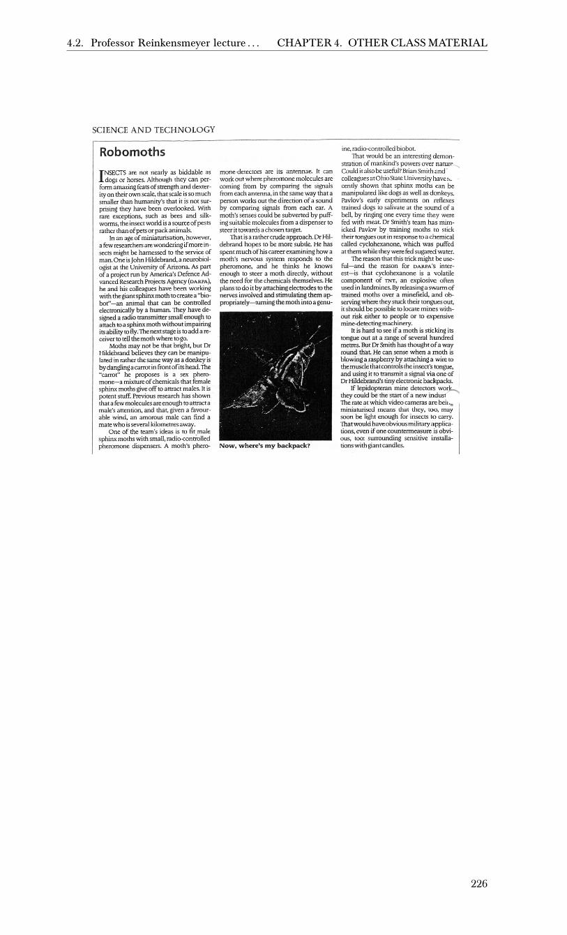
4.2. Professor Reinkensmeyer lecture . . . CHAPTER 4. OTHERCLASSMATERIAL
226

4.3. Professor Bobrow lecture notes given . . . CHAPTER 4. OTHERCLASSMATERIAL
4.3 Professor Bobrow lecture notes given to use asreference
227

4.3. Professor Bobrow lecture notes given . . . CHAPTER 4. OTHERCLASSMATERIAL
228

4.3. Professor Bobrow lecture notes given . . . CHAPTER 4. OTHERCLASSMATERIAL
229

4.3. Professor Bobrow lecture notes given . . . CHAPTER 4. OTHERCLASSMATERIAL
230

4.3. Professor Bobrow lecture notes given . . . CHAPTER 4. OTHERCLASSMATERIAL
231

4.3. Professor Bobrow lecture notes given . . . CHAPTER 4. OTHERCLASSMATERIAL
232

4.3. Professor Bobrow lecture notes given . . . CHAPTER 4. OTHERCLASSMATERIAL
233

4.3. Professor Bobrow lecture notes given . . . CHAPTER 4. OTHERCLASSMATERIAL
234

4.3. Professor Bobrow lecture notes given . . . CHAPTER 4. OTHERCLASSMATERIAL
235

4.3. Professor Bobrow lecture notes given . . . CHAPTER 4. OTHERCLASSMATERIAL
236

4.3. Professor Bobrow lecture notes given . . . CHAPTER 4. OTHERCLASSMATERIAL
237

4.3. Professor Bobrow lecture notes given . . . CHAPTER 4. OTHERCLASSMATERIAL
238

4.3. Professor Bobrow lecture notes given . . . CHAPTER 4. OTHERCLASSMATERIAL
239

4.3. Professor Bobrow lecture notes given . . . CHAPTER 4. OTHERCLASSMATERIAL
240

4.3. Professor Bobrow lecture notes given . . . CHAPTER 4. OTHERCLASSMATERIAL
241

4.3. Professor Bobrow lecture notes given . . . CHAPTER 4. OTHERCLASSMATERIAL
242

4.3. Professor Bobrow lecture notes given . . . CHAPTER 4. OTHERCLASSMATERIAL
243

4.3. Professor Bobrow lecture notes given . . . CHAPTER 4. OTHERCLASSMATERIAL
244

4.3. Professor Bobrow lecture notes given . . . CHAPTER 4. OTHERCLASSMATERIAL
245

4.3. Professor Bobrow lecture notes given . . . CHAPTER 4. OTHERCLASSMATERIAL
246

4.3. Professor Bobrow lecture notes given . . . CHAPTER 4. OTHERCLASSMATERIAL
247

4.3. Professor Bobrow lecture notes given . . . CHAPTER 4. OTHERCLASSMATERIAL
248

4.3. Professor Bobrow lecture notes given . . . CHAPTER 4. OTHERCLASSMATERIAL
249

4.3. Professor Bobrow lecture notes given . . . CHAPTER 4. OTHERCLASSMATERIAL
250

4.3. Professor Bobrow lecture notes given . . . CHAPTER 4. OTHERCLASSMATERIAL
251

4.3. Professor Bobrow lecture notes given . . . CHAPTER 4. OTHERCLASSMATERIAL
252

4.3. Professor Bobrow lecture notes given . . . CHAPTER 4. OTHERCLASSMATERIAL
253

4.3. Professor Bobrow lecture notes given . . . CHAPTER 4. OTHERCLASSMATERIAL
254
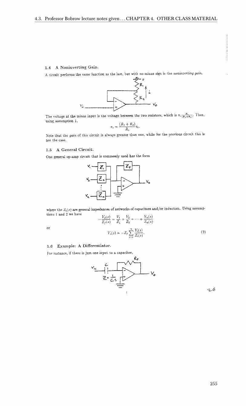
4.3. Professor Bobrow lecture notes given . . . CHAPTER 4. OTHERCLASSMATERIAL
255

4.3. Professor Bobrow lecture notes given . . . CHAPTER 4. OTHERCLASSMATERIAL
256

4.3. Professor Bobrow lecture notes given . . . CHAPTER 4. OTHERCLASSMATERIAL
257

4.3. Professor Bobrow lecture notes given . . . CHAPTER 4. OTHERCLASSMATERIAL
258

4.3. Professor Bobrow lecture notes given . . . CHAPTER 4. OTHERCLASSMATERIAL
259

4.3. Professor Bobrow lecture notes given . . . CHAPTER 4. OTHERCLASSMATERIAL
260

4.3. Professor Bobrow lecture notes given . . . CHAPTER 4. OTHERCLASSMATERIAL
261

4.3. Professor Bobrow lecture notes given . . . CHAPTER 4. OTHERCLASSMATERIAL
262

4.3. Professor Bobrow lecture notes given . . . CHAPTER 4. OTHERCLASSMATERIAL
263

4.3. Professor Bobrow lecture notes given . . . CHAPTER 4. OTHERCLASSMATERIAL
264

4.3. Professor Bobrow lecture notes given . . . CHAPTER 4. OTHERCLASSMATERIAL
265

4.3. Professor Bobrow lecture notes given . . . CHAPTER 4. OTHERCLASSMATERIAL
266

4.3. Professor Bobrow lecture notes given . . . CHAPTER 4. OTHERCLASSMATERIAL
267

4.3. Professor Bobrow lecture notes given . . . CHAPTER 4. OTHERCLASSMATERIAL
268

4.3. Professor Bobrow lecture notes given . . . CHAPTER 4. OTHERCLASSMATERIAL
269

4.3. Professor Bobrow lecture notes given . . . CHAPTER 4. OTHERCLASSMATERIAL
270

4.3. Professor Bobrow lecture notes given . . . CHAPTER 4. OTHERCLASSMATERIAL
271

4.3. Professor Bobrow lecture notes given . . . CHAPTER 4. OTHERCLASSMATERIAL
272

4.3. Professor Bobrow lecture notes given . . . CHAPTER 4. OTHERCLASSMATERIAL
273

4.3. Professor Bobrow lecture notes given . . . CHAPTER 4. OTHERCLASSMATERIAL
274

4.3. Professor Bobrow lecture notes given . . . CHAPTER 4. OTHERCLASSMATERIAL
275

4.3. Professor Bobrow lecture notes given . . . CHAPTER 4. OTHERCLASSMATERIAL
276

4.3. Professor Bobrow lecture notes given . . . CHAPTER 4. OTHERCLASSMATERIAL
277

4.3. Professor Bobrow lecture notes given . . . CHAPTER 4. OTHERCLASSMATERIAL
278

4.3. Professor Bobrow lecture notes given . . . CHAPTER 4. OTHERCLASSMATERIAL
279

4.3. Professor Bobrow lecture notes given . . . CHAPTER 4. OTHERCLASSMATERIAL
280

4.3. Professor Bobrow lecture notes given . . . CHAPTER 4. OTHERCLASSMATERIAL
281

4.3. Professor Bobrow lecture notes given . . . CHAPTER 4. OTHERCLASSMATERIAL
282

4.3. Professor Bobrow lecture notes given . . . CHAPTER 4. OTHERCLASSMATERIAL
283

4.3. Professor Bobrow lecture notes given . . . CHAPTER 4. OTHERCLASSMATERIAL
284

4.3. Professor Bobrow lecture notes given . . . CHAPTER 4. OTHERCLASSMATERIAL
285

4.3. Professor Bobrow lecture notes given . . . CHAPTER 4. OTHERCLASSMATERIAL
286

4.3. Professor Bobrow lecture notes given . . . CHAPTER 4. OTHERCLASSMATERIAL
287

4.3. Professor Bobrow lecture notes given . . . CHAPTER 4. OTHERCLASSMATERIAL
288

4.3. Professor Bobrow lecture notes given . . . CHAPTER 4. OTHERCLASSMATERIAL
289

4.3. Professor Bobrow lecture notes given . . . CHAPTER 4. OTHERCLASSMATERIAL
290

4.3. Professor Bobrow lecture notes given . . . CHAPTER 4. OTHERCLASSMATERIAL
291

4.3. Professor Bobrow lecture notes given . . . CHAPTER 4. OTHERCLASSMATERIAL
292

4.3. Professor Bobrow lecture notes given . . . CHAPTER 4. OTHERCLASSMATERIAL
293

4.3. Professor Bobrow lecture notes given . . . CHAPTER 4. OTHERCLASSMATERIAL
294

4.3. Professor Bobrow lecture notes given . . . CHAPTER 4. OTHERCLASSMATERIAL
295

4.4. OLd exam to practice from CHAPTER 4. OTHERCLASSMATERIAL
4.4 OLd exam to practice from
These are old exams given to us to practice on
Local contents4.4.1 midterm 1999 . . . . . . . . . . . . . . . . . . . . . . . . . . . . . . . . . . . . . 2964.4.2 Design Exam 2004 Solution . . . . . . . . . . . . . . . . . . . . . . . . . . . . . 3024.4.3 Design Exam Solutions 2002 2003 . . . . . . . . . . . . . . . . . . . . . . . . . 3044.4.4 MAE 106 Midterm Exam 2001 . . . . . . . . . . . . . . . . . . . . . . . . . . . 3094.4.5 MAE106 1999 Final Project Description . . . . . . . . . . . . . . . . . . . . . 3144.4.6 MAE106 2000 Final Project Description . . . . . . . . . . . . . . . . . . . . . 3164.4.7 MAE106 2001 Detailed Final Project Description . . . . . . . . . . . . . . . . 3174.4.8 MAE106 2002 Final Project Description . . . . . . . . . . . . . . . . . . . . . 3204.4.9 MAE106 2004 Final Project Description . . . . . . . . . . . . . . . . . . . . . 3214.4.10 Midterm Exam 2002 . . . . . . . . . . . . . . . . . . . . . . . . . . . . . . . . . 3224.4.11 Midterm Exam 2003 . . . . . . . . . . . . . . . . . . . . . . . . . . . . . . . . . 3264.4.12 Midterm Solution 2004 . . . . . . . . . . . . . . . . . . . . . . . . . . . . . . . 3334.4.13 midterm 2000 . . . . . . . . . . . . . . . . . . . . . . . . . . . . . . . . . . . . . 3364.4.14 Solutions to Old Midterms . . . . . . . . . . . . . . . . . . . . . . . . . . . . . 341
296

4.4. OLd exam to practice from CHAPTER 4. OTHERCLASSMATERIAL
4.4.1 midterm 1999
MAE 106 Midterm ExamWinter 1999
University of Cali fornia, IrvineDepartment of Mechanical and Aerospace Engineering
1) Based on your experience in laboratory and lecture, provide brief answers to thefollowing questions:
a) Why is it wrong to use a potentiometer in the following configuration?
b) A motor can also be used as what kind of sensor?
c) What kind of f ilter is the following circuit? (Assume Vc is the output)
VcC
-
+
R
Vr
Vin
inV 2R
Vout
R 1
297

4.4. OLd exam to practice from CHAPTER 4. OTHERCLASSMATERIAL
2) A circuit for controlli ng a light bulb with a MOSFET is shown below. The light bulbis modeled as a resistor. By changing the input gate voltage to the MOSFET, thelight bulb can be turned on and off . A table of the MOSFET’s drain/source resistance(like the one you generated in lab) is also shown.
a) To turn the light bulb on, should the input gate voltage (V in) to the MOSFET be highor low?
b) Assume RL = 1KΩ. Calculate Vout corresponding to an input gate voltage of 3.9 volts.
c) How many watts of power will t he light bulb consume with the input gate voltageequal to 3.9 volts?
V = +15Vs
Vout
inV
R L
Gate
Drain
Source
LightBulb
M OSFET
Vin (volts) RDS (K
0 1001 1002 903 80
3.4 753.6 413.9 44.2 0.15.5 0.01
298

4.4. OLd exam to practice from CHAPTER 4. OTHERCLASSMATERIAL
3) A circuit model of a DC Brush motor is:
where ω is the angular velocity of the motor shaft.
a. Write the differential equation that describes the relationship between input voltageand current for this circuit. (Hint: use Kirchoff’ s voltage law).
b. Solve this differential equation for the current through the motor as a function of timewhen:• the shaft of the motor is held fixed• a constant voltage v is applied across the motor at time = 0• the initial current i(t = 0) through the inductor is zero
c. Plot the torque that the motor generates as a function of time for the conditionsdescribed in part b. Label the axes, the final value of the torque, and the time atwhich the torque has reached 63% of its final value. Assume the motor’s torqueconstant is some constant B.
Bω
RL
v +-
+
-
i
299

4.4. OLd exam to practice from CHAPTER 4. OTHERCLASSMATERIAL
4) Consider the following op-amp circuit:
a) Derive the relationship of the output to the input:
b) What function does this circuit perform if R2 > R1?
R2
Vin
R1
Vo
300

4.4. OLd exam to practice from CHAPTER 4. OTHERCLASSMATERIAL
Problem 4 continued: If we add a capacitor, the circuit becomes a filter:
c) Derive the transfer function of the filter using the impedance of the capacitor,Kirchoff’s laws, and your knowledge of how the Op-Amp works.
d) What are the time constant and corner frequency of this filter?
e) Find the filter’s gain (i.e. the magnitude of the transfer function):
f) Assume we input a sinusoid to this filter. For frequencies much greater than thecorner frequency, what is the filter’s gain?
g) For frequencies much less than the corner frequency, what is the filter’s gain?
h) What kind of f ilter is this?
R2
Vin
R1
Vo
C
301

4.4. OLd exam to practice from CHAPTER 4. OTHERCLASSMATERIAL
5) Consider the problem of controlli ng the velocity of a motor. A simple model of themotor is given by the following block diagram:
where v is the voltage input to the motor and ω is the angular velocity of the shaft.
a) Shown below is a block diagram of an open-loop (i.e. feedforward) controller for themotor, where ωd is the desired output of the motor. What gain value should thecontroller box have to make the output equal the desired output? Write the gain in thecontroller box.
b) What is a disadvantage of an open-loop controller li ke this one?
c) Draw a block diagram of a feedback controller for the motor, label all arrows,including the error signal.
d) What hardware (beside the motor) that we have discussed in class could you use toimplement this feedback controller?
B1v ω
motor
B1v ωωd
motorfeedforwardcontroller
302

4.4. OLd exam to practice from CHAPTER 4. OTHERCLASSMATERIAL
4.4.2 Design Exam 2004 Solution
MAE 106 Mechanical Systems Laboratory Winter 2004 Design Exam
You have been hired as a control engineering consultant for a new ride for Disney’s California Adventure Theme Park, called “Bouncing Over California”. In this ride, the rider will feel like they are bungee jumping off of different bridges in California. Your job is to design a control circuit for the ride. You are given the following information: • The ride is in a 100 foot tower that has a linear track. The rider sits in a harness which slides up and
down the track. The track is driven by a motor. • The track has substantial friction, which can be modeled as viscous friction with a damping coefficient
of B (i.e. friction force = F=-Bv = damping coefficient*velocity). • The motor that drives the track is a DC brushed motor with a current amplifier. It produces a force on
the harness in response to a voltage input with a calibration coefficient of C1 N/volt. • There is a position sensor on the track that measures the position of the harness. The sensor has a
calibration coefficient of C2 volts/meter, and gives a reading of zero volts at the top of the track, where the person enters the harness.
• A typical bungee cord acts like a linear spring with a stiffness of Kb. • The Disney people would like the system to behave like an undamped spring. Design an analog circuit to control the security robot. You will get full credit if you: 1) Show your control law, in MKS units. 2) Provide appropriate control gains with units. 3) Show your control law, in units of volts 4) Draw an op-amp circuit that can implement your controller. Label what the inputs and outputs of your
circuit should be connected to. 5) Choose appropriate values for the resistors and capacitors in your circuit. PLEASE ENTER YOUR ANSWERS ON THE ANSWER SHEET
Weeeee!
303

4.4. OLd exam to practice from CHAPTER 4. OTHERCLASSMATERIAL
Solutions to MAE106 Winter 2004 Design Exam
1) Answer: (20 pts) xKxxKF ddp &−−−= )(
Overview: There are two ways to do this design. In both approaches, we will use a PD position controller to make the controlled system behave like an undamped spring with K=Kb. The PD position controller equation is:
xKxxKF ddp &−−−= )( Approach 1: Make the controller have Kp = Kb, and cancel the friction with Kd = -B. Then the controlled dynamics are:
)()()( dbdbddp xxKxMxBxxKxKxxKxBxM −−=→+−−=−−−=+ &&&&&&& which are the dynamics of an undamped spring with K=Kb. In this approach, we want the rest length of the spring to be half way down the track xd=50ft =16.5 meters Approach 2: Make the controller track the motion of an undamped spring with K=Kb. In this case, we let xd=16 (cos(ωst)-1) meters, so xd = 0, max(xd) = 33 m = 100ft. The frequency of the sinusoid ωs should be the frequency of an undamped spring with K=Kb and a rider of mass M MKbs /=ω . Then, we choose Kp and Kv so that the tracking is good. We choose the bandwidth of the controlled system ωn = 10 ωs (the factor 10 is arbitrary; the point is that we want the bandwidth significantly wider than ωs for good tracking)
bspspn KMKMK 10010010/ 2 ==→== ωωω
And choose ζ = 1 for good tracking without resonance and find Kd BMKKMKKB pdpd −=→=+= 21)2/()(ζ
3) Answer: (20 pts) Note: F=C1vo = vo = motor voltage vs = sensor voltage = C2*x vd = input voltage = C2*xd
221 /)(/ CvKvvCKvC sddspo &−−−=
)/)(/(/1 221 CvKvvCKCv sddspo &−−−=
2) Answer: (20 pts) Approach 1: Kp = Kb N/m or kg/s2
Kd = -B Ns/m or kg/s Approach 2: N/m 2100 sp MK ω=
BMKK pd −= 2 Ns/m
4) Answer: (20 pts) The circuit from Lab 6 will work for Approach 2:
C
+ -
100k
+-
100k Desired position xd
Amp motor pot
+-
R1
R1
R2
xd -xd -Kp(x-xd) - Kdx
.
x
Op amp 1 Op amp 2
Op amp 3 For Approach 1, we need to invert the voltage into the capacitor with an op-amp inverter circuit (similar to Op amp 1 circuit), in order to get a negative Kd
5) Answer: (20 pts) KP = R2/R1 Kd = R2C So choose: R2= Kd / C R1 = R2/ KP
304

4.4. OLd exam to practice from CHAPTER 4. OTHERCLASSMATERIAL
4.4.3 Design Exam Solutions 2002 2003
305

4.4. OLd exam to practice from CHAPTER 4. OTHERCLASSMATERIAL
306

4.4. OLd exam to practice from CHAPTER 4. OTHERCLASSMATERIAL
307

4.4. OLd exam to practice from CHAPTER 4. OTHERCLASSMATERIAL
308

4.4. OLd exam to practice from CHAPTER 4. OTHERCLASSMATERIAL
309

4.4. OLd exam to practice from CHAPTER 4. OTHERCLASSMATERIAL
4.4.4 MAE 106 Midterm Exam 2001
MAE 106 Midterm Exam
Winter 2001
University of California, Irvine
Department of Mechanical and Aerospace Engineering
Problem 1: Motors (25 pts)
a. Shown below is a diagram of a DC
brushed motor. Assume that the
commutation stops working, such
that current flows only in the
direction shown. At what angle
will the armature come to rest?
Assume the armature is initially at
0as shown when the
commutation fails, and that positive
is defined clockwise looking into the page, as shown.
b. For the rest of this problem, assume the commutation is working. Draw the circuit model,
and write the circuit equation describing the motor:
c. Derive and plot the torque versus velocity relationship for the motor. Plot torque on the y-
axis and velocity on the x-axis. Label the x-axis and y-axis intercepts with the appropriate
terminology. Assume that:
the motor receives a constant voltage input of V
the inertia of the motor shaft equals J
the motor’s torque constant is B and is equal to the back-EMF constant
the current into the motor does not change.
N S
I
B
310

4.4. OLd exam to practice from CHAPTER 4. OTHERCLASSMATERIAL
d. For what torque load does the motor produce maximum power?
e. Assume you have a low-power control signal from a computer, and that you would like the
unloaded motor shaft to spin at d when the control signal = +5V, and to stop spinning when the
control signal is 0 V. Design a circuit using only a MOSFET, a power supply, and resistors to
achieve this control. Label the gate, drain, and source of the MOSFET, and the control input
from the computer. Specify the voltage of the power supply assuming the motor’s torque
constant is B and is equal to the back-EMF constant.
311

4.4. OLd exam to practice from CHAPTER 4. OTHERCLASSMATERIAL
Vi Vo
Problem 2: Op Amps and Feedback (25 pts)
a. Write the name of this circuit:
b. Briefly describe a practical situation in which you might want to use the circuit in a)
c. Assume that Vo = K(V+ - V-) for the op amp. How big would K have to be such that Vo is
within 1% of Vi?
d. For a real op amp, the output takes some time to respond to the inputs due to delays in the
op-amp’s internal circuitry. We can model these dynamics with a differential equation:
)( VVAKAVV oo
where A > 0 is a constant. Given these dynamics, plot the voltage response of the circuit in a)
to a unit step input in Vi versus time. Label the time at which the output is 63% of its final
value.
e. Assume that you misconnect the circuit in a) such that the feedback goes to the non-inverting
input instead of the inverting input (i.e. positive feedback instead of negative feedback), and
the input goes to the inverting input. Assuming the op-amp has the dynamics in d), for what
values of K will the circuit be unstable (i.e. for what values of K will the output go to infinity
as time goes to infinity)?
312

4.4. OLd exam to practice from CHAPTER 4. OTHERCLASSMATERIAL
Problem 3: Filters and Signal Processing (25 pts)
You are hired to improve a wire-tapping signal for the FBI. Shown below is a Bode plot of the
typical frequency content of the signal that the FBI’s currently-used system generates:
a) Sketch (very roughly) what the signal would like in the time domain. Include a time scale.
b) What type of filter should you apply to clean up the signal?
c) You have only a few resistors and capacitors in your toolbox, as shown below. Design an
RC circuit to filter the unwanted noise. Draw the circuit, with the input and outputs labeled,
and identify the values of R and C that you would use.
d) By what factor would your filter attenuate the noise in the signal at 10000 rad/s?
|X(j)|
100 10000
Voice signal
Noise signal
[rad/s] 1000
Toolbox Contents:
R = 1, 10 100 1 K
C = 1 pF, 0.1 F, 1 F
313

4.4. OLd exam to practice from CHAPTER 4. OTHERCLASSMATERIAL
d(s)
robot feedforward
controller
2Js
B
v I(s) (s)
Problem 4: Control Theory and Laplace Transforms (25 pts)
Consider the problem of controlling the angle of a one degree-of-freedom robotic leg. The
transfer function of the robot arm is given by the following block diagram:
where I(s) is the current input to the robot’s motor, J is the inertia of the motor, B is the motor
torque constant, and is the angular position of the robot.
a) Shown to the side is a block diagram of an
open-loop (i.e. feedforward) controller for
the motor, where d is the desired angular
position of the robot. What transfer function
should the controller box have to make the
output equal the desired output? Write the
transfer function the controller box.
b) In the time domain, write the relationship between I and d
c) What is a disadvantage of an open-loop controller like this one?
d) A proportional-derivative (PD) feedback controller is a common type of controller that
provides a control signal to the plant that is the sum of a signal proportional (by a gain Kp) to
the output error and a signal proportional by (a gain Kd) to the derivative of the output error.
In the following diagram, fill in the appropriate transfer function such that the robot would be
controlled by a PD controller.
e) Find the overall transfer function for the PD-feedback controlled robot system in d)
2Js
B
v I(s) (s) Motor axis
d(s)
robot feedback
controller
2Js
B
v I(s) (s) +
_
Leg
314

4.4. OLd exam to practice from CHAPTER 4. OTHERCLASSMATERIAL
4.4.5 MAE106 1999 Final Project Description
Department of Mechanical and Aerospace EngineeringUniversity of California, Irvine
MAE 106 Mechanical Systems LaboratoryWinter 1999
Final Project Details:Cruise Control Crash Course
Project Summary:Your final project involves the design of a battery-powered car that is capable of cruising at aconstant velocity. The car should maintain its velocity whether it is travelling uphill, downhill, oron a level surface. On the day of the scheduled final (March 18, 8-10 AM in EG2110), there willbe a contest testing your car. The car will be required to traverse a course that contains a hill,then pass through a swinging pendulum. The car will have to move at the appropriate speed sothat the pendulum does not squash it.
Course Details:The course will be four feet wide and approximately 35 feet long. It will be made out of whitewall board. It will look as follows:
Notes:1) There is a 6 feet-long runway for your car to get up to constant speed.2) The time T12 it takes your car to pass between Photo Gate 1 and 2 will be measured, and
compared to the time T34 it takes to pass between Photo Gates 3 and 4. The goal is for yourcar to make T12 - T34 = 0. Cars will be rank-ordered based on how close the time difference isto zero.
3) The angle theta will be less than 30 degrees.4) The diameter of the mass at the end of the pendulum will be less than 6 inches.5) On the day of the contest, you will be given the pendulum length L and the surface distance
along the track from the starting line to the pendulum. The pendulum will be dropped from astarting angle of 15 degrees away from vertical. Based on these course parameters, you willhave to select a suitable speed for your car. You should design your car with an adjustable,calibrated speed control, and you should do the math ahead of time to predict the desiredspeed for your car based on the unknown parameters.
For extra credit, you can incorporate automatic steering into your car, and the ability to trackblack electrical tape laid in a curved pattern on top of the wallboard.
θ
θ
315

4.4. OLd exam to practice from CHAPTER 4. OTHERCLASSMATERIAL
Grading:The final project is worth 30% of your grade. You grading will be based on:
1. the performance of your car the day of the contest2. a written final project report
The goal of the written final project report is to describe your design as clearly as possible, andthe effort you put into building and testing the car. One write-up should be turned in per projectgroup.
Format for Final Project Write-Up (3-5 pages):1. Summary (200 words or less)2. Design
A. Controller Design, including:block diagrambrief summary of how the controller worksdynamical equations and solutioncircuit diagrams/equationshow you chose controller gain values
B. Mechanical Design3. Construction/Testing
A. How you built the controller (include a parts list, including where you bought/procuredthe parts and how much they cost)
B. Any tests you performed to calibrate/verify/improve performance (with graphs)
316

4.4. OLd exam to practice from CHAPTER 4. OTHERCLASSMATERIAL
4.4.6 MAE106 2000 Final Project Description
MAE 106 Mechanical Systems LaboratoryFinal Project 2000
BATAPULT
For your final project you will design and build a motorized catapult that is capable of hurling aBatman action figure over a scale representation of Gotham City Hall i n order to “ fight crime”:
The goal is to make Batman fly as far as possible without the catapult knocking over GothamCity Hall . No mechanical stops will be allowed to halt the catapult.
On the day of the scheduled final, there will be a contest testing your catapult.
You will be provided with a motor as a starting point, and will work in teams of two or three.
Discussion Question: What are some of the subproblems that you will need to solve in order tosuccessfully complete your project?
Crime inProgress
Motor
Gotham CityHall
317

4.4. OLd exam to practice from CHAPTER 4. OTHERCLASSMATERIAL
4.4.7 MAE106 2001 Detailed Final Project Description
Department of Mechanical and Aerospace Engineering
University of California, Irvine
MAE 106 Mechanical Systems Laboratory
Winter 2000
Final Project Details:
PELE 2001
Project Summary:
For your final project you will design and build a teleoperated robotic soccer player capable of
both kicking a ball into a goal and defending the goal. You are expected to work in project
groups of 2 or 3. On the day of the scheduled final (Tuesday, March 20, 4-6 PM) there will be a
tournament testing your robotic soccer player. The tournament will be held in the MAE106 Lab.
Lab Hours:
The lab will be open from 8-12 A.M. and 1-5 P.M from February 26th
until the contest. If the lab
door is locked, you must sign-in with Dwayne Gates in room EG2118 before the lab will be
opened. For safety reasons, there must always be at least two students in lab for the door to be
opened for you, so bring a partner. While you are in lab, do not leave the room unattended. You
are responsible for all laboratory equipment while you are in the lab. Sign-out with Dwayne
when you leave.
There will be no lecture March 13th
or 15th
to allow time to work on your project. Prof.
Reinkensmeyer will be available in lab during the regular lecture time on those days for
consulting. In addition, your TA’s will be available in the lab during your regular lab time that
week.
Setup:
Shooting
Robot
Manual Control Knob
Control Electronics
Motor
Defending
Robot
Manual Control Knob
Control Electronics
Motor
318

4.4. OLd exam to practice from CHAPTER 4. OTHERCLASSMATERIAL
Contest Rules:
The contest will be a single-elimination tournament similar to a soccer “shoot-out”. Two teams
will be selected. The referee will toss a coin and the team that wins the toss will take the first
kick. The kicks will be taken alternately by the teams. Subject to the conditions explained below,
both teams will take five kicks. The kicks will be taken alternately by the teams. If, before both
teams have taken five kicks, one has scored more goals than the other could score, even if it were
to complete its five kicks, no more kicks will be taken. If, after both teams have taken five kicks,
both have scored the same number of goals, or have not scored any goals, kicks will continue to
be taken in the same order until one team has scored a goal more than the other from the same
number of kicks.
Notes:
1) The distance between goals will be 31¼”.
2) The width of the goals will be 11”.
3) The robot motor will be required to rest on a ring stand.
4) The height of the ring stands will be 14”.
5) The diameter of the rings on the ring stands will be 4”.
6) Two practice fields will be available in lab.
7) The same robot and control system must be used for both kicking and defending.
8) You will be allowed to adjust the yaw angle of the robot on the ring stand before kicking or
defending.
9) The leg of the robot must be able to fit through a paper-towel core (at all times).
10) The ball will be a ping-pong ball.
11) You will be provided with a power supply for your motor (the same ones used in the labs).
12) You are not allowed to store energy in your system before the kick.
13) Your robot must be teleoperated using a potentiometer to control leg angle.
14) Your robot must use a feedback controller.
Starter Kits:
You will be provided with a starter kit comprised of:
1 Pittman DC Gearhead Motor
1 Butyrate Tube (1.5”)
1 Vinyl Tube (1.5”)
1 Garolite Collar (.5”)
2 Spring Pins
The tubing, collar, and pins are useful for coupling the motor shaft to a lever and to a
potentiometer. The kit may be checked out from Duane Gates in EG2118 beginning Feb 28th
, 8
AM – 12 PM, 1 PM – 5 PM. IMPORTANT!!!!!: You must return the kit in order to receive
your final grade. If the motor is not in working order, you will be required to pay for it
($23.50).
Other Required Parts:
You will need to purchase other components for your project, such as a protoboard,
potentiometers, resistors, wire, op-amps, and MOSFETS. The total cost of your project should
be under $20. Suggested vendors are:
319

4.4. OLd exam to practice from CHAPTER 4. OTHERCLASSMATERIAL
Radio Shack: 4716 Barranca Parkway, Irvine (949)552-1091 (and other locations)
Marvac Electronics: 2001 Harbor Blvd., Costa Mesa (949)650-2001
Fry’s Electronics: 10800 Kalama River Ave., Fountain Valley (714)378-4400 (and other
locations)
You can also purchase parts from bulk vendors, such as:
Digikey: www.digikey.com
Newark Electronics: www.newark.com
To avoid a service charge for small orders, you may want to partner with several groups when
ordering from these vendors.
Grading:
The final project is worth 30% of your grade. Your grade will be based on:
1. the performance of your catapult on the day of the contest
2. a written final project report
The goal of the written final project report is to describe your design as clearly as possible, and
the effort you put into building and testing the catapult. One write-up should be turned in per
project group.
Format for Final Project Write-Up (<= 5 pages):
1. Summary (200 words or less)
2. Design
A. Controller Design, including:
block diagram
brief summary of how the controller works
dynamical equations and solution
circuit diagrams/equations
how you chose controller gain values
B. Mechanical Design , including:
any mathematical analysis you did in the design
a parts list, including where you bought/procured the parts and how much they
3. Testing: Any tests that you performed to calibrate/verify/improve performance (with graphs)
Projects with quantitative analysis and detailed experimental testing will score higher.
320

4.4. OLd exam to practice from CHAPTER 4. OTHERCLASSMATERIAL
4.4.8 MAE106 2002 Final Project Description
MAE 106 Mechanical Systems Laboratory
Final Project 2002
SKIBOT 2002
In honor of the 2002 Winter Olympics, you will design a teleoperated robotic vehicle capable of
“skiing” down a slalom course for your final project.
The goal is to steer the gravity-powered vehicle using a manual control knob. You will be
provided with a motor for steering as a starting point, and will work in teams of two or three. On
the day of the scheduled final, there will be a contest testing your skibot.
Discussion Question: What are some of the subproblems
that you will need to solve in order to successfully complete
your project?
Manual Control Knob
Control Electronics
321

4.4. OLd exam to practice from CHAPTER 4. OTHERCLASSMATERIAL
4.4.9 MAE106 2004 Final Project Description
MAE 106 Mechanical Systems Laboratory Final Project 2004
WAKEBOT 2004
You will design a teleoperated robotic vehicle capable of wakeboarding through a slalom course for your final project. A high-power motor will pull on a string (the “leash”) attached to your robot.
Jump
Leash Gate
“Boat” – high torque wench
Control Electronics
Wakeboard Gate The goal is to control the speed of the “boat” and to steer your wakeboard using a manual control knob. You will be provided with a motor for steering as a starting point, and will work in teams of two or three. On the day of the scheduled final, there will be a contest testing your wakebot. Discussion Question: What are some of the subproblems that you will need to solve in order to successfully complete your project?
322

4.4. OLd exam to practice from CHAPTER 4. OTHERCLASSMATERIAL
4.4.10 Midterm Exam 2002
MAE 106 Midterm Exam
Winter 2002
University of California, Irvine
Department of Mechanical and Aerospace Engineering
Problem 1: Circuits (25 pts)
a) Shown below is a 10Kohm potentiometer wired incorrectly. Assume Vin is 10 V and is
provided by a 100 Watt power supply. Assume the potentiometer is rated at 1 Watt. Assume
the shaft can rotate 180 degrees, and define 0 degrees rotation as the shaft angle when the
resistance between the wiper and the ground is 10Kohm. At what shaft angle do you expect
to smell smoke?
b) What does the following circuit do? (give
proof) Assume the four resistors have
equal values.
c) Why are op amps such as the ones used in lab unsatisfactory for powering most motors?
d) Assume that you have a low-power control signal from a computer, and that you would like to
make a motor spin when the control signal is +5 v, and to stop spinning when the control signal
is 0 V. Design a circuit using a MOSFET to achieve this control.
inV 2R
V out
R 1
V1
V o V2
323

4.4. OLd exam to practice from CHAPTER 4. OTHERCLASSMATERIAL
Problem 2: Motors (25 pts)
A DC brushed motor has an internal resistance of 10 ohms. You hold the motor shaft fixed and
apply 10 V, and find that the stall torque is 0.1 Nm, and that it takes 1.5 s to generate 0.063 Nm
of torque. Assume the motor’s torque constant equals the back EMF constant.
a) How fast will the unloaded motor shaft turn if you let it go?
b) What is the inductance of the motor windings?
c) The motor takes 5 seconds to reach its no-load speed. If you double the shaft inertia, how
much longer will the motor take to reach 99% of it’s no-load speed?
d) Why does a DC brushed motor have brushes? (Explain in 15 words or less).
324

4.4. OLd exam to practice from CHAPTER 4. OTHERCLASSMATERIAL
Problem 3: Control Theory (25 pts)
1) Consider the problem of controlling the velocity of a motor. A simple model of the motor is
given by the following block diagram:
where v is the voltage input to the motor and is the angular velocity of the shaft.
a) Shown below is a block diagram of an open-loop (i.e. feedforward) controller for the motor,
where d is the desired output of the motor. What gain value should the controller box have
to make the output equal the desired output? Write the gain in the controller box.
b) Name two disadvantages and two advantages of an open-loop controller like this one.
c) Draw a block diagram of a feedback controller for the motor, label all arrows, including the
error signal.
d) Prove that your feedback controller cancels an additive disturbance Vd to the voltage input to
the motor, given a high enough feedback gain.
B
1
v
motor
B
1
v d
motor feedforward
controller
325

4.4. OLd exam to practice from CHAPTER 4. OTHERCLASSMATERIAL
Problem 4: Signal Processing, Differential Equations, and Frequency Analysis (25 pts)
a) Describe a practical situation in which the following circuit would be useful:
VcC
-
+
R
Vr
Vin
+ -
b) Assume Vin is a step input at time zero and Vc(0) = 0. Find Vc(t).
c) Find the transfer function for the above circuit.
d) Find the frequency response of the above circuit. Be sure to provide equations for how the
circuit scales and phase shifts a sinusoidal input.
e) Assume R = 100 ohm, C = .01 F. How much more attenuated will a 1000 Hz sinusoidal
input signal be than a 100 Hz input signal? (Provide proof).
326

4.4. OLd exam to practice from CHAPTER 4. OTHERCLASSMATERIAL
4.4.11 Midterm Exam 2003
MAE 106 Midterm Exam
Winter 2003
University of California, Irvine
Department of Mechanical and Aerospace Engineering
Problem 1 Circuits (25 pts)
a) Find Vo for the following two circuits. Assume all resistors values = R.
b) For the following circuit, draw conceptual sketches to show how you would simplify
the network to solve for Vo. You do not need to find Vo, just illustrate the steps.
Vi
Vo
Vi Vo Answer: Answer:
Vi
Vo
327

4.4. OLd exam to practice from CHAPTER 4. OTHERCLASSMATERIAL
c) What are the two “golden rules” of op-amp analysis?
d) What two conditions must be true for these golden rules to apply?
e) Using an op-amp and resistors, design a circuit to amplify an input signal by a factor
of 20. Show mathematically that your design works.
f) Assume that you have a low-power control signal from a computer, and that you
would like to make a motor spin when the control signal is +5 v, and to stop spinning
when the control signal is 0 V. Design a circuit using a MOSFET to achieve this
control.
328

4.4. OLd exam to practice from CHAPTER 4. OTHERCLASSMATERIAL
Problem 2: Motors (25 pts)
a. Shown below is a diagram of a DC brushed motor. Assume that the commutation
stops working, such that current flows only in the direction shown. At what angle
will the armature come to rest?
Assume the armature is initially
at 0as shown when the
commutation fails, and that
positive is defined clockwise
looking into the page, as shown.
b. For the rest of this problem,
assume the commutation is
working. Draw the circuit model, and write the circuit equation describing the motor:
b. Solve this differential equation for the current through the motor as a function of time
when:
the shaft of the motor is held fixed
a constant voltage v is applied across the motor at time = 0
the initial current i(t = 0) through the inductor is zero
N S
I
B
329

4.4. OLd exam to practice from CHAPTER 4. OTHERCLASSMATERIAL
c. Plot the torque that the motor generates as a function of time for the conditions
described in part b. Label the axes, the final value of the torque, and the time at
which the torque has reached 63% of its final value. Assume the motor’s torque
constant is some constant B, equal to the back EMF constant.
d. What is the term for the maximum torque a motor can produce when its shaft is held
constant?
e. What is the term for the maximum speed that a motor free to spin will reach?
f. What happens to an unloaded motor spinning at steady-state speed when you
double its input voltage?
g. At what speed does an ideal DC brushed motor produce maximum power and why?
330

4.4. OLd exam to practice from CHAPTER 4. OTHERCLASSMATERIAL
Problem 3: Control Theory (25 pts)
1) You design a new type of motor for which the speed is proportional to the input
voltage squared:
where v is the voltage input to the motor and is the angular velocity of the shaft and A
is a constant.
a) Shown below is a block diagram of an open-loop (i.e. feedforward) controller for the
motor, where d is the desired output of the motor. What function should the
controller box compute to make the output equal the desired output? Write this
function controller box.
b) If the estimate of A used by the feedforward controller is too small by 10%, how
much faster will the actual speed be than the desired speed?
c) Draw a block diagram of a feedback controller for the motor, label all arrows,
including the error signal.
d) Prove that, the actual velocity equals the desired velocity as the feedback gain gets
large.
v d
motor feedforward
controller
v v2
motor
A( )2
A( )2
331

4.4. OLd exam to practice from CHAPTER 4. OTHERCLASSMATERIAL
Problem 4: Frequency Analysis: Motivation, Theory, and Practice (25 pts)
a) Give two reasons for studying frequency domain analysis:
g) If you input a sinusoidal input u(t) = asin(t) into a linear, time-invariant system,
what is the output x(t)? Express your answer in terms of an equation and in words.
h) Below is a proof of the correct answer to part b). On the left are the equations for
each step of the proof. On the right is a description of what is happening in the proof.
Fill in all blanks to complete the proof.
Step Description Equation
1 An nth
order linear system with output x(t) and
input u(t) can be described by a differential
equation like this:
2 X(s)=B(s)/A(s)U(s)+IC(s)/A(s)
3 Assume the system is stable, then in the steady
state Equation 2 can be simplified to:
4 The Laplace transform of the sinusoidal input is:
5 Thus, the steady state output of the system in the
frequency domain is:
6 K1/(s+jw)+K2/(s-jw)+K3/(s-
s1)+K4(s-s2)+…
7 But the system is stable, so the K3 and K4 terms
go to zero with time, and the output in the time
domain is thus Equation 7, with K1=-a/(2j)G(-
jw), and K2 = a/(2j)G(jw), G(s)=B(s)/A(s)
8 Simplifying Equation 7 using the fact sin( =
1/2j(ej
-e-j
) gives:
PROOF COMPLETE PROOF COMPLETE
332

4.4. OLd exam to practice from CHAPTER 4. OTHERCLASSMATERIAL
i) What two pieces of information do you need to describe the frequency response of a
system?
j) Draw an example of the magnitude response of the following types of filters. Make
sure to label the axes.
k) Prove that a mass M acts like a low-pass filter, if force f is considered its input and
position x its output
Low Pass Filter High Pass Filter Notch Filter Band-pass filter
333

4.4. OLd exam to practice from CHAPTER 4. OTHERCLASSMATERIAL
4.4.12 Midterm Solution 2004
334

4.4. OLd exam to practice from CHAPTER 4. OTHERCLASSMATERIAL
335

4.4. OLd exam to practice from CHAPTER 4. OTHERCLASSMATERIAL
MAE 106 Midterm Exam: Open Book/Notes Section Winter 2004
University of California, Irvine Department of Mechanical and Aerospace Engineering
Your goal is to design a power-assist for a motorized bicycle. The device will measure the small voltage produced by leg muscles of the rider, using small electrodes taped over the muscles. This measurement is called the electromyogram, or “EMG”. The device will low-pass filter the EMG voltage signal with a cutoff frequency of 10 Hz in order to get a smooth control signal, and generate a motor torque proportional to the low-pass-filtered EMG signal. The proportionality constant should be adjustable between two values by flipping a switch, from 10 (workout mode) to 100 (cruise mode). Thus, when the rider pedals, he or she will also activate the motor attached to the bicycle, giving a power assist.
Design a circuit using operational amplifiers that can implement the power-assist controller for the bicycle. You may assume that you have a power operational amplifier capable of generating the current needed to directly power the motor. Hint: In order to control the current through the motor, you can control the voltage across a resistor that is in series with the motor, using the power op amp.
336

4.4. OLd exam to practice from CHAPTER 4. OTHERCLASSMATERIAL
4.4.13 midterm 2000
MAE 106 Midterm Exam
Winter 2000
University of California, Irvine
Department of Mechanical and Aerospace Engineering
Problem 1: Motors
a. What type of motor did we analyze in Lecture and did you use in Lab 2?
b. Draw the circuit model of such a motor, as presented in class:
c. Assume that the motor shaft is allowed to spin freely. At t = 0 a constant voltage V is applied
to the motor. Derive an expression for the angular velocity of the motor as a function of
time. Assume that the inertia of the motor shaft equals J, the motor’s torque constant is B,
and the current into the motor does not change. (Hint: Based on the model you drew in part b
and your knowledge of physics, write a differential equation in terms of and solve it).
337

4.4. OLd exam to practice from CHAPTER 4. OTHERCLASSMATERIAL
Problem 2: MOSFETS and Power Control
A circuit for controlling a motor with a MOSFET is shown below. The motor is modeled
simply as a resistor. By changing the input gate voltage to the MOSFET, the motor can be made
to spin. A table of the MOSFET’s drain/source resistance (like the one you generated in lab) is
also shown.
Vin (volts) RDS (K
0 100
1 100
2 90
3 80
3.4 75
3.6 41
3.9 4
4.2 0.1
5.5 0.01
a) To make the motor spin, should the input gate voltage (Vin) to the MOSFET be high or low
and why?
b) Assume RL = 1K. Calculate Vout corresponding to an input gate voltage of 3.9 volts.
c) How many watts of power will the motor consume with the input gate voltage equal to 3.9
volts?
Motor
V = +15V s
V out
in V
R L
Gate
Drain
Source
MOSFET
338

4.4. OLd exam to practice from CHAPTER 4. OTHERCLASSMATERIAL
Problem 3: Operational Amplifiers
a) Why are op-amps such as the ones used in lab unsatisfactory for powering most motors?
b) Find the relationship between Vo and Vi for the following non-inverting amplifier circuit:
c) Using an op-amp and resistors, design a circuit to amplify and invert an input signal by a
factor of -100. Show mathematically that your design works.
Vi Vo
R1
R2
339

4.4. OLd exam to practice from CHAPTER 4. OTHERCLASSMATERIAL
Problem 4: Filters and Frequency Response
a) Find the transfer function relating Vc to Vin for the following filter:
VcC
-
+
R
Vr
Vin
+ -
b) What kind of filter is this? Show mathematically.
c) Suppose Vin = sin t, R = 1 and C = 1 Farad. What is Vc(t) Assume Vc(0) = 0.
340

4.4. OLd exam to practice from CHAPTER 4. OTHERCLASSMATERIAL
Problem 5: Control Theory
Consider the problem of controlling the velocity of a motor. A simple model of the motor is
given by the following block diagram:
where v is the voltage input to the motor and is the angular velocity of the shaft.
a) Shown below is a block diagram of an open-loop (i.e. feedforward) controller for the motor,
where d is the desired output of the motor. What gain value should the controller box have
to make the output equal the desired output? Write the gain in the controller box.
b) What is a disadvantage of an open-loop controller like this one?
c) Draw a block diagram of a feedback controller for the motor. Label all arrows, including the
error signal.
d) Assume that the output velocity of the motor is affected by a disturbance such that =
(1/B)v + e where e is the (constant) error in velocity introduced by the disturbance. Prove
that your feedback controller, with high enough gain, can cancel the disturbance and make
the motor move at the desired velocity d.
B
1
v
motor
B
1
v d
motor feedforward
controller
341

4.4. OLd exam to practice from CHAPTER 4. OTHERCLASSMATERIAL
4.4.14 Solutions to Old Midterms
342

4.4. OLd exam to practice from CHAPTER 4. OTHERCLASSMATERIAL
343

4.4. OLd exam to practice from CHAPTER 4. OTHERCLASSMATERIAL
344

4.4. OLd exam to practice from CHAPTER 4. OTHERCLASSMATERIAL
345

4.4. OLd exam to practice from CHAPTER 4. OTHERCLASSMATERIAL
346

4.4. OLd exam to practice from CHAPTER 4. OTHERCLASSMATERIAL
347

4.4. OLd exam to practice from CHAPTER 4. OTHERCLASSMATERIAL
348

4.4. OLd exam to practice from CHAPTER 4. OTHERCLASSMATERIAL
349

4.4. OLd exam to practice from CHAPTER 4. OTHERCLASSMATERIAL
350

4.4. OLd exam to practice from CHAPTER 4. OTHERCLASSMATERIAL
351

4.4. OLd exam to practice from CHAPTER 4. OTHERCLASSMATERIAL
352

4.4. OLd exam to practice from CHAPTER 4. OTHERCLASSMATERIAL
353

4.4. OLd exam to practice from CHAPTER 4. OTHERCLASSMATERIAL
354

4.4. OLd exam to practice from CHAPTER 4. OTHERCLASSMATERIAL
355

4.4. OLd exam to practice from CHAPTER 4. OTHERCLASSMATERIAL
356

4.4. OLd exam to practice from CHAPTER 4. OTHERCLASSMATERIAL
357

4.4. OLd exam to practice from CHAPTER 4. OTHERCLASSMATERIAL
358

4.4. OLd exam to practice from CHAPTER 4. OTHERCLASSMATERIAL
359

4.4. OLd exam to practice from CHAPTER 4. OTHERCLASSMATERIAL
360

4.4. OLd exam to practice from CHAPTER 4. OTHERCLASSMATERIAL
361

4.4. OLd exam to practice from CHAPTER 4. OTHERCLASSMATERIAL
362

4.4. OLd exam to practice from CHAPTER 4. OTHERCLASSMATERIAL
363

4.4. OLd exam to practice from CHAPTER 4. OTHERCLASSMATERIAL
364

4.4. OLd exam to practice from CHAPTER 4. OTHERCLASSMATERIAL
365

4.4. OLd exam to practice from CHAPTER 4. OTHERCLASSMATERIAL
366

4.4. OLd exam to practice from CHAPTER 4. OTHERCLASSMATERIAL
367

4.4. OLd exam to practice from CHAPTER 4. OTHERCLASSMATERIAL
368