RESEARCH Open Access

Simple solution to the optimal deploymentof cooperative nodes in two-dimensionalTOA-based and AOA-based localizationsystemWeiguang Shi*, Xiaoli Qi, Jianxiong Li, Shuxia Yan, Liying Chen, Yang Yu and Xin Feng

Abstract

Cellular-based cooperative communication is a promising technique that allows cooperation among mobile devicesnot only to increase data throughput but also to improve localization services. For a certain number of cooperativenodes, the geometry plays a significant role in enhancing the accuracy of target. In this paper, a simple solution to thedeployment of cooperative nodes aiming at the lowest geometric dilution of precision (GDOP) is proposed suitable forboth time of arrival-based cooperative localization system and angle of arrival-based cooperative localization system.Inertia dependence factor is suggested to reveal the relationship among the optimal positions of each cooperativenode, which extracts the inertia and the recursiveness of deployment. It is shown in simulations that the proposedsolution almost achieves the same GDOP as that of global exclusive method but with less complexity.

Keywords: GDOP, Optimal placement, Cooperative node, TOA, AOA

1 IntroductionWith the proliferation of mobile communication tech-nology, wireless positioning has become an increasinglyimportant issue and drawn plenty of attention [1]. Overthe past several decades, a variety of location-based ser-vices emerged in the fields such as emergency medicalsystems, asset monitoring and tracking, location sensi-tive billing, fraud protection, fleet management, andeven also including intelligent transportation systems[2, 3]. However, global positioning system (GPS) andcellular positioning system (CPS), two representativepositioning technologies applied in many scenarios ofdaily life, still have some drawbacks [4–7]. On the onehand, in outdoor environment, GPS and CPS signalsare sensitive to the interference from space weather,transformer substations, geomagnetic radiation, andetc., which leads to the degradation of the accessibilityand continuity of GPS and CPS [8–11]. On the otherhand, in indoor environment, GPS and CPS face a

challenging radio propagation environment, includingmainly multi-path effect and none-line-of-sight (NLOS)effect [12–15].Indoor wireless communication (IWC) technology,

represented by ultrasonic (US), wireless sensor networks(WSN), Bluetooth (BT), radio frequency identification(RFID) and ultra wide band (UWB), provides a novel kindof approach to the data interaction and burgeons rapidlyin the last decade. Owing to their low cost, an ocean ofIWC devices has been placed in indoor environment tosupply context-awareness service for the target. Variouspositioning systems have also been proposed and unfoldedsatisfactory performance [16–20]. Meanwhile, thanks tothe continual miniaturization of the microelectronictechnology, cutting-edge cell phones equipped withIWC modules have been committed to remote control,intelligent entrance guard, instant payment, and tagidentification via the connection with surrounding IWCdevices. In this situation, if we regard all or part of thesurrounding IWC devices that could provide spatialcharacteristic about the cell phone as cooperative part-ners, a cooperative localization system on the basis oftraditional CPS or GPS can be established, which is

* Correspondence: shiweiguang12345@126.comTianjin Key Laboratory of Optoelectronic Detection Technology and Systems,School of Electronics and Information Engineering, Tianjin PolytechnicUniversity, Tianjin 300387, China

© The Author(s). 2017 Open Access This article is distributed under the terms of the Creative Commons Attribution 4.0International License (http://creativecommons.org/licenses/by/4.0/), which permits unrestricted use, distribution, andreproduction in any medium, provided you give appropriate credit to the original author(s) and the source, provide a link tothe Creative Commons license, and indicate if changes were made.

Shi et al. EURASIP Journal on Wireless Communicationsand Networking (2017) 2017:79 DOI 10.1186/s13638-017-0859-6

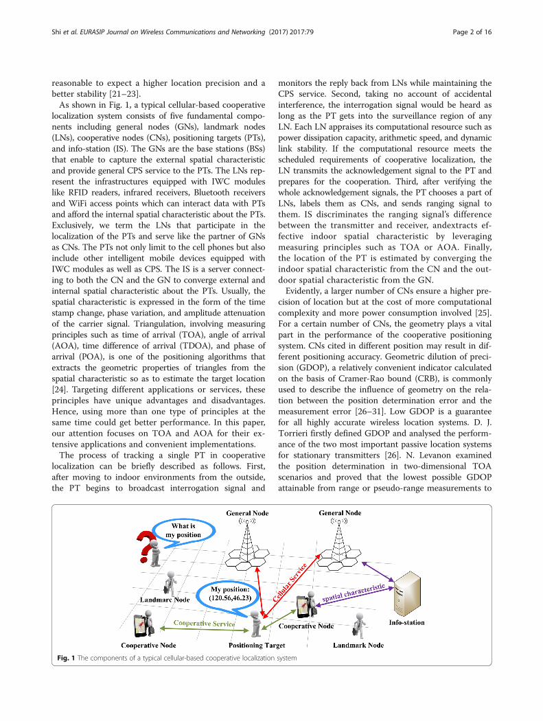
reasonable to expect a higher location precision and abetter stability [21–23].As shown in Fig. 1, a typical cellular-based cooperative

localization system consists of five fundamental compo-nents including general nodes (GNs), landmark nodes(LNs), cooperative nodes (CNs), positioning targets (PTs),and info-station (IS). The GNs are the base stations (BSs)that enable to capture the external spatial characteristicand provide general CPS service to the PTs. The LNs rep-resent the infrastructures equipped with IWC moduleslike RFID readers, infrared receivers, Bluetooth receiversand WiFi access points which can interact data with PTsand afford the internal spatial characteristic about the PTs.Exclusively, we term the LNs that participate in thelocalization of the PTs and serve like the partner of GNsas CNs. The PTs not only limit to the cell phones but alsoinclude other intelligent mobile devices equipped withIWC modules as well as CPS. The IS is a server connect-ing to both the CN and the GN to converge external andinternal spatial characteristic about the PTs. Usually, thespatial characteristic is expressed in the form of the timestamp change, phase variation, and amplitude attenuationof the carrier signal. Triangulation, involving measuringprinciples such as time of arrival (TOA), angle of arrival(AOA), time difference of arrival (TDOA), and phase ofarrival (POA), is one of the positioning algorithms thatextracts the geometric properties of triangles from thespatial characteristic so as to estimate the target location[24]. Targeting different applications or services, theseprinciples have unique advantages and disadvantages.Hence, using more than one type of principles at thesame time could get better performance. In this paper,our attention focuses on TOA and AOA for their ex-tensive applications and convenient implementations.The process of tracking a single PT in cooperative

localization can be briefly described as follows. First,after moving to indoor environments from the outside,the PT begins to broadcast interrogation signal and

monitors the reply back from LNs while maintaining theCPS service. Second, taking no account of accidentalinterference, the interrogation signal would be heard aslong as the PT gets into the surveillance region of anyLN. Each LN appraises its computational resource such aspower dissipation capacity, arithmetic speed, and dynamiclink stability. If the computational resource meets thescheduled requirements of cooperative localization, theLN transmits the acknowledgement signal to the PT andprepares for the cooperation. Third, after verifying thewhole acknowledgement signals, the PT chooses a part ofLNs, labels them as CNs, and sends ranging signal tothem. IS discriminates the ranging signal’s differencebetween the transmitter and receiver, andextracts ef-fective indoor spatial characteristic by leveragingmeasuring principles such as TOA or AOA. Finally,the location of the PT is estimated by converging theindoor spatial characteristic from the CN and the out-door spatial characteristic from the GN.Evidently, a larger number of CNs ensure a higher pre-

cision of location but at the cost of more computationalcomplexity and more power consumption involved [25].For a certain number of CNs, the geometry plays a vitalpart in the performance of the cooperative positioningsystem. CNs cited in different position may result in dif-ferent positioning accuracy. Geometric dilution of preci-sion (GDOP), a relatively convenient indicator calculatedon the basis of Cramer-Rao bound (CRB), is commonlyused to describe the influence of geometry on the rela-tion between the position determination error and themeasurement error [26–31]. Low GDOP is a guaranteefor all highly accurate wireless location systems. D. J.Torrieri firstly defined GDOP and analysed the perform-ance of the two most important passive location systemsfor stationary transmitters [26]. N. Levanon examinedthe position determination in two-dimensional TOAscenarios and proved that the lowest possible GDOPattainable from range or pseudo-range measurements to

Fig. 1 The components of a typical cellular-based cooperative localization system

Shi et al. EURASIP Journal on Wireless Communications and Networking (2017) 2017:79 Page 2 of 16

N optimally located points is 2=ffiffiffiffiN

p[27]. A.G. Dempster

obtained the expression of GDOP for two-dimensionalAOA scenarios [28]. In [29], P. Deng et al. studied therelationship between GDOP and GN number at thecentre of a polygon with and without the correlativitybetween TDOA measurements considered. A GDOPmethod for computing TDOA and TDOA/AOA undernon-line-of-sight environment was also presented.Quan investigated GDOP in absolute range-based wire-less location systems with emphasis on its low boundsand introduced angle of coverage as a parameter to de-scribe the geometry between a target and the measuringpoints [30].In addition, an efficient deployment scheme of CNs in

TOA positioning systems, which aims to minimize theGDOP, is proposed on the basis of generalized eigen-value decomposition of fisher information matrix (FIM)[31]. In this paper, we termed it as eigenvalue-basedapproach for ease of illustration. The eigenvalue-basedapproach, which could obtain optimal performance forone CN and suffer only small loss of performance formore CNs, can dramatically reduce the computationalcomplexity compared with the exhaustive method. De-veloping a practical arrangement out of the eigenvalue-based approach, however, entails some challenges. First,the eigenvalue-based approach only describes the pro-cedure of scheme rather than theoretically infers theexpression of the eigenvalue and eigenvector. Variationof GNs’ deployment will trigger the modification of FIM,which may cause recalculation of eigenvalue and eigen-vector. Second, the relationship among the optimal pos-ition of each CN has not been thoroughly investigatedand deeply summarized; unnecessary calculation cannotbe avoided when the number of the CNs is huge. Third,the eigenvalue-based approach cannot be directly ap-plied into AOA system since the FIM of AOA is morecomplicated than that of TOA. To the best of our know-ledge, few approaches are reported to tackle the issuementioned above.In this paper, we propose another solution to the

deployment of CN suitable for both TOA-based cooperativelocalization system and AOA-based cooperative localizationsystem. Optimal placement mechanism based on partialdifferentiation, termed as OPMPD, is suggested to exposethe optimal position of CN and achieves a more explicitsolution. Inertia dependence factor is also introduced toreveal the relationship among the optimal position of eachCN, which extracts the inertia and the recursiveness ofdeployment.The rest of the paper is organized as follows. CRB

based on FIM is reviewed in “Section 2.” In “Section 3,”we respectively deduce the GDOP expressions of two-dimensional TOA-based cooperative localization systemand AOA-based cooperative localization system. Ournew solution aiming at the lowest GDOP is detailed in

“Section 4.” Simulation results are illustrated in “Section5,” which proves the effectiveness and the efficiency ofthe proposed approach. Finally, the conclusion of ourwork is presented in “Section 6.”

2 Cramer-Rao bound based on FIMThe CRB, which can be derived by the inverse of theFIM, provides the lowest limit on estimation accuracy ofany unbiased estimator. Suppose a parameter vector tobe estimated is θ = [θ1, θ2,⋯ θP]

T. θp stands for the pthunknown parameter, p ∈ [1, P]. P denotes the number ofparameters to be estimated. The FIM is then

J θð Þ ¼ −E∂ lnf Λjθð Þ

∂θ

� �∂ lnf Λjθð Þ

∂θ

� �T( )

ð1Þ

where J(θ) is a P × P matrix, f(Λ|θ) is the likelihoodfunction of observation vector Λ, and E represents theexpectation operation. Assume that f(Λ|θ) follows Ndimensional Gaussian distribution denoted as

f Λjθð Þ ¼ 1ffiffiffiffiffiffiffiffiffiffiffiffiffiffiffiffiffiffiffi2πð ÞN Qj j

q e−12 Λ−μ θð Þð ÞTQ−1 Λ−μ θð Þð Þ ð2Þ

where N is the scale of Λ, Q is the covariance matrix withθ, μ(θ) is the expectation of Λ, and (⋅)T and (⋅)− 1 respect-ively represent the transpose and inverse of the matrix.Consider H ¼ ∂μ θð Þ

∂θTas the Jacobian matrix and substitute

(2) into (1), J(θ) will be updated to J(θ) =HTQ− 1H, andthe CRB of θ can be expressed as

var θ̂� �

≥diag J−1 θð Þ� � ¼ diag HTQ−1H� �−1� �

ð3Þ

where var is the variance matrix of unbiased estimatorsθ̂ ¼ θ̂1; θ̂2;⋯θ̂P

h iTand diag denotes the diagonal ele-

ments of a matrix.

3 GDOP of two-dimensional localization systems3.1 GDOP of typical localization systemConsider a two-dimensional typical localization systemwith a single PT, N GNs. Let θ = [x, y]T implies the un-known location of PT and (xn, yn) denotes the knownlocation of the nth GN. n ∈ [1,N]. Accordingly, observa-tion vector Λ in TOA measurement is [d1, d2,⋯ dN]

T inwhich dn denotes the measured distance between the PTand the nth GN given by

dn ¼ ct ¼ffiffiffiffiffiffiffiffiffiffiffiffiffiffiffiffiffiffiffiffiffiffiffiffiffiffiffiffiffiffiffiffiffiffiffiffix−xnð Þ2 þ y−ynð Þ2

q¼ dn þ en ð4Þ

Here, c denotes the light speed. t denotes the absolutearrival time. dn stands for the theoretical value. en standsfor the measurement error that follows the Gaussian

Shi et al. EURASIP Journal on Wireless Communications and Networking (2017) 2017:79 Page 3 of 16

distribution with zero mean and σn root-mean-squareerror. Given the assumption that the measured values inΛ are mutually independent, the cross-covariance matrixcan be rewritten as

var θ̂� �

¼ σ2x 00 σ2y

ð5Þ

where σ2x and σ2y represent the variance of x and y,

respectively.According to the definition in [26], the GDOP of TOA

system can be expressed as

GDOP ¼ffiffiffiffiffiffiffiffiffiffiffiffiffiffiffiffiσ2x þ σ2y

qσ2D

ð6Þ

with σD ¼ 1N

Pn¼1

Nσn , where σD is the root-mean-square

ranging error of system. Suppose σ1 = σ2 = σ3 =… = σn = σr,

(6) can be simplified as GDOP ¼ ffiffiffiffiffiffiffiffiffiffiffiffiffiffiffiffiffiffiffiffiffiG11 þ G22

p, where G11

and G22 are the diagonal elements of G given by

G ¼ 1σD

HTQ−1H� �−1 ð7Þ

Considering that all the measurement errors are inde-pendent, we have Q ¼ σ2r I with an N ×N identity matrixI. Then the G will become

G ¼ HTH� �−1 ð8Þ

Correspondingly, the Jacobian matrix H of TOA is

HTOA¼

x−x1d1

y−y1d1x−x2

d2

y−y2d2

⋮ ⋮x−xNdN

y−yNdN

26666664

37777775¼

− cosα1 − sinα1− cosα2 − sinα2

⋮ ⋮− cosαN − sinαN

2664

3775 ð9Þ

where αn is the angle of the ray from the PT to the nthGN relative to the positive X-axis.Substituting (9) into (8), we have

GTOA ¼

XNn¼1

sin2αn −XNn¼1

cosαn sinαn

−XNn¼1

cosαn sinαnXNn¼1

cos2αn

266664

377775

Xn¼1

N−1 XNm¼nþ1

sin2 αm−αnð Þ

ð10Þ

Therefore, the GDOP of TOA can be derived as

GDOPTOA ¼ffiffiffiffiffiffiffiffiffiffiffiffiffiffiffiffiffiffiffiffiffiffiffiffiffiffiffiffiffiffiffiffiffiffiffiffiffiffiffiffiffiffiffiffiffiffi

NXn¼1

N−1 XNm¼nþ1

sin2 αm−αnð Þ

vuuuut ð11Þ

Similarly, the Jacobian matrix and GDOP of AOA canbe obtained with observation vector Λ replaced by[α1, α2,⋯ αN]

T

HAOA¼

−y−y1d21

x−x1d21

−y−y2d22

x−x2d22

⋮ ⋮−y−yNd2N

x−xNd2N

266666664

377777775¼

sinα1d21

−cosα1d21

sinα2d22

−cosα2d22

⋮ ⋮sinαNd2N

−cosαNd2N

2666666664

3777777775

ð12Þ

GDOPAOA ¼

ffiffiffiffiffiffiffiffiffiffiffiffiffiffiffiffiffiffiffiffiffiffiffiffiffiffiffiffiffiffiffiffiffiffiffiffiffiffiffiffiffiffiffiffiffiffiffiffiffiffiffiffiffiffiffiffiffiffiffiffiffiffiXNn¼1

dn‐2

Xn¼1

N−1 XNm¼nþ1

dm‐2dn

‐2 sin2 αm−αnð Þ

vuuuuuuutð13Þ

3.2 GDOP of cooperative localization systemThe key idea of cooperative localization systems is im-proving the accuracy of PTs by introducing more LNsand filtering out CNs from them. Theoretically, themore CN employed, the lower GDOP received. In thissection, assume that there are totally M CNs to beallocated to a single PT for reducing the GDOP. Afterthe implementation of assignment, the Jacobian ma-trixes of the observation vector of TOA-based andAOA-based cooperative localization systems are re-spectively refreshed to

HC‐TOA ¼ HTTOA HT

c‐TOA

� �T ð14Þ

HC‐AOA ¼ HTAOA HT

c‐AOA

� �T ð15Þ

with

HC‐TOA¼

x−xc1r1

y−yc1r1

x−xc2r2

y−yc2r2

⋮ ⋮x−xcMrM

y−ycMrM

266664

377775¼

− cosβ1 − sinβ1− cosβ2 − sinβ2

⋮ ⋮− cosβM − sinβM

2664

3775

ð16Þ

Shi et al. EURASIP Journal on Wireless Communications and Networking (2017) 2017:79 Page 4 of 16

HC‐AOA¼

−y−yc1r21

x−xc1r21

−y−yc2r22

x−xc2r22

⋮ ⋮−y−ycMr2M

x−xcMr2M

2666664

3777775¼

sinβ1r21

−cosβ1r21

sinβ2r22

−cosβ2r22

⋮ ⋮sinβMr2M

−cosβMr2M

266666664

377777775

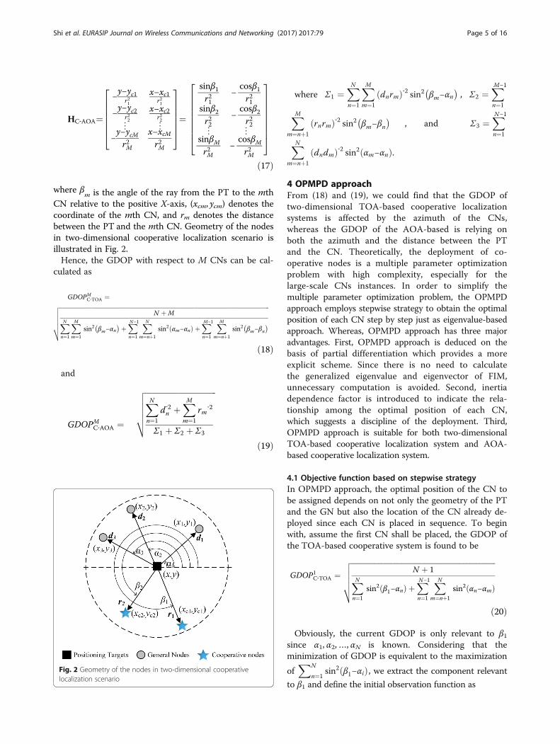
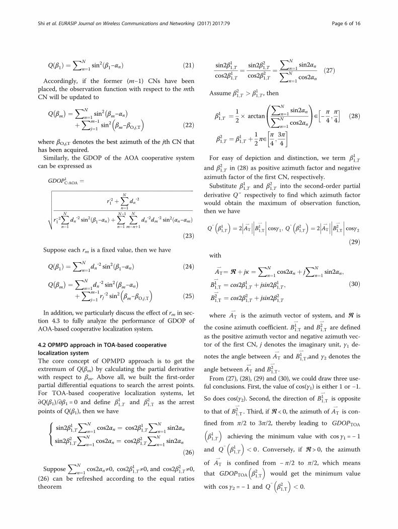
ð17Þ

where βm is the angle of the ray from the PT to the mth

CN relative to the positive X-axis, (xcm, ycm) denotes thecoordinate of the mth CN, and rm denotes the distancebetween the PT and the mth CN. Geometry of the nodesin two-dimensional cooperative localization scenario isillustrated in Fig. 2.Hence, the GDOP with respect to M CNs can be cal-

culated as

GDOPMC‐TOA ¼ffiffiffiffiffiffiffiffiffiffiffiffiffiffiffiffiffiffiffiffiffiffiffiffiffiffiffiffiffiffiffiffiffiffiffiffiffiffiffiffiffiffiffiffiffiffiffiffiffiffiffiffiffiffiffiffiffiffiffiffiffiffiffiffiffiffiffiffiffiffiffiffiffiffiffiffiffiffiffiffiffiffiffiffiffiffiffiffiffiffiffiffiffiffiffiffiffiffiffiffiffiffiffiffiffiffiffiffiffiffiffiffiffiffiffiffiffiffiffiffiffiffiffiffiffiffiffiffiffiffiffiffiffiffiffiffiffiffiffiffiffiffiffiffiffi

N þMXNn¼1

XMm¼1

sin2 βm−αn� �þX

n¼1

N−1 XNm¼nþ1

sin2 αm−αnð Þ þXn¼1

M−1 XMm¼nþ1

sin2 βm−βn� �

vuuuutð18Þ

and

GDOPMC‐AOA ¼

ffiffiffiffiffiffiffiffiffiffiffiffiffiffiffiffiffiffiffiffiffiffiffiffiffiffiffiffiffiffiffiffiffiffiffiffiffiXNn¼1

d‐2n þ

XMm¼1

rm‐2

Σ1 þ Σ2 þ Σ3

vuuuutð19Þ

where Σ1 ¼XNn¼1

XMm¼1

dnrmð Þ‐2 sin2 βm−αn� �

, Σ2 ¼Xn¼1

M−1

XMm¼nþ1

rnrmð Þ‐2 sin2 βm−βn� �

, and Σ3 ¼Xn¼1

N−1

XNm¼nþ1

dndmð Þ‐2 sin2 αm−αnð Þ.

4 OPMPD approachFrom (18) and (19), we could find that the GDOP oftwo-dimensional TOA-based cooperative localizationsystems is affected by the azimuth of the CNs,whereas the GDOP of the AOA-based is relying onboth the azimuth and the distance between the PTand the CN. Theoretically, the deployment of co-operative nodes is a multiple parameter optimizationproblem with high complexity, especially for thelarge-scale CNs instances. In order to simplify themultiple parameter optimization problem, the OPMPDapproach employs stepwise strategy to obtain the optimalposition of each CN step by step just as eigenvalue-basedapproach. Whereas, OPMPD approach has three majoradvantages. First, OPMPD approach is deduced on thebasis of partial differentiation which provides a moreexplicit scheme. Since there is no need to calculatethe generalized eigenvalue and eigenvector of FIM,unnecessary computation is avoided. Second, inertiadependence factor is introduced to indicate the rela-tionship among the optimal position of each CN,which suggests a discipline of the deployment. Third,OPMPD approach is suitable for both two-dimensionalTOA-based cooperative localization system and AOA-based cooperative localization system.

4.1 Objective function based on stepwise strategyIn OPMPD approach, the optimal position of the CN tobe assigned depends on not only the geometry of the PTand the GN but also the location of the CN already de-ployed since each CN is placed in sequence. To beginwith, assume the first CN shall be placed, the GDOP ofthe TOA-based cooperative system is found to be

GDOP1C‐TOA ¼

ffiffiffiffiffiffiffiffiffiffiffiffiffiffiffiffiffiffiffiffiffiffiffiffiffiffiffiffiffiffiffiffiffiffiffiffiffiffiffiffiffiffiffiffiffiffiffiffiffiffiffiffiffiffiffiffiffiffiffiffiffiffiffiffiffiffiffiffiffiffiffiffiffiffiffiffiffiffiffiffiffiffiffiN þ 1XN

n¼1

sin2 β1−αnð Þ þXn¼1

N−1 XNm¼nþ1

sin2 αn−αmð Þ

vuuuutð20Þ

Obviously, the current GDOP is only relevant to β1since α1, α2,…, αN is known. Considering that theminimization of GDOP is equivalent to the maximization

ofXN

n¼1sin2 β1−αið Þ , we extract the component relevant

to β1 and define the initial observation function as

Fig. 2 Geometry of the nodes in two-dimensional cooperativelocalization scenario

Shi et al. EURASIP Journal on Wireless Communications and Networking (2017) 2017:79 Page 5 of 16

Q β1ð Þ ¼XN

n¼1sin2 β1−αnð Þ ð21Þ

Accordingly, if the former (m−1) CNs have beenplaced, the observation function with respect to the mthCN will be updated to

Q βm� � ¼XN

n¼1sin2 βm−αn

� �þXm−1

j¼1sin2 βm−βO;j;T

� �ð22Þ

where βO,j,T denotes the best azimuth of the jth CN thathas been acquired.Similarly, the GDOP of the AOA cooperative system

can be expressed as

GDOP1C‐AOA ¼ffiffiffiffiffiffiffiffiffiffiffiffiffiffiffiffiffiffiffiffiffiffiffiffiffiffiffiffiffiffiffiffiffiffiffiffiffiffiffiffiffiffiffiffiffiffiffiffiffiffiffiffiffiffiffiffiffiffiffiffiffiffiffiffiffiffiffiffiffiffiffiffiffiffiffiffiffiffiffiffiffiffiffiffiffiffiffiffiffiffiffiffiffiffiffiffiffiffiffiffiffiffiffiffiffiffiffiffiffiffiffiffiffiffi

r‐21 þXNn¼1

dn‐2

r−21XNn¼1

dn‐2 sin2 β1−αnð Þ þ

Xn¼1

N−1 XNm¼nþ1

dn‐2dm

‐2 sin2 αn−αmð Þ

vuuuuuuutð23Þ

Suppose each rm is a fixed value, then we have

Q β1ð Þ ¼XN

n¼1dn

‐2 sin2 β1−αnð Þ ð24Þ

Q βm� � ¼XN

n¼1dn

‐2 sin2 βm−αn� �

þXm−1

j¼1rj‐2 sin2 βm−βO;j;T

� �ð25Þ

In addition, we particularly discuss the effect of rm in sec-tion 4.3 to fully analyze the performance of GDOP ofAOA-based cooperative localization system.

4.2 OPMPD approach in TOA-based cooperativelocalization systemThe core concept of OPMPD approach is to get theextremum of Q(βm) by calculating the partial derivativewith respect to βm. Above all, we built the first-orderpartial differential equations to search the arrest points.For TOA-based cooperative localization systems, let∂Q(β1)/∂β1 = 0 and define β11;T and β21;T as the arrestpoints of Q(β1), then we have

sin2β11;TXN

n¼1cos2αn ¼ cos2β11;T

XN

n¼1sin2αn

sin2β21;TXN

n¼1cos2αn ¼ cos2β21;T

XN

n¼1sin2αn

8<:

ð26Þ

SupposeXN

n¼1cos2αn≠0, cos2β

11;T≠0, and cos2β21;T≠0,

(26) can be refreshed according to the equal ratiostheorem

sin2β11;Tcos2β11;T

¼ sin2β21;Tcos2β21;T

¼XN

n¼1sin2αnXN

n¼1cos2αn

ð27Þ

Assume β21;T > β11;T , then

β11;T ¼ 12� arctan

XN

n¼1sin2αnXN

n¼1cos2αn

0@

1A∈ −

π

4;π

4

h i

β21;T ¼ β11;T þ 12π∈

π

4;3π4

ð28Þ

For easy of depiction and distinction, we term β11;Tand β21;T in (28) as positive azimuth factor and negativeazimuth factor of the first CN, respectively.Substitute β11;T and β21;T into the second-order partial

derivative Q″ respectively to find which azimuth factorwould obtain the maximum of observation function,then we have

Q″ β11;T

� �¼ 2 AT

* B1

1;T

*

cosγ1; Q″ β21;T

� �¼ 2 AT

* B2

1;T

*

cosγ2ð29Þ

with

AT* ¼ ℜ þ jκ ¼

XN

n¼1cos2αn þ j

XN

n¼1sin2αn;

B11;T

*

¼ cos2β11;T þ jsin2β11;T ;

B21;T

*

¼ cos2β21;T þ jsin2β21;T

ð30Þ

where AT*

is the azimuth vector of system, and ℜ is

the cosine azimuth coefficient. B11;T

*

and B21;T

*

are definedas the positive azimuth vector and negative azimuth vec-tor of the first CN, j denotes the imaginary unit, γ1 de-

notes the angle between AT*

and B11;T

*

,and γ2 denotes the

angle between AT*

and B21;T

*

.From (27), (28), (29) and (30), we could draw three use-

ful conclusions. First, the value of cos(γ1) is either 1 or −1.

So does cos(γ2). Second, the direction of B11;T

*

is opposite

to that of B21;T

*

. Third, if ℜ < 0, the azimuth of AT*

is con-

fined from π/2 to 3π/2, thereby leading to GDOPTOA

β11;T

� �achieving the minimum value with cos γ1 = − 1

and Q″ β11;T

� �< 0 . Conversely, if ℜ > 0, the azimuth

of AT*

is confined from − π/2 to π/2, which means

that GDOPTOA β21;T

� �would get the minimum value

with cos γ2 = − 1 and Q″ β21;T

� �< 0.

Shi et al. EURASIP Journal on Wireless Communications and Networking (2017) 2017:79 Page 6 of 16

Consequently, a deployment mechanism of the firstCN can be summarized as

βO;1;T ¼random

β11;T

ifℜ ¼ 0ifℜ < 0

β21;T ifℜ > 0

8<: ð31Þ

where βO,1,T represents the optimal azimuth correspond-ing to the least GDOP and BO;1;T

⇀ ¼ cos2βO;1;T þ jsin2βO;1;T represents the optimal azimuth vector of the firstCN.After the first CN is arranged at the optimum position,

both the azimuth vector of system and the objectivefunction will be refreshed to

AT* ¼ ℜ þ jκ ¼ cos2βO;1;T þ

XN

n¼1cos2αn

� �þj sin2βO;1;T þ

XN

n¼1sin2αn

� � ð32Þ

Q β2ð Þ ¼XN

n¼1sin2 β2−αnð Þ þ sin2 β2−βO;1;T

� �ð33Þ

Define β12;T and β22;T as the arrest points of Q(β2), thenwe have

β12;T ¼ β11;T; β22;T ¼ β21;T ð34Þ

since

sin2β12;Tcos2β12;T

¼ sin2β22;Tcos2β22;T

¼XN

n¼1sin2αn þ sin2βO;1;TXN

n¼1cos2αn þ cos2βO;1;T

¼XN

n¼1sin2αnXN

n¼1cos2αn

ð35Þ

The optimal azimuth of the second CN can be deter-

mined as ℜ updated toXN

n¼1cos2αn þ cos2βO;1;T .

From (35), it is clear that either the positive azimuth fac-tor or the negative azimuth factor of each successive CNequals to that of the first CN. Hence, we define β1T and

β2T as the positive azimuth factor and negative azimuth

factor of the system where β1T ¼ β11;T, β2T ¼ β21;T.

Suppose the absolute value of initial cosine azimuthcoefficient is larger than 2, the absolute value of cosineazimuth coefficient refreshed will decrease as the CN is

introduced since the directions of BO;1;T⇀

and BO;2;T⇀

are

opposite to that of initial AT*. That is

cos2βO;1;T þ cos2βO;2;T þXNn¼1

cos2αn

< cos2βO;1;T þXNn¼1

cos2αn

<

XNn¼1

cos2αn

ð36Þ

Moreover, if initial cosine azimuth coefficient is evengreater, there exists a theoretical quantity of the CNstermed as ZT satisfying

βO;ZTþ1;T≠βO;ZT;T… ¼ βO;2;T ¼ βO;1;T ð37Þ

which means that the optimal azimuth of the former ZT

CNs equal to βO,1,T rather than βO;ZTþ1;T.For simplicity, we define ZT as inertia dependency fac-

tor and estimate it by

ZT−1ð Þ⋅ cos2βO;1;T þXNn¼1

cos2αn

!XNn¼1

cos2αn > 0

ZT cos2βO;1;T þXNn¼1

cos2αn

!XNn¼1

cos2αn < 0

8>>>><>>>>:

ð38Þ

From (38), we have

1þ ZT−1ð ÞV > 0ZTV þ 1 < 0

�ð39Þ

with

V ¼ sin2βO;1;TXNn¼1

sin2αn

¼ cos2βO;1;TXNn¼1

cos2αn

ð40Þ

Hence,

ZT ¼

ffiffiffiffiffiffiffiffiffiffiffiffiffiffiffiffiffiffiffiffiffiffiffiffiffiffiffiffiffiffiffiffiffiffiffiffiffiffiffiffiffiffiffiffiffiffiffiffiffiffiffiffiffiffiffiffiffiffiffiffiffiffiffiffiffiffiffiffiffiXNn¼1

sin2αn

!2

þXNn¼1

cos2αn

!2vuut ð41Þ

where ⌈⌉ denotes of the operation of rounding up.The effect of the magnitude of M on the deployment

is also taken into consideration in our research. Assumethe initial value of ℜ is less than zero. If ZT ≥M, the re-lationship among the optimal azimuth of each CN isfound to be

βO;M;T… ¼ βO;2;T ¼ βO;1;T ¼ β1T ð42Þ

On the contrary, if ZT <M, it is necessary to explorethe optimal azimuth of CN whose index is larger thanZT. For the (ZT + 1)th CN to be placed, ℜ is updated to

Shi et al. EURASIP Journal on Wireless Communications and Networking (2017) 2017:79 Page 7 of 16

ℜ ¼ ZT⋅ cos2β1T þ

XNn¼1

cos2αn ð43Þ

Since ZT cos2β1T þ

XNn¼1

cos2αn

!< 0, we have

βO;ZTþ1;T ¼ β2T ð44Þ

Then, for the (ZT + 2)th CN to be placed, we have

ℜ ¼ ZT⋅ cos2β1T þ

XNn¼1

cos2αn

þ cos2βO;ZTþ1;T

¼ ZT−1ð Þ⋅ cos2β1T þXNn¼1

cos2αn ð45Þ

So

βO;ZTþ2;T ¼ β1T ð46Þ

Consequently, the relationship among the optimalazimuth of each CN is found to be

βO;ZTþ2K ;T ¼ … ¼ βO;ZTþ4;T ¼ βO;ZTþ2;T

¼ βO;ZT;T… ¼ βO;2;T ¼ βO;1;T

¼ β1TβO;ZTþ2K−1;T ¼ … ¼ βO;ZTþ3;T

¼ βO;ZTþ1;T ¼ β2T ð47Þ

with

K ¼ ⌊0:5 M þ 1−ZTð Þ⌋ ð48Þ

where ⌊⌋ denotes of the coperation of rounding down.Similar conclusion can also be derived in the case of theinitial value of ℜ equal or greater than zero.Hence, a solution to the optimal deployment of co-

operative nodes in two-dimensional TOA-based localizationsystem aiming at the lowest GDOP can be summarized asfollows.Step 1: According to the spatial relationship between

the GN and PT, establish the initial observation functionand calculate β1T, β

2T, ZT and the initial ℜ.

Step 2: Determine the optimal azimuth of the first CNfrom β1T and β2T, according to the polarity of ℜ.Step 3: If ZT <M, deploy the whole CNs in the same

azimuth as the first CN assigned.Step 4: If ZT ≥M, deploy the former ZT CNs in the

same azimuth as the first CN assigned while place the(ZT+1)th CN in the azimuth vertical to that of the firstCN. Then, β1T and β2T are alternatively chosen as theoptimal azimuth of the rest CNs.

4.3 OPMPD approach in AOA-based cooperativelocalization systemAs mentioned in the initial portion of the “Section 4,” intwo-dimensional AOA-based localization system, boththe azimuth and distance of each CN exert an influenceon the performance of the GDOP.First of all, we analyze the influence of β1 on the value

of GDOP1C‐AOA depicted in (23) assuming each rm is a

fixed value. With the help of a method similar to that inTOA-based system, the positive azimuth factor andnegative azimuth factor of the system can be derived as

β1A ¼ β11;A ¼ 0:5� arctanXN

n¼1dn

‐2 sin2αn=XN

n¼1dn

‐2 cos2αn� �

β2A ¼ β21;A ¼ β11;A þ 0:5π

ð49Þ

where β11;A and β21;A denote the arrest points of the ob-servation function depicted in (24). The azimuth vectorof system can also be obtained by

AA* ¼ ℜ þ jκ ¼

XN

n¼1dn

‐2 cos2αn þ jXN

n¼1dn

‐2 sin2αn

ð50Þ

Accordingly, the optimal azimuth of the first CN isupdated to

βO;1;A ¼random

β1A

ifℜ ¼ 0ifℜ < 0

β2A ifℜ > 0

8<: ð51Þ

where βO,1,A represents the optimal azimuth correspond-ing to the least GDOP.Secondly, we further discuss the influence of r1 on GD

OP1AOA. Suppose the scope of rm follows

r1;min≤rm≤r1;max ð52Þ

where r1,min and r1,max denote the minimum and max-imum. For simplicity, let

C ¼ r‐21 ;D

¼XNn¼1

dn‐2; E

¼XNn¼1

dn‐2 sin2 β1−αnð Þ; F

¼Xn¼1

N−1 XNm¼nþ1

dn‐2dm

‐2 sin2 αn−αmð Þ

ð53Þ

The first-order derivative of GDOP1AOA with respect to

r1 is expressed as follows:

Shi et al. EURASIP Journal on Wireless Communications and Networking (2017) 2017:79 Page 8 of 16

∂GDOP1AOA r1ð Þ

∂r1¼ 1

2GDOP1AOA

−2 F−DEð Þr31 F þ CEð Þ2 ð54Þ

Here, we pay our attention to the polarity of (F −DE)to investigate the monotone property of GDOP1

AOA .Based on (53), we have

2E−D ¼ − cos2βXNn¼1

cos2αndn‐2 þ sin2β

XNn¼1

sin2αndn‐2

!

¼ffiffiffiffiffiffiffiffiffiffiffiffiffiffiffiffiffiffiffiffiffiffiffiffiffiffiffiffiffiffiffiffiffiffiffiffiffiffiffiffiffiffiffiffiffiffiffiffiffiffiffiffiffiffiffiffiffiffiffiffiffiffiffiffiffiffiffiffiffiffiffiffiffiffiffiffiffiffiffiffiffiffiffiffiffiffiffiffiffiffiffiffiffiffiffiffiffiffiffiffiffiXN

n¼1

dn‐4

!þ 2Xn¼1

N−1 XNm¼iþ1

dn‐2dm

‐2 1−2sin2 αn−αmð Þð Þvuut

ð55Þ

D2−4F ¼XNn¼1

dn‐2

!2

−4Xn¼1

N−1 XNm¼nþ1

dn‐2dm

‐2 sin2 αn−αmð Þ

¼XNn¼1

dn‐4

!þ 2Xn¼1

N−1 XNm¼nþ1

dn‐2dm

‐2 1−2sin2 αn−αmð Þ� �ð56Þ

2F−D2 ¼ −Xpi¼1

di‐4

!þ 2Xi¼1

p−1Xpj¼iþ1

di‐2dj

‐2 sin2 αj−αi� �

−1� �

< 0

ð57ÞFrom (55), (56), and (57), we have

ffiffiffiffiffiffiffiffiffiffiffiffiffiffiD2−4F

p¼ 2E−D≥0≥

2F−D2

Dð58Þ

Futhermore, we have

F−DE≤0 ð59ÞObviously, GDOP1

AOA is an increasing function withrespect to r1, which means r1,min is the optimal distanceof the first CN. Similar conclusion is available for theother CN. After the former m CN have been placed, wehave

ℜ ¼Xm−1

j¼1r−2j;min cos2βO;j;A

þXN

n¼1dn

‐2 cos2αn ð60Þ

Then the optimal azimuth of the (m + 1)th CN to beplaced can be determined by

βO;mþ1;A ¼random

β1A

ifℜ ¼ 0ifℜ < 0

β2A ifℜ > 0

8<: ð61Þ

Particularly, if r1,min = r2,min =… = rM,min = rmin, theinertia dependency factor can also be calculated by

ZA−1ð Þ⋅r−2min cos2βO;1;A þXNn¼1

d−2n cos2αn

!XNn¼1

d−2n cos2αn > 0

ZAr−2min cos2βO;1;A þXNn¼1

d−2n cos2αn

!XNn¼1

d−2n cos2αn < 0

8>>>>><>>>>>:

ð62Þ

so

ZA ¼

ffiffiffiffiffiffiffiffiffiffiffiffiffiffiffiffiffiffiffiffiffiffiffiffiffiffiffiffiffiffiffiffiffiffiffiffiffiffiffiffiffiffiffiffiffiffiffiffiffiffiffiffiffiffiffiffiffiffiffiffiffiffiffiffiffiffiffiffiffiffiffiffiffiffiffiffiffiffiffiffiffiffiffiffiffiffiffiffiffiffiffiffiffiffiffiffiffiXNn¼1

r2mind−2n sin2αn

!2

þXNn¼1

r2mind−2n cos2αn

!2vuut

ð63Þ

Finally, the solution to the optimal deployment ofcooperative nodes in two-dimensional AOA-basedlocalization system can be generalized as follows.Step 1: According to the spatial relationship between

the GN and PT, establish the initial observation functionand calculate β1A, β

2A, and the initial ℜ.

Step 2: Choose the lower bound of each rm as the theoptimal distance for each CN.Step 3: Determine the optimal azimuth of the first CN

from β1A and β2A, according to the polarity of ℜ.

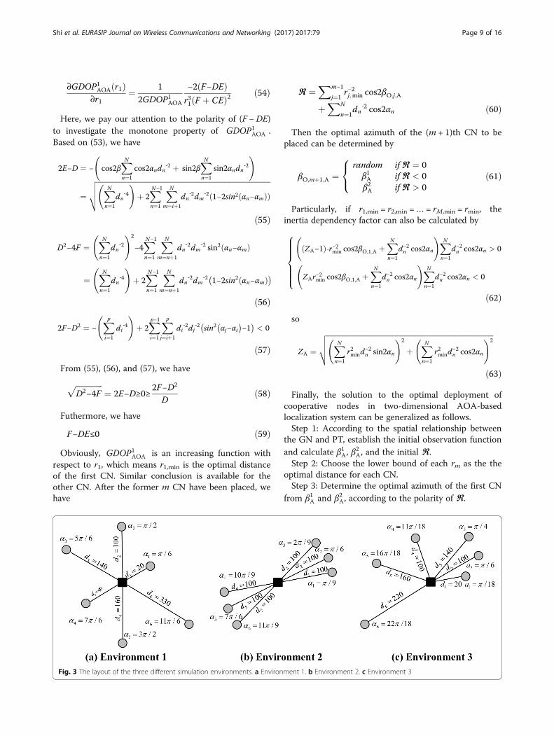
Fig. 3 The layout of the three different simulation environments. a Environment 1. b Environment 2. c Environment 3

Shi et al. EURASIP Journal on Wireless Communications and Networking (2017) 2017:79 Page 9 of 16

Step 4: If r1,min = r2,min =… = rM,min = rmin is not satis-fied, determine the optimal azimuth of the other CNaccording to the polarity of ℜ updated.Step 5: If r1,min = r2,min =… = rM,min = rmin is satisfied,

calculate ZA. If ZA <M, deploy the whole CNs in the sameazimuth as the first CN assigned. If ZA ≥M, deploy theformer ZA CNs in the same azimuth as the first CNassigned while place the (ZA+1)th CN in the azimuth ver-tical to that of the first CN. Then, β1A and β2A are alterna-tively chosen as the optimal azimuth of the rest CNs.

5 SimulationIn this section, we establish three quite different simula-tion environments to evaluate the performance ofOPMPD approach and compare it with partial exhaust-ive method, global exhaustive method, and eigenvalue-based approach. It indicates that our approach couldprovide a rapid and accurate deployment of CNs forTOA-based and AOA-based localization system and issuperior to the other approaches.

5.1 Simulation set upThese simulations are implemented in MATLAB lan-guage and tested on a PC with an Intel Core i5-3470

CPU of 3.20 GHz and DDR3 SDRAM of 8 GB. Supposethere are totally 6 CNs to be placed to improve the ac-curacy of a PT that serviced by 6 GNs. Simulation dataare collected from three environments whose detailsdepicted in Fig. 3 and Table 1. As reported in (31) and(49), if ℜ = 0, any azimuth can be regarded as the bestchoice. In our test, for the case of ℜ = 0, we respectivelychoose π/5, π/6, and π/4 as the optimal azimuth of CNin environment 1, environment, 2 and environment 3for easy of analysis. In addition, we set the domain ofβO,m,T as − π

4 ;3π4

� �, considering the periodicity of the

Q(βm) and the scope configured in (28).

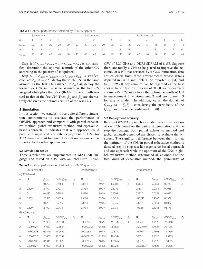
5.2 Deployment accuracyBecause OPMPD approach estimate the optimal positionof each CN based on the partial differentiation and thestepwise strategy, both partial exhaustive method andglobal exhaustive method are chosen to evaluate the ac-curacy. The significant difference between them is thatthe optimum of the CNs in partial exhaustive method isdecided step by step just like eigenvalue-based approachand our approach while the optimum of the CNs in glo-bal exhaustive method determined all at once. For thetwo kinds of exhaustive method, the granularity of

Table 1 Optimal performance obtained by OPMPD approach

Environment 1 Environment 2 Environment 3

m 1 2 3 4 5 6 1 2 3 4 5 6 1 2 3 4 5 6

rm,min 20 20 20 20 20 20 20 20 20 20 20 20 20 15 10 25 18 13

m 1 2 3 4 5 6 1 2 3 4 5 6 1 2 3 4 5 6

rm,max 40 40 40 40 40 40 40 40 40 40 40 40 40 40 40 40 40 40

Table 2 Optimal performance obtained by OPMPD approach

Environment 1 Environment 2 Environment 3

(a) TOA-based

m ℜ βO,m,T GDOPmC;TOA ZT ℜ βO,m,T GDOPmC;TOA ZT ℜ βO,m,T GDOPmC;TOA ZT

1 0 0.6283 0.7683 1 2.8794 2.9044 1.0308 6 1.6133 2.0051 0.7739 3

2 0.309 2.1991 0.7071 2.3794 2.9044 0.8010 0.9675 2.0051 0.7085

3 0 0.6283 0.6708 1.8794 2.9044 0.7004 0.3217 2.0051 0.6677

4 0.309 2.1991 0.6325 1.3794 2.9044 0.6425 −0.3241 0.4343 0.6332

5 0 0.6283 0.6055 0.8794 2.9044 0.6045 0.3217 2.0051 0.6037

6 0.309 2.1991 0.5774 0.3794 2.9044 0.5775 −0.3241 0.4343 0.5778

(b) AOA-based

m ℜ βO,m,A GDOPmC;AOA ZA ℜ βO,m,A GDOPmC;AOA ZA ℜ βO,m,A GDOPmC;AOA ZA

1 0.0015 2.1057 26.3141 2 0.0002894 2.0944 45.8142 1 0.0024 1.7526 27.4448

2 0.0002527 2.1057 22.5644 −0.0009206 0.5236 26.8686 0.0002859 1.7526 22.7065

3 −0.000948 0.5349 19.2462 0.0002894 2.0944 22.8770 −0.0041 0.1868 14.8350

4 0.0002527 2.1057 17.5197 −0.0009206 0.5236 19.4544 0.0052 1.7526 13.9309

5 −0.000948 0.5349 15.9077 0.0002894 2.0944 17.6657 0.0037 1.7526 12.8015

6 0.0002527 2.1057 14.8611 −0.0009206 0.5236 16.0237 0.0008377 1.7526 11.6386

Shi et al. EURASIP Journal on Wireless Communications and Networking (2017) 2017:79 Page 10 of 16

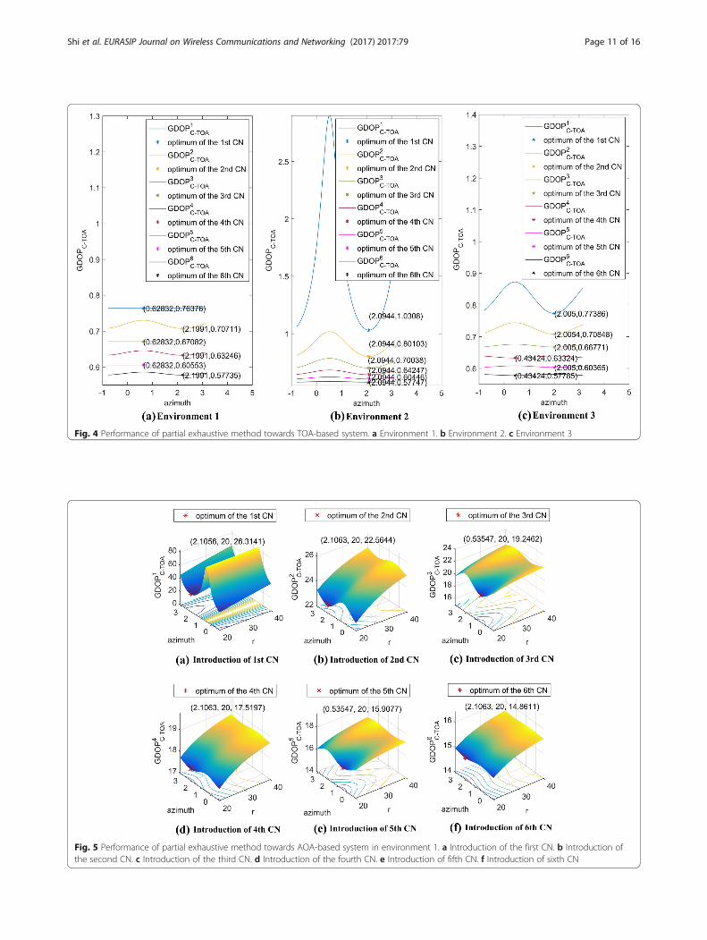
Fig. 4 Performance of partial exhaustive method towards TOA-based system. a Environment 1. b Environment 2. c Environment 3

Fig. 5 Performance of partial exhaustive method towards AOA-based system in environment 1. a Introduction of the first CN. b Introduction ofthe second CN. c Introduction of the third CN. d Introduction of the fourth CN. e Introduction of fifth CN. f Introduction of sixth CN

Shi et al. EURASIP Journal on Wireless Communications and Networking (2017) 2017:79 Page 11 of 16

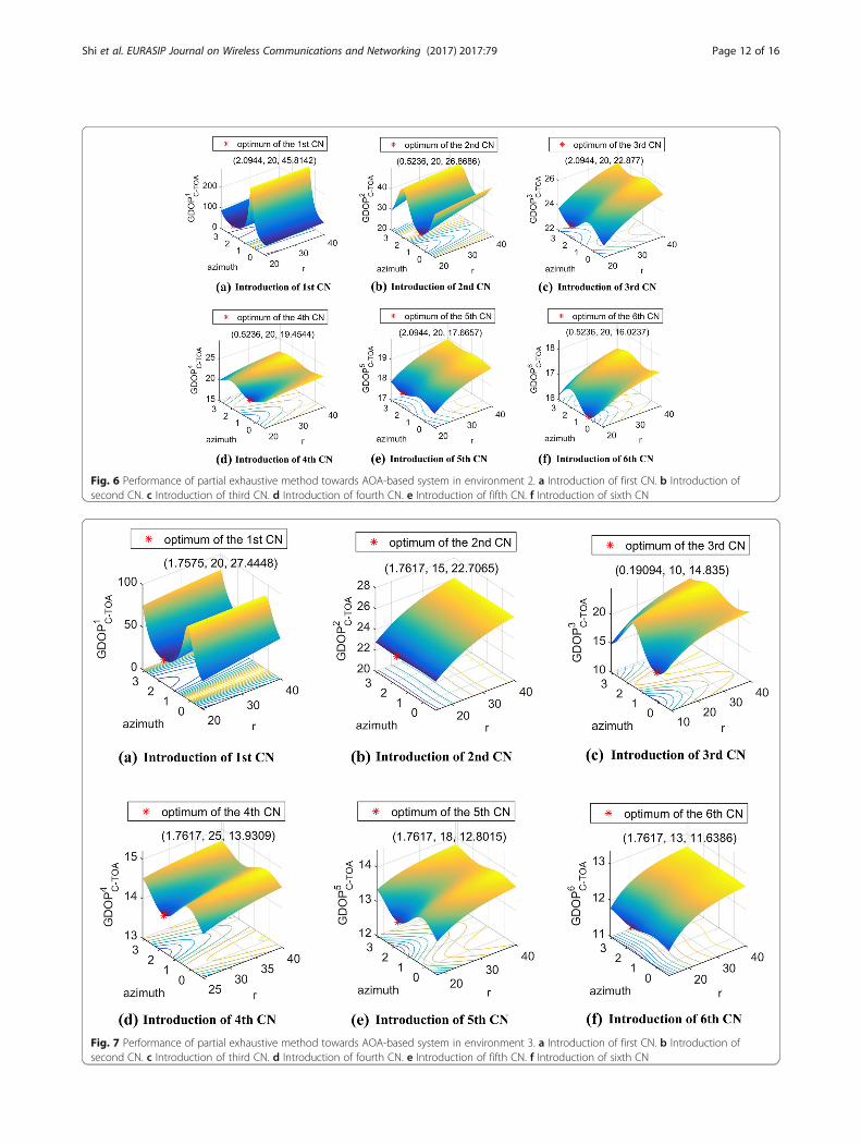
Fig. 6 Performance of partial exhaustive method towards AOA-based system in environment 2. a Introduction of first CN. b Introduction ofsecond CN. c Introduction of third CN. d Introduction of fourth CN. e Introduction of fifth CN. f Introduction of sixth CN

Fig. 7 Performance of partial exhaustive method towards AOA-based system in environment 3. a Introduction of first CN. b Introduction ofsecond CN. c Introduction of third CN. d Introduction of fourth CN. e Introduction of fifth CN. f Introduction of sixth CN

Shi et al. EURASIP Journal on Wireless Communications and Networking (2017) 2017:79 Page 12 of 16

azimuth is set π/3600 rad and the granularity of distanceis set 0.5 m.Table 2 depicts the optimal performance obtained by

OPMPD approach. As revealed in Table 2(a), 0.6283,2.9044, and 2.0051 are chosen as the optimal azimuth ofthe first CN in the three environments. Compared to theperformance depicted in Fig. 4, the optimum of each CNachieved by OPMPD nearly equals to the result affordedby partial exhaustive method, which proves the correct-ness of theoretical derivation in OPMPD approach.Similar conclusion about azimuth toward AOA-basedlocalization system can be derived from Table 2(b) andFigs. 5, 6, and 7. Besides, it is showed that the GDOP- ofAOA-based cooperative localization system decreases asthe distance of the CN shrinks, which agrees with theconclusion in (59).The accuracy comparison with global exclusive

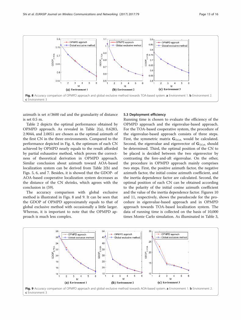
method is illustrated in Figs. 8 and 9. It can be seen thatthe GDOP of OPMPD approximately equals to that ofglobal exclusive method with occasionally a little larger.Whereas, it is important to note that the OPMPD ap-proach is much less complex.

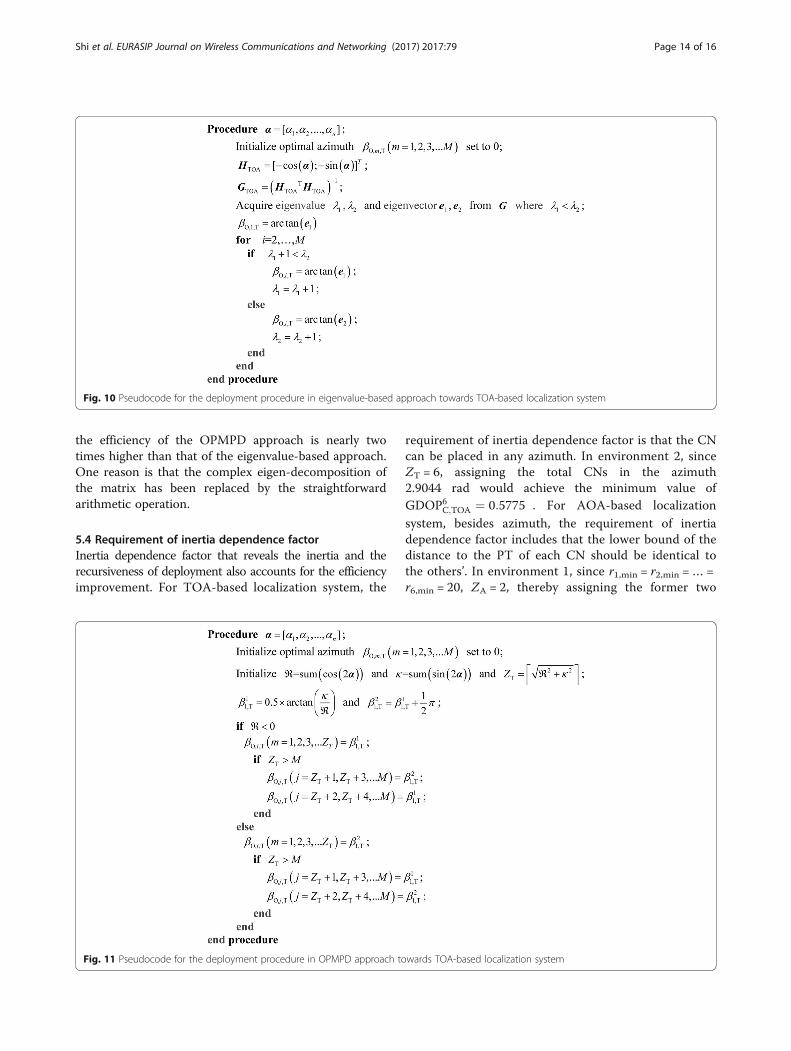
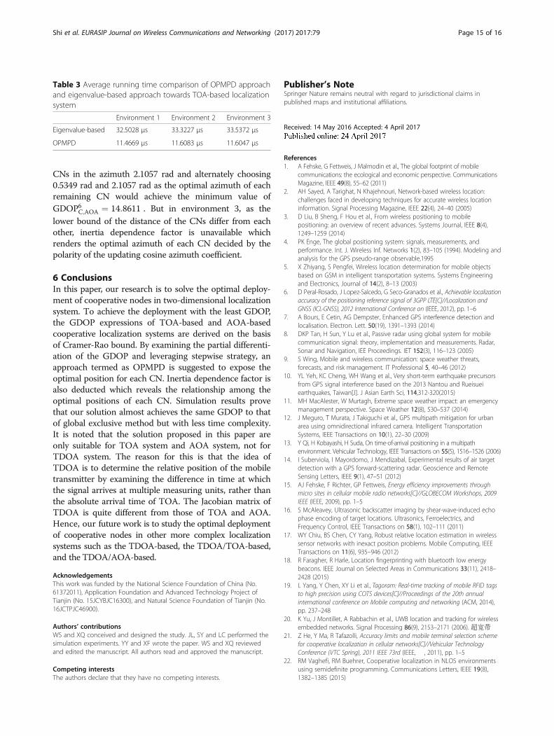
5.3 Deployment efficiencyRunning time is chosen to evaluate the efficiency of theOPMPD approach and the eigenvalue-based approach.For the TOA-based cooperative system, the procedure ofthe eigenvalue-based approach consists of three steps.First, the symmetric matrix GTOA would be calculated.Second, the eigenvalue and eigenvector of GTOA shouldbe determined. Third, the optimal position of the CN tobe placed is decided between the two eigenvector bycontrasting the fore-and-aft eigenvalue. On the other,the procedure in OPMPD approach mainly comprisestwo steps. First, the positive azimuth factor, the negativeazimuth factor, the initial cosine azimuth coefficient, andthe inertia dependence factor are calculated. Second, theoptimal position of each CN can be obtained accordingto the polarity of the initial cosine azimuth coefficientand the value of the inertia dependence factor. Figures 10and 11, respectively, shows the pseudocode for the pro-cedure in eigenvalue-based approach and in OPMPDapproach towards TOA-based localization system. Thedata of running time is collected on the basis of 10,000times Monte Carlo simulation. As illuminated in Table 3,

Fig. 8 Accuracy comparison of OPMPD approach and global exclusive method towards TOA-based system. a Environment 1. b Environment 2.c Environment 3

Fig. 9 Accuracy comparison of OPMPD approach and global exclusive method towards AOA-based system. a Environment 1. b Environment 2.c Environment 3

Shi et al. EURASIP Journal on Wireless Communications and Networking (2017) 2017:79 Page 13 of 16

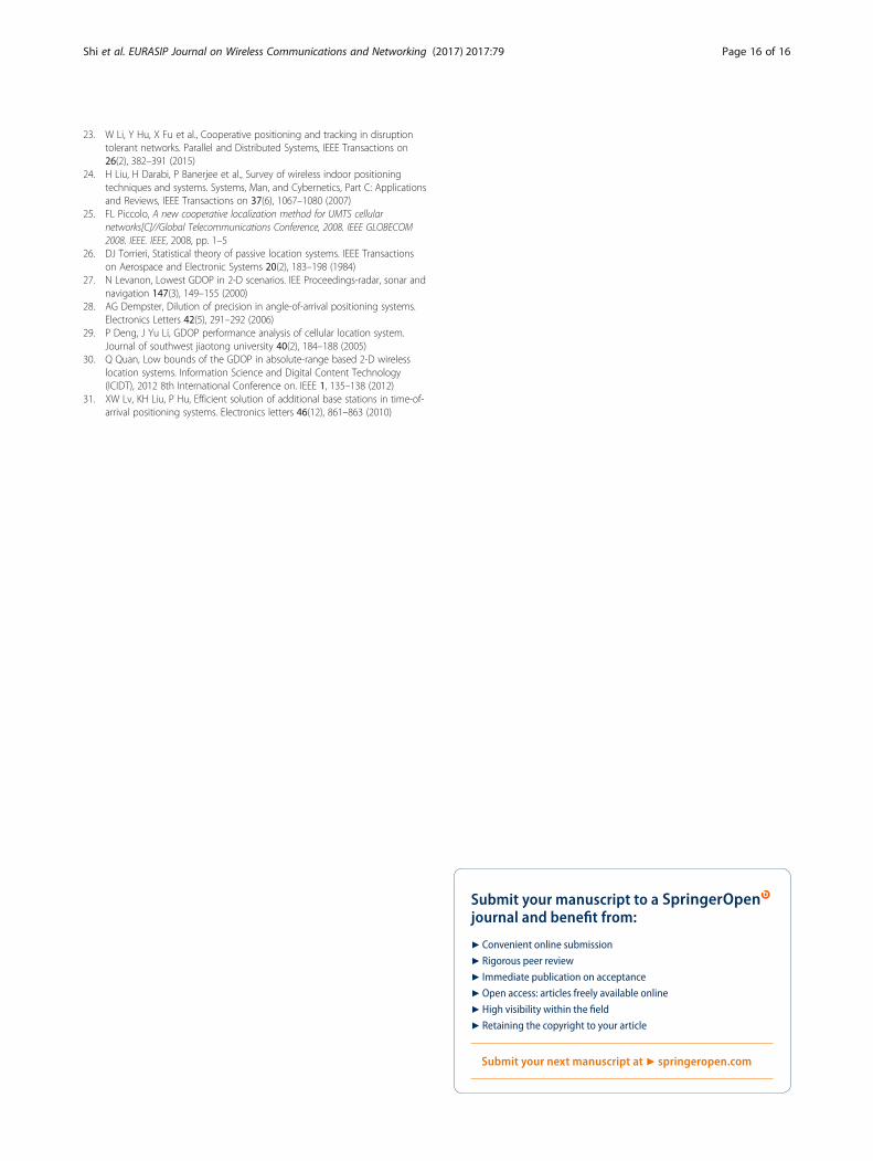
the efficiency of the OPMPD approach is nearly twotimes higher than that of the eigenvalue-based approach.One reason is that the complex eigen-decomposition ofthe matrix has been replaced by the straightforwardarithmetic operation.

5.4 Requirement of inertia dependence factorInertia dependence factor that reveals the inertia and therecursiveness of deployment also accounts for the efficiencyimprovement. For TOA-based localization system, the

requirement of inertia dependence factor is that the CNcan be placed in any azimuth. In environment 2, sinceZT = 6, assigning the total CNs in the azimuth2.9044 rad would achieve the minimum value ofGDOP6

C;TOA ¼ 0:5775 . For AOA-based localizationsystem, besides azimuth, the requirement of inertiadependence factor includes that the lower bound of thedistance to the PT of each CN should be identical tothe others’. In environment 1, since r1,min = r2,min =… =r6,min = 20, ZA = 2, thereby assigning the former two

Fig. 10 Pseudocode for the deployment procedure in eigenvalue-based approach towards TOA-based localization system

Fig. 11 Pseudocode for the deployment procedure in OPMPD approach towards TOA-based localization system

Shi et al. EURASIP Journal on Wireless Communications and Networking (2017) 2017:79 Page 14 of 16

CNs in the azimuth 2.1057 rad and alternately choosing0.5349 rad and 2.1057 rad as the optimal azimuth of eachremaining CN would achieve the minimum value ofGDOP6C;AOA ¼ 14:8611 . But in environment 3, as thelower bound of the distance of the CNs differ from eachother, inertia dependence factor is unavailable whichrenders the optimal azimuth of each CN decided by thepolarity of the updating cosine azimuth coefficient.

6 ConclusionsIn this paper, our research is to solve the optimal deploy-ment of cooperative nodes in two-dimensional localizationsystem. To achieve the deployment with the least GDOP,the GDOP expressions of TOA-based and AOA-basedcooperative localization systems are derived on the basisof Cramer-Rao bound. By examining the partial differenti-ation of the GDOP and leveraging stepwise strategy, anapproach termed as OPMPD is suggested to expose theoptimal position for each CN. Inertia dependence factor isalso deducted which reveals the relationship among theoptimal positions of each CN. Simulation results provethat our solution almost achieves the same GDOP to thatof global exclusive method but with less time complexity.It is noted that the solution proposed in this paper areonly suitable for TOA system and AOA system, not forTDOA system. The reason for this is that the idea ofTDOA is to determine the relative position of the mobiletransmitter by examining the difference in time at whichthe signal arrives at multiple measuring units, rather thanthe absolute arrival time of TOA. The Jacobian matrix ofTDOA is quite different from those of TOA and AOA.Hence, our future work is to study the optimal deploymentof cooperative nodes in other more complex localizationsystems such as the TDOA-based, the TDOA/TOA-based,and the TDOA/AOA-based.

AcknowledgementsThis work was funded by the National Science Foundation of China (No.61372011), Application Foundation and Advanced Technology Project ofTianjin (No. 15JCYBJC16300), and Natural Science Foundation of Tianjin (No.16JCTPJC46900).

Authors’ contributionsWS and XQ conceived and designed the study. JL, SY and LC performed thesimulation experiments. YY and XF wrote the paper. WS and XQ reviewedand edited the manuscript. All authors read and approved the manuscript.

Competing interestsThe authors declare that they have no competing interests.

Publisher’s NoteSpringer Nature remains neutral with regard to jurisdictional claims inpublished maps and institutional affiliations.

Received: 14 May 2016 Accepted: 4 April 2017

References1. A Fehske, G Fettweis, J Malmodin et al., The global footprint of mobile

communications: the ecological and economic perspective. CommunicationsMagazine, IEEE 49(8), 55–62 (2011)

2. AH Sayed, A Tarighat, N Khajehnouri, Network-based wireless location:challenges faced in developing techniques for accurate wireless locationinformation. Signal Processing Magazine, IEEE 22(4), 24–40 (2005)

3. D Liu, B Sheng, F Hou et al., From wireless positioning to mobilepositioning: an overview of recent advances. Systems Journal, IEEE 8(4),1249–1259 (2014)

4. PK Enge, The global positioning system: signals, measurements, andperformance. Int. J. Wireless Inf. Networks 1(2), 83–105 (1994). Modeling andanalysis for the GPS pseudo-range observable,1995

5. X Zhiyang, S Pengfei, Wireless location determination for mobile objectsbased on GSM in intelligent transportation systems. Systems Engineeringand Electronics, Journal of 14(2), 8–13 (2003)

6. D Peral-Rosado, J Lopez-Salcedo, G Seco-Granados et al., Achievable localizationaccuracy of the positioning reference signal of 3GPP LTE[C]//Localization andGNSS (ICL-GNSS), 2012 International Conference on (IEEE, 2012), pp. 1–6

7. A Bours, E Cetin, AG Dempster, Enhanced GPS interference detection andlocalisation. Electron. Lett. 50(19), 1391–1393 (2014)

8. DKP Tan, H Sun, Y Lu et al., Passive radar using global system for mobilecommunication signal: theory, implementation and measurements. Radar,Sonar and Navigation, IEE Proceedings. IET 152(3), 116–123 (2005)

9. S Wing, Mobile and wireless communication: space weather threats,forecasts, and risk management. IT Professional 5, 40–46 (2012)

10. YL Yeh, KC Cheng, WH Wang et al., Very short-term earthquake precursorsfrom GPS signal interference based on the 2013 Nantou and Rueisueiearthquakes, Taiwan[J]. J Asian Earth Sci, 114,312-320(2015)

11. MH MacAlester, W Murtagh, Extreme space weather impact: an emergencymanagement perspective. Space Weather 12(8), 530–537 (2014)

12. J Meguro, T Murata, J Takiguchi et al., GPS multipath mitigation for urbanarea using omnidirectional infrared camera. Intelligent TransportationSystems, IEEE Transactions on 10(1), 22–30 (2009)

13. Y Qi, H Kobayashi, H Suda, On time-of-arrival positioning in a multipathenvironment. Vehicular Technology, IEEE Transactions on 55(5), 1516–1526 (2006)

14. I Suberviola, I Mayordomo, J Mendizabal, Experimental results of air targetdetection with a GPS forward-scattering radar. Geoscience and RemoteSensing Letters, IEEE 9(1), 47–51 (2012)

15. AJ Fehske, F Richter, GP Fettweis, Energy efficiency improvements throughmicro sites in cellular mobile radio networks[C]//GLOBECOM Workshops, 2009IEEE (IEEE, 2009), pp. 1–5

16. S McAleavey, Ultrasonic backscatter imaging by shear-wave-induced echophase encoding of target locations. Ultrasonics, Ferroelectrics, andFrequency Control, IEEE Transactions on 58(1), 102–111 (2011)

17. WY Chiu, BS Chen, CY Yang, Robust relative location estimation in wirelesssensor networks with inexact position problems. Mobile Computing, IEEETransactions on 11(6), 935–946 (2012)

18. R Faragher, R Harle, Location fingerprinting with bluetooth low energybeacons. IEEE Journal on Selected Areas in Communications 33(11), 2418–2428 (2015)

19. L Yang, Y Chen, XY Li et al., Tagoram: Real-time tracking of mobile RFID tagsto high precision using COTS devices[C]//Proceedings of the 20th annualinternational conference on Mobile computing and networking (ACM, 2014),pp. 237–248

20. K Yu, J Montillet, A Rabbachin et al., UWB location and tracking for wirelessembedded networks. Signal Processing 86(9), 2153–2171 (2006). 超宽带

21. Z He, Y Ma, R Tafazolli, Accuracy limits and mobile terminal selection schemefor cooperative localization in cellular networks[C]//Vehicular TechnologyConference (VTC Spring), 2011 IEEE 73rd (IEEE, , 2011), pp. 1–5

22. RM Vaghefi, RM Buehrer, Cooperative localization in NLOS environmentsusing semidefinite programming. Communications Letters, IEEE 19(8),1382–1385 (2015)

Table 3 Average running time comparison of OPMPD approachand eigenvalue-based approach towards TOA-based localizationsystem

Environment 1 Environment 2 Environment 3

Eigenvalue-based 32.5028 μs 33.3227 μs 33.5372 μs

OPMPD 11.4669 μs 11.6083 μs 11.6047 μs

Shi et al. EURASIP Journal on Wireless Communications and Networking (2017) 2017:79 Page 15 of 16

23. W Li, Y Hu, X Fu et al., Cooperative positioning and tracking in disruptiontolerant networks. Parallel and Distributed Systems, IEEE Transactions on26(2), 382–391 (2015)

24. H Liu, H Darabi, P Banerjee et al., Survey of wireless indoor positioningtechniques and systems. Systems, Man, and Cybernetics, Part C: Applicationsand Reviews, IEEE Transactions on 37(6), 1067–1080 (2007)

25. FL Piccolo, A new cooperative localization method for UMTS cellularnetworks[C]//Global Telecommunications Conference, 2008. IEEE GLOBECOM2008. IEEE. IEEE, 2008, pp. 1–5

26. DJ Torrieri, Statistical theory of passive location systems. IEEE Transactionson Aerospace and Electronic Systems 20(2), 183–198 (1984)

27. N Levanon, Lowest GDOP in 2-D scenarios. IEE Proceedings-radar, sonar andnavigation 147(3), 149–155 (2000)

28. AG Dempster, Dilution of precision in angle-of-arrival positioning systems.Electronics Letters 42(5), 291–292 (2006)

29. P Deng, J Yu Li, GDOP performance analysis of cellular location system.Journal of southwest jiaotong university 40(2), 184–188 (2005)

30. Q Quan, Low bounds of the GDOP in absolute-range based 2-D wirelesslocation systems. Information Science and Digital Content Technology(ICIDT), 2012 8th International Conference on. IEEE 1, 135–138 (2012)

31. XW Lv, KH Liu, P Hu, Efficient solution of additional base stations in time-of-arrival positioning systems. Electronics letters 46(12), 861–863 (2010)

Submit your manuscript to a journal and benefi t from:

7 Convenient online submission

7 Rigorous peer review

7 Immediate publication on acceptance

7 Open access: articles freely available online

7 High visibility within the fi eld

7 Retaining the copyright to your article

Submit your next manuscript at 7 springeropen.com

Shi et al. EURASIP Journal on Wireless Communications and Networking (2017) 2017:79 Page 16 of 16